The Casimir Effect for Arbitrary Optically Anisotropic Materials

Jose C. Torres-Guzman1, 2, ∗ and W. Luis Mochan1, †

1Instituto de Ciencias Fısicas, Universidad Nacional Autonoma de Mexico,Apdo. Postal 48-3, 62251 Cuernavaca, Morelos, Mexico

2Facultad de Ciencias, Universidad Autonoma del Estado de Morelos,Avenida Universidad 1001, 62221 Cuernavaca, Morelos, Mexico

(Dated: January 31, 2013)

We extend a fictitious-cavity approach to calculate the Casimir effect for cavities bounded byflat anisotropic materials. We calculate the energy, force and torque in terms only of the opticalcoefficients of the walls of the cavity. We calculate the Casimir effect at zero and finite temperaturefor some simple systems. As a non trivial application, we calculate the torque between a semi-infiniteanisotropic plate and an anisotropic film. We study the effect of the film thickness in the torqueand find an optimal width that maximizes the torque.

PACS numbers: 42.50.Pq 31.30.jh 42.50.Lc 12.20.Ds

I. INTRODUCTION

An electromagnetic mode of frequency ω within an electromagnetic cavity is analogous to a harmonic oscillatorwith a quantized energy spectrum given by semi-integer multiples n + 1/2 of the energy quantum hω, where theinteger n is the occupation number of the mode, i.e., the number of photons in the corresponding state, hω isthe quantized energy of each photon and hω/2 is the ground state energy arising from the quantum nature of theelectromagnetic field and its zero point fluctuations. As the frequency of the electromagnetic modes depends on thegeometry of the cavity, the zero point fluctuations may not be simply disregarded as a constant contribution to theenergy and should be accounted for in calculations of the total energy of the system. A simple vacuum cavity maybe produced by positioning two flat conducting plates parallel to each other a small distance L apart, leading toa first quantization of the electromagnetic field within the cavity. In 1948, Casimir [1] predicted that the vacuumelectromagnetic energy due to the quantum fluctuations of the field would depend on L and therefore a force, whichturns out to be attractive, would act on each plate. This Casimir force also may be conceived as originated from thedifference between the radiation pressure due to the fluctuating electromagnetic modes outside the plates and themodes within [2]. Irrespective of its interpretation, the Casimir force has its origin in the linear momentum carried bythe radiation field. Nevertheless, the radiation field carries angular momentum beyond linear momentum. Therefore,if the plates are optically anisotropic, a Casimir torque might develop besides the Casimir force. In fact, the transferof angular momentum of polarized light to a macroscopic birefringent medium, resulting in a torque, has been knownfor a long time [3]. The Casimir torque may be interpreted as arising from the orientational dependence of the vacuumelectromagnetic energy, specifically from the dependence on the relative orientation of the optical axes of the plates.The resultant torque tends to align the optical axes along the configuration that minimizes the vacuum energy.

Recently, the Casimir effect has received considerable attention for its possible technological applications, besidesthe fact that experimental studies have attained the necessary accuracy to test in detail the theoretical predictions[4–17]. Therefore, theories about the Casimir effect that account realistically for the properties of actual materialshave become indispensable. The study of vacuum forces between real materials was pioneered by Lifshitz [18], whoconsidered two semi-infinite homogeneous and isotropic non-spatially dispersive dielectric slabs, whose fluctuatingcurrents were the sources of the fluctuating electromagnetic field and whose correlations were related to the dielectricresponse of the materials.

In 1972, Parsegian and Weiss derived an expression in the non-retarded limit for the interaction energy betweentwo semi-infinite dissipationless dielectric anisotropic materials [19] following a method of surface mode summation.Barash derived an expression which included retardation and dissipation effects [20] employing an auxiliary system[21] first introduced for isotropic systems. The solutions of Maxwell’s equations for the field in inhomogeneous andabsorbing media were expanded in terms of the orthogonal solutions of Maxwell’s equations for a non-dissipativeauxiliary system in which the frequency dependence of the dielectric function is only parametric.

∗Electronic address: torres@fis.unam.mx†Electronic address: mochan@fis.unam.mx

arX

iv:1

301.

7306

v1 [

quan

t-ph

] 3

0 Ja

n 20

13

2

The use of an auxiliary system was further developed in physical terms by Kupiszewska [22] in a calculation ofCasimir forces for lossy and dispersive isotropic dielectrics in the case of one dimensional propagation of electromag-netic waves. The problem of quantizing a dissipative system is attacked by accounting both for the dynamics of thevacuum modes and of the atomic dipoles to which they couple and which make up the material, together with athermal reservoir in which the atomic radiators dissipate the absorbed energy. That formalism was extended by vanEnk [23] to obtain the torque between anisotropic materials in the 1D case. In his work, van Enk calculated thetorque starting from the flux of the spin angular momentum of the electromagnetic field.

Numerical calculations have also been performed for materials with a small anisotropy using Barash’s results and ithas been shown that the torque may be large enough to be experimentally measurable in several novel experimentalconfigurations [24]. By a similar technique, the Casimir energy between anisotropic dielectric plates [25], and betweena plate with anisotropic magnetic response and another with anisotropic dielectric response [26] have been calculatedand analytical approximate expressions for the torque and force were obtained in the retarded limit. Kenneth andNussinov have also calculated the Casimir energy between parallel plates made up of arrays of wires aligned alongdifferent directions [27] using a path integral technique [28, 29].

In the works described above, specific models of the dielectric properties of the plates were assumed from the onsetin order to derive expressions for the Casimir force and torque. However, recent works [30–36] have shown that ifthe theory is set up in terms of the reflection coefficients of the media, or equivalently, in terms of their exact surfaceimpedance [37, 38], it is possible to decouple the calculation of the Casimir force from the calculation of the dielectricresponse of the materials.

Lambrecht et al. have extended their scattering approach [30, 31] to corrugated systems [39]. Moreover, they haveargued that the resulting formula for the Casimir energy has a wider range of applicability and may be used to studyother anisotropic mirrors. Their formula has been used to evaluate numerically the effects of corrugation on theCasimir force [40] and torque [41] and to calculate the Casimir force between anisotropic metamaterials [42].

Mochan et al. [32–36] have argued that in thermal equilibrium, all of the properties of the radiation field within acavity are completely determined by the optical reflection amplitudes of the walls. Indeed, whenever a photon reachesthe surface of a wall of the cavity it may be coherently reflected with an amplitude described by the optical coefficientsof the wall. Otherwise, it would be transmitted into the wall to be either absorbed, exciting the material degrees offreedom of its constituents, or transmitted across the wall and into the surrounding vacuum to be lost forever. Theprobability of these processes is again determined by the optical coefficients of the wall, and given by their squaredmodulus. In thermodynamic equilibrium, detailed balance implies that whenever a photon is lost, an equivalentphoton is incoherently injected back to the cavity, so that both, the coherently and incoherently reflected photons aredetermined by the reflection amplitudes alone. Therefore, the radiation field within a real cavity would be identicalto the field within any cavity that has walls with the same optical properties. This fact allowed the construction offictitious disipationless systems which can be simply treated quantum mechanically to obtain the vacuum energy andforce for cavities with arbitrary walls. Thus, expressions for the Casimir force obtained from the electromagnetic stresstensor can be applied to semi-infinite or finite, homogeneous or layered, local or spatially dispersive, transparent oropaque systems through a simple substitution of the appropriate optical coefficients. This formalism has allowed thecalculation of the Casimir force between photonic structures [43], non-local excitonic semiconductors [44], non-local-plasmon-supporting metals with sharp boundaries [32–36, 45], and between realistic spatially dispersive metals witha smooth self-consistent electronic density profile [46]. With a few modifications, it has also been employed for thecalculation of other macroscopic forces, such as those due to electronic tunneling across an insulating gap separatingtwo conductors [47].

The relative simplicity of the formalism developed in [32–36] has allowed its generalization to anisotropic systems[48]. In Ref. [48] a new derivation of the Casimir torque within 1D cavities with walls made up of arbitrary materialscharacterized only by their anisotropic optical coefficients was presented. By 1D cavity we mean one in which thefield is constrained to propagate only along one direction, namely, the normal to the surface of the cavity walls. Inthe present paper we generalize this formalism to 3D cavities with anisotropic walls. We calculate the Casimir forcefrom the electromagnetic stress tensor. A simple integration over the separation distance L yields then the vacuumenergy. The torque is then calculated by taking the derivative respect to the angle γ between the optical axes ofthe plates. As our formalism is based on the calculation of the force, which is a directly observable quantity, itavoids the cumbersome singularities that plague other approaches. Furthermore, our results are written directly interms of the optical coefficients of the walls of the cavity about which we make no assumption. Thus, they can beapplied immediately to manifold systems such as insulating or conducting anisotropic slabs either dissipationless ordissipative, to semiinfinite or finite walls and to homogeneous or structured materials. We test the validity of ourapproach by reproducing some known results [24, 25, 27, 30–36, 42] and we show its versatility by applying it to somepreviously unexplored systems.

The structure of the paper is the following: In section II we develop our formalism in order to arrive at expressionsfor the Casimir energy between arbitrary anisotropic plates. The use of an effective cavity allows our results to be

3

rµν2

x

z

1 V 2

z1 z2

L

(a)

II = V ′I III

rµν2 tµν2

z0 z1 z2 z3

LII = LLI LIII

(b)

FIG. 1: (a) Vacuum cavity V of width L bounded by two arbitrary anisotropic material slabs (1 and 2) with surfaces at z1and z2 and anisotropic reflection amplitudes rµνa (a = 1, 2, µ, ν = s, p). (b)Fictitious system made up three empty regionsI, II, and III, bounded by perfect mirrors at z0 and z3 and with infinitely thin sheets at z1 and z2 with identical reflectionamplitudes rµνa to those of the real system and corresponding transmission amplitudes tµνa .

applicable to arbitrary slabs at any temperature T . In section III we specialize our results to semi-infinite local uniaxialmedia and we apply our results to a calculation of the energy and torque for an idealized uniaxial system consisting ofanisotropic mirrors that are perfectly conducting along one direction and perfectly insulating along the perpendiculardirections. These calculations are performed for temperatures T = 0 and T 6= 0. We also consider systems with afinite frequency-dependent conductivity along the optical axis. As a further application of our formalism, in sectionIV we calculate the torque of a system consisting of two conducting plates with an anisotropic effective mass tensor,where one of the plates is a film with finite thickness d, and we find there is an optimum value of d that maximizesthe torque. We also calculated the same system considered by Munday et al. [24] consisting of a semi-infinite slab ofBaTiO3 and a thin film of calcite. Finally, in section V we present our conclusions.

II. THE EFFECTIVE CAVITY APPROACH

Consider the setup shown in Fig. 1(a). The slabs represents arbitrary media. According to [32–36, 48, 49], inthermodynamic equilibrium the properties of the radiation field within the cavity V are completely determined by thegeometry of the cavity, characterized by L, and by the 2× 2 reflection amplitude matrices rµνa of each slab (a = 1, 2)coupling ν-polarized incident light to µ-polarized reflected light (µ, ν = s, p). Any relevant property of the material iscompletely accounted for through its optical coefficients. Thus, the electromagnetic radiation within the real cavityV must be identical to that within a fictitious cavity V ′ = II bounded by infinitely thin sheets at z1 and z2, providedtheir reflection amplitudes rµνa are chosen to match those of the walls of the real cavity V. The transmission amplitudestµνa of the infinitely thin sheets are conveniently chosen in order to guarantee energy conservation with no absorptionwhatsoever of electromagnetic energy. Thus, there is no absorption in the fictitious system, there is no excitation ofmaterial degrees of freedom and the normal modes of its electromagnetic field form a complete orthogonal basis of the

4

corresponding Hilbert space. As a consequence, one is allowed to use well developed quantum-mechanical proceduresfor the calculation of the field properties without the requirement of a microscopic model of the material.

The field modes may be quantized and counted by choosing suitable boundary conditions. For example, we cancan add perfect mirrors far away from the walls of the real cavity (Fig. 1(b)), at z0 and z3. These quantizing mirrorsproduce a field that mimics the incoherent radiation back into the cavity that is responsible for maintaining a detailedbalance and thus the thermodynamic equilibrium.

Consider now a single wave of frequency ω with wave-vector projection ~Q along the interface. Without loss ofgenerality, we choose x− z as the plane of incidence, so the electric and magnetic fields are given by

~E(~r, t) = E0ei(Qx−ωt)[φs(z)y − 1

iq(iQz− x∂z)φ

p(z)

](1)

and

~B(~r, t) = E0ei(Qx−ωt)[φp(z)y +

1

iq(iQz− x∂z)φ

s(z)

], (2)

where q = ω/c is the free-space wavenumber, φp(z) and φs(z) are the p and s polarized components of a spinorialnormalized wave-function

φµ(z) = CµrΛ eikz + CµlΛ e−ikz, (3)

where CµζΛ are constant coefficients within each region Λ = I, II, III corresponding to µ-polarized light moving

towards the right (ζ = r) and left (ζ = l), and k =√

(ω2/c2 − Q2) is the wave-vector component perpendicular tothe interface.

We integrate the energy density,

u = (|E|2 + |B|2)/16π (4)

to obtain the total electromagnetic energy

U =A|E0|2

8π(LI ||CI ||2 + LIII ||CIII ||2), (5)

in the limit LI , LIII → ∞, where A is the area of the plates and ||CΛ||2 ≡∑µζ |C

µζΛ |2. In the same limit the

normalization condition imposed on the wave-function simplifies to

1 = (LI ||CI ||2 + LIII ||CIII ||2). (6)

Notice that most of the energy lies in the large fictitious regions I and III, so we may identify

U =A|E0|2

8π(7)

and solve for the amplitude |E0|2 = 8πU/A. To obtain the force on the slab 2, we calculate the stress tensorTij = (1/8π)Re[EiE

∗j +BiB

∗j − (|E|2 + |B|2)δij/2] at an arbitrary position z within the cavity,

− Tzz(z) =U

2Aq2

(k2(|φs|2 + |φp|2) + |∂zφs|2 + |∂zφp|2

). (8)

By applying boundary conditions at z0 and z3, we obtain for a given value of ~Q a discrete set of mode frequenciesωn and corresponding perpendicular components kn of the wave-vector. Each of these modes contributes to the stresstensor a quantity similar to that in Eq. (8), so that

− Tzz(z) =hc

2A

∑n

fnqn

[k2n(|φsn|2 + |φpn|2) + (|∂zφsn|2 + |∂zφpn|2)

]z, (fixed ~Q), (9)

where we have substituted the energy Un in terms of the equilibrium occupation number fn = f(ωn) = coth(βhωn/2)/2of a photon state with quantized energy hωn at temperature kBT = 1/β, with kB the Boltzmann’s constant. Thesum over states may be rewritten in terms of the tensorial Green’s function G(z, z′) with components

Gµνk2

(z, z′) =∑n

φµn(z)φν∗n (z′)

k2 − k2n

, µ, ν = s, p, (10)

5

for the 1D Helmholtz equation (∂2z + k2

)Gµνk2

(z, z′) = δ(z − z′)δµν . (11)

Here, k = k + iη, (η > 0), with the understanding that the limit η → 0+ is to be taken at the end of the calculation.

Using the identity Im(k2 − k2n)−1 = −πδ(k2 − k2

n), we can replace the sum (9) by the integral

− Tzz(z) =hc

A

∫dk2 f

qρk2 , (fixed ~Q), (12)

where f = f(ω) and

ρk2(z) = − 1

2πIm

(k2 + ∂z∂z′

)Tr G(z, z′)|z=z′ (13)

plays the role of a local density of states at z (number of states per unit length and per unit k2).The solution of (11), subject to the appropriate boundary conditions, may be written in terms of the solutions u(z)

and v(z) of the 1D Helmholtz equation that satisfy the boundary conditions on the right and left side of the system,respectively,

G(z, z′) = u(z)[u′(z′)− v′(z′)v−1(z′)u(z′)

]−1θ(z − z′)

−v(z)[v′(z′)− u′(z′)u−1(z′)v(z′)

]−1θ(z′ − z), (14)

where θ denotes the Heaviside unit step function. Here, u(z) and v(z) are 2× 2 matrices with matrix elements uµλ(z)and vµλ(z), λ = 1, 2 denotes the two independent spinorial solutions of Helmholtz equation, µ = s, p denotes theircorrespondent s and p components and u′(z) and v′(z) denote the derivatives of u(z) and v(z) with respect to theirargument. We remark that we first introduced a similar expression for the spinorial Green’s function in Ref. [48],where it was used to obtain the angular momentum flux within a 1D cavity.

The solutions u(z) and v(z) may be written within the cavity in terms of the reflection coefficients of the plates

ra =

(rppa rpsarspa rssa

), (a = 1, 2). (15)

These are defined through

ξµr2 =∑ν

rµν2 ξνi2, (16)

where we define the unnormalized spinors ξµi2 and ξµr2 (µ = s, p) as the amplitudes of the incident and reflected fieldsat the surface of plate 2 through

Ey(z) = ξsi2eik(z−L) + ξsr2e

−ik(z−L) (17)

and

By(z) = ξpi2eik(z−L) + ξpr2e

−ik(z−L). (18)

The other components of the electromagnetic field may be obtained from Eqs. (17), (18) through Maxwell’s curlequations. The matrix elements rµν1 of plate 1 are similarly defined. Thus, we may write,

u(z) = Ieik(z−L) + r2e−ik(z−L) (19)

and

v(z) = Ie−ikz + r1eikz, (20)

where I is the 2× 2 unit matrix.Substitution of (19) and (20) in (14), (13) and (12) yields

− Tzz =hc

πARe

∫dk2 fk

q∆(1− e4ikLr1r2), (fixed ~Q) (21)

6

where ra ≡ det ra and

∆ = det (I− e2ikLr1r2). (22)

Note that ∆ = 0 yields the dispersion relation of the lossy modes of the real cavity.

Summing equation (21) over ~Q we finally obtain

− Tzz =hc

2π3

∫d2Q Re

∫dk

fk2

q∆(1− e4ikLr1r2), (23)

where we assumed Born-von Karman periodic boundary conditions along the surface of area A → ∞ to replace∑Q . . .→ A/(2π)2

∫d2Q . . .

The flux of linear momentum −Tzz in the fictitious cavity is the same as in the real cavity between slabs 1 and 2.To obtain the force on slab 2, we have to subtract the flux in the real system between the slab and infinity. This cancan be obtained following the same derivation given above, but replacing the slab 1 by the complete system made upof slabs 1, the cavity V and slab 2, and replacing slab 2 by empty space. The result is identical to equation (23), butsubstituting r2 → 0. Thus, the total force per unit area of slab 2 is

FzA

=hc

2π3Re

∫d2Q

∫dk fk2 e

2ikL

q∆

×(

Tr(r1r2)− 2e2ikLr1r2

)= − hc

4π3Im

∫d2Q

∫dk f

k

q

d

dLlog ∆ (24)

The derivation above was performed for waves that propagate in vacuum, that is, within the light cone Q ≤ ω/cand for real k. For evanescent waves with Q > ω/c and imaginary k the approach above has to be slightly modified,as it turns to be impossible to choose fictitious transmission amplitudes tµνa that guarantee energy conservation atthe boundaries z1 and z2 of the fictitious cavity of Fig. 1. Nevertheless, the fictitious system may be easily altered toaccommodate for evanescent waves [49], and it turns out that the expression (24) and (25) remain valid even outsideof the light cone [49]. Thus, the integration region of Eq. (24) may include real and imaginary values of k, as long as

the wavenumber q ≡ ω/c =√Q2 + k2 is real, i.e., k should go along the imaginary axis from iQ to 0 and then along

the real axis towards infinity.The formalism developed above is a generalization to anisotropic systems of the formalism developed in Refs. [32–

36] for the isotropic case. The resulting force (Eq. (24)) agrees with the usual Lifshitz’s result expressed in terms ofthe reflection amplitudes in the isotropic case (rspa = rpsa = 0).

The potential energy U of the system may be now obtained by integrating the force (24) with respect to the plateseparation from ∞ towards the actual separation L, yielding

U

A=

hc

4π3Im

∫d2Q

∫dk f

k

qlog ∆. (25)

Notice that when L→∞, ∆→ 1 as e2ikL → 0 for any positive of η. We make a change of variable from k to q andperform the usual rotation in the complex plane from the positive real axis towards the imaginary axis to rewrite Eq.(25) as

U

A=

h

8π3

∫ ∞0

du

∫d2Q log ∆ (26)

at T = 0, where we introduce an imaginary frequency ω = iu, and as

U

A=kBT

4π2Re

∑`≥0

′∫d2Q log ∆` (27)

for T 6= 0, where we have accounted for the poles of f(iu) by performing residue-like integrations at the Matsubarafrequencies u` = 2π`kBT/h and we define ∆` = ∆(ω = iu`). The prime in the summation means that the ` = 0 termshould be divided by 2. Eq. (26) coincides with that derived in Refs. [30, 31, 42] for T = 0.

Notice that for anisotropic plates, the matrices ra depend on their in-plane orientation. Therefore, the energy U(Eq. (25)) depends implicitly on the relative orientation γ between the optical axes of the plates. Thus, we expect a

7

γ

x y

z

ψ11

2

FIG. 2: Schematic diagram of the system, consisting of two parallel uniaxial non-magnetic plates whose optical axes lie onthe surface. We indicate the optical axes of each plate with heavy double-headed arrows, and the projection of the axis of thesecond plate upon the first by a dashed double arrow. The z-axis is chosen to be orthogonal to the plates. We also indicatethe plane of incidence. The angle ψ1 between the plane of incidence and the optical axis of plate 1 as well as the angle γ fromthe optical axis of plate 1 towards that of plate 2 are indicated. The angle ψ2 between the plane of incidence and the opticalaxis of plate 2 is ψ2 = −ψ1 − γ. The sign is due to the convention in Eq. (29).

torque M on the plates which we may calculate simply by taking the derivative M = −∂U/∂γ. It is easily verified

that starting from Eq. (26) but setting ~Q = 0 instead of performing the integral (A/4π2)∫d2Q yields Eq. (13) of Ref.

[48], i.e., the torque for a cavity in which the field is constrained to propagate along only one dimension, namely, alongthe normal to the surfaces. In ref. [48] the torque was obtained directly from the flux of angular momentum withinthe cavity. Here, we took a different approach, obtaining the torque from the angular dependence of the energy. Thereason is that the angular momentum is well defined only for finite width beams and the overlap among the mulltiplereflections of a finite beam is incomplete for oblique incidence and ill defined for evanescent waves.

We remark that our results are written in terms of the optical coefficient matrices ra of the walls of the cavity,about which we have made no assumptions. Thus, our results may be applied to systems of arbitrary absortance,conductivity and width, and they may be homogeneous or inhomogeneous. Up to this point the dependence of theenergy, force and torque on the orientation of the plates has been implicit, through the unstated dependence of ra.In the next sections we will apply our result to specific cases where the dependence on γ can be exhibited explicitly.

III. SEMI-INFINITE UNIAXIAL SLABS

We consider semi-infinite uniaxial non-magnetic crystals with their optical axes parallel to their surface. In thiscase, the reflection matrices r1 and r2 may be obtained as particular instances for surfaces 1 and 2 of the formula [50]

r = (s−12 + s−1

1 cos θ)−1(s−11 cos θ − s−1

2 ), (28)

which we derive in the appendix following the notation of Ref. [51]. Here, s1 and s2 are the 2× 2-matrices

s1 =

(tanψJ −J

2 cotψIno

1 1

), s2 =

(n2o tanψJ2 − cotψ

1/J no/I

), (29)

and

I2 = n2on

2e − sin2 θ(n2

o sin2 ψ + n2e cos2 ψ),

J2 = n2o − sin2 θ,

(30)

where no and ne are the ordinary and extraordinary refractive indices of the uniaxial crystal, θ is the angle of incidenceand ψ is the angle from the plane of incidence to the optical axis of the crystal; its sign is chosen through the righthand rule around the normal of the surface that points outwards from the anisotropic medium. In Eqs. (29) we haveassumed that the cavity is empty and thus we took its index of refraction of the cavity as 1.

Consider the sketch depicted in Fig. 2, which displays the angle ψ1 of the optical axis of plate 1 with respect to theplane of incidence and the angle γ between the optical axis of plate 2 and that of plate 1. According to our conventionabove, the angle ψ2 between the optical axis of plate 2 and the plane of incidence is ψ2 = −ψ1 − γ. We identifyne =

√ε‖, no =

√ε⊥, where ε‖ and ε⊥ are the dielectric response functions of the plates along and perpendicular to

their optical axes, respectively. The substitution of equations (29), (30) in (28) and (27) yields after a tedious algebra

8

-0.014

-0.012

-0.01

-0.008

-0.006

-0.004

-0.002

−π/2 −π/4 0 π/4 π/2

ener

gyp

erunit

area

(L3/hc)U/A

angle γ

T = 0

T = 0.01

T = 0.1

T = 0.2

T = 0.3

T = 0.4

T = 0.5

FIG. 3: Casimir energy per unit area U/A between two ideal uniaxial plates as a function of the angle γ between their opticalaxes for different temperatures T = 0, 0.01, 0.1, 0.2, 0.3, 0.4, 0.5 in units of hc/LkB .

an expression for the Casimir energy between anisotropic plates. We have checked that the resulting expression for∆ coincide with that obtained in Ref. [25] for the same system. Nevertheless, the calculation of Ref. [25] is directlyapplicable only to local uniaxial semi-infinite homogeneous systems, as their calculation is setup in terms of the bulkdielectric function of the plates. On the other hand, our result is written in terms of the reflection amplitudes raof the plates, and thus may be applied to any system for which we can calculate these optical coefficients, as shownexplicitly in section IV.

Let us now consider an idealized case consisting of slabs which behave as perfect conductors along the optical axesbut which are perfect insulators along the other principal directions. This could be realized through an array ofperfectly conducting aligned wires insulated from each other. We further ignore the electric polarization across thewires, which would be appropriate, for example, if they were very thin. Then, each plate may be described by adielectric response ε‖ →∞ and ε⊥ → 1. In this case the reflection matrix (28) becomes simply

r(θ, ψ)=

[cos2 θ cos2 ψ − sin 2ψ cos θ/2sin 2ψ cos θ/2 − sin2 ψ

](1− sin2 θ cos2 ψ

)−1, (31)

which yields

∆ = 1− α2e2ikL (32)

when substituted into Eq. (22), where

α2 = Tr(r1r2) =

(cos γ − sin2 θ cosψ1 cosψ2

)2(1− sin2 θ cos2 ψ1)(1− sin2 θ cos2 ψ2)

. (33)

Eqs. (32) and (33) were previously obtained for this system in Ref. [27], as becomes evident by writing the latter interms of ϕ ≡ −ψ2 = ψ1 + γ.

Substitution of Eq. (32) into Eq. (26) yields the T = 0 energy of the system. Fig. 3 shows our numerical resultsfor the energy of the idealized system discussed above. We have verified that they agree with the results presented inRef. [27] where a path integral approach [28, 29] was used. Nevertheless, a similar substitution into Eq. (27) permitsus to calculate also the T 6= 0 energy of the system, shown in the same figure. Notice that for this idealized casethere is a natural temperature scale hc/kBL and a natural energy scale Ahc/L3, as they are respectively intensiveand extensive quantities with respect to the area A of the interfaces. We use these scales to normalize the units inthe figure. As T increases, the Casimir energy becomes more negative, so that the plates are more strongly bound.However, the slope of the energy as a function of the angle, and thus, the torque, diminishes with increasing T . Thisresult may appear somewhat surprising, as it is well known that increasing the temperature yields an increase of themagnitude of the Casimir force. For high enough temperatures the energy becomes independent of the angle andapproaches its value at γ = 0, which is exactly half of the energy corresponding to two perfect isotropic mirrors. Thiscan be easily verified by substituting α2 = 1 into Eq. (32) and the resulting ∆ into (26) and (27).

The torque for the ideal case may now be simply calculated by analytically deriving under the integral sign theenergy (26) or (27) with respect to the relative angle γ and performing the resulting integrals numerically. Fig. 4shows that the torque M is a periodic function of γ with period π. It is null when the optical axes are aligned, γ = 0, π,corresponding to a stable equilibrium orientation. It is also null when they are orthogonal to each other, γ = ±π/2,

9

-5

-4

-3

-2

-1

0

1

2

3

4

5

−π/2 −π/4 0 π/4 π/2

103×

(L3/hc)M/A

γ

T = 0

T = 0.01

T = 0.2

T = 0.3

T = 0.4

T = 0.1

T = 0.5

FIG. 4: Casimir torque per unit area M/A between two ideal uniaxial plates as a function of the angle γ between their opticalaxes. The torque is calculated for the same temperatures as in Fig. 3, expressed in units of hc/LkB .

corresponding to an unstable equilibrium. For T = 0 the slope of M(γ) seems singular at the stable equilibriumpoint. The existence of this singularity can actually be confirmed by deriving analytically the torque with respect tothe angle γ under the integral sign and examining the integrand after having taken the corresponding limit γ → 0and analytically performed the angular integral over ϕ. It turns out that the integrand has an infinite discontinuityat u = 0. This singularity had also been found previously in a 1D calculation [48], in which light is normally incidentat the walls of the cavity. Furthermore, qualitatively the same behaviour of the torque as a function of the angle γfound in this 1D calculation, is obtained in the 3D calculation for T = 0. The torque is not simply proportional tosin 2γ, so its extreme values are not at γ = ±π/4. However, as the temperature increases the torque becomes moresinusoidal-like. Note that the maximum torque per unit area is of the order of M/A ∼ 5× 10−3 × hc/L3. Thus, for aseparation L = 100 nm, the maximum torque per area unit is about 10−7N/m. It is interesting to compare this resultwith that of Rodrigues et al. [41] for the case of two slightly misaligned corrugated metals. It has been argued [41]that that system would yield the largest torques. Nevertheless, we obtained a torque of the same order of magnitudeas their’s. Furthermore, in our case the torque remains large over a wide angular range, independently of the area ofthe system, while in their case the torque is significant only within a very small angular range which decreases withthe size of the system.

Our theory may be applied to systems which are more realistic than the idealized case above. For example, inFig. 5 we show the zero temperature torque between two uniaxial conductors whose response along the optical axisis characterized by the Drude dielectric function

ε‖(ω) = 1−ω2p

ω2 + iω/τ. (34)

For simplicity, we assume they do not respond along the perpendicular direction, ε⊥ = 1, as could correspond toparallel plates made up of an array of very thin aligned wires, each of which is a conductor with a finite Drude-likeconductivity. We include results for different values of the electronic density and therefore of the plasma frequencyωp, as well as the ideal limit ωp →∞. In the figure we used ω0 = πc/L as a natural frequency scale and we chose theelectronic lifetime τ = 103/ω0 which would correspond to a typical values within a metal for L ∼ 102nm, althoughthe results are very insensitive to τ . In this case, ω0 would be of the order of a typical metallic plasma frequency.

When ωp � ω0 the plates behave as perfect mirrors and, as verified by Fig. 5, we recover the idealized case studiedabove, including the approach to the singularity in the slope at γ = 0. As expected, the torque increases with ωp andbecomes null at ωp = 0.

IV. FILMS

Our formalism, summarized by Eqs. (26) and (27), is written entirely in terms of the reflection amplitudes r1 and r2

of the anisotropic plates through Eq. (22). This has the enormous advantage over previous formalisms [21, 25, 26] inthat different systems may be explored simply by substituting their corresponding reflection amplitudes. For arbitraryuniaxial systems we could simply substitute the ordinary and extraordinary indices of refraction in the formulae derivedin the previous section. In this section we further illustrate the versatility of our theory by calculating the torquebetween two anisotropic dielectric plates one of which is a film with finite thickness d. For the reflection amplitudes

10

-5

-4

-3

-2

-1

0

1

2

3

4

5

−π/2 −π/4 0 π/4 π/2

103×

(L3/hc)M/A

γ

ωp →∞

ωp = 102

ωp = 10

ωp = 1

FIG. 5: Casimir torque at T = 0 between two uniaxial plates as a function of the angle γ between their optical axes. The platesare conducting along their optical axis with a response ε‖ described by a Drude dielectric function with a relaxation time τ ,and a plasma frequency ωp, and we assume the response perpendicular to the optical axis is ε⊥ = 1. We chose a fixed valueτ = 1000/ω0, and we show results for various values of ωp = 1, 10 and 102 × ω0 where ω0 = πc/L. We also include the caseωp =∞ corresponding to the ideal case studied above.

r1 of the semi-infinite plate, which we take to be plate 1, we can simply use Eq. (28), but we have to calculate thereflection coefficients r2 of the film.

Consider the reflection of an arbitrary polarized plane-wave with frequency ω from an uniaxial anisotropic free-standing homogeneous dielectric film of finite thickness d, with its optical axis parallel to its surface. We assume thatthe system is described by the same geometry as in the previous section, illustrated by Fig. 2, and that the film isnon-magnetic.

For each frequency ω and parallel projection ~Q of the wave-vector, two types of waves coexist inside the film, theordinary and extraordinary waves, each of which has a wave vector component ±kµ normal to the surface, whereµ = o for ordinary waves, µ = e for extraordinary waves and we choose the upper sign for waves travelling or decayingtowards z, i.e., we choose kµ as the solution of the dispersion relation that is consistent with Im(kµ) > 0 for evanescentwaves and for propagating waves in the presence of finite or infinitesimal absorption. This gives a total of four wavesin the film. Thus, we describe the electromagnetic field within the film as [51]

F (z) =∑σ,µ

ψµσVµσ e

iσkµz, (35)

where F is a 4-component column vector which contains the electric and magnetic field projections parallel to thesurface, F = (Ex, By, Ey,−Bx)T , ψµσ is the amplitude of the normal mode propagating in the σz direction (σ = +,−)with polarization µ = o, e, while V µ

σ is the eigenvector describing the electromagnetic field F of a single mode withpropagation direction σ and polarization µ, and σkµ = ±kµ is the component of the corresponding wave-vector alongz (see the appendix for details).

The field reflected by the film has two contributions. One of them is the field reflected by its front surface. Theother is the field transmitted back into the cavity from the film, after having entered the film from the cavity andbeing multiply reflected. Thus, we may write

r2ξi2 = r02ξi2 + t20ψ− (36)

where ψσ = (ψoσ, ψeσ)T is a 2-component column vector containing the total o and e amplitudes of the waves travelling

in the σz-direction within the film, ξi2 = (ξpi2, ξsi2)T is the vector containing the p and s contributions of the incident

field and is defined through Eqs. (17)-(18), the matrix r2 is the sought reflection amplitude of the film, r02 is thereflection amplitude of the front surface when light impinges from the cavity and therefore it is given by Eq. (28), andt20 is the transmission amplitude from the film into the cavity across the front surface. Similarly, the field that travelstowards z within the film is the sum of the field transmitted from the cavity into the film plus the field travellingtowards −z and internally reflected back at the front surface, so we may write

ψ+ = t02ξi2 + r20ψ−, (37)

where t02 is the transmission amplitude from the cavity into the film through the front surface, and r20 is the internalreflection amplitude of the front surface when light impinges from within the film. Similarly, at the rear surface, we

11

0

0.5

1

1.5

2.0

2.5

0.0001 0.001 0.01 0.1 1 10

10

4×

(L3/hc)|M|/A

d/L

1

2

3

7/10

1/2

1/3

1/4

5

FIG. 6: Casimir torque at T = 0 between a semi-infinite uniaxial, dissipation-less conducting slab and a film made up of thesame material as a function of thickness d of the film. The slabs are modelled as Drude metals with a plasma frequency ωp‖along the optical axis twice as large than its value ωp⊥ along the perpendicular direction. The curves are labelled by the valueof ωp⊥/ω0 = 1/4, 1/3, 1/2, 7/10, 1, 2, 3, 5, where ω0 = πc/L. We fixed the relative angle between the optical axes at γ = π/4.

may write

κ−1ψ− = r20κψ+ (38)

where κ = diag(eikod, eiked) is a 2 × 2 diagonal matrix that accounts for the phase acquired by the ordinary andextraordinary waves as they travel from the front surface towards the rear surface of the film. Notice that the internalreflection matrix of the rear interface coincides with the internal reflection matrix at the front interface as we considera free standing film, and hence we denote both matrices by r20. Elimination of ψ+ and ψ− from Eqs. (36)-(38) yields

r2 = r02 + t20κr20κ(I− (r20κ)2)−1t02. (39)

We remark that the same result would be obtained by generalizing Airy’s method [52], summing the amplitudes ofsuccessive multiple reflections and refractions, but taking account of their 2× 2-tensorial character due to the mixingof polarizations at the interfaces. Equivalent results may also be obtained through a 4× 4 transfer matrix formalism[51, 53], though care must be taken to avoid numerical instabilities. The calculation of the required matrices t02, t20,and r20, as well as the calculation of the wave vector components kµ is shown in the Appendix.

By substituting Eq. (39) into Eqs. (26) or (27) we finally obtain the Casimir energy corresponding to an anisotropicfilm in front of a semi-infinite, anisotropic substrate. Then, the torque is obtained as before, simply by derivinganalytically the energy under the integral sign with respect to the angle γ between the optical axes.

In Fig. 6 we show the torque between a semi-infinite anisotropic substrate and an anisotropic film as a function ofthe thickness d of the film. The substrate and the film are made of the same material which we assume is an uniaxialconductor with different plasma frequencies along its principal directions, i.e., with a tensorial anisotropic effectivemass, and which we model by a Drude-like response along and perpendicular to the optical axis

εµ(ω) = 1−ω2pµ

ω2 + iω/τ, µ =⊥, ‖ . (40)

We include results for different values of ωp⊥ for a fixed quotient ωp‖/ωp⊥ = 2 and for simplicity, we disregarded thedissipation, assuming τ =∞.

From Fig. 6 we see that for very thin films the torque becomes smaller as the normalized film thickness d becomessmaller and eventually the torque becomes null for a zero film thickness d → 0, as r2 → 0 vanishes in that limit, ascan be verified from Eq. (39). For large enough values of d the torque tends to its asymptotic value corresponding tosemi-infinite plates. Curiously, the figure shows optimal values of the film thickness for which the torque is maximized.For the chosen parameters, the maximum torque may be as large as twice its asymptotic value. The optimal thicknessshifts towards smaller values as the plasma frequency ωp⊥ is increased. Furthermore, the magnitude of the torque atthe optimal thickness is maximum for values of ωp⊥ around ω0.

In order to explain qualitatively the results shown in Fig. 6, we consider a 1D model in which light is normallyincident at the walls of the cavity. In this case, it is possible to decouple the ordinary and extraordinary rays insidethe media by choosing the polarization of the incident electrical field. Light polarized in the directions normal or

12

0

0.1

0.2

0.3

0.4

0.5

0.6

0.7

0.8

0.9

1

0.0001 0.001 0.01 0.1 1 10

|rµ 2|,|∆r 2|

film thickness ωp⊥d/c

|∆r2|

|r⊥2 ||r‖2 |

FIG. 7: Magnitude of the normal-incidence reflection coefficients |rµ2 | of an anisotropic, thin, dissipation-less Drude conductingfilm with plasma frequencies ωp‖ = 2ωp⊥, and magnitude of the reflection anisotropy |∆r2| as a function of the film thicknessd. The frequency is ω = 0.1ωp⊥.

parallel to the optical axis will only excite the ordinary or extraordinary wave inside the media and will be reflectedwithout changing its polarization with reflection amplitudes r⊥ or r‖ respectively. The torque at T = 0 for this onedimensional system can be calculated using the results of Ref. [48],

M = − h sin 2γ

2π

∫ ∞0

du∆r1∆r2 e

−2uL/c

∆r1∆r2 sin2 γe−2uL/c + (1− r‖1r‖2e−2uL/c)(1− r⊥1 r⊥2 e−2uL/c)

, (41)

where ∆ra = r‖a − r⊥a . The reflection coefficients are [54]

rµ1 =1−√εµ1 +√εµ

(42)

for plate 1, and [54]

rµ2 = rµ11− e2ikµd

1− (rµ1 )2e2ikµd(43)

for the film, where µ =‖,⊥ and kµ =√εµω/c is the wave number inside the film corresponding to µ-polarization.

According to Eq. (41), we might understand the dependence of the torque M on the thickness d of the film ifwe first understand the dependence of the anisotropy ∆r2 on d. Consider first a wave of frequency ω > ωp⊥, ωp‖,normally incident on the film 2. In this case, the film would be transparent for both polarizations and the anisotropywould be small. For intermediate frequencies, ωp⊥ < ω < ωp‖, the film would be a good reflector for one polarizationand transparent for the perpendicular polarization, yielding a large anisotropy which nevertheless would be quiteinsensitive to the thickness of the film. However, for ω < ωp⊥ < ωp‖ the penetration depth `⊥ for polarizationperpendicular to the optical axis would be larger than the penetration depth `‖ for polarization along the opticalaxis. For a sufficiently thick film, d > `⊥ > `‖ and the film would be a good reflector for both polarizations as noradiation would get across it, so the anisotropy would be small. For a sufficiently thin film `⊥ > `‖ > d, the radiationwould reach the back surface and leave the film, which would be a poor reflector for both polarizations and thusthe anisotropy would again be small. In the limit of vanishing thickness d → 0 all the incident radiation would betransmitted through the film and none reflected. Nevertheless, for an intermediate thickness such that `⊥ > d > `‖the film would be a good reflector for polarization along the optical axis but a poor reflector along the perpendiculardirection, yielding a large anisotropy.

These qualitative features are displayed in Fig. 7, where we show the magnitude of the reflection coefficients |rµ2 | aswell as the magnitude of the anisotropy |∆r2| as a function of d for the case ω = 0.1ωp⊥. In the limit of large thicknessd� c/ωp⊥, the anisotropy of the film ∆r2 tends to its asymptotic value, which is non zero due to the relative phasebetween the complex optical coefficients corresponding to both polarizations. The film thickness dm which maximizesthe anisotropy can be calculated from Eq. (43) in a straightforward way, yielding

dm ≈ 2|ω|cωp⊥ωp‖

, |ω| < ωp⊥, ωp‖ (44)

13

0

1

2

3

4

5

6

0.0001 0.001 0.01 0.1 1 10

10

3×

(L/hc)|M|

d/L

1

2

3

5

1/2

1/3

1/10

1/7

FIG. 8: Casimir torque 1D (only light normally incident is accounted for) at T = 0 of the same system considered in Fig. 6,as a function of the thickness of the film d/L. The torque is calculated for ωp⊥ = ωp = 1/10, 1/7, 1/3, 1/2, 1, 2, 3, 5 (in units ofω0 = πc/L). The rest of the parameters are the same as in Fig. 6.

0

0.5

1

1.5

2.0

2.5

10 100 1000

105×

(L3/hc)|M|/A

d (nm)

L = 200

L = 100

L = 10

L = 50

L = 400

L = 1000

L = 600

L = 800

FIG. 9: Casimir torque at T = 0 between a semi-infinite substrate of TiO3 and a film of calcite, as a function of the thicknessof the film d. The torque is calculated for several separations L = 10, 50, 100, 200, 400, 600, 800, 1000 nm. The angle betweenthe optical axes is γ = π/4.

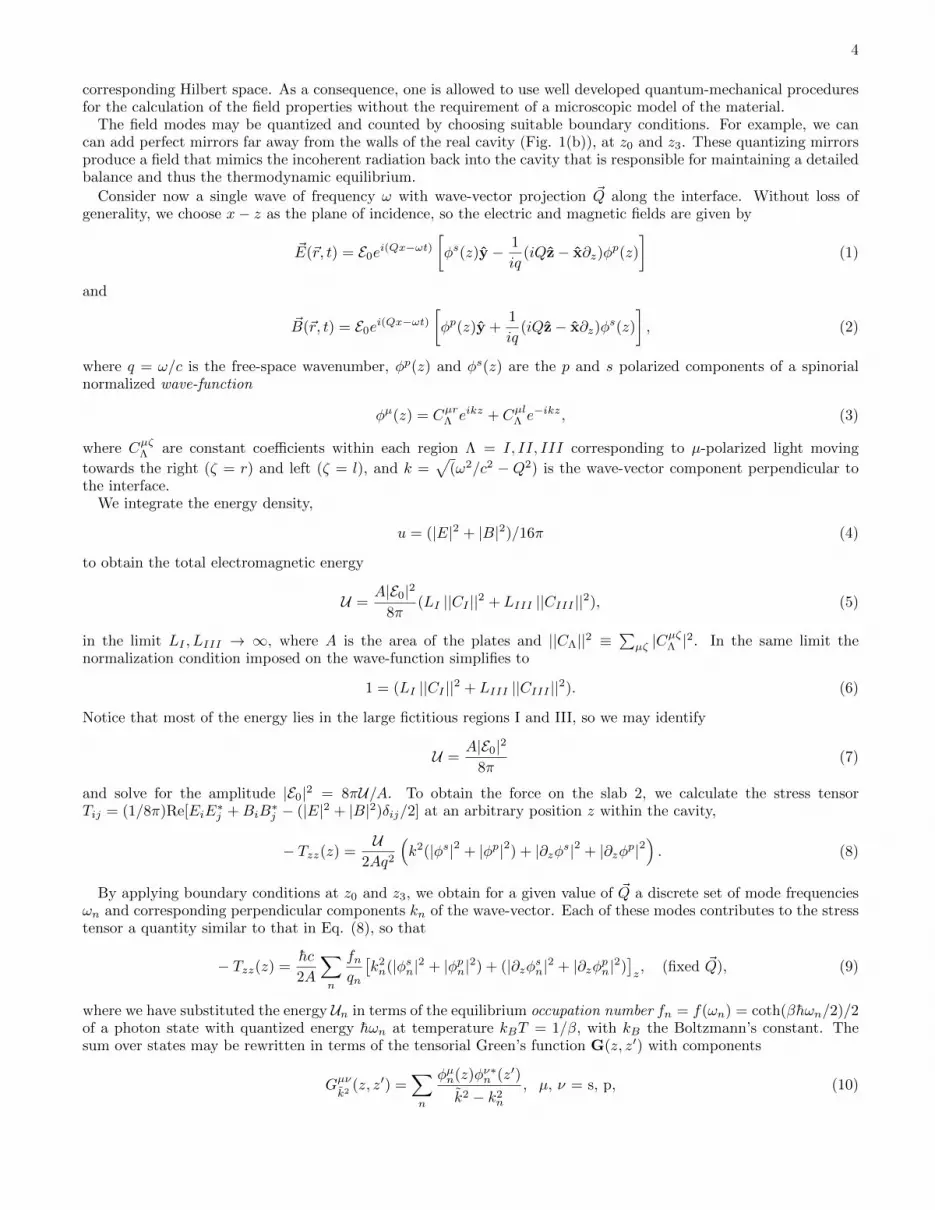
for small real or imaginary frequency.In Fig. 8 we show the torque as a function of the width d for the same system as in Fig. 6 but assuming that

the field propagates only in 1D [48]. The results display the same qualitative behavior as in the 3D case, althoughthe plasma frequency ωp⊥ for which the magnitude of the torque attains its maximum is shifted to a smaller valueωp⊥/ω0 ≈ 1/3 compared to 7/10 in Fig. 6. We may estimate the optimal width for each value of ωp⊥ throughthe following considerations: The exponential in Eq. (41) suppresses the contribution of large imaginary frequenciesu > c/2L to the Casimir effect. Thus, in the retarded regime ωp⊥ > ω0 we may consider mostly low imaginaryfrequencies u/ωpµ < 1 to understand the effect. Furthermore, as the relevant frequency scale is c/L ∼ ω0/π, then thelocalization of the optimal film thickness in the retarded regime could be estimated by substituting |ω| = u = ω0/πwithin Eq. (44). Thus, we obtain dm/L ≈ 0.025, 0.01 and 0.004 for the choices ωp⊥/ω0 = 2 , 3 and 5 respectively.These estimates are in good agreement with the 1D calculation, Fig. 8. In the 3D case one would have to take intoaccount modes that propagate along non-normal directions. However, as the reflection amplitude increases towardsunity for any polarization as the angle of incidence moves away from the normal direction, the anisotropy in thereflectance and the corresponding contribution to the torque also diminish. Thus, the most important contributionsto the torque come from modes that propagate close to the normal and our estimates for dm are also in good qualitativeagreement with our full 3D calculation, Fig. 6.

The simple estimates above fail in the non-retarded regime ωp⊥ < ω0 for both the 1D and 3D calculation, as inthis case a wider range of frequencies, going beyond ωp⊥, ωp‖, contributes to the torque. Furthermore, for smallseparations L the Casimir effect in the 3D case is dominated by surface plasmons [55] which are completely left outof the 1D calculation and of our estimates above.

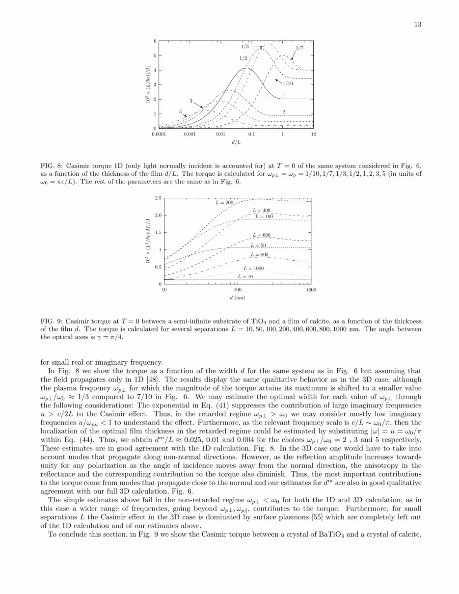
To conclude this section, in Fig. 9 we show the Casimir torque between a crystal of BaTiO3 and a crystal of calcite,

14

as in Ref. [24]. However, instead of two semi-infinite crystals, we consider a thin calcite film over a semi-infiniteBaTiO3 substrate with vacuum in between and we vary the thickness d of the film. We use the same model as in Ref.[24] to describe the dielectric response of the plates along each of their principal directions, namely, two undampedoscillators [56] to account for both the IR and UV resonances. We show results for T = 0 which we expect to holdeven at room temperature for separations in the range L < 1µm. We have confirmed that our numerical results,performed at T = 0, are in agreement with those of Ref. [24] in the limit of very thick plates.

As expected, Fig. 9 shows that for very thin films the torque becomes null, while for thick enough films it attainsits asymptotic value corresponding to semi-infinite plates. Fig. 9 displays small maxima corresponding to an optimalthickness for which the torque is maximized for each value of the separation, analogous to those found above foranisotropic conducting films, although these maxima are very broad. In this case, the maximum torque is about oneorder of magnitude smaller than for the case of anisotropic conductors shown in Fig. 6 when typical metallic plasmafrequencies are chosen, and about two orders of magnitude smaller than for the case of the ideal uniaxial plates shownin Fig. 4.

In order to observe the Casimir torque, several experimental setups have been suggested [24, 57]. If the vacuumCasimir cavity is replaced by a cavity filled with a dielectric liquid, and if the dielectric function of the fluid isintermediate between that of the cavity walls, then the sign of the Casimir force may be reversed, becoming repulsiveinstead of attractive. Munday et al. [24] took advantage of this sign reversal and estimated that a quartz or calciteanisotropic disk with a diameter and a width of some tens of µm would float at a height of about one hundred nmover the surface of a barium titanate anisotropic crystal if immersed in ethanol. At this height, the repulsive Casimirforce would balance the weight of the disk, which would then be able to rotate freely around its axis. Then it wouldbe possible to first align the disk with the polarization of a laser beam and optically monitor the rotation towardsthe equilibrium orientation after the laser beam is turned off. The characteriztic time would depend of the viscosityof the fluid and on the magnitude of the driving Casimir torque which would thus be obtained.

In a second proposal by the same group [57] a large set of much smaller disks of µm scale width and diameter arekept separated a few nanometers from the substrate not by a repulsive Casimir force but by surfactant molecules thatattach to the surfaces of both the substrate and the disks which in this case would be immersed in an electrolyte.The orientation of such small disks would be disrupted by their rotational Brownian motion, but the distribution oftheir orientations would yield **** Sepasuchi.

According to our calculations above, structured materials made up of aligned nanowires embedded in dielectricmatrices are subject to much larger torques than the birefringent crystals considered my Munday et al. [24, 57].Thus, the Casimir torque could be measured using a torsion balance. To avoid alignment problems, a sphericalanisotropic particle could be used instead of a flat disk. Hanging a 50 µm sphere from a 10 µm long aluminum wireof 50 nm radius

frecuencia =100Hz vacıo placa giratoria. 50HZ.

V. CONCLUSIONS

We have extended a fictitious-cavity approach to calculate the Casimir force, energy and torque between anisotropicmedia with a planar geometry in terms only of their optical coefficients. Our results are applicable to arbitraryanisotropic materials which may be conducting or insulating, opaque or transparent, semi-infinite or with a finitethickness, with a non-dispersive or a frequency dependent response, homogeneous or structured, as long as we can cal-culate their corresponding reflection coefficients. Our expressions for the torque were simply obtained by analyticallyderiving the energy with respect to the relative orientation of the plates. The formalism has allowed us to performcalculations at zero and at finite temperature.

We have reproduced some known results and we have calculated the torque for ideal uniaxial systems which arethe anisotropic counterparts to the ideal Casimir mirrors, namely, systems which are perfect conductors along somedirections and perfect insulators along others. We also calculated the torque for systems with a Drude conductivity.As a non trivial application of our formalism, we have calculated the torque for a system consisting of two anisotropicslabs, one of which is a semi-infinite substrate and the other a thin film of thickness d. The slabs were modelled asDrude metals and made up of the same material in order to study the effect of the film thickness in the torque. Ournumerical results show that exists an optimal value of the film thickness where the torque is maximized. We haveestimated the optimal thickness in the retarded regime by studying the anisotropy of the skin depth evaluated atthe characteristic frequency of the cavity; the maximum torque is achieved for films whose thickness is intermediatebetween the largest and the smallest of the two principal skin depths. Finally, we calculated the Casimir torque fora thin film of calcite above a barium titanate substrate. The results seem qualitatively similar although the torque issmaller than that for uniaxial conductors and for the ideal system.

In conclusion, we developed a very general formalism to calculate the Casimir torque and illustrated its use by

15

studying the torque at zero and finite temperatures for ideal and realistic, conducting and insulating systems of semi-infinite and finite widths. We expect that the simplicity and generality of our formalism motivates further studies ofthese relatively unexplored aspects of the Casimir effect between anisotropic media.

Acknowledgments

This work was partially supported by DGAPA-UNAM under grant IN120909.

Appendix

In this appendix we derive the expressions for the matrices t20, r20, t02 and the z-component of the wave-vectorsof the ordinary and extraordinary waves. We derive these expressions by following the method developed in Refs.[51, 53]. We assume that the system is described by the geometry shown in Fig. 2. Thus, the dielectric tensor isgiven by

ε =

ε‖ cos2 ψ + ε⊥ sin2 ψ (ε⊥ − ε‖) sinψ cosψ 0(ε⊥ − ε‖) sinψ cosψ ε⊥ cos2 ψ + ε‖ sin2 ψ 0

0 0 ε⊥

. (45)

All of the quantities above (the dielectric functions and the angles) refer to plate 2, but we omit the correspondingindex (2) in order to simplify our notation. On the other hand, from Maxwell equations, the components of theelectromagnetic field parallel to the x− y plane, can be cast in a set of four differential equations

∂zF = iqΓF , (46)

where

F = (Ex, By, Ey,−Bx)T , (47)

Ex, Ey, Bx and By are the electric and magnetic field components parallel to the interfaces, q is the free-spacewavenumber and Γ is a 4× 4 matrix with elements

Γ11 = − sin θεzx/εzz,Γ12 = 1− sin2 θ/εzz,Γ13 = − sin θεzy/εzz,Γ14 = Γ24 = Γ31 = Γ32 = Γ33 = Γ44 = 0,Γ21 = εxx − εxzεzx/εzz,Γ22 = − sin θεxz/εzz,Γ23 = εxy − εxzεzy/εzz,Γ34 = 1,Γ41 = εyx − εyzεzx/εzz,Γ42 = sin θεyz/εzz,Γ43 = εyy − sin2 θ − εyzεzy/εzz.

(48)

where θ is the angle of incidence. Within a homogeneous medium Γ is independent of z and Eq. (46) has fourparticular solutions of the form

F = F`(0)eik`z, ` = 1, 2, 3, 4, (49)

where k` is the component of the propagation vector parallel to the z-axis. Substitution of Eq. (49) into the Eq. (46)yields the eigenvalue equation

(k`I− qΓ)F`(0) = 0 (50)

whose eigenvalues

k` = ±ko,±ke (51)

16

are

ko = Jq, (52)

ke = Iq/√ε⊥, (53)

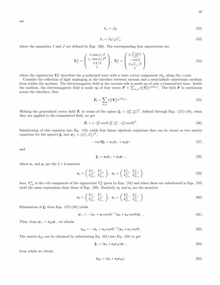
where the quantities I and J are defined by Eqs. (30). The corresponding four eigenvectors are

V o± =

± tanψ/Jε⊥ tanψ/J2

±1/J1

, V e± =

∓J

2 cotψI√ε⊥

− cotψ±√ε⊥/I1

, (54)

where the eigenvector V µσ describes the µ-polarized wave with a wave vector component σkµ along the z-axis.

Consider the reflection of light impinging at the interface between vacuum and a semi-infinite anisotropic mediumfrom within the medium. The electromagnetic field at the vacuum side is made up of only a transmitted wave. Insidethe medium, the electromagnetic field is made up of four waves F =

∑σ,µ ψ

µσV

µσ e

iσkµz. The field F is continuousacross the interface, thus

Ft =∑σ,µ

ψµσVµσ e

iσkµz. (55)

Writing the generalized vector field Ft in terms of the spinor ξt = (ξpt , ξst )T , defined through Eqs. (17)-(18), when

they are applied to the transmitted field, we get

Ft = (−ξpt cos θ, ξpt , ξst ,−ξst cos θ)T . (56)

Substitution of this equation into Eq. (55) yields four linear algebraic equations that can be recast as two matrixequations for the spinors ξt and ψ± = (ψo±, ψ

e±)T ,

− cos θξt = s1ψ+ + s3ψ− (57)

and

ξt = s2ψ+ + s4ψ−, (58)

where s1 and s2 are the 2× 2-matrices

s1 =

(V o1,+ V e1,+V o4,+ V e4,+

), s2 =

(V o2,+ V e2,+V o3,+ V e3,+

), (59)

here, V µi,σ is the i-th component of the eigenvector V µσ given by Eqs. (54) and when these are substituted in Eqs. (59)

yield the same expressions than those of Eqs. (29). Similarly, s3 and s4 are the matrices

s3 =

(V o1,− V e1,−V o4,− V e4,−

), s4 =

(V o2,− V e2,−V o3,− V e3,−

). (60)

Elimination of ξt from Eqs. (57)-(58) yields

ψ+ = −(s1 + s2 cos θ)−1(s3 + s4 cos θ)ψ−. (61)

Thus, from ψ+ = r20ψ− we obtain

r20 = −(s1 + s2 cos θ)−1(s3 + s4 cos θ). (62)

The matrix t20 can be obtained by substituting Eq. (61) into Eq. (58) to get

ξt = (s4 + s2r20)ψ−, (63)

from which we obtain

t20 = (s4 + s2r20). (64)

17

Finally, in order to calculate the matrices t02 and r02, we consider the reflection of light impinging at a semi-infiniteanisotropic medium from vacuum. The electromagnetic field at the medium side is made up of two transmitted waves,F =

∑µ ψ

µ+V

µ+ e

ikµz. Imposing continuity on F across the interface

Fi + Fr =∑µ

ψµ+Vµ

+ eikµz. (65)

Writing the generalized vector field Fi and Fr in terms of the spinors ξi = (ξpi , ξsi )T and ξr = (ξpr , ξ

sr)T we get

Fi = (ξpi cos θ, ξpi , ξsi , ξ

si cos θ)T (66)

and

Fr = (−ξpr cos θ, ξpr , ξsr ,−ξsr cos θ)T . (67)

Substitution of this equation into Eq. (65) yields four linear algebraic equations that can be recast as two matrixequations for the spinors ψ+, ξi and ξr

cos θ(ξi − ξr) = s1ψ+ (68)

and

ξi + ξr = s2ψ+. (69)

Elimination of ψ+ from the last two equations yields

ξr = r02ξi, (70)

where r02 is given by Eq. (28). Elimination of ξr from Eqs. (68)-(69) yields

t02 = s−11 cos θ(I− r02). (71)

This concludes the calculation of the reflection and transmission matrices corresponding to the front surface of thefilm.

[1] H. B. G. Casimir, Proc. Kon. Ned. Akad. Wet. 51, 793 (1948).[2] P. W. Milonni, R. J. Cook, and M. E. Goggin, Phys. Rev. A 38, 1621 (1988).[3] R. A. Beth, Phys. Rev. 50, 115 (1936).[4] S. K. Lamoreaux, Phys. Rev. Lett. 78, 5 (1997).[5] U. Mohideen, and A. Roy, Phys. Rev. Lett. 81, 4549 (1998).[6] A. Roy, C. Y. Lin, and U. Mohideen, Phys. Rev. D 60, 111101(R) (1999).[7] B. W. Harris, F. Chen, and U. Mohideen, Phys. Rev. A 62, 052109 (2000).[8] M. Bordag, U. Mohideen, and V. M. Mostepanenko, Phys. Rep. 353, 1 (2001).[9] F. Chen, U. Mohideen, G. L. Klimchitskaya, and V. M. Mostepanenko, Phys. Rev. A 66, 032113 (2002).

[10] F. Chen, U. Mohideen, G. L. Klimchitskaya, and V. M. Mostepanenko, Phys. Rev. A 73, 019905 (2006).[11] H.B. Chan, V. A. Aksyuk, R. N. Kleinman, D. J. Bishop, and F. Capasso, Science 291, 1941 (2001).[12] H. B. Chan, V. A. Aksyuk, R. N. Kleinman, D. J. Bishop, and F. Capasso, Phys. Rev. Lett. 87, 211801 (2001).[13] D. Iannuzi, M. Lisanti, and F. Capasso, Proc. Natl. Acad. of Sci. (USA) 101, 4019 (2004).[14] M. Lisanti, D. Iannuzi, and F. Capasso, Proc. Natl. Acad. of Sci. (USA) 102, 11989 (2005).[15] G. Bressi, G. Carugno, R. Onofrio, and G. Ruoso, Phys. Rev. Lett. 88, 041804 (2002).[16] R. S. Decca, E. Fischbach, G. L. Klimchitskaya, D.E. Krause, D. Lopez, and V. M. Mostepanenko, Phys. Rev. D 68,

116003 (2003).[17] R. S. Decca, D. Lopez, E. Fischbach, G. L. Klimchitskaya, D. E. Krause, and V. M. Mostepanenko, Ann. of Phys. (N. Y.)

318, 37 (2005).[18] E. M. Lifshitz, Sov. Phys. JETP 2, 73 (1956).[19] V. A. Parsegian, and G. H. Weiss, J. Adhes. 3, 259 (1972).[20] Y. S. Barash, Izv. Vyssh. Uchebn. Zaved., Radiofiz. 21, 1637 (1978)[Radiophys. and Q. Elect. 12, 1138 (1979)].[21] Y. S. Barash, and V. L. Ginzburg, Sov. Phys. Usp. 18, 305 (1975).[22] D. Kupiszewska, Phys. Rev. A 46, 2286 (1992).[23] S.J. van Enk, Phys. Rev. A 52, 2569 (1995).

18

[24] J. N. Munday, D. Iannuzzi, Y. Barash, and F. Capasso, Phys. Rev. A 71, 042102 (2005).[25] C. G. Shao, A. H. Tong, and J. Luo, Phys. Rev. A 72, 022102 (2005).[26] C. G. Shao, D. L. Zheng, and J. Luo, Phys. Rev. A 74, 012103 (2006).[27] O. Kenneth, and S. Nussinov, Phys. Rev. D 63, 121701(R) (2001).[28] H. Li, and M. Kardar, Phys. Rev. Lett. 67, 3275 (1991).[29] H. Li, and M. Kardar, Phys. Rev. A 46, 6490 (1992).[30] M. T. Jaekel, and S. Reynaud, J. Phys. 1, 1395 (1991); C. Genet, A. Lambrecht, and S. Reynaud, Phys. Rev. A 67, 043811

(2003).[31] A. Lambrecht, P. A. M. Neto, and S. Reynaud, New J. Phys. 8, 243 (2006).[32] R. Esquivel-Sirvent, C. Villarreal, W. L. Mochan, and G. H. Cocoletzi, Phys. Status Solidi B 230, 409 (2002).[33] W. L. Mochan, C. Villarreal, and R. Esquivel-Sirvent, Rev. Mex. Fıs. 48, 335 (2002).[34] R. Esquivel, C. Villarreal, and W. L. Mochan, Phys. Rev. A 68, 052103 (2003).[35] R. Esquivel, C. Villarreal, and W. L. Mochan, Phys. Rev. A 71, 029904 (2005).[36] W. L. Mochan, A. M. Contreras-Reyes, R. Esquivel-Sirvent and C. Villarreal, Statistical Physics and Beyond: 2nd Mexican

Meeting on Mathematical and Experimental Physics ed. by F. J. Uribe et al. (AIP Conference Proceedings, vol 757)(American Institute of Physics, Melville, 2005) p 66.

[37] P. Halevi, Spatial Dispersion in Solids and Plasmas, Electronic Waves Vol 1 (Amsterdam: North-Holland, 1992); P. Halevi,Photonic Probes of Surfaces (Amsterdam: Elsevier, 1995).

[38] J. A. Stratton, Electromagnetic Theory (New York: Mc Graw-Hill, 1941).[39] P. A. M. Neto, A. Lambrecht, and S. Reynaud, Phys. Rev. A 72, 012115 (2005).[40] R. B. Rodrigues, P. A. M. Neto, A. Lambrecht, and S. Reynaud, Phys. Rev. Lett. 96, 100402 (2006).[41] R. B. Rodrigues, P. A. M. Neto, A. Lambrecht, and S. Reynaud, Europhys. Lett. 76, 822 (2006).[42] F. S. S. Rosa, D. A. R. Dalvit, and P. W. Milonni Phys. Rev. A 78, 032117 (2008).[43] R. Esquivel-Sirvent, C. Villarreal, and G. H. Cocoletzi, Phys. Rev. A 64, 052108 (2001); C. Villarreal, R. Esquivel-Sirvent,

and G. H. Cocoletzi, Int. J. of Modern Phys. A 17, 798 (2002).[44] A. D. H. de la Luz, A. F. Alvarado-Garcıa, G. H. Cocoletzi et. al., Solid State Commun. 132, 623 (2004).[45] R. Esquivel-Sirvent, C. Villarreal, W. L. Mochan, A. M. Contreras-Reyes, and V. B. Svetovoy, J. Phys. A: Math. Gen. 39,

6323 (2006).[46] A. M. Contreras-Reyes, and W. L. Mochan, Phys. Rev. A 72, 034102 (2005).[47] L. M. Procopio, C. Villareal, and W. L. Mochan, J. Phys. A: Math. Gen. 39, 6679 (2006).[48] J. C. Torres-Guzman, and W. L. Mochan, J. Phys. A: Math. Gen. 39, 6791 (2006).[49] W. L. Mochan, and C. Villarreal, New J. of Phys. 8, 242 (2006).[50] T. P. Sosnowski, Opt. Commun. 4, 408 (1972).[51] R. M. A. Azzam, N. M. Bashara, Ellipsometry and polarized light (Amsterdam:North-Holland, 1977).[52] G. B. Airy, Phil. Mag. 2, 20 (1833).[53] D. W. Berreman, J. Opt. Soc. Am. 62, 502 (1972).[54] M. Born, and E. Wolf, Principles of Optics, 7th. Edition (Cambridge University Press, 1999).[55] F. Intravia, and A. Lambrecht, Phys. Rev. Lett. 94, 110404 (2005).[56] L. Bergstrom, Adv. Colloid Interface Sci. 70, 125 (1997).[57] Jeremy N. Munday, Davide iannuzzi, and Federico Capasso, New J. Phys. 8, 244 (2006).