3

The

Bas

el II

Acc

ord

on M

easu

ring

and

Man

agin

g a

Ban

k’s

Ris

ks

The Basel II Accord on Measuringand Managing a Bank’s Risks

�

Ion StancuPh.D. Professor

Academy of Economic Studies, BucharestAndrei TincaCandidate Ph.D.

Webster University, Vienna

Abstract. The abundance of risk metrics stems from the effort to measure the difference between the

expected and actual returns, under a hypothesis of normality. Under the assumption of risk aversion,

investors are likely to quantify risk using metrics which measure returns lower than the expected average.

These include the semi-variance of returns smaller than the average, the risk of loss – a return under a

chosen level, usually 0%, and value-at-risk, for the greatest losses, with a probability of less than 1-5% in

a given period of time.

The Basel II accord improves on the way risks are measured, by allowing banks greater flexibility.

There is an increase in the complexity of measuring credit risks, the market risks measurement methods

remain the same, and the measurement of operational risk is introduced for the first time.

The most advanced (and widely-used) risk metrics are based on VaR. However, it must be noted that

VaR calculations are statistical, and therefore unlikely to forecast extraordinary events. So the quality of

a VaR calculation must be checked using back-testing, and if the VaR value fails in a percentage of 1-5%

of the cases, then the premises of the model must be changed.

Key words: Risk; Value-At-Risk; Basel II; Capital Adequacy; Monte-Carlo Simulation.

�

1. Defining Risk

Risk is defined as the uncertainty of an investment’s

rate of return – the probability that the realized return

will vary from the expected return as a result of the

influence of market and environmental factors. Some of

the factors exerting influence on the investment’s return

can be forecasted, but most cannot. Risk is determined by

the frequency and the size of the differences between

expected and realized returns, and their distribution

around the average expected return.

Risk metrics quantify the uncertainty of the expected

return. These measures are important for portfolio

construction and performance assessment, because a

principal assumption if investing is that to achieve a

given level of return; investments with lower risk are

preferred over those with higher risks. Normally,

investments with higher risks are expected to have higher

returns than investments with lower risks.

4

Th

eore

tica

l an

d A

pp

lied

Eco

no

mic

s Risk estimation is based on the historical data of

different asset classes. Starting from the hypothesis that

the past is a good predictor for the future, the historical

data are the best foundation available for risk

measurement. However, the future never quite repeats the

past. The proverbial “hundred-year storm” can unsettle

even the best predictions, based on the most advanced

forecasting techniques.

Even if risk cannot be predicted with certainty, risk

metrics provide critical information to help answer the most

important questions for any investor: How should a portfolio

be invested optimally, to achieve its objectives? Risk metrics

have also proven reliable for comparing the relative risks of

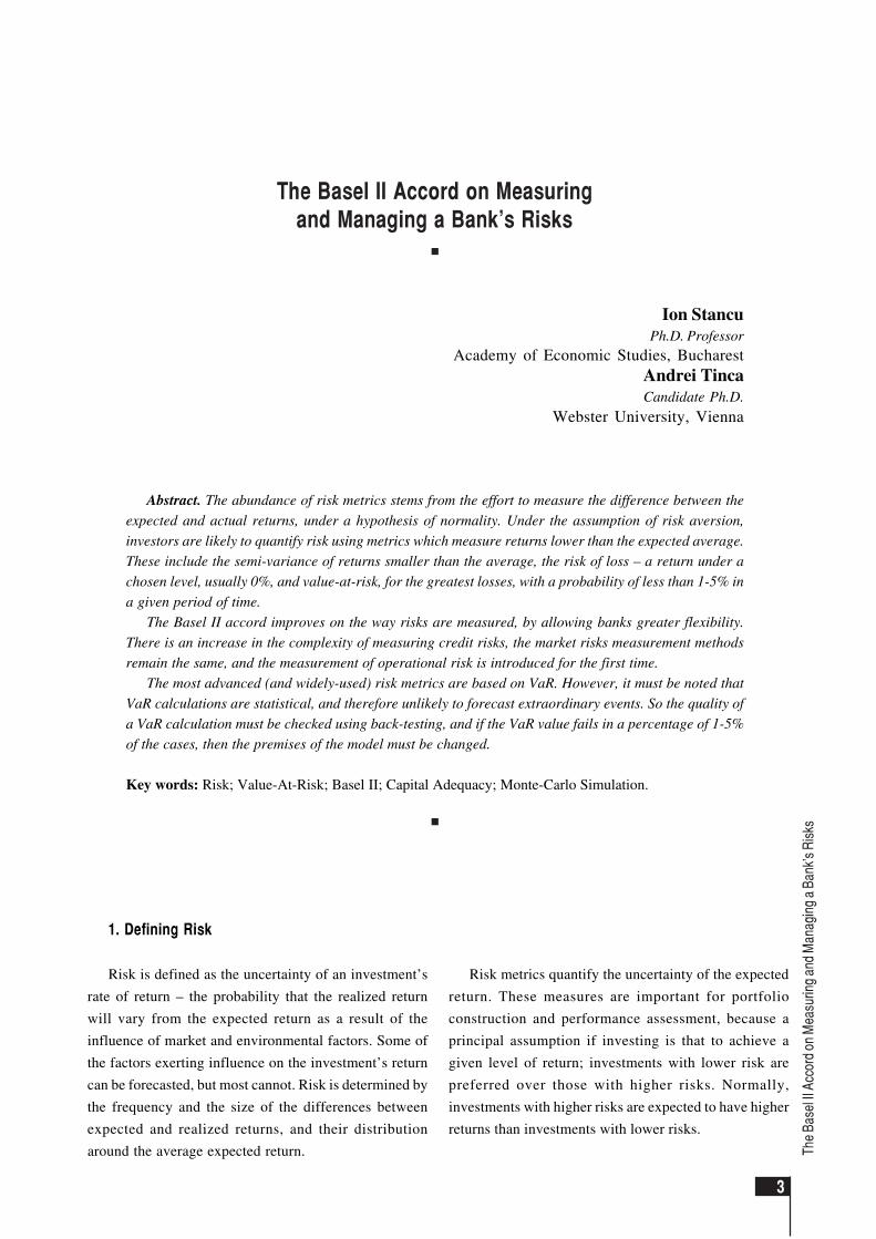
different asset classes. Figure 1 shows that increasing the

percentage of stocks in the portfolio increases volatility

(stocks have annual average returns of 10.5%, twice as large

as bonds, but stocks also have negative returns of – 40%).

Risk metrics are classified in two categories: absolute

and relative. Successful use of risk metrics depends on

selecting measures that are consistent with a portfolio’s

objectives. The amount and the quality of available data

are of great importance.

2. Risk Metrics

When using and quantifying risk metrics, we are

assuming a hypothesis of normality – that is, that the

returns are normally distributed around the average return.

This hypothesis is usually true.

Source: Ambrosio Frank, 2007, An Evaluation of Risk Metrics, Vanguard.

Figure 1. Range of returns for different stock and bond allocations, 1926-2006

2.1. Absolute Risk Metrics

The most usual absolute risk metrics are the variance,

standard deviation, value-at-risk, risk of loss and shortfall

risk. Next we will define these metrics and comment on

their limitations.

Variance )( 2σ is the average of the squared differences

between the real and expected returns(1):

( ) ( ) ( )

( )∑=

−−

=

=−

−++−+−=σ

T

1t

2t

2T

22

212

RR1T

11T

RR...RRRR

5

The

Bas

el II

Acc

ord

on M

easu

ring

and

Man

agin

g a

Ban

k’s

Ris

ks

The standard deviation (σ) is the squared root of the

variance(2):

( )∑ −−

=σt

2t

2 RR1T

1

The standard deviation, which is a basic statistical

metric, is commonly used to measure the fluctuation of a

portfolio’s return. A larger standard deviation shows a

greater fluctuation in the returns of a portfolio, as

compared to the portfolio’s average return. For example,

consider a portfolio with an average return of 10% and

standard deviation of 15%. The portfolio’s returns will

be between – 5% and 25% in 68.3% of the cases, according

to the normal distribution.

The standard deviation can be an useful measure for

portfolios such as pension funds, which are concerned with

the consequences of both positive and negative deviations

from the specific target return. The standard deviation is

less suited for investors concerned with negative deviations

from the average. Also, this metric assumes a normal

distribution, which limits its applicability somehow.

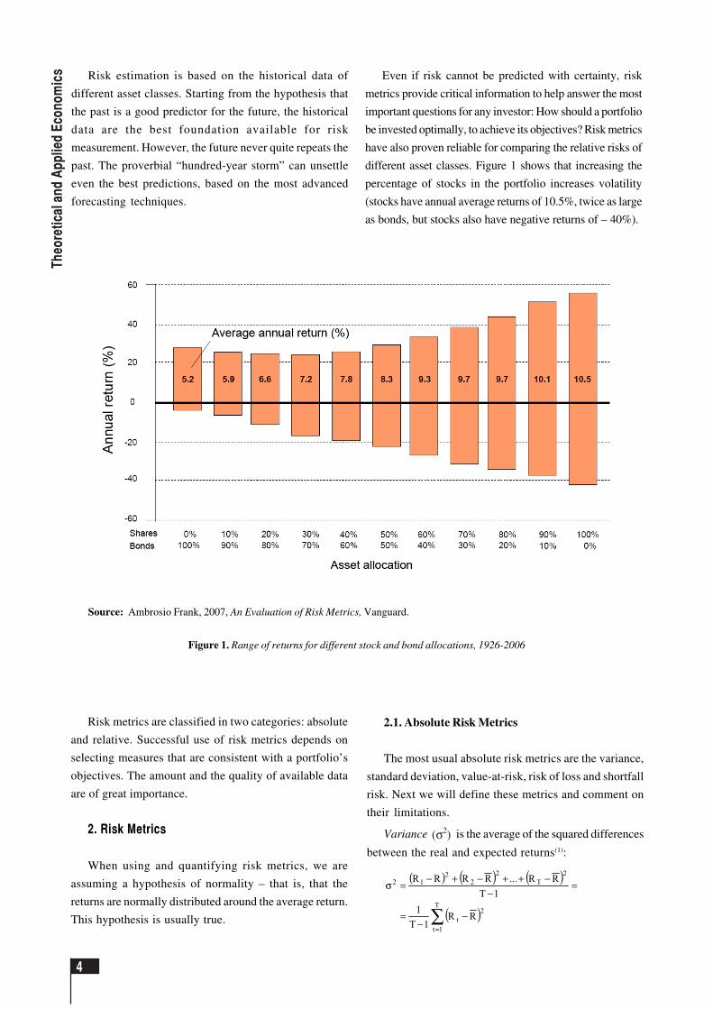
The symmetry of deviations from the average means

that the number of observations higher than the average

will be equal to the number of observations lower than

the average and so the standard deviation is a measure of

the total deviation from the average. Thus, some

researchers propose semi-variance as the risk of lower

than average returns. These negative deviations can be

compared to the average (semi-variance), or, more

interestingly, with the lowest accepted return ( R ≤ 0 ⇒zero return), which needs to be realized as a minimum-

accepted condition (the safety-first criteria).

The semi-variance measures the risks that future returns

will be less than the average, and the safety-first metric

measures the risk that returns will be less than zero.

Actually, the “safety-first” metric is an expression of

the return – risk metric, where risk is measured by the

semi-variance of the deviations, or those under break even

(BE), and not those both to the left and the right of the

average (see Figure 3).

Source: Ambrosio Frank, 2007, An Evaluation of Risk Metrics, Vanguard.

Figure 2. The different risk metrics

Figure 3. Representation of the safety-first metric

p(P M )

50% 50%

P M 0 µ

6

Th

eore

tica

l an

d A

pp

lied

Eco

no

mic

s The safety-first metric is most widely used to measure

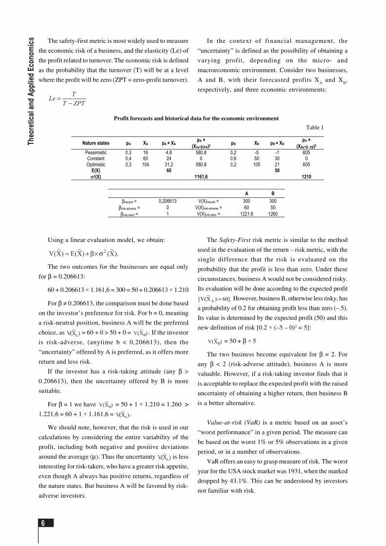
the economic risk of a business, and the elasticity (Le) of

the profit related to turnover. The economic risk is defined

as the probability that the turnover (T) will be at a level

where the profit will be zero (ZPT = zero-profit turnover).

ZPTTTLe

−=

In the context of financial management, the

“uncertainty” is defined as the possibility of obtaining a

varying profit, depending on the micro- and

macroeconomic environment. Consider two businesses,

A and B, with their forecasted profits XA and X

B,

respectively, and three economic environments:

Using a linear evaluation model, we obtain:

).X~()X~(E)X~(V 2σ×β+=

The two outcomes for the businesses are equal only

for β = 0.206613:

60 + 0.206613 × 1.161,6 = 300 = 50 + 0.206613 × 1.210

For β ≠ 0.206613, the comparison must be done based

on the investor’s preference for risk. For b = 0, meaning

a risk-neutral position, business A will be the preferred

choice, as )X~(V A = 60 + 0 > 50 + 0 = )X~(V B . If the investor

is risk-adverse, (anytime b < 0,206613), then the

“uncertainty” offered by A is preferred, as it offers more

return and less risk.

If the investor has a risk-taking attitude (any β >

0.206613), then the uncertainty offered by B is more

suitable.

For β = 1 we have )X~(V B = 50 + 1 × 1.210 = 1.260 >

1.221,6 = 60 + 1 × 1.161,6 = )X~(V A .

We should note, however, that the risk is used in our

calculations by considering the entire variability of the

profit, including both negative and positive deviations

around the average (µ). Thus the uncertainty )X~(V A is less

interesting for risk-takers, who have a greater risk appetite,

even though A always has positive returns, regardless of

the nature states. But business A will be favored by risk-

adverse investors.

Nature states pA XA pA × XA pA ×

(XAs-µXA)2 pB XB pB × XB pA ×

(XBs-µ XB)2

Pessimistic 0,3 16 4,8 580,8 0,2 -5 -1 605 Constant 0,4 60 24 0 0,6 50 30 0 Optimistic 0,3 104 31,2 580,8 0,2 105 21 605

E(X) 60 50 σ2(X) 1161,6 1210

A B

βneutral = 0,206613 V(X)neutral = 300 300 βrisk-adverse = 0 V(X)risk-adverse = 60 50 βrisk-taker = 1 V(X)risk-taker = 1221,6 1260

Profit forecasts and historical data for the economic environment

Table 1

The Safety-First risk metric is similar to the method

used in the evaluation of the return – risk metric, with the

single difference that the risk is evaluated on the

probability that the profit is less than zero. Under these

circumstances, business A would not be considered risky.

Its evaluation will be done according to the expected profit

].60)X~(V[ A = However, business B, otherwise less risky, has

a probability of 0.2 for obtaining profit less than zero (– 5).

Its value is determined by the expected profit (50) and this

new definition of risk [0.2 × (–5 – 0)2 = 5]:

)X~(V B = 50 + β × 5

The two business become equivalent for β = 2. For

any β < 2 (risk-adverse attitude), business A is more

valuable. However, if a risk-taking investor finds that it

is acceptable to replace the expected profit with the raised

uncertainty of obtaining a higher return, then business B

is a better alternative.

Value-at-risk (VaR) is a metric based on an asset’s

“worst performance” in a given period. The measure can

be based on the worst 1% or 5% observations in a given

period, or in a number of observations.

VaR offers an easy to grasp measure of risk. The worst

year for the USA stock market was 1931, when the marked

dropped by 43.1%. This can be understood by investors

not familiar with risk.

7

The

Bas

el II

Acc

ord

on M

easu

ring

and

Man

agin

g a

Ban

k’s

Ris

ks

Because VaR considers the worst results, but ignores

their frequency, many risk analysts prefer to use VaR

together with other risk metrics. Thus, VaR is frequently

used in conjunction with the risk of loss.

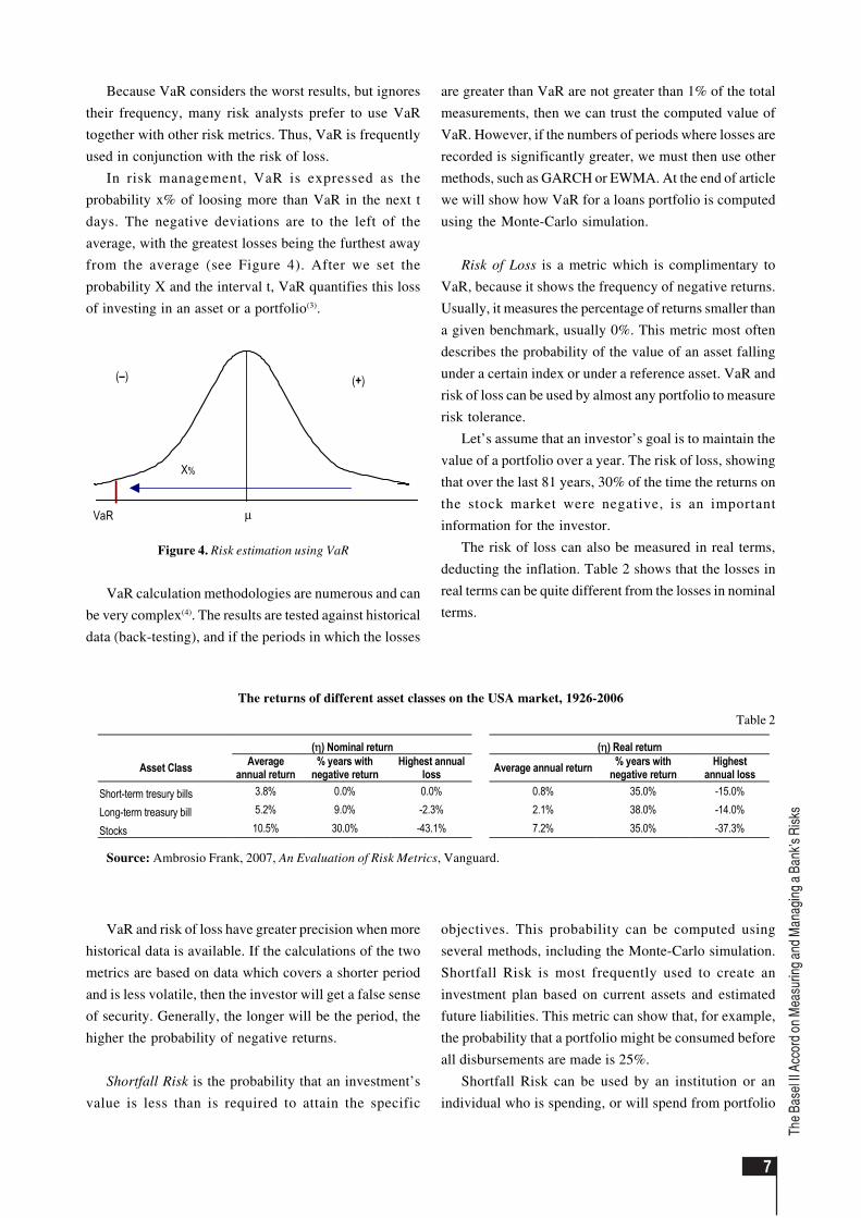
In risk management, VaR is expressed as the

probability x% of loosing more than VaR in the next t

days. The negative deviations are to the left of the

average, with the greatest losses being the furthest away

from the average (see Figure 4). After we set the

probability X and the interval t, VaR quantifies this loss

of investing in an asset or a portfolio(3).

are greater than VaR are not greater than 1% of the total

measurements, then we can trust the computed value of

VaR. However, if the numbers of periods where losses are

recorded is significantly greater, we must then use other

methods, such as GARCH or EWMA. At the end of article

we will show how VaR for a loans portfolio is computed

using the Monte-Carlo simulation.

Risk of Loss is a metric which is complimentary to

VaR, because it shows the frequency of negative returns.

Usually, it measures the percentage of returns smaller than

a given benchmark, usually 0%. This metric most often

describes the probability of the value of an asset falling

under a certain index or under a reference asset. VaR and

risk of loss can be used by almost any portfolio to measure

risk tolerance.

Let’s assume that an investor’s goal is to maintain the

value of a portfolio over a year. The risk of loss, showing

that over the last 81 years, 30% of the time the returns on

the stock market were negative, is an important

information for the investor.

The risk of loss can also be measured in real terms,

deducting the inflation. Table 2 shows that the losses in

real terms can be quite different from the losses in nominal

terms.

VaR

X%

µ

(–) (+)

Figure 4. Risk estimation using VaR

VaR calculation methodologies are numerous and can

be very complex(4). The results are tested against historical

data (back-testing), and if the periods in which the losses

VaR and risk of loss have greater precision when more

historical data is available. If the calculations of the two

metrics are based on data which covers a shorter period

and is less volatile, then the investor will get a false sense

of security. Generally, the longer will be the period, the

higher the probability of negative returns.

Shortfall Risk is the probability that an investment’s

value is less than is required to attain the specific

objectives. This probability can be computed using

several methods, including the Monte-Carlo simulation.

Shortfall Risk is most frequently used to create an

investment plan based on current assets and estimated

future liabilities. This metric can show that, for example,

the probability that a portfolio might be consumed before

all disbursements are made is 25%.

Shortfall Risk can be used by an institution or an

individual who is spending, or will spend from portfolio

The returns of different asset classes on the USA market, 1926-2006

Table 2

(η) Nominal return (η) Real return

Asset Class Average annual return

% years with negative return

Highest annual loss Average annual return % years with

negative return Highest

annual loss Short-term tresury bills 3.8% 0.0% 0.0% 0.8% 35.0% -15.0%

Long-term treasury bill 5.2% 9.0% -2.3% 2.1% 38.0% -14.0%

Stocks 10.5% 30.0% -43.1% 7.2% 35.0% -37.3%

Source: Ambrosio Frank, 2007, An Evaluation of Risk Metrics, Vanguard.

8

Th

eore

tica

l an

d A

pp

lied

Eco

no

mic

s assets. Examples include foundations, pension funds, and

persons investing in pension funds. Although the result

is a simple percentage, it can be very complex to calculate

and understand. Small changes in the premises might

cause large changes in the end results. The quality of the

calculation is strongly dependent on the initial data, and

most of the time the initial data is not accurate and

contains estimation errors.

2.2. Relative measures of risk

The most frequently used relative risk measures are

excess return, tracking error, Sharpe ratio, information

ratio, beta and Treynor ratio.

Excess return is the return of an asset above or below

an index or reference security, for example a sovereign

bond(5). Excess return is calculated by subtracting the

benchmark’s return from that of the security, for example,

if an asset has a return of 11% and its benchmark has a

return of 10%, then the excess return is 1%.

Investment advisors use excess return to compare a

portfolio’s performance with its chosen index. The

relevance of this calculation rests upon several premises:

that the total risk of a portfolio is similar to the benchmark’s

risk, and that the returns of both portfolio and benchmark

fluctuate in the same direction. If these two conditions

are not met, the metric will be of little use. For example, a

portfolio can be riskier than an index, but excess return

cannot measure this risk.

Tracking error is the standard deviation of excess

return. Like the standard deviation of the portfolio,

tracking error assumes that the returns are normally

distributed. This measure combines both positive and

negative results. For example, consider a fund which has

no excess return compared to an index, over the long

term, but it has a tracking error of 0.1%. If the benchmark

has a 10% annual return, then the asset’s return will fall

within 9.9% and 10.1% in 68% of the cases (according to

the normal distribution law).

Tracking error is used to determine how close a

portfolio’s performance matches that of a benchmark.

Fund managers which are tied to a benchmark can use

tracking error to describe the deviation from the

benchmark. The metric can also be used to monitor the

performance of funds with controlled risk, which have

objectives such as generating returns 0.5% above a certain

Sharpe Ratio 1970-1981 1982-1999 2000-2006 Commodities 0.3984 0.1654 0.3356 Real estate 0.2577 0.4724 1.392 International developed stock markets 0.0841 0.4809 0.0911 U.S. stock market 0.0301 0.7381 -0.0806 U.S. long-term Treasury bonds -0.2743 0.5647 0.5914

benchmark. Like the standard deviation of a portfolio,

tracking error is not suitable for those concentrating only

on downside risk.

Tracking error is also less relevant for funds which are

not tied to a certain benchmark. However, this metric is

used for calculating the information ratio, which is used

for comparing fund managers.

The Sharpe ratio represents the return of a portfolio

adjusted for risk. Practically, profit is measured for every

“unity” of risk. To calculate the Sharpe ration, an asset’s

excess return is divided by the asset’s standard deviation:

,/)RR(Sh portfport σ−=

The Sharpe ratio can be negative if the asset’s

performance is worse than the market. For a long-term

evaluation, the metric’s values fall between 0 to +1. A

larger value of the metric means a better performing asset.

The metric is used to measure similar class of assets or

assets with similar liquidity. The metric depends on the

time period used for calculation, which is illustrated in

Table 3:

Sharpe Ratio for different asset classes

from 1970 to 2006

Table 3

Source: Marrison Chris, 2002, The Fundamentals of Risk

Measurement, McGraw Hill.

However, the Sharpe ratio can lead to unwanted results

if used without good consideration. As Table 3 shows,

the metric has higher values during times of peak

performance, as was the case with the stock market during

1999. However, the Sharpe ratio was a poor indicator at

that point of the following period of market

underperformance.

The Information ratio represents an asset’s return

adjusted for risk, compared to a benchmark. To calculate

this metric, the excess return is divided by the tracking

error relative to a benchmark. The metric is generally

used to compare the performance of different fund

managers.

9

The

Bas

el II

Acc

ord

on M

easu

ring

and

Man

agin

g a

Ban

k’s

Ris

ks

An investment fund with excess return of 10% and a

tracking error of 20% relative to an index has an

information ratio of 0.5. Another fund with excess return

of 10% and tracking error of 40% has an information

ratio of 0.25. Everything else being constant, a higher

value of the metric indicates better performance.

Like Sharpe ratio, the information ratio is very

dependent upon the time period used for calculation. This

metric can also show high values in periods of maximum

performance, which can be misguiding.

Beta is a measure of an asset’s volatility in relation to

the rest of the market. The market is assumed to have a

beta equal to 1. If a portfolio has a beta of 1.20, then the

portfolio’s value will rise or fall by 12% when the market

rises or falls by 10%. Beta is used to measure systemic

risk (or market risk) of an investment and can be used to

aid in deciding whether an asset should be included in a

portfolio.

Portfolio and hedge fund managers regard beta as a

measure of risk. For example, managers who does not

want to be exposed to market fluctuations will use

neutralize the beta values of long positions with the beta

of short positions, to reduce the portfolio’s beta. However,

when calculating beta, the choice of the benchmark is

essential. Beta computed for a portfolio with a different

risk profile will not be relevant for the total portfolio

volatility. Also, the value of beta changes in time and

therefore a periodical re-balancing is necessary to

maintain a proper value for the metric.

The Treynor ratio describes return adjusted to risk,

compared to the market. It is calculated by dividing

excess return by beta:

,/)RR(Tr portfport β−=

The Treynor ratio measures return per unit of risk. The

metric also assumes that all non-systemic risk has been

diversified and that only systemic risk remains. Therefore,

the Treynor ratio is used to compare funds which are very

well diversified.

An investment fund with excess returns of 1% and a

beta of 1.20 will have a Treynor ratio of 0.833. A higher

value is better, all other factors being constant.

Because the Treynor ratio is based on beta, it will

share the same limitations. Moreover, the Treynor ratio

amplifies beta’s change over time, and thus changes in

the Treynor ratio do not always reflect major changes in

risk.

3. The Basel II Accord on Risks and VaR

In June 2004, the Basel Committee has finalized a

revision of Basel I. Owing to the development of risk

evaluation methods which increased the complexity

of banking operations, as well as the lack of operational

risk in Basel I, the Basel II accord was issued at the end

of 2003. From that point on, the banks had three years

to implement the Basel II accord. The deadline for

implementation was set for the end of 2006, with credit

and operational risk set for 2007. The Basel II accord

is based on three pillars, which are mutually re-

enforcing:

Pillar I: Capital adequacy. The first pillar establishes

the measurement methods for credit, market and

operational risk. The Total Cost of Risk (TCR) is obtained

by summing Credit Risk Cost (CRC), Market Risk Cost

(MRC), and Operational Risk Cost (ORC), respectively,

so that:

Capital > TCR = CRC + MRC +ORC

According to Pillar I, banks must calculate their

solvency ratio:

)loperationa.rmarket.rcredit.r(assetsweightedRiskcapitalTotal

%)8.(minCapitalBank

++=

=

The changes brought by Basel II affect in most part

the risk evaluation methods. Thus, the methods used for

measuring credit risk are the most advanced, those for

market risk are unchanged, and those for operational risk

are introduced for the first time. The Accord contains

three methods for measuring credit and operational risk

and two for market risk.

Methods for measuring credit risk

1. Standard approach (a modified Basel I version)

2. Foundation internal-rating based (IRB)

3. Advanced fundamental internal-ratings based

(A-IRB).

For credit risk, the standard approach is an extension

of Basel I, and it uses weights determined by external

rating agencies. Internal rating methods are more

advanced and use data on losses affecting the bank.

However, the most advanced methods are those based

on VaR.

10

Th

eore

tica

l an

d A

pp

lied

Eco

no

mic

s Methods for measuring market risk (similar to Basel I)

1. Basic indicator approach (BIA)

2. Internal methods.

Methods for measuring operational risk

1. Basic indicator approach (BIA)

2. Standardized approach

3. Internal based, with

3.1. Foundation IRB, and

3.2. Advanced IRB.

Each method is increasingly complex. It is appreciated

that the increasing complexity will lead to more precise

calculations and less required capital.

Pillar II: Supervisory review process. This pillar

consists in the extended role assumed by the supervisory

body, which includes assurance that banks operate with

adequate capital, and that they have the functioning

internal processes required to evaluate risks and take the

necessary measures when required. According to this

pillar, the BNR (the Romanian National Bank) requires

that every financial institution creates and validates a set

of internal processes used to calculate the required funds

in accordance with each institution’s risk profile.

This pillar is based on four principles:

1. Banks must evaluate capital requirements in

accordance with the risks;

2. The supervisor must determine whether the bank’s

capital adequacy;

3. It is expected that banks will operate above the

minimum capital level;

4. The supervisor must identify problems early on and

apply the necessary measures.

Pillar III: Market discipline. This pillar defines a series

of requirements regarding the transparency and

communication of precise information regarding risk

exposures, risk profiles and risk management. Banks are

required to publish organizational and strategic

information relating to risk, financial information

(structure and total value of own funds, accounting

methods for assets and liabilities), information relating

to credit risk (total, structure), and information relating

to operational risk (events leading to possible losses).

Banks must publish reports detailing risks and capital

requirements. The transparency is expected benefit clients,

stakeholders, and the banks themselves.

Requirements for the management of credit,

market, and operational risk

Credit risk: even banks with enough capital reserves

must analyze in detail their own capital positions. Risk

management techniques include collateral, guarantees

and derivatives (for banks dealing with derivatives).

The complexity of the required data is significant.

Therefore, a robust and auditable database is required.

Credit systems will not only have to respond to

management queries, but also to external control and

regulators. According to Basel II and to its new rating

methodology, capital requirements have grown, which

can have a negative impact for credit extension, with

unwanted macroeconomic effects.

Operational risk must be treated in financial institutions

according to the industry best-practices, making use of

adequate risk modeling and reduction techniques,

including outsourcing. Financial institutions and their

internal audit departments must pay attention to defining,

calculating, measuring and communicating risk.

Market risk: the reporting and aggregation of all risk

factors at a market level should create a transparent

environment. The Basel II accord creates the premises for

conformity at an institution’s level, as well as for the

whole market. The Basel II accord aims to significantly

increase transparency by requiring banks to issue yearly

or quarterly reports which show losses and exposures

generated by risk management. These measures are meant

to control and stop unwanted events in the credit activity,

enhancing market discipline.

In conclusion, we will present some of the new Basel

accord’s positive and negative aspects:

Source: Jorion Philippe, 2007, Value at Risk – The New

Benchmark for Managing Financial Risk, McGraw Hill.

Following are some more industry critics regarding

the new Accord:

� The implementation of a risk management system

can be very expensive;

POSITIVE NEGATIVE

Encourages banks to build performing portfolios

Mathematical models cannot emulate real-world events

Recognizes advances in risk management

There is a probability of lower external ratings

Offers incentives for improving risk management

Economic cycles will cause variations in capital requirement

Increases the role of the markets

The complexity of the new accord

11

The

Bas

el II

Acc

ord

on M

easu

ring

and

Man

agin

g a

Ban

k’s

Ris

ks

� It is possible that “cascade” events take place when

multiple institutions, using the same risk metrics

(VaR, for example) effectuate similar operations.

This behavior has been connected to the 1987

crash, and there is a probability that financial

regulation amplifies market trends;

� Regulation can give a false sense of security.

4. Calculating VaR for a loan portfolio using the

Monte Carlo simulation

Suppose a bank has a portfolio of 30 loans given out

to customers. For each of these loans we know the size,

the rating, and the probability of default in basis points.

We are required to find out VaR 5%, simulating 1,000

possible values for the portfolio. The correlation factor ñ

between the return factor F and the simulated value åi has

the given value of 0.6. If a client defaults, then the whole

sum is assumed to be lost.

The credit portfolio

Table 4

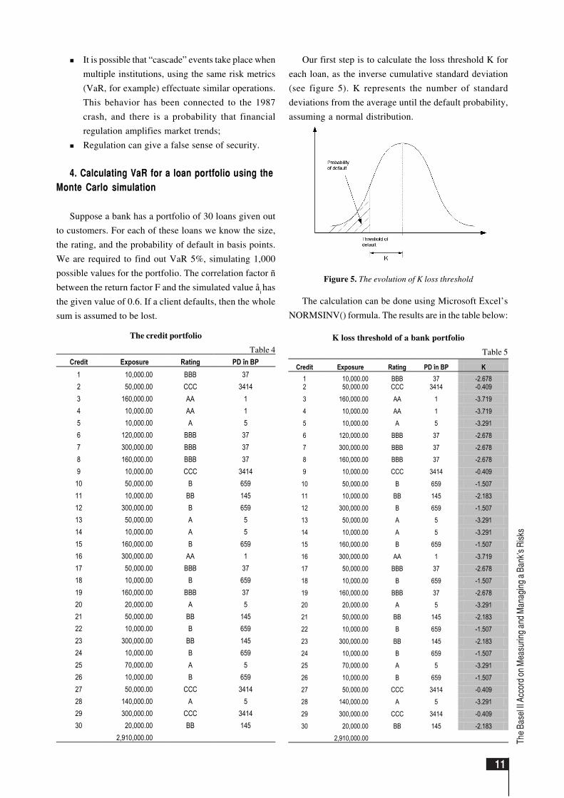
Our first step is to calculate the loss threshold K for

each loan, as the inverse cumulative standard deviation

(see figure 5). K represents the number of standard

deviations from the average until the default probability,

assuming a normal distribution.

Figure 5. The evolution of K loss threshold

The calculation can be done using Microsoft Excel’s

NORMSINV() formula. The results are in the table below:

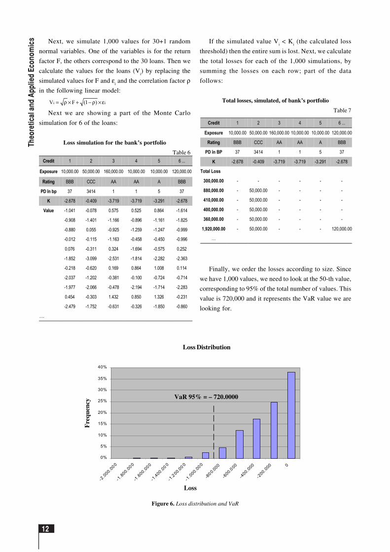
K loss threshold of a bank portfolio

Table 5

Credit Exposure Rating PD în BP K 1 10,000.00 BBB 37 -2.678 2 50,000.00 CCC 3414 -0.409 3 160,000.00 AA 1 -3.719 4 10,000.00 AA 1 -3.719 5 10,000.00 A 5 -3.291 6 120,000.00 BBB 37 -2.678 7 300,000.00 BBB 37 -2.678 8 160,000.00 BBB 37 -2.678 9 10,000.00 CCC 3414 -0.409 10 50,000.00 B 659 -1.507 11 10,000.00 BB 145 -2.183 12 300,000.00 B 659 -1.507 13 50,000.00 A 5 -3.291 14 10,000.00 A 5 -3.291 15 160,000.00 B 659 -1.507 16 300,000.00 AA 1 -3.719 17 50,000.00 BBB 37 -2.678 18 10,000.00 B 659 -1.507 19 160,000.00 BBB 37 -2.678 20 20,000.00 A 5 -3.291 21 50,000.00 BB 145 -2.183 22 10,000.00 B 659 -1.507 23 300,000.00 BB 145 -2.183 24 10,000.00 B 659 -1.507 25 70,000.00 A 5 -3.291 26 10,000.00 B 659 -1.507 27 50,000.00 CCC 3414 -0.409 28 140,000.00 A 5 -3.291 29 300,000.00 CCC 3414 -0.409 30 20,000.00 BB 145 -2.183 2,910,000.00

Credit Exposure Rating PD în BP 1 10,000.00 BBB 37 2 50,000.00 CCC 3414 3 160,000.00 AA 1 4 10,000.00 AA 1 5 10,000.00 A 5 6 120,000.00 BBB 37 7 300,000.00 BBB 37 8 160,000.00 BBB 37 9 10,000.00 CCC 3414

10 50,000.00 B 659 11 10,000.00 BB 145 12 300,000.00 B 659 13 50,000.00 A 5 14 10,000.00 A 5 15 160,000.00 B 659 16 300,000.00 AA 1 17 50,000.00 BBB 37 18 10,000.00 B 659 19 160,000.00 BBB 37 20 20,000.00 A 5 21 50,000.00 BB 145 22 10,000.00 B 659 23 300,000.00 BB 145 24 10,000.00 B 659 25 70,000.00 A 5 26 10,000.00 B 659 27 50,000.00 CCC 3414 28 140,000.00 A 5 29 300,000.00 CCC 3414 30 20,000.00 BB 145 2,910,000.00

12

Th

eore

tica

l an

d A

pp

lied

Eco

no

mic

s Next, we simulate 1,000 values for 30+1 random

normal variables. One of the variables is for the return

factor F, the others correspond to the 30 loans. Then we

calculate the values for the loans (Vi) by replacing the

simulated values for F and εi and the correlation factor ρ

in the following linear model:

ii )1(FV ε×ρ−+×ρ=

Next we are showing a part of the Monte Carlo

simulation for 6 of the loans:

Loss simulation for the bank’s portfolio

Table 6Credit 1 2 3 4 5 6 ...

Exposure 10,000.00 50,000.00 160,000.00 10,000.00 10,000.00 120,000.00

Rating BBB CCC AA AA A BBB

PD în bp 37 3414 1 1 5 37

K -2.678 -0.409 -3.719 -3.719 -3.291 -2.678

Value -1.041 -0.078 0.575 0.525 0.864 -1.614

-0.908 -1.401 -1.166 -0.896 -1.161 -1.825

-0.880 0.055 -0.925 -1.259 -1.247 -0.999

-0.012 -0.115 -1.163 -0.458 -0.450 -0.996

0.076 -0.311 0.324 -1.694 -0.575 0.252

-1.852 -3.099 -2.531 -1.814 -2.282 -2.363

-0.218 -0.620 0.169 0.864 1.008 0.114

-2.037 -1.202 -0.381 -0.100 -0.724 -0.714

-1.977 -2.066 -0.478 -2.194 -1.714 -2.283

0.454 -0.303 1.432 0.850 1.326 -0.231

-2.479 -1.752 -0.631 -0.326 -1.850 -0.860

….

If the simulated value Vi < K

i (the calculated loss

threshold) then the entire sum is lost. Next, we calculate

the total losses for each of the 1,000 simulations, by

summing the losses on each row; part of the data

follows:

Total losses, simulated, of bank’s portfolio

Table 7

Credit 1 2 3 4 5 6 ...

Exposure 10,000.00 50,000.00 160,000.00 10,000.00 10,000.00 120,000.00

Rating BBB CCC AA AA A BBB

PD în BP 37 3414 1 1 5 37

K -2.678 -0.409 -3.719 -3.719 -3.291 -2.678

Total Loss

300,000.00 - - - - - -

880,000.00 - 50,000.00 - - - -

410,000.00 - 50,000.00 - - - -

400,000.00 - 50,000.00 - - - -

360,000.00 - 50,000.00 - - - -

1,920,000.00 - 50,000.00 - - - 120,000.00

…

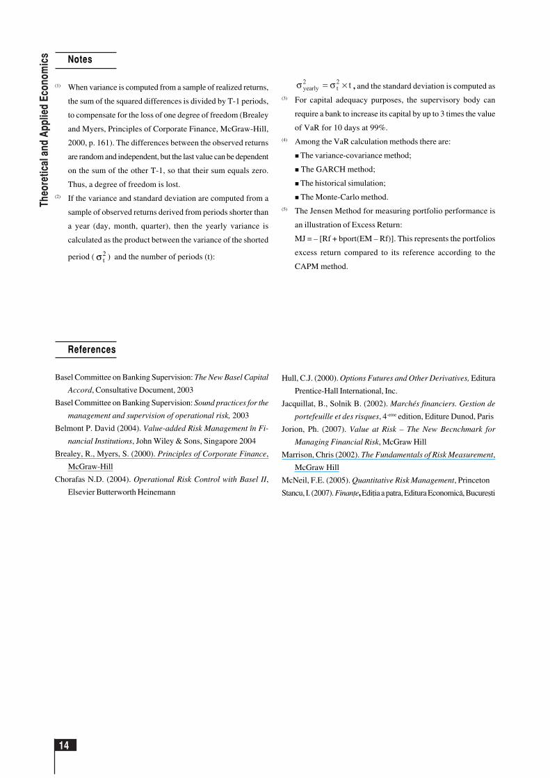
Finally, we order the losses according to size. Since

we have 1,000 values, we need to look at the 50-th value,

corresponding to 95% of the total number of values. This

value is 720,000 and it represents the VaR value we are

looking for.

Figure 6. Loss distribution and VaR

0%

5%

10%

15%

20%

25%

30%

35%

40%

-2.000.000

-1.800.000

-1.600.000

-1.400 .00 0

-1.200.00 0

-1.000.000

-800.000

-600.000

-400.000

-200.000 0

Loss

Loss Distribution

Fre

quen

cy

VaR 95% = – 720.0000

13

The

Bas

el II

Acc

ord

on M

easu

ring

and

Man

agin

g a

Ban

k’s

Ris

ks

This value signifies that the losses incurred by the

bank will be greater than 720,000 only in 5% of the cases.

5. Conclusions and critical aspects

1. The realism of the hypotheses. Firstly, risk

evaluation is undertaken assuming that financial events

follow a known distribution (normal, triangular etc.) For

example, the daily change in stock prices is assumed to

have a normal distribution. In a general climate of risk

aversion, multiple risk indicators are used, such as VaR,

safety-first, semi-variance etc. Finally it is assumed that

the future will repeat the past, and thus historical data is

used. These premises, which do not always hold true,

affect the precision of the forecasts and risk

measurements.

2. Data integrity. The data we use in our models can

represent an incomplete picture of the environment. In

less liquid markets (such as non-EU countries or those of

small-cap companies) the transaction costs can

substantially affect total returns.

Quantitative risk metrics calculations can require a

high level of data precision, which is not always available.

Also, the returns of some strategies, such as hedge funds,

are not frequently calculated, which makes their volatility

appear artificially low.

The most widely-used risk metric is VaR, because it is

expressed in terms which are very easy to understand.

But VaR is obtained using statistical simulations, which

cannot forecast extraordinary market events. Therefore,

the quantity and quality of data is essential. Generally,

the quality of a VaR calculation is tested using back-

testing and stress-testing. Usually, if the model does not

fit the data in more than 1% of the cases, then the premises

or the modeling methods must be changed.

3. Any simulation is subject to model risk. This can be

defined as the risk of losses resulting from using

inadequate models, such as assuming that the distribution

of events is normal, when instead it is strongly skewed.

Moreover, the losses can be compounded by liquidity

problems associated with selling a losing position.

4. Dependency on the time period. The 1987 stock

market crash (as well as other major economical

developments) suggests that risk is independent from the

time period being analyzed. Risk metrics based on longer-

term periods can be less influenced by the short term.

Since the whole stock market history can be considered

as a single period, the question is how we shield ourselves

from the risk of “different” time periods. One solution

would be to forecast risk based on both historical and

current data; the forecast is affected by the number of the

variables used and the length of the forecast. Another is

to use the Monte Carlo simulation.

5. Metric selection and management risk. Selecting a

metric is not an easy decision. Choosing a relative risk

metric, such as excess return, tracking error or beta is

only appropriate when the benchmark is representative

of the portfolio’s performance.

In conclusion, risk measurement is a crucial part in

building and managing a portfolio. The investment

policy must identify the relevant risk metrics for the

portfolio’s specific goals. In addition to choosing

quantitative measures, experience in judging the

qualitative aspects is paramount.

Given these factors, a top-down approach is

recommended. First, the goal of the portfolio should be

set. Given the fact that the major asset classes, such as

bonds, stocks and cash have a long history, portfolio

construction must start from finding the correct balance

between the different asset classes. Specific decisions

about investments should only be made at the end of the

process, together with a risk analysis. This process will

lead to a better understanding of the portfolio’s risks and

evaluation of its performance.

14

Th

eore

tica

l an

d A

pp

lied

Eco

no

mic

s Notes

(1) When variance is computed from a sample of realized returns,

the sum of the squared differences is divided by T-1 periods,

to compensate for the loss of one degree of freedom (Brealey

and Myers, Principles of Corporate Finance, McGraw-Hill,

2000, p. 161). The differences between the observed returns

are random and independent, but the last value can be dependent

on the sum of the other T-1, so that their sum equals zero.

Thus, a degree of freedom is lost.(2) If the variance and standard deviation are computed from a

sample of observed returns derived from periods shorter than

a year (day, month, quarter), then the yearly variance is

calculated as the product between the variance of the shorted

period ( 2tσ ) and the number of periods (t):

t2t

2yearly ×σ=σ , and the standard deviation is computed as

(3) For capital adequacy purposes, the supervisory body can

require a bank to increase its capital by up to 3 times the value

of VaR for 10 days at 99%.(4) Among the VaR calculation methods there are:

� The variance-covariance method;

� The GARCH method;

� The historical simulation;

� The Monte-Carlo method.(5) The Jensen Method for measuring portfolio performance is

an illustration of Excess Return:

MJ = – [Rf + bport(EM – Rf)]. This represents the portfolios

excess return compared to its reference according to the

CAPM method.

References

Basel Committee on Banking Supervision: The New Basel Capital

Accord, Consultative Document, 2003

Basel Committee on Banking Supervision: Sound practices for the

management and supervision of operational risk, 2003

Belmont P. David (2004). Value-added Risk Management în Fi-

nancial Institutions, John Wiley & Sons, Singapore 2004

Brealey, R., Myers, S. (2000). Principles of Corporate Finance,

McGraw-Hill

Chorafas N.D. (2004). Operational Risk Control with Basel II,

Elsevier Butterworth Heinemann

Hull, C.J. (2000). Options Futures and Other Derivatives, Editura

Prentice-Hall International, Inc.

Jacquillat, B., Solnik B. (2002). Marchés financiers. Gestion de

portefeuille et des risques, 4-eme edition, Editure Dunod, Paris

Jorion, Ph. (2007). Value at Risk – The New Becnchmark for

Managing Financial Risk, McGraw Hill

Marrison, Chris (2002). The Fundamentals of Risk Measurement,

McGraw Hill

McNeil, F.E. (2005). Quantitative Risk Management, Princeton

Stancu, I. (2007). Finanþe, Ediþia a patra, Editura Economicã, Bucureºti