Embed Size (px)
Citation preview
J Math Imaging Vis (2007) 28: 81–97DOI 10.1007/s10851-007-0015-8
Texture-Oriented Anisotropic Filtering and GeodesicActive Contours in Breast Tumor UltrasoundSegmentation
Miguel Alemán-Flores · Luis Álvarez · Vicent Caselles
Published online: 9 June 2007© Springer Science+Business Media, LLC 2007
Abstract In this paper we present an anisotropic filter forspeckle reduction in ultrasound images and an adaptationof the geodesic active contours technique for the segmenta-tion of breast tumors. The anisotropic diffusion we proposeis based on a texture description provided by a set of Ga-bor filters and allows reducing speckle noise while preserv-ing edges. Furthermore, it is used to extract an initial pre-segmentation of breast tumors which is used as initializationfor the active contours technique. This technique has beenadapted to the characteristics of ultrasonography by addingcertain texture-related terms which provide a better discrim-ination of the regions inside and outside the nodules. Theseterms allow obtaining a more accurate contour when the gra-dients are not high and uniform.
Keywords Ultrasound · Breast cancer · Segmentation ·Active contours · Anisotropic filtering
1 Introduction
Early diagnosis is a crucial factor in breast cancer treatment,and medical imaging is a very powerful assessment tool.
M. Alemán-Flores (�) · L. ÁlvarezDepartamento de Informática y Sistemas, Universidad de LasPalmas de Gran Canaria, 35017, Las Palmas, Spaine-mail: [email protected]
L. Álvareze-mail: [email protected]
V. CasellesDepartament de Tecnologia, Universitat Pompeu Fabra,08003, Barcelona, Spaine-mail: [email protected]
The two main types of images used in this kind of diag-nosis are mammography and ultrasonography. In this work,we have focussed on the latter, for which a series of crite-ria has been described to distinguish benign from malignantlesions. These criteria include hyperechogenicity (the nod-ule is brighter in the ultrasound image than the surroundingbreast fat), ellipsoid shape, two or three gentle lobulations(lobes which form the tumor) and thin echogenic capsuleas benignity criteria. On the other hand, hypoechogenic-ity (the nodule is darker in the ultrasound image than thesurrounding breast fat), acoustic shadowing (attenuation ofsound behind all or part of the nodule, which appears asa darker region under the lesion), ramifications, microlob-ulations (small rounded projections), angular margins, spic-ulation (alternating hypoechoic and relatively hyperechoicstraight lines radiating out perpendicular from surface of thenodule), calcifications (punctate bright spots within a solidnodule) and taller-than-wide shape are considered as malig-nancy findings [36]. In a computer-aided system, the accu-rate segmentation of breast nodules in ultrasonography isa major task for a further analysis of the global shape andlocal contour variations of the tumor, on which most criteriaare based. However, this task implies many problems whenautomation is intended, since the presence of speckle noiseand shadows, the low or non-uniform contrast of certainstructures, and the variability of the echogenicity of the nod-ules make it very difficult to obtain a segmentation whichcan be useful for the diagnosis. This explains the fact thatmost of the results regarding the semiautomatic segmenta-tion and characterization of breast tumors have been limitedso far [11, 12, 22, 26].
There are many different approaches for the segmen-tation of breast nodules. Manual delimitation is time-consuming, tedious and with a considerable inter- and intra-observer variability. On the other hand, fully automatic
82 J Math Imaging Vis (2007) 28: 81–97
methods require a priori knowledge of the shape of the nod-ule, which is not usually available. Between both extremes,we can find semiautomatic methods, which provide goodresults by means of a reduced interaction with the user.
We propose a combination of different techniques toextract a semiautomatic segmentation of breast nodules.Firstly, an anisotropic texture-guided diffusion is used to re-duce speckle. Secondly, a front propagation algorithm is ap-plied to obtain a pre-segmentation of the nodule. This algo-rithm starts from an inner point selected by the specialist,which is the only interaction required to the user. Finally, inorder to refine the pre-segmentation, we use an adaptationof the geodesic active regions technique (combined with theclassical geodesic active contour term) designed to tacklethe particularities of ultrasound images. In this paper, weuse known techniques, such as anisotropic diffusion, bal-loon methods, Gabor filters or geodesic active contours. Wecombine and refine such techniques with the purpose of ul-trasound image segmentation. In particular, we propose ananisotropic texture-guided diffusion and a region based geo-desic active contour using the response of a set of Gaborfilters.
In the anisotropic diffusion step, we adapt the ideas ofthe classical Perona-Malik equation [31] to the diffusion ofultrasound images. For that, we use a set of texture descrip-tors R based on Gabor filters and we inhibit the diffusionacross changes in these descriptors (determined by largevalues of the modulus of the gradient of R). This filteringwill permit us to obtain a more precise pre-segmentation.The pre-segmentation is computed with a front propagationscheme with a speed depending (inversely) on the modu-lus of the gradient, which is analogous to the inflation forceused in [13]. These balloon forces have traditionally beenincluded in the level set formulation [29] of active contours[4–6, 23, 28], but they are used here as a pre-processing stepto get an initial segmentation as close as possible to the con-tour of the nodule. In the last step, in order to improve thefinal segmentation, we use a combination of the geodesicedge based and region based active contours; the region de-scriptors being based on the responses of a set of Gabor fil-ters at several orientations and scales. We explore a localvariant of the model proposed in [8, 34, 35] and we intro-duce a new variant of it, we test both of them for our setof images. Many variants of active contours [4–6, 13, 21,23, 28] have previously been applied to the segmentationof medical images [10, 20], textured regions [2, 8, 30, 32,34, 35], and other situations whose conditions are similar toours. In particular, the works [8, 9, 15, 30, 34, 35] have alsoused region descriptors or statistical information and the lasttwo ones have used the responses of Gabor filters as texturedescriptors. Finally, let us mention that novel level set meth-ods for image segmentation include motion-based level setsegmentation [14], segmentation of natural textures [19] and
ultrasound segmentation with non-parametric intensity andshape models [33].
The rest of the paper is structured as follows: Sect. 2 ex-plains the texture-based anisotropic filtering process whichallows reducing speckle. Section 3 shows the extraction ofa pre-segmentation by means of a front propagation scheme.In Sect. 4, we review the basic region based active contoursfor scalar and vector features and we propose some exten-sions. In particular, we describe a region based active con-tour model based on a set of Gabor filter responses usedas texture descriptors. Section 5 presents some results andcomparisons. Finally, in Sect. 6, we give an account of ourmain conclusions.
2 Speckle Reducing Anisotropic Diffusion Basedon Vector Descriptors
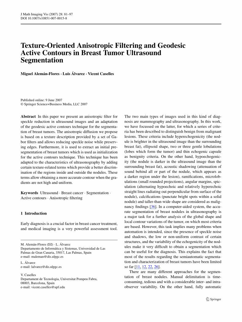
Ultrasound images present highly disturbing speckle noise.Moreover, in many cases, the low contrast between the struc-tures to be segmented and the background, as well as theshadows which may appear depending on the properties ofthe tissues, make it even harder to locate the edges of the dif-ferent elements. Figure 1 shows an example of a breast nod-ule which is very hard to process, since it combines roundedand angular margins, and present diffuse edges, prolonga-tions, concavities and non-uniform intensity. It is necessaryto remove speckle before dealing with the problem of seg-mentation. Classical speckle removing filters include localstatistics and minimum square error schemes [17, 25, 27].Truncated median [16] has proved very useful in the re-duction of speckle using an iterative algorithm to approx-imate the mode using small windows. Isotropic diffusion
Fig. 1 Original ultrasound image of a breast nodule with roundedand angular margins, diffuse edges, prolongations, concavities andnon-uniform intensity
J Math Imaging Vis (2007) 28: 81–97 83
is not suitable since it should be strong enough to reducespeckle but low enough to preserve edges. On the otherhand, anisotropic diffusion tries to reduce the noise of theimages preserving the contrast of the edges, in such a waythat the contours of the objects in the scene are not altered bythe diffusion process (see [37] for more details). In this pa-per � ⊂ R
2 denotes the image domain which we assume tobe a rectangle in R
2 and I0 :� → R denotes a given image.A typical anisotropic filter applied to I0 is given by the solu-tion I (t, x, y), t > 0, (x, y) ∈ �, of Perona–Malik equation[31]:
∂I
∂t= div(c(‖∇I‖)∇I )
(1)I (t = 0) = I0
with Neumann boundary conditions, i.e., ∇I · ν� = 0 whereν� denotes the outer unit normal to the boundary of �.
In this equation, c(r) is a monotonic decreasing functionof r > 0, such as, for example:
c(r) = e−( rk)2
, (2)
where k is a constant which determines the contrast of theedges to preserve.
This kind of filters works properly in many kinds of im-ages, mainly when the objects are defined by uniform inten-sity regions. However, in our case, the textures of the regionsmake it necessary to express the similarity between differentareas in terms of texture descriptors, instead of intensities.Speckle reducing anisotropic diffusion has previously been
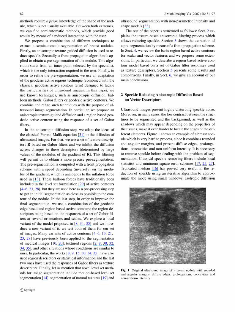
introduced, mostly in synthetic aperture radar images [38].We propose to use Gabor filters [18] to characterize the tex-tures, and the gradient of the filtered images as a texture-based edge detector. A Gabor filter whose scale and hori-zontal and vertical frequencies are given by σ > 0, kx andky in R, respectively, can be expressed as:
Gσkx,ky
(x, y) = e− x2+y2
2σ2 (cos(kxx + kyy)). (3)
We use a set of S scales, N frequencies within each scale,and two orientations (horizontal and vertical) for each fre-quency. Fixed a certain scale σ0 > 0 and a certain frequencyk0 > 0, the outputs of the filters are calculated as the convo-lution:
F snx,ny
= I ∗ Gsσ0nxk0,nyk0
, (4)
where 1 ≤ s ≤ S, −N ≤ nx ≤ N and 0 ≤ ny ≤ N .These filters combine orientation and frequency and pro-
vide a description of the distribution of the intensities in theregion where they are applied (see Fig. 2). Due to the highvariability in the aspect of the different tumors, it is difficultto establish a certain pattern in the response of the filterswhich allows identifying all of them.
Taking the Perona–Malik equation (1) as a model, wepropose to penalize the diffusion along high texture gradi-ents. If R(x, y) denotes the vector formed by the responsesof a family of Gabor filters applied to the image I (0) at point(x, y), we use the following anisotropic diffusion equation:
∂I
∂t= div(c(‖∇R‖)∇I ), (5)
Fig. 2 Example of theapplication of 8 Gabor filters toa synthetic textured imagerepresenting well definedoscillations and an ultrasoundimage. For each of the images:Top row: σ = 5, kx = 7, ky = 0;σ = 5, kx = 0, ky = 7; σ = 10,kx = 7, ky = 0; σ = 10, kx = 0,ky = 7. Bottom row: σ = 5,kx = 8, ky = 0; σ = 5, kx = 0,ky = 8; σ = 10, kx = 8, ky = 0;σ = 10, kx = 0, ky = 8
84 J Math Imaging Vis (2007) 28: 81–97
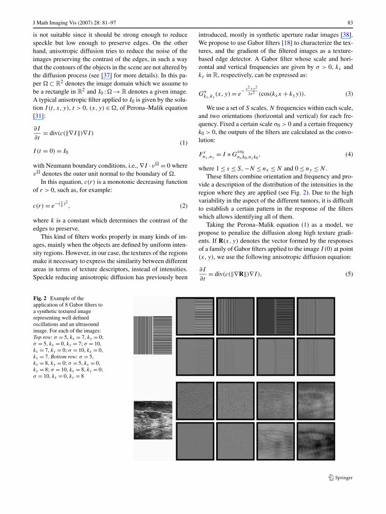
Fig. 3 Result of applying theanisotropic texture-baseddiffusion in (5) to an image withtwo well defined textures (left)using σ = 5, k = 0.5 (center)and σ = 5, k = 1 (right)
where ‖∇R‖2 = trace((∇R)t∇R) (if A is a matrix, At de-notes the transpose matrix of A). Note that diffusion is in-hibited at large values of ‖∇R‖, i.e., at points where there isa rapid transition of the texture characteristics of the image.
We apply an explicit discretization method to discreti-ze (5). For that we replace the gradients and divergencein (5) by discrete approximations; for any scalar functionf defined on the grid {1, . . . ,N} × {1, . . . ,M} where theimages are defined we shall use the notation
∇+,+f = (∇+x f,∇+
y f ), ∇+,−f = (∇+x f,∇−
y f ),
∇−,+f = (∇−x f,∇+
y f ), ∇−,−f = (∇−x f,∇−
y f ),
where
∇+x f (i, j) = f (i + 1, j) − f (i, j),
∇−x f (i, j) = f (i, j) − f (i − 1, j),
∇+y f (i, j) = f (i, j + 1) − f (i, j),
∇−y f (i, j) = f (i, j) − f (i, j − 1),
for any (i, j) ∈ {1, . . . ,N} × {1, . . . ,M}. Note that the dualoperators to ∇+,+, ∇+,−, ∇−,+, ∇−,− are, respectively, theoperators div−,−, div−,+, div+,−, div+,+ where for a dis-crete vector field (A,B) we have div−,−(A,B) = ∇−
x A +∇−
y B and similarly for the other operators. Using �x =�y = 1, the discretization of (5) :
I t+�t(i, j)
= I t (i, j)
+ �t
4
∑
α,β∈{+,−}divα∗,β∗(c(‖∇α,βR‖)∇α,βI )(i, j) (6)
for any (i, j) ∈ {1, . . . ,N} × {1, . . . ,M}, where
‖∇α,βR(i, j)‖=
√ ∑1≤s≤S
∑−N≤nx≤N
∑0≤ny≤N
|∇α,βF snx,ny
(i, j)|2.
We apply a wide range of filters varying the scale and fre-quency. In order to reduce the computational cost, we haveonly used horizontally and vertically oriented Gabor filtersand thus, the discretization of gradient magnitude has also
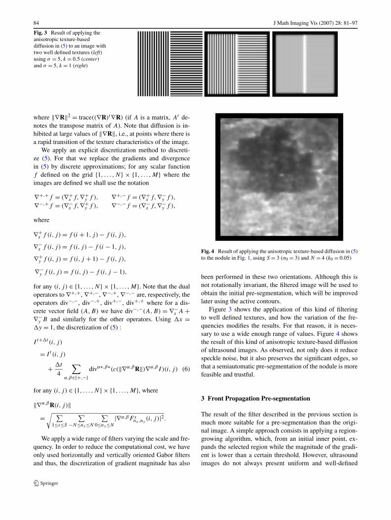
Fig. 4 Result of applying the anisotropic texture-based diffusion in (5)to the nodule in Fig. 1, using S = 3 (σ0 = 3) and N = 4 (k0 = 0.05)
been performed in these two orientations. Although this isnot rotationally invariant, the filtered image will be used toobtain the initial pre-segmentation, which will be improvedlater using the active contours.
Figure 3 shows the application of this kind of filteringto well defined textures, and how the variation of the fre-quencies modifies the results. For that reason, it is neces-sary to use a wide enough range of values. Figure 4 showsthe result of this kind of anisotropic texture-based diffusionof ultrasound images. As observed, not only does it reducespeckle noise, but it also preserves the significant edges, sothat a semiautomatic pre-segmentation of the nodule is morefeasible and trustful.
3 Front Propagation Pre-segmentation
The result of the filter described in the previous section ismuch more suitable for a pre-segmentation than the origi-nal image. A simple approach consists in applying a region-growing algorithm, which, from an initial inner point, ex-pands the selected region while the magnitude of the gradi-ent is lower than a certain threshold. However, ultrasoundimages do not always present uniform and well-defined
J Math Imaging Vis (2007) 28: 81–97 85
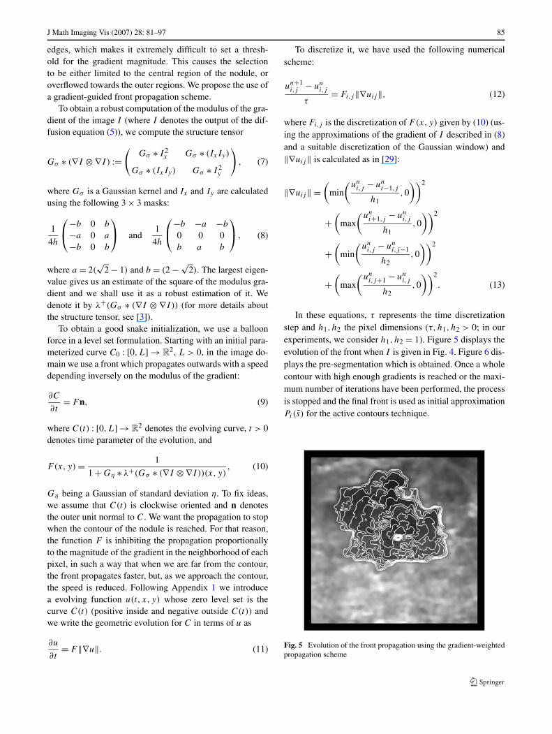
edges, which makes it extremely difficult to set a thresh-old for the gradient magnitude. This causes the selectionto be either limited to the central region of the nodule, oroverflowed towards the outer regions. We propose the use ofa gradient-guided front propagation scheme.
To obtain a robust computation of the modulus of the gra-dient of the image I (where I denotes the output of the dif-fusion equation (5)), we compute the structure tensor
Gσ ∗ (∇I ⊗ ∇I ) :=(
Gσ ∗ I 2x Gσ ∗ (IxIy)
Gσ ∗ (IxIy) Gσ ∗ I 2y
), (7)
where Gσ is a Gaussian kernel and Ix and Iy are calculatedusing the following 3 × 3 masks:
1
4h
⎛
⎝−b 0 b
−a 0 a
−b 0 b
⎞
⎠ and1
4h
⎛
⎝−b −a −b
0 0 0b a b
⎞
⎠ , (8)
where a = 2(√
2 − 1) and b = (2 − √2). The largest eigen-
value gives us an estimate of the square of the modulus gra-dient and we shall use it as a robust estimation of it. Wedenote it by λ+(Gσ ∗ (∇I ⊗ ∇I )) (for more details aboutthe structure tensor, see [3]).
To obtain a good snake initialization, we use a balloonforce in a level set formulation. Starting with an initial para-meterized curve C0 : [0,L] → R
2, L > 0, in the image do-main we use a front which propagates outwards with a speeddepending inversely on the modulus of the gradient:
∂C
∂t= Fn, (9)
where C(t) : [0,L] → R2 denotes the evolving curve, t > 0
denotes time parameter of the evolution, and
F(x, y) = 1
1 + Gη ∗ λ+(Gσ ∗ (∇I ⊗ ∇I ))(x, y), (10)
Gη being a Gaussian of standard deviation η. To fix ideas,we assume that C(t) is clockwise oriented and n denotesthe outer unit normal to C. We want the propagation to stopwhen the contour of the nodule is reached. For that reason,the function F is inhibiting the propagation proportionallyto the magnitude of the gradient in the neighborhood of eachpixel, in such a way that when we are far from the contour,the front propagates faster, but, as we approach the contour,the speed is reduced. Following Appendix 1 we introducea evolving function u(t, x, y) whose zero level set is thecurve C(t) (positive inside and negative outside C(t)) andwe write the geometric evolution for C in terms of u as
∂u
∂t= F‖∇u‖. (11)
To discretize it, we have used the following numericalscheme:
un+1i,j − un
i,j
τ= Fi,j‖∇uij‖, (12)
where Fi,j is the discretization of F(x, y) given by (10) (us-ing the approximations of the gradient of I described in (8)and a suitable discretization of the Gaussian window) and‖∇uij‖ is calculated as in [29]:
‖∇uij‖ =(
min
(un
i,j − uni−1,j
h1,0
))2
+(
max
(un
i+1,j − uni,j
h1,0
))2
+(
min
(un
i,j − uni,j−1
h2,0
))2
+(
max
(un
i,j+1 − uni,j
h2,0
))2
. (13)
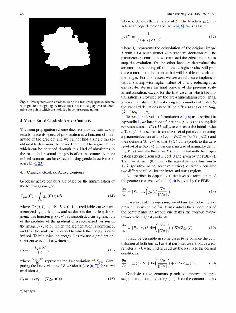
In these equations, τ represents the time discretizationstep and h1, h2 the pixel dimensions (τ,h1, h2 > 0; in ourexperiments, we consider h1, h2 = 1). Figure 5 displays theevolution of the front when I is given in Fig. 4. Figure 6 dis-plays the pre-segmentation which is obtained. Once a wholecontour with high enough gradients is reached or the maxi-mum number of iterations have been performed, the processis stopped and the final front is used as initial approximationPi(s) for the active contours technique.
Fig. 5 Evolution of the front propagation using the gradient-weightedpropagation scheme
86 J Math Imaging Vis (2007) 28: 81–97
Fig. 6 Presegmentation obtained using the front propagation schemewith gradient weighting. A threshold is set on the graylevel to deter-mine the points which are included in the presegmentation
4 Vector-Based Geodesic Active Contours
The front propagation scheme does not provide satisfactoryresults, since its speed of propagation is a function of mag-nitude of the gradient and we cannot find a single thresh-old on it to determine the desired contour. The segmentationwhich can be obtained through this kind of algorithms inthe case of ultrasound images is often inaccurate. A morerefined contour can be extracted using geodesic active con-tours [5, 6, 23].
4.1 Classical Geodesic Active Contours
Geodesic active contours are based on the minimization ofthe following energy:
Egac(C) =∫
C
gσ (C(s)) ds, (14)
where C : [0,L] → R2, L > 0, is a rectifiable curve para-
meterized by arc-length s and ds denotes the arc-length ele-ment. The function gσ (x, y) is a smooth decreasing functionof the modulus of the gradient of a regularized version ofthe image I (x, y) on which the segmentation is performed,and C is the snake with respect to which the energy is min-imized. To minimize the energy (14) we use a gradient de-scent curve evolution written as
Ct = −δEgac(C)
δC, (15)
whereδEgac(C)
δCrepresents the first variation of Egac. Com-
puting the first variation of E we obtain (see [6, 7]) the curveevolution equation
Ct = −(κgσ − 〈∇gσ ,n〉)n, (16)
where κ denotes the curvature of C. The function gσ (x, y)
acts as an edge detector and, as in [4, 6], we shall use
gσ (I ) = 1√1 + α‖∇Iσ ‖2
, (17)
where Iσ represents the convolution of the original imageI with a Gaussian kernel with standard deviation σ . Theparameter α controls how contrasted the edges must be tostop the evolution. On the other hand, σ determines theamount of smoothing of I , so that a higher value will pro-duce a more rounded contour but will be able to reach far-ther edges. For this reason, we use a multiscale implemen-tation, starting with higher values of σ and reducing it ateach scale. We use the final contour of the previous scaleas initialization, except for the first case, in which the ini-tialization is provided by the pre-segmentation step. Thus,given a final standard deviation σ0 and a number of scales S,the standard deviations used at the different scales are Sσ0,(S − 1)σ0, . . . , σ0.
To write the level set formulation of (16) as described inAppendix 1, we introduce a function u(t, x, y) as an implicitrepresentation of C(t). Usually, to construct the initial snakeu(0, x, y), the user has to choose a set of points determininga parameterization of a polygon P0(s) = (x0(s), y0(s)) andthen define u(0, x, y) so that P0(s) corresponds to the zerolevel set of u(0, x, y). In our case, instead of manually defin-ing P0(s), we take the curve Pi(s) computed with the propa-gation scheme discussed in Sect. 3 and given by the PDE (9).Then, we define u(0, x, y) as the signed distance function toPi(s) (positive inside, negative outside), or simply considertwo different values for the inner and outer regions.
As described in Appendix 1, the level set formulation ofthe geometric curve evolution (16) is given by the PDE:
∂u
∂t= ‖∇u‖div
(gσ (I )
∇u
‖∇u‖)
. (18)
If we expand this equation, we obtain the following ex-pression, in which the first term controls the smoothness ofthe contour and the second one makes the contour evolvetowards the highest gradients:
∂u
∂t= ‖∇u‖gσ (I )div
( ∇u
‖∇u‖)
+ ∇u∇gσ (I ). (19)
It may be desirable in some cases to re-balance the con-tribution of both terms. For that purpose, we introduce a pa-rameter λ > 0 which helps us adjust the results to the desiredconditions:
∂u
∂t= gσ (I )‖∇u‖div
( ∇u
‖∇u‖)
+ λ∇u∇gσ (I ). (20)
Geodesic active contours permit to improve the pre-segmentation obtained using (11) since the contour adapts
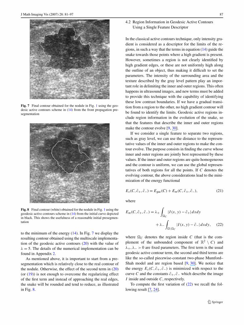
J Math Imaging Vis (2007) 28: 81–97 87
Fig. 7 Final contour obtained for the nodule in Fig. 1 using the geo-desic active contours scheme in (14) from the front propagation pre-segmentation
Fig. 8 Final contour (white) obtained for the nodule in Fig. 1 using thegeodesic active contours scheme in (14) from the initial curve depictedin black. This shows the usefulness of a reasonable initial presegmen-tation
to the minimum of the energy (14). In Fig. 7 we display theresulting contour obtained using the multiscale implementa-tion of the geodesic active contours (20) with the value ofλ = 5. The details of the numerical implementation can befound in Appendix 2.
As mentioned above, it is important to start from a pre-segmentation which is relatively close to the real contour ofthe nodule. Otherwise, the effect of the second term in (20)(or (19)) is not enough to overcome the regularizing effectof the first term and instead of approaching the real edges,the snake will be rounded and tend to reduce, as illustratedin Fig. 8.
4.2 Region Information in Geodesic Active ContoursUsing a Single Feature Descriptor
In the classical active contours technique, only intensity gra-dient is considered as a descriptor for the limits of the re-gions, in such a way that the terms in equation (14) guide thesnake towards those points where a high gradient is present.However, sometimes a region is not clearly identified byhigh gradient edges, or these are not uniformly high alongthe outline of an object, thus making it difficult to set theparameters. The intensity of the surrounding area and thetexture described by the gray level pattern play an impor-tant role in delimiting the inner and outer regions. This oftenhappens in ultrasound images, and new terms must be addedto provide this technique with the capability of identifyingthese low contrast boundaries. If we have a gradual transi-tion from a region to the other, no high gradient contour willbe found to identify the limits. Geodesic active regions in-clude region information in the evolution of the snake, sothat the features that describe the inner and outer regionsmake the contour evolve [9, 30].
If we consider a single feature to separate two regions,such as gray level, we can use the distance to the represen-tative values of the inner and outer regions to make the con-tour evolve. The purpose consists in finding the curve whoseinner and outer regions are jointly best represented by thesevalues. If the inner and outer regions are quite homogeneousand the contour is uniform, we can use the global represen-tatives of both regions for all the points. If C denotes theevolving contour, the above considerations lead to the mini-mization of the energy functional
Es(C, c+, c−) = Egac(C) + Em(C, c+, c−), (21)
where
Em(C, c+, c−) = λ+∫
�C
|I (x, y) − c+|dxdy
+ λ−∫
�\�C
|I (x, y) − c−|dxdy, (22)
where �C denotes the region inside C (that is the com-plement of the unbounded component of R
2 \ C) andλ+, λ− > 0 are fixed parameters. The first term is the usualgeodesic active contour term, the second and third terms arelike the so-called piecewise-constant two-phase Mumford–Shah model and are region based [9, 30]. We notice thatthe energy Es(C, c+, c−) is minimized with respect to thecurve C and the constants c+, c− which describe the imageI inside and outside C, respectively.
To compute the first variation of (22) we recall the fol-lowing result [7, 24].
88 J Math Imaging Vis (2007) 28: 81–97
Lemma 1 Let f : R2 → R be an integrable function. The
weighted region functional
Ef (C) =∫∫
�C
f (x, y)dxdy,
yields the first variation
δEf (C)
δC= −f (x, y) n.
Using the first variation of the energy (14) and Lemma 1we compute the first variations of Es(C, c+, c−):
δEs
δC= (κgσ − 〈∇gσ ,n〉)n + M(I, c+, c−)(x, y)n,
where
M(I, c+, c−)(x, y) = λ−|I (x, y) − c−|− λ+|I (x, y) − c+|, (23)
δEs
δc+= λ+
∫
�C
sign(c+ − I (x, y)) dxdy,
δEs
δc−= λ−
∫
�\�C
sign(c− − I (x, y)) dxdy,
where sign(r) = +1 if r > 0; −1 if r < 0; and it can be anyvalue in [−1,1] if r = 0.
For fixed C the minimum values of c+ and c− satisfy
δEs
δc+= 0 and
δEs
δc−= 0.
These equations give the values of c+, c− explicitly.Heuristically, the optimal value of c+, resp. c−, is the valueof I (x, y) in �C , resp. � \ �C , that splits its area into twoequal parts. These values are the median values
c+ = median�C(I), c− = median�\�C
(I). (24)
The gradient descent equation for the evolving curve C
is
Ct = −δEs
δC= −(κgσ − 〈∇gσ ,n〉)n
− M(I,C(t))(x, y)n, (25)
where
M(I,C(t))(x, y) = M(I, c+(t), c−(t))(x, y),
where c+(t), c−(t) are the median values given in (24) forthe curve C(t).
However, in the case of ultrasound images we deal withvery variable contours and heterogeneous regions. This isthe reason why we have used, for every point, the medians
of the inner and outer neighborhoods, so that the evolutionof the curve depends on the region where we are located. Wepropose to localize the energy (22). For that, for any recti-fiable curve C and functions c+(x, y), c−(x, y), we definethe energy functional
Esl(C, c+, c−) = Egac(C) + Eml(C, c+, c−), (26)
where
Eml(C, c+, c−)
= λ+∫
�
(∫
�C∩B(x,y)
|I (x′, y′) − c+(x, y)|dx′dy′)
dxdy
+ λ−∫
�
(∫
B(x,y)\�C
|I (x′, y′)
− c−(x, y)|dx′dy′)
dxdy, (27)
where B(x, y) is a ball around (x, y) of fixed radius, andλ+, λ− > 0 are fixed parameters.
We denote by χA(x, y) the characteristic function of a setA ⊂ R
2, i.e., χA(x, y) = 1 if (x, y) ∈ A and 0 otherwise.To compute the first variations of Es(C, c+, c−) we observethat χB(x′,y′)(x, y) = χB(x,y)(x
′, y′) and using this we have
∫
�
(∫
�C∩B(x,y)
|I (x′, y′) − c+(x, y)|dx′dy′)
dxdy
=∫
�C
(∫
�
χB(x′,y′)(x, y)|I (x′, y′)
− c+(x, y)|dxdy
)dx′dy′
=∫
�C
(∫
�∩B(x′,y′)|I (x′, y′) − c+(x, y)|dxdy
)dx′dy′.
Using this, the first variation of the energy (14) andLemma 1 we compute the first variations of Es(C, c+, c−):
δEsl
δC= (κgσ − 〈∇gσ ,n〉)n + Ml(I, c+, c−)(x, y)n,
where (changing (x, y) and (x′, y′))
Ml(I, c+, c−)(x, y)
= λ−∫
�∩B(x,y)
|I (x, y) − c−(x′, y′)|dx′dy′
− λ+∫
�∩B(x,y)
|I (x, y) − c+(x′, y′)|dx′dy′,
J Math Imaging Vis (2007) 28: 81–97 89
δEsl
δc+= λ+
∫
�C∩B(x,y)
sign(c+(x, y) − I (x′, y′)) dx′dy′,
δEsl
δc−= λ−
∫
B(x,y)\�C
sign(c−(x, y) − I (x′, y′)) dx′dy′.
For fixed C the minimum values of c+(x, y) and c−(x, y)
satisfy δEs
δc+ = 0 and δEs
δc− = 0. Heuristically, the optimal valueof c+(x, y), resp. c−(x, y), is the value of I (x, y) in �C ∩B(x, y), resp. B(x, y)\�C , that splits its area into two equalparts. These values are the median values
c+(x, y) = median�C∩B(x,y)(I ),(28)
c−(x, y) = medianB(x,y)\�C(I).
The gradient descent equation for the evolving curve C
is
Ct = −δEsl
δC
= −(κgσ − 〈∇gσ ,n〉)n − Ml(I,C(t))(x, y)n, (29)
where
Ml(I,C(t))(x, y) = Ml(I, c+(t), c−(t))(x, y),
where c+(t, x, y), c−(t, x, y) are the median values given in(28) for the curve C(t).
As described in Appendix 1 the level set formulation ofthe gradient descent equation corresponding to (27) is
∂u
∂t= ‖∇u‖div
(gσ (I )
∇u
‖∇u‖)
+ ‖∇u‖Ml(I, [u(t) ≥ 0]). (30)
For computational simplicity, assuming that c+(x′, y′)and c−(x′, y′) are approximately constant in B(x, y), wemay approximate Ml(C, c+, c−) by
Ml,app(, c+, c−) = λ−V |I (x, y) − c−(x, y)|− λ+V |I (x, y) − c+(x, y)|,
where V is the area (number of pixels) of the ball B(x, y).Since V is a constant value, it can be reabsorbed inthe parameters λ+, λ−. In our experiments, we shall useλ+ = λ− = β . In this case, we use the level set formulation
∂u
∂t= ‖∇u‖div
(gσ (I )
∇u
‖∇u‖)
+ ‖∇u‖Ml,app(I, [u(t) ≥ 0]). (31)
Developing the divergence term we may weight the term∇gσ (I ) · ∇u with a factor λ as in (20).
An alternative approach could be to use the (local) meanand the variance of the regions in a similar way as we havedone using the median, by replacing the term Ml by a com-bination of the following ones
Mm(I,m+,m−)(x, y)
= λm−∫
�∩B(x,y)
|I (x, y) − m−(x′, y′)|2 dx′dy′
− λm+∫
�∩B(x,y)
|I (x, y) − m+(x′, y′)|2 dx′dy′, (32)
Mv(I,m+,m−, v+, v−)(x, y)
= λv−∫
�∩B(x,y)
|(I (x, y) − m−(x′, y′))2
− v−(x′, y′)|dx′dy′
− λv+∫
�∩B(x,y)
|(I (x, y) − m+(x′, y′))2
− v+(x′, y′)|dx′dy′, (33)
where m−(x, y) is mean of I in B(x, y) \ �C , m+(x, y) isthe mean of I in �C ∩ B(x, y), and v−(x, y) and v+(x, y)
are the corresponding variances in B(x, y) \ �C and �C ∩B(x, y), respectively.
The median is quite robust to the possible extreme values,such as those observed when the nodule presents calcifica-tions. Furthermore, the use of local values allows identify-ing parts of the contour which present different degrees ofcontrast, since the use of global descriptors makes it verydifficult to extract values which allow identifying the wholecontour.
4.2.1 A Variant of Model (31)
We can observe that the last term in (31) is locally isotropic,since it only depends on the magnitude of ∇u, and not onits orientation. In order that the behavior of the median ina neighborhood of the point helps moving the level set inthe right direction in a more explicit way, we have intro-duced a second alternative, again to be used when our initialcontour is not far from the desired one. We can use the gra-dient of the distance to guide the evolution of the snake inorder to find those points which are as far from the medi-ans of such feature in the inner and outer regions. Since wecan be outside or inside the right border, the absolute valueis taken. This alternative considers the variation of the dif-ference with respect to the medians in the neighborhood ofthe points and, consequently, allows tackling the problemsof isolated outlying points and high local variations. If weconsider intensity, this results in the following equation:
∂u
∂t= ‖∇u‖div
(gσ (I )
∇u
‖∇u‖)
+ ∇u · ∇M(I,u), (34)
where
M(I,u)(x, y) = |λ−|I (x, y) − c−(x, y)|− λ+|I (x, y) − c+(x, y)||. (35)
90 J Math Imaging Vis (2007) 28: 81–97
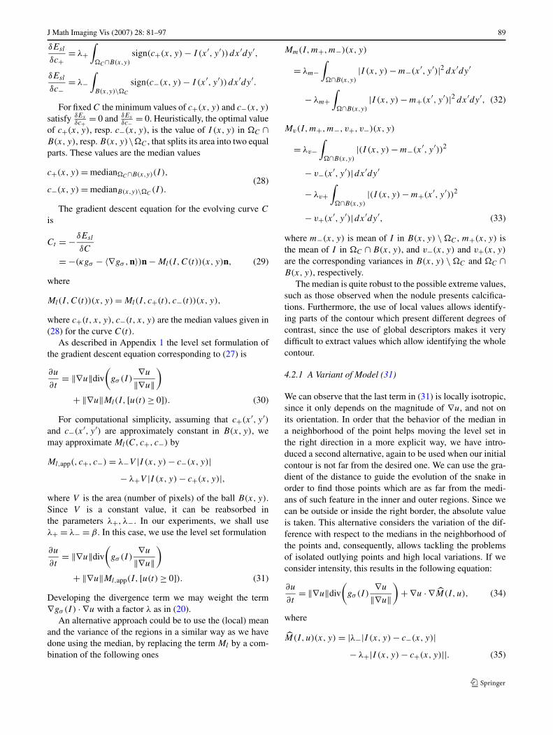
Fig. 9 Example of the use of region information. Left: nodule with diffuse contours. Center: the inner contour is an example of a bad initializationof the snake. We have computed the values of M for this initialization and we have depicted in dark gray the values which are negative and in lightgray the values which are positive. The outer contour is the validated one provided by the physicians. As observed, the function M changes its signvery close to the validated contour. Right: we have computed M using the same bad initialization. As observed, the function has a minimum closeto the validated contour provided by the physicians
When M(x, y) = 0, the value I (x, y) is equidistant tothe medians of I at the points in the neighborhood of (x, y)
which are outside and inside the snake. On the other hand,the higher the value of the modulus of ∇M , the farther theborder, and the term ∇u · ∇M will make the contour evolvetowards the border. Figure 9 shows an example with a nod-ule with diffuse contours for which M and M have beencalculated for a given initialization of the snake which isfar from the validated segmentation provided by the special-ists. As observed, M changes its sign when approaching thevalidated contour, while M has a minimum in that region.Both, the minimum of M and the sign change of M are muchcloser to the right contour (external one) than the initial ap-proximation for which they have been calculated (internalone).
4.3 Region Information in Geodesic Active ContoursUsing a Vectorial Descriptor
Not only intensity determines the limits of regions. Thetexture described by the gray level pattern plays an im-portant role in delimiting the inner and outer regions, spe-cially if we work with ultrasound images. As in [8], ourapproach considers the responses of a set of Gabor filtersin its vectorial form, and tries to use this information toobtain a texture-guided segmentation. As in Sect. 4.2, wehave tested two different ways of including this region in-formation into the active contour equation. The first onecorresponds to the local version of the model introducedin [8] (see also [10, 34]) (we use a robust term), and aimsat attracting the snakes towards the edges of the texture de-scription: as in the case of a single feature, we consider,for every point, the median values of the inner and outerneighborhoods. For that, for any rectifiable curve C andfunctions c+(x, y) = (c1+(x, y), . . . , cm+(x, y), c−(x, y) =(c1−(x, y), . . . , cm−(x, y)), we define the energy functional
EG(C, c+, c−) = Egac(C) + EGml(C, c+, c−) (36)
where
EGml(C, c+, c−)
=∑
1≤i≤m
λi+∫
�
(∫
�C∩B(x,y)
|I i(x′, y′)
− ci+(x, y)|dx′dy′)
dxdy
+∑
1≤i≤m
λi−∫
�
(∫
B(x,y)\�C
|I i(x′, y′)
− ci−(x, y)|dx′dy′)
dxdy, (37)
where I i , i = 1, . . . ,m, are the responses to m Gabor filtersof the original image, obtained for different scales, orienta-tions, and frequencies, and λi+, λi− > 0 are fixed parametersfor each channel. As explained before, the first term is theusual geodesic active contour term, but here the second andthird terms are region based active contours based on Ga-bor feature space for the segmentation of textured images[8, 34]. The energy is minimized with respect to C, c+ and c−. At the minimum, ci+(x, y), ci−(x, y) are the median val-ues of the Gabor channel I i around (x, y) inside and outsidethe curve C, respectively.
As in Sect. 4.2, equating to zero the first variations ofEG(C, c+, c−) with respect to ci+ and ci−, i = 1, . . . ,m, weobtain
ci+(x, y) = median�C∩B(x,y)(Ii),
ci−(x, y) = medianB(x,y)\�C(I i).
Now, computing the first variation of EG(C, c+, c−) withrespect to C and writing the gradient descent equation for C
Ct = −δE
δC
J Math Imaging Vis (2007) 28: 81–97 91
in a level set formulation (see Appendix 1) we obtain thePDE:
∂u
∂t= ‖∇u‖div
(gσ (I )
∇u
‖∇u‖)
+ ‖∇u‖MG(I,u), (38)
where
MG(I,u)(x, y)
=∑
1≤i≤m
λi−∫
�∩B(x,y)
|I i(x, y) − ci−(x′, y′)|dx′dy′
−∑
1≤i≤m
λi+∫
�∩B(x,y)
|I i(x, y) − ci+(x′, y′)|dx′dy′.
As in Sect. 4.2, if we assume that the functions ci+(x, y),ci−(x, y), i = 1, . . . ,m, are approximately constant inB(x, y) we may approximate MG(I,u)(x, y) by
MG,app(I, u)(x, y)
=∑
1≤i≤m
λi−|I i(x, y) − ci−(x, y)|
−∑
1≤i≤m
λi+|I i(x, y) − ci+(x, y)|, (39)
where we have normalized the area of B(x, y) to 1 (whichamounts to reabsorb this area in the notation of λi+, λi−)and consider the PDE (38) with MG(I,u) replaced byMG,app(I, u). As done with the single feature scheme, wehave also taken λi+ = λi− = β > 0 for any i = 1, . . . ,m.
When MG,app(I, u)(x, y) = 0, the outputs of the Gaborfilters at (x, y) are equidistant from the medians of the out-puts of the respective filters in the outer and inner regionsof C around (x, y). When MG,app < 0, the outputs at thatpoint are closer to those outside than to those inside, so thatits value must be decreased. When MG,app > 0, the oppositeoccurs and its value must be increased.
4.3.1 A Variant of Model (38)
Recall that our purpose is to identify the contour separatingtwo regions whose local median responses are different andseparated by a smooth transition of the texture descriptors.Arguing as in Sect. 4.2.1, if the changes in the texture arereflected as changes in the filter responses and, if they aregradual, the contour can be identified as the set of pointswhere the response is equidistant to the response on bothregions. This leads to the following equation:
∂u
∂t= ‖∇u‖div
(gσ (I )
∇u
‖∇u‖)
+ ∇u · ∇MG(I,u0), (40)
where MG is given by
MG(I,u)x,y = |MG(I,u)(x, y)|. (41)
As in the previous case, when MG(I,u)x,y = 0, the out-puts of the Gabor filters at (x, y) are equidistant to the me-dians of the outputs of the respective filters in the outer andinner neighborhoods of (x, y). However, in this case, MG
increases as we leave the edges (its gradient points out ofthe edges). Consequently, the term ∇u · ∇MG(I,u0) movesthe snake towards the edges.
5 Results
The accuracy of the different models which have been pro-posed has been tested using the manual segmentations car-ried out by the specialists. The mean distance from thepoints in the semi-automatic segmentation to those in themanual one and vice versa is a suitable measure of the pre-cision obtained.
Table 1 shows both distances and their mean for the pre-segmentation schemes proposed above (we have used thevalues α = 0.1, λ = 5, σ = 2, β = 0.1, 3 scales and 1000iterations per scale). The selection of the values for the dif-ferent parameters depends on the importance that the edgecontrast, the roundness of the contour or the texture patternare given. The results of the anisotropic texture-based diffu-sion (AD) are compared with those of the non-filtered image(NF) and the truncated median filter (TM) [16] to show the
Table 1 Comparison of the distances to/from the validated manualsegmentation for the presegmentations using different types of filters(NF = no filtering, TM = truncated median, AD = anisotropic diffu-sion, RG = region growing, FP = front propagation)
Presegmentation To manual From manual Mean
NF + RG 13.10 10.86 11.98
NF + FP 16.37 14.30 15.34
TM + RG 10.15 10.45 10.30
TM + FP 11.72 7.35 9.53
AD + RG 10.73 10.27 10.50
AD + FP 9.96 4.90 7.43
Table 2 Comparison of the distances to/from the validated manualsegmentation for the geodesic active contours and geodesic active re-gions (GAC = geodesic active contours, NRI = no region information,MR = medians of regions, GMR = medians of Gabor features in re-gions)
Segmentation To manual From manual Mean
Basic GAC 4.10 4.53 4.31
NRI 3.85 4.20 4.03
MR (M(I,u)) 3.85 4.20 4.03
MR (∇M(I,u)) 3.92 4.01 3.96
GMR (MG(I,u)) 3.85 4.20 4.03
GMR (∇MG(I,u)) 3.85 3.57 3.71
92 J Math Imaging Vis (2007) 28: 81–97
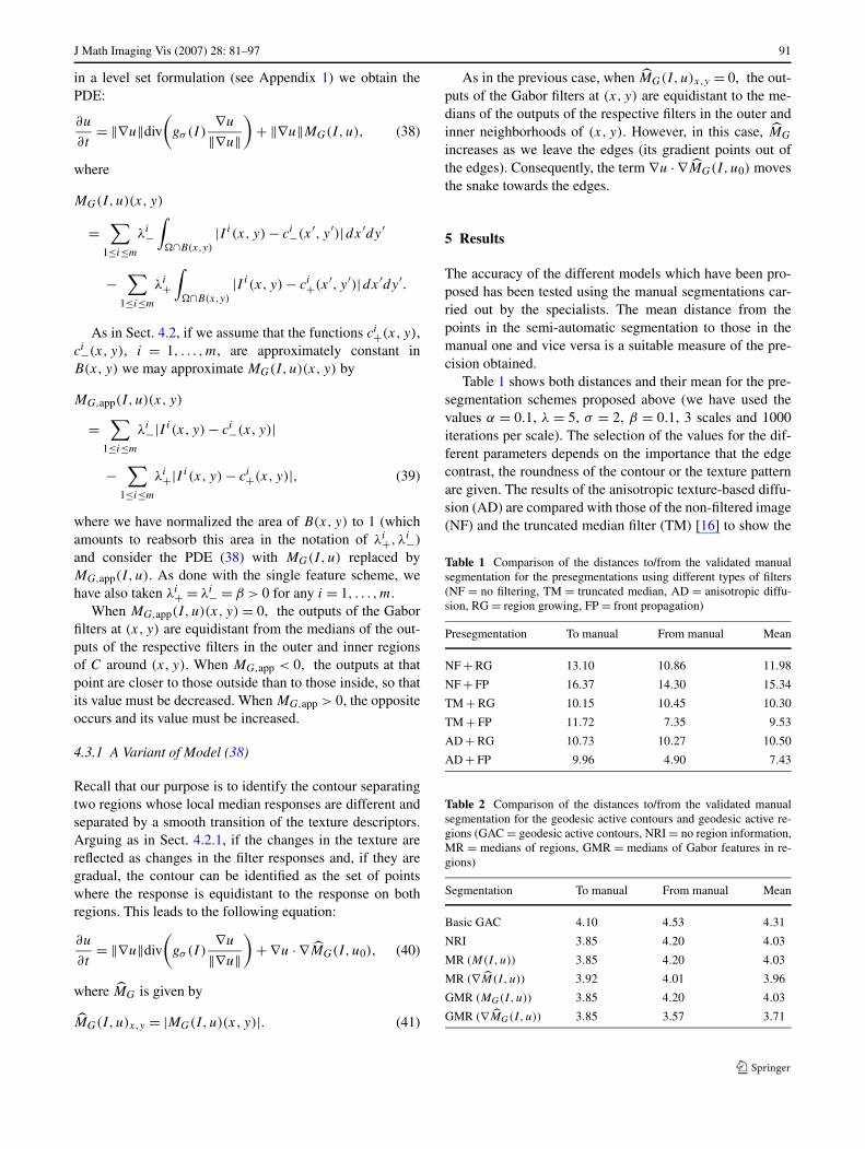
Fig. 10 Final contour obtained for the nodule in Fig. 1 using the geo-desic active contours scheme in (41) with Gabor filters from the frontpropagation presegmentation (we have used the values α = 0.1, λ = 5,σ = 2, β = 0.1, 3 scales and 1000 iterations)
accuracy of two types pre-segmentations: a region-growingalgorithm (RG) and the front propagation scheme (FP). Onthe other hand, Table 2 compares the same distances oncethe geodesic active contours with region information are ap-plied. The basic geodesic active contours technique (GAC)is improved by performing more iterations considering dif-
ferent terms. The scheme with no region information (NRI)is compared with the one described in (27) for median in-tensity separable regions (MR) using (30) and (34), and withthat described in (38) and (40) for Gabor descriptors medi-ans (GMR). Figure 10 illustrates the result of applying geo-desic active regions with Gabor descriptors.
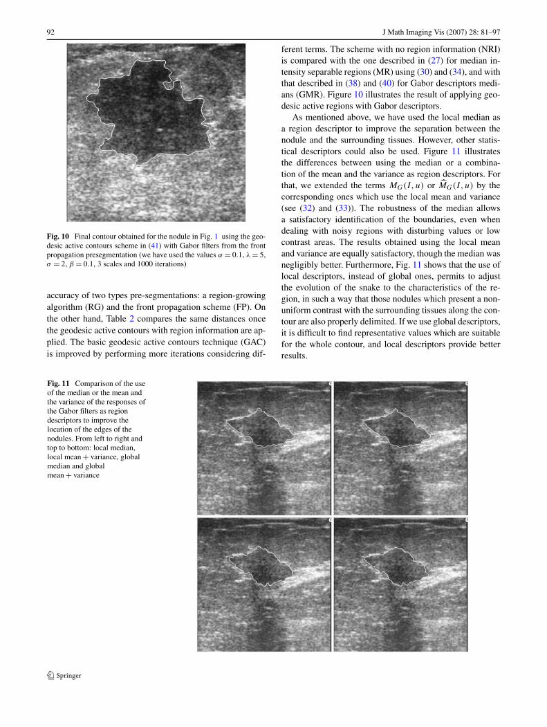
As mentioned above, we have used the local median asa region descriptor to improve the separation between thenodule and the surrounding tissues. However, other statis-tical descriptors could also be used. Figure 11 illustratesthe differences between using the median or a combina-tion of the mean and the variance as region descriptors. Forthat, we extended the terms MG(I,u) or MG(I,u) by thecorresponding ones which use the local mean and variance(see (32) and (33)). The robustness of the median allowsa satisfactory identification of the boundaries, even whendealing with noisy regions with disturbing values or lowcontrast areas. The results obtained using the local meanand variance are equally satisfactory, though the median wasnegligibly better. Furthermore, Fig. 11 shows that the use oflocal descriptors, instead of global ones, permits to adjustthe evolution of the snake to the characteristics of the re-gion, in such a way that those nodules which present a non-uniform contrast with the surrounding tissues along the con-tour are also properly delimited. If we use global descriptors,it is difficult to find representative values which are suitablefor the whole contour, and local descriptors provide betterresults.
Fig. 11 Comparison of the useof the median or the mean andthe variance of the responses ofthe Gabor filters as regiondescriptors to improve thelocation of the edges of thenodules. From left to right andtop to bottom: local median,local mean + variance, globalmedian and globalmean + variance
J Math Imaging Vis (2007) 28: 81–97 93
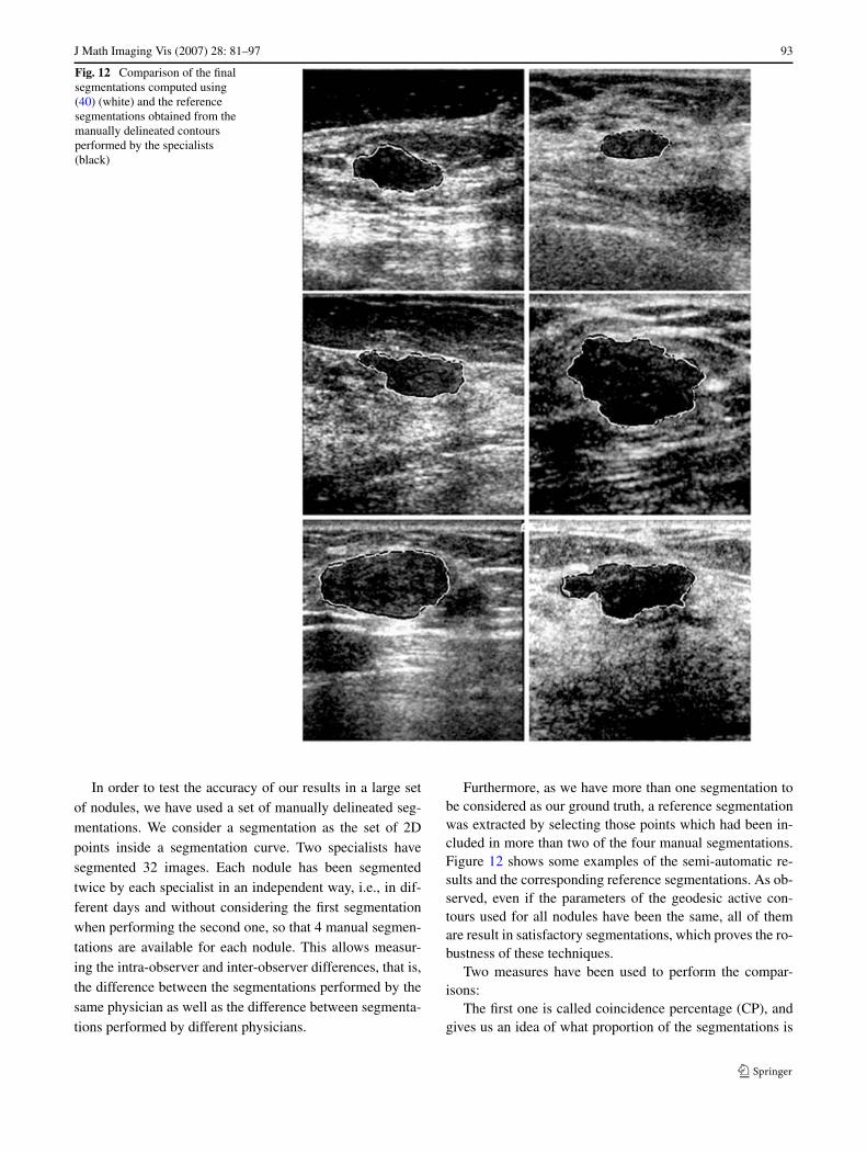
Fig. 12 Comparison of the finalsegmentations computed using(40) (white) and the referencesegmentations obtained from themanually delineated contoursperformed by the specialists(black)
In order to test the accuracy of our results in a large setof nodules, we have used a set of manually delineated seg-mentations. We consider a segmentation as the set of 2Dpoints inside a segmentation curve. Two specialists havesegmented 32 images. Each nodule has been segmentedtwice by each specialist in an independent way, i.e., in dif-ferent days and without considering the first segmentationwhen performing the second one, so that 4 manual segmen-tations are available for each nodule. This allows measur-ing the intra-observer and inter-observer differences, that is,the difference between the segmentations performed by thesame physician as well as the difference between segmenta-tions performed by different physicians.
Furthermore, as we have more than one segmentation tobe considered as our ground truth, a reference segmentationwas extracted by selecting those points which had been in-cluded in more than two of the four manual segmentations.Figure 12 shows some examples of the semi-automatic re-sults and the corresponding reference segmentations. As ob-served, even if the parameters of the geodesic active con-tours used for all nodules have been the same, all of themare result in satisfactory segmentations, which proves the ro-bustness of these techniques.
Two measures have been used to perform the compar-isons:
The first one is called coincidence percentage (CP), andgives us an idea of what proportion of the segmentations is
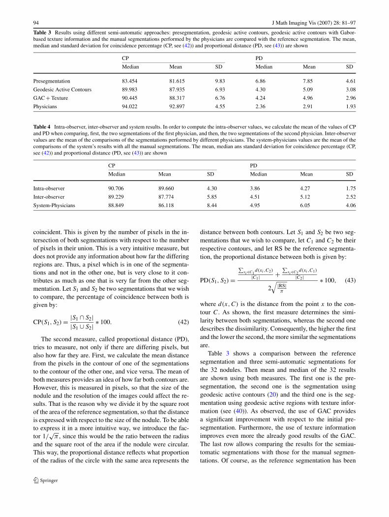
94 J Math Imaging Vis (2007) 28: 81–97
Table 3 Results using different semi-automatic approaches: presegmentation, geodesic active contours, geodesic active contours with Gabor-based texture information and the manual segmentations performed by the physicians are compared with the reference segmentation. The mean,median and standard deviation for coincidence percentage (CP, see (42)) and proportional distance (PD, see (43)) are shown
CP PD
Median Mean SD Median Mean SD
Presegmentation 83.454 81.615 9.83 6.86 7.85 4.61
Geodesic Active Contours 89.983 87.935 6.93 4.30 5.09 3.08
GAC + Texture 90.445 88.317 6.76 4.24 4.96 2.96
Physicians 94.022 92.897 4.55 2.36 2.91 1.93
Table 4 Intra-observer, inter-observer and system results. In order to compute the intra-observer values, we calculate the mean of the values of CPand PD when comparing, first, the two segmentations of the first physician, and then, the two segmentations of the second physician. Inter-observervalues are the mean of the comparisons of the segmentations performed by different physicians. The system-physicians values are the mean of thecomparisons of the system’s results with all the manual segmentations. The mean, median ans standard deviation for coincidence percentage (CP,see (42)) and proportional distance (PD, see (43)) are shown
CP PD
Median Mean SD Median Mean SD
Intra-observer 90.706 89.660 4.30 3.86 4.27 1.75
Inter-observer 89.229 87.774 5.85 4.51 5.12 2.52
System-Physicians 88.849 86.118 8.44 4.95 6.05 4.06
coincident. This is given by the number of pixels in the in-tersection of both segmentations with respect to the numberof pixels in their union. This is a very intuitive measure, butdoes not provide any information about how far the differingregions are. Thus, a pixel which is in one of the segmenta-tions and not in the other one, but is very close to it con-tributes as much as one that is very far from the other seg-mentation. Let S1 and S2 be two segmentations that we wishto compare, the percentage of coincidence between both isgiven by:
CP(S1, S2) = |S1 ∩ S2||S1 ∪ S2| ∗ 100. (42)
The second measure, called proportional distance (PD),tries to measure, not only if there are differing pixels, butalso how far they are. First, we calculate the mean distancefrom the pixels in the contour of one of the segmentationsto the contour of the other one, and vice versa. The mean ofboth measures provides an idea of how far both contours are.However, this is measured in pixels, so that the size of thenodule and the resolution of the images could affect the re-sults. That is the reason why we divide it by the square rootof the area of the reference segmentation, so that the distanceis expressed with respect to the size of the nodule. To be ableto express it in a more intuitive way, we introduce the fac-tor 1/
√π , since this would be the ratio between the radius
and the square root of the area if the nodule were circular.This way, the proportional distance reflects what proportionof the radius of the circle with the same area represents the
distance between both contours. Let S1 and S2 be two seg-mentations that we wish to compare, let C1 and C2 be theirrespective contours, and let RS be the reference segmenta-tion, the proportional distance between both is given by:
PD(S1, S2) =∑
xi∈C1d(xi ,C2)
|C1| +∑
xi∈C2d(xi ,C1)
|C2|2√
|RS|π
∗ 100, (43)
where d(x,C) is the distance from the point x to the con-tour C. As shown, the first measure determines the simi-larity between both segmentations, whereas the second onedescribes the dissimilarity. Consequently, the higher the firstand the lower the second, the more similar the segmentationsare.
Table 3 shows a comparison between the referencesegmentation and three semi-automatic segmentations forthe 32 nodules. Then mean and median of the 32 resultsare shown using both measures. The first one is the pre-segmentation, the second one is the segmentation usinggeodesic active contours (20) and the third one is the seg-mentation using geodesic active regions with texture infor-mation (see (40)). As observed, the use of GAC providesa significant improvement with respect to the initial pre-segmentation. Furthermore, the use of texture informationimproves even more the already good results of the GAC.The last row allows comparing the results for the semiau-tomatic segmentations with those for the manual segmen-tations. Of course, as the reference segmentation has been
J Math Imaging Vis (2007) 28: 81–97 95
extracted from the manual segmentations, the differencesfrom the latter to the reference one are very small, providinga measure of the dispersion of the manual results.
Table 4 shows a comparison of the intra-observer andinter-observer difference with the difference between thesemi-automatic segmentation and all manual segmentations.As expected, the intra-observer differences are lower thanthe intra-observer ones and those are less than the semi-automatic ones. However, even though the results of thesemi-automatic segmentation are not as good as the man-ual ones, the differences are small, and we could considerthem as quite satisfactory.
6 Conclusion
We have presented a new approach in the segmentation ofbreast tumors in ultrasound images. We use known tech-niques, such as anisotropic diffusion, balloon methods, Ga-bor filters or geodesic active contours. The combination ofsuch techniques, taking advantage of the benefits of eachone, as well as the introduction of certain texture descrip-tors for a better filtering, pre-segmentation and final seg-mentation provide quite satisfactory results in the case ofvery complex data, such as ultrasound images. First, the pro-posed anisotropic texture-guided diffusion generates a verysuitable image for the initial segmentation, since diffusionis performed across the regions which present similar tex-ture features and inhibited when a change in the descrip-tors is found. By means of a set of Gabor filters with differ-ent scales, orientations and frequencies, we obtain a texture-based region description which allows measuring the simi-larity between two patterns. The distance in these responsesis used to enhance or inhibit the diffusion.
Secondly, the use of the proposed front propagationscheme of balloon type, in which gradient information isused to control the speed of the propagation, produces morerobust initial segmentations. Even if there is no suitablethreshold to identify a closed contour for the nodule, the pos-sible gaps that may appear do not produce a drastic overflowin the growing process.
Finally, the use of region information in the evolution ofthe snakes allows a more accurate location of the edges ofthe tumors. The introduction of texture information in termsof Gabor filter response allows a more complete descrip-tion of the regions and, therefore, a more precise locationof their boundaries [34]. The fact that we search for equidis-tant inner and outer medians, instead of a high gradient inthe edge description, allows locating the edges when theyare blurred, non-uniform or gradual. The numerical experi-ments are quite promising. The final segmentation obtainedafter all proposed phases are very competitive with respectto the manual segmentation of the nodules performed by thespecialists.
Although these models have been developed for the par-ticular case of ultrasound images, they could also be ap-plied to any other type of images. However, the character-istic speckle noise of these images and the precision nec-essary for the study of the benign and malignant findingsrequire a deep texture analysis which could be simplified inother applications in which textures are more clearly identi-fied. Thus, the same scheme could be used in many practicalapplications for which classical methods do not provide sat-isfactory results.
Acknowledgements The authors would like to thank PatriciaAlemán-Flores, Rafael Fuentes-Pavón and José Manuel Santana-Montesdeoca, for providing the medical background, the manual seg-mentations and the suggestions to this work, as well as the HospitalUniversitario Insular de Gran Canaria for the ultrasonographic images.The third author acknowledges partial support by the Departamentd’Universitats, Recerca i Societat de la Informació de la Generalitatde Catalunya and by PNPGC project, reference BFM2003-02125. Wewould like to thank Nir Sochen for pointing out his work to us. Thefirst and second authors acknowledge the support of the Ministerio deEducación y Ciencia, reference TIN2005-02004.
Appendix 1 Level Set Formulation of Geometric CurveEvolution
Let us briefly recall the implicit level set formulation of thecurve evolution equation
Ct = γ n, (44)
where C(t, s) is an evolving curve in R2, t represents the
time parameter of the evolution, s is a parameterization of C,n is the outer unit normal to the curve C and γ is the speedof evolution of the curve which is a function of x (i.e., theposition of the curve) and the geometric quantities n and thecurvature κ of C. We assume that the curve C(t) is a level setof an evolving function u(t, x, y), (x, y) ∈ R
2. To fix ideas,let us assume that C(t) is the zero level set of u(t, x, y), andu(t, x, y) is positive inside the zero level-set, and negativeoutside (in some cases, the signed distance function is a pre-ferred choice). Thus, we have
u(t,C(t)) = 0.
Differentiating the above identity with respect to t we obtain
ut + 〈∇u,Ct 〉 = 0.
Using the relation n = −∇u/‖∇u‖, we have
ut = −〈∇u,Ct 〉 = −〈∇u,γ n〉
= γ
⟨∇u,
∇u
‖∇u‖⟩= γ ‖∇u‖.
This derivation was the basis of the level set formulation ofgeometric curve evolutions and can be found in [29].
96 J Math Imaging Vis (2007) 28: 81–97
Appendix 2 Numerical Implementation of ActiveContours
Geodesic active contours require a close initialization toreach the desired contour. Otherwise, the contour wouldtend to round and reduce. Many applications ask the userto manually introduce a set a several dozens of points tobuild a polygon which will be used as initial contour. Sincewe apply a front propagation algorithm before the snakes,the pre-segmentation obtained with this technique is usedas initial contour Cinit. Then we define u0 by assigning thesigned distance to the contour Cinit to every point (one couldalso simply define a function with two different values insideand outside Cinit). Then the level set formulation of geo-desic active contours is used to make the contour evolve.To discretize (20) we use the explicit discretization schemeobtained by adapting the standard scheme proposed in [29],which we simply write as:
un+1i,j − un
i,j
τ= gσ (In
ij )div
( ∇unij
‖∇unij‖
)‖∇un
ij‖
+ λ∇unij · ∇gσ (In
ij ), (45)
where τ > 0.To obtain gσ (In
ij ), we first use an approximation of theGaussian filter, based on the heat equation [1], then we esti-mate the gradient, and then calculate
gσ (Iij ) = 1√1 + α‖∇(Iσ )ij‖2
.
For the estimation of the gradients, we use the masks de-scribed in (8).
As explained in Sect. 4, we use a multiscale implemen-tation, starting with higher values of σ for the initializationprovided by the pre-segmentation, and reducing it at eachscale. Given a final standard deviation σ0 and a number ofscales S, the standard deviations used at the different scalesare Sσ0, (S − 1)σ0, . . . , σ0.
In the case of the vectorial descriptor, we compute theset of Gabor filters by convolving with the correspondingkernels. From the outputs of these filters, we extract the cor-responding median values (or mean values when we testedthis case) and compute the term MG,app defined in (39). Todiscretize (38) with MG,app in place of MG we adapt againthe standard scheme in [29] and we write:
un+1i,j − un
i,j
τ
= gσ (Inij )div
( ∇unij
‖∇unij‖
)‖∇un
ij‖
+ λ∇unij · ∇gσ (In
ij ) + ‖∇un‖MG,app(In,un),
where τ > 0. We also use the same type of scheme to dis-cretize (40).
References
1. Álvarez, L., Mazorra, L.: Signal and image restoration using shockfilter and anisotropic diffusion. SIAM J. Numer. Anal. 31(2), 590–605 (1994)
2. Brox, T., Weickert, J.: Level set based image segmentation withmultiple regions. In: Pattern Recognition. Lecture Notes in Com-puter Science, vol. 3175, pp. 415–423 (2004)
3. Brox, T., Weickert, J., Burgeth, B., Mrázek, P.: Nonlinear structuretensors. Image Vis. Comput. 24(1), 41–55 (2006)
4. Caselles, V., Catté, F., Coll, T., Dibos, F.: A geometric modelfor active contours in image processing. Numer. Math. 66, 1–31(1993)
5. Caselles, V., Kimmel, R., Sapiro, G.: Geodesic active contours.In: Proc. of Fifth International Conference on Computer Vision,pp. 694–699 (1995)
6. Caselles, V., Kimmel, R., Sapiro, G.: Geodesic active contours.Int. J. Comput. Vis. 22(1), 61–79 (1997)
7. Caselles, V., Kimmel, R., Sapiro, G.: Geometric active contoursfor image segmentation. In: Bovik, A. (ed.) Handbook of Videoand Image Processing, 2nd edn., pp. 613–627 (2005)
8. Chan, T.F., Sandberg, B.Y., Vese, L.A.: Active contours withoutedges for vector-valued images. J. Vis. Commun. Image Repre-sent. 11(2), 130–141 (2000)
9. Chan, T., Vese, L.: An active contour model without edges. In:Scale-Space Theory in Computer Vision. Lecture Notes in Com-puter Science, vol. 1682, pp. 141–151 (1999)
10. Chan, T.F., Vese, L.A.: Active contours and segmentation mod-els using geometric pde’s for medical imaging. In: Malladi, R.(ed.) Geometric Methods in Bio-Medical Image Processing, Se-ries: Mathematics and Visualization, pp. 63–75. Springer, Berlin(2002)
11. Chen, D.R., Chang, R.F., Juang, Y.L.: Computer-aided diagnosisapplied to us of solid breast nodules by using neural networks.Radiology 213, 407–412 (1999)
12. Cheng, C.M., Chou, Y.H., Han, K.C., Hung, G.S., Tiu, C.M.,Chiou, H.J., Chiou, S.Y.: Breast lesions on sonograms: Computer-aided diagnosis with nearly setting-independent features and arti-ficial neural networks. Radiology 226, 504–514 (2003)
13. Cohen, L.D.: On active contour models and balloons. Comput.Vis. Graph. Image Process. 53(2), 211–218 (1991)
14. Cremers, D., Soatto, S.: Motion Competition: A variational frame-work for piecewise parametric motion segmentation. Int. J. Com-put. Vis. 62(3), 249–265 (2005)
15. Cremers, D., Tischhäuser, F., Weickert, J., Schnörr, C.: Diffusionsnakes: introducing statistical shape knowledge into the Mumford-Shah functional. Int. J. Comput. Vis. 50, 295–313 (2002)
16. Davis, E.R.: On the noise suppression and image enhancementcharacteristics of the median, truncated median and mode filters.Pattern Recognit. Lett. 7, 87–97 (1988)
17. Frost, V.S., Stiles, J.A., Shanmugan, K.S., Holtzman, J.C.:A model for radar images and its application to adaptive digitalfiltering of multiplicative noise. IEEE Trans. Pattern Anal. Mach.Intell. 4, 157–165 (1982)
18. Gabor, D.: Theory of communications. J. IEEE 93, 429–459(1946)
19. Heiler, M., Schnörr, C.: Natural image statistics for natural image.Int. J. Comput. Vis. 63(1), 5–19 (2005)
20. Hernandez, M., Frangi, A.F.: Geodesic active regions using non-parametric statistical regional description and their application toaneurysm segmentation from CTA. LNCS 3150, 94–102 (2004)
J Math Imaging Vis (2007) 28: 81–97 97
21. Kass, M., Witkin, A., Terzopoulos, D.: Snakes: Active contourmodels. In: 1st International Conference on Computer Vision,pp. 259–268 (1987)
22. Kaufhold, J., Chan, R., Karl, W.C., Castanon, D.A.: Ultrasoundtissue analysis and characterization. In: Proc. of SPIE, pp. 73–83(1999)
23. Kichenassamy, S., Kumar, A., Olver, P., Tannenbaum, A., Yezzi,A.: Conformal curvature flows: from phase transitions to activevision. Arch. Ration. Mech. Anal. 134(3), 275–301 (1996)
24. Kimmel, R., Bruckstein, A.M.: On regularized Laplacian zerocrossings and other optimal edge integrators. Int. J. Comput. Vis.53, 225–243 (2003)
25. Kuan, D.T., Sawchuck, A.A., Strand, T.C., Chavel, P.: Adaptivenoise smoothing filter for images with signal-dependent noise.IEEE Trans. Pattern Anal. Mach. Intell. 7, 165–177 (1985)
26. Kuo, W.J., Chang, R.F., Moon, W.K., Lee, C.C., Chen, D.R.: Com-puteraided diagnosis of breast tumors with different us systems.Acad. Radiol. 9, 793–799 (2002)
27. Lee, J.S.: Digital image enhancement and noise filtering by useof local statistics. IEEE Trans. Pattern Anal. Mach. Intell. 2(2),165–168 (1980)
28. Malladi, R., Sethian, J.A., Vemuri, B.C.: Shape modeling withfront propagation: a level set approach. IEEE Trans. Pattern Anal.Mach. Intell. 17, 158–175 (1995)
29. Osher, S., Sethian, J.: Fronts propagating with curvature depen-dent speed: algorithms based on the Hamilton-Jacobi formulation.J. Comput. Phys. 79, 12–49 (1988)
30. Paragios, N., Deriche, R.: Geodesic active regions for supervisedtexture segmentation. In: Proc. of International Conference onComputer Vision (1999)
31. Perona, P., Malik, J.: Scale space and edge detection usinganisotropic diffusion. IEEE Trans. Pattern Anal. Mach. Intell. 12,629–639 (1990)
32. Rousson, M., Brox, T., Deriche, R.: Active unsupervised texturesegmentation on a diffusion based feature space. In: IEEE Con-ference on Computer Vision and Pattern Recognition (CVPR),pp. 699–704 (2003)
33. Rousson, M., Cremers, D.: Efficient kernel density estimation ofshape and intensity priors for level set segmentation. In: Gerig, G.(ed.) Medical Image Comput. and Comp.-Ass. Interv. (MICCAI).LNCS Springer, vol. 3750, pp. 757–764 (2005)
34. Sagiv, C., Sochen, N.: Integrated active contours for texture seg-mentation. IEEE Trans. Image Process. 1(1), 415–423 (2004)
35. Sandberg, B., Chan, T., Vese, L.: A level-set and Gabor-based ac-tive contour algorithm for segmenting textured images. TechnicalReport 39, Math. Dept. UCLA, Los Angeles, USA, July 2002
36. Stavros, A.T., Thickman, D., Rapp, C.L., Dennis, M.A., Parker,S.H., Sisney, G.A.: Solid breast nodules: Use of sonography to dis-tinguish between benign and malignant lesions. Radiology 196(1),123–134 (1995)
37. Weickert, J.: Anisotropic diffusion in image processing. In: ECMISeries, Teubner, Stuttgart (1998)
38. Yu, Y., Acton, S.T.: Speckle reducing anisotropic diffusion. IEEETrans. Image Process. 11(11), 1260–1270 (2003)
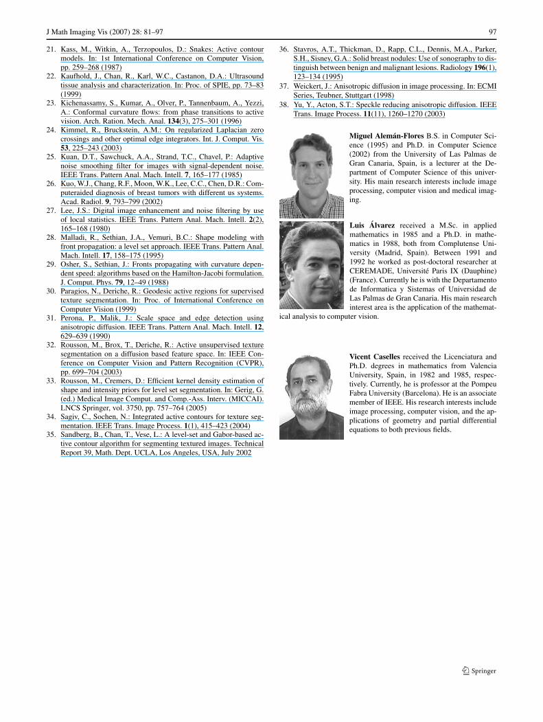
Miguel Alemán-Flores B.S. in Computer Sci-ence (1995) and Ph.D. in Computer Science(2002) from the University of Las Palmas deGran Canaria, Spain, is a lecturer at the De-partment of Computer Science of this univer-sity. His main research interests include imageprocessing, computer vision and medical imag-ing.
Luis Álvarez received a M.Sc. in appliedmathematics in 1985 and a Ph.D. in mathe-matics in 1988, both from Complutense Uni-versity (Madrid, Spain). Between 1991 and1992 he worked as post-doctoral researcher atCEREMADE, Université Paris IX (Dauphine)(France). Currently he is with the Departamentode Informatica y Sistemas of Universidad deLas Palmas de Gran Canaria. His main researchinterest area is the application of the mathemat-
ical analysis to computer vision.
Vicent Caselles received the Licenciatura andPh.D. degrees in mathematics from ValenciaUniversity, Spain, in 1982 and 1985, respec-tively. Currently, he is professor at the PompeuFabra University (Barcelona). He is an associatemember of IEEE. His research interests includeimage processing, computer vision, and the ap-plications of geometry and partial differentialequations to both previous fields.


