Techniques to Avoid Useless Packet Transmission in

Techniques to Avoid Useless Packet

Transmission in Multimedia over Best-Effort

Networks

by

Jizhong (Jim) Wu

B.S., Zhong Shan University, 1988

GradDip, Monash University, 1995

M.S., Monash University, 1997

THE UNIVERSITY OF NEW SOUTH WALES

I ~

SYDNEY• AUSTRALIA

A thesis submitted in fulfillment

of the requirements for the degree of

Doctor of Philosophy

School of Computer Science & Engineering

University of New South Wales

2003

This thesis entitled: Techniques to Avoid Useless Packet Transmission in Multimedia over Best-Effort

Networks written by Jizhong (Jim) Wu

has been approved for the School of Computer Science & Engineering

Supervisor: Assoc. Prof. Mahbub Hassan

Signature 3 July '2.d(;; Date ______ _

The final copy of this thesis has been examined by the signatory, and I find that both the content and the form meet acceptable presentation standards of scholarly work in

the above mentioned discipline.

Declaration

I hereby declare that this submission is my own work and to the best of my knowledge it contains no materials previously published or written by another person, nor material which to a substantial extent has been accepted for the award of any other degree or diploma at UNSW or any other educational institution, except where due acknowledgement is made in the thesis. Any contribution made to the research by others, with whom I have worked at UNSW or elsewhere, is explicitly acknowl~dged in the thesis.

I also declare that the intellectual content of this thesis is the product of my own work, except to the extent that assistance from others in the project's design and conception or in style, presentation and linguistic expression is acknowledged.

. D~/ul-6v?... Signature e 1 /

Abstract

In this thesis, we investigate issues related to multimedia transmission over the

Internet. We identify the Useless Packet Transmission (UPT) problem and propose

three Useless Packet Transmission Avoidance (UPTA) algorithms to address the UPT

problem, in various network situations. UPTA can effectively eliminate transmission of

useless multimedia packets, and allocate the recovered bandwidth to competing TCP

flows. As a result, UPTA improves TCP throughput and reduces file download time

with no significant impact on overall intelligibility of multimedia applications.

UPT is a side-effect of fair queueing and scheduling algorithms that enforce fair

ness. At times of congestion, a fair algorithm allocates bandwidth equally to all compet

ing sources, without considering whether or not the allocated bandwidth is useful from

application's perspective. UPT is based on the fact that for packetised audio and video,

packet loss rate must be maintained under a given threshold for any meaningful commu

nication. As best-effort networks do not support QoS guarantee, packet loss rate may be

unacceptably large for multimedia applications, at times of network congestion. When

packet loss rate exceeds a given threshold, received audio and video become unintel

ligible. A congested router transmitting multimedia packets, while inflicting a packet

loss rate beyond a given threshold, effectively transmits useless packets. UPT reduces

the available bandwidth to competing TCP flows, which in tum increases file down

load times. Longer download times increase power consumption of battery-powered

devices, and hence, have direct impact on mobile computing as well.

V

We demonstrate the implementation of UPTA in two well-known fair queue

ing/scheduling algorithms: WFQ and CSFQ. We show that UPTA can be easily incor

porated into these fair algorithms. Taking WFQ/CSFQ as example, we investigate UPT

avoidance problem in three different network situations, i.e. single congested link, mul

tiple congested links and multiple multimedia flows. We explore challenges of UPTA

enforcement in different network situations, and propose solutions to address problems

that arise.

Using OPNET Modeler and MPEG-2 video stream, we conduct extensive simu

lation study to evaluate the performance of UPTA, using a number of performance met

rics including TCP throughput, file download time, video intelligibility and throughput

fairness. Our simulation results show that the proposed algorithm effectively eliminates

useless packet transmission in all network situations simulated. As a result of that, both

TCP throughput and file download times are improved significantly. For example, in

one simulated network, file download time is reduced by 55% for typical HTML files,

36% for typical image files, and up to 30% for typical video files. A Peak-Signal-to

Noise-Ratio (PSNR) based analysis shows that the overall intelligibility of the received

video is no worse than that received without the incorporation of the proposed useless

packet transmission avoidance algorithm. Our fairness analysis confirms that imple

mentation of our algorithm into the fair algorithms (WFQ and CSFQ) does not have

any adverse effect on the fairness performance of the algorithms.

Dedication

To my wife Yan

Acknowledgements

Throughout my PhD candidature, I have been so lucky to receive so much help

and support from so many people, without whom this PhD research would not have

been completed. Please forgive me if I fail to mention your names here.

First of all, I am deeply indebted to my supervisor Prof. Mahbub Hassan who has

given me enornous encouragement and help in all aspacts. I am grateful to his generous

support and professional guidance. I have benefited immensely from countless meeting

and discussions with Prof. Hassan. I learned the recipe for good journal/conference

papers from Prof. Hassan, without whom my first ever journal paper would not have

been published.

I am grateful to Prof. Sanjay Jha (co-supervisor) and Dr. Mohammad Rezvan

at Network Research Laboratory (NRL) for many helpful discussions with them. I

give my gratitude to Dr. Tim Moors (at School of Telecommunications, UNSW) and

Prof. Jim Breen (at School of Computer Science & Software Engineering, Monash

University), for their constructive comments on my PhD research.

I am grateful to anonymous journal/conference reviewers whose professional

comments (on my papers published during my PhD candidature) have been incorpo

rated into this thesis.

I would like to thank engineers at OPNET Technical Support who have helped

me a lot with my simulation problems, and folks on OPNET users' mailing list who ...

replied to my emails on OPNET simulation problems.

viii

I would like to take this opportunity to thank the management of School of Com

puter Science & Engineering, UNSW, for funding simulation packages (OPNET Mod

eler and Matlab) which were essential to this research.

My most humble and grateful heart goes to my wife Yan who has suffered a lot

due to my working away from home, especially during her early stage of pregnancy.

I am also deeply grateful to my brother Katnin for his continual encouragement and

persistent support.

Last (but not least), special thanks to all folks at NRL who helped me a lot,

and made my stay at NRL enjoyable and memorable. A big thank you to Alfandika

Nyandoro for proofreading the thesis.

Contents

Chapter

1 Introduction 1

1.1 Problem Definition 1

1.2 Motivation ..... 2

1.3 Contribution of the Thesis 4

1.4 Outline of the Thesis 5

2 Multimedia over Best-Effort 7

2.1 Growth of Multimedia 7

2.2 Multimedia Characteristics 13

2.3 Protocols ..... 14

2.3.1 RTP/RTCP 15

2.3.2 MPEG-2 16

2.3.3 MPEG-2 over IP 18

2.3.4 IP Packet Loss 20

2.4 Conclusion ...... 20

3 Related Work 21

3.1 Fair Queueing and Scheduling Algorithms . 21

3.1.1 WFQ 22

3.1.2 CSFQ. 22

X

3.2 Adaptive Multimedia . . . . . . . . . . . . . . . 24

3.3 Forward Error Correction and Loss Concealment 25 .

3.4 QoS in the Internet ............ 25

3.5 Partial Packet Discard in ATM Networks . 26

3.6 Conclusion ................ 27

4 Useless Packet Transmission Avoidance (UPTA) 28

4.1 Formal Definition of UPT Problem . 28

4.2 UPT Avoidance Algorithm ..... 30

4.3 UPTA Implementation in WFQ and CSFQ . 31

4.3.1 UPTAin WFQ 31

4.3.2 UPTA in CSFQ . 33

4.4 Packet Loss Threshold for the Experimental Video 34

4.4.1 Packet Loss/Delay and UPT 34

4.4.2 Loss Threshold Determination 36

4.5 Simulation . . . . . . . 38

4.5.1 OPNETModel 38

4.5.2 Performance Metrics 40

4.6 WFQ Simulation Results 41

4.6.1 TCP Throughput 42

4.6.2 File Download Time 47

4.6.3 Impact on Video Intelligibility 48

4.6.4 Throughput Fairness 50

4.7 CSFQ Simulation Results . 52

4.7.1 TCP Throughput 52

4.7.2 Video Intelligibility . 52

4.8 Conclusion . . . . . . . . . ... 56

xi

5 UPTA with Multiple Congested Links 58

5.1 Scope of the Problem . . . . . . ..... 58

5.2 Analysis of End-to-End Packet Loss Rate 60

5.3 Partial UPTA (P-UPTA) . 63

5.3.1 Algorithm .... 64

5.3.2 Update of Loss Threshold 65

5.4 Centralised UPTA (C-UPTA) . . . 67

5.4.1 Upper Bound for TCP Throughput Improvement 67

5.4.2 Architecture .................... 70

5.4.3 Bottleneck Fairshare Discovery (BFD) Protocol . 72

5.5 Simulation . 75

5.6 Results ... 78

5.6.1 Basic UPTA. 78

5.6.2 Partial UPTA 81

5.6.3 Centralised UPTA 84

5.6.4 Discussion 91

5.7 Conclusion .... 93

6 UPTA with Multiple Multimedia Flows 95

6.1 Scope of the Problem . . . . . . . 95

6.2 Unintelligible Flow Management . 97

6.2.1 Random Select (RS) ... 98

6.2.2 Least Bandwidth Select (LBS) 99

6.3 Performance Evaluation . . 101

6.4 Single Congested Link . 102

6.4.1 Homogeneous Video Applications . . 103

6.4.2 Heterogeneous Video Application1t . . 107

6.5 Multiple Congested Links .......... . 111

6.5.1 Homogeneous Video Applications .

6.5.2 Heterogeneous Video Applications.

6.6 Discussion . . . . . . . . . . .

6.6.1 Single Congested Link

6.6.2 Multiple Congested Links

6.7 Conclusion

7 Conclusion

7.1 Summary

7 .2 Merits of UPTA .

7.3 Limitations of UPTA

7.4 Suggestions for Future Work

Bibliography

Appendix

A Simulation with OPNET

A.I Overview .....

A.1.1 Who Uses OPNET

A.1.2 Why Use OPNET .

A.2 OPNET Explored . . . . .

A.2.1 Project Modelling

A.2.2 Node Modelling ..

A.2.3 Process Modelling

A.2.4 Data Collection Tool

A.2.5 Simulation Tool . .

A.2.6 Data Analysis Tool

xii

. 112

. 114

. 120

. 121

. 121

. 122

124

. 124

. 127

. 128

. 129

130

136

. 136

. 137

. 138

. 141

. 142

. 144

. 145

. 147

. 147

. 148

Xlll

A.2.7 Parameter Editors . . 148

A.3 Practical Examples .... . 149

A.3.1 Process Model Development : . 149

A.3.2 Node Model Development . . . 152

A.3.3 Network Model Development . 152

A.3.4 Simulation Execution . . 152

A.4 Conclusion .......... . 153

B Program Listings 154

B.1 C Programs . 154

B.1.1 pkLdrop.c. . 154

B.1.2 video_rec.c . 156

B.1.3 picJist.c. . 158

B.2 Matlab Program . . 160

B.2.1 psnr_cal.m . 160

C Acronyms and Abbreviations 163

D Publications 165

List of Tables

Table

2.1 User Base of Multimedia Applications over the Internet . 8

4.1 Parameters of MPEG-2 Test Stream . . . . . . . . . . . 36

4.2 Levels of Bandwidth Waste for Different Simulation Scenarios 40

4.3 Comparison of TCP Throughputs with and without UPTA . . 46

4.4 Comparison of Application Throughputs with and without UPTA . 47

4.5 Comparison of Download Time with and without UPTA (Scenario 1). 48

4.6 Comparison of Video Intelligibility . 49

4.7 Throughput Fairness . . . . . . . . 51

5 .1 Packet Loss Rate of Video Flow at Various Nodes 60

5.2 Loss Threshold for Video Flow at Various Routers. 81

5.3 TCP Throughput Improvement with P-UPTA . . . 84

5.4 Comparison of TCP Throughput (in Mbps) with and without C-UPTA 86

5.5 TCP Throughput Improvement with C-UPTA . . . . . . . . . . . . . 86

5.6 Comparison of Application Throughput (in Mbps) with and without C-

UPTA ................................... 87

5.7 Comparison of Download Time (in seconds) with and without C-UPTA

(Scenario 1) . . . . . . . . . . . . . .. 87

5.8 Comparison of Video Intelligibility . 89

5.9 Throughput Fairness . . . . . . . . . . . . . . . . .

5 .10 Comparison of Various UPTA Enforcement Schemes

6.1 Algorithms Implemented for Various Simulation Scenarios

xv

90

92

. 104

6.2 Number of Video Flows Accepted in Various Scenarios (single con

gested link; homogeneous video). . . . . . . . . . . . . . . . . . . . . 105

6.3 Comparison of Average Intelligibility Index for Video Applications

(single congested link; homogeneous video) . 107

6.4 Characteristics of Heterogeneous Video . . 108

6.5 Number of Video Flows Accepted in Various Scenarios (single con-

gested Link; heterogeneous video) . . . . . . . . . . . . . . 108

6.6 Timeline of Video Flow Recovery (single Congested link) . 109


( single congested link; heterogeneous video) . . . . . . . . . . . . . . . 111

6.8 Number of Video Flows Accepted in Various Scenarios (multiple con-

gested Link; homogeneous video) .................... 113


(multiple congested links; homogeneous video) ............. 115

6.10 Number of Video Flows Accepted in Various Scenarios (multiple con-

. gested Link; heterogeneous video) . . . . . . . . . . . . . . . 117

6.11 Time line of Video Flow Recovery (multiple congested links) 118


(multiple congested links; heterogeneous video) ............. 120

A.1 Categories of OPNET Users . . . . . . . . . . 138

List of Figures

Figure

2.1 Media-on-demand. .

2.2 Real-time playback ..

2.3 Growth of Net2Phone's IP phone service.

2.4 Protocol architecture for multimedia over the Internet. .

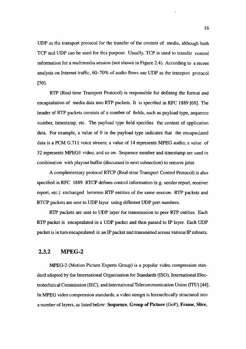
2.5 MPEG-2 video structure . . . . . . . . . . . . . .

2.6 Encapsulation of MPEG-2 TS packets in IP packets

4.1 Flow chart of UPTA. . . . . . . .

4.2 Implementation of UPTA in WFQ.

4.3 Implementation of UPTA in CSFQ.

4.4 Video packet loss rate/delay versus buffer size.

4.5 Block diagram of intelligibility analysis system.

4.6 PSNR under different packet loss rates.

4.7 OPNET simulation model. ...... .

10

10

12

15

17

19

30

31

34

35

36

37

39

4.8 Cumulative Distribution Function (CDF) of video packet delay for WFQ. 43

4.9 Packet loss rate of video flow for WFQ. . ... ! • •. • • • • • • 44

4.10 Short-term TCP throughputs for WFQ, with and without UPTA. 45

4.11 TCP throughput improvement with UPTA. . . . . . . .

4.12 Comparison of download time with and without UPTA.

4.13 Distribution of unintelligible and intelligible frames for WFQ.

47

49

50

xvii

4.14 Snapshots of unintelligible video frames. . . . . . . . . . . . . . . . . . 51


4.16 Packet loss rate of video flow for CSFQ. . . . . . . . . . . . . . 54

4.17 Short-term TCP throughputs for CSFQ, with and without UPTA. 55

4.18 Distribution of unintelligible and intelligible frames for CSFQ. 56

5.1 UPT in networks with multiple congested links ....... .

5.2 Analysis model of packet loss with multiple congested links.

5.3 End-to-end packet loss rate as a function of LPLR and number of con

gested links. . . . . . . . . . . . . . . . . . . . .

5.4 Flow-chart of Partial UPTA (P-UPTA) algorithm.

5.5 Theoretical TCP improvement against varying number of U flows in

C-UPTA ................. .

5.6 Centralised UPTA (C-UPTA) architecture.

5.7 Pseudo-code for implementation of C-UPTA in WFQ ..

5.8 QoS Probe/Report ICMP message format. ...... .

5.9 Background traffic profile in various simulation scenarios.

59

61

63

64

69

70

71

72

77


5 .11 Packet loss rate of video flow for WFQ. . . . . . . . . . . . . . . . . . 80

5.12 · Average loss rate of video packets at various routers under B-UPTA

(Scenario 6). . . . . . . . . . . . . . . . . . . . . . . . . . 82

5.13 Packet loss rate for video flow with P-UPTA (Scenario 6) .. 83

5.14 Comparison of short-term TCP throughput, with and without C-UPTA .. 85

5.15 Comparison of download time with and without C-UPTA. .. 88

5.16 Distribution of unintelligible and intelligible frames for WFQ. 89

5.17 Snapshots of unintelligible video frames during U intervals. 90

5.18 TCP throughput improvement factor agai~t unintelligible ratio. 91

6.1 UPTA in networks with multiple U flows. ............ 96

6.2 UPfA enhanced with UFM. . . . . .

6.3 Pseudo-code of Random Select (RS) ..

6.4 Pseudo-code of Least Bandwidth Select (LBS).

6.5 Simulation model for single congested link. . .

6.6 Comparison of TCP throughput and link utilisation (single congested

xviii

97

98

. 100

. 103

link; homogeneous video). . ....................... 106

6.7 Comparison of TCP throughput and link utilisation (single congested

link; heterogeneous video). . . . . . . . . . . .

6.8 Simulation model for multiple congested links.

6.9 Comparison of TCP throughput (multiple congested links; homoge-

. 110

. 112

neous video). . .............................. 114

6.10 Comparison of TCP throughput (multiple congested links; heteroge-

neous video). .................... . . . . . . . . . . . 119

A.I Growth in revenues of software licenses & services. . 139

A.2 Workspace of Project Editor. . 142

A.3 Workspace of Node Editor. . .. 144

A.4 Workspace of Process Editor. . . 146

A.5 Child process model (for queueing) of IP process. . 150

A.6 · Proto-C codes in enter executives block. . 151

A.7 Proto-C codes in Function Block (FB) .. . 151

Chapter 1

Introduction

In this chapter, we identify the problem of Useless packet Transmission (UPT),

which is a side-effect of algorithms enforcing fairness. We describe the motivation

behind our research, as well as the contribution of the thesis. Finally, we provide an

overview of the thesis.

1.1 Problem Definition

Current Internet supports only "best-effort" network service, no Quality of Ser

vice (QoS) is guaranteed. Packets may be dropped by routers at times of congestion.

Based on its reaction to network congestion condition, Internet traffic can be classified

into two broad categories - adaptive and non-adaptive traffic. Adaptive traffic is

consisted of traffic generated by adaptive sources which adjust their sending rates ac

cording to the network congestion condition. Non-adaptive traffic is characterised by its

"greedy" nature. A non-adaptive source treats the network as a "black-box" and sends

at its own rate, regardless of the network congestion condiJiQn, Among the two trans

port services available on the Internet, TCP sources are adaptive while UDP sources are

non-adaptive. Most multimedia applications over the Internet are UDP-based. These

applications tend to grab all network bandwidth and force TCP applications to close

down. This problem is known as fairness problem. Over the past few years, there has

2

been extensive research conducted to solve the fairness problem. Weighted Fair Queue

ing (WFQ) [58] and Core Stateless Fair Queue (CSFQ) [70] are two well-known fair

algorithms. Other fair algorithms include BLUE [17, 18], CHO Ke [56], and RFQ [9].

Fair algorithms solve the fairness problem by allocating bandwidth equally among

contending sources. While equal bandwidth allocation is mathematically and intellec

tually satisfying, and probably is a good solution when all contending flows are TCP

flows, it has a serious drawback when applied to routers supporting both TCP and mul

timedia traffic. Research on multimedia reveals that for packetised audio and video,

packet loss rate must be maintained under a given threshold for any meaningful com

munication [10, 21, 46]. When packet loss rate exceeds this threshold, received audio

and video become useless. Because fair algorithms do not consider the unique charac

teristic of multimedia (loss rate must be maintained below a threshold), it is possible

that a multimedia connection suffers a packet loss rate higher than the threshold at

times of serious network congestion. We call this packet transmission Useless Packet

Transmission (UPT), because multimedia packets received during these times cannot

be replayed at the receiver in an intelligible way. Interestingly, UDP-based multimedia

applications rarely have UPT problem if fairness is not enforced by routers [18, 19, 70].

Obviously, UPT has become a side-effect of fair algorithms.

1.2 Motivation

The fairness problem in the Internet is now well recognised. Many packet queue

ing and discarding algorithms have been proposed in the last few years to effectively

address the issue of fairness. Performance results confi~ t~at these algorithms can

fairly distribute link bandwidth among competing multimedia and data flows. Some

router vendors have already started incorporating these algorithms in their latest prod-.

ucts. For example, WFQ has been implemented in Cisco 2600/3600/3700 Series [37]

and Nortel Networks Passport 5430 (52].

3

The issue of UPT, however, is less understood. UPT is based on the fact that for

packetised audio and video, packet loss rate must be maintained under a given thresh

old for any meaningful communication [10, 21, 46]. When packet loss rate exceeds

this threshold, received audio and video become useless. Thus a router transmitting

multimedia packets at a fair rate (using WFQ for example), while inflicting a packet

loss rate beyond the threshold, actually transmits useless packets. These packets are

useless, because they do not contribute to any meaningful communication. UPT effec

tively reduces the available bandwidth to competing TCP flows, which in tum increases

file download times. Longer download times increase power consumption of battery

powered devices, and hence, have direct impact on mobile computing.

The UPT problem will be more significant in future due to the following trends:

(i) rising popularity of voice and video applications, (ii) increasing deployment of fair

packet queueing algorithms, and (iii) rapid proliferation of battery-powered mobile de

vices. Hence, there is a need to investigate mechanisms to effectively address the UPT

issue in fair packet queueing algorithms. In this thesis, we propose avoidance tech

niques to address the UPT problem in multimedia over best-effort networks.

We believe that the best-effort network service will be the most popular network

service for years to come, despite recent research efforts in introducing QoS into the

Internet. The reason is two-fold:

• QoS is not widely available to end users at the moment;

• Best-effort service is much cheaper than any other services.

Even after QoS services are widely deployed in the Internet, there is no way to

prevent users from running multimedia applications using best-effort network service.

This is because QoS services will definitely attract much higher charges compared with

best-effort service. Users may choose best-effort service as the platform for their multi

media applications (especially those not so business critical). On the other hand, users

4

may be reluctant to switch to QoS, as multimedia over best-effort has become a ma

ture technology, with a very large user base. Therefore, how to use network resources

efficiently in a multimedia environment has become a challenging issue.

1.3 Contribution of the Thesis

We address Useless Packet Transmission (UPT) problem in this thesis. Taking

two fair algorithms WFQ and CSFQ as examples, we demonstrate the impact of UPT

on efficiency of network resources, and propose a solution to the UPT problem. The

thesis has four major contributions as summarised below:

I. We formally define the UPT problem and propose an avoidance algorithm (we

call it UYfA) to address the problem. UPTA can be easily incorporated into

existing fair packet queueing and discarding algorithms.

2. We investigate the challenging issues related to UPT avoidance in various net

work situations, e.g. single congested link, multiple congested links and mul

tiple multimedia flows. For single congested link, basic UPTA (B-UPTA) will

suffice. For networks with multiple congested links, we propose two exten

sions to B-UPTA: partial UPTA (P-UPTA) and centralised UPTA (C-UPTA).

We demonstrate implementation of these UPTA schemes with WFQ. For C

UPTA, we propose a feedback mechanism called Bottleneck Fairshare Dis

covery (BFD) protocol to determine global fairshare on an end-to-end basis.

We propose a framework called Unintelligible Flows Management (UFM) to

address challenging issues related to UPT avoidance in networks with multi--

pie multimedia flows. We show the implementation of UFM framework with

WFQ, and propose two different UFM policies: Random Select (RS) and

Least Bandwidth Select (LBS).

3. We propose the notion of intelligibility index, a PSNR-based performance

5

metric for video intelligibility. Intelligibility index is a dimensionless fraction

between O and 1. The closer the value to 1, the higher the level of intelligi

bility. A value of 1 means all received frames are intelligible. We use this

index to measure the impact of our proposed UPf avoidance algorithm on the

quality (in terms of overall intelligibility) of the received video. Unlike many

existing assessment schemes for audio/video quality, intelligibility index is an

objective assessment scheme (as opposed to subjective schemes). Subjective

assessment (e.g. MOS) is usually time-consuming, and the results are depen

dent on opinion of individual assessors.

4. Using OPNET Modeler, we conduct extensive simulation study to evaluate the

performance of UPfA algorithm. We have incorporated UPfA into two well

known fair algorithms -WFQ and CSFQ. Using an MPEG-2 video stream as

an example in our simulation study, we evaluate the performance of UPfA in

various network configurations (i.e. single congested link, multiple congested

links and multiple multimedia flows), using a number of performance met

rics including TCP throughput, file download time, video intelligibility and

throughput fairness.

1.4 Outline of the Thesis

The rest of the thesis is organised as follows. We introduce the emerging mul

timedia applications over the Internet in Chapter 2. We present the architecture of

supporting multimedia over best-effort networks, and discuss techniques behind it. We

also discuss the unique characteristics of multimedia applications, and their impacts on

network performance in this chapter.

We discuss related work in Chapter 3. We present recent research efforts on

supporting multimedia over the Internet, and describe related issues.

6

In Chapter 4, we define the UPf problem and propose an avoidance algorithm

called UPTA. We present the architecture for implementing UPfA in WFQ and CSFQ,

and evaluate the performance of UPfA, using simulation of an MPEG-2 video stream

competing with a TCP connection in a network with single congested link.

We investigate the problem of UPfA enforcement in networks with multiple con

gested links in Chapter 5. We present the architecture of Bottleneck Fairshare Discov

ery (BFD) protocol in details, and describe the detailed operation of BFD and evaluate

the performance of UPfA in a network with multiple congested links.

We investigate the problem of UPfA enforcement in network with multiple mul

timedia flows in Chapter 6. We present the Unintelligible Rows Management (UFM)

framework, and describe the two different control policies (i.e. RS and LBS) proposed

for UFM. We also discuss advantages/disadvantages of these two control policies, in

comparison with basic UPfA.

We summarise our work and discuss merits/demerits of UPfA in Chapter 7. We

draw our conclusion and discuss future research issues in this chapter.

We present an introduction to OPNET Modeler [71] in Appendix A, and dis

cuss our simulation experience with OPNET. We list our C and Matlab programs in

Appendix B, and a list of publications is given in Appendix D.

Chapter 2

Multimedia over Best-Effort

Multimedia applications are applications that can integrate voice, video, and clas

sical data into a single application platform. The development and deployment of mul

timedia over the Internet are driven by two factors - user demands and advances in

information technology. Nowadays, many multimedia applications are available free

of charge online. This has also contributed to the widespread use of multimedia ap

plications. The past few years saw explosive growth of multimedia applications over

the Internet. While bringing us a lot of fun, these exciting multimedia applications

also introduce some challenging issues to Internet research community. In this chap

ter, we look at the architecture for supporting multimedia applications over best-effort

network service and explore the unique characteristics of multimedia applications.

2.1 Growth of Multimedia

Multimedia applications have been seen in the Internet since early 1990s. Recent

years witnessed a wide variety of multimedia applications_being deployed over the In

ternet. While more and more users are trying to use multimedia applications available

online, new multimedia applications are making their ways to the Internet from time

to time.

Multimedia applications are also referred to as continuous media applications.

8

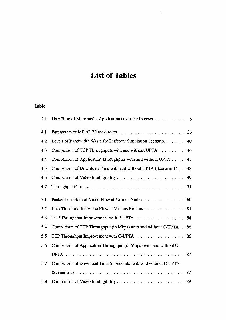
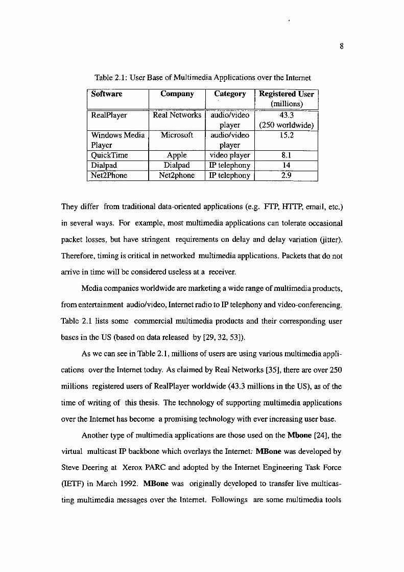
Table 2.1: User Base of Multimedia Applications over the Internet

Software Company Category Registered User - (millions)

RealPlayer Real Networks audio/video 43.3 player (250 worldwide)

Windows Media Microsoft audio/video 15.2 Player player QuickTime Apple video player 8.1 Dialpad Dialpad IP telephony 14 Net2Phone Net2phone IP telephony 2.9

They differ from traditional data-oriented applications (e.g. FTP, HTIP, email, etc.)

in several ways. For example, most multimedia applications can tolerate occasional

packet losses, but have stringent requirements on delay and delay variation (jitter).

Therefore, timing is critical in networked multimedia applications. Packets that do not

arrive in time will be considered useless at a receiver.

Media companies worldwide are marketing a wide range of multimedia products,

from entertainment audio/video, Internet radio to IP telephony and video-conferencing.

Table 2.1 lists some commercial multimedia products and their corresponding user

bases in the US (based on data released by [29, 32, 53]).

As we can see in Table 2.1, millions of users are using various multimedia appli

cations over the Internet today. As claimed by Real Networks [35], there are over 250

millions registered users of RealPlayer worldwide (43.3 millions in the US), as of the

time of writing of this thesis. The technology of supporting multimedia applications

over the Internet has become a promising technology with ever increasing user base.

Another type of multimedia applications are those used on the Mbone [24], the

virtual multicast IP backbone which overlays the Internet; MBone was developed by

Steve Deering at Xerox PARC and adopted by the Internet Engineering Task Force

(IETF) in March 1992. MBone was originally deyeloped to transfer live multicas

ting multimedia messages over the Internet. Followings are some multimedia tools

9

developed for Mbone:

• Visual Audio Tool (vat [39])

• Video Conferencing (vie [40])

• Network Voice Terminal (nvt [54])

• Network Video (nv [57])

• INRIA Videoconferencing System (ivs [15])

• Whiteboard (wb [41])

Unlike other media (e.g. text files), audio/video files are usually played back

before the whole content has been received, because of timing requirements. That is,

the media is played "on-the-fly", while the remaining parts are arriving. Therefore,

this type of multimedia application is also referred to as streaming application. In

general, multimedia applications in the Internet can be classified into three categories:

Media-on-demand, Real-time playback and Real-time interactive media.

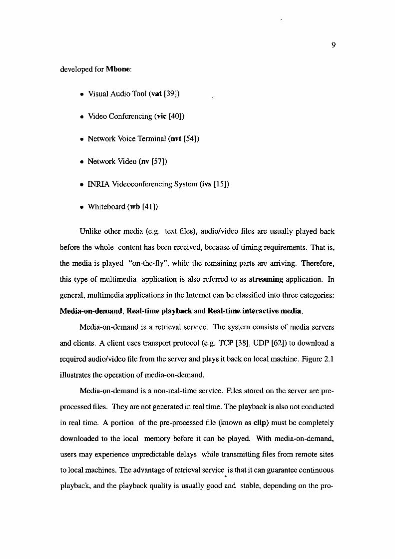
Media-on-demand is a retrieval service. The system consists of media servers

and clients. A client uses transport protocol (e.g. TCP [38], UDP [62]) to download a

required audio/video file from the server and plays it back on local machine. Figure 2.1

illustrates the operation of media-on-demand.

Media-on-demand is a non-real-time service. Files stored on the server are pre

processed files. They are not generated in real time. The playback is also not conducted

in real time. A portion of the pre-processed file (known as clip) must be completely

downloaded to the local memory before it can be played •.. With media-on-demand,

users may experience unpredictable delays while transmitting files from remote sites

to local machines. The advantage of retrieval service is that it can guarantee continuous •

playback, and the playback quality is usually good and stable, depending on the pro-

Local Machine I I

, Local Memory : I I

Video Server

Internet

Figure 2.1: Media-on-demand.

Internet

Local Machine

Figure 2.2: Real-time playback.

10

cessing capacity of the local machine. Examples of this class include Real Networks'

RealPlayer [35] , Microsoft's Media Player [31] and Apple's QuickTime [34].

In a real-time playback application, the client is synchronised with the server.

Figure 2.2 illustrates the operation of a real-time playback system.

A real-time playback system deals with real-time information. In contrast to

media-on-demand, audio/video files are not stored in locatmeinory; they must be pro

cessed and presented on-the-fl y. At the peer end, audio/video signals are al so generated

in real ti me (e.g. Internet radio) . They are fed into t~e network immediately after they

are generated, without pre-processi ng. The advantage of real-time playback is obvious

11

- it can convey timely information. Examples of real-time playback include Internet

radio and television broadcasting. Details can be found in [33, 36].

Interactive real-time media works in a similar way as real-time playback. They

are all streaming applications. The difference is that interactive real-time media has a

more stringent QoS requirement (e.g. bandwidth, delay,jitter, etc.) because it supports

interaction between a pair of ( or a group of) users in real time. Applications of this

class include IP telephony (e.g. Dialpad and Net2Phone) and video-conferencing (e.g.

NetMeeting [51] and H.323 [76]).

After ten years of evolution, supporting multimedia applications over best-effort

network service (e.g. Internet) has become a mature and promising technology. As

reported in [21, 46, 48], multimedia applications have become a major consumer of

network bandwidth, and the trend is likely to continue.

A number of facts have contributed to the increasing development and deploy

ment of multimedia applications. First, the commercialisation of the Internet has put

the development of multimedia applications on the fast track. This gives rise to the

rapid proliferation of various Web companies specialising in designing multimedia

tools. Secondly, the cost of media storage has dropped drastically over the past few

years, thanks to advances in computer hardware technology. More and more media

(e.g. audio files and video clips, etc.) is put on the Internet for download. Lastly, there

has been a huge demand for multimedia applications, especially after high-speed ac

cesses to the Internet (e.g. cable modem and ADSL, etc.) are made available to home

users at affordable costs.

Most multimedia applications over the Internet are very handy for use, and many

of them are free of charge. This has also contributed to ~he ~idespread use of mul

timedia applications. For example, a student can listen to his favourite Internet radio

station while composing an essay on his computer. A few IP telephony products (e.g.

Dial pad and Net2Phone) allow users to make free calls to any telephone number within

1.2

en 1 Q)

:5 C

°E o.8 C 0

£0.6 Q) Ol o:l V)

::> 0.4

0.2

1996 1997 1998 1999 2000 2001 Year

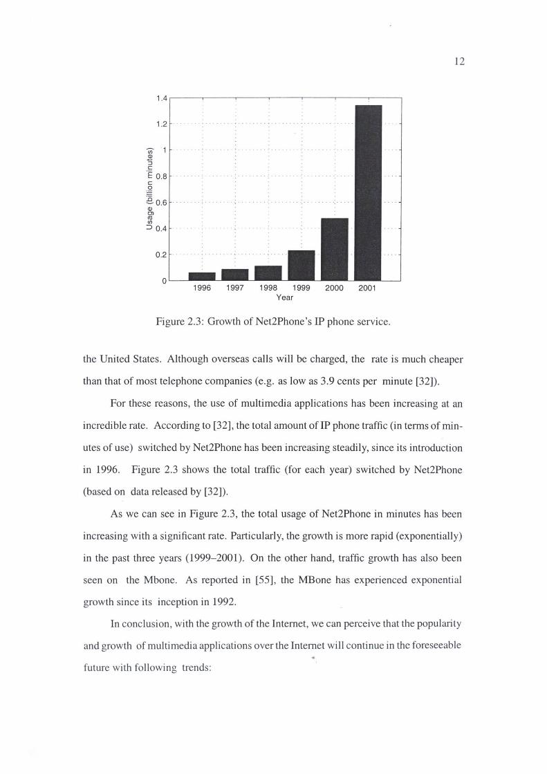
Figure 2.3: Growth of Net2Phone's IP phone service.

12

the United States. Although overseas calls will be charged, the rate is much cheaper

than that of most telephone companies (e.g. as low as 3.9 cents per minute [32]).

For these reasons, the use of multimedia applications has been increasing at an

incredible rate. According to [32], the total amount of IP phone traffic (in terms of min

utes of use) switched by Net2Phone has been increasing steadily, since its introduction

in 1996. Figure 2.3 shows the total traffic (for each year) switched by Net2Phone

(based on data released by [32]).

As we can see in Figure 2.3, the total usage of Net2Phone in minutes has been

increasing with a significant rate. Particularly, the growth is more rapid (exponentially)

in the past three years (1999-2001). On the other hand, traffic growth has also been

seen on the Mbone. As reported in [55], the MBone has experienced exponential

growth since its inception in 1992.

In conclusion, with the growth of the Internet, we can perceive that the popularity

and growth of multimedia applications over the Internet will continue in the foreseeable

future with following trends:

13

• More applications will be developed and deployed

• More media will be made available on the Web

• More users will be using multimedia applications

2.2 Multimedia Characteristics

The Internet was originally designed to support conventional data communica

tions (e.g. FTP, email, etc.) only. It was not designed with multimedia in mind. Now

that multimedia applications have been widely used on the Internet, we need to investi

gate their potential impacts on users as well as the network. This will help us to better

understand why we need to take extra care when multimedia applications are run over

the Internet.

The impact of multimedia applications is not trivial. This is determined by their

unique characteristics, as summarised below:

• Bandwidth-intensive: Multimedia application are usually bandwidth-hungry.

They consume a lot of network resources. For example, a stereo Internet radio

normally requires 128 Kbits/sec bandwidth; an MPEG-1 movie stream has a

bit rate of 1.5 Mbits/sec; a video-conference with H.261 codec requires band

width between 64 Kbits/sec to 2 Mbits/sec [75].

• Persistent: Multimedia applications tend to last longer than other web-based

applications (e.g. HTIP). This is because many multimedia websites contain

attractive audio/video contents, in order to retain visitors. A recent study of -

Real Audio on the Internet reveals that 50% of audio flows last longer than

45 minutes [50]. This indicates that durations of multimedia applications are

significantly longer than most text-oriented HTTP applications.

14

• Non-adaptive: Most multimedia applications are non-adaptive in nature. Un

like adaptive application (e.g. TCP), most multimedia applications treat the

network as a "black-box" and always send at their own rates, regardless of the

network congestion condition.

• Stringent QoS requirements: Unlike conventional data applications, multi

media applications usually have stringent requirements on QoS, in terms of

bandwidth, delay and jitter. According to [63], each application has a QoS

"spectrum", which is defined by a range from acceptable QoS to preferred

QoS. The preferred QoS corresponds to the ideal operation condition, and

the acceptable QoS represents the minimum QoS requirement, below which it

does not make sense to run that application [63]. Research on quality of media

also reveals that most multimedia applications have a baseline QoS require

ment. For example, a packet loss rate of 20% will render a voice conversation

unintelligible [78], and packet loss rates above 10-12% will make interactive

video conferencing unusable [13]. In video-conferencing, H.261 [75] specifies

a maximum delay of 150 ms [10].

2.3 Protocols

In this section, we describe protocols proposed to support multimedia over the

Internet, and the architecture on which multimedia is run. We also present a brief in

troduction to MPEG-2 video compression standard, and protocol structure for delivery

of MPEG-2 video over IP packets, as MPEG-2 has become a widely used video com

pression standard.

15

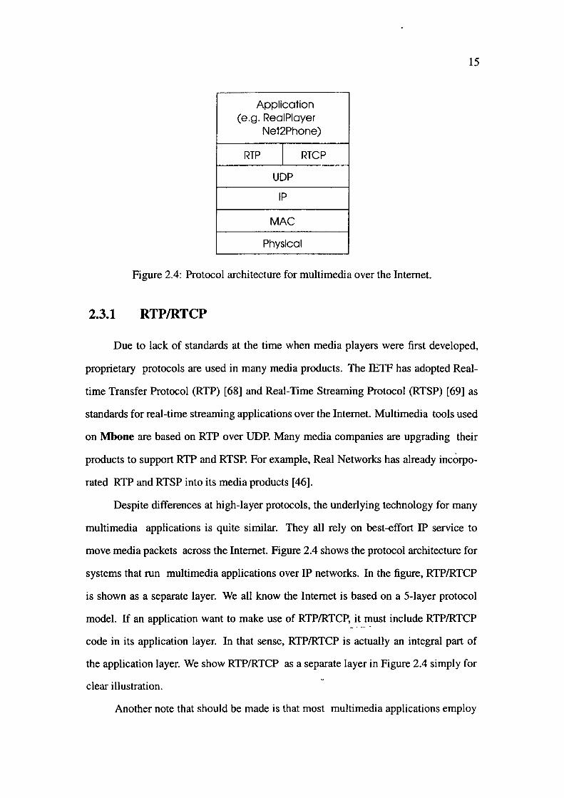
Application (e.g. RealPlayer

Net2Phone)

RTP I RTCP

UDP

IP

MAC

Physical

Figure 2.4: Protocol architecture for multimedia over the Internet.

2.3.1 RTP/RTCP

Due to lack of standards at the time when media players were first developed,

proprietary protocols are used in many media products. The IETF has adopted Real

time Transfer Protocol (RTP) [68] and Real-Time Streaming Protocol (RTSP) [69] as

standards for real-time streaming applications over the Internet. Multimedia tools used

on Mbone are based on RTP over UDP. Many media companies are upgrading their

products to support RTP and RTSP. For example, Real Networks has already incorpo

rated RTP and RTSP into its media products [46].

Despite differences at high-layer protocols, the underlying technology for many

multimedia applications is quite similar. They all rely on best-effort IP service to

move media packets across the Internet. Figure 2.4 shows the protocol architecture for

systems that run multimedia applications over IP networks. In the figure, RTP/RTCP

is shown as a separate layer. We all know the Internet is based on a 5-layer protocol

model. If an application want to make use of RTP/RTCP, it II?ust include RTP/RTCP

code in its application layer. In that sense, RTP/RTCP is actually an integral part of

the application layer. We show RTP/RTCP as a separate layer in Figure 2.4 simply for

clear illustration.

Another note that should be made is that most multimedia applications employ

16

UDP as the transport protocol for the transfer of the content of media, although both

TCP and UDP can be used for this purpose. Usually, TCP is used to transfer control

information for a multimedia session (not shown in Figure 2.4 ). According to a recent

analysis on Internet traffic, 60-70% of audio flows use UDP as the transport protocol

[50].

RTP (Real-time Transport Protocol) is responsible for defining the format and

encapsulation of media data into RTP packets. It is specified in RFC 1889 [68]. The

header of RTP packets consists of a number of fields, such as payload type, sequence

number, timestamp, etc. The payload type field specifies the content of application

data. For example, a value of O in the payload type indicates that the encapsulated

data is a PCM G.711 voice stream; a value of 14 represents MPEG audio; a value of

32 represents MPEG 1 video, and so on. Sequence number and timestamp are used in

combination with playout buffer (discussed in next subsection) to remove jitter.

A complementary protocol RTCP (Real-time Transport Control Protocol) is also

specified in RFC 1889. RTCP defines control information (e.g. sender report, receiver

report, etc.) exchanged between RTP entities of the same session. RTP packets and

RTCP packets are sent to UDP layer using different UDP port numbers.

RTP packets are sent to UDP layer for transmission to peer RTP entities. Each

RTP packet is encapsulated in a UDP packet and then passed to IP layer. Each UDP

packet is in tum encapsulated in an IP packet and transmitted across various IP subnets.

2.3.2 MPEG-2

MPEG-2 (Motion Picture Experts Group) is a popular video compression stan

dard adopted by the International Organisation for Standards (ISO), International Elec

trotechnical Commission (IEC), and International Telecommunication Union (ITU) [44].

In MPEG video compression standards, a video stre¥Jl is hierarchically structured into

a number of layers, as listed below: Sequence, Group of Picture (GoP), Frame, Slice,

Q)

E ~

LL

Sequence

I

p BB

P-' B ' , B ',

I B

B

I '

Block -------- / Slice '',

(BxB) ------.. ~....,._..,lr-----r-----,,1 1--.---,-1 1-r--,------iEH Macroblock / ,__..._.&.-_.__-'-_,__-----'------'---'-_J

(16x16)

Figure 2.5: MPEG-2 video structure

Macroblock, Block.

• • •

17

In the hierarchical structure, each layer has its own header which contains in

formation specific to that layer. The information instructs decoders to decode a video

stream correctly. On the top of the hierarchy is Sequence which delimits a video se

quence. Next in the hierarchy is GOP which is consisted of a number of frames. The

number of frames in a GOP is a configurable parameter which can be set at encoding

(e.g. 9, 12, 15, etc .). The Frame layer defines pictures in a GOP. MPEG standard de

fines three types of pictures: intra-coded I-frame, predicted P-frame, and bidirectional

B-frame. A frame is composed of slices , with each slice composed of macroblocks

(16 x 16 pixels) . The structure of MPEG-2 video is shown illustratively in Figure 2.5 .

As we can see in Figure 2.5, each macroblock con!ain~ 4 blocks (8 x 8 pixels

each) of luminance signal (Y). In MPEG compression, reduced sampling rate is usually

used for chrominance signal (Cb, Gr)- Therefore, there would be less number of CbCr ..

samples than Y samples in a macroblock. For example, in 4 :2:0 video (which is the

most popular MPEG video format), each macroblock contai ns 4 Y blocks , l Cb block

18

and 1 Cr block.

MPEG video compression takes advantages of both spatial and temporal redun

dancy of moving pictures. Spatial redundancy is reduced by spatial coding, which is

based on 2-dimensional Discrete Cosine Transform (2-D DCT). A 2-D DCT is applied

to each block in a picture. The resulting DCT coefficients are quantised (with variable

quantisation steps) and coded using Variable Length Coding (VLC). Temporal redun

dancy is reduced by temporal coding which is based on inter-frame coding with motion

prediction. Motion prediction is performed based on macroblocks. Thus, it is possible

to encode only the difference between a frame and its reference frames for P-frames

and B-frames, in order to achieve high compression ratio. More about MPEG video

compression can be found in [64].

MPEG-1 video standard specifies a maximum bit rate of 1.5 Mbps. It is typically

used in constant bit rate (CBR) applications (e.g. VCD players). MPEG-2 [44] im

proves the video quality significantly with higher bit rates (between 2 and 9 Mbps [49]).

Both constant bit rate (CBR) and variable bit rate (VBR) encodings are supported by

MPEG-2 [49, 23]. MPEG-2 has been adopted as the standard for DVD players (VBR).

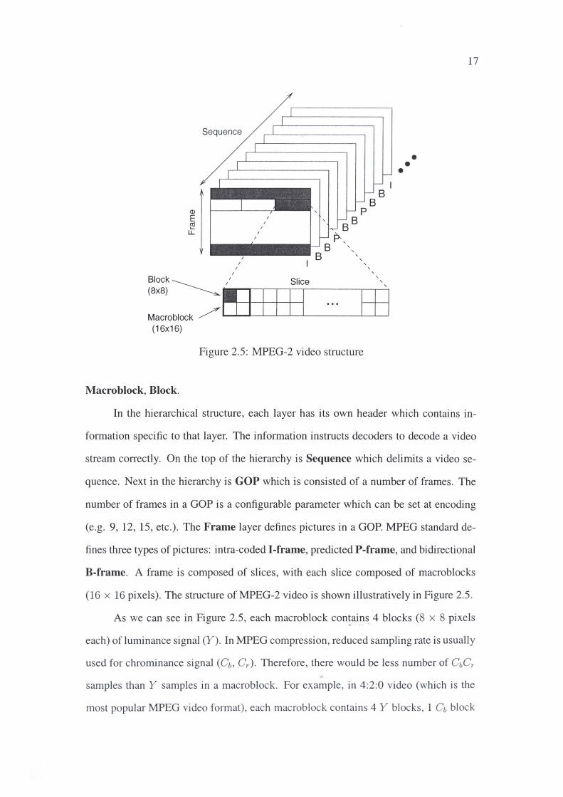
2.3.3 MPEG-2 over IP

MPEG-2 standard specifies two systems. The first simply multiplexes video,

audio, and data of a single program together to form a Program Stream (PS). Program

Streams are intended for recording applications such as DVD. The other system defines

Transport Stream (TS), a packet-based protocol for transmission applications such as

cable TV, Video on Demand (VoD), interactive games, etc. TS packets have a fixed

length of 188 bytes, including a minimum 4-byte header.- For practical purposes, the

continuous MPEG-2 bitstream (also called Elementary Stream) from source encoder

is broken into 18,800-byte segments [77]. These video segments are usually called ...

Packetised Elementary Stream packets, or PES packets. PES packets can be used to

19

PES 18,800 bytes

Min Min TS 4 bytes Up to 184 bytes 4 bytes Up to 184 bytes

Min RTP 20 bytes 4 bytes Up to 184 bytes

Min UDP 8 bytes 20 bytes 4 bytes Up to 184 bytes

Min Ip 20 bytes 8 bytes 20 bytes 4 bytes Up to 184 bytes

Figure 2.6: Encapsulation of MPEG-2 TS packets in IP packets

create Program Streams or Transport Streams.

Delivery ofMPEG-2 TS packets over packet networks has attracted great interest

from network research community. The ATM Forum has defined the encapsulation of

MPEG-2 TS packets into AAL5 in its VoD Specification 1.1 [22]. For IP networks,

the IETF has also defined the RTP payload format for MPEG TS packets, in RFC 2250

[28]. Figure 2.6 illustrates the protocol structure for delivery of MPEG-2 video over IP

networks.

As shown in Figure 2.6, normally an MPEG-2 TS packet is encapsulated in an

RTP packet. The RTP packet is then carried by a UDP packet, which is carried by an

IP packet and sent to the network. It should be noted that, although RTP is becoming

a popular protocol for real-time applications, it is possible to use proprietary protocols

instead of RTP. For example, RealNetworks and Microsoft use proprietary protocols in

their audio/video streaming products RealPlayer [35] and Media Player [31] (although

RTP has been supported in RealPlayer recently [46]).

20

2.3.4 IP Packet Loss

IP packets may be dropped in intermediate routers due to buffer overflow. In our

simulation study, we show that packet loss has significant impacts on intelligibility of

multimedia applications, especially when packet loss rate exceeds a certain threshold.

In Chapter 5, we simulate a network with multiple congested links. Our simulation

study shows that the impact of IP packet loss is accumulated at each intermediate router.

As a result, the end-to-end packet loss rate could be very high even though packet loss

rate in each intermediate router is very small.

2.4 Conclusion

In this chapter, we have presented an overview of supporting multimedia applica

tions over best-effort network service. We introduced various multimedia applications

available on the Internet and explained the underlying technology that supports them.

We have also discussed the future development trends of multimedia over the Inter

net, and analysed the potential impacts of multimedia applications. After ten years

of evolution, supporting multimedia over best-effort service has become a mature and

promising technology, with a huge and ever increasing user base. It can be perceived

that the explosive growth of multimedia applications will continue for years to come.

How to support these emerging applications efficiently on the Internet has become a

pressing research issue for Internet research community.

In following chapters, we will use techniques discussed in this chapter to sim

ulate MPEG-2 video transmission over an IP network. That is, we will employ the

multimedia over best-effort model in our simulation study, as. many real applications

based on the multimedia over best-effort model have been found on the Internet.

Chapter 3

Related Work

Since the introduction of multimedia into the Internet, research has been carried

out to combat problems (see Section 2.2) that arise as a result of supporting multimedia

over the Internet. In this chapter, we describe research work proposed to address these

problems.

3.1 Fair Queueing and Scheduling Algorithms

' Many multimedia application are bandwidth-intensive and non-adaptive in na-

ture. In current Internet, a single FIFO-based queue is used to multiplex both adaptive

and non-adaptive traffic at routers. This may cause fairness problem when multimedia

applications and other adaptive applications traverse the same router. Consider a sit

uation where a number of TCP connections share a FIFO queue with a non-adaptive

video source at a congested router. TCP connections will continuously reduce their

congestion windows because of presence of the non-adaptive video source. It can be

envisaged that TCP connections may be forced to shut UJ? if . the video source trans

mits at the data rate of the bottleneck link. Therefore, multimedia applications have a

potential to preempt adaptive data applications.

With the increasing popularity of multimedia over the Internet, fairness has be

come a challenging issue for the Internet community. Network researchers have been

22

looking for queueing/scheduling algorithms that enforce fairness. A number of fair al

gorithms, notably WFQ [58] and CSFQ [70], have been proposed as a result of these

research efforts. Results from both simulation analysis and practical implementation re

veal that these fair algorithms can maintain good fairness among all competing sources.

3.1.1 WFQ

Fair Queueing (FQ) [16] is a pioneer fair algorithm proposed by Demers et al.

in 1990. FQ allocates bandwidth equally among all competing sources. Parekh et al.

extended FQ with "weighted fair" in 1993. This allows competing flows to receive

bandwidth ( of the bottleneck link) which is proportional to their pre-allocated weights.

The algorithm is thus called Weighted Fair Queueing (WFQ) [58]. When equal weight

is allocated to all flows, WFQ becomes FQ. FQ/WFQ employs per-flow queueing, i.e.

there is a subqueue for each flow in a router. When a packet arrives at a router, it is first

classified into flow by the classifier. The packet is then put into its corresponding sub

queue for transmission. The scheduler picks packets from subqueues for transmission

in a Round-Robin fashion. FQ/WFQ can achieve perfect max-min faimess 1 , and has

been widely used (for comparison purposes) to evaluate the performance of other fair

algorithms proposed in recent years (for example in [9], [18], [47], [56], and [70]).

3.1.2 CSFQ

Core-Stateless Fair Queue (CSFQ) [70] is a simple probabilistic packet dropping

algorithm proposed by Stoica et al. in 1998. With CSFQ, per-flow state information is

only needed at edge routers (but not in the network core). Per~flow state information

is maintained at edge routers to estimated packet arrival rates. The arrival rate of each

flow is updated by each intermediate router. The intermediate router writes the arrival

1 To satisfy the max-min fairness criterion, the smallest se~ion rate in the network must be as large as possible and, subject to this constraint, the second-smallest session rate must be as large as possible, etc. (26].

23

rate into a label which is carried by the header of each packet passing through the router.

CSFQ calculates the fair share approximately based on the arrival rate of each flow and

measurements of aggregate traffic. Routers drop packets with a probability which is a

function of estimated arrival rate and fair share. Simulation results presented in [70]

show that CSFQ can achieve comparable fairness as with WFQ, without maintaining

per-flow states in the network core.

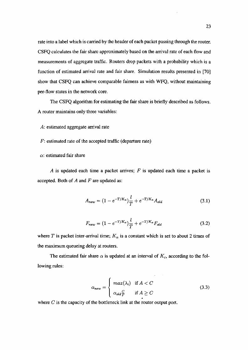
The CSFQ algorithm for estimating the fair share is briefly described as follows.

A router maintains only three variables:

A: estimated aggregate arrival rate

F: estimated rate of the accepted traffic (departure rate)

a: estimated fair share

A is updated each time a packet arrives; F is updated each time a packet is

accepted. Both of A and F are updated as:

l A - (l - e-T/K0 )- + e-T/Ko. A new - T old (3.1)

(3.2)

where T is packet inter-arrival time; Ko: is a constant which is set to about 2 times of

the maximum queueing delay at routers.

The estimated fair share a is updated at an interval of Kc, according to the fol

lowing rules:

if A< C

if A 2::: C

where C is the capacity of the bottleneck link at the router output port.

(3.3)

24

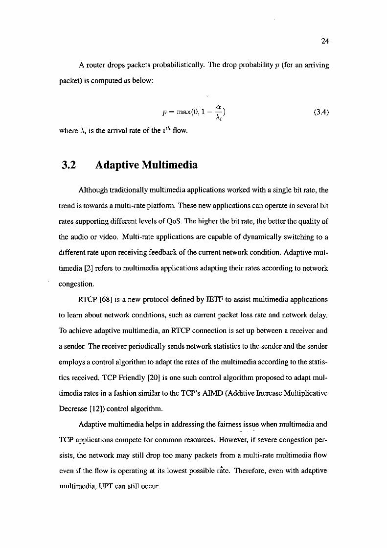
A router drops packets probabilistically. The drop probability p (for an arriving

packet) is computed as below:

Q p = max(O, 1- Ai)

where Ai is the arrival rate of the ith flow.

3.2 Adaptive Multimedia

(3.4)

Although traditionally multimedia applications worked with a single bit rate, the

trend is towards a multi-rate platform. These new applications can operate in several bit

rates supporting different levels of QoS. The higher the bit rate, the better the quality of

the audio or video. Multi-rate applications are capable of dynamically switching to a

different rate upon receiving feedback of the current network condition. Adaptive mul

timedia [2] refers to multimedia applications adapting their rates according to network

congestion.

RTCP [68] is a new protocol defined by IETF to assist multimedia applications

to learn about network conditions, such as current packet loss rate and network delay.

To achieve adaptive multimedia, an RTCP connection is set up between a receiver and

a sender. The receiver periodically sends network statistics to the sender and the sender

employs a control algorithm to adapt the rates of the multimedia according to the statis

tics received. TCP Friendly [20] is one such control algorithm proposed to adapt mul

timedia rates in a fashion similar to the TCP's AIMD (Additive Increase Multiplicative

Decrease [12]) control algorithm.

Adaptive multimedia helps in addressing the fairness issue when multimedia and

TCP applications compete for common resources. However, if severe congestion per

sists, the network may still drop too many packets from a multi-rate multimedia flow

even if the flow is operating at its lowest possible rate. Therefore, even with adaptive

multimedia, UPT can still occur.

25

3.3 Forward Error Correction and Loss Conceal-

ment

Packet loss recovery attempts to recover lost packets. Basically, there are two

loss recovery schemes. They are Forward Error Correction (FEC) [7, 61] and packet

loss concealment [60, 67]. FEC corrects corrupted packets by using redundant informa

tion. Several FEC mechanisms have been proposed in literature. Details can be found

in [5, 6, 45, 59, 61, 66]. Packet loss concealment is performed by a receiver. The idea

of loss concealment is based on the observation that most multimedia applications have

a unique property called self-similarity2 . When there is a loss, the receiver attempts to

produce a replacement for the lost packet which is similar to the original one. A number

of loss concealment mechanisms have been proposed, for example in [11, 60, 67].

Forward Error Correction (FEC) and loss concealment techniques can repair

some of the damages in the received multimedia caused by lost packets. The net ef

fect of employing such FEC and loss concealment techniques is to push the packet loss

rate threshold for effective communication to a higher limit (more packet loss can now

be tolerated). However, the fact that audio and video become unintelligible beyond a

certain packet loss rate remains valid. UPT, therefore, remains an issue for multimedia

over best-effort networks.

3.4 QoS in the Internet

As we discussed in Section 2.2, multimedia applications usually have stringent

requirements on QoS. To cater for the QoS requirements o~Il!u!fimedia, many research

efforts have been devoted to supporting QoS on the Internet. IETF is working on two

new QoS frameworks, namely Diffserv [30] and Intserv [79], to support quality of

2 Self-similarity is the property we associate with one type of fractal-an object whose appearance is unchanged regardless of the scale at which it is viewed [ 14].

26

service in the Internet. The idea of QoS in IP networks is similar to the one in ATM

networks3 • The main premise is to introduce more than one class of service in the

Internet (currently best-effort is the only service,available) and eventually guarantee the

required QoS of all multimedia flows. However, a multi-service framework requires a

significant upgrade of the existing Internet infrastructure. Given the scale of the existing

user base, this type of upgrade is unlikely to take place in the near future.

Even in the future Internet with multiple service classes, a large number of users

will continue to use the best-effort service for many multimedia applications, especially

those not so business critical. There are at least two compelling reasons for not using

the guaranteed or higher priority service classes. Firstly, these classes will attract much

higher charges compared with the best effort service. Secondly, these users have already

established a "multimedia-over-best-effort" culture, and will be happy to continue using

the same systems.

3.5 Partial Packet Discard in ATM Networks

Useless cell transmission was considered in the context of IP packet transmi'ssion

over ATM networks. One IP packet is usually transmitted over multiple ATM cells (due

to very small cell size). Once an ATM switch drops an ATM cell due to congestion,

the rest of the cells of the same IP packet become useless as they will be all discarded

at the destination (reassembly of the IP packet is not possible without receiving all

cells). A technique called Partial Packet Discard (PPD) [1] was considered to drop all

remaining cells of a packet as soon as one cell from \the packet is dropped. Although

this technique required ATM switches to detect IP packet boundaries, it was welcomed

because of its potential to reduce bandwidth waste in ATM switches. Early Packet Dis

card (EPD) [65], a more advanced version of PPD, is now widely used in commercial

3 ATM supports CBR, VBR (realtime VBR and non-reahime VBR), and UBR services, of which CBR and VBR support QoS.

27

ATM switches.

3.6 Conclusion

In this chapter, we have discussed research work proposed to address problems

related to supporting multimedia over the Internet. However, UPT remains an open

issue. The fairness problem has been solved by introducing fair queueing/scheduling

algorithms. A number of packet repair schemes for multimedia applications have been

proposed to minimise the impacts of packet loss on multimedia. However, the fact that

audio and video become unintelligible beyond a certain packet loss rate remains valid.

Therefore, with the increasing popularity of multimedia over the Internet, there is a

need to investigate UPT problem.

Chapter 4

Useless Packet Transmission Avoidance

(UPTA)

In this chapter, we formally define the UPT problem and propose an avoidance

algorithm called Useless Packet Transmission Avoidance (UPTA) to address the prob

lem. Using WFQ and CSFQ as examples, we investigate UPf avoidance problem in

networks with single congested link.

4.1 Formal Definition of UPT Problem

This section details the UPf problem and formally defines the performance pa

rameters. We make the following assumptions and observations for multimedia over

best-effort network service:

• When packet loss rate exceeds a threshold q, the media, particularly voice and

video, becomes unintelligible [10, 21, 46]. The exact value of this threshold

may vary from application to application. For the video clip used in our ex

periment, we experimentally derive this threshold (see Section 4.4). As long

as the packet loss rate remains below the threshold, the media is intelligible . .,

• If a multimedia connection is established over a best-effort network service

29

(i.e., no guarantees on packet loss rate), packet loss rate can occasionally ex

ceed the threshold. Therefore, the life-time of a multimedia connection can

be described by a series of alternating intelligible and unintelligible intervals.

In the best case, there will be no unintelligible intervals, the entire connection

time makes up a single intelligible interval. Similarly, in the worst case, the

entire connection time is composed of a single unintelligible interval.

We use the following notations:

• U: Denotes an unintelligible interval.

• I: Denotes an intelligible interval.

• !lu: Mean length of U intervals.

• !::.1: Mean length of I intervals.

• ,,.,: Mean throughput of U intervals in bits per second (bps).

We define unintelligible ratio, i.e., the fraction of time a multimedia connection

spends in U intervals, as:

,I,= !lu 'P !lu + !::.1 (4.1)

Note that in the best case, </J = 0 (because !lu 0) and in the worst case </J = 1

(because !::.1 = 0). In other cases, 0 < </J < l.

UPT is defined as transmission of packets during U intervals. These packets

do not contribute to any meaningful communication, and hence, simply waste router

bandwidth. The amount of bandwidth wasted by UPT can be obtained as:

!lu w = T/ x !::. !::. bps u+ 1

= T/ x </J bps .. (4.2)

30

Packet anival

Figure 4.1: Flow chart of UPTA.

For example, if a video connection has spent 20% of the total connection time in

U intervals, with an T/ = 1 Mbps (this can happen for a 1.5 Mbps MPEG-2 video that

becomes unintelligible when only 1 Mbps is allocated), then it has wasted 200 Kbps

router bandwidth due to UPT.

4.2 UPT Avoidance Algorithm

There are two basic ways to avoid UPT. One way is to eliminate all U intervals;

the other is simply to remove UPT from the U intervals. The former approach, which

needs to reserve bandwidth for multimedia connections, is pursued by the guaranteed

Quality of Service (QoS) efforts (see related work in Section 3). However, for best

effort network services, it is acceptable to expect occasional U intervals in multime

dia connections. We propose an UPT avoidance algorithm (henceforth called UPTA),

which aims to remove UPT from the U intervals without affecting the unintelligible

ratio (</J) of the connection. Effectively, UPTA will reduce bandwidth waste by multi

media flows, and distribute the recovered bandwidth to competing TCP flows.

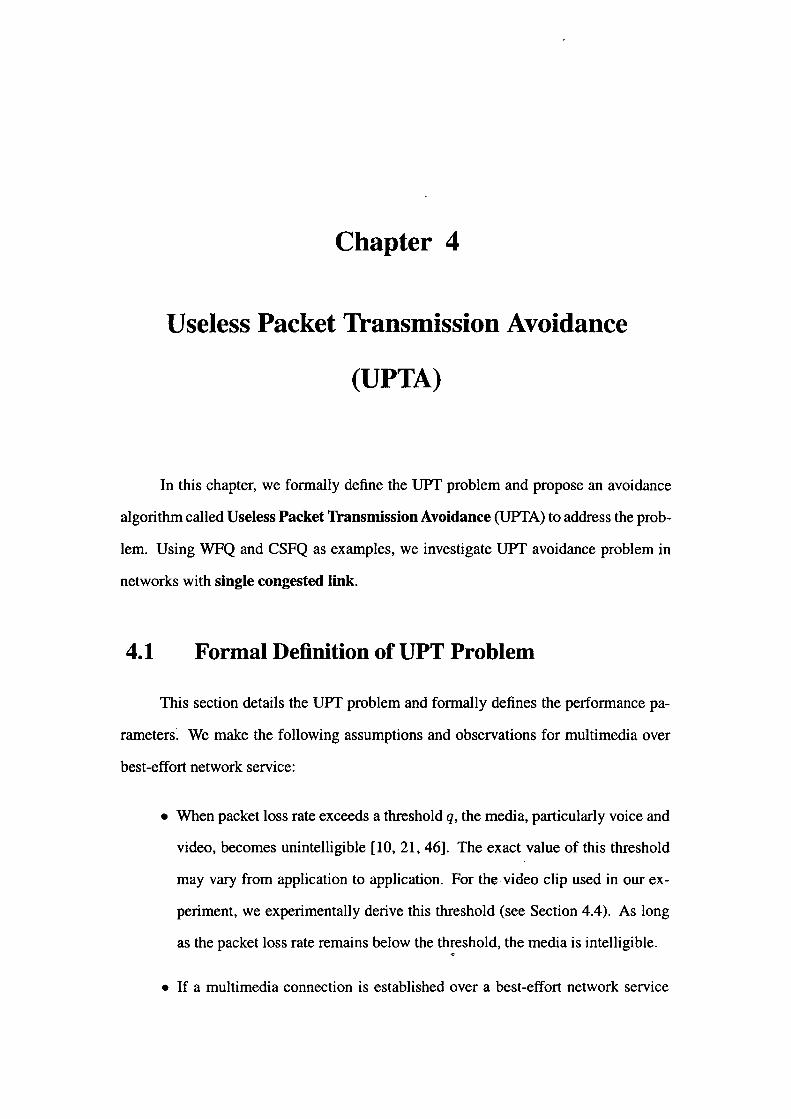
Figure 4.1 illustrates the flow chart of the proposed UPTA algorithm. UPTA

drops an arriving packet straightaway, if the current fairshare dictates a packet loss rate

exceeding the threshold. Otherwise, UPTA has no effect on the usual processing of the

packet. Some fair algorithms (e.g., CSFQ) compute·a drop probability (current packet

loss rate) for each arriving packet as part of the algorithm. Incorporation of UPTA in

Packet arrival

UPTA

UPTA controller

UPTA controller

Packet departure

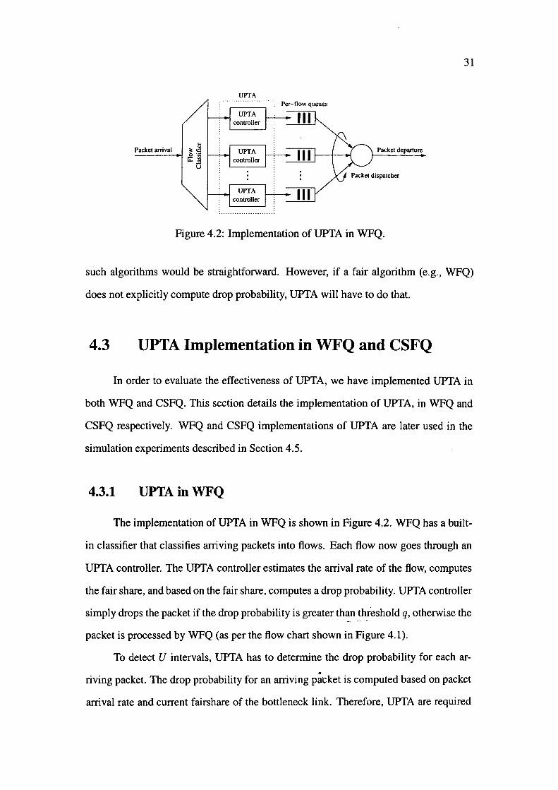
Figure 4.2: Implementation of UPTA in WFQ.

31

such algorithms would be straightforward. However, if a fair algorithm (e.g., WFQ)

does not explicitly compute drop probability, UPTA will have to do that.

4.3 UPTA Implementation in WFQ and CSFQ

In order to evaluate the effectiveness of UPTA, we have implemented UPTA in

both WFQ and CSFQ. This section details the implementation of UPTA, in WFQ and

CSFQ respectively. WFQ and CSFQ implementations of UPTA are later used in the

simulation experiments described in Section 4.5.

4.3.1 UPTAinWFQ

The implementation of UPTA in WFQ is shown in Figure 4.2. WFQ has a built

in classifier that classifies arriving packets into flows. Each flow now goes through an

UPTA controller. The UPTA controller estimates the arrival rate of the flow, computes

the fair share, and based on the fair share, computes a drop probability. UPTA controller

simply drops the packet if the drop probability is greater than th_reshold q, otherwise the

packet is processed by WFQ (as per the flow chart shown in Figure 4.1).

To detect U intervals, UPTA has to determine the drop probability for each ar

riving packet. The drop probability for an arriving picket is computed based on packet

arrival rate and current fairshare of the bottleneck link. Therefore, UPTA are required

32

to estimate packet arrival rate and fairshare, and then compute drop probability for each

arriving packet.

4.3.1.1 Estimation of Packet Arrival Rate

Packet arrival rate of Flow i is estimated upon each packet arrival, using expo

nential averaging. Exponential averaging was first used to estimate packet arrival rate

in [70]. The packet arrival rate of Flow i is updated (upon each packet arrival) as per

Eq. (4.3) [70]:

(4.3)

where l is packet length; T is packet inter-arrival time for Flow i (T = tk - tk_1); K

is a constant. In our simulations, K is set to 100 ms (about two times of the maximum

queueing delay at a router), as recommended in [70].

4.3.1.2 Estimation of Fairshare

Apart from packet arrival rate, fairshare (of the bottleneck link) is another .vari

able maintained by UPfA (in order to compute packet loss rate). UPfA estimates

fairshare based on max-min criterion [42]. We use following notations:

• C: Output link capacity.

• N: Total number of flows.

• n: Collection of all flows (n = 1, 2, ... , N).

• S: Number of unconstrained flows (>.i < ~ for i = 1, .. :, S).

• M: Number of flows currently in U intervals.

• m: Collection of U flows (m = 1, 2, ... , M).

33

• A: Vector of flow anival rates (A = >.1, >.2, ... , AN).

• a: Max-min fairshare (of bottleneck link) for flows currently in U intervals.

• a': Max-min fairshare (of bottleneck link) for flows currently in I intervals.

Assume A is sorted in ascending order, i.e.,

constrained flows

A= {>.1, >.2, ... , As-1, >.s, As+1, >-s+2, ... , AN-1, AN}

unconstrained flows

then a and a' can be derived as below, as per max-min criterion [42]:

I C - Ef=l Ai a=-----'--N-S-M

4.3.1.3 Estimation of Drop Probability

(4.4)

(4.5)

For flows currently in I intervals (i fj. m), the drop probability is computed as:

a' Pi = max(O, 1 - Ai) (i (j. m) (4.6)

If Pi is greater than the loss threshold, Flow i will be marked as U flow.

For flows currently in U intervals (i E m), the drop probability is computed as:

a Pi= max(O, 1- Ai) (i Em)

If Pi is less than the loss threshold, Flow i will be marked as J flow.

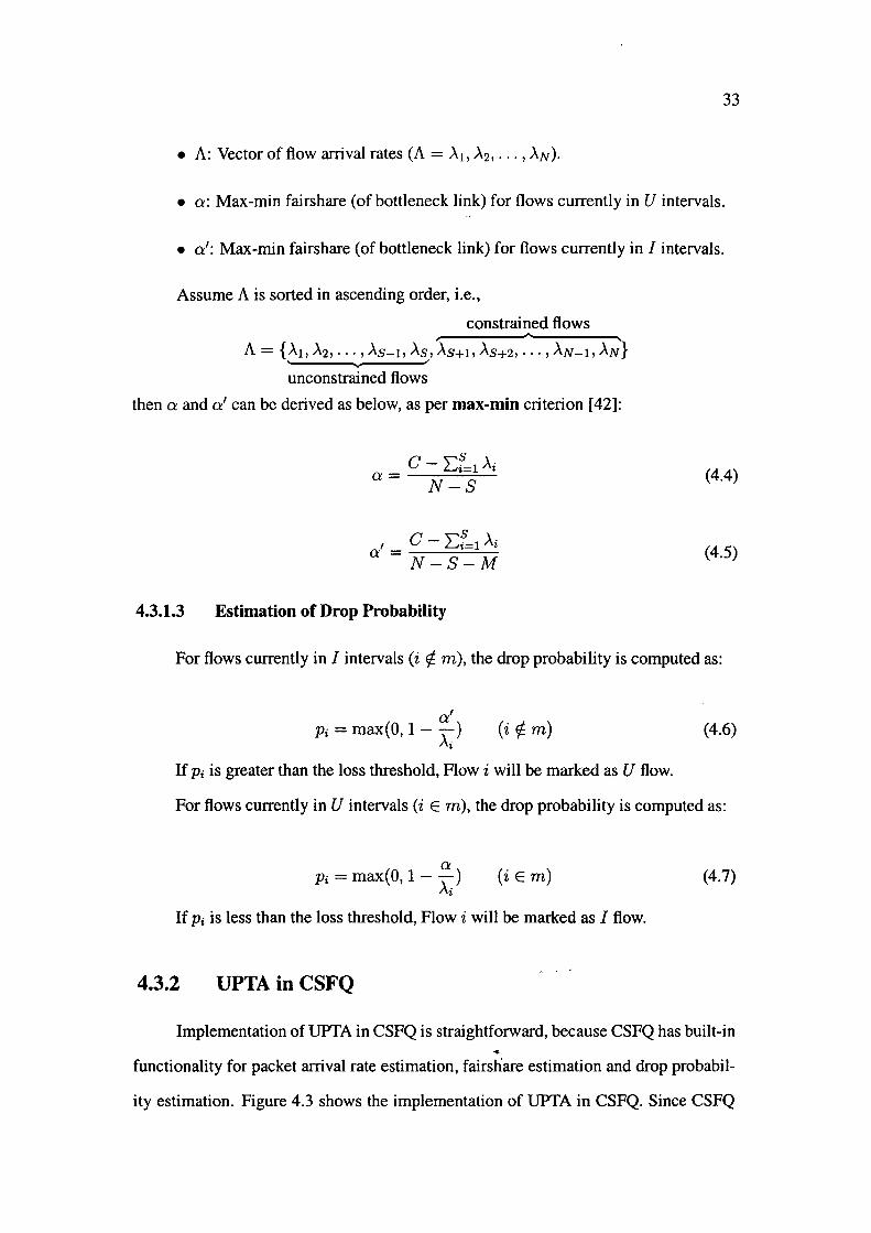
4.3.2 UPTAinCSFQ

(4.7)

Implementation ofUPTA in CSFQ is straightforward, because CSFQ has built-in . functionality for packet anival rate estimation, fairshare estimation and drop probabil-

ity estimation. Figure 4.3 shows the implementation of UPTA in CSFQ. Since CSFQ

Packet ani val

Estimate anival rate

Compute fair share

~ Compute drop prob. p / __ _

--------- ..

Drop the packet probabilistically

Figure 4.3: Implementation of UPTA in CSFQ.

34

already computes the drop probability of an arriving packet, UPTA simply compares

this drop probability with threshold q and discards the packet if it is greater than q.

Otherwise, it lets CSFQ to drop the packet probabilistically (usual CSFQ processing).

4.4 Packet Loss Threshold for the Experimental Video

Packet loss rate threshold q for intelligible communication may vary from appli

cation to application. We have carried out a series of experiments with different loss

rates in the network to determine the threshold for the MPEG-2 video clip used in our

simulation study. This section presents our experiment results.

4.4.1 Packet Loss/Delay and UPT

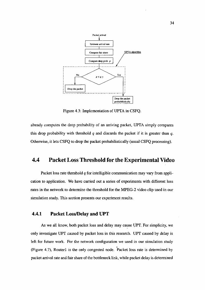
As we all know, both packet loss and delay may cal:1se ~- For simplicity, we

only investigate UPT caused by packet loss in this research. UPT caused by delay is

left for future work. For the network configuration we used in our simulation study .

(Figure 4.7), Routerl is the only congested node. Packet loss rate is determined by

packet arrival rate and fair share of the bottleneck link, while packet delay is determined

0.4 ,----.----.----.----.----.-----,0.4

Lo~

: Delay

:~

., "'O C

.. 0.3 8 CD .e ~ ai Cl

. "'O · · · · · · · ... · · · · · · · · · · 0.2 I]

I

1f "'O C w CD

· 0.1 ~

1

o~--~--~--~--~--~-~o 0 200 400 600 800 1000 1200

Buffer Size (KB)

Figure 4.4: Video packet loss rate/delay versus buffer size.

35

by the buffer capacity at the output port. To see the impact of buffer size on packet loss

and delay, we measured packet loss rate/delay of the video flow under varying buffer

size of Routerl (from 32 KB to 1024 KB). Figure 4.4 shows packet loss rate and delay

of the video flow against buffer size.

Figure 4.4 shows that packet loss of the video flow is 25%, regardless of buffer

size, and packet delay increases linearly with the increase of buffer size. The figure

suggests that, for our simulated network, packet delay can be reduced by using smaller

buffer size. In fact, there is no incentive to use large buffer size anyway, as large buffers

do not reduce packet loss (see Figure 4.4). From the figure we can also see that, for

the simulated network, video packet delay is much less than 0.1 second when buffer

size is less than 200 KB. In our simulation study that follows, we set the buffer size of

Router! to 64 KB (about 100 packets). Therefore, delay is not an issue in the simulated

network, only packet loss contributes to UPT.

4.4.2

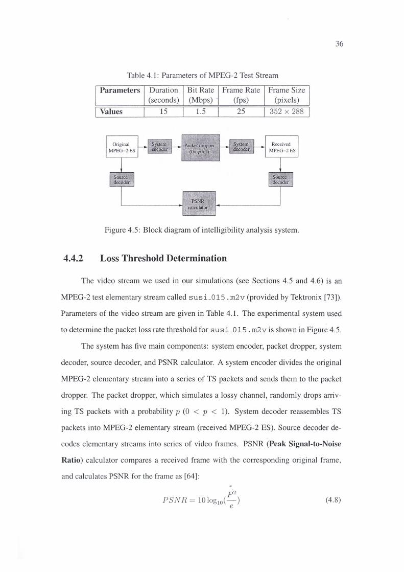
Table 4 .1: Parameters of MPEG-2 Test Stream

Parameters

I Values

Original MPEG-2ES

Duration (seconds)

15

System encoder

Bit Rate (Mbps)

1.5

J>SNR " calcu4'~r .. . .

Frame Rate (fps)

25

·system decodei:

Frame Size (pixels)

352 X 288

Received MPEG-2 ES

Figure 4.5: Block diagram of intelligibility analysis system.

Loss Threshold Determination

36

The video stream we used in our simulations (see Sections 4.5 and 4.6) is an

MPEG-2 test elementary stream called susL015. m2v (provided by Tektronix [73]).

Parameters of the video stream are given in Table 4.1 . The experimental system used

to determine the packet loss rate threshold for susL015. m2v is shown in Figure 4.5.

The system has five main components: system encoder, packet dropper, system

decoder, source decoder, and PSNR calculator. A system encoder divides the original

MPEG-2 elementary stream into a series of TS packets and sends them to the packet

dropper. The packet dropper, which simulates a lossy channel, randomly drops arriv

ing TS packets with a probability p (0 < p < 1). System decoder reassembles TS

packets into MPEG-2 elementary stream (received MPEG-2 ES). Source decoder de

codes elementary streams into series of video frames. P~NR. (Peak Signal-to-Noise

Ratio) calculator compares a received frame with the corresponding original frame,

and calculates PSNR for the frame as [64]:

p2 PSNR = 10log10(-)

e (4.8)

37

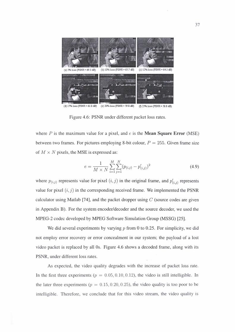
(a) 5% loss (PSNR= 693 dB) (b) 10% loss (PSNR= 65.7 dB) (c) 12% lo:s (PSNR= 643 c!8)

(d) 15% loss (PSNR = 61.0 dB) (e) 20% loss (PSNR= 59 .8 dB) (f) ]j% loso (PSNR= 58.8 dB)

Figure 4.6: PSNR under different packet loss rates.

where P is the maximum value for a pixel, and e is the Mean Square Error (MSE)

between two frames. For pictures employing 8-bit colour, P = 255. Given frame size

of M x N pixels, the MSE is expressed as:

(4.9)

where P(i, j) represents value for pixel ( i, j) in the original frame, and P(i,j) represents

value for pixel (i, j) in the corresponding received frame. We implemented the PSNR

calculator using Matlab [74], and the packet dropper using C (source codes are given

in Appendix B). For the system encoder/decoder and the source decoder, we used the

MPEG-2 codec developed by MPEG Software Simulation Group (MSSG) [25].

We did several experiments by varying p from O to 0.25. For simplicity, we did

not employ error recovery or error concealment in our system; the payload of a lost

video packet is replaced by all Os. Figure 4.6 shows a decoded frame, along with its

PSNR, under different loss rates.

As expected, the video quality degrades with the increase of packet loss rate.

In the first three experiments (JJ = 0.05, 0.10, 0.12), the video is still intelligible. In

the later three experiments (JJ = 0.15, 0.20 , 0.25), the video quality is too poor to be

intelligible. Therefore, we conclude that for this video stream, the video quality is

38

unintelligible when packet loss rate exceeds 12% (similar results were reported in (13)).

This packet loss rate threshold will be used by our UPTA algorithm in Section 4.5 to

detect U intervals and avoid useless packet transmission in the router. We also note,

that for this video, the frames become unintelligible for PSNR less than 65 dB. This

PSNR threshold will be used in Section 4.6 to assess the impact of our UPTA algorithm

on the overall intelligibility of the received video.

4.5 Simulation

This section details the network model and the performance metrics used in the

simulation study.

4.5.1 OPNETModel

Using OPNET Modeler 7.0.B (71], we simulate a well-known single bottleneck

network topology ("dumbbell") as shown in Figure 4.7. This topology simulates an

intranet over two long-distance sites interconnected by a (virtual) leased line. Three

workstations (simulating senders) are connected to Router! through 10 Mbps access

links. Their corresponding receivers are connected to Router2, also using 10 Mbps

links. Router! is the congested router; it has a buffer size of 100 packets. The two

routers are connected by a 4 Mbps link (e.g., 2 x El lines), with a propagation delay

of 1 ms. All other links have a propagation delay of 1 µs.

Among the three senders, there are a TCP source, a video source, and a deter

ministic ON-OFF source. The TCP source simulates file transfers. The video source

simulates the transmission of the MPEG-2 video clip (susi_Ol5 .m2v) described in

Section 4.4. The video source, which operates at 1.5 Mbps, employs a packet size of

188 bytes (MPEG-2 TS packet size); the TCP and ~he ON-OFF sources use 512-byte

packets. The ON-OFF source transmits at 2 Mbps during ON period, and stops trans-

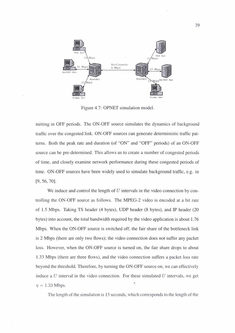
Video Src

Bottleneck: 4 Mbps

Video Ost

Figure 4.7: OPNET simulation model.

39

mitting in OFF periods. The ON-OFF source simulates the dynamics of background

traffic over the congested link. ON-OFF sources can generate deterministic traffic pat

terns. Both the peak rate and duration (of "ON" and "OFF" periods) of an ON-OFF

source can be pre-determined. This allows us to create a number of congested periods

of time, and closely examine network performance during these congested periods of

time. ON-OFF sources have been widely used to simulate background traffic, e.g. m

[9, 56, 70].

We induce and control the length of U intervals in the video connection by con

trolling the ON-OFF source as follows. The MPEG-2 video is encoded at a bit rate

of 1.5 Mbps. Taking TS header (4 bytes), UDP header (8 bytes), and IP header (20

bytes) into account, the total bandwidth required by the video application is about 1.76

Mbps. When the ON-OFF source is switched off, the fair share of the bottleneck link

is 2 Mbps (there are only two flows); the video connection does not suffer any packet

loss. However, when the ON-OFF source is turned on, the fair share drops to about

1.33 Mbps (there are three flows) , and the video connection suffers a packet loss rate

beyond the threshold. Therefore, by turning the ON-OFF source on, we can effectively

induce a U interval in the video connection. For these simulated U intervals, we get

'r/ = 1.33 Mbps.

The length of the simulation is 15 seconds, which corresponds to the length of the

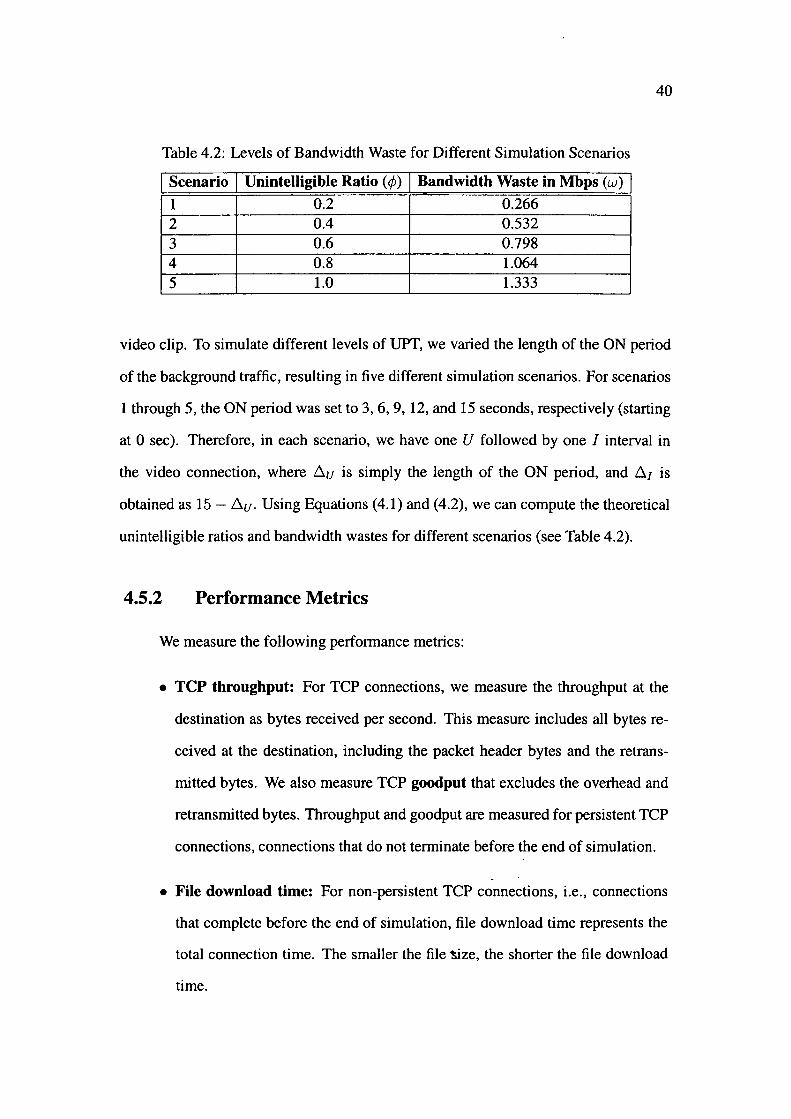
40

Table 4.2: Levels of Bandwidth Waste for Different Simulation Scenarios

Scenario Unintelligible Ratio ( </J) Bandwidth Waste in Mbps (w)

1 0.2 0.266 2 0.4 0.532 3 0.6 0.798 4 0.8 1.064 5 1.0 1.333

video clip. To simulate different levels of UPT, we varied the length of the ON period

of the background traffic, resulting in five different simulation scenarios. For scenarios

1 through 5, the ON period was set to 3, 6, 9, 12, and 15 seconds, respectively (starting

at 0 sec). Therefore, in each scenario, we have one U followed by one I interval in

the video connection, where !::,.u is simply the length of the ON period, and t:,.1 is

obtained as 15 - !::,.u, Using Equations (4.1) and (4.2), we can compute the theoretical

unintelligible ratios and bandwidth wastes for different scenarios (see Table 4.2).

4.5.2 Performance Metrics

We measure the following performance metrics:

• TCP throughput: For TCP connections, we measure the throughput at the

destination as bytes received per second. This measure includes all bytes re

ceived at the destination, including the packet header bytes and the retrans

mitted bytes. We also measure TCP goodput that excludes the overhead and

retransmitted bytes. Throughput and goodput are measured for persistent TCP

connections, connections that do not terminate before the end of simulation.

• File download time: For non-persistent TCP connections, i.e., connections

that complete before the end of simulation, file download time represents the

total connection time. The smaller the file tize, the shorter the file download

time.

41

• Video intelligibility: To measure the level of intelligibility of the received

video, we define an intelligibility index as:

intelligibility index = ~in tx

(4.10)

where Nin is the total number of intelligible video frames received, and Ntx

is the total number of video frames transmitted. A received video frame is

considered intelligible if it has a PSNR greater than or equal to 65 dB (see

Section 4.4). Intelligibility index is a dimensionless fraction between O and 1.

The closer the value to 1, the higher the level of intelligibility. A value of 1

means all received frames are intelligible. We use this index to measure the

impact of our proposed UPT avoidance algorithm on the quality (in terms of

overall intelligibility) of the received video.

• Throughput fairness: We measure throughput fairness among competing

flows using the well-known Jain's fairness index as [43]:

F _ (Ef::1 xi) 2

- N 2 NEi=l xi

(4.11)

where xi is the normalised throughput of flow i, and N is the total number of

competing flows. Normalised throughput refers to the ratio of actual measured

throughput to the maximum throughput possible in a system.

4.6 WFQ Simulation Results

In this section, we present the results obtained from the simulation with WFQ.

CSFQ simulation results are given in Section 4.7. Since OPNET does not support EPS

format for graphs, we use Matlab [74] to plot all our simulation results, so as to achieve

better graphic quality for figures.

42

4.6.1 TCP Throughput

To assess the effect of UPTA on TCP thr~ughput, we have simulated a persistent

TCP connection that continues to transfer data for the full duration (15 seconds) of

the simulation. In each of the five scenarios, we have a U interval (ON-OFF source

is turned on) followed by an I interval (ON-OFF source is switched off) in the video

connection. Figures 4.8 and 4.9 show the Cumulative Distribution Function (CDF)

of end-to-end packet delays and packet loss rates for the video connection under WFQ

(results for CSFQ are given in Section 4.7). As we can see in Figures 4.8, all video

packets have a delay of less than 0.08 second (or 80 ms). The delays are much smaller

than the tolerable delays (150-400 ms) for streaming video [10, 21, 46], but the packet

loss rates in U intervals are around 25%, much higher than the threshold of 12% for

intelligible communication (see Figure 4.9). These graphs therefore confirm that for

the simulated network, UPI' occurs because of high packet loss rates, not due to high

packet delays.

To analyse TCP throughput dynamics in different intervals, we have used OP

NET's "bucket" option to plot throughput in consecutive buckets of 100 packets re

ceived at the destination. This short-term throughput analysis a11ows us to observe any

variation of TCP throughput over short intervals. Figure 4.10 shows short-term TCP

throughput received under WFQ for all five scenarios. It is evident, that with our pro

posed UPTA in place, we receive higher TCP throughput during the U interval. The

proposed UPTA effectively recovers bandwidth that would have been otherwise wasted

in UPI', and distributes the recovered bandwidth to other competing connections. We

can also see that UPTA has no effect on TCP throughput duringthe I interval, substan

tiating the fact that our UPTA can successfully switch to -''normal" processing mode

when there is no UPI' in the system. We have received similar results for CSFQ (see

Section 4.7).

Table 4.3 shows the average TCP throughput achieved over the entire duration

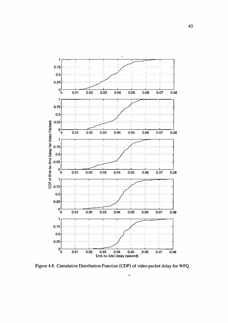
0.75

0.5 · ·

0.25 ..

0 '--------'-='--'----'---.....__ __ _,__ __ .___ _ ___,_ __ __,

0 0.01 0.02 0.03 0.04 0.05 0.06 0.07 0.08

1 r------.---.---.----.---.---;:::-r------.---,

0.75 ...... .

0.5 · .. ·

j 0.25 ..... .

~ a.. 0 Q)

0 .__ _ __._ __ ...,_.._ __ ~--~--......_ _ __..__ _ __,_ __ __, 0

"O

> .E 0.75 · · · ~ ~ 0.5 "O

Jj 0.25 I

0.01 0.02 0.03 0.04 0.05 0.06 0.07 0.08

f 0'-------'----==---'---_._ __ ..__---..J'---'---~ ~ 0 0.01 0.02 0.03 0.04 0.05 0.06 0.07 0.08 w 0 1,----.---.---.----.----.---::;::i===p--7 LL. 0 o 0.75

0.5 ...... ··:·········:····· ........ . ... .

0.25 ·

0 L_ _ _i__-===±:====:c__.......L _ ____..i __ _L_ _ ___L _ _j

0 0.01 0.02 0.03 0.04 0.05 0.06 0.07 0.08

1r---,----.---.-----r---,---::::::::::c====----"7

0.75

0.5 · · · ·

0.25

0 L------'-----'-~==:::::=-_ _._ __ J__ _ _j----'-----'---_J

0 0.01 0.02 0.03 0.04 0.05 0.06_ 0.07 0.08 End-to-End Delay (second)

43

Figure 4.8: Cumulative Distribution Function (CDF) of video packet delay for WFQ.

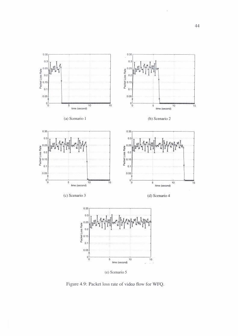
44

0.35~----~-----~-------, 0.35 ,------~-----~------,

., 0 .25 <ii a: ::l 0.2 0 ..J

]j 0 .15 0 .. a. 0.1

0 .05

0.3

., 0.25 <ii a: ~ 0.2 0 ..J

]j 0.15 0 .. a. 0 .1

0 .05 oL-__ _,.. ___________ _ 0'------~----------

0.3

., 0.25 <ii a: ~ 0.2 ..J

]j 0 .15 0 .. a. 0.1

0 .05

0 5 10 15 0 5 10 15 time (second) time (second)

(a) Scenario l (b) Scenario 2

0 .35.-----~-----~------,

., 0 .25 <ii a: ::l 0.2 0 ..J

]j 0 .15 0 .. a. 0.1

0.05

0'------~-----~----'Ml--0 5

time (second) time (second)

(c) Scenario 3 ( d) Scenario 4

0 .35~----~-----~-----

0.3

., 0 .25 <ii a: :z 0.2 0 ..J

]j 0 .15 0 .. a. 0.1

0.05

o~----~-----~----~ 0 5 10 15

time (second)

(e) Scenario 5

Figure 4.9: Packet loss rate of video flow for WFQ.

10 15

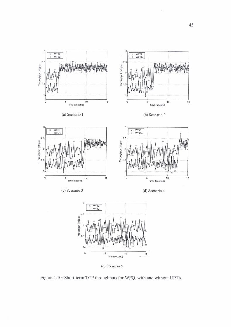
3

2 .5 -;;;-c. .0

~ 5 2 c. .c O> :::,

e ~ 1.5

-;;, c. .0

2 .5

~ 5 2 c. .c O> :::, 0

~ 15

0

0

I=:= ~~g+ I

5 time (second)

(a) Scenario I

5 time (second)

(c) Scenario 3

-;;, c. .0

2 .5

~ 5 2 c. .c O> :::,

e ~ 1.5

10

10

0

15

15

5

3

2 .5 -;;;-c. .0

~ 5 c. .c O> :::, e ~ 1.5

-;;, c. .0

~

2.5

5 2 c. .c O> :::,

e ~ 1.5

0

0

10 time (second)

(e) Scenario 5

I=:= ~~g+ I

5 10 time (second)

(b) Scenario 2

5 10 time (second)

(d) Scenario 4

15

Figure 4.10: Short-term TCP throughputs for WfQ, with and without UPTA.

45

15

15

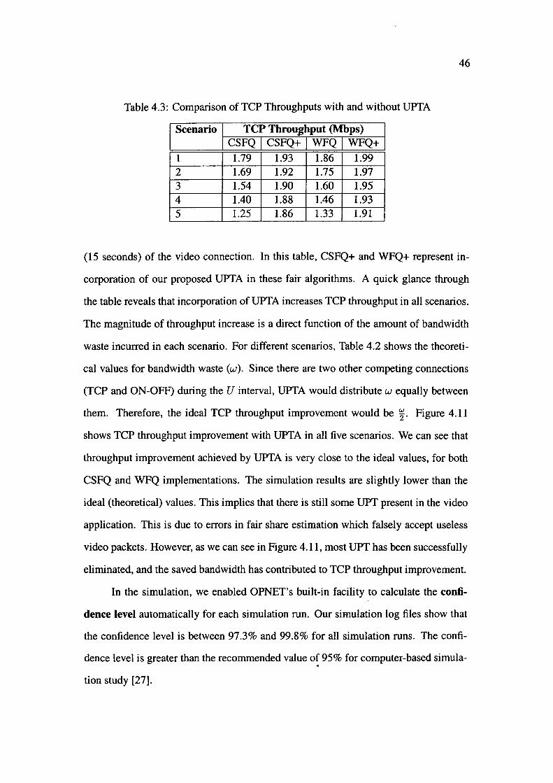
46

Table 4.3: Comparison of TCP Throughputs with and without UPTA

Scenario TCP Throu,ghput (Mbps) CSFQ CSFQ+ WFQ WFQ+

1 1.79 1.93 1.86 1.99 2 1.69 1.92 1.75 1.97 3 1.54 1.90 1.60 1.95 4 1.40 1.88 1.46 1.93 5 1.25 1.86 1.33 1.91

(15 seconds) of the video connection. In this table, CSFQ+ and WFQ+ represent in

corporation of our proposed UPTA in these fair algorithms. A quick glance through

the table reveals that incorporation of UPTA increases TCP throughput in all scenarios.

The magnitude of throughput increase is a direct function of the amount of bandwidth

waste incurred in each scenario. For different scenarios, Table 4.2 shows the theoreti

cal values for bandwidth waste (w). Since there are two other competing connections

(TCP and ON-OFF) during the U interval, UPTA would distribute w equally between

them. Therefore, the ideal TCP throughput improvement would be I. Figure 4.11

shows TCP throughput improvement with UPTA in all five scenarios. We can see that

throughput improvement achieved by UPTA is very close to the ideal values, for both

CSFQ and WFQ implementations. The simulation results are slightly lower than the

ideal (theoretical) values. This implies that there is still some UPT present in the video

application. This is due to errors in fair share estimation which falsely accept useless

video packets. However, as we can see in Figure 4.11, most UPT has been successfully

eliminated, and the saved bandwidth has contributed to TCP throughput improvement.

In the simulation, we enabled OPNET's built-in facility to calculate the confi

dence level automatically for each simulation run. Our simulation log files show that

the confidence level is between 97.3% and 99.8% for all simulation runs. The confi

dence level is greater than the recommended value of 95% for computer-based simula-~

tion study [27].

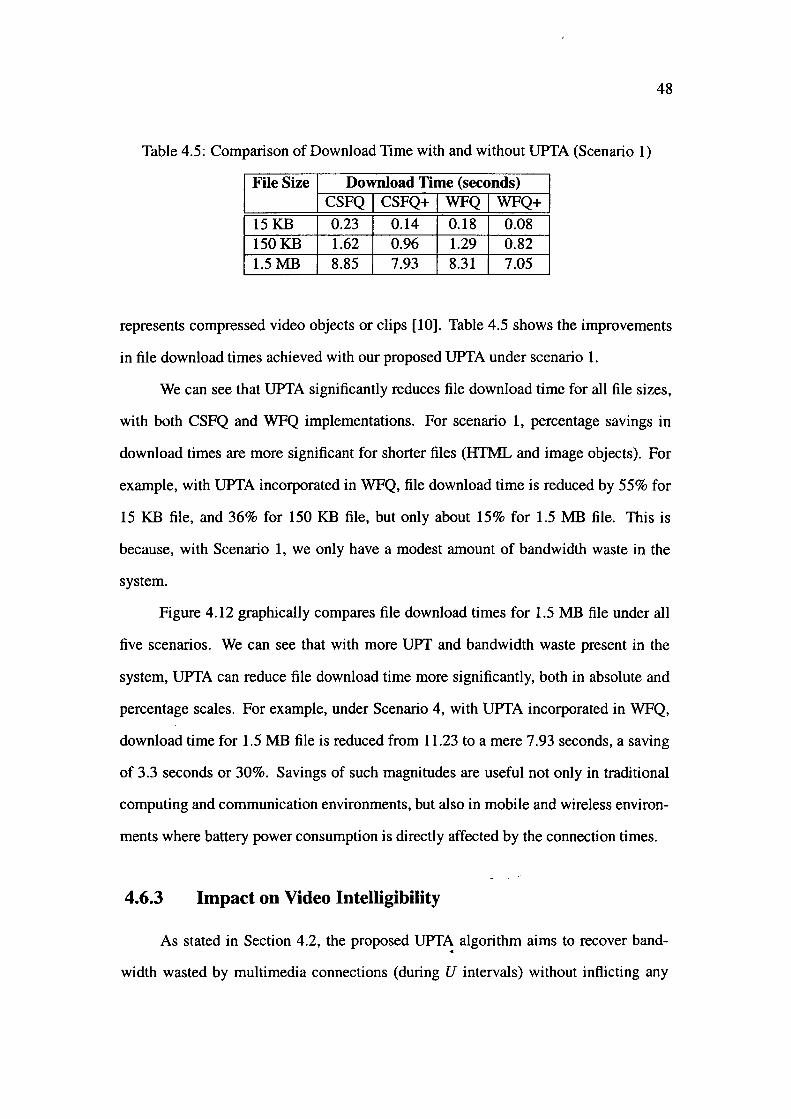
48

Table 4.5: Comparison of Download Time with and without UPTA (Scenario 1)

File Size Download Time (seconds) CSFQ CSFQ+ WFQ WFQ+

15KB 0.23 0.14 0.18 0.08 150KB 1.62 0.96 1.29 0.82 1.5MB 8.85 7.93 8.31 7.05

represents compressed video objects or clips (10]. Table 4.5 shows the improvements

in file download times achieved with our proposed UPTA under scenario 1.

We can see that UPTA significantly reduces file download time for all file sizes,

with both CSFQ and WFQ implementations. For scenario 1, percentage savings in

download times are more significant for shorter files (IITML and image objects). For

example, with UPTA incorporated in WFQ, file download time is reduced by 55% for

15 KB file, and 36% for 150 KB file, but only about 15% for 1.5 MB file. This is

because, with Scenario 1, we only have a modest amount of bandwidth waste in the

system.

Figure 4.12 graphically compares file download times for 1.5 MB file under all

five scenarios. We can see that with more UPT and bandwidth waste present in the

system, UPTA can reduce file download time more significantly, both in absolute and

percentage scales. For example, under Scenario 4, with UPTA incorporated in WFQ,

download time for 1.5 MB file is reduced from 11.23 to a mere 7 .93 seconds, a saving

of 3.3 seconds or 30%. Savings of such magnitudes are useful not only in traditional

computing and communication environments, but also in mobile and wireless environ

ments where battery power consumption is directly affected by the connection times.

4.6.3 Impact on Video Intelligibility

As stated in Section 4.2, the proposed UPT~ algorithm aims to recover band

width wasted by multimedia connections (during U intervals) without inflicting any

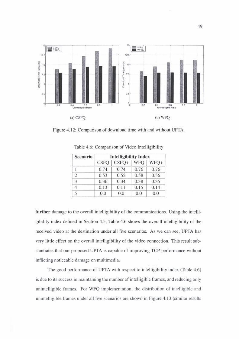
49

15"'=="c=::=:s===Foc=,---.-----.--------,---.--,

- CSFO+

15 !EaWFO I - WFO+

125 12.5

~

w 10

£ Q)

~ 7.5

"' § 10

~ Q)

~ 7.5

,_,;

i ,i' . ( ''

~ ~ 5 8

" ~ C: ~ 5 a

t f., y

2.5 2.5

0.2 0.4 0.6 0.8 0.2 0.4 0.6 0.8 Unintelligible Ratio Unintel ligible Ratio

(a) CSFQ (b) WFQ

Figure 4.12: Comparison of download time with and without UPTA.

Table 4.6: Comparison of Video Intelligibility

Scenario Intelligibility Index CSFQ CSFQ+ WFQ WFQ+

1 0.74 0.74 0.76 0.76 2 0.53 0.52 0.58 0.56 3 0.36 0.34 0.38 0.35 4 0.13 0.11 0.15 0.14 5 0.0 0.0 0.0 0 .0

further damage to the overall intelligibility of the communications. Using the intelli

gibility index defined in Section 4.5, Table 4.6 shows the overall intelligibility of the

received video at the destination under all five scenarios. As we can see, UPTA has

very little effect on the overall intelligibility of the video connection. This result sub

stantiates that our proposed UPTA is capable of improving TCP performance without

inflicting noticeable damage on multimedia.

The good performance of UPTA with respect to intelligibility index (Table 4.6)

is due to its success in maintaining the number of intelligible frames, and reducing onl y

unintelligible frames. For WFQ implementation, the di stribution of intelli gible and

un intell igible frames under all five scenarios are shown in Figure 4. 13 (similar resu lts

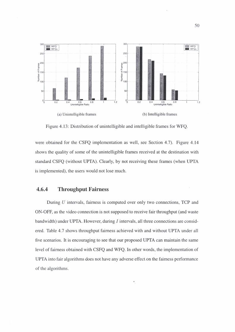
300 1-WFO I

- WFO+

250 ,....

200

i 150 .. ., . .

~. 100

! 50 i,

.t i:.<,- -0.2 0 4 0.6 0.8 Unintelligible Ratio

(a) Unintelligible frames

,. .

~ ·

'

'

- 1.2

50

300,-------,-----.----,----,--.=:Dl=:=W==::=F=;=O =,i

- WFO+

250

200

150

100

50

0.2 0.4 0.6 0.8 1.2 Unintelligible Ratio

(b) Intelligible frames

Figure 4.13: Distribution of unintelligible and intelligible frames for WFQ.

were obtained for the CSFQ implementation as well, see Section 4.7). Figure 4.14

shows the quality of some of the unintelligible frames received at the destination with

standard CSFQ (without UPTA). Clearly, by not receiving these frames (when UPTA

is implemented), the users would not lose much.

4.6.4 Throughput Fairness

During U intervals, fairness is computed over only two connections, TCP and

ON-OFF, as the video connection is not supposed to receive fair throughput (and waste

bandwidth) under UPTA. However, during I intervals, all three connections are consid

ered. Table 4.7 shows throughput fairness achieved with and without UPTA under all

five scenarios. It is encouraging to see that our proposed UPTA can maintain the same

level of fairness obtained with CSFQ and WFQ. In other words, the implementation of

UPTA into fair algorithms does not have any adverse effect-on the fairness performance

of the algorithms.

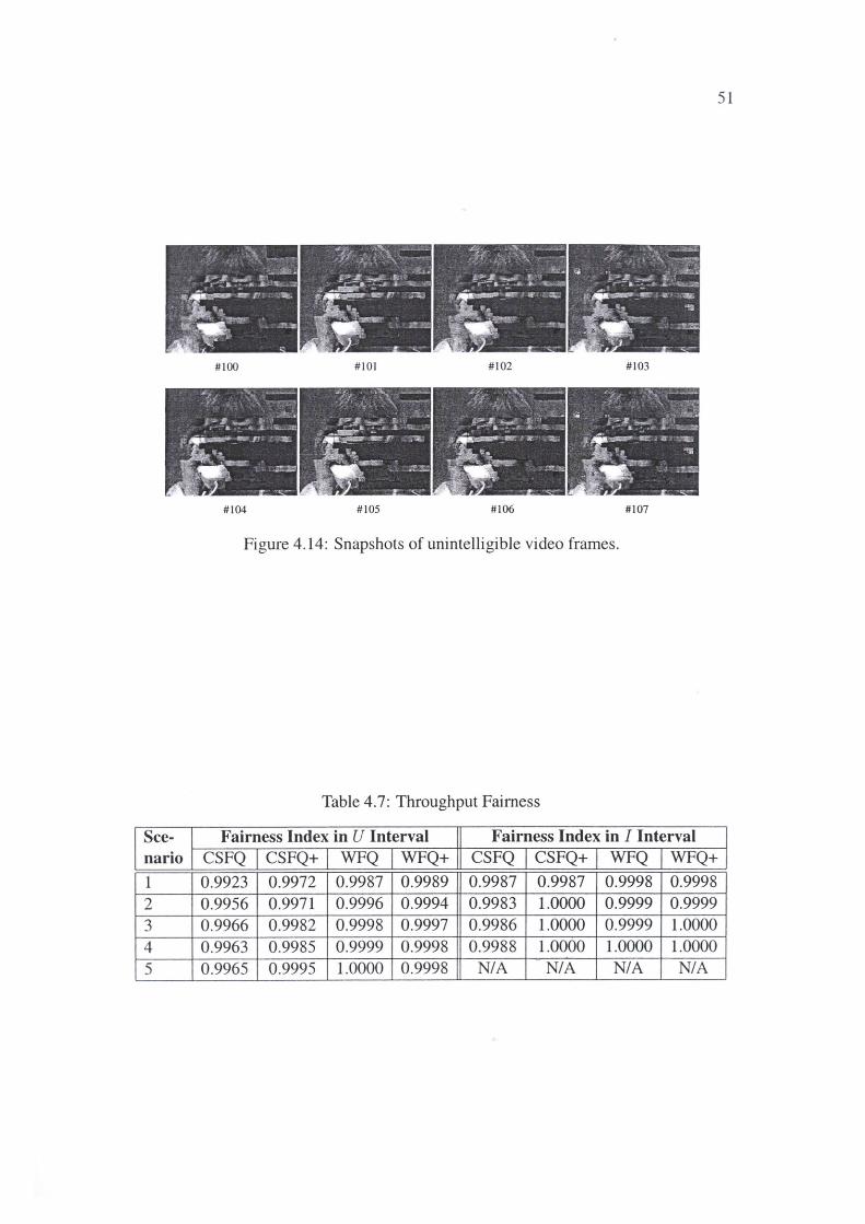
51

#100 #IOI #102 #103

#104 #105 #106 #107

Figure 4.14: Snapshots of unintelligible video frames .

Table 4.7: Throughput Fairness

See- Fairness Index in U Interval Fairness Index in I Interval nario CSFQ CSFQ+ WFQ WFQ+ CSFQ CSFQ+ WFQ WFQ+

1 0.9923 0.9972 0.9987 0.9989 0.9987 0.9987 0.9998 0.9998 2 0.9956 0.9971 0.9996 0.9994 0.9983 1.0000 0.9999 0.9999 3 0.9966 0.9982 0.9998 0.9997 0.9986 1.0000 0.9999 1.0000 4 0.9963 0.9985 0.9999 0.9998 0.9988 1.0000 1.0000 1.0000 5 0.9965 0.9995 1.0000 0.9998 NIA NIA NIA NIA

52

4. 7 CSFQ Simulation Results

In this section, we present simulation results for CSFQ implementation.

4.7.1 TCP Throughput

Figure 4.15 and Figure 4.16 show CDF of end-to-end packet delays and packet

loss rates for the video connection under CSFQ. The results are comparable with that

collected in WFQ implementation. All video packets have a delay less than 0.08 sec

ond, and the packet loss rates in U intervals are around 25%. Again, for the simulated

network, only high packet loss rates contribute to UPI'. Delays are too small to cause

any useless video packets.

Figure 4.17 shows short-term TCP throughput received under CSFQ for all five

scenarios. As we can see in the figure, the TCP connection receives higher throughput

during the U interval when UPTA is implemented (CSFQ+ ). This is because UPI'

occurs during U intervals. UPTA recovers the bandwidth that would be wasted by

useless video packets. During the I interval, the TCP throughputs under CSFQ and

CSFQ+ are essentially the same. This proves that UPTA has no impact on normal

CSFQ operation when there is no UPI' in the network (during I intervals).

4.7.2 Video Intelligibility

Figure 4.18 shows distribution of intelligible and unintelligible frames for all

five scenarios, under CSFQ implementation. As shown in the figure, there is almost no

unintelligible frames when UPTA is implemented (CSFQ+ ). Without UPTA (CSFQ),

the number of unintelligible frames is as large as 280 (see Figure 4.18(a)). On the other

hand, the number of intelligible frames remains unchanged after UPTA is implemented

(see Figure 4.18(b)). This proves that UPTA can effectively eliminate useless video •

packets, while maintaining the same level of video intelligibility.

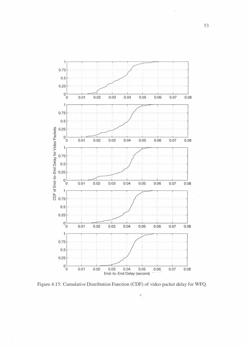
53

0.75

0.5 · · . . · · · . ,. -

0.25

0 l...-------'-=:........I.------'-----'-----'------'-------'----'

0 0.01 0.02 0.03 0.04 0.05 0.06 0.07 0.08

0.75 ... . : . . .. .. . ... · . .. ...... · .. . .. .. .. ; . . . ..............

0.5

(J)

a> 0.25 .. .... . .. . . . .Y. u <1l 0 a.. 0 0.01 0.02 0.03 0.04 0.05 0.06 0.07 0.08 0 (1) "O

> .E 0.75 . . .. . . . . . >, <1l ai 0.5 0 "O C

0.25 w I

0

' 0 "O 0 0.01 0.02 0.03 0.04 0.05 0.06 0.07 0.08 C w 15 lL 0 () 0.75

0.5 .... . .. . , .. .. . . . . -·- . . .. . . .. . \ .. . .. . . . ' ... . '.

0.25

0 0 0.01 0.02 0.03 0.04 0.05 0.06 0.07 0.08

0.75

0.5 ...... : . . . . . . . . . - ...... . . . . . . ~ . . . . . ... . .. ' .. .

0.25

0 0 0.01 0.02 0.03 0.04 0.05 0.06 0.07 0.08

End-to- End Delay (second) - .


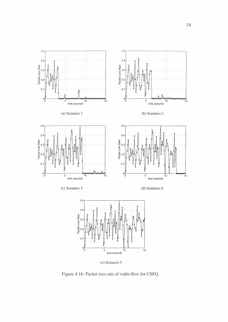
0.4

a, 1u a: 0 3 ~ . 0 _, .; TI 02 "' (l_

0 .1

15 time (second)

(a) Scenario l

0.5

0.4

!!l "' '!; 03 "' 0 _, .; TI 02 "' (l_

0.1

0 0

time (second)

(b) Scenario 2

0.5.------~------.-~-----, 0.5

0.4

a, 1u a: 0.3 ~ .3 .; TI 0 .2

"' (l_

0.1

.~.

0.4

* a: 0 3 ~ .

.3

.; TI 0 .2

"' (l_

0.1

X 11

.~

y · ) ·

o----~-------111,_-- -* 0 0 0 5 10 15 5


(c) Scenario 3 ( d) Scenario 4

0.5

0.4

* a: 0.3 .. ~ "' "'

.~

0 _, .; TI 0.2 . .

"' (l_

0.1 l

o-----~-------..,--,~---~ 0 5 10 15_

time (second)

(e) Scenario 5

Figure 4.16: Packet loss rate of video flow for CSFQ.

54

15

·-·

:i l

~

10 15

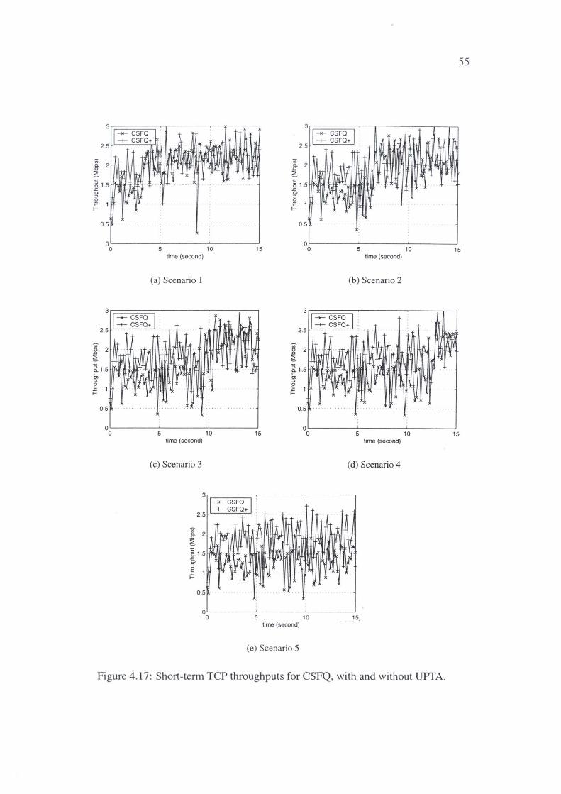
2.5

., a. 2 D

~

~ 1.5 Le O> ::,

e 1 Le I-

0.5

0 0

3

2.5

., a. 2 D

~

115 Le O> ::, e 1 Le I-

0.5

0 0

., _g- 2

~

I 15 Le 0, ::, 0 l: 1 I-

0.5

55

o~----~-----~------' 5 10 15 0 5


(a) Scenario l (b) Scenario 2

2.5

., 2 a.

D

~ I 15 Le 0, ::,

e 1 Le I-

0.5

0 5 10 15 0 5


(c) Scenario 3 (d) Scenario 4

3r;::======;-:-----:-----, _,._ CSFQ --+- CSFQ+

2.5

0.5

o~----~----~~------' 0 5 10 15.

time (second)

(e) Scenario 5

10 15

10 15

Figure 4.17: Short-term TCP throughputs for CSFQ, with and without UPTA.

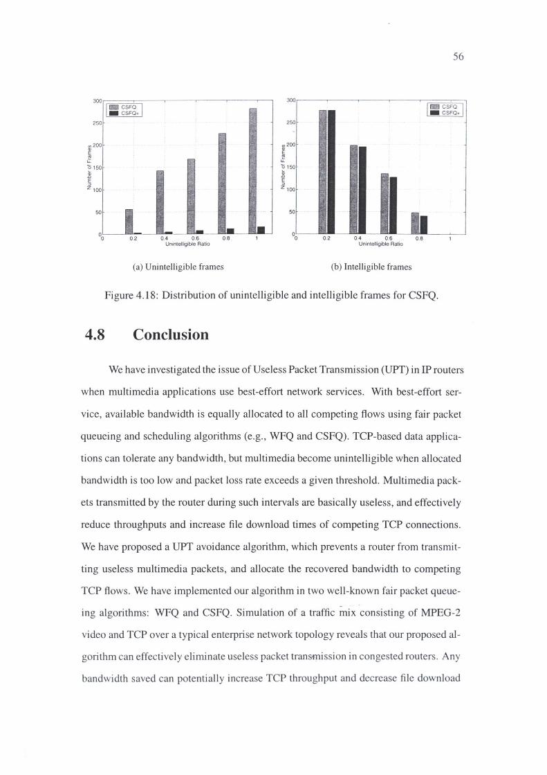
56

300r.===::::;----,----.------,----,----7 f;;;:J CSFO

- CSFO+

250 250

200 200

150 150

100 100

50 50

0.2 0 4 06 06 0.2 0.4 0.6 0.8 Unintelligible Ratio Unintelligible Ratio

(a) Unintelligible frames (b) Intelligible frames

Figure 4 .18: Distribution of unintelligible and intelligible frames for CSFQ.

4.8 Conclusion

We have investigated the issue of Useless Packet Transmission (UPT) in IP routers

when multimedia applications use best-effort network services. With best-effort ser

vice, available bandwidth is equally allocated to all competing flows using fair packet

queueing and scheduling algorithms (e.g., WFQ and CSFQ). TCP-based data applica

tions can tolerate any bandwidth, but multimedia become unintelligible when allocated

bandwidth is too low and packet loss rate exceeds a given threshold. Multimedia pack

ets transmitted by the router during such intervals are basically useless, and effectively

reduce throughputs and increase file download times of competing TCP connections.

We have proposed a UPT avoidance algorithm, which prevents a router from transmit

ting useless multimedia packets, and allocate the recovered bandwidth to competing

TCP flows. We have implemented our algorithm in two well-known fair packet queue

ing algorithms: WFQ and CSFQ. Simulation of a traffic mix consisting of MPEG-2

video and TCP over a typical enterprise network topology reveals that our proposed al

gorithm can effecti vely eliminate useless packet transm.i ssion in congested routers. Any

bandwidth saved can potentiall y increase TCP throughput and decrease fi le download

57

time. Our UPT avoidance algorithm can operate unobtrusively; it has noticeable effect

neither on the overall intelligibility of the multimedia applications, nor on the fairness .,

performance of the "host" packet queueing algorithms (WFQ and CSFQ) on which we

"mount" our algorithm.

Chapter 5

UPTA with Multiple Congested Links

We discussed UPT avoidance with single congested link in previous chapter.

However, in large-scale networks (e.g., the Internet), there are usually more than one

congested link on an end-to-end path. This chapter presents extensions of UPTA, and

associated protocols, to address performance issues germane to multiple congested

links.

5.1 Scope of the Problem

In large networks, traffic flows usually experience congestion at more than one

network node. That is, there are usually more than one congested link on an end-to-end

path. In such a circumstance, packet loss of a flow is distributed at different congested

nodes. If UPTA is enforced independently at each individual router 1 , UPT may go

undetected. This is because the cumulative packet loss rate may be greater than the loss

threshold while packet loss rate at each individual router is less than the loss threshold.

We use an example to explain the problem as following. Figqre 5.1 is an example in

which an unintelligible video flow goes undetected, as a result of distributed UPTA

(let's call it basic UPTA) enforcement.

1 We refer to such implementation of UPTA as "basic UPTA" (B-UPTA) hereafter.

59

Figure 5.1: UPT in networks with multiple congested links.

In the network shown in Figure 5.1, the link speed of each network link is as

shown in the figure. All access links have a speed of 10 Mbps. In the example network,

there are three flows, of which Flow 2 (S2-D2, shaded) is a UDP-based CBR MPEG-2

video application (encoded at 1.5 Mbps). Other flows are greedy TCP flows. Assume

the MPEG-2 video application has a loss threshold of 12%. In the example network,

assume UPTA is implemented in all routers, in conjunction with WFQ (let's call it

WFQ+ ). As the MPEG-2 video is encoded at a bit rate of 1.5 Mbps, packet arrival rate

of the video application (at router R1) is about 1.76 Mbps, after taking TS header (4

bytes), UDP header (8 bytes), and IP header (20 bytes) into account. Based on max-min

criterion (Eq. (4.4)), we calculate packet arrival rate, packet departure rate, and packet

loss rate for the video flow, as shown in Table 5.1.

From Table 5.1 we can see that the packet loss rate (of the video flow) seen by

routers R1-R7 is less than the loss threshold of 12%. Therefore, the video flow is

considered as an I flow at each individual router (R1-R7 ). However, as we can see in

the table, the end-to-end packet loss rate (cumulative loss rate) of the video application

(as perceived by the video receiver D 2 ) is more than 30%, which exceeds the the loss

threshold of 12%. Therefore, the video flow is actually transmitting useless packets,

although it is not detected by the network. A more generali sed analysis of end-to-end

packet loss rate is provided in the following section.

60

Table 5.1: Packet Loss Rate of Video Flow at Various Nodes

Node Arrival Rate Dept. Rate Loss Rate (Mbps) (Mbps) %)

R1 1.76 1.76 0 R2 1.76 1.60 9.1 R3 1.60 1.43 10 R4 1.43 1.30 9.1 R5 1.30 1.17 10 R,e, 1.17 1.17 0 R1 1.17 1.17 0 D2 1.17 NIA 33.5

5.2 Analysis of End-to-End Packet Loss Rate

In this section, we conduct a generalised analysis on end-to-end packet loss rate

of a flow traversing multiple congested links. Our analysis results show that the end-to

end packet loss rate increases exponentially with the increase of number of congested

links. Therefore, a multimedia flow may suffer an unacceptably large end-to-end packet

loss rate, even though packet loss rate at each individual router is very small.

Assume there are n routers R1 , R2, ... , Rn on an end-to-end path between a

source and its destination (as shown in Figure 5.2), we can use fluid model to de

rive the cumulative packet loss rate (for a given flow) at router Rk (k = 1, 2, ... , n)

mathematically. For a given flow f, we use following notations:

• Ak: Packet arrival rate at router Rk.

• µk: Packet departure rate at router Rk.

• Pk: Local packet loss rate (LPLR) at router Rk (pk_ = ~ - x!").

• Pk: Cumulative packet loss rate (CPLR) at router Rk.

• Pe: End-to-end packet loss rate (CPLR at the destination).

According to fluid model, we have:

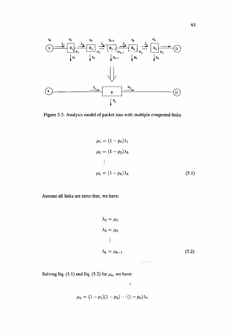
Figure 5.2: Analysis model of packet loss with multiple congested links.

µ1 = (1 - P1)..\1

µ2 = (1 - P2)..\2

Assume all links are error-free, we have:

Solving Eq. (5.1) and Eq. (5.2) for µk, we have:

61

(5.1)

(5.2)

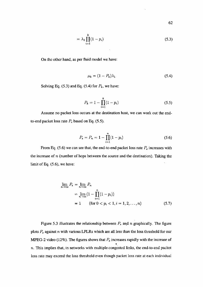
62

k

= A1 II(l - Pi) (5.3) i=l

On the other hand, as per fluid model we have:

(5.4)

Solving Eq. (5.3) and Eq. (5.4) for Pk, we have:

k

Pk = l - II (1 - Pi) (5.5) i=l

Assume no packet loss occurs at the destination host, we can work out the end

to-end packet loss rate Pe based on Eq. (5.5).

n

Pe = Pn = l - II (1 - Pi) (5.6) i=l

From Eq. (5.6) we can see that, the end-to-end packet loss rate Pe increases with

the increase of n (number of hops between the source and the destination). Taking the

limit of Eq. (5.6), we have:

lim Pe = lim Pn n--+oo n--+oo

n

= lim (1 - II(l - Pi)) n--+oo

i=l

=l (for O < Pi < l, i = 1, 2, ... , n) (5.7)

Figure 5.3 illustrates the relationship between Pe an_d n .graphically. The figure

plots Pe against n with various LPLRs which are all less than the loss threshold for our

MPEG-2 video (12% ). The figures shows that Pe increases rapidly with the increase of ...

n. This implies that, in networks with multiple congested links, the end-to-end packet

loss rate may exceed the loss threshold even though packet loss rate at each individual

0.9

0.8

-alJ.7 . ~

~ 0.6 Cl.

-g 0.5 · w

I f 0.4 . "O C w 0.3 ·

0.1

-t- LPLR=0.03 -B-- LPLR=0.05 -+- LPLR=0.07 --a-- LPLR=0.09 -A- LPLR=0.1

0 r____._ _ _L_ _ _j_____i _ __j_ _ __.______'.:;::::::::::i:==::::;:::::::::J

0 1 0 20 30 40 50 60 70 80 90 100 Number of Congested Links (n)

63

Figure 5.3: End-to-end packet loss rate as a function of LPLR and number of congested links.

router is less than the threshold. As shown in Figure 5.3, Pe is greater than 12% for all

five LPLRs when n is greater than 4. This implies that the combined effect is significant

even if LPLRs are very small.

It is clear from above analysis, that in order to eliminate UPT completely in

networks with multiple congested links, there is a need to investigate extensions to our

basic UPTA algorithm (which operates based on only LPLR). In the rest of this chapter,

we propose and evaluate two such extensions, Partial UPTA (P-UPTA) and Centralised

UPTA (C-UPTA).

5.3 Partial UPTA (P-UPTA)

The problem we discussed in Section 5 .1 stems from the fact that all routers use

the same loss threshold to detect UPT. As the same loss threshold is used, packet loss at

upstream routers is not taken into account. Partial UPTA employs variable (decreasing)

loss threshold , i.e. the loss threshold q is updated (decremented) at each router based . on local packet loss rate (LPLR) at the router. Because P-UPTA considers decreasing

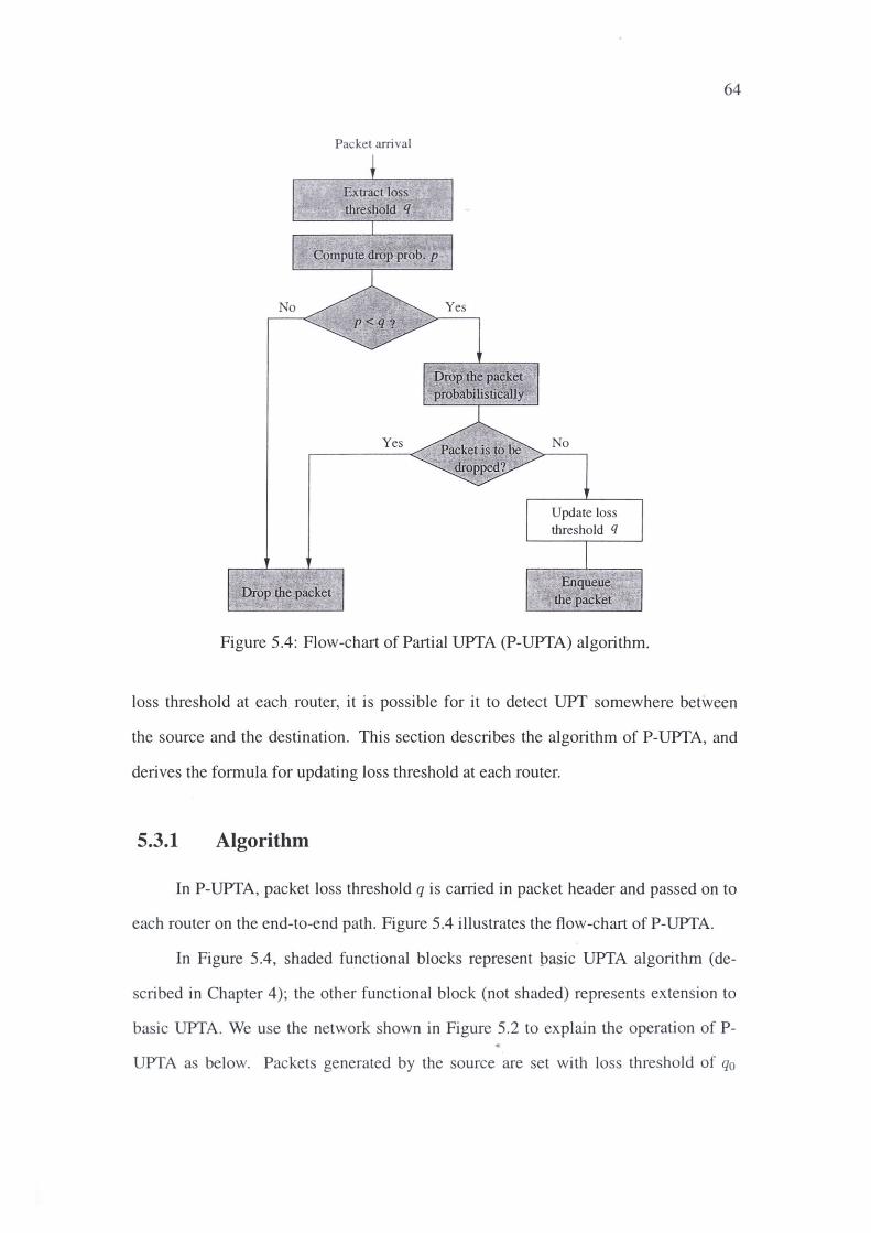
Packet arri val

Extract loss threshold q

• · Compute drrip prob. P ·

No

Yes

Diop the_piciet ~ •• ':·-• · t

Yes

No

Update loss threshold q

Figure 5.4: Flow-chart of Partial UPTA (P-UPTA) algorithm.

64

loss threshold at each router, it is possible for it to detect UPT somewhere between

the source and the destination. This section describes the algorithm of P-UPTA, and

derives the formula for updating loss threshold at each router.

5.3.1 Algorithm

In P-UPTA, packet loss threshold q is carried in packet header and passed on to

each router on the end-to-end path. Figure 5.4 illustrates the flow-chart of P-UPTA.

In Figure 5.4, shaded functional blocks represent pasic UPTA algorithm (de

scribed in Chapter 4); the other functional block (not shaded) represents extension to

basic UPTA. We use the network shown in Figure 5.2 to explain the operation of P

UPTA as below. Packets generated by the source are set with loss threshold of q0

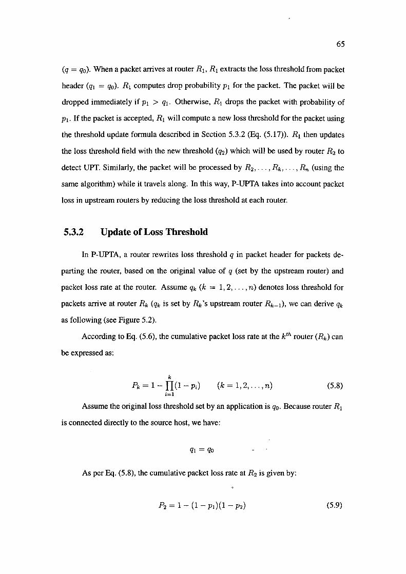
65

(q = q0 ). When a packet anives at router R 1, R 1 extracts the loss threshold from packet

header (q1 = q0 ). R 1 computes drop probability P1 for the packet. The packet will be

dropped immediately if p1 > q1. Otherwise, R 1 drops the packet with probability of

p1• If the packet is accepted, R1 will compute a new loss threshold for the packet using

the threshold update formula described in Section 5.3.2 (Eq. (5.17)). R1 then updates

the loss threshold field with the new threshold (q2) which will be used by router R2 to

detect UYf. Similarly, the packet will be processed by R2 , ... , Rk, ... , Rn (using the

same algorithm) while it travels along. In this way, P-UYfA takes into account packet

loss in upstream routers by reducing the loss threshold at each router.

5.3.2 Update of Loss Threshold

In P-UYfA, a router rewrites loss threshold q in packet header for packets de

parting the router, based on the original value of q (set by the upstream router) and

packet loss rate at the router. Assume qk (k = I, 2, ... , n) denotes loss threshold for

packets anive at router Rk (qk is set by Rk's upstream router Rk_ 1), we can derive qk

as following (see Figure 5.2).

According to Eq. (5.6), the cumulative packet loss rate at the k th router (Rk) can

be expressed as:

k

Pk = I - IT (1 - Pi) (k=l,2, ... ,n) (5.8) i=l

Assume the original loss threshold set by an application is q0 • Because router R1

is connected directly to the source host, we have:

q1 = qo

As per Eq. (5.8), the cumulative packet loss rate at R 2 is given by:

(5.9)

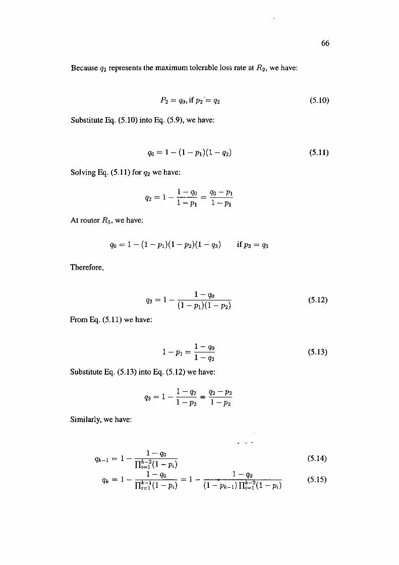
Because q2 represents the maximum tolerable loss rate at R2 , we have:

Substitute Eq. (5.10) into Eq. (5.9), we have:

Solving Eq. (5.11) for q2 we have:

At router R3, we have:

l -qo Q2=l--

l-p1 Qo - PI

l -pI

Qo = 1 - (1 - P1)(l - P2)(l - q3)

Therefore,

l-qo q3 = l - -(l ___ P_1_) (-l ---P-2)

From Eq. (5.11) we have:

l -qo l-p1=-

l-q2

Substitute Eq. (5.13) into Eq. (5.12) we have:

Similarly, we have:

l-qo q - l k-I - - n~-2(l _ ·)

i=l Pi

if p3 = q3

1- Qo 1 - Qo Qk = l - k-I = 1 - . k-2

ni=I (1 - Pi) (1 - Pk-I) ni=I (1 - Pi)

66

(5.10)

(5.11)

(5.12)

(5.13)

(5.14)

(5.15)

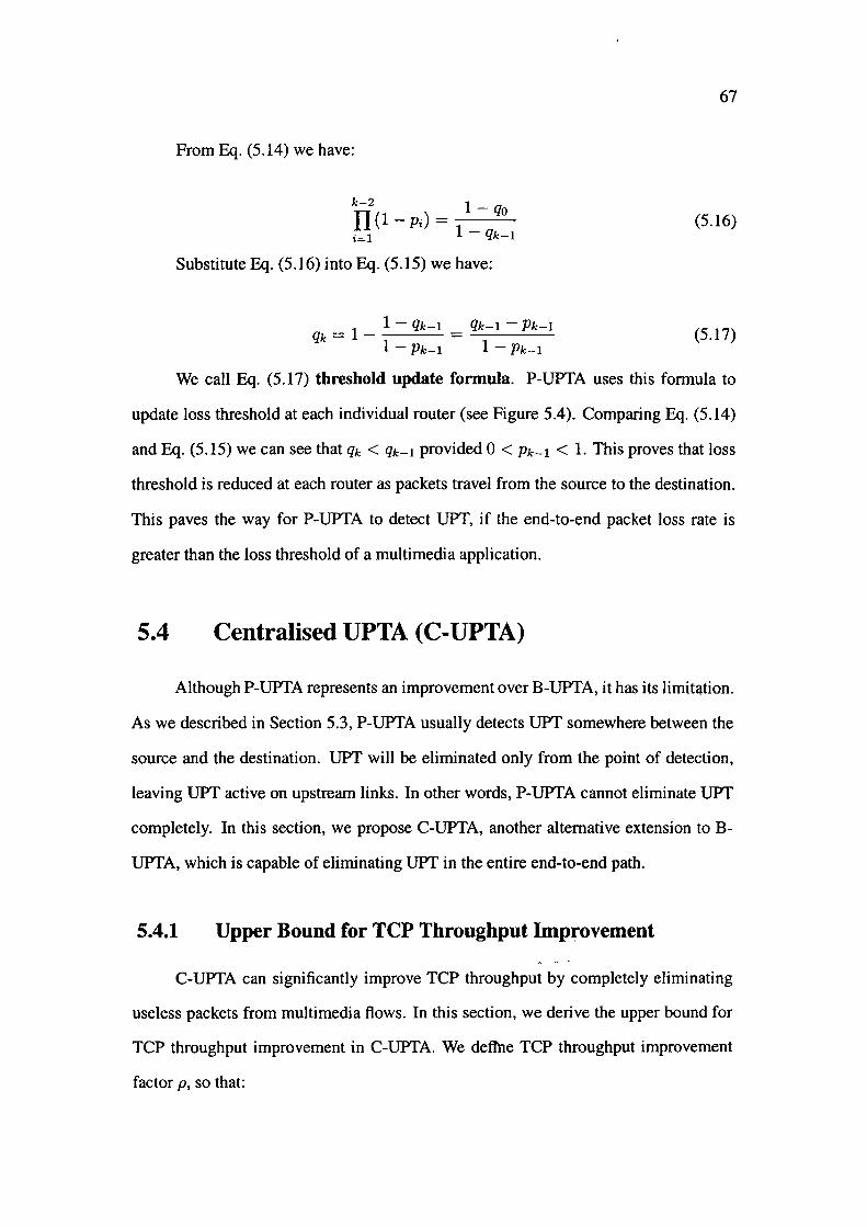
67

From Eq. (5.14) we have:

k-2 1 - Qo Il(l-vi) = -1 _--i=l Qk-1

(5.16)

Substitute Eq. (5.16) into Eq. (5.15) we have:

1 1 - Qk-1 Qk-1 - Pk-1 Qk = - -

1 - Pk-1 1 - Pk-1 (5.17)

We call Eq. (5.17) threshold update formula. P-UPTA uses this formula to

update loss threshold at each individual router (see Figure 5.4). Comparing Eq. (5.14)

and Eq. (5.15) we can see that Qk < Qk-1 provided O < Pk-I < 1. This proves that loss

threshold is reduced at each router as packets travel from the source to the destination.

This paves the way for P-UPTA to detect UPT, if the end-to-end packet loss rate is

greater than the loss threshold of a multimedia application.

5.4 Centralised UPTA (C-UPTA)

Although P-UPTA represents an improvement over B-UPTA, it has its limit::Jtion.

As we described in Section 5.3, P-UPTA usually detects UPT somewhere between the

source and the destination. UPT will be eliminated only from the point of detection,

leaving UPT active on upstream links. In other words, P-UPTA cannot eliminate UPT

completely. In this section, we propose C-UPTA, another alternative extension to B

UPTA, which is capable of eliminating UPT in the entire end-to-end path.

5.4.1 Upper Bound for TCP Throughput Improvement

C-UPTA can significantly improve TCP throughput by completely eliminating

useless packets from multimedia flows. In this section, we derive the upper bound for

TCP throughput improvement in C-UPTA. We deffne TCP throughput improvement

factor p, so that:

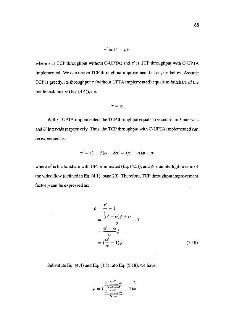
68

r' = (1 +p)r

where r is TCP throughput without C-UPfA; and r' is TCP throughput with C-UPf A

implemented. We can derive TCP throughput improvement factor p as below. Assume

TCP is greedy, its throughput r (without UPfA implemented) equals to fairshare of the

bottleneck link a (Eq. (4.4)), i.e.

T=Q

With C-UPf A implemented, the TCP throughput equals to a and a', in I intervals

and U intervals respectively. Thus, the TCP throughput with C-UPfA implemented can

be expressed as:

r' = (1 - cp)a + cpa' = (a' - a)cp + a

where a' is the fairshare with UPf eliminated (Eq. (4.5)); and cp is unintelligible ratio of

the video flow (defined in Eq. (4.1), page 29). Therefore, TCP throughput improvement

factor p can be expressed as:

r' p = - -l

T

= ( a' - a )cp + a _ 1 a

a'-a =--cp

a a'

= (- - l)cp a

Substitute Eq. (4.4) and Eq. (4.5) into Eq. (5.18), we have:

C-E~-) A; •

p = ( N-S;M _ l)cp C-Li-) A;

N-S

(5.18)

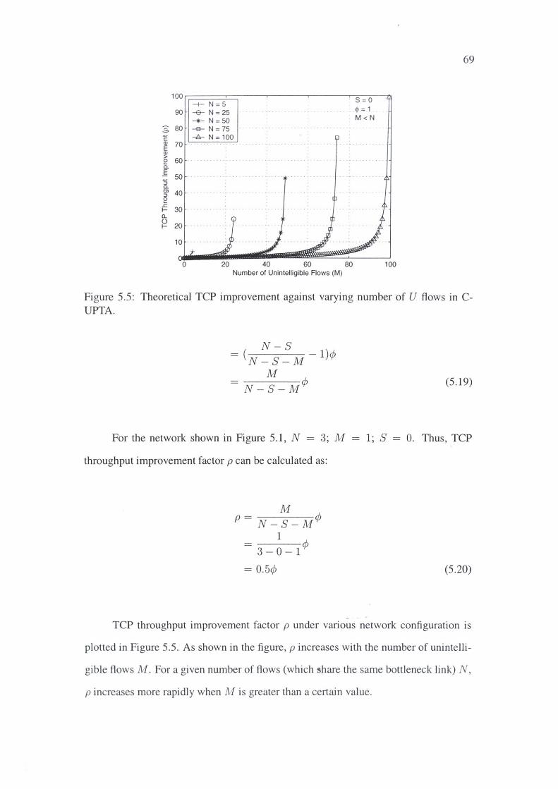
100-,---+-::::::::::::N===5:::.=,--~---~--~ . _S_=_O_ ....,._

90 --e-- N = 25 4> = 1 -+- N=50 M < N

s 80 --B- N = 75 c -A- N = 100 Q)

E 70 ·

Q)

> e 60 · · · · · · .. · · · c.

E 50 · · · · · · · · · · ···· · · · · · · · · :5 c. 0) :, 0

40 ·

.c 1- 30 Q_

~ 20

0 20 60 80 Number of Unintelligible Flows (M)

100

69

Figure 5.5: Theoretical TCP improvement against varying number of U flows in CUPTA.

N-S = (N - S - M - l)</J

M <P N-S-M

For the network shown in Figure 5.1, N = 3; M

throughput improvement factor p can be calculated as:

M P = N - S- M<P

l <P 3-0-1

= 0.5</J

(5.19)

1; S 0. Thus, TCP

(5.20)

TCP throughput improvement factor p under various network configuration is

plotted in Figure 5.5. As shown in the figure, p increases with the number of unintelli

gible flows M . For a given number of flows (which ~µare the same bottleneck link) N,

p increases more rapidly when M is greater than a certain value.

5.4.2

Hosts

JCMP Probe Packets (Type= 20)

CII

<'.'.' ~ st cc;> ~ ~ ~ t::::. ~ ~

Core Routers

JCMP Report Packets (Type= 21)

Edge Router D Core Router O Host CJI ICMP packet

Figure 5.6: Centralised UPTA (C-UPTA) architecture.

Architecture

70

Hosts

Figure 5.6 illustrates the architecture for C-UPTA. The architecture consists of

edge routers, core routers and hosts. Edge routers are located at network edge. They are

connected directly to users (Hosts in Figure 5.6). An edge router may also interconnect

two networks (e.g. networks operated by two different ISPs) if traffic flows traverse

multiple networks.

In C-UPTA, we make distinction between two types of edge routers - ingress

and egress routers. An ingress router is the edge router where traffic flows enter a net

work, while an egress router is the edge router where traffic flows exit from a network.

Core routers are located in network core (or network backbone). They have no direct

connection to users. The feedback mechanism facilitates communication between edge

routers . This allows an ingress router to determine the global fairshare for an end-to

end path and drop packets in the first place, i.e. the ingress router. In Figure 5.6, UPTA

is needed at the ingress router only. The UPTA pseudo-code implemented in the ingress

router is shown in Figure 5.7.

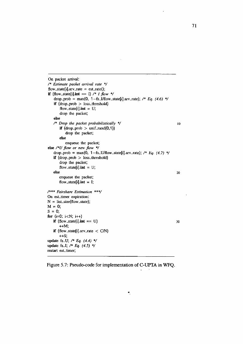
On packet arrival: /* Estimate packet arrival rate */ tlow_state[i].arv_rate = esLrate(); if (flow_state[i].int == I) /* / flow *I

drop_prob = max(0, 1-fs_I/flow_state[i].arv_rate); /* Eq. (4.6) *I if (drop_prob > loss_threshold)

flow _state[i].int = U; drop the packet;

else I* Drop the packet probabilistically *I

if (drop_prob > uniLrand(0, 1)) drop the packet;

else enqueue the packet;

else l*U flow or new flow *I drop_prob = max(0, 1-fs_U/flow_state[i].arv_rate); /* Eq. (4.7) */ if (drop_prob > loss_threshold)

drop the packet; flow _state[i].int = U;

10

else 20

enqueue the packet; flow _state[i].int = I;

/*** Fairshare Estimation ***/ On esLtimer expiration: N = lisLsize(flow_state); M = O; S = O; for (i=0; i<N; i++)

if (flow_state[i].int == U) ++M;

if (flow _state[i].arv _rate < C/N) ++S;

update fs_U; /* Eq. (4.4) *I update fs_l; /* Eq. ( 4.5) *I restart esLtimer;

Figure 5.7: Pseudo-code for implementation of C-UPTA in WFQ .

•

30

71

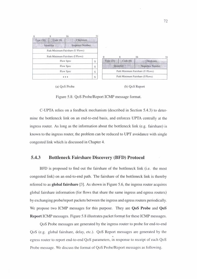
72

0 8 16 31

Type (20) I Code (0) Checksum

Identifi er Sequence Number

Path Minimum Fairshare (U Flows)

Path Minimum Fairshare (I Flows) 0 8 16 31

Flow Spee s Type (21) I Code (0) Ch~ksum

Flow Spee s Identifier _.Sequence Number ' -

Flow Spee s Path Minimum Fairshare (U Flows)

... s Path Minimum Fairshare (I Flows)

(a) QoS Probe (b) QoS Report

Figure 5.8 : QoS Probe/Report ICMP message format.

C-UPTA relies on a feedback mechanism (described in Section 5.4.3) to deter

mine the bottleneck link on an end-to-end basis, and enforces UPTA centrally at the

ingress router. As long as the information about the bottleneck link (e.g. fairshare) is

known to the ingress router, the problem can be reduced to UPT avoidance with single

congested link which is discussed in Chapter 4.

5.4.3 Bottleneck Fairshare Discovery (BFD) Protocol

BFD is proposed to find out the fairshare of the bottleneck link (i .e. the most

congested link) on an end-to-end path. The fairshare of the bottleneck link is thereby

referred to as global fairshare [3]. As shown in Figure 5.6, the ingress router acquires

global fairshare information (for flows that share the same ingress and egress routers)

by exchanging probe/report packets between the ingress and egress routers periodically.

We propose two ICMP messages for thi s purpose. They are QoS Probe and QoS

Report ICMP messages. Figure 5.8 illustrates packet form~t for these ICMP messages.

QoS Probe messages are generated by the ingress router to probe for end-to-end

QoS (e.g. global fai rshare, delay, etc.). QoS Report messages are generated by the ..

egress router to report end-to-end QoS parameters, in response to receipt of each QoS

Probe message. We discuss the format of QoS Probe/Report messages as fo llowing.

73

5.4.3.1 Header Format of QoS Probe/Report I CMP Messages

As shown in Figure 5.8, QoS Probe and QoS Report messages have the same

ICMP header format (shaded fields in Figure 5.8). The QoS Probe/Report message

header is made up of five fields. They are Type (8 bits), Code (8 bits), Checksum (16

bits), Identifier (16 bits), and Sequence Number (16 bits) fields.

The Type field specifies an ICMP message type. For QoS Probe messages (Fig

ure 5.8(a)), the Type field is assigned a value of 20. For QoS Report messages (Fig

ure 5.8(b)), a value of 21 is assigned. The Code field indicates the type of QoS infor

mation an ingress router is probing for. Because we only consider bandwidth in this

research, the Code field is set to 0. Other code values may be used to indicate other

QoS parameters.

The Checksum field is used to detect errors in ICMP messages. It carries the

checksum of the entire probe/report ICMP message. The Identifier field identifies the

output port for which a probe message is generated. It carries the output port number

of an ingress router. The Sequence Number field is used to associate report messages

with probe messages.

5.4.3.2 Payload of QoS Probe ICMP Messages

The payload of QoS Probe messages (Figure 5.8(a)) consists of Path Minimum

Fairshare (U flows), Path Minimum Fairshare (I flows), and a list of Flow Spees.

The two path minimum fairshare fields are used to record the minimum f airshare on

the network path between an ingress router and its corresponding egress router (for U

flows and I flows respectively). Let's assume that there are N rnuters on the network

path between the ingress router and its egress router (including the ingress and egress

routers). As each router will compute its local fairshare o:1 and a~ (l = 1, 2, ... , N).

The minimum fairshare (on the network path) can bs expressed as:

74

(5.21)

(5.22)

When the ingress router generates a QoS Probe packet, the path minimum fair

share fields are set to the local f airshare at the ingress router. As the probe packet travels

through the network (from ingress router to egress router), the two path minimum fair

share fields are updated by intermediate routers as below:

(l=l,2, ... ,N) (5.23)

'f I I l CTz < amin (l = l, 2, ... , N) (5.24)

The list of Flow Spees contains flow identity information for all flows sharing

the same ingress/egress pair. A Flow Spee uniquely identifies a flow. In 1Pv6, a flow is

identified by the Flow Label field in IP header. in IPv4, a flow can be identified by a

tuple of source IP address, source port number, destination IP address, and destination

port number. Each Flow Spee is followed by an 1-bit S bit. S bit is set by the ingress

router. It indicates the intelligibility status of a flow. A value of O represents U flows,

and a value of 1 represents I flows. The intelligibility status of a flow is necessary for

fairshare estimation at intermediate routers (see Eq. (4.4) and Eq. (4.5)).

5.4.3.3 Payload of QoS Report ICMP Messages

The payload of QoS Report messages (Figure 5.8(b)) is made up of two fields:

Path Minimum Fairshare (U flows) and Path Minimum Fairshare (I flows) fields.

These two fields are set to the value of Dmin and a~in respectively by the egress router.

They are sent back to the ingress router (in Report lCMP messages). This allows the

ingress router to enforce UPTA centrally at network edge.

75

QoS probe packets are sent at an interval of T. The choice of a T value is a trade

off between network responsiveness and protocol overhead. A small value of T implies

more probe packets will be sent by the ingress router in a given period of time. This

enables the ingress router to adapt quickly to changes in global fairshare. However, the

protocol overhead will be high if T is too small. On the other hand, if a large value of T

is used, the network will be less responsive to network dynamics although the protocol

overhead is small. In our simulations, T is set to the value of K which is a parameter

for packet arrival rate estimation (Eq. (4.3)).

5.4.3.4 Robustness of BFD against ICMP Packet Loss

BFD relies on QoS Probe/Report ICMP packets to find out the global fairshare

on an end-to-end path. If ICMP packets are dropped inside a network, edge routers

may have problem determining the global fairshare. This may cause malfunction of

the edge routers. However, as we mentioned in Section 5.4.3.3, QoS probe packets are

sent periodically at an interval of T. As long as packet loss inside the network is not

persistent, BFD can eventually recover from errors. This can be explained as below.

If packet loss is randomly distributed, the probability of consecutive ICMP packet loss

(multiple Probe/Report packet loss in a row) is very small. The edge router will receive

feedback information contained in the next arriving Report ICMP packet.

As we discussed in Section 5.4.3.3, there is a trade-off in choosing the value of

T. The choice of a T value represents a trade-off between robustness and protocol

overhead. In our simulation study, T is set to about 2 RTTs (Round-Trip Time). That

is, The ingress router will generate and send a probe packet every 2 RTTs.

5.5 Simulation

Using OPNET Modeler7.0.B [71], we simulate the network we discussed in Sec

tion 5.1 (see Figure 5.1). The topology simulates an intranet with three long-distance

76

sites. In the simulated network, a greedy TCP source (S1) competes for bandwidth with

a UDP video source (S2 , shaded). Another UDP source (S3 ) simulates background traf

fic. It generates dynamic traffic to create changes in fairshare on the network. In the

network as shown in Figure 5.1, all workstations are connected to the network through

10 Mbps access links. Link speeds for network links are as shown in the figure. All

routers have a buffer size of 100 packets. The propagation delay for network links is I

ms; propagation delay for access links is 1 µs.

In the simulated network, the TCP source (S1) simulates bulk file transfer. The

video source (S2) simulates transmission of an MPEG-2 video clip called susi_0l5 .m2v.

The video source, operating at 1.5 Mbps, employs a packet size of 188 bytes (MPEG-2

TS packet size). For other applications, a packet size of 512-byte is used. S3 is an ON

OFF source which transmits at 10 Mbps during ON period, and stops transmitting in

OFF periods. The ON-OFF source simulates the dynamics of background traffic over

the network.

We induce and control the length of U intervals in the video connection by con

trolling the ON-OFF source S3 as follows. The MPEG-2 video is encoded at a bit rate

of 1.5 Mbps. Taking TS header (4 bytes), UDP header (8 bytes), and IP header (20

bytes) into account, the total bandwidth required by the video application is about 1.76

Mbps. When the ON-OFF source is off, the fairshare of the bottleneck link (l5) is 1.75

Mbps; the video connection suffers almost no packet loss. However, when the ON-OFF

source is on, the fairshare of link l5 drops to 1.17 Mbps, the video connection suffers

a packet loss rate beyond the loss threshold. Therefore, by controlling the ON-OFF

source on, we can effectively induce U intervals in the video connection.

The length of the simulation is set to 15 seconds, whi~h c9rresponds to the length

of the video clip. To simulate different levels of UPT, we varied the number of ON peri

ods of the background traffic, resulting in six different simulation scenarios. Figure 5.9

shows the traffic profile for the background traffic in various simulation scenarios.

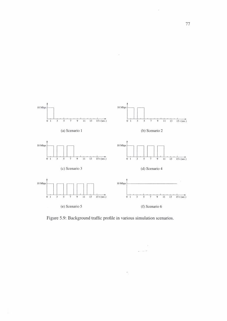
77

,OM~•h I I .

,OM~h n ' I .

0 I 3 5 7 9 II 13 15 t (sec.) 0 I 3 5 7 9 II 13 15 t (sec.)

(a) Scenario 1 (b) Scenario 2

,OM>••h n n I . .. _h n n n I .

0 I 3 5 7 9 II 13 15 t (sec.) 0 I 3 5 7 9 II 13 15 t (sec.)

(c) Scenario 3 (d) Scenario 4

. "-J I I .

0 I 5 9 II 13 15 t (sec.) 0 3 5 7 9 II 13 15 t (sec .)

(e) Scenario 5 (f) Scenario 6

Figure 5.9: Background traffic profile in various simulation scenarios.

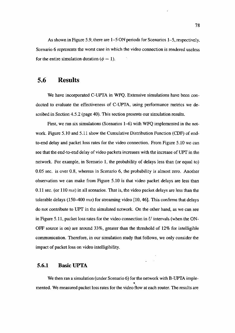
78

As shown in Figure 5.9, there are 1-5 ON periods for Scenarios 1-5, respectively.

Scenario 6 represents the worst case in which the video connection is rendered useless

for the entire simulation duration(</>= 1).

5.6 Results

We have incorporated C-UPTA in WFQ. Extensive simulations have been con

ducted to evaluate the effectiveness of C-UPTA, using performance metrics we de

scribed in Section 4.5.2 (page 40). This section presents our simulation results.

First, we ran six simulations (Scenarios 1-6) with WFQ implemented in the net

work. Figure 5.10 and 5.11 show the Cumulative Distribution Function (CDF) of end

to-end delay and packet loss rates for the video connection. From Figure 5.10 we can

see that the end-to-end delay of video packets increases with the increase of UPT in the

network. For example, in Scenario 1, the probability of delays less than ( or equal to)

0.05 sec. is over 0.8, whereas in Scenario 6, the probability is almost zero. Another

observation we can make from Figure 5.10 is that video packet delays are less than

0.11 sec. ( or 110 ms) in all scenarios. That is, the video packet delays are less than the

tolerable delays (150-400 ms) for streaming video [10, 46]. This confirms that delays

do not contribute to UPT in the simulated network. On the other hand, as we can see

in Figure 5.11, packet loss rates for the video connection in U intervals (when the ON

OFF source is on) are around 33%, greater than the threshold of 12% for intelligible

communication. Therefore, in our simulation study that follows, we only consider the

impact of packet loss on video intelligibility.

5.6.1 BasicUPTA

We then ran a simulation (under Scenario 6) for the network with B-UPTA imple-•

mented. We measured packet loss rates for the video flow at each router. The results are

(/)

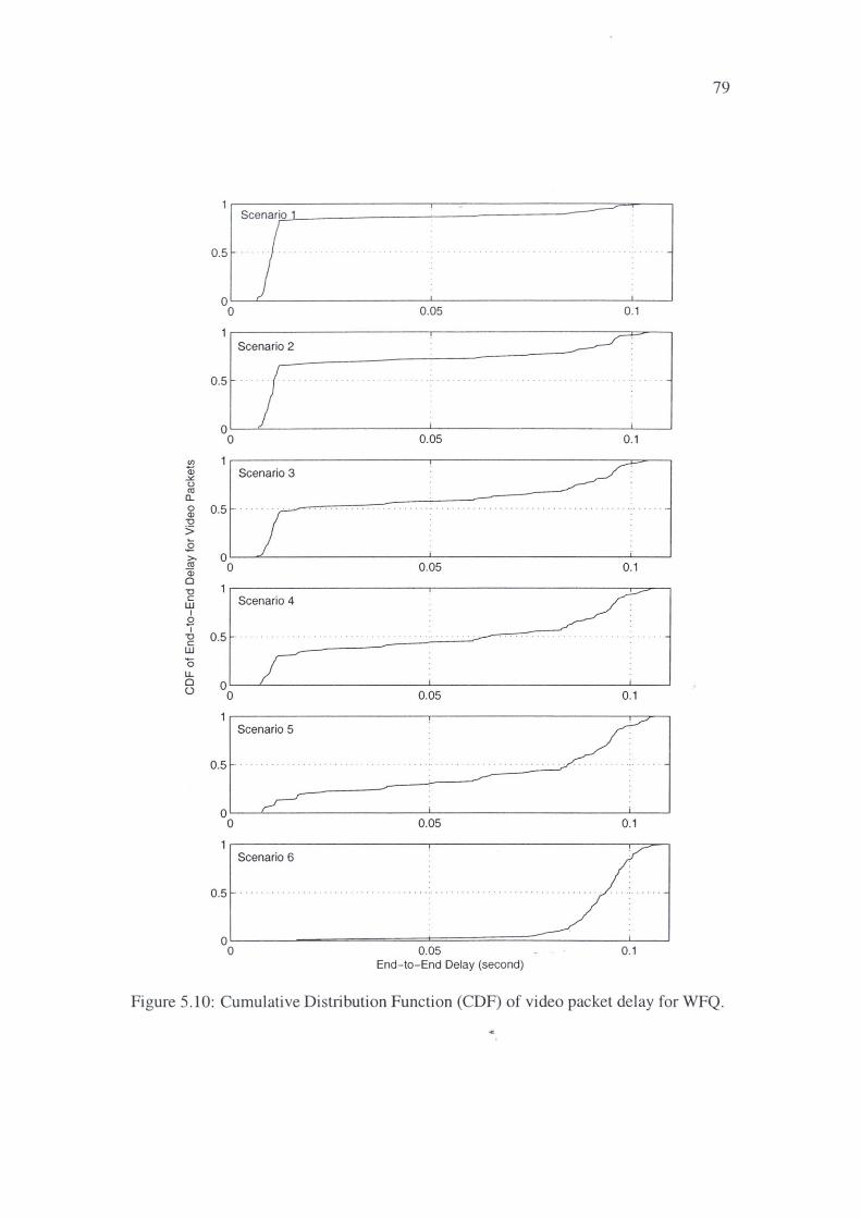
~ 0 Ol a.. 0 Q) -0

>

0.5

0 0

0.5

0 0

0.5

iu' 0 ai 0 0 -0

Scenario 1

l Scenario 2

Scenario 3

Lii Scenario 4 I

0 i' 1? 0.5 UJ

0 LL

..... -

0.05 0.1

0.05 0.1

0.05 0.1

0 0 o~~----------~-----------~-~

0 0.05 0.1

Scenario 5

~5 .... . ....... ... ... .

o~~~---------~-----------~-~ 0 0.05 0.1

Scenario 6

0.5

0L-----=====i======:::_ ____ .1____J

0 0.05 0.1 End-to-End Delay (second)

79


80

Scenario 1 0.75

0 5 10 15

0.75 Scenario 2

0 5 10 15

Scenario 3 0.75

Q)

1il a: (J) (J)

0 0 5 10 15 ....J

w .:x::

Scenario 4 (.) Ctl 0.75 a..

0 5 10 15

Scenario 5 0.75

0 5 10 15

Scenario 6 0.75

0 5 10 - .. · 15 time (second)

Figure 5.11: Packet loss rate of video flow for WFQ.

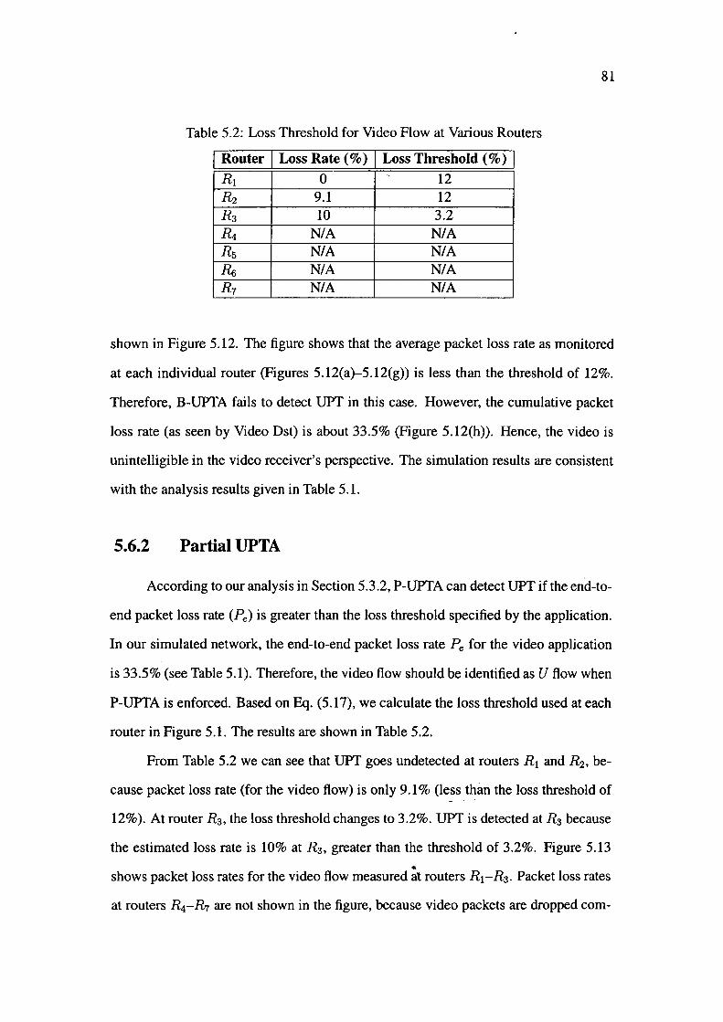
Table 5.2: Loss Threshold for Video Flow at Various Routers

I Router I Loss Rate ( % ) I Loss Threshold ( % ) I R1 0 12 R2 9.1 12 R3 10 3.2 R4 NIA NIA Rs NIA NIA R,e, NIA NIA R1 NIA NIA

81

shown in Figure 5.12. The figure shows that the average packet loss rate as monitored

at each individual router (Figures 5.12(a)-5.12(g)) is less than the threshold of 12%.

Therefore, B-UPTA fails to detect UPT in this case. However, the cumulative packet

loss rate (as seen by Video Dst) is about 33.5% (Figure 5.12(h)). Hence, the video is

unintelligible in the video receiver's perspective. The simulation results are consistent

with the analysis results given in Table 5.1.

5.6.2 Partial UPTA

According to our analysis in Section 5.3.2, P-UPTA can detect UPT if the end-to

end packet loss rate (Pe) is greater than the loss threshold specified by the application.

In our simulated network, the end-to-end packet loss rate Pe for the video application

is 33.5% (see Table 5.1). Therefore, the video flow should be identified as U flow when

P-UPTA is enforced. Based on Eq. (5.17), we calculate the loss threshold used at each

router in Figure 5.1. The results are shown in Table 5.2.

From Table 5.2 we can see that UPT goes undetected at routers R1 and R2, be

cause packet loss rate (for the video flow) is only 9 .1 % (less than the loss threshold of

12%). At router R3 , the loss threshold changes to 3.2%. UPT is detected at R3 because

the estimated loss rate is 10% at R3, greater than the threshold of 3.2%. Figure 5.13 ...

shows packet loss rates for the video flow measured at routers R1-R3 . Packet loss rates

at routers RcR7 are not shown in the figure, because video packets are dropped corn-

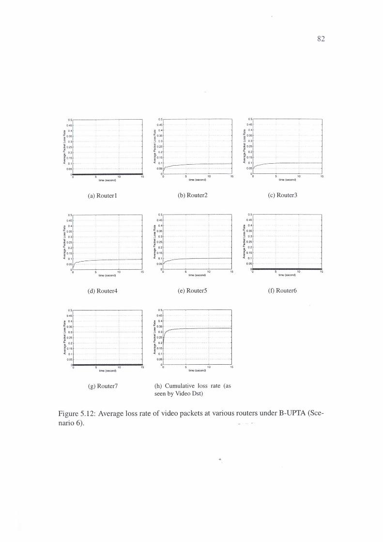
82

05 OS 05

045 045 045

.! 04 04 ! 04

~ 035 035 ~ 035

.3 03 03 .3 OJ

I 025 025 i 025

& 02 02 & 02

!! 0 15 0 15 i 0.15 ~ < 01 0 1 < 0 1

005 0.05 ~ -· 0.05 v.-0 0

10 15 0 10 15 0 10 15 time (second) lime (second) time (second)

(a) Router I (b) Router2 (c) Router3

OS OS OS

045 0.45 045

g O 4 ! 04 ! 0.4

~ 035 ~ 035 '; 0.35

.'J 03 .3 03 .S 03 ·

I 025 ! 025 I 0.2s

& 0.2 i 0.2 i 0.2

I! 0 IS ; 0.15 i 0.15 f > < 01 < 0.1 < 0.1

005 0.05 ir.:-- ... 005 ·

0 0 0 10 15 0 10 15 15

time (second) lime (sacond) timo (second)

(d) Router4 (e) Router5 (f) Router6

OS OS

045 045

!! 0.4 ! 0 4

~ 035 ~ 0.35 ..

.'J 03 .'l 0 .3 ·

! 025 ! 0.25

i 0.2 i 02

i 0.15 i 0.15

< 0 1 < 0.1

005 0.05

0 0 15 0 10 15

time (second)

(g) Router7 (h) Cumulative loss rate (as seen by Video Dst)

Figure 5.12: Average loss rate of video packets at various routers under B-UPTA (Sce

nario 6).

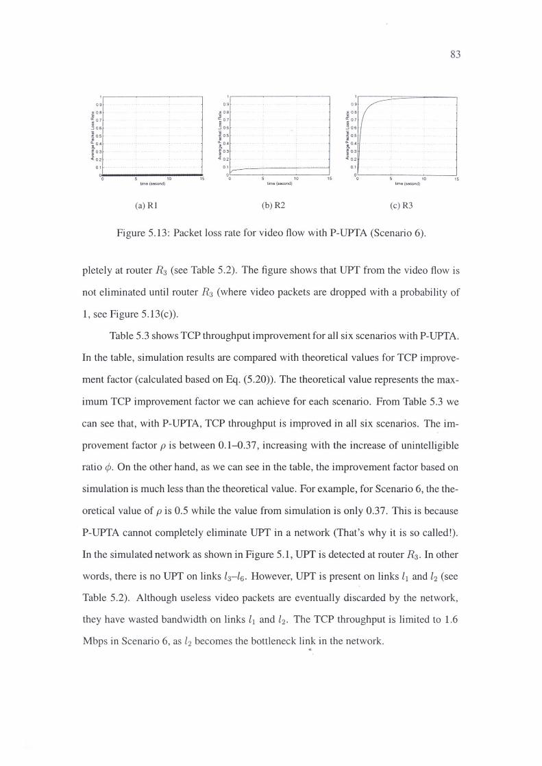
83

09 09 09

08 .! 08 08

07 ! 07 07

06 _§ 06 06

• 05 ~ 0.5 05

04 '; 0 4 0.4

03 fo3 0.3

02 > " 02 02

0 1 · 0 1 0 1

0 0 10 15 0 10 15 0 10 15

tme (second) !me (secood) tme (second)

(a) Rl (b) R2 (c) R3

Figure 5.13: Packet loss rate for video flow with P-UPTA (Scenario 6).

pletely at router R3 (see Table 5.2). The figure shows that UPT from the video flow is

not eliminated until router R3 (where video packets are dropped with a probability of

1, see Figure 5.13(c)).

Table 5.3 shows TCP throughput improvement for all six scenarios with P-UPTA.

In the table, simulation results are compared with theoretical values for TCP improve

ment factor (calculated based on Eq. (5.20)). The theoretical value represents the max

imum TCP improvement factor we can achieve for each scenario. From Table 5.3 we

can see that, with P-UPTA, TCP throughput is improved in all six scenarios. The im

provement factor p is between 0.1-0.37, increasing with the increase of unintelligible

ratio q>. On the other hand, as we can see in the table, the improvement factor based on

simulation is much less than the theoretical value. For example, for Scenario 6, the the

oretical value of p is 0.5 while the value from simulation is only 0.37. This is because

P-UPTA cannot completely eliminate UPT in a network (That's why it is so called!).

In the simulated network as shown in Figure 5.1, UPT is detected at router R3 . In other

words, there is no UPT on links l3-l6 . However, UPT is present on links l1 and l2 (see

Table 5.2). Although useless video packets are eventually discarded by the network,

they have wasted bandwidth on links Li and l2 . The TCP throughput is limited to 1.6

Mbps in Scenario 6, as l2 becomes the bottleneck link in the network . ...

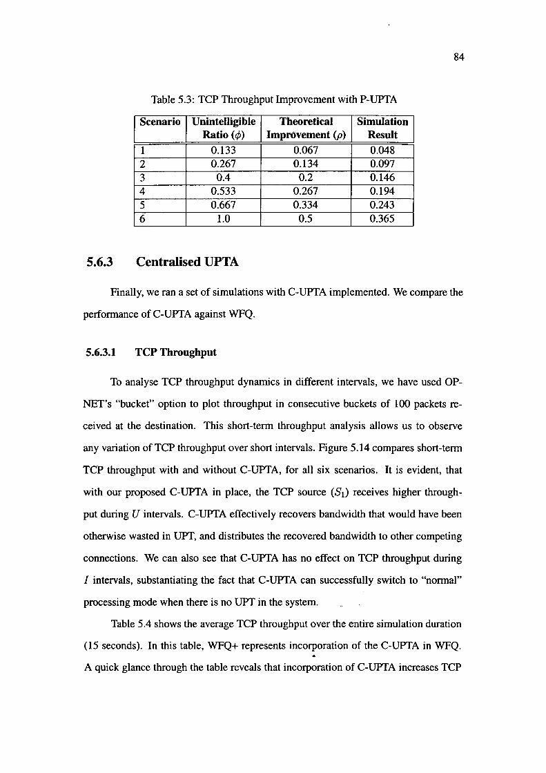
84

Table 5.3: TCP Throughput Improvement with P-UPTA

Scenario Unintelligible Theoretical Simulation Ratio (</J) lmprovement(p) Result

1 0.133 0.067 0.048 2 0.267 0.134 0.097 3 0.4 0.2 0.146 4 0.533 0.267 0.194 5 0.667 0.334 0.243 6 1.0 0.5 0.365

5.6.3 Centralised UPTA

Finally, we ran a set of simulations with C-UPTA implemented. We compare the

performance of C-UPTA against WFQ.

5.6.3.1 TCP Throughput

To analyse TCP throughput dynamics in different intervals, we have used OP

NET's "bucket" option to plot throughput in consecutive buckets of 100 packets re

ceived at the destination. This short-term throughput analysis allows us to observe

any variation of TCP throughput over short intervals. Figure 5.14 compares short-term

TCP throughput with and without C-UPTA, for all six scenarios. It is evident, that

with our proposed C-UPTA in place, the TCP source (Si) receives higher through

put during U intervals. C-UPTA effectively recovers bandwidth that would have been

otherwise wasted in UPT, and distributes the recovered bandwidth to other competing

connections. We can also see that C-UPTA has no effect on TCP throughput during

I intervals, substantiating the fact that C-UPTA can successfully switch to "normal"

processing mode when there is no UPT in the system.

Table 5.4 shows the average TCP throughput over the entire simulation duration

(15 seconds). In this table, WFQ+ represents incorporation of the C-UPTA in WFQ.

A quick glance through the table reveals that incorporation of C-UPTA increases TCP

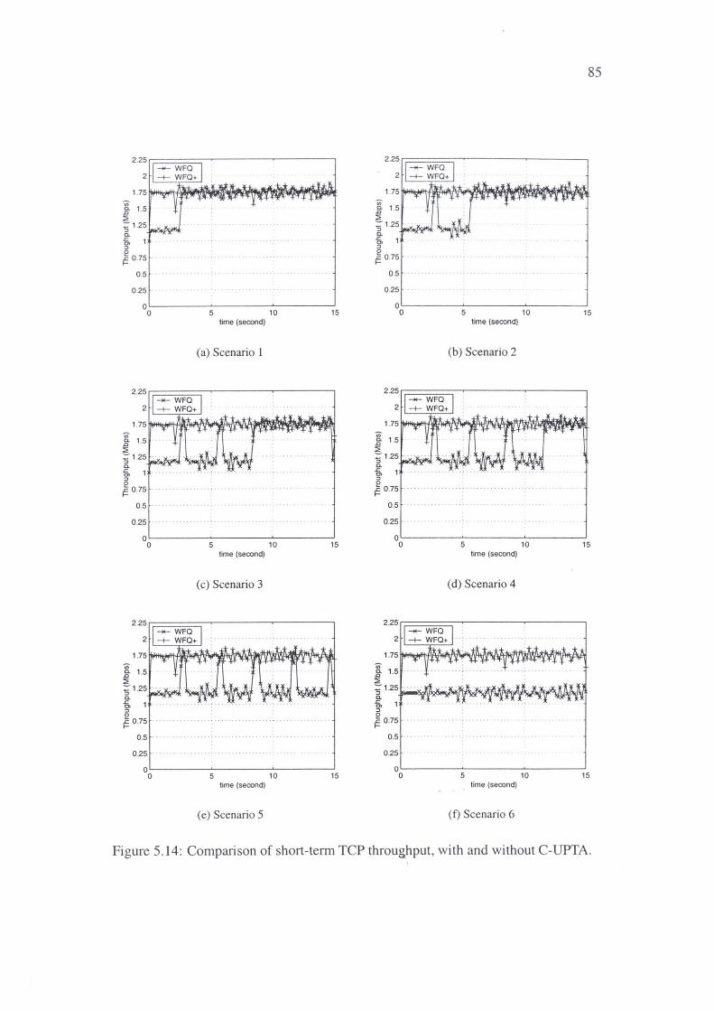
1.75 .;-_g. 1.5 ::. 51 .25 a. .c O> :::,

~ 0.75 1-

0.5

0.25

0'------~-----~------' 0 5 10 15

time (second)

(a) Scenario l

2.25r;::::===:::;-~----,-----,

"'

2

1.75

_g. 1.5 ::. 51 .25 a. .c O> :::,

e f=. 0.75

0.5

0.25

o~----~-----~----~ 0 5 10 15

time (second)

(c) Scenario 3

2.25r;:::====::::;-,----~----7

.;

2

1.75

_g. 1.5 ::. 51 .25 a. .c O> :::, 0

~ 0 .75

0.5

0 .25

0'------~-----~----~ 0 5 10 15

time (second)

(e) Scenario 5

85

2.25

2

1.75

"' 1.5 a. .0 ::. ::-1 .25 :::, a. .c O> :::,

e f=. 0.75

0.5

0 .25

0 0 5 10 15

time (second)

(b) Scenario 2

.;-a. 1.5 .0 ::. -:::1 .25 :::, a. .c O> :::,

e f=. 0.75

0.5

0.25

0 0 5 10 15

time (second)

( d) Scenario 4

2.25

2

1.75 .;-a. 1.5 .0 ::. ::- 1 .25 :::, a. .c Cl :::,

e f=. 0.75

0 .5

0 .25

0 0 5 10 15

time (second)

(f) Scenario 6

Figure 5.14: Comparison of short-term TCP throughput, with and without C-UPTA.

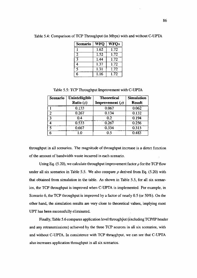
Table 5.4: Comparison of TCP Throughput (in Mbps) with and without C-UPTA

I Scenario I WFQ I WFQ+ I 1 1.62 1.72 2 1.52 1.72 3 1.44 1.72 4 1.37 1.72 5 1.31 1.72 6 1.16 1.72

Table 5.5: TCP Throughput Improvement with C-UPTA

Scenario Unintelligible Theoretical Simulation Ratio(</>) lmprovement(p) Result

1 0.133 0.067 0.062 2 0.267 0.134 0.132 3 0.4 0.2 0.194 4 0.533 0.267 0.256 5 0.667 0.334 0.313 6 1.0 0.5 0.483

86

throughput in all scenarios. The magnitude of throughput increase is a direct function

of the amount of bandwidth waste incurred in each scenario.

Using Eq. (5.20), we calculate throughput improvement factor p for the TCP flow

under all six scenarios in Table 5.5. We also compare p derived from Eq. (5.20) with

that obtained from simulation in the table. As shown in Table 5.5, for all six scenar

ios, the TCP throughput is improved when C-UPTA is implemented. For example, in

Scenario 6, the TCP throughput is improved by a factor of nearly 0.5 (or 50%). On the

other hand, the simulation results are very close to theoretical values, implying most

UPT has been successfully eliminated.

Finally, Table 5.6 compares application level throughpuf(excluding TCP/IP header

and any retransmissions) achieved by the three TCP sources in all six scenarios, with

and without C-UPTA. In consistence with TCP thr<ll;lghput, we can see that C-UPTA

also increases application throughput in all six scenarios.

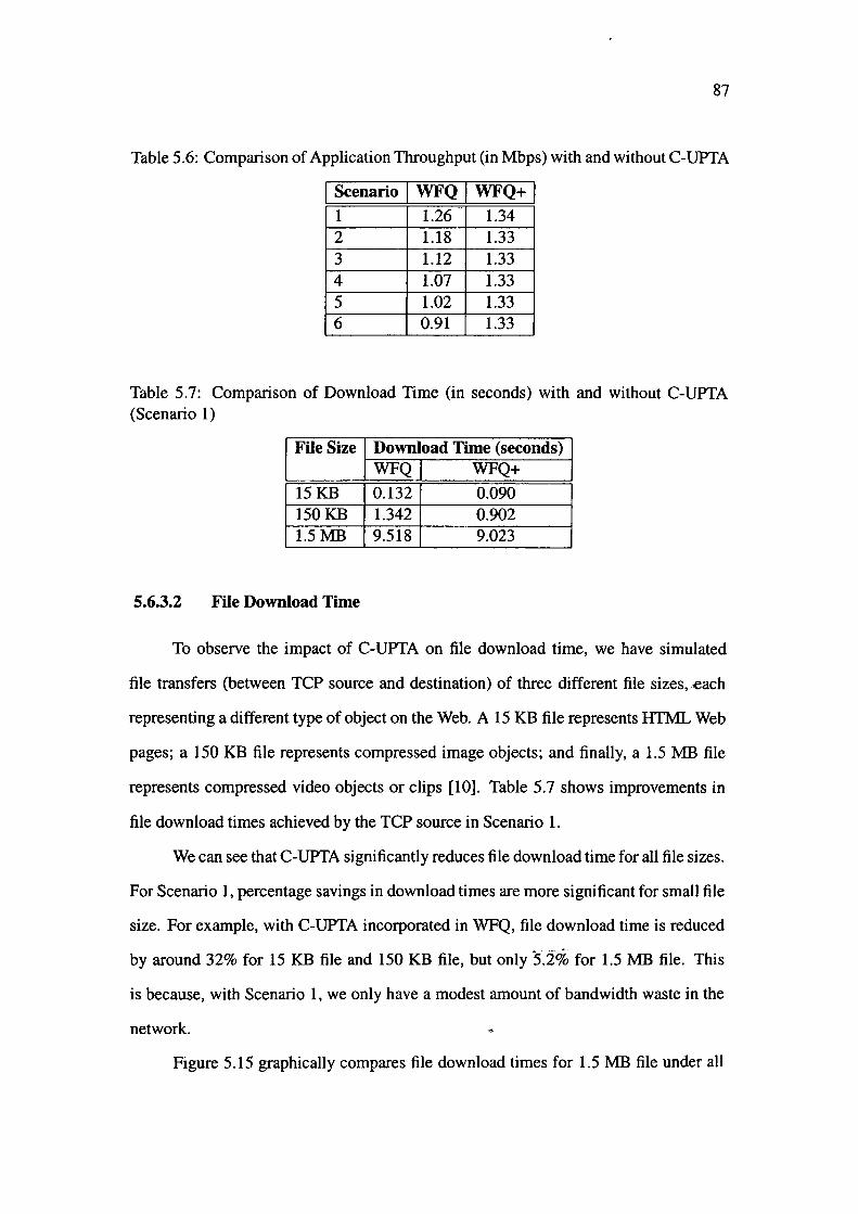
87

Table 5.6: Comparison of Application Throughput (in Mbps) with and without C-UPTA

I Scenario I WFQ I WFQ+ I --1 1.26 1.34

2 1.18 1.33 3 1.12 1.33 4 1.07 1.33 5 1.02 1.33 6 0.91 1.33

Table 5.7: Comparison of Download Time (in seconds) with and without C-UPTA (Scenario 1)

File Size Download Time (seconds) WFQ WFQ+

15 KB 0.132 0.090 150KB 1.342 0.902 1.5MB 9.518 9.023

5.6.3.2 File Download Time

To observe the impact of C-UPTA on file download time, we have simulated

file transfers (between TCP source and destination) of three different file sizes, each

representing a different type of object on the Web. A 15 KB file represents IITML Web

pages; a 150 KB file represents compressed image objects; and finally, a 1.5 MB file

represents compressed video objects or clips [10]. Table 5.7 shows improvements in

file download times achieved by the TCP source in Scenario 1.

We can see that C-UPTA significantly reduces file download time for all file sizes.

For Scenario 1, percentage savings in download times are more significant for small file

size. For example, with C-UPTA incorporated in WFQ, file download time is reduced

by around 32% for 15 KB file and 150 KB file, but only 5.2% for 1.5 MB file. This

is because, with Scenario 1, we only have a modest amount of bandwidth waste in the

network.

Figure 5.15 graphically compares file download times for 1.5 MB file under all

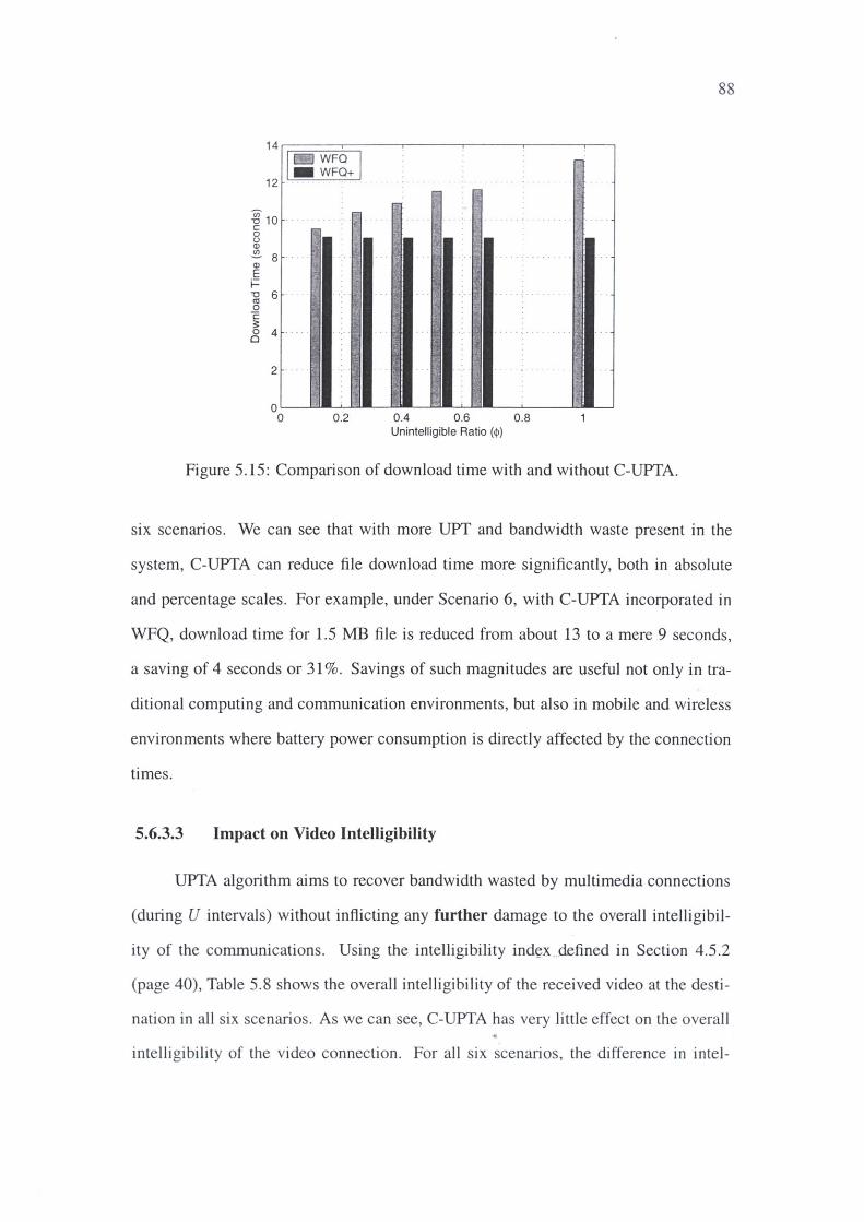
14~~---_-_-_-_---:__-~--~---~--~--~-~

I ii ~~g+ I 12

l 10 C 0 () Q)

~ 8 a, E ~ ~ 6 . 0 c ~ 8 4 .

2 .

0 0 0.2 0.4 0.6 0.8

Unintelligible Ratio ($)

Figure 5.15: Comparison of download time with and without C-UPTA.

88

six scenarios. We can see that with more UPT and bandwidth waste present in the

system, C-UPTA can reduce file download time more significantly, both in absolute

and percentage scales. For example, under Scenario 6, with C-UPTA incorporated in

WFQ, download time for 1.5 MB file is reduced from about 13 to a mere 9 seconds,

a saving of 4 seconds or 31 %. Savings of such magnitudes are useful not only in tra

ditional computing and communication environments, but also in mobile and wireless

environments where battery power consumption is directly affected by the connection

times.

5.6.3.3 Impact on Video Intelligibility

UPTA algorithm aims to recover bandwidth wasted by multimedia connections

(during U intervals) without inflicting any further damage to the overall intelligibil

ity of the communications. Using the intelligibility ind~x _defined in Section 4.5.2

(page 40), Table 5.8 shows the overall intelligibility of the received video at the desti

nation in all six scenarios. As we can see, C-UPTA has very little effect on the overall

intelligibility of the video connection. For all six scenarios, the difference in intel-

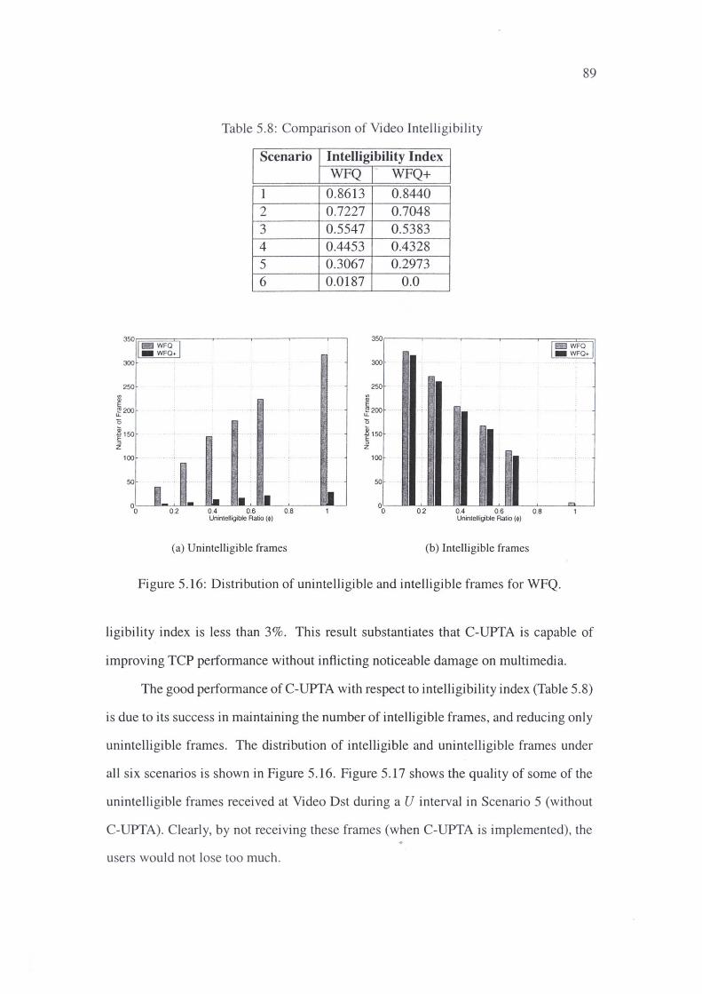
350

300

250

200

150

100

50

00

89

Table 5.8: Comparison of Video Intelligibility

Scenario

1 2 3 4 5 6

WFO -WFQ+

;. ....

0.2 0.4 0.6 0.8 Unintelligible Ratio (cl>)

(a) Unintelligible frames

Intelligibility Index WFQ WFQ+

0.8613 0.8440 0.7227 0.7048 0.5547 0.5383 0.4453 0.4328 0.3067 0.2973 0.0187 0.0

350,---.---.-----,--- ,-=== [IT;]WFQ -WFQ+

~ Q)

300

250

E ~200 u. 0

i 150 :, z

100

50

0.2 04 06 08 Unintelligible Ratio (cl>)

(b) Intelligible frames

Figure 5.16: Distribution of unintelligible and intelligible frames for WFQ.

ligibility index is less than 3%. This result substantiates that C-UPTA is capable of

improving TCP performance without inflicting noticeable damage on multimedia.

The good performance of C-UPTA with respect to intelligibility index (Table 5.8)

is due to its success in maintaining the number of intelligible frames, and reducing only

unintelligible frames. The distribution of intelligible and unintelligible frames under

all six scenarios is shown in Figure 5.16. Figure 5.17 shows the quality of some of the

unintelligible frames received at Video Dst during a U interval in Scenario 5 (without

C-UPTA). Clearly, by not receiving these frames (when C-UPTA is implemented), the

users would not lose too much.

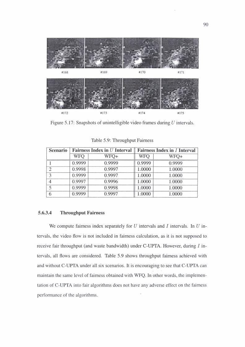
90

#168 #169 #170 #171

#172 #173 #174 #175

Figure 5.17: Snapshots of unintelligible video frames during U intervals.

Table 5.9: Throughput Fairness

Scenario Fairness Index in U Interval Fairness Index in I Interval WFQ WFQ+ WFQ WFQ+

1 0.9999 0.9999 0.9999 0.9999 2 0.9998 0.9997 1.0000 1.0000 3 0.9999 0.9997 1.0000 1.0000 4 0.9997 0.9996 1.0000 1.0000 5 0.9999 0.9998 1.0000 1.0000 6 0.9999 0.9997 1.0000 1.0000

5.6.3.4 Throughput Fairness

We compute fairness index separately for U intervals and I intervals. In U in

tervals, the video flow is not included in fairness calculation, as it is not supposed to

receive fair throughput (and waste bandwidth) under C-UPTA. However, during I in

tervals , all flows are considered. Table 5.9 shows throughput fairness achieved with

and without C-UPTA under all six scenarios. It is encouraging to see that C-UPTA can

maintain the same level of fairness obtained with WFQ. In other words, the implemen

tation of C-UPTA into fair algorithms does not have any adverse effect on the fairness

performance of the algorithms.

0.45

:s ~ 0.4 0 t5 if 0 .35 ·

c ~ 0.3 · Ql

1' 0.25 c.

-e-- Theoretical Value -¼- Basic UPT A --l- Partial UPTA -e-- Centralised UPTA

_§ 0.2 .. .... ..... . 5 0. -§,0.15 ::, 0 l: 0.1 1-

0 .05

o~~-¾-~-~-----,.,..._~-¾-~-~-~~--o 0.1 0.2 0.3 0.4 0.5 0.6 0.7 0.8 0.9

Unintelligible Ratio (cj>)

Figure 5.18: TCP throughput improvement factor against unintelligible ratio.

5.6.4 Discussion

91

We have evaluated the performance of three different UPTA enforcement schemes

(i.e., B-UPTA, P-UPTA, and C-UPTA) in the simulated network. In this section, we

present a comparison of these schemes and discuss performance sensitivity of these

schemes to network topology.

5.6.4.1 Comparison

To summarise, we plot TCP improvement factor p achieved with different ap

proaches in Figure 5.18. As shown in the figure, no improvement achieved with B

UPTA. This means, in networks with multiple congested links, UPT may go undetected

if B-UPTA is implemented. P-UPTA represents an improvement over B-UPTA, with

some improvement in TCP throughput. However, the improvement factor is far less

than the theoretical value. This implies that UPT has not been.eliminated completely.

There is still bandwidth waste due to useless packet transmission with P-UPTA. With

C-UPTA, the improvement factor is very close to the theoretical value. This proves that .. C-UPTA yields the best result in terms of UPT avoidance.

92

Table 5.10: Comparison of Various UPTA Enforcement Schemes

Feature Removal TCP Throughput Feedback Complexity ofUPT lmprovemenf Mechanism

B-UPTA No No No Low P-UPTA Partial Less than Max. No Medium C-UPTA Complete Maximum Yes High

Table 5.10 compares features and performance of the three different UPTA en

forcement schemes. Obviously, there is a trade-off between performance and com

plexity. The performance increases in order of B-UPTA, P-UPTA, C-UPTA. However,

complexity also increases in the same order. B-UPTA has minimum protocol overhead,

while C-UPTA has the maximum overhead. In C-UPTA, a feedback mechanism (BFD)

is needed to determine global fairshare. With B-UPTA and P-UPTA, no extra proto

col is needed. P-UPTA is a little more complicated than B-UPTA (as loss threshold q

needs to be updated by each router on the end-to-end path), but less complicated than

C-UPTA.

5.6.4.2 Robustness to Network Topology

The three UPTA enforcement schemes also differ in robustness to network topol

ogy. If there is only one congested link, the three enforcement schemes yield exactly

the same performance, as we presented in Chapter 4. Because in such a situation, UPTA

algorithm is only activated at one router, and the global fairshare equals to the fairshare

of the only congested link. Therefore, UPTA is enforced using the global fairshare no

matter which enforcement scheme is used. B-UPTA is sufficient in the case of single

congested link.

In the case of multiple congested links, B-UPTA/P-UPTA performance depends

on network topology. If the packet loss rate is greater than the application's maximum

' tolerable loss rate q (12% for our MPEG-2 video), B-UPTA/P-UPTA has the same

performance as that of C-UPTA. For example, in the network as shown in Figure 5.1, if

93

Flow 3 enters the network at router R3, the packet loss rate for the video flow (Flow 2)

is about 18%. Both B-UPTA and P-UPTA will detect the video flow as unintelligible

flow. UPT packets will be dropped at router R3 as a result. UPT is completely avoided.

Otherwise, UPT will go undetected with B-UPTA; and only part of UPT is eliminated

with P-UPTA. Consequently, the TCP improvement will be less than the theoretical

value (as shown in Figure 5.18).

C-UPTA operates on global fairshare. The ingress router can always enforce

UPTA on global fairshare (by employing BFD protocol), regardless of the network

topology. Therefore, C-UPTA can effectively eliminate UPT in all circumstances. In

short, Representing the simplest UPTA enforcement scheme, B-UPTA is the least ro

bust to network topology. On the other extreme, C-UPTA is the most robust scheme

with increased complexity. P-UPTA is somewhere between B-UPTA and C-UPTA, in

terms of both robustness and complexity.

5. 7 Conclusion

We have investigated the UPT problem with multiple congested links in this

chapter. In networks with multiple congested links, the end-to-end packet loss rate

of a multimedia flow may exceed the loss threshold while local loss rate at each router

en route is less than the loss threshold. This complicates UPT avoidance in networks

with multiple congested links. Using WFQ as an example, we discussed three different

UPTA enforcement schemes - B-UPTA, P-UPTA and C-UPTA. B-UPTA is enforced

independently at each router. The algorithm is the same as that used with single con

gested link (described in Chapter 4). P-UPTA extends B-UPTA by introducing variable

loss threshold at each router. The loss threshold is decreased at each router based on

local packet loss rate at the router. As the loss threshold is updated at each router, it is

possible for P-UPTA to detect UPT somewhere in thenetwork, provided the end-to-end

packet loss rate is greater than the threshold specified by an application. C-UPTA intro-

94

duces a protocol called Bottleneck Fairshare Discovery (BFD) which enables it to elim

inate UPT completely at the ingress router. BFD is a feedback mechanism proposed for

C-UPTA. It relies on ICMP probe/report messages to determine global fairshare.

Using OPNET simulation and an MPEG-2 video clip, we have evaluated the

performance of the three different UPTA enforcement schemes. For our simulated net

work, B-UPTA fails to detect UPT. As a result, the TCP source sees no improvement in

throughput even after UPTA is implemented. Although P-UPTA can eventually detect

UPT, bandwidth has been wasted on links before the router where useless packets are

dropped. Consequently, only modest TCP throughput improvement is achieved with

P-UPTA. C-UPTA always drops useless packets at the network edge (ingress router).

This effectively avoids the problem with P-UPTA. As a result, more bandwidth is made

available to the TCP flow. Our simulation results show that, with C-UPTA, the achieved

TCP throughput improvement is very close to the maximum theoretical value. This in

dicates that useless packets have been effectively prevented from entering the network.

We have also analysed the performance of C-UPTA quantitatively, in terms of

TCP throughput, file download time, impact on video intelligibility, and impact on fair

ness. Our simulation results reveal that, for all six scenarios, the TCP throughput has

been significantly improved (with improvement factor up to 50%). As a result, file

download times (for various file size) have been greatly reduced (more than 30%). On

the other hand, incorporation of C-UPTA into WFQ has no significant impact on intel

ligibility of the MPEG-2 video (with a difference less than 3% ). For all six scenarios,

C-UPTA maintains fairness which is comparable to WFQ. This proves that UPTA does

not have any adverse impact on fairness performance of fair algorithms.

Chapter 6

UPTA with Multiple Multimedia Flows

We have discussed UPT avoidance with single congested link and multiple con

gested links, in Chapter 4 and Chapter 5 respectively. Another interesting issue is UPT

avoidance in networks with multiple multimedia flows. In networks with large user

base, there are usually more than one multimedia flows sharing the same bottleneck

link. In this chapter, we investigate UPT avoidance with multiple multimedia flows,

and discuss issues related to management of multiple U flows.

6.1 Scope of the Problem

UPTA attempts to drop all packets from a multimedia flow when it is in U inter

vals. In situations where multiple multimedia flows sharing the same bottleneck link

are marked as U flows, all these flows will be cut off when UPTA is enforced. An un

desirable effect of this is that all multimedia flows become useless, and the bottleneck

link is under-utilised. This problem has adverse impacts on overall intelligibility of

multimedia applications, as well as the efficiency of netwo~k ,r~sources.

We use an example as shown in Figure 6.1 to explain this problem. The figure

shows that two MPEG-2 video flows share a bottleneck link of 2 Mbps in the network. -e

Assume MPEG-2 video stream is encoded at a bit ·rate of 1.5 Mbps (CBR), and is

transported in MPEG Transport Stream (TS) packets over UDP.

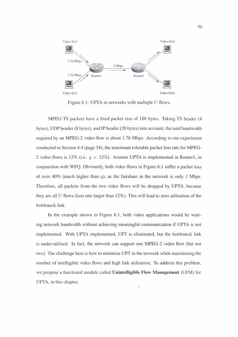
96

Video Srcl Video Dstl

l.76Mbp~ r - -~~ .,.R.,..oustte_r..,,I .-------:=====:;:~'8R11ro~ute~'2 ~

2 Mbps

Video Src2 Video Dst2

Figure 6.1: UPTA in networks with multiple U flows.

MPEG TS packets have a fixed packet size of 188 bytes. Taking TS header (4

bytes), UDP header (8 bytes), and IP header (20 bytes) into account, the total bandwidth

required by an MPEG-2 video flow is about 1.76 Mbps. According to our experiment

conducted in Section 4.4 (page 34), the maximum tolerable packet loss rate for MPEG-

2 video flows is 12% (i .e. q = 12%). Assume UPTA is implemented in Routed, in

conjunction with WFQ. Obviously, both video flows in Figure 6.1 suffer a packet loss

of over 40% (much higher than q), as the fairshare in the network is only 1 Mbps.

Therefore, all packets from the two video flows will be dropped by UPTA, because

they are all U flows (loss rate larger than 12% ). This will lead to zero utilisation of the

bottleneck link.

In the example shown in Figure 6.1, both video applications would be wast

ing network bandwidth without achieving meaningful communication if UPTA is not

implemented. With UPTA implemented, UPT is eliminated, but the bottleneck link

is under-utilised. In fact, the network can support one MPEG-2 video flow (but not

two) . The challenge here is how to minimise UPT in the network while maximising the

number of intelligible video flows and high link utilisation! To. address this problem,

we propose a functional module called Unintelligible Flow Management (UFM) for

UPTA, in this chapter.

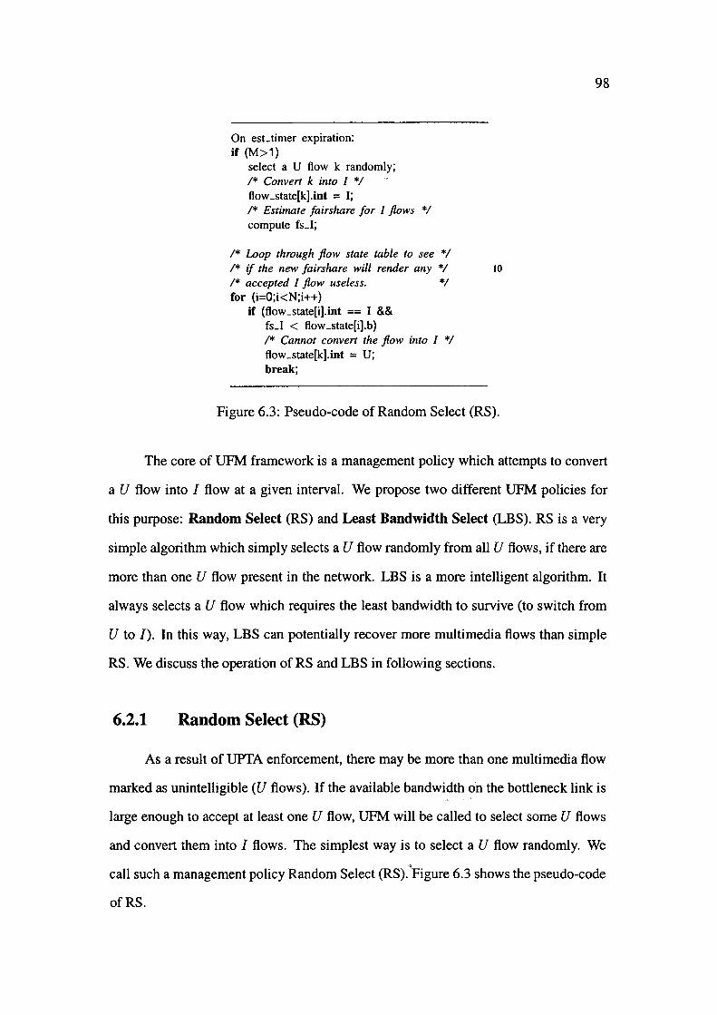
On esLtimer expiration: if (M>1)

select a U flow k randomly; I* Convert k into I *I flow _state[k].int = I; I* Estimate fairshare for I flows *I compute fs_I;

I* wop through flow state table to see *I I* if the new fairshare will render any *I 10

I* accepted I flow useless. *I for (i=0;i<N;i++)

if (flow_state[i].int == I && fs_l < flow_state[i].b) /* Cannot convert the flow into I */ flow _state[k].int = U; break;

Figure 6.3: Pseudo-code of Random Select (RS).

98

The core of UFM framework is a management policy which attempts to convert

a U flow into I flow at a given interval. We propose two different UFM policies for

this purpose: Random Select (RS) and Least Bandwidth Select (LBS). RS is a very

simple algorithm which simply selects a U flow randomly from all U flows, if there are

more than one U flow present in the network. LBS is a more intelligent algorithm. It

always selects a U flow which requires the least bandwidth to survive (to switch from

U to/). In this way, LBS can potentially recover more multimedia flows than simple

RS. We discuss the operation of RS and LBS in following sections.

6.2.1 Random Select (RS)

As a result of UPTA enforcement, there may be more than one multimedia flow

marked as unintelligible (U flows). If the available bandwidth on the bottleneck link is

large enough to accept at least one U flow, UFM will be called to select some U flows

and convert them into I flows. The simplest way is to select a U flow randomly. We

call such a management policy Random Select (RS).<Figure 6.3 shows the pseudo-code

of RS.

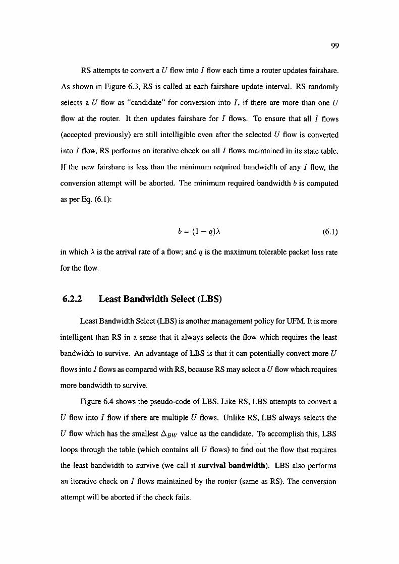
99

RS attempts to convert a U flow into I flow each time a router updates fairshare.

As shown in Figure 6.3, RS is called at each fairshare update interval. RS randomly

selects a U flow as "candidate" for conversion into I, if there are more than one U

flow at the router. It then updates fairshare for I flows. To ensure that all I flows

(accepted previously) are still intelligible even after the selected U flow is converted

into I flow, RS performs an iterative check on all I flows maintained in its state table.

If the new fairshare is less than the minimum required bandwidth of any I flow, the

conversion attempt will be aborted. The minimum required bandwidth b is computed

as perEq. (6.1):

b = (1- q).X (6.1)

in which .X is the arrival rate of a flow; and q is the maximum tolerable packet loss rate

for the flow.

6.2.2 Least Bandwidth Select (LBS)

Least Bandwidth Select (LBS) is another management policy for UFM. It is more

intelligent than RS in a sense that it always selects the flow which requires the least

bandwidth to survive. An advantage of LBS is that it can potentially convert more U

flows into I flows as compared with RS, because RS may select a U flow which requires

more bandwidth to survive.

Figure 6.4 shows the pseudo-code of LBS. Like RS, LBS attempts to convert a

U flow into I flow if there are multiple U flows. Unlike RS, LBS always selects the

U flow which has the smallest ~Bw value as the candidate. To accomplish this, LBS -

loops through the table (which contains all U flows) to find out the flow that requires

the least bandwidth to survive (we call it survival bandwidth). LBS also performs

an iterative check on I flows maintained by the router (same as RS). The conversion

attempt will be aborted if the check fails.

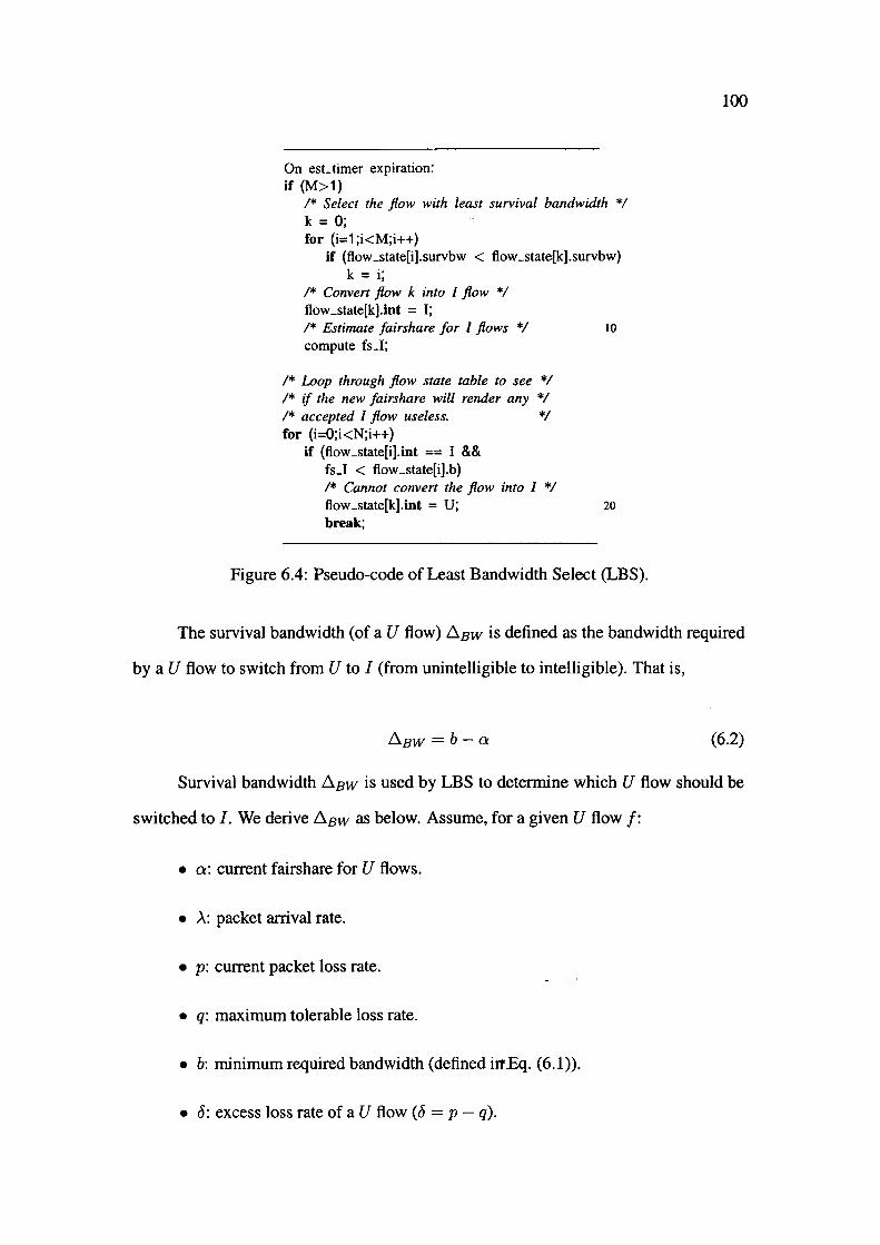
On esLtimer expiration: if (M>1)

I* Select the flow with least survival bandwidth *I k = O; for (i=1 ;i<M;i++)

if (flow _state[i].survbw < flow _state[k].survbw) k = i;

I* Convert flow k into I flow *I flow_state[k].int = I; I* Estimate fairshare for I flows *I 10

compute fs_l;

/* Loop through flow state table to see *I I* if the new fairshare will render any *I /* accepted I flow useless. *I for (i=0;i<N;i++)

if (flow _state[i].int == I && fs_l < flow_state[i].b) I* Cannot convert the flow into I *I flow_state[k].int = U; 20

break;

Figure 6.4: Pseudo-code of Least Bandwidth Select (LBS).

100

The survival bandwidth (of a U flow) D.Bw is defined as the bandwidth required

by a U flow to switch from U to I (from unintelligible to intelligible). That is,

D.Bw = b- a (6.2)

Survival bandwidth D.8w is used by LBS to determine which U flow should be

switched to I. We derive D.Bw as below. Assume, for a given U flow f:

• a: current fairshare for U flows.

• >.: packet arrival rate.

• p: current packet loss rate.

• q: maximum tolerable loss rate.

• b: minimum required bandwidth (defined iITEq. (6.1)).

• 8: excess loss rate of a U flow (8 = p - q).

as:

101

As U flows are constrained flows, packet loss rate of a U flow can be expressed

From Eq. (6.3) we obtain:

a p= 1- -

..\

a= (1 - p),\

Substitute Eq. (6.1) and Eq. (6.4) into Eq. (6.2), we have:

D.Bw = b- a

= (1 - q),\ - (1 - p),\

= (p - q),\

= (),\

(6.3)

(6.4)

(6.5)

From Eq. (6.5) we can see that a U flow with smaller excess loss rate needs less

bandwidth to switch to I flow, provided all contending U flows have the same arrival

rate (e.g. all flows are running the same type of application).

6.3 Performance Evaluation

We have implemented the two UFM policies (RS and LBS) using OPNET Mod

eler [71]. In following sections, we present our simulation study conducted to evaluate -

the performance of RS and LBS. We conduct extensive simulations to evaluate these

two management policies under various network conditions, as shown below:

• Single congested link: Simulates enterprise networks. There is only one con

gested link in the network. Basic UPTA (B-UPTA, discussed in Chapter 4) is

102

implemented.

• Multiple congested links: Simulates 1!1edium to large scale networks. There

are multiple congested links in the network. Centralised UPTA (C-UPTA,

discussed in Chapter 5) is implemented.

• Homogeneous multimedia applications: All multimedia applications are of

the same type. In our simulation, all MPEG-2 video applications have the

same data rate.

• Heterogeneous multimedia applications: Multimedia applications have dif

ferent requirements on bandwidth. In our simulation, the same MPEG-2 video

is encoded at different data rates for different video sources.

In our simulation study, we use following performance metrics:

• Number of video flows recovered: The number of video flows (which would

be marked as U flows by UPTA) converted from U flows into I flows.

• TCP throughput improvement: We compare TCP throughput achieved un

der RS/LBS against that achieved under WFQ.

• Video intelligibility: We use the intelligibility index (defined in Section 4.5.2,

page 40) to compare the overall intelligibility level of the received video.

6.4 Single Congested Link

First of all, we ran a set of simulations with single -~Qngested link. Figure 6.5

shows the network model used in the simulation. In the simulated network, there is

only one congested link (l1) which has a link speed of 15 Mbps, with a delay of 1

ms. All other links are 10 Mbps (Ethernet links), with a delay of 1 µs. As shown in

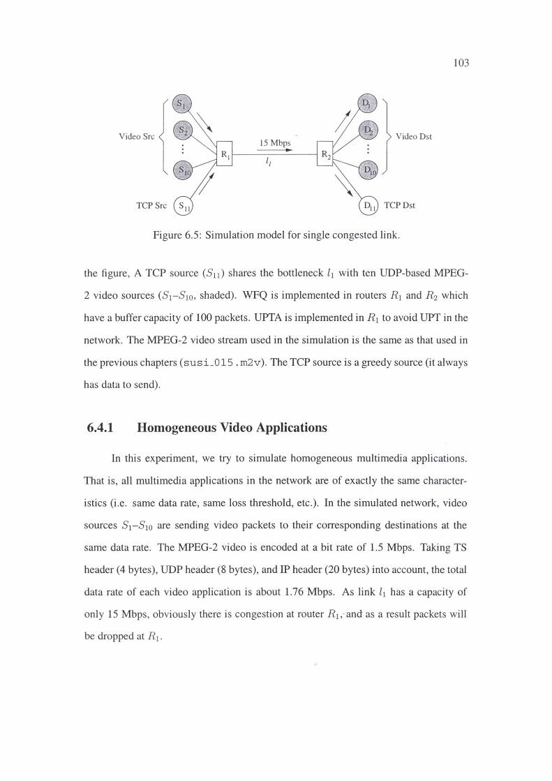
103

Video Src Video Dst 15 Mbps

TCP Src S 11 D11 TCPDst

Figure 6.5: Simulation model for single congested link.

the figure, A TCP source (S11 ) shares the bottleneck l1 with ten UDP-based MPEG-

2 video sources (S1-S10 , shaded). WFQ is implemented in routers R 1 and R 2 which

have a buffer capacity of 100 packets. UPTA is implemented in R 1 to avoid UPT in the

network. The MPEG-2 video stream used in the simulation is the same as that used in

the previous chapters (susL015. m2v). The TCP source is a greedy source (it always

has data to send).

6.4.1 Homogeneous Video Applications

In this experiment, we try to simulate homogeneous multimedia applications.

That is, all multimedia applications in the network are of exactly the same character

istics (i.e. same data rate, same loss threshold, etc.). In the simulated network, video

sources S1-S10 are sending video packets to their corresponding destinations at the

same data rate. The MPEG-2 video is encoded at a bit rate of 1.5 Mbps. Taking TS

header (4 bytes), UDP header (8 bytes), and IP header (20 bytes) into account, the total

data rate of each video application is about 1.76 Mbps. As link l1 has a capacity of

only 15 Mbps, obviously there is congestion at router R1,-and as a result packets will

be dropped at R1.

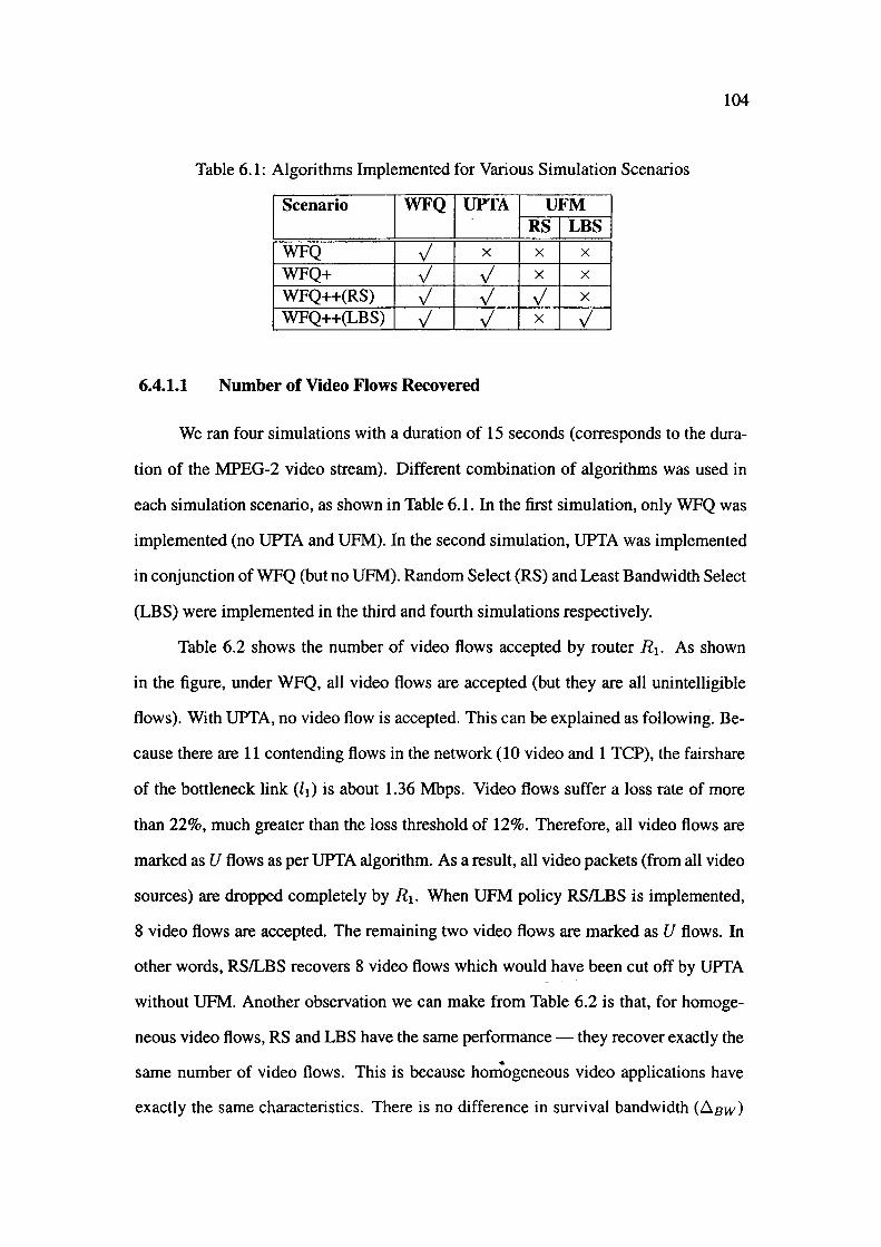
104

Table 6.1: Algorithms Implemented for Various Simulation Scenarios

I Scenario IWFQl{1,PTAI UFM I RSI LBS WFQ ✓ X X X

WFQ+ ✓ ✓ X X

WFQ++(RS) ✓ ✓ ✓ X

WFQ++(LBS) ✓ ✓ X ✓

6.4.1.1 Number of Video Flows Recovered

We ran four simulations with a duration of 15 seconds (corresponds to the dura

tion of the MPEG-2 video stream). Different combination of algorithms was used in

each simulation scenario, as shown in Table 6.1. In the first simulation, only WFQ was

implemented (no UPTA and UFM). In the second simulation, UPTA was implemented

in conjunction of WFQ (but no UFM). Random Select (RS) and Least Bandwidth Select

(LBS) were implemented in the third and fourth simulations respectively.

Table 6.2 shows the number of video flows accepted by router R1. As shown

in the figure, under WFQ, all video flows are accepted (but they are all unintelligible

flows). With UPTA, no video flow is accepted. This can be explained as following. Be

cause there are 11 contending flows in the network (10 video and 1 TCP), the fairshare

of the bottleneck link (li) is about 1.36 Mbps. Video flows suffer a loss rate of more

than 22%, much greater than the loss threshold of 12%. Therefore, all video flows are

marked as U flows as per UPTA algorithm. As a result, all video packets (from all video

sources) are dropped completely by R1. When UFM policy RS/LBS is implemented,

8 video flows are accepted. The remaining two video flows are marked as U flows. In

other words, RS/LBS recovers 8 video flows which would have been cut off by UPTA

without UFM. Another observation we can make from Table 6.2 is that, for homoge

neous video flows, RS and LBS have the same performance - they recover exactly the

same number of video flows. This is because homogeneous video applications have

exactly the same characteristics. There is no difference in survival bandwidth (~ 8 w)

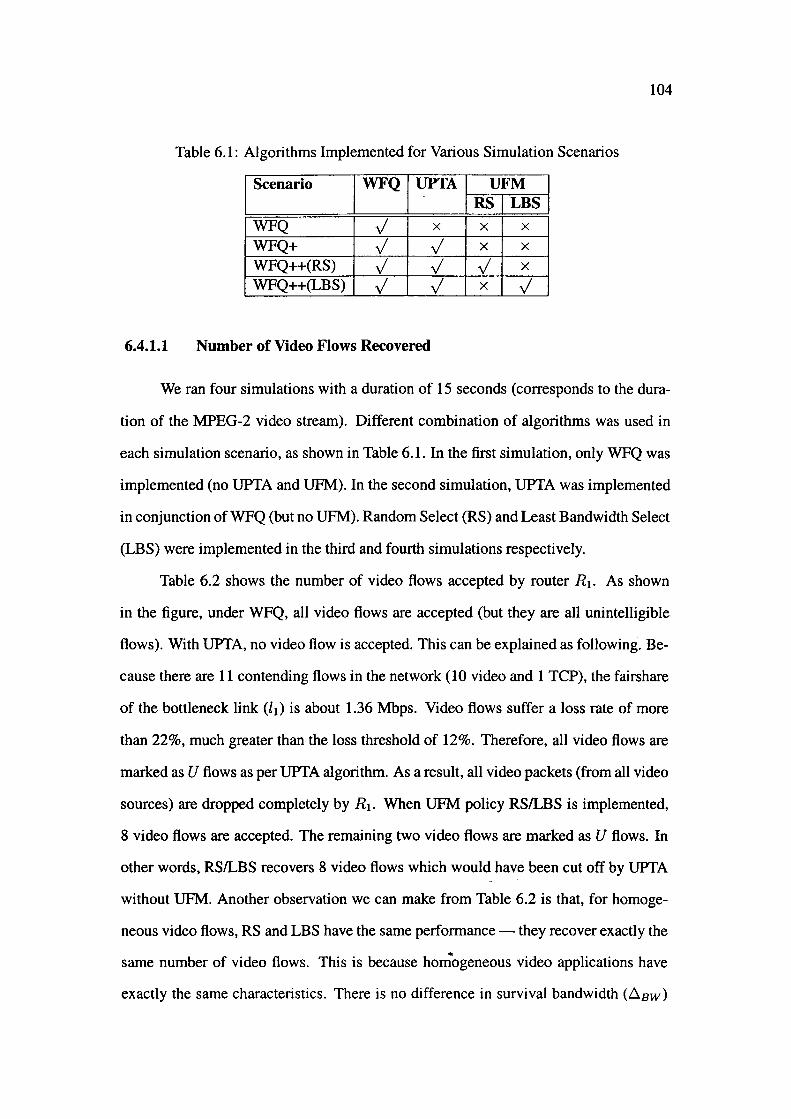
104

Table 6.1: Algorithms Implemented for Various Simulation Scenarios

I Scenario I WFQ I lJPTA I UFM I RSI LBS WFQ ✓ X X X

WFQ+ ✓ ✓ X X

WFQ++(RS) ✓ ✓ ✓ X

WFQ++(LBS) ✓ ✓ X ✓


We ran four simulations with a duration of 15 seconds (corresponds to the dura

tion of the MPEG-2 video stream). Different combination of algorithms was used in

each simulation scenario, as shown in Table 6.1. In the first simulation, only WFQ was

implemented (no UPf A and UFM). In the second simulation, UPf A was implemented

in conjunction of WFQ (but no UFM). Random Select (RS) and Least Bandwidth Select

(LBS) were implemented in the third and fourth simulations respectively.

Table 6.2 shows the number of video flows accepted by router R 1. As shown

in the figure, under WFQ, all video flows are accepted (but they are all unintelligible

flows). With UPfA, no video flow is accepted. This can be explained as following. Be

cause there are 11 contending flows in the network (10 video and 1 TCP), the fairshare

of the bottleneck link (l1) is about 1.36 Mbps. Video flows suffer a loss rate of more

than 22%, much greater than the loss threshold of 12%. Therefore, all video flows are

marked as U flows as per UPfA algorithm. As a result, all video packets (from all video

sources) are dropped completely by R 1. When UFM policy RS/LBS is implemented,

8 video flows are accepted. The remaining two video flows are marked as U flows. In

other words, RS/LBS recovers 8 video flows which would have been cut off by UPfA

without UFM. Another observation we can make from Table 6.2 is that, for homoge

neous video flows, RS and LBS have the same performance - they recover exactly the

same number of video flows. This is because homogeneous video applications have

exactly the same characteristics. There is no difference in survival bandwidth (~ 8 w)

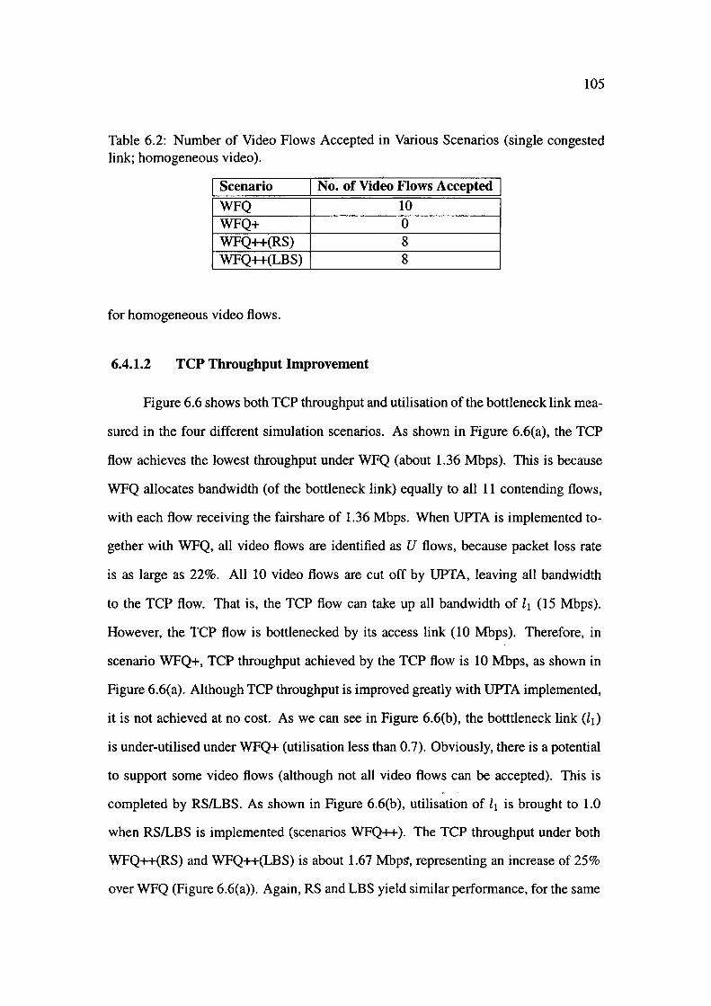
105

Table 6.2: Number of Video Flows Accepted in Various Scenarios (single congested link; homogeneous video).

I Scenario I No. of Video Flows Accepted I WFQ 10 WFQ+ 0 WFQ++(RS) 8 WFQ++(LBS) 8

for homogeneous video flows.

6.4.1.2 TCP Throughput Improvement

Figure 6.6 shows both TCP throughput and utilisation of the bottleneck link mea

sured in the four different simulation scenarios. As shown in Figure 6.6(a), the TCP

flow achieves the lowest throughput under WFQ (about 1.36 Mbps). This is because

WFQ allocates bandwidth ( of the bottleneck link) equally to all 11 contending flows,

with each flow receiving the fairshare of 1.36 Mbps. When UPTA is implemented to

gether with WFQ, all video flows are identified as U flows, because packet loss rate

is as large as 22%. All 10 video flows are cut off by UPTA, leaving all bandwidth

to the TCP flow. That is, the TCP flow can take up all bandwidth of l1 (15 Mbps).

However, the TCP flow is bottlenecked by its access link (10 Mbps). Therefore, in

scenario WFQ+, TCP throughput achieved by the TCP flow is 10 Mbps, as shown in

Figure 6.6(a). Although TCP throughput is improved greatly with UPTA implemented,

it is not achieved at no cost. As we can see in Figure 6.6(b), the botttleneck link (l1)

is under-utilised under WFQ+ (utilisation less than 0.7). Obviously, there is a potential

to support some video flows (although not all video flows can be accepted). This is

completed by RS/LBS. As shown in Figure 6.6(b), utilisation of l1 is brought to 1.0

when RS/LBS is implemented (scenarios WFQ++ ). The TCP throughput under both

WFQ++(RS) and WFQ++(LBS) is about 1.67 MbpS', representing an increase of 25%

over WFQ (Figure 6.6(a)). Again, RS and LBS yield similar performance, for the same

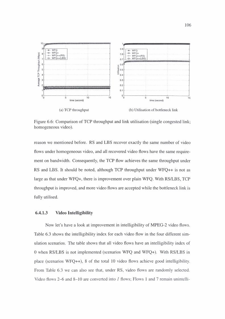
10 ~--IIHHtlllHll!lmHllmHIIIIIIIHIHIIIEIIHllllllHllllllllllllmHIIBIIIB\'

~ 8

f 7 5 a. "5, 6 :,

~ 5 f-CL u 4 f-., [ 3 .. .,

-♦- WFQ -e- WFQ+ --+- WFO++{AS) -&- WFO++{LBS)

~ 2 ...

1 .

0'-----~----~---~ 0 5 10 15

time (second)

(a) TCP throughput

0.9 -♦- WFQ

0.8 . -e- WFQ+ --+- WFO++{AS)

O.? -&- WFO++(LBS)

0.61

0.5

0.4

0.3

0.2

0.1

106

0'-----~----~-----' 0 10 15

time (second)

(b) Utilisation of bottleneck link

Figure 6.6: Comparison of TCP throughput and link utilisation (single congested link; homogeneous video).

reason we mentioned before. RS and LBS recover exactly the same number of video

flows under homogeneous video, and all recovered video flows have the same require

ment on bandwidth. Consequently, the TCP flow achieves the same throughput under

RS and LBS. It should be noted, although TCP throughput under WFQ++ is not as

large as that under WFQ+, there is improvement over plain WFQ. With RS/LBS, TCP

throughput is improved, and more video flows are accepted while the bottleneck link is

fully utilised.

6.4.1.3 Video Intelligibility

Now let's have a look at improvement in intelligibility of MPEG-2 video flows.

Table 6.3 shows the intelligibility index for each video flow in the four different sim

ulation scenarios. The table shows that all video flows have an intelligibility index of

0 when RS/LBS is not implemented (scenarios WFQ and WFQ+ ). With RS/LBS in

place (scenarios WFQ++ ), 8 of the total 10 video flows achieve good intelligibility.

From Table 6.3 we can also see that, under RS, video flows are randomly selected.

Video flows 2-6 and 8-10 are converted into I flows; Flows 1 and 7 remain unintelli -

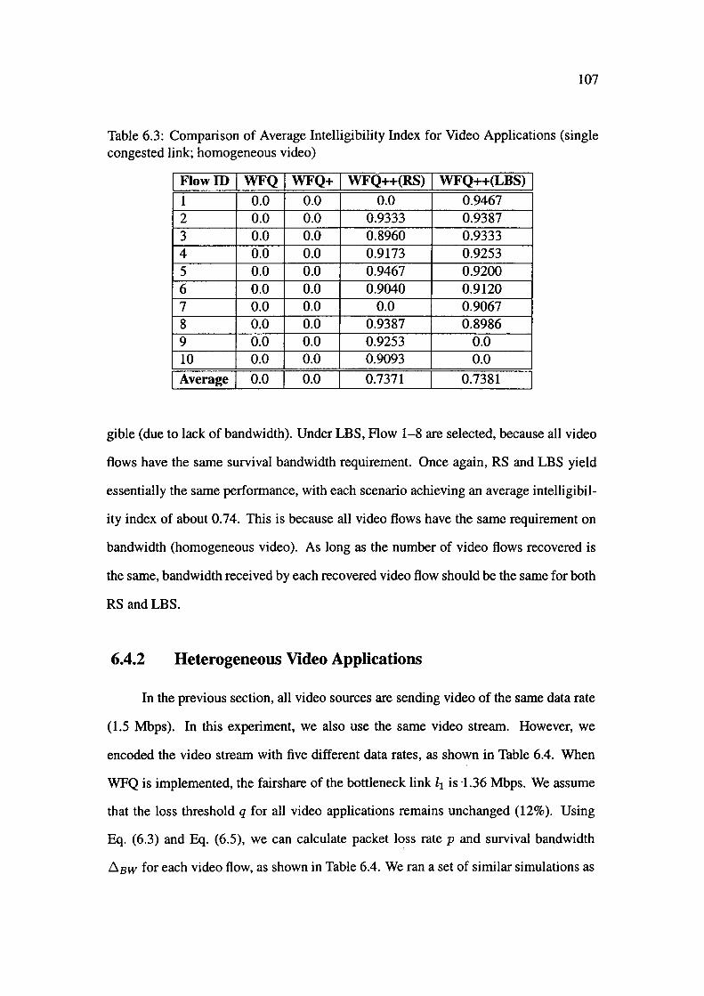
107

Table 6.3: Comparison of Average Intelligibility Index for Video Applications (single congested link; homogeneous video)

I Flow ID I WFQ I WFQ+ I WFQ++(RS) I WFQ++(LBS) I 1 0.0 0.0 0.0 0.9467 2 0.0 0.0 0.9333 0.9387 3 0.0 0.0 0.8960 0.9333 4 0.0 0.0 0.9173 0.9253 5 0.0 0.0 0.9467 0.9200 6 0.0 0.0 0.9040 0.9120 7 0.0 0.0 0.0 0.9067 8 0.0 0.0 0.9387 0.8986 9 0.0 0.0 0.9253 0.0 10 0.0 0.0 0.9093 0.0

I Average I 0.0 0.0 0.7371 0.7381

gible ( due to lack of bandwidth). Under LBS, Flow 1-8 are selected, because all video

flows have the same survival bandwidth requirement. Once again, RS and LBS yield

essentially the same performance, with each scenario achieving an average intelligibil

ity index of about 0.74. This is because all video flows have the same requirement on

bandwidth (homogeneous video). As long as the number of video flows recovered is

the same, bandwidth received by each recovered video flow should be the same for both

RS and LBS.

6.4.2 Heterogeneous Video Applications

In the previous section, all video sources are sending video of the same data rate

(1.5 Mbps). In this experiment, we also use the same video stream. However, we

encoded the video stream with five different data rates, as shown in Table 6.4. When

WFQ is implemented, the fairshare of the bottleneck link l-i· is 1.36 Mbps. We assume

that the loss threshold q for all video applications remains unchanged (12% ). Using

Eq. (6.3) and Eq. (6.5), we can calculate packet l~ss rate p and survival bandwidth

D.sw for each video flow, as shown in Table 6.4. We ran a set of similar simulations as

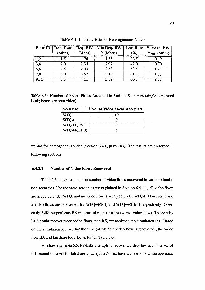
108

Table 6.4: Characteristics of Heterogeneous Video

Flow ID Data Rate Req. BW MinReq. BW Loss Rate SurvivalBW (Mbps) (Mbps) b (Mbps) (%) b.sw (Mbps)

1,2 1.5 1.76 1.55 22.5 0.19 3,4 2.0 2.35 2.07 42.0 0.70 5,6 2.5 2.93 2.58 53.5 1.21 7,8 3.0 3.52 3.10 61.3 1.73 9,10 3.5 4.11 3.62 66.8 2.25

Table 6.5: Number of Video Flows Accepted in Various Scenarios (single congested Link; heterogeneous video)

I Scenario I No. of Video Flows Accepted I WFQ 10 WFQ+ 0 WFQ++(RS) 3 WFQ++(LBS) 5

we did for homogeneous video (Section 6.4.1, page 103). The results are presented in

following sections.


Table 6.5 compares the total number of video flows recovered in various simula

tion scenarios. For the same reason as we explained in Section 6.4.1.1, all video flows

are accepted under WFQ, and no video flow is accepted under WFQ+. However, 3 and

5 video flows are recovered, for WFQ++(RS) and WFQ++(LBS) respectively. Obvi

ously, LBS outperforms RS in terms of number of recovered video flows. To see why

LBS could recover more video flows than RS, we analysed the simulation log. Based

on the simulation log, we list the time (at which a video flow is recovered), the video

flow ID, and fairshare for I flows (a') in Table 6.6.

As shown in Table 6.6, RS/LBS attempts to re.cover a video flow at an interval of

0.1 second (interval for fairshare update). Let's first have a close look at the operation

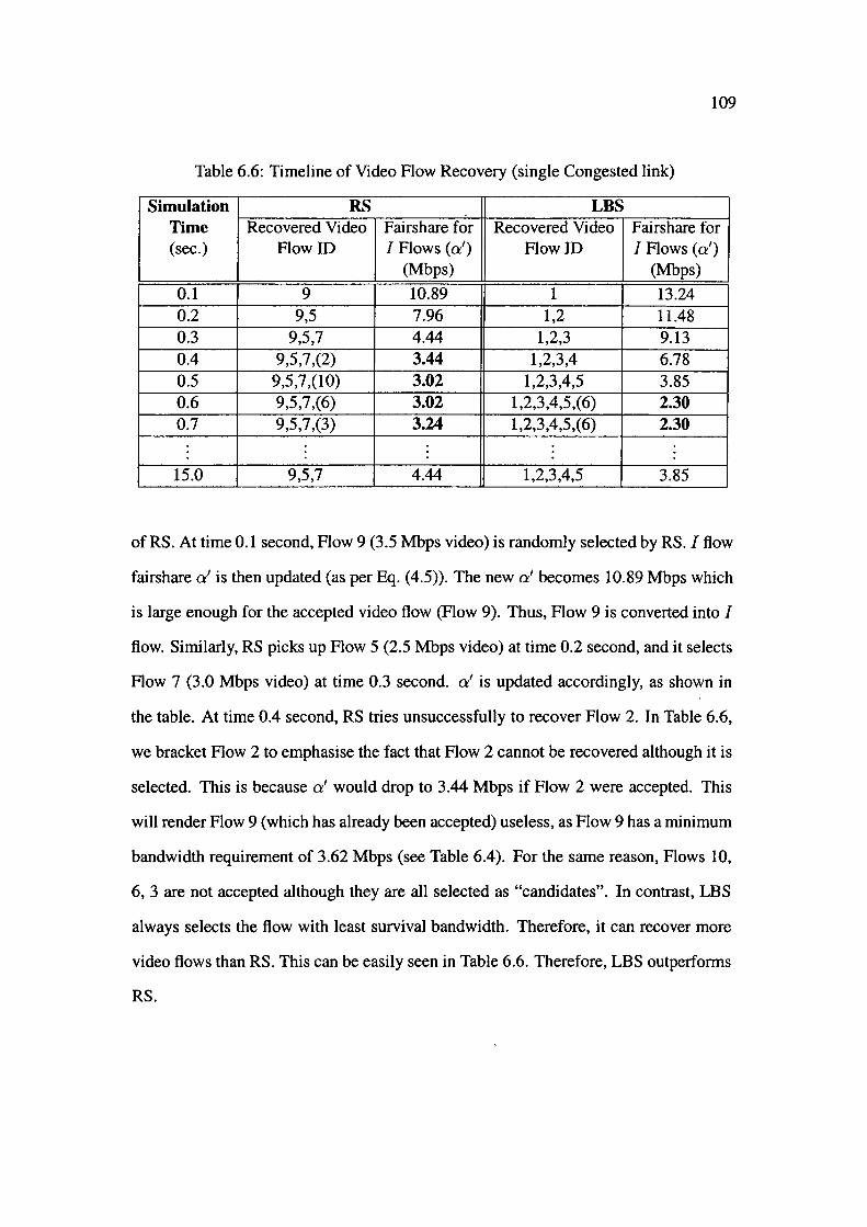
109

Table 6.6: Timeline of Video Flow Recovery (single Congested link)

Simulation RS LBS Time Recovered Video Fairshare for Recovered Video Fairshare for (sec.) Flow ID I Flows (a') Flow ID I Flows (a')

(Mbps) (Mbps)

0.1 9 10.89 1 13.24 0.2 9,5 7.96 1,2 11.48 0.3 9,5,7 4.44 1,2,3 9.13 0.4 9,5,7,(2) 3.44 1,2,3,4 6.78 0.5 9,5,7,(10) 3.02 1,2,3,4,5 3.85 0.6 9,5,7,(6) 3.02 1,2,3,4,5,(6) 2.30 0.7 9,5,7,(3) 3.24 1,2,3,4,5,(6) 2.30

15.0 9,5,7 4.44 1,2,3,4,5 3.85

of RS. At time 0.1 second, Flow 9 (3.5 Mbps video) is randomly selected by RS. I flow

fairshare a' is then updated (as per Eq. (4.5)). The new a' becomes 10.89 Mbps which

is large enough for the accepted video flow (Flow 9). Thus, Flow 9 is converted into I

flow. Similarly, RS picks up Flow 5 (2.5 Mbps video) at time 0.2 second, and it selects

Flow 7 (3.0 Mbps video) at time 0.3 second. a' is updated accordingly, as shown in

the table. At time 0.4 second, RS tries unsuccessfully to recover Flow 2. In Table 6.6,

we bracket Flow 2 to emphasise the fact that Flow 2 cannot be recovered although it is

selected. This is because a' would drop to 3.44 Mbps if Flow 2 were accepted. This

will render Flow 9 (which has already been accepted) useless, as Flow 9 has a minimum

bandwidth requirement of 3.62 Mbps (see Table 6.4). For the same reason, Flows 10,

6, 3 are not accepted although they are all selected as "candidates". In contrast, LBS

always selects the flow with least survival bandwidth. Therefore, it can recover more

video flows than RS. This can be easily seen in Table 6.6. Therefore, LBS outperforms

RS.

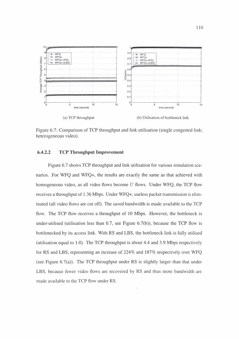
10 r;.jlll!IBIBl-OHHIIOBHBOBHBHIHIIHIHIIIIHllllllllllllllllllllHIHIIHIHIIIIIBB\1 If'

91 - -+- WFQ

~ B --e-- WFQ+ .o -+- WFO++{RS) ~ 7 --e-- WFO++{LBS) '5 a. -§, 6 . :, 0 .c 5 ..

~ ~----l+ffifl--------lttttlttl~ ~~llHIIEll:mlllllllllllllllllllllllllll!lllmllllmll:mllllllllllllllllllll!llll!l!llll!mj> ., ff 3 . <ii .i( 2

1 .

o~---~--------~ 0 5 10 15

Ii me { second)

(a) TCP throughput

110

0.9 -+- WFQ

~-8 --e-- WFQ+ -+- WFO++{RS)

0.7 _ --e-- WFQ++{LBS) _

c 0.6 0

·~ 0.5 . · - .. .. . .

5 0.4

0.3

0.2

0.1

0 0 5 10 15

time {second)

(b) Utilisation of bottleneck link

Figure 6.7: Comparison of TCP throughput and link utilisation (single congested link; heterogeneous video).


Figure 6.7 shows TCP throughput and link utilisation for various simulation sce

narios. For WFQ and WFQ+, the results are exactly the same as that achieved with

homogeneous video, as all video flows become U flows. Under WFQ, the TCP flow

receives a throughput of 1.36 Mbps. Under WFQ+, useless packet transmission is elim

inated (all video flows are cut off). The saved bandwidth is made available to the TCP

flow. The TCP flow receives a throughput of 10 Mbps. However, the bottleneck is

under-utilised (utilisation less than 0.7, see Figure 6.7(b)), because the TCP flow is

bottlenecked by its access link. With RS and LBS, the bottleneck link is fully utilised

(utilisation equal to 1.0). The TCP throughput is about 4.4 and 3.9 Mbps respectively

for RS and LBS, representing an increase of 224% and 187% respectively over WFQ

(see Figure 6.7(a)). The TCP throughput under RS is slightly larger than that under

LBS , because fewer video flows are recovered by RS and thus more bandwidth are

made avai lable to the TCP flow under RS .

111

Table 6.7: Comparison of Average Intelligibility Index for Video Applications (single congested link; heterogeneous video)

I Flow ID I WFQ I WFQ+ I WFQ++(RS) I WFQ++(LBS) I 1 0.0 0.0 0.0 0.9947 2 0.0 0.0 0.0 0.9867 3 0.0 0.0 0.0 0.9787 4 0.0 0.0 0.0 0.9733 5 0.0 0.0 0.9867 0.9627 6 0.0 0.0 0.0 0.0 7 0.0 0.0 0.9787 0.0 8 0.0 0.0 0.0 0.0 9 0.0 0.0 0.9947 0.0 10 0.0 0.0 0.0 0.0

I Average I 0.0 0.0 0.2960 0.4896


Intelligibility analysis results for the ten video flows are shown in Table 6.7. The

table shows that no video flow is intelligible under WFQ and WFQ+, and some video

flows are recovered when RS/LBS is implemented. RS recovers 3 video flows, with an

average intelligibility index of 0.2939. Whereas LBS recovers 5 video flows, wi~h an

average intelligibility index of 0.4893. Needless to say, LBS outperforms RS in terms

of video intelligibility. As we can see in Table 6.7, the recovered video flows have

identical intelligibility indices for RS and LBS. However, LBS recovers more video

flows than RS does. This explains why the average intelligibility index under LBS is

higher than that under RS.

6.5 Multiple Congested Links

Finally, we ran a set of simulations with multiple congested links. Figure 6.8

shows the network model used in the simulation. There are two groups of traffic in .. the network. Traffic Group 1 (TGl) consists of 9 video sources (S1-S9) and one TCP

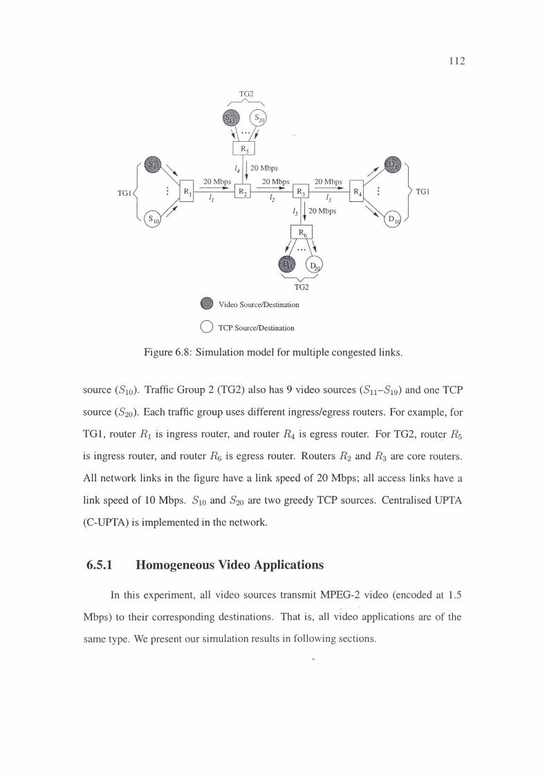
TG2 ~

• Video Source/Destination

Q TCP Source/Destination

Figure 6.8: Simulation model for multiple congested links.

112

source (S10) . Traffic Group 2 (TG2) also has 9 video sources (Su-S19) and one TCP

source (S20). Each traffic group uses different ingress/egress routers. For example, for

TGl , router R1 is ingress router, and router R4 is egress router. For TG2, router R5

is ingress router, and router ~ is egress router. Routers R2 and R3 are core routers.

All network links in the figure have a link speed of 20 Mbps; all access links have a

link speed of 10 Mbps. S 10 and S20 are two greedy TCP sources. Centralised UPTA

(C-UPTA) is implemented in the network.

6.5.1 Homogeneous Video Applications

In this experiment, all video sources transmit MPEG-2 video (encoded at 1.5

Mbps) to their corresponding destinations. That is , all video applications are of the

same type. We present our simulation results in following sections.

113

Table 6.8: Number of Video Flows Accepted in Various Scenarios (multiple congested Link; homogeneous video)

Scenario No. of Video Flows Accepted TGl TG2

WFQ 9 9 WFQ+ 0 0 WFQ++(RS) 5 5 WFQ++(LBS) 5 5


Table 6.8 shows the number of video flows accepted in each traffic group. Under

WFQ, all video flows are accepted, in both TG 1 and TG2. However, all of these video

flows are U flows. Because in the simulated network, link l2 is the bottleneck link

(most congested link). The global fairshare in the network is 1 Mbps for all flows.

All video flows suffer a packet loss rate of about 43%. Therefore, all video flows are

transmitting useless packets. When UPTA is implemented with WFQ (WFQ+ ), no

video flow is accepted (because all video flows are eliminated). For WFQ++(RS) and

WFQ++(LBS), five video flows are accepted in each traffic group. In other words,

RS/LBS successfully recovers five video flows. As we can see in Table 6.8, RS and

LBS recover exactly the same number of video flows.


Figure 6.9 compares throughputs of the two TCP sources (S10 and S20) achieved

with various algorithms. Compare Figure 6.9(a) and Figure 6.9(b), we can see that,

for a given algorithm, the two TCP flows have similar throughput. Under WFQ, both

TCP sources achieve a throughput of about 1 Mbps, which equals to the global fair

share. Under WFQ+, the two TCP flows receive a throughput of 10 Mbps, representing

an increase of 10 times over WFQ. Under WFQ++,'.RS) and WFQ++(LBS), the TCP

throughput is about 1.67 Mbps, representing an increase of 67% over WFQ. It should

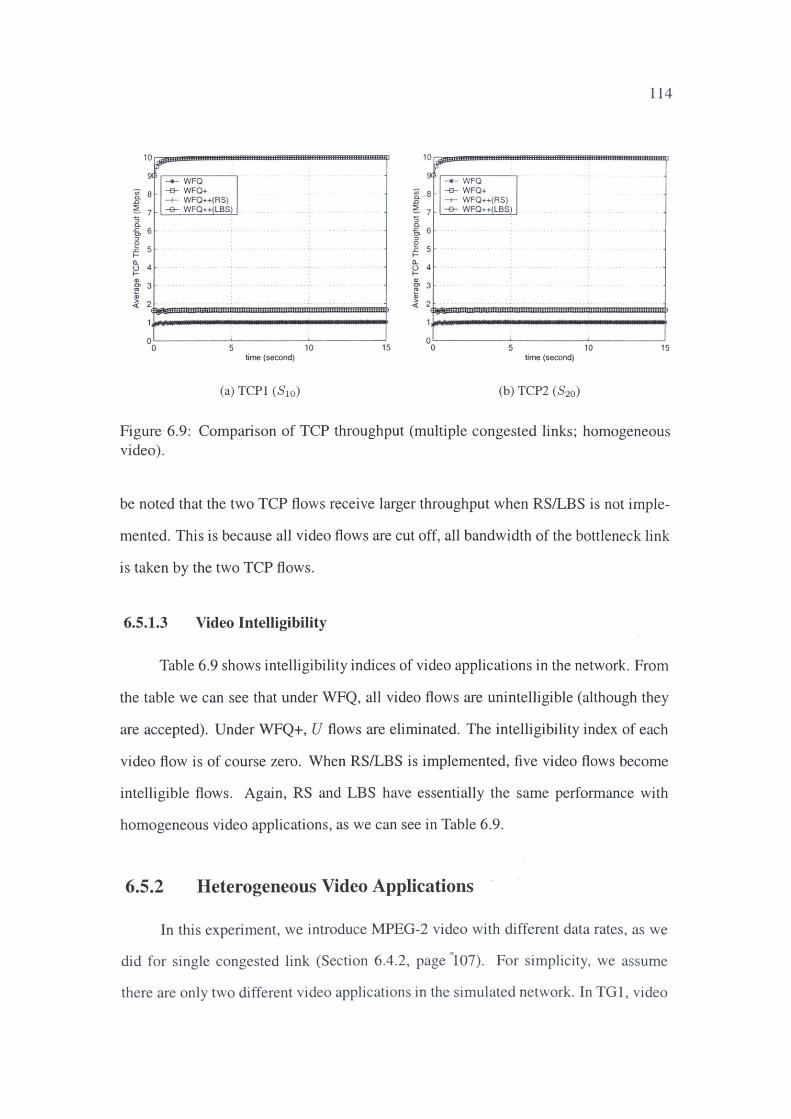
10 r.iii!JBBB'""""IIIIMIHllllllHllllllllllBIIIIIIBIBBBIIIIIIHIHIBlllllllBIIIIIIBIHIIBI\' Ii"

9 ~----~ W--ccF=a ------,

-e- WFQ+ ~ 8 .0

~ 7 s c. -§, 6 :,

i 5 la_

-+- WFQ++(RS) -e- WFO++(LBS)

U 4 , .. I-., [ 3 . . <I)

~ 2 M!!llllllrmll&Bllllll!lllllllllllll!llll!IBl!Blllllllllll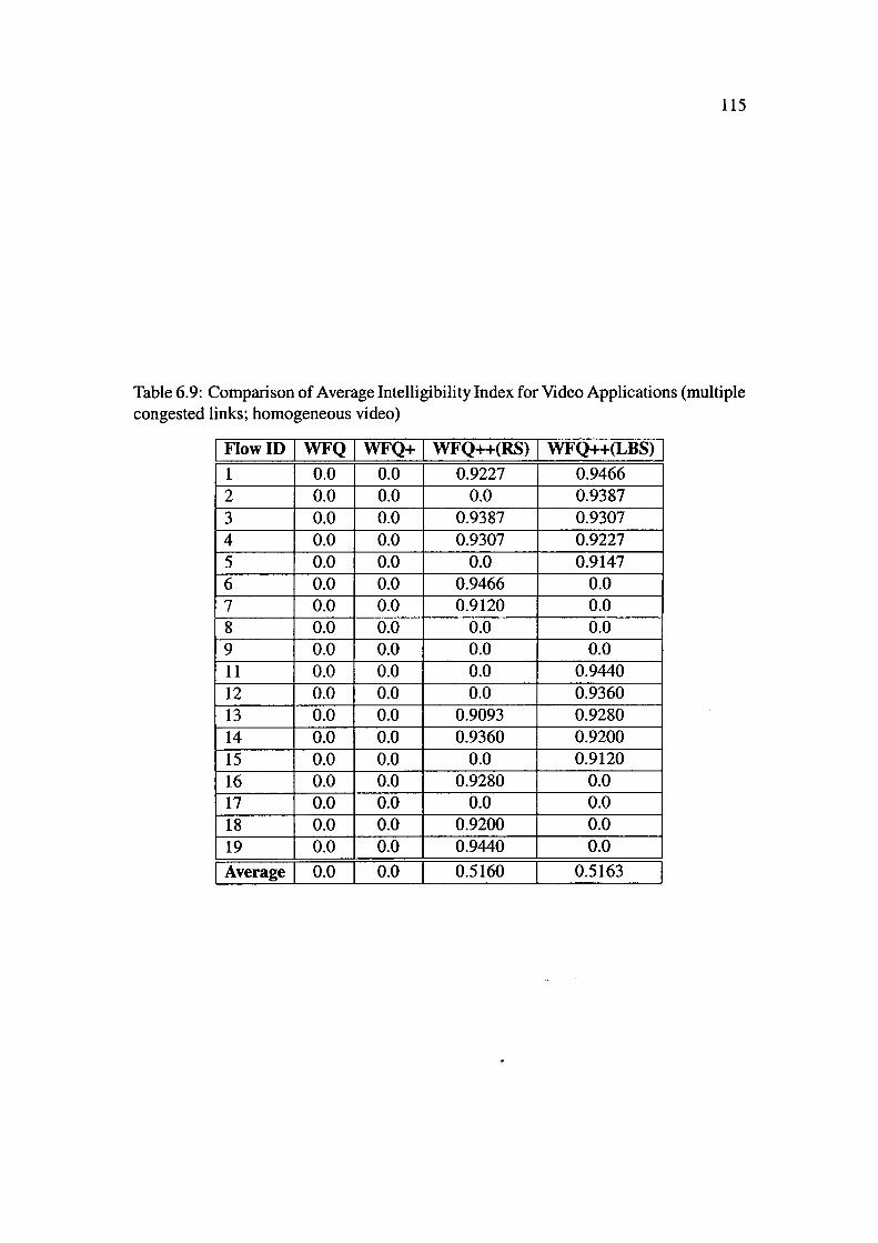![lll!IBlllllllllmllllllm!llllj)

0'-------~------'---- ---' 0 5 10 15

time (second)

(a) TCPl (S10)

114

10 r.ijjlEIBIJIE-IHllllllHllllllHllllllllllBIIIIIIBIBBBIIIIIIIIJIHIBlllllllBIBBBIIIBIBjl ,,, 9 ---- WFQ

~ B -e- WFQ+ .o -+- WFO++(RS) ~ 7 -e- WFO++(LBS) :5 c. -§, 6 :, 0 .c 5 .. .... l3 4 I., [ 3 . . <I)

~ 2 Ml!lll!llmlllllllllllll!llllllli!Hlm!llmllmll!llllllll![E!IIIIIIIIIIIIIIIIIIIIIIIH!IIB!j)

0'------~----~------' 0 5 10 15

time (second)

(b) TCP2 (S20)

Figure 6.9: Comparison of TCP throughput (multiple congested links; homogeneous video).

be noted that the two TCP flows receive larger throughput when RS/LBS is not imple

mented. This is because all video flows are cut off, all bandwidth of the bottleneck link

is taken by the two TCP flows.


Table 6.9 shows intelligibility indices of video applications in the network. From

the table we can see that under WFQ, all video flows are unintelligible (although they

are accepted). Under WFQ+, U flows are eliminated. The intelligibility index of each

video flow is of course zero. When RS/LBS is implemented, five video flows become

intelligible flows. Again, RS and LBS have essentially the same performance with

homogeneous video applications, as we can see in Table 6.9.

6.5.2 Heterogeneous Video Applications

In this experiment, we introduce MPEG-2 video with different data rates, as we

did for single congested link (Section 6.4.2, page cl07). For simplicity, we assume

there are only two different video appl ications in the simulated network. In TGl, video

115

Table 6.9: Comparison of Average Intelligibility Index for Video Applications (multiple congested links; homogeneous video)

I Flow ID I WFQ I WFQ+ I WFQ++(RS) I WFQ++(LBS) I 1 0.0 0.0 0.9227 0.9466 2 0.0 0.0 0.0 0.9387 3 0.0 0.0 0.9387 0.9307 4 0.0 0.0 0.9307 0.9227 5 0.0 0.0 0.0 0.9147 6 0.0 0.0 0.9466 0.0 7 0.0 0.0 0.9120 0.0 8 0.0 0.0 0.0 0.0 9 0.0 0.0 0.0 0.0 11 0.0 0.0 0.0 0.9440 12 0.0 0.0 0.0 0.9360 13 0.0 0.0 0.9093 0.9280 14 0.0 0.0 0.9360 0.9200 15 0.0 0.0 0.0 0.9120 16 0.0 0.0 0.9280 0.0 17 0.0 0.0 0.0 0.0 18 0.0 0.0 0.9200 0.0 19 0.0 0.0 0.9440 0.0

I Average I 0.0 0.0 0.5160 0.5163

116

sources S1-S6 are sending MPEG-2 video encoded at 1.5 Mbps. Video sources S7-S9

are sending MPEG-2 video encoded at 2.5 Mbps. Similarly, in TG2, video sources

Su-S16 employ MPEG-2 1.5 Mbps video, and video sources S17-S19 employ MPEG-

2 2.5 Mbps video. Because there are multiple ingress/egress routers in the network,

each ingress router is set to start sending QoS Probe messages randomly, so as to avoid

synchronisation problem. QoS Probe messages are sent at an interval of 100 ms. Global

fairshares are also updated at the same interval. Simulation results for heterogeneous

video are presented in following sections.


Table 6.10 shows the number of video flows accepted in each traffic group. In

Traffic Group 1, 9 video flows are accepted under WFQ (but they are unintelligible

flows). Under WFQ+, no video flow is accepted, as all video flows are marked as U

flows when UPTA is activated. For the simulated network, fairshare of the bottleneck

link (l2) is 1 Mbps. The fairshare is much smaller than the minimum required bandwidth

for both 1.5 and 2.5 Mbps MPEG-2 video (see Table 6.4, page 108). Therefore, all

video flows become unintelligible flows (U flows) under WFQ. Under WFQ+, all video

packets are dropped by UPTA (so no video flow is accepted). Under WFQ++(RS), 4

video flows are recovered. Under WFQ++(LBS), 5 video flows are recovered.

In Traffic Group 2, the number of video flows accepted under WFQ and WFQ+ is

the same as TGl, i.e. 9 and O for WFQ and WFQ+ respectively. For above-mentioned

reason, video flows accepted by WFQ are actually U flows. For WFQ++(RS) and

WFQ++(LBS), the number of accepted video flows is 3 and 5 respectively. Table 6.10

suggests that LBS has a better performance than RS.

Timeline of video flow recovery is shown in Table 6.11. Let's first look at the

operation of RS. At time 0.115 second, router R1 (ingress router for TGl) receives the •

first feedback packet, RS randomly selects Flow 3 (1.5 Mbps video) and converts it

117

Table 6.10: Number of Video Flows Accepted in Various Scenarios (multiple congested Link; heterogeneous video)

. Scenario No. of Video Flows Accepted

TGl TG2

WFQ 9 9 WFQ+ 0 0 WFQ++(RS) 4 3 WFQ++(LBS) 5 5

into I flow. I flow fairshare (a') is then updated. At time 0.139 second, router R5

(ingress router for TG2) receives the first feedback packet, it randomly selects Flow 18

(2.5 Mbps video) and updates a' to 7.66 Mbps. At time 0.215 second, R1 receives its

second feedback packet. It selects Flow 8 (2.5 Mbps video) and updates a' to 6.19

Mbps. R5 receives its second feedback packet at time 0.239 second. It selects Flow 12,

and so on ... At time 0.439, R5 tries to convert Flow 15 (1.5 Mbps video) into I flow.

However, as the fairshare will drop to 2.24 Mbps, Flow 15 cannot be converted (we

enclose it with brackets to emphasise that). This is because the fairshare is smaller

than the minimum bandwidth required by 2.5 Mbps video (see Table 6.4, page 108). If

Flow 15 were accepted, Flows 8, 9, 18 (2.5 Mbps video) would be rendered useless.

With LBS, the ingress routers (for both TG 1 and TG2) always select flows with

minimum survival bandwidth (i.e., 1.5 Mbps video). In Traffic Group 1, Flows 1,

2, 3, 4, 5 are converted into I flows respectively, each time R1 receives a feedback

packet. In Traffic Group 2, Flow 11, 12, 13, 14, 15 are converted into I flows, at time

0.139, 0.239, 0.339, 0.439, 0.539 second respectively. At time 0.615 second, R1 selects

Flow 6. However, Flow 6 is not converted into I flow because the fairshare would drop

to 1.54 Mbps (which is less than the minimum bandwidth required by 1.5 Mbps video).

Similarly at time 0.639 second, R5 tries unsuccessfully to convert Flow 16. Eventually,

RS accepts 7 video flows in total whereas LBS accepts 10.

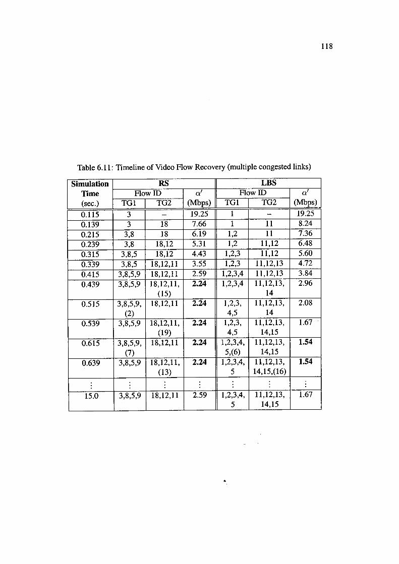
118

Table 6.11: Timeline of Video Flow Recovery (multiple congested links)

Simulation RS LBS Time Flow ID a' Flow ID a'

(sec.) TGl TG2 (Mbps) TGl TG2 (Mbps)

0.115 3 - 19.25 1 - 19.25

0.139 3 18 7.66 1 11 8.24

0.215 3,8 18 6.19 1,2 11 7.36

0.239 3,8 18,12 5.31 1,2 11,12 6.48

0.315 3,8,5 18,12 4.43 1,2,3 11,12 5.60

0.339 3,8,5 18,12,11 3.55 1,2,3 11,12,13 4.72

0.415 3,8,5,9 18,12,11 2.59 1,2,3,4 11,12,13 3.84

0.439 3,8,5,9 18,12,11, 2.24 1,2,3,4 11,12,13, 2.96 (15) 14

0.515 3,8,5,9, 18,12,11 2.24 1,2,3, 11,12,13, 2.08 (2) 4,5 14

0.539 3,8,5,9 18,12,11, 2.24 1,2,3, 11,12,13, 1.67 (19) 4,5 14,15

0.615 3,8,5,9, 18,12,11 2.24 1,2,3,4, 11,12,13, 1.54 (7) 5,(6) 14,15

0.639 3,8,5,9 18,12,11, 2.24 1,2,3,4, 11,12,13, 1.54 (13) 5 14,15,(16)

15.0 3,8,5,9 18,12,11 2.59 1,2,3,4, 11,12,13, 1.67 5 14,15

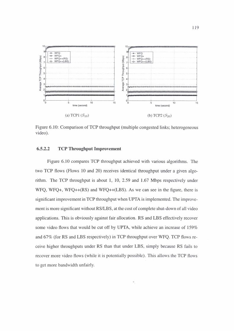
'[ 8 .0

~ 7 :5 c. ~ 6 . ::,

~ 5 1-

5 4 IQ)

--+-- WFQ --e--- WFQ+ -+- WFO++(AS) --e- WFO++ LBS

~ 3-fWl<.fflll+! ___________ fll+!ttttt-

., ~ 2·$·!1li!JlEIIIIIIIlllllllllllllllll!lllllll!lllllllllllllllllllllllllllllll!llllll!IIIBIIIIIIIIIIIIII~

o~---~----~---~ 0 5 10 15

time (second)

(a) TCPI (S10)

119

10r..ii11-'l!ll!IIBHHlfBHllfBHIIIIIIIHlllllll31111111!IIIBll!HHBIHHBllllllll31111l11111 If'

g ~-------W-F-0-~

--&- WFQ+ "[ 8

~ 7 :5 c. -§, 6 . ::,

~ 5 la.. u 4 · I-.,

-+- WFO++(AS) --e- WFO++(LBS)

[ 3-IWl<l+l+ll! ____ fl!i . . ++ll+lt . . . __ . .. .. __ ;ff,_ · ·-1tt· "llfffl-'·' ~ """"""""""'"""'""'"'"""'" .. ··· ~ 2

--il!llllllia:Bmllllllllmil!llllllill!BIIIElll!lllllllllllmllllllmllllllmmmlll~

o~---~----~---__J 0 5 10 15

time (second)

(b) TCP2 (S20)

Figure 6.10: Comparison of TCP throughput (multiple congested links; heterogeneous video).


Figure 6.10 compares TCP throughput achieved with various algorithms. The

two TCP flows (Flows 10 and 20) receives identical throughput under a given algo

rithm. The TCP throughput is about 1, 10, 2.59 and 1.67 Mbps respectively under

WFQ, WFQ+, WFQ++(RS) and WFQ++(LBS). As we can see in the figure, there is

significant improvement in TCP throughput when UPTA is implemented. The improve

ment is more significant without RS/LBS, at the cost of complete shut-down of all video

applications. This is obviously against fair allocation. RS and LBS effectively recover

some video flows that would be cut off by UPTA, while achieve an increase of 159%

and 67% (for RS and LBS respectively) in TCP throughput over WFQ. TCP flows re

ceive higher throughputs under RS than that under LBS, simply because RS fails to

recover more video flows (while it is potentially possible). This allows the TCP flows

to get more bandwidth unfairly.

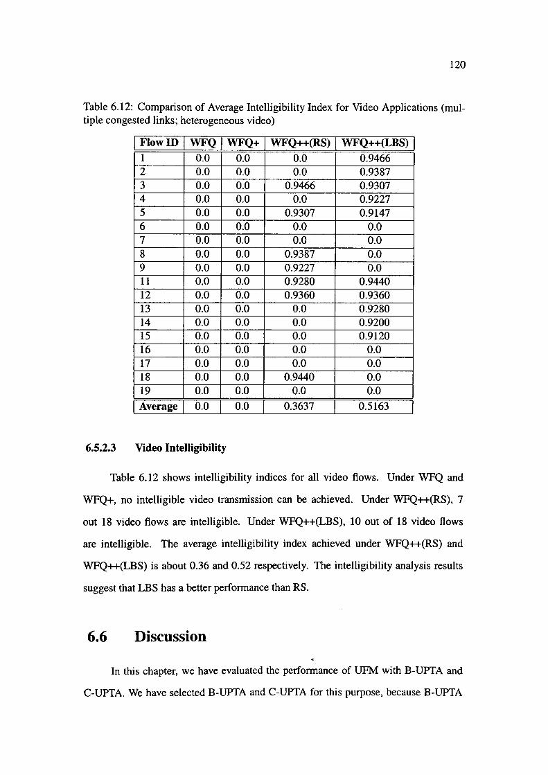
120

Table 6.12: Comparison of Average Intelligibility Index for Video Applications (multiple congested links; heterogeneous video)

I Flow ID I WFQ I WFQ+ I WFQ++(RS) I WFQ++(LBS) I 1 0.0 0.0 0.0 0.9466 2 0.0 0.0 0.0 0.9387 3 0.0 0.0 0.9466 0.9307 4 0.0 0.0 0.0 0.9227 5 0.0 0.0 0.9307 0.9147 6 0.0 0.0 0.0 0.0 7 0.0 0.0 0.0 0.0 8 0.0 0.0 0.9387 0.0 9 0.0 0.0 0.9227 0.0 11 0.0 0.0 0.9280 0.9440 12 0.0 0.0 0.9360 0.9360 13 0.0 0.0 0.0 0.9280 14 0.0 0.0 0.0 0.9200 15 0.0 0.0 0.0 0.9120 16 0.0 0.0 0.0 0.0 17 0.0 0.0 0.0 0.0 18 0.0 0.0 0.9440 0.0 19 0.0 0.0 0.0 0.0

I Average I 0.0 0.0 0.3637 0.5163


Table 6.12 shows intelligibility indices for all video flows. Under WFQ and

WFQ+, no intelligible video transmission can be achieved. Under WFQ++(RS), 7

out 18 video flows are intelligible. Under WFQ++(LBS), 10 out of 18 video flows

are intelligible. The average intelligibility index achieved under WFQ++(RS) and

WFQ++(LBS) is about 0.36 and 0.52 respectively. The intelligibility analysis results

suggest that LBS has a better performance than RS.

6.6 Discussion

In this chapter, we have evaluated the performance of UFM with B-UPTA and

C-UPTA. We have selected B-UPTA and C-UPTA for this purpose, because B-UPTA

121

and C-UPTA represent the two extremes on perlormance scale with regard to UPI'

avoidance. As we discussed in Section 5.6.4 (Page 91), for the three UPTA enforcement

schemes proposed, the perlormance increases in the order of B-UPTA, P-UPTA, C

UPTA. The perlormance of P-UPTA resides between B-UPTA and C-UPTA. In this

section, we discuss how UFM will perlorm with P-UPTA.

6.6.1 Single Congested Link

In networks with single congested link, all three proposed UPTA enforcement

algorithms (B-UPTA, P-UPTA, C-UPTA) have exactly the same perlormance. This has

been explained in Section 5.6.4 (Page 91). In the case of single congested link, UPTA is

activated at only one router (the congested router). No update of loss rate threshold will

occur. P-UPTA is equivalent to B-UPTA in such a situation. Therefore, similar results

as that presented in Section 6.4 are expected, if UFM is implemented on P-UPTA.

6.6.2 Multiple Congested Links

P-UPTA and C-UPTA are two UPTA enforcement schemes proposed for net

works with multiple congested links. The two UFM policies (i.e. RS and LBS) pro

posed in this chapter require global fairshare information to operate properly. Like

B-UPTA, P-UPTA is a distributed UPTA enforcement scheme in nature (as opposed to

C-UPTA which computes global fairshare explicitly). Global fairshare is not available

at edge routers. Therefore, RS/LBS cannot work with P-UPTA in the case of multiple

congested links. However, there may be other UFM policies which work with P-UPTA

in networks with multiple congested links. This requires futher investigation. We leave

it to future work.

122

6. 7 Conclusion

In this chapter, we have investigated UPI' avoidance with multiple multimedia

flows. We proposed a framework called Unintelligible Flow Management (UFM) to

address problems that arise with UPTA in networks supporting multiple multimedia

applications. We have presented the UFM framework using WFQ as an example. The

key component of UFM is a management policy which attempts to convert U flows

into I flows when the fairshare is large enough to accept some (but not all) multimedia

flows. We have proposed two different UFM policies in this chapter. They are Random

Select (RS) and Least Bandwidth Select (LBS). RS is the simpler UFM policy. It

simply selects a U flow randomly at a given interval if there are more than one U flow

present in the network. LBS is more intelligent than RS. It always selects the flow

which requires the least bandwidth to survive. The advantage of LBS is that it has the

potential to "rescue" more multimedia flows as compared with RS, at the expense of

increased complexity.

We have incorporated RS/LBS into WFQ. By using OPNET Modeler and MPEG-

2 video, we have conducted extensive simulation study to evaluate the performance

of RS and LBS. We have used three performance metrics: number of video flows

recovered, TCP throughput improvement and video intelligibility. We have simu

lated four different network scenarios: single/multiple congested links and homoge

neous/heterogeneous multimedia applications. Following conclusions can be drawn

from our simulation results:

• It is clear that the bottleneck link may be under-utilised without UFM (i.e. RS

or LBS), and TCP sources may receive unfairly more bandwidth than video

flows. UFM can effectively maximise link utilisation (full utilisation can be

achieved) by converting selected U flows in}o I flows.

• Both RS and LBS can significantly improve TCP throughput (up to 224% in

123

our simulated networks), as compared with plain WFQ.

• Both RS and LBS can effectively impr~_ve average intelligibility index of video

applications.

• RS and LBS yield similar performance under homogeneous video. However,

LBS out-performs RS under heterogeneous video.

Our simulation results also suggest that RS and LBS have identical performance

with homogeneous multimedia applications. In such a situation, light-weighted RS may

be sufficient. This will avoid the complexity of LBS. However, with heterogeneous

multimedia applications, it may be justifiable to implement LBS, as LBS out-performs

RS in terms of number of video flows recovered as well as video intelligibility.

Chapter 7

Conclusion

We have come to the end of the thesis. Before we conclude, we would like to

briefly summarise what have been done in this thesis, and discuss merits/demerits of

our work. We also provide suggestions for future work in this chapter.

7.1 Summary

In this thesis, we have investigated Useless Packet Transmission (UPT) avoid

ance problem in best-effort networks supporting multimedia applications. To tackle

UPT problem, we proposed an algorithm called Useless Packet Transmission Avoid

ance (UPTA) which can be easily incorporated into packet queueing and scheduling

algorithms that enforce fairness. UPTA is intended to eliminate useless packet trans

mission (UPT) which is an side-effect of fair algorithms. For networks with multiple

congested links, we proposed two extensions to basic UPTA (which is intended for

networks with single congested link): Partial UPTA (P-UPTA) and Centralised UPTA

(C-UPTA). For networks with multiple multimedia flows, _W<!. proposed a management

framework called Unintelligible Flow Management (UFM), which can enhance the per

formance of UPTA in networks with multiple unintelligible multimedia flows.

In Chapter 2, we introduced a number of popular multimedia applications on the

Internet, and the underlying technology that supports them. Generally speaking, mul-

125

timedia applications in the Internet can be classified into three categories, i.e. Media

on-demand, Real-time playback and Real-time interactive media. Current Internet sup

ports only best-effort network service, no QoS ·is guaranteed. Multimedia packets are

usually transmitted over the Internet based on RTP/UPD over IP. Multimedia applica

tions may experience unpredictable packet loss at times of network congestion. Unlike

conventional data communications, multimedia applications usually have stringent re

quirements on QoS, in terms of bandwidth, delay, jitter, etc. For example, when packet

loss rate exceeds a given threshold, received audio/video will be rendered useless. With

the growth of the Internet, we can perceive that the popularity and growth of multimedia

applications over the Internet will continue in the foreseeable future.

In Chapter 3, we discussed related work. We reported research work conducted

in the field of supporting multimedia over the Internet, and described research efforts

dedicated to solving problems that arise with the introduction of multimedia into the

Internet.

In Chapter 4, we identified the UPf problem. UPT is based on the scientific

observation that for packetised audio and video, packet loss rate must be maintained

under a given threshold for any meaningful communication [10, 21, 46]. When packet

loss rate exceeds this threshold, received audio/video become useless. We investigated

the UPf avoidance problem with single congested link. We proposed a UPf avoidance

algorithm (we call it UPTA) to avoid useless packets from multimedia applications.

UPTA can be easily incorporated into existing fair algorithms. It can effectively elim

inate useless multimedia packets, and allocate the recovered bandwidth to competing

TCP flows. We demonstrated the implementation of UPTA in WFQ and CSFQ. Sim

ulation of a traffic mix consisting of MPEG-2 video and T~P over a typical enterprise

network topology reveals that our proposed algorithm can effectively eliminate use

less packet transmission in congested routers, and as a result increase TCP throughput

and reduce file download time. The UPTA algorithm can operate unobtrusively; it has

126

noticeable effect neither on the overall intelligibility of the multimedia applications,

nor on the fairness performance of the "host" packet queueing algorithms (WFQ and

CSFQ) on which we "mount" the UPTA algorithm.

In Chapter 5, we extended UPTA to large-scale networks. We investigated UPT

avoidance problem with multiple congested links, and discussed three different UPTA

enforcement schemes - basic UPTA (B-UPTA), Partial UPTA (P-UPTA) and Cen

tralised UPTA (C-UPTA). The challenge of UPT avoidance with multiple congested

links is to determine global f airshare and enforce UPTA based on the global f airshare.

We proposed the Bottleneck Fairshare Discovery (BFD) protocol to address this issue.

BFD is a feedback mechanism proposed to assist UPTA in networks with multiple con

gested links. We described the implementation of BFD with UPTA, taking WFQ as

an example. Our simulation study shows that B-UPTA fails to detect UPT in some

situations. P-UPTA can eventually detect UPT, but bandwidth may have been wasted

on upstream links before UPT is detected. C-UPTA can avoid UPT in all situations, as

it always drops useless packets at network edge. Simulation results suggest that, with

C-UPTA, the achieved TCP throughput improvement is very close to the maximum

theoretical value. In this chapter, we have also analysed the performance of C-UPTA

quantitatively, in terms of TCP throughput, file download time, impact on video intelli

gibility, and impact on fairness. Simulation results show that C-UPTA can significantly

improve TCP throughput and reduce file download time, without significant impact on

video intelligibility and fairness performance of WFQ.

In Chapter 6, we investigated UPT avoidance problem with multiple multimedia

flows. The UFM management module was proposed to enhance UPTA in networks

with multiple multimedia flows. We proposed two differentmanagement policies for

UFM, i.e. Random Select (RS) and Least Bandwidth Select (LBS). We have demon

strated incorporation of RS/LBS into WFQ, and evaluated the effectiveness of both RS ~

and LBS under various network scenarios (e.g. single/multiple congested links, ho-

127

mogeneous/heterogeneous video applications, etc.). Simulation results show that UFM

can significantly improve TCP throughput and average video intelligibility index, as

compared with plain WFQ. On the other hand, our simulation results also suggest that

RS and LBS have similar performance with homogeneous multimedia applications.

However, with heterogeneous multimedia applications, LBS yields better performance,

in terms of total number of video flows recovered and average intelligibility index of

video applications.

7.2 Merits of UPTA

UPTA is intended to work with fair queueing and packet scheduling algorithms

(e.g. WFQ, CSFQ, FRED, etc.). It can effectively avoid useless packet transmission,

which is a side-effect of fair algorithms in best-effort networks supporting multimedia

applications. Merits of UPTA can be summarised as following:

1. Improve TCP throughput. UPTA eliminates useless packet transmission from

multimedia flows in U intervals. The recovered bandwidth can be taken by

TCP flows. As a result, TCP flows will see improvement in throughput. The

actual magnitude of improvement depends on a number of factors, including

number of U flows, number of competing flows, unintelligible ratio, etc. Our

simulation study reveals that the improvement factor is as large as 50% when

there is only one multimedia flow in the network.

2. Reduce file download time. As a result of improvement in throughput, TCP

based applications (e.g. FTP, HTTP, etc.) will also see improvement in file -

download time. For example, in one simulated network, file download time is

reduced by 55% for typical HTML files, 36% for typical image files, and up

to 30% for typical video files.

3. Reduce power consumption of battery-powered mobile devices. As useless

128

packet transmission is effectively eliminated, mobile devices can save battery

consumption by avoiding transmission of useless multimedia packets (e.g. in

Ad Hoe networks). However, quantitative analysis of reduction in power con

sumption for mobile devices is a topic beyond the scope of the thesis.

4. Improve video intelligibility. A PSNR-based analysis shows that, in the case

of single multimedia flows, the overall intelligibility of the received video is

no worse than that received without UPTA. In the case of multiple multimedia

flows, average intelligibility index is increase from Oto 0.52 in one simulated

network.

7 .3 Limitations of UPTA

In congestion management, improved ( or enhanced) performance is not achieved

at no cost. UPTA is no exception. First, UPTA requires an application to provide

information on minimum QoS requirements (e.g. packet loss rate threshold). This

information is used by our UPTA algorithm to detect the unintelligible intervals where

UPT occurs. A signalling mechanism (between user API and the network) is needed

for this purpose. A user will tell the network the maximum loss rate the user can

tolerate for a particular video. The maximum tolerable loss rate will vary from user to

user, video to video. The signalling mechanism can be as simple as using the Type of

Service (ToS) byte of IP header to carry loss rate thresholds, or as complex as periodic

ICMP messages. With the first approach, routers do not maintain per-flow states, and no

additional control traffic is generated. The second approach is more complex, as routers

have to keep per-flow states. We took the first approach in our simulations, and hence

no per-flow table was maintained to keep such information in the router. Secondly,

UPTA introduces additional complexity and extra processing overhead in routers. For .. example, BFD must be implemented for networks with multiple congested links; UFM

129

must be implemented for networks with multiple multimedia flows. On the other hand,

all routers are required to process QoS probe/report ICMP messages. These may have

adverse impact on router processing speed.

7 .4 Suggestions for Future Work

There are several issues left for future work. First, we only consider UPT due

to excessive packet loss rate in this thesis. Other QoS parameters (e.g. delay and

delay jitter) may also contribute to UPT. The impacts of delay and delay jitter have not

been investigated in this thesis. To detect UPT due to unacceptable delay/jitter, routers

are required to estimate a number of delay components, including propagation delay,

transmission delay, processing delay and queueing delay. A challenging issue here

is how to accurately determine the combined effect of delay/jitter at each individual

router. Secondly, we assume that no error control or error concealment is implemented

in our MPEG-2 video sources/destinations. If a video/audio host implements these

techniques, it may be able to tolerate larger packet loss rate. A possible enhancement

to UPTA is to make UPTA aware of the presence these video/audio repair algorithms,

so UPTA can adjust its operation accordingly to secure optimum performance. Lastly,

it may be worthwhile to investigate the possibility of integrating signalling mechanism

of UPTA with that used in Diffserv/lntserv (e.g. RSVP [8], SLA [4], etc.).

Bibliography

[1] Grenville J. Armitage and Keith M. Adams. Packet Reassembly During Cell Loss. IEEE Network, 7(5):26-34, September 1993.

[2] M. Atiquzzaman and M. Hassan. Guest Editorial: Adaptive Real-Time Multimedia Transmission over Packet Switching Networks. Real-Time Imaging, 7:219-220, 2001.

[3] Dimitri Bertsekas and Robert Gallager. Data Networks. Prentice Hall, 2nd edition, 1992.

[4] S. Blake, D. Black, M. Carlson, E. Davies, Z. Wang, and W. Weiss. An Architecture for Differentiated Service. RFC 2475, December 1998.

[5] Jean-C. Bolot and Andreas Vega-Garcia. Control Mechanisms for Packet Audio in the Internet. In Proceedings of IEEE INFOCOM '96, volume 1, pages 232-239, San Francisco, California, USA, March 1996.

[6] Jean-C. Bolot and Andres Vega-Garcia. The case for FEC-based error control for packet audio in the Internet. ACM Multimedia Systems, July 1997.

[7] Jean-Chrysostome Bolot, Sacha Fosse-Parisis, and Don Towsley. Adaptive FEC-Based Error Control for Interactive Audio in the Internet. In Proceedings of IEEE INFOCOM, volume 3, pages 1453-1460, New York, March 1999.

[8] R. Braden, L. Zhang, S. Berson, S. Herzog, and S. Jamin. Resource ReSerVation Protocol (RSVP): Version 1 Functional Specification. RFC 2205, September 1997.

[9] Zhiruo Cao, Zheng Wang, and Ellen Zegura. Rainbow Fair Queueing: Fair Bandwidth Sharing without Per-Flow State. In Proceedings of IEEE INFOCOM 2000, volume 2, pages 922-931, Tel Aviv, Israel, March 2000.

[10] N. Chapman and J. Chapman. Digital Multimedia. John Wiley & Sons, 2000.

[11] Y. L. Chen and B. S. Chen. Model-based Multirate Representation of Speech Signals and its Application to Recovery of Missing Speech Packets. IEEE Transaction on Speech and Audio Processing, 15(3):220-231, May 1997.

131

[12] D. Chiu and R. Jain. Analysis of the Increase/Decrease Algorithms for Congestion Avoidance in Computer Networks. Computer Networks and ISDN Systems, 17(1): 1-14, June 1989.

[13] Les Cottrell and Warren Matthews. Perception of Packet Loss. presented at the ESSC Review Meeting, Berkeley. http://www.slac.stanford.edu/grp/scs/net/talk/essc-may98/sld024.html, May 1998.

[14] Mark E. Crovella and Azer Bestavros. Self-Similarity in World Wide Web Traffic: Evidence and Possible Causes. IEEE/ ACM Transactions on Networking, 5(6):835-846, December 1997.

[15] Institut National de Recherche en Informatique et en Automatique (INRIA), May 2000. available at ftp://avahi.inria.fr/pub/videoconferencing.

[16] Alan Demers, Srinivasan Keshav, and Scott Shenker. Analysis and Simulation of a Fair Queueing Algorithm. Internetworking: Research and Experience, 1(1):3-26, January 1990.

[17] Wu-chang Feng. Improving Internet Congestion Control and Queue Management Algorithms. PhD thesis, University of Michigan, 1999.

[18] Wu-chang Feng, Dilip D. Kandlur, Debanjan Saha, and Kang G. Shin. BLUE: A New Class of Active Queue Management Algorithms. Technical Report CSE-TR-387-99, University of Michigan, Ann Arbor, MI 48105, April 1999.

[19] S. Floyd and K. Fall. Promoting the Use of End-to-End Congestion Control. IEEE/ACM Transactions on Networking, 7(4):458-472, August 1999.

[20] Sally Floyd, Mark Handley, Jitendra Padhye, and Joerg Widmer. Equation-Based Congestion Control for Unicast Applications. In Proceedings of ACM SIGCOMM 2000, pages 43-56, Stockholm, Sweden, September 2000.

[21] F. Fluckiger. Understanding Networked Multimedia: Applications and Technology. Prentice Hall, 1995.

[22] Steven Gringeri, Bhumip Khasnabish, Arianne Lewis, Khaled Shuaib, Roman Egorov, and Bert Basch. Transmission of MPEG-2 Video Streams over ATM. IEEE Multimedia, 5(1):58-71, January/March 1998.

[23] Steven Gringeri, Khaled Shuaib, Roman Egorov, Arianne Lewis, Bhumip Khasnabish, and Bert Basch. Traffic Shaping, Bandwidth Allocation, and Quality Assessment for MPEG Video Distribution over Broadband Networks. IEEE Network, 12(6):94-107, November/December 1998.

(24] Mbone Deployment Working Group, August 2000. http://www.ietf.org/html.charters/mboned-charter.html.

[25] MPEG Software Simulation Group. MPEG-2 Video Codec, May 2001. http://www.mpeg.org/MPEG/MSSG/.

[26] Ellen L. Hahne. Round-Robin Scheduling for Max-Min Fairness in Data Networks. IEEE Journal on Selected Areas in Communications, 9(7): 1024-1039, September 1991.

132

[27] M. Hassan et al. High Performance TCP/IP Networking. Prentice Hall, 2003.

[28] D. Hoffman, G. Fernando, V. Goyal, and M. Civanlar. RTP Payload Format for MPEG 1/MPEG2 Video. RFC 2250, January 1998.

[29] Dialpad homepage, July 2000. http://www.dialpad.com/.

[30] IETF Differentiated Services Working Group homepage. http://www.ietf.org/html.charters/diffserv-charter.html.

[31] Microsoft Media Player homepage, May 2000. http://www.microsoft.com/windows/windowsmedia/.

[32] Net2phone homepage. Press Releases, October 2001. http:/ /www.net2phone.com/.

[33] NetRadio homepage, May 2000. http://www.netradio.com/.

[34] QuickTime homepage, May 2000. http://www.apple.com/quicktime/.

[35] RealNetworks homepage, May 2000. http://www.real.com/.

[36] Yahoo Broadcast homepage. http://www.broadcast.com/.

[37] Cisco Systems Inc. Advanced QoS Services for the Intelligent Internet, May 2002. http://www.cisco.com/warp/public/cc/pd/iosw/index.shtml.

[38] Information Sciences Institute. Transmission Control Protocol. RFC 793, September 1981.

[39] Van Jacobson, May 2000. Lawrence Berkeley Laboratories (LBL), available at ftp://ftp.ee.lbl.gov/conferencing/vat.

[40] Van Jacobson, May 2000. Lawrence Berkeley Laboratories (LBL), available at ftp://ftp.ee.lbl.gov/conferencing/vic.

[41] Van Jacobson, May 2000. Lawrence Berkeley Laboratories (LBL), available at ftp://ftp.ee.lbl.gov/conferencing/wb.

[42] J.M. Jaffe. Bottleneck Flow Control. IEEE Transactions on Communications, COM-29(7):954-962, July 1981.

[43] R. Jain. The Art of Computer Systems Performance Analysis: Techniques for Experimental Design Wiley-Interscience, New York, April 1991.

133

[ 44] ISO/IEC ITC l. Information Technology-Generic Coding of Moving Pictures and Associated Audio Information-Part 1, 2 and 3, June 1996.

(45) I. Kouvelas et al. Redundancy Control in Real-Time Internet Audio conferencing. In Proceedings of AVSPN '97, Aberdeen, Scotland, September 1997.

[46] James F. Kurose and Keith W. Ross. Computer Networking: A Top-Down Approach Featuring the Internet. Addison Wesley, 2001.

(47) Dong Lin and R. Morris. Dynamics of Random Early Detection. In Proceedings of ACM SIGCOMM, pages 127-137, October 1997.

(48) Guojun Lu. Communication and computing for distributed multimedia systems. Artech House, 1996.

[49] Hairuo Ma and Magda El Zarki. Broadcast/Multicast MPEG-2 Video over Broadband Fixed Wireless Access Networks. IEEE Network, pages 80-93, November/December 1998.

[50) Art Mena and John Heidemann. An Empirical Study of Real Audio Traffic. In Proceedings of IEEE INFOCOM 2000, volume 1, pages 101-110, Tel Aviv, Israel, March 2000.

(51) Microsoft NetMeeting, May 2000. http://www.microsoft.com/windows/netmeeting/.

(52) Nortel Networks, May 2002. http://www.nortelnetworks.com/products/01/passport/wan/p5430/doclib.html.

(53) Nielsen//NetRatings, April 2002. http://www.nielsen-ratings.com/.

[54) University of Massachusetts, May 2000. available at ftp://gaia.cs.umass.edu/pub/hgschulz/nevot.

(55) Bryan O'Sullivan. http://ntrg.cs.tcd.ie/4ba2/multicast/bryan.

(56) Rong Pan, Balaji Prabhakar, and Konstantinos Psounis. CHOKe, A Stateless Active Queue Management Scheme for Approximating Fair Bandwidth Allocation. In Proceedings of IEEE INFOCOM 2000, volume 2, pages 942-951, Tel Aviv, Israel, March 2000.

(57) Xerox PARC, May 2000. available at ftp:/ /parcftp.xerox.com/net-research/nv.tar.Z.

[58) A. Parekh and R. Gallager. A Generalized Processor Sharing Approach to Flow Control in Integrated Services Networks: the ~ogle-Node Case. IEEE/ ACM Transactions on Networking, 1(3):344-357, June 1993.

134

(59] C. Perkins et al. RTP Payload for Redundant Audio Data. RFC 2198, September 1997.

(60] C. Perkins, 0. Hodson, and V. Hardman. A Survey of Packet Loss Recovery Techniques for Streaming Audio. IEEE Network, 12(6):40-48, September/October 1998.

(61] M. Podolsky, C. Romer, and S. McCanne. Simulation of FEC-based Error Control for Packet Audio on the Internet. In Proceedings of IEEE INFOCOM, volume 2, pages 505-515, San Francisco, California, USA, April 1998.

[62] J. Postel. User Datagram Protocol. RFC 768, August 1980.

[63] S. V. Raghavan and Satish K. Tripathi. Networked Multimedia Systems: Concepts, Architecture & Design. Prentice Hall, 1998.

[64] K.R. Rao and J.J. Hwang. Techniques and Standards for Image, Video, and Audio Coding. Prentice Hall, 1996.

[65] A. Romanov and S. Floyd. Dynamics of TCP Traffic over ATM Networks. IEEE Journal on Selected Areas in Communications, 13(4):633-641, May 1995.

(66] J. Rosenberg and H. Schulzrinne. An RTP Payload Format for Generic Forward Error Correction. IETF AudioNideo Transport Working Group, Internet Draft, work in progress, July 1998.

[67] Henning Sanneck, Alexander Stenger, Khaled Ben Younes, and Bernd Girod,. A New Technique for Audio Packet Loss Concealment. IEEE Global Internet, pages 48-52, November 1996.

[68] H. Schulzrinne, S. Casner, R. Frederick, and V. Jacobson. RTP: A Transport Protocol for Real-Time Applications. RFC 1889, January 1996.

(69] H. Schulzrinne, A. Rao, and R. Lanphier. Real-Time Streaming Protocol (RTSP). RFC 2326, April 1998.

(70] I. Stoica, S. Shenker, and H. Zhang. Core-Stateless Fair Queueing: Achieving Approximately Fair Bandwidth Allocations in High Speed Networks. In Proceedings of ACM SIGCOMM, pages 118-130, Vancouver, Canada, September 1998.

[71] OPNET Technologies. OPNET Modeler 7.0.B, December 2000. http://www.opnet.com/.

[72] OPNET Technologies. Prospectus 2000. OP~T Technologies, Inc., August 2000. .

(73] Tektronix, April 2001. ftp://ftp.tek.com/tv/test/streams/Element/index.html.

135

[74] The Math Works, Inc. MATLAB 6.0, March 2001. http://www.mathworks.com/.

[75] International Telecommunication Union. Video Codec for Audiovisual Services at p x 64 kbit/s. ITU-T Recommendation~H.261, March 1993. http://www.itu.int/itudoc/itu-t/rec/h/h261.html.

[76] International Telecommunication Union. Packet-based Multimedia Communications Systems. ITU-T Recommendation H.323v.4, November 2000.

[77] Olivier Verscheure and Xavier Garcia. User-Oriented QoS in Packet Video Delivery. IEEE Network, 12(6):12-21, November/December 1998.

[78] Anna Watson and Martina Angela Sasse. Multimedia Conferencing via Multicast: Determining the Quality of Service Required by the End User. Department of Computer Science, University College London, October 1995.

[79] J. Wroclawski. The Use of RSVP with IETF Integrated Services. RFC 2210, September 1997.

Appendix A

Simulation with OPNET

OPNET Modeler [71], an object-oriented simulator which provides a visualised

simulation environment for network modelling, was used extensively in this thesis. In

this appendix, we describe specific OPNET features and capabilities which are useful

to the simulation study conducted in Chapters 4-6.

A.1 Overview

OPNET Modeler is an object-oriented simulation tool which provides a visu

alised simulation environment for network modelling. It has been widely used to test

new protocols and applications in a networked environment since its inception in 1987.

It is also used by network equipment manufacturers to evaluate the performance of

newly developed products prior to manufacturing. OPNET is structured into a number

of hierarchical modelling layers (similar to communications protocols). Details of a

modelling layer is hidden from its higher layers. This allows users to concentrate on

a specific modelling problem, and frees them from the U}lnec;essary details of lower

layers.

OPNET can be run in either Unix (e.g. Solaris, HP) or Windows NT/Windows

2000. It supports concurrent users. The required number of concurrent licenses can

be specified at the time a purchase is made. OPNET's built-in model libraries contain

137

most popular network protocols and network devices, with new protocols and products

added to the libraries each year. For example, TCP/IP, ATM, frame relay, MPLS, IP

QoS and RSVP are explicitly modelled by OPNET. OPNET also models a wide range

of network equipment (e.g. routers, switches, links, etc.) manufactured by leading net

work equipment manufacturers in the world, such as 3Com, Cisco, Bays Network, Fore

Systems, etc. OPNET offers network modellers with great freedom and convenience

in simulating networks they want to study. For example, a network can be built by

selecting the desired node models from the Network Palette and connecting them with

appropriate link models, just like the way we build networks in real life. Alternatively,

a network can be built automatically by using the Network Configuration Wizard sup

ported by OPNET.

A.1.1 Who Uses OPNET

OPNET is used in virtually all sectors of telecommunications. Service providers

(e.g. telecommunications carriers and ISPs) use OPNET to aid traffic engineering

and service provisioning. By using simulated networks, service providers can. pre

dict unexpected network behaviour and diagnose network faults off-line. Network

equipment manufacturers use OPNET thoroughly in testing of new products and tech

nologies before mass production. This greatly accelerates the development process

of new products. Another major user of OPNET is research organisations. Network

researchers worldwide are using OPNET to improve the performance of existing pro

tocols. Simulation-based analysis has become a convenient method for researchers to

develop new protocols and network architecture without having to set up expensive

prototype testbed. Table A.1 lists some users of OPNET arid shows how OPNET is

used in various organisations.

OPNET Technologies has sold its products to JllOre than 600 organisations world

wide. While it is difficult to estimate how many individual users are using OPNET

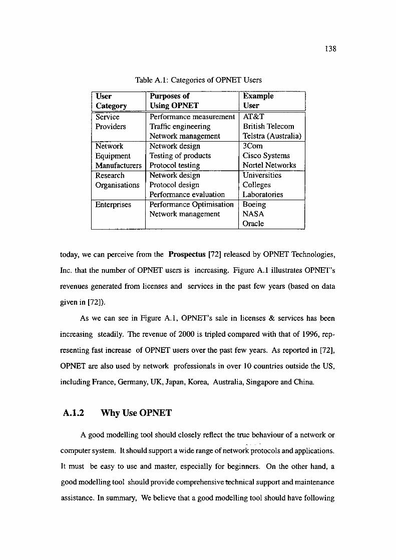
138

Table A. l: Categories of OPNET Users

User Purposes of Example Category UsingOPNET User

Service Performance measurement AT&T Providers Traffic engineering British Telecom

Network management Telstra (Australia) Network Network design 3Com Equipment Testing of products Cisco Systems Manufacturers Protocol testing Nortel Networks Research Network design Universities Organisations Protocol design Colleges

Performance evaluation Laboratories Enterprises Performance Optimisation Boeing

Network management NASA Oracle

today, we can perceive from the Prospectus [72] released by OPNET Technologies,

Inc. that the number of OPNET users is increasing. Figure A.1 illustrates OPNET's

revenues generated from licenses and services in the past few years (based on data

given in [72]).

As we can see in Figure A.1, OPNET's sale in licenses & services has been

increasing steadily. The revenue of 2000 is tripled compared with that of 1996, rep

resenting fast increase of OPNET users over the past few years. As reported in [72],

OPNET are also used by network professionals in over 10 countries outside the US,

including France, Germany, UK, Japan, Korea, Australia, Singapore and China.

A.1.2 Why Use OPNET

A good modelling tool should closely reflect the true behaviour of a network or

computer system. It should support a wide range of network protocols and applications.

It must be easy to use and master, especially for beginners. On the other hand, a

good modelling tool should provide comprehensive technical support and maintenance

assistance. In summary, We believe that a good modelling tool should have following

properties:

20,-----.------,----,-------,-------,------,

1996 1997 1998 Year

1999 2000

Figure A.I: Growth in revenues of software licenses & services.

139

• Versatile: able to simulate various network protocols/applications under a

wide range of operating conditions

• Robust: provide users with powerful modelling, simulation, and data analysis

facilities

• User-friendly: easy to use and master

• Traceable: easy to identify modelling problems and simulation faults

OPNET is hailed by network professionals because it has all these properties.

OPNET is a software package that has been designed with an extensive set of features.

It can be tailored to suit almost every need of network protocol designers, network

service providers , as well as network equipment manufacturers. OPNET supports most

network protocols in existence, both wireline and wireless. It can be used to model and

analyse a complex system by performing discrete event simulations.

We decided to use OPNET as the simulator for our simulation study because

OPNET supports some useful features and facilities which are not supported by other

140

simulators. These features/facilities include:

• Built-in confidence level: To our best~ knowledge, OPNET is the only simu

lator that has built-in confidence level facility. This allows us to determine if

the simulation results have been collected with acceptable confidence level. In

our simulation study, simulation results are collected with a confidence level

greater than 95%, as recommended in [27].

• Built-in model library: OPNET supports a wide variety of networking de

vices manufactured by leading network equipment vendors. This makes it

possible to build network model easily. More importantly, many queueing al

gorithms (e.g. WFQ, RED, CBQ, etc.) are already implemented in OPNET

routers. In our simulation study, we implement our proposed algorithms in

routers and compare with WFQ. By using OPNET, we can be confident that

various router algorithms are implemented correctly and the results are trust

worthy.

• MPEG video traffic generator: OPNET can generates MPEG video p~cket

stream based on a number of parameters specified by user. In our simulation

study, we simulate MPEG-2 video transmission over IP networks. MPEG-2

video packets are generated by video sources and transfered by UDP layer.

With OPNET MPEG video traffic generator, we just need to specify some

high-level parameters, such as bit rate, frame rate, image size, compression

algorithm, etc. This ensures that the MPEG-2 video application is simulated

correctly.

• Data collection tool: OPNET supports advanced data collection facility. The

probe object can be configured to specify the name of the probe, statistic, and

the precise location of data collection. This· allows us to monitor statistics of

any object (e.g. router, link, workstation, etc.) while simulation is running.

141

In our simulation study, we use this feature to monitor the identification of

dropped video packets.

• Data Analysis tool: OPNET's built-in analysis tool has powerful capacity to

manipulate and present simulation results graphically. This allows us to col

lect various results (e.g. short-term TCP throughput, average TCP throughput,

short-term packet loss rate, average packet loss rate, etc.) conveniently.

A.2 OPNET Explored

In OPNET, modelling is divided into a number of modelling levels (or layers),

each with different level of detail and complexity. The detailed operation of a mod

elling layer is hidden from its adjacent higher layer. This feature makes OPNET a very

powerful modelling tool which can be tailored to suit different modelling purposes.

For example, an ISP may use OPNET for resource planning on its networks. The ISP

may choose to work at the highest modelling level (Project Editor) without knowing

the detailed operation of protocols/algorithms run in routers. A protocol designer may

need to dive into the lowest level (Process Editor) to make any modification to an ex

isting protocol or algorithms. Modelling in OPNET can be divided into three levels, as

listed below:

• Project modelling

• Node modelling

• Process modelling

In this section, we take a top-down approach to explore the operation of each

modelling level, with reference to OPNET 7 .O.B. We will also briefly describe other ...

facilities (such as Simulation Tool, Data Collection Tool and Data Analysis Tool) pro-

vided by OPNET. Due to lack of space, we concentrate our description on what mod-

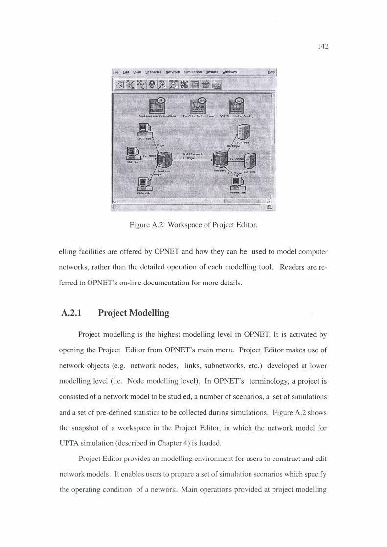
142

Figure A.2: Workspace of Project Editor.

elling facilities are offered by OPNET and how they can be used to model computer

networks, rather than the detailed operation of each modelling tool. Readers are re

ferred to OPNET's on-line documentation for more details .

A.2.1 Project Modelling

Project modelling is the highest modelling level in OPNET. It is activated by

opening the Project Editor from OPNET's main menu. Project Editor makes use of

network objects (e.g. network nodes, links, subnetworks, etc.) developed at lower

modelling level (i .e. Node modelling level) . In OPNET's terminology, a project is

consisted of a network model to be studied, a number of scenarios, a set of simulations

and a set of pre-defined statistics to be collected during simulations. Figure A.2 shows

the snapshot of a workspace in the Project Editor, in which . the network model for

UPTA simulation (described in Chapter 4) is loaded.

Project Editor provides an modelling environment for users to construct and edit

network models. It enables users to prepare a set of simulation scenarios which specify

the operating condition of a network. Mai n operations provided at project modelling

143

level can be summarised as below:

• Create and edit network models

• Edit attributes of network nodes

• Verify link consistency

• Import network topology and traffic

• Define simulation scenarios

• Collect simulation results

• View simulation results

A network model can be constructed with Project Editor by using network objects

in OPNET's built-in object palette. The network palette contains network objects

(e.g. subnetworks, network devices, links, etc.) which form the fundamental "building

blocks" for building a network model. A network model is created by "dragging and

dropping" objects from an object palette. OPNET's model libraries contain objects

that model a wide variety of network protocols and equipment. OPNET also supports

nested network modelling in which a network can be mode-led as a node in its parent

network model. The child network model is referred to as a subnetwork. Network

models can also be created automatically by using the Rapid Configuration facility.

Rapid Configuration operation supports numerous network topologies, such as star,

bus, ring, mesh, etc. A network model can also be constructed by importing network

topology information collected from a real network.

Network objects are characterised by a set of prograJnmable attributes. At

tributes specify the node model of a network object and a number of parameters

associated with the network object. It is the attributes of a network object that de

termines the behaviour of the mode-led network node. The attributes of an object can

be viewed and modified by right clicking on the object.

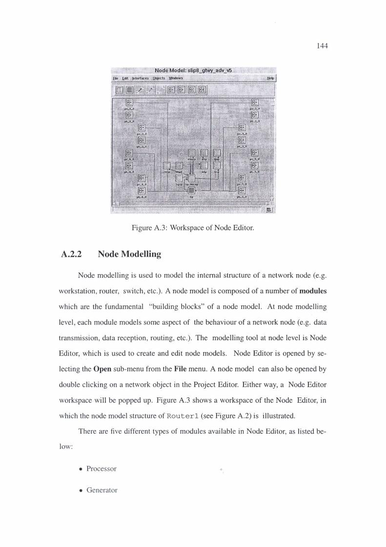
A.2.2

Node Model: slip8_gtwy_adv_v5 [lie fdit Jnterfaa!S Qajects ~$

Figure A.3: Workspace of Node Editor.

Node Modelling

144

Node modelling is used to model the internal structure of a network node (e.g.

workstation, router, switch, etc.). A node model is composed of a number of modules

which are the fundamental "building blocks" of a node model. At node modelling

level, each module models some aspect of the behaviour of a network node (e.g. data

transmission, data reception , routing, etc.). The modelling tool at node level is Node

Editor, which is used to create and edit node models. Node Editor is opened by se

lecting the Open sub-menu from the File menu. A node model can also be opened by

double clicking on a network object in the Project Editor. Either way, a Node Editor

workspace will be popped up. Figure A.3 shows a workspace of the Node Editor, in

which the node model structure of Rou terl (see Figure A.2) is illustrated.

There are five different types of modules available in Node Editor, as listed be

low:

• Processor

• Generator

145

• Queue

• Transmitter

• Receiver

Each type of module is used to model a particular function of the operation of a

network node. A processor module represents a generic process. A generator module

is used to model packet generation. The generator module can generate packets as per

specified Probability Density Function (PDF) and packet format. The queue module

models a queueing process. A queue module may consist of any number of subqueues.

Transmitter modules and receiver modules are used to model packet transmission and

packet reception respectively.

Another type of node objects is "streams", which are generally used to connect

modules (e.g. generator, queue, Tx/Rx modules, etc.). OPNET defines three different

types of streams. They are:

• Packet Stream

• Statistic Stream

• Association Stream

A.2.3 Process Modelling

A process defines a specific operation of a system, e.g. traffic generation, routing,

queueing, etc. It represents functionality that can be implemented in software. In

general, a process is composed of blocks of source cod~s. Process models are the

lowest level of objects in OPNET. A process model is used as an attribute of a node

model (which is in tum used as an attribute of a network model) in OPNET's modelling

hierarchy. In OPNET, each protocol or algorithm is mode-led as a process. A process

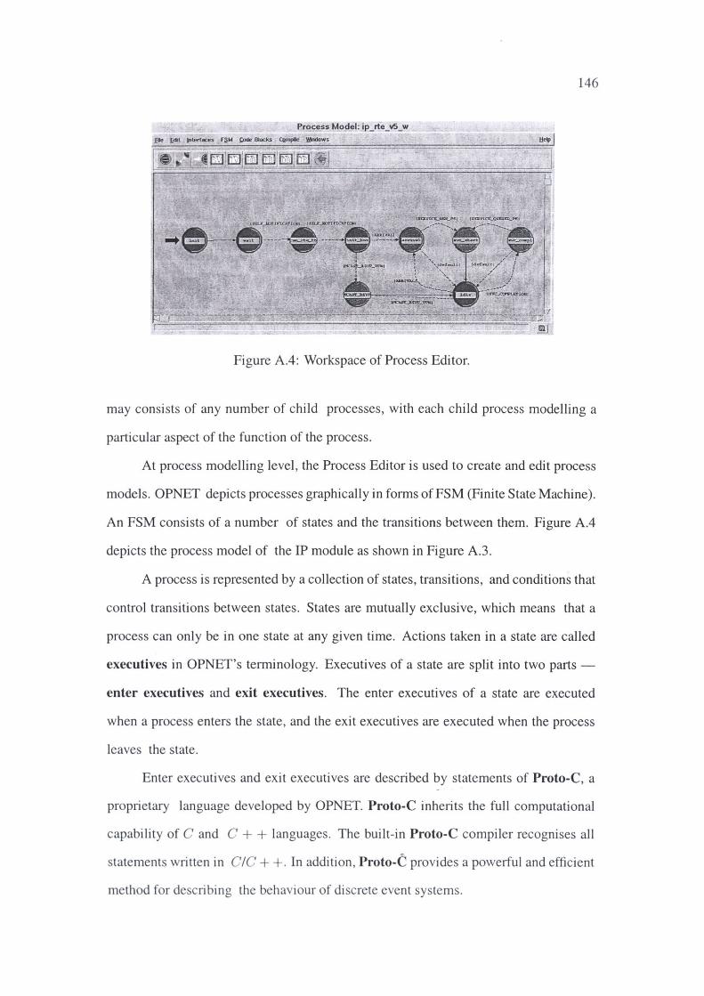
146

Process Model: ip_rte_v5_w

Figure A.4: Workspace of Process Editor.

may consists of any number of child processes, with each child process modelling a

particular aspect of the function of the process.

At process modelling level, the Process Editor is used to create and edit process

models . OPNET depicts processes graphically in forms of FSM (Finite State Machine).

An FSM consists of a number of states and the transitions between them. Figure A.4

depicts the process model of the IP module as shown in Figure A.3.

A process is represented by a collection of states, transitions, and conditions that

control transitions between states. States are mutually exclusive, which means that a

process can only be in one state at any given time. Actions taken in a state are called

executives in OPNET's terminology. Executives of a state are split into two parts -

enter executives and exit executives. The enter executives of a state are executed

when a process enters the state, and the exit executives are executed when the process

leaves the state.

Enter executives and exit executives are described by statements of Proto-C, a

proprietary language developed by OPNET. Proto-C inherits the full computational

capability of C and C + + languages. The built-in Proto-C compiler recognises all

statements written in CIC++. In addition, Proto-C provides a powerful and efficient

method for describing the behaviour of discrete event systems.

147

A.2.4 Data Collection Tool

In OPNET, advanced data collection is supported by the Probe Editor which is

activated by selecting Choose Statistics (Advanced) operation from the Simulation

pull-down menu (see Figure A.2). The Probe Editor is used to create probe objects

which specify where to collect statistics and what statistics to be collected (like the

signal probes of an oscilloscope). Like other OPNET objects, a probe object also has a

set of attributes which can be configured to specify the name of the probe, statistic, and

the precise location of data collection, etc. Probe objects created in the Probe Editor

are saved in a probe file which can be used as an attribute of a simulation object.

A.2.5 Simulation Tool

With advanced simulation tool, users can define their own simulation sequences

and control the execution of simulation. A simulation sequence may consist of any

number of simulation objects, with each simulation object containing a set of config

urable attributes. A simulation object may define one or more simulation runs, depend

ing on values of application-specific attributes. A simulation sequence can be saved in

a file for later use. The advanced simulation tool provides following capabilities which

are not supported by the Project Editor:

• Definition of simulation sequences

• Collection of both vector and scalar statistics

• Control of simulation execution

It is possible to specify more than one simulation object in a simulation sequence.

Each simulation object may even have a different set of attributes (e.g. different net

work models, probe files, durations, etc.). The sin1ulation sequence can be executed

unattended.

148

In OPNET, simulation can also be run in debugger mode. This is supported by

the OPNET Simulation Debugger (ODB). ODB enables users to control simulation

execution interactively and track down modellfog problems quickly. Numerous ODB

commands have been developed to allow users to set breakpoints, access state vari

ables, and modify object attributes, etc.

A.2.6 Data Analysis Tool

Analysis Tool provides the capability to manipulate and present simulation re

sults graphically. Simulation results are saved in the output vector file or output

scalar file during simulation execution. Analysis Tool extracts data from output vec

tor/scalar files and displays it in analysis panels. The Analysis Tool is usually used

to process statistics specified in probe objects that are created in the Probe Editor. It

is activated by selecting View Results (Advanced) operation from the Results pull

down menu, after simulations are run with advanced configuration. Action buttons

on the menu bar in the Analysis Tool support operations to create vector panels and

scalar panels, which are used to display vector statistics and scalar statistics re~pec

tivel y. Other services provided by the Analysis Tool include:

• Apply numerical processing to statistics

• Edit trace colour, style, and thickness, etc.

• Make graph template

• Export data to spreadsheet

A.2.7 Parameter Editors

Parameter models are used as assignments for attributes of objects. There are

four different parameter models (as listed below). Each parameter model is created by

its corresponding editor.

149

• Link model

• Packet format model

• Interface Control Information (ICI) model

• Probability Density Function (PDF) model

A.3 Practical Examples

In this section, we describe development of OPNET simulation models, using

the simulation model described in Chapter 4 as an example. It is intended to help new

OPNET users get familiar with some basic modelling skills of OPNET Modeler.

A.3.1 Process Model Development

Developing process models is the most difficult part in OPNET simulation. The

process model for routers in our simulated network is based on the standard IP router

process ip_rte_v4 available in OPNET's model directory op...models. We moc;lified

the IP process to implement UPTA algorithm. The modified IP process model is named

ip_rte_v5_w (shown in Figure A.4). Actually, UPTA algorithm is implemented in a

child process called ip_outpuLv5_w. The child process is responsible for queueing

at each output port of the router. It is called (by its IP parent process) after an arriving

packet has been processed and forwarded to the corresponding output port. Figure A.5

shows the queueing child process model, in workspace of Process Editor.

As shown in Figure A.5, the child process consists of four states. State en

queue is responsible for queueing, and State extract is responsible for removing

packets from the queue and transmitting them to the output link. The UPTA algorithm

is implemented in State enqueue. Proto-C code~ are composed in each state. For

example, Figure A.6 shows Proto-C codes for State enqueue, which is opened by

150

Pro~ess Model: ip_output_v5_w file fdil .Interfaces F,;iM !:ode Blocks Cqmpile '.ll!lndows !!elp

Figure A.5: Child process model (for queueing) of IP process.

double clicking at the upper half of the state (enter executives block).

The Proto-C codes in State enqueue perform all queueing functionality of

routers (where UITA resides). Function procedure calls for arrival rate estimation

(Eq. (4.3) and fairshare estimation (Eq. (4.4) and Eq. (4.5)) are defined in the Func

tion Block of the child process. The Function Block is opened by clicking at the action

button FB on the menu bar (see Figure A.5). Figure A.7 shows Proto-C codes in the

FB block.

A process is compiled into executable codes by clicking at the Compile action

button " +-" on the menu bar (see Figure A.5). To make the queueing child process

"visible" to its parent process (IP process model), we declare the child process in its

parent's process model. This is done by choosing Declare Child Process Models ...

from the File pull-down menu .

en 1.1e1.1e : Enter Execs

/ • · TnL • • to.t • 1• .:..n et;,. ... .,. o ! wnqu.-.a i. l>o;[I lh • u1o:r.u.nq '• ( , • • pa, -. <or1. . ·: ,u . ~ <l<• l ,uU L-4' v .: l &II au, u!" t ll • Jl • l • • , 1• · n r ll•+ 1111.n: .. ,:.,. r,,r,_=rn, • t·[ -.i :t •1r" n1 t-t1 i. r : c + · · , t •• 1::it~nc• c:i = c••.or u : :-• • tr.e _:,., ~ •t "'•!l e.. • ~: . • •/ f • • rb t • tl'!.a t t ll• VA Clc • t , . 11fT!'ed1 .. t• ly • ...,t .~ .s~ l qu..., .. :• • .). J: • ~ ty

f • ~ •r• t b• .nc-..aunq ~':"< • : f"rai, t h • o.~t ......,.., ,.,, . 1t ((pq,t:r ., ! Packet• ) <!-9--P='- ~"'°-c.=-• (I) • • OPC_JllL)

" I II / • ,tgp l b• 11 .1n• .. d a : , cr. ,[ tt::.• pocbt C Q.tl not bi, o c-,=-e.ac...? . ' /

ou.tp,.at_,1Ct1oc-._ wa.nu.no;a_,_ • • 09._pru,t ( ·;,;,;o...)j~ ~•;, 'Jdt u ,. l,,<> ~<·t l :':-.a. ~:.,1 "'"''""· t ;:;.1 ...::,,,.•·· .u, I

n / • ~ t t he J CJ ccn,1 nq w, th :n• p,,, ::1<et . 'l't u • re.,: " / U 1 • v , ll r•,,11: ry l:lvt ., :-r,,. .. t [ ~....,. ,.,. .. i 1•u: t.11<\ l .. r r1 ..... 1 ~ , ...... .

qQ"_ua_ptr • ap_pl(_•c. . ....s;,• t: l p!cptcr-1 1 op_1 c1_ attr_9et lq,;,,._>i=-1_ptr , •~n=~_ L!"• -::"' • ,~1.fGCe) I

II ~J>l<-_p.C.!_ • cc-• l picpt r , !1 ~. ·a• , ,p1c_N_ptrl1

"

"

f • ~• the ~. ~ot:.an .a.t' th iP::"t> •• a-> ! Cl ' / , t' (~ _.ua_ptr • • OPC...JllL)

' outp.at_ j t' o e e _wanunq~• t1111•..PTU1t ( 'T:: • ! :''l · ~ .. ! :::l,,pt:- :. ,1 1':.:.. I 1 I

/ ' •:.t l f\" • 1:. • ,:,t' t J-.• ;,,o..:kttl 'r. l • WLll I;-. u cw~ t c

/ • wr.;t• • t.it. •:. :.c; • pk_••"• • ap___P'l_~t .. :_., .. ,. ,._c;et !pk;ltd ,

JI ; · ,C.,.t ,. ~ : . t o l: h • r;:: h • .,,,,, • r • i c;ii.,_Jio<_nt'.l_ occ• •" h;,6cpt.- , t . -• i !• • , hp_ Cd.J>l d 1

, • ~t t r1e 1ou:-e-. !I- cdC:-••c o t' t."u • ~k• c ~; • rc_1p_adclr • ,p_td_pt .. ->orc:-_"6:tr,

/ • i::o. t • r.nLn• tt•• t' l~ II) !'ar t:U.f' p,, eio:ttt • ,: a t' ( Ul_.,t'•c-e ,,.. 0)

!. • ..,..I d • t'l°"_cl A•• ir'y l• .-,:,_ip_Addd 1

Figure A.6: Proto-C codes in enter executives block.

/" Flow ,; l.,,.c • •t' • -:otaan ' / •tot, c .a.nt

,.. t'law_c-1 ... . iry (IP'f'.J,ddr-• • rC'_lp_Gddrl ,., (

ip_addr_• tr UPC~-~UN} 1 t'law_l O 1

n, , . -nu. t UU(."t l<,:,i l c:l :o•• •f1 ... " ''-~ '.;..,,; ~ ,; lc.+ t • .;. nlQ , 1 .... , .. · ; 1 14 / ' for ' A~ llc: , t y . - Q{ll \' <:.'\~ t l'I ♦ ..:,,ire • IP ~ r e11.- ' /

rlN l t'k,w_el-• ify (.r,;_ip_addr)) 1

lll / • Ccxw• :-t Il- ..ddr e111 .- , nto e~u: r •t ouir;- '/ 111 a.p_oddc-•~iat (1p_oddr_e tr· , • =_.,p _ llddr),

TIO ' • O..t .. :ffl.ln•P Clnw 10 t-<i .- ""' _,., _..,. ,,-~., I:.> ao!r-• ' I

1U •t' l • t r cmp lip_lloddr_•tr , ~.i :, 1.1. ; .l' l - 0) t' law_ID • 0:

• h • 1t' l • trcq> ( 1p_ 6ddr_• t r , .tl14 .:.\> ::; . • ;,,· ) - 0l 1M l'lo._IO • l t ,n •1 • • ~t' C• trc,q, hp_addr_• tr, · ::: i:. :::.1 0 ':, .ll,)M ) .. O)

t'lo._JD • :Z : •l••

l!'lca,_ID • - 1 1 ... ,,. ntrr (l'low_IDI I

I .. , '" • tot! ,; Boolean lH wt'q__p,;,_-,qu-• IPocit•t 'pl,;ptr, o-T_Qm_Plct_ l.lll'o •pkt_lllto_ptr) tn l ... "' ... ...

~T_ oC_pkt:• , --~T_oC_pkt• _ia_subqu-• 1 C'\U"reat_t:oto..l_p....ce.-_ol!'_pkt: • : pocit•t:- •11 • 1 dr,op.J)r"QD/

Figure A.7 : Proto-C codes in Function Block (FB) . •

151

152

A.3.2 Node Model Development

Once we have all process models for a node, developing node model is a triv

ial task. We load our IP process model into the IP module of the standard IP router

node model (available in OPNET model directory opJ11odels). We first open the

standard IP router node model in Node Editor. We then open the Attributes dialog

box of the IP module (see Figure A.3), and change the process model attribute to

our modified IP process model ip_rte_v5_w. We save the node with a new name

slip8_gtwy_adv_v5. The node model for routers is now ready for use to build net

work model in Project Editor.

A.3.3 Network Model Development

The network model (shown in Figure A.2) is built in the workspace of Project

Editor, using OPNET's built-in object palette. For Routerl and Router2, we use

the node model we just developed. To do this, we open the Attributes dialog box of

Routerl andRouter2 respectively, and change the model attribute to slip8_gtwy_adv_v5

In the network model, there are three attribute objects (on top of the worksp'ace):

Application Definition, Profile Definition, and QoS Attribute Config. We define our

TCP/UDP and video applications in Application Definition, and define traffic profile

for each source host in Profile Definition. QoS Attribute Config is used to define queue

configuration, such as queue size, subqueue classification, and weight for each sub

queue (WFQ), etc.

A.3.4 Simulation Execution

Simulation can be run by clicking at the Configure/run simulation action button

on the menu bar in Project Editor (see Figure A.2). The simulation attribute dialog box . will pop up after the Configure/run simulation action button is clicked. We specify

simulation duration and other simulation parameters in the dialog box. Before we run

153

the simulation, we need to choose statistics we want to collect. This can be done by

choosing Choose Individual Statistics ... from Simulation pull-down menu, or right

clicking on each individual object we are interested.

After the simulation execution is completed, we can view simulation results

graphically by using OPNET's Analysis Tool. This can be done by choosing View

Results ... from the Results pull-down menu. To compare results for different simu

lation scenarios (for example WFQ and WFQ+ ), we can choose Compare Results ...

from the Results pull-down menu.

Graphs of results can be exported in TIFF or GIF format by pressing Ctrl-t. Since

graphs in TIFF/GIF format yield poor graphic quality after inserted into a document, we

use Matlab to plot all our simulation results (Matlab can export graphs in EPS format).

We first export simulation results to a text file, and then plot results (using Matlab) by

reading from the text file. To export simulation data, we can right click at a graph and

then choose Export Graph Data to Spreadsheet. ...

A.4 Conclusion

We have presented an introduction to OPNET Modeler, and described our expe

rience with OPNET in this appendix. OPNET Modeler is an object-oriented simulation

tool which provides a visualised simulation environment for network modelling. OP

NET takes hierarchical modelling approach and hides details of a modelling layer from

its higher layers. This greatly simplifies simulation tasks for network engineers and

researchers. We have described the fundamental structure and basic modelling skills of

OPNET Modeler, in combination with our experience with OPNET. We demonstrated

the development of the process model, node model, and network model for the net

work that implements UPTA algorithm described in Chapter 4. We found that OPNET

Modeler is one of few simulators which offer users with greatest freedom and power in

designing and modelling network protocols.

Appendix B

Program Listings

B.1

B.1.1

CPrograms

pkLdrop.c

I* This program simulates dropping packets from I* audio/video applications. It randomly selects I* an audio/video packet to drop with a given I* probability. The dropped packet is replaced /* by a packet of all Os. I* input: original audio/video file; drop prob. I* output: reconstructed audio/video file

#include <stdio.h> #include <stdlib.h> #define SEED 100 #define PKT _SIZE 184

unsigned byte_count=0; unsigned num_fulLpkt; unsigned byte_left; unsigned drop=0; long offset; float drop_prob;

char inname[20); /* input file name */ char outname[20]; /* output file name */

main() { int ij; int c; float random_ value;

FILE *fopen(),*inptr, *outptr ;

*I *I *I *I *I *I *I

10

20

30

I* Prompt for the file name of input file */ printf( 11 Enter input file name ... \n 11 );

scanf( 11 % s 11 , inname);

I* Prompt for the file name of output file *I printf("Enter output file name ... \n •); scanf( n % s n , outname);

I* Prompt for packet drop probability *I printf( 11 Enter packet drop probability ... \n 11 );

scanf(" %f ", &drop_prob);

/* Determine how many packets in the file *I if ((inptr=fopen(inname, 11 r•)) == NULL)

printf("Cannot open input file\n 11 );

while (fgetc(inptr) != EOF) byte_count++;

fclose(inptr);

/* Number of full packets *I num_fulLpkt = byte_count/PKT _SIZE;

I* Number of bytes in the last packet *I byte_left = byte_count % PKT _SIZE;

I* Print stat info *I printf("Number of full packets: %d\n 11 , num_fulLpkt); printf( 11 Number of bytes in the last packet: %d\n 11 , byte_left);

I* Process full packets ( all packets except the last one) *I if ((inptr=fopen(inname, "r 11 )) == NULL)

printf( 11 Cannot open input file to read\n"); if ((outptr=fopen(outname, 11 w")) = NULL)

printf("Cannot open output file to write\n 11 );

/*Generate a random number between O and 1 */ srand(SEED);

for (i=0; i<num_fulLpkt; i++) { random_value = (float)rand()/32768; if (random_value > drop_prob)

{I* Accept the packet *I for (i=0; j<PKT _SIZE; j++)

{ c = fgetc(inptr); fputc(c, outptr); }

} else

{I* Drop the packet (set the packet to all Os) */ for (i=0; j <PKT _SIZE; j++)

{ c= '\x00'; fputc(c, outptr);

155

40

so

60

70

80

}

}

I* Adjust file pointer for input file *I offset = (i+ 1 )*PKLSIZE; fseek(inptr,offset,O); drop++; }

I* Process the last packet *I /* As the last packet usually contains 'End of Sequence' *I I* info, we do not drop it if possible. *I if (byte_left != 0)

{ for (i=O; i<byte_left; i++)

{ c = fgetc(inptr); fputc(c, outptr); }

} printf( 11 Dropped packets: %d \n 11 , drop);

fclose(inptr);

156

90

100

fclose(outptr); 110

}

B.1.2 video_rec.c

/* This program reconstructs audio/video file at the receiver. *I I* It takes the original video file and segment list (which *I I* contains /Ds of segments received by the receiver) as *I I* input and creates a video file, simulating video *I I* transmission over a network. *I #include <stdio.h> #include <stdlib.h>

#define PKLSIZE 184 /* payload of an MPEG TS packet *I

unsigned byte_count=O; unsigned fulLseg; unsigned lasLseg; unsigned seg_id; unsigned seg_id_rcv; char fnarne_rcv[20];

FILE *fopen(),*fpl,*fp2,*fp3;

main() { int n,m; char str[1 OJ; char buff[200]; long offset;

•

10

20

/* Determine the size of the original video file *I if ((fpl=fopen(" susi_0lS .m2v", "r")) == NULL)

printf("Cannot open file susi_0lS .m2v\n"); while (fgetc(fpl) != EOF) '

byte_count++; fclose( fp 1);

I* Number of full segments in the video file */ fulLseg = byte_count/PKT _SIZE;

I* Number of bytes in the last segment *I lasLseg = byte_count - fulLseg * PKT _SIZE;

I* Open the original video file for read *I if ((fpl=fopen("susi_0lS .m2v", "r")) == NULL)

printf("Cannot open file susi_0lS .m2v\n");

I* Open received segments list for read */ if ((fp2=fopen(" segid_dst. txt ", •r•)) == NULL)

printf("Cannot open file segid_dst. txt\n");

I* Open file to save the reconstructed video file */ printf("Enter file name for the reconstructed video file ... \n"); scanf( " % s • , fname_rcv); if ((fp3=fopen(fname_rcv, "w")) == NULL)

printf("Cannot open file to write\n ");

I* Start reconstructing video file from Segment #1 *I seg_id = 1; while ((fgets(str, 10,fp2)) != NULL)

{ sscanf(str, "%d", &seg_id_rcv); if (seg_id_rcv > fulLseg)

break; else

n = seg_id_rcv - seg_id;

if (n > 0) /* n segments are lost *I { I* Write n segments of all 'O' to the reconstructed video file *I losLseg_write (n * PKLSIZE);

/* Adjust file pointer fpl *I offset = ((seg_id - 1) + n) * PKLSIZE; fseek(fpl ,offset,O); seg_id += n; }

I* Copy to received segment */ I* to the reconstructed video file. */ fread(buff,PKT _SIZE, 1,fpl); fwrite(buff,PKT _SIZE, 1,fp3); seg_id++; }

157

JO

40

50

60

70

80

m = fu!Lseg - (seg_id - 1 ); if (m > 0)

/* m segments are lost when the simulation ends */ { I* Write m segments of all '0' to the reconstructed video file *I losLseg_write (m * PKLSIZE);

I* Adjust file pointer fpl *I offset = ((seg_id - 1) + m) * PKLSIZE; fseek( fp I ,offset, 0); }

/* Copy the last segment to the reconstructed video file, *I /* as it contains 'End of Sequence' info. *I fread(buff,lasLseg, 1,fpl); fwrite(buff,lasLseg, 1,fp3);

fclose(fpl); fclose(fp2); fclose(fp3); }

I* Function definition for lost...seg_write() *I losLseg_ write (int byte_to_ write) { int i; int c;

for (i=O; i<byte_to_write; i++)

}

{ c= '\x00'; fputc(c, fp3); }

B.1.3 pic-1ist.c

I* This program correlates received frames with sent I* frames. Due to frame loss during transmission, a I* transmitted frame may have a different frame # in the /* received video sequence. e.g., Frame #100 may be received I* as Frame #80 at the receiver. Jn order to calculate PSNR I* correctly, we need to map received frames to frames I* sent by the sender. This program uses the 'start byte' I* to determine the identity of a frame. It creates 2 I* lists - one contains frames received by the receiver; I* and the other list contains the corresponding frames /* sent by the sender. These frame lists will be used to I* calculate PSNR using Matlab

#include <stdio.h> #include <stdlib.h> #include <string.h>

*/

-

158

90

JOO

110

*I *I *I

*I *I *I *I· *I *I JO

*/ *I

char info_rcv[2O]; /* header info file name for received video */ int totaLrcv = O; /* total number of frames decoded *I

FILE *fopen(),*fpl,*fp2,*fp3,*fp4;

main() { int snd_pic_num = O; int rcv_pic_num; int starLbyte; char str[1OO];

I* Open files for read *I I* Open file hdrinfo.txt I* (which contains header info for sent video file) *I if ((fpl=fopen( 11 hdrinfo. txt", 11 r 11 )) == NULL)

printf("Cannot open file hdrinfo.txt\n");

*I

I* Prompt for file name of header info for received video file *I printf("Enter header info for the received video file ... \n 11 );

scanf( 11 %s 11 , info_rcv);

I* Open file to save sent frame list *I if ((fp3=fopen( 11 ls_snd. txt 11 , 11 w11 )) == NULL)

printf( 11 Cannot open file to write\n 11 );

I* Open file to save received frame list */ if ((fp4=fopen(" ls_rcv. txt 11 , 11 w11 )) == NULL)

printf( 11 Cannot open file to write\n");

I* Loop through the hdr info file (for original video) and *I I* search for 'start..byte' of each frame while ((fgets(str,1OO,fpl)) != NULL)

{ if (strncmp(str, "picture header", 14) == 0)

}

{ sscanf(str, "picture header (byte %d) ", &starLbyte);

I* Determine whether or not the 'start..byte' appears *I I* in the hdr info for the sent video file */ rcv_pic_num = match_find (starLbyte); if (rev _pic_num != -1)

{ I* The frame is received *I fprintf(fp3, 11 ori%03d. jpg\n", snd_pic_num); fprintf(fp4, "w%03d.jpg\n", rcv_pic_num); totaLrcv++; }

snd_pic_num++; }

...

*I

printf("Total number of frames sent: %d\n", snd_pic_num); printf("Total number of frames received: %d\n 11 , totaLrcv);

159

20

30

40

50

60

70

fclose(fpl); fclose(fp3); fclose(fp4); }

I* Function to correlate received frame # with int match_find (int starLb)

sent frame # *I

{ int pic_num = O; int startbyte; char string[100];

/* Open header info file for the received video file */ if ((fp2=fopen(info_scv, "r")) == NULL)

printf("Cannot open header info file for received video file\n");

I* Loop through the hdr info file (for received video) *I I* and search for 'start...byte' of each frame *I while ((fgets(string, 100,fp2)) != NULL)

{ if (strncmp(string, "picture header", 14) == 0)

}

{ sscanf(string, "picture header (byte %d) ", &startbyte);

I* Compare 'start...byte' with the one found in */ /* the hdr info file for the original video *I if (startbyte == starLb)

{I* There is a match, return the frame # ( decoded frame) *I fclose(fp2); return (pic_num); }

I* No match yet, continue searching *I pic_num++; }

/* No match found, return -1 *I fclose( fp2); return (-1); }

B.2

B.2.1

Matlab Program

psnr_cal.m

% This program calculates PSNR for each video frame received. % It takes 2 frame name lists ( one for snd; one for rev), and % 2 frame lists ( snd frames and rev frames) as input. % It first calculates the PSNR value for each frame received. % It then calculates the intelligibility index based on PS~.

clear;

160

80

90

100

110

% Open files for read frames = fopen(' ls_rcv. txt', 'rt');

% Read frame names into a matrix [A_frm,count) = fscanf(frames,' %s '); fclose(' all');

% Open file (name list) for sent/received frames fptrl = fopen('ls_snd.txt','rt'); fptr2 = fopen(' 1s_rcv. txt', 'rt');

% Initialize total number of intelligible frames received inLfrm = O;

for frm_num = 1 :count

% Get a frame name and read the frame into a matrix snd_frm_f = fscanf(fptrl,' %s ', 1 ); snd_frm = imread(snd_frm_f); rcv_frm_f = fscanf(fptr2,' %s ', 1 ); rcv_frm = imread(rcv_frm_f);

% Determine frame size frm_size = size(snd_frm); row = frm_size(1 ); column = frm_size(2);

% Convert pixel values of the sent frame % into double (for PSNR calculation) A(:,:,:) = double(snd_frm(:,:,:))/255; snd_frm = double(A);

% Convert pixel values of the received frame % into double (for PSNR calculation) B(:,:,:) = double(rcv_frm(:,:,:))/255; rcv_frm = double(B);

% Work out difference in every pixel of a frame diff = ((snd_frm - rcv_frm).~2)/(row*column);

% Mean Square Error (MSE) for each color component difLR = 0.3*diff(:,:, 1 ); %R difLG = 0.59*diff(:,:,2); %G difLB = 0.11*diff(:,:,3); %B

o/o Calculate composite MSE and PSNR difLfrm = difLR + difLG + difLB; psnr(frm_num) = 1 O*log10(255 ~ 2./(sum(sum(difLfrm)) + eps));

% Check to see if it is an intelligible frame if psnr(frm_num) > 65

inLfrm = inLfrm + 1; end

end

161

10

20

30

40

50

60

fclose(' all');

% Calculate intelligibility index IN_index = inLfrm/375;

save psnr; save IN_index;

162

70

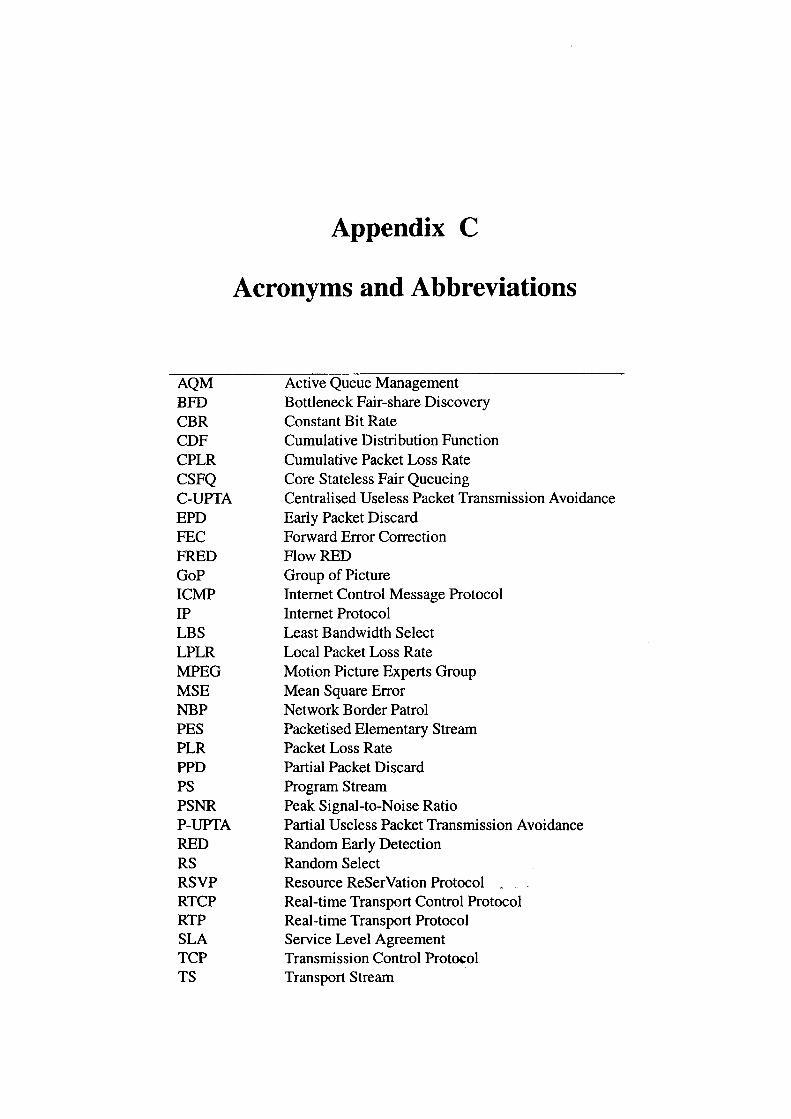
AQM BFD CBR CDF CPLR CSFQ C-UPfA EPD FEC FRED GoP ICMP IP LBS LPLR MPEG MSE NBP PES PLR PPD PS PSNR P-UPfA RED RS RSVP RTCP RTP SLA TCP TS

Appendix C

Acronyms and Abbreviations

Active Queue Management Bottleneck Fair-share Discovery Constant Bit Rate Cumulative Distribution Function Cumulative Packet Loss Rate Core Stateless Fair Queueing Centralised Useless Packet Transmission Avoidance Early Packet Discard Forward Error Correction Flow RED Group of Picture Internet Control Message Protocol Internet Protocol Least Bandwidth Select Local Packet Loss Rate Motion Picture Experts Group Mean Square Error Network Border Patrol Packetised Elementary Stream Packet Loss Rate Partial Packet Discard Program Stream Peak Signal-to-Noise Ratio Partial Useless Packet Transmission Avoidance Random Early Detection Random Select Resource ReSerVation Protocol Real-time Transport Control Protocol Real-time Transport Protocol Service Level Agreement Transmission Control Protocol Transport Stream

UDP UFM UPT UPTA WFQ

User Datagram Protocol Unintelligible Flow Management Useless Packet Transmission Useless Packet Transmission Avoidance Weighted Fair Queueing

164

Appendix D

Publications

This appendix lists all papers published during my PhD candidature. Papers related to this thesis are marked with asterisk.

1. *J. Wu and M. Hassan, "The Issue of Useless Packet Transmission for Multimedia over the Internet", accepted for publication in Computer Communications, Elsevier Science, Vol. 26, Issue 12, pp1240-1254, July 2003.

2. *J. Wu and M. Hassan "Avoiding Useless Packet Transmission for Multimedia over IP Networks: The Case of Multiple Multimedia Flows", technical report, UNSW-CSE-TR-0216, School of Computer Science & Engineering, The University of New South Wales, Sydney, Australia, November 2002.

3. *J. Wu and M. Hassan "Avoiding Useless Packet Transmission for Multimedia over IP Networks: The Case of Multiple Congested Links", technical report, UNSW-CSE-TR-0215, School of Computer Science & Engineering, TheUniversity of New South Wales, Sydney, Australia, November 2002.

4. *J. Wu and M. Hassan "Avoiding Useless Packet Transmission for Multimedia over IP Networks: The Case of Single Congested Link", technical report, UNSW-CSE-TR-0202, School of Computer Science & Engineering, The University of New South Wales, Sydney, Australia, May 2002.

5. J. Wu, part of book chapter "Simulation of TCP/IP Networks" in "High Performance TCPllP Networks", Hassan and Jain (Editors), Prentice Hall, 2003 (to be published).

6. J. Wu, M. Hassan, Huey Ling Lim and Lu Phong Huang, "Implementation of Asynchronous Performance Measurement (APM) Protocol for the Internet", to appear in IEEE International Conference on Telecommunications (IEEE ICT2003), Papeete, France, February 23-March 1, 2003.

7. *J. Wu, M. Hassan, S. Jha, "QPD: A Packet Discard Mechanism for Multimedia Traffic in the Internet", ICICE Transactions Appendix, The Communication Society, ICICE, Tokyo, Japan, 2001, E84-B (11).

166

8. M. Hassan, J. Wu, S. Jha and J. Breen, "OPS-Based Infrastructure for Internet Performance Measurement", IEEE International Conference on Telecommunications (IEEE ICT2001), Bucharest, Romania, June 4-7, 2001. The paper receives Best Paper Award at the conference.

9. M. Hassan and J. Wu, "APM: Asynchronous Performance Measurement for the Internet", the 6th Asia-Pacific Conference on Communications (APCC2000), Vol. 2, pp. 1335-1339, Seoul, South Korea, October 30-November 3, 2000.

10. *J. Wu and M. Hassan, "On Fairness of ATM UBR Service in Carrying Heterogeneous Internet Traffic", IEEE International Conference on Telecommunications (ICT2000), pp. 395-399, Acapulco, Mexico, May 2000.

11. *J. Wu and M. Hassan, "Dynamics of MBD-A Bandwidth Threshold-Based Packet Discarding Algorithm", IEEE International Conference on Telecommunications (ICT2000), pp. 973-977, Acapulco, Mexico, May 2000.

12. *J. Wu and M. Hassan, "Simulation of a Bandwidth Threshold Based Packet Discarding Algorithm for Internet Routers", ICCIT'99, pp. 127-131, Sylhet, Bangladesh, December 1999.

13. *J. Wu and M. Hassan, "Minimum Bandwidth Dropping: A Packet Dropping Mechanism for Multimedia Traffic in the Internet", IEEE International Conference on Telecommunications (IEEE ICT'99), Vol. 1, pp. 431-435, Cheju, South Korea, June 1999.

Documents

Techniques to Avoid Useless Packet Transmission in