Taxes Depress Corporate Borrowing:

Evidence from Private Firms∗

Ivan T. Ivanov† Luke Pettit‡ Toni Whited§

December 27, 2020

Abstract

We re-examine the relation between taxes and corporate leverage, using variation instate corporate income tax rates. In contrast with prior research, we document that cor-porate leverage rises after tax cuts for both privately-held and publicly-listed firms.We use an estimated dynamic equilibrium model to show that tax cuts result in lowerdefault spreads and more distant default thresholds. These effects outweigh the lossof benefits from the interest tax deduction and lead to higher leverage, especially forprivately-held firms. Overall, debt tax shields appear to be a secondary capital struc-ture consideration.

∗The views stated herein are those of the authors and are not necessarily the views of the Federal ReserveBoard or the Federal Reserve System. We thank Celso Brunetti, John Krainer, Mathias Kruttli, Marco Macchi-avelli, Carlos (Coco) Ramırez, and Ben Ranish for helpful comments. We thank Sam Dreith and Sara Shemalifor excellent research assistance. We are grateful to Marc Lovell from the Federal Reserve Board’s Legal Li-brary for preparing a database of legislature/legal library contacts and helping us identify enactments ofstate tax changes.†Federal Reserve Board, 20th Street and Constitution Avenue NW, Washington, DC 20551; 202-452-2987;

ivan.t.ivanov@frb.gov.‡Affiliation Not Provided; lajpettit@gmail.com.§University of Michigan and NBER, Ann Arbor, MI 48109; 734-764-1269; twhited@umich.edu.

1

1. Introduction

A fundamental question in financial economics is how corporate taxes affect business

borrowing. Despite the extensive literature on the topic since Modigliani and Miller (1963),

nearly all empirical evidence is based on samples of large public companies. (Titman and

Wessels 1988; Graham 1996; Heider and Ljungqvist 2015; Faccio and Xu 2015). These stud-

ies document a positive association between corporate taxes and business leverage, con-

sistent with public firms placing high value on debt interest tax shields. Yet, the majority

of economic activity occurs in smaller, bank-dependent, privately-held companies that are

significantly less well-capitalized than public firms (Brown et al. 2020). For example, the

majority of new job creation occurs in privately-held companies (Smith 2007). Moreover,

informational frictions faced by private firms imply that, in contrast to large public firms,

they cannot borrow against their future market value. Thus, taxes affect not only the bene-

fits of borrowing, but the costs. In particular, as we show in a structural model, taxes lower

lender recovery in default, as well as default thresholds via their effect on firm profitability.

Both effects cause firms to decrease leverage. Consequently, the effect of corporate taxes on

business borrowing is an open empirical question.

We attempt to fill this void by investigating both privately-held and publicly-listed com-

panies. We study the evolution of corporate borrowing around changes in state corporate

income taxes since the 1980s, relying on event study techniques in the spirit of Borusyak

and Jaravel (2017). Our results indicate that corporate taxes depress business borrowing

and that companies adjust capital structure shortly after the enactment of state corporate

income tax changes. These tax changes typically become effective one to two years after

enactment, translating into significant firm leverage responses up to two years prior to the

effective year. We find that the average private firm increases leverage up to 3% following

tax cuts, while public firms exhibit a leverage increase of about 2%. Using a comprehensive

sample of corporate borrowing from the syndicated loan market since 1992, we corrobo-

1

rate these findings for the case of tax hikes. These dynamics appear to be driven by tax

cuts (hikes) alleviating (tightening) default thresholds and spreads. Overall, debt interest

tax shields appear to be a secondary consideration for the relation between corporate taxes

and borrowing for both private and public firms.

In addition to the Compustat database, we use two confidential supervisory data sets

that provide us with a convenient empirical setting to examine how corporate taxes and

borrowing are related. Our primary data set comes from the Federal Reserve’s Y-14 Col-

lection and covers privately-held bank-dependent firms in the United States since 2011.

These data provide one of the most detailed accounts of private firms’ balance sheets that

is currently available to researchers. In robustness tests we also rely on the Shared National

Credit database that provides comprehensive coverage of both private and public firms

reliant on the syndicated loan market, which accounts for the vast majority of corporate

commercial borrowing.

We first investigate how tax changes affect privately-held firms, relying on detailed fi-

nancial statement data for small and mid-sized private borrowers from 2011 through 2017.

We focus on state corporate income tax cuts as there are only seven corporate income tax

hikes during this time period, as compared to 62 tax cuts, so state tax increases affect too

small a sample of firms for us to obtain reliable inferences. We show that corporate tax cuts

are associated with significant increases in the leverage ratios of small private firms. For

example, firms’ outstanding debt increases by approximately 3% two years prior to the ef-

fective year of the tax cut and remains significantly elevated at between 1.3% and 2.0% up

to three years after the effective year. While at a first glance the response of firms well before

the effective year of tax changes may be indicative of anticipation effects and pre-trends,

we show that these responses correspond to the enactment date of the tax changes, which

typically precede the effective dates by one to two years. Conducting the same event study

using the enactment date instead of the effective date of tax cuts indicates that firms first

respond to the tax cuts in the enactment year and do not exhibit any anticipation effects in

2

the years leading up to the tax change enactments.

We also show that the large increase in leverage ratios of small private firms is primarily

driven by changes in long-term debt. Finally, our results show that large private firms also

have leverage-increasing responses to corporate tax cuts, but that they are faster to respond

than small private firms. For example, the bulk of the leverage response of large private

firms is concentrated within a year of tax change enactment. In contrast, while small private

firms also exhibit large leverage responses in the tax enactment year, the leverage effects

appear to be longer-lived and persist for four or more years following tax cut enactment.

To provide economic intuition for these somewhat unusual results, we use our data to

estimate a dynamic model of leverage and investment. In the model, firms receive an inter-

est tax deduction. However, because their debt is not fully collateralized, they can default.

Taxes make optimal debt lower by lowering a default threshold and by decreasing lender

recovery in default. Ex ante, it is not clear which of these effects is quantitatively more im-

portant, but our estimation results indicate that the negative effects of taxes on leverage are

an order of magnitude more important than the positive effects, but only in those states of

the world in which debt is risky. Otherwise, the tax advantage is more important, although

the effects are small, as in Li et al. (2016).

Consistent with this idea, we also document that net capital expenditures of small pri-

vate firms increase significantly by approximately 2% within two years of tax cuts, lending

further support for the idea that tax cuts spur productivity, making firms more profitable

and less likely to default. In contrast, large private firms do not exhibit changes in invest-

ment. Finally, we show that pre-tax earnings increase (weakly) for both small and large

private firms, showing that even large firms experience a modest increase in investment

opportunities following tax cuts.

We next examine how tax cuts affect leverage ratios of larger, public firms using Compu-

stat data that provides financial statement information on public companies in the United

States. We show that the large public firms in this sample respond to tax cuts very similarly

3

to the private firms in our earlier results. Specifically, public firms increase total debt by be-

tween 1.9% and 2.5% around tax cuts. Once again, these dynamics are driven by long-term

debt and firms exhibit a large response in leverage ratios starting in the tax cut enactment

year. These results show that even among large public companies, taxes and corporate

leverage are negatively related. Unlike private firms, however, we do not find significant

changes in investment or pre-tax income among public firms.

Our empirical setting is similar to Heider and Ljungqvist (2015), who also study the

leverage responses of public firms to state tax changes, showing that corporate leverage

increases within a year of state corporate income tax hikes becoming effective. Similar to

Heider and Ljungqvist (2015), we also find that borrowing increases by approximately 2%

within a year of tax hikes becoming effective. We extend their study by showing that this

increase in corporate borrowing is preceded by large drops in corporate borrowing that

begin at tax hike enactment. These leverage reductions occur likely occur because the tax

changes are capitalized into default spreads, while leaving the current value of debt in-

terest tax shields unchanged. Following the effective date of tax hikes, the value of debt

interest tax shields is higher, leading to increases in leverage as documented by Heider

and Ljungqvist (2015). This evidence suggests that while debt interest tax shields are an

important consideration for capital structure decisions of public firms, default thresholds

and spreads are also a highly relevant factor for shaping the relation between taxes and

leverage among these firms.

The negative relation between taxes and corporate borrowing stands in stark contrast

with the empirical relations documented in the prior literature (Graham 1996; Givoly et al.

1992; Titman and Wessels 1988; Gordon and Lee 2001; Faccio and Xu 2015; Fleckenstein

et al. 2019). This difference comes in part from prior work focusing on samples of large,

publicly-traded companies, which are much safer than our sample of private firms and for

which debt interest tax shields may represent a first-order capital structure consideration.

In comparison, the vast majority of firms in our samples are privately-held, for which the

4

costs of debt are likely to be the main driving force of financing policy. Additionally, our

tests consider the phenomenon that state tax policy typically becomes effective up to two

years after enactment, and we examine firms’ leverage responses in the interim. Conse-

quently, our paper also contributes to this literature in that we examine firms’ dynamic

response to corporate income tax changes.

2. Data

2.1 Data on Corporate Borrowing

Our data on firm-level income statement and balance sheet information comes from

Schedule H.1 of the Federal Reserve’s Y-14Q data collection. The collection began in June

of 2012 to support the Federal Reserve’s stress tests and contains granular information on

the loan portfolio of the 33 largest banks in the United States.1 Specifically, banks provide

loan-level data on their corporate loan portfolio whenever a loan exceeds $1 million in

commitment amount together with the most recent financial statement information of the

associated borrower, if available. These data are quarterly and the sample period runs from

the third quarter of 2011 to present. Borrower financials are typically annual and provided

to satisfy loan collateral and covenant requirements.2 Given that only a minor fraction of

firms report financials quarterly, we keep the financial statement information with a re-

porting date closest to the end of each calendar year, typically the financials from Q4 for

the trailing twelve months. Finally, we restrict the sample to domestic private borrowers,

excluding government entities, individual borrowers, utilities (two-digit NAICS code of

“22”), financials (two-digit NAICS code of “52”), public administration entities (two-digit

1The panel has grown over time and included 37 institutions until 2018Q1. Regulatory changes increased thereporting threshold from $50 to $100 billion as of 2018Q2, thereby leading to the exclusion of four institutionswith total assets below $100 billion. Loans in the Y-14 Collection account for approximately three-quartersof total U.S. commercial and industrial lending.

2The smallest companies in the Y-14 collection do not have financial statement data, likely because it is toocostly for the smallest companies to prepare financials, so they submit tax returns to lenders that we do notobserve.

5

NAICS code of “92”), and nonprofit organizations. We exclude public firms as we study

those separately with Compustat data. See Appendix A in Brown et al. (2020) for a more

detailed description of the data cleaning.

Even though we do not observe firm tax filing status, the small size of the companies in

the Y-14 data suggests that a significant portion of firms are subject to individual taxation

of pass-through income. For example, half of the firm-years with financial statements in

Y-14 have less than $18 million in total assets and three quarters of firms have less than

$70 million in total assets. Considering our focus on corporate income taxes, we remove

pass-through entities such as sole proprietorships, partnerships, and S-corporations using

the following restrictions. We exclude borrowing entities where the entity is classified as

“Individual” or the guarantor of the debt is classified as “Individual”. We further exclude

companies that have less than $100 million in book total assets as of the previous year.

We impose this restriction because larger companies are significantly more likely to benefit

from choosing corporate taxation and organize as C-corporations.3 This is also unlikely to

affect the applicability of our results as the Joint Committee on Taxation reports that virtu-

ally all assets of C-corporations belong to those with total assets exceeding $100 million.4

For the purposes of our empirical tests we require the availability of the book value total

assets, net income, net sales, ebitda, total liabilities, long-term debt, and total debt. We also

require that the beginning period book value of total assets is available, which we use to

scale all financial variables. The resulting sample has 33,488 firm-year non-singleton firm-

year observations during the 2011-2017 time period. We winsorize credit commitments

and all financial statement variables at the 1st and 99th percentiles to mitigate the effect of

outliers. Variable definitions are in the Appendix.

We also study the effect of corporate taxes on borrowing using the Shared National

3For instance, the major tax benefits of organizing as a C-corporation include no restriction on the number ofshareholders or types of ownership, retaining earnings for future expansion at a lower tax cost, and widerrange of deductions than those available to pass-through entities. Despite the lower tax burden of pass-through entities relative to C-corporations when reporting labor income as profits, Smith et al. (2019) showsthat these incentives disappear for large firms (those with more $100 million in sales).

4See, Table 3 in https://www.jct.gov/publications.html?func=startdown&id=4765.

6

Credit Data that spans 1992 through the present. The SNC Program covers all syndicated

deals exceeding $20 million and held by three or more unaffiliated institutions supervised

by the Federal Reserve System (FRS), Federal Deposit Insurance Corporation (FDIC), and

the Office of the Comptroller of the Currency (OCC).5 Deals participated by supervised in-

stitutions and meeting the above inclusion criteria account for nearly the entire syndicated

loan market in the United States in terms of loan amounts. Given that we study the effect

of taxes on firm borrowing, we aggregate loan commitment amounts to the borrower-level.

While loan-level analysis is feasible, borrower-level analysis is more appropriate as lenders

often renegotiate all loans to a given borrower during the renegotiation process. Total firm

commitments therefore represent the combined amount of credit line sizes and term loan

commitments. We restrict this sample to domestic firms and exclude government entities,

utilities (two-digit NAICS code of “22”), financials (two-digit NAICS code of “52”), public

administration entities (two-digit NAICS code of “92”), and firms that have defaulted on

their debt and are either in non-accrual status or have “troubled-debt” restructurings.

Finally, our sample of public firms comes from the CRSP-Compustat Fundamentals

Annual database. We limit the sample period to 2011 through 2017 because WRDS provides

historical information on firms’ location only starting in 2007 and because we need at least

four years of past location data to identify the effect of past changes in corporate tax rates

on corporate leverage. Similar to the private firms samples, we exclude utilities (2-digit

SIC code of “49” or two-digit NAICS code of “22”), financials (1-digit SIC code of “6” or

two-digit NAICS code of “52”), public administration entities (1-digit SIC code of “9” or

two-digit NAICS code of “92”), foreign firms (where the firm’s historical headquarters or

incorporation location is outside of the US), firms with negative or missing total assets, and

firms with missing pre-tax earnings.

5The SNC inclusion criteria also covered deals with two supervised unaffiliated lenders prior to 1999. Exclud-ing these deals does not significantly affect our results. For more detail on the SNC rule change see Ivanovet al. (2019).

7

2.2 State Taxation and Economic Data

We use the data sets provided on Owen Zidar’s website6 on the top statutory state

corporate income tax rates since 1987 to identify the effective dates of changes in state

corporate taxes. For each of these tax changes we then collect the corresponding enactment

date — or the date the tax change becomes law. We gather all enactment dates since 2012

from the legislature website of each state or the Tax Foundation website. We collect data on

all enactment dates prior to 2012 from amendments to the states’ tax statutes.7 Specifically,

we obtain electronic copies/scans of the tax statutes from each state’s legislature/legal

library. We read through the statutes to identify the relevant corporate income tax rate

changes and record the respective enactment dates, typically the date the state’s governor

signs the legislation. We identify the tax enactments corresponding to 99 state corporate

income tax changes in this manner.8 For 6 of the tax changes, the state librarians directed

us to online legislative archives, and we found and downloaded the relevant bills or statute

texts ourselves. In 2 cases where the enactment or effective dates were unclear from the tax

statute text, we found information from state legislature websites or online legal resources.

Following Suarez Serrato and Zidar (2018), we control for the structure of the corporate

tax base using the fifteen measures listed below: an indicator of having throwback rules,

an indicator of having combined reporting rules, investment tax credit rates, research and

development (R&D) tax credit rates, an indicator for whether the R&D tax credit applies to

an incremental base that is a moving average of past expenditures, an indicator for whether

the R&D tax credit applies to an incremental base that is fixed on a level of past expendi-

tures, the number of years for loss carryback, number of years for loss carryforward, an

indicator for franchise taxes, an indicator for federal income tax deductibility, an indica-6See https://scholar.princeton.edu/zidar/publications/structure-state-corporate-taxation-and-its-impact-state-tax-revenues-and-economic.

7We are grateful to Marc Lovell from the Legal Library at the Federal Reserve Board for preparing a databaseof legislature/legal library contact information for each state in our sample.

8In 11 cases where state librarians could not immediately locate the relevant tax legislation, we consulted alegal librarian from the Federal Reserve Board for legislative histories from LexisNexis to provide the statelibrarian with the statute or bill number.

8

tor for federal income tax base as the state tax base, an indicator for federal accelerated

depreciation, an indicator for accelerated cost recovery system (MACRS) depreciation, an

indicator for federal bonus depreciation, and corporate tax apportionment weights. We ex-

tend the fifteen tax base measures through 2017 by collecting information from the CCH

tax handbooks and the websites of state governments. Additionally, we collect state corpo-

rate income tax rates since 2010 from the Tax Foundation website and obtain top statutory

state individual income tax rates from Tax Foundation website since 2000. Finally, we ob-

tain annual data on gross state product (GSP) and the unemployment rate for each state

from the U.S. Bureau of Economic Analysis.

2.3 Descriptive Statistics

We describe the sample of private firm-years for which we have available financial

statement information from 2012 through 2017 in Panel A of of Table 1. We do not include

post-2017 firm financials data as to be able to identify the timing of firms’ (early) responses

to tax changes that become effective or enacted in 2018 and 2019. The typical company has

$256 million in book assets, while a quarter of companies has between $100 and $151 mil-

lion in book assets. In addition, sample firms are significantly more levered than the typical

public firm with total debt-to-assets of approximately 35% and total liabilities-to-assets of

65%. Sample firms are also significantly more profitable and hold substantially less cash

than their public counterparts (see, e.g. Kahle and Stulz 2017). Overall, the sample pre-

sented here provides a comprehensive account of small bank-dependent private firms.

Panel B of Table 1 describes the sample of firm-years reliant on syndicated loan financ-

ing from 1992 through 2013. As in the case of Panel A, we do not include post-2013 data

as we are interested in examining the dynamics in corporate borrowing for up to 5 years

prior to a tax event. The majority of the firms in the sample are private companies that

are unlikely to have access to public debt and equity markets and consequently obtain

most of their external financing through bank borrowing. Thus, our sample is better suited

9

for a comprehensive examination of the relation between taxes and corporate borrowing.

The typical (median) firm reliant on syndicated financing has approximately $143 million

dollars in loan commitments, while a quarter of the sample has less than $65 million in

commitments. Additionally, the median utilized amount, which is defined as the sum of

credit line drawndowns and term loans, is approximately $50 million, while the average

utilization ratio under all credit commitments is about 50%. This suggests that sample firms

have significant amount of slack under their credit lines.

Panel C summarizes the state corporate income tax hikes and tax cuts that become ef-

fective between 1987 and 2019. State legislatures often introduce new tax packages in a

staggered fashion. For example, the state of Indiana approved a tax package in 2011 that

lowered corporate income taxes from 8.5% to 6.25% between 2013 and 2017 (a 0.5% reduc-

tion in years 2013, 2014, 2015, 2016 and a 0.25% reduction in 2017).9 In this example, the

Indiana tax package enters our estimation sample only once with 2013 as the tax cut ef-

fective year. We have a total of 36 tax hikes and 121 tax cuts. Tax hikes increase corporate

income taxes by an average of 1.31%, while tax cuts reduce taxes by about 0.59%. Prior to

the effective date of tax changes, state corporate income tax rates are lower in states with

subsequent tax hikes than in states with tax cuts. For example, initial corporate income tax

rates average 6.59% in tax hike states and 7.59% in tax cut states. The tax changes reverse

this pattern, resulting in higher state corporate income taxes in states with tax hikes.

3. Empirical Approach

We use an event study methodology around corporate tax increases and corporate tax

cuts:

yit = αi + ¯βmt +

k≥+5∑k=−5

λk1Kit = k+ δX + εit (1)

9See https://taxfoundation.org/indiana-approves-tax-changes-including-corporate-tax-rate-reduction.

10

where i, m, t, and k denote firms, industries, years, and years relative to the event of in-

terest, respectively. Specifically, k < 0 correspond to pre-trends and k ≥ 0 correspond to

dynamic effects relative to the event. Additionally, t ≥ +5 represents five or more years

after the event of interest. yit represents the outcome of interest, such as the natural log of

the firm’s total loan commitments, αi + ¯βmt are firm and industry-year fixed effects, and

X is a vector of state tax base rule and credits measures described in Section 2. Given the

inclusion of firm fixed effects, αi, the event study estimates represent deviations from the

average level of the outcome of interest for a given firm.

In specifications relying on the small firm balance sheet data or public firm balance

sheet data since 2011 we define the omitted category as years t ≤ −3 relative to tax cut

implementation due to the short time series of that sample. We do not choose the omitted

categories to be in the two years prior to the tax changes becoming effective because state

corporate tax changes are typically enacted one to two years prior to becoming effective.

For example, out of the 88 enactments of tax legislation packages between 1987 and 2019, 38

become effective immediately or retroactively, 38 become effective in the next year and 12

become effective in more than one year. However, although a number of the tax legislation

packages are effective immediately, they gradually increase/decrease rates for up to 4–5

years in the future. In these cases, our event studies based on tax effective dates estimate

firm leverage responses relative to the first instance of a tax change becoming effective.

The event studies based on tax enactments simply estimate leverage responses around the

enactment dates of tax legislation packages.

In robustness specifications relying on corporate borrowing data from the syndicated

loan market since 1992, in the spirit of Borusyak and Jaravel (2017), we choose the two

omitted categories to be apart at years t = −3 and t ≤ −6 relative to the tax change so that

we are better able to detect non-linear pre-trends. In other words, the event study estimates

in the two years leading up to tax change implementation represent tests of whether firms

respond to tax changes immediately upon announcement of changes in tax policy.

11

Despite the lower efficiency of the estimator in Equation 1 (see Borusyak and Jaravel

2017), Equation 1 is still preferable to a canonical difference-in-differences specification,

such as:

yit = αi + βt + λDit + δX + εit (2)

Specifically, Equation 2 is only valid under the restrictive assumption that λk’s in Equation

1 are all equal for k > 0. This means that the treatment leads to an immediate and perma-

nent jump in the outcome variable and no further effects. If this assumption is violated, λ

will be biased and difficult to interpret given λ is the weighted average of λk’s in Equation

1 and not all the weights need to be positive (see Goodman-Bacon 2019). As Borusyak and

Jaravel (2017) point out the bias in λ stems from using post-treatment periods to provide

counterfactuals for earlier periods. Additionally, Equation 2 assumes the absence of pre-

trends prior to the implementation of tax changes. This assumption may also be violated

in our setting because state corporate income tax changes are typically announced one to

two years prior to implementation.

4. Results

4.1 Private Firm Evidence

We first test how corporate leverage is related to state corporate income tax cuts, uti-

lizing the sample of private firms since 2011 and data on state corporate income tax cuts

since 2007. We do not conduct a similar analysis around corporate income tax hikes be-

cause there are only seven corporate income tax hikes during this time period, while there

are 62 tax cuts. Additionally, five out of the seven tax hikes occur prior to the start of our

sample period: Maryland in 2007, Michigan in 2007, Oregon in 2010, Illinois in 2011, and

Michigan in 2011. Moreover, these tax changes affect only a small minority of firms in our

sample. Given these limitations, we are unable to conduct reliable estimation of corporate

12

leverage responses around state corporate income tax hikes.

The consensus view in the prior literature is that the main mechanism through which

taxes affect borrowing is debt interest tax shields. Specifically, higher taxes increase the

value of debt interest tax shields, thereby leading to greater incentives to borrow. However,

higher taxes also decrease firms’ after-tax cash flow, thereby making firms more likely to

default on risky debt and reducing lender recovery rates given default. This is especially

the case for small private companies that do not have access to external capital markets

other than bank credit that is typically contingent on maintaining high cash flow (Sufi

2009). In other words, in addition to reducing the value of debt interest tax shields, tax cuts

are also likely to increase firms’ distance to default thresholds and increase their borrowing

capacity. Conversely, corporate tax increases enhance the value of debt interest tax shields

but also decrease firms’ distance to default thresholds. Therefore, the relation between taxes

and corporate borrowing is an empirical question.

Table 2 presents how tax cuts are related to firm balance sheet outcomes in event time.

We define the base category in the event studies as years t < −2 relative to the tax cut

effective year. We focus on three main outcomes: total debt, long-term debt, and total li-

abilities. Given that smaller private companies may be more financially constrained and

exhibit differential responses to corporate tax changes, we also split the sample at the me-

dian value of lagged total assets ($256 million), so “small” firms are defined as those with

below-median total assets and “large” firms are those with prior year assets exceeding that

value.10 Our results indicate that total debt, long-term debt, and total liabilities all increase

for small private firms around corporate income tax cuts. The change first occurs two years

prior to tax cuts becoming effective (at tax cut enactment), although the effects are initially

not statistically significant. The effects persist for up to three years after tax cuts become

effective, especially for the sample of small firms, where we see significant increases in

event year t+ 2 in the case of long-term debt. For the sample of small firms, total liabilities

10Our results are similar when we choose alternative cutoffs such as $300 million in prior year total assets orthe 75th percentile of prior year total assets.

13

increase in a very similar manner, indicating the change in total leverage is almost entirely

driven by the dynamics in long-term debt. In contrast, large private firms do not appear to

respond as strongly to tax cuts, with these effects being overall smaller and significant only

in the enactment year.

One issue with our sample of mostly small private firms is that many are insufficiently

profitable to owe taxes either in the current year or in many years into the future. Thus,

it is not surprising that the tax effects we find are small and mostly insignificant. To in-

vestigate this issue, we replicate Table 2 excluding companies with bank internal ratings

of “B” and lower. Consistent with the idea that financially distressed firms may not be af-

fected by tax changes, in Table 3 we show that the response of small firms is even stronger

when excluding financially distressed firms. For example, total debt once again increases

two years prior to tax cuts becoming effective and is persistently 2–3% higher up to three

years after tax cuts become effective. In comparison, the leverage response of large firms

continues to be insignificant. In light of these results, for the remainder of the analysis, we

focus on higher credit quality firms for which taxes are likely to affect borrowing capacity

meaningfully.

Our next set of tests aims to shed light on whether firms’ responses up to two years

prior to the effective year of tax cuts is driven by pre-trends/anticipation effects or by

firms responding to tax cuts upon the enactment of the tax changes. To do so in Table 4 we

re-estimate our event study around the enactment of tax cuts. We show that firm leverage

now increases in the enactment year as well as in some of the subsequent years, indicat-

ing that the leverage responses of firms up to two year prior to tax cuts effective dates is

driven by firms reacting promptly to the enactment of tax legislation. We do not detect

any significant pre-trends or anticipation effects for both small and large private firms. A

notable difference from Tables 2 and 3 is that large private firms also exhibit positive lever-

age responses to tax cuts which is concentrated within a year of tax cut enactments. This

difference is a byproduct of the significant gap between effective and enactment dates of

14

tax changes. In contrast, leverage ratios (in terms of both total and long-term debt) of small

firms continue to exhibit significant responses to tax cuts for up to four years following tax

enactment.

One potential concern with our tests is that changes in state individual income taxes

may spuriously drive corporate outcomes. For example, the documented leverage effects

could be attributed to changes in consumer spending triggered by changes in personal

taxation. Prior literature has demonstrated that reductions in state personal income taxes

increase personal wages and employment, thereby leading to higher personal disposable

income (Zidar 2019). Therefore, individual income tax cuts are likely to lead to higher con-

sumer spending and consequently to higher firm investment opportunities and borrowing.

Conversely, individual income tax hikes will lead to reductions in firm investment oppor-

tunities and lower leverage ratios.

To test whether changes in state personal income taxes affect the relation between cor-

porate taxes and leverage, we replicate our specifications in Table 2 where we also include

event study indicators associated with state individual income tax cuts and tax hikes.

Specifically, we include the same set of event indicators, from t = −2 through t ≥ 4+,

as in the case of corporate income tax changes. Table 5 shows that the dynamics for to-

tal debt we have documented earlier do not change in a meaningful way after accounting

for changes in individual income taxes. For example, the long-term debt, total debt, and

total liabilities of small firms exhibit the dynamics nearly identical to those documented

earlier. Given this evidence, it is unlikely that changes in individual income taxes drive

our observed leverage effects. Finally, the stability of our results after flexibly controlling

for individual income tax changes further alleviates concerns that some of the firms in our

sample may be pass-through entities subject to individual income taxes.

Overall, we document that taxes are negatively related to corporate borrowing. These

results stand in stark contrast with the empirical relations documented in the prior liter-

ature. For example, Titman and Wessels (1988), Heider and Ljungqvist (2015), and Fac-

15

cio and Xu (2015), all document that taxes are positively related to corporate leverage. A

notable difference between these studies and ours is that we rely on samples of smaller

privately-held firms that are more likely to be financially constrained than public firms.11

Specifically, prior work has focused primarily on samples of publicly-traded companies,

likely with lower growth opportunities for which debt interest tax shields may well be the

primary consideration for capital structure decisions. Additionally, in contrast with prior

studies, our sample does not include firms with access to public bond and equity markets,

making our sample a convenient empirical laboratory for studying the effect of taxes on

corporate borrowing.

Nonetheless, to understand whether the difference between our results and prior work

is attributable to differences between public and private firms, we next examine how tax

cuts affect the leverage ratios of larger, public firms, which should be arguably less fi-

nancially constrained. For this analysis, we use data from Compustat. Table 6 shows the

evolution of three measures of corporate leverage around state corporate income tax cuts:

the book values of total debt-to-total assets and long-term debt-to-total assets, as well as

the market value of long-term debt-to-total assets. Columns (1)–(3) of Table 6 present event

study results around the effective dates of tax cuts, while columns (4)–(6) show event study

results around tax cut enactments. Columns (1)–(3) show that the leverage responses of

Compustat firms are broadly similar to those documented in Section 4.1. The leverage of

public firms increases significantly two years prior to tax cuts becoming effective. Although

these results are statistically noisier than those from our sample of private firms, they are

consistent across different measures of leverage. Leverage increases lie between 1.9 and 2.5

percentage points, which are economically large magnitudes. Further, these effects persist

up to a year after the tax cuts become effective and fade to zero thereafter. Overall, the

difference between our study and prior work is likely a byproduct of exploration of the

11For example, Hadlock and Pierce (2010) show firm size is one of the most informative predictors of financialconstraints. This notion is corroborated by Erel et al. (2015), who show that small privately-held firms intheir sample appear to face financial constraints, while large private firms do not.

16

dynamics of corporate tax rate changes. We further reconcile our results with prior work

in Section 4.3.

4.2 Real Effects of Tax Cuts

While our results so far establish a robust negative relation between tax shocks and

firms’ equilibrium credit outcomes, it is also important to understand whether the changes

in borrowing affect firms’ real outcomes such as investment and profitability. Tax cuts may

ultimately lead to higher investment and profitability to the extent that increasing the dis-

tance to default thresholds allows firms to undertake investment opportunities they were

unable to pursue previously.

We test whether the asset growth effects are accompanied by increases in firm profitabil-

ity as higher investment opportunities are also likely to be reflected in firms’ profitability.

The results in columns (1)–(3) of Table 7 confirm this notion, as we observe EBITDA in-

creases for small firms following the enactment of corporate tax cuts, while larger compa-

nies do not experience significant changes in profitability following tax cut enactments.

Our data also provide information on net capital expenditures, or the difference be-

tween capital spending and proceeds from divestitures/assets sales, of each company. Be-

cause of the existence of time-to-build lags and because investment is lumpy (Doms and

Dunne 1998; Whited 2006), the effect on assets may not be immediate and may material-

ize with significant delay following the implementation of tax cuts. Consistent with this

idea Table 7 shows that net capital expenditures of small private firms increase by approx-

imately 1% within two years of tax cut enactment (column 5). In contrast, the effects for

large private companies are small and statistically insignificant (column 6). As a result, net

investment also increases in the full sample by about 1% (column 4). This result is partic-

ularly interesting, as it suggests a separate channel for our results. Firms invest following

tax cuts and borrow immediately to fund these outlays. However, because of time-to-build,

these outlays materialize more slowly, so we see an initial rise in leverage. Overall, our re-

17

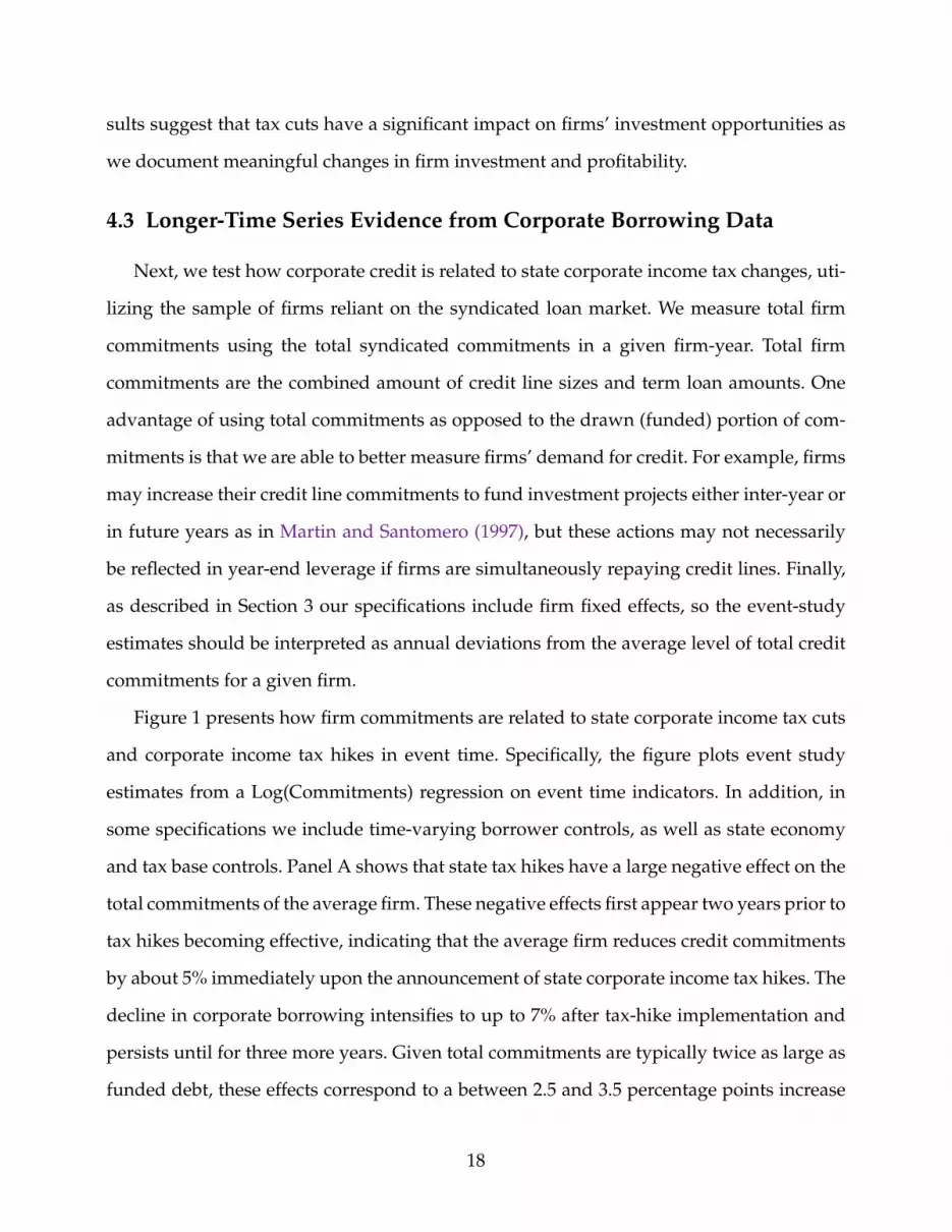
sults suggest that tax cuts have a significant impact on firms’ investment opportunities as

we document meaningful changes in firm investment and profitability.

4.3 Longer-Time Series Evidence from Corporate Borrowing Data

Next, we test how corporate credit is related to state corporate income tax changes, uti-

lizing the sample of firms reliant on the syndicated loan market. We measure total firm

commitments using the total syndicated commitments in a given firm-year. Total firm

commitments are the combined amount of credit line sizes and term loan amounts. One

advantage of using total commitments as opposed to the drawn (funded) portion of com-

mitments is that we are able to better measure firms’ demand for credit. For example, firms

may increase their credit line commitments to fund investment projects either inter-year or

in future years as in Martin and Santomero (1997), but these actions may not necessarily

be reflected in year-end leverage if firms are simultaneously repaying credit lines. Finally,

as described in Section 3 our specifications include firm fixed effects, so the event-study

estimates should be interpreted as annual deviations from the average level of total credit

commitments for a given firm.

Figure 1 presents how firm commitments are related to state corporate income tax cuts

and corporate income tax hikes in event time. Specifically, the figure plots event study

estimates from a Log(Commitments) regression on event time indicators. In addition, in

some specifications we include time-varying borrower controls, as well as state economy

and tax base controls. Panel A shows that state tax hikes have a large negative effect on the

total commitments of the average firm. These negative effects first appear two years prior to

tax hikes becoming effective, indicating that the average firm reduces credit commitments

by about 5% immediately upon the announcement of state corporate income tax hikes. The

decline in corporate borrowing intensifies to up to 7% after tax-hike implementation and

persists until for three more years. Given total commitments are typically twice as large as

funded debt, these effects correspond to a between 2.5 and 3.5 percentage points increase

18

in leverage. Importantly, these effects are not permanent and fade to zero thereafter.

Panel A of Figure 1 also indicates that total firm commitments increase around corpo-

rate tax cuts but that the magnitude of such increases is substantially smaller than in the

case of tax hikes. Specifically, the average firm increases borrowing by about 2% as tax cuts

become effective. However, these results are not statistically significant. The significantly

larger tax hike effects are likely to be a byproduct of tax hikes changing state corporate

income taxes by a greater percent than tax cuts (see the statistics in Panel C of Table 1).

Panel B of Figure 1 augments the analysis in Panel A by including time-varying firm, state

economy, and state tax base controls, painting a very similar picture to the results in Panel

A.

In Panels C and D Figure 1, we replicate the first two panels for the subsample of low-

risk firms—those that are assigned a Shared National Credit (SNC) rating of “Pass” as

of the previous year. Low credit quality firms are likely to face high costs of additional

leverage and may exhibit muted response to tax changes as the reduction/increase in the

distance to default thresholds may not be sufficient to lead to additional/less borrowing.

In line with this intuition, we find that high credit quality firms exhibit a larger increase in

borrowing of approximately 4–5% following tax cuts and that this effect is statistically sig-

nificant in some specifications. Additionally, the effect of tax hikes on corporate borrowing

is overall very similar for the subsample of high-credit quality firm.

These results also help reconcile our findings with Heider and Ljungqvist (2015) that

also studies the leverage responses of public firms to state corporate income tax changes

but finds that leverage ratios increase following tax increases. Our results complement

theirs by showing that the increase in corporate leverage after the effective date of state

corporate income tax hikes is preceded by large leverage reductions. These leverage reduc-

tions are driven by tax hikes reducing firms’ expected future income, thereby increasing

distance to default thresholds, while leaving the current value of debt interest tax shields

unchanged. Following the effective date of tax hikes, the value of debt interest tax shields

19

is higher, leading to increases in leverage as documented by Heider and Ljungqvist (2015).

This suggests that while debt interest tax shields may be an important consideration for

capital structure decisions of public firms, default thresholds are also a highly relevant fac-

tor for shaping the relation between taxes and leverage among these firms.

5. Model

While we have hinted at theoretical explanations for our results, we have not yet sup-

plied a cohesive framework to understand the underlying economics behind the empirical

patterns in our data. We now turn to this task. We use the environment of an equilibrium

economy with a representative consumer and a unit continuum of firms. The economy

also contains a government and a financial intermediary, but these players simply act as

pass-through agents for the firms and consumer.

Each of the infinitely-lived firms uses capital and labor in a stochastic, decreasing re-

turns technology to generate output, y, according to

y = zν(kαn1−α)θ , (3)

where k is the stock of capital, n is labor, z is a productivity shock, α is capital’s share,

θ governs the degree of returns to scale, and where we normalize the parameter ν to be

1− (1− α)θ. In addition to this basic technology, we assume that the firm has a fixed com-

ponent of operating costs, which we denote as f . The productivity shock, z, is lognormally

distributed and follows a process given by:

ln(z′) = ρ ln(z) + σzε′, ε′ ∼ N (0, 1), (4)

where a prime indicates the subsequent period, and no prime indicates the current period.

Investment in capital, I , is defined by a standard capital stock accounting identity:

k′ ≡ (1− δ)k + I, (5)

20

in which δ is the rate of capital depreciation. The price of the capital good has been normal-

ized to one. Adjusting the capital stock incurs quadratic costs that take the form:

ψ(k, k′) =ψ(k′ − (1− δ)k)2

2k(6)

where ψ is a parameter that governs the magnitude of adjustment costs.

Taxation in our model is simple, as there is only corporate taxation at a stochastic rate

τ , which follows an autoregressive process given by

τ ′ = ρττ + στu′, u′ ∼ N (0, 1). (7)

This tax rate applies to profits and to financing activities, as described next.

The firm can finance its optimal investment program with retained earnings or external

debt. We let p denote the stock of net debt, so p > 0 indicates that the firm has debt on the

balance sheet, and p < 0 indicates that the firm has cash on the balance sheet. We assume

that debt is raised through a zero-profit intermediary, which in turn raises the necessary

funds from the representative consumer. Debt takes the form of a one-period discount

bond, on which the firm can default. Let the interest rate on debt be r(k′, p′, z), so debt

proceeds are p′/(1 + r(k′, n′, b′, z, τ)(1 − τ)).12 As we outline below, this interest rate is de-

termined endogenously from the lender’s zero-profit condition and is therefore a function

of the model’s state variables. If instead the firm opts to save, it earns the after-tax risk-free

rate, r, with the interest taxed at a rate τ . Thus, the interest rate on debt can be expressed

as:

r(k′, b′, z, τ) =

r(k′, b′, z, τ) if p > 0

r if p ≤ 0(8)

Cash flows to shareholders, e(k, p, n, k′, p′, z, τ), are then the firm’s after-tax operating

income plus net debt issuance, minus net expenditure on investment, and minus tax-

12Note that this formulation assumes that the firm takes the tax advantage in the period in which it issuesthe debt. While not in accord with real-world debt contracts, this assumption reduces the state space andsimplifies the default condition (Strebulaev and Whited 2012).

21

deductible interest payments on debt, as follows:

e(k, p, n, k′, p′, z, τ) = (1− τ)(zν(kαn1−α)θ − wn− f) (9)

− (k′ − (1− δ)k)− ψ(k, k′) +p′

1 + r(k′, n′, b′, z, τ)(1− τ)− p,

where w is the wage rate, which is determined in equilibrium.

While a positive firm cash flow is distributed to its stockholders, we assume that nega-

tive cash flows are not allowed, that is:

e(k, p, n, k′, p′, z, τ) ≥ 0. (10)

This assumption is tantamount to eliminating external equity finance. Because much of

our sample constitutes private firms, who have no access to public equity markets, this

assumption is innocuous.13

The Bellman equation for the problem can then be expressed as:

π(k, p, z, τ) = maxk′,n,p′

e(k, p, n, k′, p′, z, τ) +

1

1 + rEπ (k′, p′, z′, τ ′)

, (11)

subject to (5) and (10).

5.1 Loan contract

We assume that a perfectly competitive financial intermediary offers the firm a one-

period loan contract, which need not be fully collateralized. As such, the firm can default.

In contrast to the models in Hennessy and Whited (2007) or Gao et al. (2020), we do not

assume that lenders can extend credit as long as the firm has positive present value. In-

stead, we follow Gilchrist et al. (2013) and Michaels et al. (2019), and assume that the firm

defaults if it does not have sufficient resources on hand to repay its debt, that is, its future

market value is not collateralizable. This assumption is particularly apt for our sample of

smaller private firms.

13In addition, we will eventually show in an appendix that allowing for costly equity issuance has little effecton our quantitative results. (To be added . . ..)

22

Specifically, default is triggered when debt repayment exceeds the firm’s current after-

tax profit plus the fraction, ξ of its capital that can be recovered in default:

(1− τ)(zν(kαn1−α)θ − wn− f)+ ξ(1− δ)k < p (12)

Note that we subtract the wage bill from output in (12) because labor is paid in full, even

if the firm subsequently defaults. Note also that taxes get paid before the the lender can

recover any payments. Both of these timing conventions are in accordance with absolute

priority rules. Finally, note that because the tax deduction is taken when the firm issues

debt, it is absent from this condition. For fixed levels of (k, n, p), (12) defines a region over

the joint domain of (z, τ) in which default occurs. We denote this region Ω.

Given this default threshold, the contractual interest rate, r(k′, b′, z, τ), is determined

by a zero-profit condition that must hold under free entry in the intermediation sector.

The payoff to the lender outside of default is simply this contractual interest rate. Inside

default, the lender recovers an amount equal to the left side of (12). Thus, under free entry

and risk-neutrality, the face value of debt discounted at the risky rate r(k′, p′, z, τ) must

equal the expected payoff discounted at the risk-free rate. Therefore, r(k′, p′, z, τ) satisfies:

1

1 + r

[∫Ω

(z′k′αn′β + ξ (1− δ) k′

)dG (z′, τ ′ | z, τ) + (1−G (Ω | z, τ)) p′

]=

p′

1 + r(k′, p′, z, τ).

(13)

For a given (p′, k′, z, τ), equations (12) and (13) pin down the loan contract.

5.2 Equilibrium

The economy also contains an infinitely lived representative consumer, who chooses

consumption and labor each period to maximize the expected present value of her utility,

discounted at the risk-free rate r. Her one-period utility function is given by ln(c)+ϕ(1−ns),

in which c is consumption, ns is the supply of labor, and ϕ is a parameter that governs the

23

utility of leisure. Her budget constraint is given by:

c+ p′d − pd(1 + r) = wns + e(·) + T, (14)

in which pd is consumer wealth, and T is the net tax revenue generated from the firms,

which we assume the government transfers to the consumer as a lump sum. Let ζ be the

stationary distribution over the firm’s states, (z, τ, k, p). We define equilibrium in this econ-

omy as follows.

Definition 1 A competitive equilibrium consists of (i) optimal firm policies for capital, labor, and

debt, k′, n, p′, (ii) allocations to the consumer of consumption, c, and labor, ns, and (iii) prices,

(w, r), such that:

1. All firms solve the problem given by (11).

2. The consumer maximizes her utility, subject to (14).

3. The labor, bond, and output markets clear.

ns =

∫ndζ (15)

pd =

∫p′dζ (16)

c =

∫(y − I + T )dζ. (17)

5.3 Solution

We solve the model using policy-function iteration and bisection, which yields an equi-

librium wage rate, a value function, π(k, p, z, τ), and policy functions for capital and debt,

given by k′(k, p, z, τ) and p′(k, p, z, τ).14

5.4 Estimation

We estimate the model parameters using our sample of small firms from the Y14 data.15

To simplify computation, we set a subset of our parameters outside the model. First, we set

14We use 15 points for z, 3 for τ , 201 for k and 201 for b in our numerical approximation.15Subsample analysis to be added later.

24

the risk-free interest rate, r, equal to 2%, which is close to the average five-year T-bill rate

during our Compustat sample period. Second, following Bloom et al. (2018), we set ϕ = 2.

Third, we set the standard deviation of the tax rate equal to the standard deviation of the

taxes observed in our sample (0.013), and we set average level of the tax rate equal to 0.2,

following Nikolov and Whited (2014). This rate is lower than the statutory national rate

because it accounts for the presence of personal taxes, as in Graham (1996).

We estimate the remaining parameters (θ, σ, ρ, ρτ , δ, ψ, ξ, and f ) jointly by minimizing

the distance between a list of moments and functions of moments constructedfrom model-

simulated data and those computed with actual data. In this estimation procedure, we use

the optimal weight matrix, constructed as in Bazdresch et al. (2018), clustered by firm and

year. Appendix B provides variable definitions for our actual data. In our simulated data,

leverage, operating profits, and investment are given by p/k, (zν (kαn1−α)θ−wn−f)/k, and

(k′ − (1− δ)k)/k.

We choose the following 12 moments to match, the first six of which are the means and

standard deviations of debt, investment, and operating income, all expressed as a ratio

of assets. We also include the serial correlation of operating income, which we calculate

using the method in Han and Phillips (2010) to account for firm fixed effects. The next

four moments are regression coefficients motivated by the benchmarks in Bazdresch et al.

(2018), which are estimates of the relations between optimal policies and the model state

variables. In our model the state variables are capital, net debt, and the two shocks, z and

τ . As suggested in Bazdresch et al. (2018), we transform these variables into measurable

counterparts, in particular, the ratio of net debt to assets and after-tax operating income

to assets. Our next four moments are then the coefficients from regressing the ratio of net

debt issuance to assets and investment on these two variables. Our final moment is the

difference-in-difference coefficient from regressing leverage on the enactment dates. We

choose the enactment dates because there is no difference between enactment and effective

dates in our model, and we want to capture the strong effects we find on enactment dates.

25

While all of the model parameters affect all of our moments, some of these moments

are particularly useful for parameter identification. First, the mean and standard devia-

tion of investment help identify the capital depreciation rate, δ, and the adjustment cost

parameter, ψ, respectively. In this class of models, steady state investment rises with the

depreciation rate, and the variance of investment naturally declines as quadratic adjust-

ment costs induce more smoothing. The serial correlation, ρ, of the process for z is directly

related to the estimated serial correlation of operating income, and all model variances in-

crease with the standard deviation, σ, of the driving process. Mean operating income is

mechanically decreasing in the profit function curvature, θ, and in the fixed cost of produc-

tion, f . Nonetheless, we can separately identify these two parameters because the variance

of operating profits is also mechanically decreasing in θ, while the fixed cost of production

has little effect on this variance. In addition, leverage is decreasing in the fixed cost, as are

all of the policy-function sensitivities, as the presence of the fixed cost breaks the scaling

properties of the model and decreases the correlations among all of the model variables.

Next, the average leverage ratio contains information about the default recovery rate, ξ,.

Finally, we identify the serial correlation of the tax process from our difference-in-

difference coefficient. In our model, in contrast to our regressions, we normalize a tax

change to be positive, so the sensitivity is negative. As shown in Figure 2, this coefficient

drops with the serial correlation of the tax shock process, ρτ . When this parameter is low,

the sensitivity is zero, as tax changes are not expected to last.

Table 8, panel A reports the model parameter estimates. All parameter estimates, except

for the estimate of the quadratic capital adjustment cost parameter are significantly differ-

ent from zero. The estimates of the profit function curvature and the standard deviation

and serial correlation of the driving process are within ranges typically reported for this

class of models (Bazdresch et al. 2018). The estimated quadratic capital adjustment cost, ψ,

at a level of 0.17, is low. The annual capital depreciation rate, δ, is estimated precisely at a

level of 0.10. The estimate of the default recovery rate is 0.113. Although this value is low,

26

it makes sense for the mostly small firms in our sample, which tend to be more distressed

when they default. Because lenders tend to be less accommodating toward small firms,

they tend to continue to operate in distress. Finally, the fixed operating cost, f , is 0.015,

which amounts to roughly 9% of steady-state operating profits.

Table 8, panel B reports the model and data moments used for estimation. In statistical

terms, seven out of the twelve moment pairs are insignificantly different from one another.

In economic terms, our model matches most of these moments well. For example, the sim-

ulated means of leverage, investment, and operating profits are all close to their real-data

counterparts.

Although five out of the 11 t-statistics for these moment pairs indicate significance, this

result is to be expected with a sample of our size, as most of the statistics we use as target

moments can themselves be estimated extremely precisely. The only simulated moment

that is economically different from its data counterpart is the standard deviation of the

ratio of operating income to assets, which is about one-third of its value in the data.

Given this model parameterizations, we now explore the aspects of the model that pro-

duce a negative sensitivity of leverage to taxes. One particularly interesting feature of the

solution is the behavior of optimal debt, which we depict in Figure 3. This figure is drawn

given the parameter estimates in Table 8, and it represents a two-dimensional slice of a

four dimensional policy function, where we have set k and p equal to their steady-state

values. On the x-axis are various levels of the productivity shock, z, and on the y axis is

p′/k′. Each line is drawn for one of the three levels of taxes in our model. As is standard

in this class of models, leverage increases with z. As productivity increases, firms find it

optimal to transfer resources through time via capital rather than via a storage technology,

which in our model is −p. Put differently, when productivity rises, optimal investment

outlays outpace internal resources, and the firm opts for debt finance. Interestingly, in this

figure, we also see that leverage is lower when the tax rate is higher. The intuition can be

understood as follows. While there is an interest tax deduction in the model, and while,

27

ceteris paribus, this feature of the model makes debt more attractive when taxes are higher,

taxes also make the firm less profitable and more likely to default, so it is optimal for the

firm to choose lower levels of leverage. For our estimated set of parameters, the latter effect

dominates the former.

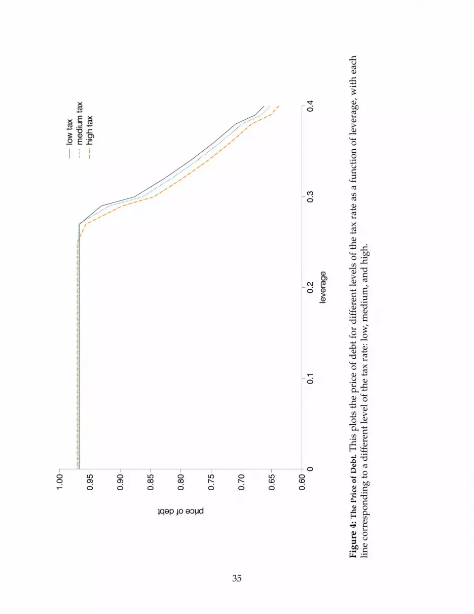
The tradeoff between the tax advantage of debt and the deleterious effect of taxes on

the default threshold can be seen in the optimal solution for the price of debt, that is 1/(1 +

r(k′, p′, z, τ)). We plot the price of debt in Figure 4 for the steady state level of capital and

the median profitability shock. On the x-axis is leverage, and on the y-axis is the price of

debt. Each of these price schedules is drawn for a different level of the tax rate. The effect

of leverage on the contract is intuitive. For any (k′, z, τ), The price of debt is decreasing in

p′, reflecting rising default risk.

The effect of taxes depends on the level of leverage. When leverage ranges between 0

and approximate 0.25, debt is safe, and the price of debt rises monotonically in the tax rate,

reflecting the interest tax deduction. However, for higher levels of leverage, this relation

between taxes and the price of debt changes in two ways. First, the price of debt falls

monotonically in the tax rate, as a higher tax rate changes the default threshold. Second,

the spread between the prices corresponding to high and low taxes widens, reflecting the

stronger effect of taxes on the default threshold than the value of the tax deduction. The

difference between the highest and lowest tax rates in our model is approximately 5%,

resulting in tax savings of 0.1%. In contrast, at a debt-to-assets ratio of 0.27, Figure 4 shows

that this tax raise raises the interest rate on debt by 1%.

6. Conclusion

Using comprehensive samples of both private and public companies and relying on

event study techniques in the spirit of Borusyak and Jaravel (2017), we study the evolution

of corporate borrowing around changes in state corporate income taxes since the 1980s. In

stark contrast with the prior literature, we show that on average corporate taxes depress

28

business borrowing and that companies adjust capital structure immediately upon the en-

actment of changes in state corporate tax policy. We show in a structural model that these

dynamics are driven by tax hikes reducing firm profitability, as well as lender recovery in

default. Both effects cause firms to decrease leverage.

Relying on detailed financial statement data for small and mid-sized private firms as

well as large public companies from 2011 through 2017, we show that the large increases in

corporate borrowing among small private firms are associated with significant real effects.

Specifically, net capital expenditures and profitability of small private firms all increase sig-

nificantly around corporate income tax cuts. While large private and public companies also

increase borrowing in response to tax cuts, they do not experience changes in investment

or profitability.

29

ReferencesBazdresch, S., R. J. Kahn, and T. M. Whited. 2018. Estimating and Testing Dynamic Corpo-

rate Finance Models. Review of Financial Studies 31:322–361.

Bloom, N., M. Floetotto, N. Jaimovich, I. Saporta-Eksten, and S. J. Terry. 2018. Really Un-certain Business Cycles. Econometrica 86:1031–1065.

Borusyak, K., and X. Jaravel. 2017. Revisiting Event Study Designs, with an Application tothe Estimation of the Marginal Propensity to Consume. Manuscript, UCL.

Brown, J., M. Gustafson, and I. Ivanov. 2020. Weathering Cash Flow Shocks. Journal ofFinance, forthcoming.

Doms, M., and T. Dunne. 1998. Capital Adjustment Patterns in Manufacturing Plants.Review of Economic Dynamics 1:409–429.

Erel, I., Y. Jang, and M. S. Weisbach. 2015. Do Acquisitions Relieve Target Firms’ FinancialConstraints? Journal of Finance 70:289–328.

Faccio, M., and J. Xu. 2015. Taxes and Capital Structure. Journal of Financial and QuantitativeAnalysis 50:277–300.

Fleckenstein, M., F. A. Longstaff, and I. A. Strebulaev. 2019. Corporate Taxes and CapitalStructure: A Long-Term Historical Perspective. Critical Finance Review 8:1–28.

Gao, X., T. M. Whited, and N. Zhang. 2020. Corporate Money Demand. Review of FinancialStudies, forthcoming.

Gilchrist, S., J. Sim, and E. Zakrajsek. 2013. Uncertainty, Financial Frictions and InvestmentDynamics. Manuscript, Federal Reserve Board.

Givoly, D., C. Hayn, A. R. Ofer, and O. Sarig. 1992. Taxes and Capital Structure: Evidencefrom Firms’ Response to the Tax Reform Act of 1986. Review of Financial Studies 5:331–355.

Goodman-Bacon, A. 2019. Difference-in-Differences with Variation in Treatment Timing.Manuscript, Vanderbilt University.

Gordon, R. H., and Y. Lee. 2001. Do taxes affect corporate debt policy? Evidence from U.S.corporate tax return data. Journal of Public Economics 82:195–224.

Graham, J. R. 1996. Debt and the marginal tax rate. Journal of Financial Economics 41:41 – 73.

Hadlock, C. J., and J. R. Pierce. 2010. New Evidence on Measuring Financial Constraints:Moving Beyond the KZ Index. Review of Financial Studies 23:1909–1940.

Han, C., and P. C. B. Phillips. 2010. GMM Estimation for Dynamic Panels with Fixed Effectsand Strong Instruments at Unity. Econometric Theory 26:119–151.

30

Heider, F., and A. Ljungqvist. 2015. As certain as debt and taxes: Estimating the tax sensi-tivity of leverage from state tax changes. Journal of Financial Economics 118:684–712.

Hennessy, C. A., and T. M. Whited. 2007. How costly is external financing? Evidence froma structural estimation. Journal of Finance 62:1705–1745.

Ivanov, I., B. Ranish, and J. Wang. 2019. Bank Supervision and Syndicated Lending.Mauscript, Federal Reserve Board.

Kahle, K., and R. M. Stulz. 2017. Is the U.S. public corporation in trouble? Journal of Eco-nomic Perspectives 31:67–88.

Li, S., T. M. Whited, and Y. Wu. 2016. Collateral, Taxes, and Leverage. Review of FinancialStudies 29:1453–1500.

Martin, J. S., and A. M. Santomero. 1997. Investment opportunities and corporate demandfor lines of credit. Journal of Banking and Finance 21:1331–1350.

Michaels, R., T. B. Page, and T. M. Whited. 2019. Labor and Capital Dynamics under Fi-nancing Frictions. Review of Finance 23:279–323.

Modigliani, F., and M. H. Miller. 1963. Corporate Income Taxes and the Cost of Capital: ACorrection. American Economic Review 53:433–443.

Nikolov, B., and T. M. Whited. 2014. Agency conflicts and cash: Estimates from a dynamicmodel. Journal of Finance 69:1883–1921.

Smith, C. W. 2007. On Governance and Agency Issues in Small Firms. Journal of SmallBusiness Management 45:176–176.

Smith, M., D. Yagan, O. Zidar, and E. Zwick. 2019. The Rise of Pass-Throughs and theDecline of the Labor Share. Manuscript, Princeton University.

Strebulaev, I. A., and T. M. Whited. 2012. Dynamic Models and Structural Estimation inCorporate Finance. Foundations and Trends in Finance 6:1–163.

Suarez Serrato, J. C., and O. Zidar. 2018. The Structure of Corporate Taxation and Its Impacton State Tax Revenues and Economic Activity. Journal of Public Economics 167:158–176.

Sufi, A. 2009. Bank Lines of Credit in Corporate Finance: An Empirical Analysis. Review ofFinancial Studies 22:1057–1088.

Titman, S., and R. Wessels. 1988. The Determinants of Capital Structure Choice. Journal ofFinance pp. 1–19.

Whited, T. M. 2006. External finance constraints and the intertemporal pattern of intermit-tent investment. Journal of Financial Economics 81:467–502.

Zidar, O. 2019. Tax Cuts for Whom? Heterogeneous Effects of Tax Changes on Growth andEmployment. Journal of Political Economy 127:1437–1472.

31

-.15-.05.05.15Firm Commitments

-5-4

-3-2

-10

+1

+2

+3

+4

Year

Rel

ativ

e to

Tax

Cha

nge

Tax

Hik

esTa

x Cu

ts

(a)

Full

Sam

ple

(No

Con

trol

s)

-.15-.05.05.15Firm Commitments

-5-4

-3-2

-10

+1

+2

+3

+4

Year

Rel

ativ

e to

Tax

Cha

nge

Tax

Hik

esTa

x Cu

ts

(b)

Full

Sam

ple

(Con

trol

s)

-.15-.05.05.15Coefficient

-5-4

-3-2

-10

+1

+2

+3

+4

Year

Rel

ativ

e to

Tax

Cha

nge

Tax

Hik

esTa

x Cu

ts

(c)

Low

Ris

k(N

oC

ontr

ols)

-.15-.05.05.15Coefficient

-5-4

-3-2

-10

+1

+2

+3

+4

Year

Rel

ativ

e to

Tax

Cha

nge

Tax

Hik

esTa

x Cu

ts

(d)

Low

Ris

k(C

ontr

ols)

Figu

re1:

Cor

pora

teTa

xes

and

Firm

Bor

row

ing.

This

figur

epr

esen

tsev

ent

stud

yco

effic

ient

sfr

oman

nual

firm

-lev

elO

LSre

gres

sion

sof

the

evol

utio

nof

synd

icat

edbo

rrow

ing

arou

ndst

ate

corp

orat

ein

com

eta

xch

ange

s.Th

eda

taco

me

from

the

Shar

edN

atio

nalC

redi

tDat

abas

ean

din

clud

eal

lsyn

dica

ted

finan

cing

toa

give

nbo

rrow

erin

agi

ven

year

from

1992

thro

ugh

2013

.All

spec

ifica

tion

sin

clud

efir

m,i

ndus

try-

year

fixed

effe

cts

defin

edat

the

four

-dig

itN

AIC

Sle

vel.

Pane

lsB

and

Dal

soin

clud

eth

ese

tof

tax

base

and

tax

cred

itco

ntro

lsfr

omSu

arez

Serr

ato

and

Zid

ar(2

018)

,lag

ged

borr

ower

char

acte

rist

ics,

asw

ell

asla

gged

chan

ges

and

leve

lsof

the

stat

eG

DP

and

the

stat

eun

empl

oym

ent

rate

.In

Pane

lsC

and

Dth

esa

mpl

eis

rest

rict

edto

borr

ower

sw

ith

“pas

s”-r

ated

com

mit

men

ts.T

hest

anda

rder

rors

are

doub

lecl

uste

red

atth

ebo

rrow

eran

dst

ate-

year

leve

l.

32

tax elasticity

−0.0

15

−0.0

10

−0.0

050

tax

seria

l cor

rela

tion

0.1

0.2

0.3

0.4

0.5

0.6

0.7

0.8

0.9

Figu

re2:

Tax

Seri

alC

orre

lati

onan

dth

eTa

xR

espo

nseT

his

figur

epl

ots

aco

mpa

rati

vest

atic

sex

erci

se,i

nw

hich

we

allo

wth

ese

rial

corr

elat

ion

ofth

eta

xpr

oces

sto

take

20di

ffer

entv

alue

s.Fo

rea

chof

thes

eva

lues

we

solv

ean

dsi

mul

ate

the

mod

elan

dpl

otth

eco

rres

pond

ing

coef

ficie

ntfr

omre

gres

sing

leve

rage

ona

dum

my

that

equa

ls1

for

ata

xin

crea

sean

d−

1fo

ra

tax

decr

ease

.

33

low

tax

med

ium

tax

high

tax

leverage

0.16

0.18

0.20

0.22

0.24

0.26

0.28

0.30

0.32

0.34

0.36

prod

uctiv

ity0.

40.

60.

81.

01.

21.

41.

61.

82.

02.

22.

4

Figu

re3:

Opt

imal

Deb

tand

Taxe

s.Th

isfig

ure

plot

sop

tim

alne

xt-p

erio

dne

tdeb

t/ca

pita

las

afu

ncti

onof

the

profi

tabi

lity

shoc

k.Ea

chlin

ere

pres

ents

adi

ffer

entl

evel

ofth

eta

xra

te:l

ow,m

ediu

m,a

ndhi

gh.

34

low

tax

med

ium

tax

high

tax

price of debt

0.60

0.65

0.70

0.75

0.80

0.85

0.90

0.95

1.00

leve

rage

00.

10.

20.

30.

4

Figu

re4:

The

Pric

eof

Deb

t.Th

ispl

ots

the

pric

eof

debt

for

diff

eren

tlev

els

ofth

eta

xra

teas

afu

ncti

onof

leve

rage

,wit

hea

chlin

eco

rres

pond

ing

toa

diff

eren

tlev

elof

the

tax

rate

:low

,med

ium

,and

high

.

35

Table 1: Summary Statistics. This table presents summary statistics for the firm-year de-tailing borrowing information (Panel A), the firm-year balance sheet sample (Panel B), andthe tax changes (Panel C) used in our analyses. Commitment amount refers to the sum ofcredit line and term loan commitments, while utilized amount is the sum of term loans andthe outstanding drawn amounts under credit lines. All firm financials variables in Panel Bwith the exception of Book Assets are scaled by firm total assets as of the prior year.

Mean St. Dev. p10 p25 p50 p75 p90Panel A: Firm-Year Financials Panel

Book Assets, $m 2,299 22,202 118 151 256 596 1,759Net Income 0.07 0.14 -0.02 0.02 0.05 0.09 0.16Net Sales 1.88 1.58 0.39 0.81 1.50 2.52 3.67EBITDA 0.14 0.15 0.03 0.07 0.11 0.17 0.25Operating Income 0.09 0.15 -0.01 0.03 0.07 0.12 0.19Cash 0.10 0.13 0.003 0.01 0.05 0.13 0.26Debt 0.35 0.27 0.01 0.13 0.32 0.54 0.73Total Liab. 0.65 0.28 0.29 0.46 0.65 0.82 0.96Interest Expense 1.45 1.52 0.03 0.34 1.03 2.02 3.58Fixed Assets 0.33 0.28 0.03 0.10 0.26 0.49 0.76Total Assets 1.10 0.25 0.93 0.99 1.05 1.14 1.27

Panel B: Firm-Year Borrowing PanelCommitment Amt, $m 380 815 37 65 143 350 865Utilized Amt, $m 154 411 0 16 52 136 342Utilization Ratio, $m 0.52 0.36 0 0.15 0.57 0.85 1Contract Maturity, months 66 28 36.5 49 61 78 99Remaining Maturity, months 36 21 10 19 34 50 61

Panel C: Characteristics of Tax ChangesTax Cuts (N=121)

Rate Change, % 0.59 0.58 0.10 0.25 0.50 0.75 1.04Initial Rate, % 7.59 2.23 5.00 6.40 7.80 9.20 10.00Resulting Rate, % 7.00 2.23 4.36 5.50 7.10 8.50 9.50

Tax Hikes (N=36)Rate Change, % 1.31 1.07 0.40 0.54 1.00 1.50 2.75Initial Rate, % 6.59 1.84 4.00 5.00 7.00 7.88 9.00Resulting Rate, % 7.90 1.84 6.00 6.50 7.95 9.25 9.98

36

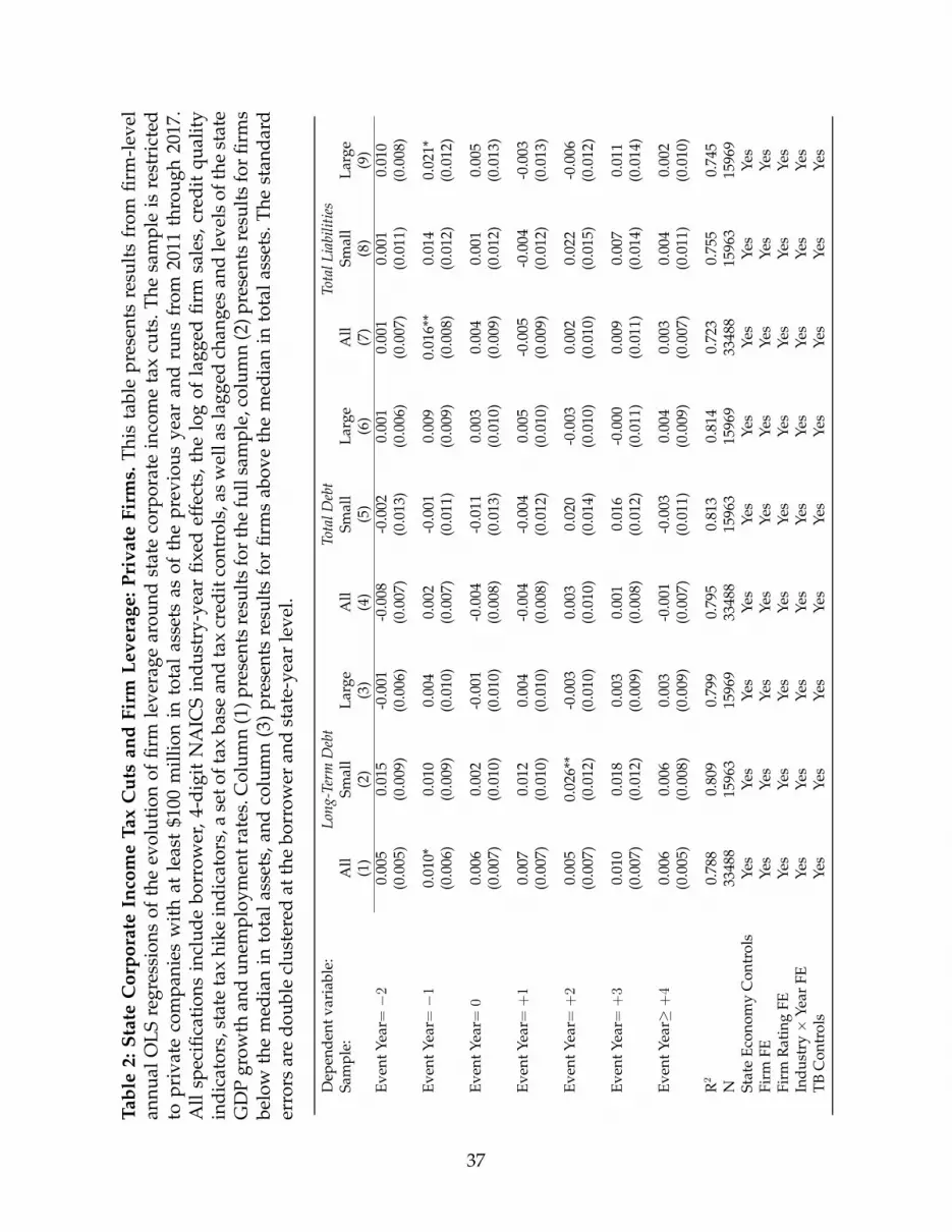
Tabl

e2:

Stat

eC

orpo

rate

Inco

me

Tax

Cut

san

dFi

rmLe

vera

ge:P

riva

teFi

rms.

This

tabl

epr

esen

tsre

sult

sfr

omfir

m-l

evel

annu

alO

LSre

gres

sion

sof

the

evol

utio

nof

firm

leve

rage

arou

ndst

ate

corp

orat

ein

com

eta

xcu

ts.T

hesa

mpl

eis

rest

rict

edto

priv

ate

com

pani

esw

ith

atle

ast

$100

mill

ion

into

tal

asse

tsas

ofth

epr

evio

usye

aran

dru

nsfr

om20

11th

roug

h20

17.

All

spec

ifica

tion

sin

clud

ebo

rrow

er,4

-dig

itN

AIC

Sin

dust

ry-y

ear

fixed

effe

cts,

the

log

ofla

gged

firm

sale

s,cr

edit

qual

ity

indi

cato

rs,s

tate

tax

hike

indi

cato

rs,a

seto

ftax

base

and

tax

cred

itco

ntro

ls,a

sw

ella

sla

gged

chan

ges

and

leve

lsof

the

stat

eG

DP

grow

than

dun

empl

oym

entr

ates

.Col

umn

(1)p

rese

nts

resu

lts

for

the

full

sam

ple,

colu

mn

(2)p

rese

nts

resu

lts

for

firm

sbe

low

the

med

ian

into

tala

sset

s,an

dco

lum

n(3

)pr

esen

tsre

sult

sfo

rfir

ms

abov

eth

em

edia

nin

tota

lass

ets.

The

stan

dard

erro

rsar

edo

uble

clus

tere

dat

the

borr

ower

and

stat

e-ye

arle

vel.

Dep

ende

ntva

riab

le:

Long

-Ter

mD

ebt

Tota

lDeb

tTo

talL

iabi

litie

sSa

mpl

e:A

llSm

all

Larg

eA

llSm

all

Larg

eA

llSm

all

Larg

e(1

)(2

)(3

)(4

)(5

)(6

)(7

)(8

)(9

)Ev

entY

ear=−

20.

005

0.01

5-0

.001

-0.0

08-0

.002

0.00

10.

001

0.00

10.

010

(0.0

05)

(0.0

09)

(0.0

06)

(0.0

07)

(0.0

13)

(0.0

06)

(0.0

07)

(0.0

11)

(0.0

08)

Even

tYea

r=−

10.

010*

0.01

00.

004

0.00

2-0

.001

0.00

90.

016*

*0.

014

0.02

1*(0

.006

)(0

.009

)(0

.010

)(0

.007

)(0

.011

)(0

.009

)(0

.008

)(0

.012

)(0

.012

)

Even

tYea

r=0

0.00

60.

002

-0.0

01-0

.004

-0.0

110.

003

0.00

40.

001

0.00

5(0

.007

)(0

.010

)(0

.010

)(0

.008

)(0

.013

)(0

.010

)(0

.009

)(0

.012

)(0

.013

)

Even

tYea

r=+

10.

007

0.01

20.

004

-0.0

04-0

.004

0.00

5-0

.005

-0.0

04-0

.003

(0.0

07)

(0.0

10)

(0.0

10)

(0.0

08)

(0.0

12)

(0.0

10)

(0.0

09)

(0.0

12)

(0.0

13)

Even

tYea

r=+

20.

005

0.02

6**

-0.0

030.

003

0.02

0-0

.003

0.00

20.

022

-0.0

06(0

.007

)(0

.012

)(0

.010

)(0

.010

)(0

.014

)(0

.010

)(0

.010

)(0

.015

)(0

.012

)

Even

tYea

r=+

30.

010

0.01

80.

003

0.00

10.

016

-0.0

000.

009

0.00

70.

011

(0.0

07)

(0.0

12)

(0.0

09)

(0.0

08)

(0.0

12)

(0.0

11)

(0.0

11)

(0.0

14)

(0.0

14)

Even

tYea

r≥+

40.

006

0.00

60.

003

-0.0

01-0

.003

0.00

40.

003

0.00

40.

002

(0.0

05)

(0.0

08)

(0.0

09)

(0.0

07)

(0.0

11)

(0.0

09)

(0.0

07)

(0.0

11)

(0.0

10)

R2

0.78

80.

809

0.79

90.

795

0.81

30.

814

0.72

30.

755

0.74

5N

3348

815

963

1596

933

488

1596

315

969

3348

815

963

1596

9St

ate

Econ

omy

Con

trol

sYe

sYe

sYe

sYe

sYe

sYe

sYe

sYe

sYe

sFi

rmFE

Yes

Yes

Yes

Yes

Yes

Yes

Yes

Yes

Yes

Firm

Rat

ing

FEYe

sYe

sYe

sYe

sYe

sYe

sYe

sYe

sYe

sIn

dust

ry×

Year

FEYe

sYe

sYe

sYe

sYe

sYe

sYe

sYe

sYe

sTB

Con

trol

sYe

sYe

sYe

sYe

sYe

sYe

sYe

sYe

sYe

s

37

Tabl

e3:

Stat

eC

orpo

rate

Inco

me

Tax

Cut

san

dFi

rmLe

vera

ge:L

ow-R

isk

Firm

s.Th

ista

ble

pres

ents

resu

lts

from

firm

-lev

elan

nual

OLS

regr

essi

ons

ofth

eev

olut

ion

offir

mle

vera

gear

ound

stat

eco

rpor

ate

inco

me

tax

cuts

.The

sam

ple

runs

from

2011

thro

ugh

2017

and

isre

stri

cted

topr

ivat

eco

mpa

nies

wit

hat

leas

t$1

00m

illio

nin

tota

las

sets

asof

the

prev

ious

year

that

are

rate

dab

ove

“B”

byth

ele

nder

.All

spec

ifica

tion

sin

clud

ebo

rrow

er,4

-dig

itN

AIC

Sin

dust

ry-y

ear

fixed

effe

cts,

the

log

ofla

gged

firm

sale

s,cr

edit

qual

ity

indi

cato

rs,s

tate

tax

hike

indi

cato

rs,a

set

ofta

xba

sean

dta

xcr

edit

cont

rols

,as

wel

las

lagg

edch

ange

san

dle

vels

ofth

est

ate

GD

Pgr

owth

and

unem

ploy

men

tra

tes.

Col

umn

(1)

pres

ents

resu

lts

for

the

full

sam

ple,

colu

mn

(2)

pres

ents

resu

lts

for

firm

sbe

low

the

med

ian

into

tal

asse

ts,a

ndco

lum

n(3

)pr

esen

tsre

sult

sfo

rfir

ms

abov

eth

em

edia

nin

tota

lass

ets.

The

stan

dard

erro

rsar

edo

uble

clus

tere

dat

the

borr

ower

and

stat

e-ye

arle

vel.

Dep

ende

ntva

riab

le:

Long

-Ter

mD

ebt

Tota

lDeb

tTo

talL

iabi

litie

sSa

mpl

e:A

llSm

all

Larg

eA

llSm

all

Larg

eA

llSm

all

Larg

e(1

)(2

)(3

)(4

)(5

)(6

)(7

)(8

)(9

)Ev

entY

ear=−

20.

008

0.01

5*0.

003

-0.0

09-0

.007

0.00

50.

002

-0.0

050.

016*

(0.0

05)

(0.0

09)

(0.0

07)

(0.0

07)

(0.0

14)

(0.0

07)

(0.0

07)

(0.0

11)

(0.0

09)

Even

tYea

r=−

10.

014*

*0.

020*

*0.

006

0.00

40.

005

0.00

90.

020*

*0.

017

0.02

5*(0

.007

)(0

.009

)(0

.012

)(0

.008

)(0

.013

)(0

.011

)(0

.009

)(0

.013

)(0

.014

)

Even

tYea

r=0

0.00

60.

016

-0.0

11-0

.011

-0.0

07-0

.013

-0.0

010.

000

-0.0

06(0

.007

)(0

.011

)(0

.010

)(0

.008

)(0

.014

)(0

.011

)(0

.009

)(0

.014

)(0

.013

)

Even

tYea

r=+

10.

013*

0.02

2**

0.00

60.

004

0.00

80.

004

-0.0

010.

002

-0.0

10(0

.007

)(0

.010

)(0

.011

)(0

.008

)(0

.014

)(0

.010

)(0

.009

)(0

.012

)(0

.014

)

Even

tYea

r=+

20.

007

0.02

9**

-0.0

110.

003

0.02

7**

-0.0

130.

007

0.02

2-0

.018

(0.0

08)

(0.0

12)

(0.0

11)

(0.0

10)

(0.0

14)

(0.0

11)

(0.0

10)

(0.0

15)

(0.0

13)

Even

tYea

r=+

30.

009

0.01

30.

001

0.00

10.

023*

-0.0

040.

010

0.00

20.

009

(0.0

07)

(0.0

11)

(0.0

10)

(0.0

08)

(0.0

12)

(0.0

11)

(0.0

12)

(0.0

15)

(0.0

15)

Even

tYea

r≥+

40.

006

0.00

20.

001

-0.0

02-0

.001

-0.0

030.

006

-0.0

00-0

.002

(0.0

06)

(0.0

09)

(0.0

10)

(0.0

07)

(0.0

12)

(0.0

09)

(0.0

08)

(0.0

12)

(0.0

11)

R2

0.80

40.

826

0.81

40.

820.

830.

840.

763

0.77

80.

793

N26

612

1287

512

392

2661

212

875

1239

226

612

1287

512

392

Stat

eEc

onom

yC

ontr

ols

Yes

Yes

Yes

Yes

Yes

Yes

Yes

Yes

Yes

Firm

FEYe

sYe

sYe

sYe

sYe

sYe

sYe

sYe

sYe

sFi

rmR

atin

gFE

Yes

Yes

Yes

Yes

Yes

Yes

Yes

Yes

Yes

Indu

stry×

Year

FEYe

sYe

sYe

sYe

sYe

sYe

sYe

sYe

sYe

sTB

Con

trol

sYe

sYe

sYe

sYe

sYe

sYe

sYe

sYe

sYe

s

38

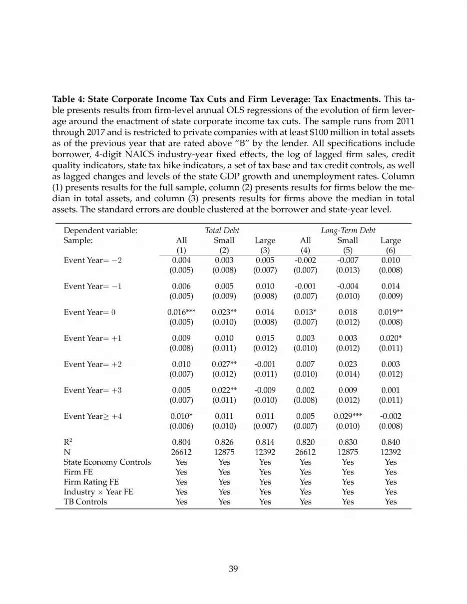
Table 4: State Corporate Income Tax Cuts and Firm Leverage: Tax Enactments. This ta-ble presents results from firm-level annual OLS regressions of the evolution of firm lever-age around the enactment of state corporate income tax cuts. The sample runs from 2011through 2017 and is restricted to private companies with at least $100 million in total assetsas of the previous year that are rated above “B” by the lender. All specifications includeborrower, 4-digit NAICS industry-year fixed effects, the log of lagged firm sales, creditquality indicators, state tax hike indicators, a set of tax base and tax credit controls, as wellas lagged changes and levels of the state GDP growth and unemployment rates. Column(1) presents results for the full sample, column (2) presents results for firms below the me-dian in total assets, and column (3) presents results for firms above the median in totalassets. The standard errors are double clustered at the borrower and state-year level.

Dependent variable: Total Debt Long-Term DebtSample: All Small Large All Small Large

(1) (2) (3) (4) (5) (6)Event Year= −2 0.004 0.003 0.005 -0.002 -0.007 0.010

(0.005) (0.008) (0.007) (0.007) (0.013) (0.008)

Event Year= −1 0.006 0.005 0.010 -0.001 -0.004 0.014(0.005) (0.009) (0.008) (0.007) (0.010) (0.009)

Event Year= 0 0.016*** 0.023** 0.014 0.013* 0.018 0.019**(0.005) (0.010) (0.008) (0.007) (0.012) (0.008)

Event Year= +1 0.009 0.010 0.015 0.003 0.003 0.020*(0.008) (0.011) (0.012) (0.010) (0.012) (0.011)

Event Year= +2 0.010 0.027** -0.001 0.007 0.023 0.003(0.007) (0.012) (0.011) (0.010) (0.014) (0.012)

Event Year= +3 0.005 0.022** -0.009 0.002 0.009 0.001(0.007) (0.011) (0.010) (0.008) (0.012) (0.011)

Event Year≥ +4 0.010* 0.011 0.011 0.005 0.029*** -0.002(0.006) (0.010) (0.007) (0.007) (0.010) (0.008)

R2 0.804 0.826 0.814 0.820 0.830 0.840N 26612 12875 12392 26612 12875 12392State Economy Controls Yes Yes Yes Yes Yes YesFirm FE Yes Yes Yes Yes Yes YesFirm Rating FE Yes Yes Yes Yes Yes YesIndustry × Year FE Yes Yes Yes Yes Yes YesTB Controls Yes Yes Yes Yes Yes Yes

39

Tabl

e5:

Cor

pora

teTa

xC

uts

and

Leve

rage

:Acc

ount

ing

for

Indi

vidu

alTa

xes.

This

tabl

epr

esen

tsre

sult

sfr

omfir

m-l

evel

annu

alO

LSre

gres

sion

sof

the

evol

utio

nof

firm

leve

rage

arou

ndst

ate

corp

orat

ein

com

eta

xcu

ts.T

hesa

mpl

eis

rest

rict

edto

priv

ate

com

pani

esw

ith

atle

ast$

100

mill

ion

into

tala

sset

sas

ofth

epr

evio

usye

aran

dru

nsfr

om20

11th

roug

h20

17th

atar

era

ted

abov

e“B

”by

the

lend

er.A

llsp

ecifi

cati

ons

incl

ude

borr

ower

,4-d

igit

NA

ICS

indu

stry

-yea

rfix

edef

fect

s,th

elo

gof

lagg

edfir

msa

les,

cred

itqu

alit

yin

dica

tors

,the

set

ofst

ate

tax

hike

even

tin

dica

tors

,the

set

ofst

ate

indi

vidu

alin

com

eta

xhi

kes

and

cuts

even

tin

dica

tors

,ase

tof

tax

base

and

tax

cred

itco

ntro

ls,a

sw

ella

sla

gged

chan

ges

and

leve

lsof

the

stat

eG

DP

grow

than

dun

empl

oym

entr

ates

.The

stan

dard

erro

rsar

edo

uble

clus

tere

dat

the

borr

ower

and

stat

e-ye

arle

vel.

Dep

ende

ntva

riab

le:

Long

-Ter

mD

ebt

Tota

lDeb

tTo

talL

iabi

litie

sSa

mpl

e:A

llSm

all

Larg

eA

llSm

all

Larg

eA

llSm

all

Larg

e(1

)(2

)(3

)(4

)(5

)(6

)(7

)(8

)(9

)Ev

entY

ear=−

20.

008

0.01

10.

007

-0.0

08-0

.011

0.01

10.

001

-0.0

100.

018*

(0.0

05)

(0.0

09)

(0.0

07)

(0.0

07)

(0.0

15)

(0.0

07)

(0.0

07)

(0.0

10)

(0.0

10)

Even

tYea

r=−

10.

016*

*0.

023*

*0.

007

0.00

70.

005

0.01

30.

020*

*0.

015

0.03

4**

(0.0

08)

(0.0

11)

(0.0

13)

(0.0

09)

(0.0

14)

(0.0

12)

(0.0

10)

(0.0

14)

(0.0

15)

Even

tYea

r=0

0.00

30.

016

-0.0

14-0

.009

-0.0

00-0

.015

-0.0

060.

006

-0.0

11(0

.008

)(0

.012

)(0

.012

)(0

.009

)(0

.016

)(0

.013

)(0

.010

)(0

.015

)(0

.015

)

Even

tYea

r=+

10.

013*

0.02

6**

0.00

20.

005

0.01

10.

001

-0.0

020.

007

-0.0

13(0

.008

)(0

.011

)(0

.012

)(0

.008

)(0

.014

)(0

.011

)(0

.010

)(0

.013

)(0

.014

)

Even

tYea

r=+

20.

008

0.03

2**

-0.0

130.

002

0.02

9*-0

.015

0.00

10.

020

-0.0

22(0

.009

)(0

.013

)(0

.011

)(0

.011

)(0

.015

)(0

.012

)(0

.010

)(0

.014

)(0

.015

)

Even

tYea

r=+

30.

011

0.02

3*-0

.004

0.00

10.

027*

-0.0

090.

011

0.01

20.

005

(0.0

08)

(0.0

12)

(0.0

11)

(0.0

09)

(0.0

14)

(0.0

12)

(0.0

12)

(0.0

16)

(0.0

16)

Even

tYea

r≥+

40.

009

0.00

8-0

.000

-0.0

02-0

.001

-0.0

070.

005

0.00

4-0

.002

(0.0

07)

(0.0

09)

(0.0

10)

(0.0

08)

(0.0

14)

(0.0

10)

(0.0

09)

(0.0

13)

(0.0

12)

R2

0.80

40.

826

0.81

40.

820.

830.

840.

763

0.77

90.

793

N26

612

1287

512

392

2661

212

875

1239

226

612

1287

512

392

Ind.

Inco

me

Tax

Even

tInd

icat

ors

Yes

Yes

Yes

Yes

Yes

Yes

Yes

Yes

Yes

Stat

eEc

onom

yC

ontr

ols

Yes

Yes

Yes

Yes

Yes

Yes

Yes

Yes

Yes

Firm

FEYe

sYe

sYe

sYe

sYe

sYe

sYe

sYe

sYe

sFi

rmR

atin

gFE

Yes

Yes

Yes

Yes

Yes

Yes

Yes

Yes

Yes

Indu

stry×

Year

FEYe

sYe

sYe

sYe

sYe

sYe

sYe

sYe

sYe

sTB

Con

trol

sYe

sYe

sYe

sYe

sYe

sYe

sYe

sYe

sYe

s

40

Table 6: State Corporate Income Tax Cuts and Leverage: Public Firms. This table presentsresults from firm-level annual OLS regressions of the evolution of leverage around statecorporate income tax cuts. The sample runs from 2011 through 2017 and is restricted topublic companies from the CRSP-Compustat database. All specifications include borrowerand 4-digit SIC industry-year fixed effects, lagged levels and changes in: log firm assets,ROA, the market-to-book ratio, asset tangibility, state tax hike indicators, a set of tax baseand tax credit controls, as well as lagged changes and levels of the state GDP growth andunemployment rates. Columns (1)-(4) present results from event studies around the ef-fective dates of state income tax cuts, while columns (5) through (8) present results fromevent studies around tax cut enactments. The standard errors are double clustered at theborrower and state-year level.

Sample: Tax Effective Dates Tax EnactmentsDependent variable: Tot Debt LT Debt LT Debt (mkt) Tot Debt LT Debt LT Debt (mkt)

(1) (2) (3) (4) (5) (6)Event Year= −2 0.016* 0.018** 0.011* -0.006 0.001 -0.000

(0.009) (0.008) (0.006) (0.008) (0.007) (0.006)

Event Year= −1 0.016 0.017 0.008 -0.007 -0.002 -0.002(0.011) (0.011) (0.008) (0.009) (0.008) (0.007)

Event Year= 0 0.022* 0.014 0.007 0.015 0.022* 0.011(0.012) (0.012) (0.009) (0.013) (0.012) (0.008)

Event Year= +1 0.025* 0.022* 0.007 0.017 0.015 0.003(0.013) (0.012) (0.008) (0.015) (0.014) (0.009)

Event Year= +2 0.013 0.009 -0.006 0.019 0.020 -0.000(0.015) (0.013) (0.011) (0.014) (0.013) (0.010)

Event Year= +3 0.021 0.020 0.007 0.024 0.027** 0.006(0.016) (0.016) (0.013) (0.014) (0.013) (0.009)

Event Year≥ +4 0.017 0.020 0.016 0.018 0.019 0.012(0.017) (0.016) (0.012) (0.016) (0.015) (0.011)

R2 .691 .674 .769 .691 .674 .768N 14207 14207 14207 14207 14207 14207State Economy Controls Yes Yes Yes Yes Yes YesFirm Controls Yes Yes Yes Yes Yes YesFirm FE Yes Yes Yes Yes Yes YesIndustry × Year FE Yes Yes Yes Yes Yes YesTB Controls Yes Yes Yes Yes Yes Yes

41

Table 7: Real Effects of State Corporate Income Tax Cuts. This table presents resultsfrom firm-level annual OLS regressions of the evolution of firm investment and profitabil-ity around the enactment of state corporate income tax cuts. The sample runs from 2011through 2017 and is restricted to private companies with at least $100 million in total assetsas of the previous year that are rated above “B” by the lender. All specifications includeborrower, 4-digit NAICS industry-year fixed effects, the log of lagged firm sales, creditquality indicators, state tax hike indicators, a set of tax base and tax credit controls, as wellas lagged changes and levels of the state GDP growth and unemployment rates. Columns(1) and (4) present results for the full sample, columns (2) and (5) present results for firmsbelow the median in total assets, and columns (3) and (6) present results for firms abovethe median in total assets. The standard errors are double clustered at the borrower andstate-year level.

Dependent variable: EBITDA Net Capital ExpendituresSample: All Small Large All Small Large

(1) (2) (3) (4) (5) (6)Event Year= −2 0.004 0.003 0.005 0.000 0.006 -0.004

(0.005) (0.008) (0.007) (0.003) (0.005) (0.004)

Event Year= −1 0.006 0.005 0.010 0.003 0.007 -0.002(0.005) (0.009) (0.008) (0.003) (0.005) (0.005)

Event Year= 0 0.016*** 0.023** 0.014 0.002 0.003 -0.000(0.005) (0.010) (0.008) (0.004) (0.006) (0.007)

Event Year= +1 0.009 0.010 0.015 0.002 -0.002 0.003(0.008) (0.011) (0.012) (0.004) (0.007) (0.007)

Event Year= +2 0.010 0.027** -0.001 0.010** 0.009 0.001(0.007) (0.012) (0.011) (0.005) (0.007) (0.006)

Event Year= +3 0.005 0.022** -0.009 0.008 0.011 -0.006(0.007) (0.011) (0.010) (0.006) (0.009) (0.006)

Event Year≥ +4 0.010* 0.011 0.011 0.002 0.002 -0.000(0.006) (0.010) (0.007) (0.004) (0.007) (0.005)

R2 0.804 0.826 0.814 0.445 0.46 0.476N 26612 12875 12392 25617 12196 12080State Economy Controls Yes Yes Yes Yes Yes YesFirm FE Yes Yes Yes Yes Yes YesFirm Rating FE Yes Yes Yes Yes Yes YesIndustry × Year FE Yes Yes Yes Yes Yes YesTB Controls Yes Yes Yes Yes Yes Yes

42

Table 8: Model Estimation. This table reports the parameters and moments from the es-timation of our model from Section 5. The parameter linear cost of equity issuance; θ isthe curvature of the production function; ρ is the serial correlation of the shock process;σ is the standard deviation of the shock process; δ is the capital depreciation rate; cost;ψ is the quadratic capital adjustment cost; ξ is the recovery rate in default; and f is thefixed operating cost. ‘debt-to-assets’ is defined as long-term debt divided by lagged totalassets; ‘investment-to-assets’ is defined as net capital expenditures divided by fixed assets;‘income-to-assets’ is defined as ebitda divided by lagged total assets; ‘debt issuance’ is de-fined as the change in ‘debt-to-assets’.

A. Parameter estimates

θ ρ σ ρτ δ ψ ξ f

0.8757 0.5594 0.1161 0.7426 0.1005 0.1693 0.1126 0.0148(0.0112) (0.1334) (0.0305) (0.0870) (0.0259) (2.1583) (0.0065) (0.0010)

B. Targeted moments

Actual Simulated t-stat.

Mean debt-to-assets 0.2432 0.2329 1.1495Standard deviation debt-to-assets 0.0867 0.0772 1.9403Mean investment-to-assets 0.1089 0.1081 0.2477Standard deviation investment-to-assets 0.1406 0.1236 1.8175Mean income-to-assets 0.1400 0.1666 −2.3224Standard deviation income-to-assets 0.0474 0.0241 9.2191Serial correlation income-to-assets 0.5788 0.5296 0.4104Coefficient of debt issuance on lagged debt −0.9793 −0.9841 0.2902Coefficient of debt issuance on income 0.0792 0.6833 −27.4918Coefficient of investment on lagged debt −0.0499 −0.8787 54.0749Coefficient of investment on income 0.1972 0.7185 −8.0656Tax coefficient −0.0122 −0.0128 0.3425

43

Appendix: Variable DefinitionsBelow we present variable definitions for the financial statement data coming from the

FR-Y-14Q Collection. The item numbers of data fields refer to Schedule H1 of the Y-14Qdata on the Federal Reserve’s website:https : //www.federalreserve.gov/reportforms/forms/FR Y − 14Q20191231 i.pdf :Book Assets – is defined as the book value of total assets as of the end of the previous

year ‘Total Assets Prior Year’ (item #71).Net Income is defined as the net income of firm i for the trailing twelve month period

ending in year t, ‘Net Income Current Year’ (item #59) divided by total assets of firm i inyear t− 1, ‘Total Assets Prior Year’ (item #71).Net Sales is defined as the net sales of firm i for the trailing twelve month period

ending in year t, ‘Net Sales Current Year’ (item #54) divided by total assets of firm i in yeart− 1, ‘Total Assets Prior Year’ (item #71).EBITDA – is defiend as the Earnings Before Iterest, Taxes, Depreciation & Amortiza-

tion of firm i for the trailing twelve month period ending in year t, divided by total assetsof firm i in year t− 1, ‘Total Assets Prior Year’ (item #71).Operating Income is defined as operating income of firm i for the trailing twelve

month period ending in year t, ‘Operating Income’ (item #56) divided by total assets offirm i in year t− 1, ‘Total Assets Prior Year’ (item #71).Cash is defined as the value of cash, depository accounts and marketable securities of

firm i as of the end of year t, divided by total assets of firm i in year t − 1, ‘Total AssetsPrior Year’ (item #71).Debt is defined as the book value of total debt of firm i as of the end of year t, ‘Short-

Term Debt’ (item #74) + ‘Long-Term Debt’ (item #78) + ‘Current Maturities of Long TermDebt’ (item #75), divided by total assets of firm i in year t−1, ‘Total Assets Prior Year’ (item#71).Long − TermDebt is defined as the book value of long-term debt of firm i as of the

end of year t, ‘Long-Term Debt’ (item #78) + ‘Current Maturities of Long Term Debt’ (item#75), divided by total assets of firm i in year t− 1, ‘Total Assets Prior Year’ (item #71).Total Liabilities is defined as the book value of total liabilities of firm i as of the end

of year t, ‘Total Liabilities’ (item #80), divided by total assets of firm i in year t − 1, ‘TotalAssets Prior Year’ (item #71).Interest Expense is defined as the interest expense of firm i for the trailing twelve

month period ending in year t, ‘Interest Expense’ (item #58), divided by total assets of firmi in year t− 1, ‘Total Assets Prior Year’ (item #71).Fixed Assets is defined as the book value of fixed assets of firm i as of the end of year

t, ‘Fixed Assets’ (item #69), divided by total assets of firm i in year t− 1, ‘Total Assets PriorYear’ (item #71).Total Assets is defined as the book value of total assets of firm i as of the end of year

t, ‘Total Assets Current Year’ (item #70), divided by total assets of firm i in year t− 1, ‘TotalAssets Prior Year’ (item #71).Net Capital Expenditures is defined as the difference between capital expendi-

tures and capital divestitures of firm i as of the end of year t, ‘Capital Expenditures’ (item

44

#82), divided by total assets of firm i in year t− 1, ‘Total Assets Prior Year’ (item #71).

Below we present definitions for the variables relying on loan data from the Shared Na-tional Credit Database:Commitment Amt is defined as the total value of syndicated loan commitments of

firm i as of the end of year t, where total commitments include both the size of credit linecommitments and outstanding term loans.Utilized Amt is defined as the value of utilized amounts under total syndicated loan

commitments of firm i as of the end of year t, where utilized commitments include bothdrawn amounts under credit line commitments and outstanding term loans.Utilization Ratio is defined as the fraction of total syndicated commitments that has

been drawn (utilized) by firm i as of the end of year t.Contract Maturity is defined as the weighted average original contract maturity

across all syndicated loan commitments of borrower i in year t.Remaining Maturity is defined as the weighted average remaining contract matu-

rity across all syndicated loan commitments of borrower i in year t.

Below we present definitions for the variables relying on financial statement data fromthe Compustat database:Tot Debt is defined as the sum of long-term debt (item dltt) and short-term debt (item

dlc) of firm i in year t, divided by the book value of total assets of firm i in year t− 1 (itemat).LT Debt is defined as the value of long-term debt (item dltt) of firm i in year t, divided

by the book value of total assets of firm i in year t− 1 (item at).Tot Debt (mkt) is defined as the sum of long-term debt (item dltt) and short-term

debt (item dlc) of firm i in year t, divided by the market value of total assets of firm i inyear t − 1. The market value of total assets is defined as the sum of long-term debt (itemdltt), short-term debt (item dlc), and the market value of equity (the product of items prcc fand csho).LT Debt (mkt) is defined as the value of long-term debt (item dltt) of firm i in year t,

divided by the market value of total assets of firm i in year t− 1. The market value of totalassets is defined as the sum of long-term debt (item dltt), short-term debt (item dlc), andthe market value of equity (the product of items prcc f and csho).

45