Tax Evasion and Corruption in TaxAdministration

A. Acconcia, M. D’Amato, and R. Martina¤

September 15, 2003

Abstract

In this paper we consider a simple economy where self interested taxpayers may have incentives to evade taxes and, to escape sanctions, tobribing public o¢cials in charge for collection. We analyze the interactionsbetween evasion, corruption and monitoring as well as their adjustmentto a change in the institutional setting. At equilibrium we …nd that thee¤ects of a tougher deterrence policy, increasing …nes, reduces evasion,whereas its e¤ect on corruption is ambiguous.

The normative analysis for a utilitarian planner shows that a maximal…ne principle holds, despite the fact that, in our setting, raising …nesincreases incentives to monitoring activities and their cost to society.

1 IntroductionIt is widely agreed that tax evasion and corruption of public o¢cials are socialphenomena whose pervasive e¤ects can seriously hurt the economic growth andthe stability of social institutions (Rose-Ackerman, 1978; Shleifer and Vishny,1993; Bardhan, 1997). Although an extensive literature has investigated theirorigins, e¤ects, and size, on both theoretical and empirical grounds, the inter-action between tax evasion and corruption has been only partially explored. Ingeneral, the level of corruption and tax evasion in the economy mutually de-pend on several structural and institutional features, such as the degree of riskaversion, the wealth of taxpayers and the wage of public o¢cials, the overall taxburden of the economy, and the organization and the e¢ciency of the enforcingauthorities.

In a normative perspective, the problem of the relationship between enforce-ment, corruption, and deterrence has been recently analyzed, among others, byPolinsky and Shavell (2001), who examine both the optimal amount of resourcesto be allocated to law enforcement and detection of bribery and the optimal …nes

¤A. Acconcia and R. Martina: Università di Napoli Federico II, Dipartimento di Teoria eStoria dell’Economia Pubblica, via Cinthia Monte S. Angelo, 80126 Napoli, Italy. M. D’Am-ato: Università di Salerno, via Ponte Don Melillo, 84084 Fisciano, Italy.

1

structure. Since bribery agreements can dilute deterrence of the underlying vio-lation, it is desirable for society to attempt to detect and penalize corruption inorder to preserve a given degree of deterrence. This result holds even if corrup-tion is not completely deterred. An application of this …nding to the context oftax evasion would imply that taxpayers have to be audited and auditors haveto be monitored since …ghting against corruption may be worthwhile in orderto foster deterrence of tax evasion. Moreover, Polinsky and Shavell also showthat both the optimal …ne for the underlying o¤ense and the optimal …ne forbribery should be maximal, mainly because detecting any violation involves acost. These results extend the classical theory of enforcement to the case whencorruption may dilute deterrence for the underlying o¤ence.

A distinctive feature of this approach, as in the classical analysis of the de-terrence problem, is the assumption that the Government can fully commit to amonitoring probability, which leads to perfect substitutability between …nes andprobability of detection for a given level of deterrence. Other contributions (seeMoohkerjee and Png, 1995, as an example) also consider the e¤ect of corruptionon deterrence of the underlying o¤ence taking the probability of detection asexogenous. In this case it is a fortiori true that raising …nes does not a¤ectthe probability of monitoring. However, committing to a given probability ofmonitoring is not necessarily a feasible policy to a planner. In principle, ex-post incentives to inspect illegal activities are not independent of the size of the…nes. For a given crime level it is possible to argue that the incentives to pro-vide monitoring activities are positively related to the magnitude of the …nes.For example, a tax authority may have incentives to strengthen its inspectionactivity when …nes for evasion are increased, since this could raise its revenue.As another example, we could think of prosecutors’ incentives to investigatecorruption to be high when the …nes for corruption are high since this providesbetter career perspectives.

In this paper we extend the standard tax evasion problem faced by a popula-tion of identical taxpayers, who can be audited by self interested public o¢cials,by introducing the possibility that the payment of a bribe arises in return fortax evasion not being reported, once discovered. In particular, we analyse theimplications of the absence of commitment to inspecting corruption. When eva-sion is discovered, the possibility of a bribing agreement may lead to corruption.The incentives to enter the illegal agreement are a¤ected by the probability thata …scal authority monitors its employees in order to collect …nes and to deterevasion. The incentives to monitor corruption, in accordance with the idea thatcommitting monitoring is not feasible, are related to the amount of …nes thatcan be collected as a result of the activity. Di¤erently from the hypotheses ofthe classical theory of enforcement, according to which the probability of detect-ing corruption (and the underlying o¤ence) and the …nes can be seen as perfectsubstitute policies for a given level of deterrence, in our setting, for a givenlevel of deterrence for both evasion and corruption, the incentives to performmonitoring activities are increasing in the level of …nes.1 More speci…cally, in

1 Notice that our analysis is performed in a setting where reward schedules for corruption

2

order to analyze the relationships between …nes and monitoring, we consideran inspection game between self interested tax auditors and corruption moni-torers within the framework of two di¤erent institutional settings which de…nethe reward structure for monitorers. In the …rst, we model a Tax Authorityhierarchy where the incentives to monitoring are provided by collections of …nesfor evasion. In the second, we assume that the incentives to the inspectors (e.g.prosecutors) are proportional to the …nes for corruption. These two alternativespeci…cations allow us to analyze in detail the e¤ects of raising …nes (amongother things) on both the underlying o¤ence and corruption.

The main results of the paper can be sinthesized as follows. Under bothinstitutional arrengements (i.e. the structure of the monitoring agency) anincrease of the …ne for evasion reduces tax evasion wheras its e¤ects on thesize of corruption are ambiguous. As for the …ne for bribe, its e¤ects are relatedto the institutional setting; namely, under the hypothesis that the monitoringagency collects …nes for corruption, an increase determines a reduction of theexpected bribe, thus reducing incentives to monitoring. The overall e¤ects turnsout to be a reduction of both corruption and tax evasion. Under the hypothesisthat the monitoring agency collects …nes for evasion, an increase of the …ne forbribe reduces the level of corruption while its e¤ects on tax evasion depend onthe level of the …ne.

The …nal issue analized in this paper is normative. Given the setting ofthe model and by considering a utilitarian government we ask the followingquestions:

1. What is the e¤ect of the costly enforcement structure on the optimal levelof the tax rate compared to the …rst best outcome?

2. What is the optimal composition of the public budget between enforce-ment expenditures and public good provision?

3. Given the absence of commitment in the inspection game does a maximal…ne principle hold?

2 Setting

We consider a simple economy composed of N identical agents ( N is normalizedto 1). The preferences of each agent are described by the utility function U =M + V (G), where M is the level of income and G the amount of public goodIn order to get resources for the provision of the public good G, tax revenueshave to be collected. Given that the tax base is veri…able only at a postive costfor society, self interested agents have incentives to under report the tax baseunless a large enough punishment for misbehavior is credibly anticipated. In

inspectors are exogenously …xed. A more general analysis would allow for the possibility forthe planner to optimally choose the wage schedule for the enforcers. This would, however,indirectly reintroduce the possibility of committing monitoring probabilities, which is not thefocus of this paper.

3

order to deter evasion society assigns to a public enforcement agency, composedby a subset of the total population n1, the right to audit tax payers and, incase evidence for evasion is found, the right to report misbehavior to the TaxAuthority. The right to collect evidence for misbehavior and apply …nes doesnot prevent agents in the enforcement structure (tax auditors or public o¢cials)to concede on the temptation to collect private gains from their activity in theform of bribes, denoted by b. This opportunity dilutes deterrence of tax evasionand, in order to keep incentives for the taxpayers to report their income largeenough, we consider the possibility that resources can be devoted to controllingbribery agreements by another fraction of (uncorruptible) monitorers, n2.

This basic institutional framework is consistent with the idea that the en-forcement structure is organized through a legal system: the legislature sets …nesfor misbehavior, crimes have to be proved at a cost and responsibility for en-forcement falls on an agency whose actual behavior cannot be precommitted atthe legislative stage. This simple society has to decide the amount of public goodto be provided given the constraints set by imperfect enforcement. Morevoer,an institutional setting specifying controls and remuneration of public o¢cialshas to be arranged.

To analyze the basic features of this problem we set up a speci…c modelwhose timeline structure is as follows:

Stage 1. Income tax rate ¿ , …nes for evasion ©e ; and …nes for corruption©Â are set, the number of public o¢cials n1 having the right to monitor …scalreports is hired, an agency, composed of n2 individuals in charge of controllingpublic o¢cials, is established.

Stage 2. Given the institutional setting above, n0 risk neutral taxpayersdecide the fraction ® of the tax base M to be reported.

Stage 3. n1 tax audits are delivered. With probability p(®) the exact amountof tax evasion is discovered and veri…ed by each tax auditor.

Stage 4. Among the subset of veri…ed tax evasion acts, p(®)n1, the possibilityof a bribe arises. The surplus to the parties is de…ned by the …ne for evasion andthe …ne for corruption to be paid in the event the bribery agreement is discoveredand is divided according to the Nash bargaining solution. Simultaneously themonitoring agency sets the level of internal monitoring to be delivered, takinginto account its bene…ts (…nes collected) and its costs. Monitoring occurs, partof the bribery agreements are discovered, punishment is implemented, the publicgood is produced and consumed.

The distinguishing features of the model outlined above are that the ratesof corruption and monitoring are endogenously determined, given the level oftax evasion, to capture the idea that no commitment to enforcement levels isassumed in the analysis. The aim will be the characterization of the decisionof atomistic taxpayers, given the enforcement structure outlined above, and thecorresponding level of monitoring and corruption emerging in the equilibriumof the game. Finally, at the normative stage optimal …nes and tax rates will bede…ned.

4

3 Tax evasion with briberyThe seminal paper by Allingham and Sandmo (1972) provides the standardframework for the economic analysis of tax evasion. Given the enforcementstructure and the tax system of an economy and assuming that the true tax baseof any taxpayer is costly observable by the Tax Authority, rational taxpayers arefaced with the decision of whether to reduce tax payments by under-reportingtheir income level. The private cost of exploiting this opportunity is relatedto both the probability that under-reporting will be detected and, in case ofdetection, to a monetary penalty. Thus, the decision of whether, and howmuch, to evade resembles the choice of whether, and how much, to gamble; itfollows that under certain circumstances the taxpayer may decide to report ataxable income below its true value. This basic version of the model has beenextended along a number of directions. Among these the most relevant for thepurpose of this paper is the one which suggests that the tax evasion decisionmay be in‡uenced by the probability of corruption of public o¢cials. In ourcase, we consider the behavior of risk neutral individuals facing the probabilityof evasion being documented, once an audit takes place, positively related tothe amount of evasion. This feature of the veri…cation technology characterizesmost tax systems and has been already introduced in the literature (Slemrod andYitzhaki, 2000). For example, Yitzhaki (1987) assumes that the probability ofproving the illicit act is an increasing function of evaded income.2 Therefore theincrease in expected income due to an increase in evasion, for a given probabilityof veri…cation, is o¤set by the increase in the probability of veri…cation, thislatter limiting the extent of evasion and yielding an interior solution for ®, thefraction of tax base reported.

As for the institutional arrangement we assume that the amount of monitor-ing to be performed in society is positively related to the expected …nes that canbe collected. For any given level of compensation w to be paid to the enforcers(tax auditors and their monitorers), an agency will monitor corruption to theextent that the expected …nes collected cover the cost of monitoring, z . For anygiven level of expected monitoring, m, the public o¢cial who managed to proveevasion has to decide whether or not entering a bribing agreement and, in thea¤ermative, the surplus from the agreement is split according to the Nash bar-gaining solution. Notice that the level of bribes, corruption and monitoring isset simultaneously, for any given level of tax auditing. Simultaneity is a naturalimplication of the following assumptions: a. the bribing coalition is atomisticwith respect to the economy and takes the probability of monitoring as given atthe aggregate level, b. the bribing coalition is secret by de…nition and, hence,the decision to monitor tax auditors is taken without observing the (aggregate)level of bribes.

2 ”The assumption that the probability of being caught is independent of the amount ofincome evaded seems very unrealistic. Usually, the tax authorities have some idea of thetaxpayer’s true income, and it seems reasonable to assume that the probablity of being caughtis an increasing function of the undeclared income (or of the ratio of undeclared to true income,as in Srinivasan, 1973).” S. Yitzhaki, 1987, p.127.

5

It is worth to stress that in our setting we assumed that the compensationto enforcers, w, is exogenous for the …scal authority and that committing mon-itoring is not feasible. These two assumptions de…ne the problem above as aninspection game where the public o¢cials who found evidence of evasion haveto decide whether to enter the bribing agreement or not and the monitoringagency has to decide whether to monitor the auditors or not, given the …nesthey expect to gain. As already suggested above, we consider two cases: onein which the expected gain to the monitorers is given by the …nes for evasioncollected from monitored bribing coalitions and one in which we assign them the…nes for corruption. The interpretation may change according to the institutioninvolved in the monitoring. In the …rst case we may think of a Tax Authoritywhich pursues monitoring in order to raise …nes for evasion while in the otherwe may think of a prosecutor whose bene…ts are linked to the enforcement ofanti corruption legislation.

The model can be summarized as follows: the economy is composed of threetypes of agents, a monitoring agency (composed of n2 monitorers), a populationof public o¢cials (tax auditors, n1), and a population of taxpayers (1¡n1¡n2).Taxpayers are measure zero with respect to the size of the economy and choosethe fraction of their taxable income, ®, to be reported to the tax authority.In doing so they take into account that, according to the auditing technology,they will be monitored with a given probability a = n1

1¡n1¡n2, and evasion will

be discovered with probability p(®) which is decreasing in the share of reportedincome. If a taxpayer evades and the evasion is discovered, she will be subjectedto a monetary …ne, ©e . At the same time the taxpayer expects that, with agiven probability, Â, a bribing agreement will be settled. In the latter case,the taxpayer would pay a bribe, b, to the tax collector instead of the …ne ©e .By exploiting the opportunity of a bribery agreement, however, the taxpayer isaware that if the illegal transaction will be detected by the monitoring agency,which can happen with a probability m, she will incur into an additional penalty©Â, over and above the penalty for evasion.

3.1 The bribery agreementLet M be the level of income earned by a taxpayer and ¿ be the income taxrate in the economy. If the taxpayer reported a fraction ® of her income, with0 · ® · 1, the net disposable income will be M ¡¿®M . Assume that a taxpayerreports less than her true income, is subject to an audit with probability aand evasion is discovered with probability p(®). If the evasion is reported, thetaxpayer will have to pay a …ne ©e , which we assume to be proportional to thetax evasion, that is ©e = Áe [¿ (1 ¡ ®) M ] where the parameter Áe (Áe > 1)measures the …ne rate for evasion.3 In this state of the world the taxpayer maybe willing to pay a bribe, b, to the auditor in return for her evasion not beingreported. In order to de…ne the surplus to be split in the bribing coalition,we examine under which conditions both the tax auditor and the taxpayer are

3 In this case, the tax payer’s disposable income will be M ¡ ¿®M ¡Áe [¿ (M ¡ ®M)].

6

willing to enter the bribery agreement.If the evader pays b, she faces a probability m that the auditor will be

monitored by the tax authority and the bribe detected. In this case the bribetransaction will be undone and the taxpayer will have to pay both the …nefor evasion, Áe [¿ (M ¡ ®M)], and a …ne for bribery which we assume to beproportional to the bribe, ÁÂb (ÁÂ > 0).4 Thus, the expected payment for thetaxpayer is

£ÁÂb + Áe¿(1 ¡ ®)M

¤m + b(1 ¡ m).5 It follows that once audited

and detected as an evader, the taxpayer will be willing to pay a bribe ratherthan comply to the …ne for evasion if and only if

£ÁÂb + Áe¿(1 ¡ ®)M

¤m + b(1 ¡ m) < Áe [¿ (M ¡ ®M )]

or equivalently

b · 1 ¡ m

1 ¡ m + ÁÂmÁe[¿(M ¡ ®M)]:

Consider now the incentives to take a bribe faced by an auditor. We assumethat if she takes a bribe and the bribery agreement will be detected, the bribingagreement is undone and she will have to pay a …ne. For simplicity, this …ne isset at the same level as for the taxpayer. Hence, the auditor will accept a bribeif and only if

b(1 ¡ m) > ÁÂbm

or, equivalently,

b > 0 and ÁÂ · 1 ¡ m

m. (1)

Thus, a bribery agreement can be implemented for any bribe b such that

0 < b <(1 ¡ m)

1 ¡ (1 ¡ ÁÂ )m[Áe¿(1 ¡ ®)M ] : (2)

We assume that when the conditions above are satis…ed, the bribery agree-ment is implemented and the outcome b¤ will be determined as the solution ofa Nash bargaining problem. In particular, by denoting with ´ the bargainingpower of the evader and with 1 ¡ ´ the bargaining power of the public o¢cial,it follows that 6

4 The assumption that the bribe transaction is undone when discovered is similar to thatin Polinsky and Shavell (2001).

5 It follows that the disposable income of the evader would be either M ¡ ¿®M ¡ b, if thepublic o¢cial will not be monitored, or M ¡ ¿®M ¡Áe¿(1¡®)M ¡ÁÂb, if the public o¢cialwill be monitored.

6 In the worst state of the world, that is after having paid both the …ne for evasion and the…ne for bribery, the taxpayer’s disposable income will be M¡¿®M¡Áe¿(1¡®)M ¡ÁÂb¤. Byrecognizing the inability of individuals to pay extreme …nes and that in general individuals arerarely …ned an amount approximating their wealth, it seems appropriate to assume at leastM ¡ ¿®M ¡Áe¿(1¡ ®)M ¡ÁÂb¤ ¸ 0. The latter implies a constraint on the …nes structuredesigned by the tax authority to be credible.

7

b¤ = (1 ¡ ´)(1 ¡ m)

1 ¡ (1 ¡ ÁÂ )m[Áe¿(1 ¡ ®)M ] (3)

Notice that the bribe is increasing in the …ne for evasion, at a rate less thanone, as well as of course in the bargaining power of the public o¢cial. At thesame time, the bribe is decreasing in the monitoring probability, a feature thatwill be crucial to characterize the equilibrium solution of the model.

3.2 The tax evasion decisionWe turn now to the taxpayer’s income reporting decision. If the taxpayerreported a fraction of her taxable income, the auditor veri…ed the illicit actand the bribery agreement is implemented, taxpayer’s income is de…ned byM ¡ ¿®M ¡

£(1 ¡ m + ÁÂm)b¤ + mÁe¿ (1 ¡ ®)M

¤. By substituting b¤ we get

M ¡ ¿®M ¡ [(1 ¡ ´)(1 ¡ m) + m] Áe¿(1 ¡ ®)M .

We can de…ne now the expected income faced by the tax payer after an audithas taken place and evasion has been veri…ed as ¦b, given by

¦b ´ M ¡ ¿®M ¡ [Áe¿(1 ¡ ®)M ] (1 ¡ Â)

¡ f[(1 ¡ ´)(1 ¡ m) + m] Áe¿(1 ¡ ®)Mg Â

= M ¡ ¿®M ¡ [1 ¡ ´Â(1 ¡ m)] Áe¿(1 ¡ ®)M .

Let now q(®) = ap(®) be the joint probability that an audit takes place,a, and that evasion is veri…ed, p(®). Let ¦e be the expected income to thetaxpayer facing the evasion decision de…ned as

¦e ´ q¦b + (1 ¡ q)(1 ¡ ¿®)M

= M ¡ ¿®M ¡ q [1 ¡ ´Â(1 ¡ m)] Áe¿ (1 ¡ ®)M .

Clearly ¦e ¸ ¦b. Under the hypothesis of risk neutrality evasion takes placeif and only if ¦e is greater than the disposable income after paying the dueamount of the income tax

¦e ¡ (1 ¡ ¿)M > 0

that is, if and only ifÁep [1 ¡ ´Â(1 ¡ m)] < 1 (4)

The higher is the probability p(®) of verifying tax evasion and/or the lowerthe joint probability Â(1 ¡ m) of a bribery agreement not being monitored,the lower would be the …ne necessary to discourage underreporting of taxableincome. The assumption of a linear …ne for bribery implies that the …ne rate ÁÂ

does not have any role in exploiting the opportunity of evasion. Moreover, forany p the expected income of the taxpayer in case of evasion ¦e is decreasing in® provided that (4) holds, which implies the usual prediction that a risk-neutral

8

taxpayer either reports the true taxable income (® = 1), or reports no incomeat all (® = 0), depending on whether evasion has a positive expected payo¤.

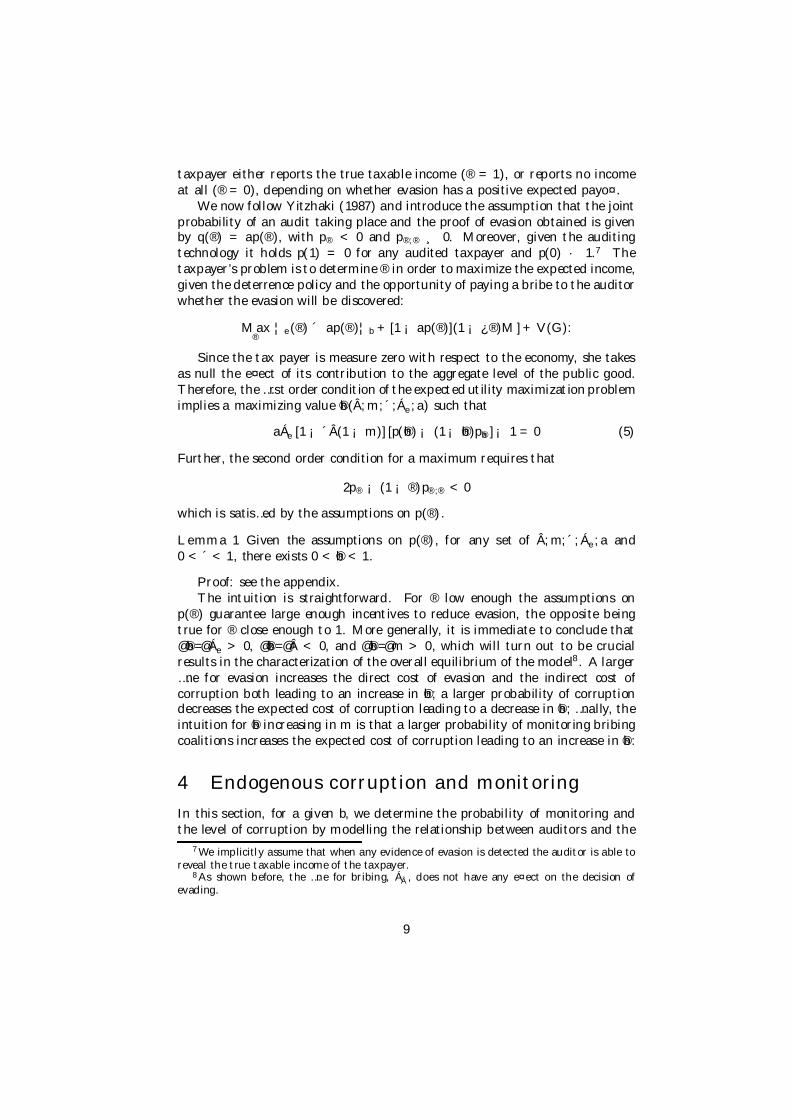
We now follow Yitzhaki (1987) and introduce the assumption that the jointprobability of an audit taking place and the proof of evasion obtained is givenby q(®) = ap(®), with p® < 0 and p®;® ¸ 0. Moreover, given the auditingtechnology it holds p(1) = 0 for any audited taxpayer and p(0) · 1.7 Thetaxpayer’s problem is to determine ® in order to maximize the expected income,given the deterrence policy and the opportunity of paying a bribe to the auditorwhether the evasion will be discovered:

M ax®

¦e(®) ´ ap(®)¦b + [1 ¡ ap(®)](1 ¡ ¿ ®)M ] + V (G):

Since the tax payer is measure zero with respect to the economy, she takesas null the e¤ect of its contribution to the aggregate level of the public good.Therefore, the …rst order condition of the expected utility maximization problemimplies a maximizing value b®(Â; m; ´;Áe ; a) such that

aÁe [1 ¡ ´Â(1 ¡ m)] [p(b®) ¡ (1 ¡ b®)pb® ] ¡ 1 = 0 (5)

Further, the second order condition for a maximum requires that

2p® ¡ (1 ¡ ®)p®;® < 0

which is satis…ed by the assumptions on p(®).

Lemma 1 Given the assumptions on p(®), for any set of Â; m; ´; Áe ; a and0 < ´ < 1, there exists 0 < b® < 1.

Proof: see the appendix.The intuition is straightforward. For ® low enough the assumptions on

p(®) guarantee large enough incentives to reduce evasion, the opposite beingtrue for ® close enough to 1. More generally, it is immediate to conclude that@b®=@Áe > 0, @b®=@Â < 0, and @b®=@m > 0, which will turn out to be crucialresults in the characterization of the overall equilibrium of the model8 . A larger…ne for evasion increases the direct cost of evasion and the indirect cost ofcorruption both leading to an increase in b®; a larger probability of corruptiondecreases the expected cost of corruption leading to a decrease in b®; …nally, theintuition for b® increasing in m is that a larger probability of monitoring bribingcoalitions increases the expected cost of corruption leading to an increase in b®:

4 Endogenous corruption and monitoringIn this section, for a given b, we determine the probability of monitoring andthe level of corruption by modelling the relationship between auditors and the

7 We implicitly assume that when any evidence of evasion is detected the auditor is able toreveal the true taxable income of the taxpayer.

8 As shown before, the …ne for bribing, ÁÂ, does not have any e¤ect on the decision ofevading.

9

monitorers as an incomplete information inspection game. In the event thatan auditor manages to prove an act of evasion, which occurs with probabilityap(®), the opportunity of forming a bribing coalition emerges with probability Âand the secret coalition is monitored with probability m. Both probabilities aredetermined in such a way that the public o¢cial is indi¤erent between taking thebribe (not reporting the act of evasion) or not. The monitoring level is such thatthe monitoring authority is indi¤erent between inspecting or not. As alreadydescribed in the introduction we consider two cases of the inspection game. Inthe …rst case a prosecutor monitors so that if any auditor takes a bribe b, shewill collect a pecuniary …ne ÁÂb from both members of the monitored bribingcoalition.9 Alternatively, we consider the case where a Tax Authority’s inspectsat a level such that that if any auditor takes a bribe b, she will collect a pecuniary…ne for evasion ©e from the tax evader.

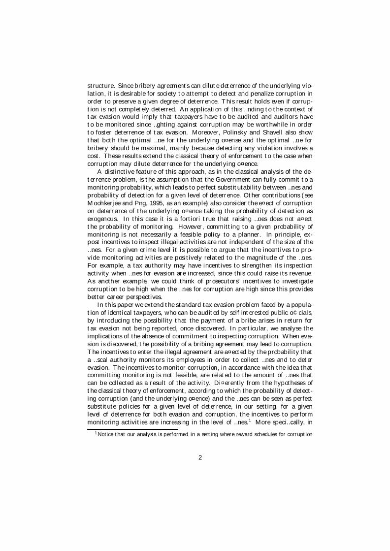
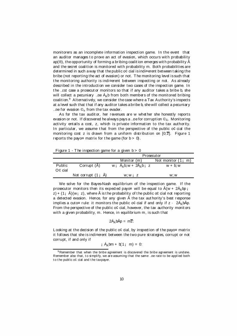
As for the tax auditor, her revenues are w whether she honestly reportsevasion or not. If discovered he always pays a …ne for corruption ©Â. Monitoringactivity entails a cost, z, which is private information to the tax authority.In particular, we assume that from the perspective of the public o¢cial themonitoring cost z is drawn from a uniform distribution on [0;z]. Figure 1reports the payo¤ matrix for the game (for b > 0).

Figure 1 - The inspection game for a given b > 0

ProsecutorMonitor (m) Not monitor (1 ¡ m)

Public Corrupt (Â) w ¡ ÁÂb;w + 2ÁÂb ¡ z w + b; wO¢cial

Not corrupt (1 ¡ Â) w; w ¡ z w; w

We solve for the Bayes-Nash equilibrium of the inspection game. If theprosecutor monitors then its expected payo¤ will be equal to Â(w + 2ÁÂbp ¡z)+(1¡Â)(w¡ z), where  is the probability of the public o¢cial not reportinga detected evasion. Hence, for any given  the tax authority’s best responseimplies a cuto¤ rule: it monitors the public o¢cial if and only if z · 2ÁÂbÂp.From the perspective of the public o¢cial, however, the tax authority monitorswith a given probability, m. Hence, in equilibrium m, is such that

2ÁÂbÂp = mz:

Looking at the decision of the public o¢cial, by inspection of the payo¤ matrixit follows that she is indi¤erent between the two pure strategies, corrupt or notcorrupt, if and only if

¡ÁÂbm + b(1 ¡ m) = 0:

9 Remember that when the bribe agreement is discovered the bribe agreement is undone.Remember also that, to simplify, we are assuming that the same …ne rate to be applied bothto the public o¢cial and the taxpayer.

10

Thus, the interior solution of the monitoring game implies

m =1

1 + ÁÂ

(6)

and =

z

2(1 + ÁÂ)ÁÂbp: (7)

For any given b the probability of a corruptive coalition to occurr decreaseswith the …ne rate ÁÂ. Moreover, in equilibrium, the proportion of public o¢cialswho take a bribe and do not report the detected evasion, Â, is inversely relatedto the amount of the bribe. A higher bribe implies that any public o¢cialexpects a higher probability of monitoring by the public o¢cial which, in turn,implies a lower probability of taking the bribe and not reporting the evasion.By assuming proportional …nes it follows that, in equilibrium, m does not varywith b.10

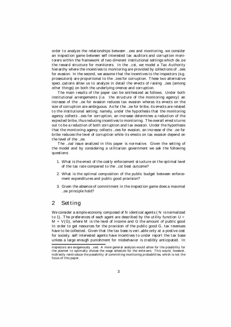
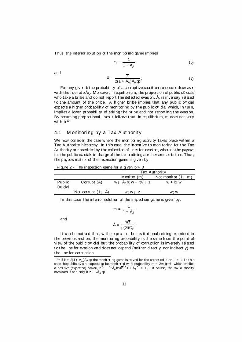
4.1 Monitoring by a Tax AuthorityWe now consider the case where the monitoring activity takes place within aTax Authority hierarchy. In this case, the incentive to monitoring for the TaxAuthority are provided by the collection of …nes for evasion, whereas the payo¤sfor the public o¢cials in charge of the tax auditing are the same as before. Thus,the payo¤s matrix of the inspection game is given by:

Figure 2 - The inspection game for a given b > 0Tax Authority

Monitor (m) Not monitor (1 ¡ m)Public Corrupt (Â) w ¡ ÁÂb; w + ©e ¡ z w + b; wO¢cial

Not corrupt (1 ¡ Â) w; w ¡ z w; w

In this case, the interior solution of the inspection game is given by:

m =1

1 + ÁÂ

and =

mz

p(®)©e:

It can be noticed that, with respect to the institutional setting examined inthe previous section, the monitoring probability is the same from the point ofview of the public o¢cial but the probability of corruption is inversely relatedto the …ne for evasion and does not depend (neither directly, nor indirectly) onthe …ne for corruption.

10 If ¹z > 2(1+ÁÂ)ÁÂbp the monitoring game is solved for the corner solution ¹ = 1. In thiscase the public o¢cial expects to be monitored with probability m= 2ÁÂbp=¹z, which impliesa positive (expected) payo¤, b

£1¡ ¡

2ÁÂbp=¹z¢ ¡1 +ÁÂ

¢¤> 0. Of course, the tax authority

monitors if and only if z · 2ÁÂbp.

11

5 Tax evasion and bribery agreement in equilib-rium

Given a set (Áe, ÁÂ, ´, ¿ , z, M ), the auditing technology p(®) and Authoritybudget constraint we solve for the equilibrium of the economy. Each taxpayerdecides the level of evasion, taking m and  as given, (this determines b®); eachpublic o¢cial decides whether to enter into a bribery agreement or not, givenm and b; at the same time, the prosecutor decides whether to monitor a givenpublic o¢cial, after having observed the monitoring cost z and given  andb. The level of b is determined as the Nash bargaining solution of the relatedproblem.

It is important to note that the taxpayer conceives his reporting strategy bytaking into account the e¤ect on p(®), but, being measure zero, she does nottake into account any e¤ect of her choice on the strategies to be chosen in thecontinuation game, Â and m. p(®) is the probability of state (tax base) veri…ca-tion, under the assumption that the larger the size of the evasion the easier is toprove it. Technically, this amounts to solve for the optimal reporting strategysimultaneously with the monitoring game between the monitoring agency andthe public o¢cials. The assumption of taxpayers being measure zero also hasthe implication that, in determining the bribe b, no e¤ect on the value of m isanticipated and taken into account. Therefore, Nash bargaining can be solvedindependently of the monitoring game.

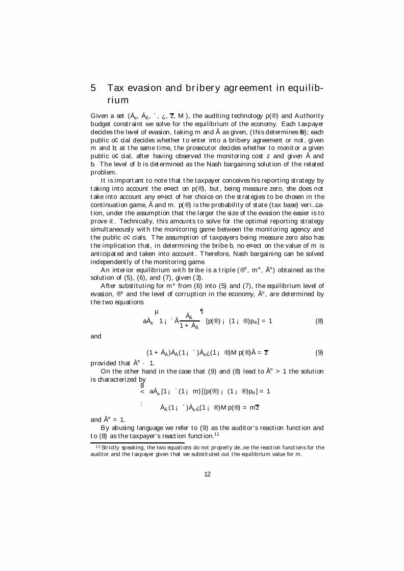
An interior equilibrium with bribe is a triple (®¤, m¤, ¤) obtained as thesolution of (5), (6), and (7), given (3).

After substituting for m¤ from (6) into (5) and (7), the equilibrium level ofevasion, ®¤ and the level of corruption in the economy, ¤, are determined bythe two equations

aÁe

µ1 ¡ ´Â

ÁÂ

1 + ÁÂ

¶[p(®) ¡ (1 ¡ ®)p®] = 1 (8)

and

(1 + ÁÂ)ÁÂ(1 ¡ ´)Áe¿ (1 ¡ ®)M p(®)Â = z (9)

provided that ¤ · 1.On the other hand in the case that (9) and (8) lead to ¤ > 1 the solution

is characterized by8<:

aÁe [1 ¡ ´(1 ¡ m)] [p(®) ¡ (1 ¡ ®)p® ] = 1

ÁÂ (1 ¡ ´)Áe¿(1 ¡ ®)Mp(®) = mz

and ¤ = 1.By abusing language we refer to (9) as the auditor’s reaction function and

to (8) as the taxpayer’s reaction function.11

11 Strictly speaking, the two equations do not properly de…ne the reaction functions for theauditor and the taxpayer given that we substituted out the equilibrium value for m.

12

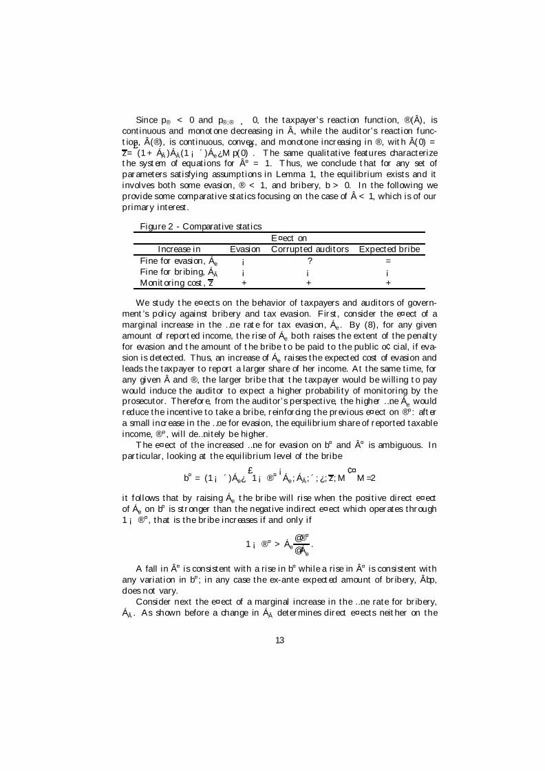
Since p® < 0 and p®;® ¸ 0, the taxpayer’s reaction function, ®(Â), iscontinuous and monotone decreasing in Â, while the auditor’s reaction func-tion, Â(®), is continuous, convex, and monotone increasing in ®, with Â(0) =z=

£(1 + ÁÂ )ÁÂ(1 ¡ ´)Áe¿M p(0)

¤. The same qualitative features characterize

the system of equations for ¤ = 1. Thus, we conclude that for any set ofparameters satisfying assumptions in Lemma 1, the equilibrium exists and itinvolves both some evasion, ® < 1, and bribery, b > 0. In the following weprovide some comparative statics focusing on the case of  < 1, which is of ourprimary interest.

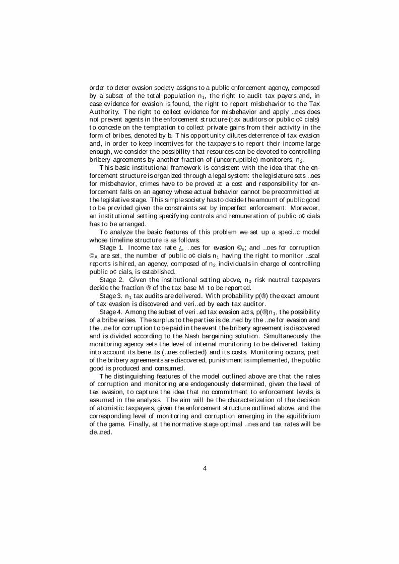
Figure 2 - Comparative staticsE¤ect on

Increase in Evasion Corrupted auditors Expected bribeFine for evasion, Áe ¡ ? =Fine for bribing, ÁÂ ¡ ¡ ¡Monitoring cost, z + + +

We study the e¤ects on the behavior of taxpayers and auditors of govern-ment’s policy against bribery and tax evasion. First, consider the e¤ect of amarginal increase in the …ne rate for tax evasion, Áe . By (8), for any givenamount of reported income, the rise of Áe both raises the extent of the penaltyfor evasion and the amount of the bribe to be paid to the public o¢cial, if eva-sion is detected. Thus, an increase of Áe raises the expected cost of evasion andleads the taxpayer to report a larger share of her income. At the same time, forany given  and ®, the larger bribe that the taxpayer would be willing to paywould induce the auditor to expect a higher probability of monitoring by theprosecutor. Therefore, from the auditor’s perspective, the higher …ne Áe wouldreduce the incentive to take a bribe, reinforcing the previous e¤ect on ®¤: aftera small increase in the …ne for evasion, the equilibrium share of reported taxableincome, ®¤, will de…nitely be higher.

The e¤ect of the increased …ne for evasion on b¤ and ¤ is ambiguous. Inparticular, looking at the equilibrium level of the bribe

b¤ = (1 ¡ ´)Áe¿£1 ¡ ®¤ ¡

Áe ; ÁÂ; ´; ¿ ; z; M¢¤

M=2

it follows that by raising Áe the bribe will rise when the positive direct e¤ectof Áe on b¤ is stronger than the negative indirect e¤ect which operates through1 ¡ ®¤, that is the bribe increases if and only if

1 ¡ ®¤ > Áe

@®¤

@Áe

.

A fall in ¤ is consistent with a rise in b¤ while a rise in ¤ is consistent withany variation in b¤; in any case the ex-ante expected amount of bribery, Âbp,does not vary.

Consider next the e¤ect of a marginal increase in the …ne rate for bribery,ÁÂ . As shown before a change in ÁÂ determines direct e¤ects neither on the

13

amount of the penalty for evasion nor on the expected cost of exploiting theopportunity of bribery, the latter being (1 ¡ ´ + ´m)Áe¿ (1 ¡ ®)M . The rise inthe penalty rate Á , however, determines a reduction in the value of m¤ whichimplies, for any given Â, that the taxpayer’s incentive to evade will be reduced.For the auditor, a larger Á increases the expected cost of taking a bribe, for anygiven b, reducing her incentive to be corrupted.1 2 It can be shown that after arise in the penalty rate for bribery the new equilibrium will be characterised bya lower level of corruption, ¤, as well as a lower level of evasion, that is higher®¤ (see appendix).13 Both the equilibrium level of b¤ and the expected amountof bribery, Âbp, will be de…nitively reduced.14

Finally, consider a change in government’s policy when the corruption rateis ¤ = 1, that is all detected evasion are not reported to the prosecutor. Asmall increase in Áe reduces the extent of evasion.

The results above may be summarized in the following

Proposition 2 If bribery is pro…table b¤ > 0, a tougher deterrence policy, inthe form of increased …nes, will always be e¤ective for reducing evasion. On theother hand the e¤ect on corruption is ambiguous if a tougher policy is imple-mented through the level of …ne for evasion.

We now brie‡y present the comparative statics results of the model in thecase where the monitoring activity of public o¢cials is delegated to the TaxAuthority.

The e¤ect of an increase of the …ne for evasion on both the level of evasion andthe level of corruption is qualitatively the same as in the framework describedabove. On the contrary, in the present case, an increase in the …ne for corruptioncan determine an increase in the level of evasion for relatively low levels of the…ne for corruption.

The intuition for this result is the following: an increase in the …ne forcorruption reduces the monitoring probability of an amount which is the samein the two institutional arrangements. Thus, the negative e¤ect on ®, throughm is the same. However, in both cases, an increase of the …ne for corruptiona¤ects ® also through the probability of corruption Â. While, in the previousframework, the positive e¤ect on ® was always stronger than the negative one,thus leading to an unambiguous prediction, in the present case the overall e¤ect

12 Given m, a larger Á reduces the incentiveof the public o¢cial to take a bribe, due to thelarger expected cost of bribery, that is reduces Â. The net e¤ect of larger Á and a lower  willinduce, however, the auditor to expect that the tax authority will monitor more, determininga further reduction in Â.

13 From the perspective of the auditor, the monitoring probability of the tax authority, m¤,will be reduced.

14 Note that even if the qualitative e¤ect of a rise in either Áe or Á on  can be similar,the mechanics are completely di¤erent. In the case of a rise in Áe the direct e¤ect as well asthe equilibrium e¤ect on  operate, coeteris paribus, mainly through a change in the bribe,that is the revenue of bribery. In particular, if in equilibrium the bribe will reduce the levelof  will increase. On the contrary, in the case of a rise in Á the bribe does not change ina direct way. Thus, the e¤ect of an increase in Á operates, in a …rst instance, through thecost of bribing.

14

on tax evasion depends on the size of the …ne for corruption: if this is greater(smaller) than one, tax evasion will be reduced (increased). The reason forthis result is to be found in the particular structure of the payo¤ matrix in thepresent setting: namely, the …ne rate for corruption does not in‡uence the sizeof the revenue form the monitoring activity.

Finally, let us consider brie‡y the case when the monitoring cost z is commonknowledge (a case of interest for the following welfare analysis). The main resultis that an increase in the …ne for corruption (in both the institutional settingsdiscussed above) determines an increase in the level of evasion.

6 Welfare Analysis (Preliminary)In this section we use the results derived above to assess the normative impli-cations of our model of tax evasion, corruption and monitoring. Let us brie‡ysummarize the …ndings obtained so far. We study an economy composed of apopulation of measure 1 = n0 + n1 + n2. A fraction n0 of it produces incomeM pays ¿ ®M as an income tax taking the gamble to evade part of it. Taxrevenues are collected to …nance the public good to be provided in the economy.A fraction n1 is paid a …xed wage w, is assigned the right to audit tax payersand is endowed with a state veri…cation technology that allows the tax audi-tors to verify the true tax base with a probability p(®). In the event evasion isproved the opportunity of corruption emerges at an equilibrium probability Â.A fraction of (uncorruptible) n2 = n1m agents is assigned the right to monitorthe tax auditors.

In order to provide normative results we need to specify the institutionalsetting of the monitoring game, the budget constraints of the monitoring au-thority and the …scal budget in the aggregate. Before doing that, however, itis worth discussing the issue of the remuneration of the law enforcers. Havingassumed no commitment to the probability of detection of corruption on thepart of the planner we let the planner to choose the number of tax auditors n1

but not the number of agents monitoring corruption. The number of agents incharge for the enforcement of anti-corruption legislation is set in equilibrium bythe model as in the previous section. The remuneration to all enforcers is set atthe expected income in the economy:

w ´ Ey = (1 ¡ ®¿)M ¡ ap [(1 ¡  + Âm)©e + bÂ(1 ¡ m) + ©Âm] (10)

Intuitively, expected income is given by net income (gross of evasion) lessexpected …nes. Notice that, by this assumption, all the agents in our economyare ex-ante indi¤erent across jobs and get utility

U(:) = Ey + V (G) (11)

satisfying the envelope condition U®(:) = dEyd®

= 0.

15

After substituting the equilibrium condition of the inspection game and theequilibrium value of the bribe and assuming ´ = 1=2 we obtain the followingexpression for the expected income

Ey = (1 ¡ ®¿)M ¡ ap[1 ¡ Â

2(1 ¡ m)]©e (12)

We can de…ne now the budget for the Tax Authority as follows

B + ©eÂmpn1 = w(1 + m)n1 + zmn1 (13)

Where B is the transfers from the …scal budget, ©eÂmpn1 is the total rev-enues from collected …nes for evasion as in the second inspection game describedin the previous section, w(1+m)n1 is the total (net) wage paid to law enforcers,zmn1 is the total amount of direct costs of monitoring. From equilibrium condi-tions in the inspection game we get B = w(1 +m)n1. The general …scal budgetis then given by

G + B = n0¿®M + n1p(1 ¡  + Âm)©e + 2n1p©Âm (14)

Where G is the value of the public good provided in the economy, n0¿ ®Mis the volontary component of tax revenues, n1p(1 ¡ Â)©e is the total value ofthe enforced …ne for evasion not accruing to the budget of the Tax Authority(voluntary payment of the …nes by tax payers not joining a bribing coalition)and, …nally, 2n1p©Âm is the value of the …nes for corruption obtained as anindirect revenue for the monitoring activity, which we assume to be accrued tothe provision of the public good. After substituting the equilibrium conditionsfrom the inspection game we get a reduced form for the amount of public goodprovided in the economy

G = [1 ¡ n1(1 + m)]M ¡ Ey ¡ n1zm (15)

The planner is modelled as an utilitarian legislator whose problem is tomaximize total welfare (remember that the total population is normalized to 1)

U (:) = Ey + u(G) (16)

with respect to the tax rate ¿ (implicitly de…ning G), the …ne rates, Áe , ÁÂ

and the number of auditors n1, subject to (??) and to the limited …scal liabilityconstraint

©e + ©Â · (1 ¡ ®¿ )M (17)

The problem can therefore be written as

M ax¿ ;Áe;ÁÂ ;n1

Ey + u(G)

s.to G = [1 ¡ n1(1 + m)]M ¡ Ey ¡ n1zm©e + ©Â · (1 ¡ ®¿ )M

U® = 0

(18)

16

the solution for this program can be characterized by standard techniques.By substitituting equilibrium values for ©e and ©Â for the case of symmet-ric bargaining power in the bribing coalition, we can write the Lagrangean asfollows. (See Appendix).

L = Ey + u(G) + ¸[(1 ¡ ®¿ )M ¡ Áe(1 ¡ ®)¿M(1 +ÁÂ

4)] (19)

By solving the Lagrangean we obtain the following

Proposition 3 At an interior equilibrium (®¤; m¤; ¤) i. maximal …nes prin-ciple holds in (18) and G = G¤ ii. Áe > 0, Á > 0.

Proof. Set ¸ = 0 in 18 and get a contradiction. See Appendix for details.The intuition is rather simple. Part i. can be explained as follows. Assume

maximal …ne does not hold. Since d®=dÁe > 0 there must be overdeterrence.The planner can increase G up to its …rst best level G¤. Furthermore in orderto save costs the planner is willing to cut on monitoring costs by reducing n1

and increasing the number of tax payers producing M at the cost of dilutingdeterrence, the reported ® by each tax payer decreases. This argument holdstrue at any given level of G¤, leading to a corner solution in n1 = 0 and ® = 0.The intuition for part ii. is an immediate implication of the equilibrium beinginterior. The reason is that both …nes are useful to deter the underlying of-fence (tax evasion): raising the …ne for evasion makes a bribing more costly andincreases deterrence on the underlying o¤ence and would tend to increase mon-itoring activities and costs (…nes for evasion can be increased only by increasingmonitoring costs, which in equilibrium of the inspection game will be paid interms of larger corruption). To save on costs of enforcement the only instru-ment to the planner is to increase the …ne for corruption. Jointly consideredthe design of the two …nes saturates the …scal liability constraint of the o¤ender(maximal …nes). Notice that, di¤erently from the classical analysis of optimaldeterrence, increasing …nes in our model tend to raise the cost of enforcement.

For future reference de…ne ~Áe and ~ÁÂ as the maximal possible …nes at theoptimum. Before characterizing the optimal trade o¤ between the …ne for eva-sion and the …ne for corruption another result is worth noticing. Let us denote~G as the amount of public good to be provided in the economy at the optimumas de…ned by (??) where ~¿ (the tax rate at the optimum), ~Áe and ~ÁÂ are usedto compute Ey. The following result can be shown to hold

Proposition 4 In an economy with imperfect commitment to monitoring andmaximal …nes a utilitarian planner will choose ~¿ such that ~G < G¤:

Proof. See appendixThe reason is the following: at maximal …ne the tax rate that implements

G = G¤ is ~¿ > ¿¤ (since the costs of the enforcement structure have to be…nanced) and underdeterrence holds. Notice also that in our model large ¿induces some deterrence since, by increasing bribes, gives larger incentives tomonitor. On the other hand total punishment is limited by the tax rate. At

17

G = G¤ the …ne for evasion is a more e¢cient instrument to deter evasiontherefore the planner is willing to reduce ¿ and increase Áe .

In other words, in our model, the planner would like to raise ¿ in order toincrease the level of monitoring. At the equilibrium cum evasion, however, theincreased incentives to monitor are settled by reducing evasion and decreasingcorruption. The limited …scal liability is thus reduced.

Notice also that since the general budget has to …nance wages to monitorer,~G < G¤ does not necessarily imply that ~¿ < ¿ ¤. The actual tax rate in aneconomy with imperfect enforcement may well be above the optimal level oftaxation obtained in the case of honest taxpayers (…rst best).

7 ConclusionsWe considered a simple economy where self interested tax payers may haveincentives to evade taxes and, to escape sanctions, to bribing public o¢cials incharge for collections. Di¤erently from the classical theory of law enforcementwe let the legislator not be committed to a given level of detecting corruptionand we analyzed the interactions between evasion, corruption and monitoring aswell as their adjustment to a change in the institutional setting. In the proposedframework, larger …nes induce two e¤ects. On the one hand, an increase in thesize of the …ne induces a stronger deterrence; on the other hand, however, itdetermines a larger incentive to corrupt, by increasing the di¤erence betweenthe disposable income if evasion is detected and the disposable income if it isnot. Furthermore, we …nd that, in equilibrium, an increase in the …nes reducestax evasion whereas the e¤ect on corruption can be ambiguous.

We also considered the optimal design of …nes in a normative perspective.Interestingly enough a maximal …ne principle holds in the case of a utilitarianlegislator, despite the fact that raising …nes increases monitoring activities andtheir cost to society. The reason for this result is that, in an environment withimperfect enforcement, the amount of public good provided by a utilitariangovernment is smaller than its level at …rst best: underdeterrence hold at theconstrained optimal tax rate. This leads to maximal …ne.

References[1] Allingham, G. Michael, and Agnar Sandmo (1972), Income Tax Evasion:

A Theoretical Analysis, Journal of Public Economics, 1(3-4), pp. 323-338.

[2] Bardhan, Pranab (1997), Corruption and Development: A Review of Issues,Journal of Economic Literature, 35(3), pp. 1320-1346.

[3] Becker, S. Gary (1968), Crime and Punishment: An Economic Approach,Journal of Political Economy, 76, pp. 169-217.

18

[4] Chandler P. and L Wilde (1992), Corruption in Tax Administration, Jour-nal of Public Economics 49, pp. 333-349.

[5] Melamud, N. and D. Mookherjee (1989), Delegation as commitment: thecase of income tax audits, Rand Journal of Economics, 20 (2), pp.139-163.

[6] Mookherjee D. and P.L. Png, (1992), Monitoring vis-à-vis Investigationinenforcement of Law, The American Economic Review, 82 (3), pp.556-565.

[7] Polinsky, A. Mitchell, and Steven Shavell (1979), The Optimal Tradeo¤between the Probability and Magnitude of Fines, The American EconomicReview, 69(5), pp. 880-891.

[8] _ and _ (2000), The Economic Theory of Public Enforcement of Law,Journal of Economic Literature, XXXVIII, pp. 45-76.

[9] _ and _ (2001), Corruption and Optimal Law Enforcement, Journal ofPublic Economics, 81, pp.1-24.

[10] Rose-Ackerman, Susan (1978), Corruption: A Study in Political Economy,New York: Academic Press.

[11] Saha, Atanu, and Graham Poole (2000), The Economics of Crime andPunishment: an Analysis of Optimal Penalty, Economics Letters, 68, pp.191-196.

[12] Sanyal, Amal, Ira N. Gang, and Omkar Goswami (2000), Corruption, TaxEvasion and the La¤er Curve, Public Choice, 105, pp. 61-78.

[13] Shleifer, Andrei, and Robert W. Vishny (1993), Corruption, QuarterlyJournal of Economics, 108(3), pp. 599-617.

[14] Stigler, J. George (1970), The Optimum Enforcement of Laws, JournalPolitical Economy, 78, pp.526-536.

[15] Yitzhaki, Shlomo. (1987), On the Excess Burden of Tax Evasion, PublicFinance Quarterly, 15(2), pp. 123-137.

19

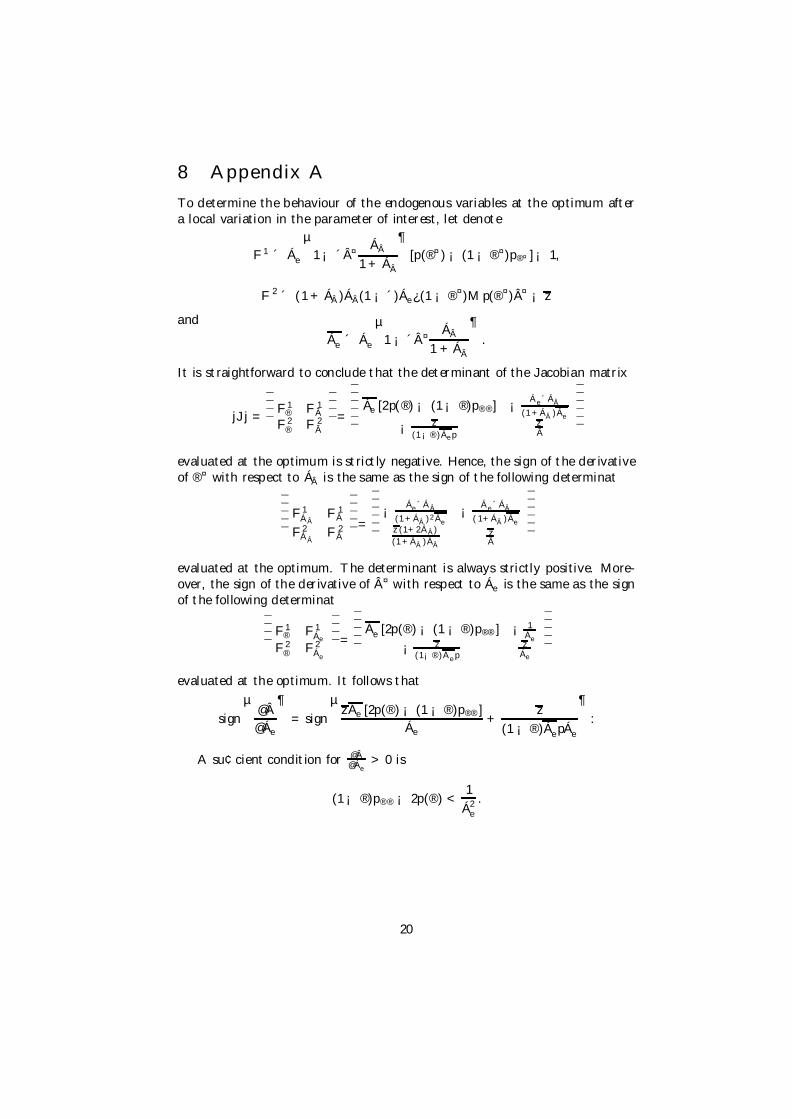
8 Appendix ATo determine the behaviour of the endogenous variables at the optimum aftera local variation in the parameter of interest, let denote

F 1 ´ Áe

µ1 ¡ ´Â¤ ÁÂ

1 + ÁÂ

¶[p(®¤ ) ¡ (1 ¡ ®¤)p®¤ ] ¡ 1,

F 2 ´ (1 + Á )ÁÂ(1 ¡ ´)Áe¿(1 ¡ ®¤)M p(®¤)¤ ¡ z

and

Áe ´ Áe

µ1 ¡ ´Â¤ ÁÂ

1 + ÁÂ

¶.

It is straightforward to conclude that the determinant of the Jacobian matrix

jJj =

¯̄¯̄ F 1

® F 1Â

F 2® F 2

Â

¯̄¯̄ =

¯̄¯̄¯̄

Áe [2p(®) ¡ (1 ¡ ®)p®®] ¡ Áe´ÁÂ

(1+ÁÂ)Áe

¡ z

(1¡®)Áep

zÂ

¯̄¯̄¯̄

evaluated at the optimum is strictly negative. Hence, the sign of the derivativeof ®¤ with respect to Á is the same as the sign of the following determinat

¯̄¯̄¯

F 1ÁÂ

F 1Â

F 2ÁÂ

F 2Â

¯̄¯̄¯ =

¯̄¯̄¯̄

¡ Áe´ÁÂ

(1+ÁÂ)2Áe

¡ Áe´ÁÂ

(1+ÁÂ)Áez(1+2ÁÂ)

(1+ÁÂ)ÁÂ

zÂ

¯̄¯̄¯̄

evaluated at the optimum. The determinant is always strictly positive. More-over, the sign of the derivative of ¤ with respect to Áe is the same as the signof the following determinat

¯̄¯̄ F 1

® F 1Áe

F 2® F 2

Áe

¯̄¯̄ =

¯̄¯̄¯

Áe [2p(®) ¡ (1 ¡ ®)p®® ] ¡ 1Áe

¡ z(1¡®)Áep

zÁe

¯̄¯̄¯

evaluated at the optimum. It follows that

signµ

@Â

@Áe

¶= sign

µzÁe [2p(®) ¡ (1 ¡ ®)p®® ]

Áe

+z

(1 ¡ ®)ÁepÁe

¶:

A su¢cient condition for @Â@Áe

> 0 is

(1 ¡ ®)p®® ¡ 2p(®) <1

Á2e

.

20

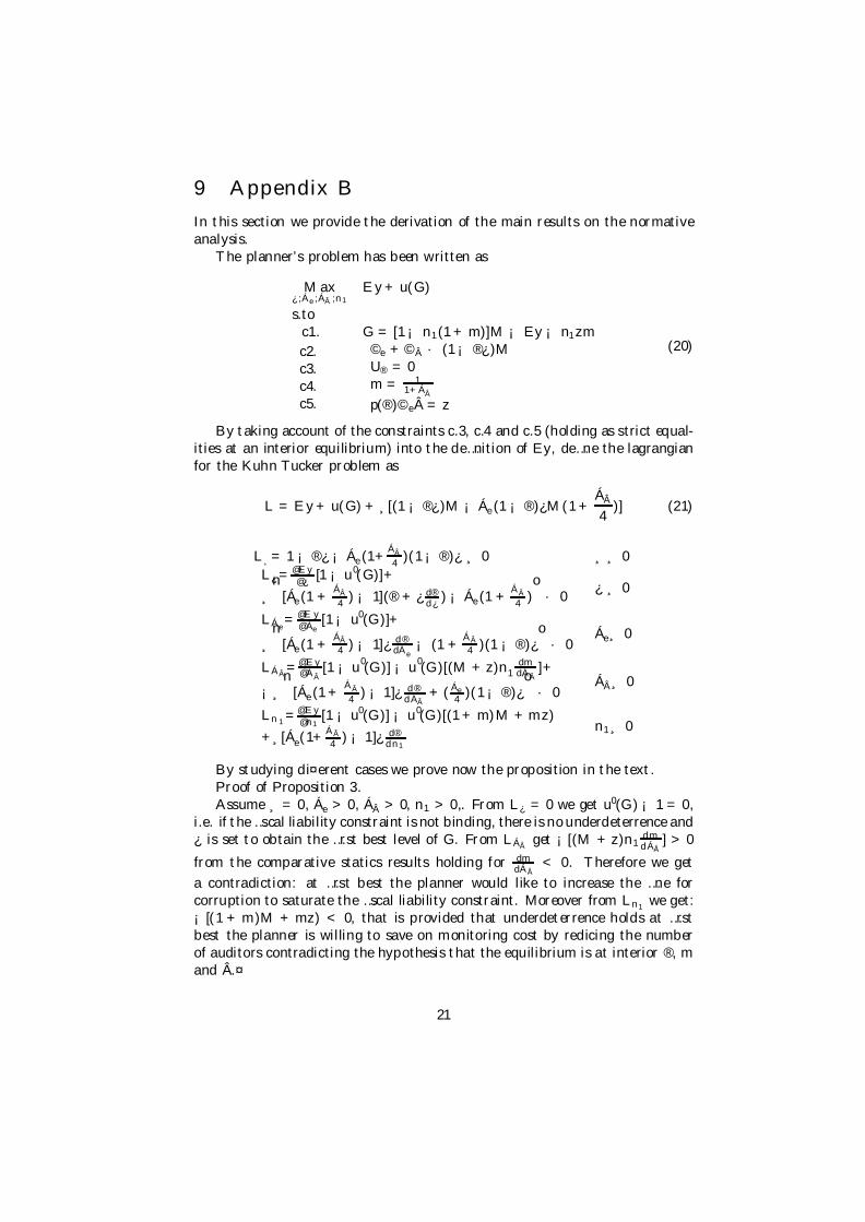
9 Appendix BIn this section we provide the derivation of the main results on the normativeanalysis.

The planner’s problem has been written as

M ax¿ ;Áe;ÁÂ ;n1

Ey + u(G)

s.toc1. G = [1 ¡ n1(1 + m)]M ¡ Ey ¡ n1zm

c2.c3.c4.c5.

©e + ©Â · (1 ¡ ®¿ )MU® = 0m = 1

1+ÁÂ

p(®)©e = z

(20)

By taking account of the constraints c.3, c.4 and c.5 (holding as strict equal-ities at an interior equilibrium) into the de…nition of Ey, de…ne the lagrangianfor the Kuhn Tucker problem as

L = Ey + u(G) + ¸[(1 ¡ ®¿ )M ¡ Áe(1 ¡ ®)¿M(1 +ÁÂ

4)] (21)

L¸= 1 ¡ ®¿ ¡ Áe(1+ÁÂ

4)(1 ¡ ®)¿ ¸ 0 ¸ ¸ 0

L¿ = @Ey@¿

[1 ¡ u0(G)]+

¸n

[Áe(1 +ÁÂ

4) ¡ 1](® + ¿ d®

d¿) ¡ Áe(1 +

ÁÂ

4)o

· 0¿ ¸ 0

LÁe= @Ey

@ Áe[1 ¡ u0(G)]+

¸n

[Áe(1 +ÁÂ

4 ) ¡ 1]¿ d®dÁe

¡ (1 +ÁÂ

4 )(1 ¡ ®)¿o

· 0Áe¸ 0

LÁÂ=@ Ey

@ÁÂ[1 ¡ u

0(G)] ¡ u

0(G)[(M + z)n1

dmdÁÂ

]+

¡¸n

[Áe(1 +ÁÂ

4) ¡ 1]¿ d®

dÁÂ+ ( Áe

4)(1 ¡ ®)¿

o· 0

Á¸ 0

Ln1=@ Ey

@n1[1 ¡ u0(G)] ¡ u0(G)[(1 + m)M + mz)

+¸[Áe(1+ÁÂ

4) ¡ 1]¿ d®

dn1

n1¸ 0

By studying di¤erent cases we prove now the proposition in the text.Proof of Proposition 3.Assume ¸ = 0, Áe > 0, ÁÂ > 0, n1 > 0,. From L¿ = 0 we get u0(G) ¡ 1 = 0,

i.e. if the …scal liability constraint is not binding, there is no underdeterrence and¿ is set to obtain the …rst best level of G. From LÁÂ

get ¡[(M + z)n1dmdÁÂ

] > 0

from the comparative statics results holding for dmdÁÂ

< 0. Therefore we geta contradiction: at …rst best the planner would like to increase the …ne forcorruption to saturate the …scal liability constraint. Moreover from Ln1

we get:¡[(1 + m)M + mz) < 0, that is provided that underdeterrence holds at …rstbest the planner is willing to save on monitoring cost by redicing the numberof auditors contradicting the hypothesis that the equilibrium is at interior ®, mand Â.¤

21

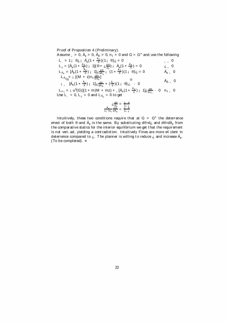
Proof of Proposition 4 (Preliminary).Assume ¸ > 0, Áe > 0, ÁÂ > 0, n1 > 0 and G = G¤ and use the following

L¸ = 1 ¡ ®¿ ¡ Áe(1 +ÁÂ

4)(1 ¡ ®)¿ = 0 ¸ ¸ 0

L¿ = [Áe(1 +ÁÂ

4) ¡ 1](® + ¿ d®

d¿) ¡ Áe(1 +

ÁÂ

4) = 0 ¿ ¸ 0

LÁe= [Áe(1 +

ÁÂ

4 ) ¡ 1]¿ d®dÁe

¡ (1 +ÁÂ

4 )(1 ¡ ®)¿ = 0 Áe ¸ 0

LÁÂ= ¡[(M + z)n1

dmdÁÂ

]

¡¸n

[Áe(1 +ÁÂ

4) ¡ 1]¿ d®

dÁÂ+ (

Áe

4)(1 ¡ ®)¿

o· 0

ÁÂ ¸ 0

Ln1 = ¡u0(G)[(1 + m)M + mz) + ¸[Áe(1 +ÁÂ

4) ¡ 1]¿ d®

dn1· 0 n1 ¸ 0

Use L¸ = 0, L¿ = 0 and LÁe= 0 to get

¿ d®d¿

= 1¡®1¡¿

Áe1¡®¿

d®dÁe

= 1¡®1¡¿

Intuitively, these two conditions require that at G = G¤ the deterrencee¤ect of both ® and Áe is the same. By substituting d®=d¿ and d®=dÁe fromthe comparative statics for the interior equilibrium we get that the requirementis not veri…ed, yielding a contradiction. Intuitively Fines are more e¢cient indeterrence compared to ¿ . The planner is willing to reduce ¿ and increase Áe .(To be completed). ¤

22