Tax-deferred retirement savings of farm households: an empirical investigation

Journal of Agricultural and Resource Economics 36(1):xxx–xxx Copyright 2011 Western Agricultural Economics Association

Tax-Deferred Retirement Savings of Farm Households: An Empirical Investigation

Ashok K. Mishra and Hung-Hao Chang

This study examines factors affecting tax-deferred retirement savings among farm house-holds. A double-hurdle model is estimated using 2003 Agricultural Resource Management Survey (ARMS) farm-level national data. Results indicate that demographic factors, total household income, off-farm work, and risk preference play important roles in retirement savings plan participation. Retirement savings increase with household size, intensity of off-farm work by farm operator and spouse, and size of farming operation. We find that the amount of retirement savings decreases with operator’s age and increases with spouse’s age, and that cash grain and dairy farmers have lower retirement savings. Key Words: double-hurdle estimation, farm households, probit, retirement savings, risk preference, total household income

Introduction Recent economic conditions and the “Great Recession” of 2008 have reignited the debate regarding the adequacy of retirement income. With looming budget deficits and shortfalls in Social Security benefits, more and more people are experiencing heightened concerns about how much to save for retirement. Although this may be a moot point for baby boomers who have already begun to retire, a recent Boston College report concluded that 43% of American households are “at risk” for substantial declines in retirement income, even after factoring in financial and housing wealth (Munnell, Webb, and Delorme, 2006). Unlike nonfarm households, farm households do little formal planning or investing specifi-cally for retirement (Hamaker and Patrick, 1996). The average U.S. farmer is about 57 years old. In addition to increasing age and approaching retirement, decreasing farm income, and increasing life expectancy, U.S. farmers and their spouses are concerned about outliving the accumulated assets in their retirement portfolio. Studies also show that most farmers’ spouses outlive them (Lycett, Dunbar, and Voland, 2000), and retirement income (other than farm assets) is becoming increasingly important in old age. This problem is exacerbated when younger family members choose not to be active in the farm business (Mishra and El-Osta, 2008). Consequently, the failure to plan carefully for retirement and the ultimate transfer of the estate can result in serious problems such as financial insecurity, personal and family dissatisfaction, and needless capital losses.

Ashok K. Mishra is professor, Department of Agricultural Economics and Agribusiness, Louisiana State University AgCenter. Hung-Hao Chang, the contact author for this research, is associate professor, Department of Agricultural Economics, National Taiwan University. An earlier version of this paper was presented at the WAEA annual meetings in Anchorage, Alaska, June 31–July 2, 2006. We are grateful to Joseph Atwood and Gary Brester for their helpful comments and suggestions. The views expressed here are not necessarily those of the Economic Research Service or the U.S. Department of Agriculture. Mishra’s time on this project was supported by the USDA Cooperative State Research, Education, and Extension Service, Hatch Project No. 0212495, and Louisiana State University Experiment Station Project No. LAB 93872. Review coordinated by Joseph A. Atwood.

2 April 2011 Journal of Agricultural and Resource Economics Farm and ranch operators face significant and unique obstacles in planning and providing for their retirement (American Corn Growers Association and Americans for Secure Retire-ment, 2002). Farmers are less likely to participate in employer-sponsored retirement plans, and their low income levels make saving for retirement difficult. Furthermore, farm wives are especially at risk of experiencing a declining standard of living in retirement, which contributes to farm households’ retirement insecurity. Robinson (2005) concludes that America’s farmers face a higher risk of declining living standards at retirement than those in other occupations. With looming budget deficits and the possibility of reductions in government payments, farm operators and their households are also more likely to experience greater income variability.1 Given the extensive engagement of farm operator households in the nonfarm economy (Ahearn, 1986; Ahearn, Perry, and El-Osta, 1993; Mishra et al., 2002), it is not surprising that some farm households participate in employer-sponsored retirement plans. However, Mishra, Durst, and El-Osta (2005) find that only 40% of farm households participate in some type of retirement savings plan, compared to 60% of all U.S. households.2 Further, the authors report that, compared to small farms, commercial farm operators are less likely to have an employer-sponsored pension and more likely to receive a larger share of their retirement income from farm assets. On the other hand, operators and spouses may choose to invest their savings back into the farm business, particularly if the farm is large. Such reinvestment may cause a farm’s value to appreciate. If this appreciation were converted into a capital gain through a sale, it could provide for the farmer’s retirement,3 but sale proceeds may be necessary to pay off debts. This study analyzes retirement savings behaviors among farm households. First, we examine the role of off-farm employment, risk preference, government payments, and level of indebt-edness on farm households’ decision to participate in tax-deferred retirement savings. Second, we investigate how those factors influence the amount that farm households save for retirement. We use a large nationwide farm-level data set, comprising farms of different economic sizes and in different regions of the United States. A better understanding of factors influencing savings behaviors will be useful not only to farm households, but also to policy makers seeking to formulate policies to help farm households maintain stable incomes in later life. Our findings can be applied by educators and financial planners to develop strategies for marketing their products to farm families seeking information on ways to improve retirement income and meet desired retirement savings levels.

Background

Congress established individual retirement accounts (IRAs) in 1974 as part of the Employee Retirement Income Security Act (ERISA) in order to encourage employees or individuals not covered by private pension plans—such as farmers—to save for retirement. Tax-deferred savings are a potentially important retirement portfolio component and could represent a

1 Growing budget concerns have prompted President Obama to recently address this issue, expressing the desire to cut direct

payments to large agricultural producers (those who make more than $500,000 in annual sales revenue), reduce crop insurance subsidies, and eliminate cotton storage credits. Obama argues that funding should be targeted toward family farms rather than “corporate megafarms” (Office of Management and Budget, 2009).

2 Household retirement savings include both employer-sponsored retirement plans and individual retirement savings plans, such as IRA, 401(k), and Keogh accounts.

3 The retiring farmer generally tries to balance the desire to keep the farm intact as a going concern with the need for a secure asset portfolio to finance retirement. Transferring the farm to the younger generation may lead to income sharing or an agreement with regard to rent sharing. Both of these choices may involve farm income—which is uncertain (Mishra and Sandretto, 2002).

Mishra and Chang Tax-Deferred Retirement Savings of Farm Households 3

substantial increase in tax-free assets for many individuals. Since the implementation of ERISA, the trend has been away from pension coverage under defined benefit plans and toward defined contribution plans (Foster, 1996). The Economic Recovery Tax Act of 1981 extended the availability of IRAs to all employees (including the self-employed) and raised the contribution limit. Several retirement savings plans for self-employed individuals have also been established to better serve small businesses, including farms. These plans include 401(k) accounts, Keogh accounts, savings incentive match plans for employees of small employers (SIMPLE), and simplified employee pensions (SEPs). Despite these options, chronic low levels of private and public savings among Ameri-cans in recent years have generated considerable concern among academics and policy makers. The Survey of Consumer Finances (SCF) (Federal Reserve Board, 2010) collects informa-tion on families’ motivations for savings. In 2004, retirement-related motivations were most frequently reported, with a 35% response, an increase of 3 percentage points since 2001. This increase may reflect the rising share of baby-boomer families in the population as well as perceived uncertainty about future retirement benefits. The next most frequently reported reason for savings (approximately 30%) was related to liquidity, a category that includes a variety of precautionary motives. In the case of farmers, 42% reported retirement as the primary motive for savings, an increase of 9 percentage points since 2001.4 Education and liquidity are important reasons given by farmers for saving. Selected reasons, by percentage, for saving among the general U.S. population are graphically displayed in figure 1. Similarly, figure 2 displays these reasons-for-saving percentages among farmers. Studies investigating retirement savings among farm households have been limited. Gustafson and Chama (1994) conducted a survey to identify the different types and sizes of financial assets held by North Dakota farmers. Their results suggest most farmers invest in low-risk financial assets held primarily for emergency and retirement reasons. Using national farm-level cross-sectional data, Mishra and Morehart (2001) examine off-farm investments among U.S. farm households and conclude that farms receiving government payments tend to save less than their unsubsidized counterparts. Serra, Goodwin, and Featherstone (2004) employ panel data for Kansas farm households to evaluate farm households’ investment in various nonfarm assets (such as retirement accounts, residence, liquid assets, saleable stock, and other interests). They find that farm income variability influences nonfarm investment. None of the studies cited above directly addressed the issue of retirement savings at the national level using farm-level data.

Conceptual Framework

Risk aversion plays an important role in the savings-consumption decision (Sandmo, 1969). Because future income may be uncertain, it is assumed that risk-averse persons will consume less in the current period and save a portion of current income for future consumption. The farm household is assumed to have two individuals (operator and spouse), a cardinal utility function, and a preference ordering for present and future consumption (C1, C2), such that:

(1) 1 2, ,U U C C

where C1, C2 ≥ 0. To introduce the effects of increased risk associated with future income on present consumption, the first-period budget constraint facing the household is given by:

4 Data from the 2004 SCF are used for comparison, since our data were collected in 2003.

4 April 2011 Journal of Agricultural and Resource Economics

Figure 1. Selected reasons for savings as reported by all U.S. individuals, 2001 and 2004

Figure 2. Selected reasons for savings as reported by farmers, 2001 and 2004

11

3231

12

35

30

0

5

10

15

20

25

30

35

40

Education Retirement Liquidity

Per

cent

2001 2004

10

33

19

15

42

15

0

5

10

15

20

25

30

35

40

45

Education Retirement Liquidity

Per

cent

2001 2004

Source: Survey of Consumer Finances, 2004

Source: Survey of Consumer Finances, 2004


(2) 1 1 1 ,I C S

where I1 is income in the first period and is assumed to be known with certainty; S1 is savings.5 Future consumption is expressed as:

(3) 2 2 1 1 ,C I S r

where I2 is future income and is not known in period 1; r is the interest rate, which is assumed to be known in this case for pure income risk. Beliefs about the value of future income can be represented as a probability density function, f(I2) with mean μ, using the von Neumann-Morgenstern term. Caclulating how the household maximizes expected utility begins with an expression combining equations (2) and (3):

(4) 2 2 1 1 1 .C I I C r

The expected utility model for the farm household can then be written as:

(5) 1 2 1 1 2 2, 1 .E U U C I I C r f I d I

Maximizing with respect to C1 leads to the first-order condition:

(6) 1 21 0,E U r U

and the second-order condition:

(7) 211 12 222 1 1 0.D E U r U r U

The impact of an increase in income I1 on consumption C1 can be obtained by differenti-ating equation (6), such that:

(8) 12 221

1

1 1.

r E U r UC

I D

We assume that 12 22 12 22(1 ) 0, and [ (1 ) ] 0.U r U E U r U To examine the effect of

an increase in the degree of risk in future income on present consumption, future income I2 is assumed to have two shifts—additive and multiplicative.6 We then denote future income as:

(9a) 2 ,I

and the expected value of future income as:

(9b) 2 ,E I

where η and θ are multiplicative and additive shift parameters, respectively. Differentiating equation (9a) yields:

(10a) 2 2 0,dE I E I d d

5 Although the household earns income from two sources (farm and nonfarm), for simplicity we are assuming that income is

earned from farming only. Also, as pointed out by Mishra et al. (2002), income from farming is more variable than income from nonfarm sources.

6 Additive shift refers to an increase in the mean with all other moments constant, while multiplicative shift refers to the “stretch” around zero. Since I 2 is a nonnegative number, the distribution will be stretched only on the right-hand side of zero.

6 April 2011 Journal of Agricultural and Resource Economics which implies:

(10b) 2 .d

E Id

Substituting equation (9a) into equation (8) and differentiating with respect to η yields:

(11) 12 22 21

1 .C

E U r U ID

After some manipulations, one can show that:

(12a) 2 2 2 2 0,E U I U E I

which implies:

(12b) 12 22 21 0.E U r U I

Decreasing temporal risk aversion is a sufficient condition for this derivative to be negative; increased uncertainty about future income decreases present consumption and increases savings. The analysis presented here is consistent with Boulding’s (1966) conjecture that increased uncertainty about future farm income leads to more savings. Following Paxson (1992), we use rainfall variability as a proxy for farm income varia-bility. Although the above model is dynamic, it can be easily transformed into a reduced-form representation of retirement savings:

(13) 1, , ..., ; ( ) ,i nU U D S S W S

where S1 denotes returns to savings from retirement accounts, S2 , . . . , Sn represents all other assets, and W(S) denotes the qualitative saving characteristics. In this representation,

(14) 1 if an individual is a saver,

0 otherwise, 1, 2.iDi

Assuming retirement savings involve a specific participation decision reflected by D1 and D2 and intertemporal separability, the current saving decision is based on an indirect utility function:

(15) 1, Max , , ..., ; ,|i nV m U D S S W S y m γ γ

where γ is a vector of returns for different retirement investment assets and m denotes total expenditures. If Di is not fixed, the farmer or farm household conducts a continual decision process. In the context of an explicit participation decision, it seems reasonable that individuals will compare their welfare at zero investment in retirement accounts with their welfare at the level of investment they will choose once they have started to save for retirement. The continuous aspects of the participation and investment choices are represented by the utility function given in equation (16):

(16) 1, , ..., ; ( ) .i nU U D S S W S

The criteria for the participation decision are expressed as:

(17) 1 if 0,

0 otherwise,iD


where * *[ ( ) ( )] [ ( ) ( )].V V W S W S In the participation decision, individuals compare their utility V(·) at positive levels of retirement investments with their utility V*(·) at zero retirement investment, given returns and income. Included in the participation equation is the term [W(S) – W*(S)], the net effect of qualitative factors (such as age, education, regional location, and employment choice) on the participation decision. If [V(·) − V*(·)] is negative, it would be because of a high price of investment or very low income. If [W(S) – W*(S)] is positive, then the qualitative factors associated with retirement and savings accounts are greater than those for no retirement account.

Estimation Procedure The traditional approach to dealing with a censored dependent variable (in our case the amount of savings in retirement accounts) has been to use the standard Tobit model, which does not permit incorporation of observations censored at zero. Heckman (1979) developed a technique to estimate a two-equation model of the Tobit type. Specifically, he constructed a two-stage procedure where only the first stage involves a nonlinear problem, i.e., the estima-tion of the parameters in a probit model. Under Heckman’s procedure, only nonparticipants can report zero amounts of retirement savings; it is also assumed that households participating in a retirement savings account do not report zero values at all (Wooldridge, 2002; Cameron and Trivedi, 2005). Cragg (1971) modified the Tobit model to overcome its inherent restrictive assumption and suggests a “double-hurdle” model to avoid the problem of too many zeros in the survey data. In order to report retirement savings, an individual must overcome the following two hurdles: (a) the first relates to whether or not the individual or household has a retirement savings account (i.e., the participation decision), and (b) the second concerns the level of savings to be placed in the retirement account. The double-hurdle model permits the possibility of independently estimating the first and second stages using a different set of explanatory variables, and zero values can be reported in both decision stages.7 Zero values reported in the first stage (participation decision) arise from nonparticipation. In contrast to Heckman’s procedure, the double-hurdle model considers the possibility of zero realizations (outcomes) in the second stage (amount saved), arising from deliberate choices or random circumstances. Wooldridge (2002) and Cameron and Trivedi (2005) conclude that a double-hurdle model can be considered an improvement over both the standard Tobit and Heckman model types. Further, a likelihood-ratio test reveals the double-hurdle to be the appropriate methodology for modeling retirement savings among farm households.8 The underlying assumption of the double-hurdle model for this study is that farm house-holds make two decisions with respect to retirement savings in an effort to maximize utility—first, whether to contribute to a retirement savings account (participation decision), and second, what percentage of income to save to a retirement account. The participation decision and the amount saved are each determined by a set of independent variables (Cragg, 1971). Therefore, in order to observe a positive level of retirement savings, two separate hurdles must be passed.

7 The double-hurdle model has been widely applied in household consumption and labor supply decisions. 8 In the empirical analysis, the result of the Cragg test yields a test statistic of 82.31, indicating that the null hypothesis of Tobit

specification is rejected in favor of a double-hurdle specification.

8 April 2011 Journal of Agricultural and Resource Economics Two latent variables are used to model each decision process, with a binary choice model determining participation and a censored model determining the savings level (Blundell and Meghir, 1987), such that:

(18) *1 1 1

*2 2

(retirement savings decision),

(amount of savings).

i i i

i i i

y

y

X

X

Using Blundell and Meghir’s formulation, the decision to save and the amount of retirement savings can be modeled as:

(19) * *1 2if 0 and 0,

0 otherwise,i i i i

iy y

E

X

where *1iy is a latent variable describing the household’s decision to save for retirement; *

2iy is the observed level of retirement savings; X1i is a vector of explanatory variables accounting for having a retirement savings account; X2i is a vector of explanatory variables associated with the amount of retirement savings; Ei is total retirement savings in dollars; and νi and μi are error terms assumed to be independent and distributed as νi ~ N(0, 1) and μi ~ N(0, σ2).9 The model assumes that both the participation decision and amount saved decision equa-tions are linear in their α and β parameters. Consistent estimates of the double-hurdle model can be obtained by estimating (maximizing) the following likelihood equation:

(20) 2 2 2 21 1 1 1

0

1LL ln 1 ln .i i i

i iE

X X

X X

The first term in equation (20) corresponds to the contribution of all the observations with a reported zero (Wooldridge, 2002). In this case, the observations with zero values are coming from households not having a retirement savings account as well as not reporting an amount saved. This model contrasts with Heckman’s (1979) model, which assumes all zeros are generated only as a result of not having a retirement savings account. Specifically, the two-stage Heckman model can be written as:

(21) 2 21 1 1 1

0

1LL ln 1 ln .i i

i iE

X

X X

The additional term,

2 2 ,i

X

in equation (21) represents the contribution of the double-hurdle model; this term captures the possibility of observing zero values in the second stage. The second term in equation (20) accounts for all observations with nonzero retirement savings. Probability in the second term is the product of the conditional probability distribution and density function coming from the censoring rule and observing nonzero values, respectively (Cameron and Trivedi, 2005). In our model, the former denotes the probability of having a retirement savings account hurdle and the latter indicates the density of retirement savings.

9 We assume the two error terms are independent, since this assumption is commonly utilized in the double-hurdle model (Su

and Yen, 1996), and there is evidence that the double-hurdle model contains too little statistical information to support the estima-tion of dependency (Smith, 2003).


Estimating equation (20) using maximum-likelihood estimation (MLE) provides consistent estimates of the double-hurdle model. However, it may not be efficient if the error term, σ2, is not homogeneous across observations. This problem can be further alleviated by accounting for the heteroskedasticity of the error term. Although there is no general rule for specifying the functional form of the standard deviation, the exponential distribution is chosen for convenience to ensure the positive value of the standard deviation (Su and Yen, 1996). Standard deviation is specified as an exponential distribution:

(22) exp( ),i k r

where k i is the vector of explanatory variables, which are also elements of X i (Mihalopoulos and Demoussis, 2001), and r represents a column of the estimated parameters. Assuming independence between the two error terms, the log-likelihood function of the double-hurdle is equivalent to the sum of the log likelihoods of a truncated regression model and a univariate probit model (McDowell, 2003; Martinez-Espineira, 2006; Aristei and Pieroni, 2008).10 Hence, the log-likelihood functions of the double-hurdle model can be maximized without loss of information by maximizing the two components separately: the probit model (overall observations), followed by a truncated regression on the nonzero observations (Jones, 1989; McDowell, 2003; Shrestha et al., 2007).

Data

Data are drawn from the 2003 Agricultural Resource Management Survey (ARMS), which is conducted annually by the Economic Research Service and National Agricultural Statistics Service branches of the USDA. The survey collects data to measure the financial condition (farm income, expenses, assets, and debts) and operating characteristics of farm businesses, the cost of producing agricultural commodities, and the well-being of farm operator house-holds in the 48 contiguous states. A farm is defined as an establishment that sold or normally would have sold at least $1,000 in agricultural products during the year. Farms can be organized as proprietorships, partnerships, family corporations, nonfamily corporations, or cooperatives. Data are collected from each farm’s senior farm operator, defined as the person who makes most day-to-day management decisions. For the purpose of this study, operator households organized as nonfamily corporations or cooperatives and farms run by hired managers were excluded. The 2003 ARMS survey also collected information on farm households, including detailed data on off-farm hours worked by spouses and farm operators, amount of income received from off-farm work, net cash income from operating another farm or ranch, net cash income from operating another business, and net income from share renting. Income received from other sources, such as disability, Social Security, unemployment payments, and gross income from interest and dividends is also counted. The 2003 ARMS queried farmers on different types of financial, production, and investment assets, including various retirement savings accounts such as IRA, 401(k), Keogh, SEP, and other retirement accounts. Farmers were questioned first about their participation in tax-deferred savings accounts and subsequently on the amount of savings in these accounts. Table 1 presents summary statistics for each of the variables in the analysis.

10 We use a double-hurdle model based on the assumption of independence between participation in retirement savings and the

amount saved in a retirement savings account (i.e., independent error terms) and homoskedastic and normally distributed error terms.

10 April 2011 Journal of Agricultural and Resource Economics Table 1. Definitions and Summary Statistics of Variables Used in the Regression Analysis (sample = 3,198)

Variable Definition Mean Std. Dev.

R_DECISION = 1 if the household has retirement savings; 0 otherwise 0.55 0.50

R_AMT Total household retirement savings ($) 51,910 140,433

HH_SIZE Household size 2.85 1.29

H_SIZE06 Number of children under 6 years of age 0.17 0.52

OP_AGE Age of the farm operator (years) 55.12 13.30

SP_AGE Age of the spouse (years) 52.35 12.94

BELOW_P = 1 if household income is below the poverty line; 0 otherwise 0.12 0.32

VPRODT_PY Value of agricultural production from previous year ($100,000s) 0.57 1.56

TOTHHI_PY Total household income from previous year ($10,000s) 5.81 7.64

OP_HROFF Annual hours of off-farm work by operator (1,000s) 1.09 1.12

SP_HROFF Annual hours of off-farm work by spouse (1,000s) 0.99 1.00

CENSUS_R1 = 1 if farm is located in Northeast census region; 0 otherwise 0.07 0.26

CENSUS_R2 = 1 if farm is located in Midwest census region; 0 otherwise 0.37 0.48

CENSUS_R3 = 1 if farm is located in South census region; 0 otherwise 0.44 0.50

F_DAIRY = 1 if the farm specializes in dairy; 0 otherwise 0.23 0.22

F_GRAIN = 1 if the farm specializes in cash grains; 0 otherwise 0.35 0.46

CV_RAIN Coefficient of variation in rainfall (inches) 0.58 0.11

RISK_PREF Measure of risk aversion (ratio of crop insurance premiums to total variable cost)

0.01 0.02

DEBT_ASST Financial leverage, farm’s debt-to-asset ratio 0.12 0.23

FT_DECOUP = 1 if farm receives government payments (decoupled payments, not related to production); 0 otherwise

0.25 0.43

FP_COUP = 1 if farm receives government payments (coupled payments, related to production); 0 otherwise

0.13 0.33

FNW_PRED a Predicted farm net worth ($1,000s) 970.00 2,310.00

Source: Agricultural Resource Management Survey (ARMS), 2003. a Due to the endogeneity problem, predicted farm net worth (total farm assets minus total farm debt) was used as an independent variable in the model.

Following Goodwin and Mishra (2004), we adopt a bootstrapping approach to account consistently for the stratification inherent in the survey design.11 The ARMS database contains a population-weighting factor, which indicates the number of farms in the population (i.e., all U.S. farms) represented by each individual observation. We use the weighting factor in a probability-weighted bootstrapping procedure. Specifically, the data (selecting N observations from the sample data) are sampled with replacement. The models are then estimated using the pseudo-sample data. We repeated this process 2,000 times; estimates of the parameters and their variances are given by sample means and variance of the replicated estimates.

11 Goodwin, Mishra, and Ortalo-Magne (2003) point out that the jackknife procedure may suffer from some limitations. They

propose the bootstrapping procedure as an alternative.


Results

Retirement Saving Decision Model

Table 2 presents estimates for factors affecting participation in retirement savings among farm households. The Cragg likelihood-ratio test indicates that the double-hurdle model is the correct approach for estimating the empirical model. Further, when specification adjustments are made for heteroskedasticity, the double-hurdle model fits the data well; three variables specified in the retirement savings equation are statistically significant at conventional levels. In addition, results suggest the presence of heteroskedastic error terms. Thus, the results are adjusted for heteroskedasticity. Table 2 also presents the marginal effects for the probit model and elasticity estimates for the truncated model. The elasticity captures the percentage change of the explanatory variables on the continuous savings levels for the subsample, indicating positive savings are also evaluated at the means of the explanatory variables.12 Farm households typically have dual employment, both on and off the farm. Spouses’ off-farm employment may also have consequences for the financial security of farm families. Goodwin et al. (1991) note that spouses’ extra income is saved or used by the farming opera-tion. Due to problems of endogeneity with respect to off-farm work and the farm household’s decision related to retirement savings, we use the predicted values of hours of off-farm work by operators and spouses as a variable in the regression.13 Not surprisingly, results reported in table 2 reveal that farm operators and spouses (OP_HROFF and SP_HROFF) who work off the farm are more likely to participate in retirement savings. More specifically, each additional hour of off-farm work increases participation in retirement savings by 9% for farm operators and 4% for spouses. These finding are consistent with the fact that many off-farm jobs, particularly full-time wage and salaried jobs (Jensen and Salant, 1988) have fringe benefits. Farm household size (HH_SIZE) has a negative and statistically significant effect on the decision to save for retirement—an increase in the size of the farm household decreases the likelihood of the household’s participation in retirement savings. This finding implies that, ceteris paribus, for each additional member in the household, the likelihood of participation in retirement savings decreases by 3%.14 This result is consistent with findings of previous studies (e.g., DeVaney, 1995; Malroutu and Xiao, 1995; Turner, Bailey, and Scott, 1994). Large households have higher consumption expenditures, resulting in lower savings, which may also put downward pressure on decisions to participate in retirement savings. Similarly, each child under the age of 6 (H_SIZE06) in the household decreases the likelihood of the household’s participation in retirement savings by about 5%. The effect of operator age (OP_AGE) on the decision to save for retirement is negative and statistically significant at the 1% level (Newman, Sherman, and Higgins, 1982). Based on our results, an additional year of age decreases the likelihood of the household’s participation in retirement savings by 0.6%. This finding is not surprising since the average age of farm operators in our sample is about 55 years—approaching age 59½ when individuals become eligible to withdraw money from retirement savings without penalty.

12 As suggested by a reviewer, we also test for the normality assumption imposed in the first-stage probit model and the second-

stage truncated model. For the probit model, we follow the LM procedure suggested by Wilde (2008), which yields a test result of 6.21. The result of the conditional test (Maddala, 1995) for testing the normality in the truncated model is 4.82. We have some confidence in the model specification, because both results are higher than the critical value at the 10% significance level

20.05,2( 5.99).

13 In addition, one reviewer raised the issue of endogeneity. We are unable to present the results of off-farm labor supply estimation here, but these are available from the authors upon request.

14 See Baum (2006) for interpretation of marginals.

12 April 2011 Journal of Agricultural and Resource Economics Table 2. Estimates of Double-Hurdle Model for Retirement Savings Decisions by Farm Households

DOUBLE-HURDLE ANALYSIS Change

in Savings

($)

Probit Model Truncated Model a

Variable

Coefficient (Std. Error)

Marginal Effect b


Marginal Effect b

Constant 0.584** (0.242)

— −12.137***(4.673)

—

Predicted annual hours worked off-farm by operator (OP_HROFF)

0.215*** (0.026)

0.085*** 1.936*** (0.446)

0.165*** 8,565

Predicted annual hours worked off-farm by spouse (SP_HROFF)

0.093*** (0.027)

0.037*** 1.400** (0.408)

0.120** 6,229

Household size (HH_SIZE) −0.074*** (0.021)

−0.029*** 0.327*** (0.417)

0.028*** 1,443

Number of children under 6 years of age (H_SIZE06)

−0.114** (0.050)

−0.045** −0.278 (1.325)

−0.024 —

Operator’s age (OP_AGE) −0.016*** (0.005)

−0.006*** −0.113*** (0.029)

−0.010*** 500

Spouse’s age (SP_AGE) 0.007 (0.005)

0.003 −0.159 (0.196)

−0.014 —

Income below poverty line (BELOW_P) −0.422*** (0.077)

−0.167*** −0.700 (1.003)

−0.060 —

Value of agricultural production from previous year (VPRODT_PY)

0.001 (0.018)

0.000 0.119** (0.113)

0.010** 527

Total household income from previous year (TOTHHI_PY)

0.017*** (0.004)

0.007*** 0.009 (0.086)

0.001 —

Farm located in Northeast census region (CENSUS_R1)

0.193 (0.156)

0.076 −2.137** (0.967)

−0.182** −9,435

Farm located in Midwest census region (CENSUS_R2)

0.201 (0.145)

0.079 1.878 (1.638)

0.160 —

Farm located in South census region (CENSUS_R3)

−0.115 (0.141)

−0.046 0.796 (1.547)

0.068 —

Dairy farm (F_DAIRY) −0.285*** (0.053)

−0.113*** −3.093*** (0.823)

−0.263*** −13,625

Cash grain farm (F_GRAIN) −0.368*** (0.094)

−0.146*** −1.980** (0.125)

−0.168** −8,743

Coefficient of variation in rainfall (CV_RAIN) 0.505 (0.398)

0.200 9.346** (4.136)

0.795** 412

Risk preference (RISK_PREF) 2.241* (1.293)

0.889* 2.632 (15.451)

0.224 —

Debt-to-asset ratio (DEBT_ASST) −0.107 (0.097)

−0.043 −0.360 (0.964)

−0.031 —

Decoupled farm program payments (FP_DECOUP)

0.082 (0.088)

0.033 −1.061 (0.879)

−0.090 —

( continued . . . )


Table 2. Continued

DOUBLE-HURDLE ANALYSIS Change

in Savings

($)

Probit Model Truncated Model a

Variable


Marginal Effect b


Marginal Effect b

Coupled farm program payments (FP_COUP) 0.114 (0.075)

0.045 0.967 (0.906)

0.082 —

Predicted farm net worth (FNW_PRED) 0.403 (0.292)

0.160 7.575 (5.592)

0.664 —

Heteroskedasticity in Variance Term

Household size −0.011*** (0.004)

Number of children under 6 years of age 0.017 (0.099)

Operator’s age −0.008 (0.009)

Spouse’s age 0.023*** (0.008)

Total household income from previous year 0.003*** (0.000)

Predicted farm net worth 0.135 (0.270)

Σ 1.891*** (0.734)

Log-Likelihood Function −1,970 (−2,094)

Cragg LR Test 82.31***

Note: Single, double, and triple asterisks (*,**,***) denote statistical significance at the 10%, 5%, and 1% levels, respectively. a The dependent variable of the retirement savings equation (truncated model) is normalized by the sample mean. b The marginal is calculated on the sample mean.

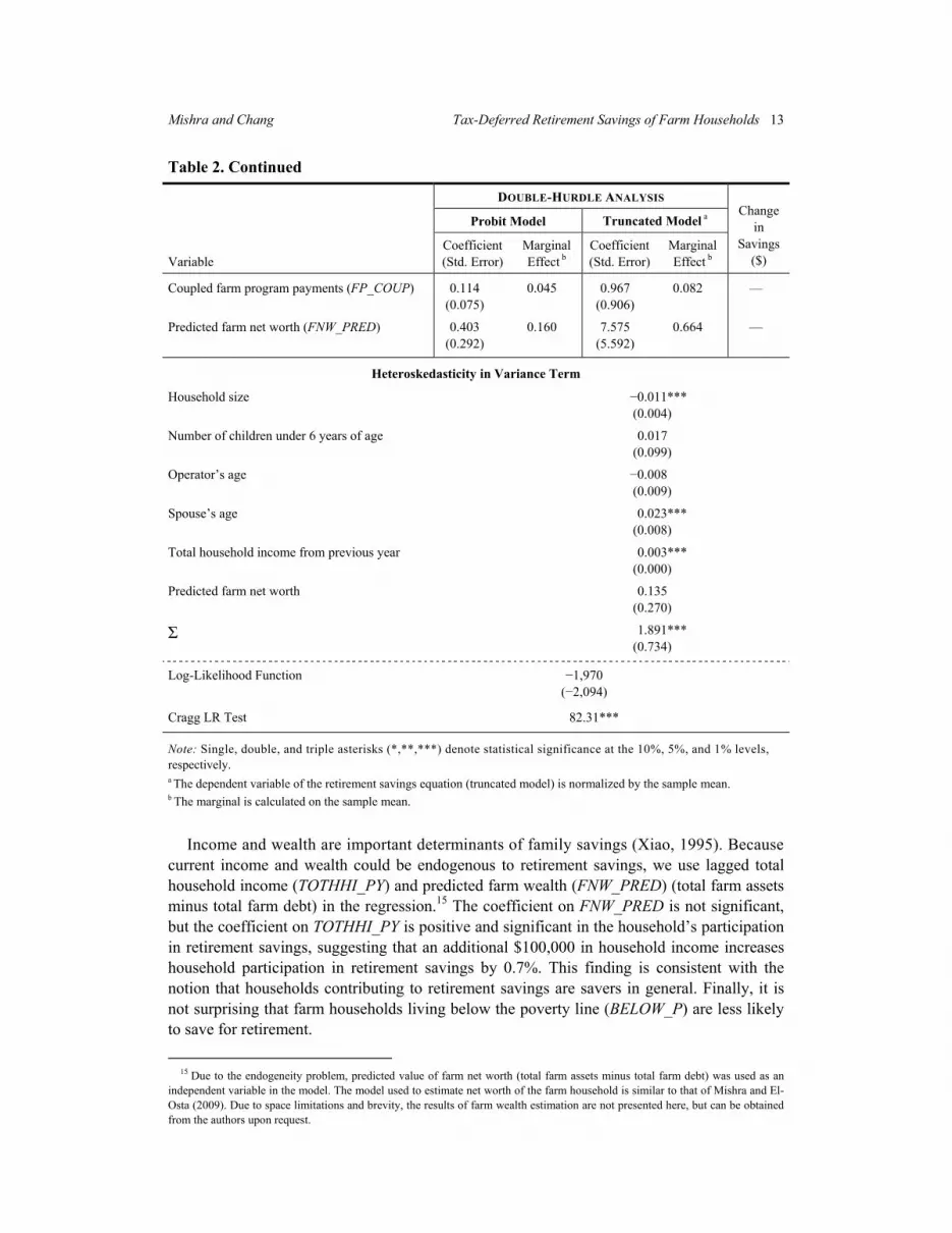
Income and wealth are important determinants of family savings (Xiao, 1995). Because current income and wealth could be endogenous to retirement savings, we use lagged total household income (TOTHHI_PY) and predicted farm wealth (FNW_PRED) (total farm assets minus total farm debt) in the regression.15 The coefficient on FNW_PRED is not significant, but the coefficient on TOTHHI_PY is positive and significant in the household’s participation in retirement savings, suggesting that an additional $100,000 in household income increases household participation in retirement savings by 0.7%. This finding is consistent with the notion that households contributing to retirement savings are savers in general. Finally, it is not surprising that farm households living below the poverty line (BELOW_P) are less likely to save for retirement.

15 Due to the endogeneity problem, predicted value of farm net worth (total farm assets minus total farm debt) was used as an

independent variable in the model. The model used to estimate net worth of the farm household is similar to that of Mishra and El-Osta (2009). Due to space limitations and brevity, the results of farm wealth estimation are not presented here, but can be obtained from the authors upon request.

14 April 2011 Journal of Agricultural and Resource Economics Degree of risk aversion (RISK_PREF),16 measured by the ratio of crop insurance expenses to total variable costs (Goodwin and Mishra, 2002), has a positive and significant effect on the likelihood of the household’s participation in retirement savings—i.e., as risk aversion increases, operators are more likely to participate in retirement savings. Farming type also has an impact on participation in retirement savings. Farms specializing in dairy (F_DAIRY) and cash grain (F_GRAIN) operations have an 11% and 15% lower probability of participating in a retirement savings plan, respectively, compared to the base category (all other types of farms), ceteris paribus. Cash grain farmers operate large farms and receive government pay-ments, which may reduce income variability;17 these farmers may expect payments to continue indefinitely. Further, farm programs are also known to be capitalized in farmland, and farm-land value comprises 70% of total farm net worth.

Results for Amount of Retirement Savings We also investigated factors affecting amount of retirement savings, once farm households make the decision to save for retirement. Table 2 reports estimated parameters and marginal effects of factors determining amount of retirement savings. Marginal effect measures changes in retirement savings (normalized by the mean level of savings) due to an additional unit of exogenous variables. For the discrete exogenous variables, marginal effect measures differ-ences in retirement savings when there is a change in the exogenous variable from 0 to 1. For example, an additional person living in the household (HH_SIZE) increases the normalized retirement savings by approximately $1,443—i.e., 0.028 (the marginal effect) times 51,190 (the normalized mean of the dependent variable). The coefficients on off-farm work by operator (OP_HROFF) and spouse (SP_HROFF) are positive and have a significant effect on the amount of retirement savings. An additional 1,000 off-farm work hours by operators and spouses increases retirement savings by approximately $8,565 and $6,229, respectively. Farm operators working off the farm save more than spouses. This finding may reflect the wage differential between male farm operators and their spouses. The coefficient on age of the farm operator (OP_AGE) is negative and statistically significant at the 1% level. An additional year in age decreases retirement savings by $500. Farm size, measured by lagged value of agricultural production (VPRODT_PY) has a positive and significant impact on the amount of retirement savings. An additional $100,000 in agricultural output increases retirement savings by only $527. Farm specialization plays an important role in the amount of retirement savings. Conditional on participation in retirement savings, when compared to all other types of farms, farms specializing in dairy (F_DAIRY) and cash grain (F_GRAIN) farming save $13,625 and $8,743 less in retirement savings, ceteris paribus. Finally, rainfall variability (CV_RAIN), a measure of farm income variability, has an impact on the amount of retirement savings. Although, the coefficient on CV_RAIN is not significant in the participation model, it is highly significant in the model for amount of retirement savings. A 1% increase in rainfall variability increases retirement savings by $412. This finding supports the argument that increased income uncertainty leads to more savings (Boulding, 1966). Further, findings here also corroborate conclusions reported by Carroll and

16 We use the share of crop insurance expense to total farm operating expenses as a measure of risk aversion; a higher share of

crop insurance expense implies risk aversion (Goodwin and Mishra, 2002). 17 Operators of large farms are more likely to report farming as their main occupation (Mishra et al., 2002).


Samwick (1997) and Paxson (1992) that wealth accumulation is higher for people with higher income variability.18

Summary and Conclusions Previous economic studies of retirement savings behaviors have examined only older Americans or those who are not self-employed. Little is known about these behaviors among U.S. farm households, not only because there is a lack of household survey data, but also as a result of the complex relationship between household and farm businesses in terms of resource allocation. This study investigates the effect of farm, operator, household, and other demo-graphic characteristics on retirement savings behavior among farm households using ARMS farm household data. We find that off-farm work by operators and spouses plays an important role in retirement savings decisions. In their income levels, farm households are virtually indistinguishable from nonfarm households. Consequently, government policies that influence general economic conditions have a profound impact on farm families. Our findings suggest that tax-deferred retirement savings are more likely to be held by households with financial resources that allow the maintenance of current consumption as well as the allocation of funds to tax-advantaged retirement savings. Consistent with the theory of savings, results confirm that risk-averse farm families are more likely to save for retirement and that increased income variability is associated with higher retirement savings. Several farm, operator, household, and demographic attributes contribute to the retirement savings decisions among farm households. Age of the operator and spouse and total household income are important factors affecting retirement decisions. Consistent with the Lundberg and Ward-Batts (2000) theory, we conclude that spouses tend to accumulate money for retirement, even when operators have already begun withdrawing money from retirement savings.

[Received June 2009; final revision received January 2011.]

References Ahearn, M. “The Financial Well-Being of Farm Operators and Their Households.” Pub. No. AER-563,

USDA/Economic Research Service, Washington, DC, 1986. Ahearn, M., J. Perry, and H. El-Osta. “The Economic Well-Being of Farm Operator Households, 1988–90.”

Pub. No. AER-666, USDA/Economic Research Service, Washington, DC, 1993. American Corn Growers Association and Americans for Secure Retirement. “Lifetime Income Crucial to

Farmer’s Retirement Security.” 2002. Online. Available at http://paycheckforlife.org/uploads/Ag_Issue_ Brief_FINAL.PDF. [Accessed July 2, 2010.]

Aristei, D., and L. Pieroni. “A Double-Hurdle Approach to Modeling Tobacco Consumption in Italy.” J. Appl. Econ. 40(2008):2463–2476.

Baum, C. An Introduction to Modern Econometrics Using STATA. College Station, TX: Stata Press, 2006. Blundell, R., and C. Meghir. “Bivariate Alternatives to the Univariate Tobit Model.” J. Econometrics 34,

1/2(1987):179–200. Boulding, K. Economic Analysis, Vol. I: Microeconomics, 4th ed. New York: Harper Collins, 1966.

18 The literature shows that wealth accumulation is driven by retirement income and bequest motives (Gale and Scholz, 1994;

Cagetti, 2003).

16 April 2011 Journal of Agricultural and Resource Economics Cagetti, M. “Wealth Accumulation over the Life-Cycle and Precautionary Savings.” J. Bus. and Econ. Statis.

21,3(2003):339–353. Cameron, A., and P. Trivedi. Microeconomterics: Methods and Applications. Cambridge, UK: Cambridge

University Press, 2005. Carroll, C. D., and A. Samwick. “The Nature of Precautionary Wealth.” J. Monetary Econ. 40(1997):41–71. Cragg, J. “Some Statistical Models for Limited Dependent Variables with Application to the Demand for

Durable Goods.” Econometrica 39,5(1971):829–844. DeVaney, S. A. “Confidence in a Financially Secure Retirement: Differences Between Retirees and Non-

retirees.” Consumer Interest Annual 41(1995):42–49. Federal Reserve Board. “Survey of Consumer Finances.” Board of Governors of the Federal Reserve

Systems, Washington, DC. Online. Available at http://www.federalreserve.gov/pubs/oss/oss2/scfindex. html. [Accessed March 11, 2010.]

Foster, A. C. “Employee Participation in Savings and Thrift Plans.” Monthly Labor Rev. 119,3(1996):17–22. Gale, W. G., and J. K. Scholz. “Intergenerational Transfers and the Accumulation of Wealth.” J. Econ.

Perspectives 8(1994):145–160. Goodwin, D., P. Draughn, L. Little, and J. Marlowe. “Wives’ Off-Farm Employment, Farm Family

Economic Status, and Family Relationships.” J. Marriage and the Family 53(1991):389–402. Goodwin, B. K., and A. K. Mishra. “The Effects of Direct Payments of Crop Production and Marketing

Decisions of United States Farmers.” OECD Doc. No. AGR/CA/APM, Organization for Economic Coop-eration and Development, Paris, France, 2002.

———. “Farming Efficiency and the Determinants of Multiple Job Holding by Farm Operators.” Amer. J. Agr. Econ. 86,3(2004):722–729.

Goodwin, B. K., A. K. Mishra, and F. Ortalo-Magne. “What’s Wrong with Our Models for Agricultural Land Values?” Amer. J. Agr. Econ. 85,3(2003):744–752.

Gustafson, C. R., and S. L. Chama. “Financial Assets Held by North Dakota Farmers.” J. Amer. Society of Farm Managers and Rural Appraisers 58(1994):90–94.

Hamakar, C. M., and G. F. Patrick. “Farmers and Alternative Retirement Investment Strategies.” J. Amer. Society of Farm Managers and Rural Appraisers 60(1996):42–51.

Heckman, J. “Sample Selection Bias as a Specification Error.” Econometrica 47(1979):153–161. Jensen, H., and P. Salant. “The Role of Fringe Benefits in Operator Off-Farm Labor Supply.” Amer. J. Agr.

Econ. 67,5(1988):1095–1100. Jones, A. “A Double-Hurdle Model for Cigarette Consumption.” J. Appl. Econometrics 4(1989):23–29. Lundberg, S., and J. Ward-Batts. “Saving for Retirement: Household Bargaining and Household Net Worth.”

Population Studies Center, University of Michigan, Ann Arbor, 2000. Lycett, J., R. Dunbar, and E. Voland. “Longevity and the Costs of Reproduction in Historical Human

Population.” Proceedings of the Royal Society of Biological Sciences 267, no. 1438 (2000):31–35. Maddala, G. S. “Specification Test in Limited Dependent Variable Models.” In Advances in Econometrics

and Quantitative Economics: Essays in Honor of C. R. Rao, eds., G. S. Maddala, P. C. B. Phillips, and T. N. Srinivasan, pp. 1–49. Oxford, UK: Blackwell Publishers, 1995.

Malroutu, Y. L., and J. J. Xiao. “Perceived Adequacy of Retirement Income.” Financial Counseling and Planning 6(1995):17–23.

Martinez-Espineira, R. “A Box-Cox Double-Hurdle Model of Wildlife Valuation: The Citizen’s Perspective.” Ecological Econ. 58(2006):192–208.

McDowell, A. “From the Help Desk: Hurdle Models.” Stata J. 3(2003):178–184. Mihalopoulos, V. G., and M. P. Demoussis. “Greek Household Consumption of Food Away from Home: A

Microeconometric Approach.” Eur. Rev. Agr. Econ. 28,4(2001):421–432. Mishra, A. K., R. Durst, and H. El-Osta. “How Do U.S. Farmers Plan for Retirement?” Amber Waves

3,2(2005):12–18. Mishra, A. K., and H. S. El-Osta. “Effect of Agricultural Policy on Succession Decisions of Farm House-

holds.” Rev. Economics of Households 6(2008):285–307. ———. “Estimating Wealth of Self-Employed Farm Households.” Agr. Fin. Rev. 69,2(2009):248–262. Mishra, A. K., and M. J. Morehart. “Off-Farm Investment of Farm Households: A Logit Analysis.” Agr. Fin.

Rev. 61,1(2001):87–101.


Mishra, A. K., M. J. Morehart, H. S. El-Osta, J. D. Johnson, and J. W. Hopkins. “Income, Wealth, and Well-

Being of Farm Operator Households.” Agr. Econ. Rep. No. 812, USDA/Economic Research Service, Washington, DC, 2002.

Mishra, A. K., and C. L. Sandretto. “Stability of Farm Income and the Role of Nonfarm Income in U.S. Agri-culture.” Rev. Agr. Econ. 24,1(2002):208–221.

Munnell, A., A. Webb, and L. Delorme. “Retirement at Risk: A New National Retirement Index.” Boston College Center for Retirement Research, 2006.

Newman, E. S., S. R. Sherman, and C. E. Higgins. “Retirement Expectations and Plans: A Comparison of Professional Men and Women.” In Women’s Retirement: Policy Implications of Recent Research, ed., M. Szinovacz, pp. 113–122. Beverly Hills, CA: Sage Publications, 1982.

Office of Management and Budget (OMB). Budget of the United States Government: Fiscal Year 2010. Washington, DC: U.S. Government Printing Office, 2009. Online. Available at http://www.gpoaccess. gov/usbudget/fy10/browse.html.

Paxson, C. H. “Using Weather Variability to Estimate Response of Savings to Transitory Income in Thailand.” Amer. Econ. Rev. 82(1992):15–33.

Robinson, E. “Study Shows Retiring Farmers Face Declining Standard of Living.” Southeast Farm Press, 2005. Online. Available at http://southeastfarmpress.com/mag/farming_study_shows_retiring/. [Accessed July 2, 2010.]

Sandmo, A. “Capital Risk, Consumption, and Portfolio Choice.” Econometrica 37(1969):586–599. Serra, T., B. K. Goodwin, and A. M. Featherstone. “Determinants of Investments in Non-Farm Assets by

Farm Households.” Selected paper presented at the AAEA annual meeting, Denver, CO, 2004. Shrestha, R. K., J. R. R. Alavalapati, A. F. Seidl, K. E. Weber, and B. Suselo. “Estimating the Local Cost of

Protecting Koshi Tappu Wildlife Reserve, Nepal: A Contingent Valuation Approach.” J. Environ., Devel-opment, and Sustainability 9(2007):413–426.

Smith, M. D. “On Dependency in Double-Hurdle Models.” Statistical Papers 44(2003):581–595. Su, S. B., and S. T. Yen. “Microeconometric Models of Infrequently Purchased Goods: An Application to

Household Pork Consumption.” Empirical Econ. 21(1996):513–533. Turner, M. J., W. C. Bailey, and J. P. Scott. “Factors Influencing Attitude Toward Retirement and Retirement

Planning Among Midlife University Employees.” J. Appl. Gerontology 13,2(1994):143–156. U.S. Department of Agriculture, Economic Research Service. “Farm Household Economics and Well-

Being.” USDA/ERS, Briefing Room, Washington, DC, 2008. Online. Available at www.ers.usda.gov/ Briefing/WellBeing/.

U.S. Department of Agriculture, National Agricultural Statistics Service. Census of Agriculture, 2007. USDA/ NASS, Washington, DC, 2008.

Wilde, J. “A Simple Representation of the Bera-Jarque-Lee Test for Probit Models.” Econ. Letters 101(2008): 119–121.

Wooldridge, J. Econometric Analysis of Cross-Section and Panel Data. Cambridge, MA: MIT Press, 2002. Xiao, J. J. “Patterns of Household Financial Asset Ownership.” Financial Counseling and Planning 6(1995):

99–106.

Documents

Tax-deferred retirement savings of farm households: an empirical investigation