Embed Size (px)
Citation preview
Learning Interpretable Pathology Features by Multi-task and Adversarial Training Improves CNNGeneralizationMara Graziani ( [email protected] )
University of Applied Sciences of Western Switzerland (HES-SO Valais) https://orcid.org/0000-0003-3456-945XSebastian Otalora
University of Applied Sciences of Western Switzerland (HES-SO Valais)Stéphane Marchand-Maillet
University of GenevaHenning Müller
University of Applied Sciences Western Switzerland, Sierre https://orcid.org/0000-0001-6800-9878Vincent Andrearczyk
University of Applied Sciences of Western Switzerland (HES-SO Valais)
Article
Keywords: Histopathology, Multi-task Learning, Adversarial Learning, Interpretable AI
Posted Date: September 9th, 2021
DOI: https://doi.org/10.21203/rs.3.rs-744740/v1
License: This work is licensed under a Creative Commons Attribution 4.0 International License. Read Full License
Draft submission 1 (2020) 1-48 Submitted 10/2019; Published 1/2020
Learning Interpretable Pathology Features by Multi-task
and Adversarial Training Improves CNN Generalization
Mara Graziani [email protected] of Applied Sciences Western Switzerland (HES-SO Valais), 3960, Sierre, SwitzerlandUniversity of Geneva (UNIGE), Department of Computer Science (CUI), 1227, Carouge, Switzerland
Sebastian Otalora [email protected] of Applied Sciences Western Switzerland (HES-SO Valais), 3960, Sierre, SwitzerlandUniversity of Geneva (UNIGE), Department of Computer Science (CUI), 1227, Carouge, Switzerland
Stephane Marchand-MailletUniversity of Geneva (UNIGE), Department of Computer Science (CUI), 1227, Carouge, Switzerland
Henning Muller [email protected] of Applied Sciences Western Switzerland (HES-SO Valais), 3960. Sierre, SwitzerlandUniversity of Geneva (UNIGE), Department of Radiology and Medical Informatics, 1211, Geneva, Switzerland
Vincent Andrearczyk [email protected] of Applied Sciences Western Switzerland (HES-SO Valais), 3960, Sierre, Switzerland
Editor: Editor Name, more names
Abstract
Adopting Convolutional Neural Networks (CNNs) in daily routine of primary diagnosis1
requires not only near-perfect precision, but also a sufficient degree of transparency and2
explainability of the decision making. With physicians being accountable for the diagno-3
sis, it is fundamental that CNNs provide a clear interpretation of their learning paradigm,4
ensuring that relevant pathology features are being considered. Building on top of suc-5
cessfully existing techniques such as multi-task learning, domain adversarial training and6
concept-based interpretability, this paper addresses the challenge of introducing diagnostic7
factors in the training objectives. Here we show that our architecture, by learning end-8
to-end an uncertainty-based weighting combination of multi-task and adversarial losses,9
is encouraged to focus on pathology features such as density and pleomorphism of nu-10
clei, e.g. variations in size and appearance, while discarding misleading features such as11
staining differences. Our results on the classification of tumor in breast lymph node tis-12
sue scans show significantly improved generalization, with best average AUC 0.89 ± 0.0113
against the baseline AUC 0.86 ± 0.005. This result is a starting point towards building14
interpretable multi-task architectures that are robust to data heterogeneity. Our code is15
available at https://bit.ly/356yQ2u.16
Keywords: Histopathology, Multi-task Learning, Adversarial Learning, Interpretable AI17
1. Introduction18
The analysis of tissue images by Convolutional Neural Networks (CNNs) is an important19
part of computer-aided systems for cancer detection, staging and grading (Litjens et al.,20
2017; Janowczyk and Madabhushi, 2016; Campanella et al., 2019; Ilse et al., 2020). The21
automated suggestion of Regions of Interest (RoIs) is one task, in particular, that may22
©2020 Graziani, .
License: CC-BY 4.0, see https://creativecommons.org/licenses/by/4.0/.
Graziani et al.
help pathologists in increasing their performance and inter-rater agreement in the diagno-23
sis (Wang et al., 2016). The training of CNNs for this task, however, presents multiple24
challenges (Janowczyk and Madabhushi, 2016; Campanella et al., 2019). Annotations are25
costly and rarely pixel-level precise. The data are highly heterogeneous, being subject to26
staining, fixation and slicing variability (Lafarge et al., 2017), multiple scanner resolutions,27
artifacts, and, at times, permanent ink annotations. Several approaches have been pro-28
posed in the literature to address these challenges. Weakly-supervised learning reduces the29
need for strong annotations (Marini et al., 2021) and adversarial training reduces the CNN30
sensitivity to staining variability (Lafarge et al., 2017; Otalora et al., 2019). Another major31
obstacle is algorithm robustness. The features learned by these architectures often suffer32
from low generalization to data from real settings. This is mostly due to the poor avail-33
ability of well-curated, multi-institutional datasets resembling real-world scenarios. The34
applicability of these methods to clinical settings is, as a consequence, surrounded by un-35
certainty on whether the model performance will be sufficiently reliable for trusting the36
algorithm output on the real-world tasks (Zech et al., 2018). As remarked in Doshi-Velez37
and Kim (2017), the answer to this question has to be found in a different approach to eval-38
uating model performance, where the reliability of the automated outcomes is evaluated39
not only by its testing and generalization performance, but also by the interpretability of40
its decision-making process.41
With physicians being the sole individuals accountable for the decision-making and the42
final diagnosis, it is a compelling need to provide a clear interpretation of the main objectives43
of the network learning paradigms, ensuring the clinical staff that relevant features are being44
considered by the model. One way to investigate the relevance of pathology features was45
proposed by concept attribution (Kim et al., 2018; Graziani et al., 2018, 2020). The work on46
Regression Concept Vectors (RCVs) (Graziani et al., 2018), in particular, highlighted that47
easy-to-understand concepts describing nuclear pleomorphism such as the area, shape and48
appearance of the nuclei are relevant factors in a CNN that distinguishes tumorous from49
non-tumorous tissue. Concept attribution was applied with high versatility to multiple50
architectures and tasks (Kim et al., 2018; Graziani et al., 2018, 2019b,a, 2020; Yeche et al.,51
2019) and eased the interaction of domain-experts with deep learning models (Cai et al.,52
2019).53
Being a post-hoc explainability method, RCVs generate an explanation of the relevance54
of a given concept to the decision making. No possibility is given, however, to act on the55
training process and modify the learning of a concept. It is not possible, for example, to dis-56
courage the learning of a confounding concept, e.g. domain, staining, watermarks. Similarly,57
the learning of discriminant concepts cannot be further encouraged. This paper proposes58
an architecture that merges the developmental efforts of three successful techniques, namely59
multi-task learning (Caruana, 1997), adversarial training (Ganin et al., 2016) and high-level60
concept learning in internal network features (Kim et al., 2018; Graziani et al., 2020). This61
architecture is trained on the histopathology task of breast cancer classification, with the62
aim of enforcing the learning of diagnostic features that match the physicians’ diagnosis63
procedure, such as nuclei morphology and density. The encoding of such diagnostically64
relevant concepts, called desired targets, is encouraged in the internal representations by65
adding auxiliary tasks in a multi-task learning setting (Caruana, 1997). Features to which66
the model should be invariant, i.e. undesired targets, exist in various kinds, e.g. image67
2
Multi-task and Adversarial CNN Training
domain, staining, presence of watermarks or pen marks. In the proposed architecture, the68
learning of these features is discouraged by a gradient reversal operation (Ganin et al., 2016;69
Xie et al., 2017). An adversarial branch is used in the experiments to obtain invariance to70
the domain differences of the multiple acquisition centers, which are due to the tissue stain-71
ing, fixation, processing and digitalization. While multi-task learning (Caruana, 1997) and72
adversarial learning (Ganin et al., 2016) are widely used techniques that are fundamental in73
our contributions is their combination for steering the learning process. This paper brings74
new insights on balancing multiple tasks for digital pathology, a technique that only re-75
cently arose interest in the digital pathology landscape (Gamper et al., 2020b). The joint76
optimization of main, auxiliary and adversarial task losses is a novel exploration in the77
histopathology field. We show that the additional tasks lead to a significant increase in the78
performance and generalization to unseen data. From our analysis of weighting strategies,79
it emerges that an uncertainty-based approach best handles the convergence and stability80
of the joint optimization.81
The paper is structured as follows. Section 2 reviews the prior studies on multi-task, on82
adversarial training and on concept-based interpretability approaches. Section 3 describes83
the proposed architecture and the implementation details such as the definition of the84
optimization function and hyperparameters. The benefits of the proposed approach are85
then demonstrated with experiments on the patch-based classification of tumorous tissue in86
breast tissue samples, the first step in automated pipelines that assess the degree of tumor87
spreading. The experimental setup is presented in Section 4. The results are reported in88
Section 5 and further discussed in Section 6.89
2. Related Work90
2.1 Multi-task Learning91
Similarly to how learning happens in humans, multi-task architectures aim at simultaneously92
learning multiple tasks that are related to each other (Ruder, 2017). Multi-task architec-93
tures divide into two families depending on the hard or soft sharing of the parameters. In94
architectures with hard parameter sharing such as the one proposed in this paper, multi-95
ple supervised tasks share the same input and some intermediate representation (Caruana,96
1997). The parameters learned up to this intermediate point are called generic parameters97
since they are shared across all tasks. In soft parameter sharing, the weight updates are98
not shared among the tasks and the parameters are task-specific, introducing only a soft99
constraint on the training process (Duong et al., 2015).100
As explained by Caruana (1997), multi-task learning leads to various benefits if the101
tasks are linked by a valid relationship, namely if what is learned for each task can help102
the other tasks to be learned better. Under these conditions, the multi-task configuration103
improves the generalization error bounds and reduces the risk of overfitting (Baxter, 1995).104
The speed of convergence is also increased, since fewer training samples are required per105
task (Baxter, 2000). However, if there is no valid relationship between the multiple tasks,106
no relevant benefit can be remarked.107
In multi-task learning, the variations in the observed data must be explained by factors108
that are shared by two or more tasks (Goodfellow et al., 2016). Learning two related109
tasks generates signals that contain extra information from which both can benefit. The110
3
Graziani et al.
(a) (b) (c)
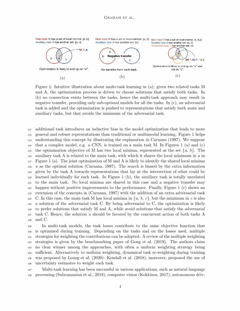
Figure 1: Intuitive illustration about multi-task learning in (a): given two related tasks Mand A, the optimization process is driven to choose solutions that satisfy both tasks. In(b) no connection exists between the tasks, hence the multi-task approach may result innegative transfer, providing only sub-optimal models for all the tasks. In (c), an adversarialtask is added and the optimization is pushed to representations that satisfy both main andauxiliary tasks, but that avoids the minimum of the adversarial task.
additional task introduces an inductive bias in the model optimization that leads to more111
general and robust representations than traditional or multimodal learning. Figure 1 helps112
understanding this concept by illustrating the explanation in Caruana (1997). We suppose113
that a complex model, e.g. a CNN, is trained on a main task M. In Figures 1 (a) and (c)114
the optimization objective of M has two local minima, represented as the set {a, b}. The115
auxiliary task A is related to the main task, with which it shares the local minimum in a in116
Figure 1 (a). The joint optimization of M and A is likely to identify the shared local minima117
a as the optimal solution (Caruana, 1997). The search is biased by the extra information118
given by the task A towards representations that lay at the intersection of what could be119
learned individually for each task. In Figure 1 (b), the auxiliary task is totally unrelated120
to the main task. No local minima are shared in this case and a negative transfer may121
happen without positive improvements to the performance. Finally, Figure 1 (c) shows an122
extension of the concepts in (Caruana, 1997) with the addition of an extra adversarial task123
C. In this case, the main task M has local minima in {a, b, c}, but the minimum in c is also124
a solution of the adversarial task C. By being adversarial to C, the optimization is likely125
to prefer solutions that satisfy M and A, while avoid solutions that satisfy the adversarial126
task C. Hence, the solution a should be favored by the concurrent action of both tasks A127
and C.128
In multi-task models, the task losses contribute to the same objective function that129
is optimized during training. Depending on the tasks and on the losses used, multiple130
strategies for weighting the contributions can be adopted. A review of the multiple weighting131
strategies is given by the benchmarking paper of Gong et al. (2019). The authors claim132
no clear winner among the approaches, with often a uniform weighting strategy being133
sufficient. Alternatively to uniform weighting, dynamical task re-weighting during training134
was proposed by Leang et al. (2020). Kendall et al. (2018), moreover, proposed the use of135
uncertainty estimates to weight each task.136
Multi-task learning has been successful in various applications, such as natural language137
processing (Subramanian et al., 2018), computer vision (Kokkinos, 2017), autonomous driv-138
4
Multi-task and Adversarial CNN Training
ing (Leang et al., 2020), radiology (Andrearczyk et al., 2021) and histology (Gamper et al.,139
2020b). The preliminary work by Gamper et al. (2020b), in particular, shows a decrease in140
the loss variance as an effect of multi-task for oral cancer, suggesting that this work may141
have high potential for histology applications.142
2.2 Adversarial Learning143
Proposed by Ganin et al. (2016), adversarial learning introduced a novel approach to solv-144
ing the so-called problem of domain adaptation, namely the minimization of the domain145
shift in the distributions of the training (also called source distribution) and testing data146
(i.e. target). Typically treated as either an instance re-weighting operation (Gong et al.,147
2013) or as an alignment problem (Long et al., 2015), domain adaptation is handled by148
adversarial learning as the optimization of a domain confusion loss. A domain classifier149
discriminates between the source and the target domains during training and its parame-150
ters are optimized to minimize the error when discriminating the domain labels. This can151
be extended to more than two domains by a multi-class domain classifier. The adversar-152
ial learning of domain-related features is obtained by a gradient reversal operation on the153
branch learning to discriminate the domains. Because of this operation, the network pa-154
rameters are optimized to maximize the loss of the domain classifier, thus making multiple155
domains impossible to distinguish one from another in the internal network representation.156
This causes a competition between the main task and the domain branch during training157
that is referred to as a min-max optimization framework. As a downside, the optimization158
of adversarial losses may be complicated, with the min-max operation affecting the stability159
of the training (Ganin et al., 2016). Convergence can be promoted, however, by activating160
and de-activating the gradient reversal branch according to a training schedule as in Lafarge161
et al. (2017).162
2.3 Concept-based Interpretability163
Concept-based explanations of deep learning decisions were introduced by the Concept Ac-164
tivation Vectors (CAVs) of Kim et al. (2018). This technique proposes to solve a binary165
classification problem to verify the presence or absence of a given concept in the internal166
representation of a deep network. A linear classifier is trained in the intermediate repre-167
sentations to infer a Boolean-valued function from input examples. The unit vector that is168
normal to the classification boundary is the CAV, which represents the direction pointing169
towards the internal representations containing the concept. The performance of the linear170
classifier indicates how well the concept was learned. RCVs extend CAVs to the problem171
of inferring a continuous-valued function, thus modelling continuous-valued concepts rather172
than binary ones. RCVs were applied to interpret the internal state of CNNs in terms of di-173
agnostic measures in a variety of medical applications (Graziani et al., 2018, 2019a,b; Yeche174
et al., 2019). Both techniques of CAVs and RCVs use linear models, that are inherently175
interpretable, to probe the internal activations of the network. This constitutes a baseline176
of linear interpretability of CNNs, formalized for applications in the medical domain as177
concept attribution (Graziani et al., 2020).178
5
Graziani et al.
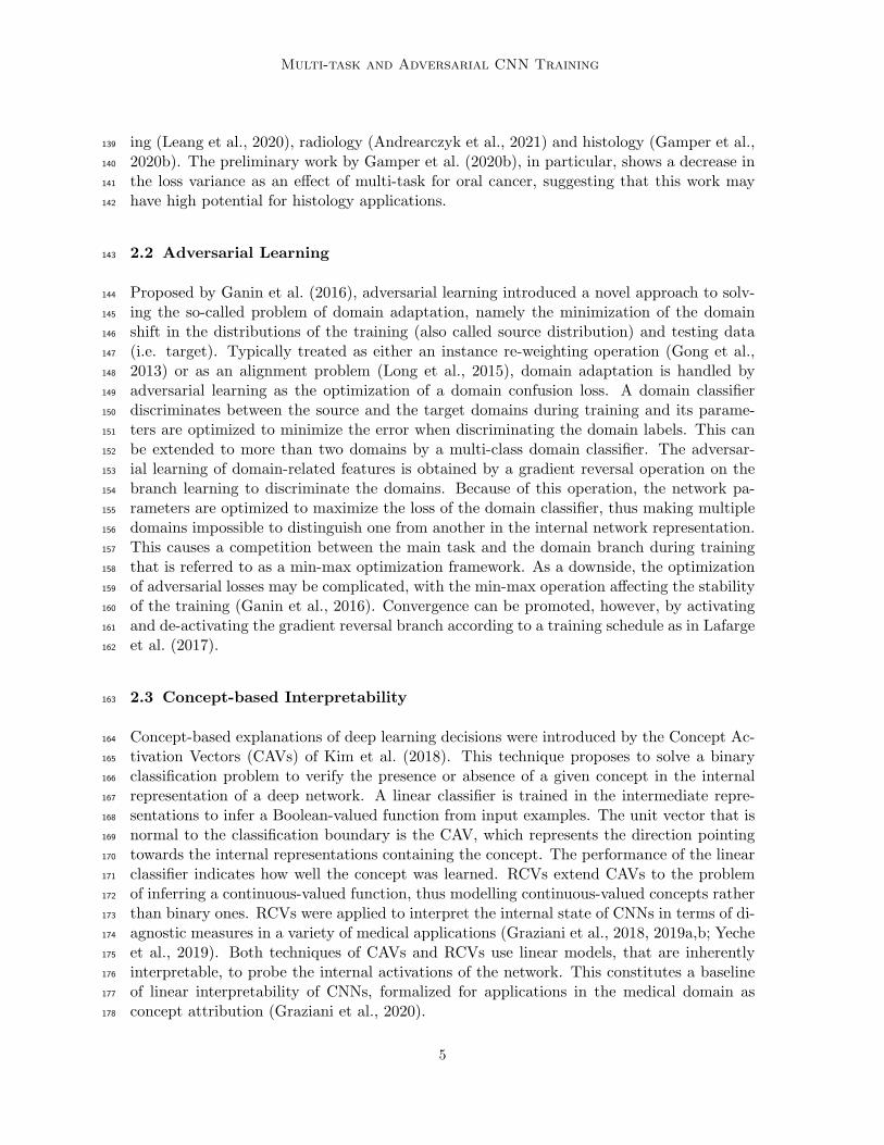
Figure 2: Multi-task adversarial architecture
3. Methods179
3.1 Proposed Architecture180
The architecture for guiding the training of CNNs is described in this section for a general181
application with pre-defined features. This general framework can be applied to multiple182
tasks. The diagnosis of cancerous tissue in breast microscopy images is proposed in this183
paper as an application for which the implementation details are described in Sections 4.2184
and 4.3.185
In the following, we clarify the notation used to describe the model. We assume that186
a set of N observations, i.e. the input images, is drawn from an unknown underlying187
distribution and split into a training subset {xi}ni=1 and a testing subset {xi}
Ni=n+1. The188
main task, namely the one for which we aim at improving the generalization, is the prediction189
of the image labels y = {yi}ni=1, for which ground truth annotations are available. A190
CNN of arbitrary structure is used as a feature encoder, of which the features are then191
passed through a stack of dense layers. The model parameters up to this point are defined192
as θf . The parameters of the label prediction output layers are identified by θy. The193
structure described up to this point replicates a standard CNN with a single main task194
branch that is addressing the classification. The remaining parameters of the architecture195
implement (i) the learning of auxiliary tasks by multi-task learning (Caruana, 1997) and (ii)196
the adversarial learning of detrimental features to induce invariance in the representations,197
as in the domain adversarial approach by Ganin et al. (2016). We combine these two198
approaches by introducing K extra targets representing desired and undesired tasks that199
must be introduced to the learning of the representations. The targets are modeled as the200
prediction of the feature values {ck,i}Ni=1, where k ∈ 1, . . . ,K is an index representing the201
extra task being considered. The feature values may be either continuous or categorical.202
Additional parameters θk are trained in parallel to θy for the K extra targets. We refer to203
all model outputs for all inputs x as f(x) ∈ RK+1 .204
The architecture is illustrated in Figure 2 and consists of two blocks. The first block is205
used to extract features from the input images. A state of the art CNN of arbitrary choice206
6
Multi-task and Adversarial CNN Training
without the decision layer is used as a feature encoder generating a set of feature maps.207
The feature maps are passed through a Global Average Pooling (GAP) operation that is208
performed to spatially aggregate the responses and connect them to a stack of dense layers.209
For this specific architecture, we use a stack of three dense layers of 1024, 512 and 256 nodes210
respectively. The second block comprises one branch per task, taking as input the output211
of the first block. The main task branch consists of the prediction of the labels y and has212
as many dense nodes as there are of unique classes in y. For binary classification tasks,213
e.g. discrimination of tumorous against non-tumorous inputs, the main task branch has a214
single node with a sigmoid activation function. K branches are added to model the extra215
targets. We refer to extra tasks for all the additional targets to the main task whether216
desired or undesired. Auxiliary tasks refer to the modeling of the desired targets, while217
adversarial tasks refer to that of undesired targets. The extra tasks are modeled by linear218
models as in Graziani et al. (2018). For continuous-valued targets, the extra branch consists219
of a single node with linear activation function. For categorical targets, the extra branch220
has multiple nodes followed by a softmax activation function. A gradient reversal operation221
(Ganin et al., 2016) is performed on the branches of the undesired targets to discourage the222
learning of these features.223
3.2 Objective Function224
The objective function of the proposed architecture balances the losses of the main task and225
the extra tasks for the desired and undesired targets. This is obtained by a combination of226
multi-task and adversarial learning. The main task loss is Liy(θf ,θy) = Ly(xi, yi;θf ,θy),227
where θf are the parameters of the first block (namely of the CNN encoder and the dense228
layers) in Figure 2 and θy those of the main task branch in the second block of the same229
figure. The extra parameters θk (k ∈ 1, . . . ,K) are trained for the branches of the desired230
and undesired target predictions, with the loss being Lik(θf ,θk) = Lk(xi, ck,i;θf ,θk).231
Training the model on n training an (N − n) testing samples consists of optimizing the232
function:233
E(θy,θf ,θ1, . . . ,θK) = λm1
n
n∑
i=1
Liy(θf ,θy) +K∑
k=1
λk
1
N
N∑
i=1
Lik(θf ,θk). (1)
234
The gradient update is:235
θf ← θf −
(
λm
∂Liy∂θf
+K∑
k=1
λk
∂Lik∂θf
)
, (2)
236
θy ← θy − λm
∂Liy∂θy
, (3)
237
θk ← θk − λkαk
∂Lik∂θk
, (4)
where λm and λk are positive scalar hyperparameters to tune the trade-off between the238
losses. For each extra branch, the hyperparameter αk ∈ {−1, 1} is used to specify whether239
7
Graziani et al.
the update is adversarial or not. A value of αk = −1 activates the gradient reversal operation240
and starts an adversarial competition between the feature extraction and the corresponding241
kth extra branch. The main task is only trained on the training data, since Liy = 0 for i > n242
in Eq. (2) and (3) as in Ganin et al. (2016). The extra tasks are learned on both training243
and test data. The training on test data can also be removed, since it is not always possible244
to fully retrain a network for new data.245
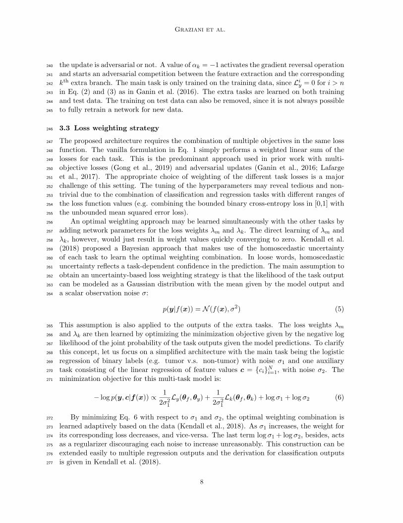
3.3 Loss weighting strategy246
The proposed architecture requires the combination of multiple objectives in the same loss247
function. The vanilla formulation in Eq. 1 simply performs a weighted linear sum of the248
losses for each task. This is the predominant approach used in prior work with multi-249
objective losses (Gong et al., 2019) and adversarial updates (Ganin et al., 2016; Lafarge250
et al., 2017). The appropriate choice of weighting of the different task losses is a major251
challenge of this setting. The tuning of the hyperparameters may reveal tedious and non-252
trivial due to the combination of classification and regression tasks with different ranges of253
the loss function values (e.g. combining the bounded binary cross-entropy loss in [0,1] with254
the unbounded mean squared error loss).255
An optimal weighting approach may be learned simultaneously with the other tasks by256
adding network parameters for the loss weights λm and λk. The direct learning of λm and257
λk, however, would just result in weight values quickly converging to zero. Kendall et al.258
(2018) proposed a Bayesian approach that makes use of the homoscedastic uncertainty259
of each task to learn the optimal weighting combination. In loose words, homoscedastic260
uncertainty reflects a task-dependent confidence in the prediction. The main assumption to261
obtain an uncertainty-based loss weighting strategy is that the likelihood of the task output262
can be modeled as a Gaussian distribution with the mean given by the model output and263
a scalar observation noise σ:264
p(y|f(x)) = N (f(x), σ2) (5)
This assumption is also applied to the outputs of the extra tasks. The loss weights λm265
and λk are then learned by optimizing the minimization objective given by the negative log266
likelihood of the joint probability of the task outputs given the model predictions. To clarify267
this concept, let us focus on a simplified architecture with the main task being the logistic268
regression of binary labels (e.g. tumor v.s. non-tumor) with noise σ1 and one auxiliary269
task consisting of the linear regression of feature values c = {ci}Ni=1, with noise σ2. The270
minimization objective for this multi-task model is:271
− log p(y, c|f(x)) ∝1
2σ21
Ly(θf ,θy) +1
2σ21
Lk(θf ,θk) + log σ1 + log σ2 (6)
By minimizing Eq. 6 with respect to σ1 and σ2, the optimal weighting combination is272
learned adaptively based on the data (Kendall et al., 2018). As σ1 increases, the weight for273
its corresponding loss decreases, and vice-versa. The last term log σ1 + log σ2, besides, acts274
as a regularizer discouraging each noise to increase unreasonably. This construction can be275
extended easily to multiple regression outputs and the derivation for classification outputs276
is given in Kendall et al. (2018).277
8
Multi-task and Adversarial CNN Training
4. Experiments278
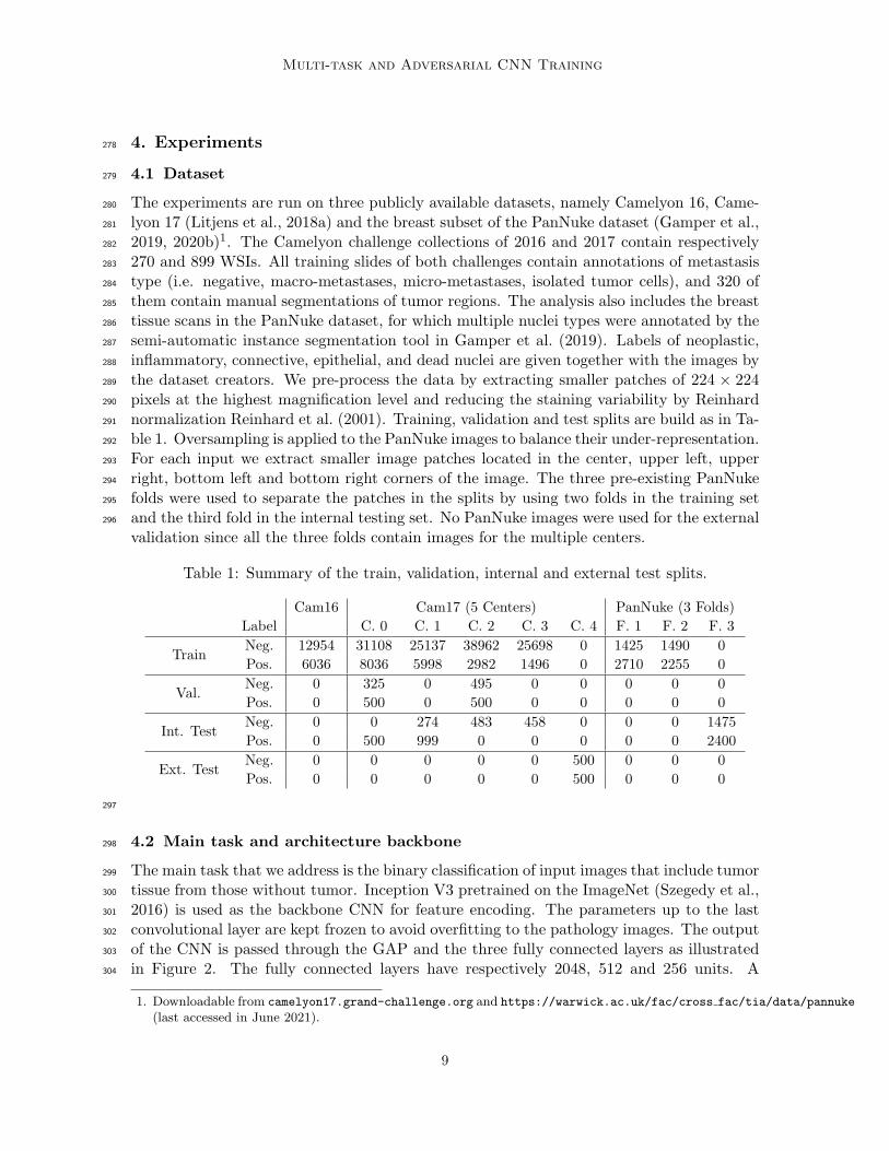
4.1 Dataset279
The experiments are run on three publicly available datasets, namely Camelyon 16, Came-280
lyon 17 (Litjens et al., 2018a) and the breast subset of the PanNuke dataset (Gamper et al.,281
2019, 2020b)1. The Camelyon challenge collections of 2016 and 2017 contain respectively282
270 and 899 WSIs. All training slides of both challenges contain annotations of metastasis283
type (i.e. negative, macro-metastases, micro-metastases, isolated tumor cells), and 320 of284
them contain manual segmentations of tumor regions. The analysis also includes the breast285
tissue scans in the PanNuke dataset, for which multiple nuclei types were annotated by the286
semi-automatic instance segmentation tool in Gamper et al. (2019). Labels of neoplastic,287
inflammatory, connective, epithelial, and dead nuclei are given together with the images by288
the dataset creators. We pre-process the data by extracting smaller patches of 224 × 224289
pixels at the highest magnification level and reducing the staining variability by Reinhard290
normalization Reinhard et al. (2001). Training, validation and test splits are build as in Ta-291
ble 1. Oversampling is applied to the PanNuke images to balance their under-representation.292
For each input we extract smaller image patches located in the center, upper left, upper293
right, bottom left and bottom right corners of the image. The three pre-existing PanNuke294
folds were used to separate the patches in the splits by using two folds in the training set295
and the third fold in the internal testing set. No PanNuke images were used for the external296
validation since all the three folds contain images for the multiple centers.
Table 1: Summary of the train, validation, internal and external test splits.
Cam16 Cam17 (5 Centers) PanNuke (3 Folds)
Label C. 0 C. 1 C. 2 C. 3 C. 4 F. 1 F. 2 F. 3
TrainNeg. 12954 31108 25137 38962 25698 0 1425 1490 0
Pos. 6036 8036 5998 2982 1496 0 2710 2255 0
Val.Neg. 0 325 0 495 0 0 0 0 0
Pos. 0 500 0 500 0 0 0 0 0
Int. TestNeg. 0 0 274 483 458 0 0 0 1475
Pos. 0 500 999 0 0 0 0 0 2400
Ext. TestNeg. 0 0 0 0 0 500 0 0 0
Pos. 0 0 0 0 0 500 0 0 0
297
4.2 Main task and architecture backbone298
The main task that we address is the binary classification of input images that include tumor299
tissue from those without tumor. Inception V3 pretrained on the ImageNet (Szegedy et al.,300
2016) is used as the backbone CNN for feature encoding. The parameters up to the last301
convolutional layer are kept frozen to avoid overfitting to the pathology images. The output302
of the CNN is passed through the GAP and the three fully connected layers as illustrated303
in Figure 2. The fully connected layers have respectively 2048, 512 and 256 units. A304
1. Downloadable from camelyon17.grand-challenge.org and https://warwick.ac.uk/fac/cross fac/tia/data/pannuke
(last accessed in June 2021).
9
Graziani et al.
dropout probability of 0.8 and L2 regularization are added to these three fully connected305
layers to avoid overfitting. The main task is the detection of patches containing tumor as306
a binary classification task. The branch consists of a single node with sigmoid activation307
function connected to the output of the third dense layer. The architecture as described308
up to here, hence without extra branches, is used as the baseline for the experiments. The309
extra tasks consist of either the linear regression or the linear classification of continuous or310
categorical labels respectively. For linear regression, the extra branch is a single node with311
linear activation function. The Mean Squared Error (MSE) between the predicted value312
and the label is added to the optimization function in Eq. 1. For the linear classification,313
the extra branch has a number of dense nodes equal to the number of classes to predict314
and a softmax activation function, also connected to the third dense layer. The Categorical315
Cross-Entropy (CCE) loss is added to the optimization in Eq. 1. Further details about the316
extra branches used for the experiments are given in Section 4.3.317
The architecture is trained end-to-end with mini-batch Stochastic Gradient Descent318
(SGD) with standard parameters (learning rate of 10−4 and Nesterov momentum of 0.9).319
The main task loss function is the class-Weighted Binary Cross-Entropy (WBCE). The class320
weights are set to weight more heavily every instance of the positive class, for instance they321
are set to the ratio of negative samples 136774/29513+ 136774 = 0.82 for the positive class322
and the ratio of positive samples 0.18 for the negative class.323
We evaluate the convergence of the network by early stopping on the total validation loss324
with patience of 5 epochs. The Area Under the ROC Curve (AUC) is used to evaluate model325
performance. For each experiment, we perform five runs with multiple initialization seeds326
to evaluate the performance variation due to initialization. The splits are kept unchanged327
for the multiple seed variations. To evaluate the performance on multiple test splits, we328
perform bootstrapping of the test sets. A number of 50 test sets of 7589 images (the total329
number of test images in the two sets) are obtained by sampling with repetition from the330
total pool of testing images. This method evaluates the variance of the test set without331
prior assumption on the data distribution and it shows the performance difference due to332
variation of the sampling of the population.333
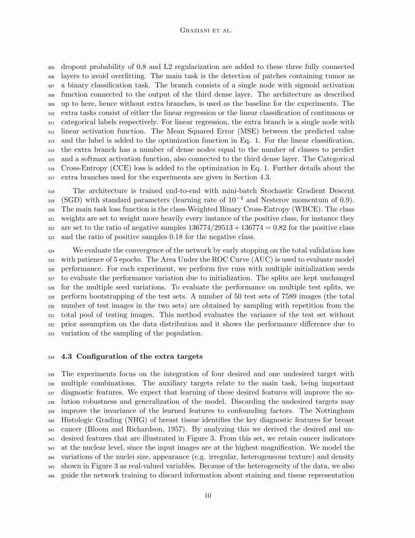
4.3 Configuration of the extra targets334
The experiments focus on the integration of four desired and one undesired target with335
multiple combinations. The auxiliary targets relate to the main task, being important336
diagnostic features. We expect that learning of these desired features will improve the so-337
lution robustness and generalization of the model. Discarding the undesired targets may338
improve the invariance of the learned features to confounding factors. The Nottingham339
Histologic Grading (NHG) of breast tissue identifies the key diagnostic features for breast340
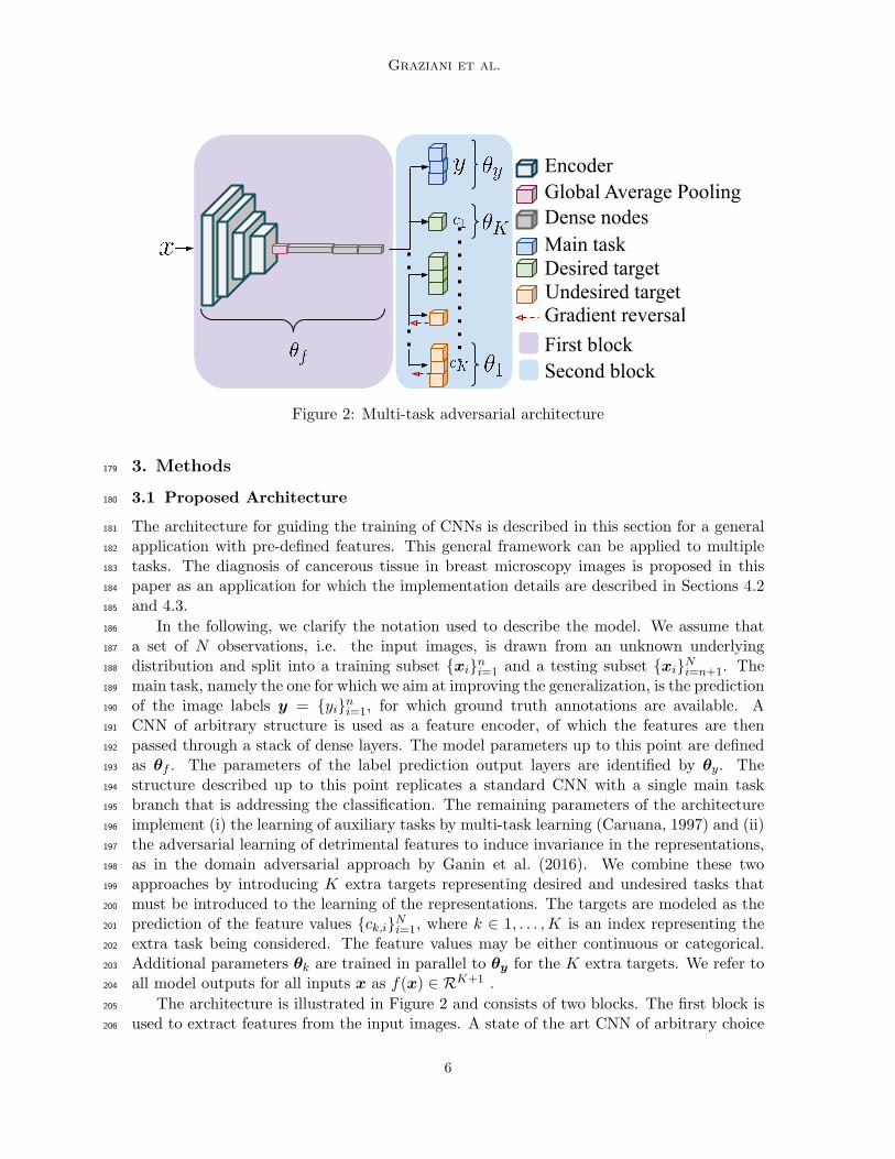
cancer (Bloom and Richardson, 1957). By analyzing this we derived the desired and un-341
desired features that are illustrated in Figure 3. From this set, we retain cancer indicators342
at the nuclear level, since the input images are at the highest magnification. We model the343
variations of the nuclei size, appearance (e.g. irregular, heterogeneous texture) and density344
shown in Figure 3 as real-valued variables. Because of the heterogeneity of the data, we also345
guide the network training to discard information about staining and tissue representation346
10
Multi-task and Adversarial CNN Training
Figure 3: Control targets for breast cancer. C and D stand for continuous and discreterespectively.
differences in the images. The processing center of the slides is modeled as an undesired347
target, encouraging feature invariance to staining and acquisition differences.348
Hand-crafted features representing the variations in the nuclei size and appearance are349
automatically extracted either from the images of from the nuclear contours. The nuclear350
contours are available in the form of manual annotations only for the PanNuke data. Au-351
tomated contours of the nuclei in the Camelyon images are obtained by the multi-instance352
deep segmentation model in Otalora et al. (2020). This model is a Mask R-CNN model (He353
et al., 2017), fine-tuned from ImageNet weights on the Kumar dataset for the nuclei segmen-354
tation task (Kumar et al., 2017). The R-CNN identifies nuclei entities and then generates355
pixel-level masks by optimizing the Dice score. ResNet50 (He et al., 2017) is used for the356
convolutional backbone as in (Otalora et al., 2020). The network is optimized by SGD with357
standard parameters (learning rate of 0.001 and momentum of 0.9).358
The number of pixels inside nuclear contours is averaged for each input image to repre-359
sent variations of the nuclei area, referred to as area in the experiments. Nuclei density is360
estimated by counting the nuclei in the image. Haralick descriptors of texture contrast and361
correlation (Haralick, 1979) are also extracted from the entire input images as in Graziani362
et al. (2018). Being continuous and unbounded measures, the values for these features are363
normalized to have zero mean and unitary standard deviation before training the model. In364
the paper, we refer to these features as area, density, contrast and correlation. The values365
of these features are used as prediction labels for the auxiliary target branches, that are also366
named as the feature that they should predict. These auxiliary branches perform a linear367
regression task, trying to minimize the Mean Squared Error between the predicted value of368
the feature and the extracted values used as labels.369
Information about the center that performed the data acquisition is present in the370
dataset as metadata. We model it as a categorical variable that may take values from 0371
to 7, namely one for each known center in the training data. Since there is no specific372
information on acquisition centers in Camelyon16 and PanNuke, these have been modeled373
as two distinct acquisition centers in addition to the five known centers of Camelyon17.374
11
Graziani et al.
This information is partly inaccurate, since we know that in both datasets more than a375
single acquisition center was involved Litjens et al. (2018b); Gamper et al. (2020a). The376
noise introduced by this information may limit the benefits introduced by the adversarial377
branch but it should not affect negatively the performance. In the future, unsupervised378
domain alignment methods may also be explored. The prediction of this variable is added379
to the architecture as an undesired target branch, referred to as center in the experiments.380
Desired and undesired targets are added as extra branches in the second block of the381
architecture following multiple configurations. We first focus on adding one extra branch382
at a time to identify the benefits of encouraging each task individually. We subsequently383
combine only the most promising branches to further improve performance. The undesired384
target branch is finally added to the most performing combinations to induce staining385
invariance in the learned features. The following combinations of extra tasks are tested386
in the experiments: density, area, contrast, correlation, center, center + density, center +387
area, center + density + area. The gradient reversal operation is only active for the center388
branch.389
We evaluate both the vanilla and the uncertainty-based functions for weighting the390
optimization targets. Where not stated otherwise, the average AUC (avg. AUC) over391
ten repetitions with multiple initialization seeds is used for the evaluation. In the vanilla392
configuration, the loss weight values are set to 1 for all branches.393
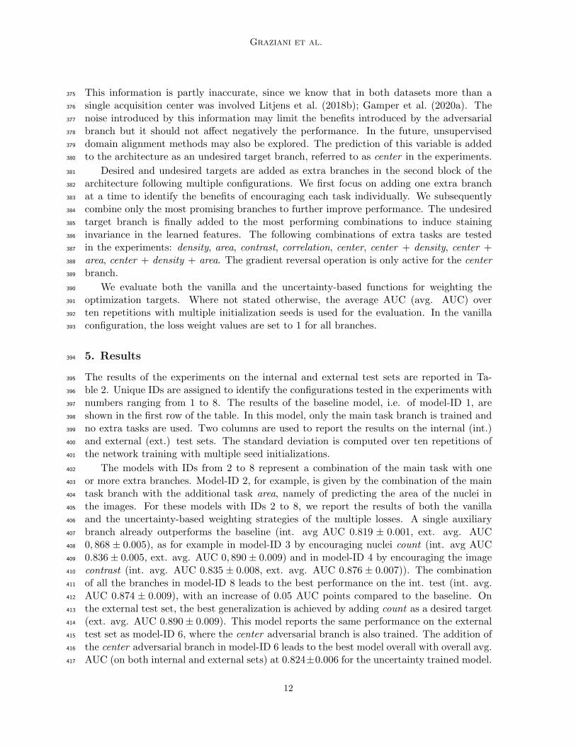
5. Results394
The results of the experiments on the internal and external test sets are reported in Ta-395
ble 2. Unique IDs are assigned to identify the configurations tested in the experiments with396
numbers ranging from 1 to 8. The results of the baseline model, i.e. of model-ID 1, are397
shown in the first row of the table. In this model, only the main task branch is trained and398
no extra tasks are used. Two columns are used to report the results on the internal (int.)399
and external (ext.) test sets. The standard deviation is computed over ten repetitions of400
the network training with multiple seed initializations.401
The models with IDs from 2 to 8 represent a combination of the main task with one402
or more extra branches. Model-ID 2, for example, is given by the combination of the main403
task branch with the additional task area, namely of predicting the area of the nuclei in404
the images. For these models with IDs 2 to 8, we report the results of both the vanilla405
and the uncertainty-based weighting strategies of the multiple losses. A single auxiliary406
branch already outperforms the baseline (int. avg AUC 0.819 ± 0.001, ext. avg. AUC407
0, 868 ± 0.005), as for example in model-ID 3 by encouraging nuclei count (int. avg AUC408
0.836± 0.005, ext. avg. AUC 0, 890± 0.009) and in model-ID 4 by encouraging the image409
contrast (int. avg. AUC 0.835 ± 0.008, ext. avg. AUC 0.876 ± 0.007)). The combination410
of all the branches in model-ID 8 leads to the best performance on the int. test (int. avg.411
AUC 0.874 ± 0.009), with an increase of 0.05 AUC points compared to the baseline. On412
the external test set, the best generalization is achieved by adding count as a desired target413
(ext. avg. AUC 0.890± 0.009). This model reports the same performance on the external414
test set as model-ID 6, where the center adversarial branch is also trained. The addition of415
the center adversarial branch in model-ID 6 leads to the best model overall with overall avg.416
AUC (on both internal and external sets) at 0.824±0.006 for the uncertainty trained model.417
12
Multi-task and Adversarial CNN Training
This represents a significant improvement compared to the overall avg. AUC 0.79 ± 0.001418
of the baseline model, with p − value < 0.001. The statistical significance of the results is419
evaluated by the non-parametric Wilcoxon test (two-sided) applied on the bootstrapping of420
the test set as described in Sec. 4.2.421
To confirm the benefit of the added related tasks, we compare these results with those422
obtained with random noise as additional targets. This experiment is performed as a sanity423
check, where an auxiliary task is trained to predict random values. As expected, the overall,424
internal and external avg. AUCs are lower for this experiment and have larger standard425
deviations (overall avg. AUC 0.819± 0.04, int. test AUC 0.834± 0.001 and ext. avg. AUC426
0.879 ± 0.03). This shows that the selected tasks are more relevant to the main task than427
the regression of random values.428
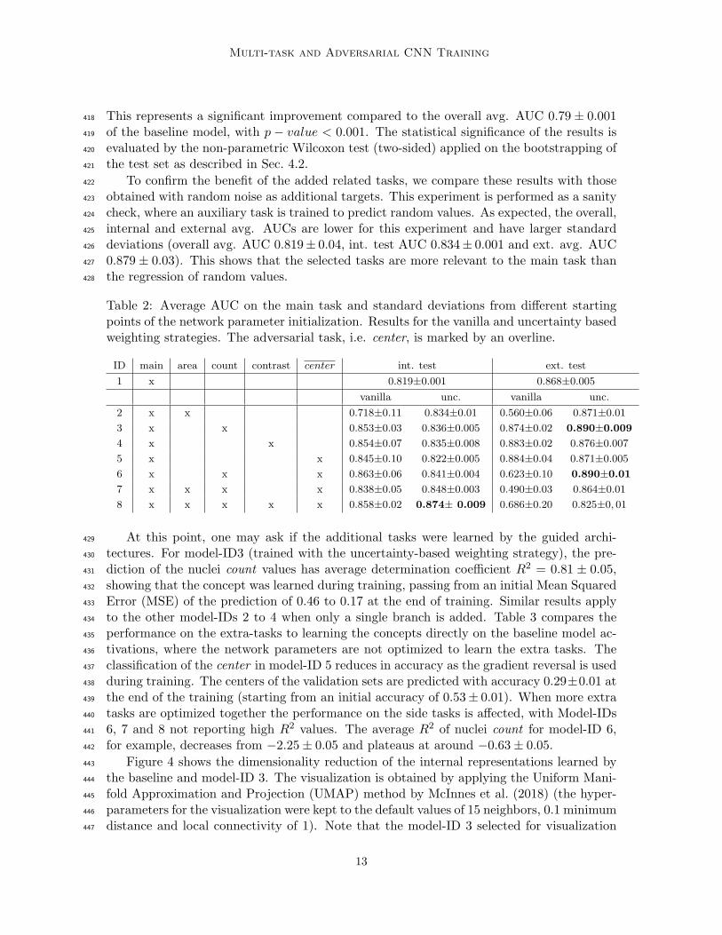
Table 2: Average AUC on the main task and standard deviations from different startingpoints of the network parameter initialization. Results for the vanilla and uncertainty basedweighting strategies. The adversarial task, i.e. center, is marked by an overline.
ID main area count contrast center int. test ext. test
1 x 0.819±0.001 0.868±0.005
vanilla unc. vanilla unc.
2 x x 0.718±0.11 0.834±0.01 0.560±0.06 0.871±0.01
3 x x 0.853±0.03 0.836±0.005 0.874±0.02 0.890±0.009
4 x x 0.854±0.07 0.835±0.008 0.883±0.02 0.876±0.007
5 x x 0.845±0.10 0.822±0.005 0.884±0.04 0.871±0.005
6 x x x 0.863±0.06 0.841±0.004 0.623±0.10 0.890±0.01
7 x x x x 0.838±0.05 0.848±0.003 0.490±0.03 0.864±0.01
8 x x x x x 0.858±0.02 0.874± 0.009 0.686±0.20 0.825±0, 01
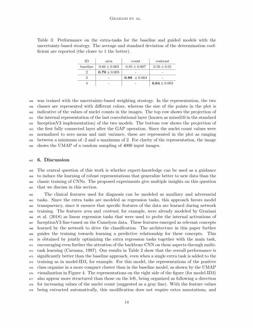
At this point, one may ask if the additional tasks were learned by the guided archi-429
tectures. For model-ID3 (trained with the uncertainty-based weighting strategy), the pre-430
diction of the nuclei count values has average determination coefficient R2 = 0.81 ± 0.05,431
showing that the concept was learned during training, passing from an initial Mean Squared432
Error (MSE) of the prediction of 0.46 to 0.17 at the end of training. Similar results apply433
to the other model-IDs 2 to 4 when only a single branch is added. Table 3 compares the434
performance on the extra-tasks to learning the concepts directly on the baseline model ac-435
tivations, where the network parameters are not optimized to learn the extra tasks. The436
classification of the center in model-ID 5 reduces in accuracy as the gradient reversal is used437
during training. The centers of the validation sets are predicted with accuracy 0.29±0.01 at438
the end of the training (starting from an initial accuracy of 0.53± 0.01). When more extra439
tasks are optimized together the performance on the side tasks is affected, with Model-IDs440
6, 7 and 8 not reporting high R2 values. The average R2 of nuclei count for model-ID 6,441
for example, decreases from −2.25± 0.05 and plateaus at around −0.63± 0.05.442
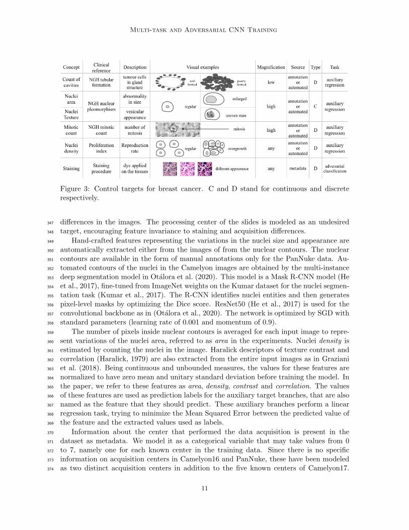
Figure 4 shows the dimensionality reduction of the internal representations learned by443
the baseline and model-ID 3. The visualization is obtained by applying the Uniform Mani-444
fold Approximation and Projection (UMAP) method by McInnes et al. (2018) (the hyper-445
parameters for the visualization were kept to the default values of 15 neighbors, 0.1 minimum446
distance and local connectivity of 1). Note that the model-ID 3 selected for visualization447
13
Graziani et al.
Table 3: Performance on the extra-tasks for the baseline and guided models with theuncertainty-based strategy. The average and standard deviation of the determination coef-ficient are reported (the closer to 1 the better).
ID area count contrast
baseline 0.66± 0.003 0.85± 0.007 0.56± 0.01
2 0.70± 0.005 - -
3 - 0.88 ± 0.004 -
4 - - 0,64± 0.003
was trained with the uncertainty-based weighting strategy. In the representation, the two448
classes are represented with different colors, whereas the size of the points in the plot is449
indicative of the values of nuclei counts in the images. The top row shows the projection of450
the internal representation of the last convolutional layer (known as mixed10 in the standard451
InceptionV3 implementation) of the two models. The bottom row shows the projection of452
the first fully connected layer after the GAP operation. Since the nuclei count values were453
normalized to zero mean and unit variance, these are represented in the plot as ranging454
between a minimum of -2 and a maximum of 2. For clarity of the representation, the image455
shows the UMAP of a random sampling of 4000 input images.456
6. Discussion457
The central question of this work is whether expert-knowledge can be used as a guidance458
to induce the learning of robust representations that generalize better to new data than the459
classic training of CNNs. The proposed experiments give multiple insights on this question460
that we discuss in this section.461
The clinical features used for diagnosis can be modeled as auxiliary and adversarial462
tasks. Since the extra tasks are modeled as regression tasks, this approach favors model463
transparency, since it ensures that specific features of the data are learned during network464
training. The features area and contrast, for example, were already modeled by Graziani465
et al. (2018) as linear regression tasks that were used to probe the internal activations of466
InceptionV3 fine-tuned on the Camelyon data. These features emerged as relevant concepts467
learned by the network to drive the classification. The architecture in this paper further468
guides the training towards learning a predictive relationship for these concepts. This469
is obtained by jointly optimizing the extra regression tasks together with the main task,470
encouraging even further the attention of the backbone CNN on these aspects through multi-471
task learning (Caruana, 1997). Our results in Table 2 show that the overall performance is472
significantly better than the baseline approach, even when a single extra task is added to the473
training as in model-ID3, for example. For this model, the representations of the positive474
class organize in a more compact cluster than in the baseline model, as shown by the UMAP475
visualization in Figure 4. The representations on the right side of the figure (for model-ID3)476
also appear more structured than those on the left, being organized as following a direction477
for increasing values of the nuclei count (suggested as a gray line). With the feature values478
being extracted automatically, this modification does not require extra annotations, and479
14
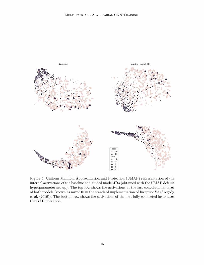
Multi-task and Adversarial CNN Training
Figure 4: Uniform Manifold Approximation and Projection (UMAP) representation of theinternal activations of the baseline and guided model-ID3 (obtained with the UMAP defaulthyperparameter set up). The top row shows the activations at the last convolutional layerof both models, known as mixed10 in the standard implementation of InceptionV3 (Szegedyet al. (2016)). The bottom row shows the activations of the first fully connected layer afterthe GAP operation.
15
Graziani et al.
only introduces a neglectable increase in complexity. One extra task, for instance, requires480
the training of only 2049 additional parameters, namely the 0.008% of Inception V3.481
The auxiliary and adversarial tasks introduced in the architecture are balanced in the482
same end-to-end training, without extra manual tuning of the loss weight nor of a specific483
training schedule that would help the convergence of the adversarial task. This novel ap-484
proach exploits the benefits of another paper in the machine learning research field that485
uses task-dependent uncertainty to balance structurally different losses such as MSE and486
BCE (Kendall et al., 2018). The vanilla weighting of the losses shows instability on unseen487
domains and poor performance on the external test set, whereas the uncertainty-based ap-488
proach is robust to data variability and consistent over random seed initializations for all489
model-IDs. The stability to data variability is shown by the performance on the external490
test set and by the testing with bootstrapping. The consistency over seed reinitializations is491
shown by the small standard deviation of the AUC on both test sets. This gives insight on492
how to handle the multiple loss types for the multi-task modeling on histopathology tasks.493
With the uncertainty-based weighting strategy the architecture did not require any spe-494
cific tuning of the loss weights, whereas a fine-tuning of the weighting parameters appears495
highly necessary in the vanilla approach, particularly for the combinations with more than496
one extra task (model-IDs 6, 7, 8). The manual fine-tuning of the loss weights in the vanilla497
approach may lead to the over-specification of the model to the specific requirements of498
the test data considered in this study. These results not only extend the preliminary work499
by Gamper et al. (2020b) to a different histology tissue and model architecture, but also500
give more insights on how to handle multiple auxiliary losses and adversarial losses without501
requiring tedious tuning of hyper-parameters.502
7. Conclusion503
We show how expert-knowledge can be used pro-actively during the training of CNNs to504
drive the representation learning process. Clinically relevant and easy-to-interpret features505
describing the visual inputs are introduced as extra tasks for the learning objective, sig-506
nificantly improving the robustness and generalization performance of the model. From a507
design perspective, our framework aligns ethically with the intent of not replacing humans,508
but rather making them part of the development of deep learning algorithms. This method509
can be used in human-computer interfaces to introduce user feedback during training. The510
extra tasks may be used as a weak-supervision to extend the training data with unlabeled511
datasets at a marginal cost of some extra automatic processing such as the extraction of512
nuclei contours or texture features. One may argue that additional annotations may be513
required for other clinical features. This represents, however, only a minor limitation of514
this method since a few annotated images may already suffice to train the extra tasks.515
A few limitations of our method require further work and analyses. Our analysis is516
restricted to uncertainty-based weighting strategies, although several approaches were pro-517
posed in the literature (Leang et al., 2020). The results on center do not show a marked518
improvement by the adversarial branch. This could be due to the fact that the acquisition519
centers were not annotated for the PanNuke dataset. An unsupervised domain adapta-520
tion approach such as the domain alignment layers proposed by Carlucci et al. (2017) may521
be used to discover this latent information. Depending on the application, a different loss522
16
Multi-task and Adversarial CNN Training
weighting approach may be used for the adversarial task and other undesired control targets523
can also be included, such as rotation, scale and image compression methods. In addition,524
our experiments show that the auxiliary tasks become harder to learn when they are scaled525
up in number, with model-ID 8 having a lower R2 for the regression of the individual fea-526
tures than those reported for model-IDs 2 to 5 in Table 3. As explained also by Caruana527
(1997), the poor performance on the extra tasks is not necessarily an issue as long as these528
help with improving the model performance and generalization on unseen data. Further529
research is necessary to verify how this architecture may be improved to ensure high perfor-530
mance on all the extra tasks, while maintaining its transparency and complexity at similar531
levels. In future work we will also focus on extracting extra features solely from unlabeled532
data and on introducing them during training as weak supervision.533
Acknowledgments534
This work is supported by the European Union’s projects ExaMode (grant s825292) and535
AI4Media (grant 951911).536
Data Availability537
The Camelyon data that support the findings of this study are available at https://538
camelyon17.grand-challenge.org/Data/ as accessed in August 2021, with the DOI iden-539
tifier of the dataset paper doi.org/10.1109/TMI.2018.2867350. The PanNuke data are540
available at https://warwick.ac.uk/fac/crossfac/tia/data/pannuke (accessed in Au-541
gust 2021), with DOI identifier of the paper doi.org/10.1007/978-3-030-23937-4_2.542
Code Availability543
The code used for the experiments is available online for reproducibility on Github (https:544
//github.com/maragraziani/multitask_adversarial) and Zenodo at https://doi.org/545
10.5281/zenodo.5243433 (accessed in August, 2021). An executable version on Code546
Ocean is currently being developed.547
References548
Vincent Andrearczyk, Pierre Fontaine, Valentin Oreiller, and Adrien Depeursinge. Multi-549
task Deep Segmentation and Radiomics for Automatic Prognosis in Head and Neck Can-550
cer. In under revision, page 1, 2021.551
Jonathan Baxter. Learning internal representations. In Proceedings of the eighth annual552
conference on Computational learning theory, pages 311–320, 1995.553
Jonathan Baxter. A model of inductive bias learning. Journal of artificial intelligence554
research, 12:149–198, 2000.555
17
Graziani et al.
HJG Bloom and WW Richardson. Histological grading and prognosis in breast cancer: a556
study of 1409 cases of which 359 have been followed for 15 years. British Journal of557
Cancer, 11(3):359, 1957.558
Carrie J Cai, Emily Reif, Narayan Hegde, Jason Hipp, Been Kim, Daniel Smilkov, Martin559
Wattenberg, Fernanda Viegas, Greg S Corrado, Martin C Stumpe, et al. Human-centered560
tools for coping with imperfect algorithms during medical decision-making. In Conference561
on Human Factors in Computing Systems, 2019.562
Gabriele Campanella, Matthew G Hanna, Luke Geneslaw, Allen Miraflor, Vitor W K Silva,563
Klaus J Busam, Edi Brogi, Victor E Reuter, David S Klimstra, and Thomas J Fuchs.564
Clinical-grade computational pathology using weakly supervised deep learning on whole565
slide images. Nature medicine, 25(8):1301–1309, 2019.566
Fabio Maria Carlucci, Lorenzo Porzi, Barbara Caputo, Elisa Ricci, and Samuel Rota Bulo.567
Just dial: Domain alignment layers for unsupervised domain adaptation. In International568
Conference on Image Analysis and Processing, pages 357–369. Springer, 2017.569
Rich Caruana. Multitask learning. Machine learning, 28(1):41–75, 1997.570
Finale Doshi-Velez and Been Kim. Towards a rigorous science of interpretable machine571
learning. arXiv preprint arXiv:1702.08608, 2017.572
Long Duong, Trevor Cohn, Steven Bird, and Paul Cook. Low resource dependency parsing:573
Cross-lingual parameter sharing in a neural network parser. In Proceedings of the 53rd574
annual meeting of the Association for Computational Linguistics and the 7th international575
joint conference on natural language processing (volume 2: short papers), pages 845–850,576
2015.577
Jevgenij Gamper, Navid Alemi Koohbanani, Ksenija Benet, Ali Khuram, and Nasir Ra-578
jpoot. PanNuke: an open pan-cancer histology dataset for nuclei instance segmentation579
and classification. In European Congress on Digital Pathology, pages 11–19. Springer,580
2019.581
Jevgenij Gamper, Navid Alemi Koohbanani, Simon Graham, Mostafa Jahanifar, Syed Ali582
Khurram, Ayesha Azam, Katherine Hewitt, and Nasir Rajpoot. Pannuke dataset exten-583
sion, insights and baselines. arXiv preprint arXiv:2003.10778, 2020a.584
Jevgenij Gamper, Navid Alemi Kooohbanani, and Nasir Rajpoot. Multi-task learning in585
histo-pathology for widely generalizable model. arXiv preprint arXiv:2005.08645, 2020b.586
Yaroslav Ganin, Evgeniya Ustinova, Hana Ajakan, Pascal Germain, Hugo Larochelle,587
Francois Laviolette, Mario Marchand, and Victor Lempitsky. Domain-adversarial train-588
ing of neural networks. The Journal of Machine Learning Research, 17(1):2096–2030,589
2016.590
Boqing Gong, Kristen Grauman, and Fei Sha. Connecting the dots with landmarks: Dis-591
criminatively learning domain-invariant features for unsupervised domain adaptation. In592
International Conference on Machine Learning, pages 222–230. PMLR, 2013.593
18
Multi-task and Adversarial CNN Training
Ting Gong, Tyler Lee, Cory Stephenson, Venkata Renduchintala, Suchismita Padhy, An-594
thony Ndirango, Gokce Keskin, and Oguz H Elibol. A comparison of loss weighting595
strategies for multi task learning in deep neural networks. IEEE Access, 7:141627–141632,596
2019.597
Ian Goodfellow, Yoshua Bengio, and Aaron Courville. Deep Learning. MIT Press, 2016.598
http://www.deeplearningbook.org.599
Mara Graziani, Vincent Andrearczyk, and Henning Muller. Regression concept vectors for600
bidirectional explanations in histopathology. In Understanding and Interpreting Machine601
Learning in Medical Image Computing Applications, pages 124–132. Springer, 2018.602
Mara Graziani, James M Brown, Vincent Andrearczyk, Veysi Yildiz, J Peter Campbell,603
Deniz Erdogmus, Stratis Ioannidis, Michael F Chiang, Jayashree Kalpathy-Cramer, and604
Henning Muller. Improved interpretability for computer-aided severity assessment of605
retinopathy of prematurity. In Medical Imaging 2019: Computer-Aided Diagnosis, 2019a.606
Mara Graziani, Henning Muller, and Vincent Andrearczyk. Interpreting intentionally flawed607
models with linear probes. In IEEE International Conference on Computer Vision Work-608
shops, 2019b.609
Mara Graziani, Vincent Andrearczyk, Stephane Marchand-Maillet, and Henning Muller.610
Concept attribution: Explaining CNN decisions to physicians. Computers in Biol-611
ogy and Medicine, page 103865, 2020. ISSN 0010-4825. doi: https://doi.org/10.1016/612
j.compbiomed.2020.103865. URL http://www.sciencedirect.com/science/article/613
pii/S0010482520302225.614
Robert M Haralick. Statistical and structural approaches to texture. Proceedings of the615
IEEE, 67(5):786–804, 1979.616
Kaiming He, Georgia Gkioxari, Piotr Dollar, and Ross Girshick. Mask r-cnn. In Proceedings617
of the IEEE International Conference on Computer Vision (ICCV), Oct 2017.618
Maximilian Ilse, Jakub M Tomczak, and Max Welling. Deep multiple instance learning for619
digital histopathology. In Handbook of Medical Image Computing and Computer Assisted620
Intervention, pages 521–546. Elsevier, 2020.621
Andrew Janowczyk and Anant Madabhushi. Deep learning for digital pathology image anal-622
ysis: A comprehensive tutorial with selected use cases. Journal of pathology informatics,623
7, 2016.624
Alex Kendall, Yarin Gal, and Roberto Cipolla. Multi-task learning using uncertainty to625
weigh losses for scene geometry and semantics. In Proceedings of the IEEE conference on626
computer vision and pattern recognition, pages 7482–7491, 2018.627
Been Kim, Martin Wattenberg, Justin Gilmer, Carrie Cai, James Wexler, Fernanda Viegas,628
et al. Interpretability beyond feature attribution: Quantitative testing with concept629
activation vectors (TCAV). In International Conference on Machine Learning, pages630
2673–2682, 2018.631
19
Graziani et al.
Iasonas Kokkinos. Ubernet: Training a universal convolutional neural network for low-,632
mid-, and high-level vision using diverse datasets and limited memory. In Proceedings633
of the IEEE Conference on Computer Vision and Pattern Recognition, pages 6129–6138,634
2017.635
N. Kumar, R. Verma, S. Sharma, S. Bhargava, A. Vahadane, and A. Sethi. A dataset and a636
technique for generalized nuclear segmentation for computational pathology. IEEE Trans-637
actions on Medical Imaging, 36(7):1550–1560, 2017. doi: 10.1109/TMI.2017.2677499.638
Maxime W Lafarge, Josien PW Pluim, Koen AJ Eppenhof, Pim Moeskops, and Mitko Veta.639
Domain-adversarial neural networks to address the appearance variability of histopathol-640
ogy images. In Deep Learning in Medical Image Analysis and Multimodal Learning for641
Clinical Decision Support, 2017.642
Isabelle Leang, Ganesh Sistu, Fabian Burger, Andrei Bursuc, and Senthil Yogamani. Dy-643
namic task weighting methods for multi-task networks in autonomous driving systems. In644
2020 IEEE 23rd International Conference on Intelligent Transportation Systems (ITSC),645
pages 1–8. IEEE, 2020.646
Geert Litjens, Thijs Kooi, Babak E. Bejnordi, Arnaud Arindra Adiyoso Setio, Francesco647
Ciompi, Mohsen Ghafoorian, Jeroen A. Van Der Laak, Bram Van Ginneken, and Clara I648
Sanchez. A survey on deep learning in medical image analysis. Medical image analysis,649
42:60–88, 2017.650
Geert Litjens, Peter Bandi, Babak Ehteshami Bejnordi, Oscar Geessink, Maschenka Balken-651
hol, Peter Bult, Altuna Halilovic, Meyke Hermsen, Rob van de Loo, Rob Vogels, et al.652
1399 H&E-stained sentinel lymph node sections of breast cancer patients: the CAME-653
LYON dataset. GigaScience, 7(6):giy065, 2018a.654
Geert Litjens, Peter Bandi, Babak Ehteshami Bejnordi, Oscar Geessink, Maschenka Balken-655
hol, Peter Bult, Altuna Halilovic, Meyke Hermsen, Rob van de Loo, Rob Vogels, and et al.656
1399 H&E-stained sentinel lymph node sections of breast cancer patients: the CAME-657
LYON dataset. GigaScience, 7(6), 2018b.658
Mingsheng Long, Yue Cao, Jianmin Wang, and Michael Jordan. Learning transferable659
features with deep adaptation networks. In International conference on machine learning,660
pages 97–105. PMLR, 2015.661
Niccolo Marini, Sebastian Otalora, Henning Muller, and Manfredo Atzori. Semi-supervised662
learning with a teacher-student paradigm for histopathology classification: a resource to663
face data heterogeneity and lack of local annotations. In Pattern Recognition. ICPR Inter-664
national Workshops and Challenges: Virtual Event, January 10–15, 2021, Proceedings,665
Part I, pages 105–119. Springer International Publishing, 2021.666
Leland McInnes, John Healy, and James Melville. Umap: Uniform manifold approximation667
and projection for dimension reduction. arXiv preprint arXiv:1802.03426, 2018.668
Sebastian Otalora, Manfredo Atzori, Vincent Andrearczyk, Amjad Khan, and Henning669
Muller. Staining invariant features for improving generalization of deep convolutional670
20
Multi-task and Adversarial CNN Training
neural networks in computational pathology. Frontiers in Bioengineering and Biotech-671
nology, 7:198, 2019.672
Sebastian Otalora, Manfredo Atzorib, Amjad Khanb, Oscar Jimenez-del Toroa, Vincent673
Andrearczykb, and Henning Mullera. Systematic comparison of deep learning strategies674
for weakly supervised gleason grading. Medical Imaging 2020: Digital Pathology, 2020.675
Erik Reinhard, Michael Adhikhmin, Bruce Gooch, and Peter Shirley. Color transfer between676
images. IEEE Computer graphics and applications, 21(5):34–41, 2001.677
Sebastian Ruder. An overview of multi-task learning in deep neural networks. arXiv preprint678
arXiv:1706.05098, 2017.679
Sandeep Subramanian, Adam Trischler, Yoshua Bengio, and Christopher J Pal. Learning680
general purpose distributed sentence representations via large scale multi-task learning.681
arXiv preprint arXiv:1804.00079, 2018.682
Christian Szegedy, Vincent Vanhoucke, Sergey Ioffe, Jon Shlens, and Zbigniew Wojna. Re-683
thinking the inception architecture for computer vision. In IEEE Conference on Computer684
Vision and Pattern Recognition, 2016.685
Dayong Wang, Aditya Khosla, Rishab Gargeya, Humayun Irshad, and Andrew H Beck.686
Deep learning for identifying metastatic breast cancer. arXiv preprint arXiv:1606.05718,687
2016.688
Qizhe Xie, Zihang Dai, Yulun Du, Eduard Hovy, and Graham Neubig. Controllable invari-689
ance through adversarial feature learning. In Advances in Neural Information Processing690
Systems, 2017.691
Hugo Yeche, Justin Harrison, and Tess Berthier. UBS: A Dimension-Agnostic Metric for692
Concept Vector Interpretability Applied to Radiomics. In Interpretability of Machine693
Intelligence in Medical Image Computing and Multimodal Learning for Clinical Decision694
Support, 2019.695
John R Zech, Marcus A Badgeley, Manway Liu, Anthony B Costa, Joseph J Titano, and696
Eric Karl Oermann. Variable generalization performance of a deep learning model to697
detect pneumonia in chest radiographs: a cross-sectional study. PLoS medicine, 15(11):698
e1002683, 2018.699
21


