Embed Size (px)
Citation preview

Univers
ity of
Cap
e Tow
n
Systems Development of a Two-Axis
Stabilised Platform to Facilitate
Astronomical Observations
James Haydn Hepworth
Supervised by Associate Professor Hendrik D. Mouton
Robotics and Agents Research Laboratory
This dissertation is presented for the degree of
Master of Science in Engineering
In the Department of Mechanical Engineering
University of Cape Town
October 2018

Univers
ity of
Cap
e Tow
n
The copyright of this thesis vests in the author. No quotation from it or information derived from it is to be published without full acknowledgement of the source. The thesis is to be used for private study or non-commercial research purposes only.
Published by the University of Cape Town (UCT) in terms of the non-exclusive license granted to UCT by the author.


i
Soli Deo Gloria
Systems Development of a Two-Axis Stabilised Platform to Facilitate Astronomical Observations
ii
DECLARATION
I know the meaning of plagiarism and declare that all the work in the document, save that
which is properly acknowledged, is my own. This dissertation has been submitted to the
Turnitin module and I confirm that my supervisor has seen my report and any concerns
revealed by such have been resolved with my supervisor.
Signed:
Date: 14 October 2018
James Haydn Hepworth
Cape Town
iii
SUMMARY
INTRODUCTION
Inertially Stabilised Platforms (ISPs) aim to control the line-of-sight between a sensor and
a target. They are required to perform two distinct operations: first, to keep track of the
target as the sensor host and the target move in inertial space and, second, to attenuate
rotational disturbances incurred to the sensor by host vehicle motion. This project aimed to
develop a two-axis ISP for use in astronomical applications. Due to the high magnifications
associated with astronomical observations, target objects are quickly lost from the field of
view (FOV) of a stand-alone telescope due to the Earth’s rotation. It was hypothesised that
by mounting a telescope on a stabilised platform with an automatic target tracker it would
be possible to overcome this problem as well as extend the allowable operating conditions of
the telescope to include mountings on moving vehicles.
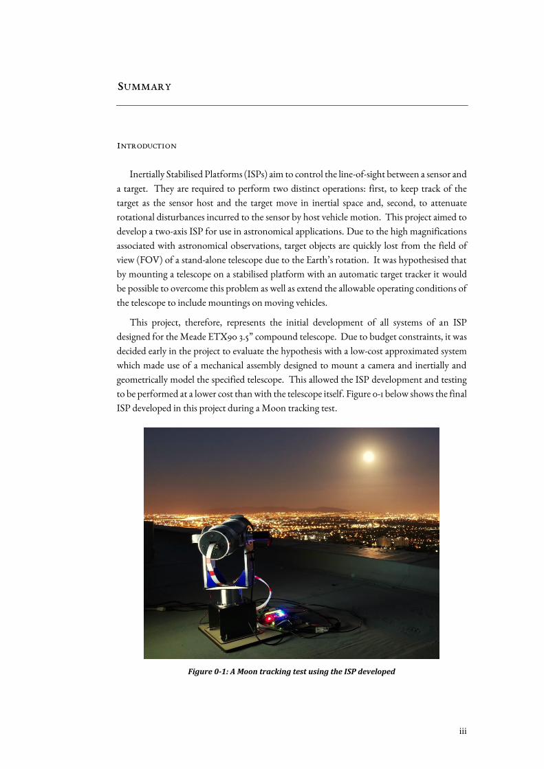
This project, therefore, represents the initial development of all systems of an ISP
designed for the Meade ETX90 3.5” compound telescope. Due to budget constraints, it was
decided early in the project to evaluate the hypothesis with a low-cost approximated system
which made use of a mechanical assembly designed to mount a camera and inertially and
geometrically model the specified telescope. This allowed the ISP development and testing
to be performed at a lower cost than with the telescope itself. Figure 0-1 below shows the final
ISP developed in this project during a Moon tracking test.
Figure 0-1: A Moon tracking test using the ISP developed
Systems Development of a Two-Axis Stabilised Platform to Facilitate Astronomical Observations
iv
PROJECT DEVELOPMENT PROCESS
In order to achieve the above aim, a relevant review of the literature surrounding the
various components of an ISP was performed to inform the design, implementation and
testing cycle which comprised most of the project. A set of ideal system specifications were
then developed to guide design decisions made and to evaluate the performance of the final
system implemented. These specifications were developed for the initial project aim of
stabilising the ETX90 telescope itself and, accordingly, served as design goals to be
approximated by the low-cost system developed in this project.
During the project, the electro-mechanical structure of the ISP was designed and
implemented. From a mechanical perspective, all parts of the physical structure, including
the telescope modelling assembly, the yaw gimbal, and the mounting stand were designed
and manufactured. The associated electrical systems required to facilitate control of this
structure were also specified and configured. These systems included the relative angle
sensors used to measure the orientations of the yaw gimbal and telescope modeller, the
inertial measurement unit (IMU) used to measure the inertial rotational rates of the telescope
modeller, the camera sensor used to acquire the image of the FOV of the telescope modeller,
the motors and drive electronics used to actuate the gimbals, and the control hardware
required to run the firmware and software written to achieve the stabilisation and tracking
functions of the ISP.
These control hardware systems included a Raspberry Pi Model 3 B computer, an
STM32F0 microcontroller, and a laptop running a User Interface (UI) program written in
LabVIEW. The Raspberry Pi was used to run an image processing script, written in Python
2.7, which was capable of detecting and locating the centre of the Moon in the camera FOV.
The STM32F0 microcontroller ran firmware, written in C, which was tasked with managing
the various control and communications tasks required by the system. Finally, the UI helped
to facilitate intuitive operator control of the system and performed datalogging of the system
runtime data.
In addition, a complete simulation model for the system was written in the simulation
language, Simul_C_EM, and used to design the various controllers for the ISP control system
which were implemented on the STM32F0. For each gimbal, compensated PI controllers
were designed to allow manual orientation control of the telescope, compensated P
controllers were designed to achieve target tracking, and compensated PI controllers were
designed to reject rotational disturbances and so achieve the inertial stabilisation of the
telescope modeller.
CONCLUSION AND RECOMMENDATIONS
Testing of the system showed a good correlation between the hardware and simulated
results which indicates an accurate simulation model that can be used to test future design
developments. Overall, most specifications developed for the initial system were met or
v
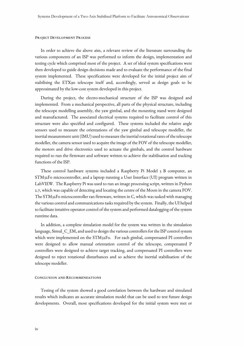
approached by the performance of the implemented model, with the notable exception of
the tracking error of the system which overshot the specification by 50 %. This was due to
the need to reduce the image resolution to 640x480 pixels in order for the Raspberry Pi to be
able to process the images and provide target position data at a rate suitable for the tracking
controller commands. Otherwise, the system showed good base motion disturbance
attenuation properties of the order -31 dB and -34 dB for the yaw and pitch channels
respectively, whilst line-of-sight (LOS) jitter was limited to a maximum of 2.5 mrad in
response to tested disturbances of up to 1 rad/s at approximately 1 – 2 Hz. Figure 0-2 below
is indicative of the type of attenuation performance achieved by the ISP for disturbances
about axes parallel the control axes.
Figure 0-2: Typical disturbance attenuation of the pitch channel
Overall it was concluded that the project successfully achieved its aims and that future
development should be continued with the ISP to include the ETX90 telescope. Suggested
improvements that should be made include the change of computation hardware on which
image processing is performed to improve the tracking performance of the system, the
upgrading of the yaw motor such that a greater torque may be applied to the yaw gimbal and
so attenuate stronger disturbance signals, and an investigation into the use of modern control
methods which may help to improve the performance of the stabilisation control system.
-100
-50
0
50
100
6 7 8 9 10 11 12 13Rate
(°/
s)
Time (s)
Pitch Attentuation Rate Base Motion Rate

Systems Development of a Two-Axis Stabilised Platform to Facilitate Astronomical Observations
vi
ACKNOWLEDGEMENTS
For their assistance with my journey through this project, in a myriad of different ways, I
would like to make the following acknowledgements:
Firstly, to my supervisor, Hennie Mouton, who has patiently helped me through this
project over the course of the past years. Your contribution to my education and
development as an engineer has been the greatest that any have made. I greatly value
the sacrifice of time, effort, and finances that you have made for me in this project.
To Ehlke de Jong, who has borne both the satisfaction of my successes and the burdens
of my trials throughout this project. Your ever-present support has been invaluable
and to have shared this journey with you has been a great joy.
To my parents, thank you for your support from afar and for making my education
possible. I am extremely grateful for all that you have done for me over so many years.
To those who have helped me to bear the financial burden of this degree, my parents,
the Department of Mechanical Engineering through the Reino-Stegen Scholarship,
and Christopher and Kerry-Lee Louw, thank you for all that you gave. Without your
assistance this degree could never have been accomplished.
To Leanne Raw and Tracey Booysen, thank you for your technical help, advice, and
contributions you have made to this project and my education.
To my various lab partners at RARL over the past three years, John, Max, Tim, Greig
and Victor, thank you for your encouragement and friendship. Each of you
contributed greatly to my enjoyment of these years.
Contents
vii
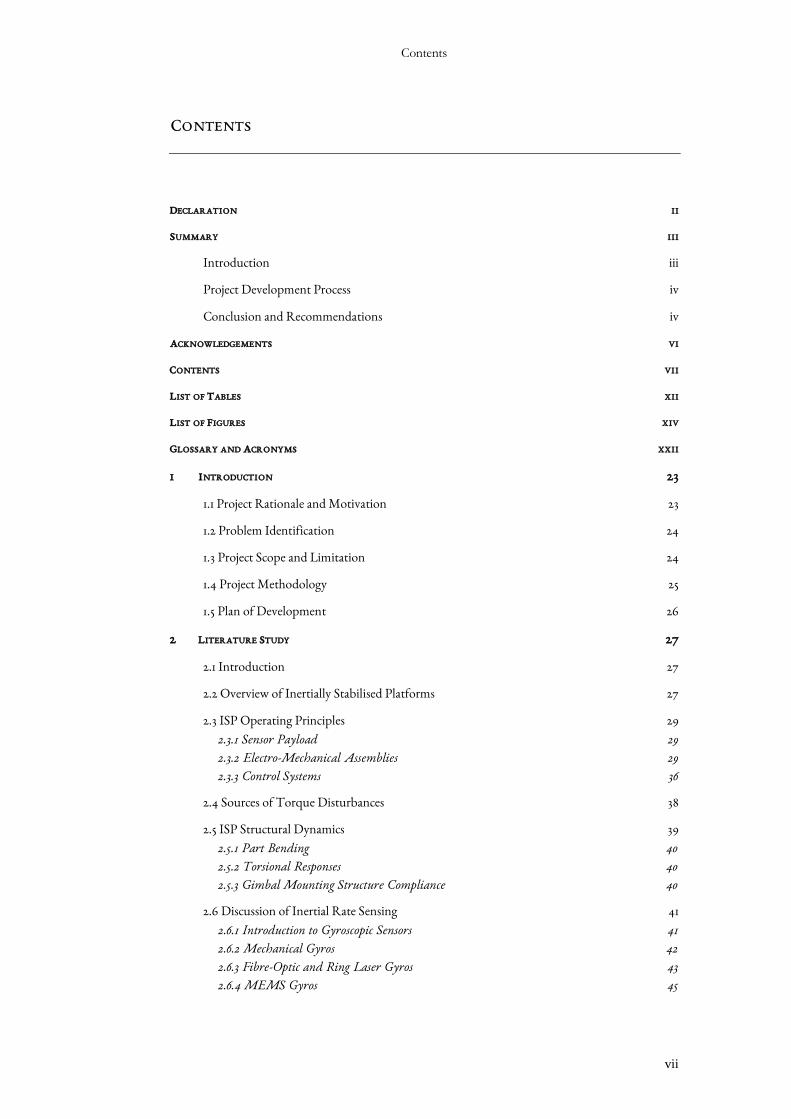
CONTENTS
DECLARATION II
SUMMARY III
Introduction iii
Project Development Process iv
Conclusion and Recommendations iv
ACKNOWLEDGEMENTS VI
CONTENTS VII
LIST OF TABLES XII
LIST OF FIGURES XIV
GLOSSARY AND ACRONYMS XXII
1 INTRODUCTION 23
1.1 Project Rationale and Motivation 23
1.2 Problem Identification 24
1.3 Project Scope and Limitation 24
1.4 Project Methodology 25
1.5 Plan of Development 26
2 LITERATURE STUDY 27
2.1 Introduction 27
2.2 Overview of Inertially Stabilised Platforms 27
2.3 ISP Operating Principles 29
2.3.1 Sensor Payload 29
2.3.2 Electro-Mechanical Assemblies 29 2.3.3 Control Systems 36
2.4 Sources of Torque Disturbances 38
2.5 ISP Structural Dynamics 39
2.5.1 Part Bending 40 2.5.2 Torsional Responses 40 2.5.3 Gimbal Mounting Structure Compliance 40
2.6 Discussion of Inertial Rate Sensing 41
2.6.1 Introduction to Gyroscopic Sensors 41 2.6.2 Mechanical Gyros 42
2.6.3 Fibre-Optic and Ring Laser Gyros 43 2.6.4 MEMS Gyros 45
Systems Development of a Two-Axis Stabilised Platform to Facilitate Astronomical Observations
viii
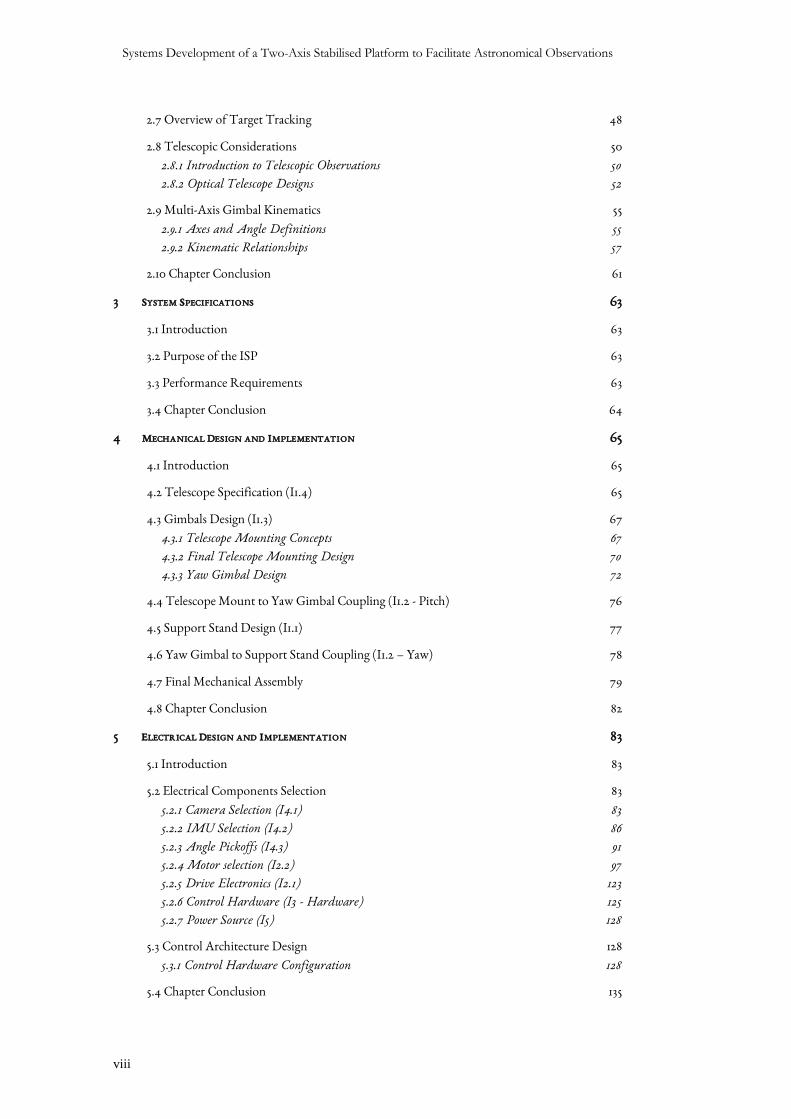
2.7 Overview of Target Tracking 48
2.8 Telescopic Considerations 50
2.8.1 Introduction to Telescopic Observations 50 2.8.2 Optical Telescope Designs 52
2.9 Multi-Axis Gimbal Kinematics 55
2.9.1 Axes and Angle Definitions 55 2.9.2 Kinematic Relationships 57
2.10 Chapter Conclusion 61
3 SYSTEM SPECIFICATIONS 63
3.1 Introduction 63
3.2 Purpose of the ISP 63
3.3 Performance Requirements 63
3.4 Chapter Conclusion 64
4 MECHANICAL DESIGN AND IMPLEMENTATION 65
4.1 Introduction 65
4.2 Telescope Specification (I1.4) 65
4.3 Gimbals Design (I1.3) 67
4.3.1 Telescope Mounting Concepts 67
4.3.2 Final Telescope Mounting Design 70 4.3.3 Yaw Gimbal Design 72
4.4 Telescope Mount to Yaw Gimbal Coupling (I1.2 - Pitch) 76
4.5 Support Stand Design (I1.1) 77
4.6 Yaw Gimbal to Support Stand Coupling (I1.2 – Yaw) 78
4.7 Final Mechanical Assembly 79
4.8 Chapter Conclusion 82
5 ELECTRICAL DESIGN AND IMPLEMENTATION 83
5.1 Introduction 83
5.2 Electrical Components Selection 83
5.2.1 Camera Selection (I4.1) 83 5.2.2 IMU Selection (I4.2) 86 5.2.3 Angle Pickoffs (I4.3) 91 5.2.4 Motor selection (I2.2) 97
5.2.5 Drive Electronics (I2.1) 123 5.2.6 Control Hardware (I3 - Hardware) 125 5.2.7 Power Source (I5) 128
5.3 Control Architecture Design 128
5.3.1 Control Hardware Configuration 128
5.4 Chapter Conclusion 135
Contents
ix
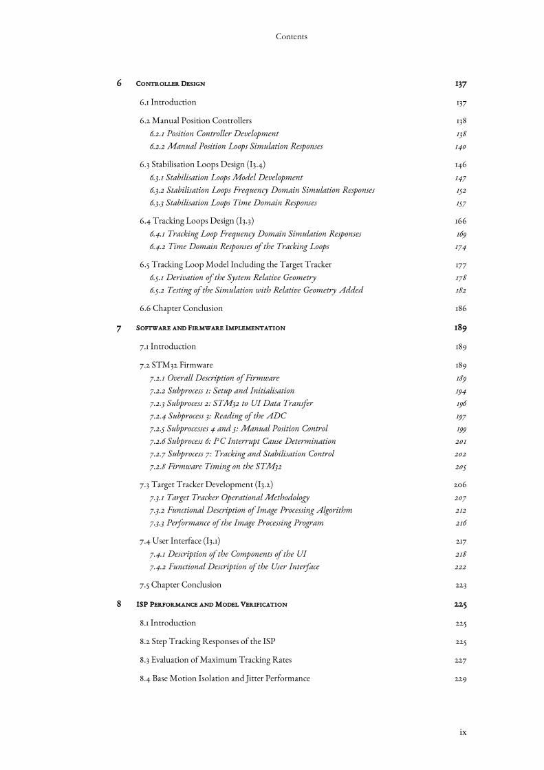
6 CONTROLLER DESIGN 137
6.1 Introduction 137
6.2 Manual Position Controllers 138
6.2.1 Position Controller Development 138
6.2.2 Manual Position Loops Simulation Responses 140
6.3 Stabilisation Loops Design (I3.4) 146
6.3.1 Stabilisation Loops Model Development 147
6.3.2 Stabilisation Loops Frequency Domain Simulation Responses 152 6.3.3 Stabilisation Loops Time Domain Responses 157
6.4 Tracking Loops Design (I3.3) 166
6.4.1 Tracking Loop Frequency Domain Simulation Responses 169 6.4.2 Time Domain Responses of the Tracking Loops 174
6.5 Tracking Loop Model Including the Target Tracker 177
6.5.1 Derivation of the System Relative Geometry 178 6.5.2 Testing of the Simulation with Relative Geometry Added 182
6.6 Chapter Conclusion 186
7 SOFTWARE AND FIRMWARE IMPLEMENTATION 189
7.1 Introduction 189
7.2 STM32 Firmware 189
7.2.1 Overall Description of Firmware 189
7.2.2 Subprocess 1: Setup and Initialisation 194 7.2.3 Subprocess 2: STM32 to UI Data Transfer 196
7.2.4 Subprocess 3: Reading of the ADC 197 7.2.5 Subprocesses 4 and 5: Manual Position Control 199 7.2.6 Subprocess 6: I2C Interrupt Cause Determination 201
7.2.7 Subprocess 7: Tracking and Stabilisation Control 202 7.2.8 Firmware Timing on the STM32 205
7.3 Target Tracker Development (I3.2) 206
7.3.1 Target Tracker Operational Methodology 207 7.3.2 Functional Description of Image Processing Algorithm 212
7.3.3 Performance of the Image Processing Program 216
7.4 User Interface (I3.1) 217
7.4.1 Description of the Components of the UI 218
7.4.2 Functional Description of the User Interface 222
7.5 Chapter Conclusion 223
8 ISP PERFORMANCE AND MODEL VERIFICATION 225
8.1 Introduction 225
8.2 Step Tracking Responses of the ISP 225
8.3 Evaluation of Maximum Tracking Rates 227
8.4 Base Motion Isolation and Jitter Performance 229

Systems Development of a Two-Axis Stabilised Platform to Facilitate Astronomical Observations
x
8.4.1 Pitch Base Motion Isolation in the Home Position 230 8.4.2 Yaw Base Motion Isolation in the Home Position 234
8.4.3 Performance of the ISP in the Worst-Case Position 237 8.4.4 Stationary System Jitter 241
8.5 Chapter Conclusion 242
9 CONCLUSION AND RECOMMENDATIONS 243
9.1 Introduction 243
9.2 Sensor Payload 243
9.2.1 Specifications of the Sensor Payload 243
9.2.2 Image Processing 244
9.3 Electro-Mechanical Assembly 244
9.3.1 Specifications of the Electro-Mechanical Assembly 245 9.3.2 Mechanical Design 245
9.3.3 Yaw Motor 246 9.3.4 Electrical Interfaces 246
9.4 Control Systems 247
9.4.1 Specifications of the Control System 247 9.4.2 Control Hardware, Software and Firmware 248
9.4.3 Current Minor Loops 248 9.4.4 Gyro-Drift Compensation 248
9.4.5 Controller implementation 249
9.5 Summary 249
LIST OF REFERENCES 251
APPENDIX A 259
A.1 Introduction 259
A.2 Purpose of the ISP 259
A.3 Performance Requirements 259
A.3.1 Fundamental performance 259 A.3.2 System constraints 260
A.3.3 Usage 260 A.3.4 Interference 260
A.3.5 Communications 260 A.3.6 Design requirements 260
A.4 Primary Items 261
A.5 Functional Allocation and Flow Chart 261
A.6 System Specifications 264
A.6.1 Mechanical Specifications 264
A.6.2 Operational Specifications 265 A.6.3 Constraints 266
A.7 Chapter Conclusion 267

Contents
xi
APPENDIX B 268
APPENDIX C 269
APPENDIX D 271
Systems Development of a Two-Axis Stabilised Platform to Facilitate Astronomical Observations
xii
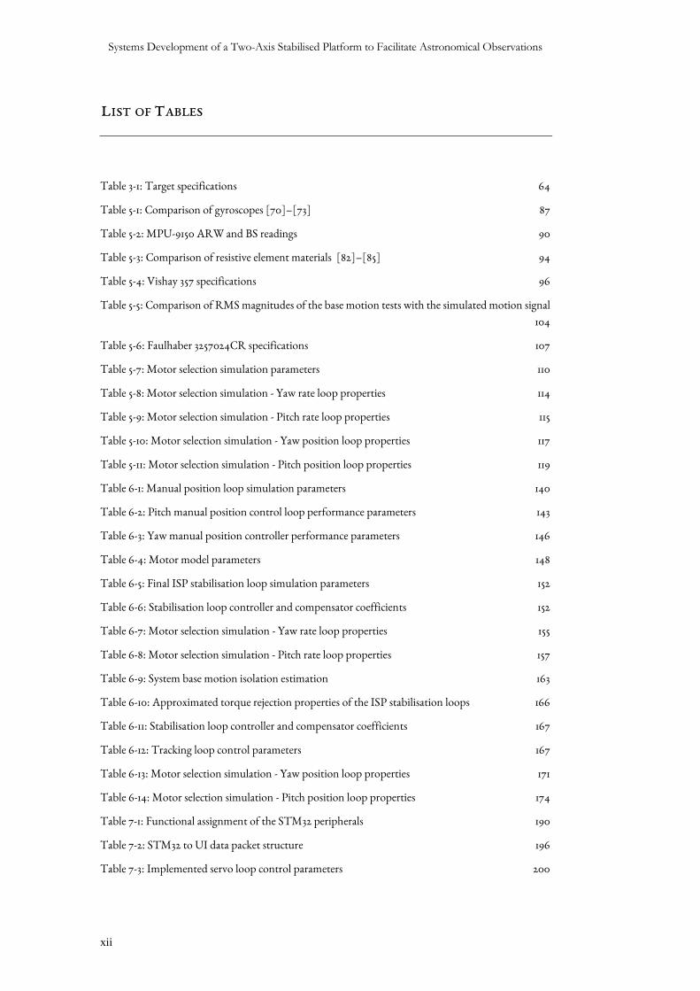
LIST OF TABLES
Table 3-1: Target specifications 64
Table 5-1: Comparison of gyroscopes [70]–[73] 87
Table 5-2: MPU-9150 ARW and BS readings 90
Table 5-3: Comparison of resistive element materials [82]–[85] 94
Table 5-4: Vishay 357 specifications 96
Table 5-5: Comparison of RMS magnitudes of the base motion tests with the simulated motion signal
104
Table 5-6: Faulhaber 3257024CR specifications 107
Table 5-7: Motor selection simulation parameters 110
Table 5-8: Motor selection simulation - Yaw rate loop properties 114
Table 5-9: Motor selection simulation - Pitch rate loop properties 115
Table 5-10: Motor selection simulation - Yaw position loop properties 117
Table 5-11: Motor selection simulation - Pitch position loop properties 119
Table 6-1: Manual position loop simulation parameters 140
Table 6-2: Pitch manual position control loop performance parameters 143
Table 6-3: Yaw manual position controller performance parameters 146
Table 6-4: Motor model parameters 148
Table 6-5: Final ISP stabilisation loop simulation parameters 152
Table 6-6: Stabilisation loop controller and compensator coefficients 152
Table 6-7: Motor selection simulation - Yaw rate loop properties 155
Table 6-8: Motor selection simulation - Pitch rate loop properties 157
Table 6-9: System base motion isolation estimation 163
Table 6-10: Approximated torque rejection properties of the ISP stabilisation loops 166
Table 6-11: Stabilisation loop controller and compensator coefficients 167
Table 6-12: Tracking loop control parameters 167
Table 6-13: Motor selection simulation - Yaw position loop properties 171
Table 6-14: Motor selection simulation - Pitch position loop properties 174
Table 7-1: Functional assignment of the STM32 peripherals 190
Table 7-2: STM32 to UI data packet structure 196
Table 7-3: Implemented servo loop control parameters 200
Contents
xiii
Table 7-4: Implemented tracking and stabilisation loop parameters 204
Table 8-1: Friction parameters of the Pitch Channel 232
Table 8-2: Analogue pitch jitter estimation 233
Table 8-3: Friction parameters of the Pitch Channel 235
Table 8-4: Analogue pitch jitter estimation 237
Table 8-5: Approximation of system jitter under stationary base conditions 241
Table 8-6: Summary of ISP tested performance parameters 242
Table 9-1: Performance of the sensor payload against its specifications 244
Table 9-2: Performance of the electro-mechanical assembly against its specifications 245
Table 9-3: Performance of the control system against its specifications 247
Table A-1: Target specifications 267
Systems Development of a Two-Axis Stabilised Platform to Facilitate Astronomical Observations
xiv
LIST OF FIGURES
Figure 0-1: A Moon tracking test using the ISP developed iii
Figure 0-2: Typical disturbance attenuation of the pitch channel v
Figure 2-1: The DJI Ronin 3-Axis Brushless Gimbal Stabilizer [4], the Cinema Pro Gimbal [5], and the
Paradigm SRP TALON Gyro-Stabilized Gun Platform [6] 28
Figure 2-2: Mass stabilised sensor [7] 31
Figure 2-3: Current feedback minor loop 33
Figure 2-4: Mirror stabilisation mechanism [1] 33
Figure 2-5: Optical doubling effect [7] 34
Figure 2-6: 2:1 drive linkage [7] 34
Figure 2-7: Cascade control structure [7] 37
Figure 2-8: Types of gyro and their applications [25] 42
Figure 2-9: Mechanical gyroscope [26] 42
Figure 2-10: Ring Laser Gyro schematic [28] 43
Figure 2-11: Schematic of an IFOG sensor [27] 44
Figure 2-12: Applications of MEMS gyros [31] 46
Figure 2-13: A typical Allan Variance plot [30] 48
Figure 2-14: Target tracker operation 50
Figure 2-15: Blackbody spectrum of hydrogen [42] 51
Figure 2-16: Telescopes across the EM spectrum [43] 51
Figure 2-17: The Messier 101 galaxy observed with various frequency images [44] 52
Figure 2-18: Achromatic lens [45] 53
Figure 2-19: Optical telescope designs [46] 53
Figure 2-20: Equatorial mount [50] (left), Alt-az mount [51] (centre), and (c) Go-To mount [52] (right)
telescopes 54
Figure 2-21: Double gimbal schematic. Adapted from [53] 55
Figure 2-22: Inertial angle definitions 56
Figure 2-23: Relative angle definitions 56
Figure 4-1: Meade ETX90 telescope [58] 66
Figure 4-2: Lightpath through the Meade ETX90 [59] 66
Figure 4-3: SOLIDWORKS model of the ETX90 telescope 66
Contents
xv
Figure 4-4: ETX90 overall dimensions 67
Figure 4-5: ETX90 Mounting Concept 1 68
Figure 4-6: Raspberry Pi Camera mounted on Mounting Concept 1 68
Figure 4-7: ETX90 Mounting Concept 2 69
Figure 4-8: Raspberry Pi Camera mounted on Mounting Concept 2 69
Figure 4-9: ETX90 final mounting design 70
Figure 4-10: Centre of mass position for the ETX90 pitch platform mounting 71
Figure 4-11: Final ETX90 modelling camera mounting platform 71
Figure 4-12: telescope modeller overall dimensions 72
Figure 4-13: Yaw gimbal final design (front) 73
Figure 4-14: Yaw gimbal final design (rear) 73
Figure 4-15: Yaw gimbal overall dimensions 75
Figure 4-16: Section view of the telescope modeller to yaw gimbal coupling mechanism 76
Figure 4-17: Motor coupling (left) and pot coupling (right) for the telescope modeller 76
Figure 4-18: Detailed section view of the motor-side mounting of the telescope modeller 77
Figure 4-19: Support stand final design 78
Figure 4-20: Section view of the yaw gimbal mounted on the support stand 79
Figure 4-21: ISP assembly with the telescope modeller mounted 80
Figure 4-22: ISP assembly with the ETX90 telescope mounted 80
Figure 4-23: Final implementation of the ISP system 81
Figure 4-24: ISP system overall dimensions 81
Figure 5-1: Optical geometry 84
Figure 5-2: Raspberry Pi Camera [65] and Aptina MT9P031 Demo Kit 2 [66] 84
Figure 5-3: C-mount Defined [68] 85
Figure 5-4: CS-mount adapter shown with the Raspberry Pi Cam and the 12 mm lens 86
Figure 5-5: Raspberry Pi Camera mounted on the ET90 telescope 86
Figure 5-6: IMU test hardware configuration (adapted from [74]) 89
Figure 5-7: X-Axis Allan Deviation 89
Figure 5-8: Y-Axis Allan Deviation 90
Figure 5-9: Z-Axis Allan Deviation 90
Figure 5-10: MPU-9150 [75] and its mounted location 91
Figure 5-11: Workings of an Optical Encoder [76] 92
Figure 5-12: Gray code disk section [77] 92
Systems Development of a Two-Axis Stabilised Platform to Facilitate Astronomical Observations
xvi
Figure 5-13: Hall-effect rotary sensor [79] 93
Figure 5-14: Workings of an Inductive Resolver [80] 93
Figure 5-15: Workings of a potentiometer [81] 94
Figure 5-16: Vishay 357 potentiometer [86] 95
Figure 5-17: Yaw pot mounting position 96
Figure 5-18: Pitch pot mounting position 97
Figure 5-19: One-axis stabilised platform and its DC motor [88] 98
Figure 5-20: IMU axes alignment with vehicle axes (image adapted from [89]) 99
Figure 5-21: Vehicle motion from Base Motion Test 2 100
Figure 5-22: Hanning window function [91] 101
Figure 5-23: Flat Top window functions [92] 101
Figure 5-24: Amplitude vs Frequency of the ximu data of Test 2 under the Hanning window 102
Figure 5-25: Amplitude vs Frequency of the ximu data of Test 2 under the Flat Top window 102
Figure 5-26: Amplitude vs Frequency of the zimu data of Test 2 under the Hanning window 103
Figure 5-27: Amplitude vs Frequency of the zimu data of Test 2 under the Flat Top window 103
Figure 5-28: Frequency domain representation of the simulated signal x axis 104
Figure 5-29: Frequency domain representation of the simulated signal y axis 104
Figure 5-30: Frequency domain representation of the simulated signal z axis 105
Figure 5-31: System identification diagram for a two-axis gimbal system 105
Figure 5-32: DC Motor block diagram used in the motor selection simulation 106
Figure 5-33: Pitch and Yaw position controllers 107
Figure 5-34: Pitch and Yaw stabilisation controllers 107
Figure 5-35: Controller structure for the Yaw and Pitch channels 108
Figure 5-36: Gimbal dynamics block diagram 109
Figure 5-37: Motor selection Simulink block diagram 111
Figure 5-38: Linear approximation of a non-linear curve about point A [94] 112
Figure 5-39: Motor selection simulation - Yaw rate open-loop bode plot 113
Figure 5-40: Motor selection simulation - Yaw rate closed-loop bode plot 113
Figure 5-41: Motor selection simulation - Yaw rate step following 114
Figure 5-42: Motor selection simulation - Pitch rate open-loop bode plot 114
Figure 5-43: Motor selection simulation - Pitch rate closed-loop bode plot 115
Figure 5-44: Motor selection simulation - Pitch rate step following 115
Figure 5-45: Motor selection simulation - Yaw position open-loop bode plot 116
Contents
xvii
Figure 5-46: Motor selection simulation - Yaw position closed-loop bode plot 116
Figure 5-47: Motor selection simulation - Yaw position step following 117
Figure 5-48: Motor selection simulation - Pitch position open-loop bode plot 118
Figure 5-49: Motor selection simulation - Pitch position closed-loop bode plot 118
Figure 5-50: Motor selection simulation - Pitch position step following 119
Figure 5-51: Simulated base motion signal 120
Figure 5-52: Home orientation position command following 120
Figure 5-53: Inertial rates of the telescope for the home position 121
Figure 5-54: Motor torques for the home position 121
Figure 5-55: Position command following for the worst-case position 122
Figure 5-56: Inertial rates of the telescope in the worst-case position 122
Figure 5-57: Motor Torques for the worst-case position 123
Figure 5-58: L298 Dual Full Bridge Driver [95] 124
Figure 5-59: Quimat Dual Motor Driver [96] 124
Figure 5-60: Raspberry Pi 3 Model B [98] 126
Figure 5-61: STM32F051 Microcontroller Board 127
Figure 5-62: Control hardware configuration 128
Figure 5-63: Overall electrical schematic for the ISP system 130
Figure 5-64: I2C protocol for 7-bit address devices [99] 131
Figure 5-65: MPU-9150 to STM32F051 connection 132
Figure 5-66: ADC readings with pot rails directly connected to VSSA and VDDA 133
Figure 5-67: Power supply decoupling capacitors recommended by STMicroelectronics for 36, 48, and
64 pin package STM32 microcontrollers such as the STM32F051 [101] 134
Figure 5-68: ADC readings with pot rails connected to VSSA and VDDA in parallel with C8 and C9
134
Figure 6-1: Manual position controller model 139
Figure 6-2: Stiction function friction model (Adapted from [103]) 139
Figure 6-3: Linear open-loop responses of the pitch manual position controller 141
Figure 6-4: Saturated open-loop responses of the pitch manual position controller 141
Figure 6-5: Linear closed-loop responses of the pitch manual position controller 142
Figure 6-6: Saturated closed-loop responses of the pitch manual position controller 142
Figure 6-7: Step response of the pitch manual position controller 143
Figure 6-8: Linear open-loop responses of the yaw manual position controller 144
Figure 6-9: Saturated open-loop responses of the yaw manual position controller 144
Systems Development of a Two-Axis Stabilised Platform to Facilitate Astronomical Observations
xviii
Figure 6-10: Linear closed-loop response of the yaw manual position controller 145
Figure 6-11: Saturated closed-loop response of the yaw manual position controller 145
Figure 6-12: Step response of the yaw manual position controller 146
Figure 6-13: ISP stabilisation system identification diagram 147
Figure 6-14: Motor model used for the ISP system simulation 147
Figure 6-15: Initial gyro model used in the ISP simulation 148
Figure 6-16: Final gyro model used in the ISP simulation 149
Figure 6-17: Final ISP stabilisation loop block diagram 150
Figure 6-18: Derivation of ωzg from ωzp and ωxp 151
Figure 6-19: Yaw rate open-loop Bode plot - Linear Response 153
Figure 6-20: Yaw rate closed-loop Bode plot - Linear Response 153
Figure 6-21: Yaw rate open-loop Bode plot - Saturated Response 154
Figure 6-22: Yaw rate closed-loop Bode plot - Saturated Response 154
Figure 6-23: Pitch rate open-loop Bode plot - Linear Response 155
Figure 6-24: Pitch rate closed-loop Bode plot - Linear Response 156
Figure 6-25: Pitch rate open-loop Bode plot - Saturated Response 156
Figure 6-26: Pitch rate closed-loop Bode plot - Saturated Response 157
Figure 6-27: Stabilisation loop step responses 158
Figure 6-28: 1.0 rad/s base motion effects when 𝜓 = 𝜃 = 0° 159
Figure 6-29: Simulated base motion signal peak effects when 𝜓 = 𝜃 = 0° 159
Figure 6-30: Yaw base motion isolation Bode plot with a 1.0 rad/s amplitude signal 161
Figure 6-31: Yaw base motion isolation Bode plot with a 0.014 rad/s amplitude signal 161
Figure 6-32: Pitch base motion isolation Bode plot with a 1.0 rad/s amplitude signal 162
Figure 6-33: Pitch base motion isolation Bode plot with a 0.01 rad/s amplitude signal 162
Figure 6-34: Simplified single channel stabilisation loop 163
Figure 6-35: Yaw torque rejection– Yaw rate command to rate error (1.0 rad/s) 164
Figure 6-36: Yaw torque rejection– Yaw rate command to rate error (0.014 rad/s) 164
Figure 6-37: Pitch torque rejection– Pitch rate command to rate error (1.0 rad/s) 165
Figure 6-38: Pitch torque rejection– Pitch rate command to rate error (0.01 rad/s) 165
Figure 6-39: System identification block diagram for the ISP control system 166
Figure 6-40: ISP model with tracking loops included around the stabilisation loops 168
Figure 6-41: Yaw track open-loop Bode plot - Linear Response 169
Figure 6-42: Yaw track closed-loop Bode plot - Linear Response 170
Contents
xix
Figure 6-43: Yaw track open-loop Bode plot - Saturated Response 170
Figure 6-44: Yaw track closed-loop Bode plot - Saturated Response 171
Figure 6-45: Pitch track open-loop Bode plot - Linear Response 172
Figure 6-46: Pitch track closed-loop Bode plot - Linear Response 172
Figure 6-47: Pitch track open-loop Bode plot - Saturated Response 173
Figure 6-48: Pitch track closed-loop Bode plot - Saturated Response 173
Figure 6-49: Tracking loops step following response 174
Figure 6-50: 1.0 rad/s base motion effect in the worst-case position 175
Figure 6-51: 0.25 rad/s base motion effect in the worst-case position 176
Figure 6-52: Base motion effect of the peaks of the simulated base motion signal at 0.1-0.2 Hz in the
worst-case position 176
Figure 6-53: System Identification Diagram of the model with the Target Tracker included 177
Figure 6-54: Host vehicle modelled as a three-axis gimbal (adapted from [104]) 178
Figure 6-55: Final ISP simulation block diagram 181
Figure 6-56: Tracking step response using a target and relative geometry 182
Figure 6-57: 1.0 rad/s base motion effect with the relative geometry model 183
Figure 6-58: 0.25 rad/s base motion effect with the relative geometry model 184
Figure 6-59: Base motion effect of peak simulation signal in the worst-case position with relative
geometry 184
Figure 6-60: Base motion effect of the simulated base motion signal on the ISP in the worst-case
position 185
Figure 6-61: Base motion effect of the simulated base motion signal on the ISP in the home position
186
Figure 7-1: Overall Description of the STM32 Firmware 193
Figure 7-2: Setup and Initialisation subprocess 195
Figure 7-3: STM32 to UI data transfer function 196
Figure 7-4: Gimbal positioning servo loop implementation 201
Figure 7-5: I2C interrupt cause determination function 202
Figure 7-6: Implementation of the Controller function which runs the tracking and stabilisation
control loops 205
Figure 7-7: Automatic state firmware timing 206
Figure 7-8: RGB and HSV colour models [110], [111] 208
Figure 7-9: Effect of the inRange() function on an image 209
Figure 7-10: Image processing kernel 209
Figure 7-11: Binary image before erosion or dilation 210
Systems Development of a Two-Axis Stabilised Platform to Facilitate Astronomical Observations
xx
Figure 7-12: Binary image after an erosion process 210
Figure 7-13: Binary image after a dilation process 211
Figure 7-14: Image processing functional flowchart 214
Figure 7-15: Calibration mode of the image processing script 215
Figure 7-16: Image processing display in the Manual state 216
Figure 7-17: Image processing display in the Automatic state 216
Figure 7-18: Moon tracking test samples 217
Figure 7-19: Final User Interface developed in LabVIEW 219
Figure 7-20: Inertial rate, 𝜔𝑦𝑏, during system operation 220
Figure 7-21: Automatic mode system command input – Unclicked, Clicked, Second Click 221
Figure 7-22: Functional flowchart of the User Interface software operation 223
Figure 8-1: Step Tracking response of the yaw channel 225
Figure 8-2: Step tracking response of the pitch channel 226
Figure 8-3: Simulated step tracking with the test command signals 226
Figure 8-4: Step tracking with current limited motors 227
Figure 8-5: Yaw tracking rate test results 228
Figure 8-6: Maximum rates of the gimbals 229
Figure 8-7: Base motion, 𝜔𝑦𝑏, for the pitch channel BMI test in the home position 230
Figure 8-8: Inertial rate, 𝜔𝑦𝑝, for the pitch channel BMI test 231
Figure 8-9: Simulation response to a 1.8 Hz, 60.89 °/s 𝜔𝑦𝑏 signal 231
Figure 8-10: Pitch channel base motion isolation with corrected friction model 232
Figure 8-11: Pitch channel jitter estimation 233
Figure 8-12: Base motion, 𝜔𝑧𝑏, for the yaw channel BMI test in the home position 234
Figure 8-13: Inertial rate, 𝜔𝑧𝑝, for the yaw channel BMI test 234
Figure 8-14: Simulation response to a 2.5 Hz, 66.50 °/s 𝜔𝑧𝑏 signal 235
Figure 8-15: Yaw channel base motion isolation with corrected friction model 236
Figure 8-16: Yaw channel jitter estimation 236
Figure 8-17: Base motion, 𝜔𝑦𝑏, for the worst-case orientation BMI test 237
Figure 8-18: Inertial rates of the telescope modeller during the worst-case orientation BMI test 238
Figure 8-19: Inertial rate, 𝜔𝑦𝑝, during the worst-case orientation BMI test 238
Figure 8-20: Inertial rate, 𝜔𝑧𝑝, during the worst-case orientation BMI test 239
Figure 8-21: Base motion effects about the 𝑦𝑏 axis in the worst-case orientation 239
Figure 8-22: Base motion effects about the 𝑥𝑏 axis in the worst-case orientation 240

Contents
xxi
Figure 8-23: Pitch jitter estimate from the worst-case test 240
Figure 8-24: Yaw jitter from the worst-case test 241
Figure A-1: Prime item diagram 261
Figure A-2: Functional allocation 262
Figure A-3: High-level functional flow chart 263

Systems Development of a Two-Axis Stabilised Platform to Facilitate Astronomical Observations
xxii
GLOSSARY AND ACRONYMS
ADC : Analogue-to-Digital Converter.
CPU : Central Processing Unit, circuitry which carries out computer program
instructions.
CNC : Computer Numerical Control, computer-based automation of a manufacturing
process.
EMF : Electromotive Force, voltage about a closed loop in a circuit.
GPIO : General Purpose Input/Output, a reconfigurable pin on an integrated circuit
chip whose function can be set to various input or output modes.
GUI : Graphical User Interface.
HSV : Hue Saturated Value, a colour model closely aligned with the human perception
of colour.
I2C/I2C : Inter-Integrated Circuit communications protocol.
MCU : Microcontroller.
NVIC : Nested Vector Interrupt Controller, a peripheral which manages the priority and
handling of interrupts on many ARM Cortex microcontrollers.
PLA : Polylactic Acid, a type of thermoplastic commonly used in 3D printing.
RGB : Red Green Blue, a colour model used in digital images.
RS-232 : An electrical standard for serial communication.
RMS : Root Mean Square average.
SAAO : South African Astronomical Observatory.
SPI : Serial Peripheral Interface communications protocol.
UCT : University of Cape Town.
USART : Universal Synchronous/Asynchronous Receiver Transmitter, serial
communications hardware.
VI : Virtual Instrument, a computer program written in LabVIEW.
Chapter 1: Introduction
23
1 INTRODUCTION
This section aims to introduce the project undertaken by describing the subject of and
motivation for the project in the context of the fields in which it lies. The rationale and
motivation for the project are here given where inertial stabilisation is introduced and the
specific application of inertial stabilisation technology applied in this project is described.
The section concludes by stating the scope and limitations of the project and by detailing the
objectives and plan of development of this report.
1.1 PROJECT RATIONALE AND MOTIVATION
Many examples of modern electronic and optical systems require inertial stabilisation for
them to achieve their maximum performance. ISPs are systems capable of isolating a sensor
from its host by attenuating rotational disturbances which may be coupled from the host to
the sensor and result in a reduction in the sensor’s performance. Examples of systems whose
performance may be improved by using an ISP include missile seeker heads, communications
systems, inertial navigation systems, surveillance systems, astronomical telescopes and
handheld cameras.
In the case of telescopes and cameras, high-quality observations and pictures may only be
achieved through stabilisation of the line-of-sight LOS of the centre of their FOV. One
method by which this may be accomplished is by using a well-stabilised platform onto which
they may be mounted. A most basic stabilised platform aims to prevent a sensor from
rotating in inertial space. However, it is often insufficient to simply keep a sensor steady in
inertial space: Most sensors requiring stabilisation are intended to point toward a given target
or object of interest. Hence, inertial stability is required in conjunction with active control
of the direction in which the sensor points to keep the sensor following the target if it is
capable of motion.
Looking at a celestial object at high magnification through a telescope illustrates the
problem clearly; even the smallest rotation of the telescope will cause, at the very least,
blurring of the image observed, but is likely to cause a loss of the target altogether from the
telescope FOV. Likewise, a high-resolution camera requires the sensor be as still as possible
for maximum image clarity to be achieved. This problem is clearly aggravated when the
observation instrument is mounted on a moving host. Even a telescope affixed to the Earth
is subject to this problem; at high magnification, celestial objects will quickly move out of the
field of view of the telescope due solely to the Earth’s rotation.
Systems Development of a Two-Axis Stabilised Platform to Facilitate Astronomical Observations
24
Modern telescopes with motor drives generally account for the Earth’s rotation using one
of two different mounting methods: An alt-azimuth (or sometimes called azimuth-elevation)
mounted telescope uses two orthogonal gimbals driven by motors to rotate the telescope in
order to keep track of the target as it moves across the sky. An equatorially mounted telescope
has only one axis of rotation to be controlled at a constant speed equal to the Earth's
rotational speed, but that axis must be aligned with the Earth's rotational axis. Thereafter an
inner elevation axis can be rotated to a fixed position with the desired celestial body in the
FOV. In both methods, the gimbals are driven in a manner governed by a predefined
algorithm which accounts for the initial setup conditions of the telescope and geophysical
constraints such as time, date, and location in order to track the desired celestial body. ISPs
in conjunction with automatic target trackers which are able to locate the target in the FOV
of the imaging sensor may also feasibly be employed to meet the tracking and stabilisation
challenges of telescopic observations.
The inclusion of automatic target tracking and gimbal stabilisation into the control
system of the telescope would provide the same tracking capabilities as the aforementioned
methods whilst adding robustness to the system: If the telescope was accidentally (or
intentionally) moved after observations had begun, the target tracker would, within design
constraints, keep the target in the centre of the FOV of the sensor. This has several positive
implications, for example, it would increase the ease of use of the telescopic system for the
amateur astronomer, or it would allow for the telescope to be mounted on a moving base
such as the deck of a ship or a moving motor vehicle.
1.2 PROBLEM IDENTIFICATION
If a telescope is mounted in an alt-azimuth configuration at least two-axes of rotational
control are required to track a celestial body as it moves across the night sky. Simultaneously,
disturbances to the telescope may cause undesired rotation about any of the three axes of
inertial space. Therefore, a mounting platform where the inertial rotation about multiple
axes is controlled is required to stabilise and isolate the telescope from rotational
disturbances. In the absence of a target tracking system, three-axes are the minimum about
which control is required to successfully stabilise the telescope. This may be reduced to two
axes if rotation of the image about the telescope LOS is allowed and a target tracker is used to
keep the telescope pointing toward the target in response to disturbances about the LOS axis.
The thesis of this project is, therefore, that a multi-axis closed-loop stabilisation controller
working in conjunction with an automatic target tracker can be implemented to keep an
optical telescope sensor pointed at a celestial target in both static and dynamic host
environments using image processing and control system design techniques.
1.3 PROJECT SCOPE AND LIMITATION
This project, therefore, had the following initial aim:
Chapter 1: Introduction
25
To develop an ISP-mounted telescope system, (a) capable of the automatic tracking
of a celestial object through the use of an optical target tracker, and (b) whose jitter
attenuation properties would facilitate the acquisition of clear images, even if
mounted on a moving host.
Interviews with Dr Vanessa McBride of UCT and SAAO revealed that scientific
telescopes are required to keep the image stable to the order of 1 arcsecond (approximately 5
µrad). Whilst modern precision ISPs are capable of reducing jitter to a similar order of
magnitude [1], it swiftly became clear that this level of precision was not achievable within
the budget and resource constraints of this Masters project. Coupled with a budget revision
and reduction early in the life of the project a revised primary aim was determined:
To implement a low-cost ISP, (a) capable of suitably approximating the initial aim
of telescopic stabilisation and automatic tracking control using a low-cost camera
instead of a telescope, and (b) designed for future project expansion with the
incorporation of a telescope to work with the design target tracker and control
system.
This revised aim was centred on determining the feasibility of the initial aim in a low-cost
fashion. It was expected that the low-cost approximation would indicate positive
implications in terms of increased robustness and ease of use of personal telescopes for
amateur astronomy where observation specifications are less stringent and tolerances are
wider.
1.4 PROJECT METHODOLOGY
To achieve the objectives above, extensive system design, modelling and simulation were
performed before successful implementation could be achieved on a physical system. The
system implementation then included the design and manufacture of the electro-mechanical
assembly of the ISP, the control system, the specification of actuators and their associated
electronic interfaces, and the development of the optical image processing target tracker.
Due to the cross-disciplinary nature of the project and the requirement for several
interfacing systems to be developed, a structured systems engineering approach was followed
in order to better define, track and verify the tasks undertaken.
The following outcomes were desired from the project: MSc (Eng.) dissertation, Master’s
journal paper, a fully-functioning ISP with high precision observation capabilities, and a
complete simulation model with an analytical comparison and resolution of discrepancies
between simulation and hardware results.

Systems Development of a Two-Axis Stabilised Platform to Facilitate Astronomical Observations
26
1.5 PLAN OF DEVELOPMENT
This dissertation attempts to detail the process by which a functional ISP well suited for
adaption to astronomical applications has been designed, simulated, and implemented.
Accordingly, in Chapter 2, this report first surveys the diverse bodies of knowledge
required for consideration in the design on an ISP.
Continuing from the literature review, Chapter 3 details the initial, quantitative system
specifications developed for the ISP and it associated systems.
Chapters 4 to 7 then detail the design and implementation of all systems associated with
the ISP, control system, and target tracker before Chapter 8 shows a discussion of the
achieved test performance of the implemented system and how the simulation model was
verified to ensure its correlation with the physical assembly.
Finally, this document concludes with the presentation of conclusions and
recommendations for future development in Chapter 9.
Chapter 2: Literature Study
27
2 LITERATURE STUDY
2.1 INTRODUCTION
This section aims to introduce and explore the factors of importance which have a bearing
on the successful achievement of the aims and goals set in Chapter 1. The section begins by
first exploring the fundamental systems and technologies associated with ISPs in general. An
overview of the field is given before the general sub-systems of ISPs are described in detail.
The section then moves to describe several key sources of performance limitation in general
stabilisation systems after which a detailed evaluation of gyroscopic sensors which are critical
to the implementation of a stabilised platform is given. A cursory discussion of target tracking
techniques and available telescope technologies is then given before the section concludes
with a detailed representation of the dynamics model of a typical two-axis gimbal system.
2.2 OVERVIEW OF INERTIALLY STABILISED PLATFORMS
A wide range of modern hardware requires inertial stabilisation to facilitate optimal
operation. Some of these systems include cameras, communication systems, missile guidance
systems, gun turret control systems and astronomical telescopes [1]. In these applications,
there is a need to control the LOS between a sensor and a target in order to reduce jitter on
the sensor which can cause unwanted effects and reduce system performance [2], [3].
Inertially stabilised platforms are frequently employed to help achieve the pointing and
stabilisation requirements of such systems. An ISP is a mechanism that is used to control the
orientation of a sensor payload. This is frequently achieved using a gimballed structure which
facilitates the orientation control of a sensor. Figure 2-1 below shows some examples of
modern stabilised platforms.
Systems Development of a Two-Axis Stabilised Platform to facilitate Astronomical Observations
28
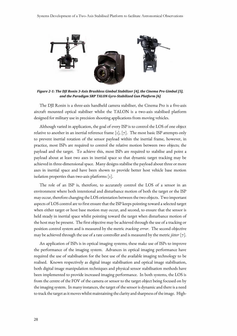
Figure 2-1: The DJI Ronin 3-Axis Brushless Gimbal Stabilizer [4], the Cinema Pro Gimbal [5],
and the Paradigm SRP TALON Gyro-Stabilized Gun Platform [6]
The DJI Ronin is a three-axis handheld camera stabiliser, the Cinema Pro is a five-axis
aircraft mounted optical stabiliser whilst the TALON is a two-axis stabilised platform
designed for military use in precision shooting applications from moving vehicles.
Although varied in application, the goal of every ISP is to control the LOS of one object
relative to another in an inertial reference frame [1], [7]. The most basic ISP attempts only
to prevent inertial rotation of the sensor payload within the inertial frame, however, in
practice, most ISPs are required to control the relative motion between two objects; the
payload and the target. To achieve this, most ISPs are required to stabilise and point a
payload about at least two axes in inertial space so that dynamic target tracking may be
achieved in three-dimensional space. Many designs stabilise the payload about three or more
axes in inertial space and have been shown to provide better host vehicle base motion
isolation properties than two-axis platforms [1].
The role of an ISP is, therefore, to accurately control the LOS of a sensor in an
environment where both intentional and disturbance motion of both the target or the ISP
may occur, therefore changing the LOS orientation between the two objects. Two important
aspects of LOS control are to first ensure that the ISP keeps pointing toward a selected target
when either target or host base motion may occur, and second, to ensure that the sensor is
held steady in inertial space whilst pointing toward the target when disturbance motion of
the host may be present. The first objective may be achieved through the use of a tracking or
position control system and is measured by the metric tracking error. The second objective
may be achieved through the use of a rate controller and is measured by the metric jitter [7].
An application of ISPs is in optical imaging systems; these make use of ISPs to improve
the performance of the imaging system. Advances in optical imaging performance have
required the use of stabilisation for the best use of the available imaging technology to be
realised. Known respectively as digital image stabilisation and optical image stabilisation,
both digital image manipulation techniques and physical sensor stabilisation methods have
been implemented to provide increased imaging performance. In both systems, the LOS is
from the centre of the FOV of the camera or sensor to the target object being focused on by
the imaging system. In many instances, the target of the sensor is dynamic and there is a need
to track the target as it moves whilst maintaining the clarity and sharpness of the image. High-
Chapter 2: Literature Study
29
performance examples of imaging systems can be expected to reduce jitter to less than 10 µrad
even in highly dynamic environments [7].
In conjunction with a target tracker, an ISP may be used to achieve the above challenge.
The target tracker is a general term used to describe any hardware or software system able to
achieve target detection and positioning within the sensor FOV. Regarding optical imaging,
two fundamental objectives for the ISP exist: First, to obtain high-quality images of the
target, and second, to determine the location of the target with respect to a defined reference
frame. The quality of the image may be affected by several factors which can be broadly
grouped into three categories; target motion, host vehicle motion and operating
environment.
A target with dynamic motion may easily move outside of the FOV whilst the host vehicle
motion may also cause a loss of tracking. Environmental factors such as atmospheric
conditions affecting the operating environment of the ISP may also cause challenges in target
tracking. An ISP must be robustly designed in conjunction with its target tracker such that
these influences do not affect the operation of the system beyond its prescribed limits during
operation.
2.3 ISP OPERATING PRINCIPLES
An ISP typically consists of three fundamental sub-systems: A sensor payload requiring
stabilisation, an electromechanical assembly which constrains the motion of the sensor
payload, and a control system used to drive the electromechanical assembly. These systems
are discussed in detail in the sections to follow.
2.3.1 SENSOR PAYLOAD
The sensor payload of an ISP is the dominant system that drives the overall size and
specifications of the ISP. A vast array of different systems may require stabilisation. Any
system which may experience a reduction in performance as a result of torque disturbances
may potentially be stabilised. The payload to be stabilised determines the type of electro-
mechanical assembly chosen.
2.3.2 ELECTRO-MECHANICAL ASSEMBLIES
ISP assemblies are complex electro-mechanical systems comprising of several different
mechanical parts and electrical subsystems. The class of stabilised platform in which a design
falls is determined by the configuration of the electromechanical assembly. The two main
categories under which ISP designs fall are known as mass stabilised (or platform stabilised)
and mirror stabilised (or steering stabilised) systems. These will be discussed in detail in the
sections to follow, however, there are several components common to both mass and mirror
stabilised systems which will first be discussed.
Systems Development of a Two-Axis Stabilised Platform to facilitate Astronomical Observations
30
ISP COMPONENTS
Gyroscopes (gyros) are inertial angular rate sensors which are used to measure the ISP
LOS rates. They are usually mounted directly on the sensor payload and so provide feedback
of the inertial rotational rate of the sensor payload [7]. The stability of a system is a measure
of its actual inertial rotational rate relative to the desired rotational rate and therefore these
sensors play a significant role in the development of an ISP. The error introduced to the
system by the gyro is directly coupled into the overall system and accordingly, they have been
shown to be the main overall performance limiting components in small-sized stabilised
platforms [1]. The appropriate selection of gyro for a system is then a critical design decision
in the development of an ISP. Section 2.6 is devoted to a more complete discussion of inertial
rate sensing and the technologies available for implementation on an ISP.
The friction and stiffness of the bearings and suspension system of an ISP’s electro-
mechanical assembly are two key factors associated with the implementation of a stabilised
platform. Friction introduces unwanted disturbances into the system which must be
overcome for successful stabilisation to be achieved, whilst a system with low stiff may suffer
a reduction in performance through a variety of resonance effects. Friction and stiffness do
however require a trade-off to be made in the design of the rotating joints and mounts of an
ISP: Stiffer mechanisms generally introduce more friction into the system yet are better in in
terms of the structural resonance properties of the mechanism [1]. Ball bearings are used to
suspend gimbals and rotating elements in most ISPs as they offer a good compromise
between structural stiffness and rotational friction. Other alternatives include gas-lubricated
bearings and magnetic suspension systems in applications where minimising friction is of
specific importance, however, these mechanisms offer lower stiffness than traditional
bearings.
Gimbal actuators of an ISP may take several forms. DC electric motors are the most
common actuators although hydraulic actuators are also sometimes used as they are able to
provide high torques at low speed when pole counts are high [1], [2]. Other types of actuators
sometimes used in ISP designs include hydraulic and pneumatic drive systems. Gimbal
actuators may either be coupled directly onto the gimbals as direct torquers or couple
through gear or belt drivetrains. Actuators should have fast response times and be able to
provide sufficient torque to overcome disturbances and achieve required tracking
specifications without excessive hysteresis, cogging, or backlash.
ISP rotational rate requirements seldom exceed speeds of 100 °/s, therefore, gearing can
be considered to reduce the mass and size of the actuators. However, when drivetrains are
used, reaction torques inside the gearboxes contribute to the total torque disturbances and
add friction, noise and torsional resonances [1]. Due to these effects, directly coupled
actuators are the preferred method of control in stabilisation systems.
The final set of components common to all ISPs to be discussed before describing the
main classes of ISPs are known as auxiliary equipment systems. This term groups the
supplementary components required to facilitate the operation of an ISP. Positioning the
target in an inertial frame requires a knowledge of where the ISP is pointing. This is achieved
Chapter 2: Literature Study
31
using relative motion sensors affixed to the gimbals which can provide position feedback to
the control and data-logging systems. Cable management systems also fall under this term.
MASS STABILISATION
Turning now to the main types of electro-mechanical configurations for stabilisation
systems, the first main class, mass stabilised systems, will now be discussed. This method
involves the stabilisation of the entire sensor payload through the rotation of a gimbal
assembly to control the sensor LOS. When the host vehicle rotates, the gimbals facilitate
sensor payload rotation in the opposite direction to the host vehicle motion in order to
maintain a steady LOS direction. Consequently, the motion of the gimbals directly controls
the LOS of the sensor. In a mass stabilised configuration, the number of orthogonal gimbals
required in the electro-mechanical assembly is equal to the number of axes in which inertial
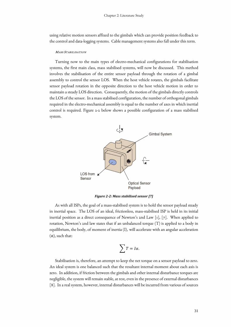
control is required. Figure 2-2 below shows a possible configuration of a mass stabilised
system.
Figure 2-2: Mass stabilised sensor [7]
As with all ISPs, the goal of a mass-stabilised system is to hold the sensor payload steady
in inertial space. The LOS of an ideal, frictionless, mass-stabilised ISP is held in its initial
inertial position as a direct consequence of Newton’s 2nd Law [1], [7]. When applied to
rotation, Newton’s 2nd law states that if an unbalanced torque (T) is applied to a body in
equilibrium, the body, of moment of inertia (I), will accelerate with an angular acceleration
(α), such that:
∑𝑇 = 𝐼𝛼.
Stabilisation is, therefore, an attempt to keep the net torque on a sensor payload to zero.
An ideal system is one balanced such that the resultant internal moment about each axis is
zero. In addition, if friction between the gimbals and other internal disturbance torques are
negligible, the system will remain stable, at rest, even in the presence of external disturbances
[8]. In a real system, however, internal disturbances will be incurred from various of sources
Systems Development of a Two-Axis Stabilised Platform to facilitate Astronomical Observations
32
including imbalance, assembly flexure, cable flexure, kinematic and geometric coupling, and
friction. Further discussion of disturbance sources is found in Section 2.4. The primary
challenge in the development of such a system is therefore to design a system which incurs
minimal disturbance effects onto the sensor [2], [7].
Kinematic disturbances are disturbances coupled into the ISP due to the dynamic
relationships between the assembly inertia characteristics and the angular motion of the
gimbal assembly, whilst geometric coupling disturbances are those induced on the system by
the geometry of the gimbal assembly; applying a rotation to one axis may cause unwanted
rotation about a second axis purely due to the geometry of the system [2]. Kinematic
disturbances in mass stabilised systems may be reduced significantly by suspending the
gimbals from their principal axes. This is an important insight to be made use of in the design
of an ISP. The process of determining the kinematic relationships between the gimbals is
detailed in Section 2.9.
Gimbals require actuation due to the fact that it is almost never sufficient to simply
stabilise the sensor; the LOS between a sensor and a target is required to be controlled which
requires the gimbals to be driven such that the sensor follows the target [1], [8]. Gimbals are
usually actuated using DC motors which have high torque and precision capabilities to move
the gimbal assembly accurately. As previously stated, motor drives may be mounted directly
onto the gimbal axes to control gimbal rotation, or they may make use of gear or belt linkages
with the motor often then being mounted on the base of the assembly. A further
disadvantage of geared or belt linked systems is that drivetrains inherently couple the base
motion of the host vehicle to the gimbal assembly and hence to the sensor payload. Due to
this, even an ideal, frictionless system must actively control the sensor LOS to account for the
rotation of the host vehicle [2], [7].
Directly coupled DC motors represent the closest approximation of an ideal direct
torquer, yet no type of electro-mechanical actuator is capable of achieving this due to viscous
damping within the system [2]; back EMF causes viscous damping in electric motors whilst
hydraulic drives are damped by flow feedback within their assemblies. These viscous
damping terms induce further torque disturbances on the ISP system which must be
accounted for. A common method for reducing these torques is to make use of current or
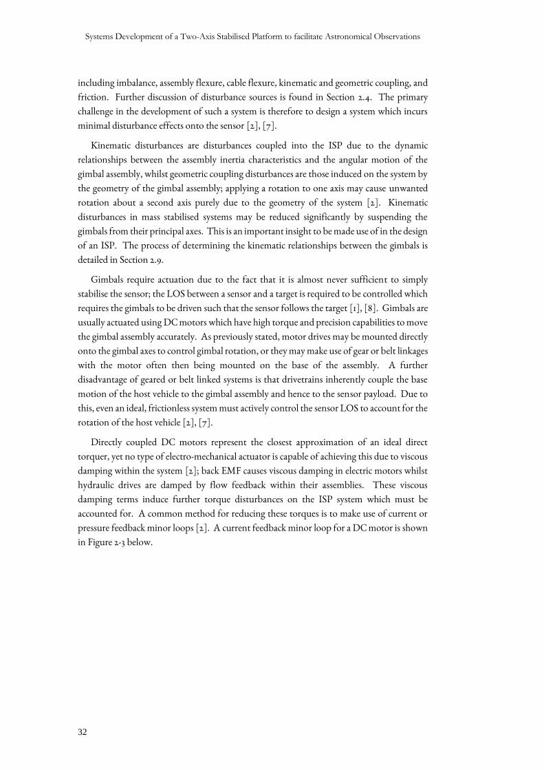
pressure feedback minor loops [2]. A current feedback minor loop for a DC motor is shown
in Figure 2-3 below.
Chapter 2: Literature Study
33
Figure 2-3: Current feedback minor loop
Figure 2-3 above shows a simplified block diagram model of a DC motor being controlled
by a command voltage Vc. Current feedback is facilitated by the scaling block Kv and the
minor loop controller gain Ki. These closed-loops have high gains and bandwidths and
therefore are effective at reducing the effects of viscous damping at low frequencies and hence
disturbance torques due to viscous damping are also reduced.
Overall, the LOS rates of a mass stabilised system are governed by the interaction of
gimbal assembly and sensor payload inertial rates and these are constrained by system
geometry [2]. These inertial rates are governed by the relationship between the inertial
characteristics of the gimbal assembly and the total resultant torque (including disturbance
and applied actuator torques) applied to each of the ISP axes.
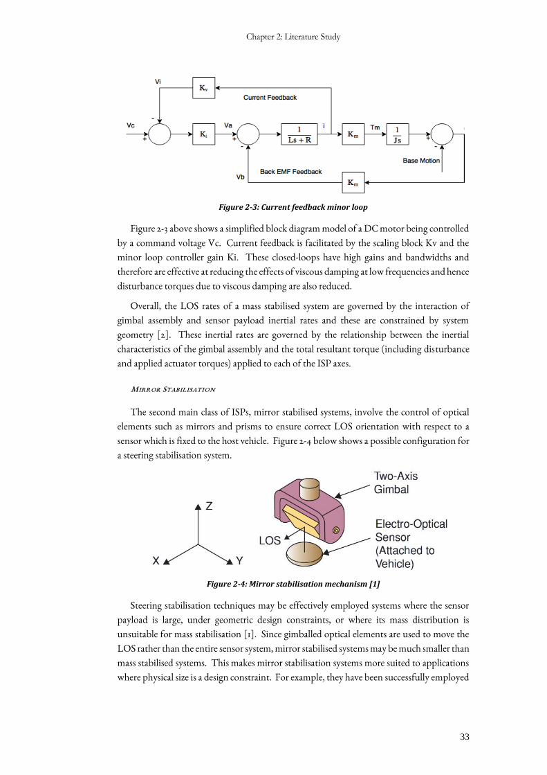
MIRROR STABILISATION
The second main class of ISPs, mirror stabilised systems, involve the control of optical
elements such as mirrors and prisms to ensure correct LOS orientation with respect to a
sensor which is fixed to the host vehicle. Figure 2-4 below shows a possible configuration for
a steering stabilisation system.
Figure 2-4: Mirror stabilisation mechanism [1]
Steering stabilisation techniques may be effectively employed systems where the sensor
payload is large, under geometric design constraints, or where its mass distribution is
unsuitable for mass stabilisation [1]. Since gimballed optical elements are used to move the
LOS rather than the entire sensor system, mirror stabilised systems may be much smaller than
mass stabilised systems. This makes mirror stabilisation systems more suited to applications
where physical size is a design constraint. For example, they have been successfully employed
Systems Development of a Two-Axis Stabilised Platform to facilitate Astronomical Observations
34
in applications where their small size aids the aerodynamic properties of a larger system, in
military application where a small target is advantageous, and where space is highly
constrained such as within handheld cameras [1], [7].
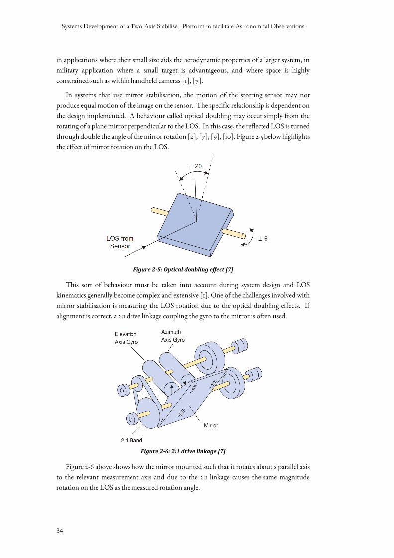
In systems that use mirror stabilisation, the motion of the steering sensor may not
produce equal motion of the image on the sensor. The specific relationship is dependent on
the design implemented. A behaviour called optical doubling may occur simply from the
rotating of a plane mirror perpendicular to the LOS. In this case, the reflected LOS is turned
through double the angle of the mirror rotation [2], [7], [9], [10]. Figure 2-5 below highlights
the effect of mirror rotation on the LOS.
Figure 2-5: Optical doubling effect [7]
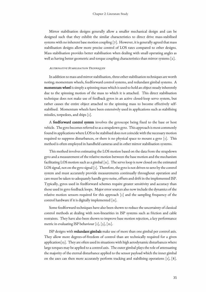
This sort of behaviour must be taken into account during system design and LOS
kinematics generally become complex and extensive [1]. One of the challenges involved with
mirror stabilisation is measuring the LOS rotation due to the optical doubling effects. If
alignment is correct, a 2:1 drive linkage coupling the gyro to the mirror is often used.
Figure 2-6: 2:1 drive linkage [7]
Figure 2-6 above shows how the mirror mounted such that it rotates about s parallel axis
to the relevant measurement axis and due to the 2:1 linkage causes the same magnitude
rotation on the LOS as the measured rotation angle.
Chapter 2: Literature Study
35
Mirror stabilisation designs generally allow a smaller mechanical design and can be
designed such that they exhibit the similar characteristics to direct drive mass-stabilised
systems with no inherent base motion coupling [7]. However, it is generally agreed that mass
stabilisation designs allow more precise control of LOS rates compared to other designs.
Mass stabilisation provides better stabilisation when dealing with small operating angles as
well as having better geometric and torque coupling characteristics than mirror systems [2].
ALTERNATIVE STABILISATION TECHNIQUES
In addition to mass and mirror stabilisation, three other stabilisation techniques are worth
noting; momentum wheels, feedforward control systems, and redundant gimbal systems. A
momentum wheel is simply a spinning mass which is used to hold an object steady inherently
due to the spinning motion of the mass to which it is attached. This direct stabilisation
technique does not make use of feedback gyros in an active closed-loop servo system, but
rather causes the entire object attached to the spinning mass to become effectively self-
stabilised. Momentum wheels have been extensively used in applications such as stabilising
missiles, torpedoes, and ships [1].
A feedforward control system involves the gyroscope being fixed to the base or host
vehicle. The gyro becomes referred to as a strapdown gyro. This approach is most commonly
found in applications where LOS to be stabilised does not coincide with the necessary motion
required to suppress disturbances, or there is no physical space to mount a gyro [1]. This
method is often employed in handheld cameras and in other mirror stabilisation systems.
This method involves estimating the LOS motion based on the data from the strapdown
gyro and a measurement of the relative motion between the base motion and the mechanism
facilitating LOS motion such as a gimbal [11]. The servo loop is now closed on the estimated
LOS signal, not on the gyro signal [1]. Therefore, the gyro is not driven to zero by the control
system and must accurately provide measurements continually throughout operation and
care must be taken to adequately handle gyro noise, offsets and drift in the implemented ISP.
Typically, gyros used in feedforward schemes require greater sensitivity and accuracy than
those used in gyro feedback loops. Major error sources also now include the dynamics of the
relative motion sensors required for this approach [1] and the sampling frequency of the
control hardware if it is digitally implemented [11].
Some feedforward techniques have also been shown to reduce the uncertainty of classical
control methods at dealing with non-linearities in ISP systems such as friction and cable
restraints. They have also been shown to improve base motion rejection, a key performance
metric in evaluating ISP behaviour [1], [3], [12].
ISP designs with redundant gimbals make use of more than one gimbal per control axis.
They allow more degrees-of-freedom of control than are technically required for a given
application[13]. They are often used in situations with high aerodynamic disturbances where
large torques may be applied to a control axis. The outer gimbal plays the role of attenuating
the majority of the eternal disturbance applied to the sensor payload which the inner gimbal
on the axes can then more accurately perform tracking and stabilising operations [1], [8].
Systems Development of a Two-Axis Stabilised Platform to facilitate Astronomical Observations
36
Redundant gimbals may also be used to prevent gimbal lock, a behaviour where a loss in a
degree-of-freedom of control of the gimbals is experienced in response to certain input
commands whilst the gimbals are in lock-specific orientations. The presence of a redundant
gimbal makes it possible to design systems always capable of maintaining tracking and
stabilisation capabilities through driving other gimbals such that they are kept away from
gimbal lock orientations [13].
2.3.3 CONTROL SYSTEMS
The third main subsystem of an ISP is the control system. Used here in a broad sense to
describe the control algorithms as well as the hardware and software through which they are
implemented and any user interface software facilitating supervisory control of the ISP.
The objective of the control system is to control the motion of the electro-mechanical
assembly such that the desired LOS rate is maintained whilst accounting for disturbances to
the ISP. This system has three primary aims:
i. To stabilise the LOS so that precise sensor data may be realised with low jitter,
ii. To maintain tracking of the target and,
iii. To measure the LOS orientation and so position the target in the inertial frame of
the ISP mechanism.
The stability and effectiveness of a control system is a function of the system dynamics of
each component comprising the total system. Therefore, to achieve the above objectives
according to the overall system specifications, the control system must be designed as part of
the total iterative design process. Classical control systems using Proportional-Integral (PI)
and Proportional-Integral-Derivative (PID) controllers are the most commonly
implemented type of controllers on ISPs ([1], [7], [14]–[17]) yet it has been demonstrated
that improved track command following and disturbance rejection is possible using a variety
of more complex control techniques. These are diverse and include fuzzy PID [18], adaptive
control, sliding mode control [19], feedforward compensation [1], 𝐻∞[8], internal model
control [16], [20], and variable feedback designs. Typical systems using classical controllers
are capable of disturbance attenuation ratios from the disturbance source to the output rate
of between -10 and -30 dB whilst advanced control methods have been shown to be capable
of improving this figure to approximately -40 dB at low frequencies up to 2 Hz [16], [20],
[21].
The main motivation for the implementation of each of these advanced control methods
has been to better deal with non-linearities in the ISP systems and to increase controller
robustness to parameter variation and uncertainty in the models. Sources of non-linearities
in ISPs include components that may saturate at their operational limits (such as actuator
amplifiers, actuators themselves, and inertial measurement sensors), structure compliance
and resonances, and disturbance torques from friction, cable restraint, and mass imbalance.
Classical control methods are theoretically only valid for linear systems and for non-linear
Chapter 2: Literature Study
37
systems at the point at which they are developed. Accordingly, they are generally sufficient
for systems with small variations from the operating point but become increasingly
inaccurate with distance from the operating point and with increasing frequency [17], [22].
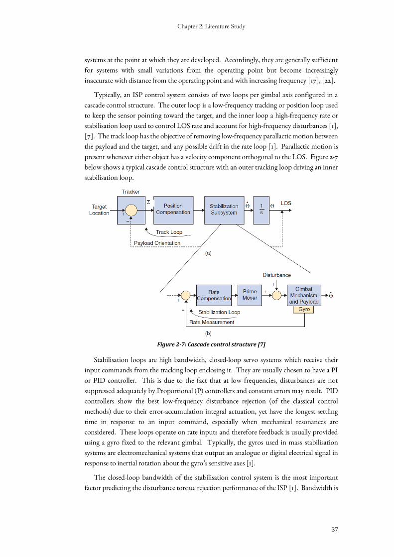
Typically, an ISP control system consists of two loops per gimbal axis configured in a
cascade control structure. The outer loop is a low-frequency tracking or position loop used
to keep the sensor pointing toward the target, and the inner loop a high-frequency rate or
stabilisation loop used to control LOS rate and account for high-frequency disturbances [1],
[7]. The track loop has the objective of removing low-frequency parallactic motion between
the payload and the target, and any possible drift in the rate loop [1]. Parallactic motion is
present whenever either object has a velocity component orthogonal to the LOS. Figure 2-7
below shows a typical cascade control structure with an outer tracking loop driving an inner
stabilisation loop.
Figure 2-7: Cascade control structure [7]
Stabilisation loops are high bandwidth, closed-loop servo systems which receive their
input commands from the tracking loop enclosing it. They are usually chosen to have a PI
or PID controller. This is due to the fact that at low frequencies, disturbances are not
suppressed adequately by Proportional (P) controllers and constant errors may result. PID
controllers show the best low-frequency disturbance rejection (of the classical control
methods) due to their error-accumulation integral actuation, yet have the longest settling
time in response to an input command, especially when mechanical resonances are
considered. These loops operate on rate inputs and therefore feedback is usually provided
using a gyro fixed to the relevant gimbal. Typically, the gyros used in mass stabilisation
systems are electromechanical systems that output an analogue or digital electrical signal in
response to inertial rotation about the gyro’s sensitive axes [1].
The closed-loop bandwidth of the stabilisation control system is the most important
factor predicting the disturbance torque rejection performance of the ISP [1]. Bandwidth is
Systems Development of a Two-Axis Stabilised Platform to facilitate Astronomical Observations
38
a measure of the control system’s ability to cause the feedback signal (or LOS output rate) to
follow the command input. It is fundamentally limited by the non-linearities caused by
components such as drive systems and sensors as well as structural compliance of the ISP.
Rate-command following error is attenuated at frequencies lower than the loop bandwidth
by a factor approximately proportional to the loop bandwidth. Also, torque disturbance
rejection ratio is roughly proportional to the squared inverse of the closed-loop bandwidth
for frequencies lower than the bandwidth frequency [1], [11].
Tracking loops are low bandwidth position loops that receive input commands from the
target tracker, therefore these components must be designed concurrently with each system
affecting the design of the other. As the target tracker is a sampled device operating at a fixed
rate, phase lag will be introduced into the control system which must be accounted for in the
design process.
2.4 SOURCES OF TORQUE DISTURBANCES
As previously stated, an ideal mass stabilised system is a design such that the LOS of the
sensor remains inertially stable in the presence of disturbances. However, in a practical
system, there are many sources of disturbance. If the disturbance torque can be nulled such
that the net applied torque is only that which is required to rotate the LOS in such a manner
as to track the target, the LOS of the sensor will be stabilised. Torque disturbance rejection
is, therefore, the most important performance metric for an ISP [7].
Some key sources of torque disturbance are discussed below [1], [2], [7]:
Torque disturbances that must be considered in ISP design include Coulomb friction
from surface interactions between parts of the electro-mechanical assembly. This type of
friction may be reduced through the careful design of the assembly and the use of bearings to
facilitate smooth inter-gimbal rotation. Spring torques may arise from flexure in the various
cables used to provide power to, and communication with the actuators and sensors.
Rotating imbalance from non-symmetric gimbal design will cause jitter in the LOS of the
sensor. Kinematic coupling from base motion which translates into gimbal rotations will also
cause undesired torque disturbances on the LOS.
It is the role of the control system to null these disturbances by applying the required
torque to the gimbals such that the resultant torque is that which facilitates target tracking.
This is accomplished by the actuators driving the different gimbals of the assembly, however,
due to the geometric and kinematic constraints of the assembly itself, inter-gimbal torque
coupling will inevitably occur to some extent: the product of inertia terms in one gimbal will
cause disturbances in another. This is detailed further in Section 2.9.
Misalignments between the LOS axis, gyroscope axis and the axis of applied torque also
cause disturbance torques in other axes and are the cause of unwanted LOS motion [1].
Further disturbance torques result from the structural dynamics of the assembly itself and
environmental disturbances [1], [2]. The structural dynamics of the system play a
Chapter 2: Literature Study
39
fundamental role in limiting the bandwidth and hence the performance of the control
system, therefore careful mechanical design is required to achieve high bandwidth
stabilisation capabilities through the reduction of the structural compliance of the electro-
mechanical assembly [1].
The impact of the structural dynamics on the performance of an ISP is further detailed
below. In order to accurately specify the torque requirements of the system, all the above
disturbances must be considered as well as external loading and noise [2].
2.5 ISP STRUCTURAL DYNAMICS
Structural resonances set up by the electromechanical assembly and the load are
fundamental to limiting the bandwidth of the ISP [1], [2], [7]. All the components of an ISP
influence the structural dynamics of the system. Their properties interact in multiple ways
producing an almost unlimited number of modes of response due to their many different
mass distributions, material properties, damping properties, geometric configurations that
change with time, and variations in forcing functions.
The structural modes of the assembly respond to all frequencies of the forcing function
whether it results from an external disturbance, actuator motion or other cause. However,
at the resonant frequencies of the components, the effects of these forcing functions are
significant. The amplitude and frequency of the forcing function and the damping
properties of the structure affect the amplitude of the frequency response. The amplitude of
the response of metallic structures with low damping and high stiffness may be 15 to 25 times
greater than the amplitude of the forcing function at the resonant frequencies [1]. The
asymmetric geometries of many parts in the gimbal structure also mean that multiple modes
of different types (bending and torsional etc.) may be excited simultaneously, further
aggravating resonance effects. Kinematic and geometric coupling may also introduce cross
axis modes that further aggravate issues [2].
The analysis of gimbal designs may be performed using finite element methods (FEM) or
physical vibration testing to determine the transfer functions and responses between
different points in the structure in response to different forcing functions. Important aspects
of these analyses are that the forcing functions used correspond well to forcing functions
found in the expected operating environment of the ISP and that tests are done that analyse
the response in the three-dimensional operating environment expected. The results of these
analyses may be used to inform controller designs and dramatically improve the dynamic
stabilisation properties of ISPs [23].
According to Hilkert [1], structural dynamics of ISP systems affect the performance
through three primary interactions. These are detailed in Sections 2.5.1 to 2.5.3 below.
Systems Development of a Two-Axis Stabilised Platform to facilitate Astronomical Observations
40
2.5.1 PART BENDING
Bending modes set up in the components by base motion vibrations and actuator torques
cause LOS displacement. This displacement is generally not sensed by feedback gyros
measuring the LOS rates due to the high-frequency nature of these disturbances and
therefore the stabilisation control system is not effective at removing these effects. These
effects may also be amplified by some sensor payloads themselves such as optical imaging
systems with high magnification or systems which employ optical elements such as mirrors.
Increasing the stiffness of the mechanism is the first step in reducing the effects of part
bending, especially where actuator torques are the cause of bending modes being excited.
When base motion is the primary cause, vibration isolation systems may be used to attenuate
vibrations.
2.5.2 TORSIONAL RESPONSES
Independently of the operating environment, the assembly structure may interact with
the control system causing torsional modes between the actuators and gyro to be excited.
These are critical interactions that limit the bandwidth of the control system and hence
directly affect the performance of the ISP. These interactions affect the transfer function
between the actuator and the feedback gyro [2]. This often results in additional actuator
travel capabilities being required.
Again, stiffening the structure is the first method of reducing these effects. However, it
has been noted that current (or pressure) feedback minor loops tend to minimise this effect
[2]. As these types of loops reduce the effects of disturbances originating internally with the
plant model, they are effective at stabilising the system against torsional responses arising
between the actuator and feedback sensor. In addition, filters such as notch filters may be
used to reduce the controller gain near resonance frequencies.
2.5.3 GIMBAL MOUNTING STRUCTURE COMPLIANCE
Compliance in the ISP mounting structure between the gimbal assembly and the host
vehicle may also affect the structural dynamics of the system. The effects of these dynamics
are seen in both the stabilisation [2] and tracking loops but are most notable in the
positioning system or tracking loops if relative motion sensors are used to provide feedback
signals to these systems.
Actuator torques driving the gimbals react against the support structure and cause
deflections that are measured by the relative motion sensors causing errors to propagate into
the positioning or tracking systems. In addition, this motion may couple further motion into
the gimbal system through the geometric constraints of the design. This problem is more
pronounced in systems that use passive damping systems as vibration isolators to assist with
part bending interactions. This makes the structural design of the ISP more complex as trade-
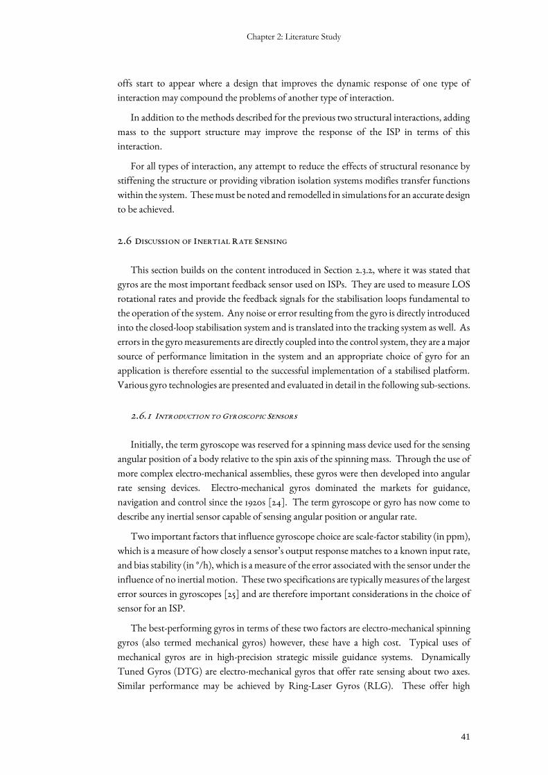
Chapter 2: Literature Study
41
offs start to appear where a design that improves the dynamic response of one type of
interaction may compound the problems of another type of interaction.
In addition to the methods described for the previous two structural interactions, adding
mass to the support structure may improve the response of the ISP in terms of this
interaction.
For all types of interaction, any attempt to reduce the effects of structural resonance by
stiffening the structure or providing vibration isolation systems modifies transfer functions
within the system. These must be noted and remodelled in simulations for an accurate design
to be achieved.
2.6 DISCUSSION OF INERTIAL RATE SENSING
This section builds on the content introduced in Section 2.3.2, where it was stated that
gyros are the most important feedback sensor used on ISPs. They are used to measure LOS
rotational rates and provide the feedback signals for the stabilisation loops fundamental to
the operation of the system. Any noise or error resulting from the gyro is directly introduced
into the closed-loop stabilisation system and is translated into the tracking system as well. As
errors in the gyro measurements are directly coupled into the control system, they are a major
source of performance limitation in the system and an appropriate choice of gyro for an
application is therefore essential to the successful implementation of a stabilised platform.
Various gyro technologies are presented and evaluated in detail in the following sub-sections.
2.6.1 INTRODUCTION TO GYROSCOPIC SENSORS
Initially, the term gyroscope was reserved for a spinning mass device used for the sensing
angular position of a body relative to the spin axis of the spinning mass. Through the use of
more complex electro-mechanical assemblies, these gyros were then developed into angular
rate sensing devices. Electro-mechanical gyros dominated the markets for guidance,
navigation and control since the 1920s [24]. The term gyroscope or gyro has now come to
describe any inertial sensor capable of sensing angular position or angular rate.
Two important factors that influence gyroscope choice are scale-factor stability (in ppm),
which is a measure of how closely a sensor’s output response matches to a known input rate,
and bias stability (in °/h), which is a measure of the error associated with the sensor under the
influence of no inertial motion. These two specifications are typically measures of the largest
error sources in gyroscopes [25] and are therefore important considerations in the choice of
sensor for an ISP.
The best-performing gyros in terms of these two factors are electro-mechanical spinning
gyros (also termed mechanical gyros) however, these have a high cost. Typical uses of
mechanical gyros are in high-precision strategic missile guidance systems. Dynamically
Tuned Gyros (DTG) are electro-mechanical gyros that offer rate sensing about two axes.
Similar performance may be achieved by Ring-Laser Gyros (RLG). These offer high
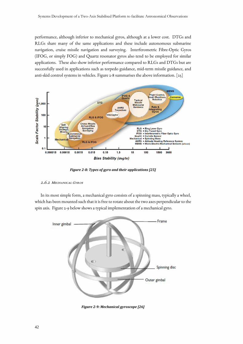
Systems Development of a Two-Axis Stabilised Platform to facilitate Astronomical Observations
42
performance, although inferior to mechanical gyros, although at a lower cost. DTGs and
RLGs share many of the same applications and these include autonomous submarine
navigation, cruise missile navigation and surveying. Interferometric Fibre-Optic Gyros
(IFOG, or simply FOG) and Quartz resonator gyros also tend to be employed for similar
applications. These also show inferior performance compared to RLGs and DTGs but are
successfully used in applications such as torpedo guidance, mid-term missile guidance, and
anti-skid control systems in vehicles. Figure 2-8 summarises the above information. [25]
Figure 2-8: Types of gyro and their applications [25]
2.6.2 MECHANICAL GYROS
In its most simple form, a mechanical gyro consists of a spinning mass, typically a wheel,
which has been mounted such that it is free to rotate about the two axes perpendicular to the
spin axis. Figure 2-9 below shows a typical implementation of a mechanical gyro.
Figure 2-9: Mechanical gyroscope [26]
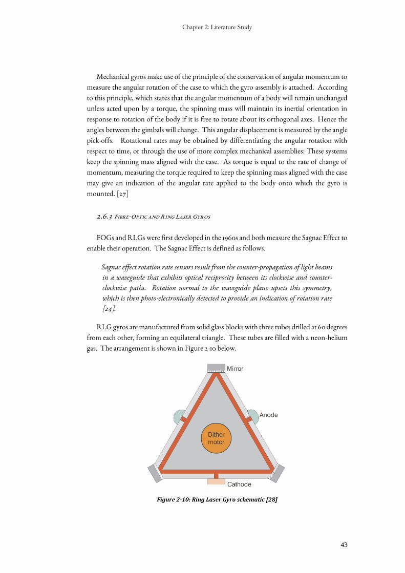
Chapter 2: Literature Study
43
Mechanical gyros make use of the principle of the conservation of angular momentum to
measure the angular rotation of the case to which the gyro assembly is attached. According
to this principle, which states that the angular momentum of a body will remain unchanged
unless acted upon by a torque, the spinning mass will maintain its inertial orientation in
response to rotation of the body if it is free to rotate about its orthogonal axes. Hence the
angles between the gimbals will change. This angular displacement is measured by the angle
pick-offs. Rotational rates may be obtained by differentiating the angular rotation with
respect to time, or through the use of more complex mechanical assemblies: These systems
keep the spinning mass aligned with the case. As torque is equal to the rate of change of
momentum, measuring the torque required to keep the spinning mass aligned with the case
may give an indication of the angular rate applied to the body onto which the gyro is
mounted. [27]
2.6.3 FIBRE-OPTIC AND RING LASER GYROS
FOGs and RLGs were first developed in the 1960s and both measure the Sagnac Effect to
enable their operation. The Sagnac Effect is defined as follows.
Sagnac effect rotation rate sensors result from the counter-propagation of light beams
in a waveguide that exhibits optical reciprocity between its clockwise and counter-
clockwise paths. Rotation normal to the waveguide plane upsets this symmetry,
which is then photo-electronically detected to provide an indication of rotation rate
[24].
RLG gyros are manufactured from solid glass blocks with three tubes drilled at 60 degrees
from each other, forming an equilateral triangle. These tubes are filled with a neon-helium
gas. The arrangement is shown in Figure 2-10 below.
Figure 2-10: Ring Laser Gyro schematic [28]
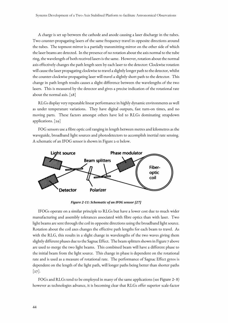
Systems Development of a Two-Axis Stabilised Platform to facilitate Astronomical Observations
44
A charge is set up between the cathode and anode causing a laser discharge in the tubes.
Two counter-propagating lasers of the same frequency travel in opposite directions around
the tubes. The topmost mirror is a partially transmitting mirror on the other side of which
the laser beams are detected. In the presence of no rotation about the axis normal to the tube
ring, the wavelength of both received lasers is the same. However, rotation about the normal
axis effectively changes the path length seen by each laser to the detector: Clockwise rotation
will cause the laser propagating clockwise to travel a slightly longer path to the detector, whilst
the counter-clockwise propagating laser will travel a slightly short path to the detector. This
change in path length results causes a slight difference between the wavelengths of the two
lasers. This is measured by the detector and gives a precise indication of the rotational rate
about the normal axis. [28]
RLGs display very repeatable linear performance in highly dynamic environments as well
as under temperature variations. They have digital outputs, fast turn-on times, and no
moving parts. These factors amongst others have led to RLGs dominating strapdown
applications. [29]
FOG sensors use a fibre optic coil ranging in length between metres and kilometres as the
waveguide, broadband light sources and photodetectors to accomplish inertial rate sensing.
A schematic of an IFOG sensor is shown in Figure 2-11 below.
Figure 2-11: Schematic of an IFOG sensor [27]
IFOGs operate on a similar principle to RLGs but have a lower cost due to much wider
manufacturing and assembly tolerances associated with fibre optics than with laser. Two
light beams are sent through the coil in opposite directions using the broadband light source.
Rotation about the coil axes changes the effective path lengths for each beam to travel. As
with the RLG, this results in a slight change in wavelengths of the two waves giving them
slightly different phases due to the Sagnac Effect. The beam splitters shown in Figure 7 above
are used to merge the two light beams. This combined beam will have a different phase to
the initial beam from the light source. This change in phase is dependent on the rotational
rate and is used as a measure of rotational rate. The performance of Sagnac Effect gyros is
dependent on the length of the light path, will longer paths being better than shorter paths
[27].
FOGs and RLGs tend to be employed in many of the same applications (see Figure 2- 8)
however as technologies advance, it is becoming clear that RLGs offer superior scale-factor
Chapter 2: Literature Study
45
stability to FOGs and therefore in applications requiring high scale factor stability, RLGs
dominate applications [25]. However, apart from these environments, FOG sensors have
become a suitable lower cost alternative to RLGs [28], [29]. In addition to lower cost, FOG
sensors have the advantage of not requiring high voltages and of being lighter in weight than
RLG sensors.
2.6.4 MEMS GYROS
Micro Electro-Mechanical System Gyros (MEMS) are a recent development in gyro
technology. These devices are designed as electronically driven resonators. They take
advantage of the Coriolis Effect to measure inertial rotation. The simplest designs are single
masses electronically vibrated along an axis. According to the Coriolis Effect, a mass (m)
moving with a linear velocity (v) experiences a force (F) in response to its reference frame
rotating at an angular velocity (ω) such that [30]:
𝐹 = −2𝑚(𝜔 × 𝑣) .
This force is orthogonal to the direction of v and ω and causes a displacement along this
orthogonal axis which may be measured capacitively or piezoelectrically. Some MEMS gyros
are designed to have a resonating tuning fork within the package. When inertial rotation is
applied about the fork’s axis, Coriolis forces are applied to the fork causing torsion about the
sensitive axis [24]. This torsion, therefore, causes the displacement to be measured which can
then be transformed into an indication of rotational rate.
These types of gyro are very low power consumption devices and may be implemented at
a fraction of the cost of other types. Their low part count compared to optical and
mechanical gyros help to reduce their cost as far few high precision parts require
manufacturing per gyro. Manufactured from silicon or quartz, MEMS gyros have great
durability and strength [29] and are small in size and weight. Their durability, therefore,
makes them ideal for implementation in applications where high acceleration is expected or
a hostile environment is present. A further advantage of these sensors is the fact that gyros
can be manufactured such that three sensitive axes may be contained within a single package.
Due to their superior size, weight and cost, MEMS sensors are expected to replace RLG and
FOG gyros in many applications in the future. These factors have made them suitable for
applications where size is a primary concern such as smartphones or hand-held cameras.
Figure 2-12 below shows the type of applications where MEMS gyros find their use.
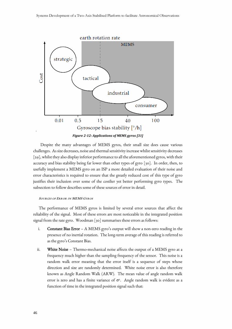
Systems Development of a Two-Axis Stabilised Platform to facilitate Astronomical Observations
46
.
Figure 2-12: Applications of MEMS gyros [31]
Despite the many advantages of MEMS gyros, their small size does cause various
challenges. As size decreases, noise and thermal sensitivity increase whilst sensitivity decreases
[29], whilst they also display inferior performance to all the aforementioned gyros, with their
accuracy and bias stability being far lower than other types of gyro [30]. In order, then, to
usefully implement a MEMS gyro on an ISP a more detailed evaluation of their noise and
error characteristics is required to ensure that the greatly reduced cost of this type of gyro
justifies their inclusion over some of the costlier yet better performing gyro types. The
subsection to follow describes some of these sources of error in detail.
SOURCES OF ERROR IN MEMS GYROS
The performance of MEMS gyros is limited by several error sources that affect the
reliability of the signal. Most of these errors are most noticeable in the integrated position
signal from the rate gyro. Woodman [30] summarises these errors as follows:
i. Constant Bias Error – A MEMS gyro’s output will show a non-zero reading in the
presence of no inertial rotation. The long-term average of this reading is referred to
as the gyro’s Constant Bias.
ii. White Noise – Thermo-mechanical noise affects the output of a MEMS gyro at a
frequency much higher than the sampling frequency of the sensor. This noise is a
random walk error meaning that the error itself is a sequence of steps whose
direction and size are randomly determined. White noise error is also therefore
known as Angle Random Walk (ARW). The mean value of angle random walk
error is zero and has a finite variance of σ2. Angle random walk is evident as a
function of time in the integrated position signal such that:
Chapter 2: Literature Study
47
𝜎𝜃(𝑡) = 𝜎√𝛿𝑡 ∙ 𝑡
It can be seen that the standard deviation of error position signals grows with the
square root of time, where δt is the time between successive sensor samples. This
noise (measured in ° √ℎ𝑟⁄ ) is specified at t = 1, therefore:
𝐴𝑅𝑊 = 𝜎 𝜃(1)
iii. Bias Stability (BS) – The bias of a MEMS device changes with time due to flicker
noise in the electronics. Bias stability is a measure of this phenomenon over a
specified period of time. It has units of °/h. The change in output due to this error
also follows a random walk process within limits (the error associated with the
integrated signal does not grow to infinity), therefore Bias Random Walk (BRW)
can be defined as follows:
𝐵𝑅𝑊 =𝐵𝑆
√𝑡
BRW has the same units as ARW, and t is the period over which BS is specified.
iv. Temperature – associated errors are caused by environment changes and affect the
constant bias of the device.
v. Calibration Errors – errors associated with scale factors, misalignments, and non-
linearities in MEMS sensors. They cause bias errors that are seen when the device is
rotating causing additional drift in the integrated position signal.
According to Woodman [30], the dominant sources of error in the output of a MEMS
gyro are white noise and unaccounted bias errors. For a specific gyro, the noise characteristics
can be determined through a process called the Allan Variance (AV) technique. Initially used
to study the frequency stability of oscillators, it has been applied to inertial sensors to study
the drift properties associated with their measurements [32]. Different variations of the Allan
Variance may be employed depending on the type of analysis being performed and the
expected noise profiles. Of these, the most suited to a general purpose analysis is the
Overlapping Allan Variance [33].
Overlapping Allan Variance is a time-based averaging function which can be computed
using the output angles of the gyroscope data in the following manner [30], [32], [34], [35]:
i. For a set of N discrete sampled gyro output rates, sampled every sample period τ0,
the output angle 𝜃 is calculated from:
𝜃(𝑡) = ∫Ω(𝑡′)𝑑𝑡′
For a discrete set of data where samples are taken at times 𝑡 = 𝑘𝜏0, where k varies
from 1 to N, the cumulative sum of the gyro rate output multiplied by the sample
period τ0 gives the angle output at each 𝑘𝜏0.
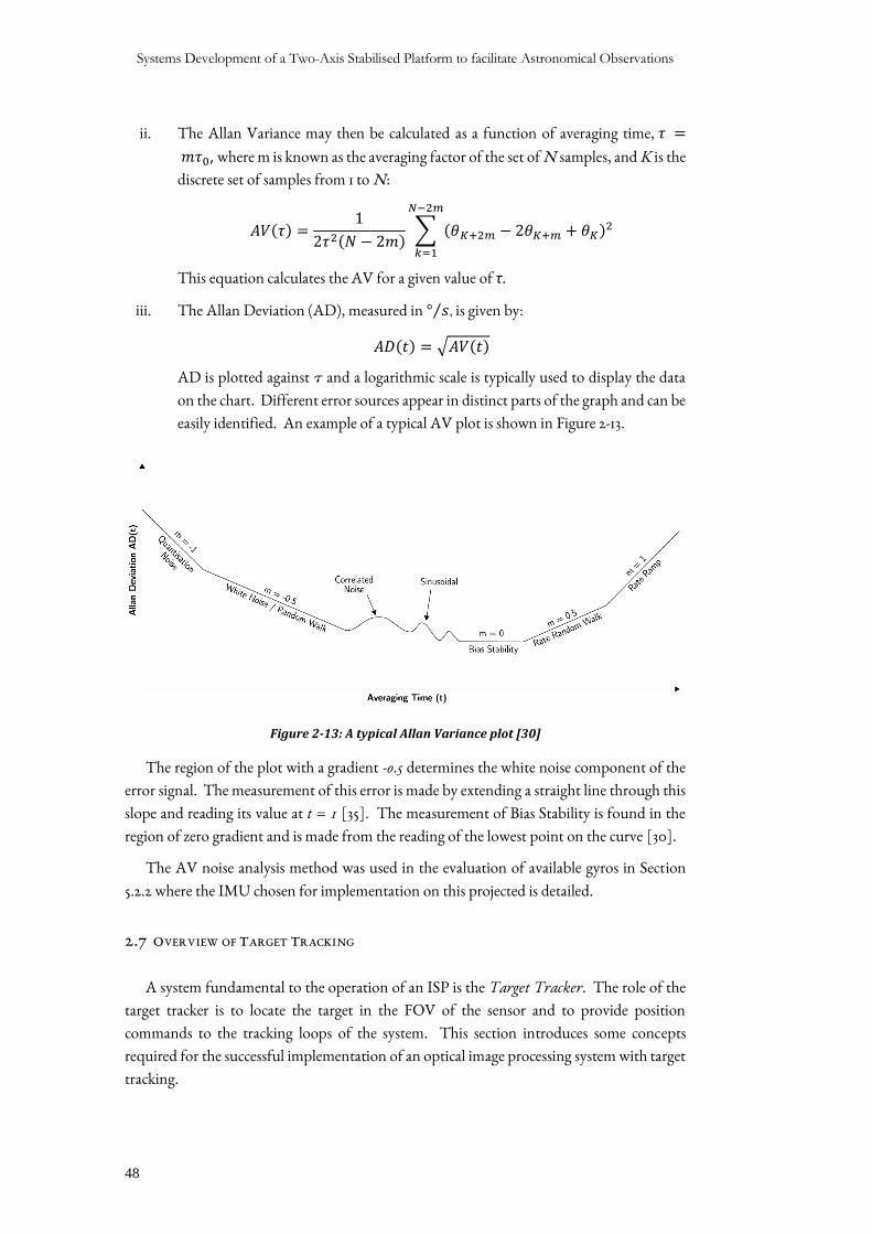
Systems Development of a Two-Axis Stabilised Platform to facilitate Astronomical Observations
48
ii. The Allan Variance may then be calculated as a function of averaging time, 𝜏 =
𝑚𝜏0, where m is known as the averaging factor of the set of N samples, and K is the
discrete set of samples from 1 to N:
𝐴𝑉(𝜏) =1
2𝜏2(𝑁 − 2𝑚)∑ (𝜃𝐾+2𝑚 − 2𝜃𝐾+𝑚 + 𝜃𝐾)2
𝑁−2𝑚
𝑘=1
This equation calculates the AV for a given value of τ.
iii. The Allan Deviation (AD), measured in ° 𝑠⁄ , is given by:
𝐴𝐷(𝑡) = √𝐴𝑉(𝑡)
AD is plotted against τ and a logarithmic scale is typically used to display the data
on the chart. Different error sources appear in distinct parts of the graph and can be
easily identified. An example of a typical AV plot is shown in Figure 2-13.
Figure 2-13: A typical Allan Variance plot [30]
The region of the plot with a gradient -0.5 determines the white noise component of the
error signal. The measurement of this error is made by extending a straight line through this
slope and reading its value at t = 1 [35]. The measurement of Bias Stability is found in the
region of zero gradient and is made from the reading of the lowest point on the curve [30].
The AV noise analysis method was used in the evaluation of available gyros in Section
5.2.2 where the IMU chosen for implementation on this projected is detailed.
2.7 OVERVIEW OF TARGET TRACKING
A system fundamental to the operation of an ISP is the Target Tracker. The role of the
target tracker is to locate the target in the FOV of the sensor and to provide position
commands to the tracking loops of the system. This section introduces some concepts
required for the successful implementation of an optical image processing system with target
tracking.
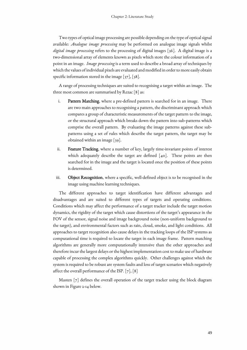
Chapter 2: Literature Study
49
Two types of optical image processing are possible depending on the type of optical signal
available: Analogue image processing may be performed on analogue image signals whilst
digital image processing refers to the processing of digital images [36]. A digital image is a
two-dimensional array of elements known as pixels which store the colour information of a
point in an image. Image processing is a term used to describe a broad array of techniques by
which the values of individual pixels are evaluated and modified in order to more easily obtain
specific information stored in the image [37], [38].
A range of processing techniques are suited to recognising a target within an image. The
three most common are summarised by Rezac [8] as:
i. Pattern Matching, where a pre-defined pattern is searched for in an image. There
are two main approaches to recognising a pattern, the discriminant approach which
compares a group of characteristic measurements of the target pattern to the image,
or the structural approach which breaks down the pattern into sub-patterns which
comprise the overall pattern. By evaluating the image patterns against these sub-
patterns using a set of rules which describe the target pattern, the target may be
obtained within an image [39].
ii. Feature Tracking, where a number of key, largely time-invariant points of interest
which adequately describe the target are defined [40]. These points are then
searched for in the image and the target is located once the position of these points
is determined.
iii. Object Recognition, where a specific, well-defined object is to be recognised in the
image using machine learning techniques.
The different approaches to target identification have different advantages and
disadvantages and are suited to different types of targets and operating conditions.
Conditions which may affect the performance of a target tracker include the target motion
dynamics, the rigidity of the target which cause distortions of the target’s appearance in the
FOV of the sensor, signal noise and image background noise (non-uniform background to
the target), and environmental factors such as rain, cloud, smoke, and light conditions. All
approaches to target recognition also cause delays in the tracking loops of the ISP systems as
computational time is required to locate the target in each image frame. Pattern matching
algorithms are generally more computationally intensive than the other approaches and
therefore incur the largest delays or the highest implementation cost to make use of hardware
capable of processing the complex algorithms quickly. Other challenges against which the
system is required to be robust are system faults and loss of target scenarios which negatively
affect the overall performance of the ISP. [7], [8]
Masten [7] defines the overall operation of the target tracker using the block diagram
shown in Figure 2-14 below.
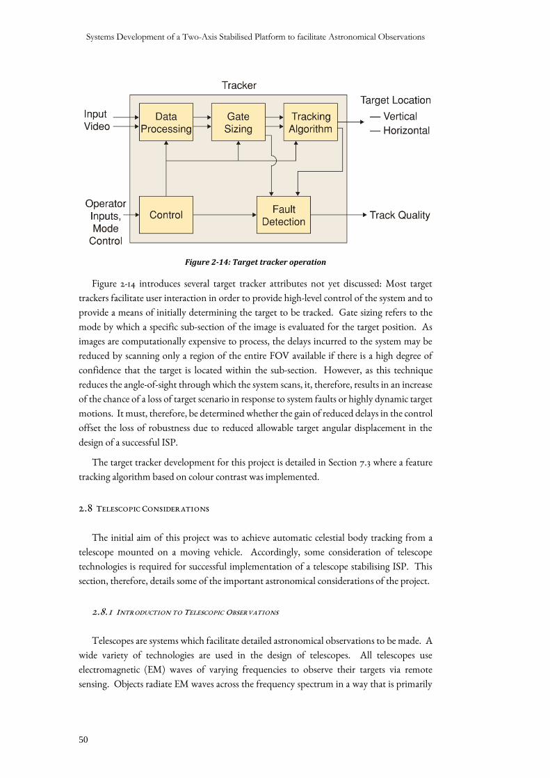
Systems Development of a Two-Axis Stabilised Platform to facilitate Astronomical Observations
50
Figure 2-14: Target tracker operation
Figure 2-14 introduces several target tracker attributes not yet discussed: Most target
trackers facilitate user interaction in order to provide high-level control of the system and to
provide a means of initially determining the target to be tracked. Gate sizing refers to the
mode by which a specific sub-section of the image is evaluated for the target position. As
images are computationally expensive to process, the delays incurred to the system may be
reduced by scanning only a region of the entire FOV available if there is a high degree of
confidence that the target is located within the sub-section. However, as this technique
reduces the angle-of-sight through which the system scans, it, therefore, results in an increase
of the chance of a loss of target scenario in response to system faults or highly dynamic target
motions. It must, therefore, be determined whether the gain of reduced delays in the control
offset the loss of robustness due to reduced allowable target angular displacement in the
design of a successful ISP.
The target tracker development for this project is detailed in Section 7.3 where a feature
tracking algorithm based on colour contrast was implemented.
2.8 TELESCOPIC CONSIDERATIONS
The initial aim of this project was to achieve automatic celestial body tracking from a
telescope mounted on a moving vehicle. Accordingly, some consideration of telescope
technologies is required for successful implementation of a telescope stabilising ISP. This
section, therefore, details some of the important astronomical considerations of the project.
2.8.1 INTRODUCTION TO TELESCOPIC OBSERVATIONS
Telescopes are systems which facilitate detailed astronomical observations to be made. A
wide variety of technologies are used in the design of telescopes. All telescopes use
electromagnetic (EM) waves of varying frequencies to observe their targets via remote
sensing. Objects radiate EM waves across the frequency spectrum in a way that is primarily
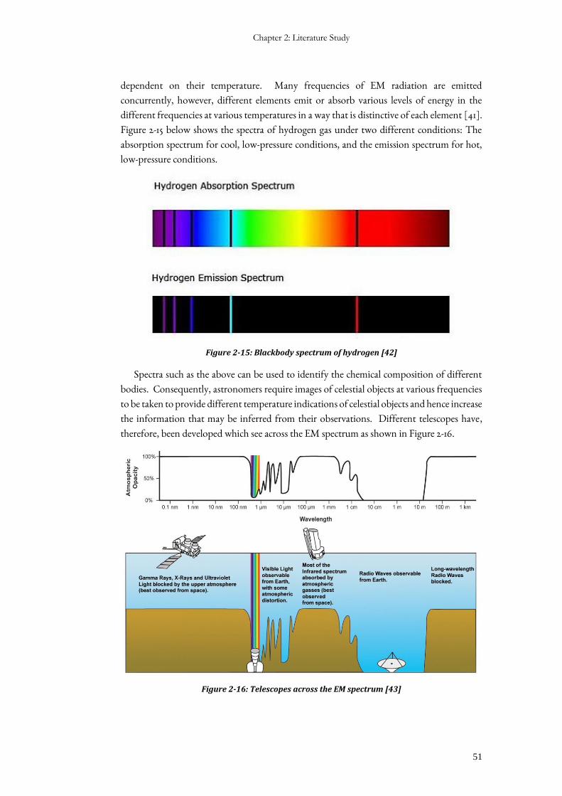
Chapter 2: Literature Study
51
dependent on their temperature. Many frequencies of EM radiation are emitted
concurrently, however, different elements emit or absorb various levels of energy in the
different frequencies at various temperatures in a way that is distinctive of each element [41].
Figure 2-15 below shows the spectra of hydrogen gas under two different conditions: The
absorption spectrum for cool, low-pressure conditions, and the emission spectrum for hot,
low-pressure conditions.
Figure 2-15: Blackbody spectrum of hydrogen [42]
Spectra such as the above can be used to identify the chemical composition of different
bodies. Consequently, astronomers require images of celestial objects at various frequencies
to be taken to provide different temperature indications of celestial objects and hence increase
the information that may be inferred from their observations. Different telescopes have,
therefore, been developed which see across the EM spectrum as shown in Figure 2-16.
Figure 2-16: Telescopes across the EM spectrum [43]
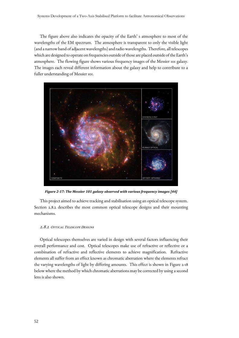
Systems Development of a Two-Axis Stabilised Platform to facilitate Astronomical Observations
52
The figure above also indicates the opacity of the Earth’ s atmosphere to most of the
wavelengths of the EM spectrum. The atmosphere is transparent to only the visible light
(and a narrow band of adjacent wavelengths) and radio wavelengths. Therefore, all telescopes
which are designed to operate on frequencies outside of those are placed outside of the Earth’s
atmosphere. The flowing figure shows various frequency images of the Messier 101 galaxy.
The images each reveal different information about the galaxy and help to contribute to a
fuller understanding of Messier 101.
Figure 2-17: The Messier 101 galaxy observed with various frequency images [44]
This project aimed to achieve tracking and stabilisation using an optical telescope system.
Section 2.8.2 describes the most common optical telescope designs and their mounting
mechanisms.
2.8.2 OPTICAL TELESCOPE DESIGNS
Optical telescopes themselves are varied in design with several factors influencing their
overall performance and cost. Optical telescopes make use of refractive or reflective or a
combination of refractive and reflective elements to achieve magnification. Refractive
elements all suffer from an effect known as chromatic aberration where the elements refract
the varying wavelengths of light by differing amounts. This effect is shown in Figure 2-18
below where the method by which chromatic aberrations may be corrected by using a second
lens is also shown.
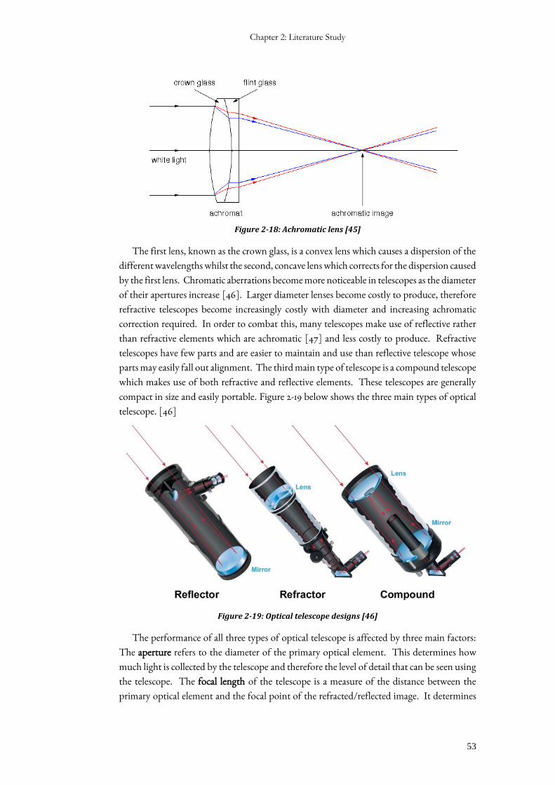
Chapter 2: Literature Study
53
Figure 2-18: Achromatic lens [45]
The first lens, known as the crown glass, is a convex lens which causes a dispersion of the
different wavelengths whilst the second, concave lens which corrects for the dispersion caused
by the first lens. Chromatic aberrations become more noticeable in telescopes as the diameter
of their apertures increase [46]. Larger diameter lenses become costly to produce, therefore
refractive telescopes become increasingly costly with diameter and increasing achromatic
correction required. In order to combat this, many telescopes make use of reflective rather
than refractive elements which are achromatic [47] and less costly to produce. Refractive
telescopes have few parts and are easier to maintain and use than reflective telescope whose
parts may easily fall out alignment. The third main type of telescope is a compound telescope
which makes use of both refractive and reflective elements. These telescopes are generally
compact in size and easily portable. Figure 2-19 below shows the three main types of optical
telescope. [46]
Figure 2-19: Optical telescope designs [46]
The performance of all three types of optical telescope is affected by three main factors:
The aperture refers to the diameter of the primary optical element. This determines how
much light is collected by the telescope and therefore the level of detail that can be seen using
the telescope. The focal length of the telescope is a measure of the distance between the
primary optical element and the focal point of the refracted/reflected image. It determines
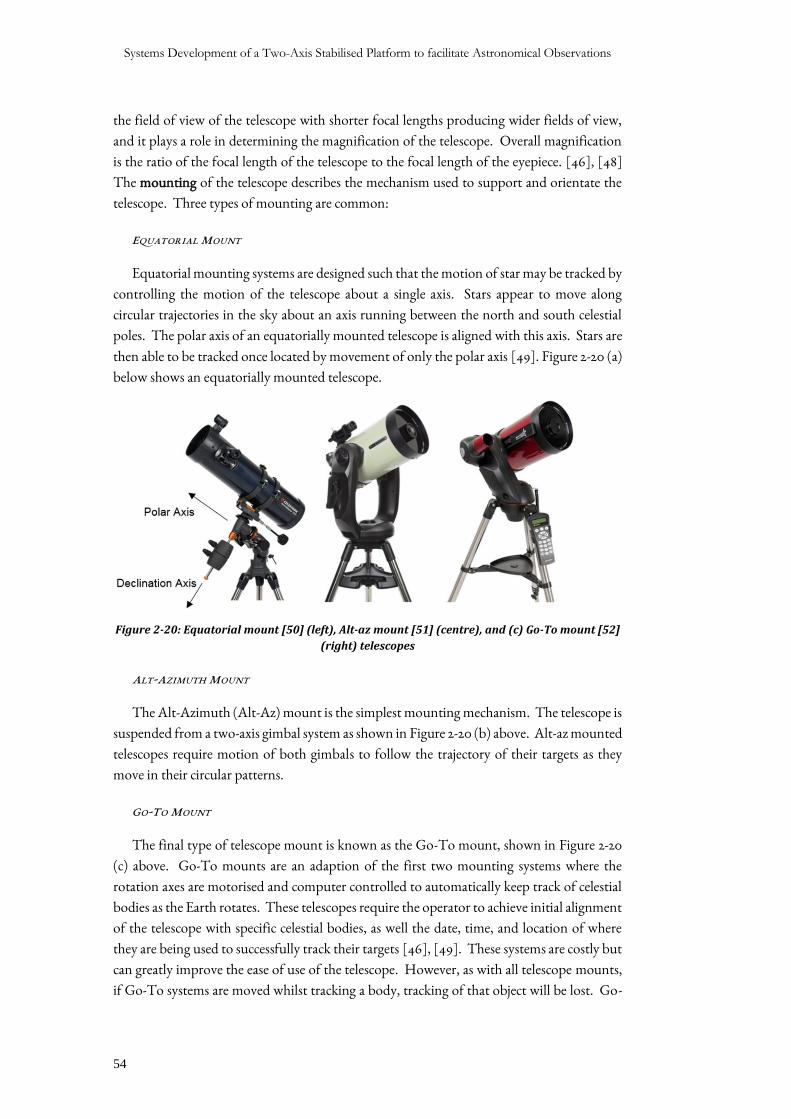
Systems Development of a Two-Axis Stabilised Platform to facilitate Astronomical Observations
54
the field of view of the telescope with shorter focal lengths producing wider fields of view,
and it plays a role in determining the magnification of the telescope. Overall magnification
is the ratio of the focal length of the telescope to the focal length of the eyepiece. [46], [48]
The mounting of the telescope describes the mechanism used to support and orientate the
telescope. Three types of mounting are common:
EQUATORIAL MOUNT
Equatorial mounting systems are designed such that the motion of star may be tracked by
controlling the motion of the telescope about a single axis. Stars appear to move along
circular trajectories in the sky about an axis running between the north and south celestial
poles. The polar axis of an equatorially mounted telescope is aligned with this axis. Stars are
then able to be tracked once located by movement of only the polar axis [49]. Figure 2-20 (a)
below shows an equatorially mounted telescope.
Figure 2-20: Equatorial mount [50] (left), Alt-az mount [51] (centre), and (c) Go-To mount [52]
(right) telescopes
ALT-AZIMUTH MOUNT
The Alt-Azimuth (Alt-Az) mount is the simplest mounting mechanism. The telescope is
suspended from a two-axis gimbal system as shown in Figure 2-20 (b) above. Alt-az mounted
telescopes require motion of both gimbals to follow the trajectory of their targets as they
move in their circular patterns.
GO-TO MOUNT
The final type of telescope mount is known as the Go-To mount, shown in Figure 2-20
(c) above. Go-To mounts are an adaption of the first two mounting systems where the
rotation axes are motorised and computer controlled to automatically keep track of celestial
bodies as the Earth rotates. These telescopes require the operator to achieve initial alignment
of the telescope with specific celestial bodies, as well the date, time, and location of where
they are being used to successfully track their targets [46], [49]. These systems are costly but
can greatly improve the ease of use of the telescope. However, as with all telescope mounts,
if Go-To systems are moved whilst tracking a body, tracking of that object will be lost. Go-
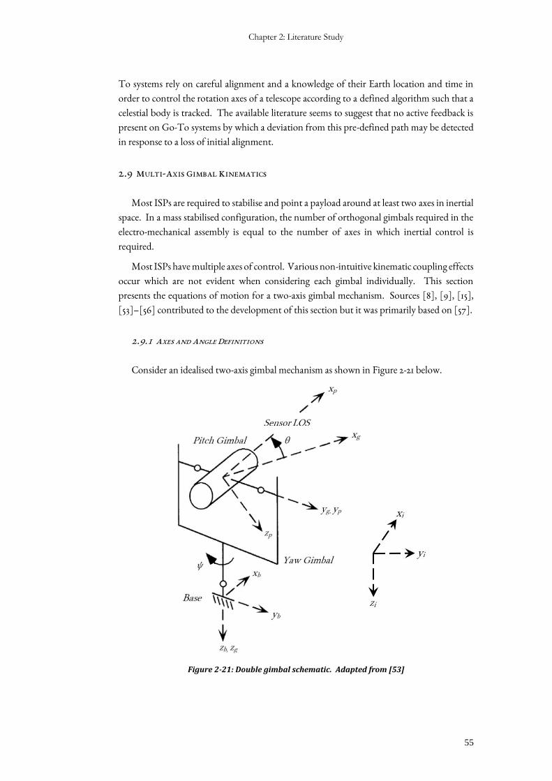
Chapter 2: Literature Study
55
To systems rely on careful alignment and a knowledge of their Earth location and time in
order to control the rotation axes of a telescope according to a defined algorithm such that a
celestial body is tracked. The available literature seems to suggest that no active feedback is
present on Go-To systems by which a deviation from this pre-defined path may be detected
in response to a loss of initial alignment.
2.9 MULTI-AXIS GIMBAL KINEMATICS
Most ISPs are required to stabilise and point a payload around at least two axes in inertial
space. In a mass stabilised configuration, the number of orthogonal gimbals required in the
electro-mechanical assembly is equal to the number of axes in which inertial control is
required.
Most ISPs have multiple axes of control. Various non-intuitive kinematic coupling effects
occur which are not evident when considering each gimbal individually. This section
presents the equations of motion for a two-axis gimbal mechanism. Sources [8], [9], [15],
[53]–[56] contributed to the development of this section but it was primarily based on [57].
2.9.1 AXES AND ANGLE DEFINITIONS
Consider an idealised two-axis gimbal mechanism as shown in Figure 2-21 below.
Figure 2-21: Double gimbal schematic. Adapted from [53]
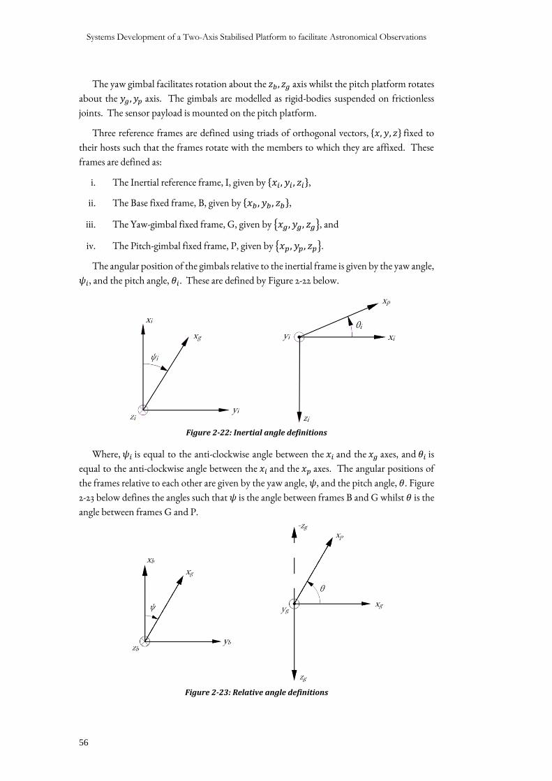
Systems Development of a Two-Axis Stabilised Platform to facilitate Astronomical Observations
56
The yaw gimbal facilitates rotation about the 𝑧𝑏, 𝑧𝑔 axis whilst the pitch platform rotates
about the 𝑦𝑔 , 𝑦𝑝 axis. The gimbals are modelled as rigid-bodies suspended on frictionless
joints. The sensor payload is mounted on the pitch platform.
Three reference frames are defined using triads of orthogonal vectors, {𝑥, 𝑦, 𝑧} fixed to
their hosts such that the frames rotate with the members to which they are affixed. These
frames are defined as:
i. The Inertial reference frame, I, given by {𝑥𝑖, 𝑦𝑖 , 𝑧𝑖},
ii. The Base fixed frame, B, given by {𝑥𝑏 , 𝑦𝑏 , 𝑧𝑏},
iii. The Yaw-gimbal fixed frame, G, given by {𝑥𝑔, 𝑦𝑔, 𝑧𝑔}, and
iv. The Pitch-gimbal fixed frame, P, given by {𝑥𝑝, 𝑦𝑝, 𝑧𝑝}.
The angular position of the gimbals relative to the inertial frame is given by the yaw angle,
𝜓𝑖, and the pitch angle, 𝜃𝑖. These are defined by Figure 2-22 below.
Figure 2-22: Inertial angle definitions
Where, 𝜓𝑖 is equal to the anti-clockwise angle between the 𝑥𝑖 and the 𝑥𝑔 axes, and 𝜃𝑖 is
equal to the anti-clockwise angle between the 𝑥𝑖 and the 𝑥𝑝 axes. The angular positions of
the frames relative to each other are given by the yaw angle, 𝜓, and the pitch angle, 𝜃. Figure
2-23 below defines the angles such that 𝜓 is the angle between frames B and G whilst 𝜃 is the
angle between frames G and P.
Figure 2-23: Relative angle definitions
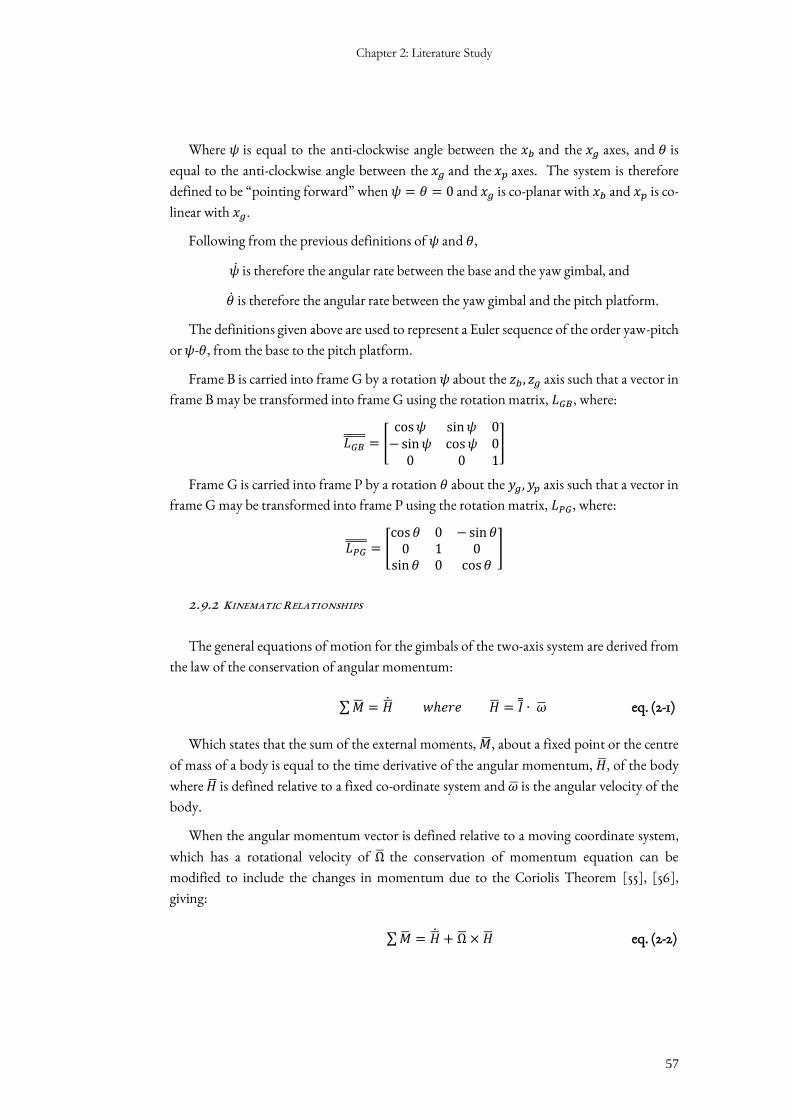
Chapter 2: Literature Study
57
Where 𝜓 is equal to the anti-clockwise angle between the 𝑥𝑏 and the 𝑥𝑔 axes, and 𝜃 is
equal to the anti-clockwise angle between the 𝑥𝑔 and the 𝑥𝑝 axes. The system is therefore
defined to be “pointing forward” when 𝜓 = 𝜃 = 0 and 𝑥𝑔 is co-planar with 𝑥𝑏 and 𝑥𝑝 is co-
linear with 𝑥𝑔.
Following from the previous definitions of 𝜓 and 𝜃,
�� is therefore the angular rate between the base and the yaw gimbal, and
�� is therefore the angular rate between the yaw gimbal and the pitch platform.
The definitions given above are used to represent a Euler sequence of the order yaw-pitch
or 𝜓-𝜃, from the base to the pitch platform.
Frame B is carried into frame G by a rotation 𝜓 about the 𝑧𝑏, 𝑧𝑔 axis such that a vector in
frame B may be transformed into frame G using the rotation matrix, 𝐿𝐺𝐵, where:
𝐿𝐺𝐵 = [
cos𝜓 sin𝜓 0−sin𝜓 cos𝜓 0
0 0 1]
Frame G is carried into frame P by a rotation 𝜃 about the 𝑦𝑔 , 𝑦𝑝 axis such that a vector in
frame G may be transformed into frame P using the rotation matrix, 𝐿𝑃𝐺, where:
𝐿𝑃𝐺 = [
cos𝜃 0 − sin 𝜃0 1 0
sin 𝜃 0 cos𝜃]
2.9.2 KINEMATIC RELATIONSHIPS
The general equations of motion for the gimbals of the two-axis system are derived from
the law of the conservation of angular momentum:
∑ �� = �� 𝑤ℎ𝑒𝑟𝑒 �� = �� ∙ �� eq. (2-1)
Which states that the sum of the external moments, ��, about a fixed point or the centre
of mass of a body is equal to the time derivative of the angular momentum, ��, of the body
where �� is defined relative to a fixed co-ordinate system and �� is the angular velocity of the
body.
When the angular momentum vector is defined relative to a moving coordinate system,
which has a rotational velocity of Ω the conservation of momentum equation can be
modified to include the changes in momentum due to the Coriolis Theorem [55], [56],
giving:
∑ �� = �� + Ω × �� eq. (2-2)
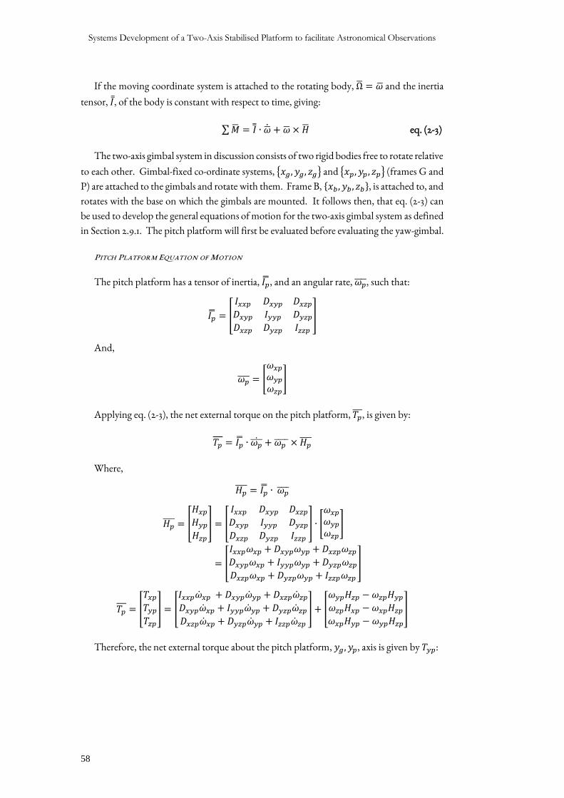
Systems Development of a Two-Axis Stabilised Platform to facilitate Astronomical Observations
58
If the moving coordinate system is attached to the rotating body, ٠= �� and the inertia
tensor, 𝐼, of the body is constant with respect to time, giving:
∑ �� = �� ∙ �� + �� × �� eq. (2-3)
The two-axis gimbal system in discussion consists of two rigid bodies free to rotate relative
to each other. Gimbal-fixed co-ordinate systems, {𝑥𝑔 , 𝑦𝑔 , 𝑧𝑔} and {𝑥𝑝, 𝑦𝑝, 𝑧𝑝} (frames G and
P) are attached to the gimbals and rotate with them. Frame B, {𝑥𝑏, 𝑦𝑏 , 𝑧𝑏}, is attached to, and
rotates with the base on which the gimbals are mounted. It follows then, that eq. (2-3) can
be used to develop the general equations of motion for the two-axis gimbal system as defined
in Section 2.9.1. The pitch platform will first be evaluated before evaluating the yaw-gimbal.
PITCH PLATFORM EQUATION OF MOTION
The pitch platform has a tensor of inertia, 𝐼��, and an angular rate, 𝜔𝑝 , such that:
𝐼�� = [
𝐼𝑥𝑥𝑝 𝐷𝑥𝑦𝑝 𝐷𝑥𝑧𝑝
𝐷𝑥𝑦𝑝 𝐼𝑦𝑦𝑝 𝐷𝑦𝑧𝑝
𝐷𝑥𝑧𝑝 𝐷𝑦𝑧𝑝 𝐼𝑧𝑧𝑝
]
And,
𝜔𝑝 = [
𝜔𝑥𝑝
𝜔𝑦𝑝
𝜔𝑧𝑝
]
Applying eq. (2-3), the net external torque on the pitch platform, 𝑇𝑝, is given by:
𝑇𝑝 = 𝐼�� ∙ 𝜔𝑝 + 𝜔𝑝 × 𝐻𝑝
Where,
𝐻𝑝 = 𝐼�� ∙ 𝜔𝑝
𝐻𝑝 = [
𝐻𝑥𝑝
𝐻𝑦𝑝
𝐻𝑧𝑝
] = [
𝐼𝑥𝑥𝑝 𝐷𝑥𝑦𝑝 𝐷𝑥𝑧𝑝
𝐷𝑥𝑦𝑝 𝐼𝑦𝑦𝑝 𝐷𝑦𝑧𝑝
𝐷𝑥𝑧𝑝 𝐷𝑦𝑧𝑝 𝐼𝑧𝑧𝑝
] ∙ [
𝜔𝑥𝑝
𝜔𝑦𝑝
𝜔𝑧𝑝
]
= [
𝐼𝑥𝑥𝑝𝜔𝑥𝑝 + 𝐷𝑥𝑦𝑝𝜔𝑦𝑝 + 𝐷𝑥𝑧𝑝𝜔𝑧𝑝
𝐷𝑥𝑦𝑝𝜔𝑥𝑝 + 𝐼𝑦𝑦𝑝𝜔𝑦𝑝 + 𝐷𝑦𝑧𝑝𝜔𝑧𝑝
𝐷𝑥𝑧𝑝𝜔𝑥𝑝 + 𝐷𝑦𝑧𝑝𝜔𝑦𝑝 + 𝐼𝑧𝑧𝑝𝜔𝑧𝑝
]
𝑇𝑝 = [
𝑇𝑥𝑝
𝑇𝑦𝑝
𝑇𝑧𝑝
] = [
𝐼𝑥𝑥𝑝��𝑥𝑝 + 𝐷𝑥𝑦𝑝��𝑦𝑝 + 𝐷𝑥𝑧𝑝��𝑧𝑝
𝐷𝑥𝑦𝑝��𝑥𝑝 + 𝐼𝑦𝑦𝑝��𝑦𝑝 + 𝐷𝑦𝑧𝑝��𝑧𝑝
𝐷𝑥𝑧𝑝��𝑥𝑝 + 𝐷𝑦𝑧𝑝��𝑦𝑝 + 𝐼𝑧𝑧𝑝��𝑧𝑝
] + [
𝜔𝑦𝑝𝐻𝑧𝑝 − 𝜔𝑧𝑝𝐻𝑦𝑝
𝜔𝑧𝑝𝐻𝑥𝑝 − 𝜔𝑥𝑝𝐻𝑧𝑝
𝜔𝑥𝑝𝐻𝑦𝑝 − 𝜔𝑦𝑝𝐻𝑧𝑝
]
Therefore, the net external torque about the pitch platform, 𝑦𝑔 , 𝑦𝑝, axis is given by 𝑇𝑦𝑝:
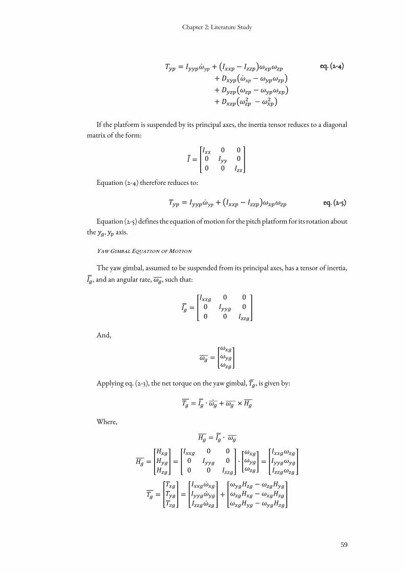
Chapter 2: Literature Study
59
𝑇𝑦𝑝 = 𝐼𝑦𝑦𝑝��𝑦𝑝 + (𝐼𝑥𝑥𝑝 − 𝐼𝑧𝑧𝑝)𝜔𝑥𝑝𝜔𝑧𝑝
+ 𝐷𝑥𝑦𝑝(��𝑥𝑝 − 𝜔𝑦𝑝𝜔𝑧𝑝)
+ 𝐷𝑦𝑧𝑝(𝜔𝑧𝑝 − 𝜔𝑦𝑝𝜔𝑥𝑝)
+ 𝐷𝑥𝑧𝑝(𝜔𝑧𝑝2 − 𝜔𝑥𝑝
2 )
eq. (2-4)
If the platform is suspended by its principal axes, the inertia tensor reduces to a diagonal
matrix of the form:
𝐼 = [
𝐼𝑥𝑥 0 00 𝐼𝑦𝑦 0
0 0 𝐼𝑧𝑧
]
Equation (2-4) therefore reduces to:
𝑇𝑦𝑝 = 𝐼𝑦𝑦𝑝��𝑦𝑝 + (𝐼𝑥𝑥𝑝 − 𝐼𝑧𝑧𝑝)𝜔𝑥𝑝𝜔𝑧𝑝 eq. (2-5)
Equation (2-5) defines the equation of motion for the pitch platform for its rotation about
the 𝑦𝑔 , 𝑦𝑝 axis.
YAW GIMBAL EQUATION OF MOTION
The yaw gimbal, assumed to be suspended from its principal axes, has a tensor of inertia,
𝐼��, and an angular rate, 𝜔𝑔 , such that:
𝐼�� = [
𝐼𝑥𝑥𝑔 0 0
0 𝐼𝑦𝑦𝑔 0
0 0 𝐼𝑧𝑧𝑔
]
And,
𝜔𝑔 = [
𝜔𝑥𝑔
𝜔𝑦𝑔
𝜔𝑧𝑔
]
Applying eq. (2-3), the net torque on the yaw gimbal, 𝑇��, is given by:
𝑇𝑔 = 𝐼�� ∙ 𝜔𝑔 + 𝜔𝑔 × 𝐻𝑔
Where,
𝐻𝑔 = 𝐼�� ∙ 𝜔𝑔
𝐻𝑔 = [
𝐻𝑥𝑔
𝐻𝑦𝑔
𝐻𝑧𝑔
] = [
𝐼𝑥𝑥𝑔 0 0
0 𝐼𝑦𝑦𝑔 0
0 0 𝐼𝑧𝑧𝑔
] ∙ [
𝜔𝑥𝑔
𝜔𝑦𝑔
𝜔𝑧𝑔
] = [
𝐼𝑥𝑥𝑔𝜔𝑥𝑔
𝐼𝑦𝑦𝑔𝜔𝑦𝑔
𝐼𝑧𝑧𝑔𝜔𝑧𝑔
]
𝑇𝑔 = [
𝑇𝑥𝑔
𝑇𝑦𝑔
𝑇𝑧𝑔
] = [
𝐼𝑥𝑥𝑔��𝑥𝑔
𝐼𝑦𝑦𝑔��𝑦𝑔
𝐼𝑧𝑧𝑔��𝑧𝑔
] + [
𝜔𝑦𝑔𝐻𝑧𝑔 − 𝜔𝑧𝑔𝐻𝑦𝑔
𝜔𝑧𝑔𝐻𝑥𝑔 − 𝜔𝑥𝑔𝐻𝑧𝑔
𝜔𝑥𝑔𝐻𝑦𝑔 − 𝜔𝑦𝑔𝐻𝑧𝑔
]
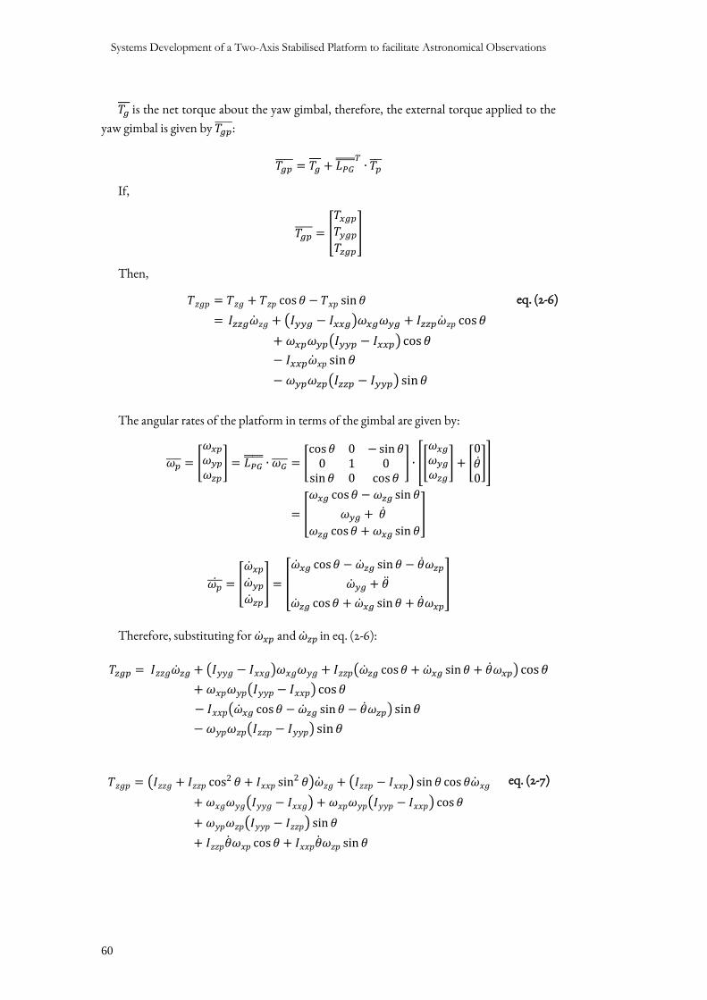
Systems Development of a Two-Axis Stabilised Platform to facilitate Astronomical Observations
60
𝑇𝑔 is the net torque about the yaw gimbal, therefore, the external torque applied to the
yaw gimbal is given by 𝑇𝑔𝑝 :
𝑇𝑔𝑝 = 𝑇𝑔 + 𝐿𝑃𝐺
𝑇∙ 𝑇𝑝
If,
𝑇𝑔𝑝 = [
𝑇𝑥𝑔𝑝
𝑇𝑦𝑔𝑝
𝑇𝑧𝑔𝑝
]
Then,
𝑇𝑧𝑔𝑝 = 𝑇𝑧𝑔 + 𝑇𝑧𝑝 cos 𝜃 − 𝑇𝑥𝑝 sin 𝜃
= 𝐼𝑧𝑧𝑔��𝑧𝑔 + (𝐼𝑦𝑦𝑔 − 𝐼𝑥𝑥𝑔)𝜔𝑥𝑔𝜔𝑦𝑔 + 𝐼𝑧𝑧𝑝��𝑧𝑝 cos𝜃
+ 𝜔𝑥𝑝𝜔𝑦𝑝(𝐼𝑦𝑦𝑝 − 𝐼𝑥𝑥𝑝) cos 𝜃
− 𝐼𝑥𝑥𝑝��𝑥𝑝 sin 𝜃
− 𝜔𝑦𝑝𝜔𝑧𝑝(𝐼𝑧𝑧𝑝 − 𝐼𝑦𝑦𝑝) sin𝜃
eq. (2-6)
The angular rates of the platform in terms of the gimbal are given by:
𝜔𝑝 = [
𝜔𝑥𝑝
𝜔𝑦𝑝
𝜔𝑧𝑝
] = 𝐿𝑃𝐺 ∙ 𝜔𝐺 = [
cos𝜃 0 − sin 𝜃0 1 0
sin 𝜃 0 cos𝜃] ∙ [[
𝜔𝑥𝑔
𝜔𝑦𝑔
𝜔𝑧𝑔
] + [0��0]]
= [
𝜔𝑥𝑔 cos𝜃 − 𝜔𝑧𝑔 sin 𝜃
𝜔𝑦𝑔 + ��
𝜔𝑧𝑔 cos𝜃 + 𝜔𝑥𝑔 sin 𝜃
]
𝜔𝑝 = [
��𝑥𝑝
��𝑦𝑝
��𝑧𝑝
] = [
��𝑥𝑔 cos𝜃 − ��𝑧𝑔 sin 𝜃 − ��𝜔𝑧𝑝
��𝑦𝑔 + ��
��𝑧𝑔 cos𝜃 + ��𝑥𝑔 sin 𝜃 + ��𝜔𝑥𝑝
]
Therefore, substituting for ��𝑥𝑝 and ��𝑧𝑝 in eq. (2-6):
𝑇𝑧𝑔𝑝 = 𝐼𝑧𝑧𝑔��𝑧𝑔 + (𝐼𝑦𝑦𝑔 − 𝐼𝑥𝑥𝑔)𝜔𝑥𝑔𝜔𝑦𝑔 + 𝐼𝑧𝑧𝑝(��𝑧𝑔 cos𝜃 + ��𝑥𝑔 sin 𝜃 + ��𝜔𝑥𝑝) cos𝜃
+ 𝜔𝑥𝑝𝜔𝑦𝑝(𝐼𝑦𝑦𝑝 − 𝐼𝑥𝑥𝑝) cos𝜃
− 𝐼𝑥𝑥𝑝(��𝑥𝑔 cos𝜃 − ��𝑧𝑔 sin 𝜃 − ��𝜔𝑧𝑝) sin𝜃
− 𝜔𝑦𝑝𝜔𝑧𝑝(𝐼𝑧𝑧𝑝 − 𝐼𝑦𝑦𝑝) sin𝜃
𝑇𝑧𝑔𝑝 = (𝐼𝑧𝑧𝑔 + 𝐼𝑧𝑧𝑝 cos2 𝜃 + 𝐼𝑥𝑥𝑝 sin2 𝜃)��𝑧𝑔 + (𝐼𝑧𝑧𝑝 − 𝐼𝑥𝑥𝑝) sin 𝜃 cos 𝜃��𝑥𝑔
+ 𝜔𝑥𝑔𝜔𝑦𝑔(𝐼𝑦𝑦𝑔 − 𝐼𝑥𝑥𝑔) + 𝜔𝑥𝑝𝜔𝑦𝑝(𝐼𝑦𝑦𝑝 − 𝐼𝑥𝑥𝑝) cos 𝜃
+ 𝜔𝑦𝑝𝜔𝑧𝑝(𝐼𝑦𝑦𝑝 − 𝐼𝑧𝑧𝑝) sin 𝜃
+ 𝐼𝑧𝑧𝑝��𝜔𝑥𝑝 cos 𝜃 + 𝐼𝑥𝑥𝑝��𝜔𝑧𝑝 sin 𝜃
eq. (2-7)
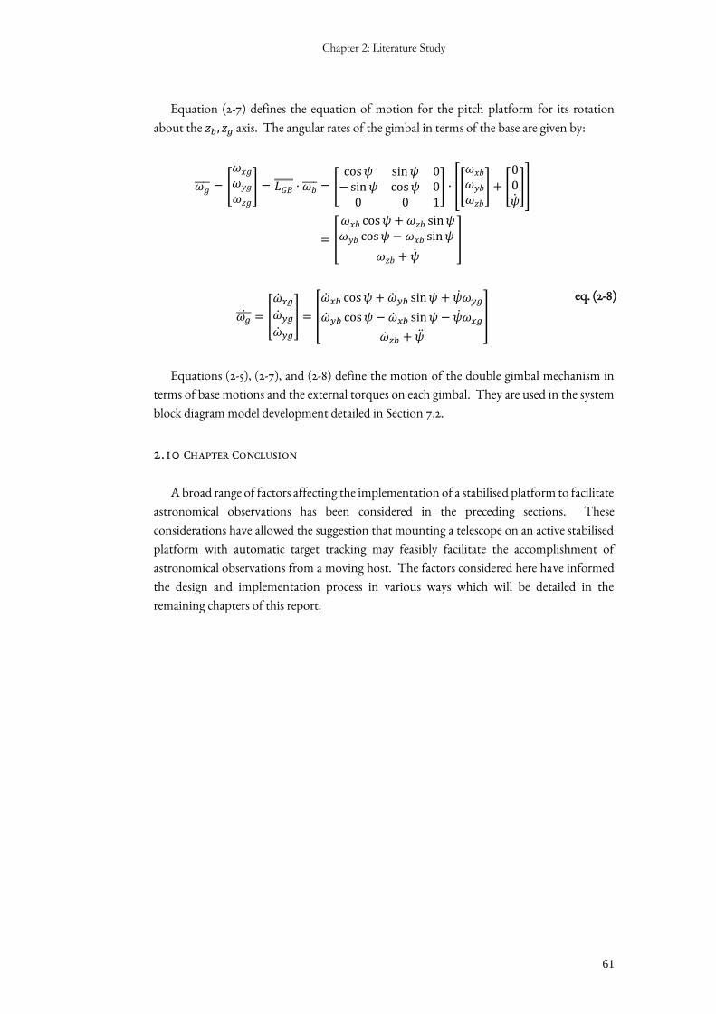
Chapter 2: Literature Study
61
Equation (2-7) defines the equation of motion for the pitch platform for its rotation
about the 𝑧𝑏, 𝑧𝑔 axis. The angular rates of the gimbal in terms of the base are given by:
𝜔𝑔 = [
𝜔𝑥𝑔
𝜔𝑦𝑔
𝜔𝑧𝑔
] = 𝐿𝐺𝐵 ∙ 𝜔𝑏 = [
cos𝜓 sin𝜓 0− sin𝜓 cos𝜓 0
0 0 1] ∙ [[
𝜔𝑥𝑏
𝜔𝑦𝑏
𝜔𝑧𝑏
] + [
00��]]
= [
𝜔𝑥𝑏 cos𝜓 + 𝜔𝑧𝑏 sin𝜓𝜔𝑦𝑏 cos𝜓 − 𝜔𝑥𝑏 sin𝜓
𝜔𝑧𝑏 + ��
]
𝜔𝑔 = [
��𝑥𝑔
��𝑦𝑔
��𝑦𝑔
] = [
��𝑥𝑏 cos𝜓 + ��𝑦𝑏 sin𝜓 + ��𝜔𝑦𝑔
��𝑦𝑏 cos𝜓 − ��𝑥𝑏 sin𝜓 − ��𝜔𝑥𝑔
��𝑧𝑏 + ��
]
eq. (2-8)
Equations (2-5), (2-7), and (2-8) define the motion of the double gimbal mechanism in
terms of base motions and the external torques on each gimbal. They are used in the system
block diagram model development detailed in Section 7.2.
2.10 CHAPTER CONCLUSION
A broad range of factors affecting the implementation of a stabilised platform to facilitate
astronomical observations has been considered in the preceding sections. These
considerations have allowed the suggestion that mounting a telescope on an active stabilised
platform with automatic target tracking may feasibly facilitate the accomplishment of
astronomical observations from a moving host. The factors considered here have informed
the design and implementation process in various ways which will be detailed in the
remaining chapters of this report.

Chapter 3: System Specifications
63
3 SYSTEM SPECIFICATIONS
3.1 INTRODUCTION
The observations and discussion of the literature study presented in Chapter 2 helped to
inform a set of system specifications which were drawn up for the project. This set of
quantitative system specifications developed from a group of qualitative desired performance
requirements aimed at facilitating the accomplishment of the project aims.
These specifications were developed using the initial aims of the project. Once the
project had been revised to aim at approximating the initial aims with a low-cost system
designed for project expansion, the target specifications developed here became idealistic
design goals which informed the design decisions made in Chapters 4 to 7. For the better
preservation of this document’s narrative, only the final specifications developed are
presented here, while the process followed to develop this set of specifications is shown in
detail in Appendix A.
3.2 PURPOSE OF THE ISP
The initial aims of this project were to design, simulate implement and test a robust multi-
axis ISP to facilitate the high precision automatic tracking of celestial objects through an
optical telescope mounted on a moving vehicle. The project entailed the development of all
subsystems associated with the overall ISP including the electro-mechanical assembly of the
ISP, the control system, and electronic interfaces.
The purpose of the system is, therefore, to achieve automatic tracking of a celestial body
using an optical telescope, and to ensure that high-quality celestial observations can be made
through the attenuation of disturbance torques incurred onto the imaging sensor by the host
vehicle motion. The following specifications, therefore, list the performance requirements
of the ISP in order to achieve this purpose.
3.3 PERFORMANCE REQUIREMENTS
Table 3-1 below details the target specifications for the ISP system developed in this
project. In the table below, ‘Trace’ values refer to qualitative requirement numbers (Rx) and
quantitative specification numbers (Sx) which may be found in Appendix A. Additionally,
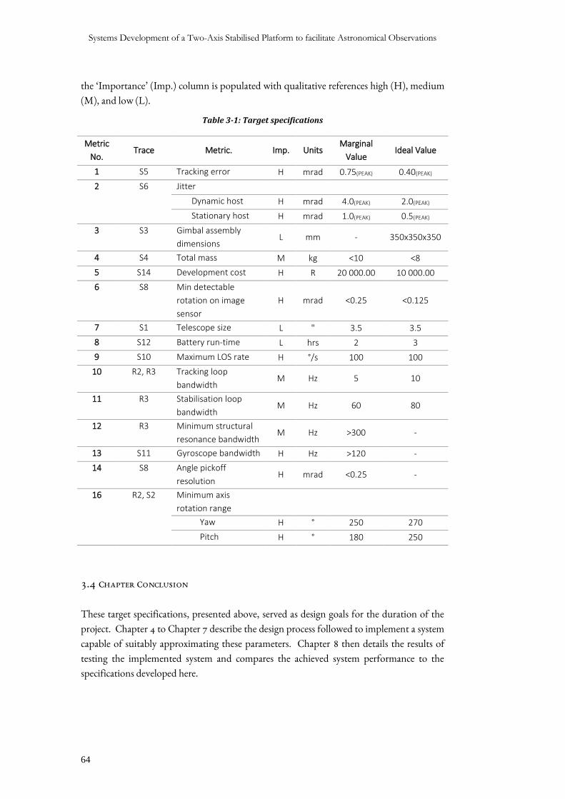
Systems Development of a Two-Axis Stabilised Platform to facilitate Astronomical Observations
64
the ‘Importance’ (Imp.) column is populated with qualitative references high (H), medium
(M), and low (L).
Table 3-1: Target specifications
Metric
No. Trace Metric. Imp. Units
Marginal
Value Ideal Value
1 S5 Tracking error H mrad 0.75(PEAK) 0.40(PEAK)
2 S6 Jitter
Dynamic host H mrad 4.0(PEAK) 2.0(PEAK)
Stationary host H mrad 1.0(PEAK) 0.5(PEAK)
3 S3 Gimbal assembly
dimensions L mm - 350x350x350
4 S4 Total mass M kg <10 <8
5 S14 Development cost H R 20 000.00 10 000.00
6 S8 Min detectable
rotation on image
sensor
H mrad <0.25 <0.125
7 S1 Telescope size L " 3.5 3.5
8 S12 Battery run-time L hrs 2 3
9 S10 Maximum LOS rate H °/s 100 100
10 R2, R3 Tracking loop
bandwidth M Hz 5 10
11 R3 Stabilisation loop
bandwidth M Hz 60 80
12 R3 Minimum structural
resonance bandwidth M Hz >300 -
13 S11 Gyroscope bandwidth H Hz >120 -
14 S8 Angle pickoff
resolution H mrad <0.25 -
16 R2, S2 Minimum axis
rotation range
Yaw H ° 250 270
Pitch H ° 180 250
3.4 CHAPTER CONCLUSION
These target specifications, presented above, served as design goals for the duration of the
project. Chapter 4 to Chapter 7 describe the design process followed to implement a system
capable of suitably approximating these parameters. Chapter 8 then details the results of
testing the implemented system and compares the achieved system performance to the
specifications developed here.

Chapter 4: Mechanical Design and Implementation
65
4 MECHANICAL DESIGN AND IMPLEMENTATION
4.1 INTRODUCTION
Chapters 4 through 7 seek to describe in detail the process followed by which an ISP with
an automatic target tracker was developed capable of approximating the target systems
specifications given in the previous chapter. This broad design and implementation section
of the report begins in this chapter by detailing the mechanical design of the ISP assembly
(item I1 of the prime item diagram, Figure A-1, of the System Specification) which includes
the telescope specification and modelling, the assembly support/mounting structure, the
gimbals, the gimbal suspension design, and finally the gearbox (items I1.1–I1.4, and I2.3
respectively).
Only subsequent to the specification of the telescope to be used could the rest of the
mechanical design be accomplished; accordingly, this section of the report begins with a
specification of the telescope ultimately to be used should project expansion occur in future.
4.2 TELESCOPE SPECIFICATION (I1.4)
On the revision of the project budget early in the project, the decision was made to
continue with the project in an approximated manner, with design for expansion being a key
factor in design decisions made. It became apparent that the project budget would not be
able to account for the purchase of a telescope in addition to the other components required
to implement a functioning stabilised platform. In response to this, it was decided that the
design for expansion principle would be best applied to the telescope itself: a low-cost camera
mounting platform designed to inertially and dimensionally model a specific telescope would
be used instead of the telescope itself and so facilitate the remainder of the systems being
developed within the revised budget.
For this project, it was decided to specify the Meade ETX90 as the telescope ultimately to
be used with the stabilised platform developed in this project. The Meade ETX90 is a 3.5”
aperture Maksutov-Cassegrain telescope (satisfying specification S1) with a resolving power
of 1.3 arcsec. Resolving power refers the minimum angle required between objects in the
FOV for them to be distinguishable from each other. Maksutov-Cassegrain telescopes are
compound telescopes which enables them to be smaller and lighter than other telescope types
which achieve the same levels of performance. This was advantageous to the project as it
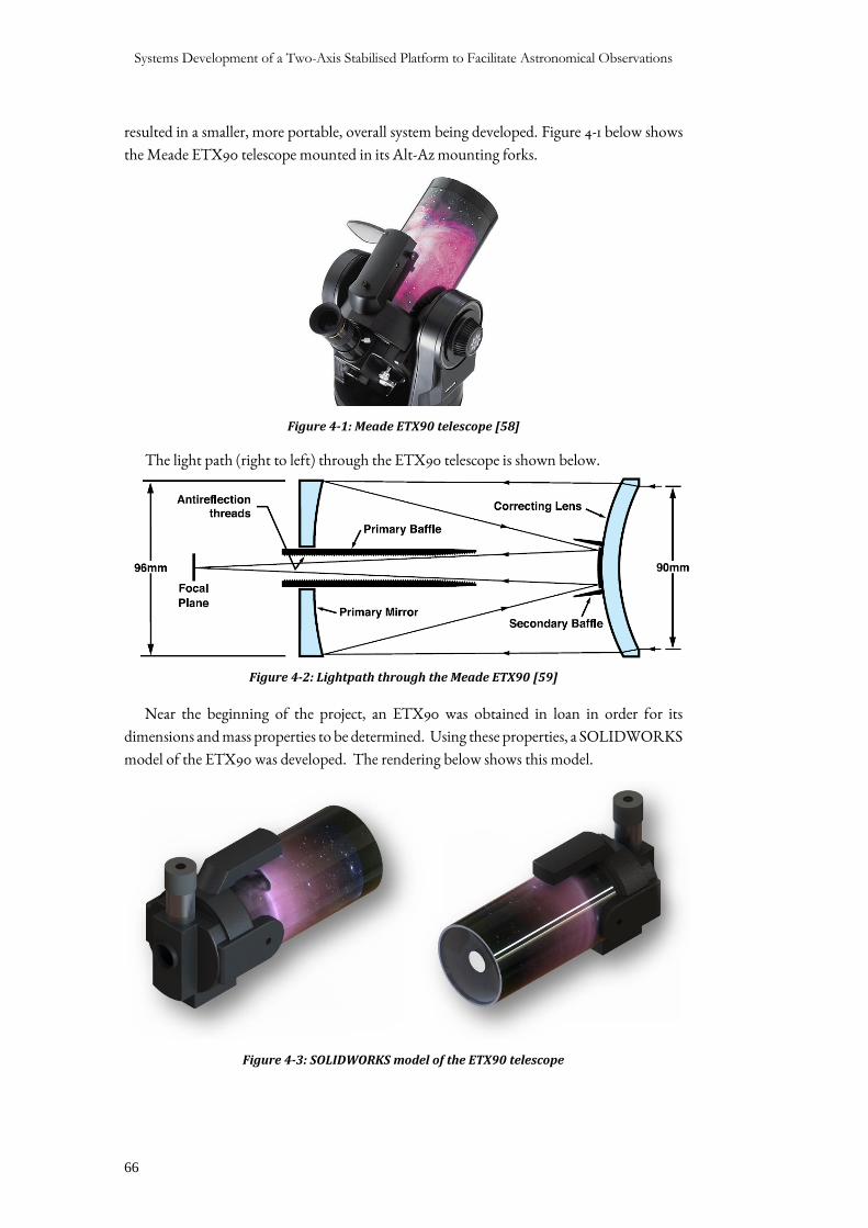
Systems Development of a Two-Axis Stabilised Platform to Facilitate Astronomical Observations
66
resulted in a smaller, more portable, overall system being developed. Figure 4-1 below shows
the Meade ETX90 telescope mounted in its Alt-Az mounting forks.
Figure 4-1: Meade ETX90 telescope [58]
The light path (right to left) through the ETX90 telescope is shown below.
Figure 4-2: Lightpath through the Meade ETX90 [59]
Near the beginning of the project, an ETX90 was obtained in loan in order for its
dimensions and mass properties to be determined. Using these properties, a SOLIDWORKS
model of the ETX90 was developed. The rendering below shows this model.
Figure 4-3: SOLIDWORKS model of the ETX90 telescope
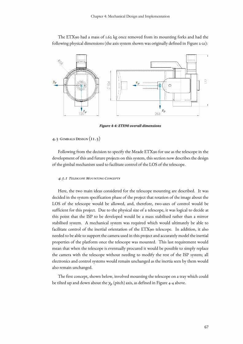
Chapter 4: Mechanical Design and Implementation
67
The ETX90 had a mass of 1.62 kg once removed from its mounting forks and had the
following physical dimensions (the axis system shown was originally defined in Figure 2-21):
Figure 4-4: ETX90 overall dimensions
4.3 GIMBALS DESIGN (I1.3)
Following from the decision to specify the Meade ETX90 for use as the telescope in the
development of this and future projects on this system, this section now describes the design
of the gimbal mechanism used to facilitate control of the LOS of the telescope.
4.3.1 TELESCOPE MOUNTING CONCEPTS
Here, the two main ideas considered for the telescope mounting are described. It was
decided in the system specification phase of the project that rotation of the image about the
LOS of the telescope would be allowed, and, therefore, two-axes of control would be
sufficient for this project. Due to the physical size of a telescope, it was logical to decide at
this point that the ISP to be developed would be a mass stabilised rather than a mirror
stabilised system. A mechanical system was required which would ultimately be able to
facilitate control of the inertial orientation of the ETX90 telescope. In addition, it also
needed to be able to support the camera used in this project and accurately model the inertial
properties of the platform once the telescope was mounted. This last requirement would
mean that when the telescope is eventually procured it would be possible to simply replace
the camera with the telescope without needing to modify the rest of the ISP system; all
electronics and control systems would remain unchanged as the inertia seen by them would
also remain unchanged.
The first concept, shown below, involved mounting the telescope on a tray which could
be tilted up and down about the 𝑦𝑝 (pitch) axis, as defined in Figure 4-4 above.
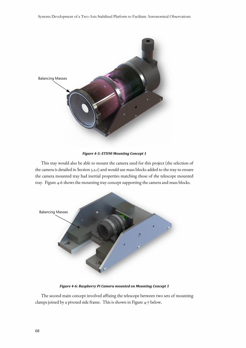
Systems Development of a Two-Axis Stabilised Platform to Facilitate Astronomical Observations
68
Figure 4-5: ETX90 Mounting Concept 1
This tray would also be able to mount the camera used for this project (the selection of
the camera is detailed in Section 5.2.1) and would use mass blocks added to the tray to ensure
the camera mounted tray had inertial properties matching those of the telescope mounted
tray. Figure 4-6 shows the mounting tray concept supporting the camera and mass blocks.
Figure 4-6: Raspberry Pi Camera mounted on Mounting Concept 1
The second main concept involved affixing the telescope between two sets of mounting
clamps joined by a pivoted side frame. This is shown in Figure 4-7 below.
Balancing Masses
Balancing Masses
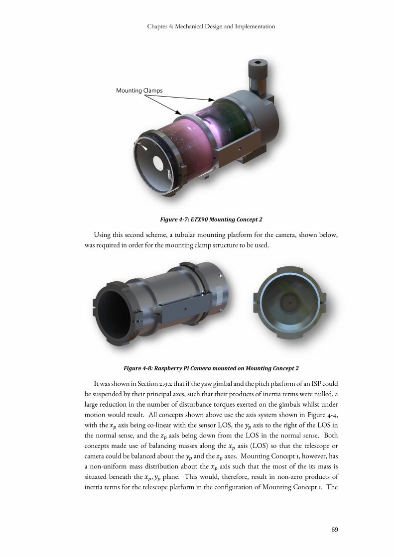
Chapter 4: Mechanical Design and Implementation
69
Figure 4-7: ETX90 Mounting Concept 2
Using this second scheme, a tubular mounting platform for the camera, shown below,
was required in order for the mounting clamp structure to be used.
Figure 4-8: Raspberry Pi Camera mounted on Mounting Concept 2
It was shown in Section 2.9.2 that if the yaw gimbal and the pitch platform of an ISP could
be suspended by their principal axes, such that their products of inertia terms were nulled, a
large reduction in the number of disturbance torques exerted on the gimbals whilst under
motion would result. All concepts shown above use the axis system shown in Figure 4-4,
with the 𝑥𝑝 axis being co-linear with the sensor LOS, the 𝑦𝑝 axis to the right of the LOS in
the normal sense, and the 𝑧𝑝 axis being down from the LOS in the normal sense. Both
concepts made use of balancing masses along the 𝑥𝑝 axis (LOS) so that the telescope or
camera could be balanced about the 𝑦𝑝 and the 𝑧𝑝 axes. Mounting Concept 1, however, has
a non-uniform mass distribution about the 𝑥𝑝 axis such that the most of the its mass is
situated beneath the 𝑥𝑝, 𝑦𝑝 plane. This would, therefore, result in non-zero products of
inertia terms for the telescope platform in the configuration of Mounting Concept 1. The
Mounting Clamps
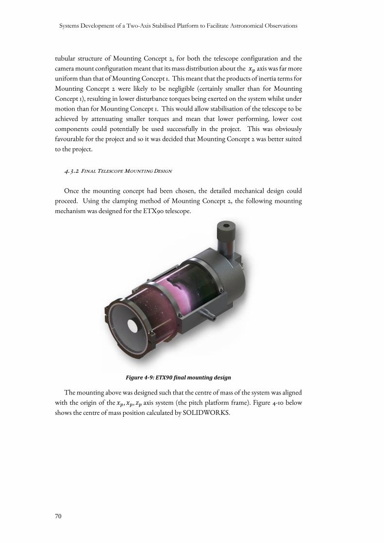
Systems Development of a Two-Axis Stabilised Platform to Facilitate Astronomical Observations
70
tubular structure of Mounting Concept 2, for both the telescope configuration and the
camera mount configuration meant that its mass distribution about the 𝑥𝑝 axis was far more
uniform than that of Mounting Concept 1. This meant that the products of inertia terms for
Mounting Concept 2 were likely to be negligible (certainly smaller than for Mounting
Concept 1), resulting in lower disturbance torques being exerted on the system whilst under
motion than for Mounting Concept 1. This would allow stabilisation of the telescope to be
achieved by attenuating smaller torques and mean that lower performing, lower cost
components could potentially be used successfully in the project. This was obviously
favourable for the project and so it was decided that Mounting Concept 2 was better suited
to the project.
4.3.2 FINAL TELESCOPE MOUNTING DESIGN
Once the mounting concept had been chosen, the detailed mechanical design could
proceed. Using the clamping method of Mounting Concept 2, the following mounting
mechanism was designed for the ETX90 telescope.
Figure 4-9: ETX90 final mounting design
The mounting above was designed such that the centre of mass of the system was aligned
with the origin of the 𝑥𝑝 , 𝑥𝑝, 𝑧𝑝 axis system (the pitch platform frame). Figure 4-10 below
shows the centre of mass position calculated by SOLIDWORKS.
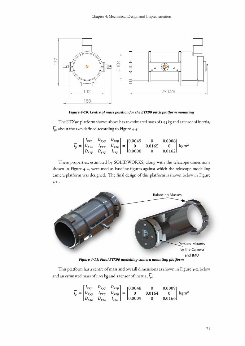
Chapter 4: Mechanical Design and Implementation
71
Figure 4-10: Centre of mass position for the ETX90 pitch platform mounting
The ETX90 platform shown above has an estimated mass of 1.95 kg and a tensor of inertia,
𝐼��, about the axes defined according to Figure 4-4:
𝐼�� = [
𝐼𝑥𝑥𝑝 𝐷𝑥𝑦𝑝 𝐷𝑥𝑧𝑝
𝐷𝑥𝑦𝑝 𝐼𝑦𝑦𝑝 𝐷𝑦𝑧𝑝
𝐷𝑥𝑧𝑝 𝐷𝑦𝑧𝑝 𝐼𝑧𝑧𝑝
] = [0.0049 0 0.0008
0 0.0165 00.0008 0 0.0162
] kgm2
These properties, estimated by SOLIDWORKS, along with the telescope dimensions
shown in Figure 4-4, were used as baseline figures against which the telescope modelling
camera platform was designed. The final design of this platform is shown below in Figure
4-11.
Figure 4-11: Final ETX90 modelling camera mounting platform
This platform has a centre of mass and overall dimensions as shown in Figure 4-12 below
and an estimated mass of 1.90 kg and a tensor of inertia, 𝐼��:
𝐼�� = [
𝐼𝑥𝑥𝑝 𝐷𝑥𝑦𝑝 𝐷𝑥𝑧𝑝
𝐷𝑥𝑦𝑝 𝐼𝑦𝑦𝑝 𝐷𝑦𝑧𝑝
𝐷𝑥𝑧𝑝 𝐷𝑦𝑧𝑝 𝐼𝑧𝑧𝑝
] = [0.0048 0 0.0009
0 0.0164 00.0009 0 0.0166
] kgm2
Balancing Masses
Perspex Mounts
for the Camera
and IMU
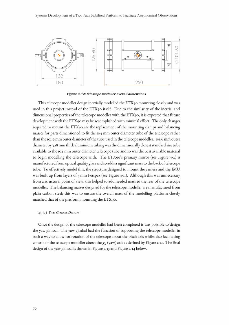
Systems Development of a Two-Axis Stabilised Platform to Facilitate Astronomical Observations
72
Figure 4-12: telescope modeller overall dimensions
This telescope modeller design inertially modelled the ETX90 mounting closely and was
used in this project instead of the ETX90 itself. Due to the similarity of the inertial and
dimensional properties of the telescope modeller with the ETX90, it is expected that future
development with the ETX90 may be accomplished with minimal effort. The only changes
required to mount the ETX90 are the replacement of the mounting clamps and balancing
masses for parts dimensioned to fit the 104 mm outer diameter tube of the telescope rather
than the 101.6 mm outer diameter of the tube used in the telescope modeller. 101.6 mm outer
diameter by 3.18 mm thick aluminium tubing was the dimensionally closest standard size tube
available to the 104 mm outer diameter telescope tube and so was the best available material
to begin modelling the telescope with. The ETX90’s primary mirror (see Figure 4-2) is
manufactured from optical quality glass and so adds a significant mass to the back of telescope
tube. To effectively model this, the structure designed to mount the camera and the IMU
was built up from layers of 5 mm Perspex (see Figure 4-11). Although this was unnecessary
from a structural point of view, this helped to add needed mass to the rear of the telescope
modeller. The balancing masses designed for the telescope modeller are manufactured from
plain carbon steel; this was to ensure the overall mass of the modelling platform closely
matched that of the platform mounting the ETX90.
4.3.3 YAW GIMBAL DESIGN
Once the design of the telescope modeller had been completed it was possible to design
the yaw gimbal. The yaw gimbal had the function of supporting the telescope modeller in
such a way to allow for rotation of the telescope about the pitch axis whilst also facilitating
control of the telescope modeller about the 𝑦𝑔 (yaw) axis as defined by Figure 2-21. The final
design of the yaw gimbal is shown in Figure 4-13 and Figure 4-14 below.
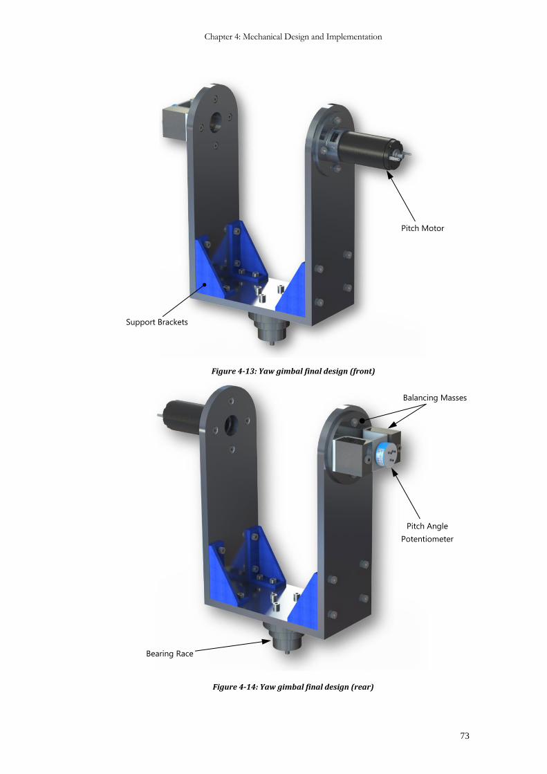
Chapter 4: Mechanical Design and Implementation
73
Figure 4-13: Yaw gimbal final design (front)
Figure 4-14: Yaw gimbal final design (rear)
Pitch Motor
Pitch Angle
Potentiometer
Balancing Masses
Support Brackets
Bearing Race
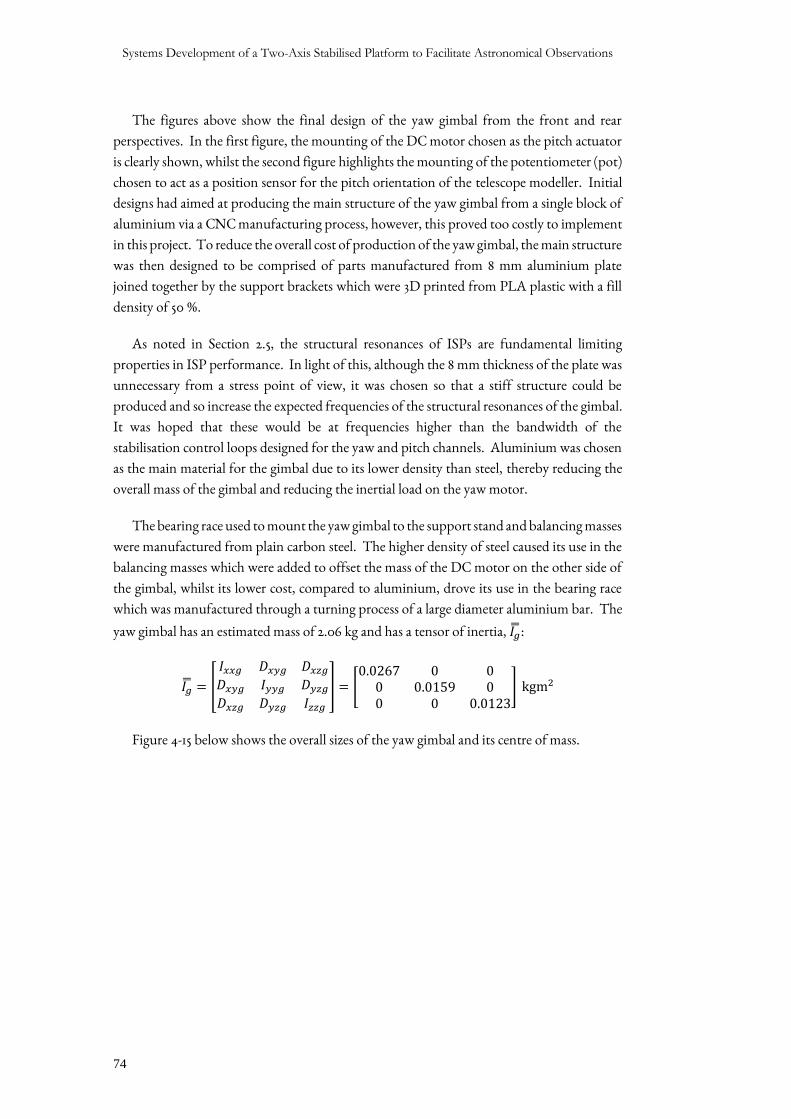
Systems Development of a Two-Axis Stabilised Platform to Facilitate Astronomical Observations
74
The figures above show the final design of the yaw gimbal from the front and rear
perspectives. In the first figure, the mounting of the DC motor chosen as the pitch actuator
is clearly shown, whilst the second figure highlights the mounting of the potentiometer (pot)
chosen to act as a position sensor for the pitch orientation of the telescope modeller. Initial
designs had aimed at producing the main structure of the yaw gimbal from a single block of
aluminium via a CNC manufacturing process, however, this proved too costly to implement
in this project. To reduce the overall cost of production of the yaw gimbal, the main structure
was then designed to be comprised of parts manufactured from 8 mm aluminium plate
joined together by the support brackets which were 3D printed from PLA plastic with a fill
density of 50 %.
As noted in Section 2.5, the structural resonances of ISPs are fundamental limiting
properties in ISP performance. In light of this, although the 8 mm thickness of the plate was
unnecessary from a stress point of view, it was chosen so that a stiff structure could be
produced and so increase the expected frequencies of the structural resonances of the gimbal.
It was hoped that these would be at frequencies higher than the bandwidth of the
stabilisation control loops designed for the yaw and pitch channels. Aluminium was chosen
as the main material for the gimbal due to its lower density than steel, thereby reducing the
overall mass of the gimbal and reducing the inertial load on the yaw motor.
The bearing race used to mount the yaw gimbal to the support stand and balancing masses
were manufactured from plain carbon steel. The higher density of steel caused its use in the
balancing masses which were added to offset the mass of the DC motor on the other side of
the gimbal, whilst its lower cost, compared to aluminium, drove its use in the bearing race
which was manufactured through a turning process of a large diameter aluminium bar. The
yaw gimbal has an estimated mass of 2.06 kg and has a tensor of inertia, 𝐼��:
𝐼�� = [
𝐼𝑥𝑥𝑔 𝐷𝑥𝑦𝑔 𝐷𝑥𝑧𝑔
𝐷𝑥𝑦𝑔 𝐼𝑦𝑦𝑔 𝐷𝑦𝑧𝑔
𝐷𝑥𝑧𝑔 𝐷𝑦𝑧𝑔 𝐼𝑧𝑧𝑔
] = [0.0267 0 0
0 0.0159 00 0 0.0123
] kgm2
Figure 4-15 below shows the overall sizes of the yaw gimbal and its centre of mass.
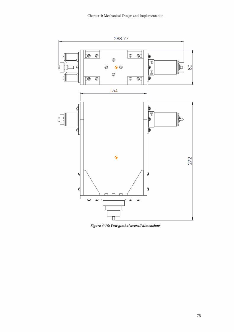
Chapter 4: Mechanical Design and Implementation
75
Figure 4-15: Yaw gimbal overall dimensions
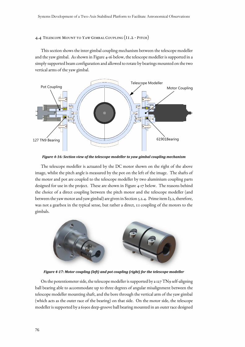
Systems Development of a Two-Axis Stabilised Platform to Facilitate Astronomical Observations
76
4.4 TELESCOPE MOUNT TO YAW GIMBAL COUPLING (I1.2 - PITCH)
This section shows the inter gimbal coupling mechanism between the telescope modeller
and the yaw gimbal. As shown in Figure 4-16 below, the telescope modeller is supported in a
simply supported beam configuration and allowed to rotate by bearings mounted on the two
vertical arms of the yaw gimbal.
Figure 4-16: Section view of the telescope modeller to yaw gimbal coupling mechanism
The telescope modeller is actuated by the DC motor shown on the right of the above
image, whilst the pitch angle is measured by the pot on the left of the image. The shafts of
the motor and pot are coupled to the telescope modeller by two aluminium coupling parts
designed for use in the project. These are shown in Figure 4-17 below. The reasons behind
the choice of a direct coupling between the pitch motor and the telescope modeller (and
between the yaw motor and yaw gimbal) are given in Section 5.2.4. Prime item I3.2, therefore,
was not a gearbox in the typical sense, but rather a direct, 1:1 coupling of the motors to the
gimbals.
Figure 4-17: Motor coupling (left) and pot coupling (right) for the telescope modeller
On the potentiometer side, the telescope modeller is supported by a 127 TN9 self-aligning
ball bearing able to accommodate up to three degrees of angular misalignment between the
telescope modeller mounting shaft, and the bore through the vertical arm of the yaw gimbal
(which acts as the outer race of the bearing) on that side. On the motor side, the telescope
modeller is supported by a 61901 deep-groove ball bearing mounted in an outer race designed
Pot Coupling Motor Coupling
Telescope Modeller
127 TN9 Bearing 61901Bearing
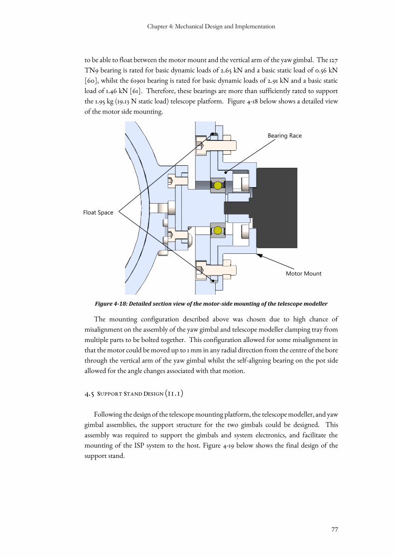
Chapter 4: Mechanical Design and Implementation
77
to be able to float between the motor mount and the vertical arm of the yaw gimbal. The 127
TN9 bearing is rated for basic dynamic loads of 2.65 kN and a basic static load of 0.56 kN
[60], whilst the 61901 bearing is rated for basic dynamic loads of 2.91 kN and a basic static
load of 1.46 kN [61]. Therefore, these bearings are more than sufficiently rated to support
the 1.95 kg (19.13 N static load) telescope platform. Figure 4-18 below shows a detailed view
of the motor side mounting.
Figure 4-18: Detailed section view of the motor-side mounting of the telescope modeller
The mounting configuration described above was chosen due to high chance of
misalignment on the assembly of the yaw gimbal and telescope modeller clamping tray from
multiple parts to be bolted together. This configuration allowed for some misalignment in
that the motor could be moved up to 1 mm in any radial direction from the centre of the bore
through the vertical arm of the yaw gimbal whilst the self-aligning bearing on the pot side
allowed for the angle changes associated with that motion.
4.5 SUPPORT STAND DESIGN (I1.1)
Following the design of the telescope mounting platform, the telescope modeller, and yaw
gimbal assemblies, the support structure for the two gimbals could be designed. This
assembly was required to support the gimbals and system electronics, and facilitate the
mounting of the ISP system to the host. Figure 4-19 below shows the final design of the
support stand.
Motor Mount
Float Space
Bearing Race
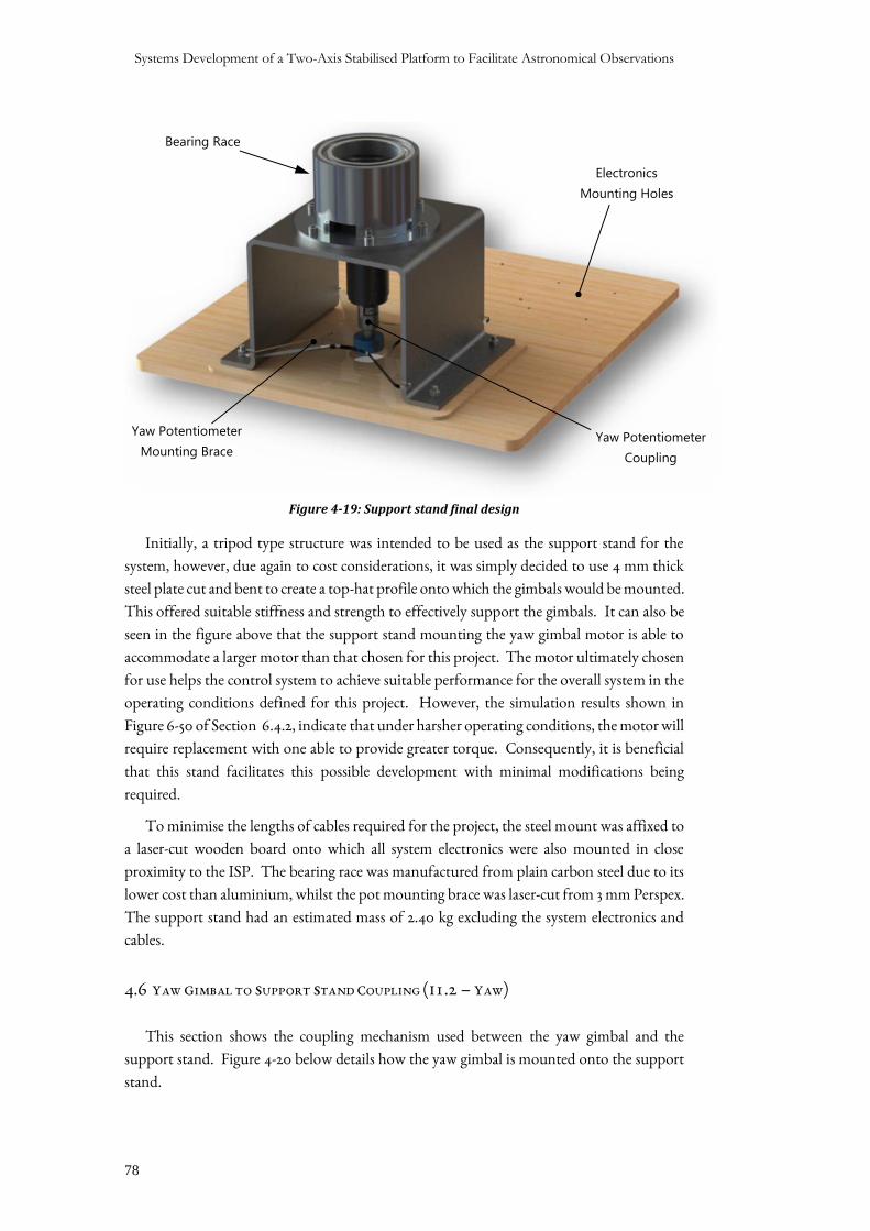
Systems Development of a Two-Axis Stabilised Platform to Facilitate Astronomical Observations
78
Figure 4-19: Support stand final design
Initially, a tripod type structure was intended to be used as the support stand for the
system, however, due again to cost considerations, it was simply decided to use 4 mm thick
steel plate cut and bent to create a top-hat profile onto which the gimbals would be mounted.
This offered suitable stiffness and strength to effectively support the gimbals. It can also be
seen in the figure above that the support stand mounting the yaw gimbal motor is able to
accommodate a larger motor than that chosen for this project. The motor ultimately chosen
for use helps the control system to achieve suitable performance for the overall system in the
operating conditions defined for this project. However, the simulation results shown in
Figure 6-50 of Section 6.4.2, indicate that under harsher operating conditions, the motor will
require replacement with one able to provide greater torque. Consequently, it is beneficial
that this stand facilitates this possible development with minimal modifications being
required.
To minimise the lengths of cables required for the project, the steel mount was affixed to
a laser-cut wooden board onto which all system electronics were also mounted in close
proximity to the ISP. The bearing race was manufactured from plain carbon steel due to its
lower cost than aluminium, whilst the pot mounting brace was laser-cut from 3 mm Perspex.
The support stand had an estimated mass of 2.40 kg excluding the system electronics and
cables.
4.6 YAW GIMBAL TO SUPPORT STAND COUPLING (I1.2 – YAW)
This section shows the coupling mechanism used between the yaw gimbal and the
support stand. Figure 4-20 below details how the yaw gimbal is mounted onto the support
stand.
Bearing Race
Yaw Potentiometer
Mounting Brace
Electronics
Mounting Holes
Yaw Potentiometer
Coupling
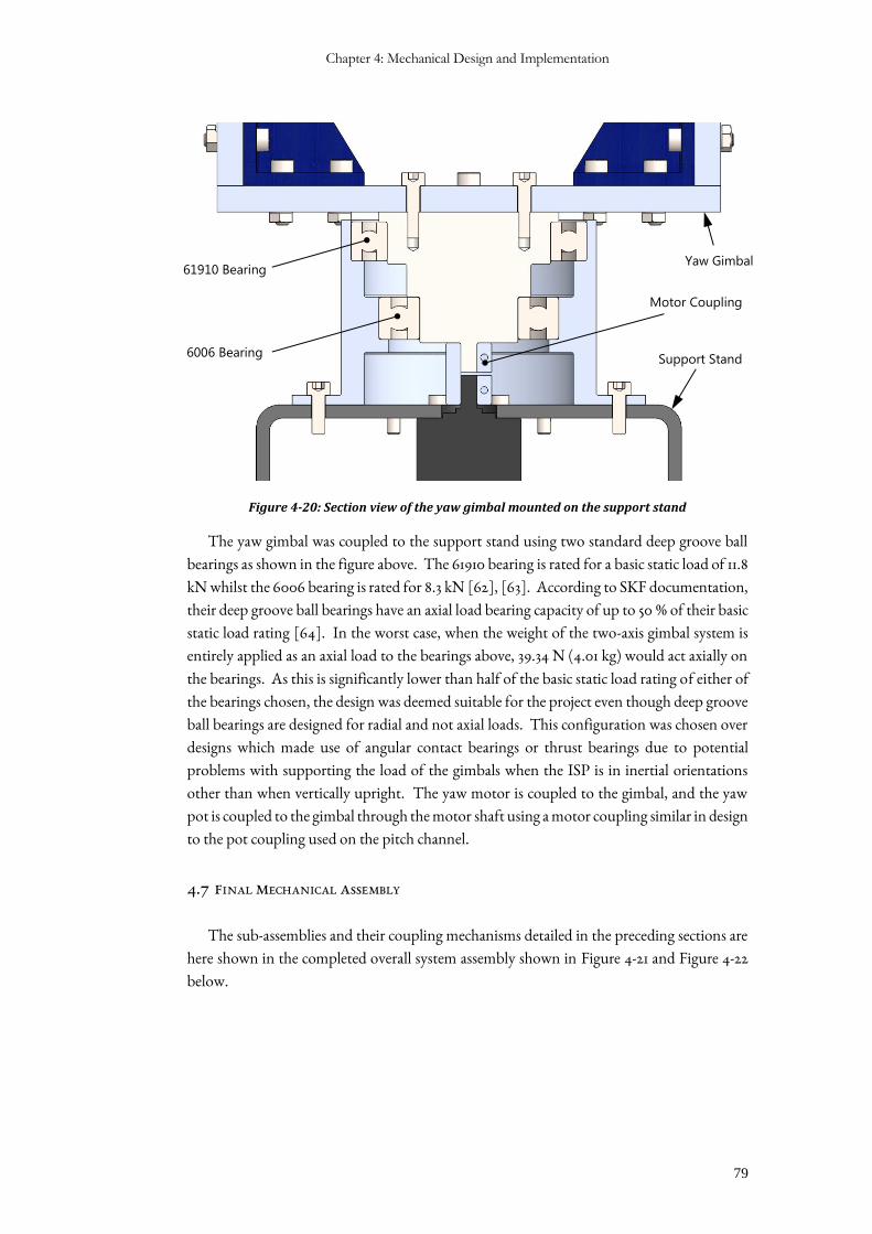
Chapter 4: Mechanical Design and Implementation
79
Figure 4-20: Section view of the yaw gimbal mounted on the support stand
The yaw gimbal was coupled to the support stand using two standard deep groove ball
bearings as shown in the figure above. The 61910 bearing is rated for a basic static load of 11.8
kN whilst the 6006 bearing is rated for 8.3 kN [62], [63]. According to SKF documentation,
their deep groove ball bearings have an axial load bearing capacity of up to 50 % of their basic
static load rating [64]. In the worst case, when the weight of the two-axis gimbal system is
entirely applied as an axial load to the bearings above, 39.34 N (4.01 kg) would act axially on
the bearings. As this is significantly lower than half of the basic static load rating of either of
the bearings chosen, the design was deemed suitable for the project even though deep groove
ball bearings are designed for radial and not axial loads. This configuration was chosen over
designs which made use of angular contact bearings or thrust bearings due to potential
problems with supporting the load of the gimbals when the ISP is in inertial orientations
other than when vertically upright. The yaw motor is coupled to the gimbal, and the yaw
pot is coupled to the gimbal through the motor shaft using a motor coupling similar in design
to the pot coupling used on the pitch channel.
4.7 FINAL MECHANICAL ASSEMBLY
The sub-assemblies and their coupling mechanisms detailed in the preceding sections are
here shown in the completed overall system assembly shown in Figure 4-21 and Figure 4-22
below.
Yaw Gimbal
Support Stand
Motor Coupling
6006 Bearing
61910 Bearing
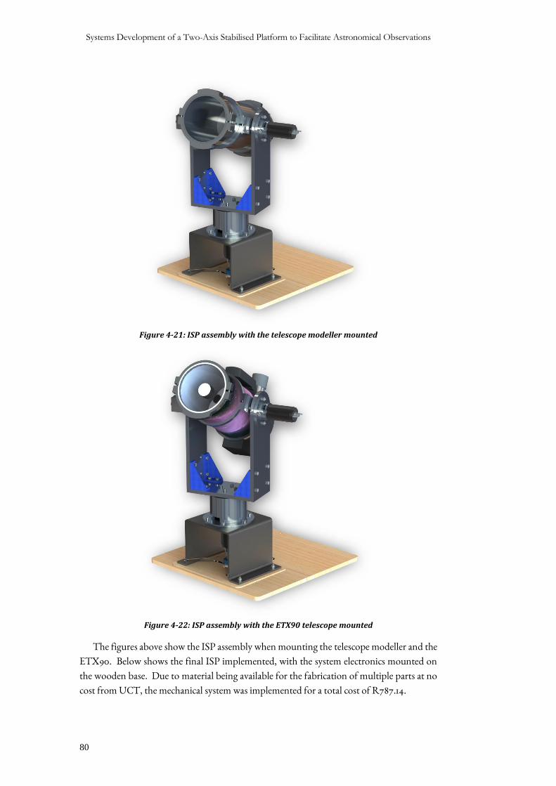
Systems Development of a Two-Axis Stabilised Platform to Facilitate Astronomical Observations
80
Figure 4-21: ISP assembly with the telescope modeller mounted
Figure 4-22: ISP assembly with the ETX90 telescope mounted
The figures above show the ISP assembly when mounting the telescope modeller and the
ETX90. Below shows the final ISP implemented, with the system electronics mounted on
the wooden base. Due to material being available for the fabrication of multiple parts at no
cost from UCT, the mechanical system was implemented for a total cost of R787.14.
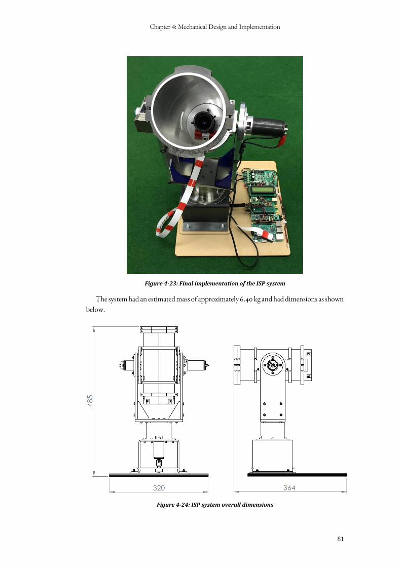
Chapter 4: Mechanical Design and Implementation
81
Figure 4-23: Final implementation of the ISP system
The system had an estimated mass of approximately 6.40 kg and had dimensions as shown
below.
Figure 4-24: ISP system overall dimensions
Systems Development of a Two-Axis Stabilised Platform to Facilitate Astronomical Observations
82
4.8 CHAPTER CONCLUSION
This chapter detailed the mechanical design of the overall system assembly. A two-axis
gimbal assembly was designed and implemented which could facilitate the accomplishment
of specifications S1, S2, S4 directly whilst contributing to the accomplishment of many of the
operational specifications and the project budget constraint of R5000.00. Ultimately prime
items I1.1 - I1.4 and I2.3 were successfully implemented. Technical drawings of all parts
designed for the implementation of the ISP system developed, including the telescope
modeller and its parts, as well as some engineering design calculations used to verify their
implementation may be found at the repository linked in Appendix B. Moving from the
mechanical design of the ISP assembly, the next chapter describes the implementation of the
electrical systems used in the project including the motors and potentiometers already
mentioned in this chapter.
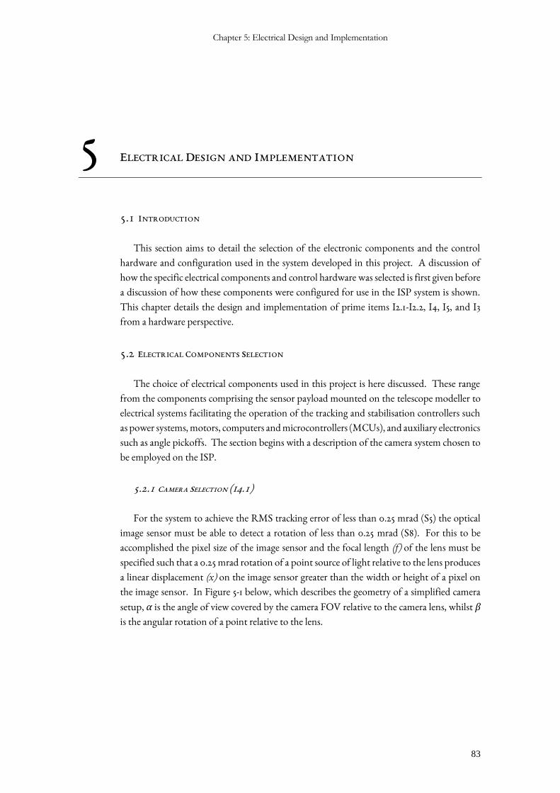
Chapter 5: Electrical Design and Implementation
83
5 ELECTRICAL DESIGN AND IMPLEMENTATION
5.1 INTRODUCTION
This section aims to detail the selection of the electronic components and the control
hardware and configuration used in the system developed in this project. A discussion of
how the specific electrical components and control hardware was selected is first given before
a discussion of how these components were configured for use in the ISP system is shown.
This chapter details the design and implementation of prime items I2.1-I2.2, I4, I5, and I3
from a hardware perspective.
5.2 ELECTRICAL COMPONENTS SELECTION
The choice of electrical components used in this project is here discussed. These range
from the components comprising the sensor payload mounted on the telescope modeller to
electrical systems facilitating the operation of the tracking and stabilisation controllers such
as power systems, motors, computers and microcontrollers (MCUs), and auxiliary electronics
such as angle pickoffs. The section begins with a description of the camera system chosen to
be employed on the ISP.
5.2.1 CAMERA SELECTION (I4.1)
For the system to achieve the RMS tracking error of less than 0.25 mrad (S5) the optical
image sensor must be able to detect a rotation of less than 0.25 mrad (S8). For this to be
accomplished the pixel size of the image sensor and the focal length (f) of the lens must be
specified such that a 0.25 mrad rotation of a point source of light relative to the lens produces
a linear displacement (x) on the image sensor greater than the width or height of a pixel on
the image sensor. In Figure 5-1 below, which describes the geometry of a simplified camera
setup, α is the angle of view covered by the camera FOV relative to the camera lens, whilst β
is the angular rotation of a point relative to the lens.
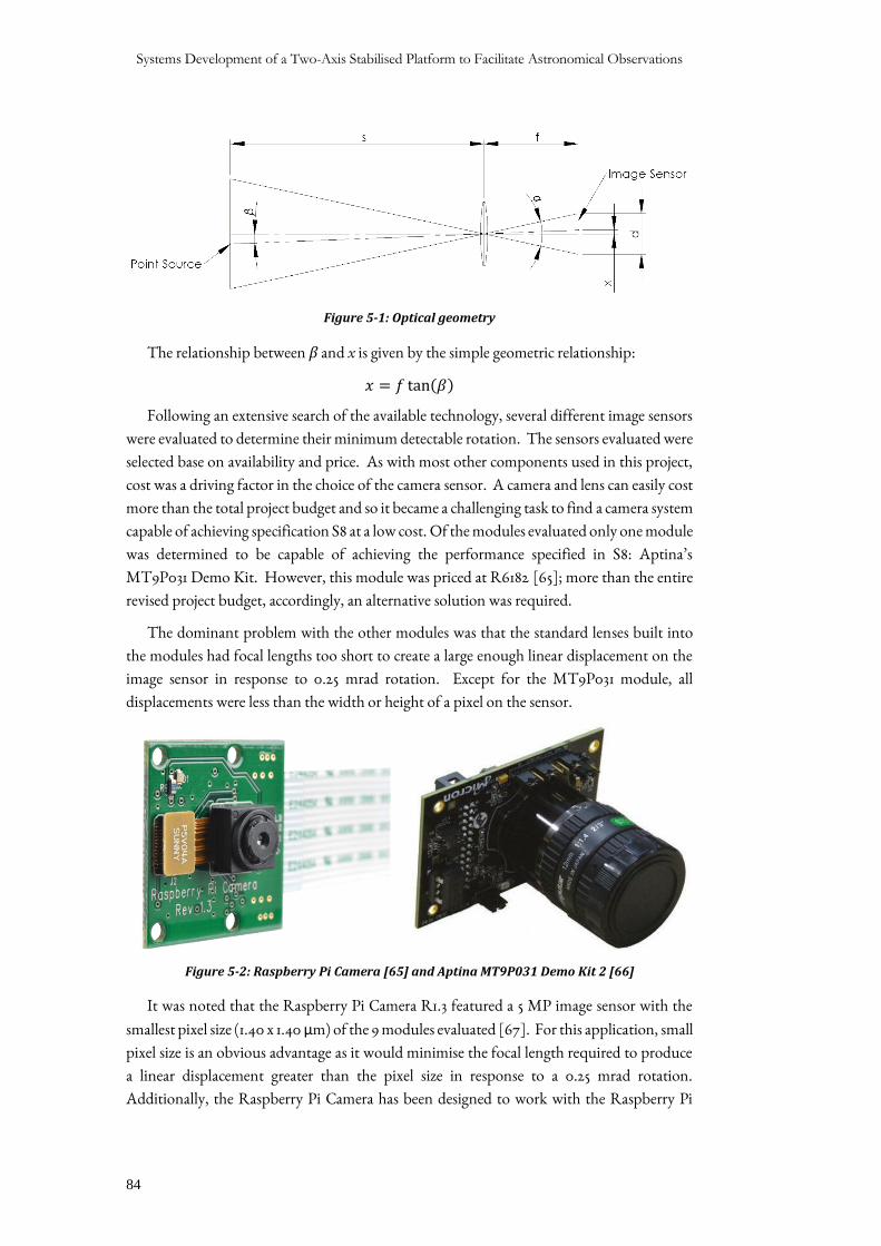
Systems Development of a Two-Axis Stabilised Platform to Facilitate Astronomical Observations
84
Figure 5-1: Optical geometry
The relationship between β and x is given by the simple geometric relationship:
𝑥 = 𝑓 tan(𝛽)
Following an extensive search of the available technology, several different image sensors
were evaluated to determine their minimum detectable rotation. The sensors evaluated were
selected base on availability and price. As with most other components used in this project,
cost was a driving factor in the choice of the camera sensor. A camera and lens can easily cost
more than the total project budget and so it became a challenging task to find a camera system
capable of achieving specification S8 at a low cost. Of the modules evaluated only one module
was determined to be capable of achieving the performance specified in S8: Aptina’s
MT9P031 Demo Kit. However, this module was priced at R6182 [65]; more than the entire
revised project budget, accordingly, an alternative solution was required.
The dominant problem with the other modules was that the standard lenses built into
the modules had focal lengths too short to create a large enough linear displacement on the
image sensor in response to 0.25 mrad rotation. Except for the MT9P031 module, all
displacements were less than the width or height of a pixel on the sensor.
Figure 5-2: Raspberry Pi Camera [65] and Aptina MT9P031 Demo Kit 2 [66]
It was noted that the Raspberry Pi Camera R1.3 featured a 5 MP image sensor with the
smallest pixel size (1.40 x 1.40 µm) of the 9 modules evaluated [67]. For this application, small
pixel size is an obvious advantage as it would minimise the focal length required to produce
a linear displacement greater than the pixel size in response to a 0.25 mrad rotation.
Additionally, the Raspberry Pi Camera has been designed to work with the Raspberry Pi
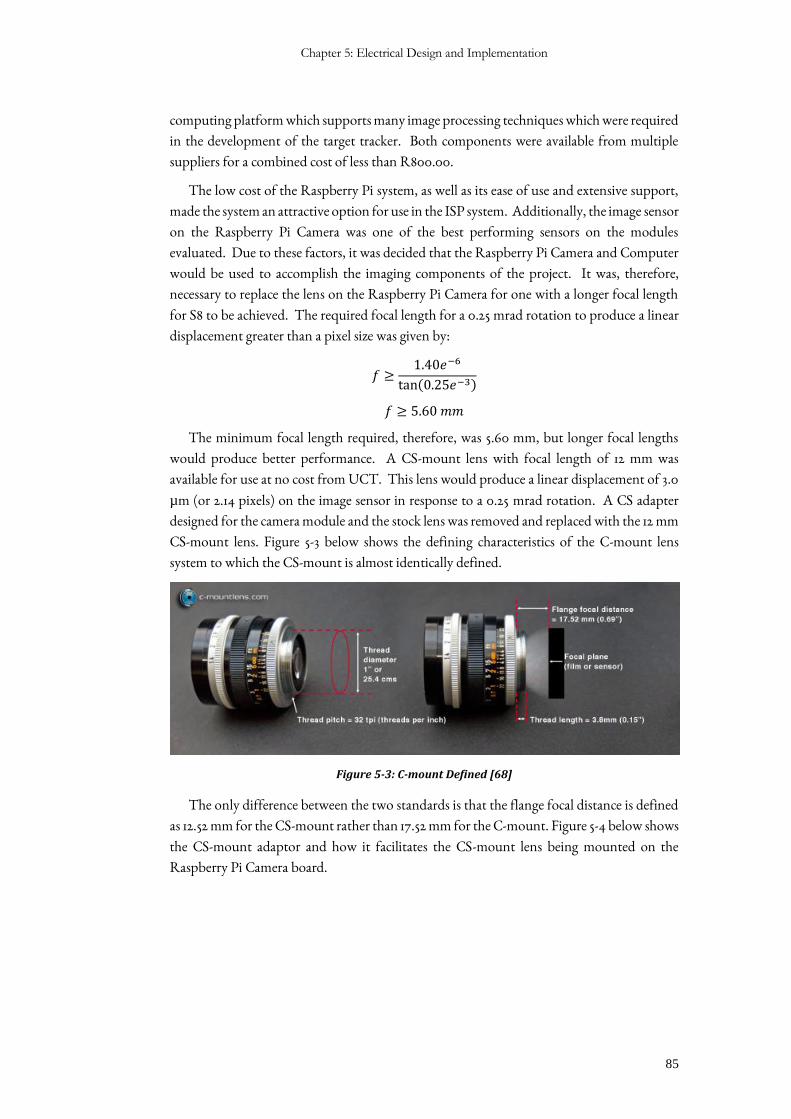
Chapter 5: Electrical Design and Implementation
85
computing platform which supports many image processing techniques which were required
in the development of the target tracker. Both components were available from multiple
suppliers for a combined cost of less than R800.00.
The low cost of the Raspberry Pi system, as well as its ease of use and extensive support,
made the system an attractive option for use in the ISP system. Additionally, the image sensor
on the Raspberry Pi Camera was one of the best performing sensors on the modules
evaluated. Due to these factors, it was decided that the Raspberry Pi Camera and Computer
would be used to accomplish the imaging components of the project. It was, therefore,
necessary to replace the lens on the Raspberry Pi Camera for one with a longer focal length
for S8 to be achieved. The required focal length for a 0.25 mrad rotation to produce a linear
displacement greater than a pixel size was given by:
𝑓 ≥1.40𝑒−6
tan(0.25𝑒−3)
𝑓 ≥ 5.60 𝑚𝑚
The minimum focal length required, therefore, was 5.60 mm, but longer focal lengths
would produce better performance. A CS-mount lens with focal length of 12 mm was
available for use at no cost from UCT. This lens would produce a linear displacement of 3.0
µm (or 2.14 pixels) on the image sensor in response to a 0.25 mrad rotation. A CS adapter
designed for the camera module and the stock lens was removed and replaced with the 12 mm
CS-mount lens. Figure 5-3 below shows the defining characteristics of the C-mount lens
system to which the CS-mount is almost identically defined.
Figure 5-3: C-mount Defined [68]
The only difference between the two standards is that the flange focal distance is defined
as 12.52 mm for the CS-mount rather than 17.52 mm for the C-mount. Figure 5-4 below shows
the CS-mount adaptor and how it facilitates the CS-mount lens being mounted on the
Raspberry Pi Camera board.
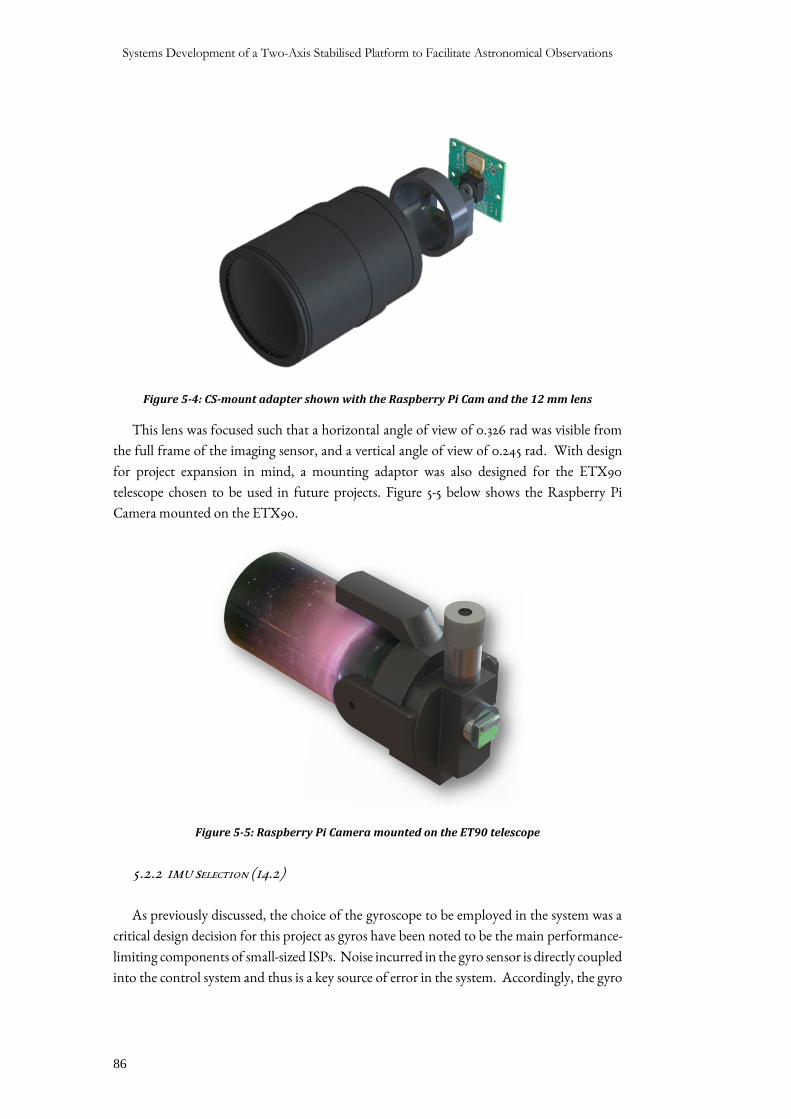
Systems Development of a Two-Axis Stabilised Platform to Facilitate Astronomical Observations
86
Figure 5-4: CS-mount adapter shown with the Raspberry Pi Cam and the 12 mm lens
This lens was focused such that a horizontal angle of view of 0.326 rad was visible from
the full frame of the imaging sensor, and a vertical angle of view of 0.245 rad. With design
for project expansion in mind, a mounting adaptor was also designed for the ETX90
telescope chosen to be used in future projects. Figure 5-5 below shows the Raspberry Pi
Camera mounted on the ETX90.
Figure 5-5: Raspberry Pi Camera mounted on the ET90 telescope
5.2.2 IMU SELECTION (I4.2)
As previously discussed, the choice of the gyroscope to be employed in the system was a
critical design decision for this project as gyros have been noted to be the main performance-
limiting components of small-sized ISPs. Noise incurred in the gyro sensor is directly coupled
into the control system and thus is a key source of error in the system. Accordingly, the gyro
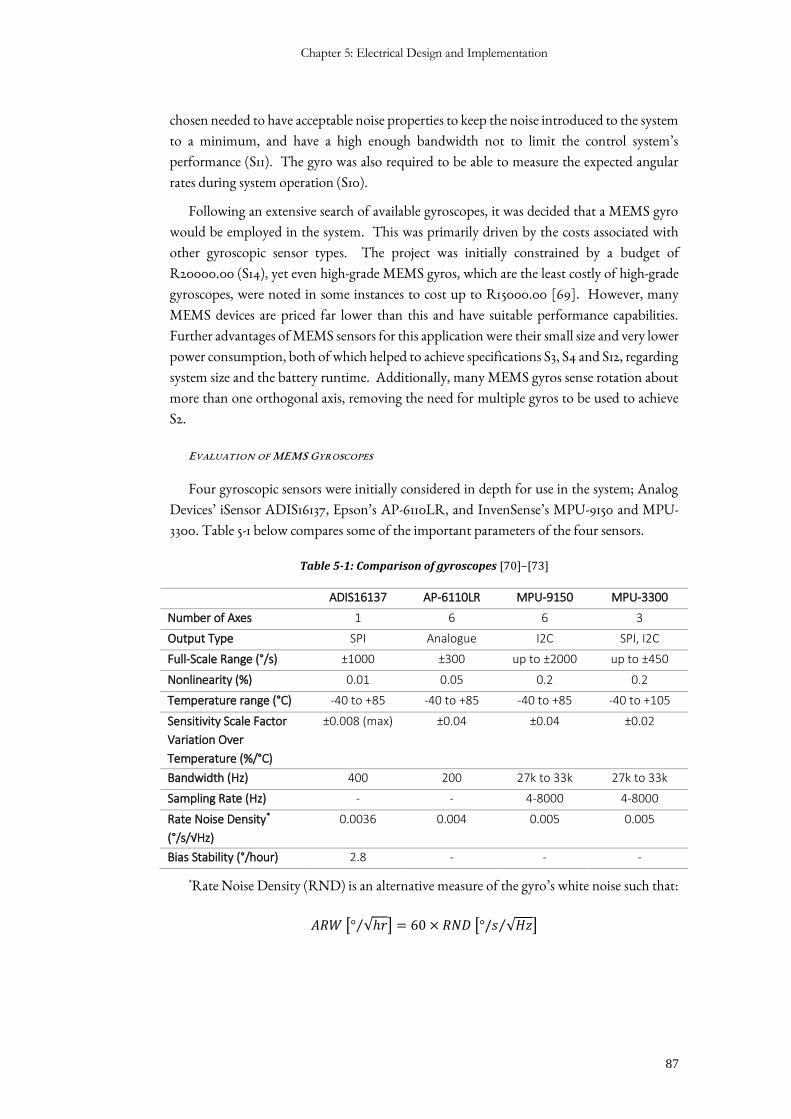
Chapter 5: Electrical Design and Implementation
87
chosen needed to have acceptable noise properties to keep the noise introduced to the system
to a minimum, and have a high enough bandwidth not to limit the control system’s
performance (S11). The gyro was also required to be able to measure the expected angular
rates during system operation (S10).
Following an extensive search of available gyroscopes, it was decided that a MEMS gyro
would be employed in the system. This was primarily driven by the costs associated with
other gyroscopic sensor types. The project was initially constrained by a budget of
R20000.00 (S14), yet even high-grade MEMS gyros, which are the least costly of high-grade
gyroscopes, were noted in some instances to cost up to R15000.00 [69]. However, many
MEMS devices are priced far lower than this and have suitable performance capabilities.
Further advantages of MEMS sensors for this application were their small size and very lower
power consumption, both of which helped to achieve specifications S3, S4 and S12, regarding
system size and the battery runtime. Additionally, many MEMS gyros sense rotation about
more than one orthogonal axis, removing the need for multiple gyros to be used to achieve
S2.
EVALUATION OF MEMS GYROSCOPES
Four gyroscopic sensors were initially considered in depth for use in the system; Analog
Devices’ iSensor ADIS16137, Epson’s AP-6110LR, and InvenSense’s MPU-9150 and MPU-
3300. Table 5-1 below compares some of the important parameters of the four sensors.
Table 5-1: Comparison of gyroscopes [70]–[73]
ADIS16137 AP-6110LR MPU-9150 MPU-3300
Number of Axes 1 6 6 3
Output Type SPI Analogue I2C SPI, I2C
Full-Scale Range (°/s) ±1000 ±300 up to ±2000 up to ±450
Nonlinearity (%) 0.01 0.05 0.2 0.2
Temperature range (°C) -40 to +85 -40 to +85 -40 to +85 -40 to +105
Sensitivity Scale Factor
Variation Over
Temperature (%/°C)
±0.008 (max) ±0.04 ±0.04 ±0.02
Bandwidth (Hz) 400 200 27k to 33k 27k to 33k
Sampling Rate (Hz) - - 4-8000 4-8000
Rate Noise Density*
(°/s/√Hz)
0.0036 0.004 0.005 0.005
Bias Stability (°/hour) 2.8 - - -
*Rate Noise Density (RND) is an alternative measure of the gyro’s white noise such that:
𝐴𝑅𝑊 [° √ℎ𝑟⁄ ] = 60 × 𝑅𝑁𝐷 [°/𝑠 √𝐻𝑧⁄ ]
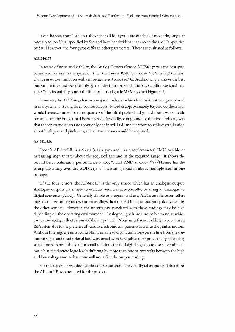
Systems Development of a Two-Axis Stabilised Platform to Facilitate Astronomical Observations
88
It can be seen from Table 5-1 above that all four gyros are capable of measuring angular
rates up to 100 °/s as specified by S10 and have bandwidths that exceed the 120 Hz specified
by S11. However, the four gyros differ in other parameters. These are evaluated as follows.
ADIS16137
In terms of noise and stability, the Analog Devices iSensor ADIS16137 was the best gyro
considered for use in the system. It has the lowest RND at 0.0036 °/s/√Hz and the least
change in output variation with temperature at ±0.008 %/°C. Additionally, it shows the best
output linearity and was the only gyro of the four for which the bias stability was specified;
at 2.8 °/hr, its stability is near the limit of tactical grade MEMS gyros (Figure 2-8).
However, the ADIS16137 has two major drawbacks which lead to it not being employed
in this system. First and foremost was its cost. Priced at approximately R15000.00 the sensor
would have accounted for three-quarters of the initial project budget and clearly was suitable
for use once the budget had been revised. Secondly, compounding the first problem, was
that the sensor measures rate about only one inertial axis and therefore to achieve stabilisation
about both yaw and pitch axes, at least two sensors would be required.
AP-6110LR
Epson’s AP-6110LR is a 6-axis (3-axis gyro and 3-axis accelerometer) IMU capable of
measuring angular rates about the required axis and in the required range. It shows the
second-best nonlinearity performance at 0.05 % and RND at 0.004 °/s/√Hz and has the
strong advantage over the ADIS16137 of measuring rotation about multiple axes in one
package.
Of the four sensors, the AP-6110LR is the only sensor which has an analogue output.
Analogue outputs are simple to evaluate with a microcontroller by using an analogue to
digital converter (ADC). Generally simple to program and use, ADCs on microcontrollers
may also allow for higher resolution readings than the 16-bit digital output typically used by
the other sensors. However, the uncertainty associated with these readings may be high
depending on the operating environment. Analogue signals are susceptible to noise which
causes low voltages fluctuations of the output line. Noise interference is likely to occur in an
ISP system due to the presence of various electronic components as well as the gimbal motors.
Without filtering, the microcontroller is unable to distinguish noise on the line from the true
output signal and so additional hardware or software is required to improve the signal quality
so that noise is not mistaken for small rotation effects. Digital signals are also susceptible to
noise but the discrete logic levels differing by more than one or two volts between the high
and low voltages mean that noise will not affect the output reading.
For this reason, it was decided that the sensor should have a digital output and therefore,
the AP-6110LR was not used for the project.
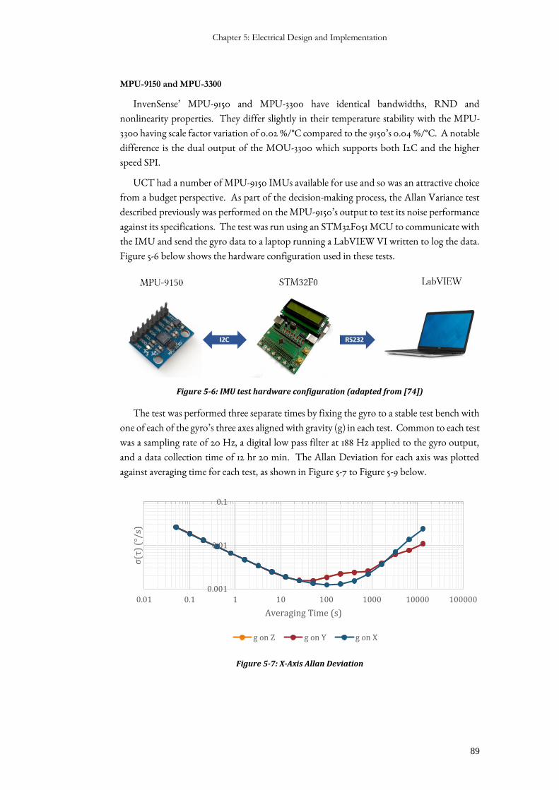
Chapter 5: Electrical Design and Implementation
89
MPU-9150 and MPU-3300
InvenSense’ MPU-9150 and MPU-3300 have identical bandwidths, RND and
nonlinearity properties. They differ slightly in their temperature stability with the MPU-
3300 having scale factor variation of 0.02 %/°C compared to the 9150’s 0.04 %/°C. A notable
difference is the dual output of the MOU-3300 which supports both I2C and the higher
speed SPI.
UCT had a number of MPU-9150 IMUs available for use and so was an attractive choice
from a budget perspective. As part of the decision-making process, the Allan Variance test
described previously was performed on the MPU-9150’s output to test its noise performance
against its specifications. The test was run using an STM32F051 MCU to communicate with
the IMU and send the gyro data to a laptop running a LabVIEW VI written to log the data.
Figure 5-6 below shows the hardware configuration used in these tests.
Figure 5-6: IMU test hardware configuration (adapted from [74])
The test was performed three separate times by fixing the gyro to a stable test bench with
one of each of the gyro’s three axes aligned with gravity (g) in each test. Common to each test
was a sampling rate of 20 Hz, a digital low pass filter at 188 Hz applied to the gyro output,
and a data collection time of 12 hr 20 min. The Allan Deviation for each axis was plotted
against averaging time for each test, as shown in Figure 5-7 to Figure 5-9 below.
Figure 5-7: X-Axis Allan Deviation
0.001
0.01
0.1
0.01 0.1 1 10 100 1000 10000 100000
σ(τ
) (°
/s)
Averaging Time (s)
g on Z g on Y g on X
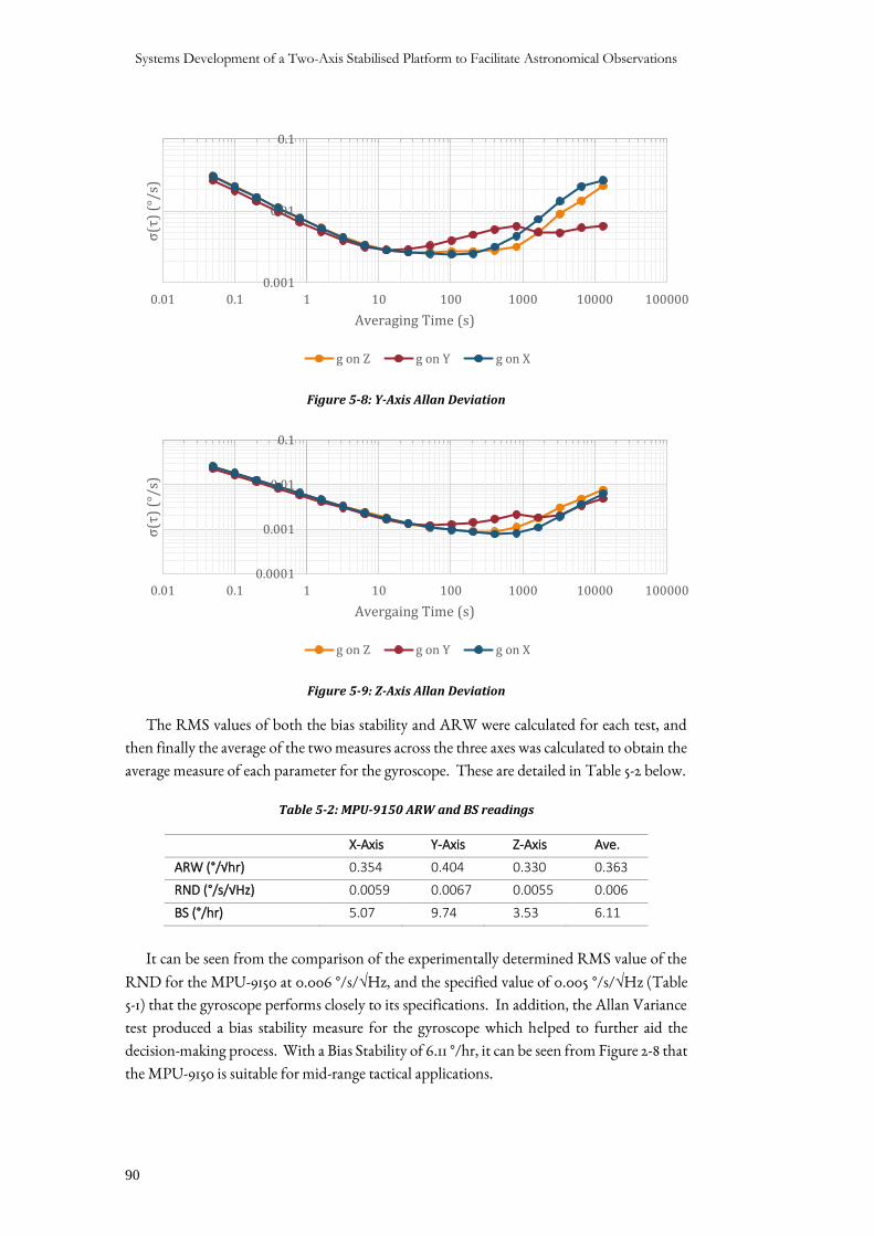
Systems Development of a Two-Axis Stabilised Platform to Facilitate Astronomical Observations
90
Figure 5-8: Y-Axis Allan Deviation
Figure 5-9: Z-Axis Allan Deviation
The RMS values of both the bias stability and ARW were calculated for each test, and
then finally the average of the two measures across the three axes was calculated to obtain the
average measure of each parameter for the gyroscope. These are detailed in Table 5-2 below.
Table 5-2: MPU-9150 ARW and BS readings
X-Axis Y-Axis Z-Axis Ave.
ARW (°/√hr) 0.354 0.404 0.330 0.363
RND (°/s/√Hz) 0.0059 0.0067 0.0055 0.006
BS (°/hr) 5.07 9.74 3.53 6.11
It can be seen from the comparison of the experimentally determined RMS value of the
RND for the MPU-9150 at 0.006 °/s/√Hz, and the specified value of 0.005 °/s/√Hz (Table
5-1) that the gyroscope performs closely to its specifications. In addition, the Allan Variance
test produced a bias stability measure for the gyroscope which helped to further aid the
decision-making process. With a Bias Stability of 6.11 °/hr, it can be seen from Figure 2-8 that
the MPU-9150 is suitable for mid-range tactical applications.
0.001
0.01
0.1
0.01 0.1 1 10 100 1000 10000 100000
σ(τ
) (°
/s)
Averaging Time (s)
g on Z g on Y g on X
0.0001
0.001
0.01
0.1
0.01 0.1 1 10 100 1000 10000 100000
σ(τ
) (°
/s)
Avergaing Time (s)
g on Z g on Y g on X
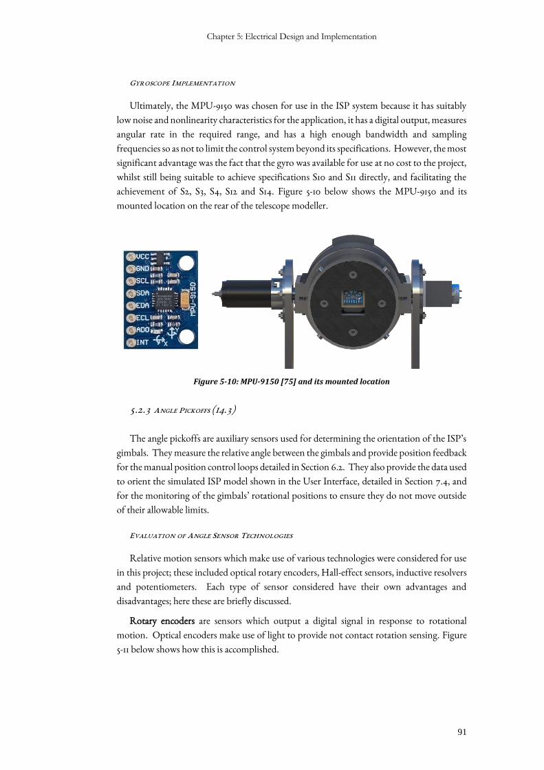
Chapter 5: Electrical Design and Implementation
91
GYROSCOPE IMPLEMENTATION
Ultimately, the MPU-9150 was chosen for use in the ISP system because it has suitably
low noise and nonlinearity characteristics for the application, it has a digital output, measures
angular rate in the required range, and has a high enough bandwidth and sampling
frequencies so as not to limit the control system beyond its specifications. However, the most
significant advantage was the fact that the gyro was available for use at no cost to the project,
whilst still being suitable to achieve specifications S10 and S11 directly, and facilitating the
achievement of S2, S3, S4, S12 and S14. Figure 5-10 below shows the MPU-9150 and its
mounted location on the rear of the telescope modeller.
Figure 5-10: MPU-9150 [75] and its mounted location
5.2.3 ANGLE PICKOFFS (I4.3)
The angle pickoffs are auxiliary sensors used for determining the orientation of the ISP’s
gimbals. They measure the relative angle between the gimbals and provide position feedback
for the manual position control loops detailed in Section 6.2. They also provide the data used
to orient the simulated ISP model shown in the User Interface, detailed in Section 7.4, and
for the monitoring of the gimbals’ rotational positions to ensure they do not move outside
of their allowable limits.
EVALUATION OF ANGLE SENSOR TECHNOLOGIES
Relative motion sensors which make use of various technologies were considered for use
in this project; these included optical rotary encoders, Hall-effect sensors, inductive resolvers
and potentiometers. Each type of sensor considered have their own advantages and
disadvantages; here these are briefly discussed.
Rotary encoders are sensors which output a digital signal in response to rotational
motion. Optical encoders make use of light to provide not contact rotation sensing. Figure
5-11 below shows how this is accomplished.
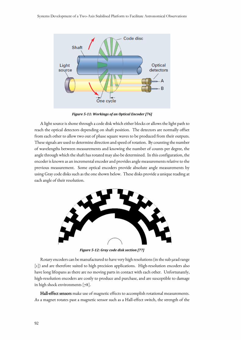
Systems Development of a Two-Axis Stabilised Platform to Facilitate Astronomical Observations
92
Figure 5-11: Workings of an Optical Encoder [76]
A light source is shone through a code disk which either blocks or allows the light path to
reach the optical detectors depending on shaft position. The detectors are normally offset
from each other to allow two out of phase square waves to be produced from their outputs.
These signals are used to determine direction and speed of rotation. By counting the number
of wavelengths between measurements and knowing the number of counts per degree, the
angle through which the shaft has rotated may also be determined. In this configuration, the
encoder is known as an incremental encoder and provides angle measurements relative to the
previous measurement. Some optical encoders provide absolute angle measurements by
using Gray code disks such as the one shown below. These disks provide a unique reading at
each angle of their resolution.
Figure 5-12: Gray code disk section [77]
Rotary encoders can be manufactured to have very high resolutions (in the sub µrad range
[1]) and are therefore suited to high precision applications. High-resolution encoders also
have long lifespans as there are no moving parts in contact with each other. Unfortunately,
high-resolution encoders are costly to produce and purchase, and are susceptible to damage
in high shock environments [78].
Hall-effect sensors make use of magnetic effects to accomplish rotational measurements.
As a magnet rotates past a magnetic sensor such as a Hall-effect switch, the strength of the
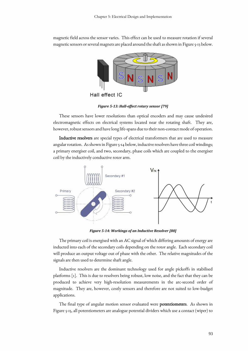
Chapter 5: Electrical Design and Implementation
93
magnetic field across the sensor varies. This effect can be used to measure rotation if several
magnetic sensors or several magnets are placed around the shaft as shown in Figure 5-13 below.
Figure 5-13: Hall-effect rotary sensor [79]
These sensors have lower resolutions than optical encoders and may cause undesired
electromagnetic effects on electrical systems located near the rotating shaft. They are,
however, robust sensors and have long life-spans due to their non-contact mode of operation.
Inductive resolvers are special types of electrical transformers that are used to measure
angular rotation. As shown in Figure 5-14 below, inductive resolvers have three coil windings;
a primary energiser coil, and two, secondary, phase coils which are coupled to the energiser
coil by the inductively conductive rotor arm.
Figure 5-14: Workings of an Inductive Resolver [80]
The primary coil is energised with an AC signal of which differing amounts of energy are
inducted into each of the secondary coils depending on the rotor angle. Each secondary coil
will produce an output voltage out of phase with the other. The relative magnitudes of the
signals are then used to determine shaft angle.
Inductive resolvers are the dominant technology used for angle pickoffs in stabilised
platforms [1]. This is due to resolvers being robust, low noise, and the fact that they can be
produced to achieve very high-resolution measurements in the arc-second order of
magnitude. They are, however, costly sensors and therefore are not suited to low-budget
applications.
The final type of angular motion sensor evaluated were potentiometers. As shown in
Figure 5-15, all potentiometers are analogue potential dividers which use a contact (wiper) to
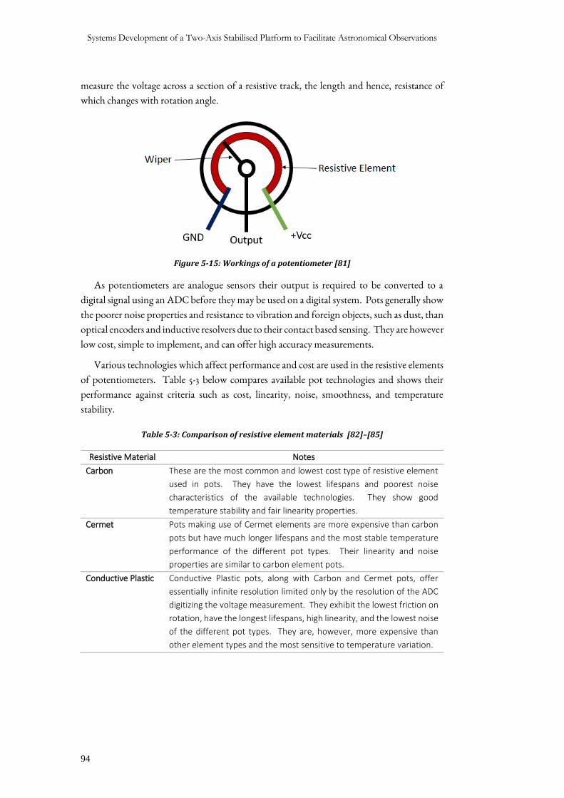
Systems Development of a Two-Axis Stabilised Platform to Facilitate Astronomical Observations
94
measure the voltage across a section of a resistive track, the length and hence, resistance of
which changes with rotation angle.
Figure 5-15: Workings of a potentiometer [81]
As potentiometers are analogue sensors their output is required to be converted to a
digital signal using an ADC before they may be used on a digital system. Pots generally show
the poorer noise properties and resistance to vibration and foreign objects, such as dust, than
optical encoders and inductive resolvers due to their contact based sensing. They are however
low cost, simple to implement, and can offer high accuracy measurements.
Various technologies which affect performance and cost are used in the resistive elements
of potentiometers. Table 5-3 below compares available pot technologies and shows their
performance against criteria such as cost, linearity, noise, smoothness, and temperature
stability.
Table 5-3: Comparison of resistive element materials [82]–[85]
Resistive Material Notes
Carbon These are the most common and lowest cost type of resistive element
used in pots. They have the lowest lifespans and poorest noise
characteristics of the available technologies. They show good
temperature stability and fair linearity properties.
Cermet Pots making use of Cermet elements are more expensive than carbon
pots but have much longer lifespans and the most stable temperature
performance of the different pot types. Their linearity and noise
properties are similar to carbon element pots.
Conductive Plastic Conductive Plastic pots, along with Carbon and Cermet pots, offer
essentially infinite resolution limited only by the resolution of the ADC
digitizing the voltage measurement. They exhibit the lowest friction on
rotation, have the longest lifespans, high linearity, and the lowest noise
of the different pot types. They are, however, more expensive than
other element types and the most sensitive to temperature variation.
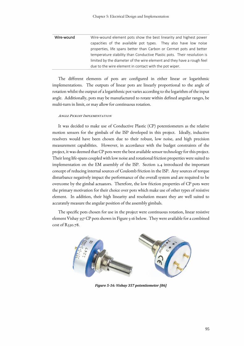
Chapter 5: Electrical Design and Implementation
95
Wire-wound Wire-wound element pots show the best linearity and highest power
capacities of the available pot types. They also have low noise
properties, life spans better than Carbon or Cermet pots and better
temperature stability than Conductive Plastic pots. Their resolution is
limited by the diameter of the wire element and they have a rough feel
due to the wire element in contact with the pot wiper.
The different elements of pots are configured in either linear or logarithmic
implementations. The outputs of linear pots are linearly proportional to the angle of
rotation whilst the output of a logarithmic pot varies according to the logarithm of the input
angle. Additionally, pots may be manufactured to rotate within defined angular ranges, be
multi-turn in limit, or may allow for continuous rotation.
ANGLE PICKOFF IMPLEMENTATION
It was decided to make use of Conductive Plastic (CP) potentiometers as the relative
motion sensors for the gimbals of the ISP developed in this project. Ideally, inductive
resolvers would have been chosen due to their robust, low noise, and high precision
measurement capabilities. However, in accordance with the budget constraints of the
project, it was deemed that CP pots were the best available sensor technology for this project.
Their long life-spans coupled with low noise and rotational friction properties were suited to
implementation on the EM assembly of the ISP. Section 2.4 introduced the important
concept of reducing internal sources of Coulomb friction in the ISP. Any sources of torque
disturbance negatively impact the performance of the overall system and are required to be
overcome by the gimbal actuators. Therefore, the low friction properties of CP pots were
the primary motivation for their choice over pots which make use of other types of resistive
element. In addition, their high linearity and resolution meant they are well suited to
accurately measure the angular position of the assembly gimbals.
The specific pots chosen for use in the project were continuous rotation, linear resistive
element Vishay 357 CP pots shown in Figure 5-16 below. They were available for a combined
cost of R530.78.
Figure 5-16: Vishay 357 potentiometer [86]
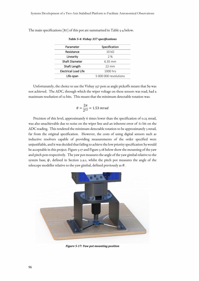
Systems Development of a Two-Axis Stabilised Platform to Facilitate Astronomical Observations
96
The main specifications [87] of this pot are summarised in Table 5-4 below.
Table 5-4: Vishay 357 specifications
Parameter Specification
Resistance 10 kΩ
Linearity 2 %
Shaft Diameter 6.35 mm
Shaft Length 22 mm
Electrical Load Life 1000 hrs
Life-span 5 000 000 revolutions
Unfortunately, the choice to use the Vishay 357 pots as angle pickoffs meant that S9 was
not achieved. The ADC, through which the wiper voltage on these sensors was read, had a
maximum resolution of 12-bits. This meant that the minimum detectable rotation was:
𝜃 =2𝜋
212= 1.53 𝑚𝑟𝑎𝑑
Precision of this level, approximately 6 times lower than the specification of 0.25 mrad,
was also unachievable due to noise on the wiper line and an inherent error of ±1 bit on the
ADC reading. This rendered the minimum detectable rotation to be approximately 3 mrad,
far from the original specification. However, the costs of using digital sensors such as
inductive resolvers capable of providing measurements of the order specified were
unjustifiable, and it was decided that failing to achieve the low priority specification S9 would
be acceptable in this project. Figure 5-17 and Figure 5-18 below show the mounting of the yaw
and pitch pots respectively. The yaw pot measures the angle of the yaw gimbal relative to the
system base, 𝜓 , defined in Section 2.9.1, whilst the pitch pot measures the angle of the
telescope modeller relative to the yaw gimbal, defined previously as 𝜃.
Figure 5-17: Yaw pot mounting position
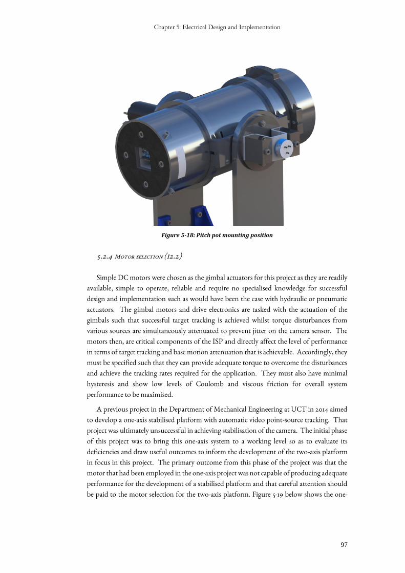
Chapter 5: Electrical Design and Implementation
97
Figure 5-18: Pitch pot mounting position
5.2.4 MOTOR SELECTION (I2.2)
Simple DC motors were chosen as the gimbal actuators for this project as they are readily
available, simple to operate, reliable and require no specialised knowledge for successful
design and implementation such as would have been the case with hydraulic or pneumatic
actuators. The gimbal motors and drive electronics are tasked with the actuation of the
gimbals such that successful target tracking is achieved whilst torque disturbances from
various sources are simultaneously attenuated to prevent jitter on the camera sensor. The
motors then, are critical components of the ISP and directly affect the level of performance
in terms of target tracking and base motion attenuation that is achievable. Accordingly, they
must be specified such that they can provide adequate torque to overcome the disturbances
and achieve the tracking rates required for the application. They must also have minimal
hysteresis and show low levels of Coulomb and viscous friction for overall system
performance to be maximised.
A previous project in the Department of Mechanical Engineering at UCT in 2014 aimed
to develop a one-axis stabilised platform with automatic video point-source tracking. That
project was ultimately unsuccessful in achieving stabilisation of the camera. The initial phase
of this project was to bring this one-axis system to a working level so as to evaluate its
deficiencies and draw useful outcomes to inform the development of the two-axis platform
in focus in this project. The primary outcome from this phase of the project was that the
motor that had been employed in the one-axis project was not capable of producing adequate
performance for the development of a stabilised platform and that careful attention should
be paid to the motor selection for the two-axis platform. Figure 5-19 below shows the one-
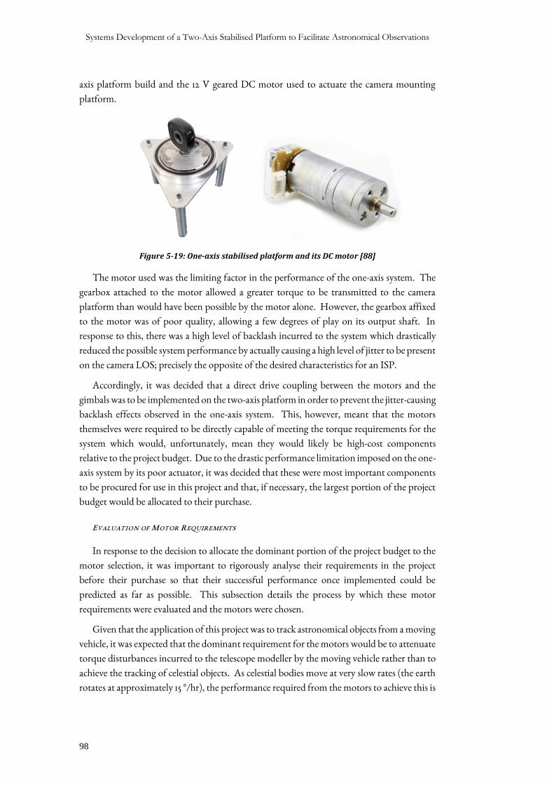
Systems Development of a Two-Axis Stabilised Platform to Facilitate Astronomical Observations
98
axis platform build and the 12 V geared DC motor used to actuate the camera mounting
platform.
Figure 5-19: One-axis stabilised platform and its DC motor [88]
The motor used was the limiting factor in the performance of the one-axis system. The
gearbox attached to the motor allowed a greater torque to be transmitted to the camera
platform than would have been possible by the motor alone. However, the gearbox affixed
to the motor was of poor quality, allowing a few degrees of play on its output shaft. In
response to this, there was a high level of backlash incurred to the system which drastically
reduced the possible system performance by actually causing a high level of jitter to be present
on the camera LOS; precisely the opposite of the desired characteristics for an ISP.
Accordingly, it was decided that a direct drive coupling between the motors and the
gimbals was to be implemented on the two-axis platform in order to prevent the jitter-causing
backlash effects observed in the one-axis system. This, however, meant that the motors
themselves were required to be directly capable of meeting the torque requirements for the
system which would, unfortunately, mean they would likely be high-cost components
relative to the project budget. Due to the drastic performance limitation imposed on the one-
axis system by its poor actuator, it was decided that these were most important components
to be procured for use in this project and that, if necessary, the largest portion of the project
budget would be allocated to their purchase.
EVALUATION OF MOTOR REQUIREMENTS
In response to the decision to allocate the dominant portion of the project budget to the
motor selection, it was important to rigorously analyse their requirements in the project
before their purchase so that their successful performance once implemented could be
predicted as far as possible. This subsection details the process by which these motor
requirements were evaluated and the motors were chosen.
Given that the application of this project was to track astronomical objects from a moving
vehicle, it was expected that the dominant requirement for the motors would be to attenuate
torque disturbances incurred to the telescope modeller by the moving vehicle rather than to
achieve the tracking of celestial objects. As celestial bodies move at very slow rates (the earth
rotates at approximately 15 °/hr), the performance required from the motors to achieve this is
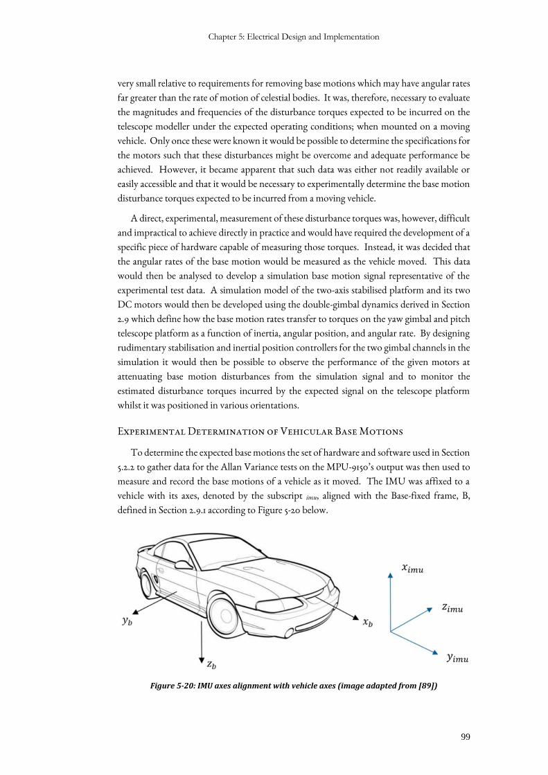
Chapter 5: Electrical Design and Implementation
99
very small relative to requirements for removing base motions which may have angular rates
far greater than the rate of motion of celestial bodies. It was, therefore, necessary to evaluate
the magnitudes and frequencies of the disturbance torques expected to be incurred on the
telescope modeller under the expected operating conditions; when mounted on a moving
vehicle. Only once these were known it would be possible to determine the specifications for
the motors such that these disturbances might be overcome and adequate performance be
achieved. However, it became apparent that such data was either not readily available or
easily accessible and that it would be necessary to experimentally determine the base motion
disturbance torques expected to be incurred from a moving vehicle.
A direct, experimental, measurement of these disturbance torques was, however, difficult
and impractical to achieve directly in practice and would have required the development of a
specific piece of hardware capable of measuring those torques. Instead, it was decided that
the angular rates of the base motion would be measured as the vehicle moved. This data
would then be analysed to develop a simulation base motion signal representative of the
experimental test data. A simulation model of the two-axis stabilised platform and its two
DC motors would then be developed using the double-gimbal dynamics derived in Section
2.9 which define how the base motion rates transfer to torques on the yaw gimbal and pitch
telescope platform as a function of inertia, angular position, and angular rate. By designing
rudimentary stabilisation and inertial position controllers for the two gimbal channels in the
simulation it would then be possible to observe the performance of the given motors at
attenuating base motion disturbances from the simulation signal and to monitor the
estimated disturbance torques incurred by the expected signal on the telescope platform
whilst it was positioned in various orientations.
Experimental Determination of Vehicular Base Motions
To determine the expected base motions the set of hardware and software used in Section
5.2.2 to gather data for the Allan Variance tests on the MPU-9150’s output was then used to
measure and record the base motions of a vehicle as it moved. The IMU was affixed to a
vehicle with its axes, denoted by the subscript imu, aligned with the Base-fixed frame, B,
defined in Section 2.9.1 according to Figure 5-20 below.
Figure 5-20: IMU axes alignment with vehicle axes (image adapted from [89])
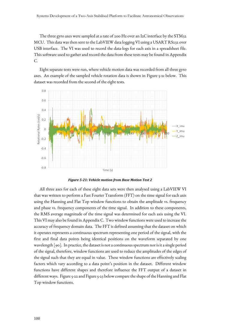
Systems Development of a Two-Axis Stabilised Platform to Facilitate Astronomical Observations
100
The three gyro axes were sampled at a rate of 200 Hz over an I2C interface by the STM32
MCU. This data was then sent to the LabVIEW data logging VI using a USART RS232 over
USB interface. The VI was used to record the data-logs for each axis in a spreadsheet file.
This software used to gather and record the data from these tests may be found in Appendix
C.
Eight separate tests were run, where vehicle motion data was recorded from all three gyro
axes. An example of the sampled vehicle rotation data is shown in Figure 5-21 below. This
dataset was recorded from the second of the eight tests.
Figure 5-21: Vehicle motion from Base Motion Test 2
All three axes for each of these eight data sets were then analysed using a LabVIEW VI
that was written to perform a Fast Fourier Transform (FFT) on the time signal for each axis
using the Hanning and Flat Top window functions to obtain the amplitude vs. frequency
and phase vs. frequency components of the time signal. In addition to these components,
the RMS average magnitude of the time signal was determined for each axis using the VI.
This VI may also be found in Appendix C. Two window functions were used to increase the
accuracy of frequency domain data. The FFT is defined assuming that the dataset on which
it operates represents a continuous spectrum representing one period of the signal, with the
first and final data points being identical positions on the waveform separated by one
wavelength [90]. In practice, the dataset is not a continuous spectrum nor is it a single period
of the signal, therefore, window functions are used to reduce the amplitudes of the edges of
the signal such that they are equal in value. These window functions are effectively scaling
factors which vary according to a data point’s position in the dataset. Different window
functions have different shapes and therefore influence the FFT output of a dataset in
different ways. Figure 5-22 and Figure 5-23 below compare the shape of the Hanning and Flat
Top window functions.
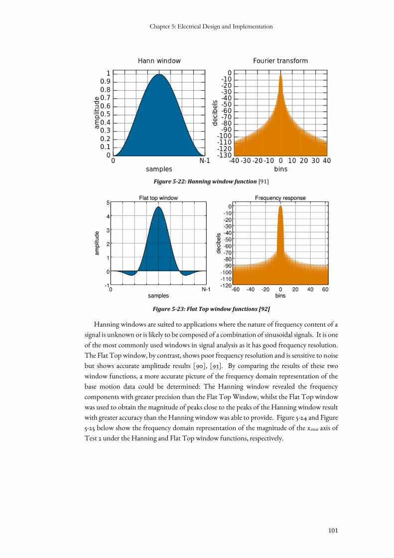
Chapter 5: Electrical Design and Implementation
101
Figure 5-22: Hanning window function [91]
Figure 5-23: Flat Top window functions [92]
Hanning windows are suited to applications where the nature of frequency content of a
signal is unknown or is likely to be composed of a combination of sinusoidal signals. It is one
of the most commonly used windows in signal analysis as it has good frequency resolution.
The Flat Top window, by contrast, shows poor frequency resolution and is sensitive to noise
but shows accurate amplitude results [90], [93]. By comparing the results of these two
window functions, a more accurate picture of the frequency domain representation of the
base motion data could be determined: The Hanning window revealed the frequency
components with greater precision than the Flat Top Window, whilst the Flat Top window
was used to obtain the magnitude of peaks close to the peaks of the Hanning window result
with greater accuracy than the Hanning window was able to provide. Figure 5-24 and Figure
5-25 below show the frequency domain representation of the magnitude of the ximu axis of
Test 2 under the Hanning and Flat Top window functions, respectively.
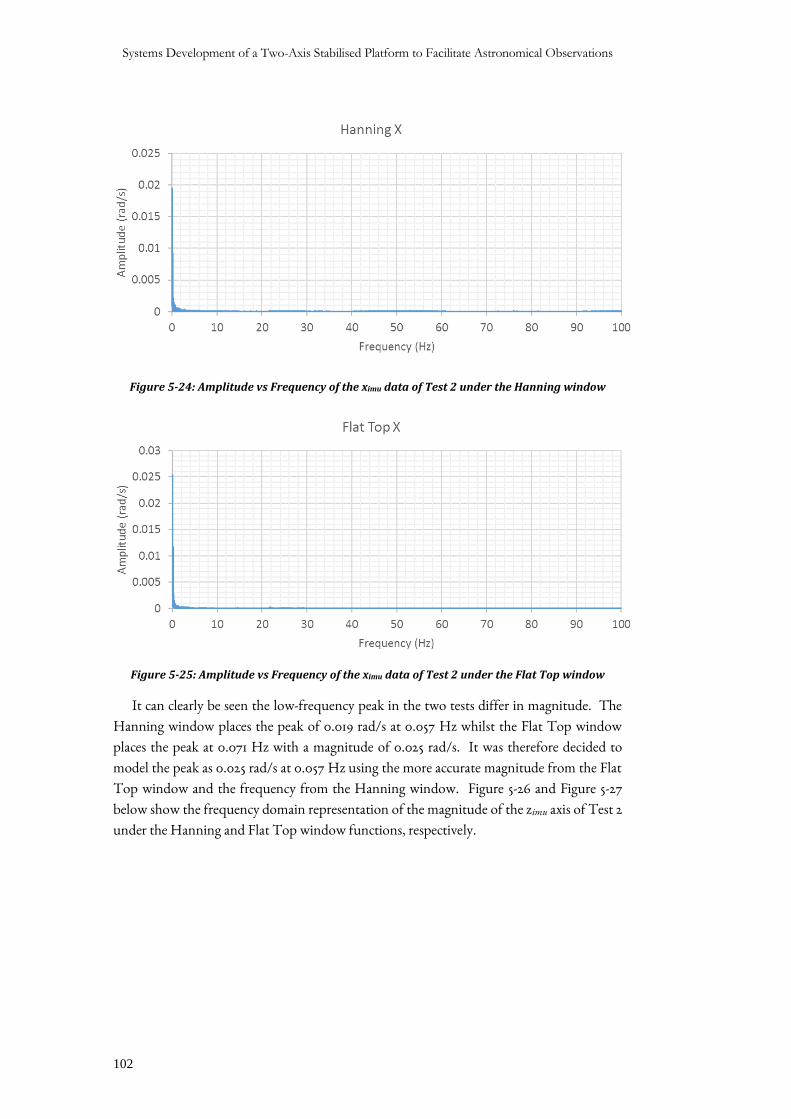
Systems Development of a Two-Axis Stabilised Platform to Facilitate Astronomical Observations
102
Figure 5-24: Amplitude vs Frequency of the ximu data of Test 2 under the Hanning window
Figure 5-25: Amplitude vs Frequency of the ximu data of Test 2 under the Flat Top window
It can clearly be seen the low-frequency peak in the two tests differ in magnitude. The
Hanning window places the peak of 0.019 rad/s at 0.057 Hz whilst the Flat Top window
places the peak at 0.071 Hz with a magnitude of 0.025 rad/s. It was therefore decided to
model the peak as 0.025 rad/s at 0.057 Hz using the more accurate magnitude from the Flat
Top window and the frequency from the Hanning window. Figure 5-26 and Figure 5-27
below show the frequency domain representation of the magnitude of the zimu axis of Test 2
under the Hanning and Flat Top window functions, respectively.
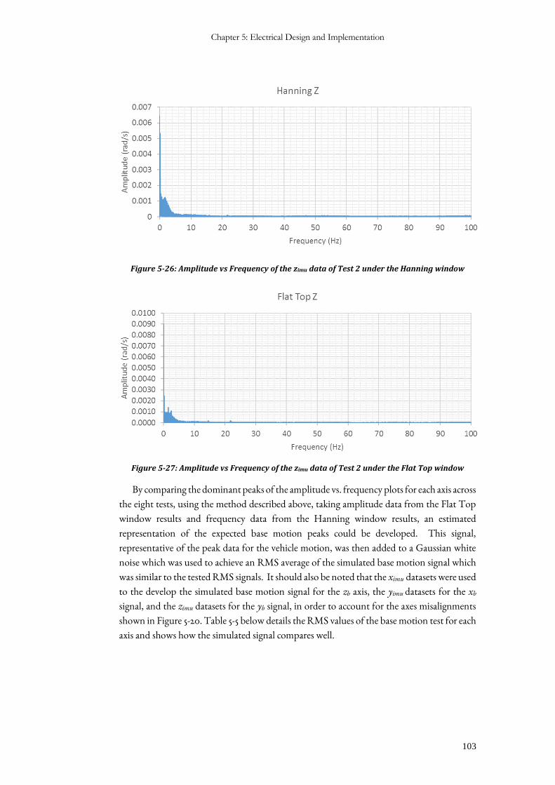
Chapter 5: Electrical Design and Implementation
103
Figure 5-26: Amplitude vs Frequency of the zimu data of Test 2 under the Hanning window
Figure 5-27: Amplitude vs Frequency of the zimu data of Test 2 under the Flat Top window
By comparing the dominant peaks of the amplitude vs. frequency plots for each axis across
the eight tests, using the method described above, taking amplitude data from the Flat Top
window results and frequency data from the Hanning window results, an estimated
representation of the expected base motion peaks could be developed. This signal,
representative of the peak data for the vehicle motion, was then added to a Gaussian white
noise which was used to achieve an RMS average of the simulated base motion signal which
was similar to the tested RMS signals. It should also be noted that the ximu datasets were used
to the develop the simulated base motion signal for the zb axis, the yimu datasets for the xb
signal, and the zimu datasets for the yb signal, in order to account for the axes misalignments
shown in Figure 5-20. Table 5-5 below details the RMS values of the base motion test for each
axis and shows how the simulated signal compares well.
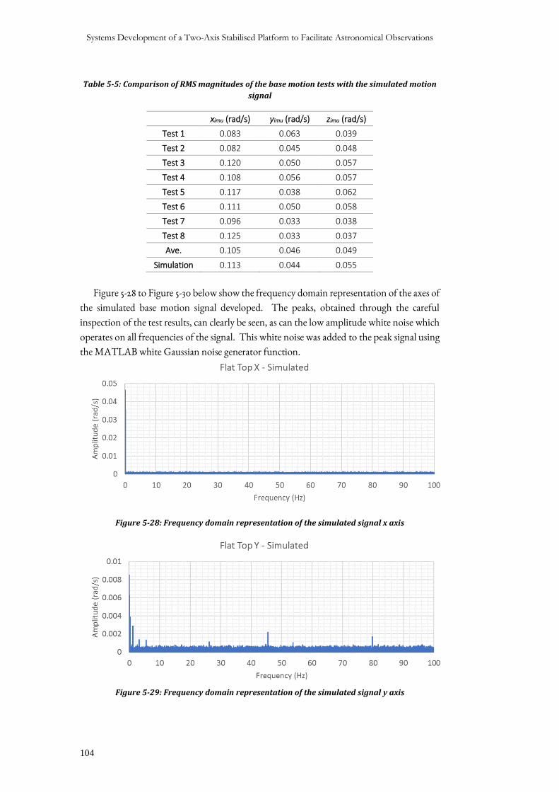
Systems Development of a Two-Axis Stabilised Platform to Facilitate Astronomical Observations
104
Table 5-5: Comparison of RMS magnitudes of the base motion tests with the simulated motion
signal
ximu (rad/s) yimu (rad/s) zimu (rad/s)
Test 1 0.083 0.063 0.039
Test 2 0.082 0.045 0.048
Test 3 0.120 0.050 0.057
Test 4 0.108 0.056 0.057
Test 5 0.117 0.038 0.062
Test 6 0.111 0.050 0.058
Test 7 0.096 0.033 0.038
Test 8 0.125 0.033 0.037
Ave. 0.105 0.046 0.049
Simulation 0.113 0.044 0.055
Figure 5-28 to Figure 5-30 below show the frequency domain representation of the axes of
the simulated base motion signal developed. The peaks, obtained through the careful
inspection of the test results, can clearly be seen, as can the low amplitude white noise which
operates on all frequencies of the signal. This white noise was added to the peak signal using
the MATLAB white Gaussian noise generator function.
Figure 5-28: Frequency domain representation of the simulated signal x axis
Figure 5-29: Frequency domain representation of the simulated signal y axis
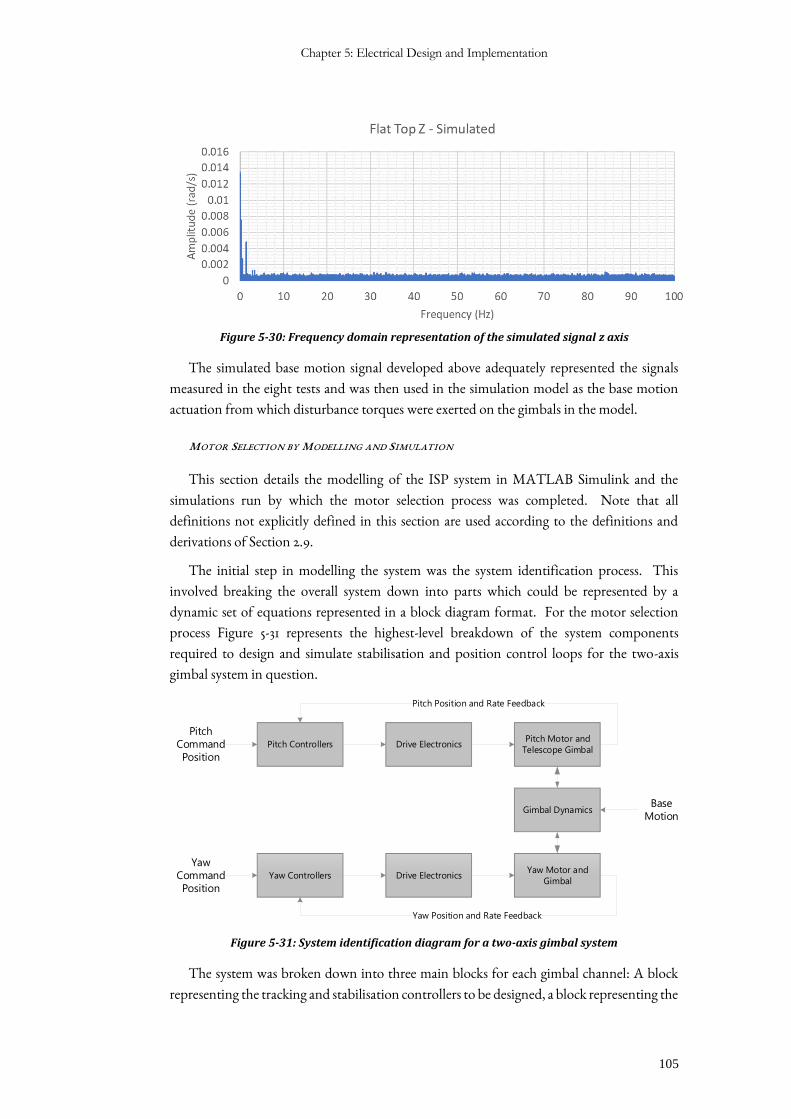
Chapter 5: Electrical Design and Implementation
105
Figure 5-30: Frequency domain representation of the simulated signal z axis
The simulated base motion signal developed above adequately represented the signals
measured in the eight tests and was then used in the simulation model as the base motion
actuation from which disturbance torques were exerted on the gimbals in the model.
MOTOR SELECTION BY MODELLING AND SIMULATION
This section details the modelling of the ISP system in MATLAB Simulink and the
simulations run by which the motor selection process was completed. Note that all
definitions not explicitly defined in this section are used according to the definitions and
derivations of Section 2.9.
The initial step in modelling the system was the system identification process. This
involved breaking the overall system down into parts which could be represented by a
dynamic set of equations represented in a block diagram format. For the motor selection
process Figure 5-31 represents the highest-level breakdown of the system components
required to design and simulate stabilisation and position control loops for the two-axis
gimbal system in question.
Gimbal Dynamics
Drive Electronics
Drive Electronics
Pitch Controllers
Yaw Controllers
Pitch Motor and
Telescope Gimbal
Yaw Motor and
Gimbal
Yaw Position and Rate Feedback
Base
Motion
Pitch
Command
Position
Yaw
Command
Position
Pitch Position and Rate Feedback
Figure 5-31: System identification diagram for a two-axis gimbal system
The system was broken down into three main blocks for each gimbal channel: A block
representing the tracking and stabilisation controllers to be designed, a block representing the
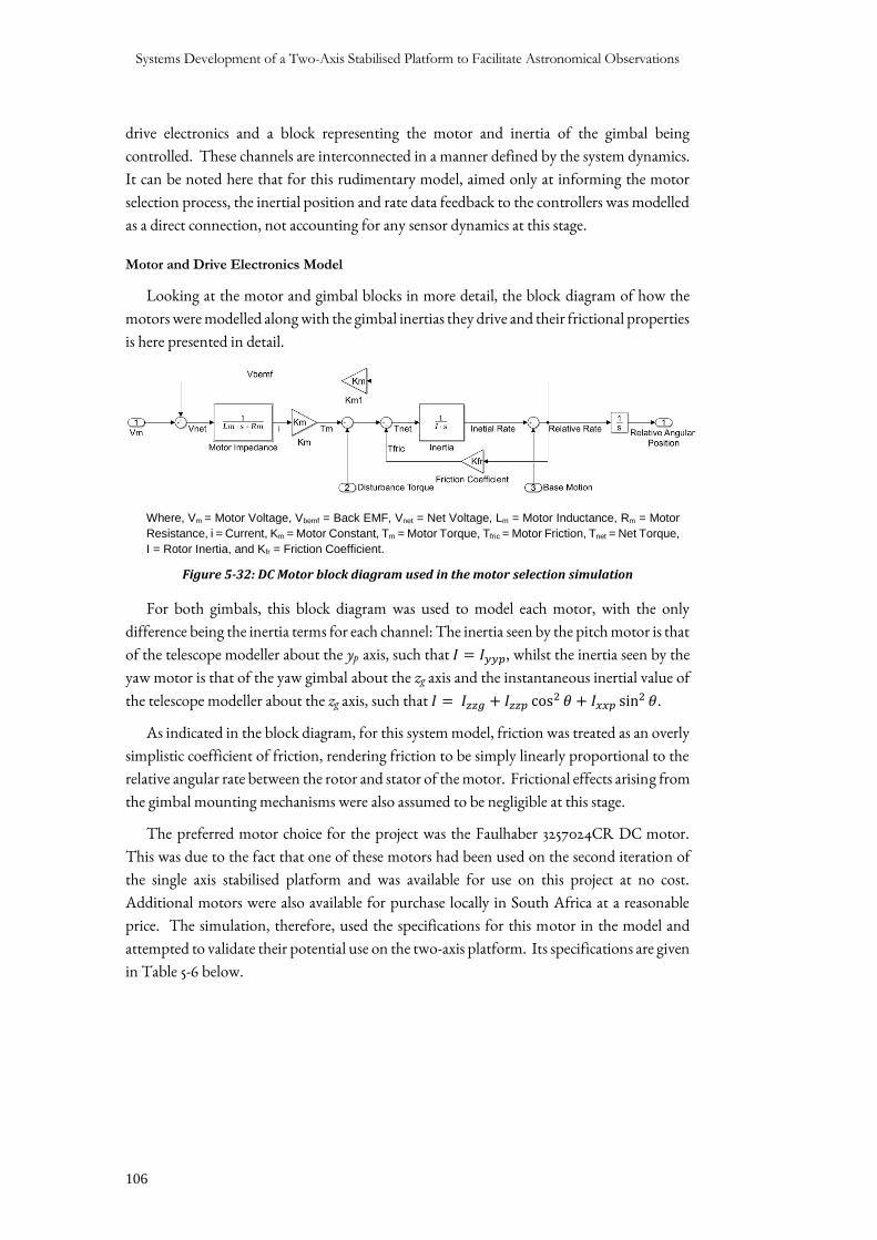
Systems Development of a Two-Axis Stabilised Platform to Facilitate Astronomical Observations
106
drive electronics and a block representing the motor and inertia of the gimbal being
controlled. These channels are interconnected in a manner defined by the system dynamics.
It can be noted here that for this rudimentary model, aimed only at informing the motor
selection process, the inertial position and rate data feedback to the controllers was modelled
as a direct connection, not accounting for any sensor dynamics at this stage.
Motor and Drive Electronics Model
Looking at the motor and gimbal blocks in more detail, the block diagram of how the
motors were modelled along with the gimbal inertias they drive and their frictional properties
is here presented in detail.
Where, Vm = Motor Voltage, Vbemf = Back EMF, Vnet = Net Voltage, Lm = Motor Inductance, Rm = Motor
Resistance, i = Current, Km = Motor Constant, Tm = Motor Torque, Tfric = Motor Friction, Tnet = Net Torque,
I = Rotor Inertia, and Kfr = Friction Coefficient.
Figure 5-32: DC Motor block diagram used in the motor selection simulation
For both gimbals, this block diagram was used to model each motor, with the only
difference being the inertia terms for each channel: The inertia seen by the pitch motor is that
of the telescope modeller about the yp axis, such that 𝐼 = 𝐼𝑦𝑦𝑝, whilst the inertia seen by the
yaw motor is that of the yaw gimbal about the zg axis and the instantaneous inertial value of
the telescope modeller about the zg axis, such that 𝐼 = 𝐼𝑧𝑧𝑔 + 𝐼𝑧𝑧𝑝 cos2 𝜃 + 𝐼𝑥𝑥𝑝 sin2 𝜃.
As indicated in the block diagram, for this system model, friction was treated as an overly
simplistic coefficient of friction, rendering friction to be simply linearly proportional to the
relative angular rate between the rotor and stator of the motor. Frictional effects arising from
the gimbal mounting mechanisms were also assumed to be negligible at this stage.
The preferred motor choice for the project was the Faulhaber 3257024CR DC motor.
This was due to the fact that one of these motors had been used on the second iteration of
the single axis stabilised platform and was available for use on this project at no cost.
Additional motors were also available for purchase locally in South Africa at a reasonable
price. The simulation, therefore, used the specifications for this motor in the model and
attempted to validate their potential use on the two-axis platform. Its specifications are given
in Table 5-6 below.
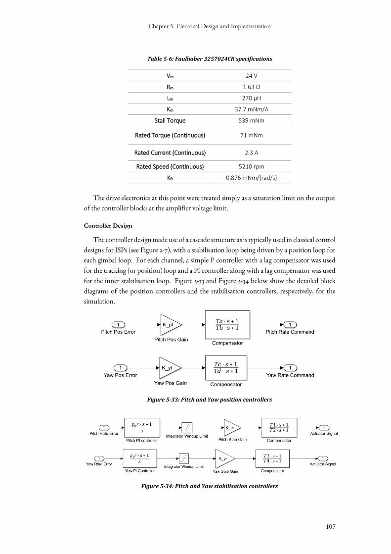
Chapter 5: Electrical Design and Implementation
107
Table 5-6: Faulhaber 3257024CR specifications
Vm 24 V
Rm 1.63 Ω
Lm 270 μH
Km 37.7 mNm/A
Stall Torque 539 mNm
Rated Torque (Continuous) 71 mNm
Rated Current (Continuous) 2.3 A
Rated Speed (Continuous) 5210 rpm
Kfr 0.876 mNm/(rad/s)
The drive electronics at this point were treated simply as a saturation limit on the output
of the controller blocks at the amplifier voltage limit.
Controller Design
The controller design made use of a cascade structure as is typically used in classical control
designs for ISPs (see Figure 2-7), with a stabilisation loop being driven by a position loop for
each gimbal loop. For each channel, a simple P controller with a lag compensator was used
for the tracking (or position) loop and a PI controller along with a lag compensator was used
for the inner stabilisation loop. Figure 5-33 and Figure 5-34 below show the detailed block
diagrams of the position controllers and the stabilisation controllers, respectively, for the
simulation.
Figure 5-33: Pitch and Yaw position controllers
Figure 5-34: Pitch and Yaw stabilisation controllers
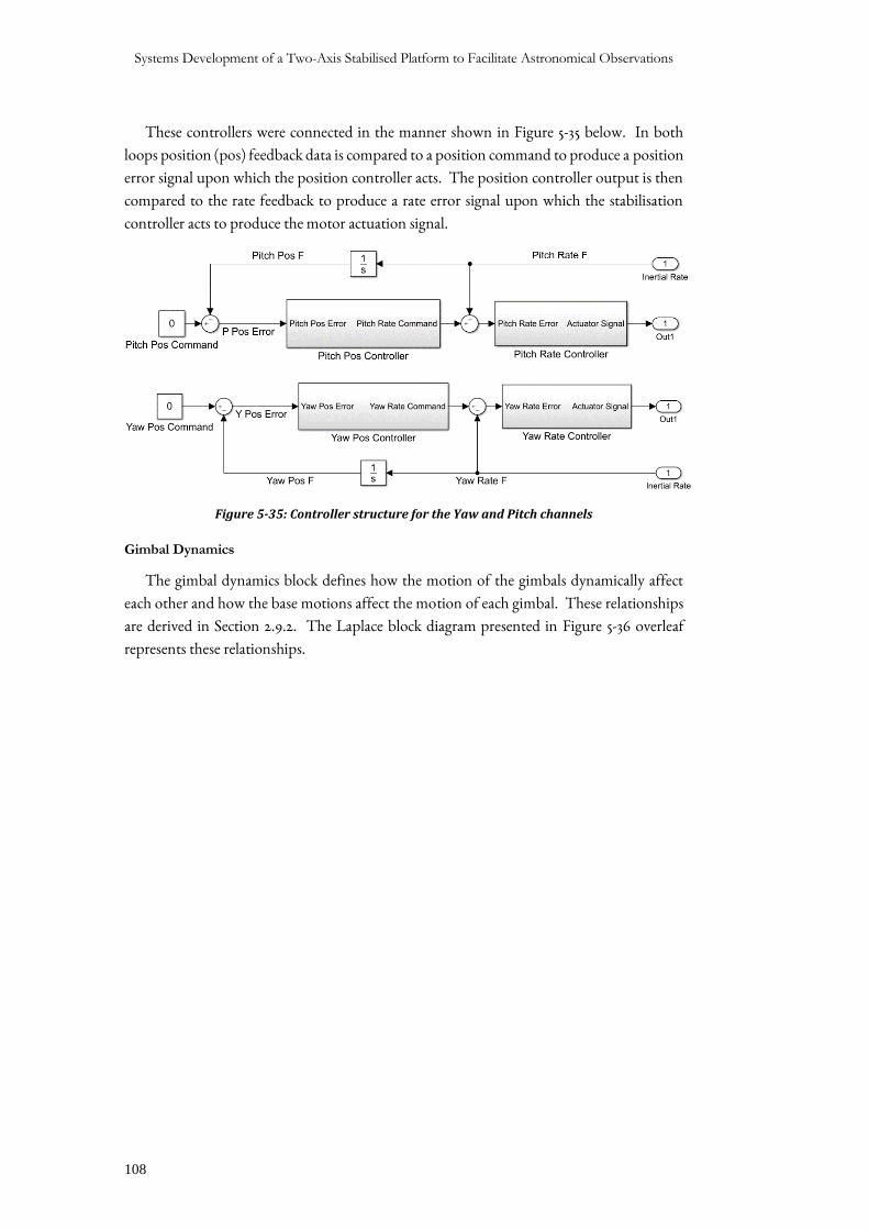
Systems Development of a Two-Axis Stabilised Platform to Facilitate Astronomical Observations
108
These controllers were connected in the manner shown in Figure 5-35 below. In both
loops position (pos) feedback data is compared to a position command to produce a position
error signal upon which the position controller acts. The position controller output is then
compared to the rate feedback to produce a rate error signal upon which the stabilisation
controller acts to produce the motor actuation signal.
Figure 5-35: Controller structure for the Yaw and Pitch channels
Gimbal Dynamics
The gimbal dynamics block defines how the motion of the gimbals dynamically affect
each other and how the base motions affect the motion of each gimbal. These relationships
are derived in Section 2.9.2. The Laplace block diagram presented in Figure 5-36 overleaf
represents these relationships.
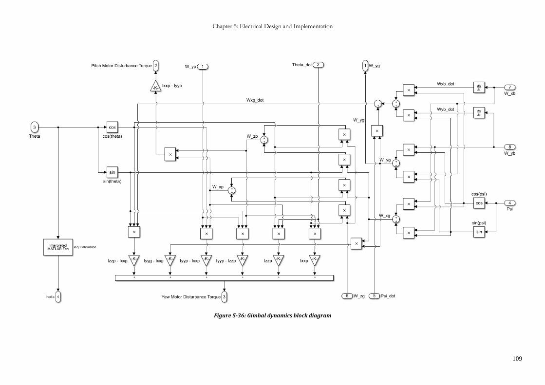
Chapter 5: Electrical Design and Implementation
109
Figure 5-36: Gimbal dynamics block diagram
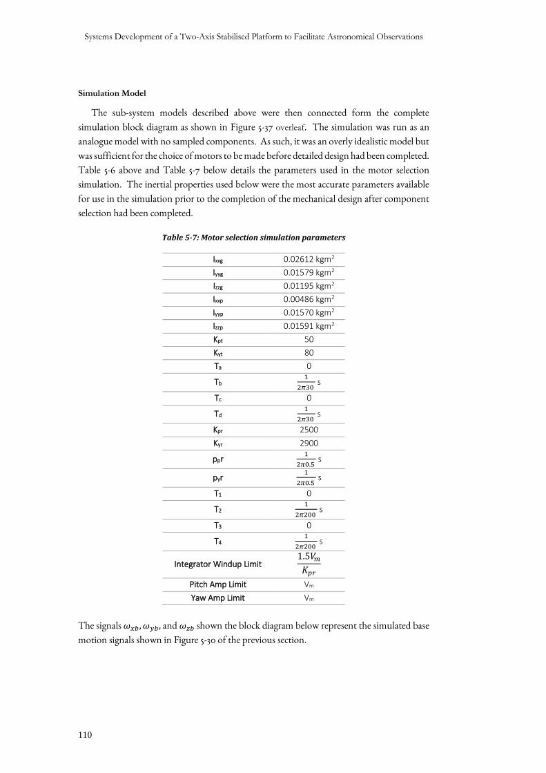
Systems Development of a Two-Axis Stabilised Platform to Facilitate Astronomical Observations
110
Simulation Model
The sub-system models described above were then connected form the complete
simulation block diagram as shown in Figure 5-37 overleaf. The simulation was run as an
analogue model with no sampled components. As such, it was an overly idealistic model but
was sufficient for the choice of motors to be made before detailed design had been completed.
Table 5-6 above and Table 5-7 below details the parameters used in the motor selection
simulation. The inertial properties used below were the most accurate parameters available
for use in the simulation prior to the completion of the mechanical design after component
selection had been completed.
Table 5-7: Motor selection simulation parameters
Ixxg 0.02612 kgm2
Iyyg 0.01579 kgm2
Izzg 0.01195 kgm2
Ixxp 0.00486 kgm2
Iyyp 0.01570 kgm2
Izzp 0.01591 kgm2
Kpt 50
Kyt 80
Ta 0
Tb 1
2𝜋30 s
Tc 0
Td 1
2𝜋30 s
Kpr 2500
Kyr 2900
ppr 1
2𝜋0.5 s
pyr 1
2𝜋0.5 s
T1 0
T2 1
2𝜋200 s
T3 0
T4 1
2𝜋200 s
Integrator Windup Limit 1.5𝑉𝑚𝐾𝑝𝑟
Pitch Amp Limit Vm
Yaw Amp Limit Vm
The signals 𝜔𝑥𝑏, 𝜔𝑦𝑏, and 𝜔𝑧𝑏 shown the block diagram below represent the simulated base
motion signals shown in Figure 5-30 of the previous section.
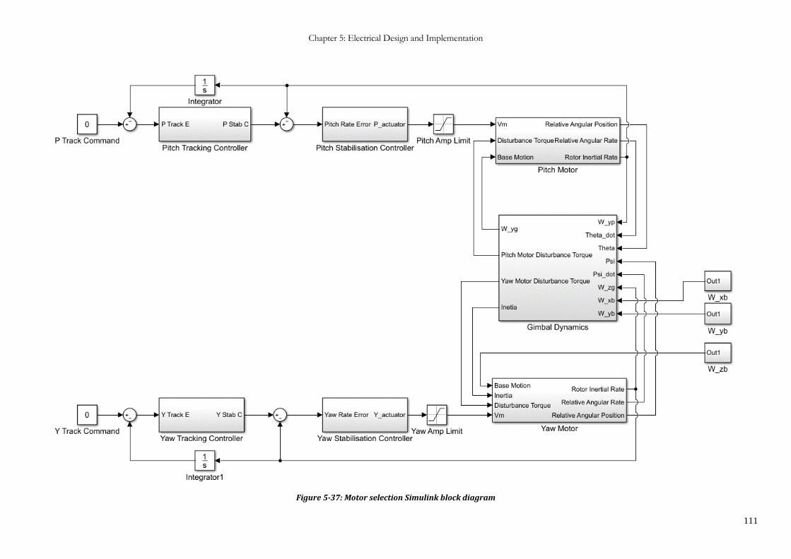
Chapter 5: Electrical Design and Implementation
111
Figure 5-37: Motor selection Simulink block diagram
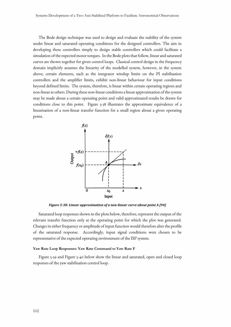
Systems Development of a Two-Axis Stabilised Platform to Facilitate Astronomical Observations
112
The Bode design technique was used to design and evaluate the stability of the system
under linear and saturated operating conditions for the designed controllers. The aim in
developing these controllers simply to design stable controllers which could facilitate a
simulation of the expected motor torques. In the Bode plots that follow, linear and saturated
curves are shown together for given control loops. Classical control design in the frequency
domain implicitly assumes the linearity of the modelled system, however, in the system
above, certain elements, such as the integrator windup limits on the PI stabilisation
controllers and the amplifier limits, exhibit non-linear behaviour for input conditions
beyond defined limits. The system, therefore, is linear within certain operating regions and
non-linear at others. During these non-linear conditions a linear approximation of the system
may be made about a certain operating point and valid approximated results be drawn for
conditions close to this point. Figure 5-38 illustrates the approximate equivalence of a
linearisation of a non-linear transfer function for a small region about a given operating
point.
Figure 5-38: Linear approximation of a non-linear curve about point A [94]
Saturated loop responses shown in the plots below, therefore, represent the output of the
relevant transfer function only at the operating point for which the plot was generated.
Changes in either frequency or amplitude of input function would therefore alter the profile
of the saturated response. Accordingly, input signal conditions were chosen to be
representative of the expected operating environment of the ISP system.
Yaw Rate Loop Responses: Yaw Rate Command to Yaw Rate F
Figure 5-39 and Figure 5-40 below show the linear and saturated, open and closed loop
responses of the yaw stabilisation control loop.
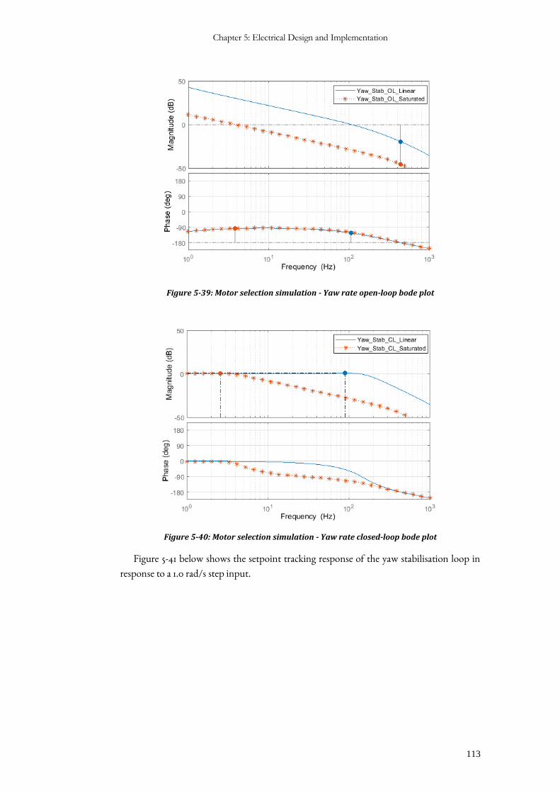
Chapter 5: Electrical Design and Implementation
113
Figure 5-39: Motor selection simulation - Yaw rate open-loop bode plot
Figure 5-40: Motor selection simulation - Yaw rate closed-loop bode plot
Figure 5-41 below shows the setpoint tracking response of the yaw stabilisation loop in
response to a 1.0 rad/s step input.
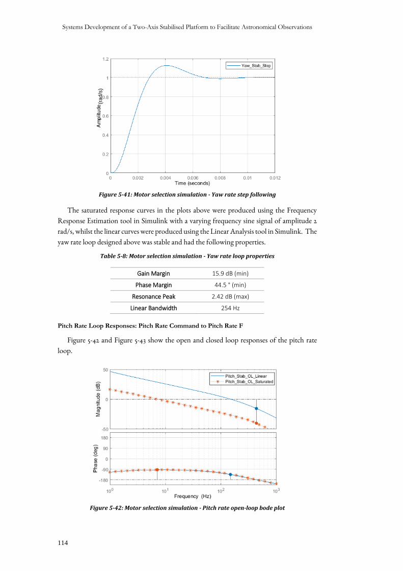
Systems Development of a Two-Axis Stabilised Platform to Facilitate Astronomical Observations
114
Figure 5-41: Motor selection simulation - Yaw rate step following
The saturated response curves in the plots above were produced using the Frequency
Response Estimation tool in Simulink with a varying frequency sine signal of amplitude 2
rad/s, whilst the linear curves were produced using the Linear Analysis tool in Simulink. The
yaw rate loop designed above was stable and had the following properties.
Table 5-8: Motor selection simulation - Yaw rate loop properties
Gain Margin 15.9 dB (min)
Phase Margin 44.5 ° (min)
Resonance Peak 2.42 dB (max)
Linear Bandwidth 254 Hz
Pitch Rate Loop Responses: Pitch Rate Command to Pitch Rate F
Figure 5-42 and Figure 5-43 show the open and closed loop responses of the pitch rate
loop.
Figure 5-42: Motor selection simulation - Pitch rate open-loop bode plot
(rad/s
)
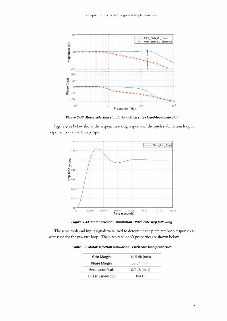
Chapter 5: Electrical Design and Implementation
115
Figure 5-43: Motor selection simulation - Pitch rate closed-loop bode plot
Figure 5-44 below shows the setpoint tracking response of the pitch stabilisation loop in
response to a 1.0 rad/s step input.
Figure 5-44: Motor selection simulation - Pitch rate step following
The same tools and input signals were used to determine the pitch rate loop responses as
were used for the yaw rate loop. The pitch rate loop’s properties are shown below.
Table 5-9: Motor selection simulation - Pitch rate loop properties
Gain Margin 19.5 dB (min)
Phase Margin 55.3 ° (min)
Resonance Peak 0.7 dB (max)
Linear Bandwidth 184 Hz
(rad/s
)
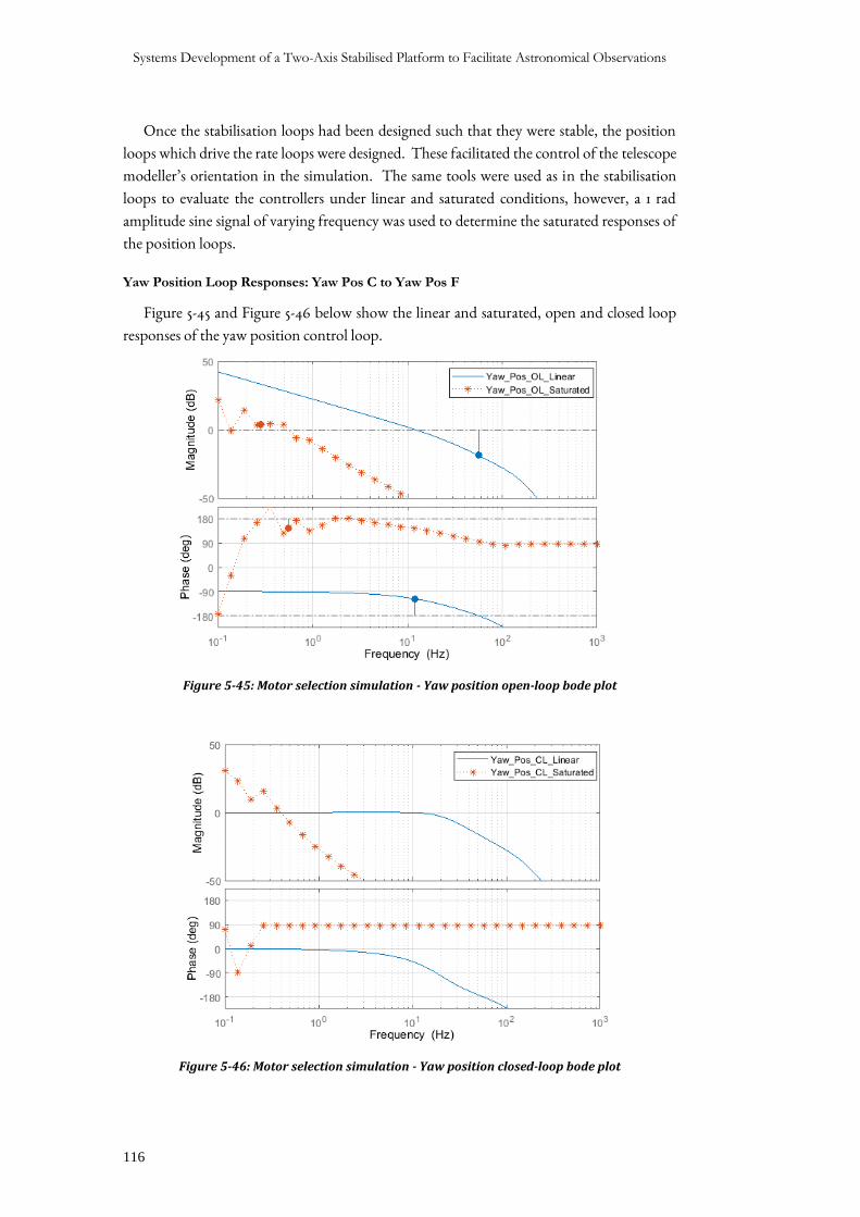
Systems Development of a Two-Axis Stabilised Platform to Facilitate Astronomical Observations
116
Once the stabilisation loops had been designed such that they were stable, the position
loops which drive the rate loops were designed. These facilitated the control of the telescope
modeller’s orientation in the simulation. The same tools were used as in the stabilisation
loops to evaluate the controllers under linear and saturated conditions, however, a 1 rad
amplitude sine signal of varying frequency was used to determine the saturated responses of
the position loops.
Yaw Position Loop Responses: Yaw Pos C to Yaw Pos F
Figure 5-45 and Figure 5-46 below show the linear and saturated, open and closed loop
responses of the yaw position control loop.
Figure 5-45: Motor selection simulation - Yaw position open-loop bode plot
Figure 5-46: Motor selection simulation - Yaw position closed-loop bode plot
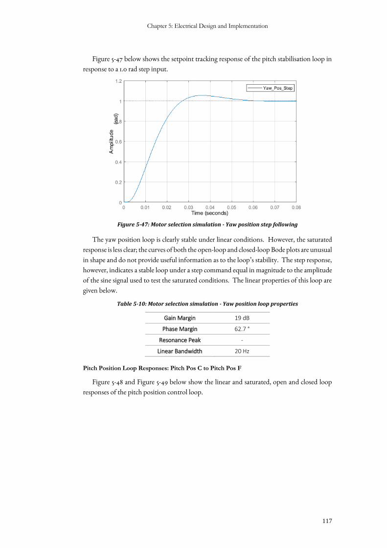
Chapter 5: Electrical Design and Implementation
117
Figure 5-47 below shows the setpoint tracking response of the pitch stabilisation loop in
response to a 1.0 rad step input.
Figure 5-47: Motor selection simulation - Yaw position step following
The yaw position loop is clearly stable under linear conditions. However, the saturated
response is less clear; the curves of both the open-loop and closed-loop Bode plots are unusual
in shape and do not provide useful information as to the loop’s stability. The step response,
however, indicates a stable loop under a step command equal in magnitude to the amplitude
of the sine signal used to test the saturated conditions. The linear properties of this loop are
given below.
Table 5-10: Motor selection simulation - Yaw position loop properties
Gain Margin 19 dB
Phase Margin 62.7 °
Resonance Peak -
Linear Bandwidth 20 Hz
Pitch Position Loop Responses: Pitch Pos C to Pitch Pos F
Figure 5-48 and Figure 5-49 below show the linear and saturated, open and closed loop
responses of the pitch position control loop.
(rad)
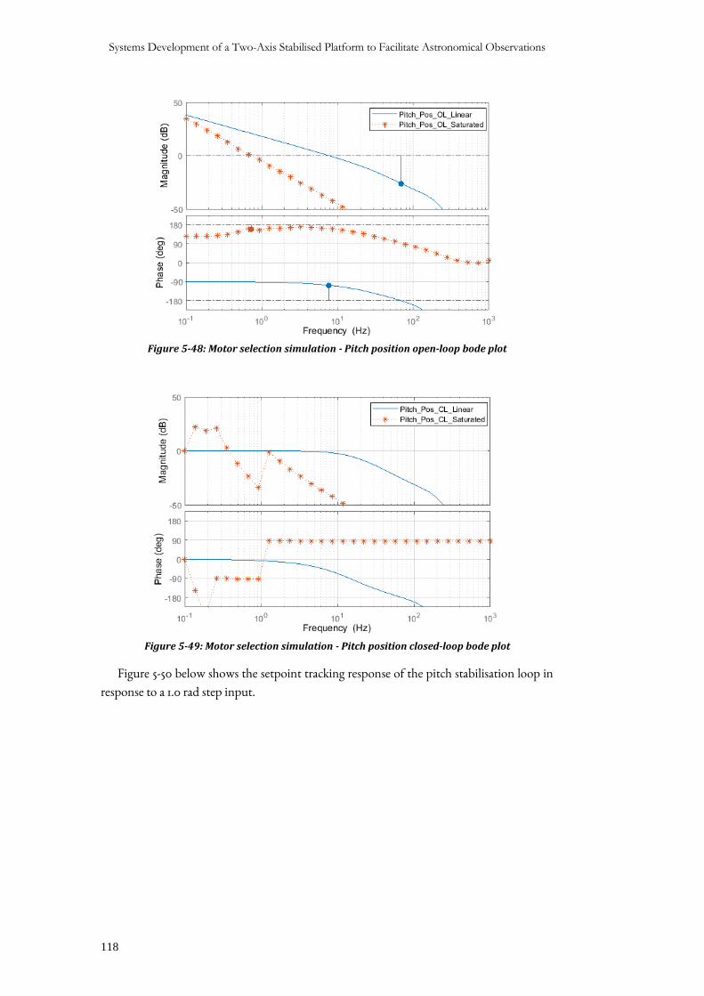
Systems Development of a Two-Axis Stabilised Platform to Facilitate Astronomical Observations
118
Figure 5-48: Motor selection simulation - Pitch position open-loop bode plot
Figure 5-49: Motor selection simulation - Pitch position closed-loop bode plot
Figure 5-50 below shows the setpoint tracking response of the pitch stabilisation loop in
response to a 1.0 rad step input.

Chapter 5: Electrical Design and Implementation
119
Figure 5-50: Motor selection simulation - Pitch position step following
In a similar way as for the position loop for the yaw channel, the linear response clearly
showed loop stability but the saturated response to the bode plots was unclear. Again,
however, the step response indicated that the loop was, in fact, stable under step commands
equal in magnitude to the sine actuation signal of the bode plot. The properties of the loop
under linear conditions are once again highlighted below.
Table 5-11: Motor selection simulation - Pitch position loop properties
Gain Margin 26.1 dB
Phase Margin 73.2 °
Resonance Peak -
Linear Bandwidth 11.2 Hz
Torque Results and Motor Verification
By running the simulation model above with the gimbals oriented in various inertial
configurations whilst under the influence of the simulated base motion signal, it was possible
to estimate the torque required from each motor to maintain stabilisation of the telescope
modeller. Testing the various configurations showed that the worst-case orientation of the
system was at when the yaw position command was at -45 °, and the pitch position command
was at 45 °. The results to follow show the motor torques required for stabilisation under the
base motion signal shown in Figure 5-51 below. Tests results are from the ‘home’ position
where 𝜓 = 𝜃 = 0° , and the worst-case position where the motor torques required for
stabilisation were greatest at 𝜓 = −45°, 𝜃 = 45°.
(rad)
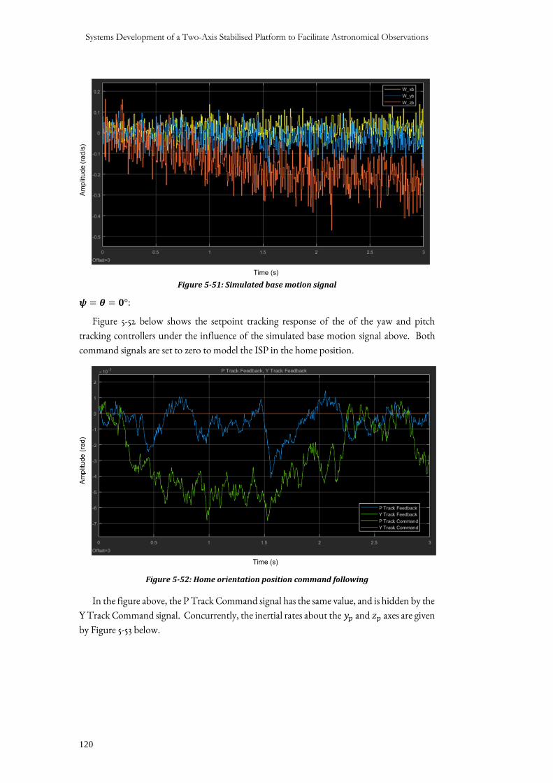
Systems Development of a Two-Axis Stabilised Platform to Facilitate Astronomical Observations
120
Figure 5-51: Simulated base motion signal
𝝍 = 𝜽 = 𝟎°:
Figure 5-52 below shows the setpoint tracking response of the of the yaw and pitch
tracking controllers under the influence of the simulated base motion signal above. Both
command signals are set to zero to model the ISP in the home position.
Figure 5-52: Home orientation position command following
In the figure above, the P Track Command signal has the same value, and is hidden by the
Y Track Command signal. Concurrently, the inertial rates about the 𝑦𝑝 and 𝑧𝑝 axes are given
by Figure 5-53 below.
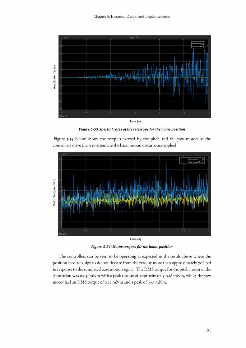
Chapter 5: Electrical Design and Implementation
121
Figure 5-53: Inertial rates of the telescope for the home position
Figure 5-54 below shows the torques exerted by the pitch and the yaw motors as the
controllers drive them to attenuate the base motion disturbance applied.
Figure 5-54: Motor torques for the home position
The controllers can be seen to be operating as expected in the result above where the
position feedback signals do not deviate from the zero by more than approximately 7e-7 rad
in response to the simulated base motion signal. The RMS torque for the pitch motor in the
simulation was 0.051 mNm with a peak torque of approximately 0.18 mNm, whilst the yaw
motor had an RMS torque of 0.18 mNm and a peak of 0.53 mNm.
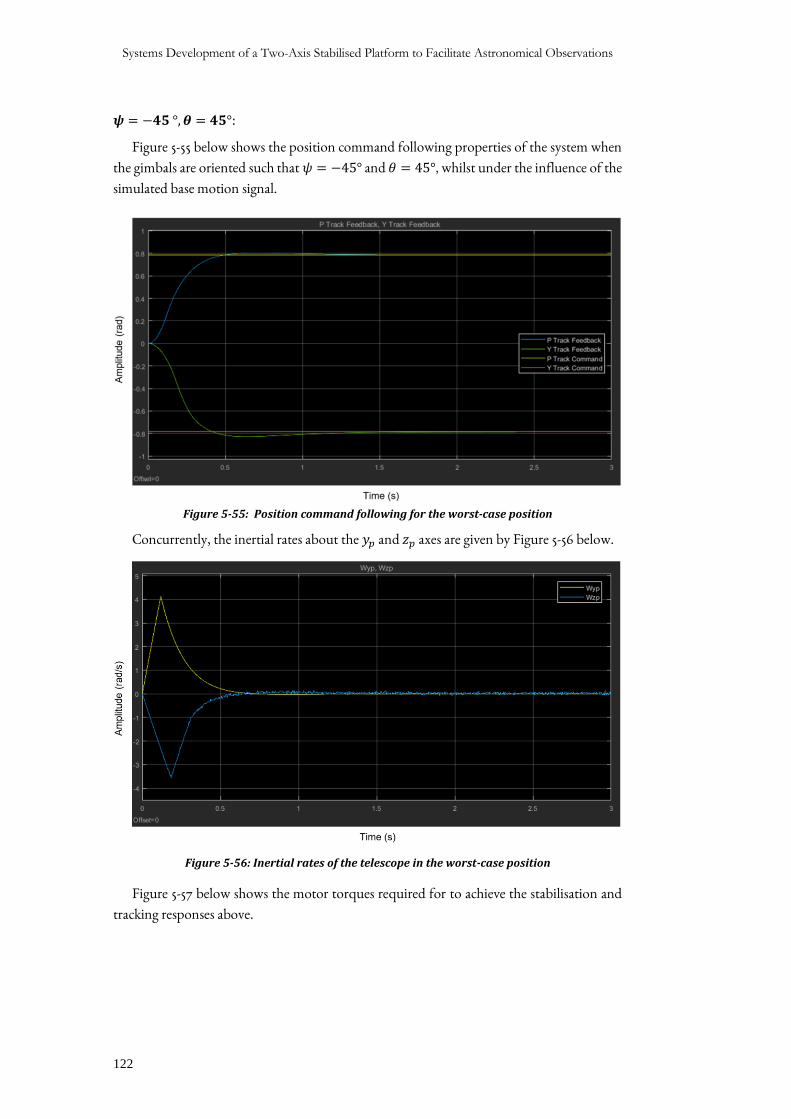
Systems Development of a Two-Axis Stabilised Platform to Facilitate Astronomical Observations
122
𝝍 = −𝟒𝟓 °, 𝜽 = 𝟒𝟓°:
Figure 5-55 below shows the position command following properties of the system when
the gimbals are oriented such that 𝜓 = −45° and 𝜃 = 45°, whilst under the influence of the
simulated base motion signal.
Figure 5-55: Position command following for the worst-case position
Concurrently, the inertial rates about the 𝑦𝑝 and 𝑧𝑝 axes are given by Figure 5-56 below.
Figure 5-56: Inertial rates of the telescope in the worst-case position
Figure 5-57 below shows the motor torques required for to achieve the stabilisation and
tracking responses above.
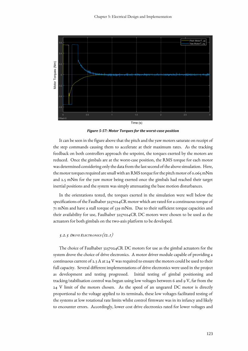
Chapter 5: Electrical Design and Implementation
123
Figure 5-57: Motor Torques for the worst-case position
It can be seen in the figure above that the pitch and the yaw motors saturate on receipt of
the step commands causing them to accelerate at their maximum rates. As the tracking
feedback on both controllers approach the setpoint, the torques exerted by the motors are
reduced. Once the gimbals are at the worst-case position, the RMS torque for each motor
was determined considering only the data from the last second of the above simulation. Here,
the motor torques required are small with an RMS torque for the pitch motor of 0.065 mNm
and 2.5 mNm for the yaw motor being exerted once the gimbals had reached their target
inertial positions and the system was simply attenuating the base motion disturbances.
In the orientations tested, the torques exerted in the simulation were well below the
specifications of the Faulhaber 3257024CR motor which are rated for a continuous torque of
71 mNm and have a stall torque of 539 mNm. Due to their sufficient torque capacities and
their availability for use, Faulhaber 3257024CR DC motors were chosen to be used as the
actuators for both gimbals on the two-axis platform to be developed.
5.2.5 DRIVE ELECTRONICS (I2.1)
The choice of Faulhaber 3257024CR DC motors for use as the gimbal actuators for the
system drove the choice of drive electronics. A motor driver module capable of providing a
continuous current of 2.3 A at 24 V was required to ensure the motors could be used to their
full capacity. Several different implementations of drive electronics were used in the project
as development and testing progressed. Initial testing of gimbal positioning and
tracking/stabilisation control was begun using low voltages between 6 and 9 V, far from the
24 V limit of the motors chosen. As the speed of an ungeared DC motor is directly
proportional to the voltage applied to its terminals, these low voltages facilitated testing of
the systems at low rotational rate limits whilst control firmware was in its infancy and likely
to encounter errors. Accordingly, lower cost drive electronics rated for lower voltages and
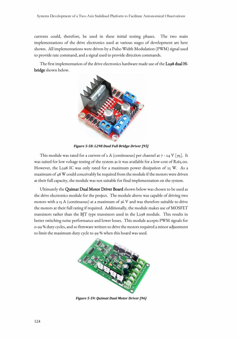
Systems Development of a Two-Axis Stabilised Platform to Facilitate Astronomical Observations
124
currents could, therefore, be used in these initial testing phases. The two main
implementations of the drive electronics used at various stages of development are here
shown. All implementations were driven by a Pulse-Width Modulation (PWM) signal used
to provide rate command, and a signal used to provide direction commands.
The first implementation of the drive electronics hardware made use of the L298 dual H-
bridge shown below.
Figure 5-58: L298 Dual Full Bridge Driver [95]
This module was rated for a current of 2 A (continuous) per channel at 7 - 24 V [95]. It
was suited for low voltage testing of the system as it was available for a low-cost of R165.00.
However, the L298 IC was only rated for a maximum power dissipation of 25 W. As a
maximum of 48 W could conceivably be required from the module if the motors were driven
at their full capacity, the module was not suitable for final implementation on the system.
Ultimately the Quimat Dual Motor Driver Board shown below was chosen to be used as
the drive electronics module for the project. The module above was capable of driving two
motors with a 15 A (continuous) at a maximum of 36 V and was therefore suitable to drive
the motors at their full rating if required. Additionally, the module makes use of MOSFET
transistors rather than the BJT type transistors used in the L298 module. This results in
better switching noise performance and lower losses. This module accepts PWM signals for
0-99 % duty cycles, and so firmware written to drive the motors required a minor adjustment
to limit the maximum duty cycle to 99 % when this board was used.
Figure 5-59: Quimat Dual Motor Driver [96]
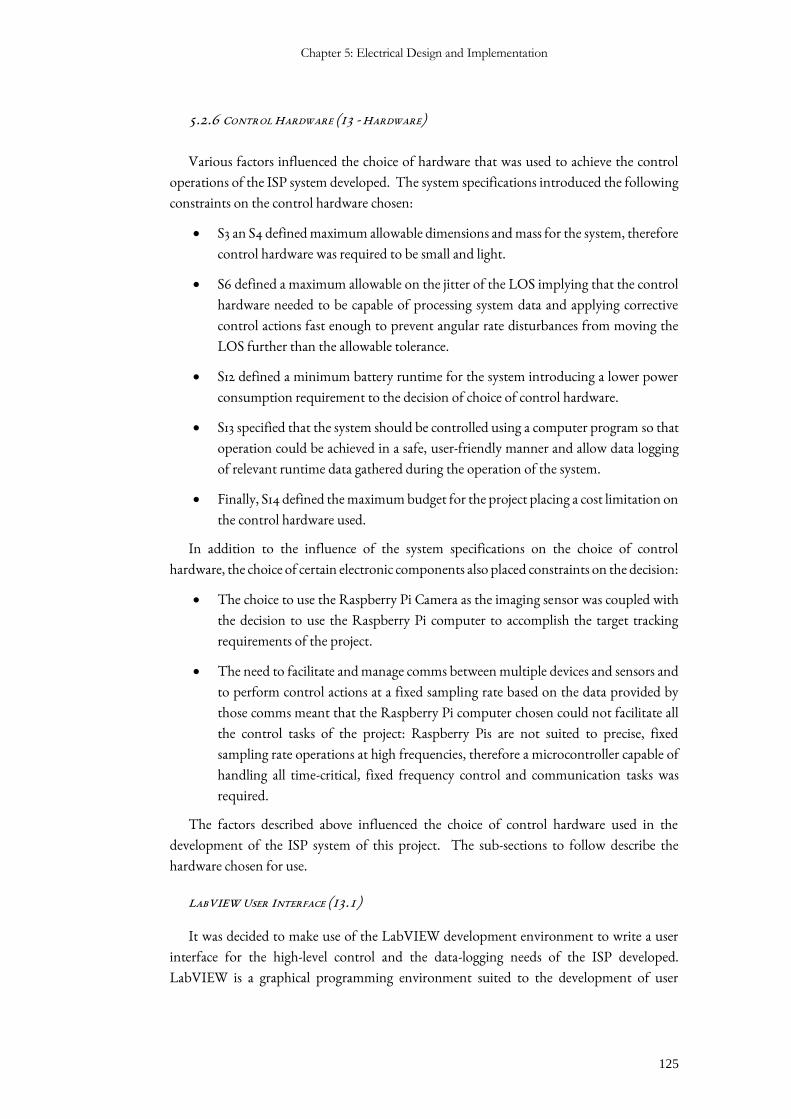
Chapter 5: Electrical Design and Implementation
125
5.2.6 CONTROL HARDWARE (I3 - HARDWARE)
Various factors influenced the choice of hardware that was used to achieve the control
operations of the ISP system developed. The system specifications introduced the following
constraints on the control hardware chosen:
• S3 an S4 defined maximum allowable dimensions and mass for the system, therefore
control hardware was required to be small and light.
• S6 defined a maximum allowable on the jitter of the LOS implying that the control
hardware needed to be capable of processing system data and applying corrective
control actions fast enough to prevent angular rate disturbances from moving the
LOS further than the allowable tolerance.
• S12 defined a minimum battery runtime for the system introducing a lower power
consumption requirement to the decision of choice of control hardware.
• S13 specified that the system should be controlled using a computer program so that
operation could be achieved in a safe, user-friendly manner and allow data logging
of relevant runtime data gathered during the operation of the system.
• Finally, S14 defined the maximum budget for the project placing a cost limitation on
the control hardware used.
In addition to the influence of the system specifications on the choice of control
hardware, the choice of certain electronic components also placed constraints on the decision:
• The choice to use the Raspberry Pi Camera as the imaging sensor was coupled with
the decision to use the Raspberry Pi computer to accomplish the target tracking
requirements of the project.
• The need to facilitate and manage comms between multiple devices and sensors and
to perform control actions at a fixed sampling rate based on the data provided by
those comms meant that the Raspberry Pi computer chosen could not facilitate all
the control tasks of the project: Raspberry Pis are not suited to precise, fixed
sampling rate operations at high frequencies, therefore a microcontroller capable of
handling all time-critical, fixed frequency control and communication tasks was
required.
The factors described above influenced the choice of control hardware used in the
development of the ISP system of this project. The sub-sections to follow describe the
hardware chosen for use.
LABVIEW USER INTERFACE (I3.1)
It was decided to make use of the LabVIEW development environment to write a user
interface for the high-level control and the data-logging needs of the ISP developed.
LabVIEW is a graphical programming environment suited to the development of user
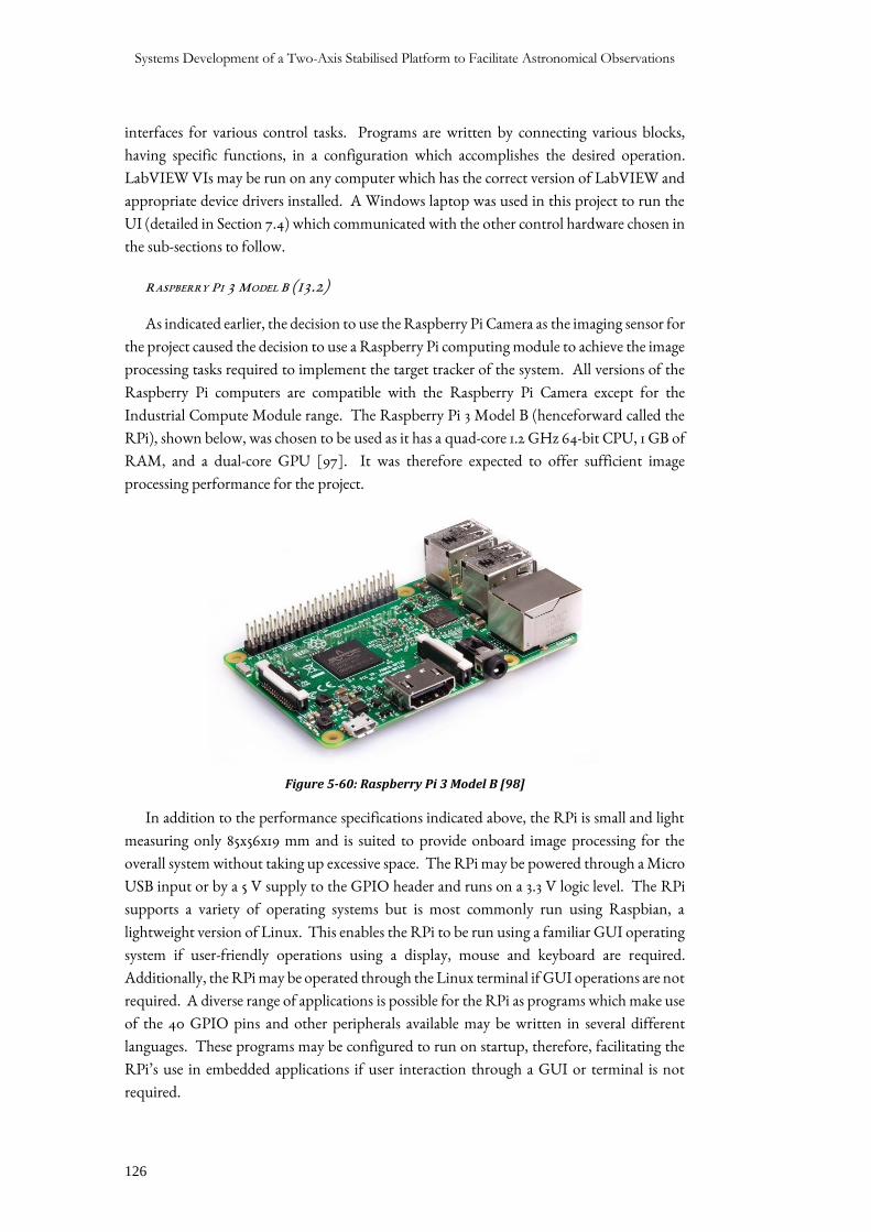
Systems Development of a Two-Axis Stabilised Platform to Facilitate Astronomical Observations
126
interfaces for various control tasks. Programs are written by connecting various blocks,
having specific functions, in a configuration which accomplishes the desired operation.
LabVIEW VIs may be run on any computer which has the correct version of LabVIEW and
appropriate device drivers installed. A Windows laptop was used in this project to run the
UI (detailed in Section 7.4) which communicated with the other control hardware chosen in
the sub-sections to follow.
RASPBERRY PI 3 MODEL B (I3.2)
As indicated earlier, the decision to use the Raspberry Pi Camera as the imaging sensor for
the project caused the decision to use a Raspberry Pi computing module to achieve the image
processing tasks required to implement the target tracker of the system. All versions of the
Raspberry Pi computers are compatible with the Raspberry Pi Camera except for the
Industrial Compute Module range. The Raspberry Pi 3 Model B (henceforward called the
RPi), shown below, was chosen to be used as it has a quad-core 1.2 GHz 64-bit CPU, 1 GB of
RAM, and a dual-core GPU [97]. It was therefore expected to offer sufficient image
processing performance for the project.
Figure 5-60: Raspberry Pi 3 Model B [98]
In addition to the performance specifications indicated above, the RPi is small and light
measuring only 85x56x19 mm and is suited to provide onboard image processing for the
overall system without taking up excessive space. The RPi may be powered through a Micro
USB input or by a 5 V supply to the GPIO header and runs on a 3.3 V logic level. The RPi
supports a variety of operating systems but is most commonly run using Raspbian, a
lightweight version of Linux. This enables the RPi to be run using a familiar GUI operating
system if user-friendly operations using a display, mouse and keyboard are required.
Additionally, the RPi may be operated through the Linux terminal if GUI operations are not
required. A diverse range of applications is possible for the RPi as programs which make use
of the 40 GPIO pins and other peripherals available may be written in several different
languages. These programs may be configured to run on startup, therefore, facilitating the
RPi’s use in embedded applications if user interaction through a GUI or terminal is not
required.
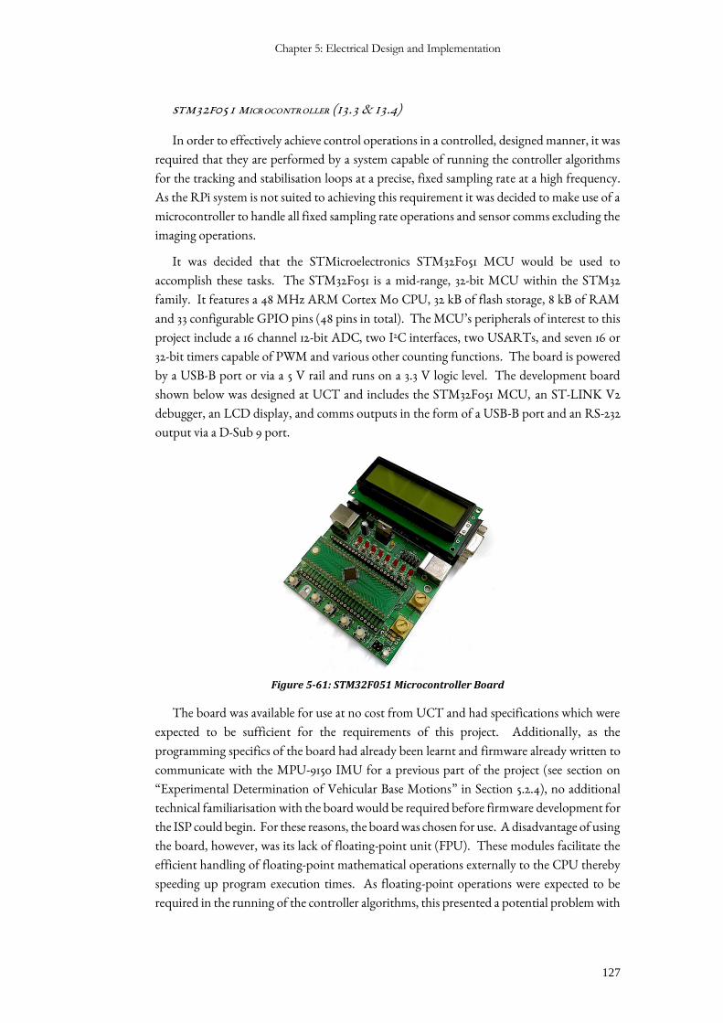
Chapter 5: Electrical Design and Implementation
127
STM32F051 MICROCONTROLLER (I3.3 & I3.4)
In order to effectively achieve control operations in a controlled, designed manner, it was
required that they are performed by a system capable of running the controller algorithms
for the tracking and stabilisation loops at a precise, fixed sampling rate at a high frequency.
As the RPi system is not suited to achieving this requirement it was decided to make use of a
microcontroller to handle all fixed sampling rate operations and sensor comms excluding the
imaging operations.
It was decided that the STMicroelectronics STM32F051 MCU would be used to
accomplish these tasks. The STM32F051 is a mid-range, 32-bit MCU within the STM32
family. It features a 48 MHz ARM Cortex M0 CPU, 32 kB of flash storage, 8 kB of RAM
and 33 configurable GPIO pins (48 pins in total). The MCU’s peripherals of interest to this
project include a 16 channel 12-bit ADC, two I2C interfaces, two USARTs, and seven 16 or
32-bit timers capable of PWM and various other counting functions. The board is powered
by a USB-B port or via a 5 V rail and runs on a 3.3 V logic level. The development board
shown below was designed at UCT and includes the STM32F051 MCU, an ST-LINK V2
debugger, an LCD display, and comms outputs in the form of a USB-B port and an RS-232
output via a D-Sub 9 port.
Figure 5-61: STM32F051 Microcontroller Board
The board was available for use at no cost from UCT and had specifications which were
expected to be sufficient for the requirements of this project. Additionally, as the
programming specifics of the board had already been learnt and firmware already written to
communicate with the MPU-9150 IMU for a previous part of the project (see section on
“Experimental Determination of Vehicular Base Motions” in Section 5.2.4), no additional
technical familiarisation with the board would be required before firmware development for
the ISP could begin. For these reasons, the board was chosen for use. A disadvantage of using
the board, however, was its lack of floating-point unit (FPU). These modules facilitate the
efficient handling of floating-point mathematical operations externally to the CPU thereby
speeding up program execution times. As floating-point operations were expected to be
required in the running of the controller algorithms, this presented a potential problem with
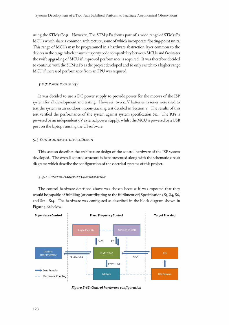
Systems Development of a Two-Axis Stabilised Platform to Facilitate Astronomical Observations
128
using the STM32F051. However, The STM32F0 forms part of a wide range of STM32Fx
MCUs which share a common architecture, some of which incorporate floating-point units.
This range of MCUs may be programmed in a hardware abstraction layer common to the
devices in the range which ensures majority code compatibility between MCUs and facilitates
the swift upgrading of MCU if improved performance is required. It was therefore decided
to continue with the STM32F0 as the project developed and to only switch to a higher range
MCU if increased performance from an FPU was required.
5.2.7 POWER SOURCE (I5)
It was decided to use a DC power supply to provide power for the motors of the ISP
system for all development and testing. However, two 12 V batteries in series were used to
test the system in an outdoor, moon-tracking test detailed in Section 8. The results of this
test verified the performance of the system against system specification S12. The RPi is
powered by an independent 5 V external power supply, whilst the MCU is powered by a USB
port on the laptop running the UI software.
5.3 CONTROL ARCHITECTURE DESIGN
This section describes the architecture design of the control hardware of the ISP system
developed. The overall control structure is here presented along with the schematic circuit
diagrams which describe the configuration of the electrical systems of this project.
5.3.1 CONTROL HARDWARE CONFIGURATION
The control hardware described above was chosen because it was expected that they
would be capable of fulfilling (or contributing to the fulfilment of) Specifications S3, S4, S6,
and S12 - S14. The hardware was configured as described in the block diagram shown in
Figure 5-62 below.
Figure 5-62: Control hardware configuration
Chapter 5: Electrical Design and Implementation
129
A three-part control scheme was decided upon, with control operations being broken
down into supervisory control, fixed frequency control, and target tracking control tasks.
The LabVIEW UI facilitates supervisory control operations such as system start/stop,
switching between manual gimbal positioning and automatic tracking and stabilising modes,
as well as performing data logging tasks. It communicates with the STM32F051 MCU via a
bi-directional serial interface over either an RS-232 or USB interface at a baud rate of 115200
bps. The MCU is tasked with reading the angle pickoffs, communicating with the MPU-
9150 IMU over an I2C interface, managing comms with the RPi which sends target position
(pixel position) data to the MCU via a direct pin-to-pin UART connection when the MCU
imitates a target data request, and running the control loops, which produce the actuation
signals for the yaw and pitch motors which are each controlled using a PWM (speed) and
direction signal. Additionally, the MCU is tasked with sending the system runtime data to
the UI for data logging. The RPi is tasked with processing the image produced by the RPi
Camera to determine the pixel position of the target centroid, which is then sent to the MCU
when the MCU initiates the data request.
ELECTRICAL SCHEMATICS
Figure 5-63 overleaf provides a reference for the electrical connections discussed in the sub-
sections to follow and shows the electrical schematic of the overall system.
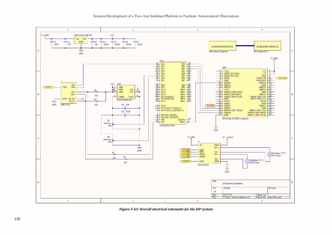
Systems Development of a Two-Axis Stabilised Platform to Facilitate Astronomical Observations
130
Figure 5-63: Overall electrical schematic for the ISP system
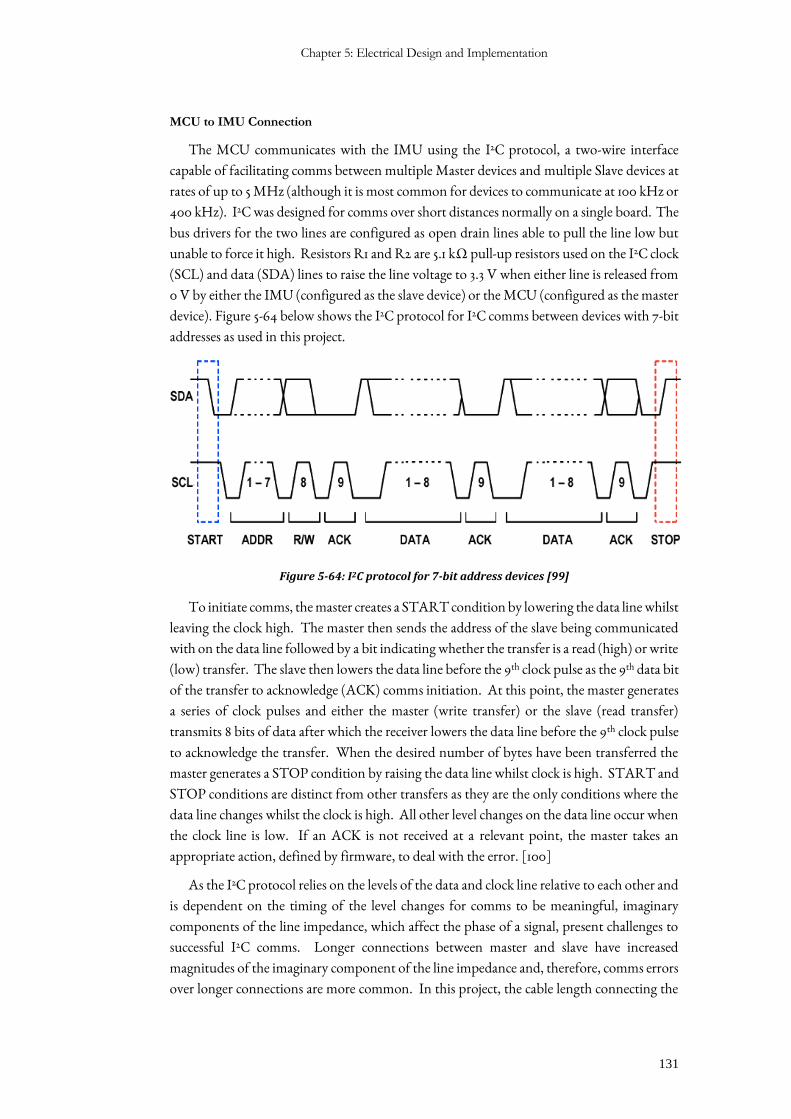
Chapter 5: Electrical Design and Implementation
131
MCU to IMU Connection
The MCU communicates with the IMU using the I2C protocol, a two-wire interface
capable of facilitating comms between multiple Master devices and multiple Slave devices at
rates of up to 5 MHz (although it is most common for devices to communicate at 100 kHz or
400 kHz). I2C was designed for comms over short distances normally on a single board. The
bus drivers for the two lines are configured as open drain lines able to pull the line low but
unable to force it high. Resistors R1 and R2 are 5.1 kΩ pull-up resistors used on the I2C clock
(SCL) and data (SDA) lines to raise the line voltage to 3.3 V when either line is released from
0 V by either the IMU (configured as the slave device) or the MCU (configured as the master
device). Figure 5-64 below shows the I2C protocol for I2C comms between devices with 7-bit
addresses as used in this project.
Figure 5-64: I2C protocol for 7-bit address devices [99]
To initiate comms, the master creates a START condition by lowering the data line whilst
leaving the clock high. The master then sends the address of the slave being communicated
with on the data line followed by a bit indicating whether the transfer is a read (high) or write
(low) transfer. The slave then lowers the data line before the 9th clock pulse as the 9th data bit
of the transfer to acknowledge (ACK) comms initiation. At this point, the master generates
a series of clock pulses and either the master (write transfer) or the slave (read transfer)
transmits 8 bits of data after which the receiver lowers the data line before the 9th clock pulse
to acknowledge the transfer. When the desired number of bytes have been transferred the
master generates a STOP condition by raising the data line whilst clock is high. START and
STOP conditions are distinct from other transfers as they are the only conditions where the
data line changes whilst the clock is high. All other level changes on the data line occur when
the clock line is low. If an ACK is not received at a relevant point, the master takes an
appropriate action, defined by firmware, to deal with the error. [100]
As the I2C protocol relies on the levels of the data and clock line relative to each other and
is dependent on the timing of the level changes for comms to be meaningful, imaginary
components of the line impedance, which affect the phase of a signal, present challenges to
successful I2C comms. Longer connections between master and slave have increased
magnitudes of the imaginary component of the line impedance and, therefore, comms errors
over longer connections are more common. In this project, the cable length connecting the
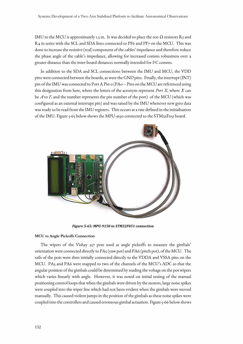
Systems Development of a Two-Axis Stabilised Platform to facilitate Astronomical Observations
132
IMU to the MCU is approximately 1.5 m. It was decided to place the 100 Ω resistors R3 and
R4 in series with the SCL and SDA lines connected to PF6 and PF7 on the MCU. This was
done to increase the resistive (real) component of the cables’ impedance and therefore reduce
the phase angle of the cable’s impedance, allowing for increased comms robustness over a
greater distance than the inter-board distances normally intended for I2C comms.
In addition to the SDA and SCL connections between the IMU and MCU, the VDD
pins were connected between the boards, as were the GND pins. Finally, the interrupt (INT)
pin of the IMU was connected to Port A Pin 0 (PA0 – Pins on the MCU are referenced using
this designation from here, where the letters of the acronym represent Port X, where X can
be A to F, and the number represents the pin number of the port) of the MCU (which was
configured as an external interrupt pin) and was raised by the IMU whenever new gyro data
was ready to be read from the IMU registers. This occurs at a rate defined in the initialisation
of the IMU. Figure 5-65 below shows the MPU-9150 connected to the STM32F051 board.
Figure 5-65: MPU-9150 to STM32F051 connection
MCU to Angle Pickoffs Connection
The wipers of the Vishay 357 pots used as angle pickoffs to measure the gimbals’
orientation were connected directly to PA5 (yaw pot) and PA6 (pitch pot), of the MCU. The
rails of the pots were then initially connected directly to the VDDA and VSSA pins on the
MCU. PA5 and PA6 were mapped to two of the channels of the MCU’s ADC so that the
angular position of the gimbals could be determined by reading the voltage on the pot wipers
which varies linearly with angle. However, it was noted on initial testing of the manual
positioning control loops that when the gimbals were driven by the motors, large noise spikes
were coupled into the wiper line which had not been evident when the gimbals were moved
manually. This caused violent jumps in the position of the gimbals as these noise spikes were
coupled into the controllers and caused erroneous gimbal actuation. Figure 5-66 below shows
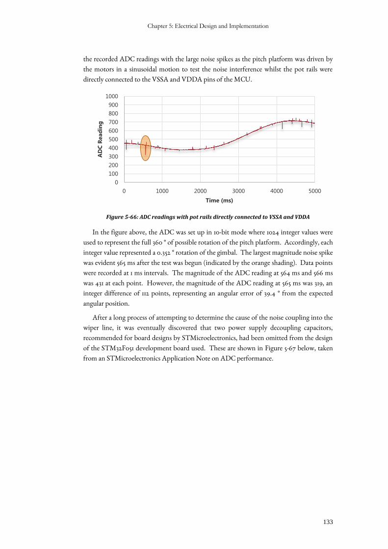
Chapter 5: Electrical Design and Implementation
133
the recorded ADC readings with the large noise spikes as the pitch platform was driven by
the motors in a sinusoidal motion to test the noise interference whilst the pot rails were
directly connected to the VSSA and VDDA pins of the MCU.
Figure 5-66: ADC readings with pot rails directly connected to VSSA and VDDA
In the figure above, the ADC was set up in 10-bit mode where 1024 integer values were
used to represent the full 360 ° of possible rotation of the pitch platform. Accordingly, each
integer value represented a 0.352 ° rotation of the gimbal. The largest magnitude noise spike
was evident 565 ms after the test was begun (indicated by the orange shading). Data points
were recorded at 1 ms intervals. The magnitude of the ADC reading at 564 ms and 566 ms
was 431 at each point. However, the magnitude of the ADC reading at 565 ms was 319, an
integer difference of 112 points, representing an angular error of 39.4 ° from the expected
angular position.
After a long process of attempting to determine the cause of the noise coupling into the
wiper line, it was eventually discovered that two power supply decoupling capacitors,
recommended for board designs by STMicroelectronics, had been omitted from the design
of the STM32F051 development board used. These are shown in Figure 5-67 below, taken
from an STMicroelectronics Application Note on ADC performance.
0
100
200
300
400
500
600
700
800
900
1000
0 1000 2000 3000 4000 5000
AD
C R
ead
ing
Time (ms)
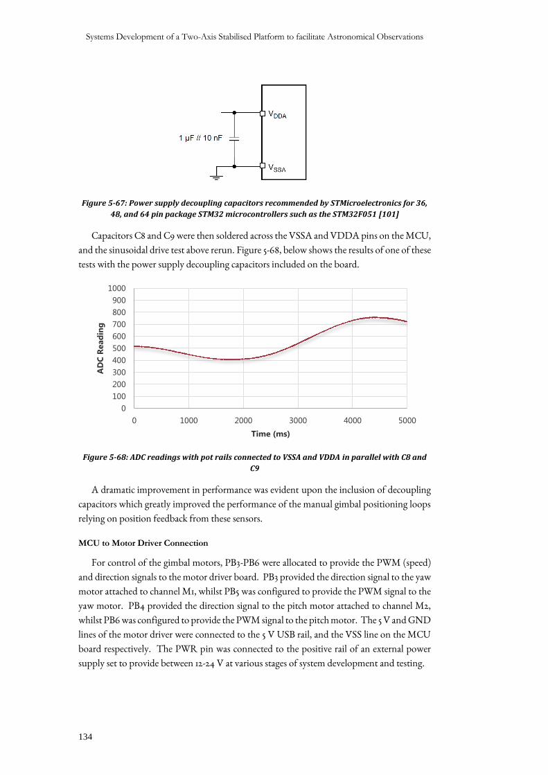
Systems Development of a Two-Axis Stabilised Platform to facilitate Astronomical Observations
134
Figure 5-67: Power supply decoupling capacitors recommended by STMicroelectronics for 36,
48, and 64 pin package STM32 microcontrollers such as the STM32F051 [101]
Capacitors C8 and C9 were then soldered across the VSSA and VDDA pins on the MCU,
and the sinusoidal drive test above rerun. Figure 5-68, below shows the results of one of these
tests with the power supply decoupling capacitors included on the board.
Figure 5-68: ADC readings with pot rails connected to VSSA and VDDA in parallel with C8 and
C9
A dramatic improvement in performance was evident upon the inclusion of decoupling
capacitors which greatly improved the performance of the manual gimbal positioning loops
relying on position feedback from these sensors.
MCU to Motor Driver Connection
For control of the gimbal motors, PB3-PB6 were allocated to provide the PWM (speed)
and direction signals to the motor driver board. PB3 provided the direction signal to the yaw
motor attached to channel M1, whilst PB5 was configured to provide the PWM signal to the
yaw motor. PB4 provided the direction signal to the pitch motor attached to channel M2,
whilst PB6 was configured to provide the PWM signal to the pitch motor. The 5 V and GND
lines of the motor driver were connected to the 5 V USB rail, and the VSS line on the MCU
board respectively. The PWR pin was connected to the positive rail of an external power
supply set to provide between 12-24 V at various stages of system development and testing.
0
100
200
300
400
500
600
700
800
900
1000
0 1000 2000 3000 4000 5000
AD
C R
ead
ing
Time (ms)
Chapter 5: Electrical Design and Implementation
135
RPi to MCU Connection
The complete detail of the nature of the connections between the MCU and RPi are given
in Section 7.3 which details the development of the target tracker. Here, only the physical
connections between the devices and the direction of signals along the lines are detailed.
The VSS line of the MCU was connected to the ground (Pin 39) of the RPi. Pin 11
(GPIO17) of the RPI was configured as an output and connected to the NSRT pin of the
MCU. Pin 8 (UART0 TX) of the RPi was connected to PA3 of the MCU which was
configured as the RX pin of the second USART peripheral on the MCU. Pin 31 (GPIO06)
of the RPi was configured as an output and connected to PA4 of the MCU which was
configured as an external interrupt input. Pin 33 (GPIO13) of the RPi was configured as an
input and connected to PB0 of the MCU which was configured as an output pin. Pin 35
(GPIO19) of the RPi was configured as an input and connected to PB1 of the MCU which
was configured as an output pin. Finally, Pin 37 (GPIO26) of the RPi was configured as an
input and connected to PB2 of the MCU which was configured as an output pin.
These connections facilitated the communications of target position data between the
RPi and MCU.
User Interface to MCU Connection
The laptop running the UI was connected to the MCU via a serial port across either an
RS-232 connection or a USB connection. Both connections communicated with USART1
peripheral of the MCU configured on PA9 (TX) and PA10 (RX).
5.4 CHAPTER CONCLUSION
This chapter detailed the process by which all electronic components were selected for use
in the system developed in this project. It presented, in detail, the reasons for the selection of
specific components over other technologies able to accomplish similar tasks, and justified
the choice of gimbal actuators through a rigorous experimental and simulation-based
method. In addition to describing the hardware chosen and their specifications, the control
architecture used in the project was presented. Within the three-part control structure
employed, control and communications tasks were assigned to each of the control
computers: Supervisory control tasks to the laptop-based UI, fixed frequency controller
algorithms and sensor communications to the MCU, and target tracking and its associated
image gathering tasks to the RPi.
Ultimately, the choice of hardware presented in this section was done such that system
prime items I2.1-I2.2, I4, I5, and I3 from a hardware perspective were successfully
implemented. The implementation of these prime items achieved specifications S8 and S10-
S13 directly, whilst contributing to the accomplishment of specifications S3-S6 and S14.
Unfortunately, S9 was not achieved due to budget constraints on the system.

Chapter 6: Controller Design
137
6 CONTROLLER DESIGN
6.1 INTRODUCTION
Following the mechanical and the electrical design of the ISP system developed, this
chapter describes the design of the various controller algorithms designed for
implementation on the control hardware. Namely, these include manual position controllers
for the yaw and pitch channels, stabilisation controllers, and finally tracking controllers for
the two channels. Together, these control loops facilitate the control of the ISP’s gimbals
such that its orientation and motion may be controlled to a desired state under various
operating conditions.
All controllers developed for the ISP were chosen to be classical controllers of type P or
PI with compensation. Although modern and non-linear control methods have been shown
to achieve better stabilisation performance, classical controllers were chosen due to the
prevalence of their use in the development of stabilised platforms, as stated in Section 2.3.3.
Additionally, as this project represented the initial systems development of this ISP, classical
controllers were the logical starting point for the development of its control system. All
controllers designed in this chapter were developed using the Bode technique and evaluated
the system responses under linear and saturated operating conditions. As illustrated
previously, by Figure 5-38 of Section 5.2.4, the saturated responses of systems evaluated by
this technique are representative only of the operating point at which they are evaluated and
therefore excitation signals were chosen to be of magnitudes and frequencies typical of the
expected operating environment of the ISP system developed.
Throughout this chapter non-standard terminology has been made used to describe the
compensators implemented in the various control loops: The term ‘lead compensator’ has
been used to describe a compensator with a single zero and no poles which causes a pure phase
lead response. The term ‘lag compensator’ has been used to describe a compensator with a
single pole and no zeroes which causes a pure phase lag. The term ‘lead-lag compensator’ has
been used to describe a compensator with one zero and one pole which causes both phase
lead and phase lag effects across the frequency spectrum. A dominant lead lead-lag
compensator has its zero at a lower frequency than its pole and causes phase lead between the
frequencies of one tenth the zero frequency and ten times the pole frequency. A dominant
lag lead-lag compensator has its pole at a lower frequency than its zero and causes phase lag
between the frequencies of one tenth the pole frequency and ten times the zero frequency.
Systems Development of a Two-Axis Stabilised Platform to facilitate Astronomical Observations
138
This terminology has been used due to the more intuitive understating off the phase effect
of the compensator associated with the term. [102]
It was decided at this point to make use of the simulation language, Simul_C_EM
(Simul_C) for the control system design and simulation needs of the remainder of the project.
Simul_C is a C++ based, analytical simulation package suited to classical control design using
the Bode technique and time domain simulations which may be observed through several
graphing capabilities [102]. Simul_C was developed by Associate Professor Hendrik D.
Mouton and is freely available for use from UCT. Simul_C has been noted to run
simulations faster than equivalent simulations run using MATLAB Simulink and, in
addition, the similarity of C++ to C, the language used to program the STM32F0 MCU on
which the control loops designed here were implemented, was beneficial in debugging of
system firmware. It allowed line-by-line comparison of simulation code with firmware code
to be made and so helped identify errors as either language or implementation errors.
Whilst not a prime item of the system, the manual position controllers are an important
aspect of the overall control of the gimbal structure. The section begins with a description of
their design before it continues to the development of the stabilisation and tracking loops
(prime items I3.3 and I3.4 from a mathematical simulation perspective after already being
described from a hardware perspective in Section 5.2.6.)
6.2 MANUAL POSITION CONTROLLERS
The firmware written for the MCU to control the low-level operation of the ISP system
developed is a state machine built on three main program states: The Setup state, Manual
state, and Automatic state. This is further detailed in Section 7.2.1, however, the Setup state
facilitates correct initialisation of the sensors and hardware, the Automatic state facilitates
tracking and stabilisation functionality, and the Manual state enables the orientation of the
telescope modeller to be controlled in a servo loop which receives angular position commands
from the User Interface. The need for these servo loops arose from the fact that it is unlikely
that the ISP will be in an orientation such that the target can be seen on system startup;
angular position control is required so that the gimbals may be moved to an orientation
where the target is visible in order for the target tracker to begin tracking of the target and
control of the gimbals. The controllers designed below facilitate this operation.
6.2.1 POSITION CONTROLLER DEVELOPMENT
As shown below, each gimbal is modelled as a single inertia driven directly by a DC motor
controlled by a P controller with a lead-lag compensator.
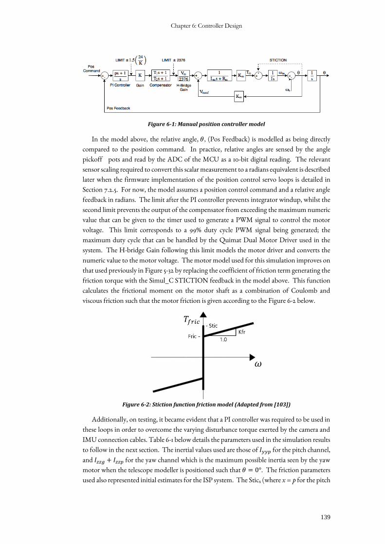
Chapter 6: Controller Design
139
Figure 6-1: Manual position controller model
In the model above, the relative angle, 𝜃, (Pos Feedback) is modelled as being directly
compared to the position command. In practice, relative angles are sensed by the angle
pickoff pots and read by the ADC of the MCU as a 10-bit digital reading. The relevant
sensor scaling required to convert this scalar measurement to a radians equivalent is described
later when the firmware implementation of the position control servo loops is detailed in
Section 7.2.5. For now, the model assumes a position control command and a relative angle
feedback in radians. The limit after the PI controller prevents integrator windup, whilst the
second limit prevents the output of the compensator from exceeding the maximum numeric
value that can be given to the timer used to generate a PWM signal to control the motor
voltage. This limit corresponds to a 99% duty cycle PWM signal being generated; the
maximum duty cycle that can be handled by the Quimat Dual Motor Driver used in the
system. The H-bridge Gain following this limit models the motor driver and converts the
numeric value to the motor voltage. The motor model used for this simulation improves on
that used previously in Figure 5-32 by replacing the coefficient of friction term generating the
friction torque with the Simul_C STICTION feedback in the model above. This function
calculates the frictional moment on the motor shaft as a combination of Coulomb and
viscous friction such that the motor friction is given according to the Figure 6-2 below.
Figure 6-2: Stiction function friction model (Adapted from [103])
Additionally, on testing, it became evident that a PI controller was required to be used in
these loops in order to overcome the varying disturbance torque exerted by the camera and
IMU connection cables. Table 6-1 below details the parameters used in the simulation results
to follow in the next section. The inertial values used are those of 𝐼𝑦𝑦𝑝 for the pitch channel,
and 𝐼𝑧𝑧𝑔 + 𝐼𝑧𝑧𝑝 for the yaw channel which is the maximum possible inertia seen by the yaw
motor when the telescope modeller is positioned such that 𝜃 = 0°. The friction parameters
used also represented initial estimates for the ISP system. The Sticx (where x = p for the pitch
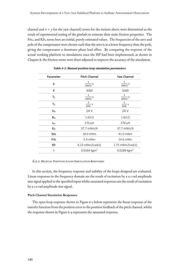
Systems Development of a Two-Axis Stabilised Platform to facilitate Astronomical Observations
140
channel and x = y for the yaw channel) terms for the motors above were determined as the
result of experimental testing of the gimbals to estimate their static friction properties. The
Fricx and Kfrx terms here are initial, purely estimated values. The frequencies of the zero and
pole of the compensator were chosen such that the zero is at a lower frequency than the pole,
giving the compensator a dominant phase lead effect. By comparing the response of the
actual working platform to simulations once the ISP had been implemented, as shown in
Chapter 8, the friction terms were there adjusted to improve the accuracy of the simulation.
Table 6-1: Manual position loop simulation parameters
Parameter Pitch Channel Yaw Channel
p 1
2𝜋0.5 s
1
2𝜋0.5 s
K 3000 5000
T1 1
2𝜋0.2 s
1
2𝜋0.2 s
T2 1
2𝜋4 s
1
2𝜋4 s
Vm 24 V 24 V
Rm 1.63 Ω 1.63 Ω
Lm 270 μH 270 μH
Km 37.7 mNm/A 37.7 mNm/A
Stic 18.0 mNm 41.0 mNm
Fric 5.4 mNm 24.6 mNm
Kfr 6.13 mNm/(rad/s) 1.75 mNm/(rad/s)
I 0.0164 kgm2 0.0289 kgm2
6.2.2 MANUAL POSITION LOOPS SIMULATION RESPONSES
In this section, the frequency response and stability of the loops designed are evaluated.
Linear responses in the frequency domain are the result of excitation by a 0.1 rad amplitude
sine signal applied to the specified input whilst saturated responses are the result of excitation
by a 1.0 rad amplitude sine signal.
Pitch Channel Simulation Responses
The open-loop response shown in Figure 6-3 below represents the linear response of the
transfer function from the position error to the position feedback of the pitch channel, whilst
the response shown in Figure 6-4 represents the saturated response.
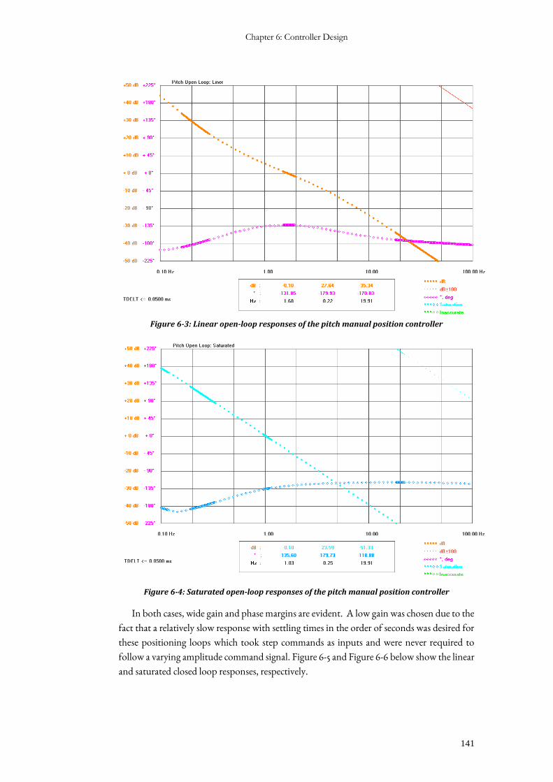
Chapter 6: Controller Design
141
Figure 6-3: Linear open-loop responses of the pitch manual position controller
Figure 6-4: Saturated open-loop responses of the pitch manual position controller
In both cases, wide gain and phase margins are evident. A low gain was chosen due to the
fact that a relatively slow response with settling times in the order of seconds was desired for
these positioning loops which took step commands as inputs and were never required to
follow a varying amplitude command signal. Figure 6-5 and Figure 6-6 below show the linear
and saturated closed loop responses, respectively.
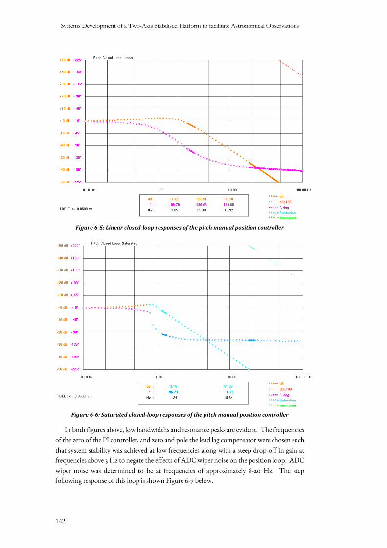
Systems Development of a Two-Axis Stabilised Platform to facilitate Astronomical Observations
142
Figure 6-5: Linear closed-loop responses of the pitch manual position controller
Figure 6-6: Saturated closed-loop responses of the pitch manual position controller
In both figures above, low bandwidths and resonance peaks are evident. The frequencies
of the zero of the PI controller, and zero and pole the lead lag compensator were chosen such
that system stability was achieved at low frequencies along with a steep drop-off in gain at
frequencies above 3 Hz to negate the effects of ADC wiper noise on the position loop. ADC
wiper noise was determined to be at frequencies of approximately 8-20 Hz. The step
following response of this loop is shown Figure 6-7 below.
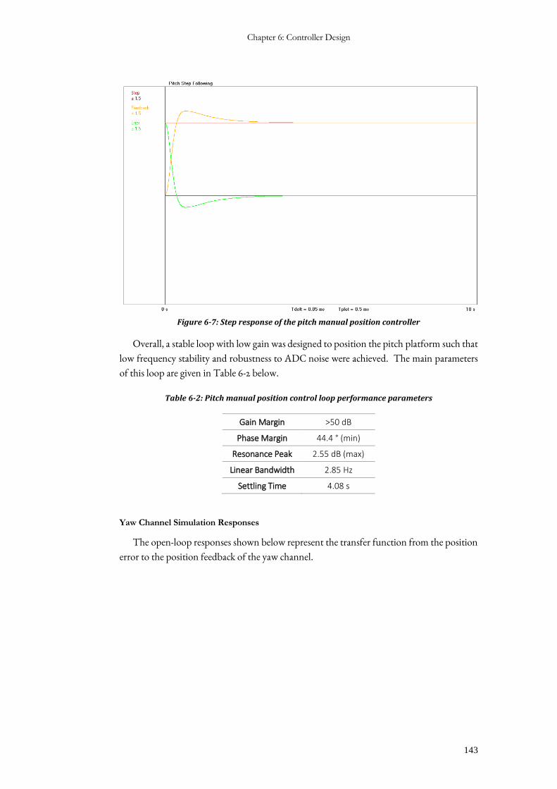
Chapter 6: Controller Design
143
Figure 6-7: Step response of the pitch manual position controller
Overall, a stable loop with low gain was designed to position the pitch platform such that
low frequency stability and robustness to ADC noise were achieved. The main parameters
of this loop are given in Table 6-2 below.
Table 6-2: Pitch manual position control loop performance parameters
Gain Margin >50 dB
Phase Margin 44.4 ° (min)
Resonance Peak 2.55 dB (max)
Linear Bandwidth 2.85 Hz
Settling Time 4.08 s
Yaw Channel Simulation Responses
The open-loop responses shown below represent the transfer function from the position
error to the position feedback of the yaw channel.
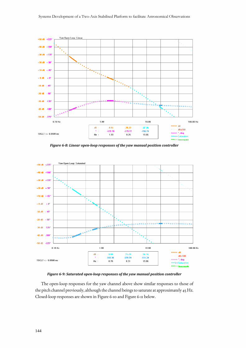
Systems Development of a Two-Axis Stabilised Platform to facilitate Astronomical Observations
144
Figure 6-8: Linear open-loop responses of the yaw manual position controller
Figure 6-9: Saturated open-loop responses of the yaw manual position controller
The open-loop responses for the yaw channel above show similar responses to those of
the pitch channel previously, although the channel beings to saturate at approximately 45 Hz.
Closed-loop responses are shown in Figure 6-10 and Figure 6-11 below.
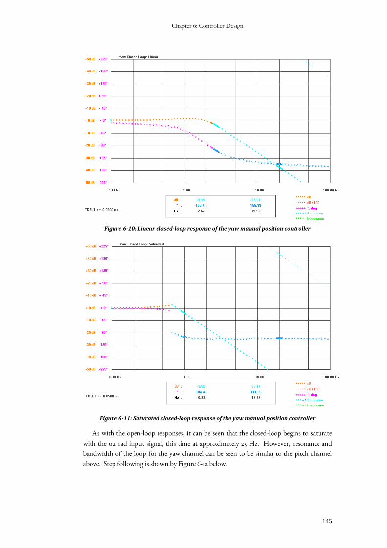
Chapter 6: Controller Design
145
Figure 6-10: Linear closed-loop response of the yaw manual position controller
Figure 6-11: Saturated closed-loop response of the yaw manual position controller
As with the open-loop responses, it can be seen that the closed-loop begins to saturate
with the 0.1 rad input signal, this time at approximately 25 Hz. However, resonance and
bandwidth of the loop for the yaw channel can be seen to be similar to the pitch channel
above. Step following is shown by Figure 6-12 below.
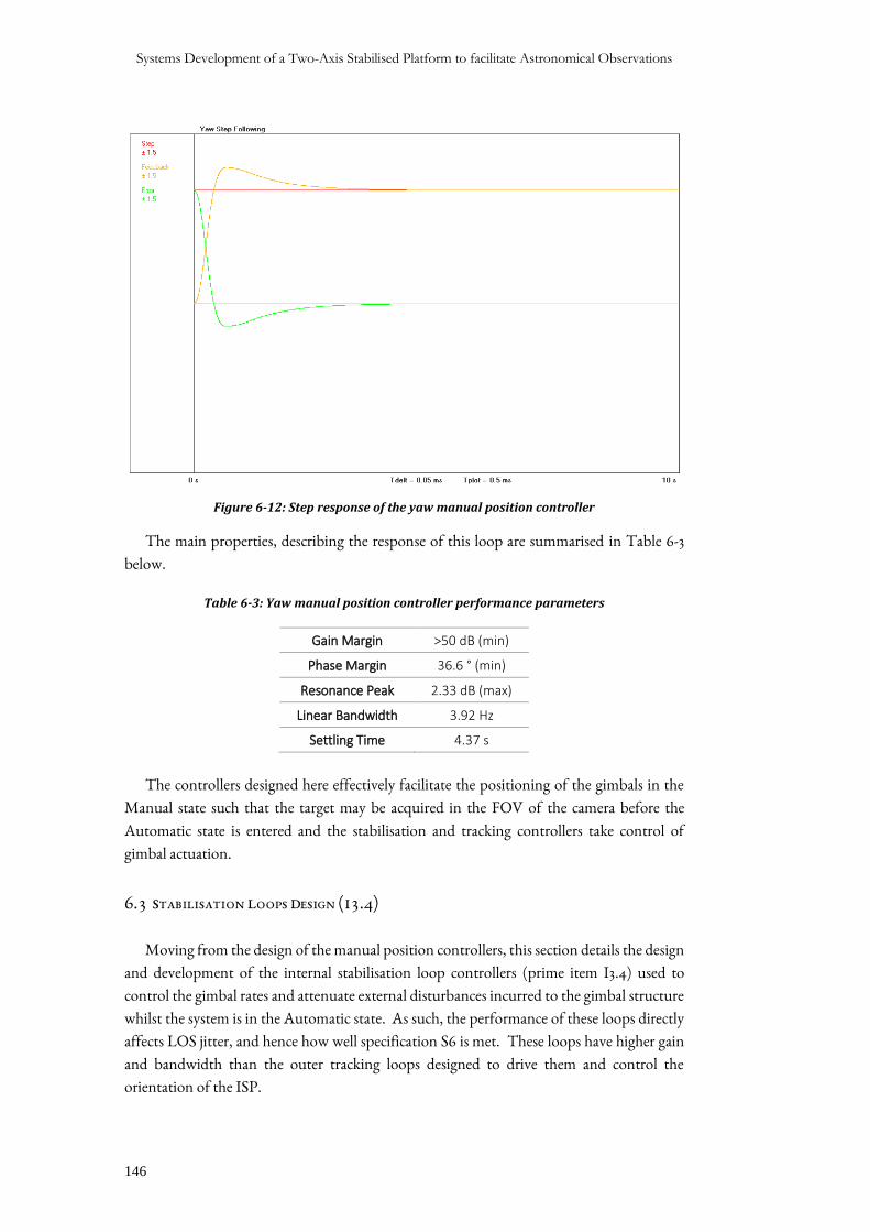
Systems Development of a Two-Axis Stabilised Platform to facilitate Astronomical Observations
146
Figure 6-12: Step response of the yaw manual position controller
The main properties, describing the response of this loop are summarised in Table 6-3
below.
Table 6-3: Yaw manual position controller performance parameters
Gain Margin >50 dB (min)
Phase Margin 36.6 ° (min)
Resonance Peak 2.33 dB (max)
Linear Bandwidth 3.92 Hz
Settling Time 4.37 s
The controllers designed here effectively facilitate the positioning of the gimbals in the
Manual state such that the target may be acquired in the FOV of the camera before the
Automatic state is entered and the stabilisation and tracking controllers take control of
gimbal actuation.
6.3 STABILISATION LOOPS DESIGN (I3.4)
Moving from the design of the manual position controllers, this section details the design
and development of the internal stabilisation loop controllers (prime item I3.4) used to
control the gimbal rates and attenuate external disturbances incurred to the gimbal structure
whilst the system is in the Automatic state. As such, the performance of these loops directly
affects LOS jitter, and hence how well specification S6 is met. These loops have higher gain
and bandwidth than the outer tracking loops designed to drive them and control the
orientation of the ISP.
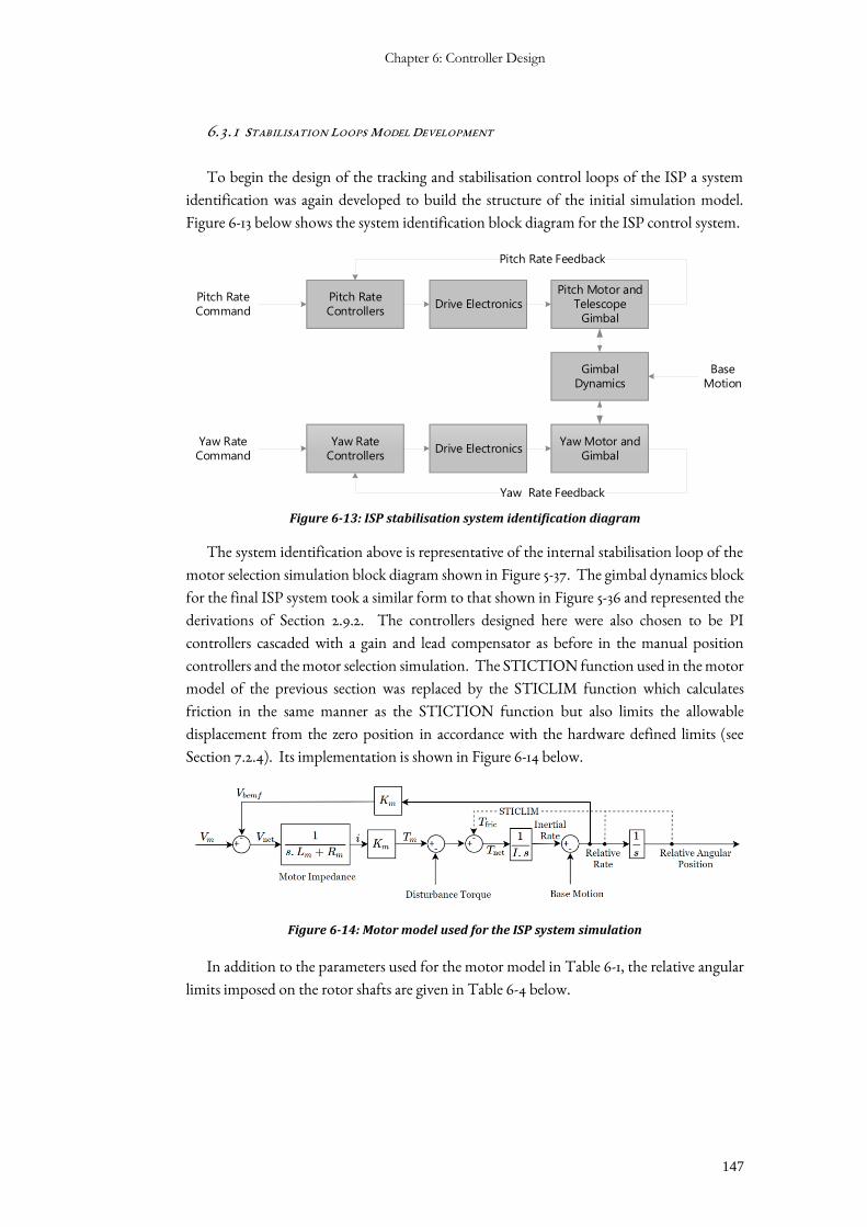
Chapter 6: Controller Design
147
6.3.1 STABILISATION LOOPS MODEL DEVELOPMENT
To begin the design of the tracking and stabilisation control loops of the ISP a system
identification was again developed to build the structure of the initial simulation model.
Figure 6-13 below shows the system identification block diagram for the ISP control system.
Gimbal
Dynamics
Drive Electronics
Drive Electronics
Pitch Rate
Controllers
Yaw Rate
Controllers
Pitch Motor and
Telescope
Gimbal
Yaw Motor and
Gimbal
Yaw Rate Feedback
Base
Motion
Pitch Rate Feedback
Pitch Rate
Command
Yaw Rate
Command
Figure 6-13: ISP stabilisation system identification diagram
The system identification above is representative of the internal stabilisation loop of the
motor selection simulation block diagram shown in Figure 5-37. The gimbal dynamics block
for the final ISP system took a similar form to that shown in Figure 5-36 and represented the
derivations of Section 2.9.2. The controllers designed here were also chosen to be PI
controllers cascaded with a gain and lead compensator as before in the manual position
controllers and the motor selection simulation. The STICTION function used in the motor
model of the previous section was replaced by the STICLIM function which calculates
friction in the same manner as the STICTION function but also limits the allowable
displacement from the zero position in accordance with the hardware defined limits (see
Section 7.2.4). Its implementation is shown in Figure 6-14 below.
Figure 6-14: Motor model used for the ISP system simulation
In addition to the parameters used for the motor model in Table 6-1, the relative angular
limits imposed on the rotor shafts are given in Table 6-4 below.
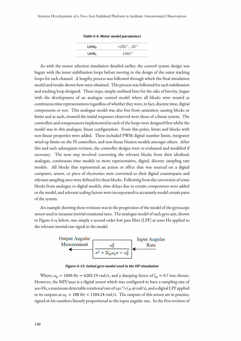
Systems Development of a Two-Axis Stabilised Platform to facilitate Astronomical Observations
148
Table 6-4: Motor model parameters
Limitp +200 °, -20 °
Limity ±360 °
As with the motor selection simulation detailed earlier, the control system design was
begun with the inner stabilisation loops before moving to the design of the outer tracking
loops for each channel. A lengthy process was followed through which the final simulation
model and results shown here were obtained. This process was followed for each stabilisation
and tracking loop designed. These steps, simply outlined here for the sake of brevity, began
with the development of an analogue control model where all blocks were treated as
continuous time representations regardless of whether they were, in fact, discrete time, digital
components or not. This analogue model was also free from saturation causing blocks or
limits and as such, ensured the initial responses observed were those of a linear system. The
controllers and compensators implemented in each of the loops were designed first whilst the
model was in this analogue, linear configuration. From this point, limits and blocks with
non-linear properties were added. These included PWM digital number limits, integrator
wind-up limits on the PI controllers, and non-linear friction models amongst others. After
this and each subsequent revision, the controller designs were re-evaluated and modified if
necessary. The next step involved converting the relevant blocks from their idealised,
analogue, continuous time models to more representative, digital, discrete sampling rate
models. All blocks that represented an action or effect that was sourced on a digital
computer, sensor, or piece of electronics were converted to their digital counterparts and
relevant sampling rates were defined for these blocks. Following from the conversion of some
blocks from analogue to digital models, time delays due to certain components were added
to the model, and relevant scaling factors were incorporated to accurately model certain parts
of the system.
An example showing these revisions was in the progression of the model of the gyroscope
sensor used to measure inertial rotational rates. The analogue model of each gyro axis, shown
in Figure 6-15 below, was simply a second order low pass filter (LPF) at 1000 Hz applied to
the relevant inertial rate signal in the model.
Figure 6-15: Initial gyro model used in the ISP simulation
Where, 𝜔𝑔 = 1000 𝐻𝑧 = 6283.19 𝑟𝑎𝑑/𝑠, and a damping factor of 𝜁𝑔 = 0.7 was chosen.
However, the MPU9150 is a digital sensor which was configured to have a sampling rate of
500 Hz, a maximum detectable rotational rate of 250 °/s (4.36 rad/s), and a digital LPF applied
to its outputs at 𝜔𝑓 = 188 𝐻𝑧 = 1184.24 𝑟𝑎𝑑/𝑠. The outputs of this sensor are in practice,
signed 16-bit numbers linearly proportional to the input angular rate. In the first revision of
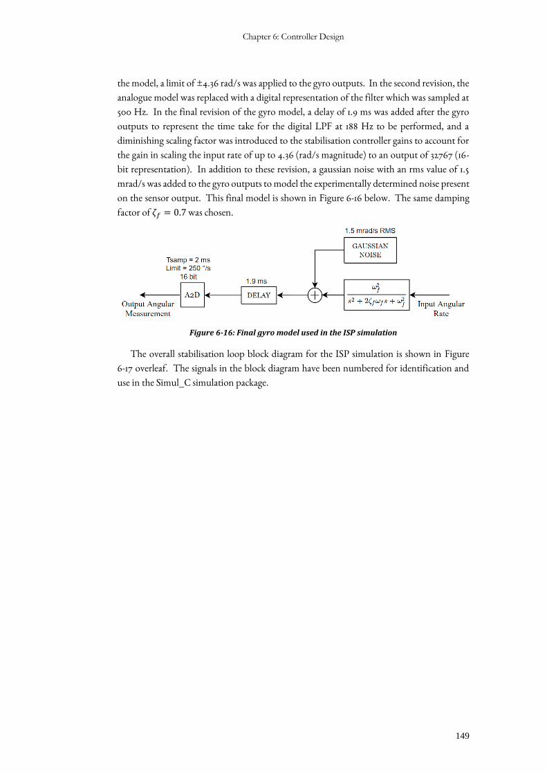
Chapter 6: Controller Design
149
the model, a limit of ±4.36 rad/s was applied to the gyro outputs. In the second revision, the
analogue model was replaced with a digital representation of the filter which was sampled at
500 Hz. In the final revision of the gyro model, a delay of 1.9 ms was added after the gyro
outputs to represent the time take for the digital LPF at 188 Hz to be performed, and a
diminishing scaling factor was introduced to the stabilisation controller gains to account for
the gain in scaling the input rate of up to 4.36 (rad/s magnitude) to an output of 32767 (16-
bit representation). In addition to these revision, a gaussian noise with an rms value of 1.5
mrad/s was added to the gyro outputs to model the experimentally determined noise present
on the sensor output. This final model is shown in Figure 6-16 below. The same damping
factor of 𝜁𝑓 = 0.7 was chosen.
Figure 6-16: Final gyro model used in the ISP simulation
The overall stabilisation loop block diagram for the ISP simulation is shown in Figure
6-17 overleaf. The signals in the block diagram have been numbered for identification and
use in the Simul_C simulation package.
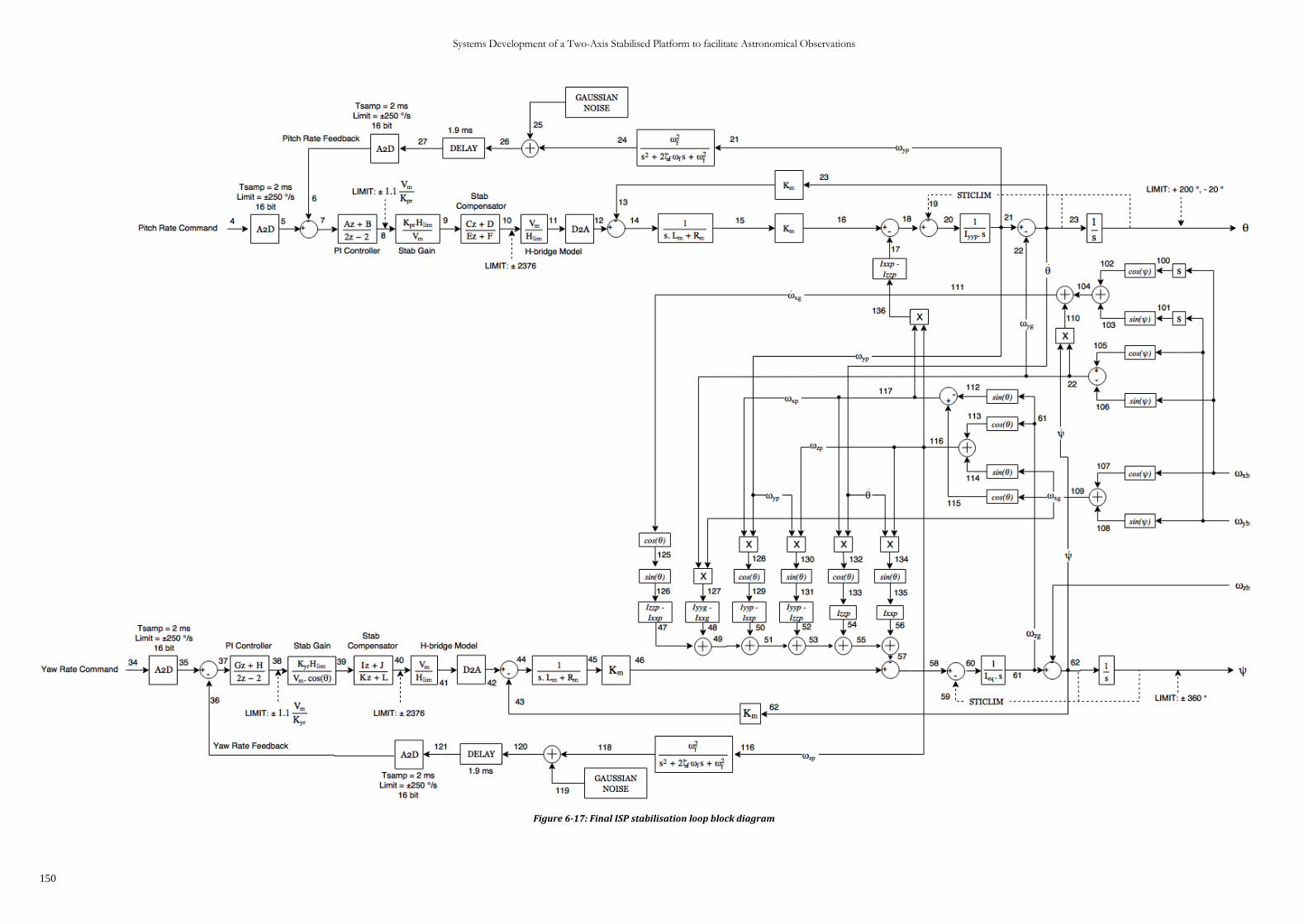
Systems Development of a Two-Axis Stabilised Platform to facilitate Astronomical Observations
150
Figure 6-17: Final ISP stabilisation loop block diagram
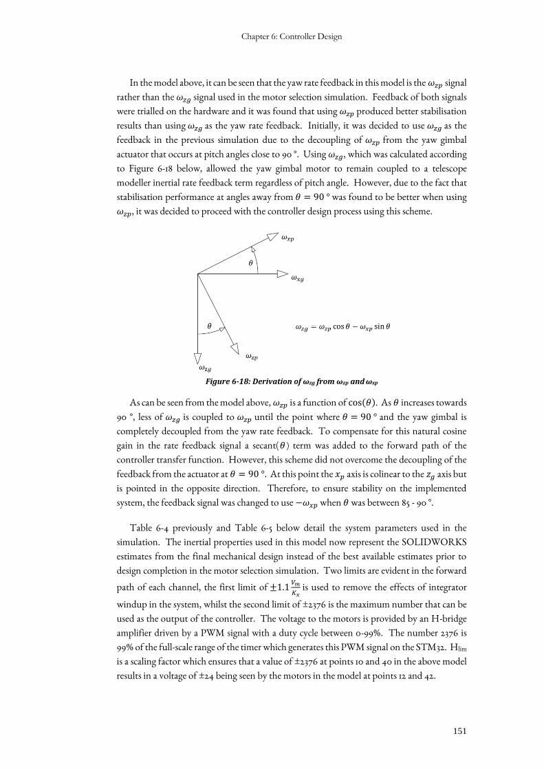
Chapter 6: Controller Design
151
In the model above, it can be seen that the yaw rate feedback in this model is the 𝜔𝑧𝑝 signal
rather than the 𝜔𝑧𝑔 signal used in the motor selection simulation. Feedback of both signals
were trialled on the hardware and it was found that using 𝜔𝑧𝑝 produced better stabilisation
results than using 𝜔𝑧𝑔 as the yaw rate feedback. Initially, it was decided to use 𝜔𝑧𝑔 as the
feedback in the previous simulation due to the decoupling of 𝜔𝑧𝑝 from the yaw gimbal
actuator that occurs at pitch angles close to 90 °. Using 𝜔𝑧𝑔, which was calculated according
to Figure 6-18 below, allowed the yaw gimbal motor to remain coupled to a telescope
modeller inertial rate feedback term regardless of pitch angle. However, due to the fact that
stabilisation performance at angles away from 𝜃 = 90 ° was found to be better when using
𝜔𝑧𝑝, it was decided to proceed with the controller design process using this scheme.
Figure 6-18: Derivation of ωzg from ωzp and ωxp
As can be seen from the model above, 𝜔𝑧𝑝 is a function of cos(𝜃). As 𝜃 increases towards
90 °, less of 𝜔𝑧𝑔 is coupled to 𝜔𝑧𝑝 until the point where 𝜃 = 90 ° and the yaw gimbal is
completely decoupled from the yaw rate feedback. To compensate for this natural cosine
gain in the rate feedback signal a secant(𝜃 ) term was added to the forward path of the
controller transfer function. However, this scheme did not overcome the decoupling of the
feedback from the actuator at 𝜃 = 90 °. At this point the 𝑥𝑝 axis is colinear to the 𝑧𝑔 axis but
is pointed in the opposite direction. Therefore, to ensure stability on the implemented
system, the feedback signal was changed to use −𝜔𝑥𝑝 when 𝜃 was between 85 - 90 °.
Table 6-4 previously and Table 6-5 below detail the system parameters used in the
simulation. The inertial properties used in this model now represent the SOLIDWORKS
estimates from the final mechanical design instead of the best available estimates prior to
design completion in the motor selection simulation. Two limits are evident in the forward
path of each channel, the first limit of ±1.1𝑉𝑚
𝐾𝑥 is used to remove the effects of integrator
windup in the system, whilst the second limit of ±2376 is the maximum number that can be
used as the output of the controller. The voltage to the motors is provided by an H-bridge
amplifier driven by a PWM signal with a duty cycle between 0-99%. The number 2376 is
99% of the full-scale range of the timer which generates this PWM signal on the STM32. Hlim
is a scaling factor which ensures that a value of ±2376 at points 10 and 40 in the above model
results in a voltage of ±24 being seen by the motors in the model at points 12 and 42.
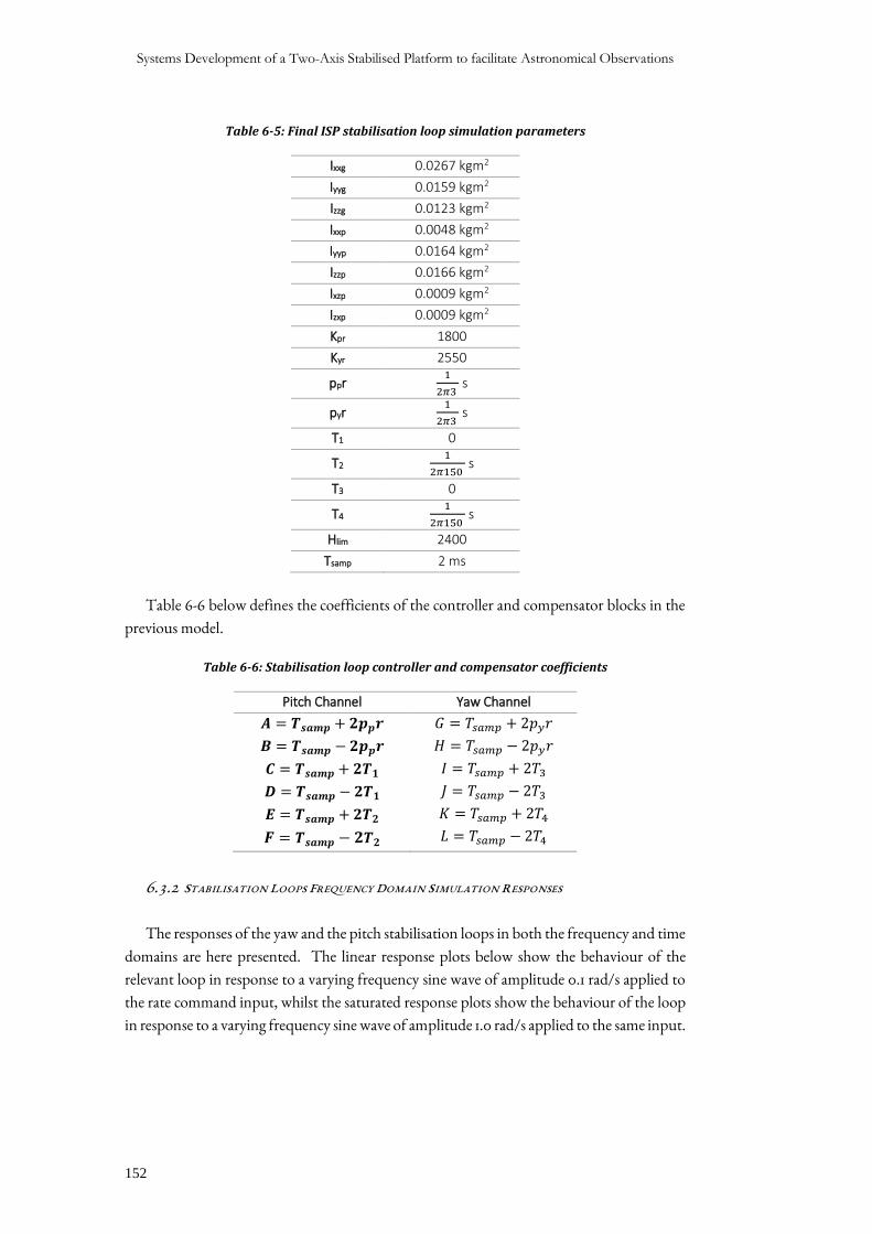
Systems Development of a Two-Axis Stabilised Platform to facilitate Astronomical Observations
152
Table 6-5: Final ISP stabilisation loop simulation parameters
Ixxg 0.0267 kgm2
Iyyg 0.0159 kgm2
Izzg 0.0123 kgm2
Ixxp 0.0048 kgm2
Iyyp 0.0164 kgm2
Izzp 0.0166 kgm2
Ixzp 0.0009 kgm2
Izxp 0.0009 kgm2
Kpr 1800
Kyr 2550
ppr 1
2𝜋3 s
pyr 1
2𝜋3 s
T1 0
T2 1
2𝜋150 s
T3 0
T4 1
2𝜋150 s
Hlim 2400
Tsamp 2 ms
Table 6-6 below defines the coefficients of the controller and compensator blocks in the
previous model.
Table 6-6: Stabilisation loop controller and compensator coefficients
Pitch Channel Yaw Channel
𝑨 = 𝑻𝒔𝒂𝒎𝒑 + 𝟐𝒑𝒑𝒓
𝑩 = 𝑻𝒔𝒂𝒎𝒑 − 𝟐𝒑𝒑𝒓
𝑪 = 𝑻𝒔𝒂𝒎𝒑 + 𝟐𝑻𝟏
𝑫 = 𝑻𝒔𝒂𝒎𝒑 − 𝟐𝑻𝟏
𝑬 = 𝑻𝒔𝒂𝒎𝒑 + 𝟐𝑻𝟐
𝑭 = 𝑻𝒔𝒂𝒎𝒑 − 𝟐𝑻𝟐
𝐺 = 𝑇𝑠𝑎𝑚𝑝 + 2𝑝𝑦𝑟
𝐻 = 𝑇𝑠𝑎𝑚𝑝 − 2𝑝𝑦𝑟
𝐼 = 𝑇𝑠𝑎𝑚𝑝 + 2𝑇3
𝐽 = 𝑇𝑠𝑎𝑚𝑝 − 2𝑇3
𝐾 = 𝑇𝑠𝑎𝑚𝑝 + 2𝑇4
𝐿 = 𝑇𝑠𝑎𝑚𝑝 − 2𝑇4
6.3.2 STABILISATION LOOPS FREQUENCY DOMAIN SIMULATION RESPONSES
The responses of the yaw and the pitch stabilisation loops in both the frequency and time
domains are here presented. The linear response plots below show the behaviour of the
relevant loop in response to a varying frequency sine wave of amplitude 0.1 rad/s applied to
the rate command input, whilst the saturated response plots show the behaviour of the loop
in response to a varying frequency sine wave of amplitude 1.0 rad/s applied to the same input.
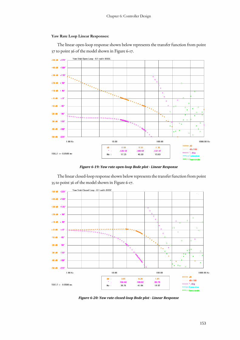
Chapter 6: Controller Design
153
Yaw Rate Loop Linear Responses:
The linear open-loop response shown below represents the transfer function from point
37 to point 36 of the model shown in Figure 6-17.
Figure 6-19: Yaw rate open-loop Bode plot - Linear Response
The linear closed-loop response shown below represents the transfer function from point
35 to point 36 of the model shown in Figure 6-17.
Figure 6-20: Yaw rate closed-loop Bode plot - Linear Response
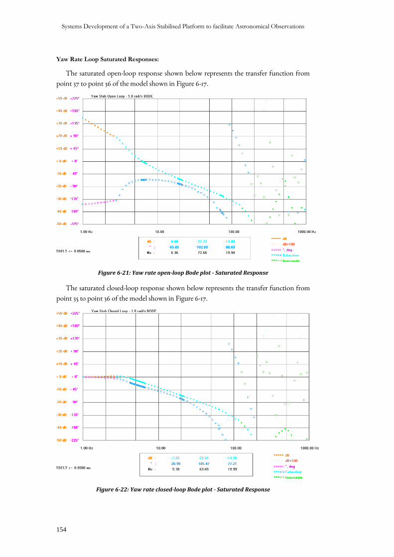
Systems Development of a Two-Axis Stabilised Platform to facilitate Astronomical Observations
154
Yaw Rate Loop Saturated Responses:
The saturated open-loop response shown below represents the transfer function from
point 37 to point 36 of the model shown in Figure 6-17.
Figure 6-21: Yaw rate open-loop Bode plot - Saturated Response
The saturated closed-loop response shown below represents the transfer function from
point 35 to point 36 of the model shown in Figure 6-17.
Figure 6-22: Yaw rate closed-loop Bode plot - Saturated Response
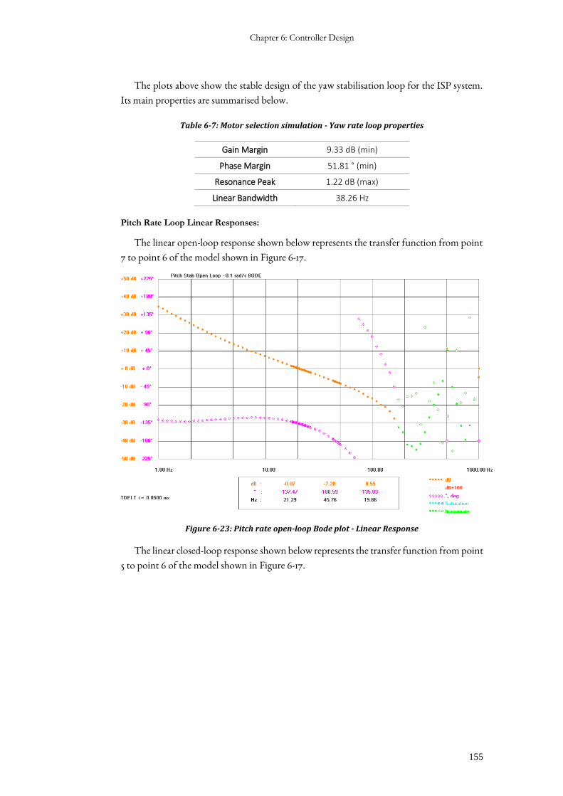
Chapter 6: Controller Design
155
The plots above show the stable design of the yaw stabilisation loop for the ISP system.
Its main properties are summarised below.
Table 6-7: Motor selection simulation - Yaw rate loop properties
Gain Margin 9.33 dB (min)
Phase Margin 51.81 ° (min)
Resonance Peak 1.22 dB (max)
Linear Bandwidth 38.26 Hz
Pitch Rate Loop Linear Responses:
The linear open-loop response shown below represents the transfer function from point
7 to point 6 of the model shown in Figure 6-17.
Figure 6-23: Pitch rate open-loop Bode plot - Linear Response
The linear closed-loop response shown below represents the transfer function from point
5 to point 6 of the model shown in Figure 6-17.
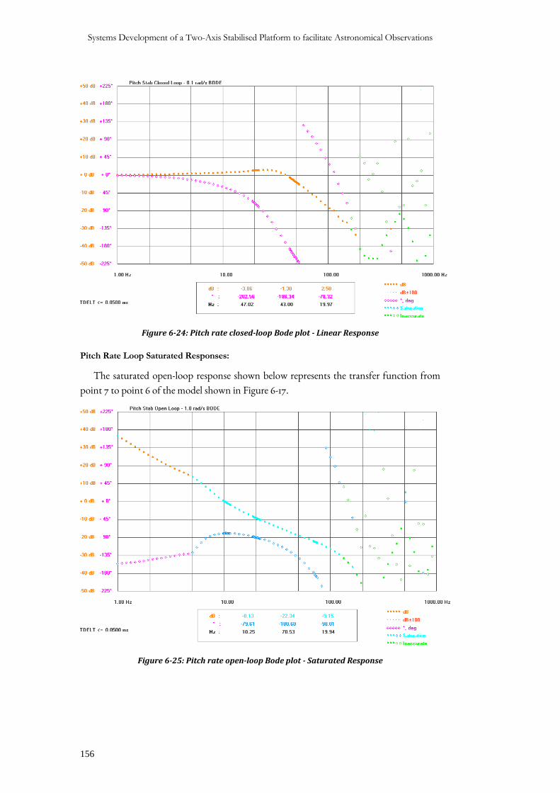
Systems Development of a Two-Axis Stabilised Platform to facilitate Astronomical Observations
156
Figure 6-24: Pitch rate closed-loop Bode plot - Linear Response
Pitch Rate Loop Saturated Responses:
The saturated open-loop response shown below represents the transfer function from
point 7 to point 6 of the model shown in Figure 6-17.
Figure 6-25: Pitch rate open-loop Bode plot - Saturated Response
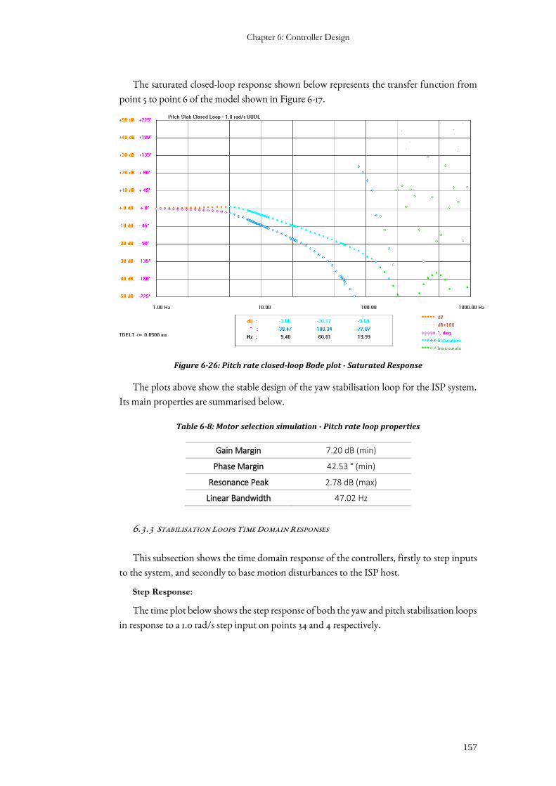
Chapter 6: Controller Design
157
The saturated closed-loop response shown below represents the transfer function from
point 5 to point 6 of the model shown in Figure 6-17.
Figure 6-26: Pitch rate closed-loop Bode plot - Saturated Response
The plots above show the stable design of the yaw stabilisation loop for the ISP system.
Its main properties are summarised below.
Table 6-8: Motor selection simulation - Pitch rate loop properties
Gain Margin 7.20 dB (min)
Phase Margin 42.53 ° (min)
Resonance Peak 2.78 dB (max)
Linear Bandwidth 47.02 Hz
6.3.3 STABILISATION LOOPS TIME DOMAIN RESPONSES
This subsection shows the time domain response of the controllers, firstly to step inputs
to the system, and secondly to base motion disturbances to the ISP host.
Step Response:
The time plot below shows the step response of both the yaw and pitch stabilisation loops
in response to a 1.0 rad/s step input on points 34 and 4 respectively.
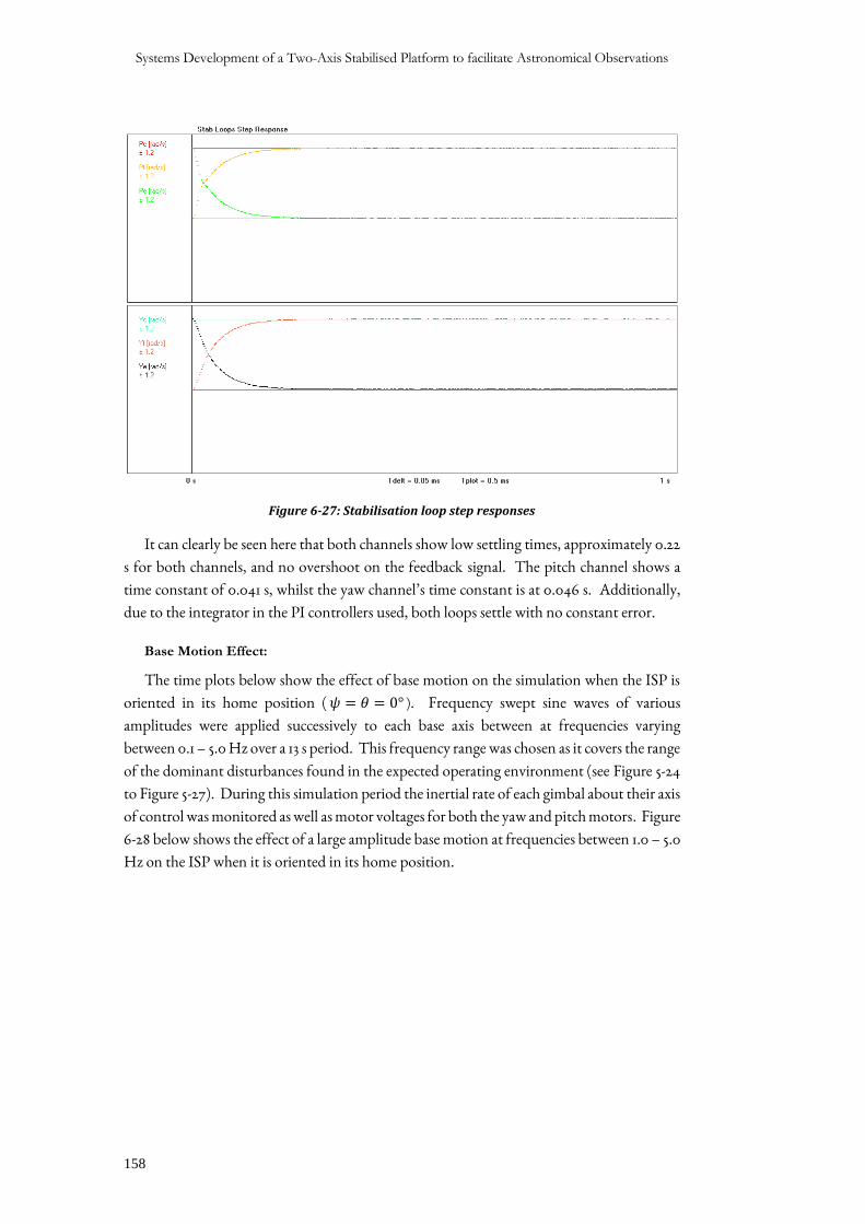
Systems Development of a Two-Axis Stabilised Platform to facilitate Astronomical Observations
158
Figure 6-27: Stabilisation loop step responses
It can clearly be seen here that both channels show low settling times, approximately 0.22
s for both channels, and no overshoot on the feedback signal. The pitch channel shows a
time constant of 0.041 s, whilst the yaw channel’s time constant is at 0.046 s. Additionally,
due to the integrator in the PI controllers used, both loops settle with no constant error.
Base Motion Effect:
The time plots below show the effect of base motion on the simulation when the ISP is
oriented in its home position ( 𝜓 = 𝜃 = 0° ). Frequency swept sine waves of various
amplitudes were applied successively to each base axis between at frequencies varying
between 0.1 – 5.0 Hz over a 13 s period. This frequency range was chosen as it covers the range
of the dominant disturbances found in the expected operating environment (see Figure 5-24
to Figure 5-27). During this simulation period the inertial rate of each gimbal about their axis
of control was monitored as well as motor voltages for both the yaw and pitch motors. Figure
6-28 below shows the effect of a large amplitude base motion at frequencies between 1.0 – 5.0
Hz on the ISP when it is oriented in its home position.
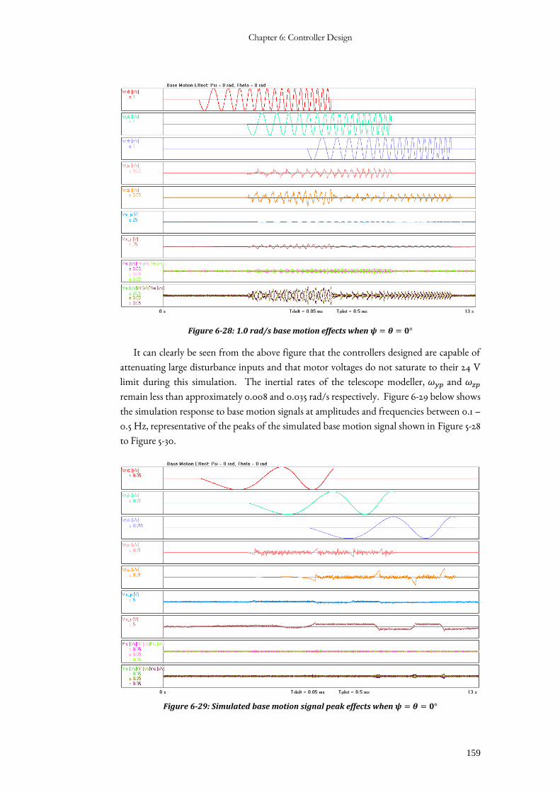
Chapter 6: Controller Design
159
Figure 6-28: 1.0 rad/s base motion effects when 𝝍 = 𝜽 = 𝟎°
It can clearly be seen from the above figure that the controllers designed are capable of
attenuating large disturbance inputs and that motor voltages do not saturate to their 24 V
limit during this simulation. The inertial rates of the telescope modeller, 𝜔𝑦𝑝 and 𝜔𝑧𝑝
remain less than approximately 0.008 and 0.035 rad/s respectively. Figure 6-29 below shows
the simulation response to base motion signals at amplitudes and frequencies between 0.1 –
0.5 Hz, representative of the peaks of the simulated base motion signal shown in Figure 5-28
to Figure 5-30.
Figure 6-29: Simulated base motion signal peak effects when 𝝍 = 𝜽 = 𝟎°
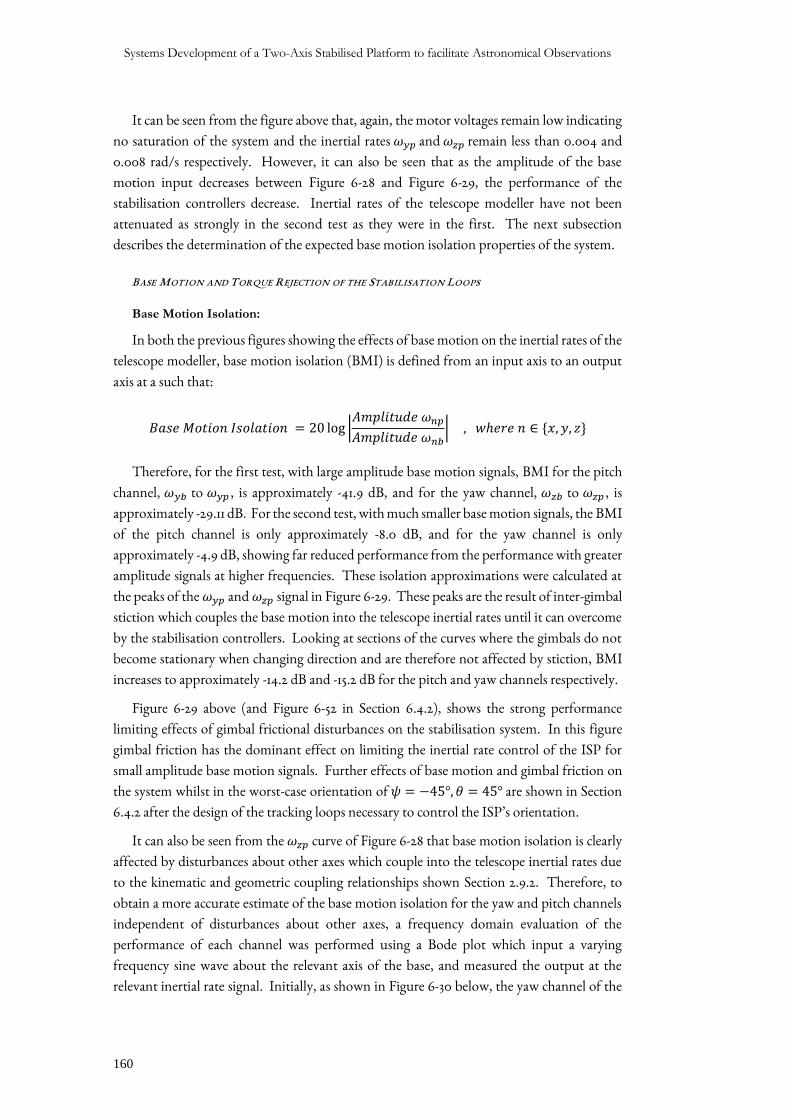
Systems Development of a Two-Axis Stabilised Platform to facilitate Astronomical Observations
160
It can be seen from the figure above that, again, the motor voltages remain low indicating
no saturation of the system and the inertial rates 𝜔𝑦𝑝 and 𝜔𝑧𝑝 remain less than 0.004 and
0.008 rad/s respectively. However, it can also be seen that as the amplitude of the base
motion input decreases between Figure 6-28 and Figure 6-29, the performance of the
stabilisation controllers decrease. Inertial rates of the telescope modeller have not been
attenuated as strongly in the second test as they were in the first. The next subsection
describes the determination of the expected base motion isolation properties of the system.
BASE MOTION AND TORQUE REJECTION OF THE STABILISATION LOOPS
Base Motion Isolation:
In both the previous figures showing the effects of base motion on the inertial rates of the
telescope modeller, base motion isolation (BMI) is defined from an input axis to an output
axis at a such that:
𝐵𝑎𝑠𝑒 𝑀𝑜𝑡𝑖𝑜𝑛 𝐼𝑠𝑜𝑙𝑎𝑡𝑖𝑜𝑛 = 20 log |𝐴𝑚𝑝𝑙𝑖𝑡𝑢𝑑𝑒 𝜔𝑛𝑝
𝐴𝑚𝑝𝑙𝑖𝑡𝑢𝑑𝑒 𝜔𝑛𝑏| , 𝑤ℎ𝑒𝑟𝑒 𝑛 ∈ {𝑥, 𝑦, 𝑧}
Therefore, for the first test, with large amplitude base motion signals, BMI for the pitch
channel, 𝜔𝑦𝑏 to 𝜔𝑦𝑝 , is approximately -41.9 dB, and for the yaw channel, 𝜔𝑧𝑏 to 𝜔𝑧𝑝 , is
approximately -29.11 dB. For the second test, with much smaller base motion signals, the BMI
of the pitch channel is only approximately -8.0 dB, and for the yaw channel is only
approximately -4.9 dB, showing far reduced performance from the performance with greater
amplitude signals at higher frequencies. These isolation approximations were calculated at
the peaks of the 𝜔𝑦𝑝 and 𝜔𝑧𝑝 signal in Figure 6-29. These peaks are the result of inter-gimbal
stiction which couples the base motion into the telescope inertial rates until it can overcome
by the stabilisation controllers. Looking at sections of the curves where the gimbals do not
become stationary when changing direction and are therefore not affected by stiction, BMI
increases to approximately -14.2 dB and -15.2 dB for the pitch and yaw channels respectively.
Figure 6-29 above (and Figure 6-52 in Section 6.4.2), shows the strong performance
limiting effects of gimbal frictional disturbances on the stabilisation system. In this figure
gimbal friction has the dominant effect on limiting the inertial rate control of the ISP for
small amplitude base motion signals. Further effects of base motion and gimbal friction on
the system whilst in the worst-case orientation of 𝜓 = −45°, 𝜃 = 45° are shown in Section
6.4.2 after the design of the tracking loops necessary to control the ISP’s orientation.
It can also be seen from the 𝜔𝑧𝑝 curve of Figure 6-28 that base motion isolation is clearly
affected by disturbances about other axes which couple into the telescope inertial rates due
to the kinematic and geometric coupling relationships shown Section 2.9.2. Therefore, to
obtain a more accurate estimate of the base motion isolation for the yaw and pitch channels
independent of disturbances about other axes, a frequency domain evaluation of the
performance of each channel was performed using a Bode plot which input a varying
frequency sine wave about the relevant axis of the base, and measured the output at the
relevant inertial rate signal. Initially, as shown in Figure 6-30 below, the yaw channel of the
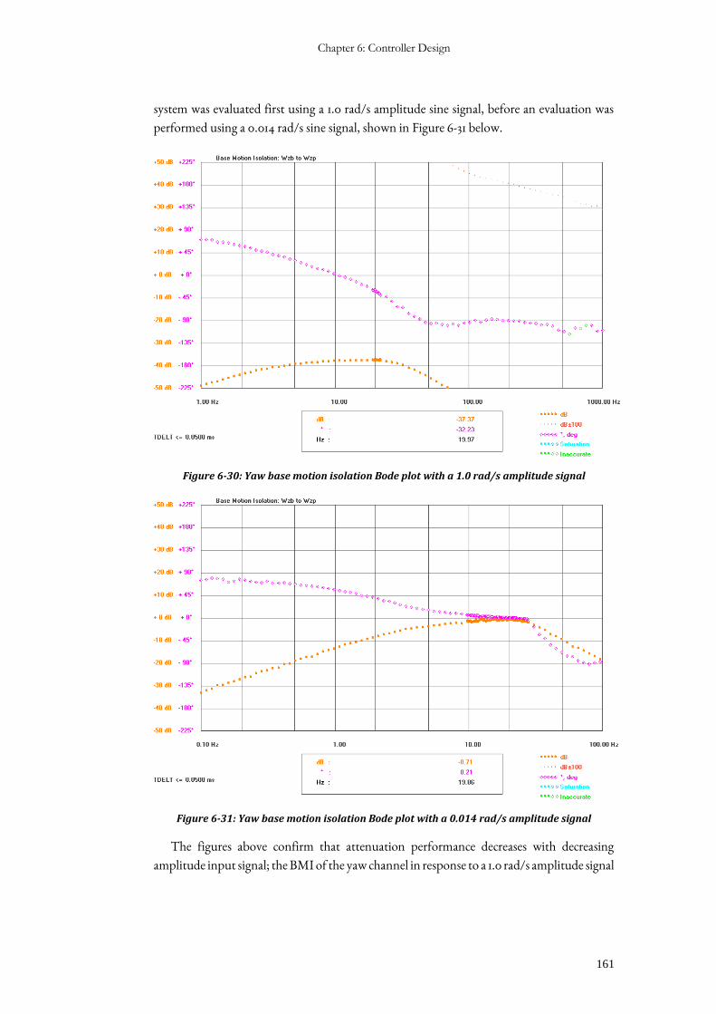
Chapter 6: Controller Design
161
system was evaluated first using a 1.0 rad/s amplitude sine signal, before an evaluation was
performed using a 0.014 rad/s sine signal, shown in Figure 6-31 below.
Figure 6-30: Yaw base motion isolation Bode plot with a 1.0 rad/s amplitude signal
Figure 6-31: Yaw base motion isolation Bode plot with a 0.014 rad/s amplitude signal
The figures above confirm that attenuation performance decreases with decreasing
amplitude input signal; the BMI of the yaw channel in response to a 1.0 rad/s amplitude signal
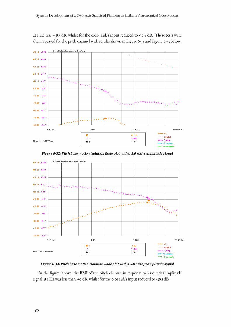
Systems Development of a Two-Axis Stabilised Platform to facilitate Astronomical Observations
162
at 1 Hz was -48.5 dB, whilst for the 0.014 rad/s input reduced to -32.8 dB. These tests were
then repeated for the pitch channel with results shown in Figure 6-32 and Figure 6-33 below.
Figure 6-32: Pitch base motion isolation Bode plot with a 1.0 rad/s amplitude signal
Figure 6-33: Pitch base motion isolation Bode plot with a 0.01 rad/s amplitude signal
In the figures above, the BMI of the pitch channel in response to a 1.0 rad/s amplitude
signal at 1 Hz was less than -50 dB, whilst for the 0.01 rad/s input reduced to -38.1 dB.
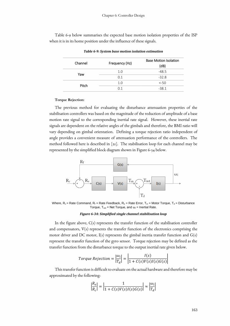
Chapter 6: Controller Design
163
Table 6-9 below summarises the expected base motion isolation properties of the ISP
when it is in its home position under the influence of these signals.
Table 6-9: System base motion isolation estimation
Channel Frequency (Hz) Base Motion Isolation
(dB)
Yaw 1.0 -48.5
0.1 -32.8
Pitch 1.0 <-50
0.1 -38.1
Torque Rejection:
The previous method for evaluating the disturbance attenuation properties of the
stabilisation controllers was based on the magnitude of the reduction of amplitude of a base
motion rate signal to the corresponding inertial rate signal. However, these inertial rate
signals are dependent on the relative angles of the gimbals and therefore, the BMI ratio will
vary depending on gimbal orientation. Defining a torque rejection ratio independent of
angle provides a convenient measure of attenuation performance of the controllers. The
method followed here is described in [21]. The stabilisation loop for each channel may be
represented by the simplified block diagram shown in Figure 6-34 below.
Where, Rc = Rate Command, Rf = Rate Feedback, Re = Rate Error, Tm = Motor Torque, Td = Disturbance
Torque, Tnet = Net Torque, and ωi = Inertial Rate.
Figure 6-34: Simplified single channel stabilisation loop
In the figure above, C(s) represents the transfer function of the stabilisation controller
and compensators, V(s) represents the transfer function of the electronics comprising the
motor driver and DC motor, I(s) represents the gimbal inertia transfer function and G(s)
represent the transfer function of the gyro sensor. Torque rejection may be defined as the
transfer function from the disturbance torque to the output inertial rate given below.
𝑇𝑜𝑟𝑞𝑢𝑒 𝑅𝑒𝑗𝑒𝑐𝑡𝑖𝑜𝑛 = |𝜔𝑖
𝑇𝑑| = |
𝐼(𝑠)
1 + 𝐶(𝑠)𝑉(𝑠)𝐼(𝑠)𝐺(𝑠)|
This transfer function is difficult to evaluate on the actual hardware and therefore may be
approximated by the following:
|𝑅𝑒
𝑅𝑐| = |
1
1 + 𝐶(𝑠)𝑉(𝑠)𝐼(𝑠)𝐺(𝑠)| ≈ |
𝜔𝑖
𝑇𝑑|
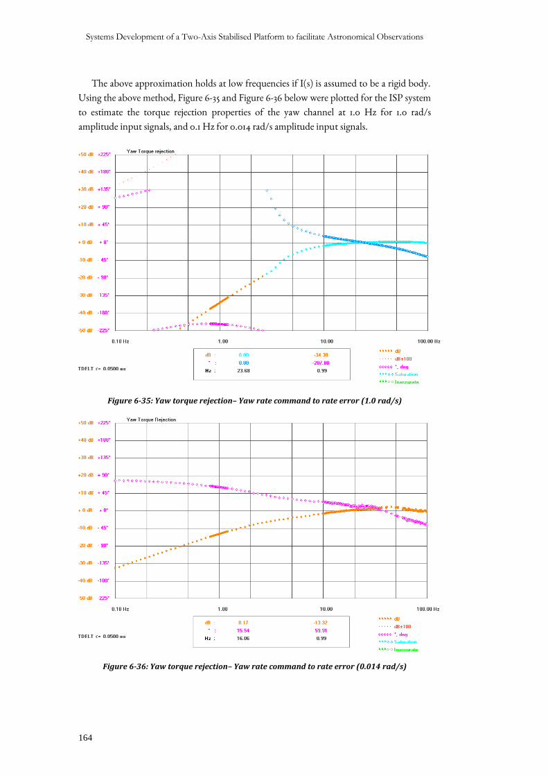
Systems Development of a Two-Axis Stabilised Platform to facilitate Astronomical Observations
164
The above approximation holds at low frequencies if I(s) is assumed to be a rigid body.
Using the above method, Figure 6-35 and Figure 6-36 below were plotted for the ISP system
to estimate the torque rejection properties of the yaw channel at 1.0 Hz for 1.0 rad/s
amplitude input signals, and 0.1 Hz for 0.014 rad/s amplitude input signals.
Figure 6-35: Yaw torque rejection– Yaw rate command to rate error (1.0 rad/s)
Figure 6-36: Yaw torque rejection– Yaw rate command to rate error (0.014 rad/s)
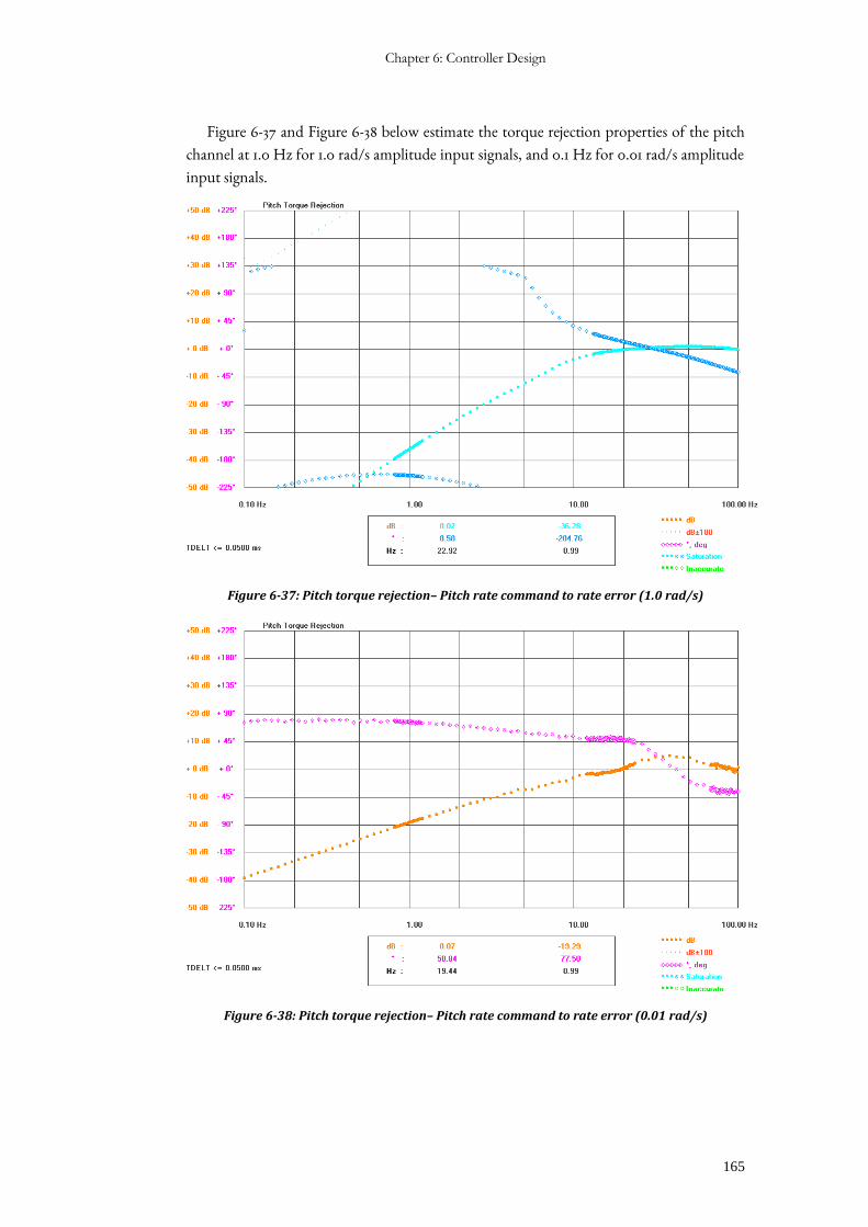
Chapter 6: Controller Design
165
Figure 6-37 and Figure 6-38 below estimate the torque rejection properties of the pitch
channel at 1.0 Hz for 1.0 rad/s amplitude input signals, and 0.1 Hz for 0.01 rad/s amplitude
input signals.
Figure 6-37: Pitch torque rejection– Pitch rate command to rate error (1.0 rad/s)
Figure 6-38: Pitch torque rejection– Pitch rate command to rate error (0.01 rad/s)
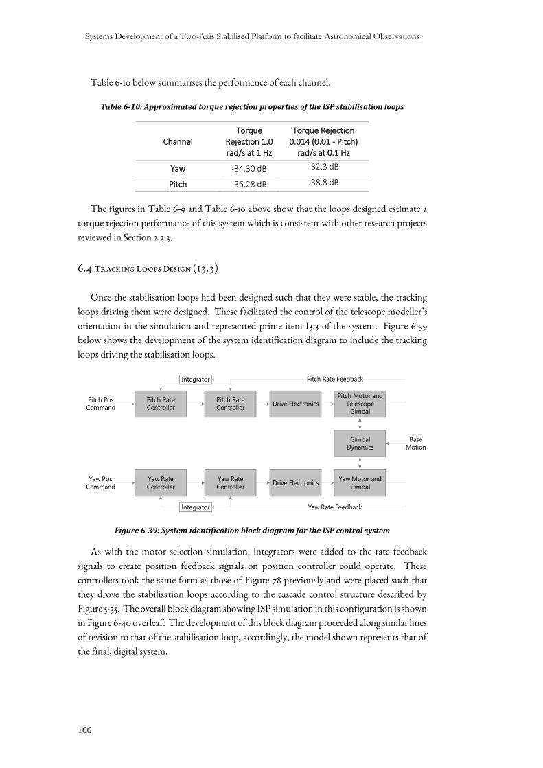
Systems Development of a Two-Axis Stabilised Platform to facilitate Astronomical Observations
166
Table 6-10 below summarises the performance of each channel.
Table 6-10: Approximated torque rejection properties of the ISP stabilisation loops
Channel Torque
Rejection 1.0 rad/s at 1 Hz
Torque Rejection 0.014 (0.01 - Pitch)
rad/s at 0.1 Hz
Yaw -34.30 dB -32.3 dB
Pitch -36.28 dB -38.8 dB
The figures in Table 6-9 and Table 6-10 above show that the loops designed estimate a
torque rejection performance of this system which is consistent with other research projects
reviewed in Section 2.3.3.
6.4 TRACKING LOOPS DESIGN (I3.3)
Once the stabilisation loops had been designed such that they were stable, the tracking
loops driving them were designed. These facilitated the control of the telescope modeller’s
orientation in the simulation and represented prime item I3.3 of the system. Figure 6-39
below shows the development of the system identification diagram to include the tracking
loops driving the stabilisation loops.
Gimbal
Dynamics
Drive Electronics
Drive Electronics
Pitch Rate
Controller
Yaw Rate
Controller
Pitch Motor and
Telescope
Gimbal
Yaw Motor and
Gimbal
Yaw Rate Feedback
Base
Motion
Pitch Rate Feedback
Pitch Rate
Controller
Yaw Rate
Controller
Integrator
Integrator
Pitch Pos
Command
Yaw Pos
Command
Figure 6-39: System identification block diagram for the ISP control system
As with the motor selection simulation, integrators were added to the rate feedback
signals to create position feedback signals on position controller could operate. These
controllers took the same form as those of Figure 78 previously and were placed such that
they drove the stabilisation loops according to the cascade control structure described by
Figure 5-35. The overall block diagram showing ISP simulation in this configuration is shown
in Figure 6-40 overleaf. The development of this block diagram proceeded along similar lines
of revision to that of the stabilisation loop, accordingly, the model shown represents that of
the final, digital system.
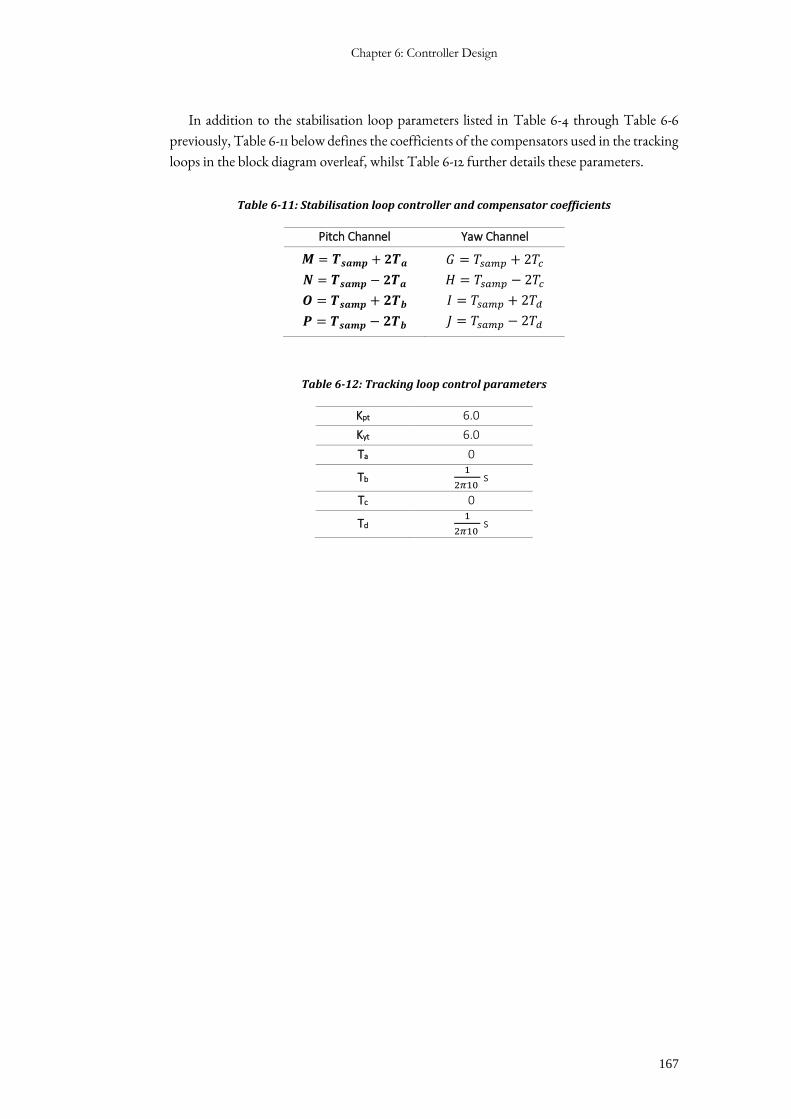
Chapter 6: Controller Design
167
In addition to the stabilisation loop parameters listed in Table 6-4 through Table 6-6
previously, Table 6-11 below defines the coefficients of the compensators used in the tracking
loops in the block diagram overleaf, whilst Table 6-12 further details these parameters.
Table 6-11: Stabilisation loop controller and compensator coefficients
Pitch Channel Yaw Channel
𝑴 = 𝑻𝒔𝒂𝒎𝒑 + 𝟐𝑻𝒂
𝑵 = 𝑻𝒔𝒂𝒎𝒑 − 𝟐𝑻𝒂
𝑶 = 𝑻𝒔𝒂𝒎𝒑 + 𝟐𝑻𝒃
𝑷 = 𝑻𝒔𝒂𝒎𝒑 − 𝟐𝑻𝒃
𝐺 = 𝑇𝑠𝑎𝑚𝑝 + 2𝑇𝑐
𝐻 = 𝑇𝑠𝑎𝑚𝑝 − 2𝑇𝑐
𝐼 = 𝑇𝑠𝑎𝑚𝑝 + 2𝑇𝑑
𝐽 = 𝑇𝑠𝑎𝑚𝑝 − 2𝑇𝑑
Table 6-12: Tracking loop control parameters
Kpt 6.0
Kyt 6.0
Ta 0
Tb 1
2𝜋10 s
Tc 0
Td 1
2𝜋10 s
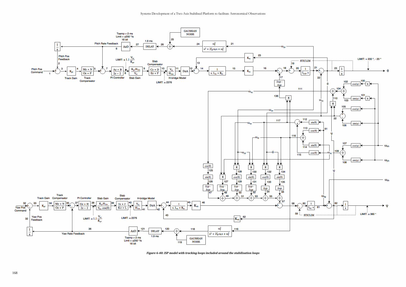
Systems Development of a Two-Axis Stabilised Platform to facilitate Astronomical Observations
168
Figure 6-40: ISP model with tracking loops included around the stabilisation loops
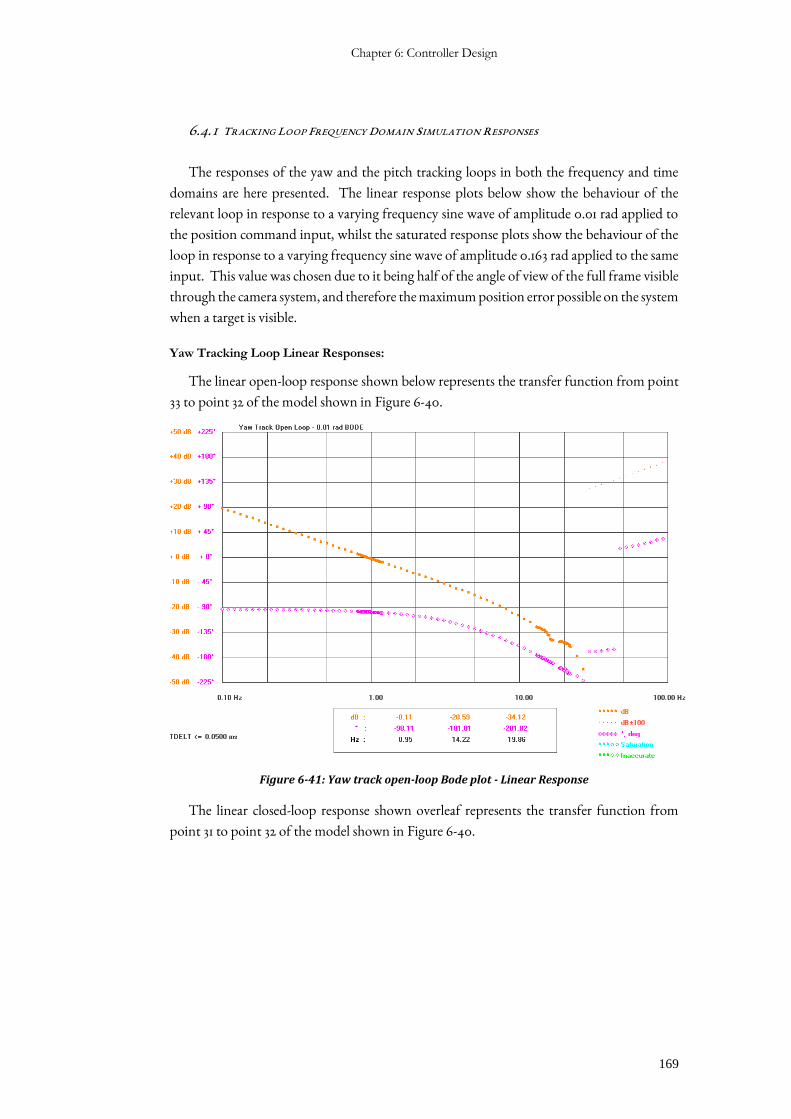
Chapter 6: Controller Design
169
6.4.1 TRACKING LOOP FREQUENCY DOMAIN SIMULATION RESPONSES
The responses of the yaw and the pitch tracking loops in both the frequency and time
domains are here presented. The linear response plots below show the behaviour of the
relevant loop in response to a varying frequency sine wave of amplitude 0.01 rad applied to
the position command input, whilst the saturated response plots show the behaviour of the
loop in response to a varying frequency sine wave of amplitude 0.163 rad applied to the same
input. This value was chosen due to it being half of the angle of view of the full frame visible
through the camera system, and therefore the maximum position error possible on the system
when a target is visible.
Yaw Tracking Loop Linear Responses:
The linear open-loop response shown below represents the transfer function from point
33 to point 32 of the model shown in Figure 6-40.
Figure 6-41: Yaw track open-loop Bode plot - Linear Response
The linear closed-loop response shown overleaf represents the transfer function from
point 31 to point 32 of the model shown in Figure 6-40.
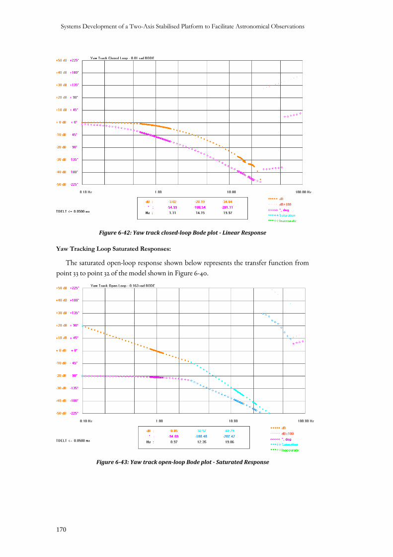
Systems Development of a Two-Axis Stabilised Platform to Facilitate Astronomical Observations
170
Figure 6-42: Yaw track closed-loop Bode plot - Linear Response
Yaw Tracking Loop Saturated Responses:
The saturated open-loop response shown below represents the transfer function from
point 33 to point 32 of the model shown in Figure 6-40.
Figure 6-43: Yaw track open-loop Bode plot - Saturated Response
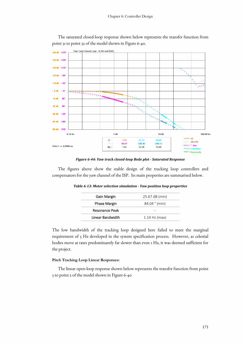
Chapter 6: Controller Design
171
The saturated closed-loop response shown below represents the transfer function from
point 31 to point 32 of the model shown in Figure 6-40.
Figure 6-44: Yaw track closed-loop Bode plot - Saturated Response
The figures above show the stable design of the tracking loop controllers and
compensators for the yaw channel of the ISP. Its main properties are summarised below.
Table 6-13: Motor selection simulation - Yaw position loop properties
Gain Margin 25.67 dB (min)
Phase Margin 84.04 ° (min)
Resonance Peak -
Linear Bandwidth 1.14 Hz (max)
The low bandwidth of the tracking loop designed here failed to meet the marginal
requirement of 5 Hz developed in the system specification process. However, as celestial
bodies move at rates predominantly far slower than even 1 Hz, it was deemed sufficient for
the project.
Pitch Tracking Loop Linear Responses:
The linear open-loop response shown below represents the transfer function from point
3 to point 2 of the model shown in Figure 6-40
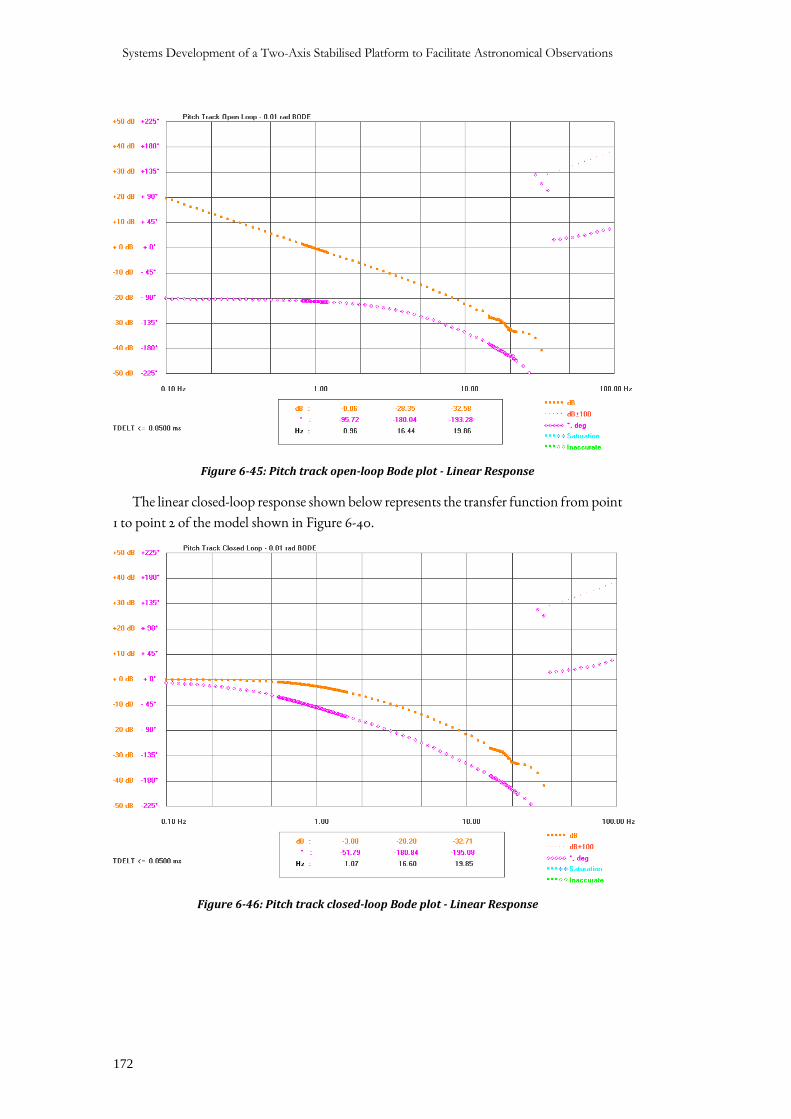
Systems Development of a Two-Axis Stabilised Platform to Facilitate Astronomical Observations
172
Figure 6-45: Pitch track open-loop Bode plot - Linear Response
The linear closed-loop response shown below represents the transfer function from point
1 to point 2 of the model shown in Figure 6-40.
Figure 6-46: Pitch track closed-loop Bode plot - Linear Response
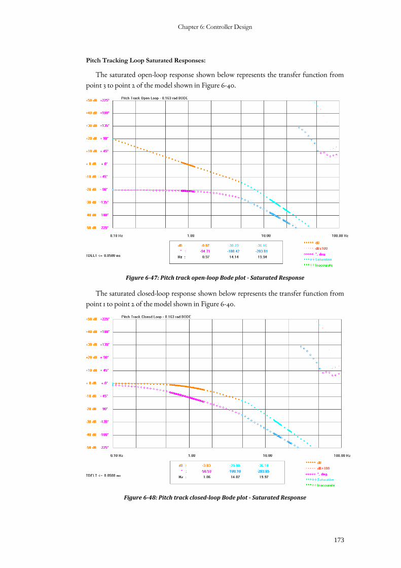
Chapter 6: Controller Design
173
Pitch Tracking Loop Saturated Responses:
The saturated open-loop response shown below represents the transfer function from
point 3 to point 2 of the model shown in Figure 6-40.
Figure 6-47: Pitch track open-loop Bode plot - Saturated Response
The saturated closed-loop response shown below represents the transfer function from
point 1 to point 2 of the model shown in Figure 6-40.
Figure 6-48: Pitch track closed-loop Bode plot - Saturated Response
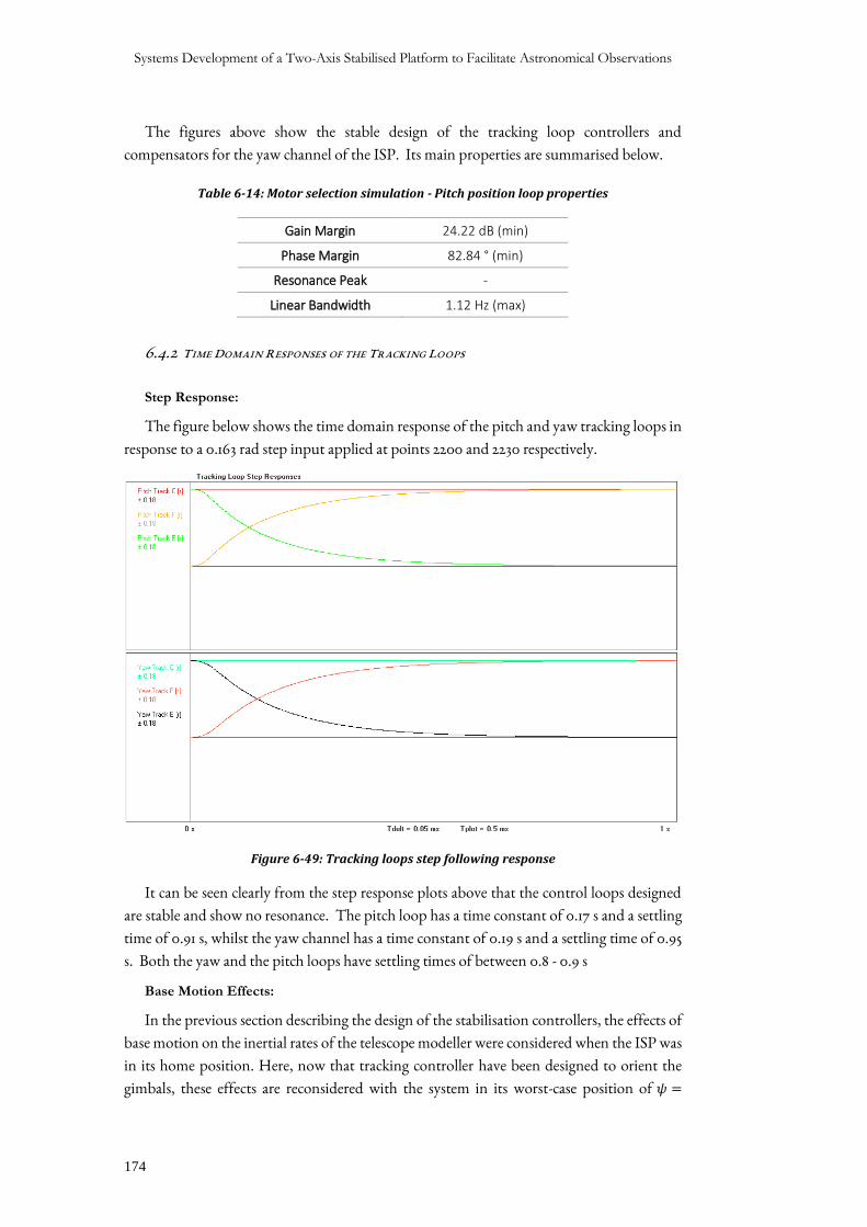
Systems Development of a Two-Axis Stabilised Platform to Facilitate Astronomical Observations
174
The figures above show the stable design of the tracking loop controllers and
compensators for the yaw channel of the ISP. Its main properties are summarised below.
Table 6-14: Motor selection simulation - Pitch position loop properties
Gain Margin 24.22 dB (min)
Phase Margin 82.84 ° (min)
Resonance Peak -
Linear Bandwidth 1.12 Hz (max)
6.4.2 TIME DOMAIN RESPONSES OF THE TRACKING LOOPS
Step Response:
The figure below shows the time domain response of the pitch and yaw tracking loops in
response to a 0.163 rad step input applied at points 2200 and 2230 respectively.
Figure 6-49: Tracking loops step following response
It can be seen clearly from the step response plots above that the control loops designed
are stable and show no resonance. The pitch loop has a time constant of 0.17 s and a settling
time of 0.91 s, whilst the yaw channel has a time constant of 0.19 s and a settling time of 0.95
s. Both the yaw and the pitch loops have settling times of between 0.8 - 0.9 s
Base Motion Effects:
In the previous section describing the design of the stabilisation controllers, the effects of
base motion on the inertial rates of the telescope modeller were considered when the ISP was
in its home position. Here, now that tracking controller have been designed to orient the
gimbals, these effects are reconsidered with the system in its worst-case position of 𝜓 =
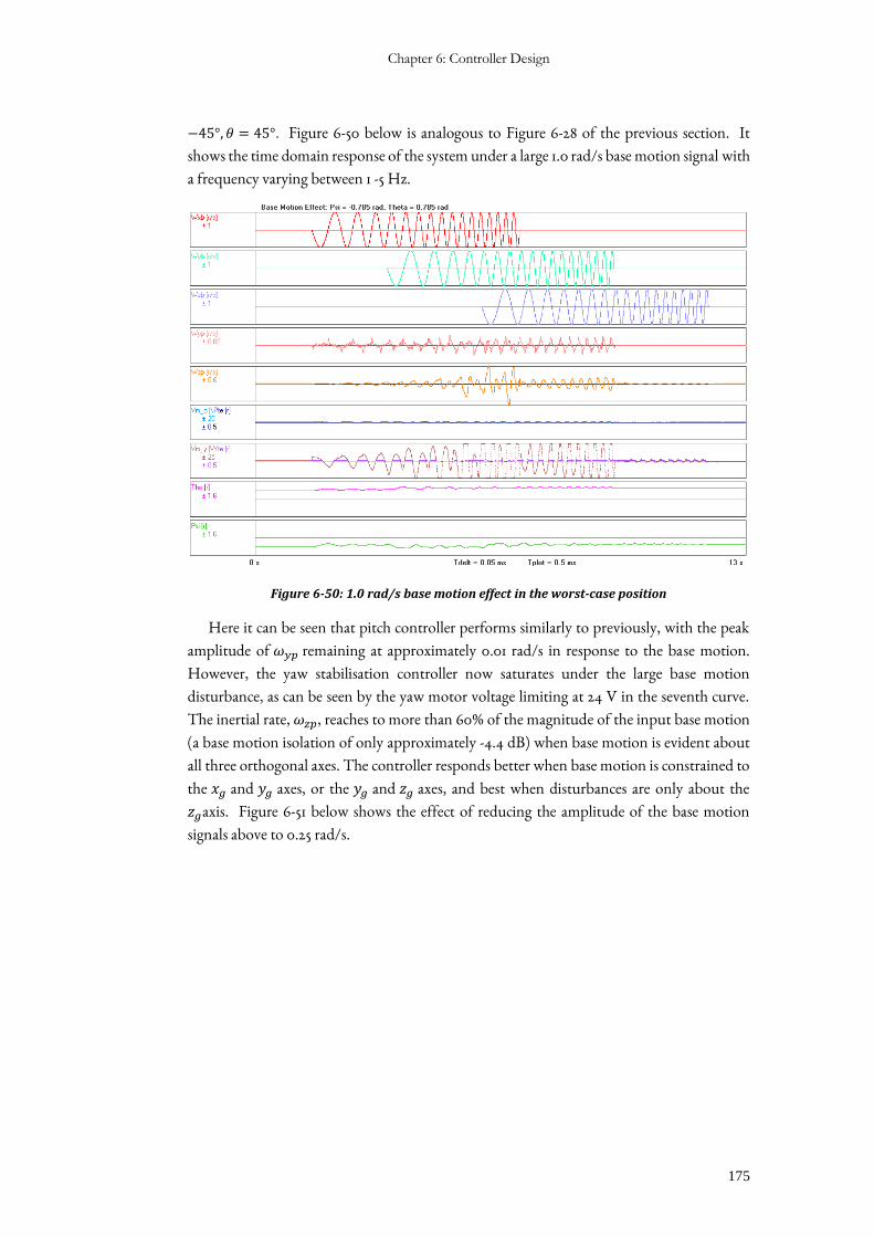
Chapter 6: Controller Design
175
−45°, 𝜃 = 45°. Figure 6-50 below is analogous to Figure 6-28 of the previous section. It
shows the time domain response of the system under a large 1.0 rad/s base motion signal with
a frequency varying between 1 -5 Hz.
Figure 6-50: 1.0 rad/s base motion effect in the worst-case position
Here it can be seen that pitch controller performs similarly to previously, with the peak
amplitude of 𝜔𝑦𝑝 remaining at approximately 0.01 rad/s in response to the base motion.
However, the yaw stabilisation controller now saturates under the large base motion
disturbance, as can be seen by the yaw motor voltage limiting at 24 V in the seventh curve.
The inertial rate, 𝜔𝑧𝑝, reaches to more than 60% of the magnitude of the input base motion
(a base motion isolation of only approximately -4.4 dB) when base motion is evident about
all three orthogonal axes. The controller responds better when base motion is constrained to
the 𝑥𝑔 and 𝑦𝑔 axes, or the 𝑦𝑔 and 𝑧𝑔 axes, and best when disturbances are only about the
𝑧𝑔axis. Figure 6-51 below shows the effect of reducing the amplitude of the base motion
signals above to 0.25 rad/s.
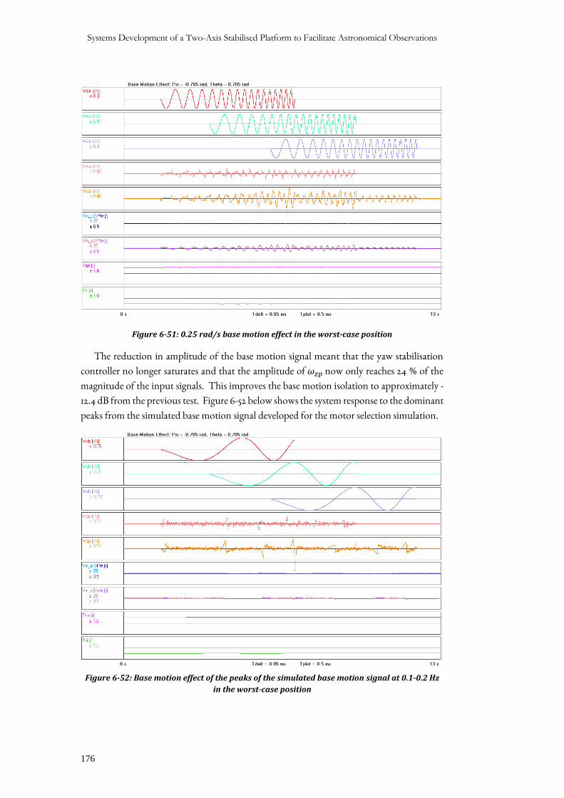
Systems Development of a Two-Axis Stabilised Platform to Facilitate Astronomical Observations
176
Figure 6-51: 0.25 rad/s base motion effect in the worst-case position
The reduction in amplitude of the base motion signal meant that the yaw stabilisation
controller no longer saturates and that the amplitude of 𝜔𝑧𝑝 now only reaches 24 % of the
magnitude of the input signals. This improves the base motion isolation to approximately -
12.4 dB from the previous test. Figure 6-52 below shows the system response to the dominant
peaks from the simulated base motion signal developed for the motor selection simulation.
Figure 6-52: Base motion effect of the peaks of the simulated base motion signal at 0.1-0.2 Hz
in the worst-case position
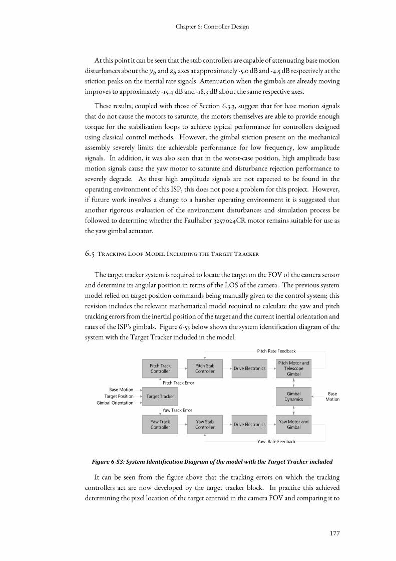
Chapter 6: Controller Design
177
At this point it can be seen that the stab controllers are capable of attenuating base motion
disturbances about the 𝑦𝑏 and 𝑧𝑏 axes at approximately -5.0 dB and -4.5 dB respectively at the
stiction peaks on the inertial rate signals. Attenuation when the gimbals are already moving
improves to approximately -15.4 dB and -18.3 dB about the same respective axes.
These results, coupled with those of Section 6.3.3, suggest that for base motion signals
that do not cause the motors to saturate, the motors themselves are able to provide enough
torque for the stabilisation loops to achieve typical performance for controllers designed
using classical control methods. However, the gimbal stiction present on the mechanical
assembly severely limits the achievable performance for low frequency, low amplitude
signals. In addition, it was also seen that in the worst-case position, high amplitude base
motion signals cause the yaw motor to saturate and disturbance rejection performance to
severely degrade. As these high amplitude signals are not expected to be found in the
operating environment of this ISP, this does not pose a problem for this project. However,
if future work involves a change to a harsher operating environment it is suggested that
another rigorous evaluation of the environment disturbances and simulation process be
followed to determine whether the Faulhaber 3257024CR motor remains suitable for use as
the yaw gimbal actuator.
6.5 TRACKING LOOP MODEL INCLUDING THE TARGET TRACKER
The target tracker system is required to locate the target on the FOV of the camera sensor
and determine its angular position in terms of the LOS of the camera. The previous system
model relied on target position commands being manually given to the control system; this
revision includes the relevant mathematical model required to calculate the yaw and pitch
tracking errors from the inertial position of the target and the current inertial orientation and
rates of the ISP’s gimbals. Figure 6-53 below shows the system identification diagram of the
system with the Target Tracker included in the model.
Gimbal
Dynamics
Drive Electronics
Drive Electronics
Pitch Stab
Controller
Yaw Stab
Controller
Pitch Motor and
Telescope
Gimbal
Yaw Motor and
Gimbal
Yaw Rate Feedback
Base
Motion
Pitch Rate Feedback
Target Tracker
Base Motion
Target Position
Pitch Track
Controller
Yaw Track
Controller
Gimbal Orientation
Pitch Track Error
Yaw Track Error
Figure 6-53: System Identification Diagram of the model with the Target Tracker included
It can be seen from the figure above that the tracking errors on which the tracking
controllers act are now developed by the target tracker block. In practice this achieved
determining the pixel location of the target centroid in the camera FOV and comparing it to
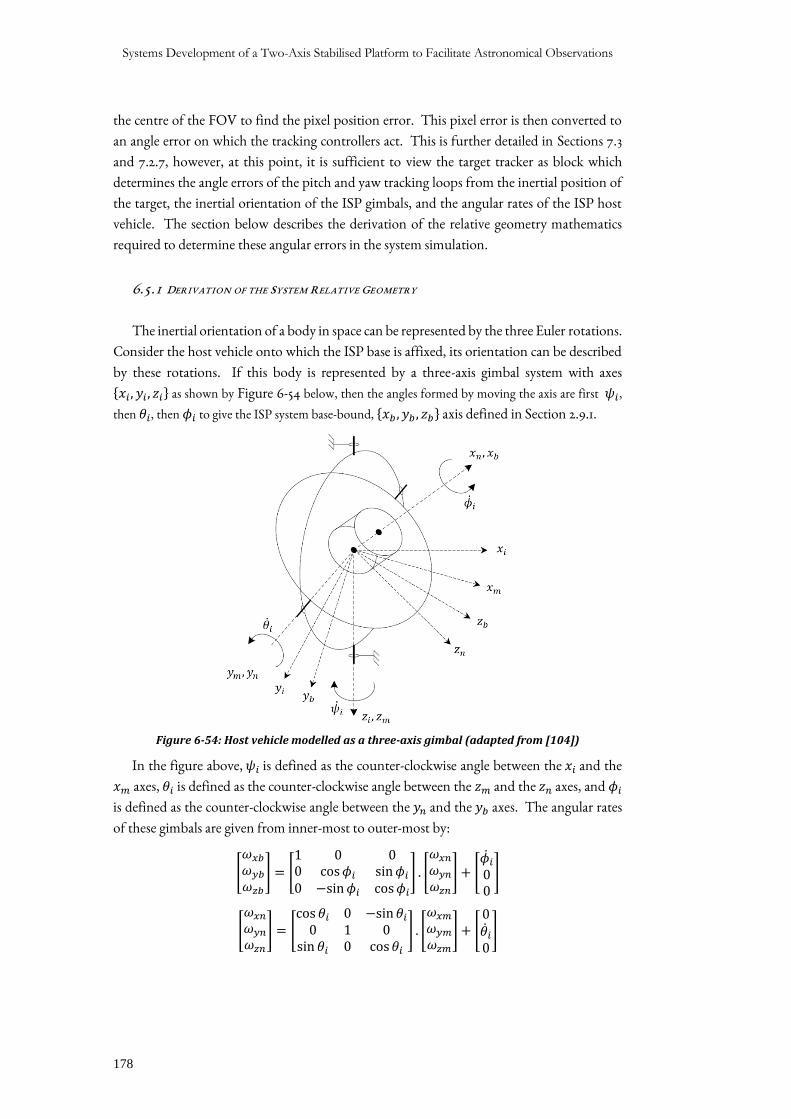
Systems Development of a Two-Axis Stabilised Platform to Facilitate Astronomical Observations
178
the centre of the FOV to find the pixel position error. This pixel error is then converted to
an angle error on which the tracking controllers act. This is further detailed in Sections 7.3
and 7.2.7, however, at this point, it is sufficient to view the target tracker as block which
determines the angle errors of the pitch and yaw tracking loops from the inertial position of
the target, the inertial orientation of the ISP gimbals, and the angular rates of the ISP host
vehicle. The section below describes the derivation of the relative geometry mathematics
required to determine these angular errors in the system simulation.
6.5.1 DERIVATION OF THE SYSTEM RELATIVE GEOMETRY
The inertial orientation of a body in space can be represented by the three Euler rotations.
Consider the host vehicle onto which the ISP base is affixed, its orientation can be described
by these rotations. If this body is represented by a three-axis gimbal system with axes
{𝑥𝑖 , 𝑦𝑖 , 𝑧𝑖} as shown by Figure 6-54 below, then the angles formed by moving the axis are first 𝜓𝑖 ,
then 𝜃𝑖, then 𝜙𝑖 to give the ISP system base-bound, {𝑥𝑏 , 𝑦𝑏 , 𝑧𝑏} axis defined in Section 2.9.1.
Figure 6-54: Host vehicle modelled as a three-axis gimbal (adapted from [104])
In the figure above, 𝜓𝑖 is defined as the counter-clockwise angle between the 𝑥𝑖 and the
𝑥𝑚 axes, 𝜃𝑖 is defined as the counter-clockwise angle between the 𝑧𝑚 and the 𝑧𝑛 axes, and 𝜙𝑖
is defined as the counter-clockwise angle between the 𝑦𝑛 and the 𝑦𝑏 axes. The angular rates
of these gimbals are given from inner-most to outer-most by:
[
𝜔𝑥𝑏
𝜔𝑦𝑏
𝜔𝑧𝑏
] = [1 0 00 cos𝜙𝑖 sin𝜙𝑖
0 −sin𝜙𝑖 cos𝜙𝑖
] . [
𝜔𝑥𝑛
𝜔𝑦𝑛
𝜔𝑧𝑛
] + [��𝑖
00
]
[
𝜔𝑥𝑛
𝜔𝑦𝑛
𝜔𝑧𝑛
] = [cos 𝜃𝑖 0 −sin 𝜃𝑖
0 1 0sin 𝜃𝑖 0 cos𝜃𝑖
] . [
𝜔𝑥𝑚
𝜔𝑦𝑚
𝜔𝑧𝑚
] + [0��𝑖
0]
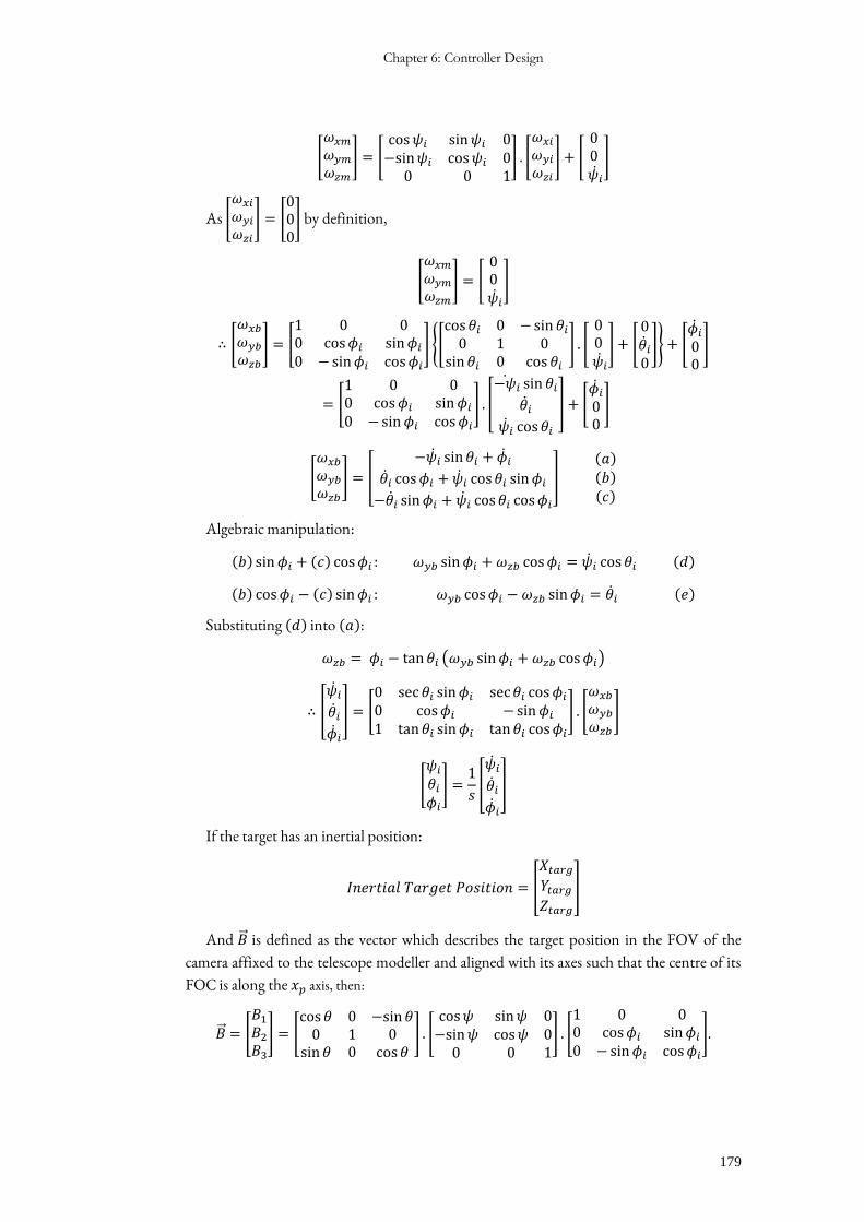
Chapter 6: Controller Design
179
[
𝜔𝑥𝑚
𝜔𝑦𝑚
𝜔𝑧𝑚
] = [cos𝜓𝑖 sin𝜓𝑖 0−sin𝜓𝑖 cos𝜓𝑖 0
0 0 1] . [
𝜔𝑥𝑖
𝜔𝑦𝑖
𝜔𝑧𝑖
] + [
00
��𝑖
]
As [
𝜔𝑥𝑖
𝜔𝑦𝑖
𝜔𝑧𝑖
] = [000] by definition,
[
𝜔𝑥𝑚
𝜔𝑦𝑚
𝜔𝑧𝑚
] = [00
��𝑖
]
∴ [
𝜔𝑥𝑏
𝜔𝑦𝑏
𝜔𝑧𝑏
] = [
1 0 00 cos𝜙𝑖 sin𝜙𝑖
0 − sin𝜙𝑖 cos𝜙𝑖
] {[cos 𝜃𝑖 0 − sin 𝜃𝑖
0 1 0sin 𝜃𝑖 0 cos 𝜃𝑖
] . [
00
��𝑖
] + [0��𝑖
0]} + [
��𝑖
00
]
= [
1 0 00 cos𝜙𝑖 sin𝜙𝑖
0 − sin𝜙𝑖 cos𝜙𝑖
] . [
−��𝑖 sin 𝜃𝑖
��𝑖
��𝑖 cos𝜃𝑖
] + [��𝑖
00
]
[
𝜔𝑥𝑏
𝜔𝑦𝑏
𝜔𝑧𝑏
] = [
−��𝑖 sin 𝜃𝑖 + ��𝑖
��𝑖 cos𝜙𝑖 + ��𝑖 cos𝜃𝑖 sin𝜙𝑖
−��𝑖 sin𝜙𝑖 + ��𝑖 cos𝜃𝑖 cos𝜙𝑖
]
(𝑎)(𝑏)(𝑐)
Algebraic manipulation:
(𝑏) sin 𝜙𝑖 + (𝑐) cos𝜙𝑖 : 𝜔𝑦𝑏 sin𝜙𝑖 + 𝜔𝑧𝑏 cos𝜙𝑖 = ��𝑖 cos 𝜃𝑖 (𝑑)
(𝑏) cos𝜙𝑖 − (𝑐) sin𝜙𝑖 : 𝜔𝑦𝑏 cos𝜙𝑖 − 𝜔𝑧𝑏 sin𝜙𝑖 = ��𝑖 (𝑒)
Substituting (𝑑) into (𝑎):
𝜔𝑧𝑏 = 𝜙𝑖 − tan𝜃𝑖 (𝜔𝑦𝑏 sin𝜙𝑖 + 𝜔𝑧𝑏 cos𝜙𝑖)
∴ [
��𝑖
��𝑖
��𝑖
] = [
0 sec 𝜃𝑖 sin𝜙𝑖 sec 𝜃𝑖 cos𝜙𝑖
0 cos𝜙𝑖 −sin𝜙𝑖
1 tan𝜃𝑖 sin𝜙𝑖 tan 𝜃𝑖 cos𝜙𝑖
] . [
𝜔𝑥𝑏
𝜔𝑦𝑏
𝜔𝑧𝑏
]
[
𝜓𝑖
𝜃𝑖
𝜙𝑖
] =1
𝑠[
��𝑖
��𝑖
��𝑖
]
If the target has an inertial position:
𝐼𝑛𝑒𝑟𝑡𝑖𝑎𝑙 𝑇𝑎𝑟𝑔𝑒𝑡 𝑃𝑜𝑠𝑖𝑡𝑖𝑜𝑛 = [
𝑋𝑡𝑎𝑟𝑔
𝑌𝑡𝑎𝑟𝑔
𝑍𝑡𝑎𝑟𝑔
]
And �� is defined as the vector which describes the target position in the FOV of the
camera affixed to the telescope modeller and aligned with its axes such that the centre of its
FOC is along the 𝑥𝑝 axis, then:
�� = [
𝐵1
𝐵2
𝐵3
] = [cos𝜃 0 −sin 𝜃
0 1 0sin 𝜃 0 cos𝜃
] . [cos𝜓 sin𝜓 0−sin𝜓 cos𝜓 0
0 0 1] . [
1 0 00 cos𝜙𝑖 sin𝜙𝑖
0 − sin𝜙𝑖 cos𝜙𝑖
].
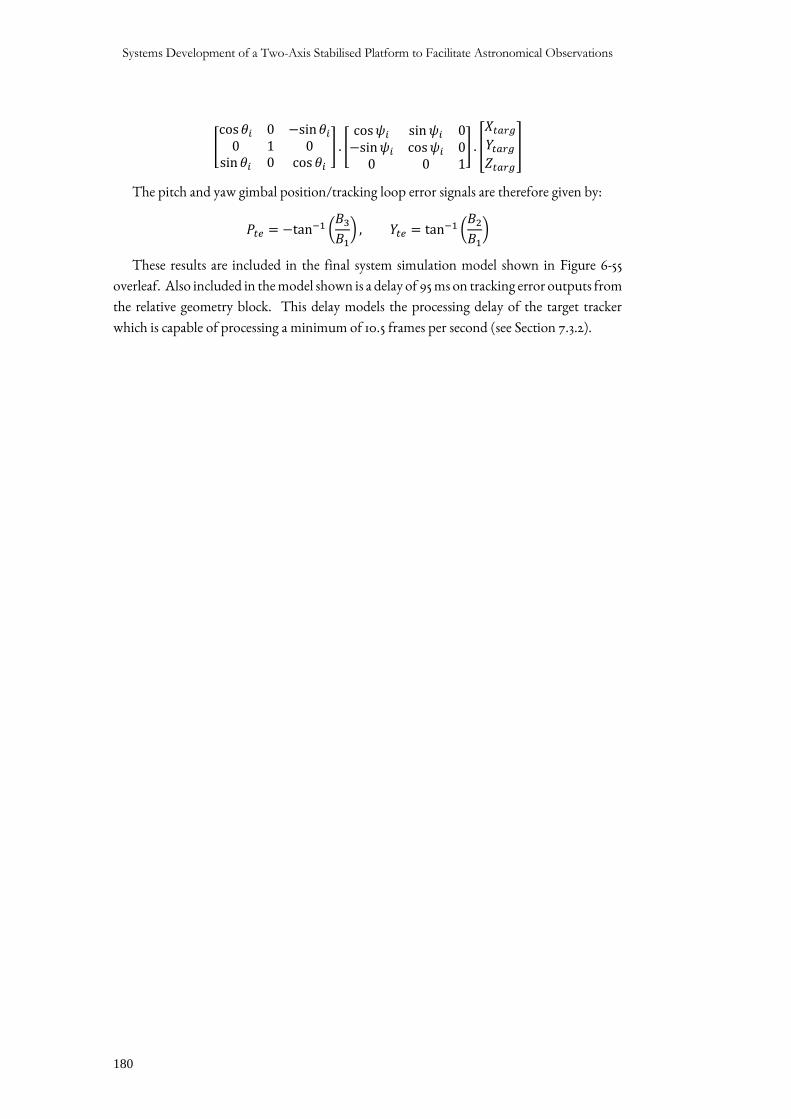
Systems Development of a Two-Axis Stabilised Platform to Facilitate Astronomical Observations
180
[cos𝜃𝑖 0 −sin𝜃𝑖
0 1 0sin 𝜃𝑖 0 cos 𝜃𝑖
] . [cos𝜓𝑖 sin𝜓𝑖 0−sin𝜓𝑖 cos𝜓𝑖 0
0 0 1] . [
𝑋𝑡𝑎𝑟𝑔
𝑌𝑡𝑎𝑟𝑔
𝑍𝑡𝑎𝑟𝑔
]
The pitch and yaw gimbal position/tracking loop error signals are therefore given by:
𝑃𝑡𝑒 = −tan−1 (𝐵3
𝐵1) , 𝑌𝑡𝑒 = tan−1 (
𝐵2
𝐵1)
These results are included in the final system simulation model shown in Figure 6-55
overleaf. Also included in the model shown is a delay of 95 ms on tracking error outputs from
the relative geometry block. This delay models the processing delay of the target tracker
which is capable of processing a minimum of 10.5 frames per second (see Section 7.3.2).
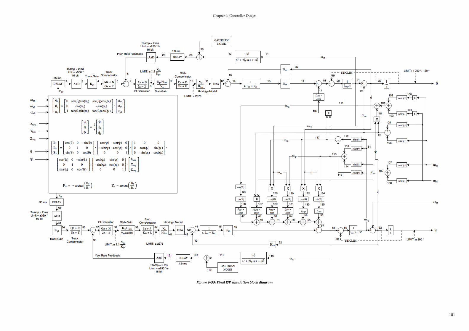
Chapter 6: Controller Design
181
Figure 6-55: Final ISP simulation block diagram
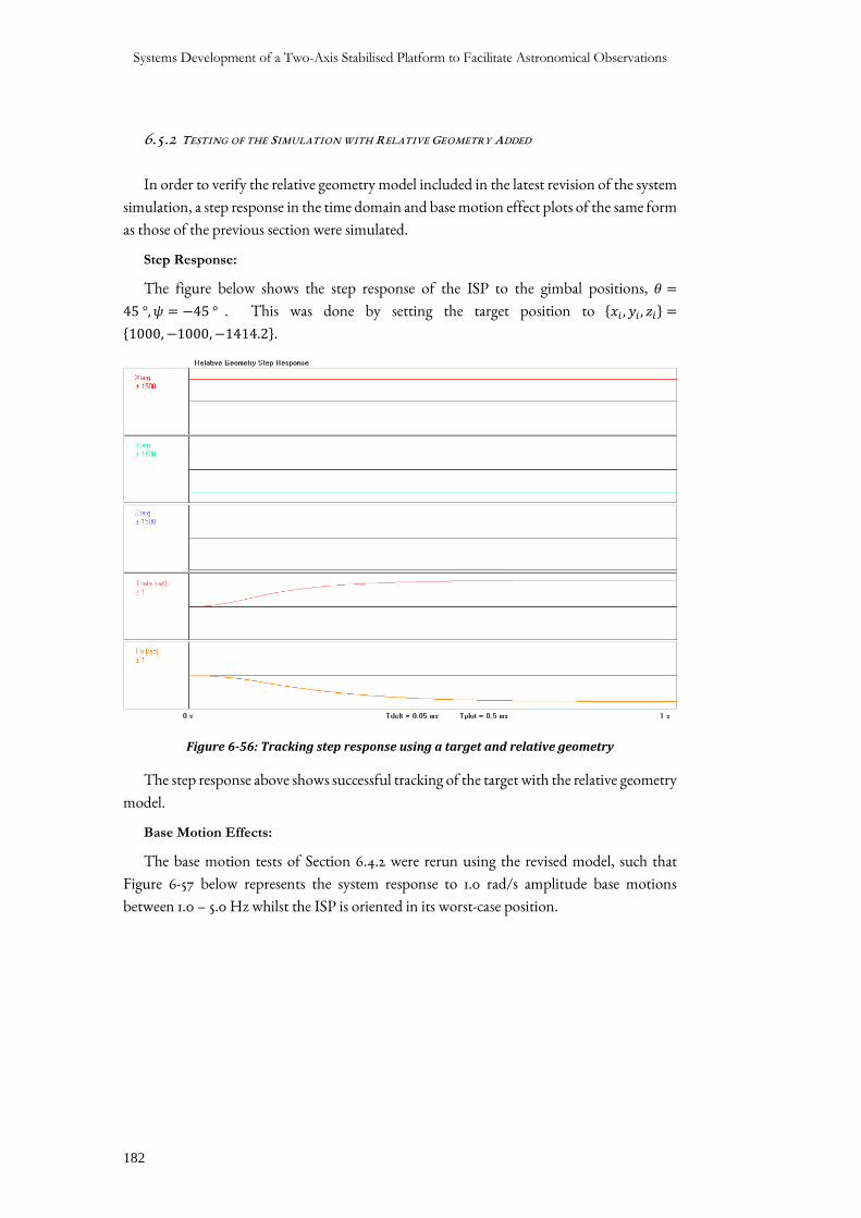
Systems Development of a Two-Axis Stabilised Platform to Facilitate Astronomical Observations
182
6.5.2 TESTING OF THE SIMULATION WITH RELATIVE GEOMETRY ADDED
In order to verify the relative geometry model included in the latest revision of the system
simulation, a step response in the time domain and base motion effect plots of the same form
as those of the previous section were simulated.
Step Response:
The figure below shows the step response of the ISP to the gimbal positions, 𝜃 =
45 °, 𝜓 = −45 ° . This was done by setting the target position to {𝑥𝑖 , 𝑦𝑖 , 𝑧𝑖} =
{1000,−1000,−1414.2}.
Figure 6-56: Tracking step response using a target and relative geometry
The step response above shows successful tracking of the target with the relative geometry
model.
Base Motion Effects:
The base motion tests of Section 6.4.2 were rerun using the revised model, such that
Figure 6-57 below represents the system response to 1.0 rad/s amplitude base motions
between 1.0 – 5.0 Hz whilst the ISP is oriented in its worst-case position.
Chapter 6: Controller Design
183
Figure 6-57: 1.0 rad/s base motion effect with the relative geometry model
Although the responses of the system here are not identical to those of the analogous
Figure 6-50, they are of the same approximate magnitudes and shapes. The small differences
that exist can largely be accounted for by the addition of the 95 ms delay which has been
included in this simulation revision to model the time taken by the target tracker to identify
and locate the target, which exacerbates the effects of saturation evident in response to large
base motion signals. In the plot above, the pitch and yaw track error signals were plotted in
the final two curves. These signals are the output of the target tracker and represent system
jitter in a circumstance like this where the target is stationary. The system specifications of
Appendix A defined maximum jitter allowances for the final system in specification S6;
under dynamic vehicle conditions, jitter was to be less than 2 mrad and less than 0.5 mrad
under stationary host conditions. In the figure above, it can be seen that the ISP is not capable
of achieving these specifications under large base motions but underperforms when saturated
by a factor of approximately 12.5. Continuing to compare the responses between tracking
methods, Figure 6-58 below shows the responses of the model with the amplitude of the base
motion signals reduced to 0.25 rad/s across the same frequency range, whilst Figure 6-59
shows the effect of a base motions representative of the peaks of the simulated base motion
signal.
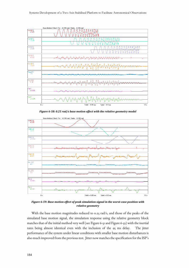
Systems Development of a Two-Axis Stabilised Platform to Facilitate Astronomical Observations
184
Figure 6-58: 0.25 rad/s base motion effect with the relative geometry model
Figure 6-59: Base motion effect of peak simulation signal in the worst-case position with
relative geometry
With the base motion magnitudes reduced to 0.25 rad/s, and those of the peaks of the
simulated base motion signal, the simulation response using the relative geometry block
matches that of the initial method very well (see Figure 6-51 and Figure 6-52) with the inertial
rates being almost identical even with the inclusion of the 95 ms delay. The jitter
performance of the system under linear conditions with smaller base motion disturbances is
also much improved from the previous test. Jitter now matches the specification for the ISP’s
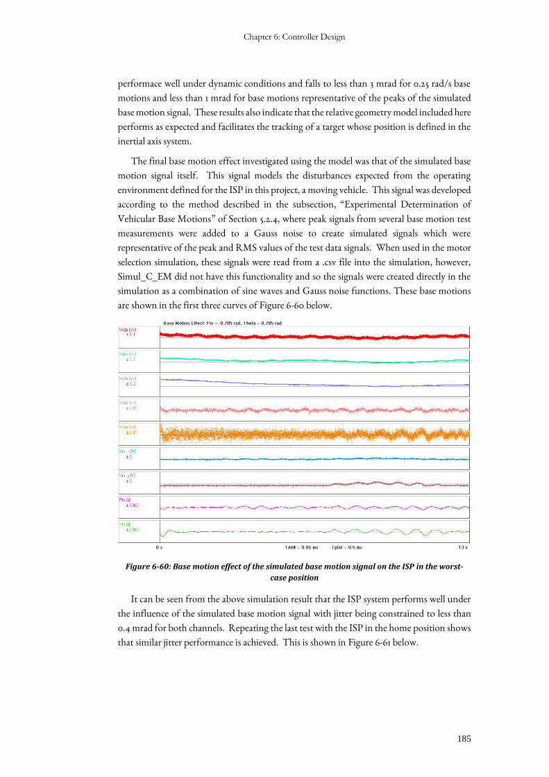
Chapter 6: Controller Design
185
performace well under dynamic conditions and falls to less than 3 mrad for 0.25 rad/s base
motions and less than 1 mrad for base motions representative of the peaks of the simulated
base motion signal. These results also indicate that the relative geometry model included here
performs as expected and facilitates the tracking of a target whose position is defined in the
inertial axis system.
The final base motion effect investigated using the model was that of the simulated base
motion signal itself. This signal models the disturbances expected from the operating
environment defined for the ISP in this project, a moving vehicle. This signal was developed
according to the method described in the subsection, “Experimental Determination of
Vehicular Base Motions” of Section 5.2.4, where peak signals from several base motion test
measurements were added to a Gauss noise to create simulated signals which were
representative of the peak and RMS values of the test data signals. When used in the motor
selection simulation, these signals were read from a .csv file into the simulation, however,
Simul_C_EM did not have this functionality and so the signals were created directly in the
simulation as a combination of sine waves and Gauss noise functions. These base motions
are shown in the first three curves of Figure 6-60 below.
Figure 6-60: Base motion effect of the simulated base motion signal on the ISP in the worst-
case position
It can be seen from the above simulation result that the ISP system performs well under
the influence of the simulated base motion signal with jitter being constrained to less than
0.4 mrad for both channels. Repeating the last test with the ISP in the home position shows
that similar jitter performance is achieved. This is shown in Figure 6-61 below.
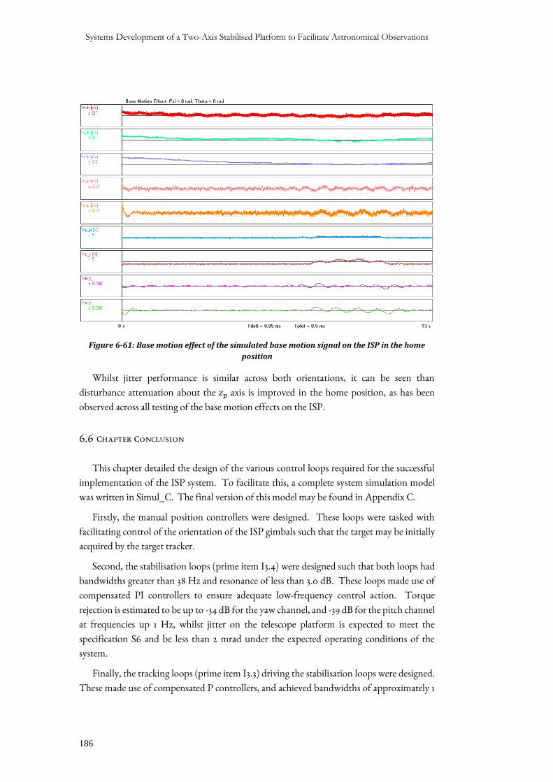
Systems Development of a Two-Axis Stabilised Platform to Facilitate Astronomical Observations
186
Figure 6-61: Base motion effect of the simulated base motion signal on the ISP in the home
position
Whilst jitter performance is similar across both orientations, it can be seen than
disturbance attenuation about the 𝑧𝑝 axis is improved in the home position, as has been
observed across all testing of the base motion effects on the ISP.
6.6 CHAPTER CONCLUSION
This chapter detailed the design of the various control loops required for the successful
implementation of the ISP system. To facilitate this, a complete system simulation model
was written in Simul_C. The final version of this model may be found in Appendix C.
Firstly, the manual position controllers were designed. These loops were tasked with
facilitating control of the orientation of the ISP gimbals such that the target may be initially
acquired by the target tracker.
Second, the stabilisation loops (prime item I3.4) were designed such that both loops had
bandwidths greater than 38 Hz and resonance of less than 3.0 dB. These loops made use of
compensated PI controllers to ensure adequate low-frequency control action. Torque
rejection is estimated to be up to -34 dB for the yaw channel, and -39 dB for the pitch channel
at frequencies up 1 Hz, whilst jitter on the telescope platform is expected to meet the
specification S6 and be less than 2 mrad under the expected operating conditions of the
system.
Finally, the tracking loops (prime item I3.3) driving the stabilisation loops were designed.
These made use of compensated P controllers, and achieved bandwidths of approximately 1

Chapter 6: Controller Design
187
Hz and showed no resonance. The low bandwidth of the tracking loops was deemed
acceptable due to the slow motion of celestial bodies which move at frequencies far lower
than 1 Hz. In addition, a mathematical model for the target tracker (prime item I3.2) was
developed to complete the system simulation model. The next chapter describes the
implementation of these controllers and their associated support functions in software and
firmware.

Chapter 7: Software and Firmware Implementation
189
7 SOFTWARE AND FIRMWARE IMPLEMENTATION
7.1 INTRODUCTION
The design and implementation section of this report concludes here with a description
of the software and firmware developed for the various systems of the project. The section
begins by describing the firmware written for the STM32 MCU which was tasked with
reading the sensors introduced in Chapter 5, running the control loops designed in Chapter
6, and managing the comms between the STM32, RPi and the PC based UI. It then moves
to detail the implementation of the target tracker on the RPi computer and concludes by
detailing this User Interface.
7.2 STM32 FIRMWARE
The firmware developed for the STM32 MCU is the most important control program
developed in the project. It handles all comms and control tasks and manages the overall
system state and timing. This section details the firmware developed for the MCU. The
firmware was written in C using a combination of register-level code and code written using
the STM32F0 Standard Peripheral Library (SPL) written by STMicroelectronics. An overall
description of the code is given before detailed function descriptions are given where
necessary. In all cases, the firmware descriptions given here are at a functional level (unless
hardware level detail is required) using flowcharts whilst the actual firmware may be found
in Appendix C.
7.2.1 OVERALL DESCRIPTION OF FIRMWARE
The firmware written for the project made use of many of the available peripherals and
pins on the STM32 development board described previously. The peripherals and pins used
and their functional assignment is detailed by Table 7-1 below.
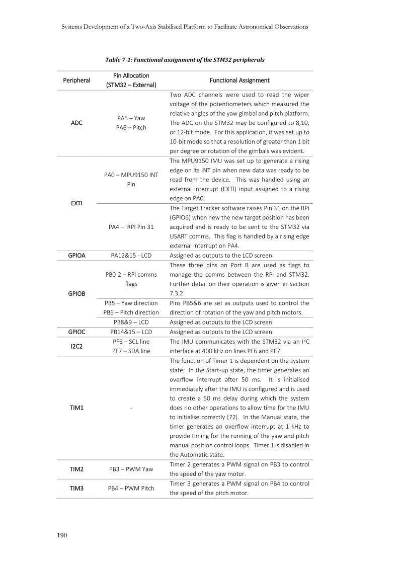
Systems Development of a Two-Axis Stabilised Platform to Facilitate Astronomical Observations
190
Table 7-1: Functional assignment of the STM32 peripherals
Peripheral Pin Allocation
(STM32 – External) Functional Assignment
ADC PA5 – Yaw
PA6 – Pitch
Two ADC channels were used to read the wiper
voltage of the potentiometers which measured the
relative angles of the yaw gimbal and pitch platform.
The ADC on the STM32 may be configured to 8,10,
or 12-bit mode. For this application, it was set up to
10-bit mode so that a resolution of greater than 1 bit
per degree or rotation of the gimbals was evident.
EXTI
PA0 – MPU9150 INT
Pin
The MPU9150 IMU was set up to generate a rising
edge on its INT pin when new data was ready to be
read from the device. This was handled using an
external interrupt (EXTI) input assigned to a rising
edge on PA0.
PA4 – RPI Pin 31
The Target Tracker software raises Pin 31 on the RPi
(GPIO6) when new the new target position has been
acquired and is ready to be sent to the STM32 via
USART comms. This flag is handled by a rising edge
external interrupt on PA4.
GPIOA PA12&15 - LCD Assigned as outputs to the LCD screen.
GPIOB
PB0-2 – RPi comms
flags
These three pins on Port B are used as flags to
manage the comms between the RPi and STM32.
Further detail on their operation is given in Section
7.3.2.
PB5 – Yaw direction
PB6 – Pitch direction
Pins PB5&6 are set as outputs used to control the
direction of rotation of the yaw and pitch motors.
PB8&9 – LCD Assigned as outputs to the LCD screen.
GPIOC PB14&15 – LCD Assigned as outputs to the LCD screen.
I2C2 PF6 – SCL line
PF7 – SDA line
The IMU communicates with the STM32 via an I2C
interface at 400 kHz on lines PF6 and PF7.
TIM1 -
The function of Timer 1 is dependent on the system
state: In the Start-up state, the timer generates an
overflow interrupt after 50 ms. It is initialised
immediately after the IMU is configured and is used
to create a 50 ms delay during which the system
does no other operations to allow time for the IMU
to initialise correctly [72]. In the Manual state, the
timer generates an overflow interrupt at 1 kHz to
provide timing for the running of the yaw and pitch
manual position control loops. Timer 1 is disabled in
the Automatic state.
TIM2 PB3 – PWM Yaw Timer 2 generates a PWM signal on PB3 to control
the speed of the yaw motor.
TIM3 PB4 – PWM Pitch Timer 3 generates a PWM signal on PB4 to control
the speed of the pitch motor.
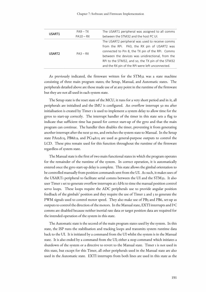
Chapter 7: Software and Firmware Implementation
191
USART1 PA9 – TX
PA10 – RX
The USART1 peripheral was assigned to all comms
between the STM32 and the host PC UI.
USART2 PA3 – RX
The USART2 peripheral was used to receive comms
from the RPi. PA3, the RX pin of USART2 was
connected to Pin 8, the TX pin of the RPi. Comms
between the devices was unidirectional, from the
RPi to the STM32, and so, the TX pin of the STM32
and the RX pin of the RPi were left unconnected.
As previously indicated, the firmware written for the STM32 was a state machine
consisting of three main program states; the Setup, Manual, and Automatic states. The
peripherals detailed above are those made use of at any point in the runtime of the firmware
but they are not all used in each system state.
The Setup state is the reset state of the MCU, it runs for a very short period and in it, all
peripherals are initialised and the IMU is configured. An overflow interrupt 50 ms after
initialisation is created by Timer 1 is used to implement a system delay to allow time for the
gyros to start-up correctly. The interrupt handler of the timer in this state sets a flag to
indicate that sufficient time has passed for correct start-up of the gyro and that the main
program can continue. The handler then disables the timer, preventing it from generating
another interrupt after the next 50 ms, and switches the system state to Manual. In the Setup
state PA12&15, PB8&9, and PC14&15 are used as general-purpose outputs to control the
LCD. These pins remain used for this function throughout the runtime of the firmware
regardless of system state.
The Manual state is the first of two main functional states in which the program operates
for the remainder of the runtime of the system. In correct operation, it is automatically
entered once the gyro start-up delay is complete. This state allows the gimbal orientation to
be controlled manually from position commands sent from the UI. As such, it makes uses of
the USART1 peripheral to facilitate serial comms between the UI and the STM32. It also
user Timer 1 set to generate overflow interrupts at 1 kHz to time the manual position control
servo loops. These loops require the ADC peripherals use to provide angular position
feedback of the gimbals’ position and they require the use of Timer 2 and 3 to generate the
PWM signals used to control motor speed. They also make use of PB5 and PB6, set-up as
outputs to control the direction of the motors. In the Manual state, EXTI interrupts and I2C
comms are disabled because neither inertial rate data or target position data are required for
the intended operation of the system in this state.
The Automatic state is the second of the main program states used by the system. In this
state, the ISP runs the stabilisation and tracking loops and transmits system runtime data
back to the UI. It is initiated by a command from the UI whilst the system is in the Manual
state. It is also ended by a command from the UI; either a stop command which initiates a
shutdown of the system or a directive to revert to the Manual state. Timer 1 is not used in
this state, but except for this Timer, all other peripherals used in the Manual state are also
used in the Automatic state. EXTI interrupts from both lines are used in this state as the

Systems Development of a Two-Axis Stabilised Platform to Facilitate Astronomical Observations
192
control loops run in here rely on target and inertial rate data from the relevant systems. New
data of both forms is indicated by EXTI interrupts on PA0 and PA6. USART2 and PB0-2
are used to facilitate and manage the serial comms between the RPi and the STM32, and the
I2C peripheral is used to communicate with the IMU.
Figure 7-1 below describes the overall function of the firmware. Several sub-processes are
used in the flowchart, and those that are numbered are detailed in the subsections that follow.
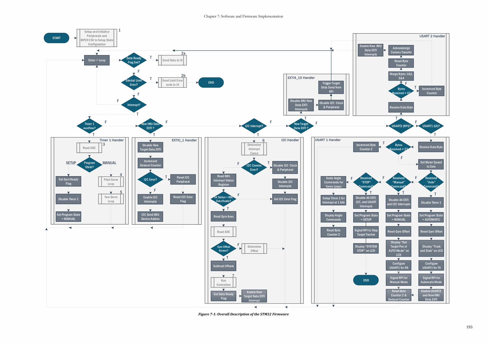
Chapter 7: Software and Firmware Implementation
193
START
Setup and Initialise
Peripherals and
MPU9150 to Setup State
Configuration
Enter LoopData Ready
Flag Set?Send Data to UI
Gimbal Limit
Error?
Interrupt?
Send Limit Error
code to UIEND
T
F
F
F
Timer 1
overflow?
Program
State?
Set Gyro Ready
Flag
Disable Timer 1
Set Program State
= MANUAL
Pitch Servo
Loop
Yaw Servo
Loop
New IMU Data
EXTI ?
Disable New
Target Data EXTI
I2C Error?
Enable I2C
Interrupts
I2C Send IMU
Device Addres
Reset I2C
Peripheral
Reset I2C Error
Flag
I2C Interrupt?
Determine
Interrupt
Cause
I2C Comms
Error?
Int Status = IMU
Data Ready?
Read Gyro Axes
Read IMU
Interrupt Status
Register
Gyro Offset
Known?
Subtract Offsets
Run
Controllers
Enable New
Target Data EXTI
Interrupt
Disable I2C Clock
& Peripheral
Set Data Ready
Flag
Disable I2C
Interrupts
Set I2C Error Flag
Determine
Offest
New Target
Data EXTI ?
Disable IMU New
Data EXTI
Interrupts
Disable I2C Clock
& Peripheral
USART2 (RPi)?
Receive Data Byte
Bytes
Received < 4?
Merge Bytes 1&2,
3&4
Reset Byte
Counter
Increment Byte
Counter
Acknowledge
Comms Transfer
Enable New IMU
Data EXTI
Interrupts
USART1 (UI)?
Receive Data ByteBytes
Received < 2?
Received
Auto
Command?
Increment Byte
Counter 2
Set Motor Speed
to Zero
Set Program State
= AUTOMATIC
Reset Gyro Offset
Disable Timer 1
Display Track
and Stab on LCD
Configure
USART1 for TX
Enable USART2
and New IMU
Data EXTI
Reset Byte
Counter 2 &
Dataset Counter
Received
Manual
Command?
Set Program State
= MANUAL
Reset Gyro Offset
Disable All EXTI
and I2C Interrupts
Display Set
Target Pos or
AUTO Mode on
LCD
Configure
USART1 for RX
Received
STOP
Command?
Set Program State
= SETUP
Disable All EXTI,
I2C, and USART
Interrupts
Display SYSTEM
STOP on LCD
Scale Angle
Commands for
Servo Loops
Setup Timer 1 for
Interrupt at 1 kHz
Display Angle
Commands
Reset Byte
Counter 2
END
T
T
T
T
T T T
T
T
T
T
T
TTT
T
F F F
F
F
F F
F
FFF
F
FT
Timer 1 Handler EXTI0_1 Handler I2C Handler
EXTI4_15 Handler
USART 1 Handler
USART 2 Handler
1
2b
2a
3
5
6
7
MANUALSETUP
Read ADC
Read ADC
4
Increment
Dataset Counter
F
Signal RPi for
Automatic Mode
Signal RPi for
Manual Mode
Signal RPi to Stop
Target Tracker
Trigger Target
Data Send from
RPi
Figure 7-1: Overall Description of the STM32 Firmware
Systems Development of a Two-Axis Stabilised Platform to Facilitate Astronomical Observations
194
From the figure above, it can be seen that the system makes heavy use of an event-driven
program structure, with the only synchronous task in the infinite while loop being to send
system runtime data or a limit error code to the UI. This structure arose naturally out of the
fact that the main control feedback data for both the tracking and the stabilisation loops is
provided from external systems which raise flags when new data is available; rate data from
the IMU at a fixed frequency of 500 Hz, and target position data from the RPi at a varying
frequency between 10.5 – 15 Hz. Running the tracking and stabilisation loops from an
untimed infinite loop, or an interrupt service routine (ISR) triggered by a timer overflow
introduced the possibility of additional delays in action on new data. It was therefore decided
to time the controller algorithms using the external interrupt generated by the MPU9150 INT
pin which is raised high each time new data is ready to be read from the IMU. This occurs at
a programmed rate of 500 Hz. The general functional sequence of events in the above
flowchart for the Automatic state is, therefore:
1. EXTI interrupt on PA0 indicating new gyro data is ready.
2. Read gyro data from the IMU.
3. Read ADC to determine gimbal positions. If they are out of bounds, stop the motors
and shut down the system.
4. Run the pitch and yaw tracking and stabilisation control loops.
5. If new target data is available, receive target data packet.
6. Send system runtime data to the UI.
At any point during the above sequence, the STM32 may receive a supervisory command
from the UI which changes the system state and breaks the above sequence of operation. The
compiled code size of the firmware above was 32491 bytes and therefore only just fit within
the 32 KB limit for the STM32F0.
7.2.2 SUBPROCESS 1: SETUP AND INITIALISATION
The first subprocess encountered in the main firmware is that which sets up and initialises
the various peripherals and sensors used in the project. This subprocess is further detailed in
Figure 7-2 below.
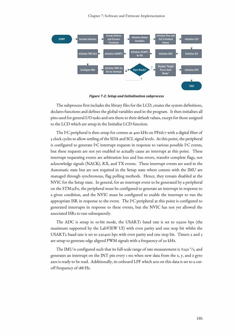
Chapter 7: Software and Firmware Implementation
195
F
START Include Libraries
Create Defines
and Declare
Functions
Initialise Global
Variables
Initialise Pins and
Set To Default
Values
Initialise LCD
Initialise I2CInitialise ADCInitialise USART1
for RXInitialise USART2
Configure IMU
Initialise TIM 2&3
Initialise TIM1 for
50 ms interruptGyro Ready?
Display Target
Pos or Auto
Mode
Initialise EXTI
END
T
Figure 7-2: Setup and Initialisation subprocess
The subprocess first includes the library files for the LCD, creates the system definitions,
declares functions and defines the global variables used in the program. It then initialises all
pins used for general I/O tasks and sets them to their default values, except for those assigned
to the LCD which are setup in the Initialise LCD function.
The I2C peripheral is then setup for comms at 400 kHz on PF6&7 with a digital filter of
5 clock cycles to allow settling of the SDA and SCL signal levels. At this point, the peripheral
is configured to generate I2C interrupt requests in response to various possible I2C events,
but these requests are not yet enabled to actually cause an interrupt at this point. These
interrupt requesting events are arbitration loss and bus errors, transfer complete flags, not
acknowledge signals (NACK), RX, and TX events. These interrupt events are used in the
Automatic state but are not required in the Setup state where comms with the IMU are
managed through synchronous, flag polling methods. Hence, they remain disabled at the
NVIC for the Setup state. In general, for an interrupt event to be generated by a peripheral
on the STM32F0, the peripheral must be configured to generate an interrupt in response to
a given condition, and the NVIC must be configured to enable the interrupt to run the
appropriate ISR in response to the event. The I2C peripheral at this point is configured to
generated interrupts in response to these events, but the NVIC has not yet allowed the
associated ISRs to run subsequently.
The ADC is setup in 10-bit mode, the USART1 baud rate is set to 115200 bps (the
maximum supported by the LabVIEW UI) with even parity and one stop bit whilst the
USART2 baud rate is set to 230400 bps with even parity and one stop bit. Timers 2 and 3
are setup to generate edge aligned PWM signals with a frequency of 20 kHz.
The IMU is configured such that its full-scale range of rate measurement is ±250 °/s, and
generates an interrupt on the INT pin every 1 ms when new data from the x, y, and z gyro
axes is ready to be read. Additionally, its onboard LPF which acts on this data is set to a cut-
off frequency of 188 Hz.
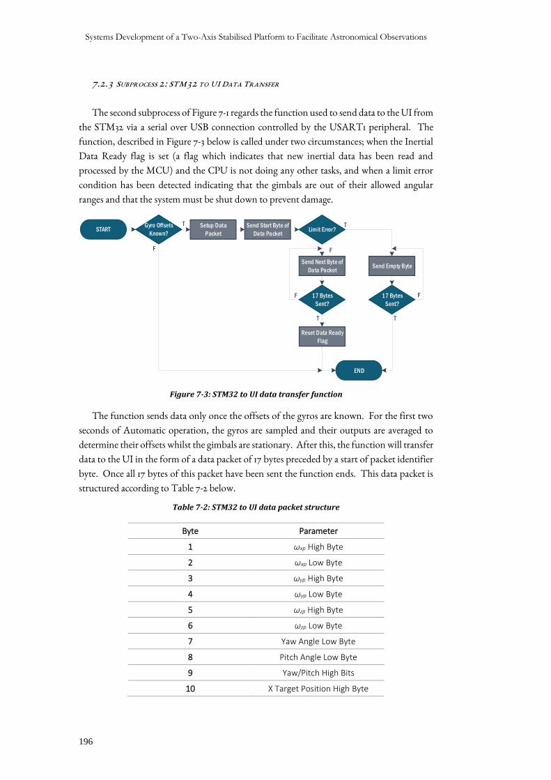
Systems Development of a Two-Axis Stabilised Platform to Facilitate Astronomical Observations
196
7.2.3 SUBPROCESS 2: STM32 TO UI DATA TRANSFER
The second subprocess of Figure 7-1 regards the function used to send data to the UI from
the STM32 via a serial over USB connection controlled by the USART1 peripheral. The
function, described in Figure 7-3 below is called under two circumstances; when the Inertial
Data Ready flag is set (a flag which indicates that new inertial data has been read and
processed by the MCU) and the CPU is not doing any other tasks, and when a limit error
condition has been detected indicating that the gimbals are out of their allowed angular
ranges and that the system must be shut down to prevent damage.
T
F
F
START
END
TGyro Offsets
Known?
Setup Data
PacketLimit Error?
Send Start Byte of
Data Packet
Send Next Byte of
Data Packet
17 Bytes
Sent?
Send Empty Byte
17 Bytes
Sent?
T
T
F
F
Reset Data Ready
Flag
Figure 7-3: STM32 to UI data transfer function
The function sends data only once the offsets of the gyros are known. For the first two
seconds of Automatic operation, the gyros are sampled and their outputs are averaged to
determine their offsets whilst the gimbals are stationary. After this, the function will transfer
data to the UI in the form of a data packet of 17 bytes preceded by a start of packet identifier
byte. Once all 17 bytes of this packet have been sent the function ends. This data packet is
structured according to Table 7-2 below.
Table 7-2: STM32 to UI data packet structure
Byte Parameter
1 ωxp High Byte
2 ωxp Low Byte
3 ωyp High Byte
4 ωyp Low Byte
5 ωzp High Byte
6 ωzp Low Byte
7 Yaw Angle Low Byte
8 Pitch Angle Low Byte
9 Yaw/Pitch High Bits
10 X Target Position High Byte
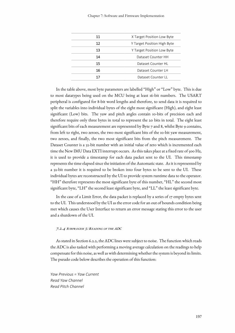
Chapter 7: Software and Firmware Implementation
197
11 X Target Position Low Byte
12 Y Target Position High Byte
13 Y Target Position Low Byte
14 Dataset Counter HH
15 Dataset Counter HL
16 Dataset Counter LH
17 Dataset Counter LL
In the table above, most byte parameters are labelled “High” or “Low” byte. This is due
to most datatypes being used on the MCU being at least 16-bit numbers. The USART
peripheral is configured for 8-bit word lengths and therefore, to send data it is required to
split the variables into individual bytes of the eight most significant (High), and eight least
significant (Low) bits. The yaw and pitch angles contain 10-bits of precision each and
therefore require only three bytes in total to represent the 20 bits in total. The eight least
significant bits of each measurement are represented by Byte 7 and 8, whilst Byte 9 contains,
from left to right, two zeroes, the two most significant bits of the 10-bit yaw measurement,
two zeroes, and finally, the two most significant bits from the pitch measurement. The
Dataset Counter is a 32-bit number with an initial value of zero which is incremented each
time the New IMU Data EXTI interrupt occurs. As this takes place at a fixed rate of 500 Hz,
it is used to provide a timestamp for each data packet sent to the UI. This timestamp
represents the time elapsed since the initiation of the Automatic state. As it is represented by
a 32-bit number it is required to be broken into four bytes to be sent to the UI. These
individual bytes are reconstructed by the UI to provide system runtime data to the operator.
“HH” therefore represents the most significant byte of this number, “HL” the second most
significant byte, “LH” the second least significant byte, and “LL” the least significant byte.
In the case of a Limit Error, the data packet is replaced by a series of 17 empty bytes sent
to the UI. This understood by the UI as the error code for an out of bounds condition being
met which causes the User Interface to return an error message stating this error to the user
and a shutdown of the UI.
7.2.4 SUBPROCESS 3: READING OF THE ADC
As stated in Section 6.2.2, the ADC lines were subject to noise. The function which reads
the ADC is also tasked with performing a moving average calculation on the readings to help
compensate for this noise, as well as with determining whether the system is beyond its limits.
The pseudo code below describes the operation of this function:
Yaw Previous = Yaw Current
Read Yaw Channel
Read Pitch Channel
Systems Development of a Two-Axis Stabilised Platform to Facilitate Astronomical Observations
198
Perform moving average calculation on Yaw
Perform moving average calculation on Pitch
Yaw Diff = Yaw Current – Yaw Previous
If Program State is Automatic
if Yaw Diff > 200
Increment Negative Crossing Counter
if Positive Crossing Counter > 0
Decrement Positive Crossing Counter
else if Yaw Diff < -200
Increment Positive Crossing Counter
if Negative Crossing Counter > 0
Decrement Negative Crossing Counter
if Positive or Negative Crossing Counter > 1
Run Limit Error Handler
else if 310° < pitch angle < 50°
Run Limit Error Handler
The function above computes the moving average (MA) on the current (i) yaw and pitch
readings according to the following algorithm [105]:
𝑀𝐴[𝑖] =
(𝑀𝐴[𝑖−1]∗ + 𝑋[𝑖] −
𝑀𝐴[𝑖−1]∗
𝑁 )
𝑁
Where N is the effective number of data points over which the moving average is
calculated (N = 16 for this average), and 𝑀𝐴[𝑥]∗ is the moving average of the xth term
multiplied by N.s
The limits for the gimbals are defined such that the pitch platform may not go within 50°
of the vertical down position from either direction, and the yaw gimbal may not cross the
zero position twice in a row from the in same direction. This limits the yaw gimbal to a
maximum of 720° of allowable rotation. The pots chosen were single turn, continuous
rotation pots, therefore at the 0/360° position, the pot wiper may almost instantaneously
change from 0V to 3.3V (or 0 to 1024) on the ADC output. This position was defined as the
zero position and aligned according to the definitions of Figure 2-23. Therefore, if the
difference between the current and previous yaw readings is sufficiently large, a zero crossing
may be identified. Testing has revealed that a scalar value of 200 for this difference is a
sufficiently large cut off to accurately identify a crossing. The direction of the crossing is
determined by the sign of the difference. The logic above counts the number of crossings in
each direction and runs the Limit Error handler if two in a row in the same direction occur.
Chapter 7: Software and Firmware Implementation
199
This handler disables ETXI interrupts, switches the motors off, and calls the data transfer
function to send the Limit Error code to the UI.
7.2.5 SUBPROCESSES 4 AND 5: MANUAL POSITION CONTROL
The pitch and yaw servo loops contained in the Timer 1 handler above are the functions
in which the control loops designed in Section 6.2 are implemented. For these loops and all
others implemented on the SMT32, compensator, controller, and other transfer functions
with non-zero orders of s or z were implemented using difference equations. Functions were
also multiplied out as far as possible to reduce the computational load on the CPU.
For the manual position control loops, the PI controller and compensator were first
converted to the z-plane using the bilinear transform:
𝑠 =2
𝑇𝑠𝑎𝑚𝑝.𝑧 − 1
𝑧 + 1
Therefore, for a system with sampling time, Tsamp, the PI controller, with input 𝐸(𝑠) and
output 𝑃(𝑠), is given by:
𝑃(𝑠)
𝐸(𝑠)=
𝑝𝑠 + 1
𝑠 ≡
𝑃(𝑧)
𝐸(𝑧)=
𝐴𝑧 + 𝐵
𝐶𝑧 + 𝐷
where,
𝐴 = 𝑇𝑠𝑎𝑚𝑝 + 2𝑝
𝐵 = 𝑇𝑠𝑎𝑚𝑝 − 2𝑝
𝐶 = 2
𝐷 = −2
And the compensator transfer function is given by:
𝑌(𝑠)
𝑋(𝑠)=
𝑇1𝑠 + 1
𝑇2𝑠 + 1 ≡
𝑌(𝑧)
𝑋(𝑧)=
𝑀𝑧 + 𝑁
𝑂𝑧 + 𝑃
where,
𝑀 = 𝑇𝑠𝑎𝑚𝑝 + 2𝑇1
𝑁 = 𝑇𝑠𝑎𝑚𝑝 − 2𝑇1
𝑂 = 𝑇𝑠𝑎𝑚𝑝 + 2𝑇2
𝑃 = 𝑇𝑠𝑎𝑚𝑝 − 2𝑇2
The difference equations for these z-plane transfer functions were then determined by
cross multiplication and expansion as follows.
For the PI controller:
𝑃(𝑧)𝐶𝑧 + 𝑃(𝑧)𝐷 = 𝐸(𝑧)𝐴𝑧 + 𝐸(𝑧)𝐵
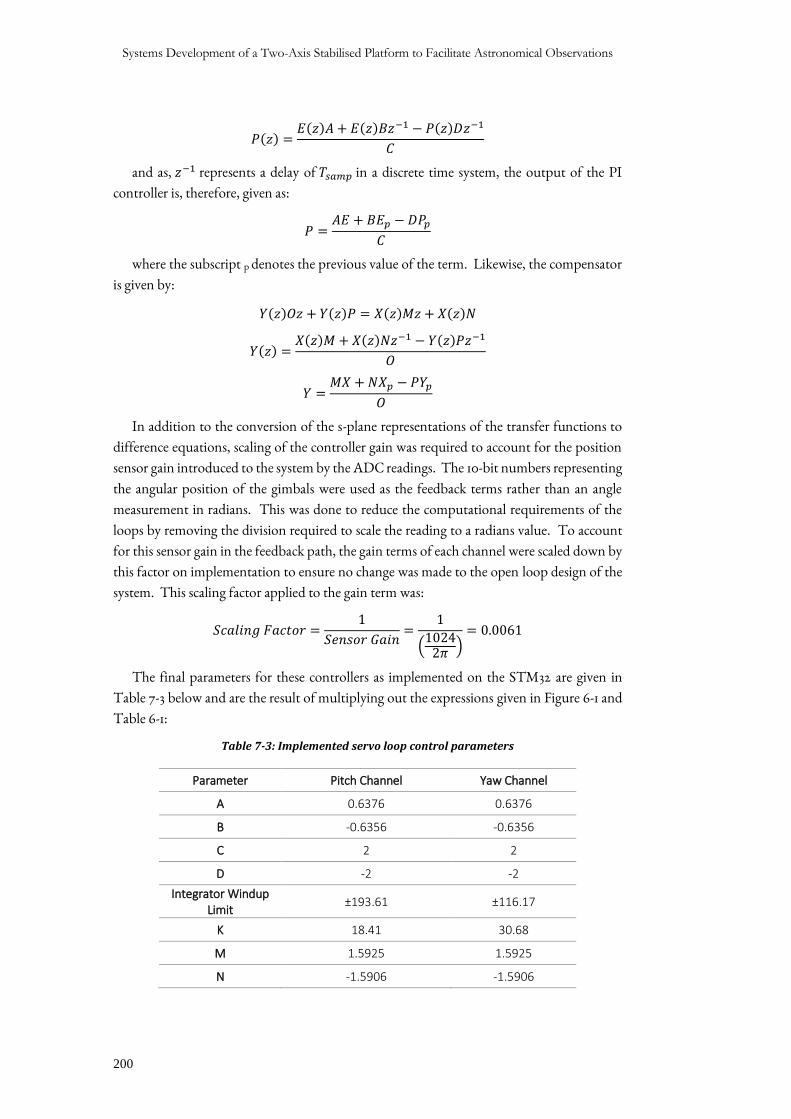
Systems Development of a Two-Axis Stabilised Platform to Facilitate Astronomical Observations
200
𝑃(𝑧) =𝐸(𝑧)𝐴 + 𝐸(𝑧)𝐵𝑧−1 − 𝑃(𝑧)𝐷𝑧−1
𝐶
and as, 𝑧−1 represents a delay of 𝑇𝑠𝑎𝑚𝑝 in a discrete time system, the output of the PI
controller is, therefore, given as:
𝑃 =𝐴𝐸 + 𝐵𝐸𝑝 − 𝐷𝑃𝑝
𝐶
where the subscript p denotes the previous value of the term. Likewise, the compensator
is given by:
𝑌(𝑧)𝑂𝑧 + 𝑌(𝑧)𝑃 = 𝑋(𝑧)𝑀𝑧 + 𝑋(𝑧)𝑁
𝑌(𝑧) =𝑋(𝑧)𝑀 + 𝑋(𝑧)𝑁𝑧−1 − 𝑌(𝑧)𝑃𝑧−1
𝑂
𝑌 =𝑀𝑋 + 𝑁𝑋𝑝 − 𝑃𝑌𝑝
𝑂
In addition to the conversion of the s-plane representations of the transfer functions to
difference equations, scaling of the controller gain was required to account for the position
sensor gain introduced to the system by the ADC readings. The 10-bit numbers representing
the angular position of the gimbals were used as the feedback terms rather than an angle
measurement in radians. This was done to reduce the computational requirements of the
loops by removing the division required to scale the reading to a radians value. To account
for this sensor gain in the feedback path, the gain terms of each channel were scaled down by
this factor on implementation to ensure no change was made to the open loop design of the
system. This scaling factor applied to the gain term was:
𝑆𝑐𝑎𝑙𝑖𝑛𝑔 𝐹𝑎𝑐𝑡𝑜𝑟 =1
𝑆𝑒𝑛𝑠𝑜𝑟 𝐺𝑎𝑖𝑛=
1
(10242𝜋 )
= 0.0061
The final parameters for these controllers as implemented on the STM32 are given in
Table 7-3 below and are the result of multiplying out the expressions given in Figure 6-1 and
Table 6-1:
Table 7-3: Implemented servo loop control parameters
Parameter Pitch Channel Yaw Channel
A 0.6376 0.6376
B -0.6356 -0.6356
C 2 2
D -2 -2
Integrator Windup Limit
±193.61 ±116.17
K 18.41 30.68
M 1.5925 1.5925
N -1.5906 -1.5906
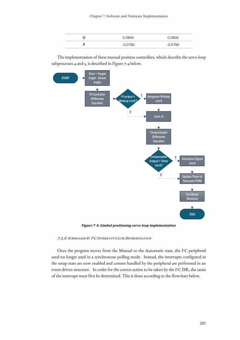
Chapter 7: Software and Firmware Implementation
201
O 0.0806 0.0806
P -0.0786 -0.0786
The implementation of these manual position controllers, which describe the servo loop
subprocesses 4 and 5, is described in Figure 7-4 below.
START
Error = Target
Angle - Actual
Angle
PI Controller
Difference
Equation
Integrator Windup
Limit
Gain, K
Compensator
Difference
Equation
Actuation Signal
Limit
END
Update Timer to
Generate PWM
PI output >
Windup Limit?
Compensator
Output > Timer
Limit?
T
T
F
F
Set Motor
Direction
Figure 7-4: Gimbal positioning servo loop implementation
7.2.6 SUBPROCESS 6: I2C INTERRUPT CAUSE DETERMINATION
Once the program moves from the Manual to the Automatic state, the I2C peripheral
used no longer used in a synchronous polling mode. Instead, the interrupts configured in
the setup state are now enabled and comms handled by the peripheral are performed in an
event-driven structure. In order for the correct action to be taken by the I2C ISR, the cause
of the interrupt must first be determined. This is done according to the flowchart below.
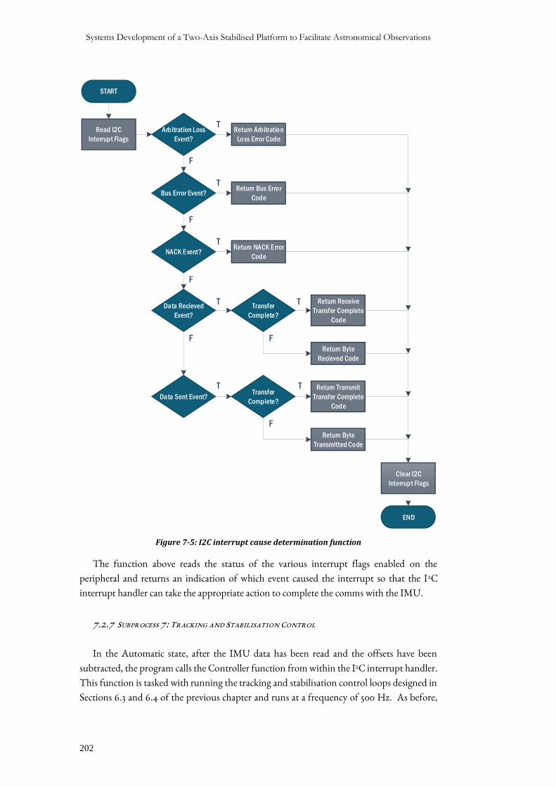
Systems Development of a Two-Axis Stabilised Platform to Facilitate Astronomical Observations
202
START
END
T
F
Read I2C
Interrupt Flags
Arbitration Loss
Event?
Bus Error Event?
NACK Event?
Data Recieved
Event?
Transfer
Complete?
Data Sent Event?Transfer
Complete?
Clear I2C
Interrupt Flags
Return Arbitration
Loss Error Code
Return Bus Error
Code
Return NACK Error
Code
Return Receive
Transfer Complete
Code
Return Byte
Recieved Code
Return Transmit
Transfer Complete
Code
Return Byte
Transmitted Code
T
T
T T
TT
F
F
F F
F
Figure 7-5: I2C interrupt cause determination function
The function above reads the status of the various interrupt flags enabled on the
peripheral and returns an indication of which event caused the interrupt so that the I2C
interrupt handler can take the appropriate action to complete the comms with the IMU.
7.2.7 SUBPROCESS 7: TRACKING AND STABILISATION CONTROL
In the Automatic state, after the IMU data has been read and the offsets have been
subtracted, the program calls the Controller function from within the I2C interrupt handler.
This function is tasked with running the tracking and stabilisation control loops designed in
Sections 6.3 and 6.4 of the previous chapter and runs at a frequency of 500 Hz. As before,
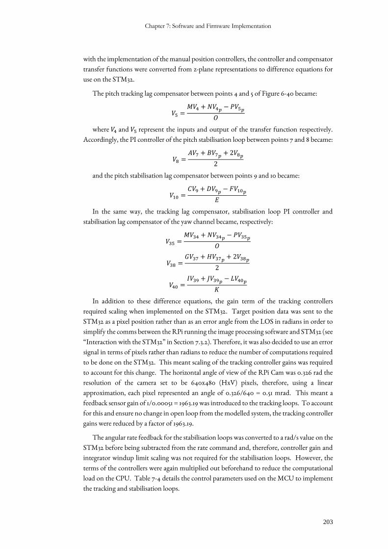
Chapter 7: Software and Firmware Implementation
203
with the implementation of the manual position controllers, the controller and compensator
transfer functions were converted from z-plane representations to difference equations for
use on the STM32.
The pitch tracking lag compensator between points 4 and 5 of Figure 6-40 became:
𝑉5 =𝑀𝑉4 + 𝑁𝑉4𝑝
− 𝑃𝑉5𝑝
𝑂
where 𝑉4 and 𝑉5 represent the inputs and output of the transfer function respectively.
Accordingly, the PI controller of the pitch stabilisation loop between points 7 and 8 became:
𝑉8 =𝐴𝑉7 + 𝐵𝑉7𝑝
+ 2𝑉8𝑝
2
and the pitch stabilisation lag compensator between points 9 and 10 became:
𝑉10 =𝐶𝑉9 + 𝐷𝑉9𝑝
− 𝐹𝑉10𝑝
𝐸
In the same way, the tracking lag compensator, stabilisation loop PI controller and
stabilisation lag compensator of the yaw channel became, respectively:
𝑉35 =𝑀𝑉34 + 𝑁𝑉34𝑝
− 𝑃𝑉35𝑝
𝑂
𝑉38 =𝐺𝑉37 + 𝐻𝑉37𝑝
+ 2𝑉38𝑝
2
𝑉40 =𝐼𝑉39 + 𝐽𝑉39𝑝
− 𝐿𝑉40𝑝
𝐾
In addition to these difference equations, the gain term of the tracking controllers
required scaling when implemented on the STM32. Target position data was sent to the
STM32 as a pixel position rather than as an error angle from the LOS in radians in order to
simplify the comms between the RPi running the image processing software and STM32 (see
“Interaction with the STM32” in Section 7.3.2). Therefore, it was also decided to use an error
signal in terms of pixels rather than radians to reduce the number of computations required
to be done on the STM32. This meant scaling of the tracking controller gains was required
to account for this change. The horizontal angle of view of the RPi Cam was 0.326 rad the
resolution of the camera set to be 640x480 (HxV) pixels, therefore, using a linear
approximation, each pixel represented an angle of 0.326/640 = 0.51 mrad. This meant a
feedback sensor gain of 1/0.00051 = 1963.19 was introduced to the tracking loops. To account
for this and ensure no change in open loop from the modelled system, the tracking controller
gains were reduced by a factor of 1963.19.
The angular rate feedback for the stabilisation loops was converted to a rad/s value on the
STM32 before being subtracted from the rate command and, therefore, controller gain and
integrator windup limit scaling was not required for the stabilisation loops. However, the
terms of the controllers were again multiplied out beforehand to reduce the computational
load on the CPU. Table 7-4 details the control parameters used on the MCU to implement
the tracking and stabilisation loops.
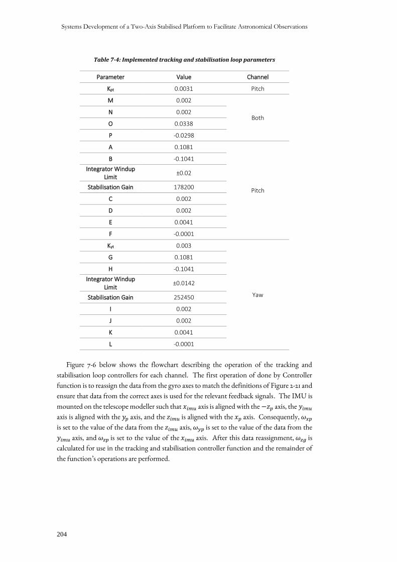
Systems Development of a Two-Axis Stabilised Platform to Facilitate Astronomical Observations
204
Table 7-4: Implemented tracking and stabilisation loop parameters
Parameter Value Channel
Kpt 0.0031 Pitch
M 0.002
Both N 0.002
O 0.0338
P -0.0298
A 0.1081
Pitch
B -0.1041
Integrator Windup Limit
±0.02
Stabilisation Gain 178200
C 0.002
D 0.002
E 0.0041
F -0.0001
Kyt 0.003
Yaw
G 0.1081
H -0.1041
Integrator Windup Limit
±0.0142
Stabilisation Gain 252450
I 0.002
J 0.002
K 0.0041
L -0.0001
Figure 7-6 below shows the flowchart describing the operation of the tracking and
stabilisation loop controllers for each channel. The first operation of done by Controller
function is to reassign the data from the gyro axes to match the definitions of Figure 2-21 and
ensure that data from the correct axes is used for the relevant feedback signals. The IMU is
mounted on the telescope modeller such that 𝑥𝑖𝑚𝑢 axis is aligned with the −𝑧𝑝 axis, the 𝑦𝑖𝑚𝑢
axis is aligned with the 𝑦𝑝 axis, and the 𝑧𝑖𝑚𝑢 is aligned with the 𝑥𝑝 axis. Consequently, 𝜔𝑥𝑝
is set to the value of the data from the 𝑧𝑖𝑚𝑢 axis, 𝜔𝑦𝑝 is set to the value of the data from the
𝑦𝑖𝑚𝑢 axis, and 𝜔𝑧𝑝 is set to the value of the 𝑥𝑖𝑚𝑢 axis. After this data reassignment, 𝜔𝑧𝑔 is
calculated for use in the tracking and stabilisation controller function and the remainder of
the function’s operations are performed.
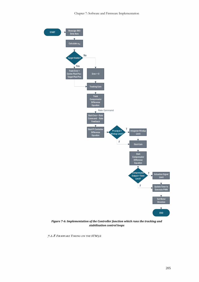
Chapter 7: Software and Firmware Implementation
205
START
Track Error =
Centre Pixel Pos -
Target Pixel Pos
Stab PI Controller
Difference
Equation
Integrator Windup
Limit
Stab Gain
Stab
Compensator
Difference
Equation
Actuation Signal
Limit
END
Update Timer to
Generate PWM
PI output >
Windup Limit?
Compensator
Output > Timer
Limit?
Target Visible?
Tracking Gain
Track
Compensator
Difference
Equation
Error = 0
Stab Error = Rate
Command – Rate
Feedback
Set Motor
Direction
Rate Command
T
T
Yes
No
F
F
Calculate ωzg
Reassign IMU
Data Axes
Figure 7-6: Implementation of the Controller function which runs the tracking and
stabilisation control loops
7.2.8 FIRMWARE TIMING ON THE STM32
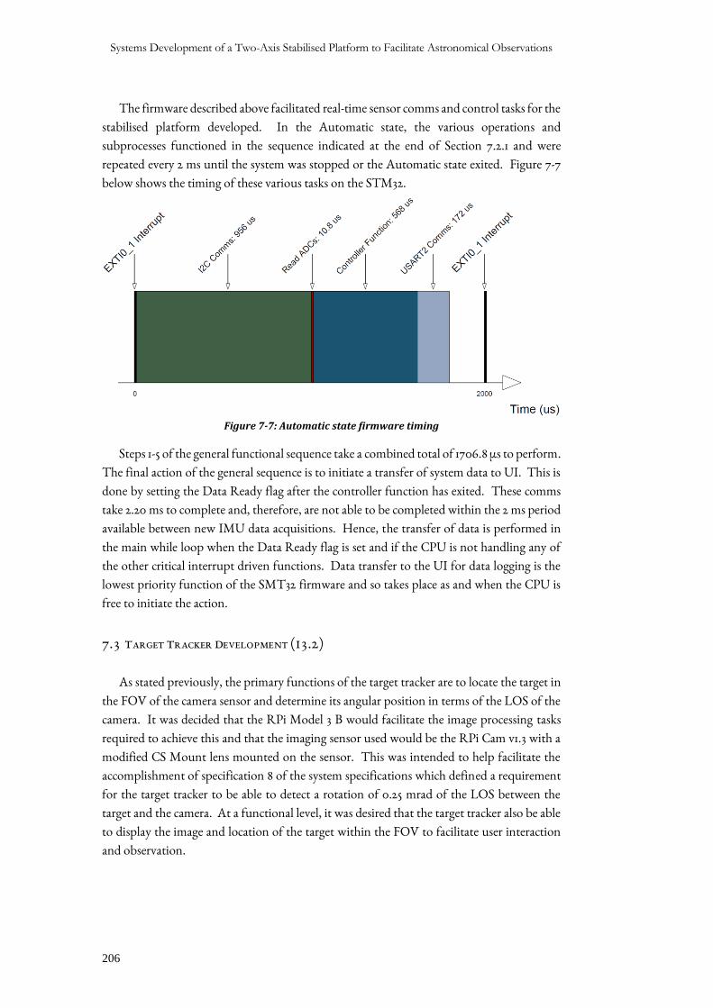
Systems Development of a Two-Axis Stabilised Platform to Facilitate Astronomical Observations
206
The firmware described above facilitated real-time sensor comms and control tasks for the
stabilised platform developed. In the Automatic state, the various operations and
subprocesses functioned in the sequence indicated at the end of Section 7.2.1 and were
repeated every 2 ms until the system was stopped or the Automatic state exited. Figure 7-7
below shows the timing of these various tasks on the STM32.
Figure 7-7: Automatic state firmware timing
Steps 1-5 of the general functional sequence take a combined total of 1706.8 µs to perform.
The final action of the general sequence is to initiate a transfer of system data to UI. This is
done by setting the Data Ready flag after the controller function has exited. These comms
take 2.20 ms to complete and, therefore, are not able to be completed within the 2 ms period
available between new IMU data acquisitions. Hence, the transfer of data is performed in
the main while loop when the Data Ready flag is set and if the CPU is not handling any of
the other critical interrupt driven functions. Data transfer to the UI for data logging is the
lowest priority function of the SMT32 firmware and so takes place as and when the CPU is
free to initiate the action.
7.3 TARGET TRACKER DEVELOPMENT (I3.2)
As stated previously, the primary functions of the target tracker are to locate the target in
the FOV of the camera sensor and determine its angular position in terms of the LOS of the
camera. It was decided that the RPi Model 3 B would facilitate the image processing tasks
required to achieve this and that the imaging sensor used would be the RPi Cam v1.3 with a
modified CS Mount lens mounted on the sensor. This was intended to help facilitate the
accomplishment of specification 8 of the system specifications which defined a requirement
for the target tracker to be able to detect a rotation of 0.25 mrad of the LOS between the
target and the camera. At a functional level, it was desired that the target tracker also be able
to display the image and location of the target within the FOV to facilitate user interaction
and observation.
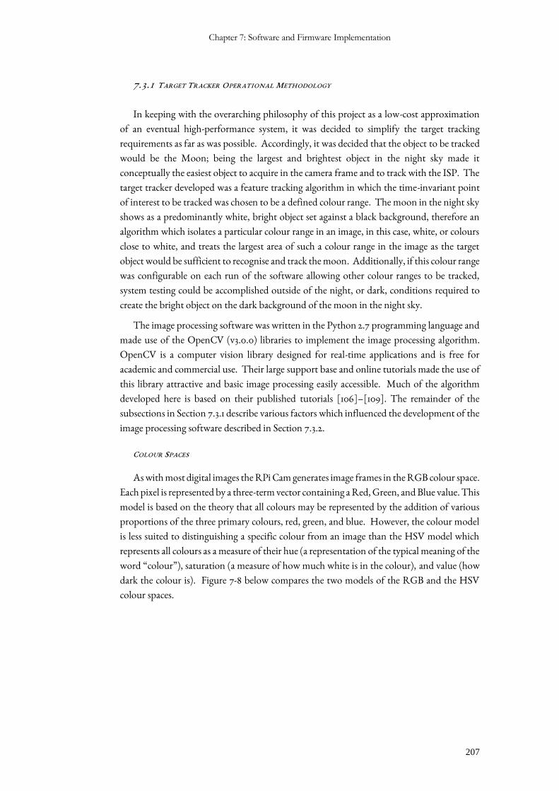
Chapter 7: Software and Firmware Implementation
207
7.3.1 TARGET TRACKER OPERATIONAL METHODOLOGY
In keeping with the overarching philosophy of this project as a low-cost approximation
of an eventual high-performance system, it was decided to simplify the target tracking
requirements as far as was possible. Accordingly, it was decided that the object to be tracked
would be the Moon; being the largest and brightest object in the night sky made it
conceptually the easiest object to acquire in the camera frame and to track with the ISP. The
target tracker developed was a feature tracking algorithm in which the time-invariant point
of interest to be tracked was chosen to be a defined colour range. The moon in the night sky
shows as a predominantly white, bright object set against a black background, therefore an
algorithm which isolates a particular colour range in an image, in this case, white, or colours
close to white, and treats the largest area of such a colour range in the image as the target
object would be sufficient to recognise and track the moon. Additionally, if this colour range
was configurable on each run of the software allowing other colour ranges to be tracked,
system testing could be accomplished outside of the night, or dark, conditions required to
create the bright object on the dark background of the moon in the night sky.
The image processing software was written in the Python 2.7 programming language and
made use of the OpenCV (v3.0.0) libraries to implement the image processing algorithm.
OpenCV is a computer vision library designed for real-time applications and is free for
academic and commercial use. Their large support base and online tutorials made the use of
this library attractive and basic image processing easily accessible. Much of the algorithm
developed here is based on their published tutorials [106]–[109]. The remainder of the
subsections in Section 7.3.1 describe various factors which influenced the development of the
image processing software described in Section 7.3.2.
COLOUR SPACES
As with most digital images the RPi Cam generates image frames in the RGB colour space.
Each pixel is represented by a three-term vector containing a Red, Green, and Blue value. This
model is based on the theory that all colours may be represented by the addition of various
proportions of the three primary colours, red, green, and blue. However, the colour model
is less suited to distinguishing a specific colour from an image than the HSV model which
represents all colours as a measure of their hue (a representation of the typical meaning of the
word “colour”), saturation (a measure of how much white is in the colour), and value (how
dark the colour is). Figure 7-8 below compares the two models of the RGB and the HSV
colour spaces.
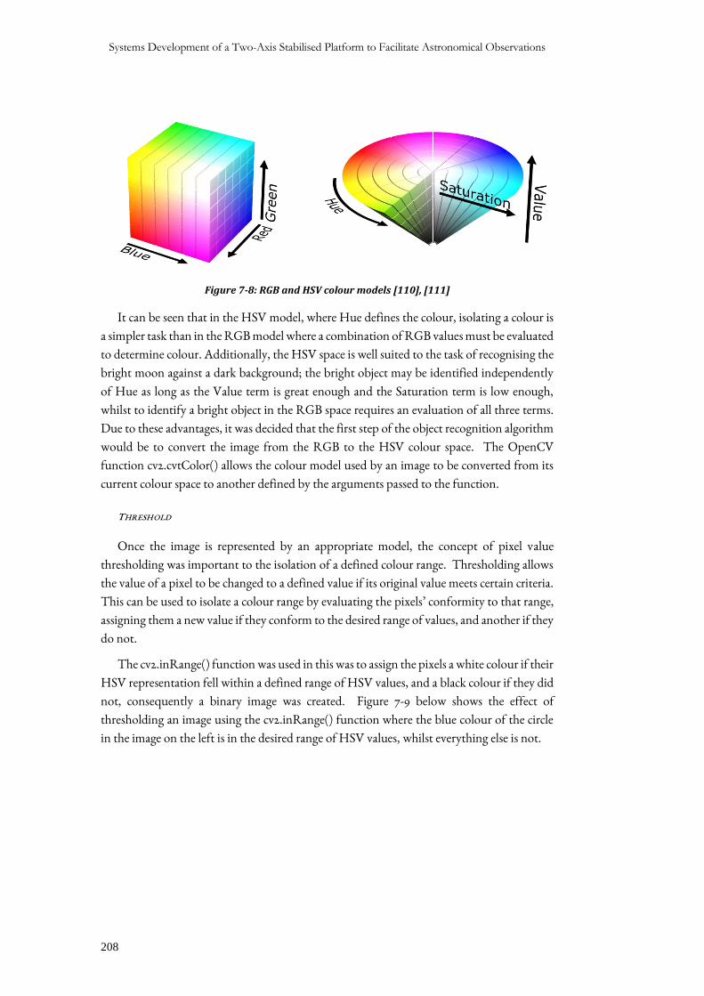
Systems Development of a Two-Axis Stabilised Platform to Facilitate Astronomical Observations
208
Figure 7-8: RGB and HSV colour models [110], [111]
It can be seen that in the HSV model, where Hue defines the colour, isolating a colour is
a simpler task than in the RGB model where a combination of RGB values must be evaluated
to determine colour. Additionally, the HSV space is well suited to the task of recognising the
bright moon against a dark background; the bright object may be identified independently
of Hue as long as the Value term is great enough and the Saturation term is low enough,
whilst to identify a bright object in the RGB space requires an evaluation of all three terms.
Due to these advantages, it was decided that the first step of the object recognition algorithm
would be to convert the image from the RGB to the HSV colour space. The OpenCV
function cv2.cvtColor() allows the colour model used by an image to be converted from its
current colour space to another defined by the arguments passed to the function.
THRESHOLD
Once the image is represented by an appropriate model, the concept of pixel value
thresholding was important to the isolation of a defined colour range. Thresholding allows
the value of a pixel to be changed to a defined value if its original value meets certain criteria.
This can be used to isolate a colour range by evaluating the pixels’ conformity to that range,
assigning them a new value if they conform to the desired range of values, and another if they
do not.
The cv2.inRange() function was used in this was to assign the pixels a white colour if their
HSV representation fell within a defined range of HSV values, and a black colour if they did
not, consequently a binary image was created. Figure 7-9 below shows the effect of
thresholding an image using the cv2.inRange() function where the blue colour of the circle
in the image on the left is in the desired range of HSV values, whilst everything else is not.
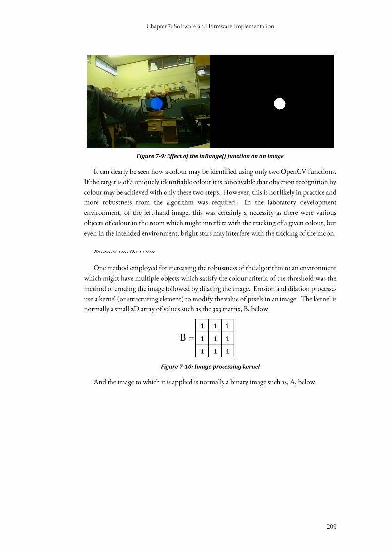
Chapter 7: Software and Firmware Implementation
209
Figure 7-9: Effect of the inRange() function on an image
It can clearly be seen how a colour may be identified using only two OpenCV functions.
If the target is of a uniquely identifiable colour it is conceivable that objection recognition by
colour may be achieved with only these two steps. However, this is not likely in practice and
more robustness from the algorithm was required. In the laboratory development
environment, of the left-hand image, this was certainly a necessity as there were various
objects of colour in the room which might interfere with the tracking of a given colour, but
even in the intended environment, bright stars may interfere with the tracking of the moon.
EROSION AND DILATION
One method employed for increasing the robustness of the algorithm to an environment
which might have multiple objects which satisfy the colour criteria of the threshold was the
method of eroding the image followed by dilating the image. Erosion and dilation processes
use a kernel (or structuring element) to modify the value of pixels in an image. The kernel is
normally a small 2D array of values such as the 3x3 matrix, B, below.
Figure 7-10: Image processing kernel
And the image to which it is applied is normally a binary image such as, A, below.
1 1 1
1 1 1
1 1 1
B =
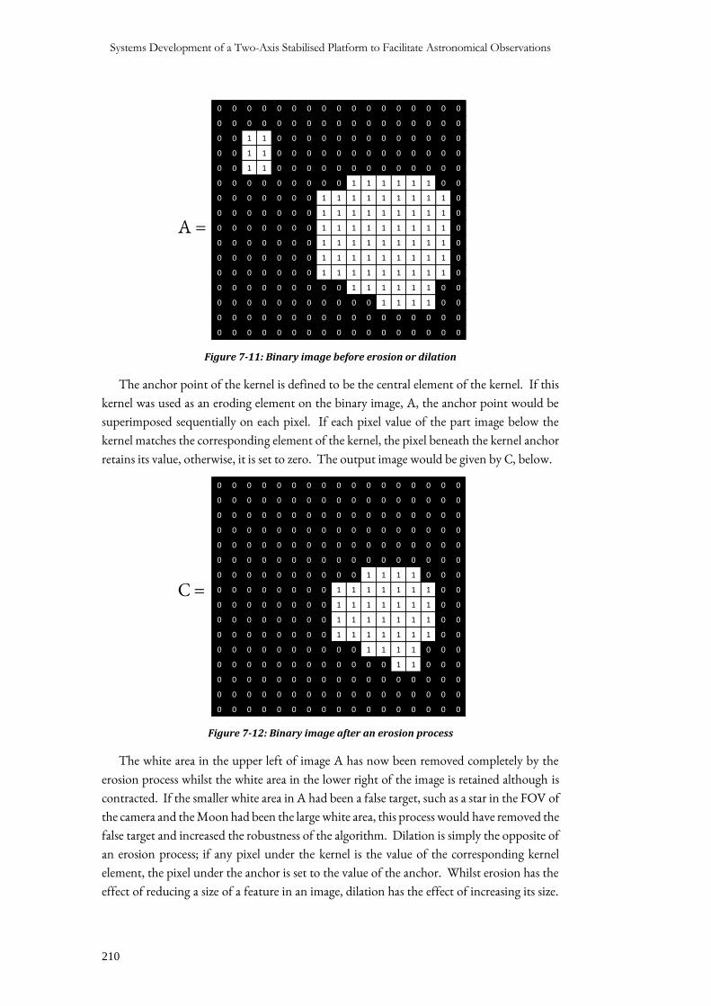
Systems Development of a Two-Axis Stabilised Platform to Facilitate Astronomical Observations
210
Figure 7-11: Binary image before erosion or dilation
The anchor point of the kernel is defined to be the central element of the kernel. If this
kernel was used as an eroding element on the binary image, A, the anchor point would be
superimposed sequentially on each pixel. If each pixel value of the part image below the
kernel matches the corresponding element of the kernel, the pixel beneath the kernel anchor
retains its value, otherwise, it is set to zero. The output image would be given by C, below.
Figure 7-12: Binary image after an erosion process
The white area in the upper left of image A has now been removed completely by the
erosion process whilst the white area in the lower right of the image is retained although is
contracted. If the smaller white area in A had been a false target, such as a star in the FOV of
the camera and the Moon had been the large white area, this process would have removed the
false target and increased the robustness of the algorithm. Dilation is simply the opposite of
an erosion process; if any pixel under the kernel is the value of the corresponding kernel
element, the pixel under the anchor is set to the value of the anchor. Whilst erosion has the
effect of reducing a size of a feature in an image, dilation has the effect of increasing its size.
0 0 0 0 0 0 0 0 0 0 0 0 0 0 0 0 0
0 0 0 0 0 0 0 0 0 0 0 0 0 0 0 0 0
0 0 1 1 0 0 0 0 0 0 0 0 0 0 0 0 0
0 0 1 1 0 0 0 0 0 0 0 0 0 0 0 0 0
0 0 1 1 0 0 0 0 0 0 0 0 0 0 0 0 0
0 0 0 0 0 0 0 0 0 1 1 1 1 1 1 0 0
0 0 0 0 0 0 0 1 1 1 1 1 1 1 1 1 0
0 0 0 0 0 0 0 1 1 1 1 1 1 1 1 1 0
0 0 0 0 0 0 0 1 1 1 1 1 1 1 1 1 0
0 0 0 0 0 0 0 1 1 1 1 1 1 1 1 1 0
0 0 0 0 0 0 0 1 1 1 1 1 1 1 1 1 0
0 0 0 0 0 0 0 1 1 1 1 1 1 1 1 1 0
0 0 0 0 0 0 0 0 0 1 1 1 1 1 1 0 0
0 0 0 0 0 0 0 0 0 0 0 1 1 1 1 0 0
0 0 0 0 0 0 0 0 0 0 0 0 0 0 0 0 0
0 0 0 0 0 0 0 0 0 0 0 0 0 0 0 0 0
0 0 0 0 0 0 0 0 0 0 0 0 0 0 0 0 0
0 0 0 0 0 0 0 0 0 0 0 0 0 0 0 0 0
0 0 0 0 0 0 0 0 0 0 0 0 0 0 0 0 0
0 0 0 0 0 0 0 0 0 0 0 0 0 0 0 0 0
0 0 0 0 0 0 0 0 0 0 0 0 0 0 0 0 0
0 0 0 0 0 0 0 0 0 0 0 0 0 0 0 0 0
0 0 0 0 0 0 0 0 0 0 1 1 1 1 0 0 0
0 0 0 0 0 0 0 0 1 1 1 1 1 1 1 0 0
0 0 0 0 0 0 0 0 1 1 1 1 1 1 1 0 0
0 0 0 0 0 0 0 0 1 1 1 1 1 1 1 0 0
0 0 0 0 0 0 0 0 1 1 1 1 1 1 1 0 0
0 0 0 0 0 0 0 0 0 0 1 1 1 1 0 0 0
0 0 0 0 0 0 0 0 0 0 0 0 1 1 0 0 0
0 0 0 0 0 0 0 0 0 0 0 0 0 0 0 0 0
0 0 0 0 0 0 0 0 0 0 0 0 0 0 0 0 0
0 0 0 0 0 0 0 0 0 0 0 0 0 0 0 0 0
A =
C =
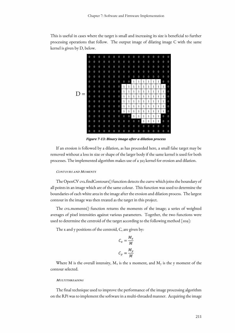
Chapter 7: Software and Firmware Implementation
211
This is useful in cases where the target is small and increasing its size is beneficial to further
processing operations that follow. The output image of dilating image C with the same
kernel is given by D, below.
Figure 7-13: Binary image after a dilation process
If an erosion is followed by a dilation, as has proceeded here, a small false target may be
removed without a loss in size or shape of the larger body if the same kernel is used for both
processes. The implemented algorithm makes use of a 3x3 kernel for erosion and dilation.
CONTOURS AND MOMENTS
The OpenCV cv2.findContours() function detects the curve which joins the boundary of
all points in an image which are of the same colour. This function was used to determine the
boundaries of each white area in the image after the erosion and dilation process. The largest
contour in the image was then treated as the target in this project.
The cv2.moments() function returns the moments of the image; a series of weighted
averages of pixel intensities against various parameters. Together, the two functions were
used to determine the centroid of the target according to the following method [109]:
The x and y positions of the centroid, C, are given by:
𝐶𝑥 =𝑀𝑥
𝑀
𝐶𝑦 =𝑀𝑦
𝑀
Where M is the overall intensity, Mx is the x moment, and My is the y moment of the
contour selected.
MULTITHREADING
The final technique used to improve the performance of the image processing algorithm
on the RPi was to implement the software in a multi-threaded manner. Acquiring the image
0 0 0 0 0 0 0 0 0 0 0 0 0 0 0 0 0
0 0 0 0 0 0 0 0 0 0 0 0 0 0 0 0 0
0 0 0 0 0 0 0 0 0 0 0 0 0 0 0 0 0
0 0 0 0 0 0 0 0 0 0 0 0 0 0 0 0 0
0 0 0 0 0 0 0 0 0 0 0 0 0 0 0 0 0
0 0 0 0 0 0 0 0 0 1 1 1 1 1 1 0 0
0 0 0 0 0 0 0 1 1 1 1 1 1 1 1 1 0
0 0 0 0 0 0 0 1 1 1 1 1 1 1 1 1 0
0 0 0 0 0 0 0 1 1 1 1 1 1 1 1 1 0
0 0 0 0 0 0 0 1 1 1 1 1 1 1 1 1 0
0 0 0 0 0 0 0 1 1 1 1 1 1 1 1 1 0
0 0 0 0 0 0 0 1 1 1 1 1 1 1 1 1 0
0 0 0 0 0 0 0 0 0 1 1 1 1 1 1 0 0
0 0 0 0 0 0 0 0 0 0 0 1 1 1 1 0 0
0 0 0 0 0 0 0 0 0 0 0 0 0 0 0 0 0
0 0 0 0 0 0 0 0 0 0 0 0 0 0 0 0 0
D =
Systems Development of a Two-Axis Stabilised Platform to Facilitate Astronomical Observations
212
on the RPi is an I/O heavy application and can cause a bottleneck in the processing algorithm
as it waits for a new image to be acquired before processing can continue. To offset this, the
image frame acquisition was moved to an independent processing thread which continually
polls the camera for new frames. The main processing algorithm then ran on a second thread
which simply used the most recent frame available from the acquisition thread. Using this
technique, it was possible to increase the number of frames processed per second (FPS) from
approximately 7 FPS to approximately 11 FPS. The imutils library written by Adrian
Rosebrock and method described by him were used as a base for the implementation of this
behaviour [112]–[114].
7.3.2 FUNCTIONAL DESCRIPTION OF IMAGE PROCESSING ALGORITHM
The previous subsections described the main processes that were involved with the
implementation of the image processing algorithm used to identify the Moon or simulated
target colour in the camera FOV. This subsection describes the software written from a
functional perspective using a flowchart and how the target position data is transferred to the
STM32.
INTERACTION WITH THE STM32
Figure 6-53 of Section 6.5 previously, defines the target tracker to be a system which takes
the target position, host vehicle rates, and the gimbals’ orientation as inputs to the system and
returns the yaw and pitch tracking errors as outputs. The image processing algorithm
introduced to this point has only indicated how the pixel positions of the centroid of the
target might be determined in the image frame. Knowing the angle covered by the FOV of
the sensor, it is possible for the yaw and pitch tracking errors in radians from the LOS to have
been determined on the RPi. However, to simplify the comms between the RPi and the
STM32 which requires these error signals to run the tracking controllers, it was decided to
send the pixel positions of the centroid to the STM32 rather than the error values. The
tracking errors would almost certainly be non-integer values which are more complex to send
over the USART comms link between the two devices than the integer pixel positions.
Consequently, the STM32 performs part of the target tracker’s function and is tasked with
converting these pixel positions to tracking errors on which to perform the tracking control
operations.
In order manage the timing of comms transfers between the devices, several pins on the
STM and RPi were allocated to act as flags whose values indicate various states of operation.
On the RPi, these pins are Pins 31, 33, 35, and 37 which are connected to the STM32 at PA4,
PB0, PB1, and PB2 respectively. The procedure by which the comms sequence is completed
is detailed below.
1. When PB0 on the STM32 is raised HIGH from its default LOW state, the image
processing script knows that the STM32 has moved into the Automatic state due to
the HIGH value being read on P33. In this state, P31 is then raised by the RPi when
Chapter 7: Software and Firmware Implementation
213
a new frame has been processed and target position data is ready to be sent to the
STM32. This causes an EXTI interrupt on PA4 of the STM32.
2. The EXTI interrupt handler for PA4 then acknowledges that new target data is ready
to be sent by lowering PB2 on the STM32 which is connected to P37 on the RPi. It
also disables the new IMU data interrupt until the comms sequence has completed.
Until the RPi sees P37 lowered, the program waits and does not initiate the comms
transfer.
3. Once P37 is lowered, the RPi sends four bytes of data to the STM32 via a USART
connection. On receipt of four bytes, the STM32 re-enables the new IMU data
interrupt and raises PB2 (P37).
4. The RPi then sets P31 (PA4) low to complete the comms sequence.
If the STM32 raises PB1 at some point during the image processing algorithm or comms
cycle, a system stop condition is met and the image processing script is stopped.
FUNCTIONAL FLOWCHART DESCRIBING THE IMAGE PROCESSING SCRIPT
The flowchart shown in Figure 7-14 below describes the image processing script used in
this project whilst the Python code itself may be found in Appendix C.
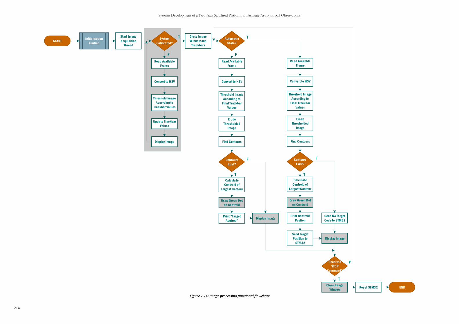
Systems Development of a Two-Axis Stabilised Platform to Facilitate Astronomical Observations
214
START
END
System
Calibrated?
T
F
Initialisation
Funtion
Start Image
Acquisition
Thread
Read Available
Frame
Convert to HSV
Threshold Image
According to
Trackbar Values
Display Image
Close Image
Window and
Trackbars
Automatic
State?
Update Trackbar
Values
Read Available
Frame
Convert to HSV
Threshold Image
According to
Final Trackbar
Values
Erode
Thresholded
Image
Find Contours
Contours
Exist?
Calculate
Centroid of
Largest Contour
Draw Green Dot
on Centroid
Print Target
Aquired Display Image
Read Available
Frame
Convert to HSV
Threshold Image
According to
Final Trackbar
Values
Erode
Thresholded
Image
Find Contours
Contours
Exist?
Calculate
Centroid of
Largest Contour
Draw Green Dot
on Centroid
Print Centroid
Postion
Display Image
Send No Target
Code to STM32
Send Target
Position to
STM32
Received
STOP
Command?
Close Image
WindowReset STM32
T
TT
F
FF
T
F
Figure 7-14: Image processing functional flowchart
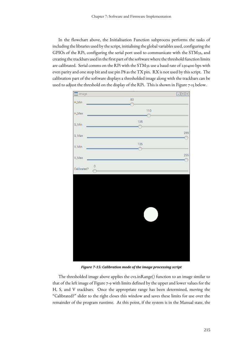
Chapter 7: Software and Firmware Implementation
215
In the flowchart above, the Initialisation Function subprocess performs the tasks of
including the libraries used by the script, initialising the global variables used, configuring the
GPIOs of the RPi, configuring the serial port used to communicate with the STM32, and
creating the trackbars used in the first part of the software where the threshold function limits
are calibrated. Serial comms on the RPi with the STM32 use a baud rate of 230400 bps with
even parity and one stop bit and use pin P8 as the TX pin. RX is not used by this script. The
calibration part of the software displays a thresholded image along with the trackbars can be
used to adjust the threshold on the display of the RPi. This is shown in Figure 7-15 below.
Figure 7-15: Calibration mode of the image processing script
The thresholded image above applies the cv2.inRange() function to an image similar to
that of the left image of Figure 7-9 with limits defined by the upper and lower values for the
H, S, and V trackbars. Once the appropriate range has been determined, moving the
“Calibrated?” slider to the right closes this window and saves these limits for use over the
remainder of the program runtime. At this point, if the system is in the Manual state, the
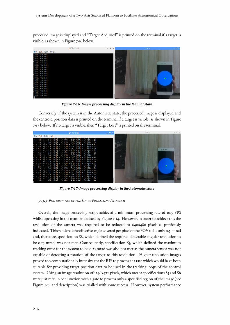
Systems Development of a Two-Axis Stabilised Platform to Facilitate Astronomical Observations
216
processed image is displayed and “Target Acquired” is printed on the terminal if a target is
visible, as shown in Figure 7-16 below.
Figure 7-16: Image processing display in the Manual state
Conversely, if the system is in the Automatic state, the processed image is displayed and
the centroid position data is printed on the terminal if a target is visible, as shown in Figure
7-17 below. If no target is visible, then “Target Lost” is printed on the terminal.
Figure 7-17: Image processing display in the Automatic state
7.3.3 PERFORMANCE OF THE IMAGE PROCESSING PROGRAM
Overall, the image processing script achieved a minimum processing rate of 10.5 FPS
whilst operating in the manner defined by Figure 7-14. However, in order to achieve this the
resolution of the camera was required to be reduced to 640x480 pixels as previously
indicated. This rendered the effective angle covered per pixel of the FOV to be only 0.51 mrad
and, therefore, specification S8, which defined the required detectable angular resolution to
be 0.25 mrad, was not met. Consequently, specification S5, which defined the maximum
tracking error for the system to be 0.25 mrad was also not met as the camera sensor was not
capable of detecting a rotation of the target to this resolution. Higher resolution images
proved too computationally intensive for the RPi to process at a rate which would have been
suitable for providing target position data to be used in the tracking loops of the control
system. Using an image resolution of 1296x972 pixels, which meant specifications S5 and S8
were just met, in conjunction with a gate to process only a specified region of the image (see
Figure 2-14 and description) was trialled with some success. However, system performance
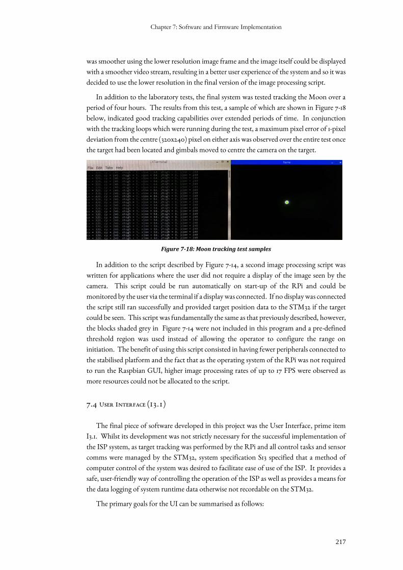
Chapter 7: Software and Firmware Implementation
217
was smoother using the lower resolution image frame and the image itself could be displayed
with a smoother video stream, resulting in a better user experience of the system and so it was
decided to use the lower resolution in the final version of the image processing script.
In addition to the laboratory tests, the final system was tested tracking the Moon over a
period of four hours. The results from this test, a sample of which are shown in Figure 7-18
below, indicated good tracking capabilities over extended periods of time. In conjunction
with the tracking loops which were running during the test, a maximum pixel error of 1-pixel
deviation from the centre (320x240) pixel on either axis was observed over the entire test once
the target had been located and gimbals moved to centre the camera on the target.
Figure 7-18: Moon tracking test samples
In addition to the script described by Figure 7-14, a second image processing script was
written for applications where the user did not require a display of the image seen by the
camera. This script could be run automatically on start-up of the RPi and could be
monitored by the user via the terminal if a display was connected. If no display was connected
the script still ran successfully and provided target position data to the STM32 if the target
could be seen. This script was fundamentally the same as that previously described, however,
the blocks shaded grey in Figure 7-14 were not included in this program and a pre-defined
threshold region was used instead of allowing the operator to configure the range on
initiation. The benefit of using this script consisted in having fewer peripherals connected to
the stabilised platform and the fact that as the operating system of the RPi was not required
to run the Raspbian GUI, higher image processing rates of up to 17 FPS were observed as
more resources could not be allocated to the script.
7.4 USER INTERFACE (I3.1)
The final piece of software developed in this project was the User Interface, prime item
I3.1. Whilst its development was not strictly necessary for the successful implementation of
the ISP system, as target tracking was performed by the RPi and all control tasks and sensor
comms were managed by the STM32, system specification S13 specified that a method of
computer control of the system was desired to facilitate ease of use of the ISP. It provides a
safe, user-friendly way of controlling the operation of the ISP as well as provides a means for
the data logging of system runtime data otherwise not recordable on the STM32.
The primary goals for the UI can be summarised as follows:

Systems Development of a Two-Axis Stabilised Platform to Facilitate Astronomical Observations
218
1. Provide a means to initialise and stop target tracking and stabilisation.
2. Provide a means to control the gimbals’ orientation whilst in the manual mode of
operation.
3. Provide a real-time visualisation of the ISP assembly.
4. Indicate the target position in the camera FOV.
5. Indicate current inertial rates of the telescope.
6. Provide a means of data logging of the system runtime data.
7.4.1 DESCRIPTION OF THE COMPONENTS OF THE UI
As previously indicated in Section 5.2.6, the UI was written in the LabVIEW environment
due to its ease of use for developing supervisory control programs. Figure 7-19 below shows
the GUI of the final UI.
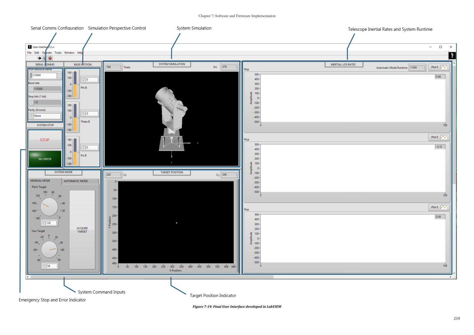
Chapter 7: Software and Firmware Implementation
219
Figure 7-19: Final User Interface developed in LabVIEW
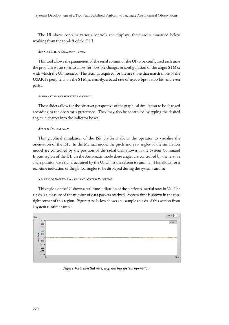
Systems Development of a Two-Axis Stabilised Platform to Facilitate Astronomical Observations
220
The UI above contains various controls and displays, these are summarised below
working from the top-left of the GUI.
SERIAL COMMS CONFIGURATION
This tool allows the parameters of the serial comms of the UI to be configured each time
the program is run so as to allow for possible changes in configuration of the target STM32
with which the UI interacts. The settings required for use are those that match those of the
USART1 peripheral on the STM32, namely, a baud rate of 115200 bps, 1 stop bit, and even
parity.
SIMULATION PERSPECTIVE CONTROL
These sliders allow for the observer perspective of the graphical simulation to be changed
according to the operator’s preference. They may also be controlled by typing the desired
angles in degrees into the indicator boxes.
SYSTEM SIMULATION
This graphical simulation of the ISP platform allows the operator to visualise the
orientation of the ISP. In the Manual mode, the pitch and yaw angles of the simulation
model are controlled by the position of the radial dials shown in the System Command
Inputs region of the UI. In the Automatic mode these angles are controlled by the relative
angle position data signal acquired by the UI whilst the system is running. This allows for a
real-time indication of the gimbal angles to be displayed during the system runtime.
TELESCOPE INERTIAL RATES AND SYSTEM RUNTIME
This region of the UI shows a real-time indication of the platform inertial rates in °/s. The
x-axis is a measure of the number of data packets received. System time is shown in the top-
right corner of this region. Figure 7-20 below shows an example an axis of this section from
a system runtime sample.
Figure 7-20: Inertial rate, 𝝎𝒚𝒃, during system operation
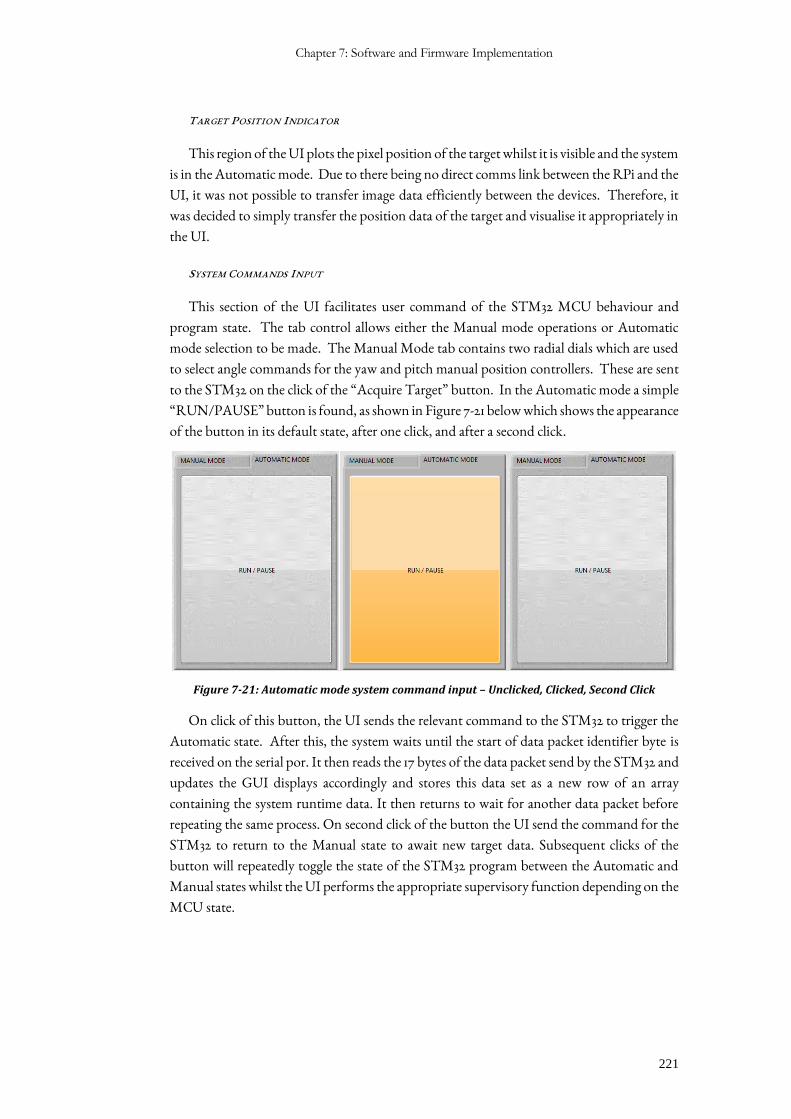
Chapter 7: Software and Firmware Implementation
221
TARGET POSITION INDICATOR
This region of the UI plots the pixel position of the target whilst it is visible and the system
is in the Automatic mode. Due to there being no direct comms link between the RPi and the
UI, it was not possible to transfer image data efficiently between the devices. Therefore, it
was decided to simply transfer the position data of the target and visualise it appropriately in
the UI.
SYSTEM COMMANDS INPUT
This section of the UI facilitates user command of the STM32 MCU behaviour and
program state. The tab control allows either the Manual mode operations or Automatic
mode selection to be made. The Manual Mode tab contains two radial dials which are used
to select angle commands for the yaw and pitch manual position controllers. These are sent
to the STM32 on the click of the “Acquire Target” button. In the Automatic mode a simple
“RUN/PAUSE” button is found, as shown in Figure 7-21 below which shows the appearance
of the button in its default state, after one click, and after a second click.
Figure 7-21: Automatic mode system command input – Unclicked, Clicked, Second Click
On click of this button, the UI sends the relevant command to the STM32 to trigger the
Automatic state. After this, the system waits until the start of data packet identifier byte is
received on the serial por. It then reads the 17 bytes of the data packet send by the STM32 and
updates the GUI displays accordingly and stores this data set as a new row of an array
containing the system runtime data. It then returns to wait for another data packet before
repeating the same process. On second click of the button the UI send the command for the
STM32 to return to the Manual state to await new target data. Subsequent clicks of the
button will repeatedly toggle the state of the STM32 program between the Automatic and
Manual states whilst the UI performs the appropriate supervisory function depending on the
MCU state.
Systems Development of a Two-Axis Stabilised Platform to Facilitate Astronomical Observations
222
EMERGENCY STOP AND ERROR INDICATOR
The final region of the GUI contains the system stop button and an error indicator. On
press of the stop button the UI sends the STOP command to the STM32, which in turn sends
the shutdown signal to the RPi. It then writes the data logs to a spreadsheet file and displays
a dialog box to the operator indicating that the stop button was pressed and that the data logs
have been saved. If a limit error is detected the same stop process is followed, but the dialog
box indicates that a limit error stopped the system, and the green indicator is lit red.
7.4.2 FUNCTIONAL DESCRIPTION OF THE USER INTERFACE
The flowchart shown in Figure 7-22 below describes the User Interface software
developed for this project. The LabVIEW project containing the main VI and sub-VIs used
by the software may be found in Appendix C.

Chapter 7: Software and Firmware Implementation
223
START
Read Values of
Angle Input
Dials
Update
Graphical
Simulation with
New Angles
Send Target
Angles to
STM32
Send STOP
Command to
STM32
END
Acquire Target
Clicked?
T RUN
STOP
ClickedLimit Error ?
Manual
Mode Tab?
RUN/PAUSE
?
Send Automatic
State Command
to STM32
Received Start
of Data Packet
Identifyier?
Read Data
Packet
Update GUI
Displays
Write Data Logs
to Spreadsheet
File
Return Stop
Cause to User
Return Limit
Error to User
Send Manual
State Command
to STM32
T
T
T
T
F
F
FFFPAUSE
Store Data from
Packet
Initialise Serial
Port and
Displays
Figure 7-22: Functional flowchart of the User Interface software operation
7.5 CHAPTER CONCLUSION
This chapter began by describing the firmware written for the STM32F0 microcontroller.
This firmware was written in C and performed all sensor communications, controller
algorithm functions and system limit protection tasks. It also manged the timing of comms
transfers contain target position data from the RPi. Finally, the firmware performed the task
of sending runtime data from each run of the controller algorithm to the LabVIEW UI.
After the description of the STM32 firmware, the multi-threaded image processing
software which performed most of the target tracker tasks was detailed. This software was

Systems Development of a Two-Axis Stabilised Platform to Facilitate Astronomical Observations
224
written in Python 2.7 and implemented on the RPi computer to process the image acquired
by the RPi Cam such that a target could be identified and located in the FOV of the camera.
Finally, the chapter concluded with a description of the User Interface software written
in LabVIEW. This software facilitated user control of the ISP system in a safe, user friendly
manner, and performed data logging operations on the system runtime data sent by the
STM32 to the host computer.
The next chapter describes various system tests that were run to characterise the
performance of the implemented ISP and to determine the correlation between the hardware
and simulation results.
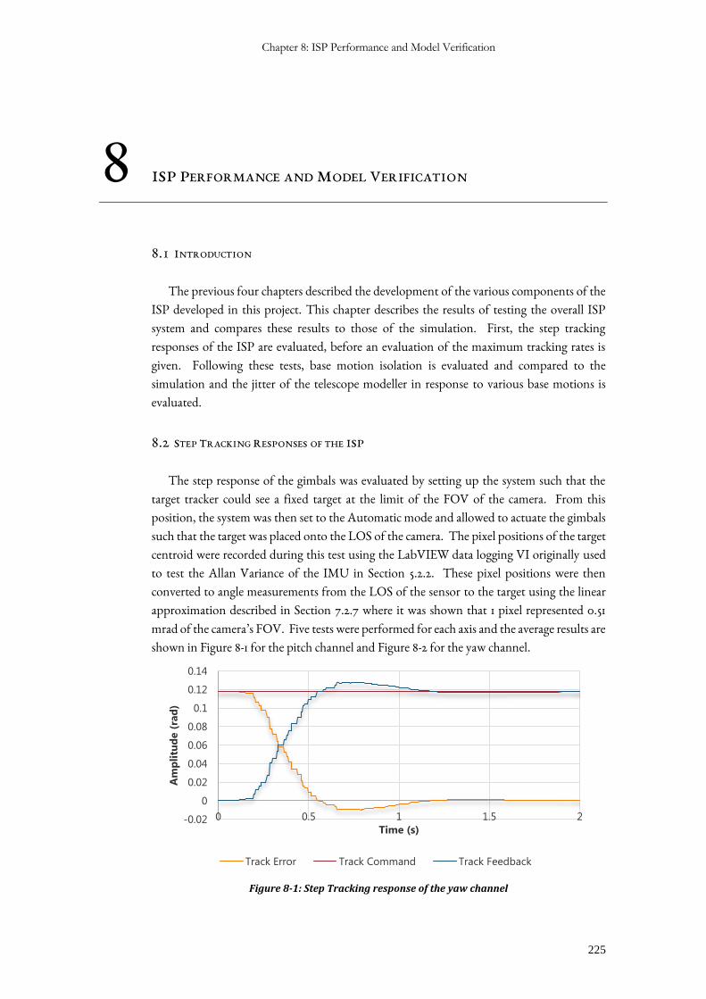
Chapter 8: ISP Performance and Model Verification
225
8 ISP PERFORMANCE AND MODEL VERIFICATION
8.1 INTRODUCTION
The previous four chapters described the development of the various components of the
ISP developed in this project. This chapter describes the results of testing the overall ISP
system and compares these results to those of the simulation. First, the step tracking
responses of the ISP are evaluated, before an evaluation of the maximum tracking rates is
given. Following these tests, base motion isolation is evaluated and compared to the
simulation and the jitter of the telescope modeller in response to various base motions is
evaluated.
8.2 STEP TRACKING RESPONSES OF THE ISP
The step response of the gimbals was evaluated by setting up the system such that the
target tracker could see a fixed target at the limit of the FOV of the camera. From this
position, the system was then set to the Automatic mode and allowed to actuate the gimbals
such that the target was placed onto the LOS of the camera. The pixel positions of the target
centroid were recorded during this test using the LabVIEW data logging VI originally used
to test the Allan Variance of the IMU in Section 5.2.2. These pixel positions were then
converted to angle measurements from the LOS of the sensor to the target using the linear
approximation described in Section 7.2.7 where it was shown that 1 pixel represented 0.51
mrad of the camera’s FOV. Five tests were performed for each axis and the average results are
shown in Figure 8-1 for the pitch channel and Figure 8-2 for the yaw channel.
Figure 8-1: Step Tracking response of the yaw channel
-0.02
0
0.02
0.04
0.06
0.08
0.1
0.12
0.14
0 0.5 1 1.5 2
Am
pli
tud
e (
rad
)
Time (s)
Track Error Track Command Track Feedback
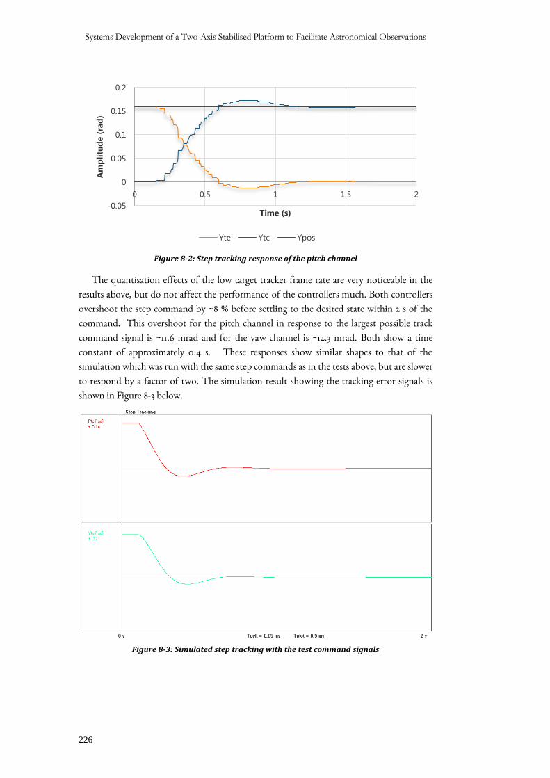
Systems Development of a Two-Axis Stabilised Platform to Facilitate Astronomical Observations
226
Figure 8-2: Step tracking response of the pitch channel
The quantisation effects of the low target tracker frame rate are very noticeable in the
results above, but do not affect the performance of the controllers much. Both controllers
overshoot the step command by ~8 % before settling to the desired state within 2 s of the
command. This overshoot for the pitch channel in response to the largest possible track
command signal is ~11.6 mrad and for the yaw channel is ~12.3 mrad. Both show a time
constant of approximately 0.4 s. These responses show similar shapes to that of the
simulation which was run with the same step commands as in the tests above, but are slower
to respond by a factor of two. The simulation result showing the tracking error signals is
shown in Figure 8-3 below.
Figure 8-3: Simulated step tracking with the test command signals
-0.05
0
0.05
0.1
0.15
0.2
0 0.5 1 1.5 2
Am
pli
tud
e (
rad
)
Time (s)
Yte Ytc Ypos
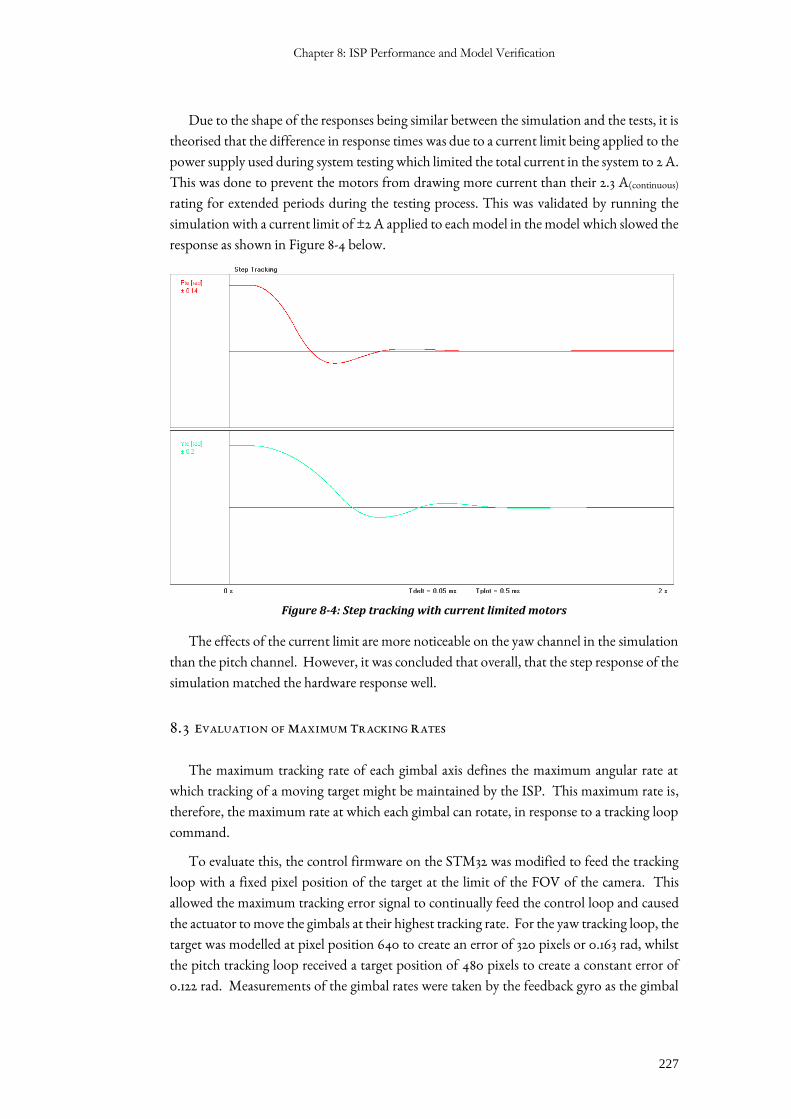
Chapter 8: ISP Performance and Model Verification
227
Due to the shape of the responses being similar between the simulation and the tests, it is
theorised that the difference in response times was due to a current limit being applied to the
power supply used during system testing which limited the total current in the system to 2 A.
This was done to prevent the motors from drawing more current than their 2.3 A(continuous)
rating for extended periods during the testing process. This was validated by running the
simulation with a current limit of ±2 A applied to each model in the model which slowed the
response as shown in Figure 8-4 below.
Figure 8-4: Step tracking with current limited motors
The effects of the current limit are more noticeable on the yaw channel in the simulation
than the pitch channel. However, it was concluded that overall, that the step response of the
simulation matched the hardware response well.
8.3 EVALUATION OF MAXIMUM TRACKING RATES
The maximum tracking rate of each gimbal axis defines the maximum angular rate at
which tracking of a moving target might be maintained by the ISP. This maximum rate is,
therefore, the maximum rate at which each gimbal can rotate, in response to a tracking loop
command.
To evaluate this, the control firmware on the STM32 was modified to feed the tracking
loop with a fixed pixel position of the target at the limit of the FOV of the camera. This
allowed the maximum tracking error signal to continually feed the control loop and caused
the actuator to move the gimbals at their highest tracking rate. For the yaw tracking loop, the
target was modelled at pixel position 640 to create an error of 320 pixels or 0.163 rad, whilst
the pitch tracking loop received a target position of 480 pixels to create a constant error of
0.122 rad. Measurements of the gimbal rates were taken by the feedback gyro as the gimbal
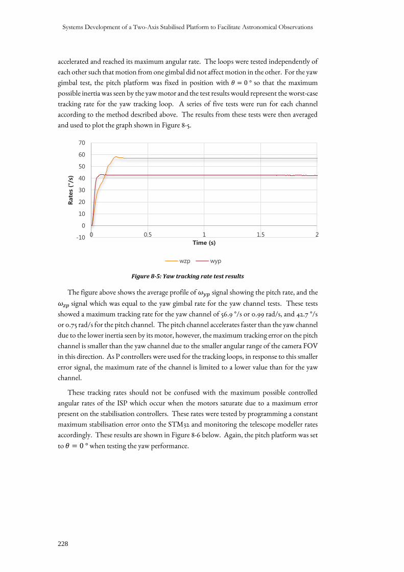
Systems Development of a Two-Axis Stabilised Platform to Facilitate Astronomical Observations
228
accelerated and reached its maximum angular rate. The loops were tested independently of
each other such that motion from one gimbal did not affect motion in the other. For the yaw
gimbal test, the pitch platform was fixed in position with 𝜃 = 0 ° so that the maximum
possible inertia was seen by the yaw motor and the test results would represent the worst-case
tracking rate for the yaw tracking loop. A series of five tests were run for each channel
according to the method described above. The results from these tests were then averaged
and used to plot the graph shown in Figure 8-5.
Figure 8-5: Yaw tracking rate test results
The figure above shows the average profile of 𝜔𝑦𝑝 signal showing the pitch rate, and the
𝜔𝑧𝑝 signal which was equal to the yaw gimbal rate for the yaw channel tests. These tests
showed a maximum tracking rate for the yaw channel of 56.9 °/s or 0.99 rad/s, and 42.7 °/s
or 0.75 rad/s for the pitch channel. The pitch channel accelerates faster than the yaw channel
due to the lower inertia seen by its motor, however, the maximum tracking error on the pitch
channel is smaller than the yaw channel due to the smaller angular range of the camera FOV
in this direction. As P controllers were used for the tracking loops, in response to this smaller
error signal, the maximum rate of the channel is limited to a lower value than for the yaw
channel.
These tracking rates should not be confused with the maximum possible controlled
angular rates of the ISP which occur when the motors saturate due to a maximum error
present on the stabilisation controllers. These rates were tested by programming a constant
maximum stabilisation error onto the STM32 and monitoring the telescope modeller rates
accordingly. These results are shown in Figure 8-6 below. Again, the pitch platform was set
to 𝜃 = 0 ° when testing the yaw performance.
-10
0
10
20
30
40
50
60
70
0 0.5 1 1.5 2
Rate
s (°
/s)
Time (s)
wzp wyp
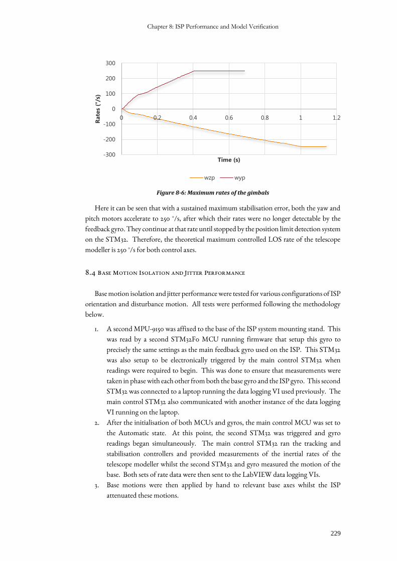
Chapter 8: ISP Performance and Model Verification
229
Figure 8-6: Maximum rates of the gimbals
Here it can be seen that with a sustained maximum stabilisation error, both the yaw and
pitch motors accelerate to 250 °/s, after which their rates were no longer detectable by the
feedback gyro. They continue at that rate until stopped by the position limit detection system
on the STM32. Therefore, the theoretical maximum controlled LOS rate of the telescope
modeller is 250 °/s for both control axes.
8.4 BASE MOTION ISOLATION AND JITTER PERFORMANCE
Base motion isolation and jitter performance were tested for various configurations of ISP
orientation and disturbance motion. All tests were performed following the methodology
below.
1. A second MPU-9150 was affixed to the base of the ISP system mounting stand. This
was read by a second STM32F0 MCU running firmware that setup this gyro to
precisely the same settings as the main feedback gyro used on the ISP. This STM32
was also setup to be electronically triggered by the main control STM32 when
readings were required to begin. This was done to ensure that measurements were
taken in phase with each other from both the base gyro and the ISP gyro. This second
STM32 was connected to a laptop running the data logging VI used previously. The
main control STM32 also communicated with another instance of the data logging
VI running on the laptop.
2. After the initialisation of both MCUs and gyros, the main control MCU was set to
the Automatic state. At this point, the second STM32 was triggered and gyro
readings began simultaneously. The main control STM32 ran the tracking and
stabilisation controllers and provided measurements of the inertial rates of the
telescope modeller whilst the second STM32 and gyro measured the motion of the
base. Both sets of rate data were then sent to the LabVIEW data logging VIs.
3. Base motions were then applied by hand to relevant base axes whilst the ISP
attenuated these motions.
-300
-200
-100
0
100
200
300
0 0.2 0.4 0.6 0.8 1 1.2
Rate
s (°
/s)
Time (s)
wzp wyp
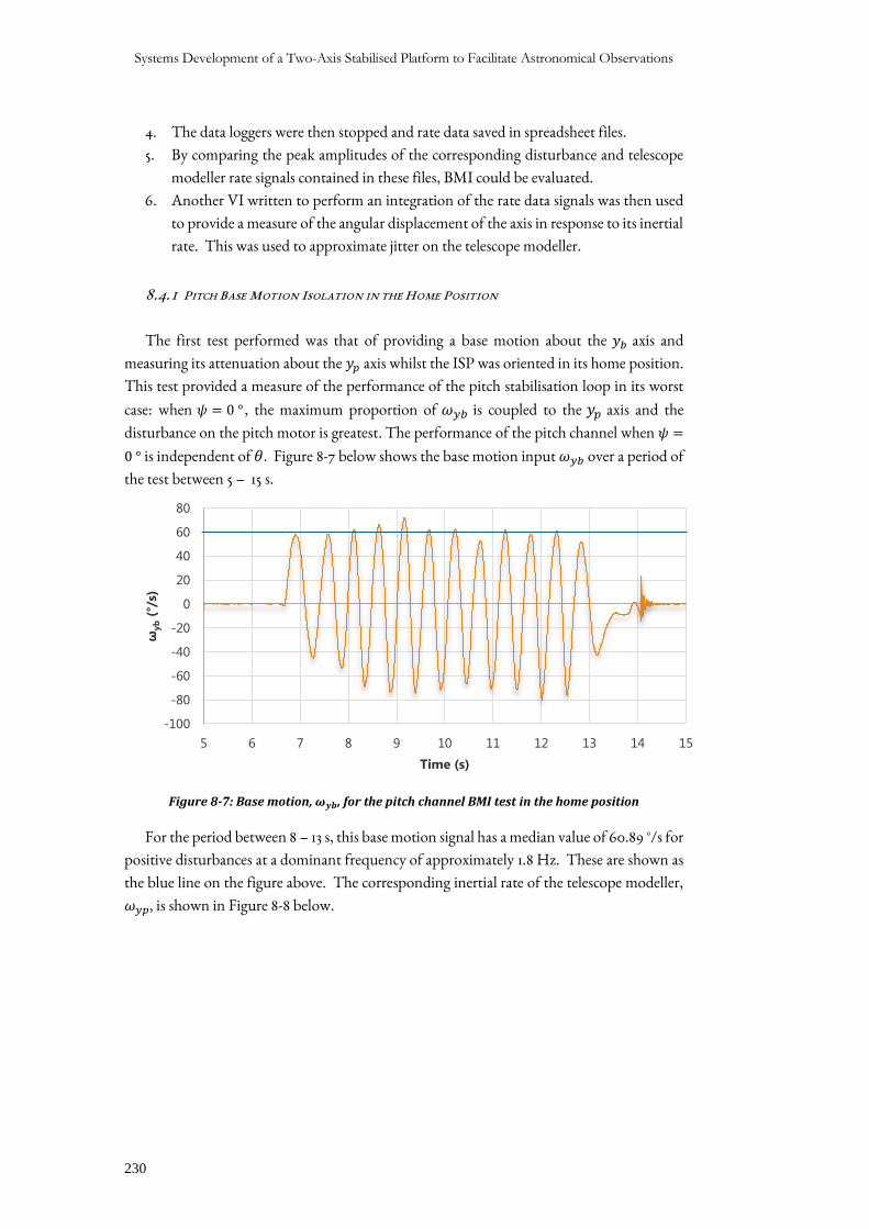
Systems Development of a Two-Axis Stabilised Platform to Facilitate Astronomical Observations
230
4. The data loggers were then stopped and rate data saved in spreadsheet files.
5. By comparing the peak amplitudes of the corresponding disturbance and telescope
modeller rate signals contained in these files, BMI could be evaluated.
6. Another VI written to perform an integration of the rate data signals was then used
to provide a measure of the angular displacement of the axis in response to its inertial
rate. This was used to approximate jitter on the telescope modeller.
8.4.1 PITCH BASE MOTION ISOLATION IN THE HOME POSITION
The first test performed was that of providing a base motion about the 𝑦𝑏 axis and
measuring its attenuation about the 𝑦𝑝 axis whilst the ISP was oriented in its home position.
This test provided a measure of the performance of the pitch stabilisation loop in its worst
case: when 𝜓 = 0 ° , the maximum proportion of 𝜔𝑦𝑏 is coupled to the 𝑦𝑝 axis and the
disturbance on the pitch motor is greatest. The performance of the pitch channel when 𝜓 =
0 ° is independent of 𝜃. Figure 8-7 below shows the base motion input 𝜔𝑦𝑏 over a period of
the test between 5 – 15 s.
Figure 8-7: Base motion, 𝝎𝒚𝒃, for the pitch channel BMI test in the home position
For the period between 8 – 13 s, this base motion signal has a median value of 60.89 °/s for
positive disturbances at a dominant frequency of approximately 1.8 Hz. These are shown as
the blue line on the figure above. The corresponding inertial rate of the telescope modeller,
𝜔𝑦𝑝, is shown in Figure 8-8 below.
-100
-80
-60
-40
-20
0
20
40
60
80
5 6 7 8 9 10 11 12 13 14 15
ωyb
(°/s
)
Time (s)
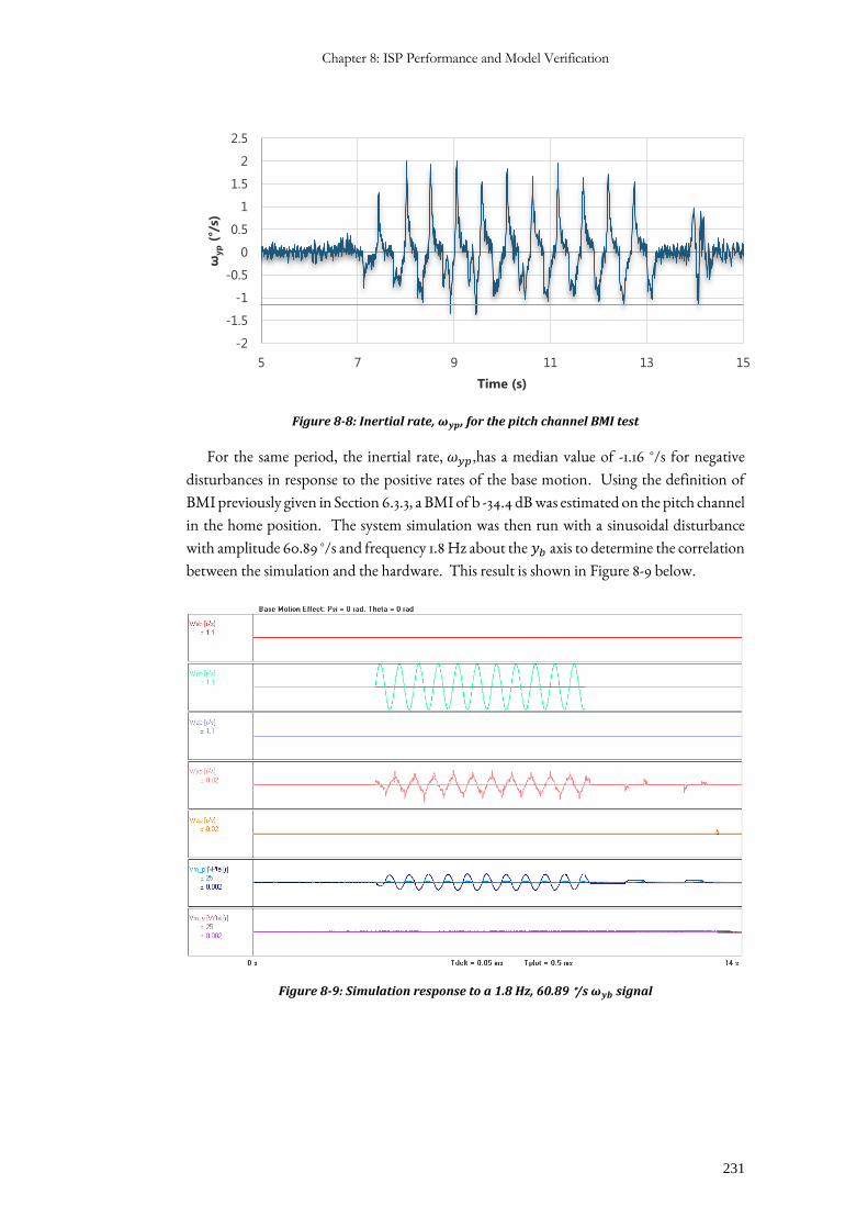
Chapter 8: ISP Performance and Model Verification
231
Figure 8-8: Inertial rate, 𝝎𝒚𝒑, for the pitch channel BMI test
For the same period, the inertial rate, 𝜔𝑦𝑝 ,has a median value of -1.16 °/s for negative
disturbances in response to the positive rates of the base motion. Using the definition of
BMI previously given in Section 6.3.3, a BMI of b -34.4 dB was estimated on the pitch channel
in the home position. The system simulation was then run with a sinusoidal disturbance
with amplitude 60.89 °/s and frequency 1.8 Hz about the 𝑦𝑏 axis to determine the correlation
between the simulation and the hardware. This result is shown in Figure 8-9 below.
Figure 8-9: Simulation response to a 1.8 Hz, 60.89 °/s 𝝎𝒚𝒃 signal
-2
-1.5
-1
-0.5
0
0.5
1
1.5
2
2.5
5 7 9 11 13 15
ωyp
(°/s
)
Time (s)
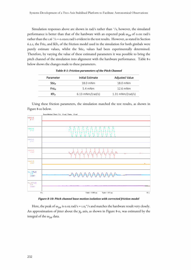
Systems Development of a Two-Axis Stabilised Platform to Facilitate Astronomical Observations
232
Simulation responses above are shown in rad/s rather than °/s, however, the simulated
performance is better than that of the hardware with an expected peak 𝜔𝑦𝑝 of 0.011 rad/s
rather than the 1.16 °/s = 0.0202 rad/s evident in the test results. However, as stated in Section
6.2.1, the Fricx and Kfrx of the friction model used in the simulation for both gimbals were
purely estimate values, whilst the Sticx values had been experimentally determined.
Therefore, by varying the value of these estimated parameters it was possible to bring the
pitch channel of the simulation into alignment with the hardware performance. Table 8-1
below shows the changes made to these parameters.
Table 8-1: Friction parameters of the Pitch Channel
Parameter Initial Estimate Adjusted Value
Sticp 18.0 mNm 18.0 mNm
Fricp 5.4 mNm 12.6 mNm
Kfrp 6.13 mNm/(rad/s) 1.31 mNm/(rad/s)
Using these friction parameters, the simulation matched the test results, as shown in
Figure 8-10 below.
Figure 8-10: Pitch channel base motion isolation with corrected friction model
Here, the peak of 𝜔𝑦𝑝 is 0.02 rad/s = 1.15 °/s and matches the hardware result very closely.
An approximation of jitter about the 𝑦𝑝 axis, as shown in Figure 8-11, was estimated by the
integral of the 𝜔𝑦𝑝 data.
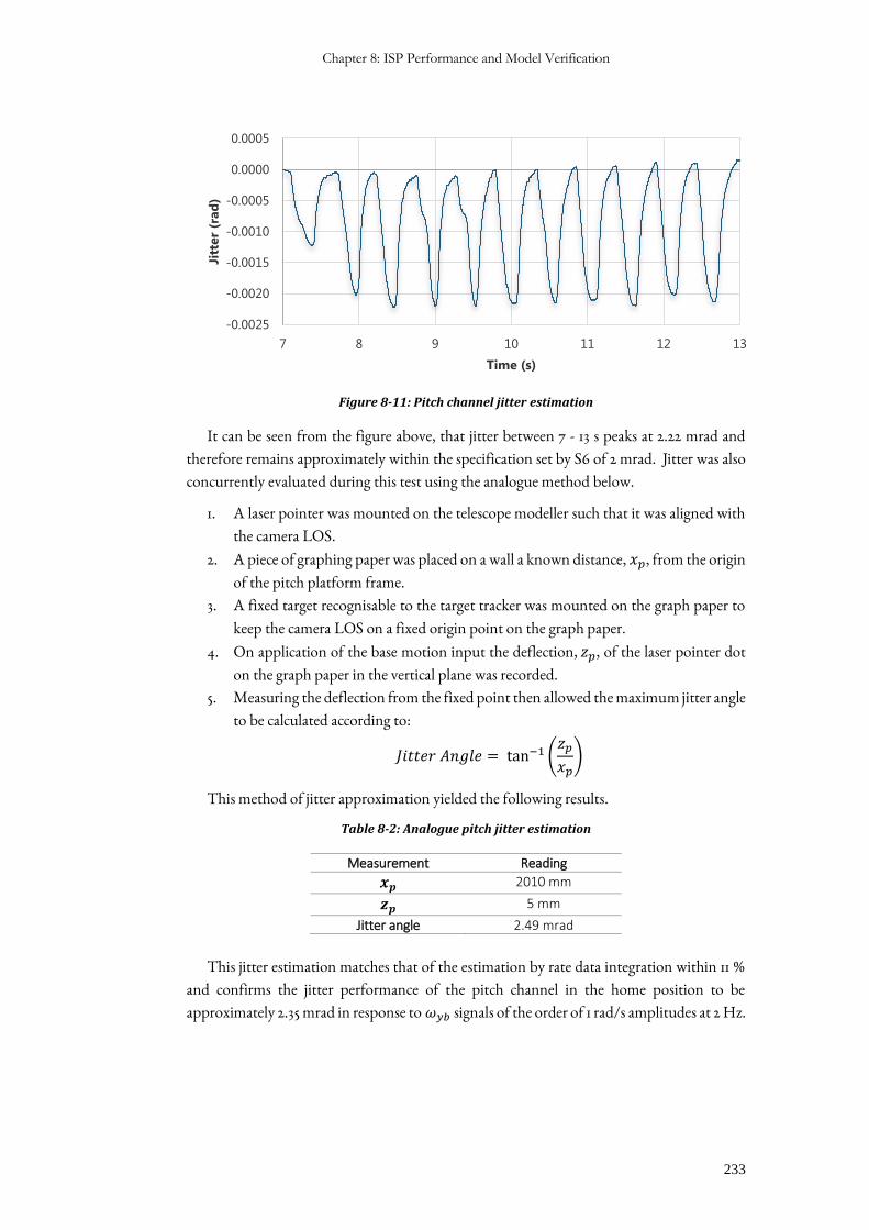
Chapter 8: ISP Performance and Model Verification
233
Figure 8-11: Pitch channel jitter estimation
It can be seen from the figure above, that jitter between 7 - 13 s peaks at 2.22 mrad and
therefore remains approximately within the specification set by S6 of 2 mrad. Jitter was also
concurrently evaluated during this test using the analogue method below.
1. A laser pointer was mounted on the telescope modeller such that it was aligned with
the camera LOS.
2. A piece of graphing paper was placed on a wall a known distance, 𝑥𝑝, from the origin
of the pitch platform frame.
3. A fixed target recognisable to the target tracker was mounted on the graph paper to
keep the camera LOS on a fixed origin point on the graph paper.
4. On application of the base motion input the deflection, 𝑧𝑝, of the laser pointer dot
on the graph paper in the vertical plane was recorded.
5. Measuring the deflection from the fixed point then allowed the maximum jitter angle
to be calculated according to:
𝐽𝑖𝑡𝑡𝑒𝑟 𝐴𝑛𝑔𝑙𝑒 = tan−1 (𝑧𝑝
𝑥𝑝)
This method of jitter approximation yielded the following results.
Table 8-2: Analogue pitch jitter estimation
Measurement Reading
𝒙𝒑 2010 mm
𝒛𝒑 5 mm
Jitter angle 2.49 mrad
This jitter estimation matches that of the estimation by rate data integration within 11 %
and confirms the jitter performance of the pitch channel in the home position to be
approximately 2.35 mrad in response to 𝜔𝑦𝑏 signals of the order of 1 rad/s amplitudes at 2 Hz.
-0.0025
-0.0020
-0.0015
-0.0010
-0.0005
0.0000
0.0005
7 8 9 10 11 12 13
Jitt
er
(rad
)
Time (s)
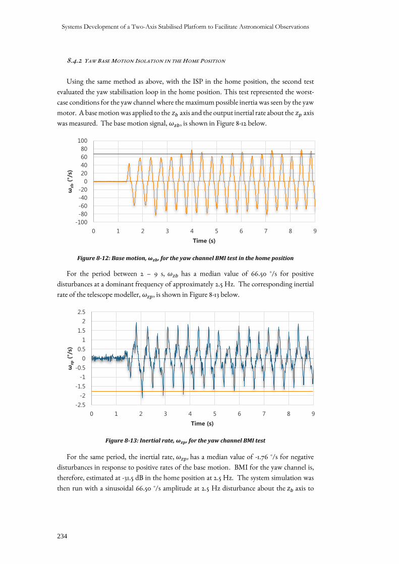
Systems Development of a Two-Axis Stabilised Platform to Facilitate Astronomical Observations
234
8.4.2 YAW BASE MOTION ISOLATION IN THE HOME POSITION
Using the same method as above, with the ISP in the home position, the second test
evaluated the yaw stabilisation loop in the home position. This test represented the worst-
case conditions for the yaw channel where the maximum possible inertia was seen by the yaw
motor. A base motion was applied to the 𝑧𝑏 axis and the output inertial rate about the 𝑧𝑝 axis
was measured. The base motion signal, 𝜔𝑧𝑏, is shown in Figure 8-12 below.
Figure 8-12: Base motion, 𝝎𝒛𝒃, for the yaw channel BMI test in the home position
For the period between 2 – 9 s, 𝜔𝑧𝑏 has a median value of 66.50 °/s for positive
disturbances at a dominant frequency of approximately 2.5 Hz. The corresponding inertial
rate of the telescope modeller, 𝜔𝑧𝑝, is shown in Figure 8-13 below.
Figure 8-13: Inertial rate, 𝝎𝒛𝒑, for the yaw channel BMI test
For the same period, the inertial rate, 𝜔𝑧𝑝, has a median value of -1.76 °/s for negative
disturbances in response to positive rates of the base motion. BMI for the yaw channel is,
therefore, estimated at -31.5 dB in the home position at 2.5 Hz. The system simulation was
then run with a sinusoidal 66.50 °/s amplitude at 2.5 Hz disturbance about the 𝑧𝑏 axis to
-100
-80
-60
-40
-20
0
20
40
60
80
100
0 1 2 3 4 5 6 7 8 9
ωzb
(°/s
)
Time (s)
-2.5
-2
-1.5
-1
-0.5
0
0.5
1
1.5
2
2.5
0 1 2 3 4 5 6 7 8 9
ωzp
(°/s
)
Time (s)
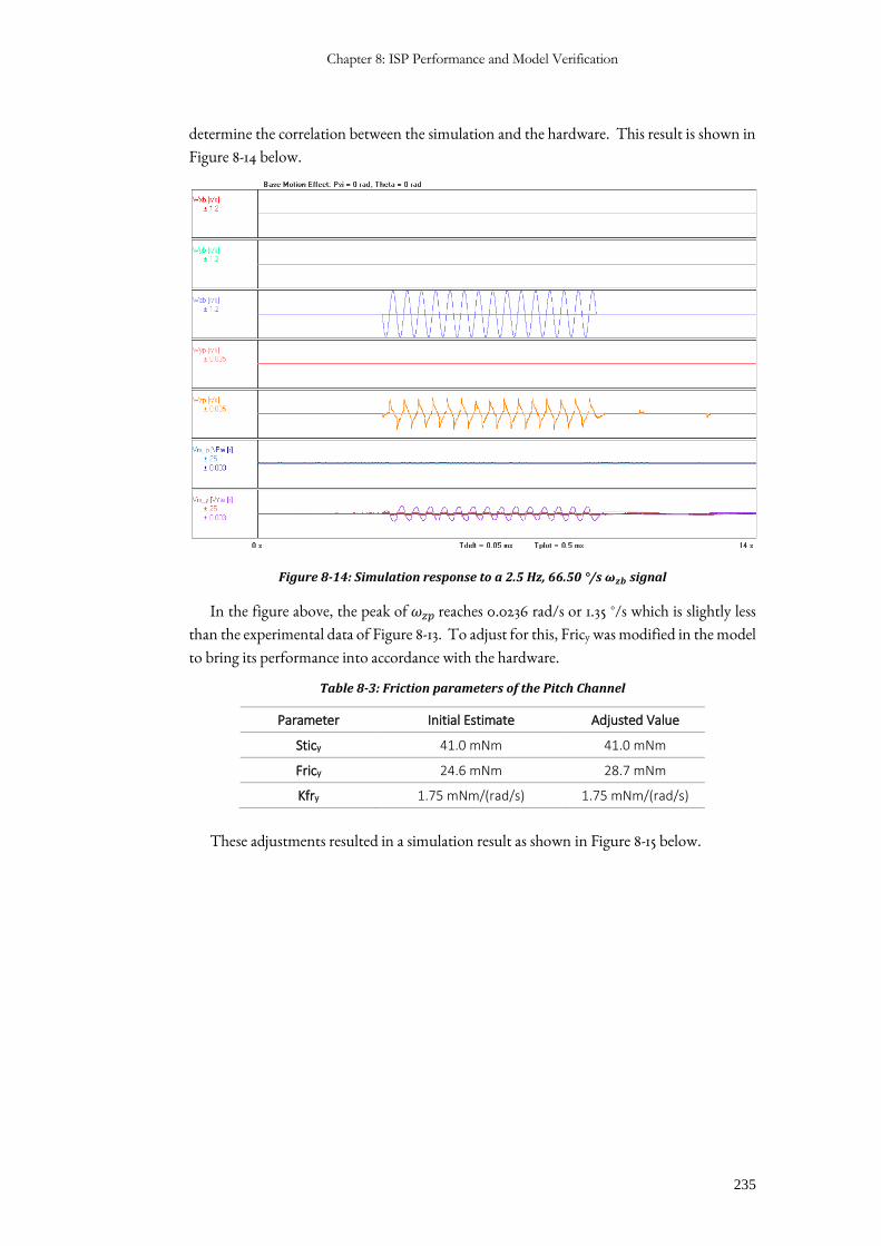
Chapter 8: ISP Performance and Model Verification
235
determine the correlation between the simulation and the hardware. This result is shown in
Figure 8-14 below.
Figure 8-14: Simulation response to a 2.5 Hz, 66.50 °/s 𝝎𝒛𝒃 signal
In the figure above, the peak of 𝜔𝑧𝑝 reaches 0.0236 rad/s or 1.35 °/s which is slightly less
than the experimental data of Figure 8-13. To adjust for this, Fricy was modified in the model
to bring its performance into accordance with the hardware.
Table 8-3: Friction parameters of the Pitch Channel
Parameter Initial Estimate Adjusted Value
Sticy 41.0 mNm 41.0 mNm
Fricy 24.6 mNm 28.7 mNm
Kfry 1.75 mNm/(rad/s) 1.75 mNm/(rad/s)
These adjustments resulted in a simulation result as shown in Figure 8-15 below.
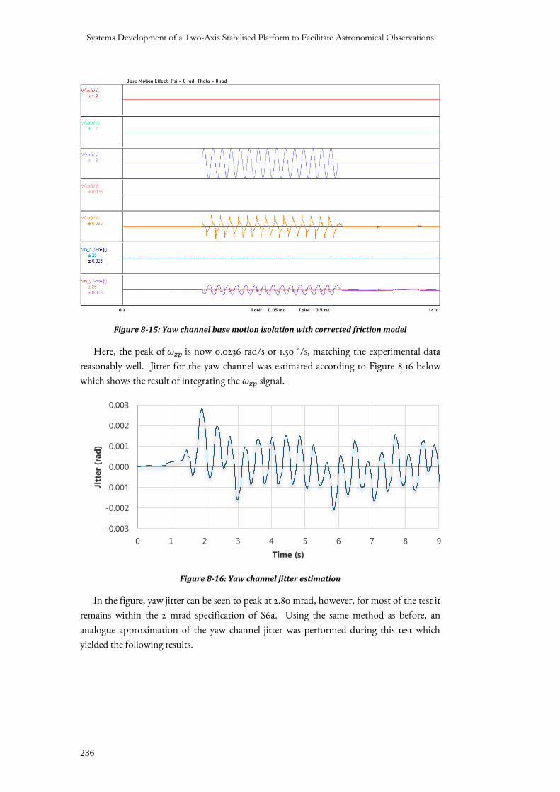
Systems Development of a Two-Axis Stabilised Platform to Facilitate Astronomical Observations
236
Figure 8-15: Yaw channel base motion isolation with corrected friction model
Here, the peak of 𝜔𝑧𝑝 is now 0.0236 rad/s or 1.50 °/s, matching the experimental data
reasonably well. Jitter for the yaw channel was estimated according to Figure 8-16 below
which shows the result of integrating the 𝜔𝑧𝑝 signal.
Figure 8-16: Yaw channel jitter estimation
In the figure, yaw jitter can be seen to peak at 2.80 mrad, however, for most of the test it
remains within the 2 mrad specification of S6a. Using the same method as before, an
analogue approximation of the yaw channel jitter was performed during this test which
yielded the following results.
-0.003
-0.002
-0.001
0.000
0.001
0.002
0.003
0 1 2 3 4 5 6 7 8 9
Jitt
er
(rad
)
Time (s)
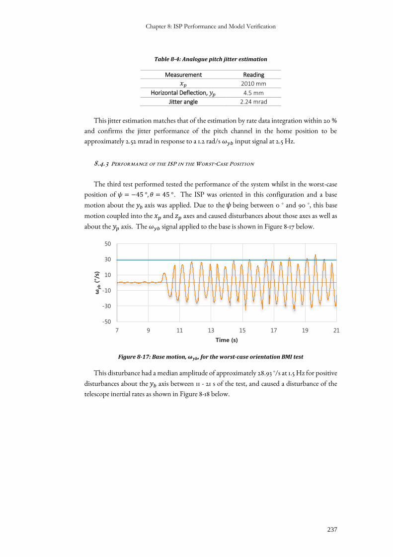
Chapter 8: ISP Performance and Model Verification
237
Table 8-4: Analogue pitch jitter estimation
Measurement Reading
𝑥𝑝 2010 mm
Horizontal Deflection, 𝑦𝑝 4.5 mm
Jitter angle 2.24 mrad
This jitter estimation matches that of the estimation by rate data integration within 20 %
and confirms the jitter performance of the pitch channel in the home position to be
approximately 2.52 mrad in response to a 1.2 rad/s 𝜔𝑦𝑏 input signal at 2.5 Hz.
8.4.3 PERFORMANCE OF THE ISP IN THE WORST-CASE POSITION
The third test performed tested the performance of the system whilst in the worst-case
position of 𝜓 = −45 °, 𝜃 = 45 ° . The ISP was oriented in this configuration and a base
motion about the 𝑦𝑏 axis was applied. Due to the 𝜓 being between 0 ° and 90 °, this base
motion coupled into the 𝑥𝑝 and 𝑧𝑝 axes and caused disturbances about those axes as well as
about the 𝑦𝑝 axis. The 𝜔𝑦𝑏 signal applied to the base is shown in Figure 8-17 below.
Figure 8-17: Base motion, 𝝎𝒚𝒃, for the worst-case orientation BMI test
This disturbance had a median amplitude of approximately 28.93 °/s at 1.5 Hz for positive
disturbances about the 𝑦𝑏 axis between 11 - 21 s of the test, and caused a disturbance of the
telescope inertial rates as shown in Figure 8-18 below.
-50
-30
-10
10
30
50
7 9 11 13 15 17 19 21
ωyb
(°/s
)
Time (s)
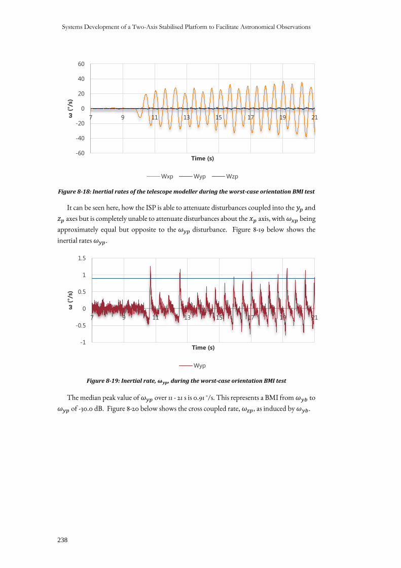
Systems Development of a Two-Axis Stabilised Platform to Facilitate Astronomical Observations
238
Figure 8-18: Inertial rates of the telescope modeller during the worst-case orientation BMI test
It can be seen here, how the ISP is able to attenuate disturbances coupled into the 𝑦𝑝 and
𝑧𝑝 axes but is completely unable to attenuate disturbances about the 𝑥𝑝 axis, with 𝜔𝑥𝑝 being
approximately equal but opposite to the 𝜔𝑦𝑝 disturbance. Figure 8-19 below shows the
inertial rates 𝜔𝑦𝑝.
Figure 8-19: Inertial rate, 𝝎𝒚𝒑, during the worst-case orientation BMI test
The median peak value of 𝜔𝑦𝑝 over 11 - 21 s is 0.91 °/s. This represents a BMI from 𝜔𝑦𝑏 to
𝜔𝑦𝑝 of -30.0 dB. Figure 8-20 below shows the cross coupled rate, 𝜔𝑧𝑝, as induced by 𝜔𝑦𝑏.
-60
-40
-20
0
20
40
60
7 9 11 13 15 17 19 21ω(°
/s)
Time (s)
Wxp Wyp Wzp
-1
-0.5
0
0.5
1
1.5
7 9 11 13 15 17 19 21
ω(°
/s)
Time (s)
Wyp
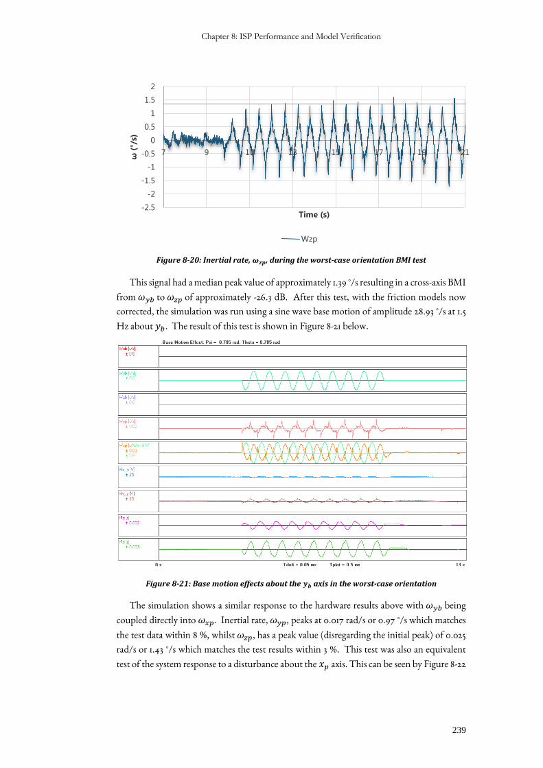
Chapter 8: ISP Performance and Model Verification
239
Figure 8-20: Inertial rate, 𝝎𝒛𝒑, during the worst-case orientation BMI test
This signal had a median peak value of approximately 1.39 °/s resulting in a cross-axis BMI
from 𝜔𝑦𝑏 to 𝜔𝑧𝑝 of approximately -26.3 dB. After this test, with the friction models now
corrected, the simulation was run using a sine wave base motion of amplitude 28.93 °/s at 1.5
Hz about 𝑦𝑏. The result of this test is shown in Figure 8-21 below.
Figure 8-21: Base motion effects about the 𝒚𝒃 axis in the worst-case orientation
The simulation shows a similar response to the hardware results above with 𝜔𝑦𝑏 being
coupled directly into 𝜔𝑥𝑝. Inertial rate, 𝜔𝑦𝑝, peaks at 0.017 rad/s or 0.97 °/s which matches
the test data within 8 %, whilst 𝜔𝑧𝑝, has a peak value (disregarding the initial peak) of 0.025
rad/s or 1.43 °/s which matches the test results within 3 %. This test was also an equivalent
test of the system response to a disturbance about the 𝑥𝑝 axis. This can be seen by Figure 8-22
-2.5
-2
-1.5
-1
-0.5
0
0.5
1
1.5
2
7 9 11 13 15 17 19 21
ω(°
/s)
Time (s)
Wzp
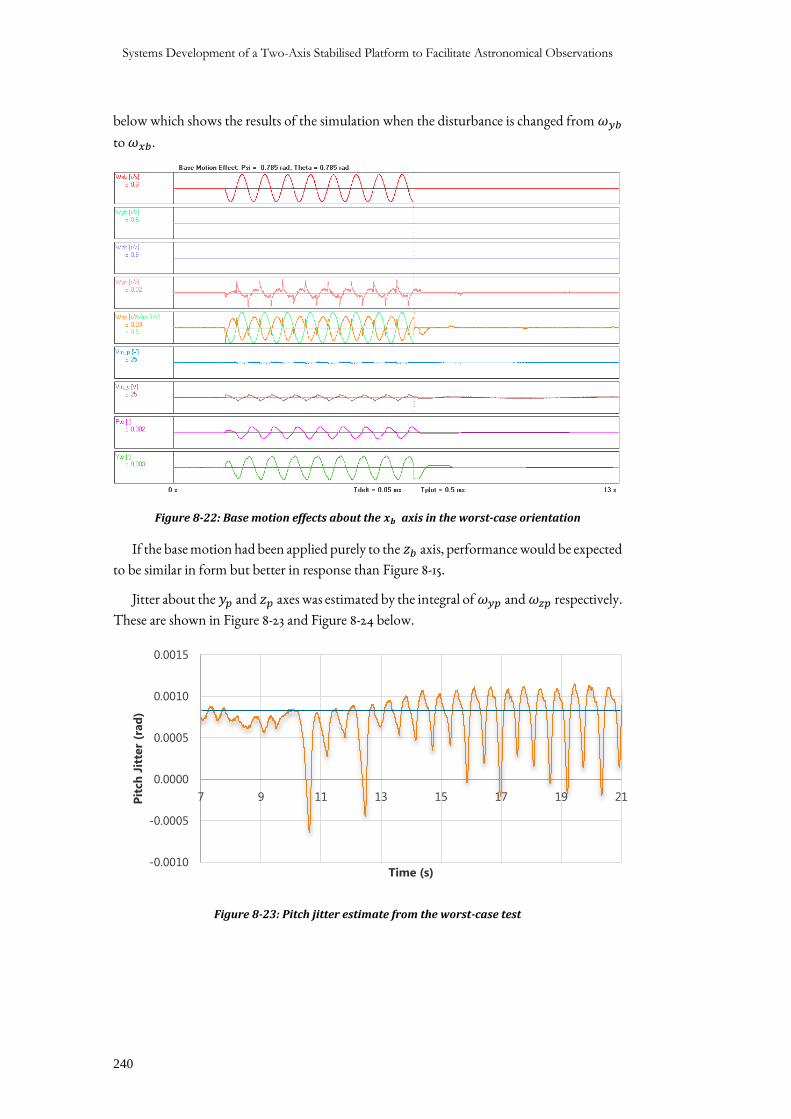
Systems Development of a Two-Axis Stabilised Platform to Facilitate Astronomical Observations
240
below which shows the results of the simulation when the disturbance is changed from 𝜔𝑦𝑏
to 𝜔𝑥𝑏.
Figure 8-22: Base motion effects about the 𝒙𝒃 axis in the worst-case orientation
If the base motion had been applied purely to the 𝑧𝑏 axis, performance would be expected
to be similar in form but better in response than Figure 8-15.
Jitter about the 𝑦𝑝 and 𝑧𝑝 axes was estimated by the integral of 𝜔𝑦𝑝 and 𝜔𝑧𝑝 respectively.
These are shown in Figure 8-23 and Figure 8-24 below.
Figure 8-23: Pitch jitter estimate from the worst-case test
-0.0010
-0.0005
0.0000
0.0005
0.0010
0.0015
7 9 11 13 15 17 19 21Pit
ch J
itte
r (r
ad
)
Time (s)
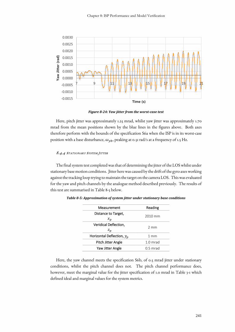
Chapter 8: ISP Performance and Model Verification
241
Figure 8-24: Yaw jitter from the worst-case test
Here, pitch jitter was approximately 1.25 mrad, whilst yaw jitter was approximately 1.70
mrad from the mean positions shown by the blue lines in the figures above. Both axes
therefore perform with the bounds of the specification S6a when the ISP is in its worst-case
position with a base disturbance, 𝜔𝑦𝑏, peaking at 0.51 rad/s at a frequency of 1.5 Hz.
8.4.4 STATIONARY SYSTEM JITTER
The final system test completed was that of determining the jitter of the LOS whilst under
stationary base motion conditions. Jitter here was caused by the drift of the gyro axes working
against the tracking loop trying to maintain the target on the camera LOS. This was evaluated
for the yaw and pitch channels by the analogue method described previously. The results of
this test are summarised in Table 8-5 below.
Table 8-5: Approximation of system jitter under stationary base conditions
Measurement Reading
Distance to Target,
𝑥𝑝 2010 mm
Veridical Deflection,
𝑧𝑝 2 mm
Horizontal Deflection, 𝑦𝑝 1 mm
Pitch Jitter Angle 1.0 mrad
Yaw Jitter Angle 0.5 mrad
Here, the yaw channel meets the specification S6b, of 0.5 mrad jitter under stationary
conditions, whilst the pitch channel does not. The pitch channel performance does,
however, meet the marginal value for the jitter specification of 1.0 mrad in Table 3-1 which
defined ideal and marginal values for the system metrics.
-0.0015
-0.0010
-0.0005
0.0000
0.0005
0.0010
0.0015
0.0020
0.0025
0.0030
7 9 11 13 15 17 19 21
Yaw
Jit
ter
(rad
)
Time (s)
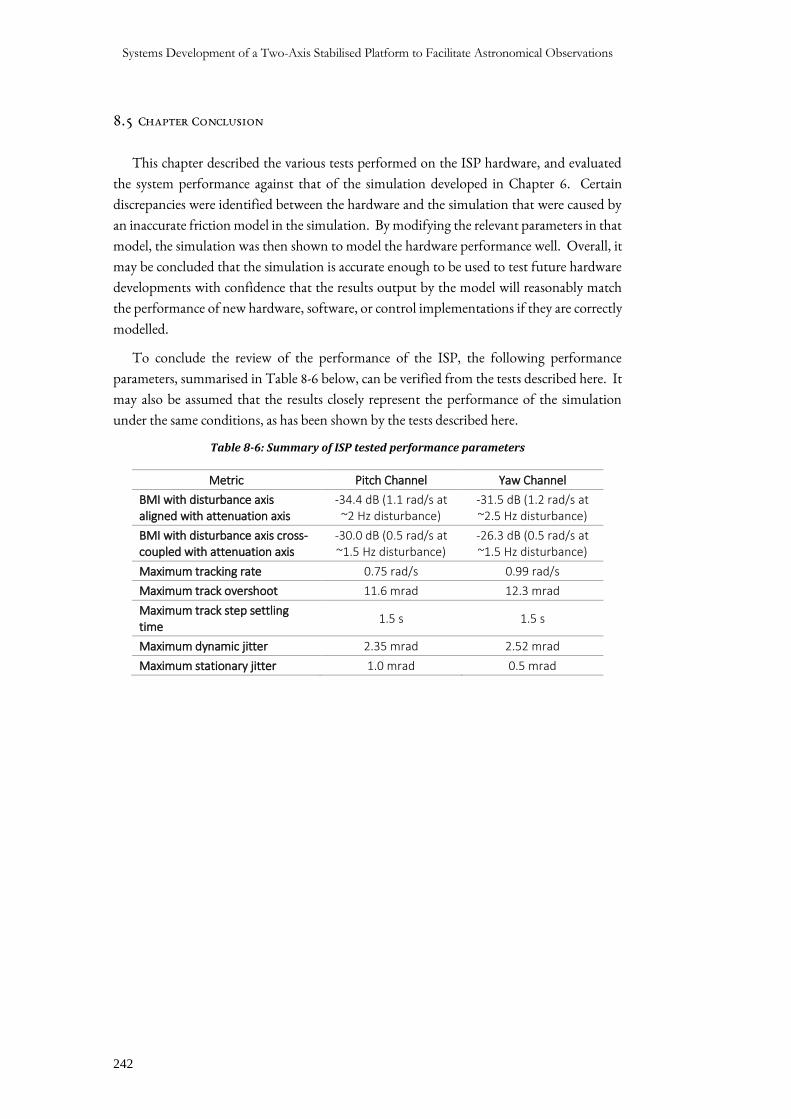
Systems Development of a Two-Axis Stabilised Platform to Facilitate Astronomical Observations
242
8.5 CHAPTER CONCLUSION
This chapter described the various tests performed on the ISP hardware, and evaluated
the system performance against that of the simulation developed in Chapter 6. Certain
discrepancies were identified between the hardware and the simulation that were caused by
an inaccurate friction model in the simulation. By modifying the relevant parameters in that
model, the simulation was then shown to model the hardware performance well. Overall, it
may be concluded that the simulation is accurate enough to be used to test future hardware
developments with confidence that the results output by the model will reasonably match
the performance of new hardware, software, or control implementations if they are correctly
modelled.
To conclude the review of the performance of the ISP, the following performance
parameters, summarised in Table 8-6 below, can be verified from the tests described here. It
may also be assumed that the results closely represent the performance of the simulation
under the same conditions, as has been shown by the tests described here.
Table 8-6: Summary of ISP tested performance parameters
Metric Pitch Channel Yaw Channel
BMI with disturbance axis aligned with attenuation axis
-34.4 dB (1.1 rad/s at ~2 Hz disturbance)
-31.5 dB (1.2 rad/s at ~2.5 Hz disturbance)
BMI with disturbance axis cross-coupled with attenuation axis
-30.0 dB (0.5 rad/s at ~1.5 Hz disturbance)
-26.3 dB (0.5 rad/s at ~1.5 Hz disturbance)
Maximum tracking rate 0.75 rad/s 0.99 rad/s
Maximum track overshoot 11.6 mrad 12.3 mrad
Maximum track step settling time
1.5 s 1.5 s
Maximum dynamic jitter 2.35 mrad 2.52 mrad
Maximum stationary jitter 1.0 mrad 0.5 mrad
Chapter 9: Conclusion and Recommendations
243
9 CONCLUSION AND RECOMMENDATIONS
9.1 INTRODUCTION
This project aimed to develop a two-axis stabilised platform with an automatic target
tracker capable of controlling the orientation of a telescope such that automatic tracking of a
celestial object might be accomplished from a moving host. Initially the project had aimed to
develop and test such a system using an actual telescope, however, due to budget constraints
it became necessary to develop an approximated system which modelled the intended
outcomes and provided a means for the system to be ultimately expanded to achieve the
initial aim.
The previous chapters described the development and performance of the various systems
that comprised the ISP that was implemented. This chapter, therefore, aims to comment on
those systems and make recommendations as to improvements that can be made in future
tasks. It was stated in Section 2.3 the ISPs typically consist of three main subsystems; a sensor
payload, an electromechanical assembly, and a control system. Comments made in this
section are, therefore, broken down by those categories.
9.2 SENSOR PAYLOAD
The primary sensor intended for this, and future projects on this system, whose motion
was to be controlled by the ISP, was the Meade ETX90 telescope. Being of small overall size
it was suitable for use in this project due to its portability, yet its 3.5” diameter compound
design meant that high quality observations could still be made. Inertial angular rate
feedback of the motion of the mounting platform designed for this telescope and its
mechanical modeller was provided using an InvenSense MPU-9150 IMU. The final sensor
which formed part of this payload was the RPi Camera v1.3 which facilitated the acquisition
of the image seen through the lens mounted on the telescope modeller and ultimately will
provide the same function for the telescope image.
9.2.1 SPECIFICATIONS OF THE SENSOR PAYLOAD
The specifications listed in Appendix A which are associated with the sensor payload and
the performance of the implemented systems in relation to these specifications are detailed in
Table 9-1 below.
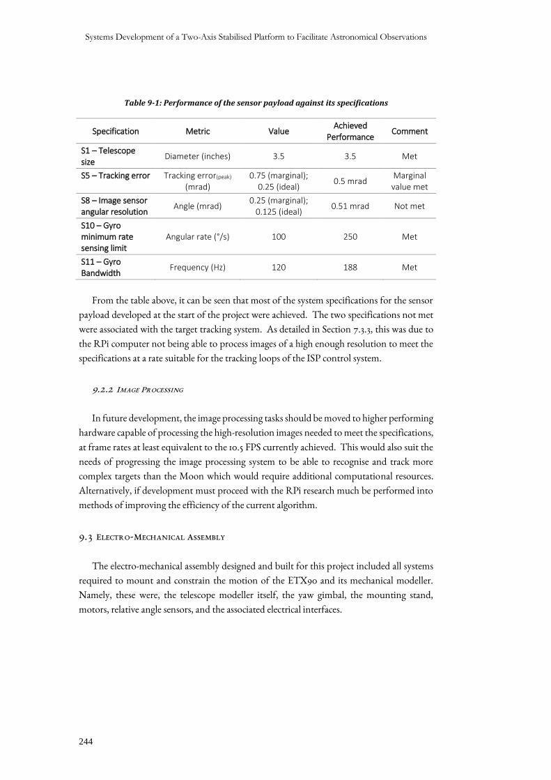
Systems Development of a Two-Axis Stabilised Platform to Facilitate Astronomical Observations
244
Table 9-1: Performance of the sensor payload against its specifications
Specification Metric Value Achieved
Performance Comment
S1 – Telescope size
Diameter (inches) 3.5 3.5 Met
S5 – Tracking error Tracking error(peak) (mrad)
0.75 (marginal); 0.25 (ideal)
0.5 mrad Marginal value met
S8 – Image sensor angular resolution
Angle (mrad) 0.25 (marginal);
0.125 (ideal) 0.51 mrad Not met
S10 – Gyro minimum rate sensing limit
Angular rate (°/s) 100 250 Met
S11 – Gyro Bandwidth
Frequency (Hz) 120 188 Met
From the table above, it can be seen that most of the system specifications for the sensor
payload developed at the start of the project were achieved. The two specifications not met
were associated with the target tracking system. As detailed in Section 7.3.3, this was due to
the RPi computer not being able to process images of a high enough resolution to meet the
specifications at a rate suitable for the tracking loops of the ISP control system.
9.2.2 IMAGE PROCESSING
In future development, the image processing tasks should be moved to higher performing
hardware capable of processing the high-resolution images needed to meet the specifications,
at frame rates at least equivalent to the 10.5 FPS currently achieved. This would also suit the
needs of progressing the image processing system to be able to recognise and track more
complex targets than the Moon which would require additional computational resources.
Alternatively, if development must proceed with the RPi research much be performed into
methods of improving the efficiency of the current algorithm.
9.3 ELECTRO-MECHANICAL ASSEMBLY
The electro-mechanical assembly designed and built for this project included all systems
required to mount and constrain the motion of the ETX90 and its mechanical modeller.
Namely, these were, the telescope modeller itself, the yaw gimbal, the mounting stand,
motors, relative angle sensors, and the associated electrical interfaces.
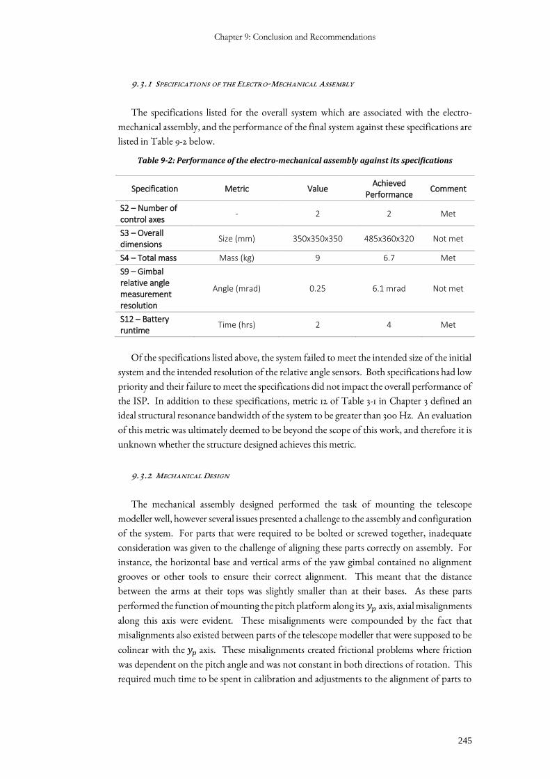
Chapter 9: Conclusion and Recommendations
245
9.3.1 SPECIFICATIONS OF THE ELECTRO-MECHANICAL ASSEMBLY
The specifications listed for the overall system which are associated with the electro-
mechanical assembly, and the performance of the final system against these specifications are
listed in Table 9-2 below.
Table 9-2: Performance of the electro-mechanical assembly against its specifications
Specification Metric Value Achieved
Performance Comment
S2 – Number of control axes
- 2 2 Met
S3 – Overall dimensions
Size (mm) 350x350x350 485x360x320 Not met
S4 – Total mass Mass (kg) 9 6.7 Met
S9 – Gimbal relative angle measurement resolution
Angle (mrad) 0.25 6.1 mrad Not met
S12 – Battery runtime
Time (hrs) 2 4 Met
Of the specifications listed above, the system failed to meet the intended size of the initial
system and the intended resolution of the relative angle sensors. Both specifications had low
priority and their failure to meet the specifications did not impact the overall performance of
the ISP. In addition to these specifications, metric 12 of Table 3-1 in Chapter 3 defined an
ideal structural resonance bandwidth of the system to be greater than 300 Hz. An evaluation
of this metric was ultimately deemed to be beyond the scope of this work, and therefore it is
unknown whether the structure designed achieves this metric.
9.3.2 MECHANICAL DESIGN
The mechanical assembly designed performed the task of mounting the telescope
modeller well, however several issues presented a challenge to the assembly and configuration
of the system. For parts that were required to be bolted or screwed together, inadequate
consideration was given to the challenge of aligning these parts correctly on assembly. For
instance, the horizontal base and vertical arms of the yaw gimbal contained no alignment
grooves or other tools to ensure their correct alignment. This meant that the distance
between the arms at their tops was slightly smaller than at their bases. As these parts
performed the function of mounting the pitch platform along its 𝑦𝑝 axis, axial misalignments
along this axis were evident. These misalignments were compounded by the fact that
misalignments also existed between parts of the telescope modeller that were supposed to be
colinear with the 𝑦𝑝 axis. These misalignments created frictional problems where friction
was dependent on the pitch angle and was not constant in both directions of rotation. This
required much time to be spent in calibration and adjustments to the alignment of parts to
Systems Development of a Two-Axis Stabilised Platform to Facilitate Astronomical Observations
246
overcome, and any disassembly of the structure will once again cause this issue to present
itself on reassembly. Whilst some of these issues were caused by inaccurate manufacturing,
the effects of these issues could have been reduced had greater care been taken in the design
phase to consider how to align the parts. It is recommended that future projects replace axis
creating parts with redesigned versions which have been designed to facilitate correct
alignment.
Should additional funding become available for this project, it is also recommended that
the yaw gimbal be replaced with a new design that has been manufactured from a single piece
via a CNC process. This should ensure better parts alignment and reduce frictional
disturbances on the ISP which were seen to have a substantial impact on performance. In
addition, a finite element analysis of the overall structure is recommended to be performed
in future work to determine the structural resonance properties of the assembly. Knowledge
of these will improve the accuracy of the simulation model and may result in improved
controller performance being possible.
9.3.3 YAW MOTOR
It was seen in Section 6.4.2 that for large base motion disturbances about multiple axes,
the yaw motor channel saturates and control command tracking is lost. Whilst suitable for
the operating conditions of this project, the yaw motor used will not be suitable for
applications under harsher conditions. It is therefore recommended that the yaw motor
either be changed for one capable of providing more torque than the Faulhaber 3257024CrR
used here, or that a gearbox be used to help increase the torque delivered to the yaw gimbal.
9.3.4 ELECTRICAL INTERFACES
As can be seen in Figure 4-23, the electrical systems of the project consist of various
development board type systems, or discrete function PCBs. Designing a PCB which can
host an equivalent motor controller and the STM32F0 on one board would reduce the form
factor of the electronics and improve the quality of the system developed. Additionally, a
better cable management system should be investigated in future projects. Whilst the current
system is functional, a system making use of slip rings, for example, would allow for
continuous rotation of the yaw gimbal and telescope platform and so increase the mechanical
robustness of the ISP and prevent system damage due to cables catching on protrusions on
the assembly.
Finally, a thermal protection system should be implemented on the motors to prevent
them drawing too much current and overheating whilst under prolonged dynamic
disturbances. This would eliminate the need for a limiting of the total current delivered tothe
system under operation and help improve certain system performance parameters such as
target tracking step response.
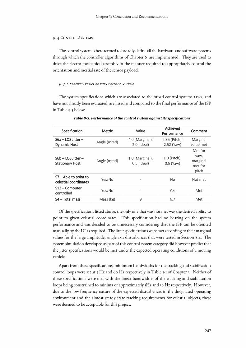
Chapter 9: Conclusion and Recommendations
247
9.4 CONTROL SYSTEMS
The control system is here termed to broadly define all the hardware and software systems
through which the controller algorithms of Chapter 6 are implemented. They are used to
drive the electro-mechanical assembly in the manner required to appropriately control the
orientation and inertial rate of the sensor payload.
9.4.1 SPECIFICATIONS OF THE CONTROL SYSTEM
The system specifications which are associated to the broad control systems tasks, and
have not already been evaluated, are listed and compared to the final performance of the ISP
in Table 9-3 below.
Table 9-3: Performance of the control system against its specifications
Specification Metric Value Achieved
Performance Comment
S6a – LOS Jitter – Dynamic Host
Angle (mrad) 4.0 (Marginal);
2.0 (Ideal) 2.35 (Pitch); 2.52 (Yaw)
Marginal value met
S6b – LOS Jitter – Stationary Host
Angle (mrad) 1.0 (Marginal);
0.5 (Ideal)
1.0 (Pitch);
0.5 (Yaw)
Met for yaw,
marginal met for
pitch
S7 – Able to point to celestial coordinates
Yes/No - No Not met
S13 – Computer controlled
Yes/No - Yes Met
S4 – Total mass Mass (kg) 9 6.7 Met
Of the specifications listed above, the only one that was not met was the desired ability to
point to given celestial coordinates. This specification had no bearing on the system
performance and was decided to be unnecessary considering that the ISP can be oriented
manually by the UI as required. The jitter specifications were met according to their marginal
values for the large amplitude, single axis disturbances that were tested in Section 8.4. The
system simulation developed as part of this control system category did however predict that
the jitter specifications would be met under the expected operating conditions of a moving
vehicle.
Apart from these specifications, minimum bandwidths for the tracking and stabilisation
control loops were set at 5 Hz and 60 Hz respectively in Table 3-1 of Chapter 3. Neither of
these specifications were met with the linear bandwidths of the tracking and stabilisation
loops being constrained to minima of approximately 1Hz and 38 Hz respectively. However,
due to the low frequency nature of the expected disturbances in the designated operating
environment and the almost steady state tracking requirements for celestial objects, these
were deemed to be acceptable for this project.
Systems Development of a Two-Axis Stabilised Platform to Facilitate Astronomical Observations
248
9.4.2 CONTROL HARDWARE, SOFTWARE AND FIRMWARE
The STM32F051C6 microcontroller used in this project was a suitable choice and was able
to run the main system firmware that was developed. However, the code size of the final
version written using the STM SPL abstraction libraries was almost exactly the same size as
the flash memory on the MCU meaning that no additional memory is available for firmware
developments. It is, therefore, suggested that the MCU be upgraded to another in the
STM32F051 series with 64 kB of flash, such as the STM32F051c8, which is fully compatible
with the code developed in this project. If, however, increased computational performance
is required, it is suggested that the MCU be upgraded to one from the STM32 F4 series which
all have FPUs and higher clock frequencies than the STM32F0 range. This should ensure
majority code portability whilst providing increased computational performance.
It is also recommended that if significant future firmware development is required, that
the use of the SPL library on the MCU be discontinued. The library has now been deprecated
by STMicroelectronics and the use of their Hardware Abstraction Layer (HAL) is now
recommended by them for the development of new projects. In line with this, it is suggested
that major developments now proceed using this library which has greater code portability
between MCUs within the STM32 family, and has a larger support base to assist with
firmware development.
For the LabVIEW User Interface, it is recommended that the software be re-written using
a parallel loop architecture to improve the overall performance if increased data logging rates
are required by future project tasks.
9.4.3 CURRENT MINOR LOOPS
To reduce the effects of inter-gimbal friction on the performance of the ISP it is suggested
that high-gain, current minor loops be incorporated onto the system as shown by Figure 2-3.
These loops have been noted by the literature surveyed to improve the effects of viscous
damping of gimbal actuators. They might be incorporated using analogue electrical
controllers and need not be implemented in firmware.
9.4.4 GYRO-DRIFT COMPENSATION
Drift of the gyro bias offsets were not compensated by the controllers developed in this
project due to the fact that their effects are removed by the tracking control loops of the
system. As the rate feedback drifts and causes an error signal on the stabilisation controllers
the gimbals are actuated. The tracking loops see this as a tracking error and then actuate the
gimbals to return the LOS to the target. These controllers working against each other cause
tracking errors and jitter to be evident on the system. It is suggested that gyro-drift be
evaluated and compensated at the sensor feedback level to improve system performance.
Possible methods by which this might be done include Kalman or equivalent filtering of the
IMU data, or by using the long-term average of the stabilisation controller actuator signals to
Chapter 9: Conclusion and Recommendations
249
estimate offset drift. For a stabilised platform these outputs should be zero for an ideal system
achieving perfect stabilisation and tracking of an inertially stationary target.
9.4.5 CONTROLLER IMPLEMENTATION
It is also recommended that if the base motion isolation performance of the ISP is
required to be improved beyond approximately -35 dB, that an investigation be made into
the use of a modern control method, or a feedforward scheme as the control method. As
stated in Section 2.3.3, these have been shown to be able to provide better base motion
rejection at the low frequencies evident in the operating environment of this project than the
classical PI scheme used here.
9.5 SUMMARY
The final specification that influenced the ISP developed was cost. Initially limited to
R20 000.00, but revised to approximately R5 000.00 early in the design process, this
specification was the determining factor in many design decisions made over the course of
the project. Ultimately the project ran over this budget and a total of approximately R6
700.00 was spent on the project.
Overall, as can be seen by the comparisons of system performance to the specifications
above, a two-axis mass stabilised platform was successfully developed which was able to
approximate the initial aim of the project well. Automatic target tracking was achieved, and
an expansion friendly mechanical design was implemented which can facilitate the inclusion
of the ETX90 telescope easily. Controllers were designed and tested using a telescope
modeller which inertially and geometrically modelled this telescope, and therefore it is not
expected that the control algorithms will require much adjustment to effectively stabilise the
ETX90 once it has been included.
The thesis of this project was, therefore, confirmed. A multi-axis closed-loop stabilisation
controller working in conjunction with an automatic target tracker may feasibly be
implemented to keep an optical telescope sensor pointed at a celestial target in both static and
dynamic host environments using image processing and control system design techniques.
The overall performance of the system developed fell short of achieving success of all the
specifications, but it may be concluded that with further development work and the
implementation of some of the recommendations made in this chapter that these might be
met and the initial project aim be achieved.

List of References
251
LIST OF REFERENCES
[1] J. M. Hilkert, “Inertially stabilized platform technology: Concepts and principles,” IEEE Control Syst. Mag., vol. 28, no. 1, pp. 26–46, 2008.
[2] A. K. Rue, “Precision Stabilization Systems,” IEEE Trans. Aerosp. Electron. Syst., vol. AES-10, no. 1, pp. 34–42, 1974.
[3] H. Khodadadi, M. R. J. Motlagh, and M. Gorji, “Robust control and modeling a 2-DOF inertial stabilized platform,” InECCE 2011 - Int. Conf. Electr. Control Comput. Eng., pp. 223–228, 2011.
[4] SKYVR LTD., “Aerial Photography Drone Technology | Aerial Filming UK.” [Online]. Available: http://skyvr.biz/our-aerial-drones/. [Accessed: 14-Nov-2017].
[5] Gyro-Stabilized Systems, “Cinema Pro Gimbal,” 2018. [Online]. Available: https://gyrostabilizedsystems.com/cinema-pro-gimbal/. [Accessed: 08-Apr-2018].
[6] Soldier Systems Daily, “Paradigm SRP - Soldier Systems Daily.” [Online]. Available: http://soldiersystems.net/tag/paradigm-srp/. [Accessed: 14-Nov-2017].
[7] M. K. Masten, “Inertially stabilized platforms for optical imaging systems,” IEEE Control Syst. Mag., vol. 28, no. 1, pp. 47–64, 2008.
[8] M. Rezac, “Inertial stabilization, estimation and visual servoing for aerial surveillance,” Ph.D. Program. Electr., no. October 2013, p. 169, 2013.
[9] A. K. Rue, “Stabilization of Precision Electrooptical Pointing and Tracking Systems,” no. 5, 1969.
[10] A. K. Rue, “Correction to ‘Stabilization of Precision Electrooptical Pointing and Tracking Systems,’” IEEE Trans. Aerosp. Electron. Syst., vol. AES-6, no. 6, pp. 855–857, 1970.
[11] P. J. Kennedy and R. L. Kennedy, “Direct versus indirect line of sight (LOS) stabilization,” IEEE Trans. Control Syst. Technol., vol. 11, no. 1, pp. 3–15, 2003.
[12] H. A. Zhu, C. L. Teo, G. S. Hong, and A. N. Poo, “A robustness enhancer for model-based controllers,” in Proceedings of IECON ’93 - 19th Annual Conference of IEEE Industrial Electronics, pp. 2033–2038.
[13] E. Jones and P. Fjeld, “Gimbal Angles, Gimbal Lock, and a Fourth Gimbal for Christmas,” Apollo Lunar Surface Journal, 2000. [Online]. Available: https://www.hq.nasa.gov/alsj/gimbals.html. [Accessed: 10-Nov-2017].
[14] Z. Hurak and M. Rezac, “Image-based pointing and tracking for inertially stabilized airborne camera platform,” IEEE Trans. Control Syst. Technol., vol. 20, no. 5, pp. 1146–1159, 2012.
[15] A. Friedrich and L. Bredenkamp, “Development and control of a 3-axis stabilised platform /,” Africa (Lond)., no. March, 2007.
Systems Development of a Two-Axis Stabilised Platform to facilitate Astronomical Observations
252
[16] S. Li and M. Zhong, “High-Precision Disturbance Compensation for a Three-Axis Gyro-Stabilized Camera Mount,” IEEE/ASME Trans. Mechatronics, vol. 20, no. 6, pp. 3135–3147, 2015.
[17] P. B. Jackson, “Overview of Missile Flight Control Systems,” Johns Hopkins APL Technical Digest, vol. 29, no. 1, 2010.
[18] M. Abdo, A. R. Vali, A. R. Toloei, and M. R. Arvan, “Modeling control and simulation of two axes gimbal seeker using fuzzy PID controller,” in 2014 22nd Iranian Conference on Electrical Engineering (ICEE), 2014, pp. 1342–1347.
[19] C. Espinosa, K. Mayen, M. Lizarraga, S. S. H. Romero, and R. Lozano, “Sliding mode line-of-sight stabilization of a two-axes gimbal system,” in 2015 Workshop on Research, Education and Development of Unmanned Aerial Systems (RED-UAS), 2015, pp. 431–438.
[20] S. Li, M. Zhong, and J. Qin, “The Internal Model Control Design of Three-axis Inertially Stabilized Platform for Airborne Remote Sensing,” in 2012 8th IEEE International Symposium on Instrumentation and Control Technology (ISICT) Proceedings, 2012, pp. 5–10.
[21] Young Shin Kwon, Hong Yeon Hwang, and Yun Seok Choi, “Stabilization Loop Design on Direct Drive Gimbaled Platform With Low Stiffness and Heavy Inertia,” in 2007 International Conference on Control, Automation and Systems, 2007, pp. 320–325.
[22] J. Osborne, G. Hicks, and R. Fuentes, “Global analysis of the double-gimbal mechanism,” IEEE Control Syst. Mag., vol. 28, no. 4, pp. 44–64, 2008.
[23] H. F. Mokbel, L. Q. Ying, A. A. Roshdy, and C. G. Hua, “Design Optimization of the Inner Gimbal for Dual Axis Inertially Stabilized Platform Using Finite Element Modal Analysis,” vol. 2, no. 2, pp. 239–244, 2012.
[24] N. Barbour and G. Schmidt, “Inertial sensor technology trends,” IEEE Sens. J., vol. 1, no. 4, pp. 332–339, 2001.
[25] G. T. Schmidt, “INS / GPS Technology Trends,” Technology, vol. 116, no. 2010, pp. 1–16, 2011.
[26] H. Sönnerlind, “Modeling the Dynamics of a Gyroscope,” 2017. [Online]. Available: https://www.comsol.com/blogs/modeling-the-dynamics-of-a-gyroscope/. [Accessed: 06-Dec-2017].
[27] P. D. Groves, Principles of GNSS, Inertial, and Mulitsensor Integrated Navigation Systems. Boston: Artech House, 2008.
[28] A. D. King, “Inertial navigation - Forty years of evolution,” Gec Rev., vol. 13, no. 3, pp. 140–149, 1998.
[29] N. Barbour, “Inertial navigation sensors,” NATO RTO Lect. Ser., vol. 116, pp. 1–24, 2004.
[30] O. J. Woodman, An Introduction to Inertial Navigation. Technical Report, 2007.
[31] J. Hol, Sensor Fusion and Calibration of Inertial Sensors, Vision, Ultra-Wideband and GPS, no. 1368. 2011.
[32] Z. Diao, H. Quan, L. Lan, and Y. Han, “Analysis and compensation of MEMS
List of References
253
gyroscope drift,” Proc. Int. Conf. Sens. Technol. ICST, no. 2, pp. 592–596, 2013.
[33] W. Riley, “Techniques for frequency stability analysis,” … Int. Freq. Control Symp. Tampa, FL, 2003.
[34] F. Semiconductor, “Allan Variance : Noise Analysis for Gyroscopes 2 Creating an Allan Deviation Plot for Noise Identification,” 2015.
[35] IEEE, “IEEE Std 952-1997 (R2008) Standard Specification Format Guide and Test Procedure for Single-Axis Interferometric Fiber Optic Gyros, Annex C,” 2008.
[36] tutorialspoint, “Digital Image Processing Introduction,” 2017. [Online]. Available: https://www.tutorialspoint.com/dip/image_processing_introduction.htm. [Accessed: 21-Nov-2017].
[37] S. Barrett, “Image Analysis — A Beginner’s Guide Image Analysis A Beginner’s Guide Introduc:on,” 2015.
[38] Robert Mullins, “Image Pi – Basic image processing: Introduction and Setup,” 2012. [Online]. Available: https://www.cl.cam.ac.uk/projects/raspberrypi/tutorials/image-processing/intro.html. [Accessed: 21-Nov-2017].
[39] King-Sun Fu and Rosenfeld, “Pattern Recognition and Image Processing,” IEEE Trans. Comput., vol. C-25, no. 12, pp. 1336–1346, Dec. 1976.
[40] M. Hassaballah, A. A. Abdelmgeid, and H. A. Alshazly, “Image Features Detection, Description and Matching,” in Image Feature Detectors and Descriptors, Springer, Cham, 2016, pp. 11–45.
[41] H. Johnstone, “Modern Astronomy: An Introduction to Astronomy,” An Introduction to Astronomy. [Online]. Available: http://www.physics.usyd.edu.au/~helenj/IAST/IA1-intro.pdf. [Accessed: 26-Nov-2017].
[42] Khan Academy, “Absorption/emission lines,” 2017. [Online]. Available: https://www.khanacademy.org/partner-content/nasa/measuringuniverse/spectroscopy/a/absorptionemission-lines. [Accessed: 29-Nov-2017].
[43] Humboldt State University, “Atmospheric Absorption & Transmission,” 2014. [Online]. Available: http://gsp.humboldt.edu/olm_2016/Courses/GSP_216_Online/lesson2-1/atmosphere.html. [Accessed: 08-Apr-2018].
[44] NASA/CXC/SAO, “More Images of M101,” 2012. [Online]. Available: http://chandra.harvard.edu/photo/2009/m101/more.html. [Accessed: 08-Apr-2018].
[45] S. Littlefair, “Telescopes | PHY241.” [Online]. Available: http://slittlefair.staff.shef.ac.uk/teaching/phy241/lectures/L04/index.html. [Accessed: 27-Nov-2017].
[46] E. Howell, “Buying Your First Telescope? What You Need to Know,” 2016. [Online]. Available: https://www.space.com/34791-first-time-telescope-buyer-guide.html. [Accessed: 27-Nov-2017].
Systems Development of a Two-Axis Stabilised Platform to facilitate Astronomical Observations
254
[47] D. Mawet, “Telescopes and Telescope Optics I Intro optics, configurations, design issues,” 2016.
[48] S. French and A. French, “Introduction to Telescopes.” [Online]. Available: http://dudleyobservatory.org/introduction-to-telescopes/. [Accessed: 28-Nov-2017].
[49] B. Ventrudo, “Telescope Mounts – One Minute Astronomer,” 2017. [Online]. Available: http://oneminuteastronomer.com/10045/telescope-mounts/. [Accessed: 28-Nov-2017].
[50] Bintel, “Celestron AstroMaster 130EQ Telescope,” 2017. [Online]. Available: https://www.bintel.com.au/product/celestron-astromaster-130eq/. [Accessed: 28-Nov-2017].
[51] Bintel, “Celestron CPC Deluxe 1100 HD,” 2017. [Online]. Available: https://www.bintel.com.au/product/celestron-cpc-deluxe-1100-hd/. [Accessed: 28-Nov-2017].
[52] L. Rother Valley Optics, “Celestron SkyProdigy 6 SCT GOTO Telescope,” 2017. [Online]. Available: http://www.rothervalleyoptics.co.uk/celestron-skyprodigy-6-sct-goto-telescope.html. [Accessed: 28-Nov-2017].
[53] B. Ekstrand, “Equations of motion for a two-axes gimbal system,” IEEE Trans. Aerosp. Electron. Syst., vol. 37, no. 3, pp. 1083–1091, 2001.
[54] F. N. Barnes, “Stable Member Equations of Motion for a Three-Axis Gyro Stabilized Platform,” IEEE Trans. Aerosp. Electron. Syst., vol. AES-7, no. 5, pp. 830–842, 1971.
[55] J. Peraire and S. Widnall, “Lecture L28 - 3D Rigid Body Dynamics : Equations of
Motion ; Euler ’ s Equations 3D Rigid Body Dynamics : Euler ’ s Equations Body-Fixed Axis,” no. 2, pp. 1–7, 2009.
[56] J. L. Meriam and L. G. Kraige, Engineering Mechanics Dynamics, 6th ed. John Wiley & Sons, Inc., 2008.
[57] H. D. Mouton, “Ondersoek Na Die Hoëprestasiebeheer en Vergelykende Vermoë van Verskillende Tipes Missielvolgkoppe Ten Opsigte van Stabilisasie en Volgakkuraathede,” Potchefstroomse Universiteit vir Christelike Hoer Onderwys, 1993.
[58] B & H Foto & Electronics Corp, “Meade ETX-90 PE Premiere Edition 3.5"/90mm Maksutov-Cassegrain Telescope Kit (1250mm f/13.8) with Motorized Altazimuth Mount (Astro Tube Version),” 2018. [Online]. Available: https://www.bhphotovideo.com/c/product/354384-REG/Meade_35140331_ETX_90_PE_3_5_Maksutov_Cassegrain.html. [Accessed: 05-Jan-2018].
[59] Meade Instruments, “Instruction Manual ETX90 Maksutov-Cassegrain Telescopes with AutoStar #497 Hand Controller.” 2011.
[60] SKF, “Self-aligning ball bearings - 127 TN9.” [Online]. Available: http://www.skf.com/group/products/bearings-units-housings/ball-bearings/self-aligning-ball-bearings/self-aligning-ball-bearings/index.html?designation=127 TN9. [Accessed: 18-Jan-2018].
List of References
255
[61] SKF, “Deep groove ball bearings - 61901.” [Online]. Available: http://www.skf.com/group/products/bearings-units-housings/ball-bearings/deep-groove-ball-bearings/deep-groove-ball-bearings/index.html?designation=61901. [Accessed: 18-Jan-2018].
[62] SKF, “Deep groove ball bearings - 61910.” [Online]. Available: http://www.skf.com/group/products/bearings-units-housings/ball-bearings/deep-groove-ball-bearings/deep-groove-ball-bearings/index.html?designation=61910. [Accessed: 19-Jan-2018].
[63] SKF, “Deep groove ball bearings - 6006.” [Online]. Available: http://www.skf.com/group/products/bearings-units-housings/ball-bearings/deep-groove-ball-bearings/deep-groove-ball-bearings/index.html?designation=6006. [Accessed: 19-Jan-2018].
[64] SKF, “Loads.” [Online]. Available: http://www.skf.com/group/products/bearings-units-housings/ball-bearings/deep-groove-ball-bearings/loads/index.html. [Accessed: 19-Jan-2018].
[65] RS Components, “DEMOKIT2 HEAD BOARD for MT9P031 I,” 2015. [Online]. Available: http://za.rs-online.com/web/p/processor-microcontroller-development-kits/6695922/. [Accessed: 22-Sep-2015].
[66] R. Elektronik, “RASPBERRY PI CAM,” 2015. [Online]. Available: http://www.reichelt.de/?ARTICLE=133871&SID=13UgpjBX8AAAIAACSYOd4eea3b3cdebcc8001d2e50ff9feeef188. [Accessed: 01-Jan-2015].
[67] Raspberry Pi Foundation, “Camera Module,” 2018. [Online]. Available: https://www.raspberrypi.org/documentation/hardware/camera/README.md. [Accessed: 08-Apr-2018].
[68] c-mountlens.com, “C-MOUNT DEFINED,” 2011. [Online]. Available: http://www.c-mountlens.com/2011/c-mount-defined/. [Accessed: 23-Sep-2015].
[69] Digi-Key Electronics, “ADIS16137BMLZ Analog Devices Inc.,” 2017. [Online]. Available: https://www.digikey.co.za/products/en?keywords=ADIS16137. [Accessed: 06-Dec-2017].
[70] Analog Devices, “ADIS16137 Data Sheet,” 2017.
[71] EPSON TOYOCOM, “AP-6110LR,” 2011.
[72] I. InvenSence, “MPU-6000 and MPU-6050 Product Specification Revision 3.4,” 2013.
[73] I. InvenSense, “MPU-3300 Product Specification Revision 1.1,” 2012.
[74] F. Wimmer, “Dell Inspiron 15-5547 Notebook Review - NotebookCheck.net Reviews,” 2014. [Online]. Available: https://www.notebookcheck.net/Dell-Inspiron-15-5547-Notebook-Review.122261.0.html. [Accessed: 12-Dec-2017].
[75] eLab Peers, “MPU9150 Gyro Accelerometer and Compass,” 2017. [Online]. Available: https://www.elabpeers.com/mpu9150.html. [Accessed: 08-Dec-2017].
[76] L. Berardinis, “Review of quadrature-encoder signals,” 2004. [Online]. Available: http://www.machinedesign.com/technologies/review-quadrature-encoder-signals. [Accessed: 07-Dec-2017].
Systems Development of a Two-Axis Stabilised Platform to facilitate Astronomical Observations
256
[77] Farhek Wiring Diagram Components, “Component Gray Code Quirkfactory Sequence Out Elcrost Blog Lordikc To Binary Conversion Dis Full Size ~ wiring diagram components.” [Online]. Available: http://farhek.com/jd/y1167t6/quirkfactory-component/56ox76/. [Accessed: 07-Dec-2017].
[78] M. Howard, “Choosing the Right Position Sensor.”
[79] Asahi Kasei Microdevices Corporation, “Detection of rotation speed.” [Online]. Available: https://www.akm.com/akm/en/product/add/magnetic_sensors/0029/. [Accessed: 10-Dec-2017].
[80] Zettlex UK Ltd, “Resolvers, Optical Encoders and Inductive Encoders,” 2017. [Online]. Available: http://www.zettlex.com/articles/resolvers-optical-encoders-and-inductive-encoders/. [Accessed: 08-Dec-2017].
[81] Random Nerd Tutorials, “Electronics Basics - How a Potentiometer Works | Random Nerd Tutorials,” 2017. [Online]. Available: https://randomnerdtutorials.com/electronics-basics-how-a-potentiometer-works/. [Accessed: 08-Dec-2017].
[82] J. Kautzor, “How to choose the right potentiometer for reliable sensing,” 2015.
[83] I. Bourns, “Sensors and Controls Solutions Guide,” 2003.
[84] Resistor Guide, “Potentiometer,” 2017. [Online]. Available: http://www.resistorguide.com/potentiometer/. [Accessed: 08-Dec-2017].
[85] State Electronics, “Potentiometer Frequently Asked Questions,” 2017. [Online]. Available: http://www.potentiometers.com/potcomFAQ.cfm?FAQID=19. [Accessed: 08-Dec-2017].
[86] RS Components (SA), “Vishay 357 Series Conductive Plastic Potentiometer with a 6.35 mm Dia. Shaft Continuous-Turn, 10kΩ, ±20%, 1W | Vishay.” [Online]. Available: https://za.rs-online.com/web/p/potentiometers/4602048/. [Accessed: 08-Dec-2017].
[87] I. Vishay Intertechnology, “Model 357 Vishay Spectrol ( 22 . 2 mm ) Conductive Plastic Potentiometer , Bushing Mount Type Model 357 Vishay Spectrol,” 2012.
[88] Communica (Pty) Ltd., “AZL GEAR MOTOR+ENCODER 95RPM@12V,” 2017. [Online]. Available: http://www.communica.co.za/catalog/Details/P1546597093. [Accessed: 12-Dec-2017].
[89] “automotive | TrashedGraphics.” [Online]. Available: https://www.trashedgraphics.com/tag/automotive/. [Accessed: 13-Dec-2017].
[90] National Instruments Corporation, “Understanding FFT and Windowing,” White Pap., pp. 1–11, 2015.
[91] W. C. Contributors, “File:Window function and frequency response - Hann.svg,” Wikimedia Commons, the free media repository., 2017. [Online]. Available: https://commons.wikimedia.org/w/index.php?title=File:Window_function_and_frequency_response_-_Hann.svg&oldid=247497443. [Accessed: 26-Mar-2018].
[92] W. C. Contributors, “File:Window function (flat top).png,” Wikimedia Commons, the free media repository., 2017. [Online]. Available:
List of References
257
https://commons.wikimedia.org/wiki/File:Window_function_(flat_top).png. [Accessed: 26-Mar-2018].
[93] National Instruments Corporation, “Characteristics of Different Smoothing Windows,” LabVIEW 2011 Help, 2011. [Online]. Available: http://zone.ni.com/reference/en-XX/help/371361H-01/lvanlsconcepts/char_smoothing_windows/. [Accessed: 13-Dec-2017].
[94] N. S. Nise, “Control Systems Engineering,” in Control Systems Engineering, Sixth., John Wiley & Sons, Inc., 2011, pp. 88–89.
[95] Micro Robotics, “L298 Dual H-Bridge Motor Driver,” 2017. [Online]. Available: https://www.robotics.org.za/IM120606013?search=l298. [Accessed: 27-Dec-2017].
[96] Amazon, “Dual Motor Driver Board for Arduino Robot, Quimat 3-36V/15A H-Bridge DC Motor Driver PWM Module Circuit Board for Smart Car Robot,” 2017. [Online]. Available: https://www.amazon.com/Driver-Arduino-Quimat-H-Bridge-Circuit/dp/B06X96MNQC. [Accessed: 27-Dec-2017].
[97] Raspberry Pi Foundation, “Raspberry Pi 3 Model B.”
[98] Raspberry Pi Foundation, “Raspberry Pi 3 Model B.” [Online]. Available: https://www.raspberrypi.org/products/raspberry-pi-3-model-b/. [Accessed: 08-Dec-2017].
[99] E. I. Inc., “Understanding I2C Errors,” 2017. [Online]. Available: https://electricimp.com/docs/resources/i2cerrors/. [Accessed: 03-Jan-2018].
[100] SparkFun Electronics, “I2C.” [Online]. Available: https://learn.sparkfun.com/tutorials/i2c. [Accessed: 03-Jan-2018].
[101] STMicroelectronics, “AN2834 Application Note How to get the best ADC accuracy in STM32 microcontrollers,” 2017.
[102] H. D. Mouton, “Fundamentals of Control Systems.” Cape Town, pp. 186–1999, 2016.
[103] J. Cerkala and A. Jadlovská, “Nonholonomic Mobile Robot with Differential Chassis Mathematical Modelling and Implementation in Simulink with Friction in Dynamics,” Acta Electrotech. Inform., vol. 15, no. 3, pp. 3–8, Sep. 2015.
[104] H. D. Mouton, “A Simplified Dynamics Block Diagram for a Four-Axis Stabilized Platform.” OpenUCT, Cape Town, 2015.
[105] I. Daycounter, “Computationally Efficient Moving Average for Microcontrollers,” 2016. [Online]. Available: http://www.daycounter.com/LabBook/Moving-Average.phtml. [Accessed: 20-Mar-2018].
[106] OpenCV, “OpenCV: Changing Colorspaces,” 2015. [Online]. Available: https://docs.opencv.org/3.0.0/df/d9d/tutorial_py_colorspaces.html. [Accessed: 26-Mar-2018].
[107] OpenCV, “OpenCV: Morphological Transformations,” 2015. [Online]. Available: https://docs.opencv.org/3.0.0/d9/d61/tutorial_py_morphological_ops.html. [Accessed: 26-Mar-2018].
[108] OpenCV, “OpenCV: Contours : Getting Started,” 2015. [Online]. Available: https://docs.opencv.org/3.0.0/d4/d73/tutorial_py_contours_begin.html.
Systems Development of a Two-Axis Stabilised Platform to facilitate Astronomical Observations
258
[Accessed: 26-Mar-2018].
[109] OpenCV, “OpenCV: Contour Features,” 2015. [Online]. Available: https://docs.opencv.org/3.0.0/dd/d49/tutorial_py_contour_features.html. [Accessed: 26-Mar-2018].
[110] W. C. Contributors, “File:RGB color solid cube.png,” Wikimedia Commons, the free media repository., 2016. [Online]. Available: https://commons.wikimedia.org/w/index.php?title=File:RGB_color_solid_cube.png&oldid=214095084. [Accessed: 26-Mar-2018].
[111] W. C. Contributors, “File:HSV color solid cone.png,” Wikimedia Commons, the free media repository., 2016. [Online]. Available: https://commons.wikimedia.org/w/index.php?title=File:HSV_color_solid_cone.png&oldid=193805320. [Accessed: 26-Mar-2018].
[112] A. Rosebrock, “Increasing Raspberry Pi FPS with Python and OpenCV,” 2015. [Online]. Available: https://www.pyimagesearch.com/2015/12/28/increasing-raspberry-pi-fps-with-python-and-opencv/. [Accessed: 30-Mar-2018].
[113] A. Rosebrock, “Increasing webcam FPS with Python and OpenCV,” 2015. [Online]. Available: https://www.pyimagesearch.com/2015/12/21/increasing-webcam-fps-with-python-and-opencv/. [Accessed: 30-Mar-2018].
[114] A. Rosebrock, “imutils,” 2015. [Online]. Available: https://github.com/jrosebr1/imutils. [Accessed: 30-Mar-2018].
[115] D. of D. H. F. E. T. A. Group, “Human Engineering Design Data Digest,” Washington DC, 2000.
Appendix A
259
APPENDIX A
SYSTEM SPECIFICATIONS
A.1 INTRODUCTION
This appendix details the process by which the systems specifications for the ISP and its
associated systems were developed. The chapter first defines a set of qualitative desired
performance requirements which were then analysed to determine a functional allocation of
requirements to primary system items. The relations of these functions to each other are then
shown in a high-level functional flow chart. Finally, a set of quantitative specifications for
the system prime items, developed from the initial requirements and functional allocation is
given and target specifications for specific components of the overall system are detailed.
A.2 PURPOSE OF THE ISP
The initial aims of this project were to design, simulate implement and test a robust multi-
axis ISP to facilitate the high precision automatic tracking of celestial objects through an
optical telescope mounted on a moving vehicle. The project entailed the development of all
subsystems associated with the overall ISP including the electro-mechanical assembly of the
ISP, the control system, and electronic interfaces.
The purpose of the system is, therefore, to achieve automatic tracking of a celestial body
using an optical telescope, and to ensure that high-quality celestial observations can be made
through the attenuation of disturbance torques incurred onto the imaging sensor by the host
vehicle motion. The following sections, therefore, list the performance requirements needed
to achieve this purpose.
A.3 PERFORMANCE REQUIREMENTS
Sections A.3.1 to A.3.6 detail the performance requirements developed for the different
aspects of the overall ISP’s operation.
A.3.1 FUNDAMENTAL PERFORMANCE
R1. The system should stabilise a 3.5” telescope.
R2. The target tracker should automatically detect and follow an astronomical object.
R3. The ISP control system should maintain the stable tracking of the object when the assembly is moved or disturbed.

Systems Development of a Two-Axis Stabilised Platform to facilitate Astronomical Observations
260
R4. The system should enable clear sharp images to be acquired by the imaging sensor.
R5. The system should be able to measure the LOS position.
R6. The system should be able to point to specified celestial coordinates.
A.3.2 SYSTEM CONSTRAINTS
R7. The system should be mechanically robust to allow for transport and multiple installations and removals.
R8. The assembly should not be excessively large in size.
R9. The system should be operable from dual power sources; mains AC or rechargeable batteries.
R10. The system should be as self-contained as possible with the control system being housed within the assembly.
A.3.3 USAGE
R11. The system should be safe to operate.
R12. The system should be designed with ease of use being a high priority.
R13. The assembly should be easily manoeuvrable and therefore should not be too heavy.
A.3.4 INTERFERENCE
R14. The ISP controller and target tracker should be insensitive to electromagnetic interference from the motors and auxiliary components.
A.3.5 COMMUNICATIONS
R15. The system should allow for communication (comms) with a PC.
R15.1. The system should include a means by which a live feed of the sensor image may be acquired.
R15.2. The system should provide feedback of relevant data such as LOS position and rates to be used for data acquisition and external system monitoring.
A.3.6 DESIGN REQUIREMENTS
R16. The assembly should allow for future expansion of the ISP system. Specifically, the future implementation of a strap-down gyro or accelerometer is expected.
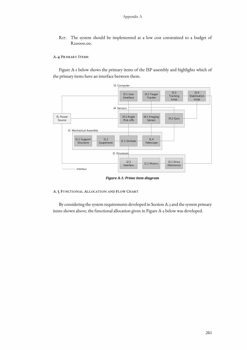
Appendix A
261
R17. The system should be implemented at a low cost constrained to a budget of R20000.00.
A.4 PRIMARY ITEMS
Figure A-1 below shows the primary items of the ISP assembly and highlights which of
the primary items have an interface between them.
I1.1 Support
Structure
I1.2
SuspensionI1.3 Gimbals
I1.4
Telescope
I4.2 GyroI4.3 Angle
Pick-offs
I4.1 Imaging
Sensor
I3.2 Target
Tracker
I3.3
Tracking
Loop
I3.4
Stabilisation
Loop
I2.3
GearboxI2.2 Motors
I2.1 Drive
Electronics
I5. Power
Source
I3.1 User
Interface
I3. Computer
I2. Drivetrain
I1. Mechanical Assembly
I4. Sensors
Interface
Figure A-1: Prime item diagram
A.5 FUNCTIONAL ALLOCATION AND FLOW CHART
By considering the system requirements developed in Section A.3 and the system primary
items shown above, the functional allocation given in Figure A-3 below was developed.
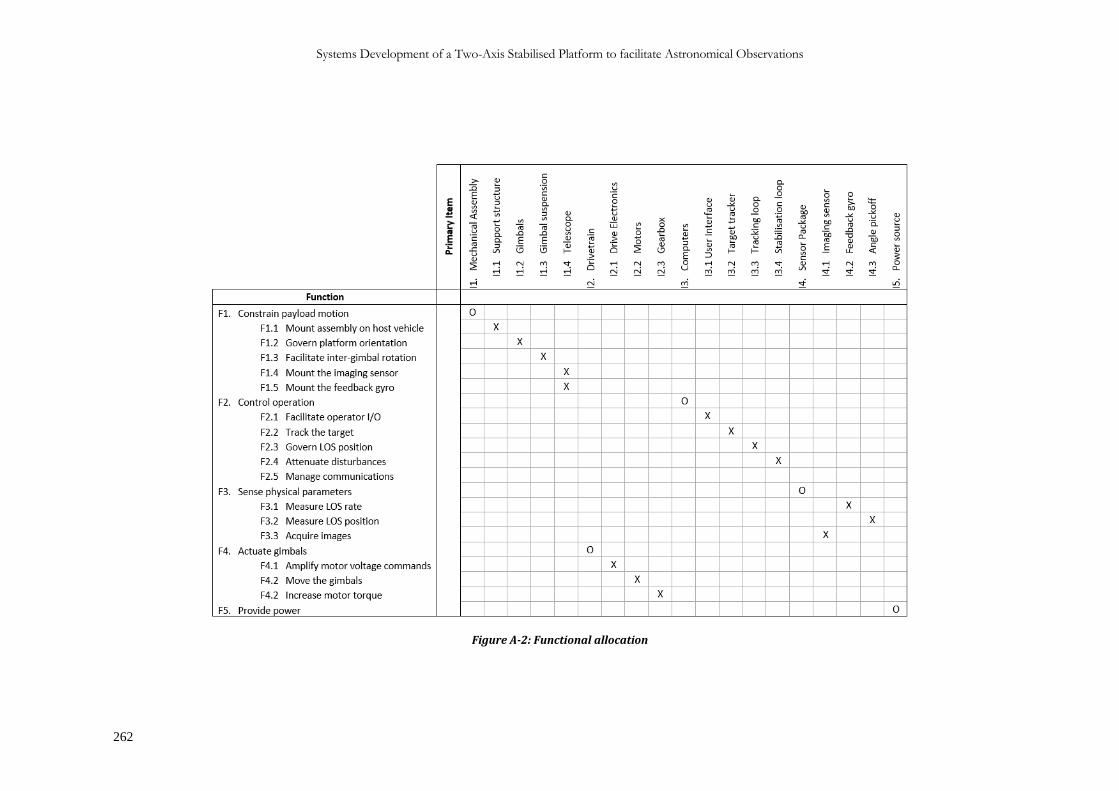
Systems Development of a Two-Axis Stabilised Platform to facilitate Astronomical Observations
262
Figure A-2: Functional allocation
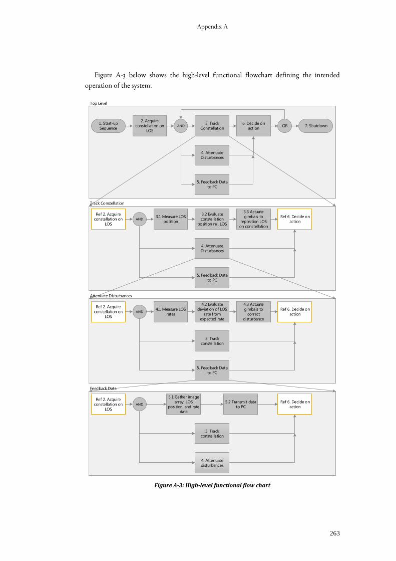
Appendix A
263
Figure A-3 below shows the high-level functional flowchart defining the intended
operation of the system.
2. Acquire constellation on
LOS
3. Track Constellation
1. Start-up Sequence
OR
4. Attenuate Disturbances
5. Feedback Data to PC
6. Decide on action
AND 7. Shutdown
Ref 2. Acquire constellation on
LOS
3.1 Measure LOS position
4. Attenuate Disturbances
5. Feedback Data to PC
3.2 Evaluate constellation
position rel. LOS
AND
3.3 Actuate gimbals to
reposition LOS on constellation
Ref 6. Decide on action
Ref 2. Acquire constellation on
LOS
4.1 Measure LOS rates
3. Track constellation
5. Feedback Data to PC
4.2 Evaluate deviation of LOS
rate from expected rate
AND
4.3 Actuate gimbals to
correct disturbance
Ref 6. Decide on action
Ref 2. Acquire constellation on
LOS
5.1 Gather image array, LOS
position, and rate data
3. Track constellation
4. Attenuate disturbances
AND5.2 Transmit data
to PCRef 6. Decide on
action
Top Level
Track Constellation
Attenuate Disturbances
Feedback Data
Figure A-3: High-level functional flow chart

Systems Development of a Two-Axis Stabilised Platform to facilitate Astronomical Observations
264
A.6 SYSTEM SPECIFICATIONS
From the analysis of the performance requirements, functions, and primary items of the
system, the following specifications have been drawn to govern the design and testing of the
system.
Glossary
Trace: Rx - Requirement number from the list of requirements.
Fx - Function number from the Functional Allocation.
Priority: H - High.
M - Medium.
L - Low.
MoC: Means of Compliance.
A.6.1 MECHANICAL SPECIFICATIONS
S1. The system shall facilitate inertial control of a 3.5” telescope.
Rationale: 3.5” telescopes are a common size for personal telescopes which offer good
light gathering properties without being overly large.
Trace: R1
Priority: L
MoC: Choose telescope to satisfy the specification.
S2. The mechanical assembly shall allow for motion control about a yaw and pitch axis.
Rationale: Yaw (azimuth) and pitch (elevation) are the two axes required to be
controlled for a star to be tracked as it moves across the sky.
Trace: R3, F1.2
Priority: H
MoC: Design ISP such that yaw and pitch are controlled.
S3. The overall dimensions of the system shall be less than 350x350x350 mm.
Rationale: The system should not be too large to compromise its portability.
Trace: R8, R10
Priority: L
MoC: Design for conformance and inspect once assembled.
S4. The total mass of the system shall be less than 9 kg.
Rationale: The system should be manoeuvrable by a single female in the 5th percentile
of anthropometric data. Using data from [115], it has been estimated that a male in the
5th percentile has an average arm strength of 65.7 N per arm. In the absence of available
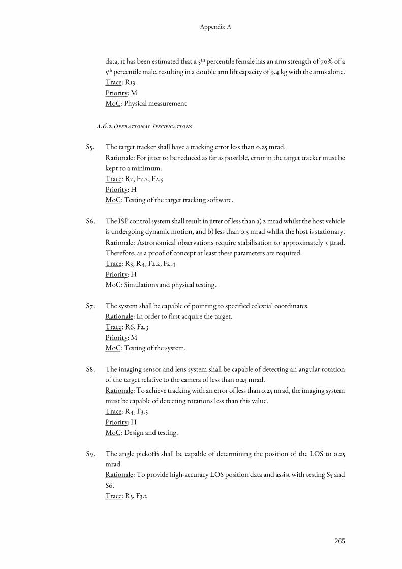
Appendix A
265
data, it has been estimated that a 5th percentile female has an arm strength of 70% of a
5th percentile male, resulting in a double arm lift capacity of 9.4 kg with the arms alone.
Trace: R13
Priority: M
MoC: Physical measurement
A.6.2 OPERATIONAL SPECIFICATIONS
S5. The target tracker shall have a tracking error less than 0.25 mrad.
Rationale: For jitter to be reduced as far as possible, error in the target tracker must be
kept to a minimum.
Trace: R2, F2.2, F2.3
Priority: H
MoC: Testing of the target tracking software.
S6. The ISP control system shall result in jitter of less than a) 2 mrad whilst the host vehicle
is undergoing dynamic motion, and b) less than 0.5 mrad whilst the host is stationary.
Rationale: Astronomical observations require stabilisation to approximately 5 µrad.
Therefore, as a proof of concept at least these parameters are required.
Trace: R3, R4, F2.2, F2.4
Priority: H
MoC: Simulations and physical testing.
S7. The system shall be capable of pointing to specified celestial coordinates.
Rationale: In order to first acquire the target.
Trace: R6, F2.3
Priority: M
MoC: Testing of the system.
S8. The imaging sensor and lens system shall be capable of detecting an angular rotation
of the target relative to the camera of less than 0.25 mrad.
Rationale: To achieve tracking with an error of less than 0.25 mrad, the imaging system
must be capable of detecting rotations less than this value.
Trace: R4, F3.3
Priority: H
MoC: Design and testing.
S9. The angle pickoffs shall be capable of determining the position of the LOS to 0.25
mrad.
Rationale: To provide high-accuracy LOS position data and assist with testing S5 and
S6.
Trace: R5, F3.2

Systems Development of a Two-Axis Stabilised Platform to facilitate Astronomical Observations
266
Priority: L
MoC: Selection of components rated for the specified accuracies.
S10. The feedback gyro shall be capable of measuring angular rates of up to 100 °/s.
Rationale: LOS rates for the ISP are not expected to exceed 100 °/s (Hilkert, 2008),
especially given the application of star tracking.
Trace: R3, F3.1
Priority: H
MoC: Selection of components rated for the specified parameter.
S11. The feedback gyro shall have a bandwidth of at least 120 Hz.
Rationale: To prevent the gyro from being the limiting factor in the overall system
bandwidth.
Trace: R3, F3.1
Priority: H
MoC: Selection of components rated for the specified parameter.
S12. The system shall be battery operable for at least 2 hours.
Rationale: With the future product in mind, the system may be used in an outdoor
location without mains electricity.
Trace: R9, F5
Priority: L
MoC: Selection of components rated for the specified parameter.
S13. A user interface computer program should facilitate operation of the ISP.
Rationale: A safe, user-friendly method of operation providing high-level control and
data-logging is required.
Trace: R11, R12, R15, F2.1
Priority: H
MoC: Design to satisfy the specification.
A.6.3 CONSTRAINTS
S14. The system shall be developed for total cost of less than R20000.00
Rationale: The budget for the project is limited to R20000.00
Trace: R17
Priority: H
MoC: Keeping careful account of project expenses.
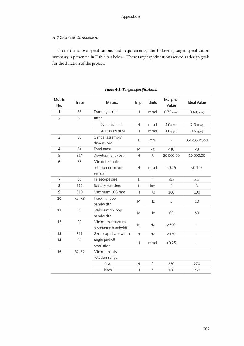
Appendix A
267
A.7 CHAPTER CONCLUSION
From the above specifications and requirements, the following target specification
summary is presented in Table A-1 below. These target specifications served as design goals
for the duration of the project.
Table A-1: Target specifications
Metric
No. Trace Metric. Imp. Units
Marginal
Value Ideal Value
1 S5 Tracking error H mrad 0.75(PEAK) 0.40(PEAK)
2 S6 Jitter
Dynamic host H mrad 4.0(PEAK) 2.0(PEAK)
Stationary host H mrad 1.0(PEAK) 0.5(PEAK)
3 S3 Gimbal assembly
dimensions L mm - 350x350x350
4 S4 Total mass M kg <10 <8
5 S14 Development cost H R 20 000.00 10 000.00
6 S8 Min detectable
rotation on image
sensor
H mrad <0.25 <0.125
7 S1 Telescope size L " 3.5 3.5
8 S12 Battery run-time L hrs 2 3
9 S10 Maximum LOS rate H °/s 100 100
10 R2, R3 Tracking loop
bandwidth M Hz 5 10
11 R3 Stabilisation loop
bandwidth M Hz 60 80
12 R3 Minimum structural
resonance bandwidth M Hz >300 -
13 S11 Gyroscope bandwidth H Hz >120 -
14 S8 Angle pickoff
resolution H mrad <0.25 -
16 R2, S2 Minimum axis
rotation range
Yaw H ° 250 270
Pitch H ° 180 250
Systems Development of a Two-Axis Stabilised Platform to facilitate Astronomical Observations
268
APPENDIX B
MECHANICAL DESIGN
Due to the number of parts designed, and the excessive potential length of this appendix,
it was decided to provide a link to a repository which contains the design files. This repository
contains all the SOLIDWORKS parts, assembly and drawing files used to manufacture the
ISP. The overall system assembly is entitled “System Assembly”. An additional folder within
the repository also shows the technical drawing of these parts in PDF format. Additionally,
the mechanical design calculations used to verify the implementation of specific parts and
components are also shown in a folder here.
Repository: https://bitbucket.org/JamesHepworth_UCT/isp-solidworks-design/
Appendix C
269
APPENDIX C
SOFTWARE AND FIRMWARE SYSTEMS
This appendix provides access to the source code for the various software and firmware
systems developed in the project. As code sizes are relatively large, this software has been made
publicly accessible via the author’s git repositories on Bitbucket to shorten the length of this
document. Software in these repositories is detailed below.
STM32F0 FIRMWARE
Repository: https://bitbucket.org/JamesHepworth_UCT/stm32f0-mcu-firmware/src
The main control firmware for the STM32 is entitled “ISP System Firmware”, whilst the
firmware written to measure motion using an MPU9150 and a data logging VI is entitled
“Motion Measurement”. The entire eclipse IDE projects have been included under these
folders. To view the main program code of both pieces of firmware, navigate to the
src/main.c file of the relevant program.
TARGET TRACKER IMAGE PROCESSING PROGRAM
Repository: https://bitbucket.org/JamesHepworth_UCT/target-tracker/src/
The main program is entitled “Target Tracker with Display.py”, whilst the script which
initialises the image acquisition thread is entitled “webcamvideostream.py” and is a modified
version of the corresponding file from the imutils [114] library which must be installed
according to the method given in the reference link. The corresponding file must then be
replaced with the version from this repository.
LABVIEW SOFTWARE
Repository: https://bitbucket.org/JamesHepworth_UCT/labview-software/src
This repository contains the main user interface, entitled “User interface”, the VI written
to perform FFT functions on gyro rate data, entitled “Spectral Analysis”, and the data logging
VIs which are contained in the folder entitled “Data Logging VIs”. All LabVIEW files were
developed in LabVIEW 2015 and therefore are not backwards compatible with older versions
of LabVIEW. The NI-VISA toolbox is also required for use with these VIs.
SYSTEM SIMULATION
Repository: https://bitbucket.org/JamesHepworth_UCT/simul_c_em-isp-system-
simulation/src

Systems Development of a Two-Axis Stabilised Platform to facilitate Astronomical Observations
270
This repository contains the system simulation written in Simul_C_EM. The main
simulation is a C++ file entitled “Final_Simulation_Model.cpp”. If required, please contact
the author or the project supervisor for details on how to run this simulation.
Appendix D
271
APPENDIX D


