Embed Size (px)
Citation preview
Supplements for “Distribution Neglect in Performance Evaluations”
Table of Contents
Supplement 1: Materials for racing times study.………………...………….……………….2
Supplement 2: Further analyses for racing times study …………………………………...11
Supplement 3: Pilot version of racing times study ………………………………………....12
Supplement 4: Pilot version of NBA study………………………………………………….15
Supplement 5: Materials for assembly line study……………………...…………………...19
Supplement 6: Further analyses for assembly line study………………..………………...28
Supplement 7: Pilot for assembly line study….………………………..………………...…30
Supplement 8: Materials for histogram study..…………………………………………….41
Supplement 9: Materials for grades study……………………………..…………………...46
Supplement 10: Further analyses for grades study………………….……………………..47
Supplement 11: Real world examples of distribution neglect…………...………………...48
Supplement 12: Range study……………..……………………………………….…………51
DISTRIBUTION NEGLECT: SUPPLEMENTS 2
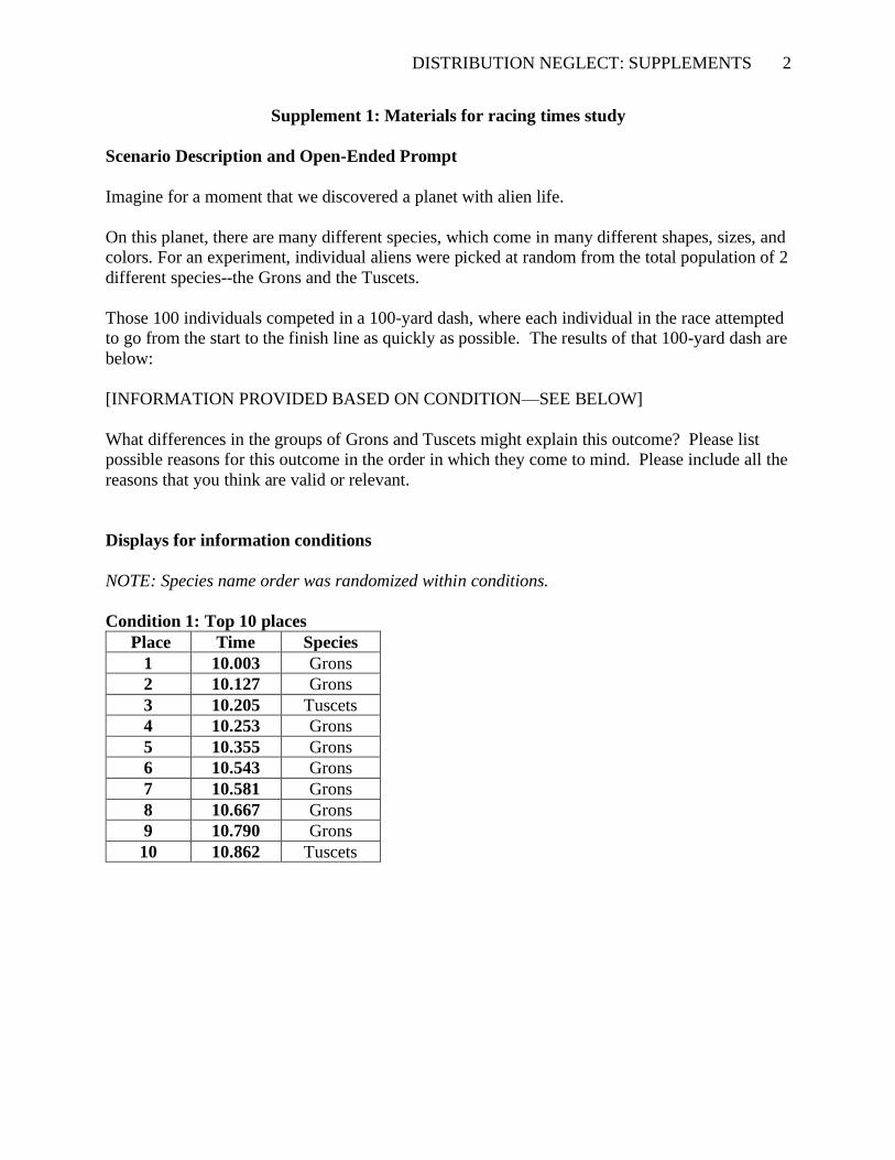
Supplement 1: Materials for racing times study
Scenario Description and Open-Ended Prompt
Imagine for a moment that we discovered a planet with alien life.
On this planet, there are many different species, which come in many different shapes, sizes, and
colors. For an experiment, individual aliens were picked at random from the total population of 2
different species--the Grons and the Tuscets.
Those 100 individuals competed in a 100-yard dash, where each individual in the race attempted
to go from the start to the finish line as quickly as possible. The results of that 100-yard dash are
below:
[INFORMATION PROVIDED BASED ON CONDITION—SEE BELOW]
What differences in the groups of Grons and Tuscets might explain this outcome? Please list
possible reasons for this outcome in the order in which they come to mind. Please include all the
reasons that you think are valid or relevant.
Displays for information conditions
NOTE: Species name order was randomized within conditions.
Condition 1: Top 10 places
Place Time Species
1 10.003 Grons
2 10.127 Grons
3 10.205 Tuscets
4 10.253 Grons
5 10.355 Grons
6 10.543 Grons
7 10.581 Grons
8 10.667 Grons
9 10.790 Grons
10 10.862 Tuscets
DISTRIBUTION NEGLECT: SUPPLEMENTS 3
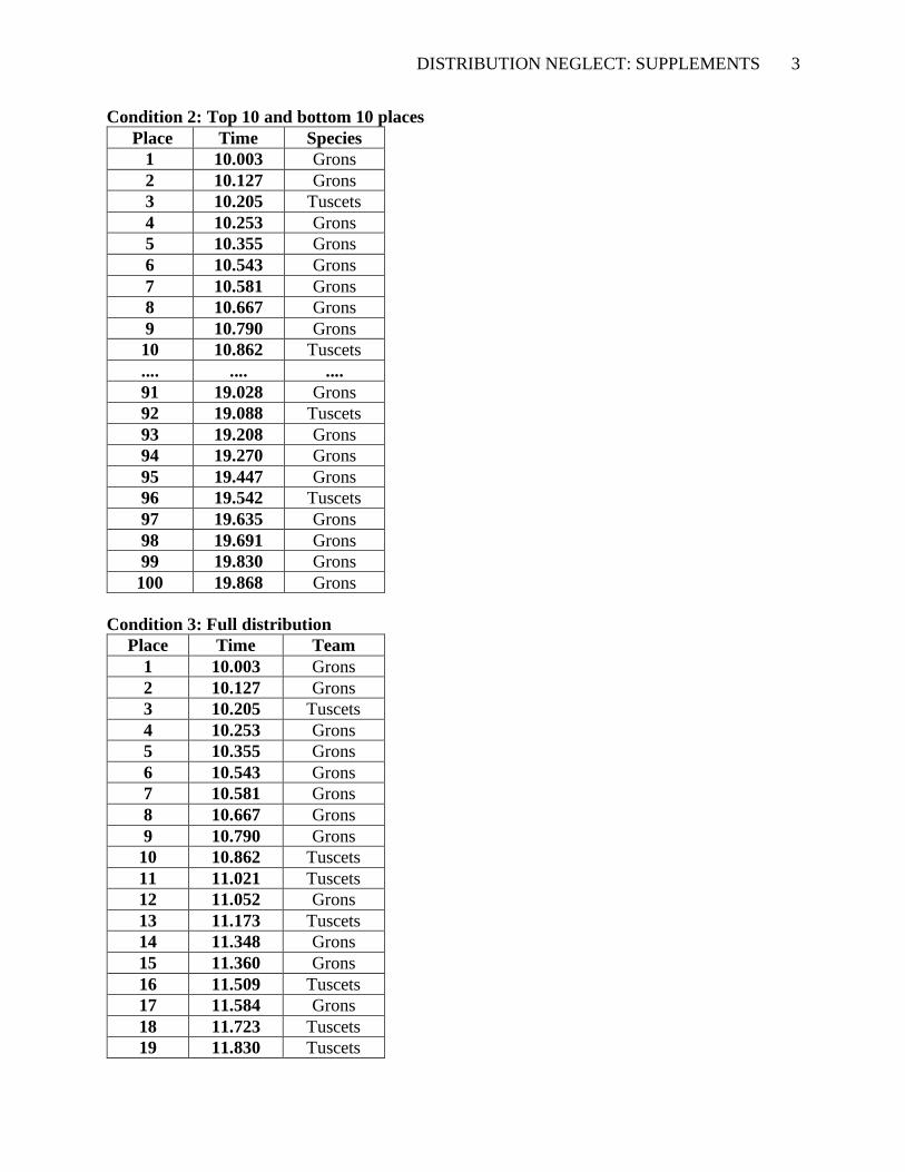
Condition 2: Top 10 and bottom 10 places
Place Time Species
1 10.003 Grons
2 10.127 Grons
3 10.205 Tuscets
4 10.253 Grons
5 10.355 Grons
6 10.543 Grons
7 10.581 Grons
8 10.667 Grons
9 10.790 Grons
10 10.862 Tuscets
.... .... ....
91 19.028 Grons
92 19.088 Tuscets
93 19.208 Grons
94 19.270 Grons
95 19.447 Grons
96 19.542 Tuscets
97 19.635 Grons
98 19.691 Grons
99 19.830 Grons
100 19.868 Grons
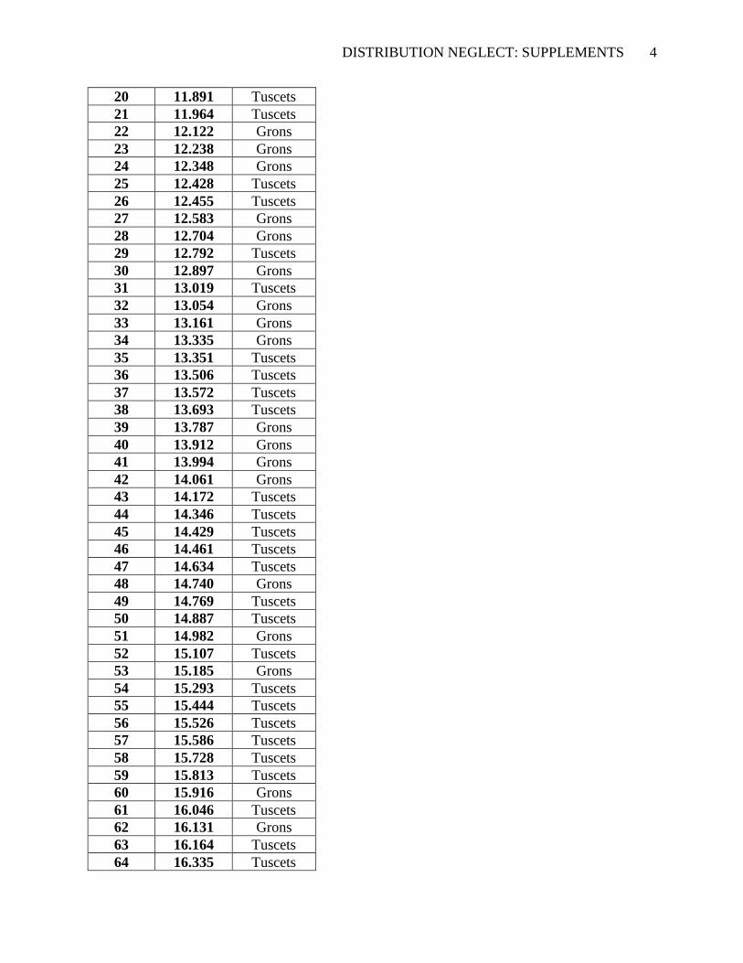
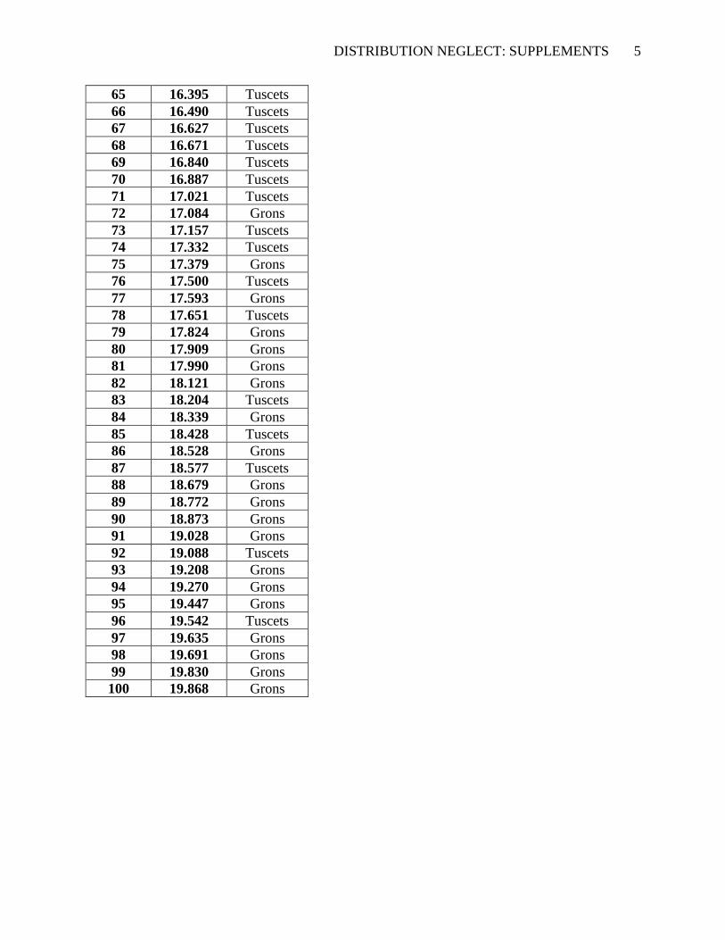
Condition 3: Full distribution
Place Time Team
1 10.003 Grons
2 10.127 Grons
3 10.205 Tuscets
4 10.253 Grons
5 10.355 Grons
6 10.543 Grons
7 10.581 Grons
8 10.667 Grons
9 10.790 Grons
10 10.862 Tuscets
11 11.021 Tuscets
12 11.052 Grons
13 11.173 Tuscets
14 11.348 Grons
15 11.360 Grons
16 11.509 Tuscets
17 11.584 Grons
18 11.723 Tuscets
19 11.830 Tuscets
DISTRIBUTION NEGLECT: SUPPLEMENTS 4
20 11.891 Tuscets
21 11.964 Tuscets
22 12.122 Grons
23 12.238 Grons
24 12.348 Grons
25 12.428 Tuscets
26 12.455 Tuscets
27 12.583 Grons
28 12.704 Grons
29 12.792 Tuscets
30 12.897 Grons
31 13.019 Tuscets
32 13.054 Grons
33 13.161 Grons
34 13.335 Grons
35 13.351 Tuscets
36 13.506 Tuscets
37 13.572 Tuscets
38 13.693 Tuscets
39 13.787 Grons
40 13.912 Grons
41 13.994 Grons
42 14.061 Grons
43 14.172 Tuscets
44 14.346 Tuscets
45 14.429 Tuscets
46 14.461 Tuscets
47 14.634 Tuscets
48 14.740 Grons
49 14.769 Tuscets
50 14.887 Tuscets
51 14.982 Grons
52 15.107 Tuscets
53 15.185 Grons
54 15.293 Tuscets
55 15.444 Tuscets
56 15.526 Tuscets
57 15.586 Tuscets
58 15.728 Tuscets
59 15.813 Tuscets
60 15.916 Grons
61 16.046 Tuscets
62 16.131 Grons
63 16.164 Tuscets
64 16.335 Tuscets
DISTRIBUTION NEGLECT: SUPPLEMENTS 5
65 16.395 Tuscets
66 16.490 Tuscets
67 16.627 Tuscets
68 16.671 Tuscets
69 16.840 Tuscets
70 16.887 Tuscets
71 17.021 Tuscets
72 17.084 Grons
73 17.157 Tuscets
74 17.332 Tuscets
75 17.379 Grons
76 17.500 Tuscets
77 17.593 Grons
78 17.651 Tuscets
79 17.824 Grons
80 17.909 Grons
81 17.990 Grons
82 18.121 Grons
83 18.204 Tuscets
84 18.339 Grons
85 18.428 Tuscets
86 18.528 Grons
87 18.577 Tuscets
88 18.679 Grons
89 18.772 Grons
90 18.873 Grons
91 19.028 Grons
92 19.088 Tuscets
93 19.208 Grons
94 19.270 Grons
95 19.447 Grons
96 19.542 Tuscets
97 19.635 Grons
98 19.691 Grons
99 19.830 Grons
100 19.868 Grons
DISTRIBUTION NEGLECT: SUPPLEMENTS 6
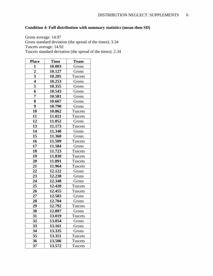
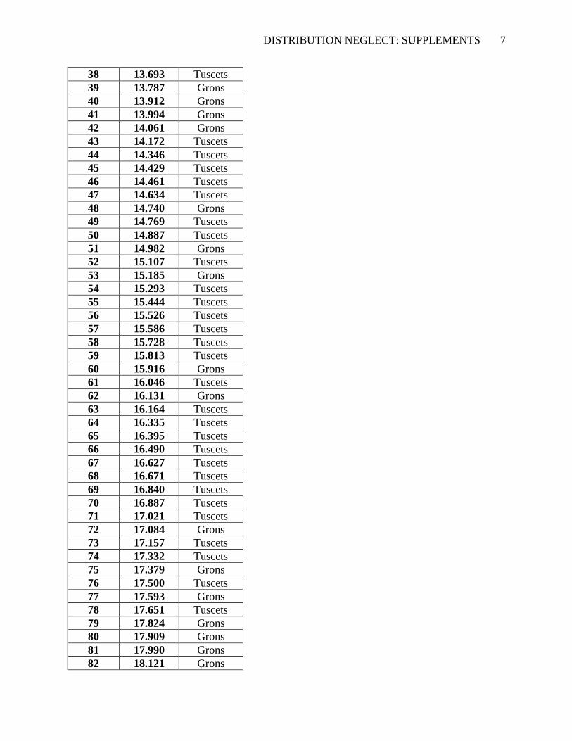
Condition 4: Full distribution with summary statistics (mean then SD)
Grons average: 14.97
Grons standard deviation (the spread of the times): 3.34
Tuscets average: 14.92
Tuscets standard deviation (the spread of the times): 2.34
Place Time Team
1 10.003 Grons
2 10.127 Grons
3 10.205 Tuscets
4 10.253 Grons
5 10.355 Grons
6 10.543 Grons
7 10.581 Grons
8 10.667 Grons
9 10.790 Grons
10 10.862 Tuscets
11 11.021 Tuscets
12 11.052 Grons
13 11.173 Tuscets
14 11.348 Grons
15 11.360 Grons
16 11.509 Tuscets
17 11.584 Grons
18 11.723 Tuscets
19 11.830 Tuscets
20 11.891 Tuscets
21 11.964 Tuscets
22 12.122 Grons
23 12.238 Grons
24 12.348 Grons
25 12.428 Tuscets
26 12.455 Tuscets
27 12.583 Grons
28 12.704 Grons
29 12.792 Tuscets
30 12.897 Grons
31 13.019 Tuscets
32 13.054 Grons
33 13.161 Grons
34 13.335 Grons
35 13.351 Tuscets
36 13.506 Tuscets
37 13.572 Tuscets
DISTRIBUTION NEGLECT: SUPPLEMENTS 7
38 13.693 Tuscets
39 13.787 Grons
40 13.912 Grons
41 13.994 Grons
42 14.061 Grons
43 14.172 Tuscets
44 14.346 Tuscets
45 14.429 Tuscets
46 14.461 Tuscets
47 14.634 Tuscets
48 14.740 Grons
49 14.769 Tuscets
50 14.887 Tuscets
51 14.982 Grons
52 15.107 Tuscets
53 15.185 Grons
54 15.293 Tuscets
55 15.444 Tuscets
56 15.526 Tuscets
57 15.586 Tuscets
58 15.728 Tuscets
59 15.813 Tuscets
60 15.916 Grons
61 16.046 Tuscets
62 16.131 Grons
63 16.164 Tuscets
64 16.335 Tuscets
65 16.395 Tuscets
66 16.490 Tuscets
67 16.627 Tuscets
68 16.671 Tuscets
69 16.840 Tuscets
70 16.887 Tuscets
71 17.021 Tuscets
72 17.084 Grons
73 17.157 Tuscets
74 17.332 Tuscets
75 17.379 Grons
76 17.500 Tuscets
77 17.593 Grons
78 17.651 Tuscets
79 17.824 Grons
80 17.909 Grons
81 17.990 Grons
82 18.121 Grons
DISTRIBUTION NEGLECT: SUPPLEMENTS 8
83 18.204 Tuscets
84 18.339 Grons
85 18.428 Tuscets
86 18.528 Grons
87 18.577 Tuscets
88 18.679 Grons
89 18.772 Grons
90 18.873 Grons
91 19.028 Grons
92 19.088 Tuscets
93 19.208 Grons
94 19.270 Grons
95 19.447 Grons
96 19.542 Tuscets
97 19.635 Grons
98 19.691 Grons
99 19.830 Grons
100 19.868 Grons
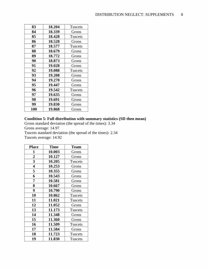
Condition 5: Full distribution with summary statistics (SD then mean)
Grons standard deviation (the spread of the times): 3.34
Grons average: 14.97
Tuscets standard deviation (the spread of the times): 2.34
Tuscets average: 14.92
Place Time Team
1 10.003 Grons
2 10.127 Grons
3 10.205 Tuscets
4 10.253 Grons
5 10.355 Grons
6 10.543 Grons
7 10.581 Grons
8 10.667 Grons
9 10.790 Grons
10 10.862 Tuscets
11 11.021 Tuscets
12 11.052 Grons
13 11.173 Tuscets
14 11.348 Grons
15 11.360 Grons
16 11.509 Tuscets
17 11.584 Grons
18 11.723 Tuscets
19 11.830 Tuscets

DISTRIBUTION NEGLECT: SUPPLEMENTS 9
20 11.891 Tuscets
21 11.964 Tuscets
22 12.122 Grons
23 12.238 Grons
24 12.348 Grons
25 12.428 Tuscets
26 12.455 Tuscets
27 12.583 Grons
28 12.704 Grons
29 12.792 Tuscets
30 12.897 Grons
31 13.019 Tuscets
32 13.054 Grons
33 13.161 Grons
34 13.335 Grons
35 13.351 Tuscets
36 13.506 Tuscets
37 13.572 Tuscets
38 13.693 Tuscets
39 13.787 Grons
40 13.912 Grons
41 13.994 Grons
42 14.061 Grons
43 14.172 Tuscets
44 14.346 Tuscets
45 14.429 Tuscets
46 14.461 Tuscets
47 14.634 Tuscets
48 14.740 Grons
49 14.769 Tuscets
50 14.887 Tuscets
51 14.982 Grons
52 15.107 Tuscets
53 15.185 Grons
54 15.293 Tuscets
55 15.444 Tuscets
56 15.526 Tuscets
57 15.586 Tuscets
58 15.728 Tuscets
59 15.813 Tuscets
60 15.916 Grons
61 16.046 Tuscets
62 16.131 Grons
63 16.164 Tuscets
64 16.335 Tuscets

DISTRIBUTION NEGLECT: SUPPLEMENTS 10
65 16.395 Tuscets
66 16.490 Tuscets
67 16.627 Tuscets
68 16.671 Tuscets
69 16.840 Tuscets
70 16.887 Tuscets
71 17.021 Tuscets
72 17.084 Grons
73 17.157 Tuscets
74 17.332 Tuscets
75 17.379 Grons
76 17.500 Tuscets
77 17.593 Grons
78 17.651 Tuscets
79 17.824 Grons
80 17.909 Grons
81 17.990 Grons
82 18.121 Grons
83 18.204 Tuscets
84 18.339 Grons
85 18.428 Tuscets
86 18.528 Grons
87 18.577 Tuscets
88 18.679 Grons
89 18.772 Grons
90 18.873 Grons
91 19.028 Grons
92 19.088 Tuscets
93 19.208 Grons
94 19.270 Grons
95 19.447 Grons
96 19.542 Tuscets
97 19.635 Grons
98 19.691 Grons
99 19.830 Grons
100 19.868 Grons
DISTRIBUTION NEGLECT: SUPPLEMENTS 11
Supplement 2: Further analyses for racing times study
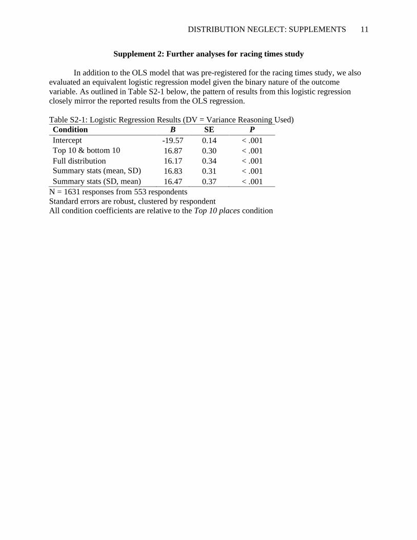
In addition to the OLS model that was pre-registered for the racing times study, we also
evaluated an equivalent logistic regression model given the binary nature of the outcome
variable. As outlined in Table S2-1 below, the pattern of results from this logistic regression
closely mirror the reported results from the OLS regression.
Table S2-1: Logistic Regression Results (DV = Variance Reasoning Used)
Condition B SE P
Intercept -19.57 0.14 < .001
Top 10 & bottom 10 16.87 0.30 < .001
Full distribution 16.17 0.34 < .001
Summary stats (mean, SD) 16.83 0.31 < .001
Summary stats (SD, mean) 16.47 0.37 < .001
N = 1631 responses from 553 respondents
Standard errors are robust, clustered by respondent
All condition coefficients are relative to the Top 10 places condition
DISTRIBUTION NEGLECT: SUPPLEMENTS 12
Supplement 3: Pilot version of racing times study
We carried out a pilot version of the racing times study, with no manipulation of
information completeness. This pilot experiment thus featured only Condition 1 (top 10
finishers) from Study 1 in the main manuscript, not Conditions 2-5 with increasing quantities of
information.
Methods
Participants. We recruited 100 participants on Amazon’s Mechanical Turk, of which 97
completed the study, receiving $0.50 for the 5 minute survey. The average age of participants
was 38 (SD = 10.5), and 48% of participants were female. The sample size and analysis plan for
the study were pre-registered ahead of time (see https://osf.io/923n6/) and the data and code for
are posted as well.
Procedure. Participants were presented with a scenario in which a planet with alien life
had been discovered with many species of different shapes, sizes, and colors (see Appendix S3).
Participants were told that an experiment had been conducted, where “100 individual aliens were
picked at random from the total population of 2 different species,” and the selected individuals
competed in a 100-yard dash. Then, they were provided information about the results of the race
for the top-five finishers only. They were told that individuals from one species finished in 1st t,
2nd, 4th, and 5th, and the other species had one individual finish in 3rd place. With only this
information, participants were asked to list reasons that would make this outcome likely, in the
order in which the ideas came to mind.
Explanation type. A pre-registered quantitative coding scheme was used to convert the
open-ended, qualitative data generated in the survey into categorical data, interpreting the
response as either related to differences in (1) mean, (2) variance, or (3) population size. Codes
for (4) vague or (5) off-topic were also included.
Explanation order. Participants were asked to report their explanations in the order in
which they came to mind; therefore, we used the position of the reason as ordinal-level
information about the order in which each response was thought of.
Numeracy: As potential moderators, we assessed self-reported mathematical reasoning
ability (1 = far below average to 7 = far above average), highest level of schooling completed,
and number of statistics courses taken.
Results
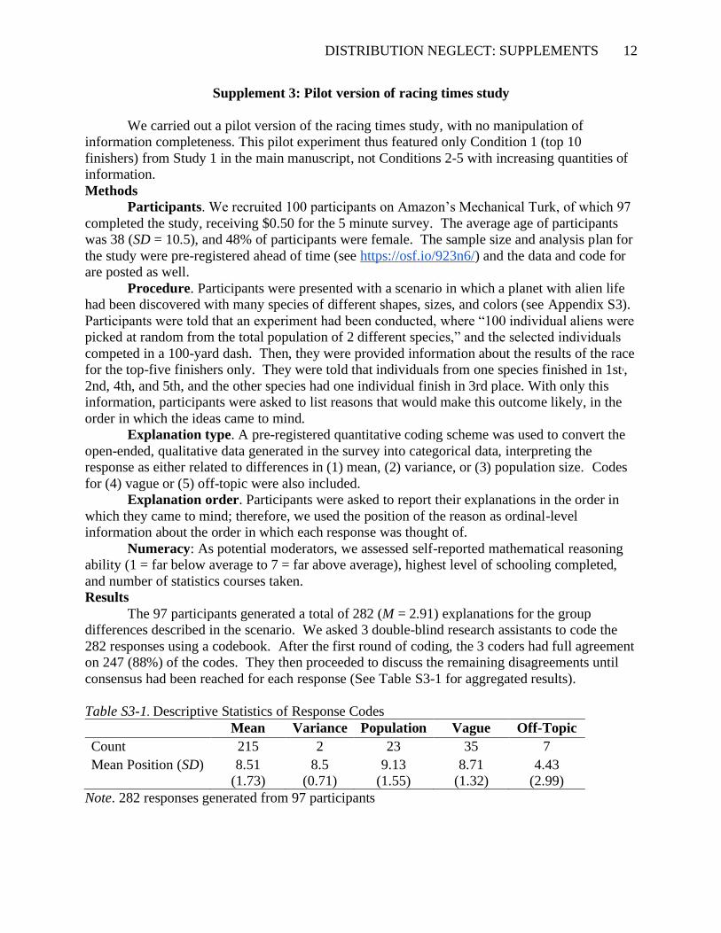
The 97 participants generated a total of 282 (M = 2.91) explanations for the group
differences described in the scenario. We asked 3 double-blind research assistants to code the
282 responses using a codebook. After the first round of coding, the 3 coders had full agreement
on 247 (88%) of the codes. They then proceeded to discuss the remaining disagreements until
consensus had been reached for each response (See Table S3-1 for aggregated results).
Table S3-1. Descriptive Statistics of Response Codes
Mean Variance Population Vague Off-Topic
Count 215 2 23 35 7
Mean Position (SD) 8.51
(1.73)
8.5
(0.71)
9.13
(1.55)
8.71
(1.32)
4.43
(2.99)
Note. 282 responses generated from 97 participants
DISTRIBUTION NEGLECT: SUPPLEMENTS 13
First, we tested if participants were significantly more likely to generate mean-type
responses than variance-type responses. We summed the total number of each type of response
for each participant and conducted a t-test comparing the resultant count variables for mean-type
responses and variance-type responses to test if mean-type responses were significantly more
frequent. The t-test (t(96) = 12.459, d = 2.54) showed that mean-type responses (M = 2.22; SD =
0.175) were significantly more frequent (p < 0.001) than variance-type responses (M = 0.02; SD
= 0.015). We also conducted a two-way test of proportions that compares the proportion of
participants that came up with at least one mean-type response to the proportion of participants
that came up with at least one variance-type response. The test of proportions (z = 12.247)
showed that a significantly (p < 0.001) greater proportion of participants generated mean-type
responses (M = 0.897; SD = 0.031) than variance-type responses (M = 0.021; SD = 0.014).
Next, we tested if participants generated mean-type responses before variance-type
responses. Because of the low number of variance-type participant responses (n = 2), we did not
expect this analysis to produce meaningful results. Nevertheless, we carried out a pre-registered
analysis strategy for assigning value to the position of responses, such that the first response was
assigned a value of 10, the second response was assigned a value of 9, the third response was
assigned a value of 8, and so on. Table S3-1 shows the average position value for each type of
response. Then, we used dummy variables for each type of response to predict the position
value. However, the regression model was not significant (p = 0.380); therefore, the coefficients
for variance and mean-type responses were not compared. Similarly, because only 2 of the 282
reasons were interpreted as variance-related, testing for moderating effects of mathematical
ability, number of statistics courses, and educational attainment was not possible.
Appendix S3: Materials for Pilot Version of Racing Times Study
Instructions
“Imagine for a moment that we discovered a planet with alien life. On this planet, there
are many different species, which come in many different shapes, sizes, and colors. For an
experiment, 100 individual aliens were picked at random from the total population of 2 different
species (the Blue Aliens and the Green Aliens), and those 100 individuals competed in a 100
yard dash. The results of that 100 yard dash are below:”
Condition 1:
“Below, you have information about the results from 1st to 5th place only.
Blue Aliens: 1st place, 2nd place, 4th place, and 5th place
Green Aliens: 3rd place
(There is no information provided about results from 6th to 100th place)”
Condition 2:
“Below, you have information about the results from 1st to 5th place only.
Green Aliens: 1st place, 2nd place, 4th place, and 5th place
Blue Aliens: 3rd place
(There is no information provided about results from 6th to 100th place)”
“Please list reasons that would make this outcome likely in the order in which they come
to mind. Please include all the reasons that you think are valid or relevant.”
“Starting with the first reason that came to mind and going in order to the last reason that
came to mind, please copy and paste each reason into a separate text box. If a single sentence or
phrase contains multiple reasons, separate each reason into a separate box. In other words, each
DISTRIBUTION NEGLECT: SUPPLEMENTS 14
box that you fill out should represent a single reason for the results. Then, retype the explanation
as clearly as possible (no more than 1 or 2 sentences per reason).
Use as many boxes below as you need to copy all of the reasons you provided and leave
the rest blank. Once you have copied all the reasons into separate boxes, leave any remaining
empty boxes blank and continue.”
Coding Strategy
Three double-blind coders independently coded the full 282 responses using the
codebook below. The coders had full agreement on 246 (87.2%) responses after the first round
of coding. The coders then reviewed the disagreements and came to a consensus through an
iterative discussion of the rationale of their codes on responses where there was disagreement.
Codebook
1 = Average difference. Definition: One species is generally faster than the other.
Examples: One species has longer legs than the other species. One species is better trained than
the other species.
2 = Variance difference. Definition: One species has more variety in their speeds and
therefore have more fast individuals AND more slow individuals. Examples: One species takes
longer to become fully mature, so they are slow when young but fast when mature. Some of the
species train a lot and others don’t train. One species grows much older than the other, so they
have more, slower individuals because they are older.
3 = Population size difference. Definition: One species has more individuals selected in
the race than the other. Example: More aliens of one species were selected to participate in the
race.
4 = Other reasons. Definition: Any other on topic response. Seems to be a response, but
doesn’t clearly fit the other 3 types of reasons. Example: Random chance.
5 = Off topic. Definition: Any off topic response. Not sincerely trying to answer the
question.
6 = Multiple differences in the distributions. Definition: The response could fit multiple
of the 1-4 code categories because the distributions seems to differ in multiple ways. Example:
Some of the aliens train (implying differences in variance AND means)
DISTRIBUTION NEGLECT: SUPPLEMENTS 15
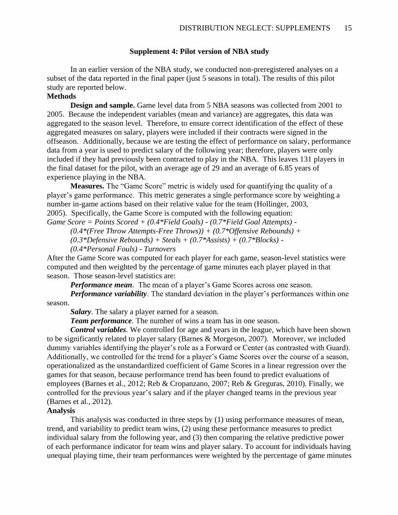
Supplement 4: Pilot version of NBA study
In an earlier version of the NBA study, we conducted non-preregistered analyses on a
subset of the data reported in the final paper (just 5 seasons in total). The results of this pilot
study are reported below.
Methods
Design and sample. Game level data from 5 NBA seasons was collected from 2001 to
2005. Because the independent variables (mean and variance) are aggregates, this data was
aggregated to the season level. Therefore, to ensure correct identification of the effect of these
aggregated measures on salary, players were included if their contracts were signed in the
offseason. Additionally, because we are testing the effect of performance on salary, performance
data from a year is used to predict salary of the following year; therefore, players were only
included if they had previously been contracted to play in the NBA. This leaves 131 players in
the final dataset for the pilot, with an average age of 29 and an average of 6.85 years of
experience playing in the NBA.
Measures. The “Game Score” metric is widely used for quantifying the quality of a
player’s game performance. This metric generates a single performance score by weighting a
number in-game actions based on their relative value for the team (Hollinger, 2003,
2005). Specifically, the Game Score is computed with the following equation:
Game Score = Points Scored + (0.4*Field Goals) - (0.7*Field Goal Attempts) -
(0.4*(Free Throw Attempts-Free Throws)) + (0.7*Offensive Rebounds) +
(0.3*Defensive Rebounds) + Steals + (0.7*Assists) + (0.7*Blocks) -
(0.4*Personal Fouls) - Turnovers
After the Game Score was computed for each player for each game, season-level statistics were
computed and then weighted by the percentage of game minutes each player played in that
season. Those season-level statistics are:
Performance mean. The mean of a player’s Game Scores across one season.
Performance variability. The standard deviation in the player’s performances within one
season.
Salary. The salary a player earned for a season.
Team performance. The number of wins a team has in one season.
Control variables. We controlled for age and years in the league, which have been shown
to be significantly related to player salary (Barnes & Morgeson, 2007). Moreover, we included
dummy variables identifying the player’s role as a Forward or Center (as contrasted with Guard).
Additionally, we controlled for the trend for a player’s Game Scores over the course of a season,
operationalized as the unstandardized coefficient of Game Scores in a linear regression over the
games for that season, because performance trend has been found to predict evaluations of
employees (Barnes et al., 2012; Reb & Cropanzano, 2007; Reb & Greguras, 2010). Finally, we
controlled for the previous year’s salary and if the player changed teams in the previous year
(Barnes et al., 2012).
Analysis
This analysis was conducted in three steps by (1) using performance measures of mean,
trend, and variability to predict team wins, (2) using these performance measures to predict
individual salary from the following year, and (3) then comparing the relative predictive power
of each performance indicator for team wins and player salary. To account for individuals having
unequal playing time, their team performances were weighted by the percentage of game minutes
DISTRIBUTION NEGLECT: SUPPLEMENTS 16
each player played. Because individual performance is dependent on team performance, our
individual-level analyses nested individuals within teams.
Results
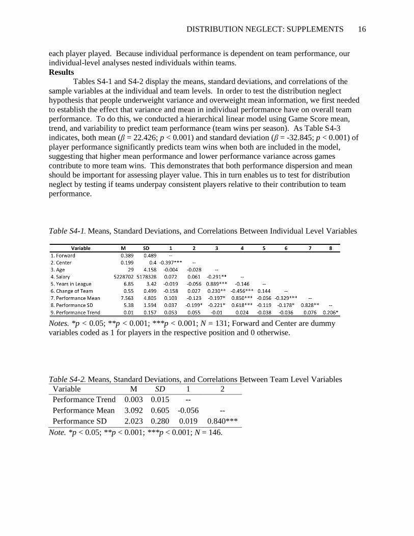
Tables S4-1 and S4-2 display the means, standard deviations, and correlations of the
sample variables at the individual and team levels. In order to test the distribution neglect
hypothesis that people underweight variance and overweight mean information, we first needed
to establish the effect that variance and mean in individual performance have on overall team
performance. To do this, we conducted a hierarchical linear model using Game Score mean,
trend, and variability to predict team performance (team wins per season). As Table S4-3
indicates, both mean (β = 22.426; p < 0.001) and standard deviation (β = -32.845; p < 0.001) of
player performance significantly predicts team wins when both are included in the model,
suggesting that higher mean performance and lower performance variance across games
contribute to more team wins. This demonstrates that both performance dispersion and mean
should be important for assessing player value. This in turn enables us to test for distribution
neglect by testing if teams underpay consistent players relative to their contribution to team
performance.
Table S4-1. Means, Standard Deviations, and Correlations Between Individual Level Variables
Notes. *p < 0.05; **p < 0.001; ***p < 0.001; N = 131; Forward and Center are dummy
variables coded as 1 for players in the respective position and 0 otherwise.
Table S4-2. Means, Standard Deviations, and Correlations Between Team Level Variables
Variable M SD 1 2
Performance Trend 0.003 0.015 --
Performance Mean 3.092 0.605 -0.056 --
Performance SD 2.023 0.280 0.019 0.840***
Note. *p < 0.05; **p < 0.001; ***p < 0.001; N = 146.
DISTRIBUTION NEGLECT: SUPPLEMENTS 17
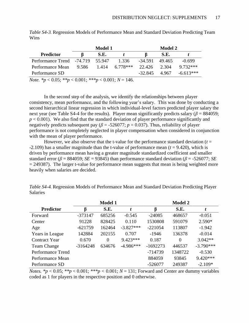
Table S4-3. Regression Models of Performance Mean and Standard Deviation Predicting Team
Wins
Model 1 Model 2
Predictor β S.E. t β S.E. t
Performance Trend -74.719 55.947 1.336 -34.591 49.465 -0.699
Performance Mean 9.586 1.414 6.778*** 22.426 2.304 9.732***
Performance SD -32.845 4.967 -6.613***
Note. *p < 0.05; **p < 0.001; ***p < 0.001; N = 146.
In the second step of the analysis, we identify the relationships between player
consistency, mean performance, and the following year’s salary. This was done by conducting a
second hierarchical linear regression in which individual-level factors predicted player salary the
next year (see Table S4-4 for the results). Player mean significantly predicts salary (β = 884059;
p < 0.001). We also find that the standard deviation of player performance significantly and
negatively predicts subsequent pay (β = -526077; p = 0.037). Thus, reliability of player
performance is not completely neglected in player compensation when considered in conjunction
with the mean of player performance.
However, we also observe that the t-value for the performance standard deviation (t =
-2.109) has a smaller magnitude than the t-value of performance mean (t = 9.420), which is
driven by performance mean having a greater magnitude standardized coefficient and smaller
standard error (β = 884059; SE = 93845) than performance standard deviation (β = -526077; SE
= 249387). The larger t-value for performance mean suggests that mean is being weighted more
heavily when salaries are decided.
Table S4-4. Regression Models of Performance Mean and Standard Deviation Predicting Player
Salaries
Model 1 Model 2
Predictor β S.E. t β S.E. t
Forward -373147 685256 -0.545 -24085 468657 -0.051
Center 91228 828425 0.110 1530808 591079 2.590*
Age -621759 162464 -3.827*** -221054 113807 -1.942
Years in League 142884 202155 0.707 -1946 136378 -0.014
Contract Year 0.670 0 9.423*** 0.187 0 3.042**
Team Change -3164248 634676 -4.986*** -1692273 446537 -3.790***
Performance Trend -714739 1348722 -0.530
Performance Mean 884059 93845 9.420***
Performance SD -526077 249387 -2.109*
Notes. *p < 0.05; **p < 0.001; ***p < 0.001; N = 131; Forward and Center are dummy variables
coded as 1 for players in the respective position and 0 otherwise.
DISTRIBUTION NEGLECT: SUPPLEMENTS 18
Finally, in the third step of the analysis, we assessed if teams are underweighting the
importance of performance variance by testing if performance standard deviation has a
significantly larger effect on team wins than it does on player salary. The difference in the effect
of performance standard deviation on the two dependent variables was tested using Paternoster,
Brame, Mazerolle, and Piquero’s (1998) method for comparing coefficients and standard errors
across regression models. We found that performance standard deviation predicts team wins
significantly better than player salary (z = 2.109; p = 0.035). This supports the hypothesis that
NBA managers underweight the importance of performance dispersion when it comes to
compensating their players, even though they do not neglect it entirely. Moreover, we find that
performance mean predicts team wins significantly less well than player salary (z = 9.420; p <
0.001). This suggests that teams overweight the importance of mean performance when
assessing player value.
DISTRIBUTION NEGLECT: SUPPLEMENTS 19
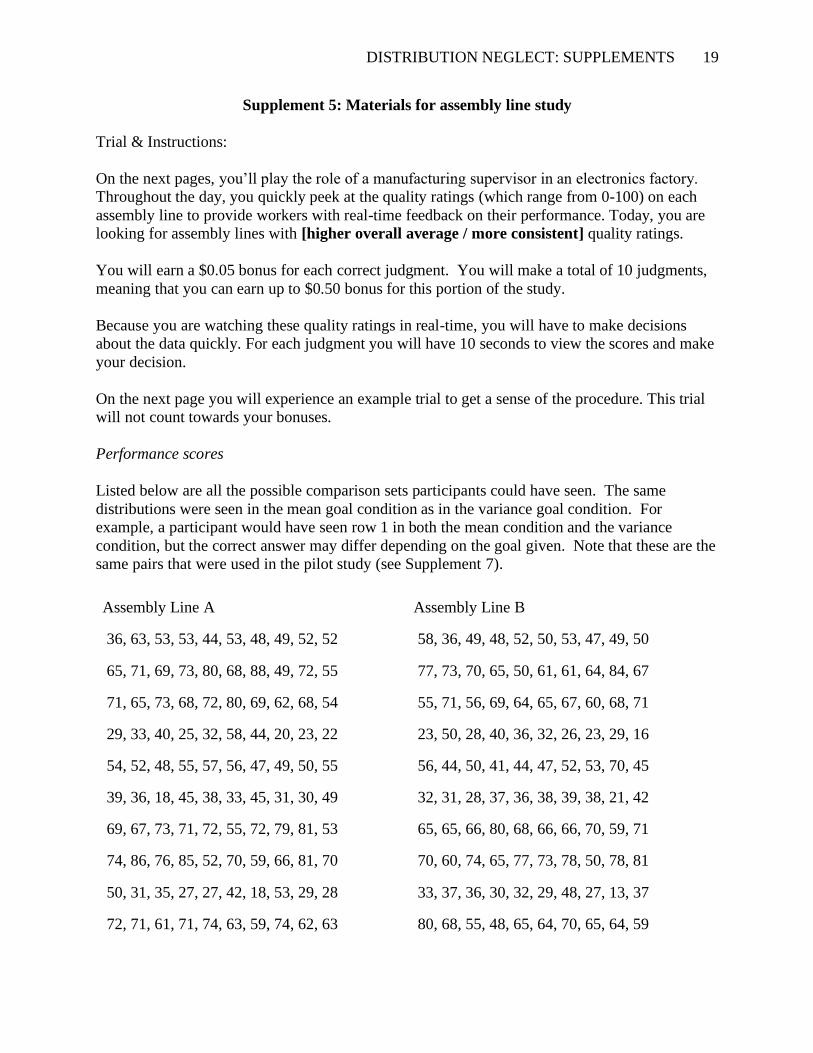
Supplement 5: Materials for assembly line study
Trial & Instructions:
On the next pages, you’ll play the role of a manufacturing supervisor in an electronics factory.
Throughout the day, you quickly peek at the quality ratings (which range from 0-100) on each
assembly line to provide workers with real-time feedback on their performance. Today, you are
looking for assembly lines with [higher overall average / more consistent] quality ratings.
You will earn a $0.05 bonus for each correct judgment. You will make a total of 10 judgments,
meaning that you can earn up to $0.50 bonus for this portion of the study.
Because you are watching these quality ratings in real-time, you will have to make decisions
about the data quickly. For each judgment you will have 10 seconds to view the scores and make
your decision.
On the next page you will experience an example trial to get a sense of the procedure. This trial
will not count towards your bonuses.
Performance scores
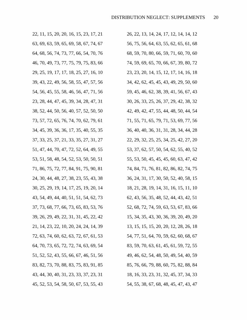
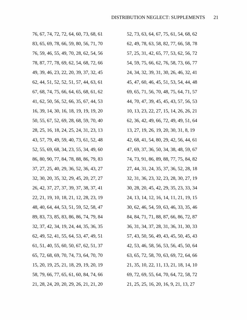
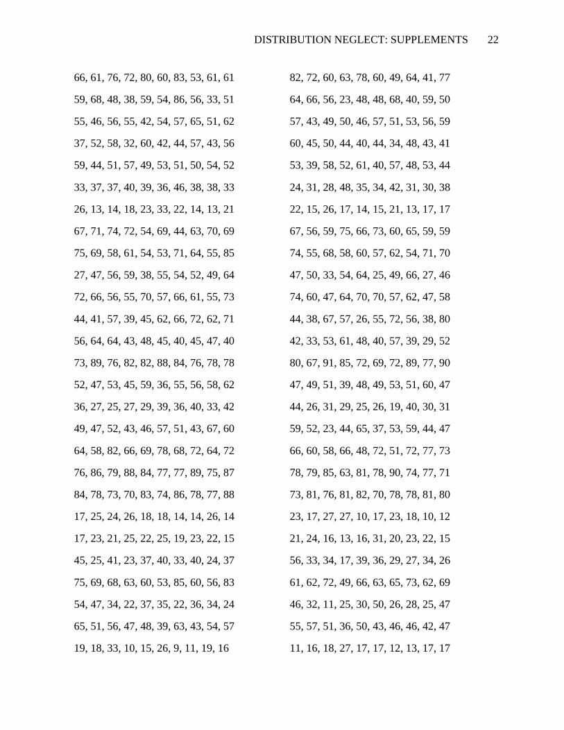
Listed below are all the possible comparison sets participants could have seen. The same
distributions were seen in the mean goal condition as in the variance goal condition. For
example, a participant would have seen row 1 in both the mean condition and the variance
condition, but the correct answer may differ depending on the goal given. Note that these are the
same pairs that were used in the pilot study (see Supplement 7).
Assembly Line A Assembly Line B
36, 63, 53, 53, 44, 53, 48, 49, 52, 52 58, 36, 49, 48, 52, 50, 53, 47, 49, 50
65, 71, 69, 73, 80, 68, 88, 49, 72, 55 77, 73, 70, 65, 50, 61, 61, 64, 84, 67
71, 65, 73, 68, 72, 80, 69, 62, 68, 54 55, 71, 56, 69, 64, 65, 67, 60, 68, 71
29, 33, 40, 25, 32, 58, 44, 20, 23, 22 23, 50, 28, 40, 36, 32, 26, 23, 29, 16
54, 52, 48, 55, 57, 56, 47, 49, 50, 55 56, 44, 50, 41, 44, 47, 52, 53, 70, 45
39, 36, 18, 45, 38, 33, 45, 31, 30, 49 32, 31, 28, 37, 36, 38, 39, 38, 21, 42
69, 67, 73, 71, 72, 55, 72, 79, 81, 53 65, 65, 66, 80, 68, 66, 66, 70, 59, 71
74, 86, 76, 85, 52, 70, 59, 66, 81, 70 70, 60, 74, 65, 77, 73, 78, 50, 78, 81
50, 31, 35, 27, 27, 42, 18, 53, 29, 28 33, 37, 36, 30, 32, 29, 48, 27, 13, 37
72, 71, 61, 71, 74, 63, 59, 74, 62, 63 80, 68, 55, 48, 65, 64, 70, 65, 64, 59
DISTRIBUTION NEGLECT: SUPPLEMENTS 20
22, 11, 15, 20, 20, 16, 15, 23, 17, 21 26, 22, 13, 14, 24, 17, 12, 14, 14, 12
63, 69, 63, 59, 65, 69, 58, 67, 74, 67 56, 75, 56, 64, 63, 55, 62, 65, 61, 68
64, 68, 56, 74, 73, 77, 66, 54, 70, 76 68, 59, 70, 80, 66, 59, 71, 60, 70, 60
46, 70, 49, 73, 77, 75, 79, 75, 83, 66 74, 59, 69, 65, 70, 66, 67, 39, 80, 72
29, 25, 19, 17, 17, 18, 25, 27, 16, 10 23, 23, 20, 14, 15, 12, 17, 14, 16, 18
39, 43, 22, 49, 56, 58, 55, 47, 57, 56 34, 42, 62, 45, 45, 43, 49, 29, 50, 60
54, 56, 45, 55, 58, 46, 56, 47, 71, 56 59, 45, 46, 62, 38, 39, 41, 56, 67, 43
23, 28, 44, 47, 45, 39, 34, 28, 47, 31 30, 26, 33, 25, 26, 37, 29, 42, 38, 32
38, 52, 44, 50, 56, 40, 57, 52, 50, 50 42, 49, 42, 47, 55, 44, 48, 50, 44, 54
73, 57, 72, 65, 76, 74, 70, 62, 79, 61 71, 55, 71, 65, 79, 71, 53, 69, 77, 56
34, 45, 39, 36, 36, 17, 35, 40, 55, 35 36, 40, 40, 36, 31, 31, 28, 34, 44, 28
37, 33, 25, 37, 21, 33, 35, 27, 31, 27 22, 29, 32, 25, 25, 34, 25, 42, 27, 20
51, 47, 44, 70, 47, 72, 52, 64, 49, 55 53, 37, 62, 57, 50, 54, 62, 55, 40, 52
53, 51, 58, 48, 54, 52, 53, 50, 50, 51 55, 53, 50, 45, 45, 45, 60, 63, 47, 42
71, 86, 75, 72, 77, 84, 91, 75, 90, 81 74, 84, 71, 76, 81, 82, 86, 82, 74, 75
24, 30, 44, 48, 27, 38, 23, 55, 43, 38 36, 24, 31, 17, 30, 50, 52, 40, 58, 15
30, 25, 29, 19, 14, 17, 25, 19, 20, 14 18, 21, 28, 19, 14, 31, 16, 15, 11, 10
43, 54, 49, 44, 40, 51, 51, 54, 62, 73 62, 43, 56, 35, 48, 52, 44, 43, 42, 51
37, 73, 68, 77, 66, 73, 65, 83, 53, 76 52, 68, 72, 74, 59, 63, 53, 67, 83, 66
39, 26, 29, 49, 22, 31, 31, 45, 22, 42 15, 34, 35, 43, 30, 36, 39, 20, 49, 20
21, 14, 23, 22, 10, 20, 24, 24, 14, 39 13, 15, 15, 15, 20, 20, 12, 28, 26, 18
72, 63, 74, 60, 62, 63, 72, 67, 61, 53 54, 77, 51, 64, 70, 59, 62, 60, 68, 67
64, 70, 73, 65, 72, 72, 74, 63, 69, 54 83, 59, 70, 63, 61, 45, 61, 59, 72, 55
51, 52, 52, 43, 55, 66, 67, 46, 51, 56 49, 46, 62, 54, 48, 50, 49, 54, 40, 59
83, 82, 73, 70, 88, 83, 75, 83, 91, 85 85, 76, 66, 79, 88, 60, 75, 82, 88, 84
43, 44, 30, 40, 31, 23, 33, 37, 23, 31 18, 16, 33, 23, 31, 32, 45, 37, 34, 33
45, 52, 53, 54, 58, 50, 67, 53, 55, 43 54, 55, 38, 67, 68, 48, 45, 47, 43, 47
DISTRIBUTION NEGLECT: SUPPLEMENTS 21
76, 67, 74, 72, 72, 64, 60, 73, 68, 61 52, 73, 63, 64, 67, 75, 61, 54, 68, 62
83, 65, 69, 78, 66, 59, 80, 56, 71, 70 62, 49, 78, 63, 58, 82, 77, 66, 58, 78
76, 59, 46, 55, 49, 70, 28, 62, 54, 56 57, 25, 31, 42, 65, 77, 53, 62, 56, 72
78, 87, 77, 78, 69, 62, 54, 68, 72, 66 54, 59, 75, 66, 62, 76, 58, 73, 66, 77
49, 39, 46, 23, 22, 20, 39, 37, 32, 45 24, 34, 32, 39, 31, 30, 26, 46, 32, 41
62, 44, 51, 52, 52, 51, 57, 44, 63, 61 45, 47, 60, 46, 45, 51, 53, 54, 44, 48
67, 68, 74, 75, 66, 64, 65, 68, 61, 62 69, 65, 71, 56, 70, 48, 75, 64, 71, 57
41, 62, 50, 56, 52, 66, 35, 67, 44, 53 44, 70, 47, 39, 45, 45, 43, 57, 56, 53
16, 39, 14, 30, 16, 18, 19, 19, 19, 20 10, 13, 23, 22, 27, 15, 14, 26, 26, 21
50, 55, 67, 52, 69, 28, 68, 59, 70, 40 62, 36, 42, 49, 66, 72, 49, 49, 51, 64
28, 25, 16, 18, 24, 25, 24, 31, 23, 13 13, 27, 19, 26, 19, 20, 30, 31, 8, 19
43, 57, 79, 49, 59, 40, 73, 61, 52, 48 42, 68, 41, 54, 80, 29, 42, 56, 44, 61
52, 55, 69, 68, 34, 23, 55, 34, 49, 60 47, 69, 37, 36, 50, 34, 38, 48, 59, 67
86, 80, 90, 77, 84, 78, 88, 86, 79, 83 74, 73, 91, 86, 89, 88, 77, 75, 84, 82
37, 27, 25, 40, 29, 36, 52, 36, 43, 27 27, 44, 31, 24, 35, 37, 36, 52, 28, 18
32, 30, 20, 35, 32, 29, 45, 20, 27, 27 32, 31, 36, 23, 32, 23, 28, 30, 27, 19
26, 42, 37, 27, 37, 39, 37, 38, 37, 41 30, 28, 20, 45, 42, 29, 35, 23, 33, 34
22, 21, 19, 10, 18, 21, 12, 28, 23, 19 24, 13, 14, 12, 16, 14, 11, 21, 19, 15
48, 40, 64, 44, 53, 51, 59, 52, 58, 47 30, 62, 46, 54, 59, 63, 46, 33, 35, 46
89, 83, 73, 85, 83, 86, 86, 74, 79, 84 84, 84, 71, 71, 88, 87, 66, 86, 72, 87
32, 37, 42, 34, 19, 24, 44, 35, 36, 35 36, 31, 34, 37, 28, 31, 36, 31, 30, 33
62, 49, 52, 41, 55, 64, 53, 47, 49, 51 57, 43, 50, 56, 49, 43, 45, 50, 45, 43
61, 51, 40, 55, 60, 50, 67, 62, 51, 37 42, 53, 46, 58, 56, 53, 56, 45, 50, 64
65, 72, 68, 69, 70, 74, 73, 64, 70, 70 63, 65, 72, 58, 70, 63, 69, 72, 64, 66
15, 20, 19, 25, 21, 18, 29, 19, 20, 19 21, 35, 10, 22, 11, 13, 21, 18, 14, 10
58, 79, 66, 77, 65, 61, 60, 84, 74, 66 69, 72, 69, 55, 64, 70, 64, 72, 58, 72
21, 28, 24, 20, 20, 29, 26, 21, 21, 20 21, 25, 25, 16, 20, 16, 9, 21, 13, 27
DISTRIBUTION NEGLECT: SUPPLEMENTS 22
66, 61, 76, 72, 80, 60, 83, 53, 61, 61 82, 72, 60, 63, 78, 60, 49, 64, 41, 77
59, 68, 48, 38, 59, 54, 86, 56, 33, 51 64, 66, 56, 23, 48, 48, 68, 40, 59, 50
55, 46, 56, 55, 42, 54, 57, 65, 51, 62 57, 43, 49, 50, 46, 57, 51, 53, 56, 59
37, 52, 58, 32, 60, 42, 44, 57, 43, 56 60, 45, 50, 44, 40, 44, 34, 48, 43, 41
59, 44, 51, 57, 49, 53, 51, 50, 54, 52 53, 39, 58, 52, 61, 40, 57, 48, 53, 44
33, 37, 37, 40, 39, 36, 46, 38, 38, 33 24, 31, 28, 48, 35, 34, 42, 31, 30, 38
26, 13, 14, 18, 23, 33, 22, 14, 13, 21 22, 15, 26, 17, 14, 15, 21, 13, 17, 17
67, 71, 74, 72, 54, 69, 44, 63, 70, 69 67, 56, 59, 75, 66, 73, 60, 65, 59, 59
75, 69, 58, 61, 54, 53, 71, 64, 55, 85 74, 55, 68, 58, 60, 57, 62, 54, 71, 70
27, 47, 56, 59, 38, 55, 54, 52, 49, 64 47, 50, 33, 54, 64, 25, 49, 66, 27, 46
72, 66, 56, 55, 70, 57, 66, 61, 55, 73 74, 60, 47, 64, 70, 70, 57, 62, 47, 58
44, 41, 57, 39, 45, 62, 66, 72, 62, 71 44, 38, 67, 57, 26, 55, 72, 56, 38, 80
56, 64, 64, 43, 48, 45, 40, 45, 47, 40 42, 33, 53, 61, 48, 40, 57, 39, 29, 52
73, 89, 76, 82, 82, 88, 84, 76, 78, 78 80, 67, 91, 85, 72, 69, 72, 89, 77, 90
52, 47, 53, 45, 59, 36, 55, 56, 58, 62 47, 49, 51, 39, 48, 49, 53, 51, 60, 47
36, 27, 25, 27, 29, 39, 36, 40, 33, 42 44, 26, 31, 29, 25, 26, 19, 40, 30, 31
49, 47, 52, 43, 46, 57, 51, 43, 67, 60 59, 52, 23, 44, 65, 37, 53, 59, 44, 47
64, 58, 82, 66, 69, 78, 68, 72, 64, 72 66, 60, 58, 66, 48, 72, 51, 72, 77, 73
76, 86, 79, 88, 84, 77, 77, 89, 75, 87 78, 79, 85, 63, 81, 78, 90, 74, 77, 71
84, 78, 73, 70, 83, 74, 86, 78, 77, 88 73, 81, 76, 81, 82, 70, 78, 78, 81, 80
17, 25, 24, 26, 18, 18, 14, 14, 26, 14 23, 17, 27, 27, 10, 17, 23, 18, 10, 12
17, 23, 21, 25, 22, 25, 19, 23, 22, 15 21, 24, 16, 13, 16, 31, 20, 23, 22, 15
45, 25, 41, 23, 37, 40, 33, 40, 24, 37 56, 33, 34, 17, 39, 36, 29, 27, 34, 26
75, 69, 68, 63, 60, 53, 85, 60, 56, 83 61, 62, 72, 49, 66, 63, 65, 73, 62, 69
54, 47, 34, 22, 37, 35, 22, 36, 34, 24 46, 32, 11, 25, 30, 50, 26, 28, 25, 47
65, 51, 56, 47, 48, 39, 63, 43, 54, 57 55, 57, 51, 36, 50, 43, 46, 46, 42, 47
19, 18, 33, 10, 15, 26, 9, 11, 19, 16 11, 16, 18, 27, 17, 17, 12, 13, 17, 17
DISTRIBUTION NEGLECT: SUPPLEMENTS 23
52, 56, 61, 47, 55, 44, 45, 41, 48, 46 53, 57, 46, 48, 50, 35, 38, 27, 48, 55
55, 47, 54, 50, 48, 47, 51, 53, 43, 52 50, 40, 51, 62, 33, 48, 44, 52, 58, 51
35, 28, 42, 40, 43, 29, 49, 37, 41, 27 37, 32, 36, 36, 37, 36, 26, 32, 32, 34
75, 62, 83, 78, 82, 87, 82, 91, 87, 79 81, 92, 78, 85, 76, 77, 73, 81, 77, 75
19, 27, 17, 28, 16, 19, 9, 9, 27, 23 20, 17, 20, 14, 13, 20, 20, 10, 19, 20
55, 52, 20, 48, 41, 39, 49, 64, 61, 58 34, 45, 45, 51, 38, 44, 53, 60, 40, 56
53, 61, 50, 39, 54, 57, 55, 54, 55, 43 48, 53, 55, 55, 44, 44, 53, 56, 53, 41
45, 65, 55, 54, 54, 51, 52, 57, 55, 48 61, 50, 55, 55, 47, 58, 50, 31, 52, 52
91, 83, 84, 82, 80, 89, 84, 86, 82, 76 86, 87, 74, 70, 88, 81, 82, 73, 81, 92
34, 33, 38, 37, 30, 42, 43, 34, 42, 34 32, 33, 21, 36, 50, 34, 22, 40, 36, 30
24, 41, 42, 36, 34, 33, 45, 53, 24, 24 29, 27, 31, 37, 33, 40, 37, 33, 22, 24
36, 38, 29, 24, 41, 32, 39, 28, 29, 31 30, 33, 26, 25, 33, 32, 27, 30, 31, 37
75, 69, 73, 68, 66, 75, 56, 69, 47, 82 63, 67, 78, 57, 58, 63, 71, 60, 67, 70
39, 40, 30, 33, 43, 41, 37, 37, 53, 25 40, 34, 41, 36, 31, 31, 39, 27, 39, 27
36, 44, 59, 48, 51, 54, 53, 46, 58, 43 50, 36, 39, 38, 59, 60, 42, 49, 42, 60
41, 27, 40, 60, 38, 28, 20, 36, 51, 27 20, 32, 42, 47, 25, 26, 33, 41, 43, 40
64, 65, 70, 72, 62, 69, 75, 74, 72, 78 69, 64, 50, 65, 77, 83, 70, 67, 68, 58
73, 78, 65, 69, 70, 65, 61, 68, 70, 66 55, 60, 60, 76, 69, 83, 71, 66, 69, 52
63, 64, 65, 69, 64, 72, 77, 71, 61, 69 66, 70, 54, 58, 61, 70, 51, 56, 75, 70
39, 67, 43, 56, 52, 50, 47, 69, 56, 64 37, 37, 44, 53, 46, 68, 61, 36, 65, 46
54, 46, 48, 58, 50, 59, 56, 58, 44, 44 44, 54, 50, 57, 45, 48, 48, 42, 51, 52
21, 34, 29, 14, 14, 21, 17, 12, 12, 15 19, 19, 28, 15, 10, 16, 17, 16, 13, 16
48, 42, 52, 65, 54, 50, 55, 40, 45, 45 56, 48, 40, 49, 46, 46, 53, 49, 45, 41
83, 91, 78, 88, 86, 67, 66, 84, 84, 74 80, 80, 83, 72, 82, 72, 68, 70, 77, 82
83, 88, 79, 88, 87, 71, 83, 85, 85, 84 73, 81, 79, 92, 74, 75, 81, 87, 78, 71
57, 47, 52, 67, 56, 50, 25, 50, 47, 57 66, 68, 40, 53, 57, 50, 53, 24, 36, 43
15, 28, 24, 22, 31, 44, 43, 39, 45, 31 32, 18, 30, 29, 29, 35, 22, 31, 27, 38
DISTRIBUTION NEGLECT: SUPPLEMENTS 24
24, 20, 39, 43, 54, 32, 59, 19, 34, 42 34, 18, 41, 23, 26, 35, 32, 47, 46, 20
53, 50, 45, 53, 56, 49, 53, 61, 45, 53 54, 50, 46, 48, 48, 47, 41, 61, 41, 60
31, 32, 40, 31, 36, 36, 34, 36, 31, 28 35, 41, 23, 19, 35, 31, 36, 29, 35, 28
80, 81, 84, 81, 71, 88, 85, 88, 78, 84 79, 74, 80, 77, 77, 84, 78, 82, 76, 85
81, 83, 82, 84, 78, 88, 73, 86, 78, 80 76, 80, 80, 75, 92, 69, 81, 74, 72, 83
34, 42, 25, 31, 37, 24, 34, 26, 39, 29 26, 41, 26, 31, 30, 46, 28, 28, 26, 20
35, 20, 39, 35, 37, 35, 44, 37, 24, 31 36, 18, 35, 48, 39, 28, 22, 19, 28, 27
52, 54, 51, 64, 48, 47, 44, 63, 40, 41 61, 45, 56, 55, 40, 70, 46, 30, 31, 40
18, 62, 48, 54, 58, 62, 46, 59, 36, 43 64, 42, 50, 33, 70, 35, 36, 47, 44, 36
65, 63, 74, 65, 64, 73, 69, 76, 56, 67 59, 73, 69, 58, 63, 82, 76, 54, 58, 64
59, 20, 48, 58, 38, 58, 65, 44, 62, 42 61, 50, 43, 52, 26, 40, 34, 40, 49, 49
64, 52, 54, 38, 51, 63, 73, 35, 45, 45 39, 58, 65, 55, 48, 45, 41, 53, 49, 46
35, 46, 39, 32, 20, 43, 28, 30, 36, 54 26, 37, 29, 25, 55, 37, 48, 28, 19, 23
80, 77, 72, 56, 77, 68, 55, 68, 71, 80 69, 68, 68, 75, 78, 70, 61, 59, 60, 58
72, 73, 69, 59, 68, 68, 61, 60, 78, 68 59, 55, 64, 63, 53, 68, 71, 77, 77, 66
70, 75, 38, 41, 46, 45, 65, 39, 58, 39 57, 57, 49, 39, 64, 44, 34, 46, 22, 57
58, 58, 35, 83, 54, 42, 46, 53, 54, 73 60, 59, 37, 83, 37, 42, 41, 49, 45, 75
57, 81, 60, 55, 68, 76, 76, 75, 50, 54 72, 70, 53, 52, 63, 74, 62, 62, 57, 51
15, 22, 28, 22, 23, 14, 24, 24, 19, 32 10, 19, 19, 20, 19, 17, 19, 14, 18, 23
74, 66, 75, 75, 47, 78, 71, 70, 69, 70 50, 81, 75, 73, 52, 73, 58, 65, 70, 79
78, 64, 59, 64, 74, 76, 64, 77, 62, 72 65, 66, 70, 65, 46, 60, 79, 69, 58, 81
45, 42, 29, 24, 44, 42, 39, 28, 35, 27 31, 38, 41, 27, 34, 25, 27, 27, 35, 34
20, 24, 24, 24, 21, 23, 15, 25, 24, 14 17, 25, 19, 23, 9, 29, 18, 13, 15, 29
57, 44, 53, 55, 61, 55, 40, 44, 42, 62 46, 40, 70, 25, 47, 53, 57, 40, 57, 50
33, 15, 19, 33, 25, 21, 23, 27, 14, 23 14, 18, 12, 16, 24, 28, 24, 18, 15, 21
32, 21, 22, 20, 33, 26, 23, 19, 13, 17 18, 27, 23, 15, 16, 16, 8, 24, 41, 25
19, 41, 39, 41, 38, 46, 30, 30, 34, 40 33, 39, 23, 24, 54, 34, 40, 25, 37, 25
DISTRIBUTION NEGLECT: SUPPLEMENTS 25
47, 59, 51, 57, 58, 49, 46, 48, 48, 49 53, 42, 50, 43, 40, 45, 49, 54, 58, 65
62, 52, 74, 57, 65, 61, 75, 58, 65, 74 62, 73, 58, 43, 72, 67, 71, 59, 65, 55
18, 31, 18, 10, 28, 29, 22, 21, 14, 16 14, 17, 23, 19, 17, 19, 13, 10, 23, 20
27, 35, 25, 35, 45, 26, 37, 46, 32, 37 38, 36, 25, 29, 20, 16, 44, 45, 30, 29
60, 73, 60, 58, 72, 73, 66, 64, 68, 75 55, 64, 72, 78, 65, 72, 68, 62, 56, 58
84, 77, 84, 86, 78, 85, 73, 83, 86, 85 76, 77, 69, 84, 88, 82, 92, 74, 78, 86
77, 78, 72, 81, 80, 87, 80, 87, 81, 81 77, 79, 86, 70, 85, 69, 82, 76, 72, 69
53, 56, 59, 57, 68, 45, 39, 57, 44, 74 49, 43, 51, 45, 55, 65, 44, 55, 56, 49
54, 42, 44, 65, 40, 55, 58, 45, 32, 59 61, 41, 48, 64, 36, 54, 35, 23, 61, 50
52, 62, 55, 48, 60, 37, 61, 50, 73, 51 47, 48, 65, 57, 53, 53, 60, 51, 40, 48
20, 27, 25, 15, 21, 17, 23, 28, 20, 27 10, 23, 26, 13, 25, 18, 22, 25, 24, 9
51, 31, 25, 22, 34, 37, 41, 26, 41, 26 26, 34, 28, 42, 23, 25, 32, 38, 32, 27
56, 52, 36, 49, 50, 47, 51, 53, 51, 44 55, 52, 50, 42, 54, 50, 34, 47, 38, 53
63, 48, 61, 27, 33, 53, 56, 41, 43, 62 39, 56, 40, 58, 43, 40, 45, 40, 46, 33
38, 34, 39, 30, 35, 37, 32, 38, 29, 42 22, 25, 37, 39, 29, 43, 31, 24, 21, 33
64, 53, 60, 49, 63, 37, 49, 51, 43, 34 39, 40, 44, 54, 57, 49, 55, 42, 62, 47
48, 50, 44, 52, 58, 53, 53, 54, 53, 51 48, 55, 50, 41, 52, 49, 39, 44, 48, 44
48, 67, 26, 50, 61, 56, 39, 63, 63, 62 58, 46, 54, 38, 42, 38, 48, 58, 58, 47
85, 56, 70, 58, 56, 70, 78, 68, 72, 75 68, 75, 73, 62, 75, 66, 57, 65, 74, 60
39, 30, 35, 32, 33, 23, 38, 36, 34, 29 34, 28, 15, 19, 43, 32, 37, 24, 38, 32
67, 40, 68, 50, 38, 62, 46, 58, 59, 63 54, 61, 38, 47, 51, 49, 45, 48, 67, 50
32, 48, 53, 49, 37, 34, 38, 33, 21, 33 39, 26, 28, 41, 37, 34, 45, 36, 31, 18
30, 36, 29, 29, 41, 48, 37, 33, 28, 39 34, 30, 20, 36, 35, 29, 30, 34, 36, 32
45, 38, 25, 31, 30, 37, 32, 33, 41, 34 39, 25, 36, 21, 32, 34, 40, 36, 24, 39
23, 35, 15, 16, 35, 34, 12, 21, 10, 19 33, 16, 9, 20, 18, 19, 27, 19, 14, 14
26, 48, 36, 28, 48, 31, 57, 31, 56, 22 31, 31, 55, 21, 35, 31, 32, 36, 33, 43
33, 44, 38, 29, 19, 33, 50, 52, 31, 42 26, 50, 29, 36, 22, 36, 36, 25, 37, 31
DISTRIBUTION NEGLECT: SUPPLEMENTS 26
61, 70, 54, 61, 67, 62, 40, 48, 54, 49 55, 47, 48, 64, 70, 39, 48, 84, 45, 43
18, 21, 28, 22, 18, 17, 20, 22, 11, 16 11, 25, 20, 32, 16, 16, 8, 20, 14, 17
73, 43, 76, 71, 77, 69, 49, 56, 81, 68 65, 55, 66, 86, 68, 46, 83, 50, 47, 82
51, 54, 52, 55, 53, 55, 43, 52, 53, 55 45, 54, 44, 45, 58, 49, 56, 48, 54, 47
50, 51, 49, 52, 56, 59, 58, 48, 55, 36 62, 41, 48, 41, 51, 35, 48, 47, 56, 49
52, 48, 46, 44, 57, 56, 48, 53, 51, 52 56, 48, 52, 41, 46, 52, 44, 47, 62, 46
79, 88, 81, 85, 80, 81, 79, 79, 82, 87 76, 81, 84, 86, 62, 81, 79, 87, 76, 86
70, 73, 41, 60, 32, 51, 59, 50, 52, 30 55, 26, 29, 58, 48, 41, 57, 64, 59, 40
22, 24, 18, 32, 20, 21, 14, 18, 29, 14 15, 25, 19, 24, 15, 22, 18, 17, 16, 12
54, 45, 46, 52, 49, 44, 51, 58, 56, 51 45, 40, 42, 55, 51, 44, 41, 46, 68, 54
32, 42, 34, 46, 37, 42, 22, 29, 15, 45 37, 22, 33, 33, 46, 35, 52, 46, 12, 15
57, 57, 78, 58, 71, 81, 54, 73, 58, 62 51, 68, 72, 69, 71, 62, 71, 55, 65, 54
27, 35, 30, 38, 29, 37, 26, 21, 36, 53 24, 38, 15, 26, 10, 26, 36, 41, 31, 36
36, 38, 42, 38, 22, 26, 27, 28, 31, 39 31, 28, 29, 34, 36, 35, 20, 28, 35, 21
30, 41, 28, 20, 32, 33, 40, 23, 30, 48 31, 37, 28, 24, 29, 22, 31, 39, 31, 27
60, 45, 44, 35, 59, 40, 53, 49, 58, 65 39, 46, 43, 43, 56, 53, 47, 53, 42, 59
68, 58, 56, 46, 57, 61, 37, 65, 43, 67 60, 46, 47, 42, 66, 55, 54, 59, 54, 49
84, 78, 82, 70, 87, 85, 80, 84, 78, 82 73, 84, 69, 77, 80, 87, 90, 80, 78, 81
32, 48, 37, 46, 63, 50, 48, 70, 54, 59 57, 45, 57, 35, 33, 43, 57, 48, 50, 35
43, 29, 36, 38, 25, 27, 30, 47, 34, 36 37, 32, 34, 28, 26, 33, 28, 45, 28, 30
63, 39, 54, 47, 78, 39, 52, 35, 49, 60 42, 28, 37, 71, 54, 54, 27, 60, 49, 60
60, 35, 45, 48, 40, 53, 39, 58, 54, 58 56, 52, 53, 57, 35, 33, 58, 30, 53, 49
29, 31, 14, 34, 43, 27, 21, 40, 53, 29 23, 31, 26, 21, 42, 20, 34, 27, 25, 37
50, 61, 57, 60, 57, 51, 49, 40, 58, 59 48, 49, 47, 48, 50, 59, 53, 55, 56, 53
57, 36, 50, 43, 46, 50, 53, 58, 64, 50 51, 43, 45, 42, 50, 42, 52, 53, 57, 39
29, 23, 20, 27, 17, 16, 18, 19, 22, 22 12, 27, 18, 14, 14, 20, 20, 24, 12, 23
70, 81, 79, 61, 58, 63, 70, 64, 69, 75 77, 55, 55, 52, 66, 64, 65, 70, 64, 77

DISTRIBUTION NEGLECT: SUPPLEMENTS 27
76, 82, 79, 90, 82, 84, 73, 82, 84, 93 73, 87, 75, 86, 91, 72, 60, 77, 87, 70
DISTRIBUTION NEGLECT: SUPPLEMENTS 28
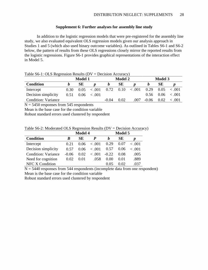
Supplement 6: Further analyses for assembly line study
In addition to the logistic regression models that were pre-registered for the assembly line
study, we also evaluated equivalent OLS regression models given our analysis approach in
Studies 1 and 5 (which also used binary outcome variables). As outlined in Tables S6-1 and S6-2
below, the pattern of results from these OLS regressions closely mirror the reported results from
the logistic regressions. Figure S6-1 provides graphical representations of the interaction effect
in Model 5.
Table S6-1: OLS Regression Results (DV = Decision Accuracy)
Model 1 Model 2 Model 3
Condition b SE p b SE p b SE p
Intercept 0.30 0.05 < .001 0.72 0.10 < .001 0.29 0.05 < .001
Decision simplicity 0.51 0.06 < .001 0.56 0.06 < .001
Condition: Variance -0.04 0.02 .007 -0.06 0.02 < .001
N = 5450 responses from 545 respondents
Mean is the base case for the condition variable
Robust standard errors used clustered by respondent
Table S6-2: Moderated OLS Regression Results (DV = Decision Accuracy)
Model 4 Model 5
Condition B SE P b SE p
Intercept 0.21 0.06 < .001 0.29 0.07 < .001
Decision simplicity 0.57 0.06 < .001 0.57 0.06 < .001
Condition: Variance -0.06 0.02 < .001 -0.22 0.08 .005
Need for cognition 0.02 0.01 .058 0.00 0.01 .889
NFC X Condition 0.05 0.02 .037
N = 5440 responses from 544 respondents (incomplete data from one respondent)
Mean is the base case for the condition variable
Robust standard errors used clustered by respondent
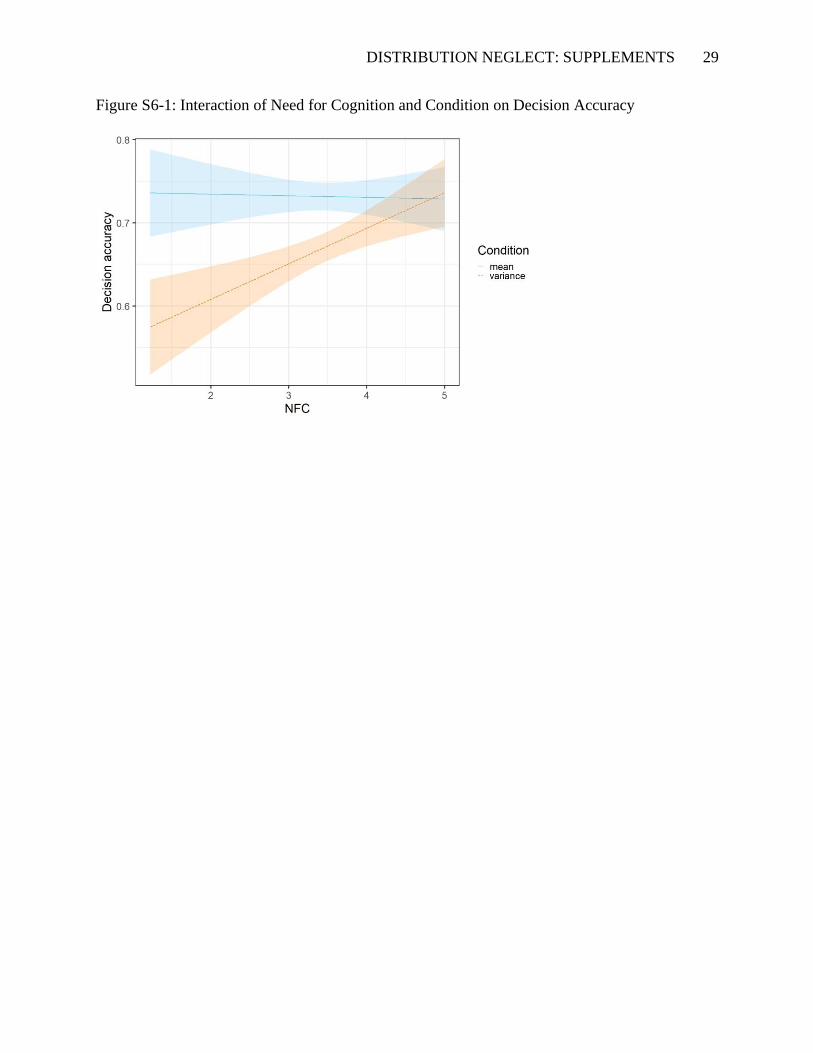
DISTRIBUTION NEGLECT: SUPPLEMENTS 29
Figure S6-1: Interaction of Need for Cognition and Condition on Decision Accuracy
DISTRIBUTION NEGLECT: SUPPLEMENTS 30
Supplement 7: Pilot for assembly line study
In a non-preregistered pilot study, we asked participants to compare the performance of
two employees and identify the employee with the higher mean performance or the greater
consistency of performance under strict time constraints (10 seconds). Study 3 in the main
manuscript pre-registers the relevant empirical predictions and uses an assembly line paradigm
where rapid evaluations of performance have greater verisimilitude.
Methods
Participants. We recruited 202 participants on Amazon’s Mechanical Turk. Because
participants were instructed not to use a calculator or write down any numbers, two participants
were removed from the sample based on a question asking them to self-identify if they cheated in
some way. The final sample was thus 200 participants. The average age of participants was
33.46 (SD = 12.11), and 43% of participants were female.
Procedure. After completing informed consent, participants were told that they would
be evaluating job candidates in a series of quick, timed judgements. Each job candidate had
completed a 10-week internship and at the end of each week was scored on the quality of their
work. Participants were randomly assigned to either try and pick the candidate with “the higher
overall average score” (the mean condition) or the candidate who had performed “most reliably”
(the variance condition), where reliability was defined for participants as receiving similar scores
from week to week such that their performance was less variable.
Participants made 10 judgements about pairs of candidates and were paid a $0.05 bonus
per correct judgement. For each judgment participants would view two candidates (labeled as
Candidate A and Candidate B) and the two candidates’ sets of 10 scores for a total of 10
seconds. The survey then automatically advanced and prompted participants for their choice of
Candidate A or B. All participants completed one trial round, so that they were familiar with the
procedure and aware that the values would disappear after 10 seconds.
The values for Candidate A and Candidate B were randomly chosen from a set of 200
possible comparisons (see Appendix S7).
Measures.
Accuracy. For each judgement, participants were given a score of 1 if they chose the
correct candidate (the candidate with the higher mean performance in the mean condition or the
lower standard deviation in the variance condition) and a score of 0 if they chose the incorrect
candidate.
Difficulty. For each possible set of two candidates’ performance distributions, we
calculated how difficult the task of assessing mean performance versus consistent performance
would be in order to generate a normative benchmark. Because mean differences are normally
distributed, while variance differences are F-distributed, absolute difference in means are not
directly equally difficult to judge as compared to absolute differences in variances. Calculating
difficulty thus allows us to better directly compare the task of judging average performance
versus consistent performance. To calculate the difficulty of determining the higher performing
candidate we calculated the probability that the candidate with the higher sample mean from
these ten weeks would have a higher population mean by at least 0.1 performance points as
compared to the candidate with the lower sample mean. To calculate the difficulty of
determining the more reliably performing candidate, we calculated the ratio of the variances of
two candidates and determined the probability that the candidate with the lower sample variance
from these ten weeks would have a lower population variance. A difficulty score of 0.99 thus
DISTRIBUTION NEGLECT: SUPPLEMENTS 31
indicated a very easy choice, while a difficulty score of 0.51 would indicate a very difficult
choice. Values of the distributions used for participants varied from 0.58 to 0.99.
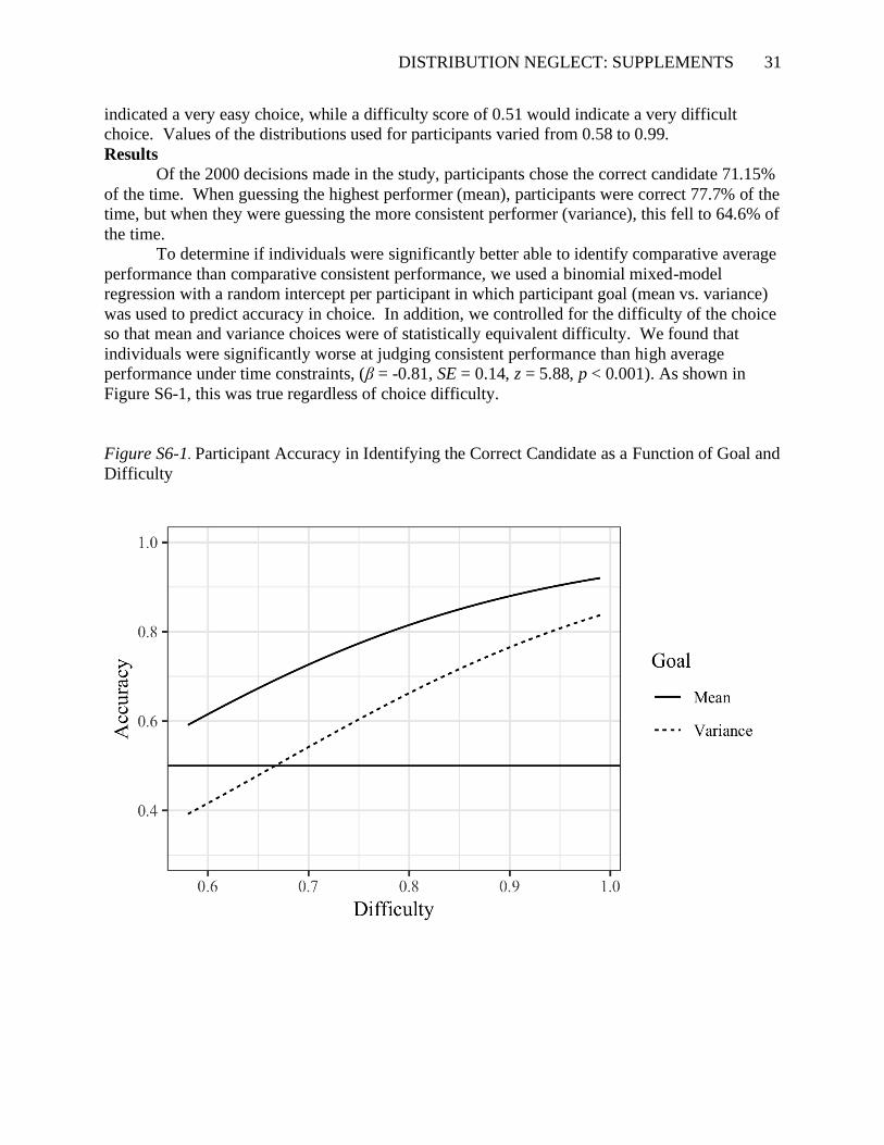
Results
Of the 2000 decisions made in the study, participants chose the correct candidate 71.15%
of the time. When guessing the highest performer (mean), participants were correct 77.7% of the
time, but when they were guessing the more consistent performer (variance), this fell to 64.6% of
the time.
To determine if individuals were significantly better able to identify comparative average
performance than comparative consistent performance, we used a binomial mixed-model
regression with a random intercept per participant in which participant goal (mean vs. variance)
was used to predict accuracy in choice. In addition, we controlled for the difficulty of the choice
so that mean and variance choices were of statistically equivalent difficulty. We found that
individuals were significantly worse at judging consistent performance than high average
performance under time constraints, (β = -0.81, SE = 0.14, z = 5.88, p < 0.001). As shown in
Figure S6-1, this was true regardless of choice difficulty.
Figure S6-1. Participant Accuracy in Identifying the Correct Candidate as a Function of Goal and
Difficulty
DISTRIBUTION NEGLECT: SUPPLEMENTS 32
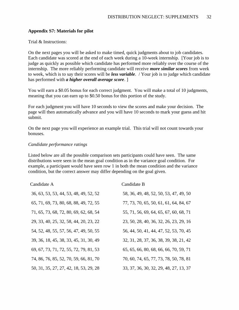
Appendix S7: Materials for pilot
Trial & Instructions:
On the next pages you will be asked to make timed, quick judgments about to job candidates.
Each candidate was scored at the end of each week during a 10-week internship. [Your job is to
judge as quickly as possible which candidate has performed more reliably over the course of the
internship. The more reliably performing candidate will receive more similar scores from week
to week, which is to say their scores will be less variable. / Your job is to judge which candidate
has performed with a higher overall average score. ]
You will earn a $0.05 bonus for each correct judgment. You will make a total of 10 judgments,
meaning that you can earn up to $0.50 bonus for this portion of the study.
For each judgment you will have 10 seconds to view the scores and make your decision. The
page will then automatically advance and you will have 10 seconds to mark your guess and hit
submit.
On the next page you will experience an example trial. This trial will not count towards your
bonuses.
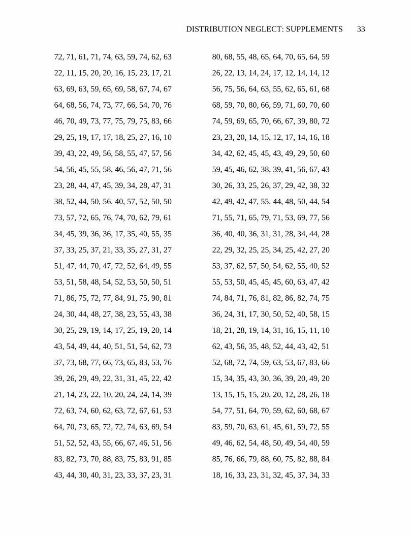
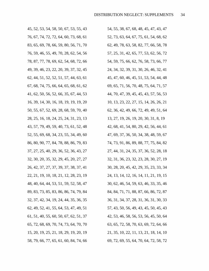
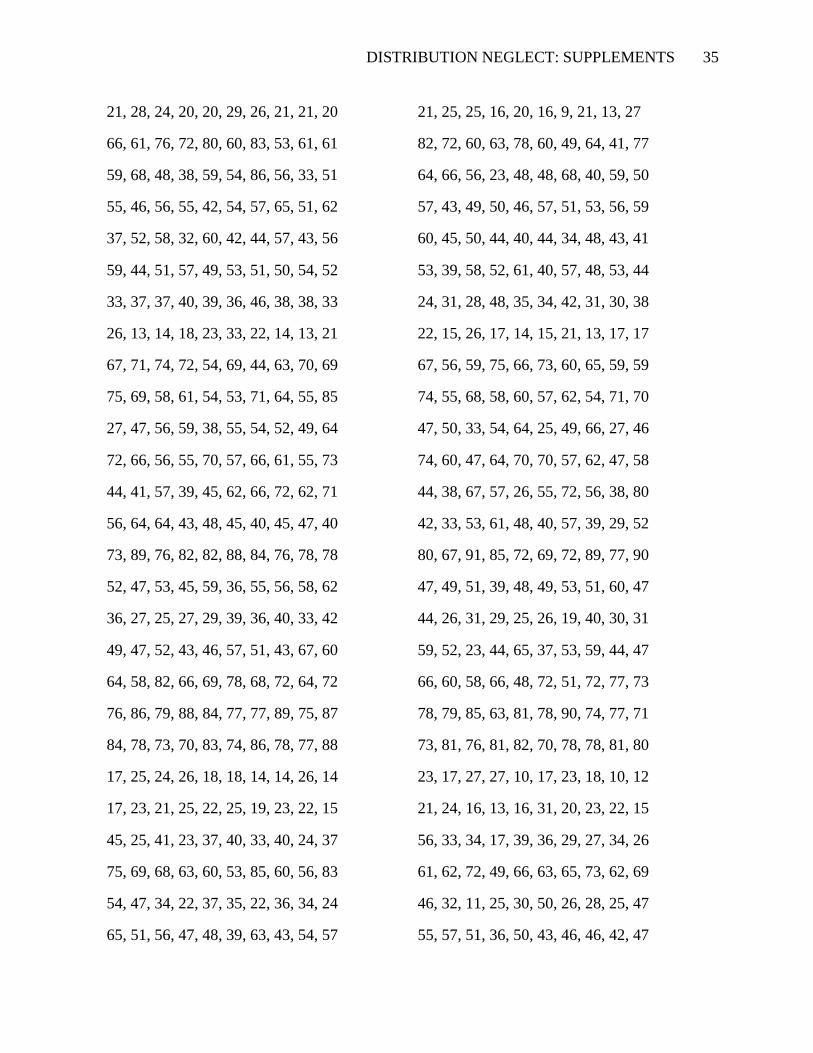
Candidate performance ratings
Listed below are all the possible comparison sets participants could have seen. The same
distributions were seen in the mean goal condition as in the variance goal condition. For
example, a participant would have seen row 1 in both the mean condition and the variance
condition, but the correct answer may differ depending on the goal given.
Candidate A Candidate B
36, 63, 53, 53, 44, 53, 48, 49, 52, 52 58, 36, 49, 48, 52, 50, 53, 47, 49, 50
65, 71, 69, 73, 80, 68, 88, 49, 72, 55 77, 73, 70, 65, 50, 61, 61, 64, 84, 67
71, 65, 73, 68, 72, 80, 69, 62, 68, 54 55, 71, 56, 69, 64, 65, 67, 60, 68, 71
29, 33, 40, 25, 32, 58, 44, 20, 23, 22 23, 50, 28, 40, 36, 32, 26, 23, 29, 16
54, 52, 48, 55, 57, 56, 47, 49, 50, 55 56, 44, 50, 41, 44, 47, 52, 53, 70, 45
39, 36, 18, 45, 38, 33, 45, 31, 30, 49 32, 31, 28, 37, 36, 38, 39, 38, 21, 42
69, 67, 73, 71, 72, 55, 72, 79, 81, 53 65, 65, 66, 80, 68, 66, 66, 70, 59, 71
74, 86, 76, 85, 52, 70, 59, 66, 81, 70 70, 60, 74, 65, 77, 73, 78, 50, 78, 81
50, 31, 35, 27, 27, 42, 18, 53, 29, 28 33, 37, 36, 30, 32, 29, 48, 27, 13, 37
DISTRIBUTION NEGLECT: SUPPLEMENTS 33
72, 71, 61, 71, 74, 63, 59, 74, 62, 63 80, 68, 55, 48, 65, 64, 70, 65, 64, 59
22, 11, 15, 20, 20, 16, 15, 23, 17, 21 26, 22, 13, 14, 24, 17, 12, 14, 14, 12
63, 69, 63, 59, 65, 69, 58, 67, 74, 67 56, 75, 56, 64, 63, 55, 62, 65, 61, 68
64, 68, 56, 74, 73, 77, 66, 54, 70, 76 68, 59, 70, 80, 66, 59, 71, 60, 70, 60
46, 70, 49, 73, 77, 75, 79, 75, 83, 66 74, 59, 69, 65, 70, 66, 67, 39, 80, 72
29, 25, 19, 17, 17, 18, 25, 27, 16, 10 23, 23, 20, 14, 15, 12, 17, 14, 16, 18
39, 43, 22, 49, 56, 58, 55, 47, 57, 56 34, 42, 62, 45, 45, 43, 49, 29, 50, 60
54, 56, 45, 55, 58, 46, 56, 47, 71, 56 59, 45, 46, 62, 38, 39, 41, 56, 67, 43
23, 28, 44, 47, 45, 39, 34, 28, 47, 31 30, 26, 33, 25, 26, 37, 29, 42, 38, 32
38, 52, 44, 50, 56, 40, 57, 52, 50, 50 42, 49, 42, 47, 55, 44, 48, 50, 44, 54
73, 57, 72, 65, 76, 74, 70, 62, 79, 61 71, 55, 71, 65, 79, 71, 53, 69, 77, 56
34, 45, 39, 36, 36, 17, 35, 40, 55, 35 36, 40, 40, 36, 31, 31, 28, 34, 44, 28
37, 33, 25, 37, 21, 33, 35, 27, 31, 27 22, 29, 32, 25, 25, 34, 25, 42, 27, 20
51, 47, 44, 70, 47, 72, 52, 64, 49, 55 53, 37, 62, 57, 50, 54, 62, 55, 40, 52
53, 51, 58, 48, 54, 52, 53, 50, 50, 51 55, 53, 50, 45, 45, 45, 60, 63, 47, 42
71, 86, 75, 72, 77, 84, 91, 75, 90, 81 74, 84, 71, 76, 81, 82, 86, 82, 74, 75
24, 30, 44, 48, 27, 38, 23, 55, 43, 38 36, 24, 31, 17, 30, 50, 52, 40, 58, 15
30, 25, 29, 19, 14, 17, 25, 19, 20, 14 18, 21, 28, 19, 14, 31, 16, 15, 11, 10
43, 54, 49, 44, 40, 51, 51, 54, 62, 73 62, 43, 56, 35, 48, 52, 44, 43, 42, 51
37, 73, 68, 77, 66, 73, 65, 83, 53, 76 52, 68, 72, 74, 59, 63, 53, 67, 83, 66
39, 26, 29, 49, 22, 31, 31, 45, 22, 42 15, 34, 35, 43, 30, 36, 39, 20, 49, 20
21, 14, 23, 22, 10, 20, 24, 24, 14, 39 13, 15, 15, 15, 20, 20, 12, 28, 26, 18
72, 63, 74, 60, 62, 63, 72, 67, 61, 53 54, 77, 51, 64, 70, 59, 62, 60, 68, 67
64, 70, 73, 65, 72, 72, 74, 63, 69, 54 83, 59, 70, 63, 61, 45, 61, 59, 72, 55
51, 52, 52, 43, 55, 66, 67, 46, 51, 56 49, 46, 62, 54, 48, 50, 49, 54, 40, 59
83, 82, 73, 70, 88, 83, 75, 83, 91, 85 85, 76, 66, 79, 88, 60, 75, 82, 88, 84
43, 44, 30, 40, 31, 23, 33, 37, 23, 31 18, 16, 33, 23, 31, 32, 45, 37, 34, 33
DISTRIBUTION NEGLECT: SUPPLEMENTS 34
45, 52, 53, 54, 58, 50, 67, 53, 55, 43 54, 55, 38, 67, 68, 48, 45, 47, 43, 47
76, 67, 74, 72, 72, 64, 60, 73, 68, 61 52, 73, 63, 64, 67, 75, 61, 54, 68, 62
83, 65, 69, 78, 66, 59, 80, 56, 71, 70 62, 49, 78, 63, 58, 82, 77, 66, 58, 78
76, 59, 46, 55, 49, 70, 28, 62, 54, 56 57, 25, 31, 42, 65, 77, 53, 62, 56, 72
78, 87, 77, 78, 69, 62, 54, 68, 72, 66 54, 59, 75, 66, 62, 76, 58, 73, 66, 77
49, 39, 46, 23, 22, 20, 39, 37, 32, 45 24, 34, 32, 39, 31, 30, 26, 46, 32, 41
62, 44, 51, 52, 52, 51, 57, 44, 63, 61 45, 47, 60, 46, 45, 51, 53, 54, 44, 48
67, 68, 74, 75, 66, 64, 65, 68, 61, 62 69, 65, 71, 56, 70, 48, 75, 64, 71, 57
41, 62, 50, 56, 52, 66, 35, 67, 44, 53 44, 70, 47, 39, 45, 45, 43, 57, 56, 53
16, 39, 14, 30, 16, 18, 19, 19, 19, 20 10, 13, 23, 22, 27, 15, 14, 26, 26, 21
50, 55, 67, 52, 69, 28, 68, 59, 70, 40 62, 36, 42, 49, 66, 72, 49, 49, 51, 64
28, 25, 16, 18, 24, 25, 24, 31, 23, 13 13, 27, 19, 26, 19, 20, 30, 31, 8, 19
43, 57, 79, 49, 59, 40, 73, 61, 52, 48 42, 68, 41, 54, 80, 29, 42, 56, 44, 61
52, 55, 69, 68, 34, 23, 55, 34, 49, 60 47, 69, 37, 36, 50, 34, 38, 48, 59, 67
86, 80, 90, 77, 84, 78, 88, 86, 79, 83 74, 73, 91, 86, 89, 88, 77, 75, 84, 82
37, 27, 25, 40, 29, 36, 52, 36, 43, 27 27, 44, 31, 24, 35, 37, 36, 52, 28, 18
32, 30, 20, 35, 32, 29, 45, 20, 27, 27 32, 31, 36, 23, 32, 23, 28, 30, 27, 19
26, 42, 37, 27, 37, 39, 37, 38, 37, 41 30, 28, 20, 45, 42, 29, 35, 23, 33, 34
22, 21, 19, 10, 18, 21, 12, 28, 23, 19 24, 13, 14, 12, 16, 14, 11, 21, 19, 15
48, 40, 64, 44, 53, 51, 59, 52, 58, 47 30, 62, 46, 54, 59, 63, 46, 33, 35, 46
89, 83, 73, 85, 83, 86, 86, 74, 79, 84 84, 84, 71, 71, 88, 87, 66, 86, 72, 87
32, 37, 42, 34, 19, 24, 44, 35, 36, 35 36, 31, 34, 37, 28, 31, 36, 31, 30, 33
62, 49, 52, 41, 55, 64, 53, 47, 49, 51 57, 43, 50, 56, 49, 43, 45, 50, 45, 43
61, 51, 40, 55, 60, 50, 67, 62, 51, 37 42, 53, 46, 58, 56, 53, 56, 45, 50, 64
65, 72, 68, 69, 70, 74, 73, 64, 70, 70 63, 65, 72, 58, 70, 63, 69, 72, 64, 66
15, 20, 19, 25, 21, 18, 29, 19, 20, 19 21, 35, 10, 22, 11, 13, 21, 18, 14, 10
58, 79, 66, 77, 65, 61, 60, 84, 74, 66 69, 72, 69, 55, 64, 70, 64, 72, 58, 72
DISTRIBUTION NEGLECT: SUPPLEMENTS 35
21, 28, 24, 20, 20, 29, 26, 21, 21, 20 21, 25, 25, 16, 20, 16, 9, 21, 13, 27
66, 61, 76, 72, 80, 60, 83, 53, 61, 61 82, 72, 60, 63, 78, 60, 49, 64, 41, 77
59, 68, 48, 38, 59, 54, 86, 56, 33, 51 64, 66, 56, 23, 48, 48, 68, 40, 59, 50
55, 46, 56, 55, 42, 54, 57, 65, 51, 62 57, 43, 49, 50, 46, 57, 51, 53, 56, 59
37, 52, 58, 32, 60, 42, 44, 57, 43, 56 60, 45, 50, 44, 40, 44, 34, 48, 43, 41
59, 44, 51, 57, 49, 53, 51, 50, 54, 52 53, 39, 58, 52, 61, 40, 57, 48, 53, 44
33, 37, 37, 40, 39, 36, 46, 38, 38, 33 24, 31, 28, 48, 35, 34, 42, 31, 30, 38
26, 13, 14, 18, 23, 33, 22, 14, 13, 21 22, 15, 26, 17, 14, 15, 21, 13, 17, 17
67, 71, 74, 72, 54, 69, 44, 63, 70, 69 67, 56, 59, 75, 66, 73, 60, 65, 59, 59
75, 69, 58, 61, 54, 53, 71, 64, 55, 85 74, 55, 68, 58, 60, 57, 62, 54, 71, 70
27, 47, 56, 59, 38, 55, 54, 52, 49, 64 47, 50, 33, 54, 64, 25, 49, 66, 27, 46
72, 66, 56, 55, 70, 57, 66, 61, 55, 73 74, 60, 47, 64, 70, 70, 57, 62, 47, 58
44, 41, 57, 39, 45, 62, 66, 72, 62, 71 44, 38, 67, 57, 26, 55, 72, 56, 38, 80
56, 64, 64, 43, 48, 45, 40, 45, 47, 40 42, 33, 53, 61, 48, 40, 57, 39, 29, 52
73, 89, 76, 82, 82, 88, 84, 76, 78, 78 80, 67, 91, 85, 72, 69, 72, 89, 77, 90
52, 47, 53, 45, 59, 36, 55, 56, 58, 62 47, 49, 51, 39, 48, 49, 53, 51, 60, 47
36, 27, 25, 27, 29, 39, 36, 40, 33, 42 44, 26, 31, 29, 25, 26, 19, 40, 30, 31
49, 47, 52, 43, 46, 57, 51, 43, 67, 60 59, 52, 23, 44, 65, 37, 53, 59, 44, 47
64, 58, 82, 66, 69, 78, 68, 72, 64, 72 66, 60, 58, 66, 48, 72, 51, 72, 77, 73
76, 86, 79, 88, 84, 77, 77, 89, 75, 87 78, 79, 85, 63, 81, 78, 90, 74, 77, 71
84, 78, 73, 70, 83, 74, 86, 78, 77, 88 73, 81, 76, 81, 82, 70, 78, 78, 81, 80
17, 25, 24, 26, 18, 18, 14, 14, 26, 14 23, 17, 27, 27, 10, 17, 23, 18, 10, 12
17, 23, 21, 25, 22, 25, 19, 23, 22, 15 21, 24, 16, 13, 16, 31, 20, 23, 22, 15
45, 25, 41, 23, 37, 40, 33, 40, 24, 37 56, 33, 34, 17, 39, 36, 29, 27, 34, 26
75, 69, 68, 63, 60, 53, 85, 60, 56, 83 61, 62, 72, 49, 66, 63, 65, 73, 62, 69
54, 47, 34, 22, 37, 35, 22, 36, 34, 24 46, 32, 11, 25, 30, 50, 26, 28, 25, 47
65, 51, 56, 47, 48, 39, 63, 43, 54, 57 55, 57, 51, 36, 50, 43, 46, 46, 42, 47

DISTRIBUTION NEGLECT: SUPPLEMENTS 36
19, 18, 33, 10, 15, 26, 9, 11, 19, 16 11, 16, 18, 27, 17, 17, 12, 13, 17, 17
52, 56, 61, 47, 55, 44, 45, 41, 48, 46 53, 57, 46, 48, 50, 35, 38, 27, 48, 55
55, 47, 54, 50, 48, 47, 51, 53, 43, 52 50, 40, 51, 62, 33, 48, 44, 52, 58, 51
35, 28, 42, 40, 43, 29, 49, 37, 41, 27 37, 32, 36, 36, 37, 36, 26, 32, 32, 34
75, 62, 83, 78, 82, 87, 82, 91, 87, 79 81, 92, 78, 85, 76, 77, 73, 81, 77, 75
19, 27, 17, 28, 16, 19, 9, 9, 27, 23 20, 17, 20, 14, 13, 20, 20, 10, 19, 20
55, 52, 20, 48, 41, 39, 49, 64, 61, 58 34, 45, 45, 51, 38, 44, 53, 60, 40, 56
53, 61, 50, 39, 54, 57, 55, 54, 55, 43 48, 53, 55, 55, 44, 44, 53, 56, 53, 41
45, 65, 55, 54, 54, 51, 52, 57, 55, 48 61, 50, 55, 55, 47, 58, 50, 31, 52, 52
91, 83, 84, 82, 80, 89, 84, 86, 82, 76 86, 87, 74, 70, 88, 81, 82, 73, 81, 92
34, 33, 38, 37, 30, 42, 43, 34, 42, 34 32, 33, 21, 36, 50, 34, 22, 40, 36, 30
24, 41, 42, 36, 34, 33, 45, 53, 24, 24 29, 27, 31, 37, 33, 40, 37, 33, 22, 24
36, 38, 29, 24, 41, 32, 39, 28, 29, 31 30, 33, 26, 25, 33, 32, 27, 30, 31, 37
75, 69, 73, 68, 66, 75, 56, 69, 47, 82 63, 67, 78, 57, 58, 63, 71, 60, 67, 70
39, 40, 30, 33, 43, 41, 37, 37, 53, 25 40, 34, 41, 36, 31, 31, 39, 27, 39, 27
36, 44, 59, 48, 51, 54, 53, 46, 58, 43 50, 36, 39, 38, 59, 60, 42, 49, 42, 60
41, 27, 40, 60, 38, 28, 20, 36, 51, 27 20, 32, 42, 47, 25, 26, 33, 41, 43, 40
64, 65, 70, 72, 62, 69, 75, 74, 72, 78 69, 64, 50, 65, 77, 83, 70, 67, 68, 58
73, 78, 65, 69, 70, 65, 61, 68, 70, 66 55, 60, 60, 76, 69, 83, 71, 66, 69, 52
63, 64, 65, 69, 64, 72, 77, 71, 61, 69 66, 70, 54, 58, 61, 70, 51, 56, 75, 70
39, 67, 43, 56, 52, 50, 47, 69, 56, 64 37, 37, 44, 53, 46, 68, 61, 36, 65, 46
54, 46, 48, 58, 50, 59, 56, 58, 44, 44 44, 54, 50, 57, 45, 48, 48, 42, 51, 52
21, 34, 29, 14, 14, 21, 17, 12, 12, 15 19, 19, 28, 15, 10, 16, 17, 16, 13, 16
48, 42, 52, 65, 54, 50, 55, 40, 45, 45 56, 48, 40, 49, 46, 46, 53, 49, 45, 41
83, 91, 78, 88, 86, 67, 66, 84, 84, 74 80, 80, 83, 72, 82, 72, 68, 70, 77, 82
83, 88, 79, 88, 87, 71, 83, 85, 85, 84 73, 81, 79, 92, 74, 75, 81, 87, 78, 71
57, 47, 52, 67, 56, 50, 25, 50, 47, 57 66, 68, 40, 53, 57, 50, 53, 24, 36, 43
DISTRIBUTION NEGLECT: SUPPLEMENTS 37
15, 28, 24, 22, 31, 44, 43, 39, 45, 31 32, 18, 30, 29, 29, 35, 22, 31, 27, 38
24, 20, 39, 43, 54, 32, 59, 19, 34, 42 34, 18, 41, 23, 26, 35, 32, 47, 46, 20
53, 50, 45, 53, 56, 49, 53, 61, 45, 53 54, 50, 46, 48, 48, 47, 41, 61, 41, 60
31, 32, 40, 31, 36, 36, 34, 36, 31, 28 35, 41, 23, 19, 35, 31, 36, 29, 35, 28
80, 81, 84, 81, 71, 88, 85, 88, 78, 84 79, 74, 80, 77, 77, 84, 78, 82, 76, 85
81, 83, 82, 84, 78, 88, 73, 86, 78, 80 76, 80, 80, 75, 92, 69, 81, 74, 72, 83
34, 42, 25, 31, 37, 24, 34, 26, 39, 29 26, 41, 26, 31, 30, 46, 28, 28, 26, 20
35, 20, 39, 35, 37, 35, 44, 37, 24, 31 36, 18, 35, 48, 39, 28, 22, 19, 28, 27
52, 54, 51, 64, 48, 47, 44, 63, 40, 41 61, 45, 56, 55, 40, 70, 46, 30, 31, 40
18, 62, 48, 54, 58, 62, 46, 59, 36, 43 64, 42, 50, 33, 70, 35, 36, 47, 44, 36
65, 63, 74, 65, 64, 73, 69, 76, 56, 67 59, 73, 69, 58, 63, 82, 76, 54, 58, 64
59, 20, 48, 58, 38, 58, 65, 44, 62, 42 61, 50, 43, 52, 26, 40, 34, 40, 49, 49
64, 52, 54, 38, 51, 63, 73, 35, 45, 45 39, 58, 65, 55, 48, 45, 41, 53, 49, 46
35, 46, 39, 32, 20, 43, 28, 30, 36, 54 26, 37, 29, 25, 55, 37, 48, 28, 19, 23
80, 77, 72, 56, 77, 68, 55, 68, 71, 80 69, 68, 68, 75, 78, 70, 61, 59, 60, 58
72, 73, 69, 59, 68, 68, 61, 60, 78, 68 59, 55, 64, 63, 53, 68, 71, 77, 77, 66
70, 75, 38, 41, 46, 45, 65, 39, 58, 39 57, 57, 49, 39, 64, 44, 34, 46, 22, 57
58, 58, 35, 83, 54, 42, 46, 53, 54, 73 60, 59, 37, 83, 37, 42, 41, 49, 45, 75
57, 81, 60, 55, 68, 76, 76, 75, 50, 54 72, 70, 53, 52, 63, 74, 62, 62, 57, 51
15, 22, 28, 22, 23, 14, 24, 24, 19, 32 10, 19, 19, 20, 19, 17, 19, 14, 18, 23
74, 66, 75, 75, 47, 78, 71, 70, 69, 70 50, 81, 75, 73, 52, 73, 58, 65, 70, 79
78, 64, 59, 64, 74, 76, 64, 77, 62, 72 65, 66, 70, 65, 46, 60, 79, 69, 58, 81
45, 42, 29, 24, 44, 42, 39, 28, 35, 27 31, 38, 41, 27, 34, 25, 27, 27, 35, 34
20, 24, 24, 24, 21, 23, 15, 25, 24, 14 17, 25, 19, 23, 9, 29, 18, 13, 15, 29
57, 44, 53, 55, 61, 55, 40, 44, 42, 62 46, 40, 70, 25, 47, 53, 57, 40, 57, 50
33, 15, 19, 33, 25, 21, 23, 27, 14, 23 14, 18, 12, 16, 24, 28, 24, 18, 15, 21
32, 21, 22, 20, 33, 26, 23, 19, 13, 17 18, 27, 23, 15, 16, 16, 8, 24, 41, 25
DISTRIBUTION NEGLECT: SUPPLEMENTS 38
19, 41, 39, 41, 38, 46, 30, 30, 34, 40 33, 39, 23, 24, 54, 34, 40, 25, 37, 25
47, 59, 51, 57, 58, 49, 46, 48, 48, 49 53, 42, 50, 43, 40, 45, 49, 54, 58, 65
62, 52, 74, 57, 65, 61, 75, 58, 65, 74 62, 73, 58, 43, 72, 67, 71, 59, 65, 55
18, 31, 18, 10, 28, 29, 22, 21, 14, 16 14, 17, 23, 19, 17, 19, 13, 10, 23, 20
27, 35, 25, 35, 45, 26, 37, 46, 32, 37 38, 36, 25, 29, 20, 16, 44, 45, 30, 29
60, 73, 60, 58, 72, 73, 66, 64, 68, 75 55, 64, 72, 78, 65, 72, 68, 62, 56, 58
84, 77, 84, 86, 78, 85, 73, 83, 86, 85 76, 77, 69, 84, 88, 82, 92, 74, 78, 86
77, 78, 72, 81, 80, 87, 80, 87, 81, 81 77, 79, 86, 70, 85, 69, 82, 76, 72, 69
53, 56, 59, 57, 68, 45, 39, 57, 44, 74 49, 43, 51, 45, 55, 65, 44, 55, 56, 49
54, 42, 44, 65, 40, 55, 58, 45, 32, 59 61, 41, 48, 64, 36, 54, 35, 23, 61, 50
52, 62, 55, 48, 60, 37, 61, 50, 73, 51 47, 48, 65, 57, 53, 53, 60, 51, 40, 48
20, 27, 25, 15, 21, 17, 23, 28, 20, 27 10, 23, 26, 13, 25, 18, 22, 25, 24, 9
51, 31, 25, 22, 34, 37, 41, 26, 41, 26 26, 34, 28, 42, 23, 25, 32, 38, 32, 27
56, 52, 36, 49, 50, 47, 51, 53, 51, 44 55, 52, 50, 42, 54, 50, 34, 47, 38, 53
63, 48, 61, 27, 33, 53, 56, 41, 43, 62 39, 56, 40, 58, 43, 40, 45, 40, 46, 33
38, 34, 39, 30, 35, 37, 32, 38, 29, 42 22, 25, 37, 39, 29, 43, 31, 24, 21, 33
64, 53, 60, 49, 63, 37, 49, 51, 43, 34 39, 40, 44, 54, 57, 49, 55, 42, 62, 47
48, 50, 44, 52, 58, 53, 53, 54, 53, 51 48, 55, 50, 41, 52, 49, 39, 44, 48, 44
48, 67, 26, 50, 61, 56, 39, 63, 63, 62 58, 46, 54, 38, 42, 38, 48, 58, 58, 47
85, 56, 70, 58, 56, 70, 78, 68, 72, 75 68, 75, 73, 62, 75, 66, 57, 65, 74, 60
39, 30, 35, 32, 33, 23, 38, 36, 34, 29 34, 28, 15, 19, 43, 32, 37, 24, 38, 32
67, 40, 68, 50, 38, 62, 46, 58, 59, 63 54, 61, 38, 47, 51, 49, 45, 48, 67, 50
32, 48, 53, 49, 37, 34, 38, 33, 21, 33 39, 26, 28, 41, 37, 34, 45, 36, 31, 18
30, 36, 29, 29, 41, 48, 37, 33, 28, 39 34, 30, 20, 36, 35, 29, 30, 34, 36, 32
45, 38, 25, 31, 30, 37, 32, 33, 41, 34 39, 25, 36, 21, 32, 34, 40, 36, 24, 39
23, 35, 15, 16, 35, 34, 12, 21, 10, 19 33, 16, 9, 20, 18, 19, 27, 19, 14, 14
26, 48, 36, 28, 48, 31, 57, 31, 56, 22 31, 31, 55, 21, 35, 31, 32, 36, 33, 43
DISTRIBUTION NEGLECT: SUPPLEMENTS 39
33, 44, 38, 29, 19, 33, 50, 52, 31, 42 26, 50, 29, 36, 22, 36, 36, 25, 37, 31
61, 70, 54, 61, 67, 62, 40, 48, 54, 49 55, 47, 48, 64, 70, 39, 48, 84, 45, 43
18, 21, 28, 22, 18, 17, 20, 22, 11, 16 11, 25, 20, 32, 16, 16, 8, 20, 14, 17
73, 43, 76, 71, 77, 69, 49, 56, 81, 68 65, 55, 66, 86, 68, 46, 83, 50, 47, 82
51, 54, 52, 55, 53, 55, 43, 52, 53, 55 45, 54, 44, 45, 58, 49, 56, 48, 54, 47
50, 51, 49, 52, 56, 59, 58, 48, 55, 36 62, 41, 48, 41, 51, 35, 48, 47, 56, 49
52, 48, 46, 44, 57, 56, 48, 53, 51, 52 56, 48, 52, 41, 46, 52, 44, 47, 62, 46
79, 88, 81, 85, 80, 81, 79, 79, 82, 87 76, 81, 84, 86, 62, 81, 79, 87, 76, 86
70, 73, 41, 60, 32, 51, 59, 50, 52, 30 55, 26, 29, 58, 48, 41, 57, 64, 59, 40
22, 24, 18, 32, 20, 21, 14, 18, 29, 14 15, 25, 19, 24, 15, 22, 18, 17, 16, 12
54, 45, 46, 52, 49, 44, 51, 58, 56, 51 45, 40, 42, 55, 51, 44, 41, 46, 68, 54
32, 42, 34, 46, 37, 42, 22, 29, 15, 45 37, 22, 33, 33, 46, 35, 52, 46, 12, 15
57, 57, 78, 58, 71, 81, 54, 73, 58, 62 51, 68, 72, 69, 71, 62, 71, 55, 65, 54
27, 35, 30, 38, 29, 37, 26, 21, 36, 53 24, 38, 15, 26, 10, 26, 36, 41, 31, 36
36, 38, 42, 38, 22, 26, 27, 28, 31, 39 31, 28, 29, 34, 36, 35, 20, 28, 35, 21
30, 41, 28, 20, 32, 33, 40, 23, 30, 48 31, 37, 28, 24, 29, 22, 31, 39, 31, 27
60, 45, 44, 35, 59, 40, 53, 49, 58, 65 39, 46, 43, 43, 56, 53, 47, 53, 42, 59
68, 58, 56, 46, 57, 61, 37, 65, 43, 67 60, 46, 47, 42, 66, 55, 54, 59, 54, 49
84, 78, 82, 70, 87, 85, 80, 84, 78, 82 73, 84, 69, 77, 80, 87, 90, 80, 78, 81
32, 48, 37, 46, 63, 50, 48, 70, 54, 59 57, 45, 57, 35, 33, 43, 57, 48, 50, 35
43, 29, 36, 38, 25, 27, 30, 47, 34, 36 37, 32, 34, 28, 26, 33, 28, 45, 28, 30
63, 39, 54, 47, 78, 39, 52, 35, 49, 60 42, 28, 37, 71, 54, 54, 27, 60, 49, 60
60, 35, 45, 48, 40, 53, 39, 58, 54, 58 56, 52, 53, 57, 35, 33, 58, 30, 53, 49
29, 31, 14, 34, 43, 27, 21, 40, 53, 29 23, 31, 26, 21, 42, 20, 34, 27, 25, 37
50, 61, 57, 60, 57, 51, 49, 40, 58, 59 48, 49, 47, 48, 50, 59, 53, 55, 56, 53
57, 36, 50, 43, 46, 50, 53, 58, 64, 50 51, 43, 45, 42, 50, 42, 52, 53, 57, 39
29, 23, 20, 27, 17, 16, 18, 19, 22, 22 12, 27, 18, 14, 14, 20, 20, 24, 12, 23
DISTRIBUTION NEGLECT: SUPPLEMENTS 40
70, 81, 79, 61, 58, 63, 70, 64, 69, 75 77, 55, 55, 52, 66, 64, 65, 70, 64, 77
76, 82, 79, 90, 82, 84, 73, 82, 84, 93 73, 87, 75, 86, 91, 72, 60, 77, 87, 70
DISTRIBUTION NEGLECT: SUPPLEMENTS 41
Supplement 8: Materials for histogram study
Instructions
A Study of Performance Evaluations
The purpose of this study is to examine how supervisors rate the performance of employees. As
you know, performance ratings are very important in determining the course of an individual’s
career. Thus, it is important for us to know how such ratings are being made.
You Are the Regional Supervisor
In this present study we would like you to play the role of a Regional Supervisor. You are in
charge of a firm that supplies wholesale appliances to retail outlets. Under your supervision are
35 junior-level sales personnel. Your task is to review their performance over the past 26 weeks
and to compare the performances of pairs of two employees. You will be asked to rate the
relative performance of 35 pairs of employees. These performance appraisals are used for
personnel record keeping and to document your judgment of their overall performance over the
pay period in question.
Your Information
You will base your judgments on data for the past 26 weeks. In other words, for each of the 35
salesperson pairs you will see their performances over 26 weeks depicted in [tables/histograms].
These performance data for each salesperson show how much money they contributed to the
company in Dollar amounts. More specifically, the number for each week expresses how much
sales revenue that person brought in relative to a long-term company average as measured over
several years and many, many salespersons.
For example, in the example below, the salesperson generated revenue of $800 more than the
long-term company average in Week 1, and $2000 less than the long-term company average in
Week 2.
Week Revenue Contribution
Week 1: 800
Week 2: -2000
Making Your Evaluations
The [tables/histograms] contain all the available information on the 35 employee pairs you need
to complete your job. Once you have evaluated an employee pair, you cannot go back and
change your evaluation. Therefore, be sure to use enough time to review the information you
have and to make your judgments carefully. You will evaluate each employee on the same
criteria.
How to Evaluate Performance
For this company, you care just as much about HIGHER AVERAGE performances as you do
about MORE CONSISTENT performances. This is because your business model equally
depends on selling many products as well as having a consistent and predictable supply chain.
DISTRIBUTION NEGLECT: SUPPLEMENTS 42
When you were first hired, you were unsure how important consistency was to the company's
overall profitability, so you hired a data scientist to analyze the company's revenue over the past
5 years. The data scientist concluded that salespeople that have HIGHER AVERAGE
performances and MORE CONSISTENT performances are equally important to the company's
profitability. As a result, you implemented bonuses for salespeople selling more as well as high
consistency in the number of sales.
Therefore, when evaluating the relative performance of employees, you should equally weight
how high the average of the performances are as well as how consistent the performances are for
each employee.
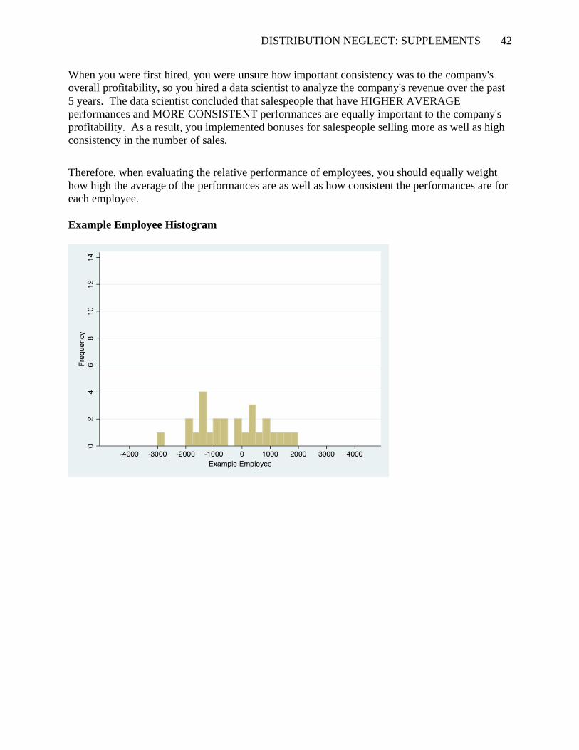
Example Employee Histogram
DISTRIBUTION NEGLECT: SUPPLEMENTS 43
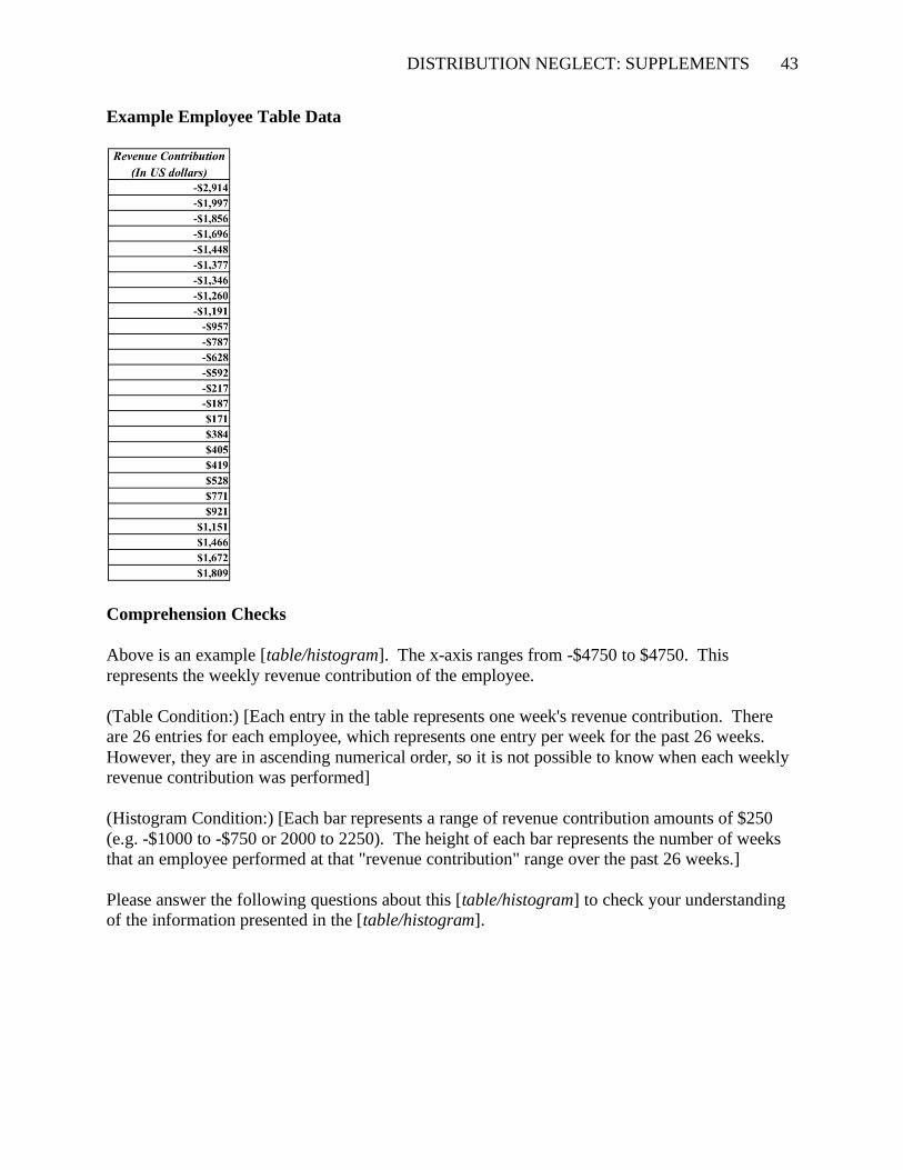
Example Employee Table Data
Comprehension Checks
Above is an example [table/histogram]. The x-axis ranges from -$4750 to $4750. This
represents the weekly revenue contribution of the employee.
(Table Condition:) [Each entry in the table represents one week's revenue contribution. There
are 26 entries for each employee, which represents one entry per week for the past 26 weeks.
However, they are in ascending numerical order, so it is not possible to know when each weekly
revenue contribution was performed]
(Histogram Condition:) [Each bar represents a range of revenue contribution amounts of $250
(e.g. -$1000 to -$750 or 2000 to 2250). The height of each bar represents the number of weeks
that an employee performed at that "revenue contribution" range over the past 26 weeks.]
Please answer the following questions about this [table/histogram] to check your understanding
of the information presented in the [table/histogram].
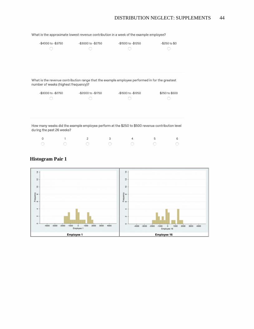
DISTRIBUTION NEGLECT: SUPPLEMENTS 44
Histogram Pair 1
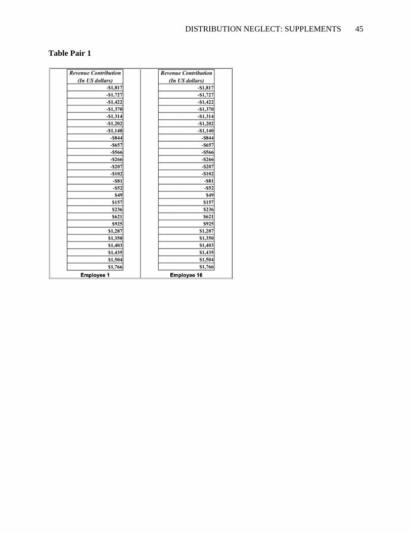
DISTRIBUTION NEGLECT: SUPPLEMENTS 45
Table Pair 1
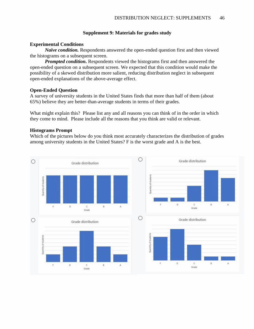
DISTRIBUTION NEGLECT: SUPPLEMENTS 46
Supplement 9: Materials for grades study
Experimental Conditions
Naïve condition. Respondents answered the open-ended question first and then viewed
the histograms on a subsequent screen.
Prompted condition. Respondents viewed the histograms first and then answered the
open-ended question on a subsequent screen. We expected that this condition would make the
possibility of a skewed distribution more salient, reducing distribution neglect in subsequent
open-ended explanations of the above-average effect.
Open-Ended Question
A survey of university students in the United States finds that more than half of them (about
65%) believe they are better-than-average students in terms of their grades.
What might explain this? Please list any and all reasons you can think of in the order in which
they come to mind. Please include all the reasons that you think are valid or relevant.
Histograms Prompt
Which of the pictures below do you think most accurately characterizes the distribution of grades
among university students in the United States? F is the worst grade and A is the best.
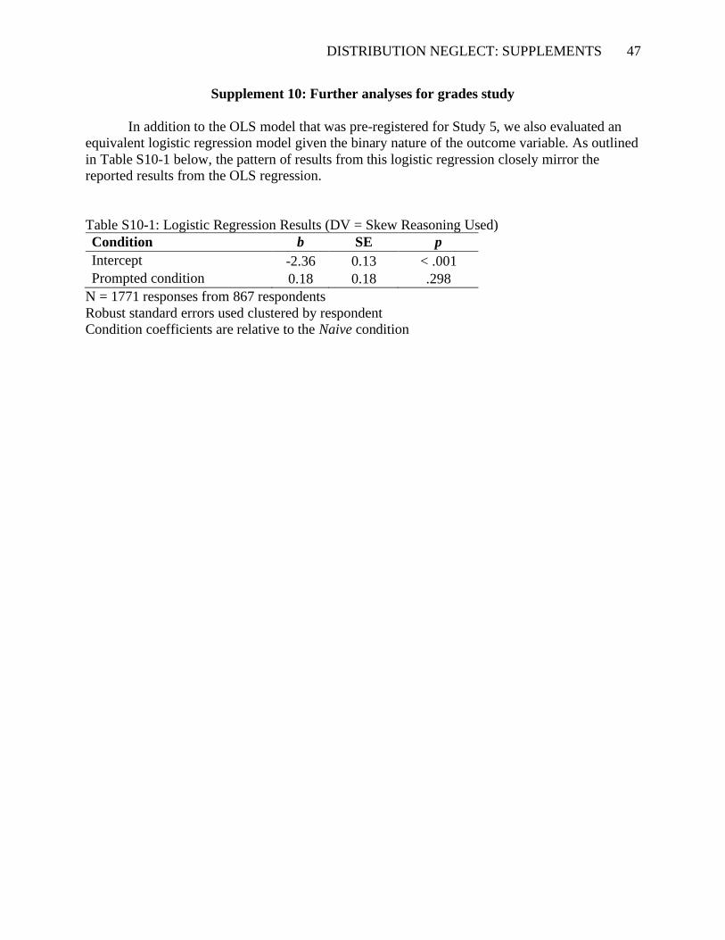
DISTRIBUTION NEGLECT: SUPPLEMENTS 47
Supplement 10: Further analyses for grades study
In addition to the OLS model that was pre-registered for Study 5, we also evaluated an
equivalent logistic regression model given the binary nature of the outcome variable. As outlined
in Table S10-1 below, the pattern of results from this logistic regression closely mirror the
reported results from the OLS regression.
Table S10-1: Logistic Regression Results (DV = Skew Reasoning Used)
Condition b SE p
Intercept -2.36 0.13 < .001
Prompted condition 0.18 0.18 .298
N = 1771 responses from 867 respondents
Robust standard errors used clustered by respondent
Condition coefficients are relative to the Naive condition
DISTRIBUTION NEGLECT: SUPPLEMENTS 48
Supplement 11: Potential real-world examples of distribution neglect
Although admittedly speculative, it is worth considering some recent events from the headlines
in which distribution neglect may have played a role.
• Financial fraud. Even experienced financial experts and investigators failed to realize
the financial information reported by fraudulent firms such as Bernard L. Madoff
Investment Securities and Enron exhibited inadequate volatility, with overly similar
profits and growth reported time period after time period (Fung, 2010).
• Academic fraud. Likewise, numerous expert scientific reviewers missed clear-cut cases
of fabricated data in scores of articles by Diederik Stapel and others, studies reporting
impossibly little volatility in standard deviations and means (Simonsohn, 2013;
Simonsohn, 2014).
• Disbelief in climate change. Enough members of the public interpret streaks of cold
weather as evidence against climate change, which involves not only gradually increasing
temperatures but also more volatile and extreme temperatures, that popular publications
such as Business Insider, USA Today, Forbes, and The Guardian have dedicated articles
to explaining “why cold weather doesn’t mean global warming isn’t real” (McGowan &
Walters, 2017; Roth, 2017; Shepherd, 2017; Spector & Harvey, 2014; Williams, 2018).
• Gender stereotypes. Women’s underrepresentation in STEM fields contributes to
strongly held social stereotypes regarding average gender differences in math ability—
yet mean gender differences are in fact trivial, and men tend to exhibit greater overall
variance in performance (Hedges & Nowell, 1995; Hyde, Fennema, & Lamon, 1990;
Hyde & Mertz, 2009).
• Athletic contracts. Anecdotal cases abound of star athletes whose high mean
performance in a streak of games leads to a big signing or new contract, neglecting
inconsistencies in long run performance (Seward, 2018; White & Sheldon, 2014).
Like most complex decisions and social phenomena, the above examples are no doubt multiply
determined. For instance, recent streaks of peak performance may bias labor contract decisions
due to the availability bias (Barnes & Morgeson, 2007; Tversky & Kahneman, 1973; Tversky &
Kahneman, 1974), and political beliefs can bias interpretations of scientific evidence related to
climate change (Lewandowsky, Oberauer, & Gignac, 2013; Lord, Ross, & Lepper, 1979).
However, we suggest that distribution neglect is an additional and novel contributor that these
real-world examples may all have in common.
References for S11
Barnes, C. M., & Morgeson, F. P. (2007). Typical performance, maximal performance, and
performance variability: Expanding our understanding of how organizations value
performance. Human Performance, 20(3), 259-274.
DISTRIBUTION NEGLECT: SUPPLEMENTS 49
Fung, K. (2010). Numbers rule your world: The hidden influence of probability and statistics on
everything you do. New York: McGraw-Hill.
Hedges, L. V., Nowell, A. (1995). Sex differences in mental test scores, variability, and numbers
of high-scoring individuals. Science, 269(5220), 41–5.
Hyde, J. S., Fennema, E., & Lamon, S. J. (1990). Gender differences in mathematics
performance: A meta-analysis. Psychological Bulletin, 107(2), 139.
Hyde, J., & Mertz, J. (2009). Gender, culture, and mathematics performance. Proceedings of the
National Academy of Sciences, 106(22), 8801-8807.
Lewandowsky, S., Oberauer, K., & Gignac, G. E. (2013). NASA faked the moon landing—
therefore,(climate) science is a hoax: An anatomy of the motivated rejection of science.
Psychological Science, 24(5), 622-633.
Lord, C. G., Ross, L., & Lepper, M. R. (1979). Biased assimilation and attitude polarization: The
effects of prior theories on subsequently considered evidence. Journal of Personality and
Social Psychology, 37(11), 2098.
McGowan, M. & Walters, J. (2017, December 29). Trump’s call for some ‘good old global
warming’ ridiculed by climate experts. The Guardian. Retrieved September 6, 2018,
from https://www.theguardian.com/us-news/2017/dec/29/donald-trump-good-old-global-
warming-us-winter
Roth, S. (2017, December 28). It’s cold outside, but that doesn’t mean climate change isn’t real.
USA Today. Retrieved September 6, 2018, from
https://www.usatoday.com/story/weather/2017/12/28/its-cold-outside-but-doesnt-mean-
climate-change-isnt-real/987948001/
Seward, J. (2018). From the $60m man who dazzled for Brazil but not at Manchester United to a
controversial Liverpool flop: 10 of the worst post-World Cup signings. Daily Mail.
Retrieved from https://www.dailymail.co.uk/sport/football/article-5795767/10-worst-
post-World-Cup-signings.html
Shepherd, M. (2017, December 28). A response for people using record cold U.S. weather to
refute climate change. Forbes. Retrieved September 6, 2018, from
https://www.forbes.com/sites/marshallshepherd/2017/12/28/a-response-for-people-using-
record-cold-u-s-weather-to-refute-climate-change/#109c8e335680
Spector, D., & Harvey, C. (2014, November 21). Why cold weather doesn't mean global
warming isn't real. Business Insider. Retrieved September 6, 2018, from
https://www.businessinsider.com/cold-weather-doesnt-discredit-climate-change-2014-
11/?IR=T
Simonsohn, U. (2013). Just post it: The lesson from two cases of fabricated data detected by
statistics alone. Psychological Science, 24(10), 1875-1888.
Simonsohn, U. (2014). Fake Data: Mendel Vs. Stapel [Blog post]. Datacolada. Retrieved from
http://datacolada.org/19
Tversky, A., & Kahneman, D. (1973). Availability: A heuristic for judging frequency and
probability. Cognitive Psychology, 5(2), 207-232.
Tversky, A., & Kahneman, D. (1974). Judgment under uncertainty: Heuristics and biases.
Science, 185(4157), 1124-1131.
White, M. H., & Sheldon, K. M. (2014). The contract year syndrome in the NBA and MLB: A
classic undermining pattern. Motivation and Emotion, 38(2), 196-205.
Williams, A. (2018). Why snow, colder weather conditions don’t debunk climate change.
AccuWeather. Retrieved September 6, 2018, from

DISTRIBUTION NEGLECT: SUPPLEMENTS 50
https://www.accuweather.com/en/weather-news/why-snow-colder-weather-conditions-
dont-debunk-climate-change/70003753
DISTRIBUTION NEGLECT: SUPPLEMENTS 51
Supplement 12: Range study
In this supplemental study, we posited that when people do think in terms of variance,
ranges may be more intuitive than standard deviations. The range of a distribution is least
correlated with its variance when extreme or outlying observations cause the range to
dramatically increase, while the variance increases comparatively less so. Individuals are
disproportionately attentive to outliers in group behavior, to the extent that they may even bias
one’s judgments of the rest of the distribution (Dannals & Miller, 2017). This suggests that
individuals may use the range of a distribution as a proxy for the variance of that distribution
because the extreme of the distribution may be more salient than the relative variability within it.
In an experimental context, we examined whether individuals tended to prefer
information about ranges versus variance when making decisions (i.e., exhibit a “range bias”).
We designed a paradigm in which participants make an incentivized choice using either range or
percentile information to aid in their decision. Percentiles capture a measure of dispersion similar
to range but are more sensitive to the general variance of the distribution than range values. To
the extent individuals prefer range information to percentiles, they lose out on some valuable
information and may become more attentive to outliers.
We asked participants to pick between two random number generators and told them that
they would be paid the number generated in cents at the end of the study. We told participants
that both distributions had the same average but that before picking one, they had the option to
receive some information about distributions of the numbers in each number generator. They
rated how useful each of two types of information would be in their decision: “The highest and
lowest number written on a ball in each machine” vs. “The 10th lowest number and the 10th
highest number written on a ball (i.e., the 20th and 80th percentile of the distribution) in each
machine.”
Methods
Participants. We recruited 234 respondents via Prolific.co, requiring residence in the
United States. Participants were required to answer a comprehension check in order to advance
in the survey and those who answered incorrectly were paid but removed from data analysis
leaving a final sample size of N = 191. The median age of participants was 25 years, 42.9% of
the sample self-identified as female, and 57.1% self-identified as male.
Procedure. After providing informed consent participants were shown two ball machines
like those used in bingo or lotteries and were told they would need to choose between the two
machines each of which contained 50 balls. Participants were told that they would receive “a
bonus payment equal to the number written on the ball in US cents. For example, if the ball read
56, you would receive $0.56 as your bonus.” Furthermore, participants learned that “each
machine has a different distribution of numbered balls” and that they would have the opportunity
to learn more about each choosing one. Participants then learned that both distributions had an
average of 14.49 but the distributions differed in other aspects.
Participants then rated how useful two measures of dispersion (“The highest and lowest
number written on a ball in each machine” and “The 10th lowest number and the 10th highest
number written on a ball (i.e. the 20th and 80th percentile of the distribution) in each machine”)
were on a scale from “1,” “Not at all Useful” to “7,” “Extremely Useful” and were asked in a
binary choice which they would prefer to learn. After making their choice participants received
their preferred information and made a binary choice of which ball machine they would like to
use for their bonus payment generation.
DISTRIBUTION NEGLECT: SUPPLEMENTS 52
Finally, participants were asked which they would prefer between two gambles: a 10%
chance of a bonus of $0.99, and a 90% chance of a bonus of $0.05 or a 44% chance of a bonus of
$0.20, and a 56% chance of a bonus of $0.10. Unbeknownst to participants, these percentages
closely mapped on to the distributions that they already chose between in the ball machines.
This was done to check whether decisions in the ball task matched true risk preferences.
Results
Participants viewed learning the percentiles, M = 4.87, SD = 1.75, as similarly useful to
learning the range, M = 5.06, SD = 1.59, t(190) = -1.08, p = 0.281. However, participants were
significantly more likely to choose to learn the percentiles, n = 113 than the range, n = 78, x2 =
6.41, p = 0.011. Participants who chose to receive the range information overwhelming chose
Machine A, n = 64, which featured a heavily skewed distribution where most values were 5 but
one outlier was 99 over Machine B, n = 14, which featured a more normally distributed set of
values around the mean. In contrast participants who chose to receive the percentile information
overwhelmingly chose Machine B, n = 95 over Machine A, n = 18.
We compared these decisions to those that participants made with complete gambling
information. Any participant who chose Machine A and then preferred the second gamble or
chose Machine B and then preferred the first gamble could be said to have inconsistent risk
preferences. Participants made similarly inconsistent decisions with regards to their risk
preference regardless of whether they received range information, ninconsistent = 34, or percentile
information, ninconsistent = 51, x2 = 0.003, p = 0.950.
In sum, offering evidence against the hypothesized preference for range information,
participants indicated that each type of information was similarly useful, and chose to learn the
percentiles significantly more often than the range information.
Reference S12
Dannals, J. E., & Miller, D. T. (2017). Social norm perception in groups with outliers. Journal of
Experimental Psychology: General, 146(9), 1342-1359.
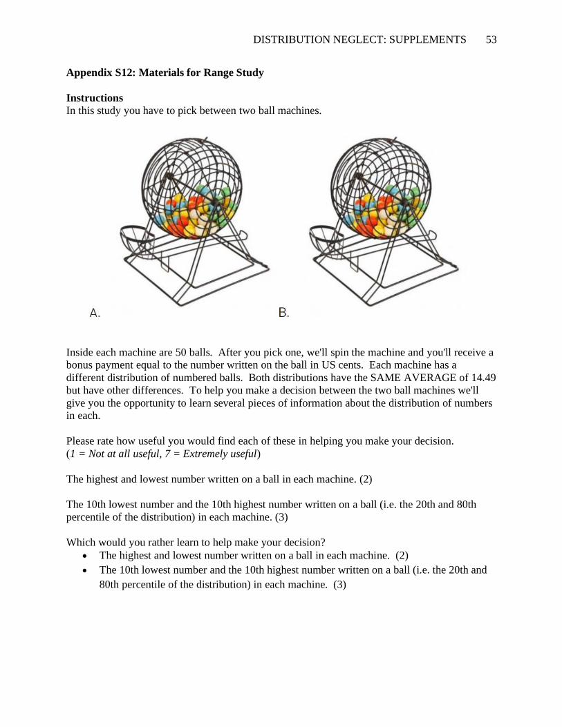
DISTRIBUTION NEGLECT: SUPPLEMENTS 53
Appendix S12: Materials for Range Study
Instructions
In this study you have to pick between two ball machines.
Inside each machine are 50 balls. After you pick one, we'll spin the machine and you'll receive a
bonus payment equal to the number written on the ball in US cents. Each machine has a
different distribution of numbered balls. Both distributions have the SAME AVERAGE of 14.49
but have other differences. To help you make a decision between the two ball machines we'll
give you the opportunity to learn several pieces of information about the distribution of numbers
in each.
Please rate how useful you would find each of these in helping you make your decision.
(1 = Not at all useful, 7 = Extremely useful)
The highest and lowest number written on a ball in each machine. (2)
The 10th lowest number and the 10th highest number written on a ball (i.e. the 20th and 80th
percentile of the distribution) in each machine. (3)
Which would you rather learn to help make your decision?
• The highest and lowest number written on a ball in each machine. (2)
• The 10th lowest number and the 10th highest number written on a ball (i.e. the 20th and
80th percentile of the distribution) in each machine. (3)
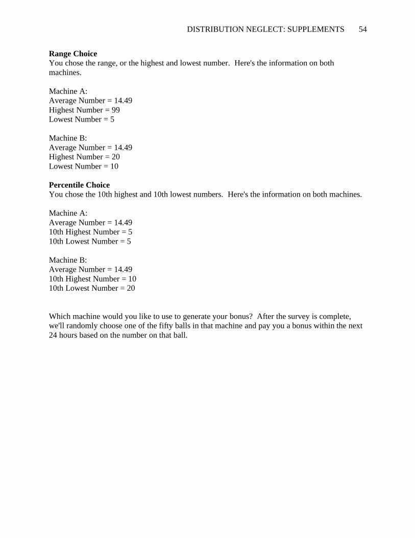
DISTRIBUTION NEGLECT: SUPPLEMENTS 54
Range Choice
You chose the range, or the highest and lowest number. Here's the information on both
machines.
Machine A:
Average Number = 14.49
Highest Number = 99
Lowest Number = 5
Machine B:
Average Number = 14.49
Highest Number = 20
Lowest Number = 10
Percentile Choice
You chose the 10th highest and 10th lowest numbers. Here's the information on both machines.
Machine A:
Average Number = 14.49
10th Highest Number = 5
10th Lowest Number = 5
Machine B:
Average Number = 14.49
10th Highest Number = 10
10th Lowest Number = 20
Which machine would you like to use to generate your bonus? After the survey is complete,
we'll randomly choose one of the fifty balls in that machine and pay you a bonus within the next
24 hours based on the number on that ball.