Embed Size (px)
Citation preview

Guidance Note 3A
Supplementary Guidance
Version 1.0
2 Guidance Note 3A – Supplementary Guidance
Document information
Document Name Supplementary Guidance to Guidance Note 3A
Version and Date Version 1.0 November 2018
Prepared by Ben du Bois
Approvals
Approval and
Authorisation
Name Position
Prepared by Ben du Bois Engineer
Major Infrastructure Projects Office (MIPO)
Approved by Mitch Pirie A/g General Manager
MIPO
Revision history
Issue Date Revision Description
Before using any downloaded PDF version of this guidance note, readers should check the
Department’s website at the below URL to ensure that the version they are reading is current. Note
that the current version of the Department’s Cost Estimation guidance supersedes and replaces all
previous cost estimation guidance published by the Department, other than that already included in
current versions of the NOA and NPA.
http://investment.infrastructure.gov.au/funding/projects/index/cost-estimation-guidance.aspx
Note that the examples in this guidance note have been developed using the proprietary software
programme @Risk and are used for demonstration purposes only. The Department does not
endorse @Risk and acknowledges the availability of similar software tools.
Guidance Note 3A – Supplementary Guidance 3
Table of Contents
1: Preamble ............................................................................................................................. 6
2: Introduction and background ............................................................................................... 6
2.1: The probabilistic nature of estimates ................................................................................... 6
2.2: Types of risk ........................................................................................................................ 8
2.3: Quantitative Risk Analysis ................................................................................................... 9
2.4: The aggregation problem .................................................................................................. 13
3: Risk models ....................................................................................................................... 15
3.1: Risk Factor methodology ................................................................................................... 16
3.2: Risk Driver methodology ................................................................................................... 17
3.3: Hybrid Parametric/Risk Event model ................................................................................. 18
3.4: First Principles Risk Analysis (FPRA) ................................................................................ 18
3.5: Line item models/3-point estimating .................................................................................. 19
3.6: The Department’s preferred approach ............................................................................... 21
4: Quantitative Risk Analysis using risk factors ...................................................................... 22
4.1: Variations from the base estimate ..................................................................................... 22
4.2: Common drivers ................................................................................................................ 22
4.3: Risk events ........................................................................................................................ 25
4.4: Uncertainty that should not be captured ............................................................................ 29
4 Guidance Note 3A – Supplementary Guidance
5: Risk Workshops and eliciting expert opinion ...................................................................... 32
5.1: Overview ........................................................................................................................... 32
5.2: Biases ............................................................................................................................... 33
5.3: Participation in assessment ............................................................................................... 34
5.4: Assessment process ......................................................................................................... 36
6: Model Structure ................................................................................................................. 43
6.1: Design principles ............................................................................................................... 43
6.2: General Structure .............................................................................................................. 46
6.3: Linking cost drivers to risk drivers ...................................................................................... 47
6.4: Choice of uncertainty distribution ....................................................................................... 49
6.5: Account for correlation between WBS element costs to properly capture cost risk ............ 52
6.6: Setting the seed ................................................................................................................ 54
6.7: Example risk factor model ................................................................................................. 54
6.8: Step through of model ....................................................................................................... 56
7: Analysis results ................................................................................................................. 63
8: Additional models .............................................................................................................. 67
8.1: Hybrid parametric/expected value method ......................................................................... 67
8.2: Risk Driver method ............................................................................................................ 73
8.3: First Principles Risk Analysis ............................................................................................. 75
Guidance Note 3A – Supplementary Guidance 5
Appendix A: Deriving risk factors .................................................................................................. 83
Appendix B: Simulation and statistical analysis ............................................................................. 89
Appendix C: Correlation ................................................................................................................ 92
Appendix D: Probability Distribution Functions ............................................................................ 104
Appendix E: Number of line items to model................................................................................. 110
Appendix F: Number of iterations to run in a simulation .............................................................. 114
Appendix G: Contingency allocation ........................................................................................... 119
Appendix H: Common modelling errors ....................................................................................... 122
Appendix I: Alternate approaches to eliciting expert opinion ....................................................... 126
Appendix J: Definitions and abbreviations ................................................................................... 128
References and further reading ................................................................................................... 131
6 Guidance Note 3A – Supplementary Guidance
1: Preamble This document is the supplementary guidance to guidance note 3A – Probabilistic Contingency
Estimation. It has been prepared to provide more in-depth discussion and supporting information
for those wishing to further enhance their understanding.
It covers the following topics:
Introduction and background – discusses the background and reasons for undertaking a
quantitative risk analysis on infrastructure projects;
Quantitative Risk Analysis (QRA) Workshops – discusses the techniques and
procedures for undertaking QRA workshops and for eliciting expert opinion, as part of
preparing a probabilistic cost estimate;
Cost Risk Model structure – accompanied by worked examples, outlines the principles to
assist analysts to build efficient and realistic risk models;
Cost risk models – discusses and provides examples of several quantitative cost risk
analysis approaches; and
Interpretation of output results – discusses how to analyse, understand and communicate
the output of a probabilistic risk analysis.
A number of appendices also support this guidance note providing further detail on:
Derivation of risk factors;
Simulation and statistical analysis;
Correlation;
Choice of probability distribution function;
Aggregation of inputs and number of line items to model;
Number of iterations to run in a simulation;
Common Monte Carlo simulation errors; and
Alternate approaches to eliciting expert opinion.
The appendices, while essentially stand-alone documents, should be read in the context of the
guidance as a whole.
2: Introduction and background “If you are sure you understand everything that is going on, you are hopelessly confused” – Walter
F. Mondale
2.1: The probabilistic nature of estimates
By their very nature, estimates are uncertain projections of future events and circumstances. Cost
(and schedule) estimating is an integral part of the project management process because
organisations use these estimates for planning purposes such as options appraisal, benefit/cost
analyses, resource allocation and budget allocation.
Guidance Note 3A – Supplementary Guidance 7
The word “estimate” itself implies uncertainty, so an estimate is not completely specified by a
single number. A distribution of possible outcomes is required to provide a realistic statement of an
estimate. The distribution of possible cost outcomes for a particular project is represented by an
estimate’s probability distribution that is calculated, or simulated, through the application of
probability and statistics. These are crucial concepts for it must be realised that the laws of
probability are the most powerful tools of risk management that we have at our disposal1; where
the future is unknown, the laws of probability will allow us to understand or make sense of the
outcome.
Uncertainty and Risk
It can be considered that there are two universal axioms in relation to estimating2:
You can’t estimate anything if you don’t understand what it is; and
All estimates are uncertain. The estimator/analyst’s job is to minimise the uncertainty, as far
as that can be done at each stage in a project.
If something is only partially understood, any estimate made about it will be uncertain. The size of
the likely error will roughly correspond to the lack of knowledge (i.e. the level of uncertainty). Early
estimates can be wrong by very large percentages which may be due to, among other things, an
incomplete understanding of all of the ramifications of the current design, and what it takes to
develop and implement it.
However, the objective is not to produce an estimate that is highly accurate from the first day of the
project (which is all but impossible), but to produce a sequence of estimates that become closer
and closer to the actual outturn cost as the project proceeds. The accuracy of the estimates at a
given point in a project’s development will reflect what is known about the project at that stage.
It is unavoidable that estimates have to be made and converted to budgets while information is still
incomplete. In that context, to the extent that the nature of the work is unknown or not clearly
understood when a funding, schedule, or other commitment must be made, there is a risk to
achieving the project forecast. It may be possible to reduce the uncertainty, and hence risk, if such
decisions to proceed and commitments against cost and schedule forecasts are made as late as
possible. However, it costs money to wait, to study a proposed project and to collect information.
Very often, waiting may not be possible due to time or other constraints3.
Thus, at the point a commitment is to be made, a realistic quantification of the risks must be
undertaken and sufficient resources, in addition to the base estimate, (i.e. contingency) allocated to
the project in order to ensure that the level of funding and other commitments that are made reflect
the organisation’s appetite to bear risk.
1 Bernstein, P., (1998) Against the Gods: The Remarkable Story of Risk, John Wiley & Sons Inc, New York 2 Adapted fom Stump E, (n.d.) Breakings Murphy’s Law: Project Risk Management (downloadable at galorath.com/wp-content/uploads/2014/08/stump_breaking_murphys_law.pdf) 3 Hamlet claimed one should not hesitate too long in the face of uncertainty because “the native hue of resolution is sicklied o’er with the pale cast of thought…and enterprises of great pith and moment…lose the name of action.” Once we act though, we lose the option of waiting until new information comes along. Thus, not acting has value and depending on the circumstances, the greater the uncertainty, the greater may be the value of waiting. (Shakespeare, W, circa 1600, The Tragedy of Hamlet, Prince of Denmark, Act III, Scene I)
8 Guidance Note 3A – Supplementary Guidance
2.2: Types of risk
ISO31000 defines risk as “the effect of uncertainty on objectives”. However, a large number of
alternate definitions are available within the literature. The majority emphasise that risk is
concerned with the chance of undesired events, usually within a specific time frame (such as
length of project, or other period of interest).
Defining risk mathematically also varies across disciplines. The value of a particular risk is not
necessarily simply calculated as the product of probability and consequence4.
In the context of risk analysis and identification, uncertainty can be thought of in two ways. The first
is a sense that the quantity we are trying to estimate (such as the volume of earthworks) has some
uncertainty attached to it. The second is risk events – random events that may or may not occur
which are of interest to us.
Terminology to distinguish between these two types of risk varies. A common distinction is to use
the terms inherent risk (to distinguish between uncertainty that is certain to have some effect) and
contingent risk (uncertainty that might have no effect or could have an effect - something like an
event). As another example, the US Federal Highway Administration Guide to Risk Assessemnt
and Allocation for Highway Construction Management5 notes that some risk may be measured
incrementally and continuously, whereas other risks are discrete
AACE International typifies risk as falling into one of two categories6: systemic risks, and project-
specific risks. Systemic risks are seen as being associated with the culture, capabilities and
practices of the engineering, estimating and construction communities that deliver projects so they
affect all projects in a particular sector, while project specific risks depend on the details of an
individual project.
Systemic risks
The term systemic implies that the risk is an artefact of the system that conceives of, estimates and
plans, and then implements the project. It includes features such as the quality of the management
team and forecasting methods and the commercial arrangements under which the work will take
place. Research suggests that the impacts of some of these risks are measurable and predictable
for projects developed within the same system. They are generally known even at the earliest
stages of project definition where the impact of these risks tend to be highly dominant7. The
challenge is that the link between systemic risks and cost impacts is complicated as well as being
stochastic in nature, which means that is very difficult to understand and to directly estimate the
aggregate impact of these risks at an individual line-item level.
4 Hayes K (2011) Uncertainty and Uncertainty Analysis Methods (downloadable at https://publications.csiro.au/rpr/pub?pid=csiro:EP102467) 5 Federal Highway Administration (2006) Report FHWA-PL-06-032 Guide to Risk Assessemnt and Allocation for Highway Construction Management 6 AACE International (2008) RP No. 42R-08 Risk Analysis and Contingency Determination Using Parametric Estimating 7 Hollmann, J (2016) Project Risk Quantification: A Practitioner’s Guide to Realistic Cost and Schedule Risk Management, Probabilistic Publishing, Gainesville, FL
Guidance Note 3A – Supplementary Guidance 9
In general, systemic risks are owner risks; the owner is responsible for early definition, planning
and so on, which are risks that cannot be readily transferred to contractors. Typical systemic risks
for infrastructure projects include:
Project definition:
o Geotechnical requirements;
o Engineering and design;
o Safety and environmental risks and/or approvals; and
o Planning and schedule development.
Project management and estimating process:
o Estimate inclusiveness;
o Team experience and competency;
o Cost information availability; and
o Estimate bias.
Project-specific risks
Project-specific risks are specific to a particular project and therefore the impacts of these risks
may not be the same from one project to the next. Measures of these risks will generally not be
known at the earliest stages of project definition. The link between project-specific risks and cost
impacts is more easily understood than systemic risk and can make it easier to estimate the impact
of these risks on specific items or activities. These risks are amenable to individual understanding
and quantification using expected value or simulation techniques. For example, it may be possible
to estimate the impact of wet weather on earthworks activities reasonably accurately or at least
appreciate the range of impacts it could have. Typical project specific risks may include:
Weather;
Site subsurface conditions;
Delivery delays;
Constructability;
Resource availability;
Project team issues; and
Quality issues;
For the purposes of this guidance note, the AACE typologies as just described are preferred and
will be utilised when distinguishing between risk types.
2.3: Quantitative Risk Analysis
Quantitative risk analysis and modelling provides a means of8:
Describing the detailed mechanisms at work in the way uncertainty affects a project;
8 Cooper D, Bosnich P, Grey S, Purdy G, Raymond G, Walker P, Wood M, (2014) Project Risk Management Guidelines: Managing Risk with ISO 31000 and IEC 62198 2nd Edition, John Wiley and Sons Ltd, Chichester

10 Guidance Note 3A – Supplementary Guidance
Evaluating the overall uncertainty in the project and the overall risk that this places on
stakeholders;
Establishing targets, commitments and contingency amounts consistent with the uncertainty
the project faces and the risk that managers are willing to accept;
Exploring the relationship between detailed instances of uncertainty and an overall level of
risk, to inform risk management resource allocation and other measures that may be taken
to optimise the project.
There are several ways to quantify risks or to estimate contingency. Each method has strengths
and weaknesses. Some have been shown to lead people into poor practices. AACE International
Recommended Practice No. 40R-08 “Contingency Estimating – General Principles”9 notes that any
methodology developed or selected for quantifying risk impact should address the following
general principles:
Meet client objectives, expectations and requirements;
Forms part of and facilitates an effective decision or risk management process;
Fit-for-use;
Starts with identifying the risk drivers with input from all appropriate parties;
Methods clearly link risk drivers and cost/schedule outcomes;
Avoids iatrogenic (self-inflicted) risks;
Employs empiricism (experience of past projects);
Employs experience/competency; and
Provides probabilistic estimating results in a way that supports effective decision making
and risk management.
Quantitative risk analysis is the process of identifying and analysing critical project risks within a
defined set of cost, schedule, and technical objectives and constraints. It assists decision makers
to balance the consequences of failing to achieve a particular outcome against the probability of
failing to achieve that outcome. Its purpose is to capture uncertainty in such areas as cost
estimating methodology, completeness and reliability of the information available, technical risk,
and programmatic factors in order to go from a deterministic point estimate to a probabilistic
estimate.
A credible base estimate (see guidance note 2 – Base Cost Estimation) is the key starting point in
generating a risk-adjusted estimate and the development of confidence intervals. Risk analysis
provides an analytical basis for establishing defensible cost estimates that quantitatively account
for the realistic effect of project risks. It is important that this analysis be continuously reviewed and
updated as more data become available during the development of a design, estimates and plans.
Throughout this process, interactions take place between the following actors10:
9 AACE International (2008) RP No. 40R-08 Contingency Estimating – General Principles, AACE International, Morgantown, WV 10 Zio & Pedroni (2012) Overview of Risk-Informed Decision-Making Processes (downloadable at https://www.foncsi.org/fr/publications/collections/cahiers-securite-industrielle/overview-of-risk-informed-decision-making-processes/CSI-RIDM.pdf)
Guidance Note 3A – Supplementary Guidance 11
The stakeholders (individuals or organisations that are affected by the outcome of a decision
but are outside the organisation doing the work or making the decision);
The risk analysts (individuals or organisations that apply probabilistic methods to the
quantification of risks and performances);
The subject matter experts (individuals or organisations with expertise in one or more topics
within the decision domain of interest);
The technical authorities; and
The decision-maker.
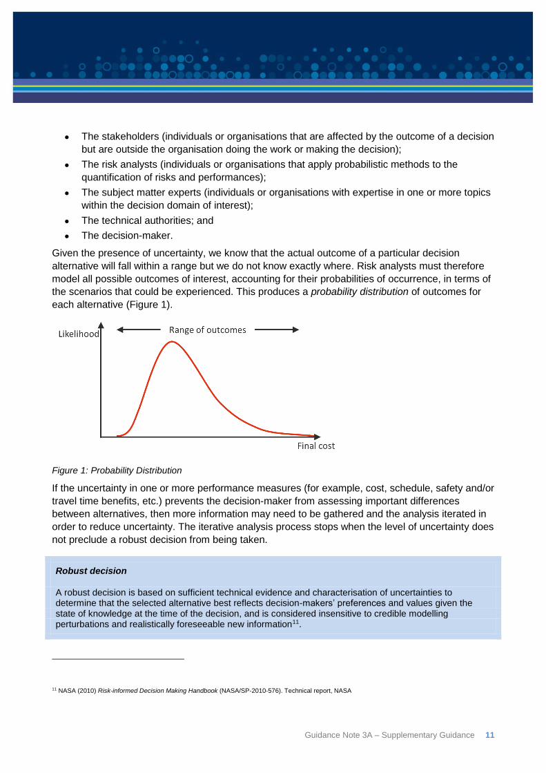
Given the presence of uncertainty, we know that the actual outcome of a particular decision
alternative will fall within a range but we do not know exactly where. Risk analysts must therefore
model all possible outcomes of interest, accounting for their probabilities of occurrence, in terms of
the scenarios that could be experienced. This produces a probability distribution of outcomes for
each alternative (Figure 1).
Figure 1: Probability Distribution
If the uncertainty in one or more performance measures (for example, cost, schedule, safety and/or
travel time benefits, etc.) prevents the decision-maker from assessing important differences
between alternatives, then more information may need to be gathered and the analysis iterated in
order to reduce uncertainty. The iterative analysis process stops when the level of uncertainty does
not preclude a robust decision from being taken.
Robust decision
A robust decision is based on sufficient technical evidence and characterisation of uncertainties to determine that the selected alternative best reflects decision-makers’ preferences and values given the state of knowledge at the time of the decision, and is considered insensitive to credible modelling perturbations and realistically foreseeable new information11.
11 NASA (2010) Risk-informed Decision Making Handbook (NASA/SP-2010-576). Technical report, NASA
12 Guidance Note 3A – Supplementary Guidance
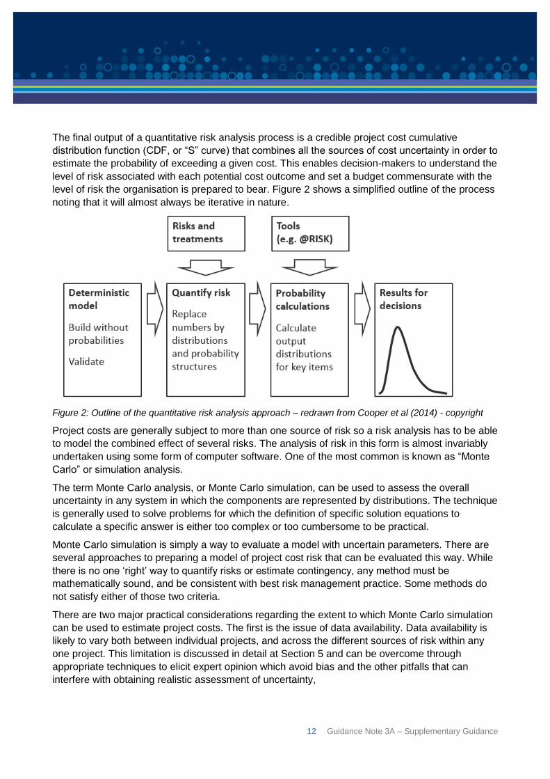
The final output of a quantitative risk analysis process is a credible project cost cumulative
distribution function (CDF, or “S” curve) that combines all the sources of cost uncertainty in order to
estimate the probability of exceeding a given cost. This enables decision-makers to understand the
level of risk associated with each potential cost outcome and set a budget commensurate with the
level of risk the organisation is prepared to bear. Figure 2 shows a simplified outline of the process
noting that it will almost always be iterative in nature.
Figure 2: Outline of the quantitative risk analysis approach – redrawn from Cooper et al (2014) - copyright
Project costs are generally subject to more than one source of risk so a risk analysis has to be able
to model the combined effect of several risks. The analysis of risk in this form is almost invariably
undertaken using some form of computer software. One of the most common is known as “Monte
Carlo” or simulation analysis.
The term Monte Carlo analysis, or Monte Carlo simulation, can be used to assess the overall
uncertainty in any system in which the components are represented by distributions. The technique
is generally used to solve problems for which the definition of specific solution equations to
calculate a specific answer is either too complex or too cumbersome to be practical.
Monte Carlo simulation is simply a way to evaluate a model with uncertain parameters. There are
several approaches to preparing a model of project cost risk that can be evaluated this way. While
there is no one ‘right’ way to quantify risks or estimate contingency, any method must be
mathematically sound, and be consistent with best risk management practice. Some methods do
not satisfy either of those two criteria.
There are two major practical considerations regarding the extent to which Monte Carlo simulation
can be used to estimate project costs. The first is the issue of data availability. Data availability is
likely to vary both between individual projects, and across the different sources of risk within any
one project. This limitation is discussed in detail at Section 5 and can be overcome through
appropriate techniques to elicit expert opinion which avoid bias and the other pitfalls that can
interfere with obtaining realistic assessment of uncertainty,
Guidance Note 3A – Supplementary Guidance 13
The second consideration is the extent of correlation between those variables selected for risk
analysis. Projects are rarely subject to only one source of risk, which is why more than one variable
at a time is modelled in the Monte Carlo simulation exercise12, and statistical complexities can
arise in the relationships between variables. Where variables may be thought to be related, the
extent of corelation between them needs to be taken into account.
The cardinal rule of Monte Carlo simulation can be expressed as: “Every iteration of a risk analysis
model must be a scenario that could physically occur”13. The model must therefore be prevented
from producing, in any iteration, any combination of values that could not possibly materialise. One
way in which this can occur is by not accounting for the interdependency between the model
inputs.
It is often poorly understood that valid Monte Carlo simulation requires that the dependencies
between model inputs be defined. In fact, being able to define the relationships between uncertain
input distributions was arguably the key motivating factor behind the development/invention of what
is now known as the Monte Carlo method by Stanislaw Ulam in the late 1940’s14.
As an example, if two variables in an analysis are market rates for locally produced concrete and
market rates for locally sourced construction plant, it will not generally be realistic to select a value
for one that is at the high end of its possible range and a value for the other at the low end of its
possible range. Similar pressures of supply and demand in the local economy will tend to drive
them both towards the high end, the low end or the middle of their ranges rather than one being
high and the other low. Misapplication of Monte Carlo simulation, or poor modelling technique, is
likely to see such implausible situations arise.
The correlation between variables in any analysis must be understood, however as explained at
Section 6 and at Appendix C this can be difficult to achieve in practice. As well as the difficulty of
addressing correlation, and in part because of not accounting for it, some approaches in common
use, such as line-item ranging, if not applied correctly will produce an unrealistically narrow range
of possible costs. They will understate the required contingency at higher confidence levels, as well
as understate the probability of achieving lower cost outcomes. Many of the inherent difficulties
within line-item ranging approaches are well recognised but attempts to overcome them, by
building in complex overlapping correlations, usually result in models that are far more complicated
than they need be without necessarily making them any more realistic.
2.4: The aggregation problem
The choice of level to which detailed costs are aggregated into components of an analysis and the
evaluation of correlation between the components are critical to the validity of results of a
simulation. Level of aggregation refers to the level of detail with which an analysis is framed, which
is almost always a lot less than the detail in an estimate. In the cost of a road, the costs of clearing
and grubbing, earthworks, base, sub-base and pavements can all be distinguished. The cost of
12 Asian Development bank (2002) Handbook for Integrating Risk Analysis in the Economic Analysis of Projects 13 Vose, D (2008) Risk Analysis: A Quantitative Guide, John Wiley and Sons Ltd, Chichester 14 Metropolis, N & Ulam, S (1949) The Monte Carlo Method, Journal of the American Statistical Association, Vol 44, No 247. (Sep., 1949), pp. 335-341

14 Guidance Note 3A – Supplementary Guidance
these elements such as the base can be further subdivided into the costs of extracting stones,
crushing them, transporting them, and laying them, and each of those stages can also be broken
down. By dealing with components separately – by disaggregating - it is possible to more
confidently understand the range of costs each component might have.
While it may seem that the more disaggregation the better, it comes at a cost because many of the
disaggregated components will be driven by the same sources of uncertainty as one another. This
means that in real life they will be correlated with one another and this has to incorporated into a
model, which is very difficult to do realistically. There is a balance to be struck between the
uncertainty that arises when cost elements are summarised to a high level and being able to
assess uncertainty more easily as costs are disaggregated.
In broad terms, we find it easier to speak with confidence about the value and uncertainty in
individual cost of small elements of a project’s cost but we find it harder and harder to build a
realistic model that takes account of correlations and other dependencies between these elements
the more there are. On the other hand, if a project’s cost is lumped into a very small number of
items, those items will often be composed of varying proportions of separate materials, trades,
services, equipment that will be difficult to disentangle.
There are essentially two ways to deal with correlation and aggregation:
a) Limit the disaggregation
Limiting disaggregation solves the problem of correlation by largely eliminating it. Working, for
example, with the total cost of a road means there is no need to worry about the correlation
between variables such as the cost of the base and the cost of the wearing surface. The
distribution used for the cost of the road as a whole will implicitly include this relationship.
However, as previously discussed, there is a limit to the amount of aggregation that still permits
clear judgements to be made about the variability of the cost of a project. Working at a very high
level of aggregation will result in very wide range of uncertainty which is not informative for
budgetary decision-making purposes. It might also result in an unrealistic assessment of the
amount of uncertainty because of the difficulty of thinking about a lot of sources of uncertainty and
their interactions all at the same time, especially if the large aggregated parts of the cost share
common sources of uncertainty.
b) Isolate the sources of uncertainty
It is specifically recommended that disaggregation of homogeneous variables within which only a
small number of uncertainties are at work be limited as much as possible so as to avoid including
too much correlation in the analysis15. It has been recognised for decades16 that it is more helpful
to think not so much in terms of disaggregating the technological components of a project, but in
terms of separating the sources of uncertainty. By defining the sources of uncertainty and
determining their impact on the different cost elements, the correlation between cost elements
caused by sharing a source of uncertainty is included within a risk model in a natural way, often as
15 Asian Development bank (2002) Handbook for Integrating Risk Analysis in the Economic Analysis of Projects 16 Pouliquen L (1970) Risk Analysis in Project Appraisal World Bank Staff Occasional Papers Number Eleven, John Hopkins Press, Baltimore
Guidance Note 3A – Supplementary Guidance 15
functional relationships such as between a quantity and a rate that both affect a major part of the
total cost.
This isolation of independent sources of uncertainty and determination of how they may affect the
cost of a project, in most cases, is the easiest and most rigorous way of avoiding the need for
complicated correlations in a model and is usually referred to as either a Risk Factor, or Risk Driver
approach.
3: Risk models Common probabilistic cost risk modelling methods can be grouped loosely into three types17:
Line item ranging, which applies a distribution to each line in an estimate or summary of an
estimate;
Risk event models, in which uncertainties are described in terms of the likelihood of them
arising and the effect they will have on the cost; and
Risk factor/risk driver models in which uncertainties are described in terms of drivers that
might each affect several cost elements and where several drivers might act together on a
single cost, with a many-to-many relationship between risks and costs.
Hybrid methods such as a model using a parametric approach for systemic risk impact combined
with expected value for project-specific risks may be regarded as a separate approach again.
A project’s cost estimate is generally updated during each phase of the project life cycle as project
scope is defined, modified and refined18. As the level of scope definition increases, the estimating
methods used become more definitive and produce estimates with increasingly narrow probabilistic
cost distributions. The specific estimating tools and techniques may vary depending upon:
The general type of risks and specific significant risks associated with a given project;
The level of definition of scope information available;
Availability or otherwise of data required to allow certain approaches to be used;
Skill and/or confidence level of the analyst. For example, while this guidance note does not
cover integrated cost-schedule risk analysis, project proponents and/or their contractors are
welcome to submit integrated cost-schedule risk analyses as part of funding submissions.
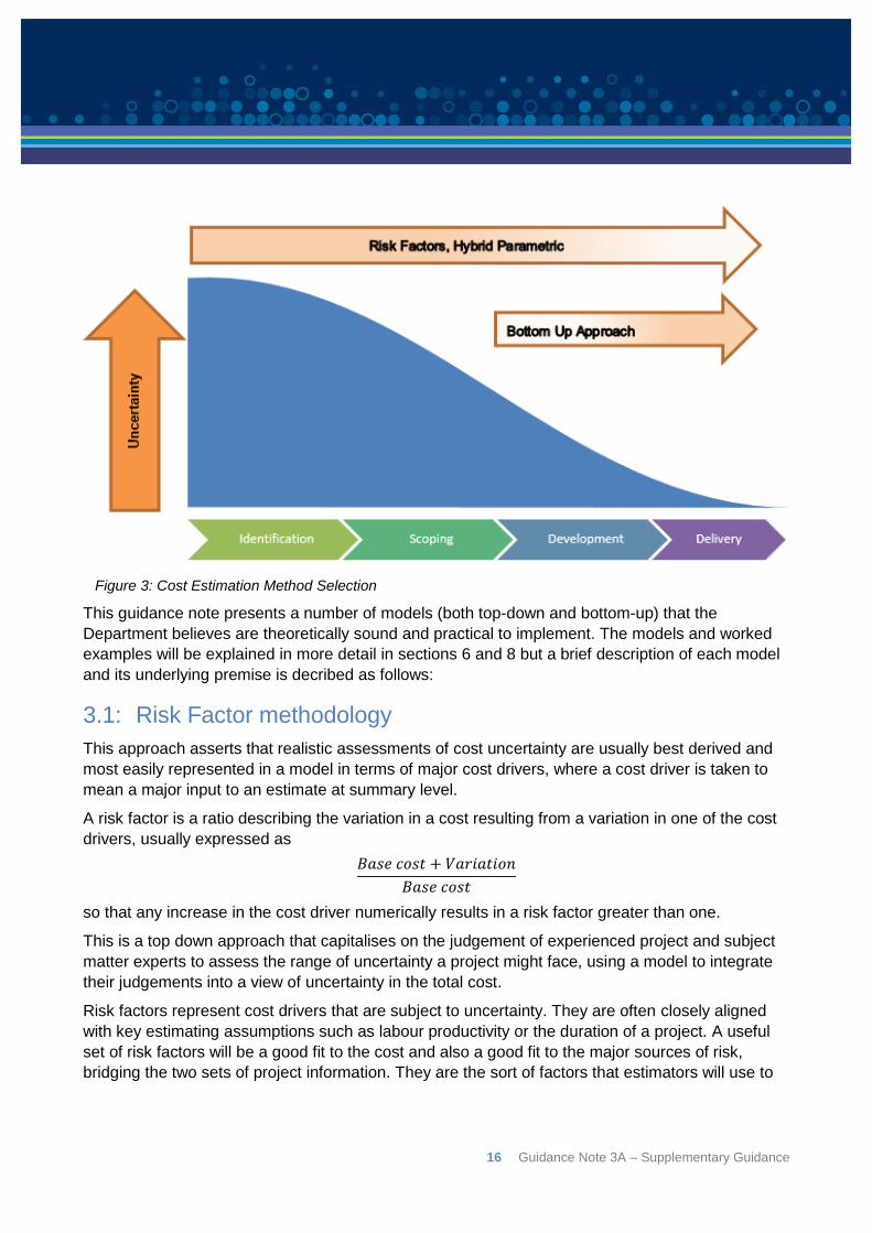
The appropriate estimate methodology may change as a project proceeds through its lifecycle. In
general, it would be expected that a top-down approach would be utilised in the earlier phases, and
that it may be appropriate to use a bottom-up approach for later estimates as a design is
increasingly refined. This is shown diagrammatically below in Figure 3.
17 Broadleaf 2014, Discussion paper: Weaknesses in common project cost risk modelling methods (downloadable at http://broadleaf.com.au/resource-material/weaknesses-of-common-project-cost-risk-modelling-methods/) 18 AACE (2015) Total Cost Management Framework: An Integrated Approach to Portfolio, Program, and Project Management, AACE International, Morgantown, WV
16 Guidance Note 3A – Supplementary Guidance
This guidance note presents a number of models (both top-down and bottom-up) that the
Department believes are theoretically sound and practical to implement. The models and worked
examples will be explained in more detail in sections 6 and 8 but a brief description of each model
and its underlying premise is decribed as follows:
3.1: Risk Factor methodology
This approach asserts that realistic assessments of cost uncertainty are usually best derived and
most easily represented in a model in terms of major cost drivers, where a cost driver is taken to
mean a major input to an estimate at summary level.
A risk factor is a ratio describing the variation in a cost resulting from a variation in one of the cost
drivers, usually expressed as
𝐵𝑎𝑠𝑒 𝑐𝑜𝑠𝑡 + 𝑉𝑎𝑟𝑖𝑎𝑡𝑖𝑜𝑛
𝐵𝑎𝑠𝑒 𝑐𝑜𝑠𝑡
so that any increase in the cost driver numerically results in a risk factor greater than one.
This is a top down approach that capitalises on the judgement of experienced project and subject
matter experts to assess the range of uncertainty a project might face, using a model to integrate
their judgements into a view of uncertainty in the total cost.
Risk factors represent cost drivers that are subject to uncertainty. They are often closely aligned
with key estimating assumptions such as labour productivity or the duration of a project. A useful
set of risk factors will be a good fit to the cost and also a good fit to the major sources of risk,
bridging the two sets of project information. They are the sort of factors that estimators will use to
Figure 3: Cost Estimation Method Selection
Guidance Note 3A – Supplementary Guidance 17
make rapid ‘what-if’ assessments of the cost diffences between options or to assess the impact of
late changes to a design or implementation strategy.
The risk factor method, assessed using Monte Carlo simulation, has a number of advantages:
In most cases will result in a simpler, cleaner risk model than other approaches;
Analysis generally requires less time than when using line-item estimating;
Risk factor models can accommodate risks that interact and overlap without introducing
intractable correlations into the model;
They model the relationship of risk drivers to cost outcomes allowing management to see
the connection between a given risk and the potential impact;
They make it easier to calculate the effect of individual risks on the cost, and then sort the
risks by priority; and
They make it simpler to take risks out of the simulation one at a time in order to determine
their marginal impact.
Despite our best endeavours, it might not be possible to devise a set of risk factors that are
completely independent of one another, such as where they depend on the same market
conditions, and it might stil be necessary to include correlation in a model. One objective of
designing a model and selecting risk factors is to minimise or avoid the need to specify
correlations. This can usually be achieved and any correlations that remain can be examined by
comparing a model with no correlation or full correlation between specific pairs. This can be used
to inform decision making and avoid the need to estimate partial correlations, which is all but
impossible to do reliably.
3.2: Risk Driver methodology
The risk driver method, described by David Hulett, has some of the same features and advantages
of the risk factor methodology and while sometimes seen as being synonomous, have subtle
differences. This guidance interprets a risk driver as per the definition given by Evin Stump19 as
follows:
A risk driver is any root cause that MAY force a project to have outcomes different to the plan.
The risk driver method in its purist form seeks to uncover the causative agents of uncertainty (root
causes) which, like the risk factor method, then assigns these drivers to the work elements that
they affect. One primary difference between the two methods is that risk factors represent cost
drivers that are subject to uncertainty and as such the risk factor method takes a pragmatic
approach to the use of inputs that might not be true root causes but do enable engineers and
estimators to describe their view of uncertainty associated with a particular aspect of a cost. The
other main difference is that the risk driver method, as generally practised, uses the existing risk
19 Stump, E. (2000) The Risk Driver Impact Approach to Estimation of Cost Risks: Clear Thinking About Project Cost Risk Analysis
18 Guidance Note 3A – Supplementary Guidance
register to identify the key risk drivers. It should also be noted that risks included in the analysis
using the risk driver method should be those at a strategic, rather than technical level.
3.3: Hybrid Parametric/Risk Event model
The premise of this approach is that systemic risks are best quantified using empirically validated
parametric modelling. Using appropriate data, the parametric tool will provide a cost distribution
(optimistic, most likely, pessimistic) representing the aggregate impact of the systemic risks. This
distribution is then combined with project specific risks and assessed using Monte Carlo
simulation.
Advantages of this approach are:
It is an easily understood approach with aspects that are already commonly used;
It employs empiricism and provides a mechanism for learning and continual improvement
as more project data is collected;
Once a parametric model has been developed and validated, using it to quantify systemic
risks should be replicable by analysts so long as they adopt the same approach to
assessing the inputs, thus providing confidence in the model.
The main disadvantages are the challenges and difficulty in obtaining and cleansing project data to
build and maintain the parametric model.
3.4: First Principles Risk Analysis (FPRA)
The Risk Engineering Society (RES) Contingency Guideline (Version 2, draft as at October 2018)
outlines a bottom-up risk-based approach which, for the purposes of that guideline, is defined as
First Principles Risk Analysis (FPRA). The approach aims to capture and validate uncertainties at
the lowest meaningful level of Work Breakdown Structure (WBS) against appropriate first principle
components of cost item (labour, plant, material and subcontract).
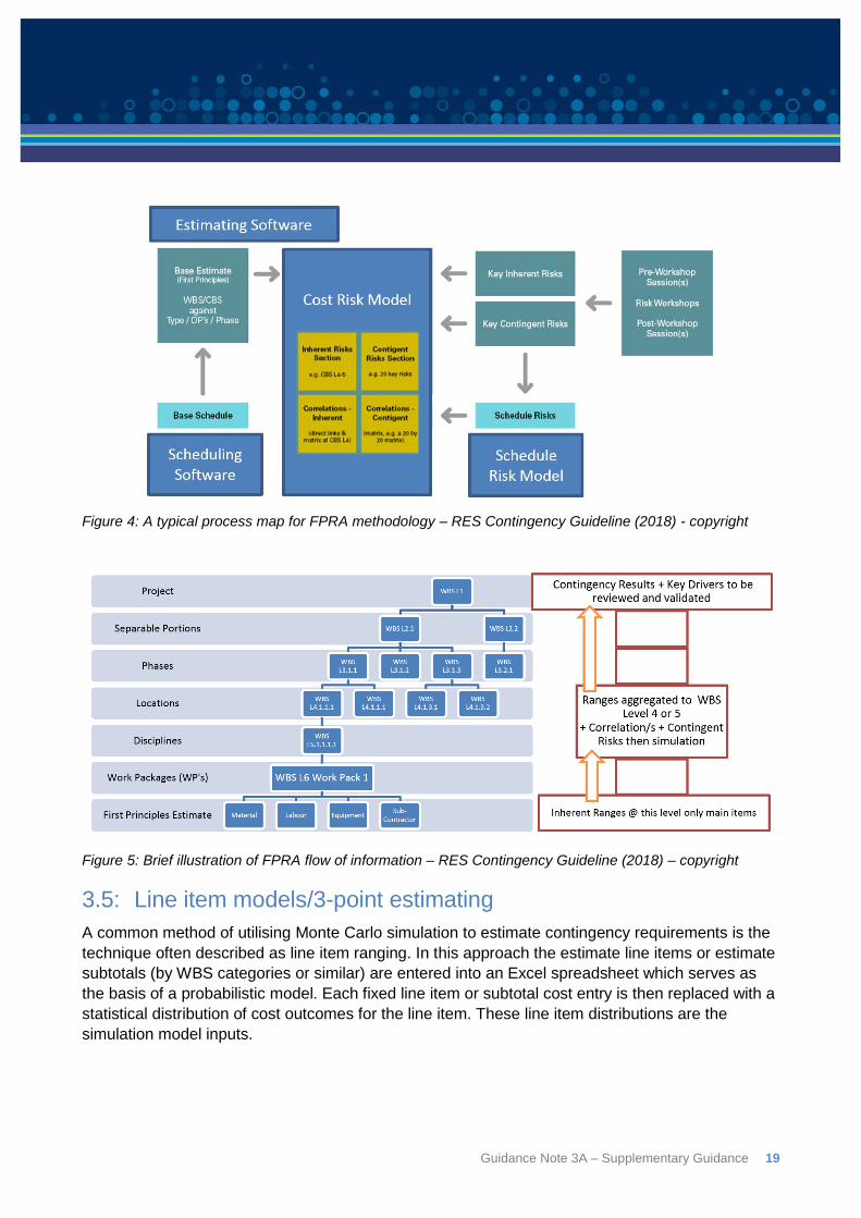
The process for the FPRA method is represented in Figure 4 and Figure 5 below.
Guidance Note 3A – Supplementary Guidance 19
Figure 4: A typical process map for FPRA methodology – RES Contingency Guideline (2018) - copyright
Figure 5: Brief illustration of FPRA flow of information – RES Contingency Guideline (2018) – copyright
3.5: Line item models/3-point estimating
A common method of utilising Monte Carlo simulation to estimate contingency requirements is the
technique often described as line item ranging. In this approach the estimate line items or estimate
subtotals (by WBS categories or similar) are entered into an Excel spreadsheet which serves as
the basis of a probabilistic model. Each fixed line item or subtotal cost entry is then replaced with a
statistical distribution of cost outcomes for the line item. These line item distributions are the
simulation model inputs.
20 Guidance Note 3A – Supplementary Guidance
Placing a distribution on the costs of items in an estimate is an easy extension of standard (base
cost) estimating practice. Modelling large numbers of items with various distributions lends an air of
accuracy and sophistication to the model20.
Unfortunately the method as generally practiced is highly flawed and in certain situations,
particularly when scope is poorly defined, has been found to be less accurate and less calibrated
than any other method, including simply relying on a predetermined percentage21.
Valid Monte Carlo assessment specifically requires that the dependencies, or correlation, between
the model inputs (the model line items) be defined. This is because models used in probabilistic
risk assessments take two kinds of inputs in order to produce an output distribution: (1) the
marginal distributions (the distributions without regard to the values of the other variables) for the
different variables and (2) the dependencies between these variables22. While software typically
incorporates correlation matrices to facilitate this task, realistic correlation modelling in project risk
cost analysis this way is rarely practicable. Most people are unable to make realistic estimates of
the amount of correlation between two costs affected by the same source of uncertainty, let alone
hundreds of line items.
Further, the task of specifying all the necessary correlations grows combinatorially with the number
of variables. A large project may have well over 1,000 cost elements. A 1,000 by 1,000 correlation
matrix requires (n2-n)/2, or 499,500 correlation values to be determined, at least in principle. Even
50 cost elements give rise to a potential 1225 correlations to be consciously excluded or evaluated.
In practice large numbers of correlations are never addressed directly. More commonly, there will
be an attempt to simplify the problem by making assumptions or by aggregating small work
elements into larger ones. Unfortunately, these assumptions or consolidations will generally make
it much more difficult to assess valid risk distributions, which can destroy the validity of the
correlations even if correlations could be assessed reliably. In fact, assessing realistic values of
partial correlations is very difficult. Very few people have a reliable understanding of the connection
between overlapping dependencies affecting cost items, such as two or more costs driven by
varying proportions of several bulk materials, and the partial correlations that will arise in reality,
which is what a model must represent. There is no reliable way to assess partial correlations
unless they can be measured from data, which is only viable if the project being analysed has the
same structure as a large number of prior projects from which data has been saved.
It has been argued23 that, despite the good intentions of analysts, line item ranging simply captures
the team’s opinion about the quality of their estimates and does not quantify risks at all. What line
item ranging seems to be good at is reliably generating the contingency and accuracy expected by
management.
20 Broadleaf (2014), Discussion paper: Weaknesses in common project cost risk modelling methods 21 Burroughs S and Juntima G (2004) AACE International Transactions, Exploring Techniques for Contingency Setting, AACE International, Morgantown, WV 22 Ferson et al (n.d.) Myths About Correlations and Dependencies and Their Implications for Risk Analysis 23 Hollmann, J 2016 Project Risk Quantification: A Practitioner’s Guide to Realistic Cost and Schedule Risk Management, Probabilistic Publishing, Gainesville, Florida
Guidance Note 3A – Supplementary Guidance 21
A combined risk analysis/contingency estimating method should start with identifying the risk
drivers before the cost impacts of the risk drivers are considered specifically for each driver using
stochastic (probabilistic) methods. It is only then that the risk drivers are linked to cost/schedule
outcomes. If decision-makers cannot explicitly see the connection between a given risk and the
potential impact, then management of the risk during execution will be difficult. Simply putting a
range around a line item without considering what is driving the uncertainty provides no insight as
to why it may vary from the base estimate and is not recommended practice.
Finally, there should not be a one-to-one correspondence between each element of the model and
the corresponding element of the system24. One should start with a “simple” model and develop it
as needed. Modelling each aspect of the system will rarely be required to make effective decisions,
and in fact may obscure important factors. As articulated by British statistician Professor George
E.P. Box, “All models are wrong, but some are useful.” In other words, is is not possible to get
every detail of the system into a model, but some models are still useful for decision-making.
3.6: The Department’s preferred approach
The Department recognises that line item ranging, combined with risk events, is a common method
of estimating contingency. However, the Department believes that structural difficulties inherent in
line-item ranging make it difficult to arrive at realistic contingency assessments.
The Department’s recommendation and preference is the use of a risk factor approach wherever
practical. As such, the remainder of the content of this guidance note is focused towards
developing such a model.
Notwithstanding, much of the material in this guidance note, notably in regard to the conduct of risk
workshops, has broad relevance to all modelling techniques and estimating practice. In addition, a
number of techniques to improve practice when using a line item ranging/risk event model, and
answers to common modelling questions, are presented as separate appendices to this guidance
note.
24 Law A (2015) Simulation Modelling and Analysis 5th Edition, McGraw Hill Education, New York
22 Guidance Note 3A – Supplementary Guidance
4: Quantitative Risk Analysis using risk factors
4.1: Variations from the base estimate
At the time an estimate is prepared to request approval for a project, design is rarely complete. If
the project is granted approval to proceed, as the design is completed, changes will be made that
affect the cost including:
Some quantities will be increased and others will be reduced;
Some material and equipment selections will be changed or simply specified more precisely
than at the time the estimate was prepared; and
Procurement and construction strategies may be refined or defined in more detail in ways
that affect the unit rates for materials, plant, services and labour or the duration of the
construction activity.
Even as project execution starts, minor engineering details will still be subject to refinement,
information from suppliers will cause changes in plans and the unit rates for materials, plant,
services and labour can turn out different from what was expected. Then, during execution,
conditions at site, the weather, industrial relations, interactions with neighbouring communities,
geotechnical conditions as well as heritage and environmental protection requirements can all
result in what is physically done and how much it costs varying from what was assumed in the
estimate.
Occasionally, there may be major events that can have a severe effect on a project’s costs.
However, few major projects are sanctioned when there are foreseeable potential events with a
significant likelihood of happening that could have very large undesirable consequences such as a
very large cost increase.
On the rare occasions when work commences in the knowledge that a large additional cost might
be incurred, the routine project contingency is unlikely to be used to cover that cost. This is
discussed further in Section 4.4. More commonly, a host of smaller events that can affect the cost
of a project can be realistically represented as the aggregate effect of all sources of uncertainty on
bulk material quantities, rates, durations and other cost drivers.
4.2: Common drivers
Research into project cost sensitivity has found that very few projects are subject to significant
uncertainty in more than about twenty basic estimating inputs25. Experience with major projects in
the infrastructure and resources sectors supports this view. Cost risk models need not be bulky.
The uncertainty in infrastructure cost risk forecasts can almost always be described in terms of the
uncertainty in:
25 AACE International (2008) RP No. 41R-08 Risk Analysis and Contingency Determination Using Range Estimating, AACE International, Morgantown, WV

Guidance Note 3A – Supplementary Guidance 23
Quantities of materials bought, moved and placed;
Unit rates for the purchase of materials, equipment or labour;
Productivity rates for labour and plant;
Running rates for management, overheads and temporary facilities;
Lump sum costs of major purchases; and
The duration of the work.
It is always worth considering how and if these uncertainties affect the basic estimating inputs.
It is neither practicable nor necessary to work with the actual physical quantities and rates as there
are many detailed instances of them throughout a project. A realistic analysis can be based on an
assessment of the extent to which uncertainty about quantities or rates could affect the cost. This
reflects the level of definition in an engineering design, the quality of and commitment behind price
indications taken from the market and past work, and the maturity of major design or strategic
decisions.
If the quantity of concrete in a slab increases by 10%, and cost is estimated on a volumetric basis
that includes supply and placement, it is reasonable to suppose that the cost will increase by 10%
as well. If the quantity is subject to ±5% variation, then the cost will be too. It is only necessary to
focus on how much uncertainty about quantities or rates could affect parts of the cost rather than
on how much the value of particular quantities or rates might vary in themselves.
This is the approach an estimator will often adopt if asked to carry out a what-if analysis. The effect
of lengthening a noise wall on a road can be assessed relatively quickly, without going back to first
principles, by identifying the cost items associated with the wall and factoring them by the
proportional increase in the length of the wall. Where there is insufficient time or an approximate
answer will be sufficient, this is a cost-effective practice. It provides sound information at the least
cost.
There is no formula for choosing the most useful risk factors to represent uncertainty in a cost
estimate. The selection of factors can change from one job to another and from early stages of
design through to project execution. The most useful way to decide on the factors to use for a
particular job is to start at the highest level, ask whether it is possible to describe the uncertainty in
the major cost drivers at that level and if not then break it down a level and try again. The question
“Why should we add more detail here?” is a good test. Extra detail will always add to the effort
required for the analysis, the difficulty of understanding the outcome and the challenge of
communicating it to decision makers or reviewers. There should be a good reason for making a
model increasingly granular.
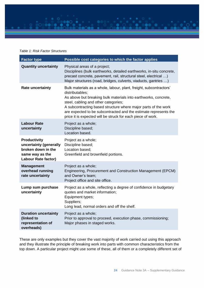
The way the costs are broken down depends on how the team understand the nature of the
uncertainty affecting the cost. Some common structures are set out in Table 1 showing how costs
might be broken down for the purposes of assessing uncertainties and the cost categories to which
they can apply. The factors refer to how much uncertainty there is associated with something that
affects the cost, not to the thing itself.
24 Guidance Note 3A – Supplementary Guidance
Table 1: Risk Factor Structures
Factor type Possible cost categories to which the factor applies
Quantity uncertainty Physical areas of a project;
Disciplines (bulk earthworks, detailed earthworks, in-situ concrete,
precast concrete, pavement, rail, structural steel, electrical …)
Major structures (road, bridges, culverts, viaducts, gantries …)
Rate uncertainty Bulk materials as a whole, labour, plant, freight, subcontractors’
distributables;
As above but breaking bulk materials into earthworks, concrete,
steel, cabling and other categories;
A subcontracting based structure where major parts of the work
are expected to be subcontracted and the estimate represents the
price it is expected will be struck for each piece of work.
Labour Rate
uncertainty
Project as a whole;
Discipline based;
Location based.
Productivity
uncertainty (generally
broken down in the
same way as the
Labour Rate factor)
Project as a whole;
Discipline based;
Location based;
Greenfield and brownfield portions.
Management
overhead running
rate uncertainty
Project as a whole;
Engineering, Procurement and Construction Management (EPCM)
and Owner’s team;
Project office and site office.
Lump sum purchase
uncertainty
Project as a whole, reflecting a degree of confidence in budgetary
quotes and market information;
Equipment types;
Suppliers;
Long lead, normal orders and off the shelf.
Duration uncertainty
(linked to
representation of
overheads)
Project as a whole;
Prior to approval to proceed, execution phase, commissioning;
Major phases in staged works.
These are only examples but they cover the vast majority of work carried out using this approach
and they illustrate the principle of breaking work into parts with common characteristics from the
top down. A particular project might use some of these, all of them or a completely different set of
Guidance Note 3A – Supplementary Guidance 25
categories. Examples of some can be seen in the sample probabilistic risk factor models
accompanying this guidance note.
The key principle when selecting risk factors is to reflect the way uncertainty in the estimate is
understood by the personnel responsible for the design, estimate and plans. If uncertainty about a
quantity or rate is markedly different from one part of the estimate to another, and both can have a
significant effect on the cost, then it may be worth separating them in the model. If the uncertainty
in the quantities or unit rates for one bulk material is affected by different matters to those affecting
another bulk material, it may be worth splitting these up. If there is uncertainty about productivity, it
is worth separating, in the model, the costs related to labour hours such as labour cost, plant cost,
supervisions and subcontractor’s distributables so that the productivity uncertainty can be applied
to those parts of the cost. Of course, if parts of the project have unusual characteristics, quite
different from the rest of the work, but are so small that they will never have a significant effect on
the total cost, there is no point splitting them out.
If costs such as plant, accommodation and supervision are wrapped into the labour rate, they
might not have to be separated from one another as they will all be driven by labour hours, which is
in turn driven by quantity and productivity uncertainty. However, it is difficult to model the effect of
productivity uncertainty on costs that consist of a mix of bulk material and labour related categories
so it is usually desirable to separate these two types of costs.
Appendix A provides further detail on the level of detail to include in a model and methods to derive
relevant risk factors on projects.
4.3: Risk events
The risk factor approach described in this guidance note avoids the practical problems of dealing
with a large number of interacting events or a large number of correlated line-item variations by
focusing on the major estimating inputs that the events will affect and which drive the individual line
items. It draws on the experience and judgement of project personnel to understand the potential
variation in these cost drivers, which are the major inputs to the estimate.
Experience shows that risk factors, such as those outlined in Table 2, provide a concise and
effective way to describe the potential variation of project costs.
Representing the uncertainty in a project’s cost directly in terms of these high level cost drivers
avoids having a large number of separate cost distributions individually affected by the one
underlying source and so having to be linked by poorly understood correlations, as is usually the
case with line item risk models. Wrapping up in a few straightforward risk factors the various small
and medium scale risk events that could affect the quantities of material, unit rates, labour
productivity and other important cost drivers, makes it easy to understand any interactions that do
arise and model them. This is in contrast to many risk register based models with a large number
of individual risk events that might have complex interactions, which are not examined or taken into
account. As noted earlier, projects are rarely approved with very large risks that have a realistic
chance of affecting them. In the rare cases where this does happen, separate financial provision
will usually be made rather than trying to wrap them into the general contingency.
26 Guidance Note 3A – Supplementary Guidance
Individual risk events can be combined with a driver-based approach but experience shows that,
once a model is constructed around high level cost drivers and the uncertainty in them, the need
for a large number of separate small and medium sized event risks falls away. Some examples of
items that are routinely modelled as separate items and the risk factors that are usually seen as
encompassing their effects, representing uncertainty in cost drivers, are listed in Table 2. This is
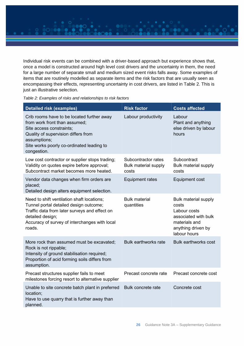
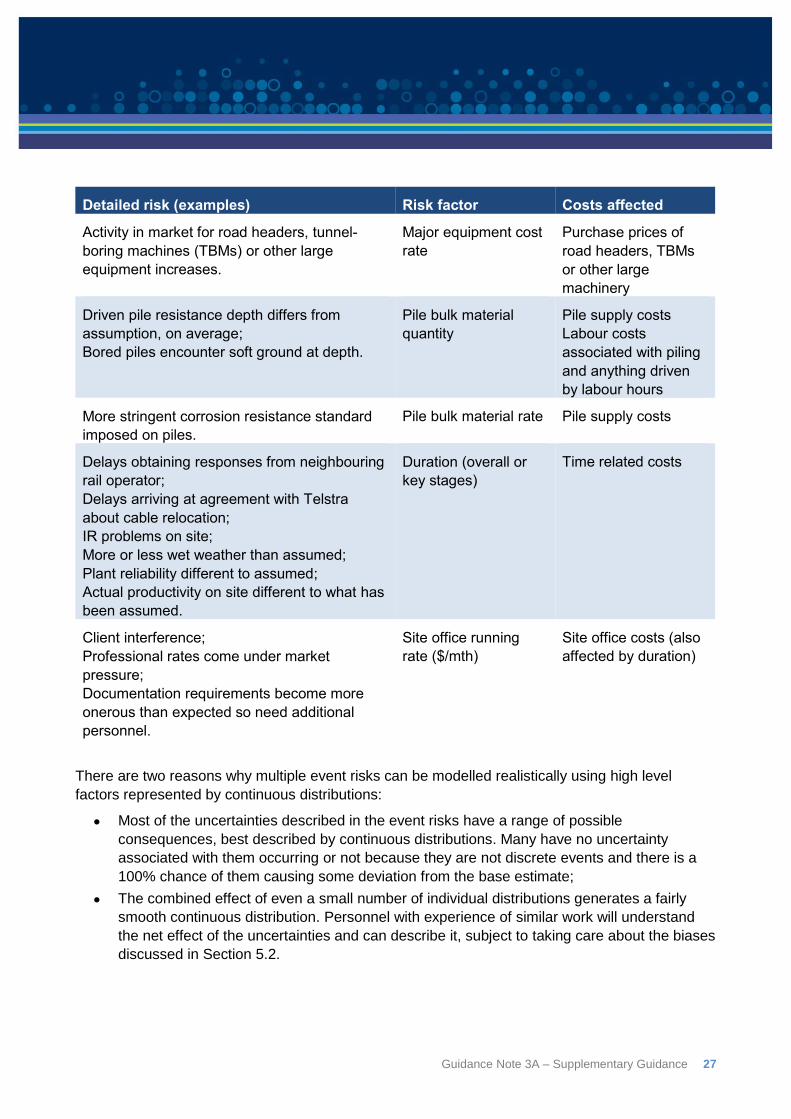
just an illustrative selection.
Table 2: Examples of risks and relationships to risk factors
Detailed risk (examples) Risk factor Costs affected
Crib rooms have to be located further away
from work front than assumed;
Site access constraints;
Quality of supervision differs from
assumptions;
Site works poorly co-ordinated leading to
congestion.
Labour productivity Labour
Plant and anything
else driven by labour
hours
Low cost contractor or supplier stops trading;
Validity on quotes expire before approval;
Subcontract market becomes more heated.
Subcontractor rates
Bulk material supply
costs
Subcontract
Bulk material supply
costs
Vendor data changes when firm orders are
placed;
Detailed design alters equipment selection.
Equipment rates Equipment cost
Need to shift ventilation shaft locations;
Tunnel portal detailed design outcome;
Traffic data from later surveys and effect on
detailed design;
Accuracy of survey of interchanges with local
roads.
Bulk material
quantities
Bulk material supply
costs
Labour costs
associated with bulk
materials and
anything driven by
labour hours
More rock than assumed must be excavated;
Rock is not rippable;
Intensity of ground stabilisation required;
Proportion of acid forming soils differs from
assumption.
Bulk earthworks rate Bulk earthworks cost
Precast structures supplier fails to meet
milestones forcing resort to alternative supplier
Precast concrete rate Precast concrete cost
Unable to site concrete batch plant in preferred
location;
Have to use quarry that is further away than
planned.
Bulk concrete rate Concrete cost
Guidance Note 3A – Supplementary Guidance 27
Detailed risk (examples) Risk factor Costs affected
Activity in market for road headers, tunnel-
boring machines (TBMs) or other large
equipment increases.
Major equipment cost
rate
Purchase prices of
road headers, TBMs
or other large
machinery
Driven pile resistance depth differs from
assumption, on average;
Bored piles encounter soft ground at depth.
Pile bulk material
quantity
Pile supply costs
Labour costs
associated with piling
and anything driven
by labour hours
More stringent corrosion resistance standard
imposed on piles.
Pile bulk material rate Pile supply costs
Delays obtaining responses from neighbouring
rail operator;
Delays arriving at agreement with Telstra
about cable relocation;
IR problems on site;
More or less wet weather than assumed;
Plant reliability different to assumed;
Actual productivity on site different to what has
been assumed.
Duration (overall or
key stages)
Time related costs
Client interference;
Professional rates come under market
pressure;
Documentation requirements become more
onerous than expected so need additional
personnel.
Site office running
rate ($/mth)
Site office costs (also
affected by duration)
There are two reasons why multiple event risks can be modelled realistically using high level
factors represented by continuous distributions:
Most of the uncertainties described in the event risks have a range of possible
consequences, best described by continuous distributions. Many have no uncertainty
associated with them occurring or not because they are not discrete events and there is a
100% chance of them causing some deviation from the base estimate;
The combined effect of even a small number of individual distributions generates a fairly
smooth continuous distribution. Personnel with experience of similar work will understand
the net effect of the uncertainties and can describe it, subject to taking care about the biases
discussed in Section 5.2.
28 Guidance Note 3A – Supplementary Guidance
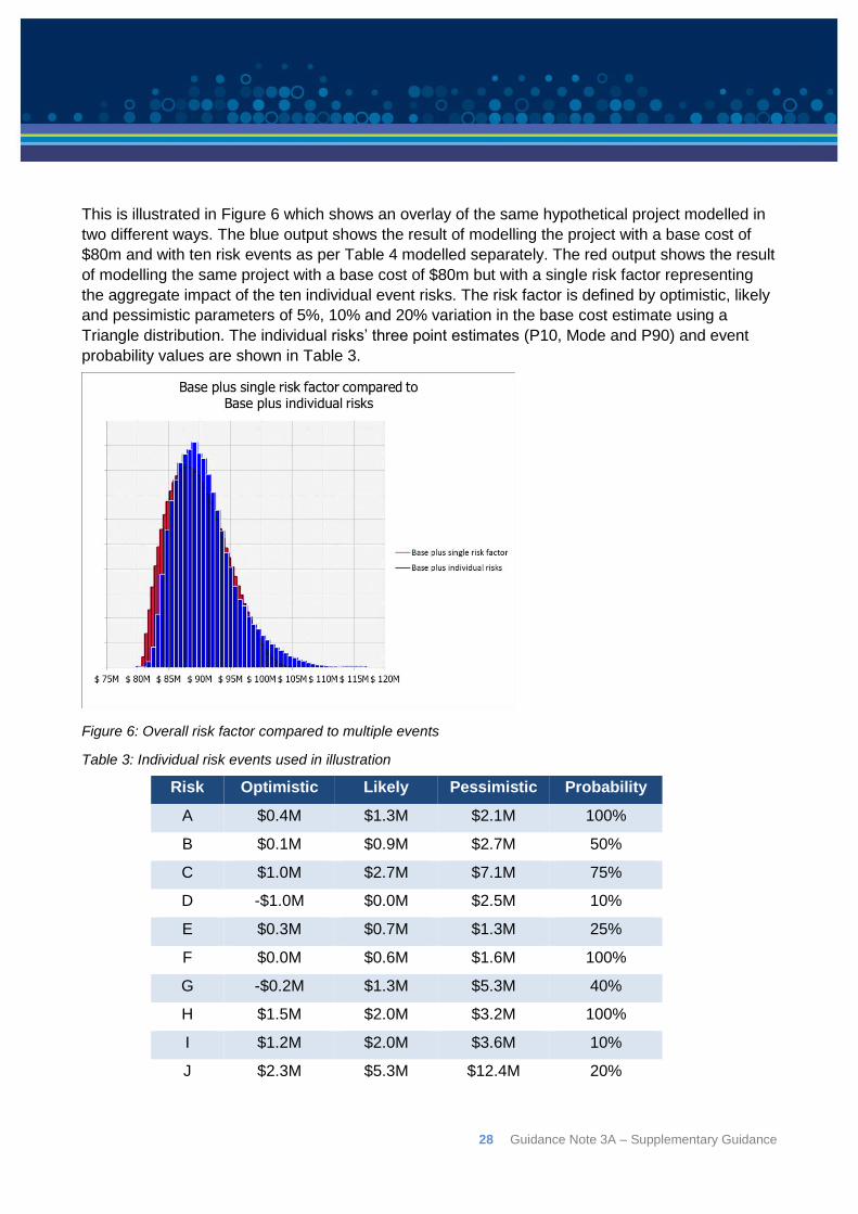
This is illustrated in Figure 6 which shows an overlay of the same hypothetical project modelled in
two different ways. The blue output shows the result of modelling the project with a base cost of
$80m and with ten risk events as per Table 4 modelled separately. The red output shows the result
of modelling the same project with a base cost of $80m but with a single risk factor representing
the aggregate impact of the ten individual event risks. The risk factor is defined by optimistic, likely
and pessimistic parameters of 5%, 10% and 20% variation in the base cost estimate using a
Triangle distribution. The individual risks’ three point estimates (P10, Mode and P90) and event
probability values are shown in Table 3.
Figure 6: Overall risk factor compared to multiple events
Table 3: Individual risk events used in illustration
Risk Optimistic Likely Pessimistic Probability
A $0.4M $1.3M $2.1M 100%
B $0.1M $0.9M $2.7M 50%
C $1.0M $2.7M $7.1M 75%
D -$1.0M $0.0M $2.5M 10%
E $0.3M $0.7M $1.3M 25%
F $0.0M $0.6M $1.6M 100%
G -$0.2M $1.3M $5.3M 40%
H $1.5M $2.0M $3.2M 100%
I $1.2M $2.0M $3.6M 10%
J $2.3M $5.3M $12.4M 20%
Guidance Note 3A – Supplementary Guidance 29
The significance of this illustration is not the specific details of the risk events or the parameters of
the single overall risk factor, which are hypothetical although not unrealistic. It is the fact that a set
of detailed items generates broadly the same type of outcome as is represented by a single factor
intended to cover their aggregate impact on a base cost estimate. So long as a team feel that they
understand the work well enough to assess the aggregate effect of several sources of uncertainty,
based on their experience with similar projects, they need not be concerned that they are doing so.
It is a perfectly reasonable approach.
This illustration uses just one factor. A real analysis will have several and the same principle
applies. The behaviour we understand for a whole project’s cost risk can be described realistically
using risk factors. Risk events are not necessary and have many drawbacks as the basis of a
model, as discussed earlier.
If a team does not feel comfortable assessing uncertainty at a high level, they might seek to break
the cost into smaller parts and apply the same approach to those parts. These might be regions of
the work subject to different sorts of risks. This is only worthwhile if the personnel concerned feel
more confident about the assessments they can make at the detailed level and are sure that they
have captured all the detail necessary for a realistic assessment of the overall uncertainty. If not,
there is no point building a more granular model.
There is no rule about where to stop breaking the analysis into ever smaller parts. Experience with
this method shows that the urge to introduce greater detail, beyond the point where it relates to
parts of the project having different risk characteristics, hardly ever makes a material difference to
the outcome but it does absorb an appreciable amount of additional effort, so long as each
assessment is diligent and takes appropriate steps to avoid bias. Only a few high level factors are
generally required to model uncertainty in an estimate. This is sufficient to allow a professional
team to consider and describe the uncertainty they can see arising in an estimate.
As previously mentioned, in most circumstances, it has been found only twenty or so factors are
required to describe the uncertainty in a project so this method results in a more compact model
than the alternatives in common use. It absorbs less effort and produces greater understanding.
Uncertainty factors do interact with one another but the interactions are generally straightforward,
such as between quantity and unit rate variations or between duration and temporary facilities cost
variation, in each case the product of the two factors represents their combined effect, and they
can be built into a model relatively easily, usually as simple functional relationships.
4.4: Uncertainty that should not be captured
Few major projects are sanctioned when there are foreseeable events with a significant likelihood
of happening that could have very large undesirable consequences such as a very large cost
increase. Those who provide the funding will not usually sanction a project that they believe has an
appreciable prospect of incurring catastrophic additional costs.
Circumstances in which projects might commence in the knowledge that a high impact event could
occur may include:

30 Guidance Note 3A – Supplementary Guidance
Work to reduce a serious threat, such as emergency flood mitigation, stabilisation of
collapsing infrastructure or reinstatement of a critical washed out transport route; and/or
Projects constrained by absolutely fixed dates such as hosting the Olympic Games or
similar situations.
If there is a strategic need to embark on work that could be subject to a very large cost increase,
this is best managed as a stand-alone contingent funding requirement with an agreed trigger and
controls on the release of the funds. To incorporate it into a general project contingency only
serves to hide the nature of the requirement and obscure the special character of the costs
involved. It is a special requirement and will be best managed apart from the general funding of a
project.
In particular, using a weighted impact to calculate the contingency required for an event such as
this is rarely satisfactory. If there is a potential event that could cost $100 million and it is thought to
have a 20% chance of happening, holding $20 million (20% of $100 million) will not help. If the
event actually occurs, $100 million will be needed. Weighting risks by their likelihood of occurring
only works when there are many small or medium events to be covered and they are independent
of one another. The way contingency funds are assessed and managed for a large number of
independent small and medium scale risks is not suited to making provision for very high impact
risks with an appreciable probability of occurring.
Earthquakes, terrorist attacks, fire destroying a yard full of earthmoving machinery, a contagious
disease being brought in by one worker and causing closure of a site for a few weeks are all
conceivable but very unlikely. These are generally regarded as normal risks associated with what
is sometimes called ‘business as usual’. There may be insurance held against some of these but
some will simply be accepted due to their rarity.
In addition to excluding extreme events, attempting to capture every one of the uncontrollable
events, such as those in the previous paragraph, which could impact on the final cost of a project
can become an unproductive exercise. It is impossible to conceive of the multitude of smaller
events that may occur or of how they might overlap or interact. The majority of these smaller risk
events will be covered by one or more major risk drivers. Identifying the key risk drivers and their
uncertainty, the range of each one and the likelihood of values within that range, before linking the
risk drivers to cost outcomes, is a far more efficient and theoretically sound approach to quantifying
project-specific risks.
There are numerous types and sources of risk. Cost risk analyses attempt to address some, but
not all of these risks. Those typically excluded are extreme events such as the cost consequences
of an earthquake occurring. There are good reasons to leave out some of these; cost risk analysis
is intended to provide decision makers with information to help them successfully manage projects
and the inclusion of extremely rare events with large impacts will not aid decision makers with
project budgeting. This exclusion of some risks is advisable and only including those factors
impacting management’s decisions is appropriate for a project estimate. Rare events might be
considered but it does not help to blend them into the general project contingency.
Guidance Note 3A – Supplementary Guidance 31
Expected Value and Risk
The following example demonstrates why using weighted impact to calculate contingency requirements for a large event risk is rarely appropriate.
The notion that expected value (probability multiplied by consequence) is the way that rational people make decisions appeared long before modern economic theory. In the early eighteenth century Daniel Bernoulli systematically attacked the idea and introduced his concept of utility whereby there is no reason to assume that the risks anticipated by each individual must be deemed equal in value; it all depends on individual circumstance26. For example, say you are offered the chance to make a wager where you have a 90% chance of winning $1 million but if you lose, you have to pay $100,000. The expected value is thus ($-100,000 * 0.1) + ($1,000,000 * 0.9) = $890,000.
Surely, it would be foolish not to take this offer? After all, you expect to pocket $890,000 from the transaction. The subtlety is that expected value is the long-run average of repetitions of the experiment it represents. In the binary case of the wager just described, $890,000 isn’t even a possibility and the problem is that, for most people, $100,000 is likely to be a catastrophic loss they are unlikely to afford. Similarly, using the expected value (weighted impact) to calculate the required contingency for a potentially catastrophic event and then believing that the risk has been accounted for is highly misleading.
The same sort of reasoning explains why we regularly pay premiums to an insurance company when the mathematical probabilities indicate that we will lose money; the premiums we pay exceed the expected value of events such as our house burning down or our car being stolen. We enter into these losing propositions because we cannot afford to take the risk of losing our home or car. We prefer the gamble that has 100% chance of small loss (the premium) rather than pocket this small saving because a disaster would be catastrophically ruinous if it were to occur.
26 Bernstein, P., (1998) Against the Gods: The Remarkable Story of Risk, Wiley
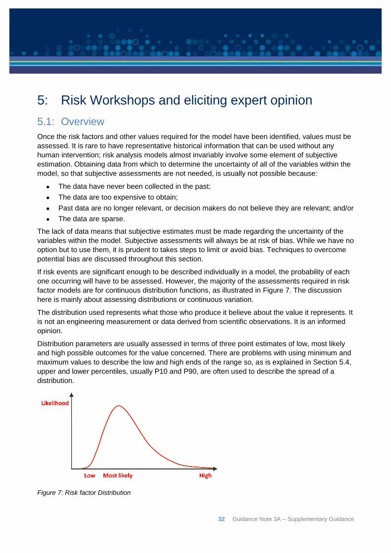
32 Guidance Note 3A – Supplementary Guidance
5: Risk Workshops and eliciting expert opinion
5.1: Overview
Once the risk factors and other values required for the model have been identified, values must be
assessed. It is rare to have representative historical information that can be used without any
human intervention; risk analysis models almost invariably involve some element of subjective
estimation. Obtaining data from which to determine the uncertainty of all of the variables within the
model, so that subjective assessments are not needed, is usually not possible because:
The data have never been collected in the past;
The data are too expensive to obtain;
Past data are no longer relevant, or decision makers do not believe they are relevant; and/or
The data are sparse.
The lack of data means that subjective estimates must be made regarding the uncertainty of the
variables within the model. Subjective assessments will always be at risk of bias. While we have no
option but to use them, it is prudent to takes steps to limit or avoid bias. Techniques to overcome
potential bias are discussed throughout this section.
If risk events are significant enough to be described individually in a model, the probability of each
one occurring will have to be assessed. However, the majority of the assessments required in risk
factor models are for continuous distribution functions, as illustrated in Figure 7. The discussion
here is mainly about assessing distributions or continuous variation.
The distribution used represents what those who produce it believe about the value it represents. It
is not an engineering measurement or data derived from scientific observations. It is an informed
opinion.
Distribution parameters are usually assessed in terms of three point estimates of low, most likely
and high possible outcomes for the value concerned. There are problems with using minimum and
maximum values to describe the low and high ends of the range so, as is explained in Section 5.4,
upper and lower percentiles, usually P10 and P90, are often used to describe the spread of a
distribution.
Figure 7: Risk factor Distribution
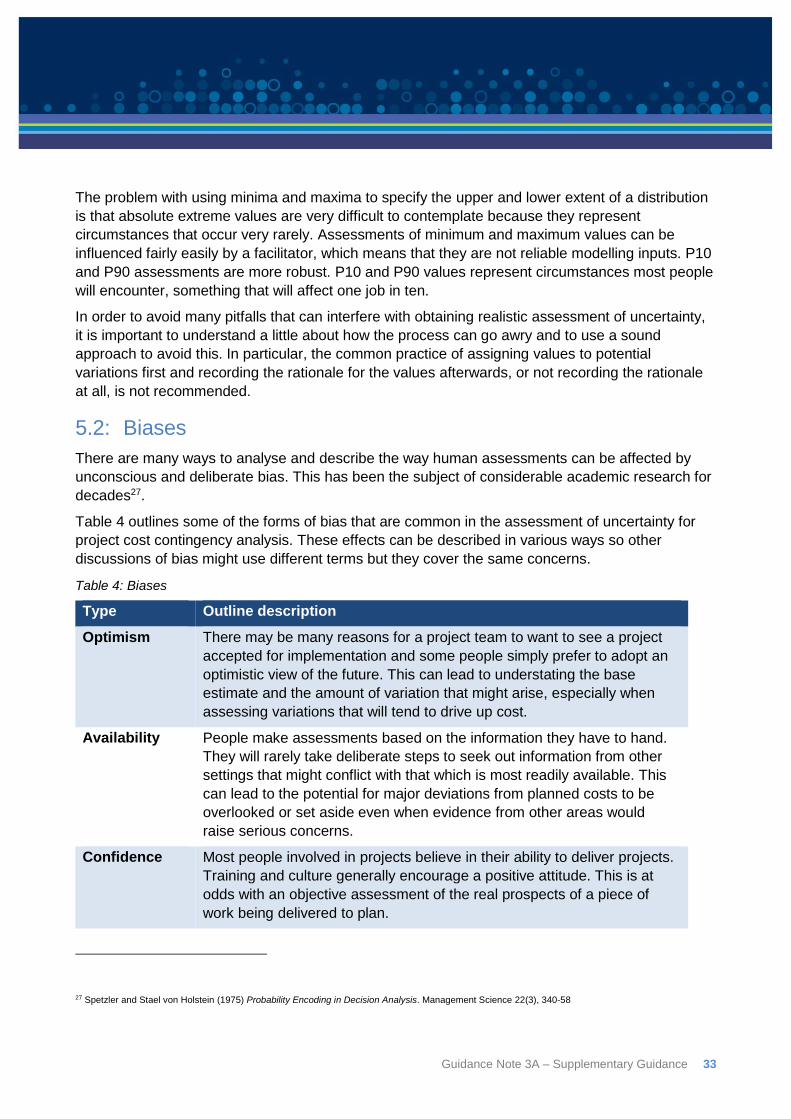
Guidance Note 3A – Supplementary Guidance 33
The problem with using minima and maxima to specify the upper and lower extent of a distribution
is that absolute extreme values are very difficult to contemplate because they represent
circumstances that occur very rarely. Assessments of minimum and maximum values can be
influenced fairly easily by a facilitator, which means that they are not reliable modelling inputs. P10
and P90 assessments are more robust. P10 and P90 values represent circumstances most people
will encounter, something that will affect one job in ten.
In order to avoid many pitfalls that can interfere with obtaining realistic assessment of uncertainty,
it is important to understand a little about how the process can go awry and to use a sound
approach to avoid this. In particular, the common practice of assigning values to potential
variations first and recording the rationale for the values afterwards, or not recording the rationale
at all, is not recommended.
5.2: Biases
There are many ways to analyse and describe the way human assessments can be affected by
unconscious and deliberate bias. This has been the subject of considerable academic research for
decades27.
Table 4 outlines some of the forms of bias that are common in the assessment of uncertainty for
project cost contingency analysis. These effects can be described in various ways so other
discussions of bias might use different terms but they cover the same concerns.
Table 4: Biases
Type Outline description
Optimism There may be many reasons for a project team to want to see a project
accepted for implementation and some people simply prefer to adopt an
optimistic view of the future. This can lead to understating the base
estimate and the amount of variation that might arise, especially when
assessing variations that will tend to drive up cost.
Availability People make assessments based on the information they have to hand.
They will rarely take deliberate steps to seek out information from other
settings that might conflict with that which is most readily available. This
can lead to the potential for major deviations from planned costs to be
overlooked or set aside even when evidence from other areas would
raise serious concerns.
Confidence Most people involved in projects believe in their ability to deliver projects.
Training and culture generally encourage a positive attitude. This is at
odds with an objective assessment of the real prospects of a piece of
work being delivered to plan.
27 Spetzler and Stael von Holstein (1975) Probability Encoding in Decision Analysis. Management Science 22(3), 340-58
34 Guidance Note 3A – Supplementary Guidance
Type Outline description
Anchoring Once a cost or a key parameter such as a bulk quantity, a rate or
productivity factor, has been declared, assessments of possible variation
from that value will tend to remain close to that starting point. This results
in a systematic tendency to understate the extent to which actual
outcomes could differ from the assumptions incorporated into an estimate
whether they will raise or lower the cost. The assessment is anchored on
the base estimate.
All these and other forms of bias can completely undermine the realism of a quantitative risk
analysis. It is important to take deliberate steps to overcome them. Two straightforward strategies
can be used to improve the realism of uncertainty assessments:
Selecting a competent team for the assessment; and
Using a process that will help avoid bias.
Feelings influence risk perception
People’s risk perception is influenced disproportionately by many things, including the rarity of the event, how much control they believe they have, the adverseness of the outcomes, and whether undertaking the risk is voluntary or not. For example, people in the United States underestimate the risks associated with having a handgun at home by 100-fold, and overestimate the risks of living close to a nuclear reactor by 10-fold28.
5.3: Participation in assessment
Participants in risk assessments can be self-selecting or sometimes unwilling conscripts. Table 5
sets out a checklist of points to bear in mind when deciding who to involve the assessment of
uncertainty factors and probabilities for a contingency model. It is almost always a bad idea to have
a single individual assess the ranges of values used for a risk model, even if their work is reviewed
later by others. A workshop process, preferably facilitated by someone independent of the project,
is almost always preferred. The assessment should involve participants challenging one another so
that tacit assumptions that might be incorrect and gaps in information are exposed and resolved.
28 Sutherland, W.J., Spiegelhalter, D. & Burgman, M.A. (2013) Twenty Tips for Interpreting Scientific Claims. Nature 503, 335-337
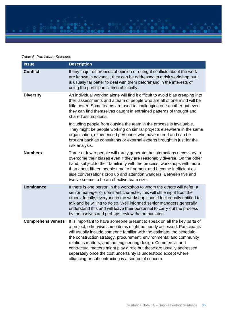
Guidance Note 3A – Supplementary Guidance 35
Table 5: Participant Selection
Issue Description
Conflict If any major differences of opinion or outright conflicts about the work
are known in advance, they can be addressed in a risk workshop but it
is usually far better to deal with them beforehand in the interests of
using the participants’ time efficiently.
Diversity An individual working alone will find it difficult to avoid bias creeping into
their assessments and a team of people who are all of one mind will be
little better. Some teams are used to challenging one another but even
they can find themselves caught in entrained patterns of thought and
shared assumptions.
Including people from outside the team in the process is invaluable.
They might be people working on similar projects elsewhere in the same
organisation, experienced personnel who have retired and can be
brought back as consultants or external experts brought in just for the
risk analysis.
Numbers Three or fewer people will rarely generate the interactions necessary to
overcome their biases even if they are reasonably diverse. On the other
hand, subject to their familiarity with the process, workshops with more
than about fifteen people tend to fragment and become inefficient as
side conversations crop up and attention wanders. Between five and
twelve seems to be an effective team size.
Dominance If there is one person in the workshop to whom the others will defer, a
senior manager or dominant character, this will stifle input from the
others. Ideally, everyone in the workshop should feel equally entitled to
talk and be willing to do so. Well informed senior managers generally
understand this and will leave their personnel to carry out the process
by themselves and perhaps review the output later.
Comprehensiveness It is important to have someone present to speak on all the key parts of
a project, otherwise some items might be poorly assessed. Participants
will usually include someone familiar with the estimate, the schedule,
the construction strategy, procurement, environmental and community
relations matters, and the engineering design. Commercial and
contractual matters might play a role but these are usually addressed
separately once the cost uncertainty is understood except where
alliancing or subcontracting is a source of concern.
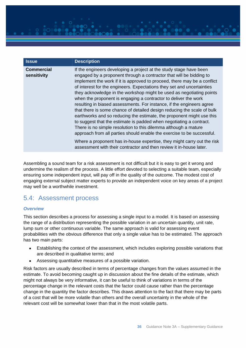
36 Guidance Note 3A – Supplementary Guidance
Issue Description
Commercial
sensitivity
If the engineers developing a project at the study stage have been
engaged by a proponent through a contractor that will be bidding to
implement the work if it is approved to proceed, there may be a conflict
of interest for the engineers. Expectations they set and uncertainties
they acknowledge in the workshop might be used as negotiating points
when the proponent is engaging a contractor to deliver the work
resulting in biased assessments. For instance, if the engineers agree
that there is some chance of detailed design reducing the scale of bulk
earthworks and so reducing the estimate, the proponent might use this
to suggest that the estimate is padded when negotiating a contract.
There is no simple resolution to this dilemma although a mature
approach from all parties should enable the exercise to be successful.
Where a proponent has in-house expertise, they might carry out the risk
assessment with their contractor and then review it in-house later.
Assembling a sound team for a risk assessment is not difficult but it is easy to get it wrong and
undermine the realism of the process. A little effort devoted to selecting a suitable team, especially
ensuring some independent input, will pay off in the quality of the outcome. The modest cost of
engaging external subject matter experts to provide an independent voice on key areas of a project
may well be a worthwhile investment.
5.4: Assessment process
Overview
This section describes a process for assessing a single input to a model. It is based on assessing
the range of a distribution representing the possible variation in an uncertain quantity, unit rate,
lump sum or other continuous variable. The same approach is valid for assessing event
probabilities with the obvious difference that only a single value has to be estimated. The approach
has two main parts:
Establishing the context of the assessment, which includes exploring possible variations that
are described in qualitative terms; and
Assessing quantitative measures of a possible variation.
Risk factors are usually described in terms of percentage changes from the values assumed in the
estimate. To avoid becoming caught up in discussion about the fine details of the estimate, which
might not always be very informative, it can be useful to think of variations in terms of the
percentage change in the relevant costs that the factor could cause rather than the percentage
change in the quantity the factor describes. This draws attention to the fact that there may be parts
of a cost that will be more volatile than others and the overall uncertainty in the whole of the
relevant cost will be somewhat lower than that in the most volatile parts.
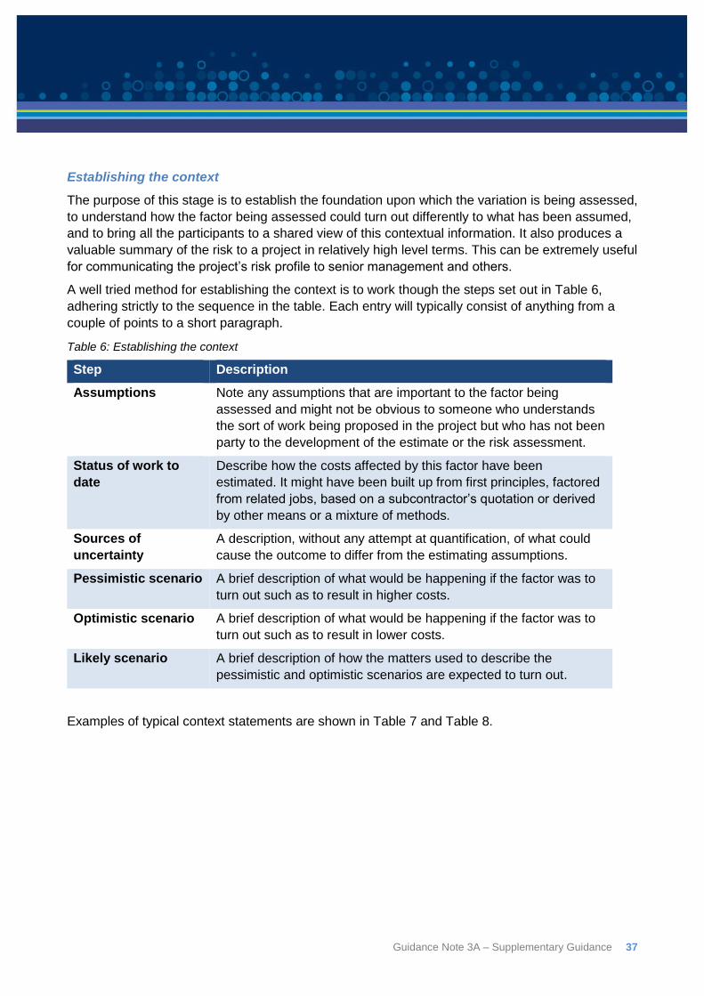
Guidance Note 3A – Supplementary Guidance 37
Establishing the context
The purpose of this stage is to establish the foundation upon which the variation is being assessed,
to understand how the factor being assessed could turn out differently to what has been assumed,
and to bring all the participants to a shared view of this contextual information. It also produces a
valuable summary of the risk to a project in relatively high level terms. This can be extremely useful
for communicating the project’s risk profile to senior management and others.
A well tried method for establishing the context is to work though the steps set out in Table 6,
adhering strictly to the sequence in the table. Each entry will typically consist of anything from a
couple of points to a short paragraph.
Table 6: Establishing the context
Step Description
Assumptions Note any assumptions that are important to the factor being
assessed and might not be obvious to someone who understands
the sort of work being proposed in the project but who has not been
party to the development of the estimate or the risk assessment.
Status of work to
date
Describe how the costs affected by this factor have been
estimated. It might have been built up from first principles, factored
from related jobs, based on a subcontractor’s quotation or derived
by other means or a mixture of methods.
Sources of
uncertainty
A description, without any attempt at quantification, of what could
cause the outcome to differ from the estimating assumptions.
Pessimistic scenario A brief description of what would be happening if the factor was to
turn out such as to result in higher costs.
Optimistic scenario A brief description of what would be happening if the factor was to
turn out such as to result in lower costs.
Likely scenario A brief description of how the matters used to describe the
pessimistic and optimistic scenarios are expected to turn out.
Examples of typical context statements are shown in Table 7 and Table 8.
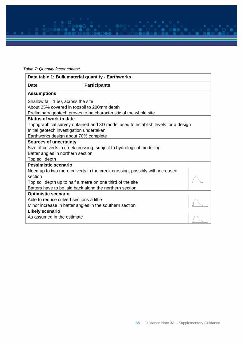
38 Guidance Note 3A – Supplementary Guidance
Table 7: Quantity factor context
Data table 1: Bulk material quantity - Earthworks
Date Participants
Assumptions
Shallow fall, 1:50, across the site
About 25% covered in topsoil to 200mm depth
Preliminary geotech proves to be characteristic of the whole site
Status of work to date
Topographical survey obtained and 3D model used to establish levels for a design
Initial geotech investigation undertaken
Earthworks design about 70% complete
Sources of uncertainty
Size of culverts in creek crossing, subject to hydrological modelling
Batter angles in northern section
Top soil depth
Pessimistic scenario
Need up to two more culverts in the creek crossing, possibly with increased
section
Top soil depth up to half a metre on one third of the site
Batters have to be laid back along the northern section
Optimistic scenario
Able to reduce culvert sections a little
Minor increase in batter angles in the southern section
Likely scenario
As assumed in the estimate
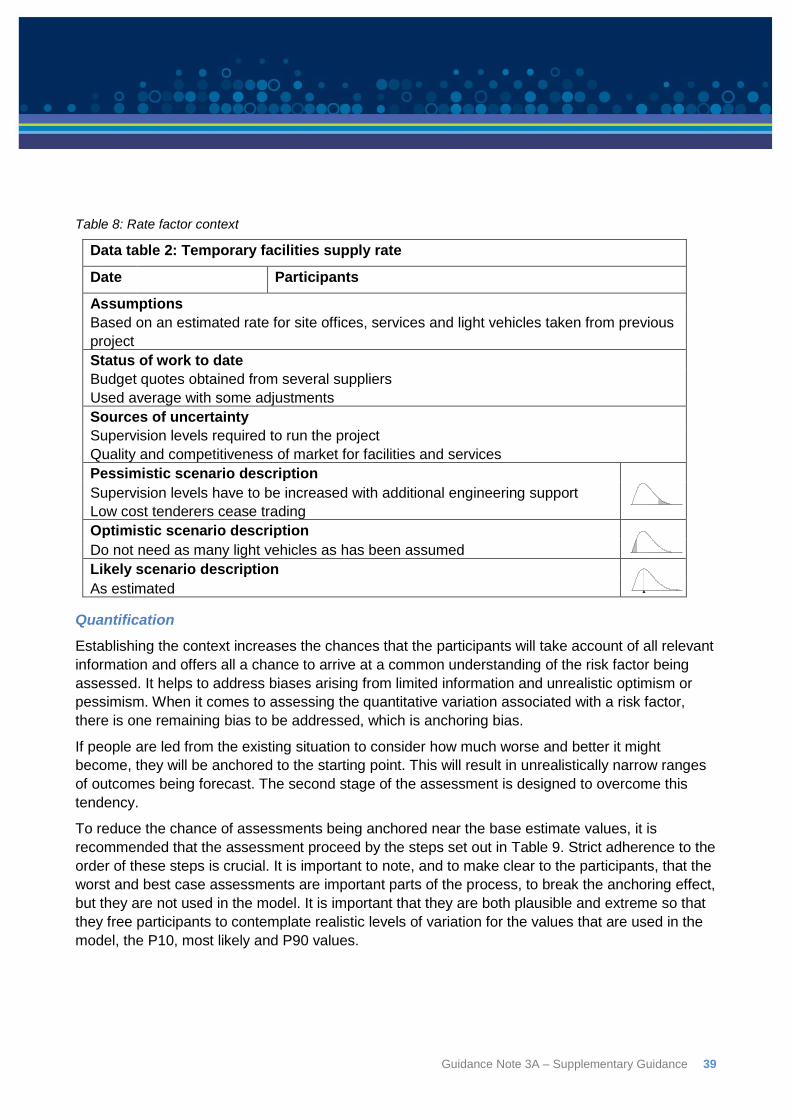
Guidance Note 3A – Supplementary Guidance 39
Table 8: Rate factor context
Data table 2: Temporary facilities supply rate
Date Participants
Assumptions
Based on an estimated rate for site offices, services and light vehicles taken from previous
project
Status of work to date
Budget quotes obtained from several suppliers
Used average with some adjustments
Sources of uncertainty
Supervision levels required to run the project
Quality and competitiveness of market for facilities and services
Pessimistic scenario description
Supervision levels have to be increased with additional engineering support
Low cost tenderers cease trading
Optimistic scenario description
Do not need as many light vehicles as has been assumed
Likely scenario description
As estimated
Quantification
Establishing the context increases the chances that the participants will take account of all relevant
information and offers all a chance to arrive at a common understanding of the risk factor being
assessed. It helps to address biases arising from limited information and unrealistic optimism or
pessimism. When it comes to assessing the quantitative variation associated with a risk factor,
there is one remaining bias to be addressed, which is anchoring bias.
If people are led from the existing situation to consider how much worse and better it might
become, they will be anchored to the starting point. This will result in unrealistically narrow ranges
of outcomes being forecast. The second stage of the assessment is designed to overcome this
tendency.
To reduce the chance of assessments being anchored near the base estimate values, it is
recommended that the assessment proceed by the steps set out in Table 9. Strict adherence to the
order of these steps is crucial. It is important to note, and to make clear to the participants, that the
worst and best case assessments are important parts of the process, to break the anchoring effect,
but they are not used in the model. It is important that they are both plausible and extreme so that
they free participants to contemplate realistic levels of variation for the values that are used in the
model, the P10, most likely and P90 values.
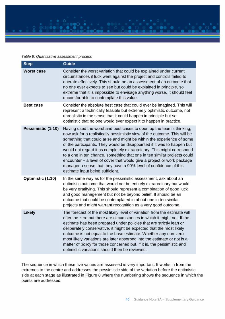
40 Guidance Note 3A – Supplementary Guidance
Table 9: Quantitative assessment process
Step Guide
Worst case Consider the worst variation that could be explained under current
circumstances if luck went against the project and controls failed to
operate effectively. This should be an assessment of an outcome that
no one ever expects to see but could be explained in principle, so
extreme that it is impossible to envisage anything worse. It should feel
uncomfortable to contemplate this value.
Best case Consider the absolute best case that could ever be imagined. This will
represent a technically feasible but extremely optimistic outcome, not
unrealistic in the sense that it could happen in principle but so
optimistic that no one would ever expect it to happen in practice.
Pessimistic (1:10) Having used the worst and best cases to open up the team’s thinking,
now ask for a realistically pessimistic view of the outcome. This will be
something that could arise and might be within the experience of some
of the participants. They would be disappointed if it was to happen but
would not regard it as completely extraordinary. This might correspond
to a one in ten chance, something that one in ten similar projects could
encounter – a level of cover that would give a project or work package
manager a sense that they have a 90% level of confidence of this
estimate input being sufficient.
Optimistic (1:10) In the same way as for the pessimistic assessment, ask about an
optimistic outcome that would not be entirely extraordinary but would
be very gratifying. This should represent a combination of good luck
and good management but not be beyond belief. It should be an
outcome that could be contemplated in about one in ten similar
projects and might warrant recognition as a very good outcome.
Likely The forecast of the most likely level of variation from the estimate will
often be zero but there are circumstances in which it might not. If the
estimate has been prepared under policies that are strictly lean or
deliberately conservative, it might be expected that the most likely
outcome is not equal to the base estimate. Whether any non-zero
most likely variations are later absorbed into the estimate or not is a
matter of policy for those concerned but, if it is, the pessimistic and
optimistic variations should then be reviewed.
The sequence in which these five values are assessed is very important. It works in from the
extremes to the centre and addresses the pessimistic side of the variation before the optimistic
side at each stage as illustrated in Figure 8 where the numbering shows the sequence in which the
points are addressed.
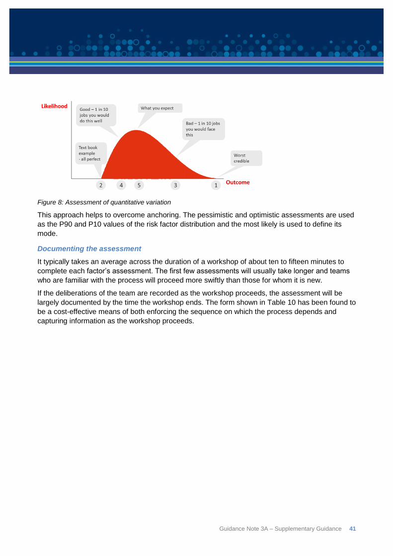
Guidance Note 3A – Supplementary Guidance 41
Figure 8: Assessment of quantitative variation
This approach helps to overcome anchoring. The pessimistic and optimistic assessments are used
as the P90 and P10 values of the risk factor distribution and the most likely is used to define its
mode.
Documenting the assessment
It typically takes an average across the duration of a workshop of about ten to fifteen minutes to
complete each factor’s assessment. The first few assessments will usually take longer and teams
who are familiar with the process will proceed more swiftly than those for whom it is new.
If the deliberations of the team are recorded as the workshop proceeds, the assessment will be
largely documented by the time the workshop ends. The form shown in Table 10 has been found to
be a cost-effective means of both enforcing the sequence on which the process depends and
capturing information as the workshop proceeds.
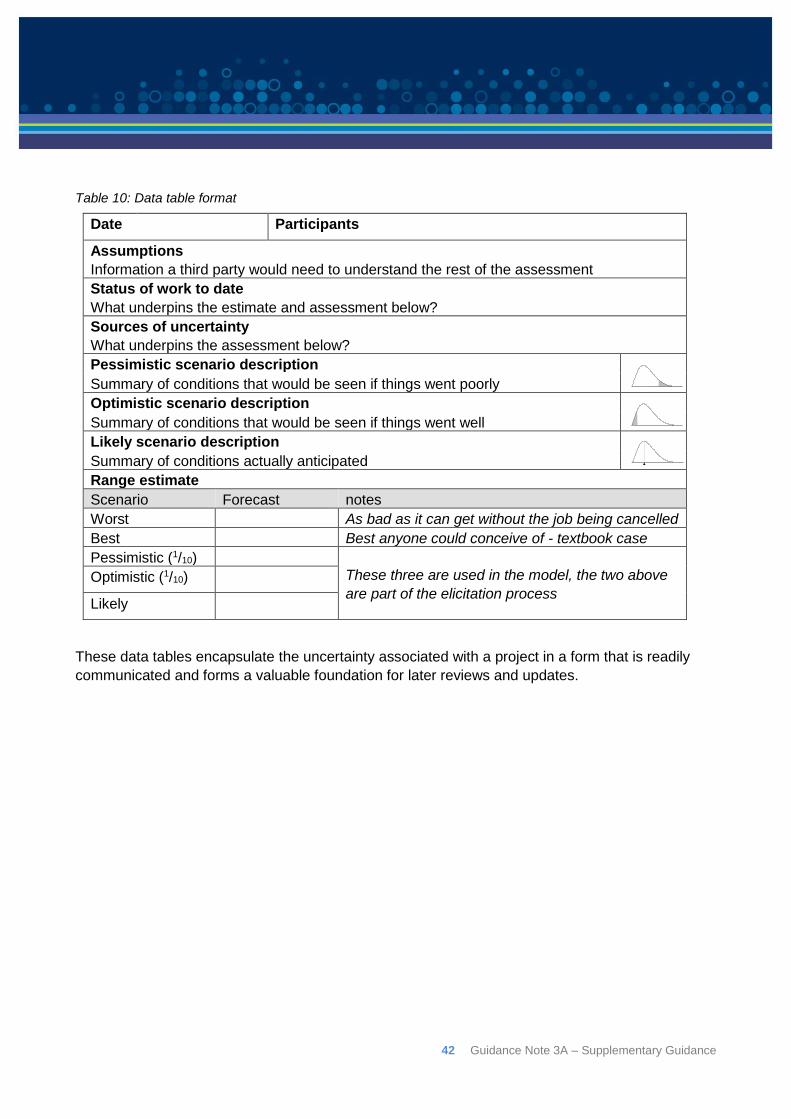
42 Guidance Note 3A – Supplementary Guidance
Table 10: Data table format
Date Participants
Assumptions
Information a third party would need to understand the rest of the assessment
Status of work to date
What underpins the estimate and assessment below?
Sources of uncertainty
What underpins the assessment below?
Pessimistic scenario description
Summary of conditions that would be seen if things went poorly
Optimistic scenario description
Summary of conditions that would be seen if things went well
Likely scenario description
Summary of conditions actually anticipated
Range estimate
Scenario Forecast notes
Worst As bad as it can get without the job being cancelled
Best Best anyone could conceive of - textbook case
Pessimistic (1/10)
These three are used in the model, the two above
are part of the elicitation process Optimistic (1/10)
Likely
These data tables encapsulate the uncertainty associated with a project in a form that is readily
communicated and forms a valuable foundation for later reviews and updates.
Guidance Note 3A – Supplementary Guidance 43
6: Model Structure
6.1: Design principles
A project cost risk model must connect sources of uncertainty to the estimate in a way that allows
their aggregate effect to be assessed. This involves deciding how to describe uncertainty or risks,
how to summarise the estimate and how to link one to the other. This part of the exercise is often
overlooked with a default model structure being used without consideration of how these three
components are designed: the way risk is described, the way the estimate is summarised and the
way the two are connected. Attention to this aspect of the analysis can improve its realism and
avoid unnecessary effort.
The key design principles recommended here are:
A model should be as simple as it can be while including enough detail to represent the
material uncertainties affecting the cost; and
The relationship between real world uncertainties and elements of the model should be as
straightforward and direct as possible.
Before explaining a methodical approach to developing a model structure, it is useful to remember
why there is uncertainty in a cost estimate so that attention remains focused on the uncertainty
being analysed rather than on the technical details of models, which are only a means to an end
not an end in their own right.
Uncertainty arises from the fact that it is impractical to develop and prove a design in advance of
construction to the point at which it could be built with no further changes. At the stage when a risk
analysis is undertaken, in general, the level of definition will be more or less uniform across large
parts of the design or even across the whole project. This means that, for example, the uncertainty
associated with bulk material quantities, for one type of material, will be more or less the same
across related parts of the estimate. In the same way, the extent to which market rates have been
assessed, using a mix of past projects, budgetary quotations, benchmarking, firm quotes or other
methods, will be fairly uniform for related classes of materials and equipment.
The level of uncertainty affecting quantities or rates across a large part of a project can be used as
a high level representation of cost uncertainty in a risk model. The approach recommended here is
to break down the project cost as a whole in such a manner that uncertainty in bulk material
quantities, unit rates, productivity assumptions, major equipment prices and other major estimating
inputs can be applied to those parts of the cost that they affect at as large a scale as possible. This
process starts with the simplest breakdown possible and only introduces more detail where it is
necessary to allow distinct uncertainties to be applied.
By only breaking the estimate into the minimum number of parts required to fit the way uncertainty
is spread across the project, the model remains as simple as it can be while having enough detail
to represent the separate areas faithfully. For instance, if the uncertainty about bulk earthworks
quantities was higher in one area of a project than in another, perhaps due to having better
geotechnical information about one region than another, quantity uncertainty in those two areas
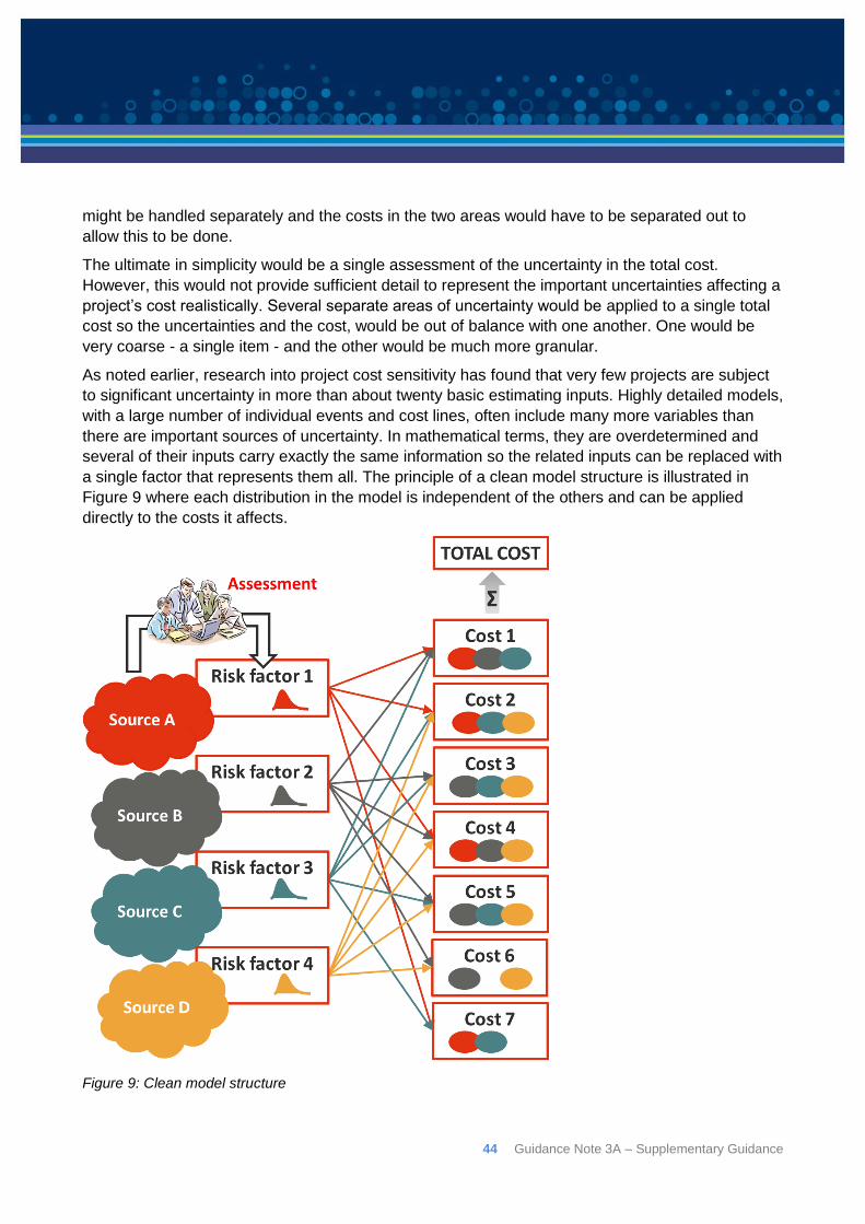
44 Guidance Note 3A – Supplementary Guidance
might be handled separately and the costs in the two areas would have to be separated out to
allow this to be done.
The ultimate in simplicity would be a single assessment of the uncertainty in the total cost.
However, this would not provide sufficient detail to represent the important uncertainties affecting a
project’s cost realistically. Several separate areas of uncertainty would be applied to a single total
cost so the uncertainties and the cost, would be out of balance with one another. One would be
very coarse - a single item - and the other would be much more granular.
As noted earlier, research into project cost sensitivity has found that very few projects are subject
to significant uncertainty in more than about twenty basic estimating inputs. Highly detailed models,
with a large number of individual events and cost lines, often include many more variables than
there are important sources of uncertainty. In mathematical terms, they are overdetermined and
several of their inputs carry exactly the same information so the related inputs can be replaced with
a single factor that represents them all. The principle of a clean model structure is illustrated in
Figure 9 where each distribution in the model is independent of the others and can be applied
directly to the costs it affects.
Figure 9: Clean model structure
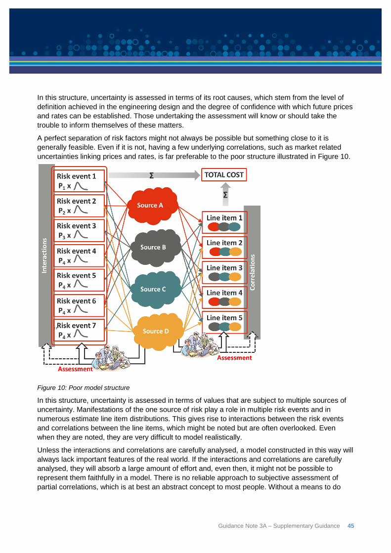
Guidance Note 3A – Supplementary Guidance 45
In this structure, uncertainty is assessed in terms of its root causes, which stem from the level of
definition achieved in the engineering design and the degree of confidence with which future prices
and rates can be established. Those undertaking the assessment will know or should take the
trouble to inform themselves of these matters.
A perfect separation of risk factors might not always be possible but something close to it is
generally feasible. Even if it is not, having a few underlying correlations, such as market related
uncertainties linking prices and rates, is far preferable to the poor structure illustrated in Figure 10.
Figure 10: Poor model structure
In this structure, uncertainty is assessed in terms of values that are subject to multiple sources of
uncertainty. Manifestations of the one source of risk play a role in multiple risk events and in
numerous estimate line item distributions. This gives rise to interactions between the risk events
and correlations between the line items, which might be noted but are often overlooked. Even
when they are noted, they are very difficult to model realistically.
Unless the interactions and correlations are carefully analysed, a model constructed in this way will
always lack important features of the real world. If the interactions and correlations are carefully
analysed, they will absorb a large amount of effort and, even then, it might not be possible to
represent them faithfully in a model. There is no reliable approach to subjective assessment of
partial correlations, which is at best an abstract concept to most people. Without a means to do
46 Guidance Note 3A – Supplementary Guidance
this, the connections between line items on the right hand side of Figure 10 cannot be assessed let
alone included in a model.
Models of the form illustrated in Figure 10 effectively represent each big source of uncertainty
many times over in a lot of separate potential events or estimate lines. As outlined earlier, it is all
but impossible to assess and represent correlations realistically between large numbers of line-
items or to allow for the number and complexity of the dependencies that can arise among a large
number of risk register entries. To build a model that ignores these is to leave out a large part of
the way risk affects a project’s costs. To build a model that deals with these interactions and
correlations realistically is at best cumbersome, time consuming and often impossible for all
practical purposes.
6.2: General Structure
Uncertainties
The first step in designing a cost risk model is to determine how best to describe the uncertainties
that affect the cost. This is best approached from the top down, using broad descriptions of
uncertainty that cover major parts of the cost wherever possible and introducing detail where, but
only where, it makes a significant difference to the quality and realism of the model. Matters that
attract a lot of attention are not always the most significant.
As noted earlier, infrastructure cost estimates are almost always subject to uncertainty in:
Quantities of materials bought, moved and placed;
Unit rates for the purchase of materials, equipment or labour;
Productivity rates for labour and plant;
Running rates for management, overheads and temporary facilities;
Lump sum costs of major purchases; and
The duration of the work.
There is no single way to arrive at a sound cost risk model but, as a general guide, it is useful to
start with these factors and consider whether, for a particular project:
They are all relevant;
Which bulk quantities are important (are subject to appreciable uncertainty and affect a
significant part of the cost);
Which rates are important (are subject to appreciable uncertainty and affect a significant
part of the cost);
Whether it is sufficient to represent the level of uncertainty in these quantities and rates
across the whole job or it is necessary to split the project into physical parts, phases or
types of work (green and brown field for instance) for some uncertainties;
Which lump sum amounts, such as major equipment purchases, it will be useful to split out;
and
Whether time dependent costs can be analysed as a whole across the entire duration or will
be subject to markedly different levels of uncertainty at different stages in the work.
Guidance Note 3A – Supplementary Guidance 47
Subcontract items can create some confusion. Once a subcontract is signed, some risk will usually
be transferred to the subcontractor. However, subcontracts might not be in place at the time an
estimate is prepared as a project is seeking approval. In this situation, uncertainty in quantities and
rates will play a role in estimating the cost of the subcontract. If it assumed that the subcontractor
will take account of the same factors as the project, the value of the subcontract will be subject to
the same quantity uncertainty as if the work was being performed by direct labour as well as often
being subject to uncertainty about subcontractors’ mark ups and overheads.
It is important to remember that the ranges represented by risk factors affecting rates and prices
are intended to represent uncertainty due to state of the design and procurement information
available at the time an estimate is prepared. They represent the potential variation that could arise
between what is in the estimate and the actual cost if orders were to be placed and work was to be
carried out immediately. There is a danger that people assessing ranges on rates and prices will
fall into the trap of including in their assessment variations that will arise due to escalation.
Escalation might also be subject to uncertainty but it is quite distinct from uncertainty associated
with material specifications, commercial arrangements with suppliers and similar matters.
Guidance note 4 (Escalation) discusses these matters in greater detail.
6.3: Linking cost drivers to risk drivers
Risk is the effect of uncertainty on objectives. Risks should not be confused with things that are
simply expensive. For example, while the pavement in many road projects may make up the
largest proportion of the cost, it will only increase and drive up the total cost significantly if the
scope grows or the design changes appreciably. This will generally not happen if development and
project planning are done well. If the scope is well-defined, subgrade conditions are well known,
material of known quality is known to be readily available, etc., then the range of possible cost
outcomes will be small in percentage terms. It is the level of scope definition and geotechnical
investigation that is the source of the uncertainty, not the fact that the pavement is a large
proportion of the total cost.
One of the core principles of a risk factor approach is to provide a clean relationship between the
factors that represent uncertainties, such as those listed earlier, and the costs that they affect.
There are several ways this can be accomplished. The example models described in this section
show one way to do this. Estimators and analysts will use their ingenuity to develop methods that
suit them and their other systems while continuing to pay attention to the principles of simplicity
and a clean structure.
A useful approach that fits many projects is to use a cost matrix that splits costs one way to match
the description of quantity uncertainties along the other axis to allow the application of rate
uncertainties. An example of this is illustrated in Figure 11.
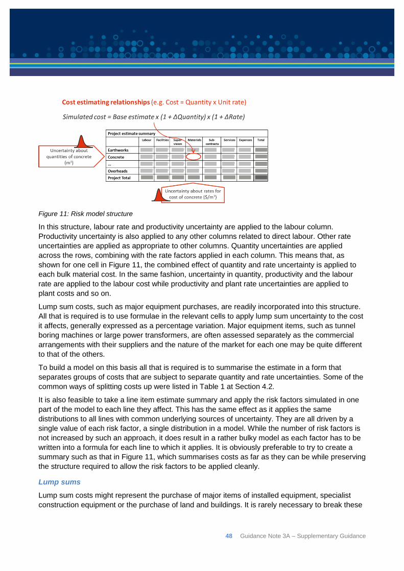
48 Guidance Note 3A – Supplementary Guidance
Figure 11: Risk model structure
In this structure, labour rate and productivity uncertainty are applied to the labour column.
Productivity uncertainty is also applied to any other columns related to direct labour. Other rate
uncertainties are applied as appropriate to other columns. Quantity uncertainties are applied
across the rows, combining with the rate factors applied in each column. This means that, as
shown for one cell in Figure 11, the combined effect of quantity and rate uncertainty is applied to
each bulk material cost. In the same fashion, uncertainty in quantity, productivity and the labour
rate are applied to the labour cost while productivity and plant rate uncertainties are applied to
plant costs and so on.
Lump sum costs, such as major equipment purchases, are readily incorporated into this structure.
All that is required is to use formulae in the relevant cells to apply lump sum uncertainty to the cost
it affects, generally expressed as a percentage variation. Major equipment items, such as tunnel
boring machines or large power transformers, are often assessed separately as the commercial
arrangements with their suppliers and the nature of the market for each one may be quite different
to that of the others.
To build a model on this basis all that is required is to summarise the estimate in a form that
separates groups of costs that are subject to separate quantity and rate uncertainties. Some of the
common ways of splitting costs up were listed in Table 1 at Section 4.2.
It is also feasible to take a line item estimate summary and apply the risk factors simulated in one
part of the model to each line they affect. This has the same effect as it applies the same
distributions to all lines with common underlying sources of uncertainty. They are all driven by a
single value of each risk factor, a single distribution in a model. While the number of risk factors is
not increased by such an approach, it does result in a rather bulky model as each factor has to be
written into a formula for each line to which it applies. It is obviously preferable to try to create a
summary such as that in Figure 11, which summarises costs as far as they can be while preserving
the structure required to allow the risk factors to be applied cleanly.
Lump sums
Lump sum costs might represent the purchase of major items of installed equipment, specialist
construction equipment or the purchase of land and buildings. It is rarely necessary to break these
Guidance Note 3A – Supplementary Guidance 49
down further and uncertainty in the cost of individual items or classes of items can usually just be
assessed directly.
If freight costs are significant, perhaps for a remote site or equipment requiring specialised
transport, unloading and placement, or if freight costs are subject to different commercial
conditions to the cost of the items themselves, it may be worthwhile breaking out freight costs and
assessing their uncertainty separately.
Events
If a project is subject to potential events that can have an appreciable effect on the project cost,
they can easily be included in the model. It is important to consider first whether:
They have a high enough likelihood to warrant including in the contingency as opposed to
being rare background risks that would be considered ‘business as usual’ operating
conditions, such as a risk of epidemic disease; and/or
They are not so large and likely to occur that they should be treated as separate
contingency items outside the main project account, as outlined in Section 4.4, such as a
requirement to reduce road noise levels to a much lower level due to a new standard being
imposed for political reasons.
Care may be required to avoid the unnecessary use of events in risk models simply by default,
because risk registers have often been used as the basis of risk models in the past. It is difficult to
be prescriptive but, if an event risk cannot affect a project’s cost by more than a few percent, it will
often fall naturally into one of the risk factor range assessments as one of a number of discrete
uncertainties felt by the project as an aggregate uncertainty in the quantities or rates affecting a
substantial part of the cost as a whole.
It will often be useful to analyse such events separately for the purposes of day to day
management or to understand the costs and benefits of strategies for treating the risks, supporting
operational management decision making. This is a separate exercise to the task of assessing the
overall contingency required for a project as a whole. There is no need to clutter the project
contingency analysis with the details of day to day management decision making. Important as
they are in their own right, not all such decisions are significant enough to warrant separate
attention when assessing project total funding requirements.
6.4: Choice of uncertainty distribution
A probability distribution represents the likelihood of an uncertain quantity taking on values within
the range that can arise.
There is no objective basis for choosing one particular distribution shape to represent an
assessment of the uncertainty in part of a project’s cost. Two shapes in common use for routine
cost modelling are the Beta PERT and triangular distributions. These are illustrated in Figure 12,
which shows examples of the two distributions with the same P10, Mode and P90 values, so they
represent the same inputs.
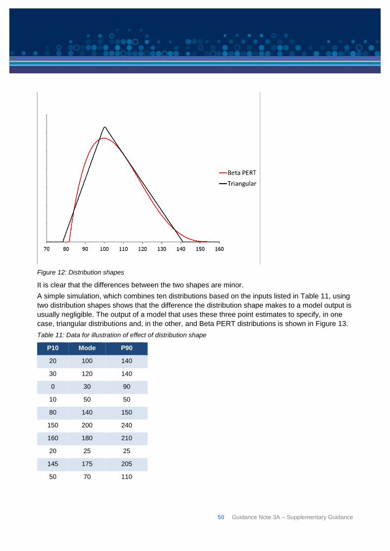
50 Guidance Note 3A – Supplementary Guidance
Figure 12: Distribution shapes
It is clear that the differences between the two shapes are minor.
A simple simulation, which combines ten distributions based on the inputs listed in Table 11, using
two distribution shapes shows that the difference the distribution shape makes to a model output is
usually negligible. The output of a model that uses these three point estimates to specify, in one
case, triangular distributions and, in the other, and Beta PERT distributions is shown in Figure 13.
Table 11: Data for illustration of effect of distribution shape
P10 Mode P90
20 100 140
30 120 140
0 30 90
10 50 50
80 140 150
150 200 240
160 180 210
20 25 25
145 175 205
50 70 110
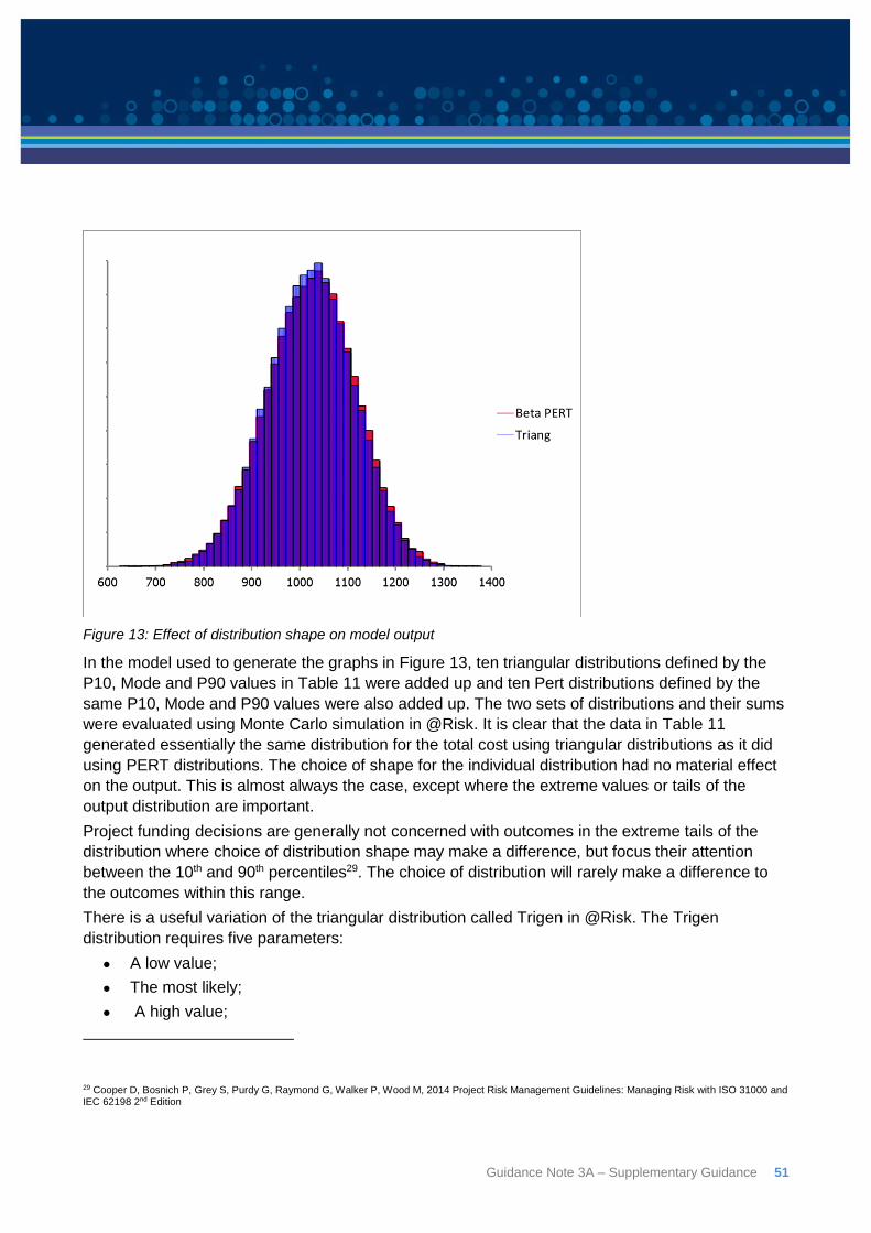
Guidance Note 3A – Supplementary Guidance 51
Figure 13: Effect of distribution shape on model output
In the model used to generate the graphs in Figure 13, ten triangular distributions defined by the
P10, Mode and P90 values in Table 11 were added up and ten Pert distributions defined by the
same P10, Mode and P90 values were also added up. The two sets of distributions and their sums
were evaluated using Monte Carlo simulation in @Risk. It is clear that the data in Table 11
generated essentially the same distribution for the total cost using triangular distributions as it did
using PERT distributions. The choice of shape for the individual distribution had no material effect
on the output. This is almost always the case, except where the extreme values or tails of the
output distribution are important.
Project funding decisions are generally not concerned with outcomes in the extreme tails of the
distribution where choice of distribution shape may make a difference, but focus their attention
between the 10th and 90th percentiles29. The choice of distribution will rarely make a difference to
the outcomes within this range.
There is a useful variation of the triangular distribution called Trigen in @Risk. The Trigen
distribution requires five parameters:
A low value;
The most likely;
A high value;
29 Cooper D, Bosnich P, Grey S, Purdy G, Raymond G, Walker P, Wood M, 2014 Project Risk Management Guidelines: Managing Risk with ISO 31000 and IEC 62198 2nd Edition
52 Guidance Note 3A – Supplementary Guidance
The probability that the parameter value could be below the low value; and
The probability that the parameter value could be above the high value.
Because the analyst can discuss what probabilities the experts would use to define optimistic and
pessimistic values, the Trigen adapts to each expert’s concept of these points. The most common
optimistic and pessimistic points used to elicit range assessments and implement distributions in a
model are the P10 and P90.
In the context of determining the most appropriate distribution for a given risk factor, all of the
parameters required to define a Trigen distribution will have been identified within the risk
workshop and recorded within Table 9. The Department considers that, unless it is known that a
distribution conforms to a certain shape, the Trigen, Triangle or PERT are all a sensible choice of
distribution to allocate to a given risk factor.
Appendix D provides a further discussion of different types of distributions, and their applications.
6.5: Account for correlation between WBS element costs to properly capture cost risk
As previously discussed, valid Monte Carlo simulation requires that the dependencies between the
model inputs be understood and included in the model. One of the main reasons for the
development of risk factor models is that they avoid the need to incorporate complicated
correlations into risk models. Risk driver/risk factor methods enable this because true root causes
are, as far as possible, chosen to be statistically independent and so that they can be combined
using simple functional relationships.
The most common use for correlations in risk factor models is to link market rate uncertainties for
bulk materials, plant and possibly subcontractors’ distributables and overheads. If the supply of
quarry materials, concrete and steel in a region are all driven by the level of similar project activity
that will be underway when the work commences, each one can be expected to take up a similar
position within its own range. They will probably all be at the high end, all at the low end or all at a
mid-point of their expected ranges. This can be implemented using correlations in the models, as is
shown in the example models.
In some circumstances, labour rate uncertainty will also be correlated with uncertainty in material
supply and plant rates. This is handled in the same way.
It sometimes happens that uncertainty in the productivity of one class of labour is different to the
uncertainty in the productivity of another class of labour, perhaps green field and brown field or
across separate disciplines. While the level of uncertainty in the productivity of each class of labour
may be different, if they all depend on site conditions, such as congestion or the quality of planning
and co-ordination, they might all tend to be high, all be low, or all fall towards the middle of their
separate ranges in unison. Here too, it is not uncommon to use correlation to represent this linkage
in a model.
This simple recognition of a single common source of uncertainty affecting a set of related risk
factors is quite different to the challenge of understanding correlations between work package
costs that depend on uncertainty in quantities and rates for two or three separate commodity unit
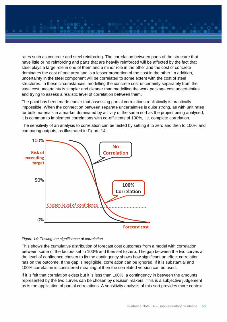
Guidance Note 3A – Supplementary Guidance 53
rates such as concrete and steel reinforcing. The correlation between parts of the structure that
have little or no reinforcing and parts that are heavily reinforced will be affected by the fact that
steel plays a large role in one of them and a minor role in the other and the cost of concrete
dominates the cost of one area and is a lesser proportion of the cost in the other. In addition,
uncertainty in the steel component will be correlated to some extent with the cost of steel
structures. In these circumstances, modelling the concrete cost uncertainty separately from the
steel cost uncertainty is simpler and cleaner than modelling the work package cost uncertainties
and trying to assess a realistic level of correlation between them.
The point has been made earlier that assessing partial correlations realistically is practically
impossible. When the connection between separate uncertainties is quite strong, as with unit rates
for bulk materials in a market dominated by activity of the same sort as the project being analysed,
it is common to implement correlations with co-efficients of 100%, i.e. complete correlation.
The sensitivity of an analysis to correlation can be tested by setting it to zero and then to 100% and
comparing outputs, as illustrated in Figure 14.
Figure 14: Testing the significance of correlation
This shows the cumulative distribution of forecast cost outcomes from a model with correlation
between some of the factors set to 100% and then set to zero. The gap between the two curves at
the level of confidence chosen to fix the contingency shows how significant an effect correlation
has on the outcome. If the gap is negligible, correlation can be ignored. If it is substantial and
100% correlation is considered meaningful then the correlated version can be used.
If it is felt that correlation exists but it is less than 100%, a contingency in between the amounts
represented by the two curves can be chosen by decision makers. This is a subjective judgement
as is the application of partial correlations. A sensitivity analysis of this sort provides more context
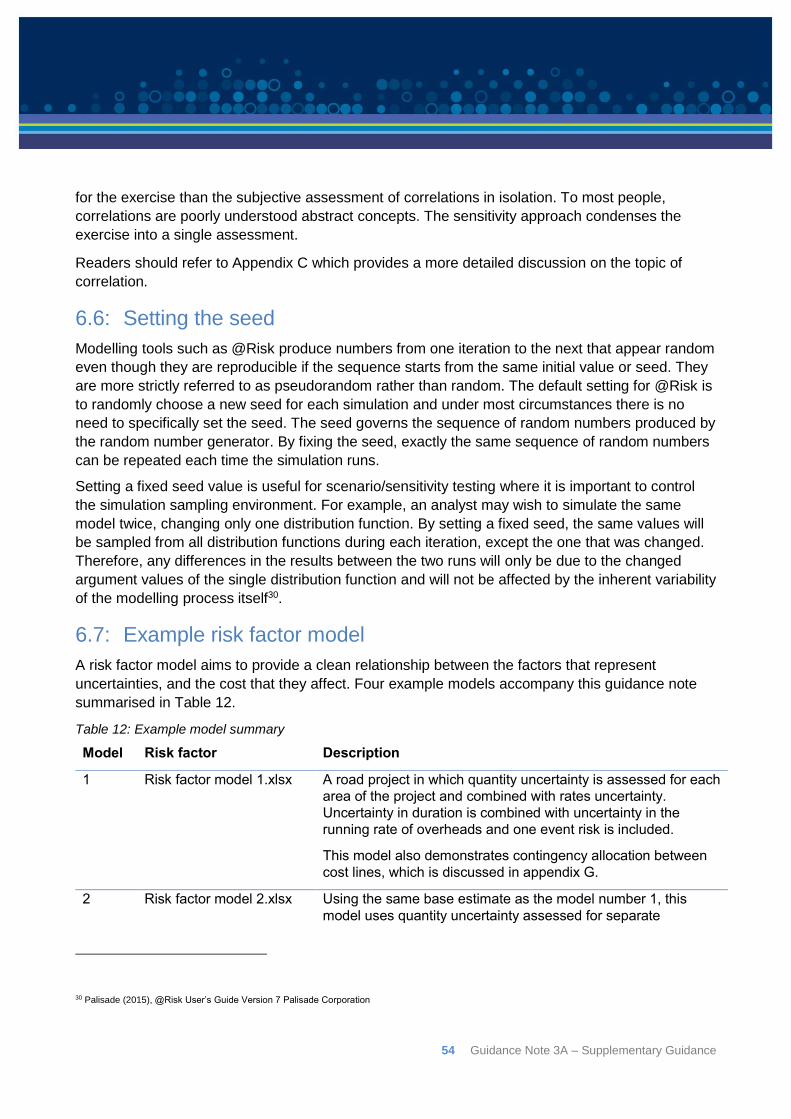
54 Guidance Note 3A – Supplementary Guidance
for the exercise than the subjective assessment of correlations in isolation. To most people,
correlations are poorly understood abstract concepts. The sensitivity approach condenses the
exercise into a single assessment.
Readers should refer to Appendix C which provides a more detailed discussion on the topic of
correlation.
6.6: Setting the seed
Modelling tools such as @Risk produce numbers from one iteration to the next that appear random
even though they are reproducible if the sequence starts from the same initial value or seed. They
are more strictly referred to as pseudorandom rather than random. The default setting for @Risk is
to randomly choose a new seed for each simulation and under most circumstances there is no
need to specifically set the seed. The seed governs the sequence of random numbers produced by
the random number generator. By fixing the seed, exactly the same sequence of random numbers
can be repeated each time the simulation runs.
Setting a fixed seed value is useful for scenario/sensitivity testing where it is important to control
the simulation sampling environment. For example, an analyst may wish to simulate the same
model twice, changing only one distribution function. By setting a fixed seed, the same values will
be sampled from all distribution functions during each iteration, except the one that was changed.
Therefore, any differences in the results between the two runs will only be due to the changed
argument values of the single distribution function and will not be affected by the inherent variability
of the modelling process itself30.
6.7: Example risk factor model
A risk factor model aims to provide a clean relationship between the factors that represent
uncertainties, and the cost that they affect. Four example models accompany this guidance note
summarised in Table 12.
Table 12: Example model summary
Model Risk factor Description
1 Risk factor model 1.xlsx A road project in which quantity uncertainty is assessed for each
area of the project and combined with rates uncertainty.
Uncertainty in duration is combined with uncertainty in the
running rate of overheads and one event risk is included.
This model also demonstrates contingency allocation between
cost lines, which is discussed in appendix G.
2 Risk factor model 2.xlsx Using the same base estimate as the model number 1, this
model uses quantity uncertainty assessed for separate
30 Palisade (2015), @Risk User’s Guide Version 7 Palisade Corporation
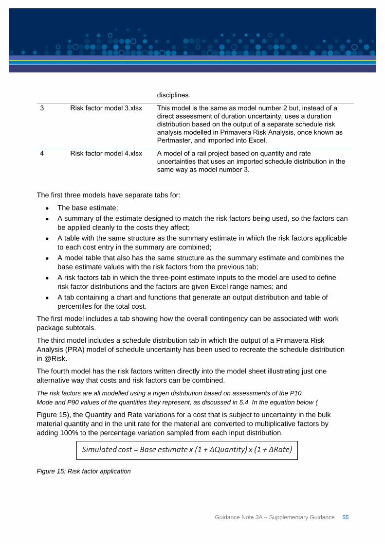
Guidance Note 3A – Supplementary Guidance 55
disciplines.
3 Risk factor model 3.xlsx This model is the same as model number 2 but, instead of a
direct assessment of duration uncertainty, uses a duration
distribution based on the output of a separate schedule risk
analysis modelled in Primavera Risk Analysis, once known as
Pertmaster, and imported into Excel.
4 Risk factor model 4.xlsx A model of a rail project based on quantity and rate
uncertainties that uses an imported schedule distribution in the
same way as model number 3.
The first three models have separate tabs for:
The base estimate;
A summary of the estimate designed to match the risk factors being used, so the factors can
be applied cleanly to the costs they affect;
A table with the same structure as the summary estimate in which the risk factors applicable
to each cost entry in the summary are combined;
A model table that also has the same structure as the summary estimate and combines the
base estimate values with the risk factors from the previous tab;
A risk factors tab in which the three-point estimate inputs to the model are used to define
risk factor distributions and the factors are given Excel range names; and
A tab containing a chart and functions that generate an output distribution and table of
percentiles for the total cost.
The first model includes a tab showing how the overall contingency can be associated with work
package subtotals.
The third model includes a schedule distribution tab in which the output of a Primavera Risk
Analysis (PRA) model of schedule uncertainty has been used to recreate the schedule distribution
in @Risk.
The fourth model has the risk factors written directly into the model sheet illustrating just one
alternative way that costs and risk factors can be combined.
The risk factors are all modelled using a trigen distribution based on assessments of the P10,
Mode and P90 values of the quantities they represent, as discussed in 5.4. In the equation below (
Figure 15), the Quantity and Rate variations for a cost that is subject to uncertainty in the bulk
material quantity and in the unit rate for the material are converted to multiplicative factors by
adding 100% to the percentage variation sampled from each input distribution.
Figure 15: Risk factor application
56 Guidance Note 3A – Supplementary Guidance
The risk factors tabs also include correlation matrices linking rate uncertainty across several inputs
and, in the first three models, the discrete risk event included in the model. The risk event has a
defined probability of occurring and an uncertain impact value if it does occur.
The fourth model does not use correlations although it could if this was deemed appropriate. It has
a separate tab for model parameters where the start and end dates of the two parts of the job are
entered and used in the two schedule models, the longest one of which drives the overheads. The
proportions of overheads that are subject to schedule variation are also entered here as
parameters and used in the model to modify the schedule variation’s impact on time related costs.
This avoids the need to separate out the time dependent and other costs from one another in the
overheads.
The schedule tabs in models number 3 and number 4 use the @Risk function RiskCumul() to
recreate from the PRA histogram of completion dates a distribution of the duration of the project.
This is turned into a distribution of the simulated duration relative to the base duration using the
planned start and end dates. That relative variation, the duration risk factor, is used to drive the
overheads, management costs and temporary facilities costs.
The summary output tabs, that create the cumulative distribution and percentile table, and the
schedule tabs that recreate the PRA output, have notes embedded explaining key points about
linking them into the model and importing the PRA data.
6.8: Step through of model
The model accompanying this guidance note has been created using @Risk31. As such, naming
conventions to create functions and distributions reflect that particular piece of software. The model
could easily be replicated in other software noting that some add-ins such as ModelRisk will allow
@Risk files to be imported directly with naming conventions for formulas automatically changed to
suit the ModelRisk software.
The structure of the model itself is the key to the risk factor approach and will remain the same
whichever software simulation tool is used.
The following section demonstrates how a risk factor approach can be applied to an estimate. Risk
factor model 2.xlsx has been used as the basis of this explanation. It is suggested that readers
open the spreadsheet model while reading through this explanation.
Note that the process has been described as a series of steps. In reality the process will be both
non-sequential and iterative. For example, as an estimator begins to build an estimate, an idea of
the risk factors likely to affect the project will begin to emerge. This in turn will affect how the
estimate is best structured and summarised in order to provide a clean relationship between the
factors that represent uncertainties and the costs that they affect.
31 The examples in this guidance note have been developed using the proprietary software programme @Risk and are used for demonstration purposes only. The Department does not endorse @Risk and acknowledges the availability of similar software tools.
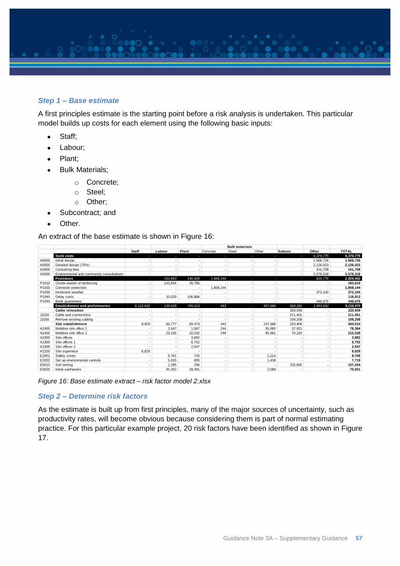
Guidance Note 3A – Supplementary Guidance 57
Step 1 – Base estimate
A first principles estimate is the starting point before a risk analysis is undertaken. This particular
model builds up costs for each element using the following basic inputs:
Staff;
Labour;
Plant;
Bulk Materials;
o Concrete;
o Steel;
o Other;
Subcontract; and
Other.
An extract of the base estimate is shown in Figure 16:
Figure 16: Base estimate extract – risk factor model 2.xlsx
Step 2 – Determine risk factors
As the estimate is built up from first principles, many of the major sources of uncertainty, such as
productivity rates, will become obvious because considering them is part of normal estimating
practice. For this particular example project, 20 risk factors have been identified as shown in Figure
17.
Staff Labour Plant Concrete Steel Other Subcon Other TOTAL
Sunk costs - - - - - - - 6,374,775 6,374,775
A0000 Initial design - - - - - - - 1,568,726 1,568,726
A0000 Detailed design (70%) - - - - - - - 2,126,023 2,126,023
A0000 Consulting fees - - - - - - - 101,708 101,708
A0000 Environmental and community consultations - - - - - - - 2,578,318 2,578,318
Provisions - 153,863 146,669 1,808,144 - - - 820,776 2,929,452
P1010 Onsite rework of reinforcing - 143,834 39,785 - - - - - 183,619
P1020 Corrosion protection - - - 1,808,144 - - - - 1,808,144
P1030 Inclement weather - - - - - - - 372,100 372,100
P1040 Delay costs - 10,029 106,884 - - - - - 116,913
P1050 Bank guarantees - - - - - - - 448,676 448,676
Establishment and preliminaries 6,122,832 139,528 745,513 443 - 457,686 669,281 1,083,692 9,218,975
Cable relocation - - - - - - 320,659 - 320,659
J1020 Cable and connections - - - - - - 211,451 - 211,451
J1030 Remove existing cabling - - - - - - 109,208 - 109,208
Site establishment 8,829 83,777 69,473 443 - 137,686 263,806 - 564,014
A2400 Mobilise site office 1 - 2,647 1,567 244 - 35,985 37,921 - 78,364
A2400 Mobilise site office 2 - 23,106 22,542 199 - 95,961 70,220 - 212,028
A2300 Site offices - - 3,892 - - - - - 3,892
A2300 Site offices 1 - - 8,752 - - - - - 8,752
A2300 Site offices 2 - - 2,547 - - - - - 2,547
A2100 Site supervisor 8,829 - - - - - - - 8,829
E2001 Safety zones - 5,761 733 - - 2,214 - - 8,708
E2002 Set up environmental controls - 5,626 655 - - 1,438 - - 7,719
E6010 Soil testing - 1,285 294 - - - 155,665 - 157,244
E6020 Initial earthworks - 45,352 28,491 - - 2,088 - - 75,931
Bulk materials
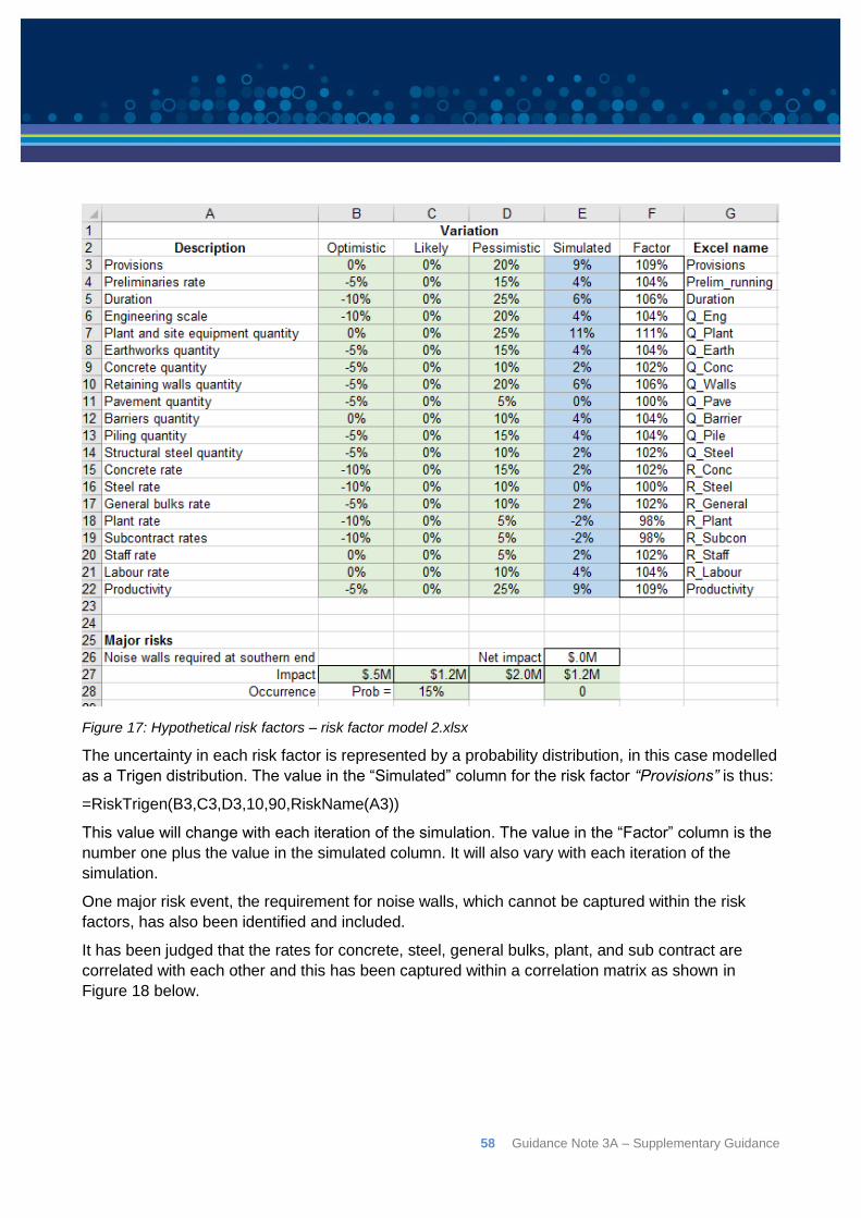
58 Guidance Note 3A – Supplementary Guidance
Figure 17: Hypothetical risk factors – risk factor model 2.xlsx
The uncertainty in each risk factor is represented by a probability distribution, in this case modelled
as a Trigen distribution. The value in the “Simulated” column for the risk factor “Provisions” is thus:
=RiskTrigen(B3,C3,D3,10,90,RiskName(A3))
This value will change with each iteration of the simulation. The value in the “Factor” column is the
number one plus the value in the simulated column. It will also vary with each iteration of the
simulation.
One major risk event, the requirement for noise walls, which cannot be captured within the risk
factors, has also been identified and included.
It has been judged that the rates for concrete, steel, general bulks, plant, and sub contract are
correlated with each other and this has been captured within a correlation matrix as shown in
Figure 18 below.
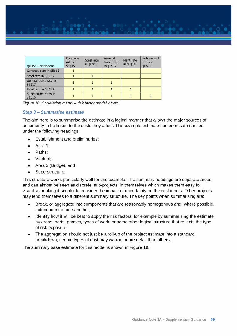
Guidance Note 3A – Supplementary Guidance 59
@RISK Correlations
Concrete rate in $E$15
Steel rate in $E$16
General bulks rate in $E$17
Plant rate in $E$18
Subcontract rates in $E$19
Concrete rate in $E$15 1
Steel rate in $E$16 1 1
General bulks rate in $E$17
1 1 1
Plant rate in $E$18 1 1 1 1
Subcontract rates in $E$19
1 1 1 1 1
Figure 18: Correlation matrix – risk factor model 2.xlsx
Step 3 – Summarise estimate
The aim here is to summarise the estimate in a logical manner that allows the major sources of
uncertainty to be linked to the costs they affect. This example estimate has been summarised
under the following headings:
Establishment and preliminaries;
Area 1;
Paths;
Viaduct;
Area 2 (Bridge); and
Superstructure.
This structure works particularly well for this example. The summary headings are separate areas
and can almost be seen as discrete ‘sub-projects’ in themselves which makes them easy to
visualise, making it simpler to consider the impact of uncertainty on the cost inputs. Other projects
may lend themselves to a different summary structure. The key points when summarising are:
Break, or aggregate into components that are reasonably homogenous and, where possible,
independent of one another;
Identify how it will be best to apply the risk factors, for example by summarising the estimate
by areas, parts, phases, types of work, or some other logical structure that reflects the type
of risk exposure;
The aggregation should not just be a roll-up of the project estimate into a standard
breakdown; certain types of cost may warrant more detail than others.
The summary base estimate for this model is shown in Figure 19.
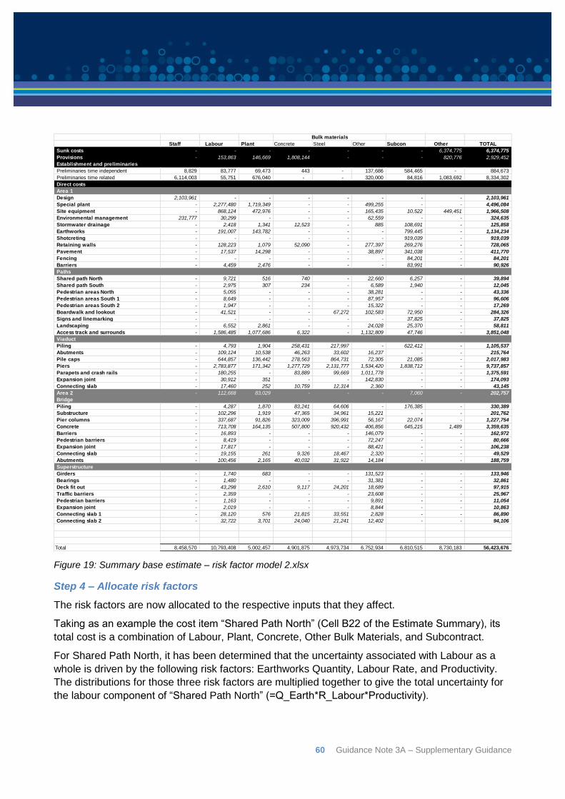
60 Guidance Note 3A – Supplementary Guidance
Figure 19: Summary base estimate – risk factor model 2.xlsx
Step 4 – Allocate risk factors
The risk factors are now allocated to the respective inputs that they affect.
Taking as an example the cost item “Shared Path North” (Cell B22 of the Estimate Summary), its
total cost is a combination of Labour, Plant, Concrete, Other Bulk Materials, and Subcontract.
For Shared Path North, it has been determined that the uncertainty associated with Labour as a
whole is driven by the following risk factors: Earthworks Quantity, Labour Rate, and Productivity.
The distributions for those three risk factors are multiplied together to give the total uncertainty for
the labour component of “Shared Path North” (=Q_Earth*R_Labour*Productivity).
Staff Labour Plant Concrete Steel Other Subcon Other TOTAL
Sunk costs - - - - - - - 6,374,775 6,374,775
Provisions - 153,863 146,669 1,808,144 - - - 820,776 2,929,452
Establishment and preliminaries
Preliminaries time independent 8,829 83,777 69,473 443 - 137,686 584,465 - 884,673
Preliminaries time related 6,114,003 55,751 676,040 - - 320,000 84,816 1,083,692 8,334,302
Direct costs
Area 1
Design 2,103,961 - - - - - - - 2,103,961
Special plant - 2,277,480 1,719,349 - - 499,255 - - 4,496,084
Site equipment - 868,124 472,976 - - 165,435 10,522 449,451 1,966,508
Environmental management 231,777 30,299 - - - 62,559 - - 324,635
Stormwater drainage - 2,418 1,341 12,523 - 885 108,691 - 125,858
Earthworks - 191,007 143,782 - - - 799,445 - 1,134,234
Shotcreting - - - - - - 919,039 - 919,039
Retaining walls - 128,223 1,079 52,090 - 277,397 269,276 - 728,065
Pavement - 17,537 14,298 - - 38,897 341,038 - 411,770
Fencing - - - - - - 84,201 - 84,201
Barriers - 4,459 2,476 - - - 83,991 - 90,926
Paths
Shared path North - 9,721 516 740 - 22,660 6,257 - 39,894
Shared path South - 2,975 307 234 - 6,589 1,940 - 12,045
Pedestrian areas North - 5,055 - - - 38,281 - - 43,336
Pedestrian areas South 1 - 8,649 - - - 87,957 - - 96,606
Pedestrian areas South 2 - 1,947 - - - 15,322 - - 17,269
Boardwalk and lookout - 41,521 - - 67,272 102,583 72,950 - 284,326
Signs and linemarking - - - - - - 37,825 - 37,825
Landscaping - 6,552 2,861 - - 24,028 25,370 - 58,811
Access track and surrounds - 1,586,485 1,077,686 6,322 - 1,132,809 47,746 - 3,851,048
Viaduct
Piling - 4,793 1,904 258,431 217,997 - 622,412 - 1,105,537
Abutments - 109,124 10,538 46,263 33,602 16,237 - - 215,764
Pile caps - 644,857 136,442 278,563 864,731 72,305 21,085 - 2,017,983
Piers - 2,783,877 171,342 1,277,729 2,131,777 1,534,420 1,838,712 - 9,737,857
Parapets and crash rails - 180,255 - 83,889 99,669 1,011,778 - - 1,375,591
Expansion joint - 30,912 351 - - 142,830 - - 174,093
Connecting slab - 17,460 252 10,759 12,314 2,360 - - 43,145
Area 2 - 112,668 83,029 - - - 7,060 - 202,757
Bridge
Piling - 4,287 1,870 83,241 64,606 - 176,385 - 330,389
Substructure - 102,296 1,919 47,365 34,961 15,221 - - 201,762
Pier columns - 337,687 91,826 323,009 396,991 56,167 22,074 - 1,227,754
Concrete - 713,708 164,135 507,800 920,432 406,856 645,215 1,489 3,359,635
Barriers - 16,893 - - - 146,079 - - 162,972
Pedestrian barriers - 8,419 - - - 72,247 - - 80,666
Expansion joint - 17,817 - - - 88,421 - - 106,238
Connecting slab - 19,155 261 9,326 18,467 2,320 - - 49,529
Abutments - 100,456 2,165 40,032 31,922 14,184 - - 188,759
Superstructure
Girders - 1,740 683 - - 131,523 - - 133,946
Bearings - 1,480 - - - 31,381 - - 32,861
Deck fit out - 43,298 2,610 9,117 24,201 18,689 - - 97,915
Traffic barriers - 2,359 - - - 23,608 - - 25,967
Pedestrian barriers - 1,163 - - - 9,891 - - 11,054
Expansion joint - 2,019 - - - 8,844 - - 10,863
Connecting slab 1 - 28,120 576 21,815 33,551 2,828 - - 86,890
Connecting slab 2 - 32,722 3,701 24,040 21,241 12,402 - - 94,106
Total 8,458,570 10,793,408 5,002,457 4,901,875 4,973,734 6,752,934 6,810,515 8,730,183 56,423,676
Bulk materials
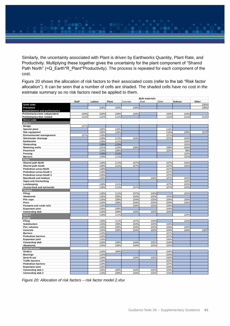
Guidance Note 3A – Supplementary Guidance 61
Similarly, the uncertainty associated with Plant is driven by Earthworks Quantity, Plant Rate, and
Productivity. Multiplying these together gives the uncertainty for the plant component of “Shared
Path North” (=Q_Earth*R_Plant*Productivity). The process is repeated for each component of the
cost.
Figure 20 shows the allocation of risk factors to their associated costs (refer to the tab “Risk factor
allocation”). It can be seen that a number of cells are shaded. The shaded cells have no cost in the
estimate summary so no risk factors need be applied to them.
Figure 20: Allocation of risk factors – risk factor model 2.xlsx
Staff Labour Plant Concrete Steel Other Subcon Other
Sunk costs 100%
Provisions 109% 109% 109% 109%
Establishment and preliminaries
Preliminaries time independent 104% 104% 104% 104% 104% 104%
Preliminaries time related 111% 111% 111% 111% 111% 111%
Direct costs
Area 1
Design 107%
Special plant 126% 118% 114%
Site equipment 126% 118% 114% 109% 122%
Environmental management 107% 118% 107%
Stormwater drainage 118% 111% 104% 107% 102%
Earthworks 118% 111% 102%
Shotcreting 118% 111% 102%
Retaining walls 121% 113% 109% 109% 104%
Pavement 114% 106% 102% 98%
Fencing 119% 111% 102%
Barriers 119% 111% 102%
Paths
Shared path North 118% 111% 107% 107% 102%
Shared path South 118% 111% 107% 107% 102%
Pedestrian areas North 118% 107%
Pedestrian areas South 1 118% 107%
Pedestrian areas South 2 118% 107%
Boardwalk and lookout 118% 104% 107% 102%
Signs and linemarking 102%
Landscaping 118% 111% 107% 102%
Access track and surrounds 118% 111% 107% 107% 102%
Viaduct
Piling 118% 111% 107% 104% 102%
Abutments 116% 109% 104% 102% 104%
Pile caps 116% 109% 104% 102% 104% 100%
Piers 116% 109% 104% 102% 104% 100%
Parapets and crash rails 116% 104% 102% 104%
Expansion joint 116% 109% 104%
Connecting slab 116% 109% 104% 102% 104%
Area 2 118% 111% 102%
Bridge
Piling 118% 111% 107% 104% 102%
Substructure 116% 109% 104% 102% 104%
Pier columns 116% 109% 104% 102% 104% 100%
Concrete 116% 109% 104% 102% 104% 100% 108%
Barriers 119% 107%
Pedestrian barriers 119% 107%
Expansion joint 116% 104%
Connecting slab 116% 109% 104% 102% 104%
Abutments 116% 109% 104% 102% 102%
Superstructure
Girders 116% 109% 104%
Bearings 116% 104%
Deck fit out 116% 104% 102% 104%
Traffic barriers 119% 107%
Pedestrian barriers 119% 107%
Expansion joint 116% 104%
Connecting slab 1 116% 109% 104% 102% 104%
Connecting slab 2 116% 109% 104% 102% 104%
Bulk materials
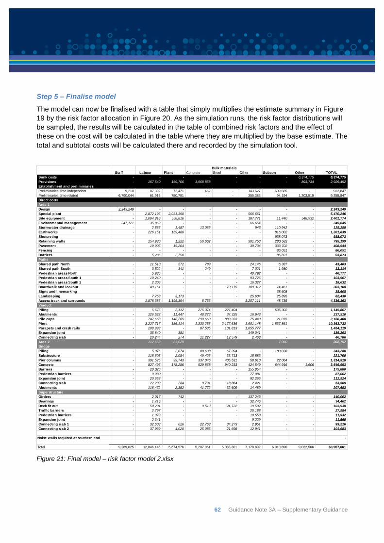
62 Guidance Note 3A – Supplementary Guidance
Step 5 – Finalise model
The model can now be finalised with a table that simply multiplies the estimate summary in Figure
19 by the risk factor allocation in Figure 20. As the simulation runs, the risk factor distributions will
be sampled, the results will be calculated in the table of combined risk factors and the effect of
these on the cost will be calculated in the table where they are multiplied by the base estimate. The
total and subtotal costs will be calculated there and recorded by the simulation tool.
Figure 21: Final model – risk factor model 2.xlsx
Staff Labour Plant Concrete Steel Other Subcon Other TOTAL
Sunk costs - - - - - - - 6,374,775 6,374,775
Provisions - 167,540 159,706 1,968,868 - - - 893,734 2,929,452
Establishment and preliminaries
Preliminaries time independent 9,210 87,392 72,471 462 - 143,627 609,685 - 922,847
Preliminaries time related 6,790,044 61,916 750,791 - - 355,383 94,194 1,203,519 9,255,847
Direct costs
Area 1
Design 2,243,249 - - - - - - - 2,243,249
Special plant - 2,872,195 2,031,390 - - 566,661 - - 5,470,246
Site equipment - 1,094,816 558,816 - - 187,771 11,440 548,932 2,401,774
Environmental management 247,121 35,869 - - - 66,654 - - 349,645
Stormwater drainage - 2,863 1,487 13,063 - 943 110,942 - 129,299
Earthworks - 226,151 159,486 - - - 816,002 - 1,201,639
Shotcreting - - - - - - 938,073 - 938,073
Retaining walls - 154,980 1,222 56,662 - 301,753 280,582 - 795,199
Pavement - 19,905 15,204 - - 39,734 333,702 - 408,544
Fencing - - - - - - 86,051 - 86,051
Barriers - 5,286 2,750 - - - 85,837 - 93,873
Paths
Shared path North - 11,510 572 789 - 24,146 6,387 - 43,403
Shared path South - 3,522 341 249 - 7,021 1,980 - 13,114
Pedestrian areas North - 5,985 - - - 40,792 - - 46,777
Pedestrian areas South 1 - 10,240 - - - 93,726 - - 103,967
Pedestrian areas South 2 - 2,305 - - - 16,327 - - 18,632
Boardwalk and lookout - 49,161 - - 70,175 109,312 74,461 - 303,108
Signs and linemarking - - - - - - 38,608 - 38,608
Landscaping - 7,758 3,173 - - 25,604 25,895 - 62,430
Access track and surrounds - 1,878,386 1,195,394 6,736 - 1,207,111 48,735 - 4,336,363
Viaduct
Piling - 5,675 2,112 275,374 227,404 - 635,302 - 1,145,867
Abutments - 126,522 11,447 48,273 34,325 16,943 - - 237,510
Pile caps - 747,668 148,205 290,669 883,333 75,449 21,075 - 2,166,400
Piers - 3,227,717 186,114 1,333,255 2,177,636 1,601,148 1,837,861 - 10,363,732
Parapets and crash rails - 208,993 - 87,535 101,813 1,055,777 - - 1,454,119
Expansion joint - 35,840 381 - - 149,041 - - 185,263
Connecting slab - 20,244 274 11,227 12,579 2,463 - - 46,786
Area 2 - 112,668 83,029 - - - 7,060 - 202,757
Bridge
Piling - 5,076 2,074 88,698 67,394 - 180,038 - 343,280
Substructure - 118,605 2,084 49,423 35,713 15,883 - - 221,709
Pier columns - 391,525 99,743 337,046 405,531 58,610 22,064 - 1,314,518
Concrete - 827,496 178,286 529,868 940,233 424,549 644,916 1,606 3,546,953
Barriers - 20,026 - - - 155,854 - - 175,880
Pedestrian barriers - 9,980 - - - 77,081 - - 87,062
Expansion joint - 20,658 - - - 92,266 - - 112,924
Connecting slab - 22,209 284 9,731 18,864 2,421 - - 53,509
Abutments - 116,472 2,352 41,772 32,609 14,489 - - 207,693
Superstructure
Girders - 2,017 742 - - 137,243 - - 140,002
Bearings - 1,716 - - - 32,746 - - 34,462
Deck fit out - 50,201 - 9,513 24,722 19,502 - - 103,938
Traffic barriers - 2,797 - - - 25,188 - - 27,984
Pedestrian barriers - 1,379 - - - 10,553 - - 11,932
Expansion joint - 2,341 - - - 9,229 - - 11,569
Connecting slab 1 - 32,603 626 22,763 34,273 2,951 - - 93,216
Connecting slab 2 - 37,939 4,020 25,085 21,698 12,941 - - 101,683
Noise walls required at southern end -
Total 9,289,625 12,846,146 5,674,576 5,207,061 5,088,301 7,178,892 6,910,890 9,022,566 60,957,661
Bulk materials
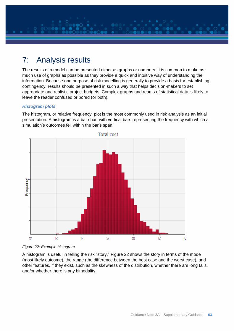
Guidance Note 3A – Supplementary Guidance 63
7: Analysis results The results of a model can be presented either as graphs or numbers. It is common to make as
much use of graphs as possible as they provide a quick and intuitive way of understanding the
information. Because one purpose of risk modelling is generally to provide a basis for establishing
contingency, results should be presented in such a way that helps decision-makers to set
appropriate and realistic project budgets. Complex graphs and reams of statistical data is likely to
leave the reader confused or bored (or both).
Histogram plots
The histogram, or relative frequency, plot is the most commonly used in risk analysis as an initial
presentation. A histogram is a bar chart with vertical bars representing the frequency with which a
simulation’s outcomes fell within the bar’s span.
Figure 22: Example histogram
A histogram is useful in telling the risk “story.” Figure 22 shows the story in terms of the mode
(most likely outcome), the range (the difference between the best case and the worst case), and
other features, if they exist, such as the skewness of the distribution, whether there are long tails,
and/or whether there is any bimodality.
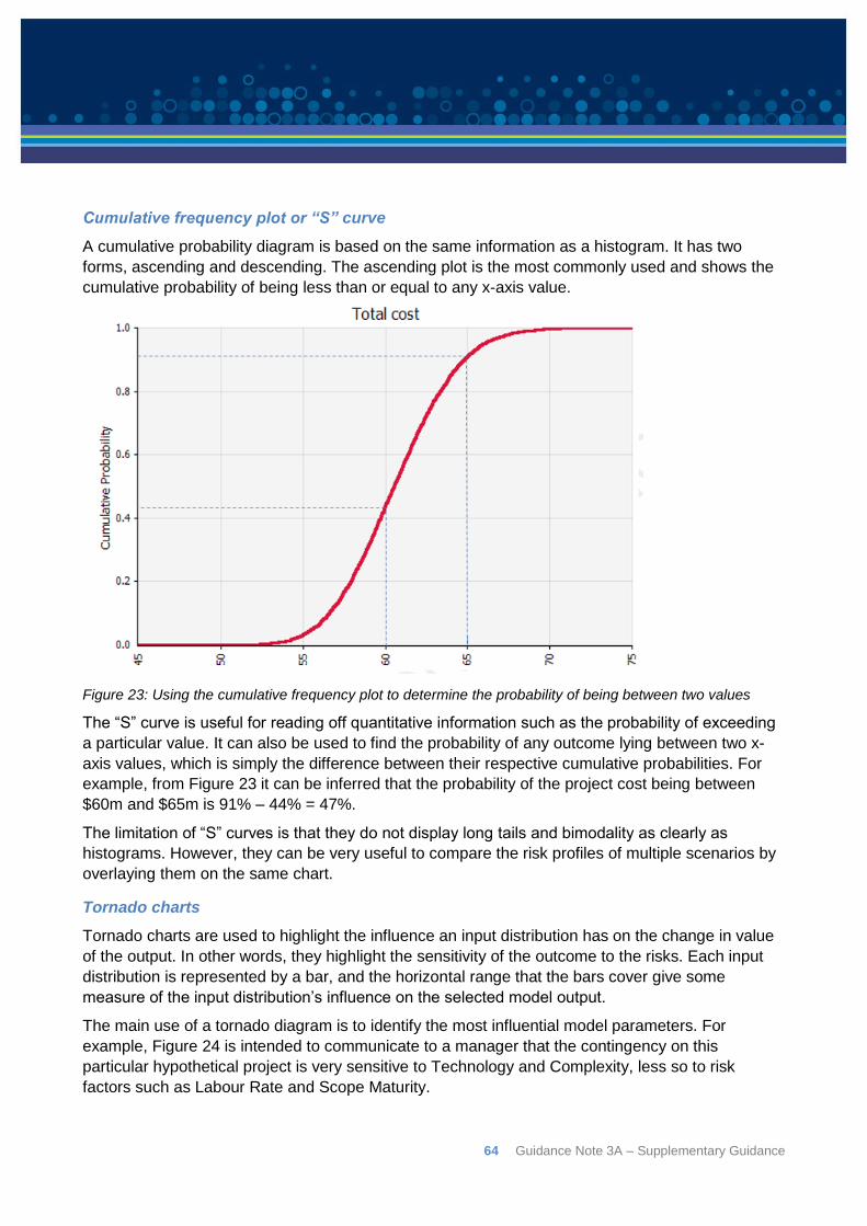
64 Guidance Note 3A – Supplementary Guidance
Cumulative frequency plot or “S” curve
A cumulative probability diagram is based on the same information as a histogram. It has two
forms, ascending and descending. The ascending plot is the most commonly used and shows the
cumulative probability of being less than or equal to any x-axis value.
Figure 23: Using the cumulative frequency plot to determine the probability of being between two values
The “S” curve is useful for reading off quantitative information such as the probability of exceeding
a particular value. It can also be used to find the probability of any outcome lying between two x-
axis values, which is simply the difference between their respective cumulative probabilities. For
example, from Figure 23 it can be inferred that the probability of the project cost being between
$60m and $65m is 91% – 44% = 47%.
The limitation of “S” curves is that they do not display long tails and bimodality as clearly as
histograms. However, they can be very useful to compare the risk profiles of multiple scenarios by
overlaying them on the same chart.
Tornado charts
Tornado charts are used to highlight the influence an input distribution has on the change in value
of the output. In other words, they highlight the sensitivity of the outcome to the risks. Each input
distribution is represented by a bar, and the horizontal range that the bars cover give some
measure of the input distribution’s influence on the selected model output.
The main use of a tornado diagram is to identify the most influential model parameters. For
example, Figure 24 is intended to communicate to a manager that the contingency on this
particular hypothetical project is very sensitive to Technology and Complexity, less so to risk
factors such as Labour Rate and Scope Maturity.
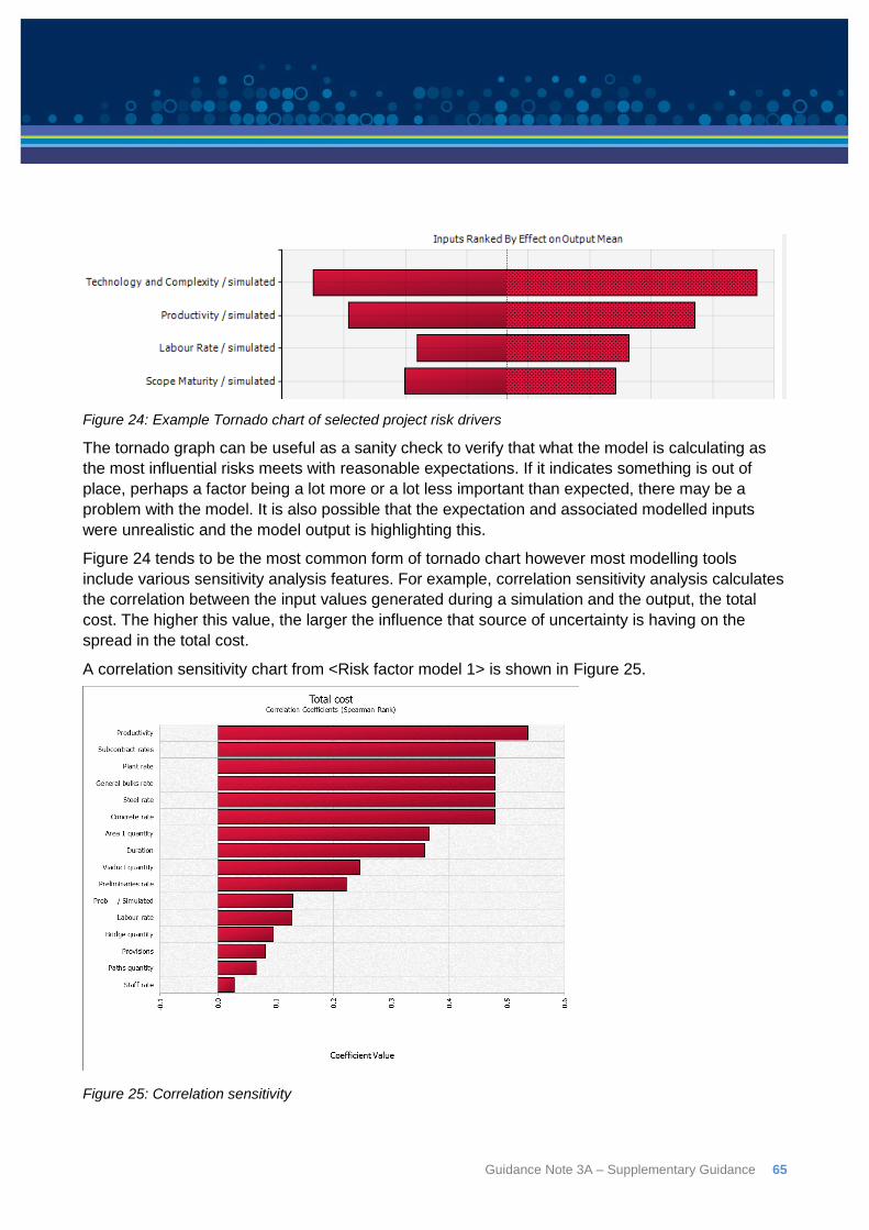
Guidance Note 3A – Supplementary Guidance 65
Figure 24: Example Tornado chart of selected project risk drivers
The tornado graph can be useful as a sanity check to verify that what the model is calculating as
the most influential risks meets with reasonable expectations. If it indicates something is out of
place, perhaps a factor being a lot more or a lot less important than expected, there may be a
problem with the model. It is also possible that the expectation and associated modelled inputs
were unrealistic and the model output is highlighting this.
Figure 24 tends to be the most common form of tornado chart however most modelling tools
include various sensitivity analysis features. For example, correlation sensitivity analysis calculates
the correlation between the input values generated during a simulation and the output, the total
cost. The higher this value, the larger the influence that source of uncertainty is having on the
spread in the total cost.
A correlation sensitivity chart from <Risk factor model 1> is shown in Figure 25.
Figure 25: Correlation sensitivity
66 Guidance Note 3A – Supplementary Guidance
This shows that uncertainty about productivity is the largest cause of uncertainty in the total cost.
Next is uncertainty in the group of rates that are expected to be correlated with one another by
their common dependence on market conditions. They have the same sensitivity rating because
they are correlated with one another and move in unison during the simulation. Uncertainty about
the bulk quantities in Area 1 is the next followed by uncertainty about the duration of the work.
Compared to these factors, the remainder are relatively insignificant.
The length of the bars in Figure 25 represent the correlation between variation in the factors and
variation in the total cost through the many iterations of the Monte Carlo simulation. These values
are very informative but cannot be used for any meaningful calculations in this context. The fact
that one factor has a correlation half the value of another cannot be interpreted as meaning that it
is half as important. The bars simply indicate the ranking of factors from most to least important.
Once a model is validated, the uncertainty sensitivity information shows where additional effort
might allow the uncertainty in the total cost to be reduced and make the outcome more predictable.
This might not result in a lower cost overall but could make it clearer what the cost will be if the
work proceeds.
Guidance Note 3A – Supplementary Guidance 67
8: Additional models “I can see that it works in practice, but does it work in theory?” – Garrett Fitzgerald, Prime Minister
of Ireland 1981-1987
This section provides details of three additional modelling techniques that, depending upon project
phase, the Department considers appropriate to use when developing estimates to accompany
funding submissions. The three techniques are:
Hybrid parametric/expected value method;
Risk Driver approach; and
First Principles Risk Analysis (FPRA).
8.1: Hybrid parametric/expected value method
As the name implies, this approach combines two separate approaches: a parametric method to
quantify systemic risks, and expected value to quantify project-specific risks. These are combined
into one model to produce a probabilistic output for decision-making.
As discussed at Section 3.3, it has been claimed32 that systemic risks are best quantified using
empirically validated parametric modelling. The disadvantage is that organisations may not initially
have suitable historical data with which to develop parametric models. However, there are publicly
available industry sources, including AACE International, that provide the basic relationships and
functioning models as a starting point which can be built upon, calibrated to a particular
organisation and improved over time. The example hybrid model that will be introduced shortly
uses Hollmann’s spreadsheet (with permission) to quantify systemic risks. It is stressed that the
example percentages in this model need to be further tested and calibrated by agencies by
applying their own knowledge and reviewing the historical performance of their projects.
Note that even when data is available, the input table can only be completed after interviews
and/or workshops with relevant subject matter experts, aided by prior project records where
available.
The parametric tool will provide a distribution (optimistic, most likely, pessimistic) for systemic risk
contingency which is applied to the base estimate as one of the model inputs which is then
assessed using Monte Carlo sampling (see model at section 8.1.1).
Using expected value for project-specific risks
Expected value is a technique that has been used for decision and risk management for decades.
This guidance note will not describe the technique in detail other than to note the importance of
screening for, and only including significant risks in the contingency calculation. Cluttering the
32 Hollmann, J (2016) Project Risk Quantification: A Practitioner’s Guide to Realistic Cost and Schedule Risk Management, Probabilistic Publishing, Gainesville, FL
68 Guidance Note 3A – Supplementary Guidance
analysis with minor risks presents a danger of double counting as the parametric model effectively
takes account of run of the mill disturbances to project implementation.
Screening
The expected value method builds on information that is already likely to exist in a risk register
where the project team may have qualitatively ranked the risks using a traditional risk matrix.
Screening involves making a quick estimate of the impact of each residual (treated) risk. If the
calculation results in a value that is not significant in relation to the base estimate, then it is
dropped from consideration (but kept in the register) and not used in the contingency calculation.
Significance is judged using the criticality criteria as per AACE RP 41R-08 as follows:
Bottom Line Critical Variances
Bottom line cost Conceptual estimates
(AACE Classes 3, 4, 5)
Detailed Estimates (AACE
Classes 1, 2)
Cost ∆ ± 0.5% ± 0.2%
Once the critical risks have been identified after screening, their values (probability of occurrence
and impact if it occurs) are refined. It has been suggested that if more than about 15 residual risk
are critical the screening has not been disciplined enough, and/or risk treatment has been
ineffective33. This guidance note suggests that 20 project-specific risks should be considered to be
the maximum for inclusion in the contingency calculation. Correlation between any risks must also
be identified and modelled.
The screening approach has two major benefits, it:
avoids the need to quantify a large number of project-specific risks; and
helps limits the number of inputs into the simulation model.
Example Parametric/Risk-Event Model
The cost risk model inputs include:
the base estimate;
the parametric model outcome distribution (i.,e. the systemic risk impact which is included
as the first risk in the expected value tool); and
the products of the distribution of probability times the distribution of the cost impact for
each project-specific risk.
A simple example model created using a hypothetical project is outlined below.
33 AACE (2011) Recommended Practice RP65R-11 Integrated Cost and Schedule Risk Analysis and Contingency Determiniation Using Expected Value
Guidance Note 3A – Supplementary Guidance 69
Quantification of systemic risks
Where reliable records of organisational performance relating to systemic risks are not available,
the Department believes that the Hollmann model is the most current and practical alternative. On
an actual project, the inputs into the parametric model must be made after interviews/workshops
with appropriate project personnel.
The input values for this example model (the yellow cells) for a hypothetical road project are based
on the following assumptions:
There is no new technology;
Process severity is not applicable;
Complexity is low given there are few projects interfaces or traffic management
requirements;
The team development, project control and estimate bias are fair;
As a road project, equipment is generally not applicable (exceptions would include items
such tolling systems, electrical equipment on rail projects, etc);
40% of the project by value will be on a firm, fixed price basis; and
Bias of the estimate is typical (i.e. biased, but not excessively over or under-biased).
Figure 26 below shows the inputs and outputs of the parametric growth model.
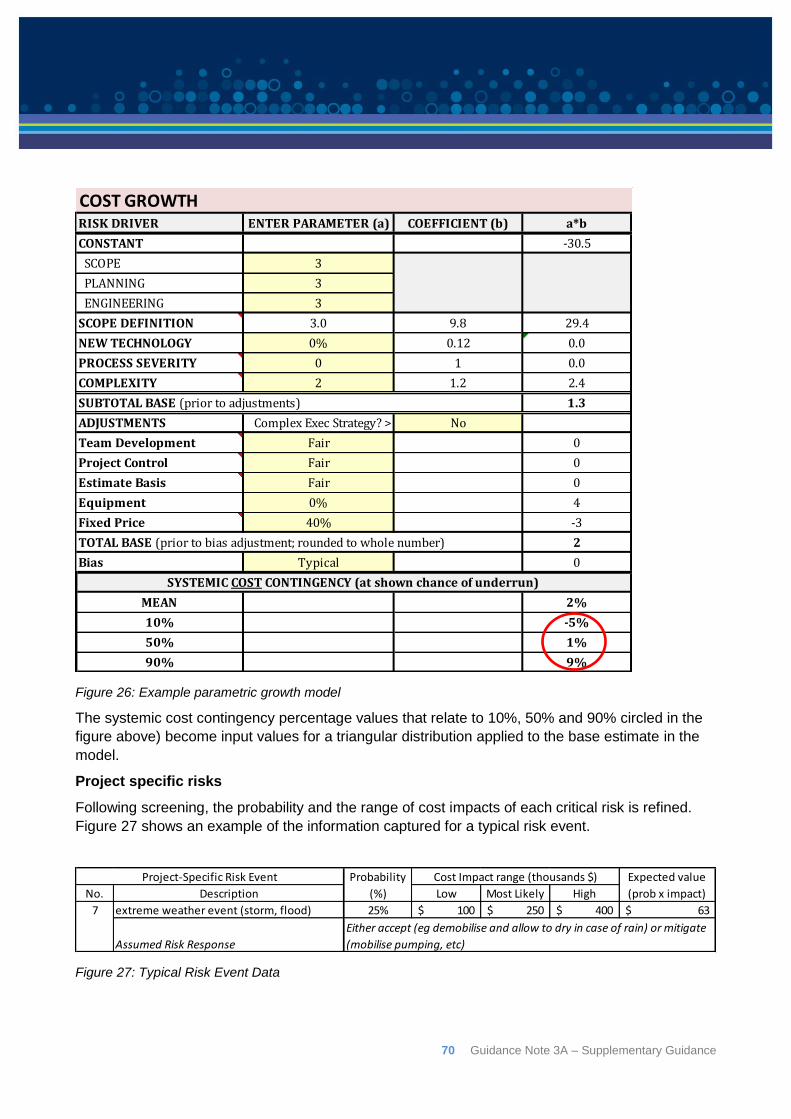
70 Guidance Note 3A – Supplementary Guidance
Figure 26: Example parametric growth model
The systemic cost contingency percentage values that relate to 10%, 50% and 90% circled in the
figure above) become input values for a triangular distribution applied to the base estimate in the
model.
Project specific risks
Following screening, the probability and the range of cost impacts of each critical risk is refined.
Figure 27 shows an example of the information captured for a typical risk event.
Figure 27: Typical Risk Event Data
COST GROWTHRISK DRIVER ENTER PARAMETER (a) COEFFICIENT (b) a*b
CONSTANT -30.5
SCOPE 3
PLANNING 3
ENGINEERING 3
SCOPE DEFINITION 3.0 9.8 29.4
NEW TECHNOLOGY 0% 0.12 0.0
PROCESS SEVERITY 0 1 0.0
COMPLEXITY 2 1.2 2.4
1.3
ADJUSTMENTS Complex Exec Strategy? > No
Team Development Fair 0
Project Control Fair 0
Estimate Basis Fair 0
Equipment 0% 4
Fixed Price 40% -3
2
Bias Typical 0
MEAN 2%
10% -5%
50% 1%
90% 9%
SUBTOTAL BASE (prior to adjustments)
TOTAL BASE (prior to bias adjustment; rounded to whole number)
SYSTEMIC COST CONTINGENCY (at shown chance of underrun)
No. Description Low Most Likely High
extreme weather event (storm, flood) 25% 100$ 250$ 400$ 63$ 7
Project-Specific Risk Event Cost Impact range (thousands $) Expected value
(prob x impact)
Probability
(%)
Assumed Risk Response
Either accept (eg demobilise and allow to dry in case of rain) or mitigate
(mobilise pumping, etc)
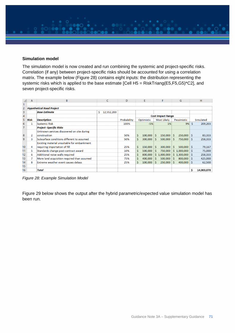
Guidance Note 3A – Supplementary Guidance 71
Simulation model
The simulation model is now created and run combining the systemic and project-specific risks.
Correlation (if any) between project-specific risks should be accounted for using a correlation
matrix. The example below (Figure 28) contains eight inputs: the distribution representing the
systemic risks which is applied to the base estimate [Cell H5 = RiskTriang(E5,F5,G5)*C2], and
seven project-specific risks.
Figure 28: Example Simulation Model
Figure 29 below shows the output after the hybrid parametric/expected value simulation model has
been run.
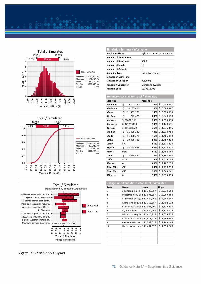
72 Guidance Note 3A – Supplementary Guidance
Figure 29: Risk Model Outputs
Workbook Name Hybrid parametric model.xlsx
Number of Simulations 1
Number of Iterations
Number of Inputs 15
Number of Outputs 1
Sampling Type Latin Hypercube
Simulation Start Time
Simulation Duration
Random # Generator
Random Seed
Statistics Percentile
Minimum 9,742,590$ 5% 10,459,481$
Maximum 14,137,414$ 10% 10,688,387$
Mean 11,562,971$ 15% 10,829,099$
Std Dev 722,421$ 20% 10,940,618$
Variance 5.21892E+11 25% 11,039,534$
Skewness 0.379253478 30% 11,140,671$
Kurtosis 2.811068529 35% 11,235,316$
Median 11,489,323$ 40% 11,313,750$
Mode 11,308,271$ 45% 11,406,919$
Left X 10,459,481$ 50% 11,489,323$
Left P 5% 55% 11,575,820$
Right X 12,873,933$ 60% 11,674,217$
Right P 95% 65% 11,784,563$
Diff X 2,414,451$ 70% 11,897,488$
Diff P 90% 75% 12,025,106$
#Errors 0 80% 12,187,256$
Filter Min Off 85% 12,378,778$
Filter Max Off 90% 12,563,241$
#Filtered 0 95% 12,873,933$
Rank Name Lower Upper
1 additional noise walls required / Simulated11,303,254$ 12,334,694$
2 Systemic Risk / Simulated11,091,554$ 12,069,484$
3 Standards change post-contract award / Simulated11,487,263$ 12,244,347$
4 More land acquisition required than assumed / Simulated (I13)11,168,684$ 11,702,112$
5 subsurface conditions different to assumed / Simulated (I9)11,306,709$ 11,819,233$
6 4 / Simulated 11,484,266$ 11,810,715$
7 More land acquisition required than assumed / Simulated (I13)11,415,927$ 11,675,636$
8 subsurface conditions different to assumed / Simulated (I9)11,418,728$ 11,669,608$
9 extreme weather event causes delays / Simulated11,502,019$ 11,743,285$
10 Unknown services discovered on site during construction / Simulated11,467,676$ 11,658,266$
Simulation Summary Information
Change in Output Statistic for Total / Simulated
5000
00:00:02
Mersenne Twister
1517812708
Summary Statistics for Total / Simulated
Guidance Note 3A – Supplementary Guidance 73
8.2: Risk Driver method
A risk driver can be defined as: any root cause that may force a project to have outcomes
different than the plan34.
If something is already causing a deviation from the plan, it is not a risk driver. It is a problem that
must be dealt with. Conversely, if there is no chance of a certain situation arising on a particular
project, it cannot be a risk driver (on that project).
David Hulett acknowledges that there are some claims that Monte Carlo simulation is unable to
quantify the impact of systemic risks to project cost (and schedule). Hulett argues that Monte Carlo
simulation methods (specificallty the Risk Driver Method) can incorporate systemic risks as well as
uncertainty and project specific risks in the one inclusive approach. The caveat is that while Hulett
asserts that systemic risks can be incorporated without parametric methods two things are
required:
A rich database of project results on comparable projects; and
Assessment of the likelihood that the systemic risks will apply to the project being
analysed35.
The risk driver approach starts with the risks that are typically prioritised in the risk register that is
usually available. Similar to the risk factor approach, the risk driver approach assigns risks directly
to the project element costs that they will affect if they occur. As with the risk factor approach, there
are often risk drivers that are assigned to more than one cost element, and some cost elements
will have more than one risk driver assigned. Hence correlation between risks is again implicitly
accounted for.
Risks and uncertainties are typically worded in keeping with the definition of a risk driver. For
example the systemic risk “Level of Technology” would be worded as “The project may use
significant new technology”. It is thus stated in such a way as to be more amenable to assigning a
probability of occurrence. It is suggested that even on very large and complex projects, there
should be no more than 20-40 risk drivers36.
Once the risks have been identified a risk workshop/interview process is undertaken to determine:
The probability that the risk may occur;
The impact range if it were to occur; and
The project elements that it affects if it does occur
The information collected regarding probability and impact for the risks will typically be similar to
the abbreviated Table 13 below37:
34 Stump, E., (2000), The Risk Driver Impact Approach to Estimation of Cost Risks: Clear Thinking About Project Cost Risk Analysis (downloadable at http://galorath.com/wp-content/uploads/2014/08/stump_risk_driver_approach.pdf) 35 Hulett D, Whitehead W, (Risk 2142) The Monte Carlo Method for Modelling and Mitigating Systemic Risk 36 Hulett D, & Norbisch M, (2012) Integrated Cost-Schedule Risk Analysis 37 Hulett D, (2011) Integrated Cost-Schedule Risk Analysis, Gower Publishing Limited, Farnham England
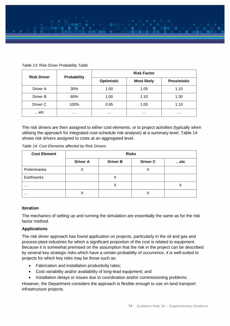
74 Guidance Note 3A – Supplementary Guidance
Table 13: Risk Driver Probability Table
Risk Driver Probability Risk Factor
Optimistic Most likely Pessimistic
Driver A 30% 1.00 1.05 1.10
Driver B 60% 1.00 1.10 1.30
Driver C 100% 0.95 1.00 1.10
…etc … … … …
The risk drivers are then assigned to either cost elements, or to project activities (typically when
utilising the approach for integrated cost-schedule risk analysis) at a summary level. Table 14
shows risk drivers assigned to costs at an aggregated level.
Table 14: Cost Elements affected by Risk Drivers
Cost Element Risks
Driver A Driver B Driver C …etc
Preliminaries X X
Earthworks X
… X X
… X X
Iteration
The mechanics of setting up and running the simulation are essentially the same as for the risk
factor method.
Applications
The risk driver approach has found application on projects, particularly in the oil and gas and
process-plant industries for which a significant proportion of the cost is related to equipment.
Because it is somewhat premised on the assumption that the risk in the project can be described
by several key strategic risks which have a certain probability of occurrence, it is well-suited to
projects for which key risks may be those such as:
Fabrication and installation productivity rates;
Cost variability and/or availability of long-lead equipment; and
Installation delays or issues due to coordination and/or commissioning problems.
However, the Department considers the approach is flexible enough to use on land transport
infrastructure projects.
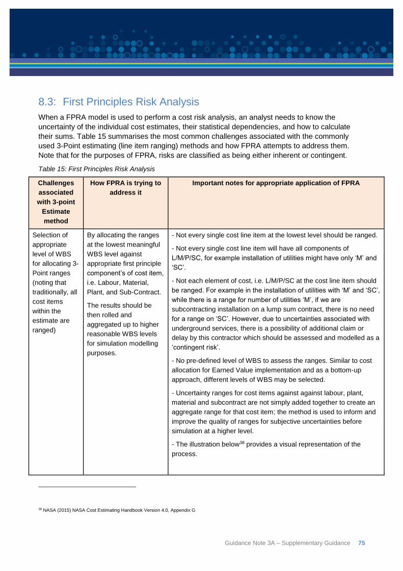
Guidance Note 3A – Supplementary Guidance 75
8.3: First Principles Risk Analysis
When a FPRA model is used to perform a cost risk analysis, an analyst needs to know the
uncertainty of the individual cost estimates, their statistical dependencies, and how to calculate
their sums. Table 15 summarises the most common challenges associated with the commonly
used 3-Point estimating (line item ranging) methods and how FPRA attempts to address them.
Note that for the purposes of FPRA, risks are classified as being either inherent or contingent.
Table 15: First Principles Risk Analysis
Challenges
associated
with 3-point
Estimate
method
How FPRA is trying to
address it
Important notes for appropriate application of FPRA
Selection of
appropriate
level of WBS
for allocating 3-
Point ranges
(noting that
traditionally, all
cost items
within the
estimate are
ranged)
By allocating the ranges
at the lowest meaningful
WBS level against
appropriate first principle
component’s of cost item,
i.e. Labour, Material,
Plant, and Sub-Contract.
The results should be
then rolled and
aggregated up to higher
reasonable WBS levels
for simulation modelling
purposes.
- Not every single cost line item at the lowest level should be ranged.
- Not every single cost line item will have all components of
L/M/P/SC, for example installation of utilities might have only ‘M’ and
‘SC’.
- Not each element of cost, i.e. L/M/P/SC at the cost line item should
be ranged. For example in the installation of utilities with ‘M’ and ‘SC’,
while there is a range for number of utilities ‘M’, if we are
subcontracting installation on a lump sum contract, there is no need
for a range on ‘SC’. However, due to uncertainties associated with
underground services, there is a possibility of additional claim or
delay by this contractor which should be assessed and modelled as a
‘contingent risk’.
- No pre-defined level of WBS to assess the ranges. Similar to cost
allocation for Earned Value implementation and as a bottom-up
approach, different levels of WBS may be selected.
- Uncertainty ranges for cost items against against labour, plant,
material and subcontract are not simply added together to create an
aggregate range for that cost item; the method is used to inform and
improve the quality of ranges for subjective uncertainties before
simulation at a higher level.
- The illustration below38 provides a visual representation of the
process.
38 NASA (2015) NASA Cost Estimating Handbook Version 4.0, Appendix G
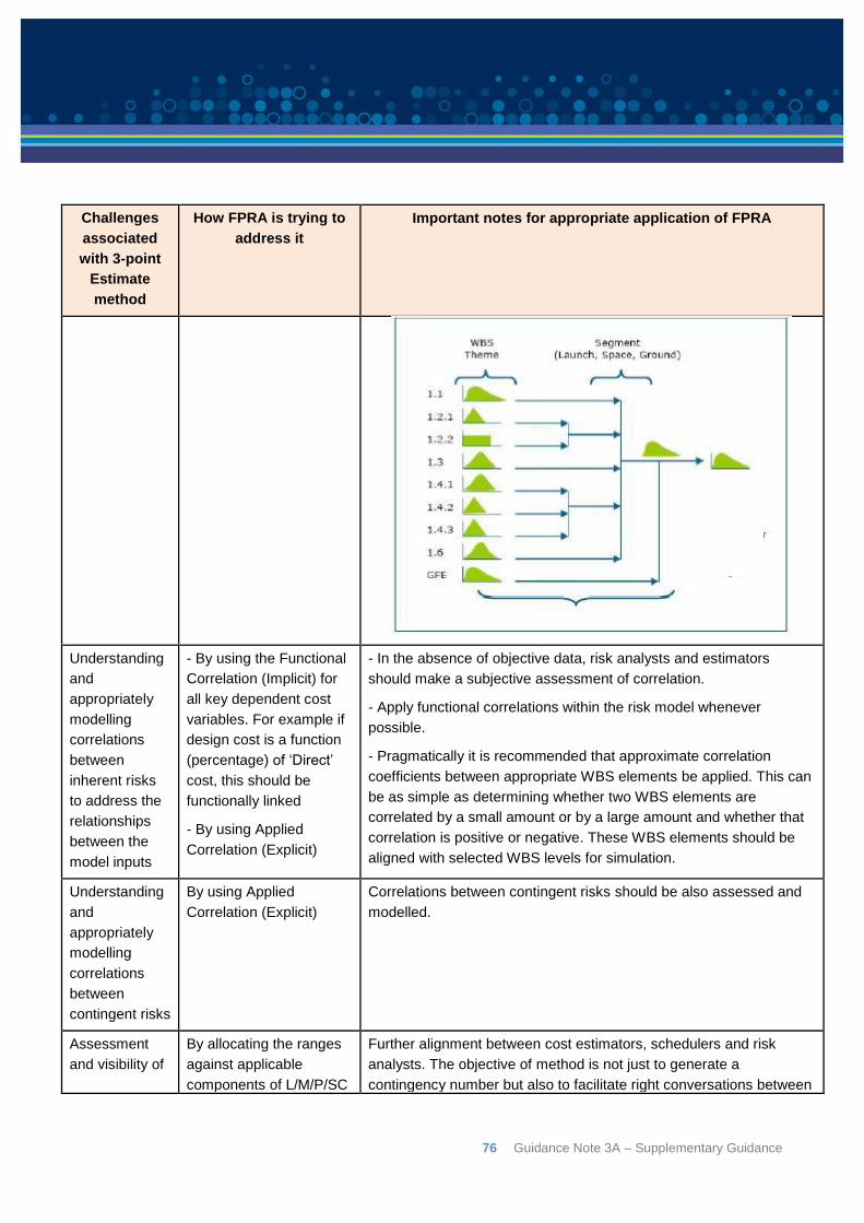
76 Guidance Note 3A – Supplementary Guidance
Challenges
associated
with 3-point
Estimate
method
How FPRA is trying to
address it
Important notes for appropriate application of FPRA
Understanding
and
appropriately
modelling
correlations
between
inherent risks
to address the
relationships
between the
model inputs
- By using the Functional
Correlation (Implicit) for
all key dependent cost
variables. For example if
design cost is a function
(percentage) of ‘Direct’
cost, this should be
functionally linked
- By using Applied
Correlation (Explicit)
- In the absence of objective data, risk analysts and estimators
should make a subjective assessment of correlation.
- Apply functional correlations within the risk model whenever
possible.
- Pragmatically it is recommended that approximate correlation
coefficients between appropriate WBS elements be applied. This can
be as simple as determining whether two WBS elements are
correlated by a small amount or by a large amount and whether that
correlation is positive or negative. These WBS elements should be
aligned with selected WBS levels for simulation.
Understanding
and
appropriately
modelling
correlations
between
contingent risks
By using Applied
Correlation (Explicit)
Correlations between contingent risks should be also assessed and
modelled.
Assessment
and visibility of
By allocating the ranges
against applicable
components of L/M/P/SC
Further alignment between cost estimators, schedulers and risk
analysts. The objective of method is not just to generate a
contingency number but also to facilitate right conversations between
Guidance Note 3A – Supplementary Guidance 77
Challenges
associated
with 3-point
Estimate
method
How FPRA is trying to
address it
Important notes for appropriate application of FPRA
key areas of
uncertainty
at the lowest appropriate
WBS level, then rolling
them up to higher levels
of WBS for simulation
purposes.
the team to discuss, assess, and mitigate key areas of uncertainties
and risks as much as possible.
The residual risks/uncertainties (depending on delivery strategies)
should be then modelled for assessing the optimum contingency.
Cognitive
Biases
As above. As Above.
The steps below represent the general process for undertaking FPRA:
1. Develop a first principles cost estimate (base estimate), representing the most likely
assumptions, structured against Labour, Plant, Material and Sub-contract as per Figure 30.
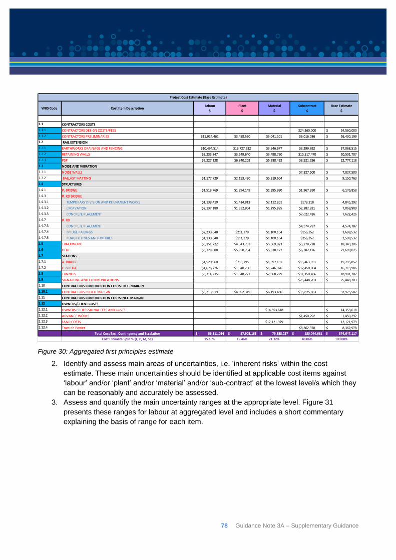
78 Guidance Note 3A – Supplementary Guidance
Figure 30: Aggregated first principles estimate
2. Identify and assess main areas of uncertainties, i.e. ‘inherent risks’ within the cost
estimate. These main uncertainties should be identified at applicable cost items against
‘labour’ and/or ‘plant’ and/or ‘material’ and/or ‘sub-contract’ at the lowest level/s which they
can be reasonably and accurately be assessed.
3. Assess and quantify the main uncertainty ranges at the appropriate level. Figure 31
presents these ranges for labour at aggregated level and includes a short commentary
explaining the basis of range for each item.
1.1 CONTRACTORS COSTS
1.1.1 CONTRACTORS DESIGN COSTS/FEES $24,560,000 24,560,000$
1.1.2 CONTRACTORS PRELIMINARIES $11,914,462 $3,458,550 $5,041,101 $6,016,086 26,430,199$
1.2 RAIL EXTENSION
1.2.1 EARTHWORKS DRAINAGE AND FENCING $10,494,514 $19,727,632 $3,546,677 $3,299,692 37,068,515$
1.2.2 RETAINING WALLS $3,235,847 $3,249,640 $3,498,750 $10,517,470 20,501,707$
1.2.3 PSP $2,227,128 $6,340,202 $5,288,492 $8,921,296 22,777,118$
1.3 NOISE AND VIBRATION
1.3.1 NOISE WALLS $7,827,500 7,827,500$
1.3.2 BALLAST MATTING $1,177,729 $2,153,430 $5,819,604 9,150,763$
1.4 STRUCTURES
1.4.1 P. BRIDGE $1,518,769 $1,294,149 $1,395,990 $1,967,950 6,176,858$
1.4.3 R. RD BRIDGE
1.4.3.1 TEMPORARY DIVISION AND PERMANENT WORKS $1,138,410 $1,414,813 $2,112,851 $179,218 4,845,292$
1.4.3.2 EXCAVATION $2,137,180 $1,352,904 $1,295,895 $2,282,921 7,068,900$
1.4.3.3 CONCRETE PLACEMENT $7,622,426 7,622,426$
1.4.7 B. RD
1.4.7.3 CONCRETE PLACEMENT $4,574,787 4,574,787$
1.4.7.4 BRIDGE RAILINGS $2,230,648 $211,379 $1,100,154 $156,352 3,698,532$
1.4.7.5 ROAD FITTINGS AND FIXTURES $1,130,648 $111,379 $1,100,154 $256,352 2,598,532$
1.5 TRACKWORK $3,151,722 $4,343,733 $5,569,023 $5,278,728 18,343,206$
1.6 OHLE $3,728,088 $5,950,734 $5,638,127 $6,382,126 21,699,075$
1.7 STATIONS
1.7.1 A. BRIDGE $1,520,960 $713,795 $1,597,151 $15,463,951 19,295,857$
1.7.2 E. BRIDGE $1,676,776 $1,340,230 $1,246,976 $12,450,004 16,713,986$
1.8 TUNNELS $3,314,235 $1,548,277 $2,968,229 $11,150,466 18,981,207$
1.9 SIGNALLING AND COMMUNICATIONS $25,448,203 25,448,203$
1.10 CONTRACTORS CONSTRUCTION COSTS EXCL. MARGIN
1.10.1 CONTRACTORS PROFIT MARGIN $6,213,919 $4,692,319 $6,193,486 $15,875,863 32,975,587$
1.11 CONTRACTORS CONSTRUCTION COSTS INCL. MARGIN
1.12 OWNERS/CLIENT COSTS
1.12.1 OWNERS PROFESSIONAL FEES AND COSTS $14,353,618 14,353,618$
1.12.2 ADVANCE WORKS $1,450,292 1,450,292$
1.12.3 LAND COSTS $12,121,979 12,121,979$
1.12.4 Traction Power $8,362,978 8,362,978$
Total Cost Excl. Contingency and Escalation 56,811,034$ 57,903,165$ 79,888,257$ 180,044,661$ 374,647,117$
Cost Estimate Split % (L, P, M, SC) 15.16% 15.46% 21.32% 48.06% 100.00%
Project Cost Estimate (Base Estimate)
WBS Code Cost Item Description Labour
$
Plant
$
Material
$
Subcontract
$
Base Estimate
$
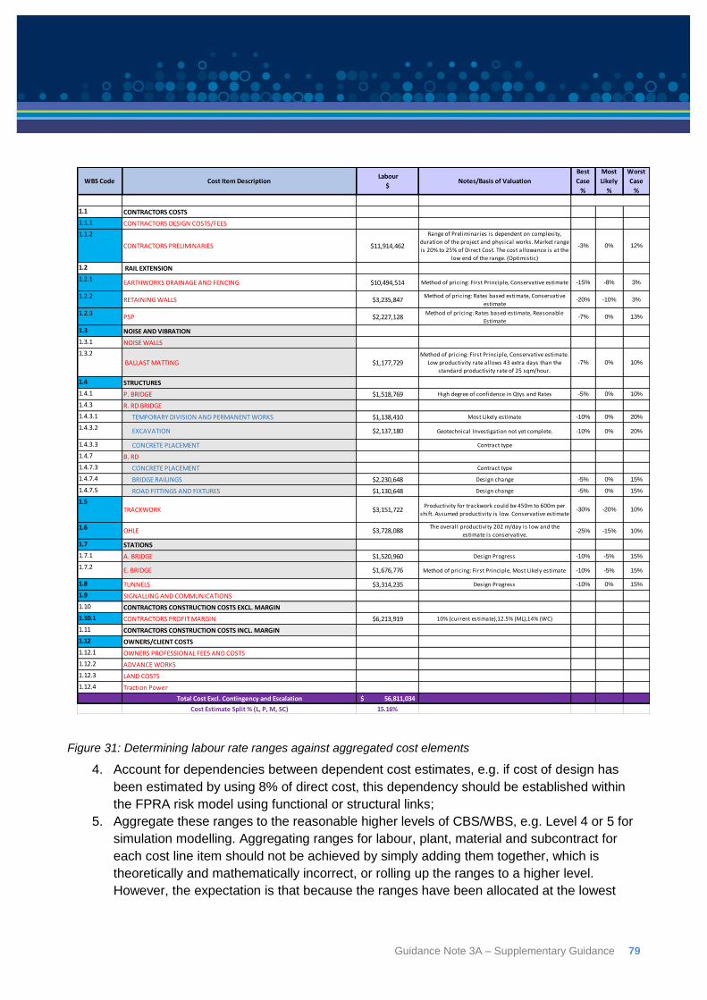
Guidance Note 3A – Supplementary Guidance 79
Figure 31: Determining labour rate ranges against aggregated cost elements
4. Account for dependencies between dependent cost estimates, e.g. if cost of design has
been estimated by using 8% of direct cost, this dependency should be established within
the FPRA risk model using functional or structural links;
5. Aggregate these ranges to the reasonable higher levels of CBS/WBS, e.g. Level 4 or 5 for
simulation modelling. Aggregating ranges for labour, plant, material and subcontract for
each cost line item should not be achieved by simply adding them together, which is
theoretically and mathematically incorrect, or rolling up the ranges to a higher level.
However, the expectation is that because the ranges have been allocated at the lowest
1.1 CONTRACTORS COSTS
1.1.1 CONTRACTORS DESIGN COSTS/FEES
1.1.2
CONTRACTORS PRELIMINARIES $11,914,462
Range of Preliminaries is dependent on complexity,
duration of the project and physical works. Market range
is 20% to 25% of Direct Cost. The cost allowance is at the
low end of the range. (Optimistic)
-3% 0% 12%
1.2 RAIL EXTENSION
1.2.1EARTHWORKS DRAINAGE AND FENCING $10,494,514 Method of pricing: First Principle, Conservative estimate -15% -8% 3%
1.2.2RETAINING WALLS $3,235,847
Method of pricing: Rates based estimate, Conservative
estimate-20% -10% 3%
1.2.3PSP $2,227,128
Method of pricing: Rates based estimate, Reasonable
Estimate-7% 0% 13%
1.3 NOISE AND VIBRATION
1.3.1 NOISE WALLS
1.3.2
BALLAST MATTING $1,177,729Method of pricing: First Principle, Conservative estimate.
Low productivity rate allows 43 extra days than the
standard productivity rate of 25 sqm/hour.
-7% 0% 10%
1.4 STRUCTURES
1.4.1 P. BRIDGE $1,518,769 High degree of confidence in Qtys and Rates -5% 0% 10%
1.4.3 R. RD BRIDGE
1.4.3.1 TEMPORARY DIVISION AND PERMANENT WORKS $1,138,410 Most Likely estimate -10% 0% 20%
1.4.3.2 EXCAVATION $2,137,180 Geotechnical Investigation not yet complete. -10% 0% 20%
1.4.3.3 CONCRETE PLACEMENT Contract type
1.4.7 B. RD
1.4.7.3 CONCRETE PLACEMENT Contract type
1.4.7.4 BRIDGE RAILINGS $2,230,648 Design change -5% 0% 15%
1.4.7.5 ROAD FITTINGS AND FIXTURES $1,130,648 Design change -5% 0% 15%
1.5TRACKWORK $3,151,722
Productivity for trackwork could be 450m to 600m per
shift. Assumed productivity is low. Conservative estimate-30% -20% 10%
1.6 OHLE $3,728,088The overall productivity 202 m/day is low and the
estimate is conservative. -25% -15% 10%
1.7 STATIONS
1.7.1 A. BRIDGE $1,520,960 Design Progress -10% -5% 15%
1.7.2 E. BRIDGE $1,676,776 Method of pricing: First Principle, Most Likely estimate -10% -5% 15%
1.8 TUNNELS $3,314,235 Design Progress -10% 0% 15%
1.9 SIGNALLING AND COMMUNICATIONS
1.10 CONTRACTORS CONSTRUCTION COSTS EXCL. MARGIN
1.10.1 CONTRACTORS PROFIT MARGIN $6,213,919 10% (current estimate),12.5% (ML),14% (WC) 0% 25% 40%
1.11 CONTRACTORS CONSTRUCTION COSTS INCL. MARGIN
1.12 OWNERS/CLIENT COSTS
1.12.1 OWNERS PROFESSIONAL FEES AND COSTS
1.12.2 ADVANCE WORKS
1.12.3 LAND COSTS
1.12.4 Traction Power
Total Cost Excl. Contingency and Escalation 56,811,034$
Cost Estimate Split % (L, P, M, SC) 15.16%
Best
Case
%
Notes/Basis of ValuationWBS Code Cost Item Description Labour
$
Most
Likely
%
Worst
Case
%
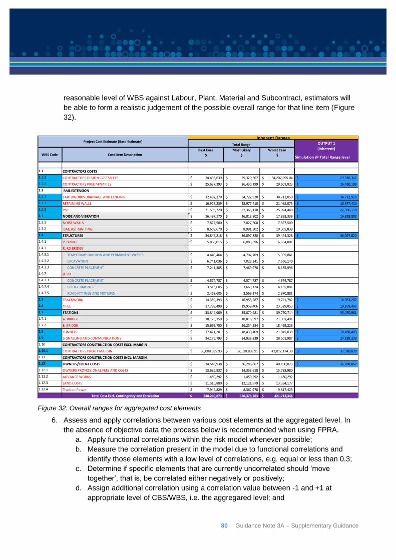
80 Guidance Note 3A – Supplementary Guidance
reasonable level of WBS against Labour, Plant, Material and Subcontract, estimators will
be able to form a realistic judgement of the possible overall range for that line item (Figure
32).
Figure 32: Overall ranges for aggregated cost elements
6. Assess and apply correlations between various cost elements at the aggregated level. In
the absence of objective data the process below is recommended when using FPRA.
a. Apply functional correlations within the risk model whenever possible;
b. Measure the correlation present in the model due to functional correlations and
identify those elements with a low level of correlations, e.g. equal or less than 0.3;
c. Determine if specific elements that are currently uncorrelated should ‘move
together’, that is, be correlated either negatively or positively;
d. Assign additional correlation using a correlation value between -1 and +1 at
appropriate level of CBS/WBS, i.e. the aggregared level; and
Simulation @ Total Range level
1.1 CONTRACTORS COSTS
1.1.1 CONTRACTORS DESIGN COSTS/FEES 24,433,639$ 29,320,367$ 34,207,095.04$ 29,320,367$
1.1.2 CONTRACTORS PRELIMINARIES 25,637,293$ 26,430,199$ 29,601,823$ 26,430,199$
1.2 RAIL EXTENSION
1.2.1 EARTHWORKS DRAINAGE AND FENCING 32,482,270$ 34,722,920$ 38,712,050$ 34,722,920$
1.2.2 RETAINING WALLS 16,927,239$ 18,977,410$ 21,462,075$ 18,977,410$
1.2.3 PSP 21,593,720$ 22,366,118$ 25,024,440$ 22,366,118$
1.3 NOISE AND VIBRATION 16,497,170$ 16,818,802$ 17,893,339$ 16,818,802$
1.3.1 NOISE WALLS 7,827,500$ 7,827,500$ 7,827,500$
1.3.2 BALLAST MATTING 8,669,670$ 8,991,302$ 10,065,839$
1.4 STRUCTURES 34,847,818$ 36,097,820$ 39,444,328$ 36,097,820$
1.4.1 P. BRIDGE 5,868,015$ 6,083,696$ 6,654,801$
1.4.3 R. RD BRIDGE
1.4.3.1 TEMPORARY DIVISION AND PERMANENT WORKS 4,440,464$ 4,707,769$ 5,395,841$
1.4.3.2 EXCAVATION 6,741,036$ 7,023,241$ 7,656,140$
1.4.3.3 CONCRETE PLACEMENT 7,241,305$ 7,469,978$ 8,155,996$
1.4.7 B. RD
1.4.7.3 CONCRETE PLACEMENT 4,574,787$ 4,574,787$ 4,574,787$
1.4.7.4 BRIDGE RAILINGS 3,513,605$ 3,669,174$ 4,135,881$
1.4.7.5 ROAD FITTINGS AND FIXTURES 2,468,605$ 2,569,174$ 2,870,881$
1.5 TRACKWORK 14,359,393$ 16,953,287$ 19,721,782$ 16,953,287$
1.6 OHLE 17,789,499$ 19,959,406$ 23,329,853$ 19,959,406$
1.7 STATIONS 33,844,909$ 35,070,981$ 39,770,714$ 35,070,981$
1.7.1 A. BRIDGE 18,175,159$ 18,816,397$ 21,301,491$
1.7.2 E. BRIDGE 15,669,750$ 16,254,584$ 18,469,223$
1.8 TUNNELS 17,421,201$ 18,430,409$ 21,045,039$ 18,430,409$
1.9 SIGNALLING AND COMMUNICATIONS 24,175,793$ 24,939,239$ 28,501,987$ 24,939,239$
1.10 CONTRACTORS CONSTRUCTION COSTS EXCL. MARGIN
1.10.1 CONTRACTORS PROFIT MARGIN 30,008,695.93$ 37,510,869.91$ 42,012,174.30$ 37,510,870$
1.11 CONTRACTORS CONSTRUCTION COSTS INCL. MARGIN
1.12 OWNERS/CLIENT COSTS 34,546,938$ 36,288,867$ 40,190,873$ 36,288,867$
1.12.1 OWNERS PROFESSIONAL FEES AND COSTS 13,635,937$ 14,353,618$ 15,788,980$
1.12.2 ADVANCE WORKS 1,450,292$ 1,450,292$ 1,450,292$
1.12.3 LAND COSTS 11,515,880$ 12,121,979$ 13,334,177$
1.12.4 Traction Power 7,944,829$ 8,362,978$ 9,617,425$
Total Cost Excl. Contingency and Escalation 340,240,873$ 370,373,283$ 421,713,346$
Project Cost Estimate (Base Estimate)
WBS Code Cost Item Description
Inherent Ranges
Best Case
$
Total Range
Most Likely
$
Worst Case
$
OUTPUT 1
(Inherent)
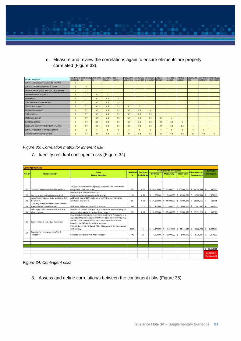
Guidance Note 3A – Supplementary Guidance 81
e. Measure and review the correlations again to ensure elements are properly
correlated (Figure 33).
Figure 33: Correlation matrix for inherent risk
7. Identify residual contingent risks (Figure 34)
Figure 34: Contingent risks
8. Assess and define correlation/s between the contingent risks (Figure 35);
@RISK CorrelationsCONTRACTO
RS DESIGN
CONTRACTO
RS
EARTHWOR
KS
RETAINING
WALLS in
PSP in
$AM$13
NOISE AND
VIBRATION
STRUCTURE
S in $AM$17
TRACKWOR
K in $AM$27
OHLE in
$AM$28
STATIONS in
$AM$29
TUNNELS in
$AM$32
SIGNALLING
AND
CONTRACTO
RS PROFIT
OWNERS/CL
IENT COSTS
CONTRACTORS DESIGN COSTS/FEES in $AM$8 1
CONTRACTORS PRELIMINARIES in $AM$9 0 1
EARTHWORKS DRAINAGE AND FENCING in $AM$11 0 0.7 1
RETAINING WALLS in $AM$12 0 0.7 0.3 1
PSP in $AM$13 0 0.7 0.3 0.5 1
NOISE AND VIBRATION in $AM$14 0 0.7 0.5 0.3 0.3 1
STRUCTURES in $AM$17 0 0.7 0.5 0.3 0.3 0.3 1
TRACKWORK in $AM$27 0 0.7 0.5 0.3 0.3 0.3 0.5 1
OHLE in $AM$28 0 0.7 0.5 0.3 0.3 0.3 0.3 0.3 1
STATIONS in $AM$29 0 0.7 0.5 0.3 0.3 0.3 0.5 0.3 0.3 1
TUNNELS in $AM$32 0 0.7 0.5 0.3 0.3 0.3 0.5 0.3 0.5 0.3 1
SIGNALLING AND COMMUNICATIONS in $AM$33 0 0.7 0.3 0.3 0.3 0.3 0.3 0.3 0.5 0.3 0.5 1
CONTRACTORS PROFIT MARGIN in $AM$35 0 0 0 0 0 0 0 0 0 0 0 0 1
OWNERS/CLIENT COSTS in $AM$37 0 0.7 0.3 0.3 0.3 0.3 0.3 0.3 0.3 0.3 0.3 0.3 0.3 1
Contingent Risks
Best Case
$
Most Likely
$
Worst Case
$
R1 Contractor may not be financially viable.
The costs associated with replacing the contractor. Project time
delay impact included in R6 1% 0.01 30,000,000$ 50,000,000$ 100,000,000$ 66,130,663$ 661,307$
R2 Shot crete and rock bolts are required.
Slower rate of bulk earth works due to having to install rock
bolting as part of bulk earth works.
Costs associated with additional materials. 25% 0.25 1,000,000$ 3,000,000$ 10,000,000$ 5,500,045$ 1,375,011$
R3
Substation is required to be built as part of
the project.
Additional cost of $57m to bring in 132kV transmission, plus
substation equipment. 1% 0.01 35,000,000$ 55,000,000$ 65,000,000$ 53,809,551$ 538,096$
R4
CCTV may be required to be fixed to radio
towers to view the rail corridor. Additional design and construction costs. 50% 0.5 300,000$ 500,000$ 1,000,000$ 661,307$ 330,653$
R5
New digital radio system is not available
when required.
Must install current analogue radio system and eventually digital
system (when available) and perform cutover. 5% 0.05 10,000,000$ 15,000,000$ 25,000,000$ 17,931,220$ 896,561$
R6 Delay in Project - Schedule risk Impact
Base Schedule represents most likely conditions. The results of a
separate schedule risk assessment have been costed for P10, P50
and P90 cases. Cost impact of the schedule risk is calculated
based on the SRS results and the burn rate.
P10 = 26 days, P50 = 78 days & P90 = 155 days with the burn rate of
$63k per day. 100% 1 2,372,650$ 7,117,950$ 14,144,643$ 8,822,704$ 8,822,704$
R7Opportunity - to engage a top Tier 2
contractor Current negotiations with XYZ Contractor 50% 0.5 4,000,000-$ 2,000,000-$ 1,000,000-$ 2,119,045-$ 1,059,522-$
11,564,809$
OUTPUT 2
(Contingent)
OUTPUT 2
(Contingent)
Residual Cost Consequence
Risk ID Risk DescriptionNotes
Basis of Valuation
Likelihood
%
Simulated
Probability
Simulated Cost
Consequence
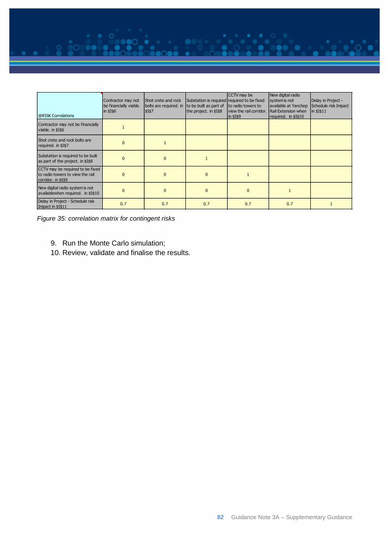
82 Guidance Note 3A – Supplementary Guidance
Figure 35: correlation matrix for contingent risks
9. Run the Monte Carlo simulation;
10. Review, validate and finalise the results.
@RISK Correlations
Contractor may not
be financially viable.
in $I$6
Shot crete and rock
bolts are required. in
$I$7
Substation is required
to be built as part of
the project. in $I$8
CCTV may be
required to be fixed
to radio towers to
view the rail corridor.
in $I$9
New digital radio
system is not
available at Yanchep
Rail Extension when
required. in $I$10
Delay in Project -
Schedule risk Impact
in $I$11
Contractor may not be financially
viable. in $I$61
Shot crete and rock bolts are
required. in $I$70 1
Substation is required to be built
as part of the project. in $I$80 0 1
CCTV may be required to be fixed
to radio towers to view the rail
corridor. in $I$9
0 0 0 1
New digital radio system is not
availablewhen required. in $I$100 0 0 0 1
Delay in Project - Schedule risk
Impact in $I$110.7 0.7 0.7 0.7 0.7 1
Guidance Note 3A – Supplementary Guidance 83
Appendix A: Deriving risk factors It is important to pay attention to the scale or materiality of any detail that is introduced into a
model. There may be a difficult part of a project that is subject to unusual sources of risk that make
it very interesting but, if its total potential impact on the project is a very small fraction of a
percentage point, it probably does not warrant separate attention. The aim is to have as little detail
as possible but as much as is necessary. Excessive detail simply results in parts of the model
being correlated in ways that are very hard to analyse and represent realistically, as discussed in
Section 6.1.
A source of cost uncertainty should not usually be included as a separate item if:
Its total impact is small;
Its likelihood is very low (see Section 4.4); and/or
It is of the same general order of magnitude as a number of other sources that can be
covered as a group and assessed in terms of their aggregate effect (see Section 4.3).
Reasons to include a source of uncertainty as a separate item include:
When it is large, has a moderate to high likelihood of occurring and has to be incorporated
into the general contingency, although see Section 4.4 concerning risks that are too large to
be encompassed in a general contingency; and/or
It represents a cost that is unrelated to any of the base estimate items, such as a fine or a
requirement to provide community infrastructure off-site as part of an arrangement with the
local community that is not expected to be incurred but might be forced on the project.
Leaving aside risk events, which are often not required to model project cost uncertainty, it is
possible to describe three principles for decomposing the overall uncertainty in a part of the cost.
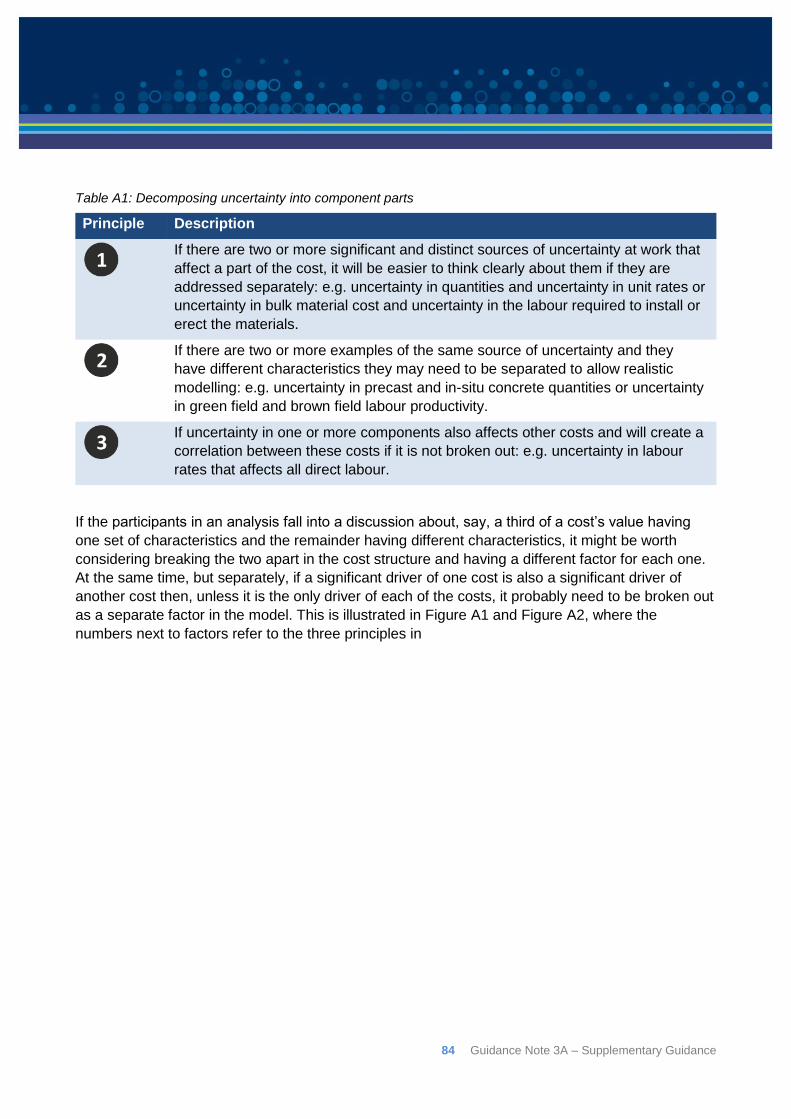
84 Guidance Note 3A – Supplementary Guidance
Table A1: Decomposing uncertainty into component parts
Principle Description
If there are two or more significant and distinct sources of uncertainty at work that
affect a part of the cost, it will be easier to think clearly about them if they are
addressed separately: e.g. uncertainty in quantities and uncertainty in unit rates or
uncertainty in bulk material cost and uncertainty in the labour required to install or
erect the materials.
If there are two or more examples of the same source of uncertainty and they
have different characteristics they may need to be separated to allow realistic
modelling: e.g. uncertainty in precast and in-situ concrete quantities or uncertainty
in green field and brown field labour productivity.
If uncertainty in one or more components also affects other costs and will create a
correlation between these costs if it is not broken out: e.g. uncertainty in labour
rates that affects all direct labour.
If the participants in an analysis fall into a discussion about, say, a third of a cost’s value having
one set of characteristics and the remainder having different characteristics, it might be worth
considering breaking the two apart in the cost structure and having a different factor for each one.
At the same time, but separately, if a significant driver of one cost is also a significant driver of
another cost then, unless it is the only driver of each of the costs, it probably need to be broken out
as a separate factor in the model. This is illustrated in Figure A1 and Figure A2, where the
numbers next to factors refer to the three principles in
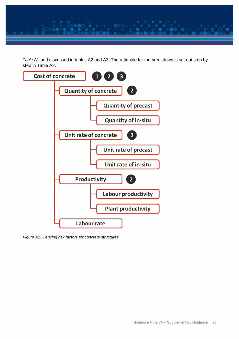
Guidance Note 3A – Supplementary Guidance 85
Table A1 and discussed in tables A2 and A3. The rationale for the breakdown is set out step by
step in Table A2.
Figure A1: Deriving risk factors for concrete structures
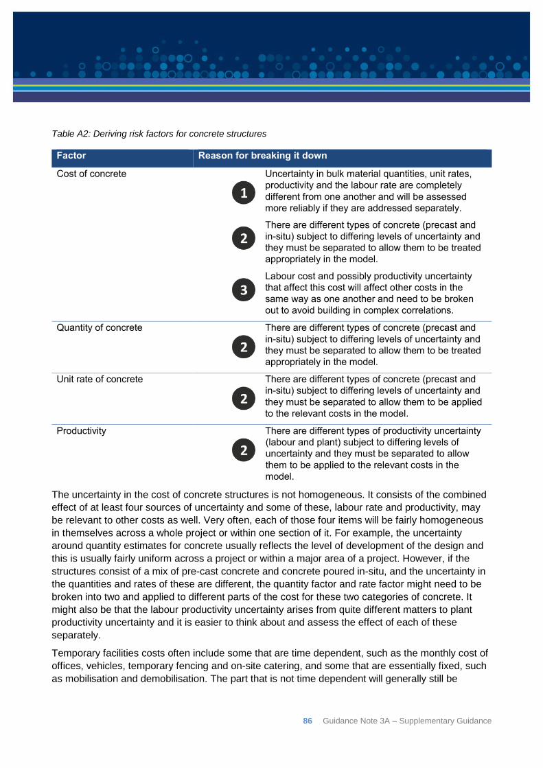
86 Guidance Note 3A – Supplementary Guidance
Table A2: Deriving risk factors for concrete structures
Factor Reason for breaking it down
Cost of concrete Uncertainty in bulk material quantities, unit rates,
productivity and the labour rate are completely
different from one another and will be assessed
more reliably if they are addressed separately.
There are different types of concrete (precast and
in-situ) subject to differing levels of uncertainty and
they must be separated to allow them to be treated
appropriately in the model.
Labour cost and possibly productivity uncertainty
that affect this cost will affect other costs in the
same way as one another and need to be broken
out to avoid building in complex correlations.
Quantity of concrete There are different types of concrete (precast and
in-situ) subject to differing levels of uncertainty and
they must be separated to allow them to be treated
appropriately in the model.
Unit rate of concrete There are different types of concrete (precast and
in-situ) subject to differing levels of uncertainty and
they must be separated to allow them to be applied
to the relevant costs in the model.
Productivity There are different types of productivity uncertainty
(labour and plant) subject to differing levels of
uncertainty and they must be separated to allow
them to be applied to the relevant costs in the
model.
The uncertainty in the cost of concrete structures is not homogeneous. It consists of the combined
effect of at least four sources of uncertainty and some of these, labour rate and productivity, may
be relevant to other costs as well. Very often, each of those four items will be fairly homogeneous
in themselves across a whole project or within one section of it. For example, the uncertainty
around quantity estimates for concrete usually reflects the level of development of the design and
this is usually fairly uniform across a project or within a major area of a project. However, if the
structures consist of a mix of pre-cast concrete and concrete poured in-situ, and the uncertainty in
the quantities and rates of these are different, the quantity factor and rate factor might need to be
broken into two and applied to different parts of the cost for these two categories of concrete. It
might also be that the labour productivity uncertainty arises from quite different matters to plant
productivity uncertainty and it is easier to think about and assess the effect of each of these
separately.
Temporary facilities costs often include some that are time dependent, such as the monthly cost of
offices, vehicles, temporary fencing and on-site catering, and some that are essentially fixed, such
as mobilisation and demobilisation. The part that is not time dependent will generally still be
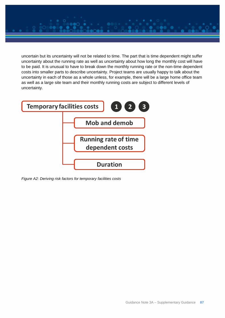
Guidance Note 3A – Supplementary Guidance 87
uncertain but its uncertainty will not be related to time. The part that is time dependent might suffer
uncertainty about the running rate as well as uncertainty about how long the monthly cost will have
to be paid. It is unusual to have to break down the monthly running rate or the non-time dependent
costs into smaller parts to describe uncertainty. Project teams are usually happy to talk about the
uncertainty in each of those as a whole unless, for example, there will be a large home office team
as well as a large site team and their monthly running costs are subject to different levels of
uncertainty.
Figure A2: Deriving risk factors for temporary facilities costs
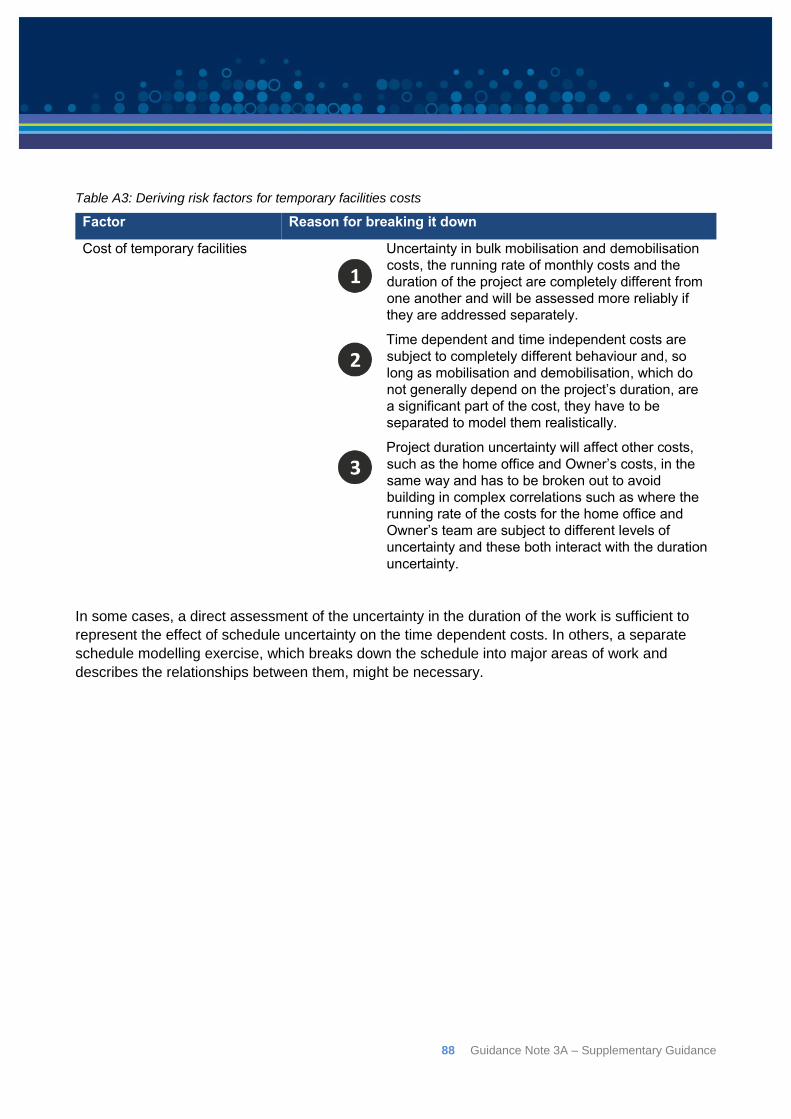
88 Guidance Note 3A – Supplementary Guidance
Table A3: Deriving risk factors for temporary facilities costs
Factor Reason for breaking it down
Cost of temporary facilities Uncertainty in bulk mobilisation and demobilisation
costs, the running rate of monthly costs and the
duration of the project are completely different from
one another and will be assessed more reliably if
they are addressed separately.
Time dependent and time independent costs are
subject to completely different behaviour and, so
long as mobilisation and demobilisation, which do
not generally depend on the project’s duration, are
a significant part of the cost, they have to be
separated to model them realistically.
Project duration uncertainty will affect other costs,
such as the home office and Owner’s costs, in the
same way and has to be broken out to avoid
building in complex correlations such as where the
running rate of the costs for the home office and
Owner’s team are subject to different levels of
uncertainty and these both interact with the duration
uncertainty.
In some cases, a direct assessment of the uncertainty in the duration of the work is sufficient to
represent the effect of schedule uncertainty on the time dependent costs. In others, a separate
schedule modelling exercise, which breaks down the schedule into major areas of work and
describes the relationships between them, might be necessary.
Guidance Note 3A – Supplementary Guidance 89
Appendix B: Simulation and statistical analysis As a general rule, decision makers prefer lower estimates to higher ones. The reason being is that
there may be a belief that if estimates are lower, either more projects can be developed within
limited available funding, or proposed projects are more appealing to funding appropriators.
However, this ignores the reality that the final project cost is independent of whether the initial cost
estimate was arbitrarily high, low, or otherwise. A project for which the cost estimate is artificially
low because risks have not been accounted for is likely to exceed its budget, whereas a project for
which the cost estimate includes excessive contingency ties up funds that could be used for other
projects. It is therefore paramount that the methodology used to quantify the risk is theoretically
sound, but also enables cost estimators to build and interpret realistic models that provide
decision-makers with clear and understandable results for budgetary purposes.
Probability tools
Statistical modelling techniques include statistical simulation and statistical analysis. Although the
goal is the same, the modelling techniques differ which will be discussed in more detail.
Statistical simulation
Statistical simulation is a numerical experiment designed to provide statistical information about the
properties of a model driven by random variables. The strong law of large numbers is the principle
upon which simulation is built39. It says that the larger the sample size (i.e. the greater the number
of iterations), the closer their distribution will be to the theoretical distribution (i.e. the exact
distribution of the model’s output if it could be mathematically derived).
The statistical simulation process follows these steps:
1. Define numerical experiment (spreadsheet, schedule network, etc.);
2. Define probability distribution functions (PDFs) for each random variable;
3. Define correlation coefficients for random variables;
4. Determine the number of experimental trials;
5. For each trial:
a. Draw correlated random variable(s) from defined PDFs;
b. Compute the experimental results;
c. Save the experimental results; and
6. At the end of the simulation, determine the statistics from the experimental results.
39 Vose, D (2008) Risk Analysis: A Quantitative Guide, John Wiley and Sons, Ltd
90 Guidance Note 3A – Supplementary Guidance
Sampling techniques
Statistical simulation tools most commonly use either:
Monte Carlo sampling: New sample points are generated without taking into account the
previously generated sample points; or
Latin Hypercube sampling: Each variable is divided into m equally probable divisions and
sampling is done without replacement for each set of m trials. Latin Hypercube takes
roughly 30% fewer trials to achieve similar accuracy to basic Monte Carlo sampling.
Commercial Excel add-ins such as @Risk normally utilise Latin Hypercube sampling. Other
approaches that can improve the efficiency of the sampling process further include Sobol
sequences, Faure sequences and Niederreiter sequences40.
The realism of the simulation results depends on the reasonableness of the user inputs, correct
modelling of PDFs for all random variables, and the correct specification of correlation between
these PDFs (even if it assumed to be 0).
The advantages of statistical simulation are its ability to provide the statistics of a simulated PDF
formed by complex mathematical modelling of random variables, and, its ease of use. Statistical
simulation requires a certain discipline. Users should be aware of these constraints to ensure that
their models have taken them into account.
Statistical Analysis
Unlike simulation, statistical analysis relies on the exact calculation of moments of the PDF.
Moments are properties of random variables. There are many of them. The moments of most
relevance to statistical analysis are raw moments, central moments and standardised moments
explained further as follows:
The zeroth moment is the total probability (i.e. one). The first moments about the origin are
called “raw moments”. The mean is the first raw moment of X about the origin, and is a
measurement of the central tendency of the data.
Central moments of a distribution are the raw moments about the mean. The first central
moment is by definition zero, but the second central moment is the variance, which is a
measure of dispersion about the mean.
Finally, we have the standardised (or normalised) moments, the most well-known being
skewness (the third standardised moment), and kurtosis (the fourth standardised moment).
Method of Moments is one example of an analytical technique used to calculate the moments of
probability distributions. The method becomes very complicated if any of the component
distributions are correlated.
40 Mascaro S (2014) Making Robust Decisions with a Model Subject to Severe Uncertainty, Report Developed for the Department of Agriculture in conjunction with CEBRA (downloadable at http://cebra.unimelb.edu.au/__data/assets/pdf_file/0011/1378676/Final_Report_RRRA_Decisions_with_uncertain_models_2014-07-111.pdf)
Guidance Note 3A – Supplementary Guidance 91
While statistical analysis is a valid method of deriving the statistics of composite probability
distributions, such as the distribution of total cost subject to the distributions of component costs
(and thereby arrive at a probabilistic cost estimate), the Department recommends that a proprietary
statistical simulation tool is used for the following reasons:
Available simulation tools in most cases have had years of development and thus come
with an implied level of reliability and sophistication through testing and upgrades;
Simulation tools come with an abundant supply of ready to use charts and tables to analyse
and report results. Those building custom models need to also develop the necessary
charts and tables;
Most analysts will find it difficult and inefficient to develop custom analytical models for
every estimate. The use of simulation tools enables an analyst who is not an expert in the
mathematics (of say, method of moments) to develop sophisticated, credible uncertainty
analyses; and
Changes to a simulation model can be made very quickly and the results compared with
previous models much more easily than with analytical techniques.
Why run a simulation?
Simulation has long been used for analysing systems and decision problems. The Prussian army would simulate wars by holding field exercises in the woods of Europe in all kinds of conditions, a practice that continues throughout the world today. Simulation is used to forecast the weather and to train pilots. NASA uses simulation to predict rocket and satellite trajectories. Simulation can even be seen in games. Monopoly simulates the real estate market by using dice as a means to generate random events.
The problem with manual simulations such as moving troops through the field is that they are very time consuming. What’s more, while physical exercises such as this can teach participants a great deal, one or two simulated outcomes provide very little information on which to base a decision about future events. However, if the simulations(s) can be implemented on a computer, thousands of replications can be performed in a few seconds, providing far more information to enable evaluation of the risks of projects and to help identify optimal solutions41.
41 Evans, J.R., and Olsen, D.L. (1998) Introduction to Simulation and Risk Analysis. Prentice Hall
92 Guidance Note 3A – Supplementary Guidance
Appendix C: Correlation The terms dependency and correlation are often used interchangeably but they have quite specific
meanings. A dependency relationship in risk analysis modelling is where the sampled value from
one variable (the independent) has a statistical relationship that affects the value that will be
generated for the other variable (the dependent). The dependent variable may be completely
determined by the independent variable or it might exhibit some uncertainty that is not due to the
independent variable.
Correlation is a statistic used to describe the degree to which two variables are related. While
dependency presumes a causal relationship between the variables, correlation need not42.
There are three reasons correlation may be observed between data:
There is a logical relationship between the two (or more) variables;
There is another external or underlying factor affecting both variables; or
An apparent correlation has occurred purely by chance and no correlation actually exists.
Many costs in a project will be linked because there is a common cause or driver that affects each
in a similar way. Usually this dependence, or correlation, will be positive; it is rare that an increase
in costs in one area will be offset by corresponding benefits in another, one going down as another
rises, because of a common underlying influence. Such offsets do happen by chance of course
when two costs are uncorrelated so that one might rise as another falls but systematic
relationships of this sort are unusual.
When performing a simulation, in most cases there are a potentially infinite number of possible
combinations of scenarios that can be generated. Each of these scenarios must be potentially
observable in real life. The model must, therefore, be prevented from producing, in any iteration, an
event that could not possibly occur.
One of the restrictions that must be placed on a model is the recognition of any interdependencies
between components. For example, if concrete pipe culvert components were to be sourced from
the same supplier, the unit cost for supply of 450mm diameter pipe and 600mm diameter pipe
would be expected to move in tandem. They are strongly positively correlated; if the price of one
goes up or down, so will the other. If the interdependency of these two components is not
modelled, the joint probabilities of the various combinations of these two parameters will be
incorrect. Impossible combinations will also be generated, such as one cost rising while the other
falls even though they are linked by a common source of uncertainty.
Such models will produce an output distribution that cannot be relied upon, or interpreted as, a
reflection of real-world behaviour. It will contain impossible scenarios and thus provides misleading
information about the reality that it is trying to represent.
42 Vose D (2008) Risk Analysis: A Quantitative Guide
Guidance Note 3A – Supplementary Guidance 93
For example, say an analyst has determined that the rate for a 450 mm reinforced concrete pipe
(RCP) is realistically represented by a triangular distribution T(350,370,425) and the rate for a 600
mm RCP can be represented by T(410,430,495). It can easily be imagined from these inputs that,
if these pipes are treated as independent variables (i.e. not correlated), in certain iterations the
simulated cost for a 450 mm RCP will be greater than for a 600 mm RCP. As an example, the
simulation software, in a particular iteration, may randomly select a rate for the 450mm RCP of
$422 and randomly select a rate of $415 for the 600mm RCP. This is a situation that in all
likelihood, would not occur in reality.
There are several ways of accounting for correlation in cost-risk analysis. Some of the main
methods are:
Using structural links, using an excel formula to reflect (or approximate), a direct functional
relationship between quantities in a model, such as the cost of overheads and a project’s
duration;
By aggregating inputs and assessing the risk together. This can be useful where there are a
number of smaller elements which are similar in nature but for which it is difficult to define a
direct relationship, such as where negotiations will influence labour for several different
trades at a site and the uncertainty in their labour rates can be assessed as a whole;
Using a correlation matrix for three or more values that are all related to one another, which
accounts for the correlation by using a matrix of related inputs, with a correlation coefficient
that defines the strength and sense (positive or negative) of their relationships. For example,
a coefficient of 0.5 specifies that when the value sampled for one input is high, the value
sampled for the second output will tend to, but not always, be high; or
Using a risk factor approach, as described throughout this guidance note, which
disaggregates the sources of uncertainty. By defining the sources of uncertainty and
determining their impact on the different cost elements, the correlation between cost
elements is automatically dealt with because the relationships are implicitly included within
the risk model.
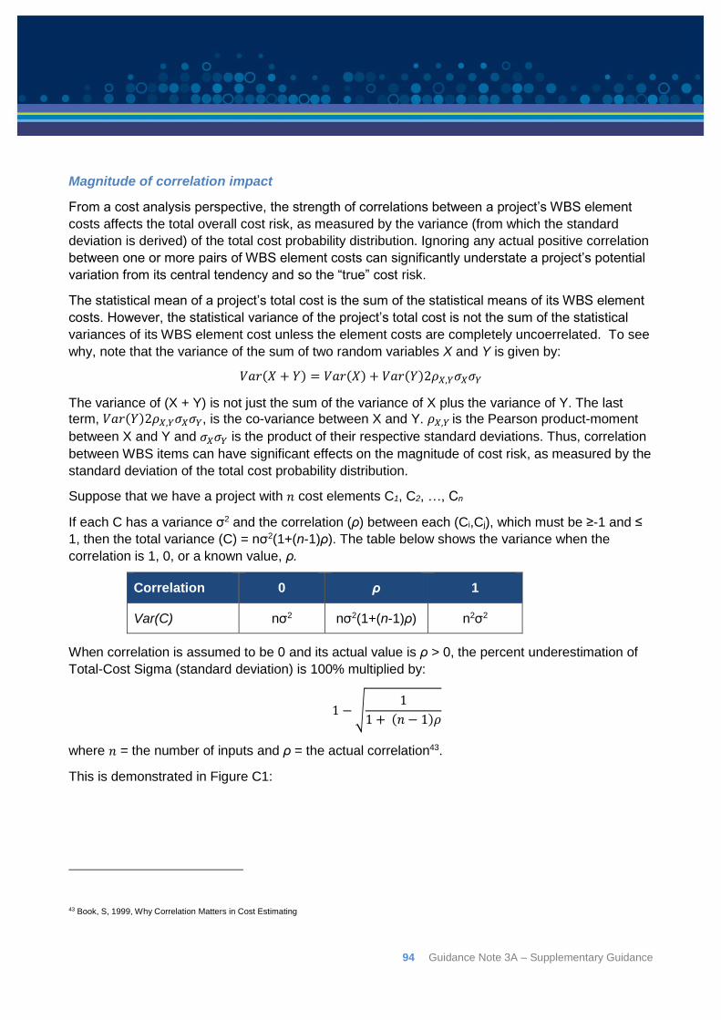
94 Guidance Note 3A – Supplementary Guidance
Magnitude of correlation impact
From a cost analysis perspective, the strength of correlations between a project’s WBS element
costs affects the total overall cost risk, as measured by the variance (from which the standard
deviation is derived) of the total cost probability distribution. Ignoring any actual positive correlation
between one or more pairs of WBS element costs can significantly understate a project’s potential
variation from its central tendency and so the “true” cost risk.
The statistical mean of a project’s total cost is the sum of the statistical means of its WBS element
costs. However, the statistical variance of the project’s total cost is not the sum of the statistical
variances of its WBS element cost unless the element costs are completely uncoerrelated. To see
why, note that the variance of the sum of two random variables X and Y is given by:
𝑉𝑎𝑟(𝑋 + 𝑌) = 𝑉𝑎𝑟(𝑋) + 𝑉𝑎𝑟(𝑌)2𝜌𝑋,𝑌𝜎𝑋𝜎𝑌
The variance of (X + Y) is not just the sum of the variance of X plus the variance of Y. The last
term, 𝑉𝑎𝑟(𝑌)2𝜌𝑋,𝑌𝜎𝑋𝜎𝑌, is the co-variance between X and Y. 𝜌𝑋,𝑌 is the Pearson product-moment
between X and Y and 𝜎𝑋𝜎𝑌 is the product of their respective standard deviations. Thus, correlation
between WBS items can have significant effects on the magnitude of cost risk, as measured by the
standard deviation of the total cost probability distribution.
Suppose that we have a project with 𝑛 cost elements C1, C2, …, Cn
If each C has a variance σ2 and the correlation (ρ) between each (Ci,Cj), which must be ≥-1 and ≤
1, then the total variance (C) = nσ2(1+(n-1)ρ). The table below shows the variance when the
correlation is 1, 0, or a known value, ρ.
Correlation 0 ρ 1
Var(C) nσ2 nσ2(1+(n-1)ρ) n2σ2
When correlation is assumed to be 0 and its actual value is ρ > 0, the percent underestimation of
Total-Cost Sigma (standard deviation) is 100% multiplied by:
1 − √1
1 + (𝑛 − 1)𝜌
where 𝑛 = the number of inputs and ρ = the actual correlation43.
This is demonstrated in Figure C1:
43 Book, S, 1999, Why Correlation Matters in Cost Estimating
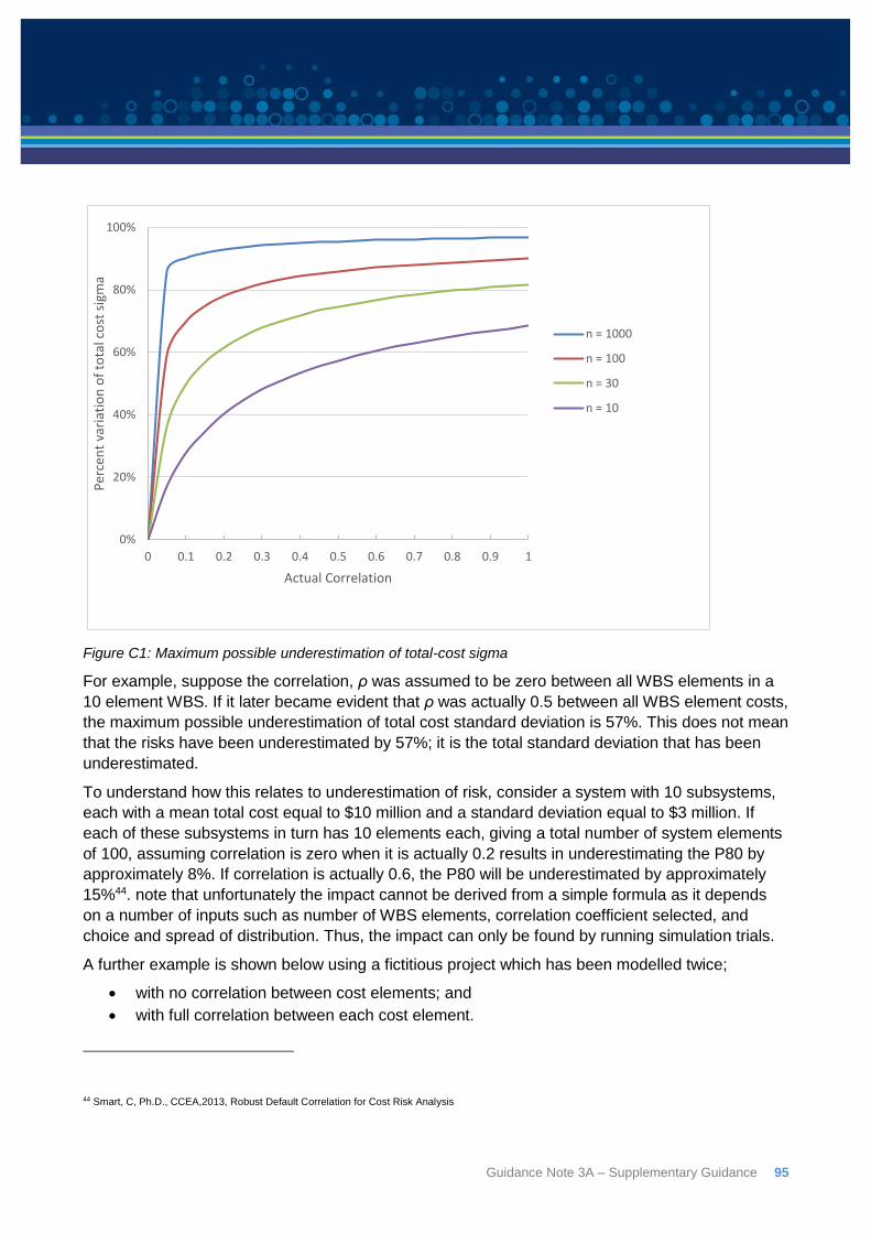
Guidance Note 3A – Supplementary Guidance 95
Figure C1: Maximum possible underestimation of total-cost sigma
For example, suppose the correlation, ρ was assumed to be zero between all WBS elements in a
10 element WBS. If it later became evident that ρ was actually 0.5 between all WBS element costs,
the maximum possible underestimation of total cost standard deviation is 57%. This does not mean
that the risks have been underestimated by 57%; it is the total standard deviation that has been
underestimated.
To understand how this relates to underestimation of risk, consider a system with 10 subsystems,
each with a mean total cost equal to $10 million and a standard deviation equal to $3 million. If
each of these subsystems in turn has 10 elements each, giving a total number of system elements
of 100, assuming correlation is zero when it is actually 0.2 results in underestimating the P80 by
approximately 8%. If correlation is actually 0.6, the P80 will be underestimated by approximately
15%44. note that unfortunately the impact cannot be derived from a simple formula as it depends
on a number of inputs such as number of WBS elements, correlation coefficient selected, and
choice and spread of distribution. Thus, the impact can only be found by running simulation trials.
A further example is shown below using a fictitious project which has been modelled twice;
with no correlation between cost elements; and
with full correlation between each cost element.
44 Smart, C, Ph.D., CCEA,2013, Robust Default Correlation for Cost Risk Analysis
0%
20%
40%
60%
80%
100%
0 0.1 0.2 0.3 0.4 0.5 0.6 0.7 0.8 0.9 1
Per
cen
t va
riat
ion
of
tota
l co
st s
igm
a
Actual Correlation
n = 1000
n = 100
n = 30
n = 10
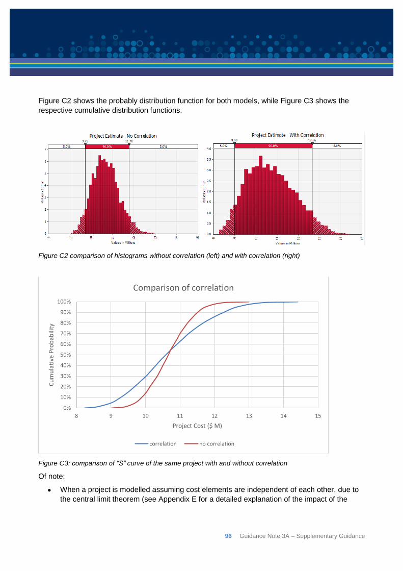
96 Guidance Note 3A – Supplementary Guidance
Figure C2 shows the probably distribution function for both models, while Figure C3 shows the
respective cumulative distribution functions.
Figure C2 comparison of histograms without correlation (left) and with correlation (right)
Figure C3: comparison of “S” curve of the same project with and without correlation
Of note:
When a project is modelled assuming cost elements are independent of each other, due to
the central limit theorem (see Appendix E for a detailed explanation of the impact of the
0%
10%
20%
30%
40%
50%
60%
70%
80%
90%
100%
8 9 10 11 12 13 14 15
Cu
mu
lati
ve P
rob
abili
ty
Project Cost ($ M)
Comparison of correlation
correlation no correlation
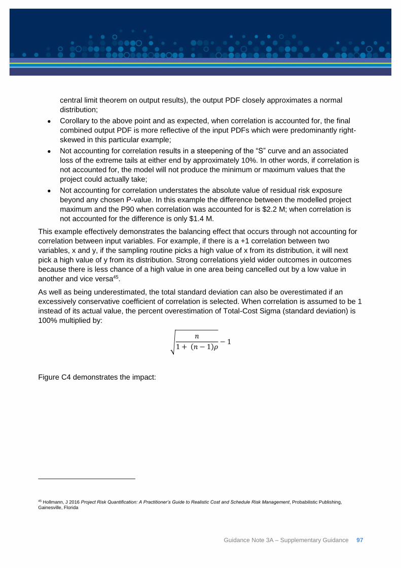
Guidance Note 3A – Supplementary Guidance 97
central limit theorem on output results), the output PDF closely approximates a normal
distribution;
Corollary to the above point and as expected, when correlation is accounted for, the final
combined output PDF is more reflective of the input PDFs which were predominantly right-
skewed in this particular example;
Not accounting for correlation results in a steepening of the “S” curve and an associated
loss of the extreme tails at either end by approximately 10%. In other words, if correlation is
not accounted for, the model will not produce the minimum or maximum values that the
project could actually take;
Not accounting for correlation understates the absolute value of residual risk exposure
beyond any chosen P-value. In this example the difference between the modelled project
maximum and the P90 when correlation was accounted for is $2.2 M; when correlation is
not accounted for the difference is only $1.4 M.
This example effectively demonstrates the balancing effect that occurs through not accounting for
correlation between input variables. For example, if there is a +1 correlation between two
variables, x and y, if the sampling routine picks a high value of x from its distribution, it will next
pick a high value of y from its distribution. Strong correlations yield wider outcomes in outcomes
because there is less chance of a high value in one area being cancelled out by a low value in
another and vice versa45.
As well as being underestimated, the total standard deviation can also be overestimated if an
excessively conservative coefficient of correlation is selected. When correlation is assumed to be 1
instead of its actual value, the percent overestimation of Total-Cost Sigma (standard deviation) is
100% multiplied by:
√𝑛
1 + (𝑛 − 1)𝜌− 1
Figure C4 demonstrates the impact:
45 Hollmann, J 2016 Project Risk Quantification: A Practitioner’s Guide to Realistic Cost and Schedule Risk Management, Probabilistic Publishing, Gainesville, Florida
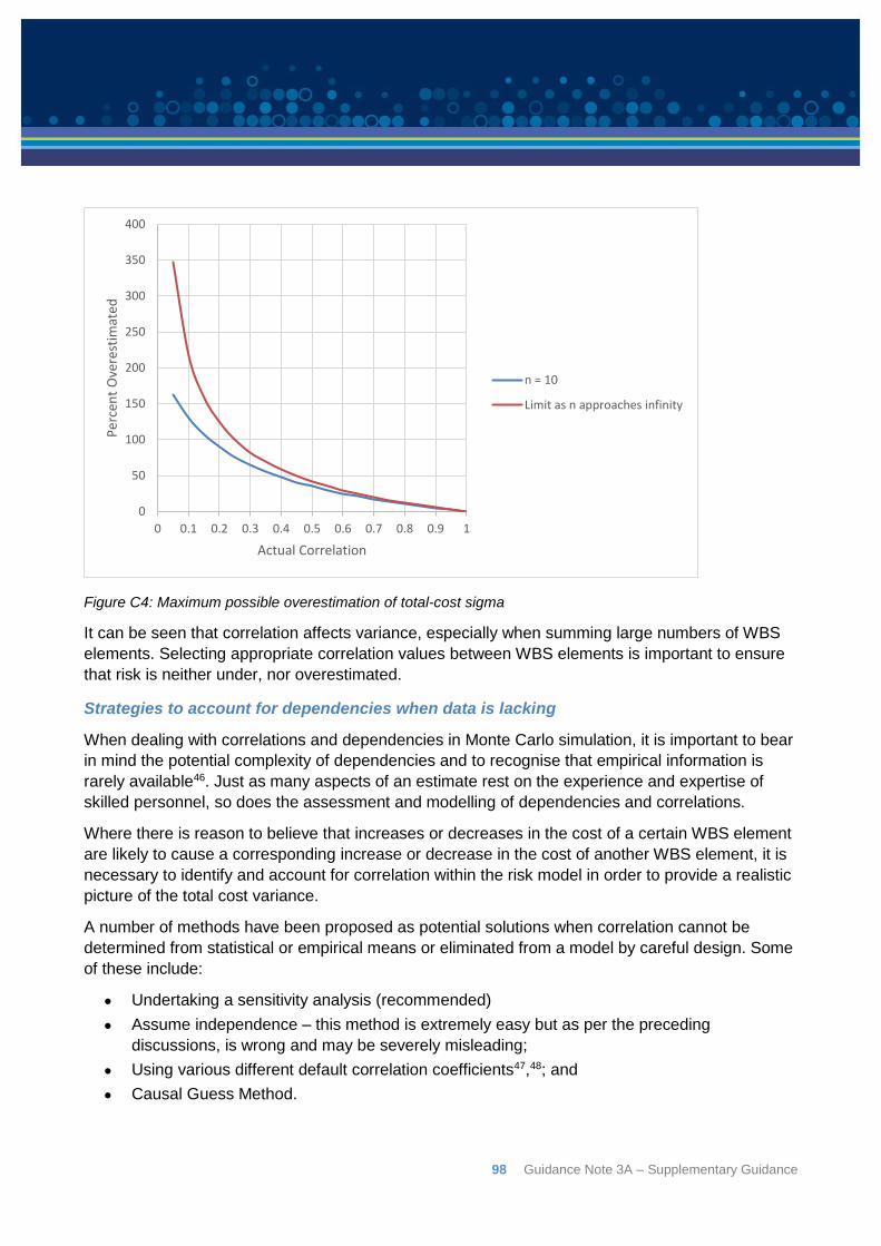
98 Guidance Note 3A – Supplementary Guidance
Figure C4: Maximum possible overestimation of total-cost sigma
It can be seen that correlation affects variance, especially when summing large numbers of WBS
elements. Selecting appropriate correlation values between WBS elements is important to ensure
that risk is neither under, nor overestimated.
Strategies to account for dependencies when data is lacking
When dealing with correlations and dependencies in Monte Carlo simulation, it is important to bear
in mind the potential complexity of dependencies and to recognise that empirical information is
rarely available46. Just as many aspects of an estimate rest on the experience and expertise of
skilled personnel, so does the assessment and modelling of dependencies and correlations.
Where there is reason to believe that increases or decreases in the cost of a certain WBS element
are likely to cause a corresponding increase or decrease in the cost of another WBS element, it is
necessary to identify and account for correlation within the risk model in order to provide a realistic
picture of the total cost variance.
A number of methods have been proposed as potential solutions when correlation cannot be
determined from statistical or empirical means or eliminated from a model by careful design. Some
of these include:
Undertaking a sensitivity analysis (recommended)
Assume independence – this method is extremely easy but as per the preceding
discussions, is wrong and may be severely misleading;
Using various different default correlation coefficients47,48; and
Causal Guess Method.
0
50
100
150
200
250
300
350
400
0 0.1 0.2 0.3 0.4 0.5 0.6 0.7 0.8 0.9 1
Per
cen
t O
vere
stim
ated
Actual Correlation
n = 10
Limit as n approaches infinity
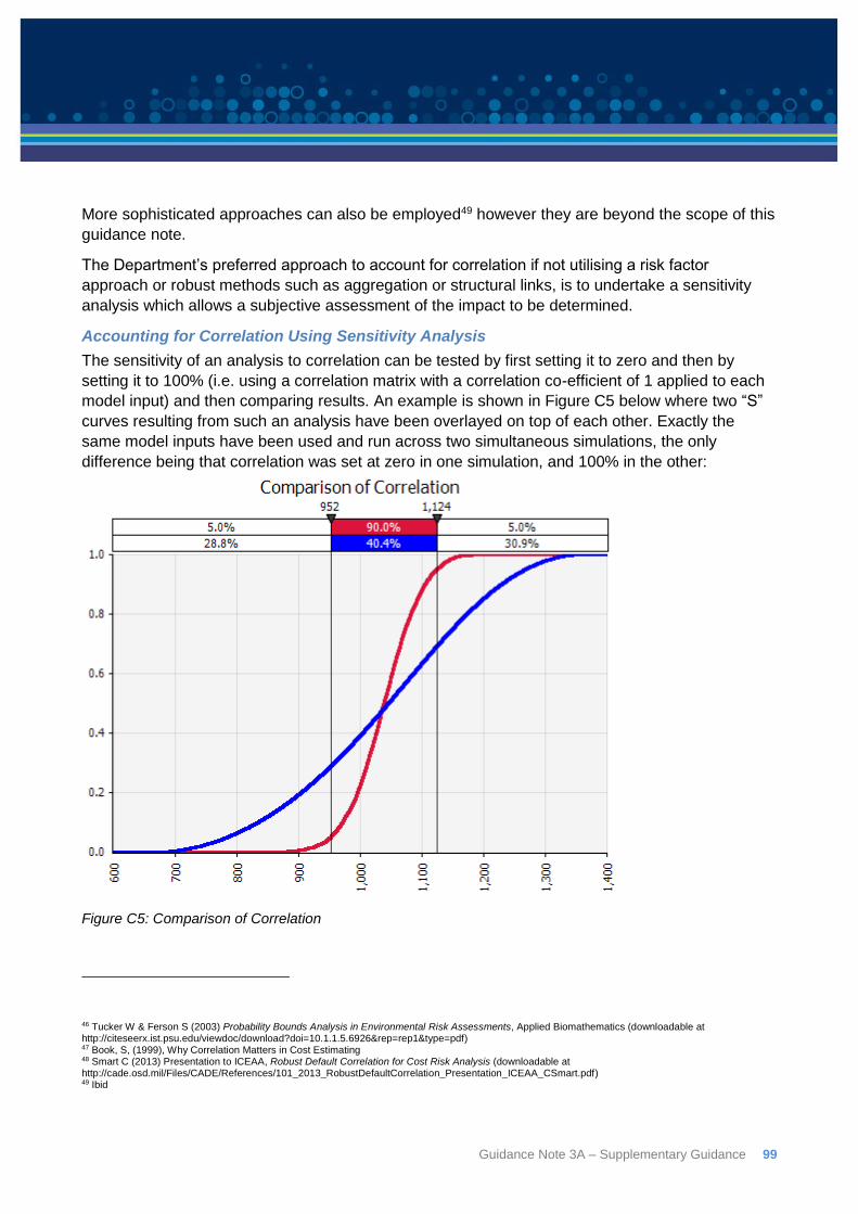
Guidance Note 3A – Supplementary Guidance 99
More sophisticated approaches can also be employed49 however they are beyond the scope of this
guidance note.
The Department’s preferred approach to account for correlation if not utilising a risk factor
approach or robust methods such as aggregation or structural links, is to undertake a sensitivity
analysis which allows a subjective assessment of the impact to be determined.
Accounting for Correlation Using Sensitivity Analysis
The sensitivity of an analysis to correlation can be tested by first setting it to zero and then by
setting it to 100% (i.e. using a correlation matrix with a correlation co-efficient of 1 applied to each
model input) and then comparing results. An example is shown in Figure C5 below where two “S”
curves resulting from such an analysis have been overlayed on top of each other. Exactly the
same model inputs have been used and run across two simultaneous simulations, the only
difference being that correlation was set at zero in one simulation, and 100% in the other:
Figure C5: Comparison of Correlation
46 Tucker W & Ferson S (2003) Probability Bounds Analysis in Environmental Risk Assessments, Applied Biomathematics (downloadable at http://citeseerx.ist.psu.edu/viewdoc/download?doi=10.1.1.5.6926&rep=rep1&type=pdf) 47 Book, S, (1999), Why Correlation Matters in Cost Estimating 48 Smart C (2013) Presentation to ICEAA, Robust Default Correlation for Cost Risk Analysis (downloadable at http://cade.osd.mil/Files/CADE/References/101_2013_RobustDefaultCorrelation_Presentation_ICEAA_CSmart.pdf) 49 Ibid
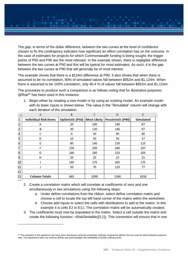
100 Guidance Note 3A – Supplementary Guidance
The gap, in terms of the dollar difference, between the two curves at the level of confidence
chosen to fix the contingency indicates how significant an effect correlation has on the outcome. In
the case of estimates for projects for which Commonwealth funding is being sought, the trigger
points of P50 and P90 are the most relevant. In the example shown, there is negligible difference
between the two curves at P50 and this will be typical for most estimates. As such, it is the gap
between the two curves at P90 that will generally be of most interest.
The example shows that there is a $124m difference at P90. It also shows that when there is
assumed to be no correlation, 90% of simulated values fall between $952m and $1,124m. When
there is assumed to be 100% correlation, only 40.4 % of values fall between $952m and $1,124m.
The procedure to produce such a comparison is as follows noting that for illustrative purposes
@Risk50 has been used in this instance:
1. Begin either by creating a new model or by using an existing model. An example model
with its basic inputs is shown below. The value in the “Simulated” column will change with
each iteration of the simulation.
2. Create a correlation matrix which will correlate at coefficients of zero and one
simultaneously in two simulations using the following steps:
a. Under define correlations from the ribbon, select define correlation matrix and
choose a cell to locate the top left hand corner of the matrix within the worksheet.
b. Choose add inputs to select the cells with distributions to add to the matrix. In this
example it is cells E2 to E11. The correlation matrix will be automatically created.
3. The coefficients must now be populated in the matrix. Select a cell outside the matrix and
create the following function: =RiskSimtable({0,1}). This convention will ensure that in one
50 The examples in this guidance note have been developed using the proprietary software programme @Risk and are used for demonstration purposes only. The Department does not endorse @Risk and acknowledges the availability of similar software tools.
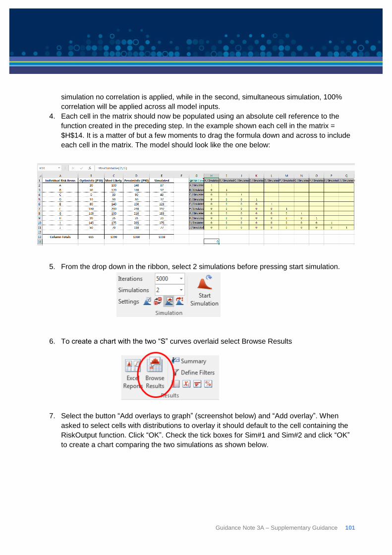
Guidance Note 3A – Supplementary Guidance 101
simulation no correlation is applied, while in the second, simultaneous simulation, 100%
correlation will be applied across all model inputs.
4. Each cell in the matrix should now be populated using an absolute cell reference to the
function created in the preceding step. In the example shown each cell in the matrix =
$H$14. It is a matter of but a few moments to drag the formula down and across to include
each cell in the matrix. The model should look like the one below:
5. From the drop down in the ribbon, select 2 simulations before pressing start simulation.
6. To create a chart with the two “S” curves overlaid select Browse Results
7. Select the button “Add overlays to graph” (screenshot below) and “Add overlay”. When
asked to select cells with distributions to overlay it should default to the cell containing the
RiskOutput function. Click “OK”. Check the tick boxes for Sim#1 and Sim#2 and click “OK”
to create a chart comparing the two simulations as shown below.
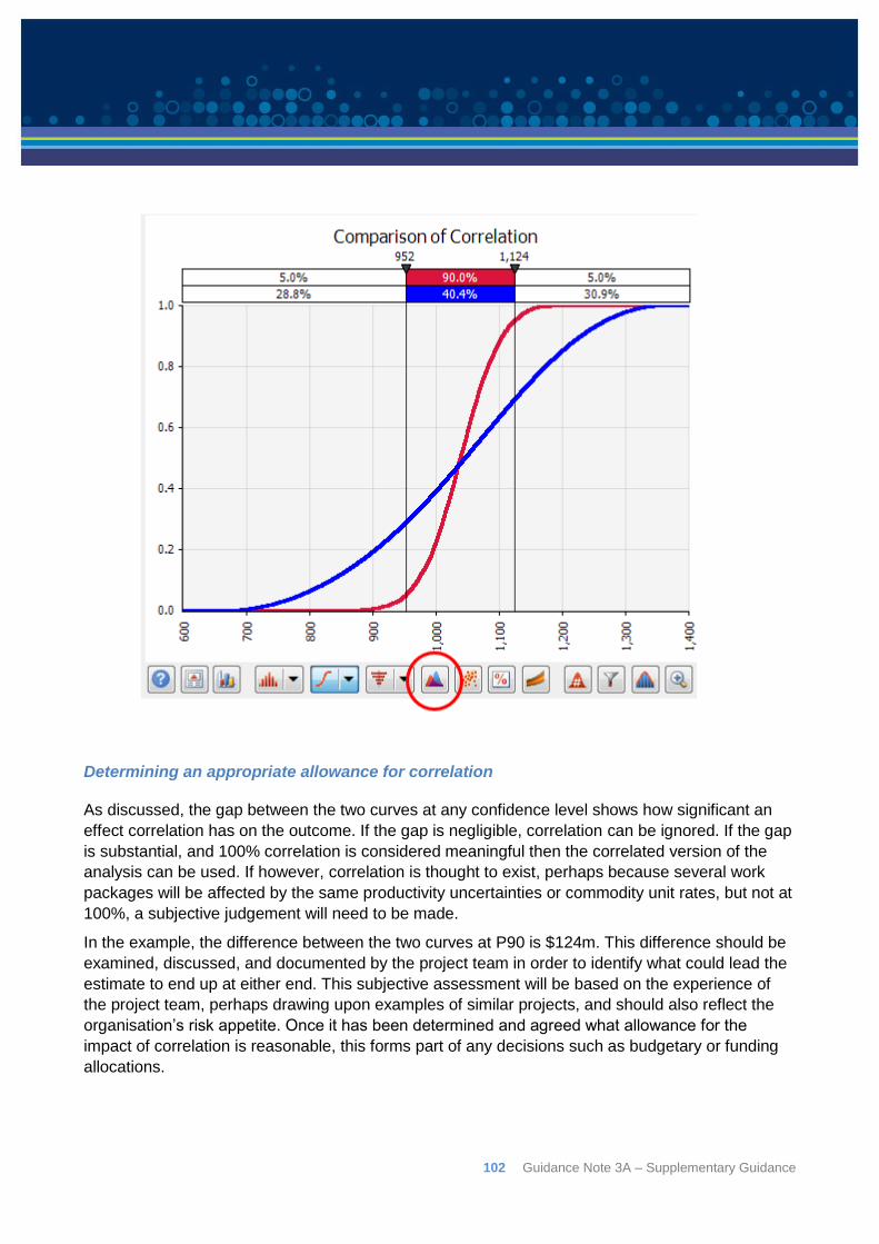
102 Guidance Note 3A – Supplementary Guidance
Determining an appropriate allowance for correlation
As discussed, the gap between the two curves at any confidence level shows how significant an
effect correlation has on the outcome. If the gap is negligible, correlation can be ignored. If the gap
is substantial, and 100% correlation is considered meaningful then the correlated version of the
analysis can be used. If however, correlation is thought to exist, perhaps because several work
packages will be affected by the same productivity uncertainties or commodity unit rates, but not at
100%, a subjective judgement will need to be made.
In the example, the difference between the two curves at P90 is $124m. This difference should be
examined, discussed, and documented by the project team in order to identify what could lead the
estimate to end up at either end. This subjective assessment will be based on the experience of
the project team, perhaps drawing upon examples of similar projects, and should also reflect the
organisation’s risk appetite. Once it has been determined and agreed what allowance for the
impact of correlation is reasonable, this forms part of any decisions such as budgetary or funding
allocations.

Guidance Note 3A – Supplementary Guidance 103
Summary of correlation
Valid Monte Carlo specifically requires that the dependencies, or correlation, between the model
inputs (the model line items) be defined, which includes being clear when there is no significant
correlation. Correlations can have a large impact on the percentiles of the cost probability
distribution and assuming no correlation can result in a large understatement of risk.
This appendix has briefly explored a number of techniques to quantify and account for correlation.
However, the difference in approaches highlights how difficult it is to arrive at defensible
assessments of correlation that are also technically sound. Methods that have arrived at suggested
levels of correlation in one sector or type of work might not apply to a different type of project or
even to the same nominal type of work when the technical, commercial or economic context
changes.
The risk driver/risk factor modelling approach which is the focus of this guidance note describes
cost uncertainty in a way that minimises the amount of correlation between model components that
has to be modelled using correlation factors. It avoids the practical problems of dealing with a large
number of interacting events or a large number of correlated line-item variations by focusing on the
major estimating inputs that uncertainty will affect and which drive the individual line items.
The advantage of using risk factors to avoid building in the need to use correlation factors has
been understood for decades51. As such, in order to overcome the inherent difficulties in dealing
with correlation, the Department strongly encourages the use of a driver-based methodology
wherever practicable.
51 Pouliquen L (1970) World Bank Occasional Papers Number Eleven
104 Guidance Note 3A – Supplementary Guidance
Appendix D: Probability Distribution Functions Shapes commonly used for routine cost modelling are the Beta PERT, Trigen, and triangular
distributions. As demonstrated at Section 6.4, the choice of shape for the individual distribution will
normally have no material effect on the output. This is almost always the case, except where the
extreme values of the output distribution are important.
Project funding decisions are generally not concerned with outcomes in the extreme tails of the
distribution where different distributions may make a difference, but focus their attention between
the 10th and 90th percentiles. The choice of distribution will rarely make a difference to the
outcomes within this range.
Further explanation and detail regarding probability distribution functions is covered in this
Appendix.
The realism of a risk analysis relies, in part, on the appropriate use of probability distributions to
represent the uncertainty and variability of the system being analysed. The most basic property
distinguishing the different of probability distributions offered by modelling tools is whether they are
continuous or discrete.
Continuous distributions
A continuous distribution is used to represent a variable that can take any value within a defined
range (domain). For example, the height of a person picked at random has a continuous
distribution. All values of height within the range found in a population are feasible.
Discrete distributions
A discrete distribution may take any one of a set of identifiable values, each of which has a
calculated probability of occurrence. The number of people in motor vehicles using a road is an
example of a discrete distribution.
Bounded and unbounded distributions
A distribution that is confined to lie between two determined values is said to be bounded.
Examples are:
uniform – bounded between minimum and maximum;
triangular – between minimum and maximum;
beta – between 0 and 1; and
binomial – between 0 and a specified number, n.
Project variables that are strictly bounded include the number of days in a year when work will be
affected by rain, between zero and three hundred and sixty five, or the proportion of cut material
that may suitable for use as select fill, between zero and one hundred per cent. Many variables
might not strictly be bounded but are so for all practical purposes, such as the length of a culvert at
a creek crossing.
A distribution that is unbounded theoretically extends from minus infinity to plus infinity. A normal
distribution is unbounded.
A distribution that is constrained at one end is said to be partially bounded. An example is the
lognormal distribution which cannot go below zero but which has an upper bound of infinity.
Guidance Note 3A – Supplementary Guidance 105
Unbounded and partially unbounded distributions may need to be constrained to remove the tail of
the distribution so that nonsensical values are avoided. For example, costs can exclusively never
go below zero (otherwise they are not a “cost”) so if a cost element is modelled using a distribution
that can generate a negative value it must be truncated. (While some contingent risks may present
an opportunity for a saving over the base estimate, again there should generally be no chance that
the cost can actually be below zero.)
The various Monte Carlo simulation software packages will allow for this functionality and will also
allow a user to test for the theoretical minimum or maximum value that a modelled input can take
(RiskTheomin/RiskTheomax in @Risk for example) in order that the analyst can test whether
truncating is required.
Analysts should be aware that that truncating the lower limit of a distribution moves the mean of
the distribution to the right, making it a more conservative estimate. This is less of a problem if the
upper limit is also truncated.
Choice of distribution
In principle, the correct distribution to assign is the maximum entropy distribution52 which is the
minimally prejudiced distribution that maximises the entropy subject to constraints supplied by
available information. In simple terms, it is the distribution that is consistent with all the available
information but includes no additional assumptions.
The difficulties in sorting out our true state of knowledge, and performing the intricate mathematics
needed to find the maximum entropy distribution that represents it, makes attempting to define and
assign the maximum entropy distribution highly impractical.
Various attempts have been made to identify the underlying empirical distribution of various sets of
cost data, with publicly available information mainly related to Defence or space programs in the
US. The 2010 US Air Force Cost Risk and Uncertainty Analysis Metrics Manual (CRUAMM)53
identified the frequency of each distribution found across 1,400 fits of various cost data. A
lognormal distribution was found to be the best fit to the data in 59% of instances followed by Beta
(19%) and Triangular (18%). Uniform was never found to be, and Normal was rarely found to be
the best fit.
It must be noted that these distributions were found to be the best fit to cost elements applicable to
the US Air Force, predominantly communications devices, aircraft components and weapons
systems, most of which are not directly comparable with Australian land transportation project cost
elements.
In addition, observations of past projects are not necessarily a good guide to a new project at this
level of detail. Systematic issues, such as discussed by Hollmann54, may be consistent within a
sector under stable economic, technical and commercial conditions. While past history is a very
52 Cover, T & Thomas J (2006) Elements of Information Theory 2nd Edition 53 Joint Agency Cost Schedule Risk and Uncertainty Handbook, March 2014 54 Hollmann, J (2016) Project Risk Quantification: A Practitioner’s Guide to Realistic Cost and Schedule Risk Management, Probabilistic Publishing, Gainesville, FL
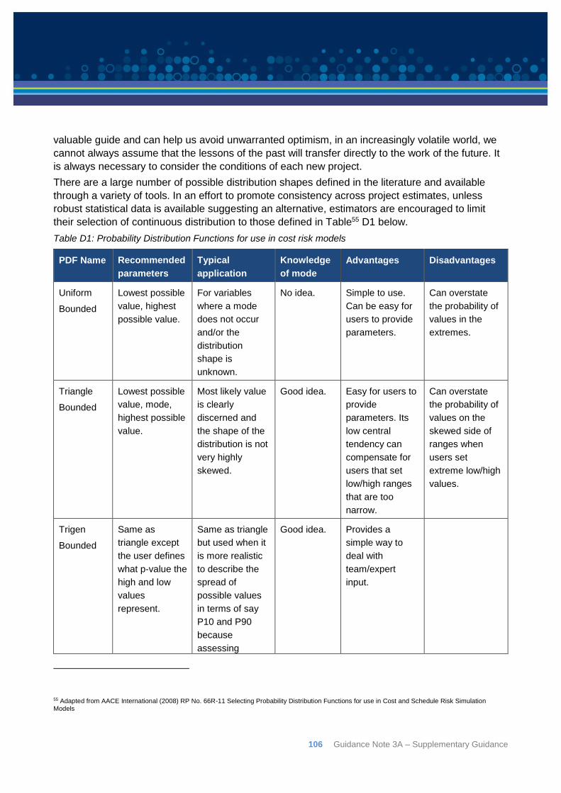
106 Guidance Note 3A – Supplementary Guidance
valuable guide and can help us avoid unwarranted optimism, in an increasingly volatile world, we
cannot always assume that the lessons of the past will transfer directly to the work of the future. It
is always necessary to consider the conditions of each new project.
There are a large number of possible distribution shapes defined in the literature and available
through a variety of tools. In an effort to promote consistency across project estimates, unless
robust statistical data is available suggesting an alternative, estimators are encouraged to limit
their selection of continuous distribution to those defined in Table55 D1 below.
Table D1: Probability Distribution Functions for use in cost risk models
PDF Name Recommended
parameters
Typical
application
Knowledge
of mode
Advantages Disadvantages
Uniform
Bounded
Lowest possible
value, highest
possible value.
For variables
where a mode
does not occur
and/or the
distribution
shape is
unknown.
No idea. Simple to use.
Can be easy for
users to provide
parameters.
Can overstate
the probability of
values in the
extremes.
Triangle
Bounded
Lowest possible
value, mode,
highest possible
value.
Most likely value
is clearly
discerned and
the shape of the
distribution is not
very highly
skewed.
Good idea. Easy for users to
provide
parameters. Its
low central
tendency can
compensate for
users that set
low/high ranges
that are too
narrow.
Can overstate
the probability of
values on the
skewed side of
ranges when
users set
extreme low/high
values.
Trigen
Bounded
Same as
triangle except
the user defines
what p-value the
high and low
values
represent.
Same as triangle
but used when it
is more realistic
to describe the
spread of
possible values
in terms of say
P10 and P90
because
assessing
Good idea. Provides a
simple way to
deal with
team/expert
input.
55 Adapted from AACE International (2008) RP No. 66R-11 Selecting Probability Distribution Functions for use in Cost and Schedule Risk Simulation Models
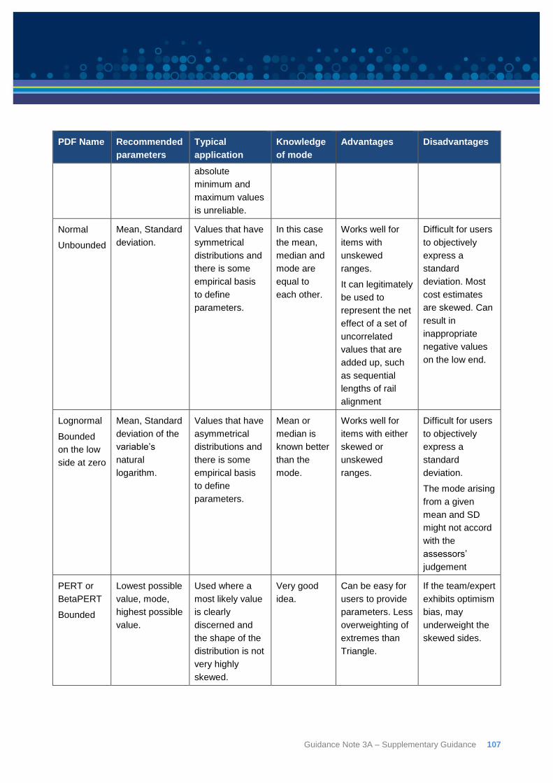
Guidance Note 3A – Supplementary Guidance 107
PDF Name Recommended
parameters
Typical
application
Knowledge
of mode
Advantages Disadvantages
absolute
minimum and
maximum values
is unreliable.
Normal
Unbounded
Mean, Standard
deviation.
Values that have
symmetrical
distributions and
there is some
empirical basis
to define
parameters.
In this case
the mean,
median and
mode are
equal to
each other.
Works well for
items with
unskewed
ranges.
It can legitimately
be used to
represent the net
effect of a set of
uncorrelated
values that are
added up, such
as sequential
lengths of rail
alignment
Difficult for users
to objectively
express a
standard
deviation. Most
cost estimates
are skewed. Can
result in
inappropriate
negative values
on the low end.
Lognormal
Bounded
on the low
side at zero
Mean, Standard
deviation of the
variable’s
natural
logarithm.
Values that have
asymmetrical
distributions and
there is some
empirical basis
to define
parameters.
Mean or
median is
known better
than the
mode.
Works well for
items with either
skewed or
unskewed
ranges.
Difficult for users
to objectively
express a
standard
deviation.
The mode arising
from a given
mean and SD
might not accord
with the
assessors’
judgement
PERT or
BetaPERT
Bounded
Lowest possible
value, mode,
highest possible
value.
Used where a
most likely value
is clearly
discerned and
the shape of the
distribution is not
very highly
skewed.
Very good
idea.
Can be easy for
users to provide
parameters. Less
overweighting of
extremes than
Triangle.
If the team/expert
exhibits optimism
bias, may
underweight the
skewed sides.
108 Guidance Note 3A – Supplementary Guidance
The table above indicates the information that the estimator requires in order to select a
distribution. It might be reasonably argued that since a triangular distribution rarely represents the
underlying distribution of a cost element “in the real world”, it is inappropriate to select it for
modelling purposes. However, it lends itself well to road and rail projects because for most of the
cost elements there will realistically be a most likely (mode) value, for example volume of asphalt
and aggregates, number of pits and pipes required, etc., as well as a reasonably realistic minimum
and maximum value. The triangular shape adds no assumptions to the analysis beyond:
There is a peak; and
The cumulative probability outside the upper and lower parameters (either zero or a defined
percentage).
Beyond this, the triangular shape adopts the simplest form that satisfies the three parameters used
to define it, a straight line decline from the peak to zero.
While a lognormal distribution may at times be more representative of highly skewed values, such
as the extent of an environmental incident with a high chance of a minor impact and a rapidly
declining chance of increasingly extreme impacts, it requires an analyst have a better idea of the
mean or median than the mode because of the way most modelling tools require it to be specified.
Unless there is good reason to be certain that a distribution has a shape where the tails fall away
quickly, as does a PERT distribution, the triangular form may be preferred. The tails of the
triangular distribution are also given more weight than the tails of a PERT or similar shape and so
do not introduce any bias towards certainty or false precision56. If anything, a triangular shape
provides a conservative view of the potential spread of an uncertain quantity as it lends a little extra
weight to the tails of the distribution.
There is a useful variation of the triangular distribution called Trigen in @Risk and other tools. The
Trigen distribution requires five parameters:
A low value;
The most likely;
A high value;
The probability that the parameter value could be below the low value; and
The probability that the parameter value could be above the high value.
The Trigen distribution is a useful way of avoiding asking experts for their estimate of the absolute
minimum and maximum of a parameter. These are questions that experts often have difficulty
answering meaningfully since there may be no theoretical minimum or maximum even though the
likelihood of realistic outcomes becomes minute a short way beyond the low and high values.
Instead the analyst can discuss what probabilities the experts would use to define low and high
values. In this way the Trigen allows a modeller to elicit assessments in terms that an expert can
respond to meaningfully and use those assessments directly in the analysis without further
adjustment.
56 Cooper D,et al, 2014 Project Risk Management Guidelines: Managing Risk with ISO 31000 and IEC 62198 2nd Edition
Guidance Note 3A – Supplementary Guidance 109
Analysts should be aware of the limitations of particular distributions when making a selection. As
mentioned, project funding decisions usually focus their attention between the 10th and 90th
percentiles, not the tails of the distribution. The choice of distribution will rarely make a difference
to the outcomes within this range. However, for some kinds of analysis, such as safety, critical
failure risk or assessment of contractual liabilities for commercial purposes, the tails may be the
area of interest, and different approaches to analysis and more attention to the distribution shapes
may be required. When this is necessary, a sensitivity approach is usually recommended,
examining alternative distribution shapes and forming a judgement on the implications for a project,
since there is no basis on which a specific shape can be selected.
Distributions to model project specific risk
Probability distribution functions can be categorised as either parametric, or non-parametric. Most
distributions – normal, lognormal, beta, etc - are parametric and are based on a mathematical
function whose shape and range is determined by one or more distribution parameters.
Non-parametric distributions such as triangular, uniform, and discrete have their shape and range
determined by their parameters directly and are generally more reliable and flexible for modelling
expert opinion about a model parameter. An exception is the PERT57 distribution, which although
strictly a parametric distribution, has been adapted so that the expert need only provide estimates
for the minimum, most likely, and maximum values, and the PERT function finds a shape that fits
these inputs.
Similar to when selecting a distribution for a risk factor, the triangular distribution’s appeal is that it
is easy to think about the three defining parameters (minimum or low, most likely, maximum or
high), and to imagine the effect of any changes.
57 The origins and limitations of the PERT form of the Beta distribution are investigated in the discussion paper Beta PERT Origins (Broadleaf 2014) availavle at: http://broadleaf.com.au/resource-material/beta-pert-origins/
110 Guidance Note 3A – Supplementary Guidance
Appendix E: Number of line items to model The greater the number of independent (i.e. uncorrelated) inputs that are put into a model, the
tighter the distribution will become as it converges to a normal distribution and the extreme tails of
heavily-skewed marginal distributions are lost.
Models with a very large number of line items are still valid, provided that the dependency between
line items is accounted for, noting that, in general, there will be various dependency relationships
between cost elements on infrastructure projects. If this is not done then the greater the number of
(uncorrelated) cost elements included in the model, the less representative of reality it becomes,
particularly at higher P-levels, and contingency is likely to be underestimated.
Probabilistic models should be limited to between 20 and 40 inputs in order to maintain the validity
of the results.
This appendix provides further explanation of the importance of limiting the number of inputs into a
model.
The central limit theorem (CLT) says that the mean of a set of n variables (where n is large), drawn
independently from the same distribution will be normally distributed. That is, the average of the
sum of a large number of independent, random variables with finite means and variances
converges to a normal random variable.
This theorem also applies to the sum (or average) of a large number of independent variables that
have different probability distribution types, in that their sum will be approximately normally
distributed providing no variable dominates the uncertainty of the sum.
How large n has to be depends on the individual distributions, but in practice the convergence to
the Gaussian, or normal, distribution is surprisingly fast.
Because most risk analysis models are a combination of adding and multiplying variables together,
it should come as no surprise that most risk analysis results appear to fall between a normal and
lognormal distribution. A lognormal distribution also looks like a normal distribution when its mean
is much larger than its standard deviation, so a risk analysis model result even more frequently
looks approximately like a normal distribution, being a roughly symmetrical bell shaped curve.
Leading from the discussion of the CLT above, it is apparent that the greater the number of
independent (i.e. uncorrelated) inputs that are put into a model, the tighter the distribution must
become as it converges to the Gaussian and the extreme tails of heavily-skewed distributions are
lost. This is best illustrated by a simple example. Consider a project with 10 independent cost
elements, each with a most likely value of $100 million with an uncertainty represented by a
triangular distribution with a low of -10% and a high of +15%.
Now consider a case of 100 independent cost elements with the same distribution but with a most
likely value of $10 million so that the total base estimate remains the same.
Two simultaneous simulations of 5,000 iterations based on the inputs as described above gives the
following results:
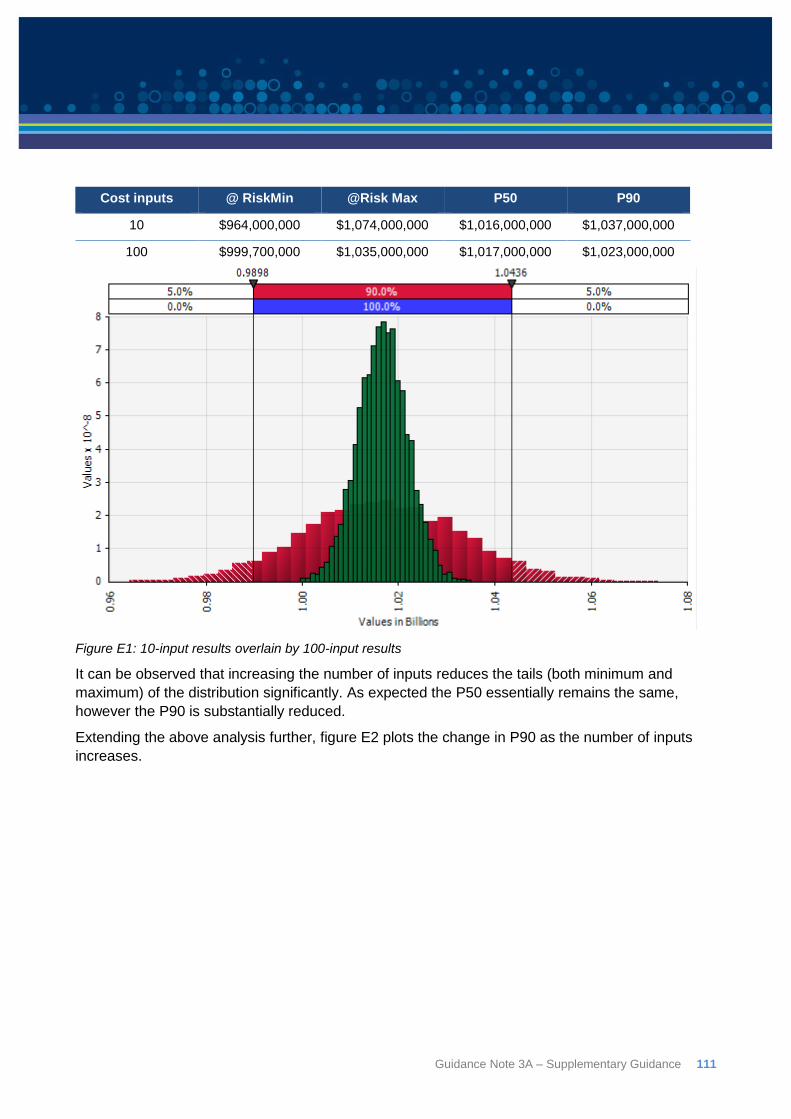
Guidance Note 3A – Supplementary Guidance 111
Cost inputs @ RiskMin @Risk Max P50 P90
10 $964,000,000 $1,074,000,000 $1,016,000,000 $1,037,000,000
100 $999,700,000 $1,035,000,000 $1,017,000,000 $1,023,000,000
Figure E1: 10-input results overlain by 100-input results
It can be observed that increasing the number of inputs reduces the tails (both minimum and
maximum) of the distribution significantly. As expected the P50 essentially remains the same,
however the P90 is substantially reduced.
Extending the above analysis further, figure E2 plots the change in P90 as the number of inputs
increases.
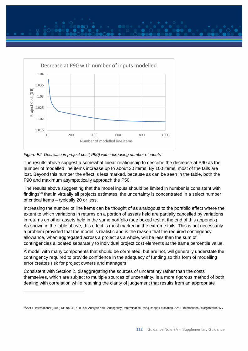
112 Guidance Note 3A – Supplementary Guidance
Figure E2: Decrease in project cost( P90) with increasing number of inputs
The results above suggest a somewhat linear relationship to describe the decrease at P90 as the
number of modelled line items increase up to about 30 items. By 100 items, most of the tails are
lost. Beyond this number the effect is less marked, because as can be seen in the table, both the
P90 and maximum asymptotically approach the P50.
The results above suggesting that the model inputs should be limited in number is consistent with
findings58 that in virtually all projects estimates, the uncertainty is concentrated in a select number
of critical items – typically 20 or less.
Increasing the number of line items can be thought of as analogous to the portfolio effect where the
extent to which variations in returns on a portion of assets held are partially cancelled by variations
in returns on other assets held in the same portfolio (see boxed test at the end of this appendix).
As shown in the table above, this effect is most marked in the extreme tails. This is not necessarily
a problem provided that the model is realistic and is the reason that the required contingency
allowance, when aggregated across a project as a whole, will be less than the sum of
contingencies allocated separately to individual project cost elements at the same percentile value.
A model with many components that should be correlated, but are not, will generally understate the
contingency required to provide confidence in the adequacy of funding so this form of modelling
error creates risk for project owners and managers.
Consistent with Section 2, disaggregating the sources of uncertainty rather than the costs
themselves, which are subject to multiple sources of uncertainty, is a more rigorous method of both
dealing with correlation while retaining the clarity of judgement that results from an appropriate
58 AACE International (2008) RP No. 41R-08 Risk Analysis and Contingency Determination Using Range Estimating, AACE International, Morgantown, WV
1.015
1.02
1.025
1.03
1.035
1.04
0 200 400 600 800 1000
Pro
ject
Co
st (
$ B
)
Number of modelled line items
Decrease at P90 with number of inputs modelled

Guidance Note 3A – Supplementary Guidance 113
level of disaggregation. In most cases it will also result in a simpler, cleaner risk model with far
fewer inputs than a line-item model while still retaining enough detail to represent the uncertainties
affecting the cost.
Contingency and variance
In 1952 an unknown graduate student at the University of Chicago, Harry Markowitz published a fourteen-page article titled “Portfolio Selection”. His aim was to construct portfolios for investors who consider expected return a desirable thing and variance of return an undesirable thing, in other words a strategy where variance of return is minimised. This is typically desirable for investors because the greater the variance or standard deviation around the average, the less the average return will signify about what the outcome is likely to be.
The impact of diversification was Markowitz’s key insight. A system with only a few strongly interacting parts will be unpredictable. Just like the example on page 34, while the expected return looks great, you may win or lose heavily with just one wager and the outcome is uncertain. Diversification reduces volatility because some assets while rise in price while others are falling, or at very least, the rates of return among the assets will differ.
The return on a diversified portfolio will be equal to the average of the rates of return on its individual holdings (recall that the means of individual distributions are additive), however its volatility will be less than the average volatility of its individual holdings. Diversification means you can combine a group of risky securities with high expected returns into a relatively low-risk portfolio with one caveat - the covariances, or correlations, among the returns of the individual securities must be minimised.
Markowitz’s paper formed the basis for much of the theoretical work in finance that followed and highlighted the need to consider risk (or more specifically variance as a proxy for risk) rather than just expected return. While methods today are more sophisticated, the idea that the value of the total project risk is less than the sum of the project’s individual risks is built on much the same premise.
Markowitz, H., (1952) Portfolio Selection, The Journal of Finance, Vol 7, No.1. pp. 77-91
114 Guidance Note 3A – Supplementary Guidance
Appendix F: Number of iterations to run in a simulation The number of iterations required for convergence is dependent upon the model being simulated
and the distribution functions included in the model. For example, more complex models with
highly skewed distributions might require more iterations than simpler models, however 5,000-
10,000 iterations are likely to be adequate for the majority of land transportation projects.
This appendix explores certain concepts, including statistical error, in greater detail which suggest
that 5,000 – 10,000 iterations are appropriate in the majority of cases.
In determining how many iterations to run in a simulation, there are generally two opposing
pressures:
Too few iterations will fail to sample a representative number of outcomes, often indicated
by output histograms that are lumpy, and result in inaccurate conclusions being drawn from
the outputs; and
Too many iterations may take a long time to simulate, a long time to produce graphs, and
there may be limitations (row limitations, etc.) if exporting data to Excel.
The law of large numbers concerns the behaviour of sums of large numbers of random variables. It
can essentially be interpreted as a statement that a Monte Carlo estimate converges to the correct
answer as the random sample size approaches infinity59. For the purposes of this guidance note it
is sufficient to say that the above can be proven60.
The strong law of large numbers can be extended in a number of ways including application of the
Central Limit Theorem, the Berry-Esseen Theorem, or the Bikelis Theorem in order to determine
the number of simulations to run to ensure convergence to a confidence interval on the accuracy61.
In the absence of any specified convergence criteria, checking for convergence can be done
manually by undertaking the following steps62:
1. Set the number of iterations to at least 5,000 and run the simulation.
2. Record the statistics for:
Mean;
Standard deviation;
5th percentile;
Median (50th percentile); and
95th percentile.
59 This interpretation is sufficient for practical purposes but not quite strictly correct. The law tells us that the average of a large sample will be more likely than the average of a small sample to vary from the true average by some stated amount. The key word is vary. What we are seeking is not the true underlying cost distribution, but for the probability that the error between the observed cost distribution and the true cost distribution is less than some stated value. note that Jacob Bernoulli explicitly excludes the case that there will be no error even if the sample size is infinite. See Bernstein pg 122. 60 Calculations using standard properties of binomial coefficients can be used to prove the law of large numbers. Stewart, I., (2012) In Pursuit of the Unknown: 17 Equations that Changed the World. Basic Books, Great Britain 61 Lapeyre B. (2007) Introduction to Monte-Carlo Methods (downloadable at http://cermics.enpc.fr/~bl/Halmstad/monte-carlo/lecture-1.pdf) 62 NASA (2011) Probabilistic Risk Assessment Procedures Guide for NASA Managers and Practitioners 2nd Edition (NASA/SP-2011-3421) NASA
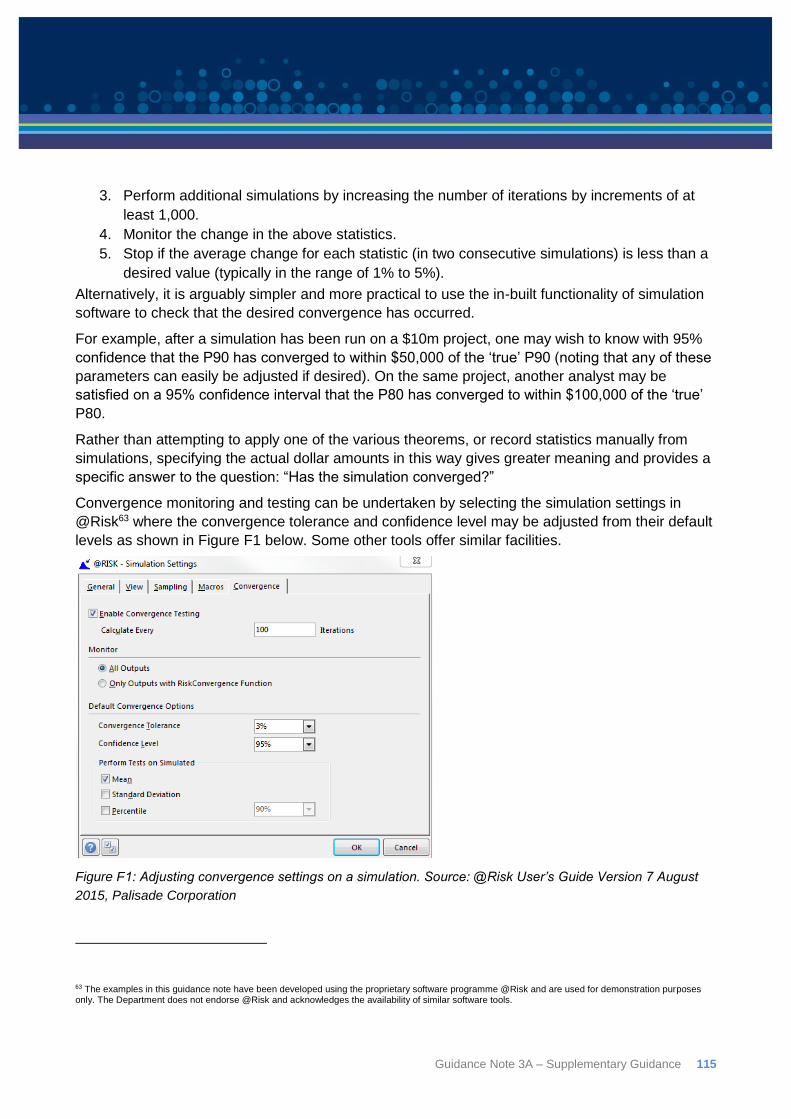
Guidance Note 3A – Supplementary Guidance 115
3. Perform additional simulations by increasing the number of iterations by increments of at
least 1,000.
4. Monitor the change in the above statistics.
5. Stop if the average change for each statistic (in two consecutive simulations) is less than a
desired value (typically in the range of 1% to 5%).
Alternatively, it is arguably simpler and more practical to use the in-built functionality of simulation
software to check that the desired convergence has occurred.
For example, after a simulation has been run on a $10m project, one may wish to know with 95%
confidence that the P90 has converged to within $50,000 of the ‘true’ P90 (noting that any of these
parameters can easily be adjusted if desired). On the same project, another analyst may be
satisfied on a 95% confidence interval that the P80 has converged to within $100,000 of the ‘true’
P80.
Rather than attempting to apply one of the various theorems, or record statistics manually from
simulations, specifying the actual dollar amounts in this way gives greater meaning and provides a
specific answer to the question: “Has the simulation converged?”
Convergence monitoring and testing can be undertaken by selecting the simulation settings in
@Risk63 where the convergence tolerance and confidence level may be adjusted from their default
levels as shown in Figure F1 below. Some other tools offer similar facilities.
Figure F1: Adjusting convergence settings on a simulation. Source: @Risk User’s Guide Version 7 August
2015, Palisade Corporation
63 The examples in this guidance note have been developed using the proprietary software programme @Risk and are used for demonstration purposes only. The Department does not endorse @Risk and acknowledges the availability of similar software tools.
116 Guidance Note 3A – Supplementary Guidance
If there are any discrete risks, those that have a defined probability of causing one type of impact
or one minus that probability of causing a disjoint impact, such as a 90% chance of zero impact
and a 10% chance of an impact lying between $100m and $120m with a most likely value of
$105m, the number of iteration might need to be larger than when there are only continuous
distributions in a model. If the probability of such an event is very low, say 1%, only a very small
number of iterations will include that event. If that event is important and its effect is to be included
in the contingency, it may be necessary to run the model for a very large number of iterations to
get a realistic view of its overall effect. However, unless the extreme tails of the distribution are
important, such low risk events will rarely be included in the analysis and, for most routine project
contingency management purposes, rare events of this scale are best handled as separate items.
They might require analysis in their own right but there is no need to blend them in with the general
contingency. In fact incorporating rare events into the general contingency is not recommended.
In summary, the number of iterations required for convergence is dependent upon the model being
simulated and the distribution functions included in the model. For example, more complex models
with highly skewed distributions might require more iterations than simpler models, however 5,000-
10,000 iterations are likely to be adequate for the majority of land transportation projects.
It should be noted that the rate of convergence (at 95% confidence) is approximately 0.98
√𝑛 so adding
one significant figure of accuracy requires increasing 𝑛 by a factor of 10064. Attempting to achieve
a high level of accuracy (i.e. a large number of significant figures) is unlikely to be practicable and
is rarely necessary.
Statistical error65
As defined by the formula in the preceding section, there is a strict mathematical relationship
between sample size and statistical error. The larger the sample, the smaller the statistical error, or
the more confident an analyst can be that a simulation has converged to the “true” underlying
distribution defined by the model. Statistical error is a verifiable source of error in any simulation,
and it is a consequence of randomness and a function of the size of the sample.
@Risk’s default convergence options are a Convergence Tolerance of 3% with a 95% confidence
level, and these bear further explanation by way of an example.
Say a simulation indicates that the cost of a particular project at some defined percentile level is
$100 million. The analyst knows that statistical error (pure randomness) might affect the result of
the simulation; the real cost might not be $100 million, but could be $99 million, or $102 million, or
even $200 million if there was an extreme random event in the sample.
If an analyst says that the convergence tolerance (which may more correctly be termed the margin
of error) is 3%, this is an expression of a defined level of confidence that randomness can only
64 https://en.wikipedia.org/wiki/Margin_of_error 65 This section adapted from Seife, C (2010) Proofiness: How you are being fooled by the numbers, Chapter 4
Guidance Note 3A – Supplementary Guidance 117
distort the answer by three percentage points up or down – the real cost is somewhere between
$97 million and $103 million. However, this confidence isn’t absolute. By convention66, margin of
error is a number larger than the imprecision caused by randomness 95 percent of the time (hence
@Risk’s default confidence level being set at 95%). This means that on occasion an unlikely set of
events could produce a result more than 3% away from the limit to which it would converge with an
infinite number of iterations. Most of the time though – in 19 out of every 20 simulations, the results
of the simulation will fall within 3% of that limit.
Note that a margin of error of 3% is achieved, in this case, through a simulation of approximately
1,000 iterations. The margin of error (to two decimal places) for 5,000 and 10,000 iterations is
shown below67:
For 5,000 iterations, the margin of error = 0.98
√5000 = 1.39%
For 10,000 iterations, the margin of error = 0.98
√10000 = 0.98%
Thus it should be borne in mind that when using Monte Carlo simulation, the final outcome is an
approximation of the correct value with respective error bounds, and the correct value is within
those error bounds.
Margin of error is a somewhat subtle concept but can be considered as no more than an
expression of how large the sample is. While this may suggest that running a greater number of
iterations in a Monte Carlo simulation will give more accurate results, this thinking is highly
misleading. The margin of error only represents statistical error and while this error is important,
there are far more potential errors which can affect the estimate of a project arising from a
simulation to a much greater extent. When a project estimate is later proven to have been
spectacularly wrong, the problem will almost never have been caused by statistical error. It is more
likely to have been caused by the inputs going into the quantitative model itself being highly flawed
– inappropriate ranges and/or distributions, not accounting for correlation, misunderstanding or
non-identification of major risk factors, and other systematic errors.
When an analyst uses convergence as the sole test of whether to believe the results of a
simulation, they are blind to the sources or error that are most likely to render the results of the
simulation meaningless.
It is also worth noting that the precision that can be attributed to the subjective inputs of a model is
limited and will often render the possible variation associated with convergence irrelevant. This is
not to say that the subjective and uncertain nature of modelling inputs undermines the value of
such analyses. It simply highlights that Monte Carlo simulation modelling of projects using
assessments created by experienced personnel is not the same as using Monte Carlo simulation
for the analysis of physical and engineering systems, for instance. It is a way of making sense and
66 It was English statistician and biologist R. A. Fisher who proposed a 1 in 20 chance of being exceeded by chance as a limit for statistical significance. He also developed the analysis of variance (ANOVA) and was one of the founders of population genetics. (https://en.wikipedia.org/wiki/Ronald_Fisher) 67 Abraham de Moivre was an early contributor to the modern theory of probability. He wasn’t satisfied with the Law of Large Numbers which says, for example, that the proportion of heads in a sequence of flips gets closer and closer to 50%; he wanted to know how much closer. It was his insight that the size of the typical distribution discrepancy is governed by the square root of the sample size. See Ellenberg

118 Guidance Note 3A – Supplementary Guidance
deriving value from the judgement of experienced people in the context of complicated interactions
between design outputs, market information and implementation forecasts.
Guidance Note 3A – Supplementary Guidance 119
Appendix G: Contingency allocation A useful form of sensitivity analysis that can be applied to risk models is contingency sensitivity.
This is an examination of what can be said to contribute most to the offset between the base
estimate and the funding level corresponding to the required level of confidence for the project.
This has to be interpreted with care as the entire foundation of a contingency is that variations in
one part of the work will be balanced by variations in other parts (refer to Contingency and
Variance within Appendix E). However, so long as it is not misused, it is a useful diagnostic tool
and can be used to allocate contingency between work packages or stakeholders on an equitable
basis, if this is necessary.
A common practice is to regard the contingency for an entire project as being distributed pro rata
across all work packages. On this basis, if the overall contingency is 15% of the total base
estimate, each work package would have a notional 15% contingency. This practice is
fundamentally flawed.
If one work package is relatively predictable, a 15% contingency might be excessive and offer the
work package manager a very low risk task. Another work package might house most of the
uncertainty on the project and find a 15% contingency leaves it seriously exposed.
The preferred means of allocating contingency between work packages or stakeholders is on the
basis of equitable provisions that represent the same percentile value in each area, leaving them
all with the same level of risk or exposure within their own budgets. Because percentile values do
not add to the same percentile of the total cost, it is necessary to search for a percentile value that,
when applied equally to the component costs generates component contingencies that add to the
value of the overall contingency. This is illustrated in <Risk factor model 1> in the contingency
analysis tab.
The contingency analysis sheet in <Risk factor model 1> is set out as follows.
The base estimate and simulated values for the lines in the estimate summary are read into
columns B and C so these values are live and vary during the simulation.
The variation between these two is calculated in column D.
The mean value of the variations is calculated in column E, using the @Risk formula
RiskMean(). This is just for interest and is not used in what is discussed below.
Percentile values of the variations are calculated in column F using the @Risk formula
RiskPercentile().
At the top of column F, the preferred percentile point at which to set the overall contingency
is set in cell F1 and the percentile point at which to allocate the contingency to line items is
set in cell F2.
The value in F1 is used in cell D23 to calculate a contingency for the whole project.
The value in F2 is used to derive percentile values for the individual line items.
Cell F3 calculates the deviation between the sum of the line item percentiles and the overall
contingency.
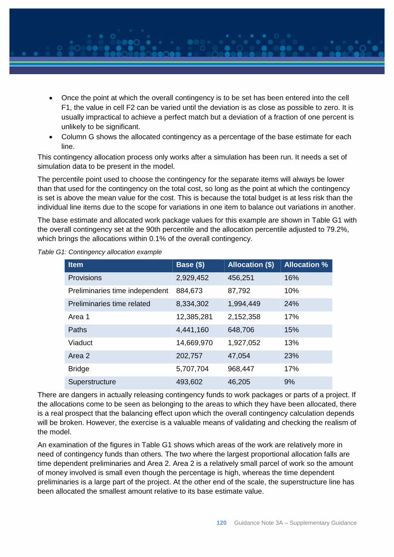
120 Guidance Note 3A – Supplementary Guidance
Once the point at which the overall contingency is to be set has been entered into the cell
F1, the value in cell F2 can be varied until the deviation is as close as possible to zero. It is
usually impractical to achieve a perfect match but a deviation of a fraction of one percent is
unlikely to be significant.
Column G shows the allocated contingency as a percentage of the base estimate for each
line.
This contingency allocation process only works after a simulation has been run. It needs a set of
simulation data to be present in the model.
The percentile point used to choose the contingency for the separate items will always be lower
than that used for the contingency on the total cost, so long as the point at which the contingency
is set is above the mean value for the cost. This is because the total budget is at less risk than the
individual line items due to the scope for variations in one item to balance out variations in another.
The base estimate and allocated work package values for this example are shown in Table G1 with
the overall contingency set at the 90th percentile and the allocation percentile adjusted to 79.2%,
which brings the allocations within 0.1% of the overall contingency.
Table G1: Contingency allocation example
Item Base ($) Allocation ($) Allocation %
Provisions 2,929,452 456,251 16%
Preliminaries time independent 884,673 87,792 10%
Preliminaries time related 8,334,302 1,994,449 24%
Area 1 12,385,281 2,152,358 17%
Paths 4,441,160 648,706 15%
Viaduct 14,669,970 1,927,052 13%
Area 2 202,757 47,054 23%
Bridge 5,707,704 968,447 17%
Superstructure 493,602 46,205 9%
There are dangers in actually releasing contingency funds to work packages or parts of a project. If
the allocations come to be seen as belonging to the areas to which they have been allocated, there
is a real prospect that the balancing effect upon which the overall contingency calculation depends
will be broken. However, the exercise is a valuable means of validating and checking the realism of
the model.
An examination of the figures in Table G1 shows which areas of the work are relatively more in
need of contingency funds than others. The two where the largest proportional allocation falls are
time dependent preliminaries and Area 2. Area 2 is a relatively small parcel of work so the amount
of money involved is small even though the percentage is high, whereas the time dependent
preliminaries is a large part of the project. At the other end of the scale, the superstructure line has
been allocated the smallest amount relative to its base estimate value.

Guidance Note 3A – Supplementary Guidance 121
In the context of a real project, these observations will have meaning to the personnel involved. If
they are consistent with what the team believes then they will confirm the validity of the model. If
they are at odds with what the team believe then either there is a flaw in the model or the team’s
expectations are unrealistic. In either case, the discrepancy should be examined and resolved.
The same approach can be used to allocate contingency funds between two parties, say a
proponent and a contractor. Instead of basing it on the lines of the summary estimate, exactly the
same calculation of base estimate, simulated value, variation, and percentiles would be applied to
the subtotals for the two parties.
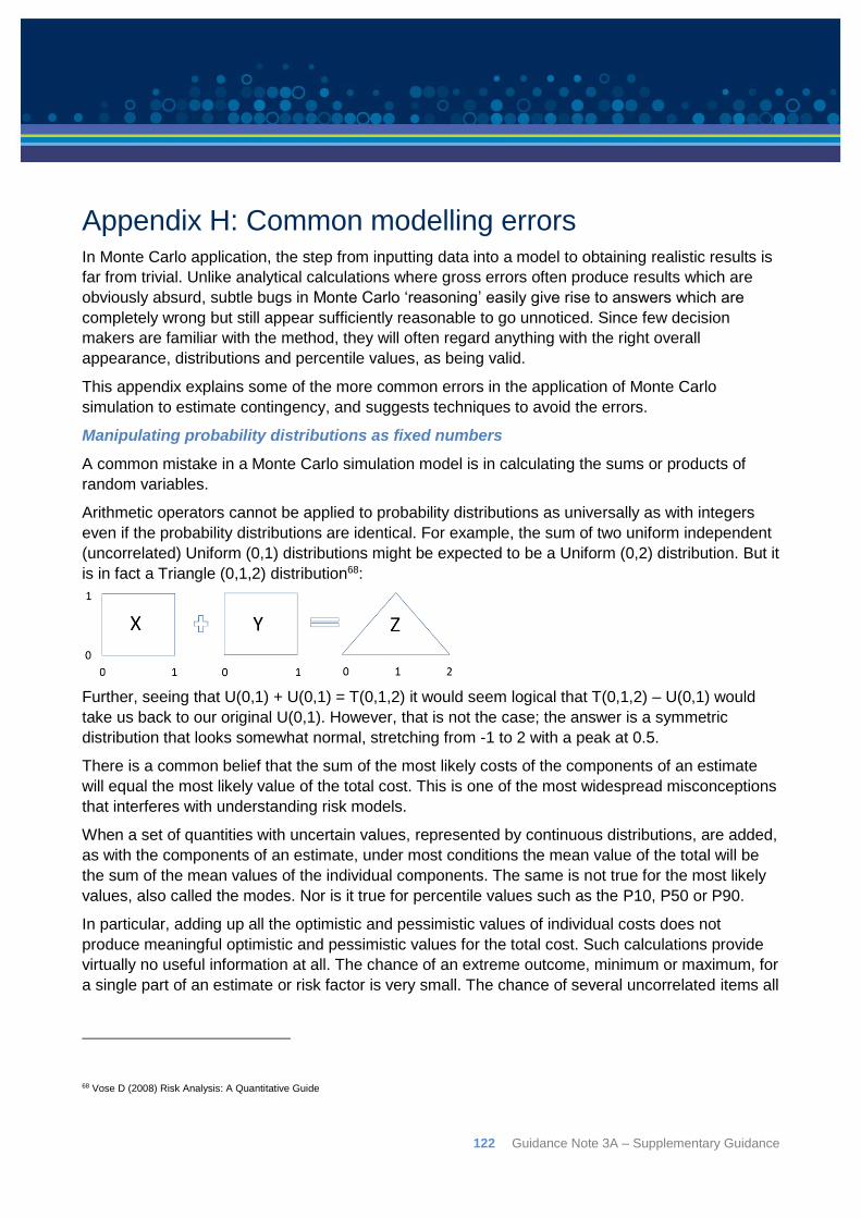
122 Guidance Note 3A – Supplementary Guidance
Appendix H: Common modelling errors In Monte Carlo application, the step from inputting data into a model to obtaining realistic results is
far from trivial. Unlike analytical calculations where gross errors often produce results which are
obviously absurd, subtle bugs in Monte Carlo ‘reasoning’ easily give rise to answers which are
completely wrong but still appear sufficiently reasonable to go unnoticed. Since few decision
makers are familiar with the method, they will often regard anything with the right overall
appearance, distributions and percentile values, as being valid.
This appendix explains some of the more common errors in the application of Monte Carlo
simulation to estimate contingency, and suggests techniques to avoid the errors.
Manipulating probability distributions as fixed numbers
A common mistake in a Monte Carlo simulation model is in calculating the sums or products of
random variables.
Arithmetic operators cannot be applied to probability distributions as universally as with integers
even if the probability distributions are identical. For example, the sum of two uniform independent
(uncorrelated) Uniform (0,1) distributions might be expected to be a Uniform (0,2) distribution. But it
is in fact a Triangle (0,1,2) distribution68:
Further, seeing that U(0,1) + U(0,1) = T(0,1,2) it would seem logical that T(0,1,2) – U(0,1) would
take us back to our original U(0,1). However, that is not the case; the answer is a symmetric
distribution that looks somewhat normal, stretching from -1 to 2 with a peak at 0.5.
There is a common belief that the sum of the most likely costs of the components of an estimate
will equal the most likely value of the total cost. This is one of the most widespread misconceptions
that interferes with understanding risk models.
When a set of quantities with uncertain values, represented by continuous distributions, are added,
as with the components of an estimate, under most conditions the mean value of the total will be
the sum of the mean values of the individual components. The same is not true for the most likely
values, also called the modes. Nor is it true for percentile values such as the P10, P50 or P90.
In particular, adding up all the optimistic and pessimistic values of individual costs does not
produce meaningful optimistic and pessimistic values for the total cost. Such calculations provide
virtually no useful information at all. The chance of an extreme outcome, minimum or maximum, for
a single part of an estimate or risk factor is very small. The chance of several uncorrelated items all
68 Vose D (2008) Risk Analysis: A Quantitative Guide
Guidance Note 3A – Supplementary Guidance 123
taking their most extreme possible values is the product of the probability of each one taking on its
most extreme value.
Calculations based on single values selected from a set of continuous distributions do not really
make sense. It is usually necessary to work with intervals within a distribution’s range to make
such calculations. However, a heuristic illustration can be used to explain what happens when all
the minima and maxima of a set of distributions are added together.
If the extreme values of a distribution are considered to have say a 1% chance of arising, a
probability of 10-1, just for the purposes of this illustration, the probability that ten uncorrelated
uncertain values will all fall at the extreme ends of their ranges in unison is (10-1)10 or 10-10. That is
a microscopic likelihood, a probability of 0.0000000001.
Another way of looking at this is from a practical perspective. It is highly unlikely that 10
independent things will all go wrong at once, otherwise projects would be impossible to estimate
and plan69. Indeed, the concept of contingency is based on the assumption that estimates for some
components will be too high, some will be too low, but in aggregate, many of the highs and lows
will net off such that overruns in some areas are paid for with savings from others.
So long as the ranges assessed for the inputs to a model are realistic and are not all correlated to
one another, the chance of all of them falling at their most pessimistic values or their most
optimistic vales at the same time as one another is as good as zero. Calculations, proposals and
business cases based on such cases are meaningless.
Adding inherent and contingent risk outputs together
Consistent with the previous discussion, if a risk model is built using a combination of a line-item
ranging approach to model inherent risks, with appropriate consideration of dependencies between
items, and a risk event approach to model contingent risks, these cannot be added together to find
total project percentile values, but must be modelled together to understand their aggregate effect.
It is often the case that a client will want to understand the potential impact of individual risks, or
will want to split out inherent and contingent risks in order to determine how much may potentially
be transferred to the contractor. This is perfectly acceptable however, all risks must first be
modelled together in a single simulation. Appendix G outlines an appropriate technique to then
allocate contingency between work packages or stakeholders on an equitable basis if this is
necessary.
Not Truncating Distributions
As discussed at Appendix D, unbounded and partially unbounded distributions may need to be
constrained to remove the tail of the distribution so that nonsensical values are avoided. For
example, costs can exclusively never go below zero (otherwise they are not a “cost”) so if a cost
element is modelled using a distribution that can generate a negative value it must be truncated.
69 Grey, S. (1995) Practical Risk Assessment for Project Management, John Wiley and Sons
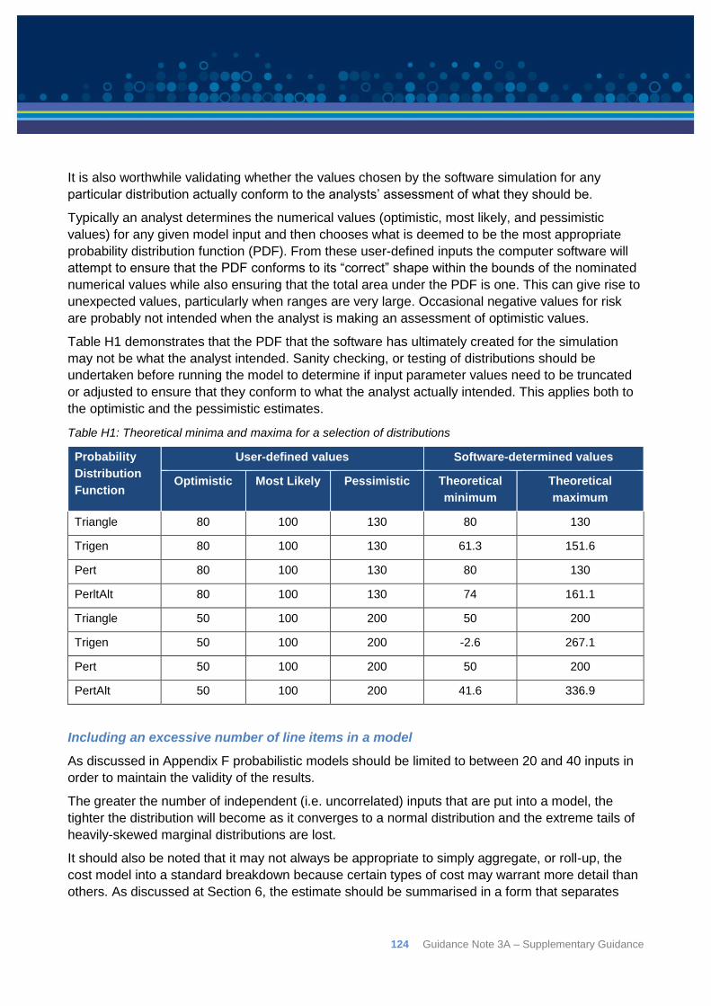
124 Guidance Note 3A – Supplementary Guidance
It is also worthwhile validating whether the values chosen by the software simulation for any
particular distribution actually conform to the analysts’ assessment of what they should be.
Typically an analyst determines the numerical values (optimistic, most likely, and pessimistic
values) for any given model input and then chooses what is deemed to be the most appropriate
probability distribution function (PDF). From these user-defined inputs the computer software will
attempt to ensure that the PDF conforms to its “correct” shape within the bounds of the nominated
numerical values while also ensuring that the total area under the PDF is one. This can give rise to
unexpected values, particularly when ranges are very large. Occasional negative values for risk
are probably not intended when the analyst is making an assessment of optimistic values.
Table H1 demonstrates that the PDF that the software has ultimately created for the simulation
may not be what the analyst intended. Sanity checking, or testing of distributions should be
undertaken before running the model to determine if input parameter values need to be truncated
or adjusted to ensure that they conform to what the analyst actually intended. This applies both to
the optimistic and the pessimistic estimates.
Table H1: Theoretical minima and maxima for a selection of distributions
Probability
Distribution
Function
User-defined values Software-determined values
Optimistic Most Likely Pessimistic Theoretical
minimum
Theoretical
maximum
Triangle 80 100 130 80 130
Trigen 80 100 130 61.3 151.6
Pert 80 100 130 80 130
PerltAlt 80 100 130 74 161.1
Triangle 50 100 200 50 200
Trigen 50 100 200 -2.6 267.1
Pert 50 100 200 50 200
PertAlt 50 100 200 41.6 336.9
Including an excessive number of line items in a model
As discussed in Appendix F probabilistic models should be limited to between 20 and 40 inputs in
order to maintain the validity of the results.
The greater the number of independent (i.e. uncorrelated) inputs that are put into a model, the
tighter the distribution will become as it converges to a normal distribution and the extreme tails of
heavily-skewed marginal distributions are lost.
It should also be noted that it may not always be appropriate to simply aggregate, or roll-up, the
cost model into a standard breakdown because certain types of cost may warrant more detail than
others. As discussed at Section 6, the estimate should be summarised in a form that separates

Guidance Note 3A – Supplementary Guidance 125
groups of costs that are subject to separate quantity and rate uncertainties. This may mean
aggregating costs by geographical area, greenfield and brownfield, types of work, subcontracts, or
some other logical structure that reflects the separate uncertainties or type of risk exposure.
Including low probability, high consequence risks
As discussed at Section 4.4, using a weighted impact (i.e. probability x impact) to calculate the
contingency required for events that could have very large undesirable consequences, is rarely
satisfactory. Weighting risks by their likelihood of occurring only works when there are many small
or medium events to be covered and they are independent of one another. Funding for very high
impact risks with an appreciable probability of occurring is not suited to the way contingency funds
are determined for a project that is subject to the net effect of a large number of independent small
and medium scale risks.
If there is a need to embark on work that could be subject to a very large cost increase due to an
identified event, this is best managed as a stand-alone contingent funding requirement with an
agreed trigger and controls on the release of the funds. To incorporate it into a general project
contingency only serves to hide the nature of the requirement and obscure the special character of
the costs involved.
Extremely rare force majeure-type events (extreme weather, terrorist attacks, etc) are all
conceivable but very unlikely. These are generally regarded as normal risks associated with what
is sometimes called ‘business as usual’. There may be insurance held against some of these but
some will simply be accepted due to their rarity.

126 Guidance Note 3A – Supplementary Guidance
Appendix I: Alternate approaches to eliciting expert opinion
Professor Mark Burgman became the foundation director of the Australian Centre of Excellence for
Risk Analysis (ACERA - now Centre for Excellence for Biosecurity Risk Analysis) on its
establishment in 2006.
While noting that estimates can be wrong in many ways, Burgman presents the following list as a
start point to break down the quality of an expert’s judgment.
Accuracy measures how close an expert’s quantitative estimate is to the truth. Accuracy can
be measured by the difference between an expert’s estimate and the correct answer. Over
several questions, it may be the average difference.
Bias measures the tendency of an expert to deviate consistently from the truth in a single
direction, either too high or too low. Bias can only be measured over the answers to several
questions.
Calibration is the frequency with which uncertainty intervals enclose the truth, compared to
the frequency with which the expert expects them to. Calibration can be measured by
counting, over several questions, the frequency with which the expert’s intervals enclose the
truth.
Reliability is a property of an expert. It is the degree to which an expert’s estimates are
repeatable and stable.
Leading from the dot points above, if an expert is routinely close to the truth but provides very wide
margins of confidence (i.e. estimates are poorly calibrated), the judgements are accurate but
uninformative. If an expert confidently provides narrow bounds but is routinely far from the truth,
the judgements are simply misleading. Good estimates are accurate and well calibrated and a
good judge is accurate, unbiased, well calibrated and reliable.
Professor Burgman has published widely on the topic of eliciting expert opinion and recommends a
structured procedure termed a four-point format. The approach attempts to both elicit an interval to
capture uncertainty, and to mitigate the overconfidence typically observed in expert estimates.
Readers of this guidance note who wish to obtain a deeper understanding of dealing with experts
may wish to investigate some of his relevant work70,71.
In the four-point approach, the bounds are intentionally asked for before the best estimate, to make
people think about extreme values, and to prevent them first thinking about and then anchoring on
a best estimate. The recommended question format is:
First, consider all the things that might lead you to conclude a low number. With these things
in mind, realistically, what do you think is the smallest plausible value?;
70 Speirs-Bridge, A., Fidler, F., McBride, M., Flander, L., Cumming, G., and Burgman, M. (2010). Reducing Overconfidence in the Interval Judgments of Experts. Risk Analysis 30, 512-523. doi: 10.1111/j.1539-6924.2009.01337.x 71 Burgman M (2015) Trusting Judgements, How to Get the Best out of Experts, Cambridge University Press
Guidance Note 3A – Supplementary Guidance 127
Second, consider all the things that might lead you to conclude a high number. With these
things in mind, realistically, what do you think is the largest plausible value?;
Third, thinking of all the things that contribute to your estimate, realistically, what is your best
estimate?
Finally, how confident are you that the inverval your created, from lowest to highest,
captures the true value? (This should be expressed as a number between 50 per cent and
100 per cent.)
Once responses have been gathered, the final step is rescale the interval (provided at the last
question) so that it is equivalent to a reasonably high level of confidence. For example, if an
interval of 60 per cent was provided, it is rescaled to be wider, typically so that it encompasses 80
percent of an expert’s beliefs. This is done in order to compare and combine intervals from
individual experts. It is also done because intervals with low confidence (say 50 per cent) are
usually not very informative.
Estimates are scaled, or normalised, using linear extrapolation to absolute lower (αabs) and upper
(βabs) bounds such that:
αabs = γ - (γ - α)(c/ρ)
βabs = γ + (β – γ)(c/ρ)
where (γ) is the most likely value, (c) is the required possibility level, and (ρ) is the expert’s stated
confidence.
For example, if an expert provided interval values of 90 (smallest plausible), 100 (best
assessments), and 115 (highest plausible) with a 60 per cent confidence level and we wanted to
rescale the intervals so that they represent the equivalent of an 80 per cent confidence level, the
absolute lower and upper bounds become:
αabs = γ - (γ - α)(c/ρ) = 100 - (100-90)(80/60) = 86.67
βabs = γ + (β – γ)(c/ρ) = 100 + (115-100)(80/60) = 120
The ACERA Elicitation Tool (comprising Process Manual72 and User Manual73 2010) provide
comprehensive guidance on the conduct of risk workshops. While this manual was developed
within the context of ecological risks, the Elicitation Tool can be used for expert panel risk
assessment in any domain where expert opinion can be articulated in the form of interval
estimates. The scaling method is approximate and the range derived from it should be considered
carefully before it is used in further analysis.
The Department considers that either the approach described earlier at Section 5.4 of this
guidance note, or the ACERA Elicitation Tool are suitable methods for eliciting expert opinion as
part of a broader risk workshop process.
72 Australian Centre of Excellence for Risk Analysis (2010) Elicitation Tool – Process Manual available at http://cebra.unimelb.edu.au/publications/acera_reports/acera_1 73 Australian Centre of Excellence for Risk Analysis (2010) Elicitation Tool – User Manual available at http://cebra.unimelb.edu.au/publications/acera_reports/acera_1
128 Guidance Note 3A – Supplementary Guidance
Appendix J: Definitions and abbreviations
Term Definition
AACE
International
Established as the American Association of Cost Engineers in 1956,
the legal name since 1992 has been AACE International.
Agency A state or territory body that generally will deliver an infrastructure
project.
Assumption A documented, cost-related factor that, for the purpose of developing
a base cost estimate is considered to be true, real or certain.
Base Date A ‘base date’ is a reference date from which changes in conditions
can be assessed. In the context of a base estimate it is the period
when the estimate has been prepared to reflect the current market
conditions.
Base Estimate The sum of the Construction Costs and Client’s Costs at the
applicable base date. It represents the best prediction of the
quantities and current rates which are likely to be associated with the
delivery of a given scope of work. It should not include any allowance
for risk (contingency) or escalation.
Contingency As per Appendix B of the notes on Administration: “the component of
a Project’s cost in excess of the Project Base Estimate that accounts
for, or reflects, risk”.
Contractor Direct
Costs
Costs that are directly attributable to a project cost object such as
materials or labour.
Contractor
Indirect Costs
Costs incurred by the contractor to perform work but which are not
directly attributable to a project cost object. These generally include
costs such as preliminaries, supervision, and general and
administrative costs.
Correlation A parameter used to describe the degree to which one variable’s
probability distribution is related to another.
Cost Driver A major input to an estimate at a summary level.
Cumulative
Distribution
Function (CDF)
The cumulative distribution function gives the probability that a real
valued random number will be less than or equal to some value x.
Guidance Note 3A – Supplementary Guidance 129
Term Definition
Dependence Two types of dependence arise regularly in risk analysis and
modelling. In some cases, one part of a project’s cost may be explicitly
determined by another part, such as contractor’s distributables (the
dependent item) that are calculated, as agreed in a contract, as a
percentage of labour costs (the independent item). This can be
modelled with a simple formula connecting the two items. A less
straightforward but more widespread form of dependence arises
where non-financial features of a project drive two or more costs, such
as where the quantities of several bulk materials drive the costs of
many work packages. This can only be modelled with risk factors,
which can be straightforward, or correlations, which are not
straightforward.
Deterministic
contingency
assessment
A deterministic model, as opposed to a stochastic (probabilistic)
model, contains no random elements. Deterministic estimation treats
all of the cost input parameters as constants, which does not capture
the variations frequently seen during construction.
A deterministic model also pertains to exactly predictable (or precise)
events, the outcome of which is assumed to be known with certainty if
the inputs are known with certainty.
First Principles
Estimate
The method of preparing a cost estimate by calculating the dollar rates
and rates of productivity required to complete each of the individual
tasks within the Work Breakdown Structure.
Iteration Iteration is the repetition of a mathematical or computational
procedure, typically as a means of obtaining successively closer
approximations to the solution of a problem. Each repetition of the
process is also called an “iteration”.
Jurisdiction An Australian state or territory.
Model A representation in mathematical terms of a system which may be
used to study the effects of different components, and/or to make
predictions.
Monte Carlo
Simulation
Monte Carlo Simulation is an algorithm that starts with a deterministic
model (e.g. a spreadsheet containing the Base Estimate) and, through
repeated sampling from possible inputs to the model, generates a
probabilistic outcome.
NOA The notes on Administration for Land Transport Infrastructure Projects
2014–15 to 2018–19 (the NOA) provide administrative guidance for
managing projects to be funded under the National Partnership
Agreement.
130 Guidance Note 3A – Supplementary Guidance
Term Definition
Probability A measure of the chance of occurrence expressed as a number
between 0 and 1, where 0 is impossibility and 1 is absolute certainty.
Probability
density function
(PDF)
A probability density function (PDF) is a representation of the range of
values a quantity might take on and the likelihood of values within that
range. A cumulative distribution function (CDF) is the probability of
choosing an element EQUAL TO OR LESS than a given individual
element; the CDF is the integral of the PDF.
Probability
distribution
function (pdf)
A probability distribution function is some function that may be used to
define a particular probability distribution. The term may refer to: either
a cumulative distribution function; a probability density function; or a
probability mass function. A continuous probability distribution is a
probability distribution characterised by a probability density function
(PDF), while a discrete probability distribution is a probability
distribution characterised by a probability mass function (PMF).
Project proposal
Report (PPR)
A statement detailing the scope, costs and expected benefits of the
project submitted by proponents as part of the project approval
process.
Project-specific
risk
Project-specific risks are uncertainties (threats or opportunities)
related to events, actions, and other conditions that are specific to the
scope of a project.
Risk The effect of uncertainty on objectives.
Risk Driver Any root cause that may force a project to have different outcomes to
the plan.
Risk Factor A ratio describing the variation in a cost resulting from a variation in
one of the cost drivers. Risk factors represent cost drivers that are
subject to uncertainty.
Stochastic A stochastic event or system is one that is unpredictable because of a
random variable.
Systemic risk Systemic risks are uncertainties (threats or opportunities) that are an
artifact of an industry, company or project system, culture, strategy,
complexity, technology, or similar over-arching characteristics.
Work Breakdown
Structure (WBS)
A hierarchical decomposition of the work to be executed to accomplish
the project objectives and create the required deliverables. The WBS
organises and defines the total scope of the project.
Guidance Note 3A – Supplementary Guidance 131
References and further reading AACE International (2008) RP No. 41R-08 Risk Analysis and Contingency Determination Using
Range Estimating, AACE International, Morgantown, WV
AACE International (2008) RP No. 42R-08 Risk Analysis and Contingency Determination Using
Parametric Estimating. AACE International, Morgantown, WV
AACE International (2008) RP No. 66R-11 Selecting Probability Distribution Functions for use in
Cost and Schedule Risk Simulation Models, AACE International, Morgantown, WV
AACE (2011) Recommended Practice RP65R-11 Integrated Cost and Schedule Risk Analysis and
Contingency Determiniation Using Expected Value, AACE International, Morgantown, WV
AACE (2015) Total Cost Management Framework: An Integrated Approach to Portfolio, Program,
and Project Management, AACE International, Morgantown, WV
Asian Development Bank (2002) Handbook for Integrating Risk Analysis in the Economic Analysis
of Projects
Australian Centre of Excellence for Risk Analysis 2010 Elicitation Tool – Process Manual available
at http://cebra.unimelb.edu.au/publications/acera_reports/acera_1
Australian Centre of Excellence for Risk Analysis 2010 Elicitation Tool – User Manual available at
http://cebra.unimelb.edu.au/publications/acera_reports/acera_1
Bakhshi and Toran (2014), An Overview of Budget Contingency Calculation Methods in
Construction Industry
Bernstein, P., (1998) Against the Gods: The Remarkable Story of Risk, John Wiley and Sons Inc,
New York
Book, S, (1999), Why Correlation Matters in Cost Estimating
Broadleaf (2014), Discussion paper: Weaknesses in common project cost risk modelling methods
Burgman, M. (2015) Trusting Judgements, How to Get the Best out of Experts, Cambridge
University Press
Burroughs, S. and Juntima, G. (2004) AACE International Transactions, Exploring Techniques for
Contingency Setting, AACE International, Morgantown, WV
Colyvan, M. (2008) Is Probability Theory the Only Coherent Approach to Uncertainty? Risk
Analysis 28, 645-652
Cooper D, Bosnich P, Grey S, Purdy G, Raymond G, Walker P, Wood M, (2014) Project Risk
Management Guidelines: Managing Risk with ISO 31000 and IEC 62198 2nd Edition
Cover, T. & Thomas, J. (2006) Elements of Information Theory 2nd Edition
Covert, R. (2013) Analytic Method for Probabilistic Cost and Schedule Risk Analysis
Ellenberg E (2015), How Not to Be Wrong: The Power of Mathematical Thinking
Evans, J.R., and Olsen, D.L. (1998) Introduction to Simulation and Risk Analysis. Prentice Hall
132 Guidance Note 3A – Supplementary Guidance
Federal Highway Administration (2006) Report FHWA-PL-06-032 Guide to Risk Assessemnt and
Allocation for Highway Construction Management
Ferson S, Nelson R, Hajagos J, Berleant D, Zhang J, Tucker W, Ginzburg L, Oberkampf W, (n.d)
Myths About Correlations and Dependencies and Their Implications for Risk Analysis
Grey, S. (1995) Practical Risk Assessment for Project Management. John Wiley and Sons
Hayes K (2011) Uncertainty and Uncertainty Analysis Methods
Hollmann, J (2016) Project Risk Quantification: A Practitioner’s Guide to Realistic Cost and
Schedule Risk Management, Probabilistic Publishing, Gainesville, FL
Hollmann, J., (2015) Reliable Risk Quantification for Project Cost and Schedule, Project Controls
Expo, London
Hulett D, Whitehead W, (Risk 2142) The Monte Carlo Method for Modelling and Mitigating
Systemic Risk
Hulett D (2010) Risk.03: Integrated Cost and Schedule Risk Analysis: A draft AACE recommended
practice, AACE international 54th annual meeting 2010 Atlanta
Hulett D, (2011) Integrated Cost-Schedule Risk Analysis, Gower Publishing Limited, Farnham
England
Hulett D, & Norbisch M, (2012) Integrated Cost-Schedule Risk Analysis
Lapeyre, B. (2007) Introduction to Monte-Carlo Methods
Law, A. M. and Kelton, W.D. (2000) Simulation Modelling and Analysis, McGraw Hill
Law A (2015) Simulation Modelling and Analysis 5th Edition, McGraw Hill Education, New York
Markowitz, H., (1952) Portfolio Selection, The Journal of Finance, Vol. 7, No. 1., pp. 77-91
Mascaro, S. (2014) Making Robust Decisions with a Model Subject to Severe Uncertainty, Report
Developed for the Department of Agriculture in conjunction with CEBRA
Metropolis, N & Ulam, S (1949) The Monte Carlo Method, Journal of the American Statistical
Association, Vol 44, No 247. (Sep., 1949), pp. 335-341
NASA (2010) Risk-informed decision making handbook (NASA/SP-2010-576). Technical report,
NASA
NASA (2011) Probabilistic Risk Assessment Procedures Guide for NASA Managers and
Practitioners 2nd Edition (NASA/SP-2011-3421) NASA
NASA (2015) NASA Cost Estimating Handbook Version 4.0, Appendix G: Cost Risk and
Uncertainty Methodologies
Palisade Corporation (2015) @Risk User’s Guide, Version 7
Pouliquen L (1970) Risk Analysis in Project Appraisal, World Bank Staff Occasional Papers
Number Eleven, John Hopkins Press, Baltimore
Seife, C (2010) Proofiness: How you are being fooled by the numbers
Guidance Note 3A – Supplementary Guidance 133
Speirs-Bridge, A., Fidler, F., McBride, M., Flander, L., Cumming, G., and Burgman, M. (2010).
Reducing Overconfidence in the Interval Judgments of Experts. Risk Analysis 30, 512-523. doi:
10.1111/j.1539-6924.2009.01337.
Spetzler and Stael von Holstein (1975) Probability encoding in decision analysis. Management
Science 22(3), 340-58
Smart, C, Ph.D., CCEA (2013), Robust Default Correlation for Cost Risk Analysis
Stewart, I., (2012) In Pursuit of the Unknown: 17 Equations that Changed the World. Basic Books,
Great Britain
Stirling, A. (2007) Science, precaution and risk assessment: towards more measured and
constructive policy debate. European Molecular Biology Organisation Reports, 8:309-315
Stump, E. (2000) The Risk Driver Impact Approach to Estimation of Cost Risks: Clear Thinking
About Project Cost Risk Analysis
Stump, E. (n.d) Breakings Murphy’s Law: Project Risk Management
Sutherland, W.J., Spiegelhalter, D. & Burgman, M.A. (2013) Twenty tips for interpreting scientific
claims. Nature 503, 335-337
Thomas, D. (Technical Director) (2014) Joint Agency Cost Schedule Risk and Uncertainty
Handbook
Tucker, W. & Ferson, S. (2003) Probability bounds analysis in environmental risk assessments
Vose, D (2008) Risk Analysis: A Quantitative Guide, John Wiley and Sons Ltd, Chichester
Zio and Pedroni (2012). Overview of risk-informed decision-making processes. Number 2012-10 of
the Cahiers de la Sécurité Industrielle, Foundation for an Industrial Safety Culture, Toulouse,
France (ISSN 2100-3874). Available at http://www.FonCSI.org/en/.
Zio and Pedroni (2013). Literature review of methods for representing uncertainty, number 2013-03
of the Cahiersde la Sécurité Industrielle, Foundation for an Industrial Safety Culture, Toulouse,
France (ISSN 2100-3874). Available at http://www.FonCSI.org/en/.