Supplemental Material: Grafted Nanoparticles as Soft Patchy Colloids:

Self-Assembly versus Phase Separation

Nathan A. Mahynski1 and Athanassios Z. Panagiotopoulos1

Department of Chemical and Biological Engineering, Princeton University,

Princeton, NJ 08544, USAa)

a)Electronic mail: azp@princeton.edu

1

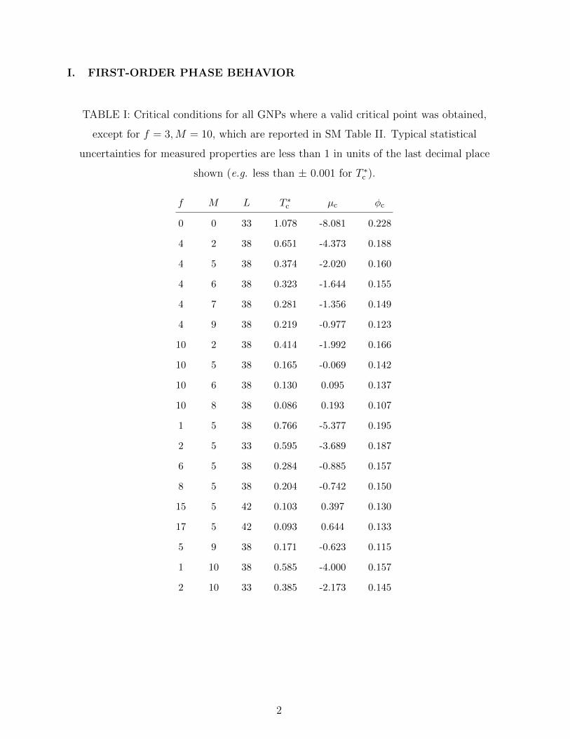
I. FIRST-ORDER PHASE BEHAVIOR

TABLE I: Critical conditions for all GNPs where a valid critical point was obtained,

except for f = 3,M = 10, which are reported in SM Table II. Typical statistical

uncertainties for measured properties are less than 1 in units of the last decimal place

shown (e.g. less than ± 0.001 for T ∗c ).

f M L T ∗c µc φc

0 0 33 1.078 -8.081 0.228

4 2 38 0.651 -4.373 0.188

4 5 38 0.374 -2.020 0.160

4 6 38 0.323 -1.644 0.155

4 7 38 0.281 -1.356 0.149

4 9 38 0.219 -0.977 0.123

10 2 38 0.414 -1.992 0.166

10 5 38 0.165 -0.069 0.142

10 6 38 0.130 0.095 0.137

10 8 38 0.086 0.193 0.107

1 5 38 0.766 -5.377 0.195

2 5 33 0.595 -3.689 0.187

6 5 38 0.284 -0.885 0.157

8 5 38 0.204 -0.742 0.150

15 5 42 0.103 0.397 0.130

17 5 42 0.093 0.644 0.133

5 9 38 0.171 -0.623 0.115

1 10 38 0.585 -4.000 0.157

2 10 33 0.385 -2.173 0.145

2

0

5

10

15

20 0 0.1 0.2 0.3 0.4 0.5

β

φGNP

(a)

f = 10, M = 2

f = 10, M = 6

f = 10, M = 8

1

1.5

2

2.5

3

3.5

4 0 0.1 0.2 0.3 0.4 0.5

β

φGNP

(b)

f = 1, M = 5

f = 2, M = 5

f = 4, M = 2

f = 2, M = 10

0

5

10

15

20 0 0.1 0.2 0.3 0.4 0.5

β

φGNP

(c)

f = 15, M = 5

f = 5, M = 9

f = 1, M = 10

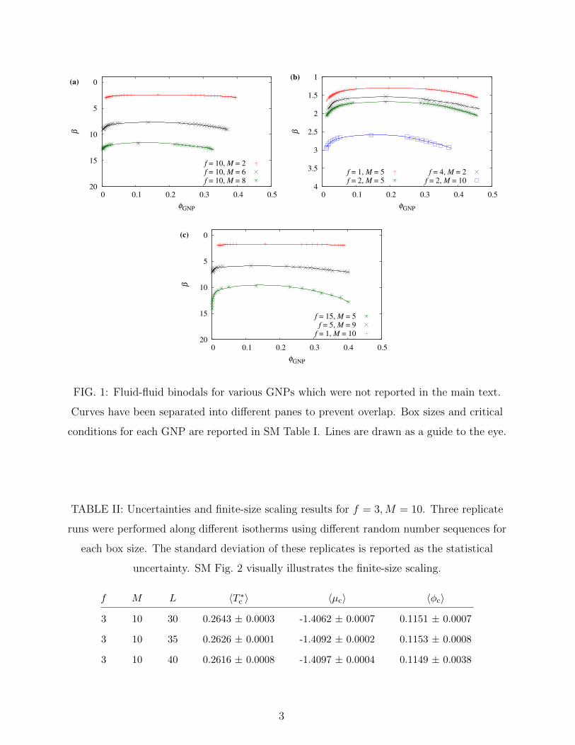
FIG. 1: Fluid-fluid binodals for various GNPs which were not reported in the main text.

Curves have been separated into different panes to prevent overlap. Box sizes and critical

conditions for each GNP are reported in SM Table I. Lines are drawn as a guide to the eye.

TABLE II: Uncertainties and finite-size scaling results for f = 3,M = 10. Three replicate

runs were performed along different isotherms using different random number sequences for

each box size. The standard deviation of these replicates is reported as the statistical

uncertainty. SM Fig. 2 visually illustrates the finite-size scaling.

f M L 〈T ∗c 〉 〈µc〉 〈φc〉

3 10 30 0.2643 ± 0.0003 -1.4062 ± 0.0007 0.1151 ± 0.0007

3 10 35 0.2626 ± 0.0001 -1.4092 ± 0.0002 0.1153 ± 0.0008

3 10 40 0.2616 ± 0.0008 -1.4097 ± 0.0004 0.1149 ± 0.0038

3

0.1

0.105

0.11

0.115

0.12

0.125

0.13

0.135

0.14

0 0.002 0.004 0.006 0.008

φG

NP

L-(1-α)/ν

(a)

0.256

0.258

0.26

0.262

0.264

0.266

0.268

0.00005 0.00010 0.00015 0.00020 0.00025

Tc*

L-(1+θ)/ν

(b)

0

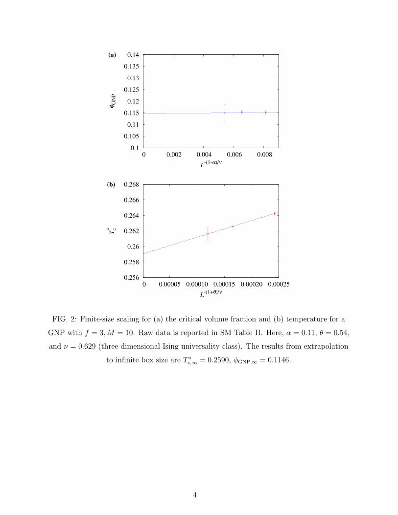
FIG. 2: Finite-size scaling for (a) the critical volume fraction and (b) temperature for a

GNP with f = 3,M = 10. Raw data is reported in SM Table II. Here, α = 0.11, θ = 0.54,

and ν = 0.629 (three dimensional Ising universality class). The results from extrapolation

to infinite box size are T ∗c,∞ = 0.2590, φGNP,∞ = 0.1146.

4

II. SELF-ASSEMBLY CHARACTERISTICS

0

0.1

0.2

0.3

0.4

0.5

0.6

-1.2 -1 -0.8 -0.6 -0.4 -0.2 0

φG

NP

µ

T* = 0.21

T* = 0.19

T* = 0.17

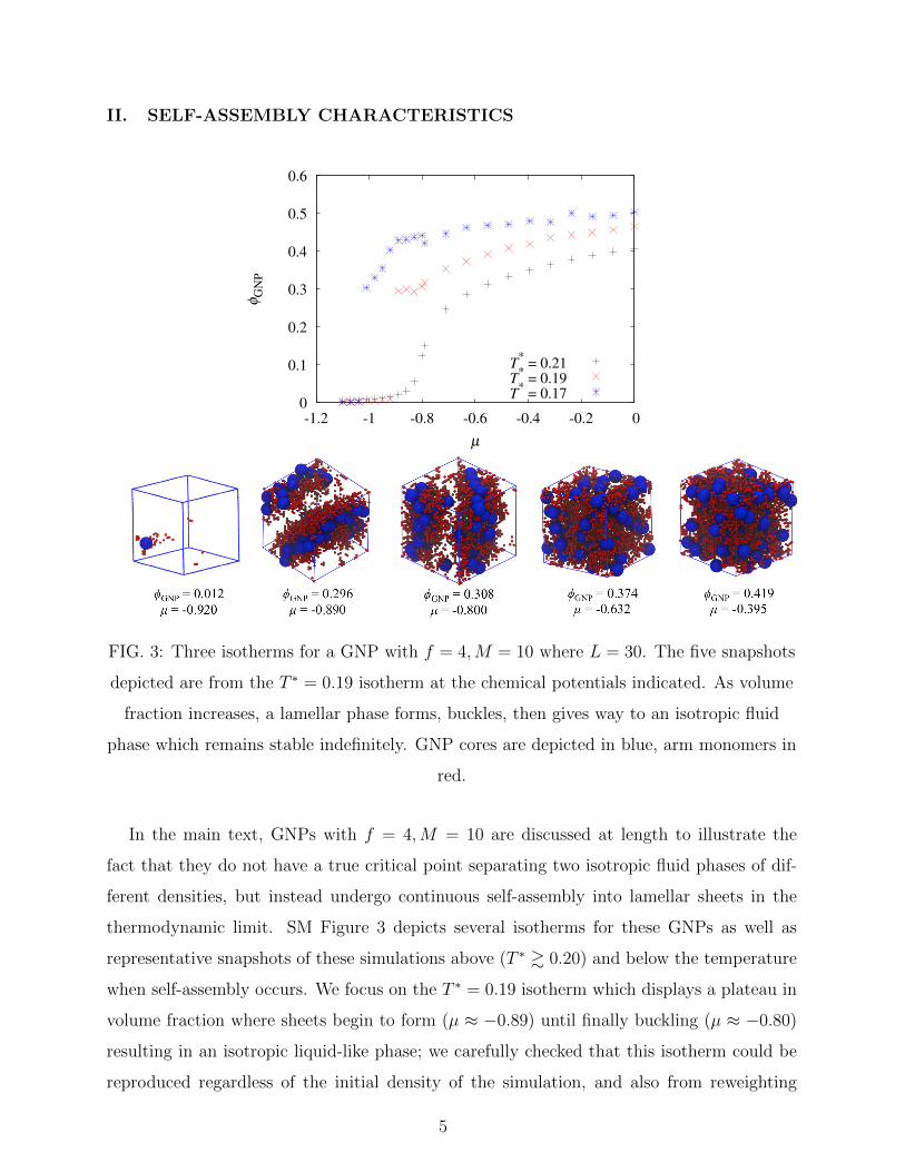
FIG. 3: Three isotherms for a GNP with f = 4,M = 10 where L = 30. The five snapshots

depicted are from the T ∗ = 0.19 isotherm at the chemical potentials indicated. As volume

fraction increases, a lamellar phase forms, buckles, then gives way to an isotropic fluid

phase which remains stable indefinitely. GNP cores are depicted in blue, arm monomers in

red.

In the main text, GNPs with f = 4,M = 10 are discussed at length to illustrate the

fact that they do not have a true critical point separating two isotropic fluid phases of dif-

ferent densities, but instead undergo continuous self-assembly into lamellar sheets in the

thermodynamic limit. SM Figure 3 depicts several isotherms for these GNPs as well as

representative snapshots of these simulations above (T ∗ & 0.20) and below the temperature

when self-assembly occurs. We focus on the T ∗ = 0.19 isotherm which displays a plateau in

volume fraction where sheets begin to form (µ ≈ −0.89) until finally buckling (µ ≈ −0.80)

resulting in an isotropic liquid-like phase; we carefully checked that this isotherm could be

reproduced regardless of the initial density of the simulation, and also from reweighting

5

0

0.01

0.02

0.03

0.04

0.05

0.06

0 0.1 0.2 0.3 0.4 0.5

P

φGNP

T* = 1.00

T* = 0.90

T* = 0.80

T* = 0.70

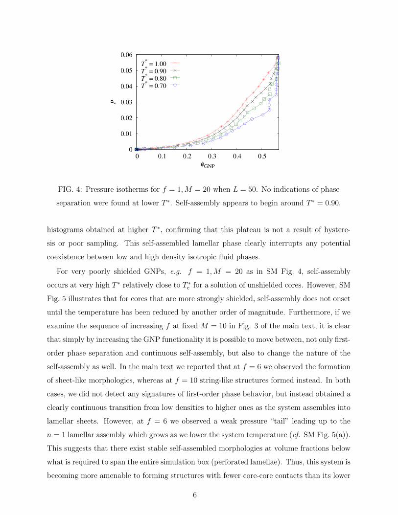
FIG. 4: Pressure isotherms for f = 1,M = 20 when L = 50. No indications of phase

separation were found at lower T ∗. Self-assembly appears to begin around T ∗ = 0.90.

histograms obtained at higher T ∗, confirming that this plateau is not a result of hystere-

sis or poor sampling. This self-assembled lamellar phase clearly interrupts any potential

coexistence between low and high density isotropic fluid phases.

For very poorly shielded GNPs, e.g. f = 1,M = 20 as in SM Fig. 4, self-assembly

occurs at very high T ∗ relatively close to T ∗c for a solution of unshielded cores. However, SM

Fig. 5 illustrates that for cores that are more strongly shielded, self-assembly does not onset

until the temperature has been reduced by another order of magnitude. Furthermore, if we

examine the sequence of increasing f at fixed M = 10 in Fig. 3 of the main text, it is clear

that simply by increasing the GNP functionality it is possible to move between, not only first-

order phase separation and continuous self-assembly, but also to change the nature of the

self-assembly as well. In the main text we reported that at f = 6 we observed the formation

of sheet-like morphologies, whereas at f = 10 string-like structures formed instead. In both

cases, we did not detect any signatures of first-order phase behavior, but instead obtained a

clearly continuous transition from low densities to higher ones as the system assembles into

lamellar sheets. However, at f = 6 we observed a weak pressure “tail” leading up to the

n = 1 lamellar assembly which grows as we lower the system temperature (cf. SM Fig. 5(a)).

This suggests that there exist stable self-assembled morphologies at volume fractions below

what is required to span the entire simulation box (perforated lamellae). Thus, this system is

becoming more amenable to forming structures with fewer core-core contacts than its lower

6

1e-06

1e-05

0.0001

0.001

0 0.05 0.1 0.15 0.2 0.25 0.3 0.35 0.4

P

φGNP

(a)

T* = 0.145

T* = 0.140

T* = 0.135

T* = 0.130

1e-06

1e-05

0.0001

0.001

0 0.05 0.1 0.15 0.2 0.25 0.3 0.35 0.4

P

φGNP

(b)

T* = 0.10

T* = 0.09

T* = 0.08

T* = 0.07

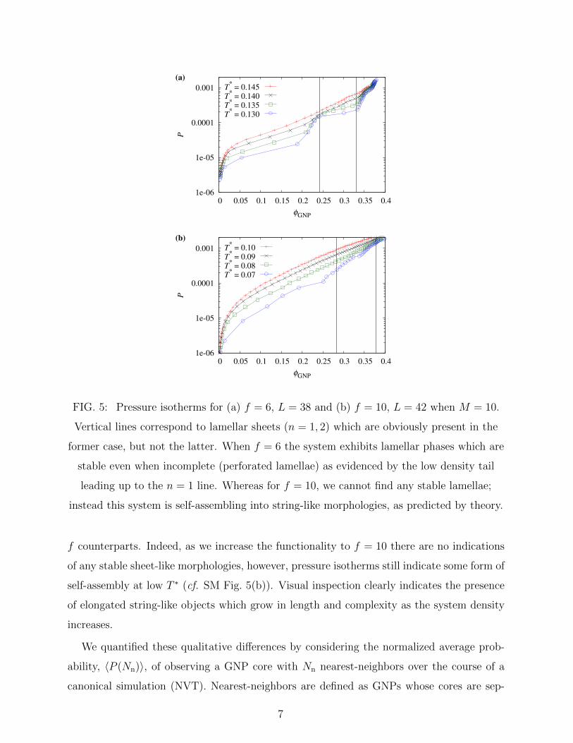
FIG. 5: Pressure isotherms for (a) f = 6, L = 38 and (b) f = 10, L = 42 when M = 10.

Vertical lines correspond to lamellar sheets (n = 1, 2) which are obviously present in the

former case, but not the latter. When f = 6 the system exhibits lamellar phases which are

stable even when incomplete (perforated lamellae) as evidenced by the low density tail

leading up to the n = 1 line. Whereas for f = 10, we cannot find any stable lamellae;

instead this system is self-assembling into string-like morphologies, as predicted by theory.

f counterparts. Indeed, as we increase the functionality to f = 10 there are no indications

of any stable sheet-like morphologies, however, pressure isotherms still indicate some form of

self-assembly at low T ∗ (cf. SM Fig. 5(b)). Visual inspection clearly indicates the presence

of elongated string-like objects which grow in length and complexity as the system density

increases.

We quantified these qualitative differences by considering the normalized average prob-

ability, 〈P (Nn)〉, of observing a GNP core with Nn nearest-neighbors over the course of a

canonical simulation (NVT). Nearest-neighbors are defined as GNPs whose cores are sep-

7

0

0.1

0.2

0.3

0.4

0.5

0.6

0.7

0 1 2 3 4 5 6 7 8 9

⟨ P

⟩

Nn

(a)

f = 3, T* = 0.250

f = 4, T* = 0.185

f = 6, T* = 0.135

f = 10, T* = 0.070

0

0.1

0.2

0.3

0.4

0.5

0.6

0.7

0 1 2 3 4 5 6 7 8 9

⟨ P

⟩

Nn

φGNP

\ f 4 6

0.26

0.31

(b)

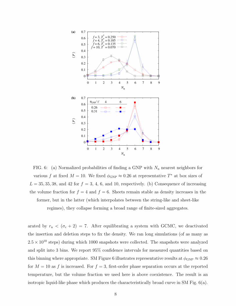
FIG. 6: (a) Normalized probabilities of finding a GNP with Nn nearest neighbors for

various f at fixed M = 10. We fixed φGNP ≈ 0.26 at representative T ∗ at box sizes of

L = 35, 35, 38, and 42 for f = 3, 4, 6, and 10, respectively. (b) Consequence of increasing

the volume fraction for f = 4 and f = 6. Sheets remain stable as density increases in the

former, but in the latter (which interpolates between the string-like and sheet-like

regimes), they collapse forming a broad range of finite-sized aggregates.

arated by rn < (σc + 2) = 7. After equilibrating a system with GCMC, we deactivated

the insertion and deletion steps to fix the density. We ran long simulations (of as many as

2.5× 1010 steps) during which 1000 snapshots were collected. The snapshots were analyzed

and split into 3 bins. We report 95% confidence intervals for measured quantities based on

this binning where appropriate. SM Figure 6 illustrates representative results at φGNP ≈ 0.26

for M = 10 as f is increased. For f = 3, first-order phase separation occurs at the reported

temperature, but the volume fraction we used here is above coexistence. The result is an

isotropic liquid-like phase which produces the characteristically broad curve in SM Fig. 6(a).

8

As f is increased, the GNPs instead begin to continuously assemble. For both f = 4 and

f = 6 we observed hexagonally packed lamellar morphologies which are clearly reflected in

the strong peak at Nn = 6. At f = 10, the distribution shifts to lower Nn values, centering

around Nn ≈ 3. This indicates the formation of strings. Visual inspection of the simulations

revealed strings which were sometimes in a straight line (Nn = 2) but often adopted a “zig-

zag” sawtooth pattern. This produces the peaks at Nn = 3 and 4, though the morphologies

we observed were still clearly stringlike. Thus, f = 6 crosses over between the sheet-like

and string-like limits, and we found that its characteristic morphology exhibits a unique

density dependence. As density increased to φGNP > 0.31 for f = 3, 4, and 10 the shape of

their respective curves in SM Fig. 6(a) changed very little. However, as Fig. 6(b) illustrates,

for f = 6 even a marginal change in density leads to a qualitatively significant change in

〈P (Nn)〉. The peak at Nn = 6 quickly decays, and the resulting distribution appears to be

more like an average between that of the f = 6 (sheets) and f = 10 (strings) curves in SM

Fig. 6(a). This suggests that at high densities, both string-like and sheet-like objects begin

to coexist for this GNP which crosses over between the two morphological regimes. Whereas

for GNPs well embedded within a specific morphological regime, the structures appear to

be qualitatively independent of density.

9

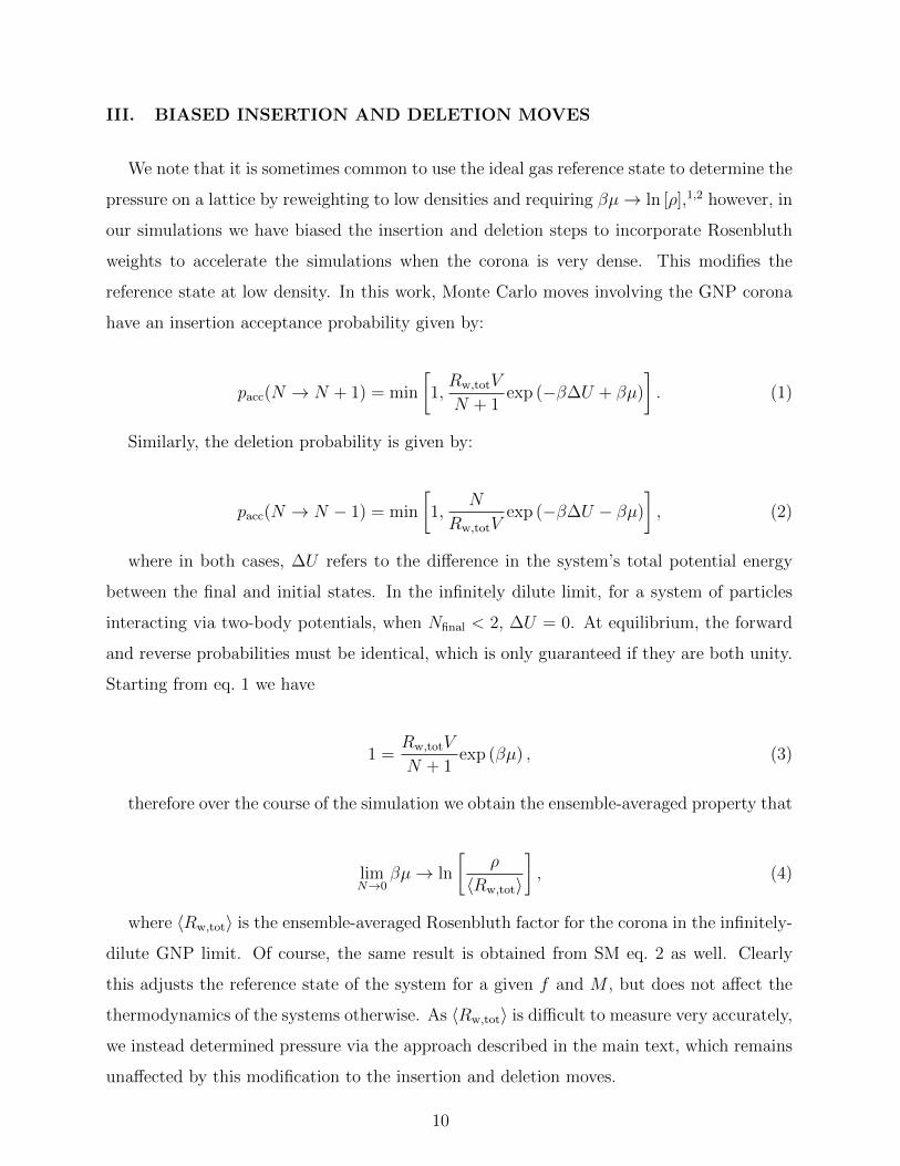
III. BIASED INSERTION AND DELETION MOVES

We note that it is sometimes common to use the ideal gas reference state to determine the

pressure on a lattice by reweighting to low densities and requiring βµ→ ln [ρ],1,2 however, in

our simulations we have biased the insertion and deletion steps to incorporate Rosenbluth

weights to accelerate the simulations when the corona is very dense. This modifies the

reference state at low density. In this work, Monte Carlo moves involving the GNP corona

have an insertion acceptance probability given by:

pacc(N → N + 1) = min

[1,Rw,totV

N + 1exp (−β∆U + βµ)

]. (1)

Similarly, the deletion probability is given by:

pacc(N → N − 1) = min

[1,

N

Rw,totVexp (−β∆U − βµ)

], (2)

where in both cases, ∆U refers to the difference in the system’s total potential energy

between the final and initial states. In the infinitely dilute limit, for a system of particles

interacting via two-body potentials, when Nfinal < 2, ∆U = 0. At equilibrium, the forward

and reverse probabilities must be identical, which is only guaranteed if they are both unity.

Starting from eq. 1 we have

1 =Rw,totV

N + 1exp (βµ) , (3)

therefore over the course of the simulation we obtain the ensemble-averaged property that

limN→0

βµ→ ln

[ρ

〈Rw,tot〉

], (4)

where 〈Rw,tot〉 is the ensemble-averaged Rosenbluth factor for the corona in the infinitely-

dilute GNP limit. Of course, the same result is obtained from SM eq. 2 as well. Clearly

this adjusts the reference state of the system for a given f and M , but does not affect the

thermodynamics of the systems otherwise. As 〈Rw,tot〉 is difficult to measure very accurately,

we instead determined pressure via the approach described in the main text, which remains

unaffected by this modification to the insertion and deletion moves.

10

REFERENCES

1N. A. Mahynski, T. Lafitte, and A. Z. Panagiotopoulos, “Pressure and density scaling for

colloid-polymer systems in the protein limit,” Physical Review E 85, 051402 (2012).

2A. Z. Panagiotopoulos, “Thermodynamic properties of lattice hard-sphere models,” Journal

of Chemical Physics 123, 104504 (2005).

11