SunPy - Python for Solar Physics

The SunPy Community,

http://sunpy.org

E-mail: sunpy@googlegroups.com

Stuart J Mumford1, Steven Christe2, David Perez-Suarez3,

Jack Ireland2,4, Albert Y Shih2, Andrew R Inglis2,5, Simon

Liedtke6, Russell J Hewett7, Florian Mayer8, Keith Hughitt9,

Nabil Freij1, Tomas Meszaros10, Samuel M Bennett1, Michael

Malocha11, John Evans12, Ankit Agrawal13, Andrew J

Leonard14, Thomas P Robitaille15, Benjamin Mampaey16, Jose

Ivan Campos-Rozo17, and Michael S Kirk2

1Solar Physics & Space Plasma Research Centre (SP2RC), School of Mathematics

and Statistics, The University of Sheffield, Hicks Building, Hounsfield Road,

Sheffield, S3 7RH, UK2NASA Goddard Space Flight Center, Greenbelt, MD, USA3South African National Space Agency - Space Science, Hospital Street, 7200

Hermanus, Western Cape, South Africa4ADNET Systems Inc., Mail Code 671.1, NASA Goddard Space Flight Center,

Greenbelt, MD, USA5The Catholic University of America, Washington, DC, USA6University of Bremen, Bibliothekstraße 1, 28359 Bremen, Germany7Department of Mathematics, Massachusetts Institute of Technology, 77

Massachusetts Ave, E17-317, Cambridge, MA, USA8Vienna University of Technology, Karlsplatz 13, 1040 Vienna, Austria9Department of Cell Biology and Molecular Genetics, University of Maryland,

College Park, MD, USA10Masaryk University, Faculty of Informatics, Botanicka 68a Brno, Czech Republic11Humboldt State University, 1 Harpst St, Arcata, CA, USA12Boston Python User Group, Boston, MA, USA13Indian Institute of Technology, Bombay, India14Department of Mathematics and Physics, Aberystwyth University, Physical

Sciences Building, Aberystwyth, SY23 3BZ, UK15Max-Planck-Institut fur Astronomie, Konigstuhl 17, Heidelberg 69117, Germany16Royal Observatory of Belgium, Brussels, Belgium17Observatorio Astronomico Nacional, Universidad Nacional de Colombia, Bogota,

D.C., Colombia

Abstract. This paper presents SunPy (version 0.5), a community-developed Python

package for solar physics. Python, a free, cross-platform, general-purpose, high-

level programming language, has seen widespread adoption among the scientific

community, resulting in the availability of a large number of software packages,

arX

iv:1

505.

0256

3v1

[as

tro-

ph.I

M]

11

May

201

5

SunPy - Python for Solar Physics 2

from numerical computation (NumPy, SciPy) and machine learning (scikit-learn)

to visualisation and plotting (matplotlib). SunPy is a data-analysis environment

specialising in providing the software necessary to analyse solar and heliospheric

data in Python. SunPy is open-source software (BSD licence) and has an open and

transparent development workflow that anyone can contribute to. SunPy provides

access to solar data through integration with the Virtual Solar Observatory (VSO),

the Heliophysics Event Knowledgebase (HEK), and the HELiophysics Integrated

Observatory (HELIO) webservices. It currently supports image data from major solar

missions (e.g., SDO, SOHO, STEREO, and IRIS ), time-series data from missions such

as GOES, SDO/EVE, and PROBA2/LYRA, and radio spectra from e-Callisto and

STEREO/SWAVES. We describe SunPy’s functionality, provide examples of solar

data analysis in SunPy, and show how Python-based solar data-analysis can leverage

the many existing tools already available in Python. We discuss the future goals of

the project and encourage interested users to become involved in the planning and

development of SunPy.

SunPy - Python for Solar Physics 3

1. Introduction

Science is driven by the analysis of data of ever-growing variety and complexity.

Advances in sensor technology, combined with the availability of inexpensive storage,

have led to rapid increases in the amount of data available to scientists in almost every

discipline. Solar physics is no exception to this trend. For example, NASA’s Solar

Dynamics Observatory (SDO) spacecraft, launched in February 2010, produces over 1

TB of data per day (Pesnell et al., 2012). Managing and analysing these data requires

increasingly sophisticated software tools. These tools should be robust, easy to use

and modify, have a transparent development history, and conform to modern software-

engineering standards. Software with these qualities provide a strong foundation that

can support the needs of the community as data volumes grow and science questions

evolve.

The SunPy project aims to provide a software package with these qualities for the

analysis and visualisation of solar data. SunPy makes use of Python and scientific

Python packages. Python is a free, general-purpose, powerful, and easy-to-learn

high-level programming language. Additionally, Python is widely used outside of

scientific fields in areas such as ‘big data’ analytics, web development, and educational

environments. For example, pandas (McKinney, 2010, 2012) was originally developed

for quantitative analysis of financial data and has since grown into a generalised time-

series data-analysis package. Python continues to see increased use in the astronomy

community (Greenfield, 2011), which has similar goals and requirements as the solar

physics community. Finally, Python integrates well with many technologies such as web

servers (Dolgert et al., 2008) and databases.

The development of a package such as SunPy is made possible by the rich ecosystem

of scientific packages available in Python. Core packages such as NumPy, SciPy (Jones

et al., 2001), and matplotlib (Hunter, 2007) provide the basic functionality expected

of a scientific programming language, such as array manipulation, core numerical

algorithms, and visualisation, respectively. Building upon these foundations, packages

such as astropy (astronomy; Astropy Collaboration et al., 2013), pandas (time-series;

McKinney, 2012), and scikit-image (image processing; van der Walt et al., 2014)

provide more domain-specific functionality.

A typical workflow begins with a solar physicist manually identifying a small

number of events of interest on the Sun. This is typically done in order to investigate in

detail the physics of these events (for example, the large solar flare of 23 July 2002 has

Astrophysical Journal Letters volume 595, dedicated to its analysis). In this workflow,

an event is investigated in depth which requires data from many different instruments.

These data are typically provided in many different formats - for example, FITS (Flexible

Image Transport System, Pence et al., 2010), CSV, or binary files - and contain many

different types of data (such as images, lightcurves and spectra). In addition, the

repositories these data reside in can have different access methods. This workflow is

characterized by the large number of heterogeneous datasets used in the investigation

SunPy - Python for Solar Physics 4

of a small number of solar events.

Another typical workflow begins with the solar physicist identifying a large sample

of data or events. The goal here is obtain information about the population in general.

An example might be to calculate the fractal dimension of a large number of active region

magnetic fields (McAteer et al., 2005), or to calculate the observed temperatures in a

population of solar flares (Ryan et al., 2012). This workflow is typically characterized

by lower data heterogeneity, but with a larger number of files.

The volume and variety of solar data used in these workflows drives the need for

an environment in which obtaining and performing common solar physics operations on

these data is as simple and intuitive as possible. SunPy is designed to be a clean, simple-

to-use, and well-structured open-source package that provides the core tools for solar

data analysis, motivated by the need for a free and modern alternative to the existing

SolarSoft (SSW) library (Freeland and Handy, 1998). While SSW is open source and

freely available, it relies on IDL (Interactive Data Language), a proprietary data-analysis

environment.

The purpose of this paper is to provide an overview of SunPy’s current capabilities,

an overview of the project’s development model, community aspects of the project,

and future plans. The latest release of SunPy, version 0.5, can be downloaded

from http://sunpy.org or can be installed using the Python package index (http:

//pypi.python.org/pypi).

2. Core Data Types

The core of SunPy is a set of data structures that are specifically designed for the three

primary varieties of solar physics data: images, time series, and spectra. These core

data types are supported by the SunPy classes: Map (2D spatial data), LightCurve (1D

temporal series), and Spectrum and Spectrogram (1D and 2D spectra). The purpose of

these classes is to provide the same core data type to the SunPy user regardless of the

differences in source data. For example, if two different instruments use different time

formats to describe the observation time of their images, the corresponding SunPy Map

object for each of them expresses the observation time in the same way. This simplifies

the workflow for the user when handling data from multiple sources.

These classes allow access to the data and associated metadata and provide

appropriate convenience functions to enable analysis and visualisation. For each of these

classes, the data is stored in the data attribute, while the metadata is stored in the meta

attribute†. It is possible to instantiate the data types from various different sources:

e.g., files, URLs, and arrays. In order to provide instrument-specific specialisation, the

core SunPy classes make use of subclassing; e.g., Map has an AIAMap sub-type for data

from the SDO/AIA (Atmospheric Imaging Assembly; Lemen et al. 2012) instrument.

All of the core SunPy data types include visualisation methods that are tailored to

each data type. These visualisation methods all utilise the matplotlib package and are

† Note, that currently only Map and LightCurve have this feature fully implemented.

SunPy - Python for Solar Physics 5

designed in such a way that they integrate well with the pyplot functional interface of

matplotlib.

This design philosophy makes the behaviour of SunPy’s visualisation routines

intuitive to those who already understand the matplotlib interface, as well as allowing

the use of the standard matplotlib commands to manipulate the plot parameters (e.g.,

title, axes). Data visualisation is provided by two functions: peek(), for quick plotting,

and plot(), for plotting with more fine-grained control.

This section will give a brief overview of the current functionality of each of the

core SunPy data types.

2.1. Map

The map data type stores 2D spatial data, such as images of the Sun and inner

heliosphere. It provides: a wrapper around a numpy data array, the images associated

spatial coordinates, and other metadata. The Map class provides methods for typical

operations on 2D data, such as rotation and re-sampling, as well as visualisation. The

Map class also provides a convenient interface for loading data from a variety of sources,

including from FITS files, the standard format for storing image data in solar physics

and astrophysics community. An example of creating a Map object from a FITS file is

shown in Listing 1.

The architecture of the map subpackage consists of a template map called

GenericMap, which is a subclass of astropy.nddata.NDData. NDData is a generic

wrapper around a numpy.ndarray with a meta attribute to store metadata. As NDData is

currently still in development, GenericMap does not yet make full use of its capabilities,

but this inheritance structure provides for future integration with astropy. In order

to provide instrument- or detector-specific integration, GenericMap is designed to be

subclassed. Each subclass of GenericMap can register with the Map creation factory,

which will then automatically return an instance of the specific GenericMap subclass

dependent upon the data provided. SunPy v0.5 has GenericMap specialisations for the

following instruments:

• Yohkoh Solar X-ray Telescope (SXT, Ogawara et al., 1991; Tsuneta et al., 1991),

• Solar and Heliospheric Observatory (SOHO, Domingo et al., 1995) Extreme

Ultraviolet Telescope (EIT; Delaboudiniere et al., 1995)

• SOHO Large Angle Spectroscopic COronagraph (LASCO, Brueckner et al., 1995)

• RHESSI - Reuven Ramaty High Energy Solar Spectroscopic Imager (Lin et al.,

2002),

• Solar TErrestrial RElations Observatory (STEREO, Kaiser, 2005) Extreme

Ultraviolet Imager (EUVI, (Wuelser et al., 2004))

• STEREO CORonagraph 1/2 (COR 1/2, Howard et al., 2002)

• Hinode XRT - X-Ray Telescope (Kosugi et al., 2007; Golub et al., 2007).

SunPy - Python for Solar Physics 6

• PRojects for On Board Autonomy 2 (PROBA2, Santandrea et al., 2013) Sun

Watcher Active Pixel (SWAP; Seaton et al., 2013)

• SDO AIA and Helioseismic Magnetic Imager, (HMI, Scherrer et al., 2012)

• Interface Region Imaging Spectrograph (IRIS, Lemen et al., 2011) SJI (slit-jaw

imager) frames.

The GenericMap class stores all of the metadata retrieved from the header

of the image file in the meta attribute and provides convenience properties for

commonly accessed metadata: e.g., instrument, wavelength or coordinate system.

These properties are dynamic mappings to the underlying metadata and all methods

of the GenericMap class modify the meta data where needed. For example, if

aiamap.meta[‘instrume’] is modified then aiamap.instrument will reflect this

change. Currently this is implemented by not preserving the keywords of the input

data, instead modifying meta data to a set of “standard” keys supported by SunPy.

Listing 1 demonstrates the quick-look functionality of Map.

SunPy - Python for Solar Physics 7

>>> import sunpy .map

>>> aiamap = sunpy .map .Map( sunpy . AIA 171 IMAGE)

>>> smap = aiamap . submap([−1200 , −200] , [−1000 , −0])

>>> smap . peek ( draw gr id=True )

1200 1000 800 600 400 200X-position [arcsec]

1000

800

600

400

200

0

Y-p

osi

tion [

arc

sec]

AIA 171 2011-03-19 10:54:00.340000

0

150

300

450

600

750

900

1050

listing 1: Example of the AIAMap specialisation of GenericMap. First, a map is created

from a sample SDO/AIA FITS file. In this case, a demonstration file contained within

the SunPy repository is used. A cutout of the full map is then created by specifying

the desired solar-x and solar-y ranges of the plot in data coordinates (in this case,

arcseconds), and then a quick-view plot is created with lines of heliographic longitude

and latitude over-plotted.

In addition to the data-type classes, the map subpackage provides two collection

classes, CompositeMap and MapCube, for spatially and temporally aligned data

respectively. CompositeMap provides methods for overlaying spatially aligned data, with

support for visualisation of images and contour lines overlaid upon each other. MapCube

provides methods for animation of its series of Map objects. Listings 2 and 3 show how

to interact with these classes.

SunPy - Python for Solar Physics 8

>>> import sunpy .map

>>> import matp lo t l i b . pyplot as p l t

>>> compmap = sunpy .map .Map(” a ia 1600 image . f i t s ” , ”RHESSI image . f i t s ” ,

. . . composite=True )

>>> compmap . s e t l e v e l s (1 , range (0 , 50 , 5 ) , percent=True )

>>> compmap . s e t c o l o r s (1 , ” Reds r ”)

#Plot the r e s u l t and crop

>>> ax = p l t . subp lot ( )

>>> compmap . p l o t ( )

>>> ax . a x i s ( [ 2 0 0 , 600 , −600, −200])

>>> p l t . show ( )

200 250 300 350 400 450 500 550 600

X-position [arcsec]

600

550

500

450

400

350

300

250

200

Y-p

osi

tion [

arc

sec]

SunPy Composite Plot

listing 2: Example showing the functionality of CompositeMap, with RHESSI X-ray

image data composited on top of an SDO/AIA 1600 A image. The CompositeMap is

plotted using the integration with the matplotlib.pyplot interface.

SunPy - Python for Solar Physics 9

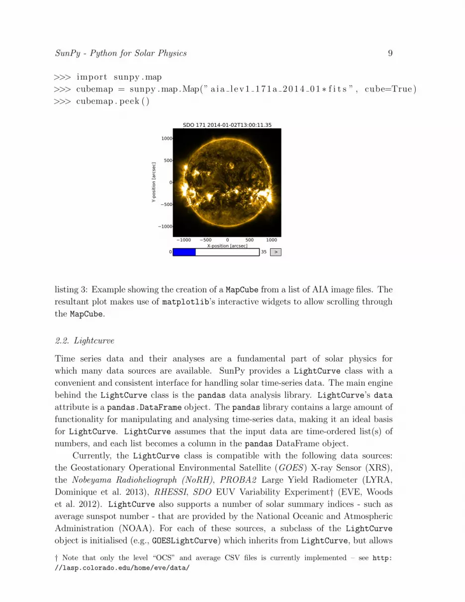
>>> import sunpy .map

>>> cubemap = sunpy .map .Map(” a i a l e v 1 1 7 1 a 2 0 1 4 0 1 ∗ f i t s ” , cube=True )

>>> cubemap . peek ( )

1000 500 0 500 1000X-position [arcsec]

1000

500

0

500

1000

Y-p

osi

tion [

arc

sec]

SDO 171 2014-01-02T13:00:11.35

0 35 >

listing 3: Example showing the creation of a MapCube from a list of AIA image files. The

resultant plot makes use of matplotlib’s interactive widgets to allow scrolling through

the MapCube.

2.2. Lightcurve

Time series data and their analyses are a fundamental part of solar physics for

which many data sources are available. SunPy provides a LightCurve class with a

convenient and consistent interface for handling solar time-series data. The main engine

behind the LightCurve class is the pandas data analysis library. LightCurve’s data

attribute is a pandas.DataFrame object. The pandas library contains a large amount of

functionality for manipulating and analysing time-series data, making it an ideal basis

for LightCurve. LightCurve assumes that the input data are time-ordered list(s) of

numbers, and each list becomes a column in the pandas DataFrame object.

Currently, the LightCurve class is compatible with the following data sources:

the Geostationary Operational Environmental Satellite (GOES ) X-ray Sensor (XRS),

the Nobeyama Radioheliograph (NoRH), PROBA2 Large Yield Radiometer (LYRA,

Dominique et al. 2013), RHESSI, SDO EUV Variability Experiment† (EVE, Woods

et al. 2012). LightCurve also supports a number of solar summary indices - such as

average sunspot number - that are provided by the National Oceanic and Atmospheric

Administration (NOAA). For each of these sources, a subclass of the LightCurve

object is initialised (e.g., GOESLightCurve) which inherits from LightCurve, but allows

† Note that only the level “OCS” and average CSV files is currently implemented – see http:

//lasp.colorado.edu/home/eve/data/

SunPy - Python for Solar Physics 10

instrument-specific functionality to be included. Future developments will introduce

support for additional instruments and data products, as well as implementing an

interface similar to that of Map. Since there is no established standard as to how time-

series data should be stored and distributed, each SunPy LightCurve object subclass

provides the ability to download its corresponding specific data format in its constructor

and parse that file type. A more general download interface is currently in development.

A LightCurve object may be created using a number of different methods. For

example, a LightCurve may be created for a specific instrument given an input time

range. In Listing 4, the LightCurve constructor searches a remote source for the GOES

X-ray data specified by the time interval, downloads the required files, and subsequently

creates and plots the object. Alternatively, if the data file already exists on the local

system, the LightCurve object may be initialised using that file as input.

>>> from sunpy import l i g h t c u r v e

>>> from sunpy . time import TimeRange

>>> t r = TimeRange(”2011−06−07 06 :00” , ”2011−06−07 08 :00”)

>>> goes = l i g h t c u r v e . GOESLightCurve . c r e a t e ( t r )

>>> goes . peek ( )

>>> pr in t ( ’ The max f l u x i s ’ + s t r ( goes . data [ ’ xrsb ’ ] . max ( ) ) +

. . . ’ at ’ + s t r ( goes . data [ ’ xrsb ’ ] . idxmax ( ) ) )

The max f l u x i s 2 .5554 e−05 at 2011−06−07 06 : 41 : 24 . 118999

06:1506:30

06:4507:00

07:1507:30

07:4508:00

2011-06-07

10-9

10-8

10-7

10-6

10-5

10-4

10-3

Watt

s m−

2

GOES Xray Flux

0.5--4.0

1.0--8.0

A

B

C

M

X

listing 4: Example retrieval of a GOES lightcurve using a time range and the output of

the peek() method. The maximum flux value in the GOES 1.0–8.0A channel is then

retrieved along with the location in time of the maximum.

SunPy - Python for Solar Physics 11

2.3. Spectra

SunPy aims to provide broad support for solar spectroscopy instruments. The variety

and complexity of these instruments and their resultant datasets makes this a challenging

goal. The spectra module implements a Spectrum class for 1D data (intensity as a

function of frequency) and a Spectrogram class for 2D data (intensity as a function of

time and frequency). Each of these classes uses a numpy.ndarray object as its data

attribute.

As with other SunPy data types, the Spectrogram class has been built so

that each instrument initialises using a subclass containing the instrument-specific

functionalities. The common functionality provided by the base Spectrogram class

includes joining different time ranges and frequencies, performing frequency-dependent

background subtraction, and convenient visualization and sampling of the data.

Currently, the Spectrogram class supports radio spectrograms from the e-Callisto (

http://www.e-callisto.org/) solar radio spectrometer network (Benz et al., 2009)

and STEREO/SWAVES spectrograms (Bougeret et al., 2008).

Listing 5 shows how the CallistoSpectrogram object retrieves spectrogram data in

the time range specified. When the data is requested using the from range() function,

the object merges all the downloaded files into a single spectrogram, across time and

frequency. In the example shown, data is provided in two frequency ranges: 20–

90 MHz and 55–355 MHz. Since the data are not evenly spaced in the frequency range,

the Spectrogram object linearises the frequency axis to assist analysis. The example

also demonstrates the implemented background subtraction method, which calculates a

constant background over time for each frequency channel.

SunPy - Python for Solar Physics 12

>>> from sunpy . spec t ra . s ou r c e s . c a l l i s t o import Ca l l i s toSpect rogram

>>> t s t a r t , tend = ”2011−06−07T06 : 0 0 : 0 0 ” , ”2011−06−07T07 : 4 5 : 0 0 ”

>>> c a l l i s t o = Cal l i s toSpect rogram . from range (”BIR” , t s t a r t , tend )

>>> c a l l i s t o n o b g = c a l l i s t o . subt rac t bg ( )

>>> c a l l i s t o n o b g . peek ( vmin=0)

listing 5: Example of how CallistoSpectrogram retrieves the data for the requested

time range and observatory, merges it, and removes the background signal. The

data requested – ‘BIR’ – is the code name of the Rosse Observatory http://www.

rosseobservatory.ie at Birr Castle in Ireland.

3. Solar Data Search and Retrieval

Several well-developed resources currently exist which provide remote access to and data

retrieval form a large number of solar and heliospheric data sources and event databases.

SunPy provides support for these resources via the net subpackage. In the following

subsections, we describe each of these resources and how to use them.

3.1. VSO

The Virtual Solar Observatory (VSO, http://virtualsolar.org) provides a single,

standard query interface to solar data from many different archives around the world

(Hill et al., 2009). Data products can be requested for specific instruments or missions

and can also be requested based on physical parameters of the data product such as

the wavelength range. In addition to the VSO’s primary web-based interface, a SOAP

SunPy - Python for Solar Physics 13

(Simple Object Access Protocol) service is also available. SunPy’s vso module provides

access to the VSO via this SOAP service using the suds package.

Listing 6 shows an example of how to query and download data from the VSO

using the vso module. Queries are constructed using one or more attribute objects.

Each attribute object is a constraint on a parameter of the data set, such as the time of

the observation, instrument, or wavelength. Listing 6 also shows how to download the

data using the constructed query. The path to which the data files will be downloaded is

defined using custom tokens which reference the file metadata (e.g., instrument, detector,

filename). This provides users the ability to organize their data into subdirectories on

download.

Listing 7 shows an example of how to make an advanced query by combining

attribute objects. Two attribute objects can be combined with a logical or operation

using the | (pipe) operator. All attribute objects provided to the query as arguments

are combined with a logical and operation.

>>> from sunpy . net import vso

>>> c l i e n t = vso . VSOClient ( )

>>> t s t a r t , tend = ”2011/6/7 05 :30” , ”2011/6/7 10 :30”

>>> l a s c o q u e r y = c l i e n t . query ( vso . a t t r s . Time( t s t a r t , tend ) ,

. . . vso . a t t r s . Instrument ( ’ l a sco ’ ) )

>>> l en ( l a s c o q u e r y )

40

>>> l a s c o q u e r y . show ( )

Sta r t time End time Source Instrument

Type

−−−−−−−−−− −−−−−−−− −−−−−− −−−−−−−−−−−−−−2011−06−07 05 : 35 : 23 2011−06−07 05 : 35 : 48 SOHO LASCO

CORONA

2011−06−07 05 : 43 : 09 2011−06−07 05 : 43 : 29 SOHO LASCO

CORONA

. . .

>>> pathformat = ”/ data /{ instrument }/{ de t e c t o r }/{ f i l e } . f i t s ”

>>> r e s u l t s = c l i e n t . get ( l a s co query , path = pathformat )

listing 6: Example of querying a single instrument over a time range and downloading

the data

SunPy - Python for Solar Physics 14

>>> cond i t i on = ( vso . a t t r s . Detector (” cor1 ”) |. . . vso . a t t r s . Wave(125 , 135) |. . . vso . a t t r s . Wave(165 , 175) ) # in angstroms

>>> advanced = c l i e n t . query ( vso . a t t r s . Time( t s t a r t , tend ) , cond i t i on )

>>> l en ( advanced )

4434

>>> advanced . show ( )

Sta r t time End time Source Instrument

−−−−−−−−−− −−−−−−−− −−−−−− −−−−−−−−−−2011−06−07 00 : 00 : 00 2011−06−08 00 : 00 : 00 SDO EVE

. . .

2011−06−07 05 : 31 : 09 2011−06−07 05 : 31 : 19 PROBA2 SWAP

. . .

2011−06−07 10 : 25 : 43 2011−06−07 10 : 25 : 45 STEREO B SECCHI

2011−06−07 10 : 30 : 00 2011−06−07 10 : 30 : 01 STEREO A SECCHI

. . .

2011−06−07 10 : 30 : 00 2011−06−07 10 : 30 : 01 SDO AIA

listing 7: Example of an advanced VSO query using attribute objects, combining both

data from a detector and any data that falls within two wavelength ranges, continuing

from Listing 6.

3.2. HEK

The Sun is an active star and exhibits a wide range of transient phenomena (e.g., flares,

radio bursts, coronal mass ejections) at many different time-scales, length-scales, and

wavelengths. Observations and metadata concerning these phenomena are collected

in the Heliophysics Event Knowledgebase (HEK, Hurlburt et al., 2012). Entries are

generated both by automated algorithms and human observers. Some of the information

in the HEK reproduces feature and event data from elsewhere (for example, the GOES

flare catalogue), and some is generated by the Solar Dynamics Observatory Feature

Finding Team (Martens et al., 2012). A key feature of the HEK is that it provides

an homogeneous and well-described interface to a large amount of feature and event

information. SunPy accesses this information through the hek module. The hek module

makes use of the HEK public API†.Simple HEK queries consist of start time, an end time, and an event type (see

Listing 8). Event types are specified as upper case, two letter strings, and these strings

are identical to the two letter abbreviations defined by HEK (see http://www.lmsal.

com/hek/VOEvent_Spec.html). Users can see a complete list and description of these

abbreviations by looking at the documentation for hek.attrs.EventType.

† For more information see http://vso.stanford.edu/hekwiki/

ApplicationProgrammingInterface

SunPy - Python for Solar Physics 15

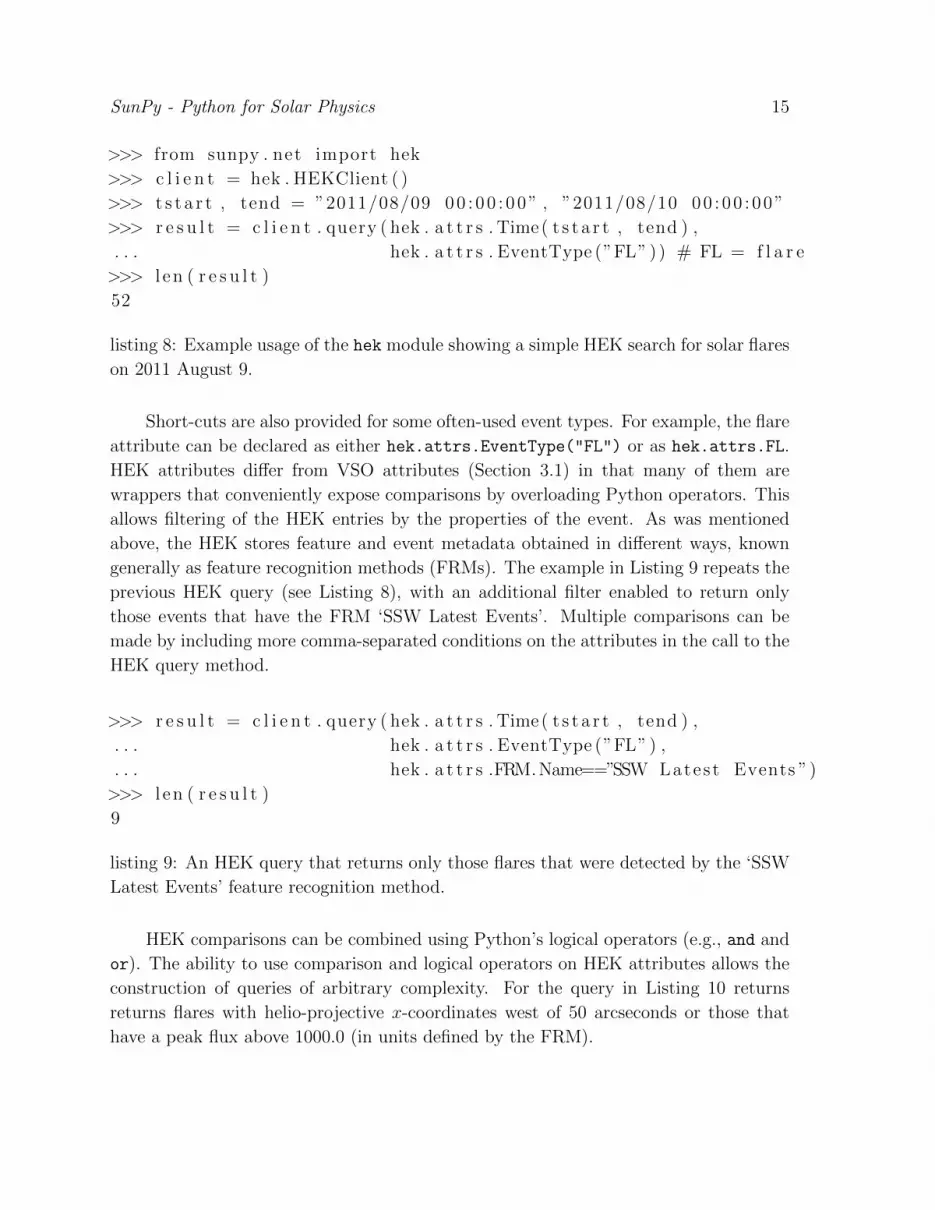
>>> from sunpy . net import hek

>>> c l i e n t = hek . HEKClient ( )

>>> t s t a r t , tend = ”2011/08/09 00 : 00 : 00” , ”2011/08/10 00 : 00 : 00”

>>> r e s u l t = c l i e n t . query ( hek . a t t r s . Time( t s t a r t , tend ) ,

. . . hek . a t t r s . EventType (”FL”) ) # FL = f l a r e

>>> l en ( r e s u l t )

52

listing 8: Example usage of the hek module showing a simple HEK search for solar flares

on 2011 August 9.

Short-cuts are also provided for some often-used event types. For example, the flare

attribute can be declared as either hek.attrs.EventType("FL") or as hek.attrs.FL.

HEK attributes differ from VSO attributes (Section 3.1) in that many of them are

wrappers that conveniently expose comparisons by overloading Python operators. This

allows filtering of the HEK entries by the properties of the event. As was mentioned

above, the HEK stores feature and event metadata obtained in different ways, known

generally as feature recognition methods (FRMs). The example in Listing 9 repeats the

previous HEK query (see Listing 8), with an additional filter enabled to return only

those events that have the FRM ‘SSW Latest Events’. Multiple comparisons can be

made by including more comma-separated conditions on the attributes in the call to the

HEK query method.

>>> r e s u l t = c l i e n t . query ( hek . a t t r s . Time( t s t a r t , tend ) ,

. . . hek . a t t r s . EventType (”FL”) ,

. . . hek . a t t r s .FRM.Name==”SSW Latest Events ”)

>>> l en ( r e s u l t )

9

listing 9: An HEK query that returns only those flares that were detected by the ‘SSW

Latest Events’ feature recognition method.

HEK comparisons can be combined using Python’s logical operators (e.g., and and

or). The ability to use comparison and logical operators on HEK attributes allows the

construction of queries of arbitrary complexity. For the query in Listing 10 returns

returns flares with helio-projective x-coordinates west of 50 arcseconds or those that

have a peak flux above 1000.0 (in units defined by the FRM).

SunPy - Python for Solar Physics 16

>>> r e s u l t = c l i e n t . query ( hek . a t t r s . Time( t s t a r t , tend ) ,

. . . hek . a t t r s . EventType (”FL”) ,

. . . ( hek . a t t r s . Event . Coord1>50)

. . . or ( hek . a t t r s .FL . PeakFlux >1000.0))

listing 10: HEK query using the logical or operator.

All FRMs report their required feature attributes (as defined by the HEK), but the

optional attributes are FRM dependent†. If a FRM does not have one of the optional

attributes, None is returned by the hek module.

After users have found events of interest the next step is to download observational

data. The H2VClient module makes this easier by providing a translation layer between

HEK query results and VSO data queries. This capability is demonstrated in Listing 11.

>>> from sunpy . net import hek2vso

>>> h2v = hek2vso . H2VClient ( )

>>> v s o r e s u l t s = h2v . t r an s l a t e an d qu e ry ( r e s u l t [ 0 ] )

>>> h2v . v s o c l i e n t . get ( v s o r e s u l t s [ 0 ] ) . wait ( )

listing 11: Code snippet continuing from Listing 10 showing the query and download of

data from the first HEK result from the VSO.

3.3. HELIO

The HELiophysics Integrated Observatory (HELIO)‡ has compiled a list of web services

which allows scientists to query and discover data throughout the heliosphere, from

solar and magnetospheric data to planetary and inter-planetary data (Perez-Suarez

et al., 2012). HELIO is built with a Service-Oriented Architecture, i.e., its capabilities

are divided into a number of tasks that are implemented as separate services. HELIO

is made up of nine different public services, which allows scientists to search different

catalogues of registered events, solar features, data from instruments in the heliosphere,

and other information such as planetary or spacecraft position in time. Additionally,

HELIO provides a service that uses a propagation model to link the data in different

points of the solar system by its original nature (e.g., Earth auroras are a signature of

magnetic field disturbances produced a few days before on the Sun). In addition to the

primary, web-based interface to HELIO, its services are available via an API.

SunPy’s hec module provides an interface to the HELIO Event Catalogue (HEC)

service. This module was developed as part of a Google Summer of Code (GSOC)

project in 2013. The HEC service currently provides access to 84 catalogues from

different sources. As with all of the HELIO services, the HEC service provides results

† See http://www.lmsal.com/hek/VOEvent_Spec.html for a list of features and their attributes.‡ For more information see http://helio-vo.eu

SunPy - Python for Solar Physics 17

in VOTable data format (defined by IVOA, see Ochsenbein et al. 2011). The hec

module parses this output using the astropy.io.votable package. This format has

the advantage of containing metadata with information like data provenance and the

performed query.

For example, Listing 12 shows how to obtain information from different catalogues

of coronal mass ejections (CMEs).

>>> from sunpy . net . h e l i o import hec

>>> hc = hec . HECClient ( )

>>> t s t a r t , tend = ”2011−06−07T06 : 0 0 : 0 0 ” , ”2011−06−07T12 : 0 0 : 0 0 ”

>>> event type = ”cme”

# From a l l the ca ta l ogue s which conta in our event type o f i n t e r e s t

>>> ca ta l ogue s = hc . ge t tab l e names ( )

>>> c a t a l o g ue s e ve n t = [ l [ 0 ] f o r l in ca ta l ogue s

. . . i f event type in l [ 0 ] and ’ l i s t ’ not in l [ 0 ] ]

# Query a l l the ca ta l ogue s that comes from cactus

>>> r e s u l t s = [ hc . t ime query ( t s t a r t , tend , event )

. . . f o r event in c a ta l og u e s e ve n t i f ’ cactus ’ in event ]

>>> f o r cat in r e s u l t s :

. . . p r i n t ”{ cat } has { nres } r e s u l t s ” . format ( cat = cat . ID , \

. . .

n re s = len ( cat . array ) )

h e l i o h e c−cac tu s s t e r eoa cme has 4 r e s u l t s

h e l i o h e c−cac tu s s t e r eob cme has 3 r e s u l t s

h e l i o h e c−cactus soho cme has 7 r e s u l t s

listing 12: Example of querying the HEC service to multiple CME catalogues, in this

case the ones detected automatically by the by the Computer Aided CME Tracking

feature recognition algorithm (CACTus - http://sidc.oma.be/cactus/; Robbrecht

et al., 2009).

3.4. Helioviewer

SunPy provides the ability to download images hosted by the Helioviewer Project

(http://wiki.helioviewer.org). The aim of the Helioviewer Project is to enable

the exploration of solar and heliospheric data from multiple data sources (such

as instrumentation and feature/event catalogues) via easy-to-use visual interfaces.

The Helioviewer Project have developed two client applications that allow users to

browse images and create movies of the Sun taken by a variety of instruments:

SunPy - Python for Solar Physics 18

http://www.helioviewer.org, a Google Maps-like web application, and http://www.

jhelioviewer.org, a movie streaming desktop application. The Helioviewer project

maintains archives of all its image data in JPEG2000 format (Muller et al. 2009). The

JPEG2000 files are typically highly compressed compared to the source FITS files from

which they are generated, but are still high-fidelity, and thus can be used to quickly

visualise large amounts of data from multiple sources. SunPy is also used in Helioviewer

production servers to manage the download and ingestion of JPEG2000 files from remote

servers.

The Helioviewer Project categorises image data based on the physical construction

of the source instrument, using a simple hierarchy: observatory → instrument →detector → measurement, where “→” means “provides a”. Each Helioviewer Project

JPEG2000 file contains metadata which are based on the original FITS header

information, and carry sufficient information to permit overlay with other Helioviewer

JPEG2000 files. Images can be accessed either as PNGs (Section 3.4.1) or as JPEG2000

files (Section 3.4.2).

3.4.1. Download a PNG file The Helioviewer API allows composition and overlay of

images from multiple sources, based on the positioning metadata in the source FITS

file. SunPy accesses this overlay/composition capability through the download png()

method of the Helioviewer client. Listing 13 gives an example of the composition of

three separate image layers into a single image.

SunPy - Python for Solar Physics 19

>>> from sunpy . net . h e l i o v i e w e r import He l i ov i ewe rC l i en t

>>> hv = He l i ov i ewe rC l i en t ( )

>>> hv . download png (”2099/01/01” , 6 ,

. . . ” [SDO, AIA , AIA, 3 0 4 , 1 , 1 0 0 ] , [SDO, AIA , AIA,193 ,1 ,50 ] , ”+

. . . ” [SOHO,LASCO, C2 , white−l i g h t , 1 , 1 0 0 ] ” ,

. . . x0=0, y0=0, width =768 , he ight =768)

listing 13: Acquisition of a PNG image composed from data from three separate sources.

The first argument is the requested time of the image, and Helioviewer selects

images closest to the requested time. In this case, the requested time is in the future

and so Helioviewer will find the most recent available images from each source. The

second argument refers to the image resolution in arcseconds per pixel (larger values

mean lower resolution). The third argument is a comma-delimited string of the three

requested image layers, the details of which are enclosed in parentheses. The image

layers are described using the observatory → instrument → detector → measurement

combination described above, along with two following numbers that denote the visibility

and the opacity of the image layer, respectively (1/0 is visible/invisible, and opacity is

in the range 0 → 100, with 100 meaning fully opaque). The quantities x0 and y0 are

the x and y centre points about which to centre the image (measured in helio-projective

cartesian coordinates), and the width and height are the pixel values for the image

dimensions.

This functionality makes it simple for SunPy users to generate complex images from

multiple, correctly overlaid, image data sources.

SunPy - Python for Solar Physics 20

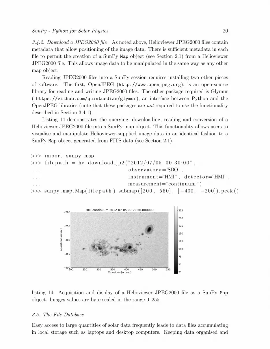
3.4.2. Download a JPEG2000 file As noted above, Helioviewer JPEG2000 files contain

metadata that allow positioning of the image data. There is sufficient metadata in each

file to permit the creation of a SunPy Map object (see Section 2.1) from a Helioviewer

JPEG2000 file. This allows image data to be manipulated in the same way as any other

map object.

Reading JPEG2000 files into a SunPy session requires installing two other pieces

of software. The first, OpenJPEG (http://www.openjpeg.org), is an open-source

library for reading and writing JPEG2000 files. The other package required is Glymur

( https://github.com/quintusdias/glymur), an interface between Python and the

OpenJPEG libraries (note that these packages are not required to use the functionality

described in Section 3.4.1).

Listing 14 demonstrates the querying, downloading, reading and conversion of a

Helioviewer JPEG2000 file into a SunPy map object. This functionality allows users to

visualise and manipulate Helioviewer-supplied image data in an identical fashion to a

SunPy Map object generated from FITS data (see Section 2.1).

>>> import sunpy .map

>>> f i l e p a t h = hv . download jp2 (”2012/07/05 00 : 30 : 00” ,

. . . observatory =’SDO’ ,

. . . instrument=”HMI” , d e t e c t o r=”HMI” ,

. . . measurement=”continuum ”)

>>> sunpy .map .Map( f i l e p a t h ) . submap ( [ 2 0 0 , 550 ] , [−400 , −200]) . peek ( )

listing 14: Acquisition and display of a Helioviewer JPEG2000 file as a SunPy Map

object. Images values are byte-scaled in the range 0–255.

3.5. The File Database

Easy access to large quantities of solar data frequently leads to data files accumulating

in local storage such as laptops and desktop computers. Keeping data organised and

SunPy - Python for Solar Physics 21

available is typically a cumbersome task for the average user. The file database is a

subpackage of SunPy that addresses this problem by providing a unified database to

store and manage information about local data files.

The database subpackage can make use of any database software supported by

SQLAlchemy (http://www.sqlalchemy.org). This library was chosen since it supports

many SQL dialects. If SQLite is selected, the database is stored as a single file, which

is created automatically. A server-based database, on the other hand, could be used by

collaborators who work together on the same data from different computers: a central

database server stores all data and the clients connect to it to read or write data.

The database can store and manage all data that can be read via SunPy’s io

subpackage, and direct integration with the vso module is supported. It is also possible

to manually add file or directory entries. The package also provides a unified data

search via the fetch() method, which includes both local files and files on the VSO.

This reduces the likelihood of downloading the same file multiple times. When a file

is added to the database, the file is scanned for metadata, and a file hash is produced.

The current date is associated with the entry along with metadata summaries such as

instrument, date of observation, field of view, etc. The database also provides the ability

to associate custom metadata to each database entry such as keywords, comments, and

favourite tags, as well as querying the full metadata (e.g., FITS header) of each entry.

The Database class connects to a database and allows the user to perform

operations on it. Listing 15 shows how to connect to an in-memory database

and download data from the VSO. These entries are automatically added to the

database. The function len() is used to get the number of records. The function

display entries() displays an iterable of database entries in a formatted ASCII table.

The headlines correspond to the attributes of the respective database entries.

A useful feature of the database package is the support of undo and redo

operations. This is particularly convenient in interactive sessions to easily revert

accidental operations. This feature will also be desirable for a planned GUI frontend

for this package.

SunPy - Python for Solar Physics 22

>>> from sunpy . net import vso

>>> from sunpy . database import Database

>>> database = Database (” s q l i t e : ///” )

>>> database . download (

. . . vso . a t t r s . Time(”2012−08−05” , ”2012−08−05 0 0 : 0 0 : 0 5 ” ) ,

. . . vso . a t t r s . Instrument ( ’AIA ’ ) )

>>> l en ( database )

2

>>> from sunpy . database . t a b l e s import d i s p l a y e n t r i e s

>>> pr in t d i s p l a y e n t r i e s (

. . . database ,

. . . [ ” id ” , ” o b s e r v a t i o n t i m e s t a r t ” , ”wavemin ” , ”wavemax ” ] )

id o b s e r v a t i o n t i m e s t a r t wavemin wavemax

−− −−−−−−−−−−−−−−−−−−−−−− −−−−−−− −−−−−−−1 2012−08−05 00 : 00 : 01 9 .4 9 .4

2 2012−08−05 00 : 00 : 02 33 .5 33 .5

listing 15: Example usage of the database subpackage.

4. Additional Functionality

SunPy is meant to provide a consistent environment for solar data analysis. In order to

achieve this goal SunPy provides a number of additional functions and packages which

are used by the other SunPy modules and are made available to the user. This section

briefly describes some of these functions.

4.1. World Coordinate System (WCS) Coordinates

Coordinate transformations are frequently a necessary task within the solar data

analysis workflow. An often used transformation is from observer coordinates (e.g.,

sky coordinates) to a coordinate system that is mapped onto the solar surface (e.g.,

latitude and longitude). This transformation is necessary to compare the true physical

distance between different solar features. This type of transformation is not unique

to solar observations, but is not often considered by astronomical packages such as

the Astropy coordinates package. The wcs package in SunPy implements the World

Coordinate System (WCS) for solar coordinates as described by Thompson (2006). The

transformations currently implemented are some of the most commonly used in solar

data analysis, namely converting from Helioprojective-Cartesian (HPC) to Heliographic

(HG) coordinates. HPC describes the positions on the Sun as angles measured from the

center of the solar disk (usually in arcseconds) using Cartesian coordinates (X, Y). This is

the coordinate system most often defined in solar imaging data (see for example, images

from SDO/AIA, SOHO/EIT, and TRACE ). HG coordinates express positions on the

SunPy - Python for Solar Physics 23

Sun using longitude and latitude on the solar sphere. There are two standards for this

coordinate system: Stonyhurst-Heliographic, where the origin is at the intersection of the

solar equator and the central meridian as seen from Earth, and Carrington-Heliographic,

which is fixed to the Sun and does not depend on Earth. The implementation of these

transformations pass through a common coordinate system called Heliocentric-Cartesian

(HCC), where positions are expressed in true (de-projected) physical distances instead

of angles on the celestial sphere. These transformations require some knowledge of the

location of the observer, which is usually provided by the image header. In the cases

where it is not provided, the observer is assumed to be at Earth. Listing 16 shows some

examples of coordinate transforms carried out in SunPy using the wcs utilities. This

will form the foundation for transformations functions to be used on Map objects.

>>> from sunpy import wcs

>>> wcs . convert hg hpc (10 , 53)

(100 .49244115330731 , 767.97438321917502)

# Convert that p o s i t i o n back to h e l i o g r a p h i c coo rd ina t e s

>>> wcs . convert hpc hg (100 . 49 , 767 .97)

(9 .9996521808465175 , 52.999563684874893)

# Try to convert a p o s i t i o n which i s not on the Sun to HG

>>> wcs . convert hpc hg (−1500 , 0)

sunpy/wcs/wcs . py : 1 8 0 : RuntimeWarning : i n v a l i d va lue encountered in s q r t

d i s t ance = q − np . s q r t ( d i s t anc e )

( nan , nan )

# Convert sky coord inate to a p o s i t i o n in HCC

>>> wcs . conver t hpc hcc (−300 , 400 , z=True )

(−216716967.63331246 , 288956420.9477042 , 594364636.2208252)

listing 16: Using the wcs subpackage.

4.2. Solar Constants and units

Physical quantities (i.e. a number associated with a unit) are an important part of

scientific data analysis. SunPy makes use of the Quantity object provided by Astropy

units sub-package. This object maintains the relationship between a number and its

unit and makes it easy to convert between units. As these objects inherit from NumPy’s

ndarray, they work well with standard representations of numbers. Using proper

quantities inside of the code base also makes it easier to catch errors in calculations.

SunPy is currently working on integrating quantities throughout the code base. In

order to encourage the use of units and to enable consistency SunPy provides the sun

subpackage which includes solar-specific data such as ephemerides and solar constants.

The main namespace contains a number of functions that provide solar ephemerides

such as the Sun-to-Earth distance, solar-cycle number, mean anomaly, etc. All of these

SunPy - Python for Solar Physics 24

functions take a time as their input, which can be provided in a format compatible with

sunpy.time.parse time().

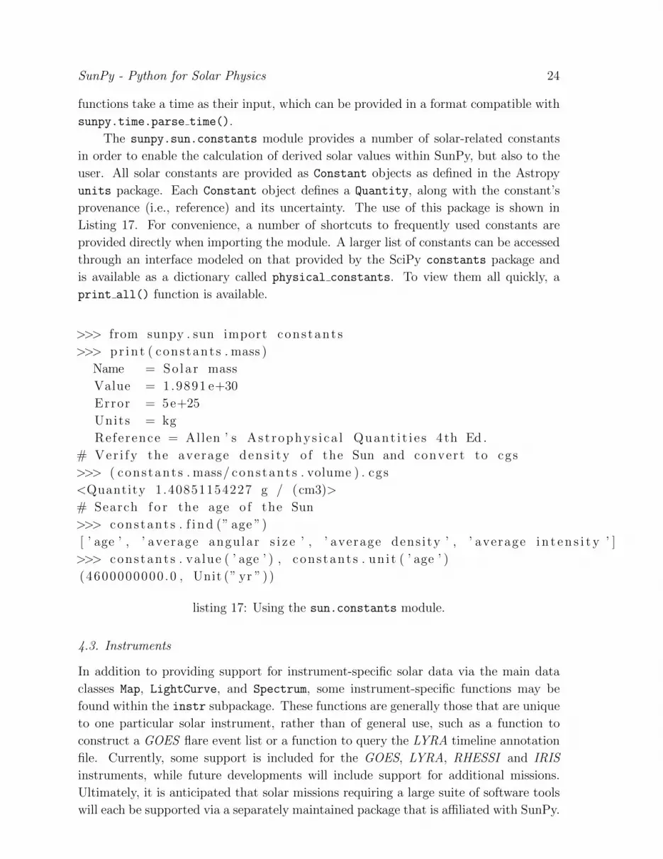
The sunpy.sun.constants module provides a number of solar-related constants

in order to enable the calculation of derived solar values within SunPy, but also to the

user. All solar constants are provided as Constant objects as defined in the Astropy

units package. Each Constant object defines a Quantity, along with the constant’s

provenance (i.e., reference) and its uncertainty. The use of this package is shown in

Listing 17. For convenience, a number of shortcuts to frequently used constants are

provided directly when importing the module. A larger list of constants can be accessed

through an interface modeled on that provided by the SciPy constants package and

is available as a dictionary called physical constants. To view them all quickly, a

print all() function is available.

>>> from sunpy . sun import cons tant s

>>> pr in t ( cons tant s . mass )

Name = So la r mass

Value = 1.9891 e+30

Error = 5e+25

Units = kg

Reference = Allen ’ s As t rophys i ca l Quant i t i e s 4 th Ed .

# Ver i fy the average dens i ty o f the Sun and convert to cgs

>>> ( cons tant s . mass/ cons tant s . volume ) . cgs

<Quantity 1.40851154227 g / (cm3)>

# Search f o r the age o f the Sun

>>> cons tant s . f i n d (” age ”)

[ ’ age ’ , ’ average angular s i z e ’ , ’ average dens i ty ’ , ’ average i n t e n s i t y ’ ]

>>> cons tant s . va lue ( ’ age ’ ) , cons tant s . un i t ( ’ age ’ )

(4600000000 .0 , Unit (” yr ” ) )

listing 17: Using the sun.constants module.

4.3. Instruments

In addition to providing support for instrument-specific solar data via the main data

classes Map, LightCurve, and Spectrum, some instrument-specific functions may be

found within the instr subpackage. These functions are generally those that are unique

to one particular solar instrument, rather than of general use, such as a function to

construct a GOES flare event list or a function to query the LYRA timeline annotation

file. Currently, some support is included for the GOES, LYRA, RHESSI and IRIS

instruments, while future developments will include support for additional missions.

Ultimately, it is anticipated that solar missions requiring a large suite of software tools

will each be supported via a separately maintained package that is affiliated with SunPy.

SunPy - Python for Solar Physics 25

5. Development and Community

SunPy is a community-developed library, designed and developed for and by the solar

physics community. Not only is all the source code publicly available online under

the permissive 2-clause BSD licence, the whole development process is also online and

open for anyone to contribute to. SunPy’s development makes use of the online service

GitHub (http://github.com) and Git† as its distributed version control software.

The continued success of an open-source project depends on many factors; three of

the most important are (1) utility and quality of the code, (2) documentation, and (3) an

active community (Bangerth and Heister, 2013). Several tools, some specific to Python,

are used by SunPy to make achieving these goals more accessible. To maintain high-

quality code, a transparent and collaborative development workflow made possible by

GitHub is used. The following conditions typically must be met before code is accepted.

(i) The code must follow the PEP 8 Python style guidelines (http://www.python.

org/dev/peps/pep-0008/) to maintain consistency in the SunPy code.

(ii) All new features require documentation in the form of doc strings as well as user

guides.

(iii) The code must contain unit tests to verify that the code is behaving as expected.

(iv) Community consensus is reached that the new code is valuable and appropriately

implemented.

This kind of development model is widely used within the scientific Python community

as well as by a wide variety of other projects, both open and closed source.

Additionally, SunPy makes use of ‘continuous integration’ provided by Travis

CI (http://travis-ci.org), a process by which the addition of any new code

automatically triggers a comprehensive review of the code functionality which are

maintained as unit tests. If any single test fails, the community is alerted before the

code is accepted. The unit-test coverage is monitored by a service called Coveralls

(http://coveralls.io).

High-quality documentation is one of the most important factors determining the

success of any software project. Powerful tools already exist in Python to support

documentation, thanks to native Python’s focus on its own documentation. SunPy

makes use of the Sphinx (http://sphinx-doc.org) documentation generator. Sphinx

uses reStructuredText as its markup language, which is an easy-to-read, what-you-see-is-

what-you-get plaintext markup syntax. It supports many output formats most notably

HTML, as well as PDF and ePub, and provides a rich, hierarchically structured view of

in-code documentation strings. The SunPy documentation is built automatically and is

hosted by Read-the-Docs (http://readthedocs.org) at http://docs.sunpy.org.

Communication is the key to maintaining an active community, and the SunPy

community uses a number of different tools to facilitate communication. For immediate

communications, an active IRC chat room (#SunPy) is hosted on freenode.net. For

† For more information see http://git-scm.com/

SunPy - Python for Solar Physics 26

more involved or less immediate needs, such as developer comments or discussions,

an open mailing list is hosted by Google Groups. Bug tracking, code reviews, and

feature-request discussions take place directly on GitHub. The SunPy community also

reaches out to the wider solar physics community through presentations, functionality

demonstrations, and informal meetups at scientific meetings.

In order to enable the long-term development of SunPy, a formal organizational

structure has been defined. The management of SunPy is the responsibility of the SunPy

board, a group of elected members of the community. The board elects a lead developer

whose is responsible for the day to day development of SunPy. SunPy also makes

use of Python-style Enhancement proposals which can be proposed by the community

and are voted on by the board. These proposals set the overal direction of SunPy’s

development.

6. Future of SunPy

Over the three years of SunPy’s development, the code base has grown to over 17,000

lines. SunPy is already a useful package for the analysis of calibrated solar data, and it

continues to gain significant new capabilities with each successive release. The primary

focus of the SunPy library is the analysis and visualisation of ‘high-level’ solar data.

This means data that has been put through instrument processing and calibration

routines, and contains valid metadata. The plan for SunPy is to continue development

within this scope. The primary components of this plan are to provide a set of data

types that are interchangeable with one another: e.g., if you slice a MapCube along

one spatial location, a LightCurve of intensity along the time range of the MapCube

should be returned. To achieve this goal, all the data types need to share a unified

coordinate system architecture so that each data type is aware of what the physical type

of its data is and how operations on that data should be performed. This will enable

useful operations such as the coordinate and solar-rotation-aware overplotting of HELIO

(Section 3.3) and HEK results (Section 3.2) onto maps (Section 2.1). Finally, support

for new data providers and services will be integrated into SunPy. For example, new

HELIO services will be supported by SunPy, aiming for seamless interaction between

the other services and tools available (e.g., hek, map).

In concert with the work on the data types, further integration with the astropy

package will enable SunPy to incorporate many new features with little effort.

Collaboration and joint development with the Astropy project (Astropy Collaboration

et al., 2013) is ongoing.

7. Summary

We have presented the release of SunPy (v0.5), a Python package for solar physics. In

this paper we have described the main functionality which includes the SunPy data

types, Map (see Section 2.1), Lightcurve (see Section 2.2), and Spectrogram (see

REFERENCES 27

Section 2.3). We have described the data and event catalogue retrieval capabilities

of SunPy for the Virtual Solar Observatory (see Section 3.1), the Heliophysics Event

Knowledgebase (see Section 3.2), as well as the Heliophysics Integrated Observatory

(see Section 3.3). We described a new organization tool for data files integrated into

SunPy (see Section 3.5) and we discussed the community aspects, development model

(see Section 5), and future plans (see Section 6) for the project. We invite members of

the community to contribute to the effort by using SunPy for their research, reporting

bugs, and sharing new functionality with the project.

8. Acknowledgements

Many of the larger features in SunPy have been developed with the generous support of

external organizations. Initial development of SunPy’s VSO and HEK implementations

were funded by ESA’s Summer of Code In Space (SOCIS 2011, 2012, 2013) program, as

well as a prototype GUI and an N-dimensional data-type implementation. In 2013, with

support from Google’s Summer Of Code (GSOC) program, through the Python Software

Foundation, the helio, hek2vso, and database subpackages were developed. The

Spectra and Spectrogram classes were implemented with support from the Astrophysics

Research Group at Trinity College Dublin, Ireland, in 2012.

References

The Astropy Collaboration, et al. Astropy: A community python package for astronomy.

Astronomy & Astrophysics, 558:A33, September 2013. URL http://www.aanda.org/

10.1051/0004-6361/201322068.

W. Bangerth and T. Heister. What makes computational open source software libraries

successful? Computational Science & Discovery, 6(1):015010, 2013. URL http:

//stacks.iop.org/1749-4699/6/i=1/a=015010.

A. O. Benz, C. Monstein, H. Meyer, P. K. Manoharan, R. Ramesh, A. Altyntsev,

A. Lara, J. Paez, and K.-S. Cho. A World-Wide Net of Solar Radio Spectrometers:

e-CALLISTO. Earth Moon and Planets, 104:277–285, April 2009.

J. L. Bougeret, et al. S/WAVES: The Radio and Plasma Wave Investigation on the

STEREO Mission. Space Sci. Rev., 136:487–528, April 2008.

G. E. Brueckner, et al. The Large Angle Spectroscopic Coronagraph (LASCO).

Sol. Phys., 162:357–402, December 1995.

J.-P. Delaboudiniere, et al. EIT: Extreme-Ultraviolet Imaging Telescope for the SOHO

Mission. Sol. Phys., 162:291–312, December 1995.

A. Dolgert, L. Gibbons, and V. Kuznetsov. Rapid web development using

AJAX and python. Journal of Physics: Conference Series, 119(4):042011,

July 2008. URL http://stacks.iop.org/1742-6596/119/i=4/a=042011?key=

crossref.eda0671577dafc3c78be7e071da5a2fe.

REFERENCES 28

V. Domingo, B. Fleck, and A. I. Poland. The SOHO mission: an overview. Solar

Physics, 162:1–37, December 1995.

M. Dominique, et al. The LYRA Instrument Onboard PROBA2: Description and In-

Flight Performance. Sol. Phys., 286:21–42, August 2013.

S.L. Freeland and B.N. Handy. Data analysis with the SolarSoft system. Solar Physics,

182(2):497–500, 1998.

L. Golub, et al. The X-Ray Telescope (XRT) for the Hinode Mission. Sol. Phys., 243:

63–86, June 2007.

P. Greenfield. What python can do for astronomy. In Astronomical Data Analysis

Software and Systems XX, volume 442, page 425, 2011.

F. Hill, et al. The virtual solar Observatory—A resource for international heliophysics

research. Earth, Moon, and Planets, 104(1-4):315–330, April 2009. URL http:

//solar.physics.montana.edu/martens/papers/Hill-VSO-Oct07.pdf.

R. A. Howard, J. D. Moses, D. G. Socker, K. P. Dere, J. W. Cook, and Secchi

Consortium. Sun earth connection coronal and heliospheric investigation (SECCHI).

Advances in Space Research, 29:2017–2026, 2002.

J. D. Hunter. Matplotlib: A 2D graphics environment. Computing in Science &

Engineering, 9(3):90–95, 2007. URL http://scitation.aip.org/content/aip/

journal/cise/9/3/10.1109/MCSE.2007.55.

N. Hurlburt, et al. Heliophysics event knowledgebase for the solar dynamics observatory

(SDO) and beyond. Solar Physics, 275:67–78, January 2012.

E. Jones, T. Oliphant, P. Peterson, and Others. SciPy: open source scientific tools for

python, 2001. URL http://www.scipy.org/.

M. L. Kaiser. The STEREO mission: an overview. Advances in Space Research, 36:

1483–1488, 2005.

T. Kosugi, et al. The Hinode (Solar-B) Mission: An Overview. Sol. Phys., 243:3–17,

June 2007.

J. Lemen, A. Title, B. De Pontieu, C. Schrijver, T. Tarbell, J. Wuelser, L. Golub, and

C. Kankelborg. The Interface Region Imaging Spectrograph (IRIS) NASA SMEX. In

AAS/Solar Physics Division Abstracts #42, page 1512, May 2011.

J. R. Lemen, et al. The atmospheric imaging assembly (AIA) on the solar dynamics

observatory (SDO). Solar Physics, 275:17–40, January 2012.

R. P. Lin, et al. The Reuven Ramaty High-Energy Solar Spectroscopic Imager

(RHESSI). Sol. Phys., 210:3–32, November 2002.

P. C. H. Martens, et al. Computer vision for the solar dynamics observatory (SDO).

Sol. Phys., 275:79–113, January 2012.

R. T. J. McAteer, P. T. Gallagher, and J. Ireland. Statistics of Active Region

Complexity: A Large-Scale Fractal Dimension Survey. ApJ, 631:628–635, September

2005.

REFERENCES 29

W. McKinney. Data structures for statistical computing in python. In S. van der Walt

and J. Millman, editors, Proceedings of the 9th Python in Science Conference, pages

51 – 56, 2010.

W. McKinney. Python for Data Analysis. O’Reilly Media, Sebastopol, CA, 2012. ISBN

9781449323622 1449323626 9781449323615 1449323618 1449319793 9781449319793.

URL http://proquest.safaribooksonline.com/?fpi=9781449323592.

D. Muller, et al. JHelioviewer: visualizing large sets of solar images using JPEG

2000. Computing in Science & Engineering, 11(5):38–47, September 2009. URL

http://ieeexplore.ieee.org/lpdocs/epic03/wrapper.htm?arnumber=5228714.

F. Ochsenbein, et al. IVOA recommendation: VOTable format definition version 1.2.

ArXiv e-prints, October 2011.

Y. Ogawara, T. Takano, T. Kato, T. Kosugi, S. Tsuneta, T. Watanabe, I. Kondo, and

Y. Uchida. The SOLAR-A Mission - An Overview. Sol. Phys., 136:1–16, November

1991.

W. D. Pence, L. Chiappetti, C. G. Page, R. A. Shaw, and E. Stobie. Definition of the

flexible image transport system (fits), version 3.0. Astronomy & Astrophysics, 524:

A42, 2010. URL http://dx.doi.org/10.1051/0004-6361/201015362.

D. Perez-Suarez, et al. Studying Sun-Planet connections using the heliophysics

integrated observatory (HELIO). Solar Physics, 280:603–621, October 2012.

W. D. Pesnell, B. J. Thompson, and P. C. Chamberlin. The solar dynamics observatory

(SDO). Solar Physics, 275:3–15, January 2012.

E. Robbrecht, D. Berghmans, and R. A. M. Van der Linden. Automated LASCO CME

Catalog for Solar Cycle 23: Are CMEs Scale Invariant? ApJ, 691:1222–1234, February

2009.

D. F. Ryan, R. O. Milligan, P. T. Gallagher, B. R. Dennis, A. K. Tolbert, R. A. Schwartz,

and C. A. Young. The Thermal Properties of Solar Flares over Three Solar Cycles

Using GOES X-Ray Observations. ApJS, 202:11, October 2012.

S. Santandrea, et al. PROBA2: Mission and Spacecraft Overview. Sol. Phys., 286:5–19,

August 2013.

P. H. Scherrer, et al. The Helioseismic and Magnetic Imager (HMI) Investigation for

the Solar Dynamics Observatory (SDO). Sol. Phys., 275:207–227, January 2012.

D. B. Seaton, et al. The SWAP EUV Imaging Telescope Part I: Instrument Overview

and Pre-Flight Testing. Sol. Phys., 286:43–65, August 2013.

W. T. Thompson. Coordinate systems for solar image data. Astronomy

and Astrophysics, 449(2):791–803, April 2006. URL http://www.aanda.

org/index.php?option=com_article&access=doi&doi=10.1051/0004-6361:

20054262&Itemid=129.

S. Tsuneta, et al. The Soft X-ray Telescope for the SOLAR-A Mission. Sol. Phys., 136:

37–67, November 1991.

REFERENCES 30

S. van der Walt, J. L. Schonberger, J. Nunez-Iglesias, F. Boulogne, J. D. Warner,

N. Yager, E. Gouillart, and T. Yu. scikit-image: image processing in python. PeerJ,

2:e453, June 2014. URL https://peerj.com/articles/453/.

T. N. Woods, et al. Extreme Ultraviolet Variability Experiment (EVE) on the Solar

Dynamics Observatory (SDO): Overview of Science Objectives, Instrument Design,

Data Products, and Model Developments. Sol. Phys., 275:115–143, January 2012.

J.-P. Wuelser, et al. EUVI: the STEREO-SECCHI extreme ultraviolet imager. In

S. Fineschi and M. A. Gummin, editors, Telescopes and Instrumentation for Solar

Astrophysics, volume 5171 of Society of Photo-Optical Instrumentation Engineers

(SPIE) Conference Series, pages 111–122, February 2004. doi: 10.1117/12.506877.