Embed Size (px)
Citation preview

SUMO - Supermodeling by combiningimperfect models
Year 2 Report - Workpackage 7
Pance Panov, Jovan Tanevski, Nikola Simidjievski,Ljupco Todorovski, and Saso Dzeroski
October 19, 2012
1

2
Contents
1 Background 7
2 State-of-the-Art 9
3 D7.1: Report on the generation of a diverse set of ODEmodels 123.1 Methods that sample the instance space . . . . . . . . . . . . 14
3.1.1 Bootstrap sampling for ODE ensembles . . . . . . . . . 143.1.2 Error-weighted sampling and boosting ODEs . . . . . . 16
3.2 Methods that sample the feature space . . . . . . . . . . . . . 173.2.1 Random subspaces . . . . . . . . . . . . . . . . . . . . 173.2.2 Random bagging . . . . . . . . . . . . . . . . . . . . . 18
3.3 Other methods . . . . . . . . . . . . . . . . . . . . . . . . . . 19
4 D7.2: Report on the selection of a complementary set ofODE models 204.1 Distance measures on multivariate time series . . . . . . . . . 21
4.1.1 Non-elastic distance measures . . . . . . . . . . . . . . 234.1.2 Elastic distance measures for time series . . . . . . . . 244.1.3 Correlation-based distance measure . . . . . . . . . . . 264.1.4 Feature-based similarity measures . . . . . . . . . . . . 26
4.2 Grouping behaviours of dynamic systems: Use of distancemeasures for hierarchical clustering . . . . . . . . . . . . . . . 274.2.1 Clustering different model structures, i.e., trajectories
produced by simulating them . . . . . . . . . . . . . . 284.2.2 Clustering observed behaviours (different datasets of
measurements) . . . . . . . . . . . . . . . . . . . . . . 314.3 Analysis of the clustering results . . . . . . . . . . . . . . . . . 35
5 D7.3: Report on learning to interconnect ODE models 365.1 Preliminary experiments with learning ensembles of ODEs . . 36
5.1.1 Experiments with bootstrap sampling with replacement 385.1.2 Experiments with bootstrap sampling w/out replacement 395.1.3 Random window samples (and experiments) . . . . . . 425.1.4 Experiments with boosting of ODEs . . . . . . . . . . 43
5.2 Plans for further work . . . . . . . . . . . . . . . . . . . . . . 46
6 Conclusion 47
3

4
Context: Workpackage 7 and its structure
WP7 Objectives. The objective of WP7 is to develop methods for compu-tational scientific discovery that can learn complete supermodels (ensemblesof ODE models) of dynamical systems. The sub-objectives of this WP includethe development of techniques for (semi)automated generation of constituentmodels, selection of an appropriate subset of models, and learning the formand coefficients of the interconnections among the models.
WP7 Description of work. WP7 will develop methods for learning com-plete supermodels. The supermodels are expected to be built in three phases:first generate diverse models, then select a set of complementary models, andfinally learn the interconnections between the constituent models of an en-semble. These three phases form the three tasks that constitute WP7:
• Task 7.1 Generate diverse set of ODE models. To generate adiverse set of models, in this task, we adapt existing approaches fromthe area of ensemble learning. These include taking different subsam-ples of the data, taking projections of the data, and taking differentlearning algorithms (or randomized algorithms). Different subsets ofdomain knowledge may also be considered.
• Task 7.2 Select a complementary set of ODE models. Givena set of models, in this task, we use a measure of similarity betweenmodels to select models that are complementary. Different measuresof similarity (or model performance/quality) can be considered. Be-sides the sum of squared errors and correlation, these can include theweighted sum of squared errors or robust statistical estimators.
• Task 7.3 Learn to interconnect ODE models. In learning theinterconnections between the constituent models of the ensemble, inthis task, we consider searching through the space of possible struc-tural forms of the interconnections, coupled with parameter fitting fora selected functional form of the possible connections. For parameterfitting, we will use global optimization methods based on meta-heuristicapproaches. The use of such parameter estimation methods is of crucialimportance in supporting the use of different quality criteria, as wellas avoiding local optima in search.
5
Deliverables in WP7. The progress of each task from WP7 is reported inthe planned deliverables as follows:
• D7.1 Report on the generation of a diverse set of ODE models.This deliverable adresses task 7.1 and presents the progress on the taskof generating a diverse set of ODE models. In the Annex 1 (Descriptionof work) this deliverable was planned for month 18 of the duration ofthe project.
• D7.2 Report on the selection of a complementary set of ODEmodels. This deliverable adresses task 7.2 and presents the progresson the task of selecting a complementary set of ODE models. In theAnnex 1 (Description of work), this deliverable was planned for month27 of the duration of the project.
• D7.3 Report on learning to interconnect ODE models. Thisdeliverable adresses task 7.1 and presents the progress on the task oflearning to interconnect ODE models. In the Annex 1 (Description ofwork), this deliverable was planned for month 36 of the duration of theproject.
The structure of the WP7 year 2 report. In the year 2 report for work-package 7, we present the progress on all three tasks planned for workpackage7 in Annex 1. The two introductory sections provides general background(Section 1) and state-of-the-art overview (Section 2) for the research withinWP7. In Section 3, we present a revised version of the deliverable D7.1 sub-mited on 31 JUL 2012. In Section 4, we present deliverable D7.2 and theprogress on the task of selecting a complementary set of ODE models. Fi-nally, in Section 5, we present initial work on learning to interconnect ODEmodels organized in a preliminary version of deliverable D7.3. Updated andrevised version of D7.3 will be provided for the Year 3 of the project.
Note that the deliverables of WP7 focus on learning ensembles of ODEmodels, i.e., supermodels. A related deliverable (Deliverable 1.6) is part ofWP1, which is concerned with the fundamentals of supermodeling. Thisdeliverable is concerned with solving the basic task of learning base ODEmodels and relies on the base learner ProBMoT for solving this task. Severalextensions of ProBMoT are necessary for the successful learning of supermod-els, e.g., the inclusion of capabilities to deal with weighted sum of squarederrors as objective function, as well as capabilities to deal with multiple ob-jective functions. Also, appropriate libraries of domain knowledge need tobe developed for the learning of combination functions for the componentmodels of a supermodel.
6
1 Background
Dynamic systems, the state of which changes over time, are ubiquitous inboth science and engineering. Experts build models of dynamic systems tosimulate and predict system behavior under various conditions. Models ofdynamic systems typically take the form of ordinary differential equations(ODEs), where the rate of change of the values of the systems variables isexpressed as a function of their current values. In the SUMO project, we focuson the task of constructing models of dynamic systems, i.e., the process ofestablishing models from observations and measurements of system behavior.
The major paradigm used when modeling dynamic systems is the ap-proach of theoretical (knowledge-driven) modeling. A domain expert derivesa proper model (ODE) structure, based on extensive knowledge about thesystem at hand, as well as domain-specific modeling knowledge. Measureddata are then used to estimate the (constant) parameters in the model. Inthe alternative paradigm of empirical (data-driven) modeling, different modelstructures are explored to fit observed data in a trial and error process. Thisparadigm has been recently used to develop machine learning approaches toconstructing ODE models from measured data.
Within the area of computational scientific discovery, equation discoverysystems have emerged that use measured data to identify both the modelstructure and the values of the constant parameters in the model. They com-bine heuristic search methods with parameter estimation techniques: Whilethe search methods explore the space of candidate model structures, the pa-rameter estimation techniques find optimal values of a single structure andevaluate its fit against observations. The result of the evaluation in turnguides the search method towards a model with a good fit.
The most recent equation discovery approaches integrate the theoreticaland empirical paradigms for modeling dynamic systems. Besides observeddata, they take into account domain knowledge about the studied system:Process-based domain knowledge describes the basic types of processes thatcan take place in such a system and provides alternative modeling templatesfor each of them. The ability to take into account domain knowledge has beena key contributor to the success of these automated modeling approaches.
Machine learning approaches for equation discovery that learn ODE mod-els from observed behaviors will be the major stepping stone for the proposedresearch. Another paradigm from machine learning that we draw upon inthe SUMO project is the paradigm of ensemble learning. Ensemble meth-ods create a set (ensemble) of diverse predictive models instead of a singleone. Diverse models are typically obtained by applying a learning algorithmto different samples of the data. The individual models from the ensemble
7
(or their predictions) are combined by averaging or in a more complicatedfashion, where the form and parameters of the combination function are alsolearned. Ensembles achieve high predictive performance, benefiting from thediversity of the individual models and outperforming them.
In machine learning, ensembles are typically employed in the contextof predictive modeling in general and classification/regression in particular.They have also been considered in the context of predicting structured out-puts, as well as other machine learning tasks, such as feature ranking andclustering. To the best of our knowledge, ensembles of (ODE) models ofdynamic systems thus have not yet been considered in the machine learningliterature. We will address them in WP7 of the SUMO project.
Ensemble predictions have been considered, however, for dynamic modelsof the climate system. Typically, a single climate model is taken and thediversity of predictions is achieved by perturbing the initial state from whichthe model is run or the constant parameters of the model: The resultingtwo types of ensembles are referred to as initial condition ensembles andperturbed physics ensembles, respectively. In contrast, the models within anensemble generated by machine learning algorithm are completely different,both in their structure and parameters. Modest changes are considered inclimate models due to the size of the models and the time complexity of theirsimulations.
A related recent development arising in the context of climate modelingis the paradigm of supermodeling. A supermodel consists of a set of intercon-nected (coupled) models: The component models are simulated (integrated)simultaneously and information is exchanged between the models (throughthe interconnections) on a time-step basis. This is in contrast to simulatingeach of the models independently and then combining their predictions.
It is important to note here that classification and regression models(typically considered in ensemble learning) do not depend on time and canbe considered to make predictions instantaneously, while the predictions ofan ODE model are obtained by simulation algorithms that are iterative. Thetask of combining ODE models and their outputs is thus more complicated,and several alternative approaches can be considered, including the modelcoupling approach taken in supermodeling.
The practical relevance of learning models of dynamic systems, on onehand, and the success of ensemble methods in yielding better predictions, onthe other hand, provides us with strong motivation to investigate the topicof learning ensemble models of dynamic systems. Additional motivation isprovided by the recent developments in supermodeling, which highlight theimportance, as well as the difficulty and complexity of the problem of combin-ing ODE models. The task at hand is thus both important and challenging.
8
2 State-of-the-Art
The tasks addressed in WP7 of the SUMO project aim at developing ap-proaches for learning ensemble models of dynamic systems. It is thus of inter-disciplinary nature and the related work that we consider comes from severalareas. First, these include machine learning [28] and two of its sub?areas,computational scientific discovery [16] and ensemble learning [30]. Second,these include ensembles for prediction of climate [8]. Finally, these includethe recent paradigm of supermodeling [40].
From the area of computational scientific discovery, we will build uponexisting equation discovery systems for learning ODE models of dynamicsystems from observational data. After initial research on this topic, whichused a completely empirical (data?driven) approach [11], further develop-ments (starting with [13]) have tried to integrate the theoretical and empir-ical paradigms for modeling dynamic systems: Besides observed data, theytake into account domain knowledge.
Recent machine learning systems for learning ODE models deal with thetask of inductive process modeling and exploit process?based domain knowl-edge [15, 37, 5]. Such knowledge describes the basic types of processes thatcan take place in the studied system (and other systems from the same do-main of study) and provides alternative modeling templates for each of them.The most recent process?based modeling tool (ProbMoT)[9], that we buildupon within the WP7 of the SUMO project, uses a cleaner representationformalism based on entity and process templates, includes several local andglobal optimization methods for parameter estimation, and allows for theuse of different objective functions (and not only the sum of squared errorsbetween measurements and predictions). Equation discovery and inductiveprocess modeling methods (for learning ODE models of dynamic systems),developed so far, deal with the task of finding a single model of an observedbehavior and do not provide support for building ensembles.
Ensemble methods [30] are machine learning methods that construct aset of models and combine their outputs into a single prediction in order toachieve better predictive performance. The key to the predictive power ofensemble models, at least intuitively, is the diversity of the base models withinthe ensemble [24]. Procedurally, ensemble methods first learn a diverse setof models and then (learn how to) combine them. The number of models inan ensemble can often be quite large, e.g., an ensemble can contain hundredsof decision trees.
In learning ensembles, a diverse set of models can be generated by modi-fying the learning data and applying the same learning algorithm or by usingthe same data and changing the learning algorithm. To modify the data, the
9
most popular ensemble methods generate different samples of the trainingexamples, as done in bagging [3], or take different subsets of the complete setof features, as done in random subspaces [22]. Other methods, such as baggedrandom subspaces [31] and random forests [4] sample both the examples andthe features.
Ensembles are typically employed in the context of predictive modeling, forsolving tasks such as classification, regression, and predicting structured out-puts: While they have been also used for other machine learning tasks, suchas feature ranking and clustering, ensembles of (ODE) models of dynamicsystems have not yet been considered in the machine learning literature.
Ensemble predictions have been considered, however, for dynamic modelsof the climate system [8]. Typically, a single climate model is taken and thediversity of predictions is achieved by perturbing the initial state from whichthe model is run [36]. Alternatively, (some of) the constant parameters ofthe model can be perturbed [29]. The resulting two types of ensembles arereferred to as initial condition ensembles and perturbed physics ensembles,respectively.
The changes made to the climate models in order to achieve diversity ofprediction are modest. This is due to the large size of the models and the timecomplexity of their simulations. In contrast, the models within an ensemblefor classification or regression, generated by a machine learning algorithm,can be completely different, both in their structure and parameters.
Ensembles for climate prediction have explored minor variations (pertur-bations) of initial conditions and model parameters and have not consideredODE models of different structure.
A related recent development arising in the context of climate modelingis the paradigm of supermodeling [40]. A supermodel consists of a set ofinterconnected (coupled) models: The component models are simulated (in-tegrated) simultaneously and information is exchanged between the models(through the interconnections) on a time? step basis. Note that a small setof component models of the supermodel is typically considered, which areprovided by domain experts and are not learned [39].
The key insight for supermodeling in the context of climate models comesfrom non?linear dynamics and concerns the synchronization of attractors:Attractors in the state space of a dynamic system consist of states that atrajectory will visit repeatedly and arbitrarily close in due time. If two sys-tems with the same or similar attractors are connected, it often happens thatthe evolutions of both attractors synchronize [42]. In supermodeling, the goalis to choose (learn) the connections between the models so that the modelsfall into synchronization with each other, as well as with reality.
10
Supermodeling assumes that a small set of component models is given,which exchange information via coupling, and focuses on learning the cou-pling coefficients: The combination of models is specific to ODE models anddifferent from the usual approaches of averaging.
In WP7 of the SUMO project, we combine the machine learning paradigmsof equation discovery and ensemble learning with insights from (supermod-eling of) dynamic systems and develop approaches for learning ensemble(ODE) models of dynamic systems. We develop methods for learning diversesets of ODE models (Task 7.1) as well as methods to (learn how to) select,combine and interconnect the models (Tasks 7.2 and 7.3). The combinationmethods considered include the combination of model outputs, as well asmodel coupling.
11
3 D7.1: Report on the generation of a diverse
set of ODE models
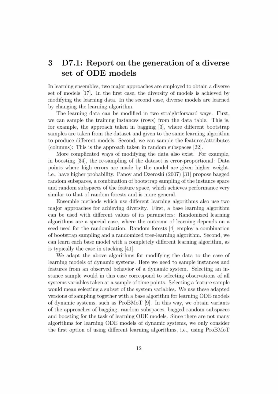
In learning ensembles, two major approaches are employed to obtain a diverseset of models [17]. In the first case, the diversity of models is achieved bymodifying the learning data. In the second case, diverse models are learnedby changing the learning algorithm.
The learning data can be modified in two straightforward ways. First,we can sample the training instances (rows) from the data table. This is,for example, the approach taken in bagging [3], where different bootstrapsamples are taken from the dataset and given to the same learning algorithmto produce different models. Second, we can sample the features/attributes(columns): This is the approach taken in random subspaces [22].
More complicated ways of modifying the data also exist. For example,in boosting [34], the re-sampling of the dataset is error-proportional: Datapoints where high errors are made by the model are given higher weight,i.e., have higher probability. Panov and Dzeroski (2007) [31] propose baggedrandom subspaces, a combination of bootstrap sampling of the instance spaceand random subspaces of the feature space, which achieves performance verysimilar to that of random forests and is more general.
Ensemble methods which use different learning algorithms also use twomajor approaches for achieving diversity. First, a base learning algorithmcan be used with different values of its parameters: Randomized learningalgorithms are a special case, where the outcome of learning depends on aseed used for the randomization. Random forests [4] employ a combinationof bootstrap sampling and a randomized tree-learning algorithm. Second, wecan learn each base model with a completely different learning algorithm, asis typically the case in stacking [41].
We adapt the above algorithms for modifying the data to the case oflearning models of dynamic systems. Here we need to sample instances andfeatures from an observed behavior of a dynamic system. Selecting an in-stance sample would in this case correspond to selecting observations of allsystems variables taken at a sample of time points. Selecting a feature samplewould mean selecting a subset of the system variables. We use these adaptedversions of sampling together with a base algorithm for learning ODE modelsof dynamic systems, such as ProBMoT [9]. In this way, we obtain variantsof the approaches of bagging, random subspaces, bagged random subspacesand boosting for the task of learning ODE models. Since there are not manyalgorithms for learning ODE models of dynamic systems, we only considerthe first option of using different learning algorithms, i.e., using ProBMoT
12
with different parameter settings or a randomized version of ProBMoT.Several complications may arise when using sampling of the data in the
context of learning ODE models. The sampling of data instances resultsin behaviors that are not observed at equidistant time points, even if thishas been the case with the initial behavior. Also, sampling of features re-sults in problems of learning ODE models under limited observability, wheremeasurements are not available for all, but only for some system variables.Finally, considering different weights of the prediction errors made for dif-ferent time points requires the use of weighted (and not ordinary) sum ofsquared errors as an objective function when learning the parameters andstructure of the ODE models.
Fortunately, our base learning method of choice (ProBMoT) can dealwith all of the above complications, since it can use full simulation in evalu-ating models (as needed for the case of limited observability or observations atnon?equidistant time points, i.e., for bagging and random subspaces), as wellas with different objective functions (needed for error? weighted samplingand boosting). However, these complications do make the original problemof learning ODE models more difficult, both in terms of computational com-plexity and in terms of the quality of the learned models. What the exactimpact is of these complications can be studied in the context of evaluationof ensemble approaches for learning ODE models.
A final approach to generating diversity can only be considered in thecontext of learning ODE models from observed data and domain knowledge,the task addressed by our base learner ProBMoT. Namely, in a manneranalogous to sampling instances and variables, we can sample from the givendomain knowledge, i.e., only consider a randomly chosen subset of processtemplates from it. However, in some cases, this can make the task of learningan ODE model much harder (if not impossible). Thus, more sophisticatedsampling methods may be needed in this case.
In the rest of this deliverable, the main focus is on the first approach togenerating ensembles, where each ODE model in the ensemble is learned byrepetitively applying the base learner on different data samples. We experi-ment here with four different data re-sampling strategies. Three of them useindependent random samples of the whole training data set for learning eachensemble model (bagging), while one of them learn the next ensemble modelon the data sample that depends on the errors of the models already includedin the ensemble (boosting). Other approaches to generating ensembles are tobe considered within the context of the experiments on learning ensemblesof ODE models performed within Task 7.3.
13
3.1 Methods that sample the instance space
3.1.1 Bootstrap sampling for ODE ensembles
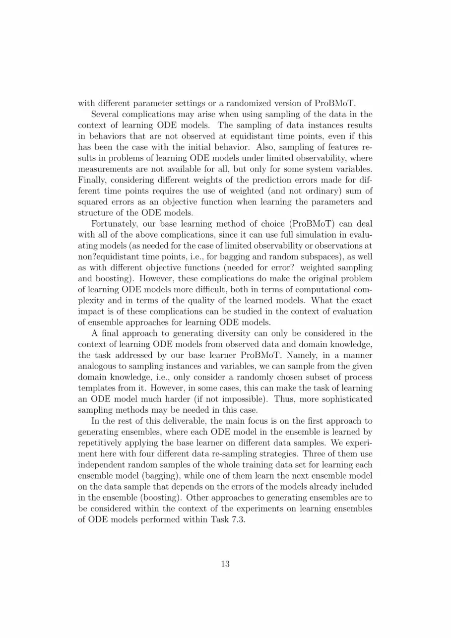
Bagging (Bootstrap sampling with aggregation) is an ensemble meta-algorithmdeveloped by Breiman et.al which is one of the first and simplest ensembletechniques. This technique uses bootstrapping for manipulating the datainstances, by sampling uniformly or with-replacements so-called bootstrapreplicates from the training data. Each base model is learned from the boot-strap replicates and combined afterwards by averaging the output (regres-sion) or voting (classification). This method successfully overcomes the over-fitting problem, but it is not useful with linear models. Another advantageof Bagging is that has no memory, and can be parallelized on different CPUsto handle different replicates which performance-vise is very useful.
Unlike the traditional method for data sampling, where part of the datais used for training the different models, which are combined into an ensem-ble afterwards (Figure 1); here we consider time point error weighting as amethod for sampling.
3.2.1. Bootstrap sampling
Unlike the traditional methods for data sampling, where part of the data is used for
training the different models, which are combined into an ensemble afterwards (Fig
2); here we consider time point error weighting as a method for sampling.
Fig 2. Classical bootstrap sampling with replacements (Bagging)
The classical approach of generating bootstrap samples for a building ensemble
models for common classification tack, includes generating samples from random
data instances in the training set T. By uniformly sampling with replacements, it is
very likely that some of the instances will repeat, and there of generating m different
training sets with size same as the original training set T. Furthermore, every sample
is used in the learning algorithm, there of learning m different model classifiers which
will participate in the ensemble. By sampling without replacements, m samples will be
created with unique instances in each of them, there of creating smaller training sets
which will be used in learning the model classifiers.
On the other hand, our approach (Fig3) differs in the sampling process from the
classical approach. Mainly, for performing bagging, we choose uniformly random time
points from the time series, and by increasing the weights (w1,w2..wn) of those
particular points in the evaluation process, we penalize (encourage) the errors made
in the learning phase (Tabele2). As long for the bagging without replacements, we
choose uniformly random time points which will participate with their error rates in the
evaluation phase. Analogically, we created the window samples, but instead of
choosing uniformly random time points form the series, we chose random starting
point and every k following time points (where k is the size of the window). With this
kind of set-up the parameters where refitted, and different models were generated.
Every of the model simulations, was then averaged or weight-averaged (using the
error rates as weights) into a descriptive ensemble model of the observed system.
Figure 1: Classical bootstrap sampling with replacement.
The classical approach of generating bootstrap samples for a buildingensemble models for common classification tack, includes generating samplesfrom random data instances in the training set T. By uniformly sampling withreplacements, it is very likely that some of the instances will repeat, and there
14
of generating m different training sets with size same as the original trainingset T. Furthermore, every sample is used in the learning algorithm, there oflearning m different model classifiers which will participate in the ensemble.By sampling without replacements, m samples will be created with uniqueinstances in each of them, there of creating smaller training sets which willbe used in learning the model classifiers.
Fig 3. Creating samples by weighting time points.
Future work
3.2.2 Random sub-spaces
The traditional approach in subspace sampling (FIGXXX) is randomly selecting
different features from the feature space a in the training set T into sub-spaces and
learning different models over each m of them. The resulting model predictions are
then ensembled into one, using variety of techniques (e.g. averaging and weighted
averaging).
FIG XXX. Random feature sampling
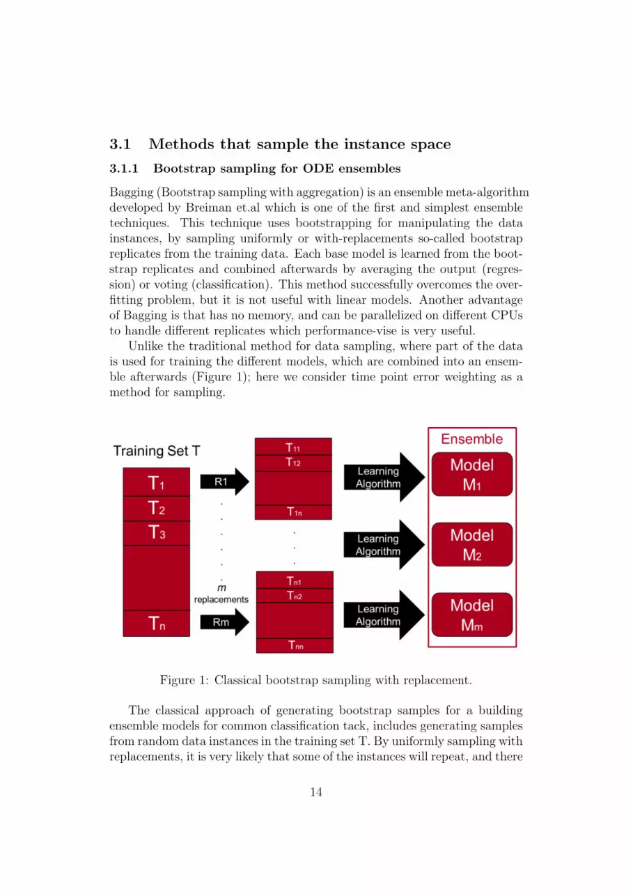
Figure 2: Creating samples by weighting time points.
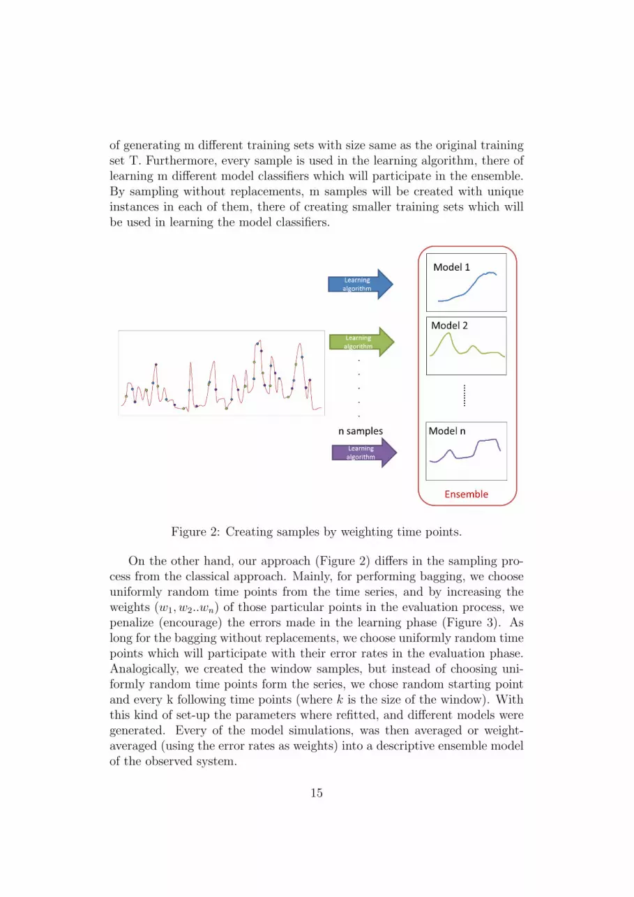
On the other hand, our approach (Figure 2) differs in the sampling pro-cess from the classical approach. Mainly, for performing bagging, we chooseuniformly random time points from the time series, and by increasing theweights (w1, w2..wn) of those particular points in the evaluation process, wepenalize (encourage) the errors made in the learning phase (Figure 3). Aslong for the bagging without replacements, we choose uniformly random timepoints which will participate with their error rates in the evaluation phase.Analogically, we created the window samples, but instead of choosing uni-formly random time points form the series, we chose random starting pointand every k following time points (where k is the size of the window). Withthis kind of set-up the parameters where refitted, and different models weregenerated. Every of the model simulations, was then averaged or weight-averaged (using the error rates as weights) into a descriptive ensemble modelof the observed system.
15
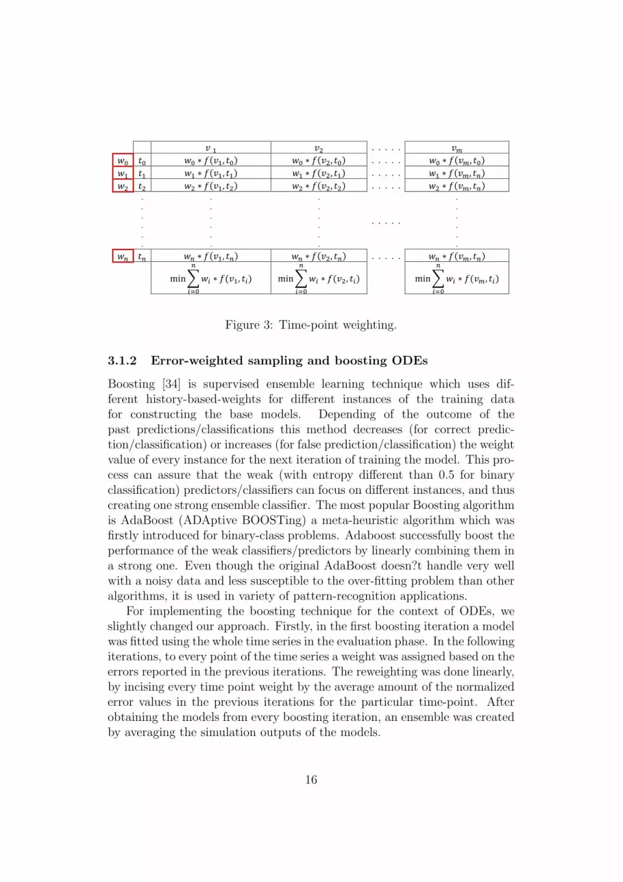
Table2. Time-point weighting
. . . . .
( ) ( ) . . . . . ( )
( ) ( ) . . . . . ( )
( ) ( ) . . . . . ( )
.
.
.
.
.
.
.
.
.
.
.
.
.
.
.
.
.
.
. . . . .
.
.
.
.
.
.
( ) ( ) . . . . . ( )
∑ ( )
∑ ( )
∑ ( )
For implementing the boosting technique, we slightly changed our approach. Firstly,
in the first boosting iteration a model was fitted using the whole time series in the
evaluation phase. In the following iterations, to every point of the time series a weight
was assigned based on the errors reported in the previous iterations. The reweighting
was done linearly, by incising every time point weight by the average amount of the
normalized error values in the previous iterations for the particular time-point. After
obtaining the models from every boosting iteration, an ensemble was created by
averaging the simulation outputs of the models.
Figure 3: Time-point weighting.
3.1.2 Error-weighted sampling and boosting ODEs
Boosting [34] is supervised ensemble learning technique which uses dif-ferent history-based-weights for different instances of the training datafor constructing the base models. Depending of the outcome of thepast predictions/classifications this method decreases (for correct predic-tion/classification) or increases (for false prediction/classification) the weightvalue of every instance for the next iteration of training the model. This pro-cess can assure that the weak (with entropy different than 0.5 for binaryclassification) predictors/classifiers can focus on different instances, and thuscreating one strong ensemble classifier. The most popular Boosting algorithmis AdaBoost (ADAptive BOOSTing) a meta-heuristic algorithm which wasfirstly introduced for binary-class problems. Adaboost successfully boost theperformance of the weak classifiers/predictors by linearly combining them ina strong one. Even though the original AdaBoost doesn?t handle very wellwith a noisy data and less susceptible to the over-fitting problem than otheralgorithms, it is used in variety of pattern-recognition applications.
For implementing the boosting technique for the context of ODEs, weslightly changed our approach. Firstly, in the first boosting iteration a modelwas fitted using the whole time series in the evaluation phase. In the followingiterations, to every point of the time series a weight was assigned based on theerrors reported in the previous iterations. The reweighting was done linearly,by incising every time point weight by the average amount of the normalizederror values in the previous iterations for the particular time-point. Afterobtaining the models from every boosting iteration, an ensemble was createdby averaging the simulation outputs of the models.
16
3.2 Methods that sample the feature space
3.2.1 Random subspaces
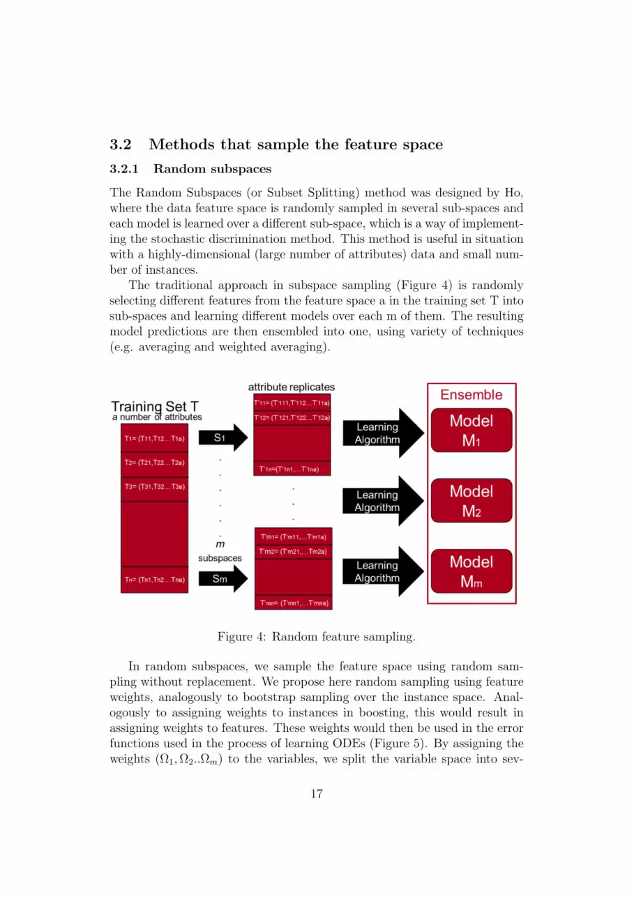
The Random Subspaces (or Subset Splitting) method was designed by Ho,where the data feature space is randomly sampled in several sub-spaces andeach model is learned over a different sub-space, which is a way of implement-ing the stochastic discrimination method. This method is useful in situationwith a highly-dimensional (large number of attributes) data and small num-ber of instances.
The traditional approach in subspace sampling (Figure 4) is randomlyselecting different features from the feature space a in the training set T intosub-spaces and learning different models over each m of them. The resultingmodel predictions are then ensembled into one, using variety of techniques(e.g. averaging and weighted averaging).
Fig 3. Creating samples by weighting time points.
Future work
3.2.2 Random sub-spaces
The traditional approach in subspace sampling (FIGXXX) is randomly selecting
different features from the feature space a in the training set T into sub-spaces and
learning different models over each m of them. The resulting model predictions are
then ensembled into one, using variety of techniques (e.g. averaging and weighted
averaging).
FIG XXX. Random feature sampling Figure 4: Random feature sampling.
In random subspaces, we sample the feature space using random sam-pling without replacement. We propose here random sampling using featureweights, analogously to bootstrap sampling over the instance space. Anal-ogously to assigning weights to instances in boosting, this would result inassigning weights to features. These weights would then be used in the errorfunctions used in the process of learning ODEs (Figure 5). By assigning theweights (Ω1,Ω2..Ωm) to the variables, we split the variable space into sev-
17
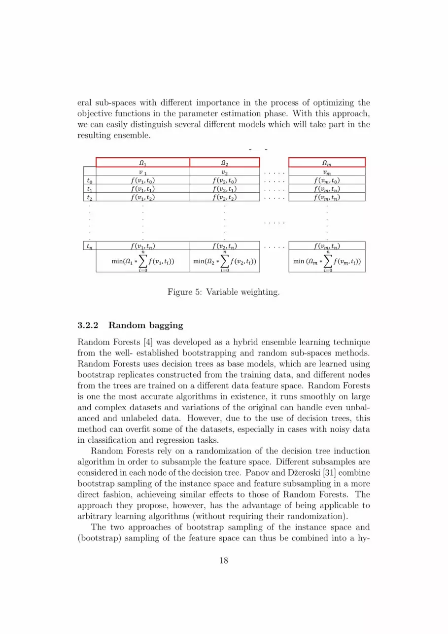
eral sub-spaces with different importance in the process of optimizing theobjective functions in the parameter estimation phase. With this approach,we can easily distinguish several different models which will take part in theresulting ensemble.
We used this approach, for developing methodology for learning ensemble models of
system of ODEs (Table3). By giving assigning random weights (Ω1, Ω2..Ωm), we
split the variable space into several sub-spaces with different importance in the
process of optimizing the objective functions in the parameter estimation phase. With
this approach, we can easily distinguish several different models which will take part
and the resulting ensemble.
Table 3 .Variable weighting
. . . . .
( ) ( ) . . . . . ( )
( ) ( ) . . . . . ( )
( ) ( ) . . . . . ( ) . . . . . .
.
.
.
.
.
.
.
.
.
.
.
.
. . . . .
.
.
.
.
.
. ( ) ( ) . . . . . ( )
( ∑ ( )
) ( ∑ ( )
) ( ∑ ( ))
3.2.3. Random Forests !?!
By combining the previous two approaches we can develop a hybrid approach,
where we add weights to every variable and every time-point.(not finished)
Table 4. Time-point and variable weighting
. . .
( ) ( ) . . . ( )
( ) ( ) . . . ( )
( ) ( ) . . . ( )
.
.
.
.
.
.
.
.
.
.
.
.
.
.
.
.
.
.
. . .
.
.
.
.
.
.
( ) ( ) . . . ( )
( ∑ ( ))
( ∑ ( )
) ( ∑ ( ))
Figure 5: Variable weighting.
3.2.2 Random bagging
Random Forests [4] was developed as a hybrid ensemble learning techniquefrom the well- established bootstrapping and random sub-spaces methods.Random Forests uses decision trees as base models, which are learned usingbootstrap replicates constructed from the training data, and different nodesfrom the trees are trained on a different data feature space. Random Forestsis one the most accurate algorithms in existence, it runs smoothly on largeand complex datasets and variations of the original can handle even unbal-anced and unlabeled data. However, due to the use of decision trees, thismethod can overfit some of the datasets, especially in cases with noisy datain classification and regression tasks.
Random Forests rely on a randomization of the decision tree inductionalgorithm in order to subsample the feature space. Different subsamples areconsidered in each node of the decision tree. Panov and Dzeroski [31] combinebootstrap sampling of the instance space and feature subsampling in a moredirect fashion, achieveing similar effects to those of Random Forests. Theapproach they propose, however, has the advantage of being applicable toarbitrary learning algorithms (without requiring their randomization).
The two approaches of bootstrap sampling of the instance space and(bootstrap) sampling of the feature space can thus be combined into a hy-
18
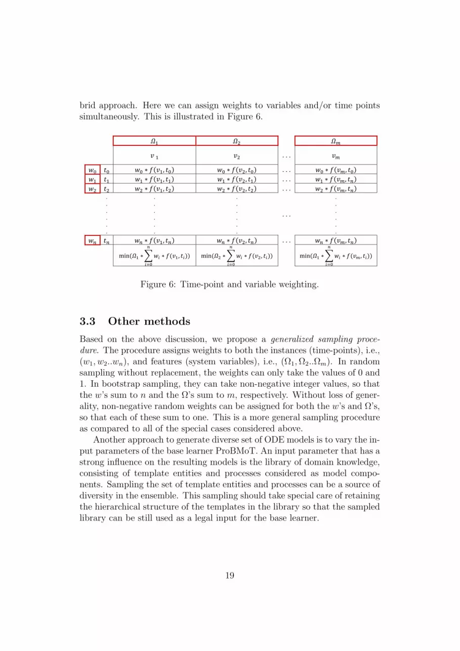
brid approach. Here we can assign weights to variables and/or time pointssimultaneously. This is illustrated in Figure 6.
We used this approach, for developing methodology for learning ensemble models of
system of ODEs (Table3). By giving assigning random weights (Ω1, Ω2..Ωm), we
split the variable space into several sub-spaces with different importance in the
process of optimizing the objective functions in the parameter estimation phase. With
this approach, we can easily distinguish several different models which will take part
and the resulting ensemble.
Table 3 .Variable weighting
. . . . .
( ) ( ) . . . . . ( )
( ) ( ) . . . . . ( )
( ) ( ) . . . . . ( ) . . . . . .
.
.
.
.
.
.
.
.
.
.
.
.
. . . . .
.
.
.
.
.
. ( ) ( ) . . . . . ( )
( ∑ ( )
) ( ∑ ( )
) ( ∑ ( ))
3.2.3. Random Forests !?!
By combining the previous two approaches we can develop a hybrid approach,
where we add weights to every variable and every time-point.(not finished)
Table 4. Time-point and variable weighting
. . .
( ) ( ) . . . ( )
( ) ( ) . . . ( )
( ) ( ) . . . ( )
.
.
.
.
.
.
.
.
.
.
.
.
.
.
.
.
.
.
. . .
.
.
.
.
.
.
( ) ( ) . . . ( )
( ∑ ( ))
( ∑ ( )
) ( ∑ ( ))
Figure 6: Time-point and variable weighting.
3.3 Other methods
Based on the above discussion, we propose a generalized sampling proce-dure. The procedure assigns weights to both the instances (time-points), i.e.,(w1, w2..wn), and features (system variables), i.e., (Ω1,Ω2..Ωm). In randomsampling without replacement, the weights can only take the values of 0 and1. In bootstrap sampling, they can take non-negative integer values, so thatthe w’s sum to n and the Ω’s sum to m, respectively. Without loss of gener-ality, non-negative random weights can be assigned for both the w’s and Ω’s,so that each of these sum to one. This is a more general sampling procedureas compared to all of the special cases considered above.
Another approach to generate diverse set of ODE models is to vary the in-put parameters of the base learner ProBMoT. An input parameter that has astrong influence on the resulting models is the library of domain knowledge,consisting of template entities and processes considered as model compo-nents. Sampling the set of template entities and processes can be a source ofdiversity in the ensemble. This sampling should take special care of retainingthe hierarchical structure of the templates in the library so that the sampledlibrary can be still used as a legal input for the base learner.
19
4 D7.2: Report on the selection of a comple-
mentary set of ODE models
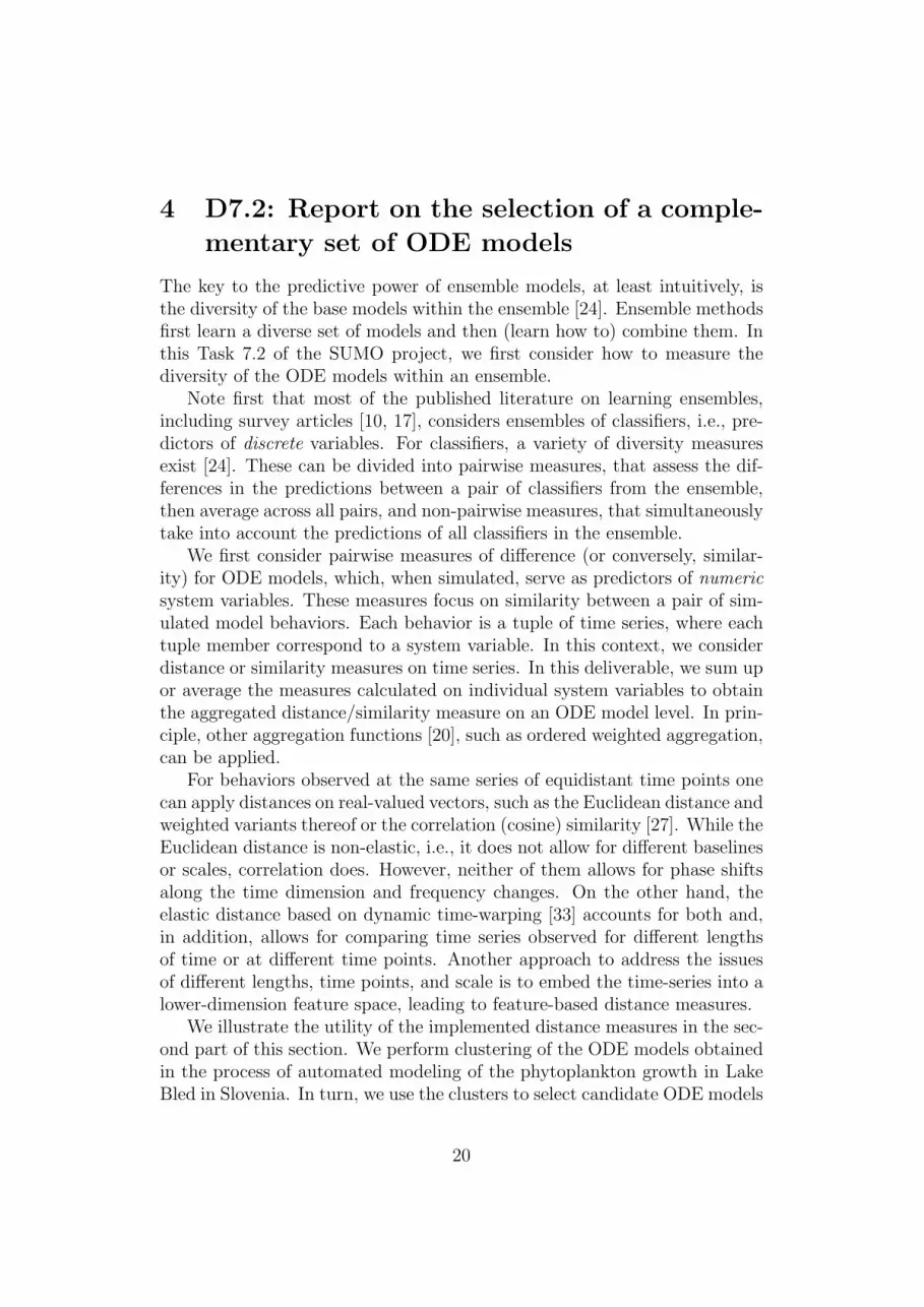
The key to the predictive power of ensemble models, at least intuitively, isthe diversity of the base models within the ensemble [24]. Ensemble methodsfirst learn a diverse set of models and then (learn how to) combine them. Inthis Task 7.2 of the SUMO project, we first consider how to measure thediversity of the ODE models within an ensemble.
Note first that most of the published literature on learning ensembles,including survey articles [10, 17], considers ensembles of classifiers, i.e., pre-dictors of discrete variables. For classifiers, a variety of diversity measuresexist [24]. These can be divided into pairwise measures, that assess the dif-ferences in the predictions between a pair of classifiers from the ensemble,then average across all pairs, and non-pairwise measures, that simultaneouslytake into account the predictions of all classifiers in the ensemble.
We first consider pairwise measures of difference (or conversely, similar-ity) for ODE models, which, when simulated, serve as predictors of numericsystem variables. These measures focus on similarity between a pair of sim-ulated model behaviors. Each behavior is a tuple of time series, where eachtuple member correspond to a system variable. In this context, we considerdistance or similarity measures on time series. In this deliverable, we sum upor average the measures calculated on individual system variables to obtainthe aggregated distance/similarity measure on an ODE model level. In prin-ciple, other aggregation functions [20], such as ordered weighted aggregation,can be applied.
For behaviors observed at the same series of equidistant time points onecan apply distances on real-valued vectors, such as the Euclidean distance andweighted variants thereof or the correlation (cosine) similarity [27]. While theEuclidean distance is non-elastic, i.e., it does not allow for different baselinesor scales, correlation does. However, neither of them allows for phase shiftsalong the time dimension and frequency changes. On the other hand, theelastic distance based on dynamic time-warping [33] accounts for both and,in addition, allows for comparing time series observed for different lengthsof time or at different time points. Another approach to address the issuesof different lengths, time points, and scale is to embed the time-series into alower-dimension feature space, leading to feature-based distance measures.
We illustrate the utility of the implemented distance measures in the sec-ond part of this section. We perform clustering of the ODE models obtainedin the process of automated modeling of the phytoplankton growth in LakeBled in Slovenia. In turn, we use the clusters to select candidate ODE models
20
to be included an ensemble; several very simple selection methods are con-sidered in the experiments. Further experiments are to be conducted withinTask 7.2.
4.1 Distance measures on multivariate time series
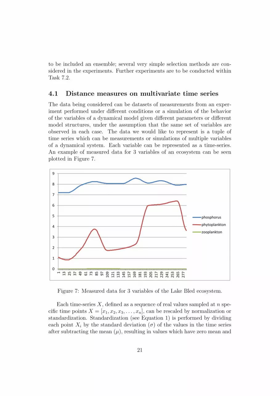
The data being considered can be datasets of measurements from an exper-iment performed under different conditions or a simulation of the behaviorof the variables of a dynamical model given different parameters or differentmodel structures, under the assumption that the same set of variables areobserved in each case. The data we would like to represent is a tuple oftime series which can be measurements or simulations of multiple variablesof a dynamical system. Each variable can be represented as a time-series.An example of measured data for 3 variables of an ecosystem can be seenplotted in Figure 7.
Each time-series X, defined as a sequence of real values sampled at n specific time points X =
[x1, x2, x3,.., xn], can be rescaled by normalization or standardization.
Figure 1 Measured data for 3 variables of the Lake Bled ecosystem
Standardization is performed by dividing each point xi by the standard deviation (σ) of the
values in the time series after subtracting the mean (μ), resulting in values which have zero
mean and unit-variance.
The plot of the data represented in Figure 1 after standardization can be seen in Figure 2.
Normalization refers to rescaling by the minimum and the range of the values to make all
values lie in the range [0-1].
( )
( ) ( )
0
1
2
3
4
5
6
7
8
9
1
13
25
37
49
61
73
85
97
10
9
12
1
13
3
14
5
15
7
16
9
18
1
19
3
20
5
21
7
22
9
24
1
25
3
26
5
27
7
phosphorus
phytoplankton
zooplankton
Figure 7: Measured data for 3 variables of the Lake Bled ecosystem.
Each time-series X, defined as a sequence of real values sampled at n spe-cific time points X = [x1, x2, x3, . . . , xn], can be rescaled by normalization orstandardization. Standardization (see Equation 1) is performed by dividingeach point Xi by the standard deviation (σ) of the values in the time seriesafter subtracting the mean (µ), resulting in values which have zero mean and
21
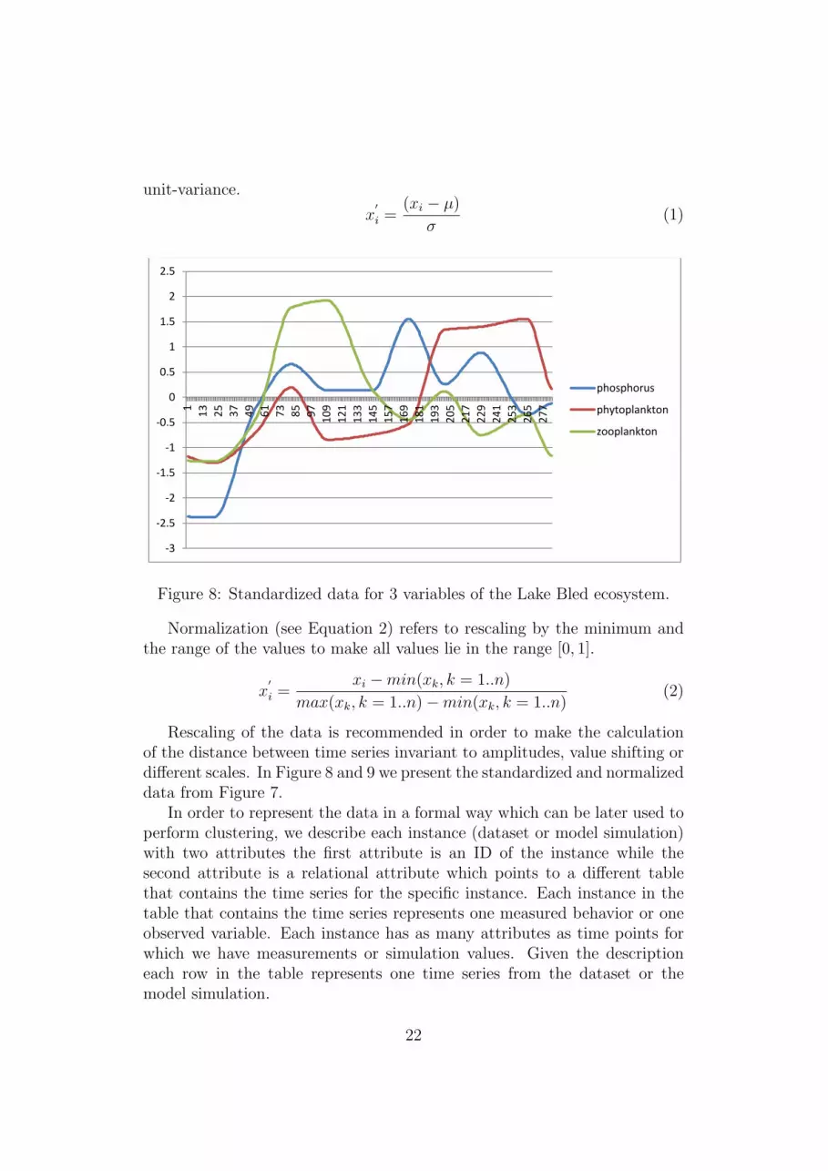
unit-variance.
x′
i =(xi − µ)
σ(1)
The plot of the data represented in Figure 1 after standardization can be seen in Figure 3.
Figure 3 Normalized data for 3 variables of the Lake Bled ecosystem
Rescaling of the data is recommended in order to make the calculation of the distance
between time series invariant to amplitudes, value shifting or different scales.
-3
-2.5
-2
-1.5
-1
-0.5
0
0.5
1
1.5
2
2.5
1
13
25
37
49
61
73
85
97
10
9
12
1
13
3
14
5
15
7
16
9
18
1
19
3
20
5
21
7
22
9
24
1
25
3
26
5
27
7
phosphorus
phytoplankton
zooplankton
0
0.2
0.4
0.6
0.8
1
1.2
1
13
25
37
49
61
73
85
97
10
9
12
1
13
3
14
5
15
7
16
9
18
1
19
3
20
5
21
7
22
9
24
1
25
3
26
5
27
7
phosphorus
phytoplankton
zooplankton
Figure 2 Standardized data for 3 variables of the Lake Bled ecosystem Figure 8: Standardized data for 3 variables of the Lake Bled ecosystem.
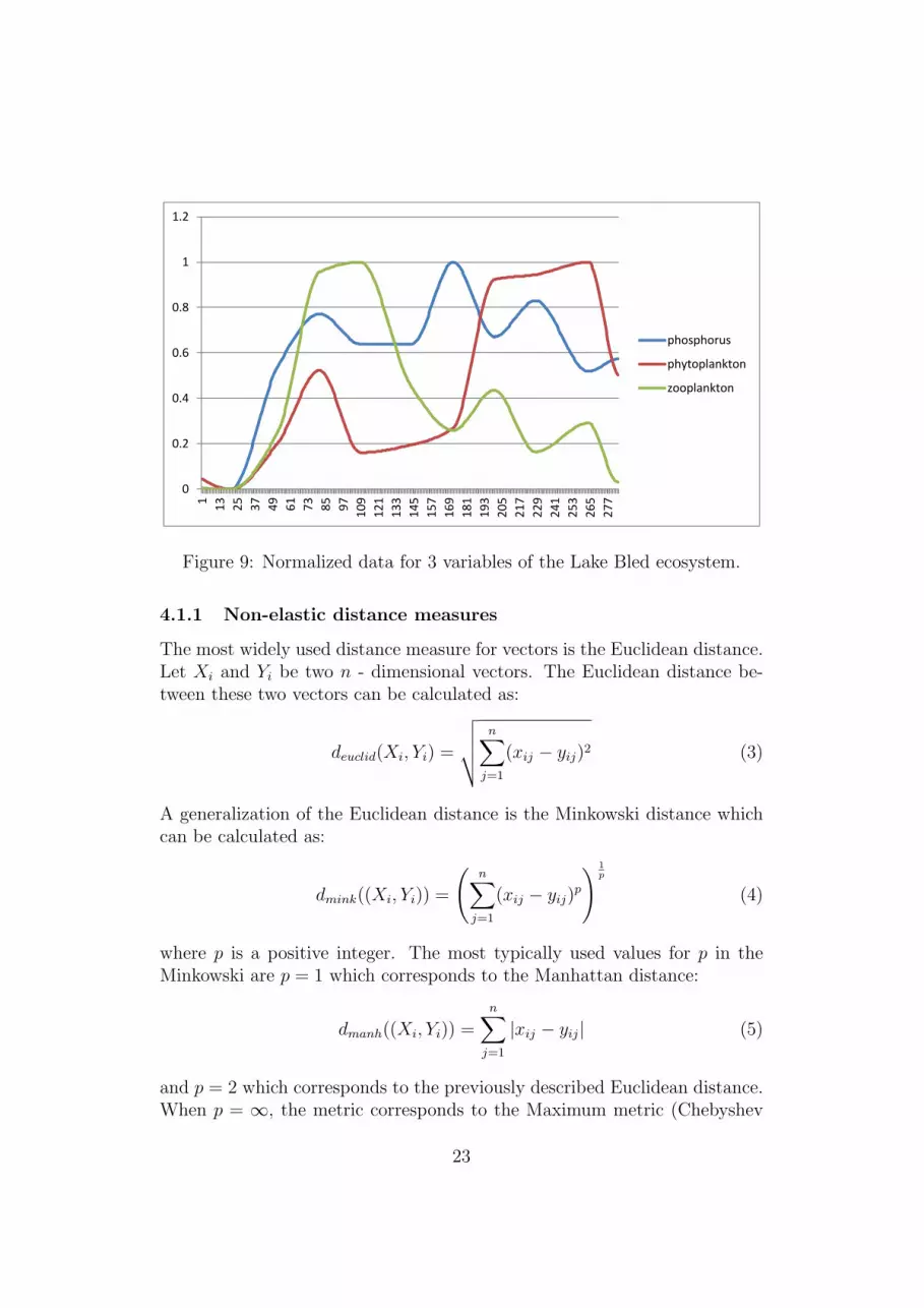
Normalization (see Equation 2) refers to rescaling by the minimum andthe range of the values to make all values lie in the range [0, 1].
x′
i =xi −min(xk, k = 1..n)
max(xk, k = 1..n)−min(xk, k = 1..n)(2)
Rescaling of the data is recommended in order to make the calculationof the distance between time series invariant to amplitudes, value shifting ordifferent scales. In Figure 8 and 9 we present the standardized and normalizeddata from Figure 7.
In order to represent the data in a formal way which can be later used toperform clustering, we describe each instance (dataset or model simulation)with two attributes the first attribute is an ID of the instance while thesecond attribute is a relational attribute which points to a different tablethat contains the time series for the specific instance. Each instance in thetable that contains the time series represents one measured behavior or oneobserved variable. Each instance has as many attributes as time points forwhich we have measurements or simulation values. Given the descriptioneach row in the table represents one time series from the dataset or themodel simulation.
22
The plot of the data represented in Figure 1 after standardization can be seen in Figure 3.
Figure 3 Normalized data for 3 variables of the Lake Bled ecosystem
Rescaling of the data is recommended in order to make the calculation of the distance
between time series invariant to amplitudes, value shifting or different scales.
-3
-2.5
-2
-1.5
-1
-0.5
0
0.5
1
1.5
2
2.5
1
13
25
37
49
61
73
85
97
10
9
12
1
13
3
14
5
15
7
16
9
18
1
19
3
20
5
21
7
22
9
24
1
25
3
26
5
27
7
phosphorus
phytoplankton
zooplankton
0
0.2
0.4
0.6
0.8
1
1.21
13
25
37
49
61
73
85
97
10
9
12
1
13
3
14
5
15
7
16
9
18
1
19
3
20
5
21
7
22
9
24
1
25
3
26
5
27
7
phosphorus
phytoplankton
zooplankton
Figure 2 Standardized data for 3 variables of the Lake Bled ecosystem
Figure 9: Normalized data for 3 variables of the Lake Bled ecosystem.
4.1.1 Non-elastic distance measures
The most widely used distance measure for vectors is the Euclidean distance.Let Xi and Yi be two n - dimensional vectors. The Euclidean distance be-tween these two vectors can be calculated as:
deuclid(Xi, Yi) =
√√√√ n∑j=1
(xij − yij)2 (3)
A generalization of the Euclidean distance is the Minkowski distance whichcan be calculated as:
dmink((Xi, Yi)) =
(n∑j=1
(xij − yij)p) 1
p
(4)
where p is a positive integer. The most typically used values for p in theMinkowski are p = 1 which corresponds to the Manhattan distance:
dmanh((Xi, Yi)) =n∑j=1
|xij − yij| (5)
and p = 2 which corresponds to the previously described Euclidean distance.When p = ∞, the metric corresponds to the Maximum metric (Chebyshev
23
distance) which can be calculated as:
dcheb((Xi, Yi)) = maxj|xij − yij| , j = 1..n (6)
4.1.2 Elastic distance measures for time series
While the Euclidean distance and its generalizations are easy to compute theycannot handle cases where the time series which are being compared are timeshifted or have different lengths. In order to deal with this problem, severalother ’elastic‘ measures have been proposed. Elastic methods for comparingtime series are derived from the methods used for string comparison wherethe distance between two strings can be defined as the minimal number ofchanges (edits) needed for one string can become identical to another. Inthe domain of vectors of real values, given two N -dimensional vectors, thesemethods try to align them in the best possible way that will minimize therequired number of edit operations for the vectors to match or the requirednumber of edit operations to minimize the distance between them. Theelastic measures, as opposed to the other described metrics, have the abilityto align and calculate the distance between time series with different lengths.
Let Xi and Yi be vectors of real values representing time-series withlengths p and q, respectively. The Edit Distance on Real sequences (EDR)[6] is based on the Levenstein distance metric [26] used for string matching.It calculates the minimum number of edit operations needed to change onetime-series into another. In EDR, two elements match if the absolute dis-tance between them is smaller than a predefined tolerance. If the elementsmatch, there is no penalty added to the final distance, otherwise a penaltyof 1 is added to the final distance. In the case of performing an operationsuch as insertion or deletion as in the Levenstein distance, a penalty of 1 isadded to the final distance. The EDR between two vectors can be recursivelydefined as follows:
dedr (Xpi , Y
qi ) = min
dedr
(Xp−1i , Y q−1
i
)+ subcost
dedr(Xp−1i , Y q
i
)+ 1
dedr(Xpi , Y
q−1i
)+ 1
(7)
where the subcost is 0 if |xip − yiq| < ε and 1 otherwise.Another string distance measure which has been considered for adapta-
tion to vectors of real values is the Longest Common Subsequence (LCSS)measure [21]. The extension to time-series LCSSε,δ (Xp
i , Yqi ) is defined in
24
[18] as follows:
min
0 if p < 1 or q < 1
1 + LCSSε,δ(Xp−1i , Y q−1
i
)if |xip − yiq| < ε and |p− q| < δ
maxLCSSε,δ
(Xp−1i , Y q
i
), LCSSε,δ
(Xpi , Y
q−1i
)otherwise
(8)
where the match is rewarded with 1 and no reward is given for insertion ordeletion. The main idea behind this approach is that two time-series aresimilar to each other if they contain a long subsequence that is identical inboth of them. The LCSS calculates the length of this sequence given thatgaps in the sequences may appear.
In order to make the LCSS a distance measure, the following transforma-tion is performed:
Dlcss = 1− LCSSε,δ (Xpi , Y
qi )
min p, q(9)
The Dynamic Time Warping (DTW) [33] distance, differs from the pre-vious approaches in that it minimizes the required number of edit operationsneeded for minimizing the distance. The cost of a match is equal to thedistance between the elements. On the other hand, the insert and deleteoperations become operations of replicating the previous value and the costof the replication is equal to the distance between the replicated elementand the currently observed element from the other time-series. The DTWdistance between two vectors can be defined as follows:
ddtw (Xpi , Y
qi ) = |xip − yiq|+min
ddtw
(Xp−1i , Y q−1
i
)ddtw
(Xp−1i , Y q
i
)ddtw
(Xpi , Y
q−1i
) (10)
The shortcoming of the previously described elastic measures is that nei-ther of them can be considered as a distance metric. The Edit Distance withReal Penalty (ERP) [7], on the other hand has been designed as a variant ofthe Manhattan distance that can handle local time shifting. The ERP usesa real penalty between non replicated elements and a constant penalty forcomputing the distance when one of the elements is replicated.The ERP canbe defined as follows:
derp (Xpi , Y
qi ) = min
derp
(Xp−1i , Y q−1
i
)+ |xip − yiq|
derp(Xp−1i , Y q
i
)+ |xip − g|
derp(Xpi , Y
q−1i
)+ |g − yiq|
(11)
where g is a constant which is usually set to g = 0, thus giving intuitivegeometric interpretation.
25
Each of the described distance measures is defined on two real vectors.In order to extend the measures to be applicable to multivariate time-seriesthat represent behaviors of dynamical system, an aggregation (sum, mean...) over the distances between the corresponding variables of each behaviorcan be calculated and for example used as a similarity measure needed forthe task of clustering.
4.1.3 Correlation-based distance measure
The correlation between two trajectories can also be used to extract infor-mation about the similarity. Let Xi and Yi be two n - dimensional vectors.The Pearson’s correlation coefficient can be calculated as:
r =
∑nj=1 (xij − µXi
)(yij − µYi)√∑n
j=1 (xij − µXi)2√∑n
j=1 (yij − µYi)2
(12)
where µXi and µY i are the means of Xi and Yirespectively. If the twotime series are maximally correlated or anti-correlated the correlations willbe 1 and −1 respectively. If the time series are uncorrelated the correlationcoefficient will be close to 0. In order to use the Pearson correlation as adistance measure a simple transformation can be performed:
dpear = 1− r (13)
Other transformations can also be devised [27, 19] in order to convert thecorrelation coefficient into a distance measure.
4.1.4 Feature-based similarity measures
A different approach to comparing time-series data is the feature based ap-proach. The positive side of these approaches is that they convert the prob-lem into lower dimensional space. On the other hand, the feature basedapproaches are dependent on the specific domain of the problem or the ap-plication and, as opposed to the approaches that consider whole time series,cannot be used for wide range of problems.
For example the authors in [38] consider representing the time series as aset of features that are commonly used to describe biological signaling net-works combined with a set of statistical and oscillation related features. Theycompare different simulation trajectories produced by a single model usingdifferent parameter values which allow for emergence of different behaviors.
In [35] the authors consider the use of simulation based numerical cal-culation of the Lyapunov exponents as features of oscillatory and chaotic
26
dynamical systems. They try to estimate the parameters based on the max-imization of the feature values, which requires comparison between modelswith different parameter values. A representation based on the features ex-tracted by a discrete Fourier transformation [1, 12] and features extracted bywavelet transformation [32] of time series have also been considered in theliterature.
4.2 Grouping behaviours of dynamic systems: Use ofdistance measures for hierarchical clustering
Hierarchical clustering methods differ by the approach used for creating clus-ters from data points. They can be divided into two groups: group of divisiveapproaches following a top-down method of creating clusters and a group ofagglomerative approaches which use the bottom-up method for creating clus-ters.
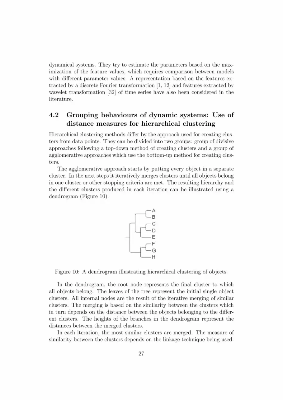
The agglomerative approach starts by putting every object in a separatecluster. In the next steps it iteratively merges clusters until all objects belongin one cluster or other stopping criteria are met. The resulting hierarchy andthe different clusters produced in each iteration can be illustrated using adendrogram (Figure 10).
statistical and oscillation related features. They compare different simulation trajectories
produced by a single model using different parameter values which allow for emergence of
different behaviors.
In [10] the authors consider the use of simulation based numerical calculation of the
Lyapunov exponents as features of oscillatory and chaotic dynamical systems and try to
estimate the parameters based on the maximization of the feature values, which requires
comparison between models with different parameter values.
A representation based on the features extracted by a discrete Fourier transformation
[11][12] and features extracted by wavelet transformation [13] of time series have also been
considered in the literature.
4. Agglomerative hierarchical clustering
Hierarchical clustering methods differ by the approach used for creating clusters from data
points. They can be divided into two groups: group of divisive approaches following a top-
down method of creating clusters and a group of agglomerative approaches which use the
bottom-up method for creating clusters.
The agglomerative approach starts by putting every object in a separate cluster. In the next
steps it iteratively merges clusters until all objects belong in one cluster or other stopping
criteria are met. The resulting hierarchy and the different clusters produced in each iteration
can be illustrated using a dendrogram (Figure 1).
In the dendrogram, the root node represents the final cluster to which all objects belong.
The leaves of the tree represent the initial single object clusters. All internal nodes are the
result of the iterative merging of similar clusters. The merging is based on the similarity
between the clusters which in turn depends on the distance between the objects belonging
to the different clusters. The heights of the branches in the dendrogram represent the
distances between the merged clusters.
Figure 4 A dendrogram illustrating hierarchical clustering of objects Figure 10: A dendrogram illustrating hierarchical clustering of objects.
In the dendrogram, the root node represents the final cluster to whichall objects belong. The leaves of the tree represent the initial single objectclusters. All internal nodes are the result of the iterative merging of similarclusters. The merging is based on the similarity between the clusters whichin turn depends on the distance between the objects belonging to the differ-ent clusters. The heights of the branches in the dendrogram represent thedistances between the merged clusters.
In each iteration, the most similar clusters are merged. The measure ofsimilarity between the clusters depends on the linkage technique being used.
27
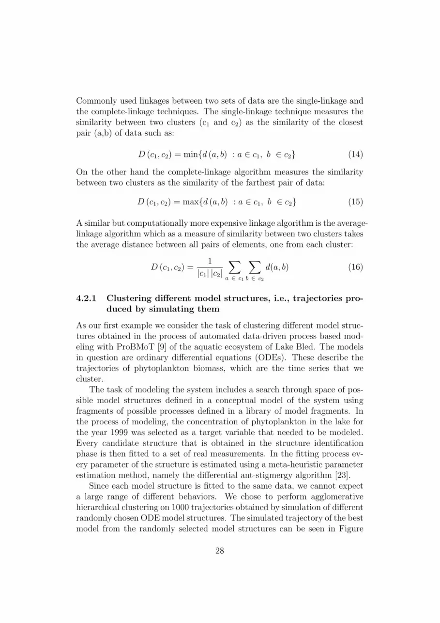
Commonly used linkages between two sets of data are the single-linkage andthe complete-linkage techniques. The single-linkage technique measures thesimilarity between two clusters (c1 and c2) as the similarity of the closestpair (a,b) of data such as:
D (c1, c2) = mind (a, b) : a ∈ c1, b ∈ c2 (14)
On the other hand the complete-linkage algorithm measures the similaritybetween two clusters as the similarity of the farthest pair of data:
D (c1, c2) = maxd (a, b) : a ∈ c1, b ∈ c2 (15)
A similar but computationally more expensive linkage algorithm is the average-linkage algorithm which as a measure of similarity between two clusters takesthe average distance between all pairs of elements, one from each cluster:
D (c1, c2) =1
|c1| |c2|∑a ∈ c1
∑b ∈ c2
d(a, b) (16)
4.2.1 Clustering different model structures, i.e., trajectories pro-duced by simulating them
As our first example we consider the task of clustering different model struc-tures obtained in the process of automated data-driven process based mod-eling with ProBMoT [9] of the aquatic ecosystem of Lake Bled. The modelsin question are ordinary differential equations (ODEs). These describe thetrajectories of phytoplankton biomass, which are the time series that wecluster.
The task of modeling the system includes a search through space of pos-sible model structures defined in a conceptual model of the system usingfragments of possible processes defined in a library of model fragments. Inthe process of modeling, the concentration of phytoplankton in the lake forthe year 1999 was selected as a target variable that needed to be modeled.Every candidate structure that is obtained in the structure identificationphase is then fitted to a set of real measurements. In the fitting process ev-ery parameter of the structure is estimated using a meta-heuristic parameterestimation method, namely the differential ant-stigmergy algorithm [23].
Since each model structure is fitted to the same data, we cannot expecta large range of different behaviors. We chose to perform agglomerativehierarchical clustering on 1000 trajectories obtained by simulation of differentrandomly chosen ODE model structures. The simulated trajectory of the bestmodel from the randomly selected model structures can be seen in Figure
28
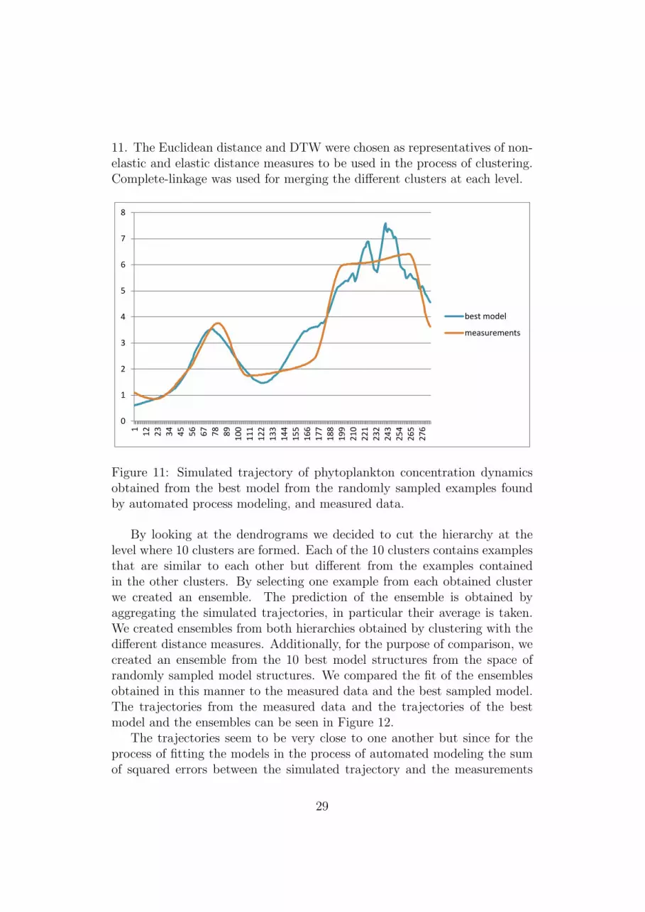
11. The Euclidean distance and DTW were chosen as representatives of non-elastic and elastic distance measures to be used in the process of clustering.Complete-linkage was used for merging the different clusters at each level.
Since each model structure is fitted to the same data, we cannot expect a large range of
different behaviors. We chose to perform agglomerative hierarchical clustering on 1000
trajectories obtained by simulation of different randomly chosen ODE model structures. The
simulated trajectory of the best model from the randomly selected model structures can be
seen in Figure 5. The Euclidean distance and DTW were chosen as representatives of non-
elastic and elastic distance measures to be used in the process of clustering. Complete-
linkage was used for merging the different clusters at each level.
By looking at the dendrograms we decided to cut the hierarchy at the level where 10 clusters
are formed. Each of the 10 clusters contains examples that are similar to each other but
different from the examples contained in the other clusters.
By selecting one example from each obtained cluster we created an ensemble. The
prediction of the ensemble is obtained by aggregating the simulated trajectories, in
particular their average is taken. We created ensembles from both hierarchies obtained by
clustering with the different distance measures.
Additionally, for the purpose of comparison, we created an ensemble from the 10 best
model structures from the space of randomly sampled model structures.
0
1
2
3
4
5
6
7
8
1
12
23
34
45
56
67
78
89
10
0
11
1
12
2
13
3
14
4
15
5
16
6
17
7
18
8
19
9
21
0
22
1
23
2
24
3
25
4
26
5
27
6
best model
measurements
Figure 5 Simulated trajectory of phytoplankton concentration dynamics obtained from the best model from the randomly sampled examples found by automated process modeling, and measured data.
Figure 11: Simulated trajectory of phytoplankton concentration dynamicsobtained from the best model from the randomly sampled examples foundby automated process modeling, and measured data.
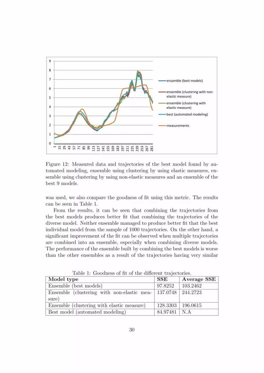
By looking at the dendrograms we decided to cut the hierarchy at thelevel where 10 clusters are formed. Each of the 10 clusters contains examplesthat are similar to each other but different from the examples containedin the other clusters. By selecting one example from each obtained clusterwe created an ensemble. The prediction of the ensemble is obtained byaggregating the simulated trajectories, in particular their average is taken.We created ensembles from both hierarchies obtained by clustering with thedifferent distance measures. Additionally, for the purpose of comparison, wecreated an ensemble from the 10 best model structures from the space ofrandomly sampled model structures. We compared the fit of the ensemblesobtained in this manner to the measured data and the best sampled model.The trajectories from the measured data and the trajectories of the bestmodel and the ensembles can be seen in Figure 12.
The trajectories seem to be very close to one another but since for theprocess of fitting the models in the process of automated modeling the sumof squared errors between the simulated trajectory and the measurements
29
We compared the fit of the ensembles obtained in this manner to the measured data and
the best sampled model. The trajectories from the measured data and the trajectories of the
best model and the ensembles can be seen in Figure 6.
Figure 6 Measured data and trajectories of the best model found by automated modeling, ensemble using clustering by using elastic measures, ensemble using clustering by using non-elastic measures and an ensemble of the best 9 models.
The trajectories seem to be very close to one another but since for the process of fitting the
models in the process of automated modeling the sum of squared errors between the
simulated trajectory and the measurements was used, we also compare the goodness of fit
using this metric. The results can be seen in Table 1.
Table 1 Goodness of fit of the different trajectories
SSE Average SSE of the individual models in the ensemble
Ensemble (best models) 97.8252 103.2462
Ensemble (clustering with non-elastic measure) 137.0748 244.2723
Ensemble (clustering with elastic measure) 128.3303 196.0615
Best model (automated modeling) 84.97481 /
From the results, it can be seen that combining the trajectories from the best models
produces better fit that combining the trajectories of the diverse model. Neither ensemble
0
1
2
3
4
5
6
7
8
9
1
15
29
43
57
71
85
99
11
3
12
7
14
1
15
5
16
9
18
3
19
7
21
1
22
5
23
9
25
3
26
7
28
1
ensamble (best models)
ensemble (clustering with non-elastic measure)
ensemble (clustering withelastic measure)
best (automated modeling)
measurements
Figure 12: Measured data and trajectories of the best model found by au-tomated modeling, ensemble using clustering by using elastic measures, en-semble using clustering by using non-elastic measures and an ensemble of thebest 9 models.
was used, we also compare the goodness of fit using this metric. The resultscan be seen in Table 1.
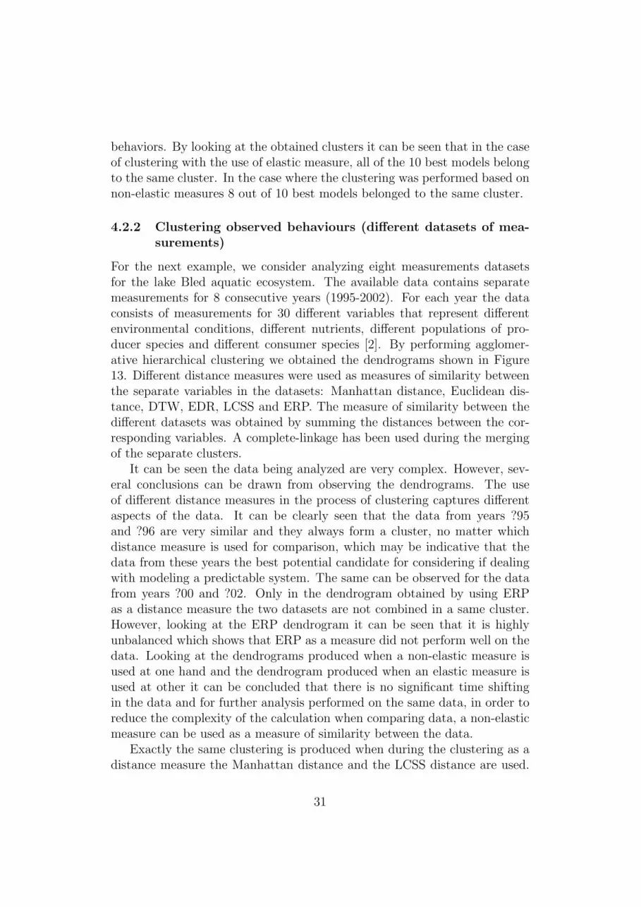
From the results, it can be seen that combining the trajectories fromthe best models produces better fit that combining the trajectories of thediverse model. Neither ensemble managed to produce better fit that the bestindividual model from the sample of 1000 trajectories. On the other hand, asignificant improvement of the fit can be observed when multiple trajectoriesare combined into an ensemble, especially when combining diverse models.The performance of the ensemble built by combining the best models is worsethan the other ensembles as a result of the trajectories having very similar
Table 1: Goodness of fit of the different trajectories.Model type SSE Average SSEEnsemble (best models) 97.8252 103.2462Ensemble (clustering with non-elastic mea-sure)
137.0748 244.2723
Ensemble (clustering with elastic measure) 128.3303 196.0615Best model (automated modeling) 84.97481 N.A
30
behaviors. By looking at the obtained clusters it can be seen that in the caseof clustering with the use of elastic measure, all of the 10 best models belongto the same cluster. In the case where the clustering was performed based onnon-elastic measures 8 out of 10 best models belonged to the same cluster.
4.2.2 Clustering observed behaviours (different datasets of mea-surements)
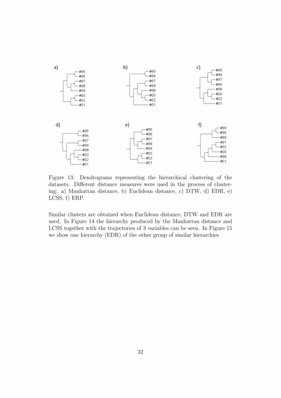
For the next example, we consider analyzing eight measurements datasetsfor the lake Bled aquatic ecosystem. The available data contains separatemeasurements for 8 consecutive years (1995-2002). For each year the dataconsists of measurements for 30 different variables that represent differentenvironmental conditions, different nutrients, different populations of pro-ducer species and different consumer species [2]. By performing agglomer-ative hierarchical clustering we obtained the dendrograms shown in Figure13. Different distance measures were used as measures of similarity betweenthe separate variables in the datasets: Manhattan distance, Euclidean dis-tance, DTW, EDR, LCSS and ERP. The measure of similarity between thedifferent datasets was obtained by summing the distances between the cor-responding variables. A complete-linkage has been used during the mergingof the separate clusters.
It can be seen the data being analyzed are very complex. However, sev-eral conclusions can be drawn from observing the dendrograms. The useof different distance measures in the process of clustering captures differentaspects of the data. It can be clearly seen that the data from years ?95and ?96 are very similar and they always form a cluster, no matter whichdistance measure is used for comparison, which may be indicative that thedata from these years the best potential candidate for considering if dealingwith modeling a predictable system. The same can be observed for the datafrom years ?00 and ?02. Only in the dendrogram obtained by using ERPas a distance measure the two datasets are not combined in a same cluster.However, looking at the ERP dendrogram it can be seen that it is highlyunbalanced which shows that ERP as a measure did not perform well on thedata. Looking at the dendrograms produced when a non-elastic measure isused at one hand and the dendrogram produced when an elastic measure isused at other it can be concluded that there is no significant time shiftingin the data and for further analysis performed on the same data, in order toreduce the complexity of the calculation when comparing data, a non-elasticmeasure can be used as a measure of similarity between the data.
Exactly the same clustering is produced when during the clustering as adistance measure the Manhattan distance and the LCSS distance are used.
31
managed to produce better fit that the best individual model from the sample of 1000
trajectories. On the other hand, a significant improvement of the fit can be observed when
multiple trajectories are combined into an ensemble, especially when combining diverse
models. The performance of the ensemble built by combining the best models is worse than
the other ensembles as a result of the trajectories having very similar behaviors. By looking
at the obtained clusters it can be seen that in the case of clustering with the use of elastic
measure, all of the 10 best models belong to the same cluster. In the case where the
clustering was performed based on non-elastic measures 8 out of 10 best models belonged
to the same cluster.
5.2. Analysis of datasets of measurements
For the next example, we consider analyzing eight measurements datasets for the lake Bled
aquatic ecosystem. The available data contains separate measurements for 8 consecutive
years (1995-2002). For each year the data consists of measurements for 30 different
variables that represent different environmental conditions, different nutrients, different
populations of producer species and different consumer species [16]. By performing
agglomerative hierarchical clustering we obtained the dendrograms shown in Figure 4.
Different distance measures were used as measures of similarity between the separate
variables in the datasets: Manhattan distance, Euclidean distance, DTW, EDR, LCSS and ERP.
The measure of similarity between the different datasets was obtained by summing the
distances between the corresponding variables. A complete-linkage has been used during
the merging of the separate clusters.
Figure 7 Dendrograms representing the hierarchical clustering of the datasets. Different distance measures were used in the process of clustering. a) Manhattan distance, b) Euclidean distance, c) DTW, d) EDR, e) LCSS, f) ERP Figure 13: Dendrograms representing the hierarchical clustering of thedatasets. Different distance measures were used in the process of cluster-ing: a) Manhattan distance, b) Euclidean distance, c) DTW, d) EDR, e)LCSS, f) ERP.
Similar clusters are obtained when Euclidean distance, DTW and EDR areused. In Figure 14 the hierarchy produced by the Manhattan distance andLCSS together with the trajectories of 3 variables can be seen. In Figure 15we show one hierarchy (EDR) of the other group of similar hierarchies
32
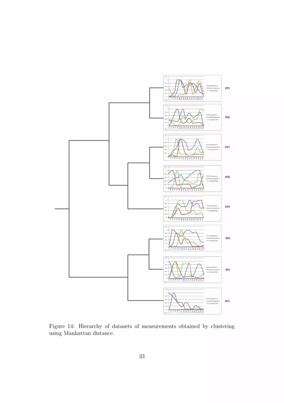
Figure 8 Hierarchy of datasets of measurements obtained by clustering using Manhattan distance
Figure 14: Hierarchy of datasets of measurements obtained by clusteringusing Manhattan distance.
33
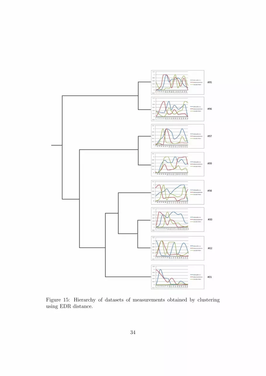
Figure 9 Hierarchy of datasets of measurements obtained by clustering using EDR distance
Figure 15: Hierarchy of datasets of measurements obtained by clusteringusing EDR distance.
34
4.3 Analysis of the clustering results
In this section, we presented a method for agglomerative hierarchical clus-tering which uses different distance measures for clustering analysis of uniand multivariate time-series. We showed the possible uses of the methodin two examples: (1)clustering of simulations of dynamical models that arestructurally different in order to build ensemble of trajectories which will im-prove the goodness of fit to the measured data and, (2) analysis of datasetsof measurements of aquatic ecosystem.
We concluded that simulated trajectories of dynamical behavior can beclustered and combined to improve the goodness of fit. We also concludedthat building ensembles of models might improve the fit to the data. Signifi-cant improvement can be achieved when constructing ensembles from diversemodels as opposed to the construction of ensembles of similar models.
For the example of analysis of different datasets of measurements weconcluded that the different distance measures used for clustering captureddifferent aspects of the dynamics. This is reflected in the hierarchy of theobtained clusters. The conclusions of the analysis can be further reffered bytaking into account that the data is used for different tasks.
As further work, given these preliminary findings, we can consider ana-lyzing the predictive behavior of an ensemble of model structures. Differentmodel structures can be learned on a certain dataset. We can then test thepredictive abilities of a certain model or ensemble of models on a similardataset. Furthermore, given simulations of fitted model structures of a dy-namical system in which more than one variable is being modeled, we canfurther analyze the possibility of combining diverse behaviors in order to im-prove the goodness of fit or analyze the predictive abilities of the ensemblesof trajectories of multiple variables.
35
5 D7.3: Report on learning to interconnect
ODE models
To evaluate the performance of the methods for generating a diverse set ofODE models (presented in the Deliverable 7.1) and methods for measuringthe diversity and selecting a complementary set of ODE models (presented inthe Deliverable 7.2), we have to integrate them into approaches for learningensembles. These approaches are based on complex combinations and inter-actions between the three basic components for generating, selecting, andcombining the components of the ensembles. Note that we can employ dif-ferent methods for coupling or interconnecting the component ODE modelsinto supermodels.
In this deliverable, we first present the results of some preliminary experi-ments with learning ensembles of ODE models. The preliminary experimentsare based on approaches that take ad-hoc combinations of the componentspresented in D7.1 and D7.2 and use averaging to aggregate the componentmodel simulations into the simulation of the supermodel ensemble. In thesecond part of the deliverable, we outline the plans for further work withinthe Task 7.3.
5.1 Preliminary experiments with learning ensemblesof ODEs
We performed several experiments to evaluate and compare the performanceof the ensembles obtained with different methods for sampling data instances.We consider the following four sampling methods: (1) simple bootstrapsampling with replacements (Bagging); (2) simple bootstrap sampling with-out replacements (random samples); (3) continuous-time bootstrap samplingwithout replacements (window samples, i.e., samples in continuous temporalwindows); and (4) error-dependent sampling as used in boosting [34].
Each model in the ensemble is obtained by re-fitting the values of theconstant parameters of an ODE model of phytoplankton growth in the LakeBled. The structure of the model, obtained by using the automated modelingtool ProBMoT[9], is as follows:
36
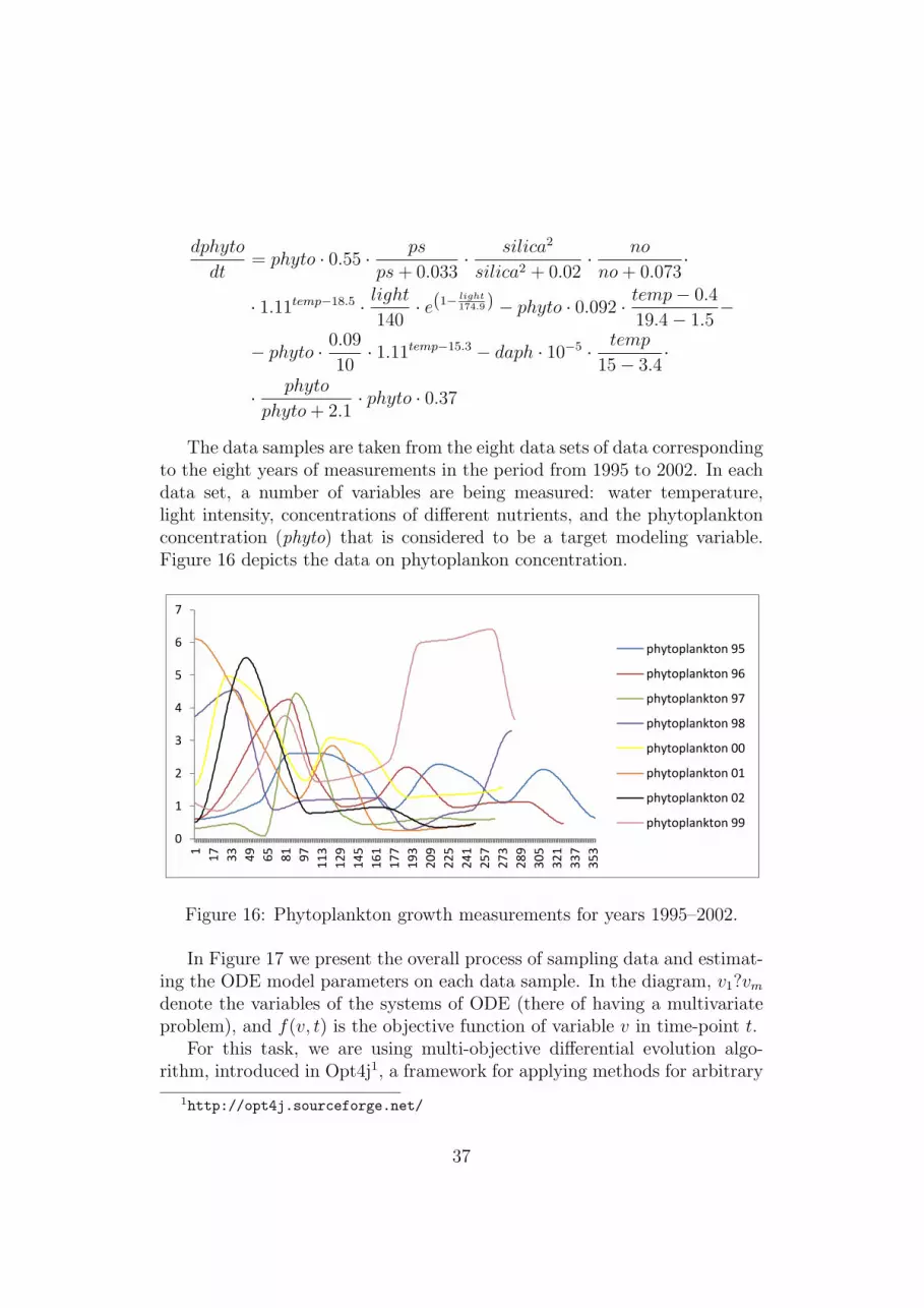
dphyto
dt= phyto · 0.55 · ps
ps+ 0.033· silica2
silica2 + 0.02· no
no+ 0.073·
· 1.11temp−18.5 · light140
· e(1− light174.9) − phyto · 0.092 · temp− 0.4
19.4− 1.5−
− phyto · 0.09
10· 1.11temp−15.3 − daph · 10−5 · temp
15− 3.4·
· phyto
phyto+ 2.1· phyto · 0.37
The data samples are taken from the eight data sets of data correspondingto the eight years of measurements in the period from 1995 to 2002. In eachdata set, a number of variables are being measured: water temperature,light intensity, concentrations of different nutrients, and the phytoplanktonconcentration (phyto) that is considered to be a target modeling variable.Figure 16 depicts the data on phytoplankon concentration.
We performed several experiments which evaluate the performance of the
ensembles. We took in consideration the classical methods for sampling data
instances mentioned in the previous section: (1) Bootstrap sampling with
replacements (Bagging); (2) Bootstrap sampling without replacements (random
samples); (3) Bootstrap sampling without replacements (window samples) and (4)
Boosting.
3.1. DATA REPRESENTATION
The data being used for performing the experiments are the measurements gathered
from the lake Bled and represented into time series where the growth of the
phytoplankton is considered as a target variable. Given the fact that the actual
measurements are not gathered on equal time basis, the working data is interpolated
for every year separately (Fig 1). Having this in mind, working with this kind of data
for constructing better descriptive models presents even a greater challenge.
Fig1. Phytoplankton growth measurements for years 1995-2002
0
1
2
3
4
5
6
7
1
17
33
49
65
81
97
11
3
12
9
14
5
16
1
17
7
19
3
20
9
22
5
24
1
25
7
27
3
28
9
30
5
32
1
33
7
35
3
phytoplankton 95
phytoplankton 96
phytoplankton 97
phytoplankton 98
phytoplankton 00
phytoplankton 01
phytoplankton 02
phytoplankton 99
Figure 16: Phytoplankton growth measurements for years 1995–2002.
In Figure 17 we present the overall process of sampling data and estimat-ing the ODE model parameters on each data sample. In the diagram, v1?vmdenote the variables of the systems of ODE (there of having a multivariateproblem), and f(v, t) is the objective function of variable v in time-point t.
For this task, we are using multi-objective differential evolution algo-rithm, introduced in Opt4j1, a framework for applying methods for arbitrary
1http://opt4j.sourceforge.net/
37
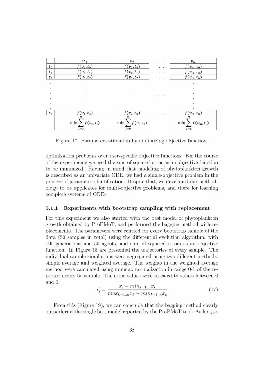
3.2. PARAMETER RE-ESTIMATION AND DATA SAMPLING
After obtaining the model structure from the ProBMoT, we perform additional
parameter estimation over the model structure over different samples of the data,
therefor obtaining several model candidates. The classical approach of parameter
estimation is presented in Table 1, where v1…vm are the variables of the systems of
ODE (there of having a multivariate problem) , and f(v,t) is the objective function of
variable v in time-point t.
Table 1. Parameter estimation by minimizing objective function
. . . . .
( ) ( ) . . . . . ( ) ( ) ( ) . . . . . ( ) ( ) ( ) . . . . . ( ) . . . . . .
.
.
.
.
.
.
.
.
.
.
.
.
. . . . .
.
.
.
.
.
.
( ) ( ) . . . . . ( )
∑ ( )
∑ ( )
∑ ( )
For this task, we are using multi-objective differential evolution algorithm, introduced
in Opt4j[OPT4J], a framework for applying methods for arbitrary optimization
problems over user-specific objective functions. For the course of the experiments we
used the sum of squared error as an objective function to be minimized. Having in
mind that modeling of phytoplankton growth is described as an univariate ODE, we
had a single-objective problem in the process of parameter identification. Despite
that, we developed our methodology to be applicable for multi-objective problems,
and there for learning complete systems of ODEs.
Figure 17: Parameter estimation by minimizing objective function.
optimization problems over user-specific objective functions. For the courseof the experiments we used the sum of squared error as an objective functionto be minimized. Having in mind that modeling of phytoplankton growthis described as an univariate ODE, we had a single-objective problem in theprocess of parameter identification. Despite that, we developed our method-ology to be applicable for multi-objective problems, and there for learningcomplete systems of ODEs.
5.1.1 Experiments with bootstrap sampling with replacement
For this experiment we also started with the best model of phytoplanktongrowth obtained by ProBMoT, and performed the bagging method with re-placements. The parameters were refitted for every bootstrap sample of thedata (50 samples in total) using the differential evolution algorithm, with100 generations and 50 agents, and sum of squared errors as an objectivefunction. In Figure 18 are presented the trajectories of every sample. Theindividual sample simulations were aggregated using two different methods:simple average and weighted average. The weights in the weighted averagemethod were calculated using minmax normalization in range 0-1 of the re-ported errors by sample. The error values were rescaled to values between 0and 1.
x‘i =
xi −mink=1..nxkmaxk=1..nxk −mink=1..nxk
(17)
From this (Figure 19), we can conclude that the bagging method clearlyoutperforms the single best model reported by the ProBMoT tool. As long as
38
the different averaging techniques, we can see imperceptibly small differencein favor of the weighted average. The difference is small, due to the manysamples with great imperfection weights vis-a-vis five-six respectable models,which in the end results in a simple average.
5.1.2 Experiments with bootstrap sampling w/out replacement
For this experiment we used the same model structure obtained by the ProB-MoT, and refitted the parameters with DE with 100 generations and 50agents. For the training data we used 25 bootstrap samples with capacityof 50% of the whole amount. After the obtaining the results, we performedsimple average over the simulations of the individual models (Figure 20).
We can conclude from Figure 21, the bagging method again outperformsthe best model generated by the ProBMoT. As long as the sample replace-ment is considered, we can see that the method which uses replacementsis slightly better that the method without replacements. Even though, themodels were fitted with different samples, the outcomes are nearly identical.
39
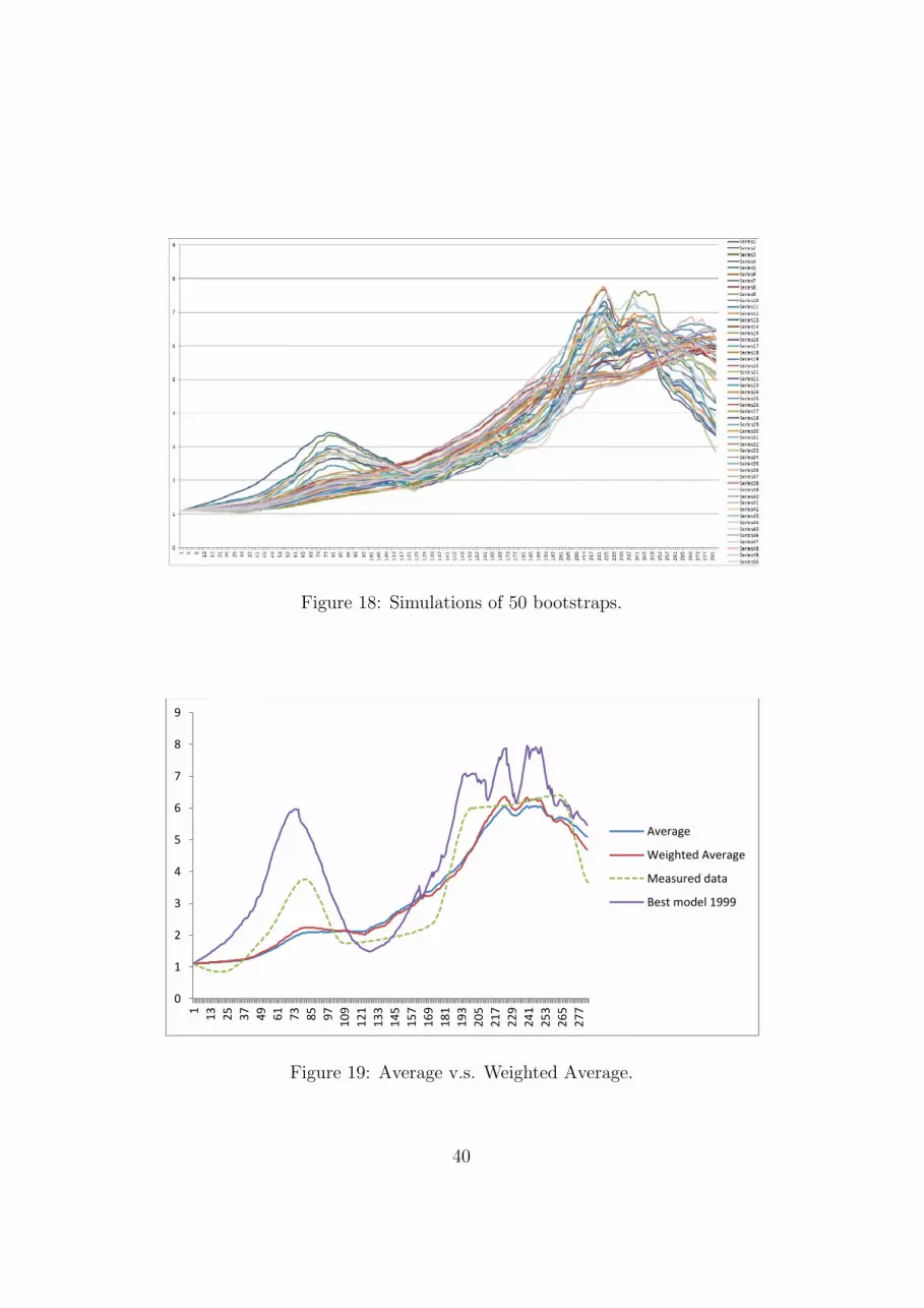
3.3 BOOTSTRAP SAMPLING
RANDOM BOOTSTRAP SAMPLING WITH REPLACEMENTS (BAGGING)
For this experiment we used the best model structure obtained by ProBMoT, and
performed the bagging method with replacements. The parameters were refitted for
every bootstrap sample of the data (50 samples in total) using the differential
evolution algorithm [DE], with 100 generations and 50 agents, and sum of squared
errors as an objective function. In Figure 4 are presented the trajectories of every
sample. The individual sample simulations were aggregated using two different
methods: simple average and weighted average. The weights in the weighted
average method were calculated using minmax normalization in range 0-1 of the
reported errors by sample. The error values were rescaled to values between 0 and
1.
Figure4 Simulations of 50 bootstraps
Figure 18: Simulations of 50 bootstraps.
Figure 5 . Average v.s. Weighted Average
From this (Fig 5), we can conclude that the bagging method clearly outperforms the
single best model reported by the ProBMoT tool. As long as the different averaging
techniques, we can see imperceptibly small difference in favor of the weighted
average. The difference is small, due to the many samples with great imperfection
weights vis-à-vis five-six respectable models, which in the end results in a simple
average.
RANDOM SAMPLES WITHOUT REPLACEMENTS
For this experiment we used the same model structure obtained by the ProBMoT,
and refitted the parameters with DE with 100 generations and 50 agents. For the
training data we used 25 bootstrap samples with capacity of 50% of the whole
amount. After the obtaining the results, we performed simple average over the
simulations of the individual models (FIG 6).
0
1
2
3
4
5
6
7
8
9
1
13
25
37
49
61
73
85
97
10
9
12
1
13
3
14
5
15
7
16
9
18
1
19
3
20
5
21
7
22
9
24
1
25
3
26
5
27
7
Average
Weighted Average
Measured data
Best model 1999
Figure 19: Average v.s. Weighted Average.
40
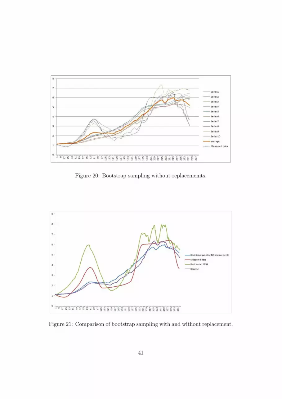
FIG 6 Bootstrap sampling with no replacememts
Fig 7. Bootstrap sampling comarasion
We can conclude from Figure 7, the bagging method again outperforms the best
model generated by the ProBMoT. As long as the sample replacement is considered,
we can see that the method which uses replacements is slightly better that the
method without replacements. Even though, the models were fitted with different
samples, the outcomes are nearly identical.
RANDOM WINDOW SAMPLES
Figure 20: Bootstrap sampling without replacememts.
FIG 6 Bootstrap sampling with no replacememts
Fig 7. Bootstrap sampling comarasion
We can conclude from Figure 7, the bagging method again outperforms the best
model generated by the ProBMoT. As long as the sample replacement is considered,
we can see that the method which uses replacements is slightly better that the
method without replacements. Even though, the models were fitted with different
samples, the outcomes are nearly identical.
RANDOM WINDOW SAMPLES
Figure 21: Comparison of bootstrap sampling with and without replacement.
41
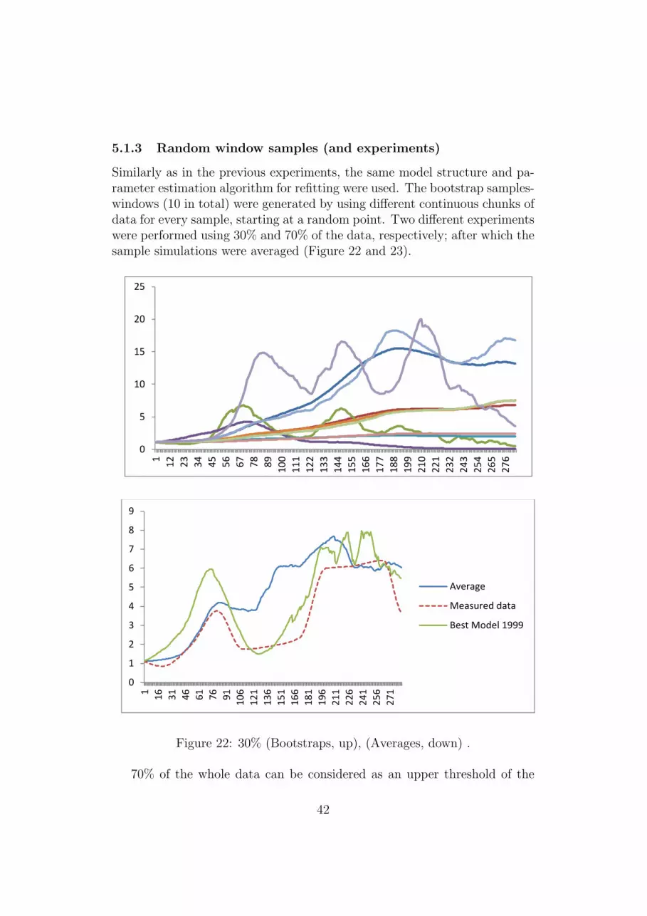
5.1.3 Random window samples (and experiments)
Similarly as in the previous experiments, the same model structure and pa-rameter estimation algorithm for refitting were used. The bootstrap samples-windows (10 in total) were generated by using different continuous chunks ofdata for every sample, starting at a random point. Two different experimentswere performed using 30% and 70% of the data, respectively; after which thesample simulations were averaged (Figure 22 and 23).
Similarly as in the previous experiments, the same model structure and parameter
estimation algorithm for refitting were used. The bootstrap samples-windows (10 in
total) were generated by using different continuous chunks of data for every sample,
starting at a random point. Two different experiments were performed using 30% and
70% of the data, respectively; after which the sample simulations were
averaged.(Figure 8,Figure 9)
Fig 8 . 30% (Bootstraps, up), (Averages, down)
0
5
10
15
20
25
1
12
23
34
45
56
67
78
89
10
0
11
1
12
2
13
3
14
4
15
5
16
6
17
7
18
8
19
9
21
0
22
1
23
2
24
3
25
4
26
5
27
6
0
2
4
6
8
10
12
1
17
33
49
65
81
97
11
3
12
9
14
5
16
1
17
7
19
3
20
9
22
5
24
1
25
7
27
3
Average
Measured data
Best Model 1999
Fig 9. 70% (Bootstraps, up) , (Averages, down)
70% of the whole data can be considered as an upper threshold of the length of the
sample, because choosing bigger can cause an overfit. Analogously, 30% can be
considered as a lower threshold of the length of training data, because choosing
smaller amounts cannot provide sufficient information.
3.4 BOOSTING
To evaluate the performance of the boosting, we performed an experiment where the
first boosting iteration was chosen as a baseline (with weight values 1), and for every
following boosting iteration (10 in total) the weights were increased based on the past
experience, i.e., the errors made by the previous model in every time point of the
series. The reweighting was done linearly, by increasing the penalty of every weight
by minmax[0-1] normalized value of the previous errors (Figure 10) or average of all
previous errors (Figure 11), according to the sum of squared errors measure. The
rest of the set-up was same as in the previous examples.
0
5
10
15
20
25
30
35
40
45
50
1
12
23
34
45
56
67
78
89
10
0
11
1
12
2
13
3
14
4
15
5
16
6
17
7
18
8
19
9
21
0
22
1
23
2
24
3
25
4
26
5
27
6
0
1
2
3
4
5
6
7
8
9
1
16
31
46
61
76
91
10
6
12
1
13
6
15
1
16
6
18
1
19
6
21
1
22
6
24
1
25
6
27
1
Average
Measured data
Best Model 1999
Figure 22: 30% (Bootstraps, up), (Averages, down) .
70% of the whole data can be considered as an upper threshold of the
42
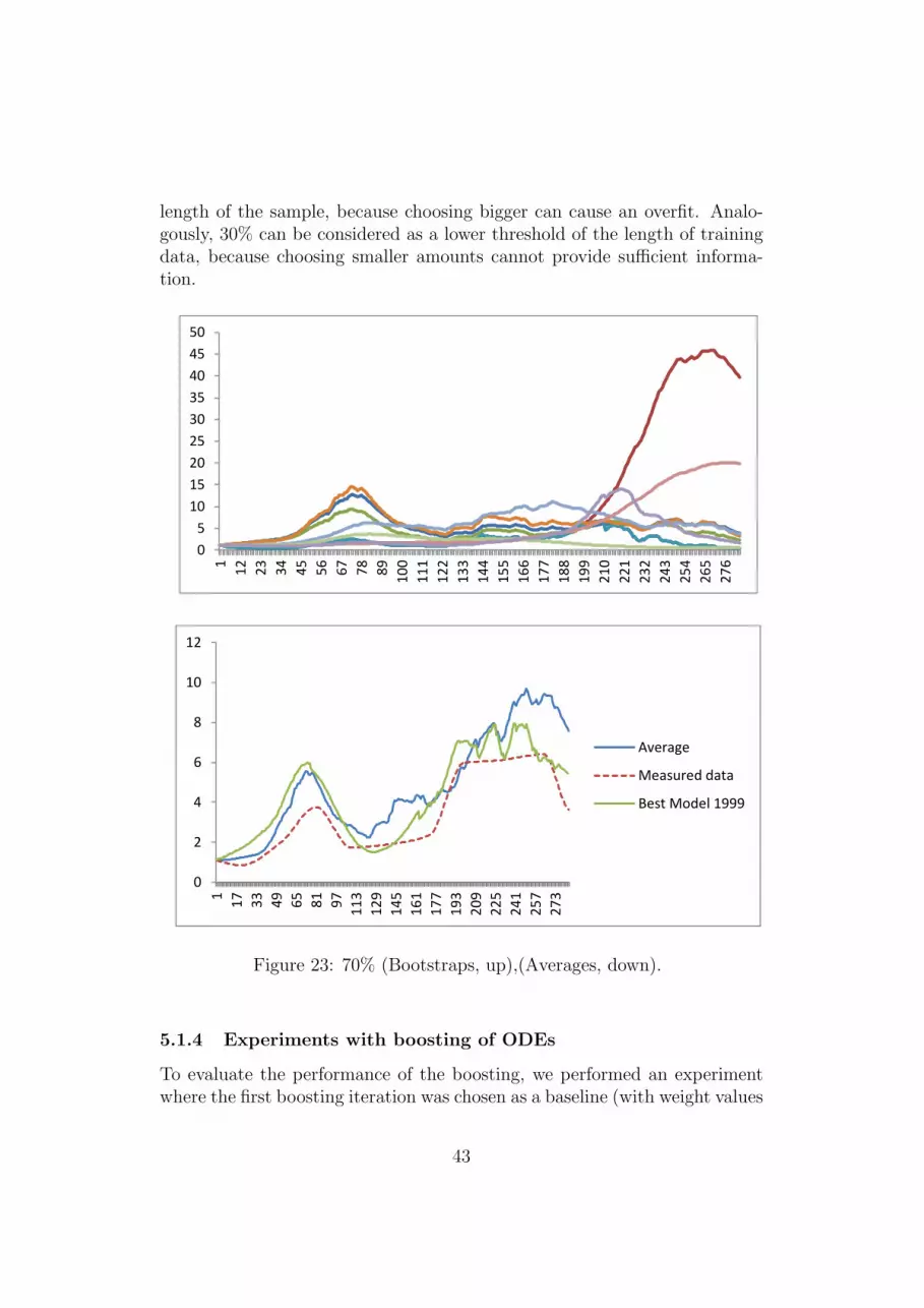
length of the sample, because choosing bigger can cause an overfit. Analo-gously, 30% can be considered as a lower threshold of the length of trainingdata, because choosing smaller amounts cannot provide sufficient informa-tion.
Fig 9. 70% (Bootstraps, up) , (Averages, down)
70% of the whole data can be considered as an upper threshold of the length of the
sample, because choosing bigger can cause an overfit. Analogously, 30% can be
considered as a lower threshold of the length of training data, because choosing
smaller amounts cannot provide sufficient information.
3.4 BOOSTING
To evaluate the performance of the boosting, we performed an experiment where the
first boosting iteration was chosen as a baseline (with weight values 1), and for every
following boosting iteration (10 in total) the weights were increased based on the past
experience, i.e., the errors made by the previous model in every time point of the
series. The reweighting was done linearly, by increasing the penalty of every weight
by minmax[0-1] normalized value of the previous errors (Figure 10) or average of all
previous errors (Figure 11), according to the sum of squared errors measure. The
rest of the set-up was same as in the previous examples.
0
5
10
15
20
25
30
35
40
45
50
1
12
23
34
45
56
67
78
89
10
0
11
1
12
2
13
3
14
4
15
5
16
6
17
7
18
8
19
9
21
0
22
1
23
2
24
3
25
4
26
5
27
6
0
1
2
3
4
5
6
7
8
9
1
16
31
46
61
76
91
10
6
12
1
13
6
15
1
16
6
18
1
19
6
21
1
22
6
24
1
25
6
27
1
Average
Measured data
Best Model 1999
Similarly as in the previous experiments, the same model structure and parameter
estimation algorithm for refitting were used. The bootstrap samples-windows (10 in
total) were generated by using different continuous chunks of data for every sample,
starting at a random point. Two different experiments were performed using 30% and
70% of the data, respectively; after which the sample simulations were
averaged.(Figure 8,Figure 9)
Fig 8 . 30% (Bootstraps, up), (Averages, down)
0
5
10
15
20
25
1
12
23
34
45
56
67
78
89
10
0
11
1
12
2
13
3
14
4
15
5
16
6
17
7
18
8
19
9
21
0
22
1
23
2
24
3
25
4
26
5
27
6
0
2
4
6
8
10
12
1
17
33
49
65
81
97
11
3
12
9
14
5
16
1
17
7
19
3
20
9
22
5
24
1
25
7
27
3
Average
Measured data
Best Model 1999
Figure 23: 70% (Bootstraps, up),(Averages, down).
5.1.4 Experiments with boosting of ODEs
To evaluate the performance of the boosting, we performed an experimentwhere the first boosting iteration was chosen as a baseline (with weight values
43
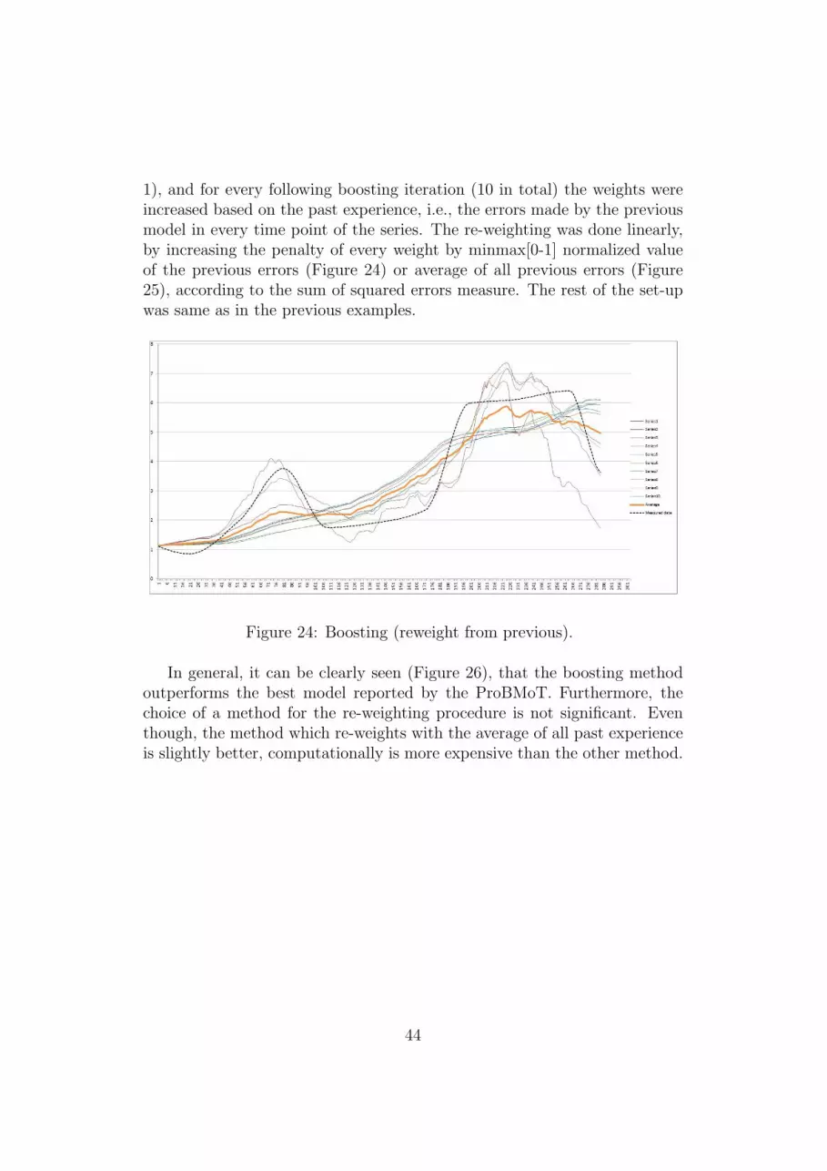
1), and for every following boosting iteration (10 in total) the weights wereincreased based on the past experience, i.e., the errors made by the previousmodel in every time point of the series. The re-weighting was done linearly,by increasing the penalty of every weight by minmax[0-1] normalized valueof the previous errors (Figure 24) or average of all previous errors (Figure25), according to the sum of squared errors measure. The rest of the set-upwas same as in the previous examples.
Fig 10. Boosting (reweight from previous)
Fig 11. Boosting (reweight from average of all previous)
In general, it can be clearly seen (Fig 12), that the boosting method outperforms the
best model reported by the ProBMoT. Furthermore, the choice of a method for the
reweighting procedure is not significant. Even though, the method which reweights
with the average of all past experience is slightly better, computationally is more
expensive than the other method.
Figure 24: Boosting (reweight from previous).
In general, it can be clearly seen (Figure 26), that the boosting methodoutperforms the best model reported by the ProBMoT. Furthermore, thechoice of a method for the re-weighting procedure is not significant. Eventhough, the method which re-weights with the average of all past experienceis slightly better, computationally is more expensive than the other method.
44
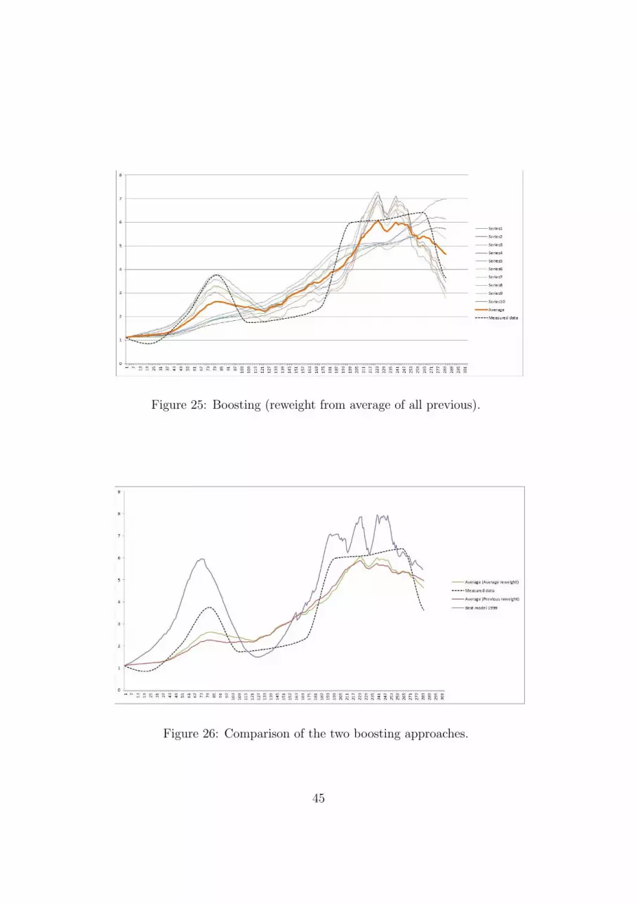
Fig 10. Boosting (reweight from previous)
Fig 11. Boosting (reweight from average of all previous)
In general, it can be clearly seen (Fig 12), that the boosting method outperforms the
best model reported by the ProBMoT. Furthermore, the choice of a method for the
reweighting procedure is not significant. Even though, the method which reweights
with the average of all past experience is slightly better, computationally is more
expensive than the other method.
Figure 25: Boosting (reweight from average of all previous).
Fig 12 Comparison of the two boosting approaches
4. CONCLUSION
Figure 26: Comparison of the two boosting approaches.
45
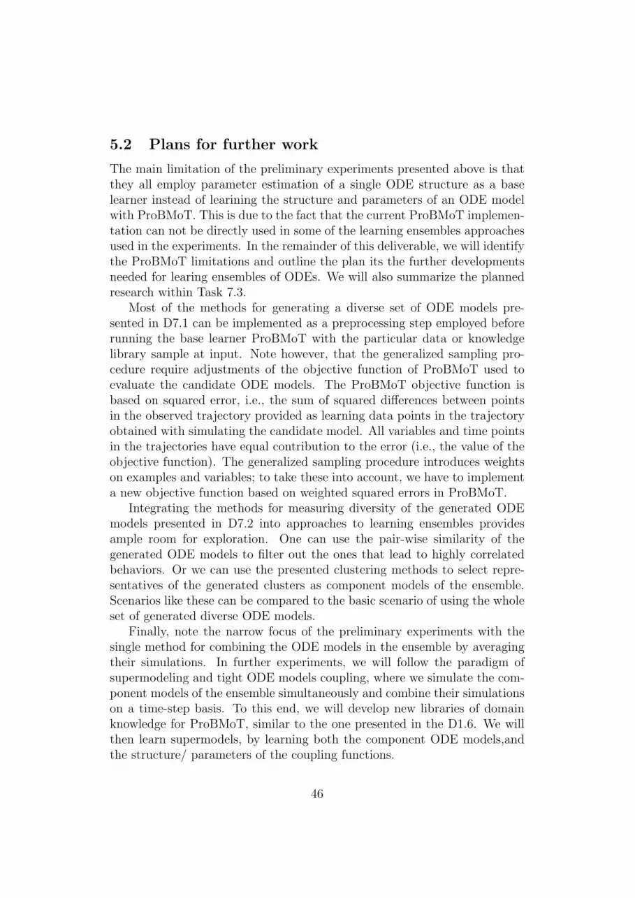
5.2 Plans for further work
The main limitation of the preliminary experiments presented above is thatthey all employ parameter estimation of a single ODE structure as a baselearner instead of learining the structure and parameters of an ODE modelwith ProBMoT. This is due to the fact that the current ProBMoT implemen-tation can not be directly used in some of the learning ensembles approachesused in the experiments. In the remainder of this deliverable, we will identifythe ProBMoT limitations and outline the plan its the further developmentsneeded for learing ensembles of ODEs. We will also summarize the plannedresearch within Task 7.3.
Most of the methods for generating a diverse set of ODE models pre-sented in D7.1 can be implemented as a preprocessing step employed beforerunning the base learner ProBMoT with the particular data or knowledgelibrary sample at input. Note however, that the generalized sampling pro-cedure require adjustments of the objective function of ProBMoT used toevaluate the candidate ODE models. The ProBMoT objective function isbased on squared error, i.e., the sum of squared differences between pointsin the observed trajectory provided as learning data points in the trajectoryobtained with simulating the candidate model. All variables and time pointsin the trajectories have equal contribution to the error (i.e., the value of theobjective function). The generalized sampling procedure introduces weightson examples and variables; to take these into account, we have to implementa new objective function based on weighted squared errors in ProBMoT.
Integrating the methods for measuring diversity of the generated ODEmodels presented in D7.2 into approaches to learning ensembles providesample room for exploration. One can use the pair-wise similarity of thegenerated ODE models to filter out the ones that lead to highly correlatedbehaviors. Or we can use the presented clustering methods to select repre-sentatives of the generated clusters as component models of the ensemble.Scenarios like these can be compared to the basic scenario of using the wholeset of generated diverse ODE models.
Finally, note the narrow focus of the preliminary experiments with thesingle method for combining the ODE models in the ensemble by averagingtheir simulations. In further experiments, we will follow the paradigm ofsupermodeling and tight ODE models coupling, where we simulate the com-ponent models of the ensemble simultaneously and combine their simulationson a time-step basis. To this end, we will develop new libraries of domainknowledge for ProBMoT, similar to the one presented in the D1.6. We willthen learn supermodels, by learning both the component ODE models,andthe structure/ parameters of the coupling functions.
46
6 Conclusion
The objective of WP7 is to develop methods for computational scientificdiscovery that can learn complete supermodels (ensembles of ODE models)of dynamical systems. The supermodels are expected to be built in threephases: generate diverse models, select a set of complementary models, andlearn the interconnections between the constituent models of an ensemble.While this decomposition allows for independent development of the differentcomponents of the approaches to learning ensembles of ODE models, wecan evaluate their performance only when we integrate them into completeapproaches to learning ensembles. Thus, the issues related to finding workingcombinations of the methods developed and proposed within D7.1 and D7.2are still open and are to be resolved within the task T7.3.
Task 7.1 is concerned with generating a diverse set of ODE models. Togenerate a diverse set of models, we adapt existing sampling approaches fromthe area of ensemble learning. The specificities of the task of subsamplingan observed behavior of a dynamic system are taken into account. After dif-ferent subsamples are generated, the base learner ProBMoT can be appliedto learn different ODE models from them. The approaches adapted includesubsampling the instance space and subsampling the feature space. Alongthe first dimension, we consider the selection of random sub-intervals of theobservation period. We adapt bootstrap sampling and error-weighted sam-pling for the case of time-series data. Preliminary experiments with learningODE models (same structure, different parameters) have been conductedwith some of these adaptations within Task 7.3.
Along the second dimension, we consider random sub-sampling of thevariable space, as in random subspaces. We consider combining it with boot-strap sampling of the instance space. Moreover, we propose a generalizedsub-sampling approach, which simultaneously subsamples both the instanceand the feature space. Finally, we also suggest to consider a procedure forsampling the template entities and processes from the library of backgroundknowledge used by ProBMoT as a way to generate a set of diverse ODEmodels. Further experiments within Taks 7.3 are needed to evaluate theperformance of these methods in the context of learning supermodels.
Task 7.2 is concerned with selecting a set of complementary ODE models.To address this task, we first attempt to define the notion of diversity for ODEmodels. While model diversity has been extensively studied in the context ofensemble models, the bulk of work has considered the task of classification.For regression, co-variance is used as a measure of similarity/diversity ofconstituent models of an ensemble. To the best of our knowledge, the notionof diversity has not been studied in the context of ensembles of ODE models.
47
Our definition of diversity is based on similarity measures between dy-namic system behaviors, i.e., multi-variate time series. These are based onsimilarity measures for single time-series. The similarities of correspondingtime-series pairs in two behaviors are aggregated into an overall similarity.We consider a range of similarity measures for time-series, which we have col-lected and implemented. We explore their use in clustering of ODE modelsand observed behaviors of dynamic systems. These clustering experimentsare important in the context of further work within Task 7.3, where a setof appropriate models has to be chosen for inclusion in the ensemble. Af-ter clustering a larger set of models, representative models from each clustercould be chosen for combination, for example.
48
References
[1] R. Agrawal and C. Faloutsos and A. Swami. (1993). Efficient SimilaritySearch In Sequence Databases. In: FODO ’93 Proceedings of the 4thInternational Conference on Foundations of Data Organization and Al-gorithms, pp. 69–84.
[2] Atanasova, N., Todorovski, L., Dzeroski, S., Rekar-Remec, S., Recknagel,F., Kompare, B. (2006). Automated modelling of a food web in Lake Bledusing measured data and a library of domain knowledge. Ecol. model. vol.194, no. 1-3, pp. 37-48
[3] L. Breiman. (1996) Bagging predictors. Machine Learning, 24(2):123–140.
[4] L. Breiman. (2001) Random forests. Machine Learning, 45(1):5–32.
[5] W. Bridewell, P. Langley, L. Todorovski, and S. Dzeroski. (2008) Induc-tive process modeling. Machine Learning, 71: 1–32.
[6] Chen, Lei and ?zsu, M. Tamer and Oria, Vincent. Robust and fast simi-larity search for moving object trajectories, In: Proceedings of the 2005ACM SIGMOD international conference on Management of data (NewYork, NY, USA: ACM, 2005), pp. 491–502.
[7] Chen, Lei and Ng, Raymond. On the marriage of Lp-norms and editdistance. In: VLDB ’04: Proceedings of the Thirtieth international con-ference on Very large data bases, pp. 792–803.
[8] M. Collins, and S. Knight. (Eds) (2007) Ensembles and probabilities: anew era in the prediction of climate change. Theme Issue. PhilosophicalTransactions of the Royal Society, 365(1857).
[9] Cerepnalkoski D., Taskova K., Todorovski L., Atanasova N., DzeroskiS. (2012). The influence of parameter fitting methods on model struc-ture selection in automated modeling of aquatic ecosystems. EcologicalModeling, In press.
[10] Dietterich T.G. (2000). Ensemble methods in machine learning. In:Proc. of the 1st international workshop on multiple classifier systems(MCS ?00), Springer, Berlin, pp. 1–15
[11] S. Dzeroski, and L. Todorovski. (1993) Discovering dynamics. In Pro-ceedings of the Tenth International Conference on Machine Learning,pages 97–103. Morgan Kaufmann, San Mateo, CA.
49
[12] Faloutsos, Christos and Ranganathan, M. and Manolopoulos, Yannis.(1994) Fast subsequence matching in time-series databases. In: Proceed-ings of the 1994 ACM SIGMOD international conference on Managementof data, pp. 419–429.
[13] L. Todorovski, and S. Dzeroski (1997) Declarative bias in equation dis-covery. In: Fisher DH (ed) Proceedings of the Fourteenth InternationalConference on Machine Learning, pp 376– 384. Morgan Kaufmann, SanMateo.
[14] S. Dzeroski, and L. Todorovski. (2002) Encoding and using domainknowledge on population dynamics for equation discovery. In: L. Mag-nani, N.J. Nersessian, C. Pizzi (eds) Logical and Computational Aspectsof Model?Based Reasoning, pp 227–247. Kluwer, Dordrecht.
[15] S. Dzeroski, and L. Todorovski. (2003) Learning population dynamicsmodels from data and domain knowledge. Ecological Modelling, 170: 129–140.
[16] S. Dzeroski, and L. Todorovski. (Eds) (2007) Computational discoveryof scientific Knowledge. Lecture Notes in Computer Science, vol. 4660.Springer
[17] Dzeroski S., Panov P., Zenko B. (2009). Machine learning ensemblemethods. Encyclopedia of complexity and systems science. New York:Springer, pp. 5317?-5325
Yoav Freund, Robert E Schapire. (1997). A Decision-Theoretic General-ization of On-Line Learning and an Application to Boosting, Journal ofComputer and System Sciences, Volume 55: 119–139
[18] Das, Gautam and Gunopulos, Dimitrios and Mannila, Heikki. (1997).Finding similar time series. In: Komorowski, Jan and Zytkow, Jan, ed.,Principles of Data Mining and Knowledge Discovery vol. 1263, pp. 88–100.
[19] Golay, Xavier and Kollias, Spyros and Stoll, Gautier and Meier, Dieterand Valavanis, Anton and Boesiger, Peter. (1998). A new correlation-based fuzzy logic clustering algorithm for FMRI. Magnetic Resonance inMedicine 40, 2, pp. 249–260.
[20] Grabisch M., Marichal J.?L., Mesiar R., Pap E. (2009). AggregationFunctions. Cambridge University Press, Encyclopedia of Mathematicsand its Applications, No 127
50
[21] Hirschberg, D. S. (1975). A linear space algorithm for computing maxi-mal common subsequences. Commun. ACM 18, 6, pp. 341–343.
[22] T.K. Ho. (1998) The random subspace method for constructing decisionforests. IEEE Transactions on Pattern Analysis and Machine Intelligence,20(8):832–844.
[23] Peter Korosec and Jurij Silc and Bogdan Filipic. The differential ant-stigmergy algorithm. Information Sciences 192, pp. 82–97.
[24] Kuncheva L.I., Whitaker C.J. (2003). Measures of diversity in classifierensembles and their relationship with the ensemble accuracy. MachineLearning 51(2):181–207
[25] Li G.?G., Wang Z.?Z. (2009). Evaluation of similarity measures for geneexpression data and their correspondent combined measures. Interdisci-plinary Sciences: Computational Life Sciences (1): 72–80
[26] Levenshtein, V. I. (1966) Binary codes capable of correcting deletions,insertions, and reversals. Soviet Physics Doklady, 707–710.
[27] Li, Gang-Guo and Wang, Zheng-Zhi. (2009). Evaluation of similaritymeasures for gene expression data and their correspondent combinedmeasures. Interdisciplinary Sciences: Computational Life Sciences 1, pp.72-80.
[28] T. Mitchell. (1997) Machine Learning. McGraw Hill.
[29] J.M. Murphy, B.B.B. Booth, M. Collins, G.R. Harris, D.M.H. Sexton,and M.J. Webb. (2007) A methodology for probabilistic predictions ofregional climate change from perturbed physics ensembles. PhilosophicalTransactions of the Royal Society, 365: 1993?-2028.
[30] O. Okun, and G. Valentini. (Eds) (2007) Supervised and UnsupervisedEnsemble Methods and their Applications. Springer, Berlin.
[31] P. Panov, and S. Dzeroski. (2007) Combining bagging and random sub-spaces to create better ensembles. Lecture Notes in Computer Science,vol. 4723, pp. 118–129.
[32] Ivan Popivanov. (2002). Similarity search over time series data usingwavelets. In: Proceedings of the 18th International Conference on DataEngineering 2002, pp. 212–221.
51
[33] Sakoe H., Chiba S. (1978). Dynamic programming algorithm optimiza-tion for spoken word recognition. Transactions on Acoustic, Speech, andSignal Processes (26): 43–49
[34] Schapire R.E. (1990).The strength of weak learnability. Machine Learn-ing 5(2):197–227
[35] Silk, D. and Kirk, P. D. W. and Barnes, C. P. and Toni, T. and Rose,A. and Moon, S. and Dallman, M. J. and Stumpf, M. P. H.. (2011).Designing attractive models via automated identification of chaotic andoscillatory dynamical regimes. Nature Communications 2.
[36] D.J. Stensrud, J.W. Bao, T. T. Warner. (2000) Using Initial Conditionand Model Physics Perturbations in Short?Range Ensemble Simulationsof Mesoscale Convective Systems. Monthly Weather Review, 128: 2077–2107.
[37] L. Todorovski, and S. Dzeroski. (2006) Integrating knowledge?drivenand data?driven approaches to modeling. Ecological Modelling 194:3–13.
[38] Thai Quang Tung and Doheon Lee. (2010). PSExplorer: whole param-eter space exploration for molecular signaling pathway dynamics, Bioin-formatics 26, 19, pp. 2477–2479.
[39] Van den Berge L. A., Selten F. M., Wiegerinck W., Duane G. S. (2011).A multi?model ensemble method that combines imperfect models throughlearning. Earth System Dynamics, Vol. 2, No. 1., pp. 161?-177
[40] W. Wiegerinck, M. Mirchev, W. Burgers, and F. Selten. (2012). Super-modeling dynamics and learning mechanisms. In L. Kocarev (ed.): In-formation consensus and synchronization in complex networks. Springer,Berlin.
[41] Wolpert D.H. (1992). Stacked generalization. Neural Networks 5(2), pp.241–259
[42] S.C. Yang, D. Baker, H. Li, K. Cordes, M. Huff, G. Nagpal, E. Okereke,J. Villafane, E. Kalnay, and G.S. Duane. (2006) Data assimilation assynchronization of truth and model: Experiments with the three?variableLorenz system. Journal of the Atmospheric Sciences, 63:2340?-2354.
52


