Embed Size (px)
Citation preview
ČESKÉ VYSOKÉ UČENÍ TECHNICKÉ V PRAZE
Fakulta stavební
Katedra mechaniky
Subsoil Influenced by Groundwater Flow
Podloží ovlivněné prouděním podzemní vody
DISERTAČNÍ PRÁCE
Ing. Miroslav Brouček Doktorský studijní program: Stavební inženýrství
Studijní obor: Fyzikální a materiálové inženýrství Školitel: prof. Ing. Pavel Kuklík, CSc.
Praha, 2013

ČESKÉ VYSOKÉ UČENÍ TECHNICKÉ V PRAZE Fakulta stavební Thákurova 7, 166 29 Praha 6
PROHLÁŠENÍ
Jméno doktoranda: Miroslav Brouček Název disertační práce: Podloží ovlivněné prouděním podzemní vody Prohlašuji, že jsem uvedenou doktorskou disertační práci vypracoval/a samostatně pod vedením školitele prof. Ing. Pavla Kuklíka, CSc. Použitou literaturu a další materiály uvádím v seznamu použité literatury. Disertační práce vznikla v souvislosti s řešením projektů: MSM 680770001, GA103/07/0246, GA103/08/1119, GA103/04/11134, GA103/08/1617 a CTU0700811. v Praze dne 28.2.2013 podpis

ACKNOWLEDGEMENT
At first I would like to express my gratitude to prof. Ing. Pavel Kuklik, CSc. for his never ending support, patience and advices during my entire study. I also would like to thank colleagues from Centre of Experimental Geotechnics for helping me with the experiments and providing many useful tools and advices during my laboratory experiments and colleagues from the Department of Geotechnics for the possibility to use their software for numerical modelling and measuring devices for lateral pressures measurement. My thanks also belong to Ing. Martin Lidmila, Ph.D. for his support during the large scale experiments and to doc. Ing Ladislav Satrapa, CSc. for his kindness, which allow me to use the laboratory of Water Management Experimental Centre for my experiments. I wish to thank all other colleagues for their valuable comments, advices and excellent working environment. Most importantly, I would like to express my deepest thanks to my wife Michaela and my parents for their support and help which allow me to concentrate fully on the subject of the interest. I would also like to acknowledge the research project MSM 680770001 and grants GA103/07/0246, GA103/08/1119, GA103/04/11134 and 103/08/1617. Part of the work was produced under kind support of the CTU internal grant CTU0700811.
TABLE OF CONTENTS
List of Figures iv
List of Tables vii
Abstract (English) viii
Abstract (Czech) x
Chapter 1: Introduction 1
1.1. Motivation……………………………………………………………… 1
1.2. Area of interest and methodical approach……………………………… 3
1.3. Historical background………………………………………………….. 4
Chapter 2: Saturated and unsaturated soils 6
2.1. General poromechanics problem formulation…………………………. 6
2.1.1. Monolithical approach for coupled processes………………….. 9
2.1.2. Staggered approach for coupled processes…………………….. 10
2.2. Fundamental principles of unsaturated soil mechanics………………… 11
2.2.1. Physical foundations and measuring techniques………………. 12
2.2.2. Stress state variables…………………………………………… 14
2.3. Numerical modelling – constitutive models…………………………… 15
2.3.1. Modified Cam-Clay constitutive model……………………….. 17
2.3.2. Hypoplasticity for clays………………………………………… 19
2.3.3. Hypoplasticity for unsaturated soils……………………………. 21
Chapter 3: Internal erosion 23
3.1. Loss or detachment of particles………………………………………… 24
3.2. Preferential flow vs. average flow……………………………………… 26
Table of contents ii
Chapter 4: Experimental analysis 28
4.1. Tested soils……………………………………………………………... 29
4.2. Static plate load test – full scale………………………………………… 33
4.2.1. Selected commented results for G2 specimens ………………… 36
4.2.2. Selected commented results for F5 specimens…………………. 40
4.3. Suction cancellation under constant load – full scale…………………... 43
4.3.1. Selected commented results for G2 specimens………………… 45
4.3.2. Selected commented results for F5 specimens…………………. 47
4.4. Wetting under constant load – small scale………………………..……. 50
4.5. Erosion under extremely high gradients………………………………... 52
4.6. Full scale experiment enhancement…………………………………….. 58
Chapter 5: Influence zone theory 60
5.1. Basic principles and governing idea……………………………………. 61
5.2. Influence zone depth estimation………………………………………... 62
5.3. Influence zone theory and groundwater table variations……………….. 64
Chapter 6: Practical applications and numerical simulations 66
6.1. Influence zone change and elastic layer theory ………………………... 66
6.1.1. Static plate load tests……………………………………………. 66
6.1.2. Dilatometric measurements and analysis……………………….. 69
6.2. General knowledge about unsaturated soils behaviour…………………. 73
6.2.1. Flood protection measures……………………………………… 73
6.2.2. Infiltration from large impermeable areas……………………… 74
6.3. Risk analysis for flood events………………………………………….. 75
6.4. Numerical modelling……….........……………………………………... 79
6.4.1. Modified Cam Clay (SIFEL) …………………………………... 79
6.4.2. Hypoplasticity for clays (Geo 5) ……………………………….. 84
6.4.3. Hypoplasticity for unsaturated soils (PLAXIS) ………………... 86
Chapter 7: Conclusions and future perspectives 87
Bibliography 89

Table of contents iii
List of author’s publications 96
Appendix A: Influence zone - software solutions 101
Appendix B: Plate load tests on poorly graded gravel 114
Appendix C: Plate load tests on silt loams 133
Appendix D: Small scale experiments 139
Appendix E: Erosion under extremely high gradients 141
LIST OF FIGURES
Fig. 1. Staggered approach - descriptive scheme ……………………………………. 10
Fig. 2. Comparison of measured (Thu et al., 2007) and calculated (Sheng, 2011 –
other authors are included) data for triaxial test on compacted kaolin clay
under 200 kPa confining pressure …………………………………………… 16
Fig. 3. Normal consolidation and swelling line describing the behaviour of soil
during isotropic compression test …………………………………………… 18
Fig. 4. Yield surface of the Cam-Clay model in the mean-deviatoric stress plane …. 19
Fig. 5. Definition of parameters N; * and * (Masin, 2005) ………………………... 20
Fig. 6. Grain distribution of poorly graded gravel (three specimens) ……………...... 30
Fig. 7. Grain distribution of silt loam (three specimens) ……………………………. 31
Fig. 8. Grain distribution of poorly graded sand (three specimens) ………………… 32
Fig. 9. Grain distribution of silty sand (three specimens) …………………………… 32
Fig. 10. Grain distribution of sandy silt (three specimens) ………………………….. 32
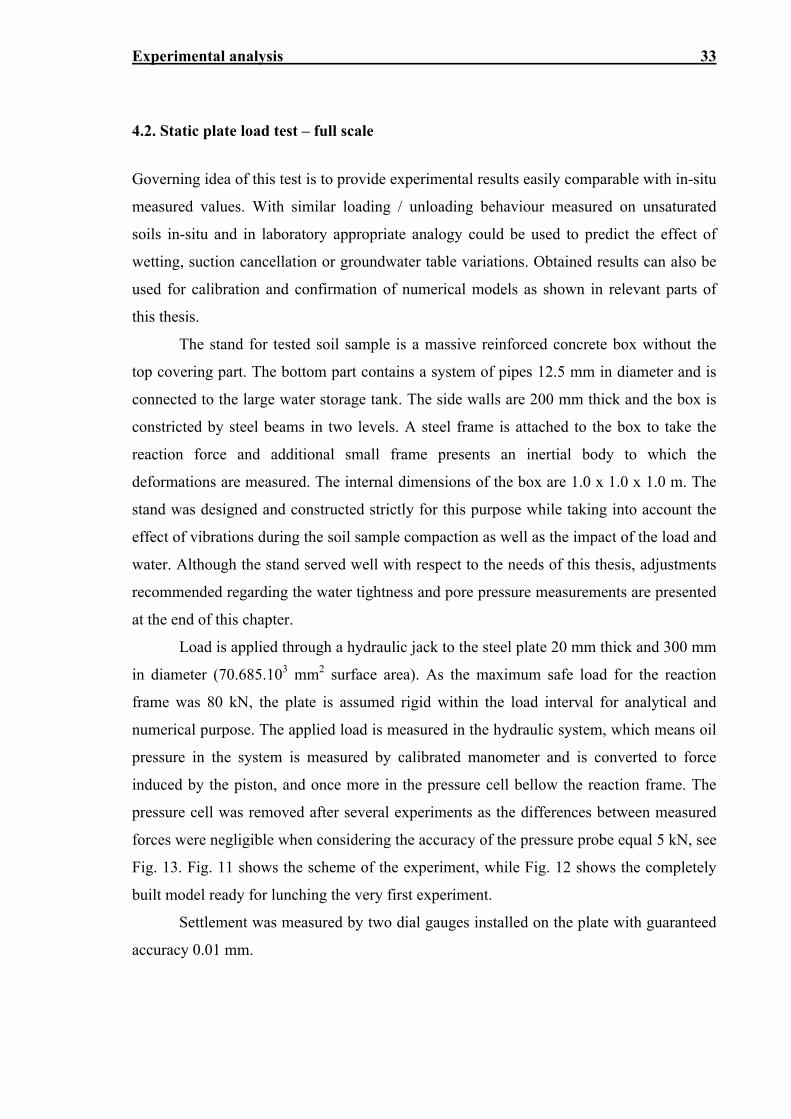
Fig. 11. Static plate load experiment – scheme ……………………………………... 34
Fig. 12. Full scale plate load test on the soil specimen ……………………………… 34
Fig. 13. Full scale plate load test on the soil specimen ……………………………… 35
Fig. 14. Results from first experiment on dry but compacted (dense) G2-GP
specimen (SM1 and SM2 stands for dial gauge no. one and two) …………... 36
Fig. 15. Results from experiment on dry but compacted (dense) G2-GP specimen
with shear zone displacement (immediate response can be observed; SM1
and SM2 stands for dial gauge no. one and two) ……………………………. 37
Fig. 16. Results from experiment on dry but compacted (dense) G2-GP specimen
with creep behaviour at 1015 kPa (SM1 and SM2 stands for dial gauge no.
one and two) ………………………………………………………………… 38
Fig. 17. Creep behaviour at 1015 kPa for G2 specimen (SM1 and SM2 stands for
dial gauge no. one and two) …………………………………………………. 38
Fig. 18. Three consecutive dry experiments – the permanent deformation cleared … 39
List of figures v
Fig. 19. Three consecutive dry experiments – the permanent deformation kept ……. 39
Fig. 20. Results from experiment on unsaturated F5 specimen under constant
suction condition (SM1 and SM2 stands for dial gauge no. one and two) ….. 40
Fig. 21. Three consecutive dry experiments – the permanent deformation kept ……. 41
Fig. 22. Vertical load vs. lateral pressure induced on the side wall …………………. 42
Fig. 23. First determining hour of the creep behaviour of F5 specimen (SM1 and
SM2 stands for dial gauge no. one and two) ………………………………… 42
Fig. 24. Improved stand for plate load test experiment including groundwater table
variation – scheme …………………………………………………………... 43
Fig. 25. Fully equipped stand for plate load test with shear zone and lateral pressure
measurement ………………………………………………………………… 44
Fig. 26. Detail view on the analogue settlement measuring devices (later on digital) 44
Fig. 27. Full scale wetting under constant load experiment (SM1 and SM2 stands
for dial gauge no. one and two) ……………………………………………... 45
Fig. 28. Full scale wetting under constant load experiment - time factor (SM1 and
SM2 stands for dial gauge no. one and two) ………………………………… 46
Fig. 29. Loading paths of subsequent experiments on the same specimen ………… 47
Fig. 30. Full scale wetting under constant load experiment (SM1 and SM2 stands
for dial gauge no. one and two) ……………………………………………... 48
Fig. 31. Full scale wetting under constant load experiment – time factor (SM1 and
SM2 stands for dial gauge no. one and two) ………………………………… 49
Fig. 32. Full scale dry experiment 3 months after wetting ………………………….. 49
Fig. 33. Full scale dry experiment 3 months after wetting – time factor and lateral
pressures ……………………………………………………………………... 50
Fig. 34. Small scale wetting under constant load experiment – scheme …………….. 51
Fig. 35. Small scale wetting under constant load experiment – example of results for
silty sand (siSa) ……………………………………………………………… 52
Fig. 36. Internal erosion experiment – scheme ……………………………………… 53
Fig. 37. Example of collapse of the specimen ………………………………………. 54
Fig. 38. Flow and settlement before collapse during the second stage ……………... 55
Fig. 39. Settlement of the weight for the internal erosion experiment with
interruptions …………………………………………………………………. 55
Fig. 40. Flow-time graph for the internal erosion experiment form Fig. 39 ………… 56
Fig. 41. Internal erosion experiment – typical result SP (grain distribution) ……….. 56
List of figures vi
Fig. 42. Internal erosion experiments - cut through specimens after collapse ………. 57
Fig. 43 The governing idea of the influence zone depth calculation (Kuklik, 2011) .. 61
Fig. 44. Fr(β) function for circular load area ………………………………………... 63
Fig. 45. F (β) function for rectangular load area and strip footing ………………….. 64
Fig. 46 Numerical simulation of dilatometric test – mesh before deformation and
detail of the contact during loading …………………………………………. 71
Fig. 47 Dilatometer test in borehole Va-B-03/04s, 986.5 m depth, chlorite schist.
Graphical representation from the DilatoII software program: average from
deformation measurements of all three extensometers (Zalesky et al., 2006) . 71
Fig. 48. Example of Loss functions for different categories of buildings
(Satrapa et al., 2006) ………………………………………………………… 76
Fig. 49. Danger zones for buildings evaluated according to USBR (1988) for flood
in the year 2002 in Veselí n. Lužnicí Town and locations of buildings with
severe structural damage (Broucek and Kuklik, 2006) ……………………… 77
Fig. 50. Absolute value of displacement and deformed mesh (left – scaled 10x) and
plastic strains (right) for the first approach and load 500 kPa ………………. 80
Fig. 51. Horizontal stress (left) and vertical stress (right) for the first approach and
load 500 kPa …………………………………………………………………. 81
Fig. 52. Horizontal (left) and vertical (right) displacement for the first approach and
load 500 kPa …………………………………………………………………. 81
Fig. 53. Absolute value of displacement and deformed mesh (left – scaled 50x) and
plastic strains (right) for the second approach and load 500 kPa …………… 82
Fig. 54. Horizontal stress (left) and vertical stress (right) for the second approach
and load 500 kPa …………………………………………………………….. 82
Fig. 55. Horizontal (left) and vertical (right) displacement for the second approach
and load 500 kPa …………………………………………………………….. 83
Fig. 56. Results comparison with full scale experiment …………………………….. 83
Fig. 57. Horizontal stress (left) and vertical stress (right) for the load 500 kPa …….. 85
Fig. 58. Horizontal (left) and vertical (right) displacement on deformed specimen
for the load 500 kPa …………………………………………………………. 85
Fig. 59. Results comparison with full scale experiment …………………………….. 86
LIST OF TABLES
Tab. 1. Parameters required by used Modified Cam Clay model …………………... 19
Tab. 2. Parameters required by used Hypoplastic model for clays …………………. 20
Tab. 3. Parameters required by used hypoplastic model for unsaturated soils ……... 22
Tab. 4. Characteristics of tested soil ………………………………………………... 30
Tab. 5. Classification of small scale specimens …………………………………….. 31
Tab. 6 Settlement increase due to repeated wetting ………………………………… 46
Tab. 7. Results summary ……………………………………………………………. 58
Tab. 8. Summary of experimental data and calculated secant moduli ……………… 67
Tab. 9. Static plate load test on G2 soil in a view of elastic layer theory …………... 68
Tab. 10. Static plate load test on F5 soil in a view of elastic layer theory ………….. 68
Tab. 11 Values of E according to new formula (Kuklik and Broucek, 2008) ……… 72
Tab. 12. Flood structural hazard categories ………………………………………… 78
Tab. 13. Additional losses to buildings ……………………………………………... 78
Tab. 14. Material parameters of MCC model ………………………………………. 80
Tab. 15. Material parameters of hypoplastic model ………………………………... 84
Czech Technical University in Prague
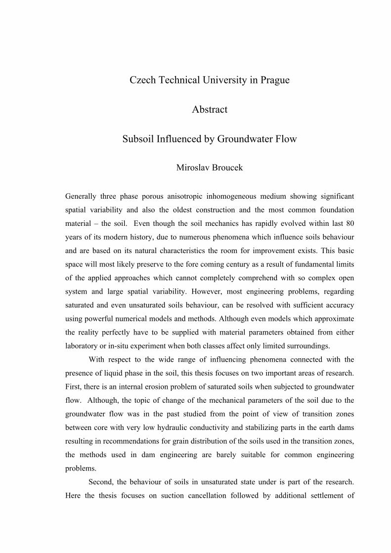
Abstract
Subsoil Influenced by Groundwater Flow
Miroslav Broucek
Generally three phase porous anisotropic inhomogeneous medium showing significant
spatial variability and also the oldest construction and the most common foundation
material – the soil. Even though the soil mechanics has rapidly evolved within last 80
years of its modern history, due to numerous phenomena which influence soils behaviour
and are based on its natural characteristics the room for improvement exists. This basic
space will most likely preserve to the fore coming century as a result of fundamental limits
of the applied approaches which cannot completely comprehend with so complex open
system and large spatial variability. However, most engineering problems, regarding
saturated and even unsaturated soils behaviour, can be resolved with sufficient accuracy
using powerful numerical models and methods. Although even models which approximate
the reality perfectly have to be supplied with material parameters obtained from either
laboratory or in-situ experiment when both classes affect only limited surroundings.
With respect to the wide range of influencing phenomena connected with the
presence of liquid phase in the soil, this thesis focuses on two important areas of research.
First, there is an internal erosion problem of saturated soils when subjected to groundwater
flow. Although, the topic of change of the mechanical parameters of the soil due to the
groundwater flow was in the past studied from the point of view of transition zones
between core with very low hydraulic conductivity and stabilizing parts in the earth dams
resulting in recommendations for grain distribution of the soils used in the transition zones,
the methods used in dam engineering are barely suitable for common engineering
problems.
Second, the behaviour of soils in unsaturated state under is part of the research.
Here the thesis focuses on suction cancellation followed by additional settlement of
Abstract ix
foundation structures in fine grained and coarse grained soils. However, the last mentioned
class is commonly referred as unaffected by suction cancellation.
The area of interest was restricted to “hydro-mechanical” point of view and does
not involve any chemical interactions between the phases inside the soil or between the
surrounding and solved domain. From the numerical modelling point of view the work is
based on continuum approach using finite element method although references the particle
float codes where appropriate.
Predominant part of the thesis concentrates on the experimental analysis and its
evaluation followed by recommendations. Stand for full scale experiments with varying
groundwater table was designed and constructed allowing for observation of all the
phenomena and possibility of estimating the effects in situ due to selected measuring
technique, i.e. static plate load test.
The results obtained from the full scale experiments proved to be very useful in
understanding and evaluating of the processes through which the groundwater influence
the behaviour of the subsoil. Some of the results obtained challenge the general
assumptions, such as fine particle loss due to groundwater flow or negligibility of the
effect of suction for coarse soils. The results were also used to calibrate and confirm the
ability of professional codes to approximate the soils behaviour during plate load tests and
suction cancellation. The success of the last mentioned simulations was very limited
despite the enormous computational time used.
Part of the thesis is devoted to search for a simple solution with large variety of use
available and understandable in common engineering practice. Here, the elastic layer
theory with adopted varying influence zone theory providing for fast analytical solution is
employed.
The thesis also contains recommendations for flood risk assessment, and several
comments on practical issues regarding the infiltration policy for large impermeable areas
and the influence of hydraulic structures and channel improvements on adjacent areas.
České vysoké učení technické v Praze
Abstrakt
Podloží ovlivněné prouděním podzemní vody
Miroslav Brouček
Popis a porozumění procesům ovlivňujících chování či odezvu zemin v návaznosti na
přítomnost nebo pohyb podzemní vody jednoznačně přispěje ke spolehlivějšímu návrhu
základových i geotechnických konstrukcí. Jejich ignorování naopak přináší zvýšená rizika
chybného návrhu nebo posouzení a z nich vyplývající, převážně materiálové byť velmi
vysoké, škody. Přestože dnešní praxe připouští výrazné rozdíly v chování nasycených a
nenasycených zemin, je ochotná je bráti do úvahy pouze v případě zemin jemnozrnných či
raději přímo jílovitých. V experimentální části práce je pak prokázán nezanedbatelný vliv
jednotlivých jevů i pro zeminy hrubozrnné, písčité i štěrkovité.
Jakkoli se může zdát teoretická báze popisující hydraulické i mechanické jevy
v pórovitém prostředí dostatečně široká, prostor pro doplnění nebo zjednodušení jinak
velice komplexních úloh je dostatečný jak v oblasti lokalizovaného proudění v nasycené
zóně spojeného s vyplavováním částic a vnitřní erozí, tak i v oblasti modelování chování
zemin nenasycených. V disertační práci je představeno několik konstitutivních modelů
popisujících chování zemin při ustáleném i neustáleném stavu kapilárního sání včetně
nedávné kritiky stran jejich nekonsistence se základními fyzikálními prvky systému, která
zaznívá zejména z důvodu použití techniky „překladu os“ k překonání potíží s kavitačními
jevy, které nastávají při experimentech využívaných standardních měřicích technik. Práce
dále představuje stručný obecný i matematický popis vnitřní eroze a vyplavování částic.
K zúžení velmi široké zájmové oblasti podloží ovlivněného působením podzemní
vody lze přistoupit z různých úhlů pohledu v závislosti na konkrétních podmínkách
zkoumaných jevů. Předložená práce si vytyčila cíle v oblasti vnitřní stability zemin při
krátkodobém působení extrémních hydraulických gradientů a v oblasti dodatečného sedání

Abstract (Czech) xi
potažmo deformací způsobených změnou nenasyceného stavu, která může být vyvolána
extrémními přírodními událostmi i lidskou činností.
Vysoce sofistikované numerické modely dokáží dobře vystihnout chování zemin
v nenasyceném stavu. Jejich komplexnost a náročnost na výpočetní čas a na kvalifikaci
uživatele však téměř vylučují jejich širší použití v současné běžné praxi ponechávajíce jim
pouze oblasti akademického bádání a zpětných analýz. Modely řešící úlohy v prostředí
nasyceném, případně nenasyceném ovšem bez možnosti změny sání coby stavové
proměnné, mají výrazně rozsáhlejší oblast působení, byť i zde je možné pozorovat příklon
k jednoduchým a ověřeným modelům Mohr-Coulomba či Drucker-Pragera i přes širokou
nabídku modelů kritického stavu.
Práce si vytkla mimo další cíle i zpracování doporučení aplikovatelných na
problémy běžné inženýrské praxe. Z tohoto důvodu je hlavní část práce zaměřená na
experimentální analýzu jevů na laboratorních modelech a zkoumání možností využití
analogie pro přenos pozorovaných jevů na řešení praktických úloh. Popsaný přístup je
patrný zejména na laboratorních experimentech na velkých vzorcích, které využívají
shodné postupy s in-situ měřením.
Výsledky měření byly využity pro kalibraci a ověřování schopností numerických
modelů popsat věrně provedené experimenty, a jsou i dále k dispozici dalším autorům.
Zjednodušené a zobecněné závěry vyvozené z měřených dat byly použity pro úpravu
výpočtu hloubky deformační zóny pod základy pomocí snížení předkonsolidace, návrh
rozšíření ztrátových funkcí při rizikové analýze povodňových škod, upozornění na
potenciální škody při zasakování srážkových vod z velkých ploch bez respektu
k ustálenému stavu okolí a další inženýrské úlohy.
Chapter 1
INTRODUCTION
Reductionism is true in a sense.
But it's seldom true in a useful sense.
Martin John Rees
The soil was used as a constructing and foundation material for thousands of years and so
it can be expected that its behaviour under all conditions is perfectly described, but it is
not. This is due to the spatial variability of soil content as well as the variability of
processes that influence the soil response (Terzaghi et al., 1996), (Fredlund and Rahardjo,
1993), (Shroff et al., 2003). The fact that soil is in general a three or more phases (Fredlund
and Morgenstern, 1977), (Vardoulakis, 2006) medium does not make things easier.
On the other hand nearly all the processes have been observed and, the ones having
very significant effect, described. Still there is enough space to improve the knowledge,
especially in soils which behaviour is influenced by the groundwater, where the worldwide
consensus regarding the stress state variables has not been established.
Typically the problem of particle loss due to the flow of a liquid phase can be
studied under different conditions with respect to the assumptions of the particular solution
of the problem (sand production in oil industry (Papamichos, 2006), water well production
and its walls stability, (Cividini et al., 2009) or stability of hydraulic structures such as
weirs and dams (ICOLD, 2013).
1.1. Motivation
The goals of this thesis are motivated strictly by practical issues and financial losses
resulting from neglecting the impact of changes in subsoil behaviour due to groundwater
flow in both saturated and unsaturated soil or missing standard recommendations for
involving these changes into design situations even though the standing standards (EN
Introduction 2
1997-1) require engineers to do so. The applied methodical approach, described further,
bears in mind the statement from Martin Rees (2010).
During past two decades the Czech Republic was affected by series of big flood
events which caused serious damage to many buildings and engineering construction.
When the floods passed and the damage to the buildings was studied, broad discussion
opened about the effect of the changes in the subsoil on the overall damage of the
constructions (Valenta et al., 2006), (Broucek and Kuklik, 2006). Although, the topic of
change of the mechanical parameters of the soil due to the groundwater flow was in the
past studied from the point of view of transition zones between core with very low
hydraulic conductivity and stabilizing parts in the earth dams resulting in recommendations
for grain distribution of the soils used in the transition zones (ICOLD, 1994), the methods
used in dam engineering are barely suitable for common engineering problems.
As the risk analysis, which can be considered as the only impartial mean for
evaluation the effect of floods and flood prevention projects, builds on the assessment of
the damage to the buildings, we found it important to search for solution that will clearly
state the effect of the groundwater to the building during and most importantly after the
flood events. To explain the last sentence it is to be stated that most of the structural
damage to the constructions was not caused by hydrodynamic loading and took place
sometime after the flood peak.
Another practical problem that extends the research area to unsaturated field is
damage observed on engineering structures constructed on artificially compacted soils as
well as on natural soils experiencing suction cancellation due to changed hydrogeological
conditions. The last mentioned can either be caused by accidents of water supply or sewer
system pipelines or are taking place due to infiltration systems constructed as a result of
the civil service requirement to infiltrate all of the precipitation water from large
impermeable areas (roofs, parking areas, etc.) without any respect to relevant
circumstances.
On the other hand, problems with artificially compacted soils can be usually
attributed to road and pavements built on the backfilled trenches from engineering
networks. Although only a part of the reported cases is caused by the groundwater flow
(especially vertical) and its influence on the soil (suction cancellation), due to the high
number of cases in total, it is still an important issue for study. Similar issues, additional
Introduction 3
settlements, were reported on natural soils improved with vibroflotation or sand or gravel
piles both Franki and vibroflotated type (Weng et al., 2009).
Last problem that is an active part of the motivation of this research represents
accidents and complete failures of several spillways and dam constructions. Last reported
case took place in the Slovak Republic in April 2008. It was a complete destruction of one
weir block of newly constructed weir structure while adjacent small hydroelectric plant
suffered also severe damage.
1.2. Area of interest and methodical approach
As the problem can be studied from different points of view, it has been decided to set the
area of interest to gain as much practical information and conclusions as possible while
avoiding decrease in generality of the results. All the processes are studied from the
geotechnical point of view and the selected area of interest is macroscopic level and
phenomenological approach to the processes. Following two areas of interest, their
subdivisions and corresponding goals were specified:
1. Increase in overall settlement due to suction cancellation
o Description of the process and review of relevant methods for rigorous
evaluation of the impact – Chapter 2
o Design of an experiment allowing for quantification of the impact of suction
cancellation for different soil types – Chapter 4
o Recommendations for fast evaluation of the impact using analytical
approach – Chapter 5
o Contribution to the flood risk assessment (involves both areas of interest) –
Chapter 6
o Provide experimental results for confirmation of numerical models –
Appendixes B - D
2. Internal erosion due to groundwater flow
o General description of the process – Chapter 3
o Stability assessment for soils under extremely high hydraulic gradient –
Chapter 4 and Appendix E
o Contribution to the flood risk assessment (involves both areas of interest) –
Chapter 6
Introduction 4
The area of interest was restricted to “hydro-mechanical” point of view and does
not involve any chemical interactions between the phases inside the soil or between the
surrounding and solved domain. It was also decided to avoid the conclusions available only
for high-risk, high-pay-off technologies, which in case of soils means only the oil
production industry, which works under conditions not applicable to our research.
From the numerical modelling point of view the work is based on continuum
approach using finite element method although references the particle float codes where
appropriate.
1.3. Historical background
The knowledge describing the movement or position of groundwater table in a phreatic
aquifer with high hydraulic conductivity adjacent to a river can be successfully traced back
to the ancient Egypt. The great temple of Kom Ombo stands witness to this knowledge
containing even today working well measuring water table in the river Nile (also called
Nilometer) and notes about observed flood peaks carved in stone for time periods more
than 3000 years ago.
G.J. Caesar (Caesar, 40 BC) in his commentaries about the war in Alexandria
describes the effort of Egyptian soldiers to deprive his forces of fresh water. The Egyptian
troops planned to contaminate wells of besieged Romans with brackish waters from nearby
estuaries by abstracting water from series of new wells bored around their positions. Such
actions could not be taken without deep understanding of flow through porous media
including depression curve development around wells as well as freshwater-saltwater
interface position and movement more than eighteen centuries before Henry Darcy
presented his experiments (Darcy, 1856) and started modern era in subsurface hydrology
and nearly twenty centuries before Karl Terzaghi (1936) described the stress state variable
controlling the behaviour of saturated soils.
Detailed description of the behaviour of unsaturated soil cannot be however
considered within the “historical background” as the worldwide consensus was not so far
established (Lu, 2008). The inability to derive one universal description of the unsaturated
soils behaviour is not due to the lack of need, quite the opposite is actually true, but rather
due to the complexity of the problem. As presented by Jones and Holtz (1973) the damage

Introduction 5
inflicted by unsaturated soils is in United States doubles the damage caused by
earthquakes, floods and tornados. This statement was supported by Krohn and Slosson
(1980) estimating the spendings on repair and reconstruction works induced by the damage
caused by expansive soils to exceed seven billions US dollars per annum. Similar problems
have been reported in many Asian and South American countries as well e.g. (Rodrigues et
al., 2006). Different standing approaches are introduced in the following chapter.
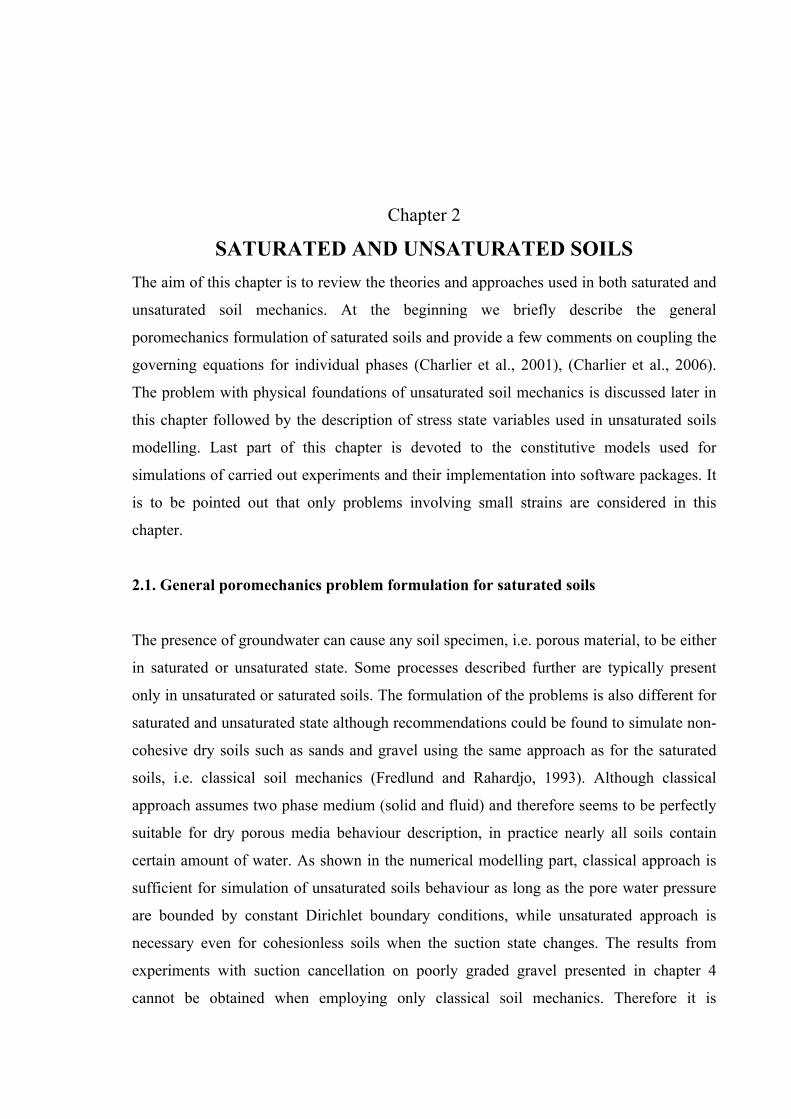
Chapter 2
SATURATED AND UNSATURATED SOILS
The aim of this chapter is to review the theories and approaches used in both saturated and
unsaturated soil mechanics. At the beginning we briefly describe the general
poromechanics formulation of saturated soils and provide a few comments on coupling the
governing equations for individual phases (Charlier et al., 2001), (Charlier et al., 2006).
The problem with physical foundations of unsaturated soil mechanics is discussed later in
this chapter followed by the description of stress state variables used in unsaturated soils
modelling. Last part of this chapter is devoted to the constitutive models used for
simulations of carried out experiments and their implementation into software packages. It
is to be pointed out that only problems involving small strains are considered in this
chapter.
2.1. General poromechanics problem formulation for saturated soils
The presence of groundwater can cause any soil specimen, i.e. porous material, to be either
in saturated or unsaturated state. Some processes described further are typically present
only in unsaturated or saturated soils. The formulation of the problems is also different for
saturated and unsaturated state although recommendations could be found to simulate non-
cohesive dry soils such as sands and gravel using the same approach as for the saturated
soils, i.e. classical soil mechanics (Fredlund and Rahardjo, 1993). Although classical
approach assumes two phase medium (solid and fluid) and therefore seems to be perfectly
suitable for dry porous media behaviour description, in practice nearly all soils contain
certain amount of water. As shown in the numerical modelling part, classical approach is
sufficient for simulation of unsaturated soils behaviour as long as the pore water pressure
are bounded by constant Dirichlet boundary conditions, while unsaturated approach is
necessary even for cohesionless soils when the suction state changes. The results from
experiments with suction cancellation on poorly graded gravel presented in chapter 4
cannot be obtained when employing only classical soil mechanics. Therefore it is
Saturated and unsaturated soils 7
important to specify the soil state prior to any numerical modelling and also to carefully
evaluate the type of the problem and select correct constitutive model.
Nowadays, large number of constitutive models can be found in the literature. The
detailed description of all used constitutive models goes beyond the scope of this thesis and
so the description is limited to several models used by the author while the detailed
description of other models presented over the last two decades can be found based on the
following example of the state-of-the-art reviews (Gens, 1996), (Wheeler and Karube,
1996), (Kohgo, 2003), (Gens et al., 2008), (Sheng and Fredlund, 2008), (Sheng et al,
2008a), (Cui and Sun, 2009) and (Gens, 2009).
Steady state seepage problems and geomechanical problems where loads are very
slowly applied are generally described by partial differential equations of elliptic type
(with the exception of localized failure in elastoplastic softening material) (Pastor and
Mira, 2002). These partial differential equations can be used for case of saturated soils but
in case of unsaturated soils where transient problems play major part the equation type is
parabolic or hyperbolic (Lewis and Schrefler, 2000), (Pastor and Merodo, 2002).
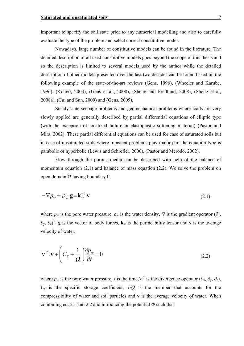
Flow through the porous media can be described with help of the balance of
momentum equation (2.1) and balance of mass equation (2.2). We solve the problem on
open domain Ω having boundary Γ.
vkg .. 1 wwwp (2.1)
where pw is the pore water pressure, ρw is the water density, is the gradient operator (∂x,
∂y, ∂z)T, g is the vector of body forces, kw is the permeability tensor and v is the average
velocity of water.
01
.
t
p
QC w
ST v (2.2)
where pw is the pore water pressure, t is the time, T is the divergence operator (∂x, ∂y, ∂z),
Cs is the specific storage coefficient, 1/Q is the member that accounts for the
compressibility of water and soil particles and v is the average velocity of water. When
combining eq. 2.1 and 2.2 and introducing the potential Φ such that
Saturated and unsaturated soils 8
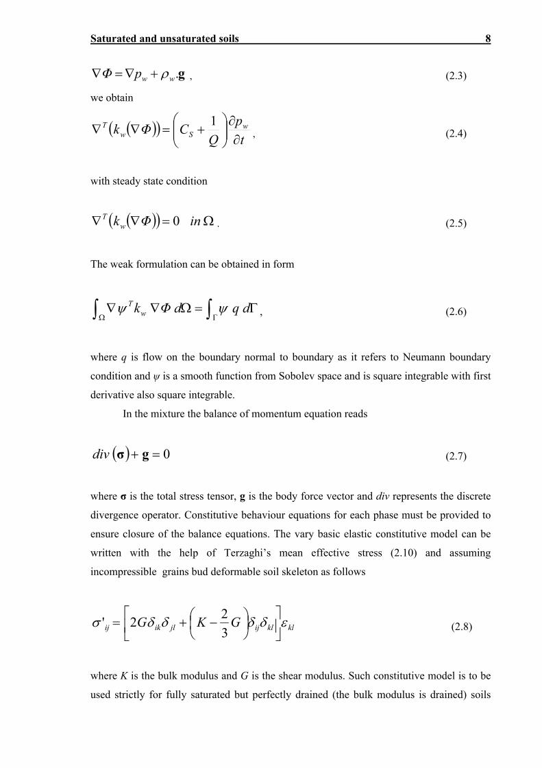
g.wwpΦ , (2.3)
we obtain
t
p
QCΦk w
SwT
1, (2.4)
with steady state condition
inΦkwT 0 . (2.5)
The weak formulation can be obtained in form
dqdΦkw
T , (2.6)
where q is flow on the boundary normal to boundary as it refers to Neumann boundary
condition and ψ is a smooth function from Sobolev space and is square integrable with first
derivative also square integrable.
In the mixture the balance of momentum equation reads
0 gσdiv (2.7)
where σ is the total stress tensor, g is the body force vector and div represents the discrete
divergence operator. Constitutive behaviour equations for each phase must be provided to
ensure closure of the balance equations. The vary basic elastic constitutive model can be
written with the help of Terzaghi’s mean effective stress (2.10) and assuming
incompressible grains bud deformable soil skeleton as follows
klklijjlikij GKG
3
22' (2.8)
where K is the bulk modulus and G is the shear modulus. Such constitutive model is to be
used strictly for fully saturated but perfectly drained (the bulk modulus is drained) soils
Saturated and unsaturated soils 9
and also only for problems that does not go over the scope of elastic deformations. More
sophisticated plastic or hypoplastic constitutive relations are described further in this
chapter.
It is also important to point out that the equations for flow and deformation of the
selected domain should not be solved separately as strong interaction between them exists.
In mass balance equation for flow there is a coupling effect present in a storage term and in
calculation of the total stress tensor is present also.
Two different approaches are today used for coupling the hydro-mechanical
processes. At first it is the monolithical approach that implies identical space and time
mashes for each coupled phenomenon. Secondly it is the staggered approach which solves
the problems separately with different time and space mesh and even with different
numerical codes and then couple them by information transfer at regular meeting point.
2.1.1. Monolithical approach for coupled processes
The monolithical approach in hydromechanical coupling presents a problem with time
dimension as well as with mixing fields of different order.
Let us assume the typical geotechnical problem of deformation of soil mass and
single fluid flow in pores. Such definition presents 4 degrees of freedom per node in 3D
analysis (3 displacements and 1 pore pressure).
The first coupling term is from mass balance. It is the storage term saying that the
change in storage is due to the volumetric change of the soil matrix
tt
S V
. (2.9)
The second coupling term is the Terzaghi’s definition of total stress (Terzaghi, 1943).
Iσσ .' wp , (2.10)
where I is the unity tensor and 'σ is the effective stress tensor. Additionally the
permeability change due to change in pore volume might be considered described by
Kozeny-Carman model e.g. (Eq. 2.11) (Kozeny, 1927), (Carman, 1937), (Davies, 1980)
Saturated and unsaturated soils 10
30
2230 /1.1/. nnnnKK (2.11)
where n is the porosity of the material, n0 is reference porosity and K0 is the hydraulic
conductivity at the reference porosity.
Using isoparametric second order finite elements and fully implicit scheme for this
problem we obtain linear stress tensor rate field (for elastic material), but the pore pressure
field is already quadratic. And so the second coupling term mixes linear and quadratic
field. Although this problem can be overcome by using quadratic shape function for the
geometry and linear shape function for the pore pressure, new problem arise with the
number of spatial integration points.
2.1.2. Staggered approach for coupled processes
The staggered approach uses the advantage of solving the coupled problems as appropriate
number of uncoupled problems leaving only the issue of information exchange between the
uncoupled processes. This approach can combine the well-known models with good
convergence and neglect the often conflicting requirements for time steps we face when
using monilithical approach (soil mechanics often requires much shorter time steps in
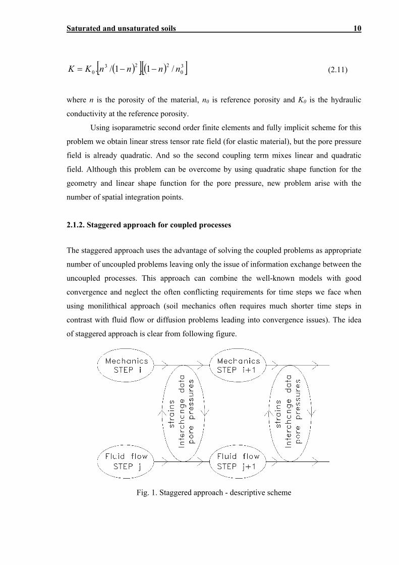
contrast with fluid flow or diffusion problems leading into convergence issues). The idea
of staggered approach is clear from following figure.
Fig. 1. Staggered approach - descriptive scheme
Saturated and unsaturated soils 11
When the spatially different meshes are used for solution of the processes or even
the finite different analysis and finite element analysis are employed, the transfer of the
information requires an interpolation scheme. This is due to the fact, that in some meshes
the information to be transferred are not available.
The accuracy of the approach is dependent on the frequency of information
transfer, which is limited by the time step, and on the type of information exchanged. The
stability and accuracy of the approach was proved by several authors eg. (Turska et al.,
1993) and (Zienckiewicz et al., 1988).
2.2. Fundamental principles of unsaturated soil mechanics
Major difference between saturated and unsaturated soils is obviously the presence of
additional non-wetting phase, usually the air. As in the case of classical soil mechanics,
solving practical engineering problems require deep understanding of shear strength,
seepage and volume change behaviour of the soil. However fundamental differences exist
in the position of theory of consolidation which is shifted towards being used in qualitative
way rather than provide clear answers about changes in total stress and corresponding
volume changes. The boundary conditions for unsaturated soils are usually also different.
Rather than change in total stress typical for saturated soils, change in flux is commonly
applied in unsaturated soils problems.
To address the problems of unsaturated soils we must understand that for
unsaturated soils the presence of negative pore-water pressures is the most typical
characteristic and vice versa soil which have negative pore-water pressures should be
described as in unsaturated state. The term “capillarity” was adopted during 1930’s
describing the observed phenomenon of vertical flux above or more precisely from stable
groundwater table, however, the theoretical concept of soil suction itself was developed in
the beginning of 20th century (Buckingham, 1907), (Richards, 1928). Further research in
this area lead to the statement that strength of unsaturated soils is heavily influenced by the
capillarity or stress state in the capillary water respectively (Hogentogler and Barber,
1941).
The definition of suction from thermodynamic context was presented in 1965 by
Aitchinson (1965) but already before that the direct shear test were performed by Donald
(1956) showing significant increase with increased matric suction. The attempts to develop
an effective stress formulation for unsaturated soils similar to saturated concept were in the
Saturated and unsaturated soils 12
center of interest during second half of 20th century resulting in several so-called effective
stress relations (Bishop, 1959 – see Eq. 2.18).
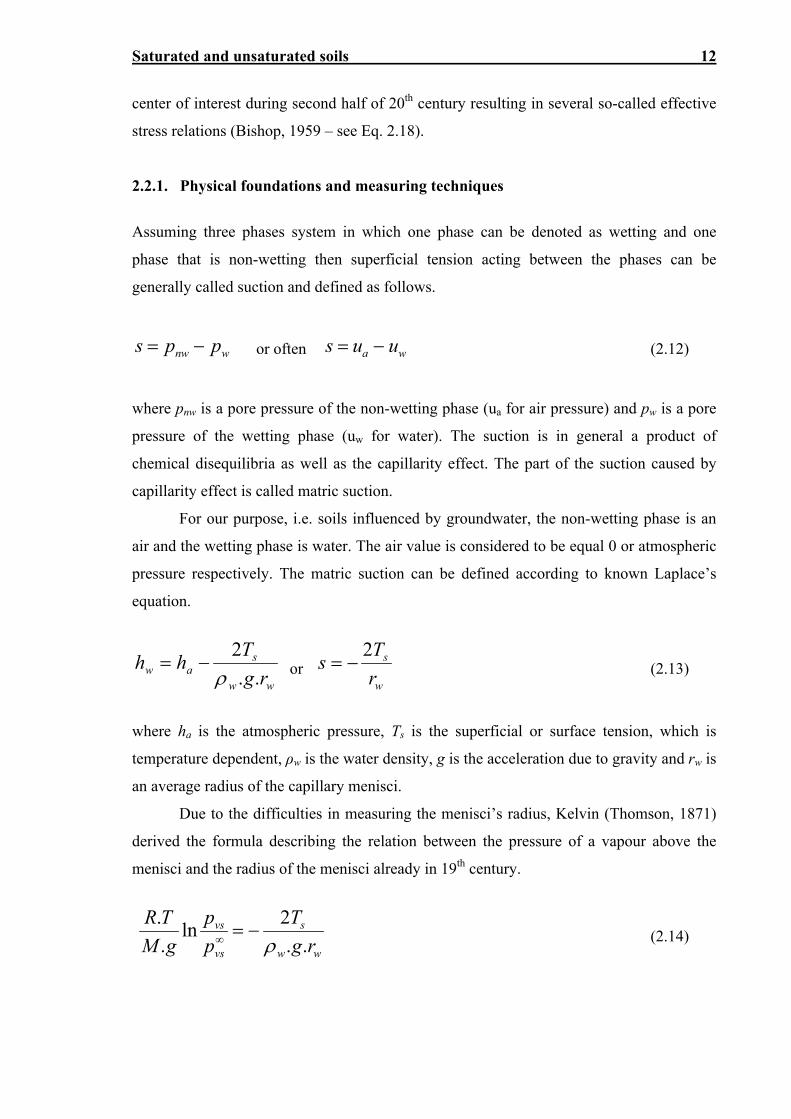
2.2.1. Physical foundations and measuring techniques
Assuming three phases system in which one phase can be denoted as wetting and one
phase that is non-wetting then superficial tension acting between the phases can be
generally called suction and defined as follows.
wnw pps or often wa uus (2.12)
where pnw is a pore pressure of the non-wetting phase (ua for air pressure) and pw is a pore
pressure of the wetting phase (uw for water). The suction is in general a product of
chemical disequilibria as well as the capillarity effect. The part of the suction caused by
capillarity effect is called matric suction.
For our purpose, i.e. soils influenced by groundwater, the non-wetting phase is an
air and the wetting phase is water. The air value is considered to be equal 0 or atmospheric
pressure respectively. The matric suction can be defined according to known Laplace’s
equation.
ww
saw rg
Thh
..
2
or
w
s
r
Ts
2 (2.13)
where ha is the atmospheric pressure, Ts is the superficial or surface tension, which is
temperature dependent, ρw is the water density, g is the acceleration due to gravity and rw is
an average radius of the capillary menisci.
Due to the difficulties in measuring the menisci’s radius, Kelvin (Thomson, 1871)
derived the formula describing the relation between the pressure of a vapour above the
menisci and the radius of the menisci already in 19th century.
ww
s
vs
vs
rg
T
p
p
gM
TR
..
2ln
.
.
(2.14)
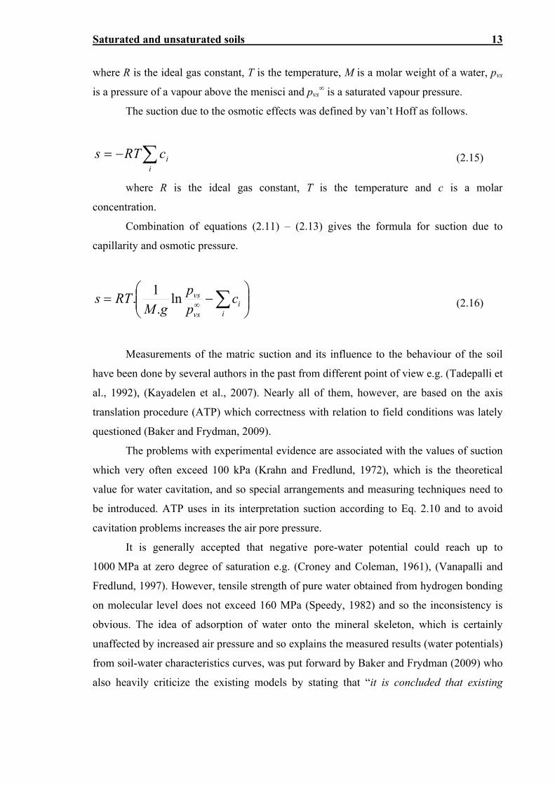
Saturated and unsaturated soils 13
where R is the ideal gas constant, T is the temperature, M is a molar weight of a water, pvs
is a pressure of a vapour above the menisci and pvs∞ is a saturated vapour pressure.
The suction due to the osmotic effects was defined by van’t Hoff as follows.
i
icRTs (2.15)
where R is the ideal gas constant, T is the temperature and c is a molar
concentration.
Combination of equations (2.11) – (2.13) gives the formula for suction due to
capillarity and osmotic pressure.
ii
vs
vs cp
p
gMRTs ln
.
1. (2.16)
Measurements of the matric suction and its influence to the behaviour of the soil
have been done by several authors in the past from different point of view e.g. (Tadepalli et
al., 1992), (Kayadelen et al., 2007). Nearly all of them, however, are based on the axis
translation procedure (ATP) which correctness with relation to field conditions was lately
questioned (Baker and Frydman, 2009).
The problems with experimental evidence are associated with the values of suction
which very often exceed 100 kPa (Krahn and Fredlund, 1972), which is the theoretical
value for water cavitation, and so special arrangements and measuring techniques need to
be introduced. ATP uses in its interpretation suction according to Eq. 2.10 and to avoid
cavitation problems increases the air pore pressure.
It is generally accepted that negative pore-water potential could reach up to
1000 MPa at zero degree of saturation e.g. (Croney and Coleman, 1961), (Vanapalli and
Fredlund, 1997). However, tensile strength of pure water obtained from hydrogen bonding
on molecular level does not exceed 160 MPa (Speedy, 1982) and so the inconsistency is
obvious. The idea of adsorption of water onto the mineral skeleton, which is certainly
unaffected by increased air pressure and so explains the measured results (water potentials)
from soil-water characteristics curves, was put forward by Baker and Frydman (2009) who
also heavily criticize the existing models by stating that “it is concluded that existing
Saturated and unsaturated soils 14
constitutive models for unsaturated soils, in their present format, are not consistent with
the basic physical elements of the system.”.
2.2.2. Stress state variables
The stress state variables are usually defined as nonmaterial variables required for
characterization of the stress conditions in particular point in time and space. From this
definition it is clear that state variables must be independent of the characteristics or
properties of the material. Constitutive models on the other hand provide relationship
between different state variables, such as stress-strain relationship (Fung, 1965).
Constitutive models therefore must incorporate physical properties of the material.
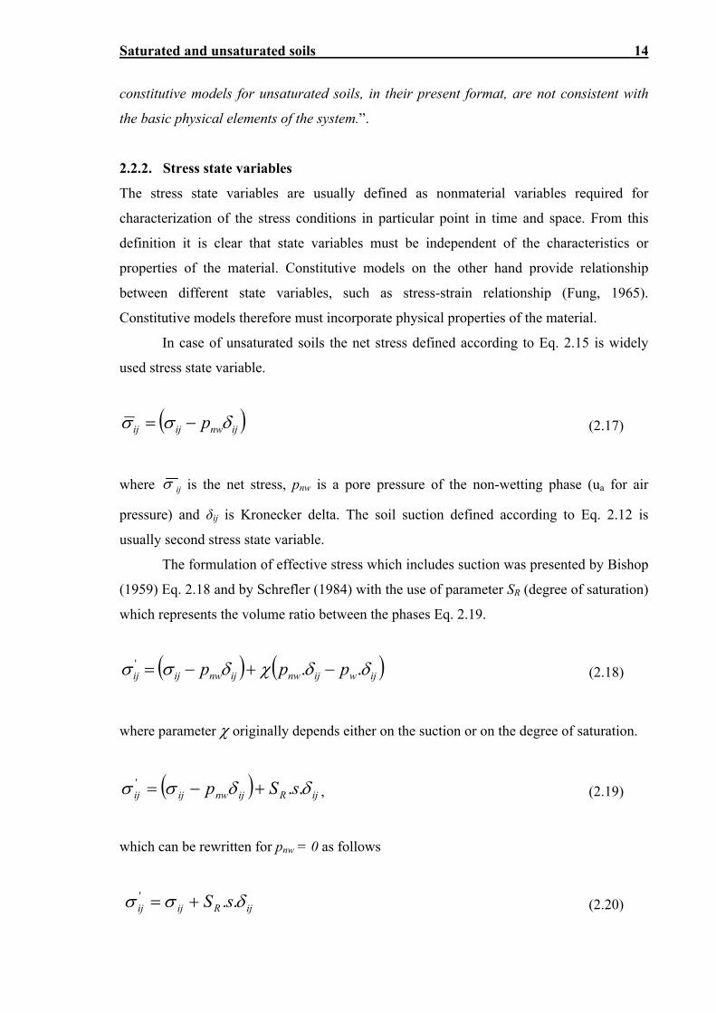
In case of unsaturated soils the net stress defined according to Eq. 2.15 is widely
used stress state variable.
ijnwijij p (2.17)
where ij is the net stress, pnw is a pore pressure of the non-wetting phase (ua for air
pressure) and δij is Kronecker delta. The soil suction defined according to Eq. 2.12 is
usually second stress state variable.
The formulation of effective stress which includes suction was presented by Bishop
(1959) Eq. 2.18 and by Schrefler (1984) with the use of parameter SR (degree of saturation)
which represents the volume ratio between the phases Eq. 2.19.
ijwijnwijnwijij ppp ..' (2.18)
where parameter originally depends either on the suction or on the degree of saturation.
ijRijnwijij sSp ..' , (2.19)
which can be rewritten for pnw = 0 as follows
ijRijij sS ..' (2.20)
Saturated and unsaturated soils 15
From the above described variables and combinations, three different approaches can be recognized when pursuing volume change behaviour.
a) net stress and suction (e.g. Fredlund and Rahardjo, 1993) – independent variables
b) effective stress (e.g. Nuth and Laloui, 2007)– combines both variables into one
c) SFG approach (Sheng et al., 2008b) – compromise approach
All of these approaches are used not only to describe volume change behaviour, but also when solving shear strength based problems as change of shear strength induced by change in the degree of saturation is often primary cause of landslides.
2.3. Numerical modelling – constitutive models
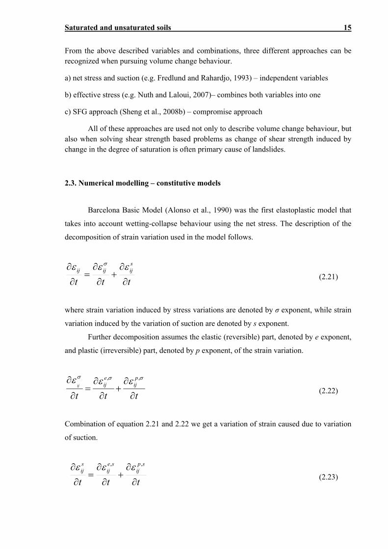
Barcelona Basic Model (Alonso et al., 1990) was the first elastoplastic model that
takes into account wetting-collapse behaviour using the net stress. The description of the
decomposition of strain variation used in the model follows.
ttt
sijijij
(2.21)
where strain variation induced by stress variations are denoted by σ exponent, while strain
variation induced by the variation of suction are denoted by s exponent.
Further decomposition assumes the elastic (reversible) part, denoted by e exponent,
and plastic (irreversible) part, denoted by p exponent, of the strain variation.
ttt
pij
eijij
,,
(2.22)
Combination of equation 2.21 and 2.22 we get a variation of strain caused due to variation
of suction.
ttt
spij
seij
sij
,, (2.23)
Saturated and unsaturated soils 16
The elastic part of the strain variation induced by variation of suction is only volumetric
and so following formula can be written
ijs
seij
t
sK
t
..
,
(2.24)
This relation can be a non-linear one as Ks (solid bulk modulus) generally depends on
stress.
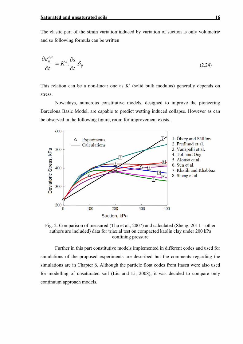
Nowadays, numerous constitutive models, designed to improve the pioneering
Barcelona Basic Model, are capable to predict wetting induced collapse. However as can
be observed in the following figure, room for improvement exists.
Fig. 2. Comparison of measured (Thu et al., 2007) and calculated (Sheng, 2011 – other authors are included) data for triaxial test on compacted kaolin clay under 200 kPa
confining pressure Further in this part constitutive models implemented in different codes and used for
simulations of the proposed experiments are described but the comments regarding the
simulations are in Chapter 6. Although the particle float codes from Itasca were also used
for modelling of unsaturated soil (Liu and Li, 2008), it was decided to compare only
continuum approach models.
Saturated and unsaturated soils 17
2.3.1. Modified Cam-Clay constitutive model
Hereafter presented numerical model of coupled hydro-mechanical of soils was
implemented into the SIFEL software package. The model follows Lewis and Schrefler’s
approach of coupled heat and moisture transfer while employing Darcy’s and Fick’s laws
for moisture transfer, Fourier’s law for heat transfer, standard mass and energy balance
equations and modified concept of effective stress according to (Bittnar and Sejnoha,
1996), i.e. one stress variable as shown in following equation
efij
gijg
wijw
sij SnSnn 111 (2.25)
where sij is the stress in grains, w
ij is the stress in liquid phase (water), gij is the stress
in gas, efij is the effective stress, nSw is a volume fraction of water and nSg is a volume
fraction of gas. In order to describe the deformation of a porous skeleton or actually the
rearrangement of grains standard constitutive equation is written in the rate form.
0 skefij D (2.26)
where skD is a tangential matrix of porous skeleton while, represents the strain rate
while 0 represents strains indirectly associated with stress changes, such as shrinkage
and swelling, creep, etc. and also involves the strain of the bulk material due to pore
pressure changes. Combining Eq 2.25 and 2.26 while assuming negligible shear stress in
fluid we obtain
sD ijskij (2.27)
where α represents the Biot’s constant and suction s is defined in agreement with volume
fractions as follows
gg
ww pSpSs (2.28)
Saturated and unsaturated soils 18
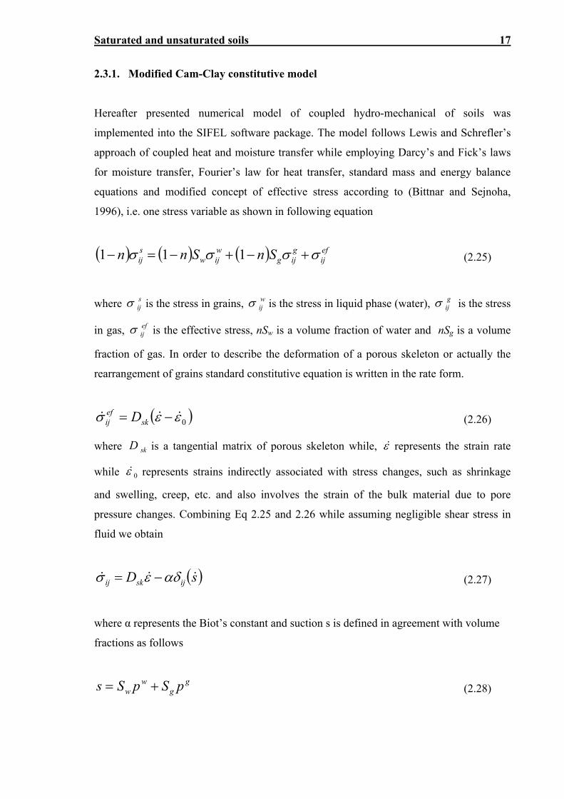
The constitutive model reflects a non-linear behaviour observed in isotropic
compression tests. The results are usually presented in semi-logarithmic scale as shown in
the following figure.
Fig. 3. Normal consolidation and swelling line describing the behaviour of soil during isotropic compression test
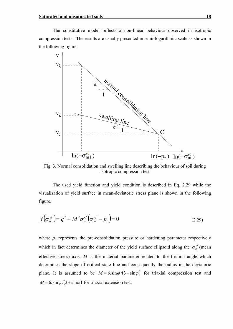
The used yield function and yield condition is described in Eq. 2.29 while the
visualization of yield surface in mean-deviatoric stress plane is shown in the following
figure.
022 cefm
efm
efij pMqf (2.29)
where pc represents the pre-consolidation pressure or hardening parameter respectively
which in fact determines the diameter of the yield surface ellipsoid along the efm (mean
effective stress) axis. M is the material parameter related to the friction angle which
determines the slope of critical state line and consequently the radius in the deviatoric
plane. It is assumed to be sin3/sin.6 M for triaxial compression test and
sin3/sin.6 M for triaxial extension test.
Saturated and unsaturated soils 19
Although implementation of the Cam Clay model was also prepared in the SIFEL
package, it was not so far successfully used for simulation of the wetting experiments
described in the chapter 4 and therefore the detail description is not provided.
Fig. 4. Yield surface of the Cam-Clay model in the mean-deviatoric stress plane
Apart from unit weight and Poisson’s ratio, the model requires 5 additional parameters
described in the following table.
Tab. 1. Parameters required by used Modified Cam Clay model
Parameter Interpretation
λ slope of the normal consolidation line
κ slope of the swelling line
e0 initial void ratio
OCR overconsolidation ratio
M slope of the critical state line* * M can be calculated using φc (critical state friction angle)
2.3.2. Hypoplasticity for clays
Hereafter presented model developed by Masin (2005) is based on combination of classical
critical state models and generalized hypoplasticity principles and was successfully
implemented into GEO 5 FEM version 16 software package (from April 2013 available at
http://www.fine.cz/) and used for simulation of unsaturated silt loams with steady no-flow
boundary condition. The adjustments required for the model to be used for simulations of
typical unsaturated problem are described in the next part of this chapter.
Saturated and unsaturated soils 20
The non-linear behaviour of the clay is in this model governed by generalized
hypoplasticity while as limit stress criteria was selected Matsuoka–Nakai failure surface.
The normal compression line for isotropic compression is similar to the NCL from
Modified Cam Clay model. The intergranular strain concept was not involved within
carried out calculations. In most basic form, the model requires five following material
parameters.
Tab. 2. Parameters required by used Hypoplastic model for clays
Parameter Interpretation
N position of the normal consolidation line for isotropic compression in the ln (1+e) vs. ln p plane
λ* slope of the normal consolidation line for isotropic compression in the ln (1+e) vs. ln p plane
κ* slope of the unloading line for isotropic compression in the ln (1+e) vs. ln p plane
φc critical state friction angle
r parameter controlling shear stiffness
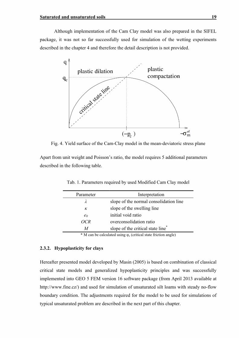
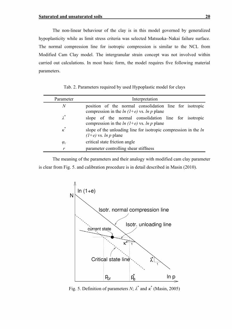
The meaning of the parameters and their analogy with modified cam clay parameter
is clear from Fig. 5. and calibration procedure is in detail described in Masin (2010).
Fig. 5. Definition of parameters N; * and * (Masin, 2005)
Saturated and unsaturated soils 21
In the figure above quantity pcr is defined as the mean stress at the critical state line
at the current void ratio and *ep is the equivalent pressure at the isotropic normal
compression line.
2.3.3. Hypoplasticity for unsaturated soils
Hypoplastic model for unsaturated soils presented by Masin and Khalili (2008) combines
principle of effective stress, represented here by “equivalent pore pressure” see Eq. 2.30
and theory of hypoplasticity.
aw uuu 1* (2.30)
where χ is defined empirically with help of material parameter se (air entry value –
separates unsaturated and saturated state of the soil) as follows
ee
e
ssfors
s
ssfor
55,0
1
(2.31)
The model attributes two effects on the soil behaviour to the suction. At first it is
the above described influence on the effective stress and second it is the increased
inhibition capacity of grain slippage represented by change in size of state boundary
surface and bounding system. This can be done even though the mathematical formulation
of hypoplastic models does not include either explicit state boundary surface or bounding
surface. More details regarding this matter can be found in Masin (2005).
Apart from five parameters necessary for the hypoplastic model, four additional
parameters are required to describe the unsaturated behaviour or more precisely two
parameters (n and l) to describe the dependence of N and * on suction – see Eq. 2.32 and
2.33, one parameter (m) which controls the structure collapse along the wetting path and
one (se) to prescribe the air entry or air expulsion value which serves to quantify the
unsaturated state.
es
snNsN ln)( (2.32)
Saturated and unsaturated soils 22
es
sls ln)( ** (2.33)
Although eight of total nine parameters are identifiable from laboratory
experiments, parameter m must be calibrated by means of parametric study of wetting
experiments on overconsolidated soils only after all other parameters are known. Moreover
for calibration of se is important which type of problem, drying or wetting, is solved as the
air entry value (wetting process) and air expulsion value (drying process) differ
significantly.
Tab. 3. Parameters required by used hypoplastic model for unsaturated soils
Parameter Interpretation
m controls the structure collapse along the wetting path
n represents dependence of N on suction
l represents dependence of * on suction
se air entry or expulsion value
N position of the normal consolidation line for isotropic compression in the ln (1+e) vs. ln p plane
λ* slope of the normal consolidation line for isotropic compression in the ln (1+e) vs. ln p plane
κ* slope of the unloading line for isotropic compression in the ln (1+e) vs. ln p plane
φc critical state friction angle
r parameter controlling shear stiffness
(Last five parameters are identical with parameters used by hypoplastic model for clay.)
Chapter 3
INTERNAL EROSION
The erosion of particles due to seepage of fluid phase is responsible for changes of the soil
behaviour and subsequently raises many issues in different areas of geotechnical
engineering. The internal erosion usually takes place only in fully saturated soils, but the
state prior to application of the water under high hydraulic gradient can make significant
difference. This is a typical problem for unsaturated levees during initial phase of flood
events.
Design recommendations for hydraulic structures are dealing with the term critical
gradient. The definition of the critical gradient describes it as a hydraulic gradient that
causes internal erosion and loss of particle. Empirical values of critical gradients for
different soils are presented in the literature (Bligh, 1910), (Lane, 1935), (Kenney and Lau,
1985) and (Sherard et al., 1984) and the design of the foundation structure should ensure
that the actual hydraulic gradients do not exceed the critical values during the effective
service life of the construction. The influence of the internal erosion to the stability and
deformations of the river structure can be perfectly shown on the recently collapsed
spillway structure in Slovak Republic.
Problems with internal erosion are enlarged by difficulties in detecting the
initializing phase. Monitoring equipment presents additional significant increase in both
investments and operation costs even when used in sparsely. When the erosion is already
progressing through the subsoil or dam the time window for successful intervention is very
limited.
The scope of this work is strictly limited to hydro-mechanical behaviour and
particularly to backward erosion and suffusion. Significant portion of the internal erosion
process, however, take place on dispersive soils
The aim of this chapter is to briefly review general approaches regarding modelling
of the internal erosion assuming continuum models and validity of averaging principles.
Particle float codes from Itasca, e.g. of applications (Lohani et al., 2008), (de Pater and
Internal erosion 24
Dong, 2007) or (Achmus and Abdel-Rahman, 2003), were found far too demanding with
respect to the computational power and also their use does not correspond with the selected
methodological approach to the studied problems.
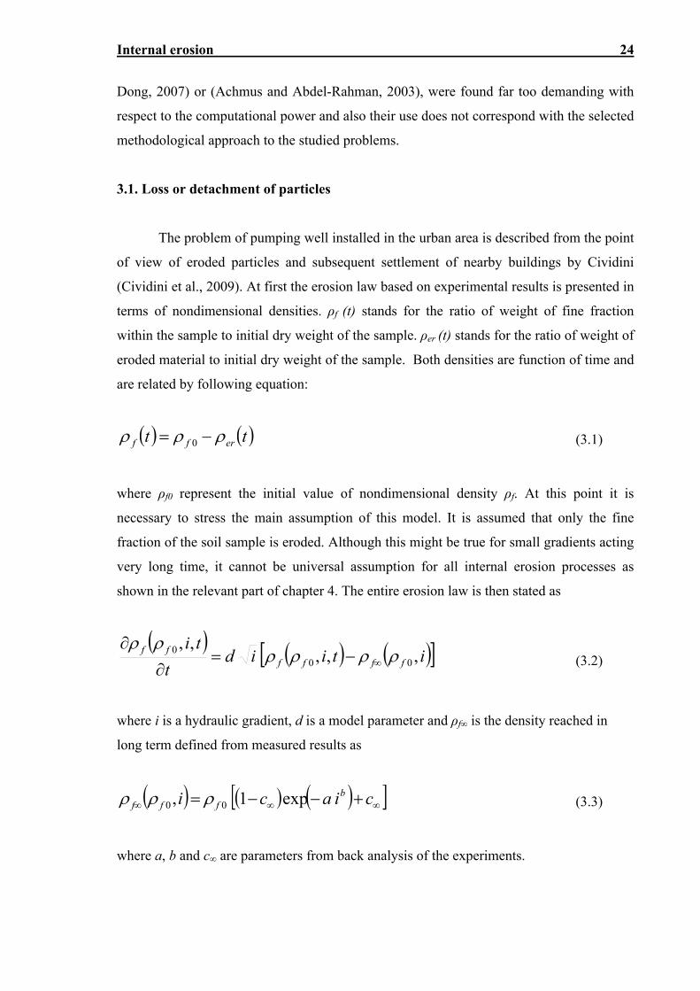
3.1. Loss or detachment of particles
The problem of pumping well installed in the urban area is described from the point
of view of eroded particles and subsequent settlement of nearby buildings by Cividini
(Cividini et al., 2009). At first the erosion law based on experimental results is presented in
terms of nondimensional densities. ρf (t) stands for the ratio of weight of fine fraction
within the sample to initial dry weight of the sample. ρer (t) stands for the ratio of weight of
eroded material to initial dry weight of the sample. Both densities are function of time and
are related by following equation:
tt erff 0 (3.1)
where ρf0 represent the initial value of nondimensional density ρf. At this point it is
necessary to stress the main assumption of this model. It is assumed that only the fine
fraction of the soil sample is eroded. Although this might be true for small gradients acting
very long time, it cannot be universal assumption for all internal erosion processes as
shown in the relevant part of chapter 4. The entire erosion law is then stated as
itiidt
tiffff
ff ,,,,,
000
(3.2)
where i is a hydraulic gradient, d is a model parameter and ρf∞ is the density reached in
long term defined from measured results as
ciaci bfff exp1, 00 (3.3)
where a, b and c∞ are parameters from back analysis of the experiments.
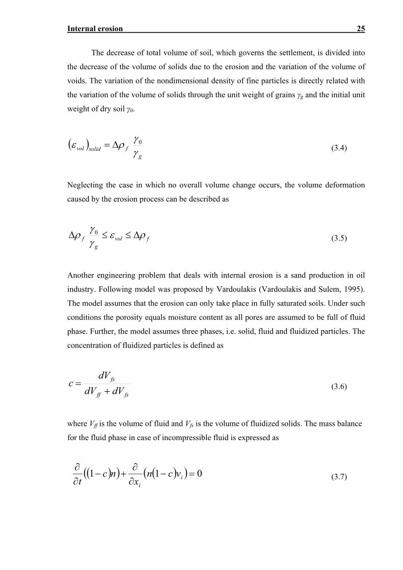
Internal erosion 25
The decrease of total volume of soil, which governs the settlement, is divided into
the decrease of the volume of solids due to the erosion and the variation of the volume of
voids. The variation of the nondimensional density of fine particles is directly related with
the variation of the volume of solids through the unit weight of grains γg and the initial unit
weight of dry soil γ0.
g
fsolidvol 0 (3.4)
Neglecting the case in which no overall volume change occurs, the volume deformation
caused by the erosion process can be described as
fvolg
f 0
(3.5)
Another engineering problem that deals with internal erosion is a sand production in oil
industry. Following model was proposed by Vardoulakis (Vardoulakis and Sulem, 1995).
The model assumes that the erosion can only take place in fully saturated soils. Under such
conditions the porosity equals moisture content as all pores are assumed to be full of fluid
phase. Further, the model assumes three phases, i.e. solid, fluid and fluidized particles. The
concentration of fluidized particles is defined as
fsff
fs
dVdV
dVc
(3.6)
where Vff is the volume of fluid and Vfs is the volume of fluidized solids. The mass balance
for the fluid phase in case of incompressible fluid is expressed as
011
ii
vcnx
nct (3.7)
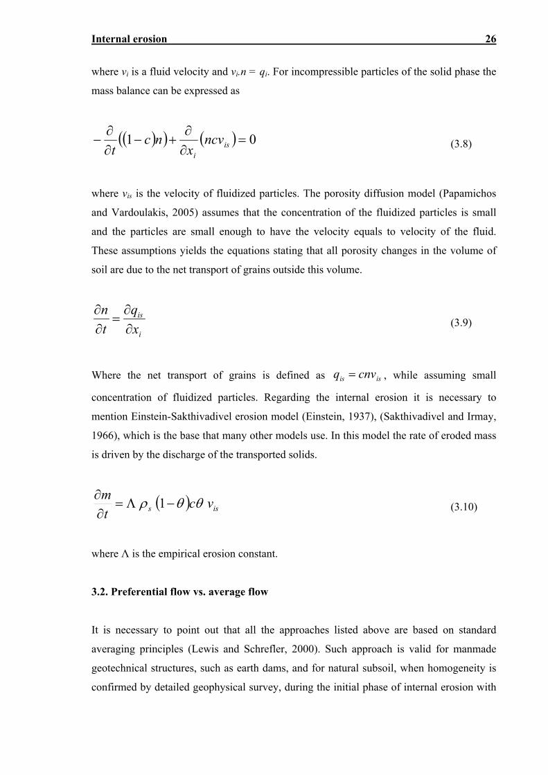
Internal erosion 26
where vi is a fluid velocity and vi.n = qi. For incompressible particles of the solid phase the
mass balance can be expressed as
01
isi
ncvx
nct (3.8)
where vis is the velocity of fluidized particles. The porosity diffusion model (Papamichos
and Vardoulakis, 2005) assumes that the concentration of the fluidized particles is small
and the particles are small enough to have the velocity equals to velocity of the fluid.
These assumptions yields the equations stating that all porosity changes in the volume of
soil are due to the net transport of grains outside this volume.
i
is
x
q
t
n
(3.9)
Where the net transport of grains is defined as isis cnvq , while assuming small
concentration of fluidized particles. Regarding the internal erosion it is necessary to
mention Einstein-Sakthivadivel erosion model (Einstein, 1937), (Sakthivadivel and Irmay,
1966), which is the base that many other models use. In this model the rate of eroded mass
is driven by the discharge of the transported solids.
iss vct
m
1 (3.10)
where Λ is the empirical erosion constant.
3.2. Preferential flow vs. average flow
It is necessary to point out that all the approaches listed above are based on standard
averaging principles (Lewis and Schrefler, 2000). Such approach is valid for manmade
geotechnical structures, such as earth dams, and for natural subsoil, when homogeneity is
confirmed by detailed geophysical survey, during the initial phase of internal erosion with

Internal erosion 27
reasonably small hydraulic gradients. According to our experiments that are described
below, the soil creates small caverns when subjected to high hydraulic gradient. The
change in the overall porosity during this process is very small but the flow inside the
caverns cannot be simulated as flux through porous materials especially when it comes to
interconnection of the caverns and creation of the preferential flow paths. Such type of
flow is closer to flux through fractured rock with very high matric flux rather than Darcy’s
flux. One possibility of modelling such combined flux is to use 2D elements for flow
through the “matric” and 1D channel element for assumed flow paths. Further evaluation
of this approach is still under consideration. Stochastic models using random spatial fields
with high correlation for adjacent elements could prove to be potentially very successful
(Duchan, 2012).
Chapter 4
EXPERIMENTAL ANALYSIS
In order to study the processes influencing the behaviour of the soil when groundwater is
present, several experiments have been designed. For this purpose we divide the processes
into two categories. The final affection of the soil behaviour could certainly be a
combination of all acting processes from both categories.
First category involves all changes in the pore pressure, including pore pressure
change in saturated soils. However, a unique position belongs to the process of suction
cancellation in unsaturated soils. Although this process is not of the same importance for
sandy soils as for clays, in this chapter we show that it still has an indispensable influence
on the soil behaviour even for coarse grained soils. More experimental results are then
available in Appendix B for poorly graded gravel, in Appendix C for silt loam and in
Appendix D for undisturbed samples of sands.
The second category covers all possible ways of losing particles. As in the case of
first category one process has special position. It is the piping process sometimes called
wash out process. Obtained results on undisturbed samples are in general commented in
this chapter together with the principles of the experiment while all measured values are
summarized in Appendix E.
Requirements for all of the proposed experiments are simplicity; repeatability;
transparency of results and their interpretation and boundary conditions being close to in-
situ boundary conditions, with the exception of small scale experiments with undisturbed
samples. Aims of the experiments coincide with goals of the thesis and follow the
proposed path, i.e. observation of the phenomena and quantification of the impact on
selected soils while leaving general recommendation for more extensive experimental
research, which would provide results for all soil classes. Tested soils were also subjected
to standard tests, such as hydraulic conductivity test, Proctor Standard test, etc. to gain
more information about the tested soils. Grain distributions of all the tested soils were also
obtained together with grain distribution of washed out particles in case of high gradient
Experimental analysis 29
internal erosion experiments. The density of the large soil samples was calculated from the
known total weight before the compaction and volume after compaction. It was measured
after all experiments were carried out with the help of rubber balloon density meter.
The full scale experiments were carried out on soil samples built in the laboratory
from excavated soils. The soil was inserted into the model stand by layers 200 mm thick.
First layer was placed on nonwoven geotextile (200 g/m2) protecting the outlets from
pipelines. Each layer was compacted by vibrating plate. The time over which was the
vibrating plate acting on each layer was estimated by compacting experiment carried out in
advance. The soil contained natural amount of moisture as it was kept in plastic covers
after being removed from the site. The time of storage was kept as short as possible. The
moisture content was monitored in selected intervals during the time of storage.
All small scale experiments, on the other hand, are carried out on undisrupted
specimens taken from the selected sites. The soil samples were obtained by pushing the
standard hollow steel cylinder into the soil in selected depth. The surrounding soil had to
be excavated to allow the cylinder to be removed without disrupting the sample. The
cylinder has inner diameter equal to 0.120m and height equal to 0.100m.
4.1. Tested soils
1) Poorly graded gravel - compacted large sample
The soil specimens were classified according to CSN 731001 as G2 – GP, i.e. poorly
graded gravel and as saGr with medium content of cobbles according to EN ISO 14688.
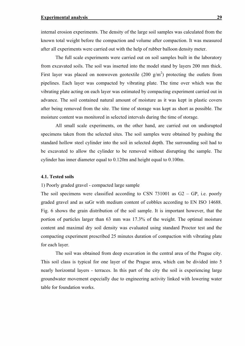
Fig. 6 shows the grain distribution of the soil sample. It is important however, that the
portion of particles larger than 63 mm was 17.3% of the weight. The optimal moisture
content and maximal dry soil density was evaluated using standard Proctor test and the
compacting experiment prescribed 25 minutes duration of compaction with vibrating plate
for each layer.
The soil was obtained from deep excavation in the central area of the Prague city.
This soil class is typical for one layer of the Prague area, which can be divided into 5
nearly horizontal layers - terraces. In this part of the city the soil is experiencing large
groundwater movement especially due to engineering activity linked with lowering water
table for foundation works.
Experimental analysis 30
Tab. 4. Characteristics of tested soil
Characteristic Value
Optimal water content from PS (%) 11
Original water content (%) 4
Maximum dry density PS (kg/m3) Measured dry density (kg/m3)
1950 2217
This soil has also proved its predisposition for internal erosion and collapse when
exposed to high hydraulic gradient or flow pressure. Several road and building accidents
were reported regarding this matter.
Fig. 6. Grain distribution of poorly graded gravel (three specimens)
2) Silt loam - compacted large sample
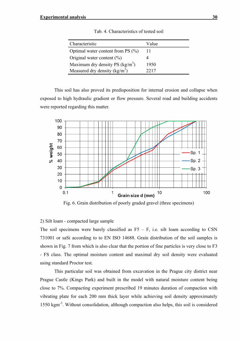
The soil specimens were barely classified as F5 – F, i.e. silt loam according to CSN
731001 or saSi according to to EN ISO 14688. Grain distribution of the soil samples is
shown in Fig. 7 from which is also clear that the portion of fine particles is very close to F3
- FS class. The optimal moisture content and maximal dry soil density were evaluated
using standard Proctor test.
This particular soil was obtained from excavation in the Prague city district near
Prague Castle (Kings Park) and built in the model with natural moisture content being
close to 7%. Compacting experiment prescribed 19 minutes duration of compaction with
vibrating plate for each 200 mm thick layer while achieving soil density approximately
1550 kgm-3. Without consolidation, although compaction also helps, this soil is considered
Experimental analysis 31
highly collapsible and moisture sensitive with high volumetric deformations due to
swelling and shrinkage.
Fig. 7. Grain distribution of silt loam (three specimens)
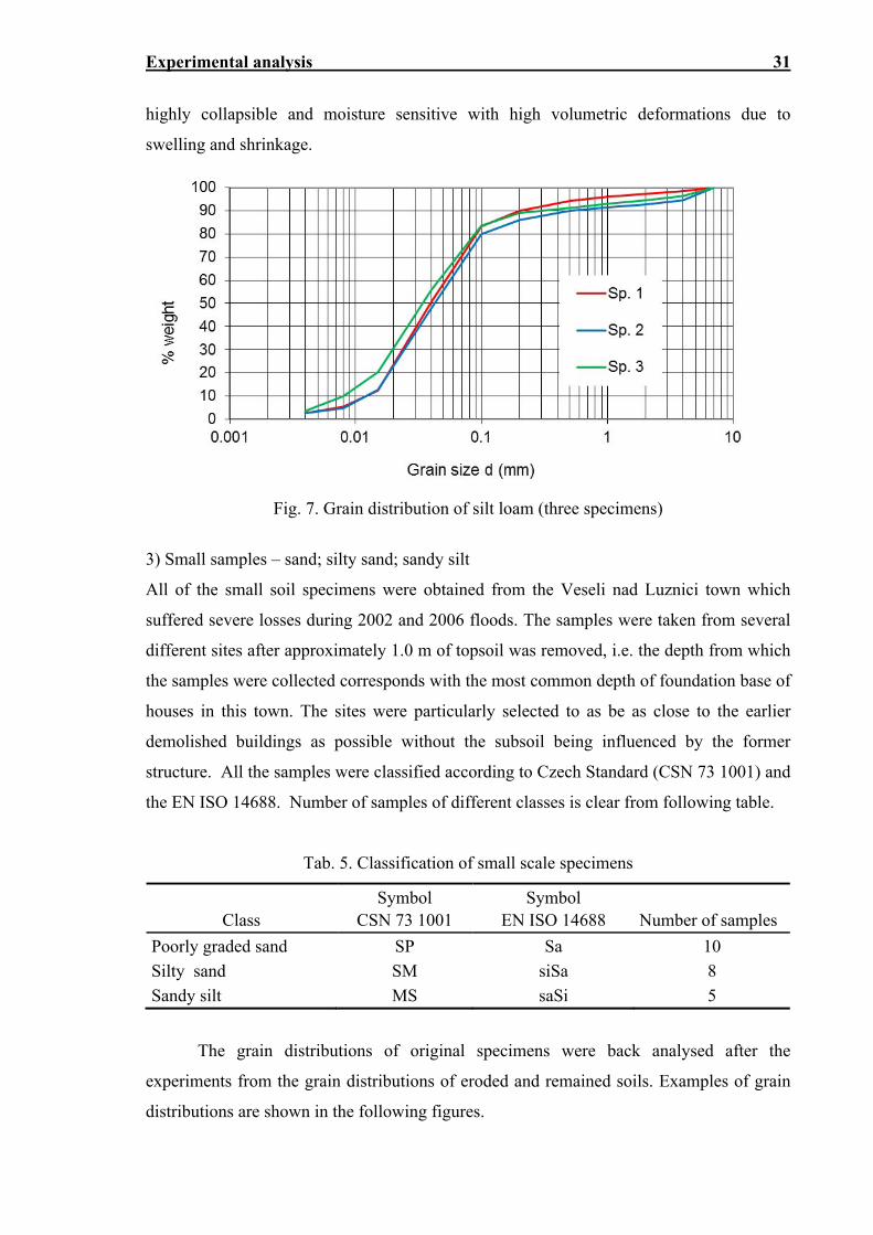
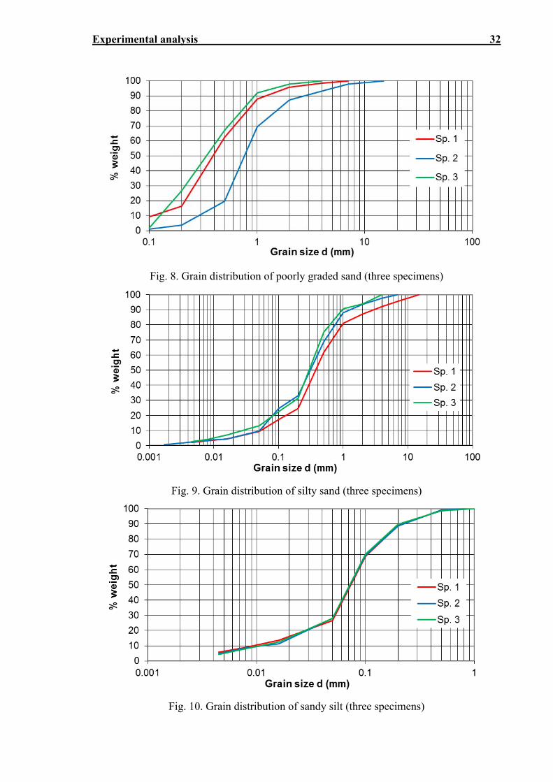
3) Small samples – sand; silty sand; sandy silt
All of the small soil specimens were obtained from the Veseli nad Luznici town which
suffered severe losses during 2002 and 2006 floods. The samples were taken from several
different sites after approximately 1.0 m of topsoil was removed, i.e. the depth from which
the samples were collected corresponds with the most common depth of foundation base of
houses in this town. The sites were particularly selected to as be as close to the earlier
demolished buildings as possible without the subsoil being influenced by the former
structure. All the samples were classified according to Czech Standard (CSN 73 1001) and
the EN ISO 14688. Number of samples of different classes is clear from following table.
Tab. 5. Classification of small scale specimens
Class
Symbol CSN 73 1001
Symbol EN ISO 14688
Number of samples
Poorly graded sand SP Sa 10
Silty sand SM siSa 8
Sandy silt MS saSi 5
The grain distributions of original specimens were back analysed after the
experiments from the grain distributions of eroded and remained soils. Examples of grain
distributions are shown in the following figures.
Experimental analysis 32
Fig. 8. Grain distribution of poorly graded sand (three specimens)
Fig. 9. Grain distribution of silty sand (three specimens)
Fig. 10. Grain distribution of sandy silt (three specimens)
Experimental analysis 33
4.2. Static plate load test – full scale
Governing idea of this test is to provide experimental results easily comparable with in-situ
measured values. With similar loading / unloading behaviour measured on unsaturated
soils in-situ and in laboratory appropriate analogy could be used to predict the effect of
wetting, suction cancellation or groundwater table variations. Obtained results can also be
used for calibration and confirmation of numerical models as shown in relevant parts of
this thesis.
The stand for tested soil sample is a massive reinforced concrete box without the
top covering part. The bottom part contains a system of pipes 12.5 mm in diameter and is
connected to the large water storage tank. The side walls are 200 mm thick and the box is
constricted by steel beams in two levels. A steel frame is attached to the box to take the
reaction force and additional small frame presents an inertial body to which the
deformations are measured. The internal dimensions of the box are 1.0 x 1.0 x 1.0 m. The
stand was designed and constructed strictly for this purpose while taking into account the
effect of vibrations during the soil sample compaction as well as the impact of the load and
water. Although the stand served well with respect to the needs of this thesis, adjustments
recommended regarding the water tightness and pore pressure measurements are presented
at the end of this chapter.
Load is applied through a hydraulic jack to the steel plate 20 mm thick and 300 mm
in diameter (70.685.103 mm2 surface area). As the maximum safe load for the reaction
frame was 80 kN, the plate is assumed rigid within the load interval for analytical and
numerical purpose. The applied load is measured in the hydraulic system, which means oil
pressure in the system is measured by calibrated manometer and is converted to force
induced by the piston, and once more in the pressure cell bellow the reaction frame. The
pressure cell was removed after several experiments as the differences between measured
forces were negligible when considering the accuracy of the pressure probe equal 5 kN, see
Fig. 13. Fig. 11 shows the scheme of the experiment, while Fig. 12 shows the completely
built model ready for lunching the very first experiment.
Settlement was measured by two dial gauges installed on the plate with guaranteed
accuracy 0.01 mm.
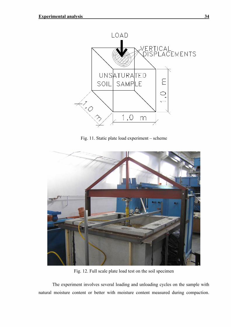
Experimental analysis 34
Fig. 11. Static plate load experiment – scheme
Fig. 12. Full scale plate load test on the soil specimen
The experiment involves several loading and unloading cycles on the sample with
natural moisture content or better with moisture content measured during compaction.
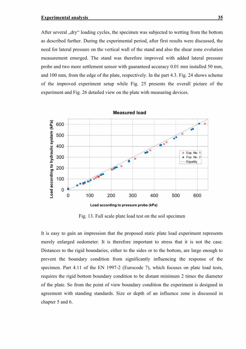
Experimental analysis 35
After several „dry“ loading cycles, the specimen was subjected to wetting from the bottom
as described further. During the experimental period, after first results were discussed, the
need for lateral pressure on the vertical wall of the stand and also the shear zone evolution
measurement emerged. The stand was therefore improved with added lateral pressure
probe and two more settlement sensor with guaranteed accuracy 0.01 mm installed 50 mm,
and 100 mm, from the edge of the plate, respectively. In the part 4.3. Fig. 24 shows scheme
of the improved experiment setup while Fig. 25 presents the overall picture of the
experiment and Fig. 26 detailed view on the plate with measuring devices.
Fig. 13. Full scale plate load test on the soil specimen
It is easy to gain an impression that the proposed static plate load experiment represents
merely enlarged oedometer. It is therefore important to stress that it is not the case.
Distances to the rigid boundaries, either to the sides or to the bottom, are large enough to
prevent the boundary condition from significantly influencing the response of the
specimen. Part 4.11 of the EN 1997-2 (Eurocode 7), which focuses on plate load tests,
requires the rigid bottom boundary condition to be distant minimum 2 times the diameter
of the plate. So from the point of view boundary condition the experiment is designed in
agreement with standing standards. Size or depth of an influence zone is discussed in
chapter 5 and 6.
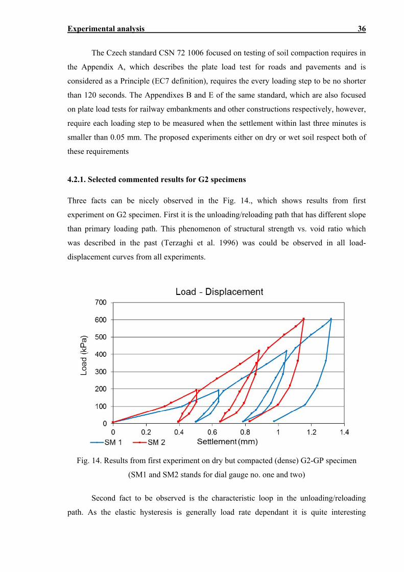
Experimental analysis 36
The Czech standard CSN 72 1006 focused on testing of soil compaction requires in
the Appendix A, which describes the plate load test for roads and pavements and is
considered as a Principle (EC7 definition), requires the every loading step to be no shorter
than 120 seconds. The Appendixes B and E of the same standard, which are also focused
on plate load tests for railway embankments and other constructions respectively, however,
require each loading step to be measured when the settlement within last three minutes is
smaller than 0.05 mm. The proposed experiments either on dry or wet soil respect both of
these requirements
4.2.1. Selected commented results for G2 specimens
Three facts can be nicely observed in the Fig. 14., which shows results from first
experiment on G2 specimen. First it is the unloading/reloading path that has different slope
than primary loading path. This phenomenon of structural strength vs. void ratio which
was described in the past (Terzaghi et al. 1996) was could be observed in all load-
displacement curves from all experiments.
Fig. 14. Results from first experiment on dry but compacted (dense) G2-GP specimen
(SM1 and SM2 stands for dial gauge no. one and two)
Second fact to be observed is the characteristic loop in the unloading/reloading
path. As the elastic hysteresis is generally load rate dependant it is quite interesting
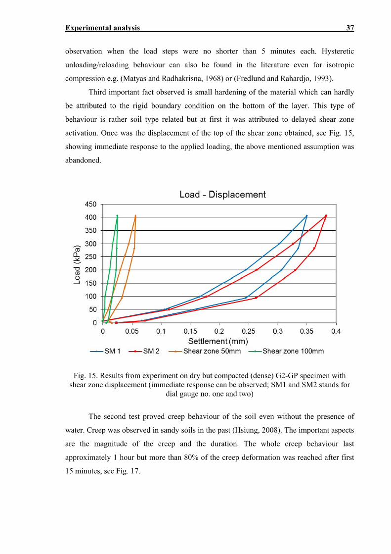
Experimental analysis 37
observation when the load steps were no shorter than 5 minutes each. Hysteretic
unloading/reloading behaviour can also be found in the literature even for isotropic
compression e.g. (Matyas and Radhakrisna, 1968) or (Fredlund and Rahardjo, 1993).
Third important fact observed is small hardening of the material which can hardly
be attributed to the rigid boundary condition on the bottom of the layer. This type of
behaviour is rather soil type related but at first it was attributed to delayed shear zone
activation. Once was the displacement of the top of the shear zone obtained, see Fig. 15,
showing immediate response to the applied loading, the above mentioned assumption was
abandoned.
Fig. 15. Results from experiment on dry but compacted (dense) G2-GP specimen with shear zone displacement (immediate response can be observed; SM1 and SM2 stands for
dial gauge no. one and two)
The second test proved creep behaviour of the soil even without the presence of
water. Creep was observed in sandy soils in the past (Hsiung, 2008). The important aspects
are the magnitude of the creep and the duration. The whole creep behaviour last
approximately 1 hour but more than 80% of the creep deformation was reached after first
15 minutes, see Fig. 17.
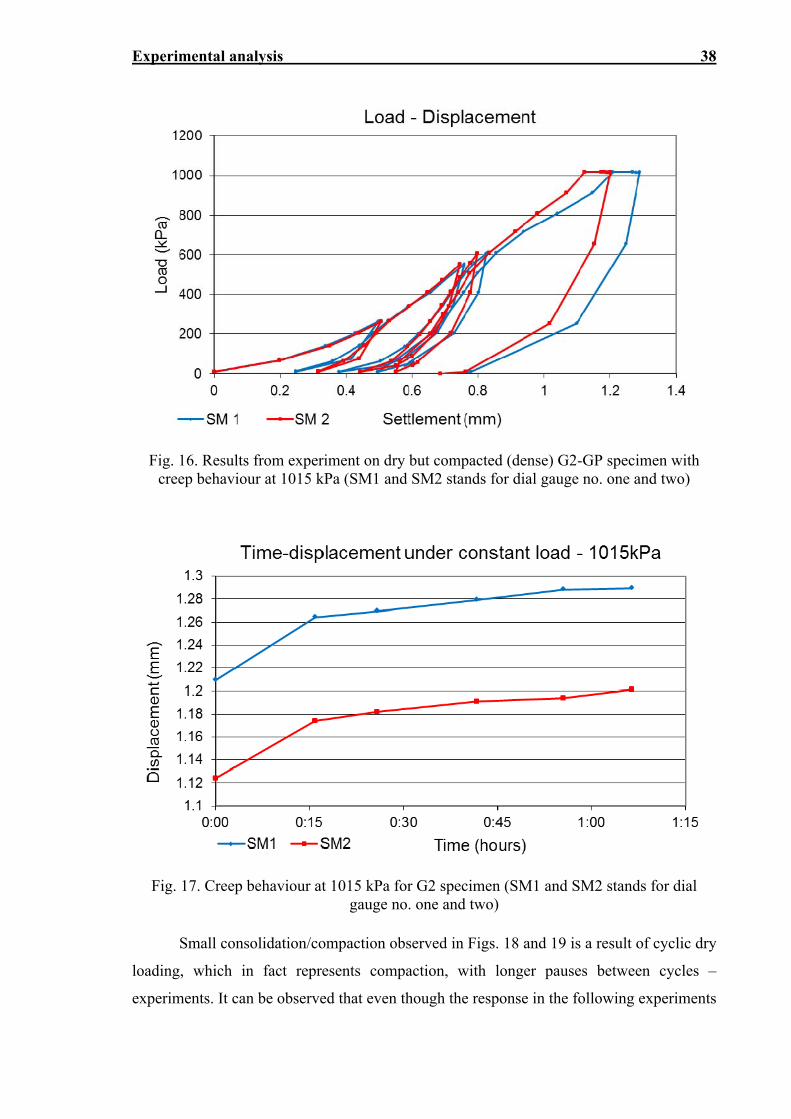
Experimental analysis 38
Fig. 16. Results from experiment on dry but compacted (dense) G2-GP specimen with creep behaviour at 1015 kPa (SM1 and SM2 stands for dial gauge no. one and two)
Fig. 17. Creep behaviour at 1015 kPa for G2 specimen (SM1 and SM2 stands for dial gauge no. one and two)
Small consolidation/compaction observed in Figs. 18 and 19 is a result of cyclic dry
loading, which in fact represents compaction, with longer pauses between cycles –
experiments. It can be observed that even though the response in the following experiments
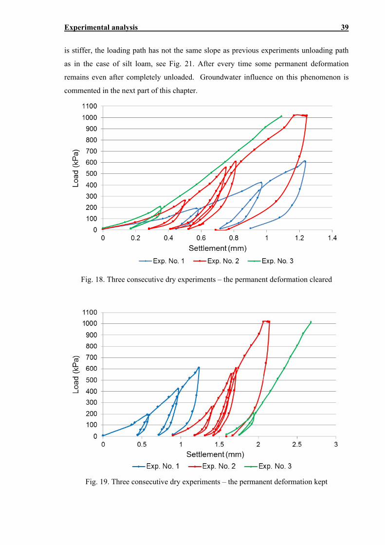
Experimental analysis 39
is stiffer, the loading path has not the same slope as previous experiments unloading path
as in the case of silt loam, see Fig. 21. After every time some permanent deformation
remains even after completely unloaded. Groundwater influence on this phenomenon is
commented in the next part of this chapter.
Fig. 18. Three consecutive dry experiments – the permanent deformation cleared
Fig. 19. Three consecutive dry experiments – the permanent deformation kept
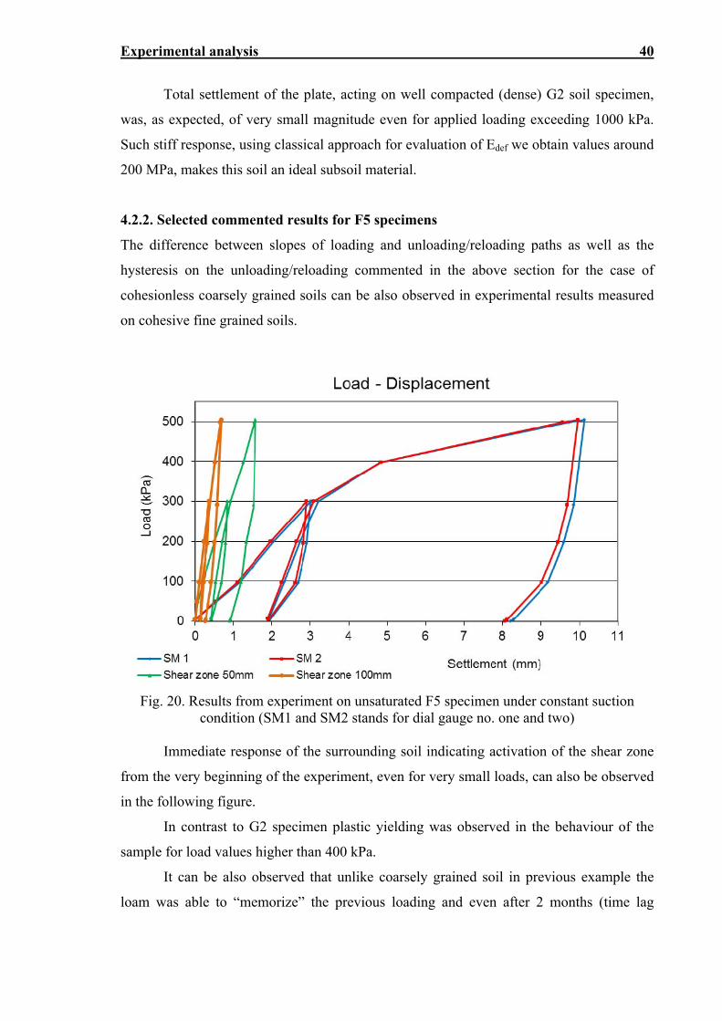
Experimental analysis 40
Total settlement of the plate, acting on well compacted (dense) G2 soil specimen,
was, as expected, of very small magnitude even for applied loading exceeding 1000 kPa.
Such stiff response, using classical approach for evaluation of Edef we obtain values around
200 MPa, makes this soil an ideal subsoil material.
4.2.2. Selected commented results for F5 specimens
The difference between slopes of loading and unloading/reloading paths as well as the
hysteresis on the unloading/reloading commented in the above section for the case of
cohesionless coarsely grained soils can be also observed in experimental results measured
on cohesive fine grained soils.
Fig. 20. Results from experiment on unsaturated F5 specimen under constant suction condition (SM1 and SM2 stands for dial gauge no. one and two)
Immediate response of the surrounding soil indicating activation of the shear zone
from the very beginning of the experiment, even for very small loads, can also be observed
in the following figure.
In contrast to G2 specimen plastic yielding was observed in the behaviour of the
sample for load values higher than 400 kPa.
It can be also observed that unlike coarsely grained soil in previous example the
loam was able to “memorize” the previous loading and even after 2 months (time lag
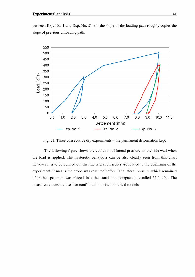
Experimental analysis 41
between Exp. No. 1 and Exp. No. 2) still the slope of the loading path roughly copies the
slope of previous unloading path.
Fig. 21. Three consecutive dry experiments – the permanent deformation kept
The following figure shows the evolution of lateral pressure on the side wall when
the load is applied. The hysteretic behaviour can be also clearly seen from this chart
however it is to be pointed out that the lateral pressures are related to the beginning of the
experiment, it means the probe was resented before. The lateral pressure which remained
after the specimen was placed into the stand and compacted equalled 33,1 kPa. The
measured values are used for confirmation of the numerical models.
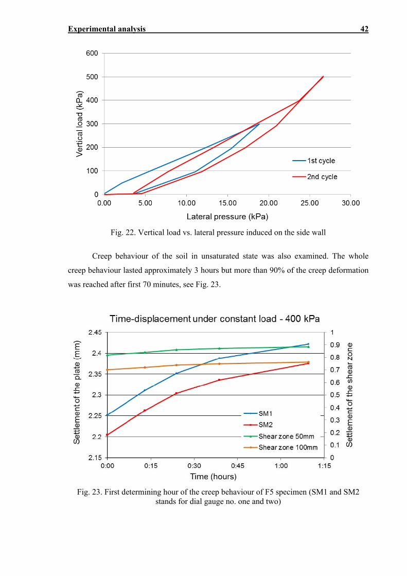
Experimental analysis 42
Fig. 22. Vertical load vs. lateral pressure induced on the side wall
Creep behaviour of the soil in unsaturated state was also examined. The whole
creep behaviour lasted approximately 3 hours but more than 90% of the creep deformation
was reached after first 70 minutes, see Fig. 23.
Fig. 23. First determining hour of the creep behaviour of F5 specimen (SM1 and SM2 stands for dial gauge no. one and two)
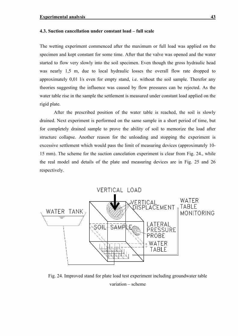
Experimental analysis 43
4.3. Suction cancellation under constant load – full scale
The wetting experiment commenced after the maximum or full load was applied on the
specimen and kept constant for some time. After that the valve was opened and the water
started to flow very slowly into the soil specimen. Even though the gross hydraulic head
was nearly 1,5 m, due to local hydraulic losses the overall flow rate dropped to
approximately 0,01 l/s even for empty stand, i.e. without the soil sample. Therefor any
theories suggesting the influence was caused by flow pressures can be rejected. As the
water table rise in the sample the settlement is measured under constant load applied on the
rigid plate.
After the prescribed position of the water table is reached, the soil is slowly
drained. Next experiment is performed on the same sample in a short period of time, but
for completely drained sample to prove the ability of soil to memorize the load after
structure collapse. Another reason for the unloading and stopping the experiment is
excessive settlement which would pass the limit of measuring devices (approximately 10-
15 mm). The scheme for the suction cancelation experiment is clear from Fig. 24., while
the real model and details of the plate and measuring devices are in Fig. 25 and 26
respectively.
Fig. 24. Improved stand for plate load test experiment including groundwater table
variation – scheme
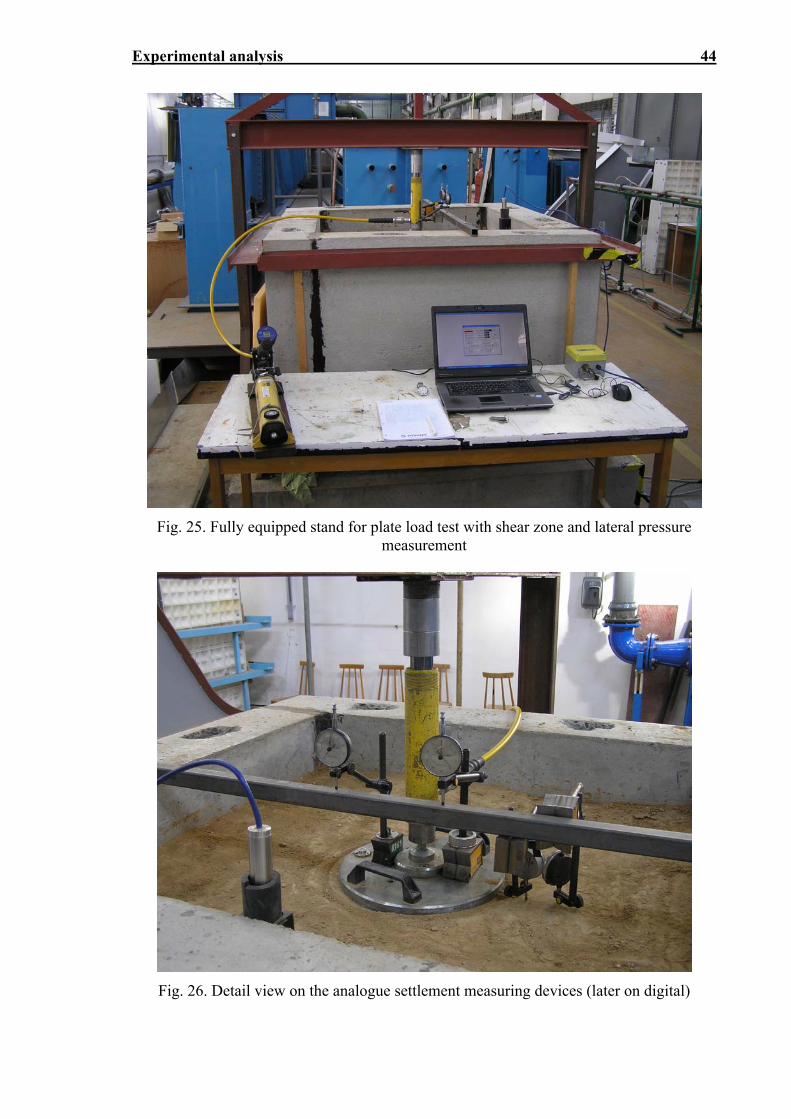
Experimental analysis 44
Fig. 25. Fully equipped stand for plate load test with shear zone and lateral pressure measurement
Fig. 26. Detail view on the analogue settlement measuring devices (later on digital)
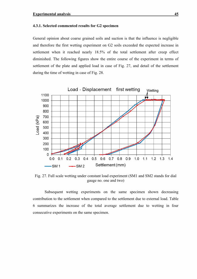
Experimental analysis 45
4.3.1. Selected commented results for G2 specimen
General opinion about coarse grained soils and suction is that the influence is negligible
and therefore the first wetting experiment on G2 soils exceeded the expected increase in
settlement when it reached nearly 18.5% of the total settlement after creep effect
diminished. The following figures show the entire course of the experiment in terms of
settlement of the plate and applied load in case of Fig. 27, and detail of the settlement
during the time of wetting in case of Fig. 28.
Fig. 27. Full scale wetting under constant load experiment (SM1 and SM2 stands for dial gauge no. one and two)
Subsequent wetting experiments on the same specimen shown decreasing
contribution to the settlement when compared to the settlement due to external load. Table
6 summarizes the increase of the total average settlement due to wetting in four
consecutive experiments on the same specimen.
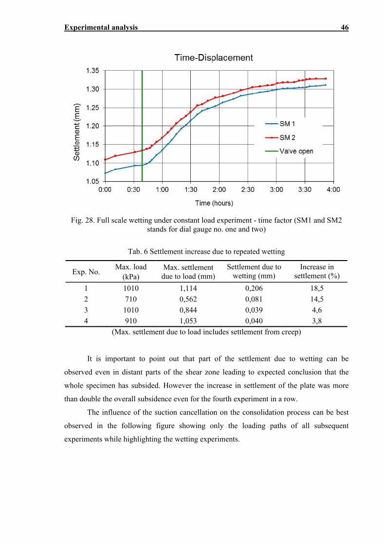
Experimental analysis 46
Fig. 28. Full scale wetting under constant load experiment - time factor (SM1 and SM2 stands for dial gauge no. one and two)
Tab. 6 Settlement increase due to repeated wetting
Exp. No. Max. load
(kPa) Max. settlement due to load (mm)
Settlement due to wetting (mm)
Increase in settlement (%)
1 1010 1,114 0,206 18,5
2 710 0,562 0,081 14,5
3 1010 0,844 0,039 4,6
4 910 1,053 0,040 3,8
(Max. settlement due to load includes settlement from creep)
It is important to point out that part of the settlement due to wetting can be
observed even in distant parts of the shear zone leading to expected conclusion that the
whole specimen has subsided. However the increase in settlement of the plate was more
than double the overall subsidence even for the fourth experiment in a row.
The influence of the suction cancellation on the consolidation process can be best
observed in the following figure showing only the loading paths of all subsequent
experiments while highlighting the wetting experiments.
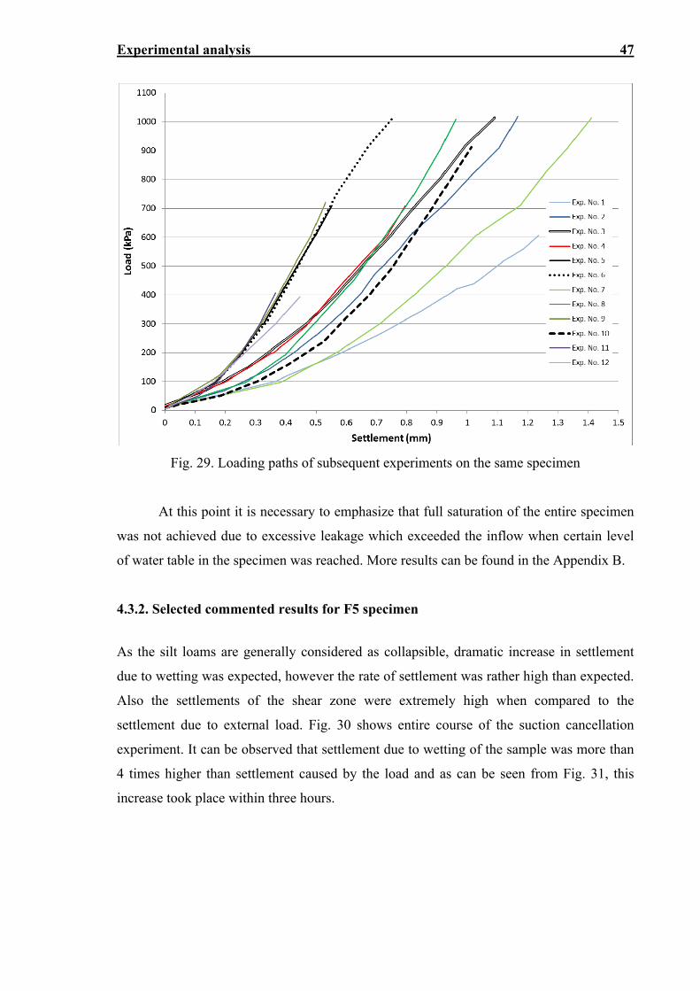
Experimental analysis 47
Fig. 29. Loading paths of subsequent experiments on the same specimen
At this point it is necessary to emphasize that full saturation of the entire specimen
was not achieved due to excessive leakage which exceeded the inflow when certain level
of water table in the specimen was reached. More results can be found in the Appendix B.
4.3.2. Selected commented results for F5 specimen
As the silt loams are generally considered as collapsible, dramatic increase in settlement
due to wetting was expected, however the rate of settlement was rather high than expected.
Also the settlements of the shear zone were extremely high when compared to the
settlement due to external load. Fig. 30 shows entire course of the suction cancellation
experiment. It can be observed that settlement due to wetting of the sample was more than
4 times higher than settlement caused by the load and as can be seen from Fig. 31, this
increase took place within three hours.
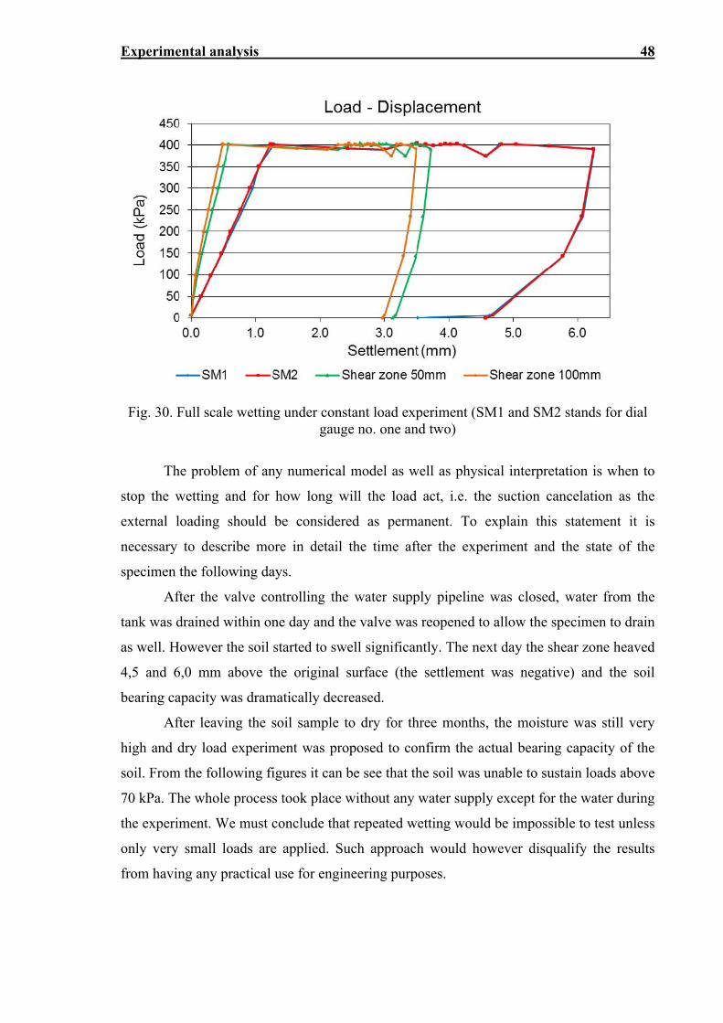
Experimental analysis 48
Fig. 30. Full scale wetting under constant load experiment (SM1 and SM2 stands for dial gauge no. one and two)
The problem of any numerical model as well as physical interpretation is when to
stop the wetting and for how long will the load act, i.e. the suction cancelation as the
external loading should be considered as permanent. To explain this statement it is
necessary to describe more in detail the time after the experiment and the state of the
specimen the following days.
After the valve controlling the water supply pipeline was closed, water from the
tank was drained within one day and the valve was reopened to allow the specimen to drain
as well. However the soil started to swell significantly. The next day the shear zone heaved
4,5 and 6,0 mm above the original surface (the settlement was negative) and the soil
bearing capacity was dramatically decreased.
After leaving the soil sample to dry for three months, the moisture was still very
high and dry load experiment was proposed to confirm the actual bearing capacity of the
soil. From the following figures it can be see that the soil was unable to sustain loads above
70 kPa. The whole process took place without any water supply except for the water during
the experiment. We must conclude that repeated wetting would be impossible to test unless
only very small loads are applied. Such approach would however disqualify the results
from having any practical use for engineering purposes.
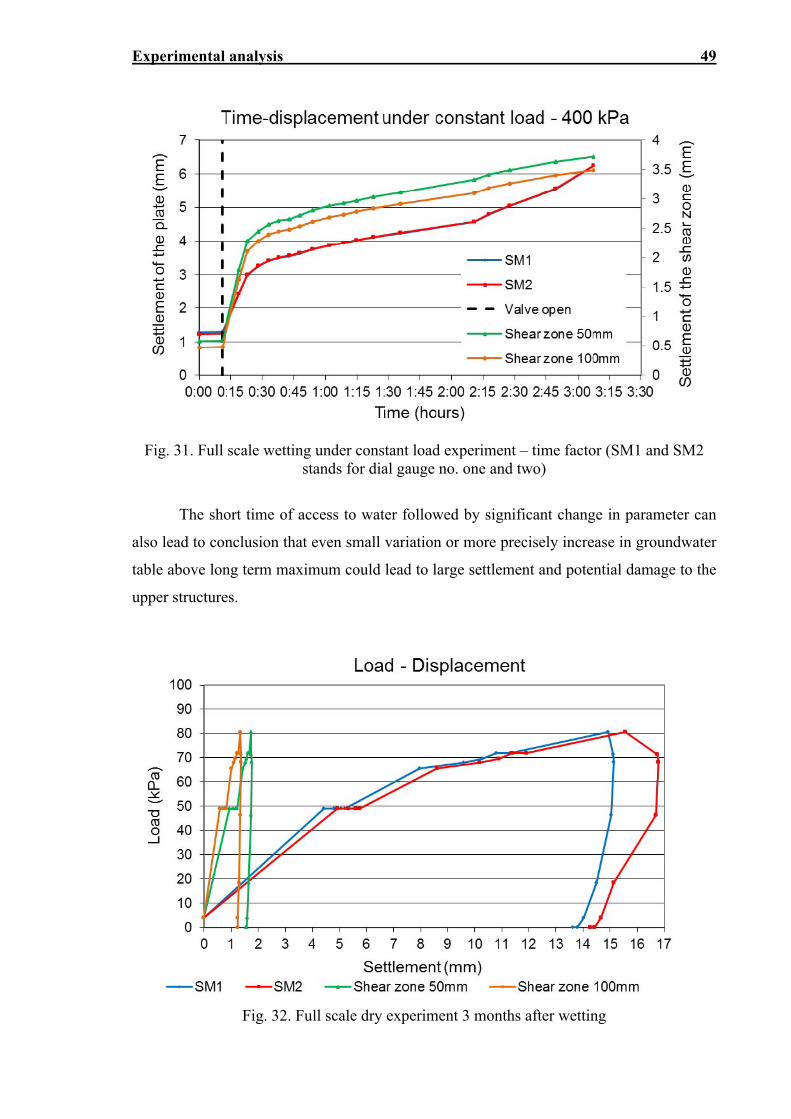
Experimental analysis 49
Fig. 31. Full scale wetting under constant load experiment – time factor (SM1 and SM2 stands for dial gauge no. one and two)
The short time of access to water followed by significant change in parameter can
also lead to conclusion that even small variation or more precisely increase in groundwater
table above long term maximum could lead to large settlement and potential damage to the
upper structures.
Fig. 32. Full scale dry experiment 3 months after wetting
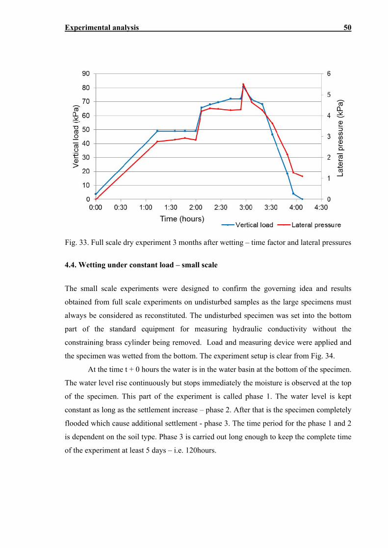
Experimental analysis 50
Fig. 33. Full scale dry experiment 3 months after wetting – time factor and lateral pressures
4.4. Wetting under constant load – small scale
The small scale experiments were designed to confirm the governing idea and results
obtained from full scale experiments on undisturbed samples as the large specimens must
always be considered as reconstituted. The undisturbed specimen was set into the bottom
part of the standard equipment for measuring hydraulic conductivity without the
constraining brass cylinder being removed. Load and measuring device were applied and
the specimen was wetted from the bottom. The experiment setup is clear from Fig. 34.
At the time t + 0 hours the water is in the water basin at the bottom of the specimen.
The water level rise continuously but stops immediately the moisture is observed at the top
of the specimen. This part of the experiment is called phase 1. The water level is kept
constant as long as the settlement increase – phase 2. After that is the specimen completely
flooded which cause additional settlement - phase 3. The time period for the phase 1 and 2
is dependent on the soil type. Phase 3 is carried out long enough to keep the complete time
of the experiment at least 5 days – i.e. 120hours.
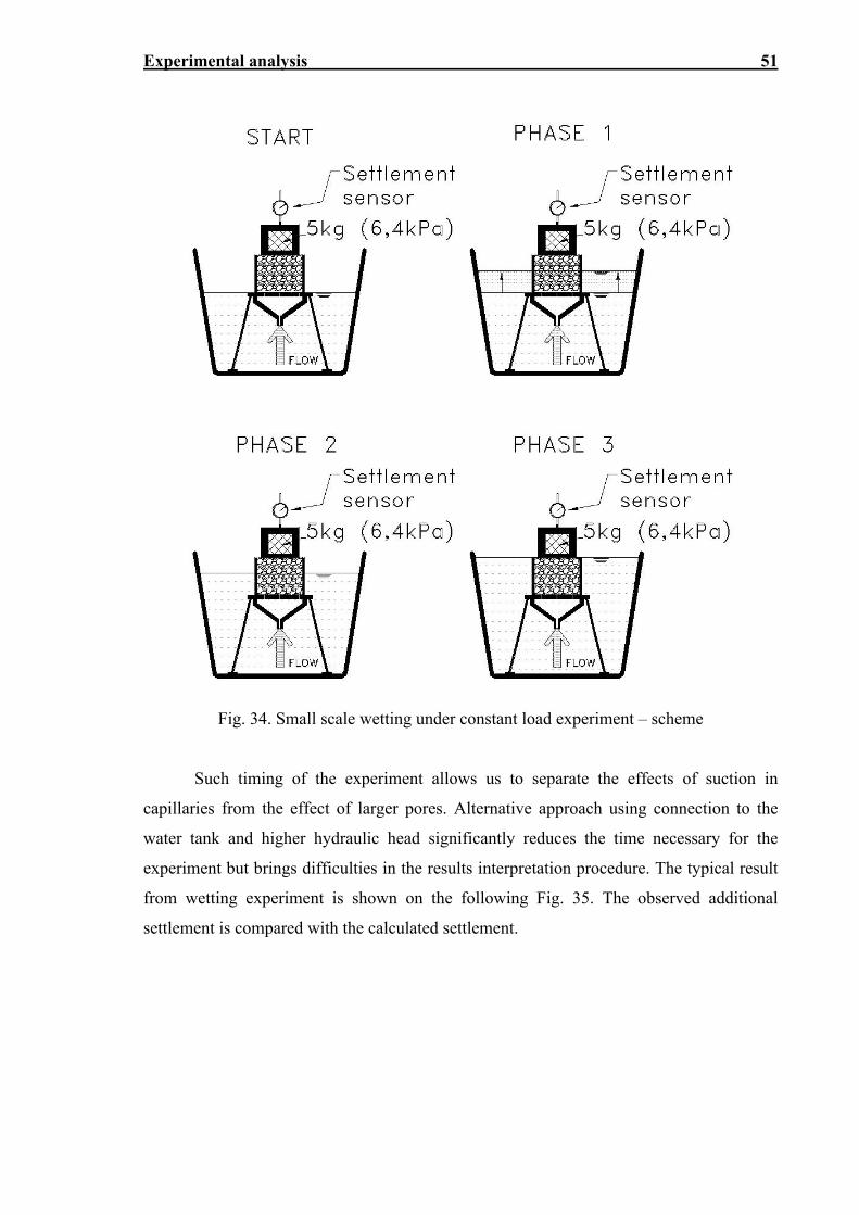
Experimental analysis 51
Fig. 34. Small scale wetting under constant load experiment – scheme
Such timing of the experiment allows us to separate the effects of suction in
capillaries from the effect of larger pores. Alternative approach using connection to the
water tank and higher hydraulic head significantly reduces the time necessary for the
experiment but brings difficulties in the results interpretation procedure. The typical result
from wetting experiment is shown on the following Fig. 35. The observed additional
settlement is compared with the calculated settlement.
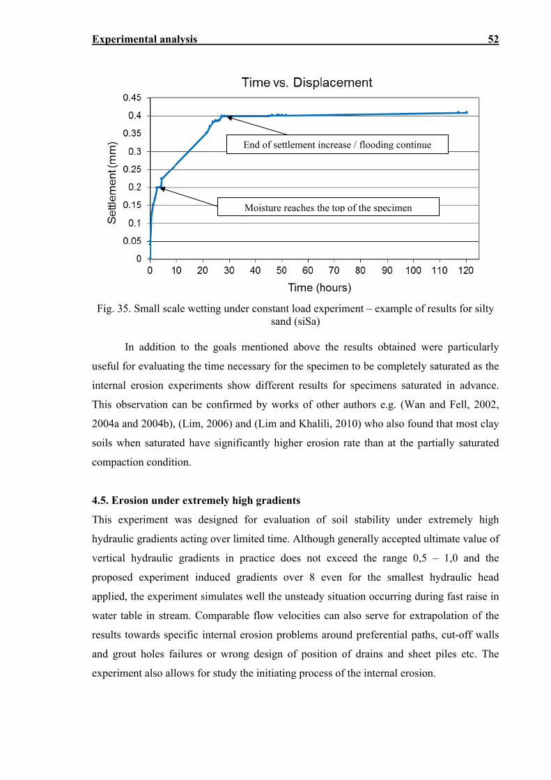
Experimental analysis 52
Fig. 35. Small scale wetting under constant load experiment – example of results for silty sand (siSa)
In addition to the goals mentioned above the results obtained were particularly
useful for evaluating the time necessary for the specimen to be completely saturated as the
internal erosion experiments show different results for specimens saturated in advance.
This observation can be confirmed by works of other authors e.g. (Wan and Fell, 2002,
2004a and 2004b), (Lim, 2006) and (Lim and Khalili, 2010) who also found that most clay
soils when saturated have significantly higher erosion rate than at the partially saturated
compaction condition.
4.5. Erosion under extremely high gradients
This experiment was designed for evaluation of soil stability under extremely high
hydraulic gradients acting over limited time. Although generally accepted ultimate value of
vertical hydraulic gradients in practice does not exceed the range 0,5 – 1,0 and the
proposed experiment induced gradients over 8 even for the smallest hydraulic head
applied, the experiment simulates well the unsteady situation occurring during fast raise in
water table in stream. Comparable flow velocities can also serve for extrapolation of the
results towards specific internal erosion problems around preferential paths, cut-off walls
and grout holes failures or wrong design of position of drains and sheet piles etc. The
experiment also allows for study the initiating process of the internal erosion.
End of settlement increase / flooding continue
Moisture reaches the top of the specimen
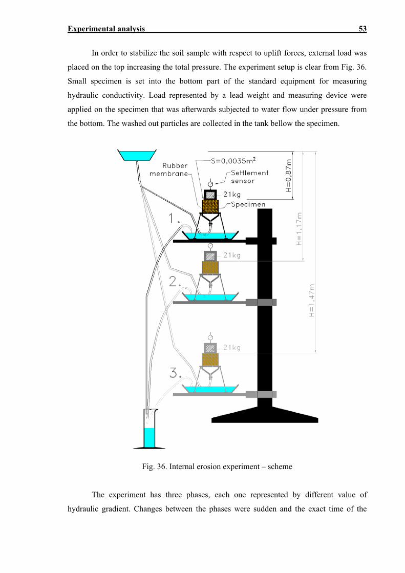
Experimental analysis 53
In order to stabilize the soil sample with respect to uplift forces, external load was
placed on the top increasing the total pressure. The experiment setup is clear from Fig. 36.
Small specimen is set into the bottom part of the standard equipment for measuring
hydraulic conductivity. Load represented by a lead weight and measuring device were
applied on the specimen that was afterwards subjected to water flow under pressure from
the bottom. The washed out particles are collected in the tank bellow the specimen.
Fig. 36. Internal erosion experiment – scheme
The experiment has three phases, each one represented by different value of
hydraulic gradient. Changes between the phases were sudden and the exact time of the
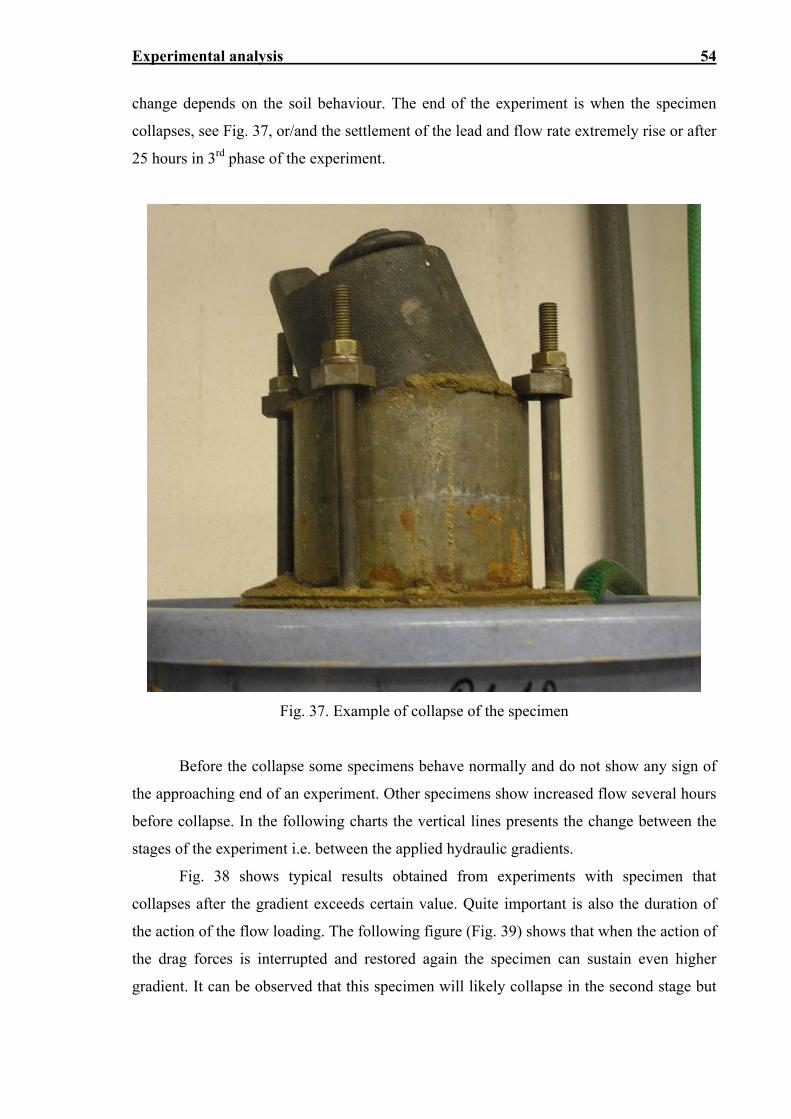
Experimental analysis 54
change depends on the soil behaviour. The end of the experiment is when the specimen
collapses, see Fig. 37, or/and the settlement of the lead and flow rate extremely rise or after
25 hours in 3rd phase of the experiment.
Fig. 37. Example of collapse of the specimen
Before the collapse some specimens behave normally and do not show any sign of
the approaching end of an experiment. Other specimens show increased flow several hours
before collapse. In the following charts the vertical lines presents the change between the
stages of the experiment i.e. between the applied hydraulic gradients.
Fig. 38 shows typical results obtained from experiments with specimen that
collapses after the gradient exceeds certain value. Quite important is also the duration of
the action of the flow loading. The following figure (Fig. 39) shows that when the action of
the drag forces is interrupted and restored again the specimen can sustain even higher
gradient. It can be observed that this specimen will likely collapse in the second stage but
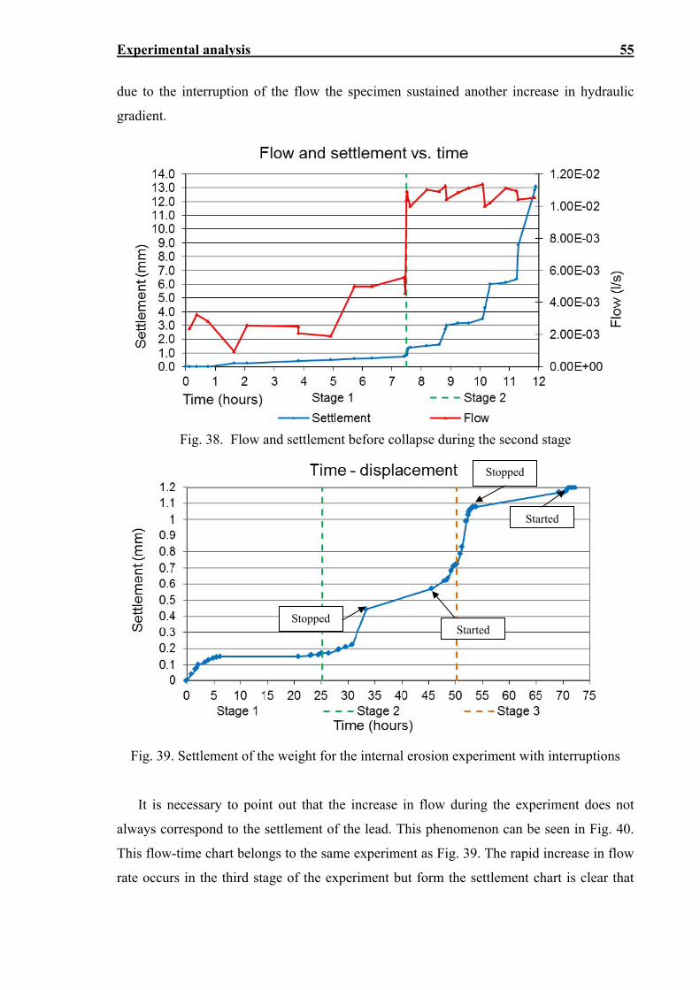
Experimental analysis 55
due to the interruption of the flow the specimen sustained another increase in hydraulic
gradient.
Fig. 38. Flow and settlement before collapse during the second stage
Fig. 39. Settlement of the weight for the internal erosion experiment with interruptions
It is necessary to point out that the increase in flow during the experiment does not
always correspond to the settlement of the lead. This phenomenon can be seen in Fig. 40.
This flow-time chart belongs to the same experiment as Fig. 39. The rapid increase in flow
rate occurs in the third stage of the experiment but form the settlement chart is clear that
Started
Started Stopped
Stopped
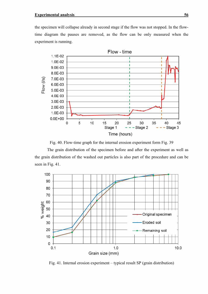
Experimental analysis 56
the specimen will collapse already in second stage if the flow was not stopped. In the flow-
time diagram the pauses are removed, as the flow can be only measured when the
experiment is running.
Fig. 40. Flow-time graph for the internal erosion experiment form Fig. 39
The grain distribution of the specimen before and after the experiment as well as
the grain distribution of the washed out particles is also part of the procedure and can be
seen in Fig. 41.
Fig. 41. Internal erosion experiment – typical result SP (grain distribution)
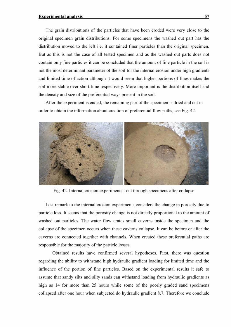
Experimental analysis 57
The grain distributions of the particles that have been eroded were very close to the
original specimen grain distributions. For some specimens the washed out part has the
distribution moved to the left i.e. it contained finer particles than the original specimen.
But as this is not the case of all tested specimen and as the washed out parts does not
contain only fine particles it can be concluded that the amount of fine particle in the soil is
not the most determinant parameter of the soil for the internal erosion under high gradients
and limited time of action although it would seem that higher portions of fines makes the
soil more stable over short time respectively. More important is the distribution itself and
the density and size of the preferential ways present in the soil.
After the experiment is ended, the remaining part of the specimen is dried and cut in
order to obtain the information about creation of preferential flow paths, see Fig. 42.
Fig. 42. Internal erosion experiments - cut through specimens after collapse
Last remark to the internal erosion experiments considers the change in porosity due to
particle loss. It seems that the porosity change is not directly proportional to the amount of
washed out particles. The water flow crates small caverns inside the specimen and the
collapse of the specimen occurs when these caverns collapse. It can be before or after the
caverns are connected together with channels. When created these preferential paths are
responsible for the majority of the particle losses.
Obtained results have confirmed several hypotheses. First, there was question
regarding the ability to withstand high hydraulic gradient loading for limited time and the
influence of the portion of fine particles. Based on the experimental results it safe to
assume that sandy silts and silty sands can withstand loading from hydraulic gradients as
high as 14 for more than 25 hours while some of the poorly graded sand specimens
collapsed after one hour when subjected do hydraulic gradient 8.7. Therefore we conclude
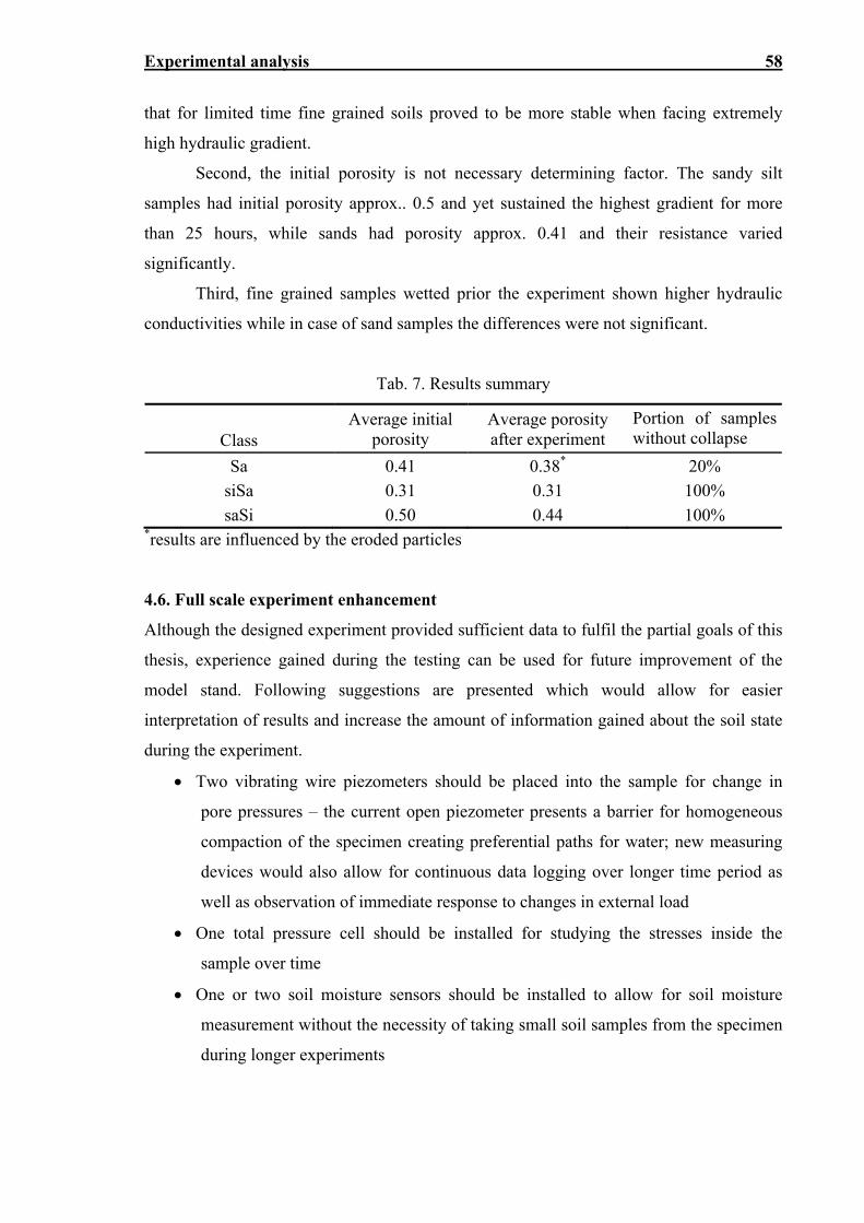
Experimental analysis 58
that for limited time fine grained soils proved to be more stable when facing extremely
high hydraulic gradient.
Second, the initial porosity is not necessary determining factor. The sandy silt
samples had initial porosity approx.. 0.5 and yet sustained the highest gradient for more
than 25 hours, while sands had porosity approx. 0.41 and their resistance varied
significantly.
Third, fine grained samples wetted prior the experiment shown higher hydraulic
conductivities while in case of sand samples the differences were not significant.
Tab. 7. Results summary
Class
Average initial porosity
Average porosity after experiment
Portion of samples without collapse
Sa 0.41 0.38* 20%
siSa 0.31 0.31 100%
saSi 0.50 0.44 100% *results are influenced by the eroded particles
4.6. Full scale experiment enhancement
Although the designed experiment provided sufficient data to fulfil the partial goals of this
thesis, experience gained during the testing can be used for future improvement of the
model stand. Following suggestions are presented which would allow for easier
interpretation of results and increase the amount of information gained about the soil state
during the experiment.
Two vibrating wire piezometers should be placed into the sample for change in
pore pressures – the current open piezometer presents a barrier for homogeneous
compaction of the specimen creating preferential paths for water; new measuring
devices would also allow for continuous data logging over longer time period as
well as observation of immediate response to changes in external load
One total pressure cell should be installed for studying the stresses inside the
sample over time
One or two soil moisture sensors should be installed to allow for soil moisture
measurement without the necessity of taking small soil samples from the specimen
during longer experiments

Experimental analysis 59
Digital gauges should be used instead of analogous one to gain all the data at once –
in coarse grained soils are changes very fast
The leakage problems would be best to solve with different stand material. Welded
steel plates creating the inner part of the stand would ensure sufficiently high water
tightness though the number of supporting beams would have to be increased.
The compaction method should be changed. To allow for easier evaluation of pre-
consolidation pressure, static load or standardized hammer weight and height of
free fall should be used instead of vibrating plate. However it must be pointed out
that vibrating plates and rollers are most common in practice.
Chapter 5
INFLUENCE ZONE THEORY
It is generally accepted that the effect of load applied on the soil will not propagate to
infinite depth. The influence zone presents an area or more precisely a domain below the
acting load. In this domain all the deformations due to the applied load take place. Below
the influence zone all the deformations from the particular load are negligible.
It is easy to see that the depth of influence zone must depend on the size of the load,
its magnitude and the characteristics of the soil. Standing standard for geotechnical design
in Europe, the Eurocode 7, (EN 1997-1; part 2.4.5.2) requires the engineers to take into
account “the extent of the zone of ground governing the behaviour of the geotechnical
structure at the limit state being considered” when selecting the characteristic values for
geotechnical parameters. It also recommends considering the influence of the supported
structure on the zone that governs geotechnical behaviour. Therefore for every in-situ
testing procedures, i.e. dilatometric and pressiometric measuring techniques, plate load
tests, standards penetration test, etc., the depth of their influence zone should be evaluated
and confronted with the expected depth of the designed structure. Also, when performing
back analysis of in-situ experiments, the size of the influence zone is crucial parameter as
shown in chapter 6. Application of this theory in numerical modelling of shallow foundations leads to
restriction of the model range especially in depth of the modelled area. In analytical
solutions this theory leads to subsoil of finite depth, i.e. elastic layer theory. The main
issue, however, is how to estimate the depth of the influence zone in practise and regarding
the groundwater how the presence of groundwater or its flow can influence this depth.
Although more sophisticated numerical methods often require the parameters
identification to be done by back analysis with the same method in order to ensure
consistency of the results, hereafter presented fast analytical approach could be used to in
practice for simple geotechnical problems as well for evaluation of the received data from
in-situ tests. Successful application of semi-analytical method on tropical residual soils
was earlier published by Cunha (Cunha et al., 2002), (Cunha and Kuklik, 2003).
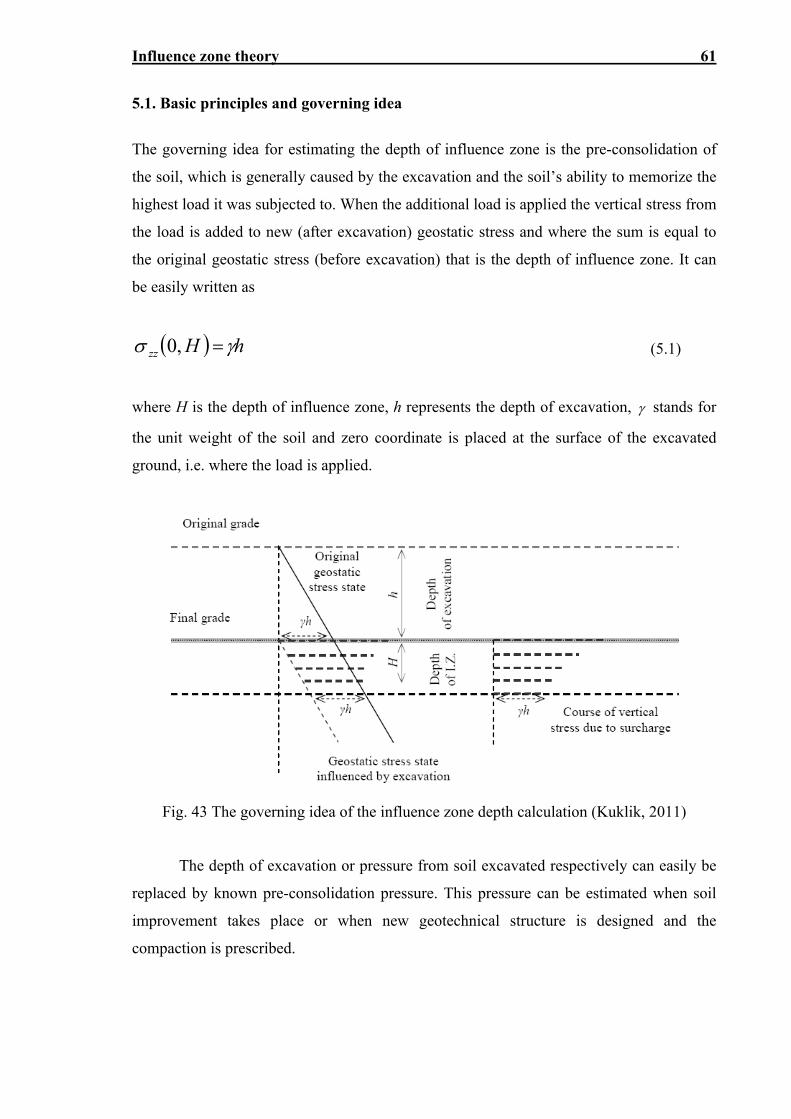
Influence zone theory 61
5.1. Basic principles and governing idea
The governing idea for estimating the depth of influence zone is the pre-consolidation of
the soil, which is generally caused by the excavation and the soil’s ability to memorize the
highest load it was subjected to. When the additional load is applied the vertical stress from
the load is added to new (after excavation) geostatic stress and where the sum is equal to
the original geostatic stress (before excavation) that is the depth of influence zone. It can
be easily written as
hHzz ,0 (5.1)
where H is the depth of influence zone, h represents the depth of excavation, stands for
the unit weight of the soil and zero coordinate is placed at the surface of the excavated
ground, i.e. where the load is applied.
Fig. 43 The governing idea of the influence zone depth calculation (Kuklik, 2011)
The depth of excavation or pressure from soil excavated respectively can easily be
replaced by known pre-consolidation pressure. This pressure can be estimated when soil
improvement takes place or when new geotechnical structure is designed and the
compaction is prescribed.
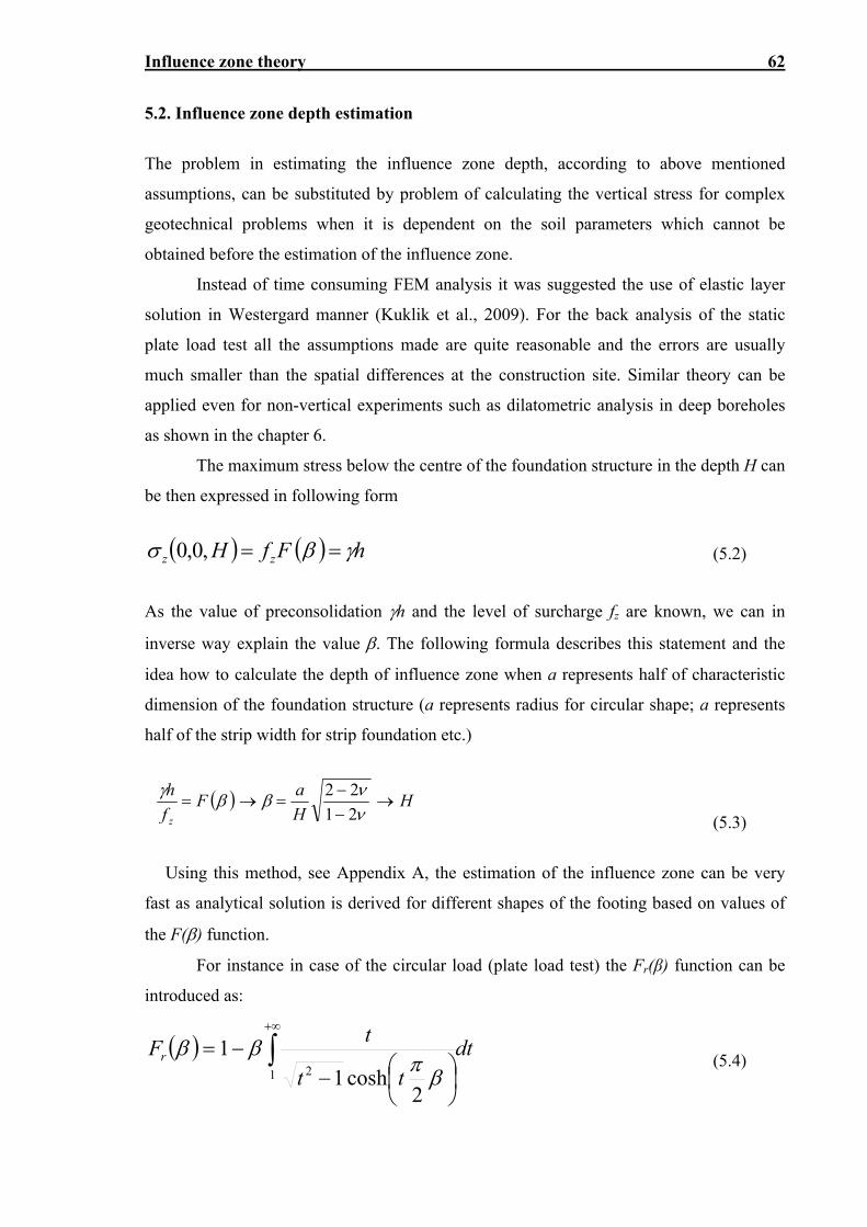
Influence zone theory 62
5.2. Influence zone depth estimation
The problem in estimating the influence zone depth, according to above mentioned
assumptions, can be substituted by problem of calculating the vertical stress for complex
geotechnical problems when it is dependent on the soil parameters which cannot be
obtained before the estimation of the influence zone.
Instead of time consuming FEM analysis it was suggested the use of elastic layer
solution in Westergard manner (Kuklik et al., 2009). For the back analysis of the static
plate load test all the assumptions made are quite reasonable and the errors are usually
much smaller than the spatial differences at the construction site. Similar theory can be
applied even for non-vertical experiments such as dilatometric analysis in deep boreholes
as shown in the chapter 6.
The maximum stress below the centre of the foundation structure in the depth H can
be then expressed in following form
hFfH zz ,0,0 (5.2)
As the value of preconsolidation h and the level of surcharge fz are known, we can in
inverse way explain the value . The following formula describes this statement and the
idea how to calculate the depth of influence zone when a represents half of characteristic
dimension of the foundation structure (a represents radius for circular shape; a represents
half of the strip width for strip foundation etc.)
HH
aF
f
h
z
21
22
(5.3)
Using this method, see Appendix A, the estimation of the influence zone can be very
fast as analytical solution is derived for different shapes of the footing based on values of
the F() function.
For instance in case of the circular load (plate load test) the Fr(β) function can be
introduced as:
dttt
tFr
1 2
2cosh1
1
(5.4)
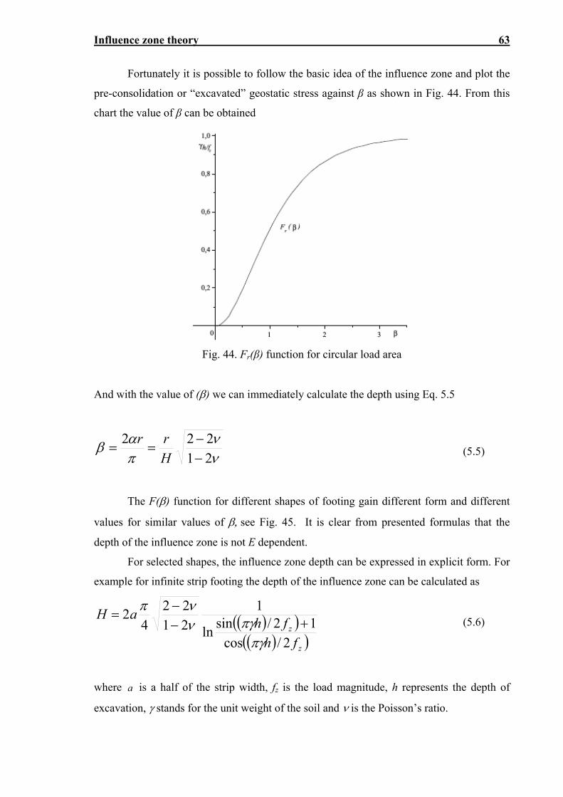
Influence zone theory 63
Fortunately it is possible to follow the basic idea of the influence zone and plot the
pre-consolidation or “excavated” geostatic stress against β as shown in Fig. 44. From this
chart the value of β can be obtained
Fig. 44. Fr(β) function for circular load area
And with the value of () we can immediately calculate the depth using Eq. 5.5
21222
Hrr
(5.5)
The F() function for different shapes of footing gain different form and different
values for similar values of see Fig. 45. It is clear from presented formulas that the
depth of the influence zone is not E dependent.
For selected shapes, the influence zone depth can be expressed in explicit form. For
example for infinite strip footing the depth of the influence zone can be calculated as
z
z
fh
fhaH
2/cos
12/sinln
12122
42
(5.6)
where a is a half of the strip width, fz is the load magnitude, h represents the depth of
excavation, stands for the unit weight of the soil and is the Poisson’s ratio.
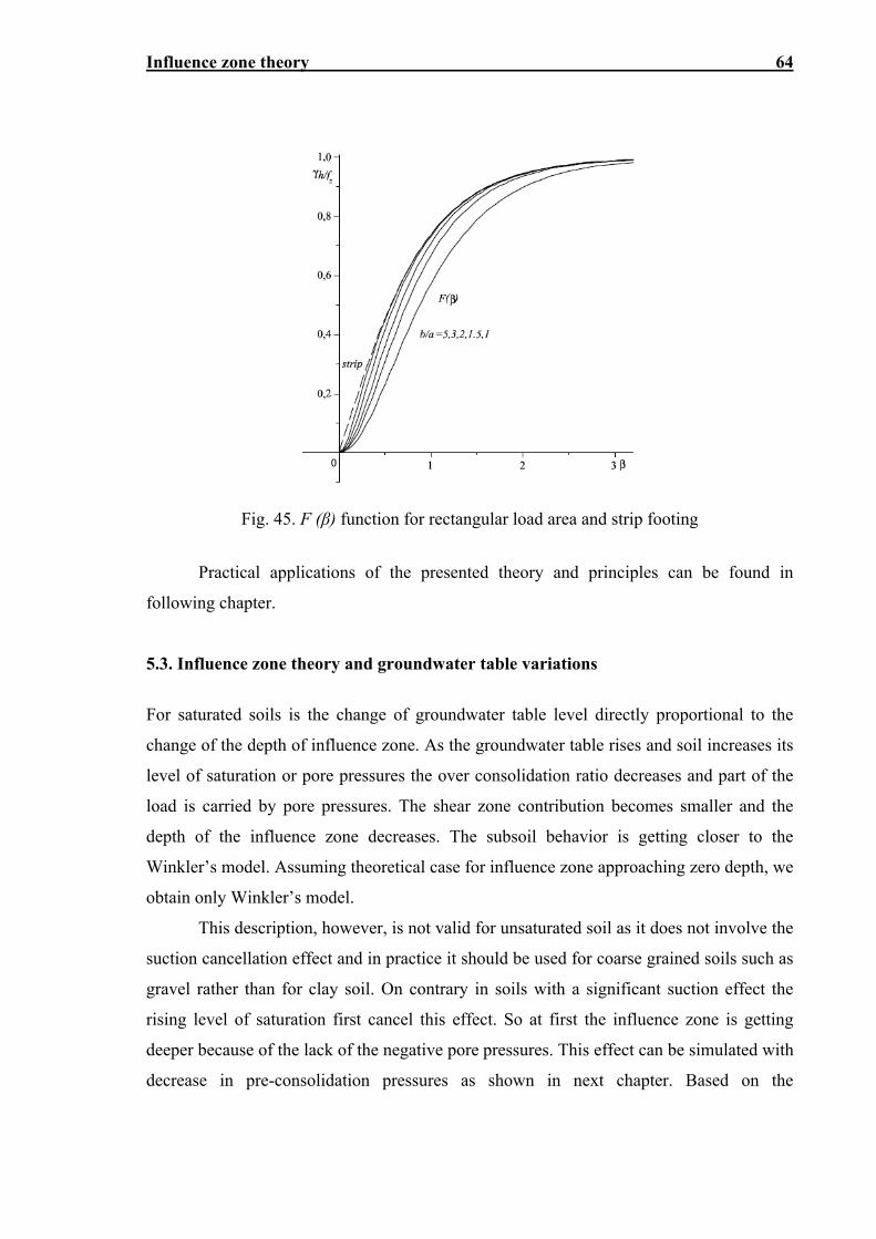
Influence zone theory 64
Fig. 45. F (β) function for rectangular load area and strip footing
Practical applications of the presented theory and principles can be found in
following chapter.
5.3. Influence zone theory and groundwater table variations
For saturated soils is the change of groundwater table level directly proportional to the
change of the depth of influence zone. As the groundwater table rises and soil increases its
level of saturation or pore pressures the over consolidation ratio decreases and part of the
load is carried by pore pressures. The shear zone contribution becomes smaller and the
depth of the influence zone decreases. The subsoil behavior is getting closer to the
Winkler’s model. Assuming theoretical case for influence zone approaching zero depth, we
obtain only Winkler’s model.
This description, however, is not valid for unsaturated soil as it does not involve the
suction cancellation effect and in practice it should be used for coarse grained soils such as
gravel rather than for clay soil. On contrary in soils with a significant suction effect the
rising level of saturation first cancel this effect. So at first the influence zone is getting
deeper because of the lack of the negative pore pressures. This effect can be simulated with
decrease in pre-consolidation pressures as shown in next chapter. Based on the
Influence zone theory 65
experimental results and practical experience we suggest following approach for pre-
consolidation pressure reduction:
a) Coarse grained soils
a1) First wetting after the soil was compacted or when groundwater table rises above
long term maximal level – the effect depends highly on the present moisture content
of the wetted soil but for rough estimation the reduction of pre-consolidation
pressure by the portion which correspond with the portion of influence zone flooded
seems to provide reasonably accurate results
a2) Repeated wetting cycles, i.e. groundwater table variation within normal positions
– for small variation of the groundwater is the effect negligible and for larger
variation (such as due to draining deep foundation pit) the effect should be taken into
account by increasing the value of F()
F
f
hh
z
ww
(5.7)
b) Fine grained soils
b1) Short term action of water or limited water access (e.g. infiltration trenches or
galleries) – – the effect depends highly on the present moisture content of the wetted
soil but for rough estimation the cancellation of pre-consolidation pressure seems to
provide reasonably accurate results
b2) Long term groundwater table rise – experimental investigation necessary
Chapter 6
PRACTICAL APPLICATIONS AND NUMERICAL
MODELLING
This chapter is focused on practical examples of use of the above described approaches and
theories. At first we concentrate on application of the influence zone (IZ) theory on back
analysis of in-situ plate load tests and full scale laboratory experiments, and on back
analysis of in-situ dilatometric measurements in deep boreholes carried out for Brenner
base tunnel excavations.
Next part focuses on application of general knowledge of unsaturated soils
behaviour on current practical issues regarding infiltration policy for new structures and
groundwater table shift due to reconstruction of hydraulic structures.
Description of risk analysis for floods and proposed enhancement of the losses on
buildings and structures is presented in the third part of this chapter.
Last part deals with numerical modelling of the full scale experiments presented in
chapter 4. Difficulties with calibration of material parameters of the used models as well as
the accepted assumptions are commented.
6.1. Influence zone change and elastic layer theory
6.1.1. Static plate load tests
It was experimentally confirmed that by using plates with different diameters and loading
forces and employing generally used Bousinesq formula (Eq. 5.2) to obtain secant modulus
of the subsoil, very different results can be achieved for the same soil. (Kuklik et al.
2008a).
tot
z
s
rfE 2
0 12
(6.1)
Practical applications and numerical modelling 67
where r is the radius of the plate, stot represents final settlement, fz is the load magnitude
and is the Poisson’s ratio.
As the formula was originally derived under the infinite half-space assumption,
which is very useful as it allows for explicit estimation of secant modulus but also limiting
as it neglect the phenomenon of soil’s memory, it should be use only, when the depth of
the influence zone exceeds approximately 2 times the diameter. For shallow influence
zones the resulting secant moduli obtained from the formula will be overestimated, i.e. the
subsoil would seem to be stiffer than it is.
This could be demonstrated on static plate load tests carried out in-situ on
construction site in Prague, which was prepared for foundation slab construction. Two
plates with diameters r1 = 0.399 m (contact area S = 0.5 m2) and r2 = 0.1785 m (contact
area S = 0.1 m2). Due to limited possibilities for reaction force constriction, which were
represented by the heaviest machinery available on construction site, the applied load in
term of stress were insufficient for the larger plate reaching only to 366 kPa in contrast to
1200 kPa for the smaller plate (Kuklik, 2006). The Poisson’s ration for the soil was
assumed equal 0.25 and the depth of the influence zone for both cases was calculated to be
approximately 0.6 m. Following table summarizes the measured data and calculated secant
moduli from three in-situ experiments.
Tab. 8. Summary of experimental data and calculated secant moduli
Test No. Applied load
(kPa) Measured settlement
(mm) Calculated secant modulus (MPa)
1 (larger plate) 366 1.27 169.3
2 (smaller plate) 1200 3.93 80.3
3 (smaller plate) 1000 2.49 105.6
Employing professional FEM code ADINA v. 8.1 results of the plate load tests
were obtained numerically for the larger plate. The settlement was calculated 0.97 mm for
secant modulus E0 = 100 MPa and 1.21 mm for E0 = 80 MPa yielding the average
settlement 1.09 mm. Comparing with measured data the numerical results (1.09 vs. 1.27
mm) seem acceptable. Small discrepancy can be explained as follows. The first
overestimation of the secant modulus is due to back analysis using Boussinesq formula,
secondly there is a shear lack inside the soil on boundary the rigid plate, which was not
simulated.
In order to confirm applicability of theory and recommendations introduced in
chapter 5, it was applied on the results from full scale experiments presented in chapter 4.
Practical applications and numerical modelling 68
For the influence zone depth estimation software DEPTH or TPS Overconsolidation was
used while for settlement calculations the subsoil reaction was described according to
known Winkler-Pasternak model, see Eq. 6.2
zfwCwC 21 (6.2)
where parameters C1 and C2 are calculated in agreement with the influence zone theory,
and while assuming elastic layer instead of original parameters, by using identity between
compliance matrixes, see Appendix A. This solution is incorporated into many software
packages. For this thesis purposes we used Geo 5 Beam on elastic foundation.
Tab. 9. Static plate load test on G2 soil in a view of elastic layer theory
Exp. No.* 3 BW 3 AW 4 5 BW 5 AW
Applied load (kPa) 1010 1010 710 710 710
Measured settlement (mm) 1.11 1.32 0.81 0.57 0.64
Measure water table from top of the specimen (m)
--- 0.41 --- --- 0.35
Calculated secant modulus (MPa)
200 200 200 290 290
Poisson’s ration 0.2 0.2 0.2 0.2 0.2
Assumed pre-consolidation (kPa)
300 150 300 300 200
Depth of IZ (m) 0.79 1.63 0.53 0.53 0.83
C1 (MNm-3) 351.6 210.4 487.1 706.3 493.9
C2 (MNm-1) 8.6 11.8 7.1 10.3 12.8
Calculated settlement (mm) 1.0 1.3 0.8 0.5 0.7 *(BW stands for “before wetting” and AW for “after wetting”)
Tab. 10. Static plate load test on F5 soil in a view of elastic layer theory
Exp. No.* 1 3 BW 3 BW adj.** 3AW
Applied load (kPa) 400 400 400 400
Measured settlement (mm) 4.82 1.25 1.25 6.25
Measure water table from top of the specimen (m)
--- --- --- 0.6
Calculated secant modulus (MPa)
16 73 37 37
Poisson’s ration 0.4 0.4 0.4 0.4
Assumed pre-consolidation 150 300 300 300
Practical applications and numerical modelling 69
(kPa)
Depth of IZ (m) 0.92 0.36 0.36 147
C1 (MNm-3) 44.2 460.1 233.4 2.1
C2 (MNm-1) 0.8 2.0 1.0 48.5
Calculated settlement (mm) 4.8 0.6 1.2 5.9 *(BW stands for “before wetting” and AW for “after wetting”)
** Secant modulus was adjusted to represent the soil as the depth of the influence zone did not correspond with the idea of half space
Two facts can be observed in tables 9 and 10. First it is the already mentioned issue
with using Boussinesq formula for calculation of secant modulus when the influence zone
is not sufficiently deep compared to the loading plate.
Second, it is the increase in the depth of the influence zone after suction is
cancelled. Even for G2 soils the depth of IZ exceeds the real depth of the specimen, which
is approximately one meter. However as the aim is to describe the change in soils
behaviour or response to suction cancellation respectively, such approach can be found
justifiable though not physically sound.
6.1.2. Dilatometric measurements and analysis
Determination of geomechanical properties of rock massif presents difficulties due to the
problems arising in sampling, specimen preparation and testing. Questionable is also the
accuracy of the results for more complex formations since the tests are usually conducted
on small specimens that cannot depict the structure. One of the methods used to directly
evaluate the actual geomechanical properties of the rock mass is a dilatometer analysis.
The dilatometer determination of the rock mass mechanical properties is based on
real time measurement of the applied pressure and change of the borehole diameter. The
deformation is directly measured by three transducers installed in the metal body of the
dilatometer probe.
A dilatometer test is usually performed in two, three or four cycles. The first testing
cycle is preceded by, so called, base pressure inflation of the probe. The first cycle should
guarantee a good contact between the probe and the borehole wall. The base pressure is
typically a hydrostatic pressure plus 0,15 – 0,5 MPa.
While the first cycle consist of loading and subsequent unloading to the base pressure,
in case of all other cycles the loading path consist of two parts. At first, the maximum
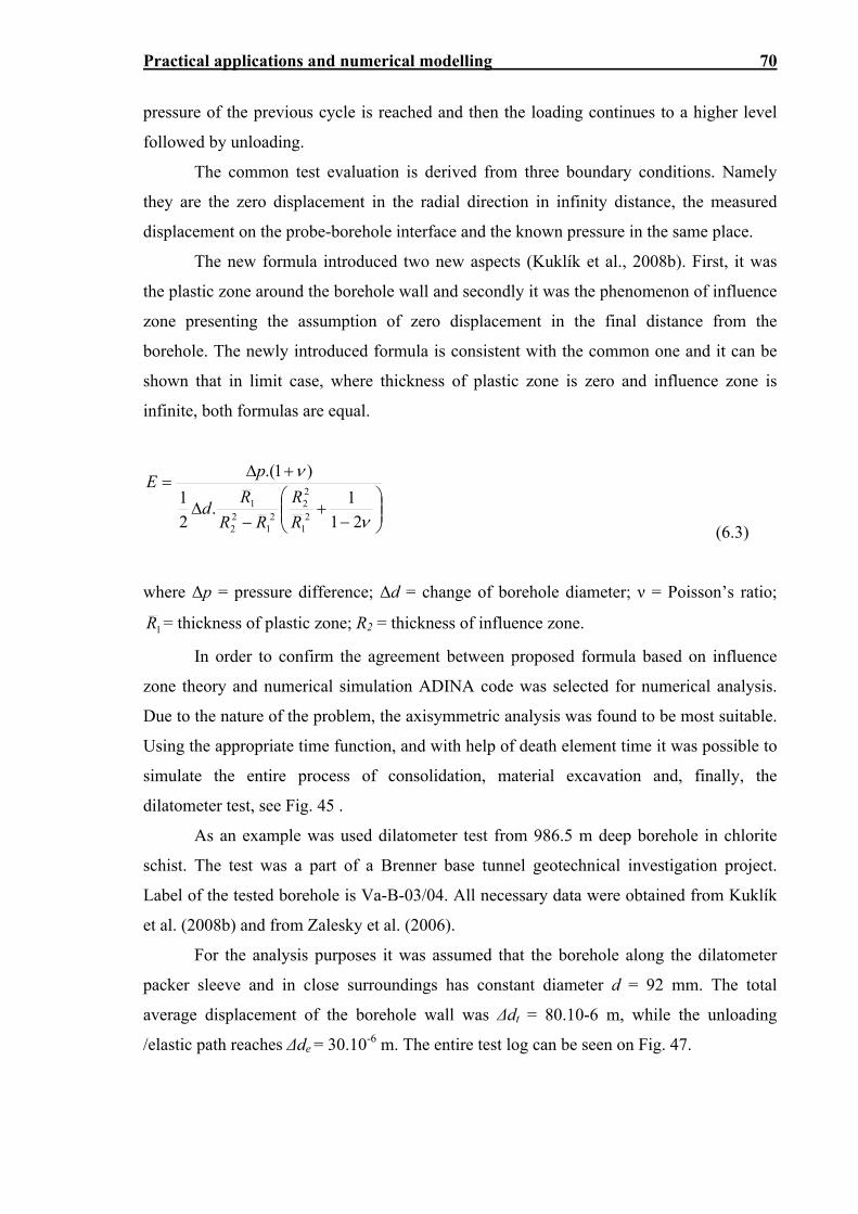
Practical applications and numerical modelling 70
pressure of the previous cycle is reached and then the loading continues to a higher level
followed by unloading.
The common test evaluation is derived from three boundary conditions. Namely
they are the zero displacement in the radial direction in infinity distance, the measured
displacement on the probe-borehole interface and the known pressure in the same place.
The new formula introduced two new aspects (Kuklík et al., 2008b). First, it was
the plastic zone around the borehole wall and secondly it was the phenomenon of influence
zone presenting the assumption of zero displacement in the final distance from the
borehole. The newly introduced formula is consistent with the common one and it can be
shown that in limit case, where thickness of plastic zone is zero and influence zone is
infinite, both formulas are equal.
21
1.
2
1
)1.(
21
22
21
22
1
R
R
RR
Rd
pE
(6.3)
where Δp = pressure difference; Δd = change of borehole diameter; ν = Poisson’s ratio;
1R = thickness of plastic zone; R2 = thickness of influence zone.
In order to confirm the agreement between proposed formula based on influence
zone theory and numerical simulation ADINA code was selected for numerical analysis.
Due to the nature of the problem, the axisymmetric analysis was found to be most suitable.
Using the appropriate time function, and with help of death element time it was possible to
simulate the entire process of consolidation, material excavation and, finally, the
dilatometer test, see Fig. 45 .
As an example was used dilatometer test from 986.5 m deep borehole in chlorite
schist. The test was a part of a Brenner base tunnel geotechnical investigation project.
Label of the tested borehole is Va-B-03/04. All necessary data were obtained from Kuklík
et al. (2008b) and from Zalesky et al. (2006).
For the analysis purposes it was assumed that the borehole along the dilatometer
packer sleeve and in close surroundings has constant diameter d = 92 mm. The total
average displacement of the borehole wall was Δdt = 80.10-6 m, while the unloading
/elastic path reaches Δde = 30.10-6 m. The entire test log can be seen on Fig. 47.
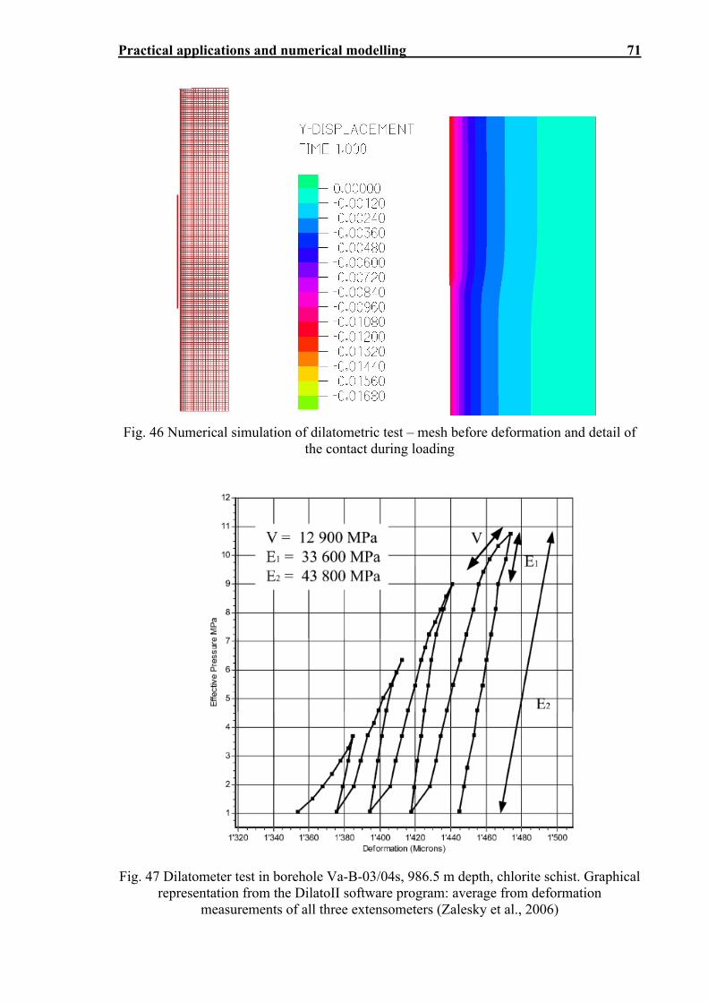
Practical applications and numerical modelling 71
Fig. 46 Numerical simulation of dilatometric test – mesh before deformation and detail of the contact during loading
Fig. 47 Dilatometer test in borehole Va-B-03/04s, 986.5 m depth, chlorite schist. Graphical representation from the DilatoII software program: average from deformation
measurements of all three extensometers (Zalesky et al., 2006)
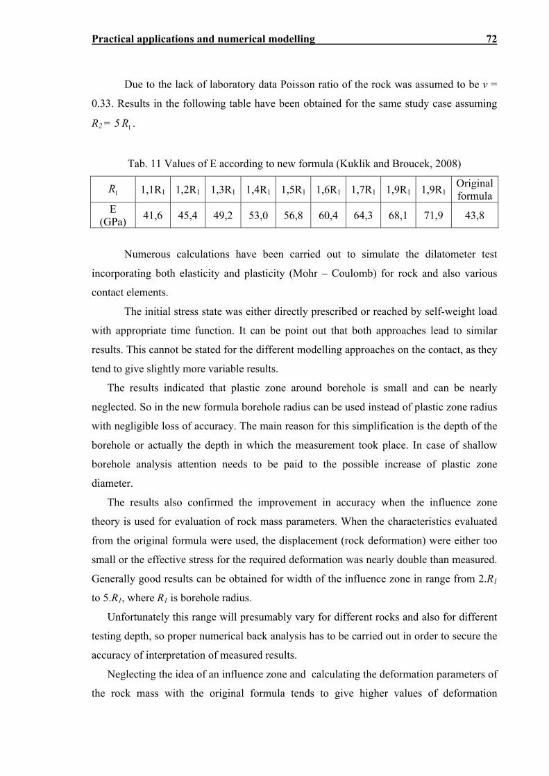
Practical applications and numerical modelling 72
Due to the lack of laboratory data Poisson ratio of the rock was assumed to be ν =
0.33. Results in the following table have been obtained for the same study case assuming
R2 = 5 1R .
Tab. 11 Values of E according to new formula (Kuklik and Broucek, 2008)
1R 1,1R1 1,2R1 1,3R1 1,4R1 1,5R1 1,6R1 1,7R1 1,9R1 1,9R1 Original formula
E (GPa)
41,6 45,4 49,2 53,0 56,8 60,4 64,3 68,1 71,9 43,8
Numerous calculations have been carried out to simulate the dilatometer test
incorporating both elasticity and plasticity (Mohr – Coulomb) for rock and also various
contact elements.
The initial stress state was either directly prescribed or reached by self-weight load
with appropriate time function. It can be point out that both approaches lead to similar
results. This cannot be stated for the different modelling approaches on the contact, as they
tend to give slightly more variable results.
The results indicated that plastic zone around borehole is small and can be nearly
neglected. So in the new formula borehole radius can be used instead of plastic zone radius
with negligible loss of accuracy. The main reason for this simplification is the depth of the
borehole or actually the depth in which the measurement took place. In case of shallow
borehole analysis attention needs to be paid to the possible increase of plastic zone
diameter.
The results also confirmed the improvement in accuracy when the influence zone
theory is used for evaluation of rock mass parameters. When the characteristics evaluated
from the original formula were used, the displacement (rock deformation) were either too
small or the effective stress for the required deformation was nearly double than measured.
Generally good results can be obtained for width of the influence zone in range from 2.R1
to 5.R1, where R1 is borehole radius.
Unfortunately this range will presumably vary for different rocks and also for different
testing depth, so proper numerical back analysis has to be carried out in order to secure the
accuracy of interpretation of measured results.
Neglecting the idea of an influence zone and calculating the deformation parameters of
the rock mass with the original formula tends to give higher values of deformation
Practical applications and numerical modelling 73
modulus and Young’s modulus. If these values should be used further for numerical
simulations of the geotechnical work (e.g. tunnel excavation) the loss in model accuracy
can be very high. Optionally such numbers should be used only as an upper limit and the
scale effect is considered.
6.2. General knowledge about unsaturated soils behaviour
Many examples of problems requiring application of general knowledge about unsaturated
soils behaviour can be found even in the temperate climate in which is located Czech
Republic. For the purpose of this part we select two current issues related to water
management. At first we describe the debate concerning groundwater table position shift
due to implementation of flood protection measures in the UNESCO listed town Cesky
Krumlov. Second, the standing requirements of the civil service for infiltration of
precipitation water from newly constructed buildings and impermeable areas is discussed
from the point of view of potential damage to the adjacent construction when the steady
state is disrupted.
6.2.1. Flood protection measures
All sorts of non-structural and structural flood protection measures were supported by EU
adaptation and mitigation programs including channel improvements, generally widening
and deepening of channels, and flood barriers with deep and impermeable foundation
structures i.e. sheet piles, pile walls etc. In most cases, no serious estimations regarding the
groundwater regime change and its possible impact to the upper structures in protected
areas were made. And again, in most of the cases, no abnormal behaviour of upper
structures was reported. In the Cesky Krlumlov town, however, cracks were reported in the
walls of historical buildings, many of them dated back to Middle Ages. The town centre is
UNESCO listed and it would seem that our cultural heritage is at stake due to flood
protection structures and channel improvement.
As presented in this thesis, and by many other authors, the soil’s ability to
memorize a certain loading history, the highest level of loading respectively, which is
mathematically represented by the over-consolidation ratio, and initial void ratio, can be
seriously influenced by the saturation level of the soil in several ways. Furthermore the
material parameters of soils and consequently the response to loading characterised as
Practical applications and numerical modelling 74
settlement are influenced by the groundwater. So in general, disruption of the long term
steady state by construction works during building phase or structures itself may cause
additional deformation of the subsoil and potentially cracks in upper structure. It should be
noted, however, that for soils in saturated state the change in pore pressures needs to be
significant with relation to the present stress state and in case of the unsaturated soils,
which do not undergo excessive shrinkage during saturation level decrease, the
deformation will only take place when the groundwater table rises above the long term
maximum.
Based on all the presented arguments and theories and experimental results
presented in this thesis we can conclude that lowering the groundwater table by several
decimetres or one meter as in the case of Cesky Krumlov can hardly cause additional
deformation of upper structures which would result in cracks development in walls of
historical buildings.
It is to be emphasized, however, that every channel improvement or other
protective measures should be considered from broader perspective carefully evaluating all
possible impacts on the steady state of the hydrogeological regime in particular areas. In
sensitive cases, such as historic town centres, passportisation of selected building and
monitoring of the hydrogeological regime can prove to be extremely helpful.
6.2.2. Infiltration from large impermeable areas
Current policy of the civil service regarding the management of water from precipitation
requires the owners of new properties to infiltrate, or use otherwise, all the whole amount
of water without using sewer systems. This approach is very unfortunate when applied
without the respect to the subsoil reaction on the large quantity of water and could be
potentially dangerous to adjacent structures.
Nowadays, the infiltration capacity of subsoil and storativities of appropriate
aquifers are estimated and analysed by field infiltration or pumping tests and numerical
simulations based on models of flow through porous material. Such analysis presents
sophisticated results and is perfectly suitable for the original purpose, i.e. to design the
infiltration galleries or trenches and confirm that the infiltration is possible. The main issue
is the absence of geotechnical analysis of the impact of estimated changes on the
foundation and upper structures. Even if such analysis is carried out it usually neglects the
Practical applications and numerical modelling 75
so important differences between saturated and unsaturated soil behaviour assuming only
deformation from positive pore pressure.
Data for the following example of newly designed block of flats were obtained
from the field but due to on-going planning enquiry it was not yet published. The present
situation involves several older buildings located on lands adjacent to the planned block.
Subsoil can be described as silt loam and silty sand followed by weathered silty sandstones
and sandstones. The neighbouring buildings which include family houses as well as tower
block are founded on the silt loams or silty sands using strip foundations under the
basement level. Results from numerical simulations of groundwater flow show permanent
increase of groundwater table by 0.35 – 0.5 m and average maximum level would even
touch the foundation base.
Applying the saturated soils (classical soil mechanics) approach would yield in
variation of effective stress between 3.5 and 5 kPa which is negligible change when
compared to present state. Applying the unsaturated approach, however, would yield in
suction cancellation and dramatic increase in settlement for the silt loams case.
Unfortunately, the understanding of unsaturated soils behaviour just only started to be
recognized by the geotechnical engineers dealing most of the time with common saturated
problems.
6.3. Risk analysis for flood events
The internal erosion problems as well as additional deformations caused by the change of
mechanical behaviour of unsaturated soils when subjected to suction cancellation can fully
emerge during flood events and be the decisive source of damage to the upper structures.
The flood risk assessment became debated on national level as well as on European level
in recent decades thanks to the concept or rather the obsession of risk evaluation and
potential damage monetization, which is enabled and supported by massive extension of
the numerical models and use of GIS software packages. Nevertheless, for evaluation of
the impact of flood events and for the effect of flood protection schemes the risk analysis
presents the most impartial tool. The definition of the risk due to flood is generally defined
in the following form
0
)()()()(b
a
Q
Q
dQQfQDdQQfQDR (6.4)
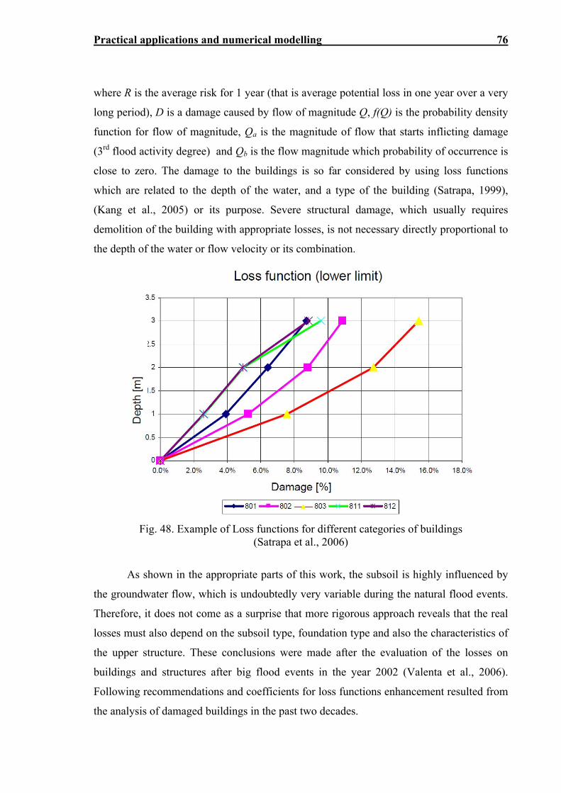
Practical applications and numerical modelling 76
where R is the average risk for 1 year (that is average potential loss in one year over a very
long period), D is a damage caused by flow of magnitude Q, f(Q) is the probability density
function for flow of magnitude, Qa is the magnitude of flow that starts inflicting damage
(3rd flood activity degree) and Qb is the flow magnitude which probability of occurrence is
close to zero. The damage to the buildings is so far considered by using loss functions
which are related to the depth of the water, and a type of the building (Satrapa, 1999),
(Kang et al., 2005) or its purpose. Severe structural damage, which usually requires
demolition of the building with appropriate losses, is not necessary directly proportional to
the depth of the water or flow velocity or its combination.
Fig. 48. Example of Loss functions for different categories of buildings (Satrapa et al., 2006)
As shown in the appropriate parts of this work, the subsoil is highly influenced by
the groundwater flow, which is undoubtedly very variable during the natural flood events.
Therefore, it does not come as a surprise that more rigorous approach reveals that the real
losses must also depend on the subsoil type, foundation type and also the characteristics of
the upper structure. These conclusions were made after the evaluation of the losses on
buildings and structures after big flood events in the year 2002 (Valenta et al., 2006).
Following recommendations and coefficients for loss functions enhancement resulted from
the analysis of damaged buildings in the past two decades.
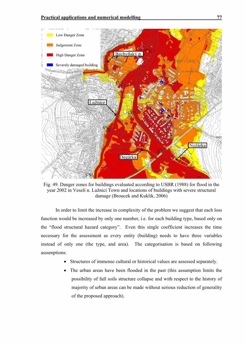
Practical applications and numerical modelling 77
Fig. 49. Danger zones for buildings evaluated according to USBR (1988) for flood in the year 2002 in Veselí n. Lužnicí Town and locations of buildings with severe structural
damage (Broucek and Kuklik, 2006)
In order to limit the increase in complexity of the problem we suggest that each loss
function would be increased by only one number, i.e. for each building type, based only on
the “flood structural hazard category”. Even this single coefficient increases the time
necessary for the assessment as every entity (building) needs to have three variables
instead of only one (the type, and area). The categorisation is based on following
assumptions:
Structures of immense cultural or historical values are assessed separately.
The urban areas have been flooded in the past (this assumption limits the
possibility of full soils structure collapse and with respect to the history of
majority of urban areas can be made without serious reduction of generality
of the proposed approach).
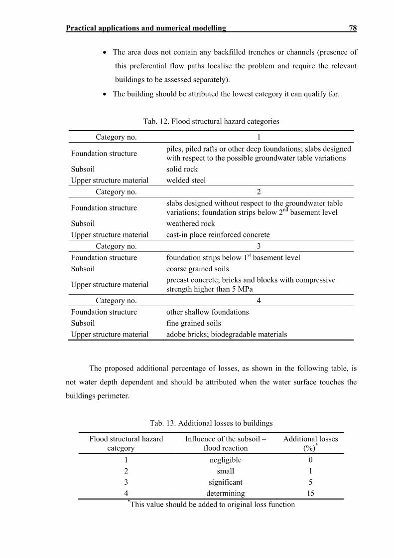
Practical applications and numerical modelling 78
The area does not contain any backfilled trenches or channels (presence of
this preferential flow paths localise the problem and require the relevant
buildings to be assessed separately).
The building should be attributed the lowest category it can qualify for.
Tab. 12. Flood structural hazard categories
Category no. 1
Foundation structure piles, piled rafts or other deep foundations; slabs designed with respect to the possible groundwater table variations
Subsoil solid rock
Upper structure material welded steel
Category no. 2
Foundation structure slabs designed without respect to the groundwater table variations; foundation strips below 2nd basement level
Subsoil weathered rock
Upper structure material cast-in place reinforced concrete
Category no. 3
Foundation structure foundation strips below 1st basement level
Subsoil coarse grained soils
Upper structure material precast concrete; bricks and blocks with compressive strength higher than 5 MPa
Category no. 4
Foundation structure other shallow foundations
Subsoil fine grained soils
Upper structure material adobe bricks; biodegradable materials
The proposed additional percentage of losses, as shown in the following table, is
not water depth dependent and should be attributed when the water surface touches the
buildings perimeter.
Tab. 13. Additional losses to buildings
Flood structural hazard category
Influence of the subsoil – flood reaction
Additional losses (%)*
1 negligible 0
2 small 1
3 significant 5
4 determining 15 *This value should be added to original loss function
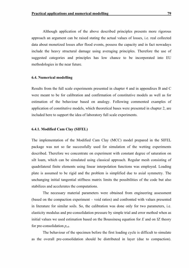
Practical applications and numerical modelling 79
Although application of the above described principles presents more rigorous
approach an argument can be raised stating the actual values of losses, i.e. real collected
data about monetized losses after flood events, possess the capacity and in fact nowadays
include the heavy structural damage using averaging principles. Therefore the use of
suggested categories and principles has low chance to be incorporated into EU
methodologies in the near future.
6.4. Numerical modelling
Results from the full scale experiments presented in chapter 4 and in appendixes B and C
were meant to be for calibration and confirmation of constitutive models as well as for
estimation of the behaviour based on analogy. Following commented examples of
application of constitutive models, which theoretical bases were presented in chapter 2, are
included here to support the idea of laboratory full scale experiments.
6.4.1. Modified Cam Clay (SIFEL)
The implementation of the Modified Cam Clay (MCC) model prepared in the SIFEL
package was not so far successfully used for simulation of the wetting experiments
described. Therefore we concentrate on experiment with constant degree of saturation on
silt loam, which can be simulated using classical approach. Regular mesh consisting of
quadrilateral finite elements using linear interpolation functions was employed. Loading
plate is assumed to be rigid and the problem is simplified due to axial symmetry. The
unchanging initial tangential stiffness matrix limits the possibilities of the code but also
stabilizes and accelerates the computations.
The necessary material parameters were obtained from engineering assessment
(based on the compaction experiment – void ratios) and confronted with values presented
in literature for similar soils. So, the calibration was done only for two parameters, i.e.
elasticity modulus and pre-consolidation pressure by simple trial and error method when as
initial values we used estimation based on the Boussinesq equation for E and on IZ theory
for pre-consolidation pc0.
The behaviour of the specimen before the first loading cycle is difficult to simulate
as the overall pre-consolidation should be distributed in layer (due to compaction).
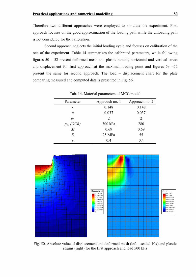
Practical applications and numerical modelling 80
Therefore two different approaches were employed to simulate the experiment. First
approach focuses on the good approximation of the loading path while the unloading path
is not considered for the calibration.
Second approach neglects the initial loading cycle and focuses on calibration of the
rest of the experiment. Table 14 summarizes the calibrated parameters, while following
figures 50 – 52 present deformed mesh and plastic strains, horizontal and vertical stress
and displacement for first approach at the maximal loading point and figures 53 –55
present the same for second approach. The load – displacement chart for the plate
comparing measured and computed data is presented in Fig. 56.
Tab. 14. Material parameters of MCC model
Parameter Approach no. 1 Approach no. 2
λ 0.148 0.148
κ 0.037 0.037
e0 2 2
pc0 (OCR) 300 kPa 280
M 0.69 0.69
E 25 MPa 55
0.4 0.4
Fig. 50. Absolute value of displacement and deformed mesh (left – scaled 10x) and plastic strains (right) for the first approach and load 500 kPa
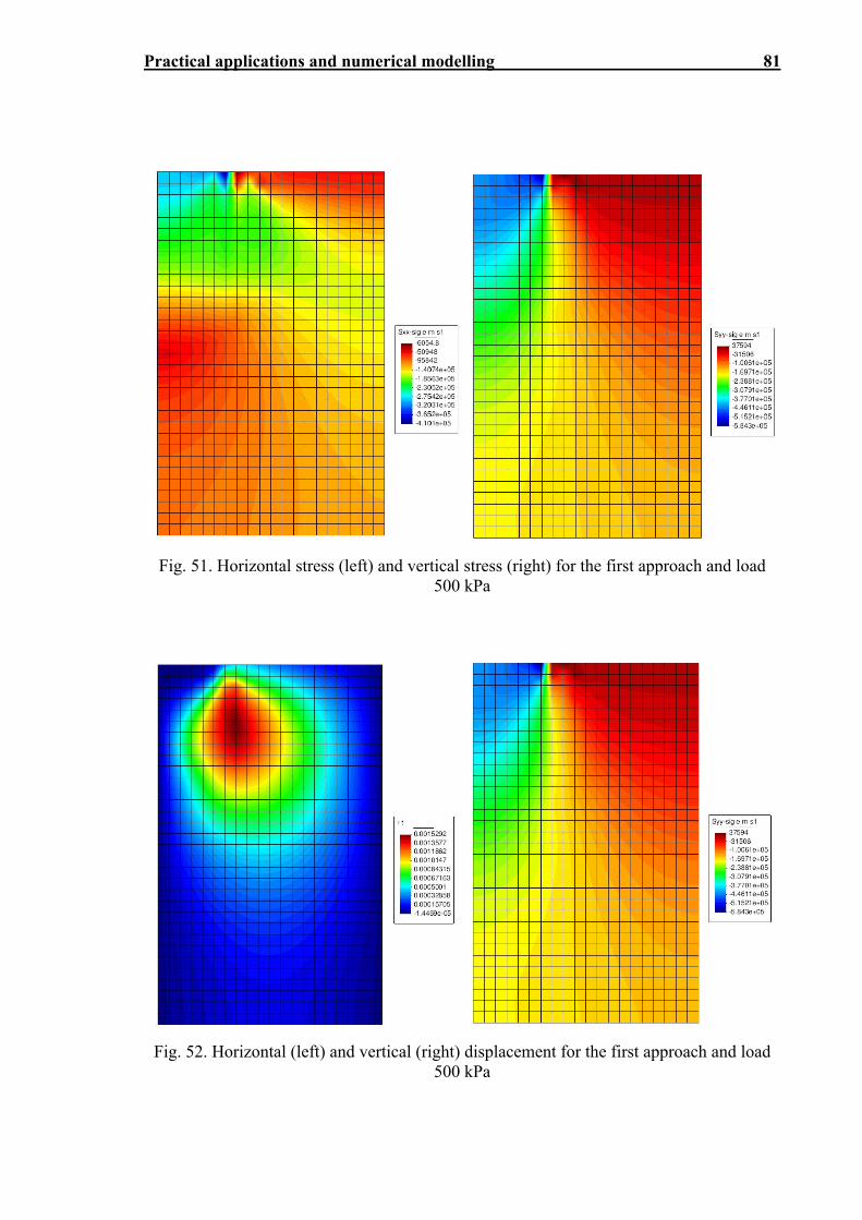
Practical applications and numerical modelling 81
Fig. 51. Horizontal stress (left) and vertical stress (right) for the first approach and load 500 kPa
Fig. 52. Horizontal (left) and vertical (right) displacement for the first approach and load 500 kPa
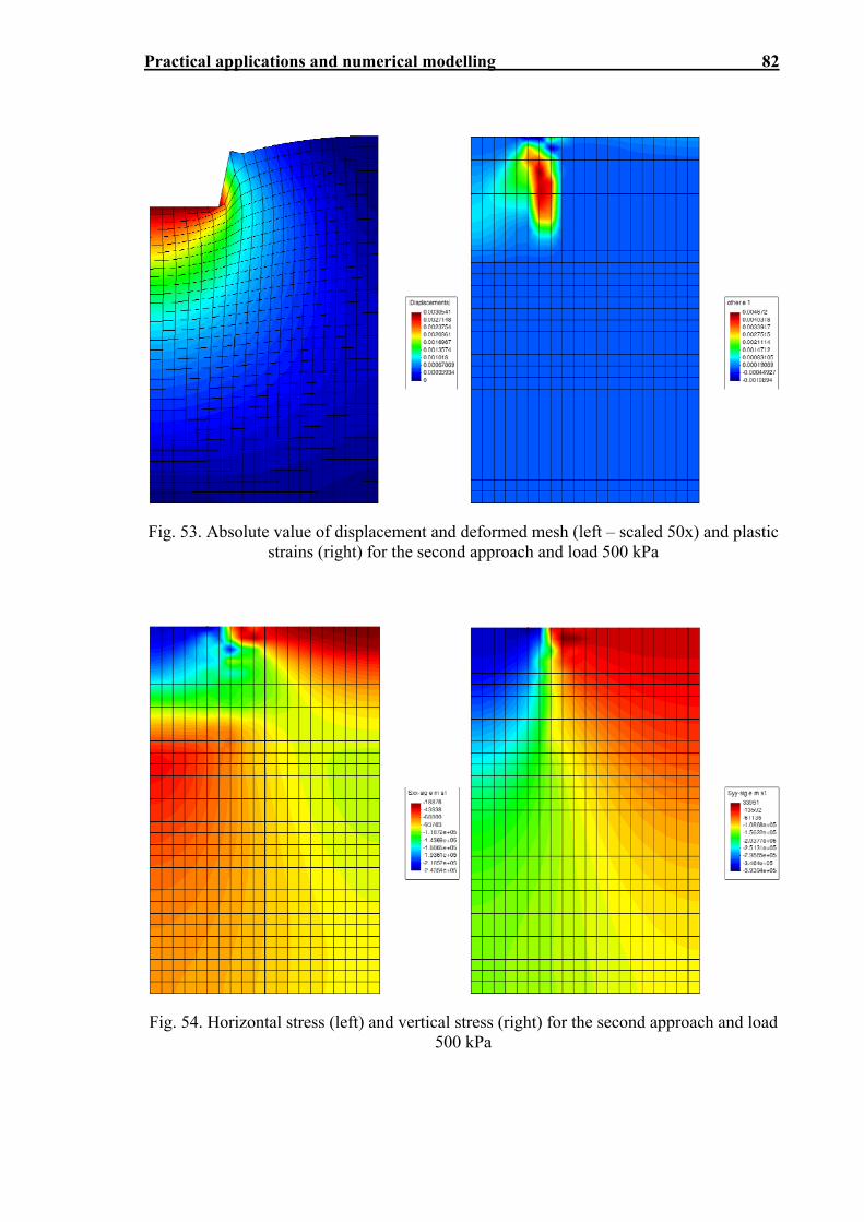
Practical applications and numerical modelling 82
Fig. 53. Absolute value of displacement and deformed mesh (left – scaled 50x) and plastic strains (right) for the second approach and load 500 kPa
Fig. 54. Horizontal stress (left) and vertical stress (right) for the second approach and load 500 kPa
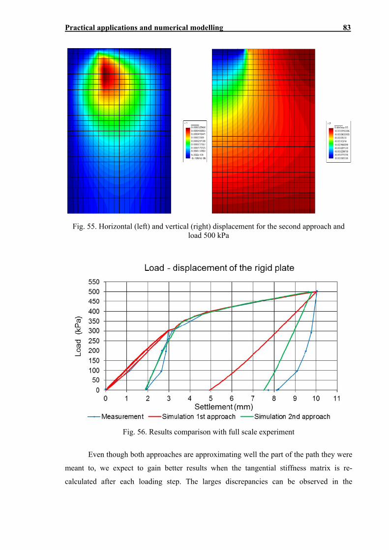
Practical applications and numerical modelling 83
Fig. 55. Horizontal (left) and vertical (right) displacement for the second approach and load 500 kPa
Fig. 56. Results comparison with full scale experiment
Even though both approaches are approximating well the part of the path they were
meant to, we expect to gain better results when the tangential stiffness matrix is re-
calculated after each loading step. The larges discrepancies can be observed in the
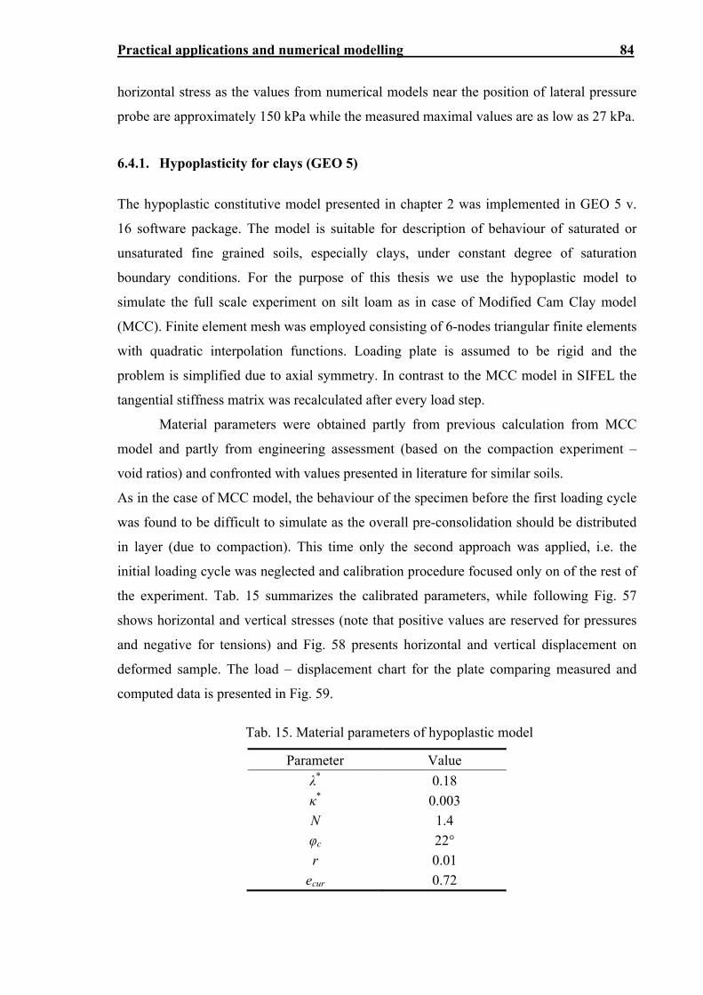
Practical applications and numerical modelling 84
horizontal stress as the values from numerical models near the position of lateral pressure
probe are approximately 150 kPa while the measured maximal values are as low as 27 kPa.
6.4.1. Hypoplasticity for clays (GEO 5)
The hypoplastic constitutive model presented in chapter 2 was implemented in GEO 5 v.
16 software package. The model is suitable for description of behaviour of saturated or
unsaturated fine grained soils, especially clays, under constant degree of saturation
boundary conditions. For the purpose of this thesis we use the hypoplastic model to
simulate the full scale experiment on silt loam as in case of Modified Cam Clay model
(MCC). Finite element mesh was employed consisting of 6-nodes triangular finite elements
with quadratic interpolation functions. Loading plate is assumed to be rigid and the
problem is simplified due to axial symmetry. In contrast to the MCC model in SIFEL the
tangential stiffness matrix was recalculated after every load step.
Material parameters were obtained partly from previous calculation from MCC
model and partly from engineering assessment (based on the compaction experiment –
void ratios) and confronted with values presented in literature for similar soils.
As in the case of MCC model, the behaviour of the specimen before the first loading cycle
was found to be difficult to simulate as the overall pre-consolidation should be distributed
in layer (due to compaction). This time only the second approach was applied, i.e. the
initial loading cycle was neglected and calibration procedure focused only on of the rest of
the experiment. Tab. 15 summarizes the calibrated parameters, while following Fig. 57
shows horizontal and vertical stresses (note that positive values are reserved for pressures
and negative for tensions) and Fig. 58 presents horizontal and vertical displacement on
deformed sample. The load – displacement chart for the plate comparing measured and
computed data is presented in Fig. 59.
Tab. 15. Material parameters of hypoplastic model
Parameter Value
λ* 0.18
κ* 0.003
N 1.4
φc 22°
r 0.01
ecur 0.72
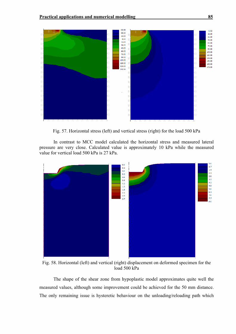
Practical applications and numerical modelling 85
Fig. 57. Horizontal stress (left) and vertical stress (right) for the load 500 kPa In contrast to MCC model calculated the horizontal stress and measured lateral pressure are very close. Calculated value is approximately 10 kPa while the measured value for vertical load 500 kPa is 27 kPa.
Fig. 58. Horizontal (left) and vertical (right) displacement on deformed specimen for the
load 500 kPa The shape of the shear zone from hypoplastic model approximates quite well the
measured values, although some improvement could be achieved for the 50 mm distance.
The only remaining issue is hysteretic behaviour on the unloading/reloading path which
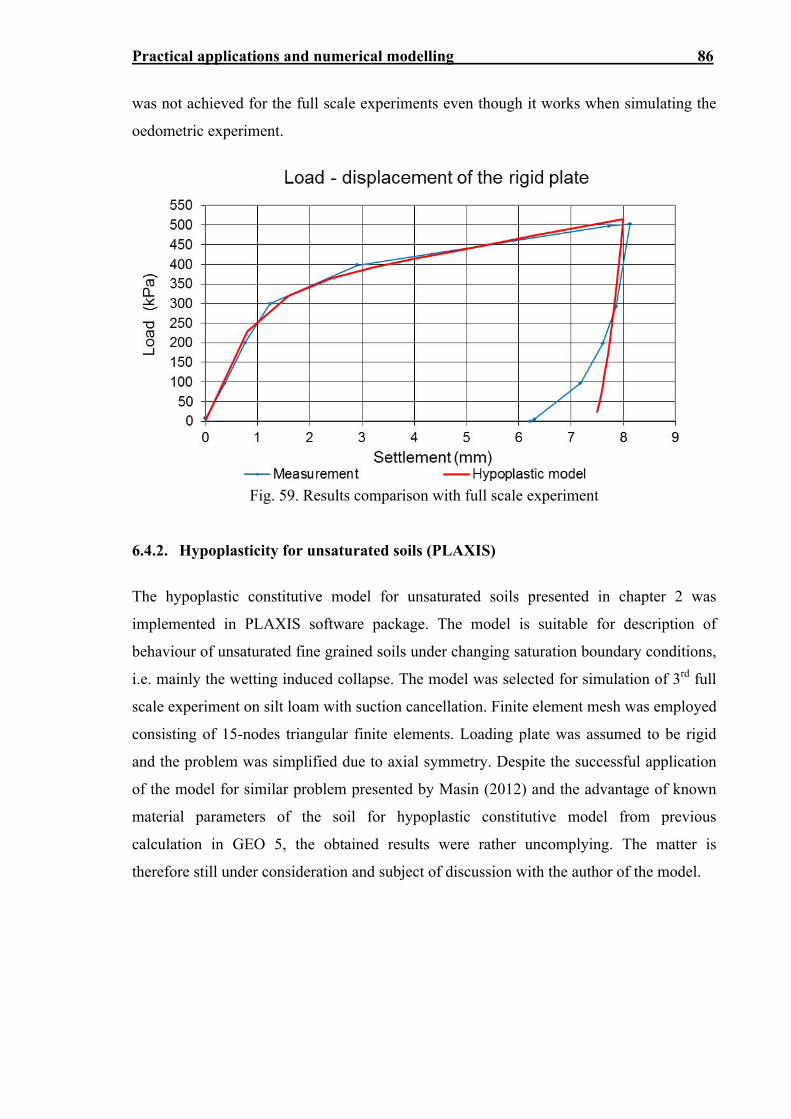
Practical applications and numerical modelling 86
was not achieved for the full scale experiments even though it works when simulating the
oedometric experiment.
Fig. 59. Results comparison with full scale experiment
6.4.2. Hypoplasticity for unsaturated soils (PLAXIS)
The hypoplastic constitutive model for unsaturated soils presented in chapter 2 was
implemented in PLAXIS software package. The model is suitable for description of
behaviour of unsaturated fine grained soils under changing saturation boundary conditions,
i.e. mainly the wetting induced collapse. The model was selected for simulation of 3rd full
scale experiment on silt loam with suction cancellation. Finite element mesh was employed
consisting of 15-nodes triangular finite elements. Loading plate was assumed to be rigid
and the problem was simplified due to axial symmetry. Despite the successful application
of the model for similar problem presented by Masin (2012) and the advantage of known
material parameters of the soil for hypoplastic constitutive model from previous
calculation in GEO 5, the obtained results were rather uncomplying. The matter is
therefore still under consideration and subject of discussion with the author of the model.
Chapter 7
CONCLUSIONS AND FUTURE PERSPECTIVES
Understanding of the processes, which influence the behaviour of the subsoil and are
caused by the presence or movement of the groundwater, can improve the design process
and help to avoid unexpected and potentially damaging additional deformations of the
upper structure. Although nowadays practice refers most of this influence to soils with
large amount of fine particles the experiments proved that such influence is not negligible
for sandy soils or gravel and is some cases it is even larger for coarse soils than for fine
soils. The last part refers to weak performance of sands subjected to high hydraulic
gradients.
Although, the theoretical base is very broad, it has been shown that it leaves enough
space for improvement, especially in case of localized preferential flow and its coupling
with mechanical behaviour but also on the field of unsaturated soils behaviour. Within the
thesis we described the theoretical bases of the unsaturated poromechanics including
different approaches to stress state variable and also the lack of consensus among leading
authorities in the field. Several constitutive models approximating saturated and
unsaturated behaviour were introduce including the criticism regarding their inconsistency
with the physical elements of the system which comes partly due to widely used axis
translation measuring technique for obtaining relevant data sets suction above cavitation
limit. Description of the internal erosion and loss of particles was introduced together with
its mathematical representation.
Due to the number of problems which could be solved with respect to the subsoil
influenced by the groundwater it was necessary to concentrate the effort only selected parts
of it. Even though highly sophisticated numerical models for unsaturated soils behaviour
can often well simulate the real stress and strain behaviour for specified situations, their
complexity, in terms of number of parameters and experiments for their identification, and
demands, in terms of computational time and experienced individuals, excludes them from
common practice towards rather unique problems and even there the spatial variability of
Conclusions and future perspectives 88
the soils characteristics together with limited possibilities of geotechnical survey limits or
decreases their accuracy. Slightly different situation can be observed around the
“classical” saturated poromechanics models. Due to the possibility of using their
assumptions and approaches even for soils with negative pore pressure but under suction
steady state conditions these model have much wider area of possible application,
however, hypoplastic or critical state constitutive models are not as widely used as Mohr-
Coulomb or Drucker-Prager.
For the common engineering practice, however, it is necessary to search for a
simple solution with large variety of use rather than increasing the overall complexity of
the problem. That is why this thesis focuses on the experimental analysis and its evaluation
followed by recommendations and sophisticated numerical models and their confirmation
stand last in the line. Stand for full scale experiments with varying groundwater table was
designed and constructed allowing for observation of all the phenomena and possibility of
estimating the effects in situ due to selected measuring technique, i.e. static plate load test.
The results obtained from the full scale experiments proved to be very useful in
understanding and evaluating of the processes through which the groundwater influence
the behaviour of the subsoil leading to sets of recommendations in the influence zone
theory and flood risk assessment. Some of the results obtained challenge the general
assumptions, such as fine particle loss due to groundwater flow or negligibility of the
effect of suction for coarse soils.
The results were also used to calibrate and confirm the ability of professional codes
to approximate the soils behaviour during plate load tests and suction cancellation. The
success of the last mentioned simulations was very limited despite the enormous
computational time used.
All the presented information encourage further research activities in both major
fields, i.e. internal erosion and unsaturated soils behaviour, with attention to both coarse
and fine soils. Enhancements for the full scale experimental setup were presented in the
thesis but large scale in-situ experiments are necessary to verify the suggested analogical
approach followed by standard recommendations.
Use of random spatial fields with high correlation for adjacent elements could
prove to be potentially very successful for evaluation of the risk of internal erosion for dam
foundation and even for earth dam body with possible extension to unsteady state and
estimation of effect of possible counter measures.

BIBLIOGRAPHY
Achmus, M., and K. Abdel-Rahman. (2003) The Influence of 'up-Scaling' on the Results of Particle Method Calculations of Non-Cohesive Soils Numerical Modeling in Micromechanics Via Particle Methods, Germany, 183-187
Aitchinson, G.D. (1965) Engineering Concepts of Moisture Equilibria and Moisture
Changes in Soils, Moisture Equilibria and Moisture Changes in Soils Beneath Covered Areas, Australia, 7-21
Alonso, E.E, Gens, A. and Josa, A.(1990). A constitutive model for partially saturated
soils. Géotechnique, 40(3), 405-430 Baker, R. and Frydman, S. (2009) Unsaturated soil mechanics, Critical review of physical
foundations, Eng. Geol., 106, 26-39 Bishop, A.W. (1959) The Principle of Effective Stress, Teknisk Ukeblad, 106(39), 859-863 Bittnar, Z. and Sejnoha, J. (1996) Numerical Methods in Structural Mechanics, ASCE
Press, New York Bligh, W.G. (1910). Dams, Barrages and Weirs on Porous Foundations. Engineering News
Record, 64 , 708-710 Broucek, M., Kuklik, P. (2006) Důsledky změn hladiny podzemní vody v podloží a
následné dopady na vrchní stavbu, In: Staticko-konštrukčné a stavebno-fyzikálne problémy stavebných konštrukcií, Košice (In Czech)
Buckingham, E. (1907) Studies of the Movement of Soil Moisture, USDA Bur. of Soils,
Bulletin No. 38 Carman, P.C. (1937). Fluid Flow through Granular Beds. Trans.Inst.Chem. Eng., 15,150 Caesar, G.J. (40BC) De Bello Alexandrino, (authorship debated since antiquity; release
date estimated) Cividini, A., Bonomi, S., Vignati, G.C., Gioda, G. (2009). Seepage-Induced Erosion in
Granular Soils and Consequent Settlements. Int. J. Geomech., 9(4), 187-194 Croney, D. and Coleman, J.D. (1961) Pore Pressure and Suction in Soils, Proc. Conf. on
Pore Pressure and Suction in Soils, London, 31-37
Bibliography 90
Cui, Y.J., Sun, D.A. (2009) Constitutive modelling: from isothermal to non-isothermal behaviour of unsaturated soils, Unsaturated soils – theoretical & numerical advances in unsaturated soil mechanics, CRC Press, 493–506.
Cunha, R.P., Kuklik, P. and Laurin, J. (2002) Evaluation of Deep Foundations in Tropical
Residual Soil by a Semi Analytical Mathematical Procedure Coded in Industrial Software, Proc. Mecánica Computacional, Santa Fe-Paraná, Argentina, vol. 21, 1045-1062
Cunha, R.P. and Kuklik, P. (2002) Experimental and Numerical Analyses of Bored Pile
Foundations in a Tropical Soil, Engineering Mechanics 2002, 9(1), 91-98 Cunha, R.P. and Kuklik, P. (2003) Numerical Evaluation of Pile Foundations in Tropical
Soils of the Federal District of Brazil by Means of a Semi-Analytical Mathematical Procedure, Soils & Rocks, 26(2), 167-182
Darcy, H. (1856) Les fontaines publiques de la ville de Dijon, Dalmont, Paris Davies, L., Dollimore, D. (1980). Theoretical and experimental values for the parameter k
of the Kozeny-Carman equation, as applied to sedimenting suspensions. J. Phys. D: Appl. Phys., 13, 2013-2020
Donald, I.B. (1956) Shear Strength Measurements in Unsaturated Non-Cohesive Soils with
Negative Pore Pressures, Proc. 2nd Australia-New Zealand Conf. Soil Mech. Found. Eng., 200-205
Duchan, D. (2012) Using Spatial Random Fields for Groundwater Modelling, PhD Thesis,
VUT Brno (in Czech). Einstein, H.A. (1937). Der Geshiebetrieb als Wahrsheinlichkeitsproblem, Mitteilungen der
Versuchsanstalt für Wasserbau, EHT Zürich Fredlund, D.G., Morgenstern, N.R. (1977) Stress state variables for unsaturated soils.
J. Geotech. Eng. Div., ASCE 103(GT5), 447-466 Fredlund, D.G. and Rahardjo, H. (1993) Soil mechanics for unsaturated soils, Wiley-IEEE Fredlund, D.G., Xing, A., Fredlund, M.D., Barbour, S.L. (1996) Relationship of the
unsaturated soil shear strength to the soil-water characteristic curve. Can. Geotech. J., 33, 440–448.
Fung, Y.C. (1965) Foundations of Solid Mechanics, Eagelwood Cliffs, NJ:Prentice-Hall Gens, A. (1996) Constitutive modelling: application to compacted soils, Unsaturated soils,
Rotterdam, vol. 3, 1179–1200 Gens, A., Guimarãs, L., Sánchez, M., Sheng, D. (2008) Developments in modelling the
generalised behaviour of unsaturated soils. Unsaturated soils: advances in geo-engineering, CRC Press, 53–62

Bibliography 91
Gens, A. (2009) Some issues in constitutive modelling of unsaturated soils. Unsaturated soils – theoretical & numerical advances in unsaturated soil mechanics, CRC Press, 613–626.
Hogentogler, C.A. and Barber, E.S. (1941) Discussion in Soil Water Phenomena, Proc.
Hwy. Research Board, 21, 452-465 Charlier, R., Radu, J.P., Collin, F. (2001) Numerical modelling of coupled transient
phenomena, Rev. Franc. G. Civ., 5(6) Charlier, R., Laloui, L., Collin, F. (2006) Numerical modelling of coupled poromechanics
processes, Rev. Eur. G. Civ., 10(6-7), 669-701 International Commission on Large Dams (ICOLD), (1994). Use of granular filters and
drains in embankment dams, Bulletin 95 International Commission on Large Dams (ICOLD), (2013). Internal Erosion of Existing
Dams, Levees, and Dikes, and Their Foundations - DRAFT, Bulletin 1XX Jones, D. E., and Holtz, W.G. (1973) Expansive Soils – The Hidden Disaster, Proc. 6th Int.
Conf. on Expansive Soils, Delhi, vol. 2, 596-601 Kang, J-L., Su, M-D., Chang, L-F. (2005) Loss Functions and Framework for Regional
Flood Damage Estimation in Residential Area, J. Mar. Sci. Tech., 13(3), 193-199 Kayadelen C., Tekinsoy, M. A., Taşkıran, T. (2007) Influence of matric suction on shear
strength behavior of a residual clayey soil, Env. Geo., 53(4), 891-901 Kenney T.C. and Lau, D. (1985). Internal stability of granular filters, Can. Geotech. J., 22,
215–225. Khalili N and Khabbaz MH. (1998) A unique relationship for the determination of the
shear strength of unsaturated soils, Géotechnique, 48, 681–687. Kohgo, Y. (2003) Review of constitutive models for unsaturated soils and initialboundary
value analyses. Unsaturated soils – geotechnical and geoenvironmental issues, 2nd Asian conf., 21–40.
Kozeny, J. (1927) Über Kapillare Leitung Des Wassers in Boden. Sitzungsber Akad.
Wiss.Wien Math.Naturwiss.Kl., Abt.2a, 136, 271-306 (In German). Krahn, J. and Fredlund, D.G. (1972) On Total Matric and Osmotic Suction, J. Soil Sci.,
114(5), 339-348 Krohn, J.P. and Slosson, J.E. (1980) Assessment of Expansive Soils in the United States,
Proc. 1st Canadian Symposium in Microcomputer Application to Geotechnique, Regina – Canada, vol. 1, 596-608
Bibliography 92
Kuklík P. (2006) Several Comments on Influence Zone Depth Progress in Deep Hole Foundations, Underground Construction and Ground Movement, Virginia ASCE, 355-362
Kuklik, P., Broucek, M., Kopackova, M (2008a) Fast estimation of the rectangular footings
influence zone depth, Contributions to numerical and experimental investigation of building materials and structures. Prague
Kuklík, P., Záleský, M., Záleský, J. (2008b) Theory and comments on standard
dilatometric back analysis, Proceedings of the ICCES 08, 7(2), 89-94 Kuklik, P., Kopackova, M., Broucek, M. (2009) Elastic Layer Theory and Geomechanics
CTU Publishing House, Prague Kuklik, P. (2011) Preconsolidation, Structural Strength of soil, and its effect on subsoil
upper structure interaction. Eng. Struc., 33(4), 1195-1204 Lane, E.W. (1935) Security from Under-Seepage Masonry Dams on Earth Foundations,
Transactions ASCE, 100, 1919-1935 Lewis, R.W., Schrefler, B.A. (2000) The Finite Element Method in the Static and Dynamic
Deformation and Consolidation of Porous Media, 2nd edition, John Wiley & Sons Lim, S.S. (2006) Experimental investigation of erosion in variably saturated clay soils.
PhD thesis, School of Civil and Environmental Engineering, University of New South Wales, Sydney, Australia
Lim, S.S. and Khalili, N.K. (2010) Laboratory measurement of erosion of clay soils using
rotating cylinder test. Geotechnical Testing Journal, Vol.32, No 3. Liu, B. and Li, H. (2008) A FLAC-based constitutive model for collapsible loess:
analytical formulation and application, Continuum and Distinct Element Numerical Modeling in Geo-Engineering, Minneapolis
Lohani, T.N., Kato, S., Sakakibara, T., Shibuya, S. and Yoshimura, Y. (2008) Strength
Parameters for Granular Soils Governed by Their Grain-Size Properties, Continuum and Distinct Element Numerical Modeling in Geo-Engineering, Minneapolis
Lu N. (2008) Is matric suction a stress variable?, J. Geotech. Geoenviron. Eng., ASCE 134(7):899–905. Masin, D. (2005) A hypoplastic constitutive model for clays, Int. J. Numer. Anal. Meth.
Geomech., 29(4), 311-336 Masin, D. and Khalili, N. (2008) A hypoplastic model for mechanical response of
unsaturated soils, Int. J. Numer. Anal. Meth. Geomech., 32(15), 1903-1926 Masin, D. (2010) Hypoplasticity for practical applications - PhD course. [calibration
procedure available at http://web.natur.cuni.cz/uhigug/masin/hypocourse]
Bibliography 93
Masin, D. (2012) PLAXIS implementation of hypoplasticity [available at http://web.natur.cuni.cz/uhigug/masin/plaxumat/download/Hypo-Plaxis.pdf]
Matyas, E.L. and Radhakrisna, H.S. (1968) Volume Change Characteristics of Partially
Saturated Soils, Geotechnique, 18(4), 432-448 Nuth, M. and Laloui, L. (2007) Effective stress concept in unsaturated soils: Clarification
and validation of unified framework, Int. J. Numer. Anal. Meth. Geomech., 32, 771-801 Öberg A and Sällfors G. (1997) Determination of shear strength parameters of unsaturated
silts and sands based on the water retention curve, Geotech. Test. J., 20, 40–48. Papamichos, E. (2006) Sand production. Physical and experimental evidence, Rev. Eur. G.
Civ., 10(6-7), 803-816 Papamichos, E., Vardoulakis, I. (2005) Sand erosion with a porosity diffusion law, Comp.
Geo., 32, 47-58 Pastor, M., Mira, P. (2002) Steady State Problems of Elliptic Type, Numerical Modelling
in Geomechanics, Lavoisier and Hermes Science Publications, 1-22 Pastor, M. and Merodo, J.A.F. (2002) Transient Problems of Parabolic Type, Numerical
Modelling in Geomechanics, Lavoisier and Hermes Science Publications, 23-39 de Pater, C. J. and Dong, Y. (2007) Experimental Study of Hydraulic Fracturing in Sand as
a Function of Stress and Fluid Rheology, SPE Hydraulic Fracturing Technology Conference; Texas
Rees, J.M. (2010) Reith Lectures 2010: Scientific Horizons – Lecture 3: What We’ll Never
Know; BBC – Radio 4 [available online at http://www.bbc.co.uk/radio4/features/the-reith-lectures/transcripts/2010/]
Richards, L.A. (1928) The Usefulness of Capillary Potential to Soil Moisture and Plant
Investigators, J.Agric. Res, 37, 719-742 Rodigues, R.A., Elis, V.R., Prado, R. and de Lollo, J.A. (2006) Laboratory tests and
applied geophysical investigations in collapsible soil horizon definition, Engineering geology for tomorrow's cities (IAEG2006), Nottingham UK, 22 [on CD-ROM, Paper 115]
Sakthivadivel, R., Irmay, S. (1966) A Review of Filtration Theories, University of
Claifornia, Berkeley Satrapa, L. (1999) Disastrous Floods-Design of GIS Model for the Prediction of Flood
Losses, First International Conference on Advanced Engineering Design, Prague, vol. A, p. 203-204
Satrapa, L., Fosumpaur, P. and Horsky, M. (2006) Možnosti a ekonomická efektivnost
protipovodňových opatření, Urbanismus a územní rozvoj, 9(5), 25-30 (in Czech)
Bibliography 94
Sheng, D., Fredlund, D.G. (2008) Elastoplastic modelling of unsaturated soils: an overview. Keynote lecture, 12th Int. conf. int. assoc. comp. methods & advances in geomechanics (IACMAG), Goa, India, 2084–105.
Sheng, D., Gens, A., Fredlund, D.G., Sloan, S.W. (2008a) Unsaturated soils: from
constitutive modelling to numerical algorithms. Com. Geotech., 35, 810–824. Sheng, D., Fredlund, D.G., Gens, A. (2008b) A new modelling approach for unsaturated
soils using independent stress variables. Can. Geotech. J., 45, 511–534. Sheng, D. (2011) Review of fundamental principles in modelling unsaturated soil
behaviour, Com. Geotech., 38, 757–776 Sherard, J.L., Dunnigan, L.P. and Talbot, J.R. (1984). Basic properties of sand and gravel
filters, ASCE J. Geotech. Eng., 110(6), 684–700 Shroff, A.V., Shah, D.L. (2003) Soil Mechanics and Geotechnical Engineering, Taylor &
Francis Schrefler, B.A. (1984) The Finite Element Method in Soil Consolidation (with applications
to surface subsidence). Ph.D.Thesis. University College of Swansea. Speedy, R.J. (1982) Stability-limit conjecture: an interpretation of the properties of water,
J. Phys. Chem., 86, 982-991 Sun, D.A., Matsuoka, H., Yao, Y.P., Ichihara, W. (2000) An elastoplastic model for
unsaturated soil in three-dimensional stresses. Soils Found., 40, 17–28. Tadepalli, R., Rahardjo, H., Fredlund, D.G. (1992) Measurements of matric suction and
volume changes during inundation of collapsible soils. Geotechnical Testing Journal, ASTM, 15(2): 115–122
Terzaghi, K. (1936) The Shear Resistance of Saturated Soils, Proc. 1st Int. Conf. Soil
Mech. Found. Eng., Cambridge, MA, 1, 54-56 Terzaghi, K. (1943) Theoretical soil mechanics, Wiley, New York Terzaghi, K., Peck, R.B., Mesri, G. (1996) Soil Mechanics in Engineering Practice, Wiley-
Interscience Thomson, W. (1871) Hydrokinetic solutions and observations, Phil. Mag., 42, 362–377 Thu T.M., Rahardjo H. and Leong E.C. (2007) Critical state behaviour of a compacted silt
specimen, Soils Found., (47),749–755. Toll, D.G. (1990) A framework for unsaturated soil behaviour. Geotechnique, 40, 31–44. Turska, E., Schrefler, B.A. (1993) On convergence conditions of partitioned solution
procedures for consolidation problems, Comp. Meth. App. Mech. Eng., 106, 51-63
Bibliography 95
USBR (1988). Downstream Hazard Classification Guidelines. ACER Technical Memorandum No. 11, U.S. Department of the Interior, Bureau of Reclamation, Denver
Valenta, P., Valentova, J., Horsky, M. and Satrapa, L. (2006) FLAMIS Project, Stage III,
Final Report, Czech Technical University in Prague Vanapalli, S.K. and Fredlund, D.G. (1997) Interpretation of undrained shear strength of
unsaturated soils in terms of stress state variables, Proc. 3rd Brazilian Symposium on Unsaturated Soils, 35-45
Vanapalli, S.K., Fredlund D.G., Pufahl, D.E., Clifton, A.W. (1996) Model for the
prediction of shear strength with respect to soil suction, Can. Geotech. J., 33, 379–392. Vardoulakis, I., Sulem, J. (1995) Bifuraction Analysis in Geomechanics, Blackie Academic
& Professional Vardoulakis, I. (2006) Sand production. Mathematical modeling, Rev. Eur. G. Civ., 10(6-
7), 817-828 Wan, C.F. and Fell, R. (2002). Investigation of internal erosion and piping of soils in
embankment dams by the slot erosion test and the hole erosion test. UNICIV Report No. R-412, ISBN: 85841 379 5, School of Civil and Environmental Engineering, The University of New South Wales
Wan, C.F. and Fell, R. (2004a). Investigation of rate of erosion of soils in embankment
dams. ASCE Journal of Geotechnical and GeoEnvironmental Engineering, 130 (4), 373-380
Wan, C.F. and Fell, R. (2004b). Laboratory tests on the rate of piping erosion of soils in
embankment dams. Geotechnical Testing Journal, 27(3), 295-303 Weng, L.K., Partzsch, S. and Daramalinggam, J. (2009) Comprehensive Site Investigation
and Construction Monitoring for Tank Farms on Improved Ground, Ground Improvement Technologies and Case Histories, Singapore, 647-654
Wheeler, S.J., Karube, D. (1996) Constitutive modelling, Proc. 1st Int. Conf. on
Unsaturated soils, vol. 3. Rotterdam, 1323–1356.
Zalesky, M., Buhler, Ch., Burger, U. and John, M. (2006): Dilatometer Tests in Deep Boreholes in Investigation for Brenner Base Tunnel, Proceedings of World Tunelling Congress 2007 in Prague, A. Balkema, Rotterdam.
Zienckiewicz, O.C., Paul, D.K., Chan, A.H.C. (1988) Unconditionally stable staggered
solution procedure for soil-pore fluid interaction problems, Int. J. Num. Meth. Eng., 26, 1039-1055
LIST OF AUTHOR’S PUBLICATIONS Year 2012
Satrapa, L., Brouček, M. and Pechar, J. (2012) Study on measures to increase the capacity
of protective structures on Orlik dam, Twenty-Fourth International Congress on Large Dams - Kyoto 2012, p. 1-10
Brouček, M., Jirsák, V., Králík, M., Nowak, P., Satrapa, L. and Zukal, M. (2012) Flow
Based Vibrations of Sluice Gates - Physical and Numerical Modelling, Engineering Mechanics 2012. Prague: Institute of Theoretical and Applied Mechanics Academy of Sciences of the Czech Republic
Šejnoha, M., Brouček, M., Novotná, E., Lehký, D., Frantík, P. and Keršner, Z. (2012)
Material Parameters of Cement and Alkali Activated Fly Ash Concrete Mixtures Laboratory Measurements and Numerical Simulation. In: Engineering Mechanics 2012, Prague: Institute of Theoretical and Applied Mechanics Academy of Sciences of the Czech Republic
Šejnoha, M., Brouček, M., Novotná, E. and Sýkora, J. (2012) Resistance of Concrete with
Fly Ash Content under the RWS Curve Fire Loading, In: Engineering Mechanics 2012, Prague: Institute of Theoretical and Applied Mechanics Academy of Sciences of the Czech Republic
Brouček, M. (2012) The Impact of Groundwater Change Due to Channel Improvement on
Soil-Structure Interaction. In: Zborník príspevkov 11. konferencia mladých vodohospodárov. Bratislava: SHMÚ, 2012, p. 1-10
Brouček, M., Jirsák, V., Králík, M., Nowak, P., Satrapa, L. and Zukal, M. (2012) Physical
and Numerical Modelling of Vibration of Spillway Gates. In Vodní toky 2012. Kostelec nad Černými Lesy: Lesnická práce,1, p. 150-155 (in Czech).
Brouček, M., Králík, M., Satrapa, L. and Zukal, M. (2012) Reliability of Flood Gates
Installed on Emergency Spillways under Extreme Hydrologic Conditions, In: Workshop Adolfa Patery - extrémní hydrologické jevy v povodích. Praha: Česká vědeckotechnická vodohospodářská společnost, p. 15-20 (in Czech).
Králík, M., Brouček, M., Satrapa, L. and Zukal, M. (2012) Hydraulic research of the
Strakonice weir. In: Vodní toky 2012, Kostelec nad Černými Lesy: Lesnická práce, 1, p. 156-161 (in Czech).
Kuklík, P. - Brouček, M. (2012) Derived Analytical Formula for the Fast Estimation of the
Influence Zone Depth in the Subsoil Beneath the Footings. In: Spolehlivost, optimalizace a trvanlivost stavebních konstrukcí, p. 84-90.
List of author’s publications 97
Kuklík, P., Brouček, M. and Blažek, V. (2012) Experimental Analysis of the Behaviour of
Soils Subjected to Wetting. In: Spolehlivost, optimalizace a trvanlivost stavebních konstrukcí, p. 91-96. (in Czech).
Year 2011
Kuklík, P., Brouček, M. and Kopáčková, M.K. (2011) Two-Parameterical Model of Subsoil, Theory, Standards and Free Codes, In: Stavební obzor, 20(1), p. 2-6. (in Czech).
Brouček, M. and Satrapa, L. (2011) Reliability assessment of the sluice gates - possible
approaches. In Sympózium hydrotechnikov 2011, Bratislava: Stavebna fakulta STU, 1, (in Czech).
Brouček, M. and Satrapa, L. (2011) Reliability of Manipulation Objects on Water
Structures – Lock Gates, In: Manažment povodí a povodňových rizík: zborník príspevkov, Bratislava: Výskumný ústav vodného hospodárstva, (in Czech).
Fošumpaur, P., Satrapa, L., Horský, M., Brouček, M. and Nešvarová Chvojková, P. (2011)
Assessment of the flood protection impacts due to rehabilitation of fishponds, small dams and landscape adjustments in the Czech Republic In: Manažment povodí a povodňových rizík: zborník príspevkov, Bratislava: Výskumný ústav vodného hospodárstva (in Czech).
Fošumpaur, P., Satrapa, L., Horský, M., Brouček, M. and Nešvarová Chvojková, P. (2011)
Assessing the effectiveness of flood protection activities in the work of expert strategic program Flood Prevention in the CR. In: Manažment povodí a povodňových rizík: zborník príspevkov, Bratislava: Výskumný ústav vodného hospodárstva (in Czech).
Satrapa, L., Fošumpaur, P., Horský, M., Zukal, M., Brouček, M. and Broža, V. (2011) The
relationship of global climate change to the assessment of dams and the solution reservoirs in the Czech Republic. In: Sympózium hydrotechnikov 2011, zborník prednášok, Bratislava: Stavebna fakulta STU, 2011, 1, p. 180-184 (in Czech).
Brouček, M. (2011) The Influence of Time during High Hydraulic Gradients Loading -
Experimental Analysis, In: Revitalizace vodního systému krajiny a měst zatíženého významnými antropogenními změnami. Prague: CTU in Prague, Faculty of Civil Engineering, p. 24-29 (in Czech).
Brouček, M. (2011) Internal Erosion and Changes in Subsoil in Sands and Sandy Soils, In:
Revitalizace vodního systému krajina a měst zatíženého významnými antropogenními změnami, Prague: CTU in Prague, Faculty of Civil Engineering, p. 7-13. (in Czech).
Brouček, M. and Kuklík, P. (2011) The Impact of Groundwater ton Artificially Compacted
Soils. In: Engineering Mechanics 2011. Prague: Institute of Thermomechanics AS CR, 1, p. 63-66
List of author’s publications 98
Valenta, P., Satrapa, L., Brouček, M. and Horský, M. (2011) The study of effectiveness of Srnčí reservoir. [Technical report]. Prague: CTU in Prague, Faculty of Civil Engineering, 11142032110. (in Czech).
Year 2010
Krejčí, T., Koudelka, T. and Brouček, M. (2010) Modelling of Coupled Heat and Moisture Transfer in Soils. In: ESCO 2010 Book of Abstracts, Pilsen: University of West Bohemia, p. 59.
Brouček, M.,Kuklík, P. and Sýkora, J. (2010) The Causes of Construction Failures - Structural Analysis. In Workshop 2010, Prague: CTU in Prague, p. 366-367
Kuklík, P. and Brouček, M. (2010) Phenomenon of preconsolidation and simple tools for the influence zone depth estimation. In: Konštrukčné a fyzikálne aspekty stavebného inžinierstva 2010, Košice: Technická univerzita v Košiciach, 1, p. 120-127
Brouček, M. - Kuklík, P. (2010) The Impact of Groundwater to Artificially Compacted Soils – Experimental Analysis, In: Proceedings of Twin International Conferences on Geotechnical and Geo-Environmental Engineering cum 7th Ground Improvement Techniques. Singapore: CI-PREMIERE PTE LTD, 1, p. 187-192
Králík, M., Brouček, M., Zukal, M., Satrapa, L. and Kučerová, J. (2010) Hydraulic models: Orlík Dam, Koryčany Dam, Harcov Dam. In: XXXII. Priehradné dni 2010 - zborník príspevkov. Banská Štiavnica: Slovenský vodohospodárský podnik, p. 349-356. (in Czech).
Valentová, J., Valenta, P., Brouček, M. and Gvoždík, L. (2010) Aktualizace záplavového území Berounky v ř. km 9,800 až 83,500, Úsek Beroun - Zvíkovec. [Technical report]. Prague: CTU in Prague, Faculty of Civil Engineering, 83046/2. 26 p. (in Czech).
Valentová, J., Valenta, P., Brouček, M. and Gvoždík, L. (2010) Aktualizace záplavového území Berounky v ř. km 9,800 až 83,500, Úsek Kazín - Beroun. [Technical report]. Prague: CTU in Prague, Faculty of Civil Engineering, 83046/1. 25 p. (in Czech).
Year 2009:
Kuklík, P., Brouček, M. and Kopáčková, M. (2009) Fast analytical estimation of the influence zone depth, its numerical verification and FEM accuracy testing, Structural Engineering and Mechanics, 33(5), 635-647
Brouček, M. and Kuklík, P. (2009) The Impact of the Groundwater Table Level on the
Influence Zone Depth – Experimental Analysis. In: 62nd Canadian Geotechnical Conference GeoHalifax 2009, X-CD Technologies
Kuklík, P., Zálesky, M. and Brouček, M. (2009) New Extended Approach to Borehole
Dilatometer Tests Back Analysis. In: Computational Methods in Tunneling EURO:TUN 2009, Aedificatio Publishers
List of author’s publications 99
Kuklík, P. and Brouček, M. (2009) Vliv biotických činitelů na stabilitu barokního krovu sv. Barbory v Otovicích, In: Střechy, fasády, izolace. vol. 16 (1) 34-37 (in Czech).
Kuklík, P., Kopáčková, M. and Brouček, M. (2009) Elastic Layer Theory and
Geomechanics 1. ed. CTU Publishing House, Prague
Year 2008
Brouček, M. and Kuklík, P. (2008) Processes Identification of Changes of Mechanical Properties of Soils Due to Groundwater Flow In: Proceedings of Workshop 2008. Czech Technical University in Prague
Brouček, M. and Kuklík, P. (2008) Sandy Soils Influenced by Groundwater Flow
In: Proceedings of GEO - CHIANGMAI 2008: An international Conference on Geotechnical Engineering. Singapore: CI-PREMIERE PTE LTD
Cordeiro, A.F., Cunha, R.P., Brouček, M. and Sales, M.M. (2008) Piled Rafts with
Defective Piles: Influence of Reinforcement Systems In: Proceedings of the Second British Geotechnical Association International Conference on Foundations, ICOF 2008. Bracknell: IHS BRE Press
Cordeiro, A.F., Cunha, R.P., Sales, M.M., Kuklík, P. and Brouček, M.
Influence of Interaction Factors and Defective Piles on Piled Raft Behaviour In: Proceedings of the Second British Geotechnical Association International Conference on Foundations, ICOF 2008. Bracknell: IHS BRE Press
Kuklík, P. and Brouček, M. (2008) Plastic and influence zone numerical evaluation for
dilatometric back analysis In: Engineering Mechanics 2008. Institute of Thermomechanics AS CR
Kuklík, P., Brouček, M. and Kopačkova, M. (2008) Fast estimation of the rectangular
footings influence zone depth In: Contributions to numerical and experimental investigation of building materials and structures. Prague, CTU in Prague
Year 2007
Brouček, M. and Kuklík, P. (2007) Experimentální vyšetřování zemin vystavených zvýšeným hydraulickým gradientům In: Spolehlivost, optimalizace a trvanlivost stavebních materiálů a konstrukcí. CTU in Prague, (in Czech)
Brouček, M. and Kuklík, P. (2007) Changes of Mechanical Parameters of Soils Due to
Groundwater Flow - Processes Identification In: Computational Plasticity IX. Barcelona: University of Catalunya
Brouček, M. and Kuklík, P. (2007) Identifikace procesů změn mechanických vlastností
zemin vlivem proudění podzemní vody In: Engineering Mechanics 2007. Institute of Thermomechanics, AS CR, (in Czech)
List of author’s publications 100
Kuklík, P., Blažek, V. and Brouček, M. (2007) Zpětná analýza poruchy základové desky In: Spolehlivost, optimalizace a trvanlivost stavebních materiálů a konstrukcí. Praha: CTU in Prague, (in Czech)
Kuklík, P., Blažek, V., Brouček, M. and Kopáčková, M. (2007) Application of the Semi-
analytical Method and the Finite Element Method to the Analysis of Bored Piles In: Recent Developments in Structural Engineering, Mechanics and Computation. Rotterdam: Millpress Science Publisher
Year 2006
Anjos, G.J.M., Cunha, R.P., Kuklík, P. and Brouček, M. (2006) Numerical Evaluation of Bored Piles in Tropical Soils by Means of the Geotechnical Engineering "GEO4" Fine Software In: Proceedings of III. European Conference on Computational Mechanics Lisboa: Technical University of Lisabon
Brouček, M. and Kuklík, P. (2006) Důsledky změn hladiny podzemní vody v podloží a
následné dopady na vrchní stavbu In: Staticko-konštrukčné a stavebno-fyzikálne problémy stavebných konštrukcií Košice: CPRESS, (in Czech)
Brouček, M. and Kuklík, P. (2006) Změny hladiny podzemní vody a jejich dopady na
vrchní stavbu In: Sanace a rekonstrukce staveb 2006. Prague: WTA CZ, 2006, (in Czech)
Kuklík, P. and Brouček, M. (2006) Dopady extrémních povodní na podloží a možné
preventivní přístupy In: Zpravodaj WTAcz. 2006, vol. 6(1-2), 19-22 (in Czech) Kuklík, P. and Brouček, M. (2006) Soil Additionally Affected by Non Force Loading and
Its Influence on Upper Structure In: Proceedings EPMESC X. Beijing: Tsinghua University Press/Springer
Kuklík, P. and Brouček, M. (2006) Tvorba výpočtových modelů v zeminách ovlivněných
povodní s využitím projektu FLAMIS In: Spolehlivost, optimalizace a trvanlivost stavebních konstrukcí. CTU Publishing House, Prague (in Czech)
Valenta, P., Valentová, J. and Brouček, M. Numerical Modelling and Analysis of Extreme
Flood Events on the Lužnice River In: Advanced Engineering Design. Prague Year 2005
Broucek, M. (2005) Numerické modelování povodňových situací na řece Lužnici v oblasti Veselí nad Lužnicí, Master thesis, CTU in Prague, (in Czech)
Kuklík, P. and Brouček, M. (2005) Vliv překonsolidace na chování pilot pod deskami v
hlubinných jamách In: Zakládání staveb Brno 2005, Brno: Academic publishing house CERM, (in Czech)
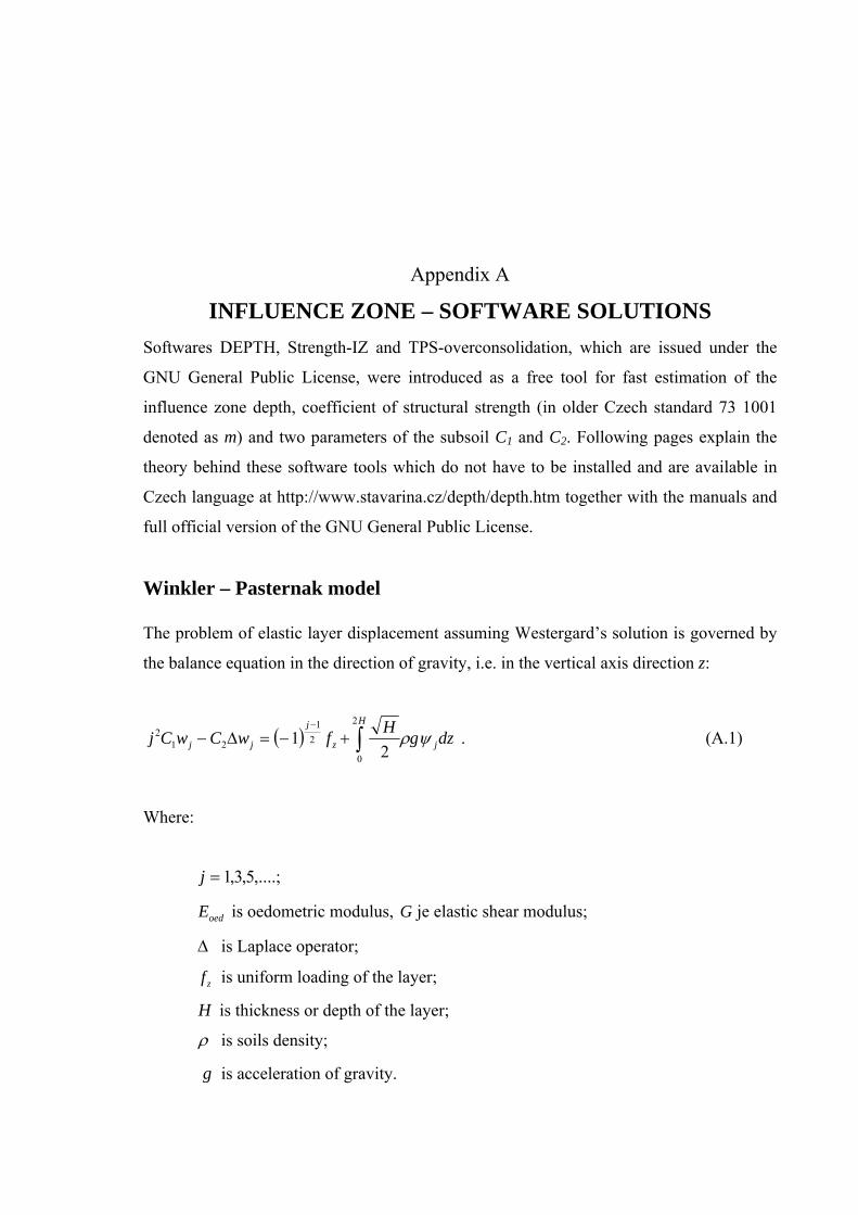
Appendix A
INFLUENCE ZONE – SOFTWARE SOLUTIONS
Softwares DEPTH, Strength-IZ and TPS-overconsolidation, which are issued under the
GNU General Public License, were introduced as a free tool for fast estimation of the
influence zone depth, coefficient of structural strength (in older Czech standard 73 1001
denoted as m) and two parameters of the subsoil C1 and C2. Following pages explain the
theory behind these software tools which do not have to be installed and are available in
Czech language at http://www.stavarina.cz/depth/depth.htm together with the manuals and
full official version of the GNU General Public License.
Winkler – Pasternak model The problem of elastic layer displacement assuming Westergard’s solution is governed by
the balance equation in the direction of gravity, i.e. in the vertical axis direction z:
.2
12
0
2
1
212 dzg
HfwCwCj j
H
z
j
jj
(A.1)
Where:
;,....5,3,1j
oedE is oedometric modulus, G je elastic shear modulus;
is Laplace operator;
zf is uniform loading of the layer;
H is thickness or depth of the layer;
is soils density;
g is acceleration of gravity.
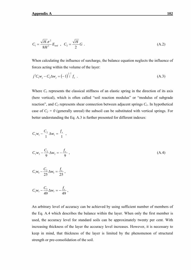
Appendix A 102
.2
,8
.22
2
1 GH
CEH
HC oed
(A.2)
When calculating the influence of surcharge, the balance equation neglects the influence of
forces acting within the volume of the layer:
.1 2
1
212
z
j
jj fwCwCj
(A.3)
Where C1 represents the classical stiffness of an elastic spring in the direction of its axis
(here vertical), which is often called “soil reaction modulus” or “modulus of subgrade
reaction”, and C2 represents shear connection between adjacent springs C1. In hypothetical
case of C2 = 0 (generally unreal) the subsoil can be substituted with vertical springs. For
better understanding the Eq. A.3 is further presented for different indexes:
,11 1
211
zfw
CwC
,99 3
231
zfw
CwC (A.4)
,2525 5
251
zfw
CwC
,4949 7
271
zfw
CwC
An arbitrary level of accuracy can be achieved by using sufficient number of members of
the Eq. A.4 which describes the balance within the layer. When only the first member is
used, the accuracy level for standard soils can be approximately twenty per cent. With
increasing thickness of the layer the accuracy level increases. However, it is necessary to
keep in mind, that thickness of the layer is limited by the phenomenon of structural
strength or pre-consolidation of the soil.
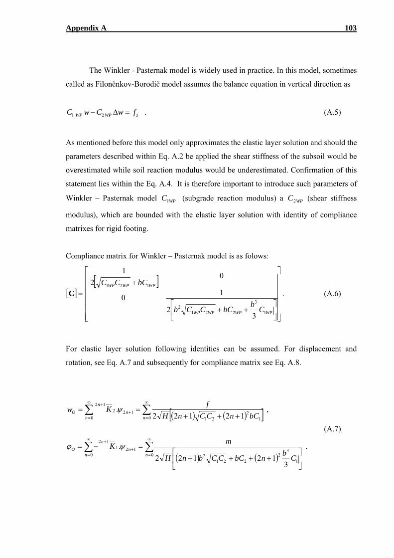
Appendix A 103
The Winkler - Pasternak model is widely used in practice. In this model, sometimes
called as Filoněnkov-Borodič model assumes the balance equation in vertical direction as
zWPWP fwCwC 21 . (A.5)
As mentioned before this model only approximates the elastic layer solution and should the
parameters described within Eq. A.2 be applied the shear stiffness of the subsoil would be
overestimated while soil reaction modulus would be underestimated. Confirmation of this
statement lies within the Eq. A.4. It is therefore important to introduce such parameters of
Winkler – Pasternak model WPC1 (subgrade reaction modulus) a WPC2 (shear stiffness
modulus), which are bounded with the elastic layer solution with identity of compliance
matrixes for rigid footing.
Compliance matrix for Winkler – Pasternak model is as folows:
WPWPWPWP
WPWPWP
Cb
bCCCb
bCCC
1
3
2212
121
32
10
02
1
C . (A.6)
For elastic layer solution following identities can be assumed. For displacement and
rotation, see Eq. A.7 and subsequently for compliance matrix see Eq. A.8.
.
312122
.
,12122
.
01
32
2212
120
112
0 12
21
120
212
nn
n
n
O
nn
n
n
O
Cb
nbCCCbnH
mK
bCnCCnH
fKw
(A.7)
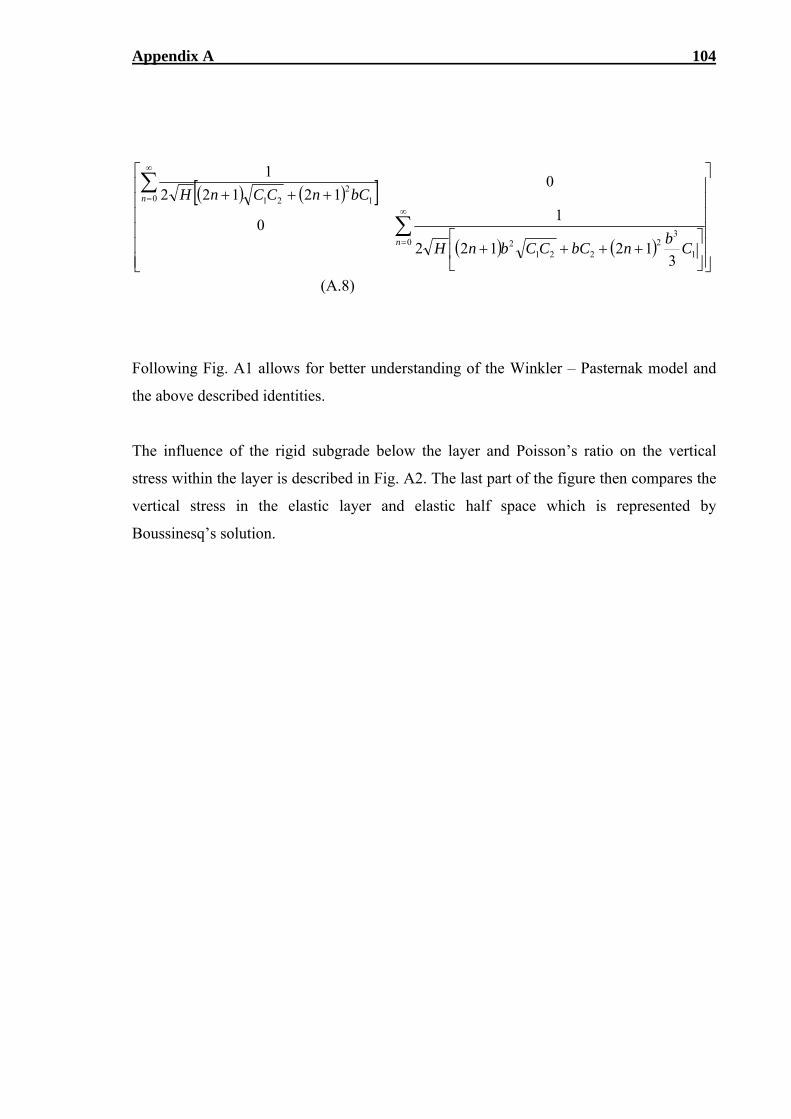
Appendix A 104
01
32
2212
0 12
21
312122
10
012122
1
n
n
Cb
nbCCCbnH
bCnCCnH
(A.8)
Following Fig. A1 allows for better understanding of the Winkler – Pasternak model and
the above described identities.
The influence of the rigid subgrade below the layer and Poisson’s ratio on the vertical
stress within the layer is described in Fig. A2. The last part of the figure then compares the
vertical stress in the elastic layer and elastic half space which is represented by
Boussinesq’s solution.
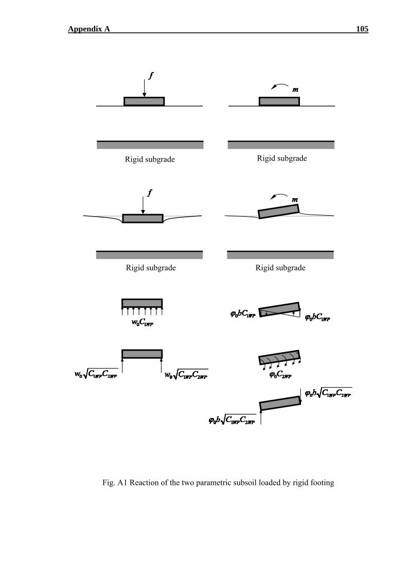
Appendix A 105
Fig. A1 Reaction of the two parametric subsoil loaded by rigid footing
Rigid subgrade
Rigid subgrade
Rigid subgrade Rigid subgrade
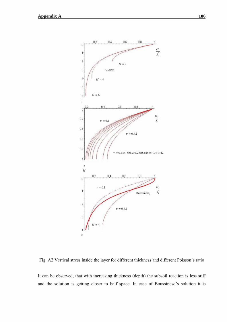
Appendix A 106
Fig. A2 Vertical stress inside the layer for different thickness and different Poisson’s ratio
It can be observed, that with increasing thickness (depth) the subsoil reaction is less stiff
and the solution is getting closer to half space. In case of Boussinesq’s solution it is
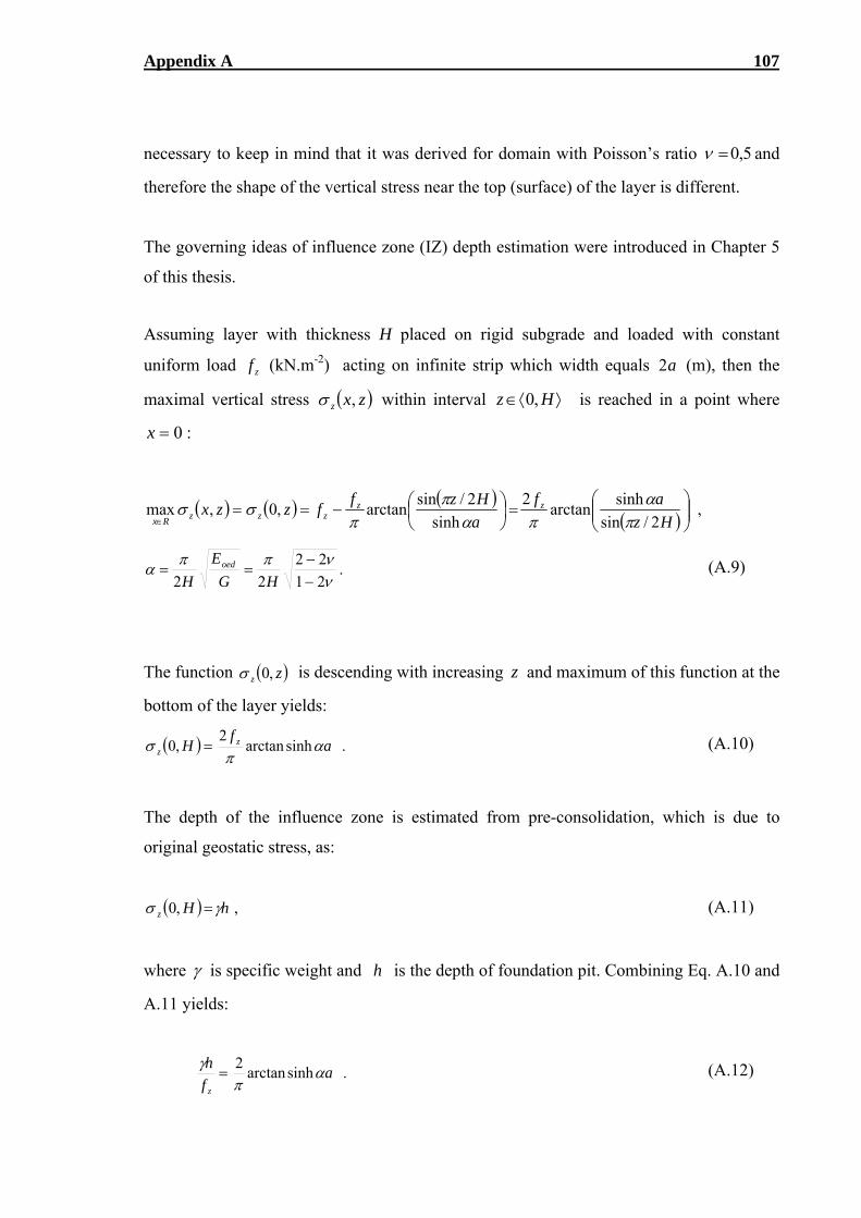
Appendix A 107
necessary to keep in mind that it was derived for domain with Poisson’s ratio 5,0 and
therefore the shape of the vertical stress near the top (surface) of the layer is different.
The governing ideas of influence zone (IZ) depth estimation were introduced in Chapter 5
of this thesis.
Assuming layer with thickness H placed on rigid subgrade and loaded with constant
uniform load zf (kN.m-2) acting on infinite strip which width equals a2 (m), then the
maximal vertical stress zxz , within interval Hz ,0 is reached in a point where
:0x
,
2/sin
sinharctan
2
sinh
2/sinarctan,0,max
Hz
af
a
Hzffzzx zz
zzzRx
.21
22
22
HG
E
Hoed (A.9)
The function zz ,0 is descending with increasing z and maximum of this function at the
bottom of the layer yields:
.sinharctan2
,0 af
H zz
(A.10)
The depth of the influence zone is estimated from pre-consolidation, which is due to
original geostatic stress, as:
,,0 hHz (A.11)
where is specific weight and h is the depth of foundation pit. Combining Eq. A.10 and
A.11 yields:
.sinharctan2
af
h
z
(A.12)
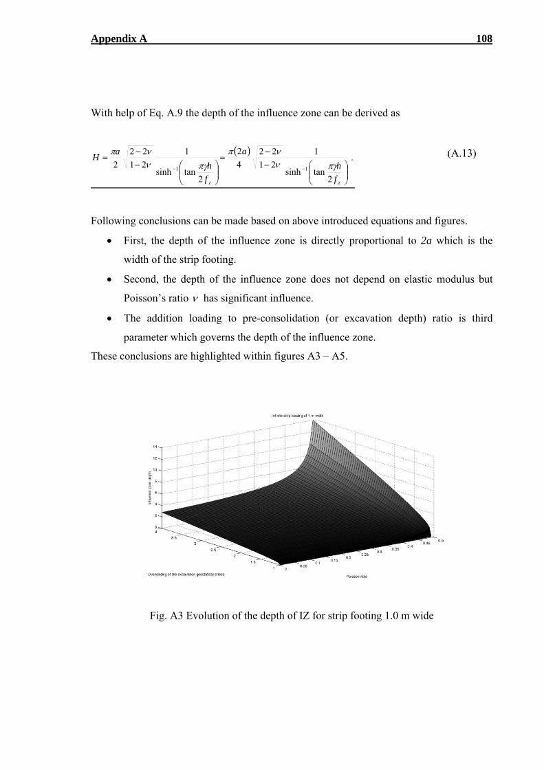
Appendix A 108
With help of Eq. A.9 the depth of the influence zone can be derived as
.
2tansinh
1
21
22
4
2
2tansinh
1
21
22
211
zz f
h
a
f
h
aH
(A.13)
Following conclusions can be made based on above introduced equations and figures.
First, the depth of the influence zone is directly proportional to 2a which is the
width of the strip footing.
Second, the depth of the influence zone does not depend on elastic modulus but
Poisson’s ratio has significant influence.
The addition loading to pre-consolidation (or excavation depth) ratio is third
parameter which governs the depth of the influence zone.
These conclusions are highlighted within figures A3 – A5.
Fig. A3 Evolution of the depth of IZ for strip footing 1.0 m wide
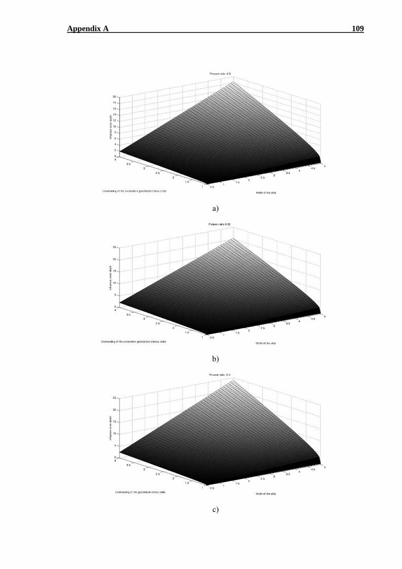
Appendix A 109
a)
b)
c)
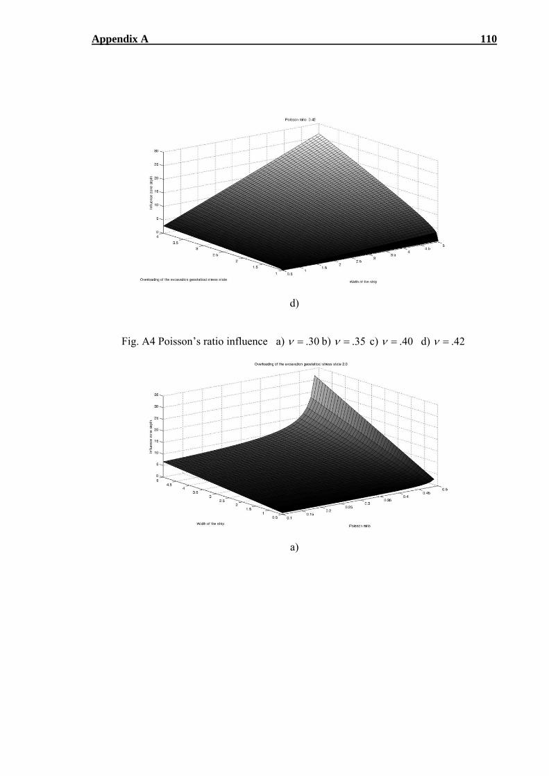
Appendix A 110
d)
Fig. A4 Poisson’s ratio influence a) 30. b) 35. c) 40. d) 42.
a)
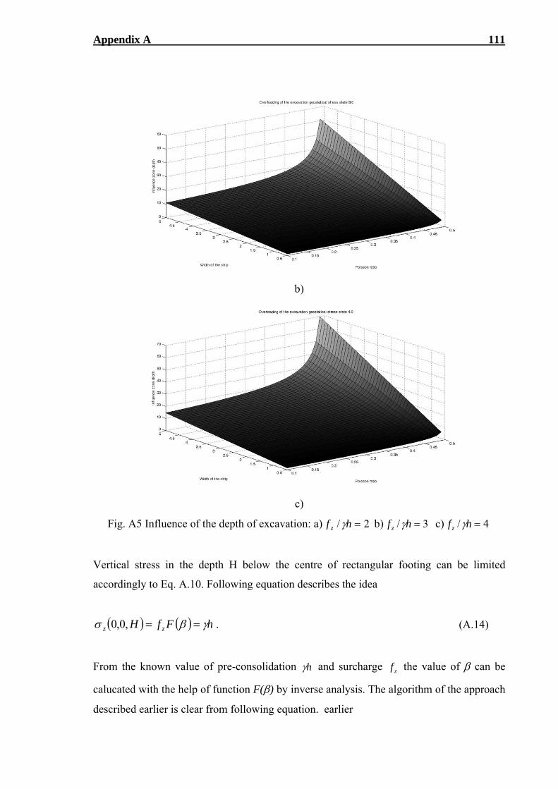
Appendix A 111
b)
c)
Fig. A5 Influence of the depth of excavation: a) 2/ hf z b) 3/ hfz c) 4/ hfz
Vertical stress in the depth H below the centre of rectangular footing can be limited
accordingly to Eq. A.10. Following equation describes the idea
.,0,0 hFfH zz (A.14)
From the known value of pre-consolidation h and surcharge zf the value of can be
calucated with the help of function F() by inverse analysis. The algorithm of the approach
described earlier is clear from following equation. earlier
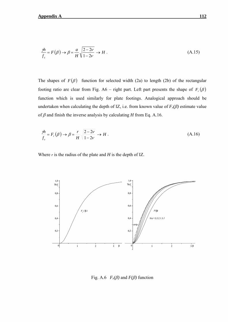
Appendix A 112
HH
aF
f
h
z
21
22 . (A.15)
The shapes of F function for selected width (2a) to length (2b) of the rectangular
footing ratio are clear from Fig. A6 – right part. Left part presents the shape of rF
function which is used similarly for plate footings. Analogical approach should be
undertaken when calculating the depth of IZ, i.e. from known value of Fr() estimate value
of and finish the inverse analysis by calculating H from Eq. A.16.
HH
rF
f
hr
z
21
22 . (A.16)
Where r is the radius of the plate and H is the depth of IZ.
Fig. A.6 Fr() and F() function
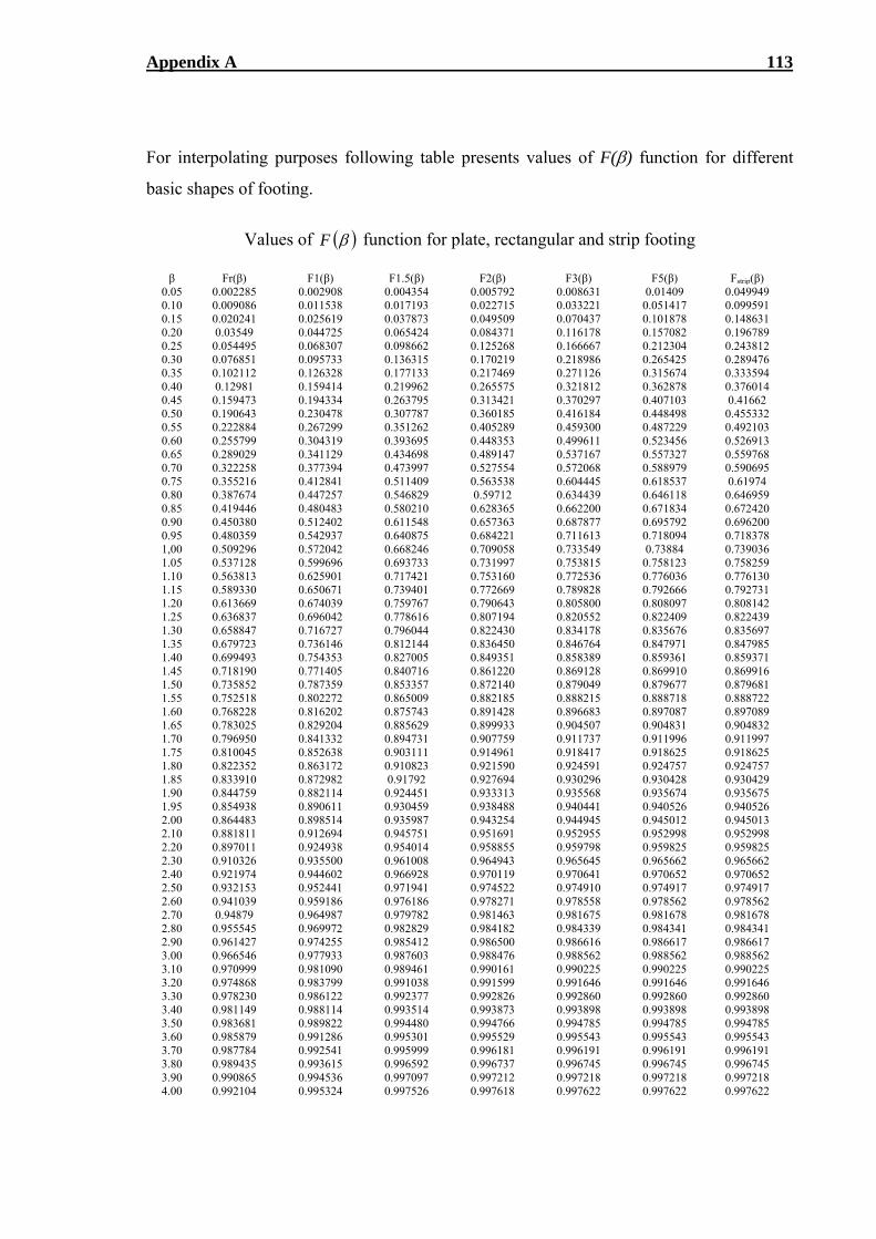
Appendix A 113
For interpolating purposes following table presents values of F() function for different
basic shapes of footing.
Values of F function for plate, rectangular and strip footing
β Fr(β) F1(β) F1.5(β) F2(β) F3(β) F5(β) Fstrip(β)
0.05 0.002285 0.002908 0.004354 0.005792 0.008631 0.01409 0.049949 0.10 0.009086 0.011538 0.017193 0.022715 0.033221 0.051417 0.099591 0.15 0.020241 0.025619 0.037873 0.049509 0.070437 0.101878 0.148631 0.20 0.03549 0.044725 0.065424 0.084371 0.116178 0.157082 0.196789 0.25 0.054495 0.068307 0.098662 0.125268 0.166667 0.212304 0.243812 0.30 0.076851 0.095733 0.136315 0.170219 0.218986 0.265425 0.289476 0.35 0.102112 0.126328 0.177133 0.217469 0.271126 0.315674 0.333594 0.40 0.12981 0.159414 0.219962 0.265575 0.321812 0.362878 0.376014 0.45 0.159473 0.194334 0.263795 0.313421 0.370297 0.407103 0.41662 0.50 0.190643 0.230478 0.307787 0.360185 0.416184 0.448498 0.455332 0.55 0.222884 0.267299 0.351262 0.405289 0.459300 0.487229 0.492103 0.60 0.255799 0.304319 0.393695 0.448353 0.499611 0.523456 0.526913 0.65 0.289029 0.341129 0.434698 0.489147 0.537167 0.557327 0.559768 0.70 0.322258 0.377394 0.473997 0.527554 0.572068 0.588979 0.590695 0.75 0.355216 0.412841 0.511409 0.563538 0.604445 0.618537 0.61974 0.80 0.387674 0.447257 0.546829 0.59712 0.634439 0.646118 0.646959 0.85 0.419446 0.480483 0.580210 0.628365 0.662200 0.671834 0.672420 0.90 0.450380 0.512402 0.611548 0.657363 0.687877 0.695792 0.696200 0.95 0.480359 0.542937 0.640875 0.684221 0.711613 0.718094 0.718378 1,00 0.509296 0.572042 0.668246 0.709058 0.733549 0.73884 0.739036 1.05 0.537128 0.599696 0.693733 0.731997 0.753815 0.758123 0.758259 1.10 0.563813 0.625901 0.717421 0.753160 0.772536 0.776036 0.776130 1.15 0.589330 0.650671 0.739401 0.772669 0.789828 0.792666 0.792731 1.20 0.613669 0.674039 0.759767 0.790643 0.805800 0.808097 0.808142 1.25 0.636837 0.696042 0.778616 0.807194 0.820552 0.822409 0.822439 1.30 0.658847 0.716727 0.796044 0.822430 0.834178 0.835676 0.835697 1.35 0.679723 0.736146 0.812144 0.836450 0.846764 0.847971 0.847985 1.40 0.699493 0.754353 0.827005 0.849351 0.858389 0.859361 0.859371 1.45 0.718190 0.771405 0.840716 0.861220 0.869128 0.869910 0.869916 1.50 0.735852 0.787359 0.853357 0.872140 0.879049 0.879677 0.879681 1.55 0.752518 0.802272 0.865009 0.882185 0.888215 0.888718 0.888722 1.60 0.768228 0.816202 0.875743 0.891428 0.896683 0.897087 0.897089 1.65 0.783025 0.829204 0.885629 0.899933 0.904507 0.904831 0.904832 1.70 0.796950 0.841332 0.894731 0.907759 0.911737 0.911996 0.911997 1.75 0.810045 0.852638 0.903111 0.914961 0.918417 0.918625 0.918625 1.80 0.822352 0.863172 0.910823 0.921590 0.924591 0.924757 0.924757 1.85 0.833910 0.872982 0.91792 0.927694 0.930296 0.930428 0.930429 1.90 0.844759 0.882114 0.924451 0.933313 0.935568 0.935674 0.935675 1.95 0.854938 0.890611 0.930459 0.938488 0.940441 0.940526 0.940526 2.00 0.864483 0.898514 0.935987 0.943254 0.944945 0.945012 0.945013 2.10 0.881811 0.912694 0.945751 0.951691 0.952955 0.952998 0.952998 2.20 0.897011 0.924938 0.954014 0.958855 0.959798 0.959825 0.959825 2.30 0.910326 0.935500 0.961008 0.964943 0.965645 0.965662 0.965662 2.40 0.921974 0.944602 0.966928 0.970119 0.970641 0.970652 0.970652 2.50 0.932153 0.952441 0.971941 0.974522 0.974910 0.974917 0.974917 2.60 0.941039 0.959186 0.976186 0.978271 0.978558 0.978562 0.978562 2.70 0.94879 0.964987 0.979782 0.981463 0.981675 0.981678 0.981678 2.80 0.955545 0.969972 0.982829 0.984182 0.984339 0.984341 0.984341 2.90 0.961427 0.974255 0.985412 0.986500 0.986616 0.986617 0.986617 3.00 0.966546 0.977933 0.987603 0.988476 0.988562 0.988562 0.988562 3.10 0.970999 0.981090 0.989461 0.990161 0.990225 0.990225 0.990225 3.20 0.974868 0.983799 0.991038 0.991599 0.991646 0.991646 0.991646 3.30 0.978230 0.986122 0.992377 0.992826 0.992860 0.992860 0.992860 3.40 0.981149 0.988114 0.993514 0.993873 0.993898 0.993898 0.993898 3.50 0.983681 0.989822 0.994480 0.994766 0.994785 0.994785 0.994785 3.60 0.985879 0.991286 0.995301 0.995529 0.995543 0.995543 0.995543 3.70 0.987784 0.992541 0.995999 0.996181 0.996191 0.996191 0.996191 3.80 0.989435 0.993615 0.996592 0.996737 0.996745 0.996745 0.996745 3.90 0.990865 0.994536 0.997097 0.997212 0.997218 0.997218 0.997218 4.00 0.992104 0.995324 0.997526 0.997618 0.997622 0.997622 0.997622
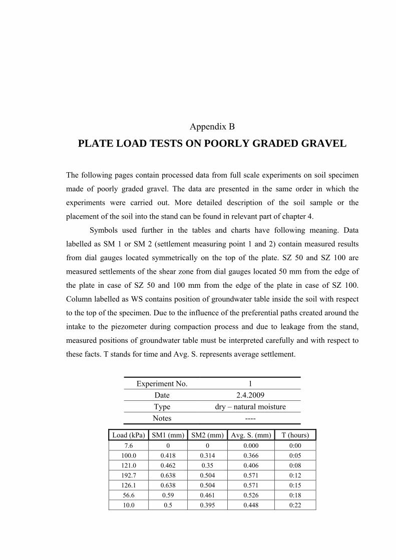
Appendix B
PLATE LOAD TESTS ON POORLY GRADED GRAVEL
The following pages contain processed data from full scale experiments on soil specimen
made of poorly graded gravel. The data are presented in the same order in which the
experiments were carried out. More detailed description of the soil sample or the
placement of the soil into the stand can be found in relevant part of chapter 4.
Symbols used further in the tables and charts have following meaning. Data
labelled as SM 1 or SM 2 (settlement measuring point 1 and 2) contain measured results
from dial gauges located symmetrically on the top of the plate. SZ 50 and SZ 100 are
measured settlements of the shear zone from dial gauges located 50 mm from the edge of
the plate in case of SZ 50 and 100 mm from the edge of the plate in case of SZ 100.
Column labelled as WS contains position of groundwater table inside the soil with respect
to the top of the specimen. Due to the influence of the preferential paths created around the
intake to the piezometer during compaction process and due to leakage from the stand,
measured positions of groundwater table must be interpreted carefully and with respect to
these facts. T stands for time and Avg. S. represents average settlement.
Experiment No. 1
Date 2.4.2009
Type dry – natural moisture
Notes ----
Load (kPa) SM1 (mm) SM2 (mm) Avg. S. (mm) T (hours)
7.6 0 0 0.000 0:00
100.0 0.418 0.314 0.366 0:05
121.0 0.462 0.35 0.406 0:08
192.7 0.638 0.504 0.571 0:12
126.1 0.638 0.504 0.571 0:15
56.6 0.59 0.461 0.526 0:18
10.0 0.5 0.395 0.448 0:22
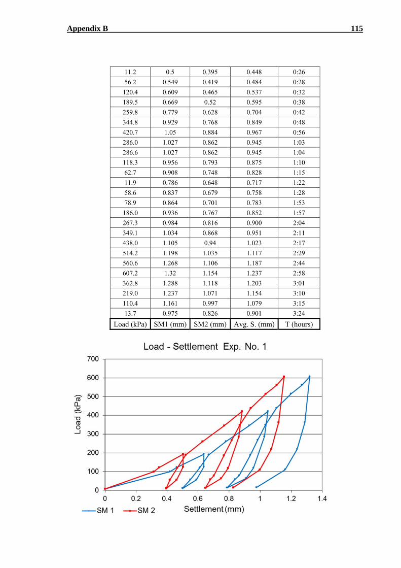
Appendix B 115
11.2 0.5 0.395 0.448 0:26
56.2 0.549 0.419 0.484 0:28
120.4 0.609 0.465 0.537 0:32
189.5 0.669 0.52 0.595 0:38
259.8 0.779 0.628 0.704 0:42
344.8 0.929 0.768 0.849 0:48
420.7 1.05 0.884 0.967 0:56
286.0 1.027 0.862 0.945 1:03
286.6 1.027 0.862 0.945 1:04
118.3 0.956 0.793 0.875 1:10
62.7 0.908 0.748 0.828 1:15
11.9 0.786 0.648 0.717 1:22
58.6 0.837 0.679 0.758 1:28
78.9 0.864 0.701 0.783 1:53
186.0 0.936 0.767 0.852 1:57
267.3 0.984 0.816 0.900 2:04
349.1 1.034 0.868 0.951 2:11
438.0 1.105 0.94 1.023 2:17
514.2 1.198 1.035 1.117 2:29
560.6 1.268 1.106 1.187 2:44
607.2 1.32 1.154 1.237 2:58
362.8 1.288 1.118 1.203 3:01
219.0 1.237 1.071 1.154 3:10
110.4 1.161 0.997 1.079 3:15
13.7 0.975 0.826 0.901 3:24
Load (kPa) SM1 (mm) SM2 (mm) Avg. S. (mm) T (hours)
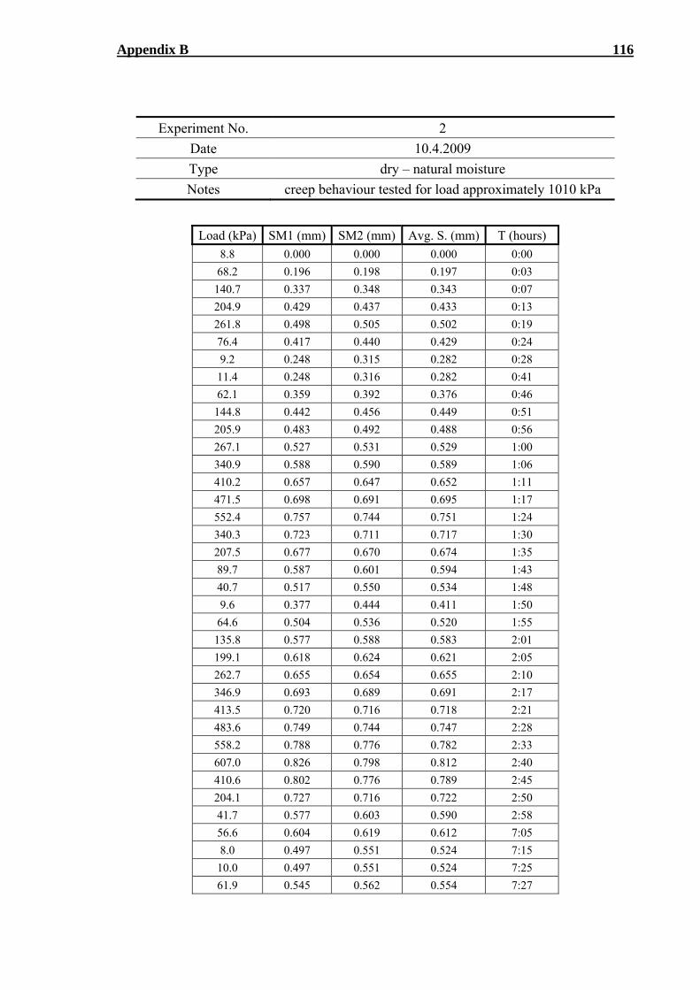
Appendix B 116
Experiment No. 2
Date 10.4.2009
Type dry – natural moisture
Notes creep behaviour tested for load approximately 1010 kPa
Load (kPa) SM1 (mm) SM2 (mm) Avg. S. (mm) T (hours)
8.8 0.000 0.000 0.000 0:00
68.2 0.196 0.198 0.197 0:03
140.7 0.337 0.348 0.343 0:07
204.9 0.429 0.437 0.433 0:13
261.8 0.498 0.505 0.502 0:19
76.4 0.417 0.440 0.429 0:24
9.2 0.248 0.315 0.282 0:28
11.4 0.248 0.316 0.282 0:41
62.1 0.359 0.392 0.376 0:46
144.8 0.442 0.456 0.449 0:51
205.9 0.483 0.492 0.488 0:56
267.1 0.527 0.531 0.529 1:00
340.9 0.588 0.590 0.589 1:06
410.2 0.657 0.647 0.652 1:11
471.5 0.698 0.691 0.695 1:17
552.4 0.757 0.744 0.751 1:24
340.3 0.723 0.711 0.717 1:30
207.5 0.677 0.670 0.674 1:35
89.7 0.587 0.601 0.594 1:43
40.7 0.517 0.550 0.534 1:48
9.6 0.377 0.444 0.411 1:50
64.6 0.504 0.536 0.520 1:55
135.8 0.577 0.588 0.583 2:01
199.1 0.618 0.624 0.621 2:05
262.7 0.655 0.654 0.655 2:10
346.9 0.693 0.689 0.691 2:17
413.5 0.720 0.716 0.718 2:21
483.6 0.749 0.744 0.747 2:28
558.2 0.788 0.776 0.782 2:33
607.0 0.826 0.798 0.812 2:40
410.6 0.802 0.776 0.789 2:45
204.1 0.727 0.716 0.722 2:50
41.7 0.577 0.603 0.590 2:58
56.6 0.604 0.619 0.612 7:05
8.0 0.497 0.551 0.524 7:15
10.0 0.497 0.551 0.524 7:25
61.9 0.545 0.562 0.554 7:27
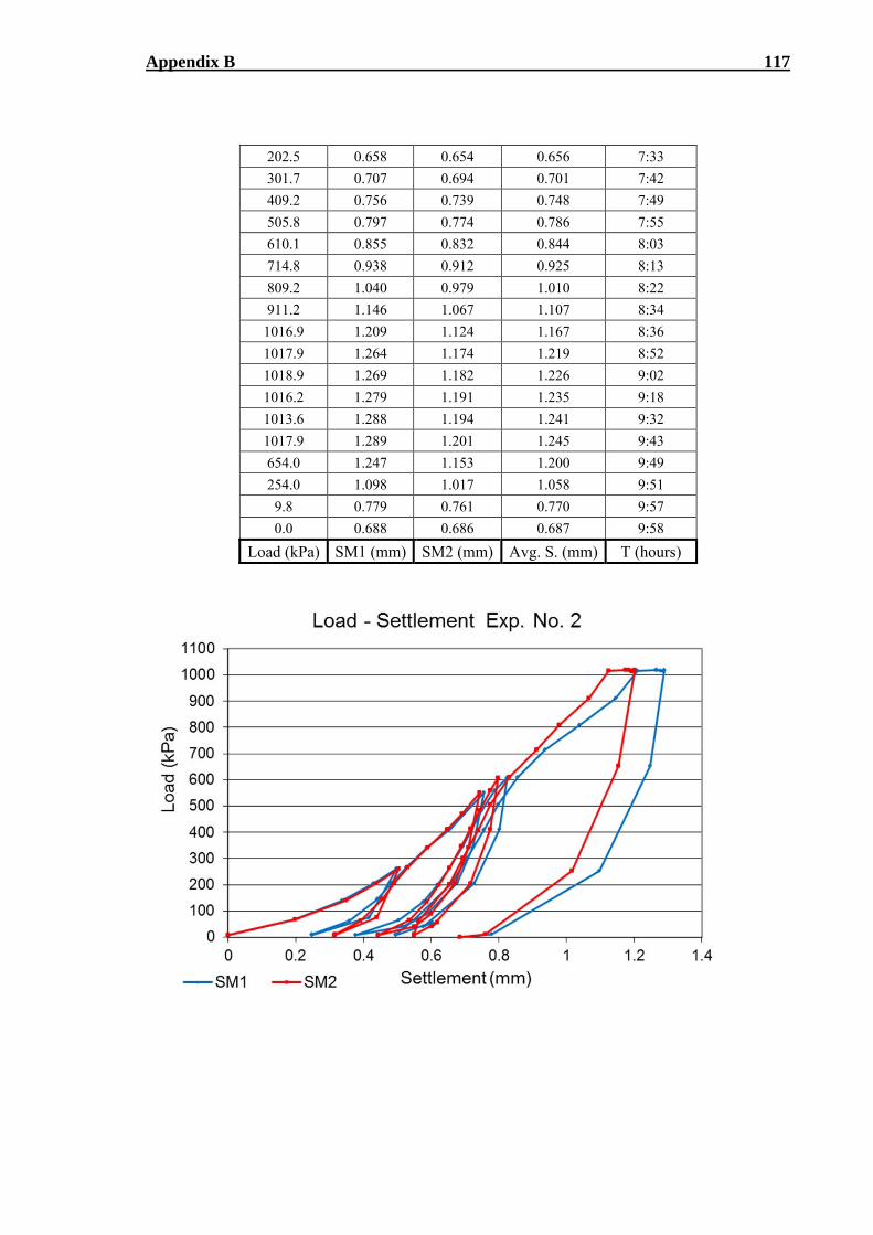
Appendix B 117
202.5 0.658 0.654 0.656 7:33
301.7 0.707 0.694 0.701 7:42
409.2 0.756 0.739 0.748 7:49
505.8 0.797 0.774 0.786 7:55
610.1 0.855 0.832 0.844 8:03
714.8 0.938 0.912 0.925 8:13
809.2 1.040 0.979 1.010 8:22
911.2 1.146 1.067 1.107 8:34
1016.9 1.209 1.124 1.167 8:36
1017.9 1.264 1.174 1.219 8:52
1018.9 1.269 1.182 1.226 9:02
1016.2 1.279 1.191 1.235 9:18
1013.6 1.288 1.194 1.241 9:32
1017.9 1.289 1.201 1.245 9:43
654.0 1.247 1.153 1.200 9:49
254.0 1.098 1.017 1.058 9:51
9.8 0.779 0.761 0.770 9:57
0.0 0.688 0.686 0.687 9:58
Load (kPa) SM1 (mm) SM2 (mm) Avg. S. (mm) T (hours)
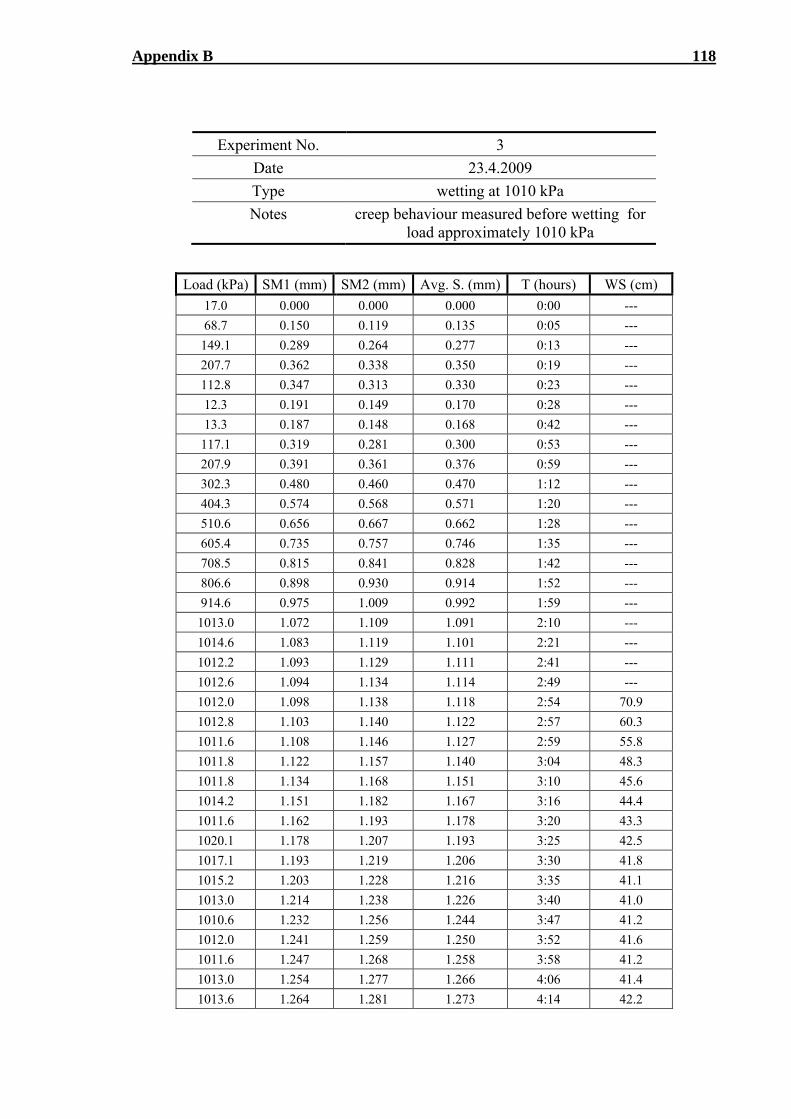
Appendix B 118
Experiment No. 3
Date 23.4.2009
Type wetting at 1010 kPa
Notes creep behaviour measured before wetting for load approximately 1010 kPa
Load (kPa) SM1 (mm) SM2 (mm) Avg. S. (mm) T (hours) WS (cm)
17.0 0.000 0.000 0.000 0:00 ---
68.7 0.150 0.119 0.135 0:05 ---
149.1 0.289 0.264 0.277 0:13 ---
207.7 0.362 0.338 0.350 0:19 ---
112.8 0.347 0.313 0.330 0:23 ---
12.3 0.191 0.149 0.170 0:28 ---
13.3 0.187 0.148 0.168 0:42 ---
117.1 0.319 0.281 0.300 0:53 ---
207.9 0.391 0.361 0.376 0:59 ---
302.3 0.480 0.460 0.470 1:12 ---
404.3 0.574 0.568 0.571 1:20 ---
510.6 0.656 0.667 0.662 1:28 ---
605.4 0.735 0.757 0.746 1:35 ---
708.5 0.815 0.841 0.828 1:42 ---
806.6 0.898 0.930 0.914 1:52 ---
914.6 0.975 1.009 0.992 1:59 ---
1013.0 1.072 1.109 1.091 2:10 ---
1014.6 1.083 1.119 1.101 2:21 ---
1012.2 1.093 1.129 1.111 2:41 ---
1012.6 1.094 1.134 1.114 2:49 ---
1012.0 1.098 1.138 1.118 2:54 70.9
1012.8 1.103 1.140 1.122 2:57 60.3
1011.6 1.108 1.146 1.127 2:59 55.8
1011.8 1.122 1.157 1.140 3:04 48.3
1011.8 1.134 1.168 1.151 3:10 45.6
1014.2 1.151 1.182 1.167 3:16 44.4
1011.6 1.162 1.193 1.178 3:20 43.3
1020.1 1.178 1.207 1.193 3:25 42.5
1017.1 1.193 1.219 1.206 3:30 41.8
1015.2 1.203 1.228 1.216 3:35 41.1
1013.0 1.214 1.238 1.226 3:40 41.0
1010.6 1.232 1.256 1.244 3:47 41.2
1012.0 1.241 1.259 1.250 3:52 41.6
1011.6 1.247 1.268 1.258 3:58 41.2
1013.0 1.254 1.277 1.266 4:06 41.4
1013.6 1.264 1.281 1.273 4:14 42.2
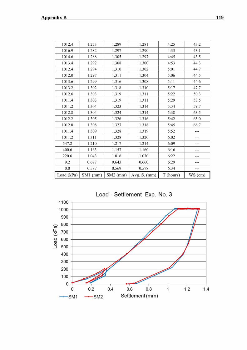
Appendix B 119
1012.4 1.273 1.289 1.281 4:25 43.2
1016.9 1.282 1.297 1.290 4:33 43.1
1014.6 1.288 1.305 1.297 4:45 43.5
1013.4 1.292 1.308 1.300 4:53 44.3
1012.4 1.294 1.310 1.302 5:01 44.7
1012.0 1.297 1.311 1.304 5:06 44.5
1013.6 1.299 1.316 1.308 5:11 44.6
1013.2 1.302 1.318 1.310 5:17 47.7
1012.6 1.303 1.319 1.311 5:22 50.3
1011.4 1.303 1.319 1.311 5:29 53.5
1011.2 1.304 1.323 1.314 5:34 59.7
1012.8 1.304 1.324 1.314 5:38 63.5
1012.2 1.305 1.326 1.316 5:42 65.0
1012.0 1.308 1.327 1.318 5:45 66.7
1011.4 1.309 1.328 1.319 5:52 ---
1011.2 1.311 1.328 1.320 6:02 ---
547.2 1.210 1.217 1.214 6:09 ---
400.6 1.163 1.157 1.160 6:16 ---
220.6 1.043 1.016 1.030 6:22 ---
9.2 0.677 0.643 0.660 6:29 ---
0.0 0.587 0.569 0.578 6:34 ---
Load (kPa) SM1 (mm) SM2 (mm) Avg. S. (mm) T (hours) WS (cm)
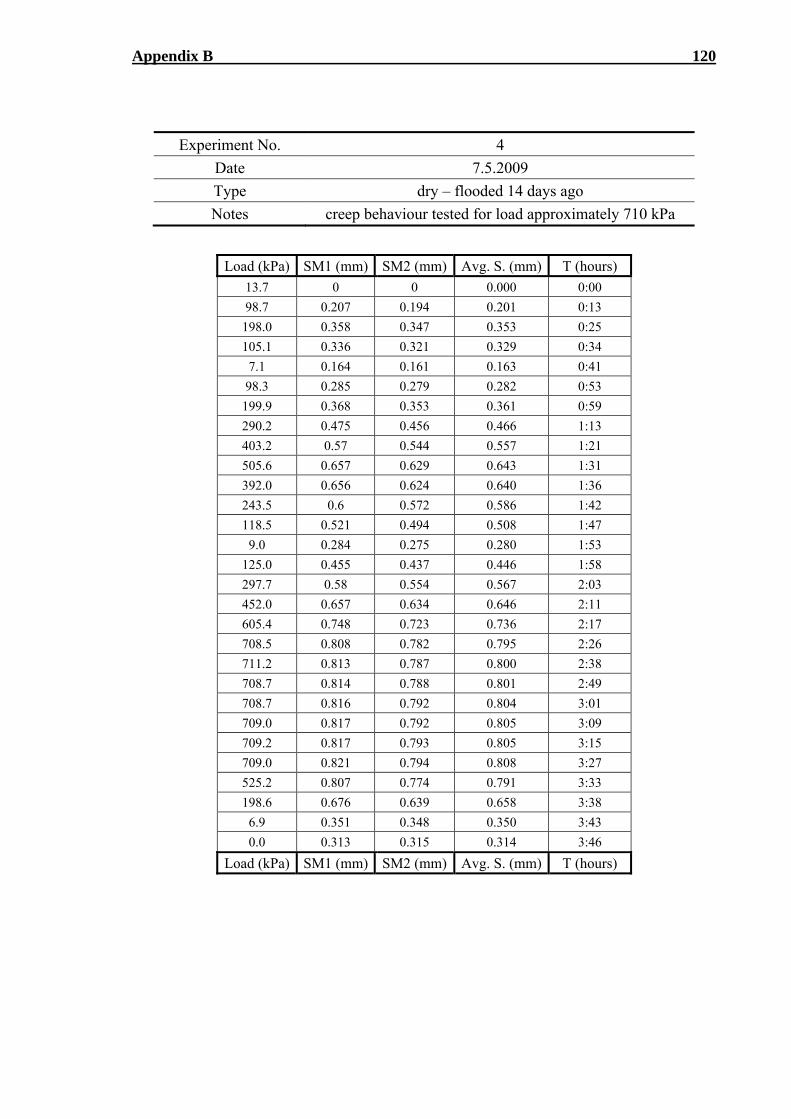
Appendix B 120
Experiment No. 4
Date 7.5.2009
Type dry – flooded 14 days ago
Notes creep behaviour tested for load approximately 710 kPa
Load (kPa) SM1 (mm) SM2 (mm) Avg. S. (mm) T (hours)
13.7 0 0 0.000 0:00
98.7 0.207 0.194 0.201 0:13
198.0 0.358 0.347 0.353 0:25
105.1 0.336 0.321 0.329 0:34
7.1 0.164 0.161 0.163 0:41
98.3 0.285 0.279 0.282 0:53
199.9 0.368 0.353 0.361 0:59
290.2 0.475 0.456 0.466 1:13
403.2 0.57 0.544 0.557 1:21
505.6 0.657 0.629 0.643 1:31
392.0 0.656 0.624 0.640 1:36
243.5 0.6 0.572 0.586 1:42
118.5 0.521 0.494 0.508 1:47
9.0 0.284 0.275 0.280 1:53
125.0 0.455 0.437 0.446 1:58
297.7 0.58 0.554 0.567 2:03
452.0 0.657 0.634 0.646 2:11
605.4 0.748 0.723 0.736 2:17
708.5 0.808 0.782 0.795 2:26
711.2 0.813 0.787 0.800 2:38
708.7 0.814 0.788 0.801 2:49
708.7 0.816 0.792 0.804 3:01
709.0 0.817 0.792 0.805 3:09
709.2 0.817 0.793 0.805 3:15
709.0 0.821 0.794 0.808 3:27
525.2 0.807 0.774 0.791 3:33
198.6 0.676 0.639 0.658 3:38
6.9 0.351 0.348 0.350 3:43
0.0 0.313 0.315 0.314 3:46
Load (kPa) SM1 (mm) SM2 (mm) Avg. S. (mm) T (hours)
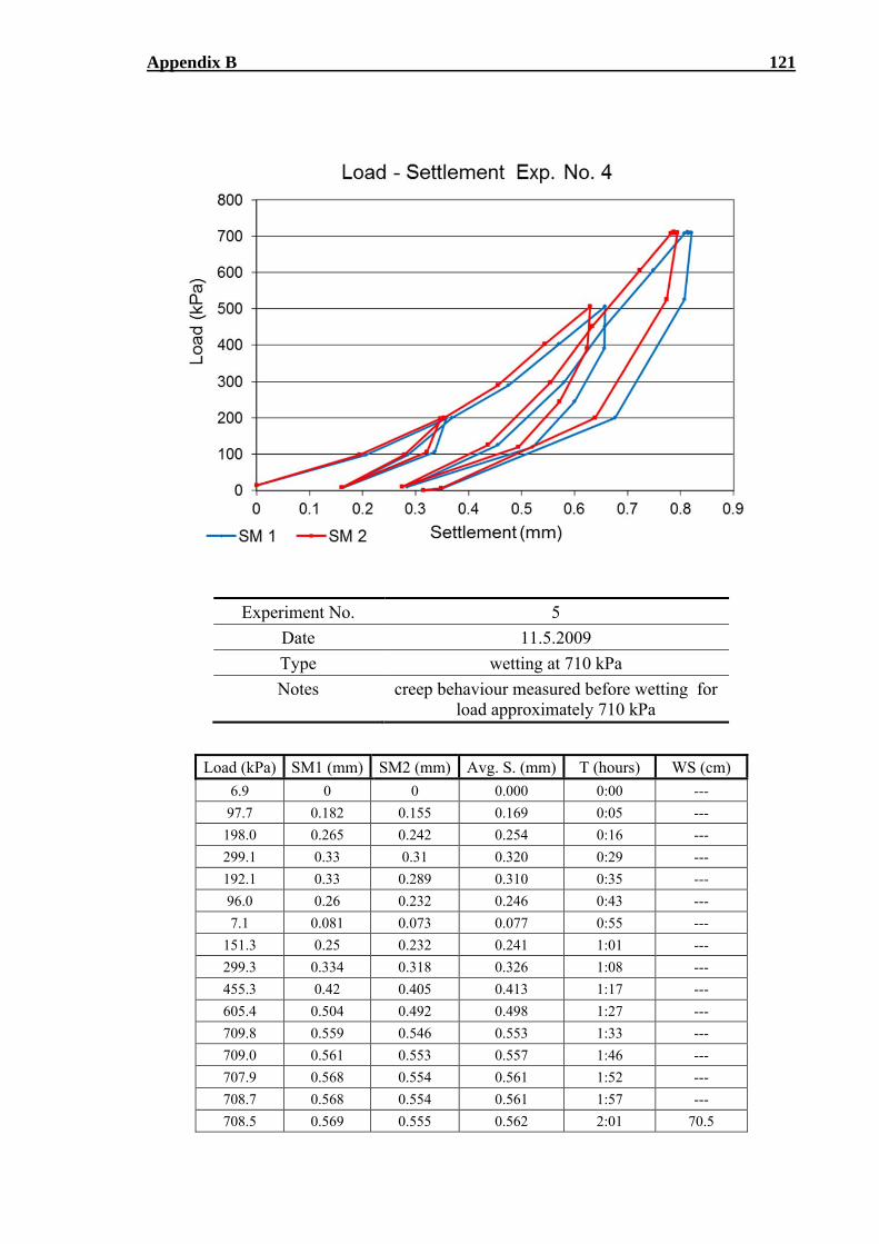
Appendix B 121
Experiment No. 5
Date 11.5.2009
Type wetting at 710 kPa
Notes creep behaviour measured before wetting for load approximately 710 kPa
Load (kPa) SM1 (mm) SM2 (mm) Avg. S. (mm) T (hours) WS (cm)
6.9 0 0 0.000 0:00 ---
97.7 0.182 0.155 0.169 0:05 ---
198.0 0.265 0.242 0.254 0:16 ---
299.1 0.33 0.31 0.320 0:29 ---
192.1 0.33 0.289 0.310 0:35 ---
96.0 0.26 0.232 0.246 0:43 ---
7.1 0.081 0.073 0.077 0:55 ---
151.3 0.25 0.232 0.241 1:01 ---
299.3 0.334 0.318 0.326 1:08 ---
455.3 0.42 0.405 0.413 1:17 ---
605.4 0.504 0.492 0.498 1:27 ---
709.8 0.559 0.546 0.553 1:33 ---
709.0 0.561 0.553 0.557 1:46 ---
707.9 0.568 0.554 0.561 1:52 ---
708.7 0.568 0.554 0.561 1:57 ---
708.5 0.569 0.555 0.562 2:01 70.5
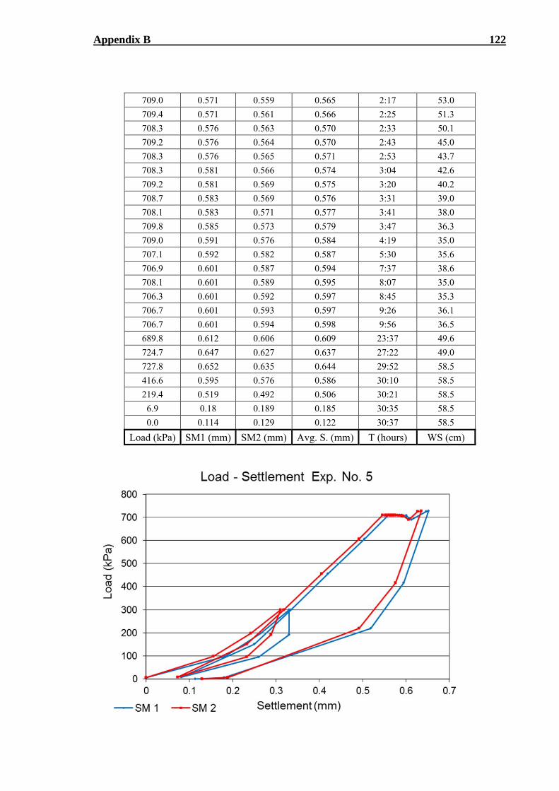
Appendix B 122
709.0 0.571 0.559 0.565 2:17 53.0
709.4 0.571 0.561 0.566 2:25 51.3
708.3 0.576 0.563 0.570 2:33 50.1
709.2 0.576 0.564 0.570 2:43 45.0
708.3 0.576 0.565 0.571 2:53 43.7
708.3 0.581 0.566 0.574 3:04 42.6
709.2 0.581 0.569 0.575 3:20 40.2
708.7 0.583 0.569 0.576 3:31 39.0
708.1 0.583 0.571 0.577 3:41 38.0
709.8 0.585 0.573 0.579 3:47 36.3
709.0 0.591 0.576 0.584 4:19 35.0
707.1 0.592 0.582 0.587 5:30 35.6
706.9 0.601 0.587 0.594 7:37 38.6
708.1 0.601 0.589 0.595 8:07 35.0
706.3 0.601 0.592 0.597 8:45 35.3
706.7 0.601 0.593 0.597 9:26 36.1
706.7 0.601 0.594 0.598 9:56 36.5
689.8 0.612 0.606 0.609 23:37 49.6
724.7 0.647 0.627 0.637 27:22 49.0
727.8 0.652 0.635 0.644 29:52 58.5
416.6 0.595 0.576 0.586 30:10 58.5
219.4 0.519 0.492 0.506 30:21 58.5
6.9 0.18 0.189 0.185 30:35 58.5
0.0 0.114 0.129 0.122 30:37 58.5
Load (kPa) SM1 (mm) SM2 (mm) Avg. S. (mm) T (hours) WS (cm)
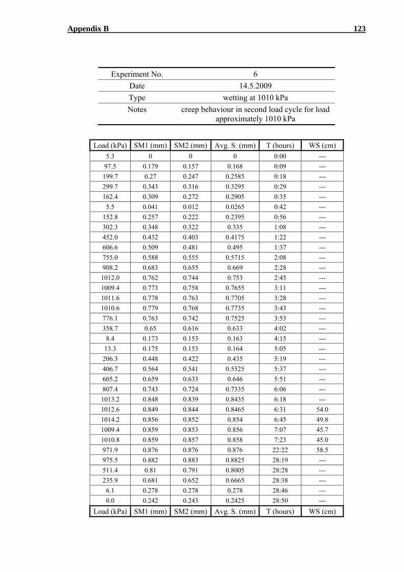
Appendix B 123
Experiment No. 6
Date 14.5.2009
Type wetting at 1010 kPa
Notes creep behaviour in second load cycle for load approximately 1010 kPa
Load (kPa) SM1 (mm) SM2 (mm) Avg. S. (mm) T (hours) WS (cm)
5.3 0 0 0 0:00 ---
97.5 0.179 0.157 0.168 0:09 ---
199.7 0.27 0.247 0.2585 0:18 ---
299.7 0.343 0.316 0.3295 0:29 ---
162.4 0.309 0.272 0.2905 0:35 ---
5.5 0.041 0.012 0.0265 0:42 ---
152.8 0.257 0.222 0.2395 0:56 ---
302.3 0.348 0.322 0.335 1:08 ---
452.0 0.432 0.403 0.4175 1:22 ---
606.6 0.509 0.481 0.495 1:37 ---
755.0 0.588 0.555 0.5715 2:08 ---
908.2 0.683 0.655 0.669 2:28 ---
1012.0 0.762 0.744 0.753 2:45 ---
1009.4 0.773 0.758 0.7655 3:11 ---
1011.6 0.778 0.763 0.7705 3:28 ---
1010.6 0.779 0.768 0.7735 3:43 ---
776.1 0.763 0.742 0.7525 3:53 ---
358.7 0.65 0.616 0.633 4:02 ---
8.4 0.173 0.153 0.163 4:15 ---
13.3 0.175 0.153 0.164 5:05 ---
206.3 0.448 0.422 0.435 5:19 ---
406.7 0.564 0.541 0.5525 5:37 ---
605.2 0.659 0.633 0.646 5:51 ---
807.4 0.743 0.724 0.7335 6:06 ---
1013.2 0.848 0.839 0.8435 6:18 ---
1012.6 0.849 0.844 0.8465 6:31 54.0
1014.2 0.856 0.852 0.854 6:45 49.8
1009.4 0.859 0.853 0.856 7:07 45.7
1010.8 0.859 0.857 0.858 7:23 45.0
971.9 0.876 0.876 0.876 22:22 58.5
975.5 0.882 0.883 0.8825 28:19 ---
511.4 0.81 0.791 0.8005 28:28 ---
235.9 0.681 0.652 0.6665 28:38 ---
6.1 0.278 0.278 0.278 28:46 ---
0.0 0.242 0.243 0.2425 28:50 ---
Load (kPa) SM1 (mm) SM2 (mm) Avg. S. (mm) T (hours) WS (cm)
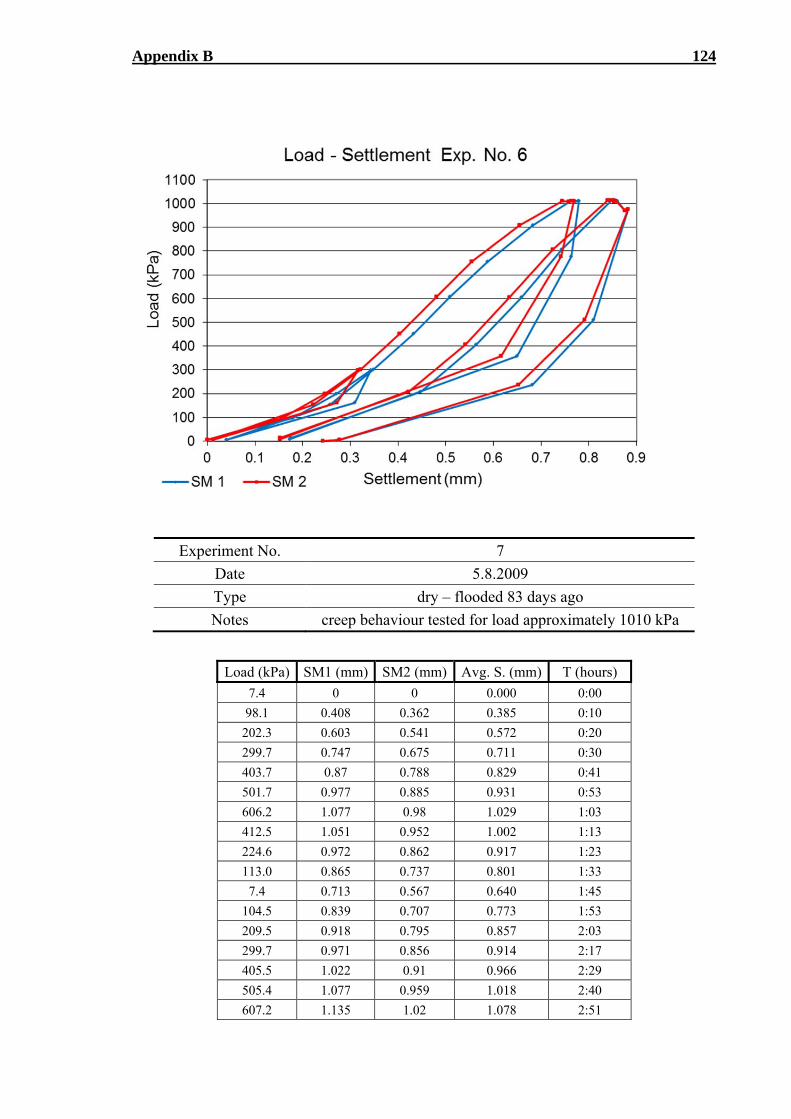
Appendix B 124
Experiment No. 7
Date 5.8.2009
Type dry – flooded 83 days ago
Notes creep behaviour tested for load approximately 1010 kPa
Load (kPa) SM1 (mm) SM2 (mm) Avg. S. (mm) T (hours)
7.4 0 0 0.000 0:00
98.1 0.408 0.362 0.385 0:10
202.3 0.603 0.541 0.572 0:20
299.7 0.747 0.675 0.711 0:30
403.7 0.87 0.788 0.829 0:41
501.7 0.977 0.885 0.931 0:53
606.2 1.077 0.98 1.029 1:03
412.5 1.051 0.952 1.002 1:13
224.6 0.972 0.862 0.917 1:23
113.0 0.865 0.737 0.801 1:33
7.4 0.713 0.567 0.640 1:45
104.5 0.839 0.707 0.773 1:53
209.5 0.918 0.795 0.857 2:03
299.7 0.971 0.856 0.914 2:17
405.5 1.022 0.91 0.966 2:29
505.4 1.077 0.959 1.018 2:40
607.2 1.135 1.02 1.078 2:51
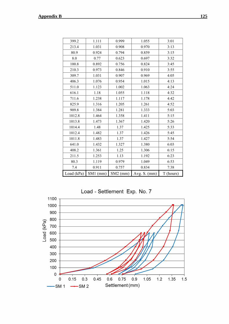
Appendix B 125
399.2 1.111 0.999 1.055 3:01
213.4 1.031 0.908 0.970 3:13
80.9 0.924 0.794 0.859 3:15
8.0 0.77 0.623 0.697 3:32
100.8 0.892 0.756 0.824 3:45
210.3 0.973 0.846 0.910 3:55
309.7 1.031 0.907 0.969 4:05
406.3 1.076 0.954 1.015 4:13
511.0 1.123 1.002 1.063 4:24
616.1 1.18 1.055 1.118 4:32
711.6 1.238 1.117 1.178 4:42
825.9 1.316 1.205 1.261 4:52
909.8 1.384 1.281 1.333 5:03
1012.8 1.464 1.358 1.411 5:15
1013.8 1.473 1.367 1.420 5:26
1014.4 1.48 1.37 1.425 5:33
1012.4 1.482 1.37 1.426 5:45
1011.8 1.483 1.37 1.427 5:54
641.0 1.432 1.327 1.380 6:03
408.2 1.361 1.25 1.306 6:15
211.5 1.253 1.13 1.192 6:23
80.3 1.119 0.979 1.049 6:53
7.4 0.911 0.757 0.834 7:38
Load (kPa) SM1 (mm) SM2 (mm) Avg. S. (mm) T (hours)
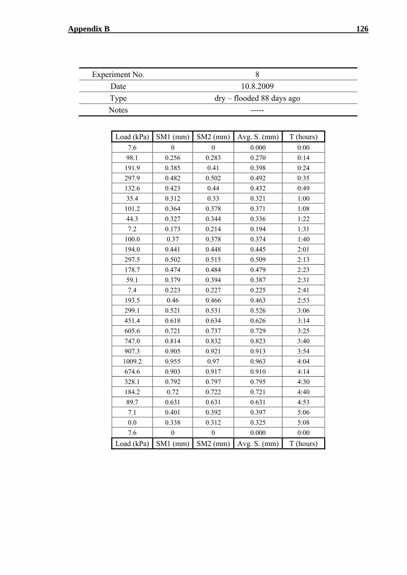
Appendix B 126
Experiment No. 8
Date 10.8.2009
Type dry – flooded 88 days ago
Notes -----
Load (kPa) SM1 (mm) SM2 (mm) Avg. S. (mm) T (hours)
7.6 0 0 0.000 0:00
98.1 0.256 0.283 0.270 0:14
191.9 0.385 0.41 0.398 0:24
297.9 0.482 0.502 0.492 0:35
132.6 0.423 0.44 0.432 0:49
35.4 0.312 0.33 0.321 1:00
101.2 0.364 0.378 0.371 1:08
44.3 0.327 0.344 0.336 1:22
7.2 0.173 0.214 0.194 1:31
100.0 0.37 0.378 0.374 1:40
194.0 0.441 0.448 0.445 2:01
297.5 0.502 0.515 0.509 2:13
178.7 0.474 0.484 0.479 2:23
59.1 0.379 0.394 0.387 2:31
7.4 0.223 0.227 0.225 2:41
193.5 0.46 0.466 0.463 2:53
299.1 0.521 0.531 0.526 3:06
451.4 0.618 0.634 0.626 3:14
605.6 0.721 0.737 0.729 3:25
747.0 0.814 0.832 0.823 3:40
907.3 0.905 0.921 0.913 3:54
1009.2 0.955 0.97 0.963 4:04
674.6 0.903 0.917 0.910 4:14
328.1 0.792 0.797 0.795 4:30
184.2 0.72 0.722 0.721 4:40
89.7 0.631 0.631 0.631 4:53
7.1 0.401 0.392 0.397 5:06
0.0 0.338 0.312 0.325 5:08
7.6 0 0 0.000 0:00
Load (kPa) SM1 (mm) SM2 (mm) Avg. S. (mm) T (hours)
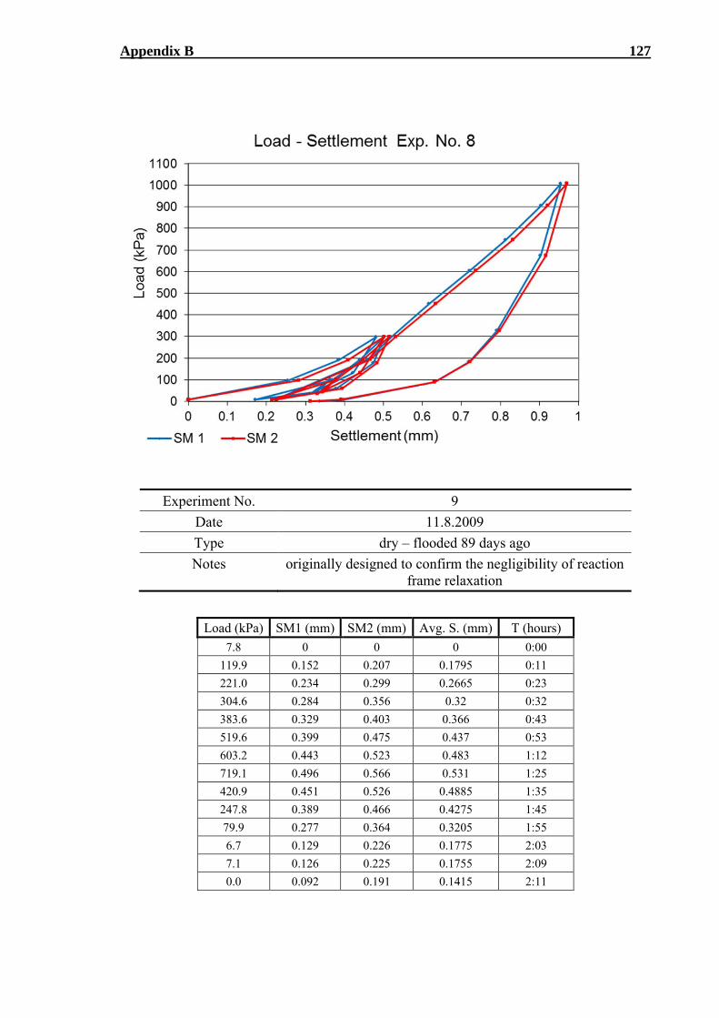
Appendix B 127
Experiment No. 9
Date 11.8.2009
Type dry – flooded 89 days ago
Notes originally designed to confirm the negligibility of reaction frame relaxation
Load (kPa) SM1 (mm) SM2 (mm) Avg. S. (mm) T (hours)
7.8 0 0 0 0:00
119.9 0.152 0.207 0.1795 0:11
221.0 0.234 0.299 0.2665 0:23
304.6 0.284 0.356 0.32 0:32
383.6 0.329 0.403 0.366 0:43
519.6 0.399 0.475 0.437 0:53
603.2 0.443 0.523 0.483 1:12
719.1 0.496 0.566 0.531 1:25
420.9 0.451 0.526 0.4885 1:35
247.8 0.389 0.466 0.4275 1:45
79.9 0.277 0.364 0.3205 1:55
6.7 0.129 0.226 0.1775 2:03
7.1 0.126 0.225 0.1755 2:09
0.0 0.092 0.191 0.1415 2:11
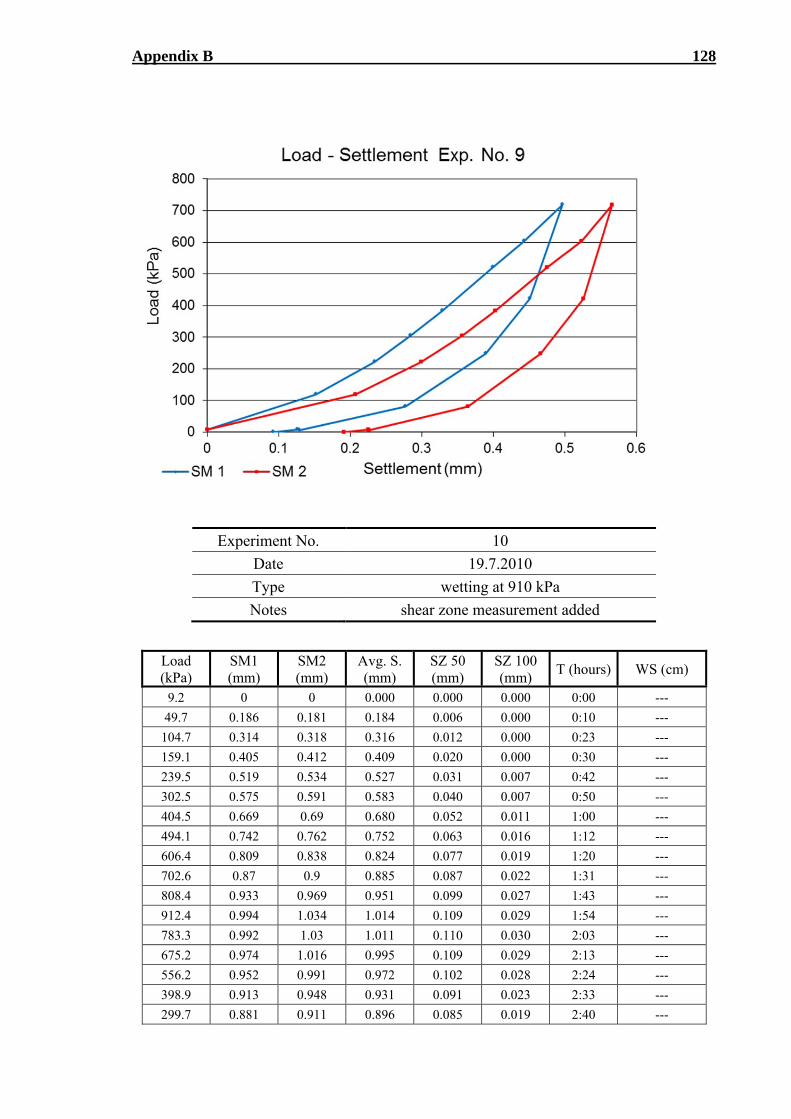
Appendix B 128
Experiment No. 10
Date 19.7.2010
Type wetting at 910 kPa
Notes shear zone measurement added
Load (kPa)
SM1 (mm)
SM2 (mm)
Avg. S. (mm)
SZ 50 (mm)
SZ 100 (mm)
T (hours) WS (cm)
9.2 0 0 0.000 0.000 0.000 0:00 ---
49.7 0.186 0.181 0.184 0.006 0.000 0:10 ---
104.7 0.314 0.318 0.316 0.012 0.000 0:23 ---
159.1 0.405 0.412 0.409 0.020 0.000 0:30 ---
239.5 0.519 0.534 0.527 0.031 0.007 0:42 ---
302.5 0.575 0.591 0.583 0.040 0.007 0:50 ---
404.5 0.669 0.69 0.680 0.052 0.011 1:00 ---
494.1 0.742 0.762 0.752 0.063 0.016 1:12 ---
606.4 0.809 0.838 0.824 0.077 0.019 1:20 ---
702.6 0.87 0.9 0.885 0.087 0.022 1:31 ---
808.4 0.933 0.969 0.951 0.099 0.027 1:43 ---
912.4 0.994 1.034 1.014 0.109 0.029 1:54 ---
783.3 0.992 1.03 1.011 0.110 0.030 2:03 ---
675.2 0.974 1.016 0.995 0.109 0.029 2:13 ---
556.2 0.952 0.991 0.972 0.102 0.028 2:24 ---
398.9 0.913 0.948 0.931 0.091 0.023 2:33 ---
299.7 0.881 0.911 0.896 0.085 0.019 2:40 ---
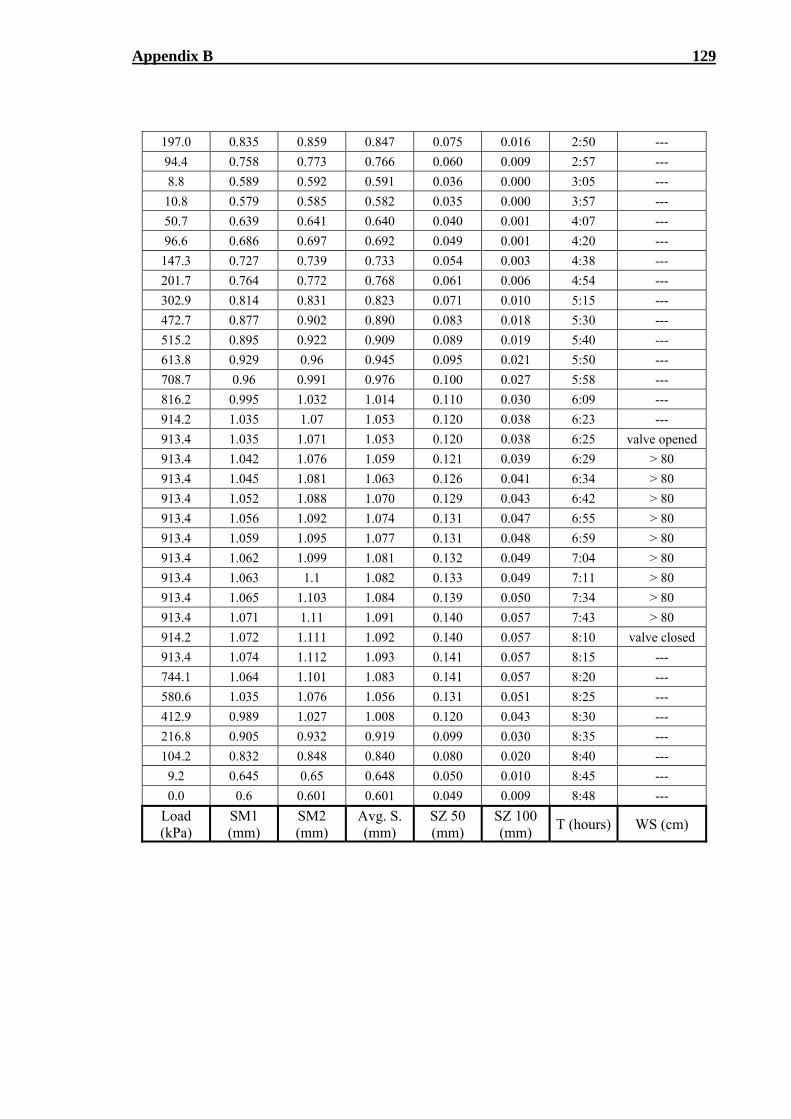
Appendix B 129
197.0 0.835 0.859 0.847 0.075 0.016 2:50 ---
94.4 0.758 0.773 0.766 0.060 0.009 2:57 ---
8.8 0.589 0.592 0.591 0.036 0.000 3:05 ---
10.8 0.579 0.585 0.582 0.035 0.000 3:57 ---
50.7 0.639 0.641 0.640 0.040 0.001 4:07 ---
96.6 0.686 0.697 0.692 0.049 0.001 4:20 ---
147.3 0.727 0.739 0.733 0.054 0.003 4:38 ---
201.7 0.764 0.772 0.768 0.061 0.006 4:54 ---
302.9 0.814 0.831 0.823 0.071 0.010 5:15 ---
472.7 0.877 0.902 0.890 0.083 0.018 5:30 ---
515.2 0.895 0.922 0.909 0.089 0.019 5:40 ---
613.8 0.929 0.96 0.945 0.095 0.021 5:50 ---
708.7 0.96 0.991 0.976 0.100 0.027 5:58 ---
816.2 0.995 1.032 1.014 0.110 0.030 6:09 ---
914.2 1.035 1.07 1.053 0.120 0.038 6:23 ---
913.4 1.035 1.071 1.053 0.120 0.038 6:25 valve opened
913.4 1.042 1.076 1.059 0.121 0.039 6:29 > 80
913.4 1.045 1.081 1.063 0.126 0.041 6:34 > 80
913.4 1.052 1.088 1.070 0.129 0.043 6:42 > 80
913.4 1.056 1.092 1.074 0.131 0.047 6:55 > 80
913.4 1.059 1.095 1.077 0.131 0.048 6:59 > 80
913.4 1.062 1.099 1.081 0.132 0.049 7:04 > 80
913.4 1.063 1.1 1.082 0.133 0.049 7:11 > 80
913.4 1.065 1.103 1.084 0.139 0.050 7:34 > 80
913.4 1.071 1.11 1.091 0.140 0.057 7:43 > 80
914.2 1.072 1.111 1.092 0.140 0.057 8:10 valve closed
913.4 1.074 1.112 1.093 0.141 0.057 8:15 ---
744.1 1.064 1.101 1.083 0.141 0.057 8:20 ---
580.6 1.035 1.076 1.056 0.131 0.051 8:25 ---
412.9 0.989 1.027 1.008 0.120 0.043 8:30 ---
216.8 0.905 0.932 0.919 0.099 0.030 8:35 ---
104.2 0.832 0.848 0.840 0.080 0.020 8:40 ---
9.2 0.645 0.65 0.648 0.050 0.010 8:45 ---
0.0 0.6 0.601 0.601 0.049 0.009 8:48 ---
Load (kPa)
SM1 (mm)
SM2 (mm)
Avg. S. (mm)
SZ 50 (mm)
SZ 100 (mm)
T (hours) WS (cm)
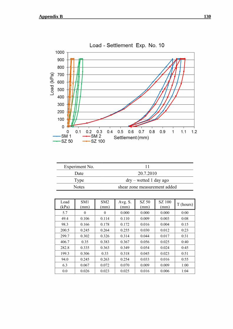
Appendix B 130
Experiment No. 11
Date 20.7.2010
Type dry – wetted 1 day ago
Notes shear zone measurement added
Load (kPa)
SM1 (mm)
SM2 (mm)
Avg. S. (mm)
SZ 50 (mm)
SZ 100 (mm)
T (hours)
5.7 0 0 0.000 0.000 0.000 0:00
49.4 0.106 0.114 0.110 0.009 0.003 0:08
98.3 0.166 0.178 0.172 0.016 0.004 0:15
200.5 0.245 0.264 0.255 0.030 0.012 0:23
299.7 0.302 0.326 0.314 0.044 0.017 0:31
406.7 0.35 0.383 0.367 0.056 0.025 0:40
282.8 0.335 0.363 0.349 0.054 0.024 0:45
199.3 0.306 0.33 0.318 0.045 0.023 0:51
94.0 0.245 0.263 0.254 0.033 0.016 0:55
6.3 0.067 0.072 0.070 0.009 0.009 1:00
0.0 0.026 0.023 0.025 0.016 0.006 1:04
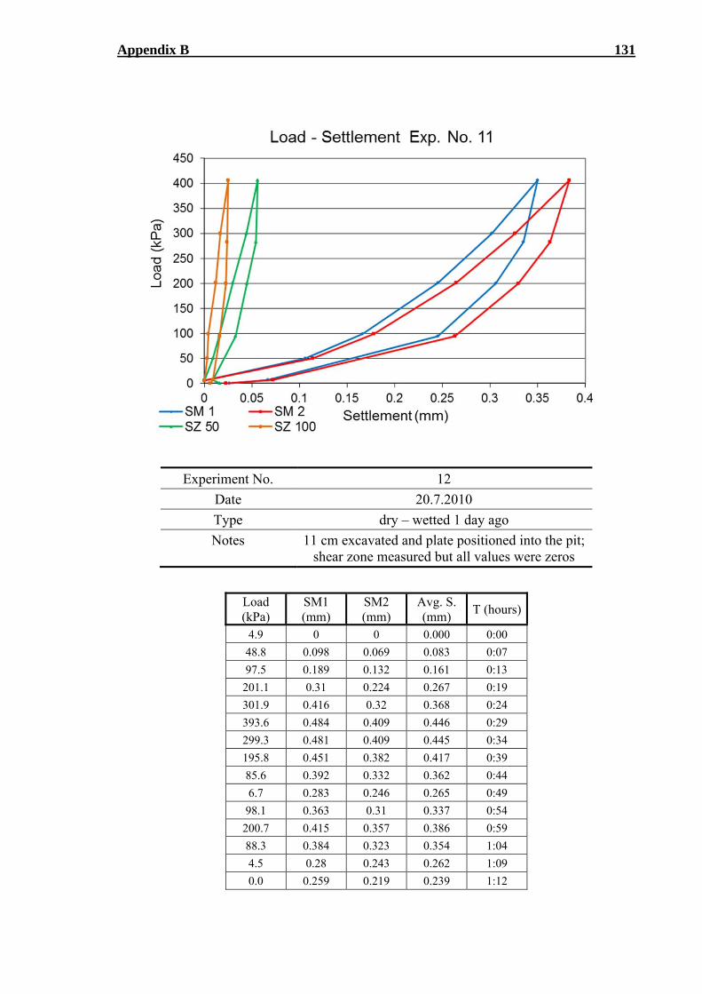
Appendix B 131
Experiment No. 12
Date 20.7.2010
Type dry – wetted 1 day ago
Notes 11 cm excavated and plate positioned into the pit; shear zone measured but all values were zeros
Load (kPa)
SM1 (mm)
SM2 (mm)
Avg. S. (mm)
T (hours)
4.9 0 0 0.000 0:00
48.8 0.098 0.069 0.083 0:07
97.5 0.189 0.132 0.161 0:13
201.1 0.31 0.224 0.267 0:19
301.9 0.416 0.32 0.368 0:24
393.6 0.484 0.409 0.446 0:29
299.3 0.481 0.409 0.445 0:34
195.8 0.451 0.382 0.417 0:39
85.6 0.392 0.332 0.362 0:44
6.7 0.283 0.246 0.265 0:49
98.1 0.363 0.31 0.337 0:54
200.7 0.415 0.357 0.386 0:59
88.3 0.384 0.323 0.354 1:04
4.5 0.28 0.243 0.262 1:09
0.0 0.259 0.219 0.239 1:12
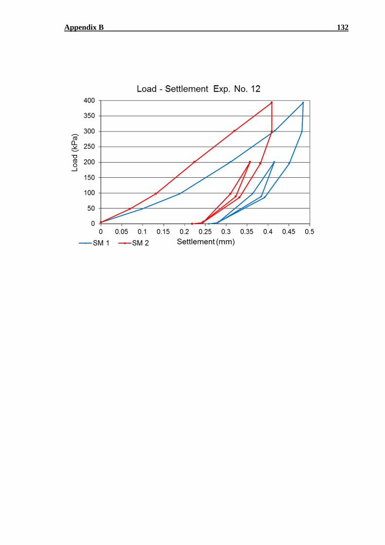
Appendix B 132
Appendix C
PLATE LOAD TESTS ON SILT LOAM
The following pages contain processed data from full scale experiments on soil specimen
made of silt loam. The data are presented in the same order in which the experiments were
carried out. More detailed description of the soil sample or the placement of the soil into
the stand can be found in relevant part of chapter 4.
Symbols used further in the tables and charts have following meaning. Data
labelled as SM 1 or SM 2 (settlement measuring point 1 and 2) contain measured results
from dial gauges located symmetrically on the top of the plate. SZ 50 and SZ 100 are
measured settlements of the shear zone from dial gauges located 50 mm from the edge of
the plate in case of SZ 50 and 100 mm from the edge of the plate in case of SZ 100.
Column labelled as WS contains position of groundwater table inside the soil with respect
to the top of the specimen. Due to the influence of the preferential paths created around the
intake to the piezometer during compaction process and due to leakage from the stand,
measured positions of groundwater table must be interpreted carefully and with respect to
these facts. T stands for time and Avg. S. represents average settlement. LP contains
measured lateral pressures.
Experiment No. 1
Date 6.5.2011
Type dry – natural moisture
Notes shear zone and lateral pressure measurement added
Load (kPa)
SM1 (mm)
SM2 (mm)
Avg. S. (mm)
SZ 50 (mm)
SZ 100 (mm)
T (hours) LP
(kPa)
4.1 0 0 0.000 0.000 0.000 0:00 0.00
49.0 0.554 0.525 0.540 0.075 0.047 0:07 2.12
97.9 1.17 1.1 1.135 0.207 0.105 0:20 5.41
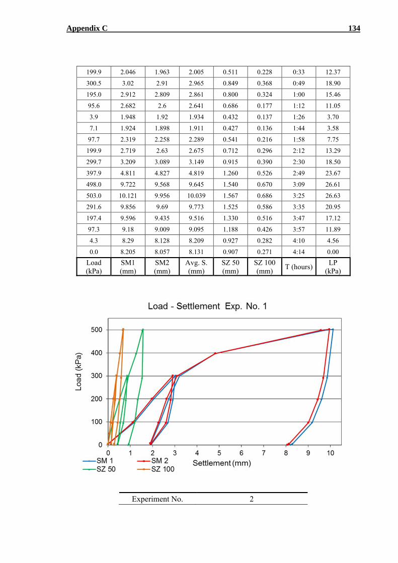
Appendix C 134
199.9 2.046 1.963 2.005 0.511 0.228 0:33 12.37
300.5 3.02 2.91 2.965 0.849 0.368 0:49 18.90
195.0 2.912 2.809 2.861 0.800 0.324 1:00 15.46
95.6 2.682 2.6 2.641 0.686 0.177 1:12 11.05
3.9 1.948 1.92 1.934 0.432 0.137 1:26 3.70
7.1 1.924 1.898 1.911 0.427 0.136 1:44 3.58
97.7 2.319 2.258 2.289 0.541 0.216 1:58 7.75
199.9 2.719 2.63 2.675 0.712 0.296 2:12 13.29
299.7 3.209 3.089 3.149 0.915 0.390 2:30 18.50
397.9 4.811 4.827 4.819 1.260 0.526 2:49 23.67
498.0 9.722 9.568 9.645 1.540 0.670 3:09 26.61
503.0 10.121 9.956 10.039 1.567 0.686 3:25 26.63
291.6 9.856 9.69 9.773 1.525 0.586 3:35 20.95
197.4 9.596 9.435 9.516 1.330 0.516 3:47 17.12
97.3 9.18 9.009 9.095 1.188 0.426 3:57 11.89
4.3 8.29 8.128 8.209 0.927 0.282 4:10 4.56
0.0 8.205 8.057 8.131 0.907 0.271 4:14 0.00
Load (kPa)
SM1 (mm)
SM2 (mm)
Avg. S. (mm)
SZ 50 (mm)
SZ 100 (mm)
T (hours) LP
(kPa)
Experiment No. 2

Appendix C 135
Date 7.7.2011
Type dry
Notes shear zone measurement added
Load (kPa)
SM1 (mm)
SM2 (mm)
Avg. S. (mm)
SZ 50 (mm)
SZ 100 (mm)
T (hours)
5.3 0 0 0.000 0.000 0.000 0:00
30.6 0.131 0.12 0.126 0.018 0.020 0:06
50.1 0.229 0.217 0.223 0.040 0.038 0:14
67.8 0.318 0.312 0.315 0.085 0.059 0:20
96.0 0.481 0.475 0.478 0.122 0.100 0:27
148.5 0.762 0.746 0.754 0.226 0.179 0:33
201.1 1.06 1.033 1.047 0.350 0.278 0:43
251.4 1.35 1.315 1.333 0.476 0.378 0:54
300.1 1.63 1.593 1.612 0.592 0.480 1:04
351.4 1.952 1.906 1.929 0.712 0.600 1:14
402.2 2.252 2.205 2.229 0.819 0.701 1:25
401.8 2.311 2.263 2.287 0.841 0.720 1:38
402.0 2.352 2.304 2.328 0.860 0.737 1:49
402.4 2.388 2.336 2.362 0.872 0.748 2:04
398.5 2.422 2.375 2.399 0.884 0.762 2:35
221.6 2.228 2.198 2.213 0.787 0.676 2:51
107.7 1.955 1.955 1.955 0.649 0.564 3:04
6.1 1.403 1.423 1.413 0.404 0.387 3:11
6.5 1.379 1.4 1.390 0.393 0.377 3:15
0.0 1.331 1.347 1.339 0.380 0.369 3:17
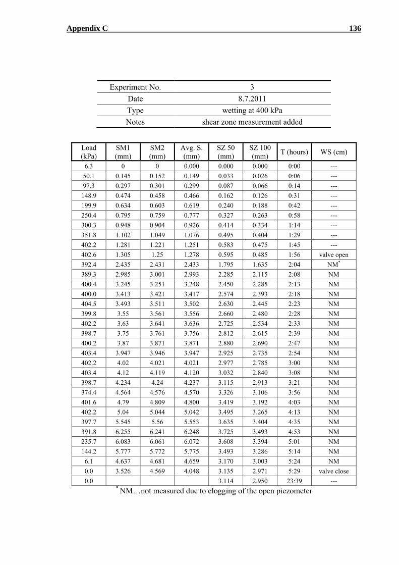
Appendix C 136
Experiment No. 3
Date 8.7.2011
Type wetting at 400 kPa
Notes shear zone measurement added
Load (kPa)
SM1 (mm)
SM2 (mm)
Avg. S. (mm)
SZ 50 (mm)
SZ 100 (mm)
T (hours) WS (cm)
6.3 0 0 0.000 0.000 0.000 0:00 ---
50.1 0.145 0.152 0.149 0.033 0.026 0:06 ---
97.3 0.297 0.301 0.299 0.087 0.066 0:14 ---
148.9 0.474 0.458 0.466 0.162 0.126 0:31 ---
199.9 0.634 0.603 0.619 0.240 0.188 0:42 ---
250.4 0.795 0.759 0.777 0.327 0.263 0:58 ---
300.3 0.948 0.904 0.926 0.414 0.334 1:14 ---
351.8 1.102 1.049 1.076 0.495 0.404 1:29 ---
402.2 1.281 1.221 1.251 0.583 0.475 1:45 ---
402.6 1.305 1.25 1.278 0.595 0.485 1:56 valve open
392.4 2.435 2.431 2.433 1.795 1.635 2:04 NM*
389.3 2.985 3.001 2.993 2.285 2.115 2:08 NM
400.4 3.245 3.251 3.248 2.450 2.285 2:13 NM
400.0 3.413 3.421 3.417 2.574 2.393 2:18 NM
404.5 3.493 3.511 3.502 2.630 2.445 2:23 NM
399.8 3.55 3.561 3.556 2.660 2.480 2:28 NM
402.2 3.63 3.641 3.636 2.725 2.534 2:33 NM
398.7 3.75 3.761 3.756 2.812 2.615 2:39 NM
400.2 3.87 3.871 3.871 2.880 2.690 2:47 NM
403.4 3.947 3.946 3.947 2.925 2.735 2:54 NM
402.2 4.02 4.021 4.021 2.977 2.785 3:00 NM
403.4 4.12 4.119 4.120 3.032 2.840 3:08 NM
398.7 4.234 4.24 4.237 3.115 2.913 3:21 NM
374.4 4.564 4.576 4.570 3.326 3.106 3:56 NM
401.6 4.79 4.809 4.800 3.419 3.192 4:03 NM
402.2 5.04 5.044 5.042 3.495 3.265 4:13 NM
397.7 5.545 5.56 5.553 3.635 3.404 4:35 NM
391.8 6.255 6.241 6.248 3.725 3.493 4:53 NM
235.7 6.083 6.061 6.072 3.608 3.394 5:01 NM
144.2 5.777 5.772 5.775 3.493 3.286 5:14 NM
6.1 4.637 4.681 4.659 3.170 3.003 5:24 NM
0.0 3.526 4.569 4.048 3.135 2.971 5:29 valve close
0.0 3.114 2.950 23:39 --- * NM…not measured due to clogging of the open piezometer
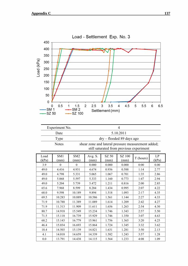
Appendix C 137
Experiment No. 4
Date 5.10.2011
Type dry – flooded 89 days ago
Notes shear zone and lateral pressure measurement added; still saturated from previous experiment
Load (kPa)
SM1 (mm)
SM2 (mm)
Avg. S. (mm)
SZ 50 (mm)
SZ 100 (mm)
T (hours) LP
(kPa) 3.9 0 0 0.000 0.000 0.000 0:00 0.00
49.0 4.416 4.931 4.674 0.936 0.588 1:14 2.77
49.0 4.798 5.331 5.065 1.067 0.701 1:35 2.86
49.0 5.068 5.597 5.333 1.160 0.773 1:47 2.94
49.0 5.204 5.739 5.472 1.211 0.816 2:00 2.85
65.6 7.968 8.599 8.284 1.434 0.995 2:07 4.22
68.0 9.598 10.189 9.894 1.518 1.093 2:17 4.35
69.5 10.283 10.889 10.586 1.561 1.144 2:27 4.33
71.9 10.788 11.389 11.089 1.614 1.209 2:42 4.27
71.9 11.313 11.909 11.611 1.656 1.263 2:54 4.30
80.7 14.918 15.549 15.234 1.746 1.343 2:57 5.50
71.5 15.118 16.739 15.929 1.746 1.350 3:07 4.63
68.2 15.143 16.779 15.961 1.756 1.365 3:20 4.25
46.4 15.034 16.693 15.864 1.724 1.345 3:32 3.62
18.4 14.503 15.139 14.821 1.631 1.281 3:50 2.13
4.1 14.018 14.659 14.339 1.582 1.243 3:57 1.28
0.0 13.791 14.438 14.115 1.564 1.233 4:08 1.09
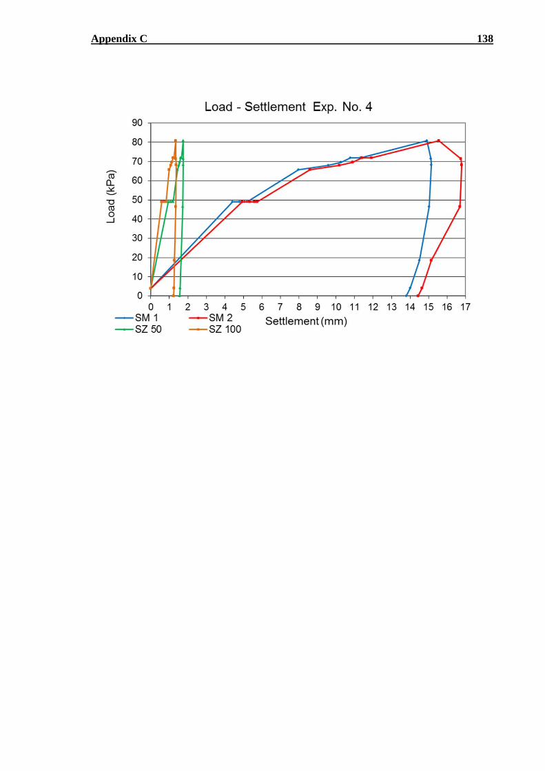
Appendix C 138
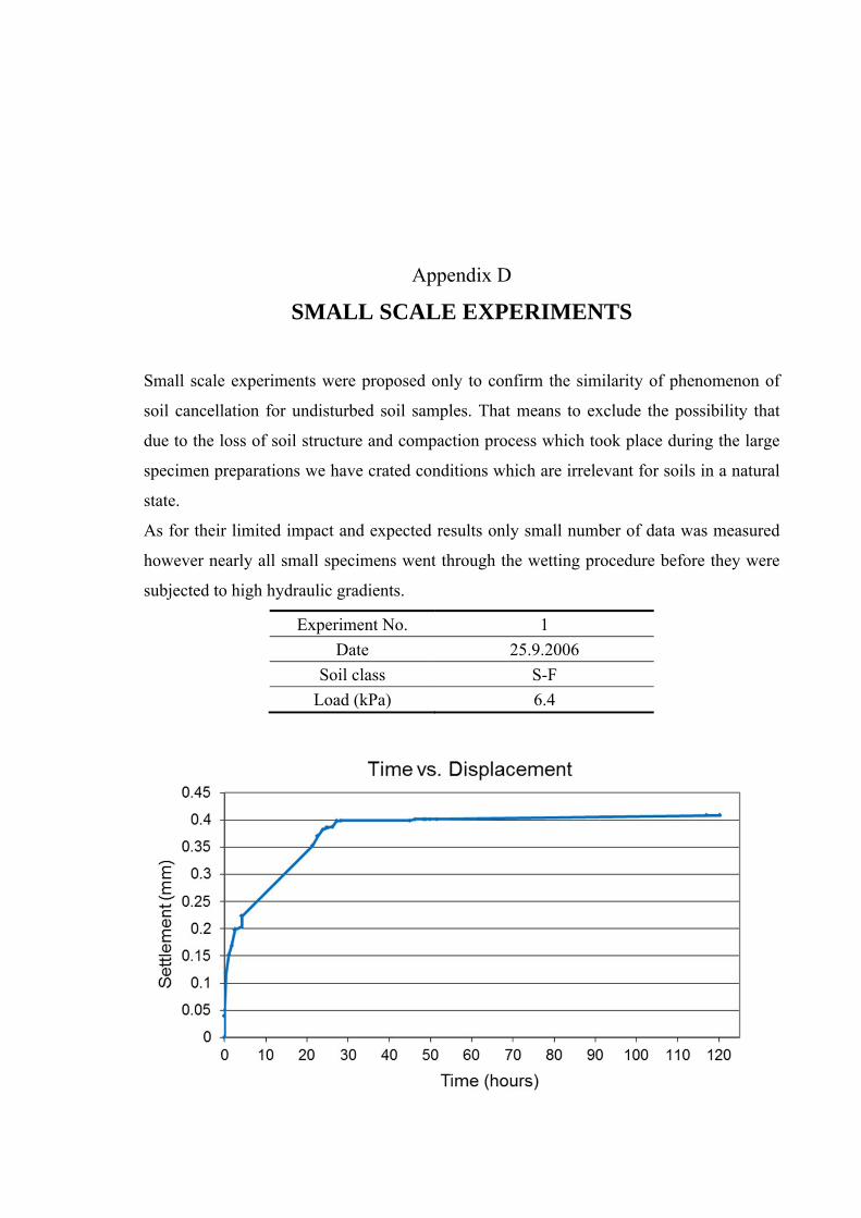
Appendix D
SMALL SCALE EXPERIMENTS
Small scale experiments were proposed only to confirm the similarity of phenomenon of
soil cancellation for undisturbed soil samples. That means to exclude the possibility that
due to the loss of soil structure and compaction process which took place during the large
specimen preparations we have crated conditions which are irrelevant for soils in a natural
state.
As for their limited impact and expected results only small number of data was measured
however nearly all small specimens went through the wetting procedure before they were
subjected to high hydraulic gradients.
Experiment No. 1
Date 25.9.2006
Soil class S-F
Load (kPa) 6.4
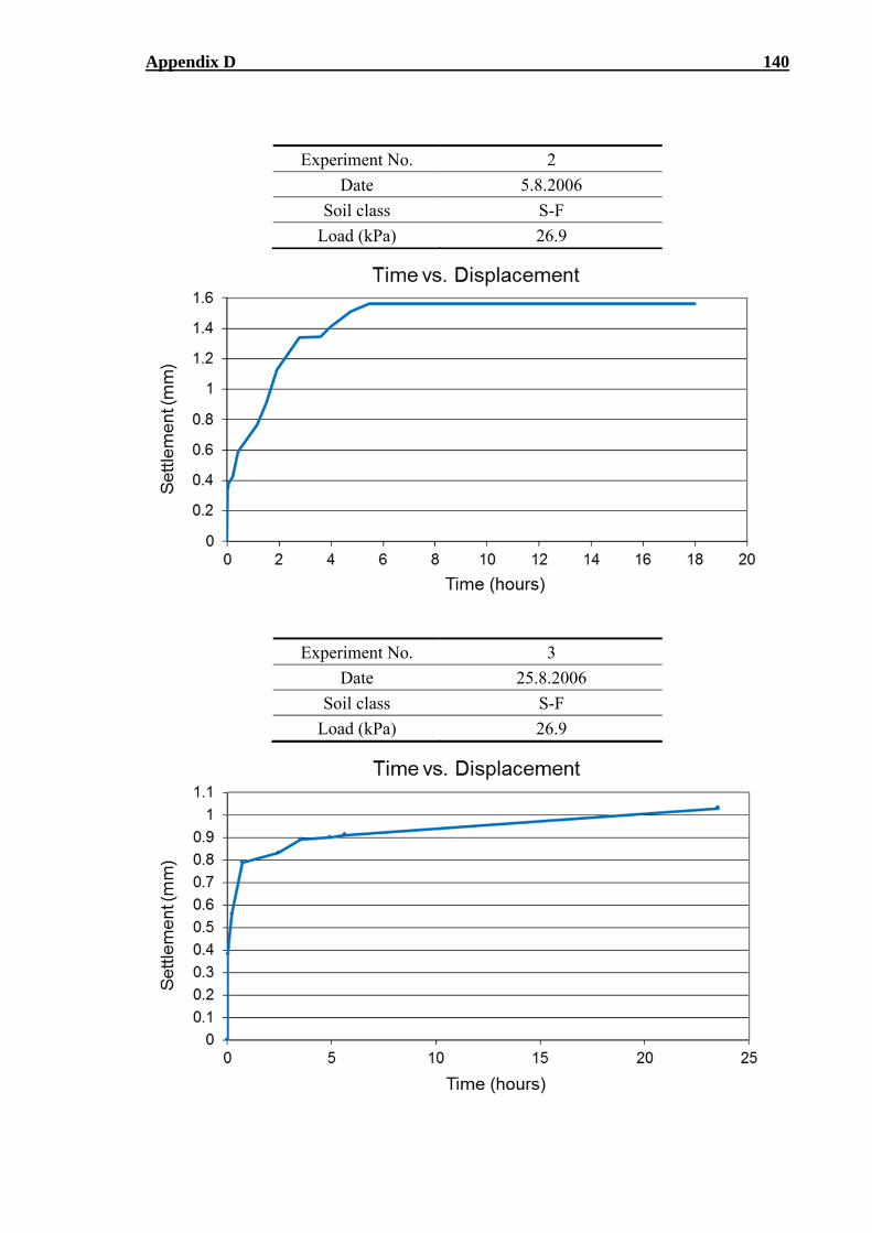
Appendix D 140
Experiment No. 2
Date 5.8.2006
Soil class S-F
Load (kPa) 26.9
Experiment No. 3
Date 25.8.2006
Soil class S-F
Load (kPa) 26.9
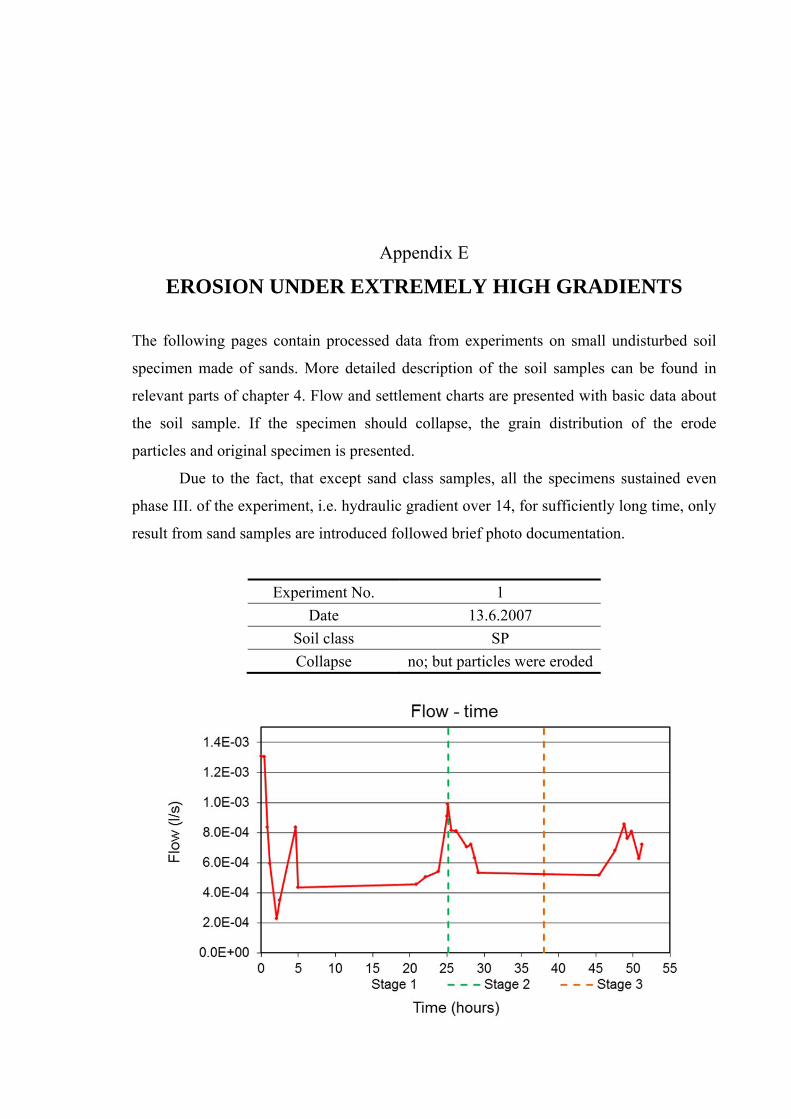
Appendix E
EROSION UNDER EXTREMELY HIGH GRADIENTS
The following pages contain processed data from experiments on small undisturbed soil
specimen made of sands. More detailed description of the soil samples can be found in
relevant parts of chapter 4. Flow and settlement charts are presented with basic data about
the soil sample. If the specimen should collapse, the grain distribution of the erode
particles and original specimen is presented.
Due to the fact, that except sand class samples, all the specimens sustained even
phase III. of the experiment, i.e. hydraulic gradient over 14, for sufficiently long time, only
result from sand samples are introduced followed brief photo documentation.
Experiment No. 1
Date 13.6.2007
Soil class SP
Collapse no; but particles were eroded
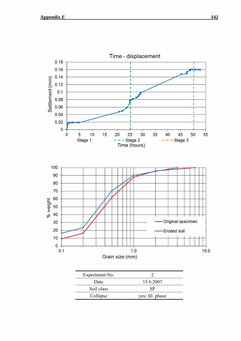
Appendix E 142
Experiment No. 2
Date 15.6.2007
Soil class SP
Collapse yes; III. phase
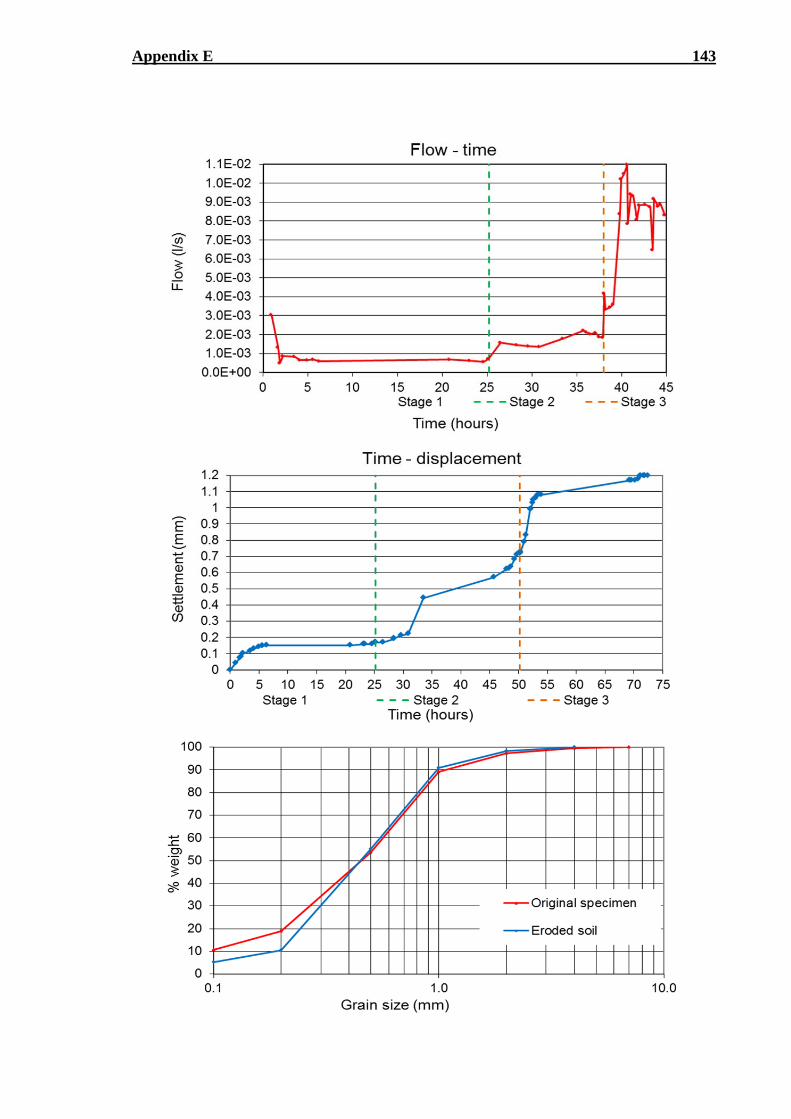
Appendix E 143
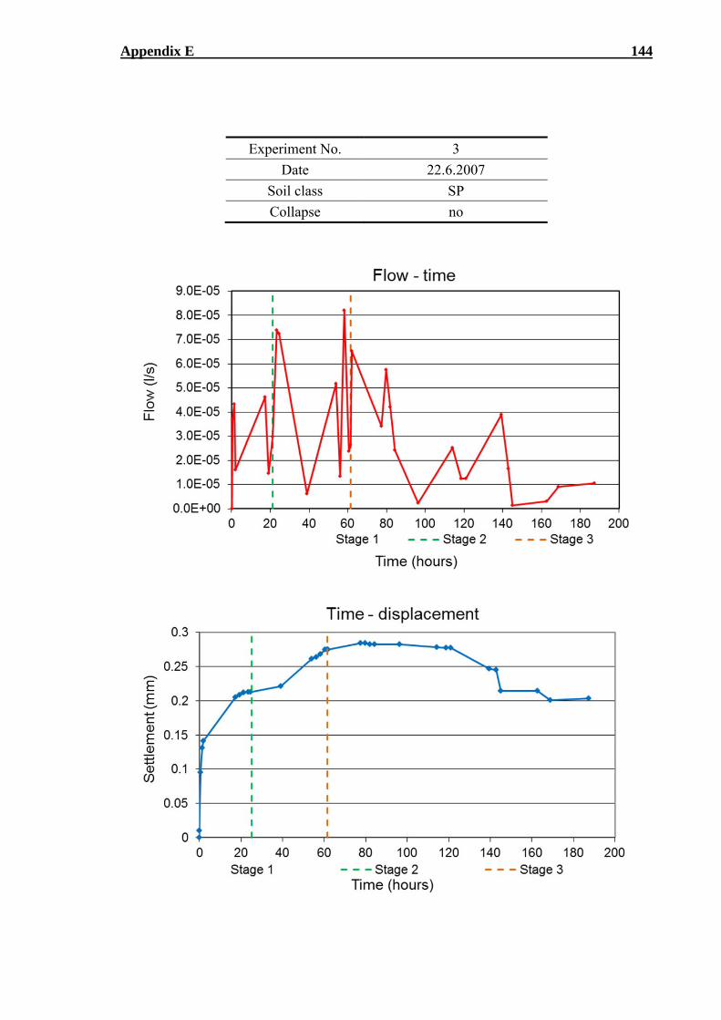
Appendix E 144
Experiment No. 3
Date 22.6.2007
Soil class SP
Collapse no
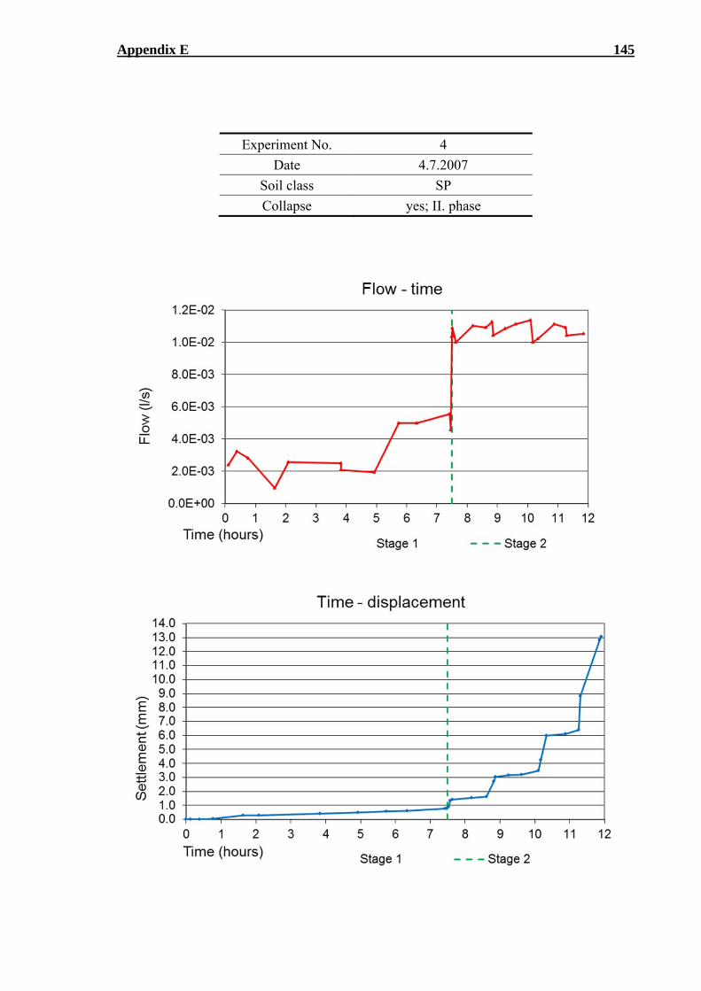
Appendix E 145
Experiment No. 4
Date 4.7.2007
Soil class SP
Collapse yes; II. phase
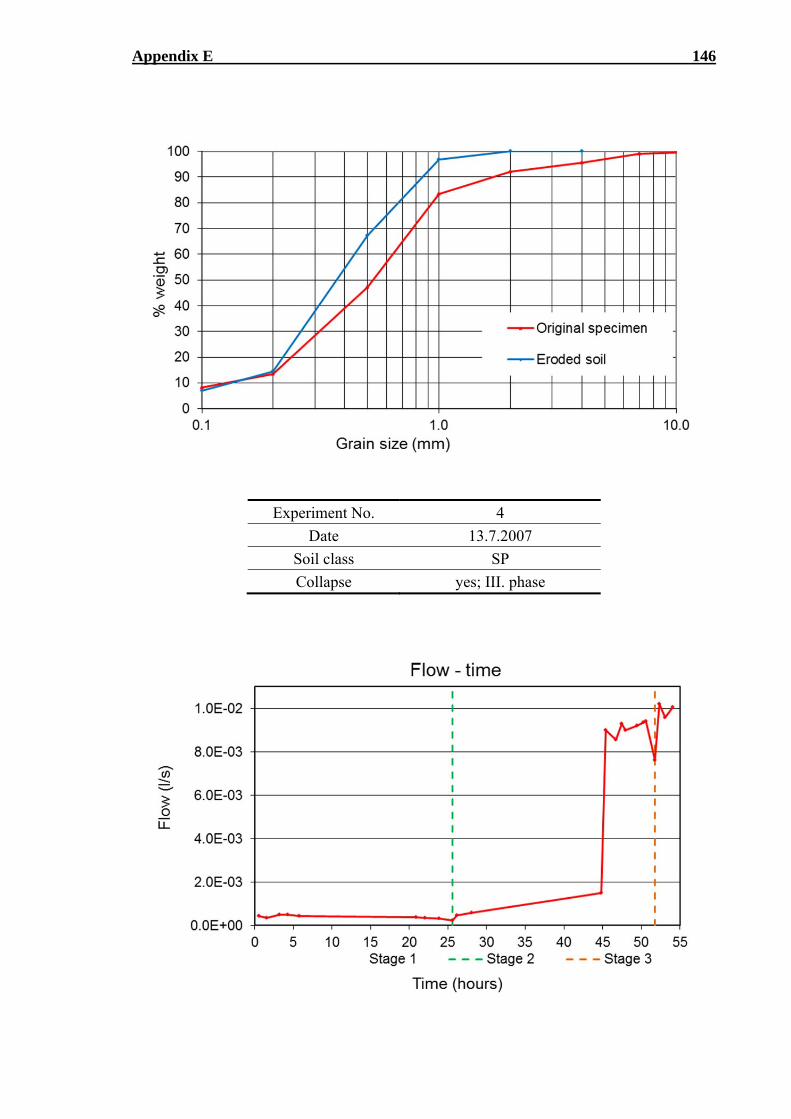
Appendix E 146
Experiment No. 4
Date 13.7.2007
Soil class SP
Collapse yes; III. phase
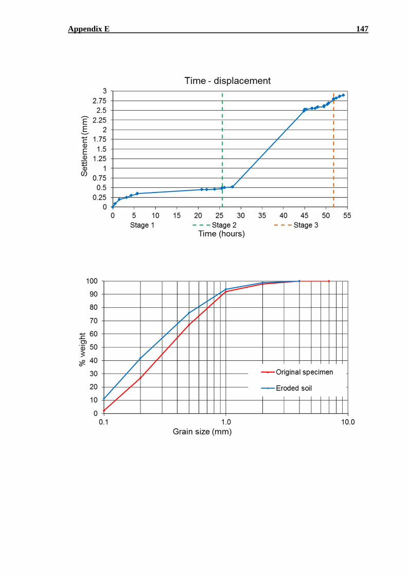
Appendix E 147
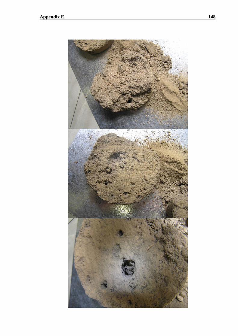
Appendix E 148
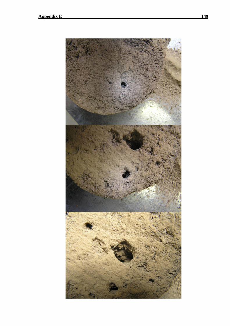
Appendix E 149


