Study of second-step Auger transitions in Auger cascades following 1s → 3p photoexcitation in Ne

INSTITUTE OF PHYSICS PUBLISHING JOURNAL OF PHYSICS B: ATOMIC, MOLECULAR AND OPTICAL PHYSICS

J. Phys. B: At. Mol. Opt. Phys. 38 (2005) 465–486 doi:10.1088/0953-4075/38/5/001

Study of second-step Auger transitions in Augercascades following 1s → 3p photoexcitation in Ne

H Yoshida1, J Sasaki1, Y Kawabe1, Y Senba1,2, A De Fanis2, M Oura3,S Fritzsche4, I P Sazhina5, N M Kabachnik5,6 and K Ueda7,8

1 Department of Physical Science, Hiroshima University, Higashi-Hiroshima 739-8526, Japan2 JASRI/SPring-8, Sayo-gun, Hyogo 679-5198, Japan3 RIKEN/SPring-8, Sayo-gun, Hyogo 679-5148, Japan4 Institut fur Physik, Universitat Kassel, Heinrich-Plett-Str. 40, D-34132 Kassel, Germany5 Institute of Nuclear Physics, Moscow State University, Moscow 119992, Russia6 Fakultat fur Physik, Universitat Bielefeld, D-33615 Bielefeld, Germany7 Institute of Multidisciplinary Research for Advanced Materials, Tohoku University,Sendai 980-8577, Japan

Received 15 September 2004Published 21 February 2005Online at stacks.iop.org/JPhysB/38/465

AbstractWe present the results of high-resolution measurements of the low-energy partof the Auger electron spectrum generated by photoexcitation of the 1s−13presonance in Ne. The spectrum was measured in the energy range of 10–33 eV where mainly the electrons from the second-step Auger transitionsof the cascades 1s−13p → 2s2p5np → 2s22p4 and 1s−13p → 2s02p6np →2s2p5 (n = 3, 4) are detected. High resolution allows us to study the multipletstructure of the transitions and to determine the widths of the intermediatestates of the Ne+ ion. Anisotropy of the angular distribution of Auger electronsis determined for all of the lines observed. The results are in reasonably goodagreement with MCDF calculations.

1. Introduction

Investigation of resonant Auger processes is a quickly developing branch of electronspectroscopy of atoms (Armen et al 2000). Here spectacular progress has been achieved in thelast decade due to a dramatic increase in the resolution of the monochromators installed in softx-ray beamlines at third generation synchrotron radiation facilities as well as the availabilityof high-resolution electron spectrometers (Ueda 2003). Among various targets used in suchinvestigations, atomic neon occupies a special place since it is the simplest closed shellmulti-electron atom for which the whole variety of many-electron processes accompanyingcore-excitation can occur. In particular, the Ne 1s → 3p resonance and the following Auger(autoionization) emission have been studied by various experimental techniques (Viefhaus

8 Author to whom correspondence should be addressed.

0953-4075/05/050465+22$30.00 © 2005 IOP Publishing Ltd Printed in the UK 465

http://dx.doi.org/10.1088/0953-4075/38/5/001

http://stacks.iop.org/jb/38/465

466 H Yoshida et al

1997, Coreno et al 1999, Yoshida et al 2000, Shimizu et al 2000, Saito et al 2000, Kivimakiet al 2001, Turri et al 2001, De Fanis et al 2002, Ueda et al 2003, De Fanis et al 2004, forearlier references see Armen et al (2000)). The high-energy part of the resonant Auger electronspectrum consists of groups of strong lines corresponding to the spectator transitions fromthe 1s−13p resonance to the Ne+ states with configurations 2s22p43p, 2s2p53p and 2s02p63p.Some ionic levels of the last two configurations lie above the double ionization threshold andtherefore they can further autoionize to the final states of Ne++ so that cascades of Augertransitions are formed. The main lines corresponding to the second step Auger emission(second step in the cascade) lie in the energy range of 10–33 eV. They are much less studiedthan the first step Auger transitions although they are even more interesting since they occurbetween the states with more than two open shells. Their theoretical interpretation is a realchallenge for modern theories of multi-electron atoms.

The second-step Auger transitions in the cascades may be considered as resonantlyenhanced inner-valence Auger transitions in Ne+. Such transitions have long been studiedas shake-up and correlation satellites in outer-shell photoionization of Ne (Svenssonet al 1988, Becker et al 1989, 1993, Wills et al 1990, Pahler et al 1993, Kikas et al 1996).Indeed, in photoionization of the 2s subshell in Ne, one of the 2p electrons can be shaken up tothe 3p or higher Rydberg orbital. Although a recombination of a pure 2s vacancy via ‘normal’Auger decay is energetically not allowed, the states populated by simultaneous ionization andexcitation may decay via the ‘participator’ Auger transition (Becker et al 1989, Becker andWehlitz 1994). These transitions which are known as inner-valence Auger transitions havethe same nature as the second-step Auger transitions in the cascades of Auger decay followingthe Ne 1s → 3p photoexcitation. The use of the resonant Auger decay for generating suchtransitions has some advantages since in this way one can reach intermediate states whichare hardly accessible via an outer-shell photoionization because of their weak coupling to thedirect ionization channel.

Early spectra of the second-step Auger transitions in resonant 1s → 3p photoexcitationof Ne were measured with relatively moderate resolution (von Raven 1992, Viefhaus 1997,Yoshida et al 2000, Turri et al 2001) which did not allow resolution of the multiplet structureof the lines. Nevertheless, all main peaks of the spectra have been identified. The angulardistribution measurements have shown that emission of almost all of the lines is anisotropic(Viefhaus 1997, Yoshida et al 2000). This anisotropy was qualitatively explained by largealignment transfer in the first step resonance Auger transitions.

In the present work, we investigate the second-step Auger transitions caused by the1s → 3p photoexcitation in Ne with much better resolution than in previous experiments. Inmany cases, this permits us to resolve the multiplet structure of the intermediate states, i.e. theinitial states of the second-step transitions. Moreover, the resolution achieved is comparablewith the natural widths of lines. Thus, in many cases, we are able to determine the latterexperimentally. Since the final states of the Ne++ ion are very narrow, the line widths aredetermined by the lifetime widths of the intermediate states of Ne+. Earlier, we publishedthe results of measurements of the lifetime widths of these states using Doppler-free resonantRaman Auger spectroscopy for the first step Auger transitions (Ueda et al 2003, De Faniset al 2004). In the present paper, we report independent determination of these widths usingthe second-step Auger emission. We have also determined the anisotropy parameters for eachof the second-step lines, which help us to identify the resolved transitions. In order to comparethe experimental results with theoretical predictions we have made multi-configuration Dirac–Fock (MCDF) calculations of the energies, intensities and anisotropy parameters for themain lines of the second-step Auger spectrum as well as the widths of the intermediatestates employing the step-wise model of the resonant Auger cascade (Kabachnik 1997,

Second-step Auger transitions in photoexcited Auger cascades in Ne 467

Table 1. Energies, Ek , and intensities for all lines in the low-energy electron spectrum generatedby photoexcitation of the 1s−13p state in Ne. We denote by I the relative intensity within one peak(total intensity of the peak is then equal to 1); I� is the intensity of the peak relative to the intensityof peak 7, the value I� may be compared with previous low-resolution data I� [I] (Yoshida et al2000).

Experiment MCHF theory

Peak Line Initial state Final state Ek (eV) I I� I� [I] Ek (eV) I I�

1 1 2s12p5(3P)3p 4P5/2 2s22p4 1D2 12.296 0.02(02) 0.22(02) 0.15 12.02 0.01 0.072 2s12p5(3P)3p 2D5/2 2s22p4 1D2 12.333 0.21(03) 12.07 0.393 2s12p5(3P)3p 2D3/2 2s22p4 1D2 12.389 0.28(05) 12.12 0.334 ? ? 12.435 0.09(09)5 2s12p5(3P)3p 2P 2s22p4 1D2 12.488 0.39(13) 12.23 0.27

2 6 2s12p5(3P)3p 2S 2s22p4 1D2 13.209 0.16(01) 0.58(04) 0.44 13.30 0.09 0.747 2s02p6(1S)3p 2P 2s12p5 1P1 13.529 0.80(04) 13.08 0.918 ? ? 13.714 0.04(01)

3 9 2s12p5(3P)3p 2D5/2 2s22p4 3P0 15.427 0.0a 0.44(03) 0.36 15.56 0.04 0.5310 2s12p5(3P)3p 2D5/2 2s22p4 3P1 15.462 0.1a 15.59 0.0911 2s12p5(3P)3p 2D3/2 2s22p4 3P0 15.483 0.1a 15.63 0.0212 2s12p5(3P)3p 2D3/2 2s22p4 3P1 15.518 0.1a 15.66 0.1013 2s12p5(3P)3p 2D5/2 2s22p4 3P2 15.541 0.2a 15.67 0.2114 2s12p5(3P)3p 2P 2s22p4 3P0 15.582 0.1a 15.76 0.0715 2s12p5(3P)3p 2D3/2 2s22p4 3P2 15.597 0.3a 15.74 0.1516 2s12p5(3P)3p 2P 2s22p4 3P1 15.617 0.1a 15.79 0.1817 2s12p5(3P)3p 2P 2s22p4 3P2 15.696 0.2a 15.87 0.15

4 18 ? ? 17.157 0.03(01) 0.12(01) 0.1019 ? ? 17.272 0.08(01)20 2s12p5(3P)4p 4P 2s22p4 1D2 17.350 0.09(01)21 2s12p5(3P)4p 2P 2s22p4 1D2 17.396 0.30(02)22 2s12p5(3P)4p 2D 2s22p4 1D2 17.450 0.31(02)23 ? ? 17.498 0.04(01)24 ? ? 17.570 0.02(01)25 ? ? 17.669 0.05(01)26 2s12p5(3P)4p 2S 2s2 2p4 1D2 17.699 0.08(01)

5 27 2s02p6(1S)4p 2P 2s12p5 1P1 18.652 0.98(05) 0.23(02) 0.2328 ? ? 18.876 0.02(02)

6 29 2s12p5(3P)4p 4P 2s22p4 3P0 20.439 0.0a 0.22(02) 0.2130 2s12p5(3P)4p 4P 2s22p4 3P1 20.474 0.0a

31 2s12p5(3P)4p 2P 2s22p4 3P0 20.485 0.0a

32 2s12p5(3P)4p 2P 2s22p4 3P1 20.520 0.1a

33 2s12p5(3P)4p 2D 2s22p4 3P0 20.539 0.1a

34 2s12p5(3P)4p 4P 2s22p4 3P2 20.553 0.1a

35 2s12p5(3P)4p 2D 2s22p4 3P1 20.574 0.2a

36 2s12p5(3P)4p 2P 2s22p4 3P2 20.599 0.4a

37 2s12p5(3P)4p 2D 2s22p4 3P2 20.653 0.1a

7 38 2s12p5(1P)3p 2D 2s22p4 1D2 22.579 0.94(05) 1.00 1.00 24.07 0.73 1.039 2s12p5(1P)3p 2P 2s2 2p4 1D2 22.840 0.06(01) 24.30 0.27

468 H Yoshida et al

Table 1. (Continued.)


Peak Line Initial state Final state Ek (eV) I I� I� [I] Ek (eV) I I�

8 40 2s02p6(1S)3p 2P 2s12p5 3P0 23.984 0.2a 0.22(02) 0.26 25.54 0.13 0.2441 2s02p6(1S)3p 2P 2s12p5 3P1 24.023 0.3a 25.57 0.3742 2s02p6(1S)3p 2P 2s12p5 3P2 24.096 0.5a 25.64 0.51

9 43 2s12p5(1P)3p 2D 2s22p4 3P0 25.664 0.0a 0.85(05) 0.89 27.61 0.04 0.3544 2s12p5(1P)3p 2D 2s22p4 3P1 25.699 0.1a 27.65 0.1145 2s12p5(1P)3p 2D 2s22p4 3P2 25.778 0.19(06) 27.72 0.1946 2s12p5(1P)3p 2P 2s22p4 3P0 25.932 0.1a 27.84 0.0847 2s12p5(1P)3p 2P 2s22p4 3P1 25.967 0.2a 27.87 0.2348 2s12p5(1P)3p 2P 2s22p4 3P2 26.046 0.36(07) 27.95 0.37

10 49 2s12p5(1P)4p 2D 2s22p4 1D2 27.817 0.97(05) 0.53(04) 0.5250 2s12p5(1P)4p 2P 2s22p4 1D2 27.900 0.03(01)

11 51 2s02p6(1S)4p 2P 2s12p5 3P0 29.102 0.1a 0.12(01) 0.1352 2s02p6(1S)4p 2P 2s12p5 3P1 29.141 0.3a

53 2s02p6(1S)4p 2P 2s12p5 3P2 29.214 0.50(28)54 ? ? 29.266 0.04(04)

12 55 2s12p5(1P)4p 2D 2s22p4 3P0 30.904 0.0a 0.36(03) 0.3356 2s12p5(1P)4p 2D 2s22p4 3P1 30.939 0.2a

57 2s12p5(1P)4p 2P 2s22p4 3P0 30.987 0.1a

58 2s12p5(1P)4p 2D 2s22p4 3P2 31.018 0.2a

59 2s12p5(1P)4p 2P 2s22p4 3P1 31.022 0.2a

60 2s12p5(1P)4p 2P 2s22p4 3P2 31.101 0.33(10)

a Uncertainties can be estimated for (partly) resolved lines and are indicated in parentheses, but could not be estimatedfor unresolved lines (see the text in section 4.1).

Kabachnik et al 1999). In general, the theoretical values agree satisfactorily with theexperimental results.

In the next section, we describe the experiment and give an overview of the main featuresof the low-energy (10–33 eV) part of the Auger spectrum. In section 3, we discuss themain approximations made in our MCDF calculations. Section 4 is devoted to the detaileddiscussion of the experimental results and their comparison with other data and the theoreticalcalculations. In conclusion we summarize our findings and discuss possible improvements inthe theoretical calculations.

2. Experiment

The experiment was carried out on the c-branch of the soft x-ray photochemistry beamline27SU (Ohashi et al 2001a) at SPring-8, the 8 GeV synchrotron radiation facility in Japan. Theradiation source is a figure-8 undulator, whose emitted radiation is linearly polarized either inthe horizontal plane of the storage ring (1st order) or in the vertical plane perpendicular to it(0.5th order) (Tanaka and Kitamura 1996). The soft x-ray monochromator of this branch isof the Hettrick type, which consists of a varied line space plane grating and a focusing mirror(Ohashi et al 2001b, Tamenori et al 2002). The degree of linear polarization was measured in aseparate experiment by observing the Ne 2s and 2p photolines and confirmed to be larger than


Table 2. Angular anisotropy parameters β for all lines in the low-energy electron spectrumgenerated by photoexcitation of the 1s−13p state in Ne. We denote by βlow the average β of thegroup which is compared with the previous low-resolution data obtained at SPring-8 (SP8) andDORIS (DOR) (Yoshida et al 2000).


Peak Line Initial state Final state β βlow SP8 DOR β βlow

1 1 2s12p5(3P)3p 4P5/2 2s22p4 1D2 1.1a 0.28(08) 0.39(07) 0.38(09) −0.198 −0.082 2s12p5(3P)3p 2D5/2 2s22p4 1D2 0.28(23) −0.1923 2s12p5(3P)3p 2D3/2 2s22p4 1D2 0.11(24) −0.0684 ? ? −0.2a

5 2s12p5(3P)3p 2P 2s22p4 1D2 0.49(49) 0.115

2 6 2s12p5(3P)3p 2S 2s22p4 1D2 0.02(12) 0.47(08) 0.6(06) 0.57(07) 0 0.8837 2s02p6(1S)3p 2P 2s12p5 1P1 0.59(08) 0.9738 ? ? −0.43(32)

3 9 2s12p5(3P)3p 2D5/2 2s22p4 3P0 1.1a 0.24(07) 0.45(04) 0.34(06) 0.797 0.10610 2s12p5(3P)3p 2D5/2 2s22p4 3P1 0.9a 0.45411 2s12p5(3P)3p 2D3/2 2s22p4 3P0 0.8a 0.25212 2s12p5(3P)3p 2D3/2 2s22p4 3P1 0.8a 0.15313 2s12p5(3P)3p 2D5/2 2s22p4 3P2 −0.0a 0.20214 2s12p5(3P)3p 2P 2s22p4 3P0 0.3a −0.27915 2s12p5(3P)3p 2D3/2 2s22p4 3P2 0.2a −0.02316 2s12p5(3P)3p 2P 2s22p4 3P1 0.2a −0.12917 2s12p5(3P)3p 2P 2s22p4 3P2 −0.1a 0.102

4 18 ? ? −0.40(58) 0.16(08) 0.45(28)19 ? ? 0.14(24)20 2s12p5(3P)4p 4P 2s22p4 1D2 −0.08(21)

21 2s12p5(3P)4p 2P 2s22p4 1D2 0.36(12)22 2s12p5(3P)4p 2D 2s22p4 1D2 −0.01(11)

23 ? ? 0.46(48)24 ? ? 0.69(70)25 ? ? 0.56(42)26 2s12p5(3P)4p 2S 2s22p4 1D2 0.01(37)

5 27 2s02p6(1S)4p 2P 2s12p5 1P1 0.81(08) 0.83(08) 0.60(19) 0.89(11)28 ? ? 2.00(79)

6 29 2s12p5(3P)4p 4P 2s22p4 3P0 0.7a 0.37(08) 0.39(19) 0.44(09)30 2s12p5(3P)4p 4P 2s22p4 3P1 0.3a

31 2s12p5(3P)4p 2P 2s22p4 3P0 0.5a

32 2s12p5(3P)4p 2P 2s22p4 3P1 0.9a

33 2s12p5(3P)4p 2D 2s22p4 3P0 0.6a

34 2s12p5(3P)4p 4P 2s22p4 3P2 −0.2a

35a 2s12p5(3P)4p 2D 2s22p4 3P1 0.9a

36 2s12p5(3P)4p 2P 2s22p4 3P2 0.2a

37 2s12p5(3P)4p 2D 2s22p4 3P2 0.4a

7 38 2s12p5(1P)3p 2D 2s22p4 1D2 0.09(07) 0.08(07) 0.06(04) 0.08(05) 0.268 0.33139 2s12p5(1P)3p 2P 2s22p4 1D2 −0.02(11) 0.499

470 H Yoshida et al

Table 2. (Continued.)


Peak Line Initial state Final state β βlow SP8 DOR β βlow

8 40 2s02p6(1S)3p 2P 2s12p5 3P0 0.8a 0.15(07) 0.21(15) 0.31(09) 0.012 0.00341 2s02p6(1S)3p 2P 2s12p5 3P1 −0.1a 0.01842 2s02p6(1S)3p 2P 2s12p5 3P2 0.1a −0.010

9 43 2s12p5(1P)3p 2D 2s2 2p4 3P0 0.4a −0.27(06) −0.28(04) −0.21(05) 0.526 −0.20144 2s12p5(1P)3p 2D 2s2 2p4 3P1 0.3a 0.51045 2s12p5(1P)3p 2D 2s2 2p4 3P2 0.31(44) 0.47846 2s12p5(1P)3p 2P 2s2 2p4 3P0 −0.7a −0.62447 2s12p5(1P)3p 2P 2s2 2p4 3P1 −0.5a −0.61148 2s12p5(1P)3p 2P 2s2 2p4 3P2 −0.60(12) −0.513

10 49 2s12p5(1P)4p 2D 2s2 2p4 1D2 0.14(07) 0.13(07) 0.11(11) 0.07(06)50 2s12p5(1P)4p 2P 2s2 2p4 1D2 −0.12(44)

11 51 2s02p6(1S)4p 2P 2s12p5 3P0 0.2a 0.10(08) −0.04(13)

52 2s02p6(1S)4p 2P 2s12p5 3P1 0.2a

53 2s02p6(1S)4p 2P 2s12p5 3P2 −0.0a

54 ? ? 0.6a

12 55 2s12p5(1P)4p 2D 2s2 2p4 3P0 0.6a −0.15(06) −0.17(04)

56 2s12p5(1P)4p 2D 2s2 2p4 3P1 0.5a

57 2s12p5(1P)4p 2P 2s2 2p4 3P0 −0.7a

58 2s12p5(1P)4p 2D 2s2 2p4 3P2 0.2a

59 2s12p5(1P)4p 2P 2s2 2p4 3P1 0.3a

60 2s12p5(1P)4p 2P 2s2 2p4 3P2 −0.55(16)

a Uncertainties can be estimated for (partly) resolved lines and are indicated in parentheses, but could not be estimatedfor unresolved lines (see the text in section 4.1).

0.98 with the present setting of optics (Yoshida et al 2004). In the analysis, we thus assumecomplete polarization. Angle-resolved electron emission measurements were performed at0◦ and 90◦ relative to the photon polarization direction only by changing the undulator gap,without rotation of the electron analyser. The electron spectroscopy apparatus consists ofa hemispherical electron energy analyser (Gammadata-Scienta SES-2002), a gas cell and adifferentially pumped chamber (Shimizu et al 2001). The analyser and photon bandwidthswere set to approximately ∼38 and ∼130 meV. The photon width does not contribute to theresolution in the present second step Auger spectrum, which is only determined by the analyserbandwidth, but a high photon resolution makes the initial state of the cascade well defined.

Figure 1 shows the part of the electron spectra measured at 0◦ (upper panel) and 90◦

(lower panel) in the electron kinetic energy interval 10–33 eV for the photon energy of867.12 eV corresponding to the Ne 1s → 3p excitation (Coreno et al 1999). The calibrationof the kinetic energy scale was carried out in the following way. The most intense structurein the spectra (line 38 in peak 7; see table 1 and figures 1 and 8) is assigned to the Augertransition Ne+ 2s12p5(1P)3p 2D → Ne++ 2s2 2p4 1D2 (von Raven 1992, Yoshida et al 2000).The Ne++ 2p4 1D2 state is 65.731 eV at higher energy than the neutral ground state (Persson1971). The energy of the Ne 1s−13p → Ne+ 2s12p5(1P)3p 2D Auger transition is 778.81 eV,as measured with the Doppler-free method (Ueda et al 2003). Then the binding energy of theNe+ 2s12p5(1P)3p 2D state is 88.31 eV and the kinetic energy of the Ne+ 2s12p5(1P)3p 2D →


10 15 20 25 300

1

2

Inte

nsity

(ar

b. u

nits

)

Kinetic energy (eV)

90o

0

1

2

12

119

10

8

7

6

5

4

2

31

0o

Figure 1. A low-energy part of the electron spectra generated at the resonant excitation of Ne1s−13p state by photons with energy of 867.12 eV with horizontal (upper) and vertical (lower)linear polarizations. The numbers indicate the groups of lines corresponding to the transitionsbetween states with particular configurations (see table 1 and discussion in the text).

Ne++ 2s22p4 1D2 transition must be 22.579 eV. These values are in good agreement with thevalues 88.3 eV and 22.57 eV reported by von Raven (1992). The energy scale of the spectrameasured was therefore shifted in such a way that the kinetic energy of this transition becomes22.579 eV. The accuracy of the absolute energies reported here is of the order of 100 meV,a direct consequence of the accuracies with which the energies of the calibration transitionsare known (Ueda et al 2003). However, the accuracy of the relative energies is much better:it is mainly determined by the possibility of statistically deconvolving partially overlappingstructure in the spectra, and it is of the order of 5 meV or better.

The raw data as measured are influenced by the transmission of the analyser, whichvaries as a function of electron energy. To discuss quantitatively the relative intensities it isimportant to correct for such transmission. This was done by comparing the intensity of theNe 1s photoelectron spectra in the horizontal direction with its expected value from its knowncross section and anisotropy parameter (both constant, Saito and Suzuki (1992), Wuilleumierand Krause (1974)). Both for this correction and for the Auger measurements, the countswere normalized by the photon flux as measured by a photocathode placed downstream of theanalyser. The obtained transmission function is normalized at the energy position of the mostintense peak (peak 7, line 38; 22.579 eV) to be unity. The additional uncertainty propagatedby this correction is estimated to be of the order of 5%, including the uncertainty in thephotocurrent reading.

The spectra resemble those obtained previously in energies and relative intensities(Yoshida et al (2000), in the following we refer to this paper as I) and we use the same

472 H Yoshida et al

12.0 12.2 12.4 12.6 12.80

20

40

52

3Inte

nsity

(ar

b. u

nits

)

Kinetic energy (eV)

90o

0

20

40

2D5/2

−> 1D2

2P −> 1D2

2D3/2

−> 1D2

2s12p5(3P)3p −> 2s22p4 1D2 [Peak 1]

0o

Figure 2. A part of the electron spectra (circles) of the second-step Auger transitions correspondingto peak 1 in figure 1. The lines are assigned as due to the 2s12p5(3P)3p → 2s22p4 1D2 transitions.The thick solid line shows the results of the fit (see the text), thin lines show contributions ofparticular transitions between multiplets indicated in the figure. Upper and lower panels correspondto horizontal and vertical photon polarizations, respectively.

notation for the main peaks. However, because in the present experiment the energy resolutionis much higher, the multiplet structures of several peaks can be resolved. For example, thepeak labelled 9 in figure 1 consists of several clearly resolved lines, as is clear from thezoomed portion in figure 10 (it will be discussed in more detail in section 4), but noneof these structures could be resolved earlier. Each group of lines indicated in figure 1has been analysed as follows. First, we have made a fit of the most intense peak 7, whichcorresponds to Ne+ 2s2p5(1P)3p 2D → 2s2 2p4 1D2. The best fit by a Voigt profile resultsin a Lorentzian width of 34 meV for the intermediate state, 2s2p5(1P)3p 2D, and a Gaussianwidth of 40 meV. The Lorentzian width is interpreted as the natural lifetime width � of thedecaying state, and is in good agreement with the value of 34 meV reported by Ueda et al(2003) by employing the Doppler free method for the first step Auger decay. The Gaussianwidth is interpreted as the combination of the analyser resolution and Doppler broadening(De Fanis et al 2004). The Doppler broadening is estimated to be of the order of 13 meV,which combined with the overall Gaussian width suggests the analyser resolution is about38 meV. The uncertainties of the natural widths are evaluated by the fitting procedure andlisted in table 3. Then the other peaks have been fitted by Voigt profiles in which the Gaussianwidth is calculated using the analyser width of 38 meV and the appropriate value of theDoppler width for the respective electron kinetic energy.


13.0 13.5 14.00

50

100

7

6

Inte

nsity

(ar

b. u

nits

)

Kinetic energy (eV)

90o

0

50

100

2S −> 1D2

2P −> 1P1

2s02p6(1S0)3p −> 2s12p5 1P

1 [Peak 2]

0o

Figure 3. The same as in figure 2 but for peak 2, attributed to the 2s02p6(1S)3p → 2s12p5 1P1transitions.

The present resolution allows us to resolve only partially the structures of the Ne++

2s22p4 3PJ and 2s12p5 3PJ final Auger states, presented in peaks 3, 6, 8, 9, 11 and 12 infigures 4, 7, 9, 10, 12 and 13. Thus in the fitting the splittings of this multiplet componentswere constrained to their literature values: 2s22p4 3P1 is 79 meV above 3P2 and 3P0 is 114 meVabove 3P2 (Persson 1971); and 2s12p5 3P1 is 73 meV above 3P2 and 3P0 is 112 meV above 3P2

(Persson et al 1991). In this way, the intensity and the angular anisotropy parameter β havebeen obtained for each transition. The results of the analysis are shown in tables 1 and 2 foreach group of lines indicated in figure 1. Figures 2–13 show the individual groups and theirdecomposition into separate lines. The assignments of the peaks correspond to those given byvon Raven (1992), Viefhaus (1997) and in I.

3. MCDF calculations

The experimental results presented in tables are compared with the results of calculationswithin the MCDF approach. In this section we briefly describe the calculations. The consideredtransitions constitute the second step of the cascades of Auger transitions after photoexcitationof the 1s−13p resonance in Ne. The intensity and the angular distribution anisotropy ofthe second step Auger electron emission crucially depend on the intensity and alignmenttransfer in the first step resonant Auger transition which populates the intermediate state,i.e. the initial state for the second step Auger transition. In the computations, it is thereforenecessary to consider the whole cascade. We have made calculations for the followingcascades: 1s−13p → 2s2p53p → 2s22p4 and 1s−13p → 2s02p63p → 2s12p5. The shake-up

474 H Yoshida et al

15.3 15.4 15.5 15.6 15.7 15.8 15.90

40

80

15

17

13Inte

nsity

(ar

b. u

nits

)

Kinetic energy (eV)

90o

0

40

80

2D5/2

−> 3P0,1,2

2P −> 3P0,1,22D

3/2−> 3P

0,1,2

2s12p5(3P)3p −> 2s22p4 3P0,1,2

[Peak 3]

0o

Figure 4. The same as in figure 2 but for peak 3, attributed to the 2s12p5(3P)3p → 2s22p4

3P0,1,2 transitions.

transitions populating the 2s2p54p and 2s02p64p intermediate states and the following decayshave not been considered because our program does not include the calculations of the shake-up probabilities. The Auger decay amplitudes are calculated within the MCDF approachusing the computer program RATIP (Fritzsche 1997, 2001, Fritzsche et al 2001) based on theMCDF atomic structure code GRASP92 (Parpia et al 1996). Both initial state configurationinteraction (ISCI) and final ionic state configuration interaction (FISCI) are taken into account.In the initial state of the cascades, there are two strongly mixed resonant states with the totalangular momentum J = 1 with a dominant configuration 1s−13p. Although these maybe excited from the ground state of the Ne atom, the dipole excitation strength for one ofthe two is 500 times larger than that for the other. Therefore, we ignored the second oneand considered the decay of only one resonance to different channels. For calculating thewavefunctions of the initial atomic state, intermediate and final ionic states, we used theminimal configuration space approximation in which only those orbitals were included whichare necessary for a description of the states involved in a single (non-relativistic) configurationapproximation. Thus the initial resonant state is described by a mixture of 4 configurationstate functions (CSF), the intermediate states by 20 and the final states by 51 CSF based on6 orbitals. The continuum wavefunctions for the Auger electron were calculated in the potentialof the corresponding final ion.

The intensity of the second step Auger transition from the intermediate level i to the finallevel j is calculated as

Ii→j = Pi�i→j /�i (1)


17.2 17.4 17.6 17.80

10

20

25 26

22

21Inte

nsity

(ar

b. u

nits

)

Kinetic energy (eV)

90o

0

10

20

2S −> 1D2

2P −> 1D2

2D −> 1D2

2s12p5(3P)4p −> 2s22p4 1D2 [Peak 4]

0o

Figure 5. The same as in figure 2 but for peak 4, attributed to the 2s12p5(3P)4p → 2s22p4 1D2transitions.

where Pi is the probability of populating the level i, that is the probability for the correspondingfirst-step resonant Auger decay to this level; �i→j is the partial decay width and �i is thetotal width of the ith level, �i = ∑

j �i→j . For unresolved intermediate levels, the intensityis simply an incoherent sum of intensities of individual levels. For the angular distribution,the situation is more complicated. In the majority of cases, the fine structure of intermediatelevels is not resolved. Moreover, the fine-structure splitting is less than or comparable withthe lifetime widths of the levels. In this case, in the calculations of the angular distributionof emitted electrons, one should take account of interference between the intermediate statesbecause they are populated coherently (Kabachnik et al 1994, Ueda et al 2001). All necessaryformulae are presented in the paper by Ueda et al (2001), and all theoretical values of theanisotropy parameter β presented in table 2 have been calculated taking into account theinterference effect.

4. Results and discussion

4.1. Intensity and anisotropy of individual lines

In this section, we discuss the results for relative intensity and anisotropy of Auger electronemission for each individual group of lines as indicated on the spectrum in figure 1. Theportions of the spectrum for the separate groups are shown in detail in figures 2–13. Althoughthe intensities are given in arbitrary units, the same units are used in all figures 2–13. Therefore,

476 H Yoshida et al

18.4 18.6 18.8 19.00

50

100

27

Inte

nsity

(ar

b. u

nits

)

Kinetic energy (eV)

90o

0

50

100

2P −> 1P1

2s02p6(1S0)4p −> 2s12p5 1P

1 [Peak 5]

0o

Figure 6. The same as in figure 2 but for peak 5, attributed to the 2s02p6(1S)4p → 2s12p5 1P1transitions.

a direct comparison of the data from different figures is possible. In tables 1 and 2, we presentthe energy of each line, its relative intensity and anisotropy parameter β as obtained from thefitting procedure described above. The relative intensities I are normalized so that their sumover a certain group is unity. Besides, the integrated intensity of the group I� is given relativeto the intensity of the strongest group 7.

The statistical uncertainty (counts), the ability to deconvolve partially overlappedstructures by the fitting routine (i.e., the overall resolution) and the uncertainty in themeasurement of the photon flux are the largest contributors for the relative uncertaintiesof intensities within one peak. The correction by the transmission of the analyser is the largestcontributor to the uncertainties of relative intensities among different peaks, but it has virtuallyno influence within one single peak. For some of the structure in peaks 1, 3, 6, 8, 9, 11 and12 (indicated by ‘a’ in table 1), the statistics and resolution are sufficiently good to convinceof the existence of the structure assigned, but not good enough to discuss quantitatively theirrelative intensities. The intensities listed are those that result from the best fit, but they must beconsidered as tentative because their uncertainties are of the order of the values reported. Theuncertainties on the values of β are propagated from the uncertainties on the correspondingintensities on the spectra measured at 0◦ and 90◦ and are listed in table 2.

In the tables, we compare our present experimental results with the low-resolutionexperiments and with the theoretical calculations. The notation of the lines in terms ofLS coupling should be considered as labels only, because, according to our calculations, thewavefunctions of all the states are mixture of terms and thus only the leading term is indicated.


20.4 20.6 20.80

40

80

3436

37

Inte

nsity

(ar

b. u

nits

)

Kinetic energy (eV)

90o

0

40

80

4P −> 3P0,1,2

2D −> 3P0,1,2

2P −> 3P0,1,2

2s12p5(3P)4p −> 2s22p4 3P0,1,2

[Peak 6]

0o

Figure 7. The same as in figure 2 but for peak 6, attributed to the 2s12p5(3P)4p → 2s22p4 3P0,1,2transitions.

4.1.1. Group 1. This group shown in figure 2 is attributed to the 2s2p5(3P)3p → 2s22p4 1D2

transitions. In our experiment, it is clearly resolved into three strong lines which we assignas 2D5/2 → 1D2,

2D3/2 → 1D2 and 2P → 1D2 transitions (lines 2, 3 and 5). This assignmentis well confirmed by the calculated energy positions of the lines and their intensity ratios. Aweaker line 1 which is seen as a shoulder on the left side of line 2 is probably the transition4P5/2 → 1D2, which is comparatively strong in the calculations. There are many other linesin this part of the spectrum according to the calculations which, however, are all very weak.Although some of them may gain strength owing to the admixtures from strong lines, thesetransitions cannot be identified by the presently available computations. In the spectrum takenat 90◦, for instance, there is an additional peak 4 between lines 3 and 5 which we cannotidentify.

The total relative intensity of the group is slightly larger than in the previous low-resolutionexperiment (see table 1), while the average β parameter (table 2) agrees well with the earlierdata (I).

The theoretical and experimental values of the branching ratios agree satisfactorily, whilethe β values of the individual lines do not agree with the experimental values. We note that theinitial levels for this group are strongly mixed and that there are several other weak transitionsin this energy interval. In this situation the theoretical results for β are very sensitive to theadmixture of other configurations which we have not considered.

478 H Yoshida et al

22.5 23.00

100

200

39

38

Inte

nsity

(ar

b. u

nits

)

Kinetic energy (eV)

90o

0

100

200

2P −> 1D1

2D −> 1D1

2s12p5(1P1)3p −> 2s22p4 1D

2 [Peak 7]

0o

Figure 8. The same as in figure 2 but for peak 7, attributed to the 2s12p5(1P)3p → 2s2 2p4 1D2transitions.

4.1.2. Group 2. In figure 3, we show the group 2 which was assigned as the 2s02p6(1S) 3p →2s2p5 1P1 transition (I). We attribute the main line at 13.529 eV (line 7) to this transition. Apartfrom this strong line we also observe a weaker line at 13.209 eV which may be assigned as2s2p5(3P)3p 2S → 2s22p4 1D2 transition. This is confirmed by the calculated energy positionof this line and the fact that within the experimental uncertainties it is isotropic as it shouldbe for the initial S state. There is an indication of the presence of a weaker line on thehigh-energy wing of the main line which we cannot assign. The measured relative intensityof the group is slightly higher than in I while the average β parameter agrees well with theprevious low-resolution measurements (I). The theoretical relative intensity and the β valuefor the main line are somewhat larger than in experiments.

4.1.3. Group 3. This group is shown in figure 4. It is assigned as the transitions 2s2p5(3P)3p → 2s22p4 3P0,1,2. In our experiment, the multiplet structure of the transitions is only partlyresolved. The three main peaks are the transitions 2D5/2 → 3P2,

2D3/2 → 3P2 and 2P → 3P2

(lines 13, 15 and 17).The corresponding individual transitions are indicated in the figure. The energy position

of the lines is well reproduced by the calculation as well as the intensity ratios and the totalrelative intensity of the group. The extracted β values agree only partly with the calculations.The average anisotropy of the group is somewhat smaller than in low-resolution experiment(I). The theoretical average is even smaller.


23.8 24.0 24.2 24.40

20

4241

Inte

nsity

(ar

b. u

nits

)

Kinetic energy (eV)

90o

0

20

2P −> 3P0,1,2

2s02p6(1S0)3p −> 2s12p5 3P

0,1,2 [Peak 8]

0o

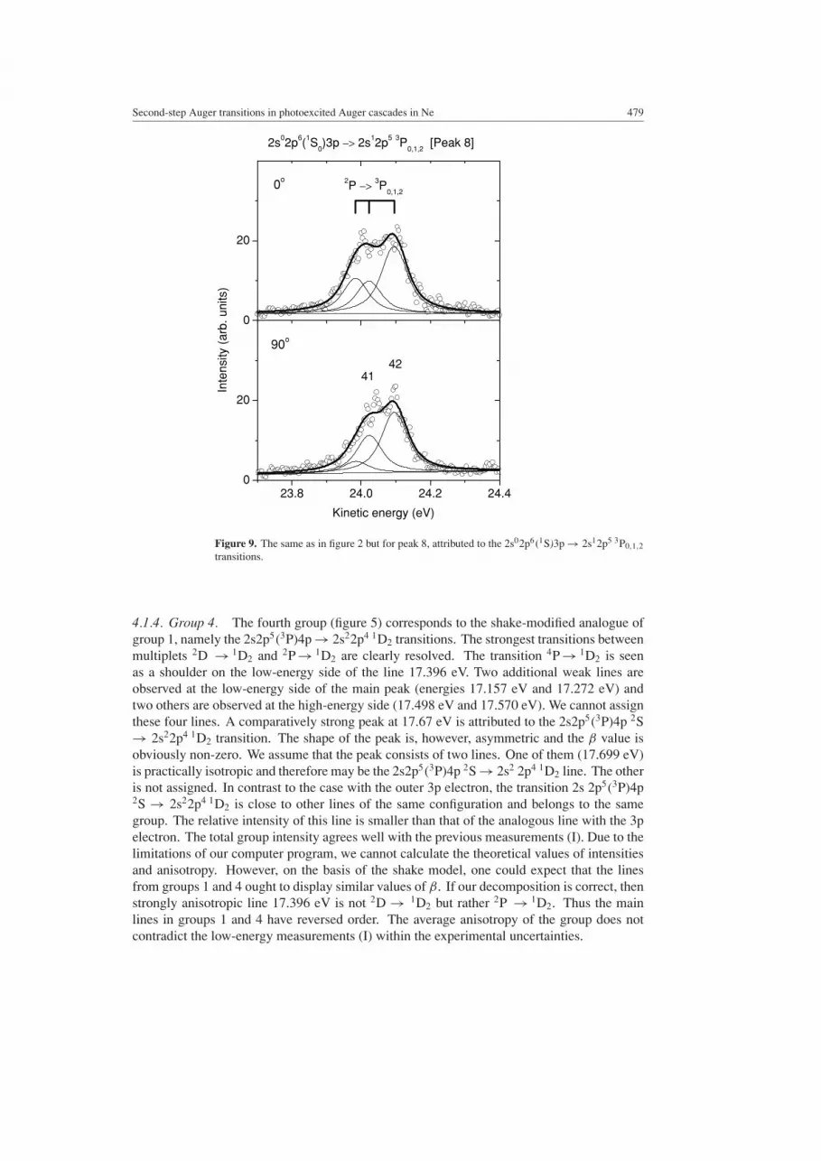
Figure 9. The same as in figure 2 but for peak 8, attributed to the 2s02p6(1S)3p → 2s12p5 3P0,1,2transitions.

4.1.4. Group 4. The fourth group (figure 5) corresponds to the shake-modified analogue ofgroup 1, namely the 2s2p5(3P)4p → 2s22p4 1D2 transitions. The strongest transitions betweenmultiplets 2D → 1D2 and 2P → 1D2 are clearly resolved. The transition 4P → 1D2 is seenas a shoulder on the low-energy side of the line 17.396 eV. Two additional weak lines areobserved at the low-energy side of the main peak (energies 17.157 eV and 17.272 eV) andtwo others are observed at the high-energy side (17.498 eV and 17.570 eV). We cannot assignthese four lines. A comparatively strong peak at 17.67 eV is attributed to the 2s2p5(3P)4p 2S→ 2s22p4 1D2 transition. The shape of the peak is, however, asymmetric and the β value isobviously non-zero. We assume that the peak consists of two lines. One of them (17.699 eV)is practically isotropic and therefore may be the 2s2p5(3P)4p 2S → 2s2 2p4 1D2 line. The otheris not assigned. In contrast to the case with the outer 3p electron, the transition 2s 2p5(3P)4p2S → 2s22p4 1D2 is close to other lines of the same configuration and belongs to the samegroup. The relative intensity of this line is smaller than that of the analogous line with the 3pelectron. The total group intensity agrees well with the previous measurements (I). Due to thelimitations of our computer program, we cannot calculate the theoretical values of intensitiesand anisotropy. However, on the basis of the shake model, one could expect that the linesfrom groups 1 and 4 ought to display similar values of β. If our decomposition is correct, thenstrongly anisotropic line 17.396 eV is not 2D → 1D2 but rather 2P → 1D2. Thus the mainlines in groups 1 and 4 have reversed order. The average anisotropy of the group does notcontradict the low-energy measurements (I) within the experimental uncertainties.

480 H Yoshida et al

25.5 26.00

50

10048

47

4544

Inte

nsity

(ar

b. u

nits

)

Kinetic energy (eV)

90o

0

50

1002P −> 3P

0,1,2

2D −> 3P0,1,2

2s12p5(1P1)3p −> 2s22p4 3P

0,1,2 [Peak 9]

0o

Figure 10. The same as in figure 2 but for peak 9, attributed to the 2s12p5(1P)3p → 2s22p4 3P0,1,2transitions.

4.1.5. Group 5. Similar to the previous group, group 5 (figure 6) is a shake-modifiedanalogue of group 2 with an outer 4p electron. It also consists of one strong line associatedwith the transition 2s02p6(1S)4p → 2s2p5 1P1 (line 27) and an unidentified weak satellite. Thestrongest line has large anisotropy which is even larger than the anisotropy of the main line(7) of group 2 and closer to the predictions of the calculations. The latter may be an indicationthat this line is less mixed than line 7. Both the anisotropy and the relative intensity measuredin this work agree well with the previous measurements (I).

4.1.6. Group 6. This is a complex of partly resolved lines (see figure 7), corresponding tothe 2s2p5(3P)4p → 2s22p4 3P0,1,2 transitions, i.e. a shake-modified analogue of group 3. Sincedecomposition of this complex into separate lines is not unambiguous, we can discuss only thetotal intensity and the average β value which perfectly agree with the previous measurements(I). A comparison with the analogous transitions with the 3p spectator (group 3) shows thatfor the transitions 4P → 3P and 2D → 3P the anisotropy in the two groups is very similar. Forthe 2P → 3P transitions, however, the anisotropy in group 6 is much larger. This is reflectedin the larger average anisotropy of the whole group 6 than of group 3.

4.1.7. Group 7. This is the strongest group in the considered part of the spectrum and isidentified as the 2s2p5(1P)3p → 2s22p4 1D2 transition which consists of two clearly resolvedlines: a very strong line 2D → 1D and a weak line 2P → 1D (see figure 8). Both lines arealmost isotropic. This confirms earlier finding with low-resolution measurements. Also in the


27.6 27.8 28.00

100

200

50

49

Inte

nsity

(ar

b. u

nits

)

Kinetic energy (eV)

90o

0

100

200

2P −> 1D1

2D −> 1D1

2s12p5(1P1)4p −> 2s222p4 1D [Peak 10]

0o

Figure 11. The same as in figure 2 but for peak 10, attributed to the 2s12p5(1P)4p → 2s22p4 1D2transitions.

calculation, the line 2D → 1D is the strongest. However, the relative strength of the 2P → 1Dline is overestimated. Also, the value of the calculated anisotropy parameter β = 0.33 is toolarge. The reason for such a discrepancy is unclear. It is necessary to make more elaboratecalculations including several non-relativistic configurations.

4.1.8. Group 8. A weak group 8 (figure 9) consists of three almost unresolved lines whichcorrespond to the 2s02p6(1S)3p 2P → 2s2p5 3P transitions. The total intensity and the averageβ are in reasonable agreement with previous measurements (I). The calculated intensities agreequite well with the experimental values. However, the anisotropy parameter for one of thelines 2P → 3P0 is significantly underestimated. This leads to the smaller calculated average β

value than the experimental value. We should note, however, that in this case, a separation ofthe two lowest lines (in energy) is ambiguous and therefore the uncertainties of the individualβ values are large.

4.1.9. Group 9. This group (figure 10), which is attributed to the 2s2p5(1P)3p → 2s22p4

3P transitions, consists of two well-separated groups of 2D → 3P0,1,2 and 2P → 3P0,1,2

transitions; each of which is also partly resolved. Both groups are strongly anisotropicbut the sign of the anisotropy is opposite. This characteristic is very well reproduced bythe calculations. The calculated values of β including the average β for the group are ingood agreement with the experimental values. The total intensity of the group, however, is

482 H Yoshida et al

29.0 29.2 29.40

10

2053

52

Inte

nsity

(ar

b. u

nits

)

Kinetic energy (eV)

90o

0

10

20

2P −> 3P0,1,2

2s02p6(1S)4p −> 2s12p5 3P0,1,2

[Peak 11]

0o

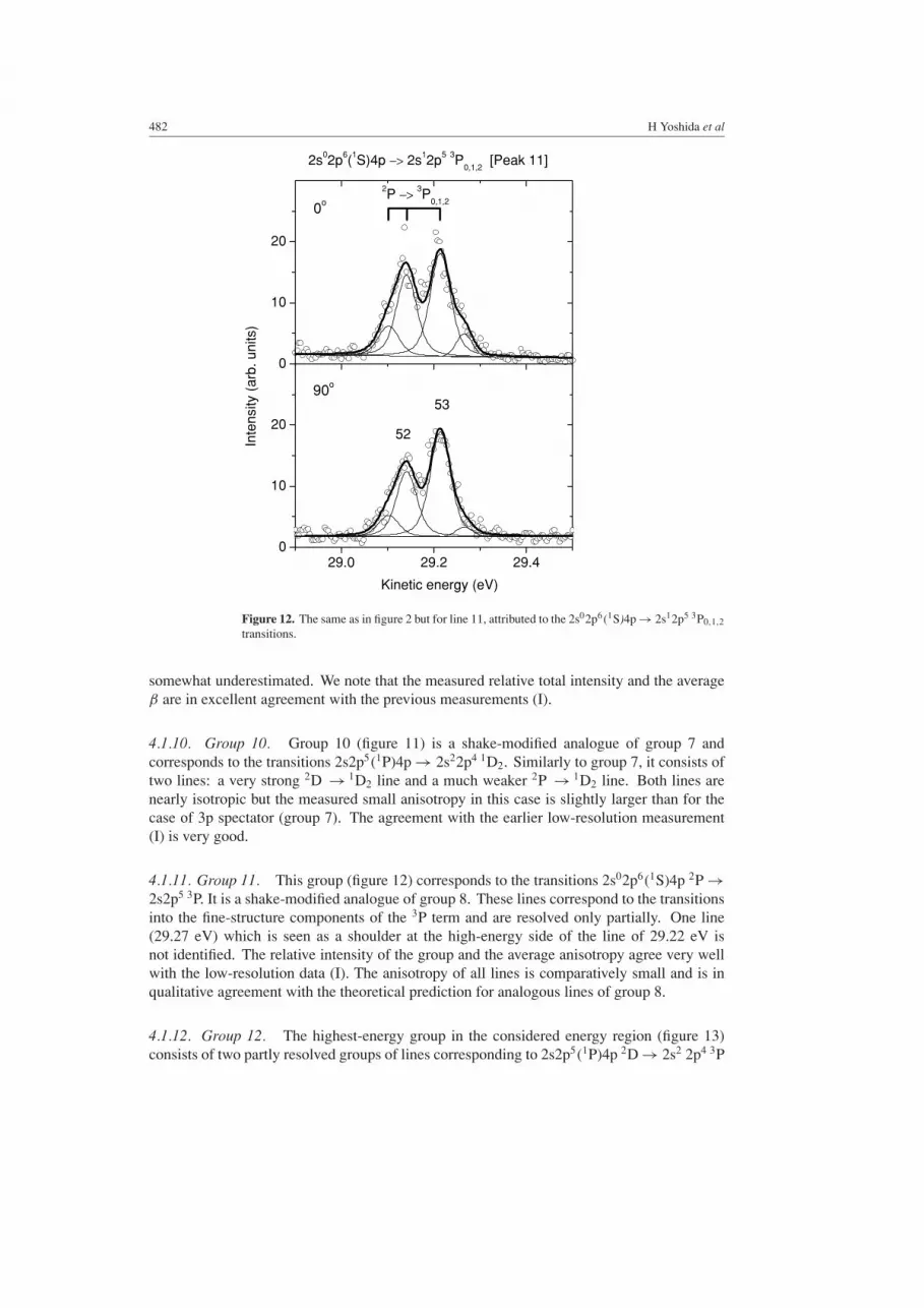
Figure 12. The same as in figure 2 but for line 11, attributed to the 2s02p6(1S)4p → 2s12p5 3P0,1,2transitions.

somewhat underestimated. We note that the measured relative total intensity and the averageβ are in excellent agreement with the previous measurements (I).

4.1.10. Group 10. Group 10 (figure 11) is a shake-modified analogue of group 7 andcorresponds to the transitions 2s2p5(1P)4p → 2s22p4 1D2. Similarly to group 7, it consists oftwo lines: a very strong 2D → 1D2 line and a much weaker 2P → 1D2 line. Both lines arenearly isotropic but the measured small anisotropy in this case is slightly larger than for thecase of 3p spectator (group 7). The agreement with the earlier low-resolution measurement(I) is very good.

4.1.11. Group 11. This group (figure 12) corresponds to the transitions 2s02p6(1S)4p 2P →2s2p5 3P. It is a shake-modified analogue of group 8. These lines correspond to the transitionsinto the fine-structure components of the 3P term and are resolved only partially. One line(29.27 eV) which is seen as a shoulder at the high-energy side of the line of 29.22 eV isnot identified. The relative intensity of the group and the average anisotropy agree very wellwith the low-resolution data (I). The anisotropy of all lines is comparatively small and is inqualitative agreement with the theoretical prediction for analogous lines of group 8.

4.1.12. Group 12. The highest-energy group in the considered energy region (figure 13)consists of two partly resolved groups of lines corresponding to 2s2p5(1P)4p 2D → 2s2 2p4 3P


30.8 31.0 31.20

50

1006058,59

56

Inte

nsity

(ar

b. u

nits

)

Kinetic energy (eV)

90o

0

50

1002P −> 3P

0,1,2

2D −> 3P0,1,2

2s12p5(1P1)4p −> 2s22p4 3P

0,1,2 [Peak 12]

0o

Figure 13. The same as in figure 2 but for the peak 12, attributed to the 2s12p5(1P)4p →2s22p4 3P0,1,2 transitions.

and 2s2p5(1P)4p 2P → 2s22p4 3P transitions. This is a shake-modified analogue of the group 9.Similarly to group 9, the transitions 2P → 3P and 2D → 3P have rather large anisotropy ofopposite sign, in agreement with the calculations for the 3p outer electron. Because of apartial cancellation, the average anisotropy of group is small. Both the relative intensity andthe angular anisotropy of group 12 are in excellent agreement with earlier measurements (I).

4.2. Widths of intermediate levels

As mentioned in the introduction, the overall energy resolution is comparable or even smallerthan the natural lifetime widths of the intermediate ionic levels in the cascade (initial levels forthe second-step Auger transitions). According to the calculations, the widths of these levelsare of tens of meV (Armen and Larkins 1991, Sinanis et al 1995). Some of the widths havebeen measured in photoionization-with-excitation experiments (Svensson et al 1988, Pahleret al 1993, Kikas et al 1996) and in resonant-Auger-decay measurements using Doppler-free Raman–Auger spectroscopy (Ueda et al 2003, De Fanis et al 2004). Here we present theresults of our analysis of the lifetime widths of the intermediate levels of 2s2p5np and 2s02p6npconfigurations, obtained from the measurements of the second-step Auger spectrum. Let usfirst discuss, however, one important difference between the calculated and the measuredwidths. Almost all considered intermediate ionic levels are doublets; one is presumably aquartet 4P . The calculations show that the fine-structure splitting of the levels is about 5 meVfor the 2s2p5(1P)3p and 2s02p6(1S)3p states and about 30–50 meV for the 2s2p5(3P)3p states.Thus the splitting in some cases is comparable with the lifetime width. In the experiment which

484 H Yoshida et al

Table 3. Lifetime widths � (meV) of some levels of Ne+ and the calculated fine-structure splitting,�E (meV). Experimental data are from this work, from Doppler-free Raman–Auger measurements(DF) by Ueda et al (2003) and De Fanis et al (2004) and from Pahler et al (1993). Theoreticalvalues are from this work, from Armen and Larkins (1991) (AL) and from Sinanis et al (1995)(SAN) calculations.

Experiment, � (meV) Theory, � (meV)

State �E This work DF Pahler This work AL SAN

2s 2p5(1P)3p 2S 530(50) 410(50) 521 687 5102P 2 37(02) 42(05) 31 20.72D 6 34(03) 34(05) 52 40.2

2s 2p5(3P)3p 2S 111(11) 120(10) 110(40) 17 18.8 1222P 27 24a 19(05) 55 10.32D3/2 49 18a 80(10) 78 62.32D5/2 18a 78 62.34P5/2 ∼0 81

2s02p6(1S)3p 2P 7 70(04) 80(05) 150

2s 2p5(1P)4p 2S 135(20) 2222P ∼0 6.52D 12(03) 13.9

2s 2p5(3P)4p 2S 34(13) 30(15) 6.02P <2 4.12D ∼0 18.04P <3

2s02p6(1S)4p 2P 20(05) 20(05)

a Uncertainties can be estimated for resolved lines and are indicated in parentheses, but could notbe estimated for unresolved lines.

cannot resolve the fine-structure components, one measures a convolution which includes boththe natural width and the splitting. Only if the splitting is much smaller than the width, do themeasurements give the lifetime width.

In table 3, we show the measured and calculated widths for some of the ionic levels togetherwith the calculated fine-structure splitting. The most reliable data are for the 2s2p5(1P)3pand 2s02p6(1S)3p states: for them the fine-structure splitting is much less than the width.The agreement between results of the present measurement and the measurements using theDoppler-free resonant Raman Auger technique (Ueda et al 2003, De Fanis et al 2004) isexcellent. For the 2s2p5(3P)3p states the fine-structure splitting is at least comparable with thewidth and should be taken into account. For the unsplit (3P)3p 2S state the measured widthagrees well with the Doppler-free measurements. Also, for the unresolved (3P)3p 2P state,both measurements give similar results but it is difficult to say how large is the lifetime widthsince the expected splitting is practically equal to the measured width. We believe that weresolve the (3P)3p 2D doublet in the present experiment. This may explain also the strongdifference between the widths obtained in this work and in Doppler-free measurements wherethe doublet was not resolved. The experimental splitting of the (3P)3p 2D doublet is 56 meVwhich is even larger than the theoretical estimate. Therefore, the large width of the unresolved(3P)3p 2D state observed earlier is mainly due to the fine-structure splitting.


The measured widths of the shake-modified states of 2s2p54p and 2s02p64p configurationsare smaller than the widths of the corresponding states with 3p outer electron. In many cases,they are smaller than the estimated experimental uncertainties.

5. Conclusion

We have reported the results of high-resolution measurements of the low-energy part (10–33 eV) of the Auger electron spectrum generated by photoexcitation of the 1s−13p resonancein Ne. This part of the spectrum is mainly dominated by the lines from the second-step Augertransitions of the 1s−13p → 2s2p5np → 2s22p4 and 1s−13p → 2s02p6np → 2s2p5(n = 3, 4)

cascades. High resolution allows us for the first time to resolve the multiplet structure andin some cases even the fine structure of the Auger lines. Relative intensities and angularanisotropy parameters are obtained from the analysis of the spectra.

In general, there is quite reasonable agreement between the measurements and thecomputations within the MCDF approach. Note, however, that a good agreement is foundmainly for the states with a singlet core (1P)3p. For the triplet-core states (3P)3p, in contrast,the calculated β values do not agree well with experiment in many cases. An analysis ofthe wavefunctions shows that the (3P)3p states are more strongly mixed than the (1P)3p ones.The β parameters for these transitions are apparently very sensitive to the quality of thewavefunctions and it seems important to perform computations in a considerably larger basis.

Acknowledgments

The experiment was carried out with the approval of the SPring-8 program reviewingcommittee. The authors are grateful to the staff of SPring-8 for their help. NMK is grateful toBielefeld University for hospitality and financial support, he also acknowledges the support andhospitality extended to him during his visit to IMRAM (Tohoku University). SF acknowledgesthe support by the Deutsche Forschungsgemeinschaft (DFG) in the framework of SPP 1145.

References

Armen G B, Aksela H, Aberg T and Aksela S 2000 J. Phys. B: At. Mol. Opt. Phys. 33 R49Armen G B and Larkins F P 1991 J. Phys. B: At. Mol. Opt. Phys. 24 741Becker U, Hemmers O, Langer B, Lee I, Menzel A, Wehlitz R and Amusia M Ya 1993 Phys. Rev. A 47 R767Becker U and Wehlitz R 1994 J. Electron Spectrosc. Relat. Phenom. 67 341Becker U, Wehlitz R, Hemmers O, Langer B and Menzel A 1989 Phys. Rev. Lett. 63 1054Coreno M, Avaldi L, Camilloni R, Prince K C, de Simone M, Karvonen J, Colle R and Simonucci S 1999 Phys. Rev.

A 59 2494De Fanis A, Saito N, Yoshida H, Senba Y, Tamenori Y, Ohashi H, Tanaka H and Ueda K 2002 Phys. Rev. Lett. 89

243001De Fanis A, Tamenori Y, Kitajima M, Tanaka H and Ueda K 2004 J. Electron Spectrosc. Relat. Phenom. 137–140

271Fritzsche S 1997 Comput. Phys. Commun. 103 51Fritzsche S 2001 J. Electron Spectrosc. Relat. Phenom. 114–116 1155Fritzsche S, Inghoff T, Bastug T and Tomaselli M 2001 Comput. Phys. Commun. 139 314Kabachnik N M 1997 X-ray and Inner-Shell Processes vol 389 ed R J Johnson, H Schmidt-Bocking and B F Sonntag

(New York: AIP) p 689Kabachnik N M, Sazhina I P and Ueda K 1999 J. Phys. B: At. Mol. Opt. Phys. 32 1769Kabachnik N M, Tulkki J, Aksela H and Ricz S 1994 Phys. Rev. A 49 4653Kikas A, Osborne S J, Ausmees A, Svensson S, Sairanen O-P and Aksela S 1996 J. Electron Spectrosc. Relat. Phenom.

77 241

486 H Yoshida et al

Kivimaki A, Heinasmaki S, Jurvansuu M, Alitalo S, Nommiste E, Aksela H and Aksela S 2001 J. Electron Spectrosc.Relat. Phenom. 114–6 49

Ohashi H, Ishiguro E, Tamenori Y, Kishimoto H, Tanaka M, Irie M, Tanaka T and Ishikawa T 2001a Nucl. Instrum.Methods A 467 529

Ohashi H et al 2001b Nucl. Instrum. Methods A 467 533Pahler M, Caldwell C D, Schaphorst S J and Krause M O 1993 J. Phys. B: At. Mol. Opt. Phys. 26 1617Parpia F A, Froese Fischer C and Grant I P 1996 Comput. Phys. Commun. 94 249Persson W 1971 Phys. Scr. 3 133Persson W, Wahlstrom C-G, Jonsson L and Di Rocco H O 1991 Phys. Rev. A 43 4791Saito N, Kabachnik N M, Shimizu Y, Yoshida H, Ohashi H, Tamenori Y, Suzuki I H and Ueda K 2000 J. Phys. B:

At. Mol. Opt. Phys. 33 L729Saito N and Suzuki I H 1992 Int. J. Mass Spectrom. Ion Process. 115 157Shimizu Y et al 2001 J. Electron Spectrosc. Relat. Phenom. 114–116 63Shimizu Y, Yoshida H, Okada K, Muramatsu Y, Saito N, Ohashi H, Tamenori Y, Fritzsche S, Kabachnik N M, Tanaka

H and Ueda K 2000 J. Phys. B: At. Mol. Opt. Phys. 33 L685Sinanis C, Aspromallis G and Nicolaides C 1995 J. Phys. B: At. Mol. Opt. Phys. 28 L423Svensson S, Eriksson B, Martenson N, Wendin G and Gelius U 1988 J. Electron Spectrosc. Relat. Phenom. 47 327Tamenori Y, Ohashi H, Ishiguro E and Ishikawa T 2002 Rev. Sci. Instrum. 73 1588Tanaka T and Kitamura H 1996 J. Synchrotron Radiat. 3 47Turri G, Battera G, Avaldi L, Camilloni R, Coreno M, Ruocco A, Colle R, Simonucci S and Stefani G 2001 J. Electron

Spectrosc. Relat. Phenom. 114–116 199Ueda K 2003 J. Phys. B: At. Mol. Opt. Phys. 36 R1Ueda K, Shimizu Y, Chiba H, Kitajima M, Tanaka H, Fritzsche S and Kabachnik N M 2001 J. Phys. B: At. Mol. Opt.

Phys. 34 107Ueda K et al 2003 Phys. Rev. Lett. 90 153005Viefhaus J 1997 Emissionsrichtungskorrelationen bei der Untersuchung von Mehrelektronenprozessen (Berlin: Verlag

Oberhofer)von Raven E 1992 Thesis Hamburg University (unpublished)Wills A A, Cafolla A A, Svensson A and Comer J 1990 J. Phys. B: At. Mol. Opt. Phys. 23 2013Wuilleumier F and Krause M O 1974 Phys. Rev. A 10 242Yoshida H et al 2000 J. Phys. B: At. Mol. Opt. Phys. 33 4343Yoshida H, Senba Y, Morita M, Goya T, De Fanis A, Saito N, Ueda K, Tamenori Y and Ohashi H 2004 AIP Conf.

Proc. 705 267

Documents

Study of second-step Auger transitions in Auger cascades following 1s → 3p photoexcitation in Ne