Stochastic Delay Accelerates Signaling in Gene NetworksKresimir Josic1,2., Jose Manuel Lopez1., William Ott1., LieJune Shiau3, Matthew R. Bennett4,5*

1 Department of Mathematics, University of Houston, Houston, Texas, United States of America, 2 Department of Biology and Biochemistry, University of Houston,

Houston, Texas, United States of America, 3 Department of Mathematics, University of Houston, Clear Lake, Texas, United States of America, 4 Department of Biochemistry

& Cell Biology, Rice University, Houston, Texas, United States of America, 5 Institute of Biosciences & Bioengineering, Rice University, Houston, Texas, United States of

America

Abstract

The creation of protein from DNA is a dynamic process consisting of numerous reactions, such as transcription, translationand protein folding. Each of these reactions is further comprised of hundreds or thousands of sub-steps that must becompleted before a protein is fully mature. Consequently, the time it takes to create a single protein depends on thenumber of steps in the reaction chain and the nature of each step. One way to account for these reactions in models ofgene regulatory networks is to incorporate dynamical delay. However, the stochastic nature of the reactions necessary toproduce protein leads to a waiting time that is randomly distributed. Here, we use queueing theory to examine the effectsof such distributed delay on the propagation of information through transcriptionally regulated genetic networks. In ananalytically tractable model we find that increasing the randomness in protein production delay can increase signalingspeed in transcriptional networks. The effect is confirmed in stochastic simulations, and we demonstrate its impact inseveral common transcriptional motifs. In particular, we show that in feedforward loops signaling time and magnitude aresignificantly affected by distributed delay. In addition, delay has previously been shown to cause stable oscillations incircuits with negative feedback. We show that the period and the amplitude of the oscillations monotonically decrease asthe variability of the delay time increases.

Citation: Josic K, Lopez JM, Ott W, Shiau L, Bennett MR (2011) Stochastic Delay Accelerates Signaling in Gene Networks. PLoS Comput Biol 7(11): e1002264.doi:10.1371/journal.pcbi.1002264

Editor: Jason M. Haugh, North Carolina State University, United States of America

Received June 7, 2011; Accepted September 19, 2011; Published November 10, 2011

Copyright: � 2011 Josic et al. This is an open-access article distributed under the terms of the Creative Commons Attribution License, which permitsunrestricted use, distribution, and reproduction in any medium, provided the original author and source are credited.

Funding: This work was supported by the Welch Foundation, grant number C-1729 (MRB), a State of Texas ARP/ATP Award (KJ), the John S. Dunn ResearchFoundation Collaborative Research Award Program administered by the Gulf Coast Consortia (KJ and MRB), and the National Science Foundation, grant number0908528 (LS). The funders had no role in study design, data collection and analysis, decision to publish, or preparation of the manuscript.

Competing Interests: The authors have declared that no competing interests exist.

* E-mail: matthew.bennett@rice.edu

. These authors contributed equally to this work.

Introduction

Gene regulation forms a basis for cellular decision-making

processes and transcriptional signaling is one way in which cells

can modulate gene expression patterns [1]. The intricate networks

of transcription factors and their targets are of intense interest to

theorists because it is hoped that topological similarities between

networks will reveal functional parallels [2]. Models of gene

regulatory networks have taken many forms, ranging from

simplified Boolean networks [3,4], to full-scale, stochastic descrip-

tions simulated using Gillespie’s algorithm [5].

The majority of models, however, are systems of nonlinear

ordinary differential equations (ODEs). Yet, because of the com-

plexity of protein production, ODE models of transcriptional

networks are at best heuristic reductions of the true system, and

often fail to capture many aspects of network dynamics. Many

ignored reactions, like oligomerization of transcription factors or

enzyme-substrate binding, occur at much faster timescales than

reactions such as transcription and degradation of proteins.

Reduced models are frequently obtained by eliminating these fast

reactions [6–9]. Unfortunately, even when such reductions are

done correctly, problems might still exist. For instance, if within

the reaction network there exists a linear (or approximately linear)

sequence of reactions, the resulting dynamics can appear to be

delayed. This type of behavior has long been known to exist in

gene regulatory networks [10].

Delay differential equations (DDEs) have been used as an

alternative to ODE models to address this problem. In protein

production, one can think of delay as resulting from the sequential

assembly of first mRNA and then protein [10–12]. Delay can

qualitatively alter the local stability of genetic regulatory network

models [13] as well as their dynamics, especially in those

containing feedback. For instance, delay can lead to oscillations

in models of transcriptional negative feedback [11,14–18], and

experimental evidence suggests that robust oscillations in simple

synthetic networks are due to transcriptional delay [19,20].

Protein production delay times are difficult to measure in live cells,

though recent work has shown that the time it takes for transcription

to occur in yeast can be on the order of minutes and is highly variable

[21]. Still, transcriptional delay is thought to be important in a host of

naturally occurring gene networks. For instance, mathematical

models suggest that circadian oscillations are governed by delayed

negative feedback systems [22,23], and this was experimentally

shown to be true in mammalian cells [24]. Delay appears to play a

role in cell cycle control [25,26], apoptosis induction by the p53

network [27], and the response of the NFkB network [15]. Delay

can also affect the stochastic nature of gene expression, and the

relation between the two can be subtle and complex [28–31].

PLoS Computational Biology | www.ploscompbiol.org 1 November 2011 | Volume 7 | Issue 11 | e1002264

In this study, we examine the consequences of randomly

distributed delay on simple gene regulatory networks: We assume

that the delay time for protein production, T , is not constant but

instead a random variable. If fT denotes the probability density

function (PDF) of T , this situation can be described determinis-

tically by an integro-delay differential equation [32] of the form

_xx(t)~

ðg x(t),x(t{s)½ �fT (s)ds, ð1Þ

where x is a positive definite state vector of protein concentrations,

and g is a vector function representing the production and

degradation rates of the proteins. Note that processes that do not

require protein synthesis (like dilution and degradation) will

depend on the instantaneous, rather than the delayed, state of the

system. Therefore g is in general a function of both the present and

past state of the system.

Equation (1) only holds in the limit of large protein numbers

[32]. As protein numbers approach zero, the stochasticity

associated with chemical interactions becomes non-negligible.

Here, we address this issue by expanding on Eq. (1) using an exact

stochastic algorithm that takes into account variability within the

delay time [32]. We further use a queueing theory approach to

examine how this variability affects timing in signaling cascades.

We find that when the mean of the delay time is fixed, increased

delay variability accelerates downstream signaling. Noise can thus

increase signaling speed in gene networks. In addition, we find that

in simple transcriptional networks containing feed-forward or

feedback loops the variability in the delay time nontrivially affects

network dynamics.

Queueing theory has recently been used to understand the

behavior of genetic networks [33–35]. Here we are mainly

interested in dynamical phenomena to which the theory of queues

in equilibrium used in previous studies cannot be applied. As we

explain below, gene networks can be modeled as thresholded

queueing systems: Proteins exiting one queue do not enter another

queue, as would be the case in typical queueing networks. Rather,

they modulate the rate at which transcription is initiated, and thus

affect the rate at which proteins enter other queues.

Results

Distributed delay in protein productionThe transcription of genetic material into mRNA and its

subsequent translation into protein involves potentially hundreds

or thousands of biochemical reactions. Hence, detailed models of

these processes are prohibitively complex. When simulating

genetic circuits it is frequently assumed that gene expression

instantaneously results in fully formed proteins. However, each

step in the chain of reactions leading from transcription initiation

to a folded protein takes time (Figure 1). Models that do not

incorporate the resulting delay may not accurately capture the

dynamical behavior of genetic circuits [17]. While earlier models

have included either fixed or distributed delay [32,36,37], here we

examine specifically the effects of delay variability on transcriptional

signaling.

In one recent study, Bel et al. studied completion time

distributions associated with Markov chains modeling linear

chemical reaction pathways [38]. Using rigorous analysis and

numerical simulations they show that, if the number of reactions is

large, completion time distributions for an idealized class of models

exhibit a sharp transition in the coefficient of variation (CV,

defined as the standard deviation divided by the mean of the

distribution), going from near 0 (indicating a nearly deterministic

completion time) to near 1 (indicating an exponentially distributed

completion time) as system bias moves from forward to reverse.

However, it is possible, and perhaps likely, that the limiting

distributions described by Bel et al. do not provide good

approximations for protein production. For instance, when the

number of rate limiting reactions is small, but greater than one, the

distribution of delay times can be more complex. Moreover, linear

reaction pathways only represent one possible and necessarily

simplified reaction scheme. Protein production involves many

reaction types that are nonlinear and/or reversible, each of which

is influenced by intrinsic and extrinsic noise [39], and these

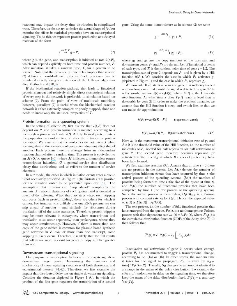
Figure 1. The origin of delay in transcriptional regulation. (A)Numerous reactions must occur between the time that transcriptionstarts and when the resulting protein molecule is fully formed andmature. Though we call this phenomenon ‘‘transcriptional’’ delay, thereare many reactions after transcription (such as translation) whichcontribute to the overall delay. (B) The creation of multiple proteins canbe thought of as a queueing process. Nascent proteins enter the queue(an input event) and emerge fully matured (an output event) some timelater depending on the distribution of delay times. Because the delay israndom, it is possible that the order of proteins entering the queue isnot preserved upon exit. (C) In a transcriptionally regulated signalingprocess the time it takes for changes in the expression of gene 1 topropagate to gene 2 depends on both the distribution of delay times,fT , and the number of transcription factors needed to overcome thethreshold of gene 2, R.doi:10.1371/journal.pcbi.1002264.g001

Author Summary

Delay in gene regulatory networks often arises from thenumerous sequential reactions necessary to create fullyfunctional protein from DNA. While the molecular mech-anisms behind protein production and maturation areknown, it is still unknown to what extent the resultingdelay affects signaling in transcriptional networks. Incontrast to previous studies that have examined theconsequences of fixed delay in gene networks, here weinvestigate how the variability of the delay time influencesthe resulting dynamics. The exact distribution of ‘‘tran-scriptional delay’’ is still unknown, and most likely greatlydepends on both intrinsic and extrinsic factors. Neverthe-less, we are able to deduce specific effects of distributeddelay on transcriptional signaling that are independent ofthe underlying distribution. We find that the time it takesfor a gene encoding a transcription factor to signal itsdownstream target decreases as the delay variabilityincreases. We use queueing theory to derive a simplerelationship describing this result, and use stochasticsimulations to confirm it. The consequences of distributeddelay for several common transcriptional motifs are alsodiscussed.

Stochastic Delay in Gene Networks

PLoS Computational Biology | www.ploscompbiol.org 2 November 2011 | Volume 7 | Issue 11 | e1002264

reactions may impact the delay time distribution in complicated

ways. Therefore, we do not try to derive the actual shape of fT , but

examine the effects its statistical properties have on transcriptional

signaling. To do this, we represent protein production as a delayed

reaction of the form

g ?l(t,P),T

gzP, ð2Þ

where g is the gene, and transcription is initiated at rate l(t,P),which can depend explicitly on both time and protein number, P.

After initiation, it takes a random time, T , for a protein to be

formed. Note that the presence of time delay implies that scheme

(2) defines a non-Markovian process. Such processes can be

simulated exactly using an extension of the Gillespie algorithm

(See Methods and [28,32]).

If the biochemical reaction pathway that leads to functional

protein is known and relatively simple, direct stochastic simulation

of every step in the network is preferable to simulation based on

scheme (2). From the point of view of multi-scale modeling,

however, paradigm (2) is useful when the biochemical reaction

network is either extremely complex or poorly mapped, since one

needs to know only the statistical properties of T .

Protein formation as a queueing systemIn the setting of scheme (2), first assume that l(t,P) does not

depend on P, and protein formation is initiated according to a

memoryless process with rate l(t). A fully formed protein enters

the population a random time T after the initiation of protein

formation. We assume that the molecules do not interact while

forming; that is, the formation of one protein does not affect that of

another. Each protein therefore emerges from an independent

reaction channel after a random time. This process is equivalent to

an M=G=? queue [40], where M indicates a memoryless source

(transcription initiation), G a general service time distribution

(delay time distribution), and ? refers to the number of service

channels.

In our model, the order in which initiation events enter a queue

is not necessarily preserved. As Figure 1 (B) illustrates, it is possible

for the initiation order to be permuted upon exit [32]. The

assumption that proteins can ‘‘skip ahead’’ complicates the

analysis of transient dynamics of such queues, and is essential in

much of the following. While there are steps where such skipping

can occur (such as protein folding), there are others for which it

cannot. For instance, it is unlikely that one RNA polymerase can

skip ahead of another – and similarly for ribosomes during

translation off of the same transcript. Therefore, protein skipping

may be more relevant in eukaryotes, where transcription and

translation must occur separately, than prokaryotes, where they

may occur simultaneously. However, if there is more than one

copy of the gene (which is common for plasmid-based synthetic

gene networks in E. coli), or more than one transcript, some

skipping is likely occur. Therefore it is likely that the full results

that follow are more relevant for genes of copy number greater

than one.

Downstream transcriptional signalingOne purpose of transcription factors is to propagate signals to

downstream target genes. Determining the dynamics and

stochasticity of these signaling cascades is of both theoretical and

experimental interest [41,42]. Therefore, we first examine the

impact that distributed delay has on simple downstream signaling.

Consider the situation depicted in Figure 1 (C), in which the

product of the first gene regulates the transcription of a second

gene. Using the same nomenclature as in scheme (2) we write

g1

l(t),T1g1zP1 ð3aÞ

g2

h(P1),T2g2zP2, ð3bÞ

where g1 and g2 are the copy numbers of the upstream and

downstream genes, P1 and P2 are the number of functional proteins

of each type, and Ti is the random delay time of gene i~1,2. The

transcription rate of gene 2 depends on P1 and is given by a Hill

function h(P1). We consider the case in which P1 activates g2

(depicted in Figure 1) and the case in which P1 represses g2.

We now ask: If P1 starts at zero and gene 1 is suddenly turned

on, how long does it take until the signal is detected by gene 2? In

other words, assume l(t)~l0H(t), where H(t) is the Heaviside

step function. At what time t does P1(t) reach a level that is

detectable by gene 2? In order to make the problem tractable, we

assume that the Hill function is steep and switch-like, so that we

can make the approximation

h(P1)~h0H(R{P1) (repressor case); ð4aÞ

h(P1)~h0H(P1{R)(activator case): ð4bÞ

Here h0 is the maximum transcriptional initiation rate of g2 and

Rw0 is the threshold value of the Hill function, i.e. the number of

molecules of P1 needed for half repression (or half activation) of

gene 2. The second gene therefore becomes repressed (or

activated) at the time SR at which R copies of protein P1 have

been fully formed.

We first examine reaction (3a). Assume that at time t~0 there

are no proteins in the system. Let I1(t) denote the number of

transcription initiation events that have occurred by time t (the

arrival process of the queueing system), Q1(t) the number of

proteins being formed at time t (the size of the queue at time t),and P1(t) the number of functional proteins that have been

completed by time t (the exit process of the queueing system).

Since the arrival process is memoryless, (I1(t))t§0 is a Poisson

process with constant rate l0 for t§0. Hence, the expected value

of I1(t) is E I1(t)½ �~l0tH(t).

The exit process, i.e. the number of fully functional proteins that

have emerged from the queue, P1(t), is a nonhomogenous Poisson

process with time-dependent rate lP1(t)~l0FT1

(t), where FT1(t) is

the cumulative distribution function (CDF) of the delay time T1. It

then follows that

P1(t):E P1(t)½ �~l0

ðt

0

FT1(s)ds:

Inactivation (or activation) of gene 2 occurs when enough

protein P1 has accumulated to trigger a transcriptional change,

according to Eq. (4a) or (4b). In other words, the random time

it takes for the signal to propagate, SR, is given by SR~

minftjP1(t)~Rg. Trivially, SR changes by an amount identical to

a change in the mean of the delay distribution. To examine the

effects of randomness in delay on the signaling time, we therefore

keep the mean of the delay distribution fixed, E½T1�~t, and vary

Var½T1�.

Stochastic Delay in Gene Networks

PLoS Computational Biology | www.ploscompbiol.org 3 November 2011 | Volume 7 | Issue 11 | e1002264

The probability density function of SR is given by (See Methods)

fSR(t)~

P1(t)R{1

(R{1)!e{P1(t) dP1

dt: ð5Þ

Consequently, the mean and variance of the time it takes for the

original signal to propagate to the downstream gene can be written

as:

E½SR�~ð?

0

sR{1e{s

(R{1)!P

{1

1 (s)ds, ð6Þ

Var½SR�~ð?

0

sR{1e{s

(R{1)!P

{1

1 (s)� �2

ds{E½SR�2: ð7Þ

To gain insight into the behaviors of Eqs. (6) and (7), we first

examine a representative, analytically tractable example. Assume

that the delay time can take on 2 discrete values, tza and t{awith equal probability. In this case,

E½SR�~t{az2R

l0z

al0C½R,al0�{C½Rz1,al0�l0(R{1)!

, ð8Þ

where C(x,y) is the upper incomplete gamma function. Expanding

for small a, we obtain (See Methods)

E½SR�&tzR

l0, ð9Þ

which is the deterministic limit. The first term is the mean delay

time and the second is the average time to initiate R proteins at

rate l0. A similar expansion for fixed R and large a gives (see panel

(c) in Figure 2)

E½SR�&tzR

l0{ a{

R

l0

� �: ð10Þ

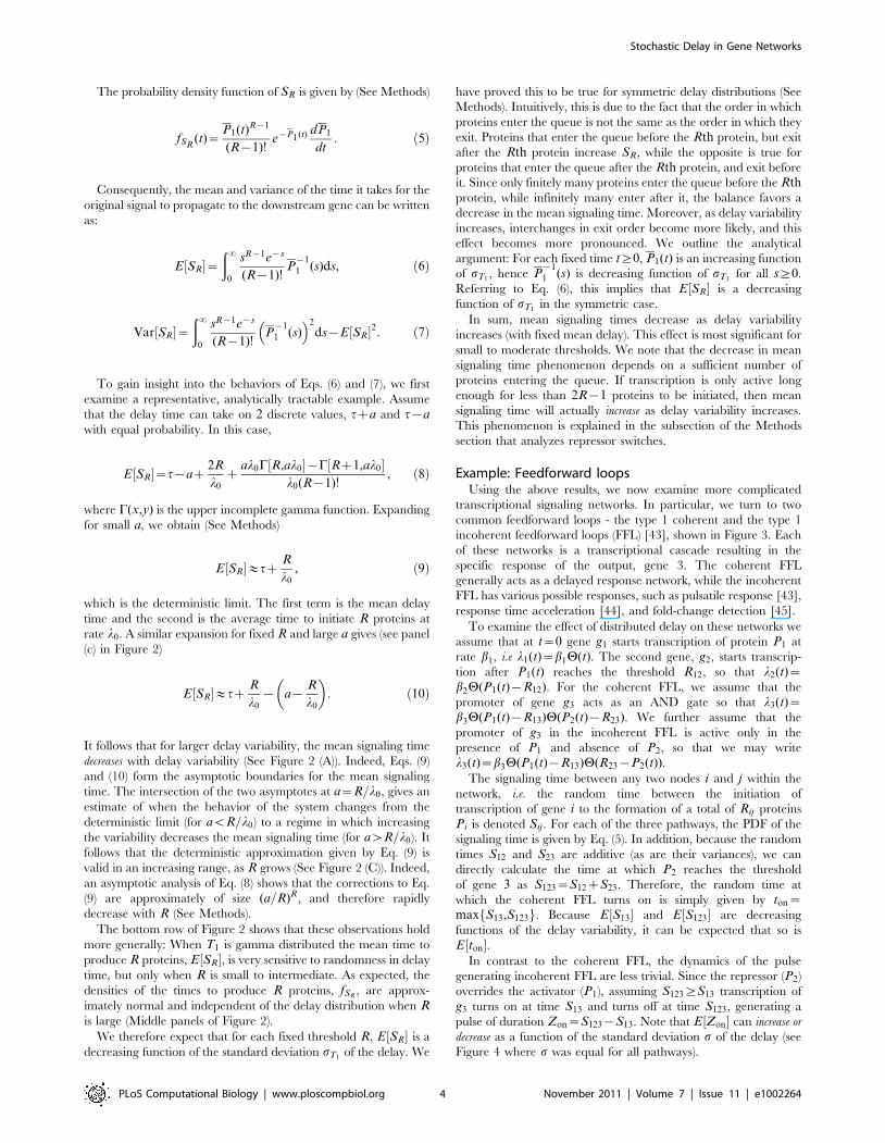
It follows that for larger delay variability, the mean signaling time

decreases with delay variability (See Figure 2 (A)). Indeed, Eqs. (9)

and (10) form the asymptotic boundaries for the mean signaling

time. The intersection of the two asymptotes at a~R=l0, gives an

estimate of when the behavior of the system changes from the

deterministic limit (for avR=l0) to a regime in which increasing

the variability decreases the mean signaling time (for awR=l0). It

follows that the deterministic approximation given by Eq. (9) is

valid in an increasing range, as R grows (See Figure 2 (C)). Indeed,

an asymptotic analysis of Eq. (8) shows that the corrections to Eq.

(9) are approximately of size (a=R)R, and therefore rapidly

decrease with R (See Methods).

The bottom row of Figure 2 shows that these observations hold

more generally: When T1 is gamma distributed the mean time to

produce R proteins, E½SR�, is very sensitive to randomness in delay

time, but only when R is small to intermediate. As expected, the

densities of the times to produce R proteins, fSR, are approx-

imately normal and independent of the delay distribution when Ris large (Middle panels of Figure 2).

We therefore expect that for each fixed threshold R, E½SR� is a

decreasing function of the standard deviation sT1of the delay. We

have proved this to be true for symmetric delay distributions (See

Methods). Intuitively, this is due to the fact that the order in which

proteins enter the queue is not the same as the order in which they

exit. Proteins that enter the queue before the Rth protein, but exit

after the Rth protein increase SR, while the opposite is true for

proteins that enter the queue after the Rth protein, and exit before

it. Since only finitely many proteins enter the queue before the Rthprotein, while infinitely many enter after it, the balance favors a

decrease in the mean signaling time. Moreover, as delay variability

increases, interchanges in exit order become more likely, and this

effect becomes more pronounced. We outline the analytical

argument: For each fixed time t§0, P1(t) is an increasing function

of sT1, hence P

{1

1 (s) is decreasing function of sT1for all s§0.

Referring to Eq. (6), this implies that E½SR� is a decreasing

function of sT1in the symmetric case.

In sum, mean signaling times decrease as delay variability

increases (with fixed mean delay). This effect is most significant for

small to moderate thresholds. We note that the decrease in mean

signaling time phenomenon depends on a sufficient number of

proteins entering the queue. If transcription is only active long

enough for less than 2R{1 proteins to be initiated, then mean

signaling time will actually increase as delay variability increases.

This phenomenon is explained in the subsection of the Methods

section that analyzes repressor switches.

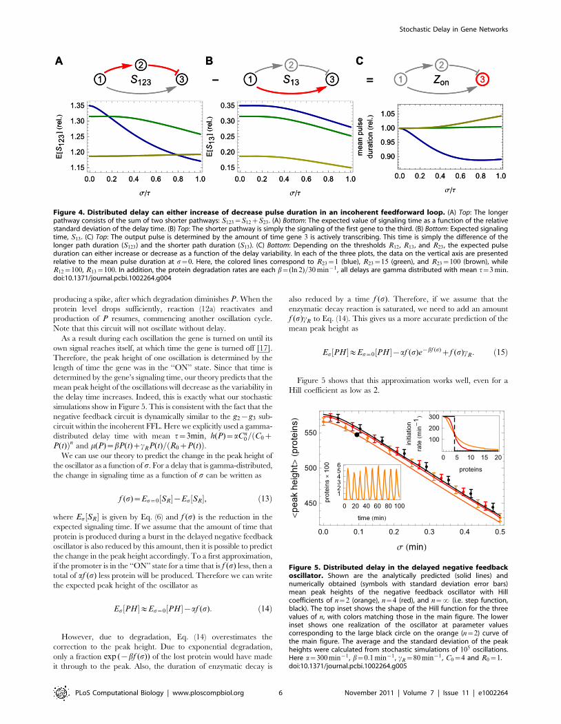
Example: Feedforward loopsUsing the above results, we now examine more complicated

transcriptional signaling networks. In particular, we turn to two

common feedforward loops - the type 1 coherent and the type 1

incoherent feedforward loops (FFL) [43], shown in Figure 3. Each

of these networks is a transcriptional cascade resulting in the

specific response of the output, gene 3. The coherent FFL

generally acts as a delayed response network, while the incoherent

FFL has various possible responses, such as pulsatile response [43],

response time acceleration [44], and fold-change detection [45].

To examine the effect of distributed delay on these networks we

assume that at t~0 gene g1 starts transcription of protein P1 at

rate b1, i.e l1(t)~b1H(t). The second gene, g2, starts transcrip-

tion after P1(t) reaches the threshold R12, so that l2(t)~b2H(P1(t){R12). For the coherent FFL, we assume that the

promoter of gene g3 acts as an AND gate so that l3(t)~b3H(P1(t){R13)H(P2(t){R23). We further assume that the

promoter of g3 in the incoherent FFL is active only in the

presence of P1 and absence of P2, so that we may write

l3(t)~b3H(P1(t){R13)H(R23{P2(t)).

The signaling time between any two nodes i and j within the

network, i.e. the random time between the initiation of

transcription of gene i to the formation of a total of Rij proteins

Pi is denoted Sij . For each of the three pathways, the PDF of the

signaling time is given by Eq. (5). In addition, because the random

times S12 and S23 are additive (as are their variances), we can

directly calculate the time at which P2 reaches the threshold

of gene 3 as S123~S12zS23. Therefore, the random time at

which the coherent FFL turns on is simply given by ton~max S13,S123f g. Because E½S13� and E½S123� are decreasing

functions of the delay variability, it can be expected that so is

E½ton�.In contrast to the coherent FFL, the dynamics of the pulse

generating incoherent FFL are less trivial. Since the repressor (P2)

overrides the activator (P1), assuming S123§S13 transcription of

g3 turns on at time S13 and turns off at time S123, generating a

pulse of duration Zon~S123{S13. Note that E½Zon� can increase or

decrease as a function of the standard deviation s of the delay (see

Figure 4 where s was equal for all pathways).

Stochastic Delay in Gene Networks

PLoS Computational Biology | www.ploscompbiol.org 4 November 2011 | Volume 7 | Issue 11 | e1002264

To see this, write E½Zon� as follows:

E½Zon�~E½S12�zE½S23�{E½S13�: ð11Þ

Each of the terms on the right side of Eq. (11) is the expected

signaling time of a single gene (g1?g2, g2?g3, and g1?g3,

respectively). Consequently, E½Zon� depends on s as a linear

combination of 3 expected signaling time curves of the type

pictured in Figure 2. The shapes of these signaling time curves

determine the behavior of E½Zon� as a function of s. Figure 4

shows that the behavior of the duration of the transcriptional pulse

as a function of the delay variability depends on the values of each

threshold within the network.

The delayed negative feedback oscillatorThese observations can also be extended to networks with

recurrent architectures. For instance, consider the transcriptional

delayed negative feedback circuit [17], which can be described

using an extension of scheme (2):

g ?h(P),T

gzP ð12aÞ

P ?m(P)

1, ð12bÞ

where h(P) is a decreasing Hill function (i.e. P represses its own

production) and m(P) is the degradation rate due to dilution and

proteolysis. Mather et al. examined the oscillations produced by

systems of the type described by scheme (12) when the delay T is

nonrandom (degrade and fire oscillators) [17]. Starting with no

proteins, P is produced at a rate governed by the Hill function h.

When the level of P exceeds the midpoint of the Hill function, gene

g effectively shuts down. The proteins remaining in the queue exit,

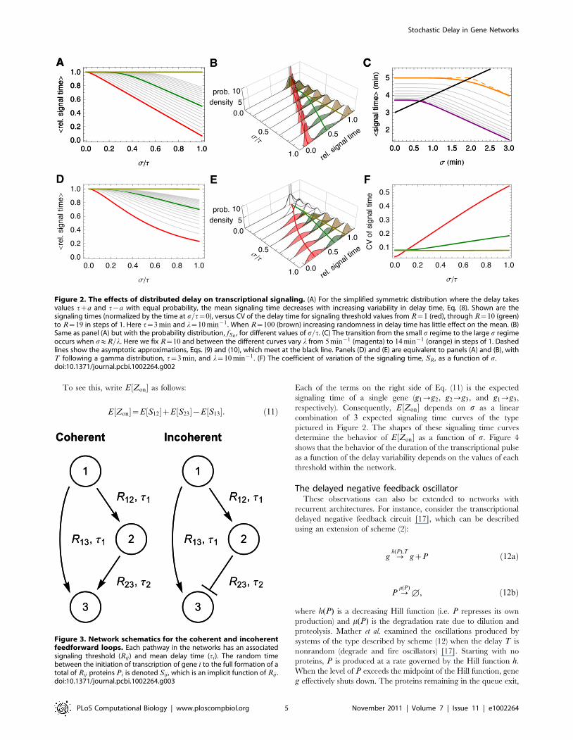
Figure 2. The effects of distributed delay on transcriptional signaling. (A) For the simplified symmetric distribution where the delay takesvalues tza and t{a with equal probability, the mean signaling time decreases with increasing variability in delay time, Eq. (8). Shown are thesignaling times (normalized by the time at s=t~0), versus CV of the delay time for signaling threshold values from R~1 (red), through R~10 (green)to R~19 in steps of 1. Here t~3 min and l~10 min{1 . When R~100 (brown) increasing randomness in delay time has little effect on the mean. (B)Same as panel (A) but with the probability distribution, fSR

, for different values of s=t. (C) The transition from the small s regime to the large s regimeoccurs when s&R=l. Here we fix R~10 and between the different curves vary l from 5 min{1 (magenta) to 14 min{1 (orange) in steps of 1. Dashedlines show the asymptotic approximations, Eqs. (9) and (10), which meet at the black line. Panels (D) and (E) are equivalent to panels (A) and (B), withT following a gamma distribution, t~3 min, and l~10 min{1 . (F) The coefficient of variation of the signaling time, SR , as a function of s.doi:10.1371/journal.pcbi.1002264.g002

Figure 3. Network schematics for the coherent and incoherentfeedforward loops. Each pathway in the networks has an associatedsignaling threshold (Rij ) and mean delay time (ti). The random timebetween the initiation of transcription of gene i to the full formation of atotal of Rij proteins Pi is denoted Sij , which is an implicit function of Rij .doi:10.1371/journal.pcbi.1002264.g003

Stochastic Delay in Gene Networks

PLoS Computational Biology | www.ploscompbiol.org 5 November 2011 | Volume 7 | Issue 11 | e1002264

producing a spike, after which degradation diminishes P. When the

protein level drops sufficiently, reaction (12a) reactivates and

production of P resumes, commencing another oscillation cycle.

Note that this circuit will not oscillate without delay.

As a result during each oscillation the gene is turned on until its

own signal reaches itself, at which time the gene is turned off [17].

Therefore, the peak height of one oscillation is determined by the

length of time the gene was in the ‘‘ON’’ state. Since that time is

determined by the gene’s signaling time, our theory predicts that the

mean peak height of the oscillations will decrease as the variability in

the delay time increases. Indeed, this is exactly what our stochastic

simulations show in Figure 5. This is consistent with the fact that the

negative feedback circuit is dynamically similar to the g2{g3 sub-

circuit within the incoherent FFL. Here we explicitly used a gamma-

distributed delay time with mean t~3min, h(P)~aCn0= C0zð

P(t)Þn and m(P)~bP(t)zcRP(t)= R0zP(t)ð Þ.We can use our theory to predict the change in the peak height of

the oscillator as a function of s. For a delay that is gamma-distributed,

the change in signaling time as a function of s can be written as

f (s)~Es~0½SR�{Es½SR�, ð13Þ

where Es½SR� is given by Eq. (6) and f (s) is the reduction in the

expected signaling time. If we assume that the amount of time that

protein is produced during a burst in the delayed negative feedback

oscillator is also reduced by this amount, then it is possible to predict

the change in the peak height accordingly. To a first approximation,

if the promoter is in the ‘‘ON’’ state for a time that is f (s) less, then a

total of af (s) less protein will be produced. Therefore we can write

the expected peak height of the oscillator as

Es½PH�&Es~0½PH�{af (s): ð14Þ

However, due to degradation, Eq. (14) overestimates the

correction to the peak height. Due to exponential degradation,

only a fraction exp ({bf (s)) of the lost protein would have made

it through to the peak. Also, the duration of enzymatic decay is

also reduced by a time f (s). Therefore, if we assume that the

enzymatic decay reaction is saturated, we need to add an amount

f (s)cR to Eq. (14). This gives us a more accurate prediction of the

mean peak height as

Es½PH�&Es~0½PH�{af (s)e{bf (s)zf (s)cR: ð15Þ

Figure 5 shows that this approximation works well, even for a

Hill coefficient as low as 2.

Figure 4. Distributed delay can either increase of decrease pulse duration in an incoherent feedforward loop. (A) Top: The longerpathway consists of the sum of two shorter pathways: S123~S12zS23. (A) Bottom: The expected value of signaling time as a function of the relativestandard deviation of the delay time. (B) Top: The shorter pathway is simply the signaling of the first gene to the third. (B) Bottom: Expected signalingtime, S13. (C) Top: The output pulse is determined by the amount of time gene 3 is actively transcribing. This time is simply the difference of thelonger path duration (S123) and the shorter path duration (S13). (C) Bottom: Depending on the thresholds R12, R13, and R23, the expected pulseduration can either increase or decrease as a function of the delay variability. In each of the three plots, the data on the vertical axis are presentedrelative to the mean pulse duration at s~0. Here, the colored lines correspond to R23~1 (blue), R23~15 (green), and R23~100 (brown), whileR12~100, R13~100. In addition, the protein degradation rates are each b~(ln 2)=30 min{1 , all delays are gamma distributed with mean t~3 min.doi:10.1371/journal.pcbi.1002264.g004

Figure 5. Distributed delay in the delayed negative feedbackoscillator. Shown are the analytically predicted (solid lines) andnumerically obtained (symbols with standard deviation error bars)mean peak heights of the negative feedback oscillator with Hillcoefficients of n~2 (orange), n~4 (red), and n~? (i.e. step function,black). The top inset shows the shape of the Hill function for the threevalues of n, with colors matching those in the main figure. The lowerinset shows one realization of the oscillator at parameter valuescorresponding to the large black circle on the orange (n~2) curve ofthe main figure. The average and the standard deviation of the peakheights were calculated from stochastic simulations of 105 oscillations.Here a~300 min{1 , b~0:1 min{1 , cR~80 min{1 , C0~4 and R0~1.doi:10.1371/journal.pcbi.1002264.g005

Stochastic Delay in Gene Networks

PLoS Computational Biology | www.ploscompbiol.org 6 November 2011 | Volume 7 | Issue 11 | e1002264

Discussion

The existence of delay in the production of protein has been known

of for some time. For many systems its presence does not seriously

impact performance. For example, the existence of fixed points in

simple downstream regulatory networks without feedback is unaffected

by delay. Delay is important if the timing of signal propagation impacts

the function of the network. Delay can also change a network’s

dynamics. In networks with feedback, for instance, delay can result in

bifurcations that are not present in the corresponding non-delayed

system. The delayed negative feedback oscillator is a prime example

[17]. Moreover, while the effect of delay in a single reaction may be

small, it is cumulative and linearly additive in directed lines.

The intrinsic stochasticity of the reactions that create mature

protein make some variation in delay time inevitable. However,

we do not yet know the exact nature of this variability or the

functional form of the probability density function fT . To further

complicate matters, there may exist a substantial amount of

extrinsic variability in the delay time – the statistics of the PDF

may vary from cell to cell.

We focused on the transient dynamics of M=G=? queues in

order to demonstrate the effects of distributed delay in a tractable

setting. However, as mentioned earlier, M=G=? queues may not

always be a good model for protein production. For genes with low

copy number or few available transcripts queues with Lv?service channels (M=G=L queues) may provide a better

description. For eukaryotic systems models in which transcription

and translation are decoupled into separate queues may also be

relevant. In addition, as protein production rates are often coupled

with extrinsic factors such as growth rate and cell cycle phase, Lmay depend on time and on the state of the system.

The complexity of biochemical reaction networks suggests the

use of networks of queues [46], and sources could be toggled on

and off by other components of a reaction network. Even protein

production from a single transcript may be more accurately

described by a sequence of M=G=1 queues with each codon as

one in a chain of service stations. In such a model ribosomes move

from one codon station to the next, and are not able to skip ahead.

Such models will be considered in future studies.

One further complication occurs if the burstiness of the

promoter is large [47]. In the above analysis, we assumed that

the initiation events of proteins were exponentially distributed in

time. Since this is not necessarily the case due to the burstiness of

promoters, some limits need to be put on the usefulness of the

above results. Equations (9) and (10) suggest that the transition to

accelerated behavior occurs when

swR=l: ð16Þ

One can think of R=l as the average time, TR, it takes to initiate Rproteins, and rewrite the boundary as swTR. One can then assume

that if the burstiness of the initiation events is not large, i.e. that the

mean burst size is less than the signal threshold, then it does not

matter what the distribution of initiation events is. In other words, as

long as approximately R proteins are initiated in the time TR, and

the variance of that number is not large, then Eq. (16) still holds.

Methods

Signaling time distributions associated with a singlegene via queueing theory

Preliminary information. We first derive the signaling time

distributions for a single gene that is modeled by an M=G=?

queue. An M=G=? queue is a queueing system consisting of a

memoryless arrival process (M) and infinitely many service

channels (?). The service time distribution is general (G) and

there exists no maximal system size. Let

1. (I(t))t§0 denote the input (arrival) process,

2. (Q(t))t§0 denote the queue size process, and

3. (P(t))t§0 denote the departure (completion) process.

Thus I(t), Q(t), and P(t) are the numbers of proteins that have

entered the queue, are in the queue, and have departed the queue,

respectively, at time t. Note that I(t)~Q(t)zP(t) for all t§0.

Suppose that (I(t))t§0 is a nonhomogeneous Poisson process with

rate function l(t). Let T denote the (random) service time and let

FT denote the cumulative distribution function (CDF) of T . This is

the amount of time that a protein spends in the queue after

entering. If the distribution of T is absolutely continuous, let fT

denote the probability density function (PDF) of T . For t§0,

define

L(t)~

ðt

0

l(s)ds:

Notice that E½I(t)�~L(t) for all t§0.

Proposition. (transient distributions; see e.g. [40]) Let t§0.

The random variables Q(t) and P(t) are Poisson with means

E½Q(t)�~L(t){

ðt

0

FT (s)l(s)ds,

E½P(t)�~ðt

0

FT (s)l(s)ds:

Signaling time distributions. Let SR denote the (random)

first time at which P(SR)~R, i.e. SR~ minft : P(t)~Rg. We

rescale time so that the rescaled completion process is a

homogeneous Poisson process with rate 1. For t§0 define

�PP(t) : ~E½P(t)�~ðt

0

FT (s)l(s)ds:

Define the rescaled departure process (~PP(f)) by ~PP(f)~P(�PP{1(f)). Let jR denote the (random) time at which ~PP(jR)~R.

The random time jR has a gamma distribution with PDF

gjR(f)~

fR{1

(R{1)!e{f, ð17Þ

so SR has PDF

fSR(t)~

(�PP(t))R{1

(R{1)!e{�PP(t) �PP0(t): ð18Þ

Computing the expectation of SR, we have

E½SR�~ð?

0

t(�PP(t))R{1

(R{1)!e{�PP(t) �PP0(t)

!dt ð19aÞ

Stochastic Delay in Gene Networks

PLoS Computational Biology | www.ploscompbiol.org 7 November 2011 | Volume 7 | Issue 11 | e1002264

~

ð �PP(?)

0

�PP{1(f)fR{1

(R{1)!e{f

!df: ð19bÞ

We now show that if T is symmetrically distributed about its

mean and l is a constant function, then for every fixed value of R,

increasing the standard deviation sT of T decreases the expected

signaling time.

Proposition. Assume that T is symmetrically distributed about its

mean and that l is a constant function. Let R[N. The function E½SR� is a

decreasing function of sT .

Proof. Suppose that l:l0. In light of (19b), it suffices to show

that for every fixed t§0, �PP(t) is an increasing function of sT . We

write �PP(t,sT ) and FT (t,sT ) to explicitly indicate the dependence

of �PP and FT on sT as well as t. Fix t§0 and let c2wc1. Define

t~E½T �. For every 0vzƒt, we have

FT (t{z,c2){FT (t{z,c1)~FT (tzz,c1){FT (tzz,c2)§0:

Therefore, if tvt, we have

�PP(t,c2)~l0

ðt

0

FT (s,c2)ds§l0

ðt

0

FT (s,c1)ds~�PP(t,c1):

If tvtv2t, we have

�PP(t,c2)~l0

ð2t{t

0

FT (s,c2)dszl0

ðt

2t{t

FT (s,c2)ds

§l0

ð2t{t

0

FT (s,c1)dszl0

ðt

2t{t

FT (s,c2)ds

~l0

ð2t{t

0

FT (s,c1)dszl0

ðt

2t{t

FT (s,c1)ds

~�PP(t,c1):

ð20Þ

Finally, if tw2t, then the inequality �PP(t,c2)§�PP(t,c1) follows from

computation (20) and the fact that for sw2t, FT (s,sT )~1 for all

relevant values of sT .

Expected value of Q(SR). Computing the expectation of

Q(SR), we have

E½Q(SR)�~E½E½Q(SR)jSR~t��~ð?0

ðt

0

l(s)(1{FT (s))ds

� � �PP(t)R{1

(R{1)!e{�PP(t) �PP0(t)dt~

ð �PP(?)

0

ð �PP{1(f)

0

l(s)(1{FT (s))ds

!fR{1

(R{1)!e{fdf:

Example - Bernoulli delay distributions. Suppose that the

rate function of the input process is constant and equal to l0, and

T is a Bernoulli random variable described by the probability

measure

bdt{2a(1{b)z(1{b)dtz2ab,

where 0vbv1. We begin by computing E½SR�.

Let x1~t{2a(1{b) and x2~tz2ab. The CDF of T is given

by

FT (t)~

0, tvx1;

b, x1ƒtvx2;

1, t§x2:

8><>:

For t§0 we have

�PP(t)~

ðt

0

l0FT (s)ds~

0, tvx1;

l0b t{x1ð Þ, x1ƒtvx2;

l0(t{t), t§x2:

8><>:

The signaling time SR has PDF

fSR(t)~

(�PP(t))R{1

(R{1)!e{�PP(t) �PP0(t)~

0, tvx1;

l0b t{x1ð Þð ÞR{1

(R{1)!e{l0b t{x1ð Þl0b, x1ƒtvx2;

l0(t{t)ð ÞR{1

(R{1)!e{l0(t{t)l0, t§x2:

8>>>>>><>>>>>>:

We compute E½SR� using (19b). The inverse of �PP is defined only

for t§x1, thus

�PP{1(f)~

f

l0bzx1, 0ƒfvl0b x2{x1ð Þ;

f

l0zt, f§l0b x2{x1ð Þ:

8>><>>:

Substituting for x1 and x2 yields

�PP{1(f)~

f

l0bzt{2a(1{b), 0ƒfv2l0ab;

f

l0zt, f§2l0ab:

8>><>>:

Using (17) and (19b), we have

E SR½ �~ð2l0ab

0

f

l0bzt{2a(1{b)

� �gjR

(f)dfz

ð?2l0ab

f

l0zt

� �gjR

(f)df

~

ð2l0ab

0

f

l0b{2a(1{b)

� �gjR

(f)dfz

ð?2l0ab

f

l0gjR

(f)dfzt

ð?0

gjR(f)df:

Stochastic Delay in Gene Networks

PLoS Computational Biology | www.ploscompbiol.org 8 November 2011 | Volume 7 | Issue 11 | e1002264

Adding and subtractingÐ 2l0ab

0 (f=l0)gjR(f)df gives

E SR½ �~ð2l0ab

0

f

l0b{2a(1{b)

� �gjR

(f)df{

ð2l0ab

0

f

l0

gjR(f)df

z

ð2l0ab

0

f

l0gjR

(f)dfz

ð?2l0ab

f

l0gjR

(f)dfzt

~

ð2l0ab

0

f

l0b{

f

l0{2a(1{b)

� �gjR

(f)dfz

ð?0

f

l0gjR

(f)dfzt:

Using (f=l0)gjR(f)~(R=l0)gjRz1

, we have

E SR½ �~tzR

l0z

ð2l0ab

0

f

l0

� �1{b

b

� �{2a(1{b)

� �fR{1

(R{1)!e{fdf:

ð21Þ

Finally, we express (21) using gamma functions:

E½SR�~(b{1) C Rz1,2abl0ð Þ{2abl0C R,2abl0ð Þð Þ

bl0C(R)z

2a(b{1)zR

bl0zt,

ð22Þ

where C(z)~Ð?

0tz{1e{tdt and C(z,a)~

Ð?a

tz{1e{tdt.

We now examine the asymptotics of E½SR� in the a?0 limit.

The first and second partial derivatives of E½SR� with respect to aare given by

LaE½SR�~2(b{1) C(R){C R,2abl0ð Þð Þ

C(R),

L2aE½SR�~

2Rz1(b{1)e{2abl0 abl0ð ÞR

aC(R):

Expanding E½SR� for small values of a gives

E½SR�*tzR

l0z

2Rz1(b{1) bl0ð ÞRaRz1

C(Rz2):

Using the Stirling approximation n!*nne{nffiffiffiffiffiffiffiffi2pnp

we therefore

obtain

2a(b{1) 2l0abð ÞR

(Rz1)R!*

2a(b{1)

(Rz1)ffiffiffiffiffiffiffiffiffi2pRp 2l0abe

R

� �R

,

and therefore

E½SR�*tzR

l0z

2a(b{1)

(Rz1)ffiffiffiffiffiffiffiffiffi2pRp 2l0abe

R

� �R

:

In particular, for b~1=2 we have

E½SR�*tzR

l0{

a

(Rz1)ffiffiffiffiffiffiffiffiffi2pRp l0ae

R

� �R

:

In this case the correction to the deterministic limit is of order

aRz1=RRz3=2.

We obtain linear large a asymptotics by noting that the first

term on the right side of (22) vanishes in the a?? limit:

E½SR�*2a(b{1)zR

bl0zt:

Figure 6 shows a comparison between these analytical results

and stochastic simulations.

Example 2- Normal delay distributions. Suppose that the

rate function of the input process is constant and equal to l0.

Suppose that T is a normal random variable with mean t and

standard deviation s.

The CDF of T is given by

FT (t)~1

2erf

t{tffiffiffi2p

s

� �z1

� �

where erf is the error function. For t§0 we have

�PP(t)~1

2l0 (t{t)erf

t{tffiffiffi2p

s

� �{t:erf

tffiffiffi2p

s

� �z

�ffiffiffi2

p

rs exp {

(t{t)2

2s2

!{ exp {

t2

2s2

� � !zt

!:

Expanding �PP(t) about s~0 we obtain

�PP(t)~

0zO s3� �

exp {(t{t)2

2s2

!z exp {

t2

2s2

� � !, tvt;

l0(t{t)zO s3� �

exp {(t{t)2

2s2

!z exp {

t2

2s2

� � !, t§t:

8>>>>><>>>>>:

Note that the corrections to the first terms in the expansions are

exponentially small in s2 in both regimes. We denote by P� the

approximation for �PP which omits terms exponentially small in s2.

The signaling time PDF of SR can then be approximated by

fSR(t)&

(P�(t))R{1

(R{1)!e{P�(t) d

dtP�(t):

Using (19a), we have

E½SR�&ð?

0

t(P�(t))R{1

(R{1)!e{P�(t) d

dtP�(t)

!dt~

ð?t

tl0e{l0(t{t)(l0(t{t))R{1

(R{1)!

!dt~

R

l0zt,

which is again correct up to terms exponentially small in s2.

Stochastic Delay in Gene Networks

PLoS Computational Biology | www.ploscompbiol.org 9 November 2011 | Volume 7 | Issue 11 | e1002264

Feed-forward network architecturesFeed-forward switches. Consider a network of two

M=G=? queues with input processes (I1(t))t§0 and (I2(t))t§0,

queue size processes (Q1(t))t§0 and (Q2(t))t§0, and departure

processes (P1(t))t§0 and (P2(t))t§0. Let l1(:) and l2(:) denote the

input rate functions of queues 1 and 2, respectively. Queueing

system 1 evolves independently of queueing system 2 and acts as a

switch: at a time which depends on the exit process of the first

system, the input process I2 switches on (activator switch) or off

(repressor switch).

Activator switches. Variances of signaling times propagate

additively through linear chains of genes in which each gene up-

regulates the next. Let R12,R23[N be threshold values for protein

1 acting on promoter 2 and protein 2 acting on promoter 3,

respectively. We assume that gene 2 is switched on at time

S12:~min t§0:P1(t)~R12f g:

Analogously, let S23 denote the length of time between S12 and the

time at which the P2 process first reaches level R23. The

distributions of S12 and S23 have PDFs of the form given in

(18). Since S12 and S23 are independent, we have

Var½S12zS23�~Var½S12�zVar½S23�:

This argument extends inductively to directed pathways in

which the product of each gene activates the subsequent gene in

the sequence.

Repressor switches. Suppose that I2 is on until time S12, at

which point I2 switches off. Queueing system 2 now has modified

input rate function l21½0,S12�, where 1J is the characteristic function

of the interval J . We compute E½P2(t)� for t§0 by conditioning

on S12. Let t§0. We have

E½P2(t)jS12~t��~Ð t

0l2(s)FT2

(s)ds, if tƒt�;Ð t�0

l2(s)FT2(t{t�zs)ds, if twt�:

(ð23Þ

Therefore

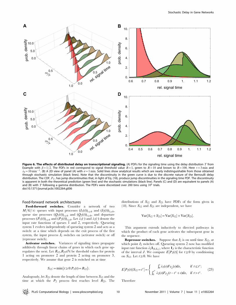
Figure 6. The effects of distributed delay on transcriptional signaling. (A) PDFs for the signaling time using the delay distribution T fromExample with b~1=2. The PDFs in red correspond to signal threshold value R~1, green to R~10 and brown to R~100. Here t~3 min andl0~10 min{1 . (B) A 2D view of panel (A) with s~1 min. Solid lines show analytical results which are nearly indistinguishable from those obtainedthrough stochastic simulation (black lines). Note that the discontinuity in the green curve is due to the discrete nature of the Bernoulli delaydistribution. The CDF, FT , has jump discontinuities that, in light of Eq. (18), produce jump discontinuities in the signaling time PDF. The discontinuityis apparent in both the theoretical prediction (green line) and the stochastic simulations (black line). Panels (C) and (D) are equivalent to panels (A)and (B) with T following a gamma distribution. The PDFs were discretized over 200 bins using 106 trials.doi:10.1371/journal.pcbi.1002264.g006

Stochastic Delay in Gene Networks

PLoS Computational Biology | www.ploscompbiol.org 10 November 2011 | Volume 7 | Issue 11 | e1002264

E½P2(t)�~E½E½P2(t)jS12~t���

~

ð?0

E½P2(t)jS12~t��fS12(t�)dt�

~

ðt

0

ðt�

0

l2(s)FT2(t{t�zs)ds

!fS12

(t�)dt�

z

ð?t

ðt

0

l2(s)FT2(s)ds

� �fS12

(t�)dt�:

Higher moments may be obtained in a similar manner.

For a repressor switch, the P2 process and therefore the ability

of gene 2 to signal downstream components depend in complex

ways on the statistical properties of T2. We examine these complex

relationships by conditioning first on S12 and then on I2. Suppose

that S12~t�. The key observation is this: for fixed twt�,E½P2(t)jS12~t�� can increase or decrease with the standard deviation

sT2of T2. We verify this assuming T2 is symmetrically distributed

about its mean and assuming l2 is a constant function.

If the midpoint t{t�=2 of the time interval ½t{t�,t� satisfies

t{t�=2vE½T2�, then

ðt�

0

FT2(t{t�zs)ds ð24Þ

is an increasing function of sT2and therefore E½P2(t)jS12~t��

increases as sT2increases. By contrast, if t{t�=2wE½T2�, then the

integral in (24) is a decreasing function of sT2and therefore

E½P2(t)jS12~t�� decreases as sT2increases. Repressive signaling

can therefore qualitatively affect the response of P2 production to

changes in the variability of T2.

We now examine the ability of gene 2 to signal downstream

components by conditioning on I2. Let R2�[N. Let S2� denote the

time at which P2 first reaches level R2�. The key observation is

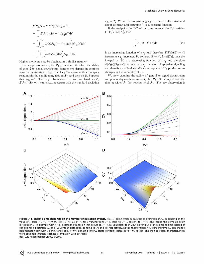
Figure 7. Signaling time depends on the number of initiation events. E½S2�jf� can increase or decrease as a function of sT2depending on the

value of f. Here R2�~l2~10. (A) E½S2�jf� vs. CV of T2 for f varying from f~10 (red) to f~19 (green) to f~? (blue) using the Bernoulli delaydistribution T2 in Example with b~1=2. Note the transition that occurs at f~19. (B) Equivalent to (A), but plotting CV of the signaling time instead ofconditional expectation. (C) and (D) Contour plots corresponding to (A) and (B), respectively. Notice that for fixed s=t, signaling time CV can changenon-monotonically with f. For instance, at s=t~0:6, signaling time CV starts low (red), increases to *0:3 (green) and then decreases thereafter. Plotswere obtained through stochastic simulation with 106 trials.doi:10.1371/journal.pcbi.1002264.g007

Stochastic Delay in Gene Networks

PLoS Computational Biology | www.ploscompbiol.org 11 November 2011 | Volume 7 | Issue 11 | e1002264

this: If we assume that gene 2 shuts off after exactly f transcription

initiation events, then E½S2�jf� can increase or decrease as a function

of sT2. Figure 7 demonstrates this numerically for a case in which

l2 is a constant function and T2 is symmetrically distributed. In

this case, we find that E½S2�jf�

1. increases as sT2increases if fv2R2�{1,

2. does not depend on sT2if f~2R2�{1, and

3. decreases as sT2increases if fw2R2�{1.

Intuitively, this is due to the fact that the order in which proteins

enter the queue is not necessarily the same as the order in which

they exit. Consider again Figure 7. When the total number of

transcription initiation events, f, is smaller than 19, then more

proteins enter the queue before the 10th protein than after it. It is

therefore more likely that a protein entering before protein 10 will

exit ahead of it than that a protein entering after protein 10 will

exit before it. As a result, the expected time E½S2�jf� increases with

sT2. When the balance favors proteins that enter the queue after

protein 10, the opposite is true, and E½S2�jf� decreases with sT2.

We conjecture that this trichotomy holds in general if l2 is a

constant function and T2 is symmetrically distributed about its

mean.

Stochastic simulationsGillespie’s stochastic simulation algorithm generates an exact

stochastic realization for a system of N species interacting through

M reactions. The state of the system is stored in the vector X , and

each reaction j is characterized by a state change vector Zj and its

propensity function aj : RN?R. If the system is in state X and

reaction j occurs then the system state changes to XzZj [5].

The idea behind extending Gillespie’s SSA to model distributed

delay is that if a reaction is to be delayed by some amount of time

then we temporarily store this reaction along with the time at

which the event will occur and we only apply this reaction at the

given time. We used a version of the algorithm equivalent to those

described in [32,48]. Note that [48] also describes a more efficient

version of the algorithm.

Acknowledgments

We wish to thank R. E. Lee DeVille for helpful discussions.

Author Contributions

Conceived and designed the experiments: KJ WO MRB. Performed the

experiments: KJ JML WO MRB. Analyzed the data: KJ JML WO LS

MRB. Wrote the paper: KJ JML WO LS MRB.

References

1. Jacob F, Monod J (1961) Genetic regulatory mechanisms in synthesis of proteins.

J Mol Biol 3: 318–356.

2. Alon U (2007) Network motifs: theory and experimental approaches. Nat RevGenet 8: 450–461.

3. De Jong H (2002) Modeling and simulation of genetic regulatory systems: a

literature review. J Comp Biol 9: 67–103.

4. Kærn M, Blake WJ, Collins JJ (2003) The engineering of gene regulatorynetworks. Annu Rev Biomed Eng 5: 179–206.

5. Gillespie DT (1977) Exact stochastic simulation of coupled chemical reactions.

J Phys Chem 81: 2340–2361.

6. Kepler TB, Elston TC (2001) Stochasticity in transcriptional regulation: originsconsequences, and mathematical representations. Biophys J 81: 3116–3136.

7. Bundschuh R, Hayot F, Jayaprakash C (2003) Fluctuations and slow variables in

genetic networks. Biophys J 84: 1606–1615.

8. Bennett MR, Volfson D, Tsimring L, Hasty J (2007) Transient dynamics of

genetic regulatory networks. Biophys J 92: 3501–3512.

9. Lan YH, Elston TC, Papoian GA (2008) Elimination of fast variables inchemical Langevin equations. J Chem Phys 129: 214115.

10. McAdams HH, Shapiro L (1995) Circuit simulation of genetic networks. Science

269: 650–656.

11. Goodwin BC (1965) Oscillatory behavior in enzymatic control processes. AdvEnzyme Regul 3: 425–438.

12. Mahaffy JM, Pao CV (1984) Models of genetic control by repression with time

delays and spatial effects. J Math Biol 20: 39–57.

13. Chen L, Aihara K (2002) Stability of genetic regulatory networks with time

delay. IEEE Trans Circ Syst 49: 602–608.

14. Smolen P, Baxter DA, Byrne JH (1999) Effects of macromolecular transport andstochastic uctuations on dynamics of genetic regulatory systems. Am J Physiol

Cell Physiol 277: C777–C790.

15. Monk NA (2003) Oscillatory expression of Hes1, p53, and NF–kB driven bytranscriptional time delays. Curr Biol 13: 1409–1413.

16. Lewis J (2003) Autoinhibition with transcriptional delay: A simple mechanism

for the zebrafish somitogeneis oscillator. Curr Biol 13: 1398–1408.

17. Mather W, Bennett MR, Hasty J, Tsimring LS (2009) Delay-induced degrade-and-fire oscillations in small genetic circuits. Phys Rev Lett 102: 068105.

18. Amir A, Meshner S, Beatus T, Stavans J (2010) Damped oscillations in the

adaptive response of the iron homeostasis network in E. coli. Molec Microbiol 76:428–436.

19. Stricker J, Cookson S, Bennett MR, Mather WH, Tsimring LS, et al. (2008) A

fast, robust and tunable synthetic gene oscillator. Nature 456: 516–519.

20. Tigges M, Marquez-Lago TT, Stelling J, Fussenegger M (2009) A tunable

synthetic mammalian oscillator. Nature 457: 309–12.

21. Larson DR, Zenklusen D, Wu B, Chao JA, Singer RH (2011) Real-timeobservation of transcription initiation and elongation on an endogenous yeast

gene. Science 332: 475–478.

22. Smolen P, Baxter DA, Byrne JH (2002) A reduced model clarifies the role offeedback loops and time delays in the drosophila circadian oscillator. Biophys J

83: 2349–2359.

23. Sriram K, Gopinathan MS (2004) A two variable delay model for the circadianrhythm of neurospora crassa. J Theor Biol 231: 23–38.

24. Ukai-Tadenuma M, Yamada RG, Xu H, Ripperger JA, Liu AC, et al. (2011)Delay in feedback repression by Cryptochrome 1 is required for circadian clock

function. Cell 144: 268–281.

25. Chen KC, Csikasz-Nagy A, Gyorffy B, Val J, Novak B, et al. (2000) Kinetic

analysis of a molecular model of the budding yeast cell cycle. Molec Biol Cell 11:

369–391.

26. Sevim V, Gong XW, Socolar JES (2010) Reliability of transcriptional cycles and

the yeast cell-cycle oscillator. PLoS Comp Biol 6: e1000842.

27. Tiana G, Jensen MH, Sneppen K (2002) Time delay as a key to apoptosis

induction in the p53 network. Eur Phys J 29: 135–140.

28. Bratsun D, Volfson D, Tsimring LS, Hasty J (2005) Delay-induced stochastic

oscillations in gene regulation. Proc Natl Acad Sci U S A 102: 14593–14598.

29. Maithreye R, Sarkar RR, Parnaik V, Sinha S (2008) Delay-induced transient

increase and heterogeneity in gene expression in negatively auto-regulated genecircuits. PLoS One 3: e2972.

30. Scott M (2009) Long delay times in reaction rates increase intrinsic uctuations.Phys Rev E 80: 031129.

31. Gronlund A, Lotstedt P, Elf J (2010) Costs and constraints from time-delayedfeedback in small regulatory motifs. Proc Natl Acad Sci U S A 107: 8171–8176.

32. Schlicht R, Winkler G (2008) A delay stochastic process with applications inmolecular biology. J Math Biol 57: 613–648.

33. Arazi A, Ben-Jacob E, Yechiali U (2004) Bridging genetic networks andqueueing theory. Physica A 332: 585–616.

34. Levine E, Hwa T (2007) Stochastic uctuations in metabolic pathways. Proc NatlAcad Sci USA 104: 9224–9229.

35. Mather WH, Cookson NA, Hasty J, Tsimring LS, Williams RJ (2010)Correlation resonance by coupled enzymatic processing. Biophys J 99:

3172–3181.

36. Zhu R, Ribeiro AS, Salahub D, Kauffman SA (2007) Studying genetic

regulatory networks at the molecular level: Delayed reaction stochastic models.

J Theor Biol 246: 725–745.

37. Zhu R, Salahub D (2008) Delay stochastic simulation of single-gene expression

reveals detailed relationship between protein noise and mean abundance. FEBSLett 582: 2905–2910.

38. Bel G, Munsky M, Nemenman I (2010) The simplicity of completion timedistributions for common complex biochemical processes. Phys Biol 7: 016003.

39. Elowitz MB, Levine AJ, Siggia ED, Swain PS (2002) Stochastic gene expressionin a single cell. Science 297: 1183–1186.

40. Gross D, Shortle J, Thompson J, Harris C (2008) Fundamentals of queueingtheory. 4th edition. Hoboken, New Jersey: John Wiley & Sons Inc.

41. Thattai M, van Oudenaarden A (2002) Attenuation of noise in ultrasensitivesignaling cascades. Biophys J 82: 2943–2950.

42. Hooshangi S, Thiberge S, Weiss R (2005) Ultrasensitivity and noise propogationin a synthetic transcriptional cascade. Proc Natl Acad Sci U S A 102:

3581–3586.

43. Mangan S, Alon U (2003) Structure and function of the feed-forward loop

network motif. Proc Natl Acad Sci U S A 100: 11980–11985.

44. Mangan S, Itzkovitz S, Zaslaver A, Alon U (2006) The incoherent feed-forward

loop accelerates the response-time of the gal system in escherichia coli. J Mol Biol356: 1073–1081.

Stochastic Delay in Gene Networks

PLoS Computational Biology | www.ploscompbiol.org 12 November 2011 | Volume 7 | Issue 11 | e1002264

45. Goentoro L, Shoval O, Kirschner MW, Alon U (2009) The incoherent

feedforward loop can provide fold-change detection in gene regulation. Mol Cell36: 894–899.

46. Amir A, Kobiler O, Rokney A, Oppenheim AB, Stavans J (2007) Noise in timing

and precision of gene activities in a genetic cascade. Mol Syst Biol 3: 71.

47. Golding I, Paulsson J, Zawilski SM, Cox EC (2005) Real-time kinetics of gene

activity in individual bacteria. Cell 123: 1025–1036.

48. Cai X (2007) Exact stochastic simulation of coupled chemical reactions with

delays. J Chem Phys 126: 124108.

Stochastic Delay in Gene Networks

PLoS Computational Biology | www.ploscompbiol.org 13 November 2011 | Volume 7 | Issue 11 | e1002264