Statistical inference on attributed random graphs: Fusion of graph features and content: An experiment on time series of Enron graphs

This article appeared in a journal published by Elsevier. The attachedcopy is furnished to the author for internal non-commercial researchand education use, including for instruction at the authors institution

and sharing with colleagues.

Other uses, including reproduction and distribution, or selling orlicensing copies, or posting to personal, institutional or third party

websites are prohibited.

In most cases authors are permitted to post their version of thearticle (e.g. in Word or Tex form) to their personal website orinstitutional repository. Authors requiring further information

regarding Elsevier’s archiving and manuscript policies areencouraged to visit:

http://www.elsevier.com/copyright

http://www.elsevier.com/copyright

Author's personal copy

Computational Statistics and Data Analysis 54 (2010) 1766–1776

Contents lists available at ScienceDirect

Computational Statistics and Data Analysis

journal homepage: www.elsevier.com/locate/csda

Statistical inference on attributed random graphs: Fusion of graphfeatures and content: An experiment on time series of Enron graphsCarey E. Priebe a,∗, Youngser Park a, David J. Marchette b, John M. Conroy c,John Grothendieck d, Allen L. Gorin ea Johns Hopkins University, United Statesb Naval Surface Warfare Center, United Statesc IDA Center for Computing Sciences, United Statesd BBN Technologies, United Statese U.S. Department of Defense, United States

a r t i c l e i n f o

Article history:Received 8 June 2009Received in revised form 10 January 2010Accepted 10 January 2010Available online 2 February 2010

Keywords:Time series analysisClusteringMetadataFeature representationStatistical methodsGraph theory

a b s t r a c t

Fusion of information from graph features and content can provide superior inference foran anomaly detection task, compared to the corresponding content-only or graph feature-only statistics. In this paper, we design and execute an experiment on a time series ofattributed graphs extracted from the Enron email corpus which demonstrates the benefitof fusion. The experiment is based on injecting a controlled anomaly into the real data andmeasuring its detectability.

© 2010 Elsevier B.V. All rights reserved.

1. Introduction

Let G1,G2, . . . be a time series of attributed graphs, with each graph Gt = (V , Et); that is, all graphs are on the samevertex set V = [n] and the attributed edges at time t , denoted by Et , are given by triples (u, v, `) ∈ V × V ×L, whereL isa finite set of possible categorical edge attributes. We think of (u, v, `) ∈ Et as a communication ormessage from vertex u tovertex v at time t . The ordered pair (u, v) represents the externals of the communication which has content labeled by topic` ∈ L, the topic set. The graph features are extracted from the overall collection of externals Ett=1,2,.... (We are consideringdirected graphs, so the (u, v) are ordered pairs.)We present here an experiment using the Enron email corpus (WWWa,b,c) which demonstrates that a statistic which

combines content and graph feature information can provide superior inference compared to the corresponding content-only or graph feature-only statistics. Furthermore, we characterize empirically the alternative space in terms of comparativepower for joint vs.marginal inference—when does a combined statistic offermore power, andwhen is it in fact less powerful.Our purpose is to begin investigation of fusion of graph features and content for statistical inference on attributed random

graphs. Grothendieck et al. (2010) presents theoretical results and simulations. This paper presents an experiment on realdata, based on injecting a controlled anomaly into the data and measuring its detectability as a function of its parameters,

∗ Corresponding address: Johns Hopkins University, Whiting School of Engineering, 21218-2682 Baltimore, MD, United States. Tel.: +1 410 516 7200;fax: +1 410 516 7459.E-mail address: [email protected] (C.E. Priebe).

0167-9473/$ – see front matter© 2010 Elsevier B.V. All rights reserved.doi:10.1016/j.csda.2010.01.008


C.E. Priebe et al. / Computational Statistics and Data Analysis 54 (2010) 1766–1776 1767

and demonstrates an anomaly detection scenario in which a graph feature-only and a content-only statistic can be fusedinto a combination statistic with understandable properties in the space of alternatives characterized by a small collectionof vertices changing their within-group activity (in terms of graph features, content, or both) while the majority of verticescontinue with their null behavior.

2. Hypotheses

The purpose of our inference is to detect a local behavior change in the time series of attributed graphs. In particular, wewish to consider as our alternative hypothesis that a small (unspecified) collection V A of vertices increase their within-groupactivity at some (unspecified) time t∗ as compared to recent past (an anomaly based on graph feature information) and thatthe content of these additional communications is also different as compared to recent past. The null hypothesis, then, issome form of temporal homogeneity—no probabilistic behavior changes in terms of either graph features or content. SeeFig. 1.We do not utilize an explicit null hypothesis. Fusion of graph features and content for statistical inference on attributed

random graphs is considered in a theoretical setting in Grothendieck et al. (2010); in that work, simple null models areposited and inference for an alternative of the form depicted in Fig. 1 is considered. However, as is the case in many realcommunication graph applications, the Enron email data set is not the result of a designed experiment, and any reasonablysimple model for time series of attributed random graphs is likely to be inappropriate. Instead, we consider an ‘‘empiricalnull’’, meaning that recent past is used to characterize baseline activity. We assume that there is no anomaly of the typerepresented by our alternative hypothesis in the time series under consideration – that every vertex is in its default stochasticstate (short-time stationarity) during the time up until the current time t – and our goal at time t is to detect deviations ofthe type represented by our anomaly alternative from this baseline activity. (For example, in the Enron email corpus, Figure1 of Priebe et al. (2005) shows that the total number of pairs of vertices which communicate during a given week increasesdramatically from 1998–2000, and drops off dramatically after 2001; during 2001 this one measure of homogeneity mightbe considered relatively stable. Similarly, Fig. 2 shows that all three of the graph feature, content, and fusion statisticsconsidered in this paper are also relatively stable during 2001—no anomaly is detected.)This insistence on considering an empirical null, and avoiding an explicit null model, allows us to sidestep the inevitable

model-mismatch criticisms. It does, however, lead to fundamental problems when attempting to assess and compareinferential procedures. Our approach will be to assume that the real data is ‘‘operating under the null’’ – and none of ourstatistics suggest otherwise – and to estimate rejection thresholds (critical values) for our tests by using a fixed-length slidingwindow, as is often done for short-time stationary signals (Rabiner and Schafer, 1978). We then seed an anomaly of interestinto the data. The strength of the anomalous signal required for rejection for each of the statistics under considerationprovides a useful comparison of detection power.

3. Statistics

Recall that for a graph G = (V , E) and a vertex v ∈ V , the closed one-neighborhood of v in G is the collection of verticesgiven by N1[v;G] = w ∈ V : dG(v,w) ≤ 1 ⊂ V , where dG denotes the graph distance—the length of the shortestpath between two vertices. Furthermore, given V ′ ⊂ V , the subgraph in G induced by V ′ is denoted byΩ(V ′;G) and is thegraph (V ′, E ′) where E ′ = (u, v) ∈ E : u, v ∈ V ′; that is, the induced subgraph Ω(V ′;G) has vertices V ′ and all edgesfrom G connecting any pair of those vertices. Therefore, Ω(N1[v;G];G) denotes the subgraph in G induced by the closedone-neighborhood of v.

3.1. Graph features

For each vertex v and time t , let

Gt(v) = Ω(N1[v;Gt ];Gt).

This locality region Gt(v) is the subgraph of Gt induced by the closed one-neighborhood in Gt of vertex v.Let

Ψt(v) = size(Gt(v)),

where the graph invariant size denotes the number of edges; thus Ψt(v) represents a local activity estimate for vertex v attime t—the number of ordered pairs of vertices in v’s neighborhood which communicate with each other at time t .Due to potentially different overall activity levels amongst vertices, we let

Ψt(v) = (Ψt(v)− µt(v))/σt(v),

where µt(v) and σt(v) are vertex-dependent normalizing parameter estimates – sample mean and variance – based onrecent past. (Here, for ‘‘recent past’’, we use times t−∆1, . . . , t−1.) For each vertex v, then, Ψt(v) represents the normalizedactivity estimate for message activity local to v (see Priebe et al. (2005) for details).

https://www.researchgate.net/publication/220556790_Scan_Statistics_on_Enron_Graphs?el=1_x_8&enrichId=rgreq-009aa66a-b957-4fd1-bdea-dd068fab32d4&enrichSource=Y292ZXJQYWdlOzQ2NDkzODUxO0FTOjEwNDE0MjgzMTg4MjI0N0AxNDAxODQwOTk0NDE5


https://www.researchgate.net/publication/46494203_Statistical_inference_on_attributed_random_graphs_Fusion_of_graph_features_and_content?el=1_x_8&enrichId=rgreq-009aa66a-b957-4fd1-bdea-dd068fab32d4&enrichSource=Y292ZXJQYWdlOzQ2NDkzODUxO0FTOjEwNDE0MjgzMTg4MjI0N0AxNDAxODQwOTk0NDE5


1768 C.E. Priebe et al. / Computational Statistics and Data Analysis 54 (2010) 1766–1776

Fig. 1. Conceptual depiction of our ‘‘anomaly’’ alternative hypothesis for time series of random graphs. The purpose of our inference is to detect localbehavior changes in the time series. The null hypothesis is ‘‘homogeneity in time’’—no probabilistic changes in terms of the graph features or contentbehavior in time. The first collection of blobs, from time t = t1 through time t = t∗ − 1, represent the collection of vertices V behaving the same throughtime. At time t∗ , a small collection of vertices (the small ‘‘egg’’, V A) change their within-group activity (in terms of graph features, content, or both), whilethe majority of vertices (the large ‘‘kidney’’) continue with their null behavior. This local alternative behavior endures for some amount of time, and thenthe anomalous vertices revert to null behavior.

Fig. 2. The three statistics T Et , TCt , and T

E&Ct , plotted as functions of time for the collection of weeks under consideration. (These are normalized versions

of the three statistics, so that their mean is zero (dotted horizontal line) and standard deviation is one. The dashed horizontal line represents the criticalvalue of ct∗ = µ + aσ with a = 4.) This figure indicates that no anomaly is detected during this time period, for any of the three statistics. Furthermore,note that all three statistics take their observed values very near their mean at time t∗ (the third week of May 2001, depicted by the large dots and verticalline).

Finally, consider the graph feature statistic T Et given by

T Et = maxvΨt(v);

a large value of T Et suggests that there is excessive communication activity in some neighborhood at time t .(NB: T Et is precisely the vertex-normalized scan statistic from Priebe et al. (2005).)

3.2. Content

For each vertex v and time t , again let Gt(v) = Ω(N1[v;Gt ];Gt).Given the topic setL of cardinality K for themessages under consideration, let the vector θt(v) be the local topic estimate

– the K -nomial parameter vector estimate, an element of the simplex z ∈ RK+: ‖z‖1 = 1 – for the collection of

messages associatedwith Gt(v); θt(v) represents the proportions ofmessages in the locality region Gt(v)which are deemedto be about each of the various topics. (NB: Clearly, this ‘‘aboutness’’ assessment requires non-trivial text processing andclassification; these issues are, however, beyond the scope of present concerns.)Then we consider the statistic

T Ct =∑v

Iargmax

kθt(v) 6= argmax

kθt−1(v)

.




T Ct counts the number of vertices which see a change in their main topics from time t− 1 to time t , and thus a large value ofT Ct suggests that an excessive number of actors experienced a change in their dominant topic for the messages associated withtheir neighborhood at time t .Under the null, we assume that a certain amount of topic changing is normal—there is some tendency to stay on a topic

for a period of time, and there is some (unknown) distribution on the number of individuals who change topics from onetime to the next. Onemight posit some ‘‘change process’’ and proceed to fit the model to the data. Instead, we are interestedin detecting these changes without regard to a particular null model.

3.3. Graph features and content combined

Wehave identified statisticswhich are appropriate for testing our null hypothesis of homogeneity against our alternative— T Et which uses graph features only, and T

Ct which uses local content. We do not claim that these are necessarily the best

such statistics – the situation is far too complicated to derive uniformly best tests even if they did exist – but these statisticssuffice to illustrate our point regarding fusion of graph features and content. To that end, we consider the combined ‘‘fusion’’statistic

T E&Ct = g(T Et , TCt )

for some g .The fusion statistic T E&Ct combines the information concerning excessive communication activity in some neighborhood

at time t compared to recent past and excessive number of actors changing their dominant topic from time t − 1 to time t .An anomaly at time t of the type described by our alternative hypothesis should, under some circumstances, be detectableusing T E&Ct even though neither T Et nor T

Ct detect. This we shall demonstrate, in the sequel.

4. Experimental design

The time series of Enron email graphs G1,G2, . . . is assumed to be observed ‘‘under the null’’; that is, we assume thatno anomaly is present during this time period, for any of the three statistics developed in the previous section. We choosea time t∗ and consider seeding the graph Gt∗ with anomalous behavior so that the seeded graph Gt∗ behaves as ‘‘under thealternative’’.

4.1. Critical values

For each time t in t∗−∆2, . . . , t∗−1we evaluate the three statistics T Et , TCt , and T

E&Ct . Since this time period is assumed

to be ‘‘under the null’’, we use these values to naively calculate the samplemean and variance and an estimated critical valuefor each statistic; since all three statistics reject for large observed values, we use ct∗ = µ+ aσ for each of T Et , T

Ct , and T

E&Ct

in turn.This approach to setting the critical values is ad hoc, but principled. Chebyshev’s inequality suggests that, for a = 4 for

example, all three tests should have a significance level in the range [0, 1/16]. This range is only approximate, because weare estimating the mean and standard deviation, and assuming (short-time) stationarity. Nevertheless, without specifyingan explicit null model (which we are loath to do for this Enron email data set) this sliding window analysis provides a usefulfirst approximation for comparative power analysis (Rabiner and Schafer, 1978).

4.2. Anomaly seeding

Our seeding procedure for time t∗ proceeds as follows:To model additional communication activity, we choose a value q ∈ (0, 1] which represents the probability that a new

edge will be added to Gt∗ as described below.To model altered topic behavior, we choose a K -nomial parameter vector θ ′ which represents the topic distribution for a

newly added edge.An anomaly graph Gt∗ based on q, θ ′, and m > 1 selected vertices V A ⊂ V is constructed from Gt∗ such that for each of

them(m−1) ordered pairs from V A, if there is not already an edge in Gt∗ , an edge is added with probability q and this addededge is given a topic value drawn according to θ ′.The effect of this anomaly seeding depends on the attributes and graph features of the selected vertices. A ‘‘coherent

signal’’ (constrained to the small set of vertices V A) with parameters q, θ ′, andm is added based on a particular choice of V A.Which V A is used strongly effects the detectability of the signal. Hence, integration over the choice of V A is necessary. MonteCarlo is employed.



Fig. 3. Conceptual depiction of the Enron email corpus data. Eachmessage includes externals (to, from, date) and content (the text of the email). In additionto information derivable solely from a given message’s externals, the overall time series of communications graphs gives rise to graph features relevant tothe exploitation task.

4.3. Monte Carlo

Given the time series of graphs G1,G2, . . . and t∗, q, θ ′,m, our Monte Carlo experiment proceeds as follows:For each Monte Carlo replicate r , we seed Gt∗ with an anomaly, randomly selecting m vertices and adding ‘‘messages’’

– new edges with topic attributes – as described above. We calculate T Et∗,r , TCt∗,r , and T

E&Ct∗,r , and for each statistic we check

whether its seeded value exceeds its associated critical value cEt∗ , cCt∗ , and c

E&Ct∗ ; that is, we evaluate the rejection indicator

ITt∗,r > ct∗ for each of the three statistics for each Monte Carlo replicate r = 1, . . . , R.The result of the Monte Carlo experiment – estimated probabilities of detection βE , βC , and βE&C , where β =

(1/R)∑Rr=1 ITt∗,r > ct∗ for each of the three statistics – provides information concerning the sensitivity of the statistics

to the signal parameterized by q, θ ′, andm.

5. Experiment

For the experiment, we use the Enron email corpus. Fig. 3 presents a conceptual depiction of the data, and Fig. 4 presentsa conceptual depiction of the experiment.The times considered are a collection of weeks in 2001, for which short-time stationarity is at least plausible. There

are n = |V | = 184 vertices and a total of 28,266 messages during this period. Fig. 2 shows that no anomaly is detectedduring this time period, for any of the three statistics T Et , T

Ct , or T

E&Ct . We choose t∗ to be the third week of May 2001. All

three statistics take their observed value very near their running mean at t∗, so that none of the statistics enjoys an obviousadvantage when it comes to detecting the seeded anomaly.For vertex-dependent normalization of T E , and for critical value estimation, we choose lags ∆1 = ∆2 = 20 to identify

‘‘recent past’’. These time-window constants should be as large as possible, so long as short-time stationarity can be safelyassumed.To identify the topic setL of cardinality K , we first chooseM= 50 messages randomly selected from each of the weeks

under consideration. We cluster the collection of messagesM into K clusters (see Appendix) and identify each resultingcluster with a topic, thus providing the topic setL = 1, . . . , K. For all of the experiments presented herein, we use K = 3.(The choice of K = 3 topics is for illustrative purposes; we make no claim that the email message content is best modeledas three topics. For instance, (Berry et al., 2007) manually index a subset of the Enron email messages into 32 topics. Ourchoice of K > 2 avoids degeneracy from multinomial to binomial, and K small avoids unnecessary complexity, for ourdemonstration.)Note that the clustering ofM described above gives rise to a classification of eachmessage inM – eachmessage is labeled

with the topic estimate given by the cluster into which that message falls. Next, for the messages not inM, we employ out-of-sample embedding and nearest neighbor classification using the now-labeled setM (see Appendix). For T C , to identifythe topic estimate θt(v) – the K -nomial parameter vector estimate for the collection of messages associated with Gt(v) – weuse the sample proportions from the now-classified messages.To model altered topic behavior, we first set θ = [θ1, . . . , θK ]T to be the K -nomial parameter vector estimate obtained

from the classification described above; we obtain θ = [0.391, 0.184, 0.425]T . We identify the altered topic vector θ ′ basedon θ and a single parameter δ, so that θ ′ = hθ (δ), by setting θ ′ to be the K -nomial parameter vector obtained by increasingthe smallest element of θ by some δ ≤ (K −1)/K and decreasing the other K −1 elements of θ by δ/(K −1), so θ ′k = θk+ δ



Fig. 4. Conceptual depiction of the experiment described in Section 5.

for k = argmink θk and θ ′k = θk − δ/(K − 1) for k 6= argmink θk. Thus our altered topic vector θ′ is obtained from θ via a

single parameter δ ∈ (0, (K − 1)/K ].To model additional communication activity, we choose q ∈ (0, 1].The alternative space for our seeded messages, then, is (δ, q) ∈ ΘA = (0, (K − 1)/K ] × (0, 1].For the combined statistic, we use a linear combination with parameter γ ;

T E&Ct = g(T Et , TCt ) = γ T

Et + (1− γ )T

Ct .

This simple form for the fusion statistic is a first consideration only; optimal fusion need not take this form (see Grothendiecket al. (2010)).

6. Experimental results

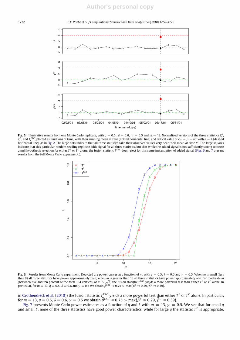
Fig. 2 shows that all three statistics, normalized to have mean zero and standard deviation one, take their observedvalues at time t∗ very near their mean. We conclude that the three tests, using critical values ct∗ = µ+ aσ with a = 4, haveapproximately the same α-level, and so power comparisons under our anomaly seeding scheme are at least illustrative.Fig. 5 depicts illustrative results from one Monte Carlo replicate, with q = 0.5 (additional communication activity),

δ = 0.6 (altered topic behavior), γ = 0.5 (combination coefficient), andm = 13 (number of anomalous vertices). The largesquares indicate that this particular random seeding replicate adds signal for all three statistics. While the added signal isnot sufficiently strong to cause a null hypothesis rejection for either T E or T C alone, the fusion statistic T E&C does reject forthe same added signal.Figs. 6 and 7 present results from the full Monte Carlo experiment. We use R = 1000 Monte Carlo replicates throughout.Fig. 6 depicts power curves, probability of detection as a function ofm, with q = 0.5, δ = 0.6, γ = 0.5.We see thatwhen

m is small (less than 9) all three statistics have power approximately zero; whenm is greater than 18 all three statistics havepower approximately one. For moderatem (between five and ten percent of the total 184 vertices, orm ≈

√n as suggested



Fig. 5. Illustrative results from one Monte Carlo replicate, with q = 0.5, δ = 0.6, γ = 0.5 and m = 13. Normalized versions of the three statistics T Et ,T Ct , and T

E&Ct , plotted as functions of time, with their running mean at zero (dotted horizontal line) and critical value of ct∗ = µ+ aσ with a = 4 (dashed

horizontal line), as in Fig. 2. The large dots indicate that all three statistics take their observed values very near their mean at time t∗ . The large squaresindicate that this particular random seeding replicate adds signal for all three statistics, but that while the added signal is not sufficiently strong to causea null hypothesis rejection for either T E or T C alone, the fusion statistic T E&C does reject for this same instantiation of added signal. (Figs. 6 and 7 presentresults from the full Monte Carlo experiment.).

Fig. 6. Results from Monte Carlo experiment. Depicted are power curves as a function of m, with q = 0.5, δ = 0.6 and γ = 0.5. When m is small (lessthan 9) all three statistics have power approximately zero; when m is greater than 18 all three statistics have power approximately one. For moderate m(between five and ten percent of the total 184 vertices, or m ≈

√n) the fusion statistic T E&C yields a more powerful test than either T E or T C alone. In

particular, form = 13, q = 0.5, δ = 0.6 and γ = 0.5 we obtain βE&C ≈ 0.75 > maxβE ≈ 0.29, βC ≈ 0.39.

in Grothendieck et al. (2010)) the fusion statistic T E&C yields a more powerful test than either T E or T C alone. In particular,form = 13, q = 0.5, δ = 0.6, γ = 0.5 we obtain βE&C ≈ 0.75 > maxβE ≈ 0.29, βC ≈ 0.39.Fig. 7 presents Monte Carlo power estimates as a function of q and δ with m = 13, γ = 0.5. We see that for small q

and small δ, none of the three statistics have good power characteristics, while for large q the statistic T E is appropriate.



Fig. 7. Results fromMonte Carlo experiment. Depicted are power values as a function of q and δ withm = 13 and γ = 0.5. Each pie has three thirds, withone third representing each of the three statistics and the amount of that third which is filled in representing the power – lightest gray for βE&C , darkestgray for βE , and medium gray for βC – for the point (q, δ) in the alternative space denoted by the center of the pie. (The top center pie corresponds toFig. 6 with m = 13.) We see that for small q and small δ, none of the three statistics have good power characteristics, while for large q the statistic T E isappropriate. For moderate q, the fusion statistic T E&C yields a more powerful test than either T E or T C alone.

For moderate q, the fusion statistic T E&C can yield a more powerful test than either T E or T C alone. Note, however, that forq = 0.3, δ = 0.6 the content-only statistic is most powerful—βE&C ≈ 0.01, βE ≈ 0.00, βC ≈ 0.15 (Nowhere in this plotdo we see T E being most powerful. Such alternatives do exist, however; for example, q = 0.5, δ = 0.1,m = 13, γ = 0.1yields βE&C ≈ 0.12, βE ≈ 0.29, βC ≈ 0.00.)Figs. 8 and 9 depict an investigation of the best fusion statistic in the class γ T Et + (1 − γ )T

Ct : γ ∈ (0, 1) for various

signal parameters q, δ with m = 13. We see that the specific anomaly parameters q, δ strongly influence the optimal γ , asexpected.These results, taken as a whole, indicate clearly that fusion of graph features and content in this setting can indeed

provide superior power than is attainable using either graph features or content alone. We also see, however, that (as thebias-variance tradeoff suggests) for some anomalies fusion can have a negative effect, due to additional estimation variancefor too little signal gain. This phenomenon indicates that, for general alternatives, more elaborate inferential proceduresare necessary, rather than simply using both graph features and content just because both are available—a version of theclassical ‘‘curse of dimensionality’’.

6.1. Incoherent signal

We have presented our experimental results in terms of comparative power, as if all three tests are constrained to havethe same α-level. Since we do not posit a specific null model, this claim is at best approximately true. Nevertheless, thechanging relative powers for various values of the signal parameters indicate that fusion has a variable effect and can besometimes wise and sometimes unwise.Another approach to the analysis considers, rather than comparative power in a null vs. alternative sense, comparative

probability of detection for coherent vs. incoherent signals. In our anomaly seeding experiments, we choose signalparameters q, δ, and m, and then choose a specific collection V A of m vertices and consider adding attributed edges foreach of the m(m − 1) directed pairs. That is, the signal is coherent in that the additional communication activity and thealtered topic behavior are concentrated amongst the m vertices V A. An incoherent version of this anomaly seeding utilizesthe same signal parameters, but considers adding attributed edges form(m− 1) directed pairs randomly selected from theentire collection of n(n−1) possible directed pairs. Thuswe have the same amount of added signal, but it is not concentratedin one coherent subgraph.Fig. 10 presents the results of such an ‘‘incoherent signal’’ Monte Carlo experiment. Depicted are power values for the

combined statistic T E&Ct∗ for fixed δ = 0.6, q = 0.5,m = 13, γ = 0.5, as a function of a in critical value ct∗ = µ+ aσ . Recallthat we obtained βE&C ≈ 0.75 > maxβE ≈ 0.29, βC ≈ 0.39 for the coherent signal experiment, with a = 4. For the



Fig. 8. Results fromMonte Carlo experiment. Depicted are power values for the combined statistic T E&Ct∗ for fixed q = 0.5 andm = 13 and selected valuesof δ, as a function of γ .

Fig. 9. Results fromMonte Carlo experiment. Depicted are power values for the combined statistic T E&Ct∗ for fixed δ = 0.6 andm = 13 and selected valuesof q, as a function of γ .

incoherent signal, all three statistics have an estimated power of zero for a ≥ 0.2. Thus we conclude that it is the coherenceof the seeded signal that is being detected throughout the foregoing experiments, and that all three statistics (with a = 4)have a Type I error rate of approximately zero with respect to the ‘‘empirical graph+ incoherent signal’’ null.

7. Discussion and conclusions

The purpose of this experiment is to begin investigation of fusion of graph features and content for statistical inferenceon attributed random graphs. This experiment on time series of Enron graphs demonstrates explicitly, constructively, and



Fig. 10. Results from ‘‘incoherent signal’’ Monte Carlo experiment. Depicted are power values for the combined statistic T E&Ct∗ for fixed δ = 0.6, q = 0.5,m = 13 and γ = 0.5, as a function of a in critical value.

quantitatively an anomaly detection scenario in which a graph feature-only and a content-only statistic can be fused intoa combination statistic with understandable properties in the space of alternatives characterized by a small collection ofvertices changing their within-group activity (in terms of graph features, content, or both) while the majority of verticescontinue with their null behavior.There are numerous choices that have been made, for expediency, which are in no way claimed to be optimal. Among

these issues, we briefly address the most noteworthy here.The individual statistics T E and T C are reasonable, but many other choices are available. As for the combined statistic,

another (better?) choice is to combine locally; e.g.,

T E&Ct = maxvg(Ψt(v), ‖θt(v)− θt−1(v)‖).

It is conjectured here that this more elaborate fusion statistic – assessing a neighborhood’s excessive activity and topicchange simultaneously – will yield dividends.Methods exist for streaming topic estimation which are superior to the simple approach employed herein. As we are

primarily interested in fusion effects, we admittedly give short shrift to this important aspect of the problem.For our Monte Carlo seeding, we write: ‘‘For each Monte Carlo replicate r , we seed Gt∗ with an anomaly, randomly

selectingm vertices and addingmessages . . . ’’ Thus, we are integrating over the specific collection ofm anomalous vertices inour experiment. Obviously, the amount of signal (graph feature, or content, or both) necessary to cause a detection dependsheavily upon the specific vertices involved in the anomaly. It seems that conditional investigations along these lineswould beof value. In particular, 14 of the n = 184 vertices are inactive during the time period under consideration. Added signal willhave a dramatic effect on these isolated vertices. However, the result obtainedwhen re-running theMonte Carlo experiment(m = 13, q = 0.5, δ = 0.6, γ = 0.5) with these isolates removed is βE&C ≈ 0.73 > maxβE ≈ 0.29, βC ≈ 0.38 — almostidentical to the result with the isolates included, βE&C ≈ 0.75 > maxβE ≈ 0.29, βC ≈ 0.39. From this we conclude thatour results are robust to a large percentage of isolates — approximately 8%, in this case.Since θ and θ ′ = hθ (δ) are global, δ = 0 is not equivalent to ‘‘no content change’’ for each local neighborhood. This

point helps explain some of the test behavior (e.g. in Fig. 7). This may be an experimental design flaw – local null andalternative content vectors θ(v) and θ ′(v) could be employed for each neighborhood – but we feel that the advantage(namely, simplicity) of this choice of a univariate content anomaly outweighs the disadvantages.Finally, we must comment on the level of the three tests being compared. We write: ‘‘We conclude that the three tests

[. . . ] have approximately the same α-level, and so power comparisons [. . . ] are at least illustrative’’. Of course, this assumesproperties of the right tail of the null distributions of the statistics that cannot be checked to our satisfaction. Nonetheless,we argue that even if the approximate sameness of level is not accepted, the fusion effect (e.g. Fig. 6) remains, with shiftsin the cut-off thresholds. Furthermore, the ‘‘incoherent signal’’ experiment indicates that all three tests have probabilityapproximately zero of detecting the incoherent signal, and thus our investigation demonstrates the comparative detectioneffect of coherence.



These and other issues notwithstanding, our Monte Carlo experimental results shed light on the behavior of fusion ofgraph features and content in the specific setting investigated, augmenting theoretical results in Grothendieck et al. (2010).It is hoped that this initial experiment, together with Grothendieck et al. (2010), will provide impetus for additional, moreelaborate experimental and theoretical investigations.

Appendix

To cluster the collection of training messagesM into K clusters, we first employ term-document mutual informationcalculations and low-dimensional Euclidean embedding via multi-dimensional scaling (see Priebe et al. (2004)). K -meansclustering is then used to identify the final clusters/topics. For all of the experiments presented herein, we use K = 3.The term-document mutual information calculations can be adapted to allow efficient out-of-sample embedding of test

data into the same space as the training data. This approach is used to put all messages not inM into the same space asM,wherein nearest neighbor classification is possible.We first calculate the mutual information feature vectors for documents in corpusM. When we calculate the mutual

information feature vector for each document x in the remaining test data setN , instead of counting the total frequency ofwordw in corpusN only, we also count it inM. That is, instead of using

mx,w = log

fx,w∑N

fN ,w∑w

fx,w

,we use

mx,w = log

fx,w∑N∪M

fN∪M,w

∑w

fx,w

= log

fx,w(∑N

fN ,w +∑M

fM,w

)∑w

fx,w

.Here fx,w = cx,w/|N | where cx,w is the number of times word w appears in document x and |N | is the total number of

words in the corpus. Since we already have a list of words and their counts inM, we can reuse that information withoutrecalculating it.This approach is not as accurate as calculating feature vectors in the whole corpusM ∪ N , but is good enough for an

approximation and also can save a significant amount of computing time.

References

www.cs.queensu.ca/home/skill/siamworkshop.html.www-2.cs.cmu.edu/~enron.www.cis.jhu.edu/~parky/Enron.Berry, M.W., Browne, M., Signer, B., 2007. 2001 Topic annotated enron email data set, Linguistic Data Consortium. Philadelphia.Grothendieck, J., Priebe, C.E., Gorin, A.L, 2010. Statistical inference on attributed random graphs: Fusion of graph features and content. ComputationalStatistics and Data Analysis 54, 1777–1790.

Priebe, C.E., et al. 2004. Iterative denoising for cross-corpus discovery. In: COMPSTAT 2004, pp. 381–392.Priebe, C.E., Conroy, J.M., Marchette, D.J., Park, Y., 2005. Scan statistics on enron graphs. Computational & Mathematical Organization Theory 11, 229–247.Rabiner, L.R., Schafer, R.W., 1978. Digital Processing of Speech Signals. Prentice-Hall, Englewood Cliffs, NJ.

Documents

Statistical inference on attributed random graphs: Fusion of graph features and content: An experiment on time series of Enron graphs