STATISTICAL APPLICATIONS IN THE EARTH SCIENCES

GEOLOGICAL SURVEY OF CANADA PAPER 89-9

STATISTICAL APPLICATIONS IN THE EARTH SCIENCES

Edited by F.P. Agterberg and G.F. Bonham-Carter

Energy, M ~ n e s and Energ~e. M ~ n e s el I*I Resources Canada Ressourccs Canada

THE ENERGY OF OUR RESOURCES

fsauve

white stamp

GEOLOGICAL SURVEY OF CANADA PAPER 89-9

Edited by: F.P. Agterberg and G.F. Bonham-Carter

STATISTICAL APPLICATIONS IN THE EARTH SCIENCES

Proceedings of a colloquim Ottawa, Ontario

14-18 November, 1988

O Minister of Supply and Services Canada 1990

Available in Canada through

authorized bookstore agents and other bookstores

or by mail from

Canadian Government Publishing Centre Supply and Services Canada Ottawa, Canada KIA OS9

and from

Geological Survey of Canada offices:

601 Booth Street Ottawa, Canada KIA 0E8

3303-33rd Street N.W.. Calgary, Alberta T2L 2A7

100 West Pender Street Vancouver, B.C. V6B 1R8

A deposit copy of this publication is also available for reference in public libraries across Canada

Cat. No. M44-8919E ISBN 0-660-13592-2

Price subject to change without notice

Cover Il lustration

The colour image shows an area of eastern shore Nova Scotia underlain by rocks of the Meguma terrane. The image was made using a FIRE system a t the Canada Centre for Remote Sensing (CCRS) by Jeff Harris (Intera Technologies and the Radarsat office of CCRS). The picture combines two image channels by meas of a n intensity, hue and saturation transform. Airborne side-looking radar values were used for intensity, estimated gold potential values (see Bonharn-Carter e t al., this volume were used for hue and saturation values were set to a constant.

Original manuscript received: 89-09-1 1

CONTENTS

Forewordl Avant-propos : D.C. FINDLAY

Introduction/Introduction: F.P. AGTERBERG and G.F. BONHAM-CARTER

PART 1: SPATIAL DATA INTEGRATION

Regional Geoscience Applications of Image Analysis

A.N. RENCZ, J . AYLSWORTH, and W.W. SHILTS Processing LANDSAT Thematic Mapper imagery for mapping surficial geology, District of Keewatin, Northwest Territories

H. ISAKSSON and C. ANDERSSON Project GEOVISION: a geological information system applied to the integration of digital elevation, remote sensing and geological data

J . HARRIS Clustering of gamma ray spectrometer data using a computer image analysis data

J.A. OSTROWSKI, D. BENMOUFFOK, D.C. HE, and D.N.H. HORLER Geoscience applications of digital elevation models

M.M. RHEAULT, R. SIMARD, P. KEATING, and M.M. PELLETIER Mineral exploration using digital image processing of LANDSAT, SPOT, magnetic and geochemical data

Image Analysis of Geophysical Data

D.J. TESKEY Statistical interpretation of aeromagnetic data

J.E. ROBINSON Deconvolution filters and image enhancement

D. NAGY Gravity field representation over Canada for geoid computation

S.E. FRANKLIN and R.T. GILLESPIE Methods and applications of image analysis using integrated data sets

M.K. PAUL and A.K. GOODACRE An investigation of statistical models of the variation of density inside the Earth, based on geopotential coefficients

M. PILKINGTON and R.A.F. GRIEVE Magnetizationtdensity ratio mapping in eastern Canada

L. YUAN Image analysis of pore size distribution and its application

Geographic Information Systems, Digital Cartography

A. CURRIE and B. ADY: GEOSIS Project knowledge representation and data structures for geoscience data

E.C. REELER and J.J. CHANDRA Using CARIS as a spatial information system for geological applications

Data Integration and Resource Assessment

J.C. BROWER and D.F. MERRIAM Geological map analysis and comparison by several multivariate algorithms

M. MELLINGER Computer tools for the integrative interpretation of geoscience spatial data in mineral exploration

G.F. BONHAM-CARTER Comparison of image analysis and geographic information systems for integrating geoscientific maps

H. GEORGE and G.F. BONHAM-CARTER An example of spatial modelling of geological data for gold exploration, Star Lake area, Saskatchewan

G.F. BONHAM-CARTER, F.P. AGTERBERG, and D.F. WRIGHT Weights of evidence modelling: a new approach to mapping mineral potential

G.P. WATSON and A.N. RENCZ Data integration studies in northern New Brunswick

H.D. MOORE and A.F. GREGORY Weighting of geophysical data with SPANS for digital geological mapping

Summaries

J. BROOME Interpretation of regional geophysical data from the Arner Lake-Wager Bay area, District of Keewatin

J . BROOME Use of an IBM-compatible workstation for interpretation of potential field data

G.L. COLE Data processing techniques for the Geochemical Atlas of Costa Rica

G.L. COLE Examples of spatial data integration and graphical presentation in mineral resource assessments from New Mexico and Costa Rica

S . CONNELL, J. ERNSTING, D. KUKAN, and A. CURRIE GEOSIS Project - integration of text and spatial data for geoscience applications

I. FINLAY, D. HOFFER, W. WOITOWICH, and A. CURRIE GEOSIS Project - integration of spatial data in geoscience information systems

G. GAAL Exploration target selection by integration of geodata using statistical and image processing techniques at the Geological Survey of Finland

R.T. HAWORTH, M.K. LEE, A.S.D. WALKER, and J.D. CORNWELL Structural trends in the British Isles from image analysis of regional geophysical data and implications for mineral exploration

B.D. LONCAREVIC, A.G. SHERIN, and J.M. WOODSIDE An evaluation of SPANS for presentation of the Frontier Geoscience Program's Basin Atlas

P.J. ROGERS, G.F. BONHAM-CARTER, and D.J. ELLWOOD Mineral exploration using catchment basin analysis to integrate regional stream sediment geochemical and geological information in the Cobequid Highlands, Nova Scotia

R.J. SAMPSON and J .A. DeGRAFFENREID Using SURFACE 111 as a research tool for spatial analysis

A.G. SHERIN and P.N. MOIR Building a GIs for the Atlantic Geoscience Centre: which direction?

V.R. SLANEY, J. HARRIS, D.F. GRAHAM, and K. MISRA 3eological activities within the RADARSAT Project

I . WHITING The regional integration of vegetation and geological lineaments derived from satellite digital jata with soils information

D.F. WRIGHT Data integration, eastern shore, Nova Scotia

PART 11: STATISTICAL ANALYSIS OF GEOSCIENCE DATA

Theory a n d Applications of Probability and Statistics

M. CSORGO and L. HORVATH On confidence bands for the quantile function

C.F. CHUNG and W.A. SPIRIT0 Estimation of distribution parameters from data with observations below detection limit, with an example from south Nahanni River area, District of Mackenzie

B. MILKEREIT and C. SPENCER Noise suppression and coherency enhancement of seismic data

A.D. FOWLER, D. ROACH, and R. THERIAULT Statistical and fractal models of nonequilibrium mineral growth

G. RANALLI and L. HARDY Statistical approach to brittle fracture in the Earth's crust

T.J. KATSUBE and F.P. AGTERBERG Use of statistical methods to extract significant information from scattered data in petrophysics

P.J. LEE, R.-Z. QIN, and Y .-M. SHI Conditional probability analysis of geological risk factors

A. J . DESBARATS An iterative least-squares method for the inversion of spectral radiometric data

D. MARCOTTE Spatial estimation of frequency distribution of acid rain data using Bigaussian kriging

R.E. ERNST and G.W. PEARCE Averaging of anisotropy of magnetic susceptibility data

Multivariate Analysis

R.G. GARRETT 4 robust multivariate allocation procedure with applications to geochemical data

R.M. RENNER, G.P. GLASBY, F.T. MANHEIM, and C.M. LANE-BOSTWICK 4 partitioning process for geochemical datasets

E. GRUNSKY Spatial factor analysis: a technique to assess the spatial relationships of multivariate data

D. MARCOTTE Multivariate analysis and variography used to enhance anomalous response for lake sedi- nents in the Manicouagan area, Quebec

W. MELLINGER Multivariate patterns of field information and geochemistry in a regional lake sediment sur- Jey: the NEAIIAEA Athabasca Test Area revisited

jummaries

'.W. BURTON seismic hazard evaluation : extreme and characteristic earthquakes in areas of low and high ieismicity

3.F. CHUNG, A.G. FABBRI, and C.A. KUSHIGHOR 4n extension of principal component analysis for multi-channel remotely sensed imagery

3.L. COLE rhe use of Monte Carlo methods to quantify uncertainties in combined plate reconstructions

VI. LABONTE :omputer programs for correspondence analysis, and dendrographs with applications to coal lata

1.E. MYERS 'ractical aspects of multivariate estimation for spatial data

Multivariate statistical analysis - a practical approach in hydrocarbon exploration?

A. ROULEAU Characterizing the spatial distribution of fractures in rocks

J.J. ROYER and H. MEZGHACHE Recognition of multivariate anomalies in exploration geochemistry

J.H. SCHUENEMEYER and L.J. DREW Exploring the lower limits of economic truncation: modelling the oil and gas discovery process

D.A. SINGER and R. KOUDA Application of geometric probability and Bayesian statistics to the search for mineral deposits

PART I11 : QUANTITATIVE STRATIGRAPHY

Artificial Intelligence and Expert Systems

Wm. R. RIEDEL and L.E. TWAY Artificial intelligence applications in paleontology and stratigraphy

J.C. DAVIS and R.A. OLEA Artificial intelligence for the correlation of well logs

R.B. McCAMMON Prospector I11 : towards a map-based expert system for regional mineral-resource assessment

Methods of Quantitative Stratigraphy

J.C. BROWER A case study for comparison of some biostratigraphic techniques using Paleogene alveolinids from Slovenia and Istria

W.G. KEMPLE, P.M. SADLER, and D.J. STRAUSS A prototype constrained optimization solution to the time correlation problem

D. YUAN and J.C. BROWER Error effects and error estimation for graphic correlation in biostratigraphy

L.F. MARCUS and P. LAMPIETTI Interactive graphic analysis and sequence comparison of host rocks containing stratiform volcanogenic massive sulphide deposits

I. SHETSEN and G. MOSSOP Recognition of stratigraphic equivalents using a graph-theoretic approach for the geological atlas of the Western Canada Sedimentary Basin

A. FRICKER A Canadian index of lithostratigraphic and lithodemic units

F.P. AGTERBERG, F.M. GRADSTEIN, and K. NAZLI Correlation of Jurassic microfossil abundance data from the Tojeira sections, Portugal

J .M. WHITE Exploration of a practical technique to estimate the relative abundance of rare palynomorphs using an exotic spike

Quantitative Basin Modelling

S. CAO and I. LERCHE Sensitivity analysis of basin modelling with applications

J.P.M. SYVITSKI Modelling the sedimentary fill of basins

S. BACHU, D. CUTHIELL, and J. KRAMERS Effects of core scale heterogeneities on fluid flow in a clastic reservoir

Scalling Stratigraphic Events

F.P. AGTERBERG and D.N. BYRON FORTRAN 77 microcomputer programs for ranking, scaling and regional correlation of stratigraphic events

M.A. D'IORIO Sensitivity of the RASC model to its critical probit value

P. HIBBERT Spline smoothing by means of an analogy to structural beams

M. A. WILLIAMSON and F.P. AGTERBERG A quantitative foraminifera1 correlation of the late Jurassic and early Cretaceous offshore Newfoundland

Summaries

F.M. GRADSTEIN and M. FEARON STRATCOR, a new method for biozonation and correlation with applications to exploration micropaleontology

M. FEARON Finding the cubic smoothing spline function by scale invariants

J.D. HUGHES A multiple-surface strategy for analysis of geological data in layered sequences

M. SCHAU Classification of granulites

A. SHOMRONY, D. GILL, and H. FLIGELMAN Application of adjacency-constrained clustering to the zonation of manifold petrophysical well logs

APPENDIX : WORKING GROUP REPORTS

1. Spatial Data Integration : Regional Geophysics 2. Spatial Data Integration : Remote Sensing 3. Geographic Information Systems for Government Geological Surveys 4. Statistics and Probability in Geoscience 5 . Geostatistical Models and Estimation 6. Artificial Intelligence in the Earth Sciences 7. Quantitative Stratigraphy 8. Basin Analysis

Statistical Applications in the Earth Sciences

Foreword The evolution of computer-assisted techniques in

the integration and analysis of multiple geoscience data sets provides a powerful stimulus to a variety of earth science investigations, including mineral resource appraisal and estimation. Coupled with GIS technologies that permit the rapid and accurate registration and layering of such multiple data sets, these new tools allow geologists investigating the regional and local characteristics of mineral endowments to construct and manipulate a variety of distribution models in rapid order. In a real sense, these techniques seem to be what has long been needed to shift the process of mineral resource appraisal away from a subjective-oriented art towards an objective- oriented science. If earth scientists have been waiting for Godot, in this (mineral resource estimation) area at least, perhaps Godot has arrived.

The papers collected in this volume, representing the formal output from the Colloquium on "Statistical Applications in the Earth Sciences" held in Ottawa in November 1988, cover the three broad subject areas addressed by the Colloquium - spatial data integration ; statistical analysis of geoscience data, and quantitative stratigraphy. They offer a wide sampling of state-of-the-art research in these fields. They also offer valuable insight into the ways in which such techniques as GIS-aided multiple data set integration, image analysis, pattern recognition, spatial statistics and expert systems technology can be used in a variety of applications to problems in geology.

It is a measure of the widespread expansion of interest in these topics that, in 1987 when the organizers began planning the Colloquium, it was anticipated that perhaps 80 to 100 people might attend. At the event, a little more than a year later, the presence of nearly 400 active participants attests to the emergence of these specialities as a major influence on geology and geological interpretations. It is to be expected that the 1988 Colloquium will be but a forerunner of many such meetings to come. For its part, the Geological Survey of Canada is pleased to have played some role in the conduct of this event and to have facilitated the publication of this extensive record of the proceedings.

L'apparition des techniques informatistes d'intkgration et d'analyse des ensembles de donnks gCologiques multiples a grandement stimulC la recherche dans plusieurs domaines des sciences de la Terre, dont celui de I'tvaluation des ressources minCrales. Utilisis de pair avec les SIG qui permettent d'enregistrer et d'ordonner de facon rapide et precise les ensembles de donnQs multiples, ces nouveaux outils permettent aux g6ologues Ctudiant les caract6ristiques regionales et locales des ressources mintrales de construire et de manipuler sans dClai divers modbles de rkpartition. Pendant longtemps, l'tvaluation des ressources minCrales faisait appel B la subjectivitt et relevait davantage d'une certaine forme d'art. Grlce B ces nouvelles techniques, elle est aujourd'hui une science objective. Si les g6ologues ont pendant longtemps attendu Godot, il se pourrait bien que Godot soit aujourd'hui arrivt, du moins pour ceux qui oeuvrent dans le domaine de 1'6va- luation des ressources mintrales.

Les ttudes rCunies dans le prCsent volume, qui ont fait l'objet de communications au cours du colloque sur les applications des statistiques dans le domaine des sciences de la Terre tenu h Ottawa en novembre 1988, couvrent les trois grands thbmes traitCs cette occasion : inttgration des donntes spatiales ; analyse statistique des donnCes gtologiques; et, stratigraphie quantitative. Ces articles couvrent une bonne partie des recherches de pointe mentes dans ces domaines. Ils donnent aussi une bonne idte de la manibre dont certaines techniques comme celles de l'intkgration des ensembles de donnCes multiples assistee par SIG, I'analyse des images, la reconnaissance de formes, les statistiques spatiales et la technologie des systbmes experts, peuvent &re utilisCes pour rtsoudre de difftrentes manikres les problbmes se posant dans le domaine de la gkologie.

LYintCr&t pour ces sujets s'est accru considCrablement au cours des dernibres annCes. En t6moigne le fait qu'en 1987, quand les organisateurs du colloque ont commenct B le planifier, ceux-ci s'attendaient B recevoir 80 B 100 personnes. Un peu plus d'une annte plus tard, prbs de 400 personnes participaient activement au colloque. Ces nouvelles disciplines ont donc commencC B jouer un rale important en gtologie et en matibre dYinterprCtation des donnCes gCologiques. 11 est 2 espCrer que le colloque de 1988 jouera un r61e de pionnier et sera suivi de plusieurs autres rencontres de ce genre. Pour sa part, la Commission gCologique du Canada est heureuse d'avoir participC & l'organisation de cet Cv6- nement et d'avoir rendu possible la publication dttaillCe des actes de ce colloque.

D.C. Findlay Director-General 1 Directeur general Mineral Resources and Continental Geoscience Branch Direction des ressources minerales e t de la geologie d u continent 1 Geological Survey of Canada 1 Commission geologique du Canada

INTRODUCTION INTRODUCTION These are the Proceedings of the Colloquium on "Statistical Applications in the Earth Sciences" hosted by the Geological Survey of Canada (GSC) in Ottawa on 14-18 November, 1988. The purposes of the Colloquium were to provide the Canadian and international earth science communities with information on mathematical research activities within the GSC, and to provide a forum for the exchange of ideas on mathematical applications in geology and discussions concerning future directions in this field. The program consisted of oral presentations of papers, microcomputer demonstrations, posters and technical workshops. Eight working groups met and prepared reports with recommendations which are contained in the Appendix of this volume.

The three parts of the Proceedings contain scientific contributions presented on the three main themes of the Colloquium which were: (1) spatial data integration, (2) statistical analysis of geoscience data, and (3) quantitative stratigraphy.

In total, 379 scientists participated in the meetings which were co-sponsored by the International Associ- ation for Mathematical Geology, the Commission on Storage, Automatic Processing and Retrieval of Geo- logical Data (COGEODATA), the Committee for Quantitative Stratigraphy of the International Com- mission on Stratigraphy, the Laboratory for Research in Statistics and Probability at Carleton University, and the Ottawa-Carleton Geoscience Centre.

Recent developments in the fields of image analysis and Geographic Information Systems (GIS) have made a significant impact on geomathematical applications for spatial data integration. Part I of these Proceedings deals with papers on spatial data analysis, several of them describing applications using image analysis and GIs. The current importance of these topics has been brought about partly by computer hardware and software advances, and partly by the ever increasing rate with which new spatial data are being gathered.

T h e computing hardware environment has changed radically during the 1980s, moving from mainframes to microcomputers for most applications. At the time of writing, micros with 25 MHz speeds, and 300 Mb hard disks are becoming common; coupled with good colour graphics boards, such hardware is capable of running the majority of image analysis and GIs tasks currently required.

The computing software environment is also in transition. At one time, geologists wishing to do any serious computing had to be competent programmers. Although good mainframe packages such as SPSS and SURFACE 11 were used in the past, the spread of menu-driven, user-friendly programs on microcomputers has greatly increased the access of non- specialists to computing resources. In the case of image analysis and GIS sof tware , o u r own

Le prtsent volume comprend les Actes du colloque sur les applications des statistiques dans le domaine des sciences de la Terre tenu sous les auspices de la Commission gtologique du Canada B Ottawa, du 14 au 18 novembre 1988. Ce colloque visait B fournir aux gtologues canadiens et Ctrangers des informations sur les recherches en mathCmatiques menbes par la CGC. I1 voulait aussi permettre aux participants de discuter des applications mathtmati- ques dans le domaine de la gCologie de m6me que des perspectives d'avenir dans ce domaine. Des prtsentations orales d'articles, des dCmonstrations dans le domaine de la micro informatique, des stances d'affichage et des ateliers techniques Ctaient au programme. Huit groupes de travail ont CtC formks et ont prtpart des rapports comportant des recommandations, lesquels se trouvent

1'Annexe du prbsent volume.

Les Actes sont divisCs en trois parties qui correspondent aux trois thkmes principaux traitts au cours du colloque: (1) inttgration des donnCes spatiales, (2) analyse statistique des donnkes gCo- logiques, et (3) stratigraphie quantitative.

Au total, 379 scientifiques ont participk aux rencontres. Ces dernikres Ctaient co-parrainCes par 1'Association internationale pour la gCologie mathtmatique, la .Commission on Storage, Automatic Processing and Retrieval of Geological Data (COGEO- DATA) D le comitt pour la stratigraphie quantitative de la Com- mission internationale de stratigraphie, le ((Laboratory for Research in Statistics and Probability )) de l'Universit6 Carleton et le Centre gkoscientifique d'ottawa-Carleton.

Les mises au point rCcentes dans les domaines de l'analyse des images et des Systkmes d'information gtographique (SIG) ont eu un impact important sur les applications gComathtmatiques relatives B l'intkgration des donntes spatiales. Les articles de la premikre partie des Actes traitent de l'analyse des donnCes spatiales. Plusieurs de ces articles portent sur des applications rCalisCes B l'aide de l'analyse des images et des SIG. Les progrks en matibre de mattriel et de logiciel informatiques et le fait que le nombre de nouvelles donntes spatiales augmente de plus en plus rapidement expliquent en partie l'importance actuelle de ces sujets.

Le matCriel informatique a connu d'importantes modifications au cours des annCes 80, passant des gros ordinateurs aux micro- ordinateurs pour la plupart des applications. Actuellement, les micro-ordinateurs ayant des vitesses de 25 MHz et des disques rigides de 300 Mb deviennent de plus en plus courants ; conjuguCs avec des cartes graphiques de bonne qualit6 pouvant donner des images en couleurs, les micro-ordinateurs peuvent remplir la plupart des tdches relatives i l'analyse des images et aux SIG.

Le monde des logiciels est aussi en pleine ptriode de transition. I1 n'y a pas si longtemps, des gtologues qui voulaient pleine- ment profiter des possibilitks des ordinateurs devaient Etre de bons prograrnmeurs. Bien que par le passb, de bons progiciels pour les gros ordinateurs tels que le SPSS et le SURFACE I1 Ctaient disponibles, la diffusion des programmes microinformatiques simples dirigCs par un menu a grandement accru l'accbs des non sptcialis- tes aux ressources informatiques. L'utilisation de progiciels commerciaux s'est a v t r t e trbs fructueuse pour la Commission gtologique du Canada dans les domaines de l'analyse des images et des SIG. Les gCologues et les informaticiens peuvent, grlce B ces nouveaux logiciels, se concentrer sur les applications plutdt

experiences with commercial packages have been very successful. Instead of devoting resources to basic program development, the geologist or computer specialist can focus on applications. Method development still continues, but at a different level, using the commercial systems as a tool-box on which to build. Good commercial software is also advantageous because it is relatively inexpensive, can be maintained and updated under contract, and is well-documented. FORTRAN is no longer the essential pre-requisite for geological computing.

The other pressing need for efficient computer analysis of spatial data comes from large data volumes. emote sensing images are being generated with ever-increasing spatial and spectral resolution, and new sensors are constantly under development. Geophysical images are now available for much of Canada, not only gravity and magnetics, but also airborne gamma ray and VLF surveys. Geochemical surveys commonly include 30 element analyses per sample, and biogeochemical media are being used in addition to rock, lake, stream and till media. In addition, geological maps are becoming available in digital form. The tools of image analysis and CIS are becoming essential for manipulating, visualizing and analyzing these data sets. Part I is broken down into four sections : Regional geoscience applications of image analysis; image analysis of geophysical data; GIs and digital cartography; and data integration and resource assessment.

The increased access to computing facilities by geologists has resulted in more use of statistical methods with supporting software for data analysis. Part I1 of the Proceedings deals with papers on applications of probability and statistics in the earth sciences. During the past 5 years, significant advances have been made in fields such as the statistical analysis of randomly censored data, application of geometric probability and Bayesian statistics to the search for mineral deposits, fractal analysis, partitioning models for closed-number geochemical data sets, least- squares inversion for stripping spectral radiometric data, and the spatial estimation of frequency distributions for element concentration data in geostatistics. This volume contains various applications of these new methods in geology, geophysics, and for energy-mineral resource evaluation.

Traditionally, statistical concepts and techniques play an important role in the design of large-scale sampling surveys and systematic treatment of the resulting vast amounts of data. Special problems arise when statistical techniques are applied to geological data because of the heterogeneity of the Earth's crust and the great differences in degree by which various rocks are exposed at the surface. The geostatistician is developing spatial methods for interpolation between observation points as well as for extrapolation downwards into the Earth.

que sur la creation de programmes de base. 11s continuent d'Clabo- rer de nouvelles mCthodes, mais d'une autre manihre. Les systbmes commerciaux leur servent de aboites B outilsn B partir desquelles ils Claborent de nouveaux programmes. Les logiciels commerciaux de bonne qualit6 sont aussi avantageux parce qu'ils sont peu coOteux et qu'il est possible, grdce au contrat pass6 avec les sociCtCs d'informatique, de les mettre B jour et de bCnCficier de services de soutien. Ces logiciels sont aussi bien documentts. Ainsi, la connaissance du langage FORTRAN n'est plus indispensable pour le traitement informatique des donnCes geologiques.

L'autre raison pour laquelle il faut amCliorer I'efficacitC de I'analyse des donnCes spatiales par ordinateur est l'accroissement de la quantitC de donnCes. Les rCsolutions spatiales et spectrales des images de tC16dCtection sont de plus en plus perfectionnees et de nouveaux capteurs sont sans cesse mis au point. On dispose actuellement de donntes gkophysiques pour presque tout le Canada et ces donnCes ne proviennent pas seulement de lev& gravimktriques et magnetiques, rnais aussi de levCs des rayons gammas et des levCs effectuCs B trks basse frCquence B I'aide d'appareils aCroportCs. Les levCs gCochimiques commandent couramment I'analyse de 30 ClCments par Cchantillon; il peut s'agir aussi bien d'Cchantillons de vCgCtaux que d'Cchantillons de la roche en place, de l'eau des lacs et des rivikes ou de till. De plus, on peut obtenir aujourd'hui des cartes gCologiques numCriques. L'analyse des images et les SIG sont des outils de plus en plus nCcessaires ?i la manipulation, la visualisation et l'analyse des ensembles de donntes. La prem5re partie des Actes est divide en quatre sections: applications gCologiques rCgionales de l'analyse des images; analyse des images des domees gkophysiques; SIG et cartographie numCrique; et enfin, intCgration des donnCes et evaluation des ressources.

Depuis que les gCologues ont plus facilement accbs aux installations de calcul, l'utilisation des mkthodes statistiques assistee par des logiciels d'analyse des donnees s'est accrue. Les articles de la deuxihme partie des Actes portent sur les applications des probabilites et statistiques dans le domaine des sciences de la Terre. Au cours des cinq dernikres annCes, des progrks importants ont CtC effecutCs dans des domaines comme l'analyse statistique des donnCes recueillies au hasard, l'utilisation des probabilitCs g6omCtriques et des statistiques bayesiennes pour la prospection des gisements minkraux, I'analyse fractale, les mod&les de fractionnement pour des ensembles de donnCes gCochimiques fermts, l'inversion des moindres c a r r b pour le dCpouillage des donnCes spectrales radiometriques et l'estimation spatiale des distributions de frCquences pour les donnCes de concentration des ClCments en gtostatistique. Plusieurs applications de ces nouvelles mCthodes en gtologie, gCochimie, gCophysique et pour 1'Cvaluation des ressources minerales et CnergCtiques sont prCsentCes dans ce volume.

Les concepts et les techniques statistiques ont toujours jouC un r61e important dans la prkparation des leves par kchantillonnage de grande Cchelle et dans le traitement systematique des grandes quantitCs de donnCes obtenues au cours de ces lev& L'application des techniques statistiques aux donnCes gCologiques pose certains problbmes particuliers B cause de l'hetCrog6nCitC de la croiite terrestre et des diffkrences importantes quant B la position des diverses formations rocheuses par rapport B la surface. Le gtostatisticien a pour tdche d'elaborer des methodes spatiales permettant d'effectuer des interpolations entre les sites CchantillonnCs de m&me que des extrapolations en direction des couches profondes de la croiite terrestre.

In general, because many different types of physical and chemical measurements are performed on rocks, multivariate statistical analysis is important for establishing relationships between the many variables confronting the geoscientist. The statistical results should be robust in that they are not unduly influenced by outlying observations. At the same time, the purpose of many multivariate geological applications is to help identify anomalies which provide possible targets for mineral exploration. Part I1 is subdivided into two sections : theory and applications of probability and statistics; and multivariate analysis.

I

/ ~ n important goal of stratigraphers is to correlate rodk sequences with one another on the basis of stratigraphic events which can be uniquely identified in different sections or wells drilled in sedimentary basins. Part I11 of the Proceedings covers quantitative stratigraphy which is of special interest for hydrocarbon resource evaluation and exploration. Quantitative stratigraphy also provides input for basin modelling which results in a better understanding of sedimentary processes and eventually may result in prediction of occurrence of petroleum, gas or coal in sedimentary sequehces.

Artificial intelligence applications including expert systems recently have become more widespread in the earth sciences, on the one hand as aids in the classification of fossils and rocks, and on the other as tools in lithostratigraphy for correlating well logs or integrating map patterns in regional mineral resource assessment. Biostratigraphic correlation is mostly based on the first and last occurrences of fossil taxa in geological time. Large computer programs have been developed to eliminate inconsistencies in event correlation due to missing data, reworking and imperfect sampling techniques. These methods have been used for automated isochron contouring with error bars in depth or time units in Cenozoic and Cre- taceous basins off eastern Canada. Attractions of quantitative stratigraphy are the use of rigorous methodology which highlights many properties of the data, the ability to handle large and complex data bases in an objective manner, and statistical evaluation of the uncertainty in the results. Generally, little conceptual orientation is required in order to use these computer- based methods and thereby gain more information from a particular data set. Part 111 consists of four sections : artificial intelligence and expert systems ; methods of quantitative stratigraphy ; quantitative basin modelling; and ranking and scaling of stratigraphic events.

We hope that these Proceedings will be a useful reference for research on statistical applications in geoscience for the near future when techniques such as GIs-based spatial data integration will become much more widely used.

En gtntral, les gtologues doivent proctder 21 des analyses statistiques B variables multiples pour Ctablir les relations entre les nombreuses variables dont ils doivent tenir compte, car les mint- raux font l'objet de plusieurs types de mesures physiques et chimiques. Les rCsultats statistiques devraient &tre robustes, c'est-a-dire qu'ils devraient pouvoir ne pas Ctre trop faussts par les donnCes excentriques. En mCme temps, les applications gtologiques de l'analyse multivarite ont souvent pour but de contribuer a l'identification d'anomalies gCochimiques qui peuvent servir B identifier I'emplacement d'explorations gCologiques futures. La deuxikme partie de ce volume est diviste en deux sections : thCorie et applications des probabilitks et statistiques, et analyse multivarite.

Un des objectifs importants des gtologues qui s'occupent de stratigraphie consiste ?I corrCler les sequences les unes avec les autres B partir d'CvCnements stratigraphiques qui ne peuvent Ctre connus que griice B des coupes structurales ou B des forages effec- tuts dans les bassins skdimentaires. La troisikme partie de ces Actes porte sur la stratigraphie quantitative, domaine qui offre un intCr6t particulier en ce qui a trait 2 1'Cvaluation et ?I l'exploration des ressources en hydrocarbures. La stratigraphie quantitative est Cgalement utile pour la modClisation des bassins et peut donc contribuer 2 l'accroissement du niveau actuel de compr6hension des processus de ddimentation et ?i prCdire la presence de pCtrole, de gaz ou de charbon dans les sequences saimentaires.

Dans le domaines des sciences de la Terre, les scientifiques ont rCcemment commenct ?I utiliser de plus en plus l'intelligence artificielle et les systkmes experts pour, d'une part, classer les fossiles et les roches et, d'autre part comme outils dans le domaine de la lithostratigraphie pour corrtler les diagraphies ou inttgrer les donntes cartographiques afin d'tvaluer les ressources minCra- les rkgionales. Les corrtlations biostratigraphiques sont principalement fondCes sur la premibre et la dernibre occurrence des taxons fossiles ?I l'tchelle des temps gCologiques. Des programmes d'ordinateur importants ont CtC ClaborCs afin d'tliminer les incohtrences pouvant apparaitre dans les corrClations des CvCne- ments en raison de donntes manquantes, de reprises du travail d t j i effectut et de l'imperfection des techniques d'tchantillonnage. Ces mtthodes ont ttC utilistes pour 1'Ctablissement automa- tist des isochrones dans des bassins du Ctnozoique ou du CrttacC au large de la c6te est du Canada. Les marges d'erreur Ctaient donntes en unitts de profondeur ou de temps. La stratigraphie quantitative offre de nombreux avantages: il s'agit d'une mtthode rigoureuse qui fait ressortir plusieurs proprittks des donnkes, elle permet de manipuler des bases de donnies imposantes et complexes de manibre objective et fournit une tvaluation statistique du degrt d'incertitude des rCsultats. En gtntral, l'utilisation de ces mtthodes assistCes par ordinateur ne requiert qu'une orientation thtorique peu importante. I1 est donc possible d'obtenir plus d'informations B partir d'un ensemble de donnCes particulier. La troisikme partie de ce volume est diviste en quatre sections : intelligence artificielle et systbmes experts ; mtthodes de stratigraphie quantitative ; modClisation quantitative des bassins ; et enfin, classement et mise en ordre des CvCnements stratigraphiques.

On esp&re que les Actes du prCsente colloque constitueront dans un avenir rapprochC, quand des techniques telles que l'inttgration des donntes spatiales assistte par SIG seront de plus en plus utilistes, une rkftrence utile pour les chercheurs qui oeuvrent dans le domaine des applications statistiques en gCologie.

F.P. Agterberg andlet G.F. Bonham-Carter

ACKNOWLEDGMENTS Thanks are due to the following individuals for critically reviewing manuscripts :

T.E. Bolton, Geological Survey of Canada (GSC), Ottawa. J. Broome, GSC, Ottawa. J.C. Brower, Syracuse University, Syracuse, New York, U.S.A. C.F. Chung, GSC, Ottawa. M. David, ~ c o l e Polytechnique, MontrCal, QuCbec. J.C. Davis, Kansas Geological Survey, Lawrence, Kansas, U.S.A. A. J. Desbarats, GSC, Ottawa. L.J. Drew, U.S. Geological Survey, Reston, Vir- ginia, U.S.A. L.E. Edwards, U.S. Geological Survey, Reston, Vir- ginia, U.S.A. D.V. Ellis, Schlurnberger-Doll Research, Ridgefield, Connecticut, U.S.A. R.L. Eubank, Southern Methodist University, Dallas, Texas, U.S.A. S.E. Franklin, University of Calgary, Calgary, Alberta. P. W.B. Friske, GSC, Ottawa. R.G. Garrett, GSC, Ottawa. J.E. Glynn, GSC, Ottawa. F.M. Gradstein, Atlantic Geoscience Centre, GSC, Dartmouth, Nova Scotia. R.L. Grasty, GSC, Ottawa. A. Gregory, Gregory Geoscience, Ottawa. J.F. Halpenny, GSC, Ottawa. J. Harris, Canada Centre for Remote Sensing, Ottawa. R.T. Haworth, British Geological Survey, Keyworth, U.K. C.W. Jefferson, GSC, Ottawa. P.J. Lee, Institute of Sedimentary and Petroleum Geology, GSC, Calgary, Alberta. I. Lerche, University of South Carolina, Columbia, South Carolina, U.S.A. D. Marcotte, ~ c o l e Polytechnique, MontrCal, QuCbec. R.W. MacQueen, Institute of Sedimentary and Petroleum Geology, GSC, Calgary, Alberta. L. Maher, University of Wisconsin, Madison, Wis- consin, U.S.A. A. Okulitch, Institute of Sedimentary and Petroleum Geology, GSC, Calgary, Alberta. M. Pilkington, GSC, Ottawa. A.N. Rencz, GSC, Ottawa. F. Robert, GSC, Ottawa. D.F. Sangster, GSC, Ottawa. C.T. Schafer, Atlantic Geoscience Centre, GSC, Dartmouth, Nova Scotia. J .H . Schuenemeyer, University of Delaware, Newark, Delaware, U.S.A. A.G. Sherin, Atlantic Geoscience Centre, GSC, Dart- mouth, Nova Scotia. A. Solow, Woods Hole Oceanographic Institution, Woods Hole, Massachusetts, U.S.A. R.A. Stephenson, Institute of Sedimentary and Petroleum Geology, GSC, Calgary, Alberta. M. Williamson, Shell Canada, Calgary, Alberta.

REMERCIEMENTS Les personnes suivantes mCritent de vifs remerciements pour leur lecture critique des manuscrits :

T.E. Bolton, Commission gCologique du Canada (CGC), Ottawa. J. Broome, CGC, Ottawa. J.C. Brower, Syracuse University, Syracuse, New York, U.S. A. C.F. Chung, CGC, Ottawa. M. David, Ecole Polytechnique, Montreal, Qutbec. J.C. Davis, Kansas Geological Survey, Lawrence, Kansas, U.S. A. A.J. Desbarats, CGC, Ottawa. L.J. Drew, U.S. Geological Survey, Reston, Virginia, U.S.A. L.E. Edwards, U.S. Geological Survey, Reston, Virginia, U.S.A. D.V. Ellis, Schlumberger-Doll Research, Ridgefield, Connecti- cut, U.S.A. R.L. Eubank, Southern Methodist University, Dallas, Texas, U.S. A. S.E. Franklin, UniversitC de Calgary, Calgary, Alberta. P.W.B. Friske, CGC, Ottawa. R.G. Garrett, CGC, Ottawa. J.E. Glynn, CGC, Ottawa. F.M. Gradstein, Cent;e geoscientifique de l'Atlantique, CGC, Dartmouth, Nouvelle-Ecosse. R.L. Grasty, CGC, Ottawa. A. Gregory, Gregory Geoscience, Ottawa. J.F. Halpenny, CGC, Ottawa. J. Harris, Centre canadien de tClCdttection, Ottawa. R.T. Haworth, British Geological Survey, Keyworth, U.K. C.W. Jefferson, CGC, Ottawa. P.J. Lee, Institut de gCologie stdimentaire et pCtrolibre, CGC, Calgary, Alberta. I. Lerche, University of South Carolina, Columbia, South Caro- lina, U.S.A. D. Marcotte, ~ c o l e Polytechnique, Montreal, QuCbec. R.W. MacQueen, Institut de gCologie skdimentaire et pCtrolibre, CGC, Calgary, Alberta. L. Maher, University of Wisconsin, Madison, Wisconsin, U.S.A. A. Okulitch, Institut de gCologie skdimentaire et pCtrolibre, CGC, Calgary, Alberta. M. Pilkington, CGC, Ottawa. A.N. Rencz, CGC, Ottawa. F. Robert, CGC, Ottawa. D.F. Sangster, CGC, Ottawa. C.T. Schafer, Cen t~e gtoscientifique de l'Atlantique, CGC, Dart- mouth, Nouvelle-Ecosse. J.H. Schuenemeyer, University of Delaware, Newark, Delaware, U.S.A. A.G. Sherin, Centfe gCoscientifique de l'Atlantique, CGC, Dart- mouth, Nouvelle-Ecosse. A. Solow, Woods Hole Oceanographic Institution, Woods Hole, Massachusetts, U.S.A. R.A. Stephenson, Institut de gCologie stdimentaire et pttrolibre, CGC, Calgary, Alberta. M. Williamson, Shell Canada, Calgary, Alberta.

Part I

SPATIAL DATA INTEGRATION

Processing LANDSAT Thematic Mapper imagery for mapping surficial geology, District Keewatin, Northwest Territories

A.N. Renczl, J. Aylsworthl, and W.W. Sliiltsl

Rencz, A. N . , Aylsworth, J . , and Shibs W. W., Processing LANDSAT Thematic Mapper imagery for mapping sur$cial geology, District Keewatin, Northwest Territories; Statistical Applications in the Earth Sciences, ed. F. P. Agterberg and G. F. Bonham-Carter; Geological Survey of Canada, Paper 89-9, p. 3-8, 1989.

Abstract

The classijcation results j?om a Landsat TM image and a surjcial geology map produced from air photo interpretation at a scale of I : 125 000 were digitally compared. The digital nature of the maps facilitated the evaluation, particularily with respect to areal comparisons. We conclude that the classij5- cation results were similar and that the data should have a wide application to mapping surjcial geology in other areas of the Arctic. The discrepancies were due to human interpretation on the conventional map or overlap in the spectral signatures on the TM map. i%e TM map has the added advantage of facilitating the integration of other geological data sets.

Les rksultats de classijcation obtenus grace aux images prises par un satellite Landsat muni d'un appareil de cartographie thkmatique ont ktk compar6s numkriquement a une carte au ] /I25 000 de la gkologie des formations en surface obtenue par interprktation de photos akriennes. Le fait que ces cartes ktaient num6riques a simplijk cette &valuation, particulitrement en ce qui a trait aux comparaisons de superjcies. Ces deux mkthodes ont donne'des re'sultats similaires et, en outre, ce type de donnkes pourrait s'avkrer trks utile pour cartographier la gkologie des formations en surface dans d'autres rkgions de I'Arctique. Les rksultats non concordants ktaient attribuables a lJinterpr&tation dans le cas de la carte classique ou 2 un recouvrement des signatures spectrales dans le cas de la carte obtenues avec l'appareil de cartographie thkmatique. Cette dernigre carte est d'autant plus pratique qu 'elle permet kgalement d'intkgrer plus facilement d'autres ensembles de donnkes gkologiques.

'. Geological Survey of Canada, 601 Booth Street, Ottawa, Ontario, KIA OE8.

INTRODUCTION

Satellite imagery has been used to map surficial sediments with varying degrees of success. Several studies have com- mented on useful results (Rencz and Shilts, 1981 ; Hornsby, 1983); whereas other studies have noted limitations (Be- langer and Rencz, 1984 ; M.D. Clarke, pers. comm., 1989). In general, the results are dependent upon several factors: type of imagery, scale of output map, and the nature of the environment.

The successful application of digital TM data to mapping would have several benefits : 1) TM imagery would greatly reduce field costs and production times ; 2) The production of digital map products would be facilitated ; 3) The digital map base would facilitate map revisions and 4) The digital mapbase would promote integration of surficial data with other forms of geological and topographic data sets.

The evaluation of LANDSAT capabilities to produce a map is difficult to undertake if a purely objective appraisal is required. Generally this is accomplished by overlaying a point grid on two maps- a LANDSAT derived map and a 'truth' map- and comparing the classification results at a number of points. A more effective method may be to digi- tize the conventional map and to register this product with a map generated from TM imagery. This could permit a comparison of the two maps by looking at the overlap between them on an areal basis rather than at sample points only.

In the current study, the objective was to determine whether TM images can be used to map surficial geology. This was assessed for a low arctic tundra location in the Dis- trict of Keewatin, by comparing a TM derived map with a 1 : 125 000 scale map of surficial geology (Aylsworth et al., 1979).

STUDY AREA

Surficial Geology

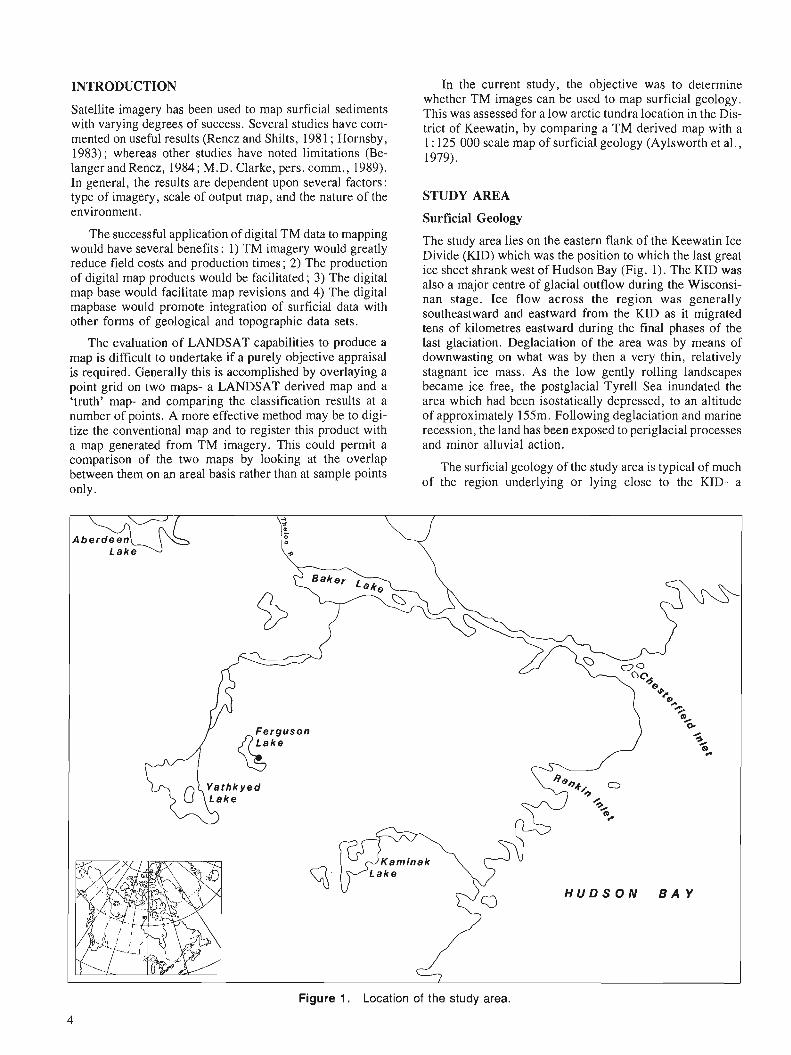
The study area lies on the eastern flank of the Keewatin Ice Divide (KID) which was the position to which the last great ice sheet shrank west of Hudson Bay (Fig. 1). The KID was also a major centre of glacial outflow during the Wisconsi- nan stage. Ice flow across the region was generally southeastward and eastward from the KID as it migrated tens of kilometres eastward during the final phases of the last glaciation. Deglaciation of the area was by means of downwasting on what was by then a very thin, relatively stagnant ice mass. As the low gently rolling landscapes became ice free, the postglacial Tyrell Sea inundated the area which had been isostatically depressed, to an altitude of approximately 155m. Following deglaciation and marine recession, the land has been exposed to periglacial processes and minor alluvial action.

'The surficial geology of the study area is typical of much of the region underlying or lying close to the KID- a

Figure 1. Location of the study area.

4

generally featureless till plain; till of varying thickness blankets the underlying bedrock and is dominant between the areas of abundant bedrock outcrop. The till surface is vegetated by shrubs, heath plants, mosses, and grasses growing in elevated peaty rings usually 1-2m in diameter. The bedrock surface is either rounded and glacially polished or covered by frost-shattered felsenmeer. Marine deposits are not common and, with the exception of a few nearshore features, consist of sand and clayey silt washed from till slopes by wave action and redeposited as a sandy apron at the base of slopes or as a silty fill in low flat areas. In the flat areas it has been covered by a 0.4-1.0m thick deposit of peat which effectively obscures the nature of the underlying silty sediment.

The units on the conventional surficial geology map of the study area can be summarized as follows. Rock (R) designates areas of greater than 80 % bedrock outcrop : in this region mainly layered Archean gneiss. Rockltill (RIT) is a generalized unit designating areas of discontinuous till plain with 20 to 80 % bedrock outcrop or bedrock very close to the surface. Till plain (Tp) consists of a blanket of pinkish or red, sandy silty till. Striped till (Ts) is a sub-unit of Tp and refers to the prominent striped pattern consisting of alternating stripes of light and dark-toned vegetation that runs parallel to slope direction. In some cases the light tone represents mineral soil. The striping probably results from solifluction processes on particularily fine grained sub- strates. There are minor areas of ice-contact stratified drift (Gk). These are mainly small esker segments but also include small hummocky gravel deposits with a probable ice-contact origin. A few beaches occur, formed during marine recession, and are difficult to distinguish from small areas of Gk. As both Mn and Gk are unvegetated gravel deposits, they will have very similar spectral signatures, and for the purpose of this paper they are treated as one unit, beachlesker (Ag). A1 is an undifferentiated unit of modern alluvium and marine mud, commonly peat covered and characterized by frost polygons and marshy areas; it also includes some areas of unvegetated alluvium.

DATA SETS

The LANDSAT TM image we have used for this study was aquired on 15 July, 1986. The thermal band (band 6) was not used in the classification. The map of surficial geology (1 : 125 000) was compiled from air photo interpretation with some ground verification (Aylsworth eta]., 1981). The two maps will be referred to as the TM map and the conventional map.

DATA PROCESSING

Digitizing Conventional M a p

The processing of the conventional map was carried out on a micro-computer using a commercially produced geographic information system (TYDAC, 1989). The boundaries of all the surficial units on the conventional map were digitized manually. An area of 30 x 30 km was outlined on the 1 : 125 000 map and all the units in this area were traced.

Each separate polygon on the map was given a unique identifying number and these were later grouped into their representative surficial geology classes using a look up table. The seven units as discussed above were: rock, rockltill, till plain, striped till, alluvium, beachlesker and water. The digitized map was 'imported' into the computer system using 5 geographic reference points. These points were used to ensure that the image of surficial data would be registered to a topographic map.

Classifying LANDSAT TM Data

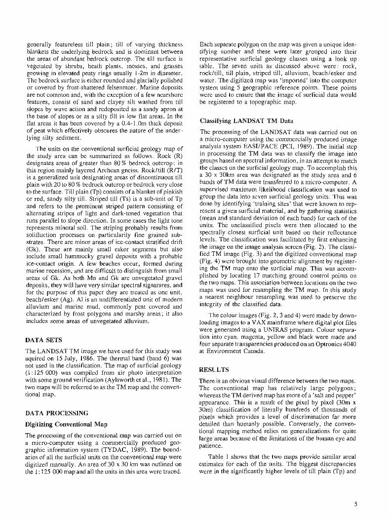
The processing of the LANDSAT data was carried out on a micro-computer using the commercially produced image analysis system EASIIPACE (PCI, 1989). The initial step in processing the TM data was to classify the image into groups based on spectral information, in an attempt to match the classes on the surficial geology map. To accomplish this a 30 x 30km area was designated as the study area and 6 bands of TM data were transferred to a m i ~ r o ~ c o m ~ u t e r . A supervised maximum likelihood classification was used to group the data into seven surficial geology units. This was done by identifying 'training sites' that were known to represent a given surficial material, and by gathering statistics (mean and standard deviation of each band) for each of the units. The unclassified pixels were then allocated to the spectrally closest surficial unit based on their reflectance levels. The classification was facilitated by first enhancing the image on the image analysis screen (Fig. 2). The classified TM image (Fig. 3) and the digitized conventional map (Fig. 4) were brought into geometric alignment by registering the TM map onto the surficial map. This was accomplished by locating 17 matching ground control points on the two maps. This association between locations on the two maps was used for resampling the TM map. In this study a nearest neighbour resampling was used to preserve the integrity of the classified data.

The colour images (Fig. 2 , 3 and 4) were made by down- loading images to a VAX mainframe where digital plot files were generated using a UNTRAS program. Colour separation into cyan, magenta, yellow and black were made and four separate transparencies produced on an Optronics 4040 at Environment Canada.

RESULTS

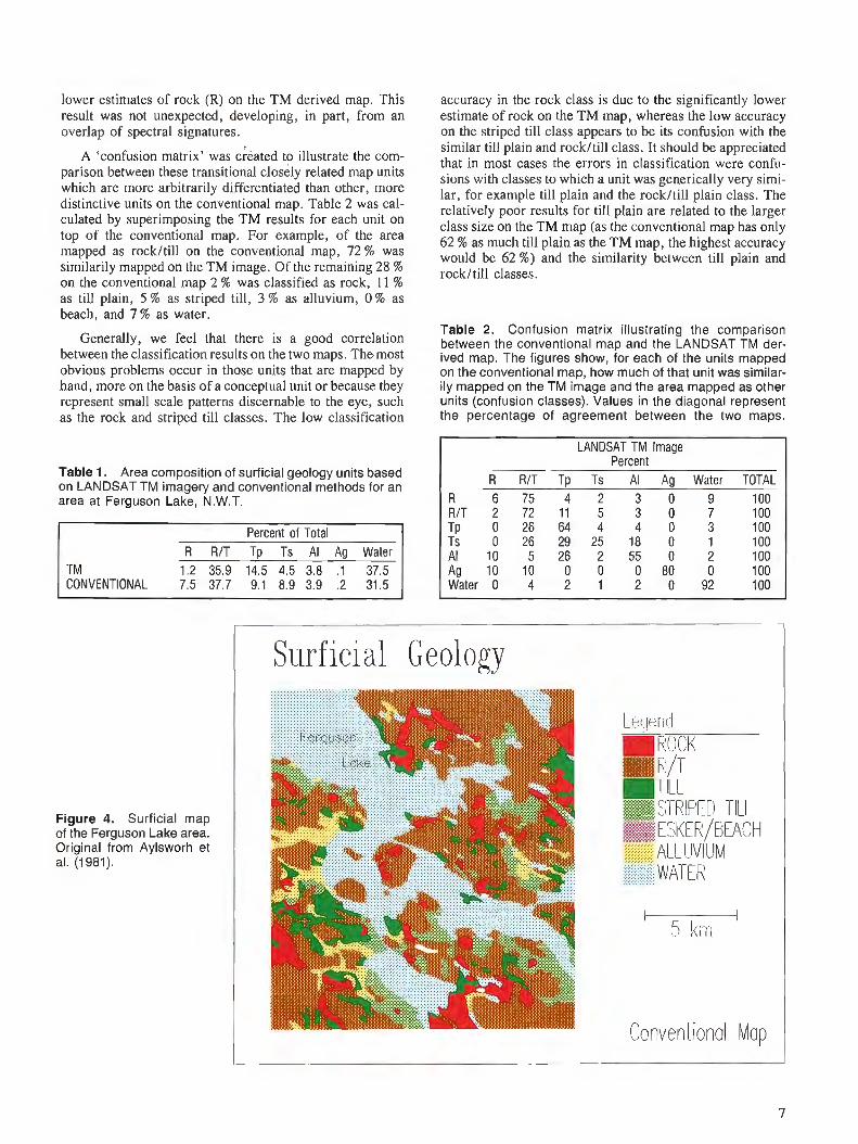
There is an obvious visual difference between the two maps. The conventional map has relatively large polygons; whereas the TM derived map has more of a 'salt and pepper' appearance. This is a result of the pixel by pixel (30m x 30m) classification of literally hundreds of thousands of pixels which provides a level of discrimination far more detailed than humanly possible. Conversely, the conventional mapping method relies on generalizations for quite large areas because of the limitations of the human eye and patience.

Table 1 shows that the two maps provide similar areal estimates for each of the units. The biggest discrepancies were in the significantly higher levels of till plain (Tp) and

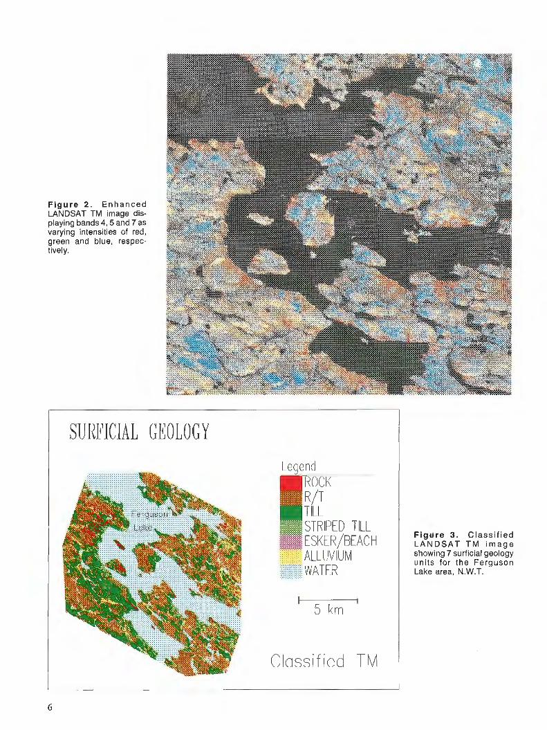
Figure 2. Enhanced LANDSAT TM image displaying bands 4,5 and 7 as varying intensities of red, green and blue, respectively.

SURFICIAL GEOLOGY

Classified TM

Figure 3. Class i f ied LANDSAT T M i m a g e showing 7 surficial geology units for the Ferguson Lake area, N.W.T.

lower estimates of rock (R) on the TM derived map. This result was not unexpected, developing, in part, from an overlap of spectral signatures.

A 'confusion matrix' was ckated to illustrate the comparison between these transitional closely related map units which are more arbitrarily differentiated than other, more distinctive units on the conventional map. Table 2 was calculated by superimposing the TM results for each unit on top of the conventional map. For example, of the area mapped as rockltill on the conventional map, 72 % was similarily mapped on the TM image. Of the remaining 28 % on the conventional map 2 % was classified as rock, 11 % as till plain, 5 % as striped till, 3 % as alluvium, 0 % as beach, and 7 % as water.

Generally, we feel that there is a good correlation between the classification results on the two maps. The most obvious problems occur in those units that are mapped by hand, more on the basis of a conceptual unit or because they represent small scale patterns discernable to the eye, such as the rock and striped till classes. The low classification

Table 1. Area composition of surficial geology units based on LANDSAT TM imagery and conventional methods for an area at Ferguson Lake, N.W.T.

Percent of Total R RIT Tp Ts Al Ag Water

CONVENTIONAL 7.5 37.7 9.1 8.9 3.9 .2 31.5

Figure 4. Surficial map of the Ferguson Lake area. Original from Aylsworh et al. (1981).

accuracy in the rock class is due to the significantly lower estimate of rock on the TM map, whereas the low accuracy on the striped till class appears to be its confusion with the similar till plain and rockltill class. It should be appreciated that in most cases the errors in classification were confu- sions with classes to which a unit was generically very similar, for example till plain and the rockltill plain class. The relatively poor results for till plain are related to the larger class size on the TM map (as the conventional map has only 62 % as much till plain as the TM map, the highest accuracy would be 62 %) and the similarity between till plain and rockltill classes.

Table 2. Confusion matrix illustrating the comparison between the conventional map and the LANDSAT TM derived map. The figures show, for each of the units mapped on the conventional map, how much of that unit was similarily mapped on the TM image and the area mapped a s other units (confusion classes). Values in the diagonal represent the percentage of agreement between the two maps.

LANDSAT TM Image Percent

R RIT Tp Ts Al Ag Water TOTAL R 6 7 5 4 2 3 0 9 100 RIT 2 72 11 5 3 0 7 100 Tp 0 26 64 4 4 0 3 100 Ts 0 26 29 25 18 0 1 100 Al 10 5 26 2 55 0 2 100 AQ 10 10 0 0 0 80 0 100 Water 0 4 2 1 2 0 92 100

Surf icial Geology

:;TRIFE[:i TILL E:;KER/BEACH

-ALL!..IVIUI\A

Conventional Map I

1 I

1 BAND 1

70 f 1

BAND 4 1 , 45

l-

BAND 7

30 t

l -r

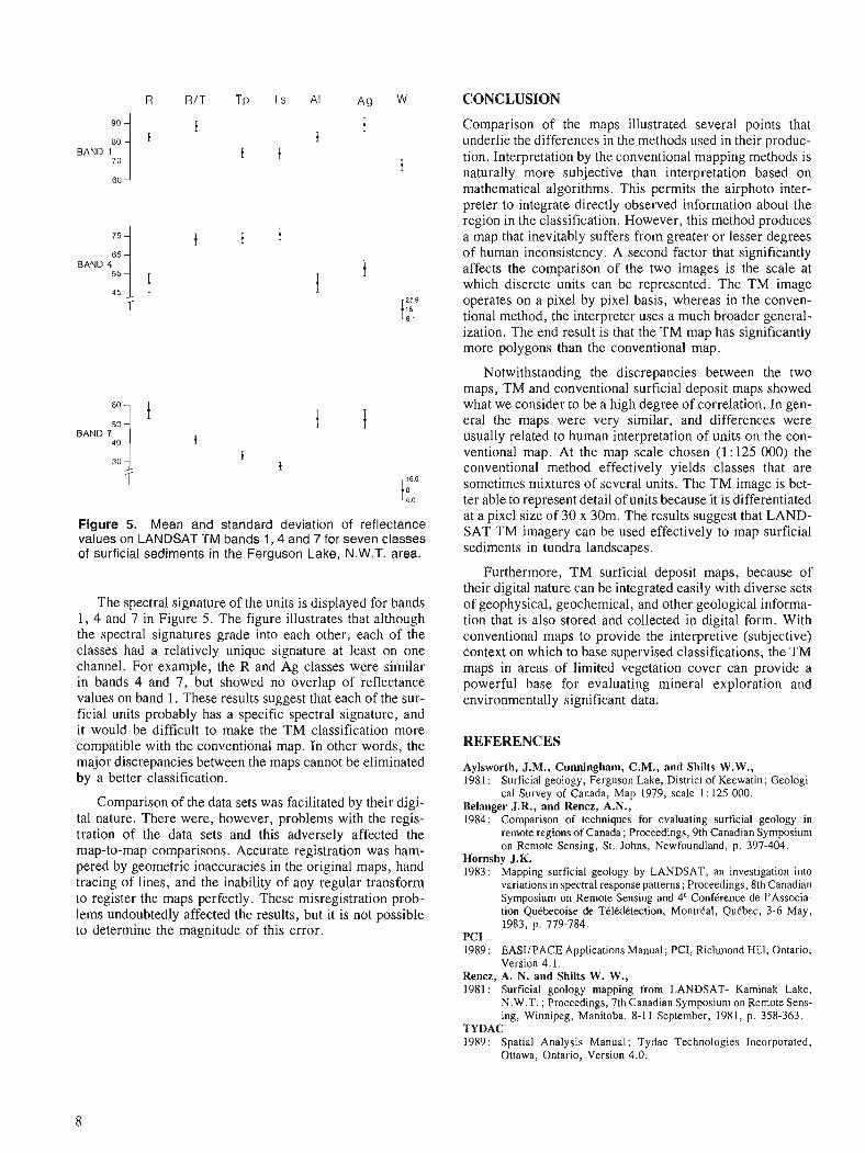
Figure 5. Mean and standard deviation of reflectance values on LANDSAT TM bands 1 , 4 and 7 for seven classes of surficial sediments in the Ferguson Lake, N.W.T. area.

The spectral signature of the units is displayed for bands 1, 4 and 7 in Figure 5. The figure illustrates that although the spectral signatures grade into each other, each of the classes had a relatively unique signature at least on one channel. For example, the R and Ag classes were similar in bands 4 and 7, but showed no overlap of reflectance values on band 1. These results suggest that each of the surficial units probably has a specific spectral signature, and it would be difficult to make the TM classification more compatible with the conventional map. In other words, the major discrepancies between the maps cannot be eliminated by a better classification.

Comparison of the data sets was facilitated by their digital nature. There were, however, problems with the registration of the data sets and this adversely affected the map-to-map comparisons. Accurate registration was hampered by geometric inaccuracies in the original maps, hand tracing of lines, and the inability of any regular transform to register the maps perfectly. These misregistration problems undoubtedly affected the results, but it is not possible to determine the magnitude of this error.

CONCLUSION

Comparison of the maps illustrated several points that underlie the differences in the methods used in their production. Interpretation by the conventional mapping methods is naturally more subjective than interpretation based on mathematical algorithms. This permits the airphoto interpreter to integrate directly observed information about the region in the classification. However, this method produces a map that inevitably suffers from greater or lesser degrees of human inconsistency. A second factor that significantly affects the comparison of the two images is the scale at which discrete units can be represented. The TM image operates on a pixel by pixel basis, whereas in the conventional method, the interpreter uses a much broader generalization. The end result is that the TM map has significantly more polygons than the conventional map.

Notwithstanding the discrepancies between the two maps, TM and conventional surficial deposit maps showed what we consider to be a high degree of correlation. In general the maps were very similar, and differences were usually related to human interpretation of units on the conventional map. At the map scale chosen (1: 125 000) the conventional method effectively yields classes that are sometimes mixtures of several units. The TM image is better able to represent detail of units because it is differentiated at a pixel size of 30 x 30m. The results suggest that LAND- SAT TM imagery can be used effectively to map surficial sediments in tundra landscapes.

Furthermore, TM surficial deposit maps, because of their digital nature can be integrated easily with diverse sets of geophysical, geochemical, and other geological information that is also stored and collected in digital form. With conventional maps to provide the interpretive (subjective) context on which to base supervised classifications, the TM maps in areas of limited vegetation cover can provide a powerful base for evaluating mineral exploration and environmentally significant data.

REFERENCES

Aylsworth, J.M., Cunningham, C.M., and Shilts W.W., 1981 : Surficial geology, Ferguson Lake, District of Keewatin; Geologi-

cal Survey of Canada, Map 1979, scale 1 : 125 000. Belanger J.R., and Rencz, A.N., 1984: Comparison of techniques for evaluating surficial geology in

remote regions of Canada; Proceedings, 9th Canadian Symposium on Remote Sensing, St. Johns, Newfoundland, p. 397-404.

Hornsby J.K. 1983: Mapping surficial geology by LANDSAT, an investigation into

variations in spectral response patterns; Proceedings,.Bth Canadian Symposium on Remote Sensing and 4' ConfCrence de I'Associa- tion QuCbecoise de TClCdCtection, MontrCal, QuCbec, 3-6 May, 1983, p. 779-784.

PC1 1989: EASIIPACE Applications Manual ; PCI, Richmond Hill, Ontario,

Version 4.1. Rencz, A. N. and Shilts W. W., 1981: Surficial geology mapping from LANDSAT- Kaminak Lake,

N.W.T. : Proceedings. 7th Canadian Svmoosium on Remote Sens- ing, winnipeg, ~a;thba. 8-11 septe;nder, 1981, p. 358-363

TYDAC 1989: Spatial Analysis Manual; Tydac Technologies Incorporated,

Ottawa, Ontario, Version 4.0.

Project GEOVISIONI : a geological information system applied to the integration of digital elevation,

remote sensing and geological data

Hans Isaksson2 and Christer Andersson3

Isaksson, H. and Andersson, C., Project GEOVISION: a geological information system applied to the integration of digital elevation, remote sensing and geological data; in Statistical Applications in the Earth Sciences, ed. F. P. Agterberg and G. F. Bonham-Carter; Geological Survey of Canada, Paper 89-9, p. 9-18, 1989.

Abstract

Soils with high content of copper in the Kiruna region, northern Sweden, are known to correspond to open grass areas with the Jlower "Viscaria Alpina ". Such locations also occur at two dijferent Cu- orebodies, Viscaria and central Pahtohavare. A study of the metal effect on vegetation has been performed using satellite data, a digital elevation model and vegetation mapping from airphotos. i%e result from the study is integrated with other geological information to provide a priority of the targets.

I1 est connu que les sols caractkrise's par une teneur klevke en cuivre, duns la re'gion du Kiruna au nord de la Su2de, correspondent aux rtfgions ouvertes & v6gtftation herbacke ou se manifeste la fleur (( Viscaria Alpina N. La situation est aussi la m&me a l'emplacement de deux difSerents corps minkralisb en Cu, Viscaria et la rkgion centrale de Pathohavare. On a rhlisk une ktude de l'influence des mktaux sur la ve'gktation, en faisant appel aux donnkes satellitaires, en employant un modgle numkrique de l'altitude, et en cartographiant la v6gktation d'apr2s les photos atfriennes. Les rksultats de l'ktude ont ktk intkgrks au reste de 1 'information gtfologique, et permettront ainsi de classer les cibles selon leurprioritb.

' The name GEOVISION is a project name. The project was formed in 1984 and is registered as a project within different government organizations in Sweden. Swedish Geological Company, Box 801, S-951 Lulea, Sweden ' Swedish Space Corporation, Box 4207, S- 17 1-04 Solna, Sweden

INTRODUCTION

The GEOVISION Project is a concentrated joint effort between the Swedish Geological Co (SGAB) and the Swed- ish Space Corporation (SSC) within the field of land information. The project work involves geological data processing, visualization and editing of map data, image processing and analysis of data matrices and integration of different information strata. The project uses the rapid technical development within the GIS field and adapts the methodology to the specific needs of geologists.

There are many striking examples of this kind of development within other sectors, for example the transition within the graphics industry to desktop publishing and the adoption of CAD by the design industry. GEOVISION is a practical method development project for the processing of geological data. We do not develop new data structures for improved GIS handling, nor do we develop hardware. Software development is also fairly limited. We adapt, sup- plement and integrate systems that are in completed form and already available on the market. In this way, we rapidly arrive at results that can be introduced directly into production.

About 40 % of GEOVISION financing is supported by the Swedish Government in the "Programme for increased exploration".

OBJECTIVES

'The aims of GEOVISION are concerned with: * developing a geologically-adapted GIS for the process-

ing and analysis of geological data; * developing methods, based on modern information tech-

nology, for rationalizing and refining the work carried out in connection with geological exploration and mapping ;

* augmenting experience and strengthening the know-how of Swedish geological operations within the fields of remote sensing and image processing.

A CASE STUDY: METAL STRESS ON VEGETATION AT PAHTOHAVARE

Objective

The aim of this summary from the project "Metal stress on vegetation", is to provide an example of the idea behind the GEOVISION project and demonstrate the practical application of the technique. The emphasis here is to describe how the project provided new tools to co-process and analyze

I Rectangular grid I I 1 Satellite 1 Ground 1 Scattered paints 1 Aerosurvey survey

I 1 Magnetic iields I Electromagnetic fields

Electrical fields Grav~ty

I

Partly continuous Natural Geochemical analysis characteristics emission

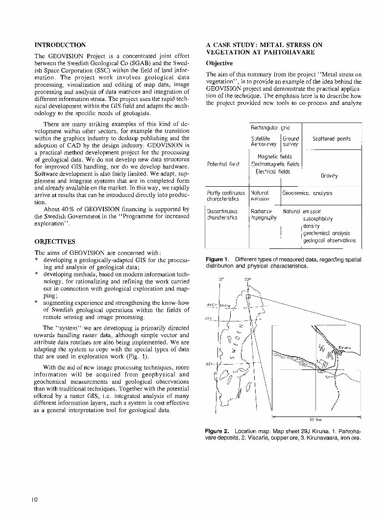
Figure 1. Different types of measured data, regarding spatial distribution and physical characteristics.

Discontinuous chamterist~cs

The "system" we are developing is primarily directed towards handling raster data, although simple vector and attribute data routines are also being implemented. We are adapting the system to cope with the special types of data that are used in exploration work (Fig. 1).

With the aid of new image processing techniques, more information will be acquired from geophysical and geochemical measurements and geological observations than with traditional techniques. Together with the potential offered by a raster GIS, i.e. integrated analysis of many different information layers, such a system is cost effective as a general interpretation tool for geological data.

Rad~ance topography

Figure 2. Location map. Map sheet 29J Kiruna. 1. Pahtoha- vare deposits, 2. Viscaria, copper ore, 3. Kirunavaara, iron ore.

Natural emission suscept~ bi l~ty density geochemical analysis geolog~cal observat~ons

geological data. The work, which has been run by SGAB for the State Mining Property Commission (NSG), describes a geobotanical study around the copper deposit at Pahtohavare-Kiruna.

Study area

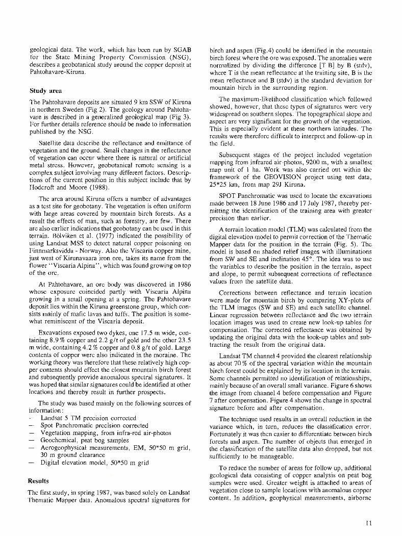
The Pahtohavare deposits are situated 9 krn SSW of Kiruna in northern Sweden (Fig 2). The geology around Pahtoha- vare is described in a generalized geological map (Fig 3). For further details reference should be made to information published by the NSG.

Satellite data describe the reflectance and emittance of vegetation and the ground. Small changes in the reflectance of vegetation can occur where there is natural or artificial metal stress. However, geobotanical remote sensing is a complex subject involving many different factors. Descrip- tions of the current position in this subject include that by Hodcroft and Moore (1988).

The area around Kiruna offers a number of advantages as a test site for geobotany. The vegetation is often uniform with large areas covered by mountain birch forests. As a result thk effects of man, such as forestry, are few. There are also earlier indications that geobotany can be used in this terrain. Bolviken et al. (1977) indicated the possibility of using Landsat MSS to detect natural copper poisoning on Finnmarksvidda - Norway. Also the Viscaria copper mine, just west of Kirunavaara iron ore, takes its name from the flower "Viscaria Alpina", which was found growing on top of the ore.

At Pahtohavare, an ore body was discovered in 1986 whose exposure coincided partly with Viscaria Alpina growing in a small opening at a spring. The Pahtohavare deposit lies within the Kiruna greenstone group, which consists mainly of mafic lavas and tuffs. The position is somewhat reminiscent of the Viscaria deposit.

Excavations exposed two dykes, one 17.5 m wide, containing 8.9 % copper and 2.2 g l t of gold and the other 23.5 m wide, containing 4.2 % copper and 0.8 g / t of gold. Large contents of copper were also indicated in the moraine. The worlung theory was therefore that these relatively high copper contents should effect the closest mountain birch forest and subsequently provide anomalous spectral signatures. It was hoped that similar signatures could be identified at other locations and thereby result in further prospects.

The study was based mainly on the following sources of information : - Landsat 5 TM precision corrected - Spot Panchromatic precision corrected - Vegetation mapping, from infra-red air-photos - Geochemical, peat bog samples - Aerogeophysical measurements, EM, 50*50 m grid,

30 m ground clearance - Digital elevation model, 50*50 m grid

Results

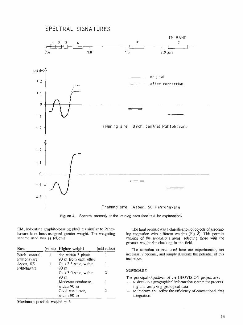
The first study, in spring 1987, was based solely on Landsat Thematic Mapper data. Anomalous spectral signatures for

birch and aspen (Fig.4) could be identified in the mountain birch forest where the ore was exposed. The anomalies were normalized by dividing the difference [T-B] by B (stdv), where T is the mean reflectance at the training site, B is the mean reflectance and B (stdv) is the standard deviation for mountain birch in the surrounding region.

The maximum-likelihood classification which followed showed, however, that these types of signatures were very widespread on southern slopes. The topographical slope and aspect are very significant for the growth of the vegetation. This is especially evident at these northern latitudes. The results were therefore difficult to interpret and follow-up in the field.

Subsequent stages of the project included vegetation mapping from infrared air-photos, 9200 m, with a smallest map unit of 1 ha. Work was also carried out within the framework of the GEOVISION project using test data, 25*25 krn, from map 295 Kiruna.

SPOT Panchromatic was used to locate the excavations made between 18 June 1986 and 17 July 1987, thereby permitting the identification of the training area with greater precision than earlier.

A terrain location model (TLM) was calculated from the digital elevation model to permit correction of the Thematic Mapper data for the position in the terrain (Fig. 5). The model is based on shaded relief images with illuminations from SW and S E and inclination 45". The idea was to use the variables to describe the position in the terrain, aspect and slope, to permit subsequent corrections of reflectance values from the satellite data.

Corrections between reflectance and terrain location were made for mountain birch by comparing XY-plots of the TLM images (SW and SE) and each satellite channel. Linear regression between reflectance and the two terrain location images was used to create new look-up tables for compensation. The corrected reflectance was obtained by updating the original data with the look-up tables and subtracting the result from the original data.

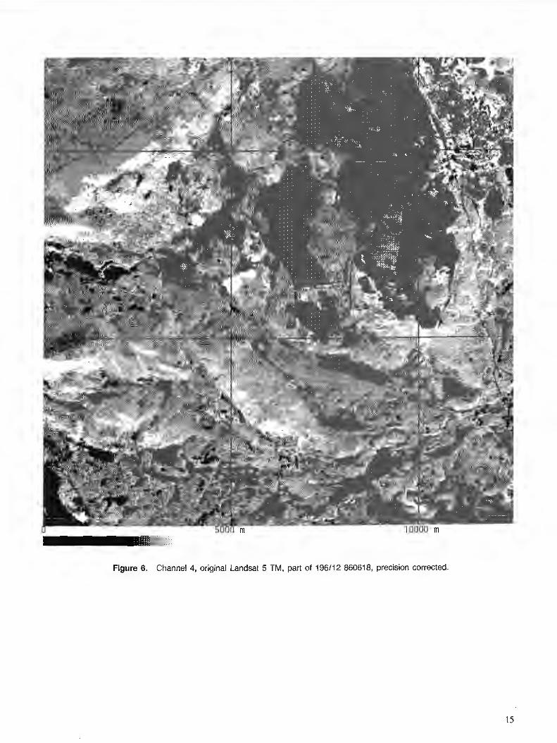
Landsat TM channel 4 provided the clearest relationship as about 70 % of the spectral variation within the mountain birch forest could be explained by its location in the terrain. Some channels permitted no identification of relationships, mainly because of an overall small variance. Figure 6 shows the image from channel 4 before compensation and Figure 7 after compensation. Figure 4 shows the change in spectral signature before and after compensation.

The technique used results in an overall reduction in the variance which, in turn, reduces the classification error. Fortunately it was then easier to differentiate between birch forests and aspen. The number of objects that emerged in the classification of the satellite data also dropped, but not sufficiently to be manageable.

To reduce the number of areas for follow up, additional geological data consisting of copper analysis on peat bog samples were used. Greater weight is attached to areas of vegetation close to sample locations with anomalous copper content. In addition, geophysical measurements, airborne

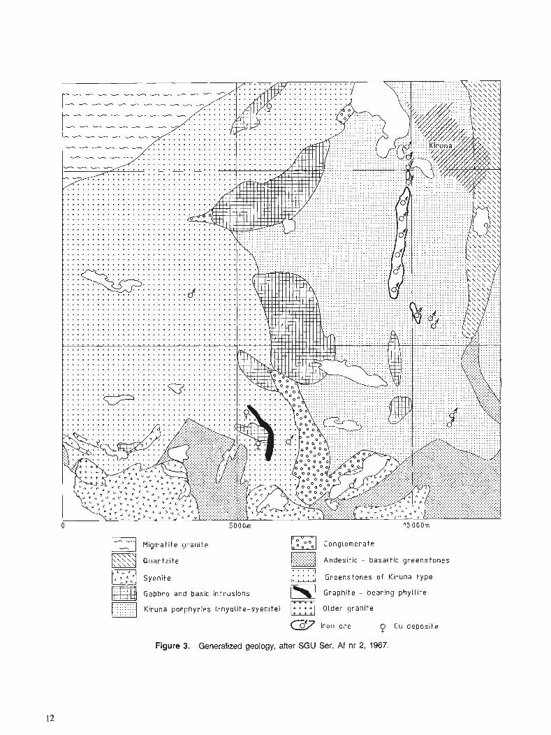
[ Migmatite gran i te Conglomerate . . . . . . , .

Qua r t z i t e m] Andesit i r - basatt ic greenstones ,... .... 17 ,. Syenite Greenstones o f Kiruna t y p e

Gabbro and basic in t rus ions Graphi te - bear ing phy l l i t e

Kiruna porphyr ies ( rhyo l i te -syen i te l Older gran i te .........,

Cdj7 l ron ore 9 Cu deposi te

Figure 3. Generalized geology, after SGU Ser. Af nr 2, 1967.

SPECTRAL SIGNATURES T M - B A N D

or ig ina l

--- a f t e r c o r r e c t i o n

- f Training s i te : Birch, c e n t r a l P a h t o h a v a r e

1 Train ing s i te ; Aspen, SE P a h t o h a v a r e

Figure 4. Spectral anomaly at the training sites (see text for explanation).

EM, indicating graphite-bearing phyllites similar to Pahto- havare have been assigned greater weight. The weighting scheme used was as follows:

Base (value) Higher weight (add value)

Birch, central 1 d:o withn 3 pixels 1 Pahtohavare 90 m from each other Aspen, SE 1 Cu>2.5 stdv, within 1 Pahtohavare 90 rn

Cu>3.0 stdv, within 2 90 m Moderate conductor, 1 within 90 m Good conductor, 2 within 90 m

Maximum possible weight = 6

The final product was a classification of objects of associat- ing vegetation with different weights (Fig 8). This permits ranking of the anomalous areas, selecting those with the greatest weight for checking in the field.

The selection criteria used here are experimental, not necessarily optimal, and simply illustrate the potential of this technique.

SUMMARY

The principal objectives of the GEOVISION project are: - to develop a geographical information system for process-

ing and analyzing geological data; - to improve and refine the efficiency of conventional data

integration.

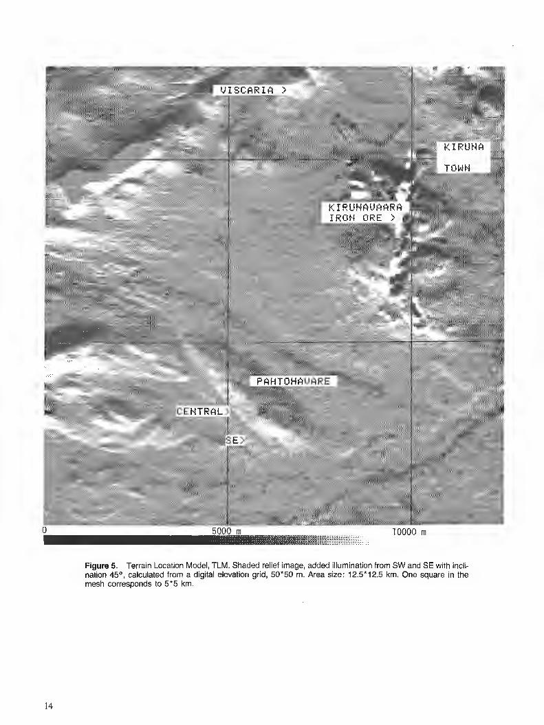
Figure 5. Terrain Location Model, TLM. Shaded relief image, added illumination from SW and SE with inclination 4 5 O , calculated from a digital elevation grid, 50*50 m. Area size: 12.5*12.5 km. One square in the mesh corresponds to 5*5 km.

3 A

.' :

Figure 6. Channel 4, original Landsat 5 TM, part of 196112 860618, precision corrected.

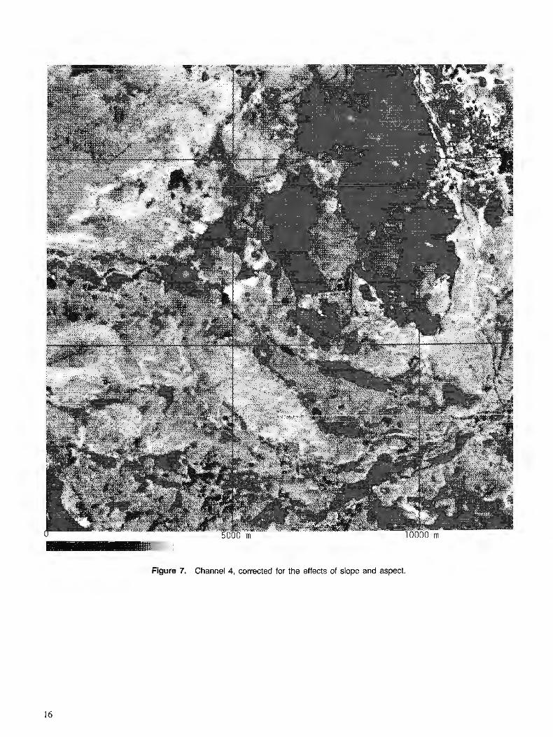
Figure 7. Channel 4, corrected for the effects of slope and aspect.

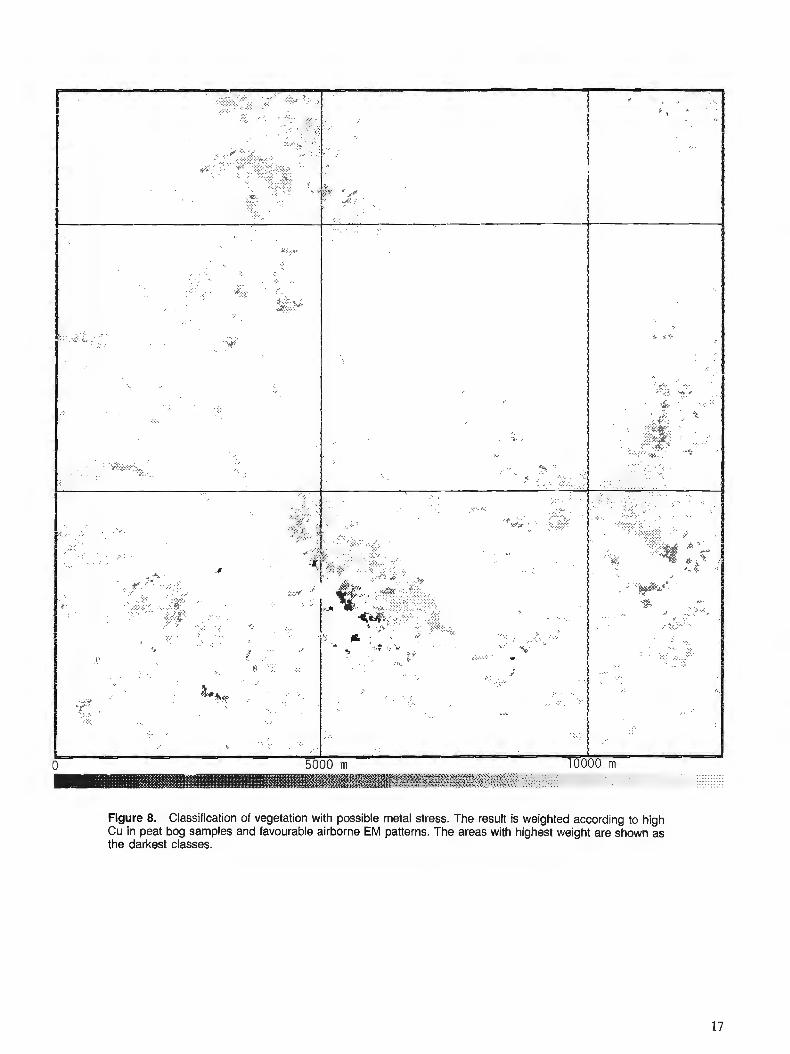
Figure 8. Classification of vegetation with possible metal stress. The result is weighted according to high Cu in peat bog samples and favourable airborne EM patterns. The areas with highest weight are shown as the darkest classes.

The project has already permitted the inclusion of "new" types of data. New co-processing and co-analysis techniques are being used. Ideas for new map products are being generated due to the flexibility of the processing system.

We believe that the technique of interactive processing, visualization and analysis are only in their infancy. Develop- ment will take place even faster and then it will be necessary to have a good and flexible basic system to continue the work. This is the type of platform that is now starting to take shape within the GEOVISION project.

ACKNOWLEDGMENTS

We thank all members of the GEOVISION project for their contributions to thjs paper. We also thank the State Mining Property Commission for permission to present the results of the "Pahtohavare-Metal stress' ' project.

REFERENCES

~olviken, B. Honey F., Levine S.R., Lyon R.J.P. and Prelat, A. 1977 : Detection of naturally heavy-metal-poisoned areas by Landsat-l digital

data, Journal of Geochemical Exploration, v. 8, p. 457471. Hodcroft A.J.T. and Moore J.McM, 1988: Remote sensing of vegetation - a promising exploration tool, Mining

Magazine, October 1988, p. 274-279. The State Mining Property Commission (NSG) 1988: Pahtohavare -gold and copper in Kiruna, A Prospectus, 1988. Isaksson, H. 1987: Pahtohavare - Digital bildanalys, satellitdata - Metodutveckling; NSG

internal report PRAP 87030. 1988: Pahtohavare - Metallstress U , NSG internal report PRAP 88043. Albertsson, J., 1988: Specialkarta - Pahtohavare" NSG-commission, LMV 1988.

Clustering of gamma ray spectrometer data using a computer image analysis system

Harris, J . , Clustering of gamma ray spectrometer data using a cotnputer image analysis system; & Statistical Applications in the Earth Sciences, ed. F. P. Agterberg and G. F. Bonham-Carter; Geological Survey of Can- ada, Paper 89-9, p. 19-31, 1989.

Abstract

High resolution airborne gamma ray spectrometer data of eastern Nova Scotia, collected by the Geologi- cal Survey of Canada, are class$ed using a migrating means unsupervised clustering algorithm, using sop- ware which is resident on a number of computer image analysis systems within the Canada Centre for Remote Sensing (CCRS). Several classijcations, comprising combinations of d~fferent spectrometer channels (eU, e n , K, eU/eTh, eU/K, e R / K ) , are produced and compared to the available bedrock andsu@cial geological maps to evaluate the spatial characteristics of each cluster. Furthermore, the classijications are compared with one another to assess the best combination of channels for use in the clustering algorithm. Techniques for displaying the clusters using an IHS (intensity, hue, saturation) transform are discussed.

Clustering was found to be an effective technique for generalizing and partitioning the gamma ray data into similar groups that, in this study, resulted in spatially continuous radioelement classes which could be related to the mapped geology. A four-channel (eU, e m , K ,eU/eTh) and a sk-channel (eU, e m , K, eUIeTh, eU/K, eTh/K) classijication produced the best results itz temw of correlation with mapped geology.

Les donne'es spectr?m'triques gamma obtenues lors de leve's akroportks de haute re'solution effectue's dans l'est de la Nouvelle-Ecosse, par la Commission g6ologique du Canada, ont ktk classkes ri l'aide d'un algonthme de groupage non dirigkci myenne mobile, le logiciel employe' e'tant rksident sur un certain nombre de syst2mes d'analyse informutique des images utilise's par le Centre canadien de te'lkde'tection (CCT). On a produit plusieurs classijications, notamment des combinuisons de divers canaux spectromkttiques (eU, e n , K, eU/el3t, eU/K, eTh/K), et on les a compare'es aux cartes ge'ologiques existantes de la roche en place et des formations en suflace, pour e'valuer les caracte'ristiques spatiales de chaque groupe. De plus, on a compare' les classijications les unes aux autres, a j n d'kvaluer la meilleure cornbinaison de canaux que l'on puisse utiliser duns 1 'algonthme de groupage. On examine les techniques de visualisation des groupes au moyen d'une transformke ITS (intensitk, teinte, saturation).

On a constate' que le groupage ktait une technique eficace pour gknkraliser et rkpartir les donnkes spec- trome'triques gamma en groupes similaires qui, dans la pr6sente ktude, ont constitue' des classes de radio- klkments spatialement continues, pouvant 2tre likes a la ge'ologie telle que cartographi6e. Une classification en fonction de quatre canaux (eU, e n , K, eU/eTh) et six canaux (eU, e m , K, eU/ei'%, eU/K, e n / K ) a donne' les meilleurs rksultats, du point de vue de la corre'lation avec la gkologie cartographike.

' RADARSAT Project Office, INTERA Technologies Ltd.lCanada Centre for Remote Sensing 110 O'comor St., Ottawa, Ontario KIP 5M9

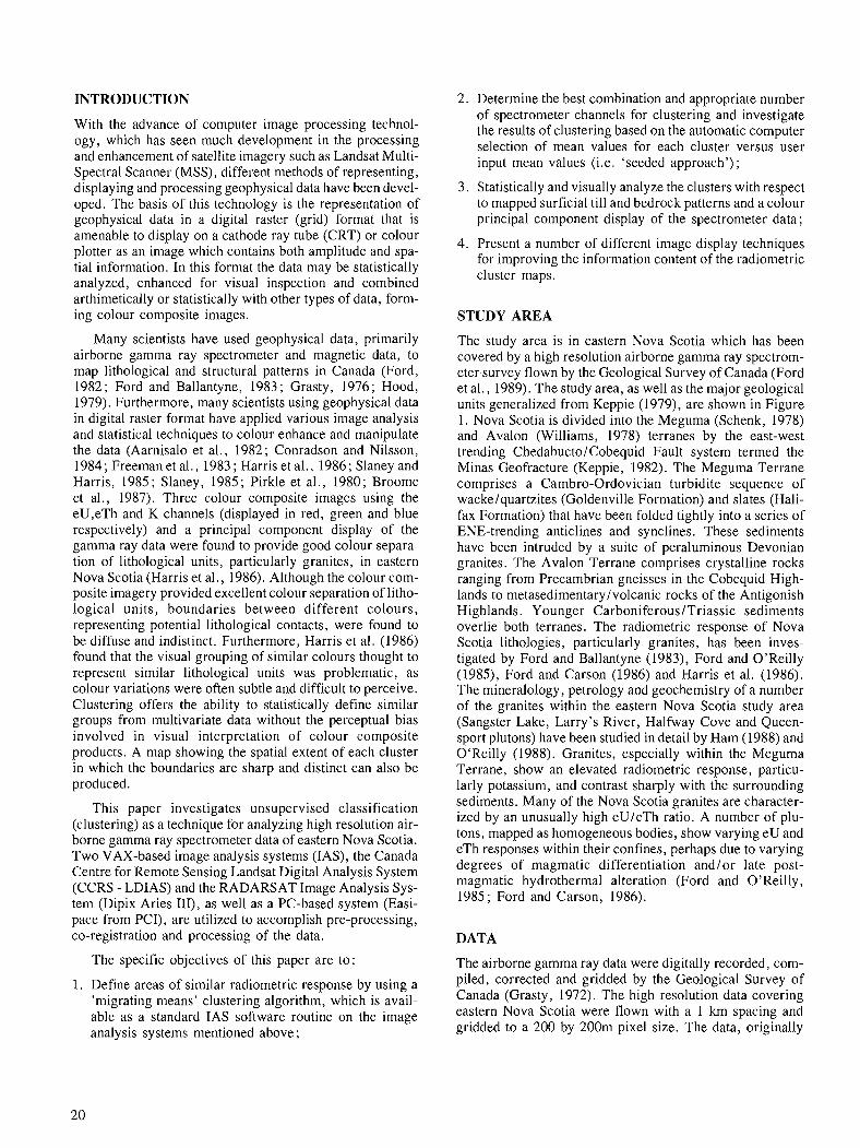
INTRODUCTION

With the advance of computer image processing technology, which has seen much development in the processing and enhancement of satellite imagery such as Landsat Multi- Spectral Scanner (MSS), different methods of representing, displaying and processing geophysical data have been developed. The basis of this technology is the representation of geophysical data in a digital raster (grid) format that is amenable to display on a cathode ray tube (CRT) or colour plotter as an image which contains both amplitude and spatial information. In this format the data may be statistically analyzed, enhanced for visual inspection and combined arthimetically or statistically with other types of data, forming colour composite images.

Many scientists have used geophysical data, primarily airborne gamma ray spectrometer and magnetic data, to map lithological and structural patterns in Canada (Ford, 1982; Ford and Ballantyne, 1983; Grasty, 1976; Hood, 1979). Furthermore, many scientists using geophysical data in digital raster format have applied various image analysis and statistical techniques to colour enhance and manipulate the data (Aarnisalo et al., 1982; Conradson and Nilsson, 1984; Freeman et al., 1983; Harris et al., 1986; Slaney and Harris, 1985 ; Slaney, 1985 ; Pirkle et al., 1980; Broome et al., 1987). Three colour composite images using the eU,eTh and K channels (displayed in red, green and blue respectively) and a principal component display of the gamma ray data were found to provide good colour separation of lithological units, particularly granites, in eastern Nova Scotia (Harris et al., 1986). Although the colour composite imagery provided excellent colour separation of lithological units, boundaries between different colours, representing potential lithological contacts, were found to be diffuse and indistinct. Furthermore, Harris et al. (1986) found that the visual grouping of similar colours thought to represent similar lithological units was problematic, as colour variations were often subtle and difficult to perceive. Clustering offers the ability to statistically define similar groups from multivariate data without the perceptual bias involved in visual interpretation of colour composite products. A map showing the spatial extent of each cluster in which the boundaries are sharp and distinct can also be produced.

This paper investigates unsupervised classification (clustering) as a technique for analyzing high resolution airborne gamma ray spectrometer data of eastern Nova Scotia. Two VAX-based image analysis systems (IAS), the Canada Centre for Remote Sensing Landsat Digital Analysis System (CCRS - LDIAS) and the RADARSAT Image Analysis Sys- tem (Dipix Aries 111), as well as a PC-based system (Easi- pace from PCI), are utilized to accomplish pre-processing, co-registration and processing of the data.

The specific objectives of this paper are to:

1. Define areas of similar radiometric response by using a 'migrating means' clustering algorithm, which is available as a standard IAS software routine on the image analysis systems mentioned above;

2. Determine the best combination and appropriate number of spectrometer channels for clustering and investigate the results of clustering based on the automatic computer selection of mean values for each cluster versus user input mean values (i.e. 'seeded approach');

3. Statistically and visually analyze the clusters with respect to mapped surficial till and bedrock patterns and a colour principal component display of the spectrometer data ;

4. Present a number of different image display techniques for improving the information content of the radiometric cluster maps.

STUDY AREA

The study area is in eastern Nova Scotia which has been covered by a high resolution airborne gamma ray spectrometer survey flown by the Geological Survey of Canada (Ford et al., 1989). The study area, as well as the major geological units generalized from Keppie (1979), are shown in Figure 1. Nova Scotia is divided into the Meguma (Schenk, 1978) and Avalon (Williams, 1978) terranes by the east-west trending Chedabucto/Cobequid Fault system termed the Minas Geofracture (Keppie, 1982). The Meguma Terrane comprises a Cambro-Ordovician turbidite sequence of wackelquartzites (Goldenville Formation) and slates (Hali- fax Formation) that have been folded tightly into a series of ENE-trending anticlines and synclines. These sediments have been intruded by a suite of peralurninous Devonian granites. The Avalon Terrane comprises crystalline rocks ranging from Precambrian gneisses in the Cobequid High- lands to metasedimentary/volcanic rocks of the Antigonish Highlands. Younger Carboniferous/Triassic sediments overlie both terranes. The radiometric response of Nova Scotia lithologies, particularly granites, has been investigated by Ford and Ballantyne (1983), Ford and O'Reilly (1985), Ford and Carson (1986) and Harris et al. (1986). The mineralology, petrology and geochemistry of a number of the granites within the eastern Nova Scotia study area (Sangster Lake, Larry's River, Halfway Cove and Queen- sport plutons) have been studied in detail by Ham (1988) and O'Reilly (1988). Granites, especially within the Meguma Terrane, show an elevated radiometric response, particularly potassium, and contrast sharply with the surrounding sediments. Many of the Nova Scotia granites are characterized by an unusually high eU/eTh ratio. A number of plutons, mapped as homogeneous bodies, show varying eU and eTh responses within their confines, perhaps due to varying degrees of magmatic differentiation and/or late post- magmatic hydrothermal alteration (Ford and O'Reilly, 1985; Ford and Carson, 1986).

DATA

The airborne gamma ray data were digitally recorded, compiled, corrected and gridded by the Geological Survey of Canada (Grasty, 1972). The high resolution data covering eastern Nova Scotia were flown with a 1 krn spacing and gridded to a 200 by 200m pixel size. The data, originally

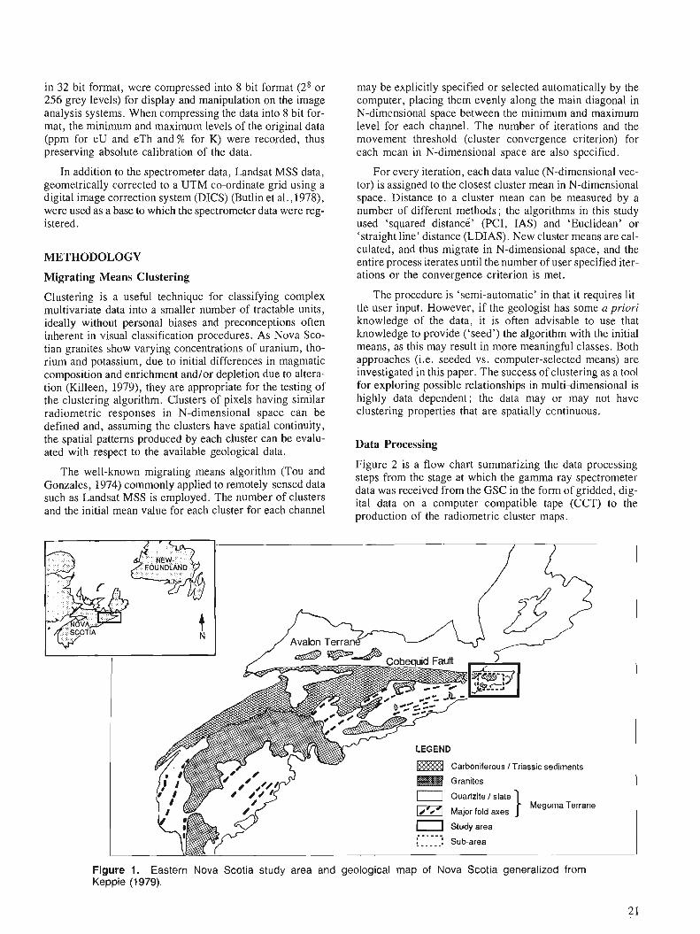
in 32 bit format, were compressed into 8 bit format (28 or may be explicitly specified or selected automatically by the 256 grey levels) for display and manipulation on the image computer, placing them evenly along the main diagonal in analysis systems. When compressing the data into 8 bit for- N-dimensional space between the minimum and maximum mat, the minimum and maximum levels of the original data level for each channel. The number of iterations and the (ppm for eU and eTh and % for K) were recorded, thus movement threshold (cluster convergence criterion) for preserving absolute calibration of the data. each mean in N-dimensional space are also specified.

In addition to the spectrometer data, Landsat MSS data, For every iteration, each data value (N-dimensional vec- geometrically corrected to a UTM co-ordinate grid using a tor) is assigned to the closest cluster mean in N-dimensional digital image correction system (DICS) (Butlin et al., 1978), space. Distance to a cluster mean can be measured by a were used as a base to which the spectrometer data were reg- number of different methods; the algorithms in this study istered. used 'squared distance' (PCI, IAS) and 'Euclidean' or

'straight line' distance (LDIAS). New cluster means are cal-

METHODOLOGY culated, and thus migrate in N-dimensional space, and the entire process iterates until the number of user specified iter-

Migrating Means Clustering ations or the convergence criterion is met.

Clustering is a useful technique for classifying complex multivariate data into a smaller number of tractable units, ideally without personal biases and preconceptions often inherent in visual classification procedures. As Nova Sco- tian granites show varying concentrations of uranium, thorium and potassium, due to initial differences in magmatic composition and enrichment and/or depletion due to alteration (Killeen, 1979), they are appropriate for the testing of the clustering algorithm. Clusters of pixels having similar radiometric responses in N-dimensional space can be defined and, assuming the clusters have spatial continuity, the spatial patterns produced by each cluster can be evaluated with respect to the available geological data.

The well-known migrating means algorithm (Tou and Gonzales, 1974) commonly applied to remotely-sensed data such as Landsat MSS is employed. The number of clusters and the initial mean value for each cluster for each channel

The procedure is 'semi-automatic' in that it requires little user input. However, if the geologist has some a priori knowledge of the data, it is often advisable to use that knowledge to provide ('seed') the algorithm with the initial means, as this may result in more meaningful classes. Both approaches (i .e, seeded vs, computer-selected means) are investigated in this paper. The success of clustering as a tool for exploring possible relationships in multi-dimensional is highly data dependent; the data may or may not have clustering properties that are spatially ccntinuous.

Data Processing

Figure 2 is a flow chart summarizing the data processing steps from the stage at which the gamma ray spectrometer data was received from the GSC in the form of gridded, digital data on a computer compatible tape (CCT) to the production of the radiometric cluster maps.

Carboniferous 1 Triassic sediments

Quartzite / slate

--.--- I - - - - -: Sub-area

Figure 1. Eastern Nova Scotia study area and geological map of Nova Scotia generalized from Keppie (1 979).

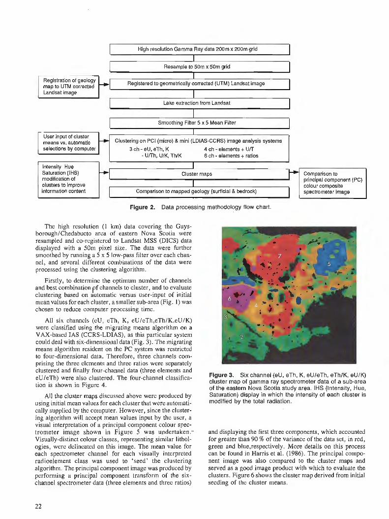
High resolution Gamma Ray data 200m x 200m grid I

I Resample to 50m x 50m grid I I

Registration of geology I

map to UTM corrected Registered to geometrically corrected (UTM) Landsat image I Landsat image I

I I I

Lake extraction from Landsat

I I

User input of cluster means vs. automatic

Intensity Hue Saturation (IHS) modification of clusters to improve information content

1 Smoothing Filter 5 x 5 Mean Filter I

Clustering on PC1 (micro) & mini (LDIAS-CCRS) image analysis systems I 3 ch - eU, eTh, K 4 ch - elements + U/T

- Unh, UIK, ThIK 6 ch - elements + ratios I I

Comparison to principal component (PC)

I colour composite Comparison to mapped geology (surficial & bedrock) spectrometer image I I

Figure 2. Data processing methodology flow chart.

The high resolution (1 krn) data covering the Guys- borough/Chedabucto area of eastern Nova Scotia were resampled and co-registered to Landsat MSS (DICS) data displayed with a 50m pixel size. The data were further smoothed by running a 5 x 5 low-pass filter over each channel, and several different combinations of the data were processed using the clustering algorithm.

Firstly, to determine the optimum number of channels and best combination pf channels to cluster, and to evaluate clustering based on automatic versus user-input of initial mean values for each cluster, a smaller sub-area (Fig. 1) was chosen to reduce computer processing time.

All six channels (eU, eTh, K, eU/eTh,eTh/K,eU/K) were classified using the migrating means algorithm on a VAX-based IAS (CCRS-LDIAS), as this particular system could deal with six-dimensional data (Fig. 3). The migrating means algorithm resident on the PC system was restricted to four-dimensional data. Therefore, three channels comprising the three elements and three ratios were separately clustered and finally four-channel data (three elements and eU/eTh) were also clustered. The four-channel classifica- Figure 3. Six channel (eU, eTh, K , eU/eTh, eTh/K, eU/K)

cluster map of gamma ray spectrometer data of a sub-area tion is shown in Figure 4. of the eastern Nova Scotia studv area. IHS Ilntensitv. Hue. All the cluster maps discussed above were produced by

using initial mean values for each cluster that were automatically supplied by the computer. However, since the clustering algorithm will accept mean values input by the user, a visual interpretation of a principal component colour spectrometer image shown in Figure 5 was undertaken.- Visually-distinct colour classes, representing similar lithologies, were delineated on this image. The mean value for each spectrometer channel for each visually interpreted radioelement class was used to 'seed' the clustering algorithm. The principal component image was produced by performing a principal component transform of the six- channel spectrometer data (three elements and three ratios)

Saturation) display in which theaintensity of 'each c lk te r is modified by the total radiation.

and displaying the first three components, which accounted for greater than 90 % of the variance of the data set, in red, green and blue,respectively. More details on this process can be found in Harris et al. (1986). The principal component image was also compared to the cluster maps and served as a good image product with which to evaluate the clusters. Figure 6 shows the cluster map derived from initial seeding of the cluster means.

The resulting cluster maps were statistically and visually evaluated with respect to lithological and surficial geological maps. Figures 7 and 8 show more detailed lithological and surficial geological maps of the same area as the cluster maps (Fig. 3, 4, 6) and are included to facilitate a visual comparison between the cluster maps and mapped geological patterns. The geology has been compiled from Keppie (1979) and Hi11 (1986, 1987) and the surficial geology from Stea and Fowler (1979).

Box and whisker plots for each cluster shown in Figure 3 (six-channel classification), are displayed in Figure 9. The mid 50 % of the eU, eTh and %K populations for each cluster is shown as a box while the median value is displayed as a horizontal line. The lines extending from the top and

Two techniques were also developed to maximize the information on the radiometric cluster maps. The first technique took the six channel derived cluster map, with each cluster displayed as a different colour, and combined the total count (radiation) channel with the clusters using an intensity-hue-saturation (IHS) colour display transform. This display technique, the details of which can be found in Harris and Murray (1989), is effective for combining diverse data types, as each data type or channel can be

bottom of each box extend to the minimum and maximum value for each cluster.

The effect of glacial till on the radiometric response was investigated as the various till types could potentially modify the spatial pattern and extent of the derived clusters. This is not surprising, as the measured gamma rays emanate from the near surface and are not only a function of bedrock lithology but also of till, soil and moisture properties of the Earth's surface. In order to quantify the effect of till type on the radiometric response, the PC1 image analysis system was employed to produce a matrix, or 'unique conditions map', from which eU, eTh and K values were calculated over each specific till group for each individual rock type. This 'unique conditions map' was produced by digitizing bedrock and surficial geology maps shown in Figures 7 and 8 and co-registering these to the spectrometer data. A set of themes was produced with each theme representing a particular bedrock and till unit. A simple Boolean operation ('ANDING') of the lithological and surficial themes produced the 'unique conditions map' (i.e. granite and outcrop, granite and till unit 1, granite and till unit 3, etc.) from which to collect the radiometric response for the three elements (eU, eTh, K). Figure 10 shows a plot of the mean value for eU,eTh and %K for each of the surficial units within each particular rock unit.

assigned to thecolour parameters of intensity, hue and satu- Figure 4' Four (eU' eTh' K1eU'eTh) 'luster map ration. The resulting cluster map (Fig. 3) shows each cluster of gamma ray spectrometer data of a sub-area of the eastern Nova Scotia study site. in a different colour (hue), with the intensity of each colour

Figure 5. Principal component colour composite gamma ray spectrometer image (PCI-R, PC2-G, PC3-B) of eastern Nova Scotia.

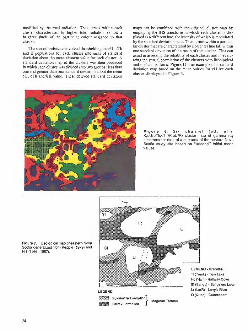
modjfied by the total radiation. Thus, areas within each cluster characterized by higher total radiation exhibit a brighter shade of the particular colour assigned to that cluster.

The second technique involved thresholding the eU, eTh and K populations for each cluster into units of standard deviation about the mean element value for each cluster. A standard deviation map of the clusters was then produced in which each cluster was divided into two groups : less than one and greater than one standard deviation about the mean eU, eTh and %K value. These derived standard deviation

maps can be combined with the original cluster map by employing the IHS transform in which each cluster is displayed as a different hue, the intensity of which is modulated by the standard deviation map. Thus, areas within a particular cluster that are characterized by a brighter hue fall within one standard deviation of the mean of that cluster. This can assist in assessing the reliablity of each cluster and in evaluating the spatial correlation of the clusters with lithological and surficial patterns. Figure 11 is an example of a standard deviation map based on the mean values for eU for each cluster displayed in Figure 3 .

F i g u r e 6 . S i x c h a n n e l ( e U , e T h , K,eUleTh,eThlK,eUIK) cluster map of gamma ray spectrometer data of a sub-area of the eastern Nova Scotia study site based on "seeded" initial mean values.

Figure 7. Geological map of eastern Nova Scotia generalized from Keppie (1979) and Hill (1986, 1987).

i LEGEND - Granites

/ TI (TomL) - Tom Lake I Hc (Half) - Halfway Cove

.-------------I

LEGEND Lr (LarR) - Larry's River Q (Quen) - Queensport

Goldenville Formation Meguma Terrane

Halifax Formation

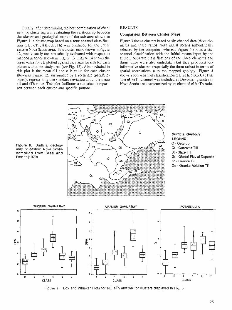
Finally, after determining the best combination of chan- RESULTS nels for clustering and evaluating the relationship between the cluster and geological maps of the sub-area shown in Figure 1, a cluster map based oh a four-channel classification (eU, eTh, %K,eU/eTh) was produced for the entire eastern Nova Scotia area. This cluster map, shown in Figure 12, was visually and statistically evaluated with respect to mapped granites shown in Figure 13. Figure 14 shows the mean value for eU plotted against the mean for eTh for each pluton within the study area (see Fig. 13). Also included in this plot is the mean eU and eTh value for each cluster shown in Figure 12, surrounded by a rectangle (parallele- piped), representing one standard deviation about the mean eU and eTh value. This plot facilitates a statistical comparison between each cluster and specific plutons.

Comparison Between Cluster Maps

Figure 3 shows clusters based on six-channel data (three elements and three ratios) with initial means automatically selected by the computer, whereas Figure 6 shows a six- channel classification with the initial means input by the author. Separate classifications of the three elements and three ratios were also undertaken but they produced less informative clusters (especially the three ratios) in terms of spatial correlations with the mapped geology. Figure 4 shows a four-channel classification (eU,eTh, %K,eU/eTh). The eU/eTh channel was included as Devonian granites in Nova Scotia are characterized by an elevated eU/eTh ratio.

Figure 8. Surficial geology map of eastern Nova Scotia compiled from S t e a a n d Fowler (1979).

Surflcial Geology LEGEND 0 - Outcrop Qt - Quartzite Till St - Slate Till Gf - Glacial Fluvial Deposits Gt - Granite Till Ga - Granite Ablation Till

THORIUM GAMMA RAY URANIUM GAMMA RAY POTASSIUM %

CLASS CLASS

0 4 ! . . . , . . . . . . 1 2 3 4 5 6 7

CLASS

Figure 9. Box and Whisker Plots for eU, eTh andO/oK for clusters displayed in Fig. 3.

Comparison of the six-channel (Fig. 3) and four-channel (Fig. 4) classifications shows that they are almost identical, indicating that the channels providing the best discrimination are the three elements supplemented by the eU/eTh ratio. The six-channel classification using computer- generated and user-selected initial means (Fig. 3 and Fig. 6 respectively) are also very similar. In general, all three cluster maps (Fig. 3, 4, 6) yield similar patterns. The Half- way Cove, Sangster's Lake and Queensport plutons and metasediments are all characterized by similar cluster patterns. One area of difference is over the western half of the Larry's River Pluton where a SSW-trending linear cluster is evident only on the four-channel (Fig.4) and six-channel "seeded" (Fig. 6) classifications. This cluster may reflect a glacial meltwater feature. In general, the results indicate that in this area means selected automatically by the computer are equally successful in defining spatially meaningful clusters as user-selected means.

Comparison of Cluster Maps With Geological Maps

Visual comparison of the cluster maps, specifically Figure 3 (six-channel classification), with the mapped geology (Fig. 7) indicates a fair degree of correlation. The box and whisker plots (Fig. 9) show that the clustering procedure has defined statistically different radiometric populations, the only exceptions being between clusters 5 and 7 (which are characterized by similar eU and %K populations), as the

Granite

median values are almost identical. However, the eTh populations are very different, as the median value for cluster 5 is greater than twice the median value for cluster 7. Cluster 6 correlates with the Sangster Lake pluton and is particularly high in eU (4.5ppm) with respect to the average background. Areas of anomalously high eTh content (7ppm), defined by cluster 5, occur within the Queensport pluton and as a linear shaped zone defining the Halifax Formation north of the Sangster Lake pluton. Cluster 7 correlates predominantly with the Halfway Cove pluton and is fairly high in eU (2.2ppm). A small area of higher eU (2.5ppm), defined by cluster 4, which characterizes much of the Larry's River and Queensport plutons, occurs in the western margin of the Halrway Cove pluton. The Queensport and Larry's River plutons are defined by a mix of clusters 5 and 4 and 4 and 7 respectively

Some of these separate clusters within plutons may be a reflection of surface till patterns, whereas others may reflect differentiationlalteration trends. The elevated level of eU within the Sangster Lake pluton is believed to be a result of considerable hydrothermal alteration involving albitization of plagioclase, appearance of secondary muscovite and apatite, and destruction of K-feldspsar (O'Reilly, 1988). The anomalous area of high eTh within the Queen- sport pluton correlates with an area of fine to medium- grained equigranular muscovite-biotite monzogranite mapped by Ham (1988). However, Ham also noted that the main mineralogy and chemical characteristics of this

Halifax Goldenville Formation Formation

---- Mean value for total area ,,3.tt.y1:.yt..w Mean and standard deviation ---------- of each lithology (formation) for each surficial unit

within specified lithology Mean value for total area of each surficial unit'

Figure 10. Plot of mean eU, eTh, K values and one standard deviation for each lithological and surficial till unit.

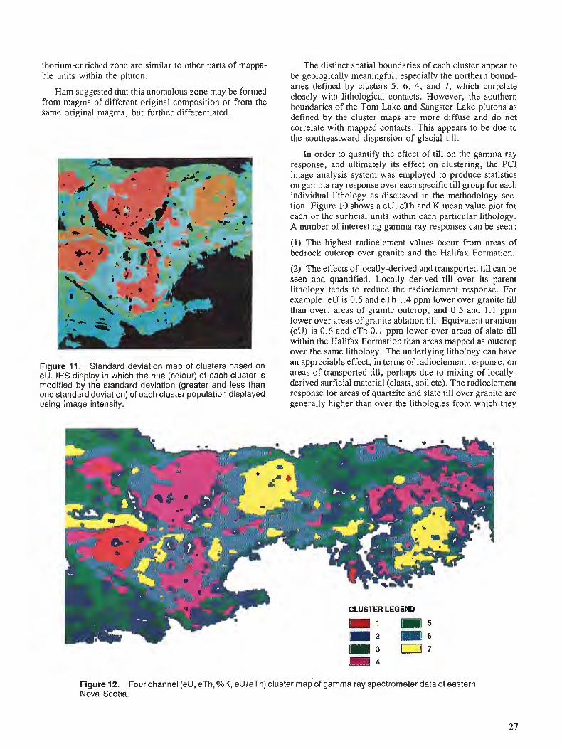
thorium-enriched zone are similar to other parts of mappa- The distinct spatial boundaries of each cluster appear to ble units within the pluton. be geologically meaningful, especially the northern bound-

aries defined by clusters 5, 6, 4, and 7, which correlate Ham suggested that this 'One may be closely with lithological contacts. However, the southern

from magma of different original composition or from the boundaries of the Tom Lake and Sangster Lake plutons as same original magma, but further differentiated. defined by the cluster maps are more diffuse and do not

correlate with mapped contacts. This appears to be due to the southeastward dispersion of glacial till.

In order to quantify the effect of till on the gamma ray response, and ultimately its effect on clustering, the PC1 image analysis system was employed to produce statistics on gamma ray response over each specific till group for each individual lithology as discussed in the methodology section. Figure 10 shows a eU, eTh and K mean value plot for each of the surficial units within each particular lithology. A number of interesting gamma ray responses can be seen :

(1) The highest radioelement values occur from areas of bedrock outcrop over granite and the Halifax Formation.

(2) The effects of locally-derived and transported till can be seen and quantified. Locally derived till over its parent lithology tends to reduce the radioelement response. For example, eU is 0.5 and eTh 1.4 ppm lower over granite till than over, areas of granite outcrop, and 0.5 and 1.1 ppm lower over areas of granite ablation till. Equivalent uranium (eU) is 0.6 and eTh 0.1 ppm lower over areas of slate till within the Halifax Formation than areas mapped as outcrop over the same lithology. The underlying lithology can have

Figure , ,. Standard deviation map of clusters based on an appreciable effect, in terms of radioelement response, on eU. IHS display in which the hue (colour) of each cluster is areas of transported till, perhaps due to mixing of locally- modified by the standard deviation (greater and less than derived ~urficial material (clasts, soil etc). The radioelement one standard deviation) of each cluster population displayed response for areas of quartzite and slate till over granite are using image intensity. generally higher than over the lithologies from which they

CLUSTER LEGEND

1 1 2 1 1 6

m 4

Figure 12. Four channel (eU, eTh, %K, eU/eTh) cluster map of gamma ray spectrometer data of eastern Nova Scotia.

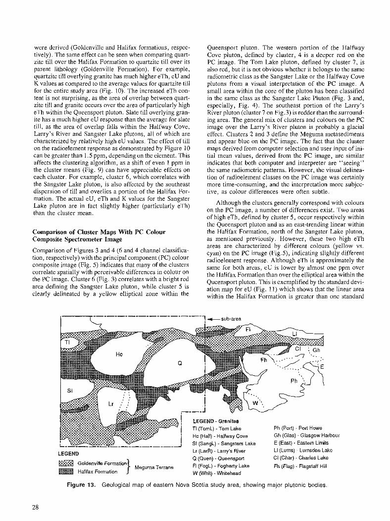
were derived (Goldenville and Halifax formations, respec- Queensport pluton. The western portion of the Halfway tively). The same effect can be seen when comparing quartzite till over the Halifax Formation to quartzite till over its parent lithology (Goldenville Formation). For example, quartzite till overlying granite has much higher eTh, eU and K values as compared to the average values for quartzite till for the entire study area (Fig. 10). The increased eTh content is not surprising, as the area of overlap between quartzite till and granite occurs over the area of particularly high eTh within the Queensport pluton. Slate till overlying granite has a much higher e~ response than the average for-slate till, as the area of overlap falls within the Halfway Cove, Larry's River and Sangster Lake plutons, all of which are characterized by relatively high eU values. The effect of till on the radioelement response as demonstrated by Figure 10 can be greater than 1.5 ppm, depending on the element. This affects the clustering algorithm, as a shift of even 1 ppm in the cluster means (Fig. 9) can have appreciable effects on each cluster. For example, cluster 6, which correlates with the Sangster Lake pluton, is also affected by the southeast dispersion of till and overlies a portion of the Halifax For- mation. The actual eU, eTh and K values for the Sangster Lake pluton are in fact slightly higher (particularly eTh) than the cluster mean.

Comparison of Cluster Maps With PC Colour Composite Spectrometer Image

Comparison of Figures 3 and 4 (6 and 4-channel classification, respectively) with the principal component (PC) colour composite image (Fig. 5) indicates that many of the clusters correlate spatially with perceivable differences in colour on the PC image. Cluster 6 (Fig. 3) correlates with a bright red area defining the Sangster Lake pluton, while cluster 5 is clearly delineated by a yellow elliptical zone within the

Cove pluton, defined by cluster, 4 is a deeper red on the PC image. The Tom Lake pluton, defined by cluster 7, is also red, but it is not obvious whether it belongs to the same radiometric class as the Sangster Lake or the Halfway Cove plutons from a visual interpretation of the PC image. A small area within the core of the pluton has been classified in the same class as the Sangster Lake Pluton (Fig. 3 and, especially, Fig. 4). The southeast portion of the Larry's River pluton (cluster 7 on Fig.3) is redder than the surrounding area. The general mix of clusters and colours on the PC image over the Larry's River pluton is probably a glacial effect. Clusters 2 and 3 define the Meguma metasediments and appear blue on the PC image. The fact that the cluster maps derived from computer selection and user input of initial mean values, derived from the PC image, are similar indicates that both computer and interpreter are "seeing" the same radiometric patterns. However, the visual delineation of radioelement classes on the PC image was certainly more time-consuming, and the interpretation more subjective, as colour differences were often subtle

Although the clusters generally correspond with colours on the PC image, a number of differences exist. Two areas of high eTh, defined by cluster 5 , occur respectively within the Queensport pluton and as an east-trending linear within the Halifax Formation, north of the Sangster Lake pluton, as mentioned previously. However, these two high eTh areas are characterized by different colours (yellow vs. cyan) on the PC image (FigS), indicating slightly different radioelement response. Although eTh is approximately the same for both areas, eU is lower by almost one ppm over the Halifax Formation than over the elliptical area within the Queensport pluton. This is exemplified by the standard deviation map for eU (Fig. 1 I) which shows that the linear area within the Halifax Formation is greater than one standard

---------------------- 1 sub-area

w -v i LEGEND - Granites

i TI (rorn~) - Tom ~ a h e Ph (Port) - Port Howe ' Hc (Half) - Halfway Cove Gh (Glas) - Glasgow Harbour

SI (SangL) - Sangstem Lake ,----------- E (East) - Eastern Limits

LEGEND Lr (LarR) - Larry's River L1 (Lums) - Lumsden Lake

Q (Quen) - Queensport CI (Char) - Charles Lake Goldenville

Meguma Terrane FI (FogL) - Fogherty Lake Fh (Flag) - Flagstaff Hill Halifax Formation W (Whit) -Whitehead

Figure 13. Geological map of eastern Nova Scotia study area, showing major plutonic bodies.

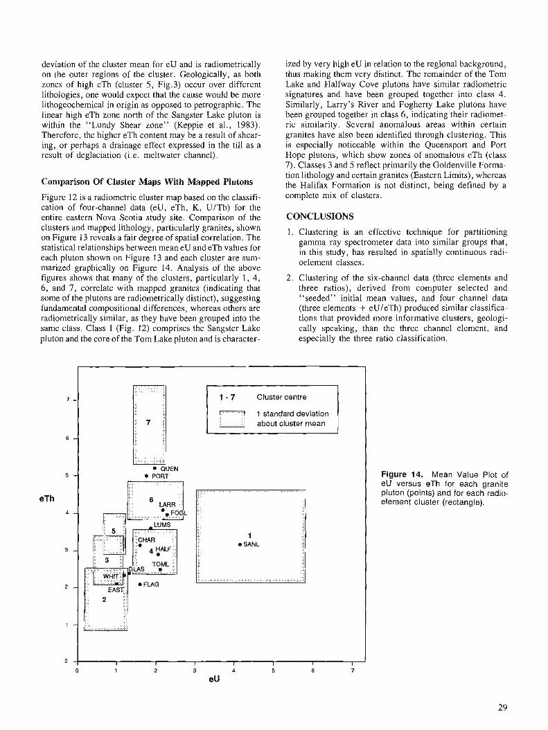
deviation of the cluster mean for eU and is radiometrically on the outer regions of the cluster. Geologically, as both zones of high eTh (cluster 5 , Fig.3) occur over different lithologies, one would expect that the cause would be more, lithogeochemical in origin as opposed to petrographic. The linear high eTh zone north of the Sangster Lake pluton is within the "Lundy Shear zone" (Keppie et al., 1983). Therefore, the higher eTh content may be a result of shearing, or perhaps a drainage effect expressed in the till as a result of deglaciation (i.e. meltwater channel).

Comparison Of Cluster Maps With Mapped Plutons

Figure 12 is a radiometric cluster map based on the classification of four-channel data (eU, eTh, K, U/Th) for the entire eastern Nova Scotia study site. Comparison of the clusters and mapped lithology, particularly granites, shown on Figure 13 reveals a fair degree of spatial correlation. The statistical relationships between mean eU and eTh values for each pluton shown on Figure 13 and each cluster are summarized graphically on Figure 14. Analysis of the above figures shows that many of the clusters, particularly 1, 4, 6, and 7, correlate with mapped granites (indicating that some of the plutons are radiometrically distinct), suggesting fundamental compositional differences, whereas others are radiometrically similar, as they have been grouped into the same class. Class 1 (Fig. 12) comprises the Sangster Lake pluton and the core of the Tom Lake pluton and is character-

ized by very high eU in relation to the regional background, thus making them very distinct. The remainder of the Tom Lake and Halfway Cove plutons have similar radiometric signatures and have been grouped together into class 4. Similarly, Larry's River and Fogherty Lake plutons have been grouped together in class 6, indicating their radiometric similarity. Several anomalous areas within certain granites have also been identified through clustering. This is especially noticeable within the Queensport and Port Hope plutons, which show zones of anomalous eTh (class 7). Classes 3 and 5 reflect primarily the Goldenville Forma- tion lithology and certain granites (Eastern Limits), whereas the Halifax Formation is not distinct, being defined by a complete mix of clusters.

CONCLUSIONS

1. Clustering is an effective technique for partitioning gamma ray spectrometer data into similar groups that, in this study, has resulted in spatially continuous radioelement classes.

2. Clustering of the six-channel data (three elements and three ratios), derived from computer selected and "seeded" initial mean values, and four channel data (three elements + eU/eTh) produced similar classifications that provided more informative clusters, geologically speaking, than the three channel element, and especially the three ratio classification.

Figure 14. Mean Value Plot of eU versus eTh for each granite pluton (points) and for each radioelement cluster (rectangle).

1 standard deviation about cluster mean

QUEN

FLAG

1 SANL

EAST

I I I I I I I

3. The "semi-automatic" approach to clustering is desirable as minimal input by the geologist is required. In this study the automatic selection of initial means by the clustering algorithm produced results similar to those obtained through the a priori "seeding" of the algorithm. However, this must be tempered (the study area is in an ideal geological environment in which to test the clustering algorithm) as radioelement contrast between lithologies is great.

4. The eU,eTH and %K standard deviation maps produced using the IHS transform display technique were useful for evaluating the reliability of each cluster. Incorporat- ing the total radiation count with the cluster map using the IHS transform assisted in determining the radiometric variability within each cluster.

5. Radioelement classes produced by clustering the spectrometer data show a fairly close spatial correlation with the mapped geology. Many of the clusters correspond with mapped plutons while a number of clusters delineate areas of anomalous eTh content within the Queen- sport and Port Howe plutons, as well as along the Lundy Shear Zone north of the Sangster Lake pluton.

6. The clustering algorithm has produced clusters with distinct spatial boundaries (unlike ternary or principal component presentations, which produce diffuse and indistinct boundaries), many of which approximate geological contacts between granites and sediments. How- ever, the effect of glacial till dispersion tends to diffuse cluster boundaries with respect to the actual position of geological contacts.

7. The effect of locally derived and transported till on the gamma ray data can be detected and quantified by comparing the radioelement response from mapped surficial and bedrock geology. These effects are manifest in the clustering procedure as the spatial extent of each cluster is modified by till.

8. The statistical sensitivity of the clustering algorithm used does not appear, in some cases, to match the colour sensitivity of ternary or principal component colour displays. The anomalous areas of eTh (within the Queensport pluton and along the Lundy Shear zone, defined as one cluster) exemplify this point, as they appear as different colours on the principal component colour display, indicating different eU levels. However, the overall objective of clustering is to provide an unbiased 'generalized picture' of multivariate data and in this study it did that successfully, resulting in radiometric clusters that were geologically meaningful. Visual interpretation of the PC image was more time consuming and certainly a more subjective exercise than clustering.

9. Clustering of radioelement images provides a useful technique for geological mapping, but its success depends on the particular geological environment (i.e. thickness of till cover, radioelement contrast between lithologies, etc.) and the quality of the original data. Smoothing of the original data is recommended, as this produced clusters that were less noisy in a spatial sense.

The area studied in this particular paper was most suitable for the application of clustering, as radiometric contrast between lithologies, particularly granites and metasediments, is optimum and tills are not overly thick and, for the most part, locally derived.

ACKNOWLEDGMENTS

Critical reviews by V.R. Slaney, G.F. Bonham-Carter, R.L. Grasty and J.M. Carson (Geological Survey of Can- ada) are appreciated. C. Kushigbor's (INTERA Technolo- gies Ltd.) help with computer processing of the data is gratefully acknowledged. Blair Moxon deserves credit for the design and computer drafting of the figures. The airborne gamma ray spectrometer data were obtained by the Geological Survey of Canada under the Canada - Nova Sco- tia ~ i n e r a l ~ e ~ e l o ~ m e n t Agreement, 1985-1989. This work was supported and funded by the Canada Centre For Remote Sensing (CCRS).

REFERENCES

Aarnisalo, J. ; Franssila E. ; Eeronheimo J. ; Lakanen E. and Pehkonen E. 1982: On the integrated use of Landsat, geophysical and other data in

exploration in theBaltic Shield, Finland; Photogrammetric Journal of Finland, v. 9, no. 1, p. 48-64.

Broome, J., Carson J.M., Grant J.A. and Ford K.L. 1987: A modified ternary radioelement mapping technique and it's appli-

cation to the south coast of Newfoundland; Geological Survey of Canada, Paper 87- 14.

Butlin, T.J., Guertin F.E. and Vishmubhatla S.S. 1978: The CCRS digital image correction system; Proceedings Fifth

Canadian Symposium on Remote Sensing, Victoria, British Columbia, p. 271-283.

Conradson, K. and Nilsson G. 1984: Application of integrated Landsat, geochemical and geophysical

data in mineral exploration; Proceedings of the Third Thematic Conference on Remote Sensing for Exploration Geology, Colorado Springs, Colorado, p. 499-5 11.

Ford, K.L. 1982: Investigation of regional gamma ray spectrometric patterns in New

Bmnswick and Nova Scotia; Current Research, Part B, Geological Survey of Canada, Paper 82-IB, p. 1-10.

Ford, K.L. and Ballantyne S.B. 1983: Uranium and thorium distribution patterns in lithogeochemistry of

Devonian granites in the Chedabucto Bay area, Nova Scotia; Cur- rent Research, Part A, Geological Survey of Canada, Paper 83-IA, p. 109-119.

Ford, K.L. and O'Reilly G.A. 1985: Airborne gamma ray spectrometric surveys as an indicator of

granophile element specialization and associated mineral deposits in the granitic rocks of the Meguma zone of Nova Scotia, Canada; Proceedings of the High Heat Production (HHP) Granites, Hydrothermal Circulation and Ore Genesis, Institute of Mining and Metallurgy, St. Austell, Cornwall, England, p. 113-133.

Ford, K.L. and Carson J.M. 1986: Application of airborne gamma ray spectrometric surveys,

Meguma terrane, Nova Scotia; Maritime Sediments and Atlantic Geology, v. 22, no. 1, p. 117-135.

Ford, K.L., Carson J.M.,. Grant J.A., and Holman P.B. 1989: Radioactivity maps of Nova Scotia, Geological Survey of Canada,

map 350066, scale 1 :500,000. Freeman, S.B., Bolivar S.L. and Weaver T.A. 1983: Display techniques for integrated data sets; Computers and Geos-

ciences, v. 9, no. 1, p. 59-64.

Grasty, R.L. 1972: Airborne gamma ray spectrometry data processing manual; Geo-

logical Survey of Canada, Open File Report 109. 1976: Applications of gamma radiation in remote sensing, ecological

studies, analysis and synthesis; Remote Sensing for Environmental Sciences, ed. E. Schanda, Springer-Verlag, Berlin, New York, v. 18, p. 257-275.

Ham, L.J. 1988: The mineralogy, petrology and geochemistry of the Halfway Cove

- Queensport pluton, Nova Scotia, Canada; unpublished MSc thesis, Dalhousie University, Halifax, Nova Scotia.

Harris, J.R., Neily, L., Pultz, T., and Slaney V.R. 1986: Principal component analysis of airborne geophysical data for

lithologic discrimination using an image analysis system; Proceed- ings of the Twentieth International Symposium on Remote Sensing of Environment, Nairobi, Kenya, p. 641-648.

Harris, J.R. and Murray R. 1989: The !.HS transform for the integration of radar data with geophysi-

cal data; Proceedings of IGARSS-89112th Canadian Symposium on Remote Sensing, Vancouver, British Columbia.

Hill, J.D. 1986: Granitoid plutons in the Canso area, Nova Scotia, Current

Research, Part A, Geological Survey of Canada, Paper 86-lA, p. 185-192.

1987: Geology of the Guysborough - Country Harbour Area, Nova Sco- tia; in Current Research, Part A, Geological Survey of Canada, Paper 87-l A, p. 415-422.

Hood, P.J. 1979: Magnetic methods applied to base metal exploration; Geophysics

and Geochemistry in the Search for Metallic Ores, ed. P.J. Hood, Geological Survey of Canada, Economic Geology Report 31, p. 77-104.

Keppie, J.D. 1979: Geological map of the province of Nova Scotia (1 :500,000);

Department of Mines and Energy, Nova Scotia. 1982: Thc Minas Geofracture, Nova Scotia; Department of Mines and

Energy, Special Paper 24. Keppie, J.D., Haynes, S.L., Henderson, J.R., Smith, P.K., O'Brien, B.H., Zentilli, M., Jensen, L.R., MacEachren, I.J., Stea, R., and Rogers, D. 1983 : Gold Deposits in the Meguma Terrane of Nova Scotia; CIM Geol-

ogy Division Excursion Guidebook Canadian Institute of Mining and Metallurgy, 104 p.

Killeen, P.G. 1979 : Gamma ray spectrometric methods in uranium exploration - Appli-

cation & Interpretation; in Geophysics and Geochemistry in the Search for Metallic Ores, ed. P.J. Hood, Geological Survey of Canada, Economic Geology Report 31, p. 163-229.

O'Reilly, G.A. 1988: Geology and geochemistry of the Sangster Lake and Larry's River

plutons, Guysborough County, Nova Scotia; unpublished MSc thesis, Dalhouse University, Halifax, Nova Scotia, 290 p.

Pirkle, F.L., Campbell K., and Wecksung G.W. 1980: Principal component analysis as a tool for interpreting NVRE aer-

ial radiometric survey data; Journal of Geology, v. 88, no. 1, p. 57-68.

Schenk, P.E. 1978: Synthesis of the Canadian Appalachians; it1 Caledonide-

Appalachian Orogen of the North Atlantic Region, Geological Sur- vey of Canada, Paper 78-13. p. 11 1-136.

Slaney, V.R. 1985 : Landsat MSS and airborne geophysical data combined for mapping

granite in southwest Nova Scotia; Proceedings of the Eleventh International Symposium on Machine Processing of Remotely Sensed Data, Purdue University, Indiana, p. 198-206.

Slaney, V.R. and Harris J.R. 1985: Granite mapping of southwest Nova Scotia using reconnaissance

airborne gamma ray data; Proceedings of the First Atlantic Canada Symposium on Remote Sensing and Geographic Information Sys- tems, Lawrencetown, Nova Scotia.

Stea, R.R. and Fowler J.H. 1979: Minor and trace element variations in Wisconsin tills, Eastern

Shore, Nova Scotia; Nova Scotia Department of Mines and Energy Paper 79-4, 20 p. and associated 1 : 100,000 scale maps.

Tou, J.T. and Gonzales R.C. 1974: Pattern Recognition Principles; Addison-Wesley Publishing Co.,

Inc., London. Williams, H. 1978: Tectonic lithofacies map of the Appalachians; Memorial Univer-

sity of Newfoundland, St. Johns, Newfoundland, Map No. 1.

Geoscience applications of digital elevation models

J.A. Ostrowskil, D. Benmouffokl, 2, D.C. He13 3, and D.N.H. Horlerl

Ostrowski, J.A., Benmouffok, D., He, D. C. and Horler, D. N. H., Geoscience applications of digital elevation models; in Statistical Applications in the Earth Sciences, ed. F.P. Agterberg and G.F. Bonham-Carter; Geological Survey of Canada, Paper 89-9, p. 33-37, 1989.

Abstract

iShis paper presents a review of digital elevation modeling from the point of view of Earth scientists. It consists of two parts. Thejrst part introduces Digital Elevation Models (DEMs) by discussing methods of their storage, representation and derivation, as well as DEM cost and availability. Since the DEMs derived automatically from satellite data are most suitable for geoscientijc uses, a brief history of satellite DEMs is presented, and automatic methods of their generation discussed. The second part presents geos- cientijic applications of DEMs in the three broad classes: geo-data processing and correcting, terrain analysis, including data visualization, and terrain processes analysis.

Cette ktude presente une revue de la modklisation numkrique de 1 'altitude du point de vue des spkcialistes des sciences de la Terre. Elle comprend deux parties; la premibre prbente les modbles numei-iques de l'altitude (MNA) par un examen des mkthodes de stockage, de reprksentation et de dkrivation qu'ils mettent en cause ainsi que des coLits et de la disponibilitk de ces modbles. Puisque les MNA dkrive's automatiquement des donnies obtenuespar satellite sont ceux qui conviennent le mieux aux applications ggos- cientijques, on prksente un bref historique de ces MNA et on examine les mkthodes automatiques permenant de les crker. La deuxitme partie de 1 'ktude prksente les applications gkoscientij?ques des MNA en les re'partissant en trois grandes catkgorries: traitement et correction de donnkes gebscientijiques, analyse des terrains, y compris la visualisation des donnkes, et analyse des processus agissant sur les terrains.

' Horler Information Inc., Suite 704, 116 Albert St., Ottawa, Ontario K1P 5G3 Presently at IDRC, 250 Albert St., P.O. Box 8500, Ottawa, Ontario KIG 3H9 ' Presently at CARTEL, University of Sherbrooke, Sherbrooke, Quebec J I K 2R1

INTRODUCTION T O DIGITAL ELEVATION MODELLING

Introduction

The production of Digital Elevation Models (DEMs) is currently a very active field. This activity opens new possibilities to Earth scientists. Terrain is the basis to which all geoscience observations are tied ; it influences processes and is often itself the subject study.

The purpose of this paper is to introduce DEMs to Earth scientists and to describe attempts already undertaken to use DEMs in the geosciences. The paper begins with a brief analysis of methods of storing and presenting topography, and then justifies the DEM approach to storing and handling topographic data. This is followed with a brief review of methods for generating DEMs, and a discussion of present DEM availability and cost. The review then concentrates on DEMs based on satellite data, since they seem to meet best the requirements of geoscientists. In the second part of the paper the current and potential application of DEMs in various fields of geoscience are presented.

Background

Up to the most recent times, elevation data have been stored and presented in an analogue form, beginning with realistic representations of mountains on old maps. Presentation methods later evolved to include shading, colours and contours. Recently, methods have been developed to store elevation in digital form - as grids, vectors, polygons, quad-trees or triangulated irregular networks. Some of these methods are a direct continuation of traditional, analogue approaches while others are, by nature, computer-oriented.

Direct extensions of analogue methods of representing topography are not necessarily the most appropriate for computer storage or use of topographic data; for example, the conversion of vectorized contours to point elevations is not a trivial computational task. In digital approaches, on the other hand, there is a tradeoff between the amount of memory required for storage, and the speed and ease of retrieving the data. With the rapidly falling price, and increasing capacity and speed of on-line data storage, data volumes are becoming less of a problem for geo-data processing. It is practical to limit the discussion to what is arguably the most basic and most flexible digital representation of elevation values, the dense-grid or raster Digital Ele- vation Model.

Most existing DEMs were created by the digitization of contour maps. Recently, DEMs are created as a byproduct of map production by stereoplotting from stereo airphotos, or are being derived by automatic correlation of stereo images. Although some countries have systems in operation for producing and disseminating Digital Elevation Models, for most countries DEMs are not available publicly. Even available DEMs are usually incomplete and often only on a coarse grid.

The cost of DEM acquisition has to be considered by any potential user of elevation data. Generation of DEMs by existing map digitization is labour intensive, and involves

significant postprocessing to remove various kinds of digitization errors. The accuracy of DEMs from digitized maps is no better than of the maps themselves ; as map collections have been built over many years, their accuracy varies, and so does the accuracy of the resulting DEMs. DEMs derived by stereoplotting of aerial photographs are the most accurate, but for many potential applications the cost of their creation is prohibitive; also, the time delay and logistics are often unacceptable.

DEMs from satellite data

DEMs derived from satellite data are well suited to geoscientific applications, due to several factors.

The first factor is the low cost of satellite data from commercial vendors. Savings are due to the reduction of effort required, to the much larger area covered by one satellite scene, the low price of the imagery, compared to dedicated aerophotographic surveys, and to the much smaller number of ground control points (GCPs) needed for correction of imagery.

Secondly, the scale and resolution of satellite DEMs are well suited to many geoscientific applications. For example, one full scene of the SPOT satellite, 60 krn by 60 krn, easily covers one Canadian National Topographic System (NTS) map sheet at 1 :50,000. Since many geoscience data bases are organized by NTS maps, merging of DEM and other data should be feasible, even for spatially extensive projects. Currently operating satellites suitable for derivation of DEMs produce imagery with pixel sizes between 10 and 30 m. Recent reports (e.g. Rodriguez et al., 1988) show that SPOT satellite stereo data have planimetric accuracy of about 6 m and vertical accuracy between 3.5 and 7 m, depending on the stereo viewing geometry. Automatically derived DEMs are also reported to achieve sub-pixel accuracy in all three coordinates.

Thirdly, satellite images offer the possibility of deriving DEMs remotely, without physically entering or overflying the area of interest. This capability can be of use either at the preparation stage of surveys in unmapped areas, or in the processing stages of surveys in which accurate elevation data are needed, but were not collected.

Finally, an important feature of DEMs from satellite data is the speed of their generation. Our experience indicates that it is possible to derive a verified DEM from a full SPOT scene within one month of receiving the imagery.

The French satellite SPOT-1, launched in 1986, provides the best commercially available data for DEM production. SPOT images have a pixel size of 10 m in panchromatic mode; SPOT sensors are of the push-broom type, thus avoiding image distortions from rotating mirrors as found on Landsat sensors; finally, SPOT'S pointable and programmable sensors can acquire data within a 27 degree swath to either side. This means that it is possible to obtain a stereo pair of images with large overlap and good base to height (BIH) ratio, over 0.5, for any point on the globe, with the exception of small areas near the poles. The radiometric quality of images is also high, due to on-board absolute calibration.

Methodologies for satellite DEM derivation

There are two main approaches to DEM derivation from satellite data - stereoplotting and automatic image correlation.

Stereoplotting offers higher accuracy, but this is offset by many drawbacks. First, stereoplotting is labour- intensive. Secondly, stereoplotting requires expensive instrumentation which has to be adapted to the satellite viewing geometry, radically different from traditional air photos; moreover, new satellites may introduce new geometry, requiring further reprogramming. Thirdly, stereoplotting requires data in analogue form, as negative film or photographic prints, introducing another stage of processing with associated errors. However, an advantage of stereoplotting is that the operator is often able to resolve problematic situations such as occluded areas and low signal levels.

Many of the disadvantages of stereoplotting are avoided by automated image correlation. Automatic correlation of digital stereo images requires much less manual labour, and a moderate amount of postprocessing (quality control, ground control point corrections). Reported analyses (e.g., Rochon and Toutin, 1986, Rose and Hegyi, 1986) indicate that automatic derivation of DEMs from satellite imagery offers savings of 75 % or better in comparison to traditional (i.e., photogrammetric) methods, thus making topographic data accessible to many scientists working within a limited budget. Once a system is developed, it can process massive amounts of data, and increased throughput can be achieved by increasing the processing power of the computer, with only a small increase in manual labour. Reprogramming to accommodate new sensors or satellites is relatively easy. Human intervention cannot be eliminated entirely ; ground control point (GCP) correction, quality control and DEM editing are the tasks most difficult to automate.

Our experience shows that major sources of errors in automatic DEM generation are the coordinates of GCPs read from a map, which are used for geocoding the scene before deriving the DEM, as well as for quality assessment of the model.

There are reports on derivation of DEMs from a single image, e.g. Wang et al. (1984), Wilson et al. (1988). The technique of photoclinometry (often referred to as "slope from shading") analyzes the illumination of a scene and der- ives slope and elevation variation under the assumption of a constant albedo within each of several land cover classes. Since the method is still at the early development stage, requires multispectral data and produces only relative elevation models, its potential for geosciences is limited. On the other hand it seems to be well suited to analyzing monoscopic images of extraterrestial objects. Another important application could be the derivation of DEMs from radar data, with dominating illumination effects.

In developing new methods and approaches, an important question concerns the availability of data in the future. For satellite derived DEMs the prospects are good. The SPOT series will continue with SPOT-2 and SPOT-3, both identical to SPOT-I and planned for launch in early and

mid-1990, respectively, and with modified SPOT-4 (1993) and SPOT-5 (1994). The Landsat series will continue with the recently re-approved Landsat-6, to be launched in early 1991. Its Enhanced Thematic Mapper will include a new panchromatic band with pixel size of 13 by 15 metres, extending to the near infrared. There will also be other satellites producing imagery from which DEMs can potentially be made, such as MAPSAT and radar satellites to be launched by Canada, the European Space Agency and Japan. Derivation of DEMs from radar imagery poses difficult problems due to its unique image distortion (layover) and the presence of speckle noise. Layover is the effect whereby mountain peaks (from which reflected electromagnetic waves return in the shortest time) seem to be closer than points at lower elevation. On the other hand, the insensitivity of radar to weather and darkness promises a continuing flow of data.

APPLICATIONS OF DIGITAL ELEVATION MODELS IN GEOSCIENCE

Applications of DEMs in geosciences can be divided into three broad classes. The first class, termed here "geo-data processing applications", comprises applications in which elevation data are used in processing or correcting other data sets, thus improving the results of the subsequent analysis and interpretation stages. The second class, "terrain analysis", covers applications where the terrain itself and its properties or parameters are the main subject of study. The third class, "terrain processes analysis", encompasses applications in which terrain influences other dynamic processes. The three classes are briefly discussed in the following sections.

The list of present and potential applications is by no means exhaustive and is given only to indicate the wide range of possible applications of DEMs in geosciences.

Geo-data processing applications

This group includes the earliest geoscientific uses of DEMs. Most involve remotely sensed data, but there are a few concerning other data sets.

Correction of geo-data sets for terrain distortion

The applications in this group include correction of visible and infrared remote sensing imagery for terrain distortion. The correction involves determination of the displacement at each pixel due to its elevation, and shifting every pixel to the proper position, producing orthographic images (e.g. Wong et a]., 1981). These images, looking as if seen directly from above, can be overlain on maps and other map-registered data sets (e.g. Simard and Slaney, 1986). Another major application in this group is the correction of radar imagery for the layover effect (Domik et al., 1988). In mountainous areas, this effect can make visual inspection and interpretation of radar imagery very difficult.

Improvements in image classification

Applications in this group include corrections for effects of slope and aspect on reflectance, with the prospect of enhancing the land cover classification (e.g. Jones et al., 1988). Also creation of perspective views showing a DEM draped with co-registered imagery may assist in better visual interpretation of the imagery (e.g. Simard and Slaney, 1986).

Watson (1985) describes the applications of DEMs in correcting thermal inertial data, derived from the HCMM satellite, for effects of slope and elevation. The corrected data, although of coarse resolution (500 m), allowed differentiation between bedrock and dry, unconsolidated material, even in areas with vegetation cover.

Correction of geophysical survey data

This group of applications includes the correction of various geophysical surveys for effects of terrain relief and absolute elevation. The natural candidates are airborne and dense surface gradiometric surveys (Tziavos et al., 1988), aeromagnetic surveys (both total field and gradient) and airborne spectrometer surveys. In most of these surveys the planimetric position is known with sufficient accuracy owing to the use of automatic navigation systems and tight ground control of the flight path ; on the other hand, absolute elevation is usually inferred from inaccurate and highly variable barometric pressure. Digital elevation models with better than 10 m accuracy in all three spatial coordinates seem to be an excellent source of the absolute elevation information required; being digital, map-registered and gridded they can be included easily in standard processing of the survey data. Finally, their cost, which is low in comparison to the costs of the surveys, should be acceptable in most cases.

Improvements in geophysical data interpretation

The applications in this group logically follow those in the previous group. Inclusion of precise elevation data can improve the accuracy of interpreted sources of the observed fields. These applications should be preceded by a careful analysis of sensitivity of the derived parameters to the elevation data, to apply DEMs in the most effective way.

Terrain analysis

Terrain analysis relates to the determination of the features of the terrain that are distinct functions of elevations or that can be logically inferred from a knowledge of elevations (Collins, 1975). The use of dense-grid DEMs, together with a suitable processing system, provides a powerful tool in the development of terrain analysis procedures.

Derivation of basic terrain elements

Point elevations are the basic terrain feature, and in a raster DEM they are available immediately or can be easily interpolated for any point of interest. The only limitation here can be the pixel size but, in most geoscientific applications, satellite DEMs are more likely to be too fine than too coarse.

In some applications, location of extreme points of the terrain is of interest; these points, pits and summits, are easily inferred from DEMs.

The aspect, slope angle and slope length of any cell or group of cells are the main features that may be obtained from DEMs. These features are the basic elements in the development of systems for deriving various terrain indices and for studying terrain-related natural or artificial processes, as discussed below. Other parameters useful in further analyses are convexity, the second spatial derivative of elevation, and elevation variance, the measure of terrain roughness (Franklin, 1987).

Another group of features that are easily derived from DEMs includes ridges, channels, depressions and hills. Knowledge of these features allows the determination of drainage networks, stream courses, pour points, watershed boundaries, lake and depression boundaries and catchment basins, as well as the study of water-flow related processes (e.g. Jenson and Domingue, 1988).

Finally, the availability of DEMs allows easy calculation of lengths, areas and volumes; they are most naturally applied in civil engineering (pipeline, road and power line routing, and dam flooding) and in land resource management, although some geoscientific applications can be fore- seen, for example in the study of landslides, glaciers, volcanic eruptions and lava flows.

Visual terrain analysis

Use of DEMs to create perspective views of the terrain, draped with the original satellite imagery and other digitized data, provides an excellent aid in visualization of complex spatial relationships (Simard and Slaney, 1986). Other applications in this group involve mathematical operations on the DEM itself, like directional filtering or edge enhancement, to detect lineaments or trends in the topography which could be masked by land cover in the original imagery.

Terrain processes analysis

Terrain processes analysis relates to the use of terrain features, indices or parameters derived from DEMs for developing thematic geoscience models. All disciplines which deal with spatial and temporal phenomena linked with Earth forms appear to be potential users of DEMs.

The ability to derive automatically and easily a wide variety of quantitative physiographic features of a given area from DEMs and the facility to replay and modify derived products make the use of DEMs attractive to geoscientists. Some such applications are discussed in the following sections.

Hydrology and hydrography

Digitized watershedlcatchment features together with rasterized thematic data allow overlay processes to be automatically performed. For this reason features and physical models, derived from DEMs, are used by hydrologists as basic elements for drainage network analysis and modelling -

of surface stream flow, water flow balance and forecasting, flood estimation, reservoir and dam simulation, and for the study of transfer of sediments, pollutants and geochemical elements.

Hydrographers may use DEMs and derived products to study stream density, stream channel networks and stream classification, and as the basic framework to develop numerical river models. These models have proved to be powerful tools in the design of improvements to river systems.

Geomorphometry and geomorphology

DEMs provide appropriate tools for geomorphometry, which consists of measures of elevations, slope, aspect, convexity and surface variability (Franklin, 1987). Many applications are possible in geomorphology in the domain of landform detection and analysis (cirques, drumlins), stream channel analysis (number, lengths and order), soil classification, soil erosion processes, terrain roughness, sun exposure, and other areas.

DEMs in GIs

As with all individual types of geoscience data, DEMs rarely provide all the information needed for a particular application. They are an extremely useful, often invaluable, data set that should be used in conjunction with other complementary types of data. They may be used as the base layer of information in a digital system, to which all other data sets are registered. The use of DEMs in geoscience applications will thus be most powerful when Geographic Information Systems (GISs) are employed as the tool for the manipulation and integration of various data sets.

SUMMARY

DEMs are a powerful and flexible means of digitally storing and manipulating elevation data, and the availability of DEMs is increasing dramatically through the automatic processing of satellite remote sensing data. DEMs have numerous applications in Earth sciences, including uses for (1) correcting and processing other geo-data, (2) the analysis of terrain, and (3) the study and modelling of dynamic terrain processes. The use of DEMs almost invariably necessitates the integration of multiple data sets which requires the use of a GIs approach to data handling.

ACKNOWLEDGMENTS

REFERENCES

Collins, S.H. 1975: Terrain parameters directly from a digital terrain model; The

Canadian Surveyor, v. 29, no. 5, p. 507-518. Domik, G., Leberl F. and Cimino J. 1988: Dependence of imagery grey values on topography in SIR-B

images; International Journal of Remote Sensing, v. 9, no. 5, p. 1013-1022.

Franklin, S.E. 1987: Terrain analysis from digital patterns in geomorphometry and

Landsat MSS spectral response; Photogrammetric Engineering & Remote Sensing, v. 53, no. I, p. 59-65.

.lenson. S.K. and Domingue J.O. - - 1988: Extracting topographic structure from digital elevation data for

geographic information system analysis; Photogrammetric Engineering & Remote Sensing, v. 54, no. 1 I, p. 1593-1600.

Jones, A.R., Settle J.J. and Wyatt B.K. 1988: Use of digital terrain data in the interpretation of SPOT-I HRV

multispectral imagery; International Journal of Remote Sensing, v. 9, no. 4, p. 669-682.

Rochon, G. and Toutin Th. 1986: SPOT a new cartographic tool; Proceedings of the ISPRSIRSS

Symposium, Edinburgh. UK, p. 192-205. Rodriguez, V., Gigord P., de Gaujac A.C. and Munier P. 1988: Evaluation of the stereoscopic accuracy of the SPOT satellite; Pho-

togrammetric Engineering & Remote Sensing, v. 54, no. 2, p. 217-221.

Rose, D.R. and Hegyi F. 1986: Applications of satellite derived digital elevation models for

resource mapping; Proceedings of the 10th Canadian Symposium on Remote Sensing, Edmonton, Alberta, p. 655-660.

Simard, R. and Slaney R. 1986: Digital terrain model and image integration for geologic interpreta-

tion; Proceedings of the Fifth Thematic Conference on Remote Sensing for Exploration Geology, Reno, Nevada, p. 49-60.

Tziavos, I.N., Sideris M.G., Forsberg R. and Schwarz K.P. 1988 : The effect of the terrain on airborne gravity and gradiornetry ; Jour- ,

nal of Geophysical Research, v. 93, no. B8, p. 9173-9186. Wang, S., Haralick R.M. and Campbell J. 1984: Relative elevation determination from Landsat imagery ; Pho-

togrammetria, v. 39, p. 193-215. Watson, K., 1985: Remote sensing - a geophysical perspective; Geophysics, v. 50,

no. 12, p. 2595-2610. Wilson, L., Lawson R., Efford N.D. and Young P.C. 1988 : Determination of topography using photoclinometry ; Proceedings

of IGARSS '88 Symposium, Edinburgh, UK, v. I , p. 429. Wong, F., Orth R. and Friedmann D.E. 1981 : The use of digital terrain model in the rectification of satellite-

borne imagery; Proceedings of the 15th International Symposium on Remote Sensing of Environment, Ann Arbor, Michigan, p. 653-662.

The research carried out by Horler Information in this field has been supported in part by the Industrial Research Assistance Program of the National Research Council of Canada and by the Unsolicited Proposals Program of the Department of Supply and Services Canada.

Mineral exploration: digital image processing of LANDSAT, SPOT, magnetic and geochemical data

M. Michel Rheaultl, Rbjean Simardl, Pierre Keatingz, and M. Magella Pe1letie1-3

Rheault, M. M. , Simard, R. Keating, P., and Pelletier, M. M. , Mineral exploration : digital image processing of LANDSAT, SPOT, magnetic and geochemical data; & Statistical Applications in the Earth Sciences, Ed. F. P. Agterberg and G. F. Bonham-Carter; Geological Survey of Canada, Paper 89-9, p. 39-46, 1989.

Abstract

LANDSATand SPOTimages covering the Joutel area of the Abitibi region of Quebec were radiometrically and geometrically corrected, and then enhanced. Similarly, aeromagnetic and pedogeochemical data were processed to produce enhanced images of the total magneticjeld, the vertical magnetic gradient and the pedogeochemical elements under study.

The structural analysis performed on the remotely sensed data identi$ed four prevailing sets of lineaments: WNW, NW, NNE and NE. Enhanced aeromagnetic images confirmed the structural origin of each lineament network.

The study revealed that the four major mineral deposits are stratiform. However, one important gold deposit is also associated with the Harricana fault, where it has a NW orientation. Therefore, attention must be paid to the NW lineaments network and, particularly, to a regional NW lineament that perhaps represents a splay of the above-mentioned fault.

The principal component and ponderation analysis carried out on the geochemical parameters revealed anomalies corresponding to existing deposits. Anomalies with similar characteristics that are located near the intersections of regional lineaments represent favourable areas for exploration.

Des images SPOT et LANDSAT, couvrant la rkgion de Joutel, en Abitibi, ont dt.4 radiomktriquement et gdomdtriquement corrigdes et rehaussdes. Parall&lement, des donnkes adromagnhiques et pkdogkochi- miques ont dtk traitdes a$n de produire des images rehauss&es du champ magnhique total, du gradient magnktique vertical et des klkments pkdog&ochimiques analysks.

L 'analyse structurale des donnkes de tdkdktection indique quatre rkseaux dominants de lindaments: ONO, NO, NNE et NE. Les images akrornagnhiques rehausskes confirment l'origine structurale de ces rkseaux de linkaments.

Les quatre plus importants dkpbts mindralisks du secteur 6 l'hude sont de type stratiforme. Toutefois, un important gisement aurifere est kgalement associk a la faille Harricana aux endroits 03 elle afiche une orientation NO. Les chercheurs devraient donc concentrer leurs efforts sur le rkseau de lindaments NO et, plus particulitrement, sur un lindament rkgional NO qui pourrait reprdsenter un embranchement de la faille ci-haut mentionnke.

L 'analyse des composantes principales ainsi que 1 'analyse de ponddration des paramttres gebchimi- ques permetrent de ddtecter des anomalies qui correspondent h quelques gisements existants. Les anomalies prdsentant des caractdristiques similaires et situdes d proximitk d'intersection de linkaments rdgionaux reprksentent des aires favorables 2 l'exploration.

' DIGIM Inc., 1 100 RenC Uvesque Boulevard West, Montreal, Quebec, H3B 4P3 A.C.S.I. Gioscience Inc., 969 Route de I'Eglise, Sainte-Foy, Quebec, GIV 3V4

"EOKEMEX, 1301 Nantes, Bernitres, Quebec, G7A 2M3

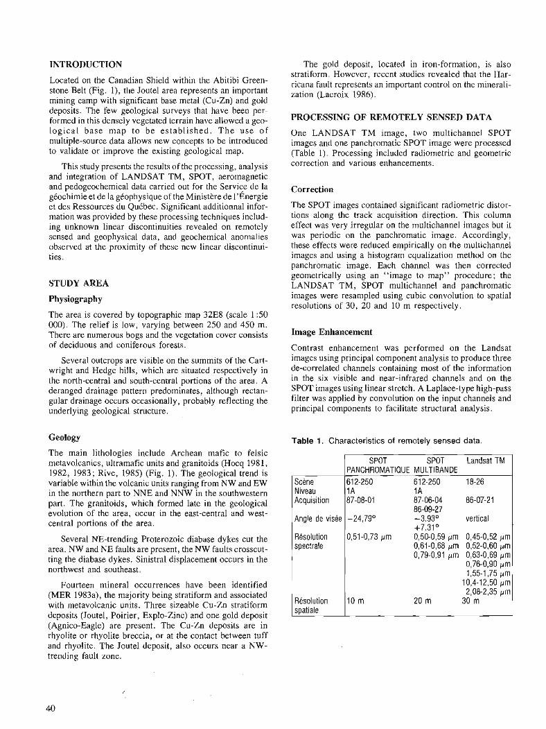
INTRODUCTION

Located on the Canadian Shield within the Abitibi Green- stone Belt (Fig. l), the Joutel area represents an important mining camp with significant base metal (Cu-Zn) and gold deposits. The few geological surveys that have been performed in this densely vegetated terrain have allowed a geological base map to be es tabl ished. T h e use of multiple-source data allows new concepts to be introduced to validate or improve the existing geological map.

This study presents the results of the processing, analysis and integration of LANDSAT TM, SPOT, aeromagnetic and pedogeochemical data carried out for the Service de la gCochimie et de la gkophysique of the Ministhe de 1'Energie et des Ressources du QuCbec. Significant additionnal information was provided by these processing techniques including unknown linear discontinuities revealed on remotely sensed and geophysical data, and geochemical anomalies observed at the proximity of these new linear discontinuities.

STUDY AREA

Physiography

The area is covered by topographic map 3288 (scale 1 :50 000). The relief is low, varying between 250 and 450 m. There are numerous bogs and the vegetation cover consists of deciduous and coniferous forests.

Several outcrops are visible on the summits of the Cart- wright and Hedge hills, which are situated respectively in the north-central and south-central portions of the area. A deranged drainage pattern predominates, although rectangular drainage occurs occasionally, probably reflecting the underlying geological structure.

Geology

The main lithologies include Archean mafic to felsic metavolcanics, ultramafic units and granitoids (Hocq 1981, 1982, 1983; Rive, 1985) (Fig. 1). The geological trend is variable within the volcanic units ranging from NW and EW in the northern part to NNE and NNW in the southwestern part. The granitoids, which formed late in the geological evolution of the area, occur in the east-central and west- central portions of the area.

Several NE-trending Proterozoic diabase dykes cut the area. NW and NE faults are present, the NW faults crosscut- ting the diabase dykes. Sinistral displacement occurs in the northwest and southeast.

Fourteen mineral occurrences have been identified (MER 1983a), the majority being stratiform and associated with metavolcanic units. Three sizeable Cu-Zn stratiform deposits (Joutel, Poirier, Explo-Zinc) and one gold deposit (Agnico-Eagle) are present. The Cu-Zn deposits are in rhyolite or rhyolite breccia, or at the contact between tuff and rhyolite. The Joutel deposit, also occurs near a NW- trending fault zone.

The gold deposit, located in iron-formation, is also stratiform. However, recent studies revealed that the Har- ricana fault represents an important control on the mineralization (Lacroix 1986).

PROCESSING OF REMOTELY SENSED DATA

One LANDSAT TM image, two multichannel SPOT images and one panchromatic SPOT image were processed (Table 1). Processing included radiometric and geometric correction and various enhancements.

Correction

The SPOT images contained significant radiometric distortions along the track acquisition direction. This column effect was very irregular on the multichannel images but it was periodic on the panchromatic image. Accordingly, these effects were reduced empirically on the multichannel images and using a histogram equalization method on the panchromatic image. Each channel was then corrected geometrically using an "image to map" procedure; the LANDSAT TM, SPOT multichannel and panchromatic images were resampled using cubic convolution to spatial resolutions of 30, 20 and 10 m respectively.

Image Enhancement

Contrast enhancement was performed on the Landsat images using principal component analysis to produce three de-correlated channels containing most of the information in the six visible and near-infrared channels and on the SPOT images using linear stretch. A Laplace-type high-pass filter was applied by convolution on the input channels and principal components to facilitate structural analysis.

Table 1. Characteristics of remotely sensed data.

Scene Niveau Acquisition

Angle de visee

Rdsolution spectrale

Resolution spatiale

SPOT SPOT Landsat TM PANCHROMATIQUE MULTIBANDE 61 2-250 612-250 18-26 1A 1A 87-08-01 87-06-04 86-07-21

86-09-27 -24,7g0 -3,93O vertical

+7,31° 0,51-0,73 pm 0,50-0,59 pm 0,45-0,52 pm

0,61-0,68 prn 0,52-0,60 prn 0,79-0,91 prn 0,63-0,69 prn

0,76-0,90 prn 1,55-1,75 pm 10,4-12,50 prn 2,08-2,35 prn

10 rn 20 rn 30 m

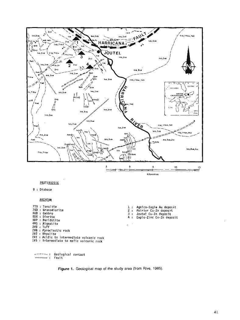
PROTEROZOIC

8 : Diabase

ARCHEAN

7T0 : Tonal i t e 7GD : Granodiorite 6GB : Gabbro 6DR : D i o r i t e 6DP : Per ido t i t e 4H5 : ~ i ~ m a t i t e 2V9 : Tuff 2V8 : Pyroclastic rock 2V2 : Rhyolite 2V1 : Acidic t o intermediate volcanic rock 1V5 : Intermediate t o mafic volcanic rock

------ : Geological contact ------ : Faul t

1 : Agnico-Eagle Au deposit 2 : Po i r i e r Cu-Zn deposit 3 : Joutel Cu-Zn deposit 4 : Explo-Zinc Cu-Zn deposit

Figure 1. Geological map of the study area (from Rive, 1985).

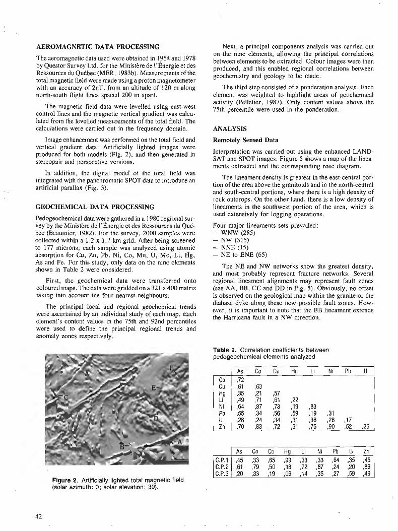
AEROMAGNETIC DATA PROCESSING

The aeromagnetic data used were obtained in 1964 and 1978 by Questor Survey Ltd. for the Ministkre de 19Bnergie et des Ressources du QuCbec (MER, 1983b). Measurements of the total magnetic field were made using a proton magnetometer with an accuracy of 2nT, from an altitude of 120 m along north-south flight lines spaced 200 m apart.

The magnetic field data were levelled using east-west control lines and the magnetic vertical gradient was calculated from the levelled measurements of the total field. The calculations were carried out in the frequency domain.

Image enhancement was performed on the total field and vertical gradient data. Artificially lighted images were produced for both models (Fig. 2), and then generated in stereopair and perspective versions.

In addition, the digital model of the total field was integrated with the panchromatic SPOT data to introduce an artificial parallax (Fig. 3).

GEOCHEMICAL DATA PROCESSING

Pedogeochemical data were gathered in a 1980 regional survey by the Ministkre de 198nergie et des Ressources du QuC- bec (Beaumier, 1982). For the survey, 2000 samples were collected within a 1.2 x 1.2 km grid. After being screened to 177 microns, each sample was analyzed using atomic absorption for Cu, Zn, Pb, Ni, Co, Mn, U, Mo, Li, Hg, As and Fe. For this study, only data on the nine elements shown in Table 2 were considered.

Next, a principal components analysis was carried out on the nine elements, allowing the principal correlations between elements to be extracted. Colour images were then produced, and this enabled regional correlations between geochemistry and geology to be made.

The third step consisted of a ponderation analysis. Each element was weighted to highlight areas of geochemical activity (Pelletier, 1987). Only content values above the 75th percentile were used in the ponderation.

ANALYSIS

Remotely Sensed Data

Interpretation was carried out using the enhanced LAND- SAT and SPOT images. Figure 5 shows a map of the lineaments extracted and the corresponding rose diagram.

The lineament density is greatest in the east-central portion of the area above the granitoids and in the north-central and south-central portions, where there is a high density of rock outcrops. On the other hand, there is a low density of lineaments in the southwest portion of the area, which is used extensively for logging operations.

Four major lineaments sets prevailed : - WNW (285) - NW (315) - NNE (15) - NE to ENE (65)

The NE and NW networks show the greatest density, and most probably represent fracture networks. Several regional lineament alignments may represent fault zones (see AA, BB, CC and DD in Fig. 5) . Obviously, no offset is observed on the geological map within the granite or the diabase dyke along these new possible fault zones. How- ever, it is important to note that the BB lineament extends the Harricana fault in a NW direction.

First, the geochemical data were transferred onto coloured maps. The data were gridded on a 321 x 400 matrix taking into account the four nearest neighbours.

The principal local and regional geochemical trends were ascertained by an individual study of each map. Each element's content values in the 75th and 92nd percentiles were used to define the principal regional trends and anomaly zones respectively.

Table 2. Correlation coefficients between pedogeochernical elements analyzed

Figure 2. Artificially lighted total magnetic field (solar azimuth: 0; solar elevation: 30).

Figure 3. SPOT panchromatic stereopair with total magnetic field parallaxe.

Table 3. Parameters used in the ponderation analysis

19,0 PPm 70,0 P P ~

, 2,4 P P ~ 25,O ppm

I 140,O ppb 8,0 P P ~

1 3 8 ppm 16,0 P P ~ 1.0 DDm

Figure 4. Ponderation imagery of the pedogeochemical data.

Aeromagnetic Data

Total magnetic field data reflect the concentration of magnetic minerals in rock and are therefore useful in lithological and structural mapping. Vertical magnetic gradient data, on the other hand, are particularly sensitive to variations in magnetization on the surface of the bedrock and allow magnetic formations to be more precisely defined.

Diabase dykes with a NE trend (A in Fig. 2) and strong anomalies in the SE sector (B in Fig. Z), which are probably associated with ultramafic units, are well defined in the total field data. The granite in the eastern part of the area has a circular zone of weak magnetism. However, the central part of the granite is slightly magnetic.

Just north of the granite, the vertical gradient data indicate several anomalous bands, which probably represent mafic lavas.

Several displacements in the general NW direction can be observed along the NE-trending dykes (C in Fig. 2). These discontinuities are associated with faults, some of which have already been documented. An elongated negative anomaly running NW, which cuts through the eastern portion of granite (D in Fig. 2), could also be associated with an undiscovered fault. NNE and NE discontinuities (E and F in Fig. 2) can also be observed above the granite.

Geochemical Data

Table 2 shows the correlation coefficients resulting from the principal component analysis. The results of this analysis indicate that the elements Hg, Cu and Pb, which show a stronger correlation with the first principal component, have high concentrations in the northern and western half of the area where metavolcanic units abound. Conversely, Ni, Zn, Co, Li and As, which show a stronger correlation with the second principal component, have high concentration in the southern and eastern half of the region where there are a number of metavolcanic, ultramafic and granitoid units.

The ponderation analysis allowed the most favourable anomaly areas to be identified. The calculations took account of each element's mobility index, as wel1.a~ the percentile below which the content is considered insignificant (Pelletier, 1987) (Table 3). This mobility index equals the ratio of the cut-off anomalous value (92nd percentile) with the cut-off geological background (75th percentile). The elements that were the least mobile therefore contributed strongly to the anomalies extracted.

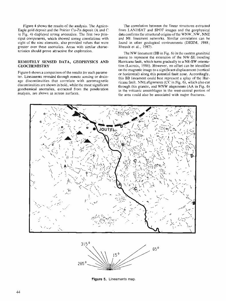
Figure 4 shows the results of the analysis. The Agnico- Eagle gold deposit and the Poirier Cu-Zn deposit (A and C in Fig. 4) displayed strong anomalies. The first two principal components, which showed strong correlations with eight of the nine elements, also provided values that were greater over these anomalies. Areas with similar characteristics should prove attractive for exploration.

REMOTELY SENSED DATA, GEOPHYSICS AND GEOCHEMISTRY

Figure 6 shows a comparison of the results for each parameter. Lineaments revealed through remote sensing or drainage discontinuities that correlate with aeromagnetic discontinuities are shown in bold, while the most significant geochemical anomalies, extracted from the ponderation analysis, are shown as screen surfaces.

The correlation between the linear structures extracted from LANDSAT and SPOT images and the geophysical data confirms the structural origins of the WNW, NW, NNE and NE lineament networks. Similar correlation can be found in other geological environments (DIGIM, 1988; Rheault et al., 1987).

The NW lineament (BB in Fig. 6) in the eastern granitoid seems to represent the extension of the NW-SE trending Harricana fault, which turns gradually to a NE-SW orientation (Lacroix, 1986). However, no offset can be identified on the magnetic image to a significant displacement (vertical or horizontal) along this potential fault zone. Accordingly, this BB lineament could best represent a splay of the Har- ricana fault. NNE alignments (CC in Fig. 6), which also cut through this granite, and WNW alignments (AA in Fig. 6) in the volcanic assemblages in the west-central portion of the area could also be associated with major fractures.

Figure 5. Lineaments map.

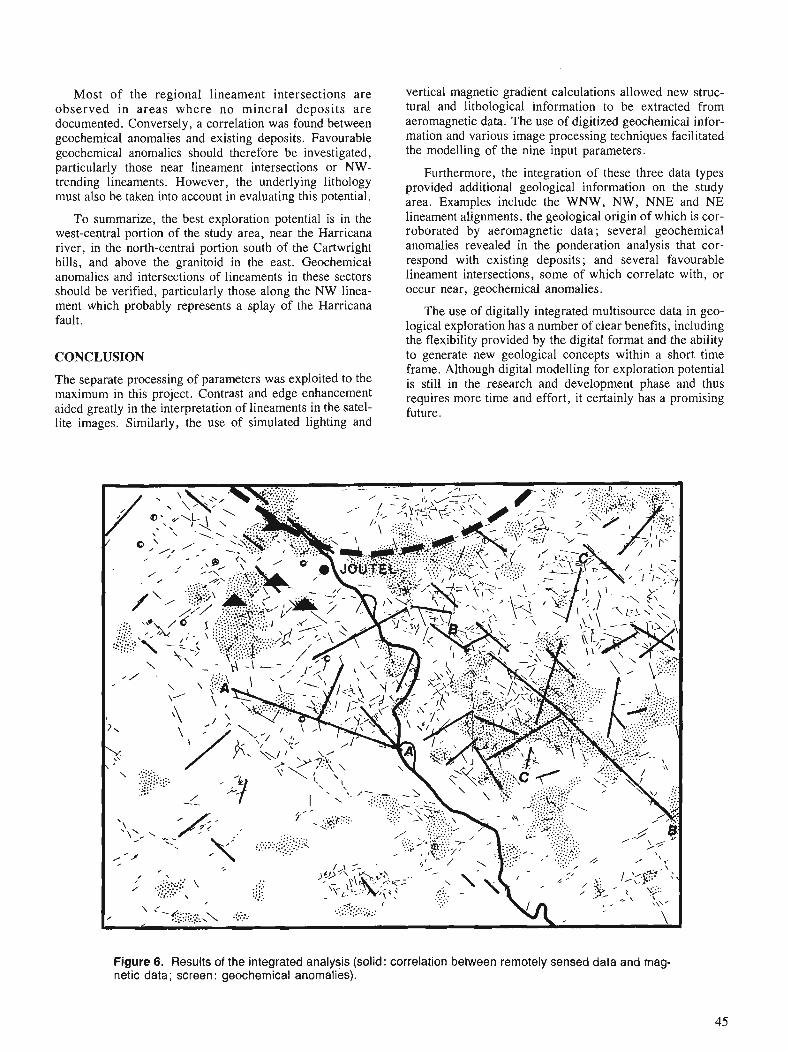
Most of the regional lineament intersections are observed in areas where no mineral deposits a re documented. Conversely, a correlation was found between geochemical anomalies and existing deposits. Favourable geochemical anomalies should therefore be investigated, particularly those near lineament intersections or NW- trending lineaments. However, the underlying lithology must also be taken into account in evaluating this potential.

To summarize, the best exploration potential is in the west-central portion of the study area, near the Harricana river, in the north-central portion south of the Cartwright hills, and above the granitoid in the east. Geochemical anomalies and intersections of lineaments in these sectors should be verified, particularly those along the NW lineament which probably represents a splay of the Harricana fault.

CONCLUSION

The separate processing of parameters was exploited to the maximum in this project. Contrast and edge enhancement aided greatly in the interpretation of lineaments in the satellite images. Similarly, the use of simulated lighting and

vertical magnetic gradient calculations allowed new structural and lithological information to be extracted from aeromagnetic data. The use of digitized geochemical information and various image processing techniques facilitated the modelling of the nine input parameters.

Furthermore, the integration of these three data types provided additional geological information on the study area. Examples include the WNW, NW, NNE and NE lineament alignments, the geological origin of which is cor- roborated by aeromagnetic data ; several geochemical anomalies revealed in the ponderation analysis that correspond with existing deposits; and several favourable lineament intersections, some of which correlate with, or occur near, geochemical anomalies.

The use of digitally integrated multisource data in geological exploration has a number of clear benefits, including the flexibility provided by the digital format and the ability to generate new geological concepts within a short time frame. Although digital modelling for exploration potential is still in the research and development phase and thus requires more time and effort, it certainly has a promising future.

Figure 6. Results of the integrated analysis (solid: correlation between remotely sensed data and magnetic data; screen: geochemical anomalies).

REFERENCES Beaumier, M. 1982: P6dogtochimie de la rtgion de Joutel, Department of Energy and

Resources of Quebec, DP 930. DIGIM 1988: Integration de donnees Landsat, aCromagnktiques et gblogiques,

region du Lac GBrido, fosse du Labrador, Final Report presented to the Service de la Gtochimie et de la GBophysique, Ministbre de 178nergie et des Ressources du Qutbec.

Hocq, M. 1981 : Carte gtologique preliminaire de la rtgion de Joutel - Guyenne;

Department of Energy and Resources of Quebec, annotated 1 : 100 000-scale map, DP 851.

1982: Projet Joutel - Qutvillon, rtgion du lac Bigniba; Department of Energy and Resources of Quebec, annotated 1 : 100 000-scale map, DP 82-05.

1983: Cantons de Dalet et de Maizerets et partie des cantons adjacents; Department of Energy and Resources of Quebec, annotated 1 :50 000-scale map, DP 83-25.

Lacroix, S. 1986: La faille aurifere de Casa-BBrardi, presented during DGEGM

seminar of the Department of Energy and Resources of Quebec, November, 1986.

MER 1983a: Rtpertoire des fiches de gite min6ral; Department of Energy and

Resources of Quebec, DPV-845, 2nd edition, 125 p. 1983b : Cartes aeromagnttiques ?I I'echelle 1 :20 000 - Region de la rivibre

Turgeon et de Joutel - Poirier; Ministkre de I'Energie et des Res- sources du Quebec, DP-83-14, 28 feuillets.

Pelletier, M. 1987: Carte d'interprttation giochimique par ponderation; Bulletin du

CIM, Vol. 80, No 908, p. 63-68. Rheault, M., Deschenes, M., Levaque, J.G. and St-Hilaire, C. 1988: Limestone Resources Extension: Interpretation of Landsat TM,

MAG and VLF Data for Structural Analysis; Proceedings Sixth Thematic Conference on Remote Sensing for Exploration Geol- ogy, Vol. 11, p. 663-670.

Rive M. 1985: Carte gtologique ?I I'tchelle de 1 : 125 000; unpublished map

produced by the Service gtologique du nord-ouest, Rouyn- Noranda.

i

IMAGE ANALYSIS OF GEOPHYSICAL DATA

d

Statistical interpretation of aeromagnetic data

D.J. Teskeyl

Teskey, D. J . , Statistical interpretation of aeromagnetic data; fi Statistical Applications in the Earth Sciences, ed. F.P. Agterberg and G.F. Bonham-Carter; Geological Survey of Canada, Paper 89-9, p. 49-55, 1989.

Abstract

Statistical techniques have been used in the analysis of aeromagnetic maps since the early 1970s and have been applied to both gridded andprofile data. Spector and Grant developed a technique for estimating the average depth of burial of an ensemble of sources using spectral techniques. One of the earlier techniques forprojle analysis, which can provide estimates of dip, depth, and magnetization of dyke-like sources (including flat lying sources such as sills) and contacts is Werner Deconvolution. This technique determines source parameters at a point by inverting a set of linear equations. Successive determinations are then analyzed for consistency to identify those that are sign$cant. The output from techniques of this type can potentially yield more information when combined with other data sets than using the mapped Jield alone.

Les mkthodes statistiques sont utiliskes pour l'analyse des cartes ae'romagne'tiques depuis le dkbut des annkes 70 et ont e'te' appliqukes tant a m donnkes portkes sur des grilles qu 'aux donnkes de profils. Spector et Grant ont mis au point une mkthode pour l'estimation de la profondeur moyenne d'enfouisse- ment d'un ensemble de sources a l'aide de mkthodes spectrales. L'une des premibres mkthodes d'analyse de profils, qui permet des estimations du pendage, de la profondeur et de la magnktisation de sources apparente'es aux dykes (y compris les sources horizontales comme les filons-couches) et des contacts, est la me'thode de la dkconvolution de Werner. Cette mkthode permet de dkterminer les parambres de la source en un point en inversant un ensemble d'kquations linkaires. Une analyse de l'uniformite' de dkterminations successives est ensuite effectue'e afin dlidentij?er celles qui sont importantes. Les rksultats obtenus par des mkthodes de ce genre peuvent renseigner davantage lorsque combinks a d'autres ensembles de donne'es que la seule utilisation du champ cartographike.

' Geophysics Division, Geological Survey of Canada, Ottawa.

INTRODUCTION

The magnetic anomalies measured above the earth's surface can be considered to be due to titanium-iron oxides and a relatively small proportion of iron-sulphides (pyrrhotite). The latter, although much less common, can be a significant indicator for the presence of sulphide mineral deposits. Titanium-iron oxide minerals can be created or destroyed in several ways e.g. deuteric (high temperature) alteration of silicates, alteration of clay minerals, serpentinization, supergene alteration and hydration-dehydration reactions. (O'Reilly , 1984).

Regardless of the cause of magnetization, examination of magnetic maps from detailed surveys to continental-sized compilations, such as the Magnetic Anomaly Map of Can- ada (Dods et a1.,1987), reveals features that can be traced over distances up to thousands of kilometres, including tectonic boundaries such as the McDonald Fault and the Gren- ville Front. These patterns indicate that a common tectonic history can result in common magnetization patterns over great distances. At a local scale, magnetic anomalies can be correlated with lithological units often enabling them to be traced beneath sedimentary cover. Truncation and offset of magnetic patterns can be used to identify and trace faults and contacts.

Attempting to determine the distribution of source depths is a more difficult task than the qualitative interpretation described above, requiring the development of analytic techniques all of which require an oversimplified model to be tractable. Numerous techniques have been developed based on the assumption that magnetization is constant over some limited zone such that the cumulative effect of all such zones accounts for the observed field.

BASIC EQUATIONS

The fundamental equation for the field due to a dipole can be written:

where U = magnetic potential M = dipole moment R = vector between the measurement point and the

dipole.

The magnetic field in a specific direction is then the derivative of U in that direction. For a distribution of dipoles U can be written

U = 111 rn.v(L) dv R

(2)

where m = magnetic momenttunit volume. Equations 1 and 2 satisfy Laplace's equation

V2U = 0

in source free regions, and have the following general solution in Cartesian co-ordinates :

I

u (x, y , Z) = j J A (u, v) e(u2 + v2)' h e im BVY dudv (3)

where u and v are the spatial frequencies in the horizontal plane and h is the vertical axis.

It can be seen from 3 that the general expression for the field in the direction given by direction cosines L, M, N is :

I

F (x, y , z) = I J [i(uL + vM) + (u2 + v2)2N] A (u, V)

and derivatives,upward continuation, integration (i.e. calculating the total field from the derivatives) can all be easily carried out in the frequency domain using Fast Fourier Transforms (FFT's). In general, however, it should be remembered that inaccuracies are introduced because :

1 . The field is not generally known on a perfect plane. In fact in areas of rugged terrain where contour flying is the preferred technique, elevations may range over hundreds of metres.

2. Calculation of the field at grid cells, as required for use by FFT's involves the interpolation of data which are often undersampled in the direction perpendicular to the flight lines and which will have positional and diurnal errors.

3. Modern magnetometers measure the 'total magnetic field'. The earth's field normally dominates, but the effect of the anomalous field can be to rotate the vector by as much as 30" over intense anomalies.

FUNDAMENTAL STATISTICAL ANALYSIS

Since equation 2 is a convolution integral, the Fourier transform can be broken down into products. The power spectrum due to a prism of horizontal dimensions a and b, at depth h and with thickness t is given in cartesian coordinates (Spector and Grant, 1970) by:

E (r, 0) = 47~IPe-~"' (1 - e-'Y2 9 (r, 0) R? (0) R 2 (0)

where : I

r = (u2 + v2)?

sin (arcose) . sin (brcos0) S (R, 0) = arcosO brcos0 '

K = magnetic dipole momenttunit depth

1, m, n are direction cosines of the geomagnetic field vector L,M,N are direction cosines of the magnetic moment vector K.

It can be seen that the expression is the product of factors related to the direction cosines of the field and the

magnetization vector, a depth term (e-2h'') a thickness term, ( ~ - e - " ) ~ and the spatial term of the form

sin x sin y -.- X Y

This expression was used by Spector and Grant (1970) to develop the theory of statistical depth estimation based on the concept that if the spatial term varied randomly around some median value, the slope of the logarithm of the power spectrum will be equal to -2h. This technique clearly requires a relatively wide sample area compared to the depth and thus is not useful for detailed interpretation. It is, however, extremely useful for estimating average depths to magnetic sources overlain by non-magnetic material.

SUSCEPTIBILITY MAPPING

Susceptibility mapping is essentially a process of downward continuation to the ground surface followed by equating the derived field to the magnetization of vertical prisms, assumed to be of infinite depth extent. One approach to this is that of Parker and Oldenberg (Parker, 1972) who expanded the Fourier transform of the magnetic (or gravity) field in terms of the depth variations h of the magnetic surface with reference depth z,:

and used this relationship to derive an iterative approach for determining the depth. Further developments have extended the technique to multiple layers (Pilkington and Crossley 1986) and to large regions in which the magnetization direction varies (Arkani-Hamed and Strangway 1986). The technique can calculate variable depth to a layer of constant magnetization or alternatively the variable magnetization of a layer of specified depth.

MODELLING

Full three-dimensional modelling is still limited by the difficulty in constructing sources by superposition of layers (Talwani, 1965) or by surfaces (Barnett, 1976). The computation time required to carry out full three-dimensional modelling is also still too great for most computers in common use. The development of a closed expression for sources of finite length, but symmetrical through the plane

of the measurement profile (two and one-half dimensional models) by Shuey and Pasquale (1973) has led to the common use of two and one-half dimensional modelling programs, which are extremely useful for the investigation of limited profile segments, either from the original data or extrapolated from a grid.

AUTOMATED TECHNIQUES

After the development of modern computers in the early 1960s, a great deal of interest was generated in the development of automated computer techniques for the estimation of the parameters of the source of magnetic anomalies. Due to the limitations of the computers available, effort was restricted largely to two-dimensional sources for which the expressions for the potential and the magnetic field for simple sources is greatly simplified. The expression for the potential due to a line of dipoles is:

where M is the complex dipole momentlunit length and z = x + i y is the vector between the observation and source point. For the total field

for a dyke where A is a complex multiplier whose amplitude and phase depend on the inclination of the component of the geomagnetic field vector and the magnetization vector in the plane of the profile, and the dip of the dyke. In the derivative field

for a contact where A now also depends on the direction of the derivative.

In 'Real' algebra, 7(b) and 7(c) become the sum of a symmetrical and anti-symmetrical term given by

where again A and B are functions of the inclination, the dip, and for the gradient, the direction of the derivative. Although techniques based on two-dimensional sources could be considered to be unduly restricting, studies have indicated that errors due to finite strike extent are small when the strike extent exceeds four times the depth to the source (Teskey, 1978). Similar errors due to sources not striking perpendicular to the flight lines can be corrected by simple geometrical factors, at least for reasonable strike angles. A detailed study of the limitations and corrections required to apply two-dimensional interpretation to real sources has recently been carried out by Ferderer (1988).

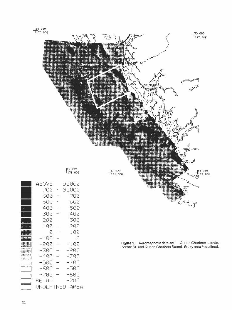
k e 111 v E 9@[ar3@ 7@(3 - Cji;jiqFj@

L - b

680 - 789 50Fj - 608

C" 4~113 - J icj k) - - 388 - 48i.5 Z[qFj - - - -388 188 - 2813

13 - 100 - I @ @ - [?I

-200 - - 188 -788 - - 3 s-1 g-j ,- I.- -

- - -309 -588 - -4@@ -6@(3 - -580 -388 - -6813

E E L 12 hl -700 I.Jb-IDEF I P.IED AREA

Figure 1. Aeromagnetic data set - Queen Charlotte Islands, Hecate St, and Queen Charlotte Sound. Study area is outlined.

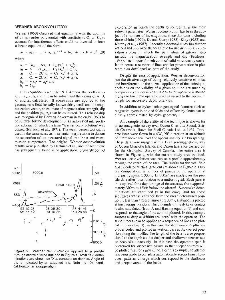
WERNER DECONVOLUTION

Werner (1953) observed that equation 8 with the addition of an nth order polynomial with coefficients C, ... C, to account for interference effects could be inverted to form a linear equation of the form

where

a, = Bz, - Ax, + C, (x,2 + z;), a l = A - 2C0x0 + C , (x,2 + z:), a2 = C, - 2Clxo + C2 ( x 2 + z;), a3 = C I - 2C2xO + C3 (xO2 + z:), b, = -xo2 - 2 2 and b l = 2x0.

If this equation is set up for N + 4 terms, the coefficients a, . . . an-3, b, and b, can be solved and the values of A, B, x, and z, calculated. If constraints are applied to the geomagnetic field (usually known fairly well) and the magnetization vector, an estimate of magnetization strength, dip and the position (x,, z,) can be estimated. This relationship was recognized by Herman Ackerman in the early 1960s to be suitable for the development of an automated interpretation scheme for which the term 'Werner deconvolution' was coined (Hartman et al., 1971). The term, deconvolution, is used in the same sense as in seismic interpretation to denote the seperation of the measured signal into input and trans- mission components. The original Werner deconvolution results were published by Hartman et al., and the technique has subsequently found wide application, primarily for oil

GRADIENT \ ': ,,,............... ..... - 0 ..... . . -A: .. :

Figure 2. Werner deconvolution applied to a profile through centre of area outlined in Figure 1. Total field determinations are shown a s 'X's, contacts a s dashes. Angle of dip is indicated by an attached line. Note the 10:l vertical :horizontal exaggeration.

exploration in which the depth to sources z, is the most relevant parameter. Werner deconvolution has been the subject of a number of investigations since that time including those of Jain (1976), Ku and Sharp (1983), Kilty (1983) and Murthy et al., (1987). Recently a doctoral study has further refined and improved the technique for use in mineral exploration studies in which the parameters of interest also include the magnetization strength and dip (Ferderer, 1988). Techniques for selection of valid solutions by correlation across a number of lines and for presentation in plan were also developed as part of the study.

Despite the ease of application, Werner deconvolution has the disadvantage of being relatively sensitive to noise and interference. In the normal application of the technique, decisions on the validity of a given solution are made by comparison of successive solutions as the operator is moved along the line. The operator span is varied to the optimum length for successive depth intervals.

In addition to dykes, other geological features such as magnetic layers in eroded folds and offsets by faults can be closely approximated by dyke geometry.

An example of the utility of the technique is shown for an aeromagnetic survey over Queen Charlotte Sound, Brit- ish Columbia, flown for Shell Canada Ltd. in 1962. Trav- erse lines were flown in a SW, NE direction at an altitude of 305m above sea level and approximately 3.2 krn spacing. These data were merged with a 1985 aerornagnetic survey of Queen Charlotte Islands and Dixon Entrance carried out for the Geological Survey of Canada. The entire area is shown in Figure 1, with the current study area outlined. Werner deconvolution was run on a profile approximately through the centre of the area. The results for the total field and calculated vertical gradient are shown in Figure 2. Dur- ing computation, a number of passes of the operator at increasing spans (1000 to 15 000m) are made over the profile data after interpolation to a uniform grid. Each pass is thus optimal for a depth range of the sources, from approximately 300m to 16km below the aircraft. Successive deter- minatlons are examined (5 in this case), and for those sequences whose variance from the mean determined position is less than a preset amount (loom), a symbol is plotted at the average position. The dip angle of the dyke or contact is also calculated (from A and Busing equation 9) and corresponds to the angle of the symbol plotted. In this example sources as deep as 4500m are 'seen' with the operator. The same process can be applied to a sequence of lines and plotted in plan (Fig. 3), in this case the determined depths are colour coded and plotted as vertical bars at the correct position along the profile. The length of the bars is also proportional to the depth so that deeper and shallower sources can be seen simultaneously. In this case the operator span is decreased for successive passes so that deeper sources will be plotted first for a given line. For this example, no attempt has been made to correlate automatically across lines ; however, patterns emerge which correspond to the shallower and deeper areas of the basin.

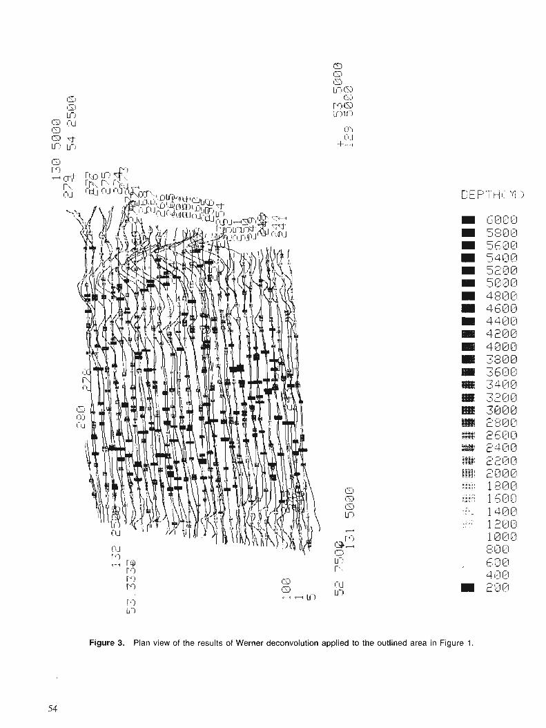
MATCHED FILTERING REFERENCES

The major problem encountered with Werner deconvolution is the sensitivity to noise. An approach to overcome this problem was developed by Naudy (1971). In this approach a matched filter is passed over data to determine anomalies of interest. At these points a number of filters are convolved with the data to determine the best model from a small set of catalogued anomalies representing dykes and thin plates.

The output of the matched filter is given by: ,

Where the values of S are taken from the measured anomaly and T from the anomaly due to the model being tested.

This technique was extended to two-dimensional data sets by Teskey (1978). In this case a filter was passed over the grid to find the optimum point for modelling, after which a set of five parallel profiles were interpolated and stored. These profiles were then 'matched' with a set of catalogued curves that extended over a range of 'slab-like' sources. Again the matched-filter criteria were used to determine the optimum fit which was then stored and served as the initial estimate for more detailed modelling if required. The difference between Werner deconvolution and matched filtering is clearly the classical trade-off between resolution and stability which is fundamental to inversion theory.

CONCLUSION

"The use of statistical techniques has made a significant contribution to the understanding of aeromagnetic maps in the past and these techniques are still being refined and expanded. The use of these techniques can greatly enhance visual interpretation, providing estimates on parameters such as the depth and dip of structures as well as their location in plan view. Information obtained from statistical analysis of aeromagnetic maps yields valuable knowledge when aeromagnetic data are integrated with geological, geochemical and other geological maps.

Arkani-Hamed, J., and Strangway, D.W. 1986: Magnetic susceptibility anomalies of lithosphere beneath Eastern

Europe and the Middle East, Geophysics v. 51, No.9, pp. 171 1-1724.

Barnett, C.T. 1976: Theoretical modelling of the magnetic and gravitational fields of

an arbitrairily shaped three-dimensional and body, Geophysics, v. 41, p. 1353-1364.

Dods, S.D., Teskey D.J., and Hood, P.J. 1987 : Magnetic Anomaly Map of Canada, Geological Survey of Canada,

Map 1255A. Ferderer, R.J. 1988: Werner deconvolution and its application to the Penokean Orogen,

East-Central Minnesota, Ph.D. Thesis University of Minnesota, p. 284.

Hartman, R.R., Teskey, D.J., and Friedberg, J.L. 1971: A system for rapid digital aeromagnetic interpretation,

Geophysics, v. 36, p. 891-918. Jain, S. 1976: An automated method of direct interpretation of magnetic profiles,

Geophysics, v. 41, p. 531-541. Kilty, K.T. 1983: Werner deconvolution of profile potential field data: Geophysics,

v. 48, p. 234-237. Ku, C.C., and Sharp J.A. 1983: Werner deconvolution for automated magnetic interpretation and

its refinement using Marquardt's inverse modelling: Geophysics, v. 48, p. 754-774.

Murthy, K.S.R., Malleswara Rao, M.M., Rao, T.C.S., and Subrahmany, A.J. 1987: A comparative study of Werner deconvolution and conventional

modelling of marine magnetic data, Geophysical Research Bulle- tin. v. 25, p. 152-157.

Naudy, H. 1971 : Automatic determination of depth on aeromagnetic profiles,

Geophysics, v. 36, p. 717-722. O'Reilly, W. 1984: Rock and Mineral Magnetism; Blackie and Son Ltd., Glasgow and

London, p. 219. Parker, R.L. 1972: The rapid calculation of potential anomalies. Geophys. Journal

Royal Astronomical Soc. p. 447-455. Pilkington, M., and Crossley D.J. 1986: Inversion of aeromagnetic data for multi-layered crustal models,

Geophysics, v. 51, No. 12, p. 2250-2254. Shuey, R.T., and Pasquale, A.S. 1973: End corrections in magnetic profile interpretation; Geophysics,

v. 38, No.3, 1973, p. 497-512. Spector, A., and Grant, F.S. 1970: Statistical models for interpreting aeromagnetic data. Geophysics

v. 35, p. 293-302. Talwani, M. 1965: Computation with the help of a digital computer of magnetic

anomalies caused by bodies of arbitrary shape, Geophysics v. 30, p. 797-817,

Teskey, D.J. 1978: Design of a semi-automated three-dimensional interpretation sys-

tem for potential field data, Ph.D thesis, McGill University, p. 417.

Werner, S. 1953 : Interpretation of magnetic anomalies at sheet like bodies, Sveriges

Geologiska Undersok, Ser. c.c., Arsbok 43, N:06, p. 130.

Deconvolution. filters and image enhancement

Joseph E. Robinson1

Robinson, J.E., Deconvolution jlters and image enhancement, @ Statistical Applications in the Earth Sciences, ed. F. P. Agterberg and G. F. Bonham-Carter; Geological Survey of Canada, Paper 89-9, p. 57-62, 1989.

Abstract

Remotely sensed imagery, particularly imagery recorded from high altitude and satellite plalforms, is subject to interference that degrades the recorded information attributed to individual pixels. This interference which results in loss of resolution and added random noise, is a function of reflection geometry, recorder characteristics, sun and sensor scan angles, background albedo and atmospheric scattering. Fifty percent or more of the reflectance recorded in even reasonably good images may be composed of systematic and random noise.

Image enhancement techniques are designed to minimize extraneous noise and to restore the range of the reflectance values. Signal stretching is often effective for restoring reflectance range and improving signal to random noise ratios. Spatial filter operators, often called deconvolution Jilters, may be applied to reduce systematic noise and clarify the signal received from individual pixels. Deconvohtion operators can be designed in either the distance domain or, by using Fourier transforms, in the frequency domain. Such filters attempt to approximate the inverse of degrading effects of the atmosphere and the radiance contribution from the surrounding areas so that they serve to emphasize the unique reflectance of each pixel.

The physical form of many of the signal attenuation phenomena have been determined experimentally so that their inverse finctions can be calculated, These inverse&nctions in the form of digital matrices are the deconvolution filters. TheJilter matrix must be physically small for computational eficiency yet contain sufJicient digital values to approximate the desired function. Fourier transforms and frequency domain displays are useful for evaluating the jlters and the effect they may have on the image.

L'imagerie de tkldddtection, en pamiculier l'imagerie enregistrde h haute altitude et h partir de plates- formes satellitaires, est susceptible a l'inte$krence qui dkgrade 1 'information enregistrde anribuke aux pixels individuels. L'intedkrence qui produit une perte de rksolution et une augmentation du bruit aldatoire, est fonction de la gdorndtrie des rejllexions, des caractkristiques de l'enregistreur, des angles entre le Soleil et le balayage par le capteur, de 1 'albkdo arnbiante et de la d ~ m i o n atmosphkrique. Au moins 50 % de la reyectance enregistrke dam des images &me raisonnablement bonnes peut 2tre constitueP par le bruit sys- tkmatique et le bruit ale'atoire.

Les techniques de rehaussement des images sont concues en vue de minimiser les bruits parasites et de restituer la garnme des valeurs de rkjectance. L'dtalement des signaux est souvent eficace pour restituer la gamme des re'flectances et pour amkliorer le rapport entre le signal et le bruit alkatoire. On peut employer des dispositifs de filtrage spatial, souvent appelds Jiltres de ddconvolution, pour rkduire le bruit systdmatique et kclaircir le signal r e p h partir des pixels individuels. Les dispositifs de dLconvolution peuvent &tre congus soit dam le domaine des distances, soit, B 1 'aide des transfomkes de Fourier, dans le domaine des fpe'quences. Ces $/tires cherchent a produire approximativement l'effet inverse des effets dkgradants de l'atmosphtre et la radiance crkke par les rkgions environnantes, de facon apouvoir accentuer la rkflectance unique de chaque pixel.

' Department of Geology, Syracuse University, Syracuse, N.Y., 132 10 U.S. A.

La conjguration physique d'un grand nombre despht!nom2nes d'attdnuation des signaux a t?te'ddtemzint!e a la suite d'expkriences, de facon h ce que leurs fonctions inverses puissent Ctre calcule'es. Ces fonctions inverses, qui se prdsentent sous forme de matrices numh-iques, sont les jltres de ddconvolution. La matrice du jiltre doit &tre sufJisamment petite pour que les calculs soient eficaces, rnais doit contenir sufisamment de valeurs num6riques pour donner approximativement la fonction ddsirke. Les transformdes de Fourier et la visualisation du domaine de fikquence aident c i dvaluer lesjltres et L'effet qu 'ils peuvent avoir sur l'image.

INTRODUCTION

The term filter is from the same root as the word felt and indeed the first filters were felt mats used to strain liquids. Modern digital filters are still strainers, and their purpose is to remove unwanted elements or noise from some form of signal. The digital filtering operation is usually carried out by a computer and can be in the time domain by convolution or in the frequency domain by multiplication and addition. The two domains are related by Fourier transforms and contain the identical information. The original image is in the distance, equivalent to time, domain while its transform in terms of functions of frequency and phase is in the 'frequency domain. at he ma tical operations can also be transformed and carried out in either domain (e.g. Lee, 1969).

Digital filtering in the time or distance domain is by convolution (e.g. Robinson and Treitel, 1964). The digital convolution operation can be described as a lagged rolling together of filter operator and data set. The two dimensional digital form is:

a-1 6-1 O(x,y) = C C I(x-a, y-0)- S(a,0)

a=o D = O

where I(x,y) is the input function, S(a,R) is the lagged filter and O(x,y) is the filtered output.

The input function, filter and the filtering operation can be transformed into functions of frequency by Fourier transforms. Filtering in the frequency domain is the operational transform of convolution and is:

where T and p are the frequency domain equivalents of x and y. The amplitude spectra of the input function is multiplied by the amplitude spectra of the filter while the phase spectra are added. Because phase controls the location of features in the filtered ou t~u t . most of the filters that are . ,

designed for application to spatial data have radial symmetry and thus have zero phase characteristics. With zero phase filters the phase spectra can be neglected and only the amplitude spectra considered in the filtering operation. However it must be remembered that a negative amplitude is the same as a 180" phase shift.

Most filtering operations are by convolution in the spatial domain, however, filters and filtering often are easier to understand when considered in the frequency domain because multiplication is easier to visualize than convolution. Fourier theory indicates that any finite function of time or space can be exactly described by a series of component frequencies of specific amplitudes and phases. Filtering alters these components. In the frequency domain individual components are eliminated by multiplying by zero. They

can be retained without change by multiplying by one or altered in amplitude by multiplying by a value other than one. Filtering operations generally are considered to refer to the elimination of unwanted components while deconvolution would be a restoring process. Although deconvolution implies inverse filtering, deconvolution filters are normal linear filters that have been designed to restore a degraded spectra to an ideal form. Because the effect of altering the phase spectra in images is very difficult to analyze or predict, image enhancement deconvolution filters usually are confined to changing the amplitudes of specific spatial frequency components.

Any analog or digital image can be thought of as being composed of a range of directional spatial frequencies whose sum describes all topographic and surficial features that are displayed in the scene. The spatial frequencies describe the appearance of the image and are related only indirectly to the reflectance electromagnetic spectra. The long wavelength spatial frequencies describe the large regional features, while the short wavelengths define the small features and abrupt discontinuities. The spatial frequency components can be displayed in the spatial domain as a Fourier series or in the complex frequency domain by means of Fourier transforms. Problems with the images are apparent in the frequency spectra and corrections can be modelled in the frequency domain. Corrective filters can be designed in the frequency domain. For instance, a frequency domain deconvolution filter is the suite of frequency components which could be multiplied by the spectra of the degraded image to produce an approximation of the virgin spectra that might have been recorded by an ideal system at ground level.

The signal recorded by the space vehicle is affected by the size of the area covered by the data elements, the optics of the system, the effect of the atmosphere on the signal and random noise from all sources (Billingsley, 1975; Jursa, 1985). Geometric and radiometric errors can be modelled and corrected (Scott, 1965). Random noise cannot be selectively removed from individual frequency components, however, signal to noise discrimination often can be improved by amplifying the spectra and systematic noise, such as banding, can be removed by specially designed notch filters. However atmospheric path distortion is a function of many parameters such as sun angle, look angle, atmospheric particle size and particle distribution as well as atmospheric turbulence, background albedo and surficial characteristics of the reflecting surface. These are complex parameters, specific to each scene, with many only pertain- ing to the instant of recording and which would be difficult if not impossible to obtain. Fortunately, even without the exact information on the ideal spectra, it is possible to apply generalized filters and models that markedly improve even badly degraded images (Robinson and Carroll, 1975).

FILTER DESIGN

Filter design in the frequency domain consists of determining the frequency spectra that when multiplied by the input spectra produces the desired output spectra. If the filter spectra has axial or radial symmetry, the filter has zero phase characteristics and phase components of the input function will not be altered. Also if the amplitude of the filter frequency component is made less than one, the amplitude of that specific output component will be decreased. If it is greater than one, the amplitude of the output will be increased. Features can be eliminated entirely if its component filter frequencies are made equal to zero. The inverse Fourier transform can be applied to convert the frequency domain filter to a distance domain function for convolution with the original data set (e.g. Otnes and Enochsson, 1972).

The filter spectra can be determined from a model of any specific interference providing it can be described accurately. If the ideal spectra is known or can be estimated, the filter spectra can be designed by determining the mul- tipliers needed to convert the degraded spectra to the ideal. Deconvolution filters can be simple single pass filters or they can be a suite of filters that can be cascaded in sequence. Also, they can be a homomorphic system in which a data set is transformed into a linear function, filtered and the output transformed back to the original form (Carroll and Robinson, 1977).

Deconvolution filters have been used successfully for the enhancement of remotely sensed images. Many of these filters have been adapted from other disciplines and may not be optimal for image enhancement. It might be better to consider the problems that are specific to images and then design deconvolution filters for their solution. The lack of resolution in remotely-sensed images can be mainly attributed to two main causes. One where extraneous energy is added to the reflectance recorded for individual pixels and two, where the recorded spatial frequency components are degraded by interference so that there is an additional loss of resolution and contrast.

Energy can be recorded from surfaces outside of the target pixel and all the energy can be distorted by the atmosphere. If it is assumed that the reflectance recorded from the ground has a Gaussian distribution about the central pixel, then a operator can be devised that will compensate in part. ow ever degradation due to atmospheric effects is harder to correct. Without ground level truth for each individual scene, the ideal spatial frequency spectrum is unknown. However it is reasonable to assume that there is a disproportionate attenuation of the higher spatial frequencies compared to the low frequencies. Where this attenuation can be estimated, a second deconvolution filter can be designed to correct the problem. These filters can then be cascaded as separate filters or convolved with each other to create a single deconvolution filter. However because the factors requiring correction will vary from image to image, from band to band and even within images, it seems better to try a number of filters and review each stage rather attempt than a single brute force correction. Although all the filters may be designed in the frequency domain they often are transformed to their spatial domain

equivalents in order to utilize convolution programs that are part of many image analysis software systems.

Spatial domain filters for image enhancement consist of a matrix of digital values or weights. Individual filters can be added, subtracted and convolved. They usually have radial symmetry with zero phase characteristics so that the output is unchanged in location. Filters often are considered to be high pass, low pass and band pass. All pass and programmed gain operators also are useful in the design of deconvolution filters. The sum of the operator weights equals one where the filter is designed to retain the average reflectance value of the image without change. The sum of the weights equals zero for filters that delete the average value, such as high pass and band pass filters. Amplification of the retained features can be increased by multiplying all operator weights by a factor greater than one or decreased by a multiplier of less than one. A filter that passes a specific range of frequencies can be converted to a reject filter by subtracting it from an all pass filter. The latter is an operator containing a single value with the nominal amplitude of unity. It passes all frequencies without change. Overall gain can be adjusted by altering the weight of the all pass filter.

Deconvolution filters for image enhancement are usually designed to pass all frequencies with a programmed gain for the higher frequency components. They may have an overall gain to compensate for lack of contrast in a scene included in the operator, although this function usually is available through stretch and histogram correction programs. As the attenuation of the higher spatial frequencies is not constant and may vary from image to image and even from band to band, the best results have been obtained by having a suite of deconvolution filters with different gains that can be tried in different situations.

Spatial domain filters consist of a matrix of weights that are convolved with the image. They should be small in size to minimize computation time, however they must consist of a sufficient number of values so that the filter is adequately described. There is an inverse size relationship between domains so that any frequency change that affects only a few frequency components requires a relatively large number of spatial domain values to be the exact equivalent. Small spatial filter operators may be only a rough approximation of the desired function, however, they are useful because the correction is only a best guess estimate and small filters are easy to design and quick to test. For this reason and because ERDAS (Earth Resources Data Analysis System) was used for the processing, all spatial filters in the illustrations have been restricted to a 3 by 3 matrix.

REFLECTANCE AREA CORRECTION

The radiance recorded by the satellite receiver includes a contribution from the area surrounding the target pixel. This extraneous radiance has been estimated to nearly equal that received from the target (Billingsley 1975) and to have a Gaussian distribution away from its centre. A model of this extraneous radiance is a matrix of weights representing the contribution from each surrounding pixel based on the distance from the center of the target pixel. The sum of the weights including that of the target pixel is one. The

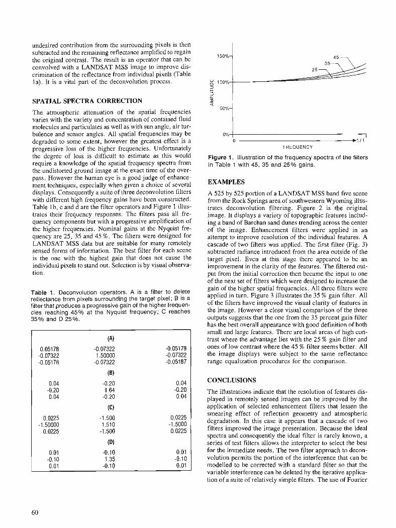
undesired contribution from the surrounding pixels is then subtracted and the remaining reflectance amplified to regain the original contrast. The result is an operator that can be convolved with a LANDSAT MSS image to improve discrimination of the reflectance from individual pixels (Table la). It is a vital part of the deconvolution process.

SPATIAL SPECTRA CORRECTION

The atmospheric attenuation of the spatial frequencies varies with the variety and concentration of contained fluid molecules and particulates as well as with sun angle, air turbulence and sensor angles. All spatial frequencies may be degraded to some extent, however the greatest effect is a progressive loss of the higher frequencies. Unfortunately the degree of loss is difficult to estimate as this would require a knowledge of the spatial frequency spectra from the undistorted ground image at the exact time of the over- pass. However the human eye is a good judge of enhancement techniques, especially when given a choice of several displays. Consequently a suite of three deconvolution filters with different high frequency gains have been constructed. Table lb, c and d are the filter operators and Figure 1 illustrates their frequency responses. The filters pass all frequency components but with a progressive amplification of the higher frequencies. Nominal gains at the Nyquist frequency are 25, 35 and 45 %. The filters were designed for LANDSAT MSS data but are suitable for many remotely sensed forms of information. The best filter for each scene is the one with the highest gain that does not cause the individual pixels to stand out. Selection is by visual observation.

Table 1. Deconvolution operators. A is a filter to delete reflectance from pixels surrounding the target pixel; B is a filter that produces a progressive gain of the higher frequencies reaching 45% at the Nyquist frequency; C reaches 35% and D 25%.

o w i I T ' FREQUENCY

Figure 1. Illustration of the frequency spectra of the filters in Table 1 with 45, 35 and 25% gains.

EXAMPLES

A 525 by 525 portjon of a LANDSAT MSS band five scene from the Rock Springs area of southwestern Wyoming illustrates deconvolution filtering. Figure 2 is the original image. It displays a variety of topographic features including a band of Barchan sand dunes trending across the center of the image. Enhancement filters were applied in an attempt to improve resolution of the individual features. A cascade of two filters was applied. The first filter (Fig. 3) subtracted radiance introduced from the area outside of the target pixel. Even at this stage there appeared to be an improvement in the clarity of the features. The filtered output from the initial correction then became the input to one of the next set of filters which were designed to increase the gain of the higher spatial frequencies. All three filters were applied in turn. Figure 3 illustrates the 35 % gain filter. All of the filters have improved the visual clarity of features in the image. However a close visual comparison of the three outputs suggests that the one from the 35 percent gain filter has the best overall appearance with good definition of both small and large features. There are local areas of high contrast where the advantage lies with the 25 % gain filter and ones of low contrast where the 45 % filter seems better. All the image displays were subject to the same reflectance range equalization procedures for the comparison.

CONCLUSIONS

The illustrations indicate that the resolution of features displayed in remotely sensed images can be improved by the application of selected enhancement filters that lessen the smearing effect of reflection geometry and atmospheric degradation. In this case it appears that a cascade of two filters improved the image presentation. Because the ideal spectra and consequently the ideal filter is rarely known, a series of test filters allows the interpreter to select the best for the immediate needs. The two filter approach to deconvolution permits the portion of the interference that can be modelled to be corrected with a standard filter so that the variable interference can be deleted by the iterative application of a suite of relatively simple filters. The use of Fourier

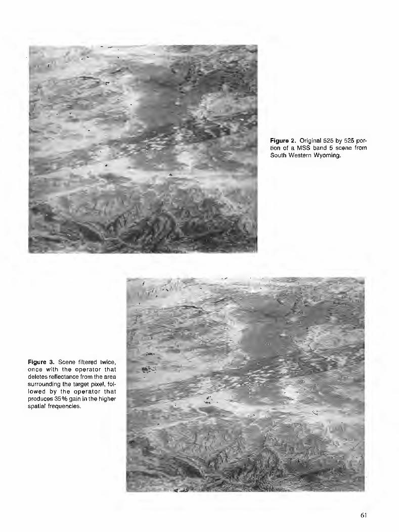
Figure 2. Original 525 by 525 portion of a MSS band 5 scene from South Western Wyoming.

transforms and the frequency spectra present a ready display of the filter requirements and a simple method of designing filters to the desired specifications.

The cascade of deconvolution filters made an improvement in the clarity of the image which may now become the input data for computer oriented mathematical analysis or visual interpretation. This type of image enhancement can be very important to the success of any subsequent classification or object extraction process, for the results are directly related to the quality of the available information. Deconvolution is a versatile enhancement procedure that can be adapted to a number of different requirements and situations.

ACKNOWLEDGMENTS

The MSS image used in the examples was a subset from remotely sensed data originally supplied by ARC0 Oil and Gas Company. The images were processed in the Syracuse University advanced graphics laboratory by Bronya Old- field.

REFERENCES

Billingsley, F.C. 1975 : Noise considerations in digital image processing hardware; Topics

in Applied Physics, Vol. 6, Picture Processing and Digital Filter- ing, ed. T.S.Huang, Springer Verlag, New York, 572 p.

Carroll, S. and Robinson, J.E., 1977: Homomorphic processing of LANDSAT data; Canadian Journal

of Remote Sensing, v. 3, no. I , p. 66-75. Jursa, A.S. 1985 : Handbook of Geophysics and the Space Environment; Air Force

Geophysics Laboratory, Air Force Systems Command, United States Air Forcc, NTIS Document ADA 167000, 850 p.

Lee, Y.W. 1969: Statistical Theory of Communication; John Wiley and Sons, 509 p. Otnes, R.K. and Enochson, L. 1972: Digital Time Series Analysis; John Wiley and Sons, 467 p. Robinson, E.A., and Treitel, S. 1964: Principles of digital filtering; Geophysics, v. 29, no. 3,

p. 395-404. Robinson, J.E. and Carroll, S. 1975: Enhancing of geological definition in LANDSAT data; Proc. 3rd.

Canadian Symposium on Remote Sensing, p. 145-153. Scott, R.M. 1965 : The practical application of modulation transfer functions; Perkin-

Elmer Corp. Electro Optical Division, March 1965, 37 p.

Gravity field representation over Canada for Geoid Computation

Nagy, D., Gravity field representation over Canada for geoid computation; @ Statistical Applications in the Earth Sciences, ed. F. P. Agterberg and G. F. Bonham-Carter; Geological Survey of Canada, Paper 89-9, p. 63-68, 1989.

Abstract

Gravity alone can be used to calculate geoid. However, to obtain maximum accuracy of both local and global geoids requires a careful examination of the preparation of the input data, i.e. the computation of the representative block gravity values to be used for geoid computation. f ie purpose of this study is to obtain practical guidelines for assessment of one of the potential errors, which may be introduced when calculating these representative block values. Over Canada, 3446 I " x I " block averages were calculated from over 600000 point values in two different ways. First, all points within any particular block were simply averaged, producing a gravity representation with a range of 21 0.27mGal. The second method consisted of two steps: using all point values, a total of 44029 15' x 15' block averages, with a range of 375.04 mGal, were determined, and then up to 16 of these values within each I " x I " block were averaged with unit weight producing another set of representative values with a range of 223.80 mGal. Using these two sets of representative values, the geoid was calculated at selected points over and outside of Canada to study the effect of differences in the input data-set. Although Canada covers less than 4 % of the surface of the Earth, the use of different representations of block averages in Canada produces more than 10 cm RMS variation in the computed geoid anywhere on the surface of the Earth.

I1 est possible d'utiliser seulement la gravitd pour calculer le gkofde. Cependant, pour que le calcul du g&olde local et du gkofde global atteigne la plus grande prtfcision, il faut soigneusement examiner la pr&paration des donnkes d'entrke, c 'est-h-dire le calcul des valeurs de gravitkde blocs reprksentatives que /'on utilisera pour calculer le gkoi'de. Cette dtude doit permettre d 'obtenir des lignes directrices pratiques, pour &valuer l'une des erreurs potentielles parfois introduites lorsque sont calculdes ces valeurs de blocs reprdsentatives. On a calcul&, pour l'ensemble du Canada, 3446 1 " x I " moyennes de blocs, a partir de plus de 600000 valeurs ponctuelles, de deux facons diffkrentes. Tout d'abord, on a fait la moyenne de tous les points h l'intkrieur d'un bloc particulier, et ainsi produit une reprksentation gravimhrique caracttfriske par une gamme de 210,27 mGal. La seconde mkthode comportait deux &tapes: en employant toutes les valeurs ponctuelles, on a dktertnind au total 44029 15' x 15' moyennes de blocs, avec une gamme de 375,04 mGal; on a ensuite fait la moyenne de 16 de ces valeurs au plus, a l'intkrieur de chaque bloc de 1 " X 1 ", lepoids unitaire produisant un autre groupe de valeurs represen- tatives, on a calculk le g&ofde en des points sdectionnb au-dessus et h l'extdrieur du Canada, afin d'dtudier l'effet des diffkrences dans /'ensemble de donnkes dJentr&e. MZme si le Canada couvre moins de 4 % de la surface du globe, l'etnploi de diverses reprdsentations des moyennes de blocs au Canada produitplus de I0 cm de variation quadratique moyenne dans le gkofde calculdn 'importe ou d la surface du globe.

- - - - - - -

' Geological Survey of Canada, 1 Observatory Crescent, Ottawa, Ontario. KIA 0Y3

INTRODUCTION REPRESENTATIVE VALUES

The geoid (loosely defined) is that particular equipotential surface of the Earth, which passes through the mean sealevel surface. The geoid has no mathematical representation, thus if needed, it must be calculated point by point. The calculation can be carried out by using surface gravity data. The origin of the computational procedure goes back to Stokes (1849) who provided the necessary mathematics for the computation. Since then, there have been a number of refinements, for which the reader may consult various textbooks and papers (Heiskanen and Moritz, 1967; ~ a n i i e k and Krakiwsky, 1986 ; Nagy, 1963 ; etc.). Parallel to the history of the development of the computational procedures, a number of papers discussed various sources of errors in the computed geoid. The errors estimated are easily up to order of the metre level. The interested reader should consult the works by Paul and Nagy (1973), Rapp (1973), Rapp and Rummel (1975) and Sjoberg (1979) and the references given there. Some of these are data specific and may require recomputation due to the increase in volume and quality of the data. The increased accuracy obtained in other related branches of geodesy place an increasing demand for improved accuracy of the computed geoid as well. Thus, it is reasonable to examine some of the limiting factors that affect the accuracy of the computed geoid. One of the major limiting factors is the lack of adequate gravity data over some parts of the surface of the Earth. A related question is how to obtain regular (gridded) representative values of gravity, required for geoid computations, from irregularly distributed point observations.

In this study, two simple ways of computing representative block gravity values are discussed. These result in different numerical values for the same blocks. Using these different data sets, geoidal heights are calculated over various parts of the Earth. The differences in the resulting geoidal heights are completely due to the differences in the ways of computing representative values. These different results give a reas~nably good indication of the minimum error in computed geoidal heights, which obviously can only be reduced by decreasing the differences between the different sets of calculated representative values. The purpose of this preliminary study is to show numerically how significant the errors in computed geoidal heights anywhere on the Earth may be due solely to the differently derived representative data sets in Canada. In doing this, attention is focussed on the question of how to make best use of the gravity data for geoid computations by improving the methods of computing representative block gravity values.

For many computations in geodesy and geophysics, the input data are required in a regular form, such as blocks, which usually are represented by single values. These blocks may be defined by either Cartesian or geographical co-ordinates, depending on the problem at hand. In our case, geographical co-ordinates are used and the blocks are either l o x l o or 15' x 15' blocks for which gravity is defined by a single numerical value.

For many purposes the simple average, i.e. the arithmetic mean of all values within the block, is acceptable. This is the first method used to calculate mean representative values for the blocks. However, this provides good representation only when the point distribution is quite regular. For irregular distribution some modification is required. For example, the block can be subdivided into sub-blocks, so that within each sub-block the point distribution is quite regular, although changes occur from sub-block to sub-block. Then, within each sub-block the representative value, such as the mean, is calculated, and finally the average of all these representative values, with unit weight, provides another representative value for the block. This is the second method for obtaining representative values.

The following designations are used for the data sets generated for sample geoid computations :

15: simple arithmetic mean for 15' x 15' blocks, P : simple arithmetic mean for 1 " X 1 " blocks (behave

like Point values), R : second method as outlined above for calculating

arithmetic mean for 1 " X 1 " blocks (calculated from 15, behave like Regional values).

Data set 15 was used recently to calculate a gravimetric geoid for Canada (Nagy, 1988a, b).

There are two additional data sets used in this study: PNT: all point gravity values held in the National

Gravity Data Base of Canada as of October, 1988,

DIF : the difference field (P - R).

Table 1 gives a summary of a number of parameters for the various data-sets. It is interesting to note how the span (the difference between the maximum and the minimum gravity values) is reduced as more and more averaging takes place.

A histogram of the gravity anomalies is shown in Figure 1A for PNT. The shape is typical of the other data sets (15, R and P), so they are not shown. The histogram of the difference field is also shown (top part truncated to emphasize extremes), so that one is not misled as to the significance of the large span (138.89 mGal) produced by the two outliers (Fig. 1B).

' First time defined by Listing (1873) as follows: Wir werden die vorhin dcfinirte mathematische Oberflache der Erde, von welcher die Oberflache des Oceans einen Theil bildet, die 'geoidische' Flache der Erde oder das Geoid nennen,. . .

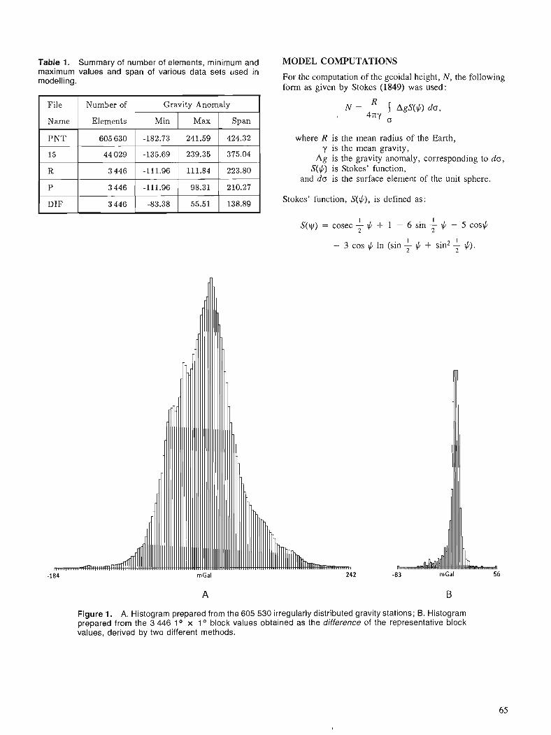
Table 1. Summary of number of elements, minimum and RIODEL OMP PUT AT IONS maximum values and span of various data sets used in modelling. For the computation o f the geoidal height, N, the following

form as given by Stokes (1849) was used:

where R is the mean radius o f the Earth, y is the mean gravity,

Ag is the gravity anomaly, corresponding to do, S($) is Stokes' function,

and do is the surface element of the unit sphere.

Stokes' function, S($), is defined as:

I 1 S(v) = cosec 1 $ + 1 - 6 sin $ - 5 cos$

I I - 3 cos $ In (sin $ + sin2 - 2 $).

Figure 1. A. Histogram prepared from the 605 530 irregularly distributed gravity stations; B. Histogram prepared from the 3 446 1 x 1 block values obtained as the difference of the representative block values, derived by two different methods.

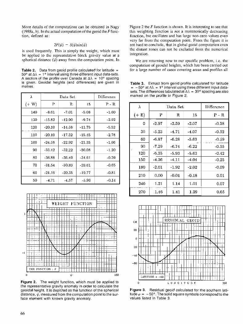
More details o f the computations can be obtained in Nagy (1988a, b). I n the actual computation o f the geoid the F function, defined as:

2F(#) = S(#)sin($) is used frequently. This is simply the weight, which must be applied to the representative block gravity value at a spherical distance (#) away from the computation point. I n

Table 2. Data from geoid profile calculated for latitude = 50° at Ah = 1 interval using three different input data-sets. A section of the profile over Canada at Ah = l o 0 spacing is given. Geoidal heights (and differences) are given in metres.

Figure 2. The weight function, which must be applied to the representative gravity anomaly in order to calculate the geoidal height. It is depicted as the function of the spherical distance, IC., measured from the computation point to the surface element with known gravity anomaly.

Figure 2 the F function is shown. I t is interesting to see that this weighting function i s not a monotonically decreasing function, but oscillates and has large non-zero values even very far from the computation point. From the figure i t is not hard to conclude, that in global geoid computation even the distant zones can not be excluded from the numerical integration.

We are returning now to our specific problem, i.e. the computation of geoidal heights, which has been carried out for a large number o f cases covering areas and profiles all

Table 3. Extract from geoid profile calculated for latitude = - 50° at Ah = 1 interval using three different input datasets. The differences tabulated at Ah = 30° spacing are also marked on the profile in Figure 2.

0 L O N G I T U D E 360

Figure 3. Residual geoid calculated for the southern latitude cp = - 50'. The solid square symbols correspond to the values listed in Table 3.

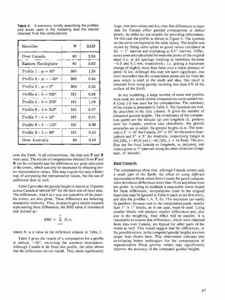
Table 4. A summary, briefly describing the profiles and areas used in the modeling and the results obtained from the computations.

I Identifier I " I """

Over Canada

Eastern Hemisphere

Profile 1 : p = 50" --- Profile 2 : cp = -50"

Profile 3 : (o = 0"

Profile 4 : X = 220"

80

80

360

360



Profile 7 : X = 50"


( Over Australia ( 80 ( 0.19 (

2.04

0.63

1.25

0.34

360

Profile 9 : X = 90"

over the Earth. In all computations, the data sets P and R were used. The results of computations obtained from P and R can be compared and the differences are good indicators of the errors, which can only be decreased by obtaining better representative values. This may require not only a better way of computing the representative values, but the use of additional data as well.

0.34

181

181

181

181

Table 2 provides the geoidal height in metres at 10 points across Canada at latitude 50" for the three sets of input data. The differences, which in a way are indicative of the possible errors, are also given. These differences are behaving essentially randomly. Thus, in order to get a simple measure representing these differences, the RMS value is introduced and defined as:

n

RMS = C Niln, i = l

1.08

0.57

0.41

0.36

I I

181

where Ni is a value in the difference column in Table 2.

181

0.40

Table 3 gives the results of a computation for a profile at latitude -50°, encircling the southern hemisphere. Although Canada is far from this profile, the table shows that the differences do not vanish. They attain significantly

0.88

large, non-zero values and it is clear that differences in input data for Canada affect geoidal computations at distant points. As tables are not suitable for providing information, for this case the profile is shown in Figure 3. The symbols on the curve correspond to the table values. The profile was drawn by fitting cubic-spline to geoid values calculated at Ah = 1 " interval and evaluating at 0.1 " interval. Differ- ences were also calculated between the points of the original input (i.e. at Ah spacing) resulting in variations between -6.5 and 6.2 mm, respectively; i.e. getting a maximum change of slightly more than 6mm over a linear distance of about 70 km. Although this may not seem significant, one must remember that the computation points are far from the area which is used in the study and also, this result is obtained from using gravity covering less than 4 % of the surface of the Earth.

In our modelling, a large number of areas and profiles were used, for which similar computations were carried out. A Cray 1-S was used for the computations. The summary of the results is presented in Table 4. The locations are briefly described in the first column. N gives the number of computed geoidal heights. The coordinates of the computation points are the latitude (p) and longitude ( A , positive west for Canada, positive east elsewhere), the gravity anomalies are in mGal, the geoidal heights in m. The intervals is 5" x 10" for Canada, 20" x 30" for the eastern hemisphere and 5" x 5" for Australia, respectively (origin at [40,220], [-60,0] and [-40,1001, h + ve East). The profiles are for fixed latitude or longitude, as indicated, and values given at 1 " intervals along the other direction (longi- tilde, or latitude).

DISCUSSION

The computations show that, although Canada covers only a small part of the Earth, the effect of using different representative block values from Canada for geoid computations introduces differences more than 10 cm anywhere over the globe. In trying to establish a reasonable lower bound for these differences, computations close to the original input data may be ignored in Table 4 (such as the first entry, and also the profiles 1, 4, 5, 6). This exclusion can easily be justified, because cose to the computation point, smaller than 1" x 1" blocks, as in our case, must be used. Using smaller blocks will produce smaller differences and, also due to the weighting, their effect will be smaller. It is reasonable to assume that differences, which were obtained from data over Canada, are typical for other parts of the world as well. This would suggest that the differences, or the possible errors, in the computed geoidal heights are even larger than shown here. This observation indicates that developing better techniques for the computation of representative block gravity values may significantly improve the accuracy of the computed geoidal heights.

REFERENCES

Heiskanen, W.A. and Moritz, H. 1967 : Physical Geodesy; W.H. Freeman and Company, San Francisco. Listing, J.B. 1873: Ueber unsere jetzige Kenntniss der Gestalt und Grosse der Erde;

Nachr. Kgl. Ges. Wiss. Gottingen. No. 3, p. 33-98. Nagy, D. 1988a: GEOID '88: A gravimetric geoid for Canada; Open File Report

No. 1977, Geophysics Division, Geological Survey of Canada. 1988b: GEOID '88: A gravimetric geoid for Canada; in Proceedings of

Chapman Conference, Fort Lauderdale, Florida, 14-18 Sept., 1988.

1963 : Gravirnetric deflections of the vertical by digital computers; Publ. Dominion Observatory, Ottawa. Canada, v. XXXVII, No. I., 72 p.

Paul, M.K. and Nagy, D. 1973 : The accuracy of geoidal height obtainable from gravity data alone;

The Canadian Surveyor, v. 27, No. 2, p. 149-156.

Rapp, R.H. 1973: Accuracy of geoid undulation computations; Journal of Geophysi-

cal Research, v. 78, p. 7589-7595. Rapp, R.H. and Rummell, R. 1975: Methods for the Computation of Detailed Geoids and their

Accuracy; Report No. 233, Department of Geodetic Science, The Ohio State University, 36 p.

Sjoberg, L. 1979: The accuracy of geoid undulations by degree implied by mean

gravity anomalies on a sphere; Journal of Geophysical Research, 84, p. 6226-6230.

Stokes, G.G. 1849: On the variation of gravity on the surface of the Earth; Transac-

tions Cambridge Philosophisc Society, v. 8, p. 672-695. Vanitek, P. and Krakiwsky, E.J. 1986 : Geodesy : The Concepts ; North-Holland Publishing Company,

Amsterdam.

Methods and applications of image analysis using integrated data sets

Steven E. Franklinl and Randall T. Gillespie2

Franklin, S. E. and Gillespie, R. T., Methods and applications of image analysis using integrated data sets; 0_ Statistical Applications in the Earth Sciences, ed. F. P. Agterberg and G. F. Bonham-Carter; Geological Survey of Canada, Paper 89-9, p. 69-78, 1989.

Abstract

Satellite remote sensing studies of complex terrain phenomena can benefit greatly from careful application of digital ancillary data. These data may be obtained from maps (e.g. geological units, soil classifications, political boundaries) or may be continuous variables (e.g. digital elevation models, aeromagnetic surveys, regional economic indicators) which are increasingly available at relatively lowcost. Their integration with remotely sensed data requires geometric accuracy and that some attention be paid to an analysis strategy which may include deterministic and probabilistic techniques. in this paper these methods are briefly reviewed, and two examples of integrated data sets in the geological investigation of a glaciated, vegetated environment in central Newfoundland and in integrated terrain analysis of a moderate relief, boreal zone in western Newfoundland are used to highlight the discussion. In the first case, I.andsat Thematic Mapper spectral response patterns and aeromagnetic response patterns within specific geological units are combined, and the interpretation is based on the search for common underlying patterns. In the second case, I.andsat Multispectral Scanner data are considered in a classifier with geomorphometric variables extracted from a dense-grid digital elevation model. The interpretation in this example is on the significant improvements in classification accuracy obtained when using an integrated data set over that which could be obtained using either data set alone.

Resume

Les etudes de teledetection par satellite de phenomenes de terrain complexes peuvent etre grandement facilities par une application soignee des donnees numeriques accessoires. Ces donnees peuvent etre tirees de cartes (p . ex. unites geologiques, classifications des sots, frontieres politiques) ou peuvent etre des variables continues (p. ex. modeles numeriques de !'altitude, leves aeromagnetiques, indicateurs economiques regionaux) de plus en plus disponibles a un cout relativement faible. Leur integration aux donnees de teledetection exige une precision geometrique et une certaine attention doit etre consacree a une strategie d'analyse pouvant englober des methodes deterministes et probabilistes. Ces methodes sont brievement examinees dans la presente etude et, afin d'eclairer la discussion, on a recours a deux exemples d'ensembles integres de donnees utilises dans !'etude geologique d'un milieu glacie recouvert de vegetation du centre de Terre-Neuve et dans !'analyse des terrains integree d 'une zone boreale au relief moderement accentue de l'ouest de Terre-Neuve. Dans le premier cas, des configurations de la reponse spectrale de l 'appareil de cartographie thematique LANDSAT sont combinees a des configurations de la reponse aeromagnetique a l 'interieur d 'unites geologiques specifiques et l 'interpretation est basee sur la recherche de configurations sous-jacentes communes. Dans le deuxieme cas, des donnees du balayeur multispectral LANDSATsont comparees dans un systeme d'analyse des images a des variables geomorphometriques tirees d 'un mode le numerique del 'altitude a quadrillage dense. Dans cet exemple' l 'interpretation parte sur les ameliorations importantes de la precision de la classification obtenues en utilisant un ensemble integre de donnees par rapport a celles que l'on obtiendrait en ayant recours uniquement a l'un ou !'autre ensemble de donnees.

1 Department of Geography, The University of Calgary, Calgary, Alberta T2N I N4 2 NORDCO Ltd., Box 8833, St. John's, Newfoundland AlB 3T2

69

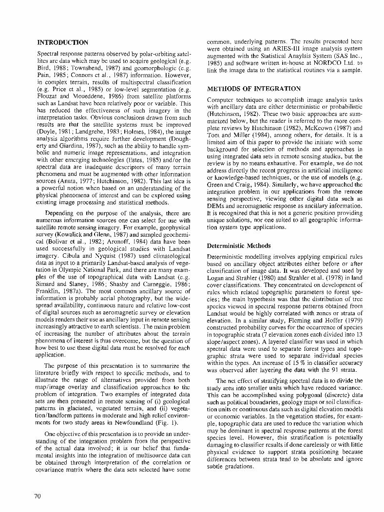
INTRODUCTION common, underlying patterns. The results presented here were obtained using an ARIES-I11 image analysis system

Spectral response patterns observed by polar-orbiting satel- augmented with the Statistical Anaylsis System (SAS Inc., lites are data which may be used to acquire geological (e.g. 1985) and software written in-house at NORDCO Ltd . to

1988; Townshendy 1987) and geomor~hologic (e.g. link the image data to the statistical routines via a sample. Pain, 1985; Connors et al., 1987) information. However, in complex terrain, results of multispectral classification (e.g. Price et al., 1985) or low-level segmentation (e.g. METHODS OF INTEGRATION ~louzat and Moueddene, 1986) from satellite platforms such as Landsat have been relatively poor or variable. This has reduced the effectiveness of such imagery in the interpretation tasks. Obvious conclusions drawn from such results are that the satellite systems must be improved (Doyle, 1981 ; Landgrebe, 1983; Holmes, 1984), the image analysis algorithms require further development (Dough- erty and Giardina, 1987), such as the ability to handle symbolic and numeric image representations, and integration with other emerging technologies (Estes, 1985) and/or the spectral data are inadequate descriptors of many terrain phenomena and must be augmented with other information sources (Anuta, 1977; Hutchinson, 1982). This last idea is a powerful notion when based on an understanding of the physical phenomena of interest and can be explored using existing image processing and statistical methods.

Depending on the purpose of the analysis, there are numerous information sources one can select for use with satellite remote sensing imagery. For example, geophysical survey (Kowalick and Glenn, 1987) and sampled geochemical (Bolivar et al., 1982; Aronoff, 1984) data have been used successfully in geological studies with Landsat imagery. Cibula and Nyquist (1987) used climatological data as input to a primarily Landsat-based analysis of vegetation in Olympic National Park, and there are many examples of the use of topographical data with Landsat (e.g. Simard and Slaney, 1986; Shasby and Carneggie, 1986; Franklin, 1987a). The most common ancillary source of information is probably aerial photography, but the widespread availability, continuous nature and relative low-cost of digital sources such as aeromagnetic survey or elevation models renders their use as ancillary input in remote sensing increasingly attractive to earth scientists. The main problem of increasing the number of attributes about the terrain phenomena of interest is thus overcome, but the question of how best to use these digital data must be resolved for each application.

The purpose of this presentation is to summarize the literature briefly with respect to specific methods, and to illustrate the range of alternatives provided from both maplimage overlay and classification approaches to the problem of integration. Two examples of integrated data sets are then presented in remote sensing of (i) geological patterns in glaciated, vegetated terrain, and (ii) vegeta- tionllandform patterns in moderate and high relief environments for two study areas in Newfoundland (Fig. 1).

One objective of this presentation is to provide an understanding of the integration problem from the perspective of the actual data involved; it is our belief that fundamental insights into the integration of multisource data can be obtained through interpretation of the correlation or covariance matrix where the data sets selected have some

Computer techniques to accomplish image analysis tasks with ancillary data are either deterministic or probabilistic (Hutchinson, 1982). These two basic approaches are summarized below, but the reader is referred to the more complete reviews by Hutchinson (1982), McKeown (1987) and Tom and Miller (1984), among others, for details. It is a limited aim of this paper to provide the initiate with some background for selection of methods and approaches in using integrated data sets in remote sensing studies, but the review is by no means exhaustive. For example, we do not address directly the recent progress in artificial intelligence or knowledge-based techniques, or the use of models (e.g. Green and Craig, 1984). Similarly, we have approached the integration problem in our applications from the remote sensing perspective, viewing other digital data such as DEMs and aeromagnetic response as ancillary information. It is recognized that this is not a generic position providing unique solutions, nor one suited to all geographic information system type applications.

Deterministic Methods

Deterministic modelling involves applying empirical rules based on ancillary object attributes either before or after classification of image data. It was developed and used by Logan and Strahler (1980) and Strahler et al. (1978) in land cover classifications. They concentrated on development of rules which related topographic parameters to forest species; the main hypothesis was that the distribution of tree species viewed in spectral response patterns obtained from Landsat would be highly correlated with zones or strata of elevation. In a similar study, Fleming and Hoffer (1979) constructed probability curves for the occurrence of species in topographic strata (7 elevation zones each divided into 13 slope/aspect zones). A layered classifier was used in which spectral data were used to separate forest types and topographic strata were used to separate individual species within the types. An increase of 15 % in classifier accuracy was observed after layering the data with the 91 strata.

The net effect of stratifying spectral data is to divide the study area into smaller units which have reduced variance. This can be accomplished using polygonal (discrete) data such as political boundaries, geology maps or soil classification units or continuous data such as digital elevation models or economic variables. In the vegetation studies, for example, topographic data are used to reduce the variation which may be dominant in spectral response patterns at the forest species level. However, this stratification is potentially damaging to classifier results if done carelessly or with little physical evidence to support strata positioning because differences between strata tend to be absolute and ignore subtle gradations.

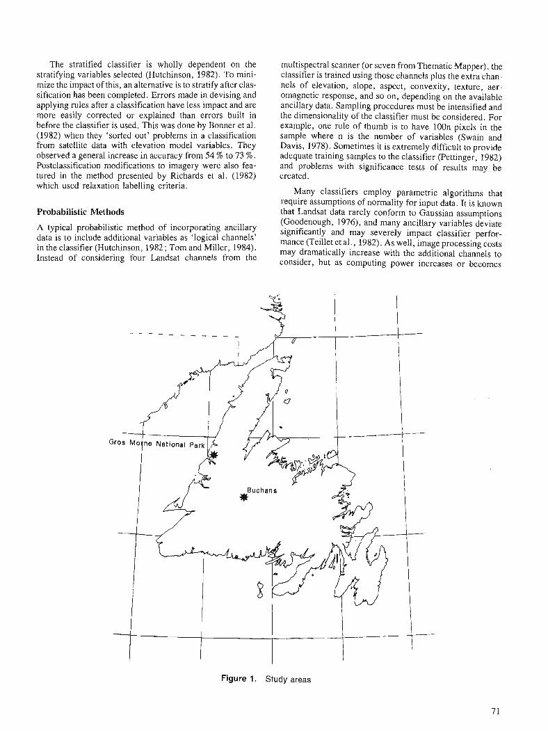
The stratified classifier is wholly dependent on the stratifying variables selected (Hutchinson, 1982). To minimize the impact of this, an alternative is to stratify after classification has been completed. Errors made in devising and applying rules after a classification have less impact and are more easily corrected or explained than errors built in before the classifier is used. This was done by Bonner et al. (1982) when they 'sorted out' problems in a classification from satellite data with elevation model variables. They observed a general increase in accuracy from 54 % to 73 % . Postclassification modifications to imagery were also featured in the method presented by Richards et al. (1982) which used relaxation labelling criteria.

Probabilistic Methods

A typical probabilistic method of incorporating ancillary data is to include additional variables as 'logical channels' in the classifier (Hutchinson, 1982; Tom and Miller, 1984). Instead of considering four Landsat channels from the

multispectral scanner (or seven from Thematic Mapper), the classifier is trained using those channels plus the extra channels of elevation, slope, aspect, convexity, texture, aeromagnetic response, and so on, depending on the available ancillary data. Sampling procedures must be intensified and the dimensionality of the classifier must be considered. For example, one rule of thumb is to have lOOn pixels in the sample where n is the number of variables (Swain and Davis, 1978). Sometimes it is extremely difficult to provide adequate training samples to the classifier (Pettinger, 1982) and problems with significance tests of results may be created.

Many classifiers employ parametric algorithms that require assumptions of normality for input data. It is known that Landsat data rarely conform to Gaussian assumptions (Goodenough, 1976), and many ancillary variables deviate significantly and may severely impact classifier performance (Teillet et al., 1982). As well, image processing costs may dramatically increase with the additional channels to consider, but as computing power increases or becomes

- - - - -

Figure 1. Study areas

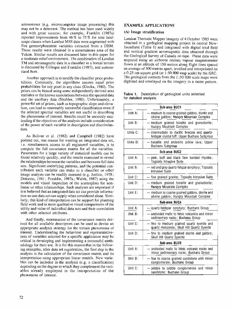
autonomous (e.g. microcomputer image processing) this may not be a deterrent. The method has been used widely and with great success; for example, Franklin (1987a) reported improvements from 46 % to 75 % for nine landscape classes when Landsat MSS data were augmented with five geomorphometric variables extracted from a DEM. Those results were obtained in a mountainous area of the Yukon. Similar results are discussed later in this paper for a moderate relief environment. The combination of Landsat TM and aeromagnetic data in a classifier in a boreal terrain is discussed by Gillespie and Franklin (1987), and summarized here.

Another approach is to modify the classifier prior probabilities. Commonly, the algorithms assume equal prior probabilities for any pixel in any class (Klecka, 1980). The priors can be biased using some independently derived area statistics or the known associations between the spectral data and the ancillary data (Strahler, 1980). Unfortunately, a powerful set of priors, such as topographic slope and elevation, can lead to reasonably successful classification even if the selected spectral variables are not useful in describing the phenomena of interest. Results could be seriously misleading if the objectives of the analysis include consideration of the power of each variable in description and discrimination.

As Bolivar et al. (1982) and Campbell (1982) have pointed out, one reason for wanting an integrated data set, i.e. simultaneous access to all registered variables, is to compute the full covariance matrix for all the variables. Parameters for a large variety of statistical models can be found relatively quickly, and the results examined to reveal the relationships between the variables and between full data sets. Significant underlying patterns, and the potential contribution each variable can make to a classifier or other image analysis can be readily assessed (e.g. Justice, 1978; Dottavio, 1981 ; Franklin, 1987a; Walsh, 1987) using the models and visual inspection of the scatterplots for non- linear or other relationships. Such analyses are important if it is believed that an integrated data set can provide information no one data set can supply when considered alone. Simi- larly, this kind of interpretation can be support for planning field work and in more qualitative visual comparisons of the utility and value of individual data sets and their correlation with other selected attributes.

And finally, examination of the covariance matrix derived for all available descriptors can be used to devise an appropriate analysis strategy for the terrain phenomena of interest. Understanding the behaviour and representative- ness of variables selected for a specific application may be critical in developing and implementing a successful methodology for their use. It is for this reason that in the following examples, after data set registration, the first step in the analysis is the calculation of the covariance matrix and its interpretation using appropriate linear models. New variables can be included in the analysis (e.g. a classification) depending on the degree to which they complement the variables already employed in the interpretation of the phenomena of interest.

EXAMPLE APPLICATIONS

(A) Image stratification

Landsat Thematic Mapper imagery of 4 October 1985 were obtained in a geological mapping project in central New- foundland (Table 1) and integrated with digital total field and vertical gradient aeromagnetic data obtained through the Geological Survey of Canada on tape. These data were acquired using an airborne cesium vapour magnetometer flown at an altitude of 150 metres along flight lines spaced an average of 300 metres apart, levelled and interpolated on a 0.25 cm square grid (at 1 5 0 000 map scale) by the GSC. The geological contacts from the 1 :50 000 scale maps were digitized and overlayed on the imagery in a raster pattern.

Table 1. Description of geological units selected for detailed analysis.

Skull Hill Quartz Syenite

Sub-area BUC5

Uni t A :

Unit B:

Unit C:

- undivided mafic to felsic volcanic rocks and minor sedimentary rocks; Buchans Group

- fine to coarse grained sandstone with minor conglomerate; Buchans Group

- pebble to cobble conglomerate and minor sandstone; Buchans Group

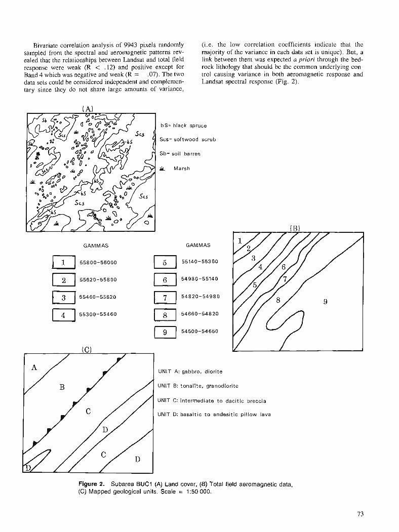
Bivariate correlation analysis of 9943 pixels randomly (i.e. the low correlation coefficients indicate that the sampled from the spectral and aeromagnetic patterns rev- majority of the variance in each data set is unique). But, a ealed that the relationships between Landsat and total field link between them was expected a priori through the bed- response were weak (R < .12) and positive except for rock lithology that should be the common underlying con- Band 4 which was negative and weak (R = - .07). The two trol causing variance in both aeromagnetic response and data sets could be considered independent and complemen- Landsat spectral response (Fig. 2). tary since they do not share large amounts of variance,

bS= black spruce

Scs= softwood scrub

Sb- soil barren

& Marsh

GAMMAS

55800-56000

55620-55800

55460-55620

55300-55460

GAMMAS

55140-55300

54980-55140

54820-54980

54660-54820

54500-54660

UNlT A: gabbro, diorite

UNlT B: tonalite, granodiorite

UNlT C: intermediate t o dacitic breccia

UNlT D: basaltic t o andesitic pi l low lava

Figure 2. Subarea BUCl (A) Land cover, (6) Total field aerornagnetic data, (C) Mapped geological units. Scale = 1 :50 000.

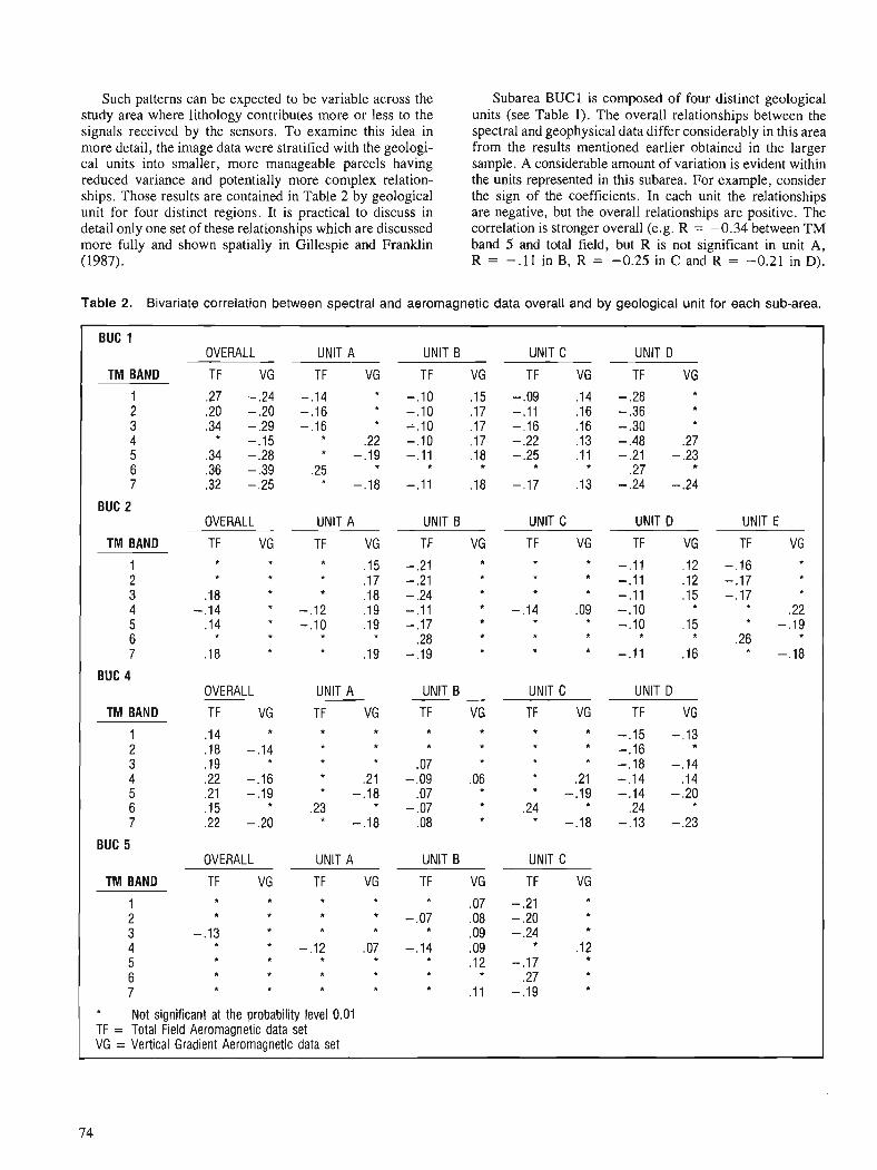
Such patterns can be expected to be variable across the study area where lithology~contributes more or less to the signals received by the sensors. To examine this idea in more detail, the image data were stratified with the geological units into smaller, more manageable parcels having reduced variance and potentially more complex relationships. Those results are contained in Table 2 by geological unit for four distinct regions. It is practical to discuss in detail only one set of these relationships which are discussed more fully and shown spatially in Gillespie and Franklin (1987).

Subarea BUCl is composed of four distinct geological units (see Table 1). The overall relationships between the spectral and geophysical data differ considerably in this area from the results mentioned earlier obtained in the larger sample. A considerable amount of variation is evident within the units represented in this subarea. For example, consider the sign of the coefficients. In each unit the relationships are negative, but the overall relationships are positive. The correlation is stronger overall (e.g. R = -0.34 between TM band 5 and total field, but R is not significant in unit A, R = -.I1 in B, R = -0.25 in C and R = -0.21 in D).

Table 2. Bivariate correlation between spectral and aeromagnetic data overall and by geological unit for each sub-area.

BUC 1 OVERALL UNIT A UNIT B UNIT C UNIT D

TM BAND TF VG TF VG TF VG TF VG TF VG

1 .27 -.24 -.I4 * -. lo -15 -.09 .14 -.28 2 .20 -.20 -.I6 * - . l o . I7 -.I1 .16 -.36 *

3 -34 -.29 - . I6 * 6 .10 . I7 - . I6 .16 -.30 4 * -.I5 .22 -.lo . I7 -.22 .13 -.48 .27 *

5 .34 -.28 -.I9 -.I1 .18 -.25 . l l -.21 -.23 6 .36 -.39 .25 * * * * .27 *

7 .32 -.25 -.I8 -.I1 -18 - . I7 .13 -.24 -.24 *

BUC 2 OVERALL UNIT A UNIT B UNIT C UNIT D UNIT E

TM BAND TF VG TF VG TF VG TF VG TF VG TF VG

1 * * * * .15 -.21 -.I1 .12 -.I6 *

2 * * * .17 -.21 -.I1 .12 -.I7 *

3 .18 * * * * * .18 -.24 -.I1 -15 -.I7 *

4 -.I4 * - . I2 .19 -.I1 * -.I4 .09 - . lo * * .22 5 .14 * - . l o .19 - . I7 * * - . lo .15 * - . I9 6 * * * * * * * * * .28 .26 *

7 .18 * * * * .19 -.I9 -.I1 .16 -.I8

BUC 4 OVERALL UNIT A UNIT B UNIT C UNIT D

TM BAND TF VG TF VG TF VG TF VG TF VG

1 .14 * * * * -.I5 -.I3 2 .18 -.I4 * * * * * -.I6 *

3 .19 * * * * .07 * - . I8 - . I4 4 .22 -.I6 .21 -.09 .06 .21 -.I4 .14 * *

5 .21 -.I9 * -.I8 .07 * * -.I9 -.I4 -.20 6 .15 .23 * -.07 * * .24 .24 7 .22 -.20 * -.I8 .08 * * -.I8 - . I3 -.23

BUC 5 OVERALL UNIT A UNIT B UNIT C

TM BAND TF VG TF VG TF VG TF VG

1 * * * * .07 -.21 *

2 + * * -.07 .08 -.20 t

3 -.I3 * * a .09 -.24

4 * * -.I2 .07 -.14 .09 * .12 5 * * * * .12 - . I7 *

6 * * * * * .27 *

7 * * * * . l l -.I9 * Not significant at the probability level 0.01 TF = Total Field Aeromagnetic data set VG = Vertical Gradient Aeromagnetic data set

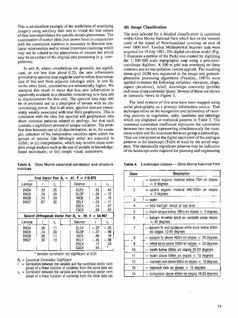
This is an excellent example of the usefulness of stratifying imagery using ancillary data sets to reveal the true nature of data interdependence for specific terrain phenomena. The examination of scatter plots (not shown here) in conjunction with the correlation statistics is necessary to discount non- linear relationships and to reveal important clustering which may not be related to the phenomena of interest but which may be an artifact of the original data processing (e.g. interpolation).

In unit A, where correlations are generally not significant, or are less than about 0.25, the new information provided by spectral data might be used to refine discrimination of this unit from adjacent lithologic units. In unit D, on the other hand, correlations are substantially higher. We interpret this result to mean that less new information is apparently available to a classifier considering new data sets as discriminators for this unit. The spectral data may still be of profound use as a descriptor of terrain with no discriminating power. But in all units, spectral data are consistently weakly associated with total field geophysics. This is consistent with the idea that spectral and geophysical data share common patterns related to geology, but that each contains a significant amount of unique variation. The problem then becomes one of (i) discrimination, as in, for example, selection of the independent variables upon which the groups of interest (the lithologic units) are expected to differ; or (ii) interpretation, which may involve more complex image analysis such as the use of models or knowledge- based techniques; or (iii) simple visual assessment.

Table 3. Gros Morne canonical correlation and structure matrices

* denotes correlation not significant at 0.01

R, = Canonical Correlation Coefficient r = Correlation between the variable and the canonical vector com-

posed of a linear function of variables from the same data set. r, = Correlation between the variable and the canonical vector com-

posed of a linear function of variables from the other data set.

(B) Image Classification

The area selected for a detailed classification is contained within Gros Morne National Park which lies on the western coast of the island of Newfoundland covering an area of over 1800 km2. Landsat Multispectral Scanner data were acquired for 19 July 1981. The digital elevation model (Fig. 3 illustrates a portion of the Park) was created by digitizing the 1 : 100 000 scale topographic map using a precision- coordinate digitizer. A 100 m grid was overlayed on these contours and an interpolation routine applied. The resulting dense-grid DEM was registered to the image and geomorphometric processing algorithms (Franklin, 1987b) were applied to extract the following variables: elevation, slope, aspect (incidence), relief, downslope convexity (profile) and cross-slope convexity (plan). Several of these are shown as isometric views in Figure 3.

The land systems of this area have been mapped using aerial photography as a primary information source. That technique relies on the recognition and delineation of recurring patterns in vegetation, soils, landform and lithology which are displayed as statistical patterns in Table 3. The canonical correlation coefficient represents the correlation between two vectors representing simultaneously the maximum within and the maximum between group relationships. They are interpreted as the digital equivalent of the analogue patterns in the landscape (Table 4) used by the aerial map- pers. The statistically significant patterns may be indicative of the landscape units required for planning and engineering

Table 4. Landscape classes - Gros Morne National Park

( a ) Elevation

Figure 3. Isometric views of digital elevation model and derivatives.

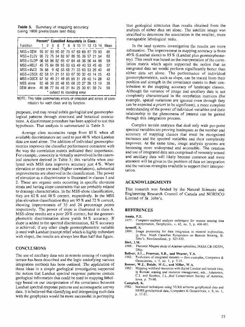
Table 5. Summary of mapping accuracy (using 1808 pixelslclass test data)

Percent* Classified Accurately in Class: Function 1 2 5 6 7 8 9 1 0 1 1 1 2 1 3 1 4 Mean

MSS+DEM 93 97 93 90 92 70 97 69 69 87 70 93 85 MSS+ELEV 95 72 75 34 82 97 86 35 39 57 21 54 62 MSS+SLOP 56 68 86 82 65 47 64 48 36 56 44 56 59 MSS+RELF 45 75 84 69 65 53 63 49 40 53 45 48 57 MSS+INCD 36 88 9 42 55 68 71 33 60 53 26 40 48 MSS+CSCX 62 58 51 21 51 63 67 30 32 42 14 25 43 MSS+DSCX 67 52 49 21 49 65 69 31 29 45 14 26 43 MSS alone 62 48 39 20 48 65 68 20 27 38 13 19 39 DEM alone 46 88 77 84 48 31 84 25 30 61 59 74 59

* subject to rounding error

NOTE: This table summarizes errors of omission and errors of commission for each class and by function.

purposes, and may reveal subtle geological and geomorpho- logical patterns through structural and botanical associations. A discriminant procedure has been applied to test this hypothesis. That analysis is summarized in Table 5.

Average class accuracies range from 85 % when all available discriminators are used to just 40 % when Landsat data are used alone. The addition of individual geomorphometrics improves the classifier performance consistent with the way the correlation matrix indicated their importance. For example, convexity is virtually uninvolved in the canonical structure derived in Table 3 ; this variable when analyzed with MSS data improves accuracy just 4 % . When elevation or slope are used (higher correlations), substantial improvements are observed in the classification. The power of elevation as a discriminator is illustrated in classes 1 and 2. These are organic units occurring in specific elevation strata and having slope constraints that are probably related to drainage characteristics. In the MSS-alone classification, they are 62 % and 48 % correct, respectively. In the MSS plus elevation classification they are 95 % and 72 % correct, showing improvements of 33 and 24 percentage points respectively. The power of slope is illustrated in class 6. MSS-alone results are a poor 20 % correct, but the geomorphometric discrimination alone yields 84 % accuracy. If slope is added to the spectral discrimination, 82 % accuracy is achieved ; if any other single geomorphometric variable is used with Landsat (except relief which is highly redundant with slope), the results are always less than half that figure.

CONCLUSIONS

The use of ancillary data sets in remote sensing of complex terrain has been described and the logic underlying various integration methods has been outlined. The application of these ideas in a simple geological investigation supported the notion that Landsat spectral response patterns contain geological information that could be used in mapping lithology based on our interpretation of the covariance between Landsat spectral response patterns and aeromagnetic survey data. It is believed that classifying and interpreting such data with the geophysics would be more successful in portraying

true geological structures than results obtained from the analysis of either data set alone. The satellite image was stratified to determine the association in the smaller, more manageable lithological units.

In the land systems investigation the results are more substantive. The improvement in mapping accuracy is from 40 % (Landsat alone) to 85 % (Landsat plus geomorphometry). This result was based on the interpretation of the correlation matrix which again supported the notion that an integrated data set would perform significantly better than either data set alone. The performance of individual geomorphometrics, such as slope, can be traced from their position and strength in the covariance matrix to their contribution to the mapping accuracy of landscape classes. Although the variance of image and ancillary data is not completely characterized in the correlation matrices (for example, spatial variations are ignored even through they can be expected apriori to be significant), a more complete understanding of the power of individual variables and their relationship to the phenomena of interest can be gained through this integration process.

Complex terrain analyses that deal only with per-point spectral variables are proving inadequate as the number and accuracy of mapping classes that must be recognized increases and the spectral variables and their complexity improves. At the same time, image analysis systems are becoming more widespread and accessible. The creation and use of integrated data sets comprised of remotely sensed and ancillary data will likely become common and .more attention will be given to the problem of data set integration and the various strategies available to support their interpretation.

ACKNOWLEDGMENTS

This research was funded by the Natural Sciences and Engineering Research Council of Canada and NORDCO Limited of St. John's.

REFERENCES Anuta, P.E. 1977: Computer-assisted analysis techniques for remote sensing data

interpretation, Geophysics, v. 42, no. 3, p. 468-481. Aronoff, S. 1984: Image processing for data integration in mineral exploration,

in Proc. Ninth Canadian Symposium on Remote Sensing, St. zhn's , Newfoundland, p. 423-432.

Bird, J.M. 1988 : Thematic Mapper study of Alaskan ophiolites, NASA CR-182554,

256p. Bolivar, S.L., Freeman, S.B., and Weaver, T.A. 1982: Evaluation of integrated datasets - four examples, Computers &

Geosciences, v. 9, no. 1 , p. 7-15. Bonner, W.J., Rohde, W.G., and Miller, W.A. 1982 : Mapping wildland resources with digital Landsat and terrain data,

in Remote sensing and resource management, eds., Johannsen, - C.J. and Sanders, J.L.,Soil Conservation Society of America, Iowa, p. 73-80.

Campbell, K. 1982 : Statistical techniques using NURE airborne geophysical data and

NURE geochemical data, Computers & Geosciences, v. 9, no. 1, p. 17-21.

Cibula, W.G. and Nyquist, M.O. 1987 : Use of topographical and climatological models in a geographical

data base to improve Landsat MSS classification of Olympic National Park, Photogrammetric Engineering and Remote Sens- ing, v. 53, no. 1, p. 67-75.

Connors, K., Kavdner, T.N., and Peterson, K.W. 1987: Classification of geomorphic features and landscape stability in

New Mexico using simulated SPOT imagery, Remote Sensing of Environment, v. 22, pp. 187-207.

Dottavio, C.L. 1981 : Effects of canopy closure on incoming solar radiance, Proc.,

Seventh Annual Symposium on Machine Processing of Remotely Sensed Data, LARS, Purdue University, p. 375-383.

Dongherty, E.R. and Giardina, C.R. 1987: Matrjx structured image processing, Prentice-Hall, Englewood

Cliffs, N.J., 200p. Doyle, F.J. 1981: Satellite systems for cartography, ITC-Journal, v. 2, no. 1, p.

153-171. Estes, J.E. 1985 : The need for improved information systems, Canadian Journal of

Remote Sensing, v. 11, no. 4, p. 124-131. Fleming, M.D., and Hoffer, R.M. 1979: Machine processing of Landsat MSS and DMA topographic data

for forest cover type mapping, fi Proc. Fifth Annual Symposium on Machine Processing of Remotely Sensed Data, LARS, Purdue University, p. 377-390.

Flouzat, G., and Moueddene, K. 1986: Computer-aided interpretation of complex geological patterns in

remote sensing, & Proc. European Space Agency International Geoscience and Remote Sensing Symposium, Zurich, p. 783-786.

Franklin, S.E. 1987a: Terrain analysis from digital patterns in geomorphometry and

Landsat spectral response, Photogrammetric Engineering and Remote Sensing, v. 53, no. 1, p. 59-65.

1987b: Geomorphometric processing of digital elevation models: Com- puters & Geosciences, v. 13, no. 6, p. 603-609.

Gillespie, R.T. and Franklin, S.E. 1987: Image analysis methods applied to mineral exploration in the

Buchans area, Newfoundland, Proc., Eleventh Canadian Symposium on Remote Sensing, Waterloo, Canada, p.. 299-309.

Goodenough, D.G. 1976: Image-100 classification methods for ERTS scanner data: Cana-

dian Journal of Remote Sensing, v. 2, no. l , p. 18-29. Green, A.A., and Craig, M. 1984: Integrated analysis of image data for mineral exploration Proc.,

Third Thematic Conference on Remote Sensing for Exploration Geology, Colorado Springs, Colorado, p. 131-137.

Holmes, R.A. 1984: Advanced sensor systems: thematic mapper and beyond, Remote

Sensing of Environment, v. 15, no. 3, p. 213-221. Hutchinson, C.F. 1982: Techniques for combining Landsat and ancillary data for digital

classification improvement, Photogrammetric Enginnering and Remote Sensing, v. 48, no. 1, p. 123-130.

Justice, C.O. 1978: An examination of the relationships between selected ground

properties and Landsat MSS data in an area of complex terrain in southern Italy, & Proc. Fall Technical Meeting of American Society for Photogrammetry, Albuquerque, New Mexico, p. 303-328.

Klecka, W.R. 1980: Discriminant analysis, Sage Publications, Beverly Hills and Lon-

don, 71 p. Kowalick, W.S. and Glenn, W.E. 1987: Image processing of aeromagnetic data and integration with Land-

sat images for improved structural interpretation, Geophysics, v. 52, no. 7, p. 875-884.

Landgrebe, D.A. 1983: Land observation sensors in perspective, Remote Sensing of

Environment, v. 13, no. 5, p. 391-402. Logan, T.L. and Strahler, A.H. 1980 : Forest cover classification from Landsat imagery : an application

of image processing, @ Proc. Workshop on Picture Data Descrip- tion and Management, IEEE Computer Society, California, p. 5-11.

McKeown, D. 1987: The role of artificial intelligence in the integration of remote sens-

ing data and geographic information systems, IEEE Transactions on Geoscience and Remote Sensing, v. 25, no. 3, p. 330-348.

Pain, C. 1985 : Mapping landforms from Landsat imagery, an example from New

South Wales, Remote Sensing of Environment, v. 17, p. 55-65. Petlinger, L.R. 1982: Digital classification of Landsat data for vegetation and landcover

mapping in the Blackfoot River watershed, southern Idaho, Profes- sional Paper No. 1219, United States Geological Survey, Washing- ton, 33 p.

Price, C.V. Birnie, R.W., Logan, T.L., Rock, B.N. and Parish, J. 1985 : Discrimination of lithologic units on the basis of botanical associa-

tions and Landsat TM spectral data in the Ridge and Valley Prov- ince, Pennsylvania: Proc. Fourth Thematic Conference on Remote Sensing for Exploration Geology, p. 531-538.

Richards, J.A., Landgrehe, D.A. and Swain, P.H. 1982: A means of utilizing ancillary information in ~nultispectral classifi-

cation, Remote Sensing of Environment, v. 12, no. 6, p. 463-477. SAS Institute Inc. 1985: SAS user's guide: basics version, edition 5, SAS Institute Inc.,

Cary, North Carolina, 1290 p. Shasby, M. and Carneggie, D. 1986: Vegetation and terrain mapping in Alaska using Landsat MSS and

digital terrain data, Photogrammetric Engineering and Remote Sensing, v. 52, no. 6, p. 779-786.

Simard, R. and Slaney, R. 1986 : Digital terrain model and image integration for geologic interpreta-

tion, Proc., Fifth Thematic Conference on Remote Sensing for Exploration Geology, p. 49-59.

Strahler, A.H. 1980 : The use of prior probabilities in maximum likelihood classification

of remotely sensed data, Remote Sensing of Environment, v. 10, no. 1, p. 135-163.

Strahler, A.H., Logan, T.L., and Bryant, N.A. 1978 : Improving forest classification accuracy from Landsat by incor-

porating topographic information, & Proc. International Sympo- sium on Remote Sensing of Environment, Ann Arbor, Michigan, p. 927-942.

Swain, P.H. and Davis, S.M. 1978 : Remote Sensing: The Quantitative Approach, McGraw-Hill, New

York, 396 p. Teillet, P.M., Guindon, B. and Goodenough, D.G. 1982: On the slope/aspect correction of MSS data, Canadian Journal of

Remote Sensing, v. 8, no. 2, p. 84-106. Tom, C.H. and Miller, L.D. 1984: An automated land-use mapping comparison of the Bayesian maxi-

mum likelihood and linear discriminant analysis algorithms: Pho- togrammetric Engineering and Remote Sensing, v. 50, no. 2, p. 193-207.

Townshend, T. 1987 : A comparison of Landsat MSS and TM imagery for interpretation

of geologic structure, Photogrammetric Engineering and Remote Sensing, v. 53, no. 9, p. 1245-1249.

Walsh, S. 1987 : Variability of Landsat MSS spectral responses of forests in relation

to stand and site characteristics, International Journal of Remote Sensing, v. 8, no. 9, p. 1289-1299.

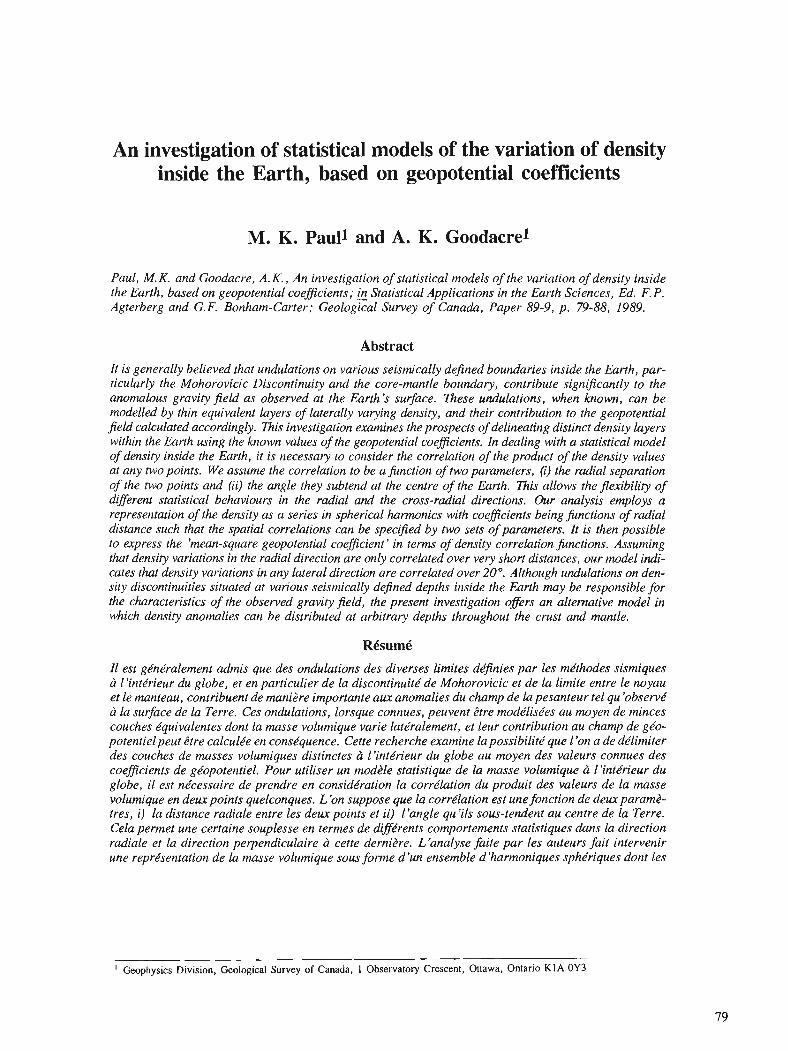
An investigation of statistical models of the variation of density inside the Earth, based on geopotential coefficients

M. K. Paul1 and A. K. Goodacrel

Paul, M. K, and Goodacre, A. K., An investigation of statistical models of the variation of density inside the Earth, based on geopotential coeflcients; & Statistical Applications in the Earth Sciences, Ed. F. P. Agterberg and G.F. Bonham-Carter; Geological Survey of Canada, Paper 89-9, p. 79-88, 1989.

Abstract

It is generally believed that undulations on various seismically defined boundaries inside the Earth, particularly the Mohorovicic Discontinuity and the core-mantle boundary, contribute sign$cantly to the anomalous gravity field as observed at the Earth S surface. These undulations, when known, can be modelled by thin equivalent layers of laterally varying density, and their contribution to the geopotential field calculated accordingly. This investigation examines the prospects of delineating distinct density layers within the Earth using the known values of the geopotential coeficients. In dealing with a statistical model of density inside the Earth, it is necessary to consider the correlation of the product of the density values at any two points. We assume the correlation to be a function of two parameters, (i) the radial separation of the two points and (ii) the angle they subtend at the centre of the Earth. This allows the flexibility of different statistical behaviours in the radial and the cross-radial directions. Our analysis employs a representation of the density as a series in spherical harmonics with coeficients being functions of radial distance such that the spatial correlations can be speciJied by two sets of parameters. It is then possible to express the 'mean-square geopotential coeficient' in terms of density correlation functions. Assuming that density variations in the radial direction are only correlated over very short distances, our model indicates t h ~ t density variations in any lateral direction are correlated over 20". Although undulations on density discontinuities situated at various seismically dejned depths inside the Earth may be responsible for the characteristics of the observed gravity field, the present investigation ofers an alternative model in which density anomalies can be distributed at arbitrary depths throughout the crust and mantle.

I1 est ge'nkralement admis que des ondulations des diverses limites dkfinies par les mkthodes sismiques h l'intkrieur du globe, et en particulier de la discontinuite'de Mohorovicic et de la limite entre le noyau et le manteau, contribuent de manitre importante aux anomalies du champ de la pesanteur tel qu 'obsewk h la surface de la Terre. Ces ondulations, lorsque connues, peuvent Ctre mode'lise'es au moyen de minces couches e'quivalentes dont la muse volumique varie late'ralement, et leur contribution au champ de gko- potentielpeut Ctre calcule'e en conskquence. Cette recherche examine la possibilitd que 1 'on a de dklimiter des couches de masses volumiques distinctes h l'intkrieur du globe au moyen des valeurs connues des coeficients de ge'opotentiel. Pour utiliser un modtle statistique de la masse volumique & l'inte'rieur du globe, il est ne'cessaire de prendre en conside'ration la corrklation du produit des valeurs de la masse volumique en deux points quelconques. L 'on suppose que la corrklation est une fonction de deux paramdtres, i) la distance radiale entre les deux points et ii) l'angle qu'ils sous-tendent au centre de la Terre. Cela permet une certaine souplesse en termes de diffkrents comportements statistiques dans la direction radiale et la direction perpendiculaire h cette dernitre. L'analyse faite par les auteurs fait intervenir une reprksentation de la masse volumique sous forme d'un ensemble d'harmoniques sphkriques dont les

' Geophysics Division, Geological Survey of Canada, I Observatory Crescent, Ottawa, Ontario KIA 0Y3

l e 9 m OS 0 0s-

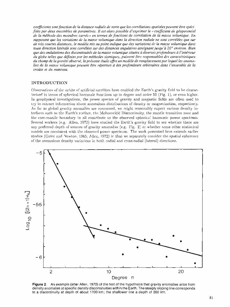
coeficients sont fonction de la distance radiale de sorte que les corrklations spatiales peuvent &tre spkci- jkes par deux ensembles de paramdtres. I1 est alors possible d'exprimer le - coeficient de gebpotentiel de la me'thode des moindres carr6s u en termes de fonctions de corrklation de la masse volumique. En supposant que les variations de la masse volumique dans la direction radiale ne sont corrklkes que sur de tr&s courtes distances, le mod&le mis au point indique que des variations de la masse volumique dans toute direction latkrale sont corre'lkes sur des distances angulaires atteignant jusqu 'a 20" environ. Bien que des ondulations des discontinuitb de la rnasse volumique situkes a diverses profondeurs a 1 'intkrieur du globe telles que dkjinies par les mkthodes sismiques, puissent Ztre responsables des caractkristiques du champ de la gravite' observe', la prksente ktude ofre un mod2le de remplacement par lequel les anomalies de la masse volumique peuvent 2tre rkparties a des profondeurs arbitraires dans l'ensemble de la croGte et du manteau.

INTRODUCTION

01)scrvations of tllc! orbits of artificial satellites have enabled the Earth's gravity field to be characterized in terms of spherical harmonic filrlctions up to degree and order 50 (Fig. 1)' or even higher. 111 geophysical investigations: the power spectra of gravity and magnetic fields are often used to try to extract inforrnatiorl abont anomalous distributions of density or magnetization, respectively. As far as global gravity anomalies are concerned, we might reasonably expect various density interfaces such as the Earth's snrface, the MolioroviEiC Discontinuity, thc mantle transition zone and the core-mantle bollndary to all contribute to the observed spherical harmonic power spectrum. Several workers (e.g. Allen, 1972) have studied the Earth's gravity field to see whether there are any preferred depth of sources of gravity anomalies (e.g. Fig. 2) or whether some other statistical models are consistent with the observed power spectrum. The work presented here extends earlier stlldics (Guicr and Newton, 1965; Allen, 1972) in that we separately consider the spatial coherence of the anomalotw density variations in both radial and cross-radial (lateral) directions.

Degree n Figure 2. An example (after Allen, 1972) of the test of the hypothesis that gravity anomalies arise from density anomalies at specific density discontinuities within the Earth. The steeply sloping line corresponds to a discontinuity at depth of about 1700 km; the shallower line a depth of 260 km.

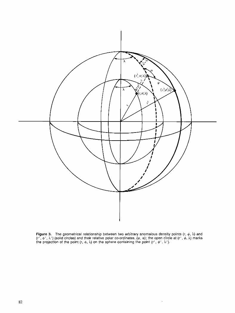
Figure 3. The geometrical relationship between two arbitrary anomalous density points (r, 4, h) and (r', d ' , 1 ' ) (solid circles) and their relative polar co-ordinates, (y, a); the open circle at (r ' , 4, h) marks the projection of the point (r, 4, h) on the sphere containing the point (r ' , d ' , 1').

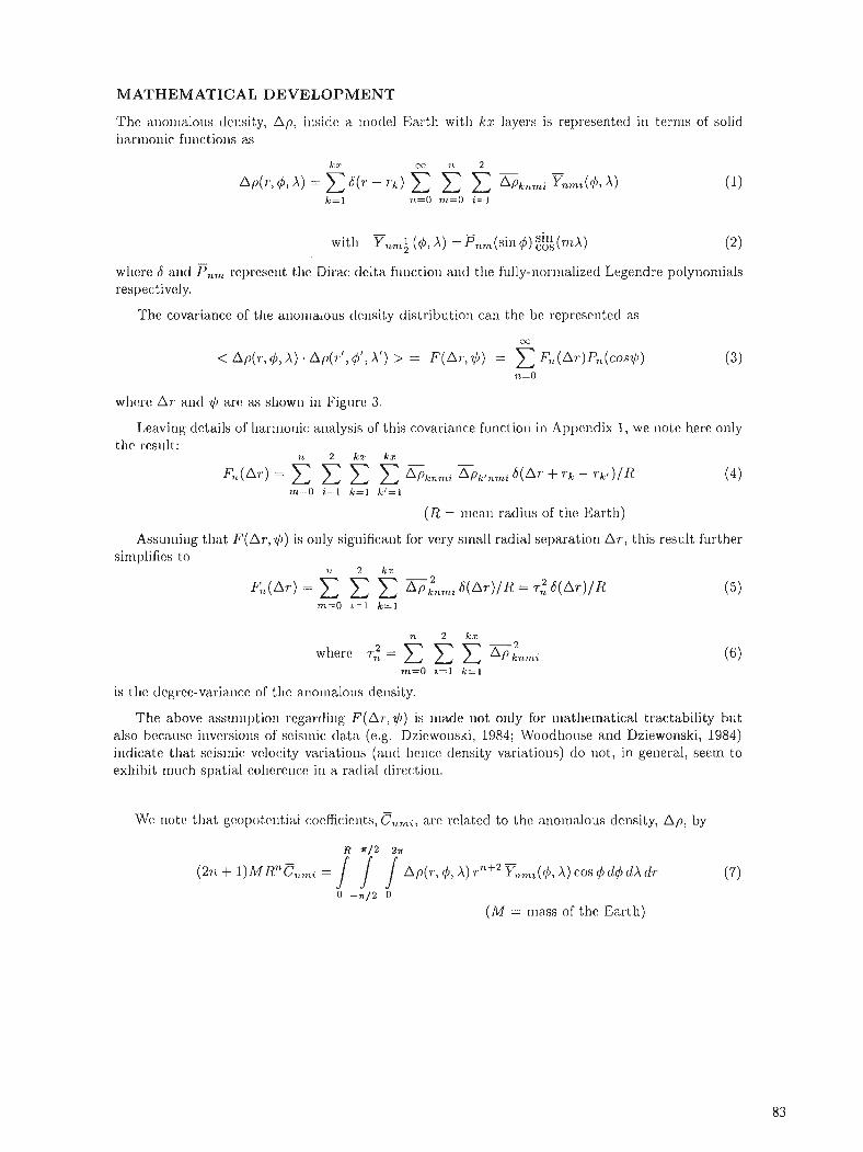
MATHEMATICAL DEVELOPMENT

The alioliialous dc~isity, Ap, ilisitlc a lnotlel Earth with kz layers is represented in terms of solid hwmonic functions as

wllcre 6 alltl fi,,,, rcprcscilt tllc! Dirac: tlcltsa fu~i(:tiol~ alid the fully-norlnalized Legendre polynonlials respectively.

The covariance of the a~io~lialous dcllsity distribution can the be represented as

X

< Ap(rI 4 , A) . Al,(ri, 4'; A') > = F ( A r , dl) = F,, (Ar)P7& ( ~ 0 ~ 2 1 , )

n = O

(3)

wlicrc A r alltl .d) arc ;IS sllowli ill Figrlro 3.

Leaving details of I~arlliol~i(: alii~lysis of this covariance functiori in Appendix 1, we note here only thc result:

7r 2 Lz hx

(R = lrlcan radius of tlic Earth)

Assuliiing that F(Ar;d)) is only sigllificallt for very small radial separation A r , this result further simplifies to

is the dcgrce-varialicc of thc anomalous density.

The above assu~llptioll r~gartlillg F ( A r , +) is 111ade not only for lriatllernatical tractability but also bccal~st: invcrsiolis of scislnic: tlat,a (c?.g. Dziewoiiski, 1984; Woodhouse and Dziewonski, 1984) indicate that scis~nic velocity variations (ant1 llclict! density variations) do not, in general, seem to exhibit much spatial colicrclico in a ratlial tlirec:tioli.

- W(: liotc: tliat gco~)ot,c:lit,i;tl c:oc.ffic:icnts, C,L,Li, arc: related to the atioirialous density, Ap, by

(271. + 1) M R ~ ~ F , , , ~ ~ ~ = i 4'7 Ap(r, d, A) rn+' x17n2(&1 A ) cos 4 d4 dX dr

O -n/2 0

(M = riiass of the Earth)

St , t~r t~i~ig with ccl~~ittioli (7): the relation between mean-square coefficients, < c:,~ >, and the tl(!grc:c! varii~ncc of tho a l lo~i i i t lo~~s dclisity, r1;; has been derived from similar harmonic analysis with dotails give11 ill Aj)~)cndix 2. The rcs~ll t is

and, hence, the r e l a t i o ~ ~ s l ~ i p hc?twc?t!n the two sets of degree-variance is:

which allows the evaluatio~i of tlic r7,'s when the 07,'s are available frorri satellite observations.

Co~isequcntly, tlic! c:ovariancc of the anornalons density is given by

Tllc: ri~.t,io C($)/C(O) will now tlefilie the (normalized) covariance of the density distribution in thc! cross-radial diraction: it, l l~ay be 110teci that we liave omitted here contributions of second and - lowm tlcgrcc i ~ l ~ t l or(Iar CT1,,,.( wlii(:h: by convention, co~ist i tute the normal component of the Earth's gravitatioi~ill pot,c!~~tiitl.

0.25 1 I I I I I I I I I I I I 0.0 45.0 90-0 135.0 180.0

Angular distance J. in degrees

Figure 4. The (normalized) covariance function for lateral density variations versus angular distance Y using degree variances of GEM T I geopotential coefficients up to n = 36.

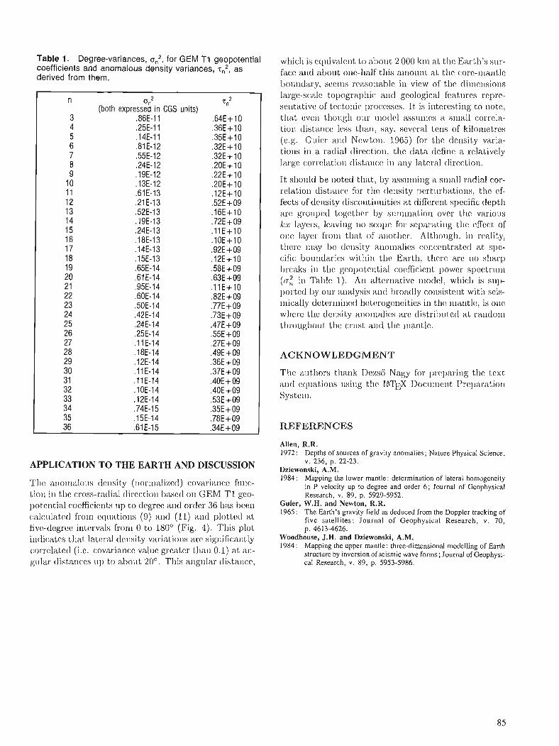
Table 1. Degree-variances, on2, for GEM T I geopotential coefficients and anomalous density variances, ~,2 , a s derived from them.

o (both expressed in CGS units)

.86E-11

.25E-11

.14E-11

.81E-12

.55E-12

.24E-12

.19E-12

.13E-12

.61E-13

.21E-13

.52E-13

.19E-13

.24E-13

.18E-13

.14E-13

.15E-13

.65E-14

.61E-14

.95E-14

.60E-14

.50E-14

.42E-14

.24E-14

.25E-14

.11E-14

.18E-14

.12E-14

. l lE-14

.11E-14

.10E-14

.12E-14

.74E-15

.15E-14

.61E-15

wliicl~ is cq~liviil(:~lt t,o i11)01lt 2 000 krii a t thc Earth 's surface! alid about ono-llalf this alliollrlt a t the (:ore-lilalltlc bouildary, sc!ollis rc?aso~iablc ill view of t,lic diliicilsions large-scale topogr~~) l i i ( : alid geological featllrcs repre- selitativc: of tc!c:tollic: 1)roc:csscs. It is ilitcrcstirig to note: that ovcii t l i o~~g l i 0111. iliotlcl asslliiics a srliall corrcla- tiou tiistall(:(: l(!ss tliali, say. several tells of kilolrlctres (e.g. Guicr ant1 N(!wtoii. 1965) for the dclisit,y varia- tiolls ill a radial tlircc:tioii, t,lic d a t a define a relatively large c:orrclatioli (list,ali(:(! ill ally lateral (lircctiori.

It shoiild be rioted that , by ass~llllillg. a slriall radial cor- relitti011 distxlic:c! for t,lic! tlerisity pc!rt~~rbations, the effects of dcl~sity tlisc:ontilii~itics a t different specific depth aro groupctl togc!t,lic!r hy s~lrniriat,ioii over the various I::[: li\y(!rs, l(!avilig 110 sc:ol)c! for scpariltiug t,llct c!fft!c:t of oil(: laytyclr fro111 t l l i~ t of i i l i ~ t l l ~ ~ . Altliollgh, iri roality, thcrc! lliay bc cl(!lisity anornalics coriccntratcd a t spc- ciiic bo111ldaric:s withill tllc! Ear th , tlicre arc 11o sharp Lrcaks ill tlia gc!o~)otelitial c:oc!fficicnt power spcc:tr~~lii (n;, ill Tal)lo 1). A11 altscrllat,ivc! lllotl(!l, w1lic:ll is sup- portotl by our a l i~ lys is alld 1)roadly consistent with scis- lilically dctonni~iotl het~crogcricitics in the ~liantlc, is one wllc!ro tlic dcilsit,y aiiol~lalies arc d is t r ib l~tc~i a t ra11(1o1ii tlirougllont tllc: c : r~~s t anti the ~nant lc .

ACKNOWLEDGMENT

The authors tharik Deasij Nagy for ~)rc!parilig. t,hc text i t ~ l ( l (!(l~lilt.iolls 11siiig ttlio BTEX Do(:i~~il(!l~t P r~para t io l l Systt!lll.

REFERENCES

APPLICATION TO THE EARTH AND DISCUSSION

TI)(! i l ~ i o ~ i ~ a l o ~ l s dclisity (i~or~iializccl) c:ovari;llic:c? f111ic:- ti011 in t,hc cross-ratlid clircc:tioli k)asc!tl 011 GEM T1 goo- pot,critial coefficients up to degree a11tl ortlcr 36 has heen c:al(:ulat,c:tl from ccl~~at,ions (0) ant1 (11) alitl plotte(1 a t five!-dcgrcc! i~it~crvals frorli 0 to 180' (Fig. 4). Tliis plot i~l(lic:ates t,liat latc!ral dcl~sity variatiolis arc? sigliific:aiitly c:orrclatctl (i.c. covarianc:c valllc greater t l iar~ 0.1) a t angular tlistanc:c?s i l l ) to aho11t 20". This aligrilar tlistallce,

Allen, R.R. 1972: Depths of sources of gravity anomalies; Nature Physical Science,

v. 236, p. 22-23. Dziewonski, A.M. 1984: Mapping the lower mantle: determination of lateral homogeneity

in P velocity up to degree and order 6; Journal of Geophysical Research, v. 89, p . 5929-5952.

Guier, W.H. and Newton, R.R. 1965: The Earth's gravity field as deduced from the Doppler tracking of

five satellites; Journal of Geophysical Research, v . 70, p. 4613-4626.

Woodhouse, J.H. and Dziewonski, A.M. 1984: Mapping the upper mantle: three-dimensional modelling of Earth

structure by inversion of seismic wave forms; Journal of Geophysi- cal Research, v. 89, p. 5953-5986.

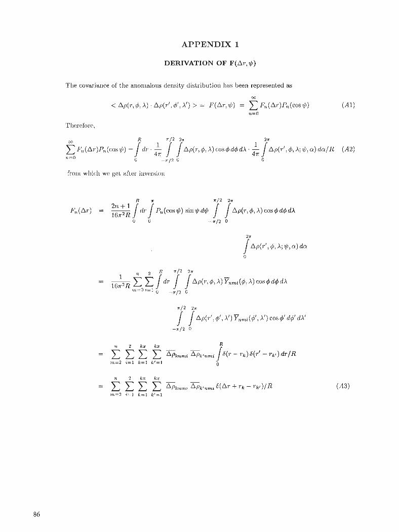
APPENDIX 1

DERIVATION O F F(Ar , @)

The covaria~ice of the arlomalous density distributio~i has been represented as

30

< Ap(r: $, A) . A,,(,,.'; $', A') > = F ( A r , $) = C &(Ar)Pn(cos?l,) (Al l ,1=0

X 7~12 2a

F,, (AT) P,,, ((:os s f i ) = rlr . - j A 4, A c o 4 4 A $> A; $, a) d o / R ( A ? ) 7 1 = 0 0 -n/2 0 0

R. n 27A + 1

F,, (AT) = - 1 r l ~ J P,& (cos $1 sin $J dd, 167r2R 7 4, A) cos 4 d m

0 0 -n/2 0

AP(r1: dl, A') Ynrni(4', A') cos 4' d4' dA' 7.7 -a12 O

APPENDIX 2

RELATION BETWEEN MEAN SQUARE GEOPOTENTIAL COEFFICIENT,

< C:,* >, AND DEGREE VARIANCE OF ANOMALOUS DENSITY, 7.2

With

wc! call write

and the anomalous gravitatiorial potential of the spherical Earth can then be expanded as

R ~ / 2 2n

4 , = G J 1 1 A p ( r ' , q5', A') r l 2 cos 4' d4' dX' dr' 1

c o n 2 - R ?r/2 2n

y 1 m i 4 J J J Ap(r', +', A') r tn t2 T n m i ( d f , A') cos 4, d4' dr' = GC C C ( 2 n + l ) r n + l 11=O ni=O i=l 0 - r / 2 0

as pc!r tlcfinition of c7,,,, the geopotential coefficient.

Therefore, for n 2 3:

(271 + 1) M R Enmi = / / / A p ( r f , + I , A') T'"'~ y n m i ( p , A') cos f dm' dr' (A7)

and, hence,

- Ynmi ( 4 , A) Elmi ($', A') r n f r'n'2 cos q5 dq5 dr cos 4' d4' dr'

- . Y71,~j~d(d: A ) %Lnli(dlr A') r7L+2 r'n+2 COS (t) d$ dr cos 4' d4' dr'

/ / (8, A') dA' Tnmi(m1, A') cos q5' dq5' dA1

using (5) alid liotiiig tliitt the right hand side is independent of m and i.

Magnetization/density ratio mapping in eastern Canada

M. Pilkingtonl and R.A.F. Grievel

Pilkington, M. and Grieve, R.A.F. , Magnetization/density ratio mapping in eastern Canada; in Statistical Applications in the Earth Sciences, ed. F.P. Agterberg and G. F. Bonham-Carter; Geological Survey of Canada, paper 89-9, p . 89-98, 1989.

Abstract

A magnetization/density ratio map has been produced for eastern Canada from the combined analysis of aeromagnetic and Bouguer gravity data. The procedure is based on Poisson 's Theorem, which relates the gravity and magnetic fields produced by a common body with a constant magnetization/density ratio. The ratio is determined by performing a simple linear regression of the two coincident data sets within a moving window. The regression results in estimates of the magnetization/density ratio, an intercept value and a correlation coefficient.

The ratio map shows distinct areas that are related to changes in regional geological structure and lithology. Suture zones are marked by linear regions of low ratios with small variability. Older shield areas are distinguished by a greater range in ratios and a higher variability compared with regions of younger crust, such as the eastern coast of the United States. Litho logical variations can be seen in the Superior Province (in northern Quebec) with the transition northward from generally granitic to granulitic terrane being marked by a change from positive to negative correlations.

Resume

Une carte du rapport entre la magnetisation et la densite a ete produite pour tout l 'est du Canada d'apres ! 'analyse combinee des donnees aeromagnetiques et gravimetriques de Bouguer. La mithode est basee sur le theoreme de Poisson mettant en relation les champs gravimetrique et magnetique dus a un me me corps dont le rapport entre la magnetisation et la densite est constant. Ce rapport est determine a l 'aide d 'une regression lineaire simple appliquee aux deux ensembles coi'ncidents de donnees a l 'interieur d 'une fenetre mobile. La regression produit des estimations du rapport de la magnetisation a la densite, une valeur d'interception et un coefficient de correlation.

La carte du rapport montre des regions distinctes qui sont reliees a des variations regionales,de la structure geologique et de la lithologie. Les zones de suture sont caracterisees par des regions lineaires ou les rapports et la variabilite sont faibles. D 'autres regions du bouclier se distinguent par une plage plus et endue de rapports et une variabilire plus grande comparativement aux regions de croute plus jeune, comme la cote est des Etats-Unis. Des variations lithologiques peuvent etre observees dans la province du lac Superieur (dans le nord du Quebec) et la transition en direction du nord de terranes generalement granitiques a granulitiques est caracterisee par un changement du signe des correlations qui passent de positives a negatives.

'Geophysics Division, Geological Survey of Canada, I Observatory Crescent , Ottawa, Ontario KIA OY3

89

INTRODUCTION

One of the methods available to reduce the ambiguity inherent in the interpretation of gravity and magnetic anomaly data is to investigate and quantify the correlation between the two (von Frese et al., 1982). In particular, treating both potential field data sets simultaneously can lessen the practical ambiguities produced by superposition of anomalies and the effects of (unknown) source configurations.

Correlation between magnetic and gravity fields from geological sources is manifested in a variety of ways. Firstly, a direct correlation between density and magnetization is predicted from the bulk properties of different rock types. As igneous rocks become more rnafic, both density and magnetization (primarily due to the level of magnetite present) increase. For sedimentary rocks, magnetization is small and in most cases can be regarded as negligible, while densities are less than igneous or metamorphic rocks. For metamorphic rocks, density tends to increase with the level of recrystallization. Generally, as for igneous rocks, as the mafic content of the metamorphic rocks increases, density increases. For the latter, however, the rule is not so strictly adhered to because of the complicated history of some metamorphic rocks. The effect of metamorphism on the magnetic properties of rocks is not simple. Serpentinization produces large amounts of magnetite and, hence, larger magnetic anomalies. High levels of metamorphism, however, effectively destroy thermal remanent magnetization resulting in a complete loss of magnetic properties at the Curie point for the particular magnetic phase present. A competing effect arises in crustal rocks existing over long time periods in the Earth's magnetic field at elevated temperatures, resulting in the gradual buildup of viscous magnetization. This phenomenon is particularly important in the lower crust, which is the most likely source of regional, long wavelength magnetic anomalies (Wasilewski and Mayhew, 1982). Thus, lower levels of metamorphism tend to produce a direct correlation while higher levels can lead to no correlation at all.

Secondly, structural features or variations in the thickness of crustal layers produces a correlation between the resulting magnetic and gravity anomalies. Areas of thinner crust will be accompanied by gravity highs, due to denser mantle material existing at higher levels within the crustal column, while the reduced amount of magnetic crust causes a magnetic low. The converse is true for thickened crust, that is, magnetic highs and corresponding gravity lows. Thus, structural variations of this form, which generally produce intermediate to long wavelength potential field anomalies, result in an inverse correlation between the two types of data. Thus, there is justification for expecting spatial correlation between gravity and magnetic fields over a wide variety of geological environments. However, the relationships discussed above are extremely broad in nature and may break down in structurally complex areas or regions that have undergone several episodes of metamorphism.

In the following, a quantitative approach is used to determine the correlation between the gravity and aeromagnetic fields over eastern Canada. The method is essentially that

of Chandler et al. (1981), who used the technique primarily for profile data. As well as a measure of the correlation, the ratio of source magnetization to density is also estimated and interpreted in terms of the regional geology.

METHODOLOGY

Determining the magnetizationldensity ratio for sources of potential field anomalies can be carried out efficiently by using the known relation between gravity and magnetic fields. Specifically, Poisson's theorem for the case of the magnetic and gravity field due to a common body can be stated in terms of the magnetic potential A and the gravitational potential U (e.g., Telford et al., 1976) :

where J is magnetization contrast, p is density contrast, a is the direction of magnetization and g, is the gravity field component in the direction a. Converting the magnetic potential into the magnetic field Bg (measured in the direction I31

For the case of vertical magnetization,

where B is the magnetic field produced by vertically magnetized sources and ag113z is the vertical gravity gradient and c is some constant that is a function of the base level of the two fields. The equation is of the form y =ax+b so that the determination of a, the rnagnetizationldensity ratio, can be done using least-squares line-fitting methods. The ratio is determined by performing a simple linear regression of the two coincident data sets within a moving window. The window is passed over the data at an interval of one grid spacing and the results assigned to the grid point at the centre of the window. The vertical gravity gradient has been arbitrarily taken as the independent regression variable. The regression results in estimates of the magnetizationldensity ratio, an intercept value and a correlation coefficient. A window size of 5x5 data points (equivalent to 30x30 km) was used for this study.

The above relation holds for fields due to one body, uncorrupted by the effects of adjacent sources. In practice, the data window is likely to contain the effects of a number of bodies, such that the calculated ratio value will represent a weighted average of the ratios for all the sources. The ratio map must be used in conjunction with the correlation coefficient map. Only in cases where there is a significant correlation between the magnetic and gravity anomalies should the densitylmagnetization ratio be considered indicative of source properties. Unfortunately, good correlations may also result from the superposition of gravity and magnetic anomalies from sources that are spatially coincident but occur at different depths.

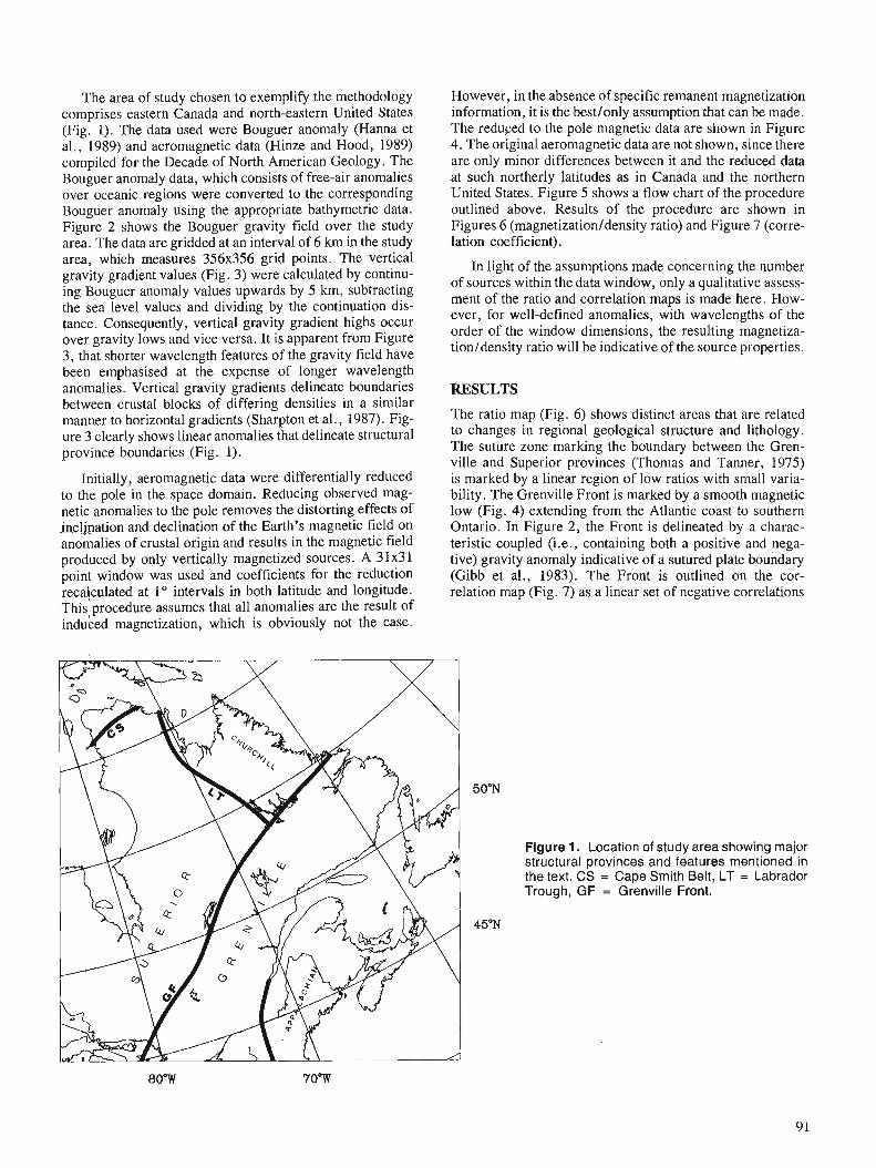
The area of study chosen to exemplify the methodology comprises eastern Canada and north-eastern United States (Fig. 1). The data used were Bouguer anomaly (Hanna et al., 1989) and aeromagnetic data (Hinze and Hood, 1989) compiled for the Decade of North American Geology. The Bouguer anomaly data, which consists of free-air anomalies over oceanic regions were converted to the corresponding Bouguer anomaly using the appropriate bathymetric data. Figure 2 shows the Bouguer gravity field over the study area. The data are gridded at an interval of 6 krn in the study area, which measures 356x356 grid points. The vertical gravity gradient values (Fig. 3) were calculated by continuing Bouguer anomaly values upwards by 5 km, subtracting the sea level values and dividing by the continuation distance. Consequently, vertical gravity gradient highs occur over gravity lows and vice versa. It is apparent from Figure 3, that shorter wavelength features of the gravity field have been emphasised at the expense of longer wavelength anomalies. Vertical gravity gradients delineate boundaries between crustal blocks of differing densities in a similar manner to horizontal gradients (Sharpton et al., 1987). Fig- ure 3 clearly shows linear anomalies that delineate structural province boundaries (Fig. 1).

Initially, aeromagnetic data were differentially reduced to the pole in the space domain. Reducing observed magnetic anomalies to the pole removes the distorting effects of incljnation and declination of the Earth's magnetic field on anomalies of crustal origin and results in the magnetic field produced by only vertically magnetized sources. A 3 1x3 1 point window was used and coefficients for the reduction recalculated at l o intervals in both latitude and longitude. This, procedure assumes that all anomalies are the result of induced magnetization, which is obviously not the case.

Figure 1. Location of study area showing major structural provinces and features mentioned in the text. CS = Cape Smith Belt, LT = Labrador Trough, GF = Grenville Front.

However, in the absence of specific remanent magnetization information, it is the bestlonly assumption that can be made. The reduced to the pole magnetic data are shown in Figure 4. The original aeromagnetic data are not shown, since there are only minor differences between it and the reduced data at such northerly latitudes as in Canada and the northern United States. Figure 5 shows a flow chart of the procedure outlined above. Results of the procedure are shown in Figures 6 (magnetizationldensity ratio) and Figure 7 (correlation coefficient).

In light of the assumptions made concerning the number of sources within the data window, only a qualitative assessment of the ratio and correlation maps is made here. How- ever, for well-defined anomalies, with wavelengths of the order of the window dimensions, the resulting magnetizationldensity ratio will be indicative of the source properties.

RESULTS

The ratio map (Fig. 6) shows distinct areas that are related to changes in regional geological structure and lithology. The suture zone marking the boundary between the Gren- ville and Superior provinces (Thomas and Tanner, 1975) is marked by a linear region of low ratios with small variability. The Grenville Front is marked by a smooth magnetic low (Fig. 4) extending from the Atlantic coast to southern Ontario. In Figure 2, the Front is delineated by a characteristic coupled (i.e., containing both a positive and negative) gravity anomaly indicative of a sutured plate boundary (Gibb et al., 1983). The Front is outlined on the correlation map (Fig. 7) as a linear set of negative correlations

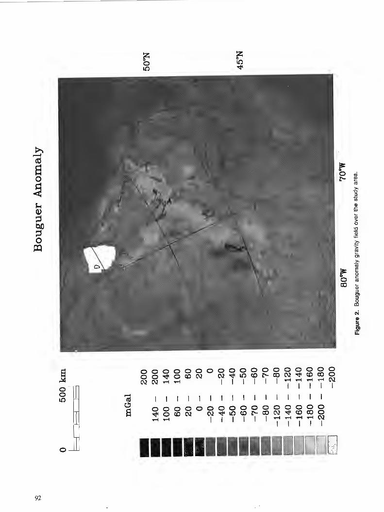
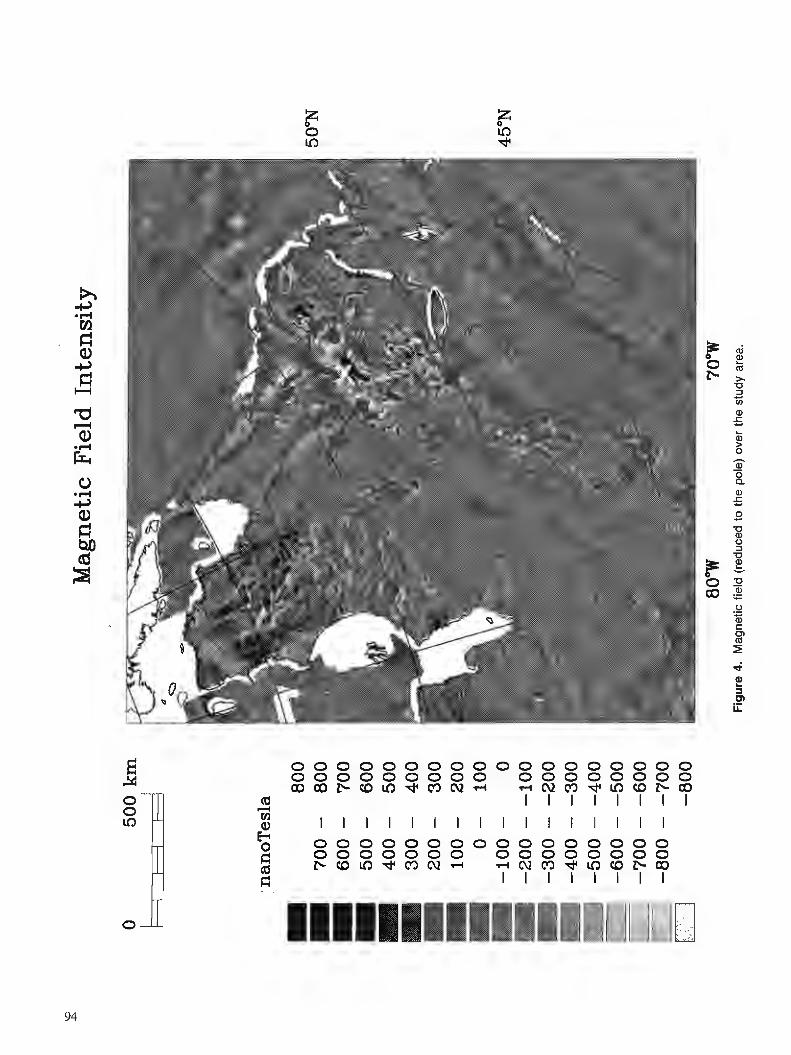
0 0 0 0 0 0 0 0 0 0 0 0 0 0 0 0 0 0 0 0 0 0 0 0 0 0 0 0 0 0 0 Q 0 0 0 COcO*\[email protected] . - r N m M m c D C D w

(d d

I I I I I I I I rn a 1 1 1 1 1 1 1 1 1 1 1 1 1 1 1 1

5 0 0 0 0 0 0 0 0 0 0 0 0 0 0 0 0 d 0 0 0 0 0 0 0 0 0 0 0 0 0 0 0

2 CDCoU3*[email protected] ~ @ . 2 r n * L n C o ~ W I I I I I I I I

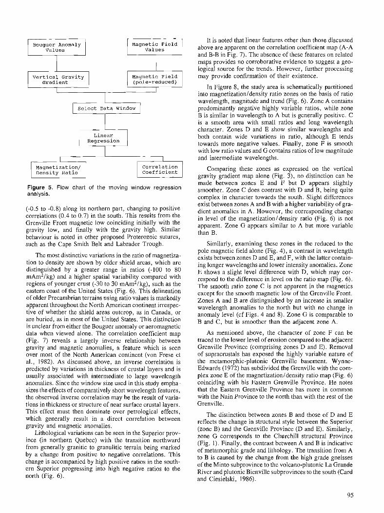
Magnetic Field Values

Vertical Gravity Gradient (pole-reduced)

I Select Data Window 1

Linear Regression

Magnetization/ Density Ratio Coefficient

Figure 5. Flow chart of the moving window regression analysis.

(-0.5 to -0.8) along its northern part, changing to positive correlations (0.4 to 0.7) in the south. This results from the Grenville Front magnetic low coinciding initially with the gravity low, and finally with the gravity high. Similar behaviour is noted in other proposed Proterozoic sutures, such as the Cape Smith Belt and Labrador Trough.

The most distinctive variations in the ratio of magnetization to density are shown by older shield areas, which are distinguished by a greater range in ratios (-100 to 80 mAm2/kg) and a higher spatial variability compared with regions of younger crust (-30 to 30 mAm2/kg), such as the eastern coast of the United States (Fig. 6). This delineation of older Precambrian terrains using ratio values is markedly apparent throughout the North American continent irrespective of whether the shield areas outcrop, as in Canada, or are buried, as in most of the United States. This distinction is unclear from either the Bouguer anomaly or aeromagnetic data when viewed alone. The correlation coefficient map (Fig. 7) reveals a largely inverse relationship between gravity and magnetic anomalies, a feature which is seen over most of the North American continent (von Frese et al., 1982). As discussed above, an inverse correlation is predicted by variations in thickness of crustal layers and is usually associated with intermediate to large wavelength anomalies. Since the window size used in this study emphasizes the effects of comparatively short wavelength features, the observed inverse correlation may be the result of variations in thickness or structure of near surface crustal layers. This effect must then dominate over petrological effects, which generally result in a direct correlation between gravity and magnetic anomalies.

Lithological variations can be seen in the Superior province (in northern Quebec) with the transition northward from generally granitic to granulitic terrain being marked by a change from positive to negative correlations. This change is accompanied by high positive ratios in the southern Superior progressing into high negative ratios to the north (Fig. 6).

It is noted that linear features other than those discussed above are apparent on the correlation coefficient map (A-A and B-B in Fig. 7). The absence of these features on related maps provides no corroborative evidence to suggest a geological source for the trends. However, further processing may provide confirmation of their existence.

In Figure 8, the study area is schematically partitioned into rnagnetizationldensity ratio zones on the basis of ratio wavelength, magnitude and trend (Fig. 6). Zone A contains predominantly negative highly variable ratios, while zone B is similar in wavelength to A but is generally positive. C is a smooth area with small ratios and long wavelength character. Zones D and E show similar wavelengths and both contain wide variations in ratio, although E tends towards more negative values. Finally, zone F is smooth with low ratio values and G contains ratios of low magnitude and intermediate wavelengths.

Comparing these zones as expressed on the vertical gravity gradient map alone (Fig. 3), no distinction can be made between zones E and F but D appears slightly smoother. Zone C does contrast with D and B, being quite complex in character towards the south. Slight differences exist between zones A and B with a higher variability of gradient anomalies in A. However, the corresponding change in level of the magnetizationldensity ratio (Fig. 6) is not apparent. Zone G appears similar to A but more variable than B.

Similarly, examining these zones in the reduced to the pole magnetic field alone (Fig. 4), a contrast in wavelength exists between zones D and E, and F, with the latter containing longer wavelengths and lower intensity anomalies. Zone E shows a slight level difference with D, which may correspond to the difference in level on the ratio map (Fig. 6). The smooth ratio zone C is not apparent in the magnetics except for the smooth magnetic low of the Grenville Front. Zones A and B are distinguished by an increase in smaller wavelength anomalies to the north but with no change in anomaly level (cf Figs. 4 and 8). Zone G is comparable to B and C, but is smoother than the adjacent zone A.

As mentioned above, the character of zone F can be traced to the lower level of erosion compared to the adjacent Grenville Province (comprising zones D and E). Removal of supracrustals has exposed the highly variable nature of the metamorphic-plutonic Grenville basement. Wynne- Edwards (1972) has subdivided the Grenville with the complex zone E of the magnetizationldensity ratio map (Fig. 6) coinciding with his Eastern Grenville Province. He notes that the Eastern Grenville Province has more in common with the Nain Province to the north than with the rest of the Grenville.

The distinction between zones B and those of D and E reflects the change in structural style between the Superior (zone B) and the Grenville Province (D and E). Similarly, zone G corresponds to the Churchill structural Province (Fig. 1). Finally, the contrast between A and B is indicative of metamorphic grade and lithology. The transition from A to B is caused by the change from the high grade gneisses of the Minto subprovince to the volcano-plutonic La Grande River and plutonic Bienville subprovinces to the south (Card and Ciesielski, 1986).

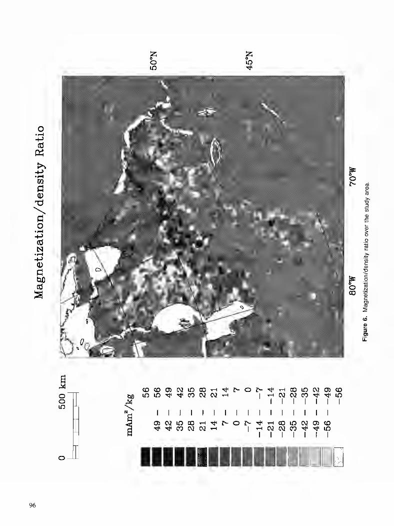
z U3 TI'

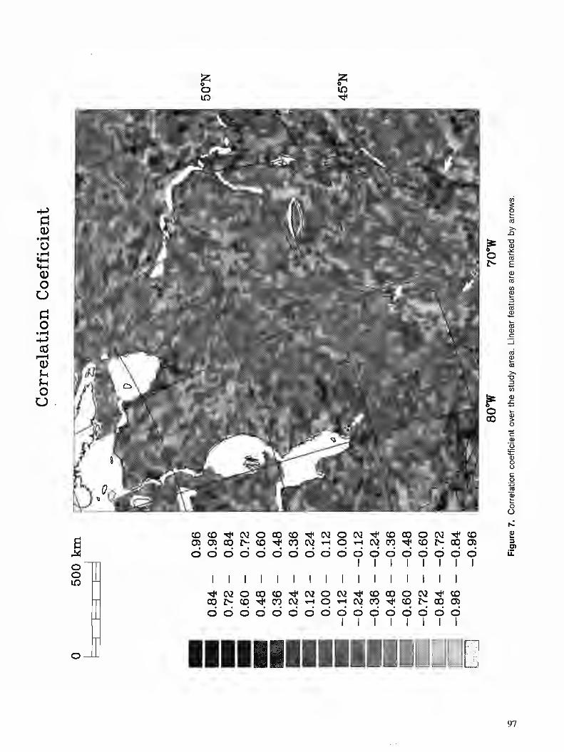
a a d N 0 m a C V N O N d ' a m o N d a C n C n m E a Y l ' m O ~ O ~ q m d ~ F ~ a 0 00000000000000000

I I I I I I I I I I I I I I I I I I I I I I I I ~ O O o O c o d N o O C V d ( D o O C V c o m F a d ' m N ~ o ~ N q * d r c O ( D a 0 0 0 0 0 0 0 0 o 0 0 0 0 0 0 0

I I I I I I I I

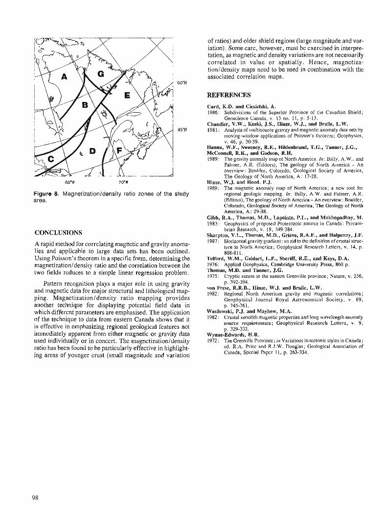
Figure 8. Magnetizationldensity ratio zones of the study area.

CONCLUSIONS

A rapid method for correlating magnetic and gravity anomalies and applicable to large data sets has been outlined. Using Poisson's theorem in a specific form, determining the magnetizationldensity ratio and the correlation between the two fields reduces to a simple linear regression problem.

Pattern recognition plays a major role in using gravity and magnetic data for major structural and lithological mapping. Magnetizationldensity ratio mapping provides another technique for displaying potential field data in which different parameters are emphasised. The application of the technique to data from eastern Canada shows that it is effective in emphasizing regional geological features not immediately apparent from either magnetic or gravity data used individually or in concert. The magnetizationldensity ratio has been found to be particularly effective in highlighting areas of younger crust (small magnitude and variation

of ratios) and older shield regions (large magnitude and variation). Some care, however, must be exercised in interpretation, as magnetic and density variations are not necessarily correlated in value or spatially. Hence, magnetizationldensity maps need to be used in combination with the associated correlation maps.

REFERENCES

Card, K.D. and Ciesielski, A. 1986: Subdivisions of the Superior Province of the Canadian Shield;

Geoscience Canada, v. 13 no. 11, p. 5-13. Chandler, V.W., Koski, J.S., Hinze, W.J., and Braile, L.W. 1981 : Analysis of multisource gravity and magnetic anomaly data sets by

moving-window applications of Poisson's theorem; Geophysics, v. 46, p. 30-39.

Hanna, W.F., Sweeney, R.E., Hildenbrand, T.G., Tanner, J.G., McConnell, R.K., and Godson, R.H. 1989: The gravity anomaly map of North America. In: Bally, A.W.. and

Palmer, A.R. (Editors), The geology of North America - An overview: Boulder, Colorado, Geological Society of America, The Geology of North America, A: 17-28.

Hinze, W.J. and Hood. P.J. 1989: The magnetic anomaly map of North America; a new tool for

regional geologic mapping. In: Bally, A.W. and Palmer, A.R. (Editors), The geology of North America - An overview : Boulder, Colorado, Geological Society of America, The Geology of North America, A: 29-38.

Gibb, R.A., Thomas, M.D., Lapointe, P.L., and Mukhopadhay, M. 1983: Geophysics of proposed Proterozoic sutures in Canada: Precam-

brian Research, v. 19, 349-384. Sharpton, V.L., Thomas, M.D., Grieve, R.A.F., and Halpenny, J.F. 1987: Horizontal gravity gradient: an aid to the definition of crustal struc-

ture in North America; Geophysical Research Letters, v. 14, p. . . 808-81 1.

Telford, W.M., Geldart, L.P., Sheriff, R.E., and Keys, D.A. 1976: Applied Geophysics, Cambridge University Press, 860 p. Thomas, M.D. and Tanner, J.G. 1975: Cwvtic suture in the eastern Grenville vrovince: Nature, v. 256.

p. 32-394. von Frese, R.R.B., Hinze, W.J. and Braile, L.W. 1982: Regional North American gravity and magnetic correlations;

Geophysical Journal Royal Astronomical Society, v. 69, p. 745-761.

Wasilewski, P.J. and Mayhew, M.A. 1982 : Crustal xenolith magnetic properties and long wavelength anomaly

source requirements; Geophysical Research Letters, v. 9, p. 329-332.

Wynne-Edwards, H.R. 1972: The Grenville Province; in Variations in tectonic styles in Canada ;

ed. R.A. Pricc and R.J.W. Douglas; Geological Association of Canada, Special Paper 11, p. 263-334.

Image analysis of pore size distribution and its application

Yuan, L., Image analysis of pore size distribution and its application;-ii Statistical Applications in the Earth Sciences, ed. F. P. Agterberg and G. F. Bonham-Carter; Geological Survey of Canada, Paper 89-9, p. 99-107, 1989.

Abstract

In order to study fluid flow through porous media, image analysis has been used to quantify 2-0 pore geometry as observed in thin sections. Pore size is one of the most important components of pore geometry. However, due to the irregular shape and the dzficulty in defining a ''single pore", the size is dificult to measure by traditional methods such as Feret's or Wadell's diameter. An erosion-dilation technique can be used as a generalized size analysis method. The '>ore size" for each pore pixel is defined as the diameter of the largest circle which is entirely within the pore area and contains the pixel. Because of the discrete nature of image processing, this "circle" has been taken to be either a square (eight neighbour distance jknction) or a diamond shape four neighbour distance function). A modijied algorithm, which alternates four and eight neighbour distance jknctions, creates an eight sided "circle" which is much closer to a Euclidean circle and provides more accurate results. The ratio of rough porosity to total porosity is used as a measure of pore connectivity.

In a study of a heavy oil reservoir in east-central Alberta, permeability and sedimentary facies were found to be highly related to pore size and connectivity. An understanding of the pore systems and the flow properties of these facies in a reservoir will aid in characterizing the reservoir for enhanced oil recovery. The generalized size analysis technique used to determine pore size can also be applied to other binary images such as grain size of the reservoir sand and fracture size of a fractured material.

Afin d'e'tudier l'e'coulement d'un fluide ci travers des milieux poreux, on a utilise' l'analyse d'images pour dkterminer la ge'omktrie bidimensionnelle telle qu'observe'e a llaide,de lames minces. La taille des pores est un des aspects les plus importants de la gkome'trie des pores. Etant donne' cependant la forme irrkgulPre de ces derniers et la dificultk de dklimiter << un seul pore )), il est dificile de mesurer la taille par des rne'thodes classiques comme le diambtre de Feret ou le diadrre de Wadell. I1 est possible d'utiliser une technique d'e'rosion-dilatation comme technique ge'nkralise'e d'analyse de la taille. La << taille des pores )> pour chaque pixel de pore est de'jnie comme le diamPtre du plus grand cercle qui se trouve entibrement a l'inte'rieur du pore et contienf le pixel. ~ t a n t donne'la nature discrtte du traitement des images, on considire ce << cercle soit comme ayant la forrne d'un carrk finction de distance de huit voisins) ou la forme d'un losange fonction de distance de quatre voisins). Un algorithme modifie', qui fait alterner les fonctions de distance de quatre et de huit voisins, cre'e un c( cercle* h huit c6te's qui se rapproche beaucoup d'un cercle euclidien et donne des re'sultats plus pre'cis. On utilise le rapport entre la porositk brute et la porosite' totale cornrne mesure de la connectivitk des pores.

Dans une ktude d'un re'servoir de pe'trole lourd, situk dans le centre est de ['Alberta, on a trouve' que la perme'abilite' et les facib skdimentaires e'taient tr&s e'troitement lie's a la taille et ci la connectivite' des pores. La compre'hension des re'seaux de pores et les proprie'tks d 'e'coulement de ces facits dans un rkservoir permettront de caractkriser ce dernier et d 'ame'liorer la rkcupe'ration du pdrole. La technique ge'ne'raliske d 'analyse de la taille utilise'e pour de'terminer la taille des pores peut e'galement Ctre appliquke a d 'autres images binaires comme la granulomJtrie du sable du re'servoir et la taille desfrac- cures d'un matgriau fracturk.

- - - - - - - - -

' Alberta Geological Survey, Alberta Research Council, Box 8330, Station F, Edmonton, Alberta, T6H 5x2

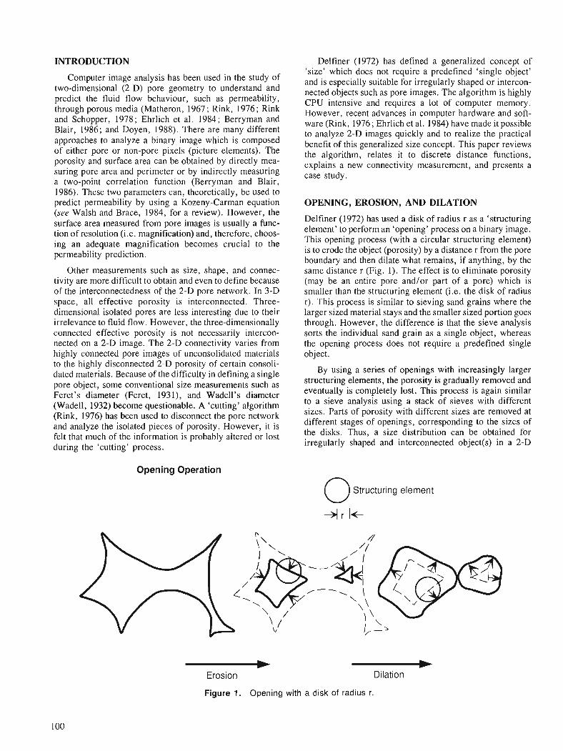
INTRODUCTION Delfiner (1972) has defined a generalized concept of

Computer image analysis has been used in the study of two-dimensional (2-D) pore geometry to understand and predict the fluid flow behaviour, such as permeability, through porous media (Matheron, 1967; Rink, 1976; Rink and Schopper, 1978; Ehrlich et al. 1984; Berryman and Blair, 1986; and Doyen, 1988). There are many different approaches to analyze a binary image which is composed of either pore or non-pore pixels (picture elements). The porosity and surface area can be obtained by directly measuring pore area and perimeter or by indirectly measuring a two-point correlation function (Berryman and Blair,

'size' which does not require a predefined 'single object' and is especially suitable for irregularly shaped or interconnected objects such as pore images. The algorithm is highly CPU intensive and requires a lot of computer memory. However, recent advances in computer hardware and software (Rink, 1976; Ehrlich et al. 1984) have made it possible to analyze 2-D images quickly and to realize the practical benefit of this generalized size concept. This paper reviews the algorithm, relates it to discrete distance functions, explains a new connectivity measurement, and presents a case study.

1986). These two parameters can, theoretically, be used to predict permeability by using a Kozeny-Carman equation OPENING, EROSION, AND DILATION (see ~ a l s h and race,. 1984,-for a review). ow ever, the surface area measured from pore images is usually a function of resolution (i .e. magnification) and, therefore, choosing an adequate magnification becomes crucial to the permeability prediction.

Other measurements such as size, shape, and connectivity are more difficult to obtain and even to define because O F the interconnectedness of the 2-D pore network. In 3-D space, all effective porosity is interconnected. Three- dimensional isolated pores are less interesting due to their irrelevance to fluid flow. However, the three-dimensionally connected effective porosity is not necessarily interconnected on a 2-D image. The 2-D connectivity varies from highly connected pore images of unconsolidated materials tothe highly disconnected 2-D porosity of certain consoli- dated materials. Because of the difficulty in defining a single pore object, some conventional size measurements such as Feret's diameter (Feret, 1931), and Wadell's diameter (Wadell, 1932) become questionable. A 'cutting' algorithm (Rink, 1976) has been used to disconnect the pore network and analyze the isolated pieces of porosity. However, it is felt that much of the information is probably altered or lost during the 'cutting' process.

Delfiner (1972) has used a disk of radius r as a 'structuring element' to perform an 'opening' process on a binary image. This opening process (with a circular structuring element) is to erode the object (porosity) by a distance r from the pore boundary and then dilate what remains, if anything, by the same distance r (Fig. 1). The effect is to eliminate porosity (may be an entire pore and/or part of a pore) which is smaller than the structuring element (i.e. the disk of radius r). This process is similar to sieving sand grains where the larger sized material stays and the smaller sized portion goes through. However, the difference is that the sieve analysis sorts the individual sand grain as a single object, whereas the opening process does not require a predefined single obiect.

By using a series of openings with increasingly larger structuring elements, the porosity is gradually removed and eventually is completely lost. This process is again similar to a sieve analysis using a stack of sieves with different sizes. Parts of porosity with different sizes are removed at different stages of openings, corresponding to the sizes of the disks. Thus, a size distribution can be obtained for irregularly shaped and interconnected object(s) in a 2-D

Opening Operation

0 Structuring element

- Erosion -

Dilation

Figure 1. Opening with a disk of radius r

image. Mathematically speaking, the size measurement of the object (such as porosity) at a point is equal to the diameter of the largest inscribed disk which contains the point and lies entirely within the object. For a digital image, each pore pixel has its own 'pore size' which is a different measurement from 'pixel size'. Neighbouring pore pixels may not have the same 'pore size' depending on the opening processes, although they have the same pixel size.

This size analysis by performing conventional opening processes on a digital computer is very slow, especially for large objects which require many opening steps and large structuring elements at the later steps. Both the structuring element and the image are stored in a computer as many small pixels on a grid pattern. In this paper, it is assumed that all pixels are square (i.e. square grid pattern) with one unit length on each side. The CPU time for one opening is proportional to the number of pixels of a structuring element. For example, a disk with radius one is usually represented by a 3 x 3 matrix; i.e. nine pixels. A disk with radius of five is represented by a 11 x 11 matrix which has 121 pixels. Therefore, the CPU time for an 11 x 1 1 structuring element opening is more than 13 times that for the opening with a 3 x 3 structuring element. It is proportional to the square of the disk radius. Moreover, the number of opening processes for a complete size analysis is in proportion to the largest feature on the image. As a result, the total CPU time is proportional to the cube of the size of the largest feature on an image. For a typical pore image, this algorithm is too slow to be practical.

A significant improvement can be made by replacing a conventional opening operation by a series of one unit erosions (with a 3 x 3 structuring element) followed by the same number of one unit dilations. The opening with a disk of radius n (n is a positive integer) is an erosion with the structuring element followed by a dilation with the same structuring element (Fig. 1). The erosion with a disk of radius n, which removes a layer of porosity with a thickness of n along the boundary, can be approximated by n erosions with a disk of unit radius, which remove n layers of porosity along the boundary with a unit thickness in each layer. Simi- larly, the dilation with a structuring element of radius n can be approximated by n one unit dilations.

Since the CPU time for one erosion with a unit disk is a constant, the total CPU time for n one unit erosions is proportional to n, while the CPU time of one erosion with a disk of radius n is proportional to the square of n. Thus, for a large n, substantial CPU time can be saved. Even for small n, such as 5, the saving is significant. This can be shown as follows. The structuring element with a radius of five has 121 pixels. On the other hand, the structuring element of a unit disk has 9 pixels and repeating the unit erosion five times results in 9 x 5 = 45 pixels. Therefore about two thirds of the CPU time is saved in the n = 5 case. The same improvement can also be made on the dilation half of the opening process. As a result, the CPU time for one opening is reduced to being proportional to n. For an image with largest feature size n,,,, a complete size analysis requires n,,, openings and therefore the total CPU time is proportional to n2,,,.

In practice, it is not necessary to start eroding from the original image in each opening step. Each eroded image can be saved in the computer memory. At the beginning of the next opening, the previously eroded image can be retrieved and eroded with a unit disk to complete the erosion half of the opening process (Parker, 1988). As a result, the total number of one unit erosions is equal to the number of openings and the CPU time for the total erosions is further reduced to being proportional to n,,,. However, the one pixel dilation has to be repeated n times at the nth opening process and no similar saving can be made. This improvement means that erosion processes are negligible compared to the dilation processes in terms of the CPU requirement, which further reduces the total CPU by almost half. A simplified flow chart with example images is shown in Figure 2.

DISCRETE DISTANCE FUNCTIONS

The previous section discussed that an erosion (or dilation) with a large structuring element can be replaced by repeated erosions (or dilations) with a basic unit disk structuring element in order to improve the efficiency. However, one compromise has to be made for this efficiency.

On a discrete grid pattern, all the distances between pixels are also discrete and usually assumed to be known as discrete distance functions. Two basic discrete functions are four-neighbour and eight-neighbour functions, which result in two different disks (Fig. 3). The four-neighbour distance function forms a disk with a diamond shape and the eight- neighbour function forms a square shaped disk. These disks can be viewed as results of repeated one unit dilations from a single pixel. In a four-neighbour distance function, a one unit dilation will add pixels at top, bottom, left, and right hand directions of the previous pixels. In an eight-neighbour distance function, a one unit dilation will add pixels at not only top, bottom, left, and right but also at the diagonal directions of the previous pixels. By repeating erosions and dilations with either one of the small structuring elements, the equivalent large structuring element in the opening process is also a diamond or a square shape. This is not satisfactory because the error in a diagonal direction is 30 - 40 % compared to an ideal circular shape.

Rink (1976) demonstrated that by using a mixture of the two basic structuring elements in the successive unit erosions and dilations, a better shaped large structuring element can be achieved for the opening process. The mixing of four-neighbour and eight-neighbour rules is actually using other kinds of discrete distance functions (Rosenfeld and Pfaltz, 1968). Rink also indicated that the sequence of applying these two basic structuring elements does not affect the final shape as a large structuring element for the opening process. However, in a series of opening operations for a complete size distribution, the sequence must be consistent to take advantage of the efficient erosion algorithm. In this study, a four-neighbour rule is alternated with an eight- neighbour rule for the successive one unit dilations (and erosions) which results in an octagon disk (Fig. 4a). The octagon is much closer to a circular shape than a diamond or square shape. This four-eight alternating distance function was used for Figure 2 in which several octagon edges can be observed.

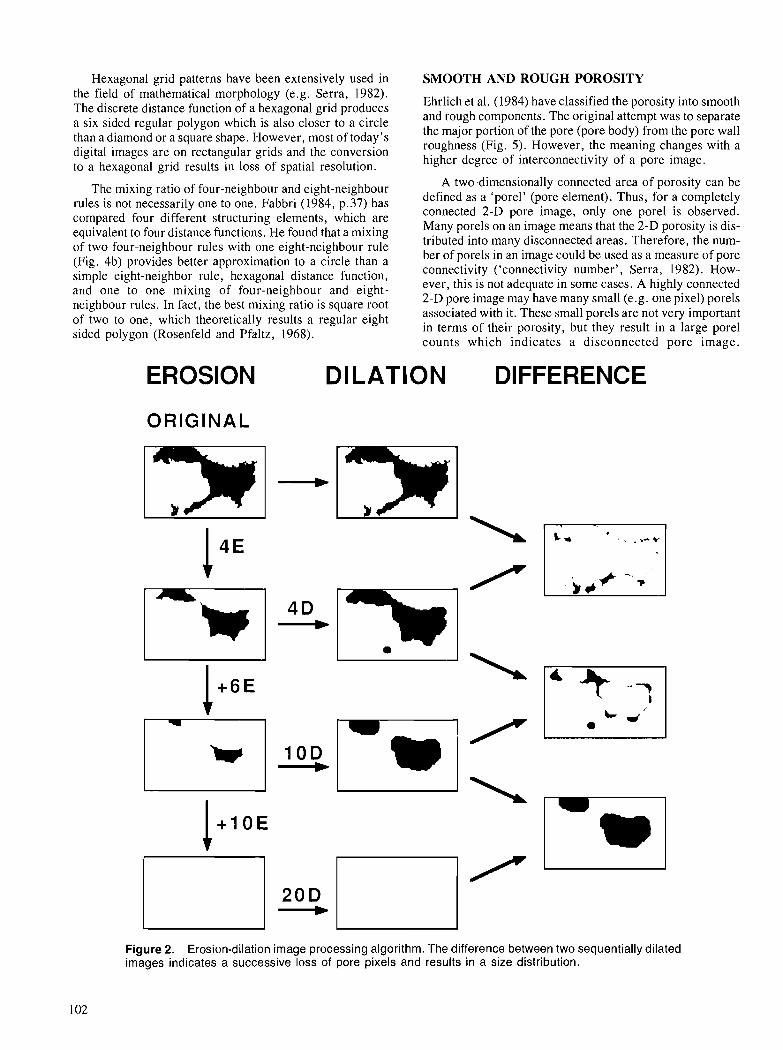
Hexagonal grid patterns have been extensively used in SMOOTH AND ROUGH POROSITY - .

the field-of mathematical morphology (e.g. Serra, 1982). The discrete distance function of a hexagonal grid produces Ehrlich et al. (1984) have classified the porosity into smooth

a six sided regular polygon which is also closer to a circle and rough components. The original attempt was to separate

than a diamond or a square shape. However, most of today's the major portion of the pore (pore body) from the pore wall

digital images are on rectangular grids and the conversion roughness (Fig. 5). However, the meaning changes with a

to a hexagonal grid results in loss of spatial resolution. higher degree of interconnectivity of a pore image.

The mixing ratio of four-neighbour and eight-neighbour rules is not necessarily one to one. Fabbri (1984, p.37) has compared four different structuring elements, which are equivalent to four distance functions. He found that a mixing of two four-neighbour rules with one eight-neighbour rule (Fig. 4b) provides better approximation to a circle than a simple eight-neighbor rule, hexagonal distance function, and one to one mixing of four-neighbour and eight- neighbour rules. In fact, the best mixing ratio is square root of two to one, which theoretically results a regular eight sided polygon (Rosenfeld and Pfaltz, 1968).

A two-dimensionally connected area of porosity can be defined as a 'porel' @ore element). Thus, for a completely connected 2-D pore image, only one porel is observed. Many porels on an image means that the 2-D porosity is distributed into many disconnected areas. Therefore, the number of porels in an image could be used as a measure of pore connectivity ('connectivity number', Serra, 1982). How- ever, this is not adequate in some cases. A highly connected 2-D pore image may have many small (e.g. one pixel) porels associated with it. These small porels are not very important in terms of their porosity, but they result in a large porel counts which indicates a disconnected pore image.

EROSION DILATION DIFFERENCE

ORIGINAL

Figure 2. Erosion-dilation image processing algorithm. The difference between two sequentially dilated images indicates a successive loss of pore pixels and results in a size distribution.

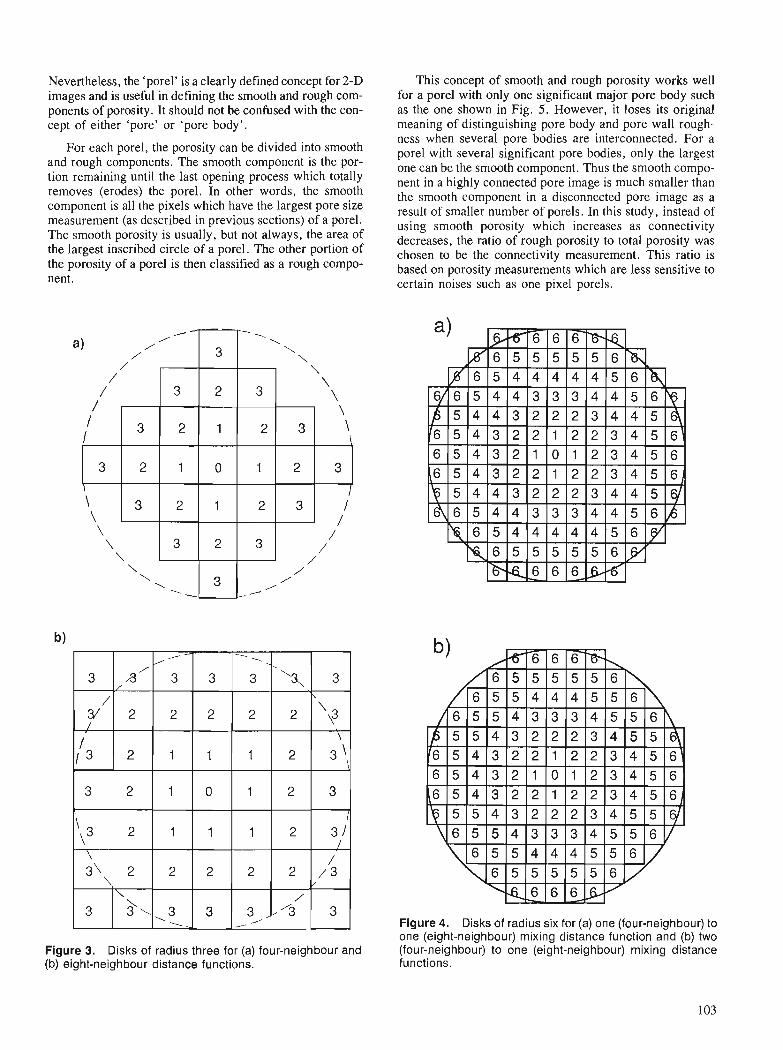
Nevertheless, the 'porel' is a clearly defined concept for 2-D images and is useful in defining the smooth and rough components of porosity. It should not be confused with the concept of either 'pore' or 'pore body'.

For each porel, the porosity can be divided into smooth and rough components. The smooth component is the portion remaining until the last opening process which totally removes (erodes) the porel. In other words, the smooth component is all the pixels which have the largest pore size measurement (as described in previous sections) of a porel. The smooth porosity is usually, but not always, the area of the largest inscribed circle of a porel. The other portion of the porosity of a porel is then classified as a rough component.

This concept of smooth and rough porosity works well for a porel with only one significant major pore body such as the one shown in Fig. 5. However, it loses its original meaning of distinguishing pore body and pore wall roughness when several pore bodies are interconnected. For a porel with several significant pore bodies, only the largest one can be the smooth component. Thus the smooth component in a highly connected pore image is much smaller than the smooth component in a disconnected pore image as a result of smaller number of porels. In this study, instead of using smooth porosity which increases as connectivity decreases, the ratio of rough porosity to total porosity was chosen to be the connectivity measurement. This ratio is based on porosity measurements which are less sensitive to certain noises such as one pixel porels.

Figure 4. Disks of radius six for (a) one (four-neighbour) to one (eight-neighbour) mixing distance function and (b) two

Figure 3. Disks of radius three for (a) four-neighbour and (four-neighbour) to one (eight-neighbour) mixing distance (b) eight-neighbour distance functions. functions.

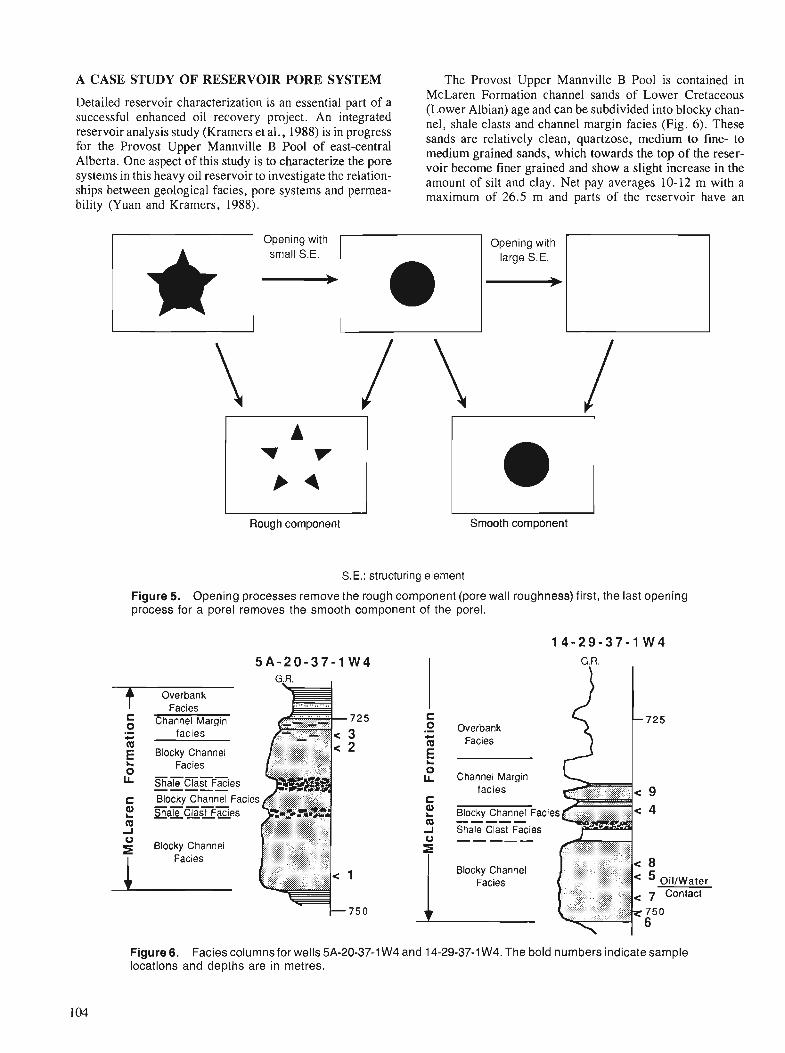
A CASE STUDY OF RESERVOIR PORE SYSTEM The Provost Upper Mannville B Pool is contained in McLaren ~ormat idn channel sands of Lower Cretaceous

Detailed reservoir characterization is an essential part of a (Lower Albian) age and can be subdivided into blocky than- successful enhanced oil recovery project. An integrated nel, shale clasts and channel margin facies (Fig. 6). These

(Kramers et 1988) is in progress sands are relatively clean, medium to fine- to for the Provost Mannville of east-centra1 medium grained sands, which towards the top of the reser- Alberta. One aspect of this study is to characterize the pore voir become finer grained and show a slight increase in the systems in this heavy oil reservoir to investigate the relation- amount of silt and clay. Net pay averages 10-12 m with a ships between geological facies, pore systems and permea- maximum of 26.5 and of the reservoir have an bility (Yuan and Kramers, 1988).

Rough component Smooth component

S.E.: structuring element

Figure 5. Opening processes remove the rough component (pore wall roughness) first, the last opening process for a porel removes the smooth component of the porel.

5 A - 2 0 - 3 7 - 1 W 4 G.R.

t Overbank Facies

Channel Margin 725 .- C facie~ 3

Blocky Channel 2 L

0 Facies

U, SaKGstFacies 7----

e Blocky Channel Facies ShaK~xstFacies

a A O Blocky Channel

Facies i 1

1 4 - 2 9 - 3 7 - 1 W 4 G.R.

0 U, Channel Marg~n

facies C

2 Blocky Channel Fac~es ----- A Shale Clast Fac~es

Blocky Channel Facies

Figure 6. Facies columns for wells 5A-20-37-1 W4 and 14-29-37-1 W4. The bold numbers indicate sample locations and depths are in metres.

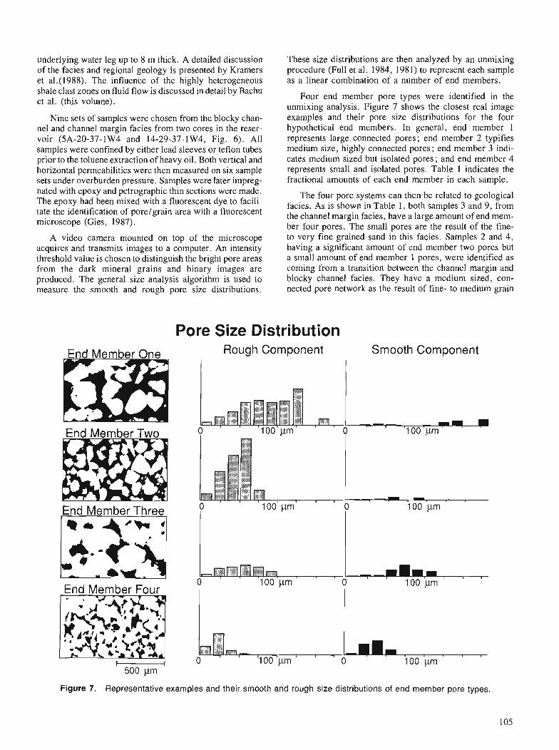
underlying water leg up to 8 m thick. A detailed discussion of the facies and regional geology is presented by Kramers et a1.(1988). The influence of the highly heterogeneous shale clast zones on fluid flow is discussed in detail by Bachu et al. (this volume).

Nine sets of samples were chosen from the blocky channel and channel margin facies from two cores in the reservoir (5A-20-37-1W4 and 14-29-37-1W4, Fig. 6 ) . All samples were confined by either lead sleeves or teflon tubes prior to the toluene extraction of heavy oil. Both vertical and horizontal permeabilities were then measured on six sample sets under overburden pressure. Samples were later impreg- nated with epoxy and petrographic thin sections were made. The epoxy had been mixed with a fluorescent dye to facilitate the identification of porelgrain area with a fluorescent microscope (Gies, 1987).

A video camera mounted on top of the microscope acquires and transmits images to a computer. An intensity threshold value is chosen to distinguish the bright pore areas from the dark mineral grains and binary images are produced. The general size analysis algorithm is used to measure the smooth and rough pore size distributions.

These size distributions are then analyzed by an unmixing procedure (Full et al. 1984, 1981) to represent each sample as a linear combination of a number of end members.

Four end member pore types were identified in the unmixing analysis. Figure 7 shows the closest real image examples and their pore size distributions for the four hypothetical end members. In general, end member 1 represents large connected pores; end member 2 typifies medium size, highly connected pores; end member 3 indicates medium sized but isolated pores; and end member 4 represents small and isolated pores. Table 1 indicates the fractional amounts of each end member in each sample.

The four pore systems can then be related to geological facies. As is shown in Table 1, both samples 3 and 9, from the channel margin facies, have a large amount of end member four pores. The small pores are the result of the fine- to very fine grained sand in this facies. Samples 2 and 4, having a significant amount of end member two pores but a small amount of end member 1 pores, were identified as coming from a transition between the channel margin and blocky channel facies. They have a medium sized, connected pore network as the result of fine- to medium grain

Pore Size Distribution End Member One

End Member Two

End Member Three I ra 4'k 41

End Member Four

-

Rough Component Smooth Component

500 prn

Figure 7. Representative examples and their smooth and rough size distributions of end member pore types.

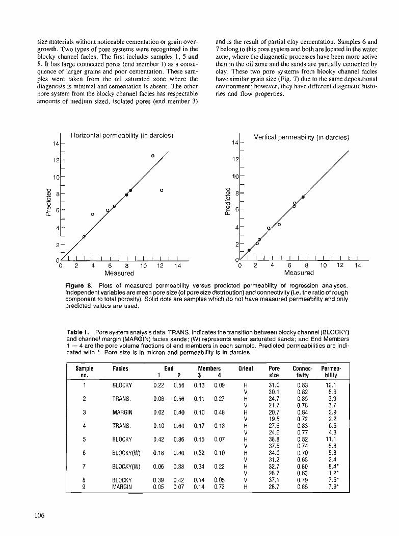
size materials without noticeable cementation or grain over- growth. Two types of pore systems were recognized in the blocky channel facies. The first includes samples 1, 5 and 8. It has large connected pores (end member 1) as a consequence of larger grains and poor cementation. These samples were taken from the oil saturated zone where the diagenesis is minimal and cementation is absent. The other pore system from the blocky channel facies has respectable amounts of medium sized, isolated pores (end member 3)

1 4 1

Horizontal permeability (in darcies)

Measured

and is the result of partial clay cementation. Samples 6 and 7 belong to this pore system and both are located in the water zone, where the diagenetic processes have been more active than in the oil zone and the sands are partially cemented by clay. These two pore systems from blocky channel facies have similar grain size (Fig. 7) due to the same depositional environment ; however, they have different diagenetic histories and flow properties.

1 4 1 Vertical permeability (in darcies)

Measured

Figure 8. Plots of measured permeability versus predicted permeability of regression analyses. Independent variables are mean pore size (of pore size distribution) and connectivity (i.e. the ratio of rough component to total porosity). Solid dots are samples which do not have measured permeability and only predicted values are used.

Table 1. Pore system analysis data. TRANS. indicates the transition between blocky channel (BLOCKY) and channel margin (MARGIN) facies sands; (W) represents water saturated sands; and End Members 1 - 4 are the pore volume fractions of end members in each sample. Predicted permeabilities are indicated with *. Pore size is in micron and permeability is in darcies.

Sample Facies End Members Orient Pore Connec- Permea- no. 1 2 3 4 size tivity bility

1 BLOCKY 0.22 0.56 0.13 0.09 H 31 .O 0.83 12.1 V 30.1 0.82 6.6

2 TRANS. 0.06 0.56 0.11 0.27 H 24.7 0.85 3.9 V 21.7 0.78 3.7

3 MARGIN 0.02 0.40 0.10 0.48 H 20.7 0.84 2.9 V 19.5 0.72 2.2

4 TRANS. 0.10 0.60 0.17 0.13 H 27.6 0.83 6.5 V 24.6 0.77 4.8

5 BLOCKY 0.42 0.36 0.15 0.07 H 38.8 0.82 11.1 V 37.5 0.74 6.6

6 BLOCKY(W) 0.18 0.40 0.32 0.10 H 34.0 0.70 5.8 V 31.2 0.65 2.4

7 BLOCKY(W) 0.06 0.38 0.34 0.22 H 32.7 0.80 8.4* V 26.7 0.63 1.2*

8 BLOCKY 0.39 0.42 0.14 0.05 V 37.1 0.79 7.5* 9 MARGIN 0.05 0.07 0.14 0.73 H 28.7 0.85 7.9*

A quantitative relationship between measured permeabilities and image data can be established by regression analysis. This can then be used to predict permeability for samples where no permeability measurements were made. In this paper, horizontal permeabilities are correlated to horizontal thin section measurements and vertical permeabilities are correlated to vertical thin section measurements. The results indicate that permeabilities are highly related to pore size and connectivity (Fig. 8). Both regression relationships are significant at the 5 % level. The permeabilities of samples 7 , 8 and 9 can thus be predicted from these relationships and the predicted values are listed in Table 1. Similar results can also be obtained by correlating horizontal permeabilities to the measurements on vertical thin sections, and vertical permeabilities to horizontal thin section measurements.

This study has shown that there is a strong link between lithofacies, pore systems and permeability. Image analysis has allowed for the prediction of permeability values where no measurements were made and the extension of flow parameters to areas in the reservoir where only geological information was available.

DISCUSSION

The general size analysis algorithm presented in this paper is a powerful tool for image analysis. It can measure the 'size distribution' of almost any feature on a segmented image. For long and narrow features, such as fractures, the results will be the width (smaller dimension) of the feature. For equidimensional features, such as sand grains, it provides a good linear size measurement. Highly irregular and complex pore images have been successfully quantified by this algorithm as shown in the paper. Other fields such as remote sensing, biomedical imaging, and material sciences are potential fields of application for this type of size analysis.

ACKNOWLEDGMENTS

The author thanks the Alberta Research Council, The Alberta Oil Sands Technology and Research Authority, and the Alberta Department of Energy for financially sponsor- ing this research program and for allowing us to publish these results. I also thank John W. Kramers, Dave Cuthiell, and Terry Stone for their helpful comments; Max Baaske for laboratory support; and Des Wynne for computing support.

REFERENCES

Bachu, S., Cuthiell, D. and Kramers, J. 1989: Effects of core scale heterogeneities on fluid flow in a reservoir;

in Statistical Analysis in the Earth Sciences, ed. F.P. Agterberg - and G.F. Bonham-Caner, Geological Survey of Canada, Paper 89-9, this volume.

Berryman, J.G. and Blair, S.C. 1987: Kozeny-Carman relations and image processing methods for

estimating Darcy's constant; Journal of Applied Physics, v. 62, no. 6, p. 2221-2228.

Delfiner, P. 1972: A generalization of the concept of size; Journal of Microscopy,

v. 95, p. 203-216. Doyen, P.M. 1988: Permeability, conductivity, and pore geometry of sandstone; Jour-

nal of Geophysical Research, v. 93, No. B7, p. 7729-7740. Ehrlich, R., Kennedy, S.K., Crabtree, S.J. and Cannon, R.L. 1984: Petrographic image analysis, I , Analysis of reservoir pore com-

plexes; Journal of Sedimentary Petrology, v. 54, p. 1365-1378. Fabbri, A.G. 1984: Image Processing of Geological Data; Van Nostrand Reinhold

Company Inc., New York, 244p. Feret, L.R. 1931 La grosseur des grains des matihres pulv6rulentes; Association

Internationale pour I'Essai des Mattriaux, v. 2D, p. 428. Full, W.E., Ehrlich, R. and Kennedy, S.K. 1984: Optimal configuration and information content of sets of frequency

distributions; Journal of Sedimentary Petrology, v. 54, p. 117-126.

Full, W.E., Ehrlich, R. and Klovan, J.E. 1981 : EXTENDED QMODEL - Objective definition of external end

members in the analysis of mixtures; Mathematical Geology, v. 13, p. 331-344.

Gies, R.M. 1987 : An improved method for viewing micropore systems in rocks with

the polarizing microscope; Society of Petroleum Engineers For- mation Evaluation, v. 2, p. 209-214.

Kramers, J.W., Bachu, S., Cuthiell, D., Lytviak, A.T., Hasiuk, J.E., Olic, J.J., Prentice, M.E. and Yuan, L.P. 1988: The Provost Upper Mannville B pool; An integrated reservoir

analysis; Fourth UNITARlUNDP Conference on Heavy Crude and Tar Sands, preprint, August 7-12, 1988, Edmonton, Alberta, Canada.

Matheron, G. 1967 : Elements pouruneThCorie des Milieux Poreux; Paris, recent Mas-

son, 168p. Parker, J.R. 1988: A faster method for erosion and dilation of reservoir pore-complex

images; Canadian Journal of Earth Sciences, v. 25, No. 7, p. 1128-1131.

Rink, M. 1976: A computerized quantitative image analysis procedure for inves-

tigating features and an adapted image process; Journal of Microscopy, v. 107, p. 267-286.

Rink, M. and Schopper, J.R. 1978: On the application of image analysis to formation evaluation; The

Log Analyst. p. 12-22. Rosenfeld, A. and Pfaltz, J.L. 1968: Distance functions on digital pictures; Pattern Recognition, v. 1,

p. 33-61. Serra, J. 1982: Image Analysis and Mathematical Morphology; New York, Aca-

demic Press, 610p. Wadell, H. 1932: Volume, shape and roundness of rock particles; Journal of Geol-

ogy, v. 40, p. 443. Walsh, J.B. and Brace, W.F. 1984: The effect of pressure on porosity and the transport properties of

rock; Journal of Geophysical Research, v. 89 p. 9425-9431. Yuan, L.P. and Kramers, J.W. 1988: Characterization of pore images in a heavy oil reservoir and its

applications; Fourth UNITARIUNDP Conference on Heavy Crude and Tar Sands, preprint, August 7-12, 1988, Edmonton, Alberta, Canada.

GEOSIS project: knowledge representation and data structures for geoscience data

Alaster Currie and Bridget Adyl

Currie, A. and Ady, B., GEOSIS project: knowledge representation and data structures for geoscience data; & Statistical Applications in the Earth Sciences, ed. F. P. Agterberg and G. F. Bonham-Carter; Geological Survey of Canada, Paper 89-9, p. 111-116, 1989.

Abstract

The goal of the GEOSIS Project (Geoscience Spatial Information System) is the creation of an integrated environment for the retrieval and analysis of all types of data related to the geosciences. To reach this objective we have had to look at the fundamental nature of the data and to assemble hardware and sofhvare capable of creating an integrated environment.

The approach taken is to represent the data and their relationships using single class hierarchies (e.g. sedimentary rocks) with multiple hierarchies above each data set as required. These hierarchies may have multiple roots forming a 'tangled hierarchy'.

Generalization (i. e. abstraction) of the data occurs as a user moves up through the nodes on a hierarchy towards the root(s). The nodes on each level of abstraction can be linked to other hierarchies using semantic networks, The semantic networks describe the relationships between particular nodes on different hierarchies. The relationships between nodes in semantic nets can be of many difSerent types to suit the data, whereas in a hierarchy the links between nodes must be of one type.

This approach to data structures will enable the user to move through all the available data as required as there are extensive explicit links in the overall data structure. It will also open the way for knowledge engineering techniques that can make use of these single class hierarchies and semantic networks.

L'objectif du projet GEOSIS ou Systtme d'information gkoscientifique spatial (Geoscience Spatial Information System) est la crkation d'un contexte d'utilisation intkgrk pour la recherche et l'amlyse de tous les types de donnkes likes aux sciences de la Terre. Afin d 'atteindre cet objectif, il a ktk nkcessaire d'examiner la nature fondamentale des donnbes et d'assembler le matkriel et les logiciels permettant de crber un contexte d'utilisation intdgrk.

La mkthode adoptke consiste h reprksenter les donnkes et les relations entre elles au moyen de hikrarchies 6 classe unique @. ex. roches skdimentaires), des hikrarchies multiples coiffant chaque ensemble de donnkes au besoin. Ces hikrarchies peuvent avoir des racines multiples de faqon a former une hikrarchie enchevgtrke n.

La gknkralisation (c. -a-d. 1 'abstraction) des donn6es 'efectue lorsqu 'un utilisateur remonte par les noeuds d'une hikrarchie en direction de(s) la racine(s). A chacun des niveaux d'abstraction, les noeuds peuvent &tre reliks 6 d'autres hikrarchies au moyen de rkseaux skmantiques. Ces demiers dkcrivent les relations entre des noeuds particuliers de hidrarchies diffkrentes. Les relations entre les noeuds de rkseaux skmantiques peuvent prendre un grand nombre de formes afin de pouvoir s 'adapter aux donnkes, alors qu'ci l'intkrieur d'une hikrarchie les liens entre les noeuds doivent Btre d'un seul type.

Cette manitre d'aborder les structures des donnkes permettra a l'utilisateur d'ktendre au besoin sa recherche a toutes les donnkes disponibles puisqu 'il existe des liens explicites duns la structure globule des donnkes. Elle ouvrira de plus la voie en matitre de mbthodes du g b i e cognitifpouvant exploiter ces hibrarchies ci classe unique et rkseaux skmantiques.

'. Geoscience Data Centre, Ontario Geological Survey, Ministry of Northern Development and Mines, Toronto, Ontario M7A 1W4.

111

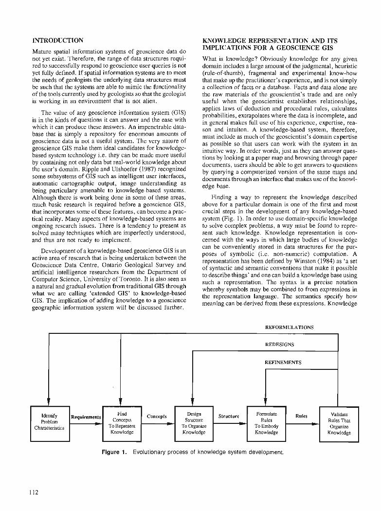
INTRODUCTION

Mature spatial information systems of geoscience data do not yet exist. Therefore, the range of data structures required to successfully respond to geoscience user queries is not yet fully defined. If spatial information systems are to meet the needs of geologists the underlying data structures must be such that the systems are able to mimic the functionality of the tools currently used by geologists so that the geologist is working in an environment that is not alien.

The value of any geoscience information system (GIs) is in the kinds of questions it can answer and the ease with which it can produce these answers. An impenetrable database that is simply a repository for enormous amounts of geoscience data is not a useful system. The very nature of geoscience GIs make them ideal candidates for knowledge- based system technology i.e, they can be made more useful by containing not only data but real-world knowledge about the user's domain. Ripple and Ulshoefer (1987) recognized some subsystems of GIs such as intelligent user interfaces, automatic cartographic output, image understanding as being particulary amenable to knowledge-based systems. Although there is work being done in some of these areas, much basic research is required before a geoscience GIs, that incorporates some of these features, can become a practical reality. Many aspects of knowledge-based systems are ongoing research issues. There is a tendency to present as solved many techniques which are imperfectly understood, and thus are not ready to implement.

Development of a knowledge-based geoscience GIs is an active area of research that is being undertaken between the Geoscience Data Centre, Ontario Geological Survey and artificial intelligence researchers from the Department of Computer Science, University of Toronto. It is also seen as a natural and gradual evolution from traditional GIs through what we are calling 'extended GIs' to knowledge-based GIs. The implication of adding knowledge to a geoscience geographic information system will be discussed further.

KNOWLEDGE REPRESENTATION AND ITS IMPLICATIONS FOR A GEOSCIENCE G I s

What is knowledge? Obviously knowledge for any given domain includes a large amount of the judgmental, heuristic (rule-of-thumb), fragmental and experimental know-how that make up the practitioner's experience, and is not simply a collection of facts or a database. Facts and data alone are the raw materials of the geoscientist's trade and are only useful when the geoscientist establishes relationshi~s. applies laws of de&ction and procedural rules, calculaies probabilities, extrapolates where the data is incomplete, and in general makes full use of his experience, expertise, reason and intuiton. A knowledge-based system, therefore, must include as much of the geoscientist's domain expertise as possible so that users can work with the system in an intuitive way. In order words, just as they can answer questions by looking at a paper map and browsing through paper documents, users should be able to get answers to questions by querying a computerized version of the same maps and documents through an interface that makes use of the knowledge base.

Finding a way to represent the knowledge described above for a particular domain is one of the first and most crucial steps in the development of any knowledge-based system (Fig. 1). In order to use domain-specific knowledge to solve complex problems, a way must be found to represent such knowledge. Knowledge representation is concerned with the ways in which large bodies of knowledge can be conveniently stored in dat; structures for the purposes of symbolic (i.e. non-numeric) computation. A representation has been defined by Winston (1984) as 'a set of syntactic and semantic conventions that make it possible to describe things' and one can build a knowledge base using such a representation. The syntax is a precise notation whereby symbols may be combined to from expressions in the representation language. The semantics specify how meaning can be derived from these expressions. Knowledge

REFORMULATIONS

Figure 1. Evolutionary process of knowledge system development.

REDESIGNS

REFINEMENTS

7 v I I Identify Problem

Characteristics

Requirements *

Design Suucture

Toorganize Knowledge

Find Concepls

To Represent Knowledge

Formulate Rules

To Embody Knowledge

Concepts C,

Rules =)

Validate Rules That Organize

Knowledge

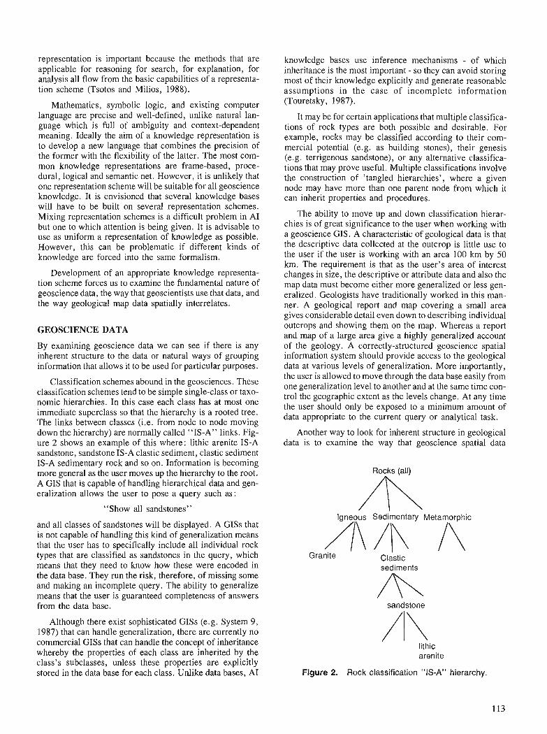
representation is important because the methods that are applicable for reasoning for search, for explanation, for analysis all flow from the basic capabilities of a representation scheme (Tsotos and Milios, 1988).

Mathematics, symbolic logic, and existing computer language are precise and well-defined, unlike natural language which is full of ambiguity and context-dependent meaning. Ideally the aim of a knowledge representation is to develop a new language that combines the precision of the former with the flexibility of the latter. The most common knowledge representations are frame-based, procedural, logical and semantic net. However, it is unlikely that one representation scheme will be suitable for all geoscience knowledge. It is envisioned that several knowledge bases will have to be built on several representation schemes. Mixing representation schemes is a difficult problem in A1 but one to which attention is being given. It is advisable to use as uniform a representation of knowledge as possible. However, this can be problematic if different kinds of knowledge are forced into the same formalism.

Development of an appropriate knowledge representation scheme forces us to examine the fundamental nature of geoscience data, the way that geoscientists use that data, and the way geological map data spatially interrelates.

GEOSCIENCE DATA

By examining geoscience data we can see if there is any inherent structure to the data or natural ways of grouping information that allows it to be used for particular purposes.

Classification schemes abound in the geosciences. These classification schemes tend to be simple single-class or taxonomic hierarchies. In this case each class has at most one immediate superclass so that the hierarchy is a rooted tree. The links between classes (i.e. from node to node moving down the hierarchy) are normally called "IS-A" links. Fig- ure 2 shows an example of this where: lithic arenite IS-A sandstone, sandstone IS-A clastic sediment, clastic sediment IS-A sedimentary rock and so on. Information is becoming more general as the user moves up the hierarchy to the root. A GIs that is capable of handling hierarchical data and generalization allows the user to pose a query such as:

"Show all sandstones"

and all classes of sandstones will be displayed. A GISs that is not capable of handling this kind of generalization means that the user has to specifically include all individual rock types that are classified as sandstones in the query, which means that they need to know how these were encoded in the data base. They run the risk, therefore, of missing some and making an incomplete query. The ability to generalize means that the user is guaranteed completeness of answers from the data base.

Although there exist sophisticated GISs (e.g. System 9, 1987) that can handle generalization, there are currently no commercial GISs that can handle the concept of inheritance whereby the properties of each class are inherited by the class's subclasses, unless these properties are explicitly stored in the data base for each class. Unlike data bases, A1

knowledge bases use inference mechanisms - of which inheritance is the most important - so they can avoid storing most of their knowledge explicitly and generate reasonable assumptions in the case of incomplete information (Touretsky , 1987).

It may be for certain applications that multiple classifications of rock types are both possible and desirable. For example, rocks may be classified according to their commercial potential (e.g. as building stones), their genesis (e.g. terrigenous sandstone), or any alternative classifications that may prove useful. Multiple classifications involve the construction of 'tangled hierarchies', where a given node may have more than one parent node from which it can inherit properties and procedures.

The ability to move up and down classification hierarchies is of great significance to the user when working with a geoscience GIs. A characteristic of geological data is that the descriptive data collected at the outcrop is little use to the user if the user is working with an area 100 km by 50 km. The requirement is that as the user's area of interest changes in size, the descriptive or attribute data and also the map data must become either more generalized or less generalized. Geologists have traditionally worked in this manner. A geological report and map covering a small area gives considerable detail even down to describing individual outcrops and showing them on the map. Whereas a report and map of a large area give a highly generalized account of the geology. A correctly-structured geoscience spatial information system should provide access to the geological data at various levels of generalization. More importantly, the user is allowed to move through the data base easily from one generalization level to another and at the same time control the geographic extent as the levels change. At any time the user should only be exposed to a minimum amount of data appropriate to the current query or analytical task.

Another way to look for inherent structure in geological data is to examine the way that geoscience spatial data

Igneous Sedimentary Metamorphic

A \ I\ Granite

sediments

A sandstone

/I\ lithic

arenite

Figure 2. Rock classification "IS-A" hierarchy.

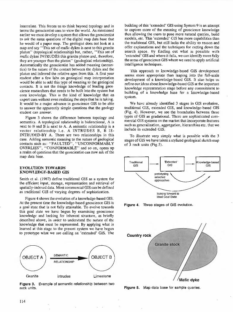
interrelate. This forces us to think beyond topology and in terms the geoscientist uses to view the world. As mentioned earlier we must develop a system that allows the geoscientist to ask the same questions of the digital map data base that he would of a paper map. The geologist does not look at a map and say "This set of mafic dykes is next to this granite pluton" (topological relationship) but, rather, "This set of mafic dykes INTRUDES this granite pluton and, therefore, they are younger than the pluton" (geological relationship). Automatically the geoscientist has added meaning (semantics) to the nature of the contact between the dykes and the pluton and inferred the relative ages from this. A first year student after a few labs on geological map interpretation would be able to add this type of meaning to the geological contacts. It is not the fringe knowledge of leading geoscience researchers that needs to be built into the system but core knowledge. This is the kind of knowledge that an expert uses without even realizing the steps that he is taking. It would be a major advance in geoscience GIs to be able to answer the apparently simple questions that the geology student can answer.

Figure 3 shows the difference between topology and semantics. A topological relationship is bidirectional, A is next to B and B is next to A. A semantic relationship is a vector relationship i . e . A INTRUDES B, B IS- INTRUDED-BY A. There are two relationships in this case. Adding semantic meaning to the nature of geological contacts such as: "FAULTED", "UNCONFORMABLY OVERLIES", "CONFORMABLE" and so on, opens up a realm of questions that the geoscientist can now ask of the map data base.

EVOLUTION TOWARDS KNOWLEDGE-BASED GIs

Smith et al. (1987) define traditional GIs as a system for the efficient input, storage, representation and retrieval of spatially-indexed data. Most commercial GIs can be defined as traditional GIs of varying degrees of sophistication.

Figure 4 shows the evolution of a knowledge-based GIs. At the present time the knowledge-based geoscience GIs is a goal state that is not fully attainable. To evolve towards this goal state we have begun by examining geoscience knowledge and looking for inherent structure, as briefly described above, in order to understand the nature of the knowledge that must be represented. By applying what is learned at this stage to the present system we have begun to prototype what we are calling an 'extended' GIs. The

(OBJECT A ) SEMANTIC OBJECT B ) RELATIONSHIP

Granite intrudes Limestone

Figure 3. Example of semantic relationship between two rock units.

building of this 'extended' GIs using System 9 is an attempt to capture more of the meaning of geoscience knowledge thus allowing the users to pose more natural queries, build models, etc. This 'extended' GIs has more capabilities than the traditional GIs, but still lacks the ability to reason and offer explanations and the techniques for cutting down the search space. By finding out what is possible with 'extended' GIs and where it fails, we can identify more fully the areas of geoscience GIs where we need to apply artificial intelligence techniques.

This approach to knowledge-based GIs development seems more appropriate than leaping into the full-scale development of a knowledge-based GIs. It also helps us refine our ideas about knowledge-based GIs at the important knowledge representation stage before any commitment to building of a knowledge base for a knowledge-based system.

We have already identified 3 stages in GIs evolution, traditional GIs, extended GIs, and knowledge-based GIs (Fig. 4). However, we see the boundaries between these types of GIS as gradational. There are sophisticated commercial GIs systems on the market that incorporate features such as generalization, aggregation, hierarchies etc. that we include in extended GIs.

To illustrate very simply what is possible with the 3 stages of GIs we have taken a stylized geological sketch map of 3 rock units (Fig.5).

Traditional 'Extended '

prototyping selected approaches

looking forward to ideal Goal State

Figure 4. Three stages of GIs evolution.

/ ~ a f i c dyke

Figure 5. Map data base for sample queries.

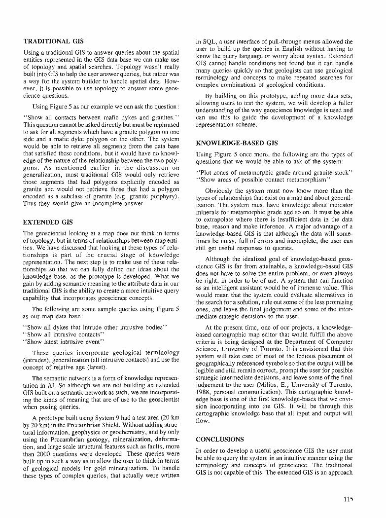
TRADITIONAL GIs

Using a traditional GIs to answer queries about the spatial entities represented in the GIs data base we can make use of topology and spatial searches. Topology wasn't really built into GIs to help the user answer queries, but rather was a way for the system builder to handle spatial data. How- ever, it is possible to use topology to answer some geoscience questions.

Using Figure 5 as our example we can ask the question:

"Show all contacts between mafic dykes and granites." This question cannot be asked directly but must be rephrased to ask for all segments which have a granite polygon on one side and a mafic dyke polygon on the other. The system would be able to retrieve all segments from the data base that satisfied these conditions, but it would have no knowledge of the nature of the relationship between the two polygons . As mentioned earlier in the discussion on generalization, most traditional GIs would only retrieve those segments that had polygons explicitly encoded as granite and would not retrieve those that had a polygon encoded as a subclass of granite (e.g. granite porphyry). Thus they would give an incomplete answer.

EXTENDED GIs

The geoscientist looking at a map does not think in terms of topology, but in terms of relationships between map entities. We have discussed that looking at these types of relationships is part of the crucial stage of knowledge representation. The next step is to make use of these relationships so that we can fully define our ideas about the knowledge base, as the prototype is developed. What we gain by adding semantic meaning to the attribute data in our traditional GIs is the ability to create a more intuitive query capability that incorporates geoscience concepts.

The following are some sample queries using Figure 5 as our map data base:

"Show all dykes that intrude other intrusive bodies" "Show all intrusive contacts" "Show latest intrusive event"

These queries incorporate geological terminology (intrudes), generalization (all intrusive contacts) and use the concept of relative age (latest).

The semantic network is a form of knowledge representation in AI. So although we are not building an extended GIs built on a semantic network as such, we are incorporating the kinds of meaning that are of use to the geoscientist when posing queries.

A prototype built using System 9 had a test area (20 km by 20 km) in the Precambrian Shield. Without adding structural information, geophysics or geochemistry, and by only using the Precambrian geology, mineralization, deformation, and large scale structural features such as faults, more than 2000 questions were developed. These queries were built up in such a way as to allow the user to think in terms of geological models for gold mineralization. To handle these types of complex queries, that actually were written

in SQL, a user interface of pull-through menus allowed the user to build up the queries in English without having to know the query language or worry about syntax. Extended GIs cannot handle conditions not found but it can handle many queries quickly so that geologists can use geological terminology and concepts to make repeated searches for complex combinations of geological conditions.

By building on this prototype, adding more data sets, allowing users to test the system, we will develop a fuller understanding of the way geoscience knowledge is used and can use this to guide the development of a knowledge representation scheme.

KNOWLEDGE-BASED GIs

Using Figure 5 once more, the following are the types of questions that we would be able to ask of the system:

"Plot zones of metamorphic grade around granite stock" "Show areas of possible contact metamorphism"

Obviously the system must now know more than the types of relationships that exist on a map and about generalization. The system must have knowledge about indicator minerals for metamorphic grade and so on. It must be able to extrapolate where there is insufficient data in the data base, reason and make inference. A major advantage of a knowledge-based GIs is that although the data will sometimes be noisy, full of errors and incomplete, the user can still get useful responses to queries.

Although the idealized goal of knowledge-based geoscience GIs is far from attainable, a knowledge-based GIs does not have to solve the entire problem, or even always be right, in order to be of use. A system that can function as an intelligent assistant would be of immense value. This would mean that the system could evaluate alternatives in the search for a solution, rule out some of the less promising ones, and leave the final judgement and some of the intermediate stategic decisions to the user.

At the present time, one of our projects, a knowledge- based cartographic map editor that would fulfill the above criteria is being designed at the Department of Computer Science, University of Toronto. It is envisioned that this system will take care of most of the tedious placement of geographically referenced symbols so that the output will be legible and still remain correct, prompt the user for possible strategic intermediate decisions, and leave some of the final judgement to the user (Milios, E., University of Toronto, 1988, personal communication). This cartographic knowledge base is one of the first knowledge-bases that we envi- sion incorporating into the GIs. It will be through this cartographic knowledge base that all input and output will flow.

CONCLUSIONS

In order to develop a useful geoscience GIs the user must be able to query the system in an intuitive manner using the terminology and concepts of geoscience. The traditional GIs is not capable of this. The extended GIs is an approach

to this challenge that uses existing GIs technology but attempts to create an intuitive geoscience query environment. The extended GIs is not an end in itself but a means to investigate the problems of creating a GIs that can be used by geoscientists for sophisticated query and analysis without the geoscientist being aware of the GIs technology that makes this possible.

REFERENCES

Ripple, W. and Ulshoefer,V. 1987: Expert systems and spatial data models for efficient geographic

data handling ; Photogrammetric Engineering and Remote Sensing, v . 53, no. 10, p. 1431-1433.

System 9 1989: Project managers manual (January 1989 edition) Prime Wild GIs

Inc. Smith, T.R., Menon, S., Star, J.L., and Estes, J.E. 1987: Requirements and principles for the implementation and construc-

tion of large-scale geographic information systems; International Journal of Geographical Information Systems, v. 1, no 1, p. 13-31.

Touretsky, D.S. 1987 : Inheritance hierarchy. in Encyclopedia of Artificial Intclligence,

Wiley-Interscience, New York, v. 1, p.422-431. Tsotsos, J., and Milios, E. 1988 : Towards computational geoscience, Unpublished Report, Depart-

ment of Computer Science, University of Toronto, 89 p. Winston, P.H. 1984: Artificial Intelligence, 2nd. Edition, Addison-Wesley, Reading,

Massachussetts, 527 p.

Using CARIS as a spatial information system for geological applications

E.C. Reeler1 and J.J. Chandra2

Reeler, E. C. and Chandra, J. J . , Using CARIS as a spatial information system for geological applications; & Statistical Applications in the Earth Sciences, ed. F.P. Agterberg and G.F. Bonham-Carter; Geological Survey of Canada, Paper 89-9, p. 117-119, 1989

Abstract

The Computer Aided Resource Information System, CARIS, is a Geographic Information System which is presently being used by mapping and information agencies to handle spatial information in a wide range of disciplines including those having geological applications.

The capabilities of the CARIS system have been successfully used by the Department of Natural Resources in New Brunswick to integrate and interrelate geoscientific data and textual attributes in a spatially based three-dimensional system.

R e CARIS system currently supports point, line and polygon data, raster data, three dimensional surface modelling and digital terrain modelling. Development of the CARIS system has also focused on a new software module, particularly suitable for geological and mining applications.

This module has capabilities of digitizing, storing and manipulating irregular three-dimensional objects in a block model environment based on an octree data structure. The 3 - 0 module is integrated with the current 2 - 0 system. Some of the module applications include simulated excavations, stope design and closest distance determination.

Le Systtme informatise'd'information sur les ressources, CARIS (Computer Aided Resource Informa- tion System), est un Systtme d'information gkographique actuellement utilise'par les organismes de cartographie et d'information pour trailer l'information ci caracttre spatial dans une gamme ktendue de disciplines incluant celles qui ont des applications en gkologie.

Les possibilitks du systtme CARIS ont kt6 exploitkes avec succts par le ministtre des Ressources naturelles du Nouveau-Brunswick pour intkgrer et reliclr des donne'es gebscientiJiques et des attributs textuels en un systtme spatial tridimensionnel.

Le systtme CARIS englobe actuellement des donnPes ponctuelles, des donnPes linkaires, des donnkes caractkrisant des polygones, des donnkes caractPrisant des trames, des modtles tridimensionnels de la surface et des mod6les numkriques de terrain. La mise au point du syst6me CARlS est kgalement axke sur un nouveau module de logicielparticulibrement bien adapte'aux applications gPologiques et minitres.

Ce module permet la numkrisation, le stockage et la manipulation d'objets tridimensionnels de forme irrkgulitre dans un contexte de modklisation en blocs basksur une structure de donnkes octarborescente. Le module tridimensionnel est intPgrk a l'actuel systtme bidimensionnel. Ce module sert, entre autres, ci la simulation d'excavations, la conception des chantiers d'abattage et la dktermination de la distance la plus courte.

'. Universal Systems Ltd., Fredericton, New Bmnswick, E3A 5H2 .Science and Technology Secretariat, Commerce and Technology, Fredericton, New Brunswick, E3B 5H1.

INTRODUCTION

The Computer Aided Resource Information System, CARIS, is presently being used by mapping and information agencies in many disciplines to handle spatial information. These disciplines deal with applications in the following fields : geology, hydrography, topographic mapping, agriculture, marine environment, forest and resource management, municipal and property management, education and research.

THE CARIS SYSTEM

The central component of CARIS is its graphical database in which spatial data is stored, Lee (1983). Spatial data can be in many forms in the system. These include:

- data digitized from conventional line maps - three dimensional point, line and polygon data digitized

from aerial photographs - raster data from satellite images or scanned raster objects - three dimensional surfaces used in surface modelling and

digital terrain modelling - and three dimensional block data used in the block

modelling of orebodies

Each graphic element in each of these categories can be associated with, and linked to, any number of textual attributes on one or more textual databases. This gives the textual information an added spatial quality, and enables textual queries to be given spatial constraints.

CARIS has many capabilities 'for manipulating spatial data. Graphic data sets can be merged or selectively displayed and plotted at different scales and projections using user defined colours and symbology. This is useful for map compilation. The graphic elements possess topology which enables them to "know" which other graphic elements are immediately adjacent or nearby; Their spatial qualities enable the calculation of area, length, height, and distance in three dimensions. This is useful for the spatial analysis of geological datasets, mine management and layout, as well as ore body modelling and excavation determination.

The CARIS system can connect each graphic element to its textual attributes contained in one or more textual databases. By pointing at graphic data on a screen, the textual information can be retrieved. Conversely by querying the textual data, the graphic locations can be displayed. Com- bined textual and graphic queries are also possible. These query the textual information while simultaneously applying spatial restrictions such as adjacency or distance from significant features. This is useful for recognizing patterns in geological data and spatially interrelating many different geological data sets.

The system is also capable of displaying textual information, such as mineral concentrations, in their spatial locations on a map and converting these values to contours or to a three dimensional surface depicting mineral concentrations. This utilizes the third dimension in CARIS as a quality other than elevation, enabling more abstract attributes and statistical results to be viewed in three dimensions.

CARIS also has raster capabilities which enable it to store satellite images as a background, scanned images such as building plans and photographs as pictorial attributes, and also to store raster objects as area features on a map having textual attributes of their own in a textual database.

GEOLOGICAL APPLICATION

CARIS has been effectively used in a geological application by the New Brunswick Department of Natural Resources. A pilot project was carried out at the University of New Brunswick, to test the suitability of CARIS for compiling and interrelating geological data sets in a Geographic Infor- mation System. The data sets used in the pilot project were of the Lake George Mine area, located 25 to 30 km west of Fredericton.

Aeromagnetic data for the area was compiled from maps of several different scales. This was interrelated with the topographical data from the same area. A layer of structural information was compiled, consisting of point symbols whose characteristics could be depicted by colour codes and symbology. For example, the direction and angle of s t r~ke and dip appeared as a pointer and value in the symbol components. Geochemical data was compiled as symbols representing samples taken at various points along rivers and streams. Any number of textual attributes could be displayed alongside each symbol. Information from gravity surveys was also compiled and related to the above data sets.

Data for the mine features and mine layout was added, including buildings, settling ponds, the survey grid, the ore body and drill hole data in three dimensions. The various levels in the mine were inserted, including the positions of stopes, pillars, survey monuments and other underground features.

Data from the textual database could be displayed in its spatial location on the map. This included the results from statistical analyses which had been stored as textual data. In this way spatial patterns were detected and changing patterns observed by varying the statistical criteria.

The pilot project was successful in being able to compile, combine and integrate the different data sets of geological interest. The system was able to amalgamate all the datasets and tie textual attributes from many separate databases to their spatial locations. The convenfional concept of two dimensional plans could be extended to include the third dimension. All spatial information including geological information, mine layout and underground information was combined into a common database, permitting the display of selected overlays and complex spatial and textual queries.

MODELLING IN THREE-DIMENSI[ONS

Three-dimensional block data can now be integrated into the graphical database. Each block can represent a spatial feature, such as part of an ore body, and have any number of textual attributes, such as ore characteristics and ore concentration. This type of flexibility enables the system to support the concept of a "pulsating" ore body. In this concept,

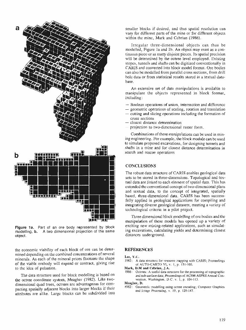
Figure la. Part of an ore body represented by block modelling, b. A two dimensional projection of the same object.

the economic viability of each block of ore can be determined depending on the combined concentrations of several minerals. As each of the mineral prices fluctuate the shape of the viable orebody will expand or contract, giving rise to the idea of pulsation.

The data structure used for block modelling is based on the octree coordinate system, Meagher (1982). Like two- dimensional quad trees, octrees are advantageous for com- pacting spatially adjacent blocks into larger blocks if their attributes are alike. Large blocks can be subdivided into

smaller blocks if desired, and thus spatial resolution can vary for different parts of the mine or for different objects within the mine, Mark and Cebrian (1986).

Irregular three-dimensional objects can thus be modelled, Figure l a and lb . An object may exist as a continuous piece or as many disjoint pieces. Its spatial precision will be determined by the octree level employed. Existing stopes, tunnels and shafts can be digitized conventionally in CARIS and converted into block model format. Ore bodies can also be modelled from parallel cross sections, from drill hole data or from statistical results stored in a textual database.

An extensive set of data manipulations is available to manipulate the objects represented in block format, including :

- Boolean operations of union, intersection and difference - geometric operations of scaling, rotation and translation - cutting and slicing operations including the formation of

cross sections - closest distance determination - projection to two-dimensional raster form.

Combinations of these manipulations can be used in mining engineering. For example, the block module can be used to simulate proposed excavations, for designing tunnels and shafts in a mine and for closest distance determination in search and rescue operations

CONCLUSIONS

The robust data structure of CARIS enables geological data sets to be stored in three-dimensions. Topological and textual data are linked to each element of spatial data. This has extended the conventional concept of two-dimensional plans and textual data, to the concept of integrated, spatially based, three-dimensional data. CARIS has been successfully applied in geological applications for compiling and integrating diverse geological datasets, meeting a variety of technological criteria in a pilot project.

Three dimensional block modelling of ore bodies and the manipulation of these models has opened up a variety of exciting new mining-related applications, such as simulating excavations, calculating yields and determining closest distances underground.

REFERENCES

Lee, Y.C. 1983: A data structure for resource mapping with CARIS; Proceedings

of AUTO-CART0 VI, v. 1 , p. 151-160. Mark, D.M and Cebrian, J.A. 1986: Octrees: A useful data structure for the processing of topographic

and sub-surface data; Proceedings of ACSM-ASPRS Annual Con- vention, Washington, D.C. v. I , p. 104-1 13.

Meagher, D. 1982: Geometric modelling using octree encoding; Computer Graphics

and Image Processing, v. 19, p. 129-147.

Geological map analysis and comparison by several multivariate algorithms

J.C. Browerl and D.F. Merriam2

Brower, J. C. and Merriam D.F., Geological map analysis and comparison by several multivariate algorithms; fi Statistical Applications in the Earth Sciences, ed. F.P. Agterberg and G.F. Bonham- Carter; Geological Survey of Canada Paper 89-9, p. 123-134, 1989

Abstract

Five structure maps from the Paleozoic of Kansas have been analyzed with multivariate statistics including principal components, principal coordinates, Q-mode vector analysis, correspondence analysis and clustering. R e original data include the elevations of 49 points located on a 7 by 7 grid for each map. Each map was standardized in standard deviation units prior to the computations. Reasonable and interpretable results were obtainedfrom some of the techniques despite the fact that they do not consider the regionalized nature of the information. Principal components, principal coordinates, and Q-mode vector analysis recovered all of the main patterns known to be present in the maps, namely the common structural framework, the unconformity between the Mississippian and Pennsylvanian, thickness variation of the Ordovician Arbuckle Limestone which rests unconformably on the Precambrian, and several components of variation unique to individual maps. Correspondence analysis and clustering provide trivial results. The cluster analysis merely separates the data points into high, low, and intermediate areas. Correspondence analysis failed to recognize the regional structural pattern although most of the other relationships were preserved. This situation probably is caused by the type of scaling inherent in the technique. The exercise suggests that some multivariate algorithms can provide useful tools for dis- secting patterns of variation and covariation in thematic maps of various types such as structure, topographic, isopachous, geophysical, and geochemical maps.

On a analyse' cinq cartes structurales du Pale'ozoi'que du Kansas d l'aide de me'thodes statistiques ci variables multiples, notamment celles des cornposantes principales, des coordonne'es principales, de l'analyse vectorielle en mode Q, de l'analyse de correspondance et du groupage. Les donne'es originelles comprennent les altitudes de 49 points situe's sur une grille de 7par 7 , sur chaque carte. On a normalise' chaque carte en unite's d 'e'cart-type avant les calculs. Quelques-unes des techniques en question ont donne' des re'sultats raisonnables et interpre'tables, m2me si elles ne tenaientpas cornpte du caract2re re'gionalisk de l'information. Les principales composantes, les coordonne'es principales et l'analyse vectorielle en mode Q ont restitue' toutes les grandes configurations dont l'existence dans les cartes est connue, en particulier le cadre structural commun, la discordance entre le Mississippien et le Pennsylvanien, les variations de puissance du calcaire ordovicien d'Arbuckle qui repose en discordance sur le Pre'carnbrien, et plusieurs composantes de variation uniques ci certaines cartes individuelles. L'analyse de correspondance et le groupage donnent des rdsultats sans importance. L'analyse de groupe permet sirnplement de se'parer les donne'es ponctuelles en re'gions e'leve'es, basses et interme'diaires. L 'analyse de correspondance n 'a pas permis dlidenti$er le schema structural regional, mais la plupart des autres relations ont he'consewe'es. La situation re'sube probablement du type de mise en ordre, qui est inhei-ent & la technique employe'e. Cet exercice semble indiquer que quelques algorithmes multivaries peuvent constituer des outils pre'cieux qui permettent de mieux diss&quer les scheinas de variation et de covariation dans les cartes thematiques de divers types, telles que les cartes structurales, topographiques, isopaques, ge'ophysiques et g&ochimiques.

' . Department of Geology, Syracuse University, Syracuse, New York 13244-1070, U.S.A. 2. Department of Geology, Wichita State University, Wichita, Kansas 67208, U.S.A.

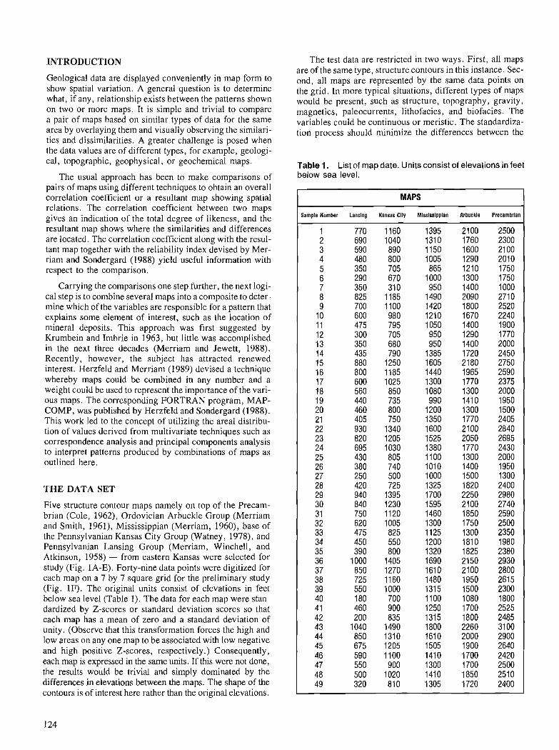
INTRODUCTION

Geological data are displayed conveniently in map form to show spatial variation. A general question is to determine what, if any, relationship exists between the patterns shown on two or more maps. It is simple and trivial to compare a pair of maps based on similar types of data for the same area by overlaying them and visually observing the similarities and dissimilarities. A greater challenge is posed when the data values are of different types, for example, geological, topographic, geophysical, or geochemical maps.

The usual approach has been to make comparisons of pairs of maps using different techniques to obtain an overall correlation coefficient or a resultant map showing spatial relations. The correlation coefficient between two maps gives an indication of the total degree of likeness, and the resultant map shows where the similarities and differences are located. The correlation coefficient along with the resultant map together with the reliability index devised by Mer- riam and Sondergard (1988) yield useful information with respect to the comparison.

Carrying the comparisons one step further, the next logical step is to combine several maps into a composite to determine which of the variables are responsible for a pattern that explains some element of interest, such as the location of mineral deposits. This approach was first suggested by Krumbein and Imbrie in 1963, but little was accomplished in the next three decades (Merriam and Jewett, 1988). Recently, however, the subject has attracted renewed interest. Herzfeld and Merriam (1989) devised a technique whereby maps could be combined in any number and a weight could be used to represent the importance of the various maps. The corresponding FORTRAN program, MAP- COMP, was published by Herzfeld and Sondergard (1988). This work led to the concept of utilizing the areal distribution of values derived from multivariate techniques such as correspondence analysis and principal components analysis to interpret patterns produced by combinations of maps as outlined here.

THE DATA SET

Five structure contour maps namely on top of the Precam- brian (Cole, 1962), Ordovician Arbuckle Group (Merriam and Smith, 1961), Mississippian (Merriam, 1960), base of the Pennsylvanian Kansas City Group (Watney, 1978), and Pennsylvanian Lansing Group (Merriam, Winchell, and Atkinson, 1958) - from eastern Kansas were selected for study (Fig. IA-E). Forty-nine data points were digitized for each map on a 7 by 7 square grid for the preliminary study (Fig. IF). The original units consist of elevations in feet below sea level (Table 1). The data for each map were standardized by Z-scores or standard deviation scores so that each map has a mean of zero and a standard deviation of unity. (Observe that this transformation forces the high and low areas on any one map to be associated with low negative and high positive Z-scores, respectively.) Consequently, each map is expressed in the same units. If this were not done, the results would be trivial and simply dominated by the differences in elevations between the maps. The shape of the contours is of interest here rather than the original elevations.

The test data are restricted in two ways. First, all maps are of the same type, structure contours in this instance. Sec- ond, all maps are represented by the same data points on the grid. In more typical situations, different types of maps would be present, such as structure, topography, gravity, magnetics, paleocurrents, lithofacies, and biofacies. The variables could be continuous or meristic. The standardization process should minimize the differences between the

Table 1. List of map date. Units consist of elevations in feet below sea level.

MAPS

Sample Number Lansing Kansas City Mlsslssipplan Arbuckle Precambrian

1 770 1160 1395 2100 2500 2 690 1040 1310 1760 2300 3 590 890 1150 1600 2100 4 480 800 1005 1290 2010 5 350 705 865 1210 1750 6 290 670 1000 1300 1750 7 350 310 950 1400 1000 8 825 1185 1490 2090 2710 9 700 1100 1420 1800 2520

10 600 980 1210 1670 2240 11 475 795 1050 1400 1900 12 300 705 950 1290 1770 13 350 680 950 1400 2000 14 435 790 1385 1720 2450 15 880 1250 1605 2180 2750 16 800 1185 1440 1965 2590 17 600 1025 1300 1770 2375 18 560 850 1080 1300 2000 19 440 735 990 1410 1950 20 460 800 1200 1300 1500 21 405 750 1350 1770 2405 22 930 1340 1600 2100 2840 23 820 1205 1525 2050 2695 24 695 1030 1380 1770 2430 25 430 805 1100 1300 2000 26 380 740 1010 1400 1950 27 250 500 1000 1500 1300 28 420 725 1325 1820 2400 29 940 1395 1700 2250 2980 30 840 1230 1595 2100 2740 3 1 750 1120 1460 1850 2590 32 620 1005 1300 1750 2500 33 475 825 1125 1300 2350 34 450 550 1200 1810 1980 35 390 800 1320 1825 2380 36 1000 1405 1690 2150 2930 37 850 1270 1610 2100 2800 38 725 1160 1480 1950 2615 39 550 1000 1315 1500 2300 40 180 700 1100 1080 1800 41 460 900 1250 1700 2525 42 200 835 1315 1800 2485 43 1040 1490 1800 2260 3100 44 850 1310 1610 2000 2900 45 675 1205 1505 1900 2640 46 590 1100 1410 1700 2420 47 550 900 1300 1700 2500 48 500 1020 1410 1850 2510 49 320 810 1305 1720 2400

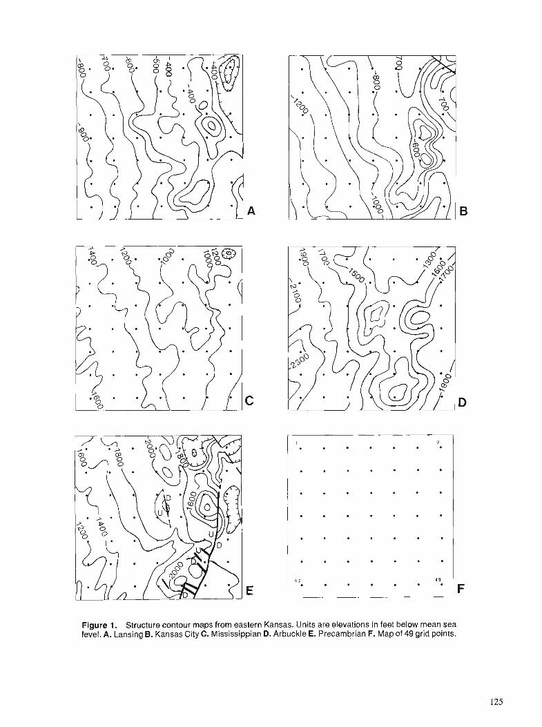
Figure 1. Structure contour maps from eastern Kansas. Units are elevations in feet below mean sea level. A. Lansing B. Kansas City C. Mississippian D. Arbuckle E. Precambrian F. Map of 49 grid points.

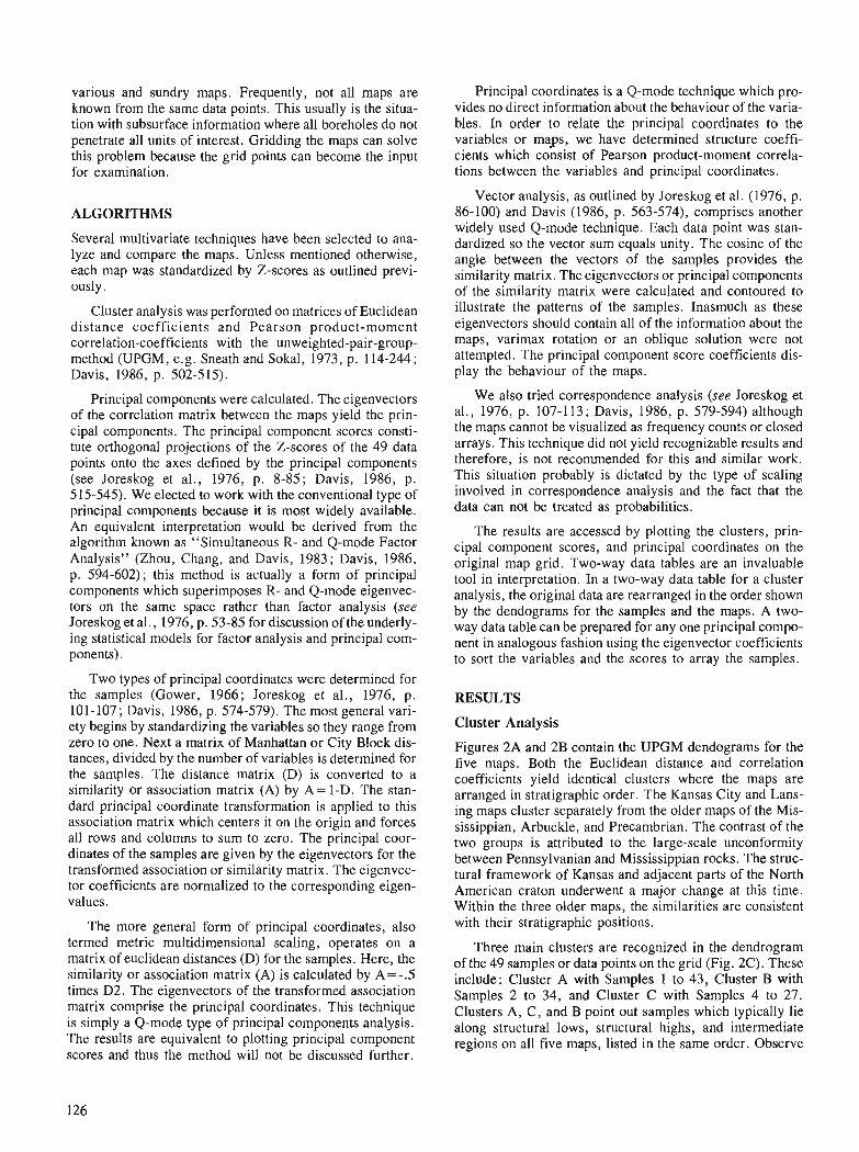
various and sundry maps. Frequently, not all maps are known from the same data points. This usually is the situation with subsurface information where all boreholes do not penetrate all units of interest. Gridding the maps can solve this problem because the grid points can become the input for examination.

ALGORITHMS

Several multivariate techniques have been selected to analyze and compare the maps. Unless mentioned otherwise, each map was standardized by Z-scores as outlined previously.

Cluster analysis was performed on matrices of Euclidean distance coefficients and Pearson product-moment correlation-coefficients with the unweighted-pair-group- method (UPGM, e.g. Sneath and Sokal, 1973, p. 114-244; Davis, 1986, p. 502-515).

Principal components were calculated. The eigenvectors of the correlation matrix between the maps yield the principal components. The principal component scores constitute orthogonal projections of the Z-scores of the 49 data points onto the axes defined by the principal components (see Joreskog et al., 1976, p. 8-85; Davis, 1986, p. 515-545). We elected to work with the conventional type of principal components because it is most widely available. An equivalent interpretation would be derived from the algorithm known as "Simultaneous R- and Q-mode Factor Analysis" (Zhou, Chang, and Davis, 1983 ; Davis, 1986, p. 594-602); this method is actually a form of principal components which superimposes R- and Q-mode eigenvectors on the same space rather than factor analysis (see Joreskog et al., 1976, p. 53-85 for discussion of the underlying statistical models for factor analysis and principal components).

Two types of principal coordinates were determined for the samples (Gower, 1966; Joreskog et al., 1976, p. 101-107 ; Davis, 1986, p. 574-579). The most general variety begins by standardizing the variables so they range from zero to one. Next a matrix of Manhattan or City Block distances, divided by the number of variables is determined for the samples. The distance matrix (D) is converted to a similarity or association matrix (A) by A = 1-D. The standard principal coordinate transformation is applied to this association matrix which centers it on the origin and forces all rows and columns to sum to zero. The principal coordinates of the samples are given by the eigenvectors for the transformed association or similarity matrix. The eigenvector coefficients are normalized to the corresponding eigenvalues.

The more general form of principal coordinates, also termed metric multidimensional scaling, operates on a matrix of euclidean distances (D) for the samples. Here, the similarity or association matrix (A) is calculated by A=-.5 times D2. The eigenvectors of the transformed association matrix comprise the principal coordinates. This technique is simply a Q-mode type of principal components analysis. The results are equivalent to plotting principal component scores and thus the method will not be discussed further.

Principal coordinates is a Q-mode technique which provides no direct information about the behaviour of the variables. In order to relate the principal coordinates to the variables or mags, we have determined structure coefficients which consist of Pearson product-moment correlations between the variables and principal coordinates.

Vector analysis, as outlined by Joreskog et al. (1976, p. 86-100) and Davis (1986, p. 563-574), comprises another widely used Q-mode technique. Each data point was standardized so the vector sum equals unity. The cosine of the angle between the vectors of the samples provides the similarity matrix. The eigenvectors or principal components of the similarity matrix were calculated and contoured to illustrate the patterns of the samples. Inasmuch as these eigenvectors should contain all of the information about the maps, varimax rotation or an oblique solution were not attempted. The principal component score coefficients display the behaviour of the maps.

We also tried correspondence analysis (see Joreskog et al., 1976, p. 107-1 13 ; Davis, 1986, p. 579-594) although the maps cannot be visualized as frequency counts or closed arrays. This technique did not yield recognizable results and therefore, is not recommended for this and similar work. This situation probably is dictated by the type of scaling involved in correspondence analysis and the fact that the data can not be treated as probabilities.

The results are accessed by plotting the clusters, principal component scores, and principal coordinates on the original map grid. Two-way data tables are an invaluable tool in interpretation. In a two-way data table for a cluster analysis, the original data are rearranged in the order shown by the dendograms for the samples and the maps. A two- way data table can be prepared for any one principal component in analogous fashion using the eigenvector coefficients to sort the variables and the scores to array the samples.

RESULTS

Cluster Analysis

Figures 2A and 2B contain the UPGM dendograms for the five maps. Both the Euclidean distance and correlation coefficients yield identical clusters where the maps are arranged in stratigraphic order. The Kansas City and Lans- ing maps cluster separately from the older maps of the Mis- sissippian, Arbuckle, and Precambrian. The contrast of the two groups is attributed to the large-scale unconformity between Pennsylvanian and Mississippian rocks. The structural framework of Kansas and adjacent parts of the North American craton underwent a major change at this time. Within the three older maps, the similarities are consistent with their stratigraphic positions.

Three main clusters are recognized in the dendrogram of the 49 samples or data points on the grid (Fig. 2C). These include: Cluster A with Samples 1 to 43, Cluster B with Samples 2 to 34, and Cluster C with Samples 4 to 27. Clusters A, C, and B point out samples which typically lie along structural lows, structural highs, and intermediate regions on all five maps, listed in the same order. Observe

CORRELATION

0.8 0.9 1 .O

I MISSISSIPPIAN

ARBUCKLE

PRECAMBRIAN

LANSING

KANSAS ClTY

EUCLIDEAN DISTANCE 2.0 1.6 1.2 0.8 0.4 0.0

7 1

EUCLIDEAN DISTANCE

I MISSISSIPPIAN

ARBUCKLE

PRECAMBRIAN

LANSING

KANSAS ClTY

Figure 2. Results of cluster analysis. A. Dendrogram for correlation matrix of maps B. Dendrogram for Euclidean distance matrix of maps C. Dendrogram for Euclidean distance matrix of samples D. Three major clusters of samples in C overlain on map.

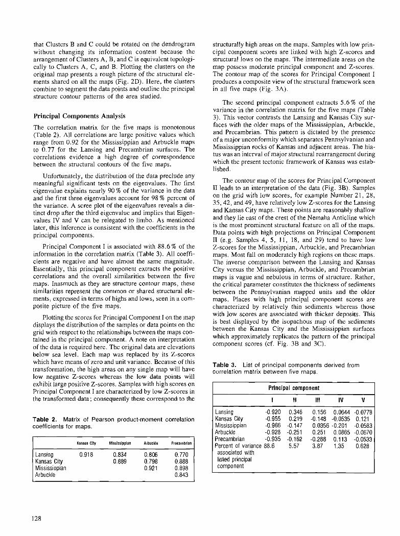
that Clusters B and C could be rotated on the dendrogram without changing its information content because the arrangement of Clusters A, B, and C is equivalent topologi- cally to Clusters A, C, and B. Plotting the clusters on the original map presents a rough picture of the structural elements shared on all the maps (Fig. 2D). Here, the clusters combine to segment the data points and outline the principal structure contour patterns of the area studied.

Principal Components Analysis

The correlation matrix for the five maps is monotonous (Table 2). All correlations are large positive values which range from 0.92 for the Mississippian and Arbuckle maps to 0.77 for the Lansing and Precambrian surfaces. The correlations evidence a high degree of correspondence between the structural contours of the five maps.

Unfortunately, the distribution of the data preclude any meaningful significant tests on the eigenvalues. The first eigenvalue explains nearly 90 % of the variance in the data and the first three eigenvalues account for 98 % percent of the variance. A scree plot of the eigenvalues reveals a distinct drop after the third eigenvalue and implies that Eigen- values IV and V can be relegated to limbo. As mentioned later, this inference is consistent with the coefficients in the principal components.

Principal Component I is associated with 88.6 % of the information in the correlation matrix (Table 3). All coefficients are negative and have almost the same magnitude. Essentially, this principal component extracts the positive correlations and the overall similarities between the five maps. Inasmuch as they are structure contour maps, these similarities represent the common or shared structural elements, expressed in terms of highs and lows, seen in a composite picture of the five maps.

Plotting the scores for Principal Component I on the map displays the distribution of the samples or data points on the grid with respect to the relationships between the maps contained in the principal component. A note on interpretation of the data is required here. The original data are elevations below sea level. Each map was replaced by its Z-scores which have means of zero and unit variance. Because of this transformation, the high areas on any single map will have low negative Z-scores whereas the low data points will exhibit large positive Z-scores. Samples with high scores on Principal Component I are characterized by low Z-scores in the transformed data; consequently these correspond to the

Table 2. Matrix of Pearson product-moment correlation coefficients for maps.

Kansas City 0.889 0.798 0.888 Mississippian 0.921 0.898 Arbuckle 0.843

structurally high areas on the maps. Samples with low principal component scores are linked with high Z-scores and structural lows on the maps. The intermediate areas on the map possess moderate principal component and Z-scores. The contour map of the scores for Principal Component I produces a composite view of the structural framework seen in all five maps (Fig. 3A).

The second principal component extracts 5.6 % of the variance in the correlation matrix for the five maps (Table 3). This vector contrasts the Lansing and Kansas City surfaces with the older maps of the Mississippian, Arbuckle, and Precambrian. This pattern is dictated by the presence of a major unconformity which separates Pennsylvanian and Mississippian rocks of Kansas and adjacent areas. The hiatus was an interval of major structural rearrangement during which the present tectonic framework of Kansas was established.

The contour map of the scores for Principal Component I1 leads to an interpretation of the data (Fig. 3B). Samples on the grid with low scores, for example Number 21, 28, 35,42, and 49, have relatively low Z-scores for the Lansing and Kansas City maps. These points are reasonably shallow and they lie east of the crest of the Nemaha Anticline which is the most prominent structural feature on all of the maps. Data points with high projections on Principal Component I1 (e.g. Samples 4, 5, 11, 18, and 29) tend to have low Z-scores for the Mississippian, Arbuckle, and Precambrian maps. Most fall on moderately high regions on these maps. The inverse comparison between the Lansing and Kansas City versus the Mississippian, Arbuckle, and Precambrian maps is vague and nebulous in terms of structure. Rather, the critical parameter constitutes the thickness of sediments between the Pennsylvanian mapped units and the older maps. Places with high principal component scores are characterized by relatively thin sediments whereas those with low scores are associated with thicker deposits. This is best displayed by the isopachous map of the sediments between the Kansas City and the Mississippian surfaces which approximately replicates the pattern of the principal component scores (cf. Fig. 3B and 3C).

Table 3. List of principal components derived from correlation matrix between five maps.

Principal component

I II 111 IV v Lansing -0.920 0.346 0.156 0.0644 -0.0778 Kansas City -0.955 0.219 -0.148 -0.0535 0.121 Mississippian -0.966 -0.147 0.0356 -0.201 -0.0583 Arbuckle -0.928 -0.251 0.251 0.0865 -0.0670 Precambrian -0.935 -0.162 -0.288 0.1 13 -0.0533 Percent of variance 88.6 5.57 3.87 1.35 0.628 associated with listed principal component

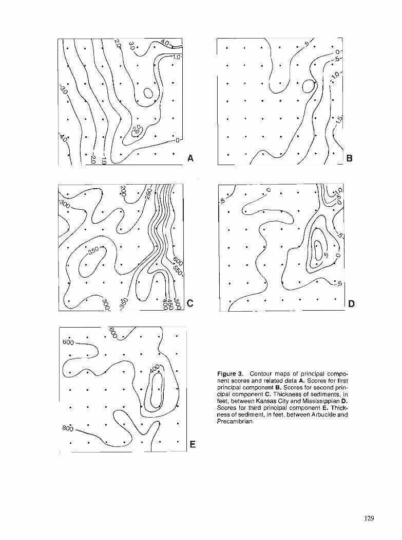
Figure 3. Contour maps of principal component scores and related data A. Scores for first principal component B. Scores for second principal component C. Thickness of sediments, in feet, between Kansas City and Mississippian D. Scores for third principal component E. Thick- ness of sediment, in feet, between Arbuckle and Precambrian.

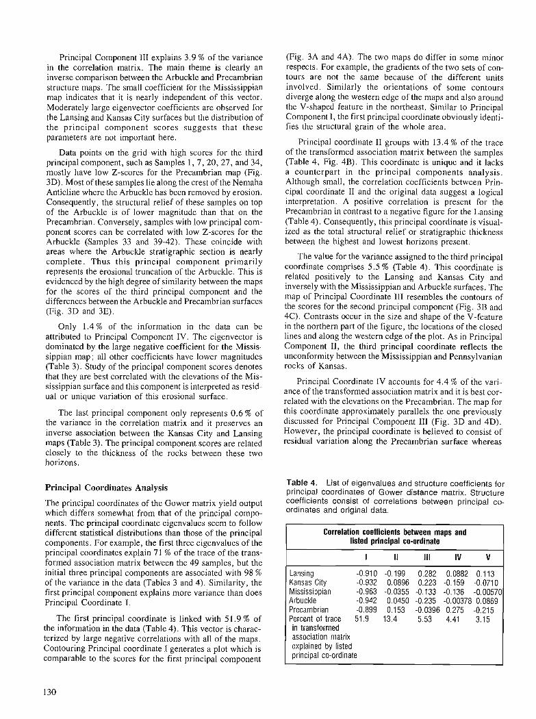
Principal Component I11 explains 3.9 % of the variance in the correlation matrix. The main theme is clearly an inverse comparison between the Arbuckle and Precambrian structure maps. The small coefficient for the Mississippian map indicates that it is nearly independent of this vector. Moderately large eigenvector coefficients are observed for the Lansing and Kansas City surfaces but the distribution of the principal component scores suggests that these parameters are not important here.

Data points on the grid with high scores for the third principal component, such as Samples 1,7,20,27, and 34, mostly have low Z-scores for the Precambrian map (Fig. 3D). Most of these samples lie along the crest of the Nemaha Anticline where the Arbuckle has been removed by erosion. Consequently, the structural relief of these samples on top of the Arbuckle is of lower magnitude than that on the Precambrian. Conversely, samples with low principal component scores can be correlated with low Z-scores for the Arbuckle (Samples 33 and 39-42). These coincide with areas where the Arbuckle stratigraphic section is nearly complete. Thus this principal component primarily represents the erosional truncation of the Arbuckle. This is evidenced by the high degree of similarity between the maps for the scores of the third principal component and the differences between the Arbuckle and Precambrian surfaces (Fig. 3D and 3E).

Only 1.4 % of the information in the data can be attributed to Principal Component IV. The eigenvector is dominated by the large negative coefficient for the Missis- sippian map; all other coefficients have lower magnitudes (Table 3). Study of the principal component scores denotes that they are best correlated with the elevations of the Mis- sissippian surface and this component is interpreted as residual or unique variation of this erosional surface.

The last principal component only represents 0.6 % of the variance in the correlation matrix and it preserves an inverse association between the Kansas City and Lansing maps (Table 3). The principal component scores are related closely to the thickness of the rocks between these two horizons.

Principal Coordinates Analysis

The principal coordinates of the Gower matrix yield output which differs somewhat from that of the principal components. The principal coordinate eigenvalues seem to follow different statistical distributions than those of the principal components. For example, the first three eigenvalues of the principal coordinates explain 71 % of the trace of the transformed association matrix between the 49 samples, but the initial three principal components are associated with 98 % of the variance in the data (Tables 3 and 4). Similarity, the first principal component explains more variance than does Principal Coordinate I.

The first principal coordinate is linked with 51.9 % of the information in the data (Table 4). This vector is characterized by large negative correlations with all of the maps. Contouring Principal coordinate I generates a plot which is comparable to the scores for the first principal component

(Fig. 3A and 4A). The two maps do differ in some minor respects. For example, the gradients of the two sets of contours are not the same because of the different units involved. Similarly the orientations of some contours diverge along the western edge of the maps and also around the V-shaped feature in the northeast. Similar to Principal Component I, the first principal coordinate obviously identifies the structural grain of the whole area.

Principal coordinate I1 groups with 13.4 % of the trace of the transformed association matrix between the samples (Table 4, Fig. 4B). This coordinate is unique and it lacks a counterpart in the principal components analysis. Although small, the correlation coefficients between Prin- cipal coordinate I1 and the original data suggest a logical interpretation. A positive correlation is present for the Precambrian in contrast to a negative figure for the Lansing (Table 4). Consequently, this principal coordinate is visualized as the total structural relief or stratigraphic thickness between the highest and lowest horizons present.

The value for the variance assigned to the third principal coordinate comprises 5.5 % (Table 4). This coordinate is related positively to the Lansing and Kansas City and inversely with the Mississippian and Arbuckle surfaces. The map of Principal Coordinate I11 resembles the contours of the scores for the second principal component (Fig. 3B and 4C). Contrasts occur in the size and shape of the V-feature in the northern part of the figure, the locations of the closed lines and along the western edge of the plot. As in Principal Component 11, the third principal coordinate reflects the unconformity between the Mississippian and Pennsylvanian rocks of Kansas.

Principal Coordinate IV accounts for 4.4 % of the variance of the transformed association matrix and it is best correlated with the elevations on the Precambrian. The map for this coordinate approximately parallels the one previously discussed for Principal Component 111 (Fig. 3D and 4D). However, the principal coordinate is believed to consist of residual variation along the Precambrian surface whereas

T a b l e 4. List of eigenvalues and structure coefficients for principal coordinates of Gower distance matrix. Structure coefficients consist of correlations between principal coordinates and original data.

Correlation coefficients between maps and listed principal co-ordinate

I II 111 IV v Lansing -0.910 -0.199 0.282 0.0882 0.113 Kansas City -0.932 0.0896 0.223 -0.159 -0.0710 Mississippian -0.963 -0.0355 -0.133 -0.136 -0.00570 Arbuckle -0.942 0.0450 -0.235 -0.00378 0.0869 Precambrian -0.899 0.153 -0.0396 0.275 -0.215 Percent of trace 51.9 13.4 5.53 4.41 3.15

in transformed association matrix explained by listed principal co-ordinate

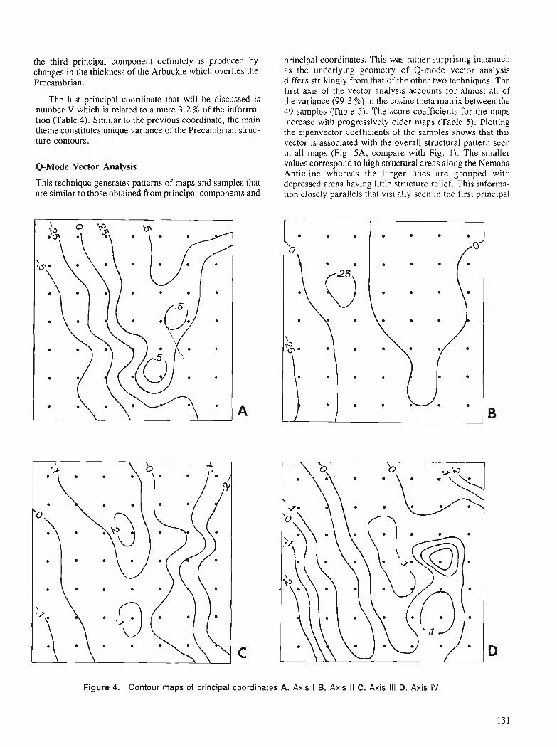
the third principal component definitely is produced by changes in the thickness of the Arbuckle which overlies the Precambrian.

The last principal coordinate that will be discussed is number V which is related to a mere 3.2 % of the information (Table 4). Similar to the previous coordinate, the main theme constitutes unique variance of the Precambrian structure contours.

Q-Mode Vector Analysis

This technique generates patterns of maps and samples that are similar to those obtained from principal components and

principal coordinates. This was rather surprising inasmuch as the underlying geometry of Q-mode vector analysis differs strikingly from that of the other two techniques. The first axis of the vector analysis accounts for almost all of the variance (99.3 %) in the cosine theta matrix between the 49 samples (Table 5). The score coefficients for the maps increase with progressively older maps (Table 5). Plotting the eigenvector coefficients of the samples shows that this vector is associated with the overall structural pattern seen in all maps (Fig. SA, compare with Fig. 1). The smaller values correspond to high structural areas along the Nemaha Anticline whereas the larger ones are grouped with depressed areas having little structure relief. This information closely parallels that visually seen in the first principal

Figure 4. Contour maps of principal coordinates A. Axis 1 B. Axis I I C. Axis I l l D. Axis IV.

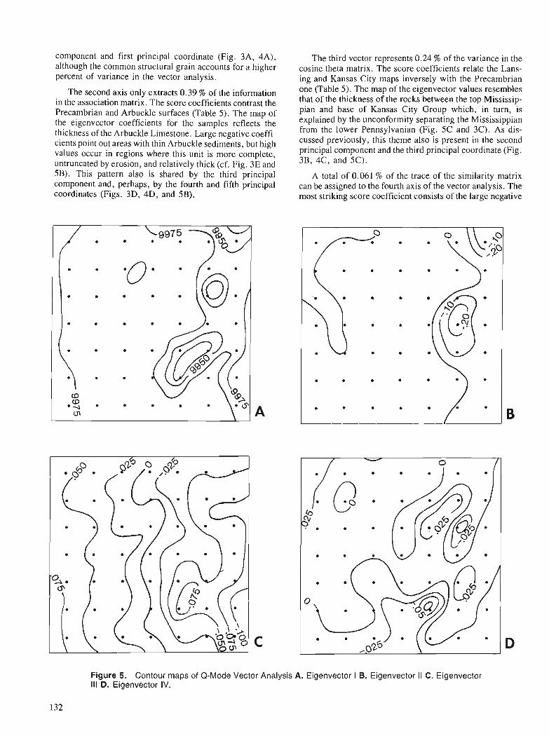
component and first principal coordinate (Fig. 3A, 4A), although the common structural grain accounts for a higher percent of variance in the vector analysis.

The second axis only extracts 0.39 % of the information in the association matrix. The score coefficients contrast the Precambrian and Arbuckle surfaces (Table 5). The map of the eigenvector coefficients for the samples reflects the thickness of the Arbuckle Limestone. Large negative coefficients point out areas with thin Arbuckle sediments, but high values occur in regions where this unit is more complete, untruncated by erosion, and relatively thick (cf. Fig. 3E and 5B). This pattern also is shared by the third principal component and, perhaps, by the fourth and fifth principal coordinates (Figs. 3D, 4D, and 5B).

The third vector represents 0.24 % of the variance in the cosine theta matrix. The score coefficients relate the Lans- ing and Kansas City maps inversely with the Precambrian one (Table 5). The map of the eigenvector values resembles that of the thickness of the rocks between the top Mississip- pian and base of Kansas City Group which, in turn, is explained by the unconformity separating the Mississippian from the lower Pennsylvanian (Fig. 5C and 3C). As discussed previously, this theme also is present in the second principal component and the third principal coordinate (Fig. 3B, 4C, and 5C).

A total of 0.061 % of the trace of the similarity matrix can be assigned to the fourth axis of the vector analysis. The most striking score coefficient consists of the large negative

D

Figure 5. Contour maps of Q-Mode Vector Analysis A. Eigenvector I B. Eigenvector I I C. Eigenvector I l l D. Eigenvector IV.

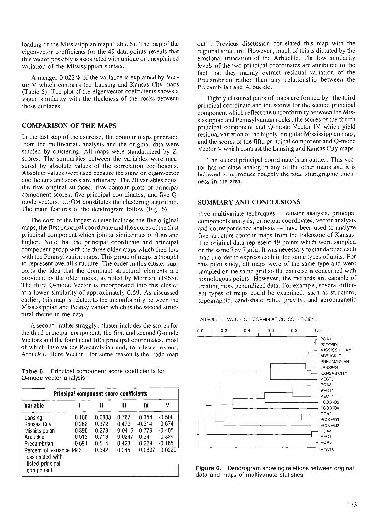
loading of the Mississippian map (Table 5). The map of the eigenvector coefficients for the 49 data points reveals that this vector possibly is associated with unique or unexplained variation of the Mississippian surface.

A meager 0.022 % of the variance is explained by Vec- tor V which contrasts the Lansing and Kansas City maps (Table 5). The plot of the eigenvector coefficients shows a vague similarity with the thickness of the rocks between these surfaces.

COMPARISON OF THE MAPS

In the last step of the exercise, the contour maps generated from the multivariate analysis and the original data were studied by clustering. All maps were standardized by Z- scores. The similarities between the variables were measured by absolute values of the correlation coefficients. Absolute values were used because the signs on eigenvector coefficients and scores are arbitrary. The 20 variables equal the five original surfaces, five contour plots of principal component scores, five principal coordinates, and five Q - mode vectors. UPGM constitutes the clustering algorithm. The main features of the dendrogram follow (Fig. 6).

The core of the largest cluster includes the five original maps, the first principal coordinate and the scores of the first principal component which join at similarities of 0.86 and higher. Note that the principal coordinate and principal component group with the three older maps which then link with the Pennsylvanian maps. This group of maps is thought to represent overall structure. The order in this cluster supports the idea that the dominant structural elements are provided by the older rocks, as noted by Merriam (1963). The third Q-mode Vector is incorporated into this cluster at a lower similarity of approximately 0.59. As discussed earlier, this map is related to the unconformity between the Mississippian and Pennsylvanian which is the second structural theme in the data.

out". Previous discussion correlated this map with the regional structure. However, much of this is dictated by the erosional truncation of the Arbuckle. The low similarity levels of the two principal coordinates are attributed to the fact that they mainly extract residual variation of the Precambrian rather than any relationship between the Precambrian and Arbuckle.

Tightly clustered pairs of maps are formed by: the third principal coordinate and the scores for the second principal component which reflect the unconformity between the Mis- sissippian and Pennsylvanian rocks; the scores of the fourth principal component and Q-mode Vector IV which yield residual variation of the highly irregular Mississippian map ; and the scores of the fifth principal component and Q-mode Vector V which contrast the Lansing and Kansas City maps.

The second principal coordinate is an outlier. This vector has no close analog in any of the other maps and it is believed to reproduce roughly the total stratigraphic thickness in the area.

SUMMARY AND CONCLUSIONS

Five multivariate techniques - cluster analysis, principal components analysis, principal coordinates, vector analysis and correspondence analysis - have been used to analyze five structure contour maps from the Paleozoic of Kansas. The original data represent 49 points which were sampled on the same 7 by 7 grid. It was necessary to standardize each map in order to express each in the same types of units. For this pilot study, all maps were of the same type and were sampled on the same grid so the exercise is concerned with homologous points. However, the methods are capable of treating more generalized data. For example, several different types of maps could be examined, such as structure, topographic, sand-shale ratio, gravity, and aeromagnetic

ABSOLUTE VALUE OF CORRElATlON COEFFICIENT A second, rather straggly, cluster includes the scores for

the third principal component, the first and second Q-mode 0 .0 0 .2 0.4 0.6 0 .8 1 . O l I l I I l I l I l /

Vectors and the fourth and fifth principal coordinates, most of which involve the Precambrian and, to a lesser extent, Arbuckle. Here Vector I for some reason is the "odd map ARBUCKLE

Principal component score coefficients

Variable I I I 111 IV V

Lansing 0.168 0.0888 0.767 0.354 -0.500 Kansas City 0.282 0.372 0.479 -0.314 0.674 Mississippian 0.390 -0.273 0.0416 -0.779 -0.405 Arbuckle 0.513 -0.718 0.0247 0.341 0.324 Precambrian 0.691 0.514 -0.423 0.229 -0.165 Percent of variance 99.3 0.392 0.245 0.0607 0.0220 associated with listed principal component

L PRECAMBRIAN LANSING

Table 5. Principal component score coefficients for KANSAS CITY Q-mode vector analysis. V E C T ~

PCA3 - VECT2 VECTI PC03RD5 PC03RD4

Figure 6. Dendrogram showing relations between original data and maps of multivariate statistics.

data. If equivalent sample points are not available, the various maps could be gridded and the grid would serve as the input for the multivariate statistics.

The algorithms employed are cluster analysis of the unweighted-pair-group-method (UPGM) on matrices of Euclidean distances and correlation coefficients and the ordination techniques of principal components of a correlation matrix, principal coordinates of a matrix of Gower coefficients, and Q-Mode Vector Analysis. All methods recover similar patterns from the data; correspondence analysis was not effective because of the types of standardizing involved in the algorithm. The several main themes in the maps consist of: (1) the common structural framework of the area as seen in all maps, (2) an inverse relationship between the Pennsylvanian and the older units which is caused by a major unconformity, (3) thickness variation of the Arbuckle Group on the Precambrian, and (4) unique or residual variation along all surfaces, especially the Missis- sippian and Precambrian.

All main patterns are recognized by the principal coordinates, principal components, and the Q-Mode Vectors although in somewhat different forms. Cluster analysis retains the least amount of information about the maps. The dendrogram for the maps shows elements of the overall structural framework, the contrasts between the Pennsylva- nian and the older surfaces, and hints at the residual variation of the Precambrian. The clusters of the samples illustrate the structures present in all of the maps.

Nevertheless, both clustering and ordination algorithms provide helpful insights into the data because they are subject to different sources of distortion. Clusters faithfully preserve the distances and similarities between similar items but at the expense of large-scale distortion. Consequently, the major clusters of the data may be arranged incorrectly. In addition dendrograms tend to segment the data'. Con- versely ordinations are effective at keeping the main patterns of the data although the true distances between similar variables or samples may be deformed or lost. Furthermore, ordinations usually emphasize the continuous aspects of the data set.

REFERENCES

Cole, V.B. 1962: Configuration of top Precambrian basement rocks in Kansas;

Kansas Geological Survey Oil and Gas Investigation No. 26, map. Davis, J.C. 1986: Statistics and Data Analysis in Geology (2nd ed.): John Wiley &

Sons, New York, 646 p. Gower, J.C. 1966: Some distance properties of latent sort and vector methods used

in multivariate analysis; Biometrika, v. 53, no. 3-4, p. 325-338. Herzfeld, U.C. and Merriam, D.F. 1989: A map-comparison technique utilizing weighted input parameters;

in press. Herzfeld, U.C. and Sondergard, M.A. 1988: MAPCOMP - a FORTRAN program for weighted thematic map

comparison; Computers & Geosciences, v. 14, no. 5, p. 699-713. Joreskog, K.G., Klovan, J.E., and Reyment, R.A. 1976: Geological Factor Analysis; Elsevier Scientific Publishing Co.,

Amsterdam, 178 p. Krumbein, W.C. and Imbrie, J. 1963: Stratigraphic factor maps; American Association of Petroleum

Geologists, Bulletin, v. 47, no. 4, p. 698-701. Merriam, D.F. 1960: Preliminary regional structural map on top of Mississippian rocks

in Kansas; Kansas Geological Survey Oil and Gas Investigation 22, map.

Merriam, D.F. 1963: The geologic history of Kansas; Kansas Geological Survey, Bulle-

tin 162, 317 p. Merriam, D.F. and Jewett, D.G. 1988: Methods of thematic map comparison; &I Current Trends in

Geomathematics; Plenum Press, New York, p. 9-18. Merriam, D.F. and Smith, P. 1961 : Preliminary regional structure contour map on the top of Arbuckle

rocks (Cambrian-Ordovician) in Kansas; Kansas Geological Sur- vey Investigation. No. 25, map.

Merriam, D.F. and Sondergard, M.A. 1988: A reliability index for the pairwise comparison of thematic maps;

Geologisches Jahrbuch, v. A104, p. 433-446. Merriam, D.F., Winchell, R.L. and Atkinson, W.R. 1958 : Preliminary regional structured contour map on top of the Lansing

Group (Pennsylvanian) in Kansas; Kansas Geological Survey Investigation. No. 19, map.

Sneath, P.H.A. and Sokal, R.R. 1973: Numerical taxonomy; W.H. Freeman and Co., San Francisco,

573 p. Watney, W.L. 1978: Structural contour map: base of Kansas City Group (Upper Penn-

sylvanian) - eastern Kansas; Kansas Geological Survey, Map M- 10.

Zhou, Di, Chang, T. and Davis, J.C. 1983: Dual extraction of R-mode and Q-mode factor solutions; Journal

of Mathematical Geology, v. 15, no. 5, p. 581-606.

Computer tools for the integrative interpretation of geoscience spatial data in mineral exploration1

Michel Mellingera

Mellinger, M., Computer tools for the integrative interpretation of geoscience spatial data in mineral exploration; & Statistical application in the Earth Sciences, ed. F. P. Agterberg and G. F. Bonham- Carter; Geological Survey of Canada, Pager 89-9, p. 135-139, 1989.

Abstract

Several types of computer tools for the integrative interpretation of geoscience spatial data are now available to the explorationist interested in integrating mineral exploration surveys. They fall into, or are a combination of three categories: (1) geographic information systems, (2) remote sensing systems, and (3) image analysis systems.

Before mineral exploration surveys can be integrated usefully, the user must be aware of a few fundamental concepts about the types of data involved and the types of information expressed by the data. Data may be spatially continuous (mono - or multi-channel), discrete (several sub-types) or textural. The information contained may be an expression of the surjcial environment, of shallow bedrockproper- ties, or of deep bedrock properties. The type of data determines which processing algorithms can be used; the type of information determines which surveys can be usefully integrated.

"Integration" most often turns out to be additive interpretation, where information from different surveys is merged by means of standard logical operations. True integrative interpretation requires the interactive interpretation of one survey with respect to another, leading to information that could not be derived from either survey alone.

Image analysis systems which include a well-developed toolbox of mathematical morphology algorithms are the most suitable for the integrative interpretation of mineral exploration surveys. For spatially discrete data mostly, geographic information systems with good analytical and modelling capabilities will also make a signiJFicant contribution. Remote sensing systems are not very usefulJor survey inlegration, due to their dedication to multi-channel pixel classification and their fairly limited overall image processing capabilities.

Now at the crossroads, the integrative interpretation of spatial data will no doubt see soon the emergence of new approaches, to which mathematical morphology will bring much needed power andjexi- bility .

Plusieurs genres de systkmes informatiques permettant 1 'intkgration de donnkes spatiales ir caracttre gkoscient$que sont maintenant d la disposition du prospecteur minier intLressC b l'intkgration des donne'es provenant de levks de prospection. Ils appartiennent ir l'une des trois catkgories suivantes, OK en combinent les caractkristiques: 1) systtmes d'information gkographique, 2) systtmes de tklkdktection, et 3) systkmes d'analyse des images.

L'usager doit ttre conscient de certains concepts de base liks ir la nature des donnkes et de l'information qu 'elles contiennent, avant de prockder h l'intkgration de donnkes de levks de prospection minikre. Les donnkes spatiales peuvent 2tre continues (canal simple OK multicanal), discr2tes (plusieurs catkgories) ou texturales. L'information contenue peut 2tre relike au milieu physique, au socle rocheux peu profond, OK au socle profond. Le ope de donnkes influencera le choix des algorithmes de traitement des donnkes alors que le type d'information contenue dkterminera quels lev& peuvent ttre intkgrks de manitre utile.

' Publication No. R-851-2-A-89 Saskatchewan Research Council, 15 Innovation Boulevard, Saskatoon, Saskatchewan, S7N 2 x 8

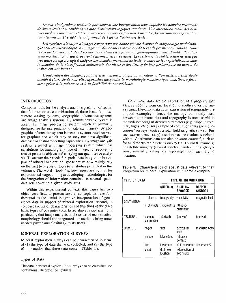
Le mot inte'gration traduit le plus souvent une interprktation dans laquelle les donnkes provenant de divers lev.& sont combinks a l'aide d'opkrations logiques standards. Une intkgration rkelle des donnkes implique une interprktation interactive d'un lev4 en fonction d'un autre, fournissant une information qui n'aurait pu &tre dkduite uniquement de l'un ou l'autre des levks.

Les syst4mes d'analyse d'images comportant une bonne gamme d'outils de morphologie mathkmatique sont les mieux adapte's 2 h'intkgration des donnkes provenant de lev& de prospection minitre. Duns le cas de donnkes spatiales discrktes, les systbmes d'information ge'ographique munis d'outils d'analyse et de modklisation avancks peuvent kgalement &tre trts utiles. Les systtmes de tklkdktection ne sont pas trks utiles lorsqu 'il s 'agit d'inte'grer des donnkes provenant de levks, h cause de leur spe'cialisation dans le domaine de la classification multicanale des pixels et des limites de leur performance au niveau du traitement des images.

L'inte'gration des donnkes spatiales a actuellement atteint un carrefour et 1'on assistera sans doute bientdt a l'arrivke de nouvelles approches awrquelles la morphologie mathkmatique contribuera fortement gr6ce 6 la puissance et fi la flexibilite' de ses mkthodes.

INTRODUCTION Continuous data are the expression of a property that

Computer tools for the analysis and interpretation of spatial data fall into, or are a combination of, three broad families: remote sensing systems, geographic information systems and image analysis systems. By remote sensing system is meant an image processing system which is primarily designed for the interpretation of satellite imagery. By geographic information system is meant a system based on vector graphics and which may or may not have significant database or spatial modelling capabilities. By image analysis system is meant an image processing system which has capabilities for handling any type of image, for processing sets of pixels as objects and carrying out quantitative analysis. To answer their needs for spatial data integration in sup-

varies smoothly from one location to another over thk survey area. Elevation data as an expression of topography are a good example; indeed, the analogy commonly used between continuous data and topography is most useful in the understanding of derived parameters (e.g, slope, curvature, highs, etc.). An example of continuous data are mono- channel surveys, such as a total field magnetic survey. For such surveys, each (x , y) location has one z value associated with it. Continuous data can also be multi-channel, such as for an airborne radiometrics survey (U, Th and K channels) or satellite imagery (several spectral bands). For such surveys, several z values are associated with each (x, y) location.

port of mineral exploration, geoscientists now mainly rely on the first two types of tools (e.g. studies presented in this Table 1. Characteristics of spatial data relevant to their volume). The word "tools" is key: users are now at the integration for mineral exploration with some examples. experimental stage, aiming at developing methodologies for the integration of information contained in several spatial data sets covering a given study area.

Within this experimental context, this paper has two objectives: first, to present several concepts that are fundamental to the useful integrative interpretation of geoscience data in support of mineral exploration; second, to compare the major characteristics and functions of the three basic types of computer tools listed above, emphasizing in particular, that image analysis in the sense of mathematical morphology should not be ignored : its methods bring much needed power and flexibility to its users.

MINERAL EXPLORATION SURVEYS

Mineral exploration surveys can be characterized in terms of (1) the type of data that was collected, and (2) the type of information that these data contain (Table 1 .).

Types of Data

The data in mineral exploration surveys can be classified as : continuous, discrete, or textural.

TYPE OF DATA TYPE OF INFORMATION

SURFlClAL SHALLOW DEEPER BEDROCK BEDROCK

1 channel topography resistivity magnetic field CONTINUOUS

n channels radiometrics lithogeochemistry

TEXTURAL various (derived) (derived) (derived) parameters

DISCRETE region lake geological magnetic body map

polygon lake edges intrusive contact

line lineament VLF conductor lineament?? point drill hole intersection of

location two faults

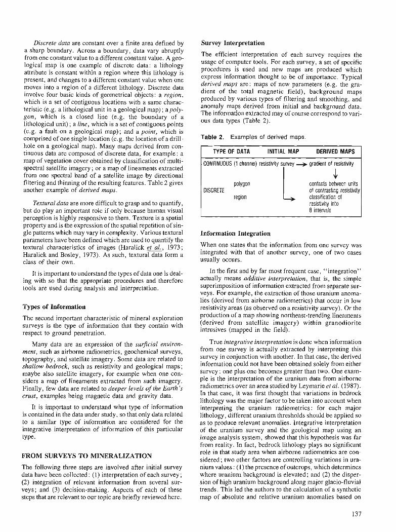
Discrete data are constant over a finite area defined by a sharp boundary. Across a boundary, data vary abruptly from one constant value to a different constant value. A geological map is one example of discrete data: a lithology attribute is constant within a region where this lithology is present, and changes to a different constant value when one moves into a region of a different lithology. Discrete data involve four basic kinds of geometrical objects: a region, which is a set of contiguous locations with a same characteristic (e.g, a lithological unit in a geological map); apoly- gon, which is a closed line (e.g. the boundary of a lithological unit) ; a line, which is a set of contiguous points (e.g. a fault on a geological map); and a point, which is comprised of one single location (e.g. the location of a drill- hole on a geological map). Many maps derived from continuous data are composed of discrete data, for example : a map of vegetation cover obtained by classification of multispectral satellite imagery; or a map of lineaments extracted from one spectral band of a satellite image by directional filtering and thinning of the resulting features. Table 2 gives another example of derived maps.

Textural data are more difficult to grasp and to quantify, but do play an important role if only because human visual perception is highly responsive to them. Texture is a spatial property and is the expression of the spatial repetition of single patterns which may vary in complexity. Various textural parameters have been defined which are used to quantify the textural characteristics of images (Haralick &, 1973; Haralick and Bosley, 1973). As such, textural data form a class of their own.

It is important to understand the types of data one is dealing with so that the appropriate procedures and therefore tools are used during analysis and interpretation.

Types of Information

The second important characteristic of mineral exploration surveys is the type of information that they contain with respect to ground penetration.

Many data are an expression of the surjcial environment, such as airborne radiometrics, geochemical surveys, topography, and satellite imagery. Some data are related to shallow bedrock, such as resistivity and geological maps; maybe also satellite imagery, for example when one considers a map of lineaments extracted from such imagery. Finally, few data are related to deeper levels of the Earth 's crust, examples being magnetic data and gravity data.

It is important to understand what type of information is contained in the data under study, so that only data related to a similar type of information are considered for the integrative interpretation of information of this particular tY Pe.

FROM SURVEYS TO MINERALIZATION

The following three steps are involved after initial survey data have been collected : (1) interpretation of each survey ; (2) integration of relevant information from several surveys; and (3) decision-making. Aspects of each of these steps that are relevant to our topic are briefly reviewed here.

Survey Interpretation

The efficient interpretation of each survey requires the usage of computer tools. For each survey, a set of specific procedures is used and new maps are produced which express information thought to be of importance. Typical derived maps are: maps of new parameters (e.g. the gradient of the total magnetic field), background maps produced by various types of filtering and smoothing, and anomaly maps derived from initial and background data. The information extracted may of course correspond to various data types (Table 2).

Table 2. Examples of derived maps.

TYPE OF DATA INITIAL MAP DERIVED MAPS

CONTINUOUS (1 channel) resistivity survey + gradient of resistivity

polygon J.

contacts between units DISCRETE of contrasting resistivity

region classification of resistivity into 8 intervals

Information Integration

When one states that the information from one survey was integrated with that of another survey, one of two cases usually occurs.

In the first and by far most frequent case, "integration" actually means additive interpretation, that is, the simple superimposition of information extracted from separate surveys. For example, the extraction of those uranium anomalies (derived from airborne radiometrics) that occur in low resistivity areas (as observed on a resistivity survey). Or the production of a map showing northeast-trending lineaments (derived from satellite imagery) within granodiorite intrusives (mapped in the field).

True integrative interpretation is done when information from one survey is actually extracted by interpreting this survey in conjunction with another. In that case, the derived information could not have been obtained solely from either survey : one plus one becomes greater than two. One example is the interpretation of the uranium data from airborne radiometrics over an area studied by Leymarie et al. (1987). In that case, it was first thought that variations in bedrock lithology was the major factor to be taken into account when interpreting the uranium radiometrics: for each major lithology, different uranium thresholds should be applied so as to produce relevant anomalies. Integrative interpretation of the uranium survey and the geological map using an image analysis system, showed that this hypothesis was far from reality. In fact, bedrock lithology plays no significant role in that study area when airborne radiometrics are considered; two other factors are controlling variations in uranium values : (1) the presence of outcrops, which determines where uranium background is elevated ; and (2) the dispersion of high uranium background along major glacio-fluvial trends. This led the authors to the calculation of a synthetic map of absolute and relative uranium anomalies based on

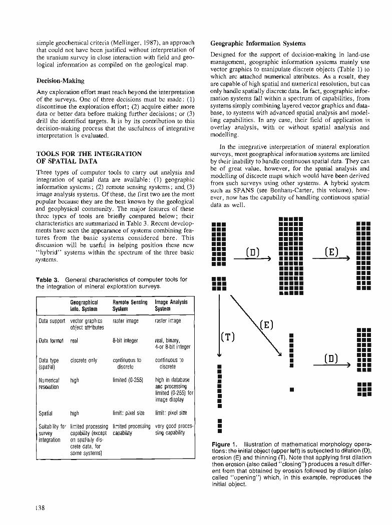
simple geochemical criteria (Mellinger, 1987), an approach that could not have been justified without interpretation of the uranium survey in close interaction with field and geological information as compiled on the geological map.

Decision-Making

Any exploration effort must reach beyond the interpretation of the surveys. One of three decisions must be made: (1) discontinue the exploration effort; (2) acquire either more data or better data before making further decisions ; or (3) drill the identified targets. It is by its contribution to this decision-making process that the usefulness of integrative interpretation is evaluated.

TOOLS FOR THE INTEGRATION OF SPATIAL DATA

Three types of computer tools to carry out analysis and integration of spatial data are available: (1) geographic information systems; (2) remote sensing systems; and. (3) image analysis systems. Of these, the first two are the most popular because they are the best known by the geological and geophysical community. The major features of these three types of tools are briefly compared below; their characteristics are summarized in Table 3. Recent developments have seen the appearance of systems combining features from the basic systems considered here. This discussion will be useful in helping position these new "hybrid" systems within the spectrum of the three basic systems.

Table 3. General characteristics of computer tools for the integration of mineral exploration surveys.

Geographical Remote Sensing Image Analysis Info. System System System

Data support vector graphics raster image raster image object attributes

Data format real &bit integer real, binary, 4-or 8-bit integer

Data type discrete only continuous to continuous to (spatial) discrete discrete

Numerical high limited (0-255) high in database resolution and processing

limited (0-255) for image display

Spatial high limit: pixel size limit: pixel size

Suitability for limited processing limited processing very good proces- survey capability (except capability sing capability integration on spatially dis-

crete data, for some systems)

Geographic Information Systems

Designed for the support of decision-making in land-use management, geographic information systems mainly use vector graphics to manipulate discrete objects (Table 1) to which are attached numerical attributes. As a result, they are capable of high spatial and numerical resolution, but can only handle spatially discrete data. In fact, geographic information systems fall within a spectrum of capabilities, from systems simply combining layered vector graphics and database, to systems with advanced spatial analysis and modelling capabilities. In any case, their field of application is overlay analysis, with or without spatial analysis and modelling.

In the integrative interpretation of mineral exploration surveys, most geographical information systems are limited by their inability to handle continuous spatial data. They can be of great value, however, for the spatial analysis and modelling of discrete maps which would have been derived from such surveys using other systems. A hybrid system such as SPANS (see Bonham-Carter, this volume), however, now has the capability of handling continuous spatial data as well.

Figure 1. Illustration of mathematical morphology operations: the initial object (upper left) is subjected to dilation (D), erosion (E) and thinning (T). Note that applying first dilation then erosion (also called "closing") produces a result different from that obtained by erosion followed by dilation (also called "opening") which, in this example, reproduces the initial object.

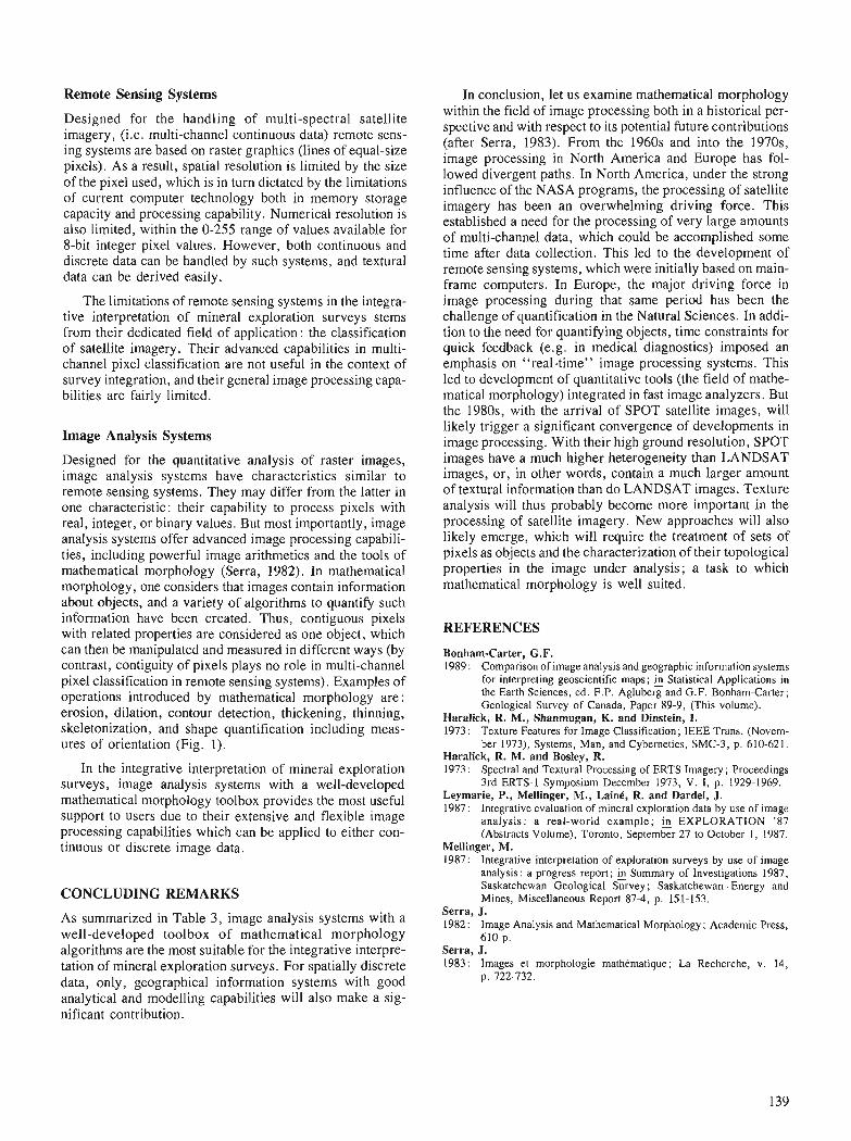
Remote Sensing Systems

Designed for the handling of multi-spectral satellite imagery, (i.e. multi-channel continuous data) remote sensing systems are based on raster graphics (lines of equal-size pixels). As a result, spatial resolution is limited by the size of the pixel used, which is in turn dictated by the limitations of current computer technology both in memory storage capacity and processing capability. Numerical resolution is also limited, within the 0-255 range of values available for 8-bit integer pixel values. However, both continuous and discrete data can be handled by such systems, and textural data can be derived easily.

The limitations of remote sensing systems in the integrative interpretation of mineral exploration surveys stems from their dedicated field of application : the classification of satellite imagery. Their advanced capabilities in multi- channel pixel classification are not useful in the context of survey integration, and their general image processing capabilities are fairly limited.

Image Analysis Systems

Designed for the quantitative analysis of raster images, image analysis systems have characteristics similar to remote sensing systems. They may differ from the latter in one characteristic: their capability to process pixels with real, integer, or binary values. But most importantly, image analysis systems offer advanced image processing capabilities, including powerful image arithmetics and the tools of mathematical morphology (Serra, 1982). In mathematical morphology, one considers that images contain information about objects, and a variety of algorithms to quantify such information have been created. Thus, contiguous pixels with related properties are considered as one object, which can then be manipulated and measured in different ways (by contrast, contiguity of pixels plays no role in multi-channel pixel classification in remote sensing systems). Examples of operations introduced by mathematical morphology are: erosion, dilation, contour detection, thickening, thinning, skeletonization, and shape quantification including measures of orientation (Fig. 1).

In the integrative interpretation of mineral exploration surveys, image analysis systems with a well-developed mathematical morphology toolbox provides the most useful support to users due to their extensive and flexible image processing capabilities which can be applied to either continuous or discrete image data.

CONCLUDING REMARKS

As summarized in Table 3, image analysis systems with a well-developed toolbox of mathematical morphology algorithms are the most suitable for the integrative interpretation of mineral exploration surveys. For spatially discrete data, only, geographical information systems with good analytical and modelling capabilities will also make a significant contribution.

In conclusion, let us examine mathematical morphology within the field of image processing both in a historical perspective and with respectto its potential future contributions (after Serra, 1983). From the 1960s and into the 1970s, image processing in North America and Europe has followed divergent paths. In North America, under the strong influence of the NASA programs, the processing of satellite imagery has been an overwhelming driving force. This established a need for the processing of very large amounts of multi-channel data, which could be accomplished some time after data collection. This led to the development of remote sensing systems, which were initially based on mainframe computers. In Europe, the major driving force in image processing during that same period has been the challenge of quantification in the Natural Sciences. In addition to the need for quantifying objects, time constraints for quick feedback (e.g. in medical diagnostics) imposed an emphasis on "real-time" image processing systems. This led'to development of quantitative tools (the field of mathematical morphology) integrated in fast image analyzers. But the 1980s, with the arrival of SPOT satellite images, will likely trigger a significant convergence of developments in image processing. With their high ground resolution, SPOT images have a much higher heterogeneity than LANDSAT images, or, in other words, contain a much larger amount of textural information than do LANDSAT images. Texture analysis will thus probably become more important in the processing of satellite imagery. New approaches will also likely emerge, which will require the treatment of sets of pixels as objects and the characterization of their topological properties in the image under analysis; a task to which mathematical morphology is well suited.

REFERENCES

Bonham-Carter, G.F. 1989: Comparison of image analysis and geographic information systems

for interpreting geoscientific maps; fi Statistical Applications in the Earth Sciences, ed. F.P. Agluberg and G.F. Bonham-Carter; Geological Survey of Canada, Paper 89-9, (This volume).

Haralick, R. M., Shanmugan, K. and Dinstein, I. 1973: Texture Features for Image Classification; IEEE Trans. (Novem-

ber 1973), Systems, Man, and Cybernetics, SMC-3, p. 6 10-62 1. Haralick, R. M. and Bosley, R. 1973: Spectral and Textural Processing of ERTS Imagery; Proceedings

3rd ERTS-I Symposium December 1973, V. I, p. 1929-1969. Leymarie, P., Mellinger, M., LainC, R. and Dardel, J. 1987 : Integrative evaluation of mineral exploration data by use of image

analysis: a real-world example; in EXPLORATION '87 (Abstracts Volume), Toronto, ~eptember 27 to Octobcr 1, 1987.

Mellinger, M. 1987: Integrative interpretation of exploration surveys by use of image

analysis: a progress report; & Summary of Investigations 1987, Saskatchewan Geological Survey ; Saskatchewan . Energy and Mines, Miscellaneous Repon 87-4, p. 151-153.

Serra, J. 1982: Image Analysis and Mathematical Morphology; Academic Press,

610 p. Serra, J. 1983: Images et morphologie mathkmatique; La Recherche, v. 14,

p. 722-732.

Comparison of image analysis and geographic information systems for integrating geoscientific maps

G.F. Bonham-Carter1

Bonham-Carter, G. F. , Comparison of image analysis and geographic information systems for integrating geoscientific maps; &I Statistical Analysis in the Earth Sciences, ed. F. P. Agterberg and G. F. Bonham- Carter, Geological Survey of Canada, Paper 89-9, p. 141-155, 1989.

Abstract

The impact of a new PC-based geographic information system (GIs) and image analysis facility for data integration is assessed after a year of operation. The facility can be used not only as the electronic equivalent of the light table, i. e. for overlaying digital maps, but also for a wide variety of analysis and modelling tasks in support of mineral resource assessment, environmental impact, and other syntheses of multi-layer geoscientijc data.

The types of operations carried out with this facility are described by comparing the data structures, video display capability, data transformations and data modelling and analysisfunctions of the quadtree- based GIs and the image analysis system. In combination, these sojfware packages permit the input of manually digitized maps bolygons, lines, points), scanned maps, geocoded point j'iles with associated attributes and raster imagery from any of the common cartographic projections, or from source images that require geometric correction (e.g. satellite images). Many of the image analysis functions complement the GIs capabilities. For example, the image analysis system is useful for image enhancement requiring operations such as jltering, principal components analysis and perspective scene generation; the CIS is superior for handling vector and point data with topological and other attributes, for allowing operations such as line dilation, Yoronoi tesselation, point interpolation and rapid spatial query of large databases. The quadtree database structure, unique conditions mapping and modelling language make the GISparticularly attractive for multi-map modelling. Both systems allowjlexible method development, either with an object library of subroutines, or by allowing easy access to shared datajles.

Because systems of this type are relatively inexpensive, not too diflcult to learn, and combine diverse functionality with a user-friendly interface, their impact for integrating geoscientij'ic maps is likely to be far-reaching. The decade of the 19903 may well see the spread of GIs and image analysis systems to the same degree that word-processing systems have spread in the 1980's.

Aprts une annke d'exploitation, on kvalue l'impact d'un nouveau systbme d'information ge'ographique (SIC) base'sur l'emploi d'un ordinateur personnel, et d'une installation d'analyse des images permettant 1 'intkgration des donnkes. L 'installation peut &tre utiliske non seulement comme 1'6quivalent e'lectronique de la table lumineuse, comme par exemple pour 1 'opkration de recouvrement de cartes nume'riques, mais aussi pour effectuer une grande diversite' de travaux d'analyse et de mod6lisation facilitant l'kvaluation des ressources mine'rales et des impacts environmentaux, et la rehlisation d'autres synthbses de donne'es. g6oscientijiques multicouches.

-

' Geological Survey of Canada, 601 Booth Street, Ottawa, Ontario KIA 0E8

On dkcrit les types d'opkrations eflectukes a l'aide de cette installation, en comparant les structures des donndes, les possibilitks dd'afJichage vidko, les transformations des donne'es et la modilisation de ces donnkes, les fonctions d'analyse du SIC a arbre et le systbme d'analyse des images. Combinks, ces ensembles deprogrammes permetlent 1 'entree de cartes numdriskes 2 la main bolygones, lignes, points), de cartes produites par balayage, de fichiers de points gdocode's avec attributs associds et imagerie de type tde'vision, d partir de n 'importe laquelle des projections cartographiques courantes, ou (j. partir d'images sources exigeant une correction gdome'trique (j. ex., images prises par satellite). Un grand nombre des fonctions d'analyse des images complbtent les possibilitds du SIC. Par exemple, le systbme d'analyse des images facilite le rehaussement des images exigeant le recours ci des opkrations telles que le Jiltrage, 1 'analyse des composantes principales et la gknkration de scines prksentkes en perspective; le SIG s 'illustre lorsqu 'il s'agit de manipuler des donnkes vectorielles et ponctuelles a attributs topologi- ques ou autres, et il permet aussi des opirations telles que l'expansion des lignes, l'organisation mat&- rielle de Voronoi, l'interpolation de points et la recherche spatiale rapide de grandes bases de donne'es. La structure d'arbre quaternaire de la base de donnkes, la cartographie de conditions uniques et le langage de la moddisation rendent le SIG particulitrement int&ressant du point de vue de la modklisation de cartes multiples. Les deux systbmes favorisent l'klaboration de mNhodes flexibles, soit avec une bibliothbque de programmes de sous-routines, soit en permettant d'acckder auxjchiers communs de donnkes.

Les systtmes de ce type ktant relativement peu cofiteux, assez faciles d apprendre, et combinant diverses fonctions avec une interface facilement accessible, ils auront sans doute une grande influence sur l'inte'gration des cartes gkoscient$ques. I1 pourrait bien y avoir, durant les anndes 90, une expansion du SIG et des systtmes d'analyse des images comparable t? celle des systtmes de traitement des textes durant les annies 80.

INTRODUCTION

Computer handling of geoscientifc maps

Computer systems for the manipulation and analysis of geoscientific map data are becoming more widely used due to several factors: the availability of regional survey data in digital form; the comparatively low cost of commercial mapping software; and the availability of fast microcomputers and workstations with high resolution colour graphics. Mathematical and statistical methods of analyzing map data, until now regarded by many geologists as esoteric exercises, can now be applied as practical tools for data integration.

Although most geological maps are still produced in analogue form, large volumes of geoscientific map data are now produced digitally. For example, the output from most geophysical and geochemical surveys are available in digital format; satellite and airborne remote-sensing data are predominantly in the form of digital raster images; many point-sample databases are available as digital files, e.g. geochemical surveys, mineral occurrence data and isotope age determinations. Furthermore, raster-scanning techniques (Bonham-Carter et al., 1988) and easily-used table digitizing software have facilitated the analogue-to-digital conversion of geological maps, although as yet there is no digital geological map database for Canada.

Geoscientists usually must deal with phenomena that involve the interaction of complex processes. In order to understand and interpret observations about the composition and structure of the earth, the ability to bring together diverse data types is essential. Although the light-table has been the traditional tool for this task, it is less than ideal for overlaying and analyzing the enormous volumes of geophysical, geochemical and geological data now available. Expensively-collected data become buried and

difficult to use; the geoscientist becomes predominantly engaged in routine manual overlay tasks, at the expense of creative synthesis.

Despite the body of research dealing with mathematical and statistical treatment of geoscientific map data published over the past 25 years, rather little of this work has made an impact on the practicing geologist, except possibly in the oil industry. During the past 5 years, the widespread availability of microcomputers has begun to change the attitude of many geologists towards computer technology. First user-friendly word processors, then spreadsheets and statistical programs and now image analysis and geographic information systems have raised the awareness and reduced the resistance of geologists to computer methods.

These factors of data volume on the one hand, and easily- used microcomputer-based mapping packages on the other, are coming together to bring about an important impact on the handling and use of geoscientific maps. The potential for replacing the light table for map overlay with an electronic equivalent is real, and geographic information and image analysis systems provide a platform on which a host of mathematical and statistical map operations can be based.

Systems for map integration and analysis

During the late 1970s and 1980s digital image analysis (software and hardware) systems have been developed and applied in the geosciences, primarily for the display and manipulation of satellite images and images of polished sections or thin sections of rocks. Satellite image analysis systems have concentrated mainly on the display and analysis of multi-spectral data (e.g. Gillespie, 1980; Lillesand and Kiefer, 1987). On the other hand, systems based on the methods of mathematical morphology (Serra, 1982), applied both to thin-section images and geological maps

(Fabbri, 1984), have concentrated more on the measurement and characterization of grains or discrete objects. Both kinds of image analysis systems deal with images defined by a raster data structure, where the image is gridded or subdivided into pixels.

During the same period, computer-aided design (CAD) software became highly developed, mainly for engineering drawings. Instead of a raster structure, CAD uses a vector structure, in which lines are described by linked points, defined as co-ordinate pairs, or vectors. The vector structure is ideal for describing the boundaries of objects, usually requires much less storage space than a raster, and is convenient for co-ordinate transformations. CAD systems, at least in their early stages of development, were not concerned with the areas between lines, nor with topological attributes such as connectivity and adjacency (cf. Cowen et a]., 1986). Primitive CAD systems are therefore of limited use for mapping applications, where the relationships between mapped units, and the link to non-spatial attributes are essential.

Geographic information systems, both raster and vector- based, are designed for handling all kinds of geocoded data, and are amenable for a much broader range of applications than either image analysis or CAD systems. Any kind of geographically-referenced data - point, line, polygon, raster image, associated attributes, textural information, topological information - is pertinent to a GIs. Many GISs operate with a spatial relational database, as well as offering flexible input, output, overlay and analysis capabilities. Some GISs are strongly vector-based, with good cartographic features; some are strong for interactive spatial query ; some are designed primarily for modelling and analysis. Applications of GISs range from municipal zoning, to utility company planning, to resource management, to global environment monitoring (Burrough, 1986).

The universality of spatial data structures and spatial data manipulation as applied to all kinds of maps and georeferenced entities makes the commercial market for GIs large. Coupled with low-cost but powerful computer workstations, linked via high speed communications networks, such systems are spreading rapidly, invading a host of subject areas not previously treated in a spatial context. Earth science applications of GISs are potentially numerous, although at present very few GISs treat 3-D data, making them unsuitable for applications such as mine design, and modelling of the subsurface in 3-dimensions (cf. Reeler and Chandra, this volume; Bak and Mill, 1989).

Geological Survey of Canada activity

In the late 1970s, the GSC developed two systems for integrating geoscientific maps. SIMSAG (Chung, 1983) is a mainframe-based program using remote Tektronix termi- nals; it has also been converted to run on PCs. Input to the program consists of gridded maps, similar to a coarse raster image. The database contains real 32-bit attributes for each cell, so that (X, Y) co-ordinates, geochemical elements, geophysical measurements, presence and number of mineral deposits and others, can be accommodated. The

strength of the system lies not only in being able to retrieve and display any map layer, or combination of layers, but in the wide choice of multivariate statistical analyses available. SIMSAG has been further expanded by Zhou (1985). The system is used primarily for mineral resource assessment with a variety of regression techniques (e.g.Agterberg et al., 1981). During this same period, a raster-based image analysis package, GIAPP (Fabbri, 1984), was developed, also designed to handle multiple-layer geological, geophysical and geochemical data, normally as binary images. GIAPP allows the capture of map data (polygons) from a digitizing tablet, and not only permits Boolean and arithmetic operations between images, but also provides for many of the operations of mathematical morphology (Serra, 1982). GIAPP operated first on a mini-computer, then on mainframes, and later on microcomputers.

During the mid 1980s, the GSC started to use raster- scanning facilities at Environment Canada for digitizing geological and catchment basin maps (Bonham-Carter et al., 1985). Software was written for a mainframe, using UNIRAS graphics software, for manipulation and analysis of both raster and vector data types (Ellwood et al., 1986), with colour hardcopy displays on an Applicon ink-jet plotter. A similar mainframe approach was used for analysis and display of satellite imagery, for geophysical images (e.g. Committee for the Magnetic Map of North America, 1987) and geochemical maps. Also during this period, the first good-quality colour CRT systems came available, and an image analysis system was written for a UNIX-based minicomputer, the Chromatics 7900, (Van der Grient, 1985); and a DOS-based colour imaging system was developed for geophysical data (Broome, 1988).

Although such internally-developed software has the advantage of being customized to user needs, it has the disadvantage of being difficult and expensive to maintain and transfer to the user-community. Commercially-developed software may not solve all the needs of a particular application, but is relatively inexpensive to acquire (compared to the development cost), comes with documentation and training courses and is updated as hardware platforms change and improvements are made.

After reviewing various commercial image analysis and GIs packages, the Mineral Resources Division of GSC decided in 1987 to purchase EASIPACE (an image analysis system from PCI, Toronto) and SPANS (a GIs from TYDAC, Ottawa). These systems were judged to be sufficiently powerful and flexible to meet the needs of most data integration projects. Furthermore, being PC-DOS based systems they were appealing for technology transfer purposes as methodology built on to the back of these packages could be readily transferred to other geologists using microcomputers.

With these general-purpose commercial systems, the challenge is now to demonstrate how they can be effectively applied to solve geological problems. Some auxiliary software development must still continue, but now the main goal is to show how such systems can be utilized, and for this methodology to be transferred to geologists with limited computer experience.

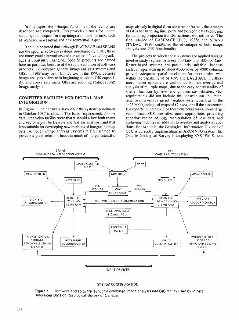
In this paper, the principal functions of the facility are maps already in digital form use a raster format, the strength described and compared. This provides a basis for under- of GISs for handling line, point and polygon data types, and standing their impact for map integration, and for tasks such for handling projection transformations, was attractive. The as resource assessment and environmental impact. final choice of EASIPACE (PCI, 1988) and SPANS

It should be noted that although EASIPACE and SPANS are the specific software systems purchased by GSC, there are many good alternatives and the status of available packages is constantly changing. Specific products are named here on purpose, because of the rapid evolution of software products. To compare generic image analysis systems and GISs in 1988 may be of limited use in the 1990s, because image analysis software is beginning to adopt GIs capability, and conversely many GISs are adopting features from image analysis.

COMPUTER FACILITY FOR DIGITAL MAP INTEGRATION

In Figure 1, the hardware layout for the systems purchased in October 1987 is shown. The basic requirements for the data integration facility were that it should allow both raster and vector input, be flexible and fast for analysis, and that it be suitable for developing new methods of integrating map data. Although image analysis systems at first seemed to provide a good solution, because much of the geoscientific

SPANS SPATIAL DATA INTEGRATION SYSTEM

. . (TYDAC, 1989) combined the advantages of both image analysis and GIS functionality.

The projects to which these systems are applied usually involve study regions between 500 km2 and 100 000 km2. Raster-based systems are particularly suitable, because raster images with up to about 4000 rows by 4000 columns provide adequate spatial resolution for most tasks, well within the capability of SPANS and EASIPACE. Further- more, raster systems are well-suited for fast overlay and analysis of multiple maps, due to the easy addressability of spatial location by row and column co-ordinates. Our requirements did not include the construction and maintenance of a very large information system, such as all the 1 :250 000 geological maps of Canada, or all the assessment file reports in Ontario. For these custodial tasks, some large vector-based GISs are often more appropriate, providing superior vector editing, manipulation of text data and archiving facilities in addition to overlay and analysis functions. For example, the Geological Information Division of GSC is currently implementing an ARC-INFO system, the Ontario Geological Survey is employing SYSTEM 9, and

PC1 IMAGE ANALYSIS SYSTEM

I d

CCT'S

TAPE DRIVE

VAX MODEM MAIN FRAME

5 1 2 x 512 80386 CPU HARD WIRE DIRECT COMMUNICATION

2.5 mb RAM

DIGITIZING TABLE 110cmx140cm

i I 160 BPI

"WORM" OPTICAL

COLOUR PLOTTER INK J E T

COLOUR PLOTTER

"WORM" OPTICAL STORAGE

REMOVABLE 230 mb DISKETTE

-

INPUT DEVICES

SYSTEM CONFIGURATION

Figure 1. Hardware and software layout for combined image analysis and GIS facility used by Mineral Resources Division, Geological Survey of Canada.

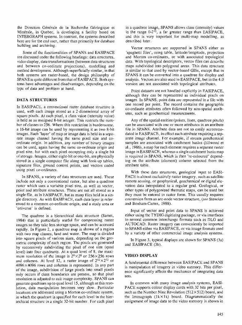
the Direction GCnCrale de la Recherche GCologique et MinCrale, in Quebec, is developing a facility based on INTERGRAPH systems. In contrast, the systems described here are for the end user, rather than primarily for database building and archiving.

Some of the functionalities of SPANS and EASIPACE are discussed under the following headings : data structures, video display, data transformations (between data structures and between co-ordinate projections), modelling and method development. Although superficially similar, in that both systems are raster-based, the design philosophy of SPANS is quite different from that of EASIPACE. Both systems have advantages and disadvantages, depending on the type of data and problem at hand.

DATA STRUCTURES

In EASIPACE, a conventional raster database structure is used, with each image stored as a 2-dimensional array of square pixels. At each pixel, a class value (intensity value) is held as an unsigned 8-bit integer. This restricts the number of classes to 256. Where this restriction is burdensome, a 16-bit image can be used by representing it as two 8-bit images. Each 'layer' of map or image data is held in a separate image channel having the same pixel size and coordinate origin. In addition, any number of binary images can be used, again having the same co-ordinate origin and pixel size, but with each pixel occupying only a single bit of storage. Images, either eight-bit or one-bit, are physically stored in a single computer file along with look-up tables, signature files, ground control points, and vectors coded using pixel co-ordinates.

In SPANS, a variety of data structures are used. These include not only a conventional raster, but also a quadtree raster which uses a variable pixel size, as well as vector, point and attribute structures. These are not all stored as a single file, as in EASIPACE, but as many files held in a single directory. As with EASIPACE, each data layer is referenced to a common co-ordinate origin, and a study area or 'universe' is defined.

The quadtree is a hierarchical data structure (Samet, 1984) that is particularly useful for compressing raster images so they take less storage space, and can be accessed rapidly. In Figure 2, a quadtree map is shown of a region with two map classes, land and water. The map is divided into square pixels of various sizes, depending on the geometric complexity of each region. The pixels are generated by successively subdividing the pixel of one size (quad level) into four quadrants. At a quad level of 8, the maximum resolution of the image is 2 8 ~ 2 ~ or 256x256 rows and columns. At level 12, a raster image of 212 ~ 2 ' ~ or 4096x4096 rows and columns is represented. In any part of the image, subdivision of large pixels into small pixels only occurs if class boundaries are present, so that pixel resolution is adjusted to suit image complexity. SPANS can generate quadtrees up to quad level 15, although at this resolution, data manipulation becomes very slow. Particular locations are addressed using a Morton co-ordinate system, in which the quadrant is specified for each level in the hierarchical structure in a single 32-bit number. For each pixel

in a quadtree image, SPANS allows class (intensity) values in the range 0-215, a far greater range than EASIPACE, and this is very important for multi-map modelling, as described later.

Vector structures are supported in SPANS either as 'spaghetti files', using table, latitudellongitude, projection and Morton co-ordinates, or with associated topological data. With topological descriptors, vector files can describe maps subdivided into polygonal areas. This data structure is similar to that used by vector-based GISs, except that in SPANS it can be converted into a quadtree for display and analysis. Vectors are also used in EASIPACE, but in the 4.0 version are not associated with topological attributes.

Point datasets are not handled explicitly in EASIPACE, although they can be represented as individual pixels on images. In SPANS, point data are represented in a file with one record per point. The record contains the geographic co-ordinate attributes often followed by non-spatial attributes, such as geochemical measurements.

Any of the spatial entities (points, lines, quadtree pixels) can be associated with one or more attributes in an attribute file in SPANS. Attribute data are not so easily accommodated in EASIPACE, in effect each attribute requiring a separate image channel. For example, if stream geochemical samples are associated with catchment basins (Ellwood et al., 1986), a map for each element requires a separate raster image in EASIPACE, whereas a single catchment basin map is required in SPANS, which is then 're-coloured' depending on the attribute (element) column selected from the attribute table.

With these data structures, geological input to EASI- PACE is almost exclusively raster imagery, such as satellite remote sensing, or geophysical, geochemical or digital elevation data interpolated to a regular grid. Geological, or other types of polygonized thematic maps, can be used but they must be entered in raster form. This usually requires conversion from an arc-node vector structure, (see Steneker and Bonham-Carter, 1988).

Input of vector and point data to SPANS is achieved either using the TYDIG digitizing package, or via interfaces to several common interchange formats such as DLG and AUTOCAD. Raster imagery can conveniently be imported to SPANS either via EASIPACE, or via image formats used by a variety of other commercial image analysis systems.

In Figure 3, typical displays are shown for SPANS (3a) and EASIPACE (3b).

VIDEO DISPLAY

A fundamental difference between EASIPACE and SPANS is manipulation of imagery in video memory. This difference significantly affects the mechanics of integrating data sets.

In common with many image analysis systems, EASI- PACE supports colour display cards with 32 bits per pixel, such as the Number Nine Revolution (512 X 5 12) board, and the Immagraph (1 k x 1 k) board. Diagrammatically the assignment of image data to the video memory is shown in

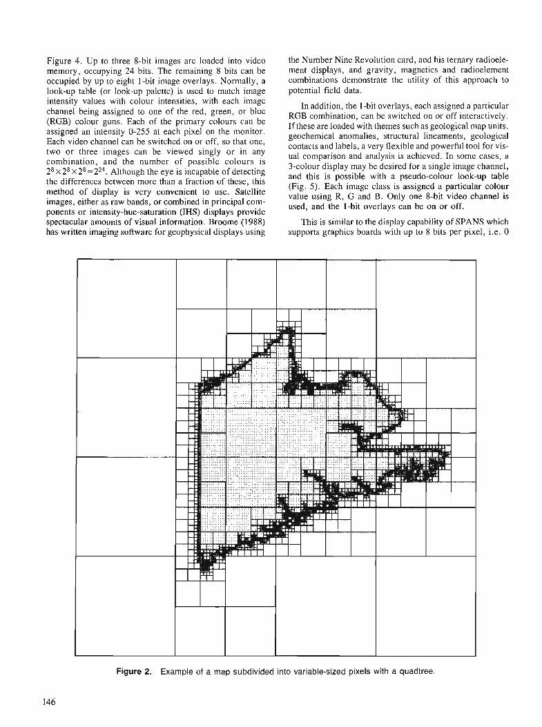
Figure 4. Up to three 8-bit images are loaded into video memory, occupying 24 bits. The remaining 8 bits can be occupied by up to eight 1-bit image overlays. Normally, a look-up table (or look-up palette) is used to match image intensity values with colour intensities, with each image channel being assigned to one of the red, green, or blue (RGB) colour guns. Each of the primary colours can be assigned an intensity 0-255 at each pixel on the monitor. Each video channel can be switched on or off, so that one, two or three images can be viewed singly or in any combination, and the number of possible colours is 2 8 ~ 2 8 ~ 2 ~ ~ 2 ~ ~ . Although the eye is incapable of detecting the differences between more than a fraction of these, this method of display is very convenient to use. Satellite images, either as raw bands, or combined in principal components or intensity-hue-saturation (IHS) displays provide spectacular amounts of visual information. Broome (1988) has written imaging software for geophysical displays using

the Number Nine Revolution card, and his ternary radioelement displays, and gravity, magnetics and radioelement combinations demonstrate the utility of this approach to potential field data.

In addition, the 1-bit overlays, each assigned a particular RGB combination, can be switched on or off interactively. If these are loaded with themes such as geological map units, geochemical anomalies, structural lineaments, geological contacts and labels, a very flexible and powerful tool for visual comparison and analysis is achieved. In some cases, a 3-colour display may be desired for a single image channel, and this is possible with a pseudo-colour look-up table (Fig. 5). Each image class is assigned a particular colour value using R, G and B. Only one &bit video channel is used, and the 1-bit overlays can be on or off.

This is similar to the display capability of SPANS which supports graphics boards with up to 8 bits per pixel, i.e. 0

-- 0. am?.';:. ': : ... r. " :.;

Figure 2. Example of a map subdivided into variable-sized pixels with a quadtree.

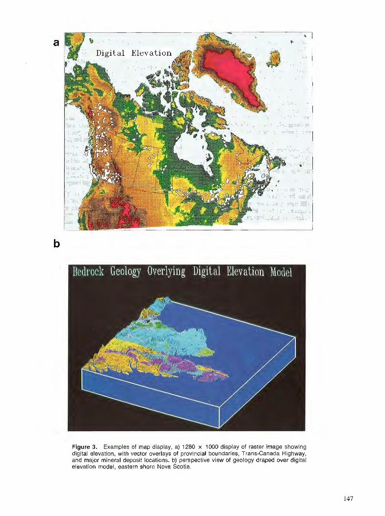
Figure 3. Examples of map display, a) 1280 x 1000 display of raster image showing digital elevation, with vector overlays of provincial boundaries, Trans-Canada Highway, and major mineral deposit locations. b) perspective view of geology draped over digital elevation model, eastern shore Nova Scotia.

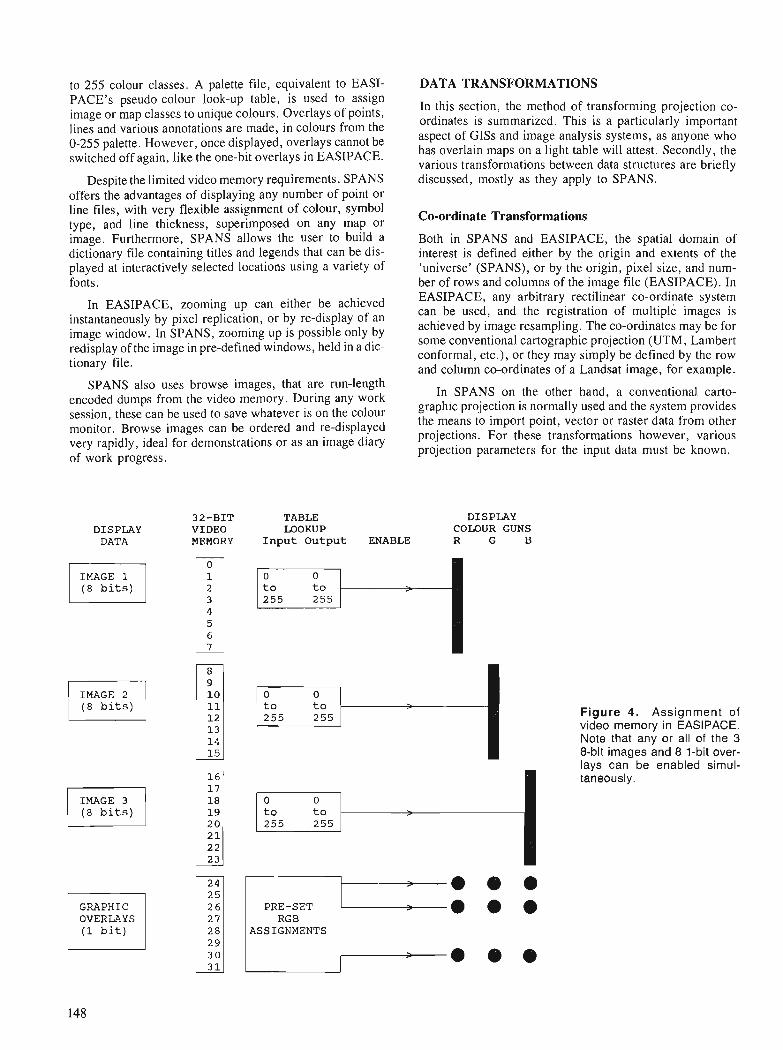
to 255 colour classes. A palette file, equivalent to EASI- DATA TRANSFORMATIONS PACE'S pseudo-colour look-up table, i s used to assign image or map classes to unique colours. Overlays of points, In this section, the method of transforming projection co-

lines and various annotations are made, in colours from the ordinates is summarized. 'This is a particularly important

0-255 palette. However, once displayed, overlays cannot be aspect of and image systems, as any0ne who

switched off again, like the one-bit overlays in EASIPACE. has overlain maps on a light table will attest. Secondly, the various transformations between data structures are briefly

Despite the limited video memory requirements, SPANS discussed, mostly as they apply to SPANS. offers the advantages of displaying any number of point or - - - -

line files, with veFy flexible assignment of colour,~symbol Co-ordinate Transformations type, and line thickness, superimposed on any map or image. Furthermore, SPANS allows the user to build a Both in SPANS and EASIPACE. the spatial domain of dictronary file containing titles and legends that can be dis- interest is defined either by the &rigin and extents of the played at interactively selected locations using a variety of 'universe' (SPANS), or by the origin, pixel size, and num- fonts. ber of rows and columns of the image file (EASIPACE). In

In EASIPACE, zooming up can either be achieved EASIPACE, any arbitrary rectilinear co:ordinate system can be used, and the registration of multiple images is instantaneously by pixel replication, or by re-display of an

image window. In SPANS, zooming up is possible only by achieved by image resampling. The co-ordinates may be for

redisplay of the image in pre-defined windows, held in a dic- some conventional cartographic projection (UTM, Lambert

tionary file. conformal, etc.), or they may simply be defined by the row and column co-ordinates of a Landsat image, for example.

SPANS also uses browse images, that are run-length encoded dumps from the video memory. During any work In SPANS on the other hand, a conventional carto-

session, these can be used to save whatever is on the colour graphic projection is normally used and the system provides

monitor. Browse images can be ordered and re-displayed the means to import point, vector or raster data from other

very rapidly, ideal for demonstrations or as an image diary projections. For these transformations however, various projection parameters for the input data must be known. of work progress.

32-BIT TABLE DISPLAY DISPLAY VIDEO LOOKUP COLOUR GUNS

DATA MEMORY I n p u t Output ENABLE R G B

(8 b i t s )

(8 bits)

I M A G E 3

OVERLAYS (1 bit)

-e O . RGB

. . Figure 4. Assignment of video memory in EASIPACE. Note that any or all of the 3 8-bit images and 8 I-bit overlays can be enabled simultaneously.

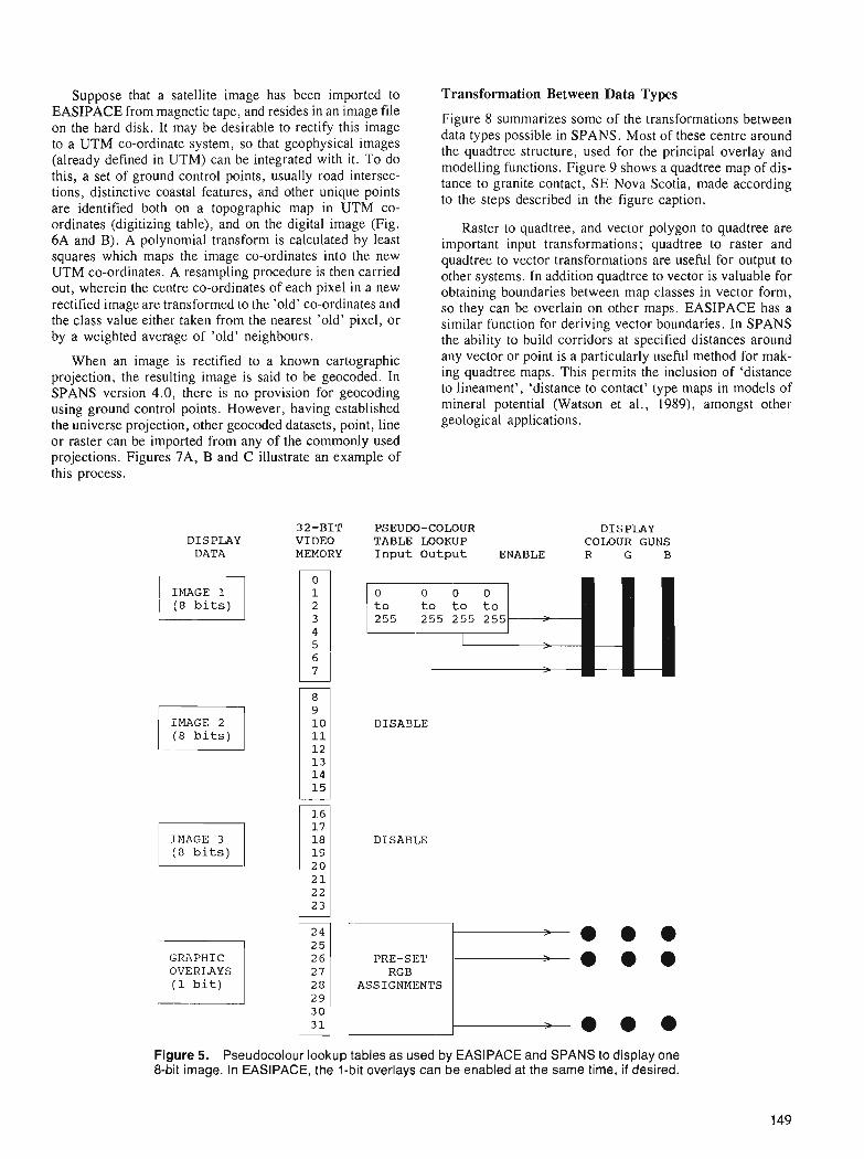
Suppose that a satellite image has been imported to Transformation Between Data Types EASIPACE from magnetic tape, and resides in an image file on the hard disk. It may be desirable to rectify this image to a UTM co-ordinate system, so that geophysical images (already defined in UTM) can be integrated with it. To do this, a set of ground control points, usually road intersections, distinctive coastal features, and other unique points are identified both on a topographic map in UTM coordinates (digitizing table), and on the digital image (Fig. 6A and B). A polynomial transform is calculated by least squares which maps the image co-ordinates into the new UTM co-ordinates. A resampling procedure is then carried out, wherein the centre co-ordinates of each pixel in a new rectified image are transformed to the 'old' co-ordinates and the class value either taken from the nearest 'old' pixel, or by a weighted average of 'old' neighbours.

When an image is rectified to a known cartographic projection, the resulting image is said to be geocoded. In SPANS version 4.0, there is no provision for geocoding using ground control points. However, having established the universe projection, other geocoded datasets, point, line or raster can be imported from any of the commonly used projections. Figures 7A, B and C illustrate an example of this process.

Figure 8 summarizes some of the transformations between data types possible in SPANS. Most of these centre around the quadtree structure, used for the principal overlay and modelling functions. Figure 9 shows a quadtree map of distance to granite contact, SE Nova Scotia, made according to the steps described in the figure caption.

Raster to quadtree, and vector polygon to quadtree are important input transformations; quadtree to raster and quadtree to vector transformations are useful for output to other systems. In addition quadtree to vector is valuable for obtaining boundaries between map classes in vector form, so they can be overlain on other maps. EASIPACE has a similar function for deriving vector boundaries. In SPANS the ability to build corridors at specified distances around any vector or point is a particularly useful method for making quadtree maps. This permits the inclusion of 'distance to lineament', 'distance to contact' type maps in models of mineral potential (Watson et al., 1989), amongst other geological applications.

32-BIT PSEUDO-COLOUR DISPLAY DISPLAY VIDEO TABLE LOOKUP COLOUR GUNS DATA MEMORY Input Output ENABLE R G B

DISABLE (8 bits)

15

DISABLE (8 bits)

GkAPHIC OVERLAYS (1 bit)

. c

PRE-SET . fl

RG B ASSIGNMENTS

. Figure 5. Pseudocolour lookup tables a s used by EASIPACE and SPANS to display one &bit image. In EASIPACE, the 1-bit overlays can be enabled at the same time, if desired.

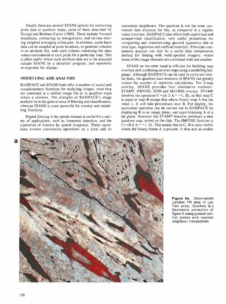
Finally there are several SPANS options for converting point data to quadtree maps, some of them described by George and Bonham-Carter (1989). These include Voronoi tesselation, contouring by triangulation, and various moving weighted averaging techniques. In addition, multi-layer data can be sampled at point locations, to generate columns in an attribute file, with each column containing the class values encountered at each point for a particular map. This is often useful where such attribute data are to be analyzed outside SPANS by a statistical program, and optionally re-imported for display.

MODELLING AND ANALYSIS

EASIPACE and SPANS both offer a number of useful and complementary functions for analyzing images, once they are contained in a unified image file or in quadtree maps within a universe. The strengths of EASIPACE's image analysis lie in the general area of filtering and classification, whereas SPANS is more powerful for overlay and modelling functions.

Digital filtering in the spatial domain is useful for a variety of applications, such as lineament detection, and the separation of features by spatial frequency. These operations involve convolution operations on a pixel and its

immediate neighbours. The quadtree is not the most convenient data structure for this, as compared to a regular raster structure. EASIPACE also offers both supervised and unsupervised classification, very useful procedures for recognizing and characterizing spectral signatures due to rock type, vegetation and surficial materials. Principal components analysis can also be a useful data compression method for dealing with multi-spectral imagery, where many of the image channels are correlated with one another.

SPANS on the other hand is efficient for building map overlays and combining several maps using a modelling language. Although EASIPACE can be used to carry out similar tasks, the quadtree data structure of SPANS can greatly reduce the number of repetitive calculations. For 2-map overlay, SPANS provides four alternative methods: STAMP, IMPOSE, JOIN and MATRIX overlay. STAMP involves the operation C = (A if A = = 1, B), so that map C is equal to map B except that where binary map A has the value 1, A will take precedence over B. For display, the equivalent operation can be carried out in EASIPACE by displaying B in an image plane, and superimposing A in a bit plane. However the STAMP function produces a new quadtree map, stored on the disk. The IMPOSE function is C = (B if A = = 1, 0). This means that in C, B is only visible where the binary theme A is present. A thus acts as cookie

Figure 6a. Uncorrected Landsat TM data of Lac Tait a r ea , Quebec b.) Geometric correction of figure 6 using ground control points and nearest neighbour interpolation.

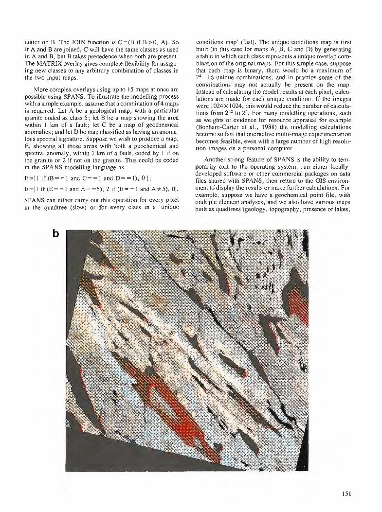
cutter on B. The JOIN function is C=(B if B>O, A). So if A and B are joined, C will have the same classes as used in A and B, but B takes precedence when both are present. The MATRIX overlay gives complete flexibility for assigning new classes to any arbitrary combination of classes in the two input maps.

More complex overlays using up to 15 maps at once are possible using SPANS. To illustrate the modelling process with a simple example, assume that a combination of 4 maps is required. Let A be a geological map, with a particular granite coded as class 5 ; let B be a map showing the area within 1 km of a fault; let C be a map of geochemical anomalies ; and let D be map classified as having an anomalous spectral signature. Suppose we wish to produce a map, E, showing all those areas with both a geochemical and spectral anomaly, within 1 km of a fault, coded by 1 if on the granite or 2 if not on the granite. This could be coded in the SPANS modelling language as

E={l if (B==1 and C = = 1 and D==1) , 0 I; E = ( l if ( E = = I and A==5) , 2 if ( E = = 1 and A#5) , 0).

SPANS can either carry out this operation for every pixel in the quadtree (slow) or for every class in a 'unique

conditions map' (fast). The unique conditions map is first built (in this case for maps A, B, C and D) by generating a table in which each class represents a unique overlap combination of the original maps. For this simple case, suppose that each map is binary, there would be a maximum of z4= 16 unique combinations, and in practice some of the combinations may not actually be present on the map. Instead of calculating the model results at each pixel, calculations are made for each unique condition. If the images were 1024 X 1024, this would reduce the number of calculations from 220 to 24. For many modelling operations, such as weights of evidence for resource appraisal for example (Bonham-Carter et al., 1988) the modelling calculations become so fast that interactive multi-image experimentation becomes feasible, even with a large number of high resolution images on a personal computer.

Another strong feature of SPANS is the ability to tem- porarily exit to the operating system, run either locally- developed software or other commercial packages on data files shared with SPANS, then return to the GIs environment to display the results or make further calculations. For example, suppose we have a geochemical point file, with multiple element analyses, and we also have various maps built as quadtrees (geology, topography, presence of lakes,

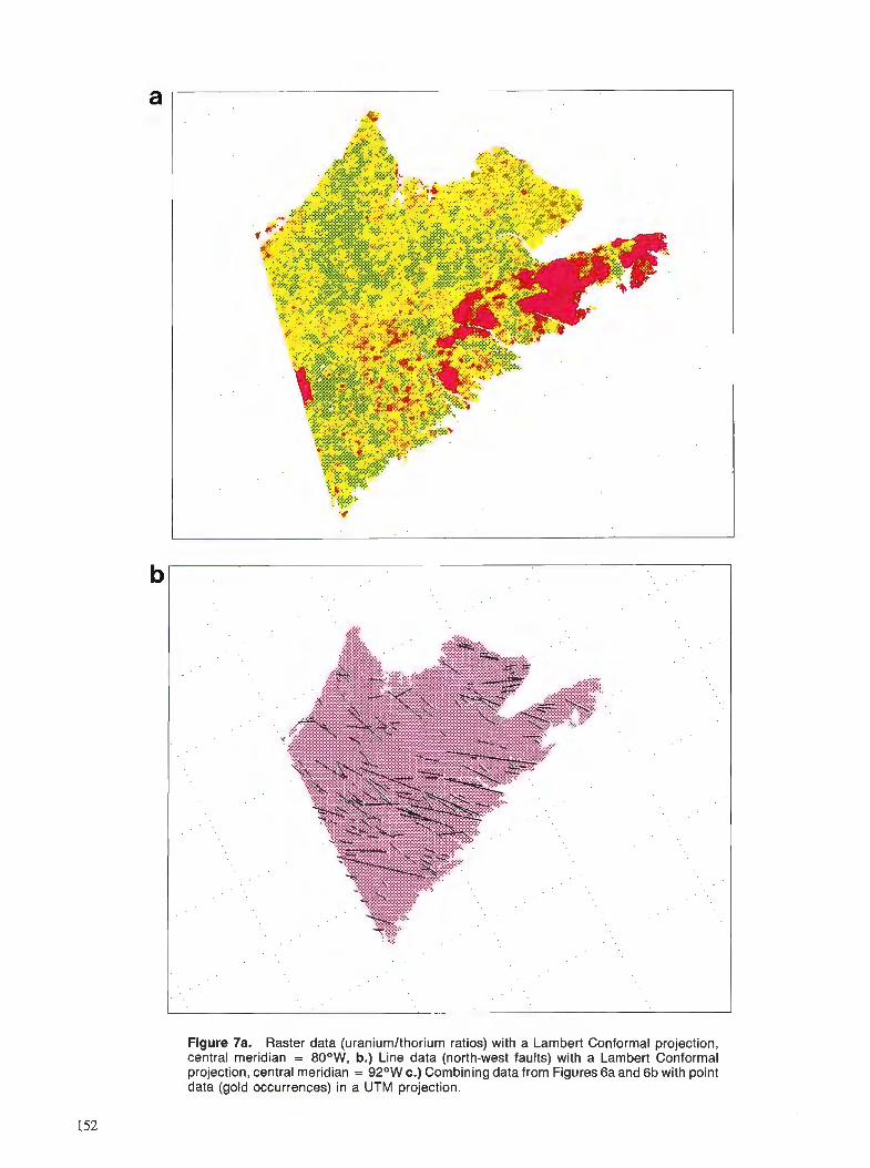
Figure 7a. Raster data (uraniumlthorium ratios) with a Lambert Conformal projection, central meridian = 80°W, b.) Line data (north-west faults) with a Lambert Conformal projection, central meridian = 92"W c.) Combining data from Figures 6a and 6b with point data (gold occurrences) in a UTM projection.

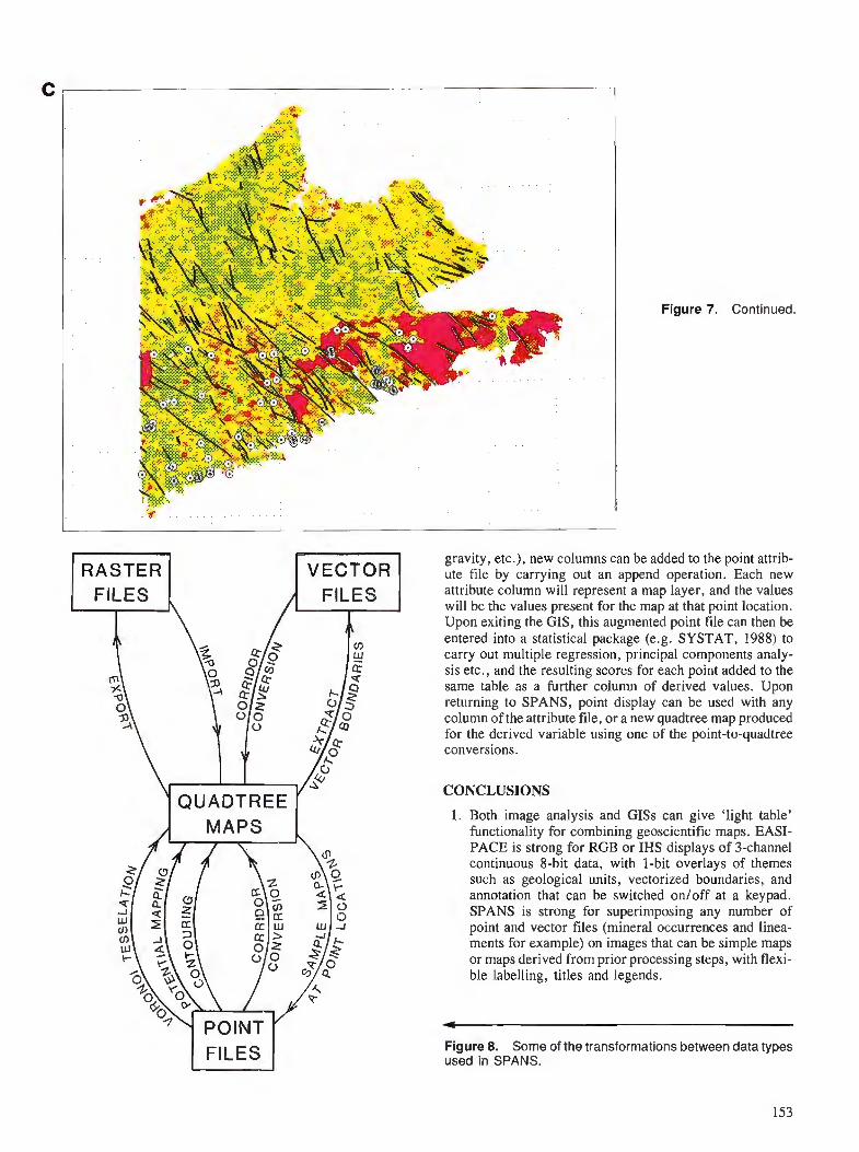
I FILES I

Figure 7. Continued.

gravity, etc.), new columns can be added to the point attribute file by carrying out an append operation. Each new attribute column will represent a map layer, and the values will be the values present for the map at that point location. Upon exiting the GIs, this augmented point file can then be entered into a statistical package (e.g. SYSTAT, 1988) to carry out multiple regression, principal components analysis etc., and the resulting scores for each point added to the same table as a further column of derived values. Upon returning to SPANS, point display can be used with any column of the attribute file, or a new quadtree map produced for the derived variable using one of the point-to-quadtree conversions.

CONCLUSIONS

1. Both image analysis and GISs can give 'light table' functionality for combining geoscientific maps. EASI- PACE is strong for RGB or IHS displays of 3-channel continuous 8-bit data, with 1-bit overlays of themes such as geological units, vectorized boundaries, and annotation that can be switched onloff at a keypad. SPANS is strong for superimposing any number of point and vector files (mineral occurrences and lineaments for example) on images that can be simple maps or maps derived from prior processing steps, with flexible labelling, titles and legends.

Figure 8. Some of the transformations between data types used in SPANS.

2. EASIPACE is mainly restricted to 8-bit and 1-bit raster images, whereas SPANS uses diverse data structures and can handle point, line, polygon and raster data, as well as associated attribute files. EASIPACE is attractive for handling satellite and geophysical imagery, whereas SPANS is more suitable for geological maps, geochemical sample data (and other point files) and labelled vectors (such as geological contacts).

3. EASIPACE is useful for carrying out convolution operations, such as spatial filtering; SPANS offers the ability to build distance corridors by dilating point or line features.

4. Raster images can be resampled in EASIPACE, after collecting ground control points. 'This is particularly useful for non-geocoded images, such as Landsat. With SPANS, a wide selection of cartographic projections can be used, both for building and display of quadtrees as well as importing data from different projections.

5. EASIPACE offers the ability to make Fast Fourier Transforms, carry out supervised and unsupervised classification, and a limited set of GIs functions using Boolean operations ; users can also write their own programs and call up image analysis subroutines from an object library; macros can be written for linking a series of tasks.

6. Maps may be combined in SPANS using a variety of arithmetic, Boolean and conditional operators in a modelling language; modelling is fast and efficient due

Jr "

Granite Contact Corridor

to the building of a unique conditions map, and to the quadtree data structure. No object library is supplied with SPANS, but macros can be written in a command language. However, independent algorithm development can be effectively linked to SPANS operations via shared ASCII data files; text editors, statistical packages and locally-developed programs can be executed without exiting completely from the GIs.

7. Neither EASIPACE nor SPANS in their present form supply much 'mathematical morphology' functionality (erosion, dilation, skeletonization, opening, closing, etc.), although SPANS does permit generation of distance corridors around vectors and points, and EASI- PACE permits the dilation of binary themes by up to 15 pixels deep.

8. Commercial GIs and image analysis packages are rapidly diversifying, taking on progressively more functionality, so present differences that now seem generic may disappear in future general-purpose systems.

9. Learning to use SPANS or EASIPACE takes about a week of basic training, with at least another three weeks of self-tutoring. Both systems can be menu-driven, and the commonly-used functions are easy to learn. How- ever, both systems provide a broad range of complex tasks that are easily-forgotten without regular use. Therefore, for most users with specific applications, these are not systems to be employed for a few weeks per year, without technical assistance.

Legend ' Goldenville/Aalifax Fm. Contact Corridor (1.00 km)

IGranites

Figure 9. Quadtree map showing distance to granite contact, made by 1) reclassifying the geology map to select only the granite, 2) doing a quadtree to vector conversion to obtain the granite contact as a vector, 3) dilating the contact vector by corridor conversion, and 4) stamp- ing the granite map on top of the corridor map.

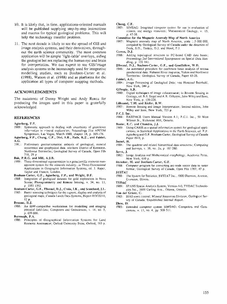
10. It is likely that, in time, applications-oriented manuals will be published supplying step-by-step instructions and macros for typical geological problems. This will help the technology transfer problem.

11. The next decade is likely to see the spread of GIs and image analysis systems, and their derivatives, throughout the earth science community. The most common application will be simple 'light-table' overlays, aiding the geologist but not replacing the human eye 2nd brain for interpretation. We can expect to see GISIimage analysis systems to be increasingly used for integrative modelling studies, such as Bonham-Carter et al. (1988), Watson et al. (1988) and as platforms for the application all types of computer mapping methods.

ACKNOWLEDGMENTS

The assistance of Danny Wright and Andy Rencz for producing the images used in this paper is gratefully acknowledged.

REFERENCES Agterberg, F.P. 1989: Systematic approach to dealing with uncertainty of geoscience

information in mineral exploration; Proceedings 21st APCOM Symposium, Las Vegas, March 1989, chapter i8 , p. 165-178.

Agterberg, F.P., Chung, C.F., Divi, S.R., Eade, K.E., and Fabbri, A.G. 1981: Preliminary geomathematical anlaysis of geological, mineral

occurrence and geophysical data, southern District of Keewatin, Northwest Territories; Geological Survey of Canada, Open File 718, 29 p.

Bak, P.R.G. and Mill, A.J.B. 1989: Three-dimensional representation in a geoscientific resource man-

agement system for the minerals industry; in Three-Dimensional Applications in Geographic Information Systems, ed. J . Raper, Taylor and Francis, London.

Bonham-Carter, G.F., Agterberg, F.P., and Wright, D.F. 1988: Integration of geological datasets for gold exploration in Nova

Scotia; Photogrammetry and Remote Sensing, v. 54, no. 11, p. 1585-1592.

Bonham-Carter, G.F., Ellwood, D.J., Crain, I.K., and Scantland, J.L. 1985: Raster scanning techniques for the capture, display and analysis of

geological maps; Canada Lands Data Systems, Report R003210, 12 p.

Broome, H.J. 1988: An IBM-compatible workstation for modelling and imaging

potential field-data; Computers and Geosciences, v. 14, no. 5, p. 659-666.

Burrough, P.A. 1986: Principles of Geographical Information Systems for Land

Resource Assessment; Oxford University Press, Oxford, 193 p.

Chung, C.F. 1983: SIMSAG: Integrated computer system for use in evaluation of

mineral and energy resources; Mathematical Geology, v. 15, p. 47-58.

Committee for the Magnetic Anomaly Map of North America 1987: Magnetic anomaly map of North America, scale 1 :5 000 000,

compiled by Geological Survey of Canada under the direction of Dods, S.D., Teskey, D.J. and Hood, P.J.

Cowen, D.J. 1986: Adding topological structure to PC-based CAD data bases;

Proceedings 2nd International Sysmposium on Spatial Data Han- dling, p. 132-141.

Ellwood, D.J., Bonham-Carter, G.F., and Goodfellow, W.D. 1986: An automated procedure for catchment basin analysis of stream

geochemical data: Nahanni River map area, Yukon and Northwest Territories; Geological Survey of Canada, Paper 85-26.

Fabbri, A.G. 1984: Image Processing of Geological Data; van Nostrand Reinhold,

New York, 244 p. Gillespie, A.R. 1980: Digital techniques of image enhancement; in Remote Sensing in

Geology, ed. B.S. Siege1 and A.R. Gillespie, John Wiley and Sons, New York, p. 139-226.

Lillesand, T.M. and Kiefer, R.W. 1987: Remote Sensing and Image Interpretation; Second edition, John

Wiley and Sons, New York, 721 p. P.C.I. Inc. 1988: EASIPACE Users Manual Version 4.1; P.C.I. Inc., 50 West

Wilmot St., Richmond Hill, Ontario. Reeler, E.C. and Chandra, J.J. 1989: Using CARIS as a spatial information system for geological appli-

cations; in Statistical Applications in the Earth Sciences, ed. F.P. Agterberg and G.F. Bonham-Carter, Geological Survey of Canada Paper 89-9, p.

Samet, H. 1984: The quadtree and related hierarchical data structures; Computing

and Surveys, v. 16, no. 2a, p. 187-260. Serra, J. 1982 : Image Analysis and Mathematical morphology ; Academic Press,

New York, 610 p. Steneker, M. and Bonham-Carter, G.F. 1988: Computer program for converting arc-node vector data to raster

format; Geological Survey of Canada, Open File 1767, 47 p. SYSTAT 1988: The System for Statistics; SYSTAT Inc., 1800 Sherman, Avenue,

Evanston, Illinois. TYDAC 1989: SPANS Spatial Analysis System, Version 4-0, TYDAC Technolo-

gies Inc., 1600 Carling Ave., Ottawa, Ontario. Van der Grient, C. 1985: BIAS users manual; Mineral Resources Division, Geological Sur-

vey of Canada, Unpublished Internal Report. Zhou, Di 1985: Extended computer system SIMSAG; Computers and Geos-

ciences, v. I I, no. 4, pp. 509-51 1.

Spatial modelling of geological data for gold exploration, Star Lake area, Saskatchewan

H. George1 and G.F. Bonham-Carter1

George, H. and Bonham-Carter, G. F., An example of spatial modelling of geological data for gold exploration, Star Lake area, Saskatchewan; & Statistical Applications in the Earth Sciences, ed. F.P. Agterberg and G.F. Bonham-Carter; Geological Survey of Canada, Paper 89-9, p. 157-1 69, 1989.

Abstract

An empirical modelling approach was used to locate zones which are favourable for gold mineralization in the Star Lake area of Saskatchewan by identifying areas where there is spatial coincidence of favourable bedrock type, proximity to faults and biogeochemical signatures which are indicative of gold. A major focus of investigation was to establish appropriate methodology for generating a 'summary' signature map of biogeochemistry, useful in spatial modelling, from a large, multi-element data set consisting of analyses for 31 elements in spruce bark collected from 566 sample sites.

Results indicate that the biogeochemical data are effectively summarized and most readily interpreted using principal components (PC) transformation on the rank-ordered data set following application of a local moving averagejlter to break tied values. Loadings on PC2 were simultaneously high on gold and gold-related elements, particularly antimony and molybdenum. Gold favourability Scores', derived by multiplying PC2 loadings by the original ranks, were calculated for each sample point and interpolated using three different techniques, namely, contouring, potential mapping and kriging. Contouring produces maps with the least satisfactory interpolations. Differences between mapsproduced usingpoten- tial mapping and kriging are minor except near the fringes of the sample pattern, if one uses a variogram to select the area of influence used in potential mapping.

Modelling results indicate that our empirical approach is effective for the Star Lake data set in that it predicts several favourable gold mineralization zones which are close to known gold occurrences. In addition, the study demonstrates the feasibility of using a micro-computer based geographic information system (GIs) for mineral exploration investigations.

On a employe'une mkthode empirique de mod6lisation pour localiser les zones favorables & une mine'- ralisation aurifere dans la r6gion de Star Lake en Saskatchewan, en ident~$ant les zones oh il existe une coiizcidence spatiale des types favorables de roches de fond, la proximitkde failles et des signatures biogkochimiques indiquant la pre'sence d'or. L'un des principaux objectifs des recherches ktait d'ktablir une me'thode appropride pour produire une carte s re'capitulative ,, des signatures bioge'ochimiques, qui facilite la modklisation spatiale, ci partir d'un vaste ensemble de donnkes multi-klkments, regroupant les dosages de 31 klkments pre'sents dans l'e'corce d'e'pinette recueillie sur 566 localitks d 'dchantillonage.

Les rdsultats indiquent que ['on peut au moins re'sumer les donne'es biogkochimiques et les interprher de la facon la plus claire en employant la transformation des composantes principales (CP) sur 1 'ensemble de donnkes classe'es selon leur rang, aprbs application d'unjltre sur lequel la moyenne peut 2tre locale- ment de'placke, permettant ainsi de dissocier les valeurs coiitcidentes. Sur CP2, les charges ont ktk simultan.4ment e'levdes pour 1 'or et les kle'ments apparentks & l'or, en particulier l'antimoine et le molyb- d6ne. On a calculk les ..points, de probabilitk de la prksence d'or, en multipliant les charges CP2 par les rungs d'origine, et cela pour chaque point d'kchantillonnage; on a interpole' les re'sultats d l'aide de trois techniques diffdrentes, notamment le track de courbes de niveau, la cartographie du potentiel et le krigeage. Le trace'de courbes de niveau donne les cartes avec les interpolations les moins satisfaisantes. Les diffkrences entres les cartes produites par cartographie du potentiel et krigeage sont peu impor- tances, sauf prbs des bords de la conjguration de l'e'chantillon, si l'on emploie un variogramme pour sklectionner la zone d'influence employke lors de la cartographie du potentiel.

-

'Geological Survey of Canada, 601 Booth Street, Ottawa, Ontario J1A OE8

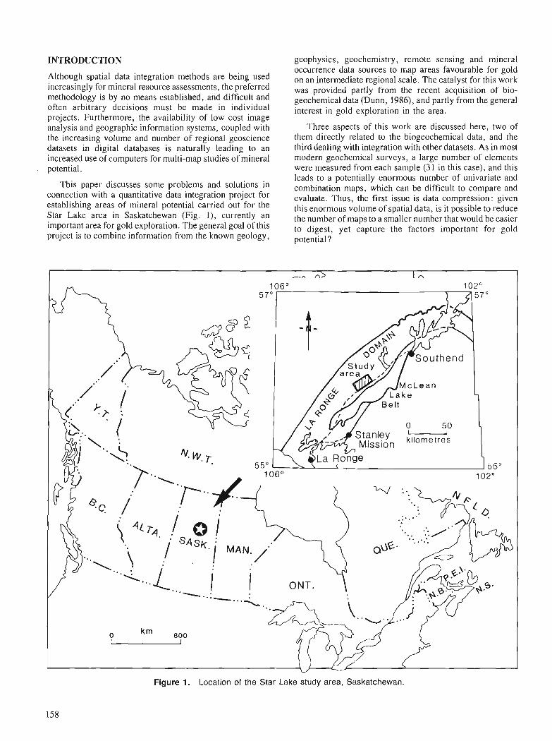
INTRODUCTION

Although spatial data integration methods are being used increasingly for mineral resource assessments, the preferred methodology is by no means established, and difficult and often arbitrary decisions must be made in individual projects. Furthermore, the availability of low cost image analysis and geographic information systems, coupled with the increasing volume and number of regional geoscience datasets in digital databases is naturally leading to an increased use of computers for multi-map studies of mineral potential.

This paper discusses some problems and solutions in connection with a quantitative data integration project for establishing areas of mineral potential carried out for the Star Lake area in Saskatchewan (Fig. l), currently an important area for gold exploration. The general goal of this project is to combine information from the known geology,

geophysics, geochemistry, remote sensing and mineral occurrence data sources to map areas favourable for gold on an intermediate regional scale. The catalyst for this work was provided partly from the recent acquisition of biogeochemical data (Dunn, 1986), and partly from the general interest in gold exploration in the area.

Three aspects of this work are discussed here, two of them directly related to the biogeochemical data, and the third dealing with integration with other datasets. As in most modern geochemical surveys, a large number of elements were measured from each sample (31 in this case), and this leads to a potentially enormous number of univariate and combination maps, which can be difficult to compare and evaluate. Thus, the first issue is data compression: given this enormous volume of spatial data, is it possible to reduce the number of maps to a smaller number that would be easier to digest, yet capture the factors important for gold potential ?

w

Figure 1. Location of the Star Lake study area, Saskatchewan.

The second issue relates to methods for converting point data into an image or map form, suitable for combining with other data layers. Inevitably, if the geochemical data are to be compared with other variables (flight line geophysical measurements, fault neighbourhoods, for example), some kind of conversion of point to surface representation is desirable . This can be an interpolation process, with attendant problems of uncertainty of estimates. Or it can be a tessellation process, identifying a polygon around each point that can be used to extend the area! zone of influence. Two tessellation examples are catchment basins (BonhamCarter et al., 1988) and Voronoi (Thiessen or Dirichlet) polygons (Burrough, 1987).

The third issue is the method of combining data layers. In areas with a developed history of exploration, the locations of known mineral occurrences provide the means to obtain regression coefficients for linear models predicting mineralization, as described by many authors, e.g., Agterberg ( 1986). A recently published method for combining map layers using Bayes statistics also assumes that the area is reasonably well-explored (Bonham-Carter et al., 1988). Alternatively, a model may be used for combining data layers, using a subjective approach based on a knowledge of ore genesis. Such a model for combining data layers may be based on formal rules, as in expert systems, or be a simple Boolean and/or arithmetic combination using heuristic reasoning. Such heuristic models are particularly appropriate in areas where exploration is at an early stage, and the known mineral occurrences provide an inadequate sample for a statistical characterization of the signatures associated with a particular deposit type.

For this study, a PC-based Geographic Information System called SPANS (Tydac Technologies, Inc., 1987) was used for much of the work. It was unclear at the outset of the project whether SPANS analytical tools for handling

Table 1. Data layers for the Star Lake data-integration study

Data name Type

Bedrock Polygonal-geology' thematic

Biogeo- Points chemistry2

Faults3 Lines

Airborne 8-bit raster radiometrics4

Airborne 8-bit raster magnetics4

Airborne VLF4 8-bit raster

Mineral points occurences5

Landsat - TM4 8-bit raster

' Thomas, 1984; Harper, 1986 2 Dunn, 1986 3 From the geological map 4 Not shown in this paper

Digital capture Attributes

Table digitized Map units,i.e., rock types

ASCII file with 31 elements, alder UTM coordinates twigs4/spruce bark

Table digitized Length, orientation

Gridded from flight K, eTh, eU, total line data count, ratios

Gridded from flight Total field line data

Gridded from flight Total field, line data quadrature

ASCII file with Commodity type, geographic status coordinates

Computer- 4 spectral bands compatible tape

5 Thomas, 1984; Harper, 1986; D. Ames, pers. comm., 1988

multivariate point data were suitable for processing the biogeochemical data. Two built-in SPANS methods which are appropriate for converting geological data from point to map form are contouring by triangulation, and interpolation by potential mapping which is explained later. SPANS can read data files created by other programs. Thus, it was possible to carry out general statistical calculations on our multivariate point data set in DOS-based packages like SYSTAT (Wilkinson, 1987), or use locally developed programs for kriging, and have the results displayed on SPANS. It is clearly desirable to use the faster, built-in GIS functions when appropriate, and an important aspect of this study involved a comparison of the SPANS methods of point-to-map conversion with results obtained by kriging outside the GIS system.

In the following sections we discuss the geological setting, the digital data inputs, the methods employed (both SPANS and outside), present some results comparing the results of point-to-map conversions, and a map showing areas favourable for gold mineralization as predicted by a model. The overall scheme is shown in Figure 2.

GEOLOGICAL SETTING

The study area is located in northern Saskatchewan, approximately !50 km northeast of La Ronge within the La Ronge granite-greenstone Domain (Fig. 1). The major lithologies are felsic to mafic metavolcanics, acid to ultrabasic intrusives, and metasediments (Thomas, 1985; Harper, 1986). Two major shear zones are present. The McLennan Lake Tectonic Zone which runs along the southern boundary of the area, is intensely foliated and marks a major lithological contact between metavolcanic and plutonic rocks of the La Ronge Domain, and meta-arenites of the McLennan Group of the south. The second major shear zone, the David Lake Shear, trends roughly north-south through David Lake in the central part of the study area. Several gold occurrences have been reported close to this fault within granitoid intrusions (Poulsen et al., 1986, 1987; Fig. 3).

Structure plays an important role in gold mineralization. Gold occurs within splay faults and parallel subsidiary faults associated with medium-sized fault zones; at the intersection of medium-sized faults and medium - to coarse -grained syntectonic intrusions, within dilatant shears and in adjacent extensional stockworks (D. Ames, personal communication, 1988). There is no evidence in this area of extensive hydrothermal alteration associated with gold mineralization . Bedrock is usually exposed or covered by a veneer of morainal deposits or colluvium (Schreiner and Alley, 1984).

DIGITAL DATA INPUTS

Bedrock geology and linear structures were captured as vectors using a SPANS digitizing routine and used either as overlays on other maps, or converted to maps in raster form. Gridded datasets such as airborne geophysical data and geometrically-rectified remote sensing imagery can also be easily input to the GIS system. Table 1 summarizes the data layers used for the Star Lake study, and includes some layers not discussed in this paper yet listed to show the diversity of the database.

159

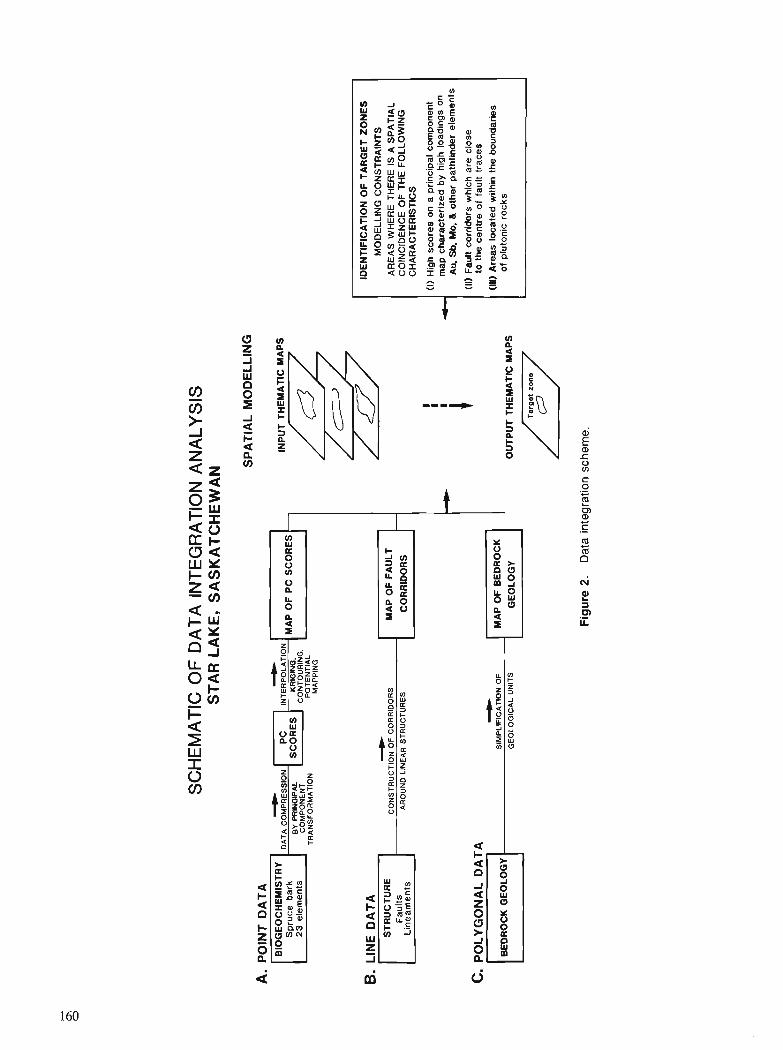
SC

HE

MA

TIC

OF

DA

TA

IN

TE

GR

AT

ION

AN

ALY

SIS

S

TA

R L

AK

E,

SA

SK

AT

CH

EW

AN

SP

AT

IAL

MO

DE

LL

ING

A

. P

OIN

T D

AT

A

C.

PO

LY

GO

NA

L D

AT

A

1

B'O

~u",

~b",

'~y

DA

T

MA

P O

F P

C S

CO

RE

S

23

ele

ments

C

OM

PO

NE

NT

6.

LIN

E D

AT

A

-

INP

UT

TH

EM

AT

IC M

AP

S

&

TR

AN

SF

OR

MA

TIO

N

POTE

NTI

AL

MAP

PING

-

ST

RU

CT

UR

E

Fa

ults

L

ine

am

en

ts

--

-

-

IDE

NT

IFIC

AT

ION

OF

TA

RG

ET

ZO

NE

S

MO

DE

LLIN

G C

ON

ST

RA

INT

S

- C

ON

STR

UC

TIO

N O

F C

OR

RID

OR

S

MA

P O

F F

AU

LT

AR

OU

ND

LIN

EA

R S

TR

UC

TU

RE

S

CO

RR

lbO

RS

A

RE

AS

WH

ER

E T

HE

RE

IS

A S

PA

TIA

L

CO

INC

IDE

NC

E O

F T

HE

FO

LLO

WIN

G

CH

AR

AC

TE

RIS

TIC

S

MA

P O

F B

ED

RO

CK

GE

OLO

GY

-

BE

DR

OC

K G

EO

LOG

Y

(1) H

igh s

core

s o

n a

pri

nci

pa

l com

ponent

map c

ha

ract

eri

zed

by

hig

h lo

adin

gs

on

Au.

Sb.

Mo,

& o

ther

pa

thfin

de

r e

lem

en

ts

- S

IMP

LIF

ICA

TIO

N

OF

OEO

LOG

ICAL

UN

ITS

(11)

Fault

corr

ido

rs w

hic

h a

re c

lose

1 to

the c

en

tre

of

fau

n t

race

s

I (Ill)

Are

as

loca

ted

with

in t

he

boundaries

OU

TP

UT

TH

EM

AT

IC M

AP

S

of

plu

tonic

ro

cks

Targ

et z

one

B7

Fig

ure

2.

Dat

a in

tegr

atio

n sc

hem

e.

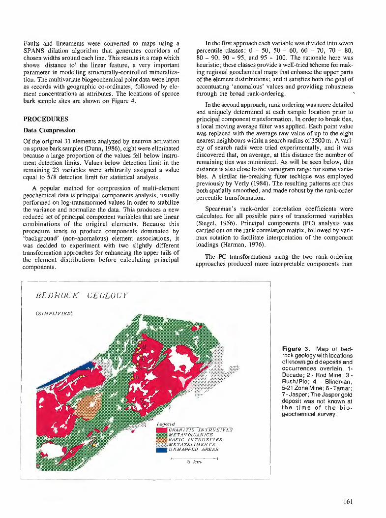
Faults and lineaments were converted to maps using a SPANS dilation algorithm that generates corridors of chosen widths around each line. This results in a map which shows 'distance to' the linear feature, a very important parameter in modelling structurally-controlled mineralization. The multivariate biogeochemical point data were input as records with geographic co-ordinates, followed by element concentrations as attributes. The locations of spruce bark sample sites are shown on Figure 4.

PROCEDURES

Data Compression

Of the original 31 elements analyzed by neutron activation on spruce bark samples (Dunn, 1986), eight were eliminated because a large proportion of the values fell below instrument detection limits. Values below detection limit in the remaining 23 variables were arbitrarily assigned a value equal to 518 detection limit for statistical analysis.

A popular method for compression of multi-element geochemical data is principal components analysis, usually performed on log-transmormed values in order to stabilize the variance and normalize the data. This produces a new reduced set of principal component variables that are linear combinations of the original elements. Because this procedure tends to produce components dominated by 'background' (non-anomalous) element associations, it was decided to experiment with two slightly different transformation approaches for enhancing the upper tails of the element distributions before calculating principal components.

In the first approach each variable was divided into seven percentile classes: 0 - 50, 50 - 60, 60 - 70, 70 - 80, 80 - 90, 90 - 95, and 95 - 100. The rationale here was heuristic; these classes provide a well-tried scheme for making regional geochemical maps that enhance the upper parts of the element distributions ; and it satisfies both the goal of accentuating 'anomalous' values and providing robustness through the broad rank-ordering.

In the second approach, rank ordering was more detailed and uniquely determined at each sample location prior to principal component transformation. In order to break ties, a local moving average filter was applied. Each point value was replaced with the average raw value of up to the eight nearest neighbours within a search radius of 1500 m. A variety of search radii were tried experimentally, and it was discovered that, on average, at this distance the number of remaining ties was minimized. As will be seen below, this distance is also close to the variogram range for some variables. A similar tie-breaking filter techique was employed previously by Verly (1984). The resulting patterns are thus both spatially smoothed, and made robust by the rank-order percentile transformation.

Spearman's rank-order correlation coefficients were calculated for all possible pairs of transformed variables (Siegel, 1956). Principal components (PC) analysis was carried out on the rank correlation matrix, followed by varimax rotation to facilitate interpretation of the component loadings (Harman, 1976).

The PC transformations using the two rank-ordering approaches produced more interpretable components than

1 BEDROCK GEOLOGY

Legend :> I GRANITIC IN T R U S I V E S

METAV OLCANICS

. . . . . . . . BASIC I N TRUST TrES

.:.:.:.:.:.:.:(ME .............. : TASEDIMEN TS UNMAPPED AREAS

Figure 3. Map of bedrock geology with locations of known gold deposits and occurrences overlain. 1 - Decade; 2 - Rod Mine; 3 - RushlPie; 4 - Blindman; 5-21 Zone Mine; 6 - Tamar; 7 -Jasper; The Jasper gold deposit was not known at t h e t ime of t h e biogeochemical survey.

those derived from the log-transformed data sets when the loadings on elements which are often geochemically associated with gold (e.g., Mo and Sb) were examined. The detailed rank-ordering approach is slightly better than the broad rank-ordering (classification) approach since it produced loadings for molybdenum which were better differentiated from 'background' levels. Only results using this approach are discussed further. The loadings of the first four principal components for the detailed rank-ordered data set are illustrated in Figure 5. The first component has an eigenvalue of 1 1.4, accounting for 49.4 % of the variance, and is associated mainly with Cr , Fe, Sc, Th, U , La, Sm and Yb. The second component has an eigenvalue of 2.5, accounting for 1 1.0 % of the variance, and represents an association of Sb, Mo, Au, Zn, Cs and U. Sb and Mo feature prominently in this association (Fig 5). For this particular study, the second PC with Au-associated elements, particularly Sb, Mo and Cs, is used subsequently as a multi- element signature, and is interpreted to be related to Au-mineralization. The remaining PCs are not used in the present paper.

The PC2 loadings were used to calculate "Au mineralization" scores, S :

23

Si = x l j r i j for i = 1, 2,.. . , n samples j=l

where Ij = loading for variable j rij = rank of variable j for sample i

In order to facilitate indentifying anomalous values, scores were later grouped into the same seven percentile classes previoudy selected for classifying the raw data using the first approach.

By mapping PC2 scores, the multi-element geochemical data were reduced to a single derived geochemical map which shows the distribution of areas where the spruce bark data are anomalous in gold and gold-related elements. The next section of the paper discusses this conversion of 'PC2-scores' point data into map form.

POINT CONVERSIONS TO MAPS

The built-in SPANS techniques of contouring by triangulation and the potential mapping (POTMAP) are treated here. Outside SPANS a kriging program was used for calculating interpolated values during point to map conversions. This was not convenient computationally, but did allow for a general evaluation of the performance of the SPANS methods. Comparisons are based on maps of the second principal component, for the three methods.

1 0 4 O 0 5'W

LOCATION OF SAMPLE P O I N T S 5 6 0 0 3 ' ~ +

0 U TLINE OF PO TMAP MASK

KRI GING-VARIANCE MASK

Figure 4. Location of spruce bark sample sites.

162

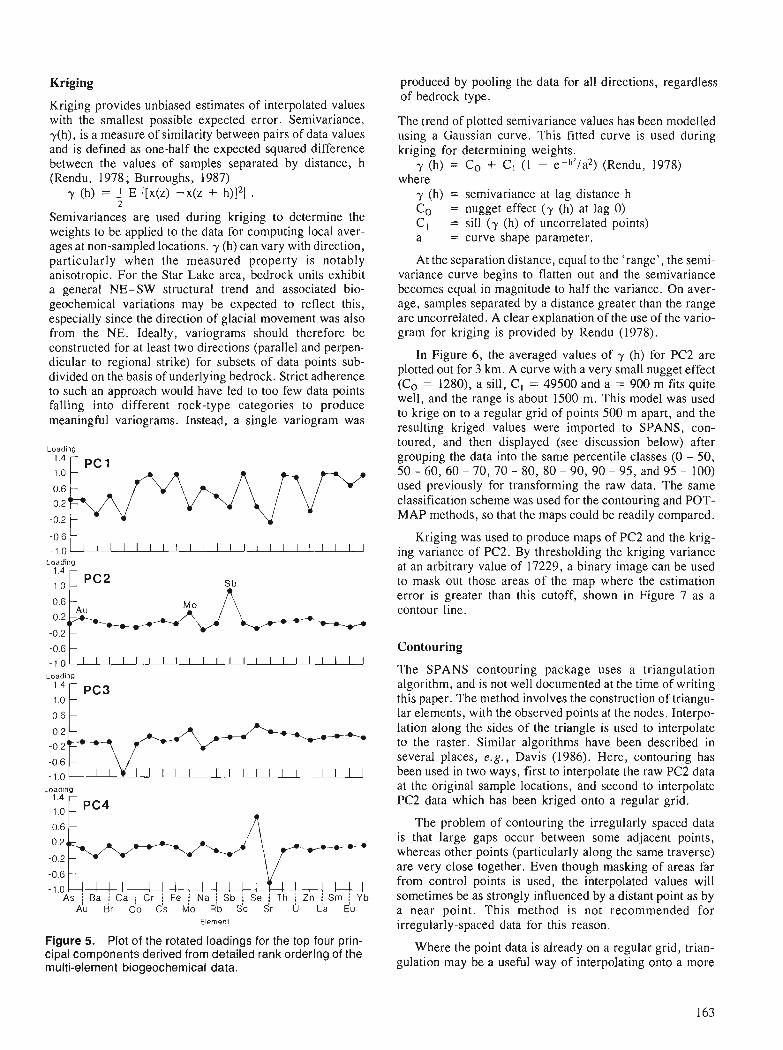
Kriging

Kriging provides unbiased estimates of interpolated values with the smallest possible expected error. Semivariance, y(h), is a measure of similarity between pairs of data values and is defined as one-half the expected squared difference between the values of samples separated by distance, h (Rendu, 1978 ; Burroughs, 1987)

7 (h) = t E {[x(z) -x(z + h)121 .

Semivariances are used during kriging to determine the weights to be applied to the data for computing local averages at non-sampled locations. y (h) can vary with direction, particularly when the measured property is notably anisotropic. For the Star Lake area, bedrock units exhibit a general NE-SW structural trend and associated biogeochemical variations may be expected to reflect this, especially since the direction of glacial movement was also from the NE. Ideally, variograms should therefore be constructed for at least two directions (parallel and perpendicular to regional strike) for subsets of data points subdivided on the basis of underlying bedrock. Strict adherence to such an approach would have led to too few data points falling into different rock-type categories to produce meaningful variograms. Instead, a single variogram was

Loading 1.4

0.2

-0.2

-0.6 - 1 . 0 1 I I I 1 I I I I I I I I I I I I I I I I 1 I

Loading

Loading ;:: 1 PC3

Loading

/

-0.6 -

-1.0 ! ! ! ! ! ! I ! I ! ! I ! I As j Ba Ca / Cr / Fe i Na ! ~b i S'e Th / Zn i Srn / Yb

AU Br C'O C'S M'o ~b ~ ' c Sr 0 L'a iu Elemenl

Figure 5. Plot of the rotated loadings for the top four principal components derived from detailed rank ordering of the multi-element biogeochemical data.

produced by pooling the data for all directions, regardless of bedrock type.

The trend of plotted semivariance values has been modelled using a Gaussian curve. This fitted curve is used during kriging for determining weights.

y (h) = Co + C I (1 - e-h21a2) (Rendu, 1978) where

y (h) = semivariance at lag distance h Co = nugget effect (y (h) at lag 0) C l = sill ( y (h) of uncorrelated points) a = curve shape parameter.

At the separation distance, equal to the 'range', the semivariance curve begins to flatten out and the semivariance becomes equal in magnitude to half the variance. On average, samples separated by a distance greater than the range are uncorrelated. A clear explanation of the use of the variogram for kriging is provided by Rendu (1978).

In Figure 6 , the averaged values of -y (h) for PC2 are plotted out for 3 km. A curve with a very small nugget effect (Co = 1280), a sill, C l = 49500 and a = 900 m fits quite well, and the range is about 1500 m. This model was used to krige on to a regular grid of points 500 m apart, and the resulting kriged values were imported to SPANS, contoured, and then displayed (see discussion below) after grouping the data into the same percentile classes (0 - 50, 50 - 60, 60 - 70, 70 - 80, 80 - 90, 90 - 95, and 95 - 100) used previously for transforming the raw data. The same classification scheme was used for the contouring and POT- MAP methods, so that the maps could be readily compared.

Kriging was used to produce maps of PC2 and the kriging variance of PC2. By thresholding the kriging variance at an arbitrary value of 17229, a binary image can be used to mask out those areas of the map where the estimation error is greater than this cutoff, shown in Figure 7 as a contour line.

Contouring

The SPANS contouring package uses a triangulation algorithm, and is not well documented at the time of writing this paper. The method involves the construction of triangular elements, with the observed points at the nodes. Interpo- lation along the sides of the triangle is used to interpolate to the raster. Similar algorithms have been described in several places, e.g., Davis (1986). Here, contouring has been used in two ways, first to interpolate the raw PC2 data at the original sample locations, and second to interpolate PC2 data which has been kriged onto a regular grid.

The problem of contouring the irregularly spaced data is that large gaps occur between some adjacent points, whereas other points (particularly along the same traverse) are very close together. Even though masking of areas far from control points is used, the interpolated values will sometimes be as strongly influenced by a distant point as by a near point. This method is not recommended for irregularly-spaced data for this reason.

Where the point data is already on a regular grid, triangulation may be a useful way of interpolating onto a more

finely divided raster. In the present study, output from the Potential Mapping - "POTMAP" kriging program consisted of x , y coordinates, kriging esti- This SPANS interpolation function assumes a circular zone mate and kriging variance for each point on a grid. It was of influence, and the points falling into the circle are convenient to convert these point data to a raster format weighted as functions of distance from the centre. Two using the SPANS contouring method, with the smoothness parameters, a and 6 , are used to define the model for of the resulting contours ultimately controlled by the pixel weighting as illustrated in Figure 8. For a point lying at a resolution of the display monitor. This was the method used distance, d, from the centre of me interpolation circle, the to produce Figure 7. weight, w , is given by a curve which passes through

Semrvariance 60000 r

1- Range 1500 metres -i

annnn L

I I I I

ffect, yo= 1280 , , , 500 1000 1500 2000 2500 3000

Distance (metres)

Figure 6. Variogram of second principal component (PC2) scores.

Figure 7. Kriging estimates of PC2 scores. The kriging-variance mask is for a cut off of 17229. A radius of 1500m was used in defining the POTMAP mask.

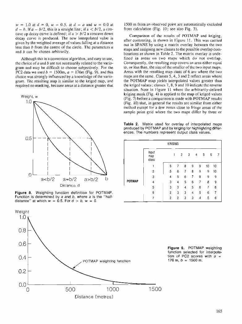
w = 1 . 0 a t d = 0, w = 0.5. a t d = a a n d w = 0.0a t d = 6. If a = 612, this is a straight line; if a < 612, a concave up decay curve is defined ; if a > 612 a concave down decay curve is produced. The new interpolated value is given by the weighted average of values falling at a distance less than b from the centre of the circle. The parameters a and b can be chosen arbitrarily.

Although this is a convenient algorithm, and easy to use, the choice of a and b are not necessarily related to the variogram and may be difficult to choose subjectively. For the PC2 data we used b = 1500m, a = 176m (Fig. 9), and this choice was strongly influenced by a knowledge of the variogram. The resulting map is similar to the kriged map, and required no masking, because areas at a distance greater that

Weight, w

a=b/2 a>b/2 lo Distance, d

Figure 8. Weighting function definition for POTMAP. Function is determined by a and b, where a is the "half- distance" at which w = 0.5. For d > b, w = 0.

Weight

1500 m from an observed point are automatically excluded from calculation (Fig. 10; see also Fig. 3).

Comparison of the results of POTMAP and kriging, after contouring, is shown in Figure 1 1 . This was carried out in SPANS by using a matrix overlay between the two maps and assigning new classes to the possible overlap combinations as shown in Table 2. The matrix overlay is undefined in areas on two maps which do not overlap. Consequently, the resulting map covers an area either equal to, or less than, the size of the smaller of the two input maps. Areas with the resulting map class of 6 are where the two maps are the same. Classes 5 ,4 , 3 and 2 reflect areas where the POTMAP map yields interpolated values greater than the kriged values; classes 7, 8, 9 and 10 indicate the reverse situation. Note in Figure 1 1 where the arbitrarily-defined kriging mask (Fig. 4) is applied to the map of kriged values (Fig. 7) before a comparison is made with POTMAP results (Fig. 10) that, in general the results are similar from either method except for a few zones close to fringe areas of the sample point grid where the two maps differ by three or

Table 2. Matrix used for overlay of interpolated maps produced by POTMAP and by kriging for highlighting differences. The numbers represent output class values.

POTMAP weighting function

1

0 500 1000 1500

KRlGlNG

Figure 9. POTMAP weighting function selected for interpolation of PC2 scores with a = 176 m, b = 1500 m.

POTMAP

Distance (metres)

Input map 1 2 3 4 5 6 7 class

1

2

3 4

5

6 7

6 7 8 9 9 1 0 1 0

5 6 7 8 9 9 1 0

4 5 6 7 8 9 9

3 4 5 6 7 8 9

3 3 4 5 6 7 8

2 3 3 4 5 6 7 2 2 3 3 4 5 6

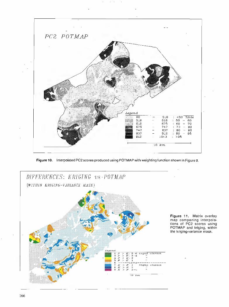
PC2 POTMAP

Figure 10. Interpolated PC2 scores produced using POTMAP with weighting function shown in Figure 8.

DIFFERENCES: KRIGJNG vs POTMAP ( W I T H I N KRIGIIVG-VARIANCE MASII )

Figure 11. Matrix overlay map cornpaning interpolations of PC2 scores using POTMAP and kriging, within the kriging-variance mask.

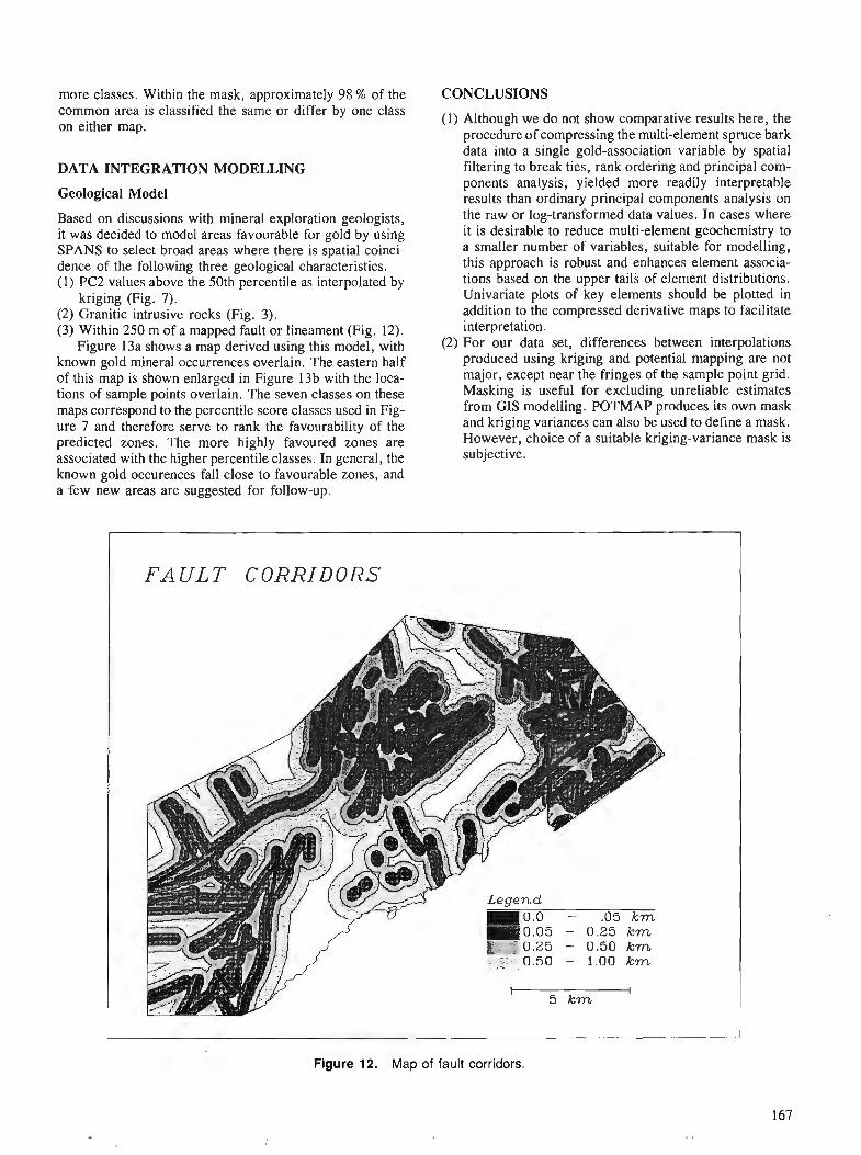
more classes. Within the mask, approximately 98 % of the CONCLUSIONS common area is classified the same or differeby one class on either map.

DATA INTEGRATION MODELLING

Geological Model

Based on discussions with mineral exploration geologists, it was decided to model areas favourable for gold by using SPANS to select broad areas where there is spatial coincidence of the following three geological characteristics. (1) PC2 values above the 50th percentile as interpolated by

kriging (Fig. 7). (2) Granitic intrusive rocks (Fig. 3). (3) Within 250 m of a mapped fault or lineament (Fig. 12).

Figure 13a shows a map derived using this model, with known gold mineral occurrences overlain. The eastern half of this map is shown enlarged in Figure 13b with the locations of sample points overlain. The seven classes on these maps correspond to the percentile score classes used in Fig- ure 7 and therefore serve to rank the favourability of the predicted zones. The more highly favoured zones are associated with the higher percentile classes. In general, the known gold occurences fall close to favourable zones, and a few new areas are suggested for follow-up.

(1) Although we do not show comparative results here, the procedure of compressing the multi-element spruce bark data into a single gold-association variable by spatial filtering to break ties, rank ordering and principal components analysis, yielded more readily interpretable results than ordinary principal components analysis on the raw or log-transformed data values. In cases where it is desirable to reduce multi-element geochemistry to a smaller number of variables, suitable for modelling, this approach is robust and enhances element associations based on the upper tails of element distributions. Univariate plots of key elements should be plotted in addition to the compressed derivative maps to facilitate interpretation.

(2) For our data set, differences between interpolations produced using kriging and potential mapping are not major, except near the fringes of the sample point grid. Masking is useful for excluding unreliable estimates from GIS modelling. POTMAP produces its own mask and kriging variances can also be used to define a mask. However, choice of a suitable kriging-variance mask is subjective.

F A U L T CORRIDORS

Figure 12. Map of fault corridors.

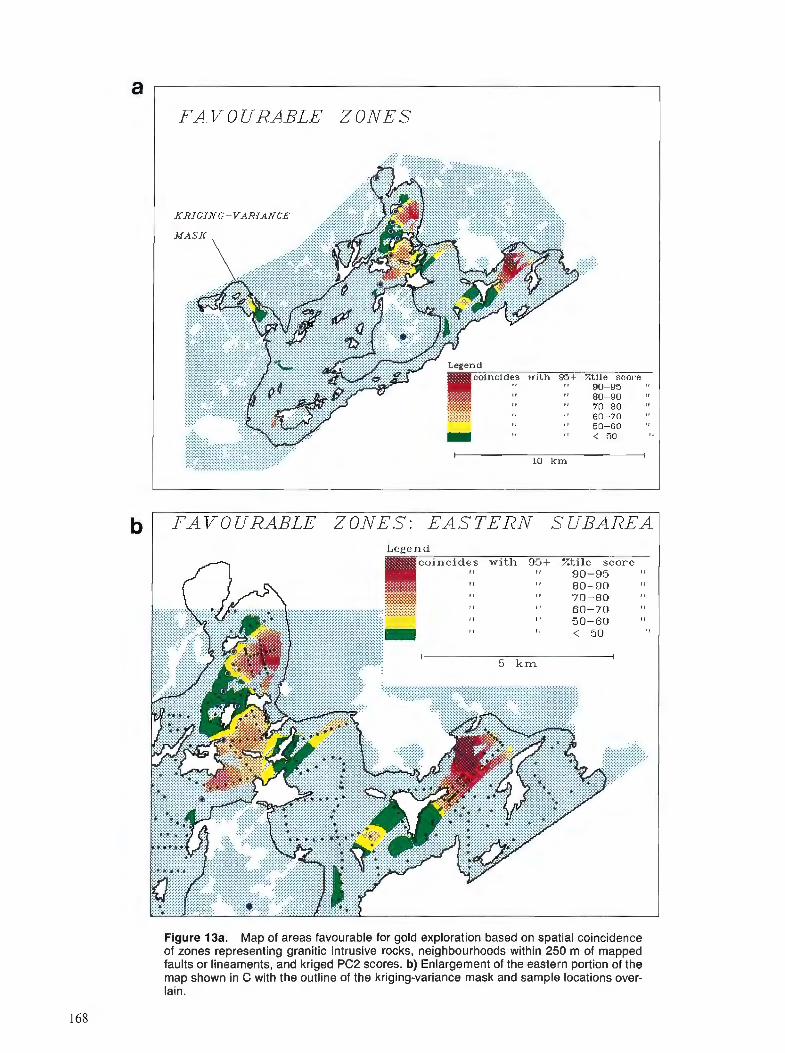
FATTOURABLE ZONES

RRIGIN G-VARIANCE

coincides with Q5+ Ztile score " 90-95 " " 80-90 "

" 70-80 "

" 60-70 "

" 50-60 "

" < 50 I

LO km I

Legend coincides with 95+ Ztile score

" 90-95 I , " 80-90 "

" 70-80

" 50-60

Figure 13a. Map of areas favourable for gold exploration based on spatial coincidence of zones representing granitic intrusive rocks, neighbourhoods within 250 m of mapped faults or lineaments, and kriged PC2 scores. b) Enlargement of the eastern portion of the map shown in C with the outline of the kriging-variance mask and sample locations overlain.

(3) Potential mapping can be used to convert point data to maps, if an interpolation procedure is desired. It is recommended, however, that a variogram be calculated for the data, to facilitate the choice of weighting parameters.

(4) A simple geological model for combining maps using Boolean operators is effective for producing a derived map showing areas favourable for gold mineralization.

(5 ) Although the data integration could be carried out without using a GIs, the major advantages of GIs for this work are: ease of data input from diverse sources, ability to use non-GIs software on shared data files, and flexible procedures for combining maps.

ACKNOWLEDGMENTS

The authors are grateful to A. Desbarats, R.G. Garrett and C.E. Dunn for practical suggestions on techniques for identifying anomalous values in multivariate geochemical data.

REFERENCES

Agterberg, F.P. 1986: Canadian experience in application of multivariate analysis tech-

niques; Proceedings, Joint USGSIGSC Workshop on Mineral Resource Appraisal, Leesburg, Virginia, September, 1985; U.S. Geological Survey Circular 980, p. 173-1 87.

Bonham-Carter, G.F., Agterberg, F.P., and Wright, D.F. 1988 : Integration of geological datasets for gold exploration in Nova Sco-

tia; Photogrammetric Engineering and Remote Sensing, v. 54, p. 1585-1592.

Burroughs, P.A. 1987: Principles of Geographical Information Systems for Land

Resource Assessment; Clarendon Press, Oxford, 193 p. Davis, J.C. 1986: Statistics and Dataanalysis in Geology; John Wiley and Sons, Inc.,

646 p. Dunn, C.E. 1986: Biogeochemical studies in the Saskatchewan gold belt; in Sum-

mary of Investigations 1986, Saskatchewan Geological Survey, Saskatchewan Energy and Mines, Miscellaneous Report 86-4, p. 129-135.

Harman, H.H. 1976: Modern Factor Analysis; University of Chicago Press, Chicago. Harper, C.T. 1986: Bedrock geological mapping, Windrum Lake area (part of NTS

64D-4, 73P-I6 and 74A-I); in Summary of Investigations 1986, Saskatchewan Geological Survey, Saskatchewan Energy and Mines, Miscellaneous Report 86-4.

Poulsen, K.H., Ames, D.E. and Galley, A.G. 1986: Gold mineralization in the Star Lake pluton, La Ronge belt,

Saskatchewan: a preliminary report; in Current Research, Part A, Geological Survey of Canada, Paper 86-lA, 205-212.

Poulsen, K.H., Ames, D.E., Galley, A.G., Derome, I., and Brommecker, R. 1987: Structural studies in the northern part of the La Ronge Domain;

in Summary of Investigations, 1987, Saskatchewan Geological Survey, Saskatchewan Energy and Mines, Miscellaneous Report 87-4.

Rendu, J.-M. 1978: An introduction to geostatistical methods of mineral evaluation.

Geostatistics 2 ; South African Institute of Mining and Metallurgy, Johannesburg, 84 p.

Schreiner, B.T. and Alley, D.W. 1984 : Quaternary gcology of the Lac La Ronge area (73-P) ; Saskatche-

wan Open File Report 84-4, Saskatchewan Energy and Mines Department.

Siegel, S. 1956: Non-parametric Statistics for the Behavioral Sciences; McGraw-

Hill Inc., 312 p. Thomas, D.J. 1985: Geological mapping, Roundish - Bervin Lakes area (part of NTS

73P-15 and -16); in Summary of Investigations, 1985, Saskatche- wan Geological Survey, Saskatchewan Energy and Mines, Miscel- laneous Report 85-4.

Tydac Technologies, Inc. 1987: Spatial Analysis System (SPANS). Reference Guide; Tydac Tech-

nologies, Inc., Ottawa, Ontario. Verly, G. 1984: The block distribution given a point multivariate normal distribu-

tion; in Geostatistics for Natural Resources Characterization, Part 1, ed. G. Verly et al., D. Reidel Publishing Company, p. 495-515.

Wilkinson, L. 1987: SYSTAT. The system for statistics, SYSTAT, Inc., Evanston,

Illinois.

Weights of evidence modelling : a new approach to mapping mineral potential

G.F. Bonham-Carterl, F.P. Agterbergl and D.F. Wright1

Bonham-Carter, G. F. Agterberg, F. P. and Wright, D. F., Weights of evidence modelling : a new approach to mapping mineral potential; & Statistical Applications in the Earth Sciences, ed. F.P. Agterberg and G. F. Bonham-Carter; Geological Survey of Canada, Paper 89-9, p. 171-183, 1989.

Abstract

Seven maps have been combined using a weights of evidence model to predict gold potential in the Meguma terrane of eastern shore Nova Scotia. f i e model uses the spatial distribution of known mineral occurrences to calculate a multi-map signature for gold mineralization, which is then employed to map gold potential.

In weights of evidence modelling, the log of the posterior odds of a mineral occurrence lying within a unit area is determined by adding a weight for each input map to the log of the prior odds; the ultimate product is a map of posterior probability, or mineral potential. When the input maps are binary, the weight added is either W+ (binary pattern present) on W- (binary pattern absent). f ie variances of the weights permit the calculation of an uncertainty map, which is augmented firther in areas where one or more of the input maps is missing. The strength of association between the input map and the known mineral occurrence points is expressed as a contrast C= W+-W-, and the significance of C can be tested by estimating o (C). The weights are calculated as log ratios of conditional probabilities. The model assumes that the input maps are conditionally independent from one another, with respect to the known occurrence points. This assumption is tested a) by painvise tests, and b) by an overall comparison of model predictions with observations, using all input maps.

Previous work demonstrated that in order of contrast, the relative importance of the input maps for predicting known gold in eastern shore Meguma terrane is 1) presence of the Goldenville Formation, 2) proximity of anticlinal axes, 3) presence of a multi-element lake-sediment anomaly, 4) proximity to the Goldenville-Halifax contact, 5) proximity to the granite contact, and 6) proximity to NW structural lineaments. The new map showing Au in balsam j r anomalies is found to be strongly predictive of the known gold occurrences, with a value of Cjust larger than that for the lake-sediment signature. Pairwise tests show that the new map is conditionally independent of the other input maps with respect to the gold occurrences. By plotting past production from known gold occurrences on a graph of posterior probability versus cumulative area, it is shown that the larger gold producers are associated with map areas having a higher posterior probability than those points with no known production.

Three new areas predicted by the model are proposed as good prospects for gold mineralization. One is about 6 km south of Goldenville, one is between the Sherbrooke pluton and Seal Harbour, and a smaller one is about 2 km north of the Sherbrooke pluton.

On a combine'sept cartes en utilisant un modtle a ponde'ration de donnke~pourp~e'voir les possibilitks de min6ralisation en or du terrane de Meguma sur la cBte est de la Nouvelle-Ecosse. A partir de la re'partition spatiale de venues mine'rales connues, le modtle calcule une signature multicarte pour la minkralisation en or; cette signature sert ensuite a cartographier le potentiel aurifere.

' Geological Survey of Canada, 601 Booth St., Ottawa, Ontario KIA 0E8

Duns la mode'lisation ponde'ration de donne'es, on de'termine le logarithme de la probabilite' poste'rieure qu 'une venue mine'rale soit situe'e duns une aire unitaire en additionnant un facteur deponde- ration pour chaque carte d'entre'e au logarithme de la probabilite' antdrieure; le produit final est une carte de la probabilite' poste'rieure ou du potentiel mine'ral. Larsque les cartes d'entre'e sont binaires, le facteur de ponde'ration ajoute' est soit W+ (prksence de configuration binaire) soit W- (absence de configuration binaire). Les variances des facteurs de ponde'ration permettent de calculer une carte d'incertitude; cette incertitude est d'ailleurs plus grande dans les re'gions ou manquent une ou plusieurs cartes d'entre'e. La force de la relation entre la carte d'entre'e et les venues mine'rales connues est exprime'e sous la forme d'un contraste C = W+ - W-, et on peut ve'r~3er la signi$cation de C en e'valu- ant o (C). Les facteurs de ponde'ration sont calcule'es sous forme de rapports logarithmiques de probabilite's conditionnelles. I1 est suppose', dans le modtle, que les cartes d'entre'e sont inde'pendantes conditionnellement les unes des autres en ce qui a trait aux venues connues. On ve'rifie cette hypothbse a) en eflectuant des essais par couples, et b) en effectuant une comparaison ge'ne'rale des pre'visions du modble avec des observations, a l'aide de toutes les cartes d'entre'e.

Des travaux antdrieurs ont montre' que par ordre de contraste, /'importance relative des cartes d'en- trtfe pour la pre'vision de mine'ralisations en or connues de la cBte est du terrane de Meguma est: I ) la pre'sence de la formation de Goldenville, 2) la proximite' d'axes anticlinaun, 3) la pre'sence d'une anomalie due a des se'diments lacustres renfermant plusieurs e'le'ments, 4) la proximite' du contact de Goldenville et Halifax, 5) la proximite' du contact granitique et 6) la proximite' de linkaments structurau. NO. On a trouve' que la nouvelle carte montrant des concentrations d'or anormales dans des sapins bau- miers, donnait d'excellentes pre'visions des venues d'or connues, la valeur de C ktant duns ce cas le'gkre- ment plus klevke que dans le cas de la signature des se'diments lacustres. Des essais par couples montrent que la nouvelle carte est inde'pendante conditionnellement des autres cartes d'entre'e en ce qui concerne les venues d'or. En reportant la production du passd provenant de venues d'or connues sur un graphique de probabilite' postkrieure en fonction d'une surface cumulative, on peut voir que les emplacements des plus grands gisements auriferes sont asocib a des zones cartographiques ayant une probabilite' poste'rieure plus grande que celle des points ne pre'sentant aucune production connue.

On propose trois nouvelles rkgions pre'vues par le modhle comme prdsentant de bonnes possibilitks de mine'ralisation en or: lapremiere se trouve environ 6 km au sud de Goldenville; la deuxihme, entre le pluton de Sherbrooke et Seal Harbour; et la troisihme, plus petite, h environ 2 km au nord du pluton de Sherbrooke.

INTRODUCTION

This paper describes the application of a new statistical approach for making a regional map of mineral potential by combining evidence from geological (including structural), geophysical and geochemical surveys. The method is called weights of evidence modelling, and is based on a statistical method developed for medical diagnosis, (Spiegelhalter, 1986; Spiegelhalter and Knill-Jones, 1984). It has been extended to deal with spatial prediction, "diagnosing" mineral deposits using the "symptoms" of geological, geophysical and geochemical signatures. The method has been applied to the prediction of volcanogenic massive sulphides in the Abitibi region of Quebec (Agterberg, 1989), to gold in the Meguma terrane of Nova Scotia (Agterberg et al., 1990; Bonham-Carter et al., 1988 ; and Bonham- Carter and Agterberg, 1990), and to gold in New Brunswick by Watson et al. (1989).

Past work on making maps of mineral potential using statistical methods has predortlinantly used regression techniques (e.g. Agterberg et al., 1981, Harris 1984). The discovered mineral occurrences in a region are used to develop a multivariate signature for mineralization, expressed as a vector of coefficients for the predictor variables. The coefficients are calculated using least squares regression; the resulting equation is used to generate regression scores whose magnitude reflect mineral potential.

Weights of evidence modelling also uses the locations of known mineral occurrences to determine coefficients for each predictor map. However, there are two coefficients, or weights, W+ and W-, for each predictor map; predictor maps are usually binary, and W+ and W- refer to those areas where the binary pattern is either present, or not present, respectively. A weight of 0 is used where the pattern is unknown or missing. Weights are calculated using measurements of the area of binary pattern, the total study area, the number of mineral occurrences within the binary pattern, and the total number of occurrences in the study area. Evidence of mineralization is combined from several predictive maps, using a formulation of Bayes Rule. Start- ing with a prior probability of a mineral deposit occurring in a unit area, a posterior probability is calculated, which may be larger or smaller than the prior probability, depending on the overlap combination of predictor maps and their weights.

In comparison with the regression method, weights of evidence are easy to interpret, simple to program, missing data can be accommodated, and patterns with complex spatial geometry can be modelled with the same computational effort as those with simple geometry. On the other hand, the assumption that the predictor patterns are conditionally independent with respect to the points, implicit in weights of evidence modelling, must be tested and satisfied; in regression modelling, no such assumption is required.

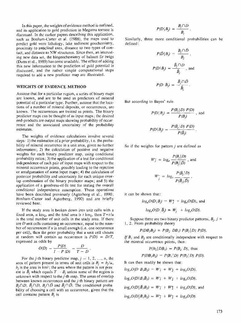
In this paper, the weights of evidence method is outlined, and its application to gold prediction in Meguma terrane is discussed. In the earlier papers describing this application, such as Bonham-Carter et al. (1988), the maps used to predict gold were lithology, lake sediment geochemistry, proximity to anticlinal axes, distance to two types of contact, and distance to NW structures. Since then, an interesting new data set, the biogeochemistry of balsam fir twigs (Dunn et al., 1989) has come available. The effect of adding this new information to the prediction of gold potential is discussed, and the rather simple computational steps required to add a new predictor map are illustrated.

WEIGHTS OF EVIDENCE METHOD

Assume that for a particular region, a series of binary maps are known, and are to be used as predictors of mineral potential of a particular type. Further, assume that the locations of a number of mineral deposits, or occurrences, are known. The occurrences are treated as points. The binary predictor maps can be thought of as input maps; the desired end-products are output maps showing probability of occurrence and the associated uncertainty of the probability estimates.

The weights of evidence calculations involve several steps : 1) the estimation of a prior probability, i.e. the probability of mineral occurrence in a unit area, given no further information; 2) the calculation of positive and negative weights for each binary predictor map, using conditional probability ratios ; 3) the application of a test for conditional independence of each pair of input maps with respect to the mineral occurrence points, possibly leading to the rejection or amalgamation of some input maps ; 4) the calculation of posterior probability and uncertainty for each unique overlap combination of the binary predictor maps; and 5) the application of a goodness-of-fit test for testing the overall conditional independence assumption. These operations have been described previously (Agterberg et al., 1990; Bonham-Carter and Agterberg, 1990) and are briefly reviewed here.

If the study area is broken down into unit cells with a fixed area, u km2, and the total area is t km2, then T=t/u is the total number of unit cells in the study area. If there are D unit cells containing an occurrence, equal to the number.of occurrences if u is small enough (i.e. one occurrence per cell), then the prior probability that a unit cell chosen at random will contain an occurrence is P(D) = D/T, expressed as odds by

O(D) = D P(D) -

1 - P ( D ) T - D

For the j-th binary predictor map, j = 1, 2, ..., n , the area of pattern present in terms of unit cells is B, = b,/u, bj is the area in km2; the area where the pattern is not present is Bj which equals T - B, unless some of the region is unknown with respect to the j-th map. The areas of overlap between known occurrences and the j-th binary pattern are Bj f l D, B, fl D, B, fl D and Bin D. The conditional probability of choosing a cell with an occurrence, given that the cell contains pattern Bj is

Similarly, three more conditional probabilities can be defined :

B,n D P(D~B,) = - , and

B,

B j n D p(D1 B,) = - .

B,

But according to Bayes' rule

P(DI Bj) = P(B, I D) PfD)

, and P (Bj)

So if the weights for pattern j are defined as

Wf = log, P(B, ID)

P(Bjl@ ' and

W: = log, PfBj I D)

J ~ ( 4 1 D)

it can be shown that:

log,O(D(B,) = Wl + log,O(D), and

log,O(D I Bj) = y~ + log,O(D).

Suppose there are two binary predictor patterns, Bj, j = 1, 2. From probability theory

p (DBIB2) = P(B2 l OBI) p (BI I D) P(D).

l f B l and B2 are conditionally independent with respect to the mineral occurrence points, then:

P(B2 1 DBl) = P(B2 1 D), thus

P(DBIB2) = P(BI ID) P(B2ID) P(D).

It can then readily be shown that:

log,O(DI BIB2) = W t + W$ + log,O(D),

log,0(D(BIB2) = Wf + W , + log,O(D),

log,O(Dl BIB2) = WT + WJ + log,O(D), and

log,O(DJ BIB2) = WT + WT + log,O(D).

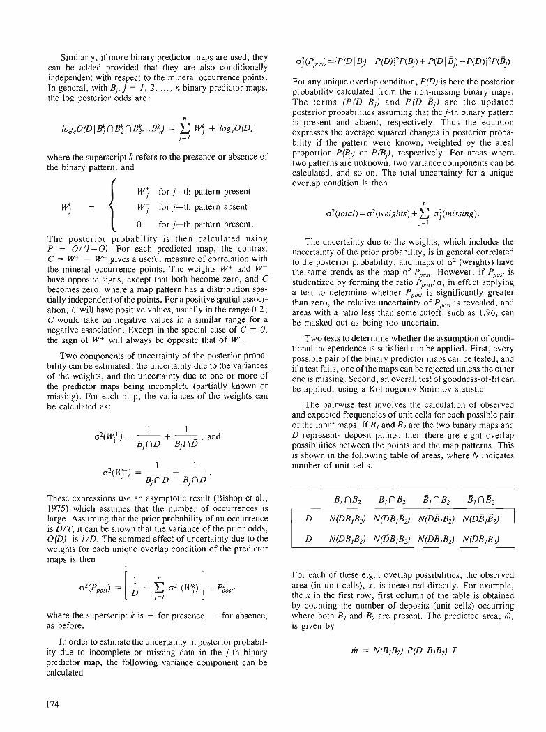
Similarly, if more binary predictor maps are used, they can be added provided that they are also conditionally independent with respect to the mineral occurrence points. In general, with Bj, j = 1, 2, ..., n binary predictor maps, the log posterior odds are:

where the superscript k refers to the presence or absence of the binary pattern, and

~f for j-th pattern present

q = WJ for j-th pattern absent

( 0 for j-th pattern present.

The posterior probability is then calculated using P = 0 / ( 1 + 0 ) . For each predicted map, the contrast C = W+ - W- gives a useful measure of correlation with the mineral occurrence points. The weights W+ and W- have opposite signs, except that both become zero, and C becomes zero, where a map pattern has a distribution spatially independent of the points. For a positive spatial association, C will have positive values, usually in the range 0-2; C would take on negative values in a similar range for a negative association. Except in the special case of C = 0, the sign of W+ will always be opposite that of W-.

Two components of uncertainty of the posterior probability can be estimated : the uncertainty due to the variances of the weights, and the uncertainty due to one or more of the predictor maps being incomplete (partially known or missing). For each map, the variances of the weights can be calculated as:

1 1 02(W;) = - + - , and

B j n D B j n D

These expressions use an asymptotic result (Bishop et al., 1975) which assumes that the number of occurrences is large. Assuming that the prior probability of an occurrence is D/T, it can be shown that the variance of the prior odds, O(D), is 1/D. The summed effect of uncertainty due to the weights for each unique overlap condition of the predictor maps is then

where the superscript k is + for presence, - for absence, as before.

In order to estimate the uncertainty in posterior probability due to incomplete or missing data in the j-th binary predictor map, the following variance component can be calculated

For any unique overlap condition, P(D) is here the posterior probability calculated from the non-missing binary maps. The terms (P(D1 Bj) and P(DI B,) a r e the updated posterior probabilities assuming that the j-th binary pattern is present and absent, respectively. Thus the equation expresses the average squared changes in posterior probability if the pattern were known, weighted by the areal proportion P(B,) or P(B,), respectively. For areas where two patterns are unknown, two variance components can be calculated, and so on. The total uncertainty for a unique overlap condition is then

The uncertainty due to the weights, which includes the uncertainty of the prior probability, is in general correlated to the posterior probability, and maps of o2 (weights) have the same trends as the map of P However, if P,,,, is studentized by forming the ratio PpoS,lo, in effect applying a test to determine whether Pp,, is significantly greater than zero, the relative uncertainty of PP,, is revealed, and areas with a ratio less than some cutoff, such as 1.96, can be masked out as being too uncertain.

Two tests to determine whether the assumption of conditional independence is satisfied can be applied. First, every possible pair of the binary predictor maps can be tested, and if a test fails, one of the maps can be rejected unless the other one is missing. Second, an overall test of goodness-of-fit can be applied, using a Kolmogorov-Smirnov statistic.

The pairwise test involves the calculation of observed and expected frequencies of unit cells for each possible pair of the input maps. If BI and B2 are the two binary maps and D represents deposit points, then there are eight overlap possibilities between the points and the map patterns. This is shown in the following table of areas, where N indicates number of unit cells.

For each of these eight overlap possibilities, the observed area (in unit cells), x, is measured directly. For example, the x in the first row, first column of the table is obtained by counting the number of deposits (unit cells) occurring where both BI and B2 are present. The predicted area, A, is given by

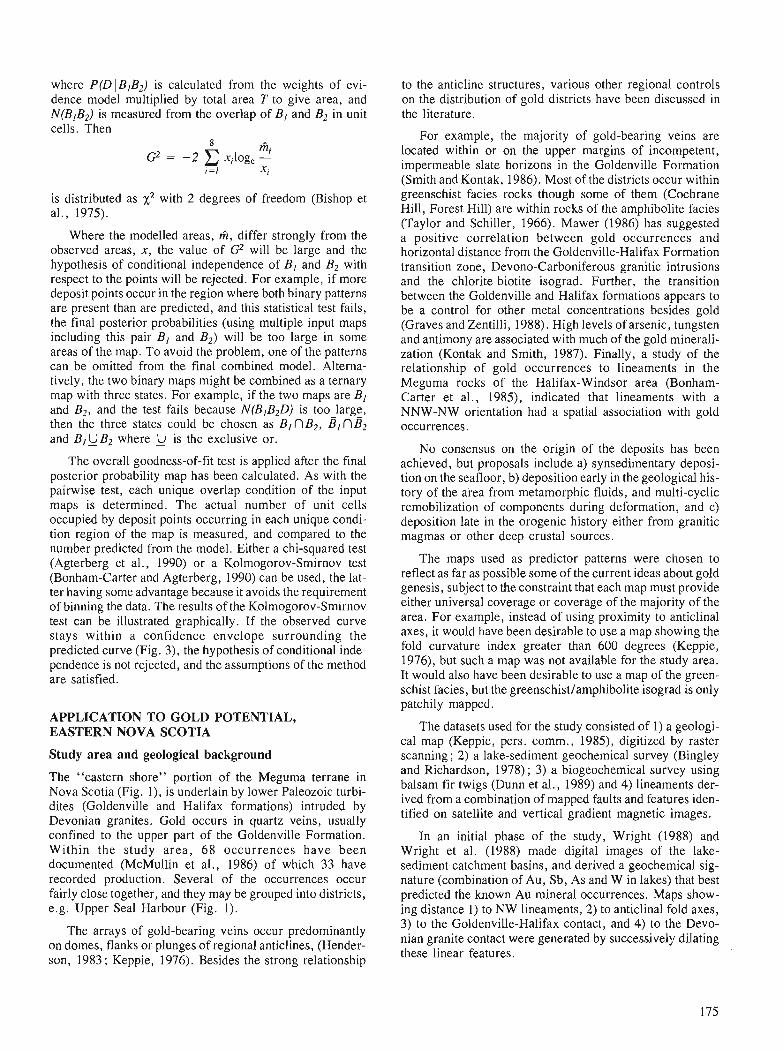
where P(DIBIB2) is calculated from the weights of evidence model multiplied by total area T to give area, and N(BIB2) is measured from the overlap of BI and B2 in unit cells. Then

is distributed as x2 with 2 degrees of freedom (Bishop et al., 1975).

Where the modelled areas, h , differ strongly from the observed areas, x , the value of G2 will be large and the hypothesis of conditional independence of B, and B2 with respect to the points will be rejected. For example, if more deposit points occur in the region where both binary patterns are present than are predicted, and this statistical test fails, the final posterior probabilities (using multiple input maps including this pair B, and B2) will be too large in some areas of the map. To avoid the problem, one of the patterns can be omitted from the final combined model. Alterna- tively, the two binary maps might be combined as a ternary map with three states. For example, if the two maps are B, and B2, and the test fails because N(BIB2D) is too large, then the three states could be chosen as BI n B 2 , B, n B2 and B I g B 2 where g is the exclusive or.

The overall goodness-of-fit test is applied after the final posterior probability map has been calculated. As with the pairwise test, each unique overlap condition of the input maps is determined. The actual number of unit cells occupied by deposit points occurring in each unique condition region of the map is measured, and compared to the number predicted from the model. Either a chi-squared test (Agterberg et al., 1990) or a Kolmogorov-Smirnov test (Bonham-Carter and Agterberg, 1990) can be used, the latter having some advantage because it avoids the requirement of binning the data. The results of the Kolmogorov-Smirnov test can be illustrated graphically. If the observed curve stays within a confidence envelope surrounding the predicted curve (Fig. 3), the hypothesis of conditional independence is not rejected, and the assumptions of the method are satisfied.

APPLICATION TO GOLD POTENTIAL, EASTERN NOVA SCOTIA

Study area and geological background

to the anticline structures, various other regional controls on the distribution of gold districts have been discussed in the literature.

For example, the majority of gold-bearing veins are located within or on the upper margins of incompetent, impermeable slate horizons in the Goldenville Formation (Smith and Kontak, 1986). Most of the districts occur within greenschist facies rocks though some of them (Cochrane Hill, Forest Hill) are within rocks of the amphibolite facies (Taylor and Schiller, 1966). Mawer (1986) has suggested a positive correlation between gold occurrences and horizontal distance from the Goldenville-Halifax Formation transition zone, Devono-Carboniferous granitic intrusions and the chlorite-biotite isograd. Further, the transition between the Goldenville and Halifax formations appears to be a control for other metal concentrations besides gold (Graves and Zentilli, 1988). High levels of arsenic, tungsten and antimony are associated with much of the gold mineralization (Kontak and Smith, 1987). Finally, a study of the relationship of gold occurrences to lineaments in the Meguma rocks of the Halifax-Windsor area (Bonham- Carter et al., 1985), indicated that lineaments with a NNW-NW orientation had a spatial association with gold occurrences.

No consensus on the origin of the deposits has been achieved, but proposals include a) synsedimentary deposition on the seafloor, b) deposition early in the geological history of the area from metamorphic fluids, and multi-cyclic remobilization of components during deformation, and c) deposition late in the orogenic history either from granitic magmas or other deep crustal sources.

The maps used as predictor patterns were chosen to reflect as far as possible some of the current ideas about gold genesis, subject to the constraint that each map must provide either universal coverage or coverage of the majority of the area. For example, instead of using proximity to anticlinal axes, it would have been desirable to use a map showing the fold curvature index greater than 600 degrees (Keppie, 1976), but such a map was not available for the study area. It would also have been desirable to use a map of the greenschist facies, but the greenschistlamphibolite isograd is only patchily mapped.

The datasets used for the study consisted of 1) a geological map (Keppie, pers. comm., 1985), digitized by raster scanning ; 2) a lake-sediment geochemical survey (Bingley

The "eastern shore" portion of the Meguma terrane in and ~ichardson, 1978); 3) a biogeochemical survey using

Nova Scotia (Fig. I ) , is underlain by lower Paleozoic turbi- balsam fir twigs (Dunn et al., 1989) and 4) lineaments derived from a combination of mapped faults and features iden- dites (Goldenville and Halifax formations) intruded by tified on and venical gradient magnetic images. Devonian granites. Gold occurs in quartz veins, usually

confined t o the upper part of the ~oidenvi l le ~drmat ion. In an initial phase of the study, Wright (1988) and Within the study area , 6 8 occurrences have been Wright et al. (1988) made dgital images of the lake- documented (McMullin et al., 1986) of which 33 have sediment catchment basins, and derived a geochemical sig- recorded production. Several of the occurrences occur nature (combination of Au, Sb, As and W in lakes) that best fairly close together, and they may be grouped into districts, predicted the known Au mineral occurrences. Maps show- e.g. Upper Seal Harbour (Fig. 1). ing distance 1) to NW lineaments, 2) to anticlinal fold axes,

The arrays of gold-bearing veins occur predominantly 3)-to the Goldenville-Halifax contact, and 4) to the Devo-

on domes, flanks or plunges of regional anticlines, (Hender- nian granite contact were generated by successively dilating

son, 1983; Keppie, 1976). Besides the strong relationship these linear features.

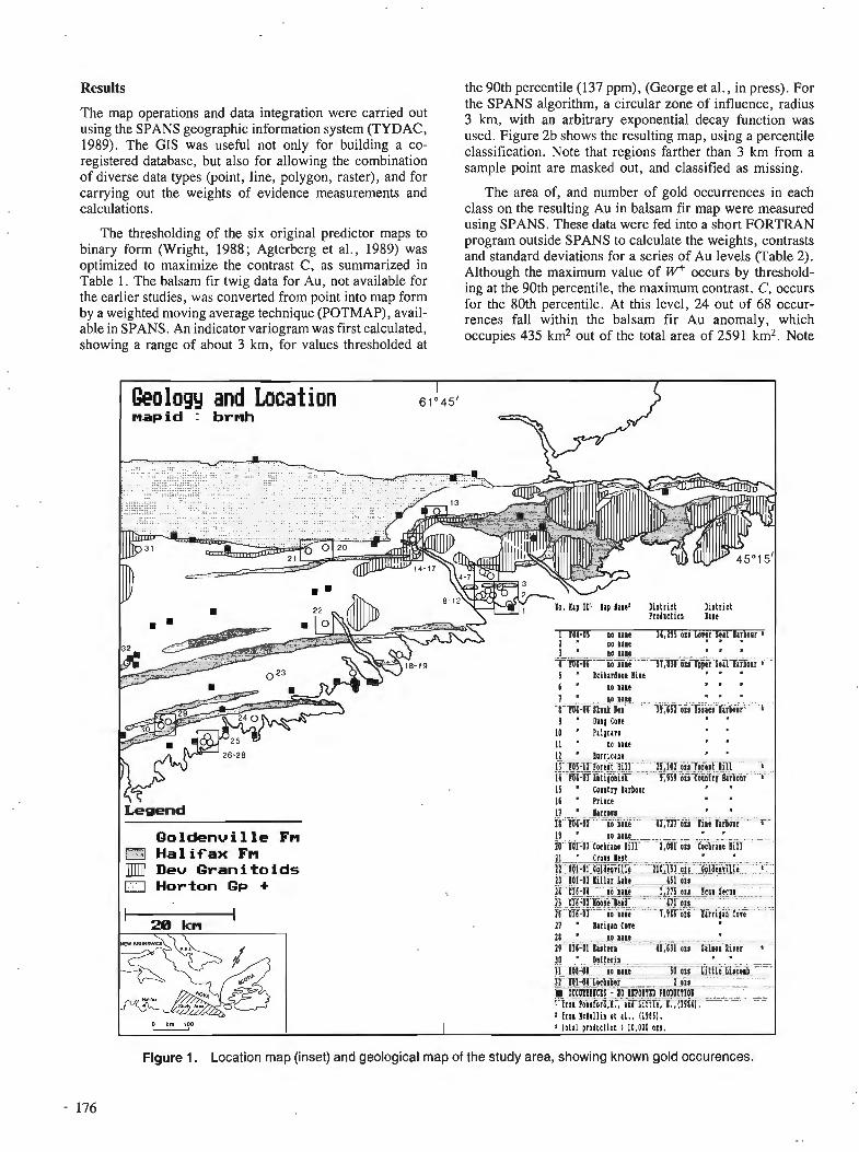
Results

The map operations and data integration were carried out using the SPANS geographic information system (TYDAC, 1989). The GIs was useful not only for building a co- registered database, but also for allowing the combination of diverse data types @oint, line, polygon, raster), and for carrying out the weights of evidence measurements and calculations.

The thresholding of the six original predictor maps to binary form (Wright, 1988; Agterberg et al., 1989) was optimized to maximize the contrast C, as summarized in Table 1. The balsam fir twig data for Au, not available for the earlier studies, was converted from point into map form by a weighted moving average technique (POTMAP), available in SPANS. An indicator variogram was first calculated, showing a range of about 3 krn, for values thresholded at

the 90th percentile (137 ppm), (George et al., in press). For the SPANS algorithm, a circular zone of influence, radius 3 km, with an arbitrary exponential decay function was used. Figure 2b shows the resulting map, using a percentile classification. Note that regions farther than 3 km from a sample point are masked out, and classified as missing.

The area of, and number of gold occurrences in each class on the resulting Au in balsam fir map were measured using SPANS. These data were fed into a short FORTRAN program outside SPANS to calculate the weights, contrasts and standard deviations for a series of Au levels (Table 2). Although the maximum value of W+ occurs by thresholding at the 90th percentile, the maximum contrast, C, occurs for the 80th percentile. At this level, 24 out of 68 occurrences fall within the balsam fir Au anomaly, which occupies 435 km2 out of the total area of 2591 km2. Note

p l a l e i D l r t r ~ c t Dirtriel P r o d w t l o ~ late

1 IO4-US l o Pale 14,295 orr Lorfr Sfal Ba!botr 1 1 ' DO hale 1 ' 10 lilt

5 ' ltlhard$ob 11ne 6 ' no nakt 1 ' PO n l l c

9 ' Dung Core 10 ' Pal(rare 11 ' no nine I1 ' lurrieane

I5 ' Colntrr Barbour 16 ' Prlnct I1 . 1arr01s-

Goldenuille Fn 19 ' I) m e - l.5 Halifax Fm 70 l01il ioi6rrne E l l 1,nl otr t o c ' b r i air1

r : I _ [IIIIII Deu Grani toids 11 l V l - 6 1 - c ~ e i i i l l e IlbJfl iu G o ~ c h i l l e 6 -

0 Horton GP + 13 016-01 %oo:t lctd 11 616-01 no tame 1,c)R or: I irri fan tore 17 ' Itrtgaa (ore 18 ' l o l r l t . - - IY D I ~ E L t t r ~ 4I.lll on STIOI l i r c r 10 ' Dafftrln ]1_18-04- DO nine 17- 101-Adodabcr_ I arCrrrlaisr - rolsanan PiaPacr~br - 1 £ ~ O I P O B S ~ O ~ ~ , I . , i ~ a ~ l t t ~ t , ~ . , ( I N ~ I

fro1 lcanl l ia et a l . , (19161.

Figure 1. Location map (inset) and geological map of the study area, showing known gold occurences.

176

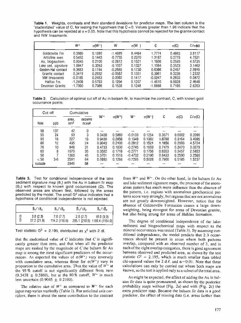
Table 1. Weights, contrasts and their standard deviations for predictor maps. The last column is the 'studentized' value of C, for testing the hypothesis that C = O . Values greater than 1.96 indicate that the hypothesis can be rejected at a = 0.05. Note that th i s hypothesis cannot be rejected for the granite contact and NW lineaments.

W+ ow-1 W- o w - ) C o(C) C/o(c)

GoldenvilleFm 0.3085 0.1280 -1.4689 0.4484 1.7774 0.4663 3.8117 Anticline axes 0.5452 0.1443 -0.7735 0.2370 1.3187 0.2775 4.7521

A u , biogeochem. 0.9045 0.2100 -0.2812 0.1521 1.1856 0.2593 4.5725 Lake sed. signature 1.0047 0.3263 -0.1037 0.1327 1.1084 0.3523 3.1462 Golden-Hal contact 0.3683 0.1744 -0.2685 0.1730 0.6368 0.2457 2.5918

Granitecontact 0.3419 0.2932 -0.0562 0.1351 0.3981 0.3228 1.2332 NW lineaments -0.0185 0.2453 0.0062 0.1417 -0.0247 0.2833 0.0872

Halifax Fm. -1.2406 0.5793 0.1204 0.1257 -1.4610 0.5928 2.4646 Devonian Granite -1.7360 0.7086 0.1528 0.1248 -1.8888 0.7195 2.6253

Table 2. Calculation of optimal cut off of Au in balsam fir, to maximize the contrast, C, with known gold occurrence points.

Cut off Cumulative

area, occurre w+ o(W+) W- o(W-) C o(C) Clo(C)

%iIe ppb krn2 nces#

98 137 42 0 - - - - - - - 95 24 93 3 0.3438 0.5869 -0.0133 0.1254 0.3571 0.6002 0.2090 90 16 227 13 0.9439 0.2856 -0.1349 0.1362 1.0788 0.3164 3.4095 80 12 435 24 0.9045 0.2100 -0.2812 0.1521 1.1856 0.2593 4.5724 70 10 848 31 0.4733 0.1830 -0.2745 0.1659 0.7479 0.2470 3.0279 60 8 1070 35 0.3582 0.1719 -0.2771 0.1756 0.6353 0.2457 2.5853 50 7 1360 45 0.3701 0.1516 -0.4732 0.2100 0.8433 0.2590 3.2560

<50 3-6 2591 64 0.0695 0.1266 -0.7295 0.5028 0.7900 0.5185 1.5237 outside 2945 68 - - - - - - -

Table 3. Test for conditional independence of the lake from Wf and W-. On the other hand, in the balsam fir Au sediment signature map (B,) with the Au in balsam f i r map and lake sediment signature maps, the presence of the anom- (B2) with respect to known gold occurrences (Dl. The alous pattern has much more influence than the absence of observed areas are shown first, followed by the areas the pattern, i.e. regions with anomalous geochemical pat- predicted by the The G2 indicates that a terns score very strongly, but regions that are not anomalous hypothesis of conditional independence is not rejected.

are not greatly downweighted. However, notice that the

Test statistic G2 = 2.195, distributed as x2 with 2 df.

that the studentized value of C indicates that C is significantly greater than zero, and that when all the predictor maps are ranked by the magnitude of C the balsam fir Au map is among the most significant predictors of the occurrences. As expected the values of ow+) vary inversely with cumulative area, whereas those for o(W-) vary in proportion to the cumulative area. Thus the value of W+ at the 95 % cutoff is not significantly different from zero (0.3438 + 0.5869), but at the 80% cutoff, W+ is much less uncertain (0.9045 k 0.2100).

The relative size of W+ as compared to W- for each input map varies markedly (Table 1). For anticlinal axis corridors, there is about the same contribution to the contrast

absence of Goldenville Formation causes a large down- weighting, being strongest for areas of Devonian granite, but also being strong for areas of Halifax formation.

The degree of conditional independence of the lake- sediment and biogeochemical maps with respect to the mineral occurrences was tested (Table 3). By assuming conditional independence, the model predicts that 2.3 occurrences should be present in areas where both patterns overlap, compared with an observed number of 3, and in each of the eight overlap categories, there is good agreement between observed and predicted area, as shown by the test statistic G2 = 2.195, which is much smaller than tabled chi-squared values for 2 d.f. and a=0.01. Note that these calculations can only be carried out where both maps are known, so the test is applied only to a subset of the total area.

As might be expected, the effect of adding the Au in balsam fir data is quite pronounced, as shown by the posterior probability maps without (Fig. 2a) and with (Fig. 2c) the extra predictor map. Because the balsam fir data is a good predictor, the effect of missing data (i.e. areas farther than

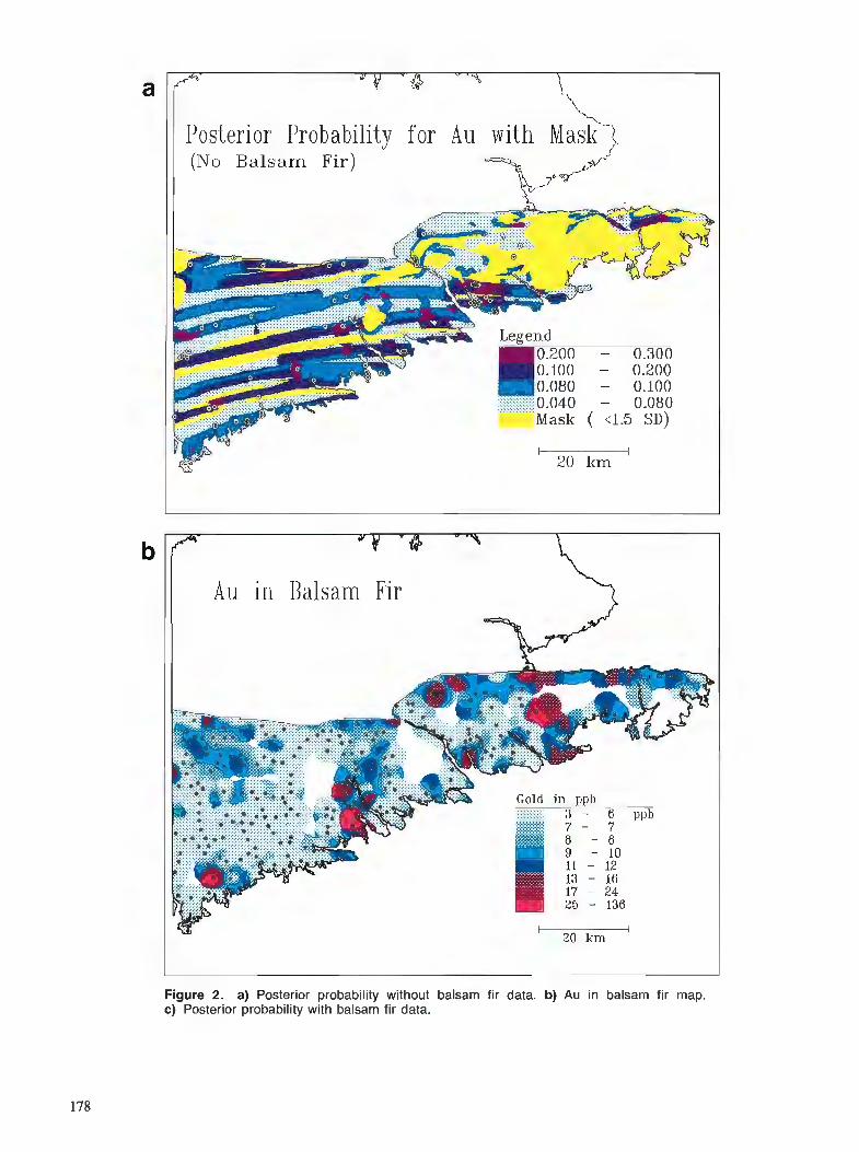
(No Balsam Fir)

Legend 0 . 2 0 0 - 0.300

D.iO0 - 0.200 0 0.080 - 0.100

0.040 - 0.080 Mask ( ~ 1 . 5 SD)

Au in Balsam Fir

in ppb 3 - 7 - 8 -

Figure 2. a) Posterior probability without balsam fir data. b) Au in balsam fir map. c) Posterior probability with balsam fir data.

3 krn from the closest biogeochemical sample) is to raise the combined uncertainty ( o ~ ~ ~ ~ ~ ~ ~ and omissing) in the missing areas to a level where Ppost < 1 .5otOta1. The areas masked out in Figures 2a, and 2c have been eliminated because the 'studentized' posterior probability (P,o,,/o,,lal) is less than 1.5, indicating a relatively large uncertainty. These masked areas include the outcrop regions of Halifax Formation and granite (because almost no occurrences are known on these formations in the study area) ; they also include regions with missing balsam fir data in Figure 2b.

To illustrate the calculation of posterior probability, three examples are shown (Table 4). In the area of the Gol- denville deposit, the four most important predictor patterns are present; the three least important are absent. Note that the posterior probability of 0.2132 f 0.1 109 is significantly greater than the prior probability of 0.023. In the case of Forest Hill before knowing the biogeochemical results, the posterior probability was only 0.0180 f 0.0071, i.e. less than the prior probability. But with the biogeochemical data, the posterior probability increased to 0.0433 + 0.0193, i.e. double the prior probability.

The overall conditional independence test (Fig. 3) indicates that the hypothesis of conditional independence is satisfied, because nowhere does the observed curve break through the confidence envelope surrounding the predicted curve. An interesting result is that if the gold occurrences with known production are plotted on a graph of posterior

probability versus cumulative area, there appears to be a positive correlation between production and posterior probability (Fig. 4). In other words, the larger gold districts are associated with higher predictions of gold potential. Although this makes sense geologically, the mineral occurrence points are not numerically weighted by production or deposit size, and there is no statistical reason that the posterior probability would automatically correlate with gold production. However, the effect may be caused by spatial clustering of points in the more important gold districts, and this has yet to be tested.

Gold prospects

Figure 5 shows an enlargement of the region roughly centred on the Sherbrooke pluton. The masked areas are where Ppos,lo < 1.5, i.e. where P,,, is not significantly greater than zero. The geological contacts are superimposed in black, and the masked areas are either granite, or Halifax Formation, or where the biogeochemical Au map is uncertain. The rectangular areas A to E are of interest, with P,,,,,,> 0.3, i.e. the probability of a gold occurrence within a 1 km2 area is about 1 in 3. Two of the areas, B (Golden- ville) and E (Seal Harbour), are known gold districts. A, C and D, on the other hand, have no reported occurrences, yet they contain essentially the same signatures as B and E. No follow-up work has yet been undertaken to investigate these prospects.

Probability for wi th

Legend > 0.300

Figure 2. Continued

M A S K ( (1.5 SD) - 20 lcin

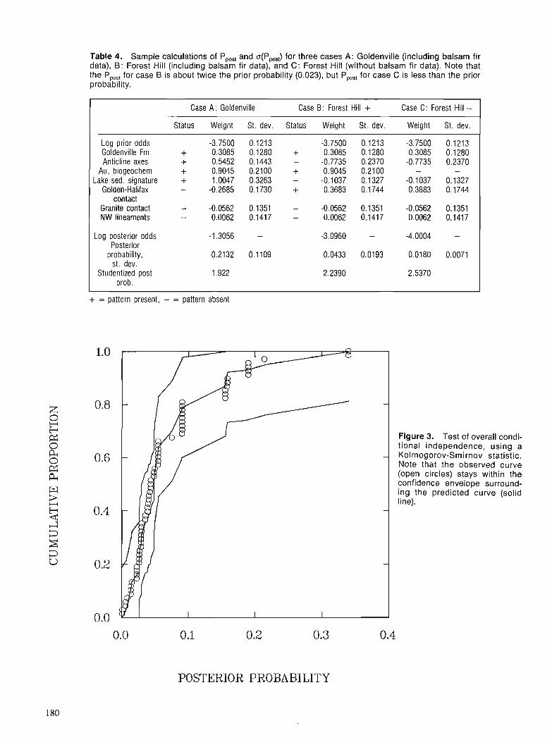
Table 4. Sample calculations of P,,,, and o(P,,,,) for three cases A: Goldenville (including balsam fir data), 6: Forest Hill (including balsam fir data), and C: Forest Hill (without balsam fir data). Note that the PPq for case 6 is about twice the prior probability (0.023), but P,,,, for case C is less than the prior probab~lity.

Case A : Goldenville Case B : Forest Hill + Case C: Forest Hill - Status Weight St. dev. Status Weight St. dev. Weight St. dev.

Log prior odds -3.7500 0.1213 -3.7500 0.1213 -3.7500 0.1213 Goldenville Fm + 0.3085 0.1280 + 0.3085 0.1280 0.3085 0.1280 Anticline axes + 0.5452 0.1443 - -0.7735 0.2370 -0.7735 0.2370

Au, biogeochem + 0.9045 0.2100 + 0.9045 0.2100 - - Lake sed. signature + 1.0047 0.3263 - -0.1 037 0.1327 -0.1037 0.1327

Golden-Halifax - -0.2685 0.1730 + 0.3683 0.1744 0.3683 0.1744 contact

Granite contact - -0.0562 0.1351 - -0.0562 0.1351 -0.0562 0.1351 NW lineaments - 0.0062 0.1417 - 0.0062 0.1417 0.0062 0.1417

Log posterior odds -1.3056 - -3.0960 - -4.0004 - Posterior

probability, 0.2132 0.1109 0.0433 0.0193 0.0180 0.0071 st, dev.

Studentized post 1.922 2.2390 2.5370 prob.

+ = pattern present, - = pattern absent

Figure 3. Test of overall conditional independence, using a Kolmogorov-Smirnov statistic. Note that the observed curve (open circles) stays within the confidence envelope surrounding the predicted curve (solid line).

POSTERIOR PROBABILITY

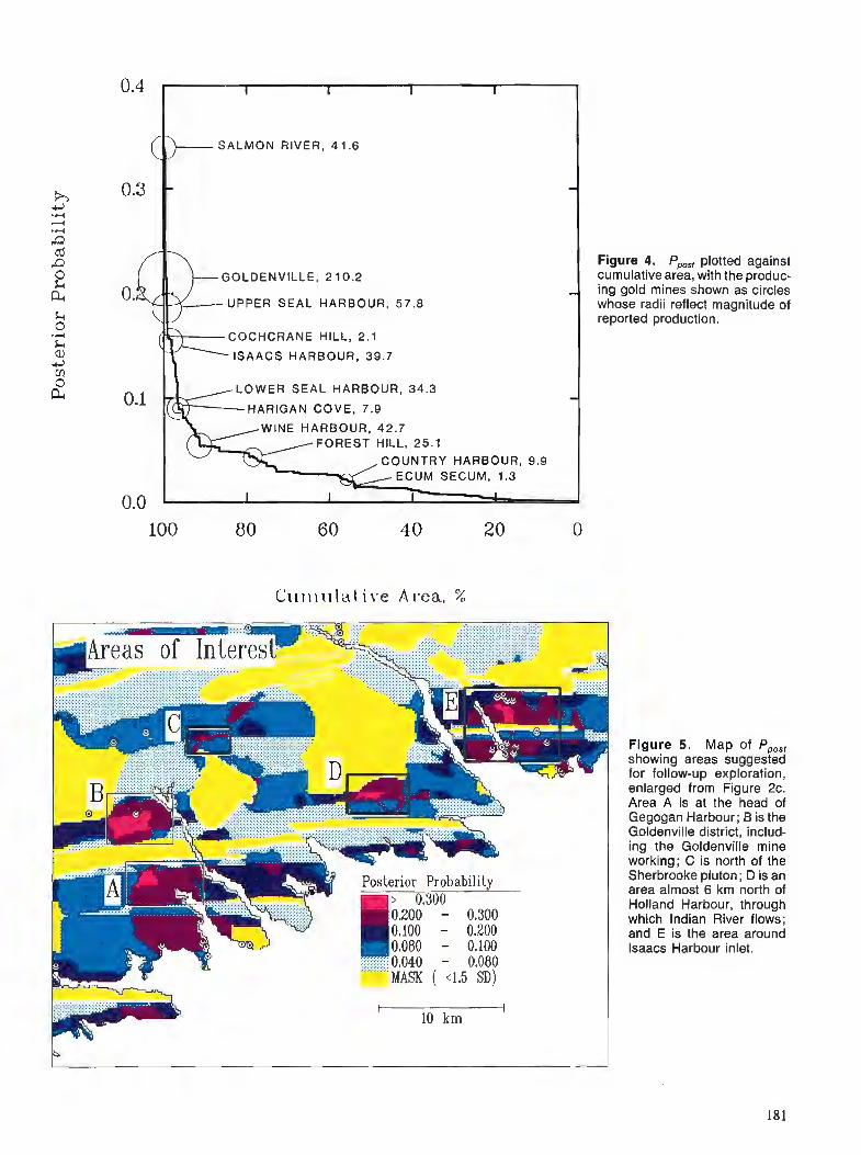
SALMON RIVER, 41.6

Figure 4. P,,,, plotted against - GoLDENVILLE, 2 10.2 cumulative area, w~th the produc-

ing gold mines shown as circles -UPPER SEAL HARBOUR, 57.8 whose radii reflect magnitude of

reported production. COCHCRANE HILL, 2.1

ISAACS HARBOUR, 39.7

LOWER SEAL HARBOUR, 34.3

HARIGAN COVE. 7.9

WINE HARBOUR, 42.7 FOREST HILL, 25.1

100 80 60 40 20 0

I \ 0,300 200 - 0.300

0.100 - 0.200 0,080 - 0.100

10,040 - 0.080 MASK ( (1.5 SD)

tlgure 5. Map of P,,,, showing areas suggested for follow-up exploration, enlarged from Figure 2c. Area A is at the head of Gegogan Harbour; B is the Goldenville district, including the Goldenville mine working; C is north of the Sherbrooke pluton; D is an area almost 6 km north of Holland Harbour, through which Indian River flows; and E is the area around lsaacs Harbour inlet.

CONCLUSIONS

1 ) Weights of evidence modelling provides a simple statistical method for predicting mineral potential for regions where a number of representative mineral occurrences are known. The weights are straightforward to interpret ; an estimate of uncertainty can be made, both using the variances of the weights and also the variance due to missing or incomplete data. The method is particularly well-suited for modelling structural information such as proximity to linear features, as well as the regional patterns of geochemical and geophysical anomalies.

2) A geographic informa.tion system, such as SPANS, is an excellent computing platform for building the database required for mapping mineral potential, for carrying out model calculations, and for visualization of the results.

3) The addition of Au in balsam fir data makes a significant contribution to the predicted mineral potential map for the eastern Meguma terrane. The predictor maps in order of their importance for predicting known Au occurrences in eastern shore Meguma are: 1) presence of Goldenville Formation; 2) proximity to the trace of an anticlinal axis; 3) the presence of a balsam fir Au anomaly; 4) the presence of a lake-sediment (Au, As, Sb, W) anomaly; 5) proximity to Goldenville-Halifax contact ; and (6) proximity to granite contact. The proximity to NW lineaments was found not to be predictive of the known occurrences in this area.

4) The posterior probability calculated for the Au occurrences shows a positive correlation with production. This gives added strength to the predictions.

5) As a result of the modelling, three prospective areas are suggested for exploration follow-up.

ACKNOWLEDGMENTS

This work was supported by the Geological Survey of Can- ada under the Canada-Nova Scotia Mineral Development Agreement (1984-1989). Duncan Keppie (Nova Scotia Department of Mines and Energy) prepared a special geological basemap for this study. Peter Rogers (Nova Scotia Department of Mines and Energy) has provided advice on the lake-sediment geochemistry. Colin. Dunn (GSC) provided a pre-publication version of the biogeochemical data, and discussion of the geological characteristics of the gold deposits with A1 Sangster (GSC) has been most helpful.

REFERENCES

Agterberg, F.P. 1989: Systematic approach to dealing with uncertainty of geoscience

information in mineral exploration; Proceedings 21st APCOM Symposium, Las Vegas, March 1989, Chapter 18, p. 165-178.

Agterberg, F.P., Bonham-Carter, G.F., and Wright, D.F. 1990: Statistical pattern integration for mineral exploration; in Gaal. G,

(ed.) P~oceedings COGEODATA Symposium on "Computer Applications in Resource Exploration", July 1988, Espo, Finland, Pergamon Press.

Agterberg, F.P., Chung, C.F., Divi, S.R., Eade, K.E., and Fabbri, A.G. 1981 : Preliminary geomathematical analysis of geological, mineral

occurrence and geophysical data, southern district of Kcewatin, Northwest Territories; Geological Survey of Canada, Open File 718, 29 p.

Bingley, J.M. and Richardson, G.G. 1978 : Regional lake sediment geochemical surveys in eastern mainland

Nova Scotia; Nova Scotia Department of Mines and Energy, Open File 37 1.

Bishop, M.M., Fienberg, S.E., and Holland, P.W. 1975 : Discrete Multivariate Analysis: Theory and Practice; MIT Press,

Cambridge, Massachusetts, 587 p. Bonham-Carter, G.F., Agterberg, F.P., and Wright, D.F. 1988: Integration of geological datasets for gold exploration in Nova Sco-

lia; Photogrammettry and Remote Sensing, v. 54, no. I I , p. 1585-1592.

Bonham-Carter, G.F. and Agterberg, F.P. 1990: Application of a microcomputer-based geographic information

system to mineral potential mapping; in Microcomputers in Geol- ogy, v. 2, ed. T. Hanley and D.F. Merriam; Pergamon Press.

Bonham-Carter, G.F., Rencz, A.N., Harris, J.R. 1985 : Spatial relationship of gold occurrences with lineaments derived

from Landsat and Seasat imagery, Meguma Group, Nova Scotia; Proceedings International Symposium on Remote Sensing of Environment, Fourth Thematic Conference : "Remote Sensing for Exploration Geology". v. 2, p. 755-767.

Dunn, C.E., Banville, R.M.P., and Adcock, S.W. 1989: Reconnaissance biogeochemical survey, Eastern Nova Scotia;

Geological Survey of Canada, Open File 2002, 95 p. George, H., Bonham-Carter, G.F., Dunn, C.E., and Rogers, P.J. in Comparative spatial analysis of anomalies derived from bio- press: geochemical and lake-sediment data, Eastern Nova Scotia; Journal

of Geochemical Exploration. Graves, M.C. and Zentilli, M. 1988: The lithochernistry of metal-enriched coticules in the Goldenville-

Halifax transition zone of the Meguma Group, Nova Scotia; in Current Research, Part B, Geological Survey of Canada, Paper 88-IB, p. 251-261.

Harris, D.P. 1984: Mineral Resources Appraisal; Clarendon Press, Oxford, 445 p. Henderson, J.R. 1983: Analysis of structure as a factor controlling gold mineralization in

Nova Scotia, k Current Research, Part B, Geological Survey of Canada, Paper 83-IB, p. 13-21.

Keppie, J.D. 1976: Structural model for the saddle reef and associated gold veins in

the Meguma Group, Nova Scotia; Nova Scotia Department of Mines and Energy, Paper 76-1, 34 p.

Kontak, D.J. and Smith, P.K. 1987: Meguma gold: The best kept secret in the Canadian mining indus-

try; Prospectors and Developers Association of Canada, Annual Meeting.

Mawer, C.K. 1986: The bedding-concordant gold-quartz veins of the Meguma Group,

Nova Scotia; k Turbidite-Hosted Gold Deposits; Geological Association of Canada, Special Paper 32, p. 135-148.

McMullin, J., Richardson, G., and Goodwin, T. 1986: Gold compilation of the Meguma Terrane in Nova Scotia; Nova

Scotia Department of Mines and Energy, Open Files 86-055,056. Smith, P.K. and Kontak, D.J. 1986: Meguma gold studies: Advances in geological insight as an aid to

gold exploration: Tenth Annual Open House and Review of Activi- ties, Program and Summaries; Nova Scotia Department of Mines and Energy, Information Series, No. 12, p. 105-114.

Spiegelhalter, D.J. 1986: Uncertainty in expert systems; Artifical Intelligence and Statis-

tics, ed. W.A. Gale; Addison-Wesley, Reading, Massachusetts, p. 17-55.

Spiegelhalter, D.J. and Knill-Jones, R.P. 1984: Statistical and knowledge-based approaches to clinical decision-

support systems, with an application in gastroenterology; Journal of the Royal Statistical Society, A, Part 1, p. 35-77.

Taylor, F.C. and Schiller, E.A. 1966: Metamorphism of the Meguma Group of Nova Scotia; Canadian

Journal of Earth Sciences, v. 3, p. 959-974. TYDAC 1989: SPANS Users Guide, Version 4.0; TYDAC Technologies Inc.,

1600 Carling Avenue, Ottawa, Ontario. Watson, G.P., Rencz, A.N., and Bonham-Carter, G.F. 1989: Computers assist prospecting; Geos., v. 18, no., 1, p. 8-15.

Wright, D.F. 1988: Data integration and geochemical evaluation of Meguma terrane,

Nova Scotia, for gold mineralization; unpublished M.Sc. Thesis, University of Ottawa, 82 p.

Wright, D.F., Bonham-Carter, G.F., and Rogers, P.J. 1988: Spatial data integration of lake-sediment geochemistry, geology

and gold occurrences, Meguma terrane, Nova Scotia; & Prospect- ing in Areas of Glaciated Terrain - 1988, ed. D.R. MacDonald and K.A. Mills, Canadian Institute of Mining and Metallurgy, p. 501-515.

Data integration studies in northern New Brunswickl

G.P. Watson2 and A.N. Rencz2

Watson, G.P. and Rencz, A.N., Data integration studies in northern New Brunswick; Statistical Analysis in the Earth Sciences, ed. F. P. Agterberg and G. F. Bonham-Carter; Geological Survey of Canada, Paper 89-9, p. 18.5-191, 1989.

Abstract

Seven different types of geoscientijk data were compiled and digitized for a study area in northern New Brunswick: i) bedrock geology, ii) mineral occurrences, iii) regional stream sediment geochemistry, iv) regional tillwgeochemistry, v) remote sensing imagery, vi) lineaments, and vii) airborne geophysics.

I..<

Weighting coeficients were assigned to each of the data sets based on the degree of spatial correspondence of each type with the location of gold-bearing mineral occurrences. The calculated coeficients for each of the seven input variables were then related in a modelling equation. The equation was evaluated for the "unique conditions" map generated by SPANS which combined the information from all of the individual thematic maps and data files used as input for the model. Z4e resulting map defines portions of the study area with high probabilities of containing gold mineralization similar to the Elmtree deposit. Generally, areas of high probability reflect known auriferous mineral occurrences or can be explained as contamination effects from active or past mining operations in the area. In this regard, the modelling equation is deemed successfil in that it accurately identifies obvious targets. There are some additional areas of high probability which are not clearly linked to known mineralization or contamination and could therefore represent viable exploration targets.

Duns le cadre d'une e'tude dans le nord du Nouveau-Brunswick, des donne'es ge'oscientijques de sept types diffdrents ont e'te' compilkes et numhiskes: i) gdologie de la roche en place, ii) venues des mine'raux, iii) ge'ochlmie des se'diments de cours d'eau re'gionaux, iv) linkaments et vii) leve's gkophysiques ae'ro- porte's.

Des coeficients de ponde'ration ont e'te' attribuds 6 chacun des ensembles de donndes en fonction du degre'de correspondance spatiale de chacun des types de donne'es avec les emplacements des manifestations des mindraux auriferes. Les coeficients calcule's pour chacune des sept variables d'entre'e on? ensuite e'tk mis en relation dans une e'quation de modklisation. Cette kquation a e'te' dvaluke pour la carte des "conditions uniques" produite au moyen du SPANS en combinant l'inforrnation de toutes les cartes the'matiques etjchiers de donnkes individuels utilisds comme donndes d'entre'e pour le mod2le. La carte rdsultante dcifinit des parties de la rdgion d'ktude ori la probabilitd est dlevde de trouver une manifestation aurifere analogue b celle du gisement Elmtree. En gdndral, les secteurs 02 la probabilitk est klevke refl2- tent des venues auriferes connues ou peuvent Ctre fxpliquds par des effets de contamination attribuables 6 des exploitations mini2res actuelles ou passe'es. A cet e'gard, l'e'quation de mode'lisation est juge'e ad&- quate puisqu 'elle permet d'identijer correctement les cibles e'videntes. La probabilitd est e'leve'e dans certains secteurs additionnels non netternent reliks d des rninkralisations ou des contaminations connues et qui constitueraient pas consdquent des cibles d'exploration viables.

' Contribution to Canada-New Brunswick Mineral Development Agreement, 1986-1989. Project carried by Geological Survey of Canada.

%eological Survey of Canada, 601 Booth Street, Ottawa, Ontario K I A 0E8

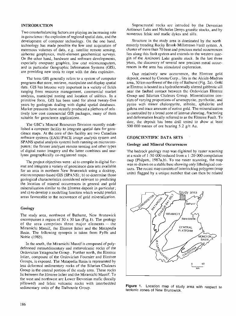
INTRODUCTION

Two counterbalancing factors are playing an increasing role in geoscience : the explosion of regional spatial data, and the development of computer technology. On the one hand, technology has made possible the low cost acquisition of enormous volumes of data, e.g. satellite remote sensing, airborne geophysics, multi-element geochemical surveys. On the other hand, hardware and software developments, especially computer graphics, low cost microcomputers, and in particular Geographic Information Systems (GIS), are providing new tools to cope with the data explosion.

The term GIS generally refers to a system of computer programs that store, retrieve, manipulate and display spatial data. GIS has become very important in a variety of fields ranging from resource management, commercial market analysis, municipal zoning and location of utilities. In a primitive form, GIS has been used for about twenty-five years by geologists dealing with digital spatial databases. Market pressures have recently produced a plethora of relatively low cost commercial GIS packages, many of them suitable for geoscience applications.

The GSC's Mineral Resources Division recently established a computer facility to integrate spatial data for geoscience maps. At the core of this facility are two Canadian software systems (EASIJPACE image analysis system and SPANS spatial analysis system) both running on microcomputers; the former analyzes remote sensing and other types of digital raster imagery and the latter combines and analyses geographically co-registered maps.

The project objectives were : a) to compile in digital format and integrate a variety of geoscience data sets available for an area in northern New Brunswick using a desktop, microcomputer-based GIS (SPANS) ; b) to determine those geological characteristics considered relevant to predicting the location of mineral occurrences in general and gold mineralization similar to the Elmtree deposit in particular; and c) to develop a modelling function which would predict areas favourable to the occurrence of gold mineralization.

Geology

The study area, northwest of Bathurst, New Brunswick encompasses a region of 30 x 30 krn (Fig. I). The geology of the area comprises three major elements - the Miramichi Massif, the Elmtree Inlier and the Matapedia Basin. The following synopsis is taken from Fyffe and Noble (1985).

In the south, the Miramichi Massif is composed of poly- deformed metasedimentary and metavolcanic rocks of the Ordovician Tetagouche Group . Further north, the Elmtree Inlier, composed of the Ordovician Fournier and Elmtree Groups, is exposed. The Matapedia Basin is represented by less deformed sedimentary rocks of the Silurian Chaleurs Group in the central portion of the study area. These rocks lie between the Elmtree Inlier and the Miramichi Massif. To the west and northwest are Lower Devonian mafic (locally pillowed) and felsic volcanic rocks with interbedded sedimentary units of the Dalhousie Group.

Supracrustal rocks are intruded by the Devonian Antinouri Lake and Nicholas Denys granitic stocks, and by numerous felsic and mafic dykes and sills.

Structure in the study area is dominated by the north- easterly trending Rocky Brook-Millstream Fault system. A cluster of more than 70 base and precious metal occurrences lies along this fault system and extends to the western margin of the Antinouri Lake granite stock. In the last three years, the discovery of several new precious metal occurrences in the area has stimulated exploration.

One relatively new occurrence, the Elmtree gold deposit, owned by Corona Corp., lies in the Alcida-Madran area, 30 km northwest of the city of Bathurst (Fig. 2a). Gold at Elmtree is hosted in a hydrothermally altered gabbroic sill near the faulted contact between the Ordovician Elmtree Group and Silurian Chaleurs Group. Mineralization consists of varying proportions of arsenopyrite, pyrrhotite, and pyrite with minor chalcopyrite, stibnite, sphalerite and galena and trace amounts of native gold. The mineralization is controlled by a broad zone of intense shearing, fracturing and deformation locally referred to as the Elmtree Fault. To date, the deposit has been drill tested to show at least 500 000 tonnes of ore bearing 5.2 g/t Au.

GEOSCIENTIFIC DATA SETS

Geology and Mineral Occurrences

The bedrock geology map was digitized by raster scanning at a scale of 1 :50 000 reduced from a 1 :20 000 compilation map (Philpott, 1987a,b). To use raster scanning, the map was re-drawn on a stable base showing only lithological contacts. The recast map consists of interlocking polygons (map units) flagged by a unique number that can then be related

Figure 1. Location map of study area with respect to tectonic zones of New Brunswick.

to an attribute (in this case rock type) through a look-up table. This map was then captured using an optical drum scanner which transformed the line information into a digital image. Subsequent processing resulted in an edited, labelled image with each polygon being represented by pixels, whose numerical value indicates the theme or map unit. The original map contained 21 different units and these were grouped into 14 classes to facilitate display in colour (Fig. 2a). The locations of all known mineral occurrences in the study area were obtained from the CANMINDEX database (Picklyk et a]., 1978). A sub-file of the locations of 18 gold- bearing mineral occurrences was also created.

Regional Geochemistry

Two sets of geochemical surveys, till and stream sediment, were used in the integration study. We used existing data from 492 till samples analyzed for 17 elements (Lamothe, 1988) and 498 stream sediment samples tested for concentrations of 1 1 elements (Boyle et al., 1966).

Till data were converted from point data into a thematic map using an interpolation routine supplied with the GIs that calculates a weighted moving average, using a sampling circle. Points occurring within the circle are assigned

weights depending on distance from the centre, according to a user-chosen model. Figure 2b shows the interpolated thematic map of gold concentration for till size fraction less than 63 micrometres and the sample locations.

Stream sediment data were converted to map form using catchment basins as the area of influence. A hand-drawn map of catchment basins was raster scanned and the basins were grouped according to element concentrations. Figure 2c shows arsenic concentration in stream sediments and sample locations.

Remote Sensing Imagery

We obtained a geometrically corrected LANDSAT Thematic Mapper (TM) image for this region. Correction was carried out using the microcomputer-based EASIIPACE image analysis system. The same system showed that vegetation around the mineralized site is spectrally different from that growing in unmineralized areas (Rencz and Wat- son, 1989). A new classified image was generated, showing areas with a spectral response similar to the Elmtree deposit area. The resulting spectral anomaly image was transferred to the SPANS GIs, and a series of corridors were generated showing distance to the spectrally anomalous areas (Fig. 2d.)

Legend CARBONIFEROUS D N FELSIC INT

a

DN MFIC INT D N FELSIC VOLC DEV MAFlC VOLC

GENERALIZED GEOLOGY and MINERAL DEPOSITS

D N SEDS D N BASALT PUIT ROCHER F R W ARMSTRONGBR FRMN SL SEDS & LlMST ORD METAMSALT ORD METAGABBRO TETAGOUCHE GP

,ELMTREE GP

Figure 2a. Generalized geology of the study area with location of Elmtree property and other gold-bearing mineral occurrences. b. Gold distribution in < 63 micrometre size fraction of till samples from study area. c. Arsenic distribution in stream sediments classified by catchment basin areas, d. Corridor map showing distances to areas of vegetation with spectral reflectance similar to the Elmtree gold occurrence. e. Corridor map showing distances to geological and LANDSAT lineaments spatially associated with mineral occurrences.

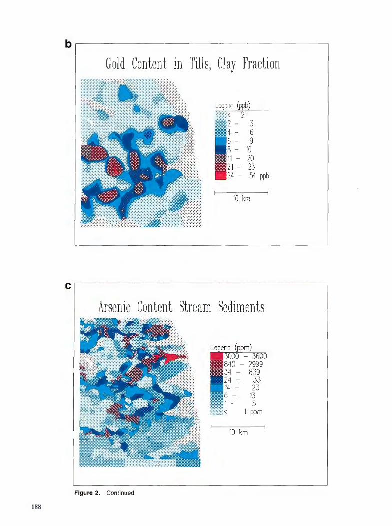
Gold Content in Tills, Clay Fraction

6 - 9 8 - 10 11 - 20 2 1 - 23 24 - 54 ppb

Arsenic Content Stream Sediments :::. .:.:.. ...

Legend (ppm)

........ ......... ........ ................. :.:.:.:.:.:.:.:.: < ........ .........

Figure 2. Continued

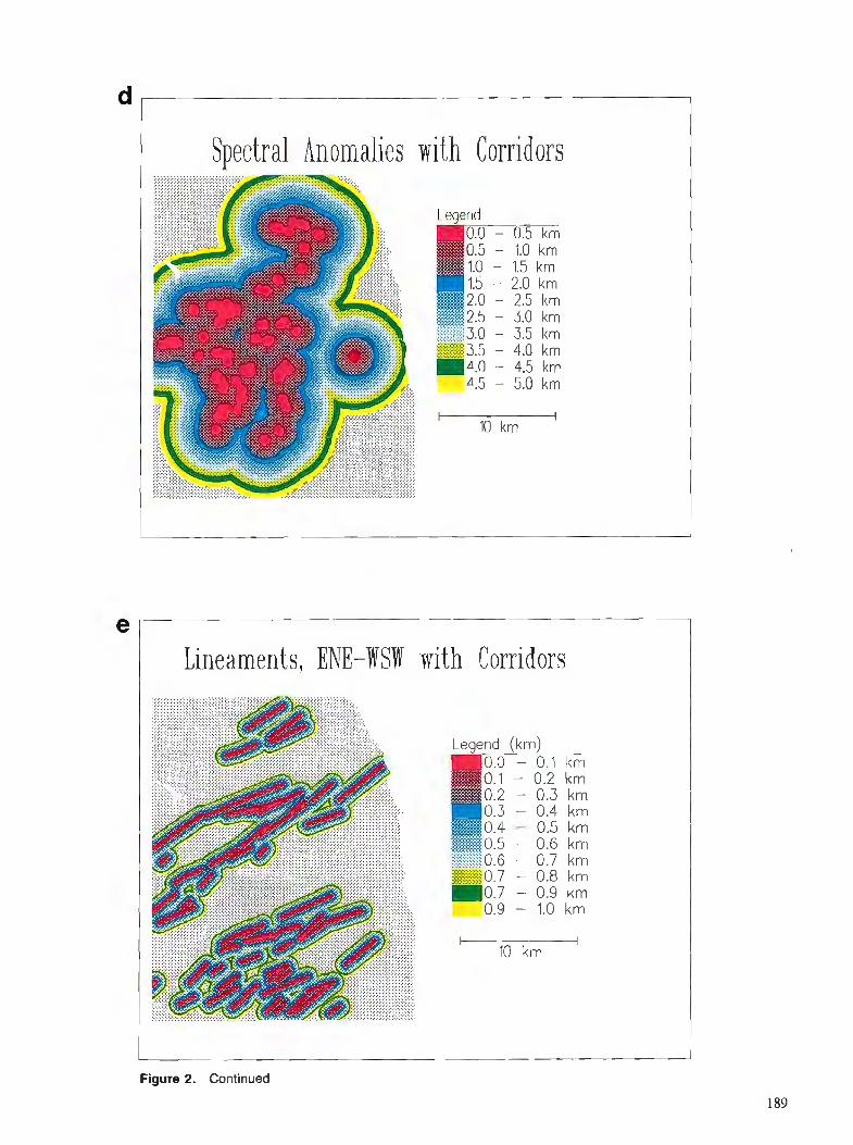
Spectral $nomalies with Corridors

Legend 0.0 - 0.5 km

Lineaments, ENE-W SW with Corridors

Legend (km) -7.0 - 0.1 k m

Figure 2. Continued

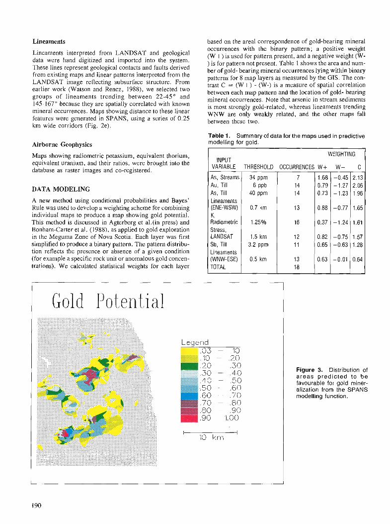
Lineaments

Lineaments interpreted from LANDSAT and geological data were hand digitized and imported into the system. These lines represent geological contacts and faults derived from existing maps and linear patterns interpreted from the LANDSAT image reflecting subsurface structure. From earlier work (Watson and Rencz, 1988), we selected two groups of lineaments trending between 22-45" and 145-167" because they are spatially correlated with known mineral occurrences. Maps showing distance to these linear features were generated in SPANS, using a series of 0.25 km wide corridors (Fig. 2e).

Airborne Geophysics

Maps showing radiometric potassium, equivalent thorium, equivalent uranium, and their ratios, were brought into the database as raster images and co-registered.

DATA MODELING

A new method using conditional probabilities and Bayes' Rule was used to develop a weighting scheme for combining individual maps to produce a map showing gold potential. This method is discussed in Agterberg et al.(in press) and Bonham-Carter et al. (1988), as applied to gold exploration in the Meguma Zone of Nova Scotia. Each layer was first simplified to produce a binary pattern. The pattern distribution reflects the presence or absence of a given condition (for example a specific rock unit or anomalous gold concentrations). We calculated statistical weights for each layer

based on the areal correspondence of gold-bearing mineral occurrences with the binary pattern; a positive weight (W +) is used for pattern present, and a negative weight (W- ) is for pattern not present. Table 1 shows the area and number of gold- bearing mineral occurrences lying within binary patterns for 8 map layers as measured by the GIs. The contrast C = (W+) - (W-) is a measure of spatial correlation between each map pattern and the location of gold- bearing mineral occurrences. Note that arsenic in stream sediments is most strongly gold-related, whereas lineaments trending WNW are only weakly related, and the other maps fall between these two.

Table 1. Summary of data for the maps used in predictive modelling for gold.

WEIGHTING INPUT

VARIABLE THRESHOLD OCCURRENCES W+ W- C

As, Till 40 PPm 14 0.73 -1.23 i:96 1 ) 0 ( 13 0 . 8 8 ( - 0 . 7 7 1 . 6 5 (

As, Streams

(WNW-ESE) 0.5 km 0.63 -0.01 0.64 ITOTAL I / 1; / 1 I I

Au, Till 6 PPb 14 0.79 -1.27 2.06 / 34 ppm

K, Radiometric Stress, LANDSAT Sb, Till Lineaments

Gold Potential

Legend 13 - . I 0

.I0 - .20

7

1.25%

1.5 km 3.2 ppm

Figure 3. Distribution of a r ea s predicted to be favourable for gold mineralization from the SPANS modelling function.

1.68

16

12 11

-0.45

0.37

0.82 0.65

2.13

-1.24

-0.75 -0.63

1.61

1.57 1.28

A 'unique conditions' map was calculated in SPANS by determining the classes resulting from the overlay of all eight binary maps. Each unique condition class represents a unique combination of the input maps. Using a SPANS routine, a modelling equation representing the combined binary map weights was applied over the unique conditions map and used to calculate the likelihood of a gold occurrence. From this we produced a new combined map (Fig. 3) divided into classes for display which portrays the probability of locating this type of mineral occurrence for the entire study area.

Generally, areas of high probability reflect known auriferous mineral occurrences or can be explained as contamination effects from active or past mining operations in the area. Figure 4 shows relative favourability compared with cumulative area of the unique conditions polygons. Note that the Elmtree property is associated with the greatest favourability, and that 10 out of the 18 gold-bearing mineral occurrences are found above the 93rd area percentile. We regard the modelling equation as successful in that it accurately identifies known targets. More importantly, when compared with Figure 2a, the predicted map (Fig. 3) indicates other areas of high favourability which are not clearly linked to known mineralization or contamination and could therefore represent viable exploration targets.

Elmtree

0.8 b .- I)

Lavigne Brook A, B, Stephens Brook 2 Rocky Brook 1, 2 2 0.6 0 > LL a I L B r a d l e y Brook A Q) Millstream # 1 0.4 1 ~arina{ m

> a LL Bradley Brook A Q) .z 0.4 - m - a, [1I

0.0

100 95 90 85 80 75

Cumulative Area, %

Figure 4. Predicted favourability for gold ve r sus cumulative area.

SUMMARY

GIs represents a significant new tool in both research and applied areas of geoscience. New forms of portraying spatial data, modelling and interpretation are now possible. Low-cost, user-friendly microcomputer- based image analysis and GIs software products are making spatial data integration and interpretation more practical and convenient. New algorithms for combining maps for estimates of mineral potential show promise. Although the gold potential map for New Brunswick is as yet untested, it suggests that favourable conditions co-exist in several areas where gold mineralization has not yet been reported.

REFERENCES

Agterberg, F.P., Bonham-Carter, G.F., and Wright, D.F. in press: Statistical pattern integration for mineral exploration; Proceed-

ings COGEODATA Symposium on Computer Applications in Resource Exploration. July 1988, Espoo, Finland.

Bonham-Carter, G.F., Agterberg, F.P., and Wright, D.F. 1988 : Integration of geological datasets for gold exploration in Nova Sco-

tia. Journal of Photgrammetric Engineering and Remote Sensing, V. 54, No. 11, p.1585- 1592.

Boyle, R.W., Tupper, W.M., Lynch, J., Freidrich, G., Ziauddin, M., Shalfiqullah, M., Carter, M., and Bygrave, K. 1966: Geochemistry of Pb, Zn, Cu, As, Sb, Mo, Sn, W, Ag, Ni, Co,

Cr, Ba, and Mn in the waters and stream sediments of the Bathurst- Jacquet River District, New Bmnswick; Geological Survey of Canada, Paper 65-42, 50 p.

Fyffe, L.R., and Noble, J.P.A. 1985: Stratigraphy and structure of the Ordovician, Silurian and Devo-

nian of northern New Brunswick; Geological Association of Can- adalMineralical Association of Canada Field Excursion No. 4, 56 P.

Larnothe, M. 1988: Till geochemistry over the northern part of the Miramichi Zone

and vicinity (New Bmnswick); A progrcss report (parts of 21 0108, 2 1 PI 11, 2 1 PI 12, 2 1 PI 13, 21 PI 14); Geological Survey of Canada, Open File 1909, 80 p., 7 maps.

Philpott, G.R. 1987a: Preliminary bedrock geological compilation of parts of the Pointe

Verte (211P13) map area; New Brunswick Department of Natural Resources, Mineral and Energy Division, Map plate 87-51A.

1987b: Preliminary bedrock geological compilation of parts of Bathurst (21lP12) map area; New Bmnswick Departmer~t of Natural Resources, Mineral and Energy Division, Map plate 87-518.

Picklyk, D.D., Rose, D.G., and Laramee, R.M. 1978: Canadian Mineral Occurrence Index (CANMINDEX) of the Geo-

logical Survey of Canada; Geological Survey of Canada, Paper 78-8, 27 p.

Rencz, A. N., and Watson, G.P. 1989: Integration of biogeochemistry and LANDSATTM data: Applica-

tion to gold exploration in northern New Brunswick; Journal of Geochemical Exploration. V. 34, p. 271-284.

Watson, G.P., and Rencz, A.N. 1988: Statistical relationship of mineral occurrences with geological and

LANDSAT-derived lineaments, northeastern New Bmnswick; in Current Research, Part B. Geological Survey of Canada, Paper 88-IB, p. 245-250.

Weighting of geophysical data with SPANS for digital geological mapping

Harold D. Moore1 and Alan F. Gregory1

Moore, H. D. and Gregory,A. F. , Weighting geophysical data with SPANS for digital geological mapping; in Statistical Applications in the EQrth Sciences, ed. F. P. Agterberg and G. F. Bonham-Carter, Geological -

Survey of Canada, Paper 89-9, p. 193-200, 1989.

Abstract

77ze integration of diflerent sets of data (geology, structure, geophysics, geochemistry, etc.) can be a powerful tool for mineral exploration and geological mapping. Modern geographic information system (GIs) technology is well suited to this task of data integration. A GIs assists the operator in studying the relationships between different data sets and in using them to map characteristic combinations. One important consideration in this process is that some types of data may be more important than others for mapping of geological units. For example, thorium concentrations may be important for mapping granites but magnetics may not be. This paper presents a method for using the SPANS2 GIS to develop weighting factors for input data for geological mapping. In essence, the process develops a locally- derived signature for the rock unit that can be used to search the data sets to locate similar units.

L'intkgration de divers ensembles de donnkes (gkologiques, structurales, gkophysiques, gkochimiques, etc.) peut constituer un outil puissant en matitre d'exploration et de cartographie gkologique. La nouvelle technologie des systbmes d'information gkographique (SIG) est un trbs bon outil d'intkgration des donnkes. Les SIG aident a ktablir les relations existant entre diflkrents ensembles de donnkes et permettent d'utiliser ces relations et ces donnkes pour cartographier certaines combinaisons caractkristiques. 11 faut cependant souligner que certains types de donnkes peuvent 2treplus importants que d'autres lorsqu 'il s'agit de cartographier des unitks gkologiques. Par exemple, les concentrations en thorium peuvent Etre importantes lorsqu 'on cartographie les formations granitiques tandis que les donnkes magnktiques peuvent s'avher duns ce cas inutiles. Cet article prksente une mkthode d'utilisation du systtme d'information gkographique SPANSpermettant d'ktablir des facteurs de pondkration relatifs aux donnkes d'entrke utiliskes en cartographie gkologique. Cette mkthode consiste essentiellement en l'ktablissement de la signature d'une unite' rocheuse, signature a l'aide de laquelle on peut rechercher les ensembles de donnkes a j n de localiser des unitks similaires.

' Gregory Geoscience Ltd., 1794 Courtwood Crescent, Ottawa, Ontario K2C 2BF Tydac Technologies Inc., 1600 Carling Avenue, Ottawa, Ontario K l Z 8R7

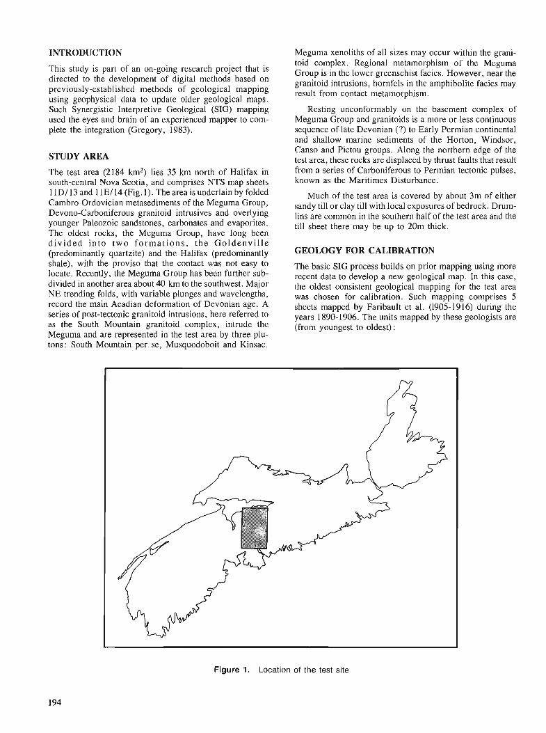
INTRODUCTION

This study is part of an on-going research project that is directed to the development of digital methods based on previously-established methods of geological mapping using geophysical data to update older geological maps. Such Synergistic Interpretive Geological (SIG) mapping used the eyes and brain of an experienced mapper to complete the integration (Gregory, 1983).

STUDY AREA

The test area (2184 km2) lies 35 km north of Halifax in south-central Nova Scotia, and comprises NTS map sheets 1 1 Dl 13 and 1 1 El 14 (Fig. 1). The area is underlain by folded Cambro-Ordovician metasediments of the Meguma Group, Devono-Carboniferous granitoid intrusives and overlying younger Paleozoic sandstones, carbonates and evaporites. The oldest rocks, the Meguma Group, have long been d i v i d e d in to t w o f o r m a t i o n s , t h e G o l d e n v i l l e (predominantly quartzite) and the Halifax (predominantly shale), with the proviso that the contact was not easy to locate. Recently, the Meguma Group has been further subdivided in another area about 40 km to the southwest. Major NE-trending folds, with variable plunges and wavelengths, record the main Acadian deformation of Devonian age. A series of post-tectonic granitoid intrusions, here referred to as the South Mountain granitoid complex, intrude the Meguma and are represented in the test area by three plutons: South Mountain per se, Musquodoboit and Kinsac.

Meguma xenoliths of all sizes may occur within the granitoid complex. Regional metamorphism of the Meguma Group is in the lower greenschist facies. However, near the granitoid intrusions, hornfels in the amphibolite facies may result from contact metamorphism.

Resting unconformably on the basement complex of Meguma Group and granitoids is a more or less continuous sequence of late Devonian (?) to Early Permian continental and shallow marine sediments of the Horton, Windsor, Canso and Pictou groups. Along the northern edge of the test area, these rocks are displaced by thrust faults that result from a series of Carboniferous to Permian tectonic pulses, known as the Maritimes Disturbance.

Much of the test area is covered by about 3m of either sandy till or clay till with local exposures of bedrock. Drum- lins are common in the southern half of the test area and the till sheet there may be up to 20m thick.

GEOLOGY FOR CALIBRATION

The basic SIG process builds on prior mapping using more recent data to develop a new geological map. In this case, the oldest consistent geological mapping for the test area was chosen for calibration. Such mapping comprises 5 sheets mapped by Faribault et al. (1905-1916) during the years 1890- 1906. The units mapped by these geologists are (from youngest to oldest) :

Figure 1. Location of the test site

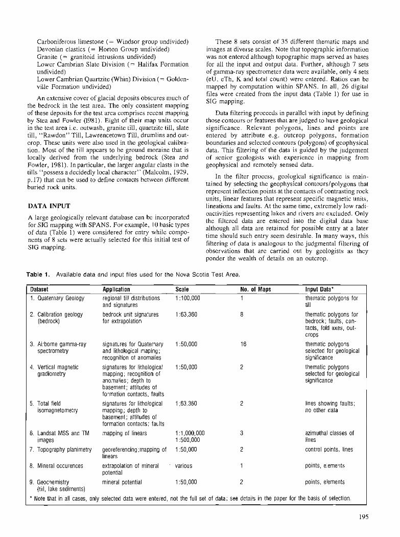
Carboniferous limestone (= Windsor group undivided) Devonian clastics (= Horton Group undivided) Granite (= granitoid intrusions undivided) Lower Cambrian Slate Division (= Halifax Formation undivided) Lower Cambrian Quartzite (Whin) Division (= Golden- ville Formation undivided)

An extensive cover of glacial deposits obscures much of the bedrock in the test area. The only consistent mapping of these deposits for the test area comprises recent mapping by Stea and Fowler (1981). Eight of their map units occur in the test area i.e, outwash, granite till, quartzite till, slate till, "Rawdon" Till, Lawrencetown Till, drumlins and outcrop. These units were also used in the geological calibration. Most of the till appears to be ground moraine that is locally derived from the underlying bedrock (Stea and Fowler, 1981). In particular, the larger angular clasts in the tills "possess a decidedly local character" (Malcolm, 1929, p. 17) that can be used to define contacts between different buried rock units.

DATA INPUT

These 8 sets consist of 35 different thematic maps and images at diverse scales. Note that topographic information was not entered although topographic maps served as bases for all the input and output data. Further, although 7 sets of gamma-ray spectrometer data were available, only 4 sets (eU, e'rh, K and total count) were entered. Ratios can be mapped by computation within SPANS. In all, 26 digital files were created from the input data (Table 1) for use in SIG mapping.

Data filtering proceeds in parallel with input by defining those contours or features that are judged to have geological significance. Relevant polygons, lines and points are entered by attribute e.g. o'utcrop polygons, formation boundaries and selected contours (polygons) of geophysical data. This filtering of the data is guided by the judgement of senior geologists with experience in mapping from geophysical and remotely sensed data.

In the filter process, geological significance is maintained by selecting the geophysical contours/polygons that represent inflection points at the contacts of contrasting rock units, linear features that represent specific magnetic units, lineations and faults. At the same time, extremelv low radi- oactivities representing lakes and rivers are excluded. Only

A large geological'~ database can be the filtered data are entered inlo the digital data base for 'IG mapping with SPANS' For lo basic types although all data are retained for possible entry at a later

data were for entry cornPo- tirne such ently seem desirable. In many ways, this nents of 8 sets were actually selected for this initial test of filtering of data is analogous to the judgmental filtering of SIG mapping. observations that are carried out by geologists as they

ponder the wealth of details on an outcrop. -

Table 1. Available data and input files used for the Nova Scotia Test Area.

Dataset Application Scale No. of Maps Input Data" 1. Quaternary Geology regional till distributions 1 :100,000 1 thematic polygons for

and signatures till 2. Calibration geology bedrock unit signatures 1 :63,360 8 thematic polygons for

(bedrock) for extrapolation bedrock; faults, contacts, fold axes, outcrops

3. Airborne gamma-ray signatures for Quaternary 1 :50,000 thematic polygons spectrometry and lithological maping; selected for geological

recognition of anomalies significance 4. Vertical magnetic signatures for lithological 1 :50,000 thematic polygons

gradiometry mapping; recognition of selected for geological anomalies; depth to significance basement; attitudes of formation contacts, faults

5. Total field signatures for lithological 1 ;63,360 isomagnetometry mapping; depth to

basement; attitudes of formation contacts; faults

6. Landsat MSS and 'TM mapping of linears 1 :1,000,000 3 azimuthal classes of images 1 :500,000 lines

7. Topography planimetry georeferencing ;mapping of 1 :50,000 2 control points, lines linears

8. Mineral occurences extrapolation of mineral ' various 1 points, elements potential

9. Geochemistry mineral potential 1 :50,000 2 points, elements (till, lake sediments)

Note that in all cases, only selected data were entered, not the full set of data; see details in the paper for the basis of selection.

lines showing faults; no other data

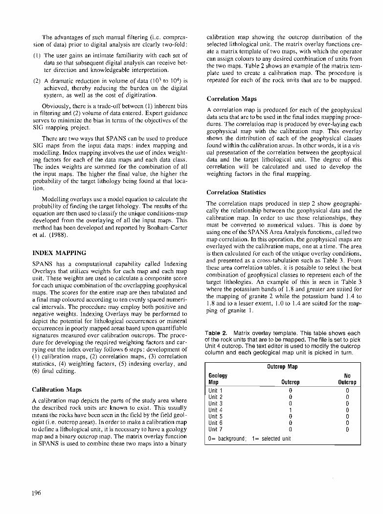
The advantages of such manual filtering (i.e. compression of data) prior to digital analysis are clearly two-fold:

( 1 ) The user gains an intimate familiarity with each set of data so that subsequent digital analysis can receive better direction and knowledgeable interpretation.

(2) A dramatic reduction in volume of data ( lo3 to lo4) is achieved, thereby reducing the burden on the digital system, as well as the cost of digitization.

Obviously, there is a trade-off between (1) inherent bias in filtering and (2) volume of data entered. Expert guidance serves to minimize the bias in terms of the objectives of the SIG mapping project.

There are two ways that SPANS can be used to produce SIG maps from the input data maps: index mapping and modelling. Index mapping involves the use of index weighting factors for each of the data maps and each data class. The index weights are summed for the combination of all the input maps. The higher the final value, the higher the probability of the target lithology being found at that location.

Modelling overlays use a model equation to calculate the probability of finding the target lithology. The results of the equation are then used to classify the unique conditions-map developed from the overlaying of all the input maps. This method has been developed and reported by Bonham-Carter et al. (1988).

INDEX MAPPING

SPANS has a computational capability called Indexing Overlays that utilizes weights for each map and each map unit. These weights are used to calculate a composite score for each unique combination of the overlapping geophysical maps. 'The scores for the entire map are then tabulated and a final map coloured according to ten evenly spaced numerical intervals. The procedure may employ both positive and negative weights. Indexing Overlays may be performed to depict the potential for lithological occurrences or mineral occurrences in poorly mapped areas based upon quantifiable signatures measured over calibration outcrops. The procedure for developing the required weighting factors and carrying out the index overlay follows 6 steps : development of (1) calibration maps, (2) correlation maps, (3) correlation statistics, (4) weighting factors, ( 5 ) indexing overlay, and (6) final editing.

Calibration Maps

A calibration map depicts the parts of the study area where the described rock units are known to exist. This usually means the rocks have been seen in the field by the field geologist (i.e. outcrop areas). In order to make a calibration map to define a lithological unit, it is necessary to have a geology map and a binary outcrop map. 'The matrix overlay function in SPANS is used to combine these two maps into a binary

calibration map showing the outcrop distribution of the selected lithological unit. The matrix overlay functions create a matrix template of two maps, with which the operator can assign colours to any desired combination of units from the two maps. Table 2 shows an example of the matrix template used to create a calibration map. The procedure is repeated for each of the rock units that are to be mapped.

Correlation Maps

A correlation map is produced for each of the geophysical data sets that are to be used in the final index mapping procedures. The correlation map is produced by over-laying each geophysical map with the calibration map. This overlay shows the distribution of each of the geophysical classes found within the calibration areas. In other words, it is a visual presentation of the correlation between the geophysical data and the target lithological unit. The degree of this correlation will be calculated and used to develop the weighting factors in the final mapping.

Correlation Statistics

The correlation maps produced in step 2 show geographically the relationship between the geophysical data and the calibration map. In order to use these relationships, they must be converted to numerical values. This is done by using one of the SPANS Area Analysis functions, called two map correlation. In this operation, the geophysical maps are overlayed with the calibration maps, one at a time. 'The area is then calculated for each of the unique overlay conditions, and presented as a cross-tabulation such as Table 3. From these area correlation tables, it is possible to select the best combination of geophysical classes to represent each of the target lithologies. An example of this is seen in Table 3 where the potassium bands of 1.8 and greater are suited for the mapping of granite 2 while the potassium band 1.4 to 1.8 and to a lesser extent, 1.0 to 1.4 are suited for the mapping of granite 1 .

Table 2. Matrix overlay template. This table shows each of the rock units that are to be mapped. The file is set to pick Unit 4 outcrop. The text editor is used to modify the outcrop column and each geological map unit is picked in turn.

Geology Mao

Outcrop Map

Outcroa Unit 1 Unit 2 Unit 3 Unit 4 Unit 5 Unit 6 Unit 7

0= background ; 1 = selected unit

No Outcrop

0 0 0 0 0 0 0

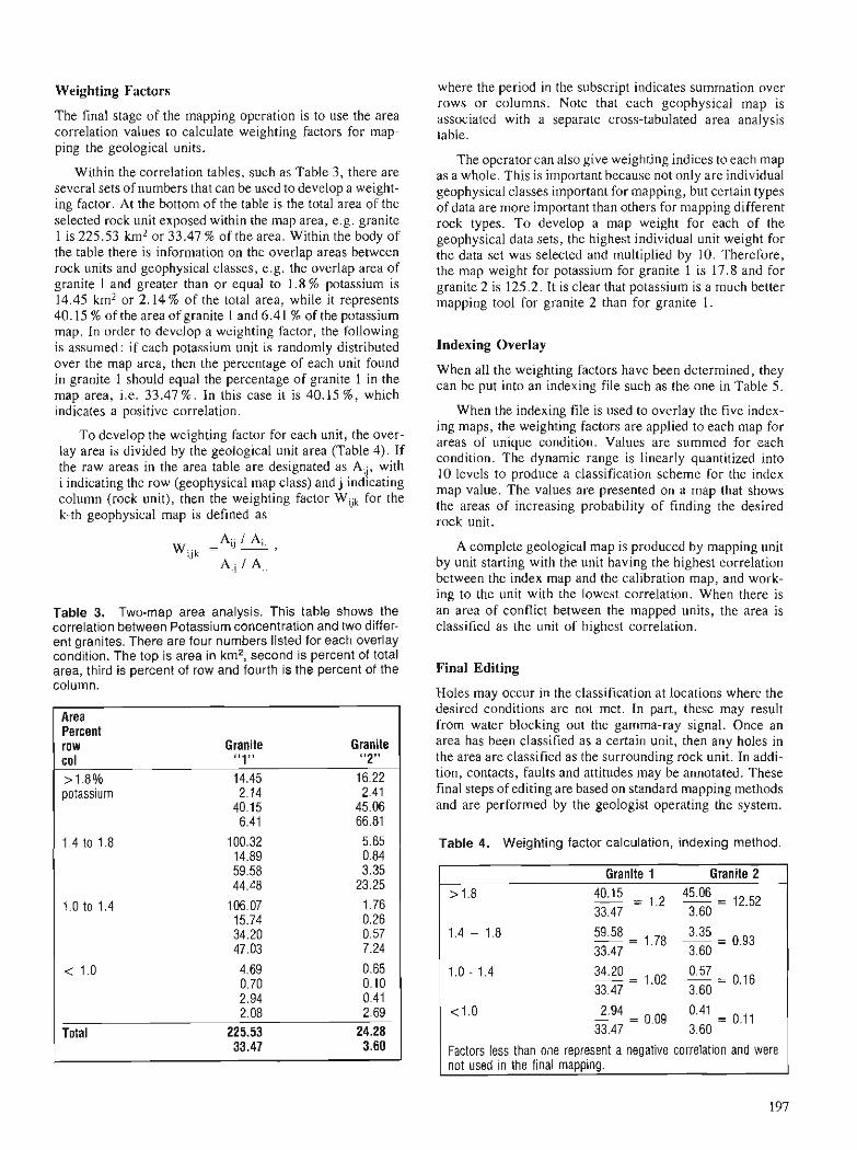
Weighting Factors

The final stage of the mapping operation is to use the area correlation values to calculate weighting factors for mapping the geological units.

Within the correlation tables, such as Table 3, there are several sets of numbers that can be used to develop a weighting factor. At the bottom of the table is the total area of the selected rock unit exposed within the map area, e.g, granite 1 is 225.53 km2 or 33.47 % of the area. Within the body of the table there is information on the overlap areas between rock units and geophysical classes, e.g. the overlap area of granite I and greater than or equal to 1.8 % potassium is 14.45 km2 or 2.14 % of the total area, while it represents 40.15 % of the area of granite 1 and 6.41 % of the potassium map. In order to develop a weighting factor, the following is assumed: if each potassium unit is randomly distributed over the map area, then the percentage of each unit found in granite 1 should equal the percentage of granite 1 in the map area, i.e. 33.47%. In this case it is 40.15 %, which indicates a positive correlation.

To develop the weighting factor for each unit, the overlay area is divided by the geological un i t area (Table 4). If the raw areas in the area table are designated as Aij, with i indicating the row (geophysical map class) and j indicating column (rock unit), then the weighting factor Wijk for the k-th geophysical map is defined as

Table 3. Two-map area analysis. This table shows the correlation between Potassium concentration and two different granites. There are four numbers listed for each overlay condition. The top is area in km2, second is percent of total area, third is percent of row and fourth is the percent of the column.

Area Percent row Granite Granite col "1" "2" > 1 .8 010 14.45 16.22 potassium 2.14 2.41

40.15 45.06 6.41 66.81

1.4 to 1.8 100.32 5.65 14.89 0.84 59.58 3.35 44.48 23.25

1.0 to 1.4 106.07 1.76 15.74 0.26 34.20 0.57 47.03 7.24

< 1.0 4.69 0.65 0.70 0.10 2.94 0.41 2.08 2.69

Total 225.53 24.28 33.47 3.60

where the period in the subscript indicates sumrnation over rows or columns. Note that each geophysical map is associated with a separate cross-tabulated area analysis table.

The operator can also give weighting indices to each map as a whole. This is important because not only are individual geophysical classes important for mapping, but certain types of data are more important than others for mapping different rock types. To develop a map weight for each of the geophysical data sets, the highest individual unit weight for the data set was selected and multiplied by 10. Therefore, the map weight for potassium for granite 1 is 17.8 and for granite 2 is 125.2. It is clear that potassium is a much better mapping tool for granite 2 than for granite 1.

Indexing Overlay

When all the weighting factors have been determined, they can be put into an indexing file such as the one in Table 5 .

When the indexing file is used to overlay the five indexing maps, the weighting factors are applied to each map for areas of unique condition. Values are summed for each condition. The dynamic range is linearly quantitized into 10 levels to produce a classification scheme for the index map value. The values are presented on a map that shows the areas of increasing probability of finding the desired rock unit.

A complete geological map is produced by mapping unit by unit starting with the unit having the highest correlation between the index map and the calibration map, and working to the unit with the lowest correlation. When there is an area of conflict between the mapped units, the area is classified as the unit of highest correlation.

Final Editing

Holes may occur in the classification at locations where the desired conditions are not met. In part, these may result from water blocking out the gamma-ray signal. Once an area has been classified as a certain unit, then any holes in the area are classified as the surrounding rock unit. In addition, contacts, faults and attitudes may be annotated. These final steps of editing are based on standard mapping methods and are performed by the geologist operating the system.

Table 4. Weighting factor calculation, indexing method

Granite 1 Granite 2

> 1.8 40.15 45'06 - 12.52 - = 1.2 - - 33.47 3.60

1.4 - 1.8 59'58 - 1.78 - - -- 33.47

3'35 - 0.93 3.60

1.0 - 1.4 34.20 - 1.02 - - -- 33.47

0'57 - 0.16 3.60

< 1 .o - - 2.94 - 0.09 - - 33.47

0.41 - 0.11 3.60

Factors less than one represent a negative correlation and were not used in the final mapping.

Table 5. Index overlay table to map Granite 1 MODELLING OVERLAY

new mapid & title: Grl l Granite 1

no. of input maps: 5 input maps (map id, max. class) TTTT 4, ThTh 3, UUUU 3, KKKK 4, VGRD 5

map weight ID title 18.600 TTTT Total Count

unit ID class unit weight 0 0

> 10 1 1.27 8 to 10 2 1.86 7 to 8 3 0 > 7 4 0

14.200 ThTh Thorium 0 0

> 6 1 1 .O 4 to 6 2 1.42 < 4 3 0

14.500 UUUU Uranium 0 0

> 2 1 0 1.4 to 2 2 1.45 < 1 3 0

17.800 KKKK Potassium > 1.8 1 1.2 1.4 to 1.8 2 1.78 1.0 to 1.4 3 1.02 < 1.0 4 0

11.700 VGRD Vertical Gradiometer 0 0

hpos 1 0 mpos 2 0 bgnd 3 1.17 mneg 4 0 hneg 5 0

The modelling function o f SPANS is similar to the index mapping, except i t uses the values calculated f rom a model equation to classify the unique conditions map. I n this case the model equation is one that was developed for predicting mineral potential by Bonham-Carter et a1. (1988). The description and application o f this equation is also reported by Bonham-Carter et a1.(1989, this volume). Instead o f predicting mineral potential, the method is here applied to the prediction o f lithological units. The procedure for using the modelling overlay is the development o f (1) calibration maps, (2) correlation maps, (3) correlation statistics, (4) weighting factors, ( 5 ) equation values and (6) probability map.

The first three steps are the same as described for index mapping.

Weighting Factors

Given the correlation statistics (the two-map area analysis cross-tabulation between the k-th geophysical map and the rock unit map), the weights for the i-th class o f the geophysical map and the j - th rock unit are defined as

Wijk = log, (Aij 1 A.j)

(Ai, - Aij) 1 (A,. - A,,)

These weights are equivalent to the expression for W + given by Bonham-Carter et al. (1988), but extended to cover multiple map classes.

Table 6. Example of SPANS equation for modelling overlay.

E postp Posterior Probability : assign map ids to shorter variable names for convenience b l = [TTTT]; b2 = [UUUU]; b3 = [ThTh]; : These are the geophysical: b4 = [KKKK]; : predictor maps: b5 = [VGRD];

"what is the prior probability?"; : interactive input follows: priorp = input; prioro = priorpl(l.0 - priorp); : calculate prior odds: lposto = log (prioro) ; : "log prior odds: : the wXXX terms are substituted before execution f l = ( w l l l if b l = = l , w211 if bl==2, w311 if bl==3, w411 if bl==4, 01; f2 = (w121 if b2==1, w221 if b2==2, w321 if b2==3, 0); f3 = (w131 if b3==1, w231 if b3==2, w331 if b3==3, 01; f4 = iw141 if b4==1, w241 if b4==2, w341 if b4==3, w441 if b4==4, 01; f5 = lw151 if b5==1, w251 if b5==2, w351 if b5==3, w541 if b5==4, w551 if b5==5, 01;

lposto = Iposto+fl+f2+f3+f4+f5; :add map weights to log prior odds: posto = exp (lposto); :calculate posterior odds: postp = posto/(l . + posto) ; :calculate posterior probability: postp ;

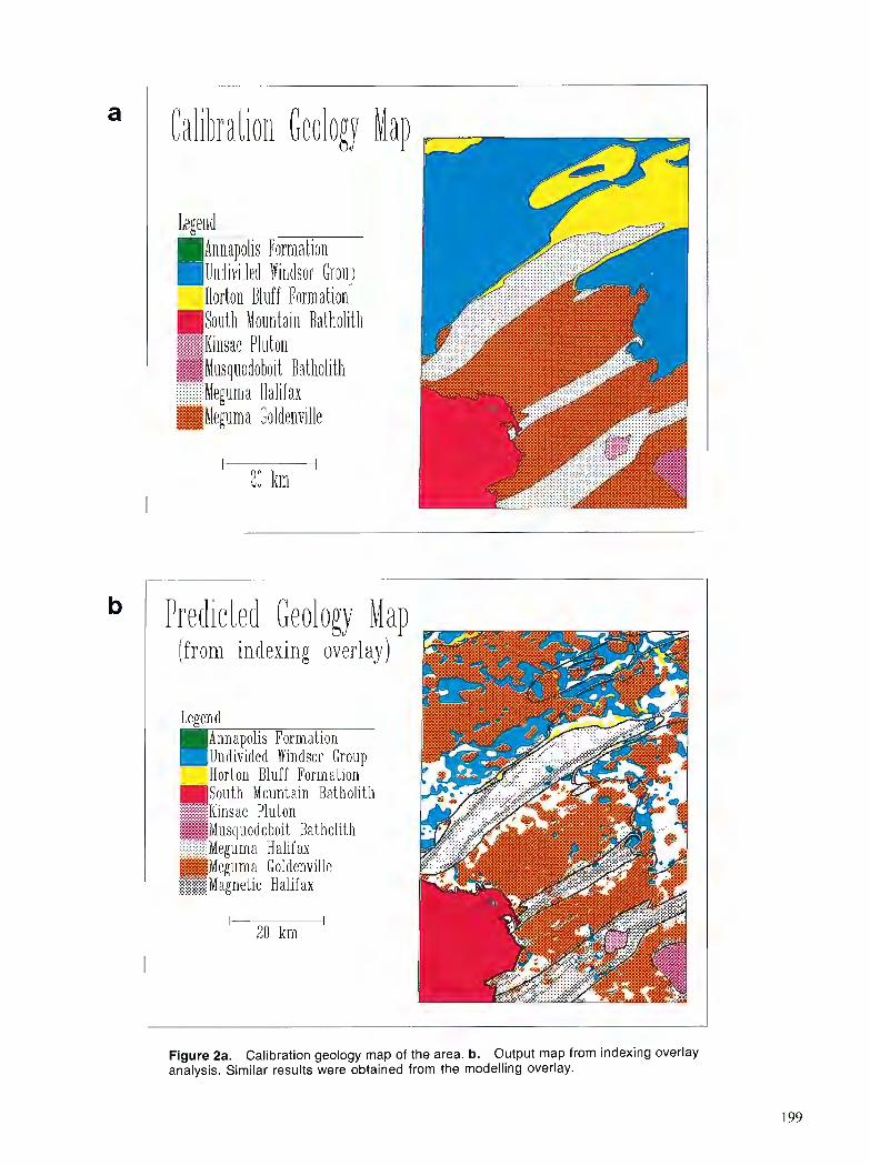
" lalibraiioii n o lap

Atiliapolis Formation U~lliisidel Wiiidsa 61~oup Hortoli Bluff Formation Soutll Mounta i~~ Bat,holith

i I(insac PILI ton ........ ........ . . . . . . .

Musqnodoboit Batholitli ........ ........ :;:;:;:::;;; Megum a Halifax lMeguma Goldenville

20 Irm

Predicted Geology Map (from indexing overlay)

I

I Legend I Annapolis Formation

Undivided Windsor Group Horto~l Bluff Forination South Mountain Batholith Kinsac Pluton

r Muscluocloboit Batholith I : ;Meguma Halifax Meguma Goldenville

!~z!lagnelie 7 ............... Halifax

20 lim

Figure 2a. Calibration geology map of the area. b. Output map from indexing overlay analysis. Similar results were obtained from the modelling overlay.

Equation Values

Although the weights for each map are linearly summed, as in the indexing method, the calculation involves some extra computation, and the indexing overlay is unsuitable. The SPANS modelling language is more flexible and permits a range of arithmetic and Boolean operations to be performed between maps. The equation used for combining the geophysical maps to predict a particular geological unit involves summing the appropriate weights with the log prior odds of that unit occurring. For the j-th rock unit the equation is

where k = 1,2..s are the geophysical maps. Oprior are the prior odds related to prior probability by

and PPrior = AJ/A, , , i.e, the proportion of the total area underlain by the selected rock type. The final posterior probability, which will be greater or less than the prior probability depending on the geophysical map combinations for each unique conditions area is given by

These equations assume that the geophysical maps are conditionally independent of one another with respect to the target rock unit, and tests for this are described by Bonham- Carter et al. (1989). The violation of this assumption will result in predicted probabilities that are either too large or too small.

In Table 6, an example of the SPANS modelling equation is shown. Note that the weights are calculated outside this program, and are substituted with a text editor before execution. Finally the output maps for rock units are combined together in a manner similar to that described in the indexing overlay. The final product is a composite map showing the areas of highest probability for the target lithologies. As with the indexing method, a final manual editing is required to fill in holes.

RESULTS

The results of both the indexing overlays and the equation modelling overlays were both very encouraging. In most cases the output maps for the two methods were similar. One possible reason for this is that the initial data filtering is more important than the method for map combination. Greater difference between the two methods might be

expected if the raw data were used, however all the advantages of data filtering stated earlier would be lost. Figure 2 shows a comparison between the calibration map (2a) and the final computed map using the indexing method (2b). The overall correlation between the two maps is good, showing much more detail in the Halifax unit predicted from the geophysical maps than on the calibration map.

CONCLUSIONS

1. The integration of the geology map and outcrop locations can be used to create a calibration map of known rock units.

2. Two-map area analysis between the target calibration map and each of the geophysical maps can be used to prepare weighting factors for each of the geophysical maps and for each unit within them. Depending on the method used to develop the weighting factors, they can be used in either the indexing method or the modelling method.

3. In general there was little difference between the maps derived from the indexing overlays and the equation modelling overlays. This may be due to the initial filtering of the input data.

4. The derived geology maps have both errors of omission and commission that can be removed with editing by a geologist using standard geological extrapolation.

ACKNOWLEDGMENT

We thank G.F.Bonham-Carter for his assistance in applying the equation modelling.

REFERENCES

Faribault, E.R. et al. 1905-1916: "Old Series" geological maps #65, 66, 67,72,73; Geologi-

cal Survey of Canada, scale 1 :63 360 Gregory, A.F. 1983: Interpretive geological mapping as an aid to exploration in

the NEAIIAEA Athabasca test area; Uranium Exploration in Athabasca Basin, Saskatchewan, Canada, ed. E.M. Came- ron; Geological Survey of Canada, Paper 82-1 I, p. 171-178.

Malcolm, W. 1929 : Gold fields of Nova Scotia; Geological Survey of Canada,

Memoir 156. Stea, R.R. and Fowler, J.H. 1981: Pleistocene geology and till geochemistry, central Nova Sco-

tia; Map 81-1, Nova Scotia Department of Mines and Energy.

Bonham-Carter, G.F., Agterberg, F.P. and Wright, D.F. 1988: Integration of geological datasets for gold exploration in

Nova Scotia; Photogrammetric Engineering and Remote Sensing, v.54, no. 11, p. 1585-1592.

1989: Weights of evidence modelling: a new approach to mapping mineral potential; 5 Statistical Applications in the Earth Sciences, ed. F.P.Agterberg and G.F.Bonham-Carter, Geo- logical Survey of Canada, Paper 89-9, p. - .

Interpretation of regional geophysical data from the Amer Lake Wager Bay area, District of Keewatin

John Broomel

SUMMARY SOMMAIRE

Geophysical data were interpreted, using qualitative and quantitative methods, for an area in the northwest Churchill Province, bounded by latitudes 64 and 68" N and longitudes 80 and 96" W degrees. This area corresponds to Interna- tional Map of the World NQ 1.51 161 17, Quoich River. Parts of this area are currently being studied by geologists in. the Geological Survey of Canada who provided some ground control for interpretation.

Althrough the northwest Churchill Province is one of the least understood areas of the Canadian Shield, good regional aeromagnetic, gravity and gamma-ray-spectrometry data are available. Gridded geophysical data were converted to a common format, registered, and used to create images. Different image processing techniques were used to enhance the data and composite images were generated to help correlate geophysical responses. Aeromagnetic images were used to aid structural interpretation of the Wager Bay shear zone and composite geophysical images were used to dis- criminate between different plutons in the calc-alkaline intrusives suite north of ~ o r d Lake. Computer modelling was used to investigate potential causes of a large Bouguer gravity anomaly centred at longitude 91" W and latitude 66" N. Modelling was performed using 2 1 I 2 and 3-dimensional algorithms on a microcomputer workstation with software developed by the author.

Les auteurs ont interprktk, B I'aide de mCthodes qualitatives et quantitatives, des donnCes gCophysiques correspondant 2 une zone du nord-ouest de la province de Churchill limitCe par les latitudcs 64" et 68" N et par les longitudes 80" et 96" 0 . Cette zone correspond h la carte internationale du monde NQ 151 161 17, rivikre Quoich. Certaines parties de cette zone font I'objet d'Ctudes actuellement par des gColo- gues de la Commission gCologique du Canada qui ont pro- cCdC B quelques contr6les au sol en vue d'aider B I 'interprktation.

' Geological Survey of Canada, I Observatory Crescent, Ottawa, Ontario K IA 0Y3

Bien que le nord-ouest de la province de Churchill soit I'une des regions du Bouclier canadien les moins bien comprises, il existe de bonnes donnCes a6romagnCtiques gravi- mttriques, et de spectromCtrie gamma pour cette rCgion. Les donnCes gCophysiques quadrillkes ont CtC converties en un format commun, reperbes et utilis6es pour crCer des images. DiffCrentes techniques de traitement d'image ont kt6 utilisCes pour rehausser les donnCes et des images compo- sCes ont CtC produites afin de corrkler les reponses geophysiques . Les images aCromagnCtiques o n t s e r v i h l'interprttation structurale de la zone de cisaillement de la baie Wager et les images gtophysiques composCes B distinguer diffkrents plutons dans la sBrie de roches intrusives calco-alcalines au nord du lac Ford. On a eu recours It la modClisation informatiske pour Ctudier les causes possibles d'une grande anomalie gravimetrique de Bouguer centree sur la longitude 91" 0 et la latitude 66" N. La modClisation a CtC effectuke h I'aide d'algorithmes 2 2 1 12 et 3 dimensions, sur micro-ordinateur, avec un logiciel mis au point par I'auteur.

in Statistical Applications in the Earth Sciences, ed. F. P. Agterberg and G. F. Bonham-Carter; Geological Survey of Canada, Paper 89-9, 1989

Use of an IBM-compatible workstation for interpretation of potential field data

John Broomel

SUMMARY SOMMAIRE

Interpretation of geophysical data is an important component of most modern resource exploration and geological mapping programs. The interpretation process is usually divided into two stages. Qualitative analysis of two- dimensional data in map form is followed by detailed quantitative analysis of select areas. Although both stages can be performed using traditional methods, computers can sigoifi- cantly facilitate the interpretation process.

Advances in computer technology have made low-cost microcomputer workstations for geophysical interpretation feasible. Increased storage capacity and specialized graphics boards now enable inexpensive microcomputers to produce graphic output of a quality previously available only with larger and more expensive minicomputer systems. A microcomputer-based workstation and software developed at the Geological Survey of Canada (GSC) for interactive display and enhancement of gridded data and gravity and magnetic profile modelling is described.

The workstation consists of an IBM-compatible microcomputer, a high-resolution colour graphics coprocessor and monitor, and a digitizing tablet for interactive control. GSC software for generating, displaying, and interactively manipulating colour-intensity and shaded- relief images is demonstrated. A 2.5 dimensional (pseudo-3D) interactive modelling program for gravity and aeromagnetic data, called MAGRAV2, is also demonstrated.

Software is written in Microsoft FORTRAN 77 with calls to Multi-Halo graphics subroutines. Source code, user's guides, and sample data may be ordered from the GSC at nominal cost.

L'interprCtation des donnkes gkophysiques est un ClCment important de la plupart des programmes modernes d'exploration des ressources et de cartographie gCologique. Le processus d'interpretation comporte gCnCralement deux Ctapes. L'analyse qualitative des donnCes bidimensionnelles reprt- sentCes sous forme de carte est suivie d'une analyse quantitative dktai116e de zones choisies. Les deux ktapes peuvent dtre rCalisCes 21 l'aide des mkthodes traditionnelles, mais les ordinateurs facilitent grandement tout le processus d'interpretation.

G r k e aux progrks rkalists en informatique, il est maintenant possible d'utiliser des postes de travail informatisks peu coOteux pour procider B l'interprktation gkophysique. Dotks d'une capacitt de mtmoire acrue et de cartes graphiques specialiskes, les micro-ordinateurs peu cofiteux'produisent maintenant des rksultats graphiques d'une qualit6 que seuls les mini-ordinateurs plus gros et plus coQteux per- mettaient d'obtenir auparavant. On dtcrit ici un poste de travail articulC sur micro-ordinateur et un logiciel mis au point B la Commission gkologique du Canada (CGC) pour l'affichage interactif et le rehaussernent de donnCes quadrillCes ainsi que pour la modClisation des profils de gravitk et des profils magnCtiques.

Le poste de travail consiste en un micro-ordinateur compatible IBM, un coprocesseur graphique pouvant donner des images de haute rksolution en couleurs accompagnk de moniteur et d'une tablette de track permettant une com- mande interactive. On dCmontre aussi le logiciel de la CGC qui permet de produire, d'afficher et de manipuler de f a ~ o n interactive des images h intensitk de couleur et B estompage d'ombre. Un programme de modClisation interactif B 2,5 dimensions (pseudo-3D) B I'intention des donnCes de gravitC et des donnkes aCromagnktiques, auquel on a donnk le nom de MAGRAV2, fait aussi l'objet d'une dkmonstration.

Le logiciel est h i t en FORTRAN 77 Microsoft avec appel de sous-programmes graphiques Multi-Halo. On peut se procurer le code source, les guides de I'utilisateur et des exemples de donnCes, pour un coOt minimal, auprbs de la CGC.

'. Geological Survey of Canada, 1 Observatory Crescent, Ottawa, Ontario KIA 0Y3

in Statistical Applications in the Earth Sciences, ed. F. P. Agterberg and G.F. Bonham-Carter; - Geological Survey of Canada, Paper 89-9, 1989.

Data processing techniques for the Geochemical Atlas of Costa Rica

Gregory L. Cole1

SUMMARY SOMMAIRE

Data analysis is an integral part of any resource survey, from inception to the final published results. At the start of the Costa Rica minerals project, goals and "deliverables" were identified. A study was then made of available computer hardware and software that could meet data analysis requirements and provide a finished product in a timely and cost-efficient manner.

Actual data analysis for the Geochemical Atlas began with an orientation survey conducted in spring 1985. Statistical analysis of data collected during this survey provided the necessary information for the design and layout of a regional survey that would identify possible sites of mineral resources.

Processing of the data from the regional surveys of the San Jose and Golfito quadrangles resulted in the colour plates and overlays of The Geochemical Atlas as well as a data base containing derivative and/or supplemental data. These other data have enable us to computerize stream networks and gradients which, when coupled with bedrock, stream cobble, mining and cultural contamination information, will aid us in modelling the geochemical anomalies due to mineralization.

L'analyse des donnCes fait partie intCgrante de toute Ctude sur les ressources, depuis le point de dCpart jusqu'h la publication finale des rbultats. Au debut du projet sur les mint- raux du Costa Rica, les objcctifs e t les .cpibces d'accompagnement~ ont Ct6 dCfinis. On a ensuite examint le matBrie1 informatique et les logiciels disponibles qui per- mettraient de rCaliser l'analyse de donnCes et d'obtenir un produit fini de f a ~ o n rapide et rentable.

Le vCritable travail d'analyse des donnCes en vue de la prCparation de l'atlas gCochimique a commencC par une Ctude d'orientation menCe au printemps de 1985. L'analyse statistique des donntes recueillies lors de cette Ctude a fourni l'information nCcessaire 8 la conception et 8 la planification d'une Ctude rCgionale dont l'objectif Ctait de dCterminer l'emplacement de sites possibles de ressources minCrales.

Le traitement des donnCes recueillies lors des Ctudes rkgionales menCes dans les quadrilatkres de San Jose et de Golfito a conduit 8 la rCalisation des planches en couleurs et des cartes-transparentes et des volumes intitulCs (<The Geochemical Atlas D, ainsi qu'8 1'Ctablissement d'une base de donn:es contenant des donnCes dCrivCes ou supplkmen- taires. A l'aide de ces autres donnCes on a pu mettre sur ordinateur les rCseaux hydrographiques et les gradients qui, combints aux donnCes sur la roche en place, les galets de cours d'eau, la contamination d'origine minibre et la contamination d'origine agricole, aideront les responsables du projet 8 modCliser les anomalies gCochimiques dues h la minkralisation.

'. Earth and Space Sciences Division, Los Alamos National Laboratory, Los Alamos, NM 87545, USA

in Statistical Applications in the Earth Sciences, ed. F. P. Agterberg and G. F. Bonham-Carter; - Geological Survey of Canada, Paper 89-9, 1989.

Examples of spatial data integration and graphical presentation in mineral resource assessments

from New Mexico and Costa Rica

Gregory L. Cole1

SUMMARY SOMMAIRE

The geochemistry group at Los Alamos National Labora- tory has been involved in the planning and execution of mineral resource assessments in diverse regions such as Alaska, New Mexico, St. Lucia and Costa Rica. Processing used in the integration and analysis of multiple data sets includes kriging, multilinear regression, factor and principal components analysis, supervised classification, and combinations of several techniques. Efforts have been made to enhance graphics as a descriptive statistic through the use of three-colour overlay plots, gradient maps, histograms with colour-coded sub-categories on the bars, and effective use of colour to assist in interactive analysis or in hard-copy output.

Drastic improvement in hard-copy output devices, as well as a significant reduction in their cost, now allows many organizations to produce inexpensive, high-quality graphics. An electrostatic plotter w a s used to create mechanical colour separations for the Geochemical Atlas of the San Jose and Golfito Quadrangles, Costa Rica with savings of 35 % on the publication costs.

Current research at Los Alamos is focused on ways to remove the background geochemistry due to bedrock. We are currently attempting to model weathering and erosional processes using as data, the digital topography, bedrock, stream connectivity, and geochemical values at a network of stream sediment sample sites. A successful model of the geomorphic processes will allow removal of bedrock contributions to the stream sediment geochemistry and thus enhance the signature of anomalous mineralization.

Le groupe de gCochimie du Los Alamos National Labora- tory a participk h la planification et B 1'exCcution d'kvalua- tions des ressources minkrales dans diverses rCgions telles que I'Alaska, le Nouveau-Mexique, Ste-Lucie et le Costa Rica. Plusieurs mCthodes ont CtC utilistes pour effectuer I'inttgration et l'analyse d'ensembles de donn6es multiples: krigeage, regression multilineaire, analyse des facteurs et des composantes principales, classification dirigCe ainsi que des combinaisons de plusieurs techniques. On a chercht a rehausser les graphiques utilisCs comme statistiques descriptives en faisant appel aux calques de recouvrement tricolores, aux cartes de gradient, aux histrogrammes avec des sous-catCgories B codage en couleurs sur les bltonnets et en utilisant efficacemrnent les couleurs pour faciliter l'analyse interactive ou la sortie des rksultats sur support en papier.

Les progrbs extraordinaires en matikre d'unitks d'impression ainsi que la rtduction importante du coQt de ces appareils permettent maintenant 2 un grand nombre d'organismes de produire B peu de frais des graphiques de grande qualitC. On a utilist une table traGante Clectrostatique pour obtenir une stparation micanique des couleurs lors de la realisation du <<Geochemical Atlas of the San Jose and Golfito Quadrangles, Costa R i c a ~ , kconomisant ainsi 35 % du coGt de publication.

La recherche actuelle B Los Alamos porte principalement sur les f a ~ o n s d'bliminer les effets dus B la gCochimie du socle. On tente presentement de modtliser les processus de mttkorisation et d'krosion en utilisant comme donnCes les valeurs numkriques relatives B la topographie, au socle, B la connectivitt des cours d'eau et 2 la gkochimie dans un rCseau de localitts d'Cchantillonage des stdiments de cours d'eau. Un modble rCussi des processus gComorphiques permettra aux chercheurs d'tliminer la contribution du socle B la gtochimie des sCdiments de cours d'eau et, partant, d'ambliorer la signature des anomalies de minCralisation.

' Earth and Space Sciences Division, Los Alamos National Laboratory, Los Alamos, NM 87545 USA

in Statistical Applications in the Earth Sciences, ed. F.P. Agterberg and G.F. Bonham-Carter; - Geological Survey of Canada, Paper 89-9, 1989

SUMMARY

GEOSIS project - integration of text and spatial data for geoscience applications

Shelley Connelll, John Ernstingl, Deborah Kukanl, and Alaster Curriel

One of the goals of the GEOSIS project is to establish a transparent link between the digital text data and the spatial data, so that the end user will be able to move easily between the two.

Within the system, the hierarchical structure of the map graphic data matches that of the text data. Explicit links between the two data types are achieved by embedding codes which "cross-link" the text to the corresponding objects in digital maps.

The user can move from spatial to text data by employing spatial searches on the graphic data, arriving at and focusing on an object, then linking across to the text data. Con- versely, the user can enter the text data, initiate a search through either structured browsing or keyword search. Structured browsing, and particularly "linked" browsing allows the user to move through the hiearchical text structure, and "cross-link" to the map graphic data as well as other text data. The keyword approach is excellent for users who are familiar with the database and can anticipate or generally determine the nature of their query results.

The integration of text data with spatial data is essential to the creation of a truly integrated user environment for geoscience data.

SOMMAIRE

L'un des objectifs du projet GEOSIS est d'Ctablir un lieu transparent entre les donnCes textuelles numkriques et les donnCes spatiales de telle sorte que I'utilisateur final puisse aller facilement des unes aux autres.

A l'intkrieur du systkme, la structure hikrarchique des donnCes graphiques correspond 2 celle des donn6es textuelles. Des liens explicites entre les deux types de donnCes ont CtC obtenus g r k e B I'intCgration de codes qui Ctablissent des <<liaisons croisCes )) entre le texte et les objets correspondants sur les cartes numkriques.

L'utilisateur peut passer des donnCes spatiales aux don- nCes textuelles en effectuant une recherche spatiale sur les donnCes graphiques; il concentre ensuite son attention sur un objet, puis il Ctablit le lien avec les donnkes textuelles. A l'inverse, l'utilisateur peut choisir les donnkes textuelles et commencer une recherche soit par balayage structurk soit par mot-clC. Le balayage structurC, et plus particulikrement le balayage << continu n, permet 2 l'utilisateur de se dkplacer dans la structure hikrarchique du texte et de se reporter aux donnCes graphiques ou 2 d'autres donnCes textuelles par l'intermkdiaire des 4 liaisons croisCes D. La recherche par mot-clC est excellente pour les utilisateurs qui connaissent bien la base de donnCes et qui peuvent prCvoir ou determiner de f a~on gCnCrale la nature des rCsultats de leur recherche.

L'intCgration de donnCes textuelles avec des donnCes spatiales est indispensable pour la crCation d'un milieu gCos- cientifique vkritablement intCgrC, du point de vue de l'utilisateur.

' Geoscience Data Centre, Ontario Geological Survey, Ministry of Northern Development and Mines, Toronto, Ontario, M7A IW4

in Statistical Applications in the Earth Sciences, ed. F. P. Agterberg and G. F. Bonham-Carter; Geological Survey of Canada, Paper 89-9, 1989.

GEOSIS project - integration of spatial data in geoscience information systems

Janet Finlay 1, Darrell Hoffer 1, William Woitowichl , and Alaster Curriel

SUMMARY SOMMAIRE

Varied types of geoscience map and image data are used by geologists on a day to day basis. To create a digital work environment that mimics the paper world the system must allow the user access in an integrated manner to image analysis, grid cell GIs (Geographic Information Systems) and vector-based GIs.

Geographic information systems have the capability for integration and analysis of various geoscience data sets. However, difficulties occur when attempting to integrate data sets that are of different data types. Raster data (map and image data) traditionally could not be integrated with vector map data so that the capabilities of their original software environments are retained.

Les gCologues utilisent quotidiennement divers types de donnCes gCoscientifiques permettant de crCer des cartes et des images. Pour produire un milieu de travail numCrique imitant le monde du papier, le systbme doit permettre 21 I'utilisateur d'accCder de f a ~ o n intbgrte 21 l'analyse des images, au SIG (Systbme d'information gkographique) 21 ClCments de quadrillage et au SIG 21 donnks vectorielles.

Les systbmes d'information gkographiques permettent l'intbgration et I'analyse de divers ensembles de donnCes gboscientifiques. Toutefois, des difficultCs surgissent lorsqu'on essaie d'intCgrer des ensembles de donn6es dans lesquels les donnCes sont de types diffkrents. Jusqu'ici, les donnCes tramCes (donnCes reproduites sous forme de carte ou d'image) ne pouvaient pas 6tre intCgrCes dans les donnCes

Developments in relational database management soft- cartographiques vectorielles de fagon 21 ce que l'on puisse ware and in workstations are making it possible to make tirer des capacitCs de leurs logiciels initiaux. advances toward a full integration of raster and vector data. Modern database software i s capable of acting as the unifying element in such a system. All graphic data are stored in the database and made available to users for analysis in the currently selected graphic mode. The user would select one or both graphic display modes each in its own window but still have access to the search and processing capabilities of the system on the full database.

This integrated approach frees the user from previous restrictions and gives access to all data types, thus supporting unimpeded retrieval and analysis of the data.

Les mises au point rkcentes dans les domaines des logiciels de gestion de base de donnCes relationnelles et des postes de travail permettent de progresser vers une intkgration complbte des donnCes tramCes et des donnCes vectorielles. Dans un tel systbme, le logiciel de base de donnCes moderne peut jouer le rBle d'bltment unificateur. Toutes les donnCes graphiques sont mises en mCmoire dans la base de donnCes et sont ii la disposition de l'utilisateur aux fins d'analyse dans le mode graphique dCsir6. L'utilisateur peut ainsi choisir l'un ou l'autre des modes d'affichage graphique, ou les deux, chacun dans sa propre fenCtre, mais il a toujours accbs aux capacitks de recherche et de traitement du systbme sur toute la base de donnCes.

Cette mCthode intCgrCe Climine les contraintes prkckdentes et permet 21 l'utilisateur d'avoir accbs 21 tous les types de donnCes. L'utilisateur peut donc extraire et analyser les donnCes sans aucune restriction.

' Geoscience Data Centre, Ontario Geological Survey, Ministry of Northern Development and Mines, Toronto, Ontario, M7A IW4


Exploration target selection by integration of geodata using statistical and image processing techniques

at the Geological Survey of Finland

SUMMARY SOMMAIRE

To develop new methodology and to test existing software in mineral resource prediction a special project was carried out in the Geological Survey of Finland, Exploration Department 1983-86 (Gaal, 1988; Kuosmanen, in press). For testing a 60 x 75 km2 area was selected from the highly mineralized Archaean-Early Proterozoic boundary in the Ladoga-Bothnian Bay Zone. Digitized geological, geophysical, geochemical and satellite data were integrated for predicting mineral resources with special reference to Cu-Zn massive sulphide deposits.

Four different approaches of data integration were applied to localize potential areas :

Un programme spCcial a CtC men6 par le ministbre de I'Exploration de la Commission gCologique de Finlande, de 1983 2 1986, en vue de mettre au point une nouvelle mCtho- dologie et d'dprouver les logiciels prtsentement disponibles en matibre de prCvision des ressources minCrales. Pour les essais, on a choisi une zone de 60 krn sur 75 km se trouvant sur la limite fortement minCralisCe de 1'ArchCen et du ProtC- rozo'ique infkrieur situte dans la zone du lac Ladoga et golfe de Bothnie. Des donnCes gCologiques, gCophysiques, gtochimiques et de tClCdCtection spatiale numCrisCes ont CtC intkgrtks en vue de la prCvision des ressources minCrales, et plus particulibrement des gisements de sulfures massifs de Cu-Zn.

(1) Updating geological data (lithology, folds and fractures) Quatre diffkrentes mithodes dlintCgration de donnCes using vector map automation. ont CtC appliquCes pour localiser des zones d'intCr2t:

(2) Similarity analysis on a 1 krn2 grid indicating a similarity with ore-bearing model cells in cos 8 values by geological, geophysical and geochemical data. Number of geochemical variables was reduced by factor analysis.

(3) Unsupervised classification by cluster analysis of airborne geophysical data in 200 X 200 m2 pixels to select analogies with ore-bearing areas.

(4) Depicting areas of overlapping geophysical anomalies given certain threshold values by digital image processing with 100 X 100 m2 pixels.

Overlapping areas resulting from the procedures (2), (3) and (4) were selected for follow-up studies. Thirty two potential sites were sampled by light mobile drilling equipment and samples analyzed in the laboratory. After analysis of chemical, petrophysical and petrographic data of the samples, 2 targets were identified (each a few hundred metres in length) as highly potential for the occurrence of Cu-Zn ore.

SELECTED REFERENCES

Gaal, G., ed. 1988 : Exploration target selection by integration of geodata using statisti-

cal and image processing techniques: an example from Central Finland. Part 1 , Text; Geological Survey of Finland, Report of Investigation 80, 156 p.

Kuosmanen, V. ed. in press- Exploration target selection by integration of geodata using statisti-

cal and image processing techniques: an example from Central Finland. Part 2, Atlas; Geological Survey of Finland, Report of Investigation.

' Geological Survey of Finland, SF-02150 Espoo, Finland

1) Mise B jour de donnCes gCologiques (lithologic, plis et fractures) par automatisation de cartes vectorielles.

2) Analyse de similarit6 effectuCe sur une grille B mailles de 1 krn2, rCvClant ?i partir de donnCes gCologiques, gCophysiques et gtochimiques une similarit6 en cos , avec des cellules de modilisation mCtalliferes. Un certain nombre de variables gtochimiques a Ctt rCduit par analyse factorielle.

3) Classification non divisCe par une analyse en groupes de donntes gCophysiques aCriennes dans des pixels de 200 m sur 200 m en vue de choisir des analogies avec des zones mttallifkres.

4) Description de zone d'anomalies gCophysiques chevauchantes compte tenu de certains seuils, par traitement d'images numCriques avec pixels de 100 m sur 100 m.

Les zones chevauchantes obtenues par les mCthodes 2), 3) et 4) ont CtC choisies pour des Ctudes complCmentaires. On a CchantillonnC dans 32 localitts d'intCr&t au moyen d'un Cquipement de forage lCger mobile, et les Cchantillons ont CtC analysCs en laboratoire. Aprbs une analyse des donnCes chimiques, pCtrophysiques et ~Ctrographiques des Cchantil- Ions, on a dtterminC deux cibles (chacune mesurant quelques centaines de mbtres de long) B forte probabilitC de minkralisation en Cu-Zn.

in Statistical Applications in the Earth Sciences, ed. F. P. Agterberg and G. F. Bonham-Carter; - Geological Survey of Canada, Paper 89-9, 1989

SUMMARY

Structural trends in the British Isles from image analysis of regional geophysical data and implications

for mineral exploration

R.T. Haworthl, M.K. Leel, A.S.D. Walker1 and J.D. Cornwelll

Digital image processing techniques have been used to analyze the regional gravity and aeromagnetic data for the Brit- ish Isles. Colour and shaded relief images have been generated of the Bouguer gravity anomaly, magnetic anomaly and gravity second vertical derivative fields. These convey information on both amplitude (as colour) and anomaly gradient (as relief) and highlight structural trends, lineaments and textural contrasts which are less easily dis- cernible on the original contour maps. The more important features are related to the evolution of the crust in each region.

On a broad scale the images emphasize Caledonoid (ENE) trends to the north of the Soloway line and arcuate (NE to SE) trends to the south. The pattern of magnetic anomalies over central England seems to define the extent of the shallow late Precambrian-early Palaeozoic basement of the Midlands Microcraton and delineates crustal elements and characteristic trends within it. The N.S. Malvern line is particulary prominent and can be traced as a deep-seated influence to the south of the Variscan Front. Magnetic lineaments and the grain of the gravity anomalies, trending in NE and NW directions on either side of the microcraton seem to relate to structures which originated during the evolution of the Welsh and eastern English Caledonides respectively. These have been subsequently reactivated and overprinted by Acadian, Variscan and later deformation. Where the lower Palaeozoic basement is exposed, such as in Wales and the Southern Uplands of Scotland, structures related to deformation and faulting prior to the closure of Iapetus show up clearly on the images. Where this basement is concealed, as in most of England, subtle lineaments and correlations between anomalies seem to reflect the influence of pre- existing basement fractures on the subsequent pattern of sedimentation.

' British Geological Survey, Keyworth, Nottingham GI2 5GC, England.

SOMMAIRE

On a utilisk des techniques d'images numkriques pour analyser des donnCes gravimitriques et aCromagnCtiques rCgionales des iles Britanniques. On a engendrC des images en couleurs et h estompage du relief des champs d'anomalies gravimktriques de Bouguer, d'anomalies magnktiques et de la seconde dkrivCe verticale de la gravitC. Ces images ren- seignent sur l'amplitude en couleurs et le gradient de l'anomalie (estompage) et font ressortir les directions structurales, les 1inCaments et les contrastes de texture plus difficiles i distinguer sur les premikres cartes hypsomk- triques. Les traits les plus importants sont lies h 1'Cvolution de la croate dans chaque region.

A une grande Cchelle, les images font ressortir les directions calCdoniennes (ENE) au nord de la ligne de Soloway et les directions arquCes (NE h SE) au sud. La configuration des anomalies magnCtiques au-dessus de la partie centrale de 1'Angleterre semble correspondre h 1'Ctendue du socle peu profond, datant du PCcambrien supCrieur ou PalCozol- que infkrieur, du microcraton des Midlands, et dClimite des ClCments de la croOte ainsi que les directions caractkristiques qui s'y trouvent. La ligne N-S de Malvern est particulikrement Cvidente et peut Ctre suivie et son influence ressemble en profondeur au sud du front varisque. Des 1inCaments magnetiques et la nature des anomalies gravimktriques, de direction prCfCrentielle NE et NO, de part et d'autre du microcraton, semblent &tre associkes i d e s structures qui ont pris naissance au cours de la formation des orogknes calCdoniennes des pays de Galles et de lYAngleterre respectivement. Ces orogtnes ont QC rkactivtes et surchargCes par des dtformations acadiennes, varisques et ultkrieures. Lh oh le socle du PalCozoi'que infkrieur affleure, comme dans le pays de Galles et les terres mCridionales de I'Ecosse, des structures associkes h la deformation et aux failles produites avant la fermeture de la mer de Tapet se voient nettement


At a larger scale, multiple data sets have been analyzed in an attempt to locate minerals whose deposition has been controlled by tectonic events in relations to structures buried beneath the post-Palaeozoic cover. A pilot study carried out in the East Midlands has established the potential for applying interactive image analysis techniques to a range of data sets in order to establish exploration and resource evaluation criteria in 'real time'. The potential for applying 'expert- system' methods to such tasks is now under investigation.

SELECTED REFERENCE

sur les images. LB oh ce socle n'affleure pas, comme dans la majeure partie de l'Angleterre, des lineaments et des corrClations subtiles entre des anomalies semblent reflkter l'influence des fractures prkexistantes du socle sur la configuration ultbrieure de la ~Cdimentation.

A plus grande tchelle, on a analyse des ensembles de donnCes multiples dans le but de localiser des minCraux dont la mise en place a CtC dCterminCe par des CvCnements tecto- niques associCs B des structures enfouies en-dessous de la couverture post-palezoi'que. Une Ctude pilote effectuCe dans la partie est des Midlands a permis d'ttablir les possibilitks d'application des techniques d'analyse d'images interactives i une gamme d'ensembles de donnCes, en vue de dCfinir des critkres d'exploration et d'evaluation des ressources en temps reel. Les possibilitCs d'application des methodes de systkme-expert B ces tdches font actuellement I'objet d'etudes.

Lee, M.K. Pharaoh, T.C., and Soper J. in press: Structural trends in central Britain from images of gravity and

aeromagnetic fields; Journal of the Geological Society.

SUMMARY

An evaluation of SPANS for presentation of the Frontier Geoscience Program's Basin Atlas

B.D. Loncarevicl , A.G. Sherinl and J.M. Woodsidel

The Frontier Geoscience Program's (FGP) Basin Atlas is a 5 volume set of geological and geophysical maps synthesiz- ing present knowledge of major sedimentary basins off the East Coast of Canada. The majority of the maps are prepared in digital form and lend themselves to manipulation by spatial analysis systems. The advantages for distribution of the Atlas as SPANS-like image files are: 1) Fast and inexpensive release of individual maps as they are prepared ; 2) The updating and revision of released maps is easy; 3) Creating overlays to study relationships between different parameters is easy ; 4) Analytical capabilities of the system could lead to new uses of the information presented in the Atlas.

Some of the problems of implementation are: 1) GIs is a new technology and there may be user resistance while at the bottom of the learning curve; 2) Cost of entering maps into the system is an unknown factor; 3) A large number of potential users may not have access to hardware and software necessary to fully utilize the potential of the new presentation formats.

SOMMAIRE

L'atlas des bassins du Programme gkoscientifique des rkgions pionnibres est un ensemble en cinq volumes de cartes gtologiques et geophysiques synthetisant le niveau de connaissances actuelles sur les principaux bassins sedimen- taires au large de la c6te Est du Canada. La majorite des cartes sont prepartes sous forme numerique et se prCtent B la manipulation h l'aide de systkme d'analyse spatiale. La prtsentation de l'atlas sous forme de fichiers d'images de type SPANS prCsente plusieurs avantages: i) on peut produire rapidement et B peu de frais des cartes individuelles ?I mesure qu'elles sont prtpartes; ii) les cartes produites sont facilement mises B jour et corrigees ; iii) il est facile de produire des calques de recouvrement pour etudier les relations entre les differents parambtres; et iv) grlce B ses capa- cites analytiques, le systbme pourrait permettre de nouvelles utilisations de l'information presentee dans l'atlas.

La mise en oeuvre du syst5me pose certains problbmes : i) la nouvelle technologie que reprksente le SIG pourrait susciter une certaine resistance de la part des utilisateurs en dCbut d'apprentissage; ii) on ne connait pas le coOt de l'introduction des cartes dans le systkme; iii) un grand nombre d'utilisateurs possibles pourraient ne pas avoir accbs au matCriel et aux logiciels ntcessaires pour profiter de tous les avantages offerts par les nouveaux formats de prhentation.

' Atlantic Geoscience Centre, Geological Survey of Canada, Dartmouth, Nova Scotia, B2Y 4A2

in Statistical Applications in the Earth Sciences, ed. F.P. Agterberg and G.F. Bonham-Carter; - Geological Survey of Canada, Paper 89-9, 1989.

Mineral exploration using catchment basin analysis to integrate regional stream sediment geochemical and geological information in the Cobequid Highlands, Nova Scotia

P. J. Rogersl, G.F. Bonham-Carter2 and D. J. Ellwood2

SUMMARY SOMMAIRE

Stream sediment and water geochemical data from the Cobequid Highlands are displayed in a series of maps, using catchment basins as the zone of influence for sample locations. The maps include: raw element plots, using a percentile classification scale; anomaly maps for each element, after background removal; and a geochemical province multi-element map based on a 3-colour plot of the first three principal components. Geochemical background is determined using a model which predicts element levels in terms of mixing of surface materials derived from the bedrock units present in each catchment basin. Catchment basins used as the area of influence allow integration of geochemical and geological maps with other geoscientific data such as geophysics and remote sensing.

The variability of many elements found in the stream sediment samples can be largely explained by the mixing model and knowledge of the underlying bedrock geology of stream catchment basins. Up to 40 % of the variability of Zn and Pb and over 30 % for Cu, F (in water), Fe, Ag As and Ni can be assigned to mapped geology. Secondary scavenging in the surficial environment of Zn, Pb, Cu, As, Ni and Co is shown by high correlations with Fe and Mn. Residual maps, where the variability associated with catchment geology and secondary scavenging has been removed, delimit more subtle anomalies indicating areas of exploration potential.

The Cobequid Highlands has been explored on an inter- mittent basis since the early 1960s for Cu, Pb, Zn, U and, to a limited extent , Au. The result of the catchment basin modelling to the stream sediment data indicate a close correlation between known mineralization and elevated values in stream catchments.

Des donntes sur les sediments fluviaux et la gCochimie de l'eau, recueillies dans les hautes terres de ~ o b e q u i d , sont reportees sur une strie de cartes, oh les bassins versants constituent la zone d'influence des sites d'tchantillonnage. Les cartes comprennent des reprksentations d'C1Cments bruts, selon une tchelle de classification par percentile; des cartes d'anomalies pour chaque Cltment aprbs Climination du fond ; et une carte 9 multiples tlCments de la province giochimique, fondCe sur un track en trois couleurs des trois premibres composantes principales. Le fond gtochimique est dCfini au moyen d'un modble qui prMit les concentrations d'ClCments en fonction du mClange des mattriaux de surface issus du socle dans chaque bassin versant. Les bassins utilisCs comme zone d'influence permettent d'inttgrer les cartes gtochimiques et g~ologiques aux autres donnCes gCoscientifiques, notamment aux donnCes gtophysiques et de tC1CdCtection.

La variabilit6 de nombreux tldments contenus dans les tchantillons de sCdiments fluviatiles peut Ctre en grande partie expliquk par le modble de mklange et les connaissances sur la gCologie du socle sous-jacent aux bassins versants. Jusqu'h 40 % de la variabilitt de Zn et Pb et plus de 30 % de Cu, F (dans l'eau), Fe, Ag, As et Ni peuvent Ctre attributs 9 la gCologie cartographite. Le balayage secondaire, en surface, de Zn, Pb, Cu, As, Ni et Co est montrt par de fortes corrClations avec Fe et Mn. Des cartes rtsiduelles des endroits oh la variabilitt associCe 9 la gtologie des bassins versants et au balayage secondaire a Ctt tliminte, mettent en relief des anomalies plus susceptibles d'indiquer la presence de zones possibles d'exploration.

Depuis le dCbut des anntes 60, les hautes-terres de Cobe- quid ont fait l'objet de recherches intermittentes en vue d'ttablir leur teneur en Cu, Pb, Zn, U et, dans une moindre mesure, en Au. Une comparaison des rCsultats de la modtli- sation des bassins versants avec les donnkes Drovenant de I'analyse des sCdiments fluviaux indique une Ctroite corrCla- tion entre la mineralisation connue et les valeurs tlevtes observtes dans les bassins versants.

'. Nova Scolia Department of Mines and Energy, 1496 Lower Water St., Halifax, Nova Scotia B3J 2x1, Geological Survey of Canada, 601 Booth Street, Ottawa, Ontario K I A 0E8


Using SURFACE I11 as a research tool for spatial analysis

SUMMARY

R.J. Sampsonl and J.A. DeGraffenreidl

SURFACE 111, the contouring program developed by the Kansas Geological Survey, is designed to serve a dual function. For most users, it will be a utility program for the routine production of high-quality contour maps and other displays. However, is has much more extensive capabilities that also make it a powerful tool for research in spatial analysis. It can be used to investigate questions of methodology, and to analyze the spatial structure of may types of geographic and geological data. These capabilities make it uniquely valuable in an academic context, and for theoretical and applied research.

SURFACE 111, like other contouring programs, generates a mathematical model of the surface being displayed. Because of its many options, SURFACE 111 can be configured to emulate the contouring algorithm in almost any other program, including those using kriging or triangulation procedures. Detailed statistical analyses can be made of the resulting surface models, permitting comparative studies to be done with a single piece of software. SUR- FACE 111 can also statistically analyze surface models created by other programs, comparing the surfaces to either the original data or to other surface representations.

An extensive library of surface transformation techniques is built into SURFACE 111. Surfaces can be filtered, differentiated, scaled in a variety of ways, levelled, and converted into drift or trend residuals. Statistical characteristics

SOMMAIRE

Le SURFACE 111, programme de track de courbes mis au point par le Kansas Geological Survey, a Ctt conGu ?i deux fins. Pour la plupart des utilisateurs i l servira de programme utilitaire de production sur une base routinkre de cartes en courbes et d'autres affichages de grande qualitC. I1 prCsente toutefois de beaucoup plus grandes possibilitCs qui en lont Cgalement un puissant outil de recherche en analyse spatiale. I1 peut Ctre utilisC pour l'ktude de questions de mkthodologie et pour analyser la structure spatiale d'un grand nombre de types de donnCes gkographiques et gkologiques. Ces pos- sibilitCs en font un outil des plus prCcieux dans le contexte acadkmique ainsi qu'en recherche theorique et appliquke.

Comme d'autres programmes de track de courbes, le SURFACE 111 produit un modble mathtmatique de la surface affichCe. En raison du grand nombre d'options qu'il comporte, le SURFACE 111, peut prendre une configuration imitant I'algorithme de trace de courbes de presque tous les autres programmes, y compris ceux qui font intervenir des procCdures de krigeage ou de triangulation. Des analyses statistiques dktailltes des modkles de surfaces produits peuvent Ctre effectuees et permettent de rCaliser des etudes com- paratives au moyen d'un unique logiciel. Le SURFACE 111 permet tgalement une analyse statistique de modbles de surfaces produits au moyen d'autres programmes par la comparaison des surfaces aux donnCes d'origine ou 2 d'autres representations de ces surfaces.

of the original and transformed surfaces can be calculated. Une imposante bibliothbque de mCthodes de transforma- The surface can be segmented vertically or areally in any tion de surfaces est intCgrCe au SURFACE 111. Les surfaces desired manner and the subsets analyzed. peuvent &tre filtrtes, diffkrencites, mises A l'tchelle par

toute une gamme de mCthodes, nivelCes et converties-en SURFACE 'I1 has powerful for rCsidus de dtrive ou de tendance. Les caracttristiqucs statis-

the analysis of point patterns. It can compute nearest- tiques des surfaces originales et transformkes peuvent Ctre neighbour, next nearest-neighbout-, natural-neighbour, and calcul,Aes. La surface peut &tre segmentte verticalement ou many other similar spatial statistics that are used to describe horizontalement de toUte mani6re souhaitCe et les sous- the patterns of points. SURFACE I11 can then map the ensembles peuvent Ctre analyds. detailed variation in these statistics across a map.

' Kansas Geological Survey, 1930 Constant Avenue, Lawrence, Kansas, 66046-2598, U.S .A.

in - Statistical Applications in the Earth Sciences, ed. F. P. Agterberg and G. F. Bonham-Carter; Geological Survey of Canada, Paper 89-9, 1989

When investigations are complete, SURFACE 111 can La puissance de SURFACE 111 se remarque particulibe- produce high-quality maps and other displays of the results, ment au niveau de l'analyse des configurations de points. in single or multiple colours, on almost any plotter or dis- I1 permet de calculer le voisin le plus proche, le voisin le play device. Styles and sizes of type, symbols, line weights plus proche suivant, le voisin nature1 et un grand nombre and patterns can be selected to produce publication-quality d'autres valeurs statistiques spatiales analogues utilisCes illustrations. pour dCcrire les configurations de points. I1 permet ensuite

de reprksenter sur une carte de manikre dCtaillCe la variation de ces valeurs statistiques.

Une fois les Ctudes complCtCes, le SURFACE 111 permet de produire des cartes de grande qualit6 ou d'autres affichages des rCsultats en une ou plusieurs couleurs, sur presque tous les types de traqeurs ou de dispositifs d'affichage. Les styles et les dimensions des caract&res, les signes conventionnels ainsi que les Cpaisseurs et les configurations des traits peuvent &tre spCcifiCs pour produire des illustrations de la qualit6 exigCes pour la publication.

A.G. Sherinl

SUMMARY

Building a GIs for the Atlantic Geoscience Centre: which direction ?

The Atlantic Geoscience Centre (AGC) has been experimenting with Geographical Information Systems since 1986. Early experiments concentrated on the application of the technology to nearshore surficial geology and coastal geomorphology and followed on the development of a prototype Coastal Information System (CIS) which was based on a generalized data base management system (Sys- tem 2000) and limited mapping capabilities. Two early experiments covered the transfer of data from the CIS to ESRI's ARCJINFO GIS and explored the data manipulation opportunities provided by the GIs environment. The second experiment explored the feasibility of ARCJINFO as a data compilation tool and the use of triangulated irregular networks (TIN) for the production of preliminary interpretations.

More recent experiments using Universal Systems Ltd.'s CARIS GIs product have been integrated with the cartographic production of the Frontier Geoscience Pro- gram's Basin Atlases. Maps compiled for the Labrador Sea Basin Atlas using the extensive suite of cartographic tools made available by CARIS have been linked with selected attribute data bases to create a limited pilot GIs.

The results of these experiments are presented and their impact on future directions for the implementation of GIs technology at AGC are presented.

and P.N. Moirl

SOMMAIRE

Les chercheurs du Centre gtoscientifique de 1'Atlantique (CGA) Ctudient les systkmes d'information gkographique depuis 1986. Les premibres exptriences ont port6 sur l'application de la technologie h la gCologie des formations en surface en zone littorale et B la gtomorphologie c8tikre, puis sur la mise au point d'un systbme d'information c6tikre (SIC) (Coastal Information System - CIS) faisant appel B un systbme gCnCral de gestion de base de donnCes (Systkme 2000) et dot6 d'une capacitC cartographique limitCe. Deux expkriences parmi les premikres ont CtC consacrkes au transfert de donnCes du SIC au SIG ARCJINFO du ESRI et aux possibilitCs de manipulation des donnCes fournies par le SIG. Au cours d'une seconde experience on a ensuite explorC la possibilitC d'utiliser ARCJINFO pour la compilation des donnCes et des rCseaux irrtguliers triangults (RIT) (triangulated irregular networks - TIN) aux fins de rCalisa- tion des interprttations prCliminaires.

Des exptriences plus recentes dans lesquelles on a utilisC les rtsultats obtenus B l'aide du SIG CARIS de la Universal Systems Ltd., ont kt6 intCgrtes avec la production des atlas des bassins du Programme gCoscientifique des rtgions pionnibres. Les cartes Ctablies pour 1'Atlas du bassin de la mer du Labrador 2 l'aide de l'importante sCrie d'outils cartographiques offerte par CARIS ont CtC assocites h certaines bases de donnCes d'attribut dans le but de crCer un SIG pilote restreint.

On pr6sente ici les rCsultats de ces expkriences et leurs consCquences sur les avenues choisies en vue de I'implanta- tion de la technologie SIG au CGA.

' . Atlantic Geoscience Centre, Geological Survey of Canada, Dartmouth, Nova Scotia B2Y 4A2

in Statistical Applications in the Earth Sciences, ed. F. P. Agterberg and G.F. Bonham-Carter; - Geological Survey of Canada, Paper 89-9, 1989

Geological activities within the RADARSAT Project

SUMMARY

V.R. Slaneyl, J. Harris2, D.F. Graham2 and K. Misra3

This summary of the RADARSAT Non-Renewable Resource Group presents some of the ongoing and past works of the Non-Renewable Resoures (N-RR) study team which was formed in 1982 to support the RADARSAT Project.

The RADARSAT Project is an interdepartmental group, which was organized to plan a Canadian controlled satellite that would carry a radar as its prime sensor. Several discipline-based study teams were associated with RADAR- SAT to ensure that the data to be produced by the satellite would satisfy the requirements of scientists within each discipline. By 1987, the Phase B (mission definition) planning was completed and the study teams became a part of the Applications Technology Division of the Canada Centre for Remote Sensing (CCRS).

An overview of Synthetic Aperture Radar (SAR) applications to geology is presented and is organized into four major application themes : satellite radar interpretation, airborne radar projects, radar stereomodels, and the digital manipulation of radar scenes.

Satellite Radars

Less than 10%. of Canada has been imaged by the short- lived Seasat SAR satellite. Two projects utilising Seasat SAR images are shown here. - Seasat and Landsat Thematic Mapper images are being

used to map fold and fault patterns across the Western Plains region of Canada. The images have been used to demonstrate how faulting has influenced the development of sedimentary basins and sedimentation within these basins. Many of these faults have evidently influenced the accumulation of hydrocarbons as is shown when producing oil and gas wells coincide with mapped faults.

SOMMAIRE

Ce sommaire du Groupe du RADARSAT sur les ressources non renouvelables prCsente certains des travaux en cours et passCs de 1'Cquipe d'Ctude des ressources non renouvelables (RNR) formCe en 1982 i l'appui du projet RADARSAT.

Le Projet RADARSAT rCunit un groupe interministeriel crCC dans le but de planifier la fabrication et l'exploitation d'un satellite command6 par le Canada et dont le principal capteur serait un radar. Plusieurs Cquipes d'ttude sptciali- sees ont Ct6 associCes au RADARSAT afin d'assurer que les donnkes fournies par le satellite satisfassent aux exigences des scientifiques oeuvrant dans chaque discipline. En 1987, la planification de la phase B (dkfinition de la mission) Ctait complttCe et les Cquipes d'6tude ont Ctt intCgrCes B la Divi- sion des applications technologiques du Centre canadien de telCdCtection (CCT).

On prCsente une vue d'ensemble des applications du Radar B ouverture synthCtique (ROS) en gCologie et ses quatre principaux thbmes d'application : interprktation de donnees obtenues par radar satellite, projets menCs 21 I'aide d'un radar aCroport6, modbles stCrCoscopiques radar et manipulations numkriques de scknes radar.

Radars de satellite

Les images obtenues pendant la courte durke d'exploitation du satellite B ROS Seasat couvrent moins de 10 % de la superficie du Canada. Deux projets exploitant les images radar du Seasat sont illustr6s ici.

- Les images des appareils de cartographie thkmatique du Seasat et du Landsat sont utilis6es pour la cartographie des configurations des plis et des failles dans la rCgion des plaines de 1'Ouest du Canada. Les images ont 6tC utilistes pour dCmontrer I'influence de la formation des fail-

' Geological Survey of Canada, 601 Booth St., Ottawa, Ontario, KIA OE8 and Canada Centre for Remote Sensing, 110 O'Connor St., Ottawa, Ontario, KIA 0Y7 Inlera Technologies Ltd. and Canada Centre for Remote Sensing, 110 O'Connor St., Ottawa, Ontario, KIA 0Y7 Canada Centre for Remote Sensing, 110 O'Connor St., Ottawa, Ontario, K I A 0Y7

in Statistical Applications in the Earth Sciences, ed. F.P. Agterberg and G.F. Bonham-Carter; -

Geological survey of Canada, Paper 89-9, 1989.

- In another project, Seasat SAR images of the Grenville Structural Province are used to prepare reconnaissance structural maps in areas of western Quebec where the geology is not well understood.

The first mission of the U.S. Shuttle Imaging Radar, (S1R.A) acquired images from around the world between 40°N and S. A selection of scenes from this mission shows how radar can be used for analysing a variety of terrains in all parts of the world. Radar is also shown to penetrate surface materials in hyperarid environments.

Airborne Radar

In 1987 and 1988, the N-RR team has sponsored more than 30 airborne radar experiments for geologists across Canada.

Radar scenes of the Sudbury region and of Newfound- land are shown to contain useful structural information.

Intera Technology's STAR 2 radar recently flew Corn- wallis Island in the high Arctic. A digitally prepared radar mosaic of the island is compared with a Landsat Thematic Mapper scene.

Stereo Radar

Stereomodels of C-SAR and STAR-2 images are displayed together with an account of the geometric requirements necessary to record this data.

Digitally Processed Radar

SAR image processing activities, which include noise (speckle) reduction, radiometric corrections and radar image enhancements, are summarized. Examples of CCRS SAR imagery of eastern Nova Scotia co-registered with Landsat Thematic Mapper, airborne digital magnetic and gamma ray spectrometer data, obtained from the Geological Survey of Canada,and lake geochemical data, obtained from the Nova Scotia Department of Mines, are presented. These co-registered products provide a useful tool for reconnaissance mapping and exploration activities as the variations in the geophyical/geochemical data are displayed by changes in colour while preserving the topographic and spectral information inherent in the SAR data.

les sur I'Cvolution des bassins sddimentaires et la sedimentation i 1'intCrieur de ces bassins. Un grand nombre de ces failles ont de toute Cvidence influencC I'accumulation des hydrocarbures, comme le montre la coi'ncidence des puits de petrole et de gaz productifs avec les failles cartographiies.

- Dans le cadre d'un autre projet, des images de la province structurale de Grenville obtenues du ROS du Seasat ont servi de prCparer des cartes structurales de reconnaissance de rCgions de I'ouest du QuCbec dont la gCologie n'est pas bien comprise.

La premibre mission du radar imageur de la navette spatiale amCricaine (S1R.A) a permis I'acquisition d'images rtparties autour du globe entre 40°N et 40"s. Une sdlection de scbnes de cette mission montre comment le radar peut Ctre utilisd pour l'analyse de toute une gamme de terrains dans toutes les rCgions du globe. On montre Cgalement que le radar permet une pCnCtration des matkriaux de surface dans les milieux hyperarides.

Radar aCroportC

En 1987 et en 1988, 1'Cquipe des RNR a parrain6 plus de 30 expCriences au radar aCroportC pour le compte de gColo- gues d'un bout ?I l'autre du Canada. Des scbnes radar de la rCgion de Sudbury et de Terre-Neuve s'avbrent contenir des renseignements structuraux utiles.

Une mission d e survol d e I'ile Cornwallis dans 1'ExtrCme Arctique a rCcemment CtC menCe B l'aide du radar STAR 2 de 1'Intera Technology. Une mosa'ique radar de l'ile prCparCe numkriquement est comparCe ?I une scbne obtenue au moyen de I'appareil de cartographie thCmatique du Landsat.

StCrCoscopie radar

Des modbles stCrCoscopiques d'images du RSO-C et du STAR-2 sont prCsentCs avec une explication des exigences gCom6triques de l'enregistrement de telles donnCes.

Images r ada r traitCes numdriquement

On rCsume dans la prCsente Ctude, les activitCs de traitement des images ROS, qui englobent la rCduction du bruit (cha- toiement), des corrections radiomktriques et le rehaussement d ' images obtenues par radar. Des exemples d'imagerie ROS du CCT de l'est de la Nouvelle-Ecosse co- repQCes avec des donnCes de l'appareil de cartographie thC- matique du Landsat, des donntes aCromagnCtiques numCri- ques et des donnCes de spectrombtre gammamdtrique obtenues de la . ~ o m m i s s i o n ~ ~ C o l o ~ i ~ u e du Canada, ainsi qu'avec des donnCes sur la gCochimi~ des lacs obtenues du Department of Mines de la Nouvelle-Ecosse sont prCsentts. ~ e s produits co-repCrCs s'avbrent utiles aux travaux de cartographie de reconnaissance et d'exploration puisque les variations des donnCes gCophysiques et gCochimiques y sont reprCsentCes par des variations de couleurs alors que I'information topographique et spectrale inhCrente aux donnhs ROS est conservke.

The regional integration of vegetation and geological lineaments derived from satellite digital data

with soils information

Jeff Whiting1

SUMMARY SOMMAIRE

LANDSAT MSS data for 1984 were geometrically corrected to the Canadian 1 :50 000 National Topographic Series maps. The MSS data were classified into forest agricultural cover types using a supervised training method along with a maximum likelihood statistical classification. The maps of vegetation cover were checked using aerial surveys. Four satellite data sets were processed on .a DIPIX ARIES I1 system. A second level of analysis was made to provide a lineament map using 4 directional filters.

These data sets were transferred to the Tydac SPANS data base through PC1 LTD EASIIPACE tape transfer software package. These data were combined with the soils data digitized from the Saskatchewan Institute of Pedology soils maps. Soil texture, parent material and slope maps were generated. The lineaments in specific directions were compared to the soils and to the vegetation data in order to evaluate the bare ground and vegetation indices as a method for assessing mineral capabilities.

Une correction gtomktrique a Ctt apportCe aux donnCes MSS LANDSAT de 1984 afin de les reprksenter sur les cartes au 1/50 000 du Systkme national de rCfCrence cartographique canadien. Les donnCes MSS ont CtC classifiCes en couverts forestier et agricole h l'aide d'une mCthode de classification dirigCe, utilisCe conjointement avec une classification statistique fondCe sur le maximum de vraisemblance. Les cartes de couvert vCgCtal ont CtC vCrifiCes h l'aide de levCs atriens. Quatre ensembles de donnCes obtenues par satellite ont CtC trait& sur un systbme DIPIX ARIES 11. Une analyse au second degrC a CtC rCalisCe pour obtenir une carte des 1inCaments B l'aide de quatre filtres directionnels.

Ces ensembles de donnCes ont CtC transfCrCs ti la base de donnCe SPANS de Tydac h l'aide du progiciel de transfert sur ruban magnCtique EASIIPACE de PC1 LTD. Ces don- nCes ont CtC combinees avec les donntes sur les sols obtenues par conversion numCrique h partir des cartes de sols du Saskatchewan Institute of Pedology. Des cartes de texture du sol, de matCriau originel et de pentes ont CtC produites. Les 1inCaments orient& suivant des directions spCcifiques ont CtC comparts aux donnCes sur les sols et la vCgCtation afin de vCrifier si les indices de sol dCnudC et de vtgktation pouvaient Ctre utilisCs pour Bvaluer les ressources minCrales possibles d'une rCgion.

' . Saskatchewan Research Council , Saskatoon, Saskatchewan S7N 2x8

in Statistical Applications in the Earth Sciences, ed. F. P. Agterberg and G. F. Bonham-Carter, - Geological Survey of Canada, Paper 89-9, 1989.

Data integration, eastern shore, Nova Scotia

Danny F.

SUMMARY

A variety of geoscience datasets have been compiled, co- registered and analyzed using a microcomputer-based geographic information system (GIS). These data can be considered as thematic, raster, point or line type. Thematic type data sets are bedrock and surficial geology. Remote sensed images and airborne geophysics represent raster type data. A number of linear features such as structural lineaments, fold axes and lithological contacts have been digitized. Point type data include lake and stream sediment samples and gold occurrences. The GIs uses a quadtree structure ideally suited to handle these diverse types of data. The goal of this study was to generate a map showing areas favourable for gold mineralization based on the relationship between the distribution of 68 known gold occurrences and the lake sediment geochemistry. -

Regression experiments, using the presence of a gold occurrence as the dependent variable and the lake sediment geochemical elements as the predictor variables, were used to find the linear combination of geochemical elements that best predict lake catchment basins containing a gold occurrence. Au in lake sediment is found to be an excellent predictor of gold mineralization along with As and W to a lesser extent. A predicted gold occurrence map, based on the geochemistry alone, showed several areas with a favourable response but no reported mineral occurrences.

SOMMAIRE

' Geological Survey of Canada, 601 Booth Street, Ottawa, Ontario, K1A 0E8

Divers ensembles de donnCes gtoscientifiques ont CtC com- piles, repCrCs et analysb h l'aide d'un systkme d'information gtographique (SIG) pilot6 sur micro-ordinateur. Ces donntes peuvent Stre considCrtes cornrne des donnCes thematiques, tramkes, ponctuelles ou 1inCaires. Les ensembles de donntes de type thCmatique concernent le socle et la gCo- logie des formations en surface. Les images de ttlCdCtection et les donnCes gCophysiques atroportCes constituent les donntes tramtes. Un certain nombre d'tltments lintaires tels que les liniaments structuraux, les axes de plis et les contacts lithologiques ont Ctt numtrists. Les donnCes ponctuelles incluent des Cchantillons de stdiments lacustres et fluviaux ainsi que les manifestations aurifires. Le SIG fait appel aux arbres quaternaires qui conviennent parfaitement au traitement de ces difftrents types de donnCes. L'objectif de la prtsente ttude Ctait de produire une carte montrant les zones propices h la mintralisation en or, basCe sur la relation entre la rtpartition de 68 venues aurieres connues et la gCo- chimie des stdiments lacustres.

On a utilisC des exptriences de rtgression, dans lesquelles la venue auriere representait la variable dkpendante et la gCochimie des ddiments lacustres, les variables prtdicti- ves, pour trouver la combinaison linCaire d'C1Cments gCo- chimiques la'plus susceptible de permettre ['identification des bassins versants de lac prtsentant une venue aurifere. La prtsence d'Au dans les sCdiments lactustres est un excellent indice de mintralisation en o r ; il en est de meme, dans une moindre mesure, de As et W. Une carte thtorique des venues aurifires, basCe sur la seule gCochimie, montrait plusieurs zones oh la rtponse ttait favorable, mais aucune venue minerale n'a CtC constatCe.

in Statistical Applications in the Earth Sciences, ed. F. P. Agterberg and G. F. Bonham-Carter, - Geological Survey of Canada, Paper 89-9, 1989

Part ZZ

STATISTICAL ANALYSIS OF GEOSCZENCE DATA

On confidence bands for the quantile function1

Mikl6s Csorgol and Lajos Horv6thz

Csorgo, M, and Horvbth, L., On conjdence bands for the quantile function; & Statistical Applications in the Earth Sciences, ed. F. P. Agterberg and G. F. Bonham-Carter; Geological Survey of Canada, Paper 89-9, p. 221-231, 1989.

Abstract

Let XI, X2, . . . , Xn be independent identically distributed random variables (i. i.d. r. v.) with a continuous distribution finction F and corresponding quantile finction Q, the inverse function of F. Let *Qn(y) =Xk;,, if (k-l)/n < y k/n (k=2, 3.. . . , n) where X,, 5 X 2 , 5.. . a Xnlipre the order statistics of the above sample. Let (E, ,] , ,~ be a sequence of positive numbers such that n E - m , E,- 0 as n- a . Assuming only that F is continuous, we show that limn- , P {Qn (y-n-1/n2cfa)) 5 Q(Y) < Q, (Y + n-lnc(a)), En

r y 5 I-E,) = P { s u ~ ~ ~ ~ , ~ 1 B(y) I I c(a)) =I-a, where B(-) is a Brownian bridge and c(a) is such a positive real number for which we have the latter equality for a€ (0,I).

A supposer que X,, X2, . . . , Xn soient des variables al&atoires indkpenduntes distribukes de facon iden- tique (independant identically distributed random variables - i. i.d, r. v.) et qu 'il y ait une fonction de distribution continue F et une fonction quantile correspondante Q, soit la fonction inverse de F. Soit Q,(y) = Xk:, si (k-l)/n < y 5 k/n (k=2, 3,. . . , n) oli XI ,, IX,,, 5.. . I Xn:, sont les statistiques d'ordre de l'tfchantillon suswntionnk. Soit l ~ , , ] , , ~ une sQuence de nombres positifs telle que n1I2& - a, E , ~ O lorsque n-- m. En admettant seulernent que F soh continu, on dkmontre que limn-, P lQn (y-n-'"cfa)) 5 Q(Y) < Qn (Y+n-1'2c(a)), E , ~ ~ ~ I - E , J = P ( S U ~ ~ , ~ ~ ~ I B ( Y ) I sc (a) )=l -a , ou B(-) est unpont Brownien et c(a) est un tel nombre rkel positif, pour lequel on obtient la demi6re kgalitk de a6 (0,l).

I Department of Mathematics and Statistics Carleton University, Ottawa, Ontario, KIS 5B6 Bolyai Institute, Szeged University, H-6720 Szeged, Aradi vkrtanlik tere 1, Hungary and Department of Mathematics, University of Utah, Salt Lake City, UT 84112, U.S.A.

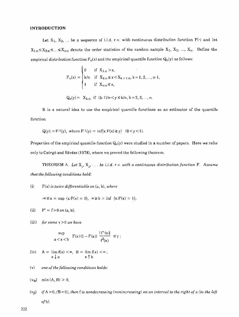
INTRODUCTION

Let XI, Xa, ... be a sequence of i.i.d. r.v. with continuous distribution function F(.) and let

X1:nSX2:nS ... 5 Xnzn denote the order statistics of the random sample Xi, X2, ..., X,. Define the

empirical distribution function F,(x) and the empirical quantile function Q,(y) a s follows:

It is a natural idea to use the empirical quantile functions a s a n estimator of the quantile

function

Q(y): = F-l(y), where F-l(y) = inf{x:F(x) 2 y) (0 < y < 1).

Properties of the empirical quantile function Q,(y) were studied in a number of papers. Here we refer

only to Csorgo and RCvesz (1978), where we proved the following theorem.

THEOREM A. Let XI, X,, . . . be i.i.d. r.v. with a continuous distribution function F. Assume

that the following conditions hold:

(i) F(x) is twice differentiable on (a, b), where

-03 5 a = sup {x:F(x) = O), 03 r b = inf {x:F(x) = 1);

(ii) F' = f > 0 on (a, b);

(iii) for some y > 0 we have

(iv) A = lim f(x) <m, B = lim f(x) < a ~ ; xis x f b

(v) one of the following conditicns holds:

(v,) min (A, B) > 0,

(vp) if A=O, (I3 =O), then f is nondecreasing (nonincreasing) on a n interval to the right of a (to the left

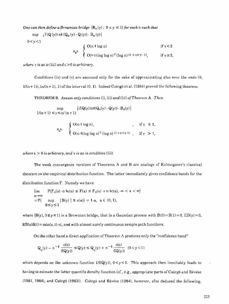
One can then define a Brownian bridge {B, (y) ; 0 s y 5 1) for each n such that

sup 1 f (Q (y)) n+ (Q, (y) - Q (y)) - B, (Y) I

- t O(n-+ log n) i f y < 2 a.s .

O(n-+(log log n)Y (log n) (1 + c ) ( Y - I), i f y 2 2 ,

where y is as is (iii) a n d E > O is arbitrary.

Conditions (iv) and (v) a re assumed only for the sake of approximating also over the ends (0,

l / (n+ I)), ( d ( n + I) , 1) of the interval (0, 1). Indeed Csorgo et al. (1984) proved the following theorem.

THEOREM B. Assum only conditions (i), (ii) and (iii) of Theorem A. Then

O h - + log n), , i f y 5 1 , als. -

O(n-+(log log n)y (log n) ( l + & ) ( Y - l ) , if y > 1 ,

where E > 0 is arbitrary, and y is as in condition (iii).

The weak convergence versions of Theorems A and B are analogs of Kolmogorov's classical

theorem on the empirical distribution function. The latter immediately gives confidence bands for the

distribution function F. Namely we have

lim P{Fn(x) -n-+c(a) 5 F(x) 5 F,(x) +n -Ma) , < x < w) n-+ CQ =P{ sup 1 B(y) ( 5 c(a)) = 1-a, cr E (0, I),

O l y l l

where (B(y), O5y 5 1) is a Brownian bridge, that is a Gaussian process with B(0) =B( l ) = 0, EB(y) = 0,

EB(s)B(t) = min(s, t)-st, and with almost surely continuous sample path functions.

On the other hand a direct application of Theorem A produces only the "confidence band"

which depends on the unknown function l/f(Q(y)), 0 < y < 1. This approach then inevitably leads to -

having to esimate the latter quantile density function (cf., e.g., appropriate parts of Csorgo and R6v6sz

(1981, 1984), and Csorgo (1983)). Csorgo and RCv6sz (19841, however, also deduced the following,

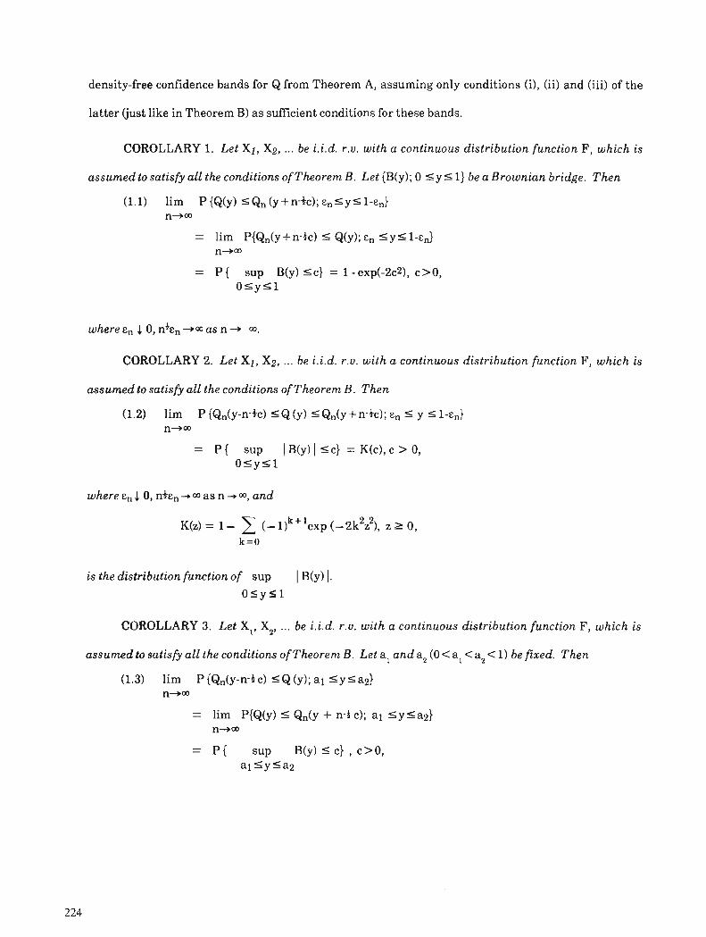
density-free confidence bands for Q from Theorem A, assuming only conditions (i), (ii) and (iii) of the

latter (just like in Theorem B) as sufficient conditions for these bands.

COROLLARY 1. Let XI, X2, ... be i.i.d. r.u. with a continuous distribution function F, which is

assumed to satisfy all the conditions of Theorem B. Let {B(y); 0 5 y S 1) be a Brownian bridge. Then

(1.1) lirn P {Q(y) I Q , (y +n-3c); & , r y l 1-en) n+w

= lim P{Q,(y + n3c) I Q(y); c, 5 y 1-cd n+m

= P { sup B(y) 5 c ) = 1 - exp(-2c2), c > 0, O I y 5 l

where en 1 0, nben +m as n + w.

COROLLARY 2. Let XI, X2, ... be i.i.d. r.u. with a continuous distribution function F, which is

assumed to satisfy all the conditions of Theorem B. Then

(1.2) lim P {Q,(~-n-+c) I Q (y) sQ,(y + n-+c); E, 5 y I 1-c,) n - m

= P { sup 1 B(y) 1 Sc} = K(c), c > 0, O S y I l

is the distribution function of sup I B(y) 1. O I y S l

COROLLARY 3. Let XI, X,, ... be i.i.d, r.u. with a continuous distribution function F, which is

assumed to satisfy all the conditions of Theorem B. Let a , and a, (0 <a, <a,< 1) be fixed. Then

(1.3) lim P {Qn(y-n-+c) IQ (y); a1 S y <a2) n+a

= lim P{Q(y) 5 Q,(y + n-3 c); a1 5 y 5 a2} n - m

= P { sup B ( y ) l c ) , c > O , a l S y l a 2

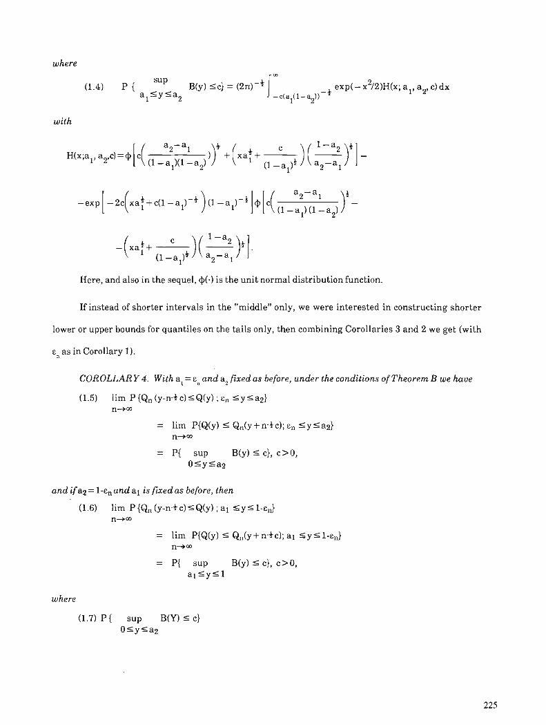
where

(1.4) P { SUP ~ ( y ) s c } = (2n)-* exp(- x 2 / 2 ) ~ ( x ; a,, a?, c) dx

a l l y l a 2 -3

with

Here, and also in the sequel, +(-) is the unit normal distribution function.

If instead of shorter intervals in the "middle" only, we were interested in constructing shorter

lower or upper bounds for quantiles on the tails only, then combining Corollaries 3 and 2 we get (with

cn as in Corollary 1).

COROLLARY 4 . With a, = cn and a, fixed as before, under the conditions of Theorem B we have

(1.5) lim P {Q, (y-n-3 c) 5 Q(y) ; cn SY (a21 n+m

= lim P{Q(y) 5 Qn(y + n-b c); E, 5 y 5 a2} n+a

= P{ sup B(y) 5 c), c >0, O S y l a 2

and if a2= 1-&,and a1 is fixed as before, then

(1.6) lim P {Q, (y-n-3 c) rQ(y) ; a1 5 y 5 l-%) n+m

= lim P{Q(y) r Q,(y -I- n-*c); a1 5 y 5 1%) n--*m

= P{ sup B(y) 5 c), c>O, a l s y l l

where

(1.7) P{ sup B(Y) 5 c) 0 r y l a 2

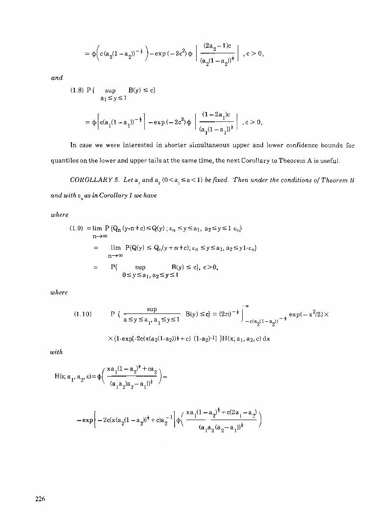
and

(1.8) P{ sup B(y) 5 c} a l l y l l

In case we were interested in shorter simultaneous upper and lower confidence bounds for

quantiles on the lower and upper tails a t the same time, the next Corollary to Theorem A is useful.

COROLLARY 5. Let a, and a, (O<a,<a< 1) be fixed. Then under the conditions of Theorem B

and with en as in Corollary 1 we have

where

(1.9) = lim P {Q, (y-n-3 c) 5 Q(y) ; c, 5 y 5 al, a 2 5 y 5 I-&,) n+a

= lim P{Q(y) 5 Q,(y + n-3 c); E , 5 y 5 a l , a2 5 yl-en) n+m

= P{ sup B(y) 5 c), c>O, O l y I a l , a 2 5 y I 1

where

x (1-exp[-2c(x(a2(1-a2))3+c) (l-az)-ll )H(x; a l , az, c) dx

with

The distribution functions of Corollaries 1 and 2 are well known and have been widely

tabulated. The formulae of (1.4), (1.7), (1.8) and (1.10) are taken from Cs6ki (1981). Chapter I of

Chung's thesis (1986), a s well a s his computer programs in his Wiener Pack (1987), summarize and

generalize many of the available methods for computing probabilities of various functionals of Wiener

and Brownian bridge processes. For further developments of ideas along the lines of Theorems A, B

and Corollaries 1-5, we refer to Volumes 44, 71, 79, 89 and 102 of the Technical Report Series of the

Laboratory for Research in Statistics and Probability, Carleton University - University of Ottawa, to the

papers by Aly e t al. (19851, BarabAs et al. (1986), Chung (1988), Chung e t al. (19881, Csorgo (1986),

Csorgo and Csorgo (1987), Csorgo e t al. (1987), Csorgo e t al. (1984), Csorgo and RCv6sz (1984), HorvAth

and Yandell (1987), to the appropriate parts of the books Csorgo (19831, Csorgo et al. (1986), Csorgo

and RCvesz (1981), and to the thesis of Chung (1986), as well a s to that of Song (1987).

One of the results in the just quoted work of Song (1987) is his Theorem 5.3, which amounts to

proving our Corollary 3 and its two-sided version via assuming only that F is continuous and strictly

increasing on its finite support (a, b) (cf. (i) of Theorem A for definition of (a, b)). Thus the conditions

(i), (ii), (iii) of Theorem A which are sufficient for Corollary 3 to be t rue are replaced in Song (1987) by

requiring F to be simply continuous and strictly increasing.

The aim of this exposition is to modify the proofs of Corollaries 1-5 so that all of them will hold

true on assuming only that F is continuous. This we do in the next section by extending the method of

Song's proof of his Theorem 5.3 of his thesis (1987) so that i t will accommodate construction of

confidence bands for the quantile function of a continuous distribution function over intervals which

expand to (0,l) at a regulated rate a s n+m.

A SUMMARY OF RESULTS AND PROOF

Here we state our results a s a theorem and then give the proof. The main idea of this proof is

that Corollaries 1-5, a s well a s further similar ones, can be deduced from combining (2.3) below with

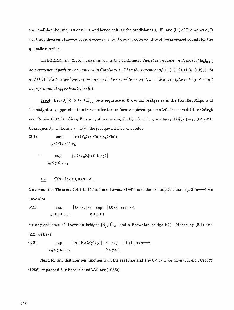
the condition that ntcn+m as n+m, and hence neither the conditions (i), (ii), and (iii) of Theorems A, B

nor these theorems themselves are necessary for the asymptotic validity of the proposed bounds for the

quantile function.

THEOREM. Let X,, X,, ... be i.i.d. r.v. with a continuous distribution function F, and let 1

be a sequence ofpositive constants as in Corollary 1 . Then the statement of (1.1), (1.2), (1.3), (1.5), (1.6)

and (1.9) hold true without assuming any furhter conditions on F , provided we replace 5 by < in all

theirpostulated upper bands for Q(.).

Proof. Let {Bn(y), O l y s l)n2, be a sequence of Brownian bridges as in the Komlbs, Major and - TusnAdy strong approximation theorem for the uniform empirical process (cf. Theorem 4.4.1 in Csorgo

and RBv6sz (1981)). Since F is a continuous distribution function, we have F(Q(y)) = y, 0 < y < 1.

Consequently, on letting x = Q(y), the just quoted theorem yields

(2.1) sup I n* (Fn(x)-F(x))-Bn(F(x)) 1 En 5 F(x) 5 l-en

%% - O(n'* log n), as n+m .

On account of Theorem 1.4.1 in Csorgo and RkvBsz (1981) and the assumption that en 10 (n+w) we

have also

(2.2) SUP 1 n Y 1 SUP 1 B(y) 1, as n+m,

c , IYS~-E, O l y S l

for any sequence of Brownian bridges {B,(-)I,,, and a Brownian bridge B(.). Hence by (2.1) and

(2.2) we have

(2.3) SUP I F n Q - 1 1 + sup 1 B(y) I , a s n+m,

en 5 y 5 1-&, o l y l l

Next, for any distribution function G on the real line and any 0 < t < 1 we have (cf., e.g., Csorgo

(1986), or pages 5-8 in Shorack and Wellner (1986))

(2.4) G(x) a t if and only if G-l(t) 5 x,

(2.5) G(x) < t if and only if G-l(t) > x,

Consequently, with G(-) = F,(.), X = Q(y) and t = + nhc, we have by (2.5)

(2.6) F,(Q(y)) < y +n-3c if and only if Q(y) < Fn-1 (y + n-tc),

for any O < y 5 1-E,, provided we take n so large that 1-en+ n-&c< 1 for a given c>O. The latter can be

done on account for assuming that nten+m, as n - m , which in turn results in

(2.7) F; '(y +n"c)= Q,O, + n-*c)

being well defined for any 0 < y 5 1-cn and c > 0 if n is large enough.

Similarly, with G(-) = F,(.), x = Q(y) and t = ~-n"c , we have by (2.4)

(2.8) Fn(Q(y)) a - ntc if and only ifQ(y) 2 F i 'O, - n-'c)

for any e n s y 5 1, provided we take n so large that O < ~ ~ - n ' ~ c for a given c>O. Again, the latter can be

done on account of assuming that nhe,+m, as n+a, which in turn results in

(2.9) ~;'(y - n - * c ) = ~ ~ ( y - n-*c)

being well defined for any cn I y < 1 and c > 0 if n is large enough.

Now (2.6)-(2.9) result in saying that (2.6) and (2.8) hold true simultaneously for any cn=y 51-en,

c>O is n is large enough, given our assumption that nten+m, a s n-+m. Thus we have arrived a t having

= ~ { ~ , ( y - n - ~ c ) s ~ ( ~ ) < ~ , ~ + n - ~ c ) , c n 5 y r 1 -rn)

for all large enough n and any c > 0, given our condition that nhcn+m as n+m.

Obviously then, given our condition that nken-*m as n+m, by (2.10) we have also

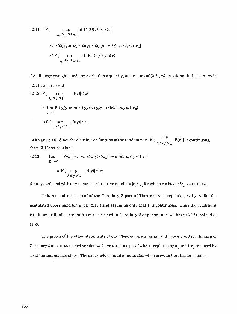
(2.11) P{ sup I n3(Fn(Q(y))-yl <c) e n s y s I-&,

5 P { sup I n* (F,(Q(y))-yl s c ) ~ , S y 5 I-&,

for all large enough n and any c>O. Consequently, on account of (2.3), when taking limits as n+m in

(2.11), we arrive a t

(2.12) P { sup 1 <c) o s y r l

I lim P{Qn(y-n-3c) 5 Q(y) < Qn(y + n-+c), en S y 5 n-+m

with any c> 0. Since the distribution function of the random variable SUP I B(y) I is continuous,

o r y s i from (2.12) we conclude

(2.13) lim P{Qn(y-n-3c) 5 Q(y) < Qn(y + n-3c), en 5 y I I-&,} n-+m

= p { sup I B(Y)I 0 l y l l

for any c>0, and with any sequence of positive numbers {en)nzI for which we have n+en+m as n+m.

This concludes the proof of the Corollary 2 part of Theorem with replacing 5 by < for the

postulated upper band for Q (cf. (2.13)) and assuming only that F is continuous. Thus the conditions

(9, (ii) and (iii) of Theorem A are not needed in Corollary 2 any more and we have (2.13) instead of

(1.2).

The proofs of the other statements of our Theorem are similar, and hence omitted; In case of

Corollary 3 and its two sided version we have the same proof with en replaced by a, and 1-en replaced by

a:! a t the appropriate steps. The same holds, mutatis mutandis, when proving Corollaries 4 and 5.

Remark. It is clear from the discussion on confidence bands for the quantile function in Section

4.2 of CsGrgo (1983) that if en of our Theorem is not a fixed constant in (0,1), then a condition like

n+cen-w as n+m is, ingeneral, also necessary as well for the asymptotic validity of these bands, and that

none of these bands remains valid with en= 0.

ACKNOWLEDGMENTS

The authors wish to thank Kjell Doksum for sending them a copy of his student's PhD thesis, Jae

Kee Song (1987). This research was supported by an EMR Canada Grant held at Carleton University

by M. Csiirgo.

REFERENCES

Aly, E-E.A.A., Csorgo, M., and Horvhth, L. 1985: Strong approximations of the quantile process of the product limit

estimator; Journal of Multivariate Analysis, v. 16, p. 185-210. Barabhs, B., Csorgo, M., Horvhth, L., and Yandell, B.S. 1986: Bootstrapped confidence bands for percentile lifetime; Annals of

the Institute of Statistical Mathematics, v. 38, p. 429-438. Chung, C.F. 1986: Confidence Bands for Quantile Function and Percentile Residual

Lifetime Under Random Censorship; unpublished PhD thesis, Carleton University.

1987: Wiener Pack: A subroutine package for computing probabilities associated with Wiener and Brownian bridge processes; Geologi- cal Survey of Canada, Paper 87-12.

1988 : Confidence bands for percentile lifetime under random censorship model; Journal of Multivariate Analysis, v. 27.

Chung, C.F., Csorgo, M., and Horvhth, L. 1988: Confidence bands for quantile function under random censorship;

Manuscript. Cshki, E. 1981: Empirical distribution function; Selected Translations in

Mathematics. Statistics and Probability, v. 15, p. 229-317. Csorgo, M. 1983: Quantile Processes with Statistical Applications; CBMS-NSF

Regional Conference Series in Applied Mathematics, SIAM No. 42, 156 p.

1986: Quantile Processes; Encyclopedia of Statistical Sciences, v. 7, ed. Kotz, Johnson, and Read, p. 412-424.

Csorgo, M. and Csorgo, S. 1987: Estimation of percentile residual life; Operations Research, v. 35,

p. 598-606. Csorgo, M. and Rkvbsz, p. 1978: Strong approximations of the quantile process; The Annals of

Statistics, v. 6, p. 882-894. 1981 : Strong Approximations in Probability and Statistics; Academic

Press, 284 p. 1984 : Two approaches to consulting simultaneous confidence bounds for

quantiles; Probability and Mathematical Statistics, v. 4, 221-236. Csorgo, M., Csorgo, S., and Horvhth, L. 1986: An AsymptoticTheory for Empirical Reliability and Concentration

Processes; Lecture Notes in Statistics, v. 35, Springer-Verlag, 171 p.

1987 : Estimation of total time on test transforms and Lorenz curves under random censorship; Statistics, v. 18, p. 77-97.

Csorgo, M., Csorgo, S., Horvfith, L., and Rbvhz, P. 1984: On weak and strong approximations of the quantile process;

Proceedings of the 7th Conference on Probability Theory, Brasov 1982, Editura Academici Republicii Socialiste Romlnia, Bucuresti, p. 81-95.

Horvhth, L. and Yandell, B. 1987: Convergence rates for the bootstrapped product-limit process; The

Annals of Statistics. v. 15, p. 1155-1173. Skornck, G.R. and Wellner, J.A. 1986: Empirical Processes with Applications to Statistics; Wiley-

Interscience, 938 p. Song, J.K. 1987: Statistical Inference in Models Based on the Percentile Residual

Lifetime Function; unpublished PhD thesis, University of Califor- nia. Berkeley.

Estimation of distribution parameters from data with observations below detection limit with an example from South Nahanni River area, District of Mackenzie

Chang-Jo F. Chungl and Wendy A. Spirit02

Chung, C. F. and Spirito, W. A., Estimation of distribution parameters JLom data with observations below detection limit with an example from South Nahanni River area, District of Mackenzie; & Statistical Applications in the Earth Sciences, ed. F. P. Agterberg and G.F. Bonham-Carter, Geological Survey of Canada, Paper 89-9, p. 233-242, 1989.

Abstract

Gold and tungsten stream sediment geochemical data obtained for a resource assessment of South Nahanni River area are used to illustrate maximum likelihood estimators (MLE) when applied to data sets with undetected values. Ideally, the data should be complete and the distribution finction should be known before statistics are computed. However, as data are commonly not complete, the maximum likelihood estimation method allows statistical analysis of censored data with the inherent assumption that their distribution is normal or lognormal. Although data with a high proportion of undetected values may not be reliable, in a mineral resource assessment these may be the only data available. Comparison of curves generated from data with ad-hoc substitutions versus curves generated by maximum likelihood estimation, shows that the MLE method provides more realistic generalizations of the sample mean and variance.

On emploie les donne'es ge'ochimiques obtenues sur des se'dimentsJuviatiles contenant de l'or et du tungsttne, pour kvalu~r les ressources de la rkgion de la rivi2re Nahanni Sud, et cela pour mettre en kvidence les estimateurs de probabilit&maximum (maximum likelihood estimators, MLE), lorsque ceux-ci sont appliquks d des groupes de donnkes comportant des valeurs non de'tecte'es. Idkalement, les donne'es doivent Ctre cornpld.tes, et la fonction de distribution doit Ctre connue avant tout calcul statistique. Cepen- dant, &ant donne' que ge'nkralement les donne'es ne sont pas compl2tes, la me'thode d'estimation de la probabilite'maximum permet une analyse statistique des donnkes censurkes, si 1 'on postule que leur distribution est norrnale ou log-normale. Mgme si les donne'es comportant une proportion gleve'e de valeurs non dktectLes ne sont pas toujoursjables, elles peuvent Ctre k s seules disponibles lors d'une kvaluation des ressources rnine'rales. En comparant les courbes produites ri partir des donne'es comportant des substitutions approprikes, avec les courbes produites par une estimation de probabilite' maximum, on voit que la mkthode MLEpermet des ge'nkralisationsplus re'alistes de la moyenne et de la variance de l'kchan- tillon.

' Geological Survey of Canada, 601 Booth St., Ottawa, Ontario K I A OE8 University of Western Ontario, London, Ontario N6A 5B7 presently at Geological Survey of Canada

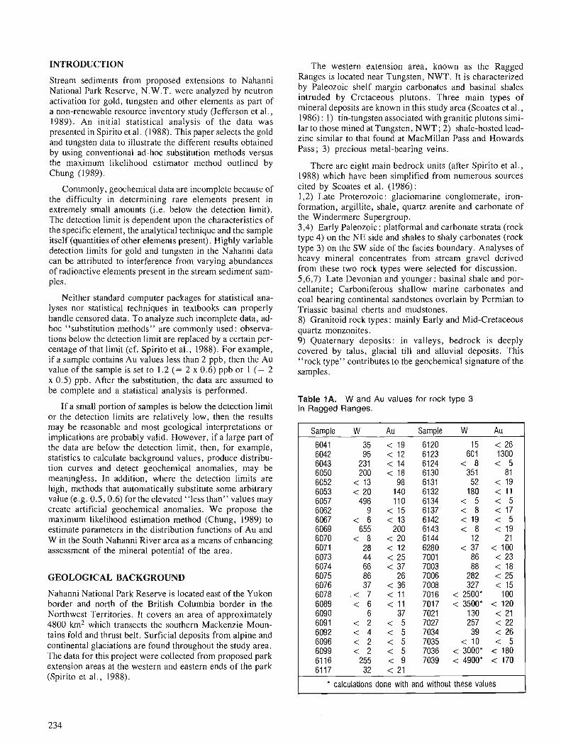
INTRODUCTION

Stream sediments from proposed extensions to Nahanni National Park Reserve, N.W.T. were analyzed by neutron activation for gold, tungsten and other elements as part of a non-renewable resource inventory study (Jefferson et al., 1989). An initial statistical analysis of the data was presented in Spirito et al. (1988). This paper selects the gold and tungsten data to illustrate the different results obtained by using conventional ad-hoc substitution methods versus the maximum likelihood estimator method outlined by Chung (1989).

Commonly, geochemical data are incomplete because of the difficulty in determining rare elements present in extremely small amounts (i.e. below the detection limit). The detection limit is dependent upon the characteristics of the specific element, the analytical technique and the sample itself (quantities of other elements present). Highly variable detection limits for gold and tungsten in the Nahanni data can be attributed to interference from varying abundances of radioactive elements present in the stream sediment samples.

Neither standard computer packages for statistical analyses nor statistical techniques in textbooks can properly handle censored data. To analyze such incomplete data, ad- hoc "substitution methods" are commonly used: observations below the detection limit are replaced by a certain percentage of that limit (cf. Spirito et a]., 1988). For example, if a sample contains Au values less than 2 ppb, then the Au value of the sample is set to 1.2 (= 2 x 0.6) ppb or 1 (= 2 x 0.5) ppb. After the substitution, the data are assumed to be complete and a statistical analysis is performed.

If a small portion of samples is below the detection limit or the detection limits are relatively low, then the results may be reasonable and most geological interpretations or implications are probably valid. However, if a large part of the data are below the detection limit, then, for example, statistics to calculate background values, produce distribution curves and detect geochemical anomalies, may be meaningless. In addition, where the detection limits are high, methods that automatically substitute some arbitrary value (e.g. 0.5,0.6) for the elevated "less than" values may create artificial geochemical anomalies. We propose the maximum likelihood estimation method (Chung, 1989) to estimate parameters in the distribution fbnctions of Au and W in the South Nahanni River area as a means of enhancing assessment of the mineral potential of the area.

GEOLOGICAL BACKGROUND

Nahanni National Park Reserve is located east of the Yukon border and north of the British Columbia border in the Northwest Territories. It covers an area of approximately 4800 km2 which transects the southern Mackenzie Moun- tains fold and thrust belt. Surficial deposits from alpine and continental glaciations are found throughout the study area. The data for this project were collected from proposed park extension areas at the western and eastern ends of the park (Spirito et al., 1988).

The western extension area, known as the Ragged Ranges is located near Tungsten, NWT. It is characterized by Paleozoic shelf margin carbonates and basinal shales intruded by Cretaceous plutons. Three main types of mineral deposits are known in this study area (Scoates et al., 1986) : 1) tin-tungsten associated with granitic plutons similar to those mined at Tungsten, NWT; 2) shale-hosted lead- zinc similar to that found at MacMillan Pass and Howards Pass; 3) precious metal-bearing veins.

There are eight main bedrock units (after Spirito et al., 1988) which have been simplified from numerous sources cited by Scoates et al. (1986): 1,2) Late Proterozoic : glaciomarine conglomerate, iron- formation, argillite, shale, quartz arenite and carbonate of the Windermere Supergroup. 3,4) Early Paleozoic : platformal and carbonate strata (rock type 4) on the NE side and shales to shaly carbonates (rock type 3) on thc SW side of the facies boundary. Analyses of heavy mineral concentrates from stream gravel derived from these two rock types were selected for discussion. 5,6,7) Late Devonian and younger: basinal shale and por- cellanite; Carboniferous shallow marine carbonates and coal-bearing continental sandstones overlain by Permian to Triassic basinal cherts and mudstones. 8) Granitoid rock types : mainly Early and Mid-Cretaceous quartz monzonites. 9) Quaternary deposits: in valleys, bedrock is deeply covered by talus, glacial till and alluvial deposits. This "rock type" contributes to the geochemical signature of the samples.

Table 1A. W and Au values for rock type 3 in Ragged Ranges.

Sample W Au Sample W Au

6041 35 < 1 9 6120 15 < 2 6 6042 95 < 1 2 6123 601 1300 6043 231 < 1 4 6124 < 8 < 5 6050 200 < 1 8 6130 351 8 1 6052 < 13 98 6131 52 < 1 9 6053 < 20 140 6132 180 < 11 6057 496 110 6134 < 5 < 5 6062 9 < 15 6137 < 8 < 17 6067 < 6 < 1 3 6142 < I 9 < 5 6069 655 200 6143 < 8 < 19 6070 < 8 < 20 6144 12 21 6071 28 < 1 2 6280 < 3 7 < I 0 0 6073 44 < 25 7001 86 < 23 6074 66 < 37 7003 88 < 1 8 6075 86 26 7006 282 < 25 6076 37 < 36 7008 327 < 15 6078 . < 7 < 1 1 7016 <2500* 100 6089 < 6 < 1 1 7017 <3500* < I 2 0 6090 6 37 7021 130 < 2 1 6091 < 2 < 5 7027 257 < 22 6092 < 4 < 5 7034 39 < 26 6096 < 2 < 5 7035 < 1 0 < 5 6099 < 2 < 5 7036 < 3000* < 180 6116 255 < 9 7039 < 4900* < 170 6117 32 < 21

* calculations done with and without these values

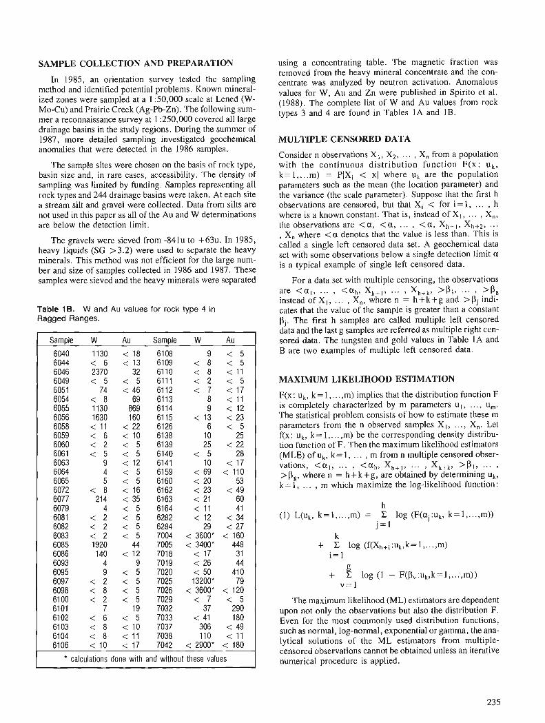
SAMPLE COLLECTION AND PREPARATION

In 1985, an orientation survey tested the sampling method and identified potential problems. Known mineralized zones were sampled at .a 1 :50,000 scale at Lened (W- Mo-Cu) and Prairie Creek (Ag-Pb-Zn). The following summer a reconnaissance survey at 1 :250,000 covered all large drainage basins in the study regions. During the summer of 1987, more detailed sampling investigated geochemical anomalies that were detected in the 1986 samples.

The sample sites were chosen on the basis of rock type, basin size and, in rare cases, accessibility. The density of sampling was limited by funding. Samples representing all rock types and 244 drainage basins were taken. At each site a stream silt and gravel were collected. Data from silts are not used in this paper as all of the Au and W determinations are below the detection limit.

The gravels wcre sieved from -841u to +63u. In 1985, heavy liquids (SG >3.2) were used to separate the heavy minerals. This method was not efficient for the large number and size of samples collected in 1986 and 1987. These samples were sieved and the heavy minerals were separated

Table 1B. W and Au values for rock type 4 in Ragged Ranges.

Sample W Au Sample W Au

6040 1130 < 18 6108 9 < 5 6044 < 6 < 1 3 6109 < 8 < 5 6046 2370 32 6110 < 8 < 11 6049 < 5 < 5 6111 < 2 < 5 6051 74 < 46 6112 < 7 < 17 6054 < 8 69 6113 8 < 11 6055 1130 869 6114 9 < 12 6056 1630 160 6115 < 1 3 < 2 3 6058 < 11 < 22 6126 6 < 5 6059 < 6 < 10 6138 10 25 6060 < 2 < 5 6139 25 < 22 6061 < 5 < 5 6140 < 5 28 6063 9 < 1 2 6141 10 < 17 6064 4 < 5 6159 < 6 9 < I 1 0 6065 5 < 5 6160 < 20 53 6072 < 8 < 1 6 6162 < 2 3 < 4 9 6077 214 < 35 6163 < 21 60 6079 4 < 5 6164 < 1 1 41 6081 < 2 < 5 6282 < 1 2 < 3 4 6082 < 2 < 5 6284 29 < 27 6083 < 2 < 5 7004 < 3600* < 160 6085 1920 44 7005 < 3400* 448 6086 140 < 12 7018 < 17 3 1 6093 4 9 7019 < 26 44 6095 9 < 5 7020 < 5 0 410 6097 < 2 < 5 7025 13200* 79 6098 < 8 < 5 7026 < 3600* < 120 6100 < 2 < 5 7029 < 7 < 5 61 01 7 19 7032 37 290 6102 < 6 < 5 7033 < 41 180 6103 < 8 < 10 7037 306 < 49 6104 < 8 < 1 1 7038 110 < 11 6106 < 1 0 < 1 7 7042 <2900* < I 8 0

* calculations done with and without these values

using a concentrating table. The magnetic fraction was removed from the heavy mineral concentrate and the concentrate was analyzed by neutron activation. Anomalous values for W, Au and Zn were published in Spirito et al. (1988). The complete list of W and Au values from rock types 3 and 4 are found in Tables 1A and 1B.

MULTIPLE CENSORED DATA

Consider n observations X , , X2, . . . , Xn from a population with the continuous distribution function F(x: uk, k= l , . . .m) = P(Xi < x) where uk are the population parameters such as the mean (the location parameter) and the variance (the scale parameter). Suppose that the first h observations are censored, but that Xi < for i = 1, . . . , h where is a known constant. That is, instead of X I , .. . , X,, the observations are < a , < a , . . . , < a , Xh+ I , Xh+29 . . . , X, where <a denotes that the value is less than. This is called a single left censored data set. A geochemical data set with some observations below a single detection limit a is a typical example of single left censored data.

For a data set with multiple censoring, the observations are < a l , ... , < a h , Xh+,, ... , Xh+k, > P I . ... , > P g instead of X I , . . . , X,, where n = h +k+g and > Bj indicates that the value of the sample is greater than a constant bj. The first h samples are called multiple left censored data and the last g samples are referred as multiple right censored data. The tungsten and gold values in Table 1A and B are two examples of multiple left censored data.

MAXIMUM LIKELIHOOD ESTIMATION

F(x: u,, k= 1,. . . ,m) implies that the distribution function F is completely characterized by m parameters u l , .. . , u,. The statistical problem consists of how to estimate these m parameters from the n observed samples X I , . . . , X,. Let f(x : uk, k= 1,. . . ,m) be the corresponding density distribution function of F. Then the maximum likelihood estimators (MLE) of uk, k = 1, . . . , m from n multiple censored observations, < a l , ... , < a h , X h + , , ... , Xh+k, > P I , ... , > bg, where n = h+ k+g, are obtained by determining uk, k = 1, . . . , m which maximize the log-likelihood function :

h (1) L(ukr k = 1 ,..., m) = C log (F(aj:uk, k = l , ..., m))

j=1 k

+ C log (f(Xh+i:uk,k= 1, ..., m) i= 1

The maximum likelihood (ML) estimators are dependent upon not only the observations but also the distribution F. Even for the most commonly used distribution functions, such as normal, log-normal, exponential or gamma, the analytical solutions of the ML estimators from multiple- censored observations cannot be obtained unless an iterative numerical procedure is applied.

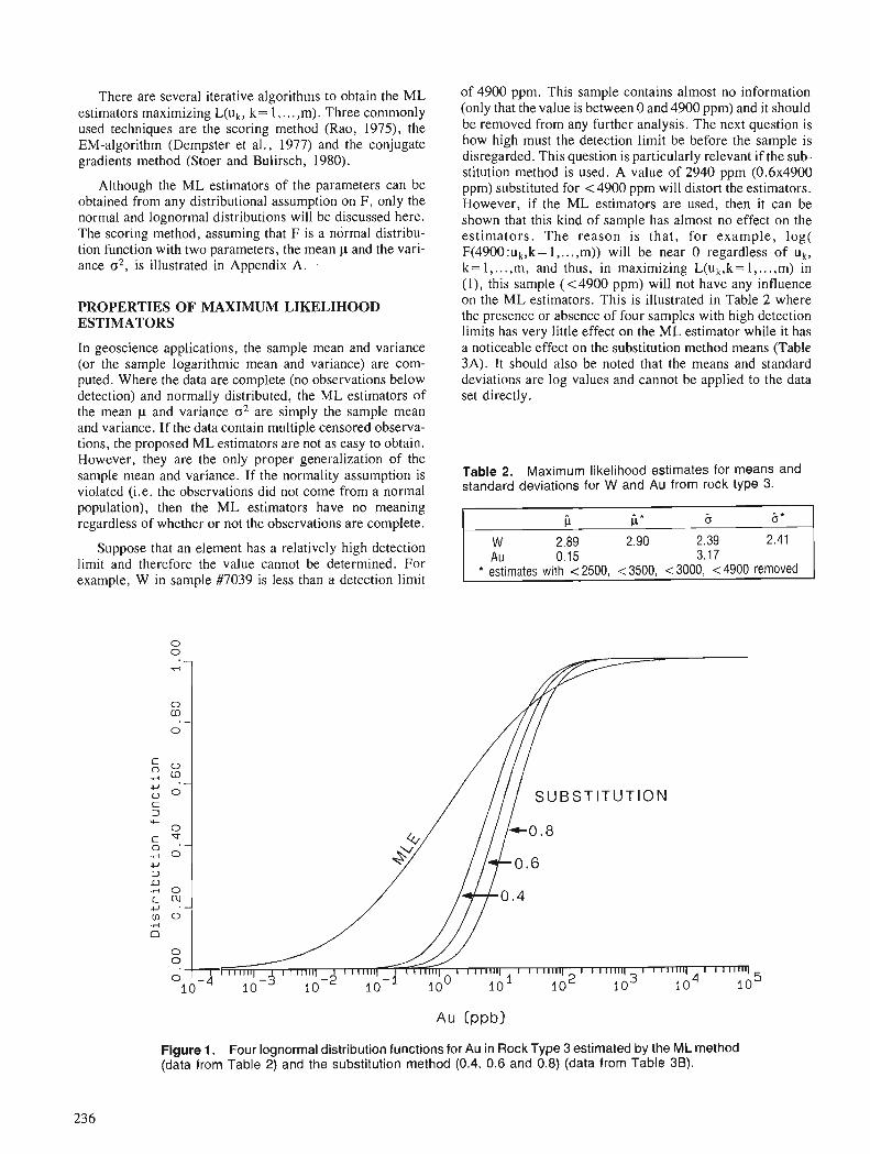
There are several iterative algorithms to obtain the ML estimators maximizing L(uk, k= 1, . . . ,m). Three commonly used techniques are the scoring method (Rao, 1975), the EM-algorithm (Dempster et al., 1977) and the conjugate gradients method (Stoer and Bulirsch, 1980).

Although the ML estimators of the parameters can be obtained from any distributional assumption on F, only the normal and lognormal distributions will be discussed here. The scoring method, assuming that F is a normal distribution function with two parameters, the mean p and the variance 02, is illustrated in Appendix A. .

PROPERTIES O F MAXIMUM LIKELIHOOD ESTIMATORS

of 4900 ppm. This sample contains almost no information (only that the value is between O and 4900 ppm) and it should be removed from any further analysis. The next question is how high must the detection limit be before the sample is disregarded. This question is particularly relevant if the substitution method is used. A value of 2940 pprn (0 .6~4900 ppm) substituted for <4900 pprn will distort the estimators. However, if the ML estimators are used, then it can be shown that this kind of sample has almost no effect on the estimators. The reason is that, for example, log( F(4900:uk,k=l, ..., m)) will be near 0 regardless of uk, k = 1,. . .,m, and thus, in maximizing L(uk,k= 1 ,. . . ,m) in ( I ) , this sample (<4900 ppm) will not have any influence on the ML estimators. This is illustrated in Table 2 where the presence or absence of four samples with high detection limits has very little effect on the ML estimator while it has

In geoscience applications, the sample mean and variance a noticeable effect on the substitution method means (Table (or the sample logarithmic mean and variance) are com- 3A). It should also be noted that the means and standard puted. Where the data are complete (no observations below deviations are log values and cannot be applied to the data detection) and normally distributed, the ML estimators of set directly. the mean p and variance o2 are simply the sample mean and variance. If the data contain multiple censored observations, the proposed ML estimators are not as easy to obtain. However, they are the only proper generalization of the sample mean and variance. 1f the normality assumption is Table 2. Maximum likelihood estimates for means and

violated (i.e. the observations did not come from a normal standard deviations and Au 'ype 3.

population), then the ML estimators have no meaning regardless of whether or not the observations are complete.

Suppose that an element has a relatively high detection limit and therefore the value cannot be determined. For example, W in sample #7039 is less than a detection limit

2.89 2.90 2.39 Au 0.15 3.17

* estimates with <2500, ~ 3 5 0 0 , <3000, ~ 4 9 0 0 removed

Figure 1. Four lognormal distribution functions for Au in Rock Type 3 estimated by the ML method (data from Table 2) and the substitution method (0.4, 0.6 and 0.8) (data from Table 36).

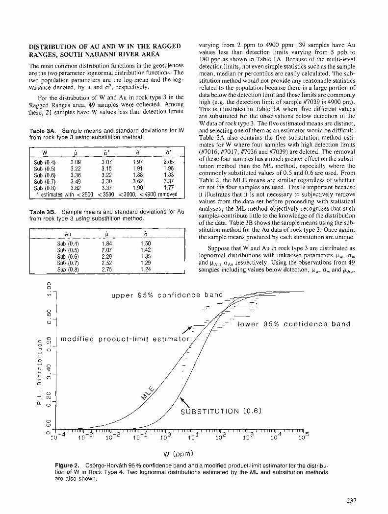
DISTRIBUTION OF AU AND W IN THE RAGGED RANGES, SOUTH NAHANNI RIVER AREA

The most common distribution functions in the geosciences are the two parameter lognormal distribution functions. The two population parameters are the log-mean and the log- variance denoted, by p and 02, respectively.

For the distribution of W and Au in rock type 3 in the Ragged Ranges area, 49 samples were collected. Among these, 21 samples have W values less than detection limits

Table 3A. Sample means and standard deviations for W from rock type 3 using substitition method.

W b b * 6 6 *

Sub (0.4) 3.09 3.07 1.97 2.05 Sub (0.5) 3.22 3.15 1.91 1.98 Sub (0.6) 3.36 3.22 1.88 1.83 Sub (0.7) 3.49 3.30 3.62 3.37 Sub (0.8) 3.62 3.37 1.90 1.77 * estimates with < 2500, <3500, <3000, <4900 removed

varying from 2 ppm to 4900 ppm; 39 samples have Au values less than detection limits varying from 5 ppb to 180 ppb as shown in Table IA. Because of the multi-level detection limits, not even simple statistics such as the sample mean, median or percentiles are easily calculated. The substitution method would not provide any reasonable statistics related to the population because there is a large portion of data below the detection limit and these limits are commonly high (e.g. the detection limit of sample #7039 is 4900 pm). This is illustrated in Table 3A where five different values are substituted for the observations below detection in the W data of rock type 3. The five estimated means are distinct, and selecting one of them as an estimator would be difficult. Table 3A also contains the five substitution method estimates for W where four samples with high detection limits (#7016, #7017, #7036 and #7039) are deleted. The removal of these four samples has a much greater effect on the substitution method than the ML method, especially where the commonly substituted values of 0.5 and 0.6 are used. From Table 2, the MLE means are similar regardless of whether or not the four samples are used. This is important because it illustrates that it is not necessary to subjectively remove values from the data set before proceeding with statistical

Table 3B. Sample means and standard deviations for Au analyses; the ML method objectively recognizes that such

from rock type 3 using substitition method. samples contribute little to the knowledge of the distribution of the data. Table 3B shows the sample means using the sub-

Sub (0.4) Sub (0.5) Sub (0.6) Sub (0.7) 2.52 Sub (0.8) 2.75 1.24

stitution method for the Au data of rock type 3. Once again, the sample means produced by each substitution are unique.

Suppose that W and Au in rock type 3 are distributed as lognormal distributions with unknown parameters pw, ow and pAu, respectively. Using the observations from 49 samples including values below detection, p,, ow and PA,,,

upper 9 5 % con f idence band - -

r- -- lower 9 5 % con f i dence

I mod i f i ed product - l imi t es t imato r :/:/

band

Figure 2. Csorgo-HorvBth 95% confidence band and a modified product-limit estimator for the distribution of W in Rock Type 4. Two lognormal distributions estimated by the ML and substitution methods are also shown.

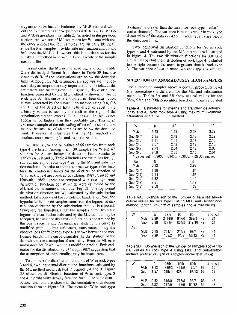
o,, are to be estimated. Estimates by MLE with and without the four samples for W (samples #7016, #7017, #7036 and #7039) are shown in Table 2. As noted in the previous section, the two sets of M L estimates for W - one with and the other without the four samples, are virtually identical, since the four samples provide little information and do not influence the MLE's. However, this is not the case for the substitution method as shown in Table 3A where the s a m ~ l e means differ.

In particular, the ML estimates of pAu and ow in Table 2 are distinctly different from those in Table 3B because close to 80 % o f the observations are below the detection limit. Although the ML estimators are appropriate, the lognormality assumption is very important, and if violated, the estimators are meaningless. In Figure 1, the distribution function generated by the ML method is shown for Au in rock type 3. This curve is compared to three distribution curves generated by the substitution method using 0.4, 0 .6 and 0.8 of the detection limit. The effect of substituting arbitrary values is seen by the shift to the right of the substitution-method curvei. In all cases, the k u values appear to be higher than they probably are. This is an extreme example of the misleading effect of the substitution method because 41 of 48 samples are below the detection limit. However, it illustrates that the ML method can produce more meaningful and realistic results.

In Table IB, W and Au values of 66 samples from rock type 4 are listed. Among them, 39 samples for W and 47 samples for Au are below the detection limit. Similar to Tables 2A, 2B and 3, Table 4 includes the estimates for u,, s,, u,, and sAu of rock type 4 using the ML and substitution methods. In order to compare these two types of estimators, the confidence bands for the distribution function of W in rock type 4 are constructed (Chung, 1987 ; ~ s o r g 6 and Horviith, 1985). These are compared with two lognormal distribution functions for W which were estimated by the ML and the substitution methods (Fig. 2). The lognormal distribution function for W, estimated by the substitution method, falls outside of the confidence band. Therefore, the hypothesis that the 66 samples came from the lognormal distribution estimated by the substitution method is rejected. However, the hypothesis that the samples came from the lognormal distribution estimated by the ML method may be accepted, because the distribution function is constrained by the confidence bands. An empirical distribution curve (a modified product limit estimator), constructed using the observations for W in rock type 4 is shown between the confidence bands. This curve estimates the distribution of the data without the assumption of normality. Even the ML estimator does not fit well with this modified product-limit estimator for the distribution (cf. Chung, 1987) suggesting that the assumption of lognormality may be inaccurate.

To compare the distribution functions of W in rock types 3 and 4, two lognormal distribution functions estimated by the ML method are illustrated in Figures 3A and B. Figure 3A shows the distribution functions of W in rock types 3 and 4 in probability density function form. The same distribution functions are shown in the cumulative distribution function form in Figure 3B. The mean for W in rock type

3 (shales) is greater than the mean for rock type 4 (platfor- ma1 carbonates). The variance is much greater in rock type 4 and 59 % of the data (vs 43 % in rock type 3) are below the detection limit.

Two lognormal distribution functions for Au in rock types 3 and 4 estimated by the ML method are illustrated in Figure 4. The two distribution functions for Au have similar shapes but the distribution of rock type 4 is shifted to the right because the mean is greater than in rock type 3. The variance of Au in these two rock types is similar.

SELECTION OF ANOMALOUSLY HIGH SAMPLES

The number of samples above a certain probability level (i.e. anomalous) is different for the M L and substitution methods. Tables 5A and 5B show critical values for the 98th, 95th and 90th percentiles based on means calculated

Table 4. Estimators for means and standard deviations for W and Au from rock type 4 using maximum likelihood estimation and substitution method.

W fi fi * 6 6 *

MLE 1.13 1.13 3.37 3.39 Sub (0.4) 2.25 2.19 2.16 2.22 Sub (0.5) 2.41 2.31 2.13 2.16 Sub (0.6) 2.57 2.42 2.12 2.10 Sub (0.7) 2.73 2.54 2.13 2.05 Sub (0.8) 2.89 2.66 2.15 2.01

values with <3600, <3400, ~ 3 6 0 0 , <2900 removed Au Ci. 6

MLE 0.82 2.92 Sub (0.4) 1.96 1.64 Sub (0.5) 2.14 1.56 Sub (0.6) 2.32 1.49 Sub (0.7) 2.51 1.43 Sub (0.8) 2.69 1.38

Table 5A. Comparison of the number of samples above critical values for rock type 3 using MLE and Substitution method. (critical value/# of samples above that value)

MLE 2.89 244410 91710 38313 49 Sub 3.36 137114 63415 319110 49

MLE 0.15 78411 21411 6717 49 Sub 2.29 15812 9118 56/12 49

Table 5B. Comparison of the number of samples above critical values for rock type 4 using MLE and Substitution method. (critical value/# of samples above that value)

MLE 1.13 173612 49115 16017 66 Sub 2.57 1019111 427111 197113 66

MLE 0.82 91610 27715 9517 66 Sub 2.32 21715 11819 69112 66

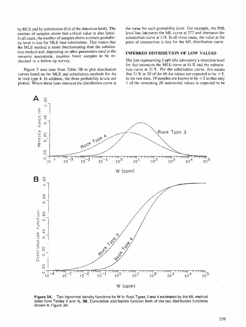
by MLE and by substitution (0.6 of the detection limit). The the value for each probability level. For example, the 95th number of samples above that critical value is also listed. level line intersects the ML curve at 277 and intersects the In all cases, the number of samples above a certain probabil- substitution curve at 1 18. In all three cases, the value at the ity level is less for MLE than substitution. This means that point of intersection is less for the ML distribution curve. the MLE method is more discriminating than the substitution method and, depending on other parameters used in the INFERRED DISTRIBUTION OF LOW VALUES resource assessment, requires fewer samples to be re- checked in a follow-up survey. The line representing 5 ppb (the laboratory's detection level

for Au) intersects the MLE curve at 61 % and the substitu- Figure 5 uses data from Table 5B to plot distribution tion curve at 31 %. For the substitution curve, this means

curves based on the MLE and substitution methods for Au that 31 % or 20 of the 66 Au values are expected to be < 5 . in rock type 4. In addition, the three probability levels are In the raw data, 19 samples are known to be < 5 so that only plotted. Where these lines intersect the distribution curve is 1 of the remaining 28 undetected values is expected to be

Figure 3A. Two lognormal density functions for W in Rock Types 3 and 4 estimated by the ML method (data from Tables 2 and 4), 38. Cumulative distribution function form of the two distribution functions shown in Figure 3A.

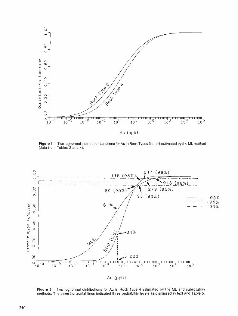
Figure 4. Two lognormal distribution functions for Au in Rock Types 3 and 4 estimated by the ML method (data from Tables 2 and 4).

Figure 5. Two lognormal distributions for Au in Rock Type 4 estimated by the ML and substitution methods. The three horizontal lines indicated three probability levels as discussed in text and Table 5.

<5. The MLE curve intersects the 5 ppb line at 61 % so that 40 of 66 samples are expected to be < 5. Again, because 19 of the samples are known to be <5, then 21 of the remaining undetected samples are expected to be <5. Because the laboratory's detection level is <5, and the presence of radioactive elements is common for this area, it is reasonable to assume that more than just one of the remaining 28 undetected values is actually < 5 , suggesting that the curve generated by the MLE method more accurately reflects the distribution of Au in rock type 4.

CONCLUDING REMARKS

Statistical analysis of incomplete geochemical data is facilitated by using maximum likelihood estimators. For data sets which are distributed normally and are complete, the maximum likelihood estimators are simply the sample mean and variance. In the case of incomplete censored data, the maximum likelihood estimators (MLE) obtained by an iterative procedure, are the most appropriate estimates of the population mean and variance. If the assumption that the data are normal or lognormal is violated, then the estimators are meaningless, even when the data set is complete.

The gold and tungsten values of heavy mineral concentrates from the Ragged Ranges contain a large proportion of undetected values. If the data are to be used in a geological assessment, they should ideally be re-analyzed to reduce the size and variability of the detection limit. If this is not possible, the data must be used as they are. The MLE method can handle such data, provides more reasonable results than the substitution method, and is more discriminating for the comparison of different geologic environments.

ACKNOWLEDGMENTS

We thank C.W. Jefferson of the Geological Survey of Can- ada for providing not only the data, which are part of a set that was acquired for a resource assessment of South Nahanni River area, but also for useful comments on our

earlier draft of this paper. We also acknowledge the referees whose suggestions improved the manuscript. The resource assessment was jointly funded by Environment Canada (Parks), Indian and Northern Affairs Canada, and the Geo- logical Survey of Canada. Polar Continental Shelf Project provided additional logistical support.

REFERENCES

Chung, C.F 1987: Confidence bands for the distribution and quantile functions for

truncated and randomly censored data; Quantitative Analysis of Mineral and Energy Resources; ed. C.F. Chung et al; Reidel, Dordrecht, p. 433-457.

1989: Regression analysis of geochemical data with observations below detection limits; Computer Applications in Resource Estima- tion: Prediction and Assessment for Minerals and Petroleum, ed. G. Gaal and D. Merriam; Pergamon, Oxford (in press).

CsorgG, S. and Horvith, L. 1986: Confidence bands from censored samples; Canadian Journal of

Statistics, v. 14, p. 131-144. Dempster, A.P., Laird, N.M. and Rubin, D.B. 1977: Maximum likelihood from incomplete data via the EM algorithm;

Journal of Royal Statistical Society, Series B, v. 39, p. 1-22. Jefferson, C.W., Spirito, W.A., Hamilton, S.M., Michel, F.A. and Pare, D. 1989: Geochemistry of stream sediments, bedrock and spring waters in

resource assessment of the South Nahanni River area, Yukon and N.W.T. ; in Program and Abstracts, Contributions of the Geologi- cal survey of Canada, Cordilleran Geology and Exploration Roundup, February 7-10, 1989, p. 18-21.

Rao, C.R. 1975: Linear Statistical Inference and its Applications, 2nd ed., John

Wiley and Sons, New York, 625p. Scoates, R.F.J., Jefferson, C.W. and Findlay, D.C. 1986: Northern Canada mineral resource assessment; Mineral

Resource Assessment on Public Lands: Proceedings of the Lees- burg Workshop, ed. S.M. Cargill and S.B. Green; U.S. Geologi- cal Survey Circular 980, p. 1 11- 139.

Spirito, W.A., Jefferson, C.W. and Pare, D. 1988: Comparison of gold, tungsten and zinc in stream silts and heavy

mineral concentrates, South Nahanni resource assessment area, District of Mackenzie; Current Research, Part E, Geological Survey of Canada Paper, 88-IE, p. 117.126.

Stoer, J. and Bulirsch, R. 1980: Introduction to Numerical Analysis; Springer-Verlag, Berlin.

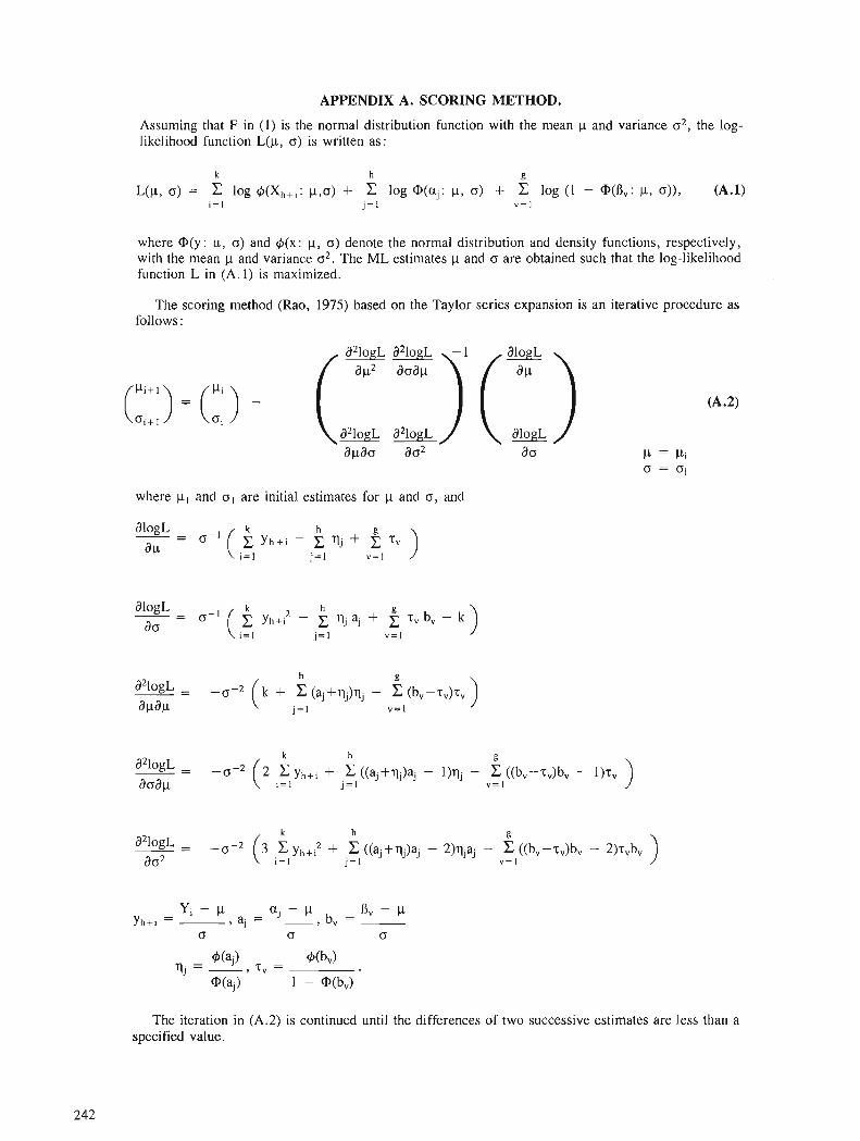
APPENDIX A. SCORING METHOD.

Assuming that F in (1) is the normal distribution function with the mean p and variance 02, the log- likelihood function L(p, a) is written as:

k h g

L(p, o) = C log 6 (Xh+i : p ,o) + C log @(aj: p, o) + C log (1 - cD(Bv: p , o)), (A.l) i = l j= l v = l

where @(y: p, o) and 4(x: p, a) denote the normal distribution and density functions, respectively, with the mean p and variance 02. The ML estimates p and a are obtained such that the log-likelihood function L in (A. 1) is maximized.

The scoring method (Rao, 1975) based on the Taylor series expansion is an iterative procedure as follows :

where p I and cs, are initial estimates for p and o, and

h g -- a210gL - (k + Z (a, +y)y - Z (bv-rv)rv a ~ a ~ j=l v= I

The iteration in (A.2) is continued until the differences of two successive estimates are less than a specified value.

Noise suppression and coherency enhancement of seismic data

Bernd Milkereit 1 and Carl Spencer 1

Milkereit, B. and Spencer, C., Noise suppression and coherency enhancement of seismic data; 0_ Statistical Applications in the Earth Sciences ed. F.P. Agterberg and G. F. Bonham-Carter; Geological Survey of Canada, Paper 89-9, p. 243-248, 1989

Abstract

Image processing techniques are applied to support the interpretation of reflection and refraction seismic data. A computer-efficient noise suppression and coherency enhancement scheme based upon the combination of multi-trace localized slant stacking and median filtering is presented. Enhanced data are weighted versions of the input data and no data mixing or smearing of information is required. This coherency enhancement scheme produces improved seismic sections and permits the interpretation of data in regions where initial seismic sections were extremely noisy.

Resume

Des techniques de traitement des images sont utilisees pour faciliter l 'interpretation de donnees de sismique rejlexion et de sismique refraction. On presente ici un algorithme de suppression du bruit et d 'amelioration de la coherence qui est peu exigeant en termes de ressources informatiques. Cet algorithme fait appel a la sommation oblique localisee des traces sismiques et a l 'utilisation de filtres medians. Les donnees ainsi traitees sont une version ponderee des donnees d 'entree : le melange et la dilution de !'information sont ainsi evitis. Cet algorithme de rehaussement de la coherence ameliore la qualite des profits sismiques et permet l 'interpretation de donnees en provenance de regions ou on a releve des profils sismiques initiaux tres bruyants.

1 Geological Survey of Canada, 1 Observatory Crescent, Ottawa, Ontario KlA OY3

243

INTRODUCTION Filter design

The major aim of deep seismic reflection and refraction profiling is to otain information about the subsurface structure of the Earth's crust. With targets often deeper than 30 km and typical profile lengths exeeding 100 km, extra effort is required to extract low amplitude signals excited by controlled sources from random or correlated background noise. Such seismic experiments are usually carried out along straight lines across geological targets. Sources (mechanical or explosive devices) and receivers (vertically or horizontally orientated sensors of ground motion) are densely spaced along the survey line. Digital recording of the band-limited (5 - 40 Hz) signals leads to a data set u(x,t) dependent on listening time (t) and spatial location of sensors (x). Receiver spacing ranges typically from 25 to 100 m and may not be constant along profiles : thus the wave field u(x,t) may not be sampled equally as a function of x.

In the presence of low signal-to-noise (s :n) ratios, conventional 1-dimensional or 2-dimensional data processing techniques such as bandpass and pie-slice filtering or deconvolution, often cannot reduce the noise level. In this paper we present a fast 2-dimensional coherency filter that is capable of suppressing uncorrelated noise as well as correlated noise outside the dip or velocity passband. The filter can be applied to large volumes of equally and unequally spaced digital data. The proposed algorithm is optimized for use on a vector computer.

COHERENCY FILTERING

In order to separate the signal and noise components of 2-dimensional data the following assumptions are made: (a) background noise has no spatial coherency, thus phase- coherent signal can be separated from background noise on the basis of coherency estimates ; and (b) coherent noise can be separated from coherent signal on the basis of different dips (slownesses). An estimate of the local spatial coherency can be obtained by the evaluation of the semblance criterion (Neidell and Taner, 1971), and a measure of the local dip (slowness) component can be obtained by means of slant stacking (a beam-forming process) (McMechan, 1983). A wide range of applications in crustal seismology have been based on the combination of semblance and slant stacking : coherency filtering of seismic data has been suggested by Leven and Roy-Chowdhury (1984) and Kong et al. (1985) ; slowness filtering has been used to improve the performance of pre- and poststack migration (Milkereit, 1987a), the separation of compressional and shear waves (Milkereit and Spencer, 1987), and the migration velocity analysis (Milkereit and Spencer, 1988). Here we describe a semblance-based filter in the time domain that has been designed to enhance coherent seismic energy by suppressing incoherent background noise.

Consider a seismic wavefield u(x,t) sampled M times along the t-axis, and N times along the x-axis. Spatial sampling of u(x,t) may not be regular, but sampling in x should be dense enough to avoid spatial aliasing. For the purpose of digital filtering we consider u(x,t) as an NxM element 2-dimensional image. In our notation x, defines the spatial coordinate for the nth sample of the wavefield u(x,t).

The dimensions of dip or slowness (p), At

P = z

of seismic data are s km-I. Let the dip passband be defined for slownesses pi, sampled at J equally spaced steps between pmin and p,,,,:

Pmin 5 Pj 5 Prnax, (1 5 j 5 J),

which should cover all apparent dips of interest of the seismic data u(x,t). A coherency estimate W must be obtained for each sample of the wavefield u(x,t); such local estimates are obtained by moving a limited aperture (L-trace) window across the wavefield u(x,t) (see Milkereit (1987b) for details). For a given slowness pj, the local multichannel coherency estimate W ( t , pi; x,) of the wavefield u(x,t) at x, and at time t is defined as:

where w(t, pi, x,) is the local slant stack (McMechan, 1983) of a finite L-trace aperture centered at x,,

where the L-trace window is defined between:

and where u(x,, r,) is the seismic data at distance x, and at time tl:

t, = t + pj(xl - x,,)

In terms of a shift-and-sum (beam-forming) operation, a time shift At, has to be applied to trace 1 before stacking in equations (1) and (2) :

At, = p,(x, - 5,). (3)

Based on the J local coherency estimates W(t, pi; x,) a simple coherency filter C(x,, t) can be defined as the maximum coherency in the given slownessldip passband:

C(x,,t) = max(W(t, pi; x,)) j, (1 I j 5 J). (4)

Equations (1-4) have to be evaluated for each sample of the observed wavefield u(x,t) resulting in a NxM image of coherency weights C(x,t). The coherency enhanced data U(x,t) are given by multiplying the observed image u(x,t) with the coherency weight image C(x,t):

where y and d are scaling factors which are discussed in the following paragraph. It is worth emphazising that the enhanced data U(x,t) are weighted versions of the input data u(x,t) and that no data mixing or smearing, similar to the ones implicit in the algorithm of Kong et al. (1985), are involved.

NW

S

E

35

00

CM

P N

o.

30

00

2

50

0

20

00

Con

nect

icut

Val

ley

-Gas

p6 S

yncl

inor

ium

Vic

tori

a F

aultl

LIN

E Q

MI

San

dy

Str

ea

m F

ault,l

Fa

ult

Bo

un

dar

y I I

Fig

ure

1.

Sei

smic

rec

ord

sect

ion

(unm

igra

ted)

from

the

the

Que

bec-

Mai

ne

tran

sect

. A

dc-

shift

of

10

per

cent

of

the

over

all

rms-

ampl

itude

was

use

d fo

r th

e va

riabl

e ar

ea d

ispl

ay.

Fro

nten

ac F

orm

atio

n T

urbi

dite

s C

hain

Lak

es M

assi

f

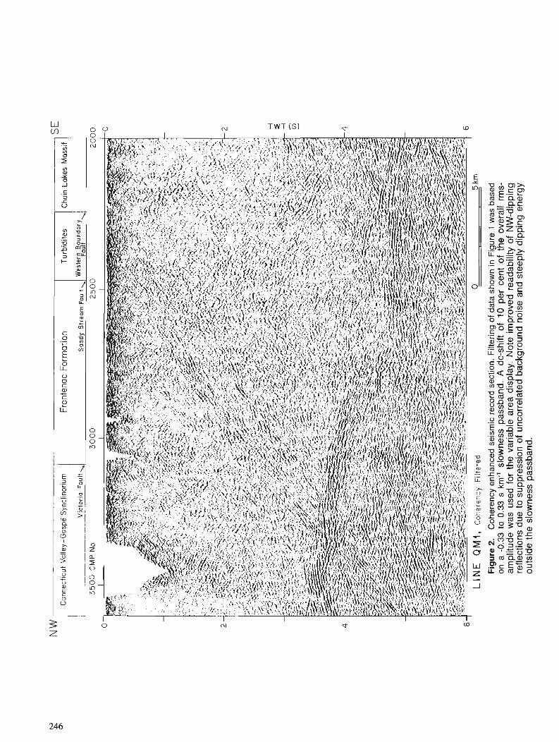
T W T ( S ) d w

E x In

0

I""" m L Qa, o-.nr 0- a m g?

? 3 . ~ ' - o z a

.+a 5 0% .PE > >. u.+.= - c 0, .- - a a, 5 $25 ~ O c U u O L L C . a u a

Q a a, -00 2.5 - 7 - L 0 0- Qt

p 0 .E .- $ S O 3 ~ 5 5 2 '" &ZF gu 2: .z a gn a, . ( /)o 0 -a .- CUB E a a on'piij g m !?! = - z a g 0 .- asc $ , m a 1 .- m a.+ $ a,.= 0 +

s a c c rn 2 3 > 0 2 o 10 0.- ? C( / )S$$ U - t- LI C ' E O Q Q

Q, 2 $03:2$ E a,cr,:sr " $ " z 5 ,ocna,o " 0 a='=

o B 5 U , - "a,?S m U I iq2.g0

.- 00 a 3 a E a m g HsCZZ - -1

Implementation

Reflection or refraction seismic studies of the Earth's crust deal with large data volumes; typical values for the observed NxM image u(x,t) are N=2000 and M=4000, respectively. The choice of the number of traces (L) for finite aperture slant stacks in equations (1-2) depends on the minimum lateral correlation length of what is considered to be phase-coherent signal. In this paper we used a 9-trace aperture (L=9) to compute the coherency estimates W(t, p;x) ; for an average trace spacing of 50 meters this results in a 400 m minimum correlation length. Examples based on noisy synthetic data and a 9-trace aperture demonstrate that local slant stacks provide stable results even for data with s:n ratios as low as 0.5 (Milkereit, 1987b; Milkereit and Spencer, 1987).

The number of beam-forming operations (J) is guided by the frequency content, the spatial sampling interval and the maximum dip/slowness of the data (see Milkereit (1987b) for details). Here we apply 61 beam-forming operations (J =61) within the slowness passband :

For each sample of the seismic section we obtain J coherency estimates W(t, pj; x), each estimate has values between 0 and 1. The lower bound describing complete incoherency and the upper bound indicating identical amplitudes u(x,t) on all L traces across the aperture, associated with a coherent wavefront of slowness (dip) p,. Zero cross- ings of the observed amplitudes can decrease the coherency estimate by decreasing the numerator in equation (1). Iso- lated spikes of low coherency have to be removed to obtain a smooth distribution of coherency weights. This can be achieved by applying a short-window 2-dimensional median filter to the J-trace coherency data W(t, pj; x) before computing the coherency weights C(x,t) from equation (4). Examples of median filtering of coherency estimates are given in Milkereit (1987a,b).

The noise suppression can be controlled by the weighting of C(x,t) in equation (5). In practice, an exponentiation of C(x,t)Y in the form of:

1.0, if s:n 2 1; Y = { I ls:n, otherwise.

gives satisfactory results, where y is the reciprocal of the low s:n ratio of the input data. For variable area displays a dc-shift, shown as d in equation ( S ) , is added to the seismic image to improve readability of the seismic section. The dc- shift introduces a threshold which is chosen to be within 10 to 25 per cent of the overall rms-amplitude.

While it is difficult to implement this type of coherency enhancement in the form of a recursive filter, a significant portion of the algorithm is vectorizable. The time shift Atl (equation (3)) is a constant for all times t for a given set of trace coordinates (x,, xl) and given slowness (pi). This

reduces the slant stack and semblance computation in equations (1-2) to a simple shift-and-sum operation with respect to recording time t . For equally spaced data, time shifts At are a function of J slownesses and L spatial coordinates and need to be computed only once. Coherency filtering of an equally spaced seismic data set with M=2000, N=2000, J=61 and L=9 requires 2 175 seconds on a Convex-CI2O mini supercomputer.

Data example

Noisy data from the the QuCbec-Maine transect (e.g. Spencer et al., 1987) are shown in variable area display in Figure 1. The cmp-processed stacked section exhibits both steeply SE-dipping noise (shear wave?) and a significant background noise level. The coherency enhanced section is shown in Figure 2. Processing and display are based on a -0.33 to 0.33 s km-I slowness passband, a scaling factor of y = 1.5 for the coherency weights, and dc-shift of 10 per cent of the overall rms-amplitude. A notable result (shown in Fig. 2) is the suppression of the steeply dipping noise trains without introducing artifacts (e.g. trace mixing effects). In additon, uncorrelated background noise has successfully been removed by the coherency filter; in the process the new scheme provides an improved section for the structural interpretaton of deep seismic data.

Discussion

The coherency enhancement scheme presented above is based on the combination of local slant stack and multitrace coherency estimates. The proposed coherency filter enables the user to specify a dip passband, to remove uncorrelated background noise fluctuations, and to suppress coherent energy outside the passband. The filter is capable of handling unequally spatially sampled data. The filter operates entirely in the time-offset domain; problems associated with forward and inverse tranformation of the data (e.g. wrap- around) are avoided. The extra effort that goes into the computation and application of coherency weights is justified when conventional processing techniques such as bandpass and pie-slice filtering, and deconvolution cannot reduce the noise level of the data.

ACKNOWLEDGMENTS

We thank L.J. Mayrand and A.G. Jones for reviewing a preliminary version of this manuscript.

REFERENCES

Kong, S.M., Phinney, R.A., and Roy-Chowdhury, K. 1985: A nonlinear signal detector for enhancement of noisy seismic sec-

tions; Geophysics, v . 50, p. 539 550. Leven, J.H. and Roy-Chowdhury, K. 1984: A semblance-weighted slowness filter in the time domain, con-

tributed paper at the 54th Annual International SEG Meeting, Soci- ety of Exploration Geophysicists, Atlanta, p. 432 - 436.

McMechan, G.A. Neidell, N.S. and Taner, M.T. 1983: P-x imaging by localized slant stacks of t-x data; Royal Astronomi- 197 1 : Semblance and other coherency measures or multichannel data,

cal Society, Geophysical Journal. v. 72, p. 213 - 221. Geophysics, v. 36, p. 482 - 497. Milkereit, B. Spencer, C., Green, A. and Luetgert J. 1987a: Migration of noisy seismic data; lournal of Geophysical 1987: More seismic evidence on the location of the Grenville basement

Research, v. 92, p. 7916 - 7930. beneath the Appalachians of QuCbec-Maine; Royal Astronomical 1987b: Decomposition and inversion of seismic data - an instantaneous Society, Geophusical Journal, v. 89, p. 177 - 182.

slowness approach; Geophysical Prospecting, v. 35, p. 875 - 894.

Milkereit, B. and Spencer, C. 1987 : A new migration method applied to the inversion of P-S converted

phases; in Deconvolution and Inversion, ed. M. Bernabini, P. Car- rion, G. Jacovitti, F. Rocca, S.Treitel and M.H. Worthington; Blackwell Scientific Publications, Oxford, p. 251 - 266.

1988: A new method for the migration velocity analysis of noisy seismic data, Signal Processing, v. 16, p. 237 - 247.

Statistical and fractal models of nonequilibrium mineral growth

A.D. Fowlerl, D. Roachl, and R. Th6riaultl

Fowler, A.D., Roach, D. and The'riault, R., Statistical andfiactal models of nonequilibrium mineral growth; in Statistical Applications in the Earth Sciences, ed. F. P. Agterberg and G. F. Bonham-Carter; Geological - Survey of Canada, Paper 89-9, p. 249-254, 1989.

Abstract

Crystals grown under conditions of extreme disequilibrium are characterized by branching nonequilibrium morphologies. 7heir random pattems can be quantiJied using the concepts of fractal geometry. 7he disequilibrium growth process is computer simulated using the difision limited aggregation algorithm, which yields pattems qualitatively and quantitatively similar to the observed crystals.

L.es cristaux fom&s &ns des conditions de de'skquilibre extr2me sont caracte'ris&s par des morphologies de ramification non e'quilibre'es. Leurs conjgurations ale'atoires peuvent Ctre quantifie'es au moyen des concepts de la g&om'trie fiactale. L.e de'se'quilibre du processus de croissance est simule' sur ordinateur au rnoyen d'un algorithm d'agrkgation limit& par la difision qui produit des conjigurations qualitativement et quan- titativement analogues 2 celles des cristaux observe's.

' Ottawa Carleton-Geoscience Centre, Ottawa, Ontario KIS 5B6 and The University of Ottawa, Ontario K I N 6N5.

INTRODUCTION

The advent of fractal geometry (Mandelbrot, 1982) has given us the ability to quantify natural objects that previously were only imprecisely described. Typically, clouds are described as puffy, trees branching, and snowflakes as being dendritic. All three of these objects are scale invariant, that is, they are made up of self-similar elements. This makes it impossible to estimate the size of a cumulus cloud from a photo, without a measure of its distance, because it is composed of nests of vari- ably sized similar whorls. Self-similarity is at the very centre of the definition of fractals.

Recent advances in the study of chaotic systems show them to be far from equilibrium, non-linear, and subject to seemingly random behavior. It turns out that many of the random patterns associated with far from equilibrium processes are fractal. Thus, the quantification of these patterns as fractals has in some cases given us insight into the underlying causes of thcir formation.

In this paper we use an intuitive approach to understanding the concepts of fractal geometry, and we show methods of calculating the fractal dimension, with examples. Finally, using a variation of the Diffusion Limited Aggregation algorithm (DLA), we demonstrate how a random process can produce fractal objects, and how this process is an analogue of disequilibrium crystal growth in nature.

Fractal Geometry

Mandelbrot (1982) defines fractal "as a set for which the Hausdorff-Besicovitch dimension strictly exceeds the topological dimension". This statement is not particularly useful to natural scientists and we are better to retain the notion that fractals are composed of parts similar to the object itself. Figure 1 contains images of a triadic Koch curve. The curve is constructed by taking a line of unit length 1, called the initiator, and dividing it into three equal parts of length r = 113. The generator is constructed of n = 4 parts of length r, and shape / \ , and placed over the initiator. Each of the resultant four segments are then replaced by a generator consisting of parts of length 119, and so on. After further iterations the area of the object quickly converges to a constant value, yet the perimeter tends to infinity. The perimeter is a line and therefore has a topological dimension = 1 ; however, it is tortuous and tends to fill the plane more than a straight line and its fractal

or "fractional dimension" is given by log nllog ( l l r ) = 1.26. In other words, the fractal dimension gives a measure of the distribution of points in this line or the tortuosity. A more ramified curve would have a higher fractal dimension.

Natural objects are seldom constructed from the repetition of such a simple rule. Nevertheless in many cases their seemingly haphazard forms can be quantified using fractal geometry. Richardson's (Mandelbrot, 1982) work on the length of coastlines is an important example. Figures 2 a and c show outlines of Anticosti Island located in the Gulf of the St. Lawrence River. The island is chiefly composed of undeformed Paleozoic carbonate rocks. Figures 2 a and b show the north coast of Newfoundland which is composed of folded and faulted allochthonous blocks of wide ranging composition. At the scale of the map the coastline of Anticosti is smoother than that of Newfoundland. We can compute the fractal dimension of these two different coastlines by attempting to estimate the length of each using a Mandelbrot-Richardson plot. The length of these coasts may simply be measured by stepping a caliper of known aperture along the coasts, summing the steps and multiplying by the scale. Progressive reduction of the caliper aperture yields longer and longer estimates of the coastlines. In fact Figure 3, a double logarithmic plot, shows that the coastline lengths tend to infinity as the caliper aperture is reduced. Note that, in absolute value, the slope of the Newfoundland segment of coast (0.27) is larger than that of Anticosti Island (.04) which is greater than that of Euclidean objects (0). The length flc) measured by a caliper of aperture c is given by

l(c) = b-c exp (1-D)

where D is the fractal dimension. For Euclidean objects the constant b is the actual length estimate because then the slope is zero (i.e. D = 1). Note that the fractal dimension of the Newfoundland coast is larger than that of Anticosti, which is what one would expect because of the variety of different rocks and processes, and hence differing responses to erosion that have led to its formation.

The examples given so far consider so-called "compact" items bounded by fractal perimeters. These have a homogeneous distribution of matter over a range of scales. Fractal analysis can also be used to describe objects in which rhe distribution of matter varies over a range of scales. An example is the Sierpinski carpet (Mandelbrot, 1982) of Fig- ure 4 which is characterized by nests of progressively

Figure 1. Triadic Koch curve produced by recursively dividing the unit line in three and applying the curve / \ to it. Note that the resulting curve is scale invariant with D = 1.26

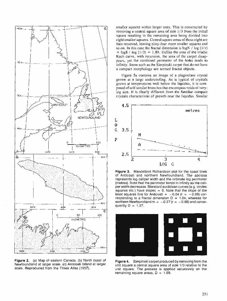
smaller squares within larger ones. This is constructed by removing a central square area of side 1 I3 from the initial square resulting in the remaining area being divided into eight smaller squares. Central square areas of these eight are then removed, leaving sixty-four more smaller squares and so on. In this case the fractal dimension is logN / log ( l / r ) = log8 / log (113) = 1.89. Unlike the area of the triadic Koch curve, with recursion, the area of the carpet disap- pears, yet the combined perimeter of the holes tends to infinity. Items such as the Sierpinski carpet that do not have a compact morphology are termed fractal objects.

Figure 5a contains an image of a plagioclase crystal grown at a large undercooling. As is typical of crystals grown at temperatures well below the liquidus, it is composed of self-similar branches that encompass voids of varying size. It is clearly different from the familiar compact crystals characteristic of growth near the liquidus. Similar

I metres I

2 3 4 LOG C

Figure 3. Mandelbrot Richardson plot for the coast lines of Anticosti and northern Newfoundland. The abcissa represents log caliper width and the ordinate log perimeter (metres). Note that the perimeter tends to infinity as the caliper width decreases. Standard euclidean curves (e.g. circles squares etc.) have slopes = 0. Note that the slope of the least squares line for Anticosti = -0.04 (r = - 0.99) corresponding to a fractal dimension D = 1.04, whereas for northern Newfoundland m = - 0.27 (r = - 0.98) and consequently D = 1.27.

Figure 2. (a) Map of eastern Canada. (b) North coast of Newfoundland at larger scale. (c) Anticosti Island at larger scale. Reproduced from the Times Atlas (1957).

Figure 4. Sierpinski carpet produced by removing from the unit square a central square area of side 113 relative to the un i t square. The process is applied recursively on the remaining square areas, D = 1.89.

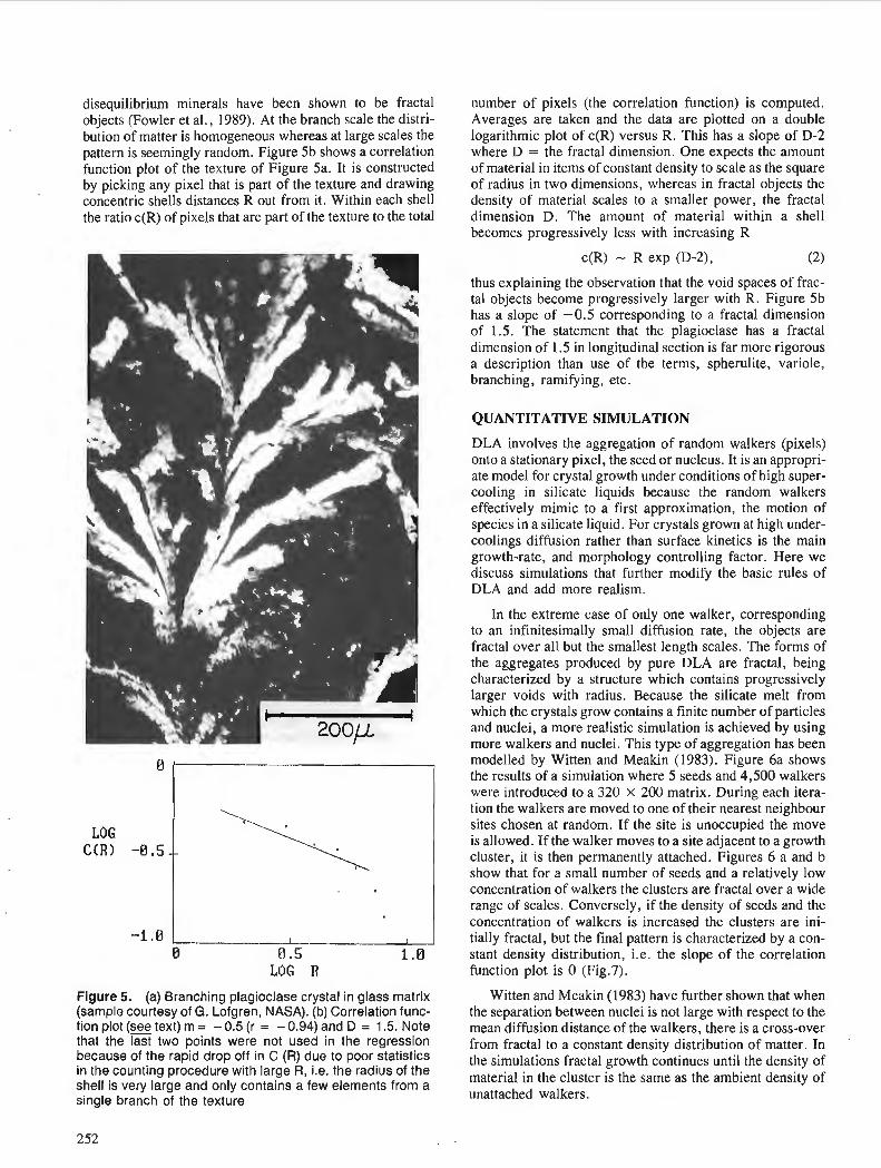
disequilibrium minerals have been shown to be fractal objects (Fowler et a]., 1989). At the branch scale the distribution of matter is homogeneous whereas at large scales the pattern is seemingly random. Figure 5b shows a correlation function plot of the texture of Figure 5a. It is constructed by picking any pixel that is part of the texture and drawing concentric shells distances R out from it. Within each shell the ratio c(R) of pixels that are part of the texture to the total

LOG R Figure 5. (a) Branching plagioclase crystal in glass matrix (sample courtesy of G. Lofgren, NASA). (b) Correlation function plot (see text) m = - 0.5 (r = - 0.94) and D = 1.5. Note that the last two points were not used in the regression because of the rapid drop off in C (R) due to poor statistics in the counting procedure with large R, i.e, the radius of the shell is very large and only contains a few elements from a single branch of the texture

number of pixels (the correlation function) is computed. Averages are taken and the data are plotted on a double logarithmic plot of c(R) versus R. This has a slope of D-2 where D = the fractal dimension. One expects the amount of material in items of constant density to scale as the square of radius in two dimensions, whereas in fractal objects the density of material scales to a smaller power, the fractal dimension D. The amount of material within a shell becomes progressively less with increasing R

c(R) - R exp (D-2), (2)

thus explaining the observation that the void spaces of fractal objects become progressively larger with R. Figure 5b has a slope of -0.5 corresponding to a fractal dimension of 1.5. The statement that the plagioclase has a fractal dimension of 1.5 in longitudinal section is far more rigorous a description than use of the terms, spherulite, variole, branching, ramifying, etc.

QUANTITATIVE SIMULATION

DLA involves the aggregation of random walkers (pixels) onto a stationary pixel, the seed or nucleus. It is an appropriate model for crystal growth under conditions of high super- cooling in silicate liquids because the random walkers effectively mimic to a first approximation, the motion of species in a silicate liquid. For crystals grown at high under- coolings diffusion rather than surface kinetics is the main growth-rate, and morphology controlling factor. Here we discuss simulations that further modify the basic rules of DLA and add more realism.

In the extreme case of only one walker, corresponding to an infinitesimally small diffusion rate, the objects are fractal over all but the smallest length scales. The forms of the aggregates produced by pure DLA are fractal, being characterized by a structure which contains progressively larger voids with radius. Because the silicate melt from which the crystals grow contains a finite number of particles and nuclei, a more realistic simulation is achieved by using more walkers and nuclei. This type of aggregation has been modelled by Witten and Meakin (1983). Figure 6a shows the results of a simulation where 5 seeds and 4,500 walkers were introduced to a 320 x 200 matrix. During each iteration the walkers are moved to one of their nearest neighbour sites chosen at random. If the site is unoccupied the move is allowed. If the walker moves to a site adjacent to a growth cluster, it is then permanently attached. Figures 6 a and b show that for a small number of seeds and a relatively low concentration of walkers the clusters are fractal over a wide range of scales. Conversely, if the density of seeds and the concentration of walkers is increased the clusters are initially fractal, but the final pattern is characterized by a constant density distribution, i.e, the slope of the correlation function plot is 0 (Fig.7).

Witten and Meakin (1983) have further shown that when the separation between nuclei is not large with respect to the mean diffusion distance of the walkers, there is a cross-over from fractal to a constant density distribution of matter. In the simulations fractal growth continues until the density of material in the cluster is the same as the ambient density of unattached walkers.

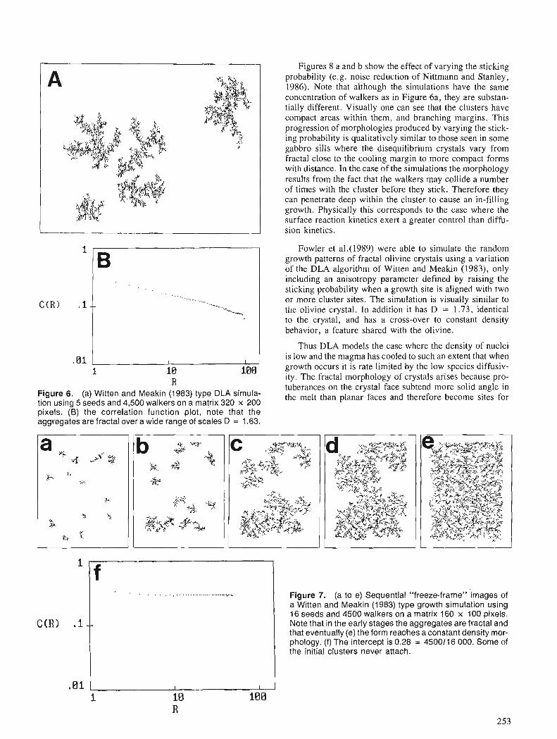
R Figure 6. (a) Witten and Meakin (1983) type DLA simulation using 5 seeds and 4,500 walkers on a matrix 320 x 200 pixels. (B) the correlation function plot, note that the aggregates are fractal over a wide range of scales D = 1.63.

Figures 8 a and b show the effect of varying the sticking probability (e.g. noise reduction of Nittmann and Stanley, 1986). Note that although the simulations have the same concentration of walkers as in Figure 6a, they are substantially different. Visually one can see that the clusters have compact areas within them, and branching margins. This progression of morphologies produced by varying the sticking probability is qualitatively similar to those seen in some gabbro sills where the disequilibrium crystals vary from fractal close to the cooling margin to more compact forms with distance. In the case of the simulations the morphology results from the fact that the walkers may collide a number of times with the cluster before they stick. Therefore they can penetrate deep within the cluster to cause an in-filling growth. Physically this corresponds to the case where the surface reaction kinetics exert a greater control than diffusion kinetics.

Fowler et a1.(1989) were able to simulate the random growth patterns of fractal olivine crystals using a variation of the DLA algorithm of Witten and Meakin (1983), only including an anisotropy parameter defined by raising the sticking probability when a growth site is aligned with two or more cluster sites. The simulation is visually similar to the olivine crystal. In addition it has D = 1.73, identical to the crystal, and has a cross-over to constant density behavior, a feature shared with the olivine.

Thus DLA models the case where the density of nuclei is low and the magma has cooled to such an extent that when growth occurs it is rate limited by the low species diffusivity. The fractal morphology of crystals arises because pro- tuberances on the crystal face subtend more solid angle in the melt than planar faces and therefore become sites for

' I f

a pi- ,$ ,."' 3

-h 6 *.

+- .. k

R .a

-r

Figure 7. (a to e) Sequential "freeze-frame" 'images of a Witten and Meakin (1983) type growth simulation using 16 seeds and 4500 walkers on a matrix 160 x I00 pixels. Note that in the early stages the aggregates are fractal and that eventually (e) the form reaches a constant density morphology. (f) The intercept is 0.28 = 4500116 000. Some of the initial clusters never attach.

z+. t... ... ;q+:2@. J*<- -3 < ,\ ~.s.$;:Si. .+ j;:.; !,:+,i

b .+.* %.. wT

"ilt :%, ++ e I

i %,'. =, " 4. -.?

d - .

:,,.?;. , ,.& ,@. \% 3 $-.& " *',

c . +kysy52:ac $ +?Y ,. :...

;twi.x .cyi +* . ~77..- .- *sf. .*$ <? ''

.;<fi .. , .,+ :@y-

.:.?> .. *i:i$i$3y .*q., , I ..,. j;r' -.-< %,l..:-'x#

.( +,.\ .. \ T.i.{?y::b,$:. -..:>%:?:.$,$

?A*+ <$y+ ;:p+.g +-&$ .<.p*.

dl . v . . , ~ ~ ~ ~ ~ ~ ~ . ~ , . .-.. .& .., .,&3Lxyty .*A %;.+$< *<y+-,,>?& &<

4x<r - ~&rYY;i"$2?:ij ) .<.,.. >&- .3 - f- . 'v ksf.<ri.+:-+ &$

,>*> &? ;:;f,&;? - ; cYG-z+~x;;& p + i > . . - - ~ . .

.;p..-F,> 22 ,.,,$< 3 *.-

-.+$;%:.zZ :<: I-, Y3L7 >>?? .%. 5-t;..?22 -2,:.

\ , ,,, $+ ,.,V> .Y&?.$$ . ? ~ > $ $ ~ ~ ~ $ ? d ? " ' l@AL$J+??j <+:.:.:I., ; -.-$+.x+ ,,&

rz. 4. e$$;;.;;;y$$;3-3+$ .-:+ ;.,- ?T7* yyz, E, >< *> ,,.<*:+5 '+ -4..

: :,..-$ : ~ ; ; , , - ~ ~ . ; ~ ; . d ~ -2 - .5&?:?p>3;&:%:.l .j;f?~yL~$~;*;$~,y~;~ <. .: -. -4.> &.F+;>?~,\<-

(.: :5-* +..>:..=::-:-+ .+.. :-$$ ;:$;~<w;p+::i:4y:&<<& 8 .-... . 7$~:;$.--i~?$<<;y ;>:. ; i-: $$;L~7x..&$.>$&~ U.. ?"; ,. s; t<:>r:.*:$fi.C

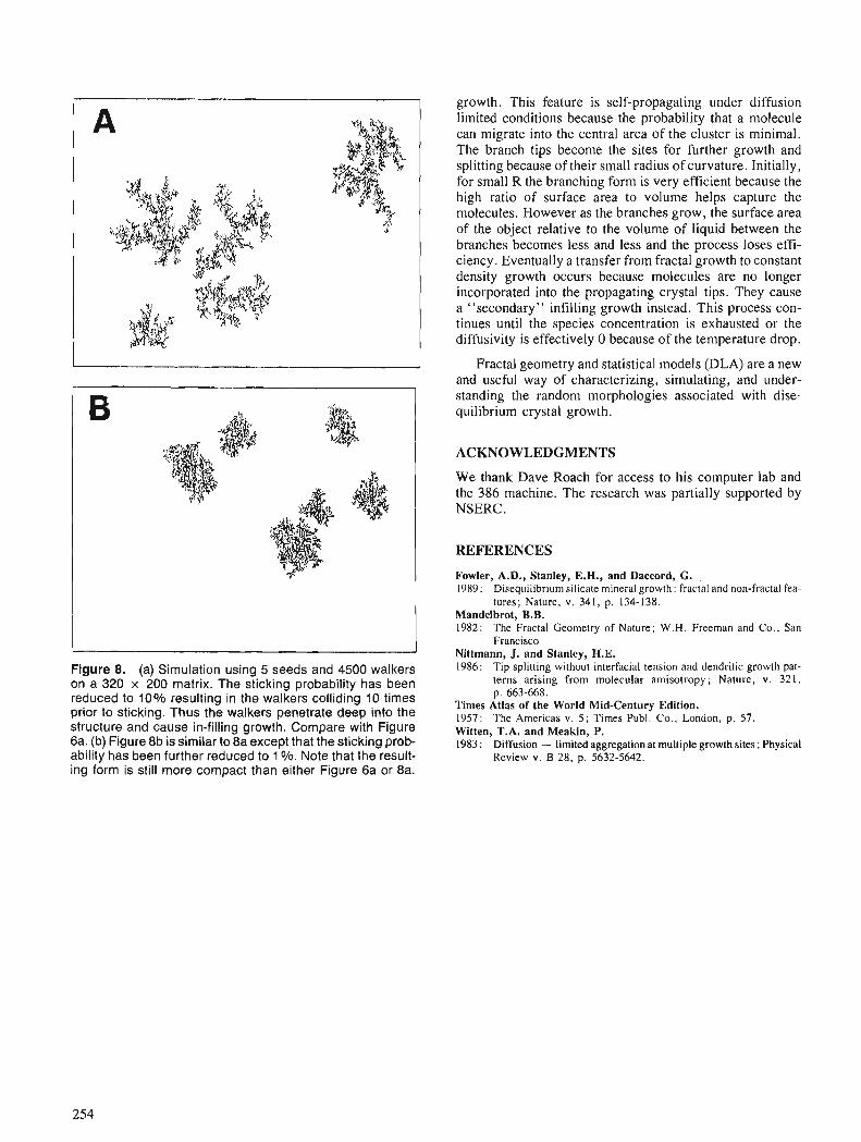
Figure 8. (a) Simulation using 5 seeds and 4500 walkers on a 320 x 200 matrix. The sticking probability has been reduced to 10% resulting in the walkers colliding 10 times prior to sticking. Thus the walkers penetrate deep into the structure and cause in-filling growth. Compare with Figure 6a. (b) Figure 8b is similar to 8a except that the sticking probability has been further reduced to 1%. Note that the resulting form is still more compact than either Figure 6a or 8a.

growth. This feature is self-propagating under diffusion limited conditions because the probability that a molecule can migrate into the central area of the cluster is minimal. The branch tips become the sites for further growth and splitting because of their small radius of curvature. Initially, for small R the branching form is very efficient because the high ratio of surface area to volume helps capture the molecules. However as the branches grow, the surface area of the object relative to the volume of liquid between the branches becomes less and less and the process loses efficiency. Eventually a transfer from fractal growth to constant density growth occurs because molecules are no longer incorporated into the propagating crystal tips. They cause a "secondary" infilling growth instead. This process continues until the species concentration is exhausted or the diffusivity is effectively 0 because of the temperature drop.

Fractal geometry and statistical models (DLA) are a new and useful way of characterizing, simulating, and understanding the random morphologies associated with disequilibrium crystal growth.

ACKNOWLEDGMENTS

We thank Dave Roach for access to his computer lab and the 386 machine. The research was partially supported by NSERC.

REFERENCES

Fowler, A.D., Stanley, E.H., and Daccord. G. ,

1989: Disequilibrium silicate mineral growth : fractal and non-fractal features; Nature, v. 341, p. 134-138.

Mandelbrot, B.B. 1982: The Fractal Geometry of Nature; W . H . Freeman and Co., San

Francisco Nittmann, J. and Stanley, H.E. 1986: Tip splitting without interfacial tension and dendritic growth pat-

terns arising from molecular amisotropy; Nature, v. 321, p. 663-668.

Times Atlas of the World Mid-Century Edition. 1957: The Americas v. 5 ; Times Publ. Co. , London, p. 57. Witten, T.A. and Meakin, P. 1983 : Diffusion - limited aggregation at multiple growth sites; Physical

Review v. B 28, p . 5632-5642.

Statistical approach to brittle fracture in the Earth's crust

G. RanallilJ and L. Hardy1

Ranalli, G. and Hardy, L., Statistical approach to brittle frQcture in the Earth's crust; & Statistical Applications in the Earth Sciences, ed. F. P. Agterberg and G. F. Bonham-Carter; Geological Survey of Canada, Paper 89-9, p. 255-262, 1989.

Abstract

77ze distribution of brittle fractures at all scales in the Earth's crust is best regarded as the outcome of a stochastic process. The frequency of fracture size has been variously described as lognormal, exponential, or hyperbolic. Kolmogorov's theory of breakage, which leads to a lognormal distribution of fracture size, provides a jrst-order model for the observations.

B e various hypotheses are tested on data sets obtainedfrom tectonic analysis. The lognormal distribution provides the best j t in all cases. Fractures do not appear to be self-similar over wide ranges of size. A nonlinear relation between size and o#set may be explained by a genetic model of allometric growth of tectonic parameters.

LA distribution desfractures cassantes a toutes les 6chelles duns la crolite terrestre est au mieuxper- gue comme l'issue d'un processus stochastique. Lafr.4quence des dimensions des fractures a At diverse- ment de'crite comme &ant log-normale, exponentielle ou hyperbolique. La thkorie de Kolmogorov concernant la rupture, qui mbne li une distribution log-normale des dimensions des fractures, fournit un mod2le de premier ordre pour les observations.

' Department of Earth Sciences, Carleton University, Ottawa, Ontario, K1S 586 Also a t : Ottawa-Carleton Geoscience Centre, Ottawa, Ontario, KIS 5B6

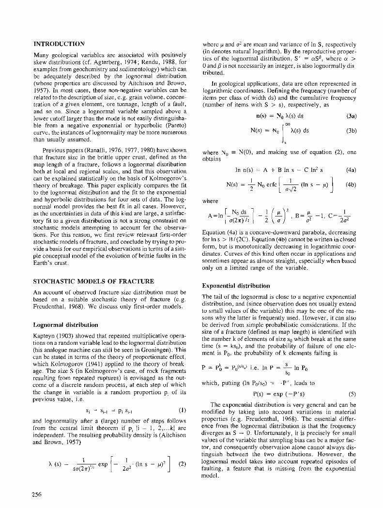
INTRODUCTION

Many geological variables are associated with positively skew distributions (cf. Agterberg, 1974; Rendu, 1988, for examples from geochemistry and sedimentology) which can be adequately described by the lognormal distribution (whose properties are discussed by Aitchison and Brown, 1957). In most cases, these non-negative variables can be related to the description of size, e.g. grain volume, concentration of a given element, ore tonnage, length of a fault, and so on. Since a lognormal variable sampled above a lower cutoff larger than the mode is not easily distinguishable from a negative exponential or hyperbolic (Pareto) curve, the instances of lognormality may be more numerous than usually assumed.

Previous papers (Ranalli, 1976, 1977,1980) have shown that fracture size in the brittle upper crust, defined as the map length of a fracture, follows a lognormal distribution both at local and regional scales, and that this observation can be explained statistically on the basis of Kolmogorov's theory of breakage. This paper explicitly compares the fit to the lognormal distribution and the fit to the exponential and hyperbolic distributions for four sets of data. The lognormal model provides the best fit in all cases. However, as the uncertainties in data of this kind are large, a satisfactory fit to a given distribution is not a strong constraint on stochastic models attempting to account for the observations. For this reason, we first review relevant first-order stochastic models of fracture, and conclude by trying to provide a basis for our empirical observations in terms of a simple conceptual model of the evolution of brittle faults in the Earth's crust.

STOCHASTIC MODELS OF FRACTURE

An account of observed fracture size distribution must be based on a suitable stochastic theory of fracture (e.g. Freudenthal, 1968). We discuss only first-order models.

Lognormal distribution

Kapteyn (1903) showed that repeated multiplicative operations on a random variable lead to the lognormal distribution (his analogue machine can still be seen in Groningen). This can be stated in terms of the theory of proportionate effect, which Kolmogorov (1941) applied to the theory of breakage. The size S (in Kolmogorov's case, of rock fragments resulting from repeated ruptures) is envisaged as the outcome of a discrete random process, at each step of which the change in variable is a random proportion pi of its previous value, i.e.

and lognormality after a (large) number of steps follows from the central limit theorem if pi {i = 1, 2, ... kl are independent. The resulting probability density is (Aitchison and Brown, 1957)

x (s) = 1 1

su(2 T)"? exp [- lo' (1. S - p)' ] (2)

where p and u2 are mean and variance of In S, respectively (In denotes natural logarithm). By the reproductive properties of the lognormal distribution, S' = aS0, where cu > 0 and fi is not necessarily an integer, is also lognormally distributed.

In geological applications, data are often represented in logarithmic coordinates. Defining the frequency (number of items per class of width ds) and the cumulative frequency (number of items with S > s), respectively, as

where No = N(O), and making use of equation (2), one obtains

1 N(s) = - No erfc

2

where

Equation (4a) is a concave-downward parabola, decreasing for In s > B / (2C). Equation (4b) cannot be written in closed form, but is monotonically decreasing in logarithmic coordinates. Curves of this kind often occur in applications and sometimes appear as almost straight, especially when based only on a limited range of the variable.

Exponential distribution

The tail of the lognormal is close to a negative exponential distribution, and (since observation does not usually extend to small values of the variable) this may be one of the reasons why the latter is frequently used. However, it can also be derived from simple probabilistic considerations. If the size of a fracture (defined as map length) is identified with the number k of elements of size so which break at the same time (s = kso), and the probability of failure of one element is Po, the probability of k elements failing is

which, putting (In Polso) = - P I , leads to

P(s) = exp (-PI s) ( 5 )

The exponential distribution is very general and can be modified by taking into account variations in material properties (e.g. Freudenthal, 1968). The essential difference from the lognormal distribution is that the frequency diverges as S - 0. Unfortunately, it is precisely for small values of the variable that sampling bias can be a major factor, and consequently observation alone cannot always distinguish between the two distributions. However, the lognormal model takes into account repeated episodes of faulting, a feature that is missing from the exponential model.

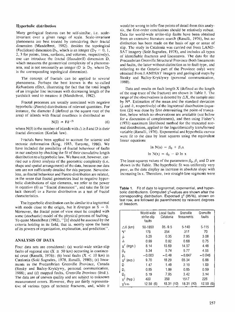
Hyperbolic distribution

Many geological features can be self-similar, i.e. scale- invariant over a given range of scale. Scale-invariant phenomena are best treated by considering their fractal dimension (Mandelbrot, 1982). Besides the topological (Euclidean) dimension DT, which is an integer (DT = 0, 1, 2, 3 for points, lines, surfaces, and volumes, respectively), one can introduce the fractal (Hausdorff) dimension D, which measures the geometrical complexity of a phenomenon, and is not necessarily an integer (D 1 DT, where DT is the corresponding topological dimension).

The concept of fractals can be applied to several phenomena. Perhaps the best known is the so-called Richardson effect, illustrating the fact that the total length of an irregular line increases with decreasing length of the yardstick used to measure it (Mandelbrot, 1982).

Fractal processes are usually associated with negative hyperbolic (Pareto) distributions of relevant quantities. For instance, the diameter 6 (defined as the square root of the area) of islands with fractal coastlines is distributed as

where N(6) is the number of islands with A 2 6 and D is their fractal dimension (Korzak law).

Fractals have been applied to account for seismic and tectonic deformation (King, 1983, Turcotte, 1986). We have included the possibility of fractal behaviour of faults in our analysis by checking the fit of their cumulative length distribution to a hyperbolic law. We have not, however, carried out a direct analysis of the geometric complexity (i.e. shape and spatial arrangement) of the data, because our data sets are not sufficiently detailed for this purpose. Neverthe- less, as fractal behaviour and Pareto distribution are related, in the sense that fractal geometries lead to negative hyperbolic distributions of size elements, we refer to the power in equation (6) as "fractal dimension", and take the fit (or lack thereof) to a Pareto distribution as a test of fractal characteristics.

The hyperbolic distribution can be similar to a lognormal with mode close to the origin, but it diverges as S - 0. Moreover, the fractal point of view must be coupled with some (stochastic) model of the physical process of faulting. To quote Mandelbrot (1982), "[it] should be assessed by the criteria holding in its field, that is, mostly upon the basis of its powers of organization, explanation, and prediction".

ANALYSIS OF DATA

Four data sets are considered: (a) world-wide strike-slip faults of regional size (X 2 50 krn) occurring in continental crust (Ranalli, 1976); (b) local faults (X < 10 km) in Catalonia (SolC Sugrafies, 1978, Ranalli, 1980); (c) lineaments in the Precambrian Grenville Province, Canada (Stesky and Bailey-Kryklywy, personal communication, 1988); and (d) mapped faults, Grenville Province (ibid.). The data are of uneven quality and are subject to unknown measurement errors. However, they are fairly representative of various types of tectonic fractures, and, while it

would be wrong to infer fine points of detail from this analysis, the first-order conclusions should be relatively robust. Data for world-wide strike-slip faults have been obtained from an extensive literature search (Ranalli, 1976), but no distinction has been made on the basis of age or sense of slip. The study in Catalonia was carried out from LAND- SAT imagery (SolC Sugraiies, 1978), and includes all types of identifiable fractures and lineaments. The data for the Precambrian Grenville Structural Province (both lineaments and faults, the latter without distinction as to fault type, and referring to the Ontario part of the Province only) were obtained from LANDSAT imagery and geological maps by Stesky and Bailey-Kryklywy (personal communication, 1988).

Data and results on fault length X (defined as the length of the map trace of the fracture) are shown in Table 1. The range of the observations is denoted by AX, the sample size by N*. Estimation of the mean and the standard deviation (ji and 6 , respectively) of the lognormal distribution (equation (2)) was done by first determining the point of truncation, below which no observations are available (see below for a discussion of completeness), and then using Fisher's (1931) maximum likelihood method for the truncated normal distribution, applied to the logarithmically transformed variable (Ranalli, 1976). Exponential and hyperbolic curves were fit to the data by least squares using the equivalent linear equations

The least-squares values of the parameters Do, PI and D are shown in the Table. The hyperbolic fit was uniformly very poor, as the data display an increase in absolute slope with increasing In x. Therefore, two straight-line segments were

Table 1. Fit of data to lognormal, exponential, and hyperbolic distributions. Computed x2-values are shown after the corresponding distribution. Expected x2 (950/0), shown on last row, are followed (in parentheses) by relevant degrees of freedom.

World-wide Local faults Grenville Grenville strike-slip Catalonia lineaments faults

faults

AX(km) 50-1650 05.-9.5 5-140 5-115 N * 176 254 31 1 70 b 5.29 0.35 2.95 3.08 6 0.99 0.92 0.68 0.75 x2 (logn.) 8.14 15.69 14.57 4.48 Po 5.34 5.74 5.77 4.55 P 1 -0.003 -0.48 -0.047 -0.046 x2 (exp.1 9.70 18.29 65.34 6.88 D 1.47 1.49 2.10 1.69 DI 0.85 1.09 0.85 0.59 D2 5.19 7.95 3.42 3.14 x2 (hyp.1 423 359 1517 226 X20.95 12.59 (6) 18.31 (10) 18.31 (10) 12.59 (6)

also fit in this case, and the parameters D l and D2 (for the lower and upper range of the variable, respectively) are also shown. Examples of the various cases are illustrated in Figures 1 to 4.

The X2-values for the lognormal, exponential, and hyperbolic fits are shown in Table 1, together with the 95 % theoretical values. As can be seen also from the figures, the lognormal provides a satisfactory fit in each case (as already pointed out by Ranalli for large-scale strike-slip faults (1976) and local faults (1980), respectively). The exponential is only marginally worse (with one exception, where the fit is much poorer). The Pareto distribution does not fit the data at all. No attempt to estimate goodness of fit was made in the case of the two-segment Pareto distribution, partly because the data were not weighted and the separation point was chosen heuristically, and partly - and more importantly - because the data appear to reflect a concave- downward trend and therefore the fit of individual straight- line segments represents an ad hoc approach.

The question of the completeness of data, especially as X approaches the point of truncation of the observations, has an important bearing on the results. This is particularly so when comparing the relative goodness of fit of the lognormal and exponential distributions. A large contribution to the x2-values in the latter case comes from frequencies for low values of the variable. If these were eliminated, the two cases would become indistinguishable. On the basis of goodness-of-fit alone, therefore, there are only weak grounds to choose the lognormal distribution; however, it will be argued in the following section that the lornormal distribution is to be preferred on physical grounds.

The poor fit to the hyperbolic distribution is a reflection of continuous downward curvature and therefore difficult to reconcile with self-similar fractal models. If our coefficient D is identified with the fractal dimension, then one must conclude that no set of data examined in this paper is self- similar for any extended range of the variable. Self- similarity may perhaps apply for intermediate values of the variable, in which case the actual fractal dimension would be between D I (which may be unduly influenced by incompleteness) and D (which is strongly influenced by the large- value tail). A value between 1 and 2 is therefore indicated, as should be the case for quantities with topological dimension unity.

DISCUSSION : SEISMICITY AND TECTONICS

The conclusions suggested by the analysis of data must be supported by mechanical models taking into account the genesis of fault length. (We refer primarily in this section to "mature", i.e. large-scale, fault systems, although the fact that local-scale systems follow the same distribution is significant .)

It can be assumed that, in the brittle upper crust, fault dimension is increased seismically, i.e. the fault length X is the outcome of repeated seismic shocks each with rupture length L. Each new seismic shock along a given fault may or may not add to the fault length, depending on its location and on its rupture length. The distribution of seismic rupture

length can be inferred from the magnitude-frequency distribution of earthquakes and the relations among seismic source parameters (Kanamori and Anderson, 1975). If the magnitude-frequency relation is of the type (we use logarithm to base 10 in keeping with seismological practice)

log n(m) = a - bm (7)

it can be proven that (Aki, 1981, Caputo, 1987)

where N(1) is the number of shocks with L > I . Usually, 1.5 I D I 2.0. The problem then is that of devising a model that reconciles a Pareto distribution of seismic rupture length with a lognormal distribution of geological fault length.

First of all, one must examine the possibility that either the lognormal distribution of fault length or the Pareto distribution of seismic rupture length is spurious. Apparent lognormality may occur from a mixture of subpopulations graded according to size and having identical coefficient of variation. This possibility is unlikely, however, since world-wide strike-slip faults do not appear to be grouped with any geographical bias (Ranalli, 1976), and at the other extreme small-scale data, which are more likely to be homogeneous, also follow a lognormal distribution (Ranalli, 1980). Direct determinations of the fractal dimension of the San Andreas fault system (Okubo and Aki, 1987) and of small fractures in a granite massif (Chil&s, 1988) show that D varies with scale, i.e. fault complexity is not self-similar over a wide range of scale. The lognormality of fault length is a robust conclusion based on the available evidence.

The Pareto distribution of seismic rupture length is a direct consequence of the magnitude-frequency distribution. Equation (7) holds only between lower and upper magnitude cutoffs which vary from region to region (cf. Aki, 1987, Rydelek and Sacks, 1989). It has been suggested (Lomnitz, 1964) that it represents only a linear approximation (in log n,m-coordinates), over a limited range of the variable, to a normal distribution, which is the one to be expected for magnitude on the basis of Kolmogorov's theory of breakage (since m o: log s, where s is the earthquake volume; see Kanamori and Anderson, 1975). A normal distribution of magnitude results in a lognormal distribution of rupture length (compare with equation (4a)). Although magnitude-frequency analyses are usually carried out in terms of equation (7) with magnitude cutoffs, the possibility that both Land X are lognormal is not totally to be excluded.

A lognormal distribution can also be derived from the superposition of different subpopulations, each following equation (7) with given magnitude cutoffs (i.e. with rupture lengths distributed hyperbolically within upper and lower bounds). This can be seen by numerical simulation, but with a few simplifying assumptions can be seen directly. Let a seismotectonic region be subdivided into K subregions, each with magnitude distribution

ni(m) = 0 otherwise

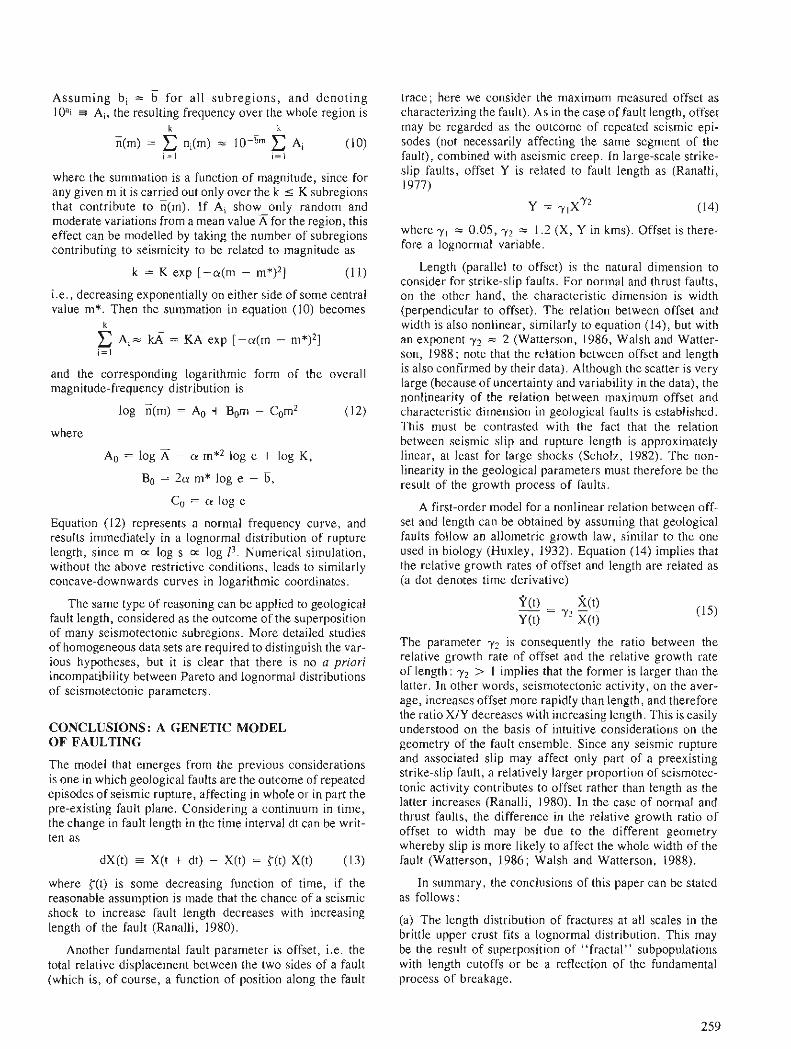
- Assuming bi = b for all subregions, and denoting 1Udi i Ai, the resulting frequency over the whole region is

k k

where the summation is a function of magnitude, since for any given m it is carried out only over the k I K subregions that contribute to n(m). I f Ai show only random and moderate variations from a mean value A for the region, this effect can be modelled by taking the number of subregions contributing to seismicity to be related to magnitude as

k = K exp [-or(m - m*)2]

i.e., decreasing exponentially on either side of some central value m*. Then the summation in equation (10) becomes

k x A , = kA = KA exp [-a(m - m*)21 i = l

and the corresponding logarithmic form of the overall magnitude-frequency distribution is

log i(m) = A. + Bom - COm2

where

A. = log A - or m*2 log e + log K ,

Bo = 2a m* log e - 6,

Co = a log e

Equation (12) represents a normal frequency curve, and results immediately in a lognormal distribution of rupture length, since m a log s a log P. Numerical simulation, without the above restrictive conditions, leads to similarly concave-downwards curves in logarithmic coordinates.

The same type of reasoning can be applied to geological fault length, considered as the outcome of the superposition of many seismotectonic subregions. More detailed studies of homogeneous data sets are required to distinguish the various hypotheses, but i t is clear that there is no a prior; incompatibility between Pareto and lognormal distributions of seismotectonic parameters.

CONCLUSIONS : A GENETIC MODEL OF FAULTING

The model that emerges from the previous considerations is one in which geological faults are the outcome of repeated episodes of seismic rupture, affecting in whole or in part the pre-existing fault plane. Considering a continuum in time, the change in fault length in the time interval dt can be written as

dX(t) E X(t + dt) - X(t) = {(t) X(t) (13)

where c(t) is some decreasing function of time, if the reasonable assumption is made that the chance of a seismic shock to increase fault length decreases with increasing length of the fault (Ranalli, 1980).

Another fundamental fault parameter is offset, i.e. the total relative displacement between the two sides of a fault (which is, of course, a function of position along the fault

trace; here we consider the maximum measured offset as characterizing the fault). As in thecase of fault length, offset may be regarded as the outcome of repeated seismic episodes (not necessarily affecting the same segment of the fault), combined with aseismic creep. In large-scale strike- slip faults, offset Y is related to fault length as (Ranalli, 1977)

Y = y1xY2 (14)

where y l = 0.05, y2 = 1.2 (X, Y in kms). Offset is therefore a lognormal variable.

Length (parallel to offset) is the natural dimension to consider for strike-slip faults. For normal and thrust faults, on the other hand, the characteristic dimension is width (perpendicular to offset). The relation between offset and width is also nonlinear, similarly to equation (14), but with an exponent y2 = 2 (Watterson, 1986, Walsh and Watter- son, 1988; note that the relation between offset and length is also confirmed by their data). Although the scatter is very large (because of uncertainty and variability in the data), the nonlinearity of the relation between maximum offset and characteristic dimension in geological faults is established. 'This must be contrasted with the fact that the relation between seismic slip and rupture length is approximately linear, at least for large shocks (Scholz, 1982). The nonlinearity in the geological parameters must therefore be the result of the growth process of faults.

A first-order model for a nonlinear relation between offset and length can be obtained by assuming that geological faults follow an allometric growth law, similar to the one used in biology (Huxley, 1932). Equation (14) implies that the relative growth rates of offset and length are related as (a dot denotes time derivative)

The parameter y2 is consequently the ratio between the relative growth rate of offset and the relative growth rate of length: y2 > 1 implies that the former is larger than the latter. In other words, seismotectonic activity, on the average, increases offset more rapidly than length, and therefore the ratio XIY decreases with increasing length. This is easily understood on the basis of intuitive considerations on the geometry of the fault ensemble. Since any seismic rupture and associated slip may affect only part of a preexisting strike-slip fault, a relatively larger proportion ofseismotec- tonic activity contributes to offset rather than length as the latter increases (Ranalli, 1980). In the case of normal and thrust faults, the difference in the relative growth ratio of " offset to width may be due to the different geometry whereby slip is more likely to affect the whole width of the fault (Watterson, 1986; Walsh and Watterson, 1988).

In summary, the conclusions of this paper can be stated as follows:

(a) The length distribution of fractures at all scales in the brittle upper crust fits a lognormal distribution. This may be the result of superposition of "fractal" subpopulatior~s with length cutoffs or be a reflection of the fundamental process of breakage.

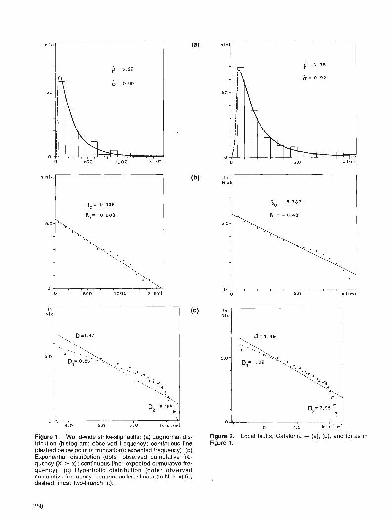
Figure 1. World-wide strike-slip faults: (a) Lognormal distribution (histogram: observed frequency; continuous line (dashed below point of truncation): expected frequency); (b) Exponential distribution (dots: observed cumulative frequency (X r x); continuous line: expected cumulative frequency); (c) Hyperbolic distribution (dots: observed cumulative frequency; continuous line: linear (In N, In x) fit; dashed lines: two-branch fit).

In N l x l

Figure 2. Local faults, Catalonia - (a), (b), and (c) as in Figure 1.

(c)

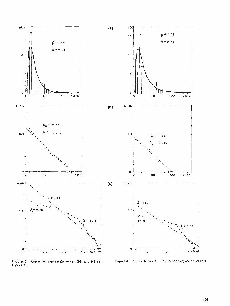
In Nlx l

I 0 5 0 100 x lkml

(b) In Nlx l

0 0 0 5 0 100 x lkml

In Nlxl

- D = l . 6 9

Figure 3. Grenville lineaments - (a), (b), and (c) as in Figure 4. Grenville faults - (a), (b), and (c) as in Figure 1. Figure 1.

(b) In large faults, the relation between offset and characteristic dimension of the fault is nonlinear, and can be interpreted in terms of an allometric growth law relating the ratio of the two parameters during the tectonic history of the fault.

ACKNOWLEDGMENTS

We thank R.M. Stesky for making available to us data collected and analyzed by his research group, participants in the Colloquium on "Statistical Applications in the Earth Sciences" for useful discussions, and E. Lambton (with the assistance of S. Thayer) for word processing. This research was supported by a grant to G.R. from the Natural Sciences and Engineering Research Council of Canada.

REFERENCES

Agterberg, F.P. 1974: Geomathematics. Elsevier, Amsterdam. Aitchison, J , and Brown, J.A.C. 1957: The Lognormal Distribution; Cambridge University Press. Aki, K. 1981 : A probabilistic synthesis of precursory phenomena; in Earthquake

Prediction, ed. D.W. Simpson and P.G. Richards, American Geophysical Union, Washington, p. 566-574.

1987: Magnitude-frequency relation for small earthquakes: a clue to the origin of f,,,, of large earthquakes; Journal of Geophysical Research, V. 92, p. 1349-1355.

Caputo, M. 1987: The interpretation of the b and bo values and its implications on

the regional deformation of the crust; Geophysical Journal of the Royal Astronomical Society, V . 90, p. 551 -573.

Chiles, J.P. 1988 : Fractal and geostatistical methods for modeling a fracture network ;

Mathematical Geology, V. 20, p. 631-654. Fisher, R.A. 1931 : The truncated normal distribution; British Association for the

Advancement of Scicnce, Mathematical Tables, V. I, p. 33-34. Freudenthal, A.M. 1968: Statistical approach to brittle failure; in Fracture - An Advanced

Treatise, ed. H. Liebowitz. V. 2, Academic Press. New York, p. 591-619.

Huxley, J.S. 1932: Problems of Relative Growth; Dial Press. New York. Kanamori, H. and Anderson, D.L. 1975 : Theoretical basis of some empirical relations in seismology ; Bulle-

t i n of the Seismological Society of America, V. 65, p. 1073-1095.

Kapteyn, J.C. 1903: Skew Frequency Curves in Biology and Statistics; Noordhoff,

Groningen. King, G. C.P. 1983 : The accommodation of large strains in the upper lithosphere of the

Earth and other solids by self-similar fault systems: the geometrical origin of the b-value; Pure and Applied Geophysics, V. 121, p. 761-815.

Kolmogorov, A.N. 1941 : Uber das logarithmisch normale Verteilungsgesetz der Dimensio-

nen der Teilchen bei Zerstiickelung; Comptes Rendus de I'AcadCmie des Sciences de I'URSS, V. 31, p. 99-101.

Lornnitz, C. 1964: Estimation problems in earthquake series; Tectonophysics. V. 2.

p. 193-203. Mandelbrot, B.B. 1982: The Fractal Geometry of Nature: Freeman. New York. Okubo, P. and Aki, K. 1987: Fractal geometry in the San Andreas fault system; Journal of

Geophysical Research, V. 92, p. 345-355. Ranalli, G. 1976: Length distribution of strike-slip faults and the process of breakage

in continental crust; Canadian Journal of Earth Sciences, V . 13, p. 704-707.

1977: Correlation between length and offset in strike-slip faults; Tec- tonophysics. V. 37, p. TI-T7.

1980: A stochastic model for strike-slip faulting; Mathematical Geology, V. 12, p. 399-412.

Rendu, J.-M.M. 1988: Applications in geology; in Lognormal Distributions, ed. E.L.

Crow and K . Shimizu; Dekker, New York, p. 357-365. Rydelek, P.A. and Sacks, I.S. 1989: Testing the completeness of earthquake catalogues and the

hypothesis of self-similarity; Nature, V. 337, p. 251-253. Scholz, C.H. 1982: Scaling laws for large earthquakes: consequences for physical

models; Bulletin of the Seismological Society of America, V. 72, p. 1-14,

Sol6 Sugraiies,. L. 1978: Alineaciones y fracturas en el sistema Catalan segun las imagenes

LANDSAT-1; Tecniterrae, V. 22, p. 1-1 1. Turcotte, D.L. 1986: A fractal model for crustal deformation; Tectonophysics, V. 132,

p. 261-269. Walsh, J.J. and Watterson, J. 1988 : Analysis of the relationship between displacements and dimensions

of faults; Journal of Structural Geology, V. 10, p. 239-247. Watterson, J. 1986: Fault dimensions, displacements and growth; Pure and Applied

Geophysics, V. 124, p. 365-373.

Use of statistical methods to extract significant information from scattered data in petrophysics

T. J. Katsube and F.P. Agterbergl

Katsube, T. J. and Agterberg, F. P., Use of statistical methods to extract significant information from scattered data in petrophysics; & Statistical Applications in the Earth Sciences, ed. F. P. Agterberg and G.F. Bonham-Carter; Geological Survey of Canada, Paper 89-9, p. 263-270, 1989.

Abstract

Porosity, 6, when plotted against the reciprocal of formation factor, I /F, (F=electrical resistivity of a rock/electrical resistivity of pore fluid) for 152 granitic rock samples showed a considerable scatter. According to a recently developed physical model of pores in rocks, there should be a linear relationship between 6 and I /F, but such a trend is hard to see in the original data. However, when the samples were grouped according to their degree of alteration, there were indications that a linear relationshb existed between the two parameters within each group. A multiple regression analysis technique which makes use of dummy variables was used to test this hypothesis. The results showed that a linear relationship existed between the two parameters for each group, and that the lines oblained by regression of 6 on I /F were generally parallel, except for an increase in slope for the group with the highest degree of alteration. The results also showed that the Y-intercept for 4, which was positive, at first increased and then decreased with increasing alteration intensity. The reduced major axis, RMA, instead of the normal regression line, NRL, for y on x, was used for further analysis within separate groups, because it was found to be more effective and accurate when characterizing the rocks.

La porosite', 4, porte'e sur graphique en fonction de l'inverse du facteur deformation, 1 /F , (F= resistivite) pour 152 e'chantillons de roches granitiques pre'sente une dispersion considkrable. D 'aprks un modtle physique des pores dans les roches rkcemment mis au point, il devrait exister une relation linkaire entre 4 et 1 /F , mais une telle tendance est dificile B percevoir dans les donne'es d'origine. Tou- tefois, lorsqu 'on a groupk les e'chantillons selon leur degrk d'altkration, il y a eu des indications qu 'une relation linkaire existait entre les deux pararnttres a 1 'inte'rieur de chaque groupe. Une mkthode d 'analyse de re'gression multiple faisant intervenir des variables factices a kt6 utilise'e pour ve'rifier cette hypoth?se. Les re'sultats indiquent qu 'il existe pour chaque groupe une relation line'aire entre ces paramPtres et que les droites obtenues lors de la rkgression de 4 sur I /F sont gkne'ralement parall2les, exception faite d'une pente accrue pour le groupe d'e'chantillons prksentant l'alteiafion la plus marque'e. Lw re'sultats indiquent e'galement que l'ordonnde B l'origine pour 4, qui est positive, augmente d'abord pour ensuite diminuer en fonction d'un degre' d'alte'ration croissant. Le grand axe rkduit a kt& utilise' plutdt que la droite de re'gression normale pour y sur x lors d'une analyse plus pousse'e c i l'inte'rieur de chacun des groupes parce qu'il a e'te' jug6 plus eficace et prkcis d 'y avoir recours lors de la caracte'risation des roches.

'. Geological Survey of Canada, 601 Booth Street. Ottawa, Ontario KIA 0E8

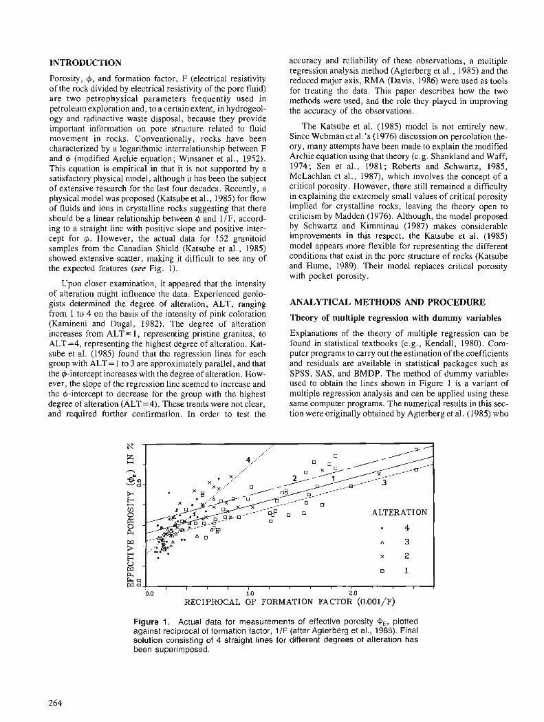
INTRODUCTION

Porosity, 4 , and formation factor, F (electrical resistivity of the rock divided by electrical resistivity of the pore fluid) are two petrophysical parameters frequently used in petroleum exploration and, to a certain extent, in hydrogeol- ogy and radioactive waste disposal, because they provide important information on pore structure related to fluid movement in rocks. Conventionally, rocks have been characterized by a logarithmic interrelationship between F and 4 (modified Archie equation; Winsaner et al., 1952). This equation is empirical in that it is not supported by a satisfactory physical model, although it has been the subject of extensive research for the last four decades. Recently, a physical model was proposed (Katsube et al., 1985) for flow of fluids and ions in crystalline rocks suggesting that there should be a linear relationship between 4 and 1 IF, according to a straight line with positive slope and positive intercept for 4. However, the actual data for 152 granitoid samples from the Canadian Shield (Katsube et al., 1985) showed extensive scatter, making it difficult to see any of the expected features (see Fig. 1).

Upon closer examination, it appeared that the intensity of alteration might influence the data. Experienced geologists determined the degree of alteration, ALT, ranging from 1 to 4 on the basis of the intensity of pink coloration (Kamineni and Dugal, 1982). The degree of alteration increases from ALT= 1 , representing pristine granites, to ALT=4, representing the highest degree of alteration. Kat- sube et al. (1985) found that the regression lines for each group with ALT = 1 to 3 are approximately parallel, and that the +intercept increases with the degree of alteration. How- ever, the slope of the regression line seemed to increase and the &intercept to decrease for the group with the highest degree of alteration (ALT=4). These trends were not clear, and required further confirmation. In order to test the

accuracy and reliability of these observations, a multiple regression analysis method (Agterberg et al., 1985) and the reduced major axis, RMA (Davis, 1986) were used as tools for treating the data. This paper describes how the two methods were used, and the role they played in improving the accuracy of the observations.

The Katsube et al. (1985) model is not entirely new. Since Webman et al.'s (1976) discussion on percolation theory, many attempts have been made to explain the modified Archie equation'using that theory (e.g. Shankland and Waff, 1974; Sen et al., 1981 ; Roberts and Schwartz, 1985, McLachlan et a]., 1987), which involves the concept of a critical porosity. However, there still remained a difficulty in explaining the extremely small values of critical porosity implied for crystalline rocks, leaving the theory open to criticism by Madden (1976). Although, the model proposed by Schwartz and Kimminau (1987) makes considerable improvements in this respect, the Katsube et al. (1985) model appears more flexible for representing the different conditions that exist in the pore structure of rocks (Katsube and Hume, 1989). Their model replaces critical porosity with pocket porosity.

ANALYTICAL METHODS AND PROCEDURE

Theory of multiple regression with dummy variables

Explanations of the theory of multiple regression can be found in statistical textbooks (e.g., Kendall, 1980). Com- puter programs to carry out the estimation of the coefficients and residuals are available in statistical packages such as SPSS, SAS, and BMDP. The method of dummy variables used to obtain the lines shown in Figure 1 is a variant of multiple regression analysis and can be applied using these same computer programs. The numerical results in this section were originally obtained by Agterberg et al. (1985) who

Figure 1. Actual data for measurements of effective porosity a,, plotted against reciprocal of formation factor, 1 IF (after Agterberg et al., 1985). Final solution consisting of 4 straight lines for different degrees of alteration has been superimposed.

n

ALTERATION

4

A 3

x 2 U - W F E r r 0 W 0

1

I I I I I I I I I I I I I

0.0 1.0 2.0 RECIPROCAL OF FORMATION FACTOR (O.OOl/F)

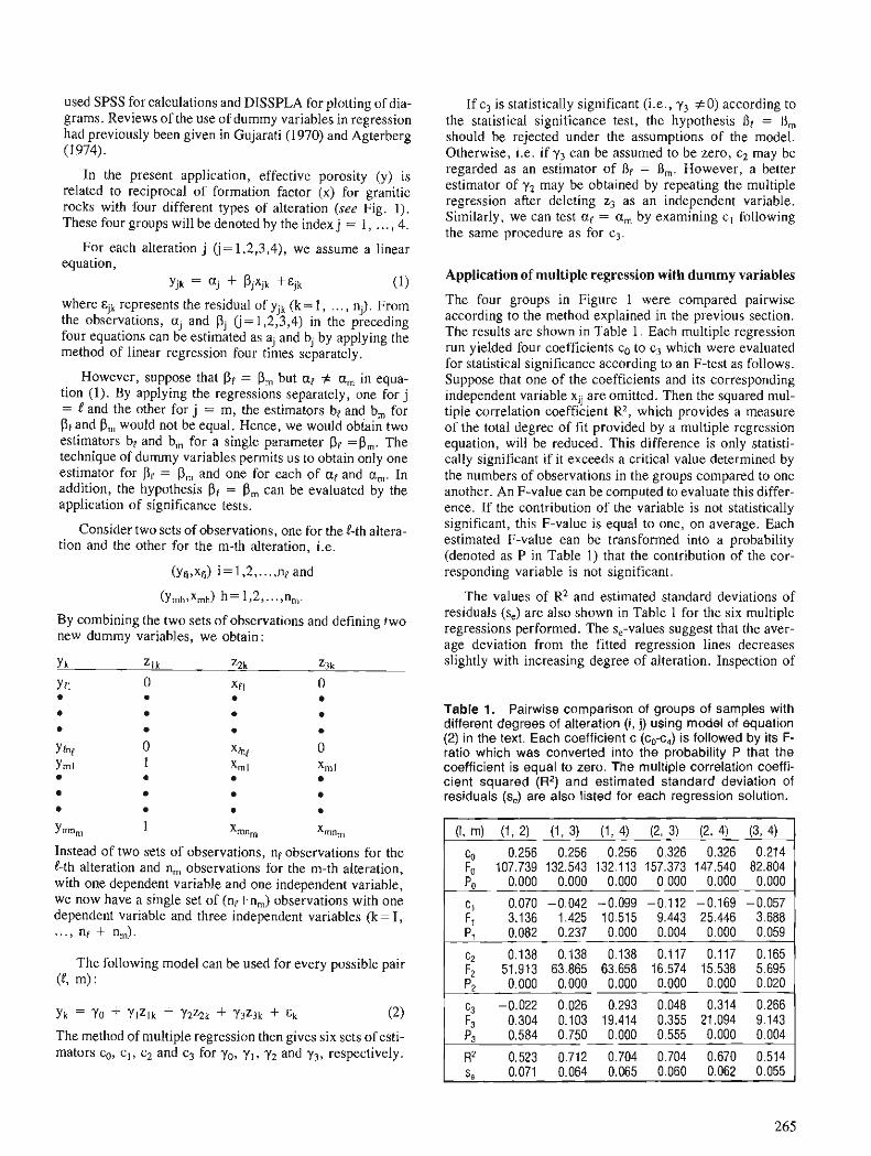
used SPSS for calculations and DISSPLA for plotting of diagrams. Reviews of the use of dummy variables in regression had previously been given in Gujarati (1970) and Agterberg (1 974).

In the present application, effective porosity (y) is related to reciprocal of formation factor (x) for granitic rocks with four different types of alteration (see Fig. 1). These four groups will be denoted by the index j = 1, . . . , 4 .

For each alteration j (j= 1,2,3,4), we assume a linear equation,

yjk = aj + Pjxjk +cjk (1) where cjk represents the residual of yjk (k = 1, . . . , n;). From the observations, a; and pj (j = 1,2,3,4) in the preceding four equations can be estimated as aj and bj by applying the method of linear regression four times separately.

However, suppose that B p = P, but at # a, in equation (1). By applying the regressions separately, one for j = f and the other for j = m, the estimators br and b, for of and Dm would not be equal. Hence, we would obtain two estimators bp and b, for a single parameter Pp =Pm. The technique of dummy variables permits us to obtain only one estimator for Sp = P, and one for each of ap and a,. In addition, the hypothesis (3p = P, can be evaluated by the application of significance tests.

Consider two sets of observations, one for the 6th alteration and the other for the m-th alteration, i.e.

(yR,xfi) i = 1,2,. . . ,np and

By combining the two sets of observations and defining two new dummy variables, we obtain:

Ymn, 1 Xmn,

Instead of two sets of observations, np observations for the !-th alteration and n, observations for the rn-th alteration, with one dependent variable and one independent variable, we now have a single set of (np+n,) observations with one dependent variable and three independent variables (k= 1, ..., np + n,).

The following model can be used for every possible pair (t, m) :

The method of multiple regression then gives six sets of estimators co, c l , c2 and c3 for yo, yl, y2 and y3, respectively.

If c3 is statistically significant (i.e., y3 + 0) according to the statistical significance test, the hypothesis Op = 0, should be rejected under the assumptions of the model. Otherwise, i.e. if y3 can be assumed to be zero, c2 may be regarded as an estimator of Rp = R,. However, a better estimator of y2 may be obtained by repeating the multiple regression after deleting z3 as an independent variable. Similarly, we can test up = a , by examining c l following the same procedure as for c3.

Application of multiple regression with dummy variables

The four groups in Figure 1 were compared pairwise according to the method explained in the previous section. The results are shown in Table 1. Each multiple regression run yielded four coefficients co to c3 which were evaluated for statistical significance according to an F-test as follows. Suppose that one of the coefficients and its corresponding independent variable xi; are omitted. Then the squared multiple correlation coefficient R2, which provides a measure of the total degree of fit provided by a multiple regression equation, will be reduced. This difference is only statistically significant if it exceeds a critical value determined by the numbers of observations in the groups compared to one another. An F-value can be computed to evaluate this difference. If the contribution of the variable is not statistically significant, this F-value is equal to one, on average. Each estimated F-value can be transformed into a probability (denoted as P in Table 1) that the contribution of the corresponding variable is not significant.

The values of R2 and estimated standard deviations of residuals (s,) are also shown in Table 1 for the six multiple regressions performed. The s,-values suggest that the average deviation from the fitted regression lines decreases slightly with increasing degree of alteration. Inspection of

Table 1. Pairwise comparison of groups of samples with different degrees of alteration ( i , j) using model of equation (2) in the text. Each coefficient c (co-c4) is followed by its F- ratio which was converted into the probability P that the coefficient is equal to zero. The multiple correlation coefficient squared (R2) and estimated standard deviation of residuals (s,) are also listed for each regression solution.

(I, m) (1, 2) (1, 3) (1, 4) (2, 3) (2, 4) (3, 4) co 0.256 0.256 0.256 0.326 0.326 0.214 Fo 107.739 132.543 132.113 157.373 147.540 82.804 Po 0.000 0.000 0.000 0.000 0.000 0.000

C, 0.070 -0.042 -0.099 -0.112 -0.169 -0.057 F, 3.136 1.425 10.515 9.443 25.446 3.688 P, 0.082 0.237 0.000 0.004 0.000 0.059

c, 0.138 0.138 0.138 0.117 0.117 0.165 F2 51.913 63.865 63.658 16.574 15.538 5.695 P2 0.000 0.000 0.000 0.000 0.000 0.020

c3 -0.022 0.026 0.293 0.048 0.314 0.266 F3 0.304 0.103 19.414 0.355 21.094 9.143 P3 0.584 0.750 0.000 0.555 0.000 0.004

R2 0.523 0.712 0.704 0.704 0.670 0.514 s, 0.071 0.064 0.065 0.060 0.062 0.055

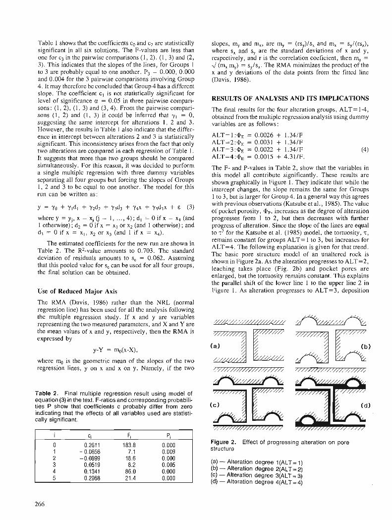
Table 1 shows that the coefficients co and c2 are statistically significant in all six solutions. The F-values are less than one for c3 in the pairwise comparisons (1, 2), (1, 3) and (2, 3). This indicates that the slopes of the lines, for Groups 1 to 3 are probably equal to one another. P3 = 0.000, 0.000 and 0.004 for the 3 pairwise comparisons involving Group 4 . It may therefore be concluded that Group 4 has a different slope. The coefficient c , is not statistically significant for level of significance a = 0.05 in three pairwise comparisons: (1, 2), ( I , 3) and (3, 4). From the pairwise comparisons ( 1 , 2) and (1, 3) it could be inferred that y, = 0, suggesting the same intercept for alterations 1, 2 and 3. However, the results in Table 1 also indicate that the difference in intercept between alterations 2 and 3 is statistically significant. This inconsistency arises from the fact that only two alterations are compared in each regression of Table 1. It suggests that more than two groups should be compared simultaneously. For this reason, it was decided to perform a single multiple regression with three dummy variables separating all four groups but forcing the slopes of Groups 1 , 2 and 3 to be equal to one another. The model for .this run can be written as:

where y = yj, x = xj (i = 1, ..., 4) ; d l = 0 if x = xl (and 1 otherwise); d2 = 0 if x = X I or x2 (and 1 otherwise); and d3 = 0 if x = x l , x2 or x3 (and 1 if x = x4).

The estimated coefficients for the new run are shown in Table 2. The R2-value amounts to 0.703. The standard deviation of residuals amounts to s, = 0.062. Assuming that this pooled value for s, can be used for all four groups, the final solution can be obtained.

Use of Reduced Major Axis

The RMA (Davis, 1986) rather than the NRL (normal regression line) has been used for all the analysis following the multiple regression study. If x and y are variables representing the two measured parameters, and X and Y are the mean values of x and y, respectively, then the RMA is expressed by

where Q is the geometric mean of the slopes of the two regression lines, y on x and x on y. Namely, if the two

Table 2. Final multiple regression result using model of equation (3) in the text. F-ratios and corresponding probabilities P show that coefficients c probably differ from zero indicating that the effects of all variables used are statistically significant.

slopes, my and m,, are my = (rsy)/s, and m, = s,/(rs,), where s, and s, are the standard deviations of x and y, respectively, and r is the correlation coeficient, then m, = J (m, my) = s,/s,. The RMA minimizes the product of the x and y deviations of the data points from the fitted line (Davis, 1986).

RESULTS OF ANALYSIS AND ITS IMPLICATIONS

The final results for the four alteration groups, ALT= 1-4, obtained from the multiple regression analysis using dummy variables are as follows:

The F- and P-values in Table 2, show that the variables in this model all contribute significantly. These results are shown graphically in Figure 1. They indicate that while the intercept changes, the slope remains the same for Groups 1 to 3, but is larger for Group 4. In a general way this agrees with previous observations (Katsube et al., 1985). The value of pocket porosity, Qip, increases as the degree of alteration progresses from 1 to 2 , but then decreases with further progress of alteration. Since the slope of the lines are equal to T* for the Katsube et al. (1985) model, the tortuosity, T, remains constant for groups ALT= 1 to 3, but increases for ALT=4. The following explanation is given for that trend. The basic pore structure model of an unaltered rock is shown in Figure 2a. As the alteration progresses to ALT=2, leaching takes place (Fig. 2b) and pocket pores are enlarged, but the tortuosity remains constant. This explains the parallel shift of the lower line 1 to the upper line 2 in Figure 1. As alteration progresses to ALT = 3, deposition

Figure 2. Effect of progressing alteration on pore structure

(a) - Alteration degree 1 (ALT = 1) (b) - Alteration degree 2(ALT = 2) (c) - Alteration degree 3(ALT= 3) (d) - Alteration degree 4(ALT = 4)

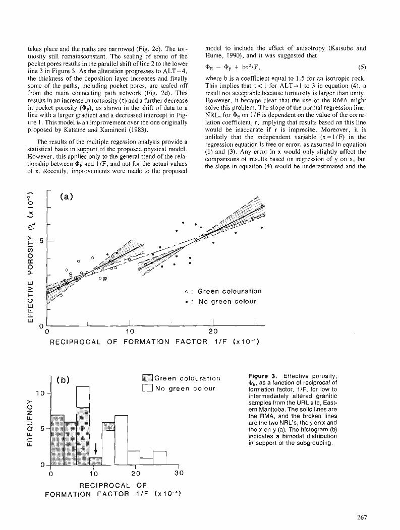
takes place and the paths are narrowed (Fig. 2c). The tortuosity still remainsconstant. The sealing of some of the pocket pores results in the parallel shift of line 2 to the lower line 3 in Figure 3. As the alteration progresses to ALT=4, the thickness of the deposition layer increases and finally some of the paths, including pocket pores, are sealed off from the main connecting path network (Fig. 2d). This results in an increase in tortuosity (2) and a further decrease in pocket porosity (ap), as shown in the shift of data to a line with a larger gradient and a decreased intercept in Fig- ure I . This model is an improvement over the one originally proposed by Katsube and Kamineni (1983).

The results of the multiple regession analysis provide a statistical basis in support of the proposed physical model. However, this applies only to the general trend of the relationship between aE and 1 IF, and not for the actual values of z. Recently, improvements were made to the proposed

model to include the effect of anisotropy (Katsube and Hume, 1990), and it was suggested that

where b is a coefficient equal to 1.5 for an isotropic rock. This implies that T < 1 for ALT= I to 3 in equation (4), a result not acceptable because tortuosity is larger than unity. However, it became clear that the use of the RMA might solve this problem. The slope of the normal regression line, NRL, for aE on 1 IF is dependent on the value of the correlation coefficient, r, implying that results based on this line would be inaccurate if r is imprecise. Moreover, it is unlikely that the independent variable (x= 1/F) in the regression equation is free or error, as assumed in equation (I) and (3). Any error in x would only slightly affect the comparisons of results based on regression of y on x, but the slope in equation (4) would be underestimated and the

J

o : Green colouration

G' : NO green colour

QGreen colouration

)No green colour

Figure 3. Effective porosity, a,, as a function of reciprocal of formation factor, 1 I F , for low to intermediately altered granitic samples from the URL site, East- ern Manitoba. The solid lines are the RMA, and the broken lines are the two NRL's, they on x and the x on y (a). The histogram (b) indicates a bimodal distribution in support of the subgrouping.

RECIPROCAL OF FORMATION FACTOR 1 IF ( X 1 o - ~ )

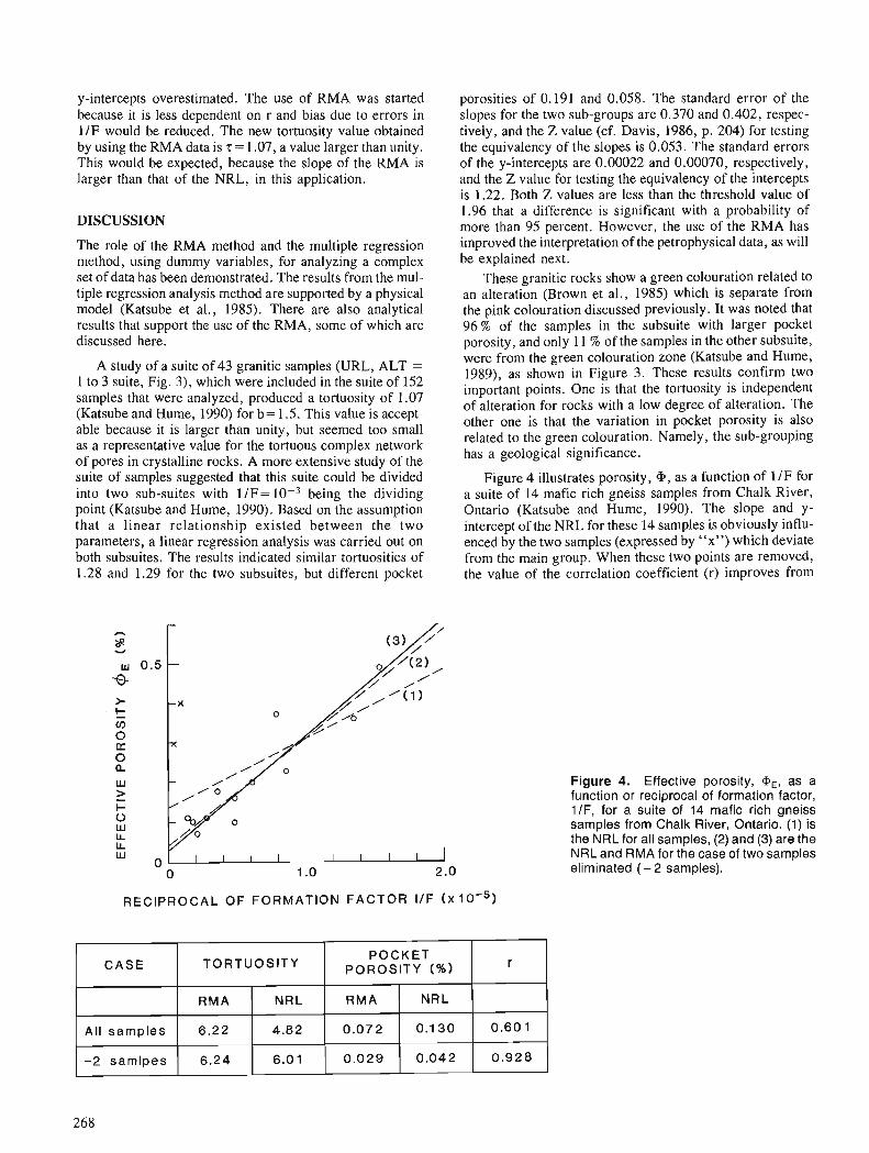
y-intercepts overestimated. The use of RMA was started because it is less dependent on r and bias due to errors in 11F would be reduced. The new tortuosity value obtained by using the RMA data is z = 1.07, a value larger than unity. This would be expected, because the slope of the RMA is larger than that of the NRL, in this application.

DISCUSSION

The role of the RMA method and the multiple regression method, using dummy variables, for analyzing a complex set of data has been demonstrated. The results from the multiple regression analysis method are supported by a physical model (Katsube et al., 1985). There are also analytical results that support the use of the RMA, some of which are discussed here.

A study of a suite of 43 granitic samples (URL, ALT = 1 to 3 suite, Fig. 3), which were included in the suite of 152 samples that were analyzed, produced a tortuosity of 1.07 (Katsube and Hume, 1990) for b= 1.5. This value is acceptable because it is larger than unity, but seemed too small as a representative value for the tortuous complex network of pores in crystalline rocks. A more extensive study of the suite of samples suggested that this suite could be divided into two sub-suites with 1/F=10-3 being the dividing point (Katsube and Hume, 1990). Based on the assumption that a linear relationship existed between the two parameters, a linear regression analysis was carried out on both subsuites. The results indicated similar tortuosities of 1.28 and 1.29 for the two subsuites, but different pocket

porosities of 0.191 and 0.058. The standard error of the slopes for the two sub-groups are 0.370 and 0.402, respectively, and the Z value (cf. Davis, 1986, p. 204) for testing the equivalency of the slopes is 0.053. The standard errors of the y-intercepts are 0.00022 and 0.00070, respectively, and the Z value for testing the equivalency of the intercepts is 1.22. Both Z values are less than the threshold value of 1.96 that a difference is significant with a probability of more than 95 percent. However, the use of the RMA has improved the interpretation of the petrophysical data, as will be explained next.

These granitic rocks show a green colouration related to an alteration (Brown et al., 1985) which is separate from the pink colouration discussed previously. It was noted that 96 % of the samples in the subsuite with larger pocket porosity, and only 11 % of the samples in the other subsuite, were from the green colouration zone (Katsube and Hume, 1989), as shown in Figure 3. These results confirm two important points. One is that the tortuosity is independent of alteration for rocks with a low degree of alteration. The other one is that the variation in pocket porosity is also related to the green colouration. Namely, the sub-grouping has a geological significance.

Figure 4 illustrates porosity, iP , as a function of 1 IF for a suite of 14 mafic rich gneiss samples from Chalk River, Ontario (Katsube and Hume, 1990). The slope and y- intercept of the NRL for these 14 samples is obviously influenced by the two samples (expressed by "x") which deviate from the main group. When these two points are removed, the value of the correlation coefficient (r) improves from

Figure 4. Effective porosity, a,, as a function or reciprocal of formation factor, lIF, for a suite of 14 mafic rich gneiss samples from Chalk River, Ontario. (1) is the NRL for all samples, (2) and (3) are the N R L and RMA for the case of two samples eliminated ( -2 samples).

RECIPROCAL O F FORMATION FACTOR IIF ( x I o - ~ )

r POCKET POROSITY (%I CASE TORTUOSITY

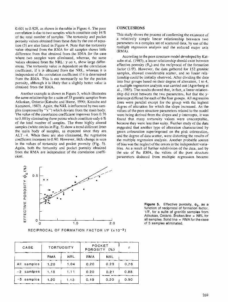
0.601 to 0.928, as shown in the table in Figure 4. The poor CONCLUSIONS correlation is due to two samples which constitute only 14 % of the total number of samples. The tortuosity and pocket porosity values obtained from these data by the use of equation (5) are also listed in Figure 4. Note that the tortuosity value obtained from the RMA for all samples shows little difference from that obtained from the RMA for the case where two samples were eliminated, whereas, the same values obtained from the NRL: y on x, show large differences. The tortuosity value is dependent on the correlation coefficient, if it is obtained from the NRL, whereas it is independent of the correlation coefficient if it is determined from the RMA. This is not necessarily so for the pocket porosity, although it is likely that a slightly better value is obtained from the RMA.

Another example is shown in Figure 5, which illustrates the same relationship for a suite of 35 granitic samples from Atikokan, Ontario (Katsube and Hume, 1990; Katsube and Kamineni, 1983). Again, the NRL is influenced by two samples (expressed by "x") which deviate from the main body. The value of the correlation coefficient improves from 0.76 to 0.88 by eliminating these points which constitute only 6 % of the total number of samples. The three highly altered samples (white circles in Fig. 5) show a trend different from the main body of samples, as expected since they are ALT=4. When these are also eliminated, the regression coefficient increases to 0.90. However, little change is seen in the values of tortuosity and pocket porosity (Fig. 5). Again, both the tortuosity and pocket porosity obtained from the RMA are independent of the correlation coefficient.

This study shows the process of confirming the existence of a relatively simple linear relationship between two parameters in a complex set of scattered data, by use of the multiple regression analysis and the reduced major axis (RMA).

According to the pore structure model developed by Kat- sube et al. (1985), a linear relationship should exist between effective porosity (GE) and the reciprocal of the formation factor (11F). However, the data gathered for 152 granitic samples, showed considerable scatter, and no linear relationship could be initially observed. After dividing the data into four groups based on their degree of alteration, 1 to 4, a multiple regression analysis was carried out (Agterberg et al., 1985). The results showed that, in fact, a linear relationship did exist between the two parameters, but that the y- intercept differed for each of the four groups. All regression lines were parallel except for the group with the highest degree of alteration for which the slope increased. As the values of the pore structure parameters related to the model were being derived from the slopes and y-intercepts, it was found that many tortuosity values were unacceptable, because they were less than unity. Further study of the data suggested that another type of alteration characterized by green colouration superimposed on the pink colouration, and the degree of data scatter, were distorting the results of the multiple regression analysis. Another probable source of bias was the neglect of the errors in the independent variables. As a result of further subdivision of the data, and by the use of the RMA, the values of the pore structure parameters deduced from multiple regression became

RECIPROCAL OF FORMATION FACTOR IIF ( x 10-3)

POROSITY (%)

Figure 5. Effective porosity, cp,, a s a function of reciprocal of formation factor, 1 IF, for a suite of granitic samples from Atikokan, Ontario. Broken line = NRL for all samples. Solid line = RMA for the case of 5 samples eliminated.

acceptable. Thus, two stages of statistical analysis were required before these data became acceptable. The first stage was the general analysis by the multiple regression method, and the second was the refined analysis by the RMA method. The use of the multiple regression analysis is supported by the agreement between the regression model and a physical model of pore structure, and the use of the RMA is supported by the benefits that were obtained from its use in separate studies.

ACKNOWLEDGMENTS

The authors are grateful to J.C. Davis (Kansas Geological Survey) and A.J. Desbarats (Geological Survey of Canada) for critically reviewing this paper, and for their comments and suggestions.

REFERENCES

Agterberg, F.P. 1974: Geomathematics: Mathematical Background and Geo-Science

Applications; Elsevier, Amsterdam, 596 p. Agterberg, F.P., Katsube, T.J., and Lew, S.N. 1985: Use of multiple regression for petrophysical characterization of

granites as a function of alteration; incurrent Research, Part B, Geological Survey of Canada, Paper S I B , p. 451-458.

Brown, A., Dugal, J.J.B., Everitt, R.A., Kamineni, D.C., Lau, J.S.O., and McEwen, J.H. 1985: Advances in geology at the URL site (RA-3); Atomic Energy of

Canada Limited, Technical Record, TR-299, p. 253-264. Davis, J.C. 1986: Statistics and Data Analysis in Geology; John Wiley and Sons,

New York, p. 200-204. Gujarati, D. 1970: Use of dummy variables in testing for equality between sets of

coefficients in linear regressions: a generalization; American Statistician, v. 24 no. 5, p. 18-21.

Kamineni, D.C. and Dugal, J.J.B. 1982: A study of rock alteration in the Eye-Dashwa Lakes pluton,

Atikokan, northwestern Ontario, Canada; Chemical Geology V. 36, p. 35-37.

Katsube, T.J. and Hume, J.P. 1990: Formation factor and porosity of crystalline rocks; Geophysics, in

press. Katsube, T.J. and Kamineni, D.C. 1983: Effect of alteration on pore structure of crystalline rocks: Core

samples from Atikokan, Ontario; Canadian Mineralogist, v. 21, p. 637-646.

Katsube, T.J., Percival, J.B., and Hume, J.P. 1985: Characterization of the rock mass by pore structure parameters;

Atomic Energy of Canada Limited, Technical Record, TR-299, p. 375-4 13.

Kendall, M.G. 1980: Multivariate Analysis (Second edition); Griffin. London. 210 p. Madden, T.R. 1976: Random networks and mixing laws; Geophysics, v. 41,

p. 1104-1 124. McLachlan, D.S., Button, M.B., Adams, S.R., Garring, V.M., Kneen, J.D., Muoe, J. and Wedepohl, E. 1987: Formation resistivity factor for a compressible solid-brine mix-

ture; Geophysics, v . 52, p. 194-203. Roberts, J. W., and Schwartz, L.M. 1985: Grain consolidation and electrical conductivity in porous media;

Phys. Rev., v. 831, p. 5990-5997. Schwartz, L.M. and Kimminau, S. 1987: Analysis of electrical conduction in grain consolidation model;

Geophysics, v . 52, p. 1402-141 1 . Sen, P.N., Scala, C., and Cohen, M.H. 1981 : A self-similar model for sedimentary rocks with application to the

dielectric constant of fused glass beads; Geophysics, v. 46. p. 781-795.

Shankland, T.J., and Waff, H.S. 1974: Conductivity of fluidbearing rocks; J. Geophys. Res., v. 79,

p. 4863-4867. Webman, I., Jortner, J., and Cohen, M.H. 1976: Numerical simulation of continuous percolation conductivity;

Phys. Rev., v. B14, p. 4737-4740. Winsauer, W.O., Shearin, H.M., Masson, P.H., and Williams, M. 1952: Resistivity of brine-saturated sands in relation to pore-geometry ;

Bull. American Association of Petroleum Geologists, v. 36, p. 253-277.

Conditional probability analysis of geological risk factors

P. J. Leel, Qin, Ruo-Zhe2 and Shi, Yan-Min2

Lee, P.J., Qin, Ruo-Zhe and Shi, Yan-Min, Conditional probability analysis of geological risk factors; in Statistical Applications in the Earth Sciences, ed. F.P. Agterberg and G.F. Bonham-Carter; Geological Survey of Canada, Paper 89-9, p. 271-276, 1989

Abstract

Geological risk factors such as presence of closure, presence of reservoir facies, adequate source, and adequate seal, to name a few, are conveniently assumed to be statistically independent when exploration risks are computed for petroleum resource evaluations and economic analysis. In this paper, data sets obtainedfrom the Huang-Hua Basin of eastern China were used to test this commonly held statistical assumption. Analysis of these data sets strongly indicates that, in general, geological risk factors may not be independent of each other. Indeed, such an assumption m y cause overestimation of exploration risk values.

Les facteurs de risque g&o!ogique cornme la prksence d'une femeture, la prksence d'un faci2s de rkservoir, une source adkquate et une couche impennkable adkquate, pour n'en nommer que quelques uns, sont de mnitre pratique supposks statistiquement indebendants lors du calcul des risques d'exploration en vue des e'valuations des ressources pktroliires et de 1 'analyse kconomique. Duns la pr&sente itude, des ensembles de donnkes obtenus dans le bassin Huang-Ha en Chine onentale ont servi rt vkn!er cette hypoth2se statistique couramment admise. L'analyse de ces ensembles de donnkes indique femement qu 'en g&n&ral, les facteurs de risque gkologique peuvent ne pas &re inde'pendants les urn des autres. En fait, une telle hypothtse peut entrainer une surestitnation des valeurs du risque d'exploration.

' Institute of Sedimentary and Petroleum Geology, Geological Survey of Canada, 3303 33rd Street N.W. Calgary, Alberta R L 2A7 ' Dagang Petroleum Administration Bureau, Dagang, Tianjing, People's Republic of China

INTRODUCTION GEOLOGICAL RISK FACTORS

A joint project, sponsored by the Dagang Petroleum Adminis- tration Bureau, the Geological Survey of Canada, and the United Nations, was undertaken to extract various types of data for the purpose of testing statistical assumptions employed in petroleum resource assessments. This paper outlines some of the results of the project.

Traditionally, exploration risk is an expression of the products of marginal probabilities of geological risk factors (Roy, 1979; Miller, 1982; Lee and Wang, 1983 ; Procter and Taylor, 1984; Bird, 1984; Baker, Gehrnan, James, and White, 1986; Crovelli and Balay, 1986; Meyer and Schenk, 1986; White, 1986). The statistical assumption presumed in such a product operation is that risk factors are independent. Lee and Wang (1983), however, have stated that, in general, geological risk factors may not, in fact, be independent. The assumption of independence of factors had not been tested using exploratory well data.

The data sets obtained from the Huang-Hua Basin of east- em China were used for the following studies: (1) to analyze all geological risk factors that influence eventual hydrocarbon accumulation in a prospect; (2) to examine each exploratory well within a play in order to determine which geological risk factors are absent; (3) to calculate the exploration risk based on the presence or absence of a factor; and (4) to examine the dependency of the geological risk factors.

The Huang-Hua Basin (area shaded with vertical lines in Fig. 1) is situated about 200 km east of Beijing, China. The basin comprises an onshore region that extends into the Bo- Hai Bay. The Tertiary sediments of the basin were deposited in a half-graben setting.

The Es, Formation (Oligocene) consisting of carbonate bank and fluvial facies (Fig. 2), was subdivided into two plays, for the purpose of petroleum resource evaluation, which are referred to herein as the limestone and sandstone plays. The sandstone play provided the data set for this risk analysis.

Geological risk factors that dictate the final accumulations of hydrocarbons include, for example, presence of closure and reservoir facies, as well as adequate seal, timing, source, migration, preservation, and recovery. For a specific play, only a few of these factors play an important role. In the Es, sandstone play, for example, factors such as presence of closure and of reservoir facies, and adequate source and seal are recognized as critical to final accumulation. Consequently, if a prospect located within the sandstone play, for example, is tested, it may prove unsuccessful for any the following reasons : lack of closure; unfavourable reservoir facies; lack of an adequate source or migration path; and/or absence of cap rock. In order to evaluate the exploration risk for the prospect, or any prospect in the

Figure 1. Location map of the Huang-Hua Basin (area shaded with the vertical lines).

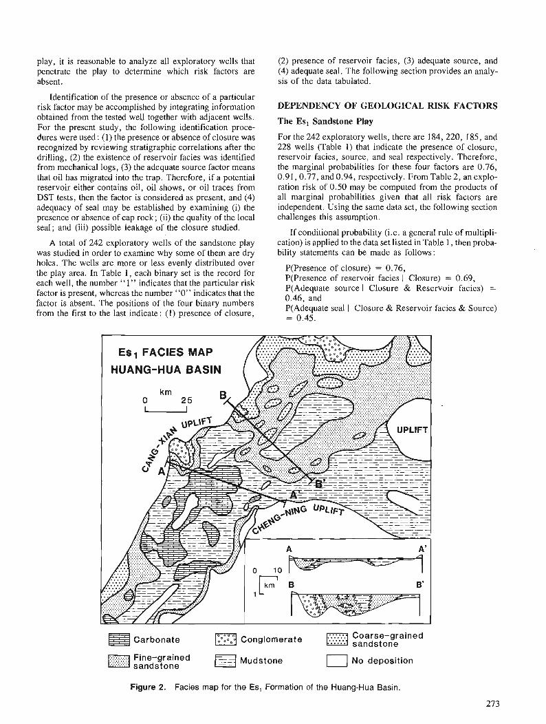
play, it is reasonable to analyze all exploratory wells that (2) presence of reservoir facies, (3) adequate source, and penetrate the play to determine which risk factors are (4) adequate seal. The following section provides an analy- absent. sis of the data tabulated.

Identification of the presence or absence of a particular risk factor may be accomplished by integrating information obtained from the tested well together with adjacent wells. For the present study, the following identification procedures were used : (1) the presence or absence of closure was recognized by reviewing stratigraphic correlations after the drilling, (2) the existence of reservoir facies was identified from mechanical logs, (3) the adequate source factor means that oil has migrated into the trap. Therefore, if a potential reservoir either contains oil, oil shows, or oil traces from DST tests, then the factor is considered as present, and (4) adequacy of seal may be established by examining (i) the presence or absence of cap rock; (ii) the quality of the local seal; and (iii) possible leakage of the closure studied.

A total of 242 exploratory wells of the sandstone play was studied in order to examine why some of them are dry holes. The wells are more or less evenly distributed over the play area. In Table 1, each binary set is the record for each well, the number "1" indicates that the particular risk factor is present, whereas the number "0" indicates that the factor is absent. The positions of the four binary numbers from the first to the last indicate: (1) presence of closure,

DEPENDENCY OF GEOLOGICAL RISK FACTORS

The Es, Sandstone Play

For the 242 exploratory wells, there are 184, 220, 185, and 228 wells (Table 1) that indicate the presence of closure, reservoir facies, source, and seal respectively. Therefore, the marginal probabilities for these four factors are 0.76, 0.91,0.77, and 0.94, respectively. From Table 2, an exploration risk of 0.50 may be computed from the products of all marginal probabilities given that all risk factors are independent. Using the same data set, the following section challenges this assumption.

If conditional probability (i.e. a general rule of multiplication) is applied to the data set listed in Table 1, then probability statements can be made as follows:

P(Presence of closure) = 0.76, P(Presence of reservoir facies I Closure) = 0.69, P(Adequate source l Closure & Reservoir facies) =

0.46, and P(Adequate seal I Closure & Reservoir facies & Source) = 0.45.

Esl FACIES MAP

HUANG-HUA BASIN

Carbonate Conglomerate 0 Coarse-grained sandstone

sandstone Mudstone ( No deposition

Figure 2. Facies map for the Es, Formation of the Huang-Hua Basin.

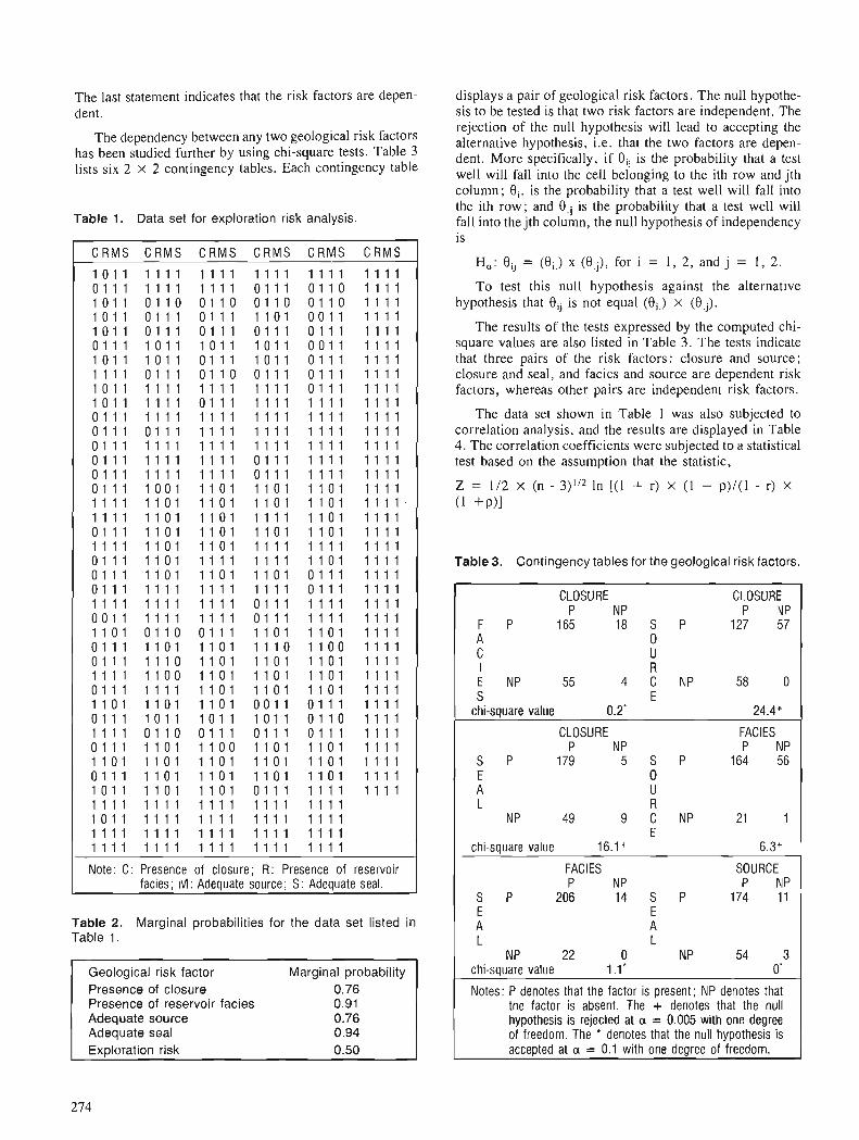
The last statement indicates that the risk factors are depen- displays a pair of geological risk factors. The null hypothe- dent. sis to be tested is that two risk factors are independent. The

rejection of the null hypothesis will lead to accepting the The between any two geological risk factors alternative hypothesis, i.e. that the two factors are

has been studied further by using chi-square tests Table 3 dent. M~~~ speci~cally, i f 8, is the probability that a test lists six 2 x 2 contingency tables. Each contingency table well will fall into the cell belonging to the ith row and jth

Table 1. Data set for exploration risk analysis.

C R M S C R M S C R M S C R M S C R M S C R M S

1 0 1 1 1 1 1 1 1 1 1 1 1 1 1 1 1 1 1 1 1 1 1 1 0 1 1 1 1 1 1 1 1 1 1 1 0 1 1 1 0 1 1 0 1 1 1 1 1 0 1 1 0 1 1 0 0 1 1 0 0 1 1 0 0 1 1 0 1 1 1 1 1 0 1 1 0 1 1 1 0 1 1 1 1 1 0 1 0 0 1 1 1 1 1 1 1 0 1 1 0 1 1 1 0 1 1 1 0 1 1 1 0 1 1 1 1 1 1 1 0 1 1 1 1 0 1 1 1 0 1 1 1 0 1 1 0 0 1 1 1 1 1 1 1 0 1 1 1 0 1 1 0 1 1 1 1 0 1 1 0 1 1 1 1 1 1 1 1 1 1 1 0 1 1 1 0 1 1 0 0 1 1 1 0 1 1 1 1 1 1 1 1 0 1 1 1 1 1 1 1 1 1 1 1 1 1 1 0 1 1 1 1 1 1 1 1 0 1 1 1 1 1 1 0 1 1 1 1 1 1 1 1 1 1 1 1 1 1 1 0 1 1 1 1 1 1 1 1 1 1 1 1 1 1 1 1 1 1 1 1 1 1 1 0 1 1 1 0 1 1 1 1 1 1 1 1 1 1 1 1 1 1 1 1 1 1 1 0 1 1 1 1 1 1 1 1 1 1 1 1 1 1 1 1 1 1 1 1 1 1 1 0 1 1 1 1 1 1 1 1 1 1 1 0 1 1 1 1 1 1 1 1 1 1 1 0 1 1 1 1 1 1 1 1 1 1 1 0 1 1 1 1 1 1 1 1 1 1 1 0 1 1 1 1 0 0 1 1 1 0 1 1 1 0 1 1 1 0 1 1 1 1 1 1 1 1 1 1 1 0 1 1 1 0 1 1 1 0 1 1 1 0 1 1 1 1 1 1 1 1 1 1 1 0 1 1 1 0 1 1 1 1 1 1 1 0 1 1 1 1 1 0 1 1 1 1 1 0 1 1 1 0 1 1 1 0 1 1 1 0 1 1 1 1 1 1 1 1 1 1 1 0 1 1 1 0 1 1 1 1 1 1 1 1 1 1 1 1 1 0 1 1 1 1 1 0 1 1 1 1 1 1 1 1 1 1 1 0 1 1 1 1 1 0 1 1 1 1 1 0 1 1 1 0 1 1 1 0 1 0 1 1 1 1 1 1 1 0 1 1 1 1 1 1 1 1 1 1 1 1 1 1 1 0 1 1 1 1 1 1 1 1 1 1 1 1 1 1 1 1 1 1 1 0 1 1 1 1 1 1 1 1 1 1 1 0 0 1 1 1 1 1 1 1 1 1 1 0 1 1 1 1 1 1 1 1 1 1 1 1 1 0 1 0 1 1 0 0 1 1 1 1 1 0 1 1 1 0 1 1 1 1 1 0 1 1 1 1 1 0 1 1 1 0 1 1 1 1 0 1 1 0 0 1 1 1 1 0 1 1 1 1 1 1 0 1 1 0 1 1 1 0 1 1 1 0 1 1 1 1 1 1 1 1 1 1 1 0 0 1 1 0 1 1 1 0 1 1 1 0 1 1 1 1 1 0 1 1 1 1 1 1 1 1 1 0 1 1 1 0 1 1 1 0 1 1 1 1 1 1 1 0 1 1 1 0 1 1 1 0 1 0 0 1 1 0 1 1 1 1 1 1 1 0 1 1 1 1 0 1 1 1 0 1 1 1 0 1 1 0 1 1 0 1 1 1 1 1 1 1 1 0 1 1 0 0 1 1 1 0 1 1 1 0 1 1 1 1 1 1 1 0 1 1 1 1 1 0 1 1 1 0 0 1 1 0 1 1 1 0 1 1 1 1 1 1 1 0 1 1 1 0 1 1 1 0 1 1 1 0 1 1 1 0 1 1 1 1 1 0 1 1 1 1 1 0 1 1 1 0 1 1 1 0 1 1 1 0 1 1 1 1 1 1 0 1 1 1 1 0 1 1 1 0 1 0 1 1 1 1 1 1 1 1 1 1 1 1 1 1 1 1 1 1 1 1 1 1 1 1 1 1 1 1 1 1 1 1 0 1 1 1 1 1 1 1 1 1 1 1 1 1 1 1 1 1 1 1 1 1 1 1 1 1 1 1 1 1 1 1 1 1 1 1 1 1 1 1 1 1 1 1 1 1 1 1 1 1 1 1 1 1 1 1 1 1 1

Note: C: Presence of closure; R: Presence of reservoir facies; I!: Adequate source; S: Adequate seal.

column; 8,. is the probability that a test well will fall into the ith row; and 0, is the probability that a test well will fall into the jth column, the null hypothesis of independency is

H,: Oij = (8i,)x(8.j) , fo r i = 1 , 2 , a n d j = 1 ,2 .

To test this null hypothesis against the alternative hypothesis that Oij is not equal (Oi.) X (O,j).

The results of the tests expressed by the computed chi- square values are also listed in Table 3. The tests indicate that three pairs of the risk factors: closure and source; closure and seal, and facies and source are dependent risk factors, whereas other pairs are independent risk factors.

The data set shown in Table 1 was also subjected to correlation analysis, and the results are displayed in Table 4. The correlation coefficients were subjected to a statistical test based on the assumption that the statistic,

Z = 112 x (n - 3) '12 In [ ( I + r) X (1 - p)/(l - r) X

(1 + P ) I

Geological risk factor Marginal probability Presence of closure Presence of reservoir facies jj Adequate Adequate seal source

Exploration risk

Table 3. Contingency tables for the geological risk factors.

NP 22 0 NP 54 3 chi-square value 1.1' 0'

Notes: P denotes that the factor is present; NP denotes that the factor is absent. The + denotes that the null hypothesis is rejected at a = 0.005 with one degree of freedom. The denotes that the null hypothesis is accepted at a = 0.1 with one degree of freedom.

Table 2. Marginal probabilities for the data set listed in Table 1 .

CLOSURE CLOSURE P N P P IVP

F P 165 18 S P 127 57 A 0 C U I R E NP 55 4 C NP 58 0 S E

chi-square value 0.2' 24.4+

CLOSURE FACIES P NP P NP

S P 179 5 S P 164 56 E 0 A U L R

N P 49 9 C NP 21 1 E

chi-square value 16.1+ 6.3+

FACIES SOURCE P N P P hlP

S P 206 14 S P 174 11 E E A A L L

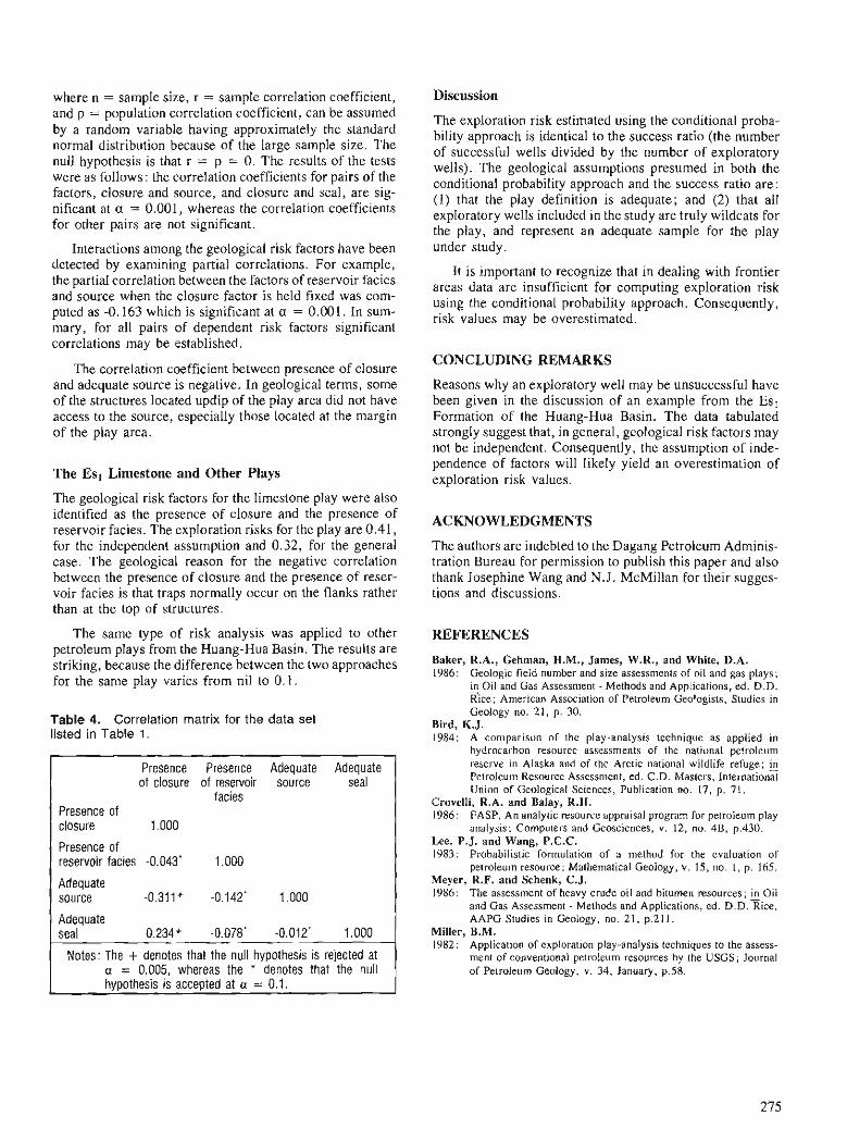
where n = sample size, r = sample correlation coefficient, and p = population correlation coefficient, can be assumed by a random variable having approximately the standard normal distribution because of the large sample size. The null hypothesis is that r = p = 0. The results of the tests were as follows : the correlation coefficients for pairs of the factors, closure and source, and closure and seal, are significant at a = 0.001, whereas the correlation coefficients for other pairs are not significant.

Interactions among the geological risk factors have been detected by examining partial correlations. For example, the partial correlation between the factors of reservoir facies and source when the closure factor is held fixed was computed as -0.163 which is significant at a = 0.001. In summary, for all pairs of dependent risk factors significant correlations may be established.

The correlation coefficient between presence of closure and adequate source is negative. In geological terms, some of the structures located updip of the play area did not have access to the source, especially those located at the margin of the play area.

The Es, Limestone and Other Plays

The geological risk factors for the limestone play were also identified as the presence of closure and the presence of reservoir facies. The exploration risks for the play are 0.41, for the independent assumption and 0.32, for the general case. The geological reason for the negative correlation between the presence of closure and the presence of reservoir facies is that traps normally occur on the flanks rather than at the top of structures.

The same type of risk analysis was applied to other petroleum plays from the Huang-Hua Basin. The results are striking, because the difference between the two approaches for the same play varies from nil to 0.1.

Table 4. Correlation matrix for the data set listed in Table 1.

Presence Presence Adequate Adequate of closure of reservoir source seal

facies Presence of closure 1.000

Presence of reservoir facies -0.043' 1.000

Adequate source -0.311 + -0.142' 1.000

Adequate seal 0.234+ -0.078' -0.012' 1.000

Notes: The + denotes that the null hypothesis is rejected at a = 0.005, whereas the * denotes that the null hypothesis is accepted at a = 0.1.

Discussion

The exploration risk estimated using the conditional probability approach is identical to the success ratio (the number of successful wells divided by the number of exploratory wells). The geological assumptions presumed in both the conditional probability approach and the success ratio are: (1) that the play definition is adequate; and (2) that all exploratory wells included in the study are truly wildcats for the play, and represent an adequate sample for the play under study.

It is important to recognize that in dealing with frontier areas data are insufficient for computing exploration risk using the conditional probability approach. Consequently, risk values may be overestimated.

CONCLUDING REMARKS

Reasons why an exploratory well may be unsuccessful have been given in the discussion of an example from the Es, Formation of the Huang-Hua Basin. The data tabulated strongly suggest that, in general, geological risk factors may not be independent. Consequently, the assumption of independence of factors will likely yield an overestimation of exploration risk values.

ACKNOWLEDGMENTS

The authors are indebted to the Dagang Petroleum Adminis- tration Bureau for permission to publish this paper and also thank Josephine Wang and N.J. McMillan for their suggestions and discussions.

REFERENCES

Baker, R.A., Gehman, H.M., James, W.R., and White, D.A. 1986: Geologic field number and size assessments of oil and gas plays;

in Oil and Gas Assessment - Methods and Applications, ed. D.D. - Rice; American Association of Petroleum Geologists, Studies in Geology no. 21, p. 30.

Bird, K.J. 1984: A comparison of the play-analysis technique as applied in

hydrocarbon resource assessments of the national petroleum reserve in Alaska and of the Arctic national wildlife refuge; Petroleum Resource Assessment, ed. C.D. Masters, International Union of Geological Sciences, Publication no. 17, p. 71.

Crovelli, R.A. and Balay, R.H. 1986: FASP. An analytic resource appraisal program for petroleum play

analysis; Computers and Geosciences, v. 12, no. 4B, p.430. Lee.P.J.and Wang,P.C.C. 1983: Probabilistic formulation of a method for the evaluation of

petroleum resource; Mathematical Geology, v. 15, no. I , p. 165. Meyer, R.F. and Schenk, C.J. 1986: The assessment of heavy crude oil and bitumen resources; Oil

and Gas Assessment - Methods and Applications, ed. D.D. Rice, AAPG Studies in Geology, no. 21, p.211.

Miller, B.M. 1982: Application of exploration play-analysis techniques to the assess-

ment of conventional petroleum resources by the USGS; Journal of Petroleum Geology, v. 34, January, p.58.

Procter, R.M. and Taylor, G.C. White, L.P. 1984 : Evaluation of oil and gas potential of an offshore Westcoast Canada 1986: A play approach to hydrocarbon resource assessment and evalua-

play - An example of Geological Survey of Canada methodology; tion; @ Oil and Gas Assessment and Applications - Methods and in Petroleum Resource Assessment, ed. C.D. Masters, Interna- - Applications, ed. D.D. Rice, American Association of Petroleum tional Union of Geological Sciences, Publication no. 17, p.58. Geologists, Studies in Geology, no. 21, p. 128.

Roy, K.J. 1979: Hydrocarbon assessment using subjective probability and Monte

Carlo methods; Methods and Models for Assessing Energy Resources, First llASA Conference on Energy Resources, ed. M. Grenon; Pergamon Press, New York, p. 285.

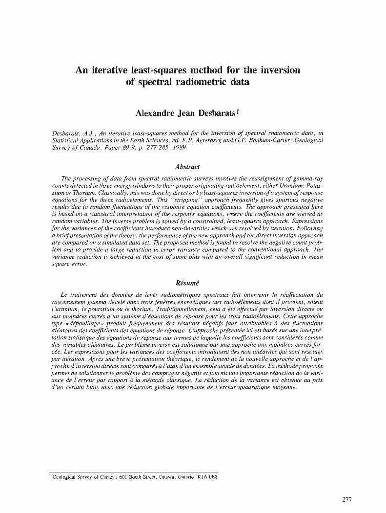
An iterative least-squares method for the inversion of spectral radiometric data

Alexandre Jean Desbaratsl

Desbarats, A.J., An iterative least-squares method for the inversion of spectral radiometric data; & Statistical Applications in the Earth Sciences, ed. F. P. Agterberg and G.F. Bonham-Carter; Geological Survey of Canada, Paper 89-9, p. 277-285, 1989.

Abstract

The processing of data from spectral radiometric surveys involves the reassignment of gamma-ray counts detected in three energy windows to their proper originating radioelement, either Uranium, Potas- sium or Thorium. Classically, this was done by direct or by least-squares inversion of a system of response equations for the three radioelements. This "stripping" approach frequently gives spurious negative results due to random jluctuations of the response equation coeficients. The approach presented here is based on a statistical interpretation of the response equations, where the coeflcients are viewed as random variables. The inverse problem is solved by a constrained, least-squares approach. Expressions for the variances of the coeficients introduce non-linearities which are resolved by iteration. Following a briefpresentation of the theory, the performance of the new approach and the direct inversion approach are compared on a simulated data set. f ie proposed method is found to resolve the negative count problem and to provide a large reduction in error variance compared to the conventional approach. The variance reduction is achieved at the cost of some bias with an overall significant reduction in mean square error.

Le traitement des donne'es de leve's radiome'triques spectrum fait intervenir la re'affectation du rayonnement gamma de'celk duns trois fenttres energe'tiques aux radio6le'ments dont il provient, soient l'uranium, le potassium ou le thorium. Traditionnellement, cela a e'te' effectue' par inversion directe ou aux moindres carre's d 'un systkme d'e'quations de re'ponse pour les trois radioe'le'ments. Cette approche type .( de'pouillage ,, produit fie'quemment des re'sultats ne'gafifs faux attribuables ir des jluctuations ale'atoires des coeficients des e'quations de re'ponse. L'approche prksente'e iic est base'e sur une interprktation statistique des e'quations de re'ponse a w termes de laquelle les coefficients sont conside'r6s comme des variables ale'atoires. Le problkme inverse est solutionne' par une approche aux moindres carre's for- eke. Les expressions pour les variances des coeflcients introduisent des non linkaritb qui sont re'solues par it6ration. Apr2s une b r h e prksentation the'orique, le rendement de la nouvelle approche et de l'approche d 'inversion directe sont compares d 1 'aide d 'un ensemble simule'de donne'es. La me'thode propose'e permet de solutionner le problkme des comptages nkgatifs et fournif une importante re'duction de la variance de l'erreur par rapport b la me'thode classique. La reduction de la variance est obtenue au prix d'un certain biais avec une re'duction globule importante de l'erreur quadratique moyenne.

' Geological Survey of Canada, 601 Booth Street, Ottawa, Ontario, K I A OE8

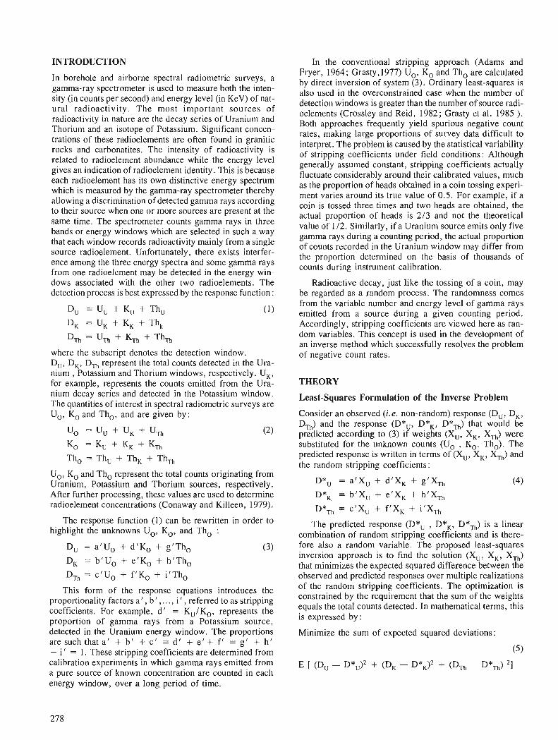
INTRODUCTION

In borehole and airborne spectral radiometric surveys, a gamma-ray spectrometer is used to measure both the intensity (in counts per second) and energy level (in KeV) of natural radioactivity. The most important sources of radioactivity in nature are the decay series of Uranium and Thorium and an isotope of Potassium. Significant concentrations of these radioelements are often found in granitic rocks and carbonatites. The intensity of radioactivity is related to radioelement abundance while the energy level gives an indication of radioelement identity. This is because each radioelement has its own distinctive energy spectrum which is measured by the gamma-ray spectrometer thereby allowing a discrimination of detected gamma rays according to their source when one or more sources are present at the same time. The spectrometer counts gamma rays in three bands or energy windows which are selected in such a way that each window records radioactivity mainly from a single source radioelement. Unfortunately, there exists interference among the three energy spectra and some gamma rays from one radioelement may be detected in the energy windows associated with the other two radioelements. The detection process is best expressed by the response function :

D, = U, + K, + Th,

D, = U, + K, + Th,

DT, = UTh + KT, + ThTh where the subscript denotes the detection window. D,, D,, D,, represent the total counts detected in the Ura- nium , Potassium and Thorium windows, respectively. U,, for example, represents the counts emitted from the Ura- nium decay series and detected in the Potassium window. The quantities of interest in spectral radiometric surveys are Uo, KO and Tho, and are given by:

Uo = Uu + U, + UTh

KO = K" + K, + KT, Th, = Th, + Th, + ThTh

Uo, KO and Tho represent the total counts originating from Uranium, Potassium and Thorium sources, respectively. After further processing, these values are used to determine radioelement concentrations (Conaway and Killeen, 1979).

The response function (1) can be rewritten in order to highlight the unknowns Uo, KO, and Tho :

This form of the response equations introduces the proportionality factors a ' , b ' , . . . , i ' , referred to as stripping coefficients. For example, d ' = K,/K,, represents the proportion of gamma rays from a Potassium source, detected in the Uranium energy window. The proportions are such that a ' + b ' + c ' = d ' + e t + f ' = g' + h' + i ' = 1. These stripping coefficients are determined from calibration experiments in which gamma rays emitted from a pure source of known concentration are counted in each energy window, over a long period of time.

In the conventional stripping approach (Adams and Fryer, 1964 ; Grasty ,1977) U,, KO and Tho are calculated by direct inversion of system (3). Ordinary least-squares is also used in the overconstrained case when the number of detection windows is greater than the number of source radioelements (Crossley and Reid, 1982 ; Grasty et al. 1985 ). Both approaches frequently yield spurious negative count rates, making large proportions of survey data difficult to interpret. The problem is caused by the statistical variability of stripping coefficients under field conditions: Although generally assumed constant, stripping coefficients actually fluctuate considerably around their calibrated values, much as the proportion of heads obtained in a coin tossing experiment varies around its true value of 0.5. For example, if a coin is tossed three times and two heads are obtained, the actual proportion of heads is 213 and not the theoretical value of 112. Similarly, if a Uranium source emits only five gamma rays during a counting period, the actual proportion of counts recorded in the Uranium window may differ from the proportion determined on the basis of thousands of counts during instrument calibration.

Radioactive decay, just like the tossing of a coin, may be regarded as a random process. The randomness comes from the variable number and energy level of gamma rays emitted from a source during a given counting period. Accordingly, stripping coefficients are viewed here as random variables. This concept is used in the development of an inverse method which successfully resolves the problem of negative count rates.

THEORY

Least-Squares Formulation of the Inverse Problem

Consider an observed ( i .e . non-random) response (DU, D,, DTh) and the response (D*U, D*,, DYTh) that would be predicted according to (3) if weights (XU, X,, XTh) were substituted for the unknown counts (U, , KO, Th,). The predicted response is written in terms of (Xu, X,, X,,) and the random stripping coefficients :

D*, = a'Xu + d l X K + gtXTh (4)

D*, = b t X U + e t X K + hlXTh D*,, = c1XU + f l X K + i'X,,

The predicted response (D*U , D*K, D*Th) is a linear combination of random stripping coefficients and is therefore also a random variable. The proposed least-squares inversion approach is to find the solution (Xu, X,, X,,) that minimizes the expected squared difference between the observed and predicted responses over multiple realizations of the random stripping coefficients. The optimization is constrained by the requirement that the sum of the weights equals the total counts detected. In mathematical terms, this is expressed by:

Minimize the sum of expected squared deviations:

subject to the conservation of counts constraint:

In this formulation of the inverse problem, (D*U, D*,, D*,,) serve as dummy variables and are of no direct interest. The weights (XU, X K, XTh) which yield optimum values of (D*,, D*,, D*Th) in (5) are taken as estimates of (U,, KO, Tho) although they may not be optimum or unbiased themselves. In order to minimize (5) subject to the constraint (6), the standard procedure is to define the quantity Q, introducing the Lagrange multiplier p :

Q = E [(Du - D*")2 + (D, - D*K) + (7) (DTh - D*Th)21 + (XU + XK + XTh - S,

The expression for Q is expanded and differentiated with respect to XU, X,, XTh and ;L. Setting the partial derivatives to zero yields a set of four equations in four unknowns. A complete derivation is presented in the appendix. In expanded matrix form, the system of equations obtained is written:

where the variance terms are defined by: unknown counts emitted, (U,, KO, Tho): It can easily be

u2, = u2, + u2b + uZc (9) shown that the conditional mean and var~ance of stripping coefficient a ' are given by:

u2, = u2, + uZe + uzf a2,, = u2, + u2, + uzi E [a ' I (U,, KO, Tho) 1 = E [a ' I U,] = a (1 1)

u2a = Var [a ' I (Uo, KO, Tho)] = and the mean and variance of a stripping coefficient a ' are written a and u2,, respectively. Var [a' 1 Uo] = a (I - a)/Uo

Thus, the system contains only terms involving the means and variances of random stripping coefficients. Although stripping coefficients from the same radioelement are correlated, this correlation does not enter in the derivation of system (8). Stripping coefficients from different radioelements are uncorrelated. System (8) resembles an ordinary least-squares inverse system (Crossley and Reid, 1982) with the important exception of the variance terms contained in the diagonal elements of the left hand side. The apparent similarity should not be allowed to obscure the fact that system (8) was derived from a formulation of the inverse problem quite different from the conventional one.

The expected sum of squared errors (5) can be written in terms of (Xu, X,, X,,) and p as:

u2, = D2, + D2, + DZTh (10) - (aDu + bD, + cD,,) Xu

- (dDu + eD, + fDTh) X,

- (gDu + hD, + iD,,)X,, - p S

When normalized by S2, u2= provides a useful index of the fit of the inverse calculation.

Mean and Variance of the Stripping Coefficients

The least-squares method presented here minimizes the expected squared diference between the observed response (D,, DK, DTh) and the dummy predicted response (D*U, D*K, D*,,) over multiple realizations of the random stripping coefficients. However, the probability distribution functions of the stripping coefficients are conditional on the

The moments of the other stripping coefficients are obtained in a similar fashion. Using (1 1) , the variance terms in ( 9) can be expanded:

where (U,, KO, Th,) are the unknown counts to be estimated by (XU, X,, X,,). The means of the stripping coefficients are assumed to be the values determined by calibration. From (1 1) it is seen that the variance of stripping coefficients decreases with increasing source counts. If the source counts from all three radioelements are high, then the variance terms (12) tend to zero. The conservation of counts constraint becomes redundant and system (8) reduces to a form identical to the ordinary least-squares inverse system.

Iteration Procedure

In the variance terms (12), the unknowns (U,, KO, Tho) are approximated by their estimates (Xu , XK, XTh). The resulting system of equations becomes non-linear and must be solved iteratively.

At iteration level i , system (8) is linearized using the solution at the previous iteration level to evaluate the variance terms. The system is then solved for (X'j, XiK, XiTh). The solution vector S is updated according to:

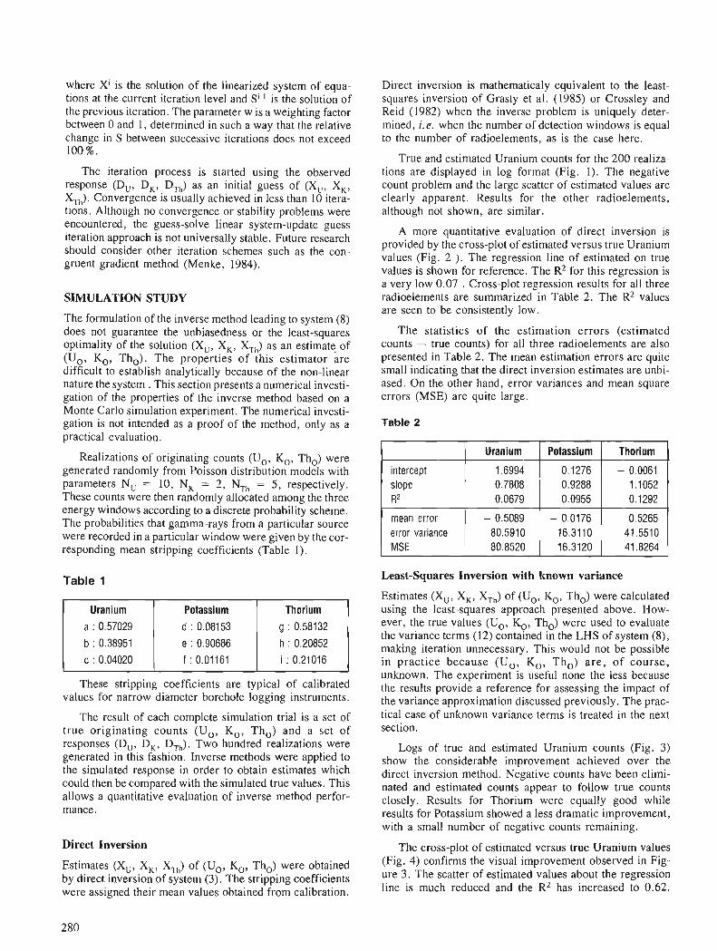
where X1 is the solution of the linearized system of equations at the current iteration level and Si-' is the solution of the previous iteration. The parameter w is a weighting factor between 0 and 1, determined in such a way that the relative change in S between successive iterations does not exceed 100%.

The iteration process is started using the observed response (Du, D,, D,,,) as an initial guess of (Xu, X,, X,,). Convergence is usually achieved in less than 10 iterations. Although no convergence or stability problems were encountered, the guess-solve linear system-update guess iteration approach is not universally stable. Future research should consider other iteration schemes such as the con- gruent gradient method (Menke, 1984).

SIMULATION STUDY

The formulation of the inverse method leading to system (8) does not guarantee the unbiasedness or the least-squares optimality of the solution (Xu, X,, X,,) as an estimate of (U,, KO, Tho). The properties of this estimator are difficult to establish analytically because of the non-linear nature the system . This section presents a numerical investigation of the properties of the inverse method based on a Monte Carlo simulation experiment. The numerical investigation is not intended as a proof of the method, only as a practical evaluation.

Realizations of originating counts (Uo, KO, Tho) were generated randomly from Poisson distribution models with parameters Nu = 10, NK = 2, NTh = 5 , respectively. These counts were then randomly allocated among the three energy windows according to a discrete probability scheme. The probabilities that gamma-rays from a particular source were recorded in a particular window were given by the corresponding mean stripping coefficients (Table 1).

Table 1

These stripping coefficients are typical of calibrated values for narrow diameter borehole logging instruments.

The result of each complete simulation trial is a set of true originating counts (U,, KO, Tho) and a set of responses (Du, D,, D,,). Two hundred realizations were generated in this fashion. Inverse methods were applied to the simulated response in order to obtain estimates which could then be compared with the simulated true values. This allows a quantitative evaluation of inverse method performance.

Direct Inversion

Estimates (Xu, X,, X,,) of (U,, KO, Tho) were obtained by direct inversion of system (3). The stripping coefficients were assigned their mean values obtained from calibration.

Direct inversion is mathematicaly equivalent to the least- squares inversion of Grasty et al. (1985) or Crossley and Reid (1982) when the inverse problem is uniquely determined, i. e. when the number of detection windows is equal to the number of radioelements, as is the case here.

True and estimated Uranium counts for the 200 realizations are displayed in log format (Fig. 1). The negative count problem and the large scatter of estimated values are clearly apparent. Results for the other radioelements, although not shown, are similar.

A more quantitative evaluation of direct inversion is provided by the cross-plot of estimated versus true Uranium values (Fig. 2 ). The regression line of estimated on true values is shown for reference. The R2 for this regression is a very low 0.07 . Cross-plot regression results for all three radioelements are summarized in Table 2. The R2 values are seen to be consistently low.

The statistics of the estimation errors (estimated counts - true counts) for all three radioelements are also presented in Table 2. The mean estimation errors are quite small indicating that the direct inversion estimates are unbiased. On the other hand, error variances and mean square errors (MSE) are quite large.

Table 2

Least-Squares Inversion with known variance

intercept slope R2

mean error error variance MSE

Estimates (XU, XK, XTh) of (UO, KO, Tho) were calculated using the least-squares approach presented above. How- ever, the true values (Uo, &, Tho) were used to evaluate the variance terms (12) contained in the LHS of system (€9, making iteration unnecessary. This would not be possible in practice because (U KO, Tho) a r e , of course,

0: unknown. The experiment is useful none the less because the results provide a reference for assessing the impact of the variance approximation discussed previously. The practical case of unknown variance terms is treated in the next section.

Logs of true and estimated Uranium counts (Fig. 3) show the considerable improvement achieved over the direct inversion method. Negative counts have been eliminated and estimated counts appear to follow true counts closely. Results for Thorium were equally good while results for Potassium showed a less dramatic improvement, with a small number of negative counts remaining.

Uranium

1.6994 0.7808 0.0679

- 0.5089 80.591 0 80.8520

The cross-plot of estimated versus true Uranium values (Fig. 4) confirms the visual improvement observed in Fig- ure 3. The scatter of estimated values about the regression line is much reduced and the R2 has increased to 0.62.

Potassium

0.1276 0.9288 0.0955

- 0.0176 16.3110 16.3120

Thorium

-0.0061 1.1052 0.1292

0.5265 41.5510 41.8264

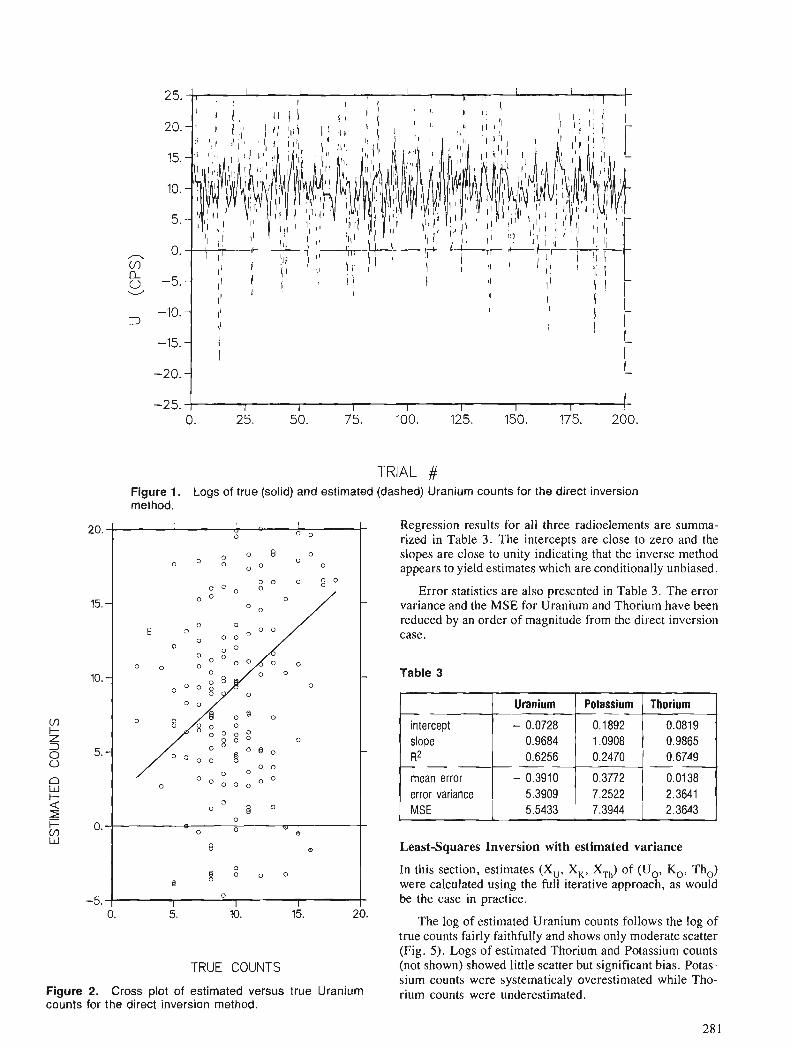
TRIAL # Figure 1. Logs of true (solid) and estimated (dashed) Uranium counts for the direct inversion method.

Regression results for all three radioelements are summarized in Table 3 . The intercepts are close to zero and the slopes are close to unity indicating that the inverse method appears to yield estimates which are conditionally unbiased.

Error statistics are also presented in Table 3. The error variance and the MSE for Uranium and Thorium have been reduced by an order of magnitude from the direct inversion case.

Table 3

-5.

Least-Squares Inversion with estimated variance

intercept slope I?


0 @ c o o

B O

0 I I I

0. 5. 10. 15. 20. The log of estimated Uranium counts follows the log of true counts fairly faithfully and shows only moderate scatter (Fig. 5). Logs of estimated Thorium and Potassium counts

TRUE COUNTS (not shown) showed little scatter but significant bias. Potas- sium counts were systematicaly overestimated while Tho-

Figure 2. Cross plot of estimated versus true Uranium rium counts were underestimated. counts for the direct inversion method.

In this section, estimates (XU, X,, X,,) of (Uo, KO, Tho) were calculated using the full iterative approach, as would be the case in practice.

Thorium

0.0819 0.9865 0.6749

0.0138 2.3641 2.3643

Uranium

- 0.0728 0.9684 0.6256

- 0.3910 5.3909 5.5433

Potassium

0.1892 1.0908 0.2470

0.3772 7.2522 7.3944

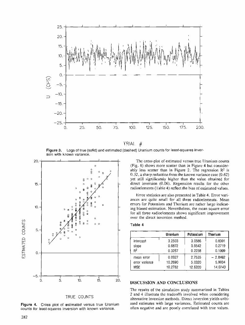
TRIAL # F igure 3. Logs of true (solid) and estimated (dashed) Uranium counts for least-squares inversion with known variance.

The cross-plot of estimated versus true Uranium counts (Fig. 6) shows more scatter than in Figure 4 but considerably less scatter than in Figure 2. The regression R2 is 0.32, a sharp reduction from the known variance case (0.62) yet still significantly higher than the value obtained for direct inversion (0.06). Regression results for the other radioelements (Table 4) reflect the bias of estimated values.

Error statistics are also presented in Table 4. Error variances are quite small for all three radioelements. Mean errors for Potassium and Thorium are rather large indicating biased estimation. Nevertheless, the mean square error for all three radioelements shows significant improvement over the direct inversion method.

Table 4

0. 5. 10. 15. 20. DISCUSSION AND CONCLUSIONS

intercept slope R2


The results of the simulation study summarized in Tables

TRUE COUNTS 2 and 4 illustrate the tradeoffs involved when considering alternative inversion methods. Direct inversion yields unbi-

Figure 4. Cross plot of estimated versus true Uranium ased estimates with large variances. Estimated counts are counts for least-squares inversion with known variance. often negative and are poorly correlated with true values.

Uranium

3.2503 0.6872 0.3267

0.0927 10.2690 10.2782

Potassium

3.0586 0.8542 0.2258

2.7535 5.0320

12.6320

Thorium

0.8301 0.2719 0.1009

- 2.8462 5.9934

14.0743

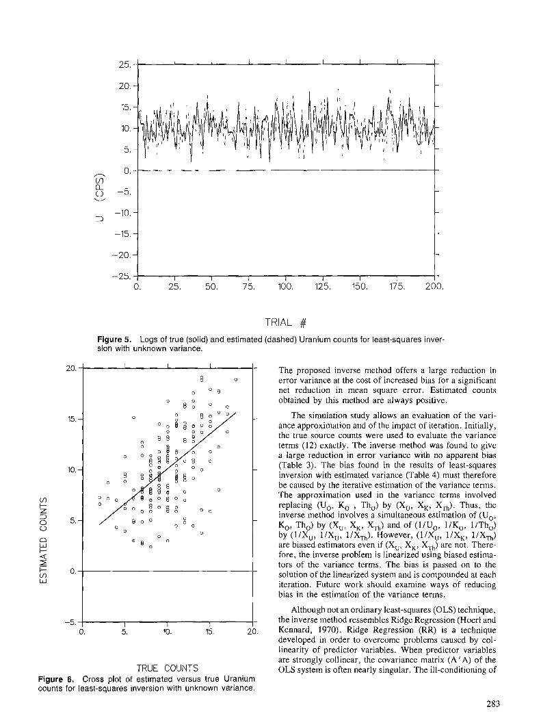
TRIAL # Figure 5. Logs of true (solid) and estimated (dashed) Uranium counts for least-squares inversion with unknown variance.

TRUE COUNTS Figure 6. Cross plot of estimated versus true Uranium counts for least-squares inversion with unknown variance.

The proposed inverse method offers a large reduction in error variance at the cost of increased bias for a significant net reduction in mean square error. Estimated counts obtained by this method are always positive.

The simulation study allows an evaluation of the variance approximation and of the impact of iteration. Initially, the true source counts were used to evaluate the variance terms (12) exactly. The inverse method was found to give a large reduction in error variance with no apparent bias (Table 3). The bias found in the results of least-squares inversion with estimated variance (Table 4) must therefore be caused by the iterative estimation of the variance terms. The approximation used in the variance terms involved replacing (Uo, KO , Tho) by (Xu, X,, X.,.,). Thus, the inverse method involves a simultaneous estimation of (U,, KO, Tho) by (Xu, XK, XTh) and of ( l /Uo, l /Ko, l/Th,) by ( l /XU, l /Xu, l/XTh). However, ( l /XU, l /XK, l/XTh) are biased estimators even if (Xu, X,, XTh) are not. There- fore, the inverse problem is linearized using biased estirna- tors of the variance terms. The bias is passed on to the solution of the linearized system and is compounded at each iteration. Future work should examine ways of reducing bias in the estimation of the variance terms.

Although not an ordinary least-squares (OLS) technique, the inverse method resembles Ridge Regression (Hoerl and Kennard, 1970). Ridge Regression (RR) is a technique developed in order to overcome problems caused by collinearity of predictor variables. When predictor variables are strongly collinear, the covariance matrix (A' A) of the OLS system is often nearly singular. The ill-conditioning of

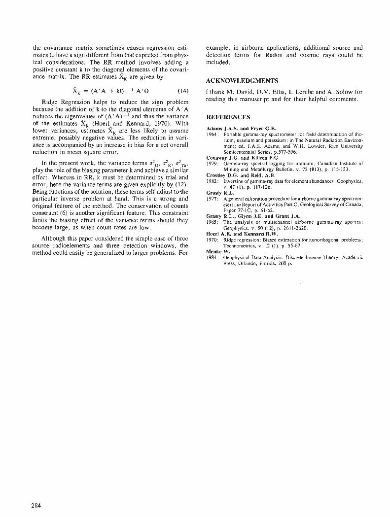
the covariance matrix sometimes causes regression estimates to have a sign different from that expected from physical considerations. The RR method involves adding a positive constant k to the diagona_l elements of the covariance matrix. The RR estimates X, are given by:

kK = (A'A + kI) - ' A'D

Ridge Regression helps to reduce the sign problem because the addition of k to the diagonal elements of A ' A reduces the eigenv~lues of (A'A) - ' and thus the variance of the estimates X, (Hoerl and Kennard, 1970). With lower variances, estimates kK are less likely to assume extreme, possibly negative values. The reduction in variance is accompanied by an increase in bias for a net overall reduction in mean square error.

In the present work, the variance terms u2,,, a2,, ST,, play the role of the biasing parameter k and achieve a similar effect. Whereas in RR, k must be determined by trial and error, here the variance terms are given explicitly by (12). Being functions of the solution, these terms self-adjust tofhe particular inverse problem at hand. This is a strong and original feature of the method. The conservation of counts constraint (6) is another significant feature. This constraint limits the biasing effect of the variance terms should they become large, as when count rates are low.

Although this paper considered the simple case of three source radioelements and three detection windows, the method could easily be generalized to larger problems. For

example, in airborne applications, additional source and detection terms for r ad on and cosmic rays could be included.

ACKNOWLEDGMENTS

I thank M. David, D.V. Ellis, I. Lerche and A. Solow for reading this manuscript and for their helpful comments.

REFERENCES

Adams J.A.S. and Fryer G.E. 1964: Portable gamma-ray spectrometer for field determination of tho-

rium, uranium and potassium; fi The Natural Radiation Environ- ment; ed. J.A.S. Adams, and W.H. Lowder, Rice University Semicentennial Series, p.577-596.

Conaway J.G. and Killeen P.G. 1979: Gamma-ray spectral logging for uranium; Canadian Institute of

Mining and Metallurgy Bulletin, v. 73 (813). p. 115-123. Crossley D.G. and Reid, A.B. 1982: Inversion of gamma-ray data for element abundances; Geophysics,

V. 47 (I), p. 117-126. Grastv R.L. 1977 : A general calibration procedure for airborne gamma-ray spectrom-

eters; in Repor( of Activities Part C, Geological Survey of Canada, Paper 77-IC, p. 61-62.

Grasty R.L., Glynn J.E. and Grant J.A. 1985: The analysis of multichannel airborne gamma-ray spectra;

Geophysics, v. 50 (12), p. 261 1-2620. Hoerl A.E. and Kennard R.W. 1970: Ridge regression: Biased estimation for nonorthogonal problems;

Technometrics, v. 12 ( I ) , p. 55-67. Menke W. 1984: Geophysical Data Analysis: Discrete Inverse Theory, Academic

Press, Orlando, Florida, 260 p.

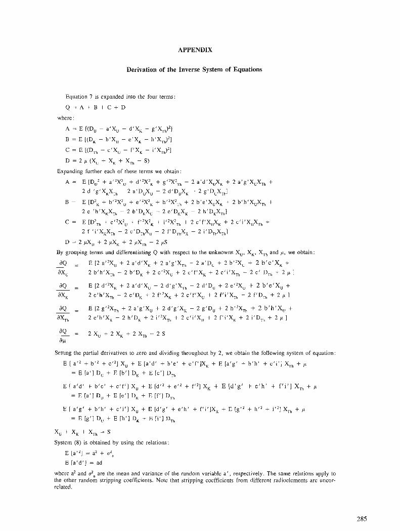
APPENDIX

Derivation of the Inverse System of Equations

Equation 7 is expanded into the four terms

Q = A + B + C + D

where :

A = E [(D, - a l X U - d'X, - g ' ~ , , ) ~ ]

B = E [(D, - b1XU - e'X, - h'XTh)2]

C = E [(DTh - c ' XU - f lXK - i ' XTh)2]

D = 2 p (Xu + X, + XTh - S)

Expanding further each of these terms we obtain:

A = E [DU2 + aI2X2, + dt2X2, + gt2XzTh + 2 ald'XuXK + 2 alg'XuXTh + 2 d 'g lXKXTh - 2 a1DUXu - 2 d lDUXK - 2 gfDUXTh]

B = E [D2, + b'2X2U + ef2XZK + hf2XZTh + 2 bfe 'XuXK + 2 bfh'XUXTh + 2 e 'hlXKXTh - 2 b1DKXU - 2 e lDKXK - 2 hfDKXTh]

C = E[D2,, + c ' ~ X ~ ~ + fI2X2, + i12X2Th + 2 c f f ' X U X K + 2c1 i 'XUXTh + 2 f ' ifXKXTh - 2 C ' DThXU - 2 f ' DThXK - 2 ilDThXTh]

D = 2 pXu + 2 pXK + 2 pXTh - 2 pS

By grouping terms and differentiating Q with respect to the unknowns Xu, XK, XTh and a, we obtain:

aQ = E [2 a t2XU + 2 a ' d f X K + 2 a1g 'XTh - 2 a1DU + 2 bI2Xu + 2 b ' e fXK + - a x u 2 b ' h f x T h - 2 b ' ~ , + 2 c T 2 x U + 2 c l f f x K + 2 c f i l X T h - 2 c r D~~ + 2 p 1

Setting the partial derivatives to zero and dividing throughout by 2 , we obtain the following system of equation:

E [ a t 2 + b i 2 + c t 2 ] XU + E [a'd' + b'e ' + c ' f l ]XK + E [a'g' + b'h ' + c ' i ' ] XTh + p

= E [a ' ] Du + E [b'] DK + E [c'] DTh

E [ a ' d ' + b ' e ' + c ' f ' ] Xu + E [dl2 + e l 2 + f f 2 ] XK + E [d 'g ' + e ' h ' + f ' i ' ] XTh + I(

= E [a ' ] Du + E [e ' ] D, + E [f '] DTh

E [ a 'g ' + b'h ' + c ' i ' ] Xu + E [d 'g ' + e 'h ' + f1i ']XK + E [g i2 + hI2 + iI2] XTh + p

= E [g'] Du + E [h'] D, + E [i '] DTh

Xu + X, + X,,, = S

System (8) is obtained by using the relations:

E [aI2] = a2 + a20

E [a'd '] = ad

where a2 and uZa are the mean and variance of the random variable a ' , respectively. The same relations apply to the other random stripping coefficients. Note that stripping coefficients from different radioelements are uncorrelated.

Spatial estimation of frequency distribution of acid rain data using Bigaussian kriging

Denis Marcottel

Marcotte, D., Spatial estimation of frequency distribution of acid rain data using bigaussian kriging; in Statistical Applications in the Earth Sciences, ed. F. P. Agterberg and G. F. Bonham-Carter; Geolo- &a1 Survey of Canada, Paper 89-9, p. 287-296, 1989

Abstract

Many problems in various fields can be formulated in terms of the probability of exceeding given threshold values. Whether in selective mining, environmental studies or geochemical exploration, an estimation of the (conditionnal or local) frequency distribution at every point in space carries much more information than the usual ordinary kriging estimates or other, similar estimators. Various methods exist to estimate such distributions, most of which have appeared in the last six years. Bigaussian kriging is the latest of these. Successful applications have been reported and its simplicity gives this method a definite edge. After a short exposte of the method, an example involving acid rain data is presented illustrating the quality of information available from the estimated distribution function as compared to the ordinary kriging estimates.

Un grand nombre de problt?mes dans plusieurs domaines peuvent Btre formults en termes de la proba- bilitt de dtpmsement de valeurs seuils donntes. Que ce soit en exploitation minitre stlective, pour les e'tudes environnementales ou l'exploration gtochimique, une estimation de la distribution de frtfquences (conditionnelle ou locale) en chaque point de 1 'espace renseigne beaucoup plus que les habituelles estimations par krigeage ordinaire ou que d'autres estimateurs analogues. I1 existe diverses mtthodes pour estimer de telles distributions, la plupart d 'entre elles ayant e'tt mises au point au cours des six dernitres annkes. La plus rtfcente est celle du krigeage bigaussien, dont des applications couronnkes de succ?s ont tte' signaltes; la simplicite' de cette mtfthode lui confere un net avantage. Un exemple portant sur les pluies acides illustre le type d'information disponible h partir de cette mtfthode comparativement au krigeage ordinaire.

- - - - - - - - -

' Dtpartement de Gtnie mineral, h o l e Polytechnique, C.P. 6079, Succursale .An, Montreal (Quebec) H3C 3A7

INTRODUCTION BIGAUSSIAN KRIGING

Estimators traditionally used in cartography associate every point in space with a value considered to be close to reality. In a probabilistic context, as in geostatistics, this value could be interpreted as estimating a conditional mathematical expectation where the conditioning set consists of all the surrounding known values (the sample).

The important notion of conditional expectation is not sufficient to truly efficiently describe various phenomena. To illustrate this fact, let us suppose that a sampling cam- paign of soils in your city led the government to make the following statement about your backyard : -"The estimated PCB (poly-chlorinated-biphenyl) concentration in the soil is half the danger level; however, there is a 10 % probability of the true value being above this threshold". Clearly the second part of the statement would attract your attention.

Like wise, in the exploitation of a deposit the distribution of the grades of ore is as important to the profitability of the mine as the mean grade of the ores in the deposit. In a highly selective operation, it is actually a more important consideration.

The preceding two examples show the importance of estimating the conditional distribution of a variable rather than merely its conditional expectation.

A first step in this direction was taken in the 60s in geostatistics with the estimation variance concept. How- ever, as is now widely recognized (Davis and Culhane, 1984), this estimation variance is only an indication of sampling adequacy except when the process under study can be considered to be gaussian. In such cases, the estimation variance obtained by simple kriging with known mean is the conditional variance.

In the last 15 years, many methods have appeared to tackle the problem of estimating conditional distributions : disjunctive kriging (Matheron, 1976), indicator kriging (Journel, 1983) probability kriging (Sullivan, 1984), multigaussian kriging (Matheron, 1974 ; Verly, 1984) and, most recently, bigaussian kriging (Marcotte et David, 1985). All these methods have their advantages and disadvantages. Published comparisons of some of these methods (Guibal and Rernacre, 1984), (Marcotte, 1988) show relatively few differences. Multigaussian kriging, with the change of support solution of Verly (1984) and bigaussian kriging, have the theoretical advantage of always providing positive probabilities. Bigaussian kriging calculation is cheaper and requires a less stringent hypothesis than multigaussian kriging.

In this paper, bigaussian kriging is used to estimate conditional distributions of the pH of precipitation measured in Quebec in summer 1982. This application is described after on a short presentation of bigaussian kriging in the next section. Other applications of geostatistics to acid rain.data could be found in Guertin and Villeneuve (1988); Seilkop and Finkelstein (1987); Bilonick (1985; 1983).

Let us start with point (or quasi-point) information at n locations, i.e. Zi, i = l ,.. .n, measured at xi i = l ,. . .n.

Our concern is with spatial averages of the random variable of interest :

Z, = ( l lv) 1, Z(x) dx

where the integral is a symbolic representation of the averaging process over a certain portion of space (here v is generally a surface or a volume).

The conditional distribution of Z, is to be estimated. Defining the point gaussian tranform function

Y(x) is the point gaussian variable associated with Z(x).

A similar spatial average is defined for Y(x). So,

where Y, is the mean over a spatial domain v of the gaussian variable. It is not the gaussian transform of Z,

The conditional distribution of Z, given Yi i = 1,. . . , n could only be estimated under the restrictive hypothesis that the Yi's follow a multigaussian law. The reduction of the conditioning set to Y,*, the simple kriging estimate of Y,, permits, using the definition of conditional density functions and after some manipulation, the following :

f(Z, I Y,*) = I:, f (zv I Y,, yV*) f(y, I Y,*) dy , (1) where

f(Z, I Y,*) is the conditional distribution of Z, given Y,*, f(Z, 1 Y,,Y,*) is the conditional distribution of Z, given Y, and Y,*, f(Y, I Y,*) is the conditional distribution of Y, given Y,*.

In order to know the right member of (I) , two assumptions have to be made:

i. Y, and Y,* follow a bigaussian law,

ii. f(Z, I Y,, Y,*) could be well approximated by

f(Z, I Y,), 1.e. :

f(Z, 1 Y,*) = f (Z, I Y,) f(Y, I Y,*) dY, (2) In practical applications, a third assumption, that of sta-

tionarity, is needed to define the gaussian transform and for the modelling of the variogram of Y(x).

Discussion of the hypothesis

i. Y, and Y,* follow a bigaussian law.

This hypothesis is comparable to what is needed for disjunctive kriging. Both a re less stringent than the multigaussian hypothesis. It follows that the distribution f(Y, I Y,*) is completely defined by the simple kriging

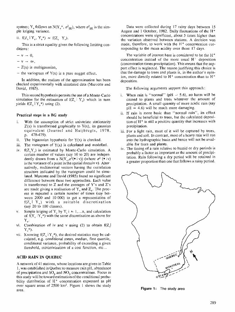
system; Y, follows an N(Y,*, a2,,), where a2sK is the simple kriging variance.

ii, f(Z, I Y,, Y,*) 5: f(ZV I YV).

This is a strict equality given the following limiting conditions :

- Z(x) is multigaussian,

- the variogram of Y(x) is a pure nugget effect.

In addition, the realism of the approximation has been checked experimentally with simulated data (Marcotte and David, 1985).

This second hypothesis permits the use of a Monte-Carlo simulation for the estimation of f(Z, I Y,) which in turn yields f(Z, I Y,*) using (2).

Practical steps in a BG study

i. With the assumption of strict univariate stationarity Z(x) is transformed graphically to Y(x), its gaussian e q u i v a l e n t ( Journe l and H u i j b r e g t s , 1 9 7 8 , p. 478-479).

ii. The bigaussian hypothesis for Y(x) is checked. iii. The variogram of Y(x) is calculated and modelled. iv. f(ZvYv) is estimated by Monte-Carlo simulation. A

certain number of values (say 10 to 20) are independently drawn from a N(Yv,a2(* I v)) (where a2 (0 Iv) is the variance of a point in the spatial domain v). Alter- natively, multinormal vectors having the correlation structure indicated by the variogram could be simulated. Marcotte and David (1985) found no significant difference between these two approaches. Each value is transformed to Z and the averages of Y's and Z's are made giving a realisation of Yv and 2,. The process is repeated a certain number of times (say between 2000 and 10 000) to get a representation of f(Z,I Y,) w i t h a s u i t a b l e d i s c r e t i s a t i o n (say 20 to 100 classes).

v. Simple kriging of Y, by Yi i = 1 ,... n, and calculation of f(Y, I Yv*) with the same discretisation as above for Yv.

vi. Combination of iv and v using (2) to obtain f(Zd YV*).

vii. Knowing f(Z, 1 Y,*), the desired statistics may be calcu~a ted , -e .~ . conditional mean, median, first quartile, conditional variance, probability of exceeding a given threshold, miniminisation of a cost function, etc.. .

ACID RAIN IN QUEBEC

A network of 41 stations, whose locations are given in Table 1, was established in Quebec to measure rain pH, abundance of precipitation and SO, and NO, concentrations. Focus in this study will be toward estimation ofthe conditional probability distribution of H + concentration expressed as pH over square areas of 2500 km2. Figure 1 shows the study area.

Data were collected during 17 rainy days between 15 August and 1 October, 1982. Daily fluctuations of the H+ concentrations were significant, about 5 times higher than the variation observed between stations. A decision was made, therefore, to work with the H+ concentration corresponding to the mean acidity over those 17 days.

The variable of interest here is considered to be the H + concentration instead of the more usual H+ deposition (concentration times precipitation). This means that the support effect is neglected. The reason justifying this choice is that the damage to trees and plants is, in the author's opinion, more directly related to H+ concentration than to H + deposition.

The following arguments support this approach:

i. When rain is "normal" (pH = 5.6), no harm will be caused to plants and trees whatever the amount of precipitation. A small quantity of more acidic rain (say pH = 4.6) will be much more damaging.

ii. If rain is more basic than "normal rain", its effect should be beneficial to trees, but the calculated deposition of H+ is still a positive quantity that increases with precipitation.

iii. For a light rain, most of it will be captured by trees, plants and soil. In contrast, most of a heavy rain will run into the hydrographic basin and hence will not be available for trees and plants.

iv. The timing of a rain relative to humid or dry periods is probably a factor as important as the amount of precipitation. Rain following a dry period will be retained in a greater proportion than one that follows a rainy period.

Figure 1 : The study area

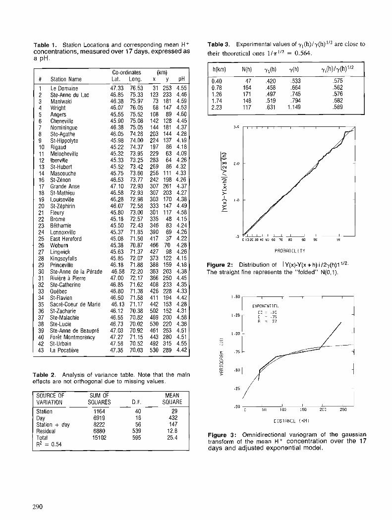
Table 1. Station Locations and corresponding mean H+ Table 3. Experimental values of r,(h)ly(h)"2 are close to concentrations, measured over 17 days, expressed as their ones ln 112 = 0.564. a pH.

Co-ordinates (km) # Station Name Lat. Long. x y pH

1 Le Domaine 47.33 76.53 31 253 4.55 2 Ste-Anne du Lac 46.85 75.33 123 233 4.46 3 Maniwaki 46.38 75.97 73 181 4.59 4 Wright 46.07 76.05 68 147 4.53 5 Angers 45.55 75.52 108 89 4.60 6 Cheneville 45.90 75.08 142 128 4.45 7 Nominingue 46.38 75.05 144 181 4.37 8 Ste-Agathe 46.05 74.28 203 144 4.28 9 St-Hippolyte 45.98 74.00 224 137 4.19 10 Rigaud 45.22 74.37 197 86 4.18 11 Melocheville 45.32 73.95 229 63 4.09 12 lberville 45.33 73.25 283 64 4.26 13 St-Hubert 45.52 73.42 269 86 4.32 14 Mascouche 45.75 73.60 256 111 4.33 16 St-Zenon 46.53 73.77 242 198 4.26 17 Grande Anse 47.10 72.93 307 261 4.37 18 St-Mathieu 46.58 72.93 307 203 4.27 19 Louiseville 46.28 72.98 303 170 4.38 20 St-Zephirin 46.07 72.58 333 147 4.49 21 Fleury 45.80 73.00 301 117 4.58 22 Brome 45.18 72.57 335 48 4.15 23 Bdthamie 45.50 72.43 346 83 4.24 24 Lennoxville 45.37 71.85 390 69 4.26 25 East Hereford 45.08 71.50 417 37 4.22 26 Woburn 45.38 70.87 466 70 4.28 27 Lingwick 45.63 71.37 427 98 4.26 28 Kingseyfalls 45.85 72.07 373 122 4.15 29 Princeville 46.18 71.88 388 159 4.18 30 Ste-Anne de la Perade 46.58 72.20 363 203 4.38 31 Riviere a Pierre 47.00 72.17 366 250 4.45 32 Ste-Catherine 46.85 71.62 408 233 4.35 33 Quebec 46.80 71.38 426 228 4.33 34 St-Flavien 46.50 71.58 411 194 4.42 35 Sacre-Coeur de Marie 46.13 71.17 442 153 4.28 36 St-Zacharie 46.12 70.38 502 152 4.31 37 Ste-Malachie 46.55 70.82 469 200 4.58 38 Ste-Lucie 46.73 70.02 530 220 4.36 39 Ste-Anne de Beaupre 47.03 70.92 461 253 4.51 40 Forit Montmorency 47.27 71.15 443 280 4.51 42 St-Urbain 47.58 70.52 492 315 4.55 43 La Pocatiere 47.35 70.03 530 289 4.42

PROBRBILITY

Figure 2: Distribution of I Y(x)-Y(x + h) 112y(h)l ' I 2 ,

The straight line represents the "folded" N(0,l).

SOURCE OF SUM OF MEAN VARIATION SQUARES D.F. SQUARE

Station 1164 40 29 Day 6919 16 432 Station + day 8222 56 147 Residual 6880 539 12.8 Total 15102 595 25.4 R2 = 0.54

L .25

OISTRNCE IKMI

EXPONENTIEL

- co = . I 0 C = .75

- R : 67

Figure 3: Omnidirectional variogram of the gaussian transform of the mean H+ concentration over the 17 days and adjusted exponential model.

1 .DO - - - r - = .75- - u

- g .so- -

Table 2. Analysis of variance table. Note that the main >

effects are not orthogonal due to missing values.

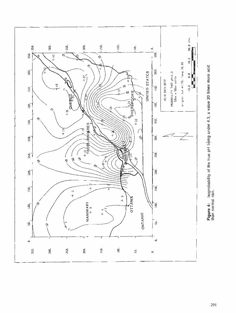
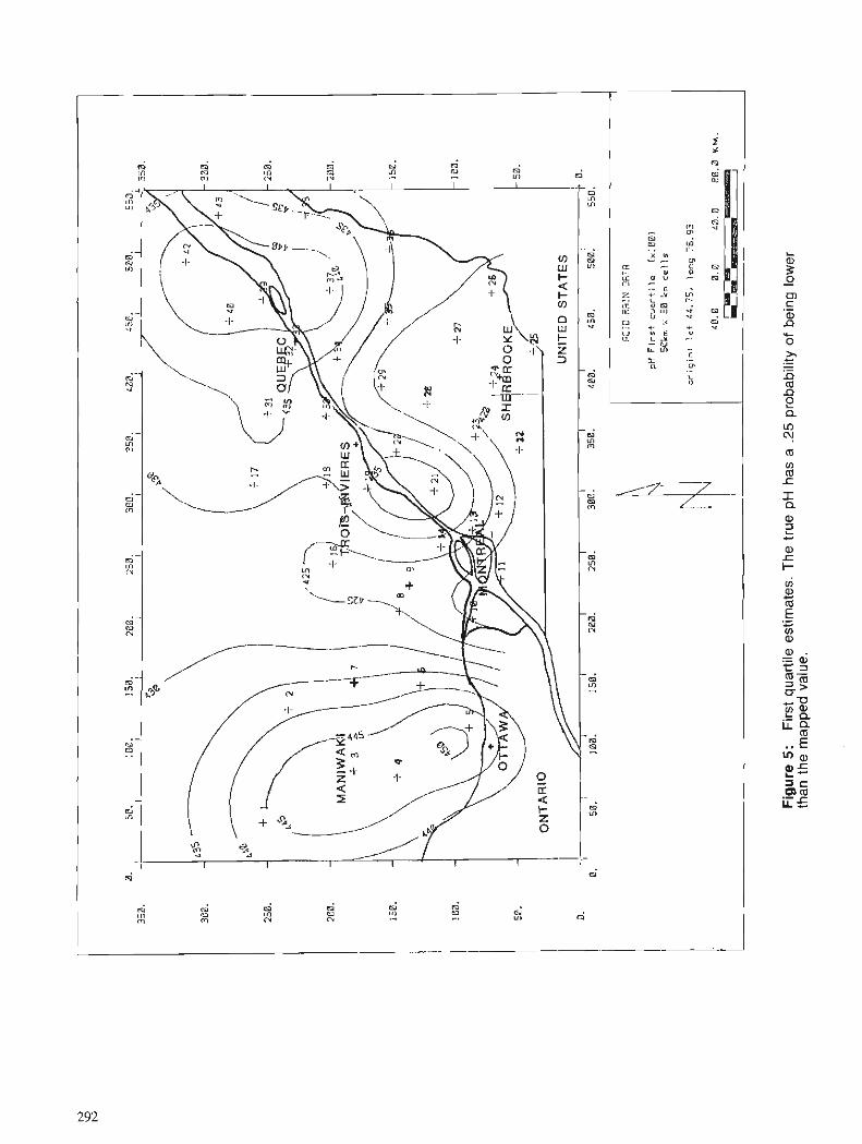
"'a, g 5 3 c m a ii5

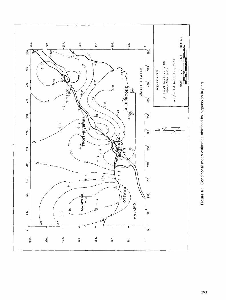
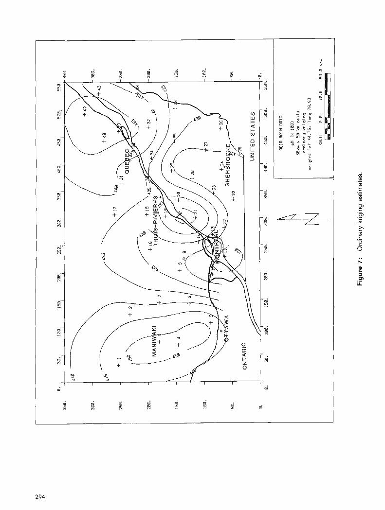
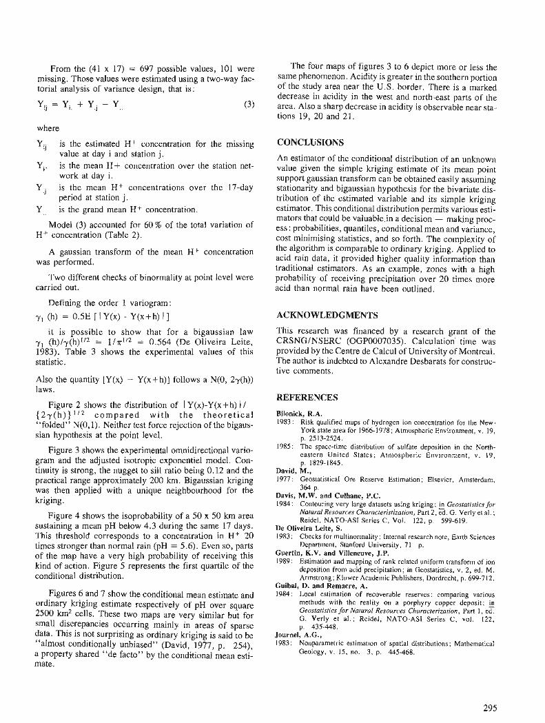
From the (41 x 17) = 697 possible values, 101 were missing. Those values were estimated using a two-way factorial analysis of variance design, that is :

where

Yij is the estimated H + concentration for the missing value at day i and station j.

Y,. is the mean H + concentration over the station network at day i.

Y j is the mean H + concentrations over the 17-day period at station j.

Y is the grand mean H+ concentration.

Model (3) accounted for 60 % of the total variation of H + concentration (Table 2).

A gaussian transform of the mean H+ concentration was performed.

Two different checks of binormality at point level were carried out.

Defining the order 1 variogram:

y , (h) = 0.5E [ 1 Y(x) - Y(x+h) I ]

it is possible to show that for a bigaussian law y1 (h)ly(h)1'2 = 1/7r'I2 = 0.564 (De Oliveira Leite, 1983). Table 3 shows the experimental values of this statistic.

Also the quantity [Y(x) - Y(x+h)] follows a N(0, 2y(h)) laws.

Figure 2 shows the distribution of I Y (x)-Y(x + h) I / { 2 y ( h ) } 1 1 2 c o m p a r e d w i t h t h e t h e o r e t i c a l "folded" N(O, 1). Neither test force rejection of the bigaussian hypothesis at the point level.

Figure 3 shows the experimental omnidirectional variogram and the adjusted isotropic exponentiel model. Con- tinuity is strong, the nugget to sill ratio being 0.12 and the practical range approximately 200 krn. Bigaussian kriging was then applied with a unique neighbourhood for the kriging .

Figure 4 shows the isoprobability of a 50 x 50 km area sustaining a mean pH below 4.3 during the same 17 days. This threshold corresponds to a concentration in H+ 20 times stronger than normal rain (pH = 5.6). Even so, parts of the map have a very high probability of receiving this kind of action. Figure 5 represents the first quartile of the conditional distribution.

Figures 6 and 7 show the conditional mean estimate and ordinary kriging estimate respectively of pH over square 2500 km2 cells. These two maps are very similar but for small discrepancies occurring mainly in areas of sparse data. This is not surprising as ordinary kriging is said to be "almost conditionally unbiased" (David, 1977, p. 254), a property shared "de facto" by the conditional mean estimate.

The four maps of figures 3 to 6 depict more or less the same phenomenon. Acidity is greater in the southern portion of the study area near the U.S. border. There is a marked decrease in acidity in the west and north-east parts of the area. Also a sharp decrease in acidity is observable near stations 19, 20 and 21.

CONCLUSIONS

An estimator of the conditional distribution of an unknown value given the simple kriging estimate of its mean point support gaussian transform can be obtained easily assuming stationarity and bigaussian hypothesis for the bivariate distribution of the estimated variable and its simple kriging estimator. This conditional distribution permits various estimators that could be valuablejn a decision - malung process : probabilities, quantiles, conditional mean and variance, cost minimising statistics, and so forth. The complexity of the algorithm is comparable to ordinary kriging. Applied to acid rain data, it provided higher quality information than traditional estimators. As an example, zones with a high probability of receiving precipitation over 20 times more acid than normal rain have been outlined.

ACKNOWLEDGMENTS

This research was financed by a research grant of the CRSNGINSERC (OGP0007035). Calculation' time was provided by the Centre de Calcul of University of Montreal. The author is indebted to Alexandre Desbarats for constructive comments.

REFERENCES

Bilonick, R.A. 1983: Risk qualified maps of hydrogen ion concentration for the New-

York state area for 1966-1978; Atmospheric Environment, v. 19, p. 2513-2524.

1985: The space-time distribution of sulfate deposition in the North- eastern Unitcd States; Atmospheric Environment, v. 19, p. 1 829- 1845.

David, M., 1977: Geostatistical Ore Reserve Estimation; Elsevier, Amsterdam,

364 p. Davis, M.W. and Culhane, P.C. 1984: Contouring very large datasets using kriging; Geostarisrics for

Natural Resources Characrerisrizarion, Part 2, ed. G. Verly et al. ; Reidel, NATO-AS1 Series C, Vol. 122, p. 599-619.

De Oliveira Leite, S. 1983: Checks for multinormality ; Internal research note, Earth Sciences

Department, Stanford University, 71 p. Guertin, K.V. and Villeneuve, J.P. 1989: Estimation and mapping of rank related uniform transform of ion

deposition from acid precipitation; in Geostatistics, v. 2, ed. M. Armstrong; Kluwer Academic Publishers, Dordrecht, p. 699-712.

Guibal, D. and Remacre, A. 1984: Local estimation of recoverable reserves: comparing various

methods with the reality on a porphyry copper deposit; Geostarisrics for Natural Resources Characreriulrion, Part 1, ed. G. Verly et a l . ; Reidel, NATO-AS1 Series C, vol. 122, p. 435-448.

Journel, A.C., 1983: Nonparametric estimation of spatial distributions; Mathematical

Geology, v. IS, no. 3, p. 445-468.

Journel, A.G., and Huijbregts, Ch.J. 1978: Mining Geostatistics; Academic Press, London, 600 p. Marcotte, D., 1989: Le krigeage bigaussien, une alternative au krigeage multigaussien

pour I'estimation des rkserves rkcu@rables'. in Geostatistics, v. 2, ed. M. Armstrong; Kluwer Academic Publishers, Dordrecht, p. 985-994.

Marcotte, D. and David, M., 1985: The bigaussian approach: a simple method for recovery estima-

tion; Mathematical Geology. v. 17, no 6, p. 625-644. Matheron, G., 1974: Les fonctions de transfert des petits panneaux; Internal research

note, CGMM N-395. 1976: Forecasting block grade distribution: the transfer functions;

Advanced Geostatistics in the Mining Industry, ed. Guarascio et al. ; Reidel, Dordrecht (Holland), p. 237-25 1.

Seilkop, S.P. and Finkelstein, P.L., 1987: Acid precipitation patterns and trends in Eastern North America,

1980-84; Journal of Climate and Applied Meteorology, v . 26, p. 980-994.

Sullivan, J., 1984: Conditional recovery estimation through probability kriging; the-

ory and practice; Geostatistics for Natural Resources Charac- terization, Part 1 , ed. G. Verly el al.; Reidel, NATO-AS1 Series C, V. 122, p. 365-384.

Verly, G., 1984: The block distribution given a point multivariate normal distribu-

tion; @ Geostatistics /or Natural Resources Characterization, Part 1, ed. G. Verly et al.; Reidel, NATO-AS1 Series C, vol. 122, p. 495-515.

Averaging of Anisotropy of Magnetic Susceptibility Data

R.E. Ernstl and G.W. Pearce2

Ernst, R. E. and Pearce, G. W., Aver-aging of anisotropy of magnetic susceptibility data; & Statistical Applications in the Earth Sciences, ed. F. P. Agterberg and G. F. Bonham-Carter; Geological Survey of Canada, Paper 89-9, p. 297-305, 1989.

Abstract

The 'average' orientation ofprincipal axes of magnetic susceptibility from N samples (n = 1, 2,. . . ,N) can be computed in two ways: (1) as an 'average' ofprincipal directions or (2) as the principal directions of the average magnetic susceptibility ellipsoid, x. The 'average' orientations computed using both approaches are similar but the second approach (K-averaging) has the advantage of ensuring that the 'average' axes are mutually perpendicular and of allowing automatic weighting by the degree of anisotropy of each sample. These two averaging techniques are compared using AMS data fiom a majic dyke.

L'orientation e moyenne ,, des principaux axes de susceptibilite' magne'tique de N 6chantiZlons (n = 1 , 2 , . . . , N) peut Ltre calculie de deux manikres: I ) sous forme d'une moyenne des directions principales ou 2) sous forme des directions principale de 1 'ellipsoide moyen de susceptibilitimagnitique K. Les orientations (cmoyennes, calculies par les deux mithodes sont analogues, rnais la deuxitme mithode (moyenne des K) prisente les avantages d'assurer que les axes a moyens ,, sont mutuellement perpen- diculaires et de permettre une pondiration automatique d 'aprks le degri d'anisotropie de chaque ichan- tillon. Les deux mithodes sont comparLes au moyen de donnies de AMS provenant d 'un dyke majique.

' Ottawa-Carleton Geoscience Centre and Department of Geology, University of Ottawa, Ontario KIN 6N5 152 Indian Road, Kingston, Ontario K7M IT4

INTRODUCTION

Consider a set of samples whose low-field anisotropy of magnetic susceptibility (AMS) has been determined (Ell- wood et al., 1988, Hrouda, 1982). The susceptibility information about the nth sample is fully expressed as a symmetrical second rank tensor K(i,j,,n (Nye, 1964) where i and j vary from 1 to 3.

The susceptibility ellipsoid, K,, can be geometrically represented as a triaxial ellipsoid having three mutually perpendicular principal axes with orientation and magnitude given by pa,, and k,,,, respectively (Nye, 1964) (notation slightly modified from Jelinek, 1978 and Ellwood et a]., 1988). Values of 1 , 2 and 3 for subscript, a, denote the maximum, intermediate and minimum principal axes, respectively.

The orientations of the principal axes can be represented by the vector variables, p(i,,a,n (for a = 1 , 2 and 3). These are computed as the eigenvectors of K, and are unit-length column vectors composed of direction cosines along the x (i= l) , y (i=2) and z (i=3) axes. Each vector, pa,, is typically reported (and plotted on stereonets) as a pair of angular values, declination and inclination, D,,, and I,,,,, although the designations trend and plunge would be more appropriate since axes rather than directed-lines are being represented. The scalar variables, k,,, for a = l , 2, and 3, are computed as the eigenvalues of K,. (Appendix 1 shows how to recompute K, from data presented in the form of Da.n: 1a.n and h,n).

Suppose that for each of N samples (where n = 1, 2, . . , N) of a rock unit, the magnetic susceptibility, K,, has been determined and the orientation and magnitudes of its principal axes, pa,, and k,,,, calculated. It is of interest to determine the 'average' orientations and magnitudes of the maximum, intermediate and minimum principal axes from the N samples. Two different methods of 'averaging' are currently in use, 'axis-averaging' and 'tensor-averaging'. In this paper, the two methods are compared and their relative merits assessed.

THE AXIS-AVERAGING METHOD

AMS directional data are frequently averaged by treating each principal axis as independent and applying the vector- averaging procedure of Fisher (1953), e.g. Knight and Walker (1988). Using this technique each axis is assumed to have unit length. However, vector-averaging of sets of principal axes is not strictly correct since it requires arbitrary choices of axis polarity (Mark, 1973).

A better approach is the axis-averaging technique of Scheidegger (1965) and Mark (1973) which is used, for example, by Ellwood and Whitney (1980) and Park et al. (1988). The mean orientation of each axis for a set of samples is obtained using a matrix technique in which each axis is assumed to have unit length and is considered to have an angular distribution about the true mean of the population (termed the expected value, Edwards, 1964) given by the Watson-Scheidegger probability distribution (Scheidegger, 1965 ; Mark, 1973 ; Fisher et a]. , 1987). For small angular

deviations, the Watson-Scheidegger probability distribution has an approximately normal distribution.

The averaging procedure is as follows:

Define A,,, for each axis:

and

fia = maximum eigenvector of Xa (3)

The vector pa is Scheidegger's estimate of the mean orientation of pa and is calculated from pa,, (n= 1, 2, ..., N).

The 'average' length of each principal axis (a = 1, 2, 3) can be calculated from:

N

ka = (1/N) C ka,n cos 0a.n n = l

(4)

where 0,,, is the angle between the 'average' axis and each individual direction. For tight distributions this becomes approximately :

N

Both the vector- and axis-averaging methods treat the principal axes as independent and hence the resultant average axes are not constrained to be orthogonal. For well-behaved and tightly clustered data, this should not present a problem, since the departure from orthogonality will be small (e.g. see Group A of Table 1 and Fig. 1A). However, for more scattered data the departure may be significant. Ellwood and Whitney (1980) contains examples in which average maximum and minimum axes depart up to 7" from being orthogonal. As an extreme case, the Group B in Table 1 and Figure 1B gives maximum and minimum axes departing 37" from orthogonality. Since orthogonality is a fundamental characteristic of the ellipsoidal representation of AMS, it would appear that the axis-averaging method may be inadequate for some data.

A second, but minor problem with this method is that a separate scalar averaging procedure (e.g. eqn. 4) must be employed to provide estimates of the relative lengths of the three 'average' principal axes.

The tensor-averaging method addresses both of these concerns.

THE TENSOR-AVERAGING METHOD

Averaging Procedure

Average properties-for a set of samples can be calculated from the average, K, matrix where each component, K(i,j, has been averaged over all samples. The 'average' orientations and magnitudes of the three principal axes are calculated as the eigenvectors and the eigenvalues of this average tensor, K. This tensor-averaging procedure assumes an approximately normal distribution for each component of K, and was briefly addressed by Hext (1963) and was first

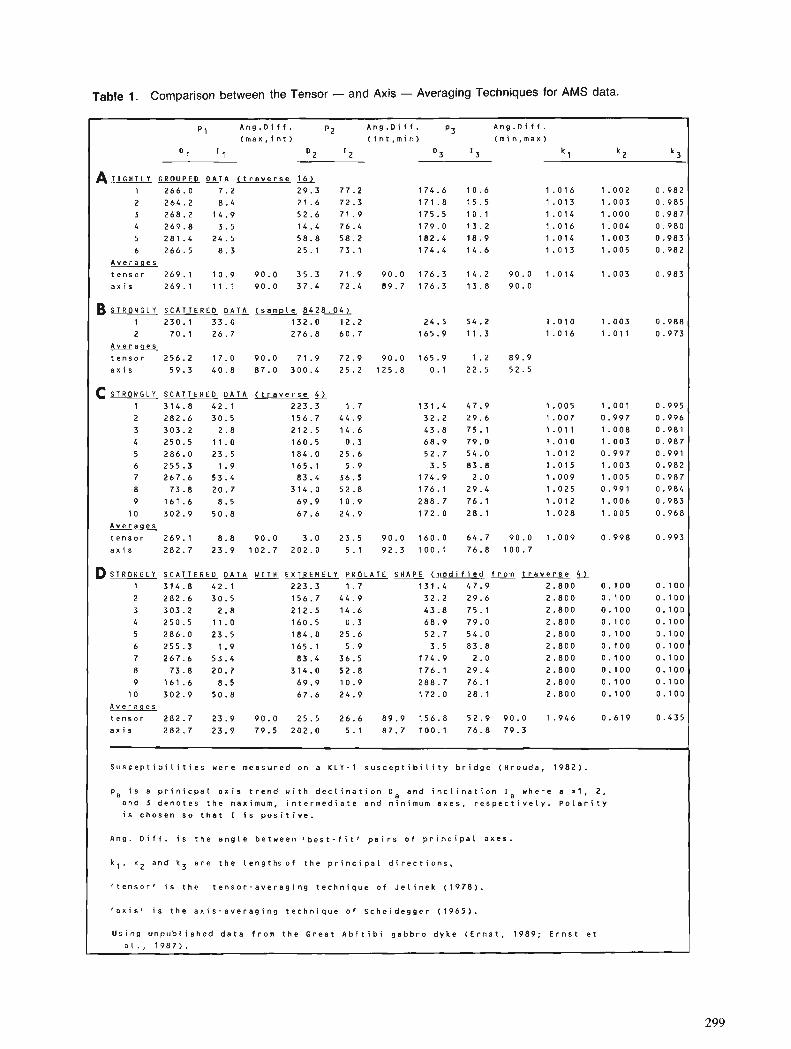
Table 1. Comparison between the Tensor - and Axis - Averaging Techniques for AMS data.

p l A n g . D i f f . p 2 A n g . D i f f . p 3 A n g . 0 i f f . ( m a x , i n t ) ( i n t , m i n ) ( m i n , m a x )

D l I 1 D2 I 2 D3 I 3 1 2 3

ATIGHTLY G R O U P E D D A T A f t r a v e r s e !6)

1 2 6 6 . 0 7 . 2 2 9 . 3 7 7 . 2 1 7 4 . 6 1 0 . 6 1 . 0 1 6 1 . 0 0 2 0 . 9 8 2

2 2 6 4 . 2 8 .4 2 1 . 6 72 .3 1 7 1 . 8 15 .5 1 . 0 1 3 1 . 0 0 3 0 . 9 8 5

3 2 6 8 . 2 1 4 . 9 5 2 . 6 7 1 . 9 1 7 5 . 5 1 0 . 1 1 . 0 1 4 1 . 0 0 0 0 . 9 8 7

4 2 6 9 . 8 3 . 5 1 4 . 4 7 6 . 4 1 7 9 . 0 1 3 . 2 1 . 0 1 6 1 . 0 0 4 0 . 9 8 0

5 2 8 1 . 4 24 .5 5 8 . 8 5 8 . 2 1 8 2 . 4 1 8 . 9 1 . 0 1 4 1 . 0 0 3 0 . 9 8 3

6 2 6 6 . 5 8 . 3 2 5 . 1 7 3 . 1 1 7 4 . 4 1 4 . 6 1 . 0 1 3 1 . 0 0 5 0 . 9 8 2

A v e r a g e s t e n s o r 2 6 9 . 1 1 0 . 9 9 0 . 0 3 5 . 3 7 1 . 9 9 0 . 0 1 7 6 . 3 1 4 . 2 9 0 . 0 1 . 0 1 4 1 . 0 0 3 0 . 9 8 3 a x i s 2 6 9 . 1 1 1 . 1 9 0 . 0 37 .4 72 .4 8 9 . 7 176.3 1 3 . 8 9 0 . 0

Ej STRONGLY SCATTEREO DATA ( s a m p l e 8 4 2 8 . 0 4 ) 1 2 3 0 . 1 3 3 . 0 1 3 2 . 0 1 2 . 2 24 .5 5 4 . 2 1 . 0 1 0 1 . 0 0 3 0 . 9 8 8

2 7 0 . 1 2 6 . 7 2 7 6 . 8 6 0 . 7 1 6 5 . 9 1 1 . 3 1 . 0 1 6 1 . 0 1 1 0 . 9 7 3

A v e r a s e s t e n s o r 2 5 6 . 2 1 7 . 0 9 0 . 0 7 1 . 9 7 2 . 9 9 0 . 0 1 6 5 . 9 1 . 2 8 9 . 9 a x i s 5 9 . 3 4 0 . 8 8 7 . 0 3 0 0 . 4 2 5 . 2 1 2 5 . 8 0 . 1 2 2 . 5 5 2 . 5

c STRONGLY SCATTEREO DATA I t r a v e r s e Q

1 3 1 4 . 8 4 2 . 1 2 2 3 . 3 1 . 7 1 3 1 . 4 4 7 . 9 1 . 0 0 5 1 . 0 0 1 0 .995 2 2 8 2 . 6 3 0 . 5 1 5 6 . 7 4 4 . 9 3 2 . 2 2 9 . 6 1 . 0 0 7 0 . 9 9 7 0 . 9 9 6 3 3 0 3 . 2 2.8 212.5 1 4 . 6 43 .8 7 5 . 1 1 . 0 1 1 1 . 0 0 8 0 . 9 8 1 4 2 5 0 . 5 1 1 . 0 1 6 0 . 5 0 .3 6 8 . 9 7 9 . 0 1 . 0 1 0 1 . 0 0 3 0 . 9 8 7 5 2 8 6 . 0 23 .5 1 8 4 . 0 2 5 . 6 5 2 . 7 5 4 . 0 1 . 0 1 2 0 . 9 9 7 0 . 9 9 1 6 2 5 5 . 3 1 . 9 1 6 5 . 1 5 . 9 3.5 8 3 . 8 1 . 0 1 5 1 . 0 0 3 0 . 9 8 2 7 2 6 7 . 6 5 3 . 4 8 3 . 4 3 6 . 5 1 7 4 . 9 2 . 0 1 . 0 0 9 1 . 0 0 5 0 . 9 8 7 8 73 .8 2 0 . 7 3 1 4 . 0 5 2 . 8 1 7 6 . 1 2 9 . 4 1 . 0 2 5 0 . 9 9 1 0 . 9 8 4

9 1 6 1 . 6 8 .5 6 9 . 9 1 0 . 9 2 8 8 . 7 7 6 . 1 1 . 0 1 2 1 . 0 0 6 0 .983

10 3 0 2 . 9 5 0 . 8 6 7 . 6 2 4 . 9 1 7 2 . 0 2 8 . 1 1 . 0 2 8 1 . 0 0 5 0 . 9 6 8 A v e r a g e s t e n s o r 2 6 9 . 1 8 . 8 9 0 . 0 3 . 0 2 3 . 5 9 0 . 0 1 6 0 . 0 6 4 . 7 9 0 . 0 1 . 0 0 9 0 . 9 9 8 0 . 9 9 3 a x i s 2 8 2 . 7 2 3 . 9 1 0 2 . 7 2 0 2 . 0 5 . 1 9 2 . 3 1 0 0 . 1 76 .8 1 0 0 . 7

D S T R O N C L Y SCATTERED DATA W I T H EXTREMELY PROLATE SHAPE ( m o d i f i e d from t r a v e r s e 1 3 1 4 . 8 4 2 . 1 2 2 3 . 3 1 . 7 1 3 1 . 4 4 7 . 9 2 . 8 0 0 0 . 1 0 0 0 . 1 0 0 2 2 8 2 . 6 3 0 . 5 1 5 6 . 7 4 4 . 9 3 2 . 2 2 9 . 6 2 . 8 0 0 0 . 1 0 0 0 . 1 0 0 3 303.2 2 . 8 2 1 2 . 5 1 4 . 6 4 3 . 8 7 5 . 1 2 . 8 0 0 0 . 1 0 0 0 . 1 0 0 4 2 5 0 . 5 1 1 . 0 1 6 0 . 5 0 . 3 6 8 . 9 7 9 . 0 2 . 8 0 0 0 . 1 0 0 0 . 1 0 0 5 2 8 6 . 0 23 .5 1 8 4 . 0 2 5 . 6 5 2 . 7 5 4 . 0 2 . 8 0 0 0 . 1 0 0 0 . 1 0 0 6 2 5 5 . 3 1 . 9 1 6 5 . 1 5 . 9 3.5 8 3 . 8 2 . 8 0 0 0 . 1 0 0 0 . 1 0 0 7 2 6 7 . 6 5 3 . 4 8 3 . 4 3 6 . 5 1 7 4 . 9 2 . 0 2 . 8 0 0 0 . 1 0 0 0 . 1 0 0 8 7 3 . 8 2 0 . 7 3 1 4 . 0 5 2 . 8 1 7 6 . 1 29 .4 2 . 8 0 0 0 . 1 0 0 0 . 1 0 0

9 1 6 1 . 6 8 . 5 6 9 . 9 1 0 . 9 2 8 8 . 7 7 6 . 1 2 . 8 0 0 0 , 1 0 0 0 . 1 0 0

1 0 3 0 2 . 9 5 0 . 8 6 7 . 6 2 4 . 9 1 7 2 . 0 2 8 . 1 2 . 8 0 0 0 . 1 0 0 0 .100 A v e r a s e s t e n s o r 2 8 2 . 7 23 .9 9 0 . 0 2 5 . 5 2 6 . 6 8 9 . 9 1 5 6 . 8 5 2 . 9 9 0 . 0 1 . 9 4 6 0 . 6 1 9 0 . 4 3 5 a x i s 2 8 2 . 7 2 3 . 9 79 .5 2 0 2 . 0 5 . 1 8 7 . 7 1 0 0 . 1 7 6 . 8 7 9 . 3

S u s c e p t i b i l i t i e s u e r e m e a s u r e d o n a K L Y - 1 s u s c e p t i b i l i t y b r i d g e ( H r o u d a , 1 9 8 2 ) .

p a i s a p r i n i c p a l a x i s t r e n d w i t h d e c l i n a t i o n Da a n d i n c l i n a t i o n la w h e r e a 3 1 , 2 , a n d 3 d e n o t e s t h e maximum, i n t e r m e d i a t e a n d m i n i m u m a x e s , r e s p e c t i v e l y . P o l a r i t y i s c h o s e n s o t h a t I i s p o s i t i v e .

Ang. O i f f . i s t h e a n g l e b e t w e e n ' b e s t - f i t 1 p a i r s o f p r i n c i p a l a x e s .

k l , k 2 a n d k 3 a r e t h e l e n g t h s o f t h e p r i n c i p a l d i r e c t i o n s .

' t e n s o r ' i s t h e t e n s o r - a v e r a g i n g t e c h n i q u e o f J e l i n e k ( 1 9 7 8 ) .

' a x i s ' i s t h e a x i s - a v e r a g i n g t e c h n i q u e o f S c h e i d e g g e r ( 1 9 6 5 ) .

U s i n g u n p u b l i s h e d d a t a f r o m t h e G r e a t A b i t i b i g a b b r o d y k e ( E r n s t , 1 9 8 9 ; E r n s t e t a l . , 1 9 8 7 ) .

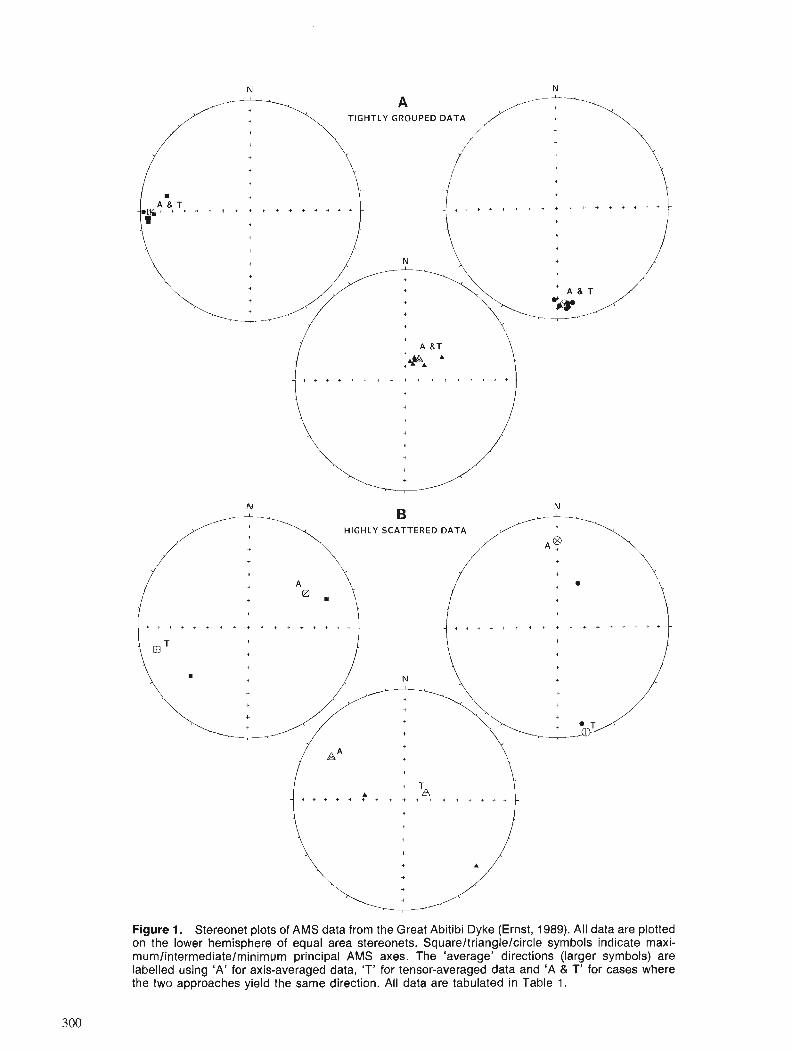
Figure 1. Stereonet plots of AMS data from the Great Abitibi Dyke (Ernst, 1989). All data are plotted on the lower hemisphere of equal area stereonets. Squareltriangle/circle symbols indicate maximum/intermediate/minimum principal AMS axes. The 'average' directions (larger symbols) are labelled using 'A' for axis-averaged data, 'T' for tensor-averaged data and 'A & T' for cases where the two approaches yield the same direction. All data are tabulated in Table 1.

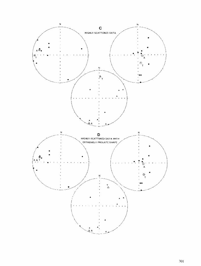
C HIGHLY SCATTERED DATA

+

- m * + + * t + + + + * + * + + * * - , + + + + + r e . + + + * a + * +

i

- I + + * + + + + + + + + + + + + +

detailed by Jelinek (1978). This averaging technique has been used, for instance, by Hirt et al. (1988).

In this technique the susceptibility tensors of a set of N samples are averaged :

N

pa = the ath eigenvector of K (7)

and

I;, = the ath eigenvalue of K (8)

6, and I;, are Jelinek's estimators of the mean orientation, pa, and mean susceptibility, k,, of the ath axis.

Prior to averaging, each susceptibility tensor, K,, is typically normalized by the bulk susceptibility in order to remove the effect of varying abundance of magnetic mineralogy (Appendix 2).

Theory

This section builds on the work of Jelinek (1978). The meaning of K can be assessed geometrically. The six independent elements of K, for each sample can be represented as the coefficients of a centred general ellipsoid (the representation quadric of Nye, 1964) given by the following equation :

This equation can be summed over N samples. N N N N

Equation 10 represents the shape of the summation of all individual ellipsoids and is itself an ellipsoid. Dividing this equation by N, the number of samples, provides an average shape for the set of sample ellipsoids. As the behaviour of the AMS of a single sample is characterized by an ellipsoid, then the behaviour of a set of samples should b e well- represented by the average AMS ellipsoid. Hence K should be a good measure of E(K), the expectation of the tensor, K

A physical meaning for K can also be developed. Con- sider a rock sample of any size. Subdivide it into N pieces (n= 1,2,3,. . . ,N) and measure the susceptibility tensor (per volume), K,, for each piece. Application of the mth applied field vector H,,, to the nth piece during data measurement causes an induced magnetism in the piece which is described by the vector M,,,. The relation between H,,, and M,,, is given by the low-field susceptibility tensor K, as follows (Nye, 1964; Payne, 1981):

The rocks being considered are very dilute mixtures of magnetic particles in an approximately non-magnetic medium. Hence, the different magnetic particles (or closely-packed groups of particles) can be considered non-interacting and the magnetic field 'experienced' by each particle (or particle-group) is the same as the external applied field (cf. Nye, 1964, p. 56-57). Therefore, for measurement of each of the n pieces of a rock sample:

From substitution of eqn (12) into (1 l), and recollection that K, and M,,, are measured per volume, it follows that:

N

where V, is the volume of the nth piece of the rock sample. VT and MT are the volume and induced magnetization of the rock sample measured as a whole. For the case in which each piece has the same size:

(This analysis can also be done when K, and MnVm are measured per mass). - K can be considered an appropriate estimate of E(K) because the induced magnetization of the rock sample as a whole, MT, given by KT H, can also be computed from - K H,. In other words, KT = K. K "is the tensor which we would obtain, if we were able to measure the geological object as a whole" (Jelinek, 1978).

In practice, however, it is unlikely that the whole rock unit is analyzed in pieces. More usually a subset of pieces is analyzed whose aggregate size is less than that of the rock unit. In this case, the average susceptibility of a randomly chosen subset of pieces can be considered an unbiased estimator of E(K) (see discussion of the properties of the arithmetic average in Edwards, 1964).

To the extent that % is representative of the population from which Kn (n=J,N) was sampled then any characteristics derived from K should be representative of the data population. In this-sense, the orientation and magnitude of principal axes of K should be considered representative of the population of principal AMS axes sampled by pa,, and k,,, (calculated from K,).

COMPARISON BETWEEN AXIS-AND TENSOR-AVERAGING

The axis- and tensor-averaging approaches can be compared using measured data from a mafic dyke given in Table 1 and Figure 1. For tightly clustered data (Fig. 1A; Group A in Table 1) both axis- and tensor-averaging approaches yield identical orientations of the average principal axes. How- ever, for more dispersed data, differences become apparent. Axis-averaging better defines the average directions of each axis considered separately, but for dispersed data the orientations of the three average principal axes do not remain mutually perpendicular. In contrast, tensor-averaging yields orthogonal average principal axes under all circumstances.

The tensor-averaging approach automatically weights data by the shape of the susceptibility ellipsoid. In contrast, the axis-averaging approach weights each axis equally. Weighting by ellipsoid shape (for tensor-averaging) essentially involves weighting the direction and magnitude of each principal AMS axis of a sample by its distinctness from the other two principal AMS axes of that sample. The distinctness of a principal axis is a measure of the statistical uncertainty in the orientation of that axis. The more distinct a principal axis the more precisely its orientation can be defined. For instance, the maximum axis of a highly prolate AMS ellipsoid is much more precisely determined than the maximum axis of a nearly spherical AMS ellipsoid. There- fore, the tensor-averaging approach automatically weights each axis of a sample by an estimate of its reliability. In most cases this weighting would be desirable and the tensor- averaging approach would be preferred.

However, the axis-averaging approach may be preferred when the samples to be averaged include some whose AMS ellipsoids are much more anisotropic than the AMS ellipsoids of the remaining samples. Such outliers will strongly constrain the mean directions determined by the tensor- averaging technique, while axis-averaging (because of its equal-weighting characterist ic) will prevent such anisotropic outlier samples from dominating the data.

The tensor-averaging approach can be modified when such outliers are present. In such cases the shape of the AMS ellipsoid of outlier samples can be arbitrarily made more 'spherical' to reduce the influence of these samples. This can be done by decreasing the spread in k,,,, k2,, and k3,n for these samples.

The effect of weighting is illustrated in Figure 1C and ID and Table 1 (Groups C and D) where the orientations of principal axes are identical but the magnitudes differ : low degree of anisotropy in Group C and extreme anisotropy in Group D. Axis-averaging gives the same 'average' orientations ;n both cases, G ~ o u p s C and D (Fig. 1C and ID), but tensor-averaging gives different results in the two cases.

Tensor averaging of the extremely prolate-shaped AMS data (Group D) results in an orientation for 'average' maximum, intermediate and minimum axes which depends solely on the distribution of the maximum axes and is independent of the orientation of intermediate and minimum axes. The average maximum axis of Group D, determined from the tensor-averaging technique, f i I is identical to that given by the axis-averaging technique, p, for the same data. The reason for this can be seen in the mathematical relationship between the two averaging techniques. From equations (1) and (A2) it can be shown that:

MEASURES OF VARIATION

Univariate statistical measures can be used to describe the dispersion of the orientation and magnitude of each principal axes about their mean values (e.g. Mardia, 1972, p. 22). For axis-averaged data, dispersion of the principal axes about mean values can also be obtained from the ratios of the eigenvalues of A, (e.g. Schmidt et al., 1988; and Ell- wood and Whitney, 1980). For tensor-averaged data the variance and confidence intervals of both the magnitude and orientation of the mean principal axes can be computed from the variance-covariance matrix of K, (Jelinek, 1978 ; based on Hext, 1963).

CONCLUSIONS

Two techniques for averaging AMS data are the tensor- averaging technique (Jelinek, 1978) and the axis-averaging approach of Scheidegger (1965). Key differences between the two approaches are as follows:

1) Tensor-averaging ensures that the resulting mean principal AMS axes will be mutually perpendicular, a result not guaranteed by axis-averaging.

2) In the tensor-averaging technique, all components of the susceptibility tensor are used in calculating the average orientation and magnitude of each of the three principal axes. In essence, each principal axis of a sample is weighted by its distinctness from the other principal axes of that sample. By contrast, in the axis averaging technique, the maximum, intermediate and minimum principal axes are averaged independantly and all axes are weighted equally.

There may be situations in which equal weighting is desired and the axis-averaging approach would be better, but in general the tensor-averaging approach provides a better estimate of the average properties of low-field magnetic susceptibility data.

ACKNOWLEDGMENTS

J. Bondar, B. Ellwood, and P.-Y Robin are all thanked for constructive criticism on the ideas in this paper. Reviewer, A. Desbarats, is thanked for valuable suggestions which greatly improved the paper. This paper was prepared during the senior author's doctoral program at Carleton University, Ottawa.

REFERENCES

Edwards, A.L. 1964: Expected Values of Discrete Random Variables and Elementary

Statistics; J. Wiley and Sons, Inc. New York, 146 p. Ellwood, B.B., Hrouda, F., and Wagner, J-J. 1988 : Symposia on magnetic fabrics: introductory comments; Physics of

the Earth and Planetary Interiors, v. 51, p. 249-252. Ellwood, B.B. and Whitney, J.A. 1980: Magnetic fabric of the Elberton Granite, Northeast Georgia; Jour-

nal of Geophysical Research, v. 85, p. 1481-1486. Ernst, R.E.

When goes k2vn and k33n go O, ' 1989: The Great Abitibi Dyke, Superior Province, Canada; unpublished approaches Al and therefore ill approaches b l . Ph.D. Thesis, Carleton University, Ottawa, Ontario, Canada.

303

Ernst, R.E., Bell, K., Ranalli, G., and Halls, H.C. 1987 : The Great Abitibi Dyke, southeastern Superior Province, Canada;

in Mafic Dyke Swarms, ed. H.C. Halls and W.F. Fahrig; Geolog- - ical Association of Canada Special Paper 34, p. 123.135.

Fisher, R.A. 1953 : Dispersion on a sphere; Proceedings of the Royal Society of Lon-

don, v. A217, p. 295-305. Fisher, N.I., Lewis, T., and Embleton, B.J.J. 1987: Statistical Analysis of Spherical Data; Cambridge University

Press, 329 p. Hext, G.R. 1963: The estimation of second-order tensors, with related tests and

designs; Biometrika, v. 50, p. 353-373. Hirt, A.M., Lowrie, W., Clendenen, W.S., and Kligfield, R. 1988: The correlation of magnetic anisotropy with strain in the Chelms-

ford Formation of the Sudbury basin, Ontario; Tectonophysics, v. 145, p. 177-189.

Hrouda, F. 1982: Magnetic anisotropy of rocks and its application in geology and

geophysics; Geophysical Surveys v. 5, p. 37-82 Jelinek, V. 1978: Statistical processing of anisotropy of magnetic susceptibility mea-

sured on groups of specimens; Studia geopliysica et geodaetika, V. 22, p. 50-62.

Knight, M.D. and Walker, G.P.L. 1988: Magma flow directions in dikes of the Koolau Complex, Oahu,

determined from magnetic fabric studies; Journal of Geophysical Research, v. 93, p. 4301-4319.

Mardia, K.V. 1972 : Statistics of Directional Data., Academic Press ; London, 357 p. Mark, D.M. 1973 : Analysis of axial orientation data, including till fabrics; Geological

Society of America, Bulletin, v. 84, p. 1369.1374. Nye, J.F. 1964: Physical Properties of Crystals; Oxford University Press, New

York, 322 p. Park, J.K., Tanczyk, E.I., and Desbarats, A. 1988: Magnetic fabric and its significance in the 1400 Ma Mealy diabase

dykes of Labrador, Canada; Journal of Geophysical Research, v. 93, p. 13689-13704.

Payne, M.A. 1981 : SI and Gaussian CGS units, conversions and equations for use in

geomagnetism; Physics of the Earth and Planetary Interiors, v. 26, p. PIO-P16.

Scheidegger, A.E. 1965: On the statistics of the orientation of bedding planes, grain axes

and similar sedimentological data; U.S. Geological Survey Profes- sional Paper 525-C, p. 164-167.

Schmidt, V.A., Nagata, T., Ellwood, B.B. and Noltimier, H.C. 1988: The measurement of anisotropy of magnetic susceptibility using a

cryogenic (SQUID) magnetometer and a comparison with results obtained from a torsion-fixer magnetometer; Physics of the Earth & Planetory Interiors, v. 51, p. 365-378.

APPENDIX 1

Calculation of K,

Frequently, AMS data are presented in the form of the orientation (D,,,, I,,,) and magnitudes (k,,,) of the principal axes. To average such data using the tensor-averaging approach requires recalculation of K,. Let P, be the 3 x 3 matrix whose column vectors are the direction cosines of the principal axis directions p,,,, p2,, and p,,,; themselves easily computed from values of D,,, and I,,,. Let L, be the 3 x 3 matrix whose diagonal elements are given by k,,,, k2,,, and k3,, and whose off diagonal elements are all zero.

P, is an orthogonal matrix and therefore,

K, = P, L, P,' (A2)

The directions of the principal axes are usually presented to no more than one decimal place (e.g. declination = 245.1 " , inclination = 34.4"). However, using principal axis directions of one-decimal accuracy to calculate K, will result in deviations from orthogonality of up to 10" between eigenvectors calculated from K. This occurs because, round-off to one decimal place means that the principal axes of each sample are not mutually perpendicular to sufficient precision. This problem can be avoided by first recomputing the eigenvectors of each sample:

P, = ( (Pn-1 + P,' ) / 2 1' (A3)

This empirically derived operation insures that eigenvectors are mutually perpendicular to sufficient precision.

APPENDIX 2

Normalization by bulk susceptibility

Prior to applying the tensor-averaging technique, it is useful to normalize each K, by its bulk susceptibility, given by one-third the trace of K,, i.e. (l/3)(trKn). This is equivalent to normalizing out the effect of differing amounts of magnetic mineralogy, so that only the shape and orientation of the susceptibility ellipsoid are being averaged and not ellipsoid-size. This can be demonstrated as follows: K, represents susceptibility per unit volume. (X, is susceptibility per unit mass and the following can also be derived for X,.) The volume being measured is the volume of the rock sample. However, the abundance of magnetic mineralogy within each sample may vary. How can K, (with units of susceptibility per unit sample volume) be normalized so as to obtain an expression for the susceptibility per unit volume of magnetic material? To do this, K, must be multiplied by a factor relating the ratio of the volume of each sample to the volume of magnetic mineral in that sample. The abundance of a magnetic mineral such as titanomagnetite in a sample is roughly proportional to the bulk susceptibility which is expressed as (1 /3)(trK,). Therefore, the susceptibility anisotropy per unit volume of titanomagnetite is approximated by [Kn/[(l /3)(trKn)].

A Robust Multivariate Allocation Procedure with Applications to Geochemical Data

Robert G. Garrett1

Garrett, R. G., A robust multivariate allocation procedure with applications to geochemical data; ~ Statistical Applications in the Earth Sciences, ed. F. P. Agterberg and G. F. Bonham-Carter; Geological Survey of Canada, Paper 89-9, p. 309-318, 1989.

Abstract

The concept of background populations of data related to lithological units and sur-cia1 enviroizmen- tal processes is well established in exploration geochemistry. Although these populations may be approximately multivariate normal it is much less likely that their covariance structures are similar, and homogeneity of covariance may be an unrealistic assumption. In exploration geochemistry one task is to identify those individuals in a survey data set that may have their geochemical variability explained by background populations and their mixtures, and those which do not 'Ifit" into the background scenario. It is these latter individuals that are most likely related to rare events such as minor, but important, lithologies, environmental factors, or, most interestingly, mineral occurrences. The procedure described contains an important interactive graphics component. Data for the selected background populations are displayed as chi-square plots, where if outlier free and multivariate normal, they plot as straight lines. Ifnecessary, outliers may be trimmed from the background data sets to yield representative approximately multivariate normal reference sets. These reference sets are used to establish a generalized rnaxi- mum likelihood discriminant. A multivariate analysis of variance is completed and tests for homogeneity of covariance are undertaken. Irrespective of homoscedasficity, as it is taken into account in the computation of the generalized maximum likelihood estimator, unknown individuals are allocated to the various background populations, accepted as possible mixtures, or classijed as probably being related to some other geochemical process, e.g. mineralization.

Le concept de la population gkne'rale de donnkes reliees aux unitks litlzologiques et aux processus environnementaux de surface en est un bien ktabli en exploration gkochimique. Bien que ces populations puissent @tre approximativernent caractkriskes par une distribution normale a plusieurs variables, il est beaucoup rnoins varisemblable que les structures de leur covariance soienr analogues et l'hornogknkitk de la variance peut s'avkrer une hypothbe non realiste. En exploration gkochimique, l'une des tdches consiste a identijkr, dans un ensemble de donntfes de levtf, les donndes invididuelles dont la variabilitk gkochimique peut Ctre expliquke en termes des populations gkntfrales et de leurs mklanges, et les donnkes qui ne s 'irzscrivent pas dans le scknario de base. Ce sont ces derni2res qui sont les plus vraisemblablement relides a des e'vknements rares tels des facteurs lithologiques ou environnementaux mineurs mais importants ou, ce qui est plus intkressant, des venues de minkraux. La prodkcure decrite comprend une importante composante d'infographie interactive. Les donne'es des populations choisies sont afJiche'es sous forme de tracks du khi carrkou elles prennent la forme de droites si elles ne renferment pas d'observations aberrantes et si e lks sont caractkrise'es par des distributions normales a plusieurs variables. Si ne'cessaire, les valeurs aberrantes peuvent &tre diminkes des ensembles de donnkes a$n d'obtenir des ensembles de rqtfrence reprksentatifs approximativement caracttfristfs par des distributions normales a plusieurs variables. Ces ensembles de rkf6rence sont utilise's pour e'tablir un discriminant gkntfralise' du maximum de vraisemblance. On proctde ensuite a une analyse de la variance h plusieurs variables et des rests d'homoge'nkite' et de covariance. Sans tenir compte de 1 'homosce'dasticite', puisqu 'il en est tenu compte dans k calcul de 1 'estimateur gknkralisk du maximum de vraisemblance, des donnkes inconnues sont attributfes aux diverses populations, acceptkes comme mklanges possibles ou classkes comme dtant probablement relikes ri d'autres processus gkochimiques comme la mintfralisation.

' Geological Survey of Canada, 601 Booth Street, Ottawa, Ontario K I A OE8

INTRODUCTION

The concept of geochemical background is well established in exploration geochemistry, and it is intimately related to the twin concept of threshold. In a simple univariate sense, as the concept was developed in the 1940s and 50s, threshold was considered to be the "upper limit of normal background fluctuation" (Hawkes and Webb, 1962). In complex geological and geochemical situations several geochemical thresholds were and are employed. Also at that time although "negative" anomalies were recognized as being possible, few examples of them had been found. Geochemi- cal data below the threshold were considered as resulting from fluctuations in chemistry associated with the natural variability of a particular lithology, possibly modified by the superimposition of a particular secondary environmental process on the lithology in question. Numerically, the average background level was represented by a mean or median, and the geochemical relief by the associated standard deviation, or more commonly the derivative coefficient of variation. Thus it is usually more realistic to view background as a range rather than an absolute value (Hawkes and Webb, 1962).

With the wide availability of multi-element geochemical data sets and access to multivariate data analysis techniques through digital computing the concept of background and threshold was broadened in the 1970s and 80s. In 1976 the consensus of a group of geochemists at the Sixth Interna- tional Geochemical Exploration Symposium was that "threshold is a real number derived by any technique that leads the geochemist to believe that he can recognize an anomalous sample that he hopes is indicative of mineralization" (Association of Exploration Geochemists, 1977). At a workshop of the Tenth International Geochemical Explo- ration Symposium an even more general definition was adopted, "if you can divide anomalous and non-anomalous data numerically then this is the threshold" (Garrett and Lestinen, 1984). However, it is likely that many geochemists would not agree with such a general definition. The discussions resented here focus on data viewed in the geochemical domain as distinct from the spatial domain. This does not imply that the inspection and display of geochemical data spatially should not be undertaken. Such work is usually carried out univariately, or on a multivariate derivative of the data as demonstrated in this study. How- ever the main focus of the current work is on multivariate procedures.

In regional geochemical surveys data are commonly drawn from many different populations related to lithological units and surficial environments. Multiple thresholds during data interpretation are the rule, not the exception. Additionally, anomalous data are generally a rarity. There are large volumes of background data but relatively small numbers of responses to mineral occurrences. Focusing directly on establishing thresholds on the basis of the small number of mineral occurrence responses is difficult, and not very reliable. It is proposed that it is far better to understand the background populations, for which there are an abundance of data in regional surveys, and define thresholds in relation to this knowledge. In one sense this is more of a return to Hawkes and Webb's original definition, which

would be rephrased in the 1980s to, "threshold is the outer limit of background variation". In terms of today's multi- element data the background population and its variation may be numerically defined by its vector of mean compositions (levels) and the associated covariance matrix. The covariance matrix not only contains the information on the variability (relief, cf. standard deviation) of the elements but also their inter-relationships (correlations). Graphically the background domain for a particular geochemical entity wor- thy of a threshold may be thought of as an ellipsoidal, or hyper-ellipsoidal, cluster of points in a space defined by the geochemical analyses. Points that are distant from the centroid of the cluster ultimately become so far from the mass of the data that they exceed some threshold and are considered outliers. It is these numerical outliers that are prime candidates for interpretation in terms of rare geochemical processes, e.g. mineral occurrences.

The following sections describc a procedure developed as a part of an interactive computer graphics package (IDEAS) for use by geochemists (Garrett, 1988) which implements the philosophical concepts concerning background and threshold described above.

BACKGROUND REFERENCE DATA

In the majority of drainage sediment based regional geochemical surveys the dominant lithology, or lithologies present, in each catchment basin are recorded as part of the field data. This information permits regional data sets to be subdivided into groups where the geochemistry is expected to be controlled by a particular lithology. Similarly, other field data permit further subsetting on the basis of important surficial environmental processes. A review of summary statistics and other exploratory data analysis procedures usually leads to the conclusion that the variability in the data are dominated by a number of geochemical processes.

In cases where such a priori geological information is not available exploratory methods of cluster analysis (e.g. Friedman and Rafsky, 1981 ; Bezdek et a]., 1984) may be used to investigate the structure of the data. If dominant data clusters are detected their geological and geochemical significance may be interpreted, and the data subsets from the clusters be used as a starting point for the preparation of background reference data sets.

Discriminant analysis techniques have been used spar- ingly in comparison with other multivariate data analysis procedures in exploration geochemistry (Garrett, 1989a). An underlying assumption of the commonly used methods is one of multivariate normality of the reference data sets. However, in the published geoscience studies little mention is made of checking for multivariate normality; although reference is more often made of checks for marginal normality. A notable exception is the paper by Smith et al. (1984) which describes a particular thorough analysis similar in spirit to that described in this paper. Convenient graphical indications of multivariate normality do exist. Although these procedures cannot be called tests in the sense of the Shapiro-Wilk statistic for univariate normality they offer effective exploratory data analysis tools. A chi-square plotting procedure has been implemented within the IDEAS

interactive computer graphics package (Garrett, 1988, 1989b).

The chi-square procedure is based on the fact that Mahalanobis distances (squared radii) for a multivariate normal distribution are asymptotically distributed as chi- square (Gnanadesikan, 1977). The distances fall on a straight line when they are ordered and plotted against chi- square for the appropriate cumulative probability and degrees of freedom equal to the number of dimensions in the data space. For the type of graphical exploratory data analysis described here the asymptotic nature of the relationship need not cause problems as long as the number of cases exceeds the number of variables b y at least three. The IDEAS implementation of the chi-square plot also permits the graphical trimming of data sets in an extension of the multivariate trimming procedures described by Devlin et al. (198 1). Many statistical procedures for identifying outliers suffer from masking (i.e. where one outlier hides another) or swamping (i.e. where non-outliers are deemed to be outliers) effects (Beckman and Cook, 1983). The graphical adaptive interactive trimming (GAIT) procedure as used in IDEAS coupled with a robust start avoids these problems in all but the worst cases. The result of the chi-square plotting and GAIT procedures in IDEAS is, either to confirm that the data set under study is likely drawn from a single multivariate normal distribution; or to permit the data set to be divided into a core subset that is likely to be multivariate normal and a subset of outliers. It is the "clean" subsets arising from this procedure that form the reference data sets for the subsequent allocation and "anomaly" selection procedure.

HOMOGENEITY OF COVARIANCE

Many of the discriminant based classification procedures used by geochemists make the assumption of homogeneity of covariance. However, when dealing with geochemical data from widely different lithologies and effected by a variety of surficial geochemical processes such an assumption is often unwarranted. Therefore, once the reference data sets have been defined two tests for homogeneity of covariance are undertaken. Although, the allocation procedure to be used is generalized to perform under conditions of heteroscedasticity (i.e. inhomogeneity of covariance) it can be s impl i f i ed f o r cases w h e r e t h e covar i ances a r e homogeneous.

Both tests are based on computations involving the determinants of the reference data set sample covariance matrices, and the pooled sample covariance matrix. The covariance matrices, S, are computed in the usual fashion, where the ij-th element of S is given by:

where the reference data set contains n individuals, and Xi and Xj are the reference data set sample means of the i-th and j-th of the p measured variables for the data. Note that the same p measured variables must be available for all of the g reference data sets to be studied. The pooled

covariance matrix, W, can be computed from the g individual reference set covariance matrices :

g g W = [1/Ck=I(nk-1)1Ck=l[Sk.(nk-1)1

where Sk and nk are respectively the covariance matrix and sample size of the k-th of the g reference data sets. In the methodology described next, the above notation is used with the addition that the determinants of covariance matrices are represented thus, ISk 1 and I W I .

The first test is that of Kullback (1959) as described by Blackith and Reyment (1971). The statistic is computed as follows :

C f = l [ ( n k - 1 ) / 2 ~ ~ n ( ( w ~ / ~ ~ k ~ )

and is distributed asymptotically as chi-square with (g - l)p(p+ 1)/2 degrees of freedom under the assumption of multivariate normality.

The second test is the M statistic of Box (1948), which is also described by Cooley and Lohnes (1962):

g M = n L n J W ( - (nkLnISkl)

Additional required parameters are:

A, = [c:=~ (111-1~)-l/n][2p2+3p-1]/[6(g-l)(p+l)l

A2 = [ ~ f = ~ (1lni)-lln21[(p- l)(p+2)11[6(g- 1)l

If (A~-A:) is positive, then

f l = (8-l)p(p+1)/2, and f2 = (f1+2)/(A2-A:)

b = f , / ( l -A,- f l / f2) , and F = M l b

Alternatively if (A2-A:) is negative, then

f l = (g-l)p(p+l)l2, and f2 = (f, + ~ ) / ( A : - A ~ )

b = f2/(l -Al +2/f2), and F = f2M/fl(b-M)

In both cases the statistic F is distributed as the F- distribution with f l (numerator) and f2 (denominator) degrees of freedom.

The Kullback statistic is not robust, when the data depart from multivariate normality the statistic is ineffective (Hawkins, 1981). However, this problem is far less severe after the reference data sets have been investigated via the chi-square plotting procedure, and trimmed if necessary. In most of the instances observed to date the two tests provide similar indications as to validity of accepting or rejecting the assumption of homogeneity of covariance.

MULTIVARIATE ANALYSIS OF VARIANCE

If the covariance matrices may be considered homogeneous it is logical to test whether the vectors of means for the reference data sets are also equal. If they are, the subsequent work may be simplified as, at least on statistical grounds, there is no justification for using separate reference data sets. In such instances a single, or fewer, reference data sets could be used by pooling the data for the appropriate data sets.

The test for equality of the data set means used here is Wilks' lambda (Rao, 1952), and is computed as :

A = I X l / l T I

where lW( is determinant of the pooled within reference sets crossproducts matrix, and IT1 is the determinant of the total data crossproducts matrix derived from the

6 N (Ck=, nk) individual data vectors. These two quantities are easily acquired during the computation of the reference data set and pooled covariance matrices; W being the immediate precursor of to the final calculation of W.

There are two tests for the significance of Wilks' lambda. Firstly, the V statistic (Bartlett, 1941):

which is distributed approximately as chi-square with p(g- 1) degrees of freedom; and secondly, a statistic proposed by Rao (1952) that is distributed approximately as F. Monte Carlo studies by Lohnes (1961) indicate that Rao's statistic is a slightly better approximation. It is, however, more complicated for computation. Let :

m = (n- 1)-(p+g+ l ) /2 ,

X = -(pg-2)/4,

r = pg/2, and

y = Ails

then the statistic is computed:

[(I -y)/yl [(ms+2X)/2rl

which is distributed as F with 2r (numerator) and ms+2 (denominator) degrees of freedom.

ALLOCATION

Once the appropriate number of reference data sets has been selected unknown individuals, or individuals that are being treated as unknowns for validation purposes, may be allocated into the reference data sets. Several points are of note here. Firstly, unlike traditional discriminant analysis it is possible to have a single reference data set. Secondly, discriminant analysis, as a result of its procedure of projecting points onto the discriminant axes, can result in miss- allocations. This problem occurs when individuals remote in the data space fall behind a data group, they will then apparently satisfactorily classify into the group they are hid- den behind; whereas in fact they should be allocated to no group.

Traditionally the task of placing an unknown individual into one of several groups has been called "classification". However, a number of authors have suggested that when totally new individuals that were not a part of the data set(s) initially studied are to be placed into a group this task should more correctly be called "allocation" (e.g. Campbell, 1984; Smith et al., 1984). In this paper this usage has been adopted.

The procedure implemented first computes the Mahalanobis distance for an individual, D;, for each of the g reference data sets, i.e. :

where x is the p dimensional vector of observations for the individual to be allocated, and Xk and Sk are respectively the vector of means for the p variates and the p x p covariance matrix for the k-th reference group. The individual is provisionally allocated to the a-th of the g groups, where k = 1,. . ,a,. . ,g (see Gnanadesikan, 1977) :

Should the covariances be considered homogeneous on the basis of Box's M statistic (see before) the Log determinant term is dropped as it is redundant. Using this scheme an individual will always be allocated to a group. However, as pointed out above, the individual could be far from any of the reference group centroids and it would perhaps be better if it was not allocated to any group. Therefore, the probability of group membership for the individual is predicted for each reference group. This is computed on the basis of standard distribution theory (Kshirsagar, 1972) as follows:

with this statistic being distributed as F with p (numerator) and N -g -p + 1 (denominator) degrees of freedom. This "predictive" probability is in contrast to the "estimated" probability that would be computed from the chi-square distribution with p degrees of freedom. The "estimative" approach will be shown in an example to underestimate the probability of group membership relative to the "predictive" procedure. With increasing Mahalanobis distance, i.e. distance from the data centroid, the probability of group membership decreases. In the implementation of this procedure in IDEAS the user is prompted for a critical level of group membership, say 2 %. If the individual being allocated has a probability of group membership that is below this critical level for all reference groups the provisional allocation is overridden and the individual is allocated to an "unknown" group. Campbell (1984) refers to these probabilities of group membership as typicality probabilities. Aitchison et al. (1977) have discussed the relative merits of the computation of "estimative" and "predictive" probabilities and strongly recommend the use of the predictive over the estimative approach ; they refer to the complement of the group membership probabilities as atypicality indexes.

The individuals that are allocated to the reference group(s) are considered as likely members of them. Whereas those individuals that are not so allocated are outliers in the background data space. This space may be pictured as a group of connected, or separate, hyper-ellipsoids ; and the background volume is defined by the surface formed by the critical level of group membership. Un-allocated individuals, the outliers, must be carefully studied to determine the cause of their character. This could be due to a variety of causes, e.g. the presence of measurement or recording errors, un-recognized lithologies, surficial processes, or mineral deposit forming processes that were not previously recognized.

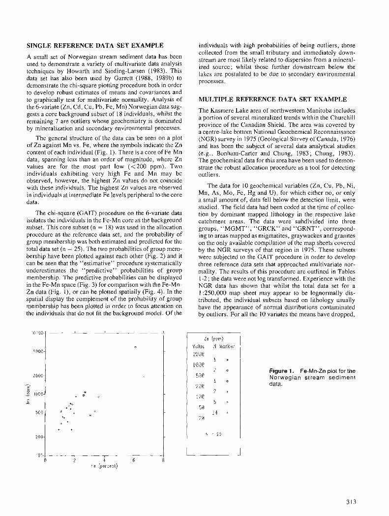
SINGLE REFERENCE DATA SET EXAMPLE individuals with high probabilities of being outliers, those

A small set of Norwegian stream sediment data has been used to demonstrate a variety of multivariate data analysis techniques by Howarth and Sinding-Larsen (1983). This data set has also been used by Garrett (1988, 1989b) to demonstrate the chi-square plotting procedure both in order to develop robust estimates of means and covariances and to graphically test for multivariate normality. Analysis of the 6-variate (Zn, Cd, Cu, Pb, Fe, Mn) Norwegian data suggests a core background subset of 18 individuals, whilst the remaining 7 are outliers whose geochemistry is dominated by mineralization and secondary environmental processes.

The general structure of the data can be seen on a plot of Zn against Mn vs. Fe, where the symbols indicate the Zn content of each individual (Fig. 1). There is a core of Fe-Mn data, spanning less than an order of magnitude, where Zn values are for the most part low ( ~ 2 0 0 ppm). Two individuals exhibiting very high Fe and Mn may bc observed, however, the highest Zn values do not coincide with these individuals. The highest Zn values are observed in individuals at intermediate Fe levels peripheral to the core data.

The chi-square (GAIT) procedure on the 6-variate data isolates the individuals in the Fe-Mn core as the background subset. This core subset (n = 18) was used in the allocation procedure as the reference data set, and the probability of group membership was both estimated and predicted for the total data set (n = 25). The two probabilities of group membership have been plotted against each other (Fig. 2) and it can be seen that the "estimative" procedure systematically underestimates the "predictive" probabilities of group membership. The predictive probabilities can be displayed in the Fe-Mn space (Fig. 3) for comparison with the Fe-Mn- Zn data (Fig. l) , or can be plotted spatially (Fig. 4). In the spatial display the complement of the probability of group membership has been plotted in order to focus attention on the individuals that do not fit the background model. Of the

collected from thesmall tributary and immediately downstream are most likely related to dispersion from a mineralized source; whilst those further downstream below the lakes are postulated to be due to secondary environmental processes.

MULTIPLE REFERENCE DATA SET EXAMPLE

The Kasmere Lake area of northwestern Manitoba includes a portion of several mineralized trends within the Churchill province of the Canadian Shield. The area was covered by a centre-lake bottom National Geochemical Reconnaissance (NGR) survey in 1975 (Geological Survey of Canada, 1976) and has been the subject of several data analytical studies (e.g., Bonham-Carter and Chung, 1983; Chung, 1983). The geochemical data for this area have been used to demonstrate the robust allocation procedure as a tool for detecting outliers.

The data for 10 geochemical variables (Zn, Cu, Pb, Ni, Mn, As, Mo, Fe, Hg and U), for which either no, or only a small amount of, data fell below the detection limit, were studied. The field data had been coded at the time of collection by dominant mapped lithology in the respective lake catchment areas. The data were subdivided into three groups, "MGMT", "GRCK" and "GRNT", corresponding to areas mapped as migmatites, graywackes and granites on the only available compilation of the map sheets covered by the NGR surveys of that region in 1975. These subsets were subjected to the GAIT procedure in order to develop three reference data sets that approached multivariate normality. The results of this procedure are outlined in Tables 1-2; the data were not log transformed. Experience with the NGR data has shown that whilst the total data set for a 1 :250,000 map sheet may appear to be lognormally distributed, the individual subsets based on lithology usually have the appearance of normal distributions contaminated by outliers. For all the 10 variates the means have dropped,

Figure 1. Fe-Mn-Zn plot for the Norwegian stream sediment data.

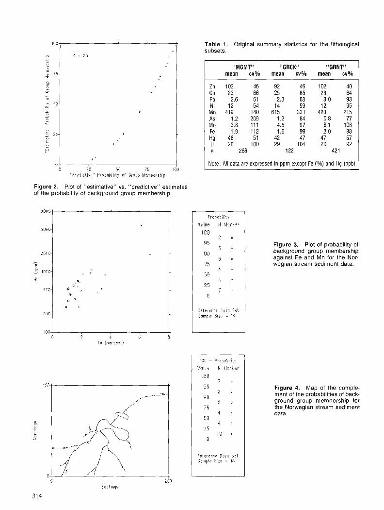
o l. I I I I 0 2 5 50 75 100

" P r e d i c t i v e " Probohil i ly o f Group hknibership

"MGMT" " G R C K "GRNT" mean cv% mean cv% mean cv%

Zn 103 46 92 46 102 40 Cu 23 66 25 85 23 64 Pb 2.6 61 2.3 63 3.0 93 Ni 12 54 14 59 12 95 Mn 419 140 615 331 423 21 5 As 1.2 209 1.2 84 0.8 77 Mo 3.8 111 4.5 97 6.1 108 Fe 1.9 112 1.6 99 2.0 98 Hg 46 5 1 42 47 47 57 U 20 100 29 104 20 92 n 266 122 421

Note: All data are expressed in ppm except Fe (%) and Hg (ppb)

Figure 2. Plot of "estimative" vs. "predictive" estimates of the probability of background group membership.

Reference Doto Set Sorncle Size = 18

0 2 4 6 S '

Fe (percent)

100 - Probabili1.y

Value N Marker 1 BB

7 0

9 5 0 fl

BB 0 0

7 5 4 9

58 4 Q

25 18 +

0

Reference D a t a Set Somple Size = 18

Figure 3. Plot of probability of background group membership against Fe and Mn for the Nor- wegian stream sediment data.

Figure 4. Map of the complement of the probabilities of background group membership for the Norwegian stream sediment data.

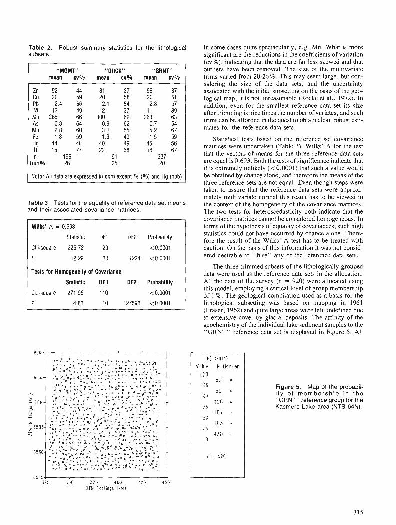
"MGMT" "GRCK" "GRNT" mean cv% mean cv% mean cv%

Zn 92 44 81 37 96 37 Cu 20 59 20 58 20 51 Pb 2.4 56 2.1 54 2.8 57 Ni 12 49 12 37 11 39 Mn 266 66 300 62 263 63 As 0.8 64 0.9 62 0.7 54 Mo 2.8 60 3.1 55 5.2 67 Fe 1.3 59 1.3 49 1.5 59 Hg 44 48 40 49 45 56 U 15 77 22 68 16 67 n 196 91 337

Trim% 26 25 20

Note: All data are expressed in ppm except Fe (010) and Hg (ppb)

Wilks' A = 0.693

Statistic DFl DF2 Probability

Chi-square 225.73 20 < 0.0001

F 12.29 20 1224 <0.0001

Tests for Homogeneity of Covariance

Statistic DF1 DF2 Probability

Chi-square 271.96 110 <0.0001

F 4.86 110 127596 <0.0001

Table 2. Robust summary statistics for the lithological in some cases quite spectacularly, e.g. Mn. What is more subsets. significant are the reductions in the coefficients of variation

(cv %), indicating that the data are far less skewed and that outliers have been removed. The size of the multivariate trims varied from 20-26 %. This may seem large, but considering the size of the data sets, and the uncertainty associated with the initial subsetting on the basis of the geological map, it is not unreasonable (Rocke et al., 1972). In addition, even for the smallest reference data set its size after trimming is nine times the number of variates, and such trims can be afforded in the quest to obtain clean robust estimates for the reference data sets.

Statistical tests based on the reference set covariance matrices were undertaken (Table 3). Wilks' A for the test that the vectors of means for the three reference data sets are equal is 0.693. Both the tests of significance indicate that it is extremely unlikely (<0.0001) that such a value would be obtained by chance alone, and therefore the means of the three reference sets are not equal. Even though steps were taken to assure that the reference data sets were approximately multivariate normal this result has to be viewed in

Table 3 Tests for the equality of reference data set means the context of the homogeneity of the covariance matrices. and their associated covariance matrices. The two tests for heteroscedasticity both indicate that the

covariance matrices cannot be considered homogeneous. In terms of the hypothesis of equality of covariances, such high statistics could not have occurred by chance alone. There- fore the result of the Wilks' A test has to be treated with caution. On the basis of this information it was not considered desirable to "fuse" any of the reference data sets.

The three trimmed subsets of the lithologically grouped data were used as the reference data sets in the allocation. All the data of the survey (n = 920) were allocated using this model, employing a critical level of group membership of 1 %. The geological compilation used as a basis for the lithological subsetting was based on mapping in 1961 (Fraser, 1962) and quite large areas were left undefined due to extensive cover by glacial deposits. The affinity of the geochemistry of the individual lake sediment samples to the "GRNT" reference data set is displayed in Figure 5 . All

Figure 5. Map of the probability of member sh ip in t h e "GRNT" reference group for the Kasmere Lake area (NTS 64N).

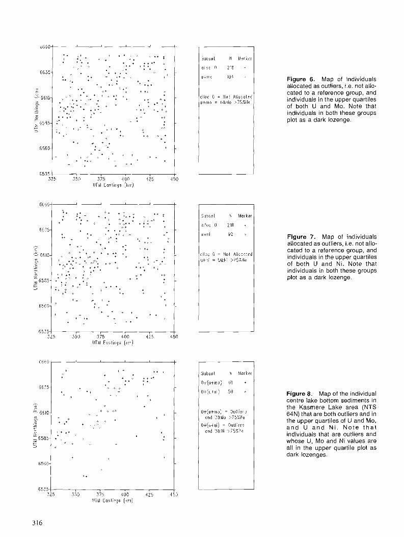
Subset 1.1 tdarker

allvx ? 213 +

u+mn 104 .>

ollos ? = 1/01 Allocotrd U t t . i ~ < ~ = LI?LMo ;-S5Xile

Figure 6. Map of individuals allocated as outliers, i.e, not allocated to a reference group, and individuals in the upper quartiles of both U and Mo. Note that individuals in both these groups plot as a dark lozenge.

6535 ( I I I 1 I

225 350 375 400 425 450 UTM Esstings [km)

Subse t N Marker

allos O 218 +

u t t j i 92 0

allor; !I = Not Allocated u t r ~ i = UBt,li >75"mle

+ * + + + * . ::+ + . O * + . . * + + 6 " I . + + O . n o t * + O * . .. +

++ * + * + + *

+ + ' + + + + + + +

> + +

0 + + + I... + Q + + + e * . t

*e + .% Je. . 0 + + + . .* 0

++ , +. + + . . + +

.o . + ,,

Figure 7. Map of individuals allocated as outliers, i.e. not allocated to a reference group, and individuals in the upper quartiles of both U and Ni. Note that individuals in both these groups plot as a dark lozenge.

6535 1 I I I I I

3?5 350 375 400 425 450 UTM Eastings jkm)

Subse t El l,{orkcr

O+(utrno) 61 +

O + ( u t n i ) 50 0

O+(utmo) = Oulliel-s und V!.:tdo :*75Xile

O+(utni) = Outliers u r~d UiF.Ii ::75Xile

Figure 8. Map of the individual centre lake bottom sediments in the Kasmere Lake area (NTS 64N) that are both outliers and in the upper quartiles of U and Mo, and U a n d N i . No te t h a t individuals that are outliers and whose U, Mo and Ni values are all in the upper quartile plot as dark lozenges.

325 350 375 400 425 450 U T U Eostings (km)

the major areas of granitoid outcrop, in the northwest, northeast and southeast part of the area are reflected in the Figure. Additionally, a number of extensions are indicated into areas which could not be geologically mapped due to outcrop sparsity. Another notable feature in Figure 5 is the probability "low" crossing the area from southwest to northeast marking the area dominantly underlain by graywackes and metasediments.

Of prime interest in geochemical exploration are the individuals whose geochemistry is so unlike the reference groups that they were considered outliers and not allocated. Almost 24 % of the data fall into this category. This indicates that the lithological subsetting was not ideal; more recent mapping in the area has revealed significant additional information. However, this fact illustrates the value of the proposed procedure in "filtering" a large data set so as to focus attention on a more manageable smaller number of individuals on the basis of imperfect lithological information. In the recent past there has been considerable interest in the Kasmere Lake area from the point of view of uranium potential. Two key types of uranium occurrence are known to exist in the area. Firstly, an association with granitoid rocks which is not considered to be of economic importance; and secondly, an association with unconformities above metasedimentary units similar to that found in the Wollaston Lake area to the southwest, e.g. the Rabbit Lake Mine. The granitoid association, which may also be extended to occurrences of pegmatite bodies, is marked geochemical ly by higher M o and F levels . T h e metasedimentary association is marked geochemically by elevated levels of Ni, Co, Cu, As, Ag and Mo amongst others.

In order to reduce the number of outliers further still subsets of data containing only individuals both of whose U and Mo, and U and Ni, values were in the upper quartile, i.e. >75 percentile, were prepared. These two subsets were then plotted spatially along with the outliers from the allocation procedure (Figs. 6 and 7).

The majority of the outliers coincident with individuals with upper quartile U and Mo levels (61) lie along the northwest flank of the southwest to northeast trending metasedimentary belt (Fig. 6). As a result of mineral exploration activities uranium occurrences associated with peg- mati te~ and bodies of fluorite rich granites have been discovered in that part of the Kasmere Lake area. In the southeast the majority of the coincident individuals fall close to the contact of a large body of porphyritic granite with its host rock. Scattered coincidences in the northwest largely relate to the presence of fluorite rich granites.

The distribution of the individuals that were allocated as outliers and show upper quartile U and Ni levels (50) is markedly restricted to the northwest flank of the southwest to northeast trending metasedimentary belt. Again, exploration in this area has revealed a number of occurrences of uranium mineralization fitting the Wollaston Lake model. As the unconformity-associated deposits are known to contain minor molybdenite the outlier and coincident U and Mo, and U and Ni individuals have been plotted on a single map (Fig. 8). This map clearly shows the tendency of the

outliers to be associated with the metasedimentary belt, and to be dominantly in the northwest half of the map area. There are a total of 22 outlier-U-Mo-Ni coincidences, and half of these fall along the northwest flank of the metasedimentary belt. The map clearly indicates a number of areas as containing clusters of coincident individuals. These must seriously be considered as true geochemical anomalies related to uranium mineral occurrences.

DISCUSSION

The procedure outlined serves two purposes. Firstly, it permits data to be allocated on the basis of a priori information into known groups of significance to the user. Secondly, it permits individuals that do not "fit" into the users conceptual model of the processes controlling the distribution of the data to be recognized. Importantly from the statistical viewpoint the procedure is executed in a manner that is robust. That is, the influence of data that could deleteriously effect the procedure is limited, and checks for the major assumptions underlying the procedure are easily made. Additionally, were necessary a generalized procedure is used that takes the important matter of inhomogeneity of covariance into account.

The resulting displays related to the probabilities of group membership permit a transformation of the data from a set of response variables to a probabilistic scale that is related to processes controlling the data. These processes are selected by the user, and therefore conform to a conceptual model that is considered an acceptable way to describe the variability of the data. Importantly, as pointed out by Garrett (1989b) the use of the Mahalanobis distance focuses attention on individuals that are far from the centroid of the data in any direction. More traditional methods of "thresholding" tend to divide the data on simple high or low cut levels. This procedure can totally miss individuals that exhibit interesting features in terms of the ratios of the variables. Certainly, in mineral exploration as the search for new buried deposits continues their geochemical reflections are likely to be more subtle than for the surface outcropping deposits. The ability to focus on individuals that are the more subtle outliers in the geochemical data will become increasing important. The current work sets out to provide a tool to help achieve this objective, and to do so within a framework that is Drocess oriented and multivariate rather than univariately response centred.

REFERENCES Aitchison, J . , Habbema, J.D.F., and Kay, J.W. 1977: A critical comparison of two methods of statistical discrimination;

Applied Statistics, v . 26, p. 15-25. Association of Exploration Geochemists 1977: Threshold - fact or fiction?; Association of Exploration

Geochemists, Newsletter, v . 21, p. 3 . Bartlett, M.S. 1941 : The statistical significance of canonical correlations; Biometrika.

v . 32, p. 29-38. Beckman, R.J. and Cook, R.D. 1983: Outlier.. . s ; Technometrics, v . 25, p. 1 19-149 Bezdek, J.C., Ehrlich, R. , and Full, W. 1984 : FCM : the fuzzy c-means clustering algorithm ; Computers and

Geosciences, v . 10, p. 191-203.

Blackith, R.E. and Reyment, R.A. 1971: Multivariate Morphometrics; Academic Press, London. 412p. Bonham-Carter, G.F. and Chung, C.F. 1983: Integration of mineral resource data for the Kasmere Lake area,

Northwest Manitoba, with emphasis on uranium; Mathematical Geology, v. 15, p. 25-45.

Box, G.E.P. 1948: A general distribution theory for a class of likelihood criteria;

Biometrika, v. 36, p. 317-346. Campbell, N.A. 1984: Some aspects of allocation and discrimination; Multivariate

Statistical Methods in Physical Anthropology, eds. W.W. Howells and G.N. van Vark; D. Reidel, Dordrecht, p. 177-192.

Chung, C.F. 1983: SIMSAG: integrated computer system for use in evaluation of

mineral and energy resources; Mathematical Geology, v. 15, p. 47-58.

Cooley, W.W. and Lohnes, P.R. 1962 : Multivariate Procedures for the Behavioural Sciences; John Wiley

and Sons, New York, 2 11 p. Devlin, S.J., Gnanadesikan, R. and Kettenring, J.R. 1981 : Robust estimation of dispersion matrices and principal compo-

nents; American Statistical Association, Journal, v. 76, p. 354-362.

Fraser, J.A. 1962 : Geology, Kasmere Lake, Manitoba; Geological Survey of Canada,

Map 31-1962. Friedman, J.H. and Rafsky, L.C. 1981 : Graphics for the multivariate twosample problem; American

Statistical Association, Journal, v. 76, p. 277-291. Garrett, R.G. 1988 : IDEAS : an interactive computer graphics tool to assist the explora-

tion geochemist; in Current Research, Part F, Geological Survey of Canada, p a p e r 8 8 - 1 ~ , p. 1-13.

1989a: The role of computers in exploration geochemistry ; & Proceedings of Exploration 87, The Third Decennial Conference on Geophysi- cal and Geochemical Exploration for Minerals and Groundwater, ed. G. Garland; Ontario Geological Survey Special Volume 3, p. 586-608.

1989b: The chi-square plot: a tool for multivariate outlier recognition; Journal of Geochemical Exploration, v. 32. p. 319-341.

Garrett, R.G. and Lestinen, P. 1984 : Workshop 5 : thresholds and anomaly interpretation ; Geochemi-

cal Exploration 1983, ed. A. Bjorklund; Journal of Geochemical Exploration, v. 21, p. 137.142.

Geological Survey of Canada 1976: National Geochemical Reconnaissance - Regional centre-lake

bottom lake sediment survey, Kasmere Lake, Manitoba, NTS 64N; Geological Survey of Canada, Open File 322.

Gnanadesikan, R. 1977: Methods for Statistical Data Analysis of Multivariate Observa-

tions; John Wiley and Sons, New York, 31 Ip. Hawkes, H.E. and Webb, J.S. 1962: Geochemistry in Mineral Exploration; Harper and Row, New

York, 415p. Hawkins, D.M. 1981 : A new test for multivariate normality and homoscedasticity; Tech-

nometrics, v . 23, p. 105-1 10. Howarth, R.J. and Sinding-Larsen, R. 1983 : Multivariate analysis; kstatistics and Data Analysis in Geochemi-

cal Prospecting, ed. R.J. Howarth; Handbook of Exploration Geochemistry v. 2 ; Elsevier Science Publishers, Amsterdam, p. 207-289.

Kshirsagar, A.M. 1972: Multivariate Analysis; Marcel Dekker, New York, 3558. Kullback, S. 1959: Information Theory and Statistics; John Wiley and Sons, New

York, 395p. Lohnes, P.R. 1961 : Test space and discriminant space classification models and related

significance tests; Educational and Pyschological Measurement, v. 21, p. 559-574.

Rao, C.R. 1952: Advanced Statistical Methods in Biometrical Research; John

Wiley and Sons, New York, 390p. Rocke, A.J., Rocke, D.M.. and Downes, G.W. 1982: Are robust estimators really necessary?; Technometrics, v. 24, p.

95-101. Smith, R.E., Campbell, N.A., and Litchfield, R. 1984: Multivariate statistical techniques applied to pisolitic laterite

geochemistry at Golden Grove, Western Australia; Geochemi- cal Exploration in Arid and Deeply Weathered Terrains, eds. R. Davy and R.H. Mazzucchelli; Journal of Geochemical Explora- tion, v. 22, p. 193-216.

A partitioning process for geochemical datasets

R.M. Rennerl, G.P. Glasbyz, F.T. Manheim3, and C.M. Lane-Bostwick3

Renner, R. M., Glasby, G. P., Manheim, F. T., and Lane-Bostwick, C. M., A partitioning process for geochemical datasets; Statistical Applications in the Earth Sciences, ed. F. P. Agterberg and G. F. Bonham-Carter; Geological Suwey of Canada Paper 89-9, p. 319-328, 1989.

Abstract

Conventional techniques for the partitioning of geochemical datasets into source end members have included Q-mode cluster and factor analysis, normative partitioning, and linear programming, as well as hybrid combinations of these. Recent research has been directed toward evaluation of the least squares regression technique as a partitioning method. It had formerly been described as unusable for that purpose because the positivity constraint on end member loadings is not satisfied. In fact, the least squares method not only yields the 'best' estimate for any sample when the end members are specijied, but the resultant regression coeficients identify which endmembers must be adjusted in order to satisfy the positivity constraint when it is violated. An algorithm which integrates least-squares partitioning with endmember adjustment procedures has been applied to the geochemical datasets that resultedfrom analyses of MANOP ferromanganese nodules (U.S. National Science Foundation) and Mid-Pacijc cobalt-rich manganese crustsfiom the U.S. Geological Survey crust data base. By exploiting the multivariate geometry of the data, the process appears to reveal more of the data structure than traditional methods.

Les mkthodes classiques de dkcoupage des ensembles de donnkes gkochimiques en termes jnals for- mateurs comprennent l'analyse par groupes en mode Q et 1 'analyse factorielle, lefractionnement norma- tif et la programmation linkaire ainsi que des combinaisons hybrides de ces mkthodes. Les recherches rkcentes ont eft! tournkes vers 1 'dvaluation de la mkthode de rkgression des moindres carre's pour ce fractionnement. Cette dernikre avait antkrieurement e'tk dkcrite comme inutilisable d cette $n parce qu 'elle ne permet pas de satisfaire la contrainte de positivitk des charges sur les termes Jnals. En rkalitk, non seulement la mkthode des moindres carrb fournit-elle la Q meilleure ,, estimation pour tout Lchantillon lorsque les termes finals sont spkcijks, mais les coeficients de rkgression qui en rksultent identifient les termes finals qui doivent etre ajustes a$n de satisfaire la contrainte de positivitk lorsqu 'elle n 'est pas respectke. Un algorithme intkgrant le fractionnement par la me'thode des moindres carrb et des pro- ckdures d'ajustement de termes finals a ktt applique' aux ensembles de donnkes gkochimiques issus des analyses de nodules de ferromangankse efectukes duns le cadre du MANOP (National Science Founda- tion des Etats-Unis) et de crofites manganbiferes riches en cobalt du centre du Pacijque, donnkes de la base de donnkes crustales du Geological Survey des Etats-Unis. L 'exploitation de la gkomdrie multivarike des donnkes a permis aux chercheurs de constater que le processus semble davantage rkve'ler la structure des donnkes que les mkthodes classiques.

' Institute of Statistics and Operations Research,Victoria University of Wellington, PO Box 600, Wellington, New Zealand. New Zealand Oceanographic Institute, Department of Scientific and Industrial Research, Private Bag, Kilbirnie, Wellington, New Zealand.

Q.S. Geological Survey. Branch of Atlantic Marine Geology, Quissett Campus, Woods Hole, MA 02543, U.S.A.

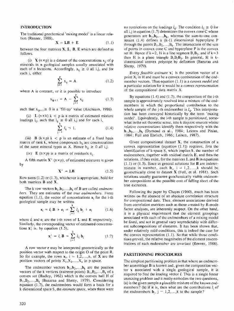
INTRODUCTION

The traditional geochemical 'mixing model' is a linear relation (Renner, 1988),

X = L B + E (1.1)

between the four matrices X, L, B, E which are defined as follows.

(i) X (n Xp) is a dataset of the concentrations xij of p minerals in n geological samples usually associated with each of n locations. Accordingly, xij 2 0 all i,j, and for each i, either

D

where A is constant, or it is possible to introduce D

such that x ~ ~ + ~ 2 0 is a 'fill-up' value (Aitchison, 1986).

(ii) L (n X k) k < p is a matrix of estimated mixture loadings lij, such that lij r 0 all i,j and for each i ,

k

(iii) B (kxp) k c p is an estimate of a fixed basis matrix of rank k, whose components bij are concentrations of the same mineral types as X. Hence bij 2 0 all i j .

(iv) E (nxp) is a matrix of residuals ei,.

A fifth matrix X' (n xp), of estimated mixtures is given by

Row sums (1.2) or (1.3), whichever is appropriate, hold for both matrices B and X.

The k row vectors b l ,b2,. . . , bk of B are called endmembers. They are estimates of the true endmembers. From equation ( 1 . l), the vector of concentrations xi for the i-th geological sample may be written

k

where li and ei are the i-th rows of L and E respectively. Similarly, the corresponding vector of estimated concentrations x f is, by equation (1.5),

k

A row vector r may be interpreted geometrically as the position vector with respect to the origin 0 of the point R. So for example, the rows xi, i = 1,2 ,..., n, of X are the position vectors of points XI ,X2,. . . ,Xn in p-space.

The endmember vectors b l ,b2 , . . . ,bk are the position vectors of the k vertices (extreme points) B I ,B2,. . . ,Bk of a convex set (Hadley, 1962) which is the convex hull H of Bl ,B2,. . . .Bk (Bazaraa and Shetty, 1979). Considering equation (1.7), the endmembers would form a basis for a k-dimensional space S, the estimate space, when there were

no restrictions on the loadings lij. The condition lij r 0 for all i,j in equation (1.7) determines the convex cone C whose generators are b l ,b2,. . . ,bk, whereas the sum-to-one constraint (1.4) defines a (k-1) dimensional hyperplane P through the points BI ,B2,. . . ,Bk. The intersection of the sets of points in convex cone C and hyperplane P is the convex set H. Hence if k=2, H is a line segment BIB2, and if k=3 then H is a plane triangle BIB2B3 In general, H is k- dimensional convex polytope by definition (Bazaraa and Shetty, 1979).

Every feasible estimate x f is the position vector of a point Xi in H and must be a convex combination of the endmember vectors. Thus equation (1.1) is a convex model and a particular solution for it would be a convex representation of the compositional data matrix X.

By equations (1.4) and (1.7), the composition of the i-th sample is approximately resolved into a mixture of the endmembers in which the proportional contribution to the whole sample of the j-th endmember is lij. This interpretation has been conveyed historically by the term 'mixing model'. Equivalently, the i-th sample is partitioned, somewhat in the set-theoretic sense, into k disjoint sources whose relative concentrations identify them respectively with the bl ,b2 ,..., bk (Dymond et al., 1984; Leinen and Pisias, 1984; Full and Ehrlich, 1986; Leinen, 1987).

Given compositional dataset X, the construction of a convex representation (equation (1.1)) requires, first the identification of k-space S, which implies k, the number of endmembers, together with residual matrix E, and then the solutions, if they exist, for the matrices L and B in equations (1.1) or (1.5). Since in general solutions for B are indeter- minate in number, each b, , i = 1,2 ,..., k should be geometrically close to dataset X (Full, et al. 1981). Such solutions usually guarantee geochemically viable endmember compositions at the possible cost of falling short of the true extremes.

Following the paper by Chayes (1960), much has been written on the absence of an absolute correlation structure for compositional data. Thus, element associations derived from correlation matrices such as those created by R-mode factor analyses, are inherently suspect. On the other hand, it is a physical requirement that the element groupings associated with each of the endmembers of a mixing model be fixed, and not in general vary unpredictably with different subcompositions of elements. It has been shown that, under relatively mild conditions, this is indeed the case for the convex representation (1.1). So that while those conditions prevail, the relative magnitudes of the element concentrations of each endmember are invariant (Renner, 1988).

PARTITIONING PROCEDURES

The simplest partitioning problem is that where an endmember assemblage B is known and, given the composition vector x associated with a single geological sample, it is required to find the loading vector I. This is a single linear unmixing problem and it really embodies the two questions, (a) is the given sample a plausible mixture of the known endmembers? (b) if it is, then what are the contributions lj of the endmembers bj, j = 1,2 ,..., k to the sample?

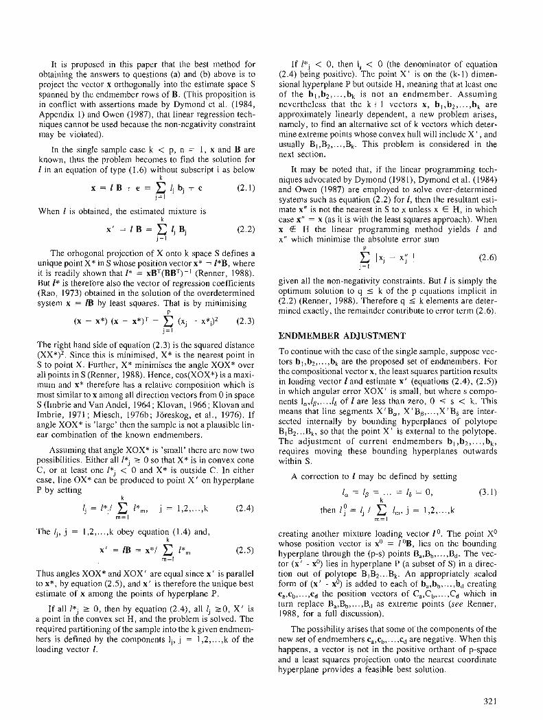
It is proposed in this paper that the best method for obtaining the answers to questions (a) and (b) above is to project the vector x orthogonally into the estimate space S spanned by the endmember rows of B. (This proposition is in conflict with assertions made by Dymond et al. (1984, Appendix 1) and Owen (1987), that linear regression techniques cannot be used because the non-negativity constraint may be violated).

In the single sample case k < p, n = 1, x and B are known, thus the problem becomes to find the solution for 1 in an equation of type (1.6) without subscript i as below

k

x = l B + e = x l j b j + e j = l

(2.1)

When 1 is obtained, the estimated mixture is k

The orhogonal projection of X onto k-space S defines a unique point X* in S whose position vector x* = l*B, where it is readily shown that I* = xBT(BBT)-I (Renner, 1988). But l* is therefore also the vector of regression coefficients (Rao, 1973) obtained in the solution of the overdetermined system x = lB by least squares. That is by minimising

P

(X - x*) (X - x * ) ~ = z (xj - x * ~ ) ~ (2.3) j = l

The right hand side of equation (2.3) is the squared distance (XX*)2. Since this is minimised, X* is the nearest point in S to point X. Further, X* minimises the angle XOX* over all points in S (Renner, 1988). Hence, cos(XOX*) is a maximum and x* therefore has a relative composition which is most similar to x among all direction vectors from 0 in space S (Imbrie and Van Andel, 1964 ; Klovan, 1966 ; Klovan and Imbrie, 1971 ; Miesch, 1976b; Joreskog, et al., 1976). If angle XOX* is 'large' then the sample is not a plausible linear combination of the known endmembers.

Assuming that angle XOX* is 'small' there are now two possibilities. Either all l*j 2 0 so that X* is in convex cone C, or at least one l*, < 0 and X* is outside C. In either case, line OX* can be produced to point X ' on hyperplane P by setting

k

lj = 1*,l l*,, j = 1,2 ,..., k m = l

(2.4)

The I,, j = 1,2,. . .,k obey equation (1.4) and, k

Thus angles XOX* and XOX' are equal since x' is parallel to x*, by equation (2.5), and x ' is therefore the unique best estimate of x among the points of hyperplane P.

If all 2 0, then by equation (2.4), all lj LO, X ' is a point in the convex set H, and the problem is solved. The required partitioning of the sample into the k given endmembers is defined by the components Ij, j = 1,2,. . . ,k of the loading vector I .

If 1*, < 0, then lj < 0 (the denominator of equation (2.4) being positive). The point X ' is on the (k-I) dimensional hyperplane P but outside H, meaning that at least one of the b l , b 2 , ..., b k is not an endmember. Assuming nevertheless that the k+ 1 vectors x , b l ,b2,. . . ,bk are approximately linearly dependent, a new problem arises, namely, to find an alternative set of k vectors which determine extreme points whose convex hull will include X ' , and usually BI ,B2,. . . ,Bk. This problem is considered in the next section.

It may be noted that, if the linear programming techniques advocated by Dymond (1981), Dymond et al. (1984) and Owen (1987) are employed to solve over-determined systems such as equation (2.2) for I , then the resultant estimate x" is not the nearest in S to x unless x E H, in which case x" = x (as it is with the least squares approach). When x (3 H the linear programming method yields 1 and x" which minimise the absolute error sum

P

given all the non-negativity constraints. But 1 is simply the optimum solution to q I k of the p equations implicit in (2.2) (Renner, 1988). Therefore q r k elements are determined exactly, the remainder contribute to error term (2.6).

ENDMEMBER ADJUSTMENT

To continue with the case of the single sample, suppose vectors b l ,b2,. . . ,bk are the proposed set of endmembers. For the compositional vector x, the least squares partition results in loading vector 1 and estimate x' (equations (2.4), (2.5)) in which angular error XOX' is small, but where s components I,,lp ,..., l6 of 1 are less than zero, 0 5 s < k. This means that line segments X' B,, X ' Bp, . . . ,X ' B6 are intersected internally by bounding hyperplanes of polytope BIB2.. .Bk, SO that the point X ' is external to the polytope. The adjustment of current endmembers b l ,b2,. . . , bk , requires moving these bounding hyperplanes outwards within S.

A correction to 1 may be defined by setting

0 then l j = 1, / z I,, j = 1,2 ,..., k

creating another mixture loading vector lo. The point X0 whose position vector is x0 = 1°B, lies on the bounding hyperplane through the (p-s) points Ba,Bb,. . . ,Bd. The vector (x' - xO) lies in hyperplane P (a subset of S) in a direction out of polytope BIB 2...Bk. An appropriately scaled form of (x' - xO) is added to each of ba,bb, ..., bd creating ca,cb ,... ,cd the position vectors of Ca,Cb ,..., Cd which in turn replace Ba,Bb,. . . ,Bd as extreme points (see Renner, 1988, for a full discussion).

The possibility arises that some of the components of the new set of endmembers ca,cb,. . . ,cd are negative. When this happens, a vector is not in the positive orthant of p-space and a least squares projection onto the nearest coordinate hyperplane provides a feasible best solution.

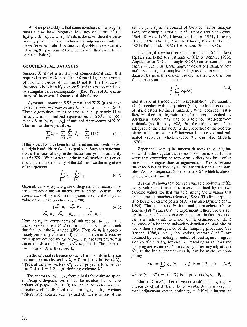
Another possibility is that some members of the original dataset now have negative loadings on some of the b,,bs,. . .,bs, c,,cb,. . ., cd. If this is the case, then the partitioning procedure and endmember adjustment outlined above form the basis of an iterative algorithm for repeatedly adjusting the positions of the k points until they are extreme (see also below).

GEOCHEMICAL DATASETS

Suppose X (nxp) is a matrix of compositional data. It is required to resolve X into a linear form (1. I), in the absence of prior knowledge of matrices B and E. The first step in the process is to identify k-space S, and this is accomplished by a singular value decomposition (Rao, 1973) of X. A summary of the essential features of this follow.

Symmetric matrices XXT (n x n) and XTX (p x p) have the same non-zero eigenvalues X I 2 X2 L .. . 2 X, 2 0. These eigenvalues are associated with n x p matrix U = [U ,uz,. . . ,up] of unitized eigenvectors of XXT, and p X p matrix V = [vl ,v2,. . . ,vD] of unitized eigenvectors of XTX. The sum of the eigenvalues,

D n D n

If the rows of X have been transformed into unit vectors then the right hand side of (4.1) is equal to n. Such a transformation is the basis of a Q-mode 'factor' analysis of similarity matrix XXT. With or without the transformation, an assessment of the dimensionality of the data rests on the magnitude of the quotient

k D

Geometrically vl ,v2,. . . ,vp are orthogonal unit vectors in p- space representing an alternative reference system. The coordinates of point Xi in this system are, by the singular value decomposition (Renner, 1988)

Now the uij are components of unit vectors so 1 uij I I 1 and suppose quotient (4.2) confirms that k < p exists such that for j > k the Xj are negligible. Then hj uij is approximately zero for j > k in (4.3) hence the rows of X occupy the k-space defined by the vl v . . . ,vk axes system within the errors determined by the xi uij. j > k. The approximate rank of X is therefore k.

In the original reference system, the n points in k-space that are obtained by setting Xj = 0 for j > k in line (4.3), represent the row vectors x * ~ which project into xl (equation (2.4)), i = l ,2, . . . ,n, defining estimate X i .

The vectors V, ,v2,. . . ,vk form a basis for estimate space S. Being orthogonal some may lie outside the positive orthant of p-space (xij 2 0) and could not determine the directions of feasible solutions for bl ,b2,. . . ,bk. Various writers have reported varimax and oblique rotations of the

set V, ,v2,. . . ,vk in the context of Q-mode 'factor' analysis (see, for example, Imbrie, 1963; Imbrie and Van Andel, 1964 ; Klovan, 1966; Klovan and Imbrie, 1971 ; Joreskog et al., 1976 ; Miesch, 1976a,b ; Clarke, 1978 ; Full et al., 1981 ; Full, et al., 1982; Leinen and Pisias, 1987).

The singular value decomposition creates X* the least squares and hence best estimate of X in S (Renner, 1988). Angular error XiOX f = angle XOX*i can be examined for each i = 1,2,. . . ,n. Large angular deviations identify both outliers among the samples and gross data errors in the dataset. Large in this context usually means more than four times the mean angular error

and is rare in a good linear representation. The quantity (4.4), together with the quotient (4.2), are initial goodness of fit indicators for the estimate X ' . When both seem satisfactory, then the logratio transformation described by Aitchison (1986) may lead to a test for 'well-behaved' residuals (see Renner, 1988). But the ultimate test of the adequacy of the estimate X i is the proportion of the p coefficients of determination (r2) between the observed and estimated variables, which exceed 0.5 (see also Miesch, 1976b).

Experience with quite modest datasets (n 2 60) has shown that the singular value decomposition is robust in the sense that correcting or removing outliers has little effect on either the eigenvalues or eigenvectors. This is because the space S is identified by all the information in all the samples. As a consequence, it is the matrix X i which is chosen to determine L and B.

It is easily shown that for each variable (column of X), every value must lie in the interval defined by the two extreme values for that variable among the k values that exist in the endmembers (Renner, 1988). The first step then is to locate k extreme points of X i (see also Dymond et al., 1984). That is, to specify the initial endmembers. (Note: Leinen (1987) states that the experiment is therefore biassed by the choice of endmember compositions. In fact, the process is a multivariate extension of the estimation of the 2 extremes of a bounded univariate distribution, and bias or not is then a consequence of the sampling procedure (see Renner, 1988)). Next, the loading vectors li of L are obtained by constructing n vectors of least squares regression coefficients Pi, for each xi, rescaling as at (2.4) and applying correction (3.1) if necessary. Then any adjustment Abh to the initial endmembers bh can be made by computing

n

Abh = ghi ( ~ f - xoi), h = 1,2 ,..., k (4.5) i = 1

where (xi - xoi) = 0 if X f is in polytope BIB2.. .Bk.

Matrix G (nx k) of error vector coefficients ghi may be chosen to adjust BI ,B2,. . . ,Bk outwards. So for a weighted mean adjustment vector, define ghi = 0 if X: is internal to

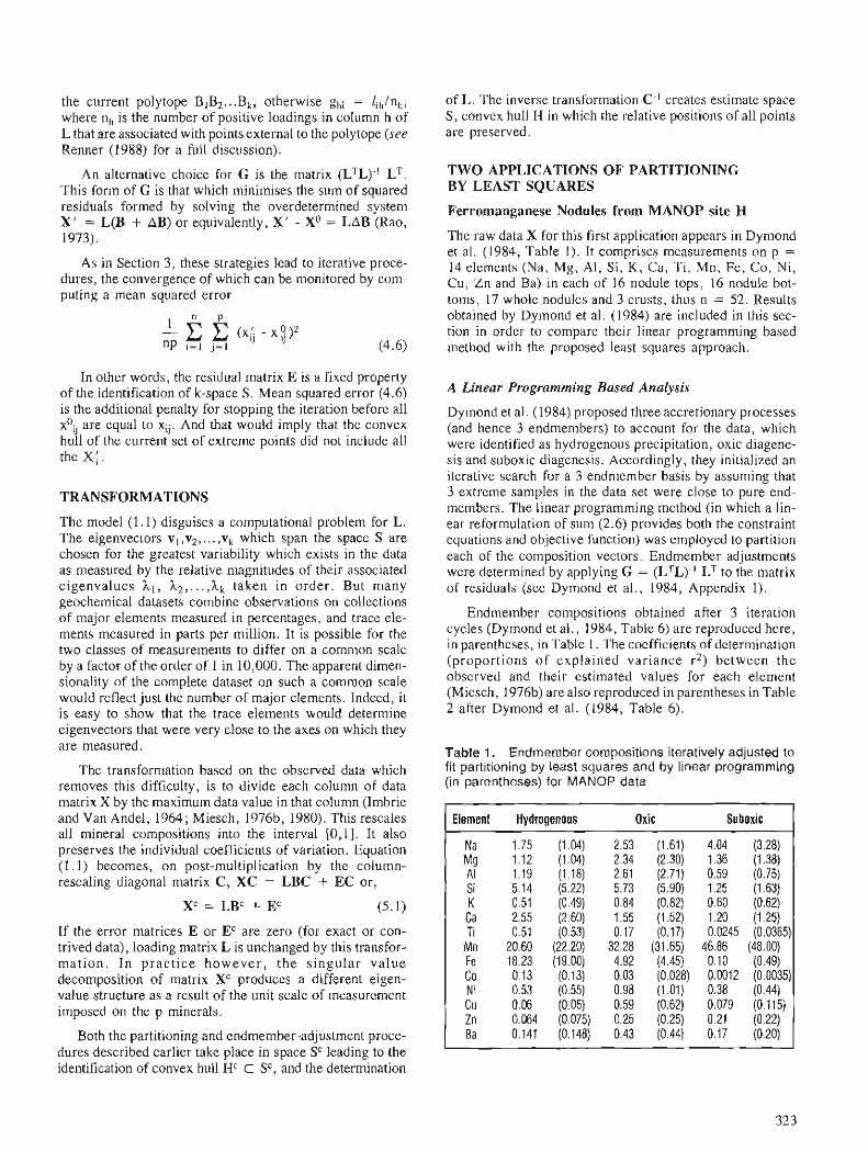
the current polytope BIB2.. .Bk, otherwise ghi = lih/nh, where nh is the number of positive loadings in column h of L that are associated with points external to the polytope (see Renner (1988) for a full discussion).

An alternative choice for G is the matrix (LTL)-I LT. This form of G is that which minimises the sum of squared residuals formed by solving the overdetermined system X ' = L(B + AB) or equivalently, X ' - X0 = LAB (Rao, 1973).

As in Section 3, these strategies lead to iterative procedures, the convergence of which can be monitored by computing a mean squared error

In other words, the residual matrix E is a fixed property of the identification of k-space S. Mean squared error (4.6) is the additional penalty for stopping the iteration before all xoij are equal to x i j And that would imply that the convex hull of the current set of extreme points did not include all the X i .

TRANSFORMATIONS

The model ( I . I) disguises a computational problem for L. The eigenvectors v,,v2,.. .,vk which span the space S are chosen for the greatest variability which exists in the data as measured by the relative magnitudes of their associated eigenvalues A,, h2,. . . ,hk taken in order. But many geochemical datasets combine observations on collections of major elements measured in percentages, and trace elements measured in parts per million. It is possible for the two classes of measurements to differ on a common scale by a factor of the order of 1 in 10,000. The apparent dimensionality of the complete dataset on such a common scale would reflect just the number of major elements. Indeed, it is easy to show that the trace elements would determine eigenvectors that were very close to the axes on which they are measured.

The transformation based on the observed data which removes this difficulty, is to divide each column of data matrix X by thc maximum data value in that column (Imbrie and Van Andel, 1964; Miesch, 1976b, 1980). This rescales all mineral compositions into the interval [0,1]. It also preserves the individual coefficients of variation. Equation (1.1) becomes, on post-multiplication by the column- rescaling diagonal matrix C , XC = LBC -t E C or,

If the error matrices E or EC are zero (for exact or con- trived data), loading matrix L is unchanged by this transformation. In practice however, the singular value decomposition of matrix XC produces a different eigenvalue structure as a result of the unit scale of measurement imposed on the p minerals.

Both the partitioning and endmember-adjustment procedures described earlier take place in space Sc leading to the identification of convex hull HC C SC, and the determination

of L. The inverse transformation C-' creates estimate space S , convex hull H in which the relative positions of all points are preserved.

TWO APPLICATIONS OF PARTITIONING BY LEAST SQUARES

Ferromanganese Nodules from MANOP site H

The raw data X for this first application appears in Dymond et al. (1984, Table 1). It comprises measurements on p = 14 elements (Na, Mg, Al, Si, K , Ca, Ti, Mn, Fe, Co, Ni, Cu, Zn and Ba) in each of 16 nodule tops, 16 nodule bottoms, 17 whole nodules and 3 crusts, thus n = 52. Results obtained by Dymond et al. (1984) are included in this section in order to compare their linear programming based method with the proposed least squares approach.

A Linear Programming Based Analysis

Dymond et a]. (1984) proposed three accretionary processes (and hence 3 endmembers) to account for the data. which were identified as hydrogenous precipitation, oxic diagenesis and suboxic diagenesis. Accordingly, they initialized an iterative search for a 3 endmember basis by assuming that 3 extreme samples in the data set were close to puri endmembers. The linear programming method (in which a linear reformulation of sum (2.6) provides both the constraint equations and objective function) was employed to partition each of the composition vectors. Endmember adjustments were determined by applying G = (L'L)-' LT to the matrix of residuals (see Dymond et al., 1984, Appendix 1).

Endmember compositions obtained after 3 iteration cycles (Dymond et al., 1984, Table 6) are reproduced here, in parentheses, in Table 1 . The coefficients of determination (proportions of explained variance r2) between the observed and their estimated values for each element (Miesch, 1976b) are also reproduced in parentheses in Table 2 after Dymond et a]. (1984, Table 6).

Table 1. Endmember compositions iteratively adjusted to fit partitioning by least squares and by linear programming (in parentheses) for MANOP data

Element Hydrogenous Oxic Suboxic

Na 1.75 (1.04) 2.53 (1.61) 4.04 (3.28) MQ 1.12 (1.04) 2.34 (2.30) 1.36 (1.38) Al 1.19 (1.18) 2.61 (2.71) 0.59 (0.75) Si 5.14 (5.22) 5.73 (5.90) 1.25 (1.63) K 0.51 (0.49) 0.84 (0.82) 0.60 (0.62)

Ca 2.55 (2.60) 1.55 (1.52) 1.20 (1.25) Ti 0.51 (0.53) 0.17 (0.17) 0.0245 (0.0365) Mn 20.60 (22.20) 32.28 (31.65) 46.86 (48.00) Fe 18.23 (19.00) 4.92 (4.45) 0.10 (0.49) Co 0.13 (0.13) 0.03 (0.028) 0.0012 (0.0035) N i 0.53 (0.55) 0.98 (1.01) 0.38 (0.44) Cu 0.06 (0.05) 0.59 (0.62) 0.079 (0.115) Zn 0.064 (0.075) 0.25 (0.25) 0.21 (0.22) Ba 0.141 (0.148) 0.43 (0.44) 0.17 (0.20)

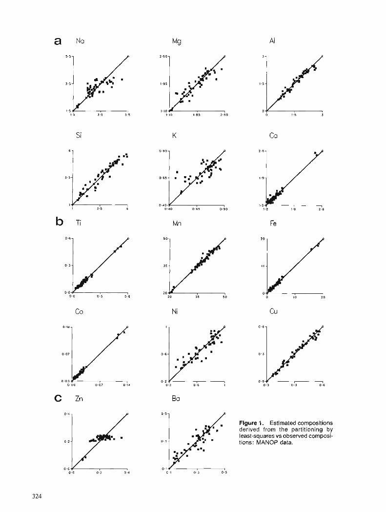
Figure 1. Estimated compositions derived from the partitioning by least-squares vs observed compositions: MANOP data.

A Least Squares Based Analysis

A 'fill-up' value was constructed (equation (1.3)) for all samples, creating X (52 x 15) which was then transformed into XC according to equation (5.1). The singular value decomposition of XC showed that the relative contributions of the first three (largest) eigenvalues to the sum (4.1) were 94.39 %, 2.76 %, 2.03 %, totalling 99.18 % (see quotient (4.2)), the 4th largest contribution being 0.30 %. A 3-space was therefore identified as the transformed estimate space SC, and the mean angular error (equation (4.4)) for angles between the rows of XC and its estimate Xc' in SC was 4.9" (mean similarity 0.9963).

Three extreme vectors belonging to XC' were used to initialize an iterative search for BC based on least squares methods for determining both L with correction (3.1)) and ABC (as in equation (4.5)). However, in equations of type (4 .3 , ghi = ((LTL)-'LT)hi only for lib > 0, otherwise gl,i = 0 thus eliminating the effect of the i-th error Fi on Abch. Iterations were stopped after 2 cycles when the mean squared error (4.6) had been reduced to 4.7 x

Endmember compositions B = BCC-1 appear unparenthesized in Table 1, coefficients of determination (prypor- tions of explained variance) between X and X' = (XC )C-' are set out, also unparenthesized, in Table 2.

Comparisons

It is evident from Table 1 that corresponding pairs of endmembers constructed by algorithms which incorporated partitioning by least squares and linear programming respectively, are not fundamentally geochemically distinct. The mean angular errors associated with each algorithm were, for untransformed data, both of the order of 1.1 ". It is difficult to assess the relative positions of the 2 sets of endmembers since one of them is maintained in estimate space S and extreme for dataset X. Nevertheless, there are 10 extreme values constructed by the linear programming approach which do not span corresponding extreme values in either the raw data X or the estimate X' .

T a b l e 2. Coefficients of determination between estimated and observed elements obtained from partitioning by least squares and by linear programming (in parentheses) for MANOP data

Element Coefficient of Determination (% explained variance)

Na 55.3 (64.0) M g 84.5 (84.1) Al 95.0 (94.8) Si 93.0 (91.6) K 55.8 (54.7)

Ca 95.2 (91.1) Ti 98.1 (97.7) Mn 96.8 (86.2) Fe 98.9 (99.5) Go 99.1 (99.6) N i 80.3 (81.9) Cu 97.6 (97.3) Zn 47.7 (47.6) Ba 76.9 (75.6)

Comparing the coefficients of determination between estimated and observed values of the elements in Table 2, it will be seen that the least squares based analysis created generally better estimates than the linear programming method, most notably in the case of Mn. It created inferior estimates for Na, which with K and Zn were the least well accounted for by either analysis. However, the database was small and particularly tractable, so it is therefore reassurring that overall, the results obtained by the two methods were very similar.

Plots of the least squares estimates of each of the variables against their observed values appear in Figure 1 (see, for example, Renner, 1982 ; and also Dymond et al., 1984, Fig.8). These plots permit a graphical assessment of the goodness of fit, and in a perfect representation, each set of points would lie on a straight line through the origin with slope one. A detail that they show quite clearly is a group of three points which appear as distinct outliers, located together but remote from the rest, for the plots of Na, Ca, Ti, Mn, Fe, Co, and Zn. Such configurations often inflate the coefficient of determination because of the apparent linearity between the centres of disjoint clusters. In each plot, these outlying points represent the three crusts PI 1-2, Pll-4, P11-5, Dymond et al. (1984, Table 1)).

Accordingly, these crusts were removed from the database, and the remaining 49 nodule compositions were transformed as at equation (5 .1) . The singular value decomposition of the resulting 49 x 15 array revealed that a remarkable 99.05 % of sum (4.1) was attributjible to the first two eigenvalues. A least squares based analysis, orthogonally projecting the data into the 2-space spanned by the corresponding eigenvectors, determined two endmembers rather close respectively to the compositions of nodule top V48-1 and nodule bottom V52- 1 (Dymond et al., 1984, Table 1). The mean angular error for the two endmember representation of the transformed data was 5.49" (mean similarity 0.9954), and the mean squared error (4.6) after one iteration was 1.5 x lo-'. The subsequent coefficients of determination were depressed further for Na, K and Zn (which were least well accounted for with 3 endmembers) but lay in the ranges 0.92 - 0.94 for Al, Si, Mn, Fe, Co, Cu, and the range 0.69 - 0.89 for Mg, Ca, Ti, Ni, Ba. In other words, the 49 nodule compositions were accounted for, almost as well with 2 endmembers, as the same data plus 3 crusts were with 3 endmembers.

These latter results suggest that a greater mathematical parsimony is possible in interpreting the data than was implied by the initial geochemical assumption of three accretionary processes. This suggestion would seem to be confirmed by the very low loadings associated with the Hydrogenous endmember in Dymond et al. (1984, Table 7) for all but the 3 crusts.

Mid-Pacific Cobalt-Rich Manganese Crusts

The raw data for this second application comprised of a Mid-Pacific subset (170°E to 150°W, 18"s to 32"N) of the United States Geological Survey world ocean- ferromanganese-crust database (Lane et al., 1986). Meas- urements on p = 22 oxides and minor elements (Si02, Ti02, Mn02, Fe203, A1203, Co3O4, NiO, CUO, CaO,

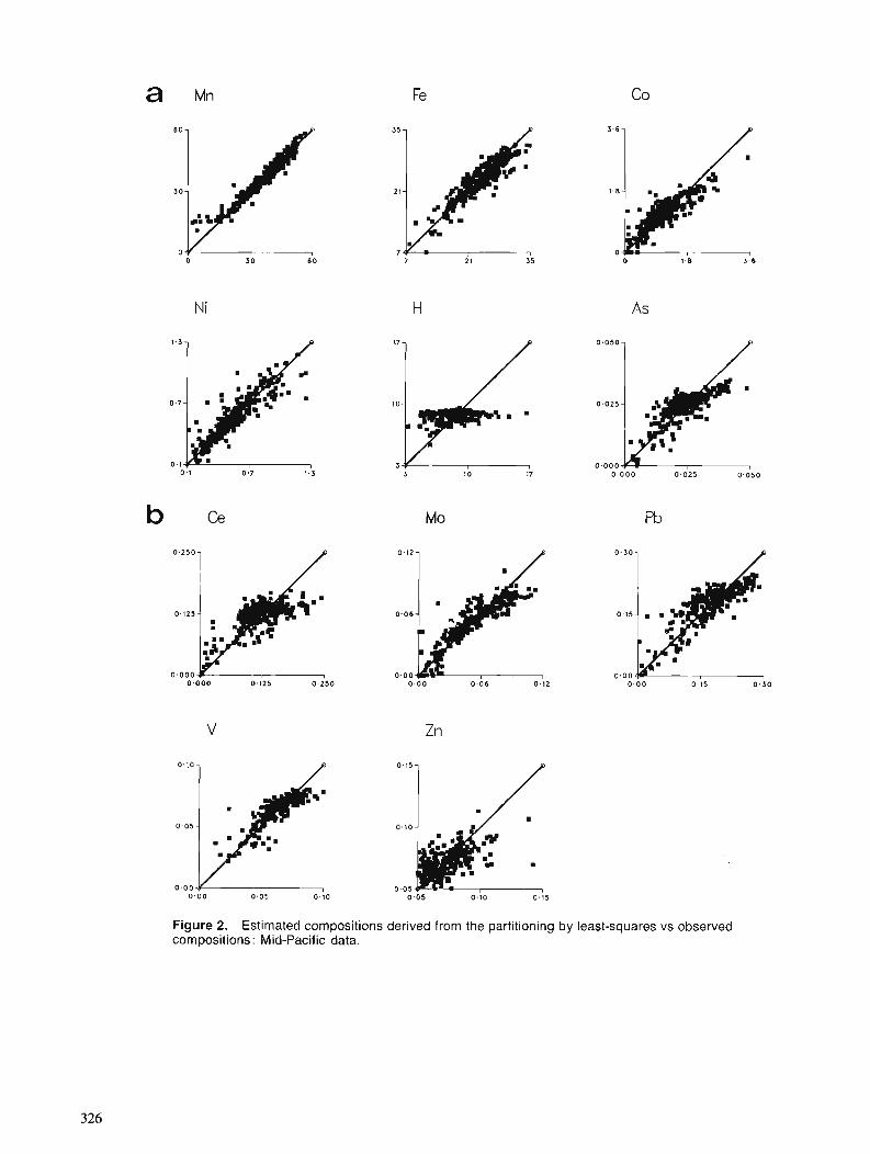
Figure 2. Estimated compositions derived from the partitioning by least-squares vs observed compositions: Mid-Pacific data.

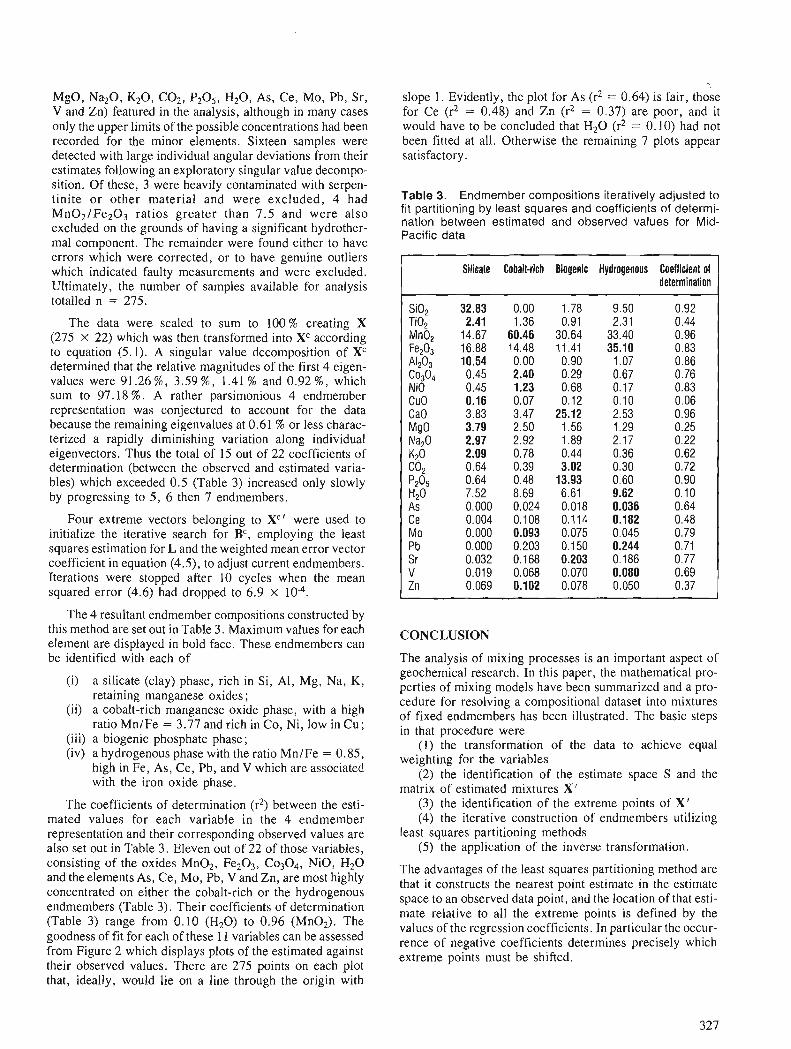
MgO, Na20, K20, C02, P2O5, H20, AS, Ce, Mo, Pb, Sr, V and Zn) featured in the analysis, although in many cases only the upper limits of the possible concentrations had been recorded for the minor elements. Sixteen samples were detected with large individual angular deviations from their estimates following an exploratory singular value decomposition. Of these, 3 were heavily contaminated with serpen- tinite or other material and were excluded, 4 had Mn02/Fe203 ratios greater than 7.5 and were also excluded on the grounds of having a significant hydrothermal component. The remainder were found either to have errors which were corrected, or to have genuine outliers which indicated faulty measurements and were excluded. Ultimately, the number of samples available for analysis totalled n = 275.

The data were scaled to sum to 100% creating X (275 X 22) which was then transformed into XC according to equation (5.1). A singular value dccomposition of XC determined that the relative magnitudes of the first 4 eigenvalues were 91.26 %, 3.59 %, 1.41 % and 0.92 %, which sum to 97.18 %. A rather parsimonious 4 endmember representation was conjectured to account for the data because the remaining eigenvalues at 0.61 % or less characterized a rapidly diminishing variation along individual eigenvectors. Thus the total of 15 out of 22 coefficients of determination (between the observed and estimated variables) which exceeded 0.5 (Table 3) increased only slowly by progressing to 5, 6 then 7 endmembers.

Four extreme vectors belonging to XC' were used to initialize the iterative search for BC, employing the least squares estimation for L and the weighted mean error vector coefficient in equation (4.5), to adjust current endmembers. Iterations were stopped after 10 cycles when the mean squared error (4.6) had dropped to 6.9 x

The 4 resultant endmember compositions constructed by this method are set out in Table 3. Maximum values for each element are displayed in bold face. These endmembers can be identified with each of

(i) a silicate (clay) phase, rich in Si, Al, Mg, Na, K , retaining manganese oxides ;

(ii) a cobalt-rich manganese oxide phase, with a high ratio Mn/Fe = 3.77 and rich in Co, Ni, low in Cu;

(iii) a biogenic phosphate phase; (iv) a hydrogenous phase with the ratio Mn/Fe = 0.85,

high in Fe, As, Ce, Pb, and V which are associated with the iron oxide phase.

The coefficients of determination (r2) between the estimated values for each variable in the 4 endmember representation and their corresponding observed values are also set out in Table 3. Eleven out of 22 of those variables, consisting of the oxides Mn02, Fe203, Co3O4, NiO, H20 and theelements As, Ce, Mo, Pb, V and Zn, are most highly concentrated on either the cobalt-rich or the hydrogenous endmembers (Table 3). Their coefficients of determination (Table 3) range from 0.10 (H20) to 0.96 (Mn02). The goodness of fit for each of these 1 1 variables can be assessed from Figure 2 which displays plots of the estimated against their observed values. There are 275 points on each plot that, ideally, would lie on a line through the origin with

slope 1. Evidently, the plot for As (r2 = 0.64) is fair, those for Ce (r2 = 0.48) and Zn (r2 = 0.37) are poor, and it would have to be concluded that H20 (r2 = 0.10) had not been fitted at all. Otherwise the remaining 7 plots appear satisfactory.

Table 3. Endmember compositions iteratively adjusted to fit partitioning by least squares and coefficients of determination between estimated and observed values for Mid- Pacific data

Silicale Cobalt-rich Biogenic Hydrogenous Coefficient ol delermination

Si02 32.83 0.00 1.78 9.50 0.92 Ti02 2.41 1.36 0.91 2.31 0.44 MnO, 14.67 60.46 30.64 33.40 0.96 Fe,O, 16.88 14.48 11.41 35.10 0.83 AI2O3 10.54 0.00 0.90 1.07 0.86 Co3o4 0.45 2.40 0.29 0.67 0.76 NiO 0.45 1.23 0.68 0.17 0.83 CuO 0.16 0.07 0.12 0.10 0.06 CaO 3.83 3.47 25.12 2.53 0.96 MgO 3.79 2.50 1.56 1.29 0.25 Na20 2.97 2.92 1.89 2.17 0.22 K20 2.09 0.78 0.44 0.36 0.62 co2 0.64 0.39 3.02 0.30 0.72 P2°5 0.64 0.48 13.93 0.60 0.90 H20 7.52 8.69 6.61 9.62 0.10 As 0.000 0.024 0.018 0.036 0.64 Ce 0.004 0.108 0.114 0.182 0.48 Mo 0.000 0.093 0.075 0.045 0.79 Pb 0.000 0.203 0.150 0.244 0.71 Sr 0.032 0.168 0.203 0.186 0.77 V 0.019 0.068 0.070 0.080 0.69 Zn 0.069 0.102 0.078 0.050 0.37

CONCLUSION

The analysis of mixing processes is an important aspect of geochemical research. In this paper, the mathematical properties of mixing models have been summarized and a procedure for resolving a compositional dataset into mixtures of fixed endmembers has been illustrated. The basic steps in that procedure were

( I ) the transformation of the data to achieve equal weighting for the variables

(2) the identification of the estimate space S and the matrix of estimated mixtures X'

(3) the identification of the extreme points of X ' (4) the iterative construction of endmembers utilizing

least squares partitioning methods (5) the application of the inverse transformation.

The advantages of the least squares partitioning method are that it constructs the nearest point estimate in the estimate space to an observed data point, and the location of that estimate relative to all the extreme points is defined by the values of the regression coefficients. In particular the occurrence of negative coefficients determines precisely which extreme points must be shifted.

REFERENCES

Aitchison, J. 1986: The Statistical Analysis of Compositional Data; Chapman and

Hall. London and New York, 416 pa. Bazaraa, M.S. and Shetty, C.M. 1979: Nonlinear Programming; John Wiley and Sons, New York, 560 p. Chayes, F. 1960: On correlation between variables of constant sum; Journal of

Geophysical Research, v. 65, p.4185-4 193. Clarke, T.L. 1978: An oblique factor analysis solution for the analysis of mixtures;

Mathematical Geology, v. 10, p.225-24 1 . Dymond, J. 1981 : Geochemistry of Nazca plate surface sediments: An evaluation of

hydrothermal, biogenic, detrital, and hydrogenous sources; Geo- logical Society of America Memoir 154, p. 133-173.

Dymond, J., Lyle, M., Finney, B., Piper, D.Z., Murphy, K., Conard, R., and Pisias, N. 1984: Ferromanganese nodules from MANOP sites H, S, and R -Control

of mineralogical and chemical composition by multiplc accretionary processes; Geochimica et Cosmochimica Acta, v. 48, p.93 1-949.

Full, W.E. and Ehrlich, R. 1986: Comment on "An objective technique for determining end-

member compositions and for partitioning sediments according to theirsources" ; Geochimica et Cosmochimica Acta, v. 50, p. 1303.

Full, W.E., Ehrlich, R., and Bezdek, J.C. 1982: Fuzzy QMODEL - A new approach for linear unmixing; Mathe-

matical Geology, v. 14, p.259-270. Full, W.E., Ehrlich, R., and Klovan, J.E. 1981: EXTENDED QMODEL - Objective definition of external end

members in the analysis of mixtures; Mathematical Geology, v . 13, p.331-344.

Hadley, G . 1962: Linear Programming; Addison-Wesley Publishing Company Inc.,

Reading, Massachusetts, 520 p. Imbrie, J. 1963: Factor and Vector Analysis Programs for Analyzing Geologic

Data; Technical Report No. 6ofONRTask No. 389-135, Contract Nonr 1228(26), Office of Naval Research, Geography Branch, 83 P.

Imbrie, J. and Van Andel, T.H. 1964: Vector analysis of heavy-mineral data; Geological Society of Ame-

rica, Bulletin, v . 75, p.1 131-1 156. Joreskog, K.G., Klovan, J.E., and Reyment, R.A. 1976: Methods in Geomathematics I ; Geological Factor Analysis; Else-

vier, Amsterdam, 178 p.

Klovan, J.E. 1966: The use of factor analysis in determining depositional environ-

ments from grain-size distributions; Journal of Sedimentary Petro- logy, v. 36, p.115-125.

Klovan, J.E. and Imbrie, J. 197 1 : An algorithm and FORTRAN-IV program for large-scale Q-mode

factor analysis and calculation of factor scores ; Mathematical Geo- logy, v. 3, p.61-76.

Lane, C.M., Manheim, F.T., Hathaway, J.C., and Ling, T.H. 1986: Station Maps of The World Ocean - Ferromanganese - Crust

data base; U.S. Geological Survey, Miscellaneous Field Studies Map, MF-1869.

Leinen, M. 1987: The origin of paleochemical signature in North Pacific pelagic

clays: Partitioning experiments; Geochimica et Cosmochimica Acta, v. 51, p.305-319.

Leinen, M. and Pisias, N. 1984: An objective technique for determining end-member compositions

and for partitioning sediments according to their sources; Geochi- mica et Cosrnochimica Acta, v. 48, p.47-62.

Miesch, A.T. 1976a: Q-mode factor analysis of compositional data; Computers and

Geosciences, v. 1, p. 147-159. 1976b: Q-mode factor analysis of geochemical and petrologic data matri-

ces with constant row sums; Statistical Studies in Field Geoche- mistry, U.S. Geological Survey, Professional Paper 574-G, 47 p.

1980: Scaling variables and interpretation of eigenvalues in principal component analysis of geologic data; ath he ma tical ~ e o l o ~ ~ , v. 12, p. 523-538.

Owen, R.M. 1987: Geostatistical problems in marine placer exploration Marine

Minerals; ed. P.G. Teleki, M.R. Dobson, J.R. Moore, and V. von Stackelberg, D. Reidel Publishing Company, Dordrecht, p. 533-540.

Rao, C.R. 1973 : Linear Statistical Inference and Its Applications, 2nd edition ; John

Wiley and Sons. New York. 625 pages. Renner, R.M. 1982: Sediment analysis: A Q-mode approach; The New Zealand Statis-

tician, v. 17, No. 2, p. 12-17. 1988: On the resolution of compositional datasets into convex combina-

tions of extreme vectors; Technical Report No. 88/02, Institute of Statistics and Operations Research, Victoria University of Wel- lington, PO Box 600, Wellington, New Zealand, 35 p.

Spatial factor analysis: a technique to assess the spatial relationships of multivariate data

Eric Grunskyl

Grunsky, E., Spatial factor analysis: a technique to assess the spatial relationships of multivariate data; in Statistical Applications in the Earth Sciences, ed. F. P. Agterberg and G. F. Bonham-Carter; Geologi- - cal Survey of Canada, Paper 89-9, p. 329-347, 1989.

Abstract

Estimates of auto- and crosscorrelations of variables can be combined to form a matrix from which linear combinations of variables can be determined representing "spatial factors". Estimates of the spatial auto- and crosscorrelation relationships are determined from quadratic function approximations. The calculation of the spatial factors requires computation of the corresponding amplitude vectors from the eigenvalue solution. The amplitude vector reflects the relative amplitudes by which the variables follow the spatial factors. Instability of some of the eigenvalue solutions requires that caution be used in interpreting the resulting factor patterns. A measure of the predictive power of the spatial factors can be determined from the autocorrelation coeflcients and squared multiple correlation coeficients. The squared multiple correlation coeficients can be used to determine the relative signijcance of the variables.

7 l e spatial factor technique has been tested by the use of unconditional simulations which provide a basis by which geological variables of varying spatial ranges can be modelled. Simulations were generated over a variety of spatial ranges. Variables were then created by constructing linear combinations of simulated the spatial patterns. The success of the spatial factor technique depends on the amount of associated noise, and the size of the neighbourhood relative to the spatial range of the variable. The predictive power of the components is dependent on these two factors. Problems with collinearity of variables can result in unrealistic eigenvalues and subsequent failure of the method.

The spatial factor technique was applied to a suite of metavolcanic rocks in Ben Nevis Township, Ontario. The method was successful in outlining areas of spatial continuity that represent a primary magmatic trend, a large regional zone of carbonatization and zones of potassium and sulphur enrichment that are related to mineralization.

Des estimations des autocorrklations et des corrklations croiskes entre variables peuvent Ctre combinkes en une matrice de laquelle des combinaisons lintfaires de variables reprksentant des .c facteurs spatiaux B peuvent Ctre dktermine'es. Des estimations des relations spatiales entre autocorr&lations et corrtflations croiskes sont dkterminkes d'aprgs des approximations de fonctions quadratiques. L'ktablissement des facteurs spatiaux exige des calculs de vecteurs d'amplitude correspondants d'aprds la solution des valeurs propres. Le vecteur d'amplitude reJlkte les amplitudes relatives en fonction desquelles les variables suivent les facteurs spatiaux. L'instabilite' de certaines des solutions des valeurs propres appelle h la prudence lors de l'interprktation des conjgurations rtfsultantes de facteurs. Une mesure de I'eficacite'prkdictive des facteurs spatiaux peut Stre deiivke des coeficients d'autocorr6lation et du carrtf des coeficients de corr&lation multiple. Les coeflcients de corrtflation multiple au carre' peuvent servir a dkterminer 1 'importance relative des variables.

La mtfthode des facteurs spatiaux a kt& kprouvke par l'utilisation de simulations non conditionnelles fournissant une base en fonction de laquelle des variables d'amplitudes spatiales varikes peuvent &tre

' Division of Exploration Geoscience, Commonwealth Scientific Industrial Research Organisation, Wembley, 6014, Western Australia

mod&lis&es. Des simulations ont itk produites pour toute Line gamme d 'amplitude spatiales. Les variables ont ensuite 6tc' crke'es par la construction de combinaisons de con$gurations spatiales simulkes. Le succks de la rnkthode du facteur spatial depend de la quantitk de bruit associe' et des dimensions du voisinage par rapport L? 1 'amplitude spatiale de la variable. L 'eficacitc' prkdictive des composantes dc'pend de ces deux facteurs. Des probltmes de colin6arit6 des variables peuvent entrafner des valeurs propres non rkalistes et url khec ultkrieur de la mkthode.

La methode du facteur spatial a c'te'appliqu6e L? un ensemble de roches volcaniques m6tamorphis6es duns le canton de Ben Nevis en Ontario. Elle a permis de dklimiter avec succts des zones de continuitc' spatiale reprc'sentant une tendarzce rnagmatique primaire, une grande zone rkgionale de houillijication et des zones d'enrichissernent en potassium et en soufie qui sont relikes d la min6ralisation.

INTRODUCTION

Multivariate relationships between variables are commonly expressed in the form of matrices that reflect variance- covariance, correlation, contingency tables, and other metrics that provide measures of association. Various methods of factor analysis have been derived by which the relationships between variables (R-mode analysis), and the relationships between samples (Q-mode analysis) can be determined (Agterberg, 1974; LeMaitre, 1982; Joreskog et al, 1976; Davis, 1986). The main advantage of these methods of data analysis is that they reduce the number of variables required to describe the relationships between the variables and the relationships between the samples. Numerous examples of applying methods of factor analysis in geological applications exist in the literature (see Agterberg, 1974; LeMaitre, 1982; Joreskog et al, 1976).

Spatial relationships between sample points are usually estimated by methods of auto- and crosscorrelation or by geostatistical methods using the semi- and covariogram. Estimates of spatial relationships have been based on several statistical models and are described by Journel and Huij- bregts (1978), Bennett (1979), and Upton and Fingleton (1985). Agterberg (1970) and Haining (1 987) employed quadratic functions as estimates of spatial auto- and crosscorrelation forming the basis of the work discussed here.

Multivariate relationships between samples that account for distance in space have been used by several workers (Agterberg, 1966, 1974; Myers, 1982, 1988; Royer, 1988; Switzer and Green, 1984; and Wackernagel, 1988).

'The application of the spatial factor technique will be demonstrated using two examples. The first example employs the use of unconditional simulations, and the second example is an application to a geochemical dataset from the Ben Nevis area of Ontario, Canada.

The use of simulations is widespread in the mining industry as a means of assessing the ore grade variability of a deposit using the spatial covariance model of the deposit itself. Discussions of simulation are given by Journel and Huijbregts (1978), and an extensive discussion on simulation techniques is given by Luster (1986). Unconditional simulations refer to randomly chosen locations of a realization of a random function and can be used to model variables with different spatial characteristics. Several variables can be modelled in which each variable can have a unique range

and sill. The application of the spatial factor technique to these modelled variables produces linear combinations of variables that share similar spatial characteristics.

Archean lode gold deposits are typically associated with alteration in the form of carbonatization, sulphur and potassium enrichment, and proximity to shears and faults (Col- vine et al, 1988). A suite of metavolcanics in the Ben Nevis area, Ontario, Canada, contains three significant spatial patterns ; a primary magmatic variation of the volcanics, a large regional zone of carbonatization centred along a major north-south fault, and smaller zones of K and S enrichment associated with Au-Cu mineralization. Several small sulphide occurrences also exist throughout the area. The application of the spatial factor technique to this geochemical dataset can be used to determine linear combinations of geochemical variables with similar spatial characteristics that represent primary magmatic trends, and zones of alteration potentially associated with mineralization. This approach can assist, along with other exploration methods, in the selection of potential exploration targets for ore mineralization.

THE AUTOCORRELATION FUNCTION AS A QUADRATIC MODEL

The technique of spatial factor analysis requires estimates of the auto- and cross correlations of the variables over a range of distances, termed, "neighbourhoods" . A simple model for estimating a quadratic approximation to the autocorrelation function from irregularly spaced data was originally proposed by Agterberg (1970) and based on the equation :

where xi and xj denote values of a random variable X with zero mean measured at two different points in the plane labelled i and j. Both i and j go from 1 to N where N denotes total number of observations. F(dij) is a quadratic function of distance dij between these two points. The function is considered to decay to zero at the maximum distance of the "neighbourhood" for which it is defined. The residual yi is the realization of a random variable Y i at point i. It satisfies E(Yi) = 0 and Yi is assumed to be independent of Xj. The function is thus defined as

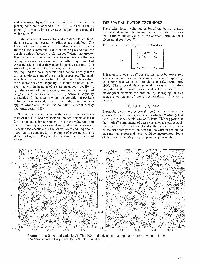
and is estimated by ordinary least squares after successively pairing each point labelled i (i = 1,2, ..., N) with the Ni points (j) located within a circular neighborhood around i with radius D.

Estimates of unknown auto- and crosscorrelation functions assume that certain conditions are satisfied. The Cauchy-Schwarz inequality requires that the autocorrelation function has a maximum value at the origin and that the absolute value of a crosscorrelation coefficient is not greater than the geometric mean of the autocorrelation coefficients of any two variables considered. A further requirement of these functions is that they must be positive definite. The parabolas, as models of estimation, do not fulfill the properties required for the autocorrelation function. Locally these estimates violate some of these basic properties. The quadratic functions are not positive definite, nor do they satisfy the Cauchy-Schwarz inequality. It should be noted, however, that within the range of use (i.e. neighbourhood limits, r,), the values of the functions are within the required range ( I 5 rh I 1) SO that the Cauchy-Schwarz inequality is satisfied. In the cases in which the condition of positive definiteness is violated, an adjustment algorithm has been applied which ensures that this condition is met (Grunsky and Agterberg, 1988).

The intercept of a parabola at the origin provides an estimate of the auto- and crosscorrelation coefficients at lag 0 for the various neighbourhoods. This is the value (a) from the quadratic equation shown above and provides a means by which the coefficients of other variables and neighbourhoods can be compared. An example of these functions is shown in Figure 2. They will be discussed in greater detail below.

THE SPATIAL FACTOR TECHNIQUE

The spatial factor technique is based on the correlation matrix R taken from the average of the quadratic functions that is the estimated values of the constant term, a, for a given neighbourhood D.

This matrix termed, Ro, is thus defined as:

a l l a12 -.-*.. a , , a 2 ~ a22 ------ a2,, . o [ : a,, an2 -..-.. a,, ]

This matrix is not a "true" correlation matrix but represents a variance-covariance matrix of signal values corresponding to standardized values of the elements (cf., Agterberg, 1970). The diagonal elements in this array are less than unity due to the "noise" component of the variables. The off-diagonal elements are obtained by averaging the two separate estimates of the crosscorrelation functions, namely,

[F~(dji) + F ~ ( d i ~ ) I / 2 . 0

Extrapolation of the crosscorrelation function to the origin can result in correlation coefficients which are usually less than the ordinary correlation coefficients. This suggests that the "noise" components of these variables are either positively correlated or not correlated with one another. It can be assumed that part of the noise in the variables is due to measurement errors and these would be uncorrelated. Some of the local variability may be positively correlated.

Figure 1. (a) Simulated variable V1. The 500 randomly chosen sample sites are shown on this map. The scale is in arbitrary units. (b) Simulated variable V5

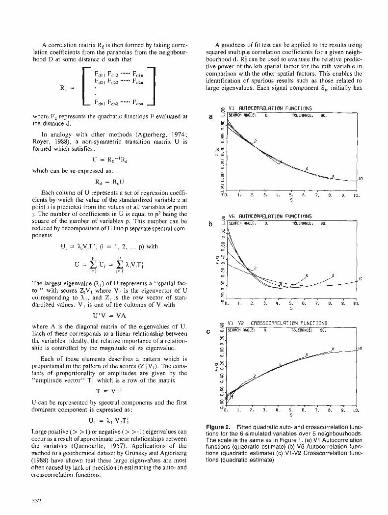
A correlation matrix Rd is then formed by taking correlation coefficients from the parabolas from the neighbourhood D at some distance d such that

Fdll Fd12 """ Fdln Fd21 Fd22 '***.. Fd2n

R. = [ ] Fdnl Fdn2 "".' Fdnn

where Fd represents the quadratic functions F evaluated at the distance d.

In analogy with other methods (Agterberg, 1974; Royer, 1988), a non-symmetric transition matrix U is formed which satisfies :

which can be re-expressed as:

Each column of U represents a set of regression coefficients by which the value of the standardized variable z at point i is predicted from the values of all variables at point j. The number of coefficients in U is equal to p2 being the square of the number of variables p. This number can be reduced by decomposition of U into p separate spectral components

Ui = XiViT1, (i = 1, 2, ... p) with

The largest eigenvalue (Al) of U represents a "spatial factor" with scores ZiVl where V, is the eigenvector of U corresponding to h , , and Zi is the row vector of standardized values. VI is one of the columns of V with

U'V = VA

where A is the diagonal matrix of the eigenvalues of U. Each of these corresponds to a linear relationship between the variables. Ideally, the relative importance of a relationship is controlled by the magnitude of its eigenvalue.

Each of these elements describes a pattern which is proportional to the pattern of the scores (Z { V ,). The constants of proportionality or amplitudes are given by the "amplitude vector" Ti which is a row of the matrix

U can be represented by spectral components and the first dominant component is expressed as:

Large positive (> > 1) or negative (> > - I ) eigenvalues can occur as a result of approximate linear relationships between the variables (Quenouille, 1957). Applications of the method to a geochemical dataset by Grunsky and Agterberg (1988) have shown that these large eigenvalues are most often caused by lack of precision in estimating the auto- and crosscorrelation functions.

A goodness of fit test can be applied to the results using squared multiple correlation coefficients for a given neighbourhood d. R i can be used to evaluate the relative predictive power of the kth spatial factor for the mth variable in comparison with the other spatial factors. This enables the identification of spurious results such as those related to large eigenvalues. Each signal component S, initially has

o V 1 RUTOCORRELRTIBN FUNCTIONS ~ ) ~ E W C H ANGLE: 0. TOLERANCE: 90. 1

g V6 FIUTOCORRELFITIBN FUNCTIONS TOLERANCE: 90. I

Figure 2. Fitted quadratic auto- and crosscorrelation functions for the 6 simulated variables over 5 neighbourhoods. The scale is the same as in Figure 1. (a) V1 Autocorrelation functions (quadratic estimate) (b) V6 Autocorrelation functions (quadratic estimate) (c) V1-V2 Crosscorrelation functions (quadratic estimate)

V1 V2 CROSSCORRELRTION FUNCTIONS

c 6 0 N.

0

SERRCH ANGLE: 0. TOLERANCE: 90.

variance a,. It can therefore be said that, with p variables, the total variation within the U transition matrix is equal to

For prediction of S, at point i from all p variables at point j,

where U,, represents the mth column of U. If Rdm is the mth column of Rd, the squared multiple correlation coefficient R,$ for predictive power with respect to the mth variable satisfies :

Total predictive power of U can be expressed by means of the quantity Q with:

P

Q = a , R $ / T rn= I

Thus each spatial factor can be tested as to its contribution to the overall spatial structure of the data and a quantitative assessment of its goodness of fit can be assigned.

EXAMPLE 1 : APPLICATION OF THE SPATIAL FACTOR TECHNIQUE TO UNCONDITIONAL SIMULATIONS

A suitable test for measuring the effectiveness of the spatial factor technique would be to use a dataset composed of variables with well known spatial structures. One such method that is commonly used in geostatistics is that of unconditional simulation.

Unconditional simulations can be used to model variables with different spatial characteristics. A series of individual simulations can be combined to form variables that are linear combinations of the simulations. In this way variables can be created which attempt to simulate geological conditions.

A variable with a true value of Zo(x) at each point x within a map area can be interpreted geostatistically as a particular realization of a random function Z(x) (Journel and Huijbregts, 1978). The random function can be characterized by its first two moments and distribution function. The simulation of the variable can then be generated as a separate realization Z,(x) which represents one of many possible realizations of Z(x) that have the same spatial characteristics. Unconditional simulations refer to randomly chosen locations of the random function Z,(x).

A method of moving averages (Luster, 1986) was employed for the generation of the simulations. By using a circular model, the unconditional simulation process can be constructed by generating a set of independent identically distributed random numbers on a grid and then smoothing them with a constant valued circular moving window.

The moving average process is first defined as a random hnction X(u) for each point u in the n-dimensional space R". X(u) is second order stationary with E(x) = 0 and

covariance C,(h). The random function Y(t) is then defined for each point t in Rn as a weighted average of X(u) such that

f(t-u) is the weight function applied to each value X(u) which depends on the distance and direction (t-u) between the point t and each location u.

The unconditional simulation is composed of the following steps:

1) Generation of a grid of uniform (0- 1) independent random numbers X(u) over a finite domain of Rn.

2) Each grid node t in the simulation domain is assigned a value Y(t) equal to the sum of all x(u) located inside the hypersphere of diameter a, centred at t. The simulation domain must be smaller than the x(u) domain by the diameter of the hypersphere (a) in each direction.

Generation of the simulated fields was considered for a number of arbitrary ranges; a = 2, 4, 6, 8, and 10 units with a 50 X 50 grid size. The simulations were carried out assuming isotropy of the random functions.

CREATION OF MULTIPLE VARIABLE SIMULATION FIELDS

From the individual simulations, a multivariate dataset was created ; composed of patterns of various ranges. Theoreti- cally, each spatial simulation is a unique factor in the multivariate dataset. The creation of variables that are a multiple combination of each spatial realization as well as varying signal/noise ratios between the variables will increase the complexity of the system. The spatial factor technique can then be tested over a range of simulations with varying degrees of complexity.

The realizations of the random functions derived above were combined to form 6 new variables. Each variable is a linear combination of the three conditioned simulated variables in which coefficients define the relative amplitudes of each of the realizations.

The realizations are defined as:

Range a = 10

Variable

Variable

The variables Z2, Z4, and Z6 are the same realizations as Z1, Z3, and Z5 but opposite in sign. This is to reflect variables that are inversely related, yet have the same spatial characteristics. An example are the magmatic relationships of Si, Fe, and Mg in volcanic rocks. Si usually tenas to be inversely proportional to Fe, and Mg. In this experiment, the elements whose abundances are related to magmatic processes are dominated by the realization of the largest range (ZI , and Z2). As well, an additional realization is imposed on the variables which simulates an additional

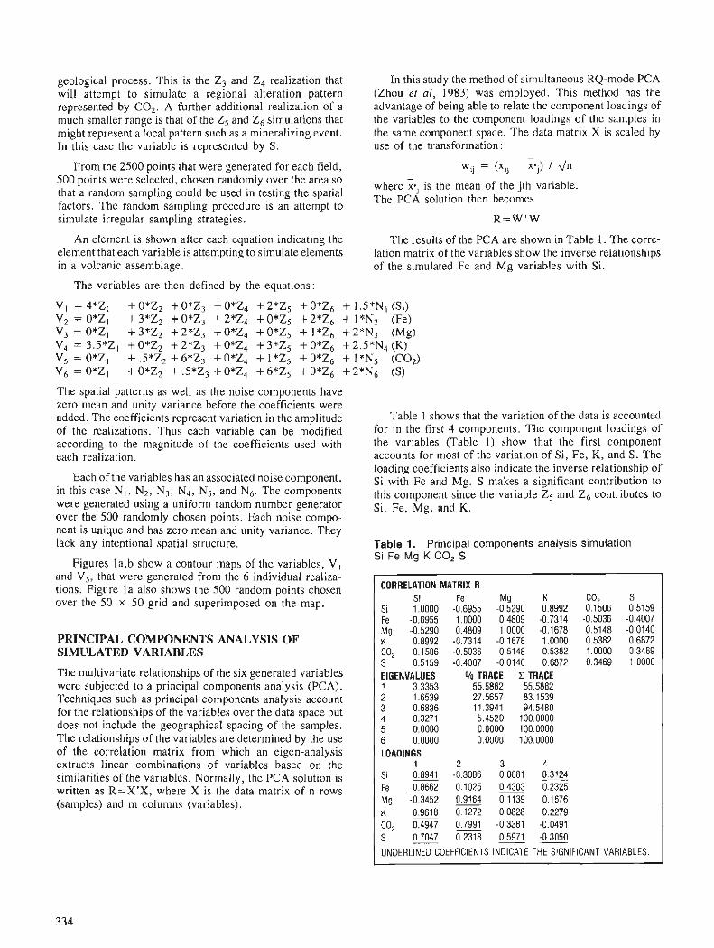
geological process. This is the Z3 and Z4 realization that will attempt to simulate a regional alteration pattern represented by C02. A further additional realization of a much smaller range is that of the Z5 and Z6 simulations that might represent a local pattern such as a mineralizing event. In this case the variable is represented by S.

From the 2500 points that were generated for each field, 500 points were selected, chosen randomly over the area so that a random sampling could be used in testing the spatial factors. The random sampling procedure is an attempt to simulate irregular sampling strategies.

An element is shown after each equation indicating the element that each variable is attempting to simulate elements in a volcanic assemblage.

In this study the method of simultaneous RQ-mode PCA (Zhou et al, 1983) was employed. This method has the advantage of being able to relate the component loadings of the variables to the component loadings of the samples in the same component space. The data matrix X is scaled by use of the transformation:

-

wij = (xij - xsj) / Jn

where ;aj is the mean of the jth variable. The PCA solution then becomes

R = W I W

The results of the PCA are shown in Table 1. The correlation matrix of the variables show the inverse relationships of the simulated Fe and Mg variables with Si.

The variables are then defined by the equations:

V I = 4*Z1 + 0*Z2 + 0*Z3 + 0*Z4 + 2*Z5 + 0*Z6 + 1 .5*Nl (Si) V2 = O*ZI + 3*Z2 + 0*Z3 + 2*Z4 + 0*Z5 + 2*Z6 + 1 *N2 (Fe) Vj = O*ZI + 3*Z2 + 2*Z3 + 0*Z4 + O*Zs + l*Z6 + 2*N3 (Mg) V4 = 3.5*Z1 + 0*Z2 + 2*Z3 + 0*Z4 + 3*Z5 + 0*Z6 + 2.5*N4 (K) V5 = O*Z I + .5*Z2 + 6*Z3 + 0*Z4 + 1 *Zs + 0*Z6 + 1 *N5 (COz) V6 = O*ZI + 0*Z2 + .5*Z3 + 0*Z4 + 6*Z5 + 0*Z6 + 2*N6 (S)

The spatial patterns as well as the noise components have zero mean and unity variance before the coefficients were added. The coefficients represent variation in the amplitude of the realizations. Thus each variable can be modified according to the magnitude of the coefficients used with each realization.

Each of the variables has an associated noise component, in this case N, , N2, N3, N4, N5, and N6. The components were generated using a uniform random number generator over the 500 randomly chosen points. Each noise component is unique and has zero mean and unity variance. They lack any intentional spatial structure.

Figures la,b show a contour maps of the variables, V, and V5, that were generated from the 6 individual realizations. Figure la also shows the 500 random points chosen over the 50 x 50 grid and superimposed on the map.

PRINCIPAL COMPONENTS ANALYSIS OF SIMULATED VARIABLES

The multivariate relationships of the six generated variables were subjected to a principal components analysis (PCA). Techniques such as principal components analysis account for the relationships of the variables over the data space but does not include the geographical spacing of the samples. The relationships of the variables are determined by the use of the correlation matrix from which an eigen-analysis extracts linear combinations of variables based on the similarities of the variables. Normally, the PCA solution is written as R=X'X, where X is the data matrix of n rows (samples) and m columns (variables).

Table 1 shows that the variation of the data is accounted for in the first 4 components. The component loadings of the variables (Table 1) show that the first component accounts for most of the variation of Si, Fe, K, and S. The loading coefficients also indicate the inverse relationship of Si with Fe and Mg. S makes a significant contribution to this component since the variable Z5 and Z6 contributes to Si, Fe, Mg, and K.

Table 1. Principal components analysis simulation Si Fe Mg K CO, S

CORRELATION MATRIX R Si Fe Mg K co, S

Si 1.0000 -0.6955 -0.5290 0.8992 0.1506 0.5159 Fe -0.6955 1.0000 0.4809 -0.7314 -0.5036 -0.4007 Mg -0.5290 0.4809 1.0000 -0.1678 0.5148 -0.0140 K 0.8992 -0.7314 -0.1678 1.0000 0.5382 0.6872 CO, 0.1506 -0.5036 0.5148 0.5382 1.0000 0.3469 S 0.5159 -0.4007 -0.0140 0.6872 0.3469 1.0000 EIGENVALUES % TRACE Z TRACE 1 3.3353 55.5882 55.5882 2 1.6539 27.5657 83.1539 3 0.6836 11.3941 94.5480 4 0.3271 5.4520 100.0000 5 0.0000 0.0000 100.0000 6 0.0000 0.0000 100.0000 LOADINGS

1 2 3 4 Si 0.8941 -0.3086 0.0881 0.3124 Fe -0.8662 0.1025 0.4303 0.2325 Mg -0.3452 0.9164 0.1139 0.1676 K 0.9618 0.1272 0.0828 0.2279 CO, 0.4947 0.7991 -0.3381 -0.0491 S 0.7047 0.2318 0.5971 -0.3050

UNDERLINED COEFFICIENTS INDICATE THE SIGNIFICANT VARIABLES.

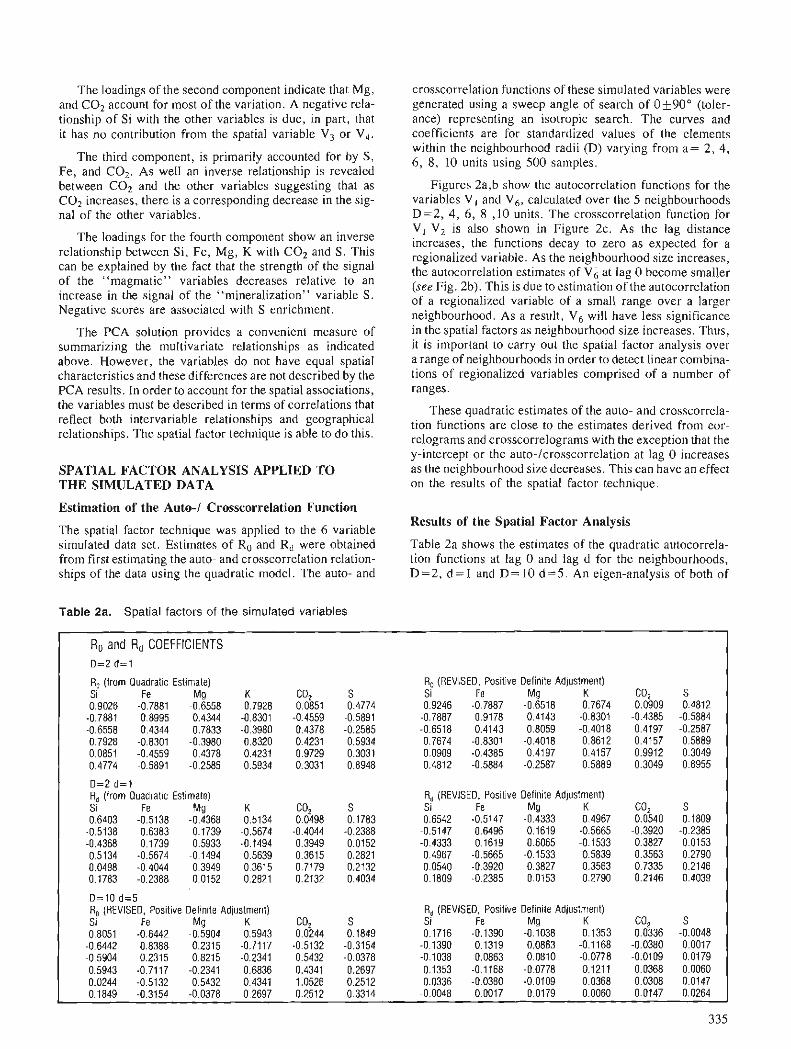
The loadings of the second component indicate that Mg, and C02 account for most of the variation. A negative relationship of Si with the other variables is due, in part, that it has no contribution from the spatial variable V3 or V4.

The third component, is primarily accounted for by S, Fe, and COz. As well an inverse relationship is revealed between C02 and the other variables suggesting that as C02 increases, there is a corresponding decrease in the signal of the other variables.

The loadings for the fourth component show an inverse relationship between Si, Fe, Mg, K with C02 and S . This can be explained by the fact that the strength of the signal of the "magmatic" variables decreases relative to an increase in the signal of the "mineralization" variable S. Negative scores are associated with S enrichment.

The PCA solution provides a convenient measure of summarizing the multivariate relationships as indicated above. However, the variables do not have equal spatial characteristics and these differences are not described by the PCA results. In order to account for the spatial associations, the variables must be described in terms of correlations that reflect both intervariable relationships and geographical relationships. The spatial factor technique is able to do this.

SPATIAL FACTOR ANALYSIS APPLIED TO THE SIMULATED DATA

Estimation of the Auto-l Crosscorrelation Function

The spatial factor technique was applied to the 6 variable simulated data set. Estimates of Ro and Rd were obtained from first estimating the auto- and crosscorrelation relationships of the data using the quadratic model. The auto- and

crosscorrelation functions of these simulated variables were generated using a sweep angle of search of 0+_90° (tolerance) representing an isotropic search. The curves and coefficients are for standardized values of the elements within the neighbourhood radii (D) varying from a= 2, 4, 6, 8, 10 units using 500 samples.

Figures 2a,b show the autocorrelation functions for the variables V , and V6, calculated over the 5 neighbourhoods D=2, 4, 6, 8 ,10 units. The crosscorrelation function for V I - V 2 is also shown in Figure 2c. As the lag distance increases, the functions decay to zero as expected for a regionalized variable. As the neighbourhood size increases, the autocorrelation estimates of Vk at lag 0 become smaller (see Fig. 2b). This is due to estimation of the autocorrelation of a regionalized variable of a small range over a larger neighbourhood. As a result, V6 will have less significance in the spatial factors as neighbourhood size increases. Thus, it is important to carry out the spatial factor analysis over a range of neighbourhoods in order to detect linear combinations of regionalized variables comprised of a number of ranges.

These quadratic estimates of the auto- and crosscorrelation functions are close to the estimates derived from cor- relograms and crosscorrelograrns with the exception that the y-intercept or the auto-/crosscorrelation at lag 0 increases as the neighbourhood size decreases. This can have an effect on the results of the spatial factor technique.

Results of the Spatial Factor Analysis

Table 2a shows the estimates of the quadratic autocorrelation functions at lag 0 and lag d for the neighbourhoods, D =2, d = l and D= 10 d =5. An eigen-analysis of both of

Table 2a. Spatial factors of the simulated variables

Ro and Rd COEFFICIENTS D=2 d=1

R, (from Quadratic Estimate) R, (REVISED, Positive Definite Adjustment) Si Fe Mg K G o 2 S Si Fe Mg K CO, S 0.9026 -0.7881 -0.6558 0.7928 0.0851 0.4774 0.9246 -0.7887 -0.651 8 0.7674 0.0909 0.4812

-0.7881 0.8995 0.4344 -0.8301 -0.4559 -0.5891 -0.7887 0.9178 0.4143 -0.8301 -0.4385 -0.5884 -0.6558 0.4344 0.7833 -0.3980 0.4378 -0.2585 -0.6518 0.4143 0.8059 -0.4018 0.4197 -0.2587 0.7928 -0.8301 -0.3980 0.8320 0.4231 0.5934 0.7674 -0.8301 -0.4018 0.8612 0.4157 0.5889 0.0851 -0.4559 0.4378 0.4231 0.9729 0.3031 0.0909 -0.4385 0.4197 0.4157 0.9912 0.3049 0.4774 -0.5891 -0.2585 0.5934 0.3031 0.8948 0.4812 -0.5884 -0.2587 0.5889 0.3049 0.8955

D=2 d = l R, (from Quadratic Estimate) R, (REVISED, Positive Definite Adjustment) Si Fe Mg K '-332 S Si Fe Mg K CO, S 0.6403 -0.5138 -0.4368 0.5134 0.0498 0.1783 0.6542 -0.5147 -0.4333 0.4967 0.0540 0.1809

-0.5138 0.6383 0.1739 -0.5674 -0.4044 -0.2388 -0.5147 0.6496 0.1619 -0.5665 -0.3920 -0.2385 -0.4368 0.1739 0.5933 -0.1494 0.3949 0.0152 -0.4333 0.1619 0.6065 -0.1533 0.3827 0.0153 0.5134 -0.5674 -0.1494 0.5639 0.3615 0.2821 0.4967 -0.5665 -0.1533 0.5839 0.3563 0.2790 0.0498 -0.4044 0.3949 0.3615 0.7179 0.2132 0.0540 -0.3920 0.3827 0.3563 0.7335 0.2146 0.1783 -0.2388 0.0152 0.2821 0.2132 0.4034 0.1809 -0.2385 0.0153 0.2790 0.2146 0.4039

D=10 d=5 R, (REVISED, Positive Definite Adjustment) R, (REVISED, Positive Definite Adjustment) Si Fe Mg K co2 S Si Fe Mg K CO, S 0.8051 -0.6442 -0.5904 0.5943 0.0244 0.1849 0.1716 -0.1390 -0.1038 0.1353 0.0336 -0.0048

-0.6442 0.8388 0.2315 -0.7117 -0.5132 -0.3154 -0.1390 0.1319 0.0863 -0.1 168 -0.0380 0.0017 -0.5904 0.2315 0.8215 -0.2341 0.5432 -0.0378 -0.1038 0.0863 0.0810 -0.0778 -0.0109 0.0179 0.5943 -0.7117 -0.2341 0.6836 0.4341 0.2697 0.1353 -0.1168 -0.0778 0.1211 0.0368 0.0060 0.0244 -0.5132 0.5432 0.4341 1.0526 0.2512 0.0336 -0.0380 -0.0109 0.0368 0.0308 0.0147 0.1849 -0.3154 -0.0378 0.2697 0.2512 0.3314 -0.0048 0.0017 0.0179 0.0060 0.0147 0.0264

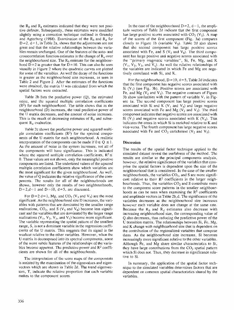
the Ro and Rd estimates indicated that they were not positive definite. Subsequently, these estimates were modified slightly using a correction technique outlined in Grunsky and Agterberg (1988). Examination of the Ro and Rd for D=2, d = 1 , in Table 2a, shows that the adjustments are not great and that the relative relationships between the variables remain unchanged. One of the features of the auto- and crosscorrelation function estimates is the change of R, over the neighbourhood size. The Ro estimate for the neighbourhood D=2 is greater than for D= 10. This can also be seen visually in Figure 2 where the quadratic curves are plotted for some of the variables. As well the decay of the functions is greater as the neighbourhood size increases, as seen in Table 2 and Figure 2. After the estimates of the functions were obtained, the matrix U was calculated from which the spatial factors were extracted.

Table 2b lists the predictive power (Q), the estimated noise, and the squared multiple correlation coefficients (R2) for each neighbourhood. The table shows that as the neighbourhood (D) increases, the total predictive power of the U matrix decreases, and the amount of noise increases. This is the result of decreasing estimates of Ro and subsequent Rd evaluation.

Table 2c shows the predictive power and squared multiple correlation coefficients (R2) for the spectral components of the U matrix for each neighbourhood. A realistic interpretation of the components can be made if 0 5 Q 5 I . As the amount of noise in the system increases, not all of the components will have significance. This is indicated where the squared multiple correlation coefficients, R2 5 0. These values are not shown, only the meaningful positive components are listed. The underlined values of the squared multiple correlation coefficients show which variables are the most significant for the given neighbourhood. As well, the value of Q indicates the relative significance of the components. The results for all of the neighbourhoods are shown, however only the results of two neighbourhoods, D=2,d= 1 and D= 10, d=5, are discussed.

For D =2 d = 1, Mg, and C 0 2 (V3 and V5) are the most significant. As the neighbourhood size D increases, the variables with patterns that are dominated by the smaller range realizations, C02, and S (V5 and V6) become less significant and the variables that are dominated by the larger range realizations (V,, V2, V3, and V4) become more significant. The variable representing the spatial pattern of the smallest range, S, is not a dominant variable in the regression coefficients of the U matrix. This suggests that its signal is the weakest relative to the other variables. However, when the U matrix is decomposed into its spectral components, some of the more subtle features of the relationships of the variables become apparent. The predictive power and R2 coefficients are shown for all of the neighbourhoods.

The interpretation of the score maps of the components is assisted by the examination of the eigenvalues and eigenvectors which are shown in Table 2d. The trend eigenvectors, T, indicate the relative proportion that each variable makes to the component scores.

In the case of the neighbourhood D=2, d= I , the amplitude vectors of Table 2d indicate that the first component has large positive scores associated with C 0 2 (V5). A map of the scores of the first component (Fig. 3a) compares closely to Figure Ib (variable V5). Table 2d also shows that the second component has large positive scores associated with Fe, and S (V2 and V6). The third component has large positive and negative scores associated with the "primary magmatic variables", Si, Fe, Mg, and K (V, , V2, V3, and V,). As well the relative relationships of the variables are indicated in which Fe and Mg are negatively correlated with Si, and K .

For the neighbourhood, D= 10, d = 5 , Table 2d indicates that the first component has negative scores associated with Si (V,) (see Fig. 3b). Positive scores are associated with Fe, and Mg (V2 and V3). The negative contours of Figure 3b show similarities with the pattern of variable V , in Fig- ure la. The second component has large positive scores associated with Si and K (V, and V4) and large negative scores associated with Fe and Mg (V2 and V3). The third component indicates that negative scores are associated with Si (V,) and negative scores associated with K (V4). This indicates the zones in which Si is enriched relative to K and vice-versa. The fourth component has large negative scores associated with Fe and C 0 2 enrichment (V2 and V5).

Discussion

The results of the spatial factor technique applied to the simulated dataset reveal the usefulness of the method. The results are similar to the principal components analysis, however, the relative significance of the variables that comprise the spatial factors is dependent upon the size of the neighbourhood that is considered. In the case of the smaller neighbourhoods, the variables C02, and S are more significant relative to their R2 coefficients in the larger neighbourhoods. Thus, the variables C 0 2 and S contribute more to the component score patterns in the smaller neighbourhoods as can be seen when examining the R2 coefficients and amplitude vectors in Table 2b,d. The significance of the variables decreases as the neighbourhood size increases however each variable does not change at the same rate. Because the Ro and Rd estimates also decrease with increasing neighbourhood size, the corresponding value of Q also decreases, thus reducing the predictive power of the U transition matrix. The relationships between Si, Fe, Mg, and K change with neighbourhood size that is dependent on the contribution of the regionalized variables that compose them. As the neighbourhood size increases, Si becomes increasingly more significant relative to the other variables. Although Fe, and Mg share similar characteristics to Si, they have large contributions from the C 0 2 spatial pattern which Si does not. Thus, they decrease in significance relative to Si.

In summary, the application of the spatial factor technique to the simulated variables determines factors that are dependent on common spatial characteristics shared by the variables.

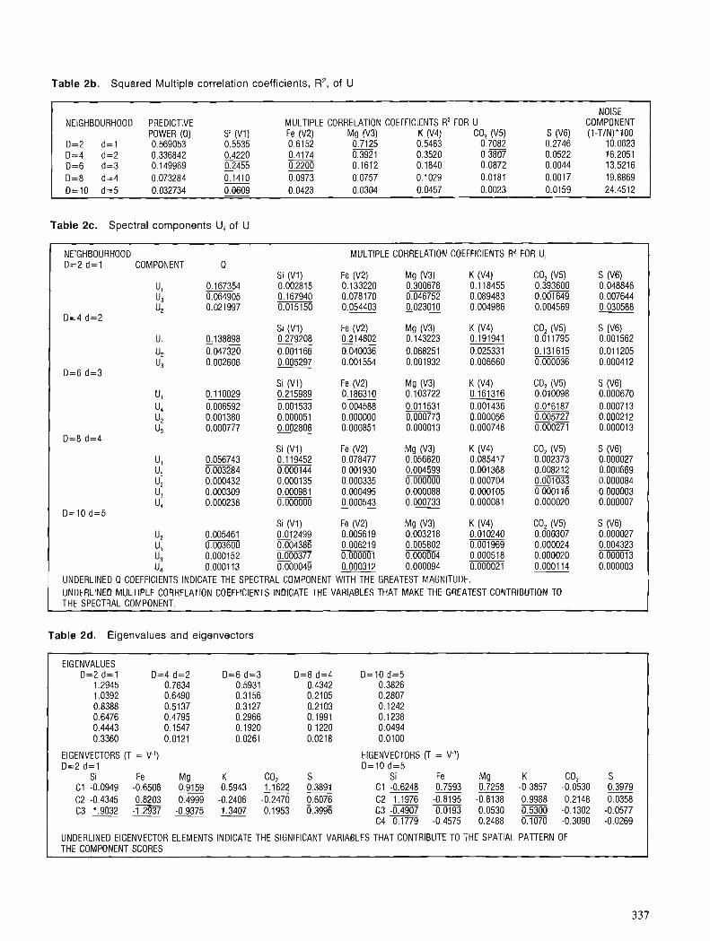
Table 2b. Squa red Mul t ip le cor re la t ion coef f ic ients, R2, o f U

NOISE NEIGHBOURHOOD PREDICTIVE MULTIPLE CORRELATION COEFFICIENTS R2 FOR U COMPONENT

POWER (a) Si (Vl) Fe (V2) Mg 0'3) K 0'4) GO2 0'5) S (V6) (1-T/N)*100 D=2 d=l 0.569053 0.5535 0.6152 - 0.7125 0.5483 0.7082 0.2746 10.0623 D=4 d=2 0.336842 0.4220 0.4174 0.3921 0.3520 0.3807 0.0522 16.2051 D=6 d=3 0.149969 [).2455 0.2200 0.1612 0.1840 0.0872 0.0044 13.5216 D=8 d=4 0.073284 0.1410 0.0973 0.0757 0.1029 0.0181 0.0017 19.8869 D=10 d=5 0.032734 0.0609 0.0423 0.0304 0.0457 0.0023 0.0159 24.4512

Table 2c. Spec t ra l c o m p o n e n t s Ui of U

NEIGHBOURHOOD MULTIPLE CORRELATION COEFFICIENTS R2 FOR Ui D=2 d= l COMPONENT Q

Si (Vl) Fe (V2) Mg (V3) K (V4) GO2 (V5) s (v6) UI 0.167354 0.002815 0.133220 0.300678 0.118455 0.393600 0.048846 "3 0.064905 0.167940 0.078170 0.046752 0.089483 0.001649 0.007644 u2 0.021997 0.054403 0.015150 0.02301 0 0.004986 0.004569 0.030588

D=4 d=2 Si (V1) Fe (V2) Mg (V3) K 0'4) c02 (v5) s (V6)

"1 0.138898 0.279208 0.214802 0.143223 0.191941 0.011795 0.001562

u2 0.047320 0.001 166 0.040036 0.068251 0.025331 0.131615 0.01 1205 "3 0.002606 0.005297 0.001554 0.001932 0.006660 0.000036 0.000412

D=6 d=3 Si (Vl) Fe (V2) Mg (V3) K 0'4) cop (V5)

0.186310 0.103722 0.161316 0.010098 S (V6)

u, 0.110029 0.215989 0.000670 u 4 0.006592 0.001533 0.004588 0.011531 0.001 436 0.016187 0.000713 u2 0.001380 0.000051 0.000000 0.000773 0.000056 0.005727 0.000212 u 3 0.000777 0.002806 0.000851 0.000013 0.000748 0.000271 0.000013

D=8 d=4 Si (Vl) Fe (V2) Mg (V3) K (V4) co2 (v5)

0.078477 0.056620 0.085417 0.002373 S (V6)

u 1 0.056743 0.119452 0.000027 "5 0.003284 iTmm4 0.001930 0.004599 0.001368 0.008212 0.000669 "2 0.000432 0.000135 0.000335 0.000000 0.000704 0.001033 0.000084 u3 0.000309 0.000981 0.000495 0.000088 0.000105 0.0001 16 0.000003 "4 0.000238 0.000000 0.000543 0.000733 0.000081 0.000020 0.000007

D=10 d=5 Si ( v i ) Fe (V2) Mg (V3) K (V4) CO, (V5) s (V6)

u2 0.005461 0.012499 0.005619 0.003218 0.010240 0.000307 0.000027 u1 0.003600 0.004386 0.006219 0.005802 0.001969 0.000024 0.004323 "3 0.000152 0.000377 0.000001 0.000004 0.000518 0.000020 0.000013 u4 0.000113 0.000049 0.000312 0.000094 0.000021 0.000114 0.000003

UNDERLINED Q COEFFICIENTS INDICATE THE SPECTRAL COMPONENT WITH THE GREATEST MAGNITUDE. UNDERLINED MLlLTlPLE CORRELATION COEFFICIENTS INDICATE THE VARIABLES THAT MAKE THE GREATEST CONTRIBUTION TO THE SPECTRAL COMPONENT.

Table 2d. Eigenva lues a n d e igenvec tors

EIGENVALUES D=2 d=1 D=4 d=2 D=6 d=3 D=8 d=4 D=10 d=5

1.2945 0.7634 0.5931 0.4342 0.3826 1.0392 0.6490 0.3156 0.2105 0.2807 0.8388 0.5137 0.3127 0.2103 0.1242 0.6476 0.4795 0.2966 0.1991 0.1238 0.4443 0.1547 0.1920 0.1220 0.0494 0.3360 0.0121 0.0261 0.0218 0.0100

EIGENVECTORS (T = V-') EIGENVECTORS (T = V.') D=2 d=1 D=10 d=5

Si Fe Mg K CO, S Si Fe Mg K CO, S C1 -0.0949 -0.6506 0.9159 0.5943 1.1622 0.3891 C1 -0.6248 0.7593 0.7258 -0.3857 -0.0530 0.3979 C2 -0.4345 0.8203 0.4999 -0.2406 -0.2470 0.6076 C2 1.1976 -0.8195 -0.6138 0.9988 0.2148 0.0358 C3 1.9032 -1.2937 -0.9375 1.3407 0.1953 0.3996 C3 -0.4907 0.0193 -0.0530 o.5300 -0.1302 -0.0577

C4 0.1779 -0.4575 0.2488 0.1070 -0.3090 -0.0269

LlNDERLlNED EIGENVECTOR ELEMENTS INDICATE THE SIGNIFICANT VARIABLES THAT CONTRIBLITE TO THE SPATIAL PATTERN OF THE COMPONENT SCORES

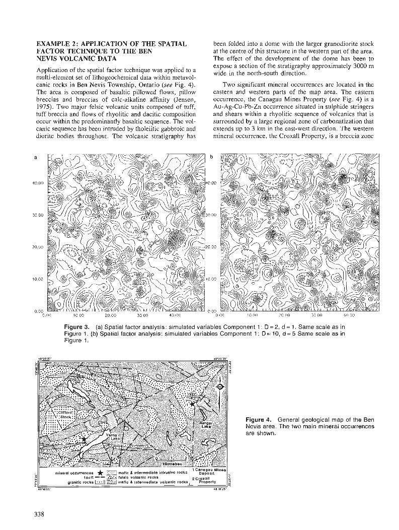
EXAMPLE 2: APPLICATION OF THE SPATIAL been folded into a dome with the larger granodiorite stock FACTOR TECHNIQUE TO THE BEN at the centre of this structure in the western part of the area. NEVIS VOLCANIC DATA The effect of the development of the dome has been to

Application of the spatial factor technique was applied to a multi-element set of lithogeochemical data within metavolcanic rocks in Ben Nevis Township, Ontario (see Fig. 4). The area is composed of basaltic pillowed flows, pillow breccias and breccias of calc-alkaline affinity (Jensen, 197.5). Two major felsic volcanic units composed of tuff, tuff breccia and flows of rhyolitic and dacitic composition occur within the predominantly basaltic sequence. The volcanic sequence has been intruded by tholeiitic gabbroic and diorite bodies throughout. The volcanic stratigraphy has

expose a section of the stratigraphy approximately 3000 m wide in the north-south direction.

Two significant mineral occurrences are located in the eastern and western parts of the map area. The eastern occurrence, the Canagau Mines Property (see Fig. 4) is a Au-Ag-Cu-Pb-Zn occurrence situated in sulphide stringers and shears within a rhyolitic sequence of volcanics that is surrounded by a large regional zone of carbonatization that extends up to 3 krn in the east-west direction. The western mineral occurrence, the Croxall Property, is a breccia zone

Figure 3. (a) Spatial factor analysis: simulated variables Component 1 : D = 2, d = 1. Same scale as in Figure 1. (b) Spatial factor analysis: simulated variables Component 1 : D = 10, d = 5 Same scale as in Figure 1.

Figure 4. General geological map of the Ben Nevis area. The two main mineral occurrences are shown.

1 Canagau Mine mineral occurrences mafic & intermediate intrusive rocks ~ e p o s l t ' ,

faul t -- felsic volcanic rocks 2 Croxall granitic rocks PIm mailc & intermediate volcanic rooks Property 2

48'1825' 18 18'25'

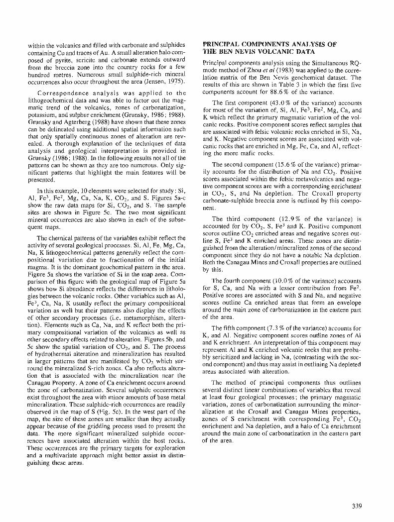
within the volcanics and filled with carbonate and sulphides containing Cu and traces of Au. A small alteration halo composed of pyrite, sericite and carbonate extends outward from the breccia zone into the country rocks for a few hundred metres. Numerous small sulphide-rich mineral occurrences also occur throughout the area (Jensen, 1975).

Correspondence analysis was applied to the lithogeochemical data and was able to factor out the magmatic trend of the volcanics, zones of carbonatization, potassium, and sulphur enrichment (Grunsky, 1986; 1988). Grunsky and Agterberg (1988) have shown that these zones can be delineated using additional spatial information such that only spatially continuous zones of alteration are revealed. A thorough explanation of the techniques of data analysis and geological interpretation is provided in Grunsky (1986; 1988). In the following results not all of the patterns can be shown as they are too numerous. Only significant patterns that highlight the main features will be presented.

In this example, 10 elements were selected for study : Si, Al, Fe3, Fe2, Mg, Ca, Na, K, C02, and S. Figures 5a-c show the raw data maps for Si, C02, and S. The sample sites are shown in Figure 5c. The two most significant mineral occurrences are also shown in each of the subsequent maps.

The chemical patterns of the variables exhibit reflect the activity of several geological processes. Si, Al, Fe, Mg, Ca, Na, K lithogeochemical patterns generally reflect the compositional variation due to fractionation of the initial magma. It is the dominant geochemical pattern in the area. Figure 5a shows the variation of Si in the map area. Com- parison of this figure with the geological map of Figure 5a shows how Si abundance reflects the differences in lithologies between the volcanic rocks. Other variables such as Al, Fe3, Ca, Na, K usually reflect the primary compositional variation as well but their patterns also display the effects of other secondary processes (i.e. metamorphism, alteration). Elements such as Ca, Na, and K reflect both the primary compositional variation of the volcanics as well as other secondary effects related to alteration. Figures 5b, and 5c show the spatial variation of C02, and S. The process of hydrothermal alteration and mineralization has resulted in larger patterns that are manifested by C02 which surround the mineralized S-rich zones. Ca also reflects alteration that is associated with the mineralization near the Canagau Property. A zone of Ca enrichment occurs around the zone of carbonatization. Several sulphide occurrences exist throughout the area with minor amounts of base metal mineralization. These sulphide-rich occurrences are readily observed in the map of S (Fig. 5c). In the west part of the map, the size of these zones are smaller than they actually appear because of the gridding process used to present the data. The more significant mineralized sulphide occurrences have associated alteration within the host rocks. These occurrences are the primary targets for exploration and a multivariate approach might better assist in distinguishing these areas.

PRINCIPAL COMPONENTS ANALYSIS OF THE BEN NEVIS VOLCANIC DATA

Principal components analysis using the Simultaneous RQ- mode method of Zhou et a1 (1983) was applied to the correlation matrix of the Ben Nevis geochemical dataset. The results of this are shown in Table 3 in which the first five components account for 88.6 % of the variance.

The first component (43.0 % of the variance) accounts for most of the variation of, Si, Al, Fe3, Fe2, Mg, Ca, and K which reflect the primary magmatic variation of the volcanic rocks. Positive component scores reflect samples that are associated with felsic volcanic rocks enriched in Si, Na, and K. Negative component scores are associated with volcanic rocks that are enriched in Mg, Fe, Ca, and Al, reflecting the more mafic rocks.

The second component (15.6 % of the variance) primarily accounts for the distribution of Na and COz. Positive scores associated within the felsic metavolcanics and negative component scores are with a corresponding enrichment in COz, S, and Na depletion. The Croxall property carbonate-sulphide breccia zone is outlined by this component.

The third component (12.9 % of the variance) is accounted for by C02, S, Fe3 and K. Positive component scores outline C02 enriched areas and negative scores outline S, Fe3 and K enriched areas. These zones are distinguished from the alterationlmineralized zones of the second component since they do not have a notable Na depletion. Both the Canagau Mines and Croxall properties are outlined by this.

The fourth component (10.0 % of the variance) accounts for S, Ca, and Na with a lesser contribution from Fe2. Positive scores are associated with S and Na, and negative scores outline Ca enriched areas that form an envelope around the main zone of carbonatization in the eastern part of the area.

The fifth component (7.3 % of the variance) accounts for K, and Al. Negative component scores outline zones of A1 and K enrichment. An interpretation of this component may represent Al and K enriched volcanic rocks that are probably sericitized and lacking in Na, (contrasting with the second component) and thus may assist in outlining Na depleted areas associated with alteration.

The method of principal components thus outlines several distinct linear combinations of variables that reveal at least four geological processes; the primary magmatic variation, zones of carbonatization surrounding the mineralization at the Croxall and Canagau Mines properties, zones of S enrichment with corresponding Fe3, C 0 2 enrichment and Na depletion, and a halo of Ca enrichment around the main zone of carbonatization in the eastern part of the area.

Figure 5. Si map of the Ben Nevis area. Si outlines the major features of the compositional variation of the igneous rocks. The scale is the same as in Figure 4. (b) CO, map of the Ben Nevis area. CO, outlines a major north-south zone of carbonate alteration extending through the area. The scale is the same as in Figure 4. (c) map of the Ben Nevis area. Sul- phide mineral occurrences are reflected in this map. Sample sites are also shown on this map.The scale is the same as in Figure 4.

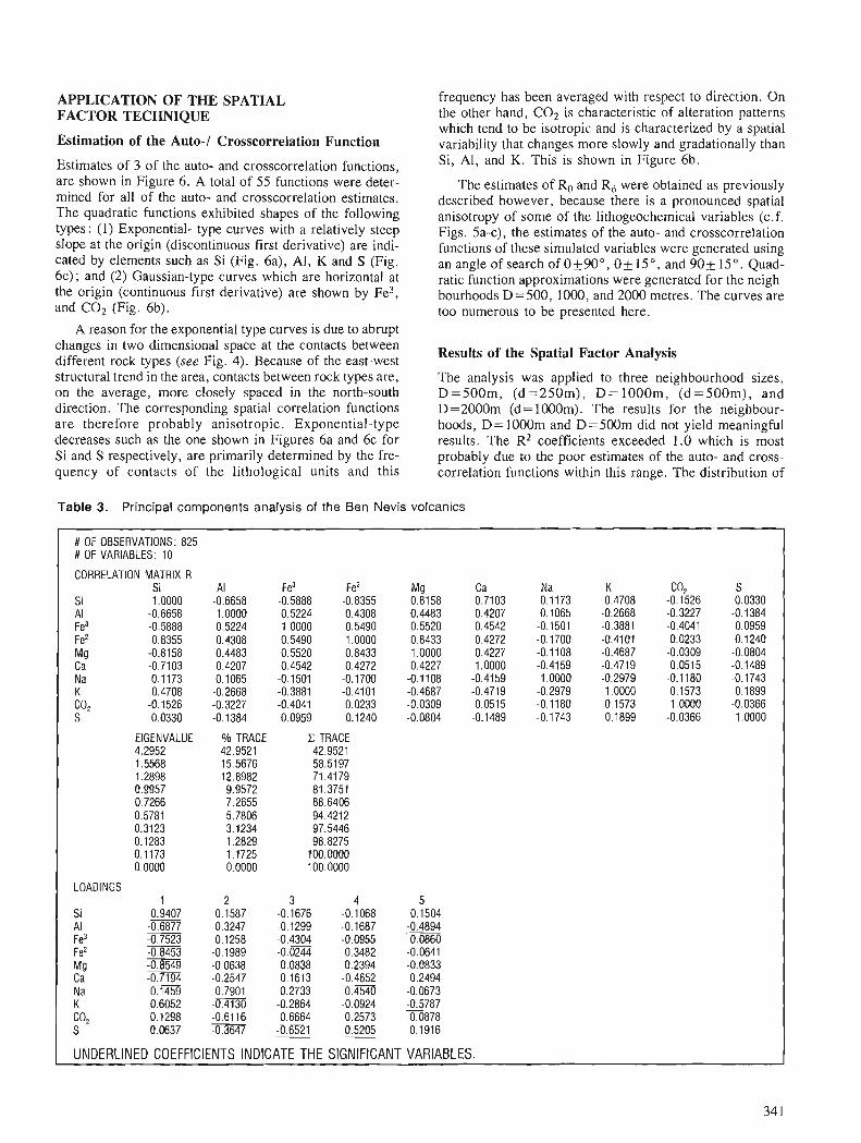
APPLICATION OF THE SPATIAL FACTOR TECHNIQUE

Estimation of the Auto-l Crosscorrelation Function

Estimates of 3 of the auto- and crosscorrelation functions, are shown in Figure 6. A total of 55 functions were determined for all of the auto- and crosscorrelation estimates. The quadratic functions exhibited shapes of the following types: (1) Exponential- type curves with a relatively steep slope at the origin (discontinuous first derivative) are indicated by elements such as Si (Fig. 6a), Al, K and S (Fig. 6c); and (2) Gaussian-type curves which are horizontal at the origin (continuous first derivative) are shown by Fe3, and C02 (Fig. 6b).

A reason for the exponential type curves is due to abrupt changes in two dimensional space at the contacts between different rock types (see Fig. 4). Because of the east-west structural trend in the area, contacts between rock types are, on the average, more closely spaced in the north-south direction. The corresponding spatial correlation functions are therefore probably anisotropic. Exponential-type decreases such as the one shown in Figures 6a and 6c for Si and S respectively, are primarily determined by the frequency of contacts of the lithological units and this

frequency has been averaged with respect to direction. On the other hand, C02 is characteristic of alteration patterns which tend to be isotropic and is characterized by a spatial variability that changes more slowly and gradationally than Si, Al, and K. This is shown in Figure 6b.

The estimates of Ro and Rd were obtained as previously described however, because there is a pronounced spatial anisotropy of some of the lithogeochemical variables (c.f. Figs. 5a-c), the estimates of the auto- and crosscorrelation functions of these simulated variables were generated using an angle of search of Of 90°, 0 + 15", and 90-L 15". Quad- ratic function approximations were generated for the neighbourhoods D=500, 1000, and 2000 metres. The curves are too numerous to be presented here.

Results of the Spatial Factor Analysis

The analysis was applied to three neighbourhood sizes, D =500m, (d =250m), D = 1000m, (d =500m), and D = 2000m (d= 1000m). The results for the neighbourhoods, D= 1000m and D =500m did not yield meaningful results. The R2 coefficients exceeded 1.0 which is most probably due to the poor estimates of the auto- and crosscorrelation functions within this range. The distribution of

Table 3. Principal components analysis of the Ben Nevis volcanics

# OF OBSERVATIONS: 825 # OF VARIABLES: 10

CORRELATION MATRIX R Si Al Fe3 Fez Mg Ca Na K co2 S

Si 1.0000 -0.6658 -0.5888 -0.8355 -0.8158 -0.7103 0.1173 0.4708 -0.1526 0.0330 Al -0.6658 1.0000 0.5224 0.4308 0.4483 0.4207 0.1065 -0.2668 -0.3227 -0.1384 Fe3 -0.5888 0.5224 1.0000 0.5490 0.5520 0.4542 -0.1501 -0.3881 -0.4041 0.0959 Fez -0.8355 0.4308 0.5490 1.0000 0.8433 0.4272 -0.1700 -0.4101 0.0233 0.1240 MQ -0.8158 0.4483 0.5520 0.8433 1.0000 0.4227 -0.1 108 -0.4687 -0.0309 -0.0804 Ca -0.7103 0.4207 0.4542 0.4272 0.4227 1.0000 -0.4159 -0.4719 0.0515 -0.1489 Na 0.1173 0.1065 -0.1501 -0.1700 -0.1108 -0.4159 1.0000 -0.2979 -0.1180 -0.1743 K 0.4708 -0.2668 -0.3881 -0.4101 -0.4687 -0.4719 -0.2979 1.0000 0.1573 0.1899 GO, -0.1526 -0.3227 -0.4041 0.0233 -0.0309 0.0515 -0.1180 0.1573 1.0000 -0.0366 S 0.0330 -0.1384 0.0959 0.1240 -0.0804 -0.1489 -0.1743 0.1899 -0.0366 1 .OOOO

EIGENVALUE % TRACE X TRACE 4.2952 42.9521 42.9521 1.5568 15.5676 58.5197 1.2898 12.8982 71.4179 0.9957 9.9572 81.3751 0.7266 7.2655 88.6406 0.5781 5.7806 94.4212 0.3123 3.1234 97.5446 0.1283 1.2829 98.8275 0.1173 1.1725 100.0000 0.0000 0.0000 100.0000

LOADINGS 1 2 3 4 5

Si 0.9407 0.1587 -0.1676 -0.1068 0.1504 Al -0.6877 0.3247 -0.1299 -0.1687 -0.4894 Fe3 -0.7523 0.1258 -0.4304 -0.0955 0.0860 Fez -0.8453 -0.1989 -0.0244 0.3482 -0.0641 Mg -0.8549 -0.0638 0.0838 0.2394 -0.0833 Ca - -0.7194 -0.2547 0.1613 -0.4652 0.2494 Na 0.1459 0.7901 0.2733 0.4540 -0.0673 K 0.6052 -0.4130 -0.2864 -0.0924 -0.5787 C 02 0.1298 -0.6116 0.6664 0.2573 -0.0878 S 0.0637 -0.3647 -0.6521 - 0.5205 0.1916

URlDERLlhlED COEFFICIENTS INDICATE THE SIGNIFICANT VARIABLES.

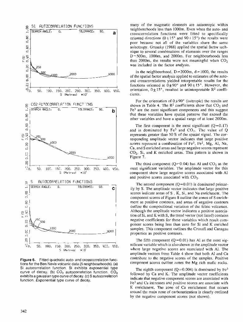
o Si RUTBCORRELQTIBN FUNCTIONS Z ISERRCH ~ G L E : 0. TOLERRNcE: go. a l

EE d 10. 50. 100. 150. 200. 250. 300. 350. 400. S O .

5 (Metres) * lo1

o CO2 FIUTCICCIRRELRTION FUNCTIONS TOLERRNCE: 90. b

0 10. SO. 100. 150. 200. 250. 300. 350. 1100. 1150.

0 10. SO. 100. 150. 200. 250. 300. 350. q00. 450.

S (Met res l ~ 1 0 '

o S RLITOCORRELRT I ON FIJNCT IONS 0

Figure 6. Fitted quadratic auto- and crosscorrelation functions for the Ben Nevis volcanic data (5 neighbourhoods). (a) Si autocorrelation function. Si exhibits exponential type curve of decay. (b) CO, autocorrelation function. CO, exhibits a gaussian type curve of decay. (c) S autocorrelation function. Exponential type curve of decay.

A

many of the magmatic elements are anisotropic within neighbourhoods less than 1000m. Even when the auto- and crosscorrelation functions were fitted to specifically oriented directions (0 f 15 " and 90+ 15 ") the results were poor because not all of the variables share the same anisotropy. Grunsky (1988) applied the spatial factor technique to several combinations of elements over the ranges D = 500m, 1000m, and 2000m. For neighbourhoods less than 2000m, the results were not meaningful when C02 was included in the factor analysis.

SEARCH ANGLE: 0. TOLERQNCE: 90. c I

In the neighbourhood, D =2000m, d = 1000, the results of the spatial factor analysis applied to estimates of the auto- and crosscorrelations yielded interpretable results for the functions oriented at Of 90" and 90f 15". However, the orientation, Of 15", resulted in uninterpretable R2 coefficients.

For the orientation of Of 90" (isotropic) the results are shown in Table 4. The R2 coefficients show that C02 and Fe3 are the most significant components and this suggest that these variables have spatial patterns that exceed the other variables and have a spatial range of at least 2000m.

The first component is the most significant (Q=0.17) and is dominated by Fe3 and CO,. The value of Q represents greater than 50 % of the spatial signal. The corresponding amplitude vector indicates that large positive scores represent a combination of Fe3, Fe2, Mg, Al, Na, Ca, and S enriched areas and large negative scores represent C02, Si, and K enriched areas. This pattern is shown in Figure 7.

The third component (Q=0.04) has A1 and C02 as the most significant variables. The amplitude vector for this component show large negative scores associated with A1 and positive scores associated with C02.

The second component (Q=0.01) is dominated primarily by S. The amplitude vector indicates that large positive scores indicate areas of S , K, Si, and Na enrichment. The component scores of Figure 8 outline the zones of S enrichment as positive contours, and areas of negative contours outline the compositional variation of the felsic volcanics. Although the amplitude vector indicates a positive association of Si, and K with S, the trend vector (not listed) contains negative coefficients for these variables which result component scores being less than zero for Si and K enriched samples. This component outlines the Croxall and Canagau properties as positive contours.

The fifth component (Q=0.01) has A1 as the most significant variable which is also shown in the amplitude vector where large negative scores are associated with Al. The amplitude vectors from Table 4 show that both A1 and Ca contribute to the negative scores of the samples. Positive component scores outline zones the Mg rich mafic rocks.

The eighth component (Q=0.004) is dominated by Fe3 followed by Ca and K. The amplitude vector coefficients indicate that negative component scores are associated with Fe3 and Ca increases and positive scores are associate with K enrichment. The zone of Ca enrichment that occurs around the main zone of carbonatization is clearly outlined by the negative component scores (not shown).

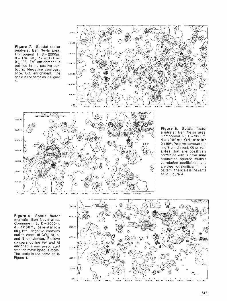
Figure 7 . Spatial factor analysis: Ben Nevis area. Component 1 ; D = 2000m, d = 1000m ; o r i en ta t i on 0 + 90°. Fe3 enrichment is outlined in the positive contours. Negative contours show CO, enrichment. The scale is the same as in Figure 4.

Figure 9. Spatial factor analysis: Ben Nevis area. Component 2 ; D = 2000m, d = 1 OOOm, o r i e n t a t i o n 90 + 15O. Negative contours outline zones of CO,, Si, K, and S enrichment. Positive contours outline Fe3 and Al enriched areas associated with the mafic igneous rocks. The scale is the same as in Figure 4.

Figure 8. Spatial factor analysis: Ben Nevis area. Component 2; D = 2000m, d = 1000m ; Or ien ta t i on 0 + 90°. Positive contours outline S enrichment. Other variables that are positively correlated with S have small associated squared multiple correlation coefficients and are thus not significant in the pattern. The scale is the same as in Figure 4.

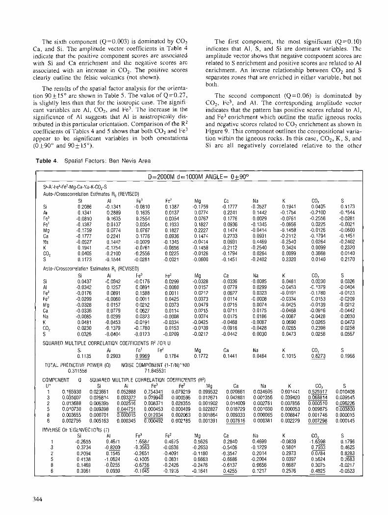
The sixth component (Q=0.003) is dominated by C02 Ca, and Si. The amplitude vector coefficients in Table 4 indicate that the positive component scores are associated with Si and Ca enrichment and the negative scores are associated with an increase in COz. The positive scores clearly outline the felsic volcanics (not shown).

The results of the spatial factor analysis for the orientation 90* 15" are shown in Table 5. The value of Q=0.27, is slightly less than that for the isotropic case. The significant variables are Al, C02, and Fe3. The increase in the significance of A1 suggests that A1 is anistropically distributed in this particular orientation. Comparison of the R2 coefficients of Tables 4 and 5 shows that both C02 and Fe3 appear to be significant variables in both orientations (0+90° and 90+ 15").

Table 4. Spatial Factors: Ben Nevis Area

The first component, the most significant (Q=0.10) indicates that Al, S, and Si are dominant variables. The amplitude vector shows that negative component scores are related to S enrichment and positive scores are related to A1 enrichment. An inverse relationship between C02 and S separates zones that are enriched in either variable, but not both.

The second component (Q=0.06) is dominated by C02, Fe3, and Al. The corresponding amplitude vector indicates that the pattern has positive scores related to Al, and Fe3 enrichment which outline the mafic igneous rocks and negative scores related to C02 enrichment as shown in Figure 9. This component outlines the compositional variation within the igneous rocks. In this case, C02, K, S, and Si are all negatively correlated relative to the other

Si-Al-Fe3-Fez-Mg-Ca-Na-K-GO2-S Auto-ICrosscorrelation Estimates R, (REVISED)

Si At Fe3 Fez Si 0.2086 -0.1341 -0.0810 -0.1387 Al -0.1341 0.2889 0.1635 0.0137 Fe3 -0.0810 0.1635 0.2554 0.0354 Fez -0.1387 0.0137 0.0354 0.1933 Mg -0.1759 0.0774 0.0767 0.1827 Ca -0.1777 0.2241 0.1776 0.0936 Na -0.0527 0.1442 -0.0029 -0.1345 K 0.1941 -0.1754 -0.0761 -0.0656 co2 0.0405 -0.2100 -0.2556 0.0225 S 0.1 173 -0.1544 -0.0281 -0.0021

Auto-/Crosscorrelation Estimates R, (REVISED) Si Al Fe3 Fez

Si 0.0437 -0.0342 -0.0176 -0.0299 Al -0.0342 0.1257 0.0891 -0.0060 Fe3 -0.0176 0.0891 0.1588 0.001 1 Fez -0.0299 -0.0060 0.001 1 0.0425 Mg -0.0328 0.0157 0.0212 0.0373 Ca -0.0336 0.0779 0.0627 0.0114 Na -0.0085 0.0299 0.0323 -0.0008 K 0.0481 -0.0453 -0.0191 -0.0334 co2 0.0230 -0.1379 -0.1780 0.0153 S 0.0326 -0.0404 -0.0123 -0.0209

SQUARED MULTIPLE CORRELATION COEFFICIENTS R2 FOR U Si Al Fe3 Fez 0.1135 0.2903 0.9969 0.1784

TOTAL PREDICTIVE POWER (Q) NOISE COMPONENT (1-TIN)*100 0.311556 71.845531

COMPONENT Q SQUARED MULTIPLE CORRELATION COEFFICIENTS (R2) U Si Al Fe3 Fez Mg Ca 1 0.165930 0.023661 0.052888 0.754341 0.079219 0.099532 0.020661 3 0.035607 0.026814 0.093372 0.019940 0.000596 0.012671 0.042881 2 0.013688 0.006395 0.002516 0.008371 0.026355 0.001902 0.014009 5 0.010730 0.009398 0.044751 0.000453 0.000409 0.022827 0.018729 8 0.003655 0.000701 0.000015 0.012034 0.002063 0.001864 0.009333 6 0.002756 0.005163 0.000345 0.000492 0.002185 0.001391 0.007616

INVERSE OF EIGENVECTORS (T) Si Al Fe3 Fez Mg Ca

1 -0.2655 0.4671 - 1.6587 0.4675 0.5626 0.2840 3 0.3734 -0.3563 -0.0536 -0.2653 -0.5406 2 0.2094 0.1545 -0.2651 -0.4091 -0.1180 -0.3547 5 0.4138 -1.0624 -0.1005 0.0831 0.6663 -0.6686 8 0.1469 -0.0255 -0.6736 -0.2426 -0.2476 -0.6137 6 0.3061 0.0930 -0.1045 -0.1916 -0.1641 - 0.4255

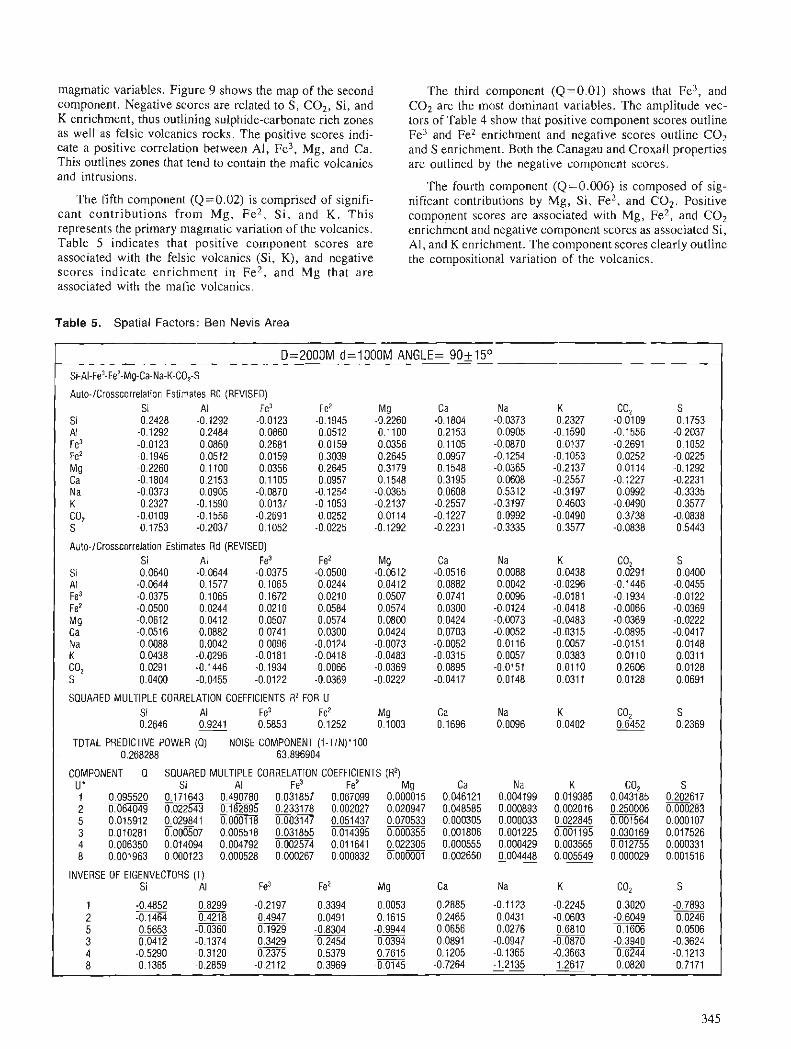
magmatic variables. Figure 9 shows the map of the second component. Negative scores are related to S, C02, Si, and K enrichment, thus outlining sulphide-carbonate rich zones as well as felsic volcanics rocks. The positive scores indicate a positive correlation between Al, Fe3, Mg, and Ca. This outlines zones that tend to contain the mafic volcanics and intrusions.

The fifth component (Q=0.02) is comprised of significant contributions from Mg, Fe2, Si, and K . This represents the primary magmatic variation of the volcanics. Table 5 indicates that positive component scores are associated with the felsic volcanics (Si, K), and negative scores indicate enrichment in Fe2, and Mg that are associated with the mafic volcanics.

The third component (Q=0.01) shows that Fe3, and C02 are the most dominant variables. The amplitude vectors of Table 4 show that positive component scores outline Fe3 and Fe2 enrichment and negative scores outline COz and S enrichment. Both the Canagau and Croxall properties are outlined by the negative component scores.

The fourth component (Q=0.006) is composed of significant contributions by Mg, Si, Fe2, and COz. Positive component scores are associated with Mg, Fe2, and C02 enrichment and negative component scores as associated Si, Al, and K enrichment. The component scores clearly outline the compositional variation of the volcanics.

Table 5. Spatial Factors: Ben Nevis Area

D=2000M d=1000M ANGLE= 90+1S0 Si-AI-Fe3-Fez-MpCa-Na-K-C0,-S

Auto-ICrosscorrelation Estimates RO (REVISED) Si Al Fe3 Fe2 Mg Ca Na K '332 S

Si 0.2428 -0.1292 -0.0123 -0.1945 -0.2260 -0.1804 -0.0373 0.2327 -0.0109 0.1753 Al -0.1292 0.2484 0.0860 0.0512 0,1100 0.2153 0.0905 -0.1590 -0.1556 -0.2037 Fe3 -0.0123 0.0860 0.2681 0.0159 0.0356 0.1105 -0.0870 0.0137 -0.2691 0.1052 Fez -0.1945 0.0512 0.0159 0.3039 0.2645 0.0957 -0.1254 -0.1053 0.0252 -0.0225 Mg -0.2260 0.1100 0.0356 0.2645 0.3179 0.1548 -0.0365 -0.2137 0.0114 -0.1292 Ca -0.1804 0.2153 0.1105 0.0957 0.1548 0.3195 0.0608 -0.2557 -0.1227 -0.2231 Na -0.0373 0.0905 -0.0870 -0.1254 -0.0365 0.0608 0.5312 -0.3197 0.0992 -0.3335 K 0.2327 -0.1590 0.0137 -0.1053 -0.2137 -0.2557 -0.3197 0.4603 -0.0490 0.3577 co2 -0.0109 -0.1556 -0.2691 0.0252 0.0114 -0.1227 0.0992 -0.0490 0.3738 -0.0838 S 0.1753 -0.2037 0.1052 -0.0225 -0.1292 -0.2231 -0.3335 0.3577 -0.0838 0.5443

Auto-ICrosscorrelation Estimates Rd (REVISED) Si Al Fe3 Fez MQ Ca Na K Coz S

Si 0.0640 -0.0644 -0.0375 -0.0500 -0.0612 -0.0516 0.0088 0.0438 0.0291 0.0400 Al -0.0644 0.1577 0.1065 0.0244 0.0412 0.0882 0.0042 -0.0296 -0.1446 -0.0455 Fe3 -0.0375 0.1065 0.1672 0.0210 0.0507 0.0741 0.0096 -0.0181 -0.1934 -0.0122 Fez -0.0500 0.0244 0.0210 0.0584 0.0574 0.0300 -0.0124 -0.0418 -0.0066 -0.0369 Mg -0.0612 0.0412 0.0507 0.0574 0.0800 0.0424 -0.0073 -0.0483 -0.0369 -0.0222 Ca -0.0516 0.0882 0.0741 0.0300 0.0424 0.0703 -0.0052 -0.0315 -0.0895 -0.0417 Na 0.0088 0.0042 0.0096 -0.0124 -0.0073 -0.0052 0.0116 0.0057 -0.0151 0.0148 K 0.0438 -0.0296 -0.0181 -0.0418 -0.0483 -0.0315 0.0057 0.0383 0.0110 0.0311 Go2 0.0291 -0.1446 -0.1934 -0.0066 -0.0369 -0.0895 -0.0151 0.01 10 0.2606 0.0128 S 0.0400 -0.0455 -0.0122 -0.0369 -0.0222 -0.0417 0.0148 0.0311 0.0128 0.0691

SQUARED MULTIPLE CORRELATION COEFFICIENTS R2 FOR U Si Al Fe3 Fez MQ Ca Na K co2 S 0.2646 0.9241 0.5853 0.1252 0.1003 0.1696 0.0096 0.0402 0.6452 0.2369

TOTAL PREDICTIVE POWER (a) NOISE COMPONENT (1-TIN)*100 0.268288 63.896904

COMPONENT Q SQUARED MULTIPLE CORRELATION COEFFICIENTS (R2) U ' Si Al Fe3 Fe2 Mg Ca Na K GO2 S 1 0.095520 0.171643 0.490780 0.031857 0.067099 0.000015 0.046121 0.004199 0.019385 0.043185 0.202617 2 0.064049 0.022543 0.182895 0.233178 0.002027 0.020947 0.048585 0.000893 0.002016 0.250006 0.000283 5 0.015912 0.029841 0.000118 0.003147 0.051437 0.070533 0.000305 0.000033 0.022845 0.001564 0.000107 3 0.010281 0.000507 0.005518 0.031855 0.014395 0.000355 0.001806 0.001225 0.001195 0.030169 0.017526 4 0.006350 0.014094 0.004792 0.002574 0.011641 0.022305 0.000555 0.000429 0.003565 0.012755 0.000331 8 0.001963 0.000123 0.000528 0.000267 0.000832 0.000001 0.002650 0.004448 0.005549 0.000029 0.001516

INVERSE OF EIGENVECTORS (T) Si Al Fe3 Fez Mg Ca Na K Coz S

1 - -0.4852 0.8299 -0.2197 0.3394 0.0053 0.2885 -0.1123 -0.2245 0.3020 -0.7893 2 -0.1464 0.4218 0.4947 0.0491 0.1615 0.2465 0.0431 -0.0603 -0.6049 -0.0246 5 0.5653 -0.0360 0.1929 -0.8304 -0.9944 0.0656 0.0276 0.6810 -0.1606 0.0506 3 0.0412 -0.1374 0.3429 0.2454 0.0394 0.0891 -0.0947 -0.0870 -0.3940 -0.3624 4 -0.5290 -0.3120 0.2375 0.5379 0.7615 0.1205 -0.1365 -0.3663 0.6244 -0.1213 8 0.1365 -0.2859 -0.2112 0.3969 -0.0145 -0.7264 -1.2135 - 1.2617 0.0820 0.7171

The eighth component (Q=0.002) is not a very significant component. The significant variables for this component are K, Na, and Ca. The amplitude vector coefficients indicate that positive scores are associated with K enrichment and negative scores are associated with Na, and Ca enrichment. This can also be interpreted as K enriched areas may be Na depleted and thus be associated with a zone of alteration that is typical of some types of gold deposits (Col- vine et al, 1988).

Discussion

The results of the spatial factor analysis provide much of the same information as the principal components analysis. In particular, the zones of carbonatization, sulphur enrichment and the primary magmatic trend, are spatial components as indicated by the spatial factor method. Potential exploration targets can be based on the one or more spatial factors that show S, K, and C02 enrichment.

For the neighbourhoods, D=500m, d=250m, and D = 1000m, d =500m, the estimates of auto- and crosscorrelations could not be properly assessed possibly due to errors in estimating the coefficients. In the case where the estimates of the auto- and crosscorrelation were more meaningful, as in the D = 2 0 0 h , d= 1000m neighbourhood, the significant variables are C02, Fe3, and Al; depending on the orientation of the function estimates.

Although the principal components analysis indicated that the primary "magmatic trend" is due to the variation of Si, Al, Fe3, Fe2, Mg, and Ca; this strong correlation between the "magmatic variables" is not represented as a dominant component in the spatial factor analysis. This suggests that although the variables are magmatically related, they have different spatial characteristics. The anisotropy of the variables that define the compositional variation of the igneous rocks reduces the significance of the auto- and crosscorrelation coefficients relative to the more isotropic variables such as C02 and S. Thus, the more isotropic variables, those with the larger autocorrelation coefficients, will be the most significant in the analysis.

SUMMARY AND CONCLUSIONS

The use of the spatial factor technique is bascd on the multivariate analysis of estimated auto- and crosscorrelation relationships of data. When the matrix of the estimates for lag 0 and lag d are positive definite, a meaningful interpretation can be extracted. The use of the values of Q for the U transition matrix indicates the ability of U to account for the spatial variation that is represented by the data. Also, the Q values that estimate the relative significance of the individual components of U enable an assessment of the most significant factors. The multiple correlation coefficients describe the relative significance of the variables for a given component and when used in conjunction with the coefficients of the amplitude vector T, the spatial patterns can be interpreted and related to geological processes. The variation of spatial ranges of the-variables determines the significance of a given variable within a the neighbourhood to which the spatial factor analysis is applied.

In several cases the lack of precision of the estimates provided meaningless results. Further work is required for providing better methods of estimating the autocorrelation function. A choice of a variety of autocorrelation models may provide better estimates of randomly distributed variables.

In the cases where satisfactory estimates of the auto- /crosscorrelation functions can be obtained, the spatial factor analysis technique is suitable for the delineation of hydrothermal alteration enrichment patterns that are associated with mineralization and other geological patterns which are characterized by gradational variation in space.

ACKNOWLEDGMENTS

Assistance from the Division of Exploration Geoscience of the Commonwealth Scientific Industrial Organisation (CSIRO) of Australia is gratefully acknowledged. The lithogeochemical data of the Ben Nevis area and support for earlier work was provided by the Northern Ontario Geologi- cal Survey program of the Ontario Ministry of Northern Development and Mines, Canada, whose assistance is also gratefully acknowledged. The preparation of this manuscript benefitted from several discussions with F.P. Agter- berg of the Geological Survey of Canada.

REFERENCES

Agterberg, F.P. 1966: The use of multivariate Markov schemes in petrology ; Journal of

Geology, v. 79, p. 764-785. 1970: Autocorrelation functions in geology; in Geostatistics, ed. D.F.

Merriam; Plenum, New York, N.Y. p. 113-142. 1974: Geomathematics; Elsevier, Amsterdam, 596 p. Bennett, R.J. 1979: Spatial Time Series; Pion, London, 674 p. Colvine, A.C., et al. 1988: Archean Lode Gold Deposits in Ontario; Ontario Geological Sur-

vey, Miscellaneous Paper 139, 136p. Davis, J.C. 1986: Statistics and Data Analysis in Geology; John Wiley &Sons Inc.,

second edition, 646p. Grunsky, E.C. 1986: Recognition of alteration in volcanic rocks using statistical analysis

of lithogeochemical data; Journal of Geochemical Exploration, v. 25, p. 157-183.

1988: Multivariate and Spatial Analysis of Lithogeochemical Data from Metavolcanics with Zones of Alteration and Mineralization in Ben Nevis Township, Ontario; unpublished Ph.D. Thesis, University of Ottawa.

Grunsky, E.C. and Agterberg, F.P. 1988: Spatial and multivariate analysis of geochemical data from

metavolcanic rocks in the Ben Nevis Area, Ontario; Mathematical Geology, vol. 20, No. 7, p. 825-861.

Haining, R. 1987: Trend surface models with regional and local scales of variation

with an application to aerial survey data; Technornetrics, vol. 29, No. 4, November 1987, p.461-469.

Jensen, L.S. 1975: Geology of Clifford and Ben Nevis Townships, District of

Cochrane; Ontario Div. Mines, GR132, 55p. Accompanied by Map 2283.

Journel, A.G. and Huijbregts, C.J. 1978: Mining Geostatistics; Academic Press, London, 600 p. Joreskog, K.G., Klovan, J.E., Reyment, R.A. 1976: Geological Factor Analysis; Elsevier Scientific Publishing Com-

pany, New York, 178p.

LeMaitre, R.W. 1982: Numerical Petrology; Statistical Interpretation of Geochemical

Data, Elsevier, New York, 281 p. Luster, G.R. 1986: Raw Materials for Portland Cement: Applications of Conditional

Simulation of Coregionalization; unpublished Ph.D. Thesis, Stan- ford University.

Myers, D.E. 1982: Matrix formulation of co-kriging; Mathematical Geology, v. 14,

p. 249-257. 1988: Some new aspects of multivariate analysis; in Fabbri, A.G.,

Chung, C.F. and Sinding-Larsen, R., Quantitative Analysis of Mineral and Energy Resources, Proc. NATO AS1 Conference held at II Ciocco, Italy, July 1986; Reidel, Dordrecht, p. 669-687.

Quenouille, M.H. 1957: The analysis of multiple time-series; Hafner, New York, 105 p. Rao, C.R. 1975: Linear statistical inference and its applications, second edition;

Wiley, New York, 625 p. Royer, J.-J. 1988: Gcochemical data analysis; in Fabbri, A.G., Chung, C.F. and

Sinding-Larsen, R., Quantitative Analysis of Mineral and Energy Resources, Proc. NATO AS1 Conference held at II Ciocco, Italy, July 1986; Reidel, Dordrecht, p. 89-1 12.

Switzer, P. and Green, A.A. 1984: MinIMax autocorrelation factors for multivariate spatial imagery;

Technical Report No. 6, April 1984, Department of Statistics, Stanford University, 14 p.

Upton, G . and Fingleton, B. 1985: Spatial data analysis by cxample, Volume 1; Wiley, New York,

410 p. Waekernagel, H. 1988: Geostatistical techniques for interpreting multivariate spatial infor-

mation, in Fabbri, A.G., Chung, C.F., and Sinding-Larsen, R., Quantitative Analysis of Mineral and Energy Resources, Proc. NATO AS1 Conference held at I1 Ciocco, Italy, July 1986; Reidel. Dordrecht, p. 393-409.

Zhou, D., Chang, T., and Davis, J.C. 1983: Dual extraction of R-mode and Q-mode factor solutions; Mathe-

matical Gcology, vol. 15, No.5, pp. 581-606.

Multivariate analysis and variography used to enhance anomalous response for

lake sediments in the Manicouagan area, Qukbec.

Denis Marcottel

Marcotte, D., Multivariate analysis and variography used to enhance anomalous response for lake sediments in the Manicouagan area, Que'bec; @ Statistical Application in the Earth Sciences, ed. F. P. Agterberg and G.F. Bonham-Carter; Geolocical Survey of Canada, Paper 89-9, p. 349-356, 1989.

Abstract

Nearlyjve thousand (4876) centre-lake bottom sediments were collected in 1977fiom the Manicoua- gun area and analyzed for nine elements (Cu, Pb, Zn, Mo, Co, Ni, Fe, U, Mn). An attempt was made to jlter out influences related to extraneous factors, other than mineralization, using two multivariate techniques: linear regression and principal component analysis. Additionally, variograms were used extensively as an aid to interpretation. Regression analysis of all the elements on Fe and Mn proved successjkl in reducing erratic, short range variations, while principal component analysis permitted the removal of long range "regional" factors, some of which were found to be spatially related to underlying rock types. Filtered data showed more clustered anomalies than raw data. A cell comprising oneJifrh of the area but containing nearly half the number of anomalies is identified for further exploration.

Neuf kliments (Cu, Pb, Zn, Mo, Co, Ni, Fe, U, Mn) ont kt6 dostfs duns prts de cinq mille (4876) kchantillons de skdiments prklevks en 1977 du centre de fonds de lacs duns la rkgion de Manicouagan. On a tentkd'e'liminer parfiltrage les influences reliies a des facteurs ktrangers, autres que la minkralisation, d l'aide de deux mkthodes li variables multiples: l'analyse de rkgression linkaire et l'analyse des composantesprincipales. De plus, des variogrammes ont i tk largement utilis6s pour faciliter l'interpre'tation. L'analyse de rkgression de tous les klkments sur le Fe et le Mn a permis de rkduire les variations irre'gulitres de faible amplitude alors que l'analyse des composantes principales a permis d'kliminer les facteurs a rkgionaux N de grande amplitude, dont il a ktk constatk que certains d'entre eux ktaient spatialement reliks a m types de roches sousjacents. Les anomalies obtenues des donne'es j l tries montrent un plus grand regroupement qu'avec les donnkes brutes. Une zone constituant un cinquihme de la rkgion, mais renferrnant prhs de la moitie' des anomalies, est identijke en vue d'une exploration ultt?rieure.

' ~ c o l e Polytechnique, C.P. 6079, Succ. "A", Montreal, Quebec

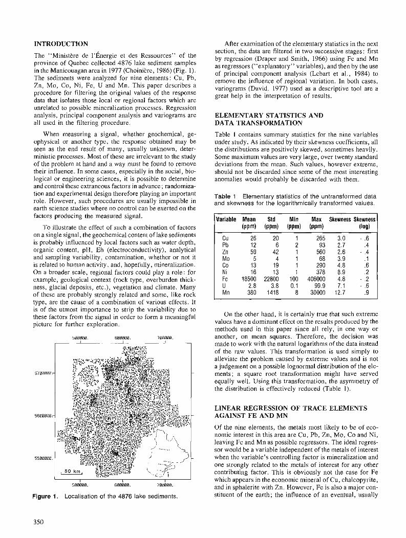
INTRODUCTION

The "Ministbre de l l~nerg ie et des Ressources" of the province of Quebec collected 4876 lake sediment samples in the Manicouagan area in 1977 (Choinikre, 1986) (Fig. 1). The sediments were analyzed for nine elements: Cu, Pb, Zn, Mo, Co, Ni, Fe, U and Mn. This paper describes a procedure for filtering the original values of the response data that isolates those local or regional factors which are unrelated to possible mineralization processes. Regression analysis, principal component analysis and variograms are all used in the filtering procedure.

When measuring a signal, whether geochemical, geophysical or another type, the response obtained may be seen as the end result of many, usually unknown, deterministic processes. Most of these are irrelevant to the study of the problem at hand and a way must be found to remove their influence. In some cases, especially in the social, biological or engineering sciences, it is possible to determine and control these extraneous factors in advance ; randomiza- tion and experimental design therefore playing an important role. However, such procedures are usually impossible in earth science studies where no control can be exerted on the factors producing the measured signal.

To illustrate the effect of such a combination of factors on a single signal, the geochemical content of lake sediments is probably influenced by local factors such as water depth, organic content, pH, Eh (electroconductivity), analytical and sampling variability, contamination, whether or not it is related to human activity, and, hopefully, mineralization. On a broader scale, regional factors could play a role: for example, geological context (rock type, overburden thickness, glacial deposits, e t ~ . ) , vegetation and climate. Many of these are probably strongly related and some, like rock type, are the cause of a combination of various effects. It is of the utmost importance to strip the variability due to these factors from the signal in order to form a meaningful picture for further exploration.

rreakiee.

Figure 1. Localisation of the 4876 lake sediments.

After examination of the elementary statistics in the next section, the data are filtered in two successive stages: first by regression (Draper and Smith, 1966) using Fe and Mn as regressors ("explanatory" variables), and then by the use of principal component analysis (Lebart et al., 1984) to remove the influence of regional variation. In both cases, variograms (David, 1977) used as a descriptive tool are a great help in the interpretation of results.

ELEMENTARY STATISTICS AND DATA TRANSFORMATION

Table 1 contains summary statistics for the nine variables under study. As indicated by their skewness coefficients, all the distributions are positively skewed, sometimes heavily. Some maximum values are very large, over twenty standard deviations from the mean. Such values, however extreme, should not be discarded since some of the most interesting anomalies would probably be discarded with them.

Table 1 Elementary statistics of the untransformed data and skewness for the logarithmically transformed values.

Variable Mean Std Min Max Skewness Skewness ( P P ~ ) (PPm) (PPm) ( P P W (log)

CU 26 20 1 265 3.0 - .6 Pb 12 6 2 93 2.7 .4 Zn 59 42 1 560 2.6 - .4 Mo 5 4 1 68 3.9 1 Co 13 19 1 290 4.8 .6 N i 16 13 1 378 8.9 .2 Fe 18500 22800 100 406000 4.8 - .2 U 2.8 3.8 0.1 99.9 7.1 - .6 Mn 380 1418 8 30000 12.7 .9

On the other hand, it is certainly true that such extreme values have a dominant effect on the results produced by the methods used in this paper since all rely, in one way or another, on mean squares. Therefore, the decision was made to work with the natural logarithms of the data instead of the raw values. This transformation is used simply to alleviate the problem caused by extreme values and is not a judgement on a possible lognormal distribution of the elements; a square root transformation might have served equally well. Using this transformation, the asymmetry of the distribution is effectively reduced (Table 1).

LINEAR REGRESSION OF TRACE ELEMENTS AGAINST FE AND MN

Of the nine elements, the metals most likely to be of economic interest in this area are Cu, Pb, Zn, Mo, Co and Ni, leaving Fe and Mn as possible regressors. The ideal regres- sor would be a variable independent of the metals of interest when the variable's controlling factor is mineralization and one strongly related to the metals of interest for any other contributing factor. This is obviously not the case for Fe which appears in the economic mineral of Cu, chalcopyrite, and in sphalerite with Zn. However, Fe is also a major constituent of the earth; the influence of an eventual, usually

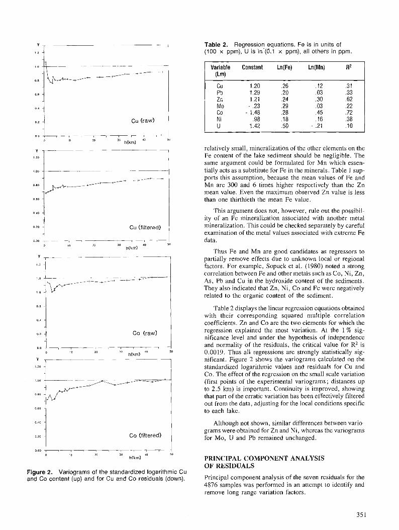
Table 2. Regression equations. Fe is in units of (100 x ppm), U is ii(O.1 x ppm), all others in ppm.

0.2 1 c u (raw) 1

Cu (filtered)

0.00

20 30 40 50 h(km)

Co (raw)

0.20 Co (filtered)

Figure 2. Variograms of the standardized logarithmic Cu .and Co content (up) and for Cu and Co residuals (down).

Variable Constant Ln(Fe) Ln(Mn) R2 (Lm)

Cu 1.20 .26 .12 .31 Pb 1.29 .20 .03 .33 Zn 1.21 .24 .30 .62 MO - .23 .29 .03 .22 CO - 1.48 .28 .45 .72 Ni .98 .18 .16 .38 U 1.42 .50 - .21 .10

relatively small, mineralization of the other elements on the Fe content of the lake sediment should be negligible. The same argument could be formulated for Mn which essentially acts as a substitute for Fe in the minerals. Table 1 supports this assumption, because the mean values of Fe and Mn are 300 and 6 times higher respectively than the Zn mean value. Even the maximum observed Zn value is less than one thirthieth the mean Fe value.

This argument does not, however, rule out the possibility of an Fe mineralization associated with another metal mineralization. This could be checked separately by careful examination of the metal values associated with extreme Fe data.

Thus Fe and Mn are good candidates as regressors to partially remove effects due to unknown local or regional factors. For example, Sopuck et al. (1980) noted a strong correlation between Fe and other metals such as Co, Ni, Zn, As, Pb and Cu in the hydroxide content of the sediments. They also indicated that Zn, Ni, Co and Fe were negatively related to the organic content of the sediment.

Table 2 displays the linear regression equations obtained with their corresponding squared multiple correlation coefficients. Zn and Co are the two elements for which the regression explained the most variation. At the 1 % significance level and under the hypothesis of independence and normality of the residuals, the critical value for R2 is 0.0019. Thus all regressions are strongly statistically significant. Figure 2 shows the variograms calculated on the standardized logarithmic values and residuals for Cu and Co. The effect of the regression on the small scale variation (first points of the experimental variograms; distances up to 2.5 km) is important. Continuity is improved, showing that part of the erratic variation has been effectively filtered out from the data, adjusting for the local conditions specific to each lake.

Although not shown, similar differences between variograms were obtained for Zn and Ni, whereas the variograms for Mo, U and Pb remained unchanged.

PRINCIPAL COMPONENT ANALYSIS OF RESIDUALS

Principal component analysis of the seven residuals for the 4876 samples was performed in an attempt to identify and remove long range variation factors.

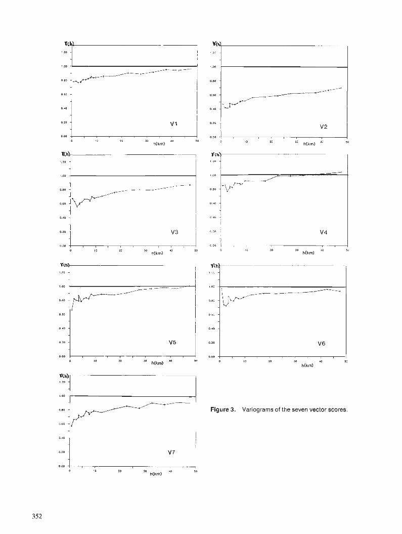
Figure 3. Variograms of the seven vector scores.

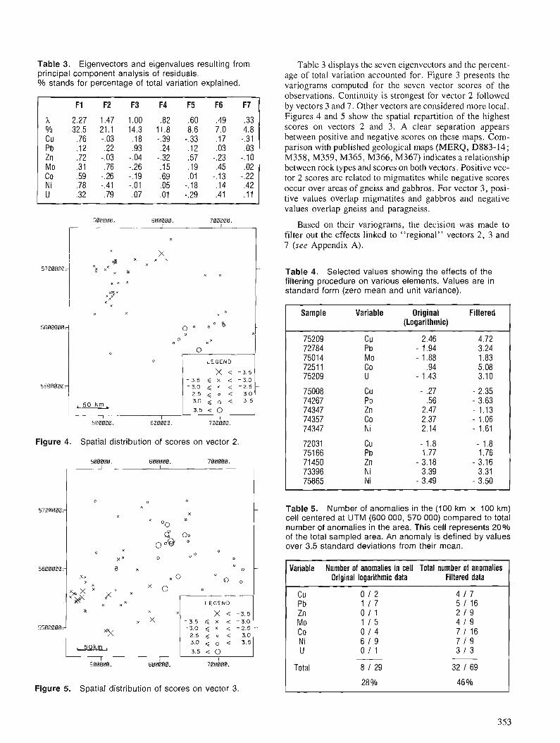
Table 3. Eigenvectors and eigenvalues resulting from principal component analysis of residuals. 010 stands for percentage of total variation explained.

Figure 4. Spatial distribution of scores on vector 2.

sseeee. seaise. 700000.

Figure 5. Spatial distribution of scores on vector 3.

Table 3 displays the seven eigenvectors and the percentage of total variation accounted for. Figure 3 presents the variograms computed for the seven vector scores of the observations. Continuity is strongest for vector 2 followed by vectors 3 and 7. Other vectors are considered more local. Figures 4 and 5 show the spatial repartition of the highest scores on vectors 2 and 3. A clear separation appears between positive and negative scores on these maps. Com- parison with published geological maps (MERQ, D883-14; M358, M359, M365, M366, M367) indicates a relationship between rock types and scores on both vectors. Positive vector 2 scores are related to migmatites while negative scores occur over areas of gneiss and gabbros. For vector 3, positive values overlap migmatites and gabbros and negative values overlap gneiss and paragneiss.

Based on their variograms, the decision was made to filter out the effects linked to "regional" vectors 2, 3 and 7 (see Appendix A).

Table 4. Selected values showing the effects of the filtering procedure on various elements. Values are in standard form (zero mean and unit variance).

Sample Variable Original Filtered (Logarithmic)

75209 Cu 2.46 4.72 72784 Pb - 1.94 3.24 75014 MO - 1.88 1.83 7251 1 Co .94 5.08 75209 U - 1.43 3.10

75008 CU - .27 - 2.35 74267 Pb .56 - 3.63 74347 Zn 2.47 - 1.13 74357 CO 2.37 - 1.06 74347 N i 2.14 - 1.61

72031 CU - 1.8 - 1.8 75166 Pb 1.77 1.76 71 450 Zn - 3.18 - 3.16 73396 Ni 3.39 3.31 75865 Ni - 3.49 - 3.50

Table 5. Number of anomalies in the (100 km x 100 km) cell centered at UTM (600 000, 570 000) compared to total number of anomalies in the area. This cell represents 20% of the total sampled area. An anomaly is defined by values over 3.5 standard deviations from their mean.

Variable Number of anomalies in cell Total number 01 anomalies Original logarithmic data Filtered data

Cu 0 1 2 4 I 7 Pb 1 1 7 5 I 1 6 Zn 0 1 1 2 I 9 Mo 1 1 5 4 1 9 Co 0 1 4 7 I 16 Ni 6 I 9 7 1 9 U 0 1 1 3 1 3

Total 8 I 29 32 1 69

28 010 46 %

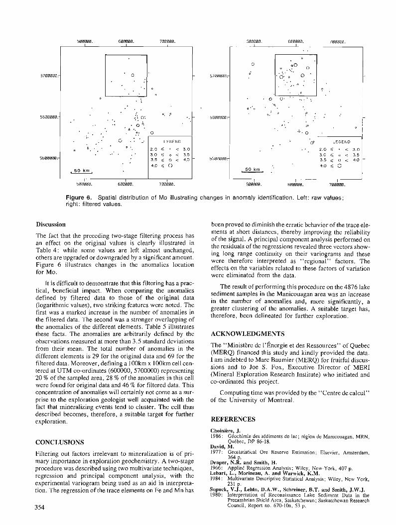
, . m 0

LEGEND

. . 3.0 $ 0 < 3.5

5500000:

4.0 < 0 5 0 km .

Figure 6. Spatial distribution of Mo illustrating changes in anomaly identification. Left: raw values; right: filtered values.

Discussion

'The fact that the preceding two-stage filtering process has an effect on the original values is clearly illustrated in Table 4 : while some values are left almost unchanged, others are upgraded or downgraded by a significant amount. Figure 6 illustrates changes in the anomalies location for Mo.

It is difficult to demonstrate that this filtering has a practical, beneficial impact. When comparing the anomalies defined by filtered data to those of the original data (logarithmic values), two striking features were noted. The first was a marked increase in the number of anomalies in the filtered data. The second was a stronger overlapping of the anomalies of the different elements. Table 5 illustrates these facts. The anomalies are arbitrarily defined by the observations measured at more than 3.5 standard deviations from their mean. The total number of anomalies in the different elements is 29 for the original data and 69 for the filtered data. Moreover, defining a lOOkrn x 100km cell centered at UTM co-ordinates (600000, 5700000) representing 20 % of the sampled area, 28 % of the anomalies in this cell were found for original data and 46 % for filtered data. This concentration of anomalies will certainly not come as a sur- prise to the exploration geologist well acquainted with the fact that mineralizing events tend to cluster. The cell thus described becomes, therefore, a suitable target for further exploration.

CONCLUSIONS

Filtering out factors irrelevant to mineralization is of primary importance in exploration geochemistry. A two-stage procedure was described using two multivariate techniqdes, regression and principal component analysis, with the experimental variogram being used as an aid in interpretation. The regression of the trace elements on Fe and Mn has

been proved to diminish the erratic behavior of the trace elements at short distances, thereby improving the reliability of the signal. A principal component analysis performed on the residuals of the regressions revealed three vectors showing long range continuity on their variograms and these were therefore interpreted as "regional" factors. The effects on the variables related to these factors of variation were eliminated from the data.

The result of performing this procedure on the 4876 lake sediment samples in the Manicouagan area was an increase in the number of anomalies and, more significantly, a greater clustering of the anomalies. A suitable target has, therefore, been delineated for further exploration.

ACKNOWLEDGMENTS

The "Ministkre de 1 '~ne rg ie et des Ressources" of Quebec (MERQ) financed this study and kindly provided the data. I am indebted to Marc Baumier (MERQ) for fruitful discussions and to Joe S. Fox, Executive Director of MERI (Mineral Exploration Research Institute) who initiated and co-ordinated this project.

Computing time was provided by the ''Centre de calcul" of the University of Montreal.

REFERENCES

Choiniere, J. 1986: Gdochimie des skdiments de lac; r6gion de Manicouagan, MRN,

Qudbec, DP 86-18. David, M. 1977: Geostatistical Ore Reserve Estimation; Elsevier, Amsterdam,

364 p. Draper, N.R. and Smith, H. 1966: Applied Regression Analysis; Wiley, New-York, 407 p. Lebart, L., Morineau, A. and Warwick, K.M. 1984: Multivariate Descriptive Statistical Analysis; Wiley, New York, --.

231 p. Sopuck, V.J., Lehto, D.A.W., Schreiner, B.T. and Smith, J.W.J. 1980: Interpretation of Reconaissance Lake Sediment Data in the

Precambrian Shield Area, Saskatchewan; Saskatchewan Research Council, Report no. 670-10a, 53 p.

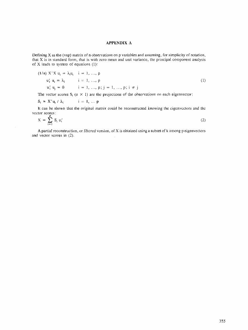
APPENDIX A

Defining X as the (nxp) matrix of n observations on p variables and assuming, for simplicity of notation, that X is in standard form, that is with zero mean and unit variance, the principal component analysis of X leads to system of equations (1 ) :

( l /n) X ' X ui = hiui i = 1, ..., p

The vector scores Si (n x 1) are the projections of the observations on each eigenvector:

It can be shown that the original matrix could be reconstructed knowing the eigenvectors and the vector scores :

D

A partial reconstruction, or filtered version, of X is obtained using a subset of k among p eigenvectors and vector scores in (2).

Multivariate patterns of field information and geochemistry in a regional lake sediment survey:

the NEAIIAEA Athabasca Test Area revisited1

Michel Mellinger2

Mellinger, M., Multivariate patterns o f j e ld information and geochemistry in a regional lake sediment survey: the NEA IIAEA Athabasca Test Area revisited; fi Statistical Applications in the Earth Sciences, ed. F. P. Agterberg and G. F. Bonham-Carter; Geological Survey of Canada, Paper 89-9, p. 357-365, 1989

Abstract

A regional lake sediment geochemical survey for which field observations were recorded and other mapped information was available, was re-interpreted using correspondence analysis. The purpose of the re-interpretation was twofold: firstly, to evaluate the influence of processes expressed by field variables on lake sediment geochemistry; and secondly, to demonstrate that a descriptive multivariate data analysis approach is effective in providing information critical to the explorationist.

f ie field variables are : drainage basin, Quaternary geology, underlying bedrock type, lake area and depth, and relative relie$ Lake sediments were analyzed for I I elements: U, Zn, Cu, Pb, Ni, Co, Ag, Mn, As, Mo, Fe, and LOI.

Multivariate relationships between field variables are well structured. Lake characteristics are self- consistent, with relatively small and shallow lakes occurring in gentler relief, and vice versa. The spatial distrib~rtion of lakes with given characteristics is not homogenous with respect to drainage basin, Quater- nary geology, or underlying bedrock.

Chemically, two opposite general trends are observed: lake sediments relatively rich in Mn-oxides are poor in organic matter, tend to occur in relatively large and deep lakes, and do not concentrate metals; lake sediments relatively rich in organic matter tend to occur in relatively small and shallow lakes, and concentrate most metals. In addition, two isolated trends are of interest to the explorationist : Fe-As-(Mo) anomalies are easily identified and the majority are associated with glacio-fluvial sediments; new U anomalies can be ident$ed in the chemical factor space which cannot be identified on the basis of U concentration alone, and they define new anomalo~is lakes in the survey area.

Un lev6 gkochimique re'gional de skdiments lacustres, don1 les observations sur le terrain avaient e'tk enregistrkes etpour lequel d'autres renseignements cartographie's e'taient disponibles, a kt6 interprkte' de nouveau au moyen de l'analyse des correspondances. L'objet de cette nouvelle interpr&tation &tait double, premierement &valuer l'injluence des processus exprimks par des variables de terrain sur la gkochimie des skdiments lacustres et deuxit.mement, dkmontrer l'avantage d'une approche d'analyse multivarike descriptive des donnkes en vue de l'obtention de renseignements indispensables d l'explorateur.

Les variables relevkes sur le terrain e'taient le bassin hydrographique, la gkologie du Quaternaire, le type de socle rocheux sous-jacent, la superjcie et la profondeur des lacs ainsi que le relief relatg Duns les skdiments lacustres, on a dosh onze klkments, U , Zn, Cu, Pb, Ni, Co, Ag, Mn, As, Mo et Fe, et de'termine' la perte au feu.

' Saskatchewan Research Council Publication No: R-851-1-D-89 Saskatchewan Research Council, 15 Innovation Blvd, Saskatoon, Saskatchewan S7N 2x8

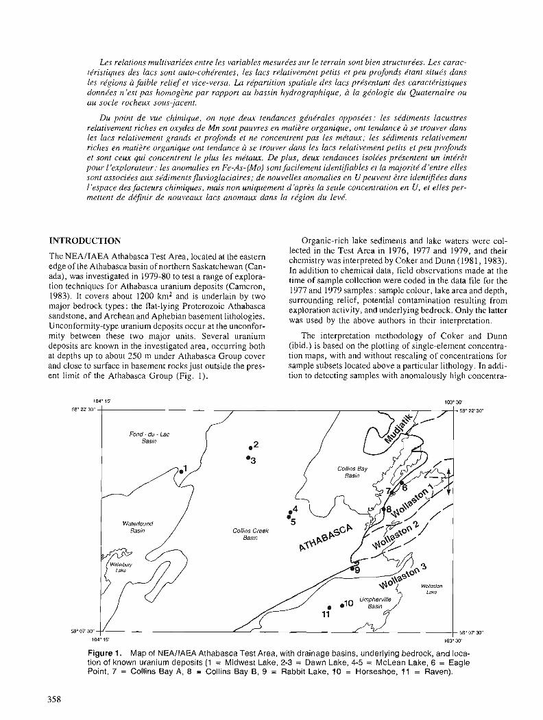
Les relations multivarie'es entre les variables mesurkes sur le terrain sont bien structure'es. Les caractkristiques des lacs sont auto-cohkrentes, les lacs relativement petits et peu profonds ktant s i tub dans les rkgions faible relief et vice-versa. La rkpartition spatiale des lacs pre'sentant des caractiristiques donnkes n'est pas homog2ne par rapport au bassin hydrographique, a la giologie du Quaternaire ou au socle rochewr sous-jacent.

Du point de vue chimique, on note deux tendances gknkrales oppos&es: les skdiments lacustres relativement riches en oxydes de Mn sont pauvres en matitre organique, ont tendance a se trouver dans les lacs relativement grands et profonds et ne concentrent pas les mhaux; les skdiments relativement riches en matiPre organique ont tendance & se trouver dans les lacs relativement petits et peu profonds et sont ceux qui concentrent le plus les mktaux. De plus, deux tendances isolkes prksentent un intkrgt pour l'explorateur: les anomalies en Fe-As-(Mo) sont facilement identifiables et la majoritkd'entre elles sont associkes aux skdiments fluvioglaciaires; de nouvelles anomalies en U peuvent &re identifie'es dans l'espace des facteurs chimiques, mais non uniquement d'aprts la seule concentration en U, et elles permettent de dtifinir de nouveaux lacs anomaux dans la rtfgion du levk.

INTRODUCTION Organic-rich lake sediments and lake waters were col-

The NEAIIAEA Athabasca Test Area, located at the eastern edge of the Athabasca basin of northern Saskatchewan (Can- ada), was investigated in 1979-80 to test a range of exploration techniques for Athabasca uranium deposits (Cameron, 1983). It covers about 1200 km2 and is underlain by two major bedrock types : the flat-lying Proterozoic Athabasca sandstone, and Archean and Aphebian basement lithologies. Unconformity-type uranium deposits occur at the unconformity between these two major units. Several uranium deposits are known in the investigated area, occurring both at depths up to about 250 m under Athabasca Group cover and close to surface in basement rocks just outside the present limit of the Athabasca Group (Fig. 1).

lected in the Test Area in 1976, 1977 and 1979, and their chemistry was interpreted by Coker and Dunn (1981, 1983). In addition to chemical data, field observations made at the time of sample collection were coded in the data file for the 1977 and 1979 samples : sample colour, lake area and depth, surrounding relief, potential contamination resulting from exploration activity, and underlying bedrock. Only the latter was used by the above authors in their interpretation.

The interpretation methodology of Coker and Dunn (ibid.) is based on the plotting of single-element concentration maps, with and without rescaling of concentrations for sample subsets located above a particular lithology. In addition to detecting samples with anomalously high concentra-

Figure 1. Map of NEAllAEA Athabasca Test Area, with drainage basins, underlying bedrock, and location of known uranium deposits (1 = Midwest Lake, 2-3 = Dawn Lake, 4-5 = McLean Lake, 6 = Eagle Point, 7 = Collins Bay A, 8 = Collins Bay B, 9 = Rabbit Lake, 10 = Horseshoe, 11 = Raven).

tions in one element or another and relating them to known uranium deposits, the authors noted indications of spatial trends in the data which may duplicate the known north- easterly trends of basement lithologies and glacial geology in the area. They also examined geochemical associations by plotting on a map those samples with concentration higher than the 90th percentile for any element.

In this paper, the same data are interpreted with two concerns in mind. Firstly, the chemistry of organic-rich lake sediments is known to be influenced by various field variables such as Quaternary geology and lake characteristics. For this survey, the availability of field observations at sampling sites, and of geological and hydrological information from other studies in the same area, offers an opportunity to evaluate the influence of processes expressed by non- chemical variables on organic-rich lake sediment chemistry. Secondly, instead of relying mostly on the visual interpretation of single-element concentration maps, the usually complex inter-relationships between measured variables - chemical or not - are examined directly by use of multivariate data analysis, without a priori assumptions about the nature of such inter-relationships. The purpose of this new interpretation being to see whether new anomalies can be detected, and also whether anomalies can be better evaluated with the knowledge of field variables for a more informed follow-up strategy.

INITIAL DATA

The data file from Coker and Dunn (1981) was obtained and the following data were extracted: sample number, UTM coordinates, field variables (underlying bedrock, lake area, lakedepth, relief), lake sediment chemistry (U, Zn, Cu, Pb, Ni, Co, Ag, Mn, As, Mo, Fe, LOI). Sediment colour being essentially constant, and potential contamination from exploration activity being rare, neither code was retrieved (the latter information can also be dealt with during interpretation). Samples taken in 1976 were deleted from the data file because no field information was available for them. A total of 403 samples collected in 1977 or 1979 remained.

Two separate data files were then created to facilitate data analysis, sharing sample number and UTM coordinates : the first containing field information, the second containing chemical information.

FIELD INFORMATION

Coding of field information

The following field variables were added to the appropriate data file : drainage basin, drainage order, presence of known mineralization in the vicinity, and Quaternary geology. Because neither drainage order nor presence of known mineralization produced useful information during interpretation, they will not be discussed further here.

The following drainage basins were located in the survey area on a 1 :50 000 topographic map (Fig. 1) : the Fond-du- lac River basin (NW), the Waterfound River basin (W), the Wollaston West-Collins Creek sub-basin (centre), the Wol- laston West-Collins Bay sub-basin (NE and E), and the Umpherville River basin (SE). For each sample, a nominal code with value from 1 to 5, respectively, indicates the drainage basin within which it is located.

Quaternary geology at each sampling site was derived from Schreiner (1983) and a nominal code with value from 1 to 4 was added to each sample, meaning respectively: hummocky moraine (Mh), other moraine (Mpvd: plain, veneer, drumlinoid), glacio-fluvial or glacio-lacustrine (GF), and organic (ORG : bog).

Underlying bedrock geology, coded in the initial data file, was modified to comply with the four basement lithologies described by Sibbald (1980). A nominal code with value from 1 to 5 describes the following lithologies, respectively and in increasingly younger stratigraphic position: Archean granite gneiss (Mudjatik Domain, called here Mudjatik), Aphebian metasediments with low magnetic response and containing numerous conductors (Wollaston Domain, called here Wollaston I), Aphebian metasediments with medium to strong magnetic response (Wollaston Domain, called here Wollaston 2), Aphebian metasediments with low uniform magnetic response (Wollaston Domain, called here Wollaston 3), and Athabasca Group sandstones.

Lake area, coded in the initial data file as a 4-column indicator variable, was kept in that form. Area categories were: < '14 km2, ' 14 to 1 km2, 1 to 5 km2, > 5 km2. A similar coding for surrounding relative relief was present in the initial data file, using a 3-column indicator variable for the following categories : low relief, medium relief, and high relief. Only the first two columns were kept because no areas of e high relief, are present.

Finally lake depth, initially coded in whole metres (range : 1 to 18 m), was recoded into a nominal variable with value from 1 to 7 based on examination of a percentile cumulative plot, and indicating the following depth categories: I m, 2 m, 3 m, 4-5 m, 6-7 m, 8-to-12 m, and 15-to-18 m.

Cross-tables between field variables were examined to verify coding and to identify spurious relationships between code values, for example (Fig. 1): only Athabasca Group sandstones underlie both the Fond-du-Lac River and Water- found River basins; only Wollaston 2 underlies the Umpherville River basin; Mudjatik rocks underlie only the Wollaston West-Collins Bay basin. Such spurious relationships will be invoked below and only when relevant to the interpretation of field variable patterns.

Data table for correspondence analysis

In order to examine multivariate field variable patterns, correspondence analysis (Benzecri, 1980; Lebart er al., 1984 ; Greenacre, 1984; Mellinger, 1987) was used. Field variables are qualitative variables, either nominal (underlying bedrock, drainage basin, Quaternary geology) or ordinal (lake area and depth, relief). Coding all qualitative variables as completely disjunctive variables permits us to examine non-linear features of both nominal and ordinal types.

The data table submitted to correspondence analysis therefore consisted of 403 sample records with 28 completely disjunctive variables each. Details of the field variables and their disjunctive coding are summarized in Table I .

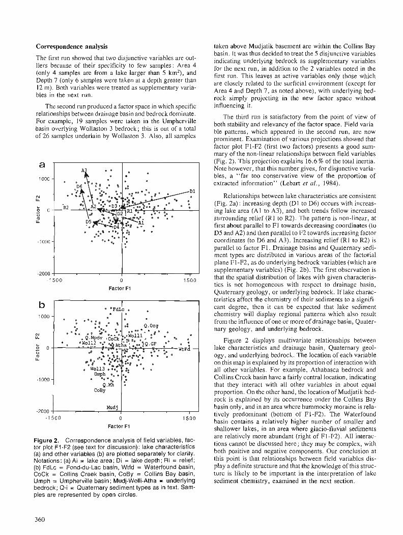
Correspondence analysis

The first run showed that two disjunctive variables are outliers because of their specificity to few samples: Area 4 (only 4 samples are from a lake larger than 5 km2), and Depth 7 (only 6 samples were taken at a depth greater than 12 m). Both variables were treated as supplementary variables in the next run.

The second run produced a factor space in which specific relationships between drainage basin and bedrock dominate. For example, 19 samples were taken in the Umpherville basin overlying Wollaston 3 bedrock; this is out of a total of 26 samples underlain by Wollaston 3. Also, all samples

0

Factor F1

taken above Mudjatik basement are within the Collins Bay basin. It was thus decided to treat the 5 disjunctive variables indicating underlying bedrock as supplementary variables for the next run, in addition to the 2 variables noted in the first run. This leaves as active variables only those which are closely related to the surficial environment (except for Area 4 and Depth 7, as noted above), with underlying bedrock simply projecting in the new factor space without influencing it.

The third run is satisfactory from the point of view of both stability and relevancy of the factor space. Field variable patterns, which appeared in the second run, are now prominent. Examination of various projections showed that factor plot F1-F2 (first two factors) presents a good summary of the non-linear relationships between field variables (Fig. 2). This projection explains 16.6 % of the total inertia. Note however, that this number gives, for disjunctive variables, a "far too conservative view of the proportion of extracted information" (Lebart et al., 1984).

Relationships between lake characteristics are consistent (Fig. 2a) : increasing depth (Dl to D6) occurs with increasing lake area (A1 to A3), and both trends follow increased surrounding relief (R1 to R2). The pattern is non-linear, at first about parallel to F1 towards decreasing coordinates (to D5 and A2) and then parallel to F2 towards increasing factor coordinates (to D6 and A3). Increasing relief (R1 to R2) is parallel to factor F1. Drainage basins and Quaternary sediment types are distributed in various areas of the factorial plane F1-F2, as do underlying bedrock variables (which are supplementary variables) (Fig. 2b). The first observation is that the spatial distribution of lakes with given characteristics is not homogeneous with respect to drainage basin, Quaternary geology, or underlying bedrock. If lake charac-

are relatively more abundant (rightof F1-F2). All interac- Figure 2. Correspondence analysis of field variables, fac- tions cannot be discussed here; may be complex, with tor plot F1-F2 (see text for discussion): lake characteristics (a) and other variables (b) are plotted separately for clarity. positive and negative Our at Notations: (a) Ai = lake area; Di = lake depth; Ri = relief; this point is that relationships between field variables dis- (b) FdLc = Fond-du-Lac basin, Wtfd = Waterfound basin, play a definite structure and that the knowledge of this struc- Cock = Collins Creek basin, CoBy = Collins Bay basin, ture is likely to be important in the interpretation of lake Umph = Umpherville basin; Mudj-Wolli-Atha = underlying sediment chemistry, examined in the next section. bedrock; Q-i = Quaternary sediment types a s in text. Sam- ples are represented by open circles.

b I teristics affect the chemistry of their sediments to a signifi-

OFdLc o cant degree, then it can be expected that lake sediment 1000 - chemistry will display regional patterns which also result

from the influence of one or more of drainage basin, Quater- nary geology, and underlying bedrock.

N LL 00 o Figure 2 displays multivariate relationships between

z 0 ".

,-. lake characteristics and drainage basin, Quaternary geol- 0 m u

ogy, and underlying bedrock. The location of each variable on this map is explained by its proportion of interaction with all other variables. For example, Athabasca bedrock and

-1000 - Collins Creek basin have a fairly central location, indicating that they interact with all other variables in about equal

-2000 - 1 500 0

tively predominant (bottom of F 1-F2). The Waterfound 500 basin contains a relatively higher number of smaller and

Factor F1 shallower lakes, in an area where glacio-fluvial sediments

COB^

MU^ j

proportion. On the other hand, the location of Mudjatik bedrock is explained by its occurrence under the Collins Bay basin only, and in an area where hummocky moraine is rela-

I

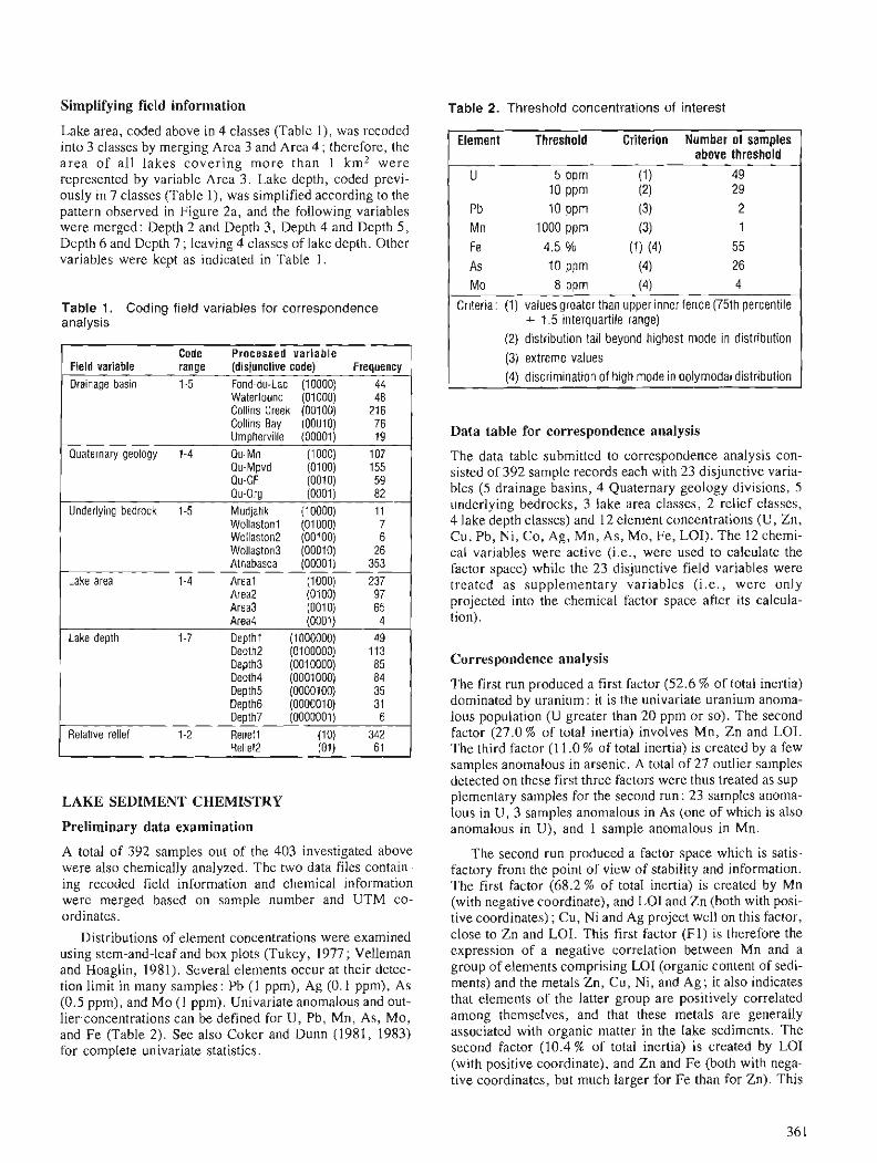
Simplifying field information Table 2. Threshold concentrations of interest

Lake area, coded above in 4 classes (Table l ) , was recoded into 3 classes by merging Area 3 and Area 4 ; therefore, the area of all lakes covering more than 1 km2 were represented by variable Area 3. Lake depth, coded previously in 7 classes (Table l), was simplified according to the pattern observed in Figure 2a, and the following variables were merged: Depth 2 and Depth 3, Depth 4 and Depth 5, Depth 6 and Depth 7 ; leaving 4 classes of Jake depth. Other variables were kept as indicated in Table 1.

Table 1 . Coding field variables for correspondence analysis 1 Field variable rye range prOce'ed (disjunctive code) Frequency

Drainage basin Fond-du-Lac (10000) Waterfound (01000) Collins Creek (00100) Collins Bav (00010) ~rn~hervilie (ooooij 19

Quaternary geology 1-4 Q u - M h (1000) 107

QU-org (0001 j 82 Underlvina bedrock 1-5 Mudiatik (10000) 11

Athabasca i00001 j 353 Lake area 1-4 Areal (1000) 237

Area4 Lake deoth 1-7 Deothl

Depth2 Depth3 Depth4 Depth5 Depth6 Depth7

Relative relief 1-2 Relief1 Relief2

LAKE SEDIMENT CHEMISTRY

Preliminary data examination

A total of 392 samples out of the 403 investigated above were also chemically analyzed. The two data files containing recoded field information and chemical information were merged based on sample number and UTM coordinates.

Distributions of element concentrations were examined using stem-and-leaf and box plots (Tukey, 1977 ; Velleman and Hoaglin, 1981). Several elements occur at their detection limit in many samples: Pb (1 ppm), Ag (0.1 pprn), As (0.5 ppm), and Mo (1 pprn). Univariate anomalous and out- 1ier.concentrations can be defined for U, Pb, Mn, AS, Mo, and Fe (Table 2). See also Coker and Dunn (1981, 1983) for complete univariate statistics.

Element Threshold Criterion Number of samples above threshold

U 5 PPm (1) 49 10 PPm (2) 29

Pb 10 PPm (3) 2 Mn 1000 ppm (3) 1 Fe 4.5 % (1) (4) 55 As 10 PPm (4) 26 Mo 8 PPm (4) 4

Criteria: (1) values greater than upper inner fence (75th percentile + 1.5 interquartile range)

(2) distribution tail beyond highest mode in distribution (3) extreme values (4) discrimination of high mode in polymodal distribution

Data table for correspondence analysis

The data table submitted to correspondence analysis consisted of 392 sample records each with 23 disjunctive variables (5 drainage basins, 4 Quaternary geology divisions, 5 underlying bedrocks, 3 lake area classes, 2 relief classes, 4 lake depth classes) and 12 element concentrations (U, Zn, Cu, Pb, Ni, Co, Ag, Mn, As, Mo, Fe, LOI). The 12 chemical variables were active (i.e., were used to calculate the factor space) while the 23 disjunctive field variables were treated as supplementary variables (i .e. , were only projected into the chemical factor space after its calculation).

Correspondence analysis

The first run produced a first factor (52.6 % of total inertia) dominated by uranium : it is the univariate uranium anomalous population (U greater than 20 pprn or so). The second factor (27.0% of total inertia) involves Mn, Zn and LOI. The third factor (1 1.0 % of total inertia) is created by a few samples anomalous in arsenic. A total of 27 outlier samples detected on these first three factors were thus treated as supplementary samples for the second run : 23 samples anomalous in U, 3 samples anomalous in As (one of which is also anomalous in U), and 1 sample anomalous in Mn.

The second run produced a factor space which is satisfactory from the point of view of stability and information. The first factor (68.2 % of total inertia) is created by Mn (with negative coordinate), and LO1 and Zn (both with positive coordinates) ; Cu, Ni and Ag project well on this factor, close to Zn and LOI. This first factor (F1) is therefore the expression of a negative correlation between Mn and a group of elements comprising LO1 (organic content of sediments) and the metals Zn, Cu, Ni, and Ag ; it also indicates that elements of the latter group are positively correlated among themselves, and that these metals are generally associated with organic matter in the lake sediments. The second factor (10.4 % of total inertia) is created by LO1 (with positive coordinate), and Zn and Fe (both with negative coordinates, but much larger for Fe than for Zn). This

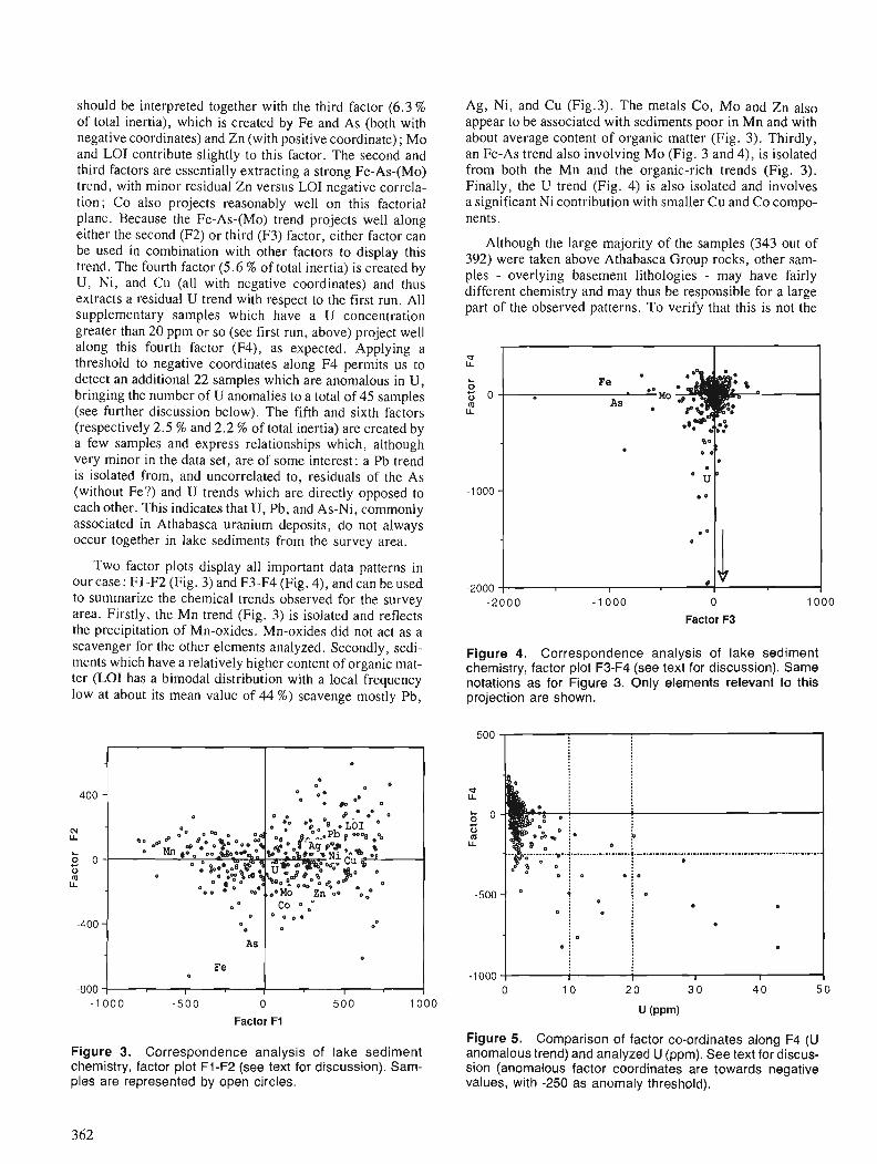
should be interpreted together with the third factor (6.3 % of total inertia), which is created by Fe and As (both with negative coordinates) and Zn (with positive coordinate) ; Mo and LO1 contribute slightly to this factor. The second and third factors are essentially extracting a strong Fe-As-(Mo) trend, with minor residual Zn versus LO1 negative correlation; Co also projects reasonably well on this factorial plane. Because the Fe-As-(Mo) trend projects well along either the second (F2) or third (F3) factor, either factor can be used in combination with other factors to display this trend. The fourth factor (5.6 % of total inertia) is created by U , Ni, and Cu (all with negative coordinates) and thus extracts a residual U trend with respect to the first run. All supplementary samples which have a U concentration greater than 20 ppm or so (see first run, above) project well along this fourth factor (F4), as expected. Applying a threshold to negative coordinates along F4 permits us to detect an additional 22 samples which are anomalous in U, bringing the number of U anomalies to a total of 45 samples (see further discussion below). The fifth and sixth factors (respectively 2.5 % and 2.2 % of total inertia) are created by a few samples and express relationships which, although very minor in the data set, are of some interest: a Pb trend is isolated from, and uncorrelated to, residuals of the As (without Fe?) and U trends which are directly opposed to each other. This indicates that U, Pb, and As-Ni, commonly associated in Athabasca uranium deposits, do not always occur together in lake sediments from the survey area.

Two factor plots display all important data patterns in our case : F1 -F2 (Fig. 3) and F3-F4 (Fig. 4), and can be used to summarize the chemical trends observed for the survey area. Firstly, the Mn trend (Fig. 3) is isolated and reflects the precipitation of Mn-oxides. Mn-oxides did not act as a scavenger for the other elements analyzed. Secondly, sediments which have a relatively higher content of organic matter (LO1 has a bimodal distribution with a local frequency low at about its mean value of 44 %) scavenge mostly Pb,

- 1 000 -500 0 500 1000

Factor F1

Figure 3. Correspondence analysis of lake sediment chemistry, factor plot F1-F2 (see text for discussion). Sam- ples are represented by open circles.

Ag, Ni, and Cu (Fig.3). The metals Co, Mo and Zn also appear to be associated with sediments poor in Mn and with about average content of organic matter (Fig. 3). Thirdly, an Fe-As trend also involving Mo (Fig. 3 and 4), is isolated from both the Mn and the organic-rich trends (Fig. 3). Finally, the U trend (Fig. 4) is also isolated and involves a significant Ni contribution with smaller Cu and Co components.

Although the large majority of the samples (343 out of 392) were taken above Athabasca Group rocks, other samples - overlying basement lithologies - may have fairly different chemistry and may thus be responsible for a large part of the observed patterns. To verify that this is not the

-2000 -1000 0 1000 Factor F3

Figure 4. Correspondence analysis of lake sediment chemistry, factor plot F3-F4 (see text for discussion). Same notations as for Figure 3. Only elements relevant to this projection are shown.

Figure 5. Comparison of factor co-ordinates along F4 (U anomalous trend) and analyzed U (ppm). See text for discussion (anomalous factor coordinates are towards negative values, with -250 as anomaly threshold).

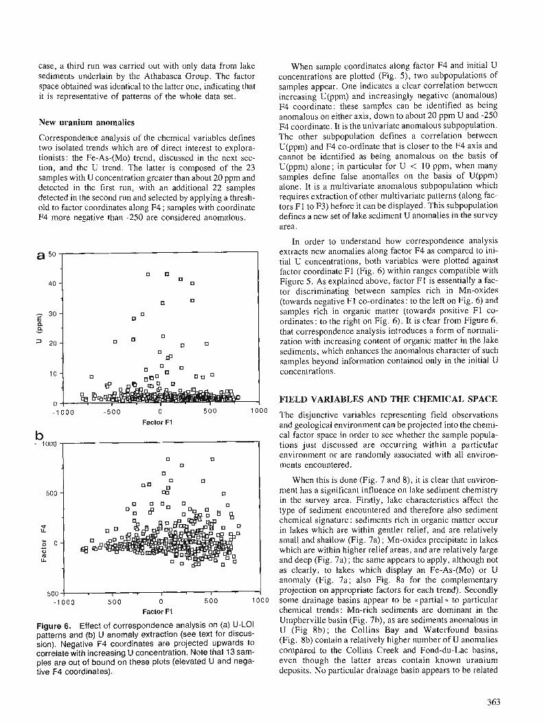
case, a third run was carried out with only data from lake When sample coordinates along factor F4 and initial U sediments underlain by the Athabasca Group. The factor concentrations are plotted (Fig. 5 ) , two subpopulations of space obtained was identical to the latter one, indicating that samples appear. One indicates a clear correlation between it is representative of patterns of the whole data set. increasing U(ppm) and increasingly negative (anomalous)

F4 coordinate: these s a m ~ l e s can be identified as being

New uranium anomalies

Correspondence analysis of the chemical variables defines two isolated trends which are of direct interest to explora- tionists: the Fe-As-(Mo) trend, discussed in the next section, and the U trend. The latter is composed of the 23 samples with U concentration greater than about 20 ppm and detected in the first run, with an additional 22 samples detected in the second run and selected by applying a threshold to factor coordinates along F4; samples with coordinate F4 more negative than -250 are considered anomalous.

1000 - 5 0 0 0 500 1000

Factor FI

500 1 I I I I - 1 000 - 5 0 0 0 500 1000

Factor F1

Figure 6. Effect of correspondence analysis on (a) U-LO1 patterns and (b) U anomaly extraction (see text for discussion). Negative F4 coordinates are projected upwards to correlate with increasing U concentration. Note that 13 samples are out of bound on these plots (elevated U and negative F4 coordinates).

anomalous on either axis, i own to about 20 ppm U and -256 F4 coordinate. It is the univariate anomalous subpopulation. The other subpopulation defines a correlation between U(ppm) and F4 co-ordinate that is closer to the F4 axis and cannot be identified as being anomalous on the basis of U(ppm) alone; in particular for U < 10 ppm, when many samples define false anomalies on the basis of U(ppm) alone. It is a multivariate anomalous subpopulation which requires extraction of other multivariate patterns (along factors F1 to F3) before it can be displayed. This subpopulation defines a new set of lake sediment U anomalies in the survey area.

In order to understand how correspondence analysis extracts new anomalies along factor F4 as compared to initial U concentrations, both variables were plotted against factor coordinate F1 (Fig. 6) within ranges compatible with Figure 5. As explained above, factor F1 is essentially a factor discriminating between samples rich in Mn-oxides (towards negative F1 co-ordinates: to the left on Fig. 6) and samples rich in organic matter (towards positive F1 coordinates: to the right on Fig. 6). It is clear from Figure 6 , that correspondence analysis introduces a form of normalization with increasing content of organic matter in the lake sediments, which enhances the anomalous character of such samples beyond information contained only in the initial U concentrations.

FIELD VARIABLES AND THE CHEMICAL SPACE

The disjunctive variables representing field observations and geological environment can be projected into the chemical factor space in order to see whether the sample populations just discussed are occurring within a particular environment or are randomly associated with all environments encountered.

When this is done (Fig. 7 and 8), it is clear that environment has a significant influence on lake sediment chemistry in the survey area. Firstly, lake characteristics affect the type of sediment encountered and therefore also sediment chemical signature: sediments rich in organic matter occur in lakes which are within gentler relief, and are relatively small and shallow (Fig. 7a); Mn-oxides precipitate in lakes which are within higher relief areas, and are relatively large and deep (Fig. 7a) ; the same appears to apply, although not as clearly, to lakes which display an Fe-As-(Mo) or U anomaly (Fig. 7a; also Fig. 8a for the complementary projection on appropriate factors for each trend). Secondly some drainage basins appear to be .partial D to particular chemical trends: Mn-rich sediments are dominant in the Umpherville basin (Fig. 7b), as are sediments anomalous in U (Fig 8b); the Collins Bay and Waterfound basins (Fig. 8b) contain a relatively higher number of U anomalies compared to the Collins Creek and Fond-du-Lac basins, even though the latter areas contain known uranium deposits. No particular drainage basin appears to be related

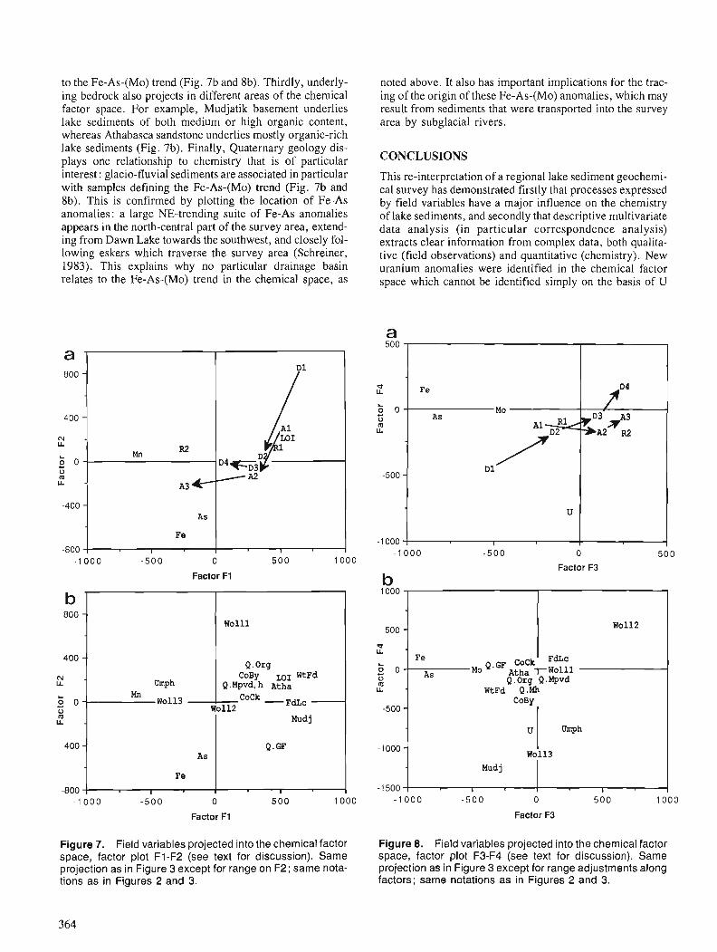
to the Fe-As-(Mo) trend (Fig. 7b and 8b). Thirdly, underlying bedrock also projects in different areas of the chemical factor space. For example, Mudjatik basement underlies lake sediments of both medium or high organic content, whereas Athabasca sandstone underlies mostly organic-rich lake sediments (Fig. 7b). Finally, Quaternary geology displays one relationship to chemistry that is of particular interest : glacio-fluvial sediments are associated in particular with samples defining the Fe-As-(Mo) trend (Fig. 7b and 8b). This is confirmed by plotting the location of Fe-As anomalies: a large NE-trending suite of Fe-As anomalies appears in the north-central part of the survey area, extending from Dawn Lake towards the southwest, and closely following eskers which traverse the survey area (Schreiner, 1983). This explains why no particular drainage basin relates to the Fe-As-(Mo) trend in the chemical space, as

-800 4 0 0 - 1 o 000 -500 0 500 1000

Factor F1

- 1 000 -500 0 500 1000

Factor F1

noted above. It also has important implications for the tracing of the origin of these Fe-As-(Mo) anomalies, which may result from sediments that were transported into the survey area by subglacial rivers.

CONCLUSIONS

This re-interpretation of a regional lake sediment geochemical survey has demonstrated firstly that processes expressed by field variables have a major influence on the chemistry of lake sediments, and secondly that descriptive multivariate data analysis (in particular correspondence analysis) extracts clear information from complex data, both qualitative (field observations) and quantitative (chemistry). New uranium anomalies were identified in the chemical factor space which cannot be identified simply on the basis of U

L

0 0 0 m Q.Org Q.*fpvd U. WtFd Q.Mh

-1000 -1 000 - 5 0 0 0 500

Factor F3

b 1000

-1 000 - 5 0 0 0 500 1000

Factor F3

500 -

Figure 7. Field variables projected into the chemical factor Figure 8. Field variables projected into the chemical factor space, factor plot F1-F2 (see text for discussion). Same space, factor plot F3-F4 (see text for discussion). Same projection a s in Figure 3 except for range on F2; same nota- projection a s in Figure 3 except for range adjustments along tions a s in Figures 2 and 3. factors; same notations a s in Figures 2 and 3.

w0112

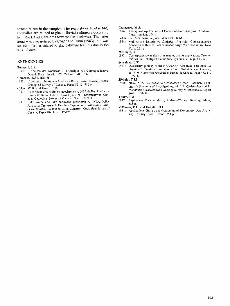
concentration in the samples. The majority of Fe-As-(Mo) anomalies are related to glacio-fluvial sediments occurring from the Dawn Lake area towards the southwest. The latter trend was also noticed by Coker and Dunn (1983), but was not identified as related to glacio-fluvial features due to the lack of data.

REFERENCES Benzecri, J.P. 1980: L'Analyse des DonnCes: 2. L'Analyse des Correspondances;

Dunod, Paris, 1st ed. 1973, 2nd ed. 1980; 632 p. Cameron, E.M. (Editor) 1983: Uranium Exploration in Athabasca Basin, Saskatchewan, Canada;

Geological Survey of Canada, Paper 82-1 1, 310 p. Coker, W.B. and Dunn, C.E. 1981 : Lake water and sediment geochemistry, NEA-IAEA Athabasca

Basin - Wollaston Lake Test Area (64L, 741), Saskatchewan, Can- ada; Geological Survey of Canada, Open File 779.

1983: Lake water and lake sediment geochemistry, NEAIIAEA Athabasca Test Area; in Uranium Exploration in Athabasca Basin, Saskatchewan, Canada; ed. E.M. Cameron; Geological Survey of Canada, Paper 82-11, p. 117-125.

Greenacre, M.J. 1984: Theory and Applications of Correspondence Analysis; Academic

Press, London, 364 p. Lebart, L., Morineau, A., and Warwick, K.M. 1984: Multivariate Descriptive Statistical Analysis: Correspondence

Analysis and Related Techniques for Large Matrices; Wiley, New York, 231 p.

Mellinger, M. 1987: Correspondence analysis: the method and its application; Chemo-

metrics and Intelligent Laboratory Systems, v. 2, p. 61-77. Schreiner, B.T. 1983: Quaternary geology of the NEAIIAEA Athabasca Test Area; in

Uranium Exploration in Athabasca Basin, Saskatchewan, Canada; ed. E.M. Cameron; Geological Survey of Canada, Paper 82-1 1, p. 27-32.

Sibbald, T.I.I. 1980: NEAllAEA Test Area: Sub-Athabasca Group, Basement Geol-

ogy; in Summary of Investigations, ed. J.E. Christopher and R. Macdonald; Saskatchewan Geology Survey Miscellaneous Report 80-4, p. 57-58.

Tukey, J.W. 1977: Exploratory Data Analysis; Addison-Wesley: Reading, Mass,

688 p. Velleman, P.F. and Hoaglin, D.C. 1981 : Applications, Basics, and Computing of Exploratory Data Analy-

sis; Duxbury Press: Boston, 354 p.

Seismic hazard evaluation : extreme and characteristic earthquakes in areas of low and high seismicity

P.W. Burton1

SUMMARY SOMMAIRE

Any evaluation of seismic hazard must be quantitative and present an awareness of the uncertainty in the results. The evaluation process must be capable of being carried out in areas of both low and high seismicity, but rather than there being a single method, there is a network of 'pathways' linking different aspects of the problem. Different 'pathways' will be taken in different circumstances rather than one route always being ideal.

Techniques are considered for the evaluation of seismic hazard as input to regional earthquake engineering codes. Three aspects of hazard assessment are explored. Regional earthquake catalogues are analyzed to obtain the probability of recurrence of earthquakes of a particular magnitude, particularly using Gumbel extreme value statistics. This method has been applied in estimating the areal distribution of the earthquakes expected to be largest during a specified time (75 years) in an area of high seismicity (Turkey). This approach is extended to assess the amplitude and accelera- tion of ground motion and their recurrence probability, parameters usually sought by earthquake engineers. This method has been applied to the estimation of 50 year ground accelerations in another area of high seismicity, Greece. The concept of earthquake 'perceptibility' has been developed, which leads to the identification of an earthquake magnitude or type which is characteristic of a region. This 'most perceptible' earthquake is that most likely to be felt at any site in a region and provides an earthquake selection criterion which can be used in a seismic design of noncritical structures. This concept has been applied in the United Kingdom and Central U.S.A. to demonstrate the potential for its application in areas of both low and medium seismicity.

Toute Cvaluation de risques sismiques doit Ctre quantitative et mettre en garde contre l'incertitude des rtsultats. Le pro- cCdC d'Cvaluation doit pouvoir &tre effectuC aussi bien dans des zones de faible que de forte sismicitC. I1 n'existe pas toutefois de mCthode unique, mais bien un rCseau de a voies D reliant les diffkrents eltments du problkme. Aucune n'est idkale, les circonstances dictant le choix de l'une plut6t que de l'autre.

On envisage d'employer des techniques d'kvaluation des risques sismiques comme donnCes d'entrCe pour 1'Clabora- tion de codes rkgionaux de genie sismique. On Ctudie trois aspects de 1'Cvaluation des risques. Des catalogues rCgio- naix de sCismes sont analysCs en vue d'obtenir la probabilitC de recurrence des stismes d'une magnitude dCterminCe i3 l'aide, plus particulikrement, des valeurs extremes de Gum- be1 (statistique). Cette mCthode a CtC appliqute pour estimer la rkpartition en surface des stismes prtvus les plus forts sur une pCriode donnCe (75 ans), dans une zone de forte sismi- citC (Turquie). On l'ernploie dans 1'Cvaluation de I'amplitude et de l'accC1Cration du sol ainsi que de la probabilitC de rCcurrence des sCismes, paramhtres gCnCralement recher- chis par les ingCnieurs du gCnie sismique. La m6thode a servi a l'tvaluation des accClCrations dusol de 50 ans dans une autre zone de forte sismicitk (Grbce). Le concept de la a perceptibilitk ,, des sCismes ayant CtC mis au point permet de determiner la magnitude ou le type de sCisme qui caractC- rise une rtgion. Le critkre du sCisme << le plus perceptible,,, c'est-&-dire celui qu'on ressentira le plus probablement dans . -

un lieu donne, est un critbre de selection utile dans la conception des structures non critiques. Le concept a CtC applique au Royaume-Uni et dans la partie centrale des Etats-Unis pour dtmontrer la possibilitC de son application dans des zones de faible sismicitC et des zones de sismicitC

For practical purposes, it is sensible to seek results by moyenne. each of these methods, thereby examining each 'pathway' towards an evaluation of seismic hazard that is an appropri- A des fins pratiques, il est raisonnable de chercher 2 - - - ate input to regional earthquake engineering codes. Local obtenir des r ~ s ~ l t a t s au rnoyen de chacune de ces mCthodes, hazard assessments may then be determined by applying en explorant chaque << voien d'6valuation des risques sismi- amplification (or damping) factors based on detailed site ques constituant des donnCes d'entrCe appropriCes aux codes inspections and geotechnical assessments. rCgionaux du gCnie sismique. Les risques locaux peuvent

alors &tre dCterminCs en appliquant des facteurs d'amplification (ou d'amortissement) b a d s sur des inspections sur place et des Cvaluations gkotechniques dCtailltes.

' British Geological Survey, Murchison House, West Mains Road, Edinburgh EH3 3LA, Scotland.

in Statistical Applications in the Earth Sciences, ed. F. P. Agterberg and G. F. Bonham-Carter, -

Geological Survey of Canada, Paper 89-9, 1989.

SUMMARY

An extension of principal component analysis for multi-channel remotely sensed imagery

C.F. Chungl, A.G. Fabbriz, and C.A. Kushighor3

When separate displays are produced of the channels in a LANDSAT image of a given region, they appear very similar - all show the main geographic features of the region, such as drainage, roads, and broad geological outlines - although each plot illustrates some specific characteristics of the corresponding channels. The similarity leads to the questions: "Can we reduce the number of images (channels) to one or two?", and "What does the reduction mean?" This parsimony of information is particularly useful when multi-channel data are to be compared with other ancillary data in the region from maps on agriculture, for-

SOMMAIRE

Lorsque des affichages distincts des canaux d'une image LANDSAT d'une rCgion donnCe sont produits, ils parais- sent trks similaires - tous representent les principales enti- t6s gkographiques de la rCgion comme le rCseau hydrographique, les routes et les grandes limites gCologi- ques - mais chaque track illustre certaines caractkristiques spCcifiques des correspondantes. Cette similitude soulbve les questions suivantes : << est-il possible de rCduire le nombre d'images (canaux) B une ou deux? D et << que signifie la rCduction? Cette parcimonie d'information est particulibrement utile lorsque des donnCes multicanales doivent Ctre

estry, geology, geophysical or mineral occurences. comparCes B d'autres donnCes auxiliaires tirees de cartes de l'agriculture, de la foresterie, de la gCologie, des caractkris-

A commonly used technique for such multidimensional tiques geophysiques ou des manifestations minCrales de la data sets is principal component analysis on the correlation rkgion. matrix or on the covariance matrix based won covariances between channels. However, a complicated problem arises because of spatial covariances between channels. This contribution presents an extended version of principal component analysis which takes into consideration the spatial covariance structures of the data. Applications are discussed for several multiple integrated and geocoded data sets in different areas in Canada. The problems studied come from agricultural, forestry and geological fields. Finally, a statistical point of view of "image processing" in general is discussed.

L'analyse des composantes principales de la matrice des corrClations ou de la matrice des covariances basCe sur les covariances entre les canaux est une mCthode couramment utiliske pour de tels ensembles multi-dimensionnels de don- nCes. Toutefois, les covariances spatiales entre les canaux posent un problbme compliquC. Cette Ctude prCsente une version ktendue de I'analyse des composantes principales

,

qui prend en considkration les structures de la covariance spatiale des donnCes. On examine des applications pour plusieurs ensembles de donnkes intkgrCs et gkocodks provenant de differentes rCgions canadiennes. Les problbmes CtudiCs sont issus des domaines de l'agriculture, de la foresterie et de la gCologie. Finalement, le << traitement des images n con- sidCrC en gCnCral d'un point de vue statistique est examink.

' Geological Survey of Canada, 601 Booth Street, Ottawa, Ontario KIA OE8 Canada Centre for Remote Sensing, 1547 Merivale Road, Ottawa, Ontario KIA 0Y7

" lntera Technologies Ltd, 1525 Carling Avenue, Ottawa, Ontario K1S 5H4


The use of Monte Carlo methods to quantify uncertainties in combined plate reconstructions

Gregory L. Cole1

SUMMARY SOMMAIRE

Computer-intensive methods have been developed for the calculation of uncertainties in plate reconstructions. The motion of rotation between adjacent plates is described by a discrete (gridded) probability density function which is constructed through analysis of measurements of locations of marine magnetic anomalies and fracture zone morphology. A discrete probability function describing relative displacement between non-adjacent plates can then be obtained through a large simulation of combined rotations, with each rotation computed by a Monte Carlo selection from the probability density functions of plate pairs linking the end member plates. When plotted in latitude-longitude-rotation space, the rotation probability density functions have the appearance of elongated, inclined, ellipsoids with increasing densities in the central regions. Confidence limits can be contoured within the ellipsoids by plotting cumulative frequencies, beginning with the grid locations with the largest probability values. The confidence levels appear as concentric shells.

Application of this method to the Pacific-Antarctic, anomaly 13 reconstruction indicates that the linear dimensions of the published worst case uncertainty region are twice as large as those of the uncertainty region at a 95 % confidence level, and 3 times as large as those at the 80 % confidence level. Similarly, the Pacific-North America combined rotation for anomaly 6 demonstrates that realistic uncertainties are apt to be significantly smaller than those previously predicted by worst case scenarios. Thus, while strict application of Murphy's Law may result in uncertainties in pole position that cause large position errors in reconstructions, the probabilistic approach indicates that expected uncertainties and resultant plate reconstruction errors should be much smaller.

Des mCthodes faisant beaucoup appel aux ordinateurs ont CtC mises au point pour les calculs d'incertitude dans les reconstitutions de plaques. Le mouvement relatif ou la rotation de plaques adjacentes sont dkcrits par une fonction de densitt de probabilitC discrkte (suivant un quadrillage) Cta- blie d'aprbs l'analyse de mesures des emplacements d'anomalies magnktiques marines et de la morphologie de la zone transformante. Une fonction de probabilitk discrkte dCcri- vant le dCplacement relatif de plaques non adjacentes peut ensuite Ctre obtenue h l'aide d'une grande simulation des rotations combinkes, chaque rotation Ctant calculCe au moyen d'une sClection de Monte Carlo, ?i partir des fonctions de distribution calculkes pour les couples de plaques reliant les plaques correspondant aux termes finals. Lorsque tracdes suivant un espace comportant longitude et latitude, les fonctions de densitt de probabilitC de rotation prksentent l'aspect d'ellipsoi'des allongCs et inclinks oh les densitCs augmentent vers les rtgions centrales. Les limites de confiance ueuvent Ctre reurCsentCes uar des courbes ?i I'intkrieur des ellipsoi'des par le track des frCquences cumulCes en commenGant aux endroits du quadrillage prksentant les valeurs de probabilitC les plus 6levCes. Les niveaux de confiance prennent la forme d'enveloppes concentriques.

L'application de cette mCthode ?I la reconstruction de l'anomalie 13 Pacifique-Antarctique indique que les dimensions 1inCaires publikes pour la rCgion d'incertitude dans le scenario de la pire CventualitC sont deux fois plus grandes que celles de la rCgion d'incertitude ?i un niveau de confiance de 95 % et trois fois plus grandes que celles au niveau de confiance de 80 %. Pareillement, la rotation combinCe Pacifique-AmCrique du Nord pour l'anomalie 6 dCmontre que les incertitudes rtalistes pourraient Ctre considerable- ment plus petites que celles prdctdemment prCvues ?I l'aide des scCnarios de la pire CventualitC. Ainsi, alors que l'application rigoureuse de la loi de Murphy peut rCsulter en des incertitudes quant aux positions initiales qui entrainent de grandes erreurs de position lors des reconstitutions, I'approche probabiliste indique que les incertitudes prCvues et les erreurs rksultantes de reconstitution de plaques devraient 2tre beaucoup plus petites.

' Earth and Space Sciences Division, Los Alamos National Laboratory, Los Alamos, N M 87545, U.S.A. and Department of Geological Sciences, University of Arizona, Tucson, AZ 85719, USA.


Computer programs for correspondence analysis, and dendrographs with applications to coal data

Marcel Labontd

SUMMARY SOMMAIRE

A range of methods that seek to uncover the structure of data-sets coming mostly from instrumental measurements is presented. These programs perform multivariate descriptive data analysis. The advent of sophisticated analytical equipment has resulted in the existence of large data-sets in geology. Analysis of geological information is often the corroboration of what a geologist suspects from earlier work. Also the presentation of graphic output is desirable as it con- forms with the spatial presentation often necessary in geology. The evolution of computer technology allows a greater variety of methods, with readily available software. The advent of personal computers in particular has made the use of statistical software easier.

L'auteur prCsente une dr ie de mCthodes dont le but est de dCcouvrir la structure d'ensembles de donntes provenant surtout de mesures instrumentales. Les programmes effec- tuent une analyse de donntes descriptives i plusieurs variables. L'apparition d'un mattriel d'analyse trhs perfectionnk est B I'origine de I'existence de grands ensembles de don- nCes en gkologie. L'analyse de renseignements gtologiques est souvent la corroboration de ce qu'un gtologue soup- Gonne de travaux antbrieurs. En outre, la prtsentation de rbsultats graphiques est souvent souhaitable car elle se con- forme 2 la prksentation spatiale souvent nCcessaire en gCologie. L'Cvolution de I'informatique permet le recours ?i une plus grande varikt.6 de mbthodes pour lesquelles on peut facilement se procurer des logiciels. L'arrivCe d'ordinateurs personnels, en particulier, a rendu I'utilisation de logiciels statistiques plus facile.

SELECTED REFERENCES

Barber, J.F., Barbash, J.E., and LabontC, M. 1988: Groundwater contamination at a landfill sited on fractured car-

bonate and shale; Journal of Contaminant Hydrology, v. 3 , p. 1-25.

~abontk , M. and Goodarzi, F. 1987: The relationship between dendrographs and Pearson product-

moment correlation coefficients; in Current Research, Part A, Geological Survey of Canada, Paper 87- I A, p. 353-356.

' Institute of Sedimentary and Petroleum Geology, 3303-33 Street N. W . , Calgary, Alberta T2L 2A7


SUMMARY

Practical aspects of multivariate estimation for spatial data

Donald E. Myers1

Multivariate spatial data are frequently encountered in many applications such as remote sensing, geochemical surveys, multimetal deposits or as the result of non-linear transformations. The data may be quantitative with no censoring or smoothing or may only be qualitative. The spatial characterization may be in the form of position co-ordinates or only subregional identifications.

The simplest form of multivariate estimation for spatial data, co-kriging, incorporates the (linear) spatial and intervariable correlation to determine the weights in a linear estimator. This estimator is only applicable to quantitative data with position co-ordinates in 1 , 2 or 3 space. Although the general theory is well known, the techniques for estima- tionlmodeling of cross-covariances are generally less satisfac tory than f o r univar ia te auto-covar iances ( o r variograms). These difficulties are in part due to the difficulty in verifying the positive definiteness. These techniques are reviewed and examples given to show their application.

When censored data or qualitative data converted to quantitative form is used, or when a non-linear transformation such as the indicator is applied, there may be auxiliary relations that should be satisfied, for example an order relation. While joint estimation may not guarantee these conditions, it is in general the preferable tool. However, the application is dependent on resolution of the difficulties alluded to above. Examples are given to illustrate the estimation of cross-covariances for transformed and censored data.

SOMMAIRE

On rencontre frtquemment des donnCes spatiales B variables multiples dans nombre d'applications cornrne en ttlCdttec- tion, dans les lev& gtochimiques, dans 1'Ctude des gisements B plus ieurs mCtaux ou comme rksultat d e transformations non lintaires. Les donntes peuvent Ctre quantitatives et ne cornporter aucune expurgation ou aucun lissage, ou encore peuvent n'Ctre que qualitatives. La caracttrisation spatiale peut prendre la forme de coordonnCes de position ou seulement d'identifications sous-regionale.

La forme la plus simple d'estimation multivariCe pour des donnCes spatiales, le co-krigeage, fait intervenir des corrClations (1inCaires) spatiales et entre variables pour dtterminer les facteurs de pondtration au moyen d'un estimateur linCaire. Cet estimateur n'est applicable qu'8 des donntes quantitatives avec coordonnCes deposition dans des espaces B une, deux ou trois dimensions. Bien que la thCorie gCnCrale soit bien connue, les mCthodes d'estimation et de modClisation de covariances croisCes sont gtnkralernent moins satisfaisantes aue celles faisant intervenir les auto- covariances univariCes (variogrammes). Ces difficult& sont en partie attribuables au problkme que pose la vkrification du caractbre dtfini de la positivitt. On examine ces mCthodes tout en prtsentant des exemples de leur application.

Lorsque des donntes expurgtes ou des donnCes qualitatives converties en donnCes quantitatives sont utiliskes, ou lorsqu'une transformation non linCaire comme celle de l'indicateur est appliquCe, il peut exister des relations auxiliaires qui devraient Ctre satisfaites, cornrne une relation d'ordre par exemple. Bien qu'il soit possible que I'estimation conjointe ne garantisse pas le respect de ces conditions, elle constitue en gCntral l'outil prtfkrable. Toutefois, son application dCpend de la solution des difficult& prtcddem- ment mentionnks. Les exemples prCsentCs ici illustrent l'estimation des covariances croisCes pour des donntes transformtes et expurgtes.

' Department o f Mathematics, University o f Arizona, Tucson, AZ 85721 U.S .A.


SUMMARY

Multivariate statistical analysis - a practical approach in hydrocarbon exploration?

John Robinsonl, Guy Masson2, Michael Marchandl and Dennis Saigeonl

A variety of multivariate statistical techniques have been used for many years in the geological sciences and in exploration to a limited extent. It appears that there is very little day to day use of these statistical techniques in hydrocarbon exploration. The question that begs to be asked is therefore "Can multivariate statistical techniques provide any practical benefits to hydrocarbon exploration?"

We carried out a short project to evaluate the potential benefits of the use of Correspondence Analysis. A current project underway was the regional geological and facies analysis of the Beaverhill Lake Formation in Alberta. This project utilized a portion of the digital lithological CAN- STRAT file containing lithological descriptions for 1810 wells. Prior to the running of the correspondence analysis, a detailed facies and geological analysis was prepared for the area from not only the digital lithological data but also core examinations and other published and unpublished information. Regional lithofacies maps were produced and interpreted in terms of depositional models. During the final days of this regional analysis, the correspondence analysis program was run on the 1810 wells using 12 lithological variables. Six factors representing 92 %of the variability of the data were extracted. Contoured maps of each of the six factor scores were produced. Factor plots (scattergrams) of each combination of two factors were generated and computer plotted as large sized (1 m by 1 m) diagrams to review the data patterns of the individual factors. The four most significant factor maps were then utilized to develop an interpreted facies map. This interpretation of the regional lithofacies closely matched the previously developed lithofacies interpretation carried out by the geologist as described above.

The statistical analysis project was successful in replicat- ing a regional lithofacies study carried out by standard techniques. It was also a very practical exercise in that the

' Husky Oil Operations Ltd.. Box 6525, Stn. 'D', Calgary, Alberta T2P 3G7 Independent consultant, 12 Butler Crescent, Calgary, Alberta, T2L IK3

SOMMAIRE

Diverses techniques statistiques i variables multiples ont CtC utilisCes dans une faible mesure, en geologie et en exploration pendant un grand nombre d'annkes. I1 semble par ailleurs que ces techniques statistiques soient peu couramment utilisCes en exploration des hydrocarbures. La question que tous se posent est donc : << Les techniques statistiques h variables multiples peuvent-elles fournir des avantages pratiques dans le domaine de I'exploration des hydrocarbures? *

Les auteurs ont rCalisC un modeste projet conGu en vue d'tvaluer les avantages possibles de l'analyse des correspondances. Une Ctude rCcente portait sur l'analyse rCgionale de la gCologie et des faciks de la formation de Beaverhill Lake en Alberta. Cette Ctude a fait appel B une partie du fichier lithologique numCrique CANSTRAT qui renferme la description lithologique de 1810 puits. Avant 1'exCcution de l'analyse des correspondances, une analyse dttaillCe rCgio- nale des faciks et de la gCologie a Cte prCparCe i partir non seulement des donnkes lithologiques numCriques, mais aussi d'ktudes de carottes et d'autres renseignements publiCs et iddits . Des cartes rCgionales de lithofaciks ont CtC produites et interprkttes en fonction de modbles de ~Cdimentation. Pendant les derniers jours de cette analyse rkgionale, on a pass6 le programme d'analyse des correspondances pour les 18 10 puits i I'aide de 12 variables lithologiques. On a extrait six facteurs reprksentant 92 % de la variabilitk des donnkes. Des cartes hypsomCtriques des rtsultats de chacun de six facteurs ont CtC produites. Des diagrarnmes de dispersion de chaque paire de facteurs ont CtC produits et restituCs par ordinateur sous forme de diagrammes de grande taille (1 m sur 1 m) en vue d'Ctudier les configurations des donnCes des facteurs individuels. Les quatre cartes de facteurs les plus importantes ont alors servi i ttablir une carte de facibs d'interprktation. Cette interpretation du lithofaci5s rtgio- nale correspond Ctroitement i l'interprttation du lithofaciks andrieure, effectuCe par le gCologue de la facon dCcrite ci- dessus.


analysis and the plotting of the maps using computer techniques took only 5 person days while the standard analysis took over 20 person days. The use of these statistical techniques provides a way of getting a "jump-start" in a new area and provides a reasonable framework from which to select areas of interest for more detailed analysis. There is a major proviso here, in that it would be rare to find a single person with appropriate skill levels and knowledge to carry out all the operations. This type of project is best carried out by a team of skilled specialists ; at a minimum a geologist highly skilled in the regional and sedimentological aspects of the study and one skilled in the data analysis aspects of the project.

Le projet d'analyse statistique a Ctt couronnt de succbs dans le cas de la reproduction d'une ttude de lithofacibs rkgionale effectute B partir de techniques normales. 11 s'agissait, en outre, d'un exercice pratique, car l'analyse et - la restitution des cartes h l'aide de techniques informatiques n'a pris que 5 jours-personnes alors que I'analyse normale a prix plus de 20 jours-personnes. L'utilisation de ces mtthodes statistiques permet une initiation rapide dans un nouveau domaine et la crkation d'un cadre raisonnable ?I partir duquel on peut choisir des domaines d'intCrbt aux fins d'analyse plus dttaillke. Une rtserve importante s'impose ntanmoins : les chances sont rares de trouver une seule per- sonne ayant la compttence et les connaissances voulues pour effectuer tous ces travaux. Pour rkussir ce type de projet, il vaut mieux avoir recours 2 une Cquipe de spkcialistes exptrimentts, comprenant au minimum, un gtologue ayant une grande experience des aspects rtgionaux et ddimento- logiques de l ' ttude et un autre ayant l'exptrience de l'analyse des donntes du projet.

SUMMARY

Characterizing the spatial distribution of fractures in rocks

The characterization of the spatial distribution of fractures in rocks provides insight into the genesis of the fracture system, and the circulation of fluids. Field observations indicate that fractures are quasi-randomly distributed in rock masses. Both tensile and shear fractures are the result of the superposition of complex processes in rock masses with initially distributed properties. Spatial distribution of fractures can be analized by at least two different methods : by considering the spacing between adjacent fractures, or by calculating the fracture density which is a function of the number, length and width of fractures.

The spacing approach is particularly suited when the width of the fractures is negligible with respect to their extent; an example is provided by the joint system in the Stripa granite, Sweden. In sheared rocks however, such as the Henderson-Portage shear belt in the Chibougarnau area (Quebec), a number of fractures have a significant width (e.g. veins, shear zones) and the density approach appears more appropriate. Fracture data, obtained from mapping the walls of the main drifts of three levels of the Henderson I1 mine, had to be transformed in order to obtain a standardized data support as required for geostatistical analysis. Preliminary analysis of the fracture density variograms, constructed for the five fracture sets identified in the rock mass, shows evidence of a spatial correlation in the order of ten metres, for each of the sets. The variograms are used to obtain a kriged estimation of fracture density over an entire mine level.

SOMMAIRE

La caracttrisation de la repartition spatiale des fractures dans les roches fournit un apercu de la gtnbse du rtseau de fractures et de la circulation des fluides. Les observations sur le terrain indiquent que les fractures se repartissent de manibre quasi-altatoire dans les masses rocheuses. Les fractures d'extension et de cisaillement rCsultent toutes deux de la superposition de processus complexes dans des masses rocheuses aux propriCtCs intitialement rtparties. La repartition spatiale des fractures peut 6tre analyske au moyen d'au moins deux mtthodes diffkrentes : en prenant en consideration I'espacement de fractures adjacentes ou en calculant la densite des fractures qui est fonction du nombre, de la longueur et de la largeur des fractures.

L'approche de l'espacement convient particulibrement bien lorsque la largeur des fractures est ntgligeable par rapport leur longueur; le rkseau de diaclases dans le granite de Stripa en Subde constitue un bon exemple. Dans les roches cisailltes toutefois, cornrne dans la zone cisaillte de Henderson et de Portage de la region de Chibougamau (Qutbec), un certain nombre de fractures prksentent une largeur importante (p. ex. veines, zones de cisaillement) et l'approche basCe sur la densitt semble mieux convenir. Les donntes sur les fractures tirtes des cartes des parois des galeries principales B trois niveaux dans la mine Henderson I1 devaient Ctre transformCes afin d'obtenir I'ensernble de donnCes normalist nkcessaire B l'analyse gtostatistique. L'analyse prtliminaire des variograrnmes de densitt des fractures, ttablis pour les cinq ensembles de fractures identifies dans la masse rocheuse, r6vkle des indices d'une correlation spatiale de l'ordre de dix mbtres pour chacun des ensembles. Les variogrammes sont utilists pour obtenir une estimation par krigeage de la densitt des fractures pour I'ensemble d'un des niveaux de la mine.

-

' UniversitC du Qutbec Chicoutimi, 555 Boulevard de I'UniversitC, Chicoutimi, Qutbec G7H 2PI

in Statistical Applications in the Earth Sciences, ed. F.P. Agterberg and G.F. Bonham-Carter; - Geological Survey of Canada, Paper 89-9, 1989

Recognition of multivariate anomalies in exploration geochemistry

J. J. Royerl and H. Mezghache2

SUMMARY SOMMAIRE

The determination of the Beginning Anomalous Grade (BAG) and of the Significant Anomalous Grade (SAG) is a classical problem in exploration geochemistry. In this paper, the theory of fuzzy indicators is used to generalize the elementary methods proposed by Lepeltier (1969), Sin- clair (1976) and Royer (1988) for univariate distributions to the multivariate case. This method consists of finite mixture distributions.

In the univariate case, several techniques including zero crossing, gradient, maximum likelihood and the dynamic cluster methods can be used to decompose the histograms or cumulative functions into a mixture of finite distributions. These different components are then identified to belong to the background or to the geochemical anomalies. The programming, the limitations and the advantages of these methods are briefly discussed.

The dynamic clustering method can be generalized to the definition of multivariate anomalies: the grades of each sample are coded by a set of fuzzy characteristics functions related to the background or to the anomalous values. The results are reported on elementary or multicomponent probability maps of occurrences with or without external data (e.g. topography, direction of the dispersion, sources of pollution). The advantages of these fuzzy indicators are: (i) the generalization of Sinclair's method to multivariate mixture distributions; (ii) the processing of truncated data; (iii) the production of probability maps for occurrences.

La dktermination de la teneur anormale seuil (TAS) et de la teneur anormale importante (TAI) constitue un problbme classique en exploration gCochimique. Dans la prCsente ttude, la thCorie des indicateurs flous est utilisCe pour gtnk- raliser les mkthodes ClCmentaires proposCes par Lepeltier (1969), Sinclair (1976) et Royer (1988) pour les distributions B une variable aux distributions B plusieurs variables. Cette methode s'appuie sur des mklanges finis de distributions.

Dans le cas d'une distribution B une variable, plusieurs mtthodes, dont celle du passage par zero, celle du gradient, celle du maximum de vraisemblance et celle du groupe dynamique, peuvent Ctre utilisCes pour dkcomposer les his- togrammes ou les fonctions cumulatives en un mClange de distributions finies. Ces differentes composantes sont ensuite identifikes comme appartenant B la teneur de fond ou aux anomalies gtochiml'ques. La programmation, les limites et les avantages de ces mCthodes sont bribvement examinks.

On peut gCnCraliser la mCthode du groupement dynamique 2 la dtfinition des anomalies B plusieurs variables: les teneurs de chaque tchantillon sont codkes B l'aide d'un ensemble de fonctions de caracttristiques floues relikes aux valeurs de la teneur de fond ou de la teneur anormale. Les rtsultats sont portts sur des cartes ClCmentaires ou composantes de probabilitCs de l'existence de manifestations avec ou sans donnCes extCrieures (p. ex. topographie, direction de la dispersion, sources de pollution). Les avantages de ces

These methods have been applied to several case studies nous sent: i) la g~n~ra l i sa t ion de la methode de to geochemical surveys and to the ex~ lo ra - Sinelair aux melanges de distributions plusieurs variables ; tion for a mercury-bearing sedimentary formation. i i ) le traitement de donnkes tronqutes: iii) la ~roduction de

cartes de probabilitis de l'existence de manifestations.

Ces mCthodes ont CtC appliquCes B plusieurs Ctudes de cas diffkrentes relikes B des levCs geochimiques de mineraux et B I'exploration d'une formation ~Cdimentaire renfermant du mercure.

' Centre de Recherches PCtrographiques et G6ochimiques. B.P. no 20, 15 rue ND des Pauvres, 54501 Vandoeuvre-Les-Nancy, France

' Entreprise Nationale de Recherches Minitres, B.P. 102, Boumerdes 35, AlgCrie

in Statistical Applications in the Earth Sciences, ed. F. P. Agterberg and G. F. Bouham-Carter; - Geological Survey of Canada, Paper 89-9, 1989

SELECTED REFERENCES

Lepeltier, CI 1969: A simplified statistical treatment of geochemical data by graphical

representation; Economic Geology, v . 64, p. 538-530. Royer, J.J. 1988: New approaches to the recognition of anomalies in exploration ge-

ochemistry; Quantitative Analysis of Mineral and Energy Resources, ed. C.F. Chung. A.G. Fabbri, and R. Sinding-Larsen; Reidel, Dordrecht, p. 89-1 12.

Sinclair, A.J. 1976: The application of Probability Plots to Mineral Exploration:

Association of Exploration Geochemists, Special Volume 4. 95p.

Exploring the lower limits of economic truncation: modelling the oil and gas discovery process

J.H. Schuenemeyerland L. J. Drew2

SUMMARY SOMMAIRE

Previous investigations into the discovery process of oil and Les recherches anttrieures concernant le processus de la gas fields suggest that the underlying field size distribution decouverte de champs pCtroliferes et gaziferes sernblent is log-geometric in form and the apparent declining fre- indiquer que cette dernikre est sous-tendue par une rtparti- quency in the smaller size classes is a consequence of an tion B loi logarithmique de la dimension des champs et que economic filtering or truncation process. la frCquence dtcroissante apparente observCe dans les

Analyses of several exploration plays and basins including the Minnelusa play, the Texas State and Federal offshore, the western Gulf of Mexico, the North Sea and the Denver and Permian basins indicate a recurrent pattern. Namely, the observed relative frequency of fields in the smaller size classes is directly related to the cost of discovery and developing oil and gas fields. In addition, the mode of the observed field size distribution shifted to smaller size classes over time, when oil and gas prices increased.

Estimation of the ultimate number of fields in those log size classes thought to be unaffected by economic truncation was accomplished with a modified Arps-Roberts discovery process model. The empirical evidence from basin and play studies suggests that each successively smaller class size (in log base units) contains r, a constant multiplier, more fields than the previous one. The multiplier r was used to derive estimates of the ultimate number of fields to be discovered in the smaller size classes just below the economic truncation boundary. These results suggest that a significant portion of the volume of oil and gas remaining to be discovered will be found in small fields.

classes de plus petites tailles est une consCquence d'un processus de filtrage ou de troncature Cconomique.

Des analyses faites pour plusieurs zones et bassins pCtroliferes d'exploration, notamment la zone de Min- nelusa, le territoire extracdtier de 1'Etat du Texas et du gou- vernement ftdtral, la partie ouest du golfe du Mexique, la mer du Nord et les bassins de Denver et ceux du Permien, indiquent un modble repetitif. C'est-8-dire que la frequence relative observCe des champs dans les classes de plus petites tailles est directement associCe au coOt de la dtcouverte et de la mise en valeur des champs de pttrole et de gaz. De plus, le mode de la rtpartition observCe de la taille des champs s'est dtplact vers les classes de plus petites tailles 8 mesure qu'augmentaient les prix du pttrole et du gaz.

L'estimation du nombre final de champs appartenant aux classes de petites tailles qu'on pensait ne pas Ctre touches par le processus de troncature Cconomique a CtC effectute au moyen d'un modhle modifit du processus de dtcouverte d'Arps-Roberts. La constatation ernpirique faite 8 partir d'Ctudes de bassins et de zones pCtroliRres porte a croire

' University of Delaware, 501 Ewing Hall, Newark, Delaware, 19716 U.S.A. ' U.S. Geological Survey, 922 National Center, Reston, Virginia, 22092 U.S.A.

in Statistical Applications in the Earth Sciences, ed. F. P. Agterberg and G.F. Bonham-Carter; - Geological Survey of Canada, Paper 89-9, 1989

An analysis of the Frio basin provides further insight into que chaque classe de taille inftrieure (en unitts logarith- the issue of economic truncation. The Frio, located in south- miques d'ordre de grandeur) renferme r, facteur constant, east Texas, is a major U.S. basin. Over 800 fields contain- fois plus de champs que la classe prtctdente. Le facteur r ing more than 10 billion barrel of oil equivalent have been a permis d'obtenir des Cvaluations du nombre final de discovered in the Frio. The analysis was performed by champs i dtcouvrir dans les classes de tailles plus petites studying discoveries on a scale of wildcat wells, through qui se trouvent imrntdiatement au-dessous du point de tron- time, on a shallow and deep horizon. cature tconomique. Ces rksultats semblent indiquer qu'une

importante partie du volume de pttrole et de gaz qui reste B dtcouvrir sera dtcouverte dans de petits champs.

Une analyse du bassin de Frio donne une vue plus approfondie du problkme de la troncature Cconomique. Ce bassin, situt d a y la partie sud-est du Texas, est un important bassin des Etats-Unis. Plus de 800 champs renfermant plus de 10 milliards de barils d'tquivalent de pttrole ont CtC dCcouverts dans le bassin de Frio. L'analyse a Ct6 effectuCe en Ctudiant les decouvertes rtv61Ces par des forages de reconnaissance effectu6s au cours des ans dans des horizons superficiels et profonds.

Application of geometric probability and Bayesian statistics to the search for mineral deposits

Donald A. Singer1 and Ryoichi Kouda2

SUMMARY SOMMAIRE

The normal probability density function, Bayesian statistics, and geometric probability (primarily the area of influence method) can be employed to integrate study area spatial and frequency data to produce a map of the probabilities of target (deposit) centres and to estimate the number of deposits present. One or more well-studied deposits serve as a control in which the means and standard deviations of each variable are estimated near a deposit (mineralized area) and away from the deposit (barren area). Multiple independent variables reflecting geological, geochemical, or geophysical information can be used. Circular, elliptical, and annular shaped target variables are possible and preferred orientations are allowed. Where information for one or more variable is missing, a neutral value for the missing sample can be substituted and the system can take advantage of the partial information. Sequential stepwise discriminant analysis can be used to identify the variables and their shapes.

FINDER, a first generation computer program employing these principles is intended to aid geologists in the assessment of, and the search for, ore deposits of particular types. In its first test, FINDER rediscovered all four of the known Kuroko deposits that it should have found and pointed to several new favourable areas, one of which has since had a newly announced discovery of a Kuroko deposit.

SELECTED REFERENCE

Singer, D.A. and Kouda, R. 1988: Integrating spatial and frequency information in the search for

kuroko deposits of the Hokuroko District, Japan; Economic Geo- logy, v. 83, p. 18-29.

La fonction de distribution normale, les statistiques bay& siennes et la probabilitk gComCtrique (principalement la mCthode de la zone d'influence) peuvent servir B I'intCgra- tion des donnCes spatiales et de frtquences d'une region d'etude donnee afin de produire une carte des probabilitks de la presence de cibles (gisements) et d'estimer les nombres de gisements prCsents. Un ou plusieurs gisements bien Ctu- dies servent de tCmoins pour lesquels les moyennes et les Ccarts-types de chaque variable sont estimCs B proximite d'un gisement (zone minCralisCe) et loin du gisement (zone sterile). De nombreuses variables indkpendantes reflitant la gCologie, la gCochimie ou la gCophysique peuvent &tre utilisees. I1 est possible d'ttablir des variables pour des cibles circulaires, elliptiques et annulaires et on permet l'utilisation d'orientations prtfCrentielles. Lorsque l'information concernant une variable ou plus est manquante, une valeur neutre peut stre substitute B celle de I'Cchantillon manquant et le systkme peut ainsi &tre exploit6 B partir de renseignements partiels. L'analyse de discrimination ~Cquentielle par Ctapes peut Ctre utilisCe pour identifier les variables et leurs formes.

Le FINDER de premikre gCnCration est un programme d'ordinateur bas6 sur ces principes et c o n g en vue d'aider les gCologues 2 tvaluer et B rechercher des gisements de minerai de types particuliers. Lors de sa prernibre mise 2 l'kpreuve, le FINDER a permis de redtcouvrir chacun des quatre gisements de Kuroko connus et a indiquC plusieurs nouvelles zones favorables dont I'une oir la dCcouverte d'un gisement de Kuroko a depuis Ctt annonck.

' U.S. Geological Survey, 345 Middlefield Road, Menlo Park, California, 94025 U.S.A Geological Survey of Japan, 1-1-3 Higashi, Yatabe, Ibaraki-ken, 305, Japan.

in Statistical Applications in the Earth Sciences, ed. F.P. Agterberg and G.F. Bonham-Carter; Geological Survey of Canada, Paper 89-9, 1989.

Part III

QUANTITATIVE STRATIGRAPHY

ARTIFICIAL INTELLIGENCE AND EXPERT SYSTEMS

Artificial intelligence applications in paleontology and stratigraphy

Wm. R. Riedell and Linda E. Twayl

Riedel, Wm. R, and Tway, L. E., Artificial intelligence applications in paleontology and stratigraphy; in Statistical Applications in the Earth Sciences, ed. F. P. Agterberg and G. F. Bonham-Carter; Geologi- cal Survey of Canada, Paper 89-9, p. 383-388, 1989.

Abstract

Using Turbo PROLOG on a personal computer, an expert system (COREXPERT) is being assembled to help geologists describe Cenozoic sequences of oceanic sediments. The databases of COREXPERT hold information on the relative proportions of major sediment components as distributed over the sea floor, stratigraphic and geographic ranges of microfossil taxa, and biostratigraphic zonations tied to absolute ages which permit the estimation of rates of accumulation. As new data are entered into the system, the program checks whether they conform to expectations based on information available up to that point. If they do not, the user has the opportunity either to revise the new observations, or to allow them to modzfy the synthesis of sediment distributions represented by the databases. Though COREXPERT at present works on open-ocean Cenozoic sediments, the sojhvare is readily adaptable to other geographic regions and scales, other segments of geological time, and other sedimenlary regimes.

Two components of the expert system are useful as stand-alone programs. STRATIGRAPHER'S ASSISTANT helps the user to arrive expeditiously at a reliable determination of the age (or mixed ages) of a fossil assemblage. IDENTIFY assists the user to identify fossil taxa consistently, despite diflculties caused by intraspeci$c variabilio and incompleteness of specimens.

Short PROLOG routines forming part of these programs are being assembled, together with explanatory text, under the name GeoProlog, to be made available to the geological community as an aid in adopting this artificial intelligence language.

Au moyen du Turbo PROLOG exploitk sur un ordinateur personnel, on proctde ri la mise au point d'un systeme expert (COREXPERT) concu en vue d'aider les gkologues a dkcrire les se'quences c6nozoi- ques de sediments ockaniques. Les bases des donne'es du COREXPERT renferment l'information concernant les proportions relatives des principaux constituants se'dimentaires tels que r6partis sur le fond marin, les champs stratigraphiques et gtfographiques des taxons de microfossiles et les zonations,biostratigraphiques rattachkes aux dges absolus qui permettent 1 'estimation des t a u d 'accumulation. A mesure que de nouvelles donnkes sont introduites duns le systtme, le programme vkriJie si elles sont conformes aux attentes d'aprts les renseignements disponibles jusqu 'h ce stade. Si tel n 'est pas le cas, l'ufilisateur peut soit re'viser les nouvelles observations, soit leur permettre de modifier la synthtse des re'partitions des skdiments que reprksentent les bases de donnkes. Bien que le COREXPERT soit actuellement utilisk pour les se'diments cknozoi'ques de haute mer, le logiciel peut facilement &tre adaptk ri d'autres rkgions et e'chelles gebgraphiques, h d'autres segments de la chronologie ge'ologique et h d'autres regimes se'dimentaires.

' A-020 Scripps Institution of Oceanography, University of California at San Diego, La Jolla, California 92093, U.S.A.

Deux composantes du systtrne expert sont utiles sous forme de programmes autonomes. Le STRATI- GRAPHER 'S ASSISTANTaide a l'utilisateur h en arriver rapidement h une d&termination$able de 1 'cige (OU des riges) d'un assemblage fossile. L 'IDENTIFY aide 1 'utilisateur a identijer uniformement les taxons de fossiles malgre' les difficult&es poskes par la variabilite' intraspdci$que et la nature incomplete des echantillons.

De courts sous-programmes du PROLOG faisant partie de ces programmes sont assemblds et accom- pagnb d'un texte explicatifsous l'appellation GeoProlog, a j n d'gtre mis a la disposition de la commu- naute' gdologique a titre d'aide en vue de l'adoption de ce langage de l'intelligence artijcielle.

INTRODUCTION

It is not easy to understand why the computer programming languages and techniques associated with the field of artificial intelligence (AI) are not yet widely used in the natural sciences. In this paper we outline some of those capabilities, describe how we are employing them in paleontology and stratigraphy, and offer some guideposts to their adoption by the wider geological community. This is not the place to provide a comprehensive overview of the various facets of AI; there are a number of good introductory texts, including those by Nilsson(l980) and Rich(1983).

There is no simple, generally applicable definition of what constitutes an artificial intelligence project or product, but complexity of the task to be performed by the software is a widely used criterion, and also difficulty of computation by normal numerical methods. The scope of the field can perhaps be conveyed more effectively by listing the areas of major A1 activity - natural language understanding, expert systems, knowledge representation, robotics, machine learning, neural networks, and so on. Though all of these aspects can eventually help geologists, it seems that the development of expert systems will provide the best return on a given investment of time and money at this early stage. An expert system is a complex software structure, capable of performing a task that is normally thought of as the domain of a human expert. A large proportion of the expense in constructing an expert system (unless it is of the do-it yourself variety) lies in eliciting knowledge from one or more human experts in a certain domain, and structuring it in such a way that it can be accessed efficiently by the computer program. We use the phrase "expert program" for a product of more modest capability, several of which together might constitute an expert system.

Although expert systems and other A1 products can be programmed in the usual procedural languages such as FORTRAN and C , there is a different class of languages, sometimes characterized as "non-procedural", that are generally used in AI. The most popular of these in the US is LISP, while PROLOG is favoured in Europe and Japan. Others include SMALLTALK and OPS-5. The reason for their being termed "non-procedural" is that these languages incorporate a mechanism for drawing inferences, or at least for operating effectively on lists, which relieves the programmer of the necessity for specifying many of the details of program execution. A declarative style of programming is thus possible, in which the user states what is known and what is required, and the language makes the

necessary inferences with a minimum amount of guidance. This is not to say that the programmer need give no thought at all to the process of execution. Declarative programming can result in very inefficient code, and can sometimes produce quite misleading results, and thus a certain amount of attention must be paid to the procedural aspects.

Al languages are better suited for non-numeric than for numeric programming. They usually have only basic mathematical capabilities, and are optimized to deal with concepts of things, their properties, and their relationships. In PROLOG, for example, a fact written as

sample (dsdp-117, 7138, 7140, 60, 10, [podocyrtis-goetheana, s t i c h o c o r y s ~ w o l f f i i , l i thoperarenzae])

can mean a sample from Deep Sea Drilling Project Site 1 17, taken at 7 138-7 140 cm below the sediment surface, containing 60 % carbonate and 10 % biogenous silica, and with a radiolarian assemblage including Podocyrtis goetheana, Stichocorys wolfii and Lithopera renzae. And a program can detect mixed ages in the microfossil assemblage on the basis of a rule such as

m i x e d a g e s (Site, T o p c m , Bot-cm) if sample (Site, Top-cm, Bot-cm, -, -, [List-of-species]) and member (Species 1, List-of-species) and member (SpecieQ, List-of-species) and not (overlapping-ranges(Species 1, Species2))

which states that mixed ages are indicated in a sample from a certain site and a certain interval below the sediment surface if that sample contains a list of species, any two members of which do not have overlapping age ranges. "member" and "overlapping-ranges" would be defined by other rules, and the age ranges of the species concerned would be available to the program as facts.

It is a simple matter also to write rules enabling a program to detect unexpected absences of mixed ages. For example, the radiolarian assemblage listed in the previous paragraph includes Eocene and Miocene forms, but no Oligocene ones. If the sample is indeed Miocene with Eocene admixture, and if Oligocene sediments in the vicinity of the collection site contain radiolarians, one would expect the list to contain Oligocene species (if it were long enough, which it is not). In fact, even if it is not known whether Oligocene sediments in that vicinity contain radiolarians, the same expectation would be justified if they are known to contain diatoms, since there are practically no

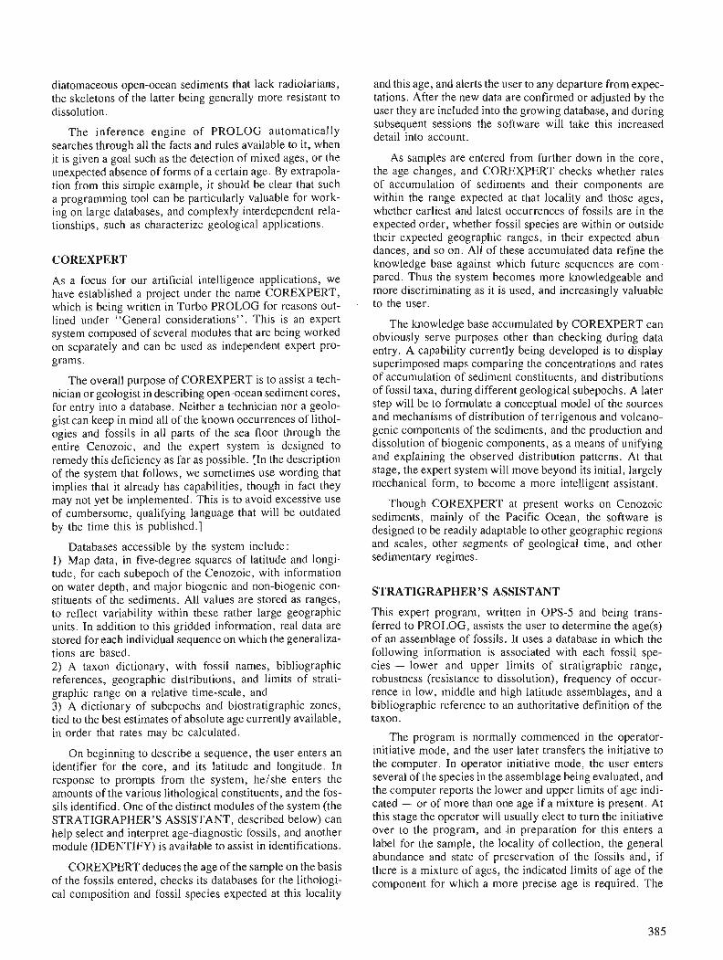
diatomaceous open-ocean sediments that lack radiolarians, the skeletons of the latter being generally more resistant to dissolution.

The inference engine of PROLOG automatically searches through all the facts and rules available to it, when it is given a goal such as the detection of mixed ages, or the unexpected absence of forms of a certain age. By extrapolation from this simple example, it should be clear that such a programming tool can be particularly valuable for working on large databases, and complexly interdependent relationships, such as characterize geological applications.

COREXPERT

As a focus for our artificial intelligence applications, we have established a project under the name COREXPERT, which is being written in Turbo PROLOG for reasons outlined under "General considerations". This is an expert system composed of several modules that are being worked on separately and can be used as independent expert programs.

The overall purpose of COREXPERT is to assist a technician or geologist in describing open-ocean sediment cores, for entry into a database. Neither a technician nor a geologist can keep in mind all of the known occurrences of lithologies and fossils in all parts of the sea floor through the entire Cenozoic, and the expert system is designed to remedy this deficiency as far as possible. [In the description of the system that follows, we sometimes use wording that implies that it already has capabilities, though in fact they may not yet be implemented. This is to avoid excessive use of cumbersome, qualifying language that will be outdated by the time this is published.]

Databases accessible by the system include: 1) Map data, in five-degree squares of latitude and longitude, for each subepoch of the Cenozoic, with information on water depth, and major biogenic and non-biogenic constituents of the sediments. All values are stored as ranges, to reflect variability within these rather large geographic units. In addition to this gridded information, real data are stored for each individual sequence on which the generalizations are based. 2) A taxon dictionary, with fossil names, bibliographic references, geographic distributions, and limits of stratigraphic range on a relative time-scale, and 3) A dictionary of subepochs and biostratigraphic zones, tied to the best estimates of absolute age currently available, in order that rates may be calculated.

On beginning to describe a sequence, the user enters an identifier for the core, and its latitude and longitude. In response to prompts from the system, helshe enters the amounts of the various lithological constituents, and the fossils identified. One of the distinct modules of the system (the STRATIGRAPHER'S ASSISTANT, described below) can help select and interpret age-diagnostic fossils, and another module (IDENTIFY) is available to assist in identifications.

COREXPERT deduces the age of the sample on the basis of the fossils entered, checks its databases for the lithological composition and fossil species expected at this locality

and this age, and alerts the user to any departure from expectations. After the new data are confirmed or adjusted by the user they are included into the growing database, and during subsequent sessions the software will take this increased detail into account.

As samples are entered from further down in the core, the age changes, and COREXPERT checks whether rates of accumulation of sediments and their components are within the range expected at that locality and those ages, whether earliest and latest occurrences of fossils are in the expected order, whether fossil species are within or outside their expected geographic ranges, in their expected abundances, and so on. All of these accumulated data refine the knowledge base against which future sequences are compared. Thus the system becomes more knowledgeable and more discriminating as it is used, and increasingly valuable to the user.

The knowledge base accumulated by COREXPERT can obviously serve purposes other than checking during data entry. A capability currently being developed is to display superimposed maps comparing the concentrations and rates of accumulation of sediment constituents, and distributions of fossil taxa, during different geological subepochs. A later step will be to formulate a conceptual model of the sources and mechanisms of distribution of terrigenous and volcanogenic components of the sediments, and the production and dissolution of biogenic components, as a means of unifying and explaining the observed distribution patterns. At that stage, the expert system will move beyond its initial, largely mechanical form, to become a more intelligent assistant.

Though COREXPERT at present works on Cenozoic sediments, mainly of the Pacific Ocean, the software is designed to be readily adaptable to other geographic regions and scales, other segments of geological time, and other sedimentary regimes.

STRATIGRAPHER'S ASSISTANT

This expert program, written in OPS-5 and being transferred to PROLOG, assists the user to determine the age(s) of an assemblage of fossils. It uses a database in which the following information is associated with each fossil species - lower and upper limits of stratigraphic range, robustness (resistance to dissolution), frequency of occurrence in low, middle and high latitude assemblages, and a bibliographic reference to an authoritative definition of the taxon.

The program is normally commenced in the operator- initiative mode, and the user later transfers the initiative to the computer. In operator initiative mode, the user enters several of the species in the assemblage being evaluated, and the computer reports the lower and upper limits of age indicated - or of more than one age if a mixture is present. At this stage the operator will usually elect to turn the initiative over to the program, and in preparation for this enters a label for the sample, the locality of collection, the general abundance and state of preservation of the fossils and, if there is a mixture of ages, the indicated limits of age of the component for which a more precise age is required. The

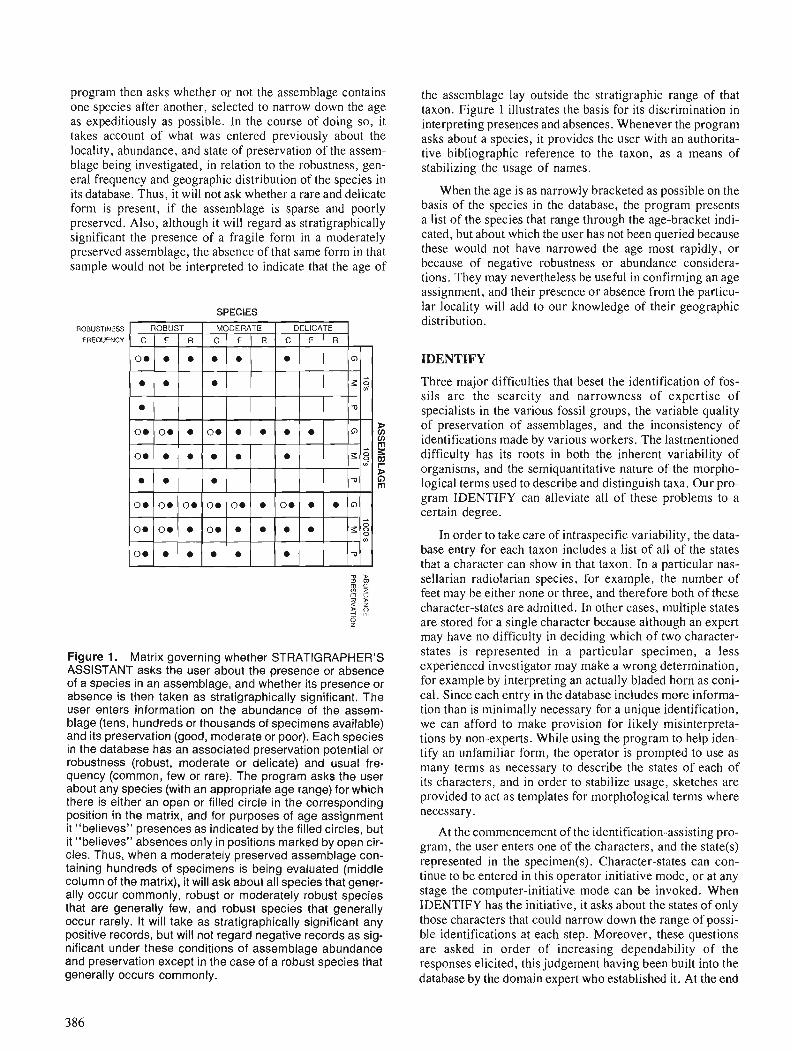
program then asks whether or not the assemblage contains one species after another, selected to narrow down the age as expeditiously as possible. In the course of doing so, it takes account of what was entered previously about the locality, abundance, and state of preservation of the assemblage being investigated, in relation to the robustness, general frequency and geographic distribution of the species in its database. Thus, it will not ask whether a rare and delicate form is present, if the assemblage is sparse and poorly preserved. Also, although it will regard as stratigraphically significant the presence of a fragile form in a moderately preserved assemblage, the absence of that same form in that sample would not be interpreted to indicate that the age of

SPECIES

Figure 1. Matrix governing whether STRATIGRAPHER'S ASSISTANT asks the user about the presence or absence of a species in an assemblage, and whether its presence or absence is then taken as stratigraphically significant. The user enters information on the abundance of the assemblage (tens, hundreds or thousands of specimens available) and its preservation (good, moderate or poor). Each species in the database has an associated preservation potential or robustness (robust, moderate or delicate) and usual frequency (common, few or rare). The program asks the user about any species (with an appropriate age range) for which there is either an open or filled circle in the corresponding position in the matrix, and for purposes of age assignment it "believes" presences as indicated by the filled circles, but it "believes" absences only in positions marked by open circles. Thus, when a moderately preserved assemblage containing hundreds of specimens is being evaluated (middle column of the matrix), it will ask about all species that generally occur commonly, robust or moderately robust species that are generally few, and robust species that generally occur rarely. It will take as stratigraphically significant any positive records, but will not regard negative records as significant under these conditions of assemblage abundance and preservation except in the case of a robust species that generally occurs commonly.

the assemblage lay outside the stratigraphic range of that taxon. Figure 1 illustrates the basis for its discrimination in interpreting presences and absences. Whenever the program asks about a species, it provides the user with an authoritative bibliographic reference to the taxon, as a means of stabilizing the usage of names.

When the age is as narrowly bracketed as possible on the basis of the species in the database, the program presents a list of the species that range through the age-bracket indicated, but about which the user has not been queried because these would not have narrowed the age most rapidly, or because of negative robustness or abundance considerations. They may nevertheless be useful in confirming an age assignment, and their presence or absence from the particular locality will add to our knowledge of their geographic distribution.

IDENTIFY

Three major difficulties that beset the identification of fossils are the scarcity and narrowness of expertise of specialists in the various fossil groups, the variable quality of preservation of assemblages, and the inconsistency of identifications made by various workers. The lastmentioned difficulty has its roots in both the inherent variability of organisms, and the semiquantitative nature of the morphological terms used to describe and distinguish taxa. Our program IDENTIFY can alleviate all of these problems to a certain degree.

In order to take care of intraspecific variability, the database entry for each taxon includes a list of all of the states that a character can show in that taxon. In a particular nas- sellarian radiolarian species, for example, the number of feet may be either none or three, and therefore both of these character-states are admitted. In other cases, multiple states are stored for a single character because although an expert may have no difficulty in deciding which of two character- states is represented in a particular specimen, a less experienced investigator may make a wrong determination, for example by interpreting an actually bladed horn as coni- cal. Since each entry in the database includes more information than is minimally necessary for a unique identification, we can afford to make provision for likely misinterpreta- tions by non-experts. While using the program to help identify an unfamiliar form, the operator is prompted to use as many terms as necessary to describe the states of each of its characters, and in order to stabilize usage, sketches are provided to act as templates for morphological terms where necessary.

At the commencement of the identification-assisting program, the user enters one of the characters, and the state(~) represented in the specimen(s). Character-states can continue to be entered in this operator initiative mode, or at any stage the computer-initiative mode can be invoked. When IDENTIFY has the initiative, it asks about the states of only those characters that could narrow down the range of possible identifications at each step. Moreover, these questions are asked in order of increasing dependability of the responses elicited, this judgement having been built into the database by the domain expert who established it. At the end

of the computer-interactive session, the user can be presented with an annotated sketch to confirm the identification if the search is narrowed down to one species, or with sketches of several species if more than one possibility remains. In a well designed, practical system, it would probably be most effective to have the expert program routinely narrow the search down to a few possibilities, and to leave the final choice to the human operator. This would eliminate the need to computerize the finest discriminating details, which would best be judged by a person with the help of good illustrations for comparison.

An early version of IDENTIFY is described by Riedel (1989). A later version uses more efficient code to handle a greater number of taxa and characters, and can deal with overlapping numerical ranges - e.g. , it recognizes that a range of thoracic widths of 100-150 micrometers overlaps a range of 120-180 micrometers. The next improvement to be incorporated will be the capability to distinguish between the usual ranges of dimensions and other characters, and the extremes of variability - this will make possible a distinction between more likely and less likely identifications.

GENERAL CONSIDERATIONS

Language

For our paleontological/stratigraphic applications, we originally considered four languages (LISP, PROLOG, OPS-5 and SMALLTALK), and several expert system shells. Though shells would seem to offer an economical means of developing one-of-a-kind A1 applications, those that could be run on personal computers did not offer the desired degree of flexibility and extensibility. Since our objective is to develop open-ended software tools that can be used and extended by other workers, it would be counter- productive to depend on specialized, expensive hardware and software systems.

We early eliminated LISP as an appropriate language for our work, because it involves a long learning curve before one can use it effectively. SMALLTALK, though offering some attractive features including powerful graphics capabilities, has too narrow a user base to have developed a substantial body of supporting literature. We programmed STRATIGRAPHER'S ASSISTANT in OPS-5, but turned to PROLOG when it became apparent that that language is at least as well suited to our purposes and is attracting a much wider body of user support.

Though our expert programs are at present written entirely in PROLOG, future versions will probably incorporate modules written in a procedural language such as C , which performs some operations more efficiently. In fact, A1 languages are often used for prototyping programs which are later translated into procedural languages because of their greater speed. Such was the experience of Schultz et al. (1988), in their development of an expert system for determining the environments of deposition of siliciclastic sediments. In the long view, it seems likely that geological expert systems will usually be linguistically hybrid, with calculation intensive components in a procedural language, components involving logical deduction in an A1 language,

and other special functions performed by graphics packages, database managers, geographic information systems, and so on.

Acceptability of an A1 product

An expert program or system cannot serve its purpose unless potential users have confidence in its output. The obvious way to enhance credibility is to have the software explain the line of reasoning by which it reaches a conclusion. The inferences drawn by our programs in their present state of development are so direct that such explanations are unnecessary, but they would be an essential part of an expert program to deal with another aspect of biostratigraphy that urgently needs codification, namely, the complex web of evidence forming the basis for biostratigraphic correlations. Integrated biochronostratigraphic systems such as that assembled by Berggren et al. (1985) for the Cenozoic are indispensable to large numbers of geologists who cannot duplicate the effort involved in their compilation. However, those systems are constantly being refined and revised, and users must accept them on faith as being the best available integrations of current evidence. If they were put into the form of expert programs, with all of the pieces of evidence kept separate, each with an indication of its reliability, and all the steps of interpretation expressed as rules in an A1 language, then all of the links in a correlation could be clearly explained, together with the weightings of conflicting pieces of evidence. In addition to clarifying the lines of biostratigraphic reasoning, such an expert program with its growing databases could readily be updated as new evidence became available.

Expert programs and their databases

When embarking on A1 applications, some thought needs be given to the anticipated useful lifetimes of expert programs and of the databases on which they operate. When conventional, expensive expert systems are written by consultants for use in industrial laboratories, there is probably an expectation that the A1 program will endure, and that the database will grow in a stable format. On the other hand, expert programs written by geologists in an academic environment are likely to be ephemeral - modified as research objectives change, or re-written as more powerful A1 tools become available. But here also, effort will be unnecessarily wasted if databases are not designed to grow in an accretionary fashion.

The lower the level of the database (i.e., the closer to raw observations), the more enduring it is likely to be because its elements are less dependent on subjective judge- ments. On the other hand, a database may be easier to build (and it certainly will be smaller) if it comprises intermediate-level interpretations or higher-level syntheses (such as the literature-based compilation of the Cambridge Arctic Shelf Programme). The databases of COREXPERT are for the most part low-level, but in the real world it will be necessary to work with databases at different levels, some of them consisting of uninterpreted original observations and others at higher levels of interpretation and abstraction.

Cost-effectiveness

Practically no expert system in the earth sciences has yet been demonstrated to be cost-effective, in the sense that the resources expended in its development have been balanced by immediate benefits resulting from its use (Walker, 1988). However, this narrow view ignores indirect benefits, which may be at least as valuable as the immediate objective. When we write an A1 program to assist in the identification of fossils, for example, we have in mind not only its use as a replacement for a taxonomic manual, but also the benefits to be derived from the rigour imposed by its requirement for clearly defined, objective descriptors, and its eventual role in guiding an automated identification system using image analysis.

GEOPROLOG

Conventional wisdom holds that expert systems must be large, expensive products resulting from several man-years of co-operation between domain experts, knowledge engineers and programmers.

"Using present techniques and programming tools, the effort required to develop an expert system appears to be converging towards five man-years, with most endeavors employing two to five people in the construction."

(Gevarter, 1984, p.78)

We believe, however, that there is also a place for modest applications of A1 by individual geologists. These individual domain experts know their own subject matter thoroughly, as well as how firmly grounded their observations are, what inferences can be drawn, with what degree of confidence, from those observations, and how extensive an inferential edifice can be built on them, using which relationships. These geologists can acquire sufficient knowledge engineering for their limited domains, and can proceed directly to building expert programs, provided that appropriate languages are easily accessible.

Fortunately, language systems now available for A1 programming on personal computers are convenient, inexpensive and easily learned. Our impression is that almost any geologist can learn enough PROLOG in six to twelve months for rudimentary though useful programming, and

can subsequently go on cost-effectively to produce expert programs. In an attempt to facilitate this learning process, we are producing a collection of geologically oriented Turbo PROLOG modules that serve both as demonstrations of the capabilities of the language, and as building blocks for practical programs. This set of demonstrations and program modules is being assembled, together with explanatory notes, under the name "GeoProlog", and is available to any interested geologist on request.

Even if we are over-optimistic about do-it-yourself AI, the geologist who knows the basics of PROLOG programming will be in a better position to evaluate and use expert system shells, or to participate in the development of conventional A1 tools.

ACKNOWLEDGMENTS

Research leading to this paper was supported by the U.S. National Science Foundation grant OCE-8707708, and by contributions from AMOCO Production Company and the Unocal Foundation.

REFERENCES

Berggren, W.A., Kent, D.V., Flynn, J.J. and Van Cowering, J.A. 1985 : Cenozoic geochronology ; Geological Society of America Bulletin,

v. 96, p. 1407-1418. Gevarter, W.B. 1984: Artificial Intelligence, Expert Systems, Computer Vision and Nat-

ural Language Processing; Noyes Publications, Park Ridge, N.J., xiv + 226 p.

Nilsson, N.J. 1980: Principles of Artificial Intelligence. Tioga Publishing Company,

Palo Alto, xv + 476 p. Rich, E. 1983: Artificial Intelligence; McGraw-Hill Book Company, New York,

xii + 436 p. Riedel, W.R. 1989: IDENTIFY : a Prolog program to help identify fossils; Computers

and Geosciences, v. 15, no. 5, p. 809-823. Schultz, A.W., Fang, J.H., Burston, M.R., Chen H.C. and Reynolds, S. 1988: XEOD: an expert system for determining clastic depositional

environments; Geobyte, v. 3, no. 2 , p. 22-32. Walker, M.G. 1988: Expert systems in geological exploration: Can they be cost effec-

tive?; Geobyte, v. 3, no. 3, p. 18-23.

Artificial Intelligence for the Correlation of Well Logs

John C. Davis1 and Ricardo A. Oleal

Davis, J. C. and Olea, R. A., Artijicial intelligence for the correlation of well logs; fi Statistical Applications in the Earth Sciences, ed. F. P. Agterberg and G. F. Bonham-Carter; Geological Survey of Canada, Paper 89-9, p. 389-394, 1989.

Abstract

Of the many branches of artificial intelligence, geologists are most intrigued by expert systems, which emulate the problem-solving behaviour of human experts. Two assumptions are implicit in expert systems: (1) It is generally known how problems are solved, (2) A body of lcnowledge exists about the specijc problem addressed. In much of geology, neither problem-solving processes nor geological principles are well understood and expert systems are not successfil.

CORRELATOR is an artijcial intelligence program that automatically correlates well logs and constructs stratigraphic cross-sections. Pairs of wells are correlated using two log traces per well. A microresistivity log provides distinctive "signatures" that are matched, and gamma-ray, density, or sonic logs provide information on lithologies. A short interval in a reference well is matched against a moving window in a second well. Weighted cross-correlation coeficients are computed at all possible match positions; the strongest match is recorded in a table of provisional correlations. Using a large collection of production rules based on stratigraphic principles, CORRELATOR 's expert system examines this table, identifying possibly spurious correlations. Inconsistencies are resolved interactively, and cross-sections are built using the corrected table of correlations.

CORRELATOR has been tested in Kansas, Louisiana, Alaska, Texas, and Chile, for sections lip to 8000 feet. Correlations are equivalent or better than those produced manually by experienced geologists, even in intervals containing unconfomities, faults, facies changes, and abrupt lateral changes in thickness. The program succeeds because principles behind both pattern recognition and stratigraphy are understood.

Parmi les nombreuses ramijkations de l'intelligence artijkielle, les systtmes experts, qui imitent le com- portement des experts humains en mati2re de solution de probl?mes, constituent celles qui intriguent le plus les gkologues. Ces systkmes sont bask sur deux hypothbes implicites, I ) la manitre dont les problkmes sont solz~tionnks est gknkralement connue et 2) il existe un corpus de connaissances concernant le problkme spkcifique abordk. Pour une partie importante de la gkologie, izi les processus de la solution des probltmes, ni les principes ge'ologiques sont bien compris et les systtmes experts ne connaissent aucun succts.

Le CORRELATOR est un programme d'intelligence art~$cielle qui met automatiquement en corrklation des diagraphies et qui dresse des coupes stratigraphiques transversales. Des paires de puits sont mise en corre'lation au rnoyen de deux diagraphies par puits. Une diagraphie de microre'sistivite'foumit des N signatures,, distinctes qui sont mises en corresporuiance el des diagraphies gammamktriques, densimhriques ou acoustiques fournissent des renseignements concernant la lithologie. Un court intervalle dans un puits de r4krence est mis en correspondance avec une fengtre mobile dans un deuxieme puits. Des coeficients de corre'lation croisee pondkrks sont calculks pour toutes les positions de correspondance possibles; la meilleure correspondance est enregistrke sur un tableau des corrklations provisoires. D'aprts une grande collection de r2gles de production base'es sur des principes stratigraphiques, le syst?me expert du CORRELATOR examine ce tableau et y identiJie des corre'lations pouvant Ptre fausses. Les contradictions sont e'limine'es de mani2re interactive et les coupes sont dresskes B l'aide du tableau corrigk des corrklations.

' Kansas Geological Survey, The University of Kansas, 1930 Constant Avenue, Lawrence, KS 66047, U.S.A.

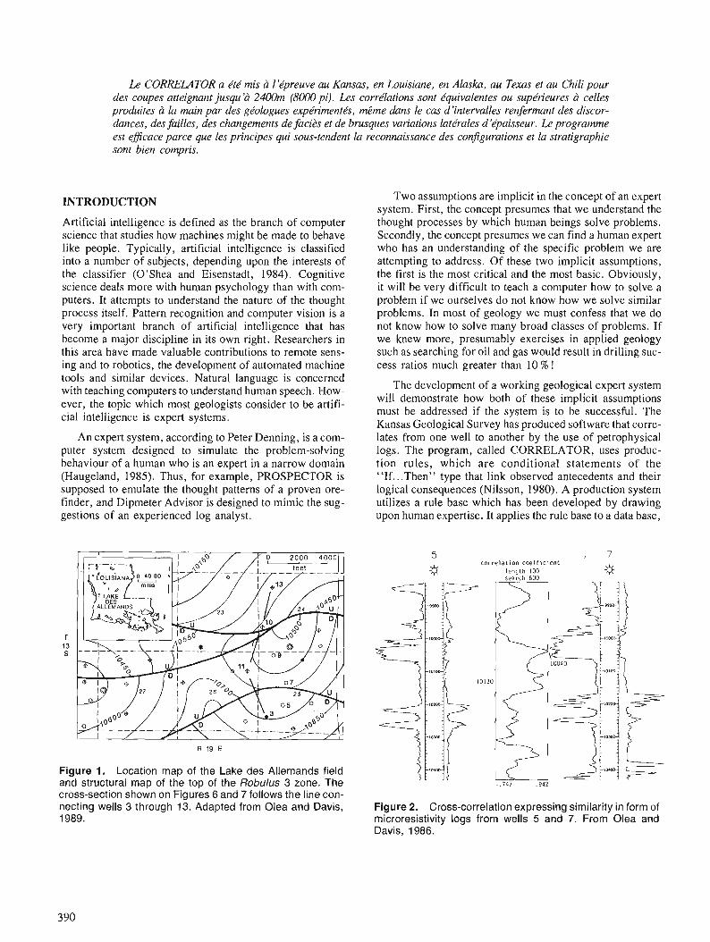
Le CORRELATOR a e't.4 rnis d l'e'preuve au Kansas, en Louisiane, en Alaska, au Texas et au Chili pour des coupes atteignant jusqu'a 2400m (8000 pi). Les corr.4latiom sont t?quivalentes ou sup&rieures celles produites h la main par des ge'ologues exp.4rirnentt!ss, m2me duns le cas d'intervalles renfermant des discordances, des failles, des changements de facih et de brusques variations latkrales d'e'paisseur. Le programme est eflcace parce que les principes qui sous-tendent la reconnaissance des configurations et la stratigraphie sont bien compris.

INTRODUCTION

Artificial intelligence is defined as the branch of computer science that studies how machines might be made to behave like people. Typically, artificial intelligence is classified into a number of subjects, depending upon the interests of the classifier (O'Shea and Eisenstadt, 1984). Cognitive science deals more with human psychology than with computers. It attempts to understand the nature of the thought process itself. Pattern recognition and computer vision is a very important branch of artificial intelligence that has become a major discipline in its own right. Researchers in this area have made valuable contributions to remote sensing and to robotics, the development of automated machine tools and similar devices. Natural language is concerned with teaching computers to understand human speech. How- ever, the topic which most geologists consider to be artificial intelligence is expert systems.

An expert system, according to Peter Denning, is a computer system designed to simulate the problem-solving behaviour of a human who is an expert in a narrow domain (Haugeland, 1985). Thus, for example, PROSPECTOR is supposed to emulate the thought patterns of a proven ore- finder, and Dipmeter Advisor is designed to mimic the suggestions of an experienced log analyst.

Two assumptions are implicit in the concept of an expert system. First, the concept presumes that we understand the thought processes by which human beings solve problems. Secondly, the concept presumes we can find a human expert who has an understanding of the specific problem we are attempting to address. Of these two implicit assumptions, the first is the most critical and the most basic. Obviously, it will be very difficult to teach a computer how to solve a problem if we ourselves do not know how we solve similar problems. In most of geology we must confess that we do not know how to solve many broad classes of problems. If we knew more, presumably exercises in applied geology such as searching for oil and gas would result in drilling success ratios much greater than 10 % !

The development of a working geological expert system will demonstrate how both of these implicit assumptions must be addressed if the system is to be successful. The Kansas Geological Survey has produced software that correlates from one well to another by the use of petrophysical logs. The program, called CORRELATOR, uses production rules, which are conditional statements of the "If ... Then" type that link observed antecedents and their logical consequences (Nilsson, 1980). A production system utilizes a rule base which has been developed by drawing upon human expertise. It applies the rule base to a data base,

Figure 1. Location map of the Lake des Allemands field and structural map of the top of the Robulus 3 zone. The cross-section shown on Figures 6 and 7 follows the line connecting wells 3 through 13. Adapted from Olea and Davis, 1989.

Figure 2. Cross-correlation expressing similarity in form of microresistivity logs from wells 5 and 7. From Olea and Davis, 1986.

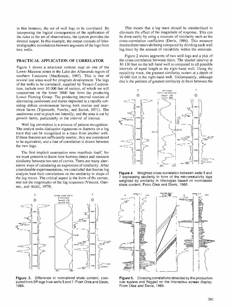
in this instance, the set of well logs to be correlated. By interpreting the logical consequences of the application of the rules to the set of observations, the system provides the desired output. In this example, the output consists of lithostratigraphic correlations between segments of the logs from two wells.

PRACTICAL APPLICATION OF CORRELATOR

Figure 1 shows a structural contour map on one of the Lower Miocene zones in the Lake des Allemands region of southern Louisiana (MacKenzie, 1967). This is one of several test areas used for program development. The logs of the wells to be correlated, supplied by Texaco Corpora- tion, include over 10 000 feet of section, of which we will concentrate on the lower 3000 feet from the producing Lower Fleming Group. The producing interval consists of alternating sandstones and shales deposited in a rapidly sub- siding deltaic environment having both marine and nearshore facies (Tipsworth, Fowler, and Sorrel, 197 1). The sandstones tend to pinch out laterally, and the area is cut by growth faults, particularly in the interval of interest.

Well log correlation is a process of pattern recognition. The analyst seeks distinctive signatures or features on a log trace that can be recognized in a trace from another well. If these features are sufficiently similar, they are considered to be equivalent, and a line of correlation is drawn between the two logs.

The first implicit assumption now manifests itself, for we must presume to know how humans detect and measure similarity between two sets of curves. There are many alternative ways of calculating an expression of similarity. After considerable experimentation, we concluded that human log analysts base their correlations on the similarity in shape of the log traces. The critical aspect is the form of the curves, and not the magnitudes of the log responses (Vincent, Gart- ner, and Attali, 1979).

5 normalized shale 7

% difference length 100 search 600

@

Figure 3. Difference in normalized shale content, computed from S P logs from wells 5 and 7. From Olea and Davis, 1986.

This means that a log trace should be standardized to eliminate the effect of the magnitude of response. This can be done easily by using a measure of similarity such as the cross-correlation coefficient (Davis, 1986). This measure standardizes intervals being compared by dividing each well log trace by the amount of variability within the intervals.

Figure 2 shows segments of two well logs and a plot of the cross-correlation between them. The shaded interval at 10 130 feet on the left-hand well is compared to all possible intervals of equal length in the right-hand well. Using the resistivity trace, the greatest similarity occurs at a depth of 10 040 feet in the right-hand well. Unfortunately, although this is the position of greatest similarity in form between the

5 weighted 7 cross-correlation

length 100

Figure 4. Weighted cross-correlation between wells 5 and 7 expressing similarity in form of the microresistivity logs weighted by similarity in lithologies based on normalized shale content. From Olea and Davis, 1986.

" W Z n.. 3 m m w SOLE

PP 9 91116 1010s IC .Z

e srrn

Figure 5. Crossing correlations detected by the production rule system and flagged on the interactive screen display. From Olea and Davis, 1989.

391

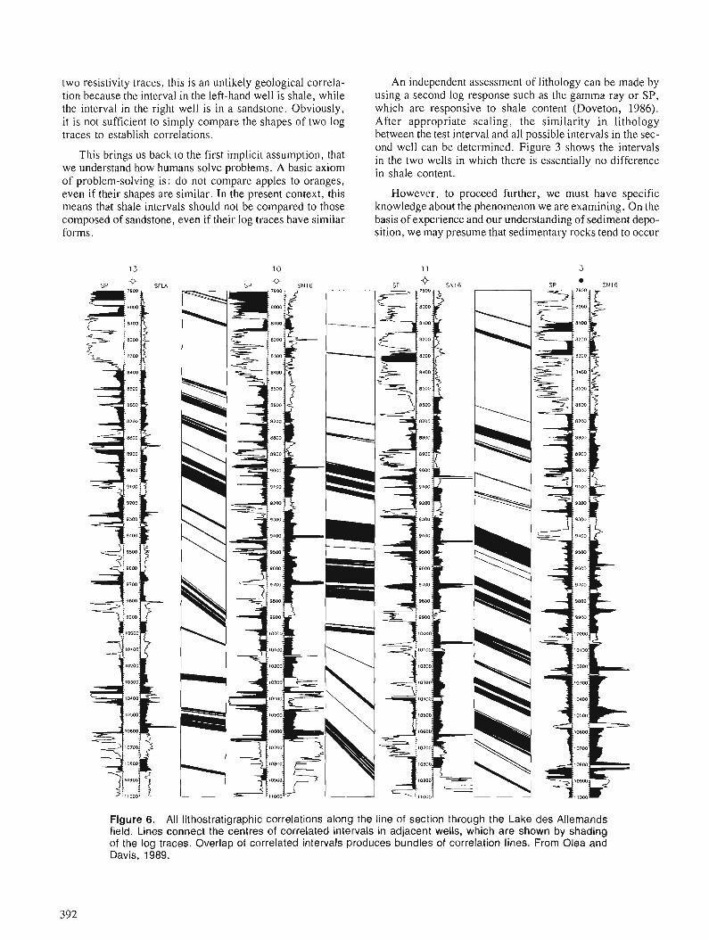
two resistivity traces, this is an unlikely geological correlation because the interval in the left-hand well is shale, while the interval in the right well is in a sandstone. Obviously, it is not sufficient to simply compare the shapes of ~ w o log traces to establish correlations.

'This brings us back to the first implicit assumption, that we understand how humans solve problems. A basic axiom of problem-solving is: do not compare apples to oranges, even if their shapes are similar. In the present context, this means that shale intervals should not be compared to those composed of sandstone, even if their log traces have similar forms.

SP ' SFI

An independent assessment of lithology can be made by using a second log response such as the gamma ray or SP, which are responsive to shale content (Doveton, 1986). After appropriate scaling, the similarity in lithology between the test interval and all possible intervals in the second well can be determined. Figure 3 shows the intervals in the two wells in which there is essentially no difference in shale content.

However, to proceed further, we must have specific knowledge about the phenomenon we are examining. On the basis of experience and our understanding of sediment deposition, we may presume that sedimentary rocks tend to occur

Figure 6. All lithostratigraphic correlations along the line of section through the Lake des Allemands field. Lines connect the centres of correlated intervals in adjacent wells, which are shown by shading of the log traces. Overlap of correlated intervals produces bundles of correlation lines. From Olea and Davis, 1989.

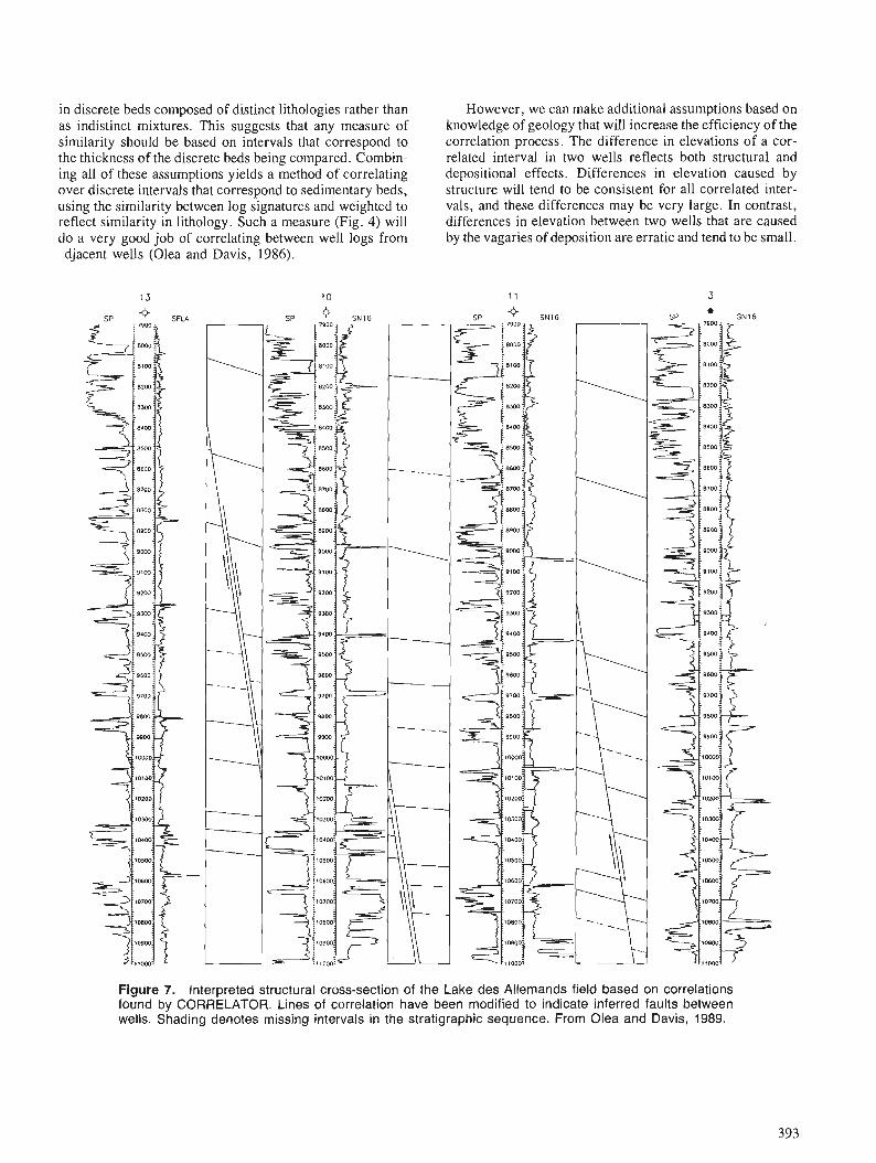
in discrete beds composed of distinct lithologies rather than as indistinct mixtures. This suggests that any measure of similarity should be based on intervals that correspond to the thickness of the discrete beds being compared. Combin- ing all of these assumptions yields a method of correlating over discrete intervals that correspond to sedimentary beds, using the similarity between log signatures and weighted to reflect similarity in lithology. Such a measure (Fig. 4) will do a very good job of correlating between well logs from .djacent wells (Olea and Davis, 1986).

However, we can make additional assumptions based on knowledge of geology that will increase the efficiency of the correlation process. The difference in elevations of a correlated interval in two wells reflects both structural and depositional effects. Differences in elevation caused by structure will tend to be consistent for all correlated intervals, and these differences may be very large. In contrast, differences in elevation between two wells that are caused by the vagaries of deposition are erratic and tend to be small.

Figure 7. Interpreted structural cross-section of the Lake des Allemands field based on correlations found by CORRELATOR. Lines of correlation have been modified to indicate inferred faults between wells. Shading denotes missing intervals in the stratigraphic sequence. From Olea and Davis, 1989.

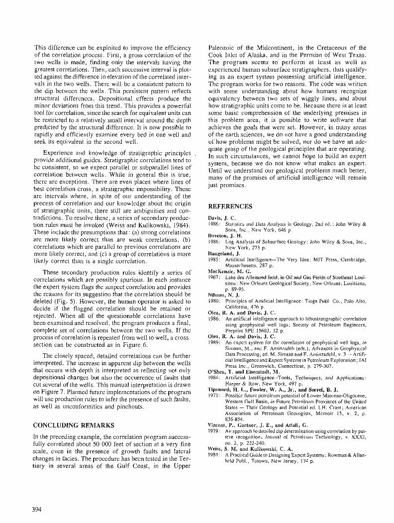
This difference can be exploited to improve the efficiency of the correlation process. First, a gross correlation of the two wells is made, finding only the intervals having the greatest correlations. Then, each successive interval is plotted against the difference in elevation of the correlated intervals in the two wells. There will be a consistent pattern to the dip between the wells. This persistent pattern reflects structural differences. Depositional effects produce the minor deviations from this trend. This provides a powerful tool for correlation, since the search for equivalent units can be restricted to a relatively small interval around the depth predicted by the structural difference. It is now possible to rapidly and efficiently examine every bed in one well and seek its equivalent in the second well.

Experience and knowledge of stratigraphic principles . provide additional guides. Stratigraphic correlations tend to be consistent, so we expect parallel or subparallel lines of correlation between wells. While in general this is true, there are exceptions. There are even places where lines of best correlation cross, a stratigraphic impossibility. These are intervals where, in spite of our understanding of the process of correlation and our knowledge about the origin of stratigraphic units, there still are ambiguities and contradictions. To resolve these, a series of secondary production rules must be invoked (Weiss and Kulikowski, 1984). These include the presumptions that : (a) strong correlations are more likely correct than are weak correlations, (b) correlations which are parallel to previous correlations are more likely correct, and (c) a group of correlations is more likely correct than is a single correlation.

These secondary production rules identify a series of correlations which are possibly spurious. In each instance the expert system flags the suspect correlation and provides the reasons for its suggestion that the correlation should be deleted (Fig. 5). However, the human operator is asked to decide if the flagged correlation should be retained or rejected. When all of the questionable correlations have been examined and resolved, the program produces a final, complete set of correlations between the two wells. If the process of correlation is repeated from well to well, a cross- section can be constructed as in Figure 6.

The closely spaced, detailed correlations can be further interpreted. The increase in apparent dip between the wells that occurs with depth is interpreted as reflecting not only depositional changes but also the occurrence of faults that cut several of the wells. This manual interpretation is drawn on Figure 7. Planned future implementations of the program will use production rules to infer the presence of such faults, as well as unconformities and pinchouts.

CONCLUDING REMARKS

In the preceding example, the correlation program successfully correlated about 50 000 feet of section at a very fine scale, even in the presence of growth faults and lateral changes in facies. The procedure has been tested in the Ter- tiary in several areas of the Gulf Coast, in the Upper

Paleozoic of the Midcontinent, in the Cretaceous of the Cook Inlet of Alaska, and in the Permian of West Texas. The program seems to perform at least a s well as experienced human subsurface stratigraphers, thus qualifying as an expert system possessing artificial intelligence. The program works for two reasons. The code was written with some understanding about how humans recognize equivalency between two sets of wiggly lines, and about how stratigraphic units come to be. Because there is at least some basic comprehension of the underlying premises in this problem area, it is possible to write software that achieves the goals that were set. However, in many areas of the earth sciences, we do not have a good understanding of how problems might be solved, nor do we have an adequate grasp of the geological principles that are operating. In such circumstances, we cannot hope to build an expert system, because we do not know what makes an expert. Until we understand our geological problems much better, many of the promises of artificial intelligence will remain just promises.

REFERENCES

Davis, J. C. 1986: Statistics and Data Analysis in Geology, 2nd ed.: John Wiley &

Sons, Inc., New York, 646 p. Doveton, J. H. 1986: Log Analysis of Subsurface Geology: John Wiley & Sons, Inc.,

New York, 273 p. Haugeland, J. 1985: Artificial Intelligence-The Very Idea; MIT Press, Cambridge,

Massachusetts, 287 p. MacKenzie, M. G. 1967: Lake des Allemand field, in Oil and Gas Fields of Southeast Loui-

siana: New Orleans Geological Society, New Orleans, Louisiana, p. 89-95.

Nilsson, N. J. 1980: Principles of Artificial Intelligence: Tioga Publ. Co., Palo Alto,

California, 476 p. Olea, R. A. and Davis, J. C. 1986: An artificial intelligence approach to lithostratigraphic correlation

using geophysical well logs; Society of Petroleum Engineers, Preprint SPE 15603, 12 p.

Olea, R. A. and Davis, J. C. 1989: An expert system for the correlation of geophysical well logs, in

Simaan, M., and F. Aminzadeh (eds.), Advances in Geophysical Data Processing, ed. M. Simaan and F. Aminzadehl, v. 3 - Artifi- cial Intelligenceand Expert Systems in Petroleum Exploration; JAI Press Inc., Greenwich, Connecticut, p. 279-307.

O'Shea, T. and Eisenstadt, M. 1984: Artificial Intelligence--Tools, Techniques, and Applications:

Harper & Row, New York, 497 p. Tipsword, H. L., Fowler, W. A., Jr., and Sorrel, B. J. 1971 : Possible future petroleum potential of Lower Miocene-Oligocene,

Western Gulf Basin, in Future Petroleum Provinces of the United States - Their Geology and Potential ed. I.H. Cram; American Association of Petroleum Geologists, Memoir 15, v. 2, p. 836-854.

Vincent, P., Gartner, J. E., and Attali, G. 1979: An approach todetailed dipdetermination using correlation by pat-

tern recognition; Journal of Petroleum Technology, v. XXXI, no. 2, p. 232-240.

Weiss, S. M. and Kulikowski, C. A. 1984: A Practical Guide to Designing Expert Systems; Rowman & Allan-

held Publ., Totowa, New Jersey, 174 p.

Prospector I11 : towards a map-based expert system for regional mineral resource assessment

Richard B. McCamrnonl

McCammon, R. B., Prospector III: towards a map-based expert system for regional mineral resource assessment; fi Statistical Applications in the Earth Sciences, ed. F. P. Agterberg and G. F. Bonham- Carter; Geological Survey of Canada, Paper 89-9, p. 395-404, 1989.

Abstract

Prospector III is a prototype map-based expert system designed to assist those engaged in regional mineral resource assessments. The successor to Prospector II , the present system can combine data represented in maps with descriptions of geological settings of areas; the combined information can be compared with the attributes of stored mineral deposit models. 7&e concept of a spatial object is introduced as a means of representing data stored in maps. A comparison of the results obtained using Prospector 111 with the results of an earlier mineral resource assessment of the Tonopah quadrangle in Nevada reveals that both results are in general agreement in identifying which major deposit types may be present. Differences in the results obtained can be explained largely on the basis of the uncertainties inherent in regional mineral resource assessments and de3ciencies in the currently stored deposit models. A future role of Prospector 111 is to ensure that all possible deposit models are considered when making regional mineral resource assessments.

Le Prospector III est un prototype de syst2me expert bast sur les cartes et coneu en vue de faciliter le travail de ceux qui eflectuent les dvaluations re'gionales des ressources minPrales. I1 succkde au Prospector II etpermet de combiner des donne'es repre'sente'es sur des cartes h des descriptions des cadres ge'ologiques de re'gions; l'information combine'e peut &re compare'e aux attributs de mod6les stocke's de gisements de mine'raux. Le concept d 'objet spatial est introduit a j n de repre'senter les donndes consig- ne'es sur des cartes. Une comparaison des re'sultats obtenus h l'aide du Prospector III h ceux d'une e'valuation ante'rieure des ressources mine'rales du quadrilat2re Tonopah au Nevada re'v2le qu'il y a concordance gdne'rale quant a 1 'identijcation des principaux types de gisements pouvant 2tre prksents. Les incertitudes inhhentes aux e'valuations rigionales des ressources mine'rales et les carences des modkles des gisements actuellement stocke's permettent de rendre compte en grande partie des diffe'rences notkes au niveau des r6sultats obtenus. L'un des r81efuturs du Prospector III sera d'assurer que tous les modsles possibles de gisements sont pris en conside'ration lors des e'valuations re'gionales des ressources mine'rales.

' U.S. Geological Survey, Reston, Virginia 22092, U.S.A.

INTRODUCTION

Whatever methodology is adopted by those engaged in regional mineral resource assessments, one of the steps that is sure to be included involves the delineation of areas that may contain undiscovered deposits of specific deposit types. These areas are said to be permissive for the deposit types. The delineation of areas is one of the three steps in the methodology proposed by Singer and Ovenshine (1979) and one of the steps in the multistep method described by Shawe (1981). It is a task that calls upon the combined skills and knowledge of geologists, geochemists, and geophysicists. The task involves the comparison of the available regional geoscience data with the existing mineral deposit models. It requires a high degree of human judgement. Such a task lends itself to an expert system.

The purpose of this paper is to describe Prospector 111, a prototype map-based expert system. Prospector 111 represents the next stage of development after Prospector I1 (McCammon, 1989), the successor to Prospector (Duda, 1980). This latest system can combine map data with the descriptions of geological settings and compare the combined information with a stored set of mineral-deposit models. Prospector I11 is designed to assist in the task of making regional mineral resource assessments.

The operations of the present system are best described using examples. Map data taken from the preliminary mineral resource assessment of the Tonopah quadrangle, Nevada (Orris and Kleinhampl, 1986) serve as the example in this paper. The results obtained by Prospector I11 are compared to those from Orris and Kleinhampl (1986).

DESIGN OF A MAP-BASED EXPERT SYSTEM

To understand what was necessary in building a prototype map-based expert system, it helps to first review the current environment of Prospector 11. Figure 1 shows the screen display of a typical session. In this instance, the user has selected a set of descriptors that characterize a particular geological setting in an area. The items selected are chosen from a glossary of geology represented by a series of taxonomic charts called up by the user. The items are those used to define the attributes of the deposit models stored in the knowledge base. For each item selected, the user specifies whether the item is present, suspected as being present (presence?), or absent. Once selected, the item appears in the appropriate window on the right. The user is free to select as many items in the glossary as desired. Even if an item is not selected, it may still be assigned to one of the three categories if it is linked to another item that has been selected. For instance, the presence of granite implies the presence of the terms, felsic-plutonic, plutonic, igneous, and rock-types. In this case, all four items will be considered as being present if granite is present. Items not assigned one of the three nominal values according to the set of rules that govern presence-presence?-absence are assigned the nominal value, missing. Consequently, every term in the glossary takes on one of four nominal values, presence, presence?, absence, or missing. Currently, the glossary contains 101 1 items and 865 links that connect items.

In order that a similar form of input could be retained for map data, it was necessary to provide that items in the glossary could be taken directly off of maps. This meant, first of all, being able to display maps on the screen. Figure 2 shows a display screen that contains a set of maps that have been overlain. Displayed are the topographic, geological, magnetic, geochemical, and mineral-occurrence maps for the south-central part of the Tonopah quadrangle [maps and data taken from Whitebread (1986), Plouff (1983), Fairfield et at. (1985), and Mineral Resource Data System (MRDS)]. A discussion of the methods that were used to scan the original maps, to create bitmaps, to save the bitmaps in files, and to redisplay these maps on the screen is beyond the scope of this paper. In the present discussion, it is sufficient to state that various computer graphics methods are available for this purpose.

A menu was created in order that a user could select one or more maps at a time and also perform operations that will be described later. The menu is shown in Figure 2 at the top right side of the window that contains the maps. Above the menu is a smaller window that displays the latitude- longitude position of the cursor as it is moved around inside the window containing the maps.

In order that the information stored in the maps could be transformed into descriptors that would be understood by the system, it was necessary to introduce the concept of spatial objects. A spatial object is defined as a data structure that contains a bitmap and slots for storing items found in the glossary. An example of a spatial object is shown in Fig- ure 3. The window in the lower left part of the display shows the geological map with the major map units. The map unit Pzg describes a chert-argillite assemblage of Mississippian to Permian age that is made up of chert, argillite, greenstone, and quartzite. This map unit has been created as a spatial object named ( $ Pzg). The slots and the values of these slots are shown in the window in the lower right part of the screen. The bitmap is shown in the upper right part of the screen. Areas created as spatial objects do not have to be contiguous.

Hereafter, spatial o,bjects are called active-regions (airegions). Whenever a map that contains airegions is displayed on the screen, those airegions will be mouse sensitive. The descriptors stored within a mouse-sensitive airegion are selectable by the user. If the mouse button is clicked when the cursor is over an airegion, the descriptors that are stored will be treated as if each descriptor had been selected from the glossary.

A special problem arises for data taken from geochemical maps. Figure 4 is a screen display that shows the drainage areas and the locations of stream-sediment samples. The shaded area refers to the airegion ( $ TZS33001) that corresponds to sample number TZS33001. This sample was analyzed for the elements listed in the slot named StrmSedGeochem shown in the lower right part of the screen. The concentration of each element is listed after its chemical symbol and is expressed either as parts per million (ppm) or as a qualified value (such as N, meaning not detected) according to standard U.S. Geological Survey practice. Where geochemical data differ from other

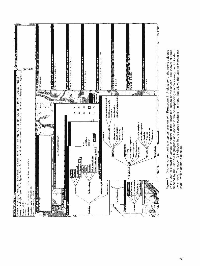
.aln3axa oi uo!i3e 4

3!q

~ uaisA

s a

yi i3n

~isu

! ol Jasn aq

l sMolle ie

qi n

ua

u a

ql su!sluo3 u

aa

~3

s aql u! M

OP

U!M

Ual ~a

dd

n aq

l .ua

a~

as aq

i lo

aP!s 1

y6!~

all1 6uo1e SM

OP

U!M

~U!P

UO

~S

~J

JO

~

ay

i u! ~e

ad

de

pue paiy6!1y6!y aJt? Jasn ayl Aq p

ap

ala

s surai! ienp!A

!pu! aq

l .ua

a~

3s ay

i 40 uo!uod U

al JaMol a

qi u! S

MO

PU

!M sno!JeA U

! UM

OY

S S! Jasn a

qi Aq

palaalas scum

aq

i 40 AJESSO~~ y .II ~

oi3

ad

so

~d

q

i!

~

uo!ssas le3!dAl e 6

~!~

np

u

aa

~3

s Aelds!a -1

alnb

!j

.. i.:.

.. ::..!;I ,.' : :';

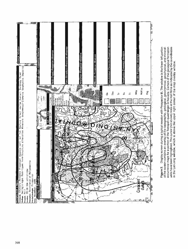
Fig

ure

2.

Dis

play

scr

een

du

rin

g a

typi

cal s

essi

on w

ith P

rosp

ecto

r Ill.

The

win

dow

in th

e lo

wer

left

port

ion

of t

he s

cree

n co

ntai

ns a

n ov

erla

y of

the

topo

grap

hic,

geo

logi

cal,

geoc

hem

ical

, geo

phys

ical

, and

min

eral

- oc

curr

ence

map

s fo

r a

port

ion

of th

e T

onop

ah q

uadr

angl

e in

Nev

ada.

Cer

tain

of t

he

geo

logi

cal f

orm

atio

n un

its h

ave

been

hig

hlig

hted

. The

cur

sor (

not s

how

n) re

sts

at th

e H

all M

ine

as in

dica

ted

by th

e co

-ord

inat

es

in t

he L

at-L

ong

win

dow

, w

hich

is

abov

e th

e up

per

right

cor

ner

of t

he

map

ove

rlay

win

dow

.

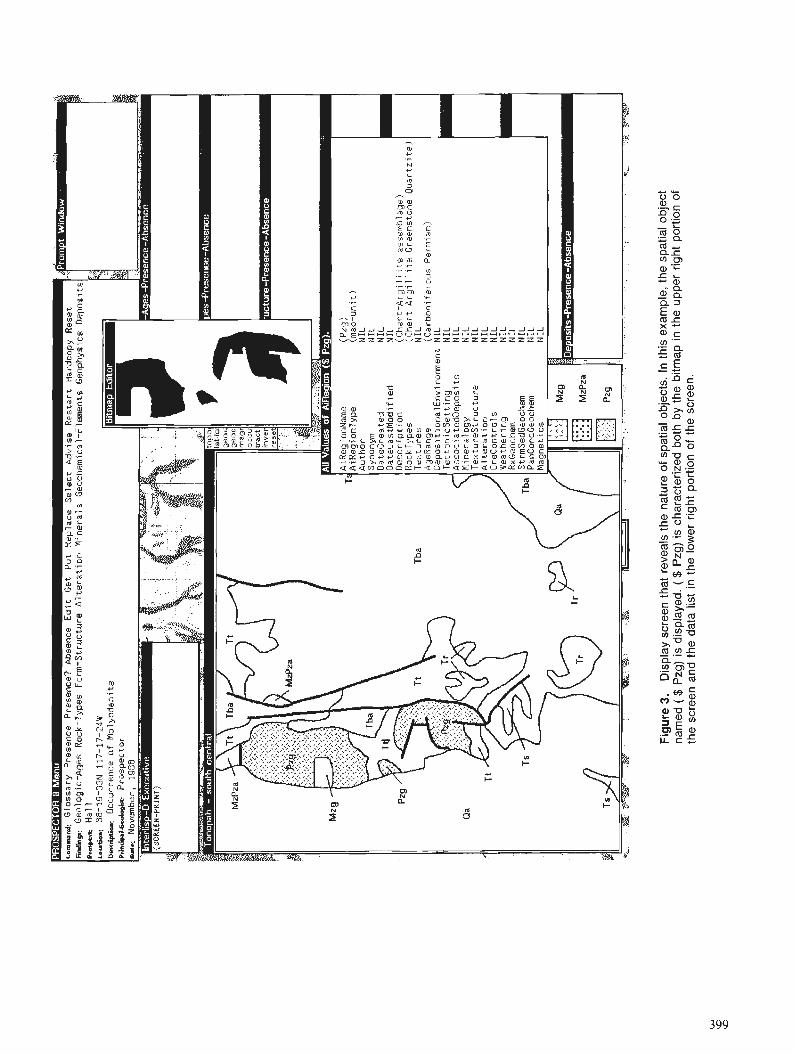
I Fid

igr:

G

eo

log

ic-A

ge

s R

ock-

Typ

es

Fo

rm-S

tru

ctu

re

Alt

era

tio

n M

inera

l ; G

roch

ern

~ca

l-E

lem

en

ts G

eo

ph

ysic

s D

epos

its

Te

cto

nic

se

ttin

y

Alt

era

tio

rt

Fig

ure

3.

Dis

play

scr

een

that

rev

eals

the

natu

re o

f sp

atia

l obj

ects

. In

this

exa

mpl

e, th

e sp

atia

l obj

ect

nam

ed (

$ P

zg)

is d

ispl

ayed

. ( $

Pzg

) is

cha

ract

eriz

ed b

oth

by t

he b

itmap

in th

e up

per

right

por

tion

of

the

scre

en a

nd t

he d

ata

list

in th

e lo

wer

rig

ht p

ortio

n of

the

scr

een.

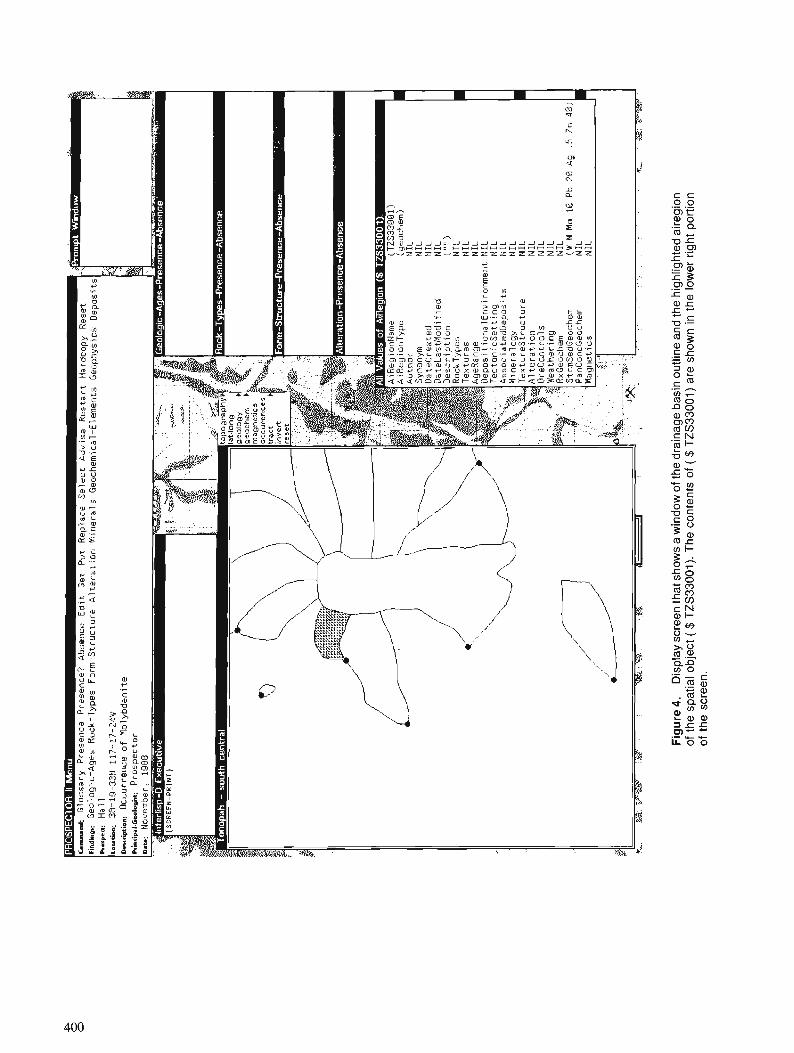
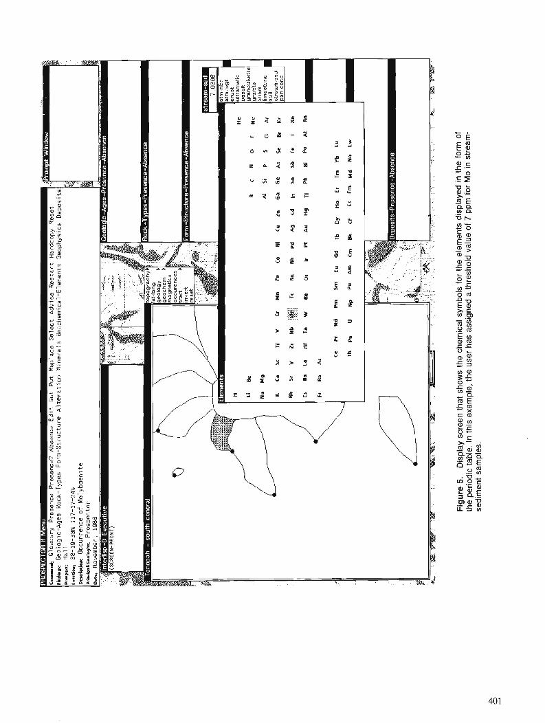
Fig

ure

5.

Dis

play

scr

een

that

sho

ws

the

chem

ical

sym

bols

for

the

elem

ents

dis

play

ed in

the

form

of

the

perio

dic

tabl

e. I

n th

is e

xam

ple,

the

use

r ha

s as

sign

ed a

thre

shol

d va

lue

of 7

ppr

n fo

r M

o in

str

eam

- se

dim

ent

sam

ples

.

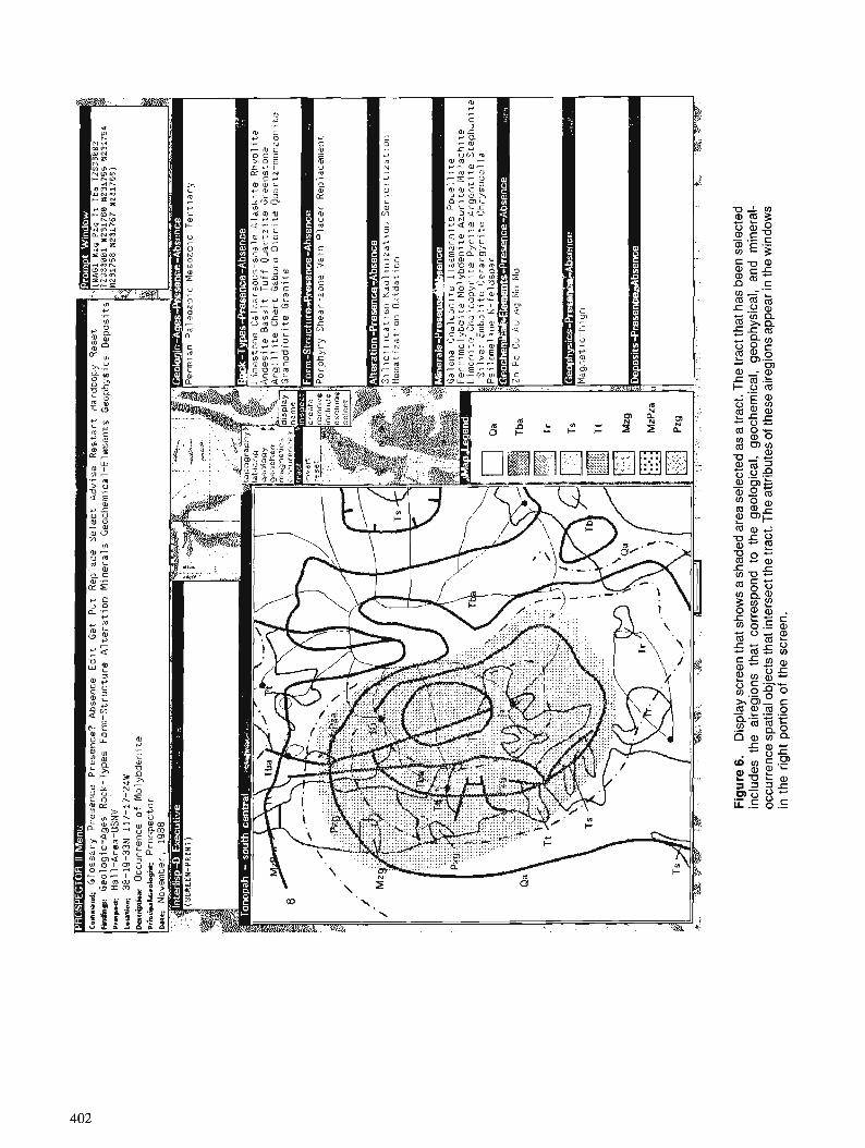
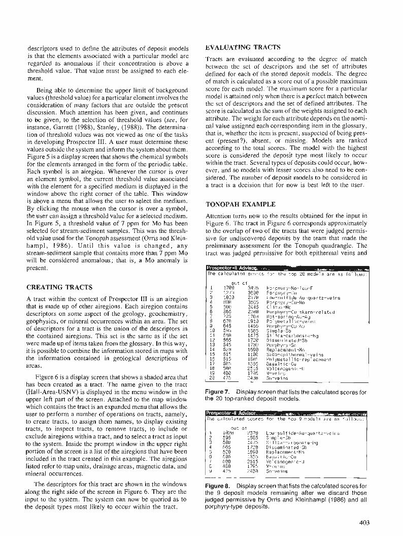
descriptors used to define the attributes of deposit models is that the elements associated with a particular model are regarded as anomalous if their concentration is above a threshold value. That value must be assigned to each element.

Being able to determine the upper limit of background values (threshold value) for a particular element involves the consideration of many factors that are outside the present discussion. Much attention has been given, and continues to be given, to the selection of threshold values (see, for instance, Garrett (1988), Stanley, (1988)). The determination of threshold values was not viewed as one of the tasks in developing Prospector 111. A user must determine these values outside the system and inform the system about them. Figure 5 is a display screen that shows the chemical symbols for the elements arranged in the form of the periodic table. Each symbol is an airegion. Whenever the cursor is over an element symbol, the-current threshold value associated with the element for a specified medium is displayed in the window above the right corner of the table. This window is above a menu that allows the user to select the medium. By clicking the mouse when the cursor is over a symbol, the user can assign a threshold value for a selected medium. In Figure 5 , a threshold value of 7 pprn for Mo has been selected for stream-sediment samples. This was the threshold value used for the Tonopah assessment (Orris and Klein- hampl , 1986) . Until this value is changed, any stream-sediment sample that contains more than 7 ppm Mo will be considered anomalous; that is, a Mo anomaly is present.

CREATING TRACTS

A tract within the context of Prospector I11 is an airegion that is made up of other airegions. Each airegion contains descriptors on some aspect of the geology, geochemistry, geophysics, or mineral occurrences within an area. The set of descriptors for a tract is the union of the descriptors in the contained airegions. This set is the same as if the set were made up of items taken from the glossary. In this way, it is possible to combine the information stored in maps with the information contained in geological descriptions of areas.

Figure 6 is a display screen that shows a shaded area that has been created as a tract. The name given to the tract (Hall-Area-USNV) is displayed in the menu window in the upper left part of the screen. Attached to the map window which contains the tract is an expanded menu that allows the user to perform a number of operations on tracts, namely, to create tracts, to assign them names, to display existing tracts, to inspect tracts, to remove tracts, to include or exclude airegions within a tract, and to select a tract as input to the system. Inside the prompt window in the upper right portion of the screen is a list of the airegions that have been included in the tract created in this example. The airegions listed refer to map units, drainage areas, magnetic data, and mineral occurrences.

The descriptors for this tract are shown in the windows along the right side of the screen in Figure 6. They are the input to the system. The system can now be queried as to the deposit types most likely to occur within the tract.

EVALUATING TRACTS

Tracts are evaluated according to the degree of match between the set of descriptors and the set of attributes defined for each of the stored deposit models. The degree of match is calculated as a score out of a possible maximum score for each model. The maximum score for a particular model is attained only when there is a perfect match between the set of descriptors and the set of defined attributes. The score is calculated as the sum of the weights assigned to each attribute. The weight for each attribute depends on the nominal value assigned each corresponding item in the glossary, that is, whether the item is present, suspected of being present (present?), absent, or missing. Models are ranked according to the total scores. The model with the highest score is considered the deposit type most likely to occur within the tract. Several types of deposits could occur, however, and so models with lesser scores also need to be considered. The number of deposit models to be considered in a tract is a decision that for now is best left to the user.

TONOPAH EXAMPLE

Attention turns now to the results obtained for the input in Figure 6. The tract in Figure 6 corresponds approximately to the overlap of two of the tracts that were judged permissive for undiscovered deposits by the team that made the preliminary assessment for the Tonopah quadrangle. The tract was judged permissive for both epithermal veins and

]The ca lcu latec l scc les f o r the top 28 motir ls are as t o l l o w 4

ou t o f 1 1700 3495 Porphyry-Mo-low-F 2 1270 36BB Porphyry-Cu 3 1920 2370 Lob)-sulf ide-Au-quartz- i tei l is 4 890 3585 Porphyry-CLI-Mo 5 880 2445 Cl imax-Mo 6 865 2200 Porphyry-Cu-skarn-re la ted 7 725 1708 Hot-spr ing-Au-Ag 8 678 1918 Pol ymeta l l i c - v e i n s 9 645 1455 Potphyry-Cu-Au I 0 595 1585 S imple-SL 11 588 1475 S i 1 ica-carbonate-Hg 12 565 1720 Disseminated-Sb 13 545 1738 Porphyry-Sn 1 4 528 1BSB Replacement-Mn 15 515 1108 Sado-epi t.herma1-veins 16 515 1805 Po lymeta l l i c - r e p l a c m e n t 17 505 1355 Basal t ic -Cu 18 500 2515 Vol canogeni c-U 19 488 1795 \\'-\lei ns 20 475 2430 Sn-vei r~s

Figure 7. Display screen that lists the calculated scores for the 20 top-ranked deposit models.

6 585 1355 Rasal t ic -Cu 7 506 2515 \ /o lcanoge~i i c-U 8 488 1795 I - v e i n s

Figure 8. Display screen that lists the calculated scores for the 9 deposit models remaining after we discard those judged permissive by Orris and Kleinhampl (1986) and all porphyry-type deposits.

ment. A future role for Pros~ector I11 is to ensure that all deposits associated with felsic intrusions (Orris and Klein- hampl, 1986). The data used in their assessment are essentially the same as those used in this example. The deposit models were based on the models described in Cox and Singer (1986), the same models upon which the current version of Prospector I1 is based. It is instructive to compare the two results.

Figure 7 shows the calculated scores for the 20 top- ranked deposit models based on the input in Figure 6. Each of the scores represents the calculated score out of a possible maximum score. The deposit types considered permissive in the preliminary assessment were: porphyry-Mo-low-F, epithermal-Au-Ag, hot-spring-Au-Ag, polymetallic-veins, and polymetallic-replacement. The permissiveness of a carbonate-hosted-Au-Ag type was judged to be questionable. Because the Sado-epithermal-veins deposit model is a subtype of the epithermal-Au-Ag deposit model, all the deposit types judged unquestionably permissive in the earlier assessment are included in the list of the 20 top- ranked models in Figure 7. This result is viewed as encouraging. In effect, the system identified those deposit models judged to be permissive by the team that made the earlier assessment. While this is an encouraging result, the obvious question to be asked is, what about the deposit models in the list in Figure 7 that were not judged to be permissive?

First, the other porphyry-type models can be disregarded. The area is favourable for porphyry-type deposits in general, and the area is judged to be most favourable for porphyry-Mo-low-F type deposits in particular. This judgment is not surprising as the Hall Mine has been described as an example of this type of deposit (Theodore and Menzie, 1984). By removing the deposit models judged permissive in the preliminary assessment together with the other porphyry-type models, we are left with the 9 deposit models listed in Figure 8.

Why was the low-sulphide-Au-quartz-vein deposit model not considered permissive in the preliminary assessment? This model is top-ranked among the remaining models in Figure 8. The problem lies in the current deficiency in the present system. Attributes that relate to the depositional environment and the tectonic setting for the descriptive models compiled by Cox and Singer (1986) have not yet been incorporated in the current knowledge base. For low-sulphide-Au-quartz veins deposits, the settings are generally continental margin mobile belts and accreted margins. This type of deposit is characterized by the presence of regionally metamorphosed volcanic and sedimentary rocks (Berger, 1986). For the geological setting in the Tonopah example, although greenstone and quartzite are present, there is no mention made of regional metamorphism. In future, descriptors for depositional environments and tectonic settings clearly will need to be added to the knowledge base.

For the remaining deposit models in the list in Figure 8, it is difficult to say why these models were not judged to be permissive. Some models perhaps were overlooked. For other models, essential attributes may have been missing or were absent but not mentioned in the earlier assessment: To resolve these uncertainties, it would be necessary to review each such model with the team that made the earlier assess-

potentially permissive deposit models be considered. Such a task is within the reach of a map-based expert system.

CONCLUSIONS

Prospector 111 represents a step closer to an expert system that can assist the geologist in delineating areas likely to contain undiscovered deposits. In taking this step, it has become possible to combine the information contained in maps with the descriptions of geological settings of areas and to match the combined information with the stored knowledge about mineral deposit models. The advice that can be provided by such a system offers the geologist an opportunity to consider a wider range of possibilities in choosing deposit models and gives the geologist greater confidence in deciding which models best fit the set of data collected in an area. The development of Prospector I11 represents a continuing effort to model more successf~~lly a specific task in regional mineral resource assessment.

REFERENCES

Berger, B. R. 1986: Descriptive model of low-sulfide-Au-quartz veins, & Mineral

Deposit Models, ed. D.P. Cox and D.A. Singer; : U.S. Geological Survey, Bulletin 1693, p. 239.

Cox, D. P. and Singer, D. A. (editors) 1986: Mineral Deposit Models; U.S. Geological Survey, Bulletin 1693,

379 p. Duda, R. 0. 1980: The Prospector system for mineral exploration; Final SRI project

report 8172, April 1980, 120 p. Fairfield, R. J., Jr., Sierns, D. F., Zuker, J. S., Hill, R. H., Nash, J. T. and Budge, S. 1985 : Analytical results and sample locality map of stream-sediment sam-

ples from the Tonopah 1 by 2" quadrangle, Nevada; U.S. Geo- logical Survey, Open-File Report 85-376, 85 p, I oversize sheet.

Garrett, R. G. 1988 : IDEAS : an interactive computer graphics tool to assist the explora-

tion geochemist, Current Research, Part F; Geological Survey of Canada, Paper 88-IF, p. 1-13.

McCammon, R. B. 1989: Prospector 11; A1 Systems in Government, March 1989, Washing-

ton, D.C., p. 88-92. Orris, G. J. and Kleinhampl, F. J. 1986: Preliminary mineral resource assessment of the Tonopah l o by 2"

quadrangle, Nevada; U.S. Geological Survey, Open-File Report 86-470, 86 p., 2 oversize sheets, scale 1 :250 000.

Plouff, D. 1983 : Preliminary aeromagnetic map of the Tonopah 1 O x 2' quadrangle,

Nevada; U.S. Geological Survey, Open-File Report 83-619, I map, scale 1 :250 000.

Shawe, D. R. (compiler) 1981 : U.S. Geological Survey workshop on nonfuel mineral-resource

appraisal of wilderness and CUSMAP areas; U.S. Geological Survey Circular 845, 18 p.

Singer, D. A. and Ovenshine, A. T. 1979: Assessing metallic resources in Alaska; American Scientist, v. 67,

no. 5, p. 582-589. Stanley, C. R. 1988: PROBPLOT: an interactive computer program to fit mixtures of

normal (or log-normal) distributions with maximum likelihood optimization procedures; Association of Exploration Geochemists, Special volume 14, 100 p.

Theodore, T . G. and Menzie, W. D. 1984: Fluorine-deficient porphyry molybdenum deposits in the western

North America Cordillera; Proceedings of the Sixth IAGOD Sym- posium, p. 463-470.

Whitebread, D. H. (compiler) 1986: Gencralized geologic map of the Tonopah 1 by 2 quadrangle,

Nevada; U.S. Geological Survey, Open-File Report 86-462, I map, scale 1 :250 000.

METHODS OF QUANTITATIVE STRATIGRAPHY

-

A case study for comparison of some biostratigraphic techniques using Paleogene alveolinids from Slovenia and Istria

James C. Browerl

Brower, J. C., A case study for comparison of some biostratigraphic techniques using Paleogene alveolinids from Slovenia and Istria; fi Statistical Applications in the Earth Sciences, ed. F. P. Agterberg and G.F. Bonham-Carter; Geological Survey of Canada, Paper 89-9, p. 407-416, 1989.

Abstract

Drobne (1977) published a study on Paleogene alveolinid foraminifera. Part of these data, including 15 species and 41 samples takenffom 11 stratigraphic sections, have been studied with three quantitative biostratigraphic techniques for the zonation of species, namely seriation, unitary associations and a ranking method. Despite short stratigraphic sections with few samples and little information about the superposition of samples along with cycles of inconsistent biostratigraphic events, seriation generates a satisfactory range chart for the species. Spearman 's rank correlation coeficients denote that tlze seriation sequence of events is more similar to that of the unitary associations than to the ranking method as would be expected from the algorithms.

The composite sequences of events and range charts given by seriation, unitary associations and the ranking method were used to calculate correlation charts for the 41 samples by means of a regression method. Predicted correlations for the samples were also obtained from the seriation row locations and the unitary association positions. f ie rank correlation coeficients indicate that all correlations of the samples are more similar than are the sequences of events or range zones from which they were computed. Nearly identical correlation charts result from the regressions on the three sequences of events. The relative ages of the samples found from the seriation row numbers and the unitary association positions are more divergent.

Drobne (1977) a publik une ktude sur les alvkolines, foraminifires dl1 Palkogtne. Les donnkes ont en partie kt6 recueillies dans 11 coupes structurales er portent sur 15 esp2ces prbentes dans 41 tchantillons qui ont it6 etudih au moyen de trois mkthodes biostratigraphiques quantitatives de zonation des espPces soient la skriation, les associations uniraires et une me'thode de classement. Malgrk les courtes coupes structurales, le faible nombre d'kchantillons et le peu de renseignements disponibles concernant la superposition des kchantillons ainsi que des cycles incompatibles d'episodes biostratigraphiques, la seriation permet de produire un graphique satisfaisant de la rkpartition de 11esp2ce. Les coeficients du rang de Spearman indiquent que la succession d'tpisodes indiquie par la striation est plus similaire ci celle indiquke par les associations unitaires qu '6 celle indiquee par la mkthode de classement comme on pouvait s 'y attendre d'aprt?s les algorithmes.

Les successions composkes d 'tpisodes et les graphiques de rkpartition obtenus par la skriation, les associations unitaires et la mkthode de classement ont servi 6 calculer des tableaux de corrklations pour les 41 kchantillons a ['aide d'une mkthode de rkgression. Des corrklations prkvues pour les kchantillons ont egalement ktk tirees des emplacements des rangkes en serie et des positions d'association unitaire. Les coeficients du rang de Spearman indiquent que toutes les corrt!lations entre les kchantillons sont plus similaires que ne le sont les successions d'eisodes ou de zones de reartition en fonction desquelles ils ont A4 calculks. Des rkgressions appliqukes aux trois successions d'kpisodes ont produit des tableaux des corr6lations presque identiques. Les dges relatifs des kchantillons dkrivks des num&ros de rangees en serie et des positions d'association unitaire s'kcartent davantage.

- - -

' Heroy Geology Laboratory, Syracuse University, Syracuse, New York 13244-1070, U.S .A

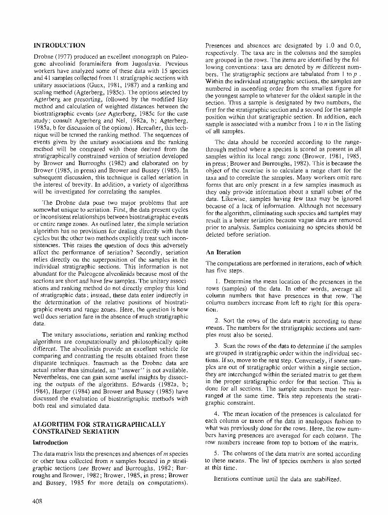
INTRODUCTION

Drobne (1977) produced an excellent monograph on Paleo- gene alveolinid foraminifera from Jugoslavia. Previous workers have analyzed some of these data with 15 species and 41 samples collected from 1 1 stratigraphic sections with unitary associations (Guex, 1981, 1987) and a ranking and scaling method (Agterberg, 198%). The options selected by Agterberg are presorting, followed by the modified Hay method and calculation of weighted distances between the biostratigraphic events (see Agterberg, 198% for the case study ; consult Agterberg and Nel, 1982a, b ; Agterberg, 1985a, b for discussion of the options). Hereafter, this technique will be termed the ranking method. The sequences of events given by the unitary associations and the ranking method will be compared with those derived from the stratigraphically constrained version of seriation developed by Brower and Burroughs (1982) and elaborated on by Brower (1985, in press) and Brower and Bussey (1985). In subsequent discussion, this technique is called seriation in the interest of brevity. In addition, a variety of algorithms will be investigated for correlating the samples.

The Drobne data pose two major problems that are somewhat unique to seriation. First, the data present cycles or inconsistent relationships between biostratigraphic events or entire range zones. As outlined later, the simple seriation algorithm has no provisions for dealing directly with these cycles but the other two methods explicitly treat such inconsistencies. This raises the question of does this adversely affect the performance of seriation? Secondly, seriation relies directly on the superposition of the samples in the individual stratigraphic sections. This information is not abundant for the Paleogene alveolinids because most of the sections are short and have few samples. The unitary associations and ranking method do not directly employ this kind of stratigraphic data; instead, these data enter indirectly in the determination of the relative positions of biostratigraphic events and range zones. Here, the question is how well does seriation fare in the absence of much stratigraphic data.

The unitary associations, seriation and ranking method algorithms are computationally and philosophically quite different. The alveolinids provide an excellent vehicle for comparing and contrasting the results obtained from these disparate techniques. Inasmuch as the Drobne data are actual rather than simulated, an "answer" is not available. Nevertheless, one can gain some useful insights by dissect- ing the outputs of the algorithms. Edwards (1982a, b ; 1984), Harper (1984) and Brower and Bussey (1985) have discussed the evaluation of biostratigraphic methods with both real and simulated data.

ALGORITHM FOR STRATIGRAPHICALLY CONSTRAINED SERIATION

Introduction

The data matrix lists the presences and absences of in species or other taxa collected from n samples located in p stratigraphic sections (see Brower and Burroughs, 1982; Bur- roughs and Brower, 1982; Brower, 1985, in press; Brower and Bussey, 1985 for more details on computations).

Presences and absences are designated by 1.0 and 0.0, respectively. The taxa are in the columns and the samples are grouped in the rows. The items are identified by the following conventions: taxa are denoted by m different numbers. The stratigraphic sections are tabulated from 1 t o p . Within the individual stratigraphic sections, the samples are numbered in ascending order from the smallest figure for the youngest sample to whatever for the oldest sample in the section. Thus a sample is designated by two numbers, the first for the stratigraphic section and a second for the sample position within that stratigraphic section. In addition, each sample is associated with a number from 1 to n in the listing of all samples.

The data should be recorded according to the range- through method where a species is scored as present in all samples within its local range zone (Brower, 1981, 1985, in press; Brower and Burroughs, 1982). This is because the object of the exercise is to calculate a range chart for the taxa and to correlate the samples. Many workers omit rare forms that are only present in a few samples inasmuch as they only provide information about a small subset of the data. Likewise, samples having few taxa may be ignored because of a lack of information. Although not necessary for the algorithm, eliminating such species and samples may result in a better seriation because vague data are removed prior to analysis. Samples containing no species should be deleted before seriation.

An Iteration

The computations are performed in iterations, each of which has five steps.

1. Determine the mean location of the presences in the rows (samples) of the data. In other words, average all column numbers that have presences in that row. The column numbers increase from left to right for this operation.

2. Sort the rows of the data matrix according to these means. The numbers for the stratigraphic sections and samples must also be sorted.

3. Scan the rows of the data to determine if the samples are grouped in stratigraphic order within the individual sections. If so, move to the next step. Conversely, if some samples are out of stratigraphic order within a single section, they are interchanged within the seriated matrix to get them in the proper stratigraphic order for that section. This is done for all sections. The sample numbers must be rearranged at the same time. This step represents the stratigraphic constraint.

4. The mean location of the presences is calculated for each column or taxon of the data in analogous fashion to what was previously done for the rows. Here, the row numbers having presences are averaged for each column. The row numbers increase from top to bottom of the matrix.

5. The columns of the data matrix are sorted according to these means. The list of species numbers is also sorted at this time.

Iterations continue until the data are stabilized.

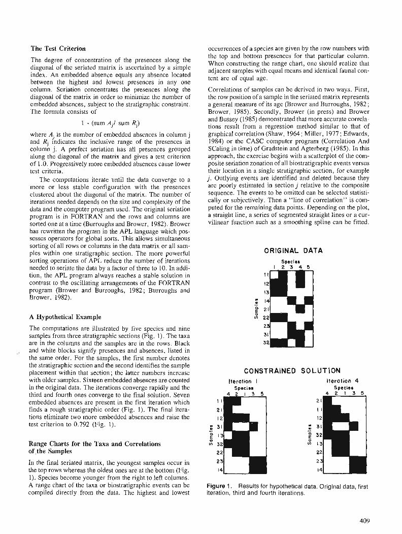
The Test Criterion

The degree of concentration of the presences along the diagonal of the seriated matrix is ascertained by a simple index. An embedded absence equals any absence located between the highest and lowest presences in any one column. Seriation concentrates the presences along the diagonal of the matrix in order to minimize the number of embedded absences, subject to the stratigraphic constraint. The formula consists of

1 - (sum Ajl sum Rj)

where Aj is the number of embedded absences in column j and R, indicates the inclusive range of the presences in column j. A perfect seriation has all presences grouped along the diagonal of the matrix and gives a test criterion of 1 .O. Progressively more embedded absences cause lower test criteria.

The computations iterate until the data converge to a more or less stable configuration with the presences clustered about the diagonal of the matrix. The number of iterations needed depends on the size and complexity of the data and the computer program used. The original seriation program is in FORTRAN and the rows and columns are sorted one at a time (Burroughs and Brower, 1982). Brower has rewritten the program in the APL language which pos- sesses operators for global sorts. This allows simultaneous sorting of all rows or-columns in the data matrix or all samples within one stratigraphic section. The more powerful sorting operations of APL reduce the number of iterations needed to seriate the data by a factor of three to 10. In addition, the APL program always reaches a stable solution in contrast to the oscillating arrangements of the FORTRAN program (Brower and Burroughs, 1982; Burroughs and Brower, 1982).

A Hypothetical Example

The computations are illustrated by five species and nine samples from three stratigraphic sections (Fig. 1). The taxa are in the columns and the samples are in the rows. Black and white blocks signify presences and absences, listed in the same order. For the samples, the first number denotes the stratigraphic section and the second identifies the sample placement within that section; the latter numbers increase with older samples. Sixteen embedded absences are counted in the original data. The iterations converge rapidly and the third and fourth ones converge to the final solution. Seven embedded absences are present in the first iteration which finds a rough stratigraphic order (Fig. 1). The final iterations eliminate two more embedded absences and raise the test criterion to 0.792 (Fig. 1).

Range Charts for the Taxa and Correlations of. the Samples

In the final seriated matrix, the youngest samples occur in the top rows whereas the oldest ones are at the bottom (Fig. 1). Species become younger from the right to left columns. A range chart of the taxa or biostratigraphic events can be compiled directly from the data. The highest and lowest

occurrences of a species are given by the row numbers with the top and bottom presences for that particular column. When constructing the range chart, one should realize that adjacent samples with equal means and identical faunal content are of equal age.

Correlations of samples can be derived in two ways. First, the row position of a sample in the seriated matrix represents a general measure of its age (Brower and Burroughs, 1982 ; Brower, 1985). Secondly, Brower (in press) and Brower and Bussey (1985) demonstrated that more accurate correlations result from a regression method similar to that of graphical correlation (Shaw, 1964; Miller, 1977 ; Edwards, 1984) or the CASC computer program (Correlation And Scaling in time) of Gradstein and Agterberg (1985). In this approach, the exercise begins with a scatterplot of the composite seriation zonation of all biostratigraphic events versus their location in a single stratigraphic section, for example j. Outlying events are identified and deleted because they are poorly estimated in section j relative to the composite sequence. The events to be omitted can be selected statistically or subjectively. Then a "line of correlation" is computed for the remaining data points. Depending on the plot, a straight line, a series of segmented straight lines or a curvilinear function such as a smoothing spline can be fitted.

ORIGINAL DATA

CONSTRAINED SO L U T l O N Iteration I

Soeeies Iteration 4

S ~ e c l r n

Figure 1. Results for hypothetical data. Original data, first iteration, third and fourth iterations.

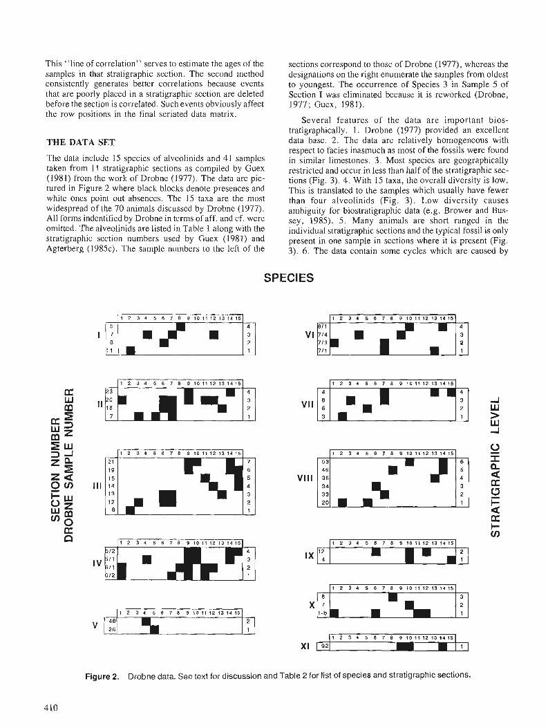
This "line of correlation" serves to estimate the ages of the samples in that stratigraphic section. The second method consistently generates better correlations because events that are poorly placed in a stratigraphic section are deleted before the section is correlated. Such events obviously affect the row positions in the final seriated data matrix.

THE DATA SET

The data include 15 species of alveolinids and 41 samples taken from 1 I stratigraphic sections as compiled by Guex (1981) from the work of Drobne (1977). The data are pictured in Figure 2 where black blocks denote presences and white ones point out absences. The 15 taxa are the most widespread of the 70 animals discussed by Drobne (1977). All forms indentified by Drobne in terms of aff. and cf. were omitted. The alveolinids are listed in Table 1 along with the stratigraphic section numbers used by Guex (1981) and Agterberg (198%). The sample numbers to the left of the

sections correspond to those of Drobne (1977), whereas the designations on the right enumerate the samples from oldest to youngest. The occurrence of Species 3 in Sample 5 of Section I was eliminated because it is reworked (Drobne, 1977; Guex, 1981).

Several features of the data are important bios- tratigraphically . 1. Drobne (1977) provided an excellent data base. 2. The data are relatively homogeneous with respect to facies inasmuch as most of the fossils were found in similar limestones. 3. Most species are geographically restricted and occur in less than half of the stratigraphic sections (Fig. 3). 4. With 15 taxa, the overall diversity is low. This is translated to the samples which usually have fewer than four alveolinids (Fig. 3). Low diversity causes ambiguity for biostratigraphic data (e.g. Brower and Bus- sey, 1985). 5. Many animals are short ranged in the individual stratigraphic sections and the typical fossil is only present in one sample in sections where it is present (Fig. 3). 6. The data contain some cycles which are caused by

SPECIES

Figure 2. Drobne data. See text for discussion and Table 2 for list of species and stratigraphic sections.

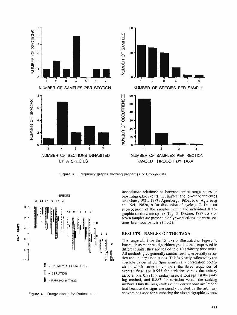
1 2 3 4 5 6 7 1 2 3 4 5 6

NUMBER OF SAMPLES PER SECTION NUMBER OF SPECIES PER SAMPLE

3 4 5 6 7 1 2 3 4

NUMBER OF SECTIOIVS INHABITED NUMBER OF SAMPLES PER SECTION BY A SPECIES RANGED THROUGH BY TAXA

Figure 3. Frequency graphs showing properties of Drobne data.

inconsistent relationships between entire range zones or SPECIES

8 14 10 9 15 4

1 = UNITARY ASSOCIATIONS

( = RANKING METHOD

Figure 4. Range charts for Drobne data.

biostratigraphic events, i.e. highest and lowest occurrences (see Guex, 1981, 1987; Agterberg, 1985a, b, c ; Agterberg and Nel, 1982a, b for discussion of cycles). 7. Data on superposition of the samples within the individual stratigraphic sections are sparse (Fig. 3; Drobne, 1977). Six or seven samples are present in only two sections and most sections bear' four o r less samples.

RESULTS - RANGES OF THE TAXA

The range chart for the 15 taxa is illustrated in Figure 4. Inasmuch as the three algorithms yield outputs expressed in different units, they are scaled into 10 arbitrary time units. All methods give generally similar results, especially seriation and unitary associations. This is clearly reflected by the absolute values of the Spearman's rank correlation coefficients which serve to compare the three sequences of events: these are 0.953 for seriation versus the unitary associations, 0.891 for unitary associations against the ranking method, and 0.887 for seriation versus the ranking method. Only the magnitudes of the correlations are important because the signs are simply dictated by the arbitrary conventions used for numbering the biostratigraphic events.

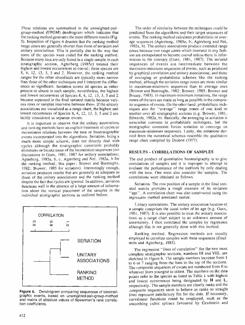
These relations are summarized in the unweighted-pair- group-method (UPGM) dendrogram which indicates that the ranking method generates the most different results (Fig. 5). Inspection of Figure 4 denotes that the ranking method range zones are generally shorter than those of seriation and unitary associations. This is partially due to the way that some of the species were coded for the ranking method. Because many taxa are only found in a single sample in each stratigraphic section, Agterberg (198%) treated their highest and lowest occurrences as coeval ; these species are 8, 4, 12, 13, 3, 5 and 2. However, the ranking method ranges for the other alveolinids are typically more narrow than those of the other techniques and I interpret the differences as significant. Seriation scores all species as either present or absent in each sample; nevertheless, the highest and lowest occurrences of Species 8, 4, 12, 13, 3, 5 and 2 become separated in the final seriated matrix because various rows or samples intervene between them. If the unitary associations are visualized as a range chart, the highest and lowest occurrences of Species 8, 4, 12, 13, 3, 5 and 2 are tacitly considered as separate events.

It is important to observe that the unitary associations and ranking methods have an explicit treatment of cycles or inconsistent relations between the taxa or biostratigraphic events incorporated into the algorithms. Seriation, being a much more simple scheme, does not directly deal with cycles although the stratigraphic constraint probably eliminates or breaks some of the inconsistent sequences (see discussions in Guex, 1981, 1987 for unitary associations; Agterberg, 1985a, b, c ; Agterberg and Nel, 1982a, b for the ranking method; this paper; Brower and Burroughs, 1982 ; Brower, 1985 for seriation). Interestingly enough, seriation produces results that are generally as adequate as those of the unitary associations and the ranking method despite the fact that cycles are ignored. In addition, seriation functions well in the absence of a large amount of information about the vertical placement of the samples in the individual stratigraphic sections as outlined before.

CORRELATION

UNITARY ASSOCIATIONS

I RANKING METHOD

Figure 5. Dendrogram comparing sequences of biostratigraphic events, based on unweighted-pair-group-method and matrix of absolute values of Spearman's rank correlation coefficients.

The order of similarity between the techniques could be predicted from the algorithms and their target sequences of events. The ranking method calculates probabilistic or average sequences (Agterberg, 1985a, b; Agterberg and Nel, l982a, b). The unitary associations produce extended range zones because two range zones which intersect in any fashion are extrapolated to become coeval unless there is information to the contrary (Guex, 198 1 , 1987). The seriated sequences of events are intermediate between the maximum-minimum sequences of events, such as produced by graphical correlation and unitary associations, and those of averaging or probabilistic schemes like the ranking method, although the seriation range zones are more similar to maximum-minimum sequences than to average ones (Brower and Burroughs, 1982; Brower, 1985; Brower and Bussey, 1985). In maximum-minimum zonations, the range zones of the taxa are made as long as possible in the composite sequence of events. On the other hand, probabilistic techniques aim for "average" range zones of one kind or another over all stratigraphic sections (e.g. Brower, 1981 ; Edwards, 1982a, b). Basically, the averaging in seriation is somewhat common to probabilistic techniques, but the stratigraphic constraint forces seriation to converge on maximum-minimum sequences. Lastly, the zonations derived from the numerical schemes resemble the qualitative range chart compiled by Drobne (1977).

RESULTS - CORRELATIONS OF SAMPLES

The end product of quantitative biostratigraphy is to give correlations of samples and it is improper to attempt to evaluate the performance of the methods by only dealing with the taxa. One must also consider the samples. The correlations were obtained as follows.

Seriation. The row position of a sample in the final seriated matrix provides a rough measure of its seriation "age". A correlation chart was also constructed using the regression method annotated earlier.

Unitary associations. The unitary association location of a sample comprises the usual index of its age (e.g. Guex, 1981, 1987). It is also possible to treat the unitary associations as a range chart subject to an unknown amount of uncertainity. I then correlated the samples by regression although this is not generally done with this method.

Ranking method. Regression methods are usually employed to correlate samples with these sequences (Grad- stein and Agterberg, 1985).

The regression "lines of correlation" for the two most complete stratigraphic sections, numbers I11 and VIII, are sketched in Figure 6 . The sample numbers increase from 1 to 6 or 7 ranging from the base to the top of the sections. The composite sequences of events are numbered from 0 to whatever from youngest to oldest. The numbers on the data points refer to the species as listed in Table 1 with highest and lowest occurrences being designated by H and L, respectively. The sample numbers are clearly ranks and the 2omposite sequences seem to behave as ranks so straight lines represent satisfactory fits for the data. If necessary, curvilinear functions could be employed, such as the smoothing cubic splines favoured by Gradstein and

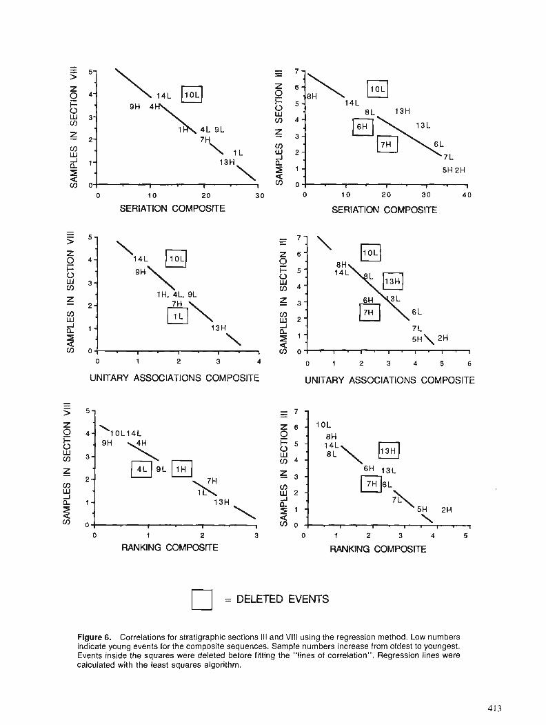
SERlATlON COMPOSITE SERlATlON COMPOSITE

0 1 2 3 4 0 1 2 3 4 5 6

UNITARY ASSOCIATIONS COMPOSITE UNITARY ASSOCIATIONS COMPOSITE

0 1 2 3 0 1 2 3 4 5

RANKING COMPOSITE RANKING COMPOSITE

= DELETED EVENTS

Figure 6. Correlations for stratigraphic sections Ill and Vlll using the regression method. Low numbers indicate young events for the composite sequences. Sample numbers increase from oldest to youngest. Events inside the squares were deleted before fitting the "lines of correlation". Regression lines were calculated with the least squares algorithm.

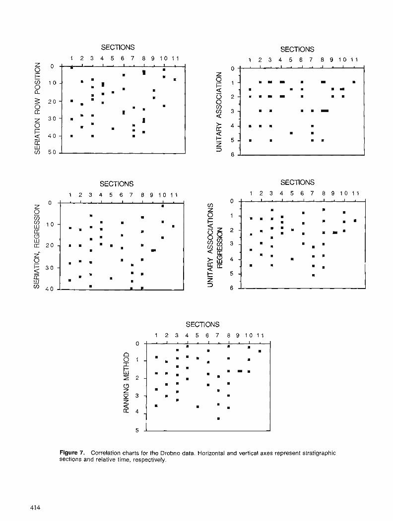
RA

NK

ING

ME

THO

D

" P

WN

0

SE

RIA

TIO

N,

RE

GR

ES

SIO

N

UN

ITA

RY

AS

SO

CIA

TIO

NS

R

EGR

ESSI

ON

O

ul

PO

IU

~O

SE

RIA

TIO

N R

OW

PO

SIT

ION

UN

ITA

RY

AS

SO

CIA

TIO

N

Table 1. List of alveolinids and stratigraphic sections for the Drobne data.

ALVEOLINIDS 1. A, moussoulensis 9. A. montanarii 2. A. aramaea 10. A. aragonensis 3. A. solida 11. A. dedolia 4. A. globosa 12. A. subpyreneica 5. A. avellana 13. A. laxa 6. A. pisiformis 14. A. guidonis 7. A. pasticillata 15. A. decipiens 8. A. leupoldi

STRATIGRAPHIC SECTIONS I . Fatji hrib

I I . Dane near ~ivata Ill. Veliko Gradiiie IV. Ritomece near Gradiiie V. Podgorje VI. Podgrad-Hruiica VII. Kozi?a-Socerb

VIII. Golez IX. tbevnica X. Dane-lstria

XI. Jel4ane (isolated sample).

Table 2. Matrix of absolute values of Spearman's rank correlation coefficients for the correlation charts. UA denotes unitary associations.

1.0 0.949 0.943 0.958 0.963 Seriation,rows

0.961 0.978 Seriation, regression 1.0 0.978 Ranking method

UA, regresstion

Agterberg (1985). Events that are poorly located in Sections VI and VIII form outliers that fall outside of most of the points. Those inclosed in boxes were deleted prior to fitting the "lines of correlation". Depending on the technique and section, one to three events were removed.

Figure 7 contains correlation charts for the 41 samples prepared with all of the methods and a high degree of similarity is observed. In fact, the correlations are more similar than the sequences of events used to generate them. Most variation between the techniques involves the shorter stratigraphic sections with the smallest numbers of samples, especially V and XI, and IX to a lesser extent. Some methods produce divergent results for individual samples in other stratigraphic sections : examples are Sample 4 in Sec- tion I by the seriation row positions and Sample 4 in Section IV by the ranking method. The high similarities between the correlation charts given by all techniques are reflected in the matrix of Spearman's rank correlation coefficients and the

Figure 8. Dendrogram comparing the correlations, based on unweighted-pair-group-method and matrix of absolute values of Spearman's rank correlation coefficients.

CORRELATION -L z : 0

0 U1 0 - SERlATlON

unweighted-pair-group-method dendrogram (Table 2, Fig. 8). The correlation coefficients are all high and range from 0.925 (seriation, regression versus unitary association position) to 0.978 (seriation, regression versus unitary associations, regression and unitary associations, regression versus ranking method, regression). Note that the correlations for the regression methods are consistently the highest. Regard- less of the type of sequence, ranking method, seriation or unitary associations, all yield very similar correlations for the samples (Table 2, Figs. 7, 8). The lower correlations characterize the seriation row locations and the unitary association positions which join the dendrogram at levels of about 0.955 and 0.945, respectively.

-

The implication for the samples is that any reasonable sequence of biostratigraphic events or range zones yields similar correlations if a regression type of technique is used. Other correlation algorithms for samples seem to produce more divergent results. If the problem is structured in terms of the samples, the selection of a regression method versus some other scheme may comprise the critical decision. This conclusion is supported by the work of Brower and Bussey (1985) who compared the performance of five quantitative methods commonly used by biostratigraphers. Addition- ally, it should be pointed out that the computer simulations of Brower (in press) and Brower and Bussey (1985) on seriation show that the regression methods give better correlations for the samples than do the seriation row positions. Perhaps, quantitative correlations should focus more on the samples than on sequences of events.

RANKING METHOD - REGRESSION

UNITARY ASSOCIATIONS

ROW POSITION

SERlATlON

-

- REGRESSlOlV

UNITARY ASSOCIATIONS - REGRESSION

REFERENCES

Agterberg, F.P. 1985a: Methods of ranking biostratigraphic events; Quantitative

Stratigraphy, F.M. Gradstein, F.P. Agterberg, J.C. Brower and W.S. Schwarzacher; D. Reidel Pub. Co.. D. 161-194.

1985b: Methods of scaling biostratigraphic events; &Quantitative Stratig- raphy, F.M. Gradstein, F.P. Agterberg, J.C. Brower and W.S. Schwarzacher; D. Reidel Pub. Co., p. 195-241.

1 9 8 5 ~ : Normality testing and comparison of RASC to Unitary Associa- tions method; ~ Quantitative Stratigraphy, F.M. Gradstein. F.P. Agterberg, J.C. Brower and W.S. Schwarzacher; D. Reidel Pub. Co., p. 243-262.

Agterberg, F.P. and Nel, L.D. 1982a: Algorithms for the ranking of stratigraphic events; Computers and

Geosciences v. 8 (no. I ) , p. 69-90. 1982b: Algorithms for the scaling of biostratigraphic events; Computers

and Geosciences v. 8, (no. 2), p. 163-189. Brower, J.C. 1981 : Quantitative biostratigraphy, 1830-1980; b Computer Applica-

tions in the Earth Sciences, an Update of the 70's. ed. D.F. Mer- riam; Plenum Press, ~ e w ~ o r k ' a n d London, p. 63-103.

1985 : Archaeological seriation of an original data matrix; ~ Quantitative Stratigraphy, F.M. Gradstein, F.P. Agterberg, J.C. Brower and W.S. Schwarzacher; D. Reidel Pub. Co., p. 95-108.

in press:Seriation of an original data matrix as applied to biostratigraphy. Brower, J.C., and Burroughs, W.A. 1982: A simple method for quantitative biostrafigraphy; ~ Quantitative

Stratigraphic Correlation, ed. J.M. Cubitt and R.A. Reyment; John Wiley and Sons, Ltd., p. 61-83.

Brower, J.C., and Bussey, D.T. 1985: A comparison of five quantitative techniques for biostratigraphy ;

in Quantitative Stratigraphy, F.M. Gradstein, F.P. Agterberg, KC. Brower and W.S. Schwarzacher; D. Reidel Pub. Co., p. 279-306.

Burroughs, W.A. and Brower, J.C. 1982: SER, a FORTRAN program for the seriation of biostratigraphic

data; Computers and Geosciences v. 8, p. 137-148.

Drobne, K. (977: Alveolines Paleogenes de la Slovenie et de I'Istrie; MCnioires

Suisses de PalContologie v. 99, 175 p. Edwards, L.E. l982a: Quantitative biostratigraphy: the methods should suit the data; 3

Quantitative Stratigraphic Correlalion, ed. J.M. Cubitt and R.A. Reyment; John Wiley and Sons, Ltd., p. 45-60.

1982b: Numerical and semi-objective biostratigraphy: review and predictions; Third North American Paleontological Convention, Proceedings v. 1 , p. 147-152.

1984: Insights on why Graphic Correlation (Shaw's method) works; Journal of Geology v. 92, p. 583-597.

Gradstein, F.M., and Agterberg, F.P. 1985: Quantitative correlation in exploration micropaleontology; fi

Quantitative Stratigraphy, F.M. Gradstein, F.P. Agterberg, J.C. Browerand W.S. Schwarzacher; D. Reidel Pub. Co., p. 309-357.

Guex, J. 1981 : Associations virtuelles et discontinuitCs dans la distribution des

espbces fossiles: un example intkressanf; SociCtC Vaudoise des Sciences Naturelles, Bulletin, vol. 75, no. 359, p. 179-197.

1987: CorrClations biochronologiques et associations unitares; Presse Polytechniques Romandes, Lasanne, Switzerland, 244 p.

Harper, C.W., Jr. 1984: A FORTRAN IV program for comparing ranking algorithms in

quantitative biostratigraphy; Computers and Geosciences, v. 10, D. 3-29.

Miller, 'F.x. 1977: The graphic correlation method in biostratigraphy; Concepts

and Methods of Biostratigraphy, ed. E.G. Kauffman and J.E. Hazel ; Dowden, Hutchinson and Ross, Inc., Stroudsburg Pennsyl- vania, p. 165-186.

Shaw, A.B. 1964: Time instratigraphy; McGraw-Hill Book Co., New York, 365 p.

A prototype constrained optimization solution to the time correlation problem

William G.Kemple,l Peter M. Sadler2 and David J. Straussl

Kemple, W. G., Sadler, P.M. and Strauss, D. J. A prototype constrained optimization solution to the time correlation problem; & Statistical Applications in the Earth Sciences, ed. F.P. Agterberg and G. F. Bonham-Carter; Geological Survey of Canada, Paper 89-9, p. 41 7-425, 1989.

Abstract

Time correlation is evolving from a primarily subjective exercise into an essentially quantitative discipline. Existing methods of performing time correlation exhibit many desirable features and much ingenuity but still lack formalism. They typically fail to specify the qualities of good solutions and the criteria for choosing the best.

We present a formal statement of the time correlation problem. It is found to have 3 separate component problems which concern the sequence, spacing and location of events. A solution technique naturally emerges in the form of a constrained optimization procedure which combines the best attributes of several existing methods. The procedure is flexible. It incorporates specified expert judgments and demonstrates the consequences of changing the judgments. In this way it yields reproducible results.

La corrklation chronologique e'volue, et au lieu d'un exercice en premier lieu subjectif, devient une discipline essentiellement quantitative. Les mhhodes existantes de corre'lation chronologique pre'sentent de nombreuses caract&istiques de'sirables et sont t r b imaginatives, mais n'obe'issent pas encore ir un sche'ma formel. De fagon typique, elles ne peuvent spkcijer les qualite's des solutions valables, ni les critPres permettant de choisir les meilleures solutions.

Cet article prksente de facon formelle le probltme de la corre'lation chronologique. L.es auteurs esti- ment que ce probltme comporte trois composantes distinctes concernant la se'quence, l'espacement el la localisation des e've'nements. Une technique de re'solution se pre'sente naturellement sous forme d'un prockdk d'optimisation confraint, combinant les meilleurs attributs de plusieurs mkthodes existantes. Le prockdk est flexible. I1 int2gre des jugements experts spe'ci$e's, et dkmontre les conse'quences d'une modiJication de ces jugements. De cette facon, il donne des re'sultats reproductibles.

' Department of Statistics, University of California, Riverside, CA 92521, U.S.A. Department of Earth Sciences, University of California, Riverside, CA 92521, U.S.A.

INTRODUCTION

Time correlation is a fundamental task in geology. The ultimate goal is to organize rocks into units according to their age ; age relations are based on fossils and other data embedded within the rocks. The sequence of events which produced these data serves as our time scale. Because the ancient events are only sporadically preserved, a single stratigraphic section will not provide enough reliable data. A usefully complete time scale emerges if the data from several local sections are correlated. Still, we must recognize that the available data are inadequate to identify the unique "true7' sequence and spacing of events in time. Our task, therefore, is to select the "best" approximation of the true solution ; and our statement of the problem must include an operational definition of "best".

We suggest that existing approaches to the time correlation problem are rather vague about the characteristics of good solutions and the criteria for choosing the best solution. Their development seems to have been focused too much on methodology and too little on the problem.

In this paper we show that the geological correlation problem can, and arguably should, be treated as an exercise in mathematical optimization. We consider the main contribution to be development of a rigorous formalism for the problem and its solution. As is often the case, development of a proper problem statement leads directly to an appropriate solution technique. First we must state precisely what we mean by time correlation.

Time correlation is a basic task of chronostratigraphy. We follow most codes of stratigraphic nomenclature (e.g. Hedberg, ed., 1976) in defining chronostratigraphy as the element of stratigraphy that organizes strata into units according to age. Time correlation demonstrates correspondence in age between units in separate stratigraphic sections. This is not the same as biostratigraphy, which organizes strata into units according to fossil content. Bios- tratigraphic units are often used as substitutes for chronostratigraphic units; but we follow those methods of true time correlation that extract evidence of age from the distribution of fossils and then correlate on the basis of age relations. The events most often available for correlation are the lowest and highest observed occurrences of a taxon within a stratigraphic section (local first and last occurrences). These most often reflect migration events, which may vary in age from place to place. It is a common observation that event sequences which reflect the beginnings and endings of the local sojourns of taxa vary from section to section (Fig. 1). The actual evolution and extinction of a taxon occur at unique times and places. When properly ordered and spaced, a sequence of these evolution and extinction times provides a true time scale.

The time correlation problem can be viewed as three smaller problems. The primary problem is to determine the temporal sequence of the evolution and extinction events (the sequencing problem). The other problems, which one may or may not wish to solve, are to find the spaces (times) between these events (the spacing problem) and to calculate the locations of horizons in each local section which correspond to their times (the horizon problem).

The paper is organized as follows: First, we briefly discuss existing methods of correlation. The succeeding section presents a systematic approach to the problem, which is carried out in the following section to give our prototype constrained optimization model. Our conclusions are presented in the final section.

EXISTING METHODS OF CORRELATION

Traditionally an "index fossil" strategy has been used for correlation. This strategy is unsatisfactory for two reasons. Firstly, it simply assumes that observed events for one small group of taxa are preserved at levels that are of the same age in all local sections, and that these are exactly recovered. In effect it presumes that the data for a few taxa are part of the true solution, and forces the other parts based on this guess. It is preferable to include information from all local observations. Their contribution should be weighted according to both the quality of the sections and to the judged chronostratigraphic quality of the individual first and last occurrences within each section. Secondly, the index fossil strategy is not really chronostratigraphic: the stratigrapher selects those biostratigraphic units believed to be least diachronous, simply using them as if they were chronostratigraphic units. As discussed before, local first and last occurrences most often reflect migration events and are not time correlatives. Since few individuals are fossi- lized, and only a small proportion of fossils are collected, even the stratigraphic position of the migration events may be imprecise1 y recovered.

The pioneering work of Shaw (1964) gave rise to what may be called semi-quantitative methods of time correlation; they seek a suitably ordered and spaced sequence of evolution and extinction events as a time scale rather than one based on index fossils. Shaw's method begins with a subjective choice of the "best" of the local sections as the initial "composite". This composite is repeatedly revised by composition with the remaining sections, which are brought into the solution one at a time in the subjective order of their quality. Composition is performed with a bivariate plot, the distance to each event in the composite being measured along one axis, and the distance to the same event in the section undergoing composition measured along the other. The stratigrapher then draws the line that in his judgment "results in the smallest net disruption of the best- established ranges". Shaw (1964, p. 254-257) calls this idea "economy of fit". This line is used to transform locations on the new section into the composite. The method solves both the sequencing and the spacing problems simultaneously by assuming that the relative sediment accumulation rate for any two sections is constant. In practice this means satisfying "economy of fit" by drawing a straight line. Where possible, discrepancies between the two sections are resolved by extending the local taxon ranges ("distance" between first and last occurrences for one taxon) in the composite. Range contractions are not allowed. The composition operations are repeated until the solution stabilizes. The locations in the sections can then be calculated by reverse transformations from the composite back into the individual sections. Zones derived using such an approach are called "conservative" by Agterberg and Gradstein (1988) : the

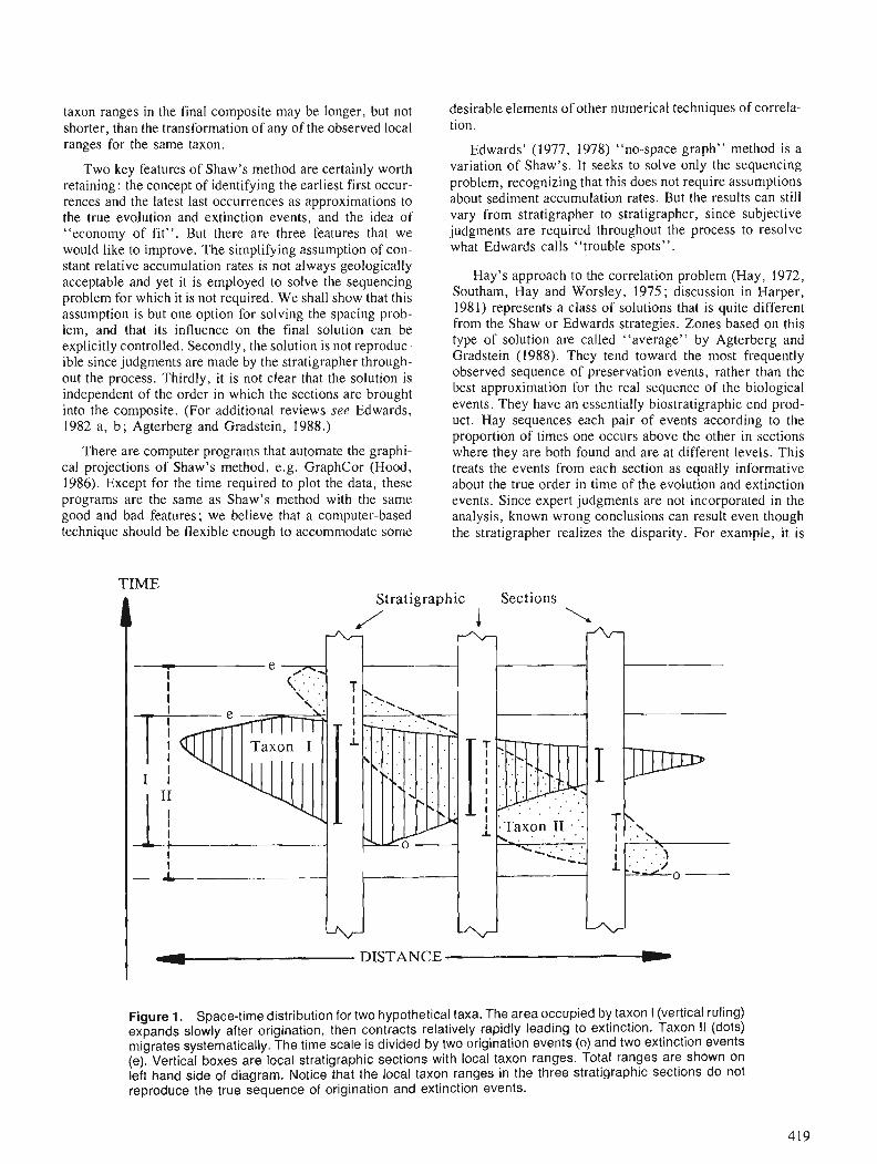
taxon ranges in the final composite may be longer, but not shorter, than the transformation of any of the observed local ranges for the same taxon.

Two key features of Shaw's method are certainly worth retaining : the concept of identifying the earliest first occurrences and the latest last occurrences as approximations to the true evolution and extinction events, and the idea of "economy of fit". But there are three features that we would like to improve. The simplifying assumption of constant relative accumulation rates is not always geologically acceptable and yet it is employed to solve the sequencing problem for which it is not required. We shall show that this assumption is but one option for solving the spacing problem, and that its influence on the final solution can be explicitly controlled. Secondly, the solution is not reproducible since judgments are made by the stratigrapher throughout the process. Thirdly, it is not clear that the solution is independent of the order in which the sections are brought into the composite. (For additional reviews see Edwards, 1982 a, b; Agterberg and Gradstein, 1988.)

desirable elements of other numerical techniques of correlation.

Edwards' (1977, 1978) "no-space graph" method is a variation of Shaw's. It seeks to solve only the sequencing problem, recognizing that this does not require assumptions about sediment accumulation rates. But the results can still vary from stratigrapher to stratigrapher, since subjective judgments are required throughout the process to resolve what Edwards calls "trouble spots".

Hay's approach to the correlation problem (Hay, 1972, Southam, Hay and Worsley, 1975; discussion in Harper, 198 1) represents a class of solutions that is quite different from the Shaw or Edwards strategies. Zones based on this type of solution are called "average" by Agterberg and Gradstein (1988). They tend toward the most frequently observed sequence of preservation events, rather than the best approximation for the real sequence of the biological events. They have an essentially biostratigraphic end product. Hay sequences each pair of events according to the proportion of times one occurs above the other in sections

There are computer programs that automate the graphi- where they are both found and are at different levels. This cal projections of Shaw's method, e.g. GraphCor (Hood, treats the events from each section as equally informative 1986). Except for the time required to plot the data, these about the true order in time of the evolution and extinction programs are the same as Shaw's method with the same events. Since expert judgments are not incorporated in the good and bad features; we believe that a computer-based analysis, known wrong conclusions can result even though technique should be flexible enough to accommodate some the stratigrapher realizes the disparity. For example, it is

I - DISTANCE C

Figure 1. Space-time distribution for two hypothetical taxa. The area occupied by taxon 1 (vertical ruling) expands slowly after origination, then contracts relatively rapidly leading to extinction. Taxon I I (dots) migrates systematically. The time scale is divided by two origination events (0) and two extinction events (e). Vertical boxes are local stratigraphic sections with local taxon ranges. Total ranges are shown on left hand side of diagram. Notice that the local taxon ranges in the three stratigraphic sections do not reproduce the true sequence of origination and extinction events.

possible to be certain from one or more good sections that They are truly chronostratigraphic, but we find them semi- two taxa coexisted and yet have the method conclude other- quantitative and to some degree they all fail to define the wise. ~ rob lem with sufficient formality to lead directlv to an

Hay does not attempt to solve the spacing problem. He does provide a graphical method (fi-om Dennison and Hay, 1967) to determine the probability that a given taxon was present at any chosen location within a section and suggests that it be used to mark the end points of the local sojourns if required. This analysis is independent of the sequencing effort and can indicate that two taxa coexist while the sequencing solution indicates they do not. Despite these shortcomings, the method provides a convenient way to generate an initial solution which may be a useful starting point in a chronostratigraphic method.

The computer-based RASC and CASC systems (Grad- stein et al . , 1985) incorporate elements of Hay's method. Taking the taxa two-by-two, the RASC system conveniently separates the algorithms for the sequencing and spacing of events. Both the sequencing (ranking) and the spacing (scaling) are based on the proportion of times one event occurs above the other. The distances measured from the bottom of the sections to the events and the distances between the events are not used. Calculated times are reported on an arbitrary (RASC) scale. The CASC system uses semi- objective spline fitting to transform these times back into the local sections. If several age estimates are available for locally observed events, the CASC system also produces a local linear time scale.

Unlike Shaw's method, the Hay and RASCICASC systems largely exclude expert judgments about the quality of local data and they seem to allow local range contractions as readily as extensions. Reworked fossils, which can cause unrealistically long local ranges are rare in many sections and can often be recognized by experts. Both Hay's and the RASCtCASC methods have the desirable feature that the results are reproducible. They appear to allow probability statements about their solutions, but neither method is built on the basis of a well defined probability model.

Hay's method, the RASCICASC systems and Shaw's method have all been widely used and have been claimed to produce satisfactory results; but it is not clear to us what satisfactory means in this context.

Methods which Edwards (1982b) classifies as "multivariate" (Hazel, 1977 ; Hohn, 1978) and "relational" (Guex, 1977; Rubel, 1978; Davaud, 1982) work from the similarities of preserved events and the observed overlap of taxon ranges respectively. They produce sequences of events akin to biostratigraphic assemblage zones. Their solutions may generate taxon ranges that extend beyond the biological appearance and extinction events (Edwards 1982b). Guex's (1977) Unitary Association method builds upon the useful observation that when two taxa are recovered at the same horizon in any section we may assume that both had evolved before either became extinct. We shall incorporate this into our method.

In summary, we are drawn to those methods that seek the earliest first occurrences and the latest last occurrences to approximate the total taxon ranges (evolution to extinction).

explicit method of solution. In the following sections we develop a systematic treatment of the problem.

MATHEMATICAL STATEMENT OF THE PROBLEM

From the viewpoint of statistics, or operations research, a proper statement of the problem must specify the data, the question, and the characteristics of a "good" answer, so exactly that a computer program can search for the "best'' among all possible solutions. This set of possible solutions is extremely large. If one starts with data for (I) taxa there are (21) ! = (21) X (21-1) x . . . X (1) permutations of the sequence of evolution and extinction events (e.g. if I=20, (21)! is about In addition there are infinitely many placements in time for these events within each permutation. Our correlation problem is to find the solution that best approximates the true order and placement in time, using the observed sequences and spacings of events in the local stratigraphic sections to quantify "best". We recognize five steps in the process, as follows:

1) Adopt a formal notation for the observed data (e.g. local taxon ranges) and any weights (e.g, based on confidence intervals for taxon ranges, see Springer and Lilje, 1988; Strauss and Sadler, 1989b; or based on completeness estimates for sections, see Sadler, 1981) that can be applied - - to reflect their relative reliability.

2) Choose the parameters (e.g. the position of local horizons corresponding to the age of a given event) that must have values assigned to them by any solution.

3) List constraints (e.g. that the first occurrence of a taxon must be older than the last occurrence) that eliminate unacceptable solutions.

4) Define an objective function (e.g. weighted net taxon range adjustment) that measures the relative plausibil- ity of the remaining solutions.The objective function may be regarded as the cumulative penalty accrued by a given - - set ofvalues for the parameters. With this metaphor the constraints eliminate sets of values that have an infinite penalty.

5) Develop an optimization procedure which will yield the "best" values of the parameters. Here the word "best" means precisely that the parameters minimize the specified objective function.

A familiar example of the optimization approach to a statistical problem is the fitting of a regression line to a set of bivariate data (an x,y plot). Here the parameters are the slope and intercept of the true line, and the usual objective function to be minimized is the sum of squared distances of the points from any fitted line (measured in the vertical direction). This particular objective function is minimized by the well-known regression line described in statistics textbooks; other objective functions would lead to different solutions. Varnes' (1987) analysis of earthquake foreshocks is a more complex geological example that uses linear regression to find the optimal values of four parameters.

In the context of time correlation it is possible to specify some characteristics of implausible solutions (step 3), so the

procedure becomes a constrained optimization ; steps 4) and 5) above may become more complicated, of course, but the principles remain the same. We shall go into more details below, but would first like to point out some advantages of this approach to the correlation problem.

1) By separating what we are trying to optimize from the optimization procedure, we are forced to clarify precisely the goal of the correlation. In current methods, exactly what is being sought is not made explicit.

2) The expert ability of stratigraphers to assess which aspects of the data are the most reliable should be incorporated into the analysis. Some methods allow this, either during the analysis (Shaw, 1964; Edwards, 1977, 1978) or after it (Unitary Association : Guex, 1977 ; Davaud, 1982 ; RASC : Gradstein et al. 1985). The expert judgments are not explicit, however, and the results would not be reproducible by a different expert. In our approach the judgments are included explicitly, at the outset, in the choice of differing weights for the data from different taxa and stratigraphic sections. Once these are determined the analysis proceeds automatically and, depending on the computer, relatively quickly.

3) Having produced a correlation, the stratigrapher will be able to re-run the analysis with different weights to examine the effects of different judgments about the data. This can be done as often as desired; the result will be a whole

suite of possible solutions, each being optimal for an explicit set of judgments. Thus, far from eliminating subjective expertise from the analysis, constrained optimization enables stratigraphers to incorporate their opinions in an objective way, and to see the effect of their judgments on the resulting correlation.

4) Since the constraints and objective function can be manipulated to mimic different methods of correlation, constrained optimization offers a framework for comparing existing systems. Formal comparisons can be made using simulated data or real sections.

A CONSTRAINED OPTIMIZATION MODEL

The elements of our prototype constrained optimization model are described in the following sections.

The Data and Weights

The basic data are local taxonomic range charts (Fig. 2). For a given taxon (indicated by subscript i), in a given section (subscript j), the observed range has a bottom (aG) and a top (bij) recorded on the local thickness scale. The chronostratigraphic quality of local taxon ranges varies with the section completeness, the mode of preservation, the sampling strategy, and the quality of the taxonomy; these rather

1 Section "j" Section "j"'

I Time Scale

r ange

/ ' Local Thickness Scales

Figure 2. Notation for the constrained optimization solution. Asterisks: local finds of taxon i; ai,, bij: first and last observed occurrences of taxon i in section j; s,, ti: times of evolution and extinction events; q j , Pii: locations of horizons in section j corresponding to times s, and ti.

subjective aspects should be evaluated and incorporated into a set of weights (wij) which express the quality of the data for each taxon in each section. If the spacing solution is desired, an assumption about the sediment accumulation is required and another set of weights (vj) should be used to reflect the quality of the individual sections relative to that assumption.

Other kinds of stratigraphic data can be included if they have sufficient chronostratigraphic significance to help constrain or improve the solution. It is permissible to enter a lithostratigraphic unit as if it were an additional taxon with an observed range (aij to bi,). Horizons may be entered as ranges with coincident tops and bottoms (aij = bij) The value assigned to the corresponding weight will determine the degree to which a plausible solution can treat the lithostratigraphic boundaries as diachronous. If a stratigraphic horizon, such as a dated ash bed or magnetic polarity change, is known to be isochronous it can either be weighted very heavily or treated as a constraint that must be satisfied.

The Parameters

A complete solution to the time correlation problem provides an approximation of the true temporal sequence and spacing of the stratigraphic events (mostly evolution and extinction events), and the positions of horizons in each section that correspond to the times of those events. The parameters, which have values specified in any solution to this problem, are the times corresponding to the beginning and end of the total timespan of the taxon (si and ti respectively, with values from a time scale), and all the corresponding local horizons (aij and Pij, with values from the local thickness scales).

A simpler solution seeks only an approximation for the sequence of evolution and extinction events and avoids most of the problem of relating time and thickness scales. This solution will assign chronological ranks to the evolution and extinction parameters rather than time values. The answer could be compared to a "no-space graph" (Edwards, 1978).

The Constraints

Some constraints on the values which the parameters can take are compulsory for time correlation. Any plausible solution must place the appearance of a taxon before its disappearance (a, 5 Pij). Obviously time correlation lines cannot cross between sections; in other words, the horizons corresponding to the ages of a pair of events must be placed in the same order in all sections (Isi - sk} {aij - akj} 1 0). Where radiometric dates are included, plausible solutions must preserve their sequence. The radiometric dates may be constrained to ranges of possible age, reflecting the analytical error.

extend the local taxon range, but they are typically taken to be quite subordinate effects (Harper, 198 1 ; Edwards, 1982b). If we can assume that the data are free of the effects of reworking, another constraint arises : the true range must be equal to or longer than the observed range (aij 5 aij ; bij 5 Pij). This effectively includes Guex's assumption that all observed co-occurrences of taxa represent overlapping ranges in the true solution. To mimic Hay's (1972) method this constraint must be dropped.

A third class of contraints includes those added in "what-if" exercises to test particular hypotheses. For example, the optimization can easily be forced to treat subjective correlation lines as isochronous by requiring that aij = aij and Pij = bij. It is possible to examine the effect of fixing facies or taxon migration patterns, that is, to specify a pattern of diachronjsm.

The Objective Function

The objective function takes the form of a weighted sum of several individual penalties assessed for undesirable placements of the si's, ti's, aij 's, and Pij's. What to penalize, and how stiffly to penalize, are geological questions. How the penalties are built into the objective function is partly a programming question: the conlplexity of the penalty terms influences the ease with which an optimization procedure can be written. For the simpler sequencing problem, our method assigns the values 1, 2, . . . , 21 to the si's and ti's which represent their order in the time sequence of events, and values on an interval scale to the ai j 's and Pij's which reflect the distance from the bottom of each section to the horizon for the corresponding si or ti.

The objective function for the complete time correlation problem is given in Figure 3. The following section gives a rather lengthy description of each term and the reasoning used to develop it.

Our basic concept of what constitutes a "reasonable approximation" to time correlation provides the penalties required to solve the sequencing problem: the solution should be as close to the local observations as possible. Each discrepancy between the observed end of a local taxon range (aij or'bij) and its true position (ai j or Pij), as estimated by a solution, must contribute to the total penalty associated with that solution. Where the local observations carry a higher quality rating, a given discrepancy must translate into a larger penalty. The size of each penalty increment is an increasing function of the size of the range adjustments (aij - a i j ; Pij - bij), and is weighted to reflect the quality of the local data (using the multiplier wij). This is the first term in Figure 3. Use of a linear relationship between the range extension and the penalty simplifies the optimization routine, but is not compulsory. The formulae for statistical confidence limits on local taxon ranges (Strauss and Sadler, 1989b) provide a natural, but non-linear, penalty function.

Other constraints are better understood as optional sim- The illustrated sequencing penalty terms can be viewed as plifications. Migration and imperfect preservation cause a formal quantified statement of Shaw's "economy of fit". local taxon ranges to be generally shorter than the rock interval that represents the total-duration of the taxon. The solution to the sequencing problem requires no Reworking and stratigraphic leaking (Jones, 1958 ; Wilson, assumption about the sediment accumulation rates. The 1964; Foster, 1966; Berger and Heath, 1968) can artificially method will work with data sets comprised of first and last

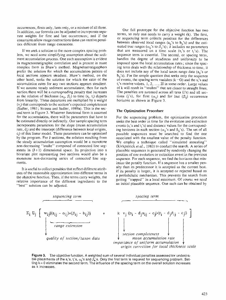
occurrences, firsts only, lasts only, or a mixture of all three. In addition, our formula can be adjusted to incorporate separate weights for first and last occurrences; and if the constraints allow range contractions these can receive penalties different from range extensions.

If we seek a solution to the more complex spacing problem, we need some simplifying assumption about the sediment accumulation process. One such assumption is evident in magnetostratigraphic correlation and is present in more complex form in Shaw's method. Magnetostratigraphers prefer the solution for which the accumulation pattern of local sections appears steadiest. Shaw's method, on the other hand, seeks the solution for which the ratio of the accumulation rates for any two sections appears steadiest. If we assume steady sediment accumulation, then for each section there will be a corresponding penalty that increases as the relation of thickness (aij, PU) to time (si, ti) departs from linearity. These departures are multiplied by a weight (vj) that corresponds to the section's expected completeness (Sadler, 1981 ; Strauss and Sadler, 1989a). This is the second term in Figure 3. Whatever functional form is assumed for the accumulation, there will be parameters that have to be estimated directly or indirectly. Our sample spacing term incorporates parameters for the slope (mean accumulation rate, dj) and the intercept (difference between local origins, cj) of this linear model. These parameters can be optimized by the program. For J sections, the solution resulting from the steady accumulation assumption would be a monotone non-decreasing "snake" composed of connected line segments in (J+ 1) dimensional space. Its projection into a bivariate plot representing two sections would also be a monotone non-decreasing series of connected line segments.

It is useful to collect penalties that reflect different attributes of the reasonable approximation into different terms in the objective function. Then, if the terms carry weights, the relative importance of the different ingredients to the "best" solution can be adjusted.

sequencing term A

I I

Our full prototype for the objective function has two terms, so only one needs to carry a weight (k). The first, or sequencing term collects penalties for the differences between observed local ranges (aU's to bij's) and the estimated true ranges (cri's to Pij's); it includes no parameters that are measured on a time scale (si's or ti's). The sequence term is essential. The second, or spacing term, handles the degree of steadiness and uniformity to be imposed upon the local accumulation rates ; since the spacing term deals with the relationship of thickness to time, it does not include any of the local taxon range data (aij's or bij's). For the simple question that seeks only the sequence of events, the spacing term vanishes (k=O) and the si's and ti's receive values, 1 , 2 , . . . , 21 in some order. Large values of k will result in "snakes" that are closer to straight lines. The penalties are summed across all taxa (i's) and all sections (j's), for first (aij) and for last (Pij) occurrence horizons as shown in Figure 3.

The Optimization Procedure

For the sequencing problem, the optimization procedure seeks the best order in time for the evolution and extinction events (si's and ti's) and distance values for the corresponding horizons in each section (crij's and nij9s). The set of all possible sequences must be searched to find the one associated with the smallest value of the penalty function. We employ a technique called "simulated annealing" (Kirkpatrick el al., 1983) to conduct the search. A series of plausible sequences is generated by randomly changing the position of one evolution or extinction event in the previous sequence. For each sequence, we find the horizons that minimize the penalty function. If a sequence has a smaller penalty than its predecessor it is accepted as the current best. If its penalty is larger, it is accepted or rejected based on a probabilistic mechanism. This prevents the search from getting "trapped" in a local minimum. Of course we need an initial plausible sequence. One such can be obtained by

spacing term 7

,. I

xi C j 1 wij[(aij - aij)+(Bij - bij)I + k V . J (Isi - d.a. . J 1J - c.l+lti J -

I ' I

range extension

section completeness quality o f section/taxon data mean accumulation rate

inlportance of uniform accurnulalion origin correction for local thickness scale

Figure 3. The objective function. A weighted sum of several individual penalties assessed for undesirable placements of the si ls , ti's, q i ' s and fiij's. Only the first term is required for sequencing problem. Set- ting k = 0 eliminates the second term. The influence of the spacing term on the overall solution increases as k increases.

randomly filling in missing values for one local section. The algorithm continues until it finds a sequence that yields the smallest penalty. This sequence and the associated horizons form our optimal solution that is "best" in terms of the pre- specified optimization criteria.

For the full problem reasonable initial values will be input for the slopes and intercepts (e.g, a stratigrapher's best estimate). The algorithm will then find optimum values for the sequence, spacings and horizon locations. These values will next be held constant and new slopes and intercepts solved for. The algorithm will iterate back and forth until the solution stabilizes.

For either solution the procedure must make repeated use of a sub-routine that searches for the minimum penalty. The complexity of this sub-routine increases with the order (linear, quadratic etc.) of the penalty terms in the objective function and the constraints. In the simplest, and certainly most manageable, case all terms are linear. The sub-routine can thus be limited to linear programming by simplifying the geological model. The tractability of objective functions with quadratic terms should be explored where this adds geological sophistication.

So far, we have developed the procedure for a linear objective function and some quadratic constraints which are used to keep time lines from crossing. By treating the sequences one at a time, we can replace the quadratic constraints with linear ones. We are applying this procedure to data sets from the literature now and hope to publish the results in the not too distant future.

CONCLUSIONS

The time correlation problem is considerably clarified when stated in the precise terms required for optimization modelling. Constrained optimization emerges as a logical approach to the solution. This approach 1) considers all local observations simultaneously, 2) includes explicit evaluation of the quality of the local sections and the local taxon ranges, 3) respects a stipulated strategy for correlation, 4) generates reproducible solutions, 5 ) quantifies the goodness of fit between a solution and the data, 6 ) permits repeated, rapid trials, in which the correlation strategy can be adjusted and hypotheses tested, and 7) allows the objective function and constraints to be adjusted to mimic features of other methods. Thus, in addition to its value for correlation, constrained optimization has potential as a means of comparing the methods.

ACKNOWLEDGMENTS

Michael Murphy introduced us to Shaw's method by explaining his own application of it to the Paleozoic of Nevada. Lucy Edwards helped us through the literature on other methods of correlation, and suggested improvements to an earlier draft of this paper. The contributions of Sadler and Strauss were supported in part by NSF grant EAR872 1 192.

REFERENCES

Agterberg, F.P. and Gradstein, F.M. 1988: Recent developments in quantitative stratigraphy ; Earth Science

Reviews, v. 25, p. 1-73. Berger, W.H. and Heath, G.R. 1968: Vertical mixing in pelagic sediments; Journal of Marine

Research, v. 26, p. 134-143. Davaud, E. 1982: The automation of biochronological correlation; in Quantitative

Stratigraphic Correlation, ed., J.M. Cubitt, and R.A. Reyment, Wiley, Chichester, p. 85-99.

Dennison, J.M. and Hay, W.W. 1967: Estimating the needed sampling area for subaquatic ecologic

studies; Journal of Paleontology, v. 41, p. 706-708. Edwards, L.E. 1977 : Range charts as chronostratigraphic hypotheses, with applications

to tertiary dinoflagellates; Ph.D. dissertation, University of California, Riverside, California.

1978: Range charts and no-space graphs; Computers and Geosciences, v. 4, p. 247-255.

1982a: Numerical and semi-objcctive biostratigraphy: review and predictions; Third North American Paleontological Convention, Proceedings, v. 1 , p. 47-52.

1982b: Quantitative biostratigraphy: the method should suit the data; in Quantitative Stratigraphic Correlation, ed. J.M. Cubitt and R.A. Reyment, Wiley, ~hichester, p. 45-60.

Foster, N.H. 1966: Stratigraphic leak; American Association of Petroleum Geolo-

gists, Bulletin, v. 50, p. 2604-2606. Guex, J. 1977: Une nouvelle methode d'analyse biochronologique; Note

prCliminaire, Laboratoire de GCologie, MinCralogie, Gtophy- sique, et MusCe GCologique de I'UniversitC de Lausanne, Bulletin V . 224, p. 309-321.

Gradstein, F.M., Agterberg, F.P., Brower, J.C. and Schwarzacher, W.S. 1985: Quantitative Stratigraphy, UNESCO, 589 pp. Harper, C.W. 1981 : Inferring succession of fossils in time: the need for a quantitative

and statistical approach; Journal of Paleontology, v. 55, p. 442-452.

Hay, W.W. 1972: Probabilistic stratigraphy; Eclogae Geologica Helvetica, v. 65,

p. 255-266. Hazel, J.E. 1977: Use of certain multivariate and other techniques in assemblage

zonal biostratigraphy : examples utilizing Cambrian, Cretaceous, and Tertiary benthic invertebrates; in Concepts and Methods of Biostratigraphy, e.d., E.G. Kaufmann and J.E. Hazel, Dowden. Hutchison and Ross, Stroudsburg, Penn., p. 187-212.

Hedberg, H.D. (Editor) 1976: International Stratigraphic Guide; Wiley, New York. 200 pp. Hohn, M.E. 1978: Stratigraphic correlation by principal components - effects of

missing data; Journal of Geology, v. 86, p. 524-532. Hood, K.C. 1986: Interactive Graphic Correlation for Microcomputers Jones, D.J. 1958 : Displacement of microfossils; Journal of Sedimentary Petrology,

v. 28. p. 453-467. Kirkpatrick, S., Gelatt, C.D. Jr. and Vecchi, M.P. 1983: Optimization by simulated annealing; Science, v. 220, No 4598,

p. 671-679. Rubel, M. 1978: Principles of construction and use of biostratigraphic scales for

correlation; Computers and Geosciences, v. 4, p. 243-246. Sadler, P.M. 1981 : Sediment accumulation rates and the completeness of strati-

graphic sections; Journal of Geology, v. 89, p. 569-584. Shaw, A.B. 1964: Time in Stratigraphy; McGraw-Hill, New York, 365 p.

Southam, J.R., Hay, W.W., and Worsley, T.R. Varnes, D.J. 1975: Quantitative formulation of reliability in stratigraphic correla- 1987: Foreshock seismic-ene1.g~-release functions: tools for estimating

tion; Science, v. 188, p. 357-359. time and magnitude of main shocks; U.S.G.S. Open-file Report, Springer, M. and Lilje, A. 87-429, 38 p. 1988: Biostratigraphy and gap analysis: the expected sequence of bios- Wilson, L.R.

tratigraphic events; Journal of Geology, v. 96, p. 228-236. 1964: Recycling, stratigraphic leakage, and faulty techniqucs in paly- Strauss, D. and Sadler, P.M. nology; Grana Palynologica, v. 5, p. 427-436. 1989a: Stochastic models for the completeness of stratigraphic sections;

Mathematical Geology, v. 21, No. I , p. 37-59. 1989b: Classical confidence intervals and Bayesian probability estimates

for ends of local taxon ranges; Mathematical Geology, v. 2 1 , no. 4, p. 411-427.

Error effects and error estimation for graphic correlation in biostratigraphy

D. Yuan1 and J. C. Browerl

Yuan, D. and Brower, J . C. , Error effects and error estimation for graphic correlation in biostratigraphy; in Statistical Applications in the Earth Sciences, ed. F. P. Agterberg and G. F. Bonham-Carter; Geologi- - cal Survey of Canada, Paper 89-9, p. 427-438, 1989.

Abstract

Graphical correlation, sometimes called ShawS method, has been commonly applied by biostratigraphers over the past 20 years or so. h has been touted as the method which is both the simplest and most powerful. Strangely enough, the technique is largely empirical and is not based on any concrete statistical theory. The method relies on jtting lines of correlation (LOCs) to observed data for stratigraphic sections or composite sections. Currently, biostratigraphers use either straight or segmented straight lines although curved lines could be employed. In principle the errors and calibrations discussed here should be valid for both straight and curved LOCS. The use of an incorrect LOC introduces three basic types of error effects which are termed the shifring, thrusting and reversing effects. The jrst two effects are caused by relatively small errors in the initial intercepts and slopes, respectively, and both can result in over-extended range zones in the composite section. Given larger displacements of the adopted LOC with respect to the true one, two biostratigraphic events can be reversed in the composite section to produce the last kind of error. If time planes, such as bentonites, are available, graphical correlation can provide direct mapping in a framework of relative or absolute geological time. In effect, the time planes serve as calibrations or tie points with graphical correlation being used within the adjacent time planes to give better resolution. An error estimate for such a calibrated LOC is formulated.

Au cours des 20 derni2res anne'es environ, la correlation graphique, parfois appele'e la mhhode de Shaw, a he' couramment appliqude par les spicialistes en biostratigraphie. Elle a e'ti vante'e comme e'tant la me'thode la plus simple et la plus puissante. I1 est assez itrange de constater que cette mithode est en grande partie empirique et n'est base'e sur aucune thiorie statistique concr2te. La mithode est fondie sur l'ajustement de lignes de corre'lation (LC) aux donnies observe'es de coupes structurales ou de coupes compose'es. Actuellement, les spicialistes en biostratigraphie utilisent des droites ou des segments de droites bien que des courbes pourraient aussi bien servir. En principe, les erreurs et les e'talonnages discute's ici devraient &tre valides tant pour les droites que pour les courbes de corre'lation. L'utilisation d'une LC incorrecte introduit trois types fondamentaux d'effets d'erreur dits de de'calage, de chevauche- ment et d'interversion. Les d e w premiers de ces efets d'erreur sont respectivement causb par des erreurs relativement faibles au niveau des coordonnees a l'origine et des pentes initiales, et peuvent entrainer des zones de re'partition surestime'es dans la coupe composde. Avec des dcarts plus importants de la LC adopte'e par rapport a la ligne re'elle, deux @isodes biostratigraphiques peuvent &re intervertis dans la coupe compose'e pour produire le dernier type d'erreur. Si des plans de re'fe'rence chronologiques comme celui des bentonites sont disponibles, la corre'lation graphique peut permettre une cartographie directe suivant une chronologie ge'ologique relative ou absolue. En fait, les plans chronologiques servent a l'e'talonnage ou comme points de rattachement aux corre'lations graphiques utilise'es au sein de plans chronologiques adjacents a j n d'obtenir une meilleure re'solution. Les auteurs proposent une estimation d'erreur pour une telle LC e'talonne'e.

' Department of Geology, Syracuse University Syracuse, New York, 13244-1070 USA

INTRODUCTION

Since it was proposed by Shaw in 1964, the graphic method of biostratigraphic correlation has become widely accepted. It has been described as the quantitative correlation method that is the most powerful, easiest to understand and visualize, and most simple to calculate (e.g. Miller, 1977; Edwards, 1984). Shaw's method for correlation was truly revolutionary. Prior to Shaw's method, correlations between two stratigraphic sections were carried out subjectively aside from a few primitive examples of multivariate analysis (see Brower, 1981, for review). Paleontological sequences were determined largely by the personal view of the stratigrapher concerned with the data. Shaw's method provided a more or less objective criterion for correlation. 'The graphical correlation method also produces a visible display for the process of correlation. This display, or in mathematical words, the "point to point mapping projection" between the two stratigraphic sections is widely favoured by stratigraphers and probably accounts for the popularity of this method.

Rather ironically, little attention has been paid to the principal basis and limitations of this method. Although the idea of Shaw's method is clever, the technique is still in need of verification and improvement. In this paper we provide a detailed discussion about the error effects of Shaw's method as it is currently practiced. We believe that the dog- legged line-of-correlation (LOC) based on a calibration system of time planes is an optimum use of graphic correlation. In addition, we formulate the error estimation for a calibrated dog-legged LOC.

REVIEW OF THE GRAPHIC CORRELATION METHOD (SHAW'S METHOD)

Detailed discussion of the graphic method can be found in Shaw's book (1964). Recent annotations are available in Miller (1977) and Edwards (1984). Only a brief review is presented here.

Two stratigraphic sections are to be correlated. The letters a, b, c,. . . , represent the different biota in the sections. As usual, we take '0' and '+ ' to denote the lowest and the highest occurrences, respectively. Then the correlation between the two sections may be represented by the graph in Figure 1. The line of correlation (LOC) is either derived from connecting some of the fossil occurrences, or from a statistically modelled line of the scattered points on the graph. At present, biostratigraphers use either single straight lines or segmented straight lines although the method is not limited to this practice. One section is considered to be the reference and the other section will be eventually used to update the data on the reference axis to produce a composite section. On our graphs, the section on the horizontal or X Axis constitutes the reference.

There are two basic ingredients to Shaw's method. 1. The critical one is the line of correlation (LOC)

which gives a refraction line for the sections being correlated. As mentioned above, previous workers have used either straight lines or segmented straight lines. This line or its individual straight segments has or have been obtained in three ways. 1 .) Lines that are statistically fitted by the

least squares or some other algorithm (e. g. Shaw, 1964; Hohn, 1978, 1982). 2.) Connecting two selected biostratigraphic events, either highest or lowest occurrences, on the correlation graph (e.g. Miller, 1977). 3.) Extending a line that intersects all of the "error boxes", each of which is enclosed by the highest and lowest occurrence of a single taxon (e. g. Edwards, 1984). Brower (1981) suggested fitting curved lines and this is now being done by Gradstein and coworkers with smoothing splines (Gradstein, personal communication, 1988). However, this paper is limited to discussing straight and segmented straight lines. In principle, the errors and calibrations outlined here should also be applicable to curvilinear data. Interestingly enough, straight lines and segmented lines are clearly adequate for some data sets which can be calibrated in terms of absolute or relative time. For example, Prell et al. (1986) used graphical correlation to analyze time equivalent changes in oxygen isotopes for deep sea sediments of the Quaternary and found that plots of all pairs of cores could be described by segmented straight lines.

Miller (1977) explained an LOC as a rate line (rate = distance or stratigraphic thickness / time) which is rnislead- ing. Actually, the line is not determined by stratigraphic thickness and time of deposition for the concerned sections ; rather, it is dictated by the distribution of fossil occurrences. These lines only give relative rates in the framework defined by the taxa involved. Subsequently, we will discuss the the errors in these lines as originally defined. We conclude that the LOC under the original definition is not necessarily the proper correlation refraction line. A straight LOC or a straight part of a segmented line has a slope equal to the ratio of the depositional rates of the two sections concerned only if the highest and lowest points on that LOC or the segment are known to represent relative or absolute time planes. In many cases, the whole LOC should not be treated as a single straight line. Better fits frequently result from employing several straight line segments.

2. After ascertaining the LOC, the data in the second section (Y axis on our graphs) are incorporated into the reference section to create a composite for both sections; here, the LOC functions as a refraction line. Basically the data are updated in order to maximize the range zones of the species involved (see Miller, 1977, for excellent illustrations). The following procedure is used for biostratigraphic events, either highest or lowest occurrences, present in both sections (Fig. 1). Highest occurrences above the LOC are projected parallel to the reference axis to the LOC and then vertically down onto the reference axis. This displaces these highest occurrences up or higher (younger) in the composite section. Lowest occurrences below the LOC are translated parallel to the reference axis to the LOC and then vertically downward onto the reference section to form the composite. This displaces such lowest occurrences down or lower (older) in the composite section. Lowest occurrences above the LOC and highest occurrences below the LOC add no new information to the reference or composite section and are not used in updating. Some biostratigraphic events may be present in the section on the Y-axis but not in the reference section; these are incorporated into the reference section as above employing the LOC as a refraction line.

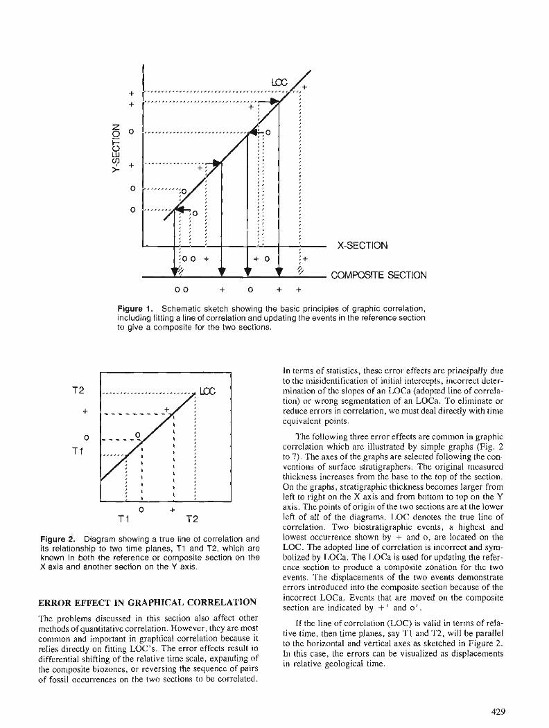
j o o + + 0 : + ~3 7 7 7 %

X-SECTION

COMPOSITE SECTION 0 0 + 0 + +

Figure 1. Schematic sketch showing the basic principles of graphic correlation, including fitting a line of correlation and updating the events in the reference section to give a composite for the two sections.

In terms of statistics, these error effects are principally due to the misidentification of initial intercepts, incorrect determination of the slopes of an LOCa (adopted line of correlation) or wrong segmentation of an LOCa. To eliminate or reduce errors in correlation, we must deal directly with time equivalent points.

The following three error effects are common in graphic correlation which are illustrated by simple graphs ( ~ i g . 2 to 7). The axes of the graphs are selected following the conventions of surface stratigraphers. The original measured thickness increases from thebase to the top of the section. On the graphs, stratigraphic thickness becomes larger from left to right on the X axis and from bottom to top on the Y axis. The points of origin of the two sections are at the lower left of all of the diagrams. LOC denotes the true line of correlation. Two biostratigraphic events, a highest and

Figure 2. Diagram showing a true line of correlation and 10west OCcurrence Shown by + and 0, are located on the its relationship to two time planes, TI and T2, which are LOC. The adopted line of correlation is incorrect and sym- known in both the reference or composite section on the bolized by LOCa. The LOCa is used for updating the refer- X axis and another section on the Y axis. ence section to produce a composite zonation for the two

events. The displacements of the two events demonstrate errors introduced into the composite section because of the

ERROR EFFECT IN GRAPHICAL CORRELATION incorrect LOCa. Events that are moved on the composite section are indicated by + ' and 0 ' .

The problems discussed in this section also affect other If the line of correlation (LOC) is valid in terms of rela- methods of quantitative correlation. However, they are most tive time, then time planes, say T I and T2, will be parallel common and important in graphical correlation because it relies directly on fitting LOC's. The error effects result in

to the horizontal and vertical axes as sketched in Figure 2.

differential shifting of the relative time scale, expanding of In this case, the errors can be visualized as displacements in relative geological time.

the composite biozones, or reversing the sequence of pairs of fossii occurrences on the two sections to-be correlated.

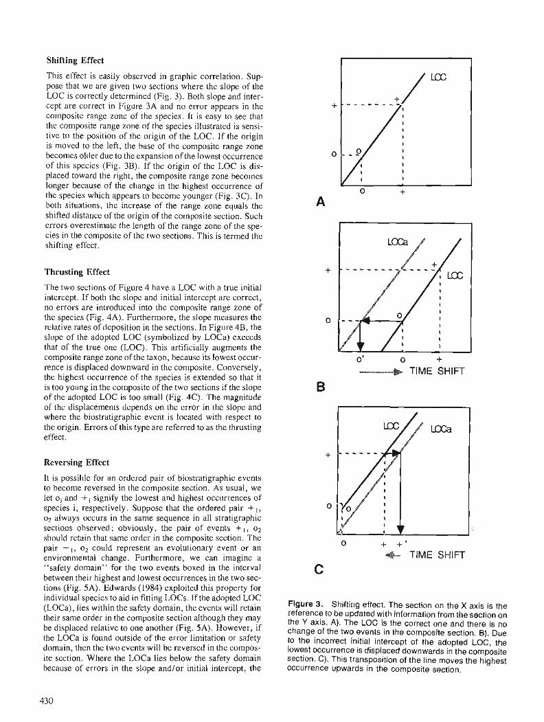
Shifting Effect

This effect is easily observed in graphic correlation. Sup- pose that we are given two sections where the slope of the LOC is correctly determined (Fig. 3). Both slope and intercept are correct in Figure 3A and no error appears in the composite range zone of the species. It is easy to see that the composite range zone of the species illustrated is sensitive to the position of the origin of the LOC. If the origin is moved to the left, the base of the composite range zone becomes older due to the expansion of the lowest occurrence of this species (Fig. 3B). If the origin of the LOC is displaced toward the right, the composite range zone becomes longer because of the change in the highest occurrence of the species which appears to become younger (Fig. 3C). In both situations, the increase of the range zone equals the shifted distance of the origin of the composite section. Such errors overestimate the length of the range zone of the species in the composite of the two sections. This is termed the shifting effect.

Thrusting Effect

The two sections of Figure 4 have a LOC with a true initial intercept. If both the slope and initial intercept are correct, no errors are introduced into the composite range zone of the species (Fig. 4A). Furthermore, the slope measures the relative rates of deposition in the sections. In Figure 4B, the slope of the adopted LOC (symbolized by LOCa) exceeds that of the true one (LOC). This artificially augments the composite range zone of the taxon, because its lowest occurrence is displaced downward in the composite. Conversely, the highest occurrence of the species is extended so that it is too young in the composite of the two sections if the slope of the adopted LOC is too small (Fig. 4C). The magnitude of the displacements depends on the error in the slope and where the biostratigraphic event is located with respect to the origin. Errors of this type are referred to as the thrusting effect.

Reversing Effect

It is possible for an ordered pair of biostratigraphic events to become reversed in the composite section. As usual, we let oi and + signify the lowest and highest occurrences of species i, respectively. Suppose that the ordered pair + ,, o2 always occurs in the same sequence in all stratigraphic sections observed ; obviously, the pair of events + , , o2 should retain that same order in the composite section. The pair + ,, 02 could represent an evolutionary event or an environmental change. Furthermore, we can imagine a "safety domain" for the two events boxed in the interval between their highest and lowest occurrences in the two sections (Fig. 5A). Edwards (1984) exploited this property for individual species to aid in fitting LOCs. If the adopted LOC (LOCa), lies within the safety domain, the events will retain their same order in the composite section although they may be displaced relative to one another (Fig. 5A). However, if the LOCa is found outside of the error limitation or safety domain, then the two events will be reversed in the composite section. Where the LOCa lies below the safety domain because of errors in the slope and/or initial intercept, the

0' 0 + TlME SHIFT

0 + + ' .+- TlME SHIFT

Figure 3. Shifting effect. The section on the X axis is the reference to be updated with information from the section on the Y axis. A). The LOC is the correct one and there is no change of the two events in the composite section. 8). Due to the incorrect initial intercept of the adopted LOC, the lowest occurrence is displaced downwards in the composite section. C). This transposition of the line moves the highest occurrence upwards in the composite section.

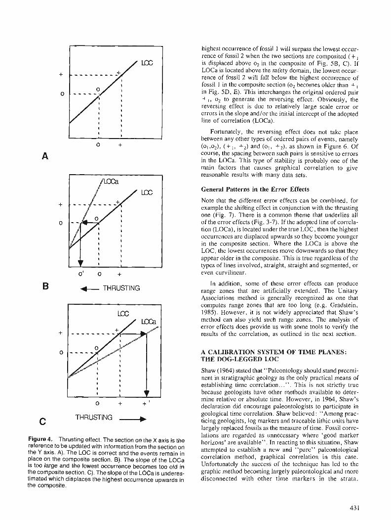
0' 0 + B 1 THRUSTING

C THRUSTING I

Figure 4. Thrusting effect. The section on the X axis is the reference to be updated with information from the section on the Y axis. A). The LOC is correct and the events remain in place on the composite section. B). The slope of the LOCa is too large and the lowest occurrence becomes too old in the composite section. C). The slope of the LOCa is underestimated which displaces the highest occurrence upwards in the composite.

highest occurrence of fossil 1 will surpass the lowest occurrence of fossil 2 when the two sections are composited (+, is displaced above o2 in the composite of Fig. 5B, C). If LOCa is located above the safety domain, the lowest occurrence of fossil 2 will fall below the highest occurrence of fossil 1 in the composite section (02 becomes older than + , in Fig. 5D, E). This interchanges the original ordered pair + ,, o2 to generate the reversing effect. Obviously, the reversing effect is due to relatively large scale error or errors in the slope andlor the initial intercept of the adopted line of correlation (LOCa).

Fortunately, the reversing effect does not take place between any other types of ordered pairs of events, namely (01,02), +2) and (o,, +2), as shown in Figure 6. Of course, the spacing between such pairs is sensitive to errors in the LOCa. This type of stability is probably one of the main factors that causes graphical correlation to give reasonable results with many data sets.

General Patterns in the Error Effects

Note that the different error effects can be combined, for example the shifting effect in conjunction with the thrusting one (Fig. 7). There is a common theme that underlies all of the error effects (Fig. 3-7). If the adopted line of correlation (LOCa), is located under the true LOC, then the highest occurrences are displaced upwards so they become younger in the composite section. Where the LOCa is above the LOC, the lowest occurrences move downwards so that they appear older in the composite. This is true regardless of the types of lines involved, straight, straight and segmented, or even curvilinear.

In addition, some of these error effects can produce range zones that are artificially extended. The Unitary Associations method is generally recognized as one that computes range zones that are too long (e.g. Gradstein, 1985). However, it is not widely appreciated that Shaw's method can also yield such range zones. The analysis of error effects does provide us with some tools to verify the results of the correlation, as outlined in the next section.

A CALIBRATION SYSTEM OF TIME PLANES: THE DOG-LEGGED LOC

Shaw (1964) stated that "Paleontology should stand preemi- nent in stratigraphic geology as the only practical means of establishing time correlation.. . " . This is not strictly true because geologists have other methods available to determine relative or absolute time. However, in 1964, Shaw's declaration did encourage paleontologists to participate in geological time correlation. Shaw believed : "Among practicing geologists, log markers and traceable lithic units have largely replaced fossils as the measure of time. Fossil correlations are regarded as unnecessary where 'good marker horizons' are available". In reacting to this situation, Shaw attempted to establish a new and "pure" paleontological correlation method, graphical correlation in this case. Unfortunately the success of the technique has led to the graphic method becoming largely paleontological and more disconnected with other time markers in the strata.

Figure 5. Reversing effect. The section on the X-axis is the reference to be updated with information from the section on the Y-axis. A). LOCa's lie within the safety domain of the two events and the order of the two events remains the same in the composite section with the highest occurrence below the lowest one. In B) through C), the LOCa's lie outside of the safety domain for the two events. 6). Reversal of the two events with the highest occurrence being displaced above the lowest occurrence in the composite section because of the low slope of LOCa. C). Same type of reversal can be produced by an LOCa with an abnormally small initial intercept. D). Reversal of the two events where the lowest occurrence is moved below the highest one in the composite section due to an unusually high slope of the LOCa. E). Same type of reversal caused by a large initial intercept for the LOCa.

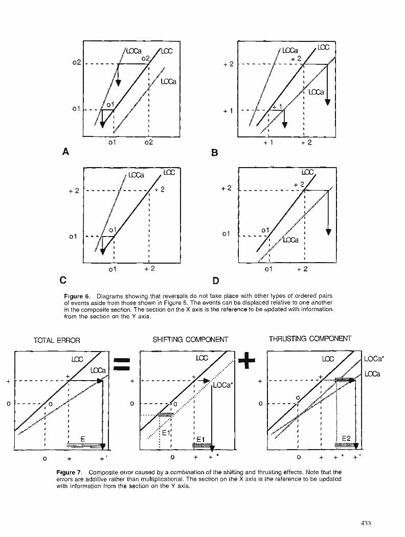
Figure 6. Diagrams showing that reversals do not take place with other types of ordered pairs of events aside from those shown in Figure 5. The events can be displaced relative to one another in the composite section. The section on the X axis is the reference to be updated with information from the section on the Y axis.

TOTAL ERROR SHIFTING COMPONENT THRUSTING COMPONENT

Figure 7. Composite error caused by a combination of the shifting and thrusting effects. Note that the errors are additive rather than multiplicational. The section on the X axis is the reference to be updated with information from the section on the Y axis.

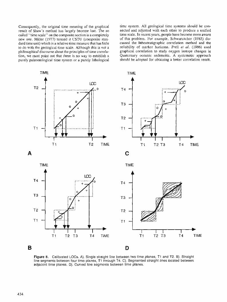
Consequently, the original time meaning of the graphical result of Shaw's method has largely become lost. The so called "time scale" on the composite section is a completely new one. Miller (1977) termed it CSTU (composite standard time unit) which is a relative time measure that has little to do with the geological time scale. Although this is not a philosophical discourse about the principles of time correlation, we must point out that there is no way to establish a purely paleontological time system or a purely lithological

time system. All geological time systems should be connected and adjusted with each other to produce a unified time scale. In recent years, people have become more aware of this problem. For example, Schwarzacher (1985) discussed the lithostratigraphic correlation method and the reliability of marker horizons. Prell et al. (1986) used graphical correlation to study oxygen isotope changes in Quaternary oceanic sediments. A systematic approach should be adopted for obtaining a better correlation result.

TIME TIME

T2 TIME T I T 2 T 3 T4 TIME

TlME

4

T I T 2 T 3 T4 TIME

TlME

A

. T 1 T2 T3 T 4 TIME

Figure 8. Calibrated LOCs. A). Single straight line between two time planes, T I and T2. B). Straight line segments between four time planes, T I through T4. C). Segmented straight lines located between adjacent time planes. D). Curved line segments between time planes.

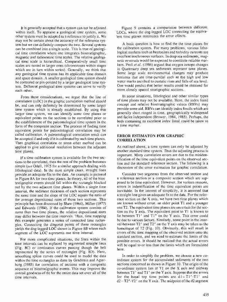
It is generally accepted that a system can not be adjusted within itself. To appraise a geological time system, some other system must be adopted-as a reference to justify it. We may not be certain about the accuracy of the reference system but we can definitely compare the two. Several systems can be combined into a single scale. This is true of geological time correlation where one integrates biostratigraphic, magnetic and radiometric time scales. The relative geological time scale is hierarchical. Comparatively small time scales are nested in larger ones (chroiozones within stages which are in turn within series). Generally, we think that any geological time system has its applicable time domain and space domain. A smaller geological time system should be controled or pin-pointed by a larger geological time system. Different geological time systems can serve to verify each other.

From these considerations, we argue that the line of correlation (LOC) in the graphic correlation method should be, and can only definitely be determined by some larger time system which is already established. By using this larger time system, we can identify some time planes or equivalent points on the sections to be correlated prior to the establishment of the paleontological time system in the form of the composite section. The process of finding time equivalent points for paleontological correlation may be called calibration. A paleontological correlation result can be accepted if and only if it is calibrated by such time planes. Then graphical correlation or some other method can be applied to give additional resolution between the adjacent time planes.

If a time calibration system is available for the two sections to be correlated, then the rest of the problem becomes simple (see Odell, 1975 for a similar approach dealing with lithological data). In the most simple cases, straight lines provide an adequate fits to the data. An example is pictured in Figure 8A for two time planes. In theory, all of the biostratigraphic events should fall within the rectangle blocked out by the two adjacent time planes. Within a single time interval, the sediment thickness of each section represents the same time and the slope of the LOC equals the ratio of the average depositional rates of these two sections. This principle has been discussed by Shaw (1964), Miller (1977) and Edwards (1984). If the calibration system consists of more than two time planes, the relative depositional rates may differ between the time intervals. Thus, time mapping this example generates a series of connected time rectangles. Connecting the diagonal points of these rectangles yields the dog-legged LOC shown in Figure 8B where each segment of the LOC represents one time interval.

For more complicated situations, the lines within the time intervals can be replaced by segmented straight lines (Fig. 8C) or continuous curves passing though the belt represented by the series of rectangles (Fig. 8D). Here, smoothing spline curves could be used to model the data within the time rectangles as done by Gradstein and Agter- berg (1985) for correlation of sections with a composite sequence of biostratigraphic events. This may improve the overall goodness-of-fit for the entire data set over all of the time intervals.

Figure 9 contains a comparision between different LOCs, where the dog-legged LOC connecting the equivalent time planes minimizes the error effects.

A basic question is how to find the the time planes for the calibration system. For many problems, various lithological markers such as bentonites and turbidity currents are excellent isochronous surfaces. In deep sea sediments, magnetic reversals would be expected to constitute reliable markers. Prell e[ al. (1986) argued that oxygen isotope changes in Quaternary deep sea sediments represent time planes. Some large scale environmental changes may produce horizons that are time-parallel such as the high and low water marks ascribed to eustatic rises and falls of sea level. One would predict that better results could be obtained for more closely spaced stratigraphic sections.

In some situations, lithological and other similar types of time planes may not be available. Here, the index fossil concept and relative biostratigraphic values (RBVs) may provide some aid. RBVs can identify index fossils which are generally short ranged in time, geographically widespread and facies independent (Brower, 1984, 1985). Perhaps, the beds containing an excellent index fossil could be taken as a time marker.

ERROR ESTIMATON FOR GRAPHIC CORRELATION

As outlined above, a time system can only be adjusted by another standard time system. Thus the adjusting process is important. Many correlation errors are due to the misidentification of the time equivalent points on the observed section and the standard reference section. The following is a discussion of the error estimation for graphic correlation.

Consider two segments from the observed section and a reference section or a composite section which are supposed to be time equivalent. However, for various reasons, errors in indentification of the time equivalent points are inevitable. In the interest of simplicity, it is assumed that a straight line gives an adequate fit to the data. For the reference section on the X axis, we have two time planes which are known without error, an older point T1 and a younger one T2. The equivalent time planes are uncertain for the section on the Y axis. The equivalent point to TI is known to lie between T I ' and T I " on the Y axis. This error could be due to various factors. Similarly, some point in the interval between T2' and T2" on the Y axis may be taken as the homologue of T2 (Fig. 10). Obviously, this will result in errors of the time mapping of the observed section onto the standard section, and we need to estimate the limits of the possible errors. It should be realized that the actual errors will be equal to or less than the limits which are formulated here.

In order to simplify the problem, we choose a new coordinate system for the accumulated sediments of the two sections concerned as shown in Figure 10. The origin of the co-ordinate system lies at T I on the X axis and midway between T1' and T1" on the Y axis. Suppose that the errors for the basal top time points are d l =TI" -T1 ' and d2 =T2"-T2' on the Y axis. The midpoint of the d2 segment

A LOC extrapolated from the real LOC within a single time ' interval.

T 6 A dog-legged LOC.

Note, a reversing effect may occur if some other LOC than

T 5 the dog-legged one is taken.

T 4 Note, a thrusting effect may occur if some other LOC than

T3 T2 the dog-legged one is taken.

Note, a shifting effect may T 1 occur if some other LOC than

the dog-legged one is taken. I 1

T 1 T2 T3 T4 T6 TIME T5

COMPOSITE SEC-TION

Figure 9. Diagram demonstrating that a calibrated LOC connecting equivalent time planes minimizes the total error effects in comparison to one line extrapolated from the true LOC within one of the time intervals.

TlME

'maximum error

minimum error

COMPOSITE SECTION

I T 2 TIME

Figure 10. Graphical picture showing the derivation of the maximum and minimum possible error limits as discussed in the text. The section on the X axis is the reference which will be updated with information from the section on the Y axis.

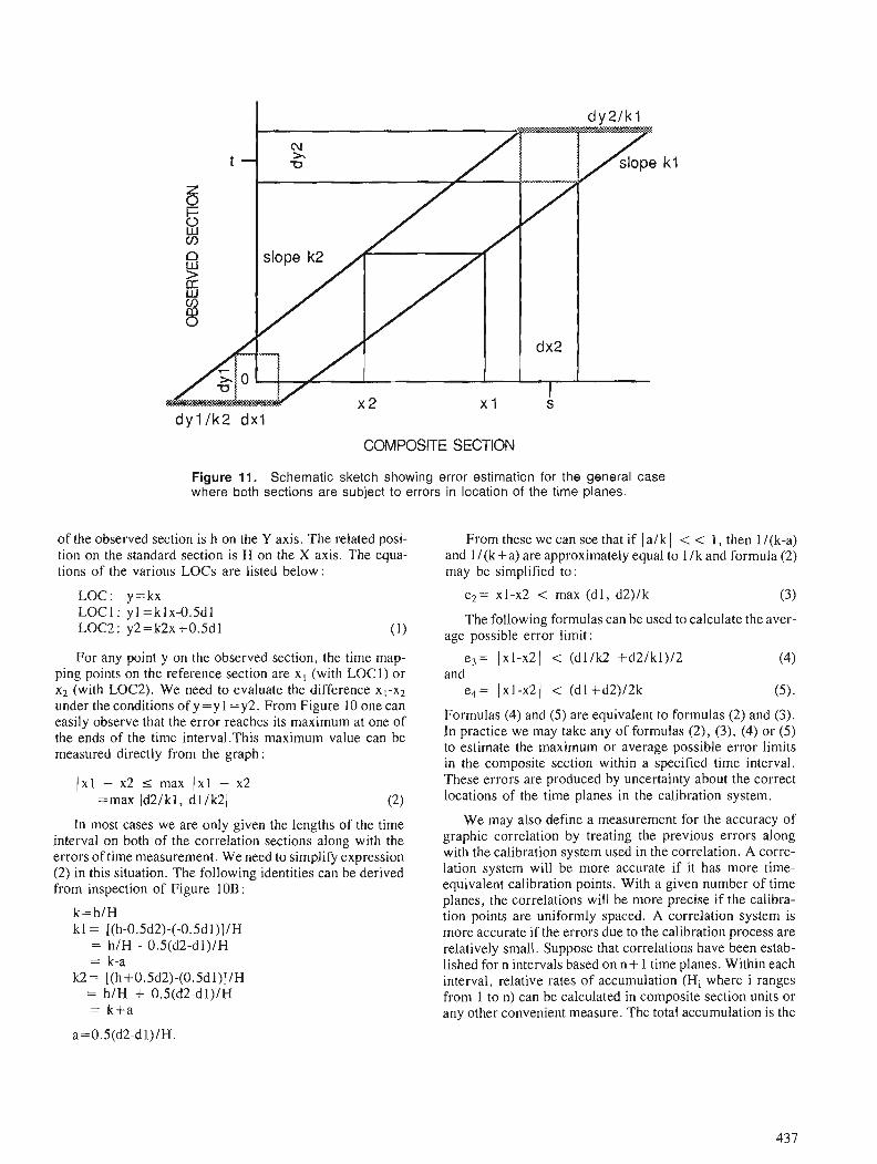
d y l I k 2 d x l

COMPOSITE SECTION

Figure 11. Schematic sketch showing error estimation for the general case where both sections are subject to errors in location of the time planes.

of the observed section is h on the Y axis. The related posi- From these we can see that if (a lk ( < < 1 , then 1 /(k-a) tion on the standard section is H on the X axis. The equa- and 1 /(k+a) are approximately equal to 1 /k and formula (2) tions of the various LOCs are listed below: may be simplified to:

LOC: y=kx e2= XI-x2 < max (dl, d2)lk (3) LOCI : yl=klx-0.5dl LOC2: y2=k2x+0.5dl

The following formulas can be used to calculate the aver- (') age possible error limit :

For any point y on the observed section, the time map- e,= 1x1-x21 < (dlIk2 +d2/k1)/2 (4) ping points on the reference section are x, (with LOCI) or and x2 (with LOC2). We need to evaluate the difference x,-x2 ed= 1x1-x2( < (dl+d2)/2k (5). under the conditions of y = y I = y2. From Figure 10 one can easily observe that the error reaches its maximum at one of Formulas (4) and (5) are equivalent to formulas (2) and (3).

the ends of the time interval.This maximum value can be In practice we may take any of formulas (2), (3), (4) or (5)

measured directly from the graph: to estimate the maximum or average possible error limits in the composite section within a specified time interval.

1x1 - x2 I max 1x1 - x2 =max ld2Ik1, dllk21

In most cases we are only given the lengths of the time interval on both of the correlation sections along with the errors of time measurement. We need to simplify expression (2) in this situation. The following identities can be derived from inspection of Figure 10B:

k=h/H k l = [(h-0.5d2)-(-0.5dl)JlH

= h/H - 0.5(d2-dl)/H = k-a

k2= [(h+O.5d2)-(0.5dl)]/H = h/H + 0.5(d2-dl)/H = k+a

These errors are produced by uncertainty about the correct

(2) locations of the time planes in the calibration system.

We may also define a measurement for the accuracy of graphic correlation by treating the previous errors along with the calibration system used in the correlation. A correlation system will be more accurate if it has more time- equivalent calibration points. With a given number of time planes, the correlations will be more precise if the calibration points are uniformly spaced. A correlation system is more accurate if the errors due to the calibration process are relatively small. Suppose that correlations have been established for n intervals based on n + 1 time planes. Within each interval, relative rates of accumulation (Hi where i ranges from 1 to n) can be calculated in composite section units or any other convenient measure. The total accumulation is the

sum of all of the His or simply H. The correlation calibration coefficient (C) for the reference or composite section is :

C = max (Hi/H) (6) If it is difficult to estimate the possible error limits for the time calibrations between two sections or between a composite and another section, the calibration coefficient C itself may be taken as a crude measure of the accuracy for the graphic correlation. Smaller values of C are associated with more precise correlations.

If we can calculate the possible error limits of the time calibrations for two sections or for a composite section versus some other section, then there is a better way to estimate the correlation error. Similarly for each of the n intervals mentioned above, we can define a 'local' LOC, calculate its slope ki and estimate the possible error Ei expressed by any of the previous equations, namely numbers (2) through (5). Therefore the total accuracy of the correlation (A) may be expressed by:

where error,,= (EIH I +E2H2 + . . . +E,H,)/H. Increasing values of A denote progressively less accurate correlations. The parameter A represents a compound of the number and spacing of the time planes or calibration points and the possible error limits within the individual segments. Of course many other measurements for the accuracy of graphic correlation can be deduced from these and similar considerations. However, we believe that expression (7) is an acceptable one.

In most of the practical cases the error for time measurement is a constant (e. g. isotopic measurements). Thus d = d 1 = d2 = . . . and error,, based on equation 5 may be simplified to

error,, = d * C I lk i

Note that it is natural to assume that the error of measurement is smaller than the measurement itself. This implies that if ki = 0 than the relevant di must also be 0 (ki = hi/Hi = O = = > h i = O = = > d i ~ h i = O ) , s o t h a t t h e s u m i n (8) is only referred to the terms with ki > 0.

For the general case with errors in both the observed and composite sections (e.g. in the case of isotopic data correlation), the correlation errors can be estimated similarly. Con- sider the error within one time interval (Fig. 11). Obviously, the error reaches its maximum at one end of the time interval. The following error estimation is easily obtained from a simple geometric analysis:

E = I x ~ - x ~ I 5 max (dx, + dy, I kZ, dx2 + dy2 I k,]. (9)

Here dx,, dx2, dy, , dy2 are the errors at the ends of the time interval on the composite section and observed section whereas k l and k2 are the slopes of the highest and the lowest possible lines of correlation within the time interval. Although this expression is more complicated than the previous one, it can be estimated graphically so that the error can be measured directly from the correlation diagram. Thus equation 9 provides an analogue to equation 2 where both the observed and composite sections are subject to errors of placement of the time planes .

REFERENCES

Brower, J.C., 1981 : Quantitative biostratigraphy, 1830-1980; in Computer Applica-

tions in the Earth Sciences, an Update of the 70's, ed. D.F. Mer- riarn; Plenum Press, New York and London, p. 63-103.

1984: The relative biostratigraphic values of fossils; Computers and Geosciences, v. 10, no. 1, p. 11 1-133.

1985: The index fossil concept and its application to quantitative biostratigraphy; in Quantitative Stratigraphy, F . M . Gradstein, F.P. Agterberg, J.C. Brower and W.S. Schwarzacher; D. Reidel Pub- lishing Company, Dordrecht, p. 43-64.

Edwards, L.E. 1984: Insights on why graphic correlation (Shaw's method) works; Jour-

nal of Geology, v. 92, p. 583-597. Gradstein, F.M. 1985: Unitary associations and ranking of Jurassic radiolarians; in

Quantitative Stratigraphy, F.M. Gradstein, F.P. Agterberg, J.C. Brower and W.S. Schwarzacher ; D. Reidel Publishing Company, Dordrecht, p. 263-278.

Gradstein, F.M. and Agterberg, F.P. 1985 : Quantitativc correlation in exploration micropaleontology ; in

Quantitative Stratigraphy, F.M. Gradstein, F.P. Agterberg, J.C. Brower and W.S. Schwarzacher; D. Reidel Publishing Company, Dordrecht, p. 309-357.

Hohn, M.E. 1978 : Stratigraphic correlation by principal components: effects of miss-

ing data; Journal of Geology, v. 86, no. 4, p. 524-532. 1982: Properties of composite sections constructed by least squares; in

Quantitative Stratigraphic Correlation, ed. J.E. Cubitt and R.E. Reyment; John Wiley & Sons, Ltd., New York, p. 107-117.

Miller, F. X. 1977: The graphic correlation method in biostratigraphy; in Concepts

and Methods of Biostratigraphy, ed. E.G. Kauffman and J.E. Hazel; Dowden, Hutchinson & Ross, Inc.. Stroudsburg, Pennsyl- vania, p. 165-186.

Odell, J. 1975: Error estimation in stratigraphic correlation; Mathematical Geol-

ogy, v. 7, p. 167-182. Prell, W.L., Imbrie, J., Martinson, D.G., Morley, J.J., Pisias, N.G., Shackleton, N.J., and Streeter, H.F. 1986: Graphic correlation of oxygen isotope stratigraphy: Application to

the late Quaternary; Paleooceanography, v. 1, no. 2, p. 137.162. Schwarzacher, W. 1985: Lithostratigraphic correlation and sedimentation models, in Quan-

titative Stratigraphy, F . M . Gradstein, F . P . Agterberg, J.C. Brower and W.S. Schwarzacher; D. Reidel Publishing Com- pany, Dordrecht, p. 387-418.

Shaw, A. B. 1964: Time in Stratigraphy; McGraw-Hill Book Co., New York, 365 p.

Interactive graphic analysis and sequence comparison of host rocks containing stratiform volcanogenic

massive sulphide deposits

Leslie F. Marcus1 and Philippe Lampiettiz

L.F. Marcus and P. Lampietti, Interactive graphic analysis and sequence comparison of host rocks containing stratiform volcanogenic m s i v e sulphide deposits; Statistical Applications in the Earth Sciences, ed. F.P Agterberg and G.F. Bonham-Carter; Geological Survey of Canada Paper 89-9, p. 439-446, 1989.

Abstract

Sofiware has been developed to interactively construct stratigraphic column interpretations of host rocks containing volcanogenic massive sulphide deposits. Data bases are being built of maps and columns for known deposits. i%e program includes editing capability for modifying and building the stratigraphic columns.

Comparison of columns is based on dynamic programming to produce similarity sequence measures between all pairs of columns. f ie simplest form of the algorithm counts all insertions or gaps equally. Modijcations including a scale of penalties for substitutions, variable weights for gaps depending on length, and compurison of short sections to parts of long sections are being considered.

The matrices of similarities generated are submitted to standard clustering procedures to produce a hierarchical classiJication of the deposits using the unweighted pair group method of analysis (UPGMA). A dendrogram is used to display the hierarchy of relationships.

Un logiciel a e'te' mis au point en vue de l'tflaboration interactive d'interpre'tations de colonnes stratigraphiques de roches hBtes renfermant des gisements de sulfures massifs d'origine volcanique. Les cartes et colonnes pour des gisements connus servent a 1 'assemblage de bases de donne'es. Le programme comprend une possibilite' de mise en page pour la modijcaton et la construction des colonnes stratigraphiques.

La comparaison des colonnes est base'e sur la programmation dynamique en vue de la production de mesures des sdquences de similarite' de toutes les paires de colonnes. Un algorithme de la plus simple forme dinombre avec un poids &gal toutes les insertions et lacunes. Des modifications incluant une e'chelle des pknalitds pour les substitutions, une ponde'ration variable pour les lacunes en fonction de la longueur et une comparaison de coupes courtes a des parties de coupes longues sont envisage'es.

Les matrices de similarite' produites sont soumises a des procddures de groupage ordinaires afin de produire une classijication hikrarchique des gisements bade sur la mkthode d'analyse pour agrdgation suivant la distance moyenne (unweighted pair group method, UPGMA). On utilise un dendrogramme pour repre'senter la hikrarchie des relations.

' Department of Biology, Queens College of the City University of New York, New York, U.S.A. Mailing address: American Museum of Natural History, Central Park West at 79Ih Street, New York, New York 10024-5192, U.S.A. New York University, New York, U.S.A.

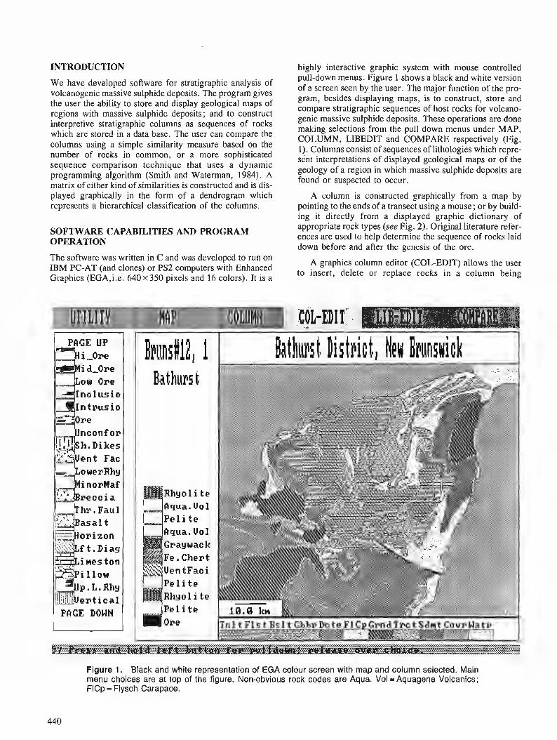
INTRODUCTION highly interactive graphic system with mouse controlled pull-down menus. Figure 1 shows a black and white version

We have lor of of a screen seen by the user. The major function of the pro- volcanogenic massive sulphide deposits. The program gives gram, besides displaying maps, is to construct, store and lhe user the to store and geological maps of compare stratigraphic sequences of host rocks for volcano- regions with massive sulphide deposits; and to construct genic massive sulphide deposits. These operations are done interpretive stratigraphic columns as sequences of rocks which are stored in a data base. The user can compare the making selections from the pull down menus under MAP,

columns using a simple similarity measure based on the COLUMN, LIBEDIT and COMPARE respectively (Fig. 1). Columns consist of sequences of lithologies which repre-

number of rocks in common, or a more sophisticated sent interpretations of displayed geological maps or of the sequence comparison technique that uses a dynamic geology of a region in which massive sulphide deposits are programming algorithm (Smith and Waterman, 1984). A found or suspected to occur. matrix of either kind of similarities is constructed and is displayed graphically in the form of a dendrogram which A column is constructed graphically from a map by represents a hierarchical classification of the columns. pointing to the ends of a transect using a mouse; or by build-

ing it directly from a displayed graphic dictionary of

SOFTWARE CAPABILITIES AND PROGRAM appropriate rock types (see Fig. 2). Original literature refer-

OPERATION ences are used to help determine the sequence of rocks laid down before and after the genesis of the ore.

The software was written in C and was developed to run on A graphics column editor (COL-EDIT) allows the user IBM PC-AT (and clones) or PS2 computers with Enhanced to insert, delete or replace rocks in a column being Graphics (EGA,i.e. 640 x 350 pixels and 16 colors). It is a

PClCE UP

L-pi I I ow ~ % ~ . L . R W

i i : crt ica l PAGE DOWN

Figure 1. Black and white representation of EGA colour screen with map and column selected. Main menu choices are at top of the figure. Non-obvious rock codes are Aqua. Vol= Aquagene Volcanics; FlCp = Flysch Carapace.

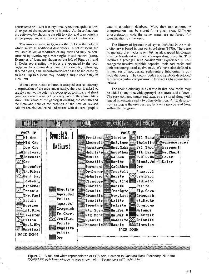
constructed or to edit it at any time. A rotation option allows all or part of the sequence to be inverted. All these functions are activated by choosing the edit function and then pointing at the proper rocks in the column and rock dictionary.

The user can overlay icons on the rocks in the column which serve as additional descriptors. A set of icons are available as visual modifiers of any rock and may be constructed by overlaying a meaningful visual pattern (icon). Examples of icons are shown on the left of Figures 1 and 2. Codes representing the icons are appended to the rock codes in the column data base. For example, pillowing, sheeted dykes, and uncomformities can each be indicated by an icon. Up to 5 icons may modify a single rock entry in a column.

When a constructed column is accepted as a satisfactory interpretation of the area under study, the user is asked to supply a name, the column's geographic location, and short comments which may include a reference to the source literature. The name of the geologist creating the column and the time and date of the creation of the new or revised column are also collected and stored with the stratigraphic

data in a column database. More than one column or interpretation may be stored for a given area. Different interpretations with the same name are numbered for identification by the user.

The library of igneous rock types included in the rock dictionary is based in part on Streckeisen (1976). There are no metamorphic rocks in our list, as all mapped lithologies must be translated into their corresponding protolith. This requires a geologist with considerable experience in volcanogenic massive sulphide deposits, their host rocks and their metamorphosed equivalents. We have also defined a limited set of appropriate sedimentary lithologies in our rock dictionary. The colour codes and symbols developed represent a partial compromise in terms of EGA colour limitations.

The rock dictionary is dynamic in that new rocks may be added at any time with appropriate textures and colours. The rock colours, names and textures are stored along with legend mnemonics and a two line definition. A full description, as long as the user desires, for a rock may be read from within the program.

Figure 2. Black and white representaton of EGA colour screen to illustrate Rock Dictionary. Note the COMPARE pull-down window is also shown with "Sequence simi" highlighted.

The program has more general capabilities than application to volcanogenic massive sulphide deposits. It was developed to be independent of specific geological applications. An entirely different rock dictionary can be created interactively for a different kind of project. New textures and icons can also be developed for different applications as well. Cartoons and other types of illustration materials may be used in addition to maps.

RESULTS TO DATE

We have accumulated 6 geological maps and their stratigraphic columns together with another 80 columns representing many of the major volcanogenic massive sulphide deposits throughout the world. Our goal is to include representative maps and columns from all of the major volcanogenic massive sulphide deposits. We feel that we will have an adequate database for detailed research into the relations and patterns of such columns when we have accumulated about 200 columns.

Present and future research is being concentrated on the columns. We are interested in similarities of massive sulphide deposits within geographic and geological regions, similarities between regions and the comparison of our classification to published classifications of volcanogenic massive sulphide deposits. In addition we would hope to identify likelihood of presence of ore from similarities between new, less-explored, regions where ore has not been detected and columns in the data base.

COMPARISON OF COLUMNS

The remaining operations of the program construct similarity indices among all of the columns for comparison purposes and use these to organize the columns into a hierarchical classification based on rocks they have in common. These empirical classifications will be the basis for further comparisons.

We have used two similarity measures based on the rocks shared between two columns. The simpler and perhaps less informative one, is Ruzicka's index (Pielou, 1984), which does not pay attention to the sequence of the rocks in the columns.

The index for comparing the ith column displayed in the column construction window to the jth column in the data base is:

S(ij) = 100*Sum[min(xik,xjk)]/Sum[max(xik,xjk)] The index k goes from 1 to n, the number of kinds of rocks in the ith and jth compared column; xik and xjk are the number of replications of rock type k in the ith displayed column and the jth column respectively.

More interesting is an index based on sequence similarity, which is derived from applications in molecular biology sequence comparison. Pertinent references are Smith and Waterman (1980), Waterman and Raymond (1987), and Waterman (1984). While they develop a considerable number of possible applications and extensions of this approach to geology, we are unaware of any published applications other than the geological examples they use to illustrate their

methods in two of the papers. Howell (1983) has published a FORTRAN program for some of the algorithms in Smith and Waterman (1980) with some geological examples. A very basic reference to sequence comparison and the use of dynamic programming is a book edited by Sankoff and Kruskal (1983).

We have used the basic approach in Smith and Waterman (1980), and are beginning to consider more sophisticated modifications; such as considering thickness of the rocks in a column in the comparison procedure.

In the simplest form of a comparison of two columns, one inserts gaps in one column opposite those rocks not present in the other.

If each gap is weighted as 1, then a distance measure between columns can be taken as the number of gaps inserted in the two columns. The relationship between the number of rocks in the two columns, the number of matches and the number of gaps is:

N +M =2*matches +number of gaps where Nand M are the numbers of rocks in the two columns being compared. A simple distance function would be the number of gaps, and a simple similarity function would be the number of matches. We have developed a similarity index as:

Sequence Similarity Index = 100*(N +M-gaps)/(N + M) It is given in terms of the numbers of gaps, as that is what is computed using the dynamic programming algorithm. If N is not equal to M, then N is arbitrarily taken to be the number of rock elements in the longer column. The index goes from 0 to 200*M/(N+M) and achieves 100 as its upper bound only when N=M. For columns of very different length, the upper value of the index may be far from one hundred. In our most disparate case where M=4 and N= 16 then its upper bound is only 40. A very short column may be alternatively compared to the best fitting segment of the same length in a very long column.

If the similarity index is divided by 2*M/(N+M) it will always go from 0 to 100, but this has not been implemented. Waterman has defined a different similarity measure which has also not been implemented.

The dynamic programming algorithm, is presented here after Smith and Waterman (1980). It is cornputationally very efficient. An example, taking two columns from our data base, is given below using the data exactly as it is stored. Rocks are coded in terms of 4 letter mnemonics and the full names are given below for the rocks in the examples. The same columns are compared in Figure 3 : * Nukundamu,Fiji ;Cooley and Rice, 1975 ,p. 1373-86 Fiji Nukundam,l,Drew,11/13/87,13:13:38 ANDS DCTE AQVO ORES AQVO ANDS BSLT

Length = 7

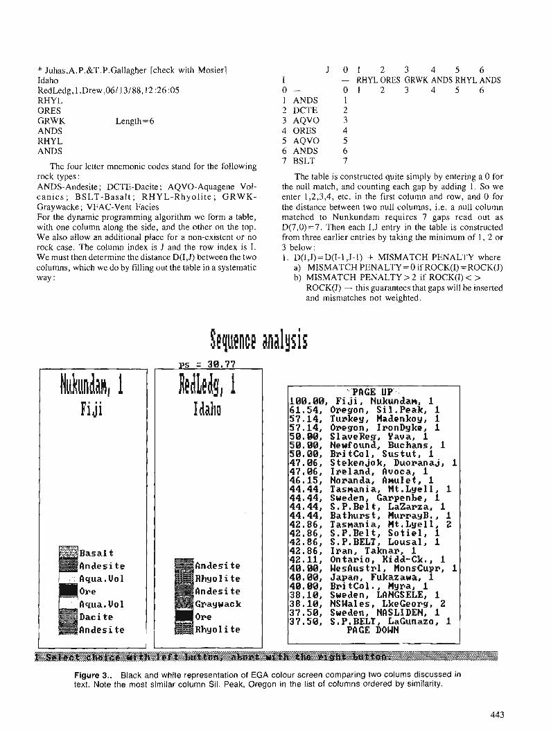
* Juhas,A.P.&T.P.Gallagher [check with Mosier] Idaho RedLedg,l,Drew,06/13/88,12:26:05 RHYL ORES GRWK Length = 6 ANDS RHYL ANDS

The four letter mnemonic codes stand for the following rock types : ANDS-Andesite; DCTE-Dacite; AQVO-Aquagene Vol- c a n i c ~ ; BSLT-Basal t ; RHYL-Rhyol i t e ; GRWK- Graywacke; VFAC-Vent Facies For the dynamic programming algorithm we form a table, with one column along the side, and the other on the top. We also allow an additional place for a non-existent or no rock case. The column index is J and the row index is I. We must then determine the distance D(1,J) between the two columns, which we do by filling out the table in a systematic way :

J O 1 2 3 4 5 6 I - RHYL ORES GRWK ANDS RHYL ANDS 0 - 0 1 2 3 4 5 6 1 ANDS 1 2 DCTE 2 3 AQVO 3 4 ORES 4 5 AQVO 5 6 ANDS 6 7 BSLT 7

The table is constructed quite simply by entering a 0 for the null match, and counting each gap by adding 1. So we enter 1,2,3,4, etc. in the first column and row, and 0 for the distance between two null columns, i.e. a null column matched to Nunkundam requires 7 gaps read out as D(7,0)=7. Then each I,J entry in the table is constructed from three earlier entries by taking the minimum of 1, 2 or 3 below : 1. D(I,J) =D(I-1 ,J-1) + MISMATCH PENALTY where

a) MISMATCH PENALTY = 0 if ROCK(1) = ROCK(J) b) MISMATCH PENALTY > 2 if ROCK(1) < >

ROCK(J) - this guarantees that gaps will be inserted and mismatches not weighted.

Sequence anal pis

Fiji

Aqua. Uo 1 Daci t e Andesi t e

Andesi t e Rhyo l i t e Bndesi t e Craywack Ore Rhyo l i t e

r'PCIGE"UP": 10B.BB, F i j i , Nukundaw, 1 61.54, Oregon, S i l .Peak, 1 57.14, Turkey, Madenkoy, 1 57.14, Oregon, IronDyke, 1 50.00, SlaveReg, Yava, 1 58.00, Newfound, Buchans, 1 50.00, Br i tCo l , S u s t u t , 1 47.86, S tekenjok , Duomnaj , 1 47.06, I r e l a n d , Buoca, 1 46.15, Noranda, Bmulet, 1 44.44, Tasnania, Mt.Lyel1, 1 44.44, Sweden, Carpenbe, 1 44.44, S . P. Be 1 t , LaZarza, 1 44.44, B a t h u r s t , MurrayB., 1 42.86, Tasmania, Mt.Lyel1, 2 42.86, S .P .Bel t , S o t i e l , 1 42.86, S.P.BELT, Lousal, 1 42.86, I r a n , Taknar, 1 42.11, On ta r io , Kidd-Ck,, 1 40.80, WesAustrl, MonsCupr, 1 40.00, Japan, Fukazawa, 1 48.00, B r i t C o l . , Myra, 1 38.16, Sweden, LflNGSELE, 1 38 ,10 , NSWalcs, LkeGeorg, 2 37.50, Sweden, NASLIDENj 1 37.50, S.P.BELT, LaGunazo, 1

PAGE DOWN

Figure 3.. Black and white representation of EGA colour screen comparing two colums discussed in text. Note the most similar column Sil. Peak, Oregon in the list of columns ordered by similarity.

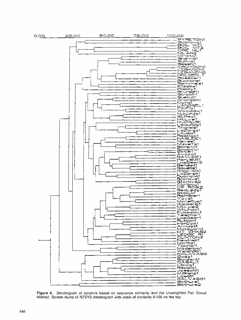
0.90 25.00 5 0.00 75.00 100.po PYRETON1 S k m r o v a l DOlL MTI BOIL MT2 ORE HlLl MILAN2

Figure 4. Dendrogram of columns based on sequence similarity and the Unweighted Pair Group Method. Screen dump of NTSYS dendrogram with scale of similarity 0-100 on the top.

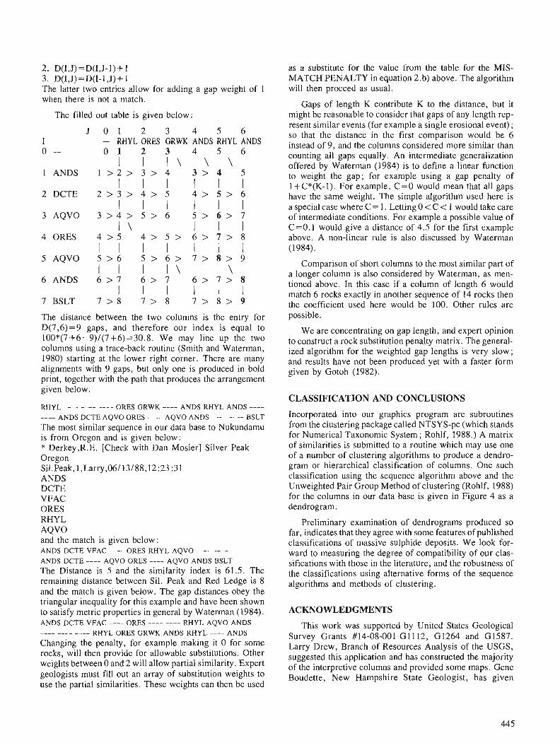
2. D(I,J)=D(I,J-I)+ I 3. D(I,J)=D(I-1 ,J) + 1 The latter two entries allow for adding a gap weight of 1 when there is not a match.

The filled out table is given below:

J O 1 2 3 4 5 6 I - RHYL ORES GRWK ANDS RHYL ANDS 0 - 0 1 2 3 4 5 6

I l l \ \ \ SANDS 1 > 2 > 3 > 4 3 > 4 5

I I I I I I

The distance between the two columns is the entry for D(7,6)=9 gaps, and therefore our index is equal to 100*(7+6-9)/(7+6)=30.8. We may line up the two columns using a trace-back routine (Smith and Waterman, 1980) starting at the lower right corner. There are many alignments with 9 gaps, but only one is produced in bold print, together with the path that produces the arrangement given below.

RHYL ---- ---- ---- ORES GRWK ---- ANDS RHYL ANDS ---- ---- ANDS DCTE AQVO ORES ---- AQVO ANDS ---- ---- BSLT

The most similar sequence in our data base to Nukundamu is from Oregon and is given below: * Derkey,R.E. [Check with Dan Mosier] Silver Peak Oregon Sil.Peak,l,Larry,06/ 13/88,12:23:31 ANDS DCTE VFAC ORES RHYL AQVO and the match is given below: ANDS DCTE VFAC ---- ORES RHYL AQVO ---- ---- ANDS DCTE ---- AQVO ORES ---- AQVO ANDS BSLT The Distance is 5 and the similarity index is 61.5. The remaining distance between Sil. Peak and Red Ledge is 8 and the match is given below. The gap distances obey the triangular inequality for this example and have been shown to satisfy metric properties in general by Waterman (1984). ANDS DCTE VFAC ---- ORES ---- ---- RHYL AQVO ANDS - - - - - - - - - - - - RHYL ORES GRWK ANDS RHYL ---- ANDS

Changing the penalty, for example making it 0 for some rocks, will then provide for allowable substitutions. Other weights between 0 and 2 will allow partial similarity. Expert geologists must fill out an array of substitution weights to use the partial similarities. These weights can then be used

as a substitute for the value from the table for the MIS- MATCH PENALTY in equation 2.b) above. The algorithm will then proceed as usual.

Gaps of length K contribute K to the distance, but it .might be reasonable to consider that gaps of any length represent similar events (for example a single erosional event) ; so that the distance in the first comparison would be 6 instead of 9, and the columns considered more similar than counting all gaps equally. An intermediate generalization offered by Waterman (1984) is to define a linear function to weight the gap; for example using a gap penalty of 1 +C*(K-1). For example, C=O would mean that all gaps have the same weight. The simple algorithm used here is a special case where C= 1. Letting 0 < C < 1 would take care of intermediate conditions. For example a possible value of C=O.l would give a distance of 4.5 for the first example above. A non-linear rule is also discussed by Waterman (1984).

Comparison of short columns to the most similar part of a longer column is also considered by Waterman, as mentioned above. In this case if a column of length 6 would match 6 rocks exactly in another sequence of 14 rocks then the coefficient used here would be 100. Other rules are possible.

We are concentrating on gap length, and expert opinion to construct a rock substitution penalty matrix. The generalized algorithm for the weighted gap lengths is very slow; and results have not been produced yet with a faster form given by Gotoh (1982).

CLASSIFICATION AND CONCLUSIONS

Incorporated into our graphics program are subroutines from the clustering package called NTSYS-pc (which stands for Numerical Taxonomic System; Rohlf, 1988.) A matrix of similarities is submitted to a routine which may use one of a number of clustering algorithms to produce a dendrogram or hierarchical classification of columns. One such classification using the sequence algorithm above and the Unweighted Pair Group Method of clustering (Rohlf, 1988) for the columns in our data base is given in Figure 4 as a dendrogram.

Preliminary examination of dendrograms produced so far, indicates that they agree with some features of published classifications of massive sulphide deposits. We look forward to measuring the degree of compatibility of our classifications with those in the literature, and the robustness of the classifications using alternative forms of the sequence algorithms and methods of clustering.

ACKNOWLEDGMENTS

This work was supported by United States Geological Survey Grants #14-08-001-GI 112, GI264 and G1587. Larry Drew, Branch of Resources Analysis of the USGS, suggested this application and has constructed the majority of the interpretive columns and provided some maps. Gene Boudette, New Hampshire State Geologist, has given

important consultation at every stage of the project, provided the rock nomenclature and definitions, and has drawn some of the maps.

REFERENCES

Gotoh, 0. 1982 : An improved algorithm for matching biological sequences; Journal

of Molecular Biology, v. 162, p. 705-708. Howell, J. A. 1983 : A FORTRAN 77 program for automatic stratigraphic correlation;

Computers and Geosciences, v. 9(3), p. 31 1-327. Pielou, E. C. 1984: The Interpretation of Ecological Data: A Primer on Classification

and Ordination; John Wiley & Sons, New York. Rohlf, F. J. 1988: NTSYS-pc. Numerical and Taxonomy and Multivariate Analysis

System. Version 1.40; Exeter Publishing, Ltd, Setauket, New York.

Sankoff, D. and Kruskal J. B. , ed. 1983: Time Warps, String Edits, and Macromolecules: The Theory and

Practice of Sequence Comparison ; Addison Wesley, London. Smith, T. F. and Waterman M. S. 1980: New stratigraphic correlation techniques; Journal of Geology,

v. 88(4), p. 451-457. Streckeisen, A. L. 1976: To each plutonic rock its proper name; Earth-Science Reviews,

v . 12, p. 1-33. Waterman, M. S. 1984: Efficient sequence alignment algorithms; Journal of Theoretical

Biology, v. 108, p. 333-337. Waterman, M. S. and Raymond, Jr., R. R. 1987: The match game: New stratigraphic correlation algorithms;

Mathematical Geology ; v. 19(2), p. 109- 127.

Recognition of stratigraphic equivalents using a graph-theoretic approach for the

geological atlas of the Western Canada Sedimentary Basin

Irina Shetsenl and Grant Mossopl

Shetsen, I. and Mossop, G. , Recognition of stratigraphic equivalents using a graph-theoretic approach for the geological atlas of the Western Canada Sedimentary Basin; & Statistical Applications in the Earth Sciences, ed. F. P. Agterberg and G. F. Bonham-Carter; Geological Survey of Canada, Paper 89-9, p. 447-458, 1989.

Abstract

A multi-institutional, multi-disciplinary project to produce a new atlas of the subsurface geology of the Western Canada Sedimentary Basin is now underway. It involves computer processing of stratigraphic and lithologic data from over 180 000 wells.

One of the most problematic aspects of the subsurface mapping relates to establishing the stratigraphic equivalents of selected horizons - taking into account synonomy of terms in a given region and identifying correlative relationships between regions of distinct terminology.

The algorithm for isolating equivalents, on a township-by-township basis, encompasses the following. ( I ) The stratigraphic sequence is modelled by an exact directed acyclic graph G = < V.R > where V is a set of stratigraphic markers, and R is a hard binary relation ''marker A overlies marker B ", derived from the subsurface stratigraphic data. (2) Graph G is used to construct an inexact undirected graph IG' = < V,P > , where P is a fuzzy binary relation "marker B may be an equivalent of marker C", induced by the adjacency matrix of G and the results of statistical tests on elevation means of the various markers. The painvise similarity measure in the characteristic matrix of IG is obtained as a function of the proximiry of edges in a current graph G, and the linkage data retained by the program from the preceding graphs. (3) A clustering procedure is applied to decompose IG into a series of complete maximal subgraphs, which correspond to all possible clusters of equivalents. (4) Through iterative comparison of cluster cohesiveness, graph IG' is partitioned into a collection of pairwise disjoint, strongly connected subgraphs that comprise a similarity graph IG = < V,Q > , where Q is an equivalence relation under threshold conditions.

Testing shows that the program correctly classijes about 98 % of the candidate stratigraphic markers.

On re'alise actuellement un projet multi-institutionnel et multi-disciplinaire, en vue de produire un nouvel atlas de la gdologie de subsurface du bassin skdimentaire de 1'Ouest canadien. Ce projet comprend le traitement informatique de donne'es stratigraphiques et lithologiques provenant de plus de 180 000 puits.

L'un des aspects les plus probleinatiques de la cartographie de subsurface est l'e'tablissement des kquivalences stratigraphiques d'horizons se'Lectionnks; tout en tenant compte de la synonymie des termes duns une rdgion donnde et en identijant les possibilitks de corre'lation entre les rdgions de terminologie distincte.

' Alberta Geological Survey, Alberta Research Council, P.O. Box 8330, Postal Station F, Edmonton, Alberta, Canada T6H 5x2

L'algorithme qui permet d'isoler les kquivalents, canton par canton, comprend les de'tails suivants. I) La skquence stratigraphique est modklise'e au moyen d'un graphique acyclique exact dirigk, G = < V , R > oh V est un ensemble de marqueurs stratigraphiques, et R est la relation binaire rigide suivante M le marqueur A recouvre le marqueur B n, dkrive'e des donnkes stratigraphiques de subsurface. 2) On emploie le graphique G pour construire un graphique inexact non digige' IG' = < V,P>, 03 P est la relation binaire $oue suivante a le marqueur B peut Ptre un kquivalent du marqueur C,,, induite par la matrice de contiguile' de G et par les re'sultats des essais statistiques sur les moyennes des cotes des divers marqueurs. On obtient une mesure de la similarite'de paires dans la matrice de caracte'ristiques de IG, en fonction de la proximite' des bords dans un graphique courant G, et les donnkes de liaison retenues par le programme d1apr2s les graphiques pre'ckdents. 3) On emploie un proce'dk de groupe pour de'composer IG en une se'rie de sous-graphiques maxirnaux complets, qui correspondent a tous les groupes possibles d'kquivalents. 4) Au moyen d'une comparaison ith-ative de la cohe'sion des groupes, on subdivise le graphique IG' en une collection de sous-graphiques couplks, non cons6cut$s, fortement liks les uns aux autres, qui comprennent un graphique de similarite' IG= < V,Q > , 03 Q est une relation d'e'quivalence dans des conditions de seuil.

Lfexp6rimentation montre que le programme classe correctement environ 98 % des marqueurs stratigraphiques possibles.

INTRODUCTION

The reality of synonymy in stratigraphic terms is inherent in the principles of stratigraphic nomenclature, and in the historically-rooted practice of stratigraphic designation. This is manifest in two modes. First, within a given geographic region, a specific marker horizon or stratigraphic top may be legitimately designated at any rank in the hierarchy of stratigraphic classes, e.g. group, formation, member. Second, it is not uncommon that stratigraphic units which were originally designated in different regions or sub- basins are ultimately recognized as correlative, giving rise to intermingling of names in the areas of overlap.

In the conduct of regional-scale basin analysis, the appropriate identification of synonymy in lithostratigraphic terminology is clearly essential. In a geological province as large as the Western Canada Sedimentary Basin, specific stratigraphic levels destined for regional mapping may carry a dozen or more stratigraphic names. This paper outlines a technique for automatic recognition of stratigraphic equivalents, as developed for use in the compilation of a new Geological Atlas of the Western Canada Sedimentary Basin.

The Atlas Project

The goal of the Atlas project is to compile and produce a new atlas of the subsurface geology of the Western Canada Sedimentary Basin. There are two principal objectives : (1) to establish an electronic database of consistently interpreted subsurface information, with associated software; and (2) to produce a printed atlas volume, for publication in 1991. The key output elements for each of the nineteen chapters dealing with cross-basin stratigraphic slices are : structural, isopach, lithofacies, paleogeological, and basic paleogeo- graphic maps (1 :5 000 000); regional, log-based cross- sections ; type logs and type cross-sections ; stratigraphic correlation charts; and text, with integrated or separate chapter treatment of the geological, geophysical, geochemical, and geotechnical parameters that are inherent in a modern basin analysis.

The project is multi-disciplinary and multi-institutional, involving scores of individuals from institutions and corpo- rations across the west, namely contributors/authors, project sponsors, data donors and financial patrons. The success of the project is critically dependent upon the cumulative endeavour of all parties, centered on the geological expertise embodied in the 90 to 100 contributors/authors.

Also of critical importance is the development and application of computer-based data processing techniques. Such is the volume and complexity of the digital subsurface information in Western Canada that manual compilation is clearly out of the question. It is also true that automated and integrated data processing can produce synthesis results that are simply not possible by alternate means.

Atlas approach to data processing

The new Atlas is being compiled on the basis of a number of existing digital databases, the most important of which are the provincial files for index and stratigraphic data, and the Canstrat files for lithology. Integrated computer processing of these large databases is designed to automate as many as possible of the stages of investigation that a geologist would manually undertake in the course of such a synthesis project. The advantages of an integrated and automated approach include : (1) the processing naturally provides insights into the nature and scope of the data themselves, giving rise to prevj- ously uncontemplated lines of further investigation; (2) the 90 to 100 contributors to the various chapters of the atlas are free to devote most of their time and energies to the most critical and most subjective interpretative questions; and (3) comprehensive logical and statistical evaluation of the raw data and the derivative data provides contributors with invaluable guides as to where application of their specialized knowledge might best be concentrated.

For further information on the background rationale, structure and status of the Atlas Project, readers are referred to Mossop (1988).

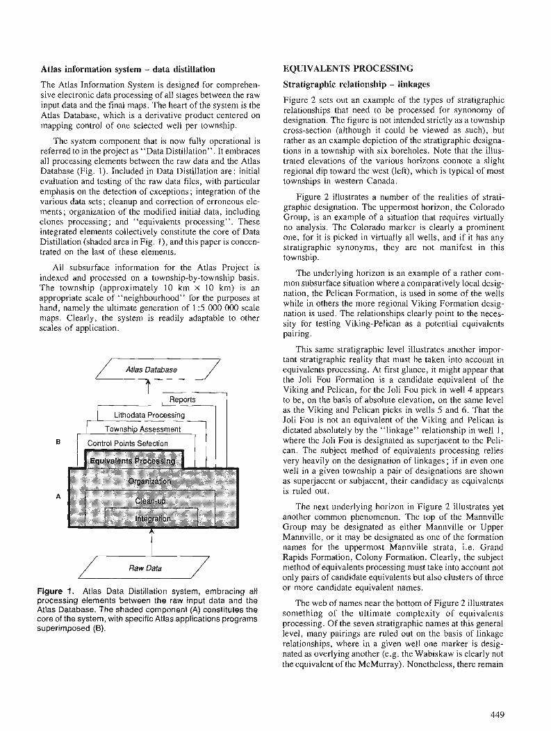
Atlas information system - data distillation

The Atlas Information System is designed for comprehensive electronic data processing of all stages between the raw input data and the final maps. The heart of the system is the Atlas Database, which is a derivative product centered on mapping control of one selected well per township.

The system component that is now fully operational is referred to in the project as "Data Distillation". It embraces all processing elements between the raw data and the Atlas Database (Fig. 1). Included in Data Distillation are: initial evaluation and testing of the raw data files, with particular emphasis on the detection of exceptions ; integration of the various data sets; cleanup and correction of erroneous elements; organization of the modified initial data, including clones processing ; and "equivalents processing". These integrated elements collectively constitute the core of Data Distillation (shaded area in Fig. I ) , and this paper is concentrated on the last of these elements.

All subsurface information for the Atlas Project is indexed and processed on a township-by-township basis. The township (approximately 10 km X 10 km) is an appropriate scale of "neighbourhood" for the purposes at hand, namely the ultimate generation of 1 :5 000 000 scale maps. Clearly, the system is readily adaptable to other scales of application.

B Control Points Selection

Organization

A Clean-up

Figure 1. Atlas Data Distillation system, embracing all processing elements between the raw input data and the Atlas Database. The shaded component (A) constitutes the core of the system, with specific Atlas applications programs superimposed (6).

EQUIVALENTS PROCESSING

Stratigraphic relationship - linkages

Figure 2 sets out an example of the types of stratigraphic relationships that need to be processed for synonomy of designation. The figure is not intended strictly as a township cross-section (although it could be viewed as such), but rather as an example depiction of the stratigraphic designations in a township with six boreholes. Note that the illustrated elevations of the various horizons connote a slight regional dip toward the west (left), which is typical of most townships in western Canada.

Figure 2 illustrates a number of the realities of stratigraphic designation. The uppermost horizon, the Colorado Group, is an example of a situation that requires virtually no analysis. The Colorado marker is clearly a prominent one, for it is picked in virtually all wells, and if it has any stratigraphic synonyms, they are not manifest in this township.

The underlying horizon is an example of a rather common subsurface situation where a comparatively local designation, the Pelican Formation, is used in some of the wells while in others the more regional Viking Formation designation is used. The relationships clearly point to the necessity for testing Viking-Pelican as a potential equivalents pairing.

This same stratigraphic level illustrates another important stratigraphic reality that must be taken into account in equivalents processing. At first glance, it might appear that the Joli Fou Formation is a candidate equivalent of the Viking and Pelican, for the Joli Fou pick in well 4 appears to be, on the basis of absolute elevation, on the same level as the Viking and Pelican picks in wells 5 and 6. That the Joli Fou is not an equivalent of the Viking and Pelican is dictated absolutely by the "linkage" relationship in well 1, where the Joli Fou is designated as superjacent to the Peli- can. The subject method of equivalents processing relies very heavily on the designation of linkages ; if in even one well in a given township a pair of designations are shown as superjacent or subjacent, their candidacy as equivalents is ruled out.

The next underlying horizon in Figure 2 illustrates yet another common phenomenon. The top of the Mannville Group may be designated as either Mannville or Upper Mannville, or it may be designated as one of the formation names for the uppermost Mannville strata, i.e. Grand Rapids Formation, Colony Formation. Clearly, the subject method of equivalents processing must take into account not only pairs of candidate equivalents but also clusters of three or more candidate equivalent names.

The web of names near the bottom of Figure 2 illustrates something of the ultimate complexity of equivalents processing. Of the seven stratigraphic names at this general level, many pairings are ruled out on the basis of linkage relationships, where in a given well one marker is designated as overlying another (e.g. the Wabiskaw is clearly not the equivalent of the McMurray). Nonetheless, there remain

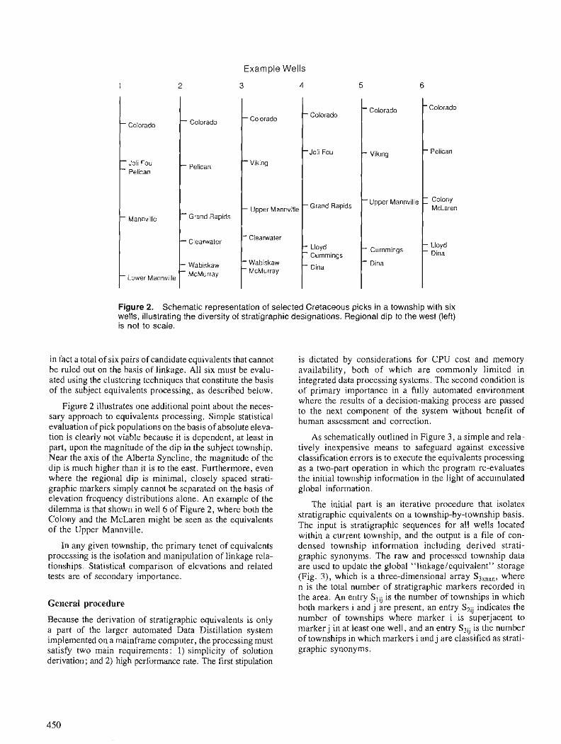
Example Wells

- Colorado

- Viking

- Upper Mannville

- Clearwater

- Wabiskaw - McMurray

- Colorado

- Joli Fou - Pelican

- Mannville

- Lower Mannville

- Colorado

- Pelican

- Grand Rapids

- Clearwater

- Wabiskaw - McMUrray

- Colorado

- Viking

- Upper Mannville

- Curnrnings

- Dina

,

-Colorado

- Pelican

- Colony McLaren

- Lloyd - Dina

- Colorado

- Joli Fou

- Grand Rapids

- Lloyd - Curnrnings

- Dina

Figure 2. Schematic representation of selected Cretaceous picks in a township with six wells, illustrating the diversity of stratigraphic designations. Regional dip to the west (left) is not to scale.

in fact a total of six pairs of candidate equivalents that cannot be ruled out on the basis of linkage. All six must be evaluated using the clustering techniques that constitute the basis of the subject equivalents processing, as described below.

Figure 2 illustrates one additional point about the necessary approach to equivalents processing. Simple statistical evaluation of pick populations on the basis of absolute elevation is clearly not viable because it is dependent, at least in part, upon the magnitude of the dip in the subject township. Near the axis of the Alberta Syncline, the magnitude of the dip is much higher than it is to the east. Furthermore, even where the regional dip is minimal, closely spaced stratigraphic markers simply cannot be separated on the basis of elevation frequency distributions alone. An example of the dilemma is that shown in well 6 of Figure 2, where both the Colony and the McLaren might be seen as the equivalents of the Upper Mannville.

In any given township, the primary tenet of equivalents processing is the isolation and manipulation of linkage relationships. Statistical comparison of elevations and related tests are of secondary importance.

General procedure

Because the derivation of stratigraphic equivalents is only a part of the larger automated Data Distillation system implemented on a mainframe computer, the processing must satisfy two main requirements: 1) simplicity of solution derivation; and 2) high performance rate. The first stipulation

is dictated by considerations for CPU cost and memory availability, both of which are commonly limited in integrated data processing systems. The second condition is of primary importance in a fully automated environment where the results of a decision-making process are passed to the next component of the system without benefit of human assessment and correction.

As schematically outlined in Figure 3, a simple and relatively inexpensive means to safeguard against excessive classification errors is to execute the equivalents processing as a two-part operation in which the program re-evaluates the initial township information in the light of accumulated global information.

The initial part is an iterative procedure that isolates stratigraphic equivalents on a township-by-township basis. The input is stratigraphic sequences for all wells located within a current township, and the output is a file of condensed township information including derived stratigraphic synonyms. The raw and processed township data are used to update the global "linkagelequivalent" storage (Fig. 3), which is a three-dimensional array S3xnxn, where n is the total number of stratigraphic markers recorded in the area. An entry SIij is the number of townships in which both markers i and j are present, an entry S2ij indicates the number of townships where marker i is superjacent to marker j in at least one well, and an entry S3ij is the number of townships in which markers i and j are classified as stratigraphic synonyms.

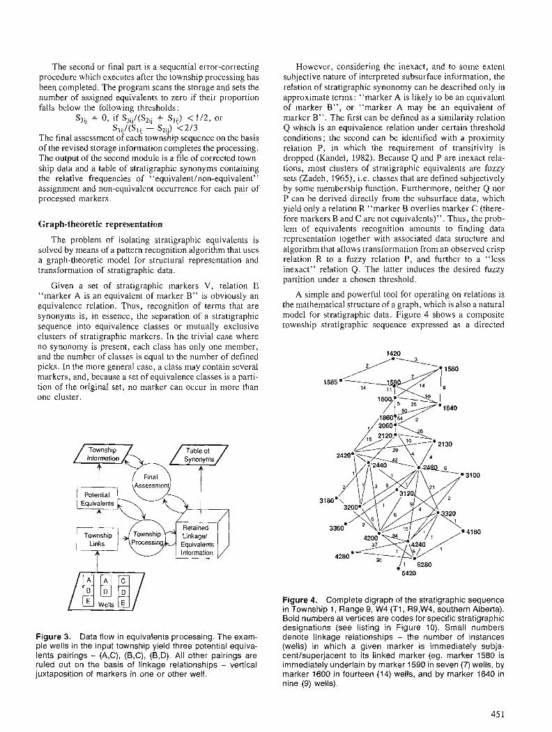
The second or final part is a sequential error-correcting procedure which executes after the township processing has been completed. The program scans the storage and sets the number of assigned equivalents to zero if their proportion falls below the following thresholds:

S3ij = 0, if S3ij/(SZij + Ssij) < 112, or S3ij/(S,ij - Szij) <213

The final assessment of each township sequence on the basis of the revised storage information completes the processing. The output of the second module is a file of corrected township data and a table of stratigraphic synonyms containing the relative frequencies of "equivalent/non-equivalent" assignment and non-equivalent occurrence for each pair of processed markers.

Graph-theoretic representation

The problem of isolating stratigraphic equivalents is solved by means of a pattern recognition algorithm that uses a graph-theoretic model for structural representation and transformation of stratigraphic data.

Given a set of stratigraphic markers V, relation E "marker A is an equivalent of marker B" is obviously an equivalence relation. Thus, recognition of terms that are synonyms is, in essence, the separation of a stratigraphic sequence into equivalence classes or mutually exclusive clusters of stratigraphic markers. In the trivial case where no synonomy is present, each class has only one member, and the number of classes is equal to the number of defined picks. In the more general case, a class may contain several markers, and, because a set of equivalence classes is a partition of the original set, no marker can occur in more than one cluster.

However, considering the inexact, and to some extent subjective nature of interpreted subsurface information, the relation of stratigraphic synonomy can be described only in approximate terms: "marker A is likely to be an equivalent of marker B", or "marker A may be an equivalent of marker B". The first can be defined as a similarity relation Q which is an equivalence relation under certain threshold conditions; the second can be identified with a proximity relation P, in which the requirement of transitivity is dropped (Kandel, 1982). Because Q and P are inexact relations, most clusters of stratigraphic equivalents are fuzzy sets (Zadeh, 1965), i.e. classes that are defined subjectively by some membership function. Furthermore, neither Q nor P can be derived directly from the subsurface data, which yield only a relation R "marker B overlies marker C (therefore markers B and C are not equivalents)". Thus, the problem of equivalents recognition amounts to finding data representation together with associated data structure and algorithm that allows transformation from an observed crisp relation R to a fuzzy relation P, and further to a "less inexact" relation Q. The latter induces the desired fuzzy partition under a chosen threshold.

A simple and powerful tool for operating on relations is the mathematical structure of a graph, which is also a natural model for stratigraphic data. Figure 4 shows a composite township stratigraphic sequence expressed as a directed

Township Information

Figure 3. Data flow in equivalents processing. The example wells in the input township yield three potential equivalents pairings - (A,C), (B,C), (B,D). All other pairings are ruled out on the basis of linkage relationships - vertical juxtaposition of markers in one or other well.

Figure 4. Complete digraph of the stratigraphic sequence in Township 1, Range 9, W4 (Tl, R9,W4, southern Alberta). Bold numbers at vertices are codes for specific stratigraphic designations (see listing in Figure 10). Small numbers denote linkage relationships - the number of instances (wells) in which a given marker is immediately subja- centlsuperjacent to its linked marker (eg. marker 1580 is immediately underlain by marker 1590 in seven (7) wells, by marker 1600 in fourteen (14) wells, and by marker 1640 in nine (9) wells).

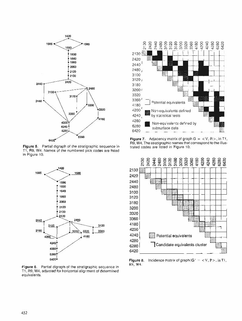
Figure 5. Partial digraph of the stratigraphic sequence in T I , R9, W4. Names of the numbered pick codes are listed in Figure 10.

Figure 6. Partial digraph of the stratigraphic sequence in TI, R9, W4, adjusted for horizontal alignment of determined equivalents.

Non-equivalents defined

4280 Non-equivalents defined by

6280 subsurface data 6420

Figure 7. Adjacency matrix of graph G = <V, R > , in T I , R9, W4. The stratigraphic names that correspond to the illustrated codes are listed in Figure 10.

/ 1 Candidate equivalents cluster -@I Figure 8. Incidence matrix of graph IG' = <V, P>, in TI, R9, W4.

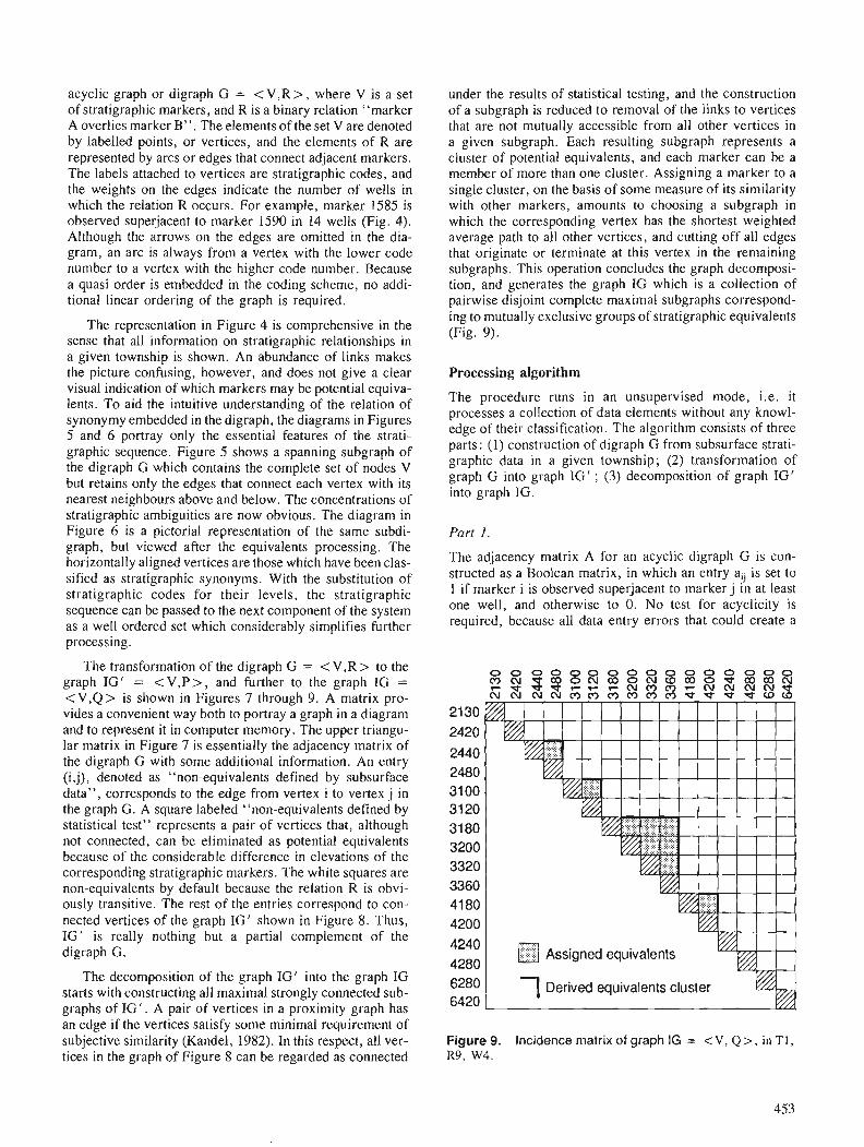
acyclic graph or digraph G = < V,R > , where V is a set of stratigraphic markers, and R is a binary relation "marker A overlies marker B' '. The elements of the set V are denoted by labelled points, or vertices, and the elements of R are represented by arcs or edges that connect adjacent markers. The labels attached to vertices are stratigraphic codes, and the weights on the edges indicate the number of wells in which the relation R occurs. For example, marker 1585 is observed superjacent to marker 1590 in 14 wells (Fig. 4). Although the arrows on the edges are omitted in the diagram, an arc is always from a vertex with the lower code number to a vertex with the higher code number. Because a quasi order is embedded in the coding scheme, no additional linear ordering of the graph is required.

The representation in Figure 4 is comprehensive in the sense that all information on stratigraphic relationships in a given township is shown. An abundance of links makes the picture confusing, however, and does not give a clear visual indication of which markers may be potential equivalents. To aid the intuitive understanding of the relation of synonymy embedded in the digraph, the diagrams in Figures 5 and 6 portray only the essential features of the stratigraphic sequence. Figure 5 shows a spanning subgraph of the digraph G which contains the complete set of nodes V but retains only the edges that connect each vertex with its nearest neighbours above and below. The concentrations of stratigraphic ambiguities are now obvious. The diagram in Figure 6 is a pictorial representation of the same subdi- graph, but viewed after the equivalents processing. The horizontally aligned vertices are those which have been classified as stratigraphic synonyms. With the substitution of stratigraphic codes for their levels, the stratigraphic sequence can be passed to the next component of the system as a well ordered set which considerably simplifies further processing.

The transformation of the digraph G = < V,R > to the graph IG' = < V,P > , and further to the graph IG = < V,Q > is shown in Figures 7 through 9. A matrix provides a convenient way both to portray a graph in a diagram and to represent it in computer memory. The upper triangular matrix in Figure 7 is essentially the adjacency matrix of the digraph G with some additional information. An entry (i,j), denoted as "non-equivalents defined by subsurface data", corresponds to the edge from vertex i to vertex j in the graph G. A square labeled "non-equivalents defined by statistical test" represents a pair of vertices that, although not connected, can be eliminated as potential equivalents because of the considerable difference in elevations of the corresponding stratigraphic markers. The white squares are non-equivalents by default because the relation R is obviously transitive. The rest of the entries correspond to connected vertices of the graph IG' shown in Figure 8. Thus, IG' is really nothing but a partial complement of the digraph G.

The decomposition of the graph IG' into the graph IG starts with constructing all maximal strongly connected subgraphs of IG' . A pair of vertices in a proximity graph has an edge if the vertices satisfy some minimal requirement of subjective similarity (Kandel, 1982). In this respect, all vertices in the graph of Figure 8 can be regarded as connected

under the results of statistical testing, and the construction of a subgraph is reduced to removal of the links to vertices that are not mutually accessible from all other vertices in a given subgraph. Each resulting subgraph represents a cluster of potential equivalents, and each marker can be a member of more than one cluster. Assigning a marker to a single cluster, on the basis of some measure of its similarity with other markers, amounts to choosing a subgraph in which the corresponding vertex has the shortest weighted average path to all other vertices, and cutting off all edges that originate or terminate at this vertex in the remaining subgraphs. This operation concludes the graph decomposition, and generates the graph IG which is a collection of pairwise disjoint complete maximal subgraphs corresponding to mutually exclusive groups of stratigraphic equivalents (Fig. 9).

Processing algorithm

The procedure runs in an unsupervised mode, i.e. it processes a collection of data elements without any knowledge of their classification. The algorithm consists of three parts : (1) construction of digraph G from subsurface stratigraphic data in a given township; (2) transformation of graph G into graph IG' ; (3) decomposition of graph IG' into graph IG.

Part I .

The adjacency matrix A for an acyclic digraph G is constructed as a Boolean matrix, in which an entry aij is set to 1 if marker i is observed superjacent to marker j in at least one well, and otherwise to 0. No test for acyclicity is required, because all data entry errors that could create a

G2B0 1 Derived equivalents cluster 6420

Figure 9. Incidence matrix of graph IG = < V , Q > , in TI, R9. W4.

cycle have been eliminated prior to the equivalents processing. The only operation performed on the matrix A is a test for connectivity . To avoid the classification errors that may result from processing disconnected vertices or groups of vertices, all disjoint components of the digraph are removed.

Part 2.

A Boo lean incidence matrix B is built for graph IG 1 in the following way. A two-tailed Student's Hest of elevation means at the level of significance a: = 0.001 is performed for each pair of markers that constitute possible equivalents. If the number of sample points is insufficient for a statistical test because each marker is observed in only one well, a subjective measure of elevation similarity, t, is calculated as follows

where di, d· are the elevations of markers i and j, respectively, and Js is the pooled township standard deviation.

The threshold value t0 is empirically defined at 0.05 . An entry b .. in matrix B is set to l if the test statistic calculated for m~rkers i and j does not fall in the rejection region, or t(di ,dj) > t

0, and otherwise to 0.

Matrix B is converted to the proximity matrix C by computing the measure of subjective similarity for every pair (i,j) such that bij = I. This measure can b.e derive? in one of two ways, depending on the amount of m formatiOn contained in the global storage (Fig. 3). Let the stratigraphic codes of markers k and I in the storage array S be the same as the stratigraphic codes of markers i and j, respectively, in the incidence matrix B. Then a proximity score cij is calculated as:

I. If s 1k1 > 0 for all entries (I ,k,l) in S such that code(k) = code(i) and code(!) = codeU), then

s2kl Cij = 1.0--

slkl

where s1k1 is the number of townships in which markers k and 1 are encountered together, and s2k1 is the number of townships where marker k is observed superadjacent to marker I prior to processing of a given township sequence.

2. Otherwise, n

cij = 1.0 - N

where n is the shortest path from vertex i to vertex j, and N is the longest path between any two vertices in the graph G.

The second computation is performed if sufficient accumulated linkage information does not exist for all markers in a current stratigraphic sequence. The intuitive justification for this derivation is that markers located close to each other are more likely to be equivalents than remote markers.

454

Part 3.

The decomposition of a graph IG 1 into a graph IG is an iterative procedure divided in three main steps.

I. First, the procedure identifies all possible clusters of equivalents that correspond to strongly connected maximal subgraphs of the graph IG 1

• As demonstrated by Figure 8, this is a straightforward operation.

2 . In the second step, a current cluster representative is chosen among the stratigraphic markers under consideration. The marker with the highest township occurrence is identified as a current pivotal element on the assumption that the most popular stratigraphic code is also the best defined. The average affinity c of the cluster representative to other markers is computed for all clusters of which the pivotal element is a member, as follows :

1 n c = - r; Cjj ·O

n j= 1

where n is the number of elements in a current cluster, i is the pivotal vertex, and

{

0, if i = j o=

1, otherwise

The cluster with the maximum average affinity is designated as a viable class. .

3. The third step removes the subgraph correspondmg to the selected cluster from the collection of subgraphs. In the remaining subgraphs, all edges connecting the selec~ed vertices with other nodes are cut off, i.e. the correspondmg entries in matrix B are set to 0. Inasmuch as this operation redefines the graph IG 1 , the whole procedure repeats starting with step l. The processing continues until each vertex in the graph IG 1 is either assigned to one of t~e cla~ses, or becomes a disconnected single node. At each JteratJOn, the current partition of a set of markers refines the previous partition . The procedure always terminates because the number of markers is finite.

RESULTS

As indicated above, the results of equivalents processing take two forms : 1) township information, in which pairs or clusters of determined equivalents are generated and output as reports, on a township-by-township basis; and 2). a summary report of stratigraphic synonyms, embracmg the whole of the study area.

In the example cited below, results are shown from the province of Alberta - 5431 townships , with a cumulative total of 113 776 assessed wells.

Township output

Initial Assessment

Figure 10 shows an example output of initial ~ssessment for a single township in southern Alberta. The f1ve clusters of determined equivalents are indicated by the leftmost numbers which pair or group adjacent entries according to thei~ overall stratigraphic levels (level 1 at the top is the Pakowk1

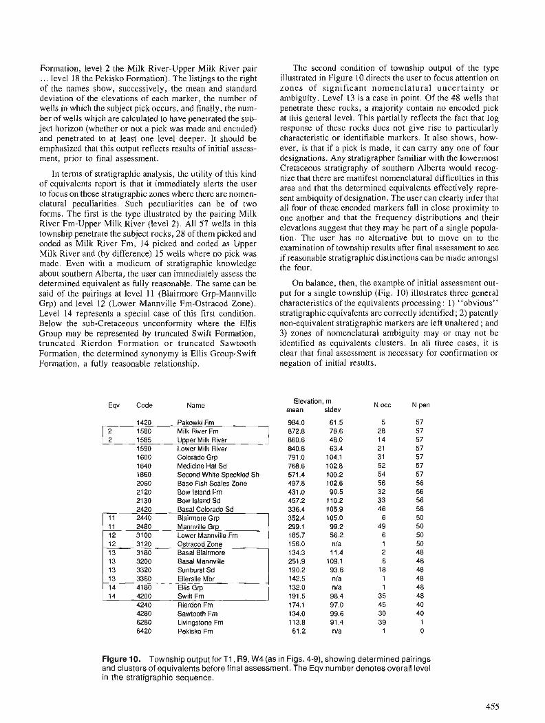
Formation, level 2 the Milk River-Upper Milk River pair .. . level 18 the Pekisko Formation). The listings to the right of the names show, successively, the mean and standard deviation of the elevations of each marker, the number of wells in which the subject pick occurs, and finally, the number of wells which are calculated to have penetrated the subject horizon (whether or not a pick was made and encoded) and penetrated to at least one level deeper. It should be emphasized that this output reflects results of initial assessment, prior to final assessment.

In terms of stratigraphic analysis, the utility of this kind of equivalents report is that it immediately alerts the user to focus on those stratigraphic zones where there are nomenclatural peculiarities. Such peculiarities can be of two forms. The first is the type illustrated by the pairing Milk River Frn-Upper Milk River (level 2). All 57 wells in this township penetrate the subject rocks, 28 of them picked and coded as Milk River Fm, 14 picked and coded as Upper Milk River and (by difference) 1.5 wells where no pick was made. Even with a modicum of stratigraphic knowledge about southern Alberta, the user can immediately assess the determined equivalent as fully reasonable. The same can be said of the pairings at level 11 (Blairmore Grp-Mannville Grp) and level 12 (Lower Mannville Fm-Ostracod Zone). Level 14 represents a special case of this first condition. Below the sub-cretaceous unconformity where the Ellis Group may be represented by truncated Swift Formation, truncated Rierdon Formation or truncated Sawtooth Formation, the determined synonymy is Ellis Group-Swift Formation, a fully reasonable relationship.

Eqv Code Name

1420 Pakowki Fm 2 1580 Milk River Fm 2 1585 Upper Milk River

1590 Lower Milk River 1600 Colorado Grp 1640 Medicine Hat Sd 1860 Second White Speckled Sh 2060 Base Fish Scales Zone 21 20 Bow Island Fm 21 30 Bow Island Sd 2420 Basal Colorado Sd

I 11 2440 Blairmore Gm 1 Mannville G Lower Mannville Fm Ostracod Zone

3180 Basal Blairmore 3200 Basal Mannville 3320 Sunburst Sd

13 3360 Ellerslie Mbr 14 4180 Ellis Grp 14 4200 Swift Fm

4240 Rierdon Fm 4280 Sawtooth Fm 6280 Livingstone Fm 6420 Pekisko Fm

The second condition of township output of the type illustrated in Figure 10 directs the user to focus attention on zones of significant nomenclatural uncertainty o r ambiguity. Level 13 is a case in point. Of the 48 wells that penetrate these rocks, a majority contain no encoded pick at this general level. This partially reflects the fact that log response of these rocks does not give rise to particularly characteristic or identifiable markers. It also shows, however, is that if a pick is made, it can carry any one of four designations. Any stratigrapher familiar with the lowermost Cretaceous stratigraphy of southern Alberta would recognize that there are manifest nomenclatural difficulties in this area and that the determined equivalents effectively represent ambiquity of designation. The user can clearly infer that all four of these encoded markers fall in close proximity to one another and that the frequency distributions and their elevations suggest that they may be part of a single population. The user has no alternative but to move on to the examination of township results after final assessment to see if reasonable stratigraphic distinctions can be made amongst the four.

On balance, then, the example of initial assessment output for a single township (Fig. 10) illustrates three general characteristics of the equivalents processing : 1) "obvious" stratigraphic equivalents are correctly identified ; 2) patently non-equivalent stratigraphic markers are left unaltered ; and 3) zones of nomenclatural ambiguity may or may not be identified as equivalents clusters. In all three cases, it is clear that final assessment is necessary for confirmation or negation of initial results.

Elevation, rn N occ N pen mean stdev

61.5 78.6 48.0 63.4

104.1 102.8 100.2 102.6 90.5

110.2 105.9 105.0 99.2 56.2 n/a 11.4

109.1 93.8 nla nla

98.4 97.0 99.6 91.4 nla

Figure 10. Township output for TI , R9, W4 (as in Figs. 4-9), showing determined pairings and clusters of equivalents before final assessment. The Eqv number denotes overall level in the stratigraphic sequence.

Final Assessment

Figure 1 1 juxtaposes initial assessment output (1 la) against final assessment output (1 1 b) for another single township in southern Alberta. As with the example shown in Figure 10, virtually all of the obvious equivalents pairings are isolated, in both the initial and the final assessment reports.

The impact of final assessment is illustrated at the level of the Lower Mannville Fm-Ostracod Zone-Basal Mannville-Sunburst Sd. Initial assessment (Fig. 1 la) clusters all four designations as equivalents. Final assessment considers processing results from all other townships and shows that in fact this four element cluster should really be divided into two discrete pairings (Fig. 1 Ib). The Lower Mannville Fm-Ostracod Zone pairing (Fig. I lb, level 13) is a fully legitimate equivalents assignment, and the Basal Mannville-Sunburst Sd pairing constitutes a discrete equivalents assignment (Fig. I lb , level 14).

Another example of the impact of final assessment is the reinterpretation of the Joli Fou Fm-Basal Colorado Sd pairing. This is a demonstrably spurious pairing because the Joli Fou Fm is a marine shale and the Basal Colorado is a sandstone stringer. Although they may occur in close proximity to one another, they are not legitimate equivalents, and the final assessment processing correctly overturns the initial classification.

Thus the utility of final assessment is manifest. While initial assessment in any one township can give rise to results that alert users to clusters of closely spaced and potentially ambiguous stratigraphic designations, there is commonly too little information in a single township to finally resolve the finer questions of stratigraphic distinction. By using the "retained linkageslequivalents information" from all other townships and applying it to the redefinition of equivalents in a single township, final assessment produces considerable improvements in equivalents assignments.

Table of synonyms

The merged results of final assessment processing can be output as a Table of Synonyms. An example of a small part of the output for the province of Alberta is illustrated in Figure 12. The table provides information on the number of townships in which a given pairing is evaluated and the overall results achieved, both in terms of absolute numbers and in terms of percentages. It should be remembered that the total number of townships processed in Alberta is 5431.

The first entry in Figure 12 is illustrative of a pairing that is overwhelmingly skewed in favour of equivalents legitimacy. In the 151 1 townships in which both the Blair- more Grp designation and the Mannville Grp appear together, equivalents processing shows that in 1419 instances the two are stratigraphically synonymous. In only one case (0.07 %) is there a linkage relationship between the two (denoting that in at least one well the two are vertically juxtaposed), which almost certainly reflects an error in the coding. In 91 cases, stratigraphic data from a given township are insufficient to allow for a conclusive assignment of equivalency, and the default assignment is therefore invoked (assigned non-equivalent).

(a) Eqv Code Name

1 1580 Milk River Fm 1 1585 Upper Milk River

1590 Lower Milk River 1600 Colorado Grp 1640 Medicine Hat Sd 1660 Badheart Fm 1860 Second White Speckled Sh 2060 Base Fish Scales Zone 21 20 Bow Island Frn 2130 Bow Island Sd

1 10 2360 Joli Fou Fm 10 2420 Basal Colorado Sd 11 2440 Blairmore Grp 11 2480 Mannville Gr 12 31 00 Lower Mannville Fm 12 3120 Ostracod Zone 12 3200 Basal Mannville

1 1 12 3440 Cutbank Ss

1 14 4000 Jurassic System 1 1 14 4200 Swift Fm 1 4240 Rierdon Fm 4280 Sawtooth Fm 6280 Livingstone Fm 6420 Pekisko Fm

Eqv Code Name

1 1 1580 Milk River Fm 1 1 1585 Upper Milk River I

1590 Lower Milk River 1600 Colorado Grp 1640 Medicine Hat Sd 1660 Badheart Frn 1860 Second White Speckled S h 2060 Base Fish Scales Zone 21 20 Bow Island Fm 21 30 Bow Island Sd 2360 Joli Fou Frn

Basal Colorado Sd Blairmore Grp Mannville Gr Lower Mannville Fm

3120 Ostracod Zone 14 3200 Basal Mannville

3320 Sunburst Sd 3440 Cutbank Ss

1 16 4000 Jurassic System 1 16 4200 Swift Fm

4240 Rierdon Fm 4280 Sawtooth Fm 6280 Livingstone Fm 6420 Pekisko Fm

Figure 11. Stratigraphy and equivalents output for T I , R10, W4 (immediately adjacent to the township that is the subject of Figs. 4-10). a) Equivalents pairs and clusters determined before final assessment. b) Equivalents isolated after final assessment.

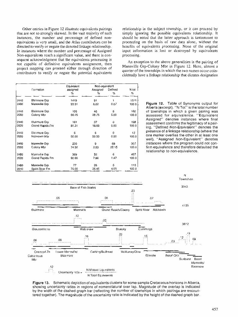
Other entries in Figure 12 illustrate equivalents pairings that are not so strongly skewed. In the vast majority of such instances, the number and percentage of defined non- equivalents is very small, and the Atlas contributors can be directed to verify or negate the denoted linkage relationship. In instances where the number and percentage of Assigned Non-equivalents reach a significant value, and there is con- sequent acknowledgment that the equivalents processing is not capable of definitive equivalents assignment, then project mapping can proceed either through direction of contributors to verify or negate the potential equivalents

relationship in the subject township, or it can proceed by simply ignoring the possible equivalents relationship. It should be noted that the latter approach is tantamount to proceeding on the basis of raw data alone, without the benefits of equivalents processing. None of the original input information is lost or destroyed by equivalents processing.

An exception to the above generalities is the pairing of Mannville Grp-Colony Mbr in Figure 12. Here, almost a quarter of the townships in which the two names occur coin- cidehtally have a linkage relationship that dictates designation

Equivalent Formation assigned

2440 Blairmore Grp 1419 2480 Mannville Grp 93.91

2440 Blairmore Grp 106 2560 Colony Mbr 66.25

2440 Blairmore Grp 161 2620 Grand Rapids Fm 81.31

2440 Elairmore Grp 6 2660 Notikewin Mbr 50.00

2480 Mannville Grp 230 2560 Colony Mbr 74.92

I 2480 Mannville Grp 369 2620 Grand Rapids Fm 90.66

Non-equivalent Assigned Defined

% To N tot 1 70

Figure 12. Table of Synonyms output for Alberta (excerpt). "N Tot" is the total number of townships in which a given pairing was assessed for equivalence. "Equivalent Assigned" denotes instances where final assessment confirms the legitimacy of a pairing. "Defined Non-Equivalent" denotes the presence of a linkage relationship (where the one marker overlies the other in at least one well). "Assigned Non-Equivalent" denotes instances where the program could not confirm equivalence and therefore defaulted the relationship to non-equivalence,

2480 Mannville Grp 77 28 5 110 2640 Spirit River Frn 70.00 25.45 4.55 100.0 -

N Townsh~ps

....................................................................................................

Base ol Fish Scales 3943 .23 , , , . , .

.06 .08 . . , . ............ . . . . .02

....................................... ....... ..... . . . . . . . . . . . . . . I . . . . . . . . . . _ , . . . . . . . . . . . . I . . . , - 41 35

Blairmore Mannville Grand RapidsIColony Spirit River Notikewin

- - - Glauconitic ss Wabiskaw Bluesky Curnrnings

- - Ostracod Zn Lower Mannvillel Geth~ngIBullhead McMurraylDina -

Calcareous Blairmore Ellerslie Basal Qrtz - - Mbr Sunburst Basal

Mannvillel .12 Blairmore . . . . . . N Missed Equivalents

- . .: : . . Uncertainty ratio = - N Total Equivalents

Figure 13. Schematic depiction of equivalents clusters for some sample Cretaceous horizons in Alberta, showing uncertainty ratios in regions of nomenclatural over lap. Magnitude of the overlap is indicated by the width of the dashed graph bar (reflecting the number of townships in which pairings are encountered together). The magnitude of the uncertainty ratio is indicated by the height of the dashed graph bar.

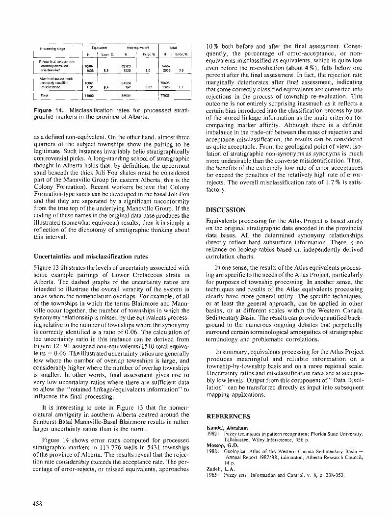
- mrrectly classilied . misclassilied

- mrreclly classified . misclassilied

Equivalenl Non-equivalent Total

N ( Error. O/o N I Erm. % N I Error. % I I I I I I

Figure 14. Misclassification rates for processed stratigraphic markers in the province of Alberta.

as a defined non-equivalent. On the other hand, almost three quarters of the subject townships show the pairing to be legitimate. Such instances invariably belie stratigraphically controversial picks. A long-standing school of stratigraphic thought in Alberta holds that, by definition, the uppermost sand beneath the thick Joli Fou shales must be considered part of the Mannville Group (in eastern Alberta, this is the Colony Formation). Recent workers believe that Colony Formation-type sands can be developed in the basal Joli Fou and that they are separated by a significant unconformity from the true top of the underlying Mannville Group. If the coding of these names in the original data base produces the illustrated (somewhat equivocal) results, then it is simply a reflection of the dichotomy of stratigraphic thinking about this interval.

Uncertainties and misclassification rates

Figure 13 illustrates the levels of uncertainty associated with some example pairings of Lower Cretaceous strata in Alberta. The dashed graphs of the uncertainty ratios are intended to illustrate the overall veracity of the system in areas where the nomenclature overlaps. For example, of all of the townships in which the terms Blairmore and Mann- ville occur together, the number of townships in which the synonymy relationship is missed by the equivalents processing relative to the number of townships where the synonymy is correctly identified is a ratio of 0.06. The calculation of the uncertainty ratio in this instance can be derived from Figure 12 : 91 assigned non-equivalentsll510 total equivalents = 0.06. The illustrated uncertainty ratios are generally low where the number of overlap townships is large, and considerably higher where the number of overlap townships is smaller. In other words, final assessment gives rise to very low uncertainty ratios where there are sufficient data to allow the "retained linkagelequivalents information" to influence the final processing.

It is interesting to note in Figure 13 that the nomenclatural ambiguity in southern Alberta centred around the Sunburst-Basal Mannville-Basal Blairmore results in rather larger uncertainty ratios than is the norm.

Figure 14 shows error rates computed for processed stratigraphic markers in 113 776 wells in 5431 townships of the province of Alberta. The results reveal that the rejection rate considerably exceeds the acceptance rate. The percentage of error-rejects, or missed equivalents, approaches

10 % both before and after the final assessment. Conse- quently, the percentage of error-acceptance, or non- equivalents misclassified as equivalents, which is quite low even before the re-evaluation (about 4 %), falls below one percent after the final assessment. In fact, the rejection rate marginally deteriorates after final assessment, indicating that some correctly classified equivalents are converted into rejections in the process of township re-evaluation. This outcome is not entirely surprising inasmuch as it reflects a certain bias introduced into the classification process by use of the stored linkage information as the main criterion for comparing marker affinity. Although there is a definite imbalance in the trade-off between the rates of rejection and acceptance misclassification, the results can be considered as quite acceptable. From the geological point of view, isolation of stratigraphic non-synonyms as synonyms is much more undesirable than the converse misidentification. Thus, the benefits of the extremely low rate of error-acceptances far exceed the penalties of the relatively high rate of error- rejects. The overall misclassification rate of 1.7 % is satisfactory.

DISCUSSION

Equivalents processing for the Atlas Project is based solely on the original stratigraphic data encoded in the provincial data bases. All the determined synonymy relationships directly reflect hard subsurface information. There is no reliance on lookup tables based on independently derived correlation charts.

In one sense, the results of the Atlas equivalents processing are specific to the needs of the Atlas Project, particularly for purposes of township processing. In another sense, the techniques and results of the Atlas equivalents processing clearly have more general utility. The specific techniques, or at least the general approach, can be applied in other basins, or at different scales within the Western Canada Sedimentary Basin. The results can provide quantified background to the numerous ongoing debates that perpetually surround certain terminological ambiguities of stratigraphic terminology and problematic correlations.

In summary, equivalents processing for the Atlas Project produces meaningful and reliable information on a township-by-township basis and on a more regional scale. Uncertainty ratios and misclassification rates are at accepta- bly low levels. Output from this component of "Data Distil- lation" can be transferred directly as input into subsequent mapping applications.

REFERENCES

Kandel, Abraham 1982: Fuzzy tecllniques in pattern recognition; Florida State University,

Tallahassee, Wiley-Interscience, 356 p. Mossop, G.D. 1988: Geological Atlas of the Western Canada Sedimentary Basin -

Annual Report 1987188; Edmonton, Alberta Research Council, 14 p.

Zadeh, L.A. 1965: Fuzzy sets; Information and Control, v. 8, p. 338-353.

A Canadian index of lithostratigraphic and lithodemic units

Aubrey Frickerl

Fricker, A., A Canadian index of lithostratigraphic and lithodemic units; & Statistical Applications in the Earth Sciences, ed. F. P Agterberg and G. F. Bonham-Carter; Geological Survey of Canada, Paper 89-9, p. 459-466, 1989.

Abstract

A data base has been developed (vreviously called "Lexfile") of geological formations and intrusive bodies for the Atlantic region, which is being released as a Geological Survey of Canada Open File. A printed version is planned, with a loose-leaf format to facilitate revisions. A Cunadian Index of Lithos- tratigraphic and Lithodemic Units is proposed, with similar structure and content, to provide a nation- wide data base..

The essential content is ( I ) the name, status and locality of each unit, (2) the spatial (i, e. stratigraphic) relationship between units, (3) the assigned ages, (4) the definition and redefinition history, and (5) the bibliography. The compiler and the year of the most recent revision are included for each unit name. m e data base was developed from the CSPG Lexicon Volume VI (Atlantic Region), and will be similarly maintained with support from local geologists.

The data base will be a reference for local geological studies, will co-ordinate formal definition of the stratigraphy, and could replace present card index systems. A bibliography for all the rock units of Canada will also be useful in its own right.

The file has been used to make time range charzs for units (useful starting points for presenting the tectonic history of New Brunswick) and directed graphs of the spatial relationships (to check the integrity and completeness of the stratigruphy in selected areas). The file therefore has considerable value as a research tool.

Une base de donnkes (antkrieurernent appelke cc Lexfile D ) sur les formations gkologiques et les corps intrusifs de la re'gion de I'Atlantique a kte' mise au point et est dif iske sous forme de dossier public de la Commission gkologique du Canada. La difision d'une version imprimke sur feuilles dktache'es afin de faciliter les revisions est prkvue. La pre'paration d'un index canadien des unite's lithostratigraphiques et lithodkmiques de structure et de contenu analogues est proposke comme base de donnkes a l'echelle du pays.

Le contenu sera essentiellement le m h e , soit I ) k nom, l'ktat et l'emplacernent de chaque unite', 2) les relations spatiales (c. -&-d. stratigraphiques) entre les unitks, 3) les dges assignis, 4) un historique de de'finition et de redkfinition et 5) une bibliographie. Pour chaque nom d'unitkfigurera le nom du com- pilateur et l'annee de la rkvision la plus re'cente. La base de donne'es a etk mise au point a partir du Volume VI du Lexique de la C.S. P. G. (rkgion de 1 iltlantique) et sera semblablement entretenue avec l'appui de ge'ologues locaux.

La base de donnkes servira de re'fkrence pour les ktudes gkologiques locales et permettra de coordon- ner la dkfinition formelle de la stratigraphic. Elle pourrait remplacer les systtmes actuels index surfiches. Une bibliographie pour toutes les unitks lithostratigraphiques du Canada sera e'galement utile en soi.

' Atlantic Geoscience Centre, Bedford Institute of Oceanography, P.O. Box 1006, Dartmouth, Nova Scotia B2Y 4A2

Le jichier a tfttf utilise' pour construire des graphiques des amplitudes chronologiques des unitks (points de dtfpart utiles pour la prtfsentation de l'histoire tectonique du Nouveau-Brunswick) et des graphiques orientks des relations spatiales @our vkrij?er l'intkgrittf et le caract6re exhaustif de la stratigruphie duns des rtfgions choisies). Lejichier s 'avdre donc d'une utilitk considtfrable en runt qu 'outil de recherche.

INTRODUCTION

Canada has no readily available index of names of geological units, nor any comprehensive reference for essential information about geological units. A computer database has been created for the Atlantic region (four provinces and the offshore) (Fricker et al., 1986) and support is solicited for a freely distributed and comprehensive Canadian Index of Stratigraphic and Lithodemic Units.

A computer file is valuable for searching and sorting, and for insights into the information that would be tedious to obtain from paper documents. The file should be sufficient for these purposes, and does not duplicate the more complete geological discussion found in the original source documents. Improved acessibility of information will avoid much confusion and resolve ambiguities in nomenclature.

LEXICONS

The United States Geological Survey (USGS) bulletins on geological names appear about once in ten years. The summary bulletin on names through 1975 (Swanson et al., 1981) listed 25,150 units. Each entry includes 10 items necessary for proper establishment of a formal unit. The most recent bulletin (1976-80, Luttrell et a]., 1986) contained just over 600 new names, a growth of over 2 % per annum.

The only comprehensive list of units in Canada is a card index system kept by the GSC in Ottawa (T. Bolton, pers. comm., 1988), which can be consulted by telephone and has provided an informal national registry of names. The index is primarily bibliographic. Additional information can be obtained by consulting provincial geological surveys. How- ever, personal contacts are necessary and time is needed to acquire appropriate publications. The formal erection of a name cannot always be determined, particularly from publications which predate modern standards.

The Canadian Society of Petroleum Geology (CSPG) series of eight Lexicons for all of Canada (Fig. 1) has adopted a format that seeks to maximize the reference value. The technique of appointing an expert compiler for each unit, who is responsible for assessing the quality of the information, eliminates much uncertainty and the need for research. The compilers and editors have unavoidably found themselves deciding on the formal status of many names. Decisions of this kind have been far from easy, given the age of publications and the criteria needed for the decision. Thus, inclusion in a lexicon (such as these or those of the USGS) amounts in practice to an official formal status.

Unfortunately, only three of the eight planned volumes in the CSPG series have been completed. The work is daun- ting, and the volumes for the Cordillera, Western Canada and Ontario may not be published for some time. The

Atlantic Region Lexicon was growing by 4 % per annum at the time of publication. By extrapolation, each volume will be one-third obsolete less than ten years after publication.

A prototype computer data base for Atlantic Canada arose from the compilation of Volume VI of the CSPG series (G.L. Williams et al., 1985). It has been developed using dBase H I + . The data base does not attempt to duplicate the descriptive content of the Lexicon, but concentrates on appropriate indexing and search items as well as on the bibliography. It is being issued as a GSC Open File on floppy discs, which will be regularly updated. Circulation on a printed version in loose-leaf binder format (Table 1) is proposed.

Much effort in compiling the CSPG Atlantic Lexicon arose from reconciliation of the published definition of units with the standards of the North American Stratigraphic Code (North American Commission on Stratigraphic Nomencla- ture, 1983). Checking the integrity of the data base revealed inconsistencies in the original information in the Lexicon. Production of future editions of the Lexicon will only be practical if the Lexicon file is maintained.

Bound volumes of the quality of the CSPG series are popular and will probably not be replaced by computer files. Even so, we estimate that the effort to produce the printed Lexicons would be more than halved if such an up-to-date computer file already existed. Having produced the digital file for one region, it seems logical to extend it to the rest of Canada. The card index is unlikely to be maintained. A Canadian database is essential.

Table 1. An example bulletin page produced from the Atlantic region database.

North Mountain Basalt, formal formation Compiled by Stevens G.R., 1985 Rhaetian-Hettangian N.S. ref: 21 B18 215-204 ma 0.00 N.O.00 W

Senior units: Fundy Group Newark Supergroup

Junior units: none

Equivalent units: Shelburne Dyke, equivalent

Earlier units: Blomidon Formation, conform

Later units: Scots Bay Formation, conclunc

History: original : North Mountain Basalt Powers, S. 1916

THE CONTENTS

To summarize (Table 2), USGS bulletins provide an index and include basic data for formal erection of a name. Infor- mal and abandoned names are not included. Bolton's card index provides an index and a bibliography for names, regardless of the formal status. The CSPG Lexicons provide an index, include the status and contain a synopsis of pertinent information, with a selective bibliography.

A Canadian Index should complement the descriptive printed Lexicons, and not replace them. It can be a basis for

co-ordinating stratigraphic names and could pre-empt (1) the indexing, (2) the status recognition and (3) the biblo- graphic role. A bibliography in the simplest objective to meet. If a consistent program of abstracting is maintained, then the index objective can be reliably met also.

The status of names is a greater problem, since many of those published are at variance with the Stratigraphic Code. Geological names now should be established or revised according to the guidelines of the North American Strati- graphic Code (1983). Proper erection of a formal geological name requires publication, in a recognized scientific

Figures 1. Areas covered by Lexicons of Canadian Stratigraphy. (With permission, from Volume VI, Wiliams et al., 1985.) Volume 1. Arctic Archipelago (District of Franklin). Volume 2. Yukon-Mackenzie (Yukon Territory and District of Mackenzie). Volume 3. Western Cordillera (southwestern Yukon Territory and western British Columbia). Volume 4. Western Canada (eastern British Columbia, Alberta, and southern Saskatchewan and

Manitoba. Volume 5. Central Canada (Ontario, Quebec, northern Saskatchewan and Manitoba, and District of

Keewatin). Volume 6. Atlantic Region (New Brunswick, Newfoundland and Labrador, Nova Scotia, Prince Edward

Island, Offshore Eastern Canada).

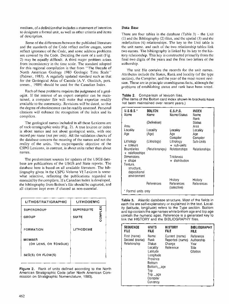
medium, of a definition that includes a statement of intention to designate a formal unit, as well as other criteria and items of description.

Some of the differences between the published literature and the standards of the Code reflect earlier usages, some reflect ignorance of the Code, and some address problems not covered by the Code. Deciding the rank of a unit (Fig. 2) may be equally difficult. A third major problem arises from inconsistency in the time scale. The standard adopted for this regional compilation is that from "The Decade of North American Geology 1983 Geologic Time Scale" (Palmer, 1983). A regularly updated standard such as that for the Geological Atlas of Canada (A.V. Okulitch, pers. comm., 1989) should be used for the Canadian Index.

Each of these problems requires the judgement of a geologist. If the interest of an expert compiler can be maintained, a computer file will make that expertise readily available to the community. Revisions will be dated, so that the degree of obsolescence can be readily assessed. Personal citations will enhance the recognition of the index and its compilers.

The geological names included in all these Lexicons are of rock-stratigraphic units (Fig. 2). A true lexicon or index is about names and not about geological units, with one record per name (not per unit). All the validation checks of the database concern the meaning of the names and not the reality of the units. The encyclopaedic objective of the CSPG Lexicons, in contrast, is about units rather than about names.

The predominant sources for updates of the USGS database are publications of the USGS and State reports. The database here is based on all available literature. The bibliography given in the CSPG Volume VI Lexicon is somewhat selective, reflecting the publications regarded as essential by the compilers. If a Canadian Index is developed, the bibliography from Bolton's file should be captured, and all citations kept even if classed as non-essential.

LITHOSTRATIGRAPHIC LlTHODEMlC

SUPERGROUP

GROUP SUITE

FORMATION LITHODEME

MEMBER (OR LENS, OR TONGUE)

Figure 2. Rank of units defined according to the North American Stratigraphic Code (after North American Com- mission on Stratigraphic Nomenclature, 1983).

Data Base

There are four tables in the database (Table 3) - the Unit (1) and the Bibliography (2) files, and the spatial (3) and the redefinition (4) relationships. The key to the Unit table is the unit name, and each of the two relationship tables link two names. The bibliography is linked by its key to the history relationship. This key is constructed primarily from the final two digits of the years and the first two letters of the authorship.

The unit file contains the records for the unit names. Attributes include the Status, Rank and locality (of the type section), the Compiler, and the year of the most recent revision. These are in principle unambiguous facts, although the problems of establishing status and rank have been noted.

Table 2. Comparison of lexicon files. (The items of the Bolton card index shown in brackets have not been maintained over recent years.)

U.S.G.S.* BOLTON C.S.P.G. INDEX Name Name NameIStatus Name

R a n k (Definition) Status

Area Area Locality Locality Locality Locality Age (Age) Age Age

Compiler Compiler Lithology (Lithology) Lithology Sub-units + colours + sub-units Boundaries (Relationships) Relationships Relationships + relationships Dimensions Thickness + shape + distribution Texture,

structure, depositional environment

History History References References References

(selective) * Formal units only

Table 3. Atlantic database structure. Most of the fields in each file are self-explanatory or explained in the text. Local- ity (latitude, longitude) refers to the Type section. Bottom and top contain the age names while bottom age and top age contain the numeric ages. Reference is a generated key to link the HISTORY and the BIBLIOGRAPHY files.

SEQUENCE UNITS HISTORY BIBLIOGRAPHY FILE FILE FILE FILE First (name) Name Current (name) Reference Second (name) Rank Reported (name) Authorship Relationship Status Change, Year

Locality Reference Title Latitude Citation Longitude Province Bottom Bottom-age Top Top-age Compiler Currency

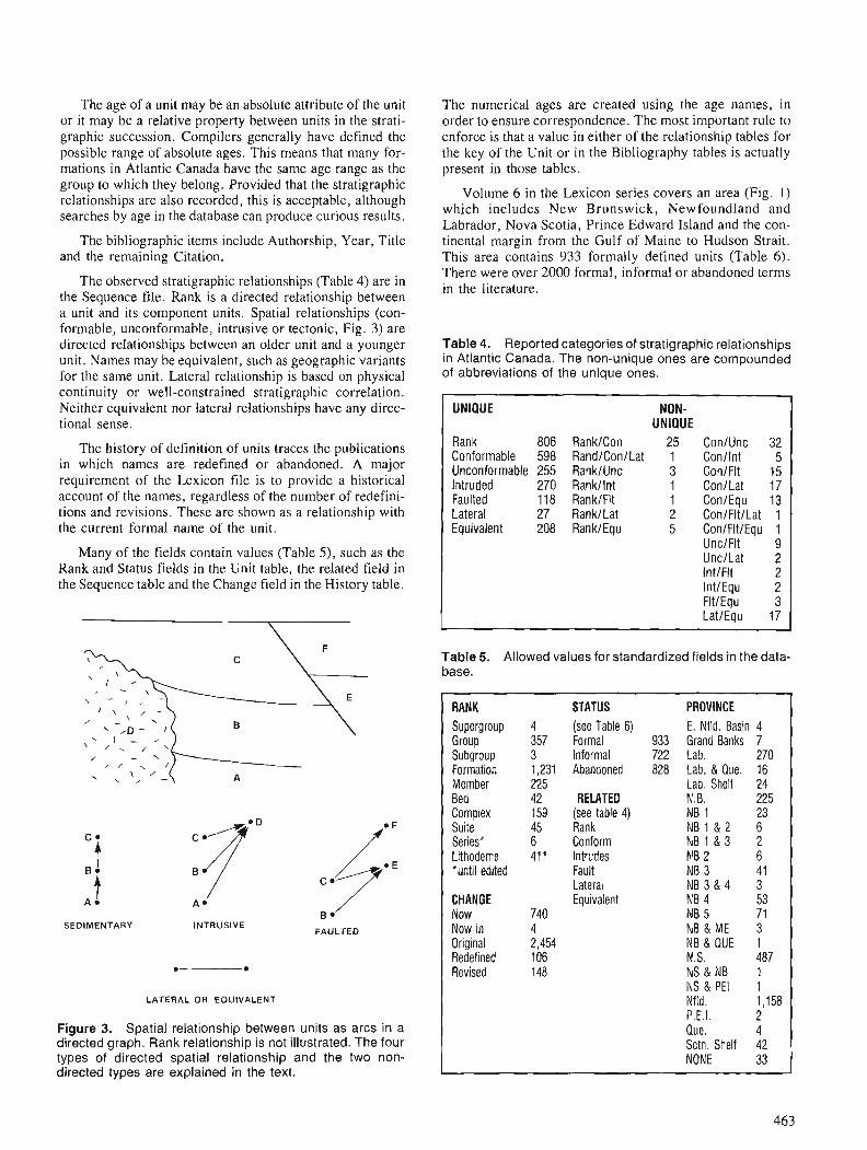
The age of a unit may be an absolute attribute of the unit or it may be a relative property between units in the stratigraphic succession. Compilers generally have defined the possible range of absolute ages. This means that many formations in Atlantic Canada have the same age range as the group to which they belong. Provided that the stratigraphic relationships are also recorded, this is acceptable, although searches by age in the database can produce curious results.

The bibliographic items include Authorship, Year, Title and the remaining Citation.

The observed stratigraphic relationships (Table 4) are in the Sequence file. Rank is a directed relationship between a unit and its component units. Spatial relationships (conformable, unconformable, intrusive or tectonic, Fig. 3) are directed relationships between an older unit and a younger unit. Names may be equivalent, such as geographic variants for the same unit. Lateral relationship is based on physical continuity or well-constrained stratigraphic correlation. Neither equivalent nor lateral relationships have any directional sense.

The history of definition of units traces the publications in which names are redefined or abandoned. A major requirement of the Lexicon file is to provide a historical account of the names, regardless of the number of redefini- tions and revisions. These are shown as a relationship with the current formal name of the unit.

Many of the fields contain values (Table 5), such as the Rank and Status fields in the Unit table, the related field in the Sequence table and the Change field in the History table.

The numerical ages are created using the age names, in order to ensure correspondence. The most important rule to enforce is that a value in either of the relationship tables for the key of the Unit or in the Bibliography tables is actually present in those tables.

Volume 6 in the Lexicon series covers an area (Fig. 1) which includes New Brunswick, Newfoundland and Labrador, Nova Scotia, Prince Edward Island and the continental margin from the Gulf of Maine to Hudson Strait. This area contains 933 formally defined units (Table 6). There were over 2000 formal, informal or abandoned terms in the literature.

Table 4. Reported categories of stratigraphic relationships in Atlantic Canada. The non-unique ones are compounded of abbreviations of the unique ones.

UNIQUE NON- UNIQUE

Rank 806 RankICon 25 ConlUnc 32 Conformable 598 RandIConlLat 1 Conllnt 5 Unconformable 255 RankIUnc 3 ConlFlt 15 Intruded 270 Rankllnt 1 ConILat 17 Faulted 118 RanklFlt 1 ConlEqu 13 Lateral 27 RankILat 2 ConlFltlLat 1 Equivalent 208 RankIEqu 5 ConIFltlEqu 1

UnclFlt 9 UnclLat 2 IntlFlt 2 IntIEqu 2 FltIEqu 3 LatlEqu 17

Table 5. Allowed values for standardized fields in the database.

I \

/ - \ '\- ' D '

SEDIMENTARY INTRUSIVE FAULTED

LATERAL OR EQUIVALENT

Figure 3. Spatial relationship between units as arcs in a directed graph. Rank relationship is not illustrated. The four types of directed spatial relationship and the two non- directed types are explained in the text.

>

RANK STATUS PROVINCE Supergroup 4 (see Table 6) E. Nfld. Basin 4 Group 357 Formal 933 Grand Banks 7 Subgroup 3 Informal 722 Lab. 270 Formation 1,231 Abandoned 828 Lab. & Que. 16 Member 225 Lab. Shelf 24 Bed 42 RELATED N.B. 225 Complex 159 (see table 4) NB 1 23 Suite 45 Rank NB1&2 6 Series* 6 Conform NB1&3 2 Lithodeme 411 Intrudes hlB 2 6 *until edited Fault NB 3 41

Lateral N83&4 3 CHANGE Equivalent NB 4 53 Now 740 NB 5 71 Now in 4 NB&ME 3 Original 2,454 NB & QUE 1 Redefined 106 N.S. 487 Revised 148 NS & NB 1

INS & PEI 1 Nfld. 1,158 P.E.I. 2 Que. 4 Sctn. Shelf 42 NONE 33

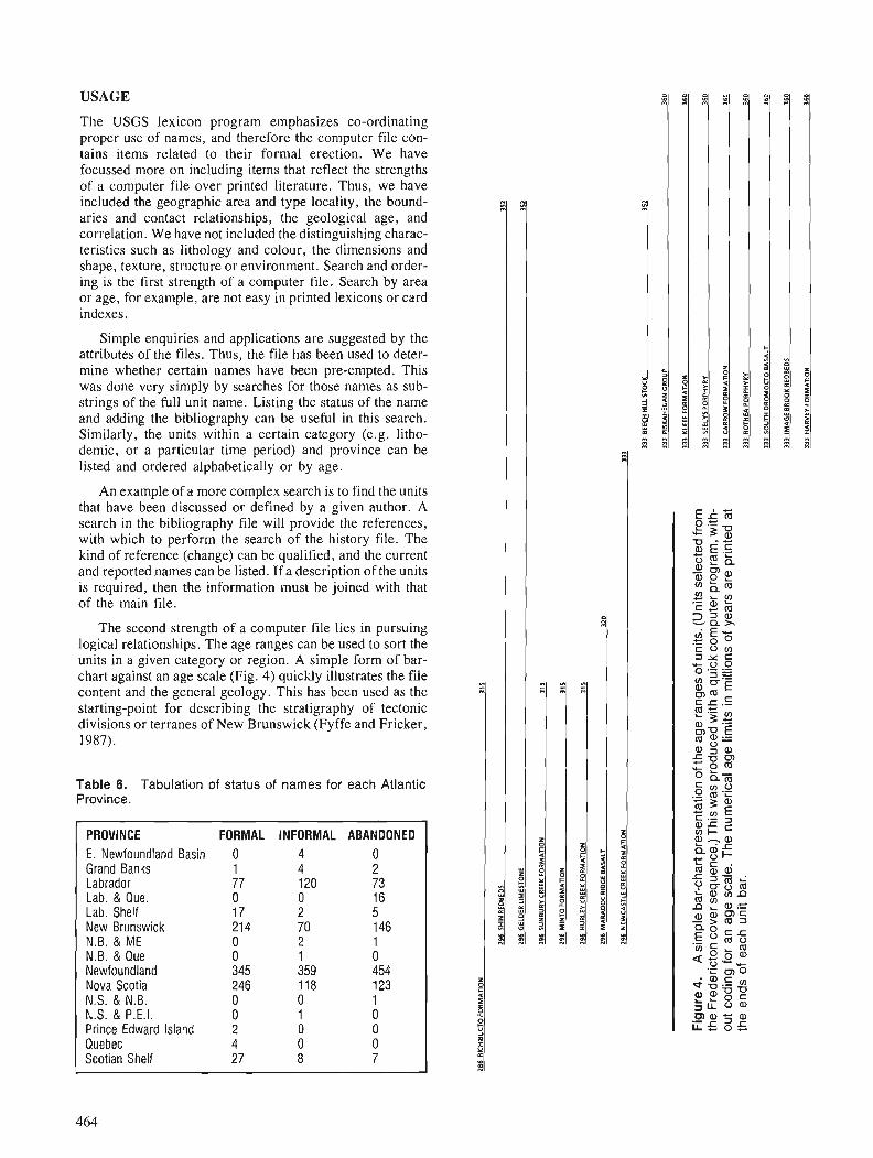
USAGE 81 I I !I 81 !I I I I I t l

The USGS lexicon program emphasizes co-ordinating proper use of names, and therefore the computer file contains items related to their formal erection. We have focussed more on including items that reflect the strengths of a computer file over printed literature. Thus, we have included the geographic area and type locality, the boundaries and contact relationships, the geological age, and correlation. We have not included the distinguishing characteristics such as lithology and colour, the dimensions and shape, texture, structure or environment. Search and ordering is the first strength of a computer file. Search by area or age, for example, are not easy in printed lexicons or card indexes.

Simple enquiries and applications are suggested by the attributes of the files. Thus, the file has been used to determine whether certain names have been pre-empted. This was done very simply by searches for those names as sub- strings of the full unit name. Listing the status of the name and adding the bibliography can be useful in this search. Similarly, the units within a certain category (e.g. lithodemic, or a particular time period) and province can be listed and ordered alphabetically or by age.

An example of a more complex search is to find the units that have been discussed or defined by a given author. A search in the bibliography file will provide the references, with which to perform the search of the history file. The kind of reference (change) can be qualified, and the current and reported names can be listed. If a description of the units is required, then the information must be joined with that of the main file.

The second strength of a computer file lies in pursuing logical relationships. The age ranges can be used to sort the units in a given category or region. A simple form of bar- chart against an age scale (Fig. 4) quickly illustrates the file content and the general geology. This has been used as the starting-point for describing the stratigraphy of tectonic divisions or terranes of New Brunswick (Fyffe and Fricker, 1987).

Table 6. Tabulation of status of names for each Atlantic Province.

PROVINCE FORMAL INFORMAL ABANDONED E. Newfoundland Basin 0 4 0 Grand Banks 1 4 2 Labrador 77 120 73 Lab. & Que. 0 0 16 Lab. Shelf 17 2 5 New Brunswick 214 70 146 N.B. & ME 0 2 1 N.B. & Que 0 1 0 Newfoundland 345 359 454 Nova Scotia 246 118 123 N.S. & N.B. 0 0 1 N.S. & P.E.I. 0 1 0 Prince Edward Island 2 0 0 Quebec 4 0 0 Scotian Shelf 27 8 7

E i Z g- - 3% -0 -- a E.E - $ gCL - $ 2 2 a m

L? L . r s 2 m 2.2% "5 6~ - .- corn Z Y c - U 0 0 .=j U) u'- a, E cnm K c .5 m C y) L a 3 .= g'g g ass g n rs, .cognt a%

0 2.: .- ti 3 r . c E, z g c 2 n$ a a r :'- m cu ai 5 sz 2 fqrnn n a c

0 ) K 2 $ m 3

e 8 c r .zcag ag.!?:

'C 00 - a , c dm.- '0

a F Z Z 5 l L o a w a , 5 a , ii505

The most fundamental logical relationships describe the observed stratigraphy. Superposition, intrusion or tectonic boundaries have a sequence direction. These may be portrayed as a directed graph. Conventionally the direction, or "arrow", in the graph may go from the older or earlier to the younger or later. Equivalent or laterally correlated units must be treated as the same node in such a graph. The graph is acyclic, for if unit A precedes unit B, which in turn precedes unit C, then unit C cannot precede unit A. This is the basis of an important final integrity check of the information. Once the stratigraphic relationships are verified, the overall stratigraphy of a region or of a group or complex may be portrayed (Fig. 5). This may bring anomalies to light, or may illustrate the gaps in defining the succession.

QUALITY

The first phase of quality control involves programmed checking. The checks performed formally are as follows. (1) Values in the fields called "Rank", "Status", "Prov- ince", "Change" and "Related" are standardized by ordered lists and inspection. (2) Geological ages are likewise standardized and the corresponding numerical ages are correlated using the decade of North American Geology (DNAG) standard. (3) Unit names in the Sequence and His- tory files must be in the Unit file. (4) Reference keys in the History file must be in the Bibliography file. (5) Duplicate records in the Sequence and History files are eliminated, and this includes records with the unit names swapped between the two name fields or different stratigraphic relationships reported for the same two units. (6 ) Cycles in stratigraphic succession (as described above) are detected, and the relationship is replaced with one called "cycle" if and until an editorial decision is needed.

GROUP

WINDSOR GROUP UNCON

t

FISSET BROOK FORMATION

UNCON HORTON A

BOURINOT GROUP

U N C O N A

FORCHU GROUP

I CAPE SMOKY PLUTON

GEORGE RIVER GROUP

Figure 5. Spatial chart drawn from the stratigraphic relationships between some intrusives in Cape Breton and with the regional stratigraphic groups. The positions of each unit in the chart reflect the relative stratigraphic position with younger at the top, older at the bottom. Arrows indicate the sequence from older to younger intrusive body. If not otherwise indicated, the relationship is intrusive. Horizontal double lines represent equivalence.

The second phase of quality control will rely of the compilers. All information, including the reported relationships for a unit, can be brought together for editing. This will be particularly important in checking the relationships between names.

The final factor in improving the quality of the file should be wide availability. If the index serves its purpose, a relationship should develop between common usage in the literature and the formal status of names as reflected in the database. The availability of a reference and standard should heighten the awareness of authors, journal reviewers and editors to the criteria for formal erection and usage of a name.

PROPOSAL

The computer database for the Atlantic provinces has been checked for internal consistency and verified against Vol- ume VI of the CSPG Lexicon (Williams et al., 1985) and is being made available as a GSC Open File. Preliminary hard copies are being circulated to compilers for their units, leading to printed versions of the information being started in 1989.

A Canadian Index of Lithostratigraphic and Lithodemic Units is proposed. Structured like the one here, it will contain the names of all units in Canada. Such a database would need 10-15 megabytes, which will require a substantial personal computer to manage, however, subsets for specific regions would be well within the capacity of most personal computers.

Table 7. Steps in creating a Canadian Index database.

PHASE 1 - Photocopying Bolton's cards - Data entry: Name

Authorship Year Title References

- Draft abstraction : Change Status Rank Province

- Validation of the referencing - Status reportslopen files

PHASE 2 - Draft abstraction: Locality of type section

Ages Stratigraphic relationships

- Assignment of compiler - Draft bulletins - Validation by compilers - Status reportslopen Files

ONGOING - Monitoring literature - Routine compiler feedback - Routine (Annual?) reports

The present ability to co-ordinate and standardize nomenclature and to provide bibliographic histories of units will be significantly enhanced. Allocation of responsibilities and compilation in projects such as the current CSPG Lexi- cons could be considerably accelerated by producing up-to- date pseudo-Lexicons on demand. Bulletins will be published on a regular and timely basis. The addition of unit interrelationships to the database permits its application as a research tool.

The Index will be a national resource, in co-ordination and co-operation with all appropriate provincial and ter- ritorial government departments. Providing a comprehensive digital bibliography in itself should be a considerable asset for many purposes.

Names and bibliographic information will be obtained from Bolton's card file. Upon entry (Phase 1, Table 7), the computer and card files can operate concurrently until the former is judged satisfactory. In Phase 2 descriptions and relationships will be added. In the case of the Atlantic Can- ada file, this was done during the preparation of the CSPG Lexicon. The program of reporting, and developing a clien- tele of editors and compilers will take about 2-3 years to evolve satisfactorily. The project should stabilize at a maintenance level by 1994.

The only significant resource required is the time to abstract, enter and check the file. Based on the Atlantic Can- ada experience, compiling Phases 1 and 2, together with operating the file as a service, is estimated as 4 person- years.

ACKNOWLEDGMENTS

The central work for the Lexicon was done by the editors and compilers of Volume VI of the CSPG Lexicon. M.S. Barss gave advice for the original file. Computer file compilation was assisted by M. Daneau, B. Perry, W. MacMillan and G. Walls. The significant revisions for Version 3 were

'

assisted by K. McCarthy and D. Filteau.

REFERENCES

Fricker, A., MacMillan, W.C., Williams, G.L., and Fyffe, L.R. 1986: The stratigraphic nomenclature of Atlantic Canada: G.A.C.,

M.A.C., C.G.U. Joint Annual Meeting, Program with Abstracts, v. 11, p. 70.

Fyffe, L.R. and Fricker, A. 1987: Tectonostratigraphic terrane analysis of New Bmnswick; Mari-

time Sediments and Atlantic Geology, v. 23, p. 113-122. Luttrell, G.W., Hubert, M.L., and Jussen, V.M. 1986: Lexicon of new formal geologic names of the United States

1976-1980; United States Geological Survey, Bulletin 1564, 191 p.

North American Commission of Stratigraphic Nomenclature 1983: North American Stratigraphic code; American Association of

Petroleum Geologists, Bulletin 2, v. 67, pp. 841-875. Palmer, A.R. 1983: The decade of North American geology, geological time scale;

Geology v . 11, p. 503-508. Swanson, R.W., Hubert, M.L., Luttrell, G.W., and Jussen, V.M. 1981 : Geologic names of the United States through 1975; United States

Geological Survey, Bulletin 1535. 643 p. Wiliams, G.L., Fyffe, L.R., Wardle, R.J., Colman-Sadd, S.P. and Boehner, R.C. (editors) 1985: Lexicon of Canadian stratigraphy, Volume VI, Atlantic Region;

Canadian Society of Petroleum Geologists, Calgary, Alberta, Canada, 572 p.

Correlation of Jurassic microfossil abundance data from the Tojeira sections, Portugal

F.P. Agterbergl, F.M. Gradsteinz, and K. Nazli3

Agterberg, F. P. , Gradstein, F. M. , and Nazli, K. , Correlation of Jurassic microfossil abundance data from the Tojeira sections, Portugal; & Statistical Applications in the Earth Sciences, ed. F. P. Agterberg and G.F. Bonham-Carter; Geological Survey of Canada, Paper 89-9, p. 467-482, 1989.

Abstract

Late Jurassic Tojeira shales in the Montejunto Basin, central Portugal, contain a rich and divers~$ed (over 45 taxa) planktonic and benthic foraminifera1 fauna, including Epistomina mosquensis, E. uhligi, E. volgensis, Pseudolomarckina rjasanensis, Lenticulina quenstedti and Globuligerina oxfordina. Exponential autocorrelation trends in the relative abundances of E. mosquensis, Eoguttulina spp., Ophthalmidium strumosum and Spirilina tenuissima indicate existence of systematic changes through time. These patterns are obscured by large amounts of noise due to small sample size, local random variability and other factors. An indirect method of cubic spline-curve fitting can be used to eliminate as much noise as possible in order to retain the patterns of changing abundance which may be useful for biostratigraphic correlation between sections. This indirect method consists of combining spline- curves with one another for (a) ordered abundance data, and (b) ordered intervals between samples.

Successive increases and decreases in abundance of E. mosquensis as extracted by noise elimination correlate well between the Tojeira 1 and 2 sections which are about 2 km apart in the Montejunto Basin. Application of this technique to the plankton/benthos ratio suggests existence of oscillations in abundance of Jurassic planktonic Foraminifera through time, probably reflecting a succession of periods of bloom due to increased surface water fertility.

Les schistes argileun de Tojeira datant du Jurassique supbieur et provenant du bassin de Montejunto dans la rkgion centrale du Portugal, contiennent une faune planctonique et benthique riche et diversijke (avec plus de 45 taxons), notamment Epistomina mosquensis, E. uhligi, R. volgensis, Pseudolamarckina rjasanensis, Lenticulina quenstedti et Globuligerina oxfordiana. Les tendances d'autocorre'lation exponentielle que rnanifestent les abondances relatives de E. mosquensis, Eoguttilina spp. Ophtalmidium strumosum et Spirilina tenuissima indiquent l'existence de modi$cations syst.6matiques avec le temps. Ces sch6mas sont obscurcis par de grandes quantit6s de bruit dues h la petite dimension de 1 'e'chantillon, h la variabilitkal6atoire locale et ci d'autres facteurs. On peut employer une mkthode indirecte d'ajustement des courbes splines cubiques, pour diminer autanr de bruit que possible, a j n de conserver les sche'rnas d'abondance variable susceptibles de servir a des fins de corr.6lation biostratigraphique entre les projls. Cette mkthode indirecte consiste h combiner les courbes splines les unes aux autres pour obtenir, a) des donnkes ordonne'es d'abondance et, b) des intervalles ordonne's entre les e'chantillons.

Les augmentations et diminutions successives d 'abondance de E. mosquensis, telles que de'duites par &linination du bruit, sont bien corrt!lables entre les projls 1 et 2 de Tojeira, qui sont distants d'environ 2 km dans le bassin de Montejunto. Les r6sultats de l'application de cette technique au rapport entre le plancton et le benthos semblent indiquer l'existence d'oscillations de l'abondance des foraminifires planctoniques du Jurassique au cours des temps, oscillations qui traduisent probablement une succession de pkriodes de prolife'ration dues h l'accroissement de la fertilite' des eaux superjcielles.

' Geological Survey of Canada, 601 Booth Street, Ottawa, Ontario, KIA OE8 Atlantic Geoscience Centre, Geological Survcy of Canada, P.O. Box 1006, Dartmouth. Nova Scotia, B2Y 4A2

' Department of Geology. University of Ottawa, Ottawa, Ontario, KIN 6N.5

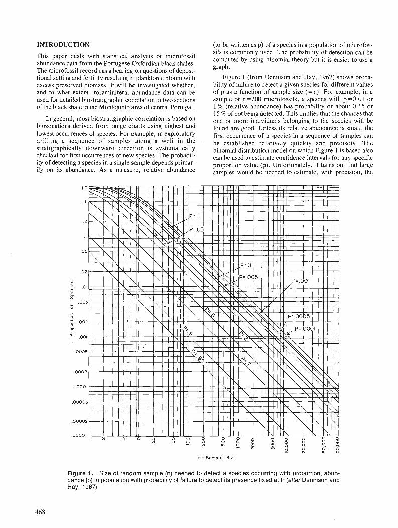
INTRODUCTION

This paper deals with statistical analysis of microfossil abundance data from the Portugese Oxfordian black shales. The microfossil record has a bearing on questions of depositional setting and fertility resulting in planktonic bloom with excess preserved biomass. It will be investigated whether, and to what extent, foraminifera] abundance data can be used for detailed biostratigraphic correlation in two sections of the black shale in the Montejunto area of central Portugal.

In general, most biostratigraphic correlation is based on biozonations derived from range charts using highest and lowest occurrences of species. For example, in exploratory drilling a sequence of samples along a well in the stratigraphically downward direction is systematically checked for first occurrences of new species. The probability of detecting a species in a single sample depends primarily on its abundance. As a measure, relative abundance

(to be written as p) of a species in a population of microfossils is commonly used. The probability of detection can be computed by using binomial theory but it is easier to use a graph.

Figure 1 (from Dennison and Hay, 1967) shows probability of failure to detect a given species for different values of p as a function of sample size (=n). For example, in a sample of n=200 microfossils, a species with p=0.01 or 1 % (relative abundance) has probability of about 0.15 or 15 % of not being detected. This implies that the chances that one or more individuals belonging to the species will be found are good. Unless its relative abundance is small, the first occurrence of a species in a sequence of samples can be established relatively quickly and precisely. The binomial distribution model on which Figure 1 is based also can be used to estimate confidence intervals for any specific proportion value (p). Unfortunately, it turns out that large samples would be needed to estimate, with precision, the

n = Sample Size

Figure 1. Size of random sample (n) needed to detect a species occurring with proportion, abundance (p) in population with probability of failure to detect its presence fixed at P (after Dennison and Hay, 1967)

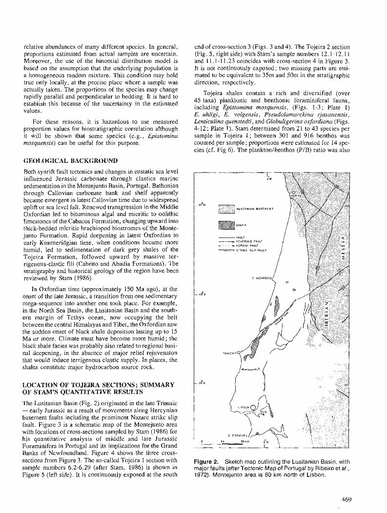
relative abundances of many different species. In general, proportions estimated from actual samples are uncertain. Moreover, the use of the binomial distribution model is based on the assumption that the underlying population is a homogeneous random mixture. This condition may hold true only locally, at the precise place where a sample was actually taken. The proportions of the species may change rapidly parallel and perpendicular to bedding. It is hard to establish this because of the uncertainty in the estimated values.

For these reasons, it is hazardous to use measured proportion values for biostratigraphic correlation although it will be shown that some species (e.g., Epistomina mosquensis) can be useful for this purpose.

GEOLOGICAL BACKGROUND

Both synrift fault tectonics and changes in eustatic sea level influenced Jurassic carbonate through clastics marine sedimentation in the Montejunto Basin, Portugal. Bathonian through Callovian carbonate bank and shelf apparently became emergent in latest Callovian time due to widespread uplift or sea level fall. Renewed transgression in the Middle Oxfordian led to bituminous algal and micritic to oolithic limestones of the Cabacos Formation, changing upward into thick-bedded micritic brachiopod biostromes of the Monte- junto Formation. Rapid deepening in latest Oxfordian to early Kimmeridgian time, when conditions became more humid, led to sedimentation of dark grey shales of the Tojeira Formation, followed upward by massive terrigenous-clastic fill (Cabrito and Abadia Formations). The stratigraphy and historical geology of the region have been reviewed by Stam (1986).

In Oxfordian time (approximately 150 Ma ago), at the onset of the late Jurassic, a transition from one sedimentary mega-sequence into another one took place. For example, in the North Sea Basin, the Lusitanian Basin and the southern margin of Tethys ocean, now occupying the belt between the central Himalayas and Tibet, the Oxfordian saw the sudden onset of black shale deposition lasting up to 15 Ma or more. Climate must have become more humid ; the black shale facies was probably also related to regional basinal deepening, in the absence of major relief rejuvenaton that would induce terrigenous clastic supply. In places, the shales constitute major hydrocarbon source rock.

LOCATION OF TOJEIRA SECTIONS; SUMMARY OF STAM'S QUANTITATIVE RESULTS

The Lusitanian Basin (Fig. 2) originated in the late Triassic - early Jurassic as a result of movements along Hercynian basement faults including the prominent Nazare strike slip fault. Figure 3 is a schematic map of the Montejunto area with locations of cross-sections sampled by Stam (1986) for his quantitative analysis of middle and late Jurassic Foraminifera in Portugal and its implications for the Grand Banks of Newfoundland. Figure 4 shows the three cross- sections from Figure 3. The so-called Tojeira 1 section with sample numbers 6.2-6.29 (after Stam, 1986) is shown in Figure 5 (left side). It is continuously exposed at the south

end of cross-section 3 (Figs. 3 and 4). The Tojeira 2 section (Fig. 5, right side) with Stam's sample numbers 12.1-12.1 1 and 11.1- 1 1.23 coincides with cross-section 4 in Figure 3. It is not continuously exposed; two missing parts are estimated to be equivalent to 35m and 50m in the stratigraphic direction, respectively.

Tojeira shales contain a rich and diversified (over 45 taxa) planktonic and benthonic foraminifera1 fauna, including Epistomina mosquensis, (Figs. 1-3; Plate 1) E. uhligi, E. volgensis, Pseudolamarckina rjasanensis, Lenticulina quenstedti, and Globuligerina oxfordiana (Figs. 4-12; Plate 1). Stam determined from 21 to 43 species per sample in Tojeira 1; between 301 and 916 benthos was counted per sample; proportions were estimated for 14 species (cf. Fig 6). The planktonlbenthos (PIB) ratio was also

Figure 2. Sketch map outlining the Lusitanian Basin, with major faults (after Tectonic Map of Portugal by Ribeiro et al., 1972). Montejunto area is 60 km north of Lisbon.

Plate 1.

Figs. 1-3. Epistomina mosquensis Uhlig, Tojeira 1 section, sample 6.10, Planula-Platynota Zones (Late Oxfordian-Early Kimmeridgian), XlOO (figs. 1, 2), XI10 (fig. 3), Figs. 4-12. Globuligerina oxfordiana Grigelis Tojeira 1 section, sample 6.24, XI70 (fig. 4); sample 6.11, XI45 (fig. 5); sample 6.21, XI40 (fig. 6); sample 6.20, XI70 (fig. 7); sample 6.14, X170 (figs. 8, 9); sample 6.11, XI50 (figs. 10, 11); sample 6.28, XI90 (fig. 12). All samples from the Platynota Zone (Early Kimmeridgian).

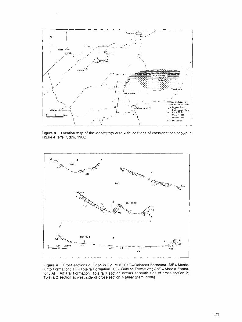
Figure 3. Location map of the Montejunto area with locations of cross-sections shown in Figure 4 (after Stam, 1986).

Figure 4. Cross-sections outlined in Figure 3; CaF = Cabacos Formaton; MF= Monte- junto Formation ; TF = Tojeira Formation ; CF = Cabrito Formation ; AbF = Abadia Forma- ton; AF=Amaral Formation. Tojeira 1 section occurs at south side of cross-section 2; Tojeira 2 section at west side of cross-section 4 (after Stam, 1986).

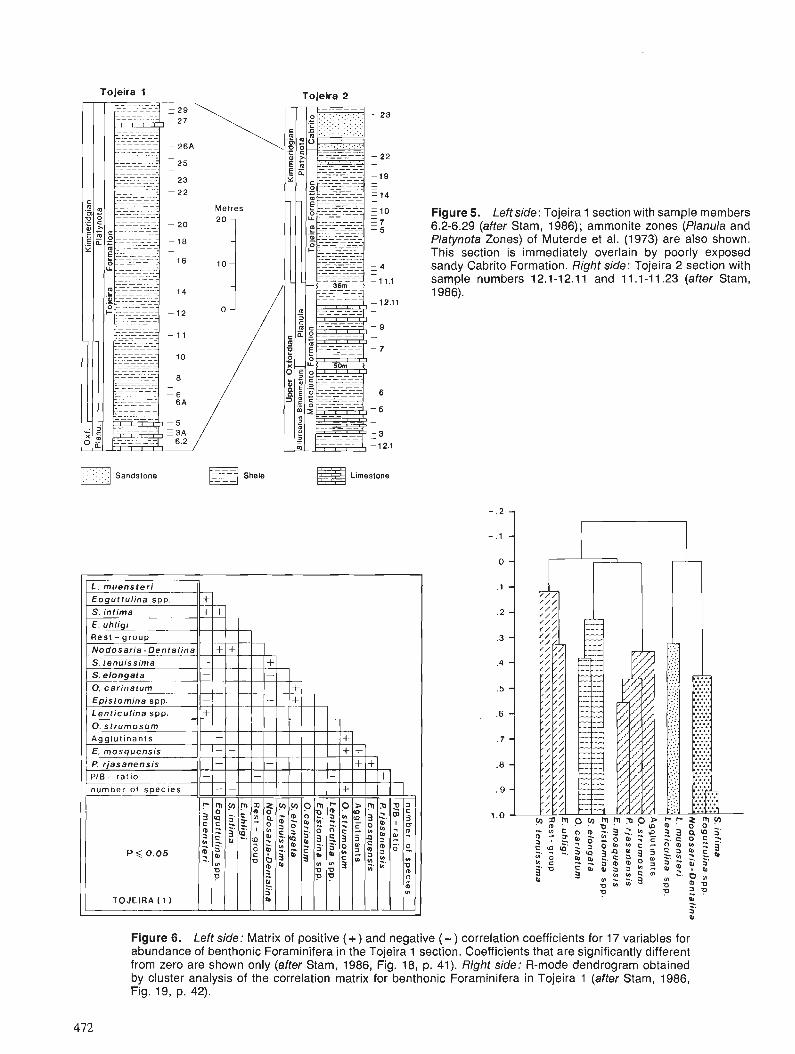
Tojeira 1 Toieira 2

Sandstone Shale Limestone

Figure 5. Leftside: Tojeira 1 section with sample members 6.2-6.29 (after Stam, 1986); ammonite zones (Planula and Platynofa Zones) of Muterde et al. (1973) are also shown. This section is immediately overlain by poorly exposed sandy Cabrito Formation. Right side: Tojeira 2 section with sample numbers 12.1-12.1 1 and 11 .l-11.23 (after Stam, 1986).

Figure 6. Left side: Matrix of positive (+) and negative ( - ) correlation coefficients for 17 variables for abundance of benthonic Foraminifera in the Tojeira 1 section. Coefficients that are significantly different from zero are shown only (after Stam, 1986, Fig. 18, p. 41). Right side: R-mode dendrogram obtained by cluster analysis of the correlation matrix for benthonic Foraminifera in Tojeira 1 (after Stam, 1986, Fig. 19, p. 42).

determined for each sample. Some quantitative results for the Tojeira 1 section due to Stam (1986) are shown in Fig- ure 6 . Correlation coefficients for the benthonic foraminifera are close to zero but several of these coefficients were shown to be significantly greater or less than zero (plus and minus signs in Fig. 6, left side). R- and Q- mode factor analysis and cluster analysis (Fig 6, right side) gave separate assemblages of mutually associated species. For example, the group with E. mosquensis, P. rjasanensis, 0, strumosum and agglutinants prefers the deep-water Tojeira shales to the underlying shallow-water Montejunto Formation. Similar results were obtained by Stam for the Tojeira 2 section.

ADDITIONAL SAMPLING AND NAZLI'S AUTOCORRELATION ANALYSIS

Two of us (Gradstein and Agterberg, 1982) had worked previously with highest occurrences of Foraminifera in offshore wells drilled on the Labrador Shelf and Grand Banks. The samples were cuttings obtained during exploratory drilling by oil companies. Such samples are small, taken over large intervals and subject to down-hole contamination

Tojeira 1 Tojeira 2

0 Sandstone Shale Limestone

Figure 7. Left side: Tojeira 1 section with sample numbers T111-TI I17 obtained by the authors in 1986. Seven samples where taken at sites previously sampled by Stam (cf., Fig. 5). The sandy Cabrito Formation (poorly exposed) immediately overlies the upper shales in Tojeira 1. Right side: Tojeira 2 section with sample numbers T2/1 -T2/13 collected by Grad- stein and Nazli in 1986. Eleven samples were taken at sites previously sampled by Stam (cf., Fig. 6).

so that only highest occurrences (not lowest occurrences) of Foraminifera can be determined. These problems associated with exploratory drilling can be avoided on land if continuous outcrop sampling is possible. According to paleogeo- graphic reconstructions (Stam, 1986), the Lusitanian and Grand Banks basins were close to one another during the Jurassic and had comparable sedimentary, tectonic and faunal history. On land continuous outcrop sampling can be undertaken only in the Lusitanian Basin.

After preliminary statistical autocorrelation analysis of Stam's data, the authors collected new samples from the two Tojeira sections during summer 1988 (Fig. 7). One of us (FMG) identified the foraminifera1 taxa. Only relatively few samples were taken at exactly the same places where Stam had sampled before. Figures 8 and 9 show typically poor correlations between proportions estimated from Stam's and Gradstein's counts for species in samples taken at the same spots. These scattergrams reflect random (binomial) counting errors, local spatial variability of the (unknown) mean proportion values, as well as possible determination errors. In another sampling experiment, five samples were taken laterally at 5m interval from the same stratigraphic horizon at the base of Tojeira 1. Estimated proportion values as well as total benthos counted for these 5 samples are shown in Table 1. The measured proportions are markedly different, again illustrating the uncertainty commonly associated with microfossil abundance data.

0 .;.-.. ; 0 5 10

8 0; 15 0 10 20 30 40

0. strumosum S. tenuissima

1: . ; 0 - I 1 0-7-8 8 1

0 5 10 15 0 10 20 30 40 Eogultulina spp. E. mosquensis

Figure 8. Proportions of four benthonic Foraminifera for seven replicate samples from same sites in Tojeira 1 section based on determinations by Stam (horizontal axis) and Gradstein (vertical axis). See test for discussion of lack of agreement (cf., Fig. 7 for locations and Table 3 for sample sizes).

18 -

15-

- S w

g 10- .- - B P g

5 -

40 -

30 -

20-

10-

.

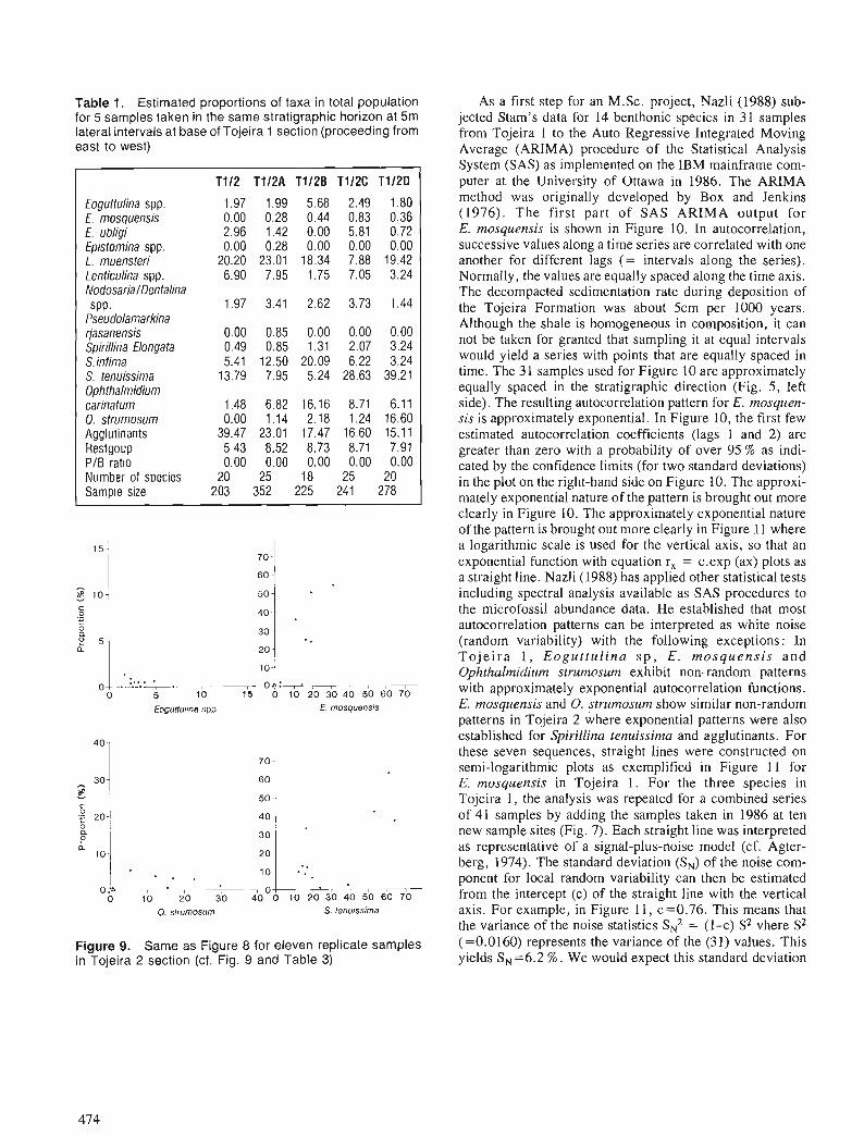
Table 1. Estimated proportions of taxa in total population for 5 samples taken in the same stratigraphic horizon at 5m lateral intervals at base of Tojeira 1 section (proceeding from east to west)

TI12 T112A T112B T112C T112D

Eogunulina spp. 1.97 1.99 5.68 2.49 1.80 E, mosquensis 0.00 0.28 0.44 0.83 0.36 E, ubligi 2.96 1.42 0.00 5.81 0.72 Epistomina spp. 0.00 0.28 0.00 0.00 0.00 I . muensteri 20.20 23.01 18.34 7.88 19.42 Lenticulina spp. 6.90 7.95 1.75 7.05 3.24 NodosarialDentalina SPP. 1.97 3.41 2.62 3.73 1.44

Pseudolamarkina rjasanensis 0.00 0.85 0.00 0.00 0.00 Spirillina Elongata 0.49 0.85 1.31 2.07 3.24 S. infima 5.41 12.50 20.09 6.22 3.24 S. tenuissima 13.79 7.95 5.24 28.63 39.21 Ophthalmidium carinatum 1.48 6.82 16.16 8.71 6.11 0. strumosum 0.00 1.14 2.18 1.24 16.60 Agglutinants 39.47 23.01 17.47 16.60 15.11 Restgoup 5.43 8.52 8.73 8.71 7.91 PIB ratio 0.00 0.00 0.00 0.00 0.00 Number of species 20 25 18 25 20 Sample size 203 352 225 241 278

, o$: , ' , , , , , , 0 5 10 15 0 10 20 3 0 4 0 50 60 70

Eoguttul~na s p ~ E, mosquensis

I ;. . , . OC- ,lOL 0 0 10 20 30 40 0 10 20 30 40 50 60 70

0. strumosum S. tenurssima

Figure 9. Same as Figure 8 for eleven replicate samples in Tojeira 2 section (cf. Fig. 9 and Table 3)

As a first step for an M.Sc. project, Nazli (1988) subjected Stam's data for 14 benthonic species in 31 samples from Tojeira 1 to the Auto Regressive Integrated Moving Average (ARIMA) procedure of the Statistical Analysis System (SAS) as implemented on the IBM mainframe computer at the University of Ottawa in 1986. The ARIMA method was originally developed by Box and Jenkins (1976). The first part of SAS ARIMA output for E. mosquensis is shown in Figure 10. In autocorrelation, successive values along a time series are correlated with one another for different lags (= intervals along the series). Normally, the values are equally spaced along the time axis. The decompacted sedimentation rate during deposition of the Tojeira Formation was about 5cm per 1000 years. Although the shale is homogeneous in composition, it can not be taken for granted that sampling it at equal intervals would yield a series with points that are equally spaced in time. The 31 samples used for Figure 10 are approximately equally spaced in the stratigraphic direction (Fig. 5 , left side). The resulting autocorrelation pattern for E. mosquensis is approximately exponential. In Figure 10, the first few estimated autocorrelation coefficients (lags 1 and 2) are greater than zero with a probability of over 95 % as indicated by the confidence limits (for two standard deviations) in the plot on the right-hand side on Figure 10. The approximately exponential nature of the pattern is brought out more clearly in Figure 10. The approximately exponential nature of the pattern is brought out more clearly in Figure 11 where a logarithmic scale is used for the vertical axis, so that an exponential function with equation r, = c.exp (ax) plots as a straight line. Nazli (1988) has applied other statistical tests including spectral analysis available as SAS procedures to the microfossil abundance data. He established that most autocorrelation patterns can be interpreted as white noise (random variability) with the following exceptions: In Tojeira 1 , Eoguttul ina s p , E. mosquensis and Ophthalmidium strumosum exhibit non-random patterns with approximately exponential autocorrelation functions. E. mosquensis and 0. strumosum show similar non-random patterns in Tojeira 2 where exponential patterns were also established for Spirillina tenuissima and agglutinants. For these seven sequences, straight lines were constructed on semi-logarithmic plots as exemplified in Figure 11 for E. mosquensis in Tojeira 1. For the three species in Tojeira 1, the analysis was repeated for a combined series of 41 samples by adding the samples taken in 1986 at ten new sample sites (Fig. 7). Each straight line was interpreted as representative of a signal-plus-noise model (cf. Agter- berg, 1974). The standard deviation (SN) of the noise component for local random variability can then be estimated from the intercept (c) of the straight line with the vertical axis. For example, in Figure 11, c=0.76. This means that the variance of the noise statistics SN2 = (I-C) S2 vhere S2 (=0.0160) represents the variance of the (31) values. This yields SN =6.2 %. We would expect this standard deviation

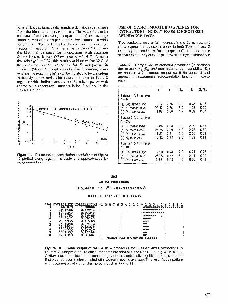
to be at least as large as the standard deviation (SB) arising USE OF CUBIC SMOOTHING SPLINES FOR from the binomial counting process. The value SB can be EXTRACTING "NOISE" FROM MICROFOSSIL estimated from the average proportion (=p) and average ABUNDANCE DATA number (=a) of counts per sample. For example, H=443 for Stam's 3 1 Tojeira 1 samples; the corresponding average proportion value for E. mosquensis is p=22.5 %. From the binomial variance for proportions with equation s2 ,-p(1-@/Ti, -- it then follows that SB= 1.98 %. Because the ratio SB/SN=0.32, this result would mean that 32 % of the measured random variability for E, mosquensis in Tojeira 1 (Stam's 3 1 samples only) is due to counting errors whereas the remaining 68 % can be ascribed to local random variability in the rock. This result is shown in Table 2 together with similar statistics for the other species with approximate exponential autocorrelation functions in the Tojeira sections.

.- C

E. mosquensis (N=3 1 )

lag x

Figue 11. Estimated autocorrelation coefficients of Figure 10 plotted along logarithmic scale and approximated by exponential function.

Two benthonic species (E. mosquensis and 0. strumosum) show exponential autocorrelations in both Tojeira 1 and 2 and are good candidates for attempts to filter out the noise in order to retain systematic patterns of change of abundance

Table 2. Comparison of standard deviations (in percent) due to counting (S,) and total local random variability (S,) for species with average proportion j5 (in percent) and approximate exponential autocorrelation function r, = c.exp (-ax)

P c SN SB SBISN Tojeira 1 (31 samples; n=443) (a) Eoguttulina spp. 2.77 0.76 2.2 0.78 0.36 (b) E. mosquensis 22.47 0.76 6.2 1.98 0.32 (c) 0. strumosum 1.93 0.50 1.7 0.59 0.34

Tojeira 2 (30 samples; ii=250) (a)E.mosquensis 13.84 0.88 3.8 2.19 0.57 (b) S. tenuissima 25.75 0.90 5.5 2.76 0.50 (c) 0. strumosum 11.25 0.91 2.8 2.00 0.71 (d) Agglutinants 10.42 0.58 3.2 1.93 0.61

Tojeira 1 (41 samples; ii=408) (a) Eoguttulina spp. 2.20 0.48 2.9 0.71 0.25 (b) E. mosquensis 23.76 0.52 8.4 2.11 0.25 (c) 0. strumosum 2.39 0.60 1.8 0.76 0.41

A R M PROCEDURE

T o j e i r a 1: E. m o s q u e n s i s

I A G COVARIANCE CORRELATION 0 160.079 1.00000 1 79.9485 0.49943 2 85.2347 0.53245

1 9 0 7 6 5 4 3 2 1 0 1 2 3 4 5 6 7 8 9 1 . * * * * * * * * t * * * * * * t * * l ****.**ttt

**.******** .I.*.** . t*.. a*. * * . t*

t . C t t ** . MARKS'TWO STPNDARD ERRORS

Figure 10. Partial output of SAS ARlMA procedure for E. mosquensis proportions in Stam's 31 samples from Tojeira 1 (for complete print-out, see Nazli, 198, Fig. 4-12, p. 98). ARlMA maximum likelihood estimation gave three statistically significant coefficients for first order autocorrelation coupled with two-term moving average. This result is compatible with assumption of signal-plus-noise model in Figure 11.

in the stratigraphic direction which may be useful for biostratigraphic correlation. E. mosquensis was selected for further work because it is relatively abundant throughout the entire shale section of Tojeira 1 and 2 whereas 0. strumosum is nonexistent or rare in the lower half of the Tojeira Formation.

Various statistical methods are available for elimination of noise from data. These include curve-fitting using polynomial or Fourier series, geostatistical "Kriging", signal extraction as in statistical theory of communication, and construction of smoothing splines. A variant of the latter technique will be used here because it is particularly well suited for coping with the problem of irregular sampling intervals is one dimension.

Figure 12 illustrates the concepts of interpolation and smoothing spline functions. Although splines of higher and lower orders can be constructed, the third-order or cubic spline seems to be optimum in our kind of application (see later). Spline functions have a long history of use for interpolation; e.g., in numerical integration. Their use for

Figure 12. Schematic diagrams of cubic interpolation spline (Fig. 12A) and cubic smoothing spline (Fig. 128). The cubic polynomials between successive knots have continuous first and second derivatives at the knots. The smoothing factor (SF) is zero for interpolation splines. In our applications, the abscissae of the knots coincide with those of the data points.

smoothing is a relatively recent development which commenced in the late 1960s after the discovery of smoothing splines by Schoenberg (1964) and Reinsch (1967). Whit- taker (1923) had proposed an early variant.

The interpolation spline curve passes through all (n) observed values. Along the curve, there are a number of knots where various derivatives of the spline function are forced to be continuous. In the example of Figure 12, the knots coincide with the data points. A separate cubic polynomial with 4 coefficients is computed for each interval between successive data points. These cubics must have continuous first and second derivatives. After setting the second derivative equal to zero at the first and last data points, the continuity constraints yield so many conditions, that all (4n-4) coefficients can be computed. Smoothing splines have the same properties as interpolation spline except that they do not pass through the data points. Instead of this, they deviate from the observed values by an amount that can be regulated by means of the smoothing factor (SF) representing the average mean squared deviation.

For each specific value of SF, which can be set in advance, or estimated by cross-validation (Agterberg and Gradstein, 1988), a single smoothing spline is obtained. In his recent book on spline smoothing and non-parametric regression, Eubank (1988, e.g., p. 153) discusses that unequally spaced data points may give poor results for smoothing splines. De Boor (1978) pointed this out for interpolation splines. In order to avoid results obtained by following cubic smoothing splines to biostratigraphic data for constructing age-depth curves, Agterberg et al. (1985) proposed a simple "indirect" method. The age data in this approach have relatively large errors while the depths are irregularly spaced. First, a cubic spline is fitted to the ages using relative depths (levels) at a regular interval instead of the actual, irregularly spaced depth measurements. For this purpose the actual depth levels are equally spaced with interval distance set equal to unity.

A separate spline is fitted to the depth measurements along a depth scale, but expressing them as a monotonically increasing function of level. In practice this second curve is nearly an interpolation spline. Combination of the two curves, accompanied by further smoothing if required, yields the final cubic spline for the age-depth relationship. This result is not subject to unrealistic oscillations as may arise in data gaps if a spline-curve is directly fitted to the data. In this paper, the indirect method will be applied to our microfossil abundance data. These data show increases as well as decreases in the stratigraphic direction; oscillations due to irregular spacing in the stratigraphic direction arise even more frequently than in age-depth curve applications for which the spline-curves must be monotonically increasing with age and depth.

The following experiment with interpolation splines illustrates how the problem of unrealistic oscillations can be avoided, using the indirect method. It should be kept in mind that the problem of oscillations in data gaps becomes even

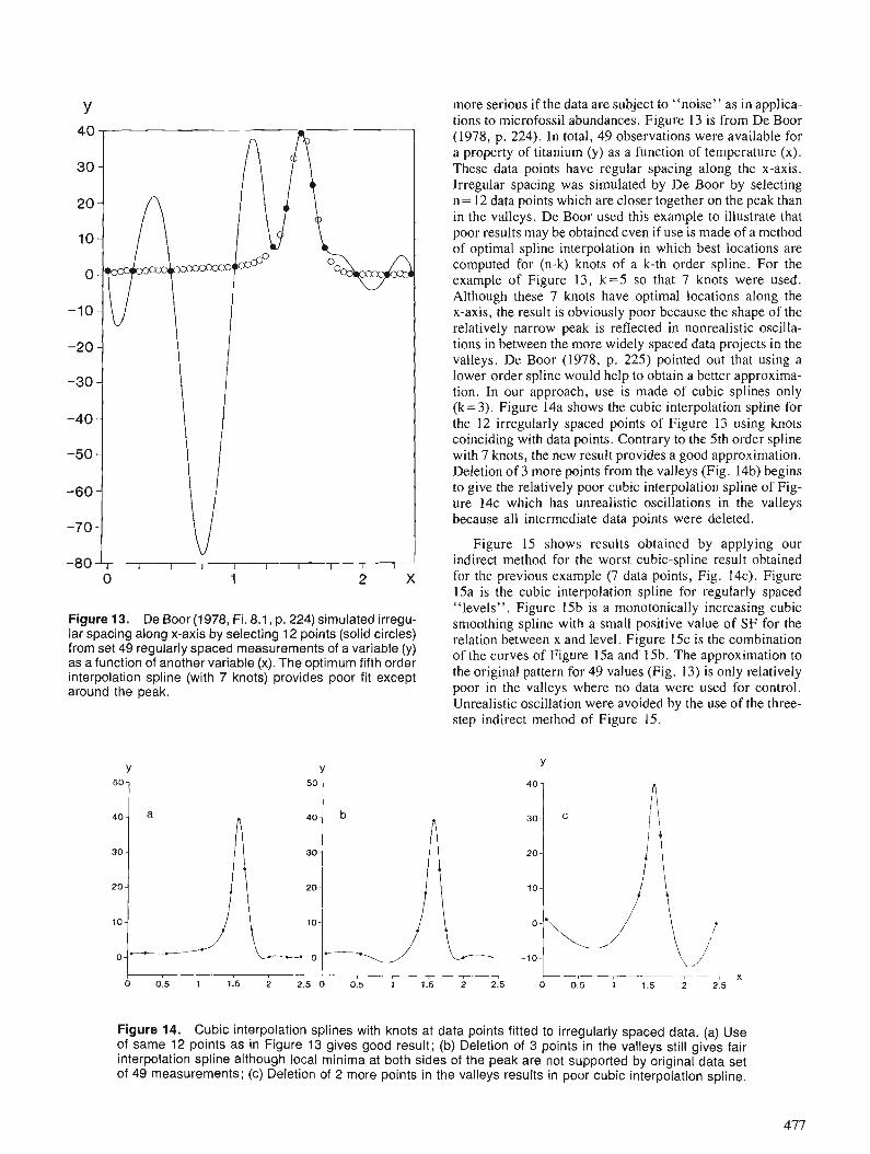
Figure 13. De Boor (1978, Fi. 8.1, p. 224) simulated irregular spacing along x-axis by selecting 12 points (solid circles) from set 49 regularly spaced measurements of a variable (y) as a function of another variable (x). The optimum fifth order interpolation spline (with 7 knots) provides poor fit except around the peak.

more serious if the data are subject to "noise" as in applications to microfossil abundances. Figure 13 is from De Boor (1978, p. 224). In total, 49 observations were available for a property of titanium (y) as a function of temperature (x). These data points have regular spacing along the x-axis. Irregular spacing was simulated by De Boor by selecting n= 12 data points which are closer together on the peak than in the valleys. De Boor used this example to illustrate that poor results may be obtained even if use is made of a method of optimal spline interpolation in which best locations are computed for (n-k) knots of a k-th order spline. For the example of Figure 13, k=5 so that 7 knots were used. Although these 7 knots have optimal locations along the x-axis, the result is obviously poor because the shape of the relatively narrow peak is reflected in nonrealistic oscillations in between the more widely spaced data projects in the valleys. De Boor (1978, p. 225) pointed out that using a lower-order spline would help to obtain a better approximation. In our approach, use is made of cubic splines only (k=3). Figure 14a shows the cubic interpolation spline for the 12 irregularly spaced points of Figure 13 using knots coinciding with data points. Contrary to the 5th order spline with 7 knots, the new result provides a good approximation. Deletion of 3 more points from the valleys (Fig. 14b) begins to give the relatively poor cubic interpolation spline of Fig- ure 14c which has unrealistic oscillations in the valleys because all intermediate data points were deleted.

Figure 15 shows results obtained by applying our indirect method for the worst cubic-spline result obtained for the previous example (7 data points, Fig. 14c). Figure 15a is the cubic interpolation spline for regularly spaced "levels". Figure 15b is a monotonically increasing cubic smoothing spline with a small positive value of SF for the relation between x and level. Figure 15c is the combination of the curves of Figure 15a and 15b. The approximation to the original pattern for 49 values (Fig. 13) is only relatively poor in the valleys where no data were used for control. Unrealistic oscillation were avoided by the use of the three- step indirect method of Figure 15.

Figure 14. Cubic interpolation splines with knots at data points fitted to irregularly spaced data. (a) Use of same 12 points as in Figure 13 gives good result; (b) Deletion of 3 points in the valleys still gives fair interpolation spline although local minima at both sides of the peak are not supported by original data set of 49 measurements; (c) Deletion of 2 more points in the valleys results in poor cubic interpolation spline.

BIOSTRATIGRAPHIC CORRELATION BETWEEN TOJEIRA 1 AND 2 SECTIONS USING E. MOSQUENSlS AND P/B RATIO

Table 3 shows sequences of samples (combined Stam and Nazli data) for the Tojeira 1 and 2 sections. Distances in the stratigraphic direction are given in metres measuring downward from Stam's stratigraphically highest samples with microfossil abundance data for the Tojeira Formation (No. 6.29 in Tojeira 1 and No. 11.19 in Tojeira 2) closest to the base of the overlying Cabrito Formation. No. 6.29 was taken just below the base of the Cabrito Formation and No. 11.19 about 6m below this base. It is noted that 3 samples taken by Stam in Tojeira 2 above 11.19 (cf. Fig. 5 , right side) contained too few Foraminifera for abundance data to be determined. Abundance data for E. mosquensis, and the PIB ratio are given in Table 3. The last two columns of Table 3 contain transformed values used for statistical analysis. As shown in Nazli (1988), Tojeira microfossil abundances are normalized when the probit transformation is applied. The transformation applied to P/B ratio is 2+loglo (P/B+O. 10). The purpose of the latter expression is to reduce the relative influence of both relatively high and low values. Such "normalization" is desirable because smoothing splines are fitted by using the method of least squares in which the influence of each deviation from the curve increases according to the square of its magnitude. The smoothing factor (SF) should not be mainly determined by relatively few values only.

Results for the indirect method applied to E. mosquensis in Tojeira 1 and 2 are shown in Figures 16 and 17, respectively. The two spline-curves were slid with respect to one another until a "best" fit was found (fig. 18). A 10m downward movement of the Tojeira 2 sequence, which places,the base of the overlying Cabrito Formation in nearly the same

Toje i ra 1 sect ion E. mosquensis

Figure 16. Indirect method of cubics~line-fitting illustrated in Figure 15 applied to probits of E. mosquensis abundance data for Tojeira 1 (see Table 3 for original data).

LEVEL LEVEL

Figure 15. Indirect method of cubic spline-fitting proposed by Agterberg et al. (1985) applied to 7 data points in Figure 14c. (a) The six intervals along the x-axis between data points were made equal before calculation of cubic interpolation spline; (b) Non-decreasing cubic spline with small positive value of smoothing factor (SF= 0.038) was fitted to interval as function of "levels"; (c) Curves of (a) and (b) were combined with one another and re-expressed as cubic spline function which does not show the unrealistic fluctuations of the cubic interpolation spline of Figure 14c.

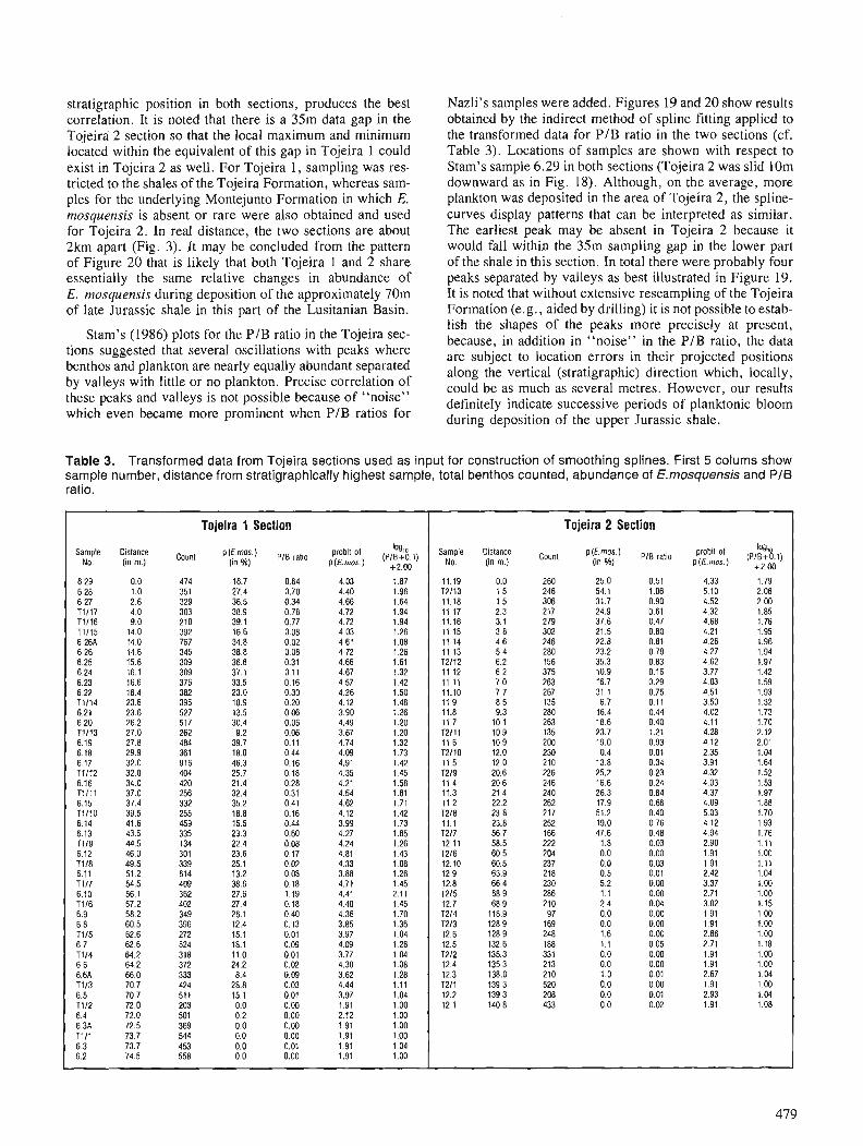
stratigraphic position in both sections, produces the best correlation. It is noted that there is a 35m data gap in the Tojeira 2 section so that the local maximum and minimum located within the equivalent of this gap in Tojeira 1 could exist in Tojeira 2 as well. For Tojeira 1, sampling was restricted to the shales of the Tojeira Formation, whereas samples for the underlying Montejunto Formation in which E. mosquensis is absent or rare were also obtained and used for Tojeira 2. In real distance, the two sections are about 2km apart (Fig. 3). It may be concluded from the pattern of Figure 20 that is likely that both Tojeira 1 and 2 share essentially the same relative changes in abundance of E, mosquensis during deposition of the approximately 70m of late Jurassic shale in this part of the Lusitanian Basin.

Stam's (1986) plots for the P/B ratio in the Tojeira sections suggested that several oscillations with peaks where benthos and plankton are nearly equally abundant separated by valleys with little or no plankton. Precise correlation of these peaks and valleys is not possible because of "noise" which even became more prominent when P/B ratios for

Nazli's samples were added. Figures 19 and 20 show results obtained by the indirect method of spline fitting applied to the transformed data for PIB ratio in the two sections (cf. Table 3). Locations of samples are shown with respect to Stam's sample 6.29 in both sections (Tojeira 2 was slid 10m downward as in Fig. 18). Although, on the average, more plankton was deposited in the area of Tojeira 2, the spline- curves display patterns that can be interpreted as similar. The earliest peak may be absent in Tojeira 2 because it would fall within the 35m sampling gap in the lower part of the shale in this section. In total there were probably four peaks separated by valleys as best illustrated in Figure 19. It is noted that without extensive reseampling of the Tojeira Formation (e.g., aided by drilling) it is not possible to establish the shapes of the -peaks more precisely at present, because, in addition in "noise" in the P/B ratio, the data are subject to location errors in their projected positions along the vertical (stratigraphic) direction which, locally, could be as much as several metres. However, our results definitely indicate successive periods of planktonic bloom during deposition of the upper Jurassic shale.

Table 3. Transformed data from Tojeira sections used as input for construction of smoothing splines. First 5 colums show sample number, distance from stratigraphically highest sample, total benthos counted, abundance of E.mosquensis and P I 6 ratio.

Tojeira 1 Section

count ~$27) pie mtio (P/~%,I) No. (in rn.) +2.00

6.29 0.0 474 16.7 0.64 4.03 1.87 6.28 1 .O 351 27.4 0.70 4.40 1.96 6.27 2.6 329 36.5 0.34 4.66 1.64 TI117 4.0 303 38.9 0.78 4.72 1.94 TI116 9.0 210 39.1 0.77 4.72 1.94 TI115 14.0 392 16.6 0.08 4 03 1 26 6 26A 14.0 767 34.8 0.02 4.61 1.08 6.26 14.6 345 38.8 0.08 4.72 1.26 6.25 15.6 309 36.6 0.31 4.66 1.61 6.24 16.1 309 37.1 0.11 4.67 1.32 6.23 16.6 376 33.5 0.16 4 57 1.42 6.22 18.4 382 23.0 0.30 4.26 1.50 T1114 23.6 396 18.9 0 20 4.12 1.48 6.21 23.6 527 13.5 0.06 3.90 1.26 6.20 26.2 517 30.4 0.06 4.49 1.20 11/13 27.0 262 9.2 0.06 3.67 1.20 6.19 27.8 484 39.7 0.11 4.74 1.32 6.18 29.9 361 18.0 0.44 4.09 1.73 6.17 32.0 916 46.3 0.16 4.91 1.42 Ti112 32.0 404 25.7 0 18 4.35 1.45 6.16 34.0 420 21.4 0.28 4.21 1.58 Ti111 37.0 256 32.4 0.31 4.54 1.61 6.15 37.4 332 35.2 0.41 4.62 1.71 T1l10 39.5 255 18.8 0.16 4.12 1.42 6.14 41.6 459 15.5 0.44 3.99 1.73 6.13 43.6 335 23.3 0.60 4.27 1.85 1119 44.5 134 22.4 0.08 4.24 1.26 6 12 46.0 301 23.6 0.17 4.81 1.43 Ti18 49.5 339 25.1 0.02 4.33 1.08 6.11 51.2 614 13.2 0.08 3.88 1.26 Ti17 54.5 409 38.6 0.18 4.71 1.45 6.10 56.1 362 27.6 1.19 4.41 2.11 TI16 57.2 402 27.4 0.18 4.40 1.45 6.9 58.2 349 26.1 0.40 4.36 1.70 6.8 60.5 396 12.4 0.13 3.85 1.36 Ti15 62.6 272 15.1 0.01 3.97 1.04 6 7 62.6 524 18.1 0.09 4.09 1.28 Ti14 64.2 318 11.0 0.01 3.77 1.04 6.6 64.2 372 24 2 0.02 4.30 1.08

333 8.4 0.09 3.62 1.28 424 28.8 0.03 4.44 1.11 51 1 15.1 0.01 3.97 1.04 203 0.0 0.00 1.91 1.00 501 0.2 0.00 2.12 1.00

72.5 369 0.0 0.00 1.91 1.00 73.7 544 0.0 0.00 1.91 1.00 73.7 453 0.0 0.01 1.91 1.04 74.5 558 0.0 0.00 1.91 1.00

Tojeira 2 Section

loo,, S$y ! Count Pf,,TT) PIB ratio ! ) (PlB10.1) +2.00

11.19 0.0 260 25.0 0.51 4.33 1.79 T2113 1.5 246 54.1 1.06 5.10 2.06 11.18 1.5 306 31.7 0.90 4.52 2.00 11.17 2.3 217 24.9 0.61 4.32 1.85 11.16 3.1 279 37.6 0.47 4.68 1.76 11 15 3.8 302 21 5 0.80 4.21 1.95 11.14 4.6 246 22.8 0.81 4.26 1.96 11.13 5.4 280 23.2 0.78 4.27 1.94 T2112 6.2 156 35.3 0.83 4.62 1.97 11.12 6.2 375 10.9 0.16 3.77 1.42 11.11 7.0 263 16.7 0.29 4.03 1.59 11.10 7.7 267 31.1 0.75 4.51 1.93 11.9 8.5 135 6.7 0.11 3.50 1.32 11.8 9.3 280 16.4 0.44 4.02 1.73 11.7 10.1 2 63 18.6 0.40 4.11 1.70 T2111 10.9 135 23.7 1.21 4.28 2.12 11.6 10.9 200 19.0 0.93 4.12 2.01 T2110 12.0 230 0.4 0.01 2.35 1.04 11.5 12.0 210 13.8 0.34 3.91 1.64 T219 20.6 226 25.2 0.23 4.32 1.52 11.4 20.6 246 16.6 0 24 4.03 1.53 11.3 21.4 240 26.3 0.84 4.37 1.97 11.2 22.2 262 17.9 0.66 4.09 1.88 T218 23.8 217 51.2 0 40 5 03 1 70 11.1 23.8 252 19.0 0.76 4.12 1.93 T217 56.7 166 47.6 0 48 4.94 1 76 12.11 58.5 222 1.8 0.03 2.90 1.11 T216 60.5 204 0.0 0.00 191 1.00 12.10 60.5 237 0.0 0.03 1.91 1.11 12.9 63.9 218 0.5 0.01 2.42 1.04 12.8 66.4 230 5.2 0.00 3.37 1.00 T215 68.9 286 1.1 0.00 2.71 1 .OO 12.7 68.9 210 2.4 0.04 3.02 1.15 T214 118.9 97 0.0 0.00 191 1 00 T2/3 128.9 169 0.0 0.00 1.91 1.00 12.6 128.9 248 1.6 0.00 2.86 1.00 12.5 132.6 188 1.1 0 05 2.71 1.18 T2/2 135.3 331 0.0 0.00 1.91 1.00 12.4 135.3 213 0.0 0.00 1.91 1 00 12.3 138.0 210 1.0 0.01 2.67 1.04 T2H 139 3 520 0.0 0 00 1.91 1.00 12.2 139.3 208 0.0 0.01 2.93 1.04 12.1 140 8 433 0.0 0.02 1.91 1.08

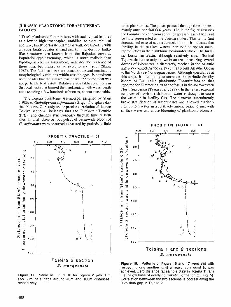
JURASSIC PLANKTONIC FORAMINIFERAL BLOOMS

"True" planktonic Foraminifera, with such typical features as a low to high trochospire, umbilical to extraumbilical aperture, finely perforate bilamellar wall, occasionally with an imperforate equatorial band and kummer-form or bulla- like structures are known from the Bajocian onward. Population-type taxonomy, which is more realistic than typological species assignment, indicates the presence of three taxa, but limited or no evolutionary trends (Stam, 1986). The fact that there are considerable and continuous morphological variations within assemblages, is consistent with the idea that the surface marine water environment was not particularly stresfull. Relatively equitable conditions in the local basin that housed the planktonics, with water depth not exceeding a few hundreds of metres, appear reasonable.

The Tojeira planktonic assemblage, assigned by Stam (1986) to Globuligerina oxfordiana (Grigelis) displays distinct blooms. Our study on the precise correlation of the two Tojeira sections, indicates that the PlanktonicIBenthic (PIB) ratio changes synchronously through time at both sites. In total, three or four pulses of basin-wide bloom of G. oxfordiana were observed deparated by periods of little

Tojeira 2 section E. mosquensis

Figure 17. Same a s Figure 16 for Tojeira 2 with 35m and 50m data gaps around 40m and lOOm distances, respectively.

or no planktonics. The pulses proceed through time approximately once per 500 000 years. The latter figure assumes the Planula and Platynota zones to represent each 1 Ma, and be fully represented in the Tojeira shales. This is the first documented case of such a Jurassic bloom. It indicates that fertility in the surface waters increased to spawn mass- reproduction in the planktonic foraminifer stock. The Juras- sic Lusitanian Basin, although relatively small (basinal Tojeira shales are only known in an area measuring several dozens of kilometres in diameter), reached in the Atlantic gateway connecting the early central North Atlantic Ocean to the North Sea-Norwegian basins. Although speculative at this stage, it is tempting to correlate the periodic fertility bloom of Lusitanian planktonic Foraminifera to that reported for Kimmeridgian nannofossils in the southwestern North Sea basins (Tyson et al., 1979). In the latter, seasonal turnover of nutrient-rich bottom water is thought to cause ., the variation in fertility flux. The turnover intermittently broke stratification of watermasses and allowed nutrient- rich bottom water in a relatively anoxic basin to mix with surface water and cause blooming of planktonic biomass.

Tojeira 1 and 2 sections E. mosquens is

Figure 18. Patterns of Figure 16 and 17 were slid with respect to one another until a reasonably good fit was achieved. Zero distance (at sample 6.29 in Tojeira 1) falls just below base of overlying Cabrito Formation (cf. Fig. 5). Correlation betwween the two sections is poorest along the 35m data gap in Tojeira 2.

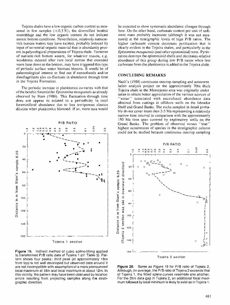
Tojeira shales have a low organic carbon content as measured in few samples (<0 ,5 %); the diversified benthic assemblage and the low organic content do not indicate anoxic bottom conditions. Nevertheless, relatively nutrient- rich bottom waters may have existed, probably induced by input of terrestrial organic material that is abundantly present in palynological preparations of Tojeira shale. Turnover of nutrient-rich bottom waters, for whatever reason, e.g. windstress induced after rare local storms that extended wave base down to the bottom, may have triggered this type of periodic surface water biomass blooms. It would be of paleontological interest to find out if nannofossils and/or dinoflagellates also co-fluctuate in abundance through time in the Tojeira Formation.

The periodic increase in planktonics co-varies with that of the benthic foraminifer Epistomina mosquensis as already observed by Stam (1986). This fluctuation through time does not appear to related to a periodicity in total foraminifera1 abundance due to less terrigenous clastics dilution when planktonics bloomed. If so, more taxa would

PIB RATIO

Tojeira 1 section

Figure 19. Indirect method of cubic spline-fitting applied to transformed P/B ratio data of Tojeira 1 (cf. Table 3). Pat- tern shows four peaks; third peak (at approximately 18m from top) is not well developed but observed data around it are not incompatible with assumption of a more pronounced local maximum at 18m and local maximum at about 12m. In this vicinity, the pattern may have been obscured by location errors resulting from projecting samples along the stratigraphic direction.

be expected to show systematic abundance changes through time. On the other hand, carbonate content per unit of sediment mass probably increases (although it was not measured) at the stratigraphic levels of hign PIB ratios. The higher carbonate content decreases pyritization that is clearly evident in the Tojeira shales, and particularly in the Epistomina mosquensis (and other epistominid) tests. Pyriti- zation destroys the epistominid shells and decreases relative abundance of this group during low PIB ratios when less carbonate from the planktonics is added to the Tojeira shale.

CONCLUDING REMARKS

Nazli's (1988) continuous outcrop sampling and autocorrelation analysis project on the approximately 70m thick Tojeira shale in the Montejunto area was originally undertaken to obtain better appreciation of the various sources of "noise" associated with microfossil abundance data obtained from cuttings in offshore wells on the labrador Shelf and Grand Banks. The rocks sampled in detail probably do not cover more than 2-3 Ma representing a relatively narrow time interval in comparison with the approximately 150 Ma time span covered by exploratory wells on the Grand Banks. The problem of observed versus "true" highest occurrences of species in the stratigraphic column could not be studied because continuous outcrop sampling

P I B RATIO

Tojeira 2 section

Figure 20. Same as Figure 19 for P I 8 ratio of Tojeira 2. Although, on average, the P/B ratio of Tojeira2 exceeds that of Tojeira 1, the fitted spline-curves resemble one another. For the 35m data gap in Tojeira 2, an additional local maximum followed by local minimum is likely to exist as in Tojeira 1.

of the equivalent of a longer time interval would be needed for this. By means of the detailed sampling of the Tojeira Formation using Stam's (1986) data augmented by new information, followed by autocorrelation analysis, it was possible to separate variance of microfossil abundance data into three distinct parts : (1) binomial counting error related to limited number of counts; (2) other white "noise" due to local random variability ; and (3) "signals" representing systematic changes of abundance in the stratigraphic direction.

In this paper, the signals were extracted from E. mosquensis yield similar patterns for Tojeira 1 and 2 moving downward from the base of the overlying Cabrito Forma- tion. Skrinking or stretching of the sections with respect to one another was not required. The biostratigraphic correlation and chronostratigraphic framework earlier established by means of ammonites were confirmed by the E. mosquensis abundance data.

Precise correlation is of importance to check whether the observed strong P/B ratio changes in the Tojeira Formation were synchronous. In total, four pulses of basin-wide blooms of primitive planktonic foraminifera were indicated by signal extraction applied to the transformed P/B ratio values. This is the first documented case of such a Jurassic bloom. Tyson et al. (1979) have suggested that the organic content of the Kimmeridgian shale basin in the North Sea is at least partially related to periodic (seasonal?) fertility bloom of nannofossils in a restricted basin setting. Seasonal turnover of nutrient-rich bottom water may have triggered this type of North Sea surface-waters bloom.

In the Tojeira shales we have mapped successive periods of bloom of planktonic Foraminifera. These were not seasonal but incidental events of increased fertility in nutrient- rich water. The increases in plankton probably had less effect on total organic content than plant debris. If our pattern with four peaks for the deep water Tojeira shales is correct, bloom would have occurred with approximate frequency of once per 500 000 years. Comparison of Fig- ure 16 to 20 shows positive correlation between relative abundance of E. mosquensis among the benthonic species and the P/B ratio. We suggest that increased calcareous planktonic sedimentation increased the preservation potential of the epistominid (including E. mosquensis) tests in the slightly pyritic shale.

REFERENCES

Agterberg, F.P. 1974: Geomathematics; Elsevier, Amsterdam, 596 p. Agterberg, F.P. and Gradstein, F.M. 1988 : Recent developments in quantitative stratigraphy ; Earth-Science

Reviews, v. 25, p. 1-73. Agterberg, F.P., Olivier, J., Lew, S.N., Gradstein, F.M. and Williamson, M.A. 1985: CASC Fortran IV interactive computer program for Correlation

And Scaling in time of biostratigraphic events; Geological Survey of Canada, Open File 1179.

Box, G.E.P., and Jenkins, G.M. 1976: Time Series Analysis : Forecasting and Control ; Holden-Day, San

Francisco, 575 p. De Boor, C. 1978: A Practical Guide to Splines; Springer-Verlag, New York, 392 p. Dennison, J.M. and Hay, W.W. 1967: Estimating the needed sampling area for subaquatic ecologic

studies; Journal of Paleontology, v. 41, 706-708. Eubank, R.L. 1988 : Spline Smoothing and Nonparametric Regression; Dekker, New

York, 438 p. Gradstein, F.M. and Agterberg, F.P. 1982: Models of Cenozoic foraminifera1 stratigraphy - northwestern

Atlantic margin; in Quantitative Stratigraphic Correlation, ed. J.M. Cubitt and R.A. Reyment, Wiley, New York, p. 119-170.

Mouterde, R., Ruget, C., and Tintant, H. 1973 : Le passage Oxfordien-Kimmeridgien au Portugal (regions de

Torres-Vedras et du Montejunto); Comptes rendus des Sciences de I'AcadBmie des Sciences, Paris, v. 277, SBr. D, p. 2645-2648.

Nazli, K. 1988: Geostatistical modelling of microfossil abundance data in upper

Jurassic shale, Tojeira sections, central Portugal; unpublished M.Sc. thesis, University of Ottawa, 369 p.

Reinsch, C.H. 1967: Smoothing by spline functions; Numerische Mathematik, v. 10,

p. 177-183. Ribeiro, A., Conde, L., and Monteiro, J. 1972: Carta Tectonics de Portugal; Direccao General de Minas e Ser-

vices Geologicos, Lisboa, Portugal. Schoenberg, I.J. 1964: Spline functions and the problem of graduations; National Acad-

emy of Science, Proceedings v. 52, p. 947-950. Stam, B. 1986: Quantitative analysis of Middle and Late Jurassic Foraminifera

from Portugal and its implications for the Grand banks of New- foundland; Utrecht Micropaleontological Bulletin, v. 34, 167 p.

Tyson, R.V., Wilson, R.C.L., and Downie, C. 1979: A stratified water column environmental model for the type

Kimmeridge Clay; Nature, v . 277, no. 5695, p. 377-380. Whittaker, E.T. 1923: On a new method of graduation; Edinburgh Mathematical Society,

Proceedings, v . 41, p. 63-75.

The new statistical technique for stratigraphic correlation of local fossil abundance data has good potential for economic and regional stratigraphic surveys when high resolution within a single biostratigraphic zone is required.

Exploration of a practical technique to estimate the relative abundance of rare palynomorphs

using an exotic spike

James M. Whitel

White, J. M., Exploration of a practical technique to estimate the relative abundance of rare palynomorphs using an exotic spike; & Statistical Applications in the Earth Sciences, ed. F. P. Agterberg and G.F. Bonham-Carter; Geological Survey of Canada, Paper 89-9, p. 483-486, 1989.

Abstract

It has been shown previously that a tally of 300 to 500 palynomorphs is eficient for evaluating the relative abundance of t a u . A taxon too rare to occur in the tally is normally classijed as ((present ,,, which gives other workers little information about just how rare it may be. A quantitative technique has been explored for estimation of the relative abundance of rare taxa encountered during the analysis of the Tow Hill No. I Well, Queen Charlotte Islands, British Columbia. An exotic spike ,, of microspheres was used to measure the concentration of palynomorphs, and to quantib the relative abundance of rare palynomorphs. Fossil palynomorphs were tallied to a predetermined sum and a parallel, independent tally was maintained for the microspheres. The slide was then scanned for rare types and the microsphere count continued. Thejrst appearance of a rare taxon was recorded along with its position in the parallel microsphere count, and this information allowed an estimate of the relative abundance of the rare taxon. In the Tow Hill No. I well the relative abundance of one previously described stratigraphic indicator is estimated at 0.03 %. Alternative applications of the method are considered.

On a d 4 a dkmontre' que le comptage de 300 Q 500 palynomorphes sufit pour e'valuer l'abondance relative des tarons. Un taxon trop rare pour jgurer dans le compte est normalement classe' comme dpre'sent D , ce qui donne aux autres chercheurs peu d'information sur son degre' possible de rarete. On a explore' les possibilite's d'utiliser une technique quantitative pour estimer l'abondance relative des taxons rares rencontre's durant l'analyse du puits n o 1 de Tow Hill, duns les iles de la Reine-Charlotte, en Colombie-Britannique. On a employe une technique de marquage exotique * par des microsphtres pour mesurer la concentration des palynomorphes, et pour quantifier l'abondance relative des palynomorphes rares. On a effectuC le comptage des palynornorphes fossiles jusqu '6 une sommepre'de'fer- mine'e, et retenu un compte paralltle et inde'pendant pour les microsphdres. Par la suite la lame a e'te' parcourue rapidement de facon a identiJier les types rares, et continue' le compte des microsphtres. On a enregistre' la premitre apparition d'un taxon rare, en m2me temps que sa position dans le compte paralltle des microsphtres, et cette information a semi a estimer 1 abondance relative du taxon rare. Duns le puits n " I de Tow Hill, on estime a 0,03 % 1 'abondance relative d'un indicateur stratigraphique d 4 a de'crit. On examine d'autres applications possibles de cette mkthode.

' Institute of Sedimentary and Petroleum Geology, Geological Survey of Canada, 3303-33rd. Street N . W . , Calgary, Albena T2L 2A7

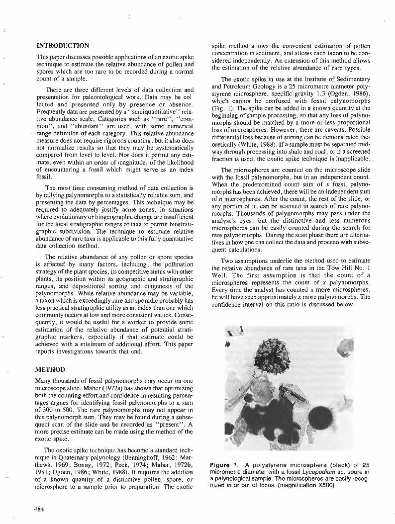
INTRODUCTION

This paper discusses possible applications of an exotic spike technique to estimate the relative abundance of pollen and spores which are too rare to be recorded during a normal count of a sample.

There are three different levels of data collection and presentation for paleontological work. Data may be collected and presented only by presence or absence. Frequently data are presented by a "semiquantitative" relative abundance scale. Categories such as "rare", "common", and "abundant" are used, with some numerical range definition of each category. This relative abundance measure does not require rigorous counting, but it also does not normalize results so that they may be systematically compared from level to level. or does it permit any estimate, even within an order of magnitude, of the likelihood of encountering a fossil which might serve as an index fossil.

The most time consuming method of data collection is by tallying palynomorphs to a statistically reliable sum, and presenting the dara by percentages. 'This technique may be required to adequately justify acme zones, in situations where evolutionary or biogeographic change are insufficient for the local stratigraphic ranges of taxa to permit biostratigraphic subdivision. The technique to estimate relative abundance of rare taxa is applicable to this fully quantitative data collection method.

The relative abundance of any pollen or spore species is affected by many factors, including; the pollination strategy of the plant species, its competitive status with other plants, its position within its geographic and stratigraphic ranges, and depositional sorting and diagenesis of the palynomorphs. While relative abundance may be variable, a taxon which is exceedingly rare and sporadic probably has less practical stratigraphic utility as an index than one which commonly occurs at low and more consistent values. Conse- quently, it would be useful for a worker to provide some estimation of the relative abundance of potential stratigraphic markers, especially if that estimate could be achieved with a minimum of additional effort. This paper reports investigations towards that end.

METHOD

Many thousands of fossil palynomorphs may occur on one microscope slide. Maher (1972a) has shown that optimizing both the counting effort and confidence in resulting percentages argues for identifying fossil palynomorphs to a sum of 300 to 500. The rare palynomorphs may not appear in this palynomorph sum. They may be found during a subsequent scan of the slide and be recorded as "present". A more precise estimate can be made using the method of the exotic spike.

The exotic spike technique has become a standard technique in Quaternary palynology (Benninghoff, 1962; Mat- thews, 1969; Bonny, 1972; Peck, 1974; Maher, 1972b, 1981; Ogden, 1986; White, 1988). It requires the addition of a known quantity of a distinctive pollen, spore, or microsphere to a sample prior to preparation. The exotic

spike method allows the convenient estimation of pollen concentration in sediment, and allows each taxon to be considered independently. An extension of this method allows the estimation of the relative abundance of rare types.

The exotic spike in use at the Institute of Sedimentary and Petroleum Geology is a 25 micrometre diameter polystyrene microsphere, specific gravity 1.3 (Ogden, 1986), which cannot be confused with fossil palynomorphs (Fig. 1). The spike can be added in a known quantity at the beginning of sample processing, so that any loss of palynomorphs should be matched by a more-or-less proportional loss of microspheres. However, there are caveats. Possible differential loss because of sorting can be demonstrated theoretically (White, 1988). If a sample must be separated midway through processing into shale and coal, or if a screened fraction is used, the exotic spike technique is inapplicable.

The microspheres are counted on the microscope slide with the fossil palynomorphs, but in an independent count. When the predetermined count sum of x fossil palynornorphs has been achieved, there will be an independent sum of n microspheres. After the count, the rest of the slide, or any portion of it, can be scanned in search of rare palynomorphs. Thousands of palynomorphs may pass under the analyst's eyes, but the distinctive and less numerous microspheres can be easily counted during the search for rare palynomorphs. During the scan phase there are alternatives in how one can collect the data and proceed with subsequent calculations.

Two assumptions underlie the method used to estimate the relative abundance of rare taxa in the Tow Hill No. 1 Well. The first assumption is that the count of n microspheres represents the count of x palynomorphs. Every time the analyst has counted n more microspheres, he will have seen approximately x more palynomorphs. The confidence interval on this ratio is discussed below.

Figure 1. A polystyrene microsphere (black) of 25 micrometre diameter with a fossil Lycopodium sp. spore in a palynological sample. The microspheres are easily recognized in or out of focus. (magnification X500)

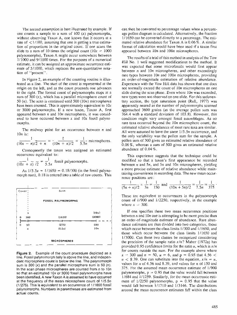
The second assumption is best illustrated by example. If one counts a sample to a sum of 100 (x) palynomorphs, without observing Taxon A, one knows that it occurs at a rate of < 11 100, assuming that one is getting a true estimation of proportions in the original count. If one scans the slide to a sum of 10 times the original count (lox = 1000 palynomorphs), Taxon A might occur somewhere between 111000 and 911000 times. For the purposes of a numerical estimate, it can be assigned an approximate occurrence estimate of 5/ 1000, which replaces the non-quantitative notation of "present".

In Figure 2, an example of the counting routine is illustrated as-a line. The start of the count is represented at the origin on the left, and as the count proceeds one advances to the right. The formal count of palynomorphs stops at a sum of 300 (x), which has a parallel microsphere count of 50 (n). The scan is continued until 500 (10n) microspheres have been counted. This is approximately equivalent to lox or 3000 palynomorphs. If a new taxon, Taxon A, first appeared between n and 10n microspheres, it was considered to have occurred between x and lox fossil palynomorphs.

The midway point for an occurrence between n and 10n is:

- - 1 microspheres. 5.51

Consequently the taxon was assigned an estimated occurrence equivalent to :

1 - - - I fossil palynomorphs. (lox + x ) 12 5 . 5 ~

As 115 .5~ = 1 I 1650 = 0.181300 (in the fossil palynomorph sum), 0.18 is entered into a table of raw counts. This

Count : I : Scan

FOSSIL PALYNOMORPHS

X ( l o x )

Figure 2. Example of the count procedure depicted as a line. Fossil palynomorph tally is above the line, and independent microsphere count is below the line. The palynomorph sum is 300 ( x ) and the parallel microsphere sum is 50 (n). In the scan phase microspheres are counted from n to 10n so that an estimated l o x or 3000 fossil palynomorphs have been identified. A new Taxon A is assumed to have occurred at the frequency of the mean microsphere count of 115.5n (1 1275). This is equivalent to an occurrence of 111 650 fossil palynomorphs. Numbers in parentheses are estimated from actual counts.

can then be converted to percentage values when a percentage pollen diagram is calculated. Alternatively, the fraction 11 1650 can be converted directly to a percentage. The estimated relative abundance for Taxon A is 0.06 %. A similar format of calculation would have been used if a taxon first appeared between 10n and lOOn microspheres.

The results of a trial of this method in analysis of the Tow Hill No. 1 well suggested modifications to the method. It was expected that some microfossils would first appear between n and 10n microspheres, and other exceedingly rare types between 10n and lOOn microspheres, providing an order-of-magnitude estimation of relative abundance. Experience with the Tow Hill data has shown that one does not normally exceed the count of Ion microspheres on one slide during the scan phase. Even where 10n was exceeded, new types were not observed on one slide. For this sedimentary section, the type saturation point (Rull, 1977) was apparently neared as the number of palynomorphs scanned approached 3600 grains (as the average pollen sum was 364.4 with a standard deviation of 103.8). However, this condition might vary amongst fossil assemblages. As no rare taxa occurred beyond the 10n microsphere count, the estimated relative abundances of most rare taxa are similar. All were assumed to have the same 115.511 occurrence, and the only variability was the pollen sum for the sample. A pollen sum of 300 gives an estimated relative abundance of 0.06 %, whereas a sum of 500 gives an estimated relative abundance of 0.04 %.

This experience suggests that the technique could be modified so that a taxon's first appearance be recorded between n and 5n, and 5n and 10n microspheres, yielding a more precise estimate of relative abundance while maintaining convenience in recording data. The new mean occurrence positions are :

1 - 1 - I and 1 - 1 - 1 (5n + n)/2 3n 150 (10n + 5n)/2 7.5n 375

These are equivalent to occurrences in the palynomorph count of 11900 and 112250, respectively, in the example where x = 300.

If one specifies these two mean occurrence positions between n and 10n one is attempting to be more precise than an order-of-magnitude estimate of abundance. Rare abundance estimates are thus divided into two categories, those which occur between the class limits 1 1300 and 11 1650, and those which occur between the class limits 111650 and 113000. Can these two classes be recognized considering the precision of the sample ratio x/n? Maher (1972a) has provided 0.95 confidence limits for the ratio u, which is x/n for counts outside the sum. For the example above where x = 300 and n = 50, u = 6, and p = 0.95 that 4.56 < u < 8.39. One can substitute into the equation, x/n = u , values for u of 4.56 and 8.39, and values for n of 150 and 375. For the assumed mean occurrence estimate of 1 /900 palynornorphs, p = 0.95 that the value would fall between 1 1684 and 1 / 1259. Similarly, for the mean occurrence estimate of 112250 palynomorphs, p = 0.95 that the value would fall between 1 / 1710 and 1 /3 146. The distributions around the mean occurrence estimates fall within the class

limits (except for 1/3146), and the classes do not significantly overlap. This indicates that one could reliably subdivide the occurrence scale given the original count ratio.

It should be noted that this calculation does not give true confidence intervals for the frequency of occurrence of the taxon because the taxon is assumed to occur at the mean position. The justification of this assumption is that it was observed to occur first somewhere within that class.

The technique for estimating relative abundance of rare taxa could be varied in other ways. It would be possible to estimate the relative abundance of a rare palynomorph based on its first occurrence relative to the microsphere count. This would require an individual calculation for entry of each rare taxon into the raw data table, whereas it is easy to recognize that something occurred between specified limits of n microspheres and enter one number into a raw data table.

Alternatively, one could count all occurrences of a rare taxon between n and any multiple of n microspheres which could be conveniently achieved while scanning the microscope slide. This option would yield the best estimate of relative abundance. In retrospection to the Tow Hill No. 1 well analysis, it would not have been excessively laborious to count all of the individual occurrences of the rare taxa. However, the additional effort is not just in additional counting, but for each rare taxon the need for a summation and calculation of the number to be entered into the raw data table.

In palynology, only one sample (that observed on the microscope slide) is normally drawn from each population (the sample). Consequently, the confidence interval for the relative abundance of rare taxa must necessarily be broad. The extra precision in estimation resulting from additional counting may not be worth the added effort.

RESULTS AND CONCLUSIONS

In general, it seems best to maintain broad limits for the estimated relative abundances, recognizing them as estimates which improve on the alternative of recording rare taxa as "present".

In the Tow Hill No. 1 Well, the relative abundance of the rare taxa has been estimated as occurring between n and 10n. Jussiaea sp., a taxon previously described from an Oligocene assemblage from central British Columbia (Piel, 1971), is estimated at 0 . 0 3 % in one sample only. This remote occurrence does not carry as much stratigraphic weight as a more abundant presence.

The extinction of Liquidambar sp. has been interpreted as a Neogene stratigraphic marker in the Queen Charlotte Basin (Champigny et al., 1981). In this same paper it was reported to not occur at 649 m in the Tow Hill No. 1 Well.

The writer did find the species at this level, but at an estimated relative abundance of 0.05 %, or 1 in 2000 palynomorphs. This estimate of low relative abundance shows that the difference in observation of Liquidambar sp. in this sample by different palynologists could be entirely fortuitous.

Because of the labour involved, counting techniques will probably only be applied in long surface or subsurface sections meriting detailed study. The technique described in this paper can be easily applied where count data is generated, an exotic spike is already employed, and calculations are done by a computer. It is a useful addition to the methods by which palynologists can report the results of their research.

ACKNOWLEDGMENT

This paper has benefited from critical reading by F. P. Agterberg and L.J. Maher, Jr.

REFERENCES

Benninghoff, W.S. 1962: Calculation of pollen and spore density in sediments by addition

of exotic pollen in known quantities; Pollen et Spores, v.4, p. 332-333.

Bonny, A.P. 1972: A method for determining absolute pollen frequencies in lake

sediments; New Phytologist, v.71, p. 393-405. Champigny, N., Henderson, C. M., and Rouse, G.E. 1981: New evidence for the age of the Skonun Formation, Queen

Charlotte Islands, British Columbia; Canadian Journal of Earth Sciences, v. 18, no. 12, p. 1900-1903.

Maher, L.J., Jr. 1972a: Nomograms for computing 0.95 confidence limits of pollen data;

Review of Palaeobotany and Palynology, v. 13, p. 85-93. 1972b: Absolute pollen diagram of Redrock Lake, Boulder County,

Colorado; Quaternary Research, v. 2, p. 531-553. 1981 : Statistics for microfossil concentration measurements employing

samples spiked with marker grains; Review of Palaeobotany and Palynology, v. 32, p. 153-191.

Matthews, J. 1969: The assessment of a method for the determination of absolute

pollen frequencies; New Phytologist, v. 68, p. 161-166. Ogden, J.G., 111, 1986: An alternative to exotic spore or pollen addition in quantitative

microfossil studies; Canadian Journal of Earth Sciences, v. 23, p. 102-106.

Peck, R. 1974: A comparison of four absolute pollen preparation techniques;

New Phytologist, v.73, p. 576-587. Piel, K.M. 1971 : Palynology of Oligocene sediments from central British Colum-

bia; Canadian Journal of Botany, v. 49. p. 1885-1920. Rull, V. 1987 : A note on pollen counting in palaeoecology ; Pollen et Spores, v.

29, p. 471-480. White, J.M. 1988: Methodology of the exotic spike: differential settling of palyno-

morphs during sample preparation; Pollen et Spores, v. 30, no. 1, p. 131-148.

Sensitivity analysis of basin modelling with applications

S. Caol and I. Lerchel

Cao, S. and Lerche, I . , Sensitivity analysis of basin modelling with applications; @ Statistical Applications in the Earth Sciences, ed. F. P. Agterberg and G. F. Bonham-Carter; Geological Survey of Canada, Paper 89-9, p. 489-504, 1989.

Abstract

Geological processes related to petroleum generation, migration and accumulation are complicated in terms of time and the variables involved. Accordingly many mathematical/computer models have been developed to simulate these processes based on geological, geophysical and geochemical principles. Sensitivity analysis is a comprehensive ~xamination on how geological, geophysical and geochemical parameters influence the reconstructions of geohistory, thermal history, and hydrocarbon generation history. We use a I-Dfluidflow/compaction model developed in the Basin Modeling Group at the Univer- sity of South Carolina. This study examines the effects of some commonly usedparameters (such as depth, age, lithology, porosity, permeability, unconformify (eroded thickness and erosion time), temperature at sediment surface, bottom hole temperature, present day heat flow, thermal gradient, thermal conductivity, and kerogen type and content) on the evolution of formation thickness, porosity, permeability, pressure with time and depth, heat flow with time, temperature with time and depth, vitrinite reflectance (4) and TTI with time and depth, the "oil window" in terms of time and depth, and the amount of hydrocarbons generated with time and depth.

The sensitivity variations are helphl ( I ) to understand better the importance of the parameters in the reconstructions of geohistory, thermal history and hydrocarbon generation history in sedimentary basins; and (2) to provide knowledge of resolution capabilities of models with respect to input data, input parameters and intrinsic assumptions so that basin evolution models are more useful and effective in hydrocarbon exploration.

Les processus ge'ologiques relie's h la formation, h la migration et h l'accumulation du pe'trole sont complexes en termes de chronologie et des variables en cause. Un grand nornbre de modiles mathe'matiques et inforrnatise's base's sur les principes de la ge'ologie, de la ge'ophysique et de la ge'ochimie ont par conskquent he' mis au point a jn de stimuler ces processus. L'analyse de sensibilite' est un examen exhaustifde la manibre dont les parambtres ge'ologiques, ge'ophysiques et ge'ochimiques influencent les reconstitutions de l'histoire ge'ologique, de l'histoire thermique et de l'histoire de la formation des hydrocarbures. Le modile utilise'ici est un modile d'e'coulementfluide et de compaction en une dimension mis au point par le Basin Modeling Group de 1'Universite' de la Caroline du Sud. La prisente e'tude examine les eflets de certains paramitres couramment utilise's (commme la profondeur, l'cige, la lithologie, la porosite', la permkabilite', la discordance (e'paisseur e'rodge et e'poque d'e'rosion), la tempe'rature h la surface des se'diments, la tempkrature au fond du trou, le flux thermique actuel, le gradient thermique, la conductivite'thermique et le type de ke'rogkne ainsi que sa teneur) sur l'e'volution, duns la formation, de l'e'paisseur, la porosite', la perme'abilite' et la pression en fonction du temps et de la profondeur, le flux thermique en fonction du temps, la tempe'rature en fonction du temps et de la profondeur, la rkflectance et ITT de la vitrinite (R,) en fonction du temps et le la profondeur, la fen&tre de pe'trole ,, en fonction du temps et de la prodondeur et les quantite's d 'hydrocarbures forme's

en fonction du temps et de la profondeur.

Les variations de la sensibilite' sont utiles pour I ) mieux comprendre l'importance des paramhres lors de la reconstitution de l'histoire ge'ologique, de l'histoire thermique et de l'histoire de la formation des hydrocarbures duns les bassins se'dimentaires et, 2) connaitre les possibilite's de re'solution des modkles en fonction des donne'es d'entre'e, des parambtres d'entrke et des hypothtses intrinsiques, de facon h rendre les modbles plus eficaces et plus ictiles au niveau de la recherche d'hydrocarbures.

' Depr. of Geological Sciences, University of Sourh Carolina, Columbia, SC 29208, U.S.A.

INTRODUCTION

Geological processes related to petroleum generation, migration and accumulation are complicated and none of the models can simulate these processes exactly. Sensitivity analysis of a model is a comprehensive examination of how the results of the model are influenced by the change in the assumptions and parameters of the model, and of errors in the data. From sensitivity analysis, we can determine what error range in the input data is permitted in order to give accurate results and also how strongly the model depends on the assumptions made, thereby making the model a more effective tool in basin analysis.

The purposes of this paper are (1) to examine how sensi- tively models depend on variations in the input data, the equation parameters and the assumptions of the model; (2) to estimate the probability of the results produced corresponding to the variations in (1); and (3) to provide constraint conditions for variations in the input data, the equation parameters and the assumptions of a model. In order to provide a comprehensive investigation of behaviour patterns, throughout we restrict our discussion to the one- dimensional fluid-flow/compaction model - although similar analyses can be performed on any model.

PRECIS OF INTEGRATED MODELS

The fluid flow model consists of three parts: a geohistory model, a thermal history model and a hydrocarbon generation model. Since the model simulations are one- dimensional, the input data for the model are those commonly used: geological and geochemical data from a single well, which makes the simulations useful both in frontier basins where only a few wells are available and also in well developed basins.

a. Geohistory model. Through a simulation of the fluid flow movement in sediments caused by the compaction of the sediments, the geohistory model reconstructs-the burial history, basement subsidence, vertical fluid flow, and the changes of porosity, permeability, pressure and fluid flow rate with both time and depth. Also the evolution of cementation, dissolution, and fracturing caused by abnormally high pore pressure, are simulated in terms of the change in formation permeability. The input data required to run the geohistory model are the depth and age of each formation base, the lithology and paleowater depth of each formation.

b. Thermal history model. Based on the burial history created in the geohistory model, the thermal history model reconstructs the thermal history by (a) comparing predicted thermal indicator values (such as vitrinite reflectance) to measurements down a borehole and (b) adjusting the paleoheat flux to minimize discordances. The outputs are (i) a heat flow change with time, (ii) a temperature change with time and depth, (iii) vitrinite reflectance and TTI changes with time and depth. The input data required to run the thermal history model are the temperature at the sediment surface, bottom hole temperature (or thermal gradientlpresent day heat flow), and some thermal indicator measurements with depth.

c. Hydrocarbon generation model. The hydrocarbon generation model is based on the kinetics of kerogen degradation and the general scheme of evolution uses two mathematical models to simulate hydrocarbon generation : Tissot's model (Tissot and Welte, 1978) which simulates the formation of oil from kerogen in six parallel reactions (first stage) and the formation of gas from oil in a single reaction (second stage), and a modified model (Cao et al., 1986) which adds the major gaseous products from both kerogen degradation and oil cracking. Based on the burial history and temperature history produced in the model, the generation model gives the absolute amount of hydrocarbons generated (per gram kerogen) with time and depth. The input data required to run the generation model are the content of different kerogen types of each formation.

Results which need to be examined in the sensitivity analysis include: formation thickness, formation porosity, formation permeability, formation pressure, heat flow with time, temperature with time and depth, R, and TTI with time and depth, "oil window" in terms of time and depth, amount of hydrocarbons generated.

There are three groups of variables which need to be examined : input data, equation parameters and intrinsic assumptions.

(1). Input data. Very commonly there are errors in the measurements of the geological and geochemical data. The variables which need to be tested in the input data are: depth and age of each formation base, lithology and paleowater depth of each formation, unconformity time and eroded thickness, temperature at sediment surface, bottom hole temperature, heat flow at present day, thermal gradient, vitrinite reflectance, kerogen type and content of each formation.

(2). Equation parameters. Most of the parameterslcons- tants in the equations used in the models are based on empirical data, for example, depositional porosity of shale, 0.62, is used in the model. The following parameters need to be tested : depositional porosity, permeability and frame pressure, viscosity of the fluid in the sediments, parameter A in the void ratio - frame pressure function, parameter B in the void ratio - permeability function, critical temperature and doubling temperature in the R, equation, thermal conductivity of each lithology, activation energies and frequency factors in the generation model.

(3). Assumptions. The following assumptions have been used in the model and will be tested here: change the power law functions of void ratio - frame pressure and void ratio - permeability to exponential functions, change constant sediment surface temperature with time to a variable sediment surface temperature, change linear heat flow function to a non linear heat flow function.

Not tested in this paper are intrinsic assumptions of the model such as the 1-D nature versus a 2-D problem, such as the replacement of complete isostatic movement of basement motion by a partial flexural compensation, etc. Exami- nation of these assumptions would make for a very long

paper, and on this ground is not included, although we recognize the pressing need for such a development (Cao, 1987).

According to Yukler and Kokesh (1984) mathematical models are used to simulate complex processes with one or more variables and thus they are essential in the assessment of hydrocarbon resources. Mathematical models are applied either as statistical models or as deterministic models to reconstruct and predict geological processes assuming that these processes are deterministic. The statistical models are mainly used in estimation of hydrocarbon resources because they cannot directly analyze the dynamic processes of hydrocarbon generation, migration and accumulation. A Monte Carlo simulation is usually employed in the statistical models to construct various probability curves with the most commonly used assessment methods being geological analogy (Weeks, 1952 ; Conybeare, 1965 ; Bally, 1975 ; Pitcher, 1976; Warren, 1979), delphi (Miller et al., 1975), areal and volumetric yields (Stoian, 196.5; Walstrom et al., 1967; Smith, 1968; Jones, 1975; Newendorp, 197.5; Roadifer, 1975), geochemical yields (Conybeare, 1965; Halbouty et al., 1970; McDowell, 1975; Tissot and Welte, 1978), and field distribution (Atwater, 1956; Roy et al., 1975).

SIMULATION MODELS

The simulation of sedimentary basin development was established in the 1960s (Chorafas, 1965; Griffiths, 1967; Harbaugh and Merriam, 1968). The initial models were basically process-response models and were followed by simple static and deterministic models which evolved into more complex static models and then into dynamic models (Har- baugh and Bonham-Carter, 1970).

In the past ten years, more comprehensive models have been developed to simulate the dynamic processes related to hydrocarbon generation, migration and accumulation (Yukler et al., 1978 ; Ungerer et al., 1984 ; Cao, 1985 ; Cao et al., 1986 ; Nakayama, 1986). The simulation of hydrocarbon generation, migration and accumulation can be divided into four general parts : (1) reconstruction of the geohistory, which includes basement subsidence, sediment deposition, changes of porosity, permeability, fluid pressure, and fluid flow with time and depth ; (2) reconstruction of the thermal history, which includes heat flux evolution with time, temperature (thermal gradient) changes with time and depth, and thermal maturation history in terms of thermal indicator evolution with time and depth; (3) reconstruction of the hydrocarbon generation history, thereby modeling the change of the amount of hydrocarbons generated with time and depth, and determining the time a n d depth of peak hydrocarbon generation; (4) reconstruction of hydrocarbon migration and accumulation history, including the amount of hydrocarbons migrated, the time and depth of peak hydrocarbon migration, the direction of hydrocarbon migration and the relation among the accumulations (traps), migration and the "kitchen" where the hydrocarbons

In choosing a mathematical model the following aspects are important:

(1) The "reasonableness" of the model: 1s the model quantifiable in terms of the principles upon which the model is based? Can one set up the geological, geophysical and geochemical factors considered in the model, and find a satisfactory method to be used in the solution technique?

(2) The practicality of the model : Is the model of practical use considering the input data, computer time and storage, etc.?

(3) The accuracy of the model : How well do the model results compare with the observed geological, geophysical and geochemical data?

No model can simulate exactly the geological, geophysical and geochemical processes related to hydrocarbon generation, migration and accumulation. A simulation model usually has three pitfalls: (1) assuming the input data are correct without any error or with negligible error; (2) assuming that the equation parameters in the model are independent from the input data; and (3) assuming that sim- plifications made in the model do not affect the accuracy of the simulation.

METHODOLOGY OF SENSITIVITY ANALYSIS

Sensitivity analysis is a study of the sensitivity of a system's response to various disturbances in the system. These disturbances may have widely different characters. They may be small or large, transient or permanent, they may be related to initial conditions, to coefficients and parameters, etc. (Yukler, 1979). In this study, the following disturbances to the 1-D model are considered: (i) errors in the input data, e.g. the depth, age and lithology of individual formations; (ii) errors in the equation parameters, e.g. the surface porosity, permeability; and (iii) errors in the assumptions, e.g. constant sediment surface temperature.

There are usually two ways to handle parametric sensitivity : perturbation methods and direct methods. The disadvantage of perturbation methods is the excessive amount of computer time involved. Because of these disadvantages, direct methods have been developed and widely used by many people (Tomoric, 1963 ; Anderson, 1965 ; Yukler, 1979; Fiacco, 1984). The direct methods first derive a sensitivity equation by taking the partial derivative of the equation used in a system and then solve the sensitivity equation by computer.

For this study, a perturbation-type method is used because (1) The I-D model is a complex system which involve more than one partial differential equation. In some cases, it is impossible to devise a closed form sensitivity equation by the direct method; (2) A perturbation type method has more flexibility to handle the problem of sensitivity testing of the assumptions made in the model.

matured.

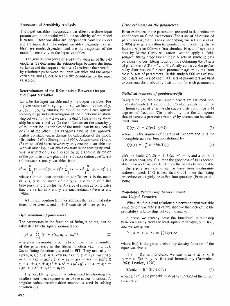
Procedure of Sensitivity Analysis

The input variables (independent variables) are those input parameters in the model which the sensitivity of the model is to test. These variables are independent from the model and are input data. The output variables (dependent variables) are model-dependent and are the responses of the model's sensitivity to the input variables.

The general procedure of sensitivity analysis of the 1-D model is (1) determine the relationships between the input variables and the output variables ; (2) estimate the probability relationships between the input variables and the output variables; and (3) define restrictive conditions for the input variables.

Determination of the Relationship Between Output and Input Variables.

Let x be the input variable and y the output variable. For n given values of x, x , , x2, ..., x,, we have n values of y, y , , y2, . . . , yn by running the model n times. Least-squares techniques permit determination of the functional relationship between x and y if we assume that (1) there is a relationship between x and y ; (2) the influence on the quantity y of the other input variables of the model can be neglected; or (3) all the other input variables have at least approximately constant values during the calculation of the model (Brownlee, 1960 ; Shchigolov, 1965). Assumptions (2) and (3) are satisfied because we vary only one input variable and keep all other input variables constant in the sensitivity analysis. Assumption (1) is checked by (i) graphic distribution of the points in an x-y plot and (ii) the correlation coefficient (r) between x and y variables from

n n n r2 = C (xi - K ) ~ ( Y ~ - Y ) ~ / ,C (xi - x ) ~ ,C (yi - yI2 (1)

i =l 1 = 1 ] = I where r is the linear correlation coefficient, x is the mean of xi's, y is the mean of the yi's. The value of r lies between -1 and 1, inclusive. A value of r near zero indicates that the variables x and y are uncorrelated (Press et al., 1986).

A fitting procedure (FIT) establishes the functional relationship between x and y. FIT consists of three parts:

Determination of parameters

The parameters in the function of fitting n points, can be estimated by chi square minimization

n x2 .C (yi - Y(x~, a , . . . a d 2

1 = 1 (2)

where n is the number of points to be fitted, m is the number of the parameters in the fitting function y(xi; a , . . .a,). Seven fitting functions are used in FIT. They are: a) y = alexp(-a2x); b) y = a , exp(a21nx); c) y = a , + a2x; d) y = a , + a2x + a3x2; e) y = a , + a2x + a3x2 + a4x3; f) y = a , + a2x + a3x2 + a4x3 + a5x4; g) y = a , + a2x + a3x2 + a4x3 + a5x4 + a6x5.

The best fitting function is determined by choosing the smallest root mean-square error of the seven functions. A singular value decomposition method is used in solving equation (2).

Error estimates on the parameters

Error estimates on the parameters are used to determine the confidence on fitted parameters. For a set of M estimated parameters A, there is some underlying true set. Press et al. (1986) give an algorithm to simulate the probability distributions A(i) as follows: first simulate N sets of synthetic data by Monte Carlo realization; second apply a "chi- square" fitting procedure to these N sets of synthetic data by using the best fitting function thus obtaining the N sets of parameters A(i) (i = 1,. . . ,N) ; finally construct the probability distributions for each parameter ai(i = 1, m) from these N sets of parameters. In this study 8 000 sets of synthetic data are created and 8 000 sets of parameters are used to construct the probability distribution for each parameter.

Statistical measure of goodness-of-fit

In equation (2), the measurement errors are assumed normally distributed. Therefore the probability distribution for different values of x2 is the chi-square distribution for n-M degrees of freedom. The probability that the chi-square should exceed a particular value X2 by chance can be calculated from

where v is the number of degrees of freedom and Q is the incomplete gamma function defined by

with the limits Q(a,O) = 1, Q(a, m) = 0 , and a > 0 . If Q is larger than, say, 0.1, then the goodness-of-fit is acceptable; if larger than, say, 0.01, then the fit may be acceptable if the errors are non-normal or have been moderately underestimated. If Q is less than 0.001, then the fitting procedure can rightly be called into question (Press et al., 1986).

Probability Relationship between Input and Output Variables.

When the functional relationship between input variable x and output variable y is established we then determine the probability relationship between x and y.

Suppose we already have the functional relationship between x and y from the least-square technique, y = f(x), and we are given

where B(c) is the given probability density function of the input variable x.

If y = f(x) is monotone, we can write a x < b < = = > f(a) I y < f(b) and immediately (Brownlee, 1960; Lumley, 1970)

where B' (c) is the probability density function of the output variable y.

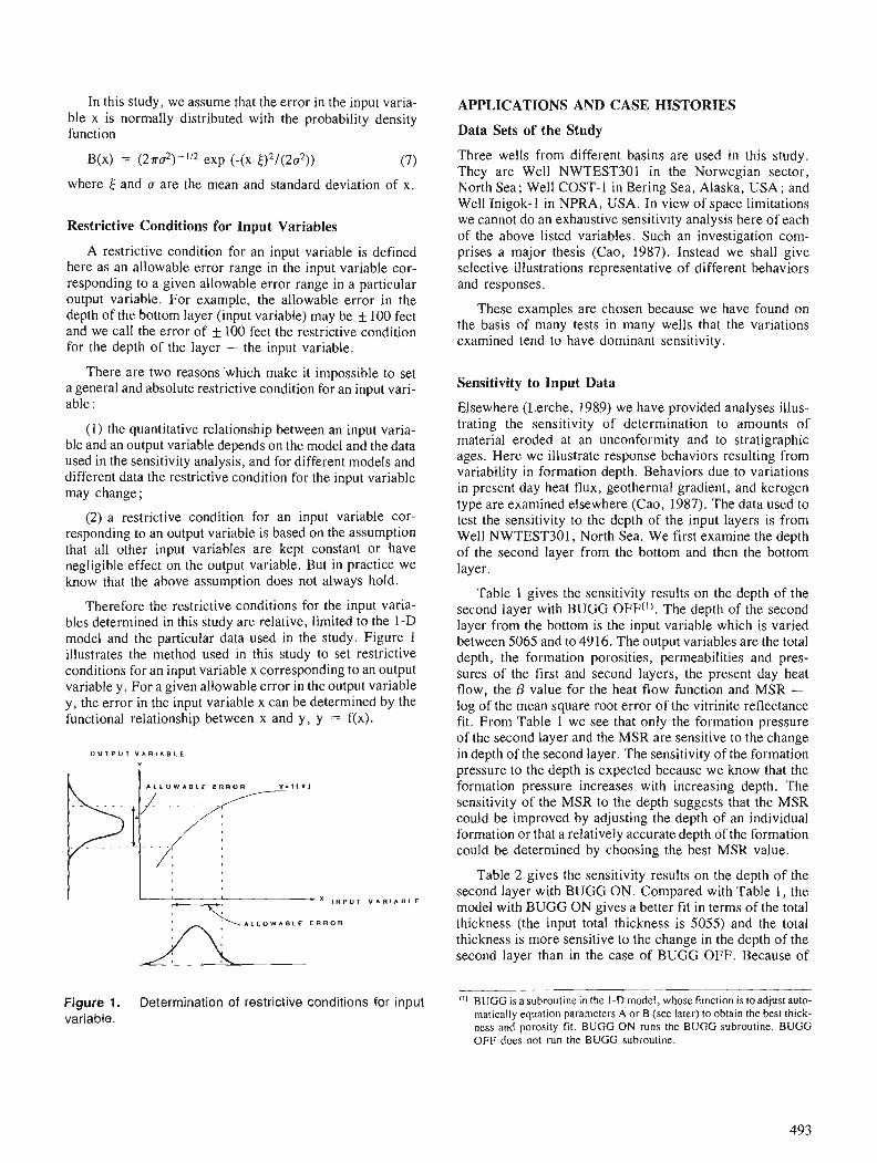
In this study, we assume that the error in the input variable x is normally distributed with the probability density function

B(x) = (27ru2) - ' I 2 exp (-(x-E)~/ (2u2)) (7)

where [ and a are the mean and standard deviation of x.

Restrictive Conditions for Input Variables

A restrictive condition for an input variable is defined here as an allowable error range in the input variable corresponding to a given allowable error range in a particular output variable. For example, the allowable error in the depth of the bottom layer (input variable) may be f 100 feet and we call the error of k 100 feet the restrictive condition for the depth of the layer - the input variable.

There are two reasons 'which make it impossible to set a general and absolute restrictive condition for an input variable :

(1) the quantitative relationship between an input variable and an output variable depends on the model and the data used in the sensitivity analysis, and for different models and different data the restrictive condition for the input variable may change;

(2) a restrictive condition for an input variable corresponding to an output variable is based on the assumption that all other input variables are kept constant or have negligible effect on the output variable. But in practice we know that the above assumption does not always hold.

Therefore the restrictive conditions for the input variables determined in this study are relative, limited to the 1-D model and the particular data used in the study. Figure 1 illustrates the method used in this study to set restrictive conditions for an input variable x corresponding to an output variable y. For a given allowable error in the output variable y, the error in the input variable x can be determined by the functional relationship between x and y, y = f(x).

O U T P U T V A R I A B L E

v

I i I N P U T V A R I A B L E

\ A L L O W A B L E E R R O R _/i Figure 1. Determination of restrictive conditions for input variable.

APPLICATIONS AND CASE HISTORIES

Data Sets of the Study

Three wells from different basins are used in this study. They are Well NWTEST301 in the Norwegian sector, North Sea; Well COST-1 in Bering Sea, Alaska, USA ; and Well Inigok-1 in NPRA, USA. In view of space limitations we cannot do an exhaustive sensitivity analysis here of each of the above listed variables. Such an investigation comprises a major thesis (Cao, 1987). Instead we shall give selective illustrations representative of different behaviors and responses.

These examples are chosen because we have found on the basis of many tests in many wells that the variations examined tend to have dominant sensitivity.

Sensitivity to Input Data

Elsewhere (Lerche, 1989) we have provided analyses illustrating the sensitivity of determination to amounts of material eroded at an unconformity and to stratigraphic ages. Here we illustrate response behaviors resulting from variability in formation depth. Behaviors due to variations in present day heat flux, geothermal gradient, and kerogen type are examined elsewhere (Cao, 1987). The data used to test the sensitivity to the depth of the input layers is from Well NWTEST301, North Sea. We first examine the depth of the second layer from the bottom and then the bottom layer.

Table 1 gives the sensitivity results on the depth of the second layer with BUGG OFF('). The depth of the second layer from the bottom is the input variable which is varied between 5065 and to 4916. The output variables are the total depth, the formation porosities, permeabilities and pressures of the first and second layers, the present day heat flow, the /3 value for the heat flow function and MSR - log of the mean square root error of the vitrinite reflectance fit. From Table 1 we see that only the formation pressure of the second layer and the MSR are sensitive to the change in depth of the second layer. The sensitivity of the formation pressure to the depth is expected because we know that the formation pressure increases with increasing depth. The sensitivity of the MSR to the depth suggests that the MSR could be improved by adjusting the depth of an individual formation or that a relatively accurate depth of the formation could be determined by choosing the best MSR value.

Table 2 gives the sensitivity results on the depth of the second layer with BUGG ON. Compared with Table 1, the model with BUGG ON gives a better fit in terms of the total thickness (the input total thickness is 5055) and the total thickness is more sensitive to the change in the depth of the second layer than in the case of BUGG OFF. Because of

'I' BUGG is a subroutine in the I-D model, whose function is to adjust automatically equation parameters A or B (see later) to obtain the best thickness and porosity fit. BUGG ON runs the BUGG subroutine. BUGG OFF does not run the BUGG subt.outine.

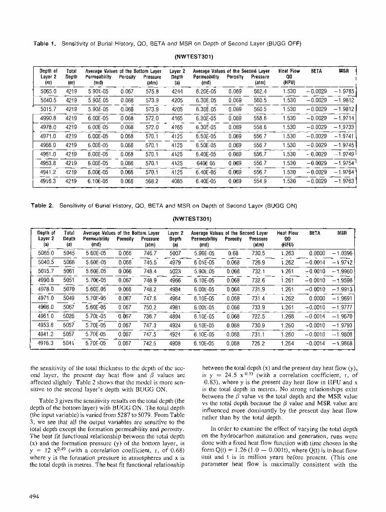
Table 1. Sensitivity of Burial History, QO, BETA and MSR on Depth of Second Layer (BUGG OFF)

(NWTESTBOl)

Depth of Total Average Values of the Bottom Layer Layer 2 Average Values of the Second Layer Heat Flow BETA MSR Layer2 Depth Permeability Porosity Pressure Depth Permeability Porosity Pressure (I0

(m) (m) (md) (atm) (a) (md) (aim) (HFU)

5065.0 4219 5.90E-05 0.067 575.8 4244 6.20E-05 0.069 562.4 1.530 -0.0029 -1.9785

5040.5 4219 5.90E.05 0.068 573.9 4205 6.30E.05 0.069 560.5 1.530 -0.0029 -1.9812

5015.7 4219 5.90E-05 0.068 573.9 4205 6.30E.05 0.069 560.5 1.530 -0.0029 -1.9812

4990.8 4219 6.00E-05 0.068 572,O 4165 6.30E-05 0.069 558.6 1.530 -0.0029 -1.9714

4978.0 4219 6.00E-05 0.068 572.0 4165 6.30E-05 0.069 558.6 1.530 -0.0029 -1,9733

4971.0 4219 6.00E-05 0.068 570.1 ' 4125 6.50E-05 0.069 556.7 1.530 -0.0029 -1.9741

4966.0 4219 6.00E-05 0.068 570.1 4125 6.50E-05 0.069 556.7 1.530 -0.0029 -1.9745

4961.0 4219 6.00E-05 0.068 570.1 4125 6.40E-05 0.069 556.7 1.530 -0.0029 -1.9749

4953.8 4219 6.00E-05 0.068 570.1 4125 640E-05 0.069 556.7 1.530 -0.0029 -1.9754

4941.2 4219 6.00E-05 0.068 570.1 4125 6.40E-05 0.069 556.7 1.530 -0.0029 -1.9764

4916.3 4219 6.10E-05 0.068 568.2 4085 6.40E-05 0.069 554.9 1.530 -0.0029 -1.9763

Table 2. Sensitivity of Bur ia l History, QO, BETA and M S R on Depth of Second Layer (BUGG ON)

(NWTESTBOI)

Depth of Total Average Values of the Bottom Layer Layer 2 Average Values of the Second Layer Heat Flow BETA MSR Layer 2 Depth Permeability Porosity Pressure Depth Permeabllily Porosity Pressure QO

(a) (a) (md) (atm) (a) (md) (atm) (HFU)

5065.0 5045 5.60E-05 0.066 746.7 5007 5.96E-05 0.68 730.5 1.263 0.0000 - 1.0396

5040.5 5066 5.60E-05 0.066 745.5 4979 6.01E-05 0.068 726.9 1.262 -0.0014 -1.9712 5015.7 5061 5.60E.05 0.066 748.4 5023 5.90E.05 0.068 732.1 1.261 -0.0010 -1.9960 4990.8 5051 5.70E-05 0.067 748.9 4966 6.10E-05 0.068 732.6 1.261 -0.0010 -1.9598 4978.0 5070 5.60E.05 0.066 748.2 4984 6.00E-05 0.068 731.9 1.261 -0.0010 -1.9913 4971.0 5049 5.70E-05 0.067 747.6 4964 6.10E-05 0.068 731.4 1.262 0.0000 -1.9691 4966.0 5067 5.60E-05 0.067 750.2 4981 6.00E-05 0.068 733.9 1.261 -0.0010 -1.9777

4961.0 5026 5.70E-05 0.067 738.7 4894 6.10E-05 0.068 722.5 1.268 -0.0014 -1.9670 4953.8 5057 5.70E-05 0.067 747.3 4924 6.10E-05 0.068 730.9 1.260 -0.0010 -1.9793 4941.2 5057 5.70E-05 0.067 747.5 4924 6.10E-05 0.068 731.1 1.260 -0.0010 -1.9808

4916.3 5041 5.70E-05 0.067 742.5 4908 6.10E-05 0.068 726.2 1.264 -0.0014 -1.9868

the sensitivity of the total thickness to the depth of the second layer, the present day heat flow and /3 values are affected slightly. Table 2 shows that the model is more sensitive to the second layer's depth with BUGG ON.

Table 3 gives the sensitivity results on the total depth (the depth of the bottom layer) with BUGG ON. The total depth (the input variable) is varied from 5287 to 5079. From Table 3, we see that all the output variables are sensitive to the total depth except the formation permeability and porosity. The best fit functional relationship between the total depth (x) and the formation pressure (y) of the bottom layer, is y = 12 x0.49 (with a correlation coefficient, r, of 0.68) where y is the formation pressure in atmospheres and x is the total depth in metres. The best fit functional relationship

between the total depth (x) and the present day heat flow (y), is y = 24.5 x - ~ , ~ ~ (with a correlation coefficient, r, of -0.83), where y is the present day heat flow in HFU and x is the total depth in metres. No strong relationships exist between the p value vs the total depth and the MSR value vs the total depth because the 0 value and MSR value are influenced more dominantly by the present day heat flow rather than by the total depth.

In order to examine the effect of varying the total depth on the hydrocarbon maturation and generation, runs were done with a fixed heat flow function with time chosen in the form Q(t) = 1.26 (1.0 - 0.001t), where Q(t) is in heat flow unit and t is in million years before present. (This one parameter heat flow is maximally consistent with the

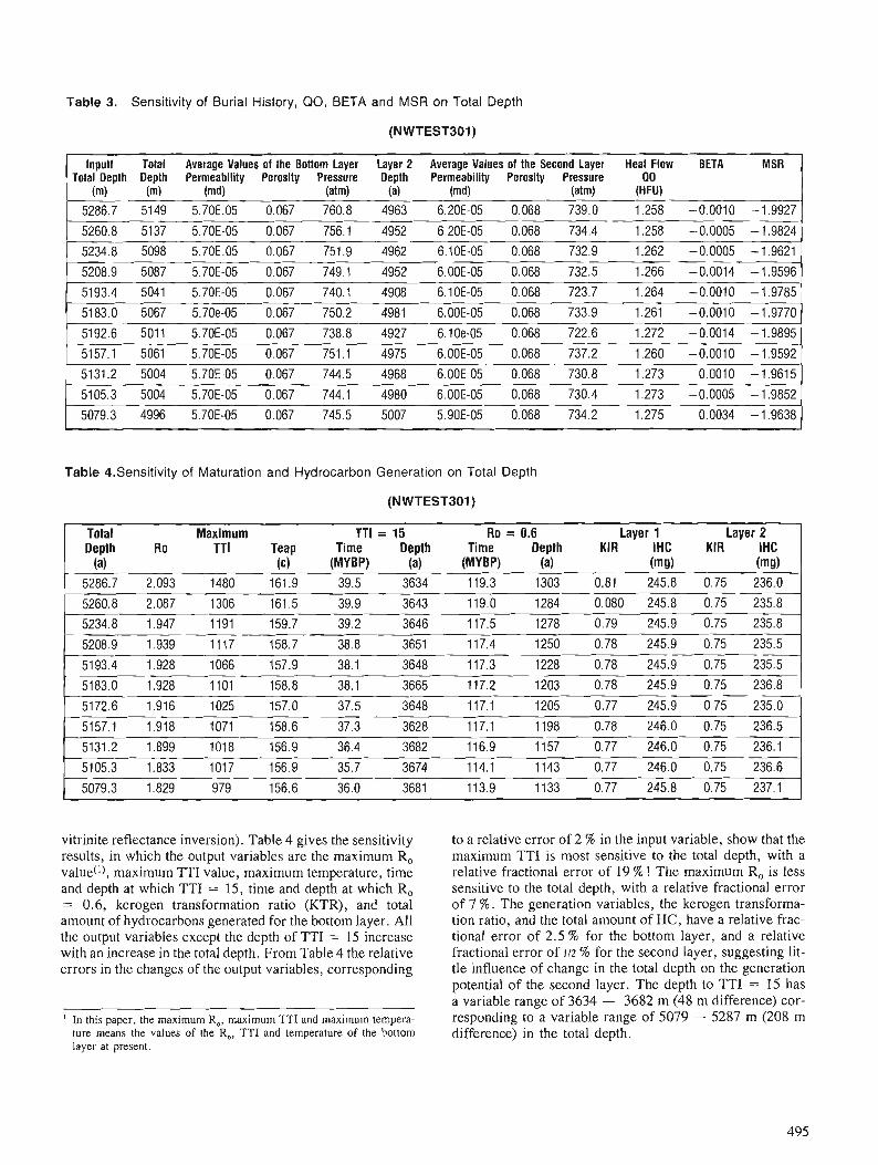
Table 3. Sensitivity of Burial History, QO, BETA and MSR on Total Depth

lnputf Total Average Values of the Bottom Layer Layer 2 Average Values of the Second Layer Heat Flow BETA MSR Total Depth Depth Permeability Porosity Pressure Depth Permeability Porosity Pressure 00

Table 4.Sensitivity of Maturation and Hydrocarbon Generation on Total Depth

- Total Maximum TTl = 15 Ro = 0.6 Layer 1 Layer 2 Depth Ro TTI Teap Time Depth Time Depth KIR IHC KIR IHC

(a) (c) (MYBP) (a) (MYBP) (a) (mg) (mg) 5286.7 2.093 1480 161.9 39.5 3634 119.3 1303 0.81 245.8 0.75 236.0

5260.8 2.087 1306 161.5 39.9 3643 119.0 1284 0.080 245.8 0.75 235.8

5234.8 1.947 1191 159.7 39.2 3646 117.5 1278 0.79 245.9 0.75 235.8

vitrinite reflectance inversion). Table 4 gives the sensitivity results, in which the output variables are the maximum R, value('), maximum TTI value, maximum temperature, time and depth at which TTI = 15, time and depth at which R, = 0.6, kerogen transformation ratio (KTR), and total amount of hydrocarbons generated for the bottom layer. All the output variables except the depth of TTI = 15 increase with an increase in the total depth. From Table 4 the relative errors in the changes of the output variables, corresponding

' In this paper, the maximum R,, maximum TTI and maximum temperature means the values of the R,, TTI and temperature of the bottom layer at present.

to a relative error of 2 % in the input variable, show that the maximum TTI is most sensitive to the total depth, with a relative fractional error of 19 % ! The maximum R, is less sensitive to the total depth, with a relative fractional error of 7 %. The generation variables, the kerogen transformation ratio, and the total amount of HC, have a relative fractional error of 2.5 % for the bottom layer, and a relative fractional error of 112 % for the second layer, suggesting little influence of change in the total depth on the generation potential of the second layer. The depth to TTI = 15 has a variable range of 3634 - 3682 m (48 m difference) corresponding to a variable range of 5079 - 5287 m (208 m difference) in the total depth.

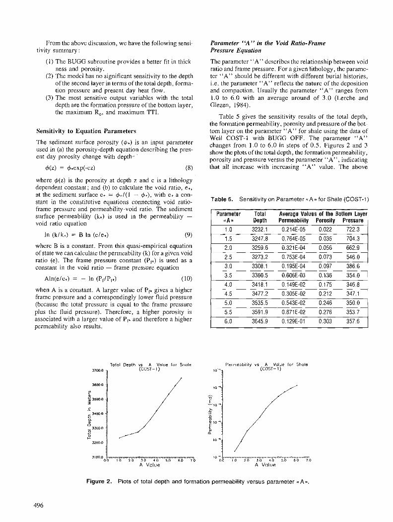
From the above discussion, we have the following sensitivity summary:

(1) The BUGG subroutine provides a better fit in thickness and porosity.

(2) The model has no significant sensitivity to the depth of the second layer in terms of the total depth, formation pressure and present day heat flow.

(3) The most sensitive output variables with the total depth are the formation pressure of the bottom layer, the maximum R,, and maximum TTI.

Sensitivity to Equation Parameters

The sediment surface porosity (4,) is an input parameter used in (a) the porosity-depth equation describing the present day porosity change with depth-"

where 4(z) is the porosity at depth z and c is a lithology dependent constant; and (b) to calculate the void ratio, e*, at the sediment surface e, = &l(l - &), with e, a constant in the constitutive equations connecting void ratio- frame pressure and perme~bility-void ratio. The sediment surface permeability (k*) is used in the permeability - void ratio equation

where B is a constant. From this quasi-empirical equation of state we can calculate the permeability (k) for a given void ratio (e). The frame pressure constant (Pr) is used as a constant in the void ratio - frame pressure equation

when A is a constant. A larger value of Pp* gives a higher frame pressure and a correspondingly lower fluid pressure (because the total pressure is equal to the frame pressure plus the fluid pressure). Therefore, a higher porosity is associated with a larger value of Pr* and therefore a higher permeability also results.

Total Depth vs A Volue lor Shole (COST- 1 )

s lOOo 0 -o 0 A Value

Parameter "A" in the Void Ratio-Frame Pressure Equation

The parameter "A" describes the relationship between void ratio and frame pressure. For a given lithology, the parameter "A" should be different with different burial histories, i.e. the parameter "A" reflects the nature of the deposition and compaction. Usually the parameter "A" ranges from 1.0 to 6.0 with an average around of 3.0 (Lerche and Glezen, 1984).

Table 5 gives the sensitivity results of the total depth, the formation permeability, porosity and pressure of the bottom layer on the parameter "A" for shale using the data of Well COST-1 with BUGG OFF. The parameter "A" changes from 1.0 to 6.0 in steps of 0.5. Figures 2 and 3 show the plots of the total depth, the formation permeability, porosity and pressure versus the parameter "A", indicating that all increase with increasing "A" value. The above

Table 5. Sensitivity on Parameter <(A B) for Shale (COST-1)

Parameter Total Average Values of the Bottom Layer cc A w Depth Permeability Porosity Pressure

1 .O 3232.1 0.214E-05 0.022 722.3

1.5 3247.8 0.764E-05 0.035 704.3

2.0 3259.6 0.321E-04 0.056 662.9

2.5 3273.2 0.753E-04 0.073 546.0

3.0 3308.1 0.195E-04 0.097 386.6

3.5 3360.5 0.606E-03 0.136 354.0

4.0 3418.1 0.149E-02 0.175 346.8

4.5 3477.2 0.305E-02 0.212 347.1

5.0 3535.5 0.543E-02 0.246 350.0

5.5 3591.9 0.871E-02 0.276 353.7

6.0 3645.9 0.129E-01 0.303 357.6

l o - ~ ~ r n o A Value

Figure 2. Plots of total depth and formation permeability versus parameter . A m .

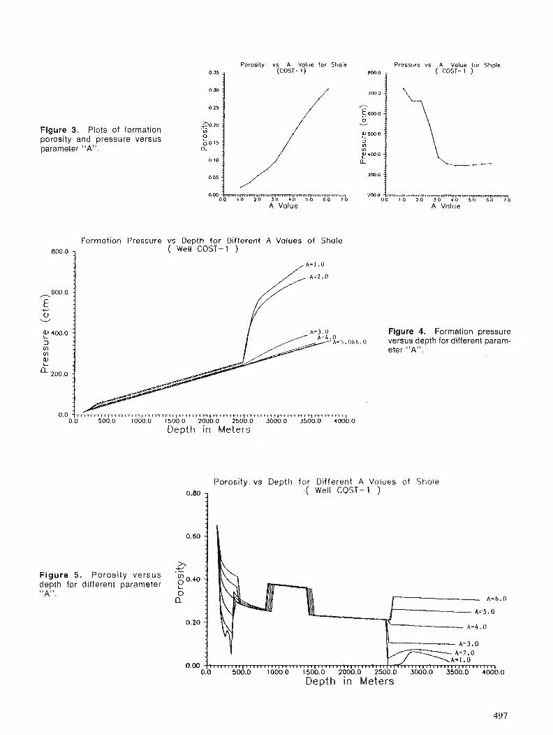
Figure 3. Plots of formation porosity and pressure versus parameter "A".

Formation Pressure

Porosity vs A Volue for Shale (COST- 1 )

0 . 0 0 0 - 5 m o A Value

vs Depth for ( Well COST-

Different A Values of Shole 1 )

Pressure vs A Volue for Shale

" O 1 ( cosr-1 )

200.0

A Value

400.0 Figure 4. Formation pressure 3 8 = 5 . 0 6 6 . 0 versus depth for different param- m m eter "A". a, L

200 0

0.0 ~ ~ ~ I I I , T ~ ~ T ~ T ~ T ~ I T ~ ~ ~ ~ ~ Q I I I I ~ I I ~ I ~ I I I ~ ~ ~ ~ ~ I ~ I ~ I I I

0 0 500 0 I000 0 1500 0 2000 0 2500 0 3000 0 3500.0 4000.0 Depth in Meters

Porosity. vs Depth for Different A Values of Shale .( Well COST-1 )

Figure 5 . Poros i ty versus depth for different parameter "A".

0.20 I,, ,!, ,, , , ,m, , , , ,, r ~ ~ ~ g A=2.0

A = I . O 0.00

0.0 500.0 1000.0 1500.0 2000.0 2500.0 3000.0 3500.0 4000.0

Depth in Meters

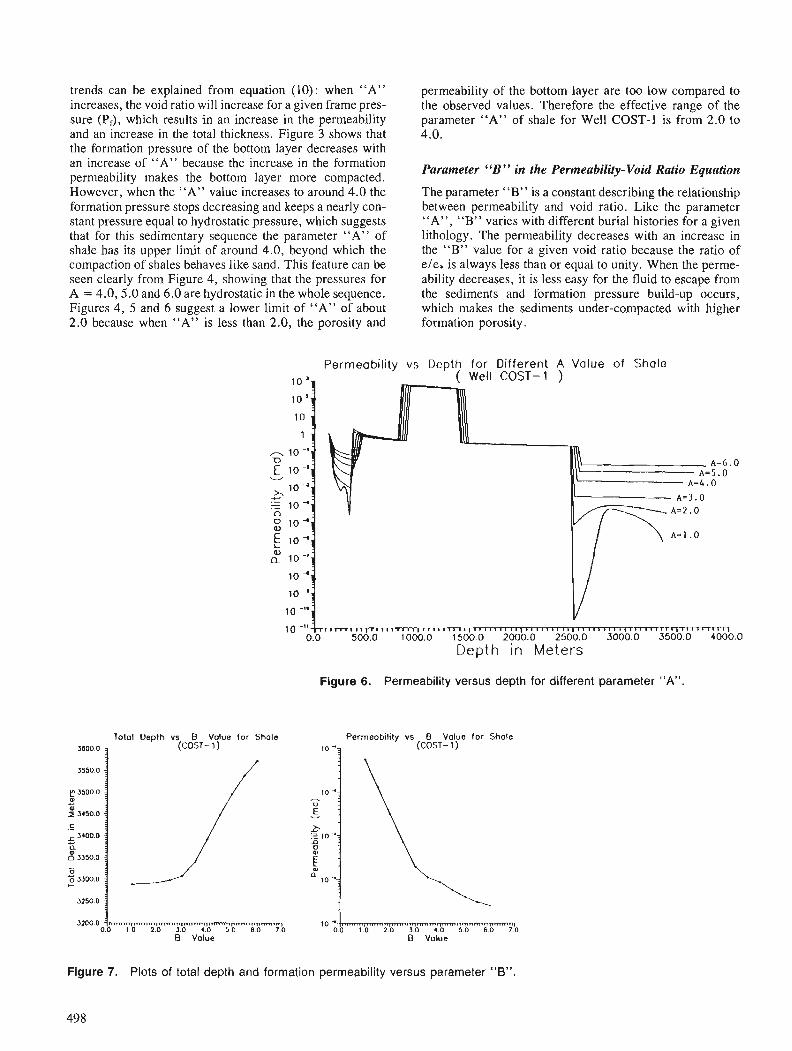
trends can be explained from equation (10): when "A" increases, the void ratio will increase for a given frame pressure (Pf), which results in an increase in the permeability and an increase in the total thickness. Figure 3 shows that the formation pressure of the bottom layer decreases with an increase of "A" because the increase in the formation permeability makes the bottom layer more compacted. However, when the "A" value increases to around 4.0 the formation pressure stops decreasing and keeps a nearly constant pressure equal to hydrostatic pressure, which suggests that for this sedimentary sequence the parameter "A" of shale has its upper limit of around 4.0, beyond which the compaction of shales behaves like sand. This feature can be seen clearly from Figure 4, showing that the pressures for A = 4.0,5.0 and 6.0 are hydrostatic in the whole sequence. Figures 4, 5 and 6 suggest a lower limit of "A" of about 2.0 because when "A" is less than 2.0, the porosity and

permeability of the bottom layer are too low compared to the observed values. Therefore the effective range of the parameter "A" of shale for Well COST-1 is from 2.0 to 4.0.

Parameter "B" in the Permeability-Void Ratio Equation

The parameter "B" is a constant describing the relationship between permeability and void ratio. Like the parameter "A". "B" varies with different burial histories for a given " lithology. The permeability decreases with an increase in the "B" value for a given void ratio because the ratio of e/e* is always less than or equal to unity. When the permeability decreases, it is less easy for the fluid to escape from the sediments and formation pressure build-up occurs, which makes the sediments under-compacted with higher formation porosity.

Total Depth vs B Value for Shole 3600 0 (COST- 1)

3 2 0 0 . 0 0 ~ 5 ' 6 " m 0 8 Value

Permeability vs Depth for Different A Value o f Shale ( Well COST-1 )

l o - * ' l l l ~ ~ ~ ~ ~ ~ T l ~ ~ ~ ~ ~ . ~ ~ ~ l ~ ~ ~ ~ ~ ~ ~ ~ ~ l ~ ~ ~ ~ ~ ~ ~ ~ ~ l ~ ~ ~ ~ ~ ~ ~ ~ ~ l ~ ~ ~ ~ ~ ~ ~ ~ ~ l ~ ~ ~ ~ ~ ~ ~ ~ l ~ ~ ~ ~ ~ ~ ~ ~ ~ l

0.0 500.0 1000.0 1500.0 2000.0 2500.0 3000.0 3500.0 4000.0

Depth in Meters

Figure 6. Permeability versus depth for different parameter "A"

Permeability vs I3 Value for Shale (COST- 1 )

10 -60 - 7 0

8 Value

Figure 7. Plots of total depth and formation permeability versus parameter "B"

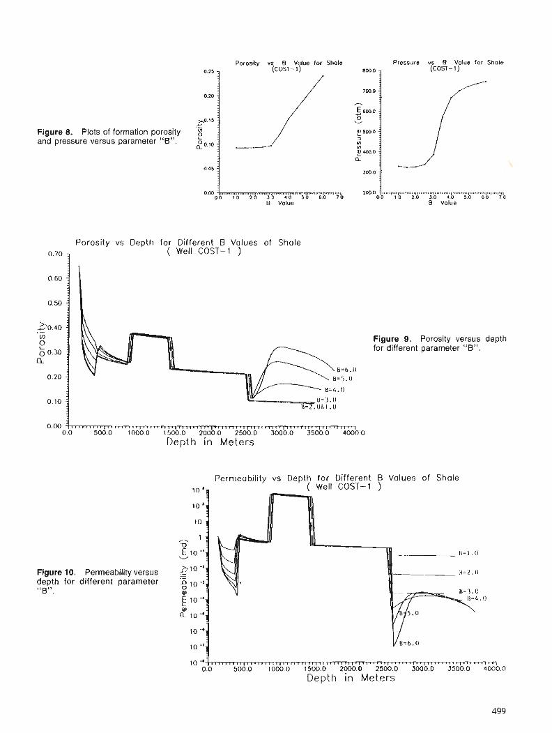
Figure 8. Plots of formation porosity and pressure versus parameter "5".

Porosity vs 8 Volue for Shale (COST- 1)

O . ~ ~ + ~ T ~ O B Volue

Pressure vs 0 Volue for Shole (COST - 1 )

Porosity vs Depth for Different B Volues of Shale

0.70 ( Well COST-1 )

0.60

0.50

20.40 . - rn

g 0.30 a

0.20

0.10

200.0 0 0 2.0 3.0 4.0 5.0 6 0 7 0

8 Volue

0 . 0 L ~ n ~ l l ~ ~ 1 l ~ ~ ~ l ~ T ~ T ~ l ~ 1 ~ ~ l ~ r r ~ r ~ ~ ~ l ~ ~ ~ l l r ~ l ~ ~ r l l ~ r ~ l I l 0.0 500.0 1000.0 1500.0 2000.0 2500.0 3000.0 3500.0 4000.0

Depth In Meters

Figure 10. Permeability versus depth for different parameter "5".

Figure 9. Porosity versus depth for different parameter "6".

Permeability vs Depth for Different B Values of Shole ( Well COST-1 )

0.0 500.0 1000.0 1500.0 2000.0 2500.0 3000.0 3500.0 4000.0 Depth in Meters

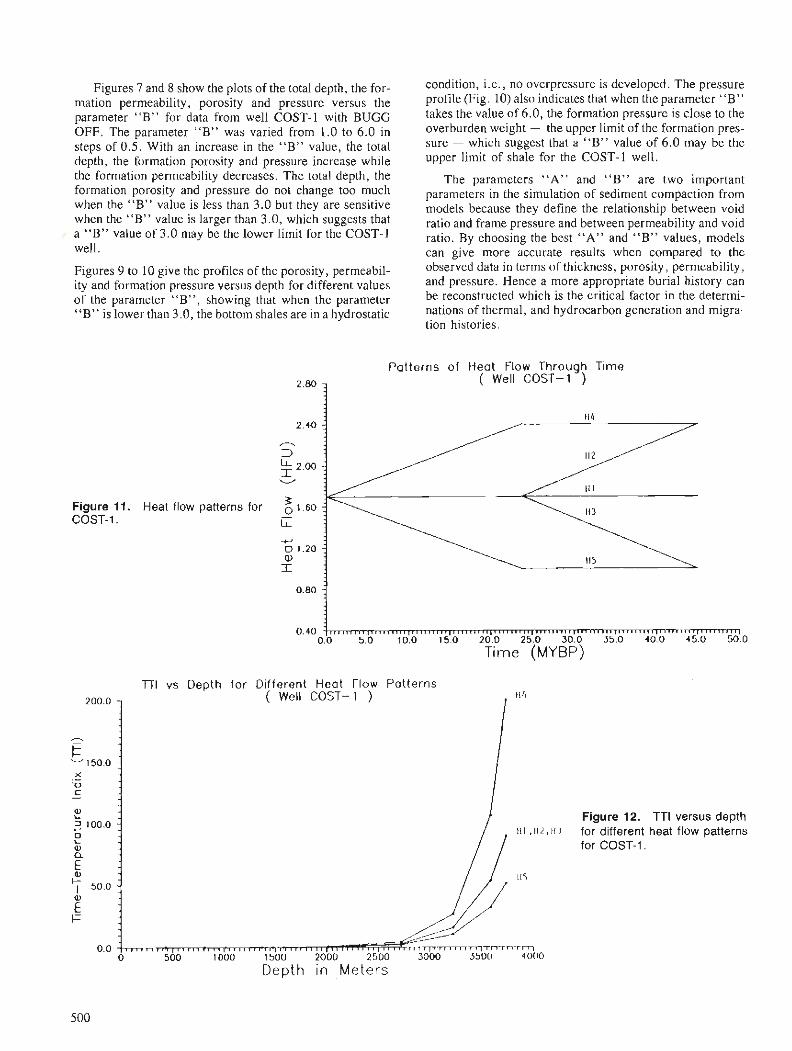
Figures 7 and 8 show the plots of the total depth, the formation permeability, porosity and pressure versus the parameter "B" for data from well COST-1 with BUGG OFF. The parameter "B" was varied from 1.0 to 6.0 in steps of 0.5. With an increase in the "B" value, the total depth, the formation porosity and pressure increase while the formation permeability decreases. The total depth, the formation porosity and pressure do not change too much when the "B" value is less than 3 .0 but they are sensitive when the "B" value is larger than 3.0, which suggests that a "B" value of 3.0 may be the lower limit for the COST-I well.

Figures 9 to 10 give the profiles of the porosity, permeability and formation pressure versus depth for different values of the parameter "B", showing that when the parameter "B" is lower than 3.0, the bottom shales are in a hydrostatic

Figure 11. COST-1.

Heat flow patterns for

condition, i.e., no overpressure is developed. The pressure profile (Fig. 10) also indicates that when the parameter "B" takes the value of 6.0, the formation pressure is close to the overburden weight - the upper limit of the formation pressure - which suggest that a "B" value of 6.0 may be the upper limit of shale for the COST-1 well.

The parameters "A" and "B" are two important parameters in the simulation of sediment compaction from models because they define the relationship between void ratio and frame pressure and between permeability and void ratio. By choosing the best "A" and "B" values, models can give more accurate results when compared to the observed data in terms of thickness, porosity, permeability, and pressure. Hence a more appropriate burial history can be reconstructed which is the critical factor in the determinations of thermal, and hydrocarbon generation and migration histories.

Pat terns of Heat Flow Through Time ( Well COST-1 )

0.40

Time (MYBP)

TTI vs Depth for Different Heat Flow Pat terns ( Well COST-1 )

X .- u C

?! 3 100.0 - o L Q, a E Q,

Figure 12. TTI versus depth 11 I .II? .II 1 for different heat flow patterns

for COST-1 .

115 7 50.0

E I=

0.0 - - r r m m t m i ~ u ~ ~ m ~ r 0 500 1000 1500 2000 2500 3000 3500 4000

Depth in Meters

Sensitivity to Assumptions then is constant; and pattern 5 (H5) - heat flow decreases

Heat flow variation with time is very important in the reconstruction of temperature history which, in turn, is the key factor controlling the maturation and hydrocarbon generation of source rocks. In the simplest models, heat flow changes are described by a one-parameter variation which we take to be either linear or exponential with time. This section examines how sensitive the model is to a variable heat flow with time (nonlinear and/or non-exponential). Five heat flow patterns were tested. Pattern 1 (Hl) - heat flow constant with time; pattern 2 (H2) - heat flow constant for a certain time and then increases; pattern 3 (H3) - heat flow constant for a certain time and then decreases; pattern 4 (H4) - heat flow increases to a certain time and

to a certain time and then is constant. Figure 11 shows graphically the five heat flow patterns for Well COST-1 with cu = 0.01 and T, = 295°K. Figures 12 and 13 show the profiles of the TTI and Ro versus depth for different heat flow patterns. From Figures 12 and 13 we see that heat flow patterns 1, 2 , and 3 cause little change in the TTI, R, and generation calculations, heat flow pattern 4 gives the highest values in the maximum TTI, maximum %, the kerogen transformation ratio and total amount of hydrocarbon, and pattern 5 gives the lowest values in these output variables. The reason for the above features can be explained as follows: even though heat flow patterns 1 ,2 , and 3 have different values before 23.7 MYBP, they keep the same values (1.7 HFU) from present to 23.7 MYBP (Fig. 11). This

Ro vs Depth for Different Heat Flow Pat terns

3 ( Well COST-1 )

Figure 14. Heat flow patterns for NWTEST301.

Figure 13. Ro versus depth for different heat flow patterns for COST-1.

0 500 1000 1500 2000 2500 3000 3500 4000

Depth in Meters

Pat terns of Heat Flow Through T ~ m e ( Well NWTEST301 )

o . ~ + r n n T v r r n a 1 r n n l n m n r n 1 o n n r r r v t r r u l u r t l r r 7 r v v m j v l v n ( r t u v r l 1

0.0 50.0 100.0 156.0 200 0 250.0 >% 0

Time (MYBP)

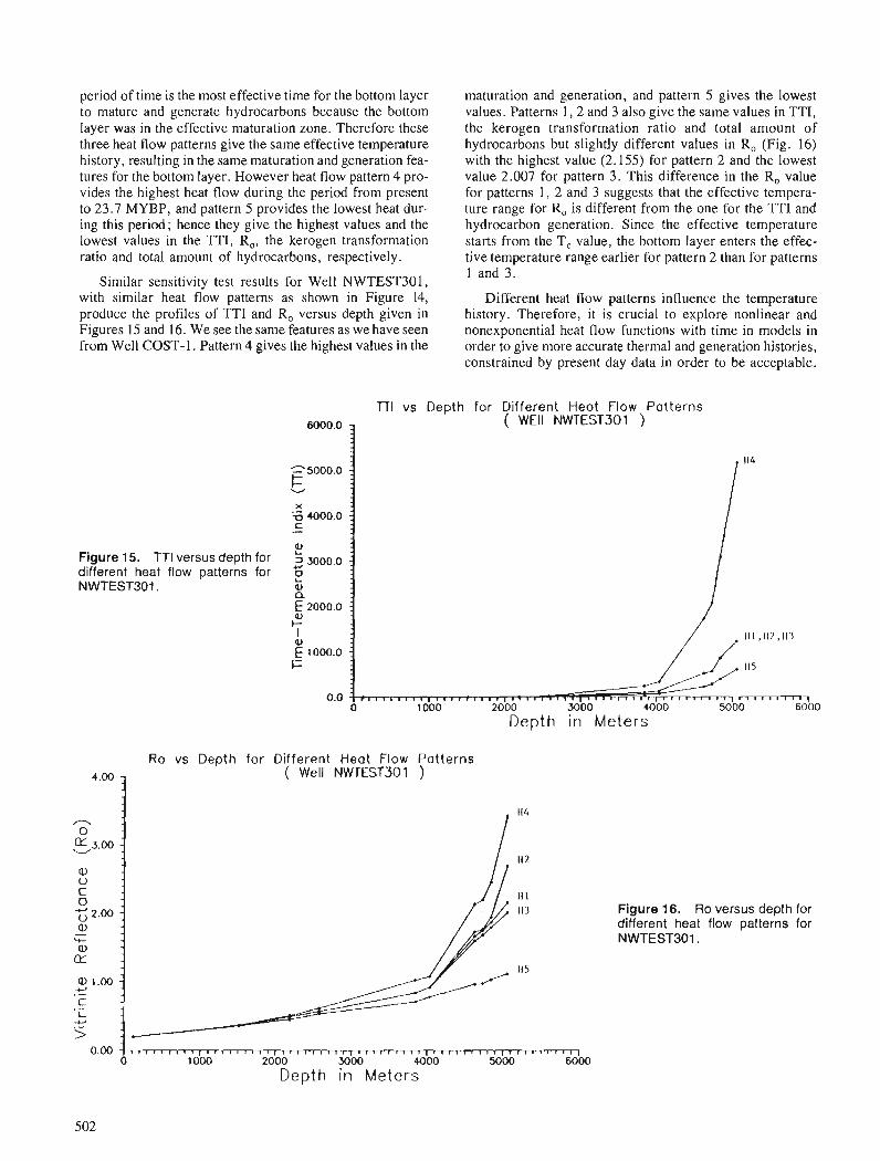
period of time is the most effective time for the bottom layer to mature and generate hydrocarbons because the bottom layer was in the effective maturation zone. Therefore these three heat flow patterns give the same effective temperature history, resulting in the same maturation and generation features for the bottom layer. However heat flow pattern 4 provides the highest heat flow during the period from present to 23.7 MYBP, and pattern 5 provides the lowest heat during this period; hence they give the highest values and the lowest values in the TTI, R,, the kerogen transformation ratio and total amount of hydrocarbons, respectively.

Similar sensitivity test results for Well NWTEST301, with similar heat flow patterns as shown in Figure 14, produce the profiles of TTI and R, versus depth given in Figures 15 and 16. We see the same features as we have seen from Well COST-1. Pattern 4 gives the highest values in the

maturation and generation, and pattern 5 gives the lowest values. Patterns 1 , 2 and 3 also give the same values in TTI, the kerogen transformation ratio and total amount of hydrocarbons but slightly different values in R, (Fig. 16) with the highest value (2.155) for pattern 2 and the lowest value 2.007 for pattern 3. This difference in the R, value for patterns 1 , 2 and 3 suggests that the effective temperature range for R, is different from the one for the TTI and hydrocarbon generation. Since the effective temperature starts from the T, value, the bottom layer enters the effective temperature range earlier for pattern 2 than for patterns 1 and 3.

Different heat flow patterns influence the temperature history. Therefore, it is crucial to explore nonlinear and nonexponential heat flow functions with time in models in order to give more accurate thermal and generation histories, constrained by present day data in order to be acceptable.

TTI vs Depth for Different Heat Flow Patterns ( WEll NWTEST301 )

Figure 15. TTI versus depth for different heat flow patterns for NWTEST301.

Depth in Meters

Ro vs Depth for Different Heat Flow Patterns 4.00 7 ( Well NWEST301 )

Figure 16. Ro versus depth for different heat flow patterns for NWTEST301.

0 1000 2000 3000 WOO 5000 6000

Depth in Meters

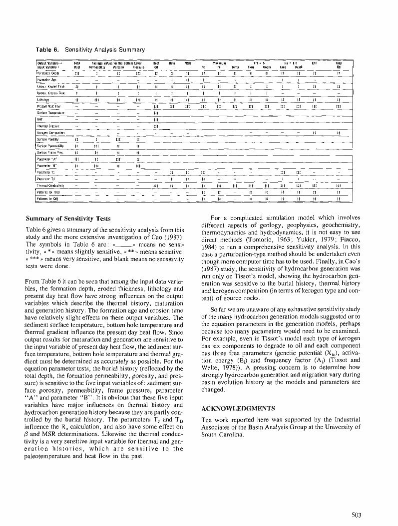
Table 6. Sensitivity Analysis Summary

Dulpul Variable - Tolal Average Values lor the Bollom Layer Beal Bela MSR Maxlmum T l i = 5 RO = 0.6 KTR Total lnpul Variable 8 Depl Permeablllly Porosily Preuurs 00 Ro TI1 Temp Tlme Osulh Tlme Daplh HC

Formalion Deplh $ti t f t 111 tt $t f t tt f t f t i tt tt t$ t$ u I Fnrrnalinn Ana - - - - - i f i f - - k f - - 1 . -. - =.

Uncon. Kroded Thick, t t t tt t t t t i t t t tt tt t t t t t t Uocon. Kfosion Time t t t t t t t t t t t t - - - - L i l h o l o ~ ~ f f l l f i t f f t it it 11 f t tt tt $ 2 tt tt tt t t t t

1 Present Heal llow - - - - f i t i l t i f f i f f i f f lit f t f t t i itt i f f f i t ttt 1 Surface Temperature - - - - t t f I -

BHT - - - - ttt Thermal Gradient - - - - t f t Kerogen Compos~lion - - - - - - - - - - - - - - tt i t

Sumce Porosilv :t f ttt tt

Surlace frame Pres. tt $1 tt lt Parameler "A" ttt tt ttt tt Parameter "8" 11 ttt $1 ttt Panmeler Tc - - - - - tt tt ttt - - - - f f t $tt - - Parameler Td - - - - - t 1: t f - - - - i t - - Thermal Conductivity - - - - t t t t t it #t ttt t t t #t ttt ttt #t ttt 1 Palterns lor 1011) - - - - - - - t t f t - t t t t t t 14 $1 it Pallems lor D(1) - - - - - - - $ 1 tt - t tt tt tt U tt

Summary of Sensitivity Tests For a complicated simulation model which involves

Table 6 gives a summary of the sensitivity analysis from this study and the more extensive investigation of Cao (1987). The symbols in Table 6 are: c< means no sensitivity, << * means slightly sensitive, a ** ,, means sensitive, (< *** n means very sensitive, and blank means no sensitivity tests were done.

From Table 6 it can be seen that among the input data variables, the formation depth, eroded thickness, lithology and present day heat flow have strong influences on the output variables which describe the thermal history, maturation and generation history. The formation age and erosion time have relatively slight effects on these output variables. The sediment surface temperature, bottom hole temperature and thermal gradient influence the present day heat flow. Since output results for maturation and generation are sensitive to the input variable of present day heat flow, the sediment surface temperature, bottom hole temperature and thermal gradient must be determined as accurately as possible. For the equation parameter tests, the burial history (reflected by the total depth, the formation permeability, porosity, and pressure) is sensitive to the five input variables of: sediment surface porosity, permeability, frame pressure, parameter "A" and parameter "B". It is obvious that these five input variables have major influences on thermal history and hydrocarbon generation history because they are partly controlled by the burial history. The parameters T, and TD influence the R, calculation, and also have some effect on B and MSR determinations. Likewise the thermal conduc-

different aspects of geology, geophysics, geochemistry, thermodynamics and hydrodynamics, it is not easy to use direct methods (Tomoric, 1963 ; Yukler, 1979 ; Fiacco, 1984) to run a comprehensive sensitivity analysis. In this case a perturbation-type method should be undertaken even though more computer time has to be used. Finally, in Cao's (1987) study, thesensitivity of hydrocarbon generation was run only on Tissot's model, showing the hydrocarbon generation was sensitive to the burial history, thermal history and kerogen composition (in terms of kerogen type and content) of source rocks.

So far we are unaware of any exhaustive sensitivity study of the many hydrocarbon generation models suggested or to the equation parameters in the generation models, perhaps because too many parameters would need to be examined. For example, even in Tissot's model each type of kerogen has six components to degrade to oil and each component has three free parameters (genetic potential (Xi,), activation energy (Ei) and frequency factor (Ai) (Tissot and Welte, 1978)). A pressing concern is to determine how strongly hydrocarbon generation and migration vary during basin evolution history as the models and parameters are changed.

ACKNOWLEDGMENTS

The work reported here was supported by the Industrial Associates of the Basin Analysis Group at the University of South Carolina.

tivity is a very sensitive input variable for thermal and gen- e r a t i c n h i s t o r i e s , w h i c h a r e s e n s i t i v e t o t h e paleotemperature and heat flow in the past.

REFERENCES

Anderson, R.B. 1965 : The sensitivity problem in control system optimization; Ph.D. Dis-

sertation, Georgia Institute of Technology. Atwater, G.I. 1956: Future of Louisiana offshore oil province; American Association

of Pctroleum Geologists Bullo. v. 40. p. 2624-2634. Bally, A.W. 1975 : A geodynamic scenario for hydrocarbon occurrences; Proceedings

Ninth World Petroleum Congress, Tokyo, v. 2, p. 33-44. Brownlee, K.A. 1960: Statistical Theory and Methodology in Science and Engineering;

John Wiley and Sons. Inc.. New York. Cao, S. 1985: A quantitative dynamical model for basin analysis and its applica-

tion to the northern North Sea basin; M.S. Thesis, University of South Carolina.

1987: Sensitivity Analysis of I-D Dynamical Model for Basin Analysis; Ph.D. Dissertation, University of South Carolina.

Cao, S., Glezen, W.H. and Lerche, I. 1986: Fluid flow, hydrocarbon generation and migration: A quantitative

model of dynamical evolution i n sedimentary basins; Proceeding Offshore Technology Conference (Houston, TX) paper 5182, v. 2, p. 267-276.

Chorafas, D.H. 1965: System and Simulation; Academic Press, New York and London. Conybeare, C.E.B. 1965: Hydrocarbon generation potential and hydrocarbon yield capacity

of sedimentary basin; Bulletin Canadian Petroleum Geologists, V. 13, p. 509-528.

Fiacco, A.V. 1984: Sensitivity. Stability and Parametric Analysis; Mathematical

Programming Study 21, North-Holland, Amsterdam. Griffiths, W.C. 1967: Scioltific Methodin the Analysis ofsediments; McGraw-Hill, New

York. Halbouty, M.T. et al. 1970: Factors affecting formarion of giant oil and gas fields. and basin

classification, Part 11; in Geology of Giant Petroleum Fields ed M.T. Halbouty; American Association of Petroleum Geologists Memoir 14, p. 528-555.

Harbaugh, J.W. and Merriam, D.F. 1968: Computer Applications in Stratigraphic Analysis; John Wiley and

Sons, New York. Harbaugh, J.W. and Bonham-Carter, G. 1970: Comnputer Simulation in Geology; John Wiley and Sons, New

York. Jones, R.W. 1975: A quantitative geologic approach to prediction of petroleum

resources; in Methods of Estimating the Volume of Undiscovered Oil and Gas Resources American Association Petroleum Geolo- gists Studies in Gcology I, Tulsa, Oklahoma, p. 186-195.

Lerche, I. 1989: Basin Analysis: Quantitalivr Methods; Academic Press, Orlando. Lerche, J. and Glezen, W.H. 1984: Deposition, compaction and fluid migration: time dependent

models in one and two dimensions; Gulf Oil Corp., Pittsburgh, Pennsylvania

Lumley, J. L. 1970: Stochastic Tools in Turbulence; Academic Press, New York. McDowell, A. N. 1975: What are the problems in estimating the oil potcntial of a basin?;

Oil and Gas Journal, June 9, 1975, p. 85-90. Miller, B.M. et al. 1975: Geological estimation of undiscovered recoverable oil gas

resources in the United States; U. S. Geological Survey Circular 725, p. 78.

Nakayama, K. 1986: Two-Dimensional Basin Analysis for Petroluem Exploration;

Ph.D. Thesis, University of South Carolina. Newendorp, P.D. 1975 : Decision Analysis for Petrolewn Explorarion ; Petroleum Publ .

Co., Tulsa. Pitcher, M.G. 1976: U.S. discovery rate tied to technology; Oil and Gas Journal, March

22, 1976, p. 34-35. Press, W.H., Flannery, B.P., Teukosky, S.A. and Vetterling, W.T. 1986: Numerical Recipes: the Art of Scientific Cotnputing; Cambridge

University Press, New York. Roadifer, R. 1975 : A probability approach to estimate volumesof undiscovered oil and

gas; in Probability Methods in Oil Exploration; ed. J.C. Davis, et al. ; American Association of Petroleum Geologists Research Symposium, Stanford University, p. 18.

Roy, K. J., Procter, R.M. and McCrossan, R.C. 1975: Hydrocarbon assessment using subjective probability; in Probabi-

lity Methods in Oil Exploration; ed. J.C. Davis, J.C. et al. ; Ameri- can Association of Pktroleum Geologists Research Symposium, Stanford University, p. 56-60.

Shchigolov, B.M. 1965: Mathematical Analysis of Observations, Elsevier, New York. Smith, M.B. 1968 : Estimate resources by using computer simulation method; Oil and

Gas Journal, March 1 I , 1968, p. 8 1-84. Stoian, E. 1965: Fundamentals and applications of the Monte Carlo method; Jour-

nal of Canadian Petroleum Technology, v. 4, p. 120-129. Tissot, B. and D. H. Welte 1978: Petroleum Formation and Occurrences; Springer-Vcrlag, New

York. Tomoric, R. 1963: Sensitivity Analysis of Dynamic Systems; McGraw-Hill, New

York. Ungerer, P. el al. 1984 : Geological and geochemical methods in oil exploration, principles

and practical examples; American Association of Petroleum Geo- logists Memoir 35, p. 53-77.

Walstrom, J.E., Mueller, T.D. and McFarlane, R.C. 1967: Evaluating uncertainty in engineering calculation; Journal

Petroleum Technology. v. 19. p. 1595.1603. Warren, J. E. 1979: Basin evaluation; Society of Petroleum Engineers Economics and

Evaluation Symposium, Dallas, February, 1979. ' Weeks, L.G. 1952: Factors of sedimentary basin development that control oil occur-

rence; American Association of Petroleum Geologists Bull., v. 36, p. 2071-2124.

Yukler, M.A. 1979: Sensitivity analysis of groundwater flow system and an application

to a real case; 5 Geomathematical and Petrophysical Studies in Sedimentology ed. D.F. Mcrriam; Pergamon Press, New York.

Yukler, M.A. and Kokesh, F. 1984: An overview of models used in petroleum resource estimation and

organic geochemistry; Advances in Petroleum Geochemistry (Volume I), ed. J. Brooks and D. Welte, Academic Press. New York. p. 69-73.

Yukler, M.A., Cornford, C. and Welte, D.H. 1978: One dimensional model to simulate geologic, hydrodynamic and

thermodynamic development of a sedimentary basin; Geologische Rundschau, v. 67, p. 960-979.

Modelling the sedimentary fill of basins

James P.M. Syvitskil

Syvitski, P.M., Modelling thefill of sedimentary basins; in Statistical Applications in the Earth Sciences, ed. F. P. Agterberg and G. F. Bonham-Carter; ~ e o l o ~ i c a l Survey of Canada, Paper 89-9, p. 505-515, 1989.

Abstract

SEDFLUX is an example of a unified process-response model for the growth of a prograding delta into a coastal basin. Sediment accumulation of various particle size fractions is predicted spatially, ji-om a parabolic partial differential equation that combines four mechanisms for depositing sediment within a basin: (1) bedload dumping along the delta front, (2) hemipelagic sedimentation under the seaward flowing river plume, (3) proximal slope bypassing by sediment gravity flows, and (4) downslope diffusion of the accreting sediment mass. The numerical solution employs a finite difference approximation of the parabolic equation and is solved by an explicit method. Sensitivity analysis was used to demonstrate that the rate of delta progradation is most sensitive to those processes which transfer marine sediments fiom the nearshore into deeper water, i.e. creep, small slides, and turbidity currents. The factors that control the steepness of the foreset beds, such as bedload transport and the removal rate by sediment gravity jlows, are of particular importance.

Le SEDFLUX est un exemple de modtle uniJiPde processus et rPponse conqu pour I'Ptude de la croissance de deltas en progression vers la mer dans un bassin cbtier. L'accumulation de sediments composPs de particules de diverses granulomAries est pre'vue dans 1 'espace d'aprts une Pquation parabolique aux diff&rentielles partielles qui combine quatre mPcanismes d 'accumulation des sddiments li 1 'interieur d 'un bassin: I ) de'versement de la charge de fond le long du front deltai'que, 2) se'dimentation he'mipPlagique sous le panache du cours d'eau s'e'coulant vers le large, 3) contournement de la pente proximale par Pcoulement par gravite' de sgdiments, et 4) d i ' s i o n vers le bas de la pente de la masse de sPdiments en accr&tion. La solution numtrique fait intervenir une approximation aux diffe'rences$nies de 1 'Pquation parabolique et une me'thode explicite. L'analyse de sensibilitk a Pte' utilisde pour dPmontrer que le taux de progradation est tr2.r susceptible aux processus qui transferent les sediments marins cbtiers vers les eaux plus profondes, c. -a-d, reptation, petits glissements et courants de turbidite', Les facteurs qui dPter- minent lapente des lits deltaiijues frontaux, comme le transport dans la charge de fond et le taux d'enltve- ment par &coulement par gravitt de sddiments, sont d'une importance particulitre.

' Atlantic Geoscience Centre, Geological Survey of Canada, Bedford Institute of Oceanography, P.O. Box 1006, Dartmouth, Nova Scotia B2Y 4A2.

INTRODUCTION temporal and spatial distribution of sedimentary deposits by

Recently, the discipline of quantitative dynamic stratigraphy has been formalized (Cross, 1990), whereby the character and origin of sedimentary deposits are investigated through computer simulation models that attempt to replicate sedimentary systems. Such models enhance our understanding by allowing quantitative inferences to be obtained, both on the nature of the sedimentary deposit and the interactions controlling sedimentation. The models tend to be complex, involving a number of independent or interacting sediment transport processes and geological controls. In their most complete form, the fundamental laws of physics are used to understand the resultant sedimentary deposits. This paper describes SEDFLUX, a process-response model for the study of basin filling, with emphasis on sensitivity analysis. The historical development of this type of numerical approach, the theoretical considerations, the algorithms and source code, and the application to the petroleum industry can be found in Syvitski (1990), Syvitski, Smith, Calabrese and Boudreau (1988), Calabrese and Syvitski (1987) and Syvitski and Farrow (1989), respectively.

THE PROCESS-RESPONSE MODEL

In the past there have been two approaches to the modelling of basin filling (Fig. l), i.e. either Response or Process- models. The Response Model begins with careful observations of the geological record and attempts to discern the

A The Response Model

f""""' * x-\%%v - * --?< ., " ""

Geometr ic C o n c e p t u a l Statistical

(observal~onal) (~nferentlal) (regression analysIS)

B I The Process Model

I I Determin is t ic I (conservation of inputs 8 oulpuls)

1 I h lluld mechanics) 1 \ I

(steady-slate I co~d~t~ons in flux) I

comparison (observations vs

Figure 1. The two major approaches to the "Process- Response" model a s related to sediment transport and the filling of sedimentary basins.

- .

some form of best-fit approximations. The key components include: (I) a geometric stage wherein geological information is represented in map or schematic form; (2) a conceptual stage wherein all of the relevant factors are identified and critical facets are inferred, the system to be modelled is set up as dynamically interrelated components whereby changes to any component would have repercussions throughout the system; (3) a statistical stage, in which the relationships amongst the simultaneously varying attributes are analyzed; and (4) a final empirical stage, in which variables can be interrelated in the form of predictive algorithms, although such predictions are limited to environments with similar environmental conditions. The closure of the Response Model loop (Fig. 1) includes: (1) generation of predictions, (2) collection of new observations to compare with these predictions, (3) where warranted, modifications to the conceptual model, and (4) statistical testing and generation of a refined empirical model. Three recent examples of basin-fill response models include those of Harbaugh and Bonham-Carter (1977), Bitzer and Harbaugh (1987), Tet- zlaff and Harbaugh (1989), and Flemings and Jordan

The Process Model approach is based on the fundamental theory governing fluid mechanics and sediment transport. It also begins with (1) a conceptual model (Fig. l), although expressed in more detail and rigour where primary and secondary processes and parameters are identified. This leads to (2) a mathematical model where theory is expressed in the form of the physical laws of fluid mechanics. These include the conservation equations of mass, momentum and energy. The conservation of fluid mass is typically substituted for one involving volume, and referred to as the equation of continuity. Such equations keep track of the total volume (water or sediment) and its distribution within the system being modelled. The conservation of energy equation specifically tracks the conversion of turbulence to heat, partly as a function of boundary friciton. The conservation of momentum equations evaluate the operating forces at a given location including the boundary shear stresses. Stage (3), the deterministic model, has the relevant response characteristics incorporated in a unifying differential equation. Such models contain no element of chance and thus their solution at any point in time is completely predetermined. Although theoretically-based, these models can have a wide range of solutions depending on the theoretical expression used and the complexity of the solution evoked. stage (4), the probabilistic model, includes some random or stochastic components and thus no two model runs will be precisely the same. Examples of stochastic geologic processes include river discharge, earthquake-generated slides, and storm-driven waves. Such models are especially useful where portions of the underlying mathematical model are weak (Fox, 1978). The final stage ( 5 ) , the computer model, provides simulations of key parameters using numerical analysis through the use of finite difference methods (based on localized approximations) or finite element methods (based on global constraints of the full domain). Generally a unified differential equation is solved by one of three methods (explicit schemes, implicit schemes

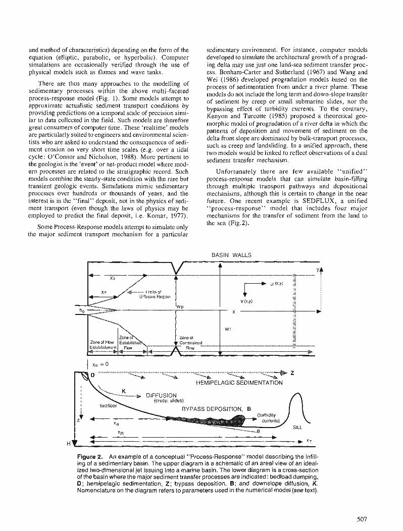
and method of characteristics) depending on the form of the equation (elliptic, parabolic, or hyperbolic). Computer simulations are occasionally verified through the use of physical models such as flumes and wave tanks.

There are thus many approaches to the modelling of sedimentary processes within the above multi-faceted process-response model (Fig. 1). Some models attempt to approximate actualistic sediment transport conditions by providing predictions on a temporal scale of precision similar to data collected in the field. Such models are therefore great consumers of computer time. These 'realtime' models are particularly suited to engineers and environmental scientists who are asked to understand the consequences of sediment erosion on very short time scales (e.g. over a tidal cycle: O'Connor and Nicholson, 1988). More pertinent to the geologist is the 'event' or net-product model where modern processes are related to the stratigraphic record. Such models combine the steady-state condition with the rare but transient geologic events. Simulations mimic sedimentary processes over hundreds or thousands of years, and the interest is in the "final" deposit, not in the physics of sediment transport (even though the laws of physics may be employed to predict the final deposit, i.e. Komar, 1977).

Some Process-Response models attempt to simulate only the major sediment transport mechanism for a particular

sedimentary environment. For instance, computer models developed to simulate the architectural growth of a prograding delta may use just one land-sea sediment transfer process. Bonham-Carter and Sutherland (1967) and Wang and Wei (1986) developed progradation models based on the process of sedimentation from under a river plume. These models do not include the long term and down-slope transfer of sediment by creep or small submarine slides, nor the bypassing effect of turbidity currents. To the contrary, Kenyon and Turcotte (1985) proposed a theoretical geomorphic model of progradation of a river delta in which the patterns of deposition and movement of sediment on the delta front slope are dominated by bulk-transport processes, such as creep and landsliding. In a unified approach, these two models would be linked to reflect observations of a dual sediment transfer mechanism.

Unfortunately there are few available "unified" process-response models that can simulate basin-filling through multiple transport pathways and depositional mechanisms, although this is certain to change in the near future. One recent example is SEDFLUX, a unified "process-response" model that includes four major mechanisms for the transfer of sediment from the land to the sea (Fig.2).

BASIN WALLS

\\\\\\\\\\\\\\\\\\\...,......,..\..,............\...,..,..,..,...,..... .\\\.\\\\\\\\\\\\\\..,.., \ -a, 2-2e, \ \+z

HEMIPELAGIC SEDIMENTATION

Figure 2. An example of a conceptual "Process-Response" model describing the infilling of a sedimentary basin. The upper diagram is a schematic of an areal view of an idealized two-dimensional jet issuing into a marine basin. The lower diagram is a cross-section of the basin where the major sediment transfer processes are indicated: bedload dumping, D; hemipelagic sedimentation, Z; bypass deposition, 8 ; and downslope diffusion, K. Nomenclature on the diagram refers to parameters used in the numerical model (see text).

SEDFLUX

SEDFLUX is a theoretically-based model developed to simulate the sediment fill of a marine basin by the progradation of a delta. The model simulates four mechanisms for the transfer of sediment from the land to the sea: (1) hemipelagic sedimentation of particles carried seaward by the river plume; (2) bedload dumping along the delta front ; (3) proximal slope bypassing by turbidity currents; and (4) the combined effects of both short term (wave and tidal action) and long term (creep and small slides) downslope diffusion of the accreting sediment mass. Below is a brief description of how the model simulates these mechanisms of sediment deposition.

River plume sedimentation

Hemipelagic sedimentation is described as a function of grain size, initial load and time, where to is the time at which the sediment leaves the river mouth and enters the basin. It is assumed that sedimentation is the only means by which particles are removed from the water column and that the removal rate is constant. Suspended sediment enters the basin from the river at an initial concentration, C,, and subsequently undergoes both settling and advection down the basin. Particles are removed from the water column at a rate, Z(x) in units of mass per area per time, and for a plug flow:

Z(X) = h Q, (u, b,)-l e -(hluo)x

where h is a first-order removal rate-constant, in units of time-', Q, is the suspended load, u, is the longitudinal plume velocity, b, is the width of the river mouth, and x is distance along the plume. This simple model predicts that the sedimentation rate under a river plume will decrease exponentially with increasing distance out from the river mouth.

To model the velocity distribution within highly- stratified marine basins, a buoyancy-dominated, free, two- dimensional jet is considered. The longitudinal and lateral components of the surface water velocity, are residual or tidally-averaged values. The velocity distribution within three dynamic zones of the river plume are considered (Fig.2), i.e. zone (1) where the plume is not yet established (nearest the river mouth) and where the center of the plume continues to behave as a plug flow, followed by zone (2) where the established flow decreases as the plume spreads, and zone (3) where plume spreading is affected and constrained by the basin boundaries. The analytical solution for predicting the sedimentation rate along the axis of such a plume may take the form of:

Z(x) = Z, exp [ -(h,/u,) x] for x I 5.2b0

Z(x) = Z, exp [ - h (1 .76b0/u0 + 0.29 ( ~ , b , ) - ~ . ~ ) ]

for 5.2b0 < x <xb

Z(X) = Zo eXp [ -h (1.76b,/~, -0.15 ~ ~ l ' ~ (U~~ , ) -O .~) ]

for x > xb

where Z, is the sedimentation rate at x=x, and is equal to h Q, (u, b,)-I. As the SPM load is composed of a mixture

of particle sizes, each particle size of class d, is characterized by a unique removal constant, hd. [The value of each hd can be obtained from the slope of the regression between the change in particle concentration of size class d, along the length of the plume seaward of the river mouth - for details see Syvitski et al. (1988)l. Thus the total sedimentation rate, ZT(x), is equal to the summation of the individual sedimentation rates Zd(x) for each size class:

z,(x) = C hd Qs (u, b d - e-hdt = C Zdo e-&df

Model predictions were found to compare favourably with- sediment flux data collected from basins found along the coast of Alaska, Norway and British Columbia, that differ widely in their sediment concentrations and discharge conditions (Syvitski et a]., 1988). All measured flux data were similarily derived from anchored sediment traps.

The accumulated thickness of sediment deposited from hemipelagic sedimentation, Z, between to and t , , at any given position out from the river mouth may be given as

where pb is the appropriate bulk density of size fraction d. Sedimentation rates are also integrated to the lateral boundaries of the plume, to obtain the total sediment deposition rate averaged across the basin, such that

where Wf is the width of the basin floor.

Delta front bedload dumping

Only the fluvial bedload that enters the marine environment, Qb, is considered in the model, i.e, topset deposits are not considered. It is also assumed that a portion of the bedload, a b , may be removed by turbidity flows and that the remainder, ad , is dumped close to the river mouth. Bed- load is distributed evenly over the width of the active delta front, Wd, and out to some distance, L. The dumping function of bedload, D, in units of thickness per unit time is given by

D = a d Qb (Wd L ~ b ) - l

where ad is the fraction of the bedload that remains within the delta front environment and pb is the bulk density of the deposited sediment (i.e. pb = n-I C pbd where n is the number of size fractions considered). The longitudinal cross-section of this deposit is rhomboidally shaped.

Bypassing transport and deposition

Some transport processes operate by removing sediment from the nearshore, whereby a significant portion of the prodelta environment is bypassed before the sediment is deposited. Highly fluid and initially turbulent gravity flows are the prime mechanism. Such flows are generated from failure along the distal portion of mouth bars as a result of rapid progradation over steep foreset beds. Submarine channels normally serve as conduits for these sandy gravity flows.

In the model, the amount of material deposited by turbidity currents at a distance, x, from the river mouth is a function of the slope near the river mouth and the slope of the basin floor. If the foreset slope is gentle (less than some critical value, 8), SEDFLUX assumes that no delta front failure occurs and channelized flows are not generated (i.e. bedload is deposited wholly by dumping near the river mouth). If a foreslope failure can occur, foreset sediment is deposited where the prodelta slope falls below some critical angle, 0, and therefore at some distance x4, out from the delta front. 0 is dependent on changes in the flow characteristics, including the friction forces acting on the flow, flow viscosity and velocity, and the type of particles transported by the flow. The run-out distance, XR, depends primarily on the rate of flow deceleration.

Accumulation of bypass material, B in units of thickness pertime, is assumed to decrease linearly as a function of x in such a way that:

XR

j B(x) dx = B (xR - x6) and B = a,, Qb pb-l W f - ' x&

where ab is the fraction of the bedload entering the delta front environment that fails and moves downslope along the conduits of the submarine channel system and Wf is the average width of the basin floor. Values of p,,, x~ and x4 are averages for the possible variations in the gravity flows. The SEDFLUX model also allows the basin to be partially disconnected from the open ocean by a basement high called a sill. A sill would effectively stop the long-distance transport of turbidites but would not interfere with the passage of suspended load still remaining in the surface plume. Where the distance from the river mouth to the sill is < x~ then theentire deposition of sediment from the turbidity current is spread between x, and the distance to the sill.

Down-slope diffusion

This action includes all processes, other than channelized sediment flows, that move previously deposited material away from the proximal prodelta slopes into deeper water. Diffusion may be influenced by both short-term (e.g. tidal action) and long-term (e.g, creep) processes. Diffusion is most important on steep basin slopes which, at least initially, are a consequence of the original basement geometry. Diffusive processes operate at a rate proportional to the bathymetric slope, such that:

where K is the coefficient of diffusion and K = -

S[dh/ax]-I, S is the rate of sediment transport and ah/& = -aS/ax is used to conserve mass. Thus the effect of downslope diffusion decreases with decreasing concavity of the slope.

In the model, diffusion operates independently of the primary methods of sediment deposition. A delta profile can therefore be adjusted even in the absence of sediment input so as to simulate a marine transgression without evoking a

relative sea level adjustment. This method can also be used to simulate the action of a short-lived mass transfer of sediment, e.g. earthquake-generated submarine slope failure, by adjusting K with time.

Numerical delta model

Sediment accumulation is modelled with a parabolic partial differential equation,

where K is the coefficient of the sediment diffusion effect and the remaining three terms represent contributions to the seafloor from bedload dumping, bypassing and hemipelagic sedimentation, respectively. The corresponding finite difference equation is solved numerically using an explicit method. All the sediment input to the basin being modelled is accounted for. In the case of small basins, a significant amount of sediment may exit the basin via thc seaward flowing river plume, or in the case of a basin that is not silled (i.e, seperated from the open ocean by a basement high) a portion of the sediment deposited from a turbidity current may be transported outside the basin. In either case, the model keeps track of the sediment volume deposited within the basin and the fraction that is able to leave the basin.

The final model consists of: (1) a high-resolution (temporal) 2-D particle-scavenging model capable of predicting hemipelagic sedimentation rates beneath a river plume, on time scales less than a year; and (2) a lower temporal resolution portion of the model that predicts the accumulation of sediment by bedload dumping at the river mouth, deposition by turbidity currents, and mass transfer processes such as creep and slides. The resultant model allows for the prediction of changing lithologies, including sediment size distributions, with time and space and at a predictive resolution of tens to hundreds of years.

Every numerical model makes assumptions about the system that is being simulated. The major assumptions behind SEDFLUX are listed in Table 1. As the predictive capabilities of a model increases in its required simulation

Table 1. Model Assumptions behind SEDFLUX.

(1) Lateral variations in the position of the river channel and the shape of the delta are insignificant over the time span of the simulation.

(2) Lateral cross-sections of the basin and the river mouth are rectangular.

(3) The delta head is perpendicular to the basin margins. (4) The basin has a basement high or sill, thus partially

separating the basin from the ocean. (5) The river plume is two-dimensional, maintaining a constant

depth as it flows into a two-layer, stratified basin. (6) Flow velocity within the river channel is as a plug flow, i.e.

uniform in depth and width. (7) The model distributes the total sediment deposited in any

cross-section of the plume evenly across the width of the basin.

(8) The input parameters are time and tidally averaged values.

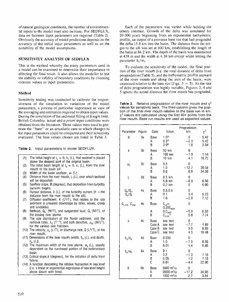
of natural geological conditions, the number of environmental inputs to the model must also increase. For SEDFLUX, data on fourteen input parameters are required (Table 2). Obviously the accuracy of model predictions depends on the accuracy of the initial input parameters as well as on the suitability of the model assumptions.

SENSITIVITY ANALYSIS OF SEDFLUX

This is the method whereby the many parameters used in a model can be examined to determine their importance in affecting the final result. It also allows the modeller to test the stability or validity of boundary conditions by choosing extreme values as input parameters.

Method

Sensitivity testing was conducted to calibrate the responsiveness of the simulation to variations of the model parameters, a process of particular importance in view of the averaging and estimation required to obtain input values. During the simulation of the sediment filling of Knight Inlet, British Columbia, actual and a priori input conditions were obtained from the literature. These values were used to generate the "base" or an actualistic case to which changes to the input parameters could be compared and their sensitivity evaluated. The base values chosen are listed in Table 3.

Table 2. Input parameters to model SEDFLUX.

(1) The initial height at to = 0, h, [L], that sealevel is placed above the deepest part of the original basin.

(2) The initial basin length at to = 0, x, [L], from the river mouth to the basin sill.

(3) Width of the basin seafloor, w, [L]. (4) Distance from the river mouth, L [L], over which bedload

will be deposited. (5) Seafloor slope, 0 [degrees], that deposition from turbidity

currents begins. (6) Runout distance, k [L], of the turbidity current (if <the

distance from the river mouth to the sill). (7) Diffusion coefficient, K [L2/T], that relates to the rate

sediment is smeared downslope by tides, waves, creep and landslides.

(8) Bedload, Qbl [MIT], and suspended load, Q, [MITI, of the issuing river plume.

(9) The size distribution of the fluvial sediment, and the removal rates, h, [T-'1, and bulk densities, p,, [MIL3], for the various size fractions.

(10) The velocity, uo [LIT], or discharge rate, Q [L3/T], at the river mouth.

(11) Dimensions of the river mouth (width, b, [L], and depth, ho [Ll).

(12) The maximum width of the river plume, w, [L], usually dependent on the narrowest portion of the sedimentary basin.

(13) Critical slope,0 [degrees], for the initiation of delta front failure.

(14) A function describing the relative fluctuation in sea level (i.e. a linear or exponential expression of sea level height above datum with time).

Each of the parameters was varied while holding the others constant. Growth of the delta was simulated for 20 000 years beginning from an exponential bathymetric profile, an output of a previous base run that had prograded the delta 15.8 km into the basin. The distance from the origin to the sill was set at 100 krn, establishing the length of the basin at 84.2 krn. The depth of the basin was maintained at 438 m and the width at 4.38 km except while testing the parameter hc/wF

To evaluate the sensitivity of the model, the final position of the river mouth (i.e. the total distance of delta front progradation (Table 3), and the bathymetric profile seaward of the river mouth and along the axis of the basin, were examined relative to the base run (Figs. 3 - 5). As the rate of delta progradation was highly variable, Figures 3, 4 and 5 ignore the actual distance the river mouth has prograded,

Table 3. Relative progradation of the river mouth and x2 values for sensitivity tests. The third column gives the position of the final river mouth relative to the base run in km. x2 values are calculated using the first 401 points from the river mouth. Base run results are used a s expected values.

Parameter Figure

0 3a

Case

Base A B

Base A B

Base A B

Base A B

Base A B

Base

A B

Base Case A Case B Case C

Base A B Base A B c Base A B

Value

1 .oO 0.3' 3.0'

50 km 100 km 10 km

0.5 1 .o 0.0

Progradation, km

0 -2.3

1.6

0 -1.0

4.1

0 -12.7

6.9

see text see text see text see text

0.033 1 .o 0.01 0.1 0.2 0.05 0.01

5000 m21a 25000 m21a 1000 m21a

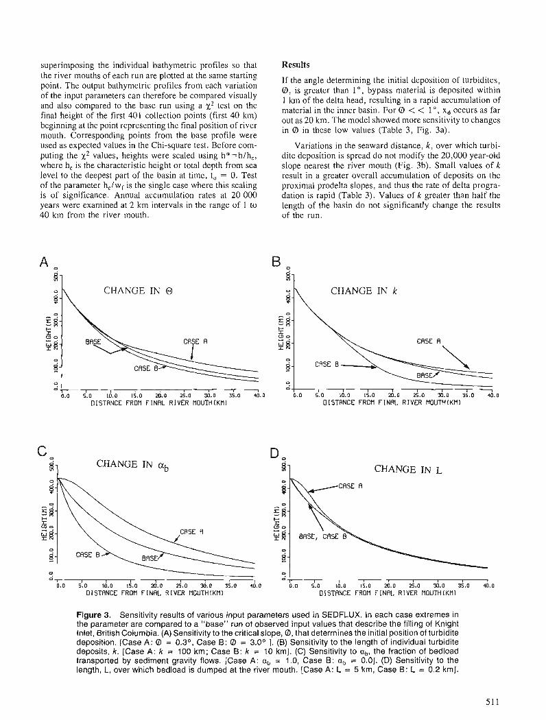
superimposing the individual bathymetric profiles so that the river mouths of each run are plotted at the same starting point. The output bathymetric profiles from each variation of the input parameters can therefore be compared visually and also compared to the base run using a x2 test on the final height of the first 401 collection points (first 40 km) beginning at the point representing the final position of river mouth. Corresponding points from the base profile were used as expected values in the Chi-square test. Before computing the x2 values, heights were scaled using h*=h/h,, where h, is the characteristic height or total depth from sea level to the deepest part of the basin at time, to = 0. Test of the parameter h,/wf is the single case where this scaling is of significance. Annual accumulation rates at 20 000 years were examined at 2 km intervals in the range of 1 to 40 km from the river mouth.

n l I I I I I I I t 0.0 5.0 10.0 15.0 20.0 25.0 50.0 35.0 40.0

DISTANCE FROM FINAL RIVER MOUTHLKMI

C CHANGE IN a b

Results

If the angle determining the initial deposition of turbidites, 0, is greater than l o , bypass material is deposited within 1 krn of the delta head, resulting in a rapid accumulation of material in the inner basin. For 0 < < 1 ", x+ occurs as far out as 20 km. The model showed more sensitivity to changes in 0 in these low values (Table 3, Fig. 3a).

Variations in the seaward distance, k, over which turbidite deposition is spread do not modify the 20,000 year-old slope nearest the river mouth (Fig. 3b). Small values of k result in a greater overall accumulation of deposits on the proximal prodelta slopes, and thus the rate of delta progradation is rapid (Table 3). Values of k greater than half the length of the basin do not significantly change the results of the run.

i\ CHANGE IN k

\ CASE A

CASE B

0.0 5 .0 10.0 15.0 i.0 25.0 ~ . o 35.0 4.0 OISTANCE FROM FINAL RIVER MOUTH(KM1

CHANGE IN L

i- s g- + 1 E ? r W - 9 s - : I I I I I

I 1 I 0.0 5.0 10.0 15.0 20.0 25.0 50.0 35.0 40.0 0.0 5.0 10.0 15.0 20.0 25.0 a.o 35.0 40.0

DISTANCE FROM FINFlL RIVER MOUTH(KM1 DISTANCE FROM FINAL RIVER MOUTH[KMI

Figure 3. Sensitivity results of various input parameters used in SEDFLUX. In each case extremes in the parameter are compared to a "base" run of observed input values that describe the filling of Knight Inlet, British Columbia. (A) Sensitivity to the critical slope, 0, that determines the initial position of turbidite deposition. [Case A: 0 = 0.3O, Case B: 0 = 3.0° 1. (B) Sensitivity to the length of individual turbidite deposits, k. [Case A: k = 100 km; Case B: k = 10 km]. (C) Sensitivity to ab, the fraction of bedload transported by sediment gravity flows. [Case A: a, = 1.0, Case B: a, = 0.01. (D) Sensitivity to the length, L, over which bedload is dumped at the river mouth. [Case A: L = 5 km, Case B : L = 0.2 km].

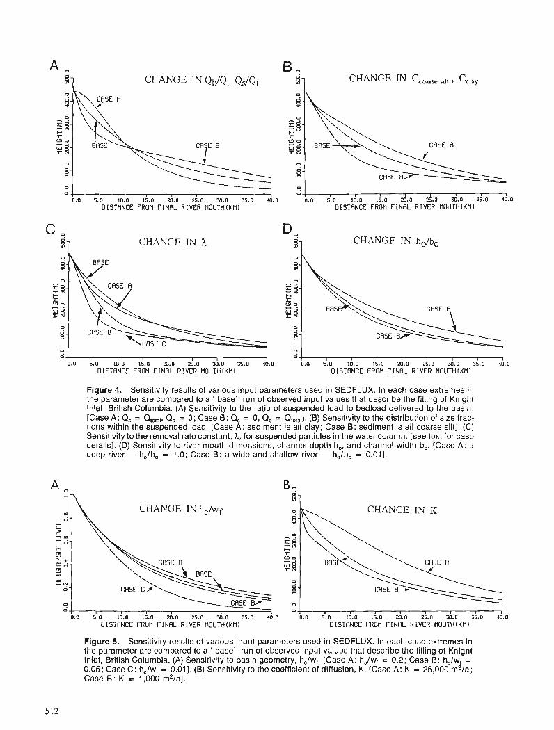
CHANGE IN Ccoarse silt 9 Cclay

-

0 I 1 0 , I 1 I I I I I I I I 9 I

0.0 5.0 10.0 15.0 20.0 25.0 30.0 35.0 40.0 0.0 5.0 10.0 15.0 20.0 25.0 30.0 35.0 40.0 OISTANCE FROM FINAL RIVER MOUTH(KM) DISTANCE FROM FINAL RIVER ROUTHIKMI

CHANGE IN h@, CHANGE IN h

0 1

0 I I I I I I I I I I I I I I

0.0 5.0 10.0 15.0 20.0 25.0 30.0 35.0 40.0 0.0 5.0 10.0 15.0 20.0 25.0 30.0 35.0 40.0 OISTANCE FROM FINAL RIVER MOUTH(KM1 DISTANCE FROM FINRL RIVER MOUTH(KMI

Figure 4. Sensitivity results of various input parameters used in SEDFLUX. In each case extremes in the parameter are compared to a "base" run of observed input values that describe the filling of Knight Inlet, British Columbia. (A) Sensitivity to the ratio of suspended load to bedload delivered to the basin. [Case A: Q, = Q,o,,I, Q, = 0; Case 6: Q, = 0, Q, = Q,o,a,]. (B) Sensitivity to the distribution of size fractions within the suspended load. [Case A: sediment is all clay; Case B : sediment is all coarse silt]. (C) Sensitivity to the removal rate constant, h, for suspended particles in the water column. [see text for case details]. (D) Sensitivity to river mouth dimensions, channel depth h,, and channel width b,. [Case A: a deep river - h,/b, = 1.0; Case B : a wide and shallow river - h,/b, = 0.011.

m.- CHANGE IN hc/wf J O W > W -I '?- m W m

2-'- 16 E W = z-

X I I I I I I I I

0.0 5.0 10.0 15.0 20.0 25.0 30.0 35.0 40.0 OISTRNCE FROM FINAL RIVER NOUTH(KM1

0.0 5.0 10.0 1 i . 0 20.0 25.0 3i).o 35.0 4.0 DISTANCE FROM FINAL RIVER MOUTH(KM1

Figure 5. Sensitivity results of various input parameters used in SEDFLUX. In each case extremes in the parameter are compared to a "base" run of observed input values that describe the filling of Knight Inlet, British Columbia. (A) Sensitivity to basin geometry, h,lw,. [Case A: hclwf = 0.2; Case B : hc/wf = 0.05; Case C: h,/w, = 0.011. (B) Sensitivity to the coefficient of diffusion, K. [Case A: K = 25,000 m2/a; Case B : K = 1,000 m2/a].

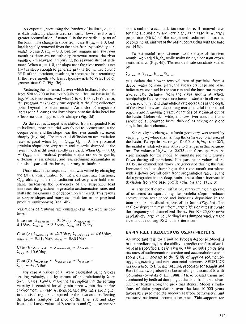
As expected, increasing the fraction of bedload, a , that is distributed by channelized sediment flows, results in a greater accumulation of material in the more distal parts of the basin. The change in slope from case B (ab = 1 .O, bedload is totally removed from the delta front by turbidity currents) to case A (ab = 0.0, bedload remains near the river mouth as there are no turbidity currents) moves the river mouth 6 km seaward, amplifying the seaward shift of sediment. When a, = 1 .O, the slope near the river mouth is not always steep enough to generate gravity flows, i.e. during 35 % of the iterations, resulting in some bedload remaining at the river mouth and less responsiveness to values of ab greater than 0.7 (Fig. 3c).

Reducing the distance, L, over which bedload is dumped from 500 to 200 m has essentially no effect on basin infilling. Mass is not conserved when L is < 100 m. In this case, the program makes only one deposit at the first collection point beyond the river mouth. An order of magnitude increase in L causes shallow slopes near the delta head but effects no other appreciable change (Fig. 3d).

As the sediment input was shifted from suspended load to bedload, more material was found to accumulate in the deeper basin and the slope near the river mouth increased sharply (Fig. 4a). The impact of diffusion on accumulation rates is great when Q, = Qlotal, Q, = 0 ; the proximal prodelta slopes are very steep and material dumped at the river mouth is diffused rapidly seaward. When Qb = 0, Qs = Qtoral, the proximal prodelta slopes are more gentle, diffusion is less intense, and less sediment accumulates in the distal parts of the basin, contrary to intuition.

Grain size in the suspended load was varied by changing the fluvial concentration for the individual size fractions, Cdo, although the total sediment delivery was held constant. Increasing the coarseness of the suspended load increases the gradient in prodelta sedimentation rates and shifts the maximum site of deposition landward. This results in steeper slopes and more accumulation in the proximal prodelta environment (Fig. 4b).

Variations of removal rate constant (Fig. 4c) were as follows :

- Base run : hcOase silt = 10.6/day, hmedium silt - 4. llday, htine = 2.3/day, hClay = I .7lday

Case (A) hcoarse silt = 42.7fdayy hlnediurn silr = 4 . 6 3 / d a ~ , hfine sil t = 0.515/day, hcl,, = 0.021 /day

- Case (B) hcoarse silt = h e d i u m silt = l f ine silt - hclay = 10.6/day

- - Case (C) hcoarse silt = hrnedium silt - I f ine silt - hClay = 42.7Jday

For case A values of hd were calculated using Stokes settling velocity, o, by means of the relationship h = o / h o . Cases B and C make the assumption that the settling velocity is constant for all grain sizes within the marine environment. In case A, hemipelagic flux rates are higher in the distal regions compared to the base case, reflecting the greater transport distance of the finer silt and clay fractions. Large values of h (cases B and C) cause steeper

slopes and more accumulation near shore. If removal rates for fine silt and clay are very high, as in case B, a larger proportion (36 %) of the suspended sediment is carried beyond the sill and out ofthe basin, contrasting with the base run (4 %).

To test model responsiveness to the shape of the river mouth, we varied ho/bo while maintaining a constant cross- sectional area (Fig. 4d). The removal rate constants varied by

case = base ho caseJho base

to simulate the slower removal rate of particles from a deeper water column. Here, the subscripts, case and base, indicate values used in the test run and the base run respectively. The distance from the river mouth at which hemipelagic flux reaches a maximum is similar in all cases. The gradient in the sedimentation rate decreases as the depth of the river increases, depositing more material in the distal regions and removing greater quantities of sediment out of the basin. Deltas with wide, shallow river mouths, i.e. a sandur delta, prograde faster than deltas having only one single but deep channel.

Sensitivity to changes in basin geometry was tested by varying hc/wf while maintaining the cross-sectional area of the basin. Except in the range, 0.019 < h,/wf < 0.023, the model is relatively insensitive to changes in this parameter. For values of hc/wf > 0.023, the foreslope remains steep enough for the model to simulate sediment gravity flows during all iterations. For parameter values of 5 0.019, no channelized flows are generated during the run. Increased bedload dumping at the river mouth correlates with a slower overall delta front progradation rate, i.e, the delta progrades into a deep basin, and a sharp increase in deviation from the base profile (Fig. 5a and Table 3).

A large coefficient of diffusion, representing a high rate of sediment transport along the prodelta slopes, reduces accumulation near shore and increases deposition in the intermediate and distal regions of the basin (Fig. 5b). The shallow slopes that result from large diffusion rates decrease the frequency of channelized flows. For K=25,000 m2/a (a relatively large value), bedload was dumped wholly at the river mouth during 96 % of the iterations.

BASIN FILL PREDICTIONS USING SEDFLUX

An important task for a unified Process-Reponse Model is in site predictions, i.e. the ability to predict the flux of sediment at a specified sites in a basin. This includes predicting the rates of sedimentation, erosion and accumulation and is specifically important to the fields of applied sedimentology, engineering and environmental sciences. SEDFLUX has been used to simulate infilling processes for Knight and Bute inlets, two graben-like basins along the coast of British Columbia (Syvitski et al., 1988). These coastal basins are dominated by bedload dumping at the delta front and subsequent diffusion along the proximal slopes. Model simulations of delta progradation over the last 10,000 years favourably predicted the modern seafloor bathymetry, and measured sediment accumulation rates. This supports the

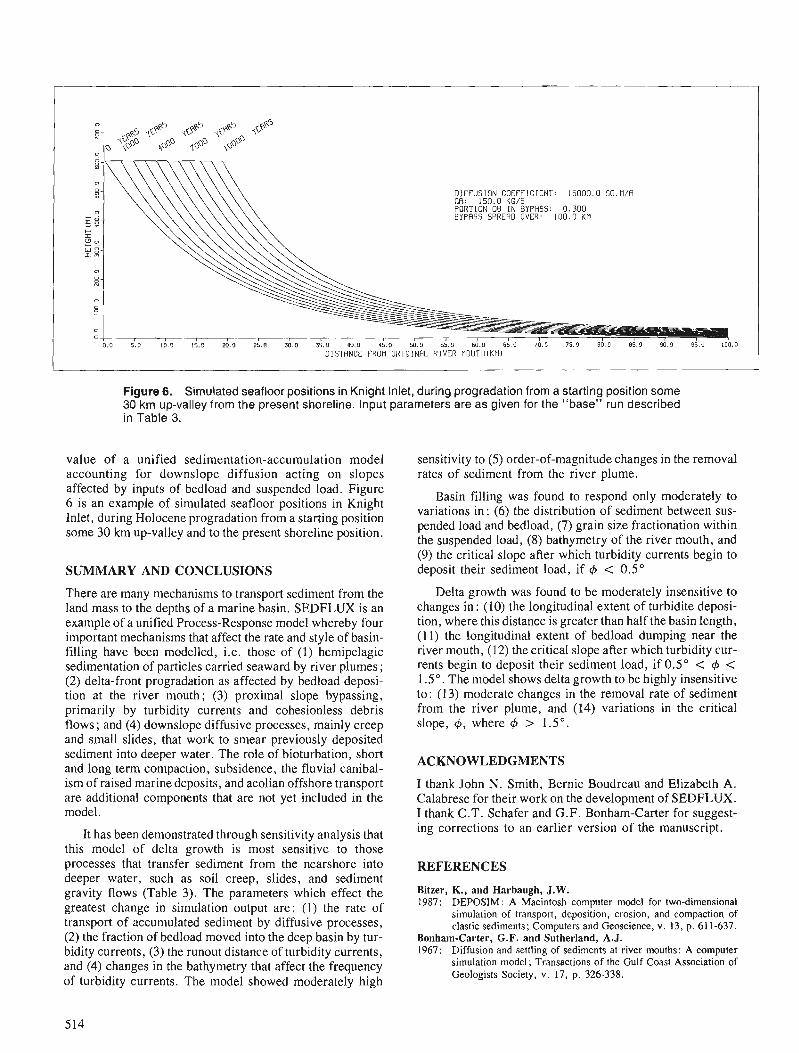
DIFFUSION COEFFICIENT: 15000.0 SO.N/R 00: 150.0 KG/S PORTION 05 IN BYPASS: 9.300 BYPRSS SPREAD OVER: 100.9 KN

OlSTANCE TROM ORIGINAL RIVER MOUTHIKIII

Figure 6. Simulated seafloor positions in Knight Inlet, during progradation from a starting position some 30 km up-valley from the present shoreline. Input parameters are a s given for the "base" run described in Table 3.

value of a unified sedimentation-accumulation model sensitivity to (5) order-of-magnitude changes in the removal accounting for downslope diffusion acting on slopes rates of sediment from the river plume. affected by inputs of bedload and suspended load. Figure 6 is an example of simulated seafloor positions in Knight Basin filling was found to respond only moderately to

variations in: (6) the distribution of sediment between sus- Inlet, during Holocene progradation from a starting position pended load and bedload, (7) grain fractionation within some 30 km up-valley and to the present shoreline position. the suspended load, (8) bathymetry of the river mouth, and (9) the critical slope after which turbidity currents begin to -

SUMMARY AND CONCLUSIONS deposit their sedihent load, if 4 < 0.5"

There are many mechanisms to transport sediment from the land mass to the depths of a marine basin. SEDFLUX is an example of a unified Process-Response model whereby four important mechanisms that affect the rate and style of basin- filling have been modelled, i.e. those of (1) hemipelagic sedimentation of particles carried seaward by river plumes ; (2) delta-front progradation as affected by bedload deposition at the river mouth; (3) proximal slope bypassing, primarily by turbidity currents and cohesionless debris flows ; and (4) downslope diffusive processes, mainly creep and small slides, that work to smear previously deposited sediment into deeper water. The role of bioturbation, short and long term compaction, subsidence, the fluvial canibal- ism of raised marine deposits, and aeolian offshore transport are additional components that are not yet included in the model.

It has been demonstrated through sensitivity analysis that this model of delta growth is most sensitive to those processes that transfer sediment from the nearshore into deeper water, such as soil creep, slides, and sediment gravity flows (Table 3). The parameters which effect the greatest change in simulation output are: (1) the rate of transport of accumulated sediment by diffusive processes, (2) the fraction of bedload moved into the deep basin by turbidity currents, (3) the runout distance of turbidity currents, and (4) changes in the bathymetry that affect the frequency of turbidity currents. The model showed moderately high

Delta growth was found to be moderately insensitive to changes in : (10) the longitudinal extent of turbidite deposition, where this distance is greater than half the basin length, (I I ) the longitudinal extent of bedload dumping near the river mouth, (12) the critical slope after which turbidity currents begin to deposit their sediment load, if 0.5" < 4 < 1.5". The model shows delta growth to be highly insensitive to: (13) moderate changes in the removal rate of sediment from the river plume, and (14) variations in the critical slope, 6, where 4 > 1 . S o .

ACKNOWLEDGMENTS

I thank John N. Smith, Bernie Boudreau and Elizabeth A. Calabrese for their work on the development of SEDFLUX. I thank C.T. Schafer and G.F. Bonham-Carter for suggesting corrections to an earlier version of the manuscript.

REFERENCES

Bitzer, K. , and Harbaugh, J.W. 1987: DEPOSIM: A Macintosh computer model for two-dimensional

simulation of transport, deposition, erosion, and compaction of clastic sediments; Computers and Geoscience, v. 13, p. 61 1-637.

Bonham-Carter, G.F. and Sutherland, A.J. 1967: Diffusion and settling of sediments at river mouths: A computer

simulation model; Transactions of the Gulf Coast Association of Geologists Society, v. 17, p. 326-338.

Calabrese, E.A. and Syvitski, J.P.M. 1987 : Modelling the growth of a prograding delta : Numerics, sensitivity,

program code and users guide; Geological Survey of Canada, Open File 1624, 61 p.

Cross, T.A. (ed.) 1990: Quantitative Dynamic Stratigraphy ; Prentice-Hall, New York,

625 p. Flemings, P.B. and Jordan, T.E. 1989: A synthetic stratigraphic model of foreland basin development;

Journal of Geophysical Research, v. 94, p. 3851-3866. Fox, W.T. 1978 : Modeling coastal environments. In : Coastal Sedimentary Environ-

ments, ed. R.A. Davis Jnr.. Springer-Verlag, New York, p. 385-413.

Harbaugh, J.W. and Bonharn-Carter, G. 1977: Computer simulation of continental margin sedimentation; In The

Sea, V. 6, Marine Modeling, ed. E.D. Goldberg, I.N. McCave, J.J. O'Brien, and J.H. Steele, Wiley Interscience, New York, p. 623-649.

Kenyon, P.M. and Turcotte, D.L. 1985: Morphology of a delta prograding by bulk sediment transport;

Geological Society of America Bulletin, v. 96, p. 1457-1465. Komar, P.D. 1977: Modeling of sand transport on beaches and the resulting shoreline

evolution; In The Sea, v. 6, Marine Modeling ed. E.D. Goldberg, I.N. McCave, J.J. O'Brien, and J .H . Steele Wiley Interscience, New York, p. 499-513.

O'Connor, B.A. and Nicholson, J. 1988: A three-dimensional model of suspended particulate sediment

transport; Coastal Engineering, v. 12, p. 157-174. Syvitski, J.P.M. 1990: The process-response model in Quantitative Dynamic Stratigra-

phy; In Quantitative Dynamic Stratigraphy, ed. T.A. Cross, Prentice-Hall, New York. p. 309-334.

Syvitski, J.P.M. and Farrow, G.E. 1989: Fjord sedimentation as an analogue for small hydrocarbon-bearing

fan deltas; In Deltas: Sites and Traps for Fossil Fuels, ed. M.K.G. VJhateley & K.T. Pickering, Geological Society of London, Spe- cial Publication No. 41, pp. 21-43.

Syvitski, J.P.M., Smith, J.N., Calabrese, E.A., and Boudreau, B.P. 1988: Basin sedimentation and the growth of prograding deltas; Journal

of Geophysical Research, v. 93, p. 6895-6908. Tetzlaff, D.M. and Harbaugh, J.W. 1989: Simulating Clastic Sedimentation; Van Nostrand Reinhold. New

York, 202 p. Wang, F.C. and Wei, J.S. 1986: River mouth mechanisms and coastal sediment deposition; In

River Sedimentation, v. 3, ed. S.Y. Wang, H.W. Shen & L.Z. Ding, School of Engineering Publication, University of Missis- sippi, p. 290-299.

Effects of core scale heterogeneities on fluid flow in a clastic reservoir

Stefan Bachul, David Cuthielll, and John Kramersl

Bachu, S., Cuthiell, D., and Kramers, J . , Effects of core scale heterogeneities on fluid flow in a clastic reservoir; & Statistical Applications in the Earth Sciences, ed. F. P. Agterberg and G. F. Bonham-Carter; Geological Survey of Canada, Paper 89-9, p. 51 7-523, 1989.

Abstract

The Provost Upper Mannville B Pool is located in the heavy oil belt of east-central Alberta in McLaren Formation channel sands of Early Cretaceous age. The reservoir contains zones of shale clasts in a matrix of fine- to medium-grained sands. These shale clast zones range in thickness from several centimetres to several metres, and have lateral continuity on the order of tens to hundreds of metres. The clasts make up as much as 85 % by volume in some zones and represent a signijcant barrier to fluid flow in the reservoir, thus having a direct impact on the eficiency of enhanced oil recovery processes.

The presence of the shale clasts within the homogeneous sand matrix creates a macro-scale heterogeneity within the reservoir. The effect of this heterogeneity on fluid flow was studied usingjnite element modelling of real cases at the scale of borehole core. R e results were scaled up to reservoir scale in order to assess the overall impact of such shale clast zones on fluidflow. This numerical modelling experiment shows that the presence of shale clasts reduces the equivalent permeability of the region by an order of magnitude or more, depending on the shale clast density within the zone. Moreover, owing to the shape and orientations of the clasts, the permeability reduction is different in horizontal and vertical directions.

In order to relate permeability reduction to clast characteristics, a study has been undertaken to describe the clasts statistically, based on a large data set of actual digitized clast outlines obtainedfrom core. Results to date include probability distribution jknctions for a number of geometrical properties such as clast dimensions, area, shape and orientation.

La nappe Upper Mannville B de Provost se situe dans la zone de pArole lourd du centre-est de 1 'Al- berta, dans les grts fluviatiles de la formation de McLaren datant du Cre'tace' infe'rieur. Le re'servoir contienl des zones de fragments compose's de schiste argileux, dans une matrice sableuse dont la taille des grains varie define a moyenne. Ces zones, dont l'e'paisseur varie de plusieurs centim?tres h plusieurs metres, presentent une continuite' late'rale de 1 'ordre de plusieurs dizaines 6 plusieurs centaines de mttres. Les fragments de roches de'tritiques consituent jusqu'a 85 % de la roche en volume duns certaines zones et une barritre importante a 1 'e'coulement des fluides dans le re'servoir; ils ont donc un effet direct sur l'eficacite' des proce'de's de re'cupkration ame'liore'e du pe'trole.

La pre'sence de fragments compose's de schiste argileux h l'inte'rieur de la matrice sableuse homogtne confire une he'teroge'nie'te macroscopique a l'intei-ieur du re'servoir. On a e'tiidie' l'effet de cette he'te'r- ogene'ite' sur 1 'e'coulement des fluides en employant la modt!lisation par e'le'ments finis de situations re'elles a l'e'chelle de carottes de sondage. On a e'largi les re'sultats a l'e'chelle du re'servoir, afin d'e'valuer l'effet global de ces zones de fragments compose's de schiste argileux sur l'e'coulement des jluides. Cette expe'rience de mode'lisation nume'rique montre que la pre'sence des fragments en question re'duit la perme'abilitc! e'quivalente de la re'gion d'un ordre de grandeur au moins, selon la densite' des fragments a 1 'intei-ieur de la zone. En outre, &rant donne' la configuration et 4,'orientation des fragmetzts, la re'duction de perme'abilite' est diffe'rente dans le sens horizontal et le sens vertical.

Duns le but d'e'tablir une corre'lation entre la re'duction et la permeabilite' et les caracte'ristiques des fragments, on a entrepris une e'fude qui cherche a les de'crire statistiquement en fonction d'un vaste ensemble de donne'es dkcrivant les contours re'els nume'risb de ces fragments tels qu'obtenus sur une carotte. Les re'sultats acquis jusqu'h pre'sent comprennent les fonctions de distribution de probabilite' dans le cas d'un certain nombre de proprie'te's ge'ome'triques comme les dimensions, la surface, la forme et l'orientation des fragments.

' Alberta Geological Survey, Alberta Research Council, P.O. Box 8330, Postal Station F. Edmonton, Alberta T6H 5x2

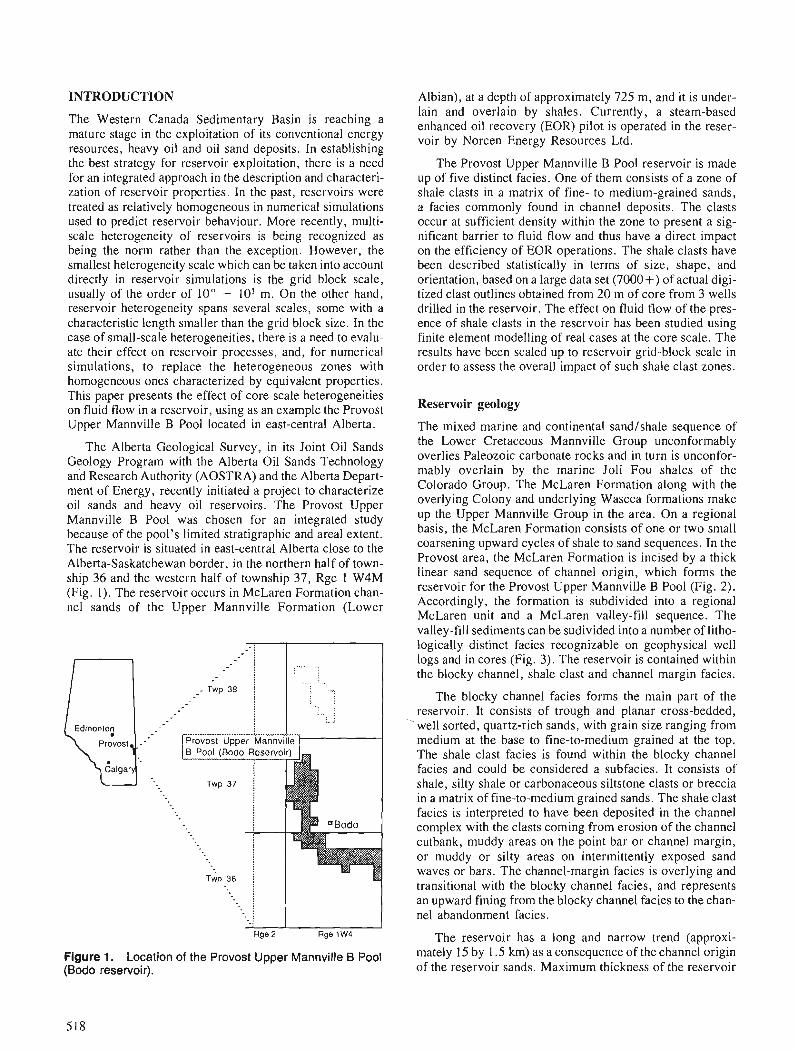
INTRODUCTION

The Western Canada Sedimentary Basin is reaching a mature stage in the exploitation of its conventional energy resources, heavy oil and oil sand deposits. In establishing the best strategy for reservoir exploitation, there is a need for an integrated approach in the description and characterization of reservoir properties. In the past, reservoirs were treated as relatively homogeneous in numerical simulations used to predict reservoir behaviour. More recently, multi- scale heterogeneity of reservoirs is being recognized as being the norm rather than the exception. However, the smallest heterogeneity scale which can be taken into account directly in reservoir simulations is the grid block scale, usually of the order of 10" - 10' m. On the other hand, reservoir heterogeneity spans several scales, some with a characteristic length smaller than the grid block size. In the case of small-scale heterogeneities, there is a need to evaluate their effect on reservoir processes, and, for numerical simulations, to replace the heterogeneous zones with homogeneous ones characterized by equivalent properties. This paper presents the effect of core scale heterogeneities on fluid flow in a reservoir, using as an example the Provost Upper Mannville B Pool located in east-central Alberta.

The Alberta Geological Survey, in its Joint Oil Sands Geology Program with the Alberta Oil Sands Technology and Research Authority (AOSTRA) and the Alberta Depart- ment of Energy, recently initiated a project to characterize oil sands and heavy oil reservoirs. The Provost Upper Mannville B Pool was chosen for an integrated study because of the pool's limited stratigraphic and areal extent. The reservoir is situated in east-central Alberta close to the Alberta-Saskatchewan border, in the northern half of township 36 and the western half of township 37, Rge 1 W4M (Fig. 1). The reservoir occurs in McLaren Formation channel sands of the Upper Mannville Formation (Lower

Figure 1. Location of the Provost Upper Mannville B Pool (Bodo reservoir).

Albian), at a depth of approximately 725 m, and it is underlain and overlain by shales. Currently, a steam-based enhanced oil recovery (EOR) pilot is operated in the reservoir by Norcen Energy Resources Ltd.

The Provost Upper Mannville B Pool reservoir is made up of five distinct facies. One of them consists of a zone of shale clasts in a matrix of fine- to medium-grained sands, a facies commonly found in channel deposits. The clasts occur at sufficient density within the zone to present a significant barrier to fluid flow and thus have a direct impact on the efficiency of EOR operations. The shale clasts have been described statistically in terms of size, shape, and orientation, based on a large data set (7000+) of actual digitized clast outlines obtained from 20 m of core from 3 wells drilled in the reservoir. The effect on fluid flow of the presence of shale clasts in the reservoir has been studied using finite element modelling of real cases at the core scale. The results have been scaled up to reservoir grid-block scale in order to assess the overall impact of such shale clast zones.

Reservoir geology

The mixed marine and continental sandtshale sequence of the Lower Cretaceous Mannville Group unconformably overlies Paleozoic carbonate rocks and in turn is unconformably overlain by the marine Joli Fou shales of the Colorado Group. The McLaren Formation along with the overlying Colony and underlying Waseca formations make up the Upper Mannville Group in the area. On a regional basis, the McLaren Formation consists of one or two small coarsening upward cycles of shale to sand sequences. In the Provost area, the McLaren Formation is incised by a thick linear sand sequence of channel origin, which forms the reservoir for the Provost Upper Mannville B Pool (Fig. 2). Accordingly, the formation is subdivided into a regional McLaren unit and a McLaren valley-fill sequence. The valley-fill sediments can be sudivided into a number of lithologically distinct facies recognizable on geophysical well logs and in cores (Fig. 3). The reservoir is contained within the blocky channel, shale clast and channel margin facies.

The blocky channel facies forms the main part of the reservoir. It consists of trough and planar cross-bedded, well sorted, quartz-rich sands, with grain size ranging from medium at the base to fine-to-medium grained at the top. The shale clast facies is found within the blocky channel facies and could be considered a subfacies. It consists of shale, silty shale or carbonaceous siltstone clasts or breccia in a matrix of fine-to-medium grained sands. The shale clast facies is interpreted to have been deposited in the channel complex with the clasts coming from erosion of the channel cutbank, muddy areas on the point bar or channel margin, or muddy or silty areas on intermittently exposed sand waves or bars. The channel-margin facies is overlying and transitional with the blocky channel facies, and represents an upward fining from the blocky channel facies to the channel abandonment facies.

The reservoir has a long and narrow trend (approximately 15 by 1.5 km) as a consequence of the channel origin of the reservoir sands. Maximum thickness of the reservoir

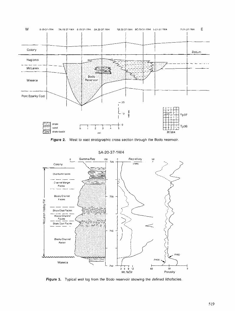
Colony Datum

Regional ------

McLaren

Waseca

Post Sparky Coal

shale

sand

shale clasls

Figure 2. West to east stratigraphic cross section through the Bodo reservoir.

3 6 9 1 2 60 30 0

Wt.%Oil Porosity

Figure 3. Typical well log from the Bodo reservoir showing the defined lithofacies.

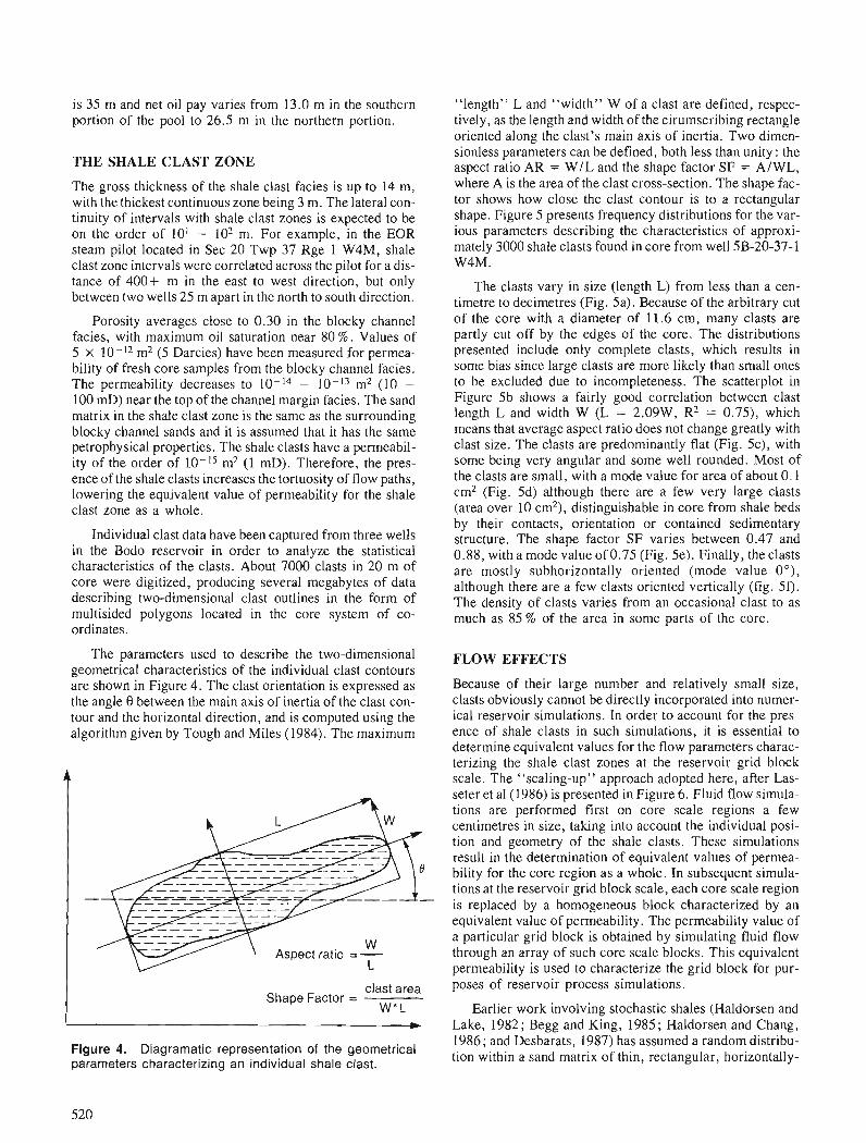
is 35 m and net oil pay varies from 13.0 m in the southern portion of the pool to 26.5 m in the northern portion.

THE SHALE CLAST ZONE

The gross thickness of the shale clast facies is up to 14 m, with the thickest continuous zone being 3 m. The lateral continuity of intervals with shale clast zones is expected to be on the order of 10' - lo2 m. For example, in the EOR steam pilot located in Sec 20 Twp 37 Rge I W4M, shale clast zone intervals were correlated across the pilot for a distance of 400+ m in the east to west direction, but only between two wells 25 m apart in the north to south direction.

Porosity averages close to 0.30 in the blocky channel facies, with maximum oil saturation near 80 %. Values of 5 X 10-l2 m2 (5 Darcies) have been measured for permeability of fresh core samples from the blocky channel facies. The permeability decreases to 10-l4 - 10-l3 m2 (10 - 100 mD) near the top of the channel margin facies. The sand matrix in the shale clast zone is the same as the surrounding blocky channel sands and it is assumed that it has the same petrophysical properties. The shale clasts have a permeability of the order of 10-15 m2 (1 mD). Therefore, the presence of the shale clasts increases the tortuosity of flow paths, lowering the equivalent value of permeability for the shale clast zone as a whole.

Individual clast data have been captured from three wells in the Bodo reservoir in order to analyze the statistical characteristics of the clasts. About 7000 clasts in 20 m of core were digitized, producing several megabytes of data describing two-dimensional clast outlines in the form of multisided polygons located in the core system of coordinates.

The parameters used to describe the two-dimensional geometrical characteristics of the individual clast contours are shown in Figure 4. The clast orientation is expressed as the angle 0 between the main axis of inertia of the clast contour and the horizontal direction, and is computed using the algorithm given by Tough and Miles (1984). The maximum

W Aspect ratio = -

L

clast area Shape Factor =

W * L

Figure 4. Diagramatic representation of the geometrical parameters characterizing an individual shale clast.

"length" L and "width" W of a clast are defined, respectively, as the length and width of the cirumscribing rectangle oriented along the clast's main axis of inertia. Two dimen- sionless parameters can be defined, both less than unity : the aspect ratio AR = WIL and the shape factor SF = A/WL, where A is the area of the clast cross-section. The shape factor shows how close the clast contour is to a rectangular shape. Figure 5 presents frequency distributions for the various parameters describing the characteristics of approximately 3000 shale clasts found in core from well 5B-20-37-1 W4M.

The clasts vary in size (length L) from less than a centimetre to decimetres (Fig. 5a). Because of the arbitrary cut of the core with a diameter of 11.6 cm, many clasts are partly cut off by the edges of the core. The distributions presented include only complete clasts, which results in some bias since large clasts are more likely than small ones to be excluded due to incompleteness. The scatterplot in Figure 5b shows a fairly good correlation between clast length L and width W (L = 2.09W, R2 = 0.75), which means that average aspect ratio does not change greatly with clast size. The clasts are predominantly flat (Fig. 5c), with some being very angular and some well rounded. Most of the clasts are small, with a mode value for area of about 0.1 cm2 (Fig. 5d) although there are a few very large clasts (area over 10 cm2), distinguishable in core from shale beds by their contacts, orientation or contained sedimentary structure. The shape factor SF varies between 0.47 and 0.88, with a mode value of 0.75 (Fig. 5e). Finally, the clasts are mostly subhorizontally oriented (mode value 0°), although there are a few clasts oriented vertically (fig. 50. The density of clasts varies from an occasional clast to as much as 85 % of the area in some parts of the core.

FLOW EFFECTS

Because of their large number and relatively small size, clasts obviously cannot be directly incorporated into numerical reservoir simulations. In order to account for the presence of shale clasts in such simulations, it is essential to determine eauivalent values for the flow Parameters characterizing the shale clast zones at the reservoir grid block scale. The "scaling-up" approach adopted here, after Las- seter et a1 (1986) is presented in Figure 6. Fluid flow simulations are performed first on core scale regions a few centimetres in size, taking into account the individual position and geometry of the shale clasts. These simulations result in the determination of equivalent values of permeability for the core region as a whole. In subsequent simulations at the reservoir grid block scale, each core scale region is replaced by a homogeneous block characterized by an equivalent value of permeability. The permeability value of a particular grid block is obtained by simulating fluid flow through an array of such core scale blocks. This equivalent permeability is used to characterize the grid block for purposes of reservoir process simulations.

Earlier work involving stochastic shales (Haldorsen and Lake, 1982; Begg and King, 1985; Haldorsen and Chang, 1986; and Desbarats, 1987) has assumed a random distribution within a sand matrix of thin, rectangular, horizontally-

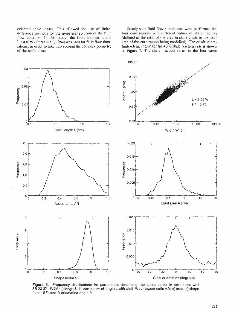
oriented shale lenses. This allowed the use of finite- difference methods for the numerical solution of the fluid flow equation. In this study, the finite-element model FE3DGW (Gupta et al., 1984) was used for fluid flow simulations, in order to take into account the complex geometry of the shale clasts.

Clast length L (cm)

2.5 I I I I

" 0 0.2 0.4 0.6 0.8 1 .O

Aspect ratio AR

Steady-state fluid flow simulations were performed for four core regions with different values of shale fraction (defined as the ratio of the area in shale clasts to the total area of the core region being modelled). The quadrilateral finite-element grid for the 40 % shale fraction case is shown in Figure 7. The shale fraction varies in the four cases

0.011 I I I I 0.01 0.10 1 .oo 10.00 100.00

Width W (cm)

0.01 0.01 0.1 1 10 100

Clast area A (cm2)

Shape factor SF Clast orientation (degrees)

Figure 5. Frequency distributions for parameters describing the shale clasts in core from well 58-20-37-1 W4M: a) length L; b) correlation of length L with width W; c) aspect radio A R ; d) area; e) shape factor SF; and f) orientation angle 0.

between 15 % and 49 %, with correspondingly 800 to 2100 nodes in the finite element grids. Vertical fluid flow was simulated in each case by imposing a constant vertical pressure difference across the region and assuming impermeable boundaries on the sides. Horizontal flow was simulated in a similar manner. Initial simulations of vertical and horizontal flow were performed assuming that the entire region being simulated had a homogeneous permeability, in order to validate the finite element model. The resulting flow rates agreed to within 0.3 % of the theoretical values. For purposes of simulating the clast system, the sand matrix and shale were each assumed to be uniform and isotropic with a sand-to-shale permeability ratio of 1000. Vertical and horizontal flow simulations produced flow rates

Shale clasts at act Same sue un~forrn

differenl perrneabil block with equivalent hor~zontal and vertical permeability

Scaled up to actual shale clast zone slze (reservoir simulation block scale)

Reservoir scale

Figure 6 . Diagramatic representation of the scaling up process.

Figure 7. Finite element grid used to model fluid flow through a core-size area containing 40% shale clasts.

corresponding to the assumed pressure drop and actual distribution of shale clasts. Equivalent values of vertical and horizontal permeability, kVeq and kheq, were calculated from these flow rates using Darcy's law. The results are presented graphically in Figure 8. The difference in the values of the vertical and horizontal components of permeability reflects the fact that the clasts have predominantly a flat shape and a subhorizontal orientation. Also it shows that the presence in a homogeneous matrix of randomly distributed heterogeneities characterized by a dominant shape and orientation changes the nature of equivalent permeability from scalar to tensorial.

The next step in the scaling-up process is to find the equivalent values of horizontal and vertical permeability for a grid block comprised of a number of core scale areas, each one characterized by a different content of shale clasts (shale fraction). Considering the actual dimensions of the shale clast zone, a grid block of 15 x 1 m2 was dividcd into 100 x 10 square areas of 15 x 10 cm2 each. The shale fraction at each end of the grid block was defined based on actual values from core. In the absence of geological information concerning horizontal variations within a zone, values of shale fraction were allocated within the grid block by horizontally interpolating between actual core data assigned at the ends of the grid block. A normally distributed random component (zero mean, standard deviation 0.07) was added to the interpolated values to provide greater realism. Subse- quently, values of horizontal and vertical permeability were allocated to each core scale area according to its shale fraction. These values were obtained from Figure 8 by interpolation, knowing that the equivalent permeability must equal the sand matrix permeability for zero shale fraction, and assuming that it practically equals the shale permeability when the shale fraction has values greater than 90%. Numerical simulations of fluid flow through the grid block array of core scale regions produced flow rates corresponding to a reduction in horizontal and vertical permeability - values to 33 % and 11 % of sand permeability, respectively. Thus, the scaling up process shows that the presence in a

Shale clast fraction (010)

K 0 .- - 0 2 0.8 73 s? X L .-

0.6 a z 5 0.4 a

Figure 8. Reduction of equivalent permeability with respect to sand matrix permeability, as a function of shale fraction.

Horizontai - Vertical -

0 ksslksh = 1000

- . -

- -

reservoir of core scale heterogeneities, in this case shale clasts, has an important effect on the flow of fluids in that reservoir by significantly reducing the effective permeability of the heterogeneous zone as a whole.

CONCLUSIONS

An integrated, multidisciplinary approach was used in the study of the Provost Upper Mannville B Pool of east-central Alberta. The long and narrow reservoir occurs in channel sands of the McLaren valley-fill sequence, itself part of the McLaren Formation of the Mannville Group. The valley fill sediments can be subdivided into a number of lithofacies, three of which make up the reservoir. These are the blocky channel, shale clast and channel margin facies. The heterogeneous shale clast facies consists mainly of shale clasts in a matrix of fine-to-medium grained sands. It has a thickness of up to 14 m and lateral continuity of the order of 101 - lo2 m. The cross-sectional contours of approximately 7000 individual clasts were digitized from 20 m of core taken from three wells in the reservoir. Statistical analysis of the clast contours has shown that they range in length from less than a centimetre to at least a decimetre. Their individual cross-sectional areas are generally less than 1 cm2, although there are a few very large clasts distinguishable from shale beds by their contacts or orientation. The clasts are mostly flat, with an aspect ratio between 0.2 and 0.8, and most of them are subhorizontally oriented. The clasts reach a density of up to 85 % of the shale clast facies in some zones.

Numerical simulations of fluid flow through core scale regions were performed considering actual clast distributions for four cases of shale fraction: 0.15, 0.35, 0.40 and 0.49. The simulations show that the effective permeability is reduced with respect to sand permeability by up to one order of magnitude, depending on the shale fraction and on

the flow direction. Similar results were obtained for a fluid flow simulation at grid block scale considering an array of 100 x 10 core scale regions characterized by different shale fraction values. Basically, as a result of the generally flat shape and subhorizontal orientation of the shale clasts, the reduction is greater in the vertical than in the horizontal direction, creating anisotropy at the core and facies scale. Thus, the presence of shale clasts in a sand matrix significantly reduces the effective permeability of the layer, thereby affecting the recovery processes in a reservoir.

REFERENCES

Begg, S.H. and King, P.R. 1985 : Modelling the effects of shales on reservoir performance: calcula-

tion of effective vertical permeability; Society of Petroleum Engineers, Paper 13529, available from Society of Petroleum Engineers, Richardson, Texas 75083-3836.

Desbarats, A.J. 1987: Numerical estimation of cffective permeability in sand-shale for-

mations; Water Resources Research, v. 23, p. 273-286. Gupta, S.K., Cole, C.R., and Pinder, G.F. 1984: A finite-element three-dimensional groundwater FE3DGW) model

for a multiaquifer system; Water Resources Research, v. 20, p. 553-563.

Haldorsen, H.H. and Chang, D.M. 1986: Notes on stochastic shales: from outcrop to silnulation model;

Reservoir Characterization, ed. L. W. Lake and H.B. Caroll, Aca- demic Press, London, p. 445-485.

Haldorsen, H.H. and Lake, L.W. 1982: A new approach to shale management in field scale simulation

models; Society of Petroleum Engineers, Paper 10976, available from Society of Petroleum Engineers, Richardson, Texas 75083-3836.

Lasseter, T.J., Waggoner, J.R., and Lake, L.W. 1986: Reservoir heterogeneities and their influence on ultimate recovery ;

in Reservoir Characterization, ed. L.W. Lake and H.B. Caroll, - Academic Press. London. p. 545-559.

Tough, J.G. and Miles, R.G. 1984: A method for characterizing polygons in terms of the principal

axes; Computers & Geosciences, v . 10. p. 347-350.

RANKING AND SCALING OF STRATIGRAPHIC EVENTS

r

FORTRAN 77 microcomputer programs for ranking, scaling and regional correlation of stratigraphic events

F.P. Agterbergl and D.N. Byron1

Agterberg, F. P. and Byron, D. N., FORTRAN 77 microcomputer programs for ranking, scaling and regional correlation of stratigraphic events; & Statistical Applications in the Earth Sciences, ed. F. P. Agterberg and G.F. Bonham-Carter; Geological Survey of Canada, Paper 89-9, p. 527-535, 1989

Abstract

The RASC computer program for ranking and scaling of biostratigraphic events was originally written between 1978 and I981 for mainframe computers. it was followed by the CASCprogram for correlation and scaling in time. In 1985, it became possible, after relatively minor modijcation, to compile the FOR- TRAN code of the RASC and CASC computer programs on IBM compatible microcomputers. The Micro- RASC system of 12 separate programs is now being developed to make better use of the characteristic features of microcomputers and to allow greaterflexibili~ for inserting new algorithms into existing FOR- TRAN 77 code.

On a initialement rddige' entre 1978 et 1981, pour des gros ordinateurs, le programme informatique RASC qui permet de classer et de mettre en ordre les dv&nements biostratigraphiques. On a ensuite &la- bore' le programme CASC qui permet une correlation et une mise en ordre dans le temps. En 1985, on a pu, aprbs des modifications relativement mineures, compiler le code FORTRAN des programmes informatiques RASC et CASC sur des micro-ordinateurs compatibles IBM. On dabore actuellement le systbme Micro-RASC de 12 programmes distincts, en vue de miew utiliser les dktails caractbistiques des micro- ordinateurs, et de disposer d'une plus grandejexibilite' lors de 1 'insertion de nouveaux algorithmes dans le code FORTRAN 77 existant.

' Geological Survey of Canada, 601 Booth Street, Ottawa, Ontario KIA OE8

INTRODUCTION

The Micro-RASC system consists of 12 separate program modules. Except for Module 1 which can be used to create new input files, each module reads one or more input files and creates one or more output files. This allows flexibility for new program development because separate modules can be revised and replaced without changing the remainder of the system.

Micro-RASC contains slightly modified code previously published in the RASC (RAnking and Scaling) and CASC (Correlation And Scaling in time) mainframe computer programs for ranking, scaling and correlation of biostratigraphic events. This code has been supplemented by more recently developed algorithms including use of the jackknife method for estimating variances of cumulative RASC distances in scaling, modified RASC for frequency distribution analysis of stratigraphic events, and cross-validation to decide on optimum smoothing factors in spline-curve fitting for CASC. Micro-RASC can be used on any IBM compatible microcomputer with math co-processor and a FOR- TRAN compiler. This version of RASC and CASC is exclusively numerical using simple graphics programmed in FORTRAN 77.

The contents of the 12 modules are summarized in the next section. Important decisions to be made by the RASC user in order to create the parameter (PAR) file needed for running the modules are listed separately, in Appendix 1, together with those parameters that can be changed from their default values. A brief history of the development of RASC and CASC with references is given at the end of this paper.

It should be kept in mind that the purpose of the Micro- RASC computer programs is to order and correlate stratigraphic events. In most applications, the events are stratigraphically highest and lowest occurrences of (micro-) fossils, although peak occurrences and abrupt changes in relative abundance can be used equally well for correlation if these can be defined systematically. Lithostratigraphic, seismic and magnetostratigraphic events can be combined with biostratigraphic events. However, these other types of events may need special consideration; e.g., by defining them as marker horizons or by evaluating their relative uncertainty independently by means of modified RASC for frequency distribution analysis.

SUMMARY OF CONTENTS OF THE 12 MODULES OF MICRO-RASC

Module 1 : DATA INPUT

The RASC method requires as input a sequence (SEQ) file with coded sequences of stratigraphic events for individual sections, a dictionary with event names (DIC file), and a parameter (PAR) file with settings of switches and values of parameters. The CASC method requires depth (DEP) files for individual sections. Module 1 allows preparation of data (DAT) files from which SEQ files and preliminary

DEP files are generated automatically. Examples of DAT file formats are: (a) Depths (in feet or metres) followed by dictionary code

numbers of events (feet will be converted into metres) ; and

(b) Fossil code numbers followed by depths of lowest and highest occurrences (DIC file for use in RASC then must have separate entries for lowest and highest occurrence of each fossil).

Module 2 : PREPROCESSING

Frequencies of events are determined as follows : (a) Num- ber of sections for each event; (b) Number of events occurring in k sections and number of events occurring in k or more sections (k= 1, 2, . . . , n ; n represents total number of sections). A threshold parameter k, must be selected. Fur- ther analysis will be restricted to events that occur in at least k, sections. Special, rare events ("unique" events) which are to be re-inserted later in the biozonation, but which occur in fewer than kc sections, should be identified. It is also possible to define marker horizons (e.g., seismic events or bentonite layers) which are not subject to biostratigraphic uncertainty.

Module 3: RANKING

The optimum sequence of events is determined by "presorting" with or without the modified Hay method. Presorting is a relatively simple probabilistic method for ordering events. The sequence obtained by presorting may be improved by sorting on the basis of superpositional relations ("above", "below", coeval) between pairs of events using the modified Hay method. Inconsistencies involving three or more events (cycles) will be identified. A threshold parameter mc, may be selected by changing its default value mcl = 1. The modified Hay method will be applied only to pairs of events occurring in at least mcl sections. It may not be possible to determine the relative order of two or more events in the optimum sequence. This type of uncertainty is expressed by means of the uncertainty range assigned to all events in the optimum sequence.

Module 4: SCALING

The scaled optimum sequence of events is determined by estimating intervals between successive events in the optimum sequence previously obtained by ranking. This process usually involves minor reordering of the events. Final distances between successive events are clustered in a dendrogram which is useful as a regional biozonation. A threshold parameter m,c must be selected. Scaling calculations are restricted to frequencies of order relations between pairs of events occurring in at least m, sections. Unweighted and weighted scaling can be performed. Further analysis (e.g., normality test) will be based on weighted scaling with the weights determined by frequencies of superpositional relations between events. Standard deviations of inter-event

distances are provided. The cumulative RASC distance of each event is computed and added to the preliminary DEP files in order to create (complete) DEP files if CASC will be used.

Module 5: RANK EVALUATION

The optimum sequence resulting from Module 3 or 4 can be used for construction of the occurrence table and "step model". Events are shown for individual sections in the occurrence table. Their observed sequence in each sectionis compared with the optimum sequence in the step model. Penalty points are assigned for each position that an event is out of place in a section. Kendall's rankcorrelation coefficient can be computed from the total number of penalty points per section.

Module 6: NORMALITY TEST

The observed sequence of events in each section is compared to the scaled optimum sequence using cumulative RASC distances. Second-order differences are computed for events by comparing their observed positions to those of their neighbors in the stratigraphically upward and downward directions. Events that are out of place with probabilities greater than 95 % and 99 % are identified. A frequency distribution analysis of second-order differences is performed in order to evaluate : (a) auto-correlation of successive events in the scaled optimum sequence; and (b) overall frequencies of anomalous events occurring either too low (e.g., due to contamination during drilling), or too high (e.g., due to geological reworking) in the sections.

Module 7: JACKKNIFE SCALING

In scaling, each estimated distance Dij between successive events (i and j) is the average of a number of primary distance estimates Dl., based on the superpositional relations of i and j with other events (k). By successively deleting individual events, and scaling of the reduced data sets, it may be possible to obtain measures of precision of the estimates by means of the jackknife method which is nonparametric. This also results in jackknife estimates of the cumulative RASC distances of the events. Only if the latter estimates are close to the original cumulative RASC distances, as obtained by Module 4, can their jackknife standard deviations be used as standard deviations of the cumulative RASC distances.

Module 8: MODIFIED RASC

The scaling method is based on transforming frequencies for superpositional relations between events into quantiles of the normal distribution in standard form. It is assumed that all events have the same variance for deviations between their regional mean positions and observed positions within individual sections. In modified RASC, it is assumed that the variances of the events can be different. They are estimated by means of an iterative procedure. Firstly, spline- curves are fitted to the events in common between the scaled optimum sequence and individual sections in order to

project the regional mean positions onto the sections, and to collect all deviations for each event. Secondly, the variance of the deviations for each event is used for scaling which yields a new set of cumulative RASC distances. These two steps are repeated until convergence is reached. Modified RASC allows identification of low-variance events which can be used as marker horizons. In addition to different event variances, this procedure provides frequency distributions of individual events which may be positively or negatively skewed. Maximum deviations can be used for constructing a conservative range chart in which the ranges are based on regional highest and lowest observed occurrences of fossils.

Module 9: REGIONAL TIME SCALE

The age (in millions of years) may be known for a subgroup of the stratigraphic events used in a regional RASC study. It may be possible to establish the relationship between age and cumulative RASC distance for this subgroup. This relationship, expressed as a spline-curve function can then be used to transform all RASC distances into ages in linear time. These ages can be used to replace the cumulative RASC distances in the DEP files for CASC. Events can be weighted differently, either by using standard deviations resulting from Module 7, or by using subjective weights.

Module 10: CASC 1: AGE-DEPTH CURVES

The CASC (Correlation And Scaling in time) method consists of two steps: (a) construction of age-depth curves (this module or Module 11) ; and (b) multiwell comparison (Mod- ule 12). Module 10 closely resembles the age-depth curve- fitting part of the CASC mainframe computer program. Supplementary statistical techniques (cross-validation, jackknife spline-curve fitting) are given in Module 11 which amplifies Module 10. Input for CASC in Module 10 consists of DEP files for the sections to be studied. A spline-curve is fitted for each section. The dependent variable is (a) rank, (b) RASC distance, or (c) age in Ma; the independent variable is (a) relative event level, or (b) depth (in metric units). Because events generally are spaced irregularly along the depth-axis, an indirect method can be used for estimating the age-depth curve. This algorithm consists of fitting separate spline-curves lor the age-level and depth-level relations. Elimination of level then gives an age-depth curve which usually is better than the one obtained by direct spline-curve fitting. Sediment accumulation curves can be obtained from the first derivatives of the spline-curves.

Module 11: CASC 2: STATISTICAL ANALYSIS

The shape of a spline-curve is to a large extent controlled by its smoothing factor (SF) representing the standard deviation of the differences between observed and fitted values. The law of superposition of strata requires that age never decreases in the stratigraphically downward direction. This provides an estimate of the minimum smoothing factor. The maximum smoothing factor correspond to the best-fitting straight line of least squares. The optimum smoothing factor has a value within the open interval bounded by these two

extremes. Cross-validation is a method for estimating the optimum smoothing factor. The best-fitting spline-curve deviates from the unknown true age-depth curve. The error of the fitted spline-curve values can be estimated by using the jackknife method.

Module 12: CASC 3: MULTIWELL COMPARISON

Probable depths of selected events or isochrons (e.g., multiples of 10 Ma) determined by means of the age-depth curves can be correlated between sections. This multiwell comparison is performed by means of a table in which the probable depths are accompanied by estimated 68 % or 95 % confidence intervals. Various types of confidence intervals can be obtained. These include the local and modified local error bars for deviations between observed depth of events and the probable depths used for correlation. Local and modified local error bars are basically error bars along the time axis which have been projected along the depth axis by assuming locally constant and variable rates of sediment accumulation, respectively.

Brief History of the Development of RASC and CASC

The basic ideas incorporated in the RASC RAnking and Scaling computer program originated during 1978 in collaboration with F.M. Gradstein (Atlantic Geoscience Centre Bedford Institute of Oceanography in Dartmouth, Nova Scotia). For initial program development in FORTRAN IV, use was made of the Cyber 74 computer of the Department of Energy, Mines and Resources in Ottawa. Agterberg and Nel (1982a, b) published the ranking and scaling algorithms in the journal "Computers and Geosciences". Stratigraphic and statistical model verification with applications in exploration biostratigraphy in petroleum basins were given in Gradstein and Agterberg (1982).

During spring, 1979, an earlier version of the program was implemented by W.A. Burroughs on the DECSystem 10 of Syracuse University and tested by graduate students participating in a seminar on quantitative stratigraphic correlation. Their comments and discussions with J.C. Brower (Syracuse University) resulted in many improvements. The program also was implemented by K.G. Shih and A. Johnston at the Bedford Institute of Oceanography for demonstration in August, 1979, during the first meeting of the Canadian Working Group of the International Geo- logical Correlation Programme (IGCP) Project 148 (Quan- titative Stratigraphic Correlation Techniques). Suggestions were received during this workshop and later from participants including P.H. Doeven (Petro-Canada, Calgary, Canada), L.E. Edwards (U.S. Geological Survey, Reston, Virginia, U.S. A,), P. Moore (Shell Resources Canada, Cal- gary, Canada), E.M. Oliver (Robertson Research, Calgary, Canada), and R.J. Price (Amoco Canada, Calgary, Can- ada). A number of results obtained by RASC were presented during the second meeting of the Canadian working group for ICGP Project 148 in Ottawa, February, 1980 (Agterberg and Gradstein, 1981). This included comprehensive scaling studies carried out in Ottawa by C.B. Hudson (University of South Carolina, Columbia, U.S.A.; see Hudson and

Agterberg, 1982), and presentation of RASC output using DISSPLA by A. Jackson (Bedford Institute of Oceanogra- phy, Dartmouth, Canada). The version of RASC published in "Computers and Geosciences" was implemented by S. Briggs on the DECSystem 10 and IBM 370 computers of Syracuse University during spring, 1981.

An interactive version of mainframe RASC using a Tek- tronix 4014 terminal was prepared with the help of C.F. Chung (Geological Survey of Canada, Ottawa) and R. Les- sard (University of Sherbrooke, Quebec) and used for demonstration during the Second International Quantitative Stratigraphy Short Course held during the Calgary 1982 meetings of the American Association of Petroleum Geolo- gists (co-sponsored by IGCP Project-148, the Canadian Society of Petroleum Geologists and the University of Cal- gary). New implementations by oil companies including use on the UNIVAC 1108 by Shell Resources Canada in Cal- gary resulted in further suggestions for improvement. M. Heller and W.S. Gradstein (Consultants in Halifax, Nova Scotia) prepared a user guide for RASC which was released in 1983 as Geological Survey of Canada (GSC) Open File 922 (Heller et al., 1983). This Open File also contained revised FORTRAN IV code for mainframe RASC (printout with examvles and magnetic tape). - . ,

In 1982, with the help of J. Oliver (University of Ottawa), development of CASC (Correlation And Scaling in time) commenced in Ottawa (Agterberg and Gradstein, 1983). This interactive program was developed in FOR- TRAN IV using a Cyber 730 mainframe with Tektronix 4014 terminal. The program was demonstrated during the Third International Quantitative Stratigraphy Short Course, held in Dartmouth, Nova Scotia, October 1983 and the Sev- enth Meeting of the Canadian Working Group for IGCP Project 148 held in Ottawa, March 1984. The CASC program was released in 1985 as GSC Open File 1179 (Agter- berg et al., 1985). Applications of CASC are described in ~radstein and Agterbkrg (1985), Williamson (1987) and D'Iorio and Agterberg (1989).

By 1985, microcomputer hardware and software had advanced to the stage that RASC and CASC could be run on IBM PC's and compatibles equipped with the 8087 Math Co-processor. S.N. Lew prepared a FORTRAN 77 version of RASC which, together with the revised user's manual, was published as GSC Open File 1203 (Heller et al., 1985). This program can be compiled and run on microcomputers. GSC Open Files 1179 and 1203 can be obtained from the Publications Office of the Geological Survey of Canada, 601 Booth Street, Ottawa KIA 0E8 (Each Open File consists of a manual and two 5.25-inch double-sided, double- density diskettes with IBM-PC readable code; cost $20.00 for OF 1 179 and $25.00 for OF 1203). The DEN0 program (Jackson et a]., 1984) serves to display dendrograms of scaled optimum sequences and the optimum sequences of stratigraphic events from RASC output by means of a CAL- COMP plotter. It is written in the plotting language DISSPLA.

Alethic Software Incorporated (52 Parkhill Road, Hali- fax, Nova Scotia, B3P 1R5) has developed three computer programs in the language C for IBM personal computers

(XT, AT, PS2) and compatibles (with math co-processor). Their GEOSCI-I program is for data entry. It prepares sequence files and dictionaries for GEOSCI-2 which is a C version of RASC. Alethic's GEOSCI-3 program is a C version of CASC. These programs are marketed by Alethic and can be obtained at the address shown above or by phoning 902-423-9860.

Assisted by D. Gillis (Atlantic Geoscience Centre, Dart- mouth, N.S.), F.M. Gradstein introduced output redirec- tion to the code of RASC for IBM-PC. This feature improves its use on microcomputers that usually lack high- speed printers. This version (RASCOI 1) was later used during the Eighth International Quantitative Stratigraphy Short- course held at the Free University, Amsterdam, February 1989.

With the help of S.N. Lew (Geological Survey of Can- ada, Ottawa), a FORTRAN 77 program called SPLIN for microcomputers using IBM Graphics Development Toolkit was developed for spline-fitting of age-depth curves with cross-validation. Use was made of De Boor's (1978) earlier FORTRAN programs. SPLIN was demonstrated during the Fifth International Quantitative Stratigraphy Short Course held in Aberdeen, Scotland, April 1986. For method and applications, see Agterberg and Gradstein (1988) and Grad- stein et al. (1989). Discussions with M. Fearon (Consultant in Halifax, Nova Scotia) resulted in improvements of the spline-fitting algorithm.

SPLIN was combined with a microcomputer version of CASC with the help of J. Kirk (Informatics Applications Division, Energy, Mines and Resources Canada, Ottawa). This program (SPLIN2) was demonstrated during the Sev- enth International Quantitative Stratigraphy Short Course held at PETROBRAS, Rio de Janeiro, Brazil, November 1987. Modified RASC for frequency distributionanalysis of biostratigraphic events (Agterberg and D'Iorio, in press) was developed in collaboration with M.A. D'Iorio (1988) whose doctoral dissertation contains FORTRAN 77 and BASIC programs for modified RASC.

Development of the Micro-RASC computer programs (this paper) was commenced in 1988 with the help of D. Byron at the Geological Survey of Canada in Ottawa, with contributions by P. Hibbert (Informatics Applications Divi- sion, Energy, Mines and Resources Canada, Ottawa). F.M. Gradstein provided valuable contributions by reviewing the blueprints several times with many comments. Micro- RASC will be made available as a GSC open file (Agterberg and Byron, 1989).

REFERENCES

Agterberg, F.P. and Gradstein, F.M. 1981 : Workshop on quantitative stratigraphic correlation; Mathematical

Geology, v. 13, no. 1, p. 81-91. 1983: Interactive system of computer programs for stratigraphic correla-

tion, in Current Research, Pasta. Geological Survey of Canada. Paper 83-IA, p. 83-87.

1988: Recent developments in quantitative stratigraphy; Earth-Science Reviews, v. 25, no. I, p. 1-73.

Agterberg, F.P. and Byron, D.N. 1990: Micro-RASC System of 12 fortran 77 microcomputer programs for

ranking, scaling and regional correlation of biostratigraphic events; Geological Survey of Canada, Open File (in preparation).

Agterberg, F.P. and Nel, L.D. 1982a: Algorithms for the ranking and scaling of stratigraphic events;

Computers and Geosciences, v. 8, no. I , p. 69-90. 1982b: Algorithms for the scaling of stratigraphic events; Computers and

Geosciences, v. 8, no. 2, p. 163-189. Agterberg, F.P., Oliver, J., Lew, S.N., Gradstein, F.M. and Williamson, M.A. 1985: CASC FORTRAN IV interactive computer program for Correla-

tion and Scaling in time of biostratigraphic events; Geological Sur- vey of Canada, Open File 1179.

De Boor, C. 1978: A Practical Guide to Splines; Springer Verlag, New York, 392 p. D'Iorio, M.A. 1988: Quantitative biostratigraphic analysis of the Cenozoic of the

Labrador Shelf and Grand Banks; Unpublished Ph.D. thesis. University of Ottawa, 404 p.

D'Iorio, M.A. and Agterberg, F.P. 1989: Marker event identification technique and correlation of Cenozoic

biozones on the Labrador Shelf and Grand Banks; Bulletin of Canadian Society of Petroleum Geologists, v. 37, p. 346-357.

Gradstein, F.M. and Agterberg, F.P. 1982: Models of Cenozoic foraminiferal stratigraphy-northwestern

Atlantic margin; in Quantitative Stratigraphic Correlation, ed. J.M. Cubitt and RI. Reyment; Wiley, New York, p. 119-173.

1985: Quantitative correlation in exploration micropaleontology; In Quantitative Stratigraphy, ed. F.M. Gradstein, Reidel, Dordrecht and UNESCO, Paris, p. 309-357.

Gradstein, F.M., Agterberg, F.P. and D'Iorio, M.A. 1989: Time in quantitative stratigraphy: Quantitative Dynamic Strati-

graphy, ed. T.A. Cross; Prentice-Hall, Englewood Cliffs, N.J., p. 519-542.

Heller, M. Gradstein, W.S., Gradstein, F.M. and Agterberg, F.P. 1983: RASC FORTRAN IV computer program for ranking and scaling

of biostratigraphic events; Geological Survey of Canada, Open File 922.

Heller, M., Gradstein, W.S., Gradstein, F.M., Agterberg, F.P. and Lew, S.N. 1985: RASC Fortran 77 computer program for ranking and scaling of

biostratigraphic events; Geological Survey of Canada, Open File 1203.

Hudson, C.B. and Agterberg, F.P. 1982: Paired comparison models in biostratigraphy ; Mathematical Geol-

ogy, v. 14, no. 2, p. 141-159. Jackson, A., Lew, S.N. and Agterberg, F.P. 1984: DISSPLA program for display of dendrograms from RASC out-

put; Computers and Geosciences, v. 10, no. I, p. 159.165. Williamson, M.A. 1987: A quantitative foraminiferal biozonation of the Late Jurassic and

Early Cretaceous of the East Newfoundland Basin; Micropaleon- tology, v. 33, no. I, p. 37-65.

Agterberg, F.P. and D'Iorio, M.A. In press: Frequency distributions of highest occurrences of Cenozoic

Foraminifera along the northwestern Atlantic Margin; Proceedings, 4th South American COGEODATA Symposium, held in Ouro Preto, Brazil, November 1987.

APPENDIX 1

List of 80 Decisions to be made by User of the Micro-RASC System of FORTRAN 77 Computer Programs

During a complete RASC session, the user can be asked 80 questions numbered separately in each of the twelve modules. The answer to each question is "yes" or "no". If the answer is "yes", the switch corresponding to the question is turned on. It is left off if the answer is "no" and a default decision would be made which is displayed on the monitor. The user then is given the chance to change "no" into "yes". Some questions are asked only if certain conditions are satisfied. Eleven questions are about a parameter with a default value that can be changed. The settings of the switches and the values of the parameters are entered in the PAR file needed to run the Micro-RASC programs. At the beginning of each module, the user is asked if the switches are to be set for that module. If the answer is "no", an existing PAR file must be used.

Module 1 : DATA INPUT

1.1 Do you wish to prepare a new dictionary? Default: It will be assumed that you work with an existing dictionary.

1.2 Do entries represent stratigraphic events? Default: It will be assumed that you wish to work with the highest and lowest occurrences of fossils.

1.3 Do you wish to make a HI and LO occurrences dictionary? Default: It will be assumed that a HI and LO dictionary is in existence, and will not have to be created from a single entry dictionary.

1.4 Are you working in the stratigraphically downward direction? Default: It will be assumed that you work in the stratigraphically upward direction.

1.5 Will you work with the depths of the samples? Default: It will be assumed that you work with event levels along a relative depth scale.

1.6 Do you wish to enter rotary table height and water depth? Condition: Switch 1.5 is on.

1.7 Are your depths metric? Condition: Switch 1.5 is on. Remark: If Switch 1.7 is turned on, the following supplementary question is asked : Are your depths in metres? If the answer to the supplementary question is "no", the user is asked to: Enter conversion factor from metres to the units of your depth (Example: if your depths are in kilometres, enter 1000). Default: It is assumed that you work with feet. These will be automatically changed into metric units.

1.8 Do you want the depth files for use in CASC? Default: It will be assumed that you will not wish to use CASC.

1.9 Do you wish to create preliminary depth files? Default: It will be assumed that your depth files already exist.

1.10 Do you wish to create a new sequence (RASC input) file ? Default: It will be assumed that you work with an existing sequence file.

1.11 Do you wish to create a new data file? Default: It will be assumed that you work with an existing data file.

1.12 Do you wish to subtract a constant from all dictionary numbers that are read in? Pa rame te r name: NSTART (Default value NSTART = 0). Default: As usual, no changes are made in the dictionary numbers.

Module 2 : PREPROCESSING

2.1 Do you wish to set the threshold parameter for minimum number of sections in which an event should occur? Parameter name: IOCR (Default value : IOCR = 3) Default: The minimum number of sections in which an event should occur is equal to 3.

2.2 Are you dealing with two separate groups of fossils which should have different threshold parameters? Condition: Switch 1.12 is on. Parameter name : IOCR2 (Default value : IOCR2 = 0) Default: As usual, you wish to use a single threshold parameter for minimum number of sections.

2.3 Do you wish to define unique events? (i.e., special rare evcnts that occur fewer than IOCR times)

2.4 Do you wish to define marker horizons? 2.5 Do you wish to see intermediate tabulations?

Default: Intermediate tabulations (e.g., recoded sequence data) will not be shown in the output.

Module 3: RANKING

3.1 Do you wish to perform presorting? 3.2 Do you wish to apply the modified Hay method? 3.3 Do you wish to set the threshold parameter for mini-

mum number of sections in which a pair of events should occur? Parameter name: CRITl (Default value : CRITl = 1 .O) Default: All frequencies will be used for the modified Hay method.

3.4 Do you wish to re-set the tolerance? Parameter name: TOL (Default value: TOL=O.O) Default: As usual, the tolerance parameter is kept equal to zero.

3.5 Do you wish to change the maximum number of iterations? Parameter name: ITER (Default value: ITER =

l0,OOO) Default: The maximum number of iterations allowed for the modified Hay method is 10,000.

3.6 Do you wish to see the cycling tabulations? Default: The cycling tabulations will not be shown in the output.

3.7 Do you wish to see all intermediate tabulations? Default : Intermediate tabulations (e.g., matrices with initial and reordered frequency scores) will not be shown in the output.

3.8 Do you wish to go on to the scaling module? Default: RASC run will be terminated after ranking and input for Module 4 will not be created.

3.9 Do you wish to perform ranking evaluation? Default: Input for ranking evaluation (Module 5) will not be created.

3.10 Do you wish to add ranking results to depth files for use in CASC? Condition: Switch 1.9 is on. Default: As usual, CASC will not be applied to ranking results.

3.11 Do you wish to re-insert unique events into the optimum sequence? Default: Unique events will not be re-inserted into the optimum sequence.

Module 4: SCALING

4.1 Do you wish to set the threshold parameter for minimum number of sections in which a pair of events should occur? Parameter name: CRIT2 (Default value: CRIT2 = 2.0) Default: All frequencies for pairs occurring in two or more sections will be used for scaling.

4.2 Do you wish to change the truncation limit? Parameter name: AAA (Default value: AAA = 0.95) Default: Frequency of an event observed to occur above another event in all sections (containing both events) will be changed from 1 .OO to 0.95.

4.3 Do you wish to delete scaling tables from output? Default: Only dendrograms will be shown in the output.

4.4 Should long distances be suppressed during estimation? Default: As usual, long distances will not be suppressed.

4.5 Should final reordering be applied?

4.6 Do you wish to apply scaling more than five times before accepting the final reordering results? Condition: Switch 4.5 is on. Parameter name: KKL (Default value: KKL = 5) Default : Total number of iterations during reordering is not allowed to exceed 5.

4.7 Do you wish to see intermediate tabulations? Default: Intermediate tabulations (tables of fractiles) will not be shown in the output.

4.8 Do you wish to suppress re-insertion of unique events into the scaled optimum sequence? Default: As usual, unique events will be re-inserted into the scaled optimum sequence.

4.9 Do you wish to perform rank evaluation? Default: Rank evaluation (Module 5) of scaling results will not be performed.

4.10 Do you wish to perform the normality test? Default: Normality test (Module 6) will not be performed.

4.1 1 Do you wish to perform jackknife scaling? Default: Jackknife scaling (Module 7) will not be performed.

4.12 Do you wish to apply the modified RASC method? Default: Modified RASC (Module 8) will not be performed.

4.13 Are you planning to construct a regional time scale using ages (in Ma) of selected events? Default: Regional time scale (Module 9) will not be constructed.

4.14 Do you wish to add scaling results to depth files for use in CASC? Condition: Switch 1.9 is on; Switch 3.10 is off.

Module 5: RANK EVALUATION

5.1 Do you wish to construct the occurrence table? 5.2 Do you wish to apply the step model? 5.3 Do you wish to see scattergrams for separate sec-

tions?

Module 6 : NORMALITY TEST

6.1 Do you wish to see the detailed statistical analysis results? (i.e., study of auto-correlation based on second-order differences).

Module 7 : JACKKNIFE SCALING

7.1 Do you wish to change the width of the window on the RASC scale? Parameter name: WDW (Default value: WDW = 2.0) Default: No use will be made of observed superpositional relations between events that are above one another in the original scaled optimum sequence with a probability of 95 percent.

7.2 Do you wish to use the jackknife standard deviations for construction of a regional time scale? Condition: Switch 4.13 is on.

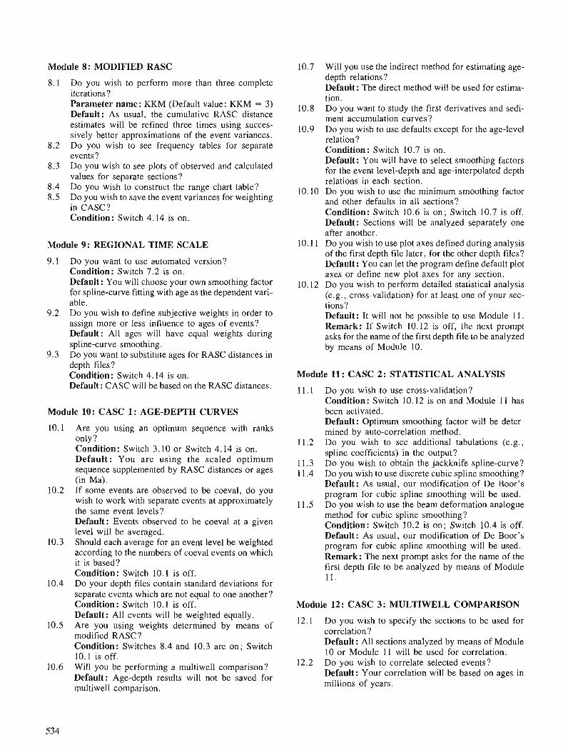
Module 8: MODIFIED RASC

8.1 Do you wish to perform more than three complete iterations? Parameter name: KKM (Default value: KKM = 3) Default: As usual, the cumulative RASC distance estimates will be refined three times using successively better approximations of the event variances.

8.2 Do you wish to see frequency tables for separate events?

8.3 Do you wish to see plots of observed and calculated values for separate sections?

8.4 Do you wish to construct the range chart table? 8.5 Do you wish to save the event variances for weighting

in CASC? Condition: Switch 4.14 is on.

Module 9: REGIONAL TIME SCALE

9.1 Do you want to use automated version? Condition: Switch 7.2 is on. Default: You will choose your own smoothing factor for spline-curve fitting with age as the dependent variable.

9.2 Do you wish to define subjective weights in order to assign more or less influence to ages of events? Default: All ages will have equal weights during spline-curve smoothing.

9.3 Do you want to substitute ages for RASC distances in depth files? Condition: Switch 4.14 is on. Default: CASC will be based on the RASC distances.

Module 10: CASC 1: AGE-DEPTH CURVES

10.1 Are you using an optimum sequence with ranks only? Condition: Switch 3.10 or Switch 4.14 is on. Default: You are using the scaled optimum sequence supplemented by RASC distances or ages (in Ma).

10.2 If some events are observed to be coeval, do you wish to work with separate events at approximately the same event levels? Default: Events observed to be coeval at a given level will be averaged.

10.3 Should each average for an event level be weighted according to the numbers of coeval events on which it is based? Condition: Switch 10.1 is off.

10.7 Will you use the indirect method for estimating age- depth relations? Default: The direct method will be used for estimation.

10.8 Do you want to study the first derivatives and sediment accumulation curves?

10.9 Do you wish to use defaults except for the age-level relation? Condition: Switch 10.7 is on. Default: You will have to select smoothing factors for the event level-depth and age-interpolated depth relations in each section.

10.10 Do you wish to use the minimum smoothing factor and other defaults in all sections? Condition: Switch 10.6 is on; Switch 10.7 is off. Default: Sections will be analyzed separately one after another.

10.1 1 Do you wish to use plot axes defined during analysis of the first depth file later, for the other depth files? Default: You can let the program define default plot axes or define new plot axes for any section.

10.12 Do you wish to perform detailed statistical analysis (e.g., cross-validation) for at least one of your sections? Default: It will not be possible to use Module 11. Remark: If Switch 10.12 is off, the next prompt asks for the name of the first depth file to be analyzed by means of Module 10.

Module 11 : CASC 2: STATISTICAL ANALYSIS

11.1 Do you wish to use cross-validation? Condition: Switch 10.12 is on and Module 11 has been activated. Default: Optimum smoothing factor will be determined by auto-correlation method.

11.2 Do you wish to see additional tabulations (e.g., spline coefficients) in the output?

11.3 Do you wish to obtain the jackknife spline-curve? 1 1.4 Do you wish to use discrete cubic spline smoothing?

Default: As usual, our modification of De Boor's program for cubic spline smoothing will be used.

11.5 Do you wish to use the beam deformation analogue method for cubic spline smoothing? Condition: Switch 10.2 is on; Switch 10.4 is off. Default: As usual, our modification of De Boor's program for cubic spline smoothing will be used. Remark: The next prompt asks for the name of the first depth file to be analyzed by means of Module 1 1 1 1 .

10.4 Do your depth files contain standard deviations for separate events which are not equal to one another? Condition: Switch 10.1 is off. Module 12: CASC 3: MULTIWELL COMPARISON Default: All events will be weighted equally. Are you using weights determined by means of 12.1 Do you wish to specify the sections to be used for

modified RASC? correlation?

Condition: Switches 8.4 and 10.3 are on; Switch Default: All sections analyzed by means of Module

10.1 is off. 10 or Module 11 will be used for correlation.

Will you be performing a multiwell comparison? 12.2 Do you wish to correlate selected events?

Default: Age-depth results will not be saved for Default: Your correlation will be based on ages in

multiwell comparison. millions of years.

12.3 Do you wish to compute probable positions of isochrons? Condition: Switch 12.2 is off. Default: Ages for correlation between sections will have to be selected individually.

12.4 Do you want modified local error bars? Default: Local error bars will be given only.

12.5 Do you want approximate 95 per cent confidence intervals? Default: Standard deviations will be used for the error bars (i.e., approximate 68 per cent confidence intervals will be given).

12.6 Do you wish to define a new t-value for the error bars? Condition: Switch 12.5 is on. Parameter name: TVALUE (Default value: TVALUE = 2.0) Default: As usual, the approximation t = 2.0 for 95 per cent confidence intervals will be used.

12.7 Do you want statistical analysis results for spline- curve values and studentized residuals as well? Default: As usual, statistical analysis will be restricted to deviations between observed and calculated values.

Sensitivity of the RASC model to its critical probit value

Marc A. D'Ioriol

D'lorio, M . A . , Sensitivity of the RASC model to its critical probit value; in Statistical Applications in the Earth Sciences, ed. F. P.Agterberg and G. F. Bonham-Carter; Geological Survey of Canada, Paper 89-9, p. 537-543, 1989.

Abstract

A high-resolution Cenozoic biozonation model is developed using an integrated data set of last occurrences offoraminifers andpalynomorphs. The biozonution is erected using the RASC (Ranking And SCal- ing) computer algorithms. The sequential order of the events, as published in the literature, and the RASC optimum sequence show a statisticalljl .~ign$cant rank-correlation coeficient. This optimum sequence is tested against others created with the same data set with variations of the maximum probit parameter (AAA). These zonations show no sign~$cant change in the rank of events. The length of the scaled sequence generally increases with an increasing value of AAA. Varying this parameter produces greater fluctuations in scaling near zones bounded by marked unconformities or disconformities where a few microfossils may have been reworked or caved-in. These results are consistent with the deviations observed in the frequency distribution study.

Un modtle de biozonation a haute rksolution pour le Cknozo~que est mis au point a 1 'aide d'un ensemble intkgrk de donnkes sur les dernitres manifestations de foraminiferes et de palynomorphes. La biozonation est ktablie au moyen des algorithmes RASC (Ranking and Scaling, classement et mise en ordre) pour ordinateurs. L'ordre skquentiel des kvknements, tel que prksentk dans la documentation, et la skquence RASC optimale prksentent un coeficient de corrklation de rungs statistiquement signijicat$ Cette s6quence optirnale est vkrifike par comparaison a d'autres produites avec le m&me ensemble de donnkes et des variations du paramttre probit maximum (AAA). Ces zonations ne prksentent aucune modification importante du rang des kvknements. La longueur de la skquence cadrke augmente en g&n&ral en fonction de valeurs croissantes de AAA. Des variations de ce paramttre produisent de plus grandes jluctuations au niveau de la mise en ordre prts des zones limitkes par des discordances marqukes ou quelques microfossiles peuvent avoir kt4 rernaniks ou s '&tre affaisks. Ces rksultats sont conformes aux kcarts observks dans 1'6tu.de des distributions de frkquences.

'Canada Centre for Remote Sensing, 1547 Mer~vale Road, Nepean, Ontario KIA 0Y7

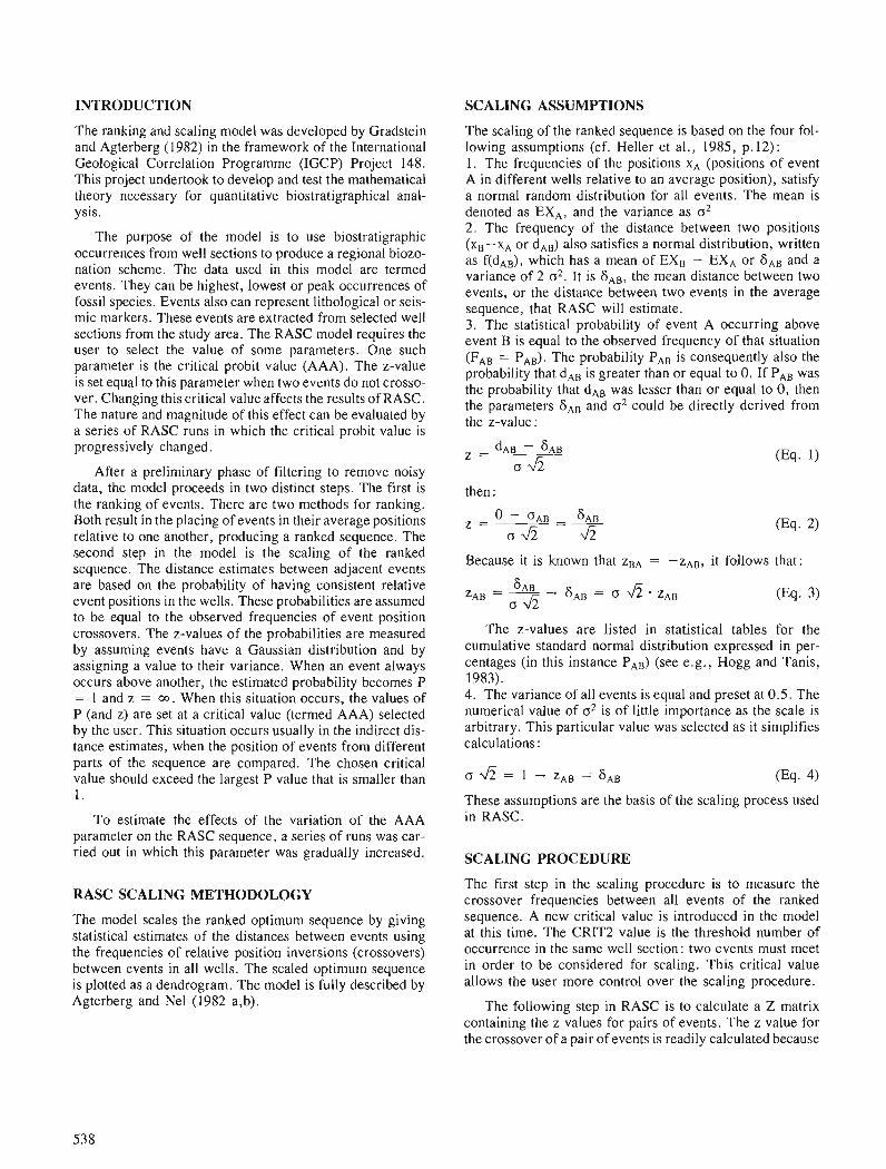
INTRODUCTION SCALING ASSUMPTIONS

The ranking and scaling model was developed by Gradstein and Agterberg (1982) in the framework of the International Geological Correlation Programme (IGCP) Project 148. This project undertook to develop and test the mathematical theory necessary for quantitative biostratigraphical analysis.

The purpose of the model is to use biostratigraphic occurrences from well sections to produce a regional biozonation scheme. The data used in this model are termed events. They can be highest, lowest or peak occurrences of fossil species. Events also can represent lithological or seismic markers. These events are extracted from selected well sections from the study area. The RASC model requires the user to select the value of some parameters. One such parameter is the critical probit value (AAA). The z-value is set equal to this parameter when two events do not crossover. Changing this critical value affects the results of RASC. The nature and magnitude of this effect can be evaluated by a series of RASC runs in which the critical probit value is progressively changed.

After a preliminary phase of filtering to remove noisy data, the model proceeds in two distinct steps. The first is the ranking of events. There are two methods for ranking. Both result in the placing of events in their average positions relative to one another, producing a ranked sequence. The second step in the model is the scaling of the ranked sequence. The distance estimates between adjacent events are based on the probability of having consistent relative event positions in the wells. These probabilities are assumed to be equal to the observed frequencies of event position crossovers. The z-values of the probabilities are measured by assuming events have a Gaussian distribution and by assigning a value to their variance. When an event always occurs above another, the estimated probability becomes P = 1 and z = 03. When this situation occurs, the values of P (and z) are set at a critical value (termed AAA) selected by the user. This situation occurs usually in the indirect distance estimates, when the position of events from different parts of the sequence are compared. The chosen critical value should exceed the largest P value that is smaller than 1.

To estimate the effects of the variation of the AAA parameter on the RASC sequence, a series of runs was carried out in which this parameter was gradually increased.

RASC SCALING METHODOLOGY

The model scales the ranked optimum sequence by giving statistical estimates of the distances between events using the frequencies of relative position inversions (crossovers) between events in all wells. The scaled optimum sequence is plotted as a dendrogram. The model is fully described by Agterberg and Nel (1982 a,b).

The scaling of the ranked sequence is based on the four following assumptions (cf. Heller et al., 1985, p. 12) : 1. The frequencies of the positions x, (positions of event A in different wells relative to an average position), satisfy a normal random distribution for all events. The mean is denoted as EXA, and the variance as o2 2. The frequency of the distance between two positions (xB-xA or dAB) also satisfies a normal distribution, written as f(dAB), which has a mean of EXB - EXA or tiAB and a variance of 2 0 2 . It is SAB, the mean distance between two events, or the distance between two events in the average sequence, that RASC will estimate. 3. The statistical probability of event A occurring above event B is equal to the observed frequency of that situation (FA, = PAB) The probability PAB is consequently also the probability that dAB is greater than or equal to 0. If PAB was the probability that dAB was lesser than or equal to 0, then the parameters SAB and o2 could be directly derived from the z-value:

then :

Because it is known that zBA = -zAB, it follows that:

The z-values are listed in statistical tables for the cumulative standard normal distribution expressed in percentages (in this instance PAB) (see e.g., Hogg and Tanis, 1983). 4. The variance of all events is equal and preset at 0.5. The numerical value of o2 is of little importance as the scale is arbitrary. This particular value was selected as it simplifies calculations :

These assumptions are the basis of the scaling process used in RASC.

SCALING PROCEDURE

The first step in the scaling procedure is to measure the crossover frequencies between all events of the ranked sequence. A new critical value is introduced in the model at this time. The CRIT2 value is the threshold number of occurrence in the same well section : two events must meet in order to be considered for scaling. This critical value allows the user more control over the scaling procedure.

The following step in RASC is to calculate a Z matrix containing the z values for pairs of events. The z value for the crossover of a pair of events is readily calculated because

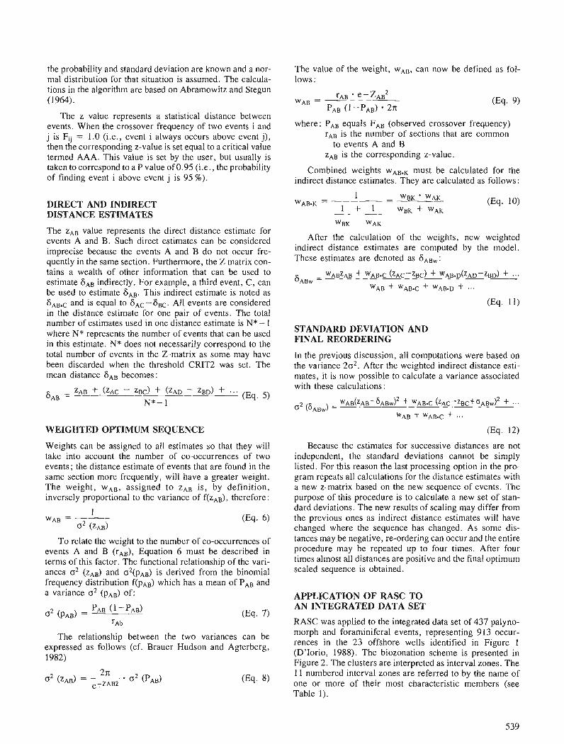
the probability and standard deviation are known and a normal distribution for that situation is assumed. The calculations in the algorithm are based on Abramowitz and Stegun (1964).

The z value represents a statistical distance between events. When the crossover frequency of two events i and j is Fij = 1.0 (i.e., event i always occurs above event j), then the corresponding z-value is set equal to a critical value termed AAA. This value is set by the user, but usually is taken to correspond to a P value of 0.95 (i.e., the probability of finding event i above event j is 95 %).

DIRECT AND INDIRECT DISTANCE ESTIMATES

The z,, value represents the direct distance estimate for events A and B. Such direct estimates can be considered imprecise because the events A and B do not occur frequently in the same section. Furthermore, the Z matrix contains a wealth of other information that can be used to estimate tiAB indirectly. For example, a third event, C, can be used to estimate ti,,. This indirect estimate is noted as 8AB.C and is equal to 8AC-6BC. All events are considered in the distance estimate for one pair of events. The total number of estimates used in one distance estimate is N*- 1 where N* represents the number of events that can be used in this estimate. N* does not necessarily correspond to the total number of events in the Z-matrix as some may have been discarded when the threshold CRIT2 was set. The mean distance tiAB becomes :

WEIGHTED OPTIMUM SEQUENCE

Weights can be assigned to all estimates so that they will take into account the number of co-occurrences of two events; the distance estimate of events that are found in the same section more frequently, will have a greater weight. The weight, WAB, assigned to ZAB is, by definition, inversely proportional to the variance of f(zAB), therefore:

To relate the weight to the number of co-occurrences of events A and B (rAB), Equation 6 must be described in terms of this factor. The functional relationship of the variances o2 (zAB) and 02(pAB) is derived from the binomial frequency distribution f(pAB) which has a mean of PAB and a variance u2 (pAB) of:

The relationship between the two variances can be expressed as follows (cf. Brauer Hudson and Agterberg, 1982)

The value of the weight, w,,, can now be defined as follows :

where: PA, equals FAB (observed crossover frequency) r,, is the number of sections that are common

to events A and B z,, is the corresponding z-value.

Combined weights WAB.K must be calculated for the indirect distance estimates. They are calculated as follows :

1 - - WBK ' WAK WAB.K =

1 + 1 w,, + w,, - - WBK WAK

After the calculation of the weights, new weighted indirect distance estimates are computed by the model. These estimates are denoted as GABw:

STANDARD DEVIATION AND FINAL REORDERING

In the previous discussion, all computations were based on the variance 2u2. After the weighted indirect distance estimates, it is now possible to calculate a variance associated with these calculations :

W , B ( Z A B - ~ A B W ) ~ + WAB.C ( z A c - z B c ~ ~ A B ~ ) ~ + . ,. u2 (~ABW) =

WAB + WAB.C + ...

(Eq. 12)

Because the estimates for successive distances are not independent, the standard deviations cannot be simply listed. For this reason the last processing option in the program repeats all calculations for the distance estimates with a new z-matrix based on the new sequence of events. The purpose of this procedure is to calculate a new set of standard deviations. The new results of scaling may differ from the previous ones as indirect distance estimates will have changed where the sequence has changed. As some distances may be negative, re-ordering can occur and the entire procedure may be repeated up to four times. After four times almost all distances are positive and the final optimum scaled sequence is obtained.

APPLICATION OF RASC TO AN INTEGRATED DATA SET

RASC was applied to the integrated data set of 437 palynomorph and foraminifera1 events, representing 913 occurrences in the 23 offshore wells identified in Figure 1 (D'Iorio, 1988). The biozonation scheme is presented in Figure 2. The clusters are interpreted as interval zones. The 11 numbered interval zones are referred to by the name of one or more of their most characteristic members (see Table 1).

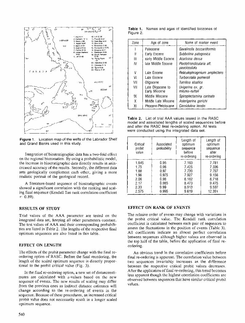
I . RuI H.11 2 Karlseln~ H-I3 3. Smrrl J.90 4 Herjoll M-92 5. Blslnl H.81 6. Gudrid H-55 7 Csn~er 0 78 8. lndlan Harbour

M.52 9. Led M.48

I 0 Leil € 3 8 I I . Freydis 8.87 12. Hale Bay H.31 % 13. Blue H-28 14 BonavbsM '2.99 15. Cumberland 8-55 16. Bonanza M.71 17. DOm#nlOn 0 2 3 la. Smlh TempeSl

G-88 IS. Flying Foam 55D-

1-13 20. Adol~hus DMI 21. Hlbelnla P.15 22. Egrel K-36 23. Ospfey H 84

A ILANTIC

50' - OCEAN

0 a5' -

Figure 1. Location map of the wells of the Labrador Shelf and Grand Banks used in this study.

Integration of biostratigraphic data has a two-fold effect on the regional biozonation. By using a probabilistic model, the increase in biostratigraphic data directly results in anin- creased accuracy of the results. Secondly, the different data sets geologically complement each other, giving a more realistic portrait of the geological record.

A literature-based sequence of biostratigraphic events showed a significant correlation with the ranking and scaling final sequence (Kendall Tau rank correlation coefficient = 0.89).

RESULTS OF STUDY

Trial values of the AAA parameter are tested on the integrated data set, keeping all other parameters constant. The test values of AAA and their corresponding probabilities are listed in Table 2. The lengths of the respective final optimum sequences are also listed in this table.

EFFECT ON LENGTH

The effects of the probit parameter change with the final re- ordering option of RASC. Before the final reordering, the length of the scaled optimum sequence is directly proportional to the probit critical value (Fig. 3).

In the final re-ordering option, a new set of distanceesti- mates are calculated with z-values based on the new sequence of events. The new results of scaling may differ from the previous ones as indirect distance estimates will change according to the re-ordering of events in the sequence. Because of these procedures, an increased critical probit value does not necessarily result in a longer scaled optimum sequence.

Table 1. Names and ages of identified biozones of Figure 2.

Table 2. List of trial AAA values tested in the RASC model and associated lengths of scaled sequences before and after the RASC final re-ordering option. All tests were conducted using the integrated data set.

r

Zone

I I I

I l l IV

V VI VII VII

IX X XI

EFFECT ON RANK OF EVENTS

Age of zone

Paleocene Early Eocene early Middle Eocene late Middle Eocene

Late Eocene Late Eocene Oligocene Late Oligocene to Early Miocene Middle Miocene Middle Late Miocene Pliocene-Pleistocene

The relative order of events may change with variations in the probit critical value. The Kendall rank correlation coefficient is calculated between each pair of sequences to assess the fluctuations in the position of events (Table 3). All coefficients indicate an almost perfect correlation between sequences although higher values are observed in the top half of the table, before the application of final re- ordering.

Name of marker event

Gavelinella beccariiformis Subbotina patagonica Acarinina densa Plectofrondicularia aff. paucicostata Reticulophragmium amplectens lurborotalia pomeroli lurrilina alsatica Uvigerina ex. gr. miozea-nuttali Spiroplectamina carinata Asterigerina gurichi Cassidulina teretis

Critical probit value

1.645 1.75 1.88 1.96 2.06 2.17 2.33 2.575

An obvious trend in the correlation coefficients before final re-ordering is apparent. The correlation value between two sequences invariably increases as the difference between the respective critical probit values decreases. After the application of final re-ordering, this trend becomes less apparent though the highest correlation coefficients are observed between sequences that have similar critical probit values.

Associated probability

0.95 0.96 0.97 0.975 0.98 0.985 0.99 0.995

Length of optimum sequence

before re-ordering

7.193 7.425 7.730 7.927 8.182 8.473 8.913 9.619

T

Length of optimum sequence

after re-ordering

7.781 7.336 7.797 9.156 8.718 9.475 9.597

12.351

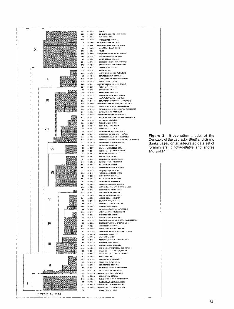
PINUS

ISI!CAEPOLLENllCS INCNICULUS

ELPNlOlUY SPP.

CASSlDULlNA TERETIS

uGLOB0ROTALIA INFLATA

rGLOBOROiALIA CRASSAFORYIS

UVIGERINA CANARIENSIS

A I I E S

~HEOOLOBOOUAORINA AILANTICA

SYSTEUATOPHORA ANCYRCA

ASTERIOERINA OURlCNl

OPCRCULOPlNlUY CENTROCARPUU

SPINI rER l IES PSEUOOFURCATUS

OSYUNOACIDITES 0 1

XENIKOON 0 A

HYSTRICHOKOLPOYA RICAUOIAE

CERATOBULIYINA CONTRARIA

LlNOULODlNlUY UACHAEROPNORUY

IOUBACACIOITES OA

rASTERIOERINA 0URICNI (PEAK)

PODOCARPlDlTES 0 1

SCAPHOPOO SP..l

EPISTOYINA ELEOANS

CHlROPTCRlOlUY YCSPILANUY

SPIROPLECTAYYINA CARlNATA

OETLANDREA SPINULOSA (REWORKED)

..0LOBOROTALIA SCITULA PRAESCIIULA

CORDOSPHAERIDIUY CANTHARLLLUY

PNIHANOPCRIOIHIUY COYATUY (REWORKED)

OAPSILIOINIUY PASTlELSll

uOLOBlOERlNOlDES PRIYOROIUS

NVSTRlCNOKOLPOYA C lNClUY (RLWORKCO)

OUTTULINA PROBLEUA

PNTNANOPERIDINIUY

GYR0101NA GIRAROANA

ALABAYINA SCITULA

0LOBlOERlHA PRAEBULLOIDES

AREOSPHAERIOIUY PECTINIFORUE (REWORKED)

DEFLANDREA PWOSPHORITICA

IURRILIHA ALSATICA

COARSE ARENACEOUS SPP.

NOOOSARIA CF. ELCOAWTISSIUA

EPONIOES UUBONATUS

AUYODISCUS LATUS

OLOBIOERINA VENEZUELANA

OLAPNROCVSTA EXUBERAIIS

WETZELIELLA OVALIS

CRlBROPERlOlNlUY GIUSEPPEI

YAROINULINA DECORATA

WETZELIELLA ARTICULATA

OLOBICERINA LINAPERIA

HAPLOPHRAOYOIDLS WALTER1

AUUOBACULITCS ATF POLVTNALAYUS

OLO0IGERINA YEOUAENSIS

DAPSILIOINIUU SIMPLEX

AYYOSPHAEROIDINA SP. 1

KARRERIELLA CONVERSA

BULIYINA ALAZANENSIS

PSEUOOHASTIOCRINA UICRA

DIPWYES COLLIDERUM

RETICULOPHRAOYIUY AUPLCCTENS

APECTOOINIUY HOYOYORPNUY

ClBlClOOlDES ALLEN1

C lB lC lDOlDES BLANPICOI

~TOFRONDICQ&IA AFF. PAUCLEeUdIh

SPIROPLECTAUYINA SPECTABILIS LO

AREOLIOERA CORONAIA

COROOSPHAERIOIUY GRACILE

SPIROPLECTAYUINA SPECTABILIS LC0

TVRRlLlNA ROBERTS1

ACARININA OENSA

PSEUOOHASTIOERINA WILCOXENSIS

BULlYlNA TRIGONALIS

GLAPHROCYSIA OROINATA

HYSlRlCHOSPNlERlDlUU TUBIFERUU

..ACARIHINA AFF. BROEOERYANNI

ACARlNlNA AFF. PENTACAYERATA

YEGASPORE SP. I

DRACOOINIUY CONOYLOS

SUBBOTINA PATAGONICA

CERATIOPSIS SPECIOSA

SPIROPLECTAYUINA NAVARROANA

ACARININA SOLOAOOENSIS

.~PLANOROTALITES CNAPYANI

OLOYOSPIRA CORONA

PALAEOPERIDINIUU PYROPHORUY

FAVELINELLA BECCIRIIFORUIS

..SUBBOTINA TRILOCULINOIDES

..SUBBOTINA PSEUOOBULLOIDES

RZCHAKINI LPICONA

I N T E R E V E N T D I S T A N C E S

Figure 2. Biozonation model of the Cenozoic of the Labrador Shelf and Grand Banks based on an integrated data set of foraminifers, dinoflagellates and spores and pollen.

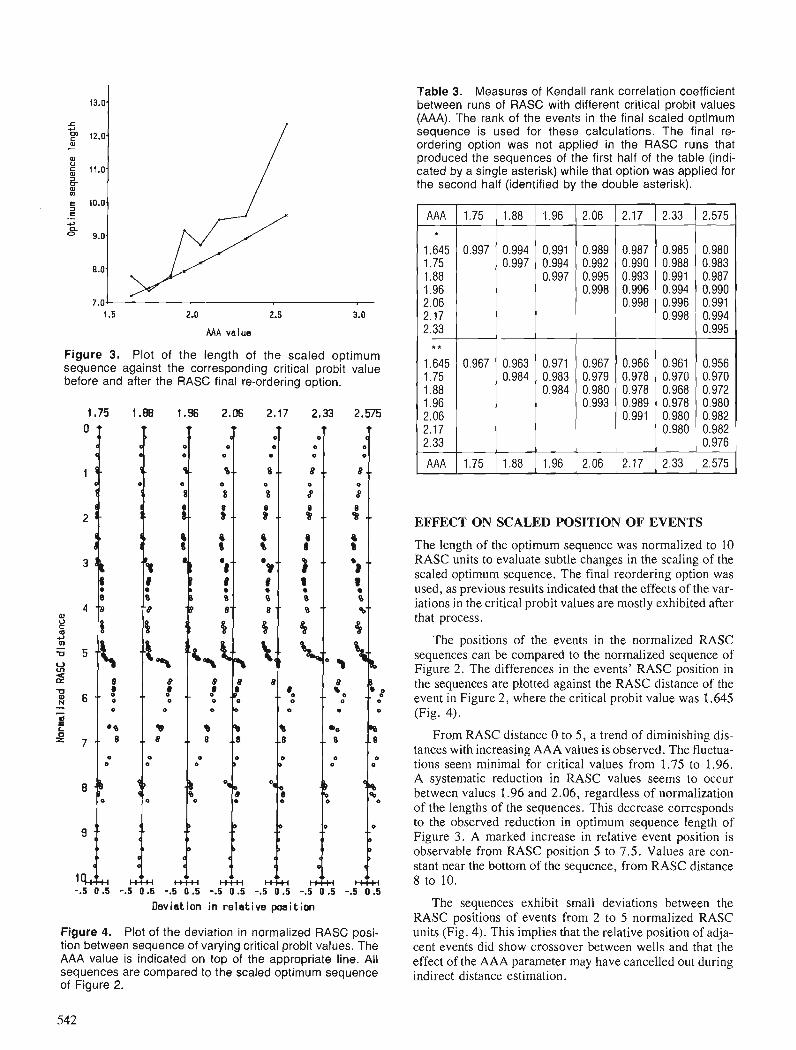
AAA value

Figure 3. Plot of the length of the scaled optimum sequence against the corresponding critical probit value before and after the RASC final re-ordering option.

1.88 1.96 2.06 2.17 2.33

8 B "

.5 0.5 -.5 0.5 -.5 0 .5 -.5 0 .5 -.5 0 .5 - Deviation in relative position

Figure 4. Plot of the deviation in normalized RASC position between sequence of varying critical probit values. The AAA value is indicated on top of the appropriate line. All sequences are compared to the scaled optimum sequence of Figure 2.

Table 3. Measures of Kendall rank correlation coefficient between runs of RASC with different critical probit values (AAA). The rank of the events in the final scaled optimum sequence is used for these calculations. The final re- ordering option was not applied in the RASC runs that produced the sequences of the first half of the table (indicated by a single asterisk) while that option was applied for the second half (identified by the double asterisk).

EFFECT ON SCALED POSITION OF EVENTS

AAA *

1.645 1.75 1.88 1.96 2.06 2.17 2.33

* *

1.645 1.75 1.88 1.96 2.06 2.17 2.33

AAA

The length of the optimum sequence was normalized to 10 RASC units to evaluate subtle changes in the scaling of the scaled optimum sequence. The final reordering option was used, as previous results indicated that the effects of the variations in the critical probit values are mostly exhibited after that process.

The positions of the events in the normalized RASC sequences can be compared to the normalized sequence of Figure 2. The differences in the events' RASC position in the sequences are plotted against the RASC distance of the event in Figure 2, where the critical probit value was 1.645 (Fig. 4).

1.75

0.997

0.967

1.75

From RASC distance 0 to 5 , a trend of diminishing distances with increasing AAA values is observed. The fluctuations seem minimal for critical values from 1.75 to 1.96. A systematic reduction in RASC values seems to occur between values 1.96 and 2.06, regardless of normalization of the lengths of the sequences. This decrease corresponds to the observed reduction in optimum sequence length of Figure 3. A marked increase in relative event position is observable from RASC position 5 to 7.5. Values are constant near the bottom of the sequence, from RASC distance 8 to 10.

The sequences exhibit small deviations between the RASC positions of events from 2 to 5 normalized RASC units (Fig. 4). This implies that the relative position of adjacent events did show crossover between wells and that the effect of the AAA parameter may have cancelled out during indirect distance estimation.

1.88

0.994 0.997

0.963 0.984

1.88

1.96

0.991 0.994 0.997

0.971 0.983 0.984

1.96

2.06

0.989 0.992 0.995 0.998

0.967 0.979 0.980 0.993

2.06

2.17

0.987 0.990 0.993 0.996 0.998

0.966 0.978 0.978 0.989 0.991

2.17

2.33

0.985 0.988 0.991 0.994 0.996 0.998

0.961 0.970 0.968 0.978 0.980 0.980

2.33

2.575

0.980 0.983 0.987 0.990 0.991 0.994 0.995

0.956 0.970 0.972 0.980 0.982 0.982 0.976

2.575

The deviations from the original sequence are accentu- ated with increasing AAA values, from 5 to 7 RASC units. The critical probit value will affect the scaling process in the indirect distance estimates, especially when one of the two events being compared will crossover with a third event and the second will not. This situation mav occur if certain microfossils are reworked in some wells and not in others. This type of effect is more likely to occur within zones bounded by large intercluster distances. The deviations observed in Figure 4 correspond to the Late Eocene (zones V and VI in Fig. 2). As large intercluster distances occur between zones V, VI and VII, it is likely that microfossils for a few events may have been either reworked or caved-in in some wells, causing the notable and progressively larger deviations of Figure 4.

CONCLUSIONS

(a) Increasing the critical probit value causes a proportional increase in the length of the optimum sequence before the final re-ordering option of RASC. The latter RASC option obscures this obvious trend, though the general pattern is apparent. (b) The ranking of events is not significantly affected by varying the probit critical value, although a general pattern of increasing discrepancies is observed between sequences with increasingly different AAA values. (c) The scaling of both ends of the optimum sequence is systematically affected by variations in the critical probit value, presumably because of the lower abundance and frequency of data and of sampling problems at the top and bottom of some wells. (d) The scaling of zones V and VI is seemingly more affected by the probit critical value than other parts of the optimum sequence. This is explained by the proximity (in time) of marked unconformities or disconformities and by the postulated presence of a few reworked or caved-in microfossils. (e) The effect of the AAA value is related to the quality of the data. (f) RASC is a very sturdy model which shows little sensitivity towards the variation of its critical probit value.

ACKNOWLEDGMENTS

I am very grateful to Frits Agterberg for his invaluable advice and guidance. Dan Merriam and Felix Gradstein are thanked for their comments and suggestions.

REFERENCES

Abramowitz, M. and Stegun, I.A. (eds.) 1964: Handbook of Mathematical Functions; Applied Mathematics

Series, v. 55, National Bureau of Standards, Washington, 1046 p. Agterberg, F.P. and Nel, L.D. 1982a: Algorithm for the ranking of stratigraphic events; Computers &

Geosciences, v. 8, no. I, p. 69-90. 1982b: Algorithm for the scaling of stratigraphic events; Computers &

Geosciences, v. 8, no.2, p. 1 63- 182. Brauer Hudson, C.B. and Agterberg, F.P. 1982: Paired comparison models in biostratigraphy; Journal of Mathe-

matical Geology, v. 14, 110.2, p. 141-159. D'Iorio, M.A. 1988: Quantitative Biostratigraphic Analysis of the Cenozoic of the

Labrador Shelf and Grand Banks; unpublished Ph D thesis, University of Ottawa, 401 p.

Gradstein, F.M. and Agterberg, F.P. 1982: Models of Cenozoic foraminifera1 stratigraphy- northwestern

Atlantic Margin; & J.M. Cubitt and R.A. Reyment, Quantitative Stratigraphic Correlation, ed. John Wiley & Sons, New York, p. 119.170.

1985: Quantitative correlation in exploration micropaleontology; 5 F.M. Gradstein, F.P. Agterberg, J.C. Brower and W.W. Schwar- zacher, Quantitative Stratigraphy, ed. Reidel Publishing Co., and UNESCO, Paris, p. 309-357.

Heller, M., Gradstein, W.S., Gradstein, F.M., Agterberg, F.P., and Lew, S.N. 1985: RASC FORTRAN 77 computer program for ranking and scaling

of biostratigraphic events; Geological Survey of Canada, Open File 1203.

Hogg, R.V. and Tanis E.A. 1983: Probability and Statistical Inference, second edition; MacMillan

Publishing Co., New York, 533 p.

Spline smoothing by means of an analogy to structural beams1

Paul Hibbert2

Hibbert, P., Spline smoothing by means of an analogy to structural beams; Statistical Applications in the Earth Sciences, ed. F. P. Agterberg and G. F. Bonham-Carter; Geological Survey of Canada, Paper 89-9, p. 545-555, 1989.

Abstract

An algorithm for smoothing a set of experimental data by means of a cubic spline is given. The method originatesfrom the observation that the deflection equarion of a structural beam subjected to end conditions of bending moment and shear is a cubic polynomial. A development of the diferential equation of the elastic equation of the beam is given and a resume of the Stiffness Method for solving structural systems is presented. The Fortran program which uses the BASCS (Beam Analogy for Smoothing Cubic Splines) algorithm allows any degree of smoothing from that of a perfectjt to a linear approximation. Particular attention is paid to the problem of selecting a smoothing factor whose magnirude is a reasonable representation of the actual degree of smoothing. m e program allows interactive trial and error "shaping" of the curve by lerting the user arbitrarily change the stifiess properties on any longitudinal intervals of the beam. The logical structure of the Fortran program is presented.

Un algorithme pour le lissage d'un ensemble de donne'es expe'rimentales au moyen d'une foncrion pistolet cubique est pr4sentb La mkhode ernane de l'observation du fait que 1 'e'quation de fle'chissement d'une poutre de construction soumise tt des conditions extr2mes de moment fle'chissant et de cisaillement est une equation polynomiale de troisi2me ordre. Un dkveloppement de la forme diffe'rentielle de l'e'quation d'dlasticite' de la poutre est donne', et un re'sume' de la me'thode de la rigidite'pour la solution de systkmes structuraux est pr4sentb Le programme en Fortran qui fait intervenir l'algorithme BASCS (Beam Analogy for Smoothing Curve Splines) permet tous les degre's de lissage, depuis l'ajustement parfait a une approximation linkaire. Une attention particuli2re est accorde'e au probl2me du choix d'un facteur de lissage dont l'ordre de grandeur constitue une representation raisonnable du degrk re'el de lissage. Le programme permet un cr modelage n interactif par approximations successives de la courbe en laissant l'utilisateur modifier arbitrairement les propri4t4s de rigidite' de tout intervalle longitudinal de la poutre. La structure logique du programme en Fortran est pre'sente'e.

- - -

' Uses an exerpt from STRENGTH OF MATERIALS by Ferdinand L. Singer. Copyright 1951 by Harper & Row, Publishers, Inc. Reprinted by permission. Senior Engineer, IDON Corporation, 875 Carling Ave., Ottawa, Ontario K1S 2E9. Formerly w~th lnfomatics Applications Division, Department of Energy, Mines and Resources, 588 Booth St., Ottawa, Ontario KIA OE4

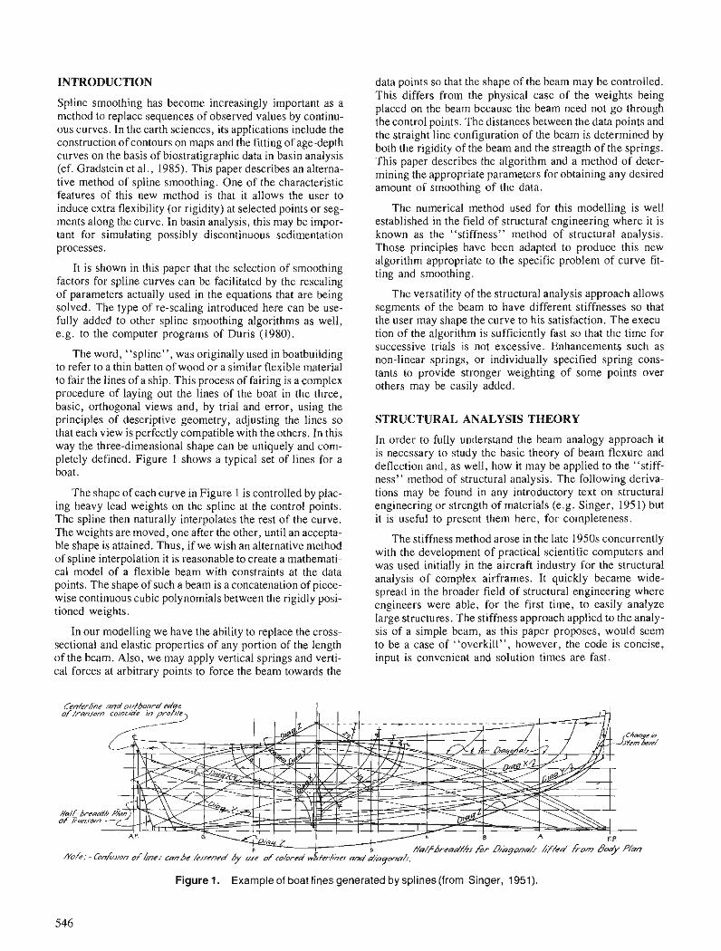
INTRODUCTION data points so that the shape of the beam may be controlled.

Spline smoothing has become increasingly important as a method to replace sequences of observed values by continuous curves. In the earth sciences, its applications include the construction of contours on maps and the fitting of age-depth curves on the basis of biostratigraphic data in basin analysis (cf. Gradstein et al., 1985). This paper describes an alternative method of spline smoothing. One of the characteristic features of this new method is that it allows the user to induce extra flexibility (or rigidity) at selected points or segments along the curve. In basin analysis, this may be important for simulating possibly discontinuous sedimentation processes.

It is shown in this paper that the selection of smoothing factors for spline curves can be facilitated by the rescaling of parameters actually used in the equations that are being solved. The type of re-scaling introduced here can be usefully added to other spline smoothing algorithms as well, e.g. to the computer programs of Duris (1980).

The word, "spline", was originally used in boatbuilding to refer to a thin batten of wood or a similar flexible material to fair the lines of a ship. This process of fairing is a complex procedure of laying out the lines of the boat in the three, basic, orthogonal views and, by trial and error, using the principles of descriptive geometry, adjusting the lines so that each view is perfectly compatible with the others. In this way the three-dimensional shape can be uniquely and completely defined. Figure 1 shows a typical set of lines for a boat.

The shape of each curve in Figure 1 is controlled by placing heavy lead weights on the spline at the control points. The spline then naturally interpolates the rest of the curve. The weights are moved, one after the other, until an acceptable shape is attained. Thus, if we wish an alternative method of spline interpolation it is reasonable to create a mathematical model of a flexible beam with constraints at the data points. The shape of such a beam is a concatenation of piece- wise continuous cubic polynomials between the rigidly posi- tioned weights.

~his 'differs from the physical case of the weights being placed on the beam because the beam need not go through the control points. The distances between the data points and the straight line configuration of the beam is determined by both the rigidity of the beam and the strength of the springs. This paper describes the algorithm and a method of determining the appropriate parameters for obtaining any desired amount of smoothing of the data.

The numerical method used for this modelling is well established in the field of structural engineering where it is known as the "stiffness" method of structural analysis. Those principles have been adapted to produce this new algorithm appropriate to the specific problem of curve fitting and smoothing.

The versatility of the structural analysis approach allows segments of the beam to have different stiffnesses so that the user may shape the curve to his satisfaction. The execution of the algorithm is sufficiently fast so that the time for successive trials is not excessive. Enhancements such as non-linear springs, or individually specified spring constants to provide stronger weighting of some points over others may be easily added.

STRUCTURAL ANALYSIS THEORY

In order to fully understand the beam analogy approach it is necessary to study the basic theory of beam flexure and deflection and, as well, how it may be applied to the "stiffness" method of structural analysis. The following deriva- tions may be found in any introductory text on structural engineering or strength of materials (e.g. Singer, 195 1) but it is useful to present them here, for completeness.

The stiffness method arose in the late 1950s concurrently with the development of practical scientific computers and was used initially in the aircraft industry for the structural analysis of complex airframes. It quickly became widespread in the broader field of structural engineering where engineers were able, for the first time, to easily analyze large structures. The stiffness approach applied to the analysis of a simple beam, as this paper proposes, would seem to be a case of "overkill", however, the code is concise, input is convenient and solution times are fast.

In our modelling we have the ability to replace the cross- sectional and elastic properties of any portion of the length of the beam. Also, we may apply vertical springs and vertical forces at arbitrary points to force the beam towards the

Cder4he and outboard Pd r o f f m o m co/ncide h proz /e ,

G . * 8 \ I " / Oia . z B A CP t

I I D H'/f brcud/h, fir Dayonah h7A-d from Bo* Pian

Noh: - h f i ~ / o n ofhher can be /enrned by uJe of c o / o d w ~ t r r h ~ r ~ am.+ d/b9m~h.

Figure 1. Example of boat lines generated by splines (from Singer, 1951).

Derivation of the Flexure Formula

The flexure formula allows the calculation of the amount of curvature resulting from an applied bending moment on a structural member of specified material and section properties. It is one of the basic equations of strength of materials.

The assumptions inherent are : 1. Plane cross-sections of the beam, originally plane,

remain plane. (Fig. 2), 2. The material of the beam is homogeneous and obeys

Hooke's Law (stress is proportional to strain), 3. The elastic moduli for tension and compression are

equal, 4. The beam is initially straight and of constant cross-

section.

In Figure 2, the two sections ab and cd are separated by the distance dx. Because of the bending caused by the load, P, section ab and cd rotate relative to each other by the amount do, but remain straight and undistorted, in accordance with the premise that plane sections remain plane. Fibre ac at the top is shortened while the fibre bd at the bottom is lengthened. Somewhere between them is located fibre ef, whose length is unchanged. Drawing the line c ' d ' through f parallel to ab shows that fibre ac is shortened by an amount cc ' and is in compression, and that fibre bd is lengthened by an amount d 'd and is in tension.

Consider the deformation of a typical fibre gh located y units from the neutral surface. Its elongation hk is the arc of a circle of radius y subtended by the angle de and is given by :

The strain is found by dividing the deformation by the original length of the fibre:

Define p to be the radius of curvature of the neutral surface, then the curved length ef is p dB, and the strain becomes:

Assuming that the material is homogeneous and obeys Hooke's Law, the stress in fibre gh is given by

where E is Young's modulus of elasticity.

dx , Ne&

C

P I - ' f -

dB

b d i ;, R l R2

b d ' d

Figure 2. Conventions and nomenclature for a beam under flexure.

It is now necessary to examine the equilibrium of a small

section of beam (Fig. 3). For horizontal equilibrium, 1 S dA = 0, and replacing S with its previously derived value yields

(Eip) y dA = 0.

To satisfy the condition that the bending moment is balanced by the resisting moment, the resisting moment about the neutral axis is

Hence for all elements in the cross-section, the bending moment is

M = S y(S dA),

which by replacing S by Eylp becomes

M = (Eip) S y2 dA.

Since the integral of the value of y2 times the elemental area is, by definition, the moment of inertia, I :

M = EI/p.

This is the flexure formula which will be used in the next section.

Derivation of the Beam Equation

The following "double-integration" method is a conventional derivation of the beam equation. It allows the solution of the vertical displacement, y, of any point in terms of its x coordinate (Fig. 4).

Figure 3. The forces acting on a beam in a state of equilibrium.

Figure 4. Conventions and nomenclature of the elastic curve.

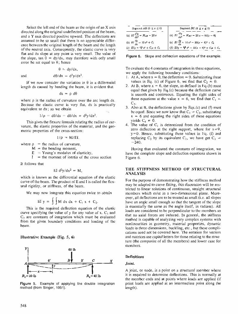
Select the left end of the beam as the origin of an X axis directed along the original undeflected position of the beam, and a Y axis directed positive upward. The deflections are assumed to be so small that there is no appreciable difference between the original length of the beam and the length of the neutral axis. Consequently, the elastic curve is very flat and its slope at any point is very small. The value of the slope, tan 0 = dyldx, may therefore with only small error be set equal to 0 ; hence

0 = dyldx,

and d01dx = d2y/dx2.

If we now consider the variation in 0 in a differential length ds caused by bending the beam, it is evident that

where p is the radius of curvature over the arc length ds. Because the elastic curve is very flat, ds is practically equivalent to dx; so we obtain .

l / p = de/ds = deldx = d2y/dx2.

This gives the flexure formula relating the radius of curvature, the elastic properties of the material, and the geometric properties of the cross-section:

where p = the radius of curvature, M = the bending moment, E = Young's modulus of elasticity, I = the moment of inertia of the cross section

It follows that

EI d2y/dx2 = M,

which is known as the differential equation of the elastic curve of the beam. The product of E and I is called the flexural rigidity, or stiffness, of the beam.

We may now integrate this equation twice to obtain

EI y = j M d x d x + C , x + C2.

This is the required deflection equation of the elastic curve specifying the value of y for any value of x. C , and C2 are constants of integration which must be evaluated from the given boundary conditions and loading of the beam.

Illustrative Example (Fig. 5, 6)

Segment AB (0 5 z 5 6) 1 Segment BC (6 $ x g 9)

(a) E I ~ = MAS = 202 d% dza

I (d) E 1 a = M ~ ~ = 2 0 ~ - S O ~ - 6 )

( b ) El * = 10 2' + C, dz

= 10 za - aO(z - 6)¶+ C:

( c ) EIy = 9 9 + CAX + Ca ( f ) EIy = $axs - 10(z - 6)3 + C S ~ +C4

Figure 6. Slope and deflection equations of the example.

To evaluate the 4 constants of integration in these equations, we apply the following boundary conditions : 1 . At A, where x = 0 , the deflection = 0. Substituting these

values in Eq. (c) of Figure 6, we find that C2 = 0. 2. At B, where x = 6, the slope, as defined in Eq.(b) must

equal that given by Eq.(e) because the deflection curve is smooth and continuous. Equating the right sides of these equations at the value x = 6, we find that C , =

c3. 3. Also at B, the deflections given by Eqs.(c) and (f) must

be equal. Since we now know that C , = C3, substituting x = 6 and equating the right sides of these equations yields C4 = 0.

4. The value of C , is determined from the condition of zero deflection at the right support, where for x=9, y=O. Hence, substituting these values in Eq. (f) and replacing C3 by its equivalent C , , we have get C, = - 240.

Having thus evaluated the constants of integration, we have the complete slope and deflection equations shown in Figure 6.

THE STIFFNESS METHOD OF STRUCTURAL ANALYSIS

For the purpose of demonstrating how the stiffness method may be adapted to curve fitting, this discussion will be restricted to linear solutions of continuous, straight structural members which exist in a two-dimensional plane. More- over, all deflections are to be treated as small (i.e. all slopes have an angle small enough so that the tangent of the slope is essentially the same as the angle itself, in radians). All loads are considered to be perpendicular to the members so that no axial forces are induced. In general, the stiffness method is capable of analyzing very complex systems with nonlinearities in geometry, material properties, dynamic loads in three-dimensions, buckling, etc., but these compli- cations need not be covered here. The notation for vectors and matrices use capital letters for those relating to the structure (the composite of all the members) and lower case for members.

Definitions

Joint.

A joint, or node, is a point on a structural member where it is required to determine deflections. This is normally at the member ends and at points where loads are applied (if

Figure 5. Example of applying the double integration point loads are applied at an intermediate point aiong the method (from Singer, 1951). length).

548

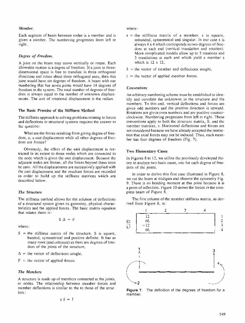
Member. where :

Each segment of beam between nodes is a member and is given a number. The numbering progresses from left to right.

Degree of Freedom.

A joint on the beam may move vertically or rotate. Each allowable motion is a degree of freedom. If a joint in three- dimensional space is free to translate in three orthogonal directions and rotate about three orthogonal axes, then this joint would have six degrees of freedom. A beam with our numbering that has seven joints would have 14 degrees of freedom in the system. The total number of degrees of freedom is always equal to the number of unknown displacements. The unit of rotational displacement is the radian.

The Basic Premise of the Stiffness Method

The stiffness approach to solving problems relating to forces and deflections in structural systems requires the answer to the question :

What are the forces resulting from giving degree of freedom, n, a unit displacement while all other degrees of freedom are frozen?

Obviously, the effect of the unit displacement is restricted in its extent to those nodes which are connected to the node which is given the unit displacement. Because the adjacent nodes are frozen, all the forces beyond them must be zero. All the displacements are successively applied with the unit displacement and the resultant forces are recorded in order to build up the stiffness matrices which are described below.

The Structure

The stiffness method allows for the solution of deflections of a structural system given its geometry, physical characteristics and the applied forces. The basic matrix equation that relates them is:

where :

S = the stiffness matrix of the structure. S is square, banded, symmetrical and positive definite. It has as many rows (and columns) as there are degrees of freedom of the joints of the structure,

A = the vector of deflections sought,

F = the vector of applied forces.

The Members

A structure is made up of members connected at the joints, or nodes. The relationship between member forces and member deflections is similar to the to those of the structure :

s S = f

s = the stiffness matrix of a member. s is square, unbanded, symmetrical and singular. In our case s is always 4 x 4 which corresponds to two degrees of freedom at each end (vertical translation and rotation). More complicated models allow up to 3 rotations and 3 translations at each end which yield a member s which is 12 x 12,

S = the vector of member end deflections sought,

f = the vector of applied member forces.

Conventions

An arbitrary numbering scheme must be established to identify and correlate the unknowns in the structure and the members. To this end, vertical deflections and forces are given odd numbers and the positive direction is upward. Rotations are given even numbers and are positive counter- clockwise. Numbering progresses from left to right. These conventions apply to both the structure matrix, S, and the member matrices, s. Horizontal deflections and forces are not considered because we have already accepted the restriction that axial forces may not be induced. Thus, each member has four degrees of freedom (Fig. 7).

Two Elementary Cases

In Figures 8 to 12, we utilize the previously developed theory to analyze two basic cases, one for each degree of freedom of the joints.

In order to derive this first case illustrated in Figure 8, we cut the beam at midspan and observe the symmetry Fig. 9. There is no bending moment at this point because it is a point of inflection. Figure 10 shows the forces in the complete beam of Figure 8.

The first column of the member stiffness matrix, as derived from Figure 8, is :

1 2 3 4

1

Figure 7. The definition of the degrees of freedom for a member.

J Horizontal tangent

Figure 8. A beam with degree of freedom 1 given a unit displacement.

Figure 9. The forces on the left half of the above beam.

Figure 10. The forces in the beam of Figure 8.

6EI - L2

Figure 12. The forces on the beam of Figure 11.

Similarly, let us now impose a unit rotation on the left end for degree of freedom 2 (Fig. 11). The forces on the beam of Figure 1 1 are shown in Figure 12.

The second column of s is therefore:

The complete (4 x 4) member stiffness matrix is obtained by symmetry :

Note that this matrix is singular. The physical significance of the singularity is that no solution is possible, because the member may translate or rotate indefinitely in rigid body mode under negligible forces. However, if the rigid body modes are prevented by removing the appropriate degrees of freedom then the trivial solution becomes cvi- dent. In complex, three-dimensional structural engineering applications of the stiffness method there may be three translations and three rotations at each end so the problem is not inherently trivial.

Interpolation on the Curve of the Member

Once the vector of deflections has been obtained, the smooth curve must be interpolated. The displacement numbers of the structure are used to extract the appropriate four displacements for each member. The coefficients, A, B, C, and D of the cubic equation

are readily calculated as shown in Figure 13.

Figure 11. Beam with degree of freedom 2 given a unit displacement.

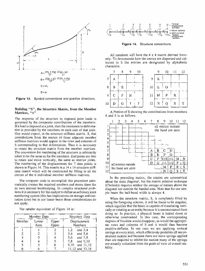
Figure 13. Symbol conventions and positive directions.

Building "S", the Structure Matrix, from the Member Matrices, "s"

The response of the structure to imposed joint loads is governed by the composite contributions of the members. If a load is imposed at a joint, then the resistance to deformation is provided by the members on each side of that joint. One would expect, in the structure stiffness matrix, S , that contributions from the entries of those adjacent member stiffness matrices would appear in the rows and columns of S corresponding to that deformation. Thus it is necessary to create the structure matrix from the member matrices. The convention for numbering of the structure is arbitrarily taken to be the same as for the members. End joints are free to rotate and move vertically, the same as interior joints. The numbering of the displacements for 7 data points is shown in Figure 14. This results in a 14 x 14 structure stiffness matrix which will be constructed by filling in all the entries of the 6 individual member stiffness matrices.

The computer code to accomplish this procedure automatically creates the required numbers and stores them for its own internal bookkeeping. In complex structural problems it is necessary for the analyst to define an arbitrary joint numbering system (this has implications on storage and execution time) but in our linear beam these considerations do not apply.

The tabular equivalent of Figure 14 is:

1 3 2 1 ! Vertical I! '2 Cd~splacemenl

numbers

I 2 3 4 5 6 -Beam numbers 6 7 c J o ~ n t numbers 12 14+Rotalion

displacement numbers

Figure 14. Structure conventions.

Structure Data Displacement

Numbers 1,2 and 3,4 3,4 and 5,6 5,6 and 7,8 7,8 and 9,10 9,10 and 11,12 11,12 and 13,14

Member Data

All members will have the 4 x 4 matrix derived formerly. To demonstrate how the entries are dispersed and collected in S the entries are designated by alphabetic characters.

7 8 9 1 0 9 10 11 12

Member

1 2 3 4 5 6

A Portion of S showing the contributions from members 4 and 5 is as follows.

1 all entries outside 2 he band are zero 3 4 5

Lower Joint

1 2 3 4 5 6

A B C D B E F G

Upper Upper

2 3 4 5 6 7

the band are zero

In the preceding matrix, the entries are symmetrical about the main diagonal, but the matrix solution technique (Choleski) requires neither the storage of entries above the diagonal nor outside the banded area. Note that for our simple beam the half-band width is always 4.

When the structure matrix, S, is completely filled by using the foregoing scheme, it will be found to be singular, which signifies that the beam is capable of translating vertically or rotating as an entity because it is unconstrained from doing so. In practice, a physical beam is bolted down or otherwise constrained. In this case, the corresponding degrees of freedom would disappear, as would the appropriate rows and columns of S and it would thus become positive-definite. In our case we are applying vertical springs at every joint, which effectively prohibits all unconstrained motion and because there are more springs applied than are required to inhibit the motion many of the springs are actually redundant from the point of view of overall stability.

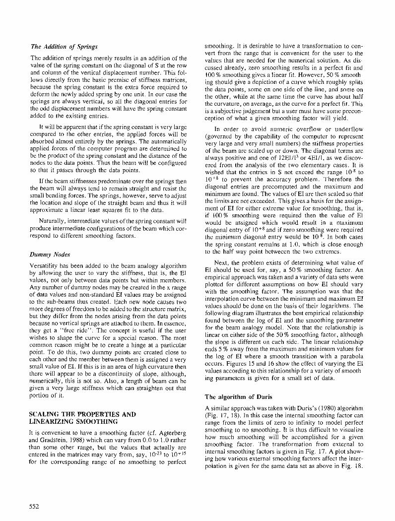
The Addition of Springs

The addition of springs merely results in an addition of the value of the spring constant on the diagonal of S at the row and column of the vertical displacement number. This follows directly from the basic premise of stiffness matrices, because the spring constant is the extra force required to deform the newly added spring by one unit. In our case the springs are always vertical, so all the diagonal entries for the odd displacement numbers will have the spring constant added to the existing entries.

It will be apparent that if the spring constant is very large compared to the other entries, the applied forces will be absorbed almost entirely by the springs. The automatically applied forces of the computer program are determined to be the product of the spring constant and the distance of the nodes to the data points. Thus the beam will be configured so that it passes through the data points.

If the beam stiffnesses predominate over the springs then the beam will always tend to remain straight and resist the small bending forces. The springs, however, serve to adjust the location and slope of the straight beam and thus it will approximate a linear least squares fit to the data.

Naturally, intermediate values of the spring constant will produce intermediate configurations of the beam which correspond to different smoothing factors.

Dummy Nodes

Versatility has been added to the beam analogy algorithm by allowing the user to vary the stiffness, that is, the EI values, not only between data points but within members. Any number of dummy nodes may be created in the x range of data values and non-standard EI values may be assigned to the sub-beams thus created. Each new node causes two more degrees of freedom to be added to the structure matrix, but they differ from the nodes arising from the data points because no vertical springs are attached to them. In essence, they get a "free ride". The concept is useful if the user wishes to shape the curve for a special reason. The most common reason might be to create a hinge at a particular point. To do this, two dummy points are created close to each other and the member between them is assigned a very small value of EI. If this is in an area of high curvature then there will appear to be a discontinuity of slope, although, numerically, this is not so. Also, a length of beam can be given a very large stiffness which can straighten out that portion of it.

SCALING THE PROPERTIES AND LINEARIZING SMOOTHING

It is convenient to have a smoothing factor (cf. Agterberg and Gradstein, 1988) which can vary from 0.0 to 1.0 rather than some other range, but the values that actually are entered in the matrices may vary from, say, to 10+15 for the corresponding range of no smoothing to perfect

smoothing. It is desirable to have a transformation to convert from the range that is convenient for the user to the values that are needed for the numerical solution. As discussed already, zero smoothing results in a perfect fit and 100 % smoothing gives a linear fit. However, 50 % smoothing should give a depiction of a curve which roughly splits the data points, some on one side of the line, and some on the other, while at the same time the curve has about half the curvature, on average, as the curve for a perfect fit. This is a sl~bjectivejudgement but a user must have some precon- ception of what a given smoothing factor will yield.

In order to avoid numeric overflow or underflow (governed by the capability of the computer to represent very large and very small numbers) the stiffness properties of the beam are scaled up or down. The diagonal terms are always positive and one of 12EI/13 or 4EIl1, as we discovered from the analysis of the two elementary cases. It is wished that the entries in S not exceed the range to

to prevent the accuracy problem. here fore the diagonal entries are precomputed and the maximum and minimum are found. The values of EI are then scaled so that the limits are not exceeded. This gives a basis for the assignment of EI for either extreme value for smoothing, that is, if 100 % smoothing were required then the value of EI would be assigned which would result in a maximum

u

diagonal entry of lo+* and if zero smoothing were required the minimum diagonal entry would be In both cases the spring constant remains at 1.0, which is close enough to the half way point betweeen the two extremes.

Next, the problem exists of determining what value of EI should be used for, say, a 50 % smoothing factor. An empirical approach was taken and a variety of data sets were plotted for different assumptions on how EI should vary with the smoothing factor. The assumption was that the interpolation curve between the minimum and maximum EI values should be done on the basis of their logarithms. The following diagram illustrates the best empirical relationship found between the log of EI and the smoothing parameter for the beam analogy model. Note that the relationship is linear on either side of the 50 % smoothing factor, although the slope is different on each side. The linear relationship ends 5 % away from the maximum and minimum values for the log of EI where a smooth transition with a parabola occurs. Figures 15 and 16 show the effect of varying the EI values according to this relationship for a variety of smoothing parameters is given for a small set of data.

The algorithm of Duris

A similar approach was taken with Duris's (1980) algorithm (Fig. 17, 18). In this case the internal smoothing factor can range from the limits of zero to infinity to model perfect smoothing to no smoothing. It is thus difficult to visualize how much smoothing will be accomplished for a given smoothing factor. The transformation from external to internal smoothing factors is given in Fig. 17. A plot showing how various external smoothing factors affect the interpolation is given for the same data set as above in Fig. 18.

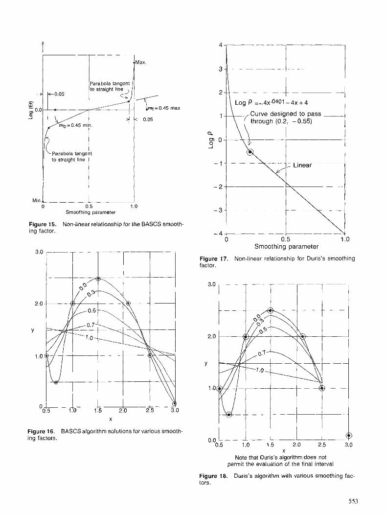
Max.

Para bola tangent

3 ~ 0 . 0 5

= W - , 0.0 mt = 0.45 max

0 1 --t t0.05

0 0.5 1 .O Smoothing parameter

Figure 15. Non-linear relationship for the BASCS smoothing factor.

Figure 16. BASCS algorithm solutions for various smoothing factors.

I \ Log P ,-4xJ3401- 4x + 4

Curve designed to pass through (0.2, - 0.55)

I

- 1 Linear

0 0.5 1 .O Smoothing parameter

Figure 17. Non-linear relationship for Duris's smoothing factor.

X

Note that Duris's algorithm does not permit the evaluation of the final interval

Figure 18. Duris's algorithm with various smoothing factors.

The BASCS algorithm description

BASCS (Beam Analogy for Smoothing Cubic Splines) is the computer program developed by the author which utilizes the foregoing principles.

Assumptions

The assumptions and limitations inherent in the application of the beam analogy approach to spline fitting and smoothing are as follows :

The data points are single valued, that is, for each x value there is only one y value. The generated curve may not turn back on itself.

The deflections are computed using what is known as "small deflection" theory in structural analysis. This implies that there are no axial forces induced in the beam and that the solution for scaled up y values will correspond to that of the unscaled values.

There is no shear deflection of the beam. (Shear deflection is normally very small in slender beams). In any case the equation for shear deflection is not a cubic polynomial.

The extreme ends of the beam are unconstrained for rotation, that is, the beam has no curvature at the ends (but may have slope). This is not an inherent limitation and the algorithm could be extended to allow the experimentor to apply a couple to a beam end.

Inputs

The x and y co-ordinates of the data points

The smoothing parameter which varies from 0.0 (zero smoothing, exact fit) to 1.0 (perfect smoothing, linear fit).

Optional, additional control over the shape of the curve may be obtained by specifying dummy points on the beam and the flexural stiffness of beam segments.

Algorithm termination criteria which are: - the maximum number of iterations, and - the maximum change in deflection of any data point,

from iteration to iteration, before the solution will be accepted.

The number of points that will be interpolated on the smoothed curve, between data points. This is for cosmetic purposes for the graphical output.

Initial Conditions

The undeformed beam is initially considered to lie horizontally at y = 0. This is an arbitrary starting position and it can be argued that it would be more efficient to start with the undeformed beam lying on the first and last data points.

Vertical springs are attached to each non-dummy point on the beam. The spring constant (in units of force per unit of deformation) is arbitrarily taken as 1.0. The smoothing parameter is now used to compute the standard flexural

rigidity of the beam so that the desired amount of smoothing is obtained, that is, for perfect smoothing the beam stiffness will be very large compared to the stiffness of the springs, and for a perfect fit the spring stiffness will predominate.

We compute the forces that are to be applied to the nodes of the beam. Each is the product of the distance of the present location of the node (y=O) to the data point and is directed so as to distort the beam in the direction of the data point.

The Iterative Procedure

This procedure consists of the following steps:

First we apply the forces to the nodes of the beam. If all the forces are absorbed by the springs and none by the beam, the beam will deform from its current location in the iterative process to the data points. On the other hand, if the beam is stiff relative to the springs then most of the force will be absorbed in the flexure of the beam rather than the deformation of the springs, hence smoothing will predominate.

The beam is released and allowed to reach a new configuration. If all the deflections are within the previously specified tolerance compared to the previous cycle then convergence has been attained and the iterations stop.

A new, sloping, position of the beam is taken to be the straight line joining the new beam end points. The iterations continue in that each cycle finds a new pair of end points on the beam, new vertical offsets from the straight line joining them are computed and new vertical forces are found.

Thus the solution of the configuration of the beam under the action of the current set of forces is computed, but because the flexural rigidity of the beam distributes those forces longitudinally the beam is not in equilibrium. The successive iterations come closer to the equilibrium position until finally the configuration of the physical beam is attained.Convergence normally occurs in three cycles when zero smoothing is specified. For beams with many segments and a significant amount of smoothing more than ten cycles may be required.

Any standard matrix solution routine for square, symmetric, banded, positive-definite matrices may be used, but the one used for this program is the Choleski (Square Root) method. This takes advantage of the symmetrical nature and stores only the lower half. The following steps are taken:

Read data point co-ordinates Read x co-ordinates of any extra joints Read any non-standard beam stiffnesses Read the smoothing parameter and iteration control parameters Compute the range of diagonal entries of S and compute the value of EI corresponding the the smoothing required Compute the structure displacement numbers Compute the member stiffness matrices, s Build the structure stiffness matrix, S, from all the s's Add the springs to S

Start of iterations : Zero out the load vector Compute the magnitude and direction of the applied loads (for real nodes only) Solve for the deflections using the Choleski method Check for convergence by comparing current deflections with those of the previous iteration.

If converged, For each member: - Find the coefficients of the cubic polynomial

using the rotations and vertical deflections at each end

- Interpolate the smooth curve using the coefficients just found. Add those co-ordinates to those corresponding to the sloping beam at the start of this iteration

Plot the results Stop

If not converged, Compute new beam slope and new y co-ordinates for each real node for next iteration

Repeat for next iteration

The Computer Program

The BASCS program was developed on an IBM XT microcomputer equipped with a math co-processor. The operating system is PC-DOS. It was written in Fortran 77 and compiled with the IBM Personal Computer Professional Fortran (Profort) sold by the Ryan-McFarland Corporation. The Fortran source code is in the public domain and should run without modification on any MS-DOS machine with a math co-processor and a standard conforming compiler.

CONCLUSIONS

The BASCS algorithm provides an alternative approach to smoothing cubic splines. Its major advantage lies in its intuitive character which allows much flexibility in its implementation. Enhancements such as weighting according to distance by means of non-linear spring constants, or weighting particular data points by varying the strength of the corresponding springs may be easily created without recourse to rigorous mathematics by virtue of understanding the physical analogy. In general, any physical modification involving the properties of the beams and springs may be modeled, subject to the basic restrictions.

Although no extensive comparative testing was done, the BASCS approach appears to be at least as fast and accurate as other, well known routines.

REFERENCES

Agterberg, F.P. and Gradstein, F.M. 1988: Recent developments in quantitative stratigraphy; Eanh-Science

Reviews, v. 25, p. 1-73. Duris, S. 1980: Algorithm 547: Fortran routines for discrete cubic spline interpo-

lation and smoothing; Association for Computing Machinery, Transactions on Mathematical Software, v. 6, no.1, p. 92-103.

Gradstein, F.M., Agterberg, F.P., Brower, J.C., and Schwartzacher, W.S. 1985: Quantitative Stratigraphy; UNESCO. Paris and Reidel,

Dordrecht, 598 p. Singer, F.L. 1951 : Strength of Materials; Harper and Row, New York, N.Y ., 469 p.

A quantitative foraminifera1 correlation of the late Jurassic and early Cretaceous offshore NewfouncUand

Mark A. Williamson1 and Frederik P. Agterbergz

Williamson, M.A., and Agterberg, F. P., A quantitative foraminiferal correlation of the late Jurassic and early Cretaceous offshore Newfoundland; @ Statistical Applications in the Earth Sciences, ed. F. P. Agterberg and G. F. Bonham-Carter; Geological Survey of Canada, Paper 89-9, p. 557-566, 1989.

Abstract Treatment of last occurrence data of Mesozoic benthic Forarninefera from east Newfoundland explo-

ration wells with the quantitative biostratigraphy program RASC f i r RAnking and SCaling) allowed an elevenfold subdivision of Kimmeridgian to Cenomanian strata. The numerical expression of the RASC results was further subjected to the quantitative correlation program CASC (Correlation and SCaling in time) which aims to attach statistically derived confidence limits to correlation tie lines. CASC operations can be reduced to three steps. Firstly, the individual well sequence can be expressed as a function of the RASC derived optimum or average sequence. Secondly, the individual well sequence can be expressed as a finction of depth (in the well). Thirdly, the determination of the optimum sequence as a function of depth is derived fi-om the two previous steps. When repeated for each of 14 Grand Banks wells, probabilistic event correlation is possible. 172e RASC produced scaled optimum sequence can be rescaled in terms of linear time using known estimates of extinction (in Ma) for a select number of well constrained marker species. Substitution of the linear time scale for the optimum sequence in the above relationships allows the correlation of isochrons throughout the area together with accompanying error bars. Quantitative CASC correlation of isochrons permits a precise determination of the chronological interrelationships of early Cretaceous/Jurassic sandstone bodies of the Hibernia area. Avalon sandstones are associated with the 115 Ma isochron; the Catalina sandstones with the 133-138 Ma isochrons and the Hibernia sandstones with the 142-148 Ma isochrons.

Le traitement des dernieres donne'es portant sur la pre'sence de foramintj2t-es benthiques me'sozo~ues pre'leve's duns des puits d'exploration de l'est de Terre-Neuve avec le programme de biostratigraphie quantitative RASC (remplace RAnking and Scaling), permet d'obtenir 1 I subdivisions du Kimmkridgien au Ce'nomanien. L'expression nume'rique des re'sultats de RASC a he' plus turd soumise au programme de corre'lation quantitative CASC (Correlation and SCaling in time) dont le but est d'attacher des limites de confiance obtenues siatistiquement aux profils de raccordement de corre'lation. Les opkrations de CASCpeuvent Etre rkduites a trois hapes. Premitrement, on peut exprimer la se'quence individuelle d'un puits comme une fonction de la se'quence optimale ou moyenne obtenue au moyen du RASC. Deuxi2me- ment, on peut exprimer la se'quence individuelle du puits comme une fonction de la profondeur (dans le puits). Troisitmement, la de'termination de la skquence optimale comme fonction de la profondeur est obtenue a partir des deux premitres ktapes. Lorsque ces opkrations sont rtpkte'es pour chacun des 14 puits des Grands Bancs, une corrklation probabiliste des tvknements est possible. La se'quence optimale ktablie d l'kchelle et produite par le RASC peut Etre reprise a une autre kchelle en termes de temps line'aire en utilisant des estimations connues de l'extinction (en Ma) d'un certain nombre d'esptces rep6 res particulieres aux puits. Le remplacement de la se'quence optimale par l'kchelle en temps linkaire dans les relations ci-dessus permet la corrklation des isochrones dans toute la re'gion, avec indication des marges d'erreur correspondantes. La corre'lation quantitative par le CASC des isochrones permet de de'lerminer d'une facon pre'cise des relations chronologiques de massifs grkseux du Jurassique et Crk- tack inferieur de la region d'Hibernia. Les gr&s dJAvalon sont associe's 6 l'isochrone de 115 Ma; les gres de Catalina, aux isochrones de 133 ci 138 Ma; et les gris d'Hibernia, aux isochrones de 142 B 148 Ma.

' Shell Canada Ltd., P.O. Box 100 Stn. "M", Calgary, Alberta, T2P 2H5 Geological Survey of Canada, 601, Booth Street, Ottawa, Ontario, KIA OE8

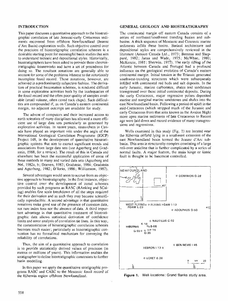
INTRODUCTION GENERAL GEOLOGY AND BIOSTRATIGRAPHY

This paper discusses a quantitative approach to the biostratigraphic correlation of late Jurassic-early Cretaceous sediments recovered from offshore Newfoundland (Jeanne d'Arc Basin) exploration wells. Such objective control over the precision of biostratigraphic correlation schemes is a desirable starting point for meaningful basin studies that aim to understand tectonic and depositional styles. Historically, biostratigraphers have been asked to provide these chronostratigraphic frameworks and have a set of procedures for doing so. The resultant zonations are generally able to account for some of the problems inherent to the notoriously incomplete fossil record. These zonations, however, are achieved in a predominantly subjective fashion. The derivation of practical biozonation schemes, is rendered difficult in some exploration activities both by the inadequacies of the fossil record and the often poor quality of samples available (small volume, often caved rock chips). Such difficulties are compounded if, as on Canada's eastern continental margin, no adjacent outcrops are available for study.

The advent of computers and their increased access to earth scientists of many disciplines has allowed a more efficient use of large data sets particularly as generated by exploration activities. In recent years, researchers in Can- ada have played an important role under the aegis of the International Geological Correlation Programme (IGCP) Project 148, in the development of quantitative biostratigraphic systems that aim to extract significant trends and associations from large data sets (see Agterberg and Grad- stein, 1988, for a review). The result of this in Canada and elsewhere has been the successful application of some of these methods to many and varied data sets (Agterberg and Nel, 1982a, b; Doeven, 1983 ; Gradstein, 1984 ; Gradstein and Agterberg, 1982; D'Iorio, 1986; Williamson, 1987).

Several advantages would seem to accrue from an objective approach to biostratigraphy. In the first instance, objective control over the development of zonal schemes provided by such programs as RASC (RAnking and SCal- ing) enables fine scale breakdown of all the steps required for their derivation and as such they may become scientifi- cally reproducible. A second advantage is that quantitative zonations make good use of the presence of common data, not rare index taxa nor the absence of data. A third important advantage is that quantitative treatment of biostratigraphic data allows statistical derivation of confidence limits and error analysis of correlation tie lines. In this way, the communication of biostratigraphic correlation schemes becomes much easier; particularly as biostratigraphic convention has no formalized mechanism for conveying the reliability of correlations.

Thus, the aim of a quantitative approach to correlation is to provide statistically derived values of precision (in metres or millions of years). This information enables the stratigrapher to define biostratigraphic constraints to further basin modelling.

In this paper we apply the quantitative stratigraphic programs RASC and CASC to the Mesozoic fossil record of the Hibernia region offshore Newfoundland.

The continental margin off eastern Canada consists of a series of northeast/southwest trending basins and sub- basins. A thick sequence of Mesozoic and Cenozoic marine sediments infills these basins. Basinal architecture and depositional styles are comprehensively reviewed in the literature (Amoco Canada Ltd., 1973; Benteau and Shep- pard, 1982; Jansa and Wade, 1975; McWhae, 1980; McKenzie, 1981 ; Sherwin, 1977). The early rifting of the Atlantic between Canada and Portugal had a profound influence on the geological evolution-of ~anada's eastern continental margin. Initial tension in the Triassic generated southwest-trending structures which were subsequently infilled with continental red beds and salt de~osits. In the early Jurassic, marine carbonates, shales and sandstones transgressed over these initial continental deposits. During the early Cretaceous, major regressive pulses deposited marine and marginal marine sandstones and shales into thc east Newfoundland basin. Following a period of uplift in the mid-Cretaceous (which stripped much of the Jurassic and early Cretaceous from that area known as the Avalon High) more open marine sediments of late Cretaceous to Recent age were laid down and record evidence of many transgres- sions and regressions.

Wells examined in this study (Fig. 1) are located near the Hibernia oilfield lying in a southwest extension of the east Newfoundland besin termed the Jeanne d'Arc sub- basin. This area is structurally complex consisting of a large roll-over anticline that is further complicated by a series of normal faults. A major feature, the main hinge or listric fault is thought to be basement controlled.

I NEWFOUNDLAND

0 DOMINION D-28

t WEST'FLYINGO o FLYING FOAM 1-13 FOAM L-23

0 ADOLPHUS D-50

0 NAUTILUS C-92 K-18

HIBERNIA OOB-08 G.55 0 0 P-l

0-35

0 BEN NEVIS 1-45 HEBRON 1-13 0

0 EGRET K-36 0 km 20

01 +

m

Figure 1. Well locations: Grand Banks study area.

Williamson (1987) summarized the general biostratigraphy for this area and described an eleven fold RASC derived quantitative subdivision of early Cretaceous and older deposits based on foraminiferal tops. The results of this zonation are reproduced here in Figure 2 (from Williamson, 1987) which illustrates the scaled optimum sequence of fossil events and interpretation in terms of eleven late Jurassic to early Cretaceous biozones. Each designated RASC bio- zone represents a cluster or group of fossil events and internally show a degree of inconsistency of relative disappearance levels from well to well. As such they resemble assemblage zones of conventional stratigraphic practice. Similarly, because the top of one zone defines the base of the zone above, RASC biozones also resemble interval zones of the Norh American Stratigraphic Code (Art. 45, 3, 1983). A subjective correlation of these RASC derived zones is described in Williamson (1987) (Fig. 3). Brief mention was made in the latter of a quantitative CASC correlation. In this paper, we expand on that and describe the details of the CASC application to the fossil data set.

METHODS

The objective correlation scheme described in the paper was derived through an application of the program CASC (Correlation and Scaling in time). The CASC program has been developed by Geological Survey of Canada scientists since 1982 and has three aims:

1. The automated correlation of zones or fossil events in a ranked optimum sequence with accompanying error bars in depth units.

2. The interpretation of scaled 'optimum sequences (see later) in terms of linear time.

3. The automated correlation of stages and isochrons with confidence limits in time units.

The initial concepts of CASC are discussed in Agterberg and Gradstein (1983). The statistical assumptions and algorithms are complex and are documented more comprehensively in Agterberg et al. (1985), Gradstein et al. (1985) and Agterberg and Gradstein (1988). The latter also applies the method to Cenozoic subsurface geology of the eastern Canadian margin. For present purposes we briefly describe the main features of the program.

Prior to any application of the objective correlation program CASC, the basic biostratigraphic data (i.e. fossil event data or in the case of well cutting samples as used in this study, the last occurrence datum or extinction point) must be subjected to a sister program, RASC (RAnking and SCal- ing). It is the numeric expression of the RASC results that forms the primary input data of the CASC program.

RASC is a quantitative biostratigraphic method the aim of which is to quantitatively reduce large bodies of biostratigraphic event data obtained from numerous well sections into more manageable, optimum or average sequences. Each well under study has a unique sequence of fossil events. These events represent extinction points or "tops" of a particular organism. The present study uses foraminiferal tops although any fossil group can be used, i.e. palynomorphs have been utilized in RASC (D'Iorio,

1986), as have nannofossils (Doeven, 1983). This body of data is summarized by RASC in two ways : Firstly, an optimum sequence of fossil events is described through a ranking algorithm and is essentially an average sequence of events determined through consideration of their relative positions from well to well. Secondly, a scaled optimum sequence is determined; this differs from the ranked optimum sequence in that the fossil events have been scaled or grouped together on the basis of their cross-over frequency from well to well. The underlying assumption is that the more events cross over in position from well to well (i.e. are uncertain in their position), the closer together these events are in time or stratigraphic distance. The resultant groupings can be interpreted as interval zones.

RASC, together with several applications is documented in the literature (Agterberg and Nel, 1982a; b; Gradstein and Agterberg, 1982; Doeven, 1983; Gradstein et al., 1985). The application of RASC to the East Newfoundland Basin is described in Williamson (1987). It is the ranked optimum and scaled optimum sequences described in that article which are used as input to the CASC program and derived correlation schemes described here.

In addition to the RASC generated information, two other input files are required for the CASC program to operate. One is a file containing observed depths for each event in each well. Unlike CASC, the RASC program has no need for these depth values as it computes the biozonation entirely from information based on the relative position of events. A final file includes estimates (from the literature) of the absolute age (in Ma) of extinction points of selected data involved in the RASC computations. The following describes how CASC makes use of these files.

The results to be described in this paper were generated on a mainframe (Cyber 730) computer at the Geological Survey of Canada, in Ottawa, using a Tectronix 4014 terminal for graphics.

For present purposes the operation of CASC has been reduced to several steps. Two starting points can be used for the CASC procedures using either the RASC produced ranked optimum sequence or the RASC scaled optimum sequence with distance values. The former is able to quantitatively correlate events while the latter, using information from the age depth file is able to correlate isochrons. Only the latter option is described in this paper.

DISTANCE CASC

As mentioned earlier, the RASC scaled optimum sequence is expressed as a "distance" value between fossil events (interfossil distance) and is a function of the cross-over frequency of these events from well to well. It is possible to show a mathematical relationship between any individual well sequence of events and the RASC derived scaled (distance) optimum sequence (step 1) and subsequently the RASC distance values can be expressed as a function of depth (step 2). The derivation of isochrons from these relationships requires the replacement of the RASC distance scale by a time scale. This may be accomplished through the use of estimated ages of selected fossil disappearance

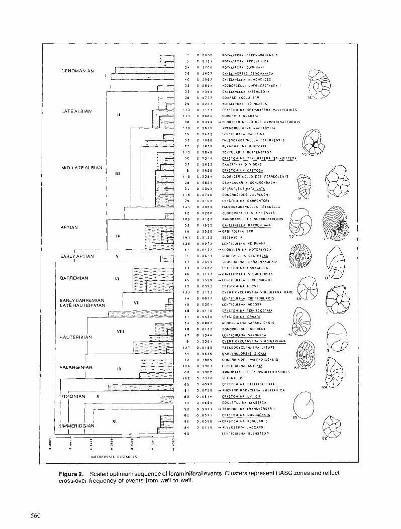
Figure 2. Scaled optimum sequence of foraminifera1 events. Clusters represent RASC zones and reflect cross-over frequency of events from well to well.

3 0 0 6 5 8 COTALIPORA CRCENH0RNEhS.S

5 0 . 0 3 5 1 QOTAL'PORA A P P L N I N I C A

2 4 0 J 7 C 6 Q 0 7 A L I P O R A CUSHMANI CENOMANIAN

7 6 0 3 9 5 7 SAVEL.NOPSIS CENJM&N!CA

* O 0 . 3 9 8 ) CAVELINELLA AMMONOIDES

3 2 0 0 6 2 4 ~COBCRCE:LA INFRACRC'nCEA ' 3 5 0 4 2 6 9 GAVELINELLA INTCRMEOlA @ , ., 3 6 0 . 0 7 7 7 COARSE ACCLU SPP 7 6 '

2 9 0 0 2 3 3 ROTALIPORA T I C I N E N S I S

LATE ALBlAN 1 I 3 0 1 1 7 3 E P l S T O M l N A SPINULIFERA OOLYPlOlOES

I l l 0 0 6 6 4 O O R O T H I A C R A O A T A

J 8 0 0 3 9 9 ~ ~ C L O B I G C R I N E L L O I O E S C Y R O I O I N A E f O R U I S

1 1 0 0 2 6 1 6 ARENOBULIMINA MACFAOYEhl

1 5 0 0 4 3 2 L E N r I C U L I N A GAULTINA

3 3 0 1 6 6 0 fALSOCAUORYNELLA TEALBYENSIS

2 7 0 . 1 9 3 6 OLANOMALINA BUXTORFI

1 1 5 0 . 0 8 4 8 T E X T U L A R I A BETTENSTADTI

5 0 0 0 3 1 4 E P I S T O M I N A T P I N U L I F E R A S D ' N U L I f E R A

3 7 0 0 6 2 3 GAUORYINA 0 : V I O E N S MID-LATE ALPIAN

6 0 . 0 9 5 6 E P I S T O M I N A CRETOSA

1 1 8 0 . 0 5 8 4 C L O B I G E R I N E L L O I O E S FERREOLCNIS

@ 2 8 0 , 0 6 3 4 O S A N C U L A R I A SCHLOENBACHI

5 1 0 0 3 9 2 S P I R O P L E C T I N A T A L A T A

1 1 6 0 . 0 7 2 0 CONORBOIOES LAMPLUCHI

@ 51 ' @ 7 9 0 . 0 1 0 6 E P I S T O M I N A C A f f P E N T f R I

1 4 1 0 . 3 0 5 9 FALSOCAUORYNELLA T R I A N C b L A

4 2 0 0 2 8 8 JLOBOROTALITES A P T I E N S I S

1 0 9 0 4 I 8 2 AMM08ACULi 'ES SUBCRETACEOUS

APTIAN 5 3 0 1 6 5 5 CAVELINELLA BARRCMIANA

1 6 0 . 0 5 5 6 . I O R B I T O L I N A S P P

1 6 1 0 . 0 1 5 2 S E I S M I C A

1 3 5 0 . 0 9 7 2 LENTICULINA H E I R M A N I

r 4 0 . 6 4 2 2 . .GLOBIGERINA HOIERIVICA

7 0 . 0 6 1 1 C H O F F A T E L L A O E C I P I C N S

1 7 0 . 7 6 9 4 TROCHOLINA INFRACRANULATA

1 3 0 . 2 4 5 7 E P I S T O M I N A CARACOLLA

4 6 0 . 1 I 7 7 ..CAVfLINELLA SlGMOlCOSTA

BARREMIAN 4 5 0 . 1 5 2 9 ..LCNTICULINA EICHENBERCI

1 2 0 0 0 2 3 E P l S T O M l N A HECHTl

1 3 3 0 . 3 1 2 3 EVERTICYCLAMMINA VIRGULIANA RARE

EARLY BARREMIAN 1 4 0 . 0 0 7 7 L E N T l C U L l N A C R E P I D U L A R I S

1 0 0 0 3 0 1 LCNTICULINA NOOOSA

4 9 0 4 1 I 0 E P I S T O M I N A TENUICOSTATA

I I 0 . 5 5 3 4 E P I S T O M I N A ORNATA

6 4 0 . 0 9 6 7 NEOBULIMINA VARSOVIENSIS

4 8 0 0 1 3 2 CONORBOIOES HOFKERI

1 7 0 1 3 4 4 L E N T I C U L I N A S A X O N I C A

9 0 . 2 3 9 1 E V f R T I C Y C L A U U I N A V I R C U L I N I A N A

1 3 7 0 0 1 6 5 PSEUOOCYCLAMMINA L l T U U S

5 4 0 . 5 6 3 6 MARGINULOP~IS SICALI

2 2 0 . 1 6 8 5 CONORBOIOES VALENDISENSIS

1 2 4 0 1 9 0 3 LENTICULINA CUTIATA

80 0 1 9 8 2 AMMOBACULI TES C O P R O L I T H I C O R U I S

I 6 2 0 . 7 3 1 6 S E I S M I C B

. . . . . . . . . . . . . . . . . . . . . . . . . . . . . - . . . . . . . . . . . . . . . . . . . . . . . . . . . . . . . . . . . . . . . . . . . . . . . ...... . . . . . . . . . . . . . . . . . . . . . . . . . . . . . . . . . . . . . I - ....... TlTHONlAN X . . . . . ...... . . . . . . . . -

6 5 0 4 0 9 6 C P I S T O U I N A SIELLICOSTATA

8 1 0 . 6 7 5 6 .. A N C H I S P I R O C Y C L I N A L U S I T A N I C A

6 s 0 . 0 6 1 4 EPISTOUINA UHLICNI

7 4 0 5 6 5 5 EOGUTTULINA L I A S S I C A

I 9 2 0 5 0 7 1 .. TROCHOLINA TRANSVCRSAP!!

0 . 0 5 7 1 E P I S T O M I N A MOSOUENSIS

9 6 0 0 3 9 0 . .EPISTOMINA REGULARIS

KlMMERlDGlAN I I I 1

8 4 0 0 7 7 9 ..ALvEOSEPTA J A C C A R D I

L E N T I C U L I N A QUENSTEDTI

I N T E R F O S S I L DISTANCES

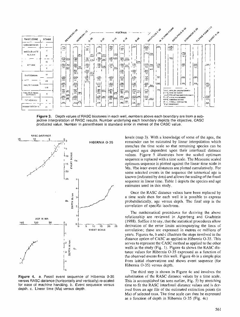
(39 '%!d) SE-0 e!Ulaq!H u! yldap jo uo!i~ury e sa passaidxa aq uaql ue3 ales amp ayl .exe) papalas jo (en u!) ~u!od uo!13u!ixa palewpsa aql jo a[!j a8a ue mo~j pa+ -lap s! pue sanlm a3ueis!p pssojlam! 3s~~ aqi ig 01 aw!i %u!q3la~is Aq (S 'Bq '~a!paa uaas sa) paqs![dwo33e s! s~q~, .altr3s aw!l e Aq sanren a~~els!p 3s~~ aql jo uo!inlrisqns aql saqoAu! pug 3p alns!~ uy u~oqs s! dais p.~!ql au

'qldap snsJalz (SE-0 e!u-laq!H loj) amanbas luaha s~oqs pue suo!ier\Jasqo ~a~i!u! woy ioid aldm!s e s! q~ a~n%!d 'IlaM s!ql10j siuaha par\Jasqo aqi jo uop3unj e sa passa~dxa SE-0 e!ulaq!H JOJ san1eA a3uei -s!p 3s~~ aqi s~oqs ep aln8!,1 '(1 '%!d) Apnis aq1 u! sIIaM Jayio aqi oi pagdda sa poqlaw 3~~3 aqi iuasa~da~ oi sahlas s!y~ 'SE-O e!ulaq!H 01 pagdde sv 3~~3 jo uo!ldo a3ueis!p ayi u! paqor\u! sdals aql alensnII! 3 pue q 'ep sa~n%!d meah jo suo!lI!m JO sallaw u! passa~dxa ale asaql fuog~~a~~o~ jo sauy aql 8u!Auedu103~e sl!w!l loua aql jo uoper\!lap MoIle salnpa3o~d le3!is!iais aqi ieqi 'Les 01 I! ~~LIJ~S '(8861) u!alspals pue %~aqlai%v u! pama!AaJ ale d!qsuo!ie]a~ alzoqa aqi %u!n!lap JOJ sa~npa3o.xd [e3!leruaqiem aqL

-suo~q3os! 3ypads jo uo!lela~~o3 aqi s! da~s reug aqL 'qidap snslah a%e 'rl1le3!is!l!qeqo~d ssa~dxa 01 alq!ssod s! i! lIaM q3ea JOJ uaqi ale3s am!l s Xq pa3elda~ uaaq aAeq sanIeA a~~as!p 3s~~ aqi a3uo

.Apnis srqi u! pasn saleur!lsa a%e pup sagads aqj si3rdap .[ alqeL .awy Jaauq u! amanbas ~!ssoj aqljo %uqe3s aql ~MOTIB PUB (slop Aq pa$a3n>u!) u~oq s! aSe le3!.1awnu ayi amanbas aqi u! siualza pal3aIas amos JO~ 'Xla~pe1nmn3 pallold ale sa~uais!p )uaAa-Iarn! ayJ 'em u! aps am!i Jeaug aqt isu!a%e panoid s! a3uanbas mnruydo pap~s 3!ozosayy. aqL -ale3s awg a qi!~ pa3e~da-1 s! amanbas wnm!ldo palex aql ~oq sanqsnll! s a.1n9!d .sanleA a~ueis!p pssojJam! .r!aql uodn iuapuadap sa%a pau%!sse aq ue3 sapads Bu!u!aura~ leql os a1e3s amp aql saq31a~is q3!q~ uo!lslod~a~uy leau!I Aq palew!lsa aq ue3 Japu!amal aql 'sa3e aqi jo amos jo a8par~ouy a ql!~ '(E dais) sIaAa1

'yidap snsJah (eyy) au!i leau!l 3 qidap snsJah aauanbas iuah3 .q ,6u!lpuey au!y3ew 40 asea ~oj paleas-a~ (Al~eai~a~ pue A~leiuoz!~oy) aoueis!p 3s~~ snsJaA cjc-0 e!uJaq!H jo amanbas luaha l!ssoj 'e 'p aJn6!j

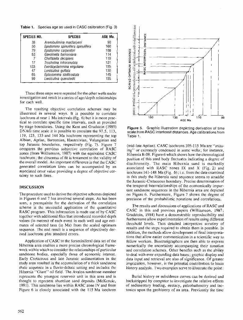
Table 1. Species age as used in CASC calibration (Fig. 3) 2 1

4H I

SPECIES NO. SPECIES AGE Ma. 38 Arenobulimina macfadyeni 90 50 Epistomina spinulifera spinulifera 100 79 Epistomina carpenteri 108 53 Gavelinella barremiana 114 7 Choffatella decipiens 119

17 Trocholina infraranulata 121 1 33 Everticyclammina virguliana 125 47 Lenticulina guttata 130 65 Episotomina stellicostata 145 90 Lenticulina guenstedti 155

These three steps were repeated for the other wells under investigation and result in a series of ageldepth relationships for each well.

The resulting objective correlation schemes may be illustrated in several ways. It is possible to correlate isochrons at near 1 Ma intervals (fig. 6) but it is more practical to correlate specific time intervals, such as provided by stage boundaries. Using the Kent and Gradstein (1985) DNAG time scale it is possible to correlate the 97.5, 113, 119, 125, 133 and 144 Ma isochrons representing the top Albian, Aptian, Barremian, Hauterivian, Valanginian and top Jurassic boundaries, respectively (Fig. 7). Figure 7 compares the previous subjective correlation of RASC zones (from Williamson, 1987) with the equivalent CASC isochrons; the closeness of fit is testament to the validity of the overall model. An important difference is that the CASC generated correlation lines can be accompanied by an associated error value providing a degree of objective cer- tainty to such lines.

DISCUSSION

The procedure used to derive the objective schemes depicted in Figures 6 and 7 has involved several steps. As has been seen, a prerequisite for the derivation of the correlation scheme is the successful application of the quantitative RASC program. This information is made use of by CASC together with additional files that introduced recorded depth values (in metres) of each event in each well and age estimates of selected taxa (in Ma) from the scaled optimum sequence. The end result is a sequence of objectively derived isochrons plus standard errors.

Application of CASC to the foraminifera1 data set of the Hibernia area enables a more precise chronological framework within which to consider the relationships of particular sandstone bodies, especially those of economic interest. Early Cretaceous and late Jurassic sedimentation in the study area resulted in the accumulation of a thick sandstone shale sequence in a fluvio-deltaic setting and includes the Hibernia "Giant" oil field. The Avalon sandstone member represents the youngest reservoir unit in this area and is thought to represent shoreline sand deposits (McKenzie, 1981). This sandstone lies within RASC zone IV and from Figure 6 is closely associated with the 115 Ma isochron

AGE Ma

Figure 5. Graphic illustration depicting derivation of time scale from RASC interfossil distances. Age calibrations from Table 1.

(mid-late Aptian). CASC isochrons 105- 1 15 Ma are "missing'' or extremely condensed in some wells; for instance, Hibernia B-08. Figure 6 which shows how the chronological position of this sand body fluctuates indicating a degree of diachroneity. The main Hibernia sand is markedly associated with RASC zones IX and X (Fig. 2) and isochrons 141-148 Ma (Fig. 6) ; i.e. from the data examined in this study the Hibernia sand sequence seems to straddle the Jurassic-Cretaceous boundary. Precise determination of the temporal interrelationships of the economically important sandstone sequences in the Hibernia area are depicted on Figure 6. Furthermore, Figure 7 shows the degree of precision of the probabilistic zonations and correlations.

The results and discussions of applications of RASC and CASC in this and previous papers (Williamson, 1987; Gradstein, 1984) have a demonstrable reproducibility and furthermore allow experimentation of results using different threshold levels. Thus detailed interpretive scrutiny of results and the steps required to obtain them is possible. In addition, the methods allow development of final interpretations that allow easier communication in a scientific way to fellow workers. Biostratigraphers are then able to express numerically the uncertainty accompanying their zonation and correlation schemes. Other benefits such as the ability to deal with ever expanding data bases ; graphic display and data input and retrieval are also of significance. Of greater implication, however, is the potential contribution to basin history analysis. Two examples serve to illustrate the point:

Burial history or subsidence curves can be derived and backstripped by computer to investigate the relative effects of sedimentary loading, eustacy, paleobathmetry and tectonics upon the geohistory of an area. Previously the time

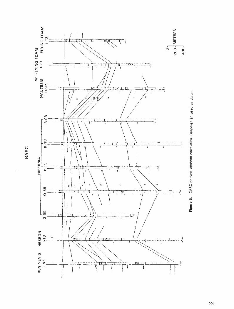
RA

SC

200

ME

TR

ES

O

l

( HHlERNlA - BEN NEVlS 1-45 HEBRON 1-13 G-55 0-35 P-15 K-18 648 NAUTILUS C-92

0 0 0 0 0 0 0 0

Figure 7. CASC derived stage correlation (solid) and comparison with subjective RASC correlation (dashed).

I H l B E R N l A 0 - 3 5 ] W E S T F L Y I N G F O A M FLY ING FOAM

A G E Ma

Figure 8. Burial history of Hibernia 0-35 accounting for CASC derived error limits. Curve A has minimum associated error, Curve B has maximum error.

sochrons M a

Figure 9. lsochron correlation between West Flying Foam and Flying Foam showing unconformity and estimates of "missing" sections.

scale or rather the biozonation which provides the chronostratigraphic control has been derived through conventional methods. The quantitative RASC and CASC approach with accompanying error analysis allows important timing constraints to be imposed on basin modelling. In this way, the procedures allow important testing of hypotheses. Figure 8 shows this procedure as applied to Hibernia 0-35. The burial history curve of Hibernia 0-35 was derived using the program Bursub described in Gradstein et al. (1985). The minimum and maximum age value as derived from error analysis of CASC was input into the program producing the two observed subsidence curves shown. Such an approach provides an error envelope of burial within which maturity calculations an be made which would help determine the effect of chronology on the timing of peak generation and expulsion of hydrocarbons.

Another application stems from an idea of van Hinte (1984) who described the construction of synthetic seismic sections from biostratigraphic data (the term synthetic isogram is perhaps more appropriate). The theory is quite simple and assumes that a seismic section "is an image of time stratigraphic depositional patterns" (van Hinte, 1984) ; and further : ". . .seismic section is a record of chronostratigraphic depositional and structural patterns and not a record of time transgressive lithostratigraphy" (Vail and Mitchum, 1979). Assuming that biostratigraphic correlation reflects these natural time stratigraphic markers, the correlation of routinely produced CASC isochrons (in 1 Ma intervals) between suitable sections should mimic seismic sections and allow reconstruction of the general geometry of depositional sequences.

Such an isogram approach would not only enable a better integration of seismic sections and paleontological data (i.e. to determine if, and where, the two do not key together) but will also allow the use of seismic terminology of toplap, downlap, offlap and concordance with paleontologically derived schemes (improved communication through a common glossary of terms).

Similarly, van Hinte (1984) believed that improved regional age calibrations of seismic sections would be apparent as would be the improvement of the correlation of regional seismostratigraphy to Vail and Mitchum's (1979) Global Cycle Charts thus enhancing our understanding of the eustatics causing these changes in depositional styles (van Hinte, 1984).

The "isogram" between the wells Flying Foam and West Flying Foam (Fig. 9) resembles seismic sections between these wells and successfully predicts missing sections. Such correspondence is testament to the predictive ability of the overall model.

CONCLUSIONS

1. A previously described (Williamson, 1987) quantitative RASC biozonation allows an eleven fold sub-division of the Jurassic-Lower Cretaceous foraminiferal record of the east Newfoundland Basin.

2. The information provided by RASC, namely the ranked optimum sequence and the interfossil distance values of the scaled optimum sequence, together with information on the depth to event in each well and a file of age estimates for selected taxa in the optimum sequence, is suitable input for the objective automated correlation program CASC. This program aims to correlate events or isochrons between wells providing statistically derived error bars.

3. Application of CASC to the foraminiferal biozonation of the east Newfoundland Basin has enabled an objective correlation of individual events and isochrons in the lower Cretaceous.

4. The objective CASC correlation schemes compare well to a previous subjective correlation and independently verified the CASC models.

5. Examination of the correlation and isochrons indicates the absence of late Barremian, early Aptian and early Albian sections for many of the wells corresponding to the pre-Aptian and Avalon unconformities.

6. The chronological inter-relationships of the economically important sandstone sequence in the Hibernia area can be more precisely determined using a CASC approach.

7. Objective control on lines of correlation has strong implications for quantitative basin analysis and facilitates the experimental modelling approach. Similarly there are intriguing possibilities for the further integra- ton of biostratigraphic and seismic data.

ACKNOWLEDGMENTS

Ning Lew and Jacqueline Oliver are thanked for programming support. MW wishes to gratefully acknowledge the tenure of an NSERC Visiting Fellowship held at the Atlantic Geoscience Centre, Geological Survey of Canada, Dart- mouth, Nova Scotia. Felix Gradstein of the GSC providcd much discussion, advice and enthusiasm and critically read the manuscript.

REFERENCES

Agterberg, F.P. 1982: Introduction - IGCP Project 148: background, objectives and

impact; Quantitative Stratigraphic Correlation, ed. J.M. Cubitt and R.A. Reyment, Wiley, Chichester, England. p. 1-4.

Agterberg, F.P. and Gradstein, F.M. 1983: System of interactive computer programs for quantitative strati-

graphic correlation; & Current Research, Part A, Geological Survey of Canada, Paper 83-I A, p. 83-87.

1988 : Recent developments in quantitative stratigraphy; Earth Science Reviews, v. 25, p. 1-72.

Agterberg, F.P. and Nel, L.D. 1982a: Algorithms for the ranking of stratigraphic events; Computers and

Geosciences, v. 8, no. 1, p. 69-90. 1982b: Algorithms for the scaling of stratigraphic events; Computers and -

Geoscience, v. 8, no. 1, p. 163-189. Agterberg, F.P., Oliver, J., Lew, S.N., Gradstein, F.M., and Williamson, M.A. 1985: CASC Fortran IV interactive computer program for correlation

and scaling in time of biostratigraphic events; Geological Survey of Canada, Open File 1179.

Arnoco Canada and Imperial Oil 1973: Regional geology of the Grand Banks; Bulletin Canadian Society

of Petroleum Geology, v. 21, no. 4, p. 479-503. Benteau, R.I. and Sheppard, M.G. 1978: Hibernia - a petrophysical and geological review; Journal of Cana-

dian Petroleum Technology, Nov.-Dec., 1982 issue, p. 59-72. D'lorio, M.A. 1986: Integration of foraminiferal and dinoflagellate data sets in quantita-

tive stratigraphy of the Grand Banks and Labrador Shelf; Bulletin Canadian Society of Petroleum Geologists, v. 34, no. 2, p. 277-283.

Doeven, P.M. 1983: Cretaceous nannofossil stratigraphy and paleoecology of the

Northwestcrn Atlantic; Gevlogical Survey of Canada, Bulletin 356, 69 p.

Gradstein, F.M. 1984: On stratigraphy normality; Computers and Geosciences; v. 10,

no. I, p. 43-57. Gradstein, F.M. and Agterberg, F.P. 1982: Models of Cenozoic foraminiferal stratigraphy - Northwestern

Atlantic Margin ; Quantitative Stratigraphi Correlation, ed. J.M. Cubitt and R.A. Reyment, Wiley. Chichester, England, p. 119-173.

Gradstein, F.M., Agterberg, F.P., Brower, J.C. and Schwarzacher, W.S. 1985: Quantitative Stratigraphy; D. Reidel Publishing Company,

Dordrecht and UNESCO, Paris, 598 p. Jansa, L.F. and Wade, J.A. 1975: Geology of the continental margin off Nova Scotia and Newfound-

land; Geological Survey of Canada, Paper 74-30, p. 51-105. Kent, D.V. and Gradstein, F.M. 1985: A Cretaceous and Jurassic Geochronology: Geological Society of

America, Bulletin, v. 96, p. 1419-1425. McKenzie, R.M. 198 1 : The Hibernia.. . a classic structure ; Oil and Gas Journal, Septem-

ber, 198 1, p. 243-247. McWhae, J. 1980: Structure and spreading history of the Northwestern Atlantic

Region from the Scotian Shelf to Baffin Bay; Canadian Society of Petroleum Geologists, Memoir 7, p. 299-332.

Sherwin, D. 1977: Scotian Shelf and Grand Banks; Canadian Society of Petroleum

Geologists, Memoir 5, p. 519-559. Vail, P.R. and Mitchum, R.M. Jr. 1979: Global cycles of relative changes of sea-level from seismic stratig-

raphy; American Association of Petroleum Geologists, Mern- oir 29, p.469-472.

van Hinte, J. 1984: Synthetic seismic sections from biostratigraphy; ~ Studies in

Continental margin Geology, American Association of Petroleum Geology, Memoir 34, p. 674-685.

Williamson, M.A. 1987: A quantitative foraminiferal biozonation of the late Jurassic and

early Cretaceous of the East Newfoundland Basin; Micropaleon- tology, v . 33, no. 1, p. 37-65.

SUMMARIES

w

Stratcor, a new method for biozonation and correlation with applicaiton to exploration micropaleontology

F.M. Gradstein' and M. Fearon2

SUMMARY SOMMAIRE

The interactive program STRATCOR proceeds in two stages. In the first stage, the ordinal sequences of events observed in a series of sections are transformed into a composite ordinal sequence for the series as a whole by a method similar to graphical correlation. In the second stage, the equivalent depth in each of the original sections is found for every event in the composite sequence. Some preliminary results obtained with this method are presented and compared to results obtained with other methods.

The initial composite sequence is the ordinal position of events observed in the first section of the series. Thereafter the composite is built up as follows:

(a) Events common to the current composite and the next section in the series are identified; and their ordinal positions in the two sequences are found. A cubic smoothing spline function r(x), is fitted to these data.

(b) An event's actual position in the current section is used, by interpolation with ((x), to calculate an equivalent position in the composite sequence. This "interpolated position" is found for every event in the current section.

(c) A common event's position in the composite sequence is updated from : (i) its current position, and (ii) its interpolated position. The user has a choice of methods by which this may be done; e.g. the highest, lowest or average of the two.

(d) An event in the current section, but not yet in the composite, is inserted in the latter at its interpolated position.

When the final composite sequence has been obtained, a cubic smoothing spline is fitted between this sequence and the measured depth of common events in a section. The equivalent depth of a composite event not present in the section is calculated by interpolation with the spline function.

Le programme interactif STRATCOR prockde en deux Cta- pes. Pendant la premikre Ctape, les successions ordinales d'CvCnements observCs au sein d'un ensemble de coupes sont transformCes en une succession ordinale composCe pour l'ensemble a l'aide d'une rnCthode analogue h la corrB lation graphique. Dans la deuxibme Ctape, la profondeur Cquivalente dans chacune des coupes originales est trouvCe pour chaque CvCnement de la succession composCe. Cer- tains rCsultats prkliminaires obtenus au moyen de cette mCthode sont prCsentCs et comparCs aux rCsultats obtenus au moyen d'autres mCthodes.

La succession composCe initiale est la position ordinale des CvCnements observCs dans la premikre coupe de l'ensemble, aprks quoi la succession composCe est Ctablie comme suit: a) Les CvCnements communs h la coupe composCe courante

et h la coupe suivante dans l'ensemble sont identifikes et leur position ordinale -dans les deux coupes est trou- vCe. Une spline cubique de lissage r(x) est ajustCe 5 ces donnCes.

b) La position rtelle d'un CvCnement dans la coupe courante est utiliste, par interpolation avec r(x), pour calculer une position Cquivalente dans la succession composCe. Cette a position interpolCe )> est Ctablie pour chaque CvCnement de la coupe courante.

c) La position d'un CvCnement commun dans la succession composCe est mise h jour d'aprbs : i) sa position courante et ii) sa position interpolke. L'utilisateur dispose d'un choix de mCthodes pour ce faire; il utilise p. ex. la valeur la plus Clevte, la plus basse ou une moyenne des deux.

d) Un CvCnement dans la coupe courante, mais non encore dans la coupe composCe, est insCrC dans cette dernibre et reprCsente sa position interpolke.

' Atlantic Geoscience Centre, Geological Survey of Canada, P.O. Box 1006, Dartmouth, Nova Scotia B2T 4A2 Systems Consultant, 6080 South Street, Halifax, Nova Scotia B3H IT1

in Statistical Applications in the Earth Sciences, ed. F.P. Agterberg and G. F. Bonham-Carter; - Geological Survey of Canada, Paper 89-9, 1989.

In both stages of the program, the user selects a spline function according to the desired degree of residual error between r(x) and the data. Before a seleciton is made, the data are graphed. As many spline functions as needed can be selected.

Lorsque la succession composCe finale a CtC obtenue, une fonction spline cubique de lissage est ajustCe entre cette succession et la profondeur mesurCe d'CvCnements communs dans une coupe. La profondeur Cquilavente d'un CvCnement composte non prCsent dans la coupe est calculCe par interpolation au moyen de la fonction pistolet.

A chacune des deux etapes du programme, l'utilisateur choisit une fonction spline d'aprb le degrC souhait6 d'erreur rCsiduelle entre { (x) et les donnCes. Avant de procaer h une selection, les donnCes sont portCes sur un graphique. On ~Clectionne autant de fonctions splines que nCcessaire.

Finding the cubic smoothing spline function by scale invariants

SUMMARY SOMMAIRE

The cubic smoothing spline function, r(x), is useful in geology for three principal reasons: (a) It can be fitted to any set of data which a scientist might

want to approximate by a function. (b) The spline can be chosen to attain any given degree of

residual error between <(x) and the data.-~hus the scientist can select that spline which in his judgment best dis- criminates the true trend of the data from irrelevant random variation.

(c) The spline is the best of a very wide class of approximating functions, in the sense that ((x) is smoother than any other continuous function with two or more derivatives that approximates the data at least as well as I;(x).

Because of these properties, <(x) is particularly valuable as a means of correlating events between sedimentary columns, where divergent rates of sedimentation may generate a "true" trend of arbitrary shape.

Algorithms for finding ((x) have been published by Reinsch (1967, 1971) and de Boor (1978), but were developed for data with a relatively small component of "error". When used with geological data, they tend to be slow and even at times inaccurate. An examination of variables which are impervious to changes of scale in the data suggests algorithms which are faster and whose accuracy is under the user's control.

La fonction spline de lissage cubique, ((x), est utile en gCologie pour les trois raisons suivantes: a) Elle peut s'appliquer h toute sCrie de donnCes qu'un

scientifique voudrait Cvaluer par approximation B I'aide d'une fonction.

b) Le spline peut Ctre choisi pour obtenir tout niveau donnt d'erreur rCsiduelle entre <(x) et les donntes. Le scientifique peut donc choisir le spline qui, selon lui, met le mieux en evidence la tendance rCelle des donnCes partir de la variation alCatoire non pertinente.

C) Le spline est la meilleure fonction d'approximation h choisir parrni un grand nombre, du fait que ((x) est plus lisse que toute autre fonction continue comportant deux ou plusieurs dCrivCes et dont 1'Cvaluation approximative des donnCes est au moins Cquivalente B ((x).

Ces propriCtts rendent ((x) particulikrement valable pour mettre en corrtlation les CvCnements entre des colonnes skdimentaires oh des taux divergents de ~Cdimentation peuvent produire une tendance << rkellen de forme arbitraire.

Des algorithmes permettant de trouver ((x) ont C t t publiCs par Reinsch (1977, 1971) et de Boor (1978), mais les donnCes pour lesquelles ils ont CtC Claborts contenaient une composante d'cc erreur * relativement petite. AppliquCs B des donnCes gCologiques, ils ont tendance h fonctionner lentement, et m&me parfois, 2 manquer d'exactitude. I1 res- sort d'une analyse de variables non sujettes B des changements d'Cchelle dans les donnCes qu'il est possible d'utiliser des algorithmes plus rapides et dont l'exactitude peut Ctre contr61Ce par l'utilisateur.

SELECTED REFERENCES

De Boor, C. 1978: A Practical Guide to Splines; Springer Verlag, New York, 392 p. Reinsch, C.H. 1967: Smoothing by spline functions; Nurnerische Mathernatik, v. 10,

p. 177-183. 1971 : Smoothing by spline functions, 11; Numerische Mathematik, v. 16,

p. 451-454.

' Systems Consultant, 6080 South Street, Halifax, Nova Scotia B3H IT1


SUMMARY

A multiple-surface strategy for analysis of geological data in layered sequences

J.D. Hughes1

Computer models of subsurface horizons can be developed from borehole or other geological data using a wide variety of gridding and contouring software. Many of these systems, however, map horizons as isolated surfaces, resulting in flaws in the model when several surfaces are considered in context. Much manual editing of input data is then required to develop a geologically acceptable model from which other types of assessments can be made.

A considerable improvement in the integrity of geological models can be achieved if information about the order of surfaces in the stratigraphic succession, and about the positions of unconformities, faults, surface topography and the bedrock surface, can be considered simultaneously in the modelling process. Computer software has been developed which incorporates a multiple surface approach in the analysis of borehole or other geological data in layered sequences. This system first determines which horizons were penetrated at each control point, and then estimates the position of horizons which were not penetrated using elevation and thickness data from neighbouring control points. Using these estimates and information about the stratigraphic order of horizons and the position of bedrock and other surfaces, the probable reason a horizon was not intersected can also be determined (i.e. if it was eroded, truncated by an unconformity, not deposited or if the hole was not deep enough). Horizon elevation grids generated from this derived dataset are merged with surface topography, unconformity and bedrock grids to automatically determine the areal extent, and the subcrop and pinchout locations of each horizon in the succession. The completed model is then incorporated with other information and used to answer a wide variety of geological and economic questions about the modelled area.

SOMMAIRE

Des modbles informatisCs des horizons de subsurface peuvent &tre mis au point d'aprbs des donnCes sur les trous de sonde ou d'autres donnCes gCologiques B I'aide de toute une gamme de logiciels de track de quadrillages et de courbes. Un grand nombre de ces systbmes representent toutefois sur les cartes les horizons comme des surfaces isoles, ce qui engendre des imperfections dans le modkle lorsque plusieurs surfaces sont prises en considtration en fonction du contexte. I1 faut alors proceder a une considCrable rCvision manuelle des donntes afin de mettre au point un modble acceptable du point de vue giologique i partir duquel d'autres types d'Cvaluations peuvent &tre effectutes.

Une amCLioration considkrable de I'integritC des modeles gCologiques est possible si les renseignements concernant I'ordre des surfaces de la succession stratigraphique et les positions des discordances, des failles, ainsi que la topographie de la surface et la surface du socle rocheux peuvent ?tre pris en considCration simultanCment lors du processus de modClisation. Des logiciels incorporant une approche basCe sur de multiples surfaces pour I'analyse des donnCes de trous de sonde et d'autres donnCes gCologiques de sequences stratifiCes ont CtC mis au point. Ce systbme dCtermine d'abord quels horizons ont Ctt pCnCtrCs en chacun des points de contr6le, puis estime la position des horizons qui n'ont pas CtC pCnCtrCs d'aprks les donnCes sur l'altitude et 1'Cpais- seur prClevCes aux points de contrble avoisinants. D'aprks ces estimations et I'information concernant l'ordre stratigraphique des horizons ainsi que la position du socle rocheux et des autres surfaces, la raison probable pour laquelle un horizon n'a pas 6tC recoup6 peut Cgalement &trc dCterminCe (c.4-d. CrodC, tronque par une discordance, non mis en place ou profondeur insuffisante du trou). Les quadrillages d'altitude d'horizons produits avec cet ensemble de dondes derive sont hsionnCs avec les quadrillages de donnkes sur la topographie de la surface, sur les discordances et sur le

' Institute of Sedimentary and Petroleum Geology, Geological Survey of Canada, 3303-33rd. Street N.W., Calgary. Alberta T2L 2A7

in Statistical Applications in the Earth Sciences, ed. F.P. Agterberg und G.F. Bonham-Carter; - Geological Survey of Canada, Paper 89-9, 1989.

This software has been applied extensively to coalfield socle rocheux afin de dCterminer autornatiquement la super- studies in the plains of Western Canada, although it is suited ficie et les positions des sous-affleurements et des amincis- to the analysis of lithostratigraphic data in any relatively sements pour chaque horizon de la sucession. Le modkle undeformed succession. The software has also been used 60-2 ainsi complCtC est ensuite incorporC i d'autres inforrna- with success in developing downhole predictions for drilling tions et est utilisC pour rCpondre toute une garnme de ques- programs in the western plains. tions concernant la gCologie et 1'Cconornie de la region

modClisCe.

Ce logiciel a CtC abondamment utilisC pour les dtudes des bassins houillers des plaines de I'Ouest canadien, bien qu'il convienne aussi l'analyse de donnCes lithostratigraphiques concernant toute succession relativement non dCforrnte. Le logiciel a Cgalement CtC utilisC avec succks pour obtenir des prCvisions de fonds de trou dans le cadre de programmes de forage dans les plaines de I'Ouest.

Classification of granulites

SUMMARY

"Granulite" is a term used in metamorphic petrology which currently incorporates a heterogeneous mix of different rock types. A preliminary classification of this mix into different kinds of granulites is based on a data structure which results from using a process response model that encorporates available data from each of the five stages in the history of a granulite terrane (protolith, tectonic immersion, metamorphism, tectonic excavation, and weathering at surface). The preliminary data base is derived from a literature survey and personal experience with various types of granulites from Canada. A set of rules derived from petrological principles and heuristic knowledge derived from experience and the literature help restrict the domain. These are incorporated into a frame-based expert system. The user interface, albeit primitive, allows entry of a data set for a granulite locality and the system will access the available knowledge in the data base, then add the unknowns supplied by the user. A tentative classification will be returned. A trace will provide reasons for choice. A passive portion of the user interface will be in the form of primitive hypertext.

' Geological Survey of Canada, 601 Booth Street, Ottawa, Ontario K I A OE8

SOMMAIRE

Le terme .granulite * est actuellement utilisC en petrologic metamorphique pour designer un melange httbogbne de differents types de roches. Une classification prkliminaire de ce melange en diffkrents types de granulites est basCe sur des donnCes produites par un mod&le de rCponse aux processus qui traite les donnCes recueillies B chacune des cinq &apes de la formation d'un terrain B granulites (pro- tolithe, immersion tectonique, m6tamorphisme, excavation tectonique et altCration en surface). Une recherche documentaire et l'acquisition de donnies d'observation per- sonnelle de diffirents types de granulites au Canada ont permis d'Ctablir la base de donnCes prkliminaire. Une sCrie de rBgles fondtes sur des principes pCtrologiques ainsi qu'une connaissance heuristique b a d e sur I'experience et l'analyse de la documentation permettent de circonscrire le domaine. Ces rbgles sont int6grCes B un systbme expert B trame. L'interface avec l'utilisateur, bien qu'tltmentaire, permet d'entrer une sCrie de donnees sur les granulites d'une IocalitC; le systbme aura accbs aux connaissances disponibles dans la base de donnCes avant d'ajouter les inconnues fournies par l'utilisateur. Une classification provisoire sera produite, dont le choix sera expliquC par un programme d'analyse. Une partie passive de I 'interface avec I'utilisateur prendra la forme d'un hypertexte primitif.

in Statistical Applicarions in the Earth Sciences, ed. F. P. Agrerberg and G. F. Bonham-Carter; - Geological Survey of Canada, Paper 89-9, 1989.

Application of adjacency-constrained clustering to the zonation of manifold petrophysical well logs

A. Shomronyl, D. Gill2, and H. Fligelmanz

SUMMARY SOMMAIRE

This study examines the ability of an objective quantitative multivariate clustering procedure to simultaneously com- prehend a suite of digitized well logs and partition it into zones in a geologically correct way. The results were produced by computer program CONISS (Grimm, 1987) which was originally developed for the biostratigraphic zonation of palynological data. The program employs an agglomerative and hierarchical multivariate clustering technique referred to as the "incremental sum of squares" method, which was originally developed by Ward (1963), and uses an efficient computational algorithm proposed by Wishart (1969). The objective of the procedure is grouping for maximum homogeneity, that is, to define clusters so that their within-group variance (or dispersion, measured by the sum of squared deviation from the cluster's mean) will be minimum. The special requirements of the stratigraphic context of the clustering are observed by the addition of an "adjacency constraint" which prohibits the fusion of individual depth levels or lower-order clusters if their members are not vertically contiguous.

The performance of the method was tested on log suites from several reference wells whose subdivision is well established. The logs were digitized at a sampling rate of 5 points per metre. A Lagrange polynomial was fitted to the readings in every metre and the value at the midpoint of the polynomial curve was taken as the value for this 1 m interval. Here we present results for two cases which are representative of more or less two extreme situations, a succession whose subdivisions are clear-cut, and a monotonous and homogeneous sequence in which the subdivisions are rather subtle.

' Oil Exploration (Investment) Ltd., Tel-Aviv, Israel Geological Survey of Israel, 30 Malkhe Yisrael St., 95 501 Jerusalem

La prCsente Ctude examine les possibilites d'une methode quantitative objective de groupement multivariC pour l'analyse et la ripartition gtologique correcte d'un ensemble de diagraphies numbistes. Les rCsultats ont CtC produits 2 l'aide du programme machine CONISS (Grimm, 1987) qui avait h l'origine CtC mis au point pour la zonation biostratigraphique de donnCes palynologiques. Ce programme fait intervenir une mCthode agglomCrative et hierarchique de groupement multivarie dite de la << somme cumulative des carrCs d'abord mise au point par Ward (1963), et qui utilise un algorithme de calcul efficace proposC par Wishart (1969). L'objectif de la mtthode est un groupement suivant un maximum d'homogCnCitC, c'est-A-dire la dCfinition de groupes de facon h ce que la variance h I'intCrieur de chaque groupe (ou la dispersion telle que mesurCe par la somme des carrks des Ccarts a la moyenne du groupe) soit minimide. Les exigences particulibres du contexte stratigraphique du groupement sont respectees par l'addition d'une << contrainte de contigui'tt D interdisant la fusion de niveaux de profondeur ou la crkation de groupes d'ordre infkrieur si leurs membres ne sont pas verticalement contigus.

Le rendement de la mCthode a CtC CprouvC h I'aide d'ensembles de diagraphies provenant de plusieurs puits de rCfCrence pour lesquels la subdivision est bien Ctablie. Les diagraphies ont CtC numCrisCes suivant un Cchantillonnage de 5 points au mbtre. Le polyn6me de Lagrange a CtC ajustC aux lectures pour chaque intervalle de un metre et la valeur au point central de la courbe polyn6miale a CtC retenue pour I'intervalle. Les auteurs prCsentent ici les rCsultats pour deux cas reprksentant deux situations plus ou moins extr&mes, soit une succession dont les subdivisions sont trbs nettes, et une sequence monotone et homogbne dont les subdivisions ont plutbt tendance 2 Cchapper 2 I'analyse.


The first case is represented by the interval 2100-2610 m in the Ashdod-5 well. The suite of logs included SP, deep induction (RILD), GR and acoustic logs. The selected interval contains well-defined lithostratigraphic units which differ from each other lithologically and are readily distinguishable in logs and cuttings. The reference division of this interval is (depth in metres to top of unit) : Talme Yafe For- mation (Lower Cretaceous), marl, top is above 2100; Judea Tongue (Lower Cretaceous), dolomite, 2316; Unnamed interval, (Oxfordian), limestone and shale, 2347; Kidod Formation (Callovian), shale, 2478; and Zohar Formation (Bathonian), dolomite, 2563. All the depth points listed above were correctly selected by the program as cluster boundaries.

The second situation is represented by the Nirim Forma- tion (Lower Jurassic) in the Pleshet-1 well (depth interval 33 17-41 85 m). Six different logs were available, including SP, RILD, GR, acoustic, neutron, and density. Throughout the western part of Israel this formation consists of a thick monotonous sequence of nearly homogeneous limestones and dolomites which is difficult to partition into subunits. The reference section was subdivided on the basis of petrographic observations of thin sections of cuttings material sampled at about 10 m intervals. The manual analysis divided the formation into 6 units, distinguished by subtle compositional and textual differences. For five units the clustering results match the manual ones to within less than 14 m. Considering the inherent limitations of cutting samples, this margin of error is understandable. One boundary was offset by 44 m. This discrepancy is probably due to an error in the manual analysis. Furthermore, the numerical zonation identified some additional divisions in the studied interval, and the "integrity" of the numerically defined zones was born out by density-neutron and other conventional cross plots. Therefore, there is reason to believe that the numerical zonation is better founded than the manual one.

In other experiments it was found that the set of logs conventionally used for correlation purposes, including the SP, resistivity/induction and GR, does indeed contain most of the stratigraphic information. Results based on these three logs alone are practically identical to those obtained from the complete suite of logs. The porosity logs suite (acoustic, neutron, and density) is apparently quite adequate to distinguish major units. As can be expected, the presence of hydrocarbons may bias the division towards the recognition of fluid-type zones, which do not necessarily have to coincide with rock-stratigraphic zones.

SELECTED REFERENCES

Grimm, E.C. 1987: CONISS: A FORTRAN 77 program for stratigraphically con-

strained cluster analysis by the method of incremented sum of squares; Computers and Geosciences. v. 13, p. 13-35.

Ward, J.H. 1963: Hierarchical grouping to optimize an objective function; American

Statistical Association, Journal, v . 58, p. 236-244. Wishart, D. 1969: An algorithm for hierarchical classifications; Biornetrics, v. 22,

p. 165-170.

Le premier cas est celui de l'intervalle de 2 100 B 2610 m au puits Ashdod-5. L'ensemble de diagraphies Ctait compose de diagraphies de PT, de diagraphies profondes par induction (RILD), de diagraphies gammametriques et de diagraphies acoustiques. L'intervalle choisi comporte des unitCs lithostratigraphiques bien dCfinies diffCrant les unes des autres par la lithologie et qui se distinguent facilement dans les diagraphies et les dCblais de forage. La division de rCfCrence pour cet intervalle est (profondeur en mbtres au sommet de I'unit6): formation de Talme Yafe (CrCtacC infkrieur), marne, sommet au-dessus de 2100; Judea Tongue (CrCtacC inferieur), dolomie, 2316; intervalle non nommC (Oxfordien), calcaire et schiste argileux, 2347 ; formation de Kidod (Callovien), schiste argileux, 2478; et formation de Zohar (Bathonien), dolomie, 2563. Toutes les profondeurs susmentionnCes ont etC correctement choisies par le programme comme limites de groupes.

La deuxikme situation est celle representde par la formation de Nirim (Jurassique infkrieur) ail puits Pleshet-l (intervalle de 3317 9 4185 m). Les six diagraphies disponibles Ctaient les diagraphies de PT, RILD, gammametriques, acoustiques, neutroniques et de densitC. Dans toute la partie occidentale d'Israe1, cette formation se compose d'une Cpaisse sequence monotone de calcaires et de dolomies presque homogbnes et difficiles ?i sCparer en sous-unit&. La coupe de rCfCrence a CtC subdivide en fonction d'observations pktrographiques de lames minces de dtblais de forage CchantillonnCs 9 des intervalles d'environ 10 m. L'analyse manuelle a permis de stparer la formation en six unitCs qui se distinguent par de subtiles diffkrences de composition et de texture. Pour cinq des unites, les rCsultats de groupement correspondent 9 moins de 14 m prks B ceux de la subdivision manuelle. Cette marge d'erreur est explicable compte tenu des limites inhCrentes aux Cchantillons de dCblais. L'une des limites Ctait dCcalee de 44 m. Cet Ccart est probablement attribuable 2 une erreur lors de I'analyse manuelle. De plus, la zonation numCrique a permis d'identifier des divisions additionnelles dans l'intervalle Ctudii et 1'. intCgritC* des zones dCfinies numkriquement Ctait confirmCe par les tracks densimktriques et neutroniques et d'autres traces croids classiques. I1 est par consCquent justifik de croire que la zonation numkrique est mieux Ctablie que la zonation Ctablie a la main.

Lors d'autres expkriences, il a CtC constat6 que I'ensemble de diagraphies utilisC de manikre classique a des fins dc mise en corrClation, incluant la diagraphie de PS, la diagraphie de rCsistivitC et par induction et par la diagraphie gammamktriques, recele riellement la plus grande partie de I'information stratigraphique. Les resultats basts uniquement sur ces trois diagraphies sont pratiquement identiques ?i ceux obtenus avec I'ensemble complet. L'ensemble des diagraphies de porositt (acoustique, neutronique et de den- sitC) suffit pour distinguer les unitks principales. Comme on pouvait s'y attendre, la prCsence d'hydrocarbures peut fausser la division et I'amener 2 reconnaitre plut6t des zones de type fluides, qui ne coi'ncident pas nkcessairement avec les zones lithostratigraphiques.

APPENDIX

WORKING GROUP REPORTS

WORKING GROUP 1 SPATIAL DATA INTEGRATION : REGIONAL GEOPHYSICS

Chairman: R.T. Haworth, British Geological Survey, Keyworth, U.K. Rapporteur: J. Broome, Geological Survey of Canada, Ottawa Participants :

J.M. Carson, GSC, Ottawa K.L. Currie, GSC, Ottawa A.G. Green, GSC, Ottawa R.A.F. Grieve, GSC, Ottawa A. Gubins, B.P.-Selco, Toronto, Ontario M.T. Holroyd, Earth Science Informatics, Ottawa H. Isaksson, Swedish Geological Co., Lulea, Sweden J.L. Irvine, Consulting Geophysicist, Nepean, Ontario T. Kilfoil, Department of Mines and Energy, St. John's, Newfoundland B.D. Loncarevic, Atlantic Geoscience Centre, GSC, Dartmouth, Nova Scotia R.K. McConnell, GSC, Ottawa J. Ostrowski, Horler Information Inc., Ottawa D.J. Teskey, GSC, Ottawa M.D. Thomas, GSC, Ottawa K.E. Witherly, Utah Mines Ltd., Toronto, Ontario

To focus the discussion, five selected participants responded to questions posed by the workshop organizers. They were chosen to represent different viewpoints, and included a plate tectotzist, a government database manager, a geophysical data processing consultant, a mineral exploration industry geophysicist, and a government geophysicist involved in data integration.

Early in the discussion it became apparent that the diflerent participants interpreted "spatial data integration " diferenty Interpretations included the collection and storage of different types of data, the hardware and sofiware used to combine and interpret the data, and the interpretation approach for combination of the data. For clarity, the organization, storage and distribution of geophysical data will be discussedfirst, followed by integration methods and equipment.

Storage and distribution of the data

Early in the discussion one participant asked for a definition of the diffcrence between data and information and which should be stored in the database. It was concluded that information is derived from data, therefore the raw data should be stored referenced in 3-dimensional space and time, together with error limits and other essential information. The quality of data must be carefully maintained for the database to have credibility. The data could then be processed to produce derived products, such as grids, containing the best information available. It was agreed that information must be supplied with an audit trail of processing and corrections that have been applied. This method preserves the original data while providing information to users in a compact form at the level of detail required for their particular application. The raw data should also be available to satisfy users with specialized needs.

Processing and correction procedures must be carefully documented and strictly adhered to. The combination of precisely defined processing and an audit trail allows accurate reproduction of derived products and guards against processing errors.

Mining industry participants agreed that confidential commer- cia1 data could be incorporated in a government database because it has a limited "shelf life". It was generally agreed that private sector contributions to the database should be encouraged, possibly as part of the work credit requirements. Such data must be subject to standard quality verification before inclusion in the database.

The discussion revealed little difference between the geophysical data requirements of the plate tectonist and the mineral exploration geophysicist other than the scale of the studies.

When designing the database, current hardware constraints, such as memory limitations, should not be major considerations. Tech- nological change is proceeding so rapidly in the field of computer science that many of the current limitations are rapidly being eliminated.

Data accessability to potential users is paramount and a single source for data distribution is preferred. Formats for common digital products such as grids should be clearly defined and documented. Digital data distribution to microcomputers users must be considered as these systems become more popular. The database should also be able to provide standard output products such as colour maps and profiles.

A national geophysical database was preferred but whether more localized provincial databases are also needed was questioned. It was concluded that the government can assist the geoscience community by developing a national geophysical database and data distribution mechanism. The participants recognized the need for a firm commitment in terms of financing and manpower for such a system to become a reality.

Integration methods

Integration of geophysical data is often interpreted to mean simultaneous interpretation of the various data sets to produce a more hlly constrained geological model. Interpretation methods range from qualitative approaches involving overlay of registered grids of geophysical data on an image analysis system to more quantitative approaches involving inversion and interactive modelling.

Qualitative analysis of images generated from gridded geophysical data was identified as a popular and successful method for interpreting geophysical data. Image analysis workstations facilitate image display and allow images to be overlain simplifying correlation of anomalies in the different data sets. There was general agreement that combination of different data sets without consideration of their characteristics, to produce visually pleasing results, usually contributes little to the understanding of the geology.

Quantitative approaches to interpretation are usually limited to single data sets due to the complexity of multiple data set modelling or inversion. The complexity of the problem is caused by ambiguities in the interpretation of individual data sets and the lack of coincidence between the zones of anomalous physical properties which cause the various anomalies. Interpretation is further complicated by the different dimensional distribution of zones of physical properties causing the geophysical anomalies. For example, potential field anomalies are due to a three-dimensional source distribution in the upper crust while gamma-ray spectrometry indicates a two- dimensional distribution of surface radioelement concentration. Mining industry pa lcipants felt qualitative modelling was of little use and were scepti al of statistical measures such as statistically significant dip.

a Some participants argued that "data integration" should only

extend to those data sets that pertain to the "body" responsible for those effects while others felt that integration of data could improve the geological interpretation in spite of these limitations. Fundamental ambiguities in the interpretation of various data sets must be recognized when conclusions are drawn. Automatic inversion is of limited use due to these ambiguities and user controlled modelling is preferred for generation of quantitative results. This underlines the importance of expert assistance to guide the interpretation process.

The importance of using physical property measurements to help constrain the interpretation was pointed out. There is a need for a more systematic approach to rock properties measurement during regional mapping. The results should be stored in a national database. The lack of a systematic approach for collection and storage results in many measurements made during specific investigations being lost.

The merits of geographic information systems (GIs) for integrated analysis of geophysical data were discussed. The 2-dimensional nature of GIs was seen as a limitation for integration and interpretation of 3-dimensional, and sometimes 4-dimensional geophysical data.

A number of participants felt that most users do not know enough about GIs and integrated interpretation to define a system that could solve their interpretation problems. Most participants agreed that any integration system should be able to perform standard functions such as extraction and display of profile and gridded data registered with geological and topographic mapping. All participants agreed that geologists will not use the system unless it is easy to use.

Some participants felt that since the optimum method for integration of geophysical data is uncertain, small scale systems involving microcomputer workstations were the more sensible approach. These inexpensive installations would allow users to become more experienced with the strengths and limitations of integrated interpretation thus allowing a more accurate assessment of their ultimate needs.

One participant from the mineral exploration industry described a sophisticated 3-dimensional data integration workstation developed at great expense. The system was a technical success and worked well but was an economic failure because data input was too slow with the result that computer-based interpretation severely lagged other parts of the exploration process. As a result, the system was eventually abandoned. This example illustrates the importance of understanding the limitations of integration systems and the value of defining and encouraging the use of standard data formats for the various common forms of geophysical data.

Concluding remarks

In general the discussion revealed that methods for integration of the data are varied and dependent on the application. A recurring theme in the discussion was concern that many recent GIs-based interpretations of geophysical data have produced attractive images and derivative data sets without devoting adequate effort to understanding the observed correlations and relating them to the geology. Many users felt that data manipulation and display methodology are adequately developed and interpreters should now concentrate on using basic scientific principles to understand the observed correlations.

WORKING GROUP 2 SPATIAL DATA INTEGRATION : REMOTE SENSmG

Chairmar? : A. F . Gregory, Gregory Geoscience, Ottawa Rapporteur: A.N. Rencz, GSC, Ottawa Participants :

C. Anderson, Swedish Space Corporation, Solna, Sweden D. Barber, University of Waterloo, Ontario D. Broscoe, Kenting Earth Sciences, Ottawa G. Conley, Manitoba Department of Energy, Winnipeg, Manitoba S.L. Connell, Ontario Geological Survey, Toronto, Ontario L.M. Cumming, GSC, Ottawa M.A. D'Iorio, Canada Centre for Remote Sensing, Ottawa J . Fin!ay, Ontario Geological Survey, Toronto, Ontario R.T. Gillespie, NORDCO, St. John's, Newfoundland J . Harris, INTERA Technologies, Ottawa D. Horler, Horler Information, Ottawa J . Hornsby, INTERA Technologies, Ottawa B. Jones, Newfoundland Department of Mines, St. John's, Newfoundland G. Lipton, BHP-Utah Mines, Toronto, Ontario H. Moore, Gregory Geoscience, Ottawa B. Oldfield, Syracuse University, Syracuse, New York, U.S.A. M. Pastushak, PC1 Inc., Richmond Hill, Ontario W. Pickering, Institute of Sedimentary and Petroleum Geology, GSC, Calgary, Alberta M.M. Rheault, DIGIM, Montreal, Quebec J . Robinson, Syracuse University, Syracuse, New York, U.S.A. R. Slaney, GSC, Ottawa R. Stanton-Grey, PC1 Inc., Richmond Hill, Ontario J . Whiting, Saskatchewan Research Council, Saskatoon, Saskatchewan Li-Ping Yuan, Alberta Geological Survey, Edmonton, Alberta

Has remote sensing been oversold? The views of many of the members of the working group would certainly concur that since the inception of ERTS-I (LANDSAT) in the early 1970's, the initial geological expectations of the data were somewhat unrealistic. Due to false claims regarding the use of remote sensing technology and the fact that it was regarded as a general panacea for all geologists' woes rather than simply as another tool to assist geologists in unravelling the clues of a complex Earth, remote sensing has often been regarded sceptically by many earth scientists. However, this "acceptance dilemma" has not been unique to the field of remote sensing. After all, as pointed out by one panel member, airborne magnetic data experienced slow acceptance as a visible mapping tool over a ten year period during the 1960s within the Geological Survey of Canada.

Over the last five years or so, remote sensing has experienced a transition and is emerging, albeit slowly, as a valuable geological tool, as evidenced by more exploration companies at least expressing interest in what remote sensing has to offer. This has led to a nimber of joint projects between organizations (GSC, CCRS. Provincial De~artments of Mines) and commercial comva- nies. With the increased involvement of people with an "earth science" background as opposed to a strictly managerial/technical background, the advantages and, perhaps more importantly, the limitations of remote sensing are now being recognized. Remote sensing is certainly not a panacea, but it can offer useful information, depending on the particular geological problem to be addressed and the particular geological environment. Quite simply, remote sensing works better in arid environments ; however, this does not preclude its use in more "difficult" terrains typical of much of Canada, as important geological information can still be extracted, provided a careful and thorough interpretation is undertaken. It must be remembered that "difficult" terrain poses problems for field geologists as well !

The recent emphasis on digital as opposed to analog integration of data using image analysis and GIs systems presents a prime opportunity to use remotely sensed data because the majority of remotely sensed data has been acquired digitally. Many algorithms developed for the computer analysis of remotely sensed data can now be successfully applied to other types of digital data, such as geophysical data. Remotely sensed data can provide a wealth of information regarding the spectral, morphological and textural properties of the Earth's surface, all of which are valuable inputs into GIs. The ongoing development of new sensors, especially synthetic aperture radar, by many countries, including Canada, will add valuable information appropriate for entry into large databases. This increasing volume and complexity of remotely sensed data will present logistical problems with regard to archiving, transferability and ultimately in processing. Remote sensing technologists have always considered it a priority to have in place standard data (CCT) formats. However, this is not the norm when considering other data types including geophysical and geochemical data. A determined effort is required to ensure that a national database is established in which the standardization of data formats is realized, thus allowing flexible use and transfer of data between a variety of computer image analysis and GIs systems. Our emphasis as earth scientists should be on data analysis as opposed to data preparation. Such an effort is being undertaken within the confines of CCRS, but more national support from all geological institutions is mandatory. Further- more, with the virtual explosion of data we must not lose focus on the problem at hand; the geological problem we are trying to solve should guide and provide impetus for developing technology and not vice versa. The value of digital data integration using IAS and GIs is that it allows quick and efficient organization, handling and comparison of diverse data types, which in turn ultimately assists the geologist by giving him more time to think and test geological hypotheses. However, we must not lose sight of our roots; the visual photogeological, or 'cerebral approach', as some call it, is equally

as important and viable, as the majority of geologistslexploratio- nists still require a hard cold image product from which to make their own interpretations. The art of photogeology is not extinct in an increasingly digital world!

At the present time, government, university and in some cases, commercial, institutions have made great strides in understanding the mechanics of remotely sensed data as well as providing quantitative and qualitative analysis techniques. Private companies are now making use of this technology and developing the necessary software and hardware tools for data analysis to allow for a consistent and well planned marketing effort of remote sensing services and products. But where are the markets? Too often remote sensing is criticized For being after the fact: 'Look what we have identified on our wonderJir1 image ry.. . wow, that S astounding, but I already knew fhat from my field studies.. . it's too bad you didn't have that imagery I0 years ago!' Look to the inaccessible and underexplored portions of the Earth! Yes, there is a lot of it! Obviously, it is in these areas that remote sensing will be expected to make its greatest contribution.

A definite aid to the marketing of remotely sensed imagery would be a compilation of 'success stories'. Where has remote sensing played a role in aiding in a particular geological problem? Perhaps a government institution such as CCRS should undertake such a project. If, in reality, we took a hard look at exploration, the 'prospector's pick' would still win any mineral discovery con- test over any type of base or precious metal exploration method; but, things are getting harder as our attentions turn toward more remote and inaccessible parts of the world!

In summary, remote sensing is not without its problems, both in terms of the age old 'acceptance of a new innovation' and also recognizing where and why remote sensing imagery and associated technology will or will not provide useful geological information. However, over the last five years, more exploration companies and government institutions are realizing that in order to gain that extra bit of information all technologies, including remote sensing, should not be overlooked. The recent emphasis on several international radar programs (RADARSAT, ERS-I , J-ERS-l, SIR-C) bear witness to this trend. It is up to earth scientists, and not managers, to provide a future direction for remote sensing, a direction which will see increased use in exploration programs.

WORKING GROUP 3 GEOGRAPHIC INFORMATION SYSTEMS FOR GOVERNMENT GEOLOGICAL SURVEYS

Chairinan: A. Currie, Ontario Geological Survey, Toronto, Ontario Rapporteur: P.B. Charlesworth, GSC, Ottawa Participants :

J. Boon, Alberta Geological Survey, Edmonton, Alberta A. Brown, Atomic Energy of Canada, Pinewa, Manitoba G. Cole, Los Alamos National Laboratory, Los Alamos, New Mexico, U.S.A. P. Davenport, Newfoundland Geological Survey, St. John's, Newfoundland C. Ellis, Department of Indian and Northern Development, Yellowknife, N.W.T. R.G. Garrett, GSC, Ottawa D. Gill, Geological Survey of Israel, Jerusalem, Israel R . Irrinki, New Brunswick Natural Resources and Energy, Fredericton, New Brunswick D. Kukan, Ontario Geological Survey, Toronto, Ontario P.J. Lee, Institute of Sedimentary and Petroleum Geology, GSC, Calgary, Alberta G. Mandryk, Alberta Geological Survey, Edmonton, Alberta S. Manimalether, Wild Leitz Canada Ltd., Ottawa L.F. Marcus, American Museum of Natural History, New York, N.Y., U.S.A. (i. Martin, Canada Oil and Gas Lands Administration, Ottawa G. McArthur, British Columbia Geological Survey, Victoria, British Columbia D. McRitchie, Manitoba Geological Survey, Winnipeg, Manitoba P. Moir, Atlantic Geoscience Centre, GSC, Dartmouth, Nova Scotia L. Nolan, Newfoundland Geological Survey, St. John's, Newfoundland D. Read, GSC, Ottawa W.R. Riedel, Scripps Institute of Oceanography, La Jolla, California, U.S.A. A.G. Sherin, Atlantic Geoscience Centre, GSC, Dartmouth, Nova Scotia

Advantages of GIs

The opening question posed to the participants was why do you want to use GIs? The responses, reflecting different viewpoints, were quite varied : some wished to use the functionality of GIs as a resource management tool, as a tool for policy related decision making, for the administrative functions of resource management and as a side benefit, for doing science. Others wished to use the technology to stimulate mineral exploration. Most wished to make

data such as mineral titles and deposit data available to the public, but in some cases the survey had a mandate to sell the data while in other cases it is almost negative to sell data because industry should deliver the products. A number of participants wished to use GIs primarily as a scientific research tool to maximize the use of spatial databases for internal users. There was general agreement that GIS technology is useful for the creation of reports and map products, and will generally make them more available in both hard copy and digital format. Several participants justified the use

of GIs for the enhancement of map production. It was felt that organizations dealing with spatial data will be left far behind if they do not go into geoscience information systems, and that they cannot afford not to. It was clear that since many agencies are taking manual data and digitizing it, potentially redigitizing the same data, there is a lot of room for co-operation.

In the past, a large proportion of the data collected was never published anywhere and was lost. Old data could not be reused because it could not be found, or understood, and field notes and data are costing more and more to archive. One of the advantages of GIs technology might be to force organizations to organize their data collection activities to keep a larger proportion of the data and avoid the waste of resources inherent in loss of data.

Definitions of CIS

Having determined a variety of uses for GIs technology, the group was asked to define the term GIs. All the participants agreed that a GIs was spatial databases, with graphical input and output PLUS something. The 'somethings' varied, but included modelling capability, overlay capability, and analysis the checking of various assumptions to see whether you can produce an algorithm or hypothesis consistent with the data. Although much of what is wanted and done can be termed spatial information systems, in today's marketplace it was felt that there was a need to use impressive technological titles to indicate and sell impressive technology and keep up with the other disciplines.

Software and data requirements for CIS

The group agreed that future geoscience information systems would need a third dimension, true 3D, to model geological structures, and that the required software was not yet available, although some work is being done in this area by industry. The need for a system that allows interaction with numerical models was also identified in order to integrate results of a model with other GIs data.

Another issue raised was the problem associated with the integration of various products and data sets, especially from different systems. The importance of exchanging data led to the requirement for data exchange standards. The group agreed that it is not desirable for everybody to use the same system, but that it is desirable to use standards and to be able to exchange data. The requirement for digital geological standards including standard dictionaries should be looked at, possibly by the National Geologi- cal Surveys Committee standards subcommittee. It was agreed that it is highly desirable that industry develop standards, and only where no suitable standards exist should users of the technology get involved.

The lack of appropriate digital base map data, Digital Terrain Models and Digital Elevation Models was discussed. Several provinces lack complete base map coverage. It was pointed out that since base map data should be at a smaller scale than the thematic data (e.g. 1 :250K base for 1 :50K maps), the federal digital data would be useful if it were complete and in an integrated database instead ofjust a database of map sheets. The lack of edge matching results in duplication of effort as each user group is forced to do their own. The need for continuous Canada wide coverage with coastline, major lakes and rivers, and important place names at several scales was identified along with the related requirement for government departments to reach an agreement about the coastline (the tide dependent mismatch).

Problems associated with existing data

when the usefulness of digitizing existing geological maps was discussed, more questions were found than answers. The problem of edge matching geology maps based upon different, and in some cases obsolete, concepts and interpretations is extremely complex. When geologists on one mapping project at times cannot agree on the interpretation, is there any point in even attempting to integrate digital forms of maps done at different times and by different groups? How do we reconcile problems with shifting topography, conflicting geological interpretations and changes in the geological knowledge base? Should there be a cut off for digitization at, for example, 20 years? How do we get the data instead of just the interpretation into the database? One suggestion was to get systems in place which offer opportunities for reducing the work in the preparation of manuscripts so that staff will be motivated to record useful underlying data. It was agreed that since standards change over time, it is essential to label information in the database as to source and if possible, accuracy. Since absolute position is often unknown, particularly in the case of older maps, it was suggested that the technology be used to merge geology and geophysics to tie down the contacts. The idea of moving geology to meet geophysics generated some amusement. ~ c c u ~ a c ~ of the data was considered to be a serious vroblem. For examvle, a claims database, which is a representahon of a legal document, must not be full of errors. There is a requirement for maps of uncertainty as well as for error estimates on every typelsource of data so that an overall accuracy determination can be tied to any analysis. It was suggested that holders of data should warn users about making assumptions without checking the accuracy of the data. It is not enough to assume all users are experts. Instead we must write down 'common knowledge' if we are to use this technology.

In summary, the participants in the workshop were quite positive about GIs technology, its capabilities and long term prospects. It was clear that a great deal of costly data capture, and conversion is required to take full advantage of this existing technology.

The difficulty of getting the data into (suitable) digital form was considered to be a major problem. It was thought to be easier to get organizational databases established in agencies which do not have a research program, mainly because of the directed focus of these organizations.

WORKING GROUP 4 PROBABILITY AND STATISTICS IN GEOSCIENCE

Chairman: M. Csorgo, Carleton University, Ottawa Rapporteur: C.F. Chung, GSC, Ottawa Participants :

T. Beswick, Laurentian University, Sudbury, Ontario A. Brown, Atomic Energy of Canada, Pinawa, Manitoba G. GaAl, Geological Survey of Finland, Espoo, Finland D. Grant, BHP-Utah, San Francisco, California, U.S.A. E.C. Grunsky, CSIRO, Perth, Australia S. Lacroix, MERQ Mines, Rouyn, QuCbec M. Lasserre, Canada Centre for Remote Sensing, Ottawa P.J. Lee, Institute of Sedimentary and Petroleum Geology, GSC, Calgary, Alberta L.F. Marcus, American Museum of Natural History, New York, N.Y., U.S.A. P.J. Rogers, Nova Scotia Department of Mines and Energy, Halifax, Nova Scotia A. Rouleau, UniversitC de QuCbec, Chicoutimi, QuCbec J.H. Schuenemeyer, University of Delaware, Newark, Delaware, U.S. A. D.A. Singer, U.S. Geological Survey, Menlo Park, California, U.S.A. K . Touysinhthiphonexay, ARC0 Oil and Gas Company, Plano, Texas, U.S.A. Li-Ping Yuan, Alberta Geological Survey, Edmonton, Alberta

The working group discussed the role of government geoscience research institutes including geological surveys in the$eld of probability and mathematical statistics in the geosciences. Due to the limited time frame, among the many topics related to the je ld, the participants concentrated on two subtopics, namely (i) areas of inadequacy ofprobabilistic and statistical methodologies for the analysis of geoscience data, and (ii) recommendations to address the problems related to these shortcomings.

Inadequacy of probabilistic and statistical methodologies in geoscience

Problem areas 1-5 are of a general nature, whereas problem areas 6-9 are more specific.

1. Quantification of qualitative geoscience phenomena and the quality of coded data. The difficulties relate to how to quantify qualitative spatial phenomena such as structural data. Also, some regions may be covered by till or debris while others are well exposed. Thus the quality of data varies from area to area. In a multivariate data set, one variable can be more accurate than others. Sometimes the quality of data is associated with the sample size.

2 . New methodologies and technologies are chasing geoscience. It should be the other way around, however ; geoscience problems and their associated data should be th;: reason for the development of the necessary methodologies and technologies.

3. Due to developments in computer and graphic technologies, geographic information systems (CIS) have become widely available. Although such systems provide easy management and graphic display of spatial data, we do not have adequate quantitative methods utilizing the capability of GIs which by itself cannot improve our understanding of geoscience data. The point is summed up by the following question: Based upon a set of geoscience data, GIs makes it possible to produce wonderful looking graphic outputs easily enough, but how do we interpret these displays?

4. Techniques related to integration of geoscience data. Typical geoscience data sets contain point data (e.g. mineral deposits in maps), non-overlapping polygon data (geological maps, drainage catchment maps), partial-area-wise continuous two- or three-dimensional patterns (geophysical measurements),

pixel data (LANDSAT, TM imageries), vector data (geological structural data such as faults, dykes), geochemical lake or sediment data. One major problem is the geological interpre- fation and understanding of the observed values and of their interrelationships.

5 . Statistical analysis of spatially distributed multivariate data. Some progress in the fields of regression analysis and principal components analysis is being made, but existing techniques are still very much in their infancy. The difficulties relate to the problem of how to handle statistical dependence due to the spatial nature of the data.

6 . Quantitative evaluation of mineral and oil resources. Here, the most difficult problem is the estimation of the number of undiscovered deposits after the delineation of a favourable area. Additional problems are related to probabilistic and statistical frameworks.

7 . Geochemical data analysis. (1) Statistical techniques to handle geochemical observations below the detection limits should be developed. (2) To adequately analyze and interpret geochemical data, one fundamental problem which is commonly not addressed is how to determine the size of samples to minimize field work (data collection) and to maximize the inference of the data.

8. Analysis offracture data and structural data. Although some univariate techniques to handle orientation data have been developed, we do not yet have the proper methodologies for considering the spatial characteristics of multivariate observations.

9. Ident~$cation ofgeologicalpopulations. Due to the complexi- ties of geological processes, it is sometimes difficult to identify or define the geological target population for a given problem.

Recommendations 3. Recognition. he mutual distrust of each other's activities should be replaced by appreciation of interdisciplinary inter-

1 . Providing "clean '' and "published "geoscience data. So far face activities. This would create a more conducive it has been extremely difficult for practising statisticians and atmosphere for recognizing the importance of doing research academics interested in statistics to obtain ready-to-use geos- in both disciplines. cience data. If such data were more readilv available. esue- , . cially in published form, then this alone would give the 4. Support. It should be recognized that, so far, obtaining ade- possibility as well as encouragement for statisticians to quate funding for interdisciplinary research has been difficult develop and apply new techniques in geoscience. or even impossible on occasions, in the ~resent atmosuhere .. - -

of misunde;standing. Needs of support of: both parties kould 2. Education. Both geoscience and statistics are complex enough be much better understood if mistrust were to disappear. It

on their own. In addition, there is also a lack of information would then be also easier to resolve the present problem of and understanding of mutual peculiarities of the "two almost total lack of support for interdisciplinary research. camps". Hence learning from and educating each other, wouid be most desirable-for the sake of breaking down the artificial barricades presently around.

WORKING GROUP 5 GEOSTATISTICAL MODELS AND ESTIMATION

Clzairman: M. David, Ecole Polytechnique, Montreal, QuCbec Rapporteur: A.J. Desbarats, GSC, Ottawa Participants :

J. Ayer, Ontario Geological Survey, Toronto, Ontario S. L. Connell, Ontario Geological Survey, Toronto, Ontario K. Guertin, INRS EAU, Ste-Foy, Qudbec B. Jones, Newfoundland Department of Mines, St. John's, Newfoundland D. Marcotte, Ecole Polytechnique, Montreal, QuCbec H. Missan, Newfoundland Department of Mines, St. John's, Newfoundland D.E. Myers, University of Arizona, Tucon, Arizona, U.S.A. L. Nowlan, Newfoundland Department of Mines, St. John's, Newfoundland J.J. Royer, Centre de Recherches Pktrographiques et GCochimiques, Vandceuvre-lbs-Nancy, France M. Srivastava, FSS International, Vancouver, British Columbia

The purpose of the workshop was to provide a forum for discussions on the present state of geostatistics and on directions of future trends. The report concludes with recommendations on potential areas for geostatistical research within the Geological Survey of Canada.

In order to situate present developments in geostatistics, it is necessary to briefly review the history of the field using as reference points the International Geostatistical Conferences of Rome (1976), Tahoe (1983) and Avignon (1988).

The period extending from the beginnings of geostatistics in the early 1960s until the Rome conference saw the establishment of most of the linear theory and some development of non-linear methods. During this period, the international diffusion of geostatistics was hampered by linguistic barriers and by the lack of widespread computing facilities in universities and mining companies.

The period between the Rome and Tahoe conferences saw strong developments in advanced non-linear theory and the appearance in journals of an increasing number of sophisticated case studies. Geostatistics gained increasing acceptance in North Amer- ica and was applied to some non-mining problems.

The period since the Tahoe conference has seen relatively few major theoretical developments but a tremendous boom in applications to a wide range of disciplines. The boom can be attributed to the present general acceptance of geostatistics and to the availability of micro-computer based geostatistical software. This period has also seen a movement to take stock of geostatistics, to examine the limitations of the approach and to question many established practices.

The present state of geostatistics is reflected by the number and diversity of papers presented at the third International Geostatistics Conference held recently in Avignon. According to working group participants who attended the conference, a large number of papers were devoted to basic methods applied to new fields and to reworking of older theoretical material. This indicates a healthy influx of newcomers to geostatistics and a relative slowdown in theoretical activity. However, some significant theoretical developments were noted in the areas of indicator geostatistics and numerical algorithms for faster and more efficient simulations.

Working group participants agreed that many "pseudo- theoretical" problems remain in geostatistics today. Problems include the proper estimation of the variogram function, the determination of declusterized histograms and the non-positive definite nature of some variogram models in current use. A strong plea was made for more rigorous standards in the reporting of geostatistical studies with the aim of making results reproducible. Reproducible results are desirable because they imply some degree of quality control and because they require a thorough documentation of algorithms, assumptions and approximations involved in a study. Standards for reproducible results combined with publicly available data sets would make published papers of significant educational value for geostatistical training.

Several important new areas for theoretical reseaich were identified during the workshop discussions. Problems in environmental studies and fisheries resource estimation require the extension of geostatistics into the time dimension. A rigorous theoretical framework for such fully integrated spatio-temporal estimation problems remains to be developed.

Problems relating to the transport of fluids and heat in heter- to the development and management of natural resources. The ogeneous geological media require the integration of geostatistics workshop participants therefore recommend the two following with stochastic partial differential equations. This research area is research areas as most promising and as of most benefit to society : currently very active although much work remains to be done.

In remote sensing, geostatistics must deal not with spatial estimation problems due to sparse data but rather with data compression problems. The techniques of spectral analysis and mathematical morphology are seen to have strong potential for the synthesis of remote sensing information. There was a censensus among workshop participants that continued efforts be made to integrate geostatistics with computer graphics and expert systems.

In accordance with its mandate, the Geological Survey of Ca- nada should direct geostatistical research towards methods relevant

The field of remote sensing appears particularly promising for a multifaceted research effort encompassing spectral analysis, mathematical morphology, computer graphics and expert systems. Such research would benefit the interpretation and presentation of data from mineral exploration surveys. Nuclear waste disposal, groundwater contamination and enhanced oil recovery are current and future problems of national importance where the integration of geostatistics with partial differential equations describing fluid transport is essential if progress towards a solution is to be made.

WORKING GROUP 6

ARTIFICIAL INTELLIGENCE IN THE EARTH SCIENCES

Chairman: J.C. Davis, Kansas Geological Survey, Lawrence, Kansas, U.S.A. Rapporteur:R.G. Garrett, GSC, Ottawa Participants :

B. Ady, Ontario Geological Survey, Toronto, Ontario D. Benmouffok, Horler Information Inc., Ottawa J.C. Brower, Syracuse University, Syracuse, New York, U.S.A. S.L. Connell, Ontario Geological Survey, Toronto, Ontario P.B. Charlesworth, GSC, Ottawa J . DeGraffenreid, Kansas Geological Survey, Lawrence, Kansas, U.S.A. J. Finlay, Ontario Geological Survey, Toronto, Ontario H. George, GSC, Ottawa D. Gill, Geological Survey of Israel, Jerusalem, Israel A. Gubins, BP Resources Canada, Toronto, Ontario R.T. Haworth, British Geological Survey, Keyworth, U.K. J. Iisaka, Canada Centre for Remote Sensing, Ottawa D. Kukan, Ontario Geological Survey, Toronto, Ontario B.D. Loncarevic, Atlantic Geoscience Centre, GSC, Dartmouth, Nova Scotia M. Marchand, Husky Oil, Calgary, Alberta R.B. McCammon, U.S. Geological Survey, Reston, Virginia, U.S.A. M. Mellinger, Saskatchewan Research Council. Saskatoon, Saskatchewan H. Missan, Department of Mines and Energy, St. John's, Newfoundland J. Mwenifumbo, GSC, Ottawa J . Ostrowski, Horler Information Inc., Ottawa W. Pickering, Institute of Sedimentary and Petroleum Geology, GSC, Calgary, Alberta W.R. Riedel, Scripps Institute of Oceanography, La Jolla, California, U.S.A. J. Robinson, Syracuse University, Syracuse, New York, U.S.A. M. Schau, GSC, Ottawa A.G. Sherin, Atlantic Geoscience Centre, GSC, Dartmouth, Nova Scotia E. Siekierska, Canada Centre for Mapping, Ottawa D.J. Teskey, GSC, Ottawa K.E. Witherly, BHP-Utah Minerals, Toronto Ding Yuan, Syracuse University, Syracuse, New York, U.S.A.

Introduction

The workshop participants discussed and shared their experiences in Artificial Intelligence (A!). Ajer a brief introduction, the Chairman asked how many of the participants had either developed, were developing, or had used, an expert system. Eleven, about a third of those present indicated that they had some expert system experience. The Chairman went on to note that expert systems were only one aspect of AI, other examples being robotics, natural language processing, and vision and pattern recognition. Although some of the participants were aware ofprojects in these areas, e.g. the use ofpattern recognition in seismic data processing, none had any experience with them in the A1 context. It was noted that some natural language interfaces were being developed as friendly wpont-ends w

for software. An example ofsuch a system in the microcomputer environment is the Intelligent Assistant of the Qtabase management system. Tne interests and experiences of the workshop members constrained the following discussions dominantly to expert systems.

Expert experiences: utility, applicability and costs

A general discussion followed where many of the participants offered comments on expert systems applications they had been involved with, or had been developed by their colleagues. One participant added a note of caution in relating the story of the . Kelly Syndrome*. A major western U.S. power utility working in conjunction with Texas Instruments had spent two years developing an expert system concerning hydro-electric dam maintenance. However, company staff were loathe to use it as it was always easier to "ask Kelly ". The participant made the point that people need to be transferred, not knowledge. However, a number of successful counter-examples were cited, e.g. the expert system developed from the experience of Campbell's Soups' master chef prior to his retirement. In many such cases hard won experience has been systematically organized so that it would not be lost with the retirement or transfer of an individual. Several participarlts noted that the expert systems that seemed to be the most successful were those that carry out well defined tasks that are already being undertaken by domain specialists. One rule of thumb appears to be that if the problem can be solved in a 20 minute consultation with an expert or specialist it may well be amenable to an expert system approach. Where much larger problems can be broken down to elements of this magnitude they too may be tackled using expert systems. Cost savings are often a selling point in proposing many expert system based solutions to problems; however, it is apparent that most people underestimate the time and cost of developing expert systems. The discussion continued with the problems that knowledge engineers have in winning the confidence of domain experts and systematizing the knowledge they offer. It was reported that with the USGS Prospector System the initial mineral deposit models took up to six months to develop. With time and experience this interval was reduced to two weeks, and now encompasses only two days in many cases.

Shells or languages

The question was introduced as to whether people were using shells, i.e. Expert System Building Tools (ESBT), to assist their work. This generated a lively discussion and two schools became apparent. The first believed that expert systems should be developed from high level languages, e.g, functional ones like Prolog, Lisp, Smalltalk, OPS5, or procedural ones like Pascal or C, whilst the second believed that much useful work could be undertaken using commercial ESBTs, e.g. ART, KEE, PC Consultant+, Knowledgepro, VP-Expert, etc. The high level language school suggested that the programming activity was not too onerous and that it ensured the developer was aware of the logical and pseu- doprobabilistic procedures being used. It was also mentioned that a large volume of public domain software and shareware is now available for the curious to experiment with from "Bulletin Boards". Those run by A1 Expert and Computer Language are particularly rich sources. Experimenting with such codes has proven to be an effective way of learning how certain activities and operations may be undertaken. Whereas, the ESBT users noted that many expert system problems could be quickly prototyped and implemented through the use of shells. There was some discussion of the merits of the domain expert becoming familiar with high level languages or shells. The question was posed as to how much is lost in transferring knowledge from an expert through a knowledge engineer to a Clearly there are losses, and if interested domain experts could become familiar with languages or shells these losses could be reduced.

Frequent major criticisms of expert systems in the geosciences, and other fields, have arisen due to failures to produce a product, late delivery and cost overruns, and unfulfilled expectations in the final product. The ESBT users pointed out that with a domain

expert, a suitable shell, someone familiar with that shell and a knowledge of systems analysis, many problems can be successfully handled. Most of the examples offered by the participants were from the oil and gas industry. The most notable example was a system developed to assist in oil well lease evaluation. In a short time prior to a lease sale, which was to actually take place offshore, an expert system was developed and packaged in a PC-portable. The company representative, who had to travel alone to the offshore sale, had with him the experience of his colleagues in lease evaluation, which turned out to be most useful. Examples were also mentioned where expert systems had been used for training, paleontological classification, disposal site risk assessment, and the selection of geochemical pathfinder elements for gold exploration. One participant likened the current ESBTs to the Fourth Gen- eration Languages (4GL) of the database field. Twenty years ago geologists thought their data were unique and set out to design their own database management systems (DBMSs). Nowadays such an activity would be extremely unlikely, and an off-the-shelf DBMS would be selected for the task in hand. Perhaps the structure of much of our geological knowledge is not as unique as we might think, and with many expert system activities we have reached the same point much faster with the present availability of commercial ESBTs.

A1 and database management

The relationship between A1 and DBMSs was a topic of major interest to many participants. The discussions were initiated with a description of a system being developed in Prolog at Scripps Institute of Oceanography to assist the curation of deep sea core and dredge samples. The database contains information on the location, subsurface depth, age, thickness and lithology of pelagic sediments. The user describes the core section being studied, the description is checked against the database and the system either accepts the information for incorporation and updates the appropriate expectations, or suggests that checks be carried out, e.g. re- measurement or a search for a hiatus. A number of participants stated that a major benefit of such a system was that it encouraged the systematic observation of all relevant database variables, and forced the user to state "don't know" if such was the case. Several people expressed concerns over database validation with such systems. It was stated that the system required the co-operation of its users, but also that very divergent observations were set aside for scrutiny by a domain expert or the database manager before they were accepted for the database and the resulting modification of system expectations. In such a mode the system relieves the database manager of the more tedious aspects of database validation and is really just an intelligent extension of the thesaurus and range checks currently undertaken by many DBMSs on data entry. Several participants stressed that they saw a major role for expert systems as user-friendly front ends to large DBMSs that helped users pose requests in the most appropriate fashion and as browsing assistants. The matter of moving around between multiple databases was also introduced, and the Knowledge-Navigator system was mentioned as one approach to providing assistance in this area.

Into the future: expert systems for experts

During the discussions three requirements became apparent. Firstly, for traditional expert system that could be used for technology transfer; secondly, for expert systems that could be used as training tools or teaching assistants; and thirdly, for expert systems for the experts themselves. The use of expert systems to transfer technology and practical experience or to assist in teaching people to become experts in a field is now well established in the industrial and service sections, and some universities. The use of expert systems to assist experts is still an area of experimentation. Several

systems for automated knowledge acquisition have been developed, e.g. KnowledgeShaper, Auto-Intelligence, IDA, RULES. However, i t seems that many of the geoscientific requirements are more advanced. A common thread from participants was the need for expert systems to help in the synthesis of knowledge from all the disparate items of information an individual domain expert may accumulate, or a whole group or institution may have at its disposal. For the foreseeable future such major systems are "wish- list" items; one participant reported that ARC0 had tried such a project through the use of a distributed network and a central acquisition node to accumulate institutional knowledge. However, the major problem that caused the demise of the project was in systematizing the information. The use of hypertext, e.g. products such as Knowledgepro and AskSam, to help experts scan large volumes of information can assist in this work; however, experience has shown that one can easily get "lost" down the hypertext trail after more than 5-10 linkages have been made.

This need for systems that can learn in a domain expert's field, and become more expert than the experts themselves is a field for research in A1 as a whole. However, even such a system is still likely to need human intervention in evaluating different hypotheses and selecting the new information to be acquired and fed to the system. It is in this area that the associative processing mode of

the human brain still outperforms any machine model. In this respect neural network models were briefly mentioned as one hope for future advancement in the field. At this time the synthesis of information into working hypotheses and models is still an area reserved for the most experienced individuals among the domain experts. In such problems R.B. McCammon pointed out that real experts "degrade gracefully" as they approach the edge of their knowledge, and the handling of uncertainty still poses a major challenge to expert system developers.

Concluding remarks

The workshop provided a unique opportunity for those interested in A1 applications in the geosciences to gather together and share their experiences. No formal recommendations were forthcoming, the general feeling being that too few applications had yet been completed on which to form a base for recommendations. Rather it was intended that this record of the workshop would be a stimulant to further discussions among A1 users, and a sharing of experiences with those interested in working in the field. The chairman and rapporteur thank both the Colloquium organizers for setting up the forum for the discussions and the participants for freely sharing their experiences and concerns.

WORKING GROUP 7 QUANTITATIVE STRATIGRAPHY

Chairman: F.M. Gradstein, Atlantic Geoscience Centre, GSC, Dartmouth, Nova Scotia Rapporteur: J.M. White, Institute of Sedimentary and Petroleum Geology, GSC, Calgary, Alberta Participants :

J.C. Brower, Syracuse University, Syracuse, New York, U.S.A. D.W. Ford, Mobil Exploration, New Orleans, Louisiana, U.S.A. W .G. Kemple, University of California, Riverside, California, U.S .A. L.F. Marcus, American Museum of Natural History, New York, N.Y., U.S.A. U. Rossi, AGIP, San Donato Milanese, Italy Ding Yuang, Syracuse University, Syracuse, New York, U.S.A.

Applications of quantitative stratigraphic techniques Errors

About a dozen quantitative stratigraphic techniques are available, but there has been limited published application of the techniques. T o some extent, quantitative techniques automate qualitative analyses that biostratigraphers have used for 100 years. Possibly a different approach is required in certain basin analyses. A problem in application might be that paleontological data collection is very laborious, and quantitative techniques are ideally applied to large datasets.

Quantitative techniques will likely be required to sort out "messy" data. To some extent project requirements will always demand that subjectively obvious conclusions be "creamed off" early in research. Quantitative techniques will be required to deal with difficult datasets, from which conclusions are not subjectively obvious. It follows that some datasets might be too "noisy" for even quantitative techniques to deal with. However, quantitative techniques are a fast method of locating and purging data of inconsistencies and outliers.

Error is derived from many sources. The effect of error on quantitative techniques can be roughly estimated where i t stems from the sampling strategy. However, the effects of caving, microfossil recycling, and inconsistent taxonomy are known only qualitatively. The likelihood and magnitude of effect of these factors is difficult to estimate. In spite of these problems, quantitative biostratigraphy still yields useful results, suggesting that there is commonly more "signal" than "noise". However, the signal may not always be time-dependent, but may be environment-dependent.

Noisy data can be intrinsically interesting. For example, the error in seriation data due to environmental, biogeographical, or other causes could be estimated relative to the time-stratigraphic signal by comparing seriation results with and without stratigraphic constraints.

Integration with other data

One may wish to apply quantitative techniques to a "dirty" Most researchers want to integrate their data with those of other dataset which incorporates pre-existing data, not collected for specialists, but the methods are not readily obvious and few quantitative applications, and possibly collected with inconsistent stratigraphers seriously try. Can one really integrate data, or just recording procedures. This raises the consideration of error. overlay results? Quantitative techniques like Ranking and Scaling,

Composite Standard, and Seriation allow simultaneous analysis of paleontologically diverse datasets, and are ideally suited for data integration. Data integration is also achieved by the interactive process in which a result from one discipline leads to a question which another discipline can elucidate. The whole interaction process requires early paleontological input so that other specialists know the chronological framework that they are working in, and what time-equivalent events require explanation.

Objectives and limitations

The ultimate objective of quantitative stratigraphy is global correlation, established ideally with continuous sequences. Per- haps only 10% of the original lithostratigraphic record is preserved, and this sets a fundamental limit to the zonation which can be achieved. The gaps may be greater than the section present.

Basins will differ in the degree of preservation of the record. An integration of global zonation and local zonation is required to optimize both local and global resolution. Other techniques, like paleomagnetometry can assist in correlation, but require initial biostratigraphic or radiometric input to be of service.

The various geological Systems have different potential levels of zonation. For example, in the Lower Paleozoic, the biostratigraphic framework is a starting point that is refined by lithostratigraphy .

Teaching

Historical geology is taught with little emphasis on the methods by which the chronological subdivision is achieved. Stratigraphic methods should be introduced early in a geological curriculum, emphasizing complete basin history analysis.

WORKING GROUP 8 BASIN ANALYSIS

Chairman: I. Lerche, University of South Carolina, Columbia, South Carolina, U.S.A. Rapporteur: R.A. Stephenson, Institute of Sedimentary and Petroleum Geology, GSC, Calgary, Alberta Participants :

A. Fricker, Atlantic Geoscience Centre, GSC, Dartmouth, Nova Scotia R.T. Haworth, British Geological Survey, Keyworth, U.K. F.E. Hobson, Statistical Consultant, Ottawa M. Labonte, Institute of Sedimentary and Petroleum Geology, GSC, Calgary, Alberta R.W. MacQueen, Institute of Sedimentary and Petroleum Geology, GSC, Calgary, Alberta

Introduction

I . Basin analysis encompasses all aspects of studies relating to the temporal and spatial characteristics of sedimentary basins ranging from their origins and gross tectonic developmental controls to their internal architecture at the microscopic scale and controls on internal fluid pow. For practical purposes, temporal and spatial scales in basin analysis may vary by as much as$fieen orders of magnitude (seconds to hundreds of millions of years; angstroms, the size of organic compounds, to hundreds of kilometres).

2. Basin analysis is limited here to those sedimentary basin processes/geometries studied by means of quantitative, computer-based, modelling.

Quantitative modelling in basin analysis

1. Quantitative models include statistical or "geometric" models, in which small-scale, under-resolved objects are assessed, and analogue or "process" models, in which larger-scale, resolved or partially resolved situations are assessed. Both types of models are based on interpretations and direct uses of available observations.

2. Quantitative modelling in sedimentary basin analysis allows for rigorous testing of a concept or qualitative model by making predictions (either in a forward sense or an inverse sense). Predictions provide insight into physical processes and/or geometries, either directly or by means of sensitivity studies (of model parameters/assumptions), therefore directing further study by further model developn~ent or by acquisition of new, better, or different kinds of data.

Datasets and quantitative basin analysis models

1 . The fundamental value of quantitative modelling of sedimentary basin geometries or processes is that it provides a method of sensibly integrating diverse data sets and of spanning the diverse temporal and spatial scales inherent to basin analysis.

2. The utility of quantitative models in basin analysis is similar to, but potentially more powerful than that envisaged for geological applications of Geographic Information Systems (GIs), which are essentially database management programs. Quan- titative basin analysis models are mainly process-oriented rather than mainly descriptive (such as GIs).

3. As with GIs, quantitative basin analysis models are subject to problems of database availability and format. Because basin analysis models are often the result of individual, or limited, specific studies, it is difficult to generalize their requirements in terms of uniform databases, including, for example, the quality and scope of data and data formats.

4. The most important data requirement in quantitative basin analysis relates to paleo-temperatures: particularly the require- m e n t s f o r b e t t e r and m o r e ( d i f f e r e n t ) k inds of paleothermometric indicators and for a better understanding of the physics and chemistry controlling paleothermometric indicators. Significant improvements in thermokinetic models of hydrocarb;on are also urgently needed. Secondarily, continued improvements in sedimentary basin chronostratigraphy are crucially important to applications of quantitative basin analysis in exploration driven economic assessments of basins.

Fluid flow models for basin analysis

1. One important class of integrated basin analysis models consists of fluid flow models, in which the geological processes related to petroleum generation, migration, and accumulation are simulated in order to predict the occurrence of hydrocarbons.

2. Fluid flow models incorporate the thermal and mechanical controls on, and effects of, sediment accu~nulation and fluid flow in a basin (subsidence, deposition, and diagenesis) with models of the kinetics of kerogen degradation.

3. Fluid flow models may include as input data such variables as depth, age, lithology, and depositional paleobathymetry of geological formations (biostratigraphy and lithostratigraphy) intersected within a single well; ages and duration of attendant unconformities, and thicknesses of missing (eroded) strata; formation temperatures within the well, in conjunction with thermal gradients and/or thermal conductivities; paleotemperature indicators such as vitrinite reflectance measurements, biomar- kers, pollen translucency, 3 9 ~ r / 4 0 ~ r , and/or apatite fission- track distributions with depth; and kerogen type and content of intersected formations. Fluid flow models also require the adoption of various equation parameters/constants, oftcn empirically-derived, relating to depositional and secondary porosities, permeabilities, and fluid pressures as well as to critical temperatures, activation energies, and frequency factors encountered in the hydrocarbon generation component of the model. The models are also dependent upon inherent assumptions, often having to do with the functional nature of model equations: for example, whether paleoheat flow has behaved according to a linear, exponential, step-wise, or some other function through time; or whether the isostatic basement response is treated locally or flexurally (elastic, or viscoelas- tic); and so on.

4. A limited number of integrated basin analysis programs, incorporating ranges of variables, parameters, and assumptions similar to those above, exists in documented form. The

commercially-valuable nature of these programs means that they are generally not available openly through typical channels of scientific communication. In terms of the integration of diverse datasets, and of spanning the diverse temporal and spatial scales inherent to basin analysis, these computer programs represent the "state-of-the-art" in quantitative sedimentary basin analysis.

5. The initiation of studies incorporating integrated basin analysis models, within an organization such as the Geological Survey of Canada, is facilitated by the purchase of several of the available software packages for use by fulltime practitioners. The best facets of each model then can be evaluated and compared and the result will likely evolve in adaptation to specific geological problems and data limitationslavailability.

Summary

I . Basin analysis is limited here to those sedimentary basin processeslgeometries studied by means of quantitative, computer-based, modelling.

2. The fundamental value of quantitative modelling in basin analysis is that it sensibly integrates diverse datasets and spans the diverse temporal and spatial scales inherent to basin analysis.

3. The most important data requirement in quantitative basin analysis relates to paleo-temperatures, in particular to a more reliable knowledge of paleothermometric indicators and to a better understanding of the origins of paleothermometric indicators. More such indicators are urgently needed, as is a better understanding of thermokinetic models of hydrocarbon generation and refinements to existing chronostratigraphy.

4. In terms of the synthesis of diverse datasets and of spanning the diverse temporal and spatial scales inherent to basin analysis, integrated fluid flow/compaction models, available as documented computer programs, represent the state-of-the- art ,, in quantitative sedimentary basin analysis.

Documents

STATISTICAL APPLICATIONS IN THE EARTH SCIENCES