Standardisation of North Atlantic Albacore (Thunnus Alalunga), Cpue

SCRS/2009/101 Collect. Vol. Sci. Pap. ICCAT, 65(4): 1357-1382 (2010)

1357

STANDARDISATION OF NORTH ATLANTIC ALBACORE (THUNNUS ALALUNGA), CPUE

Laurence T. Kell1 Carlos Palma1 and Alex Tidd2

SUMMARY Catch and effort data from the ICCAT database were standardised using General Linear Models to provide indices of abundance for the 2009 Atlantic MFCL stock assessment. A systematic approach based upon inspection of diagnostics was used. While to allow analyses to be run prior to and efficiently at the meeting and to aid in transparency the analysis was developed using the open source R statistical environment (cran.r-project.org) and code, data and this manuscript are all available as part of a Google code project at http://code.google.com/p/glmscrs/.

RÉSUMÉ

Les données de prise et d’effort de la base de données de l’ICCAT ont été standardisées en utilisant des modèles linéaires généralisés afin de fournir des indices d’abondance pour l’évaluation du stock de germon de l'Atlantique avec le MFCL de 2009. Une approche systématique fondée sur l'inspection de diagnostics a été utilisée. Afin que les analyses puissent être menées plus efficacement pendant la réunion et afin qu'elles soient plus transparentes, l'analyse a été menée en utilisant le contexte statistique R de code ouvert (cran.r-project.org). Le code, les données et le présent manuscrit font partie d’un projet de codes de Google et sont disponibles à l’adresse suivante : http://code.google.com/p/glmscrs/.

RESUMEN Se estandarizaron los datos de captura y esfuerzo de la base de datos de ICCAT utilizando modelos lineales generalizados para proporcionar índices de abundancia para la evaluación de stock de atún blanco del Atlántico con MFCL de 2009. Se utilizó un enfoque sistemático basado en la inspección de diagnósticos. Para que se pudieran llevar a cabo los análisis de forma eficaz durante la reunión y para añadir transparencia, el análisis se desarrolló utilizando el entorno estadístico R de código abierto (cran.r-project.org). El código, los datos y este manuscrito están todos disponibles como parte de un proyecto de códigos de Google en http://code.google.com/p/glmscrs/.

KEYWORDS

Thunnus alalunga, albacore, CPUE, GLM, Google code project,

North Atlantic, R, standardisation

1. Introduction In preparation for the Multifan-CL assessment of Atlantic albacore stocks, extensive work has to be carried out to prepare standardised CPUE time series using general linear models (GLMs) by year and quarter for all fisheries; see appendix 4 of the Report of the Ad Hoc Meeting to Prepare Multifan-CL Inputs for the 2007 Albacore Assessment held in March 2007. For some series detailed log book data is available and is used by national scientists for standardisation. However, for many fisheries this is not the case and therefore CPUE series have to be standardised using catch and effort data from the ICCAT database without detailed knowledge of the fisheries. Although standardisation has to be performed in advance of the meeting and there is a subjective element to the choice of any model and to help in reaching a consensus about the relative plausibility of alternative choices a systematic approach based upon inspection of diagnostics Ortiz and Arocha (2004) was

1 ICCAT Secretariat, C/Corazón de María, 8. 28002 Madrid, Spain; [email protected]; Phone: 34 914 165 600 Fax: 34 914 152 612. 2 Cefas, Lowestoft Laboratory, Pakefield Rd, Lowestoft, Suffolk, NR33 0HT, Suffolk, UK [email protected]

1358

used. This approach by presenting alternatives with diagnostics will hopefully help the stock assessment group coming to such agreement. Also to allow analyses to be run prior to and efficiently at the meeting and to aid in transparency the analysis was developed using the open source R statistical environment (cran.r-project.org) and code, data and this manuscript are all available as part of a google project at http://code.google.com/p/glmscrs/. The project can be accessed by non members who may check out read-only working copies or by project members to allow committing changes, see http://code.google.com/p/glmscrs/source/checkout for more details. The project is managed using subversion and under windows TottoiseSVN provides an easy to use user interface; see http://code.google.com/p/mseflr/wiki/UsingTortoiseSVN for a guide on how to use tortoise. 2. Materials and methods 2.1 Data The fisheries defined for the multifan assessment (Table 1) comprise a mix of gears, flag states and effort measures, for example fishery1 “ALBN01” (Table 2) comprises fleets fishing under different flags (US, Spain France and Ireland) both as bait boats and mid water trawlers reporting in a variety of effort measures i.e. days fished, successful days fished and number of sets. Other fisheries combine additional gears such as long liners, trawlers, gillnets and other gears, while effort measures can also include days at sea, no of trips, number of hooks, number of pole days, number of boats and fishing hours (Table 3). Therefore GLMs were used to calculate the calibration coefficients between flags states, gear and effort measures when providing the standardised indices of abundance. Catch and effort data are taken from the ICCAT database, the variables in the catch and effort data based were, fishery, fleet, gear and effort measure, trimester, month, percentage of albacore, albacore, all tuna, effort and CPUE. The data were divided into 10 fisheries within the North Atlantic as described in the Report of the Ad Hoc Meeting i.e.

ALBN01− The first component of fisheries (ESP BB Recent) includes the time series of catch and effort for Spanish baitboats since 1981 to 2007 and the

European mid-water pair pelagic trawlers since 1989 and other minor fleets

(France baitboat) in the North Atlantic.

ALBN02− The most remarkable fishery is the second fishery component (ESP-FR TR all) which includes the troll fleet activity from France and Spain. The data

available in the ICCAT database begins in 1950. However, previous fishing years

were compiled from published documents (Bard, 1977) that extended the time

series of France (since 1930) and Spain (since 1932) troll catches back to 1930

which represented at that time the total albacore catch in North Atlantic

exploited by the troll fleets. The result is the longest fishery data series

available for the purpose of the analyses of North Atlantic stock of albacore.

ALBN03− The third fishery component (FR+SP BB early) includes the time series of catch and effort for Spanish and French baitboats since 1948 to 1980,

representing the beginning of this fishery in the Bay of Biscay area

(northeastern Atlantic). ALBN04− The forth fishery component (PRT BB) represents the Portuguese baitboat fishery around the AzoresIslands, as well the Spanish baitboat fishery around

the Canary Islands and the Spanish baitboats whoseactivity develops

occasionally during autumn in the Gulf of Cadiz area (southwestern Iberian

Peninsula).

ALBN05, ALBN06, ALBN07− The fifth, sixth and seventh fishery components are based on the Japanese longline fleet activity in the North Atlantic Ocean since

1359

1956. The catch and effort data of this fleet have been analyzed by Japanese

national scientist and split into these three periods based on the development

of the Japanese longline activity, shifting from a period of targeting albacore

(years 1956 to 1969) to by-catch albacore (years 1976 to 2007) through a

transition period from 1970 to 1975 by the same fleet. This data are in ICCAT

database and comprises information up to 2004.

ALBN08− The eighth fishery component represents the Chinese Taipei longline fleet, which was analyzed by a Chinese Taipei scientist and reported to ICCAT.

The available time series goes back to the beginning of this longline fleet

targeting albacore in 1962 up to 2007. It was added to this component of all

other longline gear catches reported to ICCAT from 1960, which aggregates

catches representing a non-target catch of albacore by other longline fleets

including USA longline, Grenada, Trinidad and Tobago, St. Vincent and the

Grenadines.

ALBN09− The ninth fisheries component (KOR+PAN+CUB) was based on the longline fisheries developed by Korea, Panama and Cuba at the beginning of the albacore

exploitation by longline vessels operating in the North Atlantic Ocean from

1964 up to 1993.

ALBN10− The last group (10th fishery) corresponds to minor surface fisheries including some baitboat (Cap Verde, Venezuela, etc.) or troll (Ireland,

Portugal, Grenada, St. Vincent and the Grenadines, St. Lucia, USA) fisheries

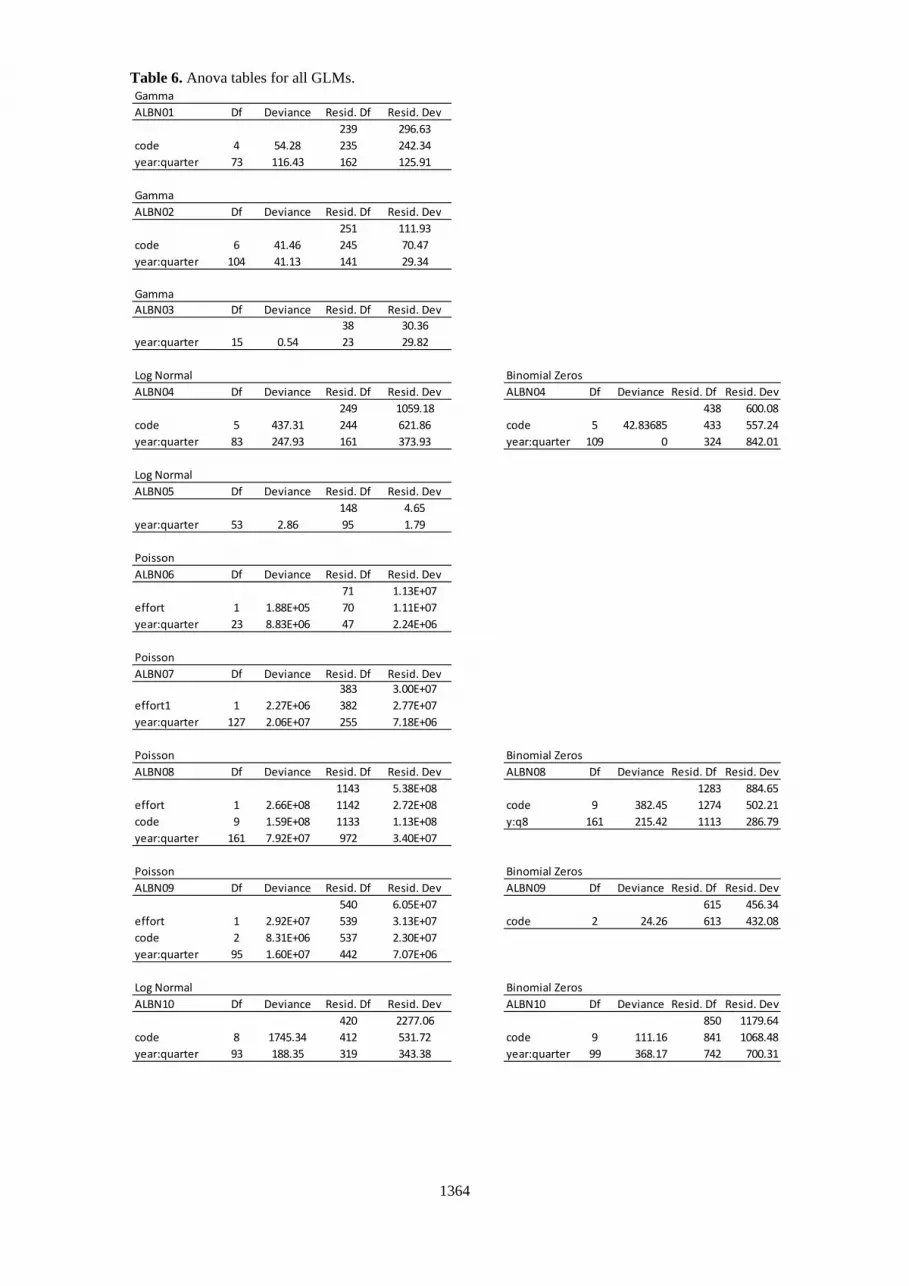
and other catches not included in the previous groups. Nominal CPUE are plotted in Figure 1a and b, where rows correspond to trimester (1st, 2nd, 3rd, 4th from top to bottom) and columns to fishery. Different colours within a panel correspond to different gears, flag states and effort measures within a fishery, while the lines are lowess smoothers. 2.2 Models Analyses were performed using the glm package in R and the glm.nb package in MASS (Venables and Ripley 2002). A first step when fitting GLMs is to choose an appropriate error distribution and alternative error distributions were examined for each series i.e. i) log normal (plus a value of 1 to avoid 0 values), ii) poisson, iii) log-gamma, iv) negative binomial and Delta models combining v) binomial and log normal, vi) binomial and poisson and v) binomial and gamma. The Dependent variables and link functions considered for each error distributions are given in Table 5. Model selection was based upon systematic inspection of diagnostics based upon model checking and fit diagnostics (McCullagh and Nelder, 1989, Chapter 12) allowing the selection of the most appropriate error distribution for each species (Ortiz & Arocha 2004). This entailed plotting (a) standardised deviance residuals against the fitted values to check for systematic departures from the assumptions underlying the error distribution; (b) the absolute values of the residuals against the fitted values as a check of the assumed variance function; and (c) the dependent variable against the linear predictor function as a check of the assumed link function. This evaluation of goodness of fit was performed on a model that included all the main factors (i.e the most-complex model since if the most complex model is a reasonable fit, then any simpler models that are selected will fit adequately because if they didn't they wouldn't be selected. Based upon the diagnostic plots to check the error distributions (Figures 2a,b,c,d,e,f and g), the assumed variance function (Figures 3a,b,c and d) and link function (Figures 4a,b,c, and d) the chosen model specifications are given in table 5. Where code is a unique combination of fleet, gear and effort measurement units and year:quarter represents main effects and interactions (i.e. + year + quarter + year*quarter). 3. Results and discussion

1360

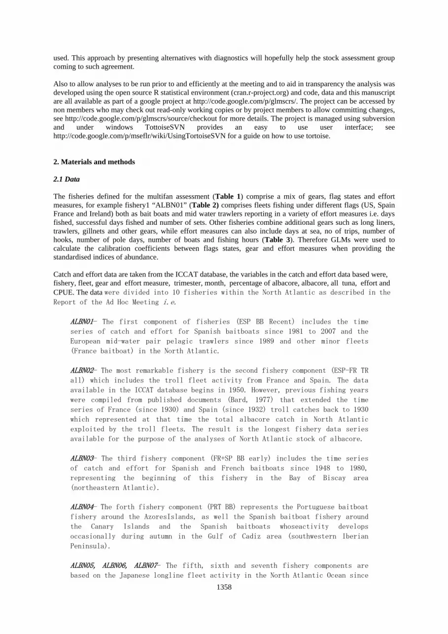
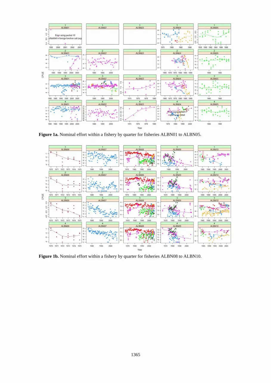
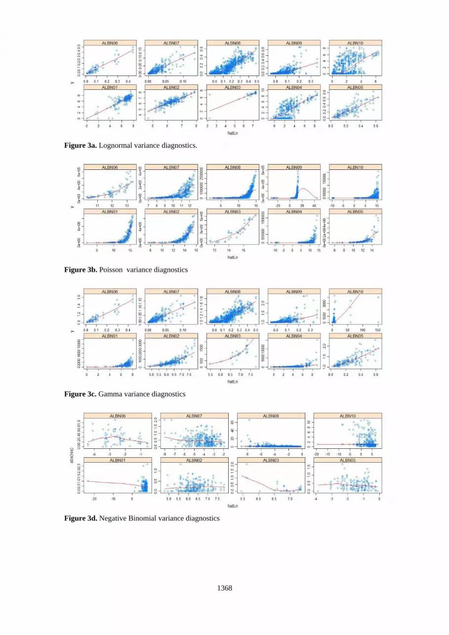
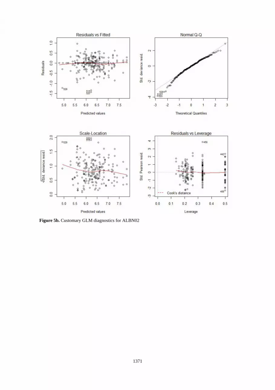
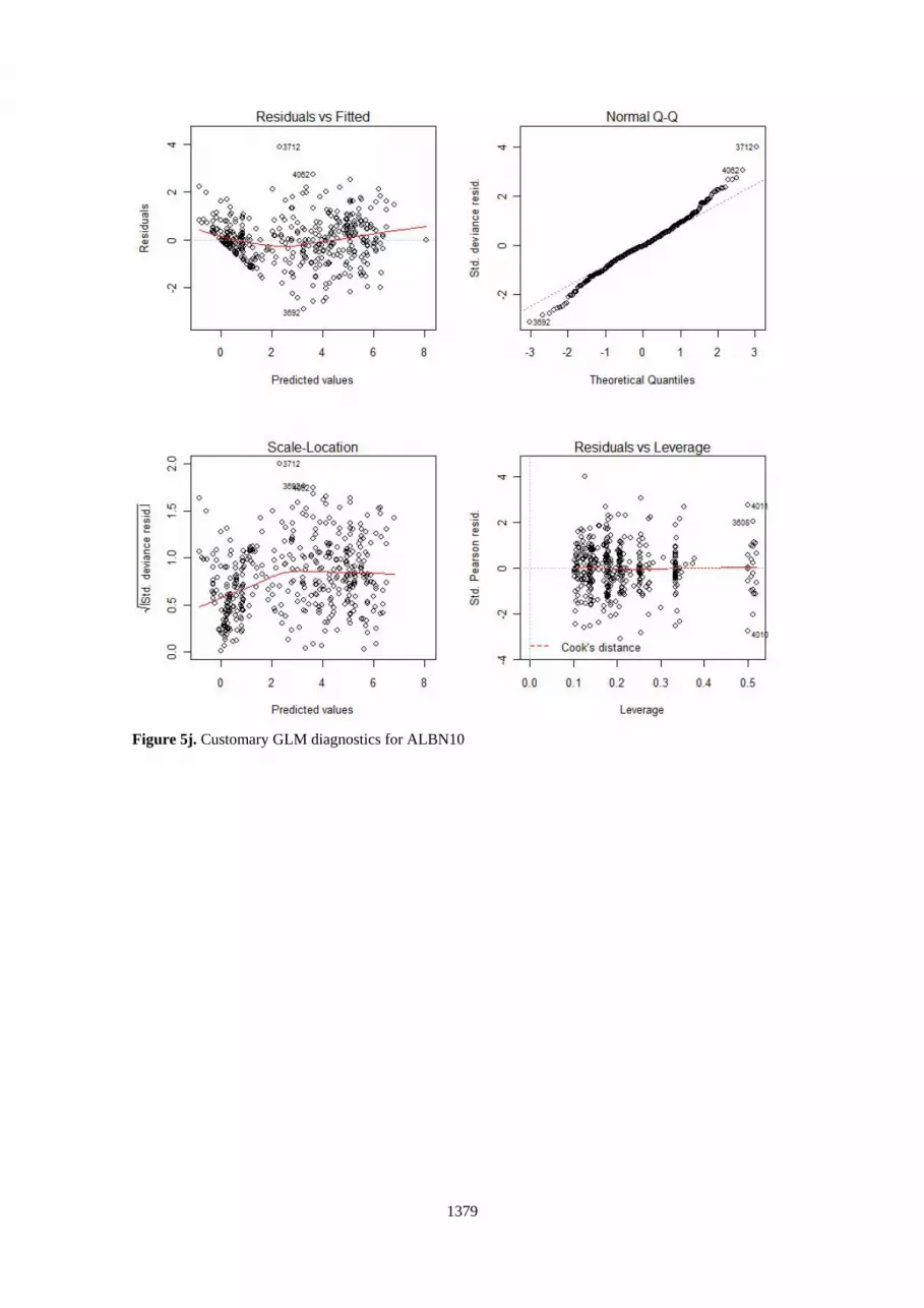
Inspection of Figure 2a suggests that ALBN02 and ALBN05 could be modelled using a log normal error distribution; Figure 2b ALBN06 and ALBN07 poisson; Figure 2c ALBN01, ALBN02 and ALBN03 gamma; Figure 2d ALBN04 and ALBN10 delta log normal and Figure 2e ALBN08 and ALBN09 delta poisson. Inspection of the plots from the negative binomial Figure 2g and delta gamma Figure 2f didn’t suggest any candidates for these distributions. This process has allowed error distributions to be posed for each fishery, in the case of ALBN02 there are two choices and a gamma distribution was chosen for the next stage. Plots (b) and (c) are uninformative for a binomial distribution (McCullagh and Nelder, 1989) and so are not presented for the delta models. Inspection of the diagnostics for the variance Figures 3a, 3b, 3c, 3d showing the absolute values of the residuals plotted against the fitted values and for the link function Figures 4a, 4b, 4c, 4d where the dependent variable was plotted against the linear predictor confirm the chosen error distributions. Once the GLM specifications were fitted "usual" graphical diagnostic were run and these are presented for each series in Figures 5a to j; i.e. checking the scale of the linear predictor, scaled variances are homogeneous; distributions within groups follow the expected distribution, no gross outliers or points with large leverage. For series ALBN08, ALBN09 and ALBN10 there is evidence of over dispersion therefore the delta poisson error distribution GLMs were rerun using a quasi Poison family to allow the dispersion parameter to be estimated. Anova tables are presented in Tables 6a to j. Standardised CPUE series from the 2007 assessment are compared with those produced in this document in Figure 6 and with the nominal values in Figure 7. The standardized CPUE are available at: http://glmscrs.googlecode.com/svn/trunk/Results/cpueStd2009.txt

4. References

Ortiz,M. and Arocha, F. 2004, Alternative error distribution models for standardization of catch rates of non-target species from a pelagic longline fishery: billfish species in the Venezuelan tuna longline fishery. Fisheries Research 70 (2004) 275-297.

McCullagh P. and Nelder, J.A. 1989, Generalized Linear Models. London: Chapman and Hall. Venables, W. N. and Ripley, B.D. 2002, Modern Applied Statistics with S. New York: Springer.

1361

Table 1. Fisheries defined for the Multifan-CL assessment for albacore.

North Atlantic stock

Fish. Name Years Gears/Flags Notes

1 ESP BB Recent

1981-2007

a- ESP BB b- MWTD all flags c- FR BB 1981- 2007

a- CPUE in SCRS/2007/040 (Ortiz de Zárate & O. de Urbina) a-Only Cantabrian sea-North east Atlantic

2 ESP FR TR all 1930-2007

a- MIX.FR+ES TR 1930- 1949 b- ESP-TR, FRA-TR 1950- 2007 c- GN (ESP, FRA, UK, IRL) 1987- 2007

a1- CPUE in 1931-1975 from Bard (SCRS/1976/059); split by quarters with fixed proportions based on recent data TR ESP a2- France TR CPUE in Goujon et al. 1967-1981 (SCRS/1996/ ) re-analized by Year*quarter by Arrizabalaga using the extended France TR time series to 1986 done by Santiago ( 2005) during ALB WG. b- CPUE ESP TR 1981-2005 in SCRS/2006/056 (Ortiz de Zárate & O. de Urbina) c- ICCAT analysis at WG , source: catdis

3 FR+SP BB early 1948-1980

a- ESP+FR BB

a- CPUE from SCRS/76/59 (Bard); split by quarters with fixed proportions based on recent data BB ESP

4 PRT BB 1958-2007

a- PRT BB (Madeira, Azores) b- ESP BB (Canary Islands, Cadiz)

a- CPUE obtained at meeting

5 JPN target LL 1956-1969

a- JPN LL a- CPUE sent by Koji

6 JPN Trans LL 1970-1975


7 JPN Byc LL 1976-2007


8 CHTAI LL 1962-2007

a- Chinese Taipei LL b- all other LL 1960- 2007 (except Fishery 9)

a- CPUE presented by Yeh

9 KOR+PAN+CUB LL

1964-2007

a- LL (KOR, PAN) 1964-2007 b- LL (CUBA) 1964-1993

a- CPUE obtained at meeting

10 OTH SURF 1950-2007

a- BB (CPV, VEN, others not above) b- TR (IRL, PRT, Grenada, SVG, St Lucia,USA) c- All the remainder surf catches

a- CPUE Source: catdis

1362

Table 2. Summary of fleets, gears, effort measures by fishery.

Fishery Code Fleet Gear Effort N Obs

ALBN01 1 EC.ESP‐ES‐CANT_ALB BB Days Fished 138 1, 2, 3, 4 1981 2007

2 EC.FRA TW Days Fished 4 3, 4 1989 1989

3 EC.FRA TW Number of Sets 64 1, 2, 3, 4 1999 2007

4 EC.FRA TW Successful Days Fished 4 3, 4 1990 1990

5 EC.IRL TW Days at Sea 15 1, 3, 4 2003 2007

6 EC.IRL TW Days Fished 18 1, 2, 3, 4 2000 2002

7 USA TW Number of Sets 24 1, 2, 3, 4 1991 1995

ALBN02 8 EC.ESP‐ES‐CANT_ALB TR Days Fished 197 2, 3, 4 1973 2007

9 EC.FRA GN Days Fished 16 2, 3, 4 1989 1994

10 EC.FRA GN Number of Sets 16 2, 3, 4 1999 2002

11 EC.FRA GN Successful Days Fished 4 2, 3 1990 1990

12 EC.FRA TR Days at Sea 5 2, 3, 4 1975 1975

13 EC.FRA TR Days Fished 20 2, 3, 4 1977 2006

14 EC.FRA TR Number of Sets 11 3, 4 2000 2007

15 EC.FRA TR Successful Days Fished 9 2, 3, 4 1983 1990

16 EC.IRL GN Days Fished 14 2, 3, 4 1993 2001

ALBN03 17 EC.ESP‐ES‐CANT_ALB BB Days Fished 41 2, 3, 4 1973 1980

18 EC.FRA BB Days at Sea 4 3, 4 1975 1975

19 EC.FRA BB Days Fished 4 3, 4 1977 1977

ALBN04 20 EC.ESP‐CANT_AZS_ALB BB Days Fished 7 4 1990 1993

21 EC.ESP‐CANT_CDZ_ALB BB Days Fished 16 3, 4 1992 2002

22 EC.ESP‐ES‐CANARY BB Days at Sea 120 1, 2, 3, 4 1975 1984

23 EC.PRT‐PT‐AZORES BB Days Fished 167 1, 2, 3, 4 1963 1986

24 EC.PRT‐PT‐MADEIRA BB Days at Sea 12 1, 2, 3, 4 2002 2002

25 EC.PRT‐PT‐MADEIRA BB Days Fished 36 1, 2, 3, 4 1981 1983

26 EC.PRT‐PT‐MADEIRA BB Number of Trips 95 1, 2, 3, 4 1984 1991

ALBN05 27 JPN LL Number of Hooks 149 1, 2, 3, 4 1956 1969



ALBN08 30 CHN LL Number of Hooks 89 1, 2, 3, 4 1999 2007

31 TAI LL Number of Hooks 485 1, 2, 3, 4 1967 2007

32 TTO‐TTO‐TRINID LL Number of Hooks 48 1, 2, 3, 4 2004 2007

33 USA LL Number of Hooks 252 1, 2, 3, 4 1986 2006

34 USA‐Com LL Number of Hooks 12 1, 2, 3, 4 2007 2007

35 VCT LL Number of Hooks 60 1, 2, 3, 4 2002 2007

36 VEN LL Number of Hooks 178 1, 2, 3, 4 1970 2007

37 VEN‐FOR.FLTS LL Number of Hooks 24 1, 2, 3, 4 1984 1987

38 VEN.ARTISANAL LL Number of Hooks 94 1, 2, 3, 4 1992 1999

39 VEN.INDUSTRIAL LL Number of Hooks 24 1, 2, 3, 4 2004 2005

40 VUT LL Number of Hooks 33 1, 2, 3, 4 2004 2006

ALBN09 41 CUB LL Number of Hooks 198 1, 2, 3, 4 1973 1990

42 KOR LL Number of Hooks 275 1, 2, 3, 4 1966 2007

43 MIX.KR+PA LL Number of Hooks 143 1, 2, 3, 4 1975 1987

44 PAN‐PAN‐TTO LL Number of Hooks 12 1, 2, 3, 4 2006 2007

ALBN10 45 EC.ESP‐CANT_CDZ_ALB TR Days Fished 1 4 2002 2002

Quarters Year Range

1363

Table 3. Effort measures.

Variable Description

D.FISH Days Fished

SUC.D.FI Successful Days Fished

NO.SETS Number of Sets

D.AT SEA Days at Sea

NO.TRIPS No of Trips

NO.HOOKS Number of Hooks

N.POLE-D Number of Pole days

NO.BOATS Number of Boats

FISH.HOUR Fishing Hours Table 4. Summary of zero observations by fishery.

Table 5. Error distributions and link functions chosen for each fishery time series. Fishery Series Error

Distribution Dependent Variable

Link Function Factors

ALBN01 Gamma cpue+1 log year:quarter,code



ALBN04 Delta log norm log(cpue+1) year:quarter,code

ALBN05 Log normal log(cpue+1) year:quarter

ALBN06 Poisson alb log year:quarter

ALBN07 Poisson alb log year:quarter

ALBN08 Delta poisson alb log year:quarter,code

ALBN09 Delta poisson alb log year:quarter,code

ALBN10 Delta log norm cpue year:quarter

Non Zeros % Zeros N Obs

ALBN01 255 4% 267

ALBN02 289 1% 292

ALBN03 47 4% 49

ALBN04 262 42% 453

ALBN05 148 1% 149

ALBN06 72 0% 72

ALBN07 374 3% 384

ALBN08 1159 11% 1299

ALBN09 549 13% 628

ALBN10 449 49% 889

1364

Table 6. Anova tables for all GLMs.

Gamma

ALBN01 Df Deviance Resid. Df Resid. Dev

239 296.63

code 4 54.28 235 242.34

year:quarter 73 116.43 162 125.91

Gamma


251 111.93

code 6 41.46 245 70.47

year:quarter 104 41.13 141 29.34

Gamma


38 30.36

year:quarter 15 0.54 23 29.82

Log Normal Binomial Zeros

ALBN04 Df Deviance Resid. Df Resid. Dev ALBN04 Df Deviance Resid. Df Resid. Dev

249 1059.18 438 600.08

code 5 437.31 244 621.86 code 5 42.83685 433 557.24

year:quarter 83 247.93 161 373.93 year:quarter 109 0 324 842.01

Log Normal


148 4.65

year:quarter 53 2.86 95 1.79

Poisson


71 1.13E+07

effort 1 1.88E+05 70 1.11E+07

year:quarter 23 8.83E+06 47 2.24E+06

Poisson

ALBN07 Df Deviance Resid. Df Resid. Dev383 3.00E+07

effort1 1 2.27E+06 382 2.77E+07

year:quarter 127 2.06E+07 255 7.18E+06

Poisson Binomial Zeros


1143 5.38E+08 1283 884.65

effort 1 2.66E+08 1142 2.72E+08 code 9 382.45 1274 502.21

code 9 1.59E+08 1133 1.13E+08 y:q8 161 215.42 1113 286.79

year:quarter 161 7.92E+07 972 3.40E+07

Poisson Binomial Zeros


540 6.05E+07 615 456.34

effort 1 2.92E+07 539 3.13E+07 code 2 24.26 613 432.08

code 2 8.31E+06 537 2.30E+07

year:quarter 95 1.60E+07 442 7.07E+06

Log Normal Binomial Zeros


420 2277.06 850 1179.64

code 8 1745.34 412 531.72 code 9 111.16 841 1068.48

year:quarter 93 188.35 319 343.38 year:quarter 99 368.17 742 700.31

1365

Figure 1a. Nominal effort within a fishery by quarter for fisheries ALBN01 to ALBN05.

Figure 1b. Nominal effort within a fishery by quarter for fisheries ALBN08 to ALBN10.

1366

Figure 2a. Lognormal error distribution diagnostics.

Figure 2b. Poisson error distribution diagnostics.

Figure 2c. Gamma error distribution diagnostics.

Figure 2d. Negative Binomial error distribution diagnostics.

1367

Figure 2e. Delta Lognormal error distribution diagnostics.

Figure 2f. Delta Poisson error distribution diagnostics.

Figure 2g. Delta Gamma error distribution diagnostics.

1368

Figure 3a. Lognormal variance diagnostics.

Figure 3b. Poisson variance diagnostics

Figure 3c. Gamma variance diagnostics

Figure 3d. Negative Binomial variance diagnostics

1369

Figure 4a. Lognormal link function diagnostics.

Figure 4b. Poisson link function diagnostics.

Figure 4c. Gamma link function diagnostics.

Figure 4d. Negative Binomial link function diagnostics.

1370

Figure 5a. Customary GLM diagnostics for ALBN01

1371

Figure 5b. Customary GLM diagnostics for ALBN02

1372

Figure 5c. Customary GLM diagnostics for ALBN03

1373

Figure 5d. Customary GLM diagnostics for ALBN04

1374

Figure 5e. Customary GLM diagnostics for ALBN05

1375

Figure 5f. Customary GLM diagnostics for ALBN06

1376

Figure 5g. Customary GLM diagnostics for ALBN07

1377

Figure 5h. Customary GLM diagnostics for ALBN08

1378

Figure 5i. Customary GLM diagnostics for ALBN09

1379

Figure 5j. Customary GLM diagnostics for ALBN10

1380

Figure 6a. 2007 standardised CPUEs within a fishery by quarter for fisheries ALBN01 to ALBN05.

Figure 6b. 2007 standardised CPUEs within a fishery by quarter for fisheries ALBN06 to ALBN10.

1381

Figure 7a. 2009 standardised CPUEs within a fishery by quarter for fisheries ALBN01 to ALBN05.

Figure 7b. 2009 standardised CPUEs within a fishery by quarter for fisheries ALBN06 to ALBN10.

1382

Figure 8a. 2009 standardised CPUEs and nominal CPUE within a fishery by quarter for fisheries ALBN01 to ALBN05.

Figure 8b. 2009 standardised CPUEs and nominal CPUE within a fishery by quarter for fisheries ALBN06 to ALBN10.

Documents

Standardisation of North Atlantic Albacore (Thunnus Alalunga), Cpue