Embed Size (px)
Citation preview
arX
iv:p
hysi
cs/0
3061
89v1
[ph
ysic
s.op
tics]
27
Jun
2003
STANDARD AND EMBEDDED SOLITONS
IN NEMATIC OPTICAL FIBERS
R. F. Rodrıguez1,3∗†, J. A. Reyes1,3 ‡,A. Espinosa-Ceron4, J. Fujioka2,3 and B.A. Malomed5
1Departamento de Fısica Quımica2Departamento de Materia Condensada
3Instituto de Fısica. Universidad NacionalAutonoma de Mexico.Apdo. Postal 20-364
01000 Mexico, D. F., Mexico4Facultad de Ciencias, UAEMEX, Toluca 50000,
Edo. de Mexico, Mexico5Department of Interdisciplinary Studies,
Faculty of Engineering, Tel Aviv University,Tel Aviv 69978, Israel
Abstract
A model for a non-Kerr cylindrical nematic fiber is presented. Weuse the multiple scales method to show the possibility of construct-ing different kinds of wavepackets of transverse magnetic (TM) modespropagating through the fiber. This procedure allows us to generatedifferent hierarchies of nonlinear partial differential equations (PDEs)which describe the propagation of optical pulses along the fiber. We gobeyond the usual weakly nonlinear limit of a Kerr medium and derive acomplex modified Korteweg-de Vries equation (cmKdV) which governsthe dynamics for the amplitude of the wavepacket. In this derivationthe dispersion, self-focussing and diffraction in the nematic are taken
∗Fellow of SNI, Mexico†Correspondence author. E-mail: [email protected]‡Fellow of SNI, Mexico
1
into account. It is shown that this cmKdV equation has two-parameterfamilies of bright and dark complex solitons. We show analytically thatunder certain conditions, the bright solitons are actually double em-bedded solitons. We explain why these solitons do not radiate at all,even though their wavenumbers are contained in the linear spectrumof the system. We study (numerically and analytically) the stabilityof these solitons. Our results show that these embedded solitons arestable solutions, which is an interesting property since in most systemsthe embedded solitons are weakly unstable solutions. Finally, we closethe paper by making comments on the advantages as well as the limita-tions of our approach, and on further generalizations of the model andmethod presented.
PACS numbers: 42.65.Tg, 61.30G, 77.84.N
2
1 Introduction
Theoretical studies on the existence of solitons in liquid crystals (LCs) startedin the late sixties and early seventies [1]-[4], and experimental confirmationswere reported subsequently [5]-[8]. In the case of static solitons in LCs, themolecular configurations may be obtained from the Lagrange equations derivedfrom the Helmholtz free energy, whereas for propagating solitons the continu-ous change in these configurations makes it necessary to take into account thedamping of the molecular motion. For liquid-crystal waveguides, the nonlin-earity necessary for the existence of solitons is provided by the coupling withthe optical field.
Coupling of the dynamics of the velocity and director fields in LCs to ex-ternal optical fields renders the relevant dynamical equations highly nonlinear,which makes it possible to have solitary waves of the director field with orwithout involving the fluid motion. Furthermore, the strong coupling of thedirector to light makes any director-wave more easily detectable by opticalmethods than it is in isotropic fluids, where only the flow field is observable.
Some nonlinear partial differential equations (PDEs) appearing in theliquid-crystal theory give rise to exact soliton solutions. These are the Korteweg-de Vries (KdV ), nonlinear Schrodinger (NLS), and the sine-Gordon (sG)equations [9]. The KdV equation describes a medium with weak nonlinearityand weak dispersion, whereas the NLS equation describes situations whereweak nonlinearity and strong dispersion prevail, such as the propagation ofsignals in liquid-crystal optical fibers.
Passing continuous laser beams through nematic LCs reveals the existenceof static spatial patterns in cylindrical [10] and planar [11] geometries. The ba-sic physical mechanism which support these time-independent patterns is thebalance between the nonlinear refraction (self-focussing) and spatial diffrac-tion in the nematic. However, when the propagation of wavepackets, ratherthan continuous beams, is considered, a different situation occurs. The en-velope of the wavepacket obeys an NLS equation, which takes into accountself-focussing, dispersion and diffraction in the nematic [12], [14], [15]. Thisequation has soliton solutions whose speed, time and length scales may beestimated by using experimentally measured values of the corresponding pa-rameters [16]. However, the usual analysis of this situation is based on theassumption that the LC behaves as a Kerr medium and that, consequently,strong dispersion and weak nonlinearity, at order O(q3), with respect the fieldamplitude q, should be taken into account As it will be discussed below, qmeasures the ratio of the electric-field energy density and the elastic-energydensity of the nematic and it is, therefore, a measure of the coupling betweenthe optical field and the fluid. However, although truncating the analysis atthe O(q3) order may be a very reasonable assumption for solid-state optical
3
media, the soft nature of the LCs suggest that the neglect of higher-ordercontributions may not necessarily be a good assumption in this case.
Recently, the formation of spatial solitary waves in nematic LCs with atthe light-power level of a few milliwatts has attracted a good deal of interest[17], [18], [19], [20]. It has been experimentally shown that the nonlinearity ofthese media can support solitons in LC line waveguides [21], [22].
The main purpose of the present work is to develop an approach that al-lows to generate PDEs which describe the propagation of optical pulses innematic LC waveguides beyond the weakly nonlinear limit corresponding tothe Kerr medium. More specifically, we show that to O(q4), and assumingthat attenuation effects are small, the evolution of the amplitude of propagat-ing transverse-magnetic transverse-magnetic (TM) modes is governed by anequation with a derivative nonlinearity, which is the complex modified KdV(cmKdV ) equation,
uz − ε uttt − γ |u|2 ut = 0. (1)
see Eq. (32) below.The paper is organized as follows. In Sec. 2 we introduce a model of a
cylindrical nematic cell and set up basic coupled equations for the orienta-tional and optical fields. We formulate an iterative procedure to expand theseequations in terms of the coupling parameter q, which leads to a specific hi-erarchy of PDEs. Then, in Sec. 3 we derive dynamical equations governingthe evolution of the amplitude of propagating TM modes up to the orderO(q4). Rescaling the equations, we show that the standard NLS equation isobtained at order O(q3), and that the equation corresponding to O(q4) is in-deed the cmKdV equation (1). In Sec. 4, soliton solutions to this equation arestudied. In particular, it is shown that the equation has ordinary bright- anddark-soliton solutions, and a continuous family of embedded solitons (ESs),i.e. solitary waves which exist inside the system’s continuous spectrum of lin-ear waves [23]. In Sec. 5 we discuss why the ESs can exist in Eq. (1) withoutemitting any radiation, even though their wave numbers belong to the linearspectrum. In Sec. 6 we study the stability of the ESs. We conclude the pa-per in Sec. 7, which summarizes the results and compares them to previouslypublished ones. We also point out advantages and limitations of our approach,and discuss possible ways to generalize it.
2 The Model and Basic Equations
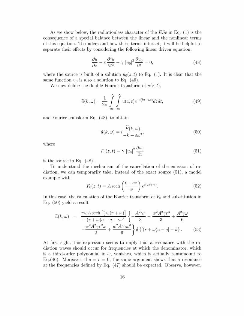
We consider a cylindrical waveguide with an isotropic core of radius a, dielectricconstant ǫc and a quiescent nematic LC cladding of radius b. The initialorientational state is depicted in Fig. 1, where the director field obeys the
4
following axial strong-anchoring boundary conditions,
n(r = a, z) = n(r = b, z) = ez. (2)
An optical beam is launched into the guide and propagates through the LC.If the field is strong enough to exceed the orientation-transition threshold, theinitial configuration is changed by reorienting the director field. We assumethat the induced reorientation occurs only occurs in the (r, z) plane, so that
n(r, z) = sin θer + cos θez, (3)
where er and ez are the unit vectors of the cylindric coordinates.Although the incident beam is neither planar nor Gaussian, the normal
modes within the cavity are cylindrical plane waves propagating along thez axis. In previous works it has been shown that only the TM modes, withnonzero components Er(r, z, t), Ez(r, z, t) and Hφ(r, z, t) of the electromagneticfield, couple to the reorientation dynamics of the director field [14], [12], [24].As it can be shown that Er(r, z, t) and Ez(r, z, t) may be expressed in terms ofHφ(r, z, t), below we only describe the dynamics of the component Hφ(r, z, t).The relevant dynamical equations, which take into account retardation effects,are given by Eqs. (8) and (9) of Ref. [24], namely,
∂2θ
∂ζ2 +1
x
∂
∂r
(x
∂θ
∂x
)− sin θ cos θ
x2
−q2
[cos 2θ
x
(E∗
z
∫ t
dt′∂xHφ
∂x+ E∗
r
∫ t
dt′∂Hφ
∂ζ
)+
sin 2θ
x2
(−xE∗
r
∫ t
dt′∂Hφ
∂ζ+ E∗
z
∫ t
dt′∂xHφ
∂x
)]= 0, (4)
a2
c2
∂2Hφ
∂t2= −
∫dt
′
(∂2Hφ
∂ζ2 +∂2Hφ
∂x2
) (t − t
′)
ǫ⊥
(−→r′ , t′
) +∂2
∂t∂ζ
∫dt
′
ǫa
ǫ⊥ǫ‖(t′)
[− sin2 θ
∂Hφ
∂ζ+ sin θ cos θ
1
x
∂
∂xxHφ
](t − t
′
)
− ∂2
∂t∂x
∫dt
′ ǫa
ǫ⊥ǫ‖(t′)
[− sin θ cos θ
∂Hφ
∂ζ+
cos2 θ1
x
∂
∂xxHφ
] (t − t
′
), (5)
5
with
→
E (−→r , t) =1
ǫ0
∫dt
′
∫ t
dt”ǫa
ǫ⊥ǫ‖
(t” − t
′
)nn · ∇ × −→H
(−→r′ , t′
). (6)
In these equations, we have used dimensionless variables, ζ ≡ z/a, x ≡ r/a,Hφ ≡ Hφ/(cǫ0E0), Ea
i ≡ Eai /E0 , i = r, z, where E0 is the amplitude of the
incident field. The speed of light in vacuum is c = 1/√
µ0ǫ0 , where µ0 andǫ0 are, respectively, the magnetic permeability and electric permittivity of freespace. The dielectric anisotropy of the nematic, ǫa ≡ ǫ‖−ǫ⊥, is defined in termsof the dielectric constant for directions parallel (ǫ‖) and perpendicular (ǫ⊥) tothe director. As mentioned in Sec. 1, q2 ≡ ǫ0E
20a
2/K is the dimensionless ratiobetween the electric-field energy density and the elastic-energy density of thenematic, where K is its elastic constant in the equal constants approximation.Thus, q2 is a measure of the coupling between the optical field and the LC. Westress that, in writing Eqs. (4) and (5), large difference between the time scalesof slow reorientation dynamics and rapid variations of the electromagnetic fieldwas explicitly taken into account, and as a consequence the time derivativesof θ were ignored.
When the coupling between the TM mode Hφ(r, z, t) and the reorientationfield θ(r, z, t) is negligible (q = 0), the propagating modes are represented byquasi-planar waves. However, if the nonlinearities in Eq. (4) are taken intoaccount by considering finite q, they cause space and time variations of thefield Hφ(r, z, t), due to generation of higher-order harmonics which feedbackto the original modes.
We assume that the interaction between the optical field and the reori-entation in the nematic is stronger than in the weakly nonlinear limit (Kerrmedium) which corresponds to q = 1 [12]. Furthermore, in all the analysiswe neglect all the backflow effects associated with the reorientation or causedby external flows [13]. Thus, we solve the coupled equations (4) and (5) byassuming the following coupled expansions of θ and Hφ in powers of q,
θ = θ(o) + q2 |A(Ξ, T )U(x, ω)|2 θ(1)(x) + q4 |A(Ξ, T )U(x, ω)|4 θ(2)(x) + ..., (7)
Hφ (x, ζ, t) = qUφ
(x, ω0 + iλ
∂
∂T
)A(Ξ, T ) + q2U (2) + q3U (3)
+q4U (4) + q5U (5) + c.c. + ..., (8)
where c.c. stands for the complex conjugate.The rationale behind this assumption is the following. As indicated in
Eq. (4), the lowest-order coupling between θ and Hφ occurs at order q2, and
6
it is therefore reasonable to expect that higher-order terms will also be evenin q. The fields θ(n) with n = 0, 1, 2.. are contributions to θ at order n ,which satisfy the same hard-anchoring homeotropic boundary conditions aswere given above by Eq. (2), θ(x = 1) = θ(x = b/a) = 0. As usual, theamplitude A(Ξ, T ) in Eqs. (7) and (8), which represents an envelope of anarrow wavepacket of width λ ≡ (ω−ω0)/ω0, whose central frequency is ω0, isassumed to be a slowly varying function of the variables Ξ ≡ λζ and T ≡ λt .Here λ is a small parameter which measures the dispersion of the wavepacket.In Eqs. (7) and (8), Uφ (x, ω0) is the well-known linear solution for Hφ whichis given explicitly by [26]
Uφ(x, ω0) = J21
(√ǫc(
ω0a
c)2 − β2a2
)√π
2γaxexp(−iβaζ − γax), (9)
with γ =√
ǫ‖(β2/ǫ⊥ − (ω0/c)
2). Here J1(x) is the Bessel function of order 1,
and β is the propagation constant, which only takes allowed values calculatedin Ref. [24]. The terms proportional to U (n), n = 2, 3, ... in (8) are contribu-tions to the TM modes from to the higher-order optical harmonics that aregenerated by the nonlinearities in Eqs. (5) and (4).
Note, however, that the relation between the parameters q and λ is notunique. For instance, when the wavepacket is very narrow, this relation is λ = qand up to O(q3), the expansion leads to the standard nonlinear Schrodinger(NLS) equation for A(Ξ, T ) (which corresponds to the Kerr medium) [25],[12], [24]. Therefore the model may be generalized in various ways. Since qand λ are small parameters, we assume that λ ≡ qα with some positive α.Then α = 1/2 represents a wider and α = 2 a narrower wavepacket. Note thatthe presence of higher powers of q implies that these higher-order contributionsare smaller than the dominant term in (7), which describes a small-amplitudenarrow wavepacket.
Inserting the expression (7) into Eq.(5) and expanding in powers of q, itis straightforward to rewrite Eq.(5) as
L(β, ω, x)Hφ + q2F (Hφ) + q4G(Hφ) = 0, (10)
where the linear L operator and nonlinear ones, F and G, are defined, respec-tively, as
L ≡ 1
x2ǫ⊥ǫ‖
[−ǫ⊥ + x2ǫ‖
(ǫ⊥
(ω0
ca)2
− (βa)2
)+ xǫ⊥
∂
∂x+ x2ǫ⊥
∂2
∂x2
], (11)
7
F ≡ ǫa |A(ζ)Uφ(x, ω)|2xǫ⊥ǫ‖
iβa
(Uφθ
(1)(x) + 3xθ(1)(x)dUφ
dx+ Uφx
dθ(1)(x)
dx
)A.
(12)
G = −ǫa |A(ζ)Uφ(x, ω)|4 A(ζ)
x2ǫ⊥ǫ‖
[{(x2β2 − 1)
(θ(1)(x)
)2
− ixβθ(2)(x)
+2xθ(1)(x)dθ(1)(x)
dx− ix2β
dθ(2)(x)
dx
}Uφ(x, ω) +
{x(θ(1)(x)
)2
−6ix2βθ(2)(x) + 2x2θ(1)(x)dθ(1)(x)
dx
}dUφ(x, ω)
dx
+x2(θ(1)(x)
)2 d2Uφ(x, ω)
dx2
−6ix2βθ(2)(x)]. (13)
Zero-order solutions for the orientation, with θ(0) = 0, and first-order ones,which gives rise to θ(1)(x), were found in Ref. [24] by inserting expressions(7) and (8) into Eqs. (4), (10) and solving the resulting equations. This way,θ(1)(x) turned out to be
θ(1)(x) =βaǫaJ
21 [√
ǫc(ω0ac
)2 − β2a2]
πǫ⊥ǫ‖x (a2 − b2)
{(a2 − b2)eγa(1−x)
+ (b2 − x2a2) + eγ(a−b)a2(1 − x2)}
. (14)
To study the dynamics beyond the Kerr approximation, we need to calcu-late the fourth-order terms in Eq. (7), that is, θ(2)(x). To this end,we insertEqs. (9), (7) into Eq. (4) and expand the result in powers of q up to the fourthorder. This leads to
ǫaγa
(4x2
[ǫ⊥ǫ‖(
ω0ac
)2 − β2a2]− ǫ⊥
)
2πx2ǫ⊥ǫ2‖
(β2a2 − ǫ⊥(ω0a
c)2) θ(1)(x) +
θ(2)(x)
x− dθ(2)(x)
dx− x
d2θ(2)(x)
dx2= 0. (15)
After substituting θ(1)(x) from Eq. (14), this equation takes the form
8
βǫ2aγa2
2π2ǫ2⊥ǫ3
‖x3 (a2 − b2)
(4x2
[ǫ⊥ǫ‖(
ω0ac
)2 − β2a2]− ǫ⊥
)(β2a2 − ǫ⊥(ω0a
c)2)
J21 [
√ǫc(
ω0a
c)2 − β2a2]
{(a2 − b2)eγa(1−x) + (b2 − x2a2) + eγ(a−b)a2(1 − x2)
}
+θ(2)(x)
x− dθ(2)(x)
dx− x
d2θ(2)(x)
dx2= 0. (16)
In spite of its apparent complexity, this linear differential equation for θ(2)(x)can be easily solved by imposing the planar strong-anchoring boundary condi-tions for θ, as explained above. The solution can then be written in terms ofthe exponential-integral function, and if the resulting expressions are approx-imated by asymptotic expressions for this function, we obtain
θ(2)(x) =βǫae
−(b+ax)γJ21 [√
ǫc(ω0ac
)2 − β2a2]
24x2a2b(a + b)2(b − a)π3γ2ǫ3⊥ǫ2
‖[e(1+x)aγ [A4x
4 + A3x3 + A2x
2
+A1x + A0] + e−(b+a)γ(B1x + B0)]
+ e(b+ax)γ(C4x4 + C3x
3 + C2x2 + C1x + C0)
]. (17)
While this compact form for θ(2)(x) is sufficient for our discussion below, ex-pressions for the coefficients A0, A1, A2, A3, A4, B0, B1, C0, C1, C2, C3 andC4 that appear in Eq. (17) are given in Appendix A.
To conclude this section, it is relevant to stress that the above derivationignored dissipative loss in the LC medium. In fact, the physical conditionfor the applicability of this assumption is that the propagation distance tobe passed by excitations (solitons) is essentially smaller than a characteristicdissipative-loss length. This condition can be readily met in situations ofphysical relevance.
3 The Envelope Dynamics
We now aim to derive an equation for the envelope A(Ξ, T ) by dint of the sameprocedure that was used in Ref. [12] for the weakly nonlinear case. To thisend, we substitute Eq. (8) into Eq. (10), and identify the Fourier variables
iβa = iβ0a + qα ∂
∂Ξ1
+ q2α ∂
∂Ξ2
+ q3α ∂
∂Ξ3
+ q4α ∂
∂Ξ4
, (18)
9
−iω = −iω0 + qα ∂
∂T, (19)
where the variables Ξn, n = 1, 2, 3, 4, are related to the spatial scales associatedwith upper harmonics contributions, that is, Z ≡ qnαΞn. This substitutionleads to an equation,
0 = L[iβ0a + qα ∂
∂Ξ1
+ q2α ∂
∂Ξ2
+ q3α ∂
∂Ξ3
+ q4α ∂
∂Ξ4
,−iω0 (20)
+qα ∂
∂T]Hφ(x, ζ, t) + q2F [Hφ (x, ζ, t)] + q4G[(Hφ (x, ζ, t)]. (21)
We now fix α = 1, which means selection of the type of the wave packetto be considered; choosing α = 2 or α = 1/2 would imply, respectively, anarrower or wider packet of the TM modes than for α = 1. In this case, wecollect contributions to the same power of q, arriving at the expressions
q1 : L (iβ0a,−iω0, x)Uφ (x, ω0) A = 0, (22)
q2 : LU (1) =
(iL (iβ0a,−iω0)
∂Uφ
∂ω
∂
∂T+ UφL2
∂
∂T+ L1Uφ
∂
∂Ξ1
)A, (23)
q3 : LU (2) = S2
(∂2Uφ
∂ω2,∂Uφ
∂ω, Uφ
)A − F (Uφ (x, ω0)A), (24)
q4 : LU (3) = S3
(∂3Uφ
∂ω3,∂2Uφ
∂ω2,∂Uφ
∂ω, Uφ
)A +
R3
(∂Uφ
∂ω,∂Uφ
∂x,∂2Uφ
∂ω∂x, θ(1)(x),
dθ(1)(x)
dx
)|A|2 A, (25)
where Ln, n = 1, 2, denotes the derivative of L (iβ0a,−iω0) with respect toits first or second argument. Clearly, the same procedure can be carried outfor α = 1/2 or 2.
Note that Eq. (22) is actually the usual dispersion relation L (iβ0a,−iω0)Uφ (x, ω0) = 0, which confirms our approximation, since Hφ (x, ω0) alreadysatisfies this equation to the first order in q. To simplify Eqs. (23) – (25) wetake the first four derivatives of Eq. (22) with respect to ω. This leads to a setof linear inhomogeneous equations for U (n), the existence of solutions to whichis secured by the so-called alternative Fredholm condition [27]. This condition
10
is fulfilled if LUφ (x, ω0) = 0 and if Uφ (x, ω0) → 0 as x → ∞. In our case, thisreads explicitly
⟨LU (n), Uφ
⟩=
∫ b/a
1
UφLU (n)dx = 0, n = 1, 2, 3, 4. (26)
By applying the relations (26) to Eqs. (23) – (25), substituting the four firstderivatives of Eq. (22) into them, and collecting terms in front of the samepower of q, we obtain the following equations for A(Ξ, T ) on each of the spatialscales Ξ, Ξ1, Ξ2, Ξ3, Ξ4, for the successive orders in q,
q2 :∂A
∂Ξ1+ a
dβ
dω
∂A
∂T= 0, (27)
q3 :∂A
∂Ξ2+ i
d2β
dω2
∂2A
∂T 2+ iβn2A |A|2 = 0, (28)
q4 :∂A
∂Ξ3
− 1
6
d3β
dω3
∂3A
∂T 3− βn3 |A|2 ∂A
∂T= 0. (29)
Here, dimensionless coefficients n2 and n3 are defined as follows:
n2 =1
4ǫ2aβa3J1
(a
c
√(ǫcω2
0 − β2c2))4
e−γb+2γa
−ae−3γb + aeγ(a−4b) + be−γ(4a−b) − be−3γa
πǫ2‖b (a2 − b2) ǫ⊥ (−e−2γb + e−2γa)
, (30)
n3 = −ǫ⊥ω0
4β
∫ b/a
1
(in2
ǫ⊥Uφ
[β
∂Uφ
∂ω− Uφ
dβ
dω
]+
3βǫa
xǫ⊥ǫ‖(Uφ)
3 ∂Uφ
∂ω
dxθ(1)(x)
dx+
2βǫa
xǫ⊥ǫ‖θ(1)(x) (Uφ)2
[2∂Uφ
∂x
∂Uφ
∂ω+ Uφ
∂2Uφ
∂x∂ω
])dx/
∫ b/a
1
(Uφ)2 dx, (31)
The coefficient n2 is related with the nonlinear diffraction index n2 through theexpression n2 ≡ Kn2/ǫ0a
2. Similarly, we define a nonlinear diffraction indexat the next order beyond the Kerr approximation by n3 ≡ ω0Kn3/ǫ0a
2; it isproportional to the coefficient in front of the nonlinear term in Eq. (29). Notethat Eq. (27) simply describes a wavepacket in the linear medium, while Eq.(28) is the well-known NLS equation which gives rise to robust soliton pulses.The equations corresponding to the orders q2 and q3 are well-known ones, andthey have also been derived and analyzed in Ref. [24]. In the next section wefocus on Eq. (29), which was derived at order q4.
11
4 Double Embedded Solitons
Equation (29) may be rewritten in a rescaled form by introducing the dimen-sionless variables u ≡ A/A0, ξ ≡ Ξ4/Z04, and τ ≡ T/T04, where Z04 and T04
are space and time scales, and A0 is the initial amplitude of the optical pulse.In terms of these variables, Eq. (29) becomes
∂u
∂ξ− ε
∂3u
∂τ 3− γ |u|2 ∂u
∂τ= 0, (32)
where we have defined the dimensionless coefficients ε and γ as
ε =1
6
Z04
T 304
d3β
dω3, (33)
γ = βn3A20
Z04
T04
. (34)
In what follows below, we will consider Eq. (32) in the form of Eq. (1), i.e.,with ξ and τ replaced by z and t.
Equation (32), or equivalently Eq. (1), reduces to the real modified Ko-rteweg de Vries (mKdV ) equation when we restrict u(z, t) to be real, henceall the real solutions of the mKdV equation, including N -soliton ones, arealso solutions of (1). On the other hand, Eq. (1) also has complex solutionswhich include, as it will be discussed below, two-parameter families of brightand dark complex solitons. Actually, the existence of these complex solutionsof Eq. (1) was pointed out by Ablowitz and Segur as early as 1981 [29]. Theprecise form of the bright solitons in the particular case when ε = 6γ waspresented recently by Karpman et al. [30].
In the general case the bright-soliton solutions to Eq. (1) may be found bysubstituting a straightforward trial function in this equation,
u(z, t) = A sech
(t − az
w
)ei(qz+rt). (35)
This substitution shows that (35) is indeed a solution of (1), provided that
A2w2 =6ε
γ, (36)
a = 3εr2 − 1
6γA2, (37)
q =1
2γA2r − εr3. (38)
12
Condition (36) implies that the bright soliton solution (35) only exists forǫγ > 0, which implies that, in the opposite case, the nonlinearity and lineardispersion cannot be in balance. Moreover, since we have five free parametersin Eq. (35) and only three conditions (36) – (38), these expressions definea two-parameter family of bright soliton solutions of Eq. (1), so that thefollowing pairs of the parameters can be chosen arbitrarily: (A, r), (w, r),(A, q), or (w, q). The family includes, as particular cases, the real one-solitonsolutions of the mKdV equation, which are obtained when r = 0.
In a similar way, dark solitons of Eq. (1) can be found by substituting thetrial function
u(z, t) = Ad tanh
(t − ad z
wd
)ei(qd z + rd t). (39)
This substitution shows that this ansatz solves Eq. (1) if the following condi-tions are satisfied
A 2d w 2
d = −6 ε
γ, (40)
ad = 3 ε r 2d − 1
3γ A 2
d , (41)
qd = γ A 2d rd − ε r 3
d , (42)
which are similar to the conditions (36) – (38) for the bright solitons. As inthe bright case, the conditions (40) – (42) permit us to choose freely any ofthe following pairs of parameters: (A, r), (w, r), (A, q), or (w, q). Thus, Eqs.(39)-(42) define a two-parameter family of dark-soliton solutions of Eq. (1),Eq. (40) showing that this family only exists if εγ < 0, i.e., exactly in the caseopposite to that in which bright solitons are found.
Out of the two families of the above soliton solutions (bright and dark)of Eq. (1), the bright family is the most interesting one. In spite of theirsimilarity to ordinary bright solitons, the bright soliton solutions of Eq. (32)feature a special property which distinguishes them from ordinary solitarywaves, namely, they are double-embedded solitons. The concept of embeddedsolitons (ESs) was formulated, in a general form, in Ref. [23]. It refers tosolitary waves which do not emit radiation, in spite of the fact that the soliton’swavenumber (spatial frequency) is embedded in the system’s linear spectrum.Still earlier, solitons of this type were found in particular models [17], forinstance, in a generalized NLS equation involving a quintic nonlinear term[31]. Recently, more systems supporting ESs have been found [32] – [40]. Tothe best of our knowledge, the existence of ESs has not been reported beforein models of LC media.
13
So far, the embedded solitons were classified in two groups, namely, thosewhich obey NLS-like equations (or systems thereof), and those which aregoverned by KdV -like equations. In the former case, an ES has its wavenumberembedded in the range of wavenumbers permitted to linear waves (as it wasalready mentioned above). In the latter case, the velocity of an ES is foundin the range of phase velocities of linear waves. There are, accordingly, twodifferent ways to decide whether a solitary-wave solution to a nonlinear PDEsystem is embedded, viz., the wavenumber (WN) and velocity (VE) criteria.
In Ref. [30] it was pointed out that Eq. (1) is a particular case of a moregeneral NLS-like equation possessing ESs. For this reason, and also in viewof the significance of Eq. (1) for physical applications, it is interesting todetermine if the bright-soliton solutions of Eq. (1) may be ESs. It shouldbe noted that Eq. (1) may be regarded as both a KdV -like equation, dueto its similarity to the mKdV one, and an NLS-like equation, because, inthe context of wave propagation in LCs, Eq. (1) in its complex form playsa role similar to that of the NLS equation, i.e., the one governing evolutionof a slowly varying envelope of a rapidly oscillating wave. Therefore, it maybe possible to apply both criteria, WN and VE ones, to decide if the solitonsolutions of Eq. (1) are ESs.
First, we apply the WN criterion. To this end, we must determine if thewavenumber of the solution (35) is contained within the range of the wavenum-bers allowed to linear waves. To identify the intrinsic wavenumber of the so-lution, we must transform it into the reference frame moving along the timeaxis with the reciprocal velocity a, see Eq. (35). The transformation adds aDoppler term to the soliton’s internal spatial frequency (wavenumber), makingit equal to q + ar. On the other hand, plane-wave solutions to the linearizedversion of Eq. (1) in the same reference frame can be sought for as
u(z, t) = exp i [kz − ω(t − az)] , (43)
which leads to the following dispersion relation
k(ω) = εω3 − aω. (44)
Since the range in which the function (44) takes its values covers all the realnumbers, including the soliton’s wavenumber q + ar, all the soliton solutionsto Eq. (1), given by Eqs. (35)-(38), are classified as ESs as per the WNcriterion.
Now, we address the question whether these solitons are also embeddedaccording to the V E criterion. As the evolution variable in Eq. (1) is thedistance z, rather than the time t, it is the reciprocal velocity which determinesif the moving solutions are embedded according to the V E criterion. Thus,we should find out if the reciprocal velocity of the soliton (35), given by the
14
parameter a, is contained within the range of the reciprocal velocities permittedto linear waves. The dispersion relation (44) implies that the reciprocal phasevelocities of the linear waves (in the reference frame moving along with thesoliton) are given by
k
ω= −a + εω2, (45)
while the reciprocal velocity of the soliton proper is, obviously, zero in thesame reference frame. Obviously, the expression (45) takes the value zero ifaε is positive, hence the soliton solutions given by Eqs. (35) – (38) are ESsaccording to the V E criterion provided that aε > 0. As these solitons arealso embedded according to the WN criterion, we call them double-embeddedsolitons. On the other hand, when aε < 0, the soliton solutions of Eq. (1) areonly embedded with respect to the WN criterion, but not as per the V E one,therefore in this case we apply the term single-embedded solitons.
5 Radiation Inhibition and Continuity of the
Embedded Solitons
As in any other system with ESs, the fact that the solitons do not emitradiation despite being embedded in the linear spectrum should be explained.Since the wavenumber q + ar of the soliton solution (35) is contained in thelinear spectrum defined by the dispersion relation (44), a resonance of thesoliton is expected with the linear waves whose frequencies satisfy the condition
q + ar = εω3 − aω. (46)
Moreover, when aε > 0 the soliton’s reciprocal velocity a coincides with thereciprocal phase velocities (εω2) of two linear waves whose frequencies satisfythe condition
a = εω2, (47)
consequently one could also expect the soliton to resonate with these waves.Different explanations for the absence of resonant radiation in other systemswhich support ESs were proposed [34], [41]. However, an explanation for theradiationless character of the ESs in Eq. (1) has not been presented.
Another unexpected property of the same ESs in Eq. (1) is the fact thatthey exist in a continuous family. In most cases, ESs are isolated solutions;usually they do not appear in families, although examples of continuous fam-ilies of ESs are known too, for instance, in a fifth-order KdV equation [35].It is also necessary to explain why Eq. (1) has a two-parameter family of theES solutions.
15
As we show below, the radiationless character of the ESs in Eq. (1) is theconsequence of a special balance between the linear and the nonlinear termsof this equation. To understand how these terms interact, it will be helpful toseparate their effects by considering the following linear driven equation,
∂u
∂z− ε
∂3u
∂t3− γ |u0|2
∂u0
∂t= 0, (48)
where the source is built of a solution u0(z, t) to Eq. (1). It is clear that thesame function u0 is also a solution to Eq. (46).
We now define the double Fourier transform of u(z, t),
u(k, ω) =1
2π
∞∫
−∞
∞∫
−∞
u(z, t)e−i(kz−ωt)dzdt, (49)
and Fourier transform Eq. (48), to obtain
u(k, ω) = iF (k, ω)
−k + εω3, (50)
where
F0(z, t) = γ |u0|2∂u0
∂t(51)
is the source in Eq. (48).To understand the mechanism of the cancellation of the emission of ra-
diation, we can temporarily take, instead of the exact source (51), a modelexample with
F0(z, t) = A sech
(t − az
w
)ei(qz+rt). (52)
In this case, the calculation of the Fourier transform of F0 and substitution inEq. (50) yield a result
u(k, ω) =πwA sech
[π2w(r + ω)
]
−(r + ω)a − q + ǫω3
{−A2γr
3− w2A2γr3
3+
A2γω
6
−w2A2γr2ω
2+
w2A2γω3
6
}δ {[(r + ω)a + q] − k} . (53)
At first sight, this expression seems to imply that a resonance with the ra-diation waves should occur for frequencies at which the denominator, whichis a third-order polynomial in ω, vanishes, which is actually tantamount toEq.(46). Moreover, if q = r = 0, the same argument shows that a resonanceat the frequencies defined by Eq. (47) should be expected. Observe, however,
16
that the numerator on the right-hand side of (53) also contains a third-orderpolynomial in ω. Consequently, if the two polynomials happen to coincide,they will cancel each other, which also implies the cancellation of the resonantgeneration of the radiation modes. Equating the coefficients in front of powersof ω in the two polynomials in (53), we obtain three equations which, aftersome manipulations, take the precise forms of Eqs. (36) – (38). Thus, thesethree equations are the necessary and sufficient conditions for the mutual can-cellation of the two polynomials in Eq. (53). This explains why the forcingterm F0(z, t) of the form (52) does not generate any radiation, provided thatthe parameters A, a, w, q and r satisfy Eqs. (36) – (38). Furthermore, observethat the polynomial that appears in the numerator of the expression (53)contains the nonlinear coefficient γ, while the polynomial in the denominatorcontains the dispersion coefficient ε. Consequently, the cancellation betweenthese two polynomials is a result of the balance between the nonlinearity anddispersion in Eq. (1). Finally, if the forcing term in Eq. (50) is taken in theexact form (51), rather than in the simplified form of Eq. (52), it is easy tocheck that the prediction for the cancellation of the radiation emission will bethe same.
In the case of the full equation (1), the same cancellation argument explainswhy an initial condition of the form
u(z = 0, t) = A sech
(t
w
)eirt (54)
does not radiate at the frequencies defined by Eqs. (46) and (47) if A and wdo not satisfy Eq. (36). On the other hand, if A and w this condition, weexpect the resonances to occur. In the next section, we will verify numericallythat this indeed the case.
To close this section, it is relevant to stress that the cancellation of thetwo polynomials in Eq. (53) imposes only three conditions, while the so-lution (35) involves five parameters. Therefore, the cancellation conditionsdo not uniquely determine the soliton parameters, which explains why thesoliton solution (35)-(38) involves two arbitrary parameters, thus defining atwo-parameter continuous family of the ESs.
6 Stability of the Embedded Solitons
In this section we will study the stability of the bright-soliton solutions of Eq.(1). As it was explained in Sec. 4, these solitons may be either single-embeddedor double-embedded, depending on the sign of the parameter combination aε.
17
In the following we will separately consider the cases of positive and negativeaε.
We begin by considering a single-embedded soliton of Eq. (1), setting ε = 1and γ = 6 [these values were chosen as they correspond to those at which therelated Hirota equation [42], which is connected to Eq. (1) by the Galileantransform [30], is an exactly integrable one [43]]. We start with the followingvalues of the soliton parameters
As =
√5
8≈ 0.790 (55)
ws =
√8
5(56)
rs = 1/√
24 (57)
as = −1/2 (58)
qs =11
6√
24. (59)
These values satisfy the conditions (36) – (38), and therefore they characterizean exact bright soliton of the form (35). Since asε < 0, this soliton is a single-embedded one (i.e., it is embedded solely according to the WN criterion).
To test stability of this soliton, we consider an initial condition of the form
u (z = 0, t) = A0 sech
(t
w0
)exp (ir0t) , (60)
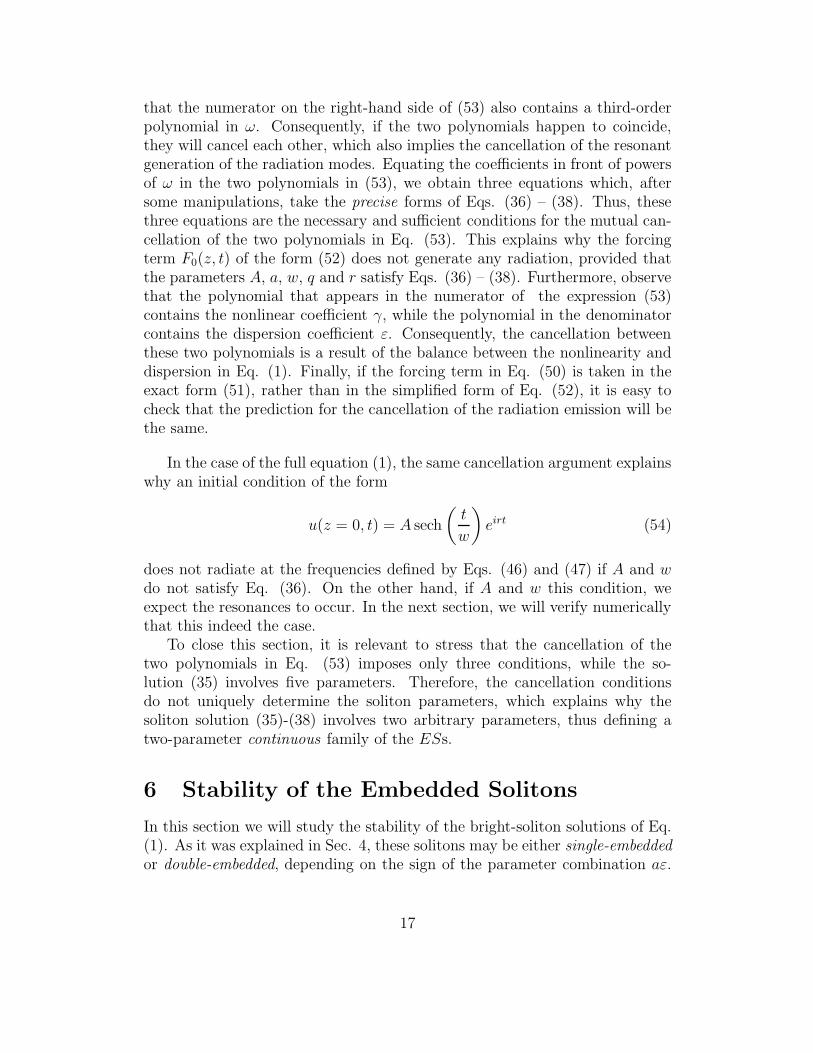
where w0 = ws and r0 = rs, but A0 is slightly different from As. If we give A0
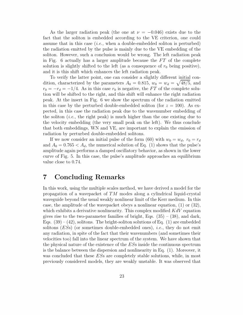
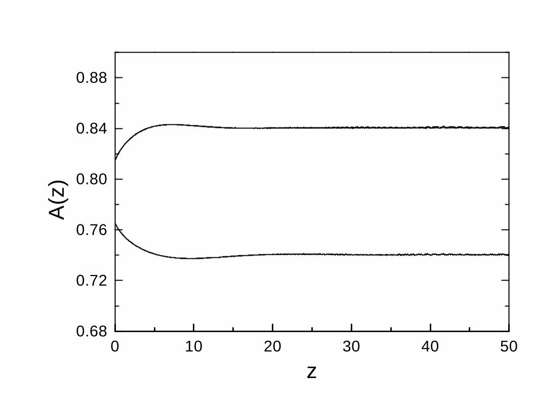
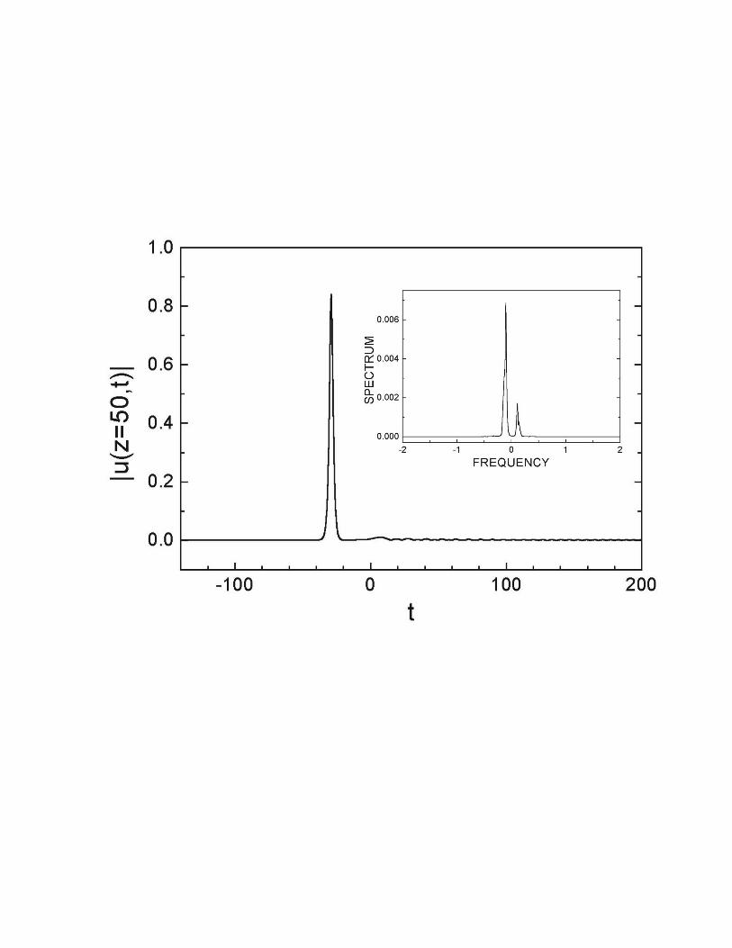
a value 0.815, which is larger than As, the numerical solution of Eq. (1) showsthat the pulse moves to the right along the temporal axis with a reciprocalvelocity equal to −0.58, which is slightly lower than as, and the pulse’s ampli-tude evolves as shown in the upper curve of Fig. 2. The observation that thereciprocal velocity of the perturbed pulse is lower than as is consistent withEq. (37), which indicates that a should decrease if A is increased. Figure 2(the upper curve) shows that the pulse’s amplitude stabilizes and approachesan equilibrium value close to A = 0.84. The temporal profile of the pulseat z = 50 is displayed in Fig. 3. It shows a small-amplitude radiation waveemitted by the trailing edge of the pulse. The frequency composition of thistiny radiation wave can be determined by calculating the Fourier transform(FT ) of the radiation contained in the interval 40 ≤ t ≤ 168. The insert inFig. 3 shows the power spectrum (i.e., the square of the FT amplitude) of
18
this radiation, which contains two peaks located at the frequencies ν1 = −0.10and ν2 = 0.12. These peaks are close to the resonant frequencies (ν = ±0.07)predicted by the resonance condition
qs + asrs = εω3 − asω (61)
[cf. Eq. (46)] and the partial resonance condition [40]
− (qs + asrs) = εω3 − asω. (62)
These radiation peaks imply that the perturbed pulse emits radiation accordingto the way the soliton’s wavenumber is embedded in the spectrum of linearwaves.
If we now consider an initial condition of the form (60), with wo = ws,ro = rs and Ao = 0.765 < As, the behavior of the perturbed pulse is similar.In this case the amplitude evolves as shown in the lower curve of Fig. 2 wherewe can see that the pulse’s amplitude approaches an equilibrium value closeto A = 0.74. The reciprocal velocity of the perturbed pulse is −0.42, whichis slightly higher than as. This change is consistent with Eq. (37), whichindicates that a should increase if A is diminished.
The two curves shown in Fig. 2 demonstrate that the single-embeddedsoliton solutions of Eq. (1) are stable. This is an interesting result, sinceusually ESs display a weak (nonlinear) one-sided instability [34]. In fact, thecomplete stability of the ESs in Eq. (1) may be expected, due to the fact thatin this case we are dealing with a continuous two-parameter family of the ESs,while in most other systems ESs are isolated solutions, which explains theirnonlinear instability.
Figure 2 also shows that if the amplitude of one of the single-embeddedsolitons of Eq. (1) is slightly increased, the perturbed soliton stabilizes itselfat an even higher amplitude. On the contrary, if the soliton’s amplitude isslightly decreased, the perturbed soliton stabilizes at a still lower amplitude.This behavior can be better understood if we analyze the evolution of theperturbed solitons of Eq. (1) by means of the averaged variational techniqueintroduced by Anderson [44], which is one of the approximately analyticalmethods used successfully in nonlinear optics [45] – [51], see also a recentreview [52].
In order to apply the variational technique, we start with the ansatz of theordinary form,
u(z, t) = A(z) sech
[t − V (z)
W (z)
]exp i
[Q(z) + R(z) t + P (z) t2
]. (63)
Introducing this trial function in the Lagrangian density of Eq. (1),
L = i (uzu∗ − u∗
zu) + iε (u u∗ttt − u∗uttt) +
iγ
2
[u2u∗u∗
t − (u∗)2u ut
], (64)
19
and integrating over time, we calculate the averaged (effective) Lagrangian
L =
∫ ∞
−∞
L dt. (65)
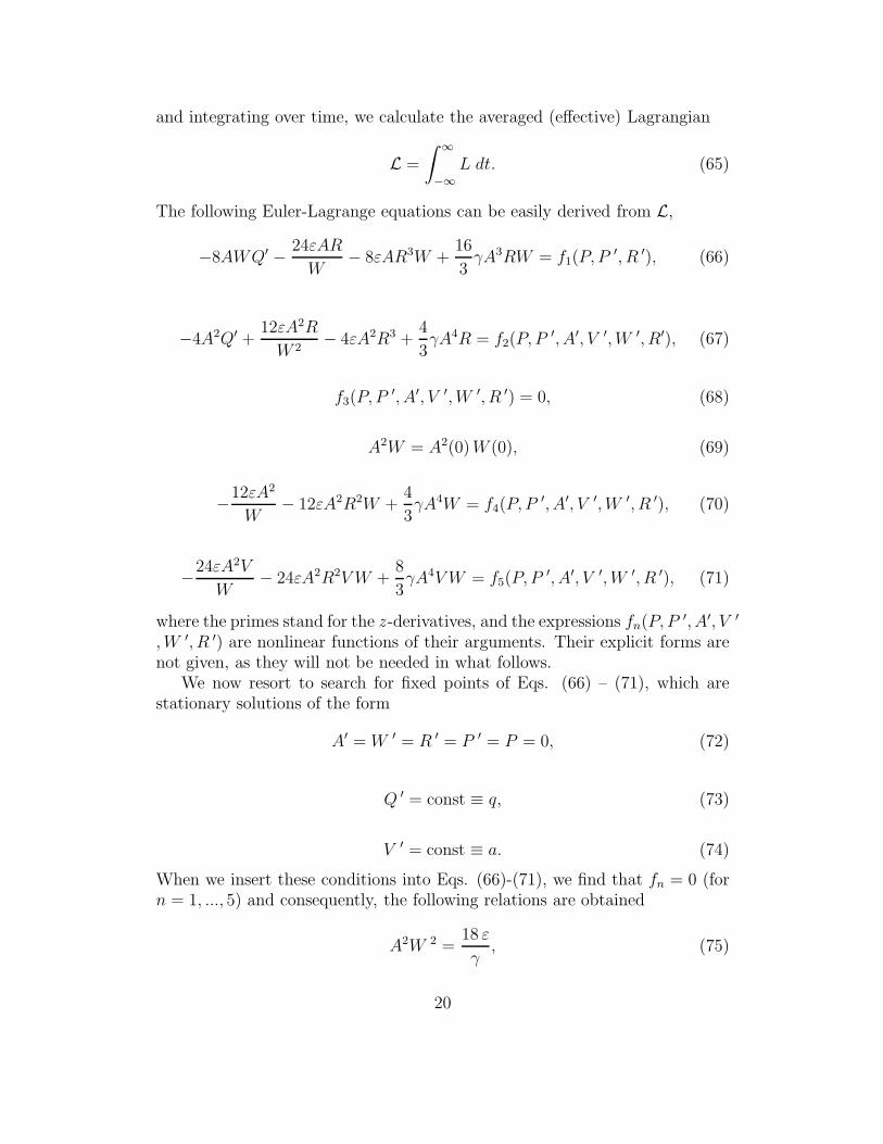
The following Euler-Lagrange equations can be easily derived from L,
−8AWQ′ − 24εAR
W− 8εAR3W +
16
3γA3RW = f1(P, P ′, R ′), (66)
−4A2Q′ +12εA2R
W 2− 4εA2R3 +
4
3γA4R = f2(P, P ′, A′, V ′, W ′, R′), (67)
f3(P, P ′, A′, V ′, W ′, R ′) = 0, (68)
A2W = A2(0) W (0), (69)
−12εA2
W− 12εA2R2W +
4
3γA4W = f4(P, P ′, A′, V ′, W ′, R ′), (70)
−24εA2V
W− 24εA2R2V W +
8
3γA4V W = f5(P, P ′, A′, V ′, W ′, R ′), (71)
where the primes stand for the z -derivatives, and the expressions fn(P, P ′, A′, V ′
, W ′, R ′) are nonlinear functions of their arguments. Their explicit forms arenot given, as they will not be needed in what follows.
We now resort to search for fixed points of Eqs. (66) – (71), which arestationary solutions of the form
A′ = W ′ = R ′ = P ′ = P = 0, (72)
Q ′ = const ≡ q, (73)
V ′ = const ≡ a. (74)
When we insert these conditions into Eqs. (66)-(71), we find that fn = 0 (forn = 1, ..., 5) and consequently, the following relations are obtained
A2W 2 =18 ε
γ, (75)
20
a = 3 εR 2 − 1
6γA2, (76)
q =1
2γA2R − εR 3, (77)
A2W = const = A2(0) W (0). (78)
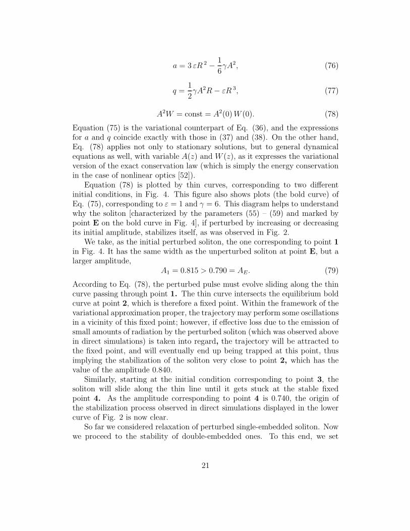
Equation (75) is the variational counterpart of Eq. (36), and the expressionsfor a and q coincide exactly with those in (37) and (38). On the other hand,Eq. (78) applies not only to stationary solutions, but to general dynamicalequations as well, with variable A(z) and W (z), as it expresses the variationalversion of the exact conservation law (which is simply the energy conservationin the case of nonlinear optics [52]).
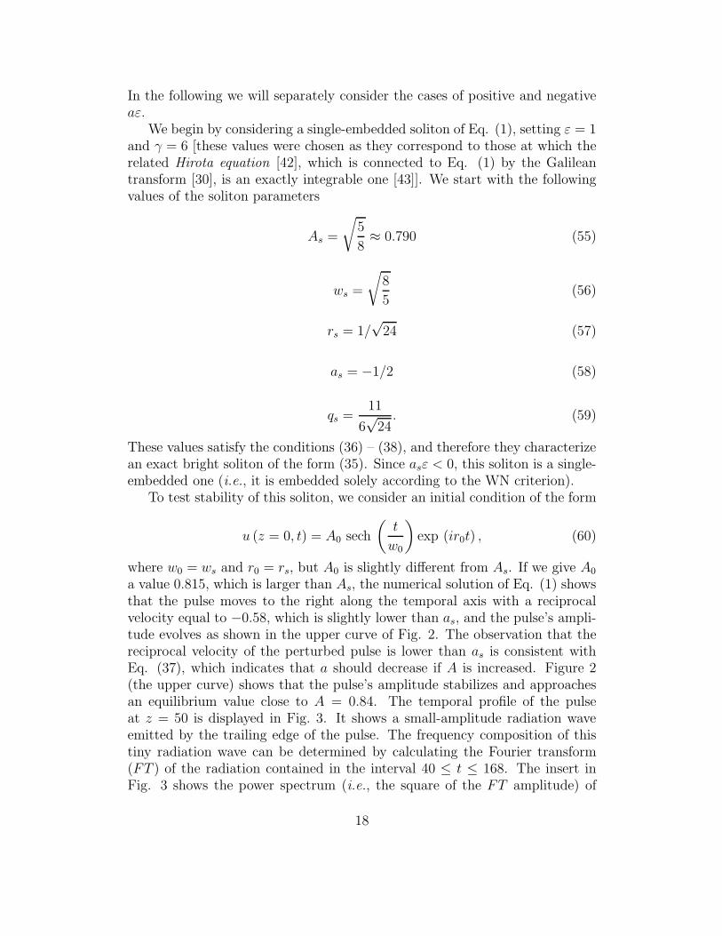
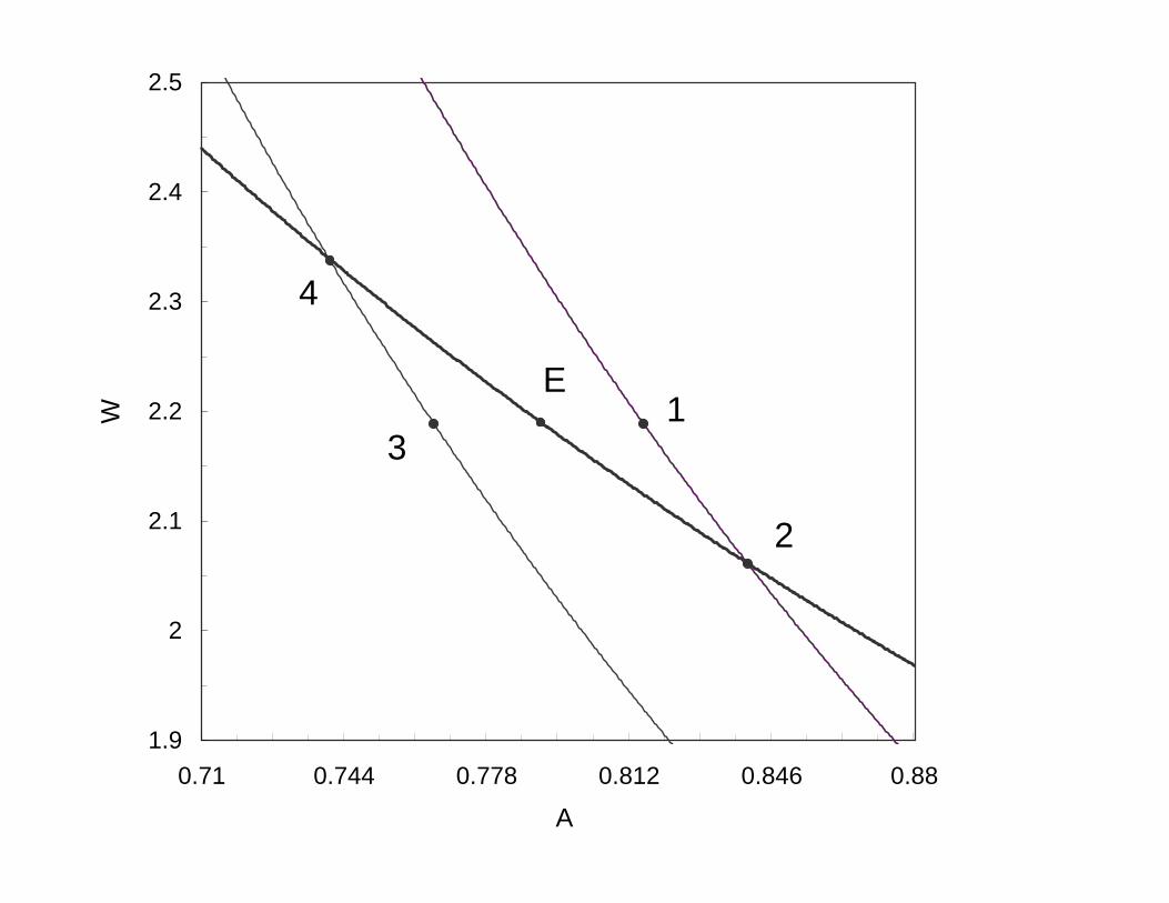
Equation (78) is plotted by thin curves, corresponding to two differentinitial conditions, in Fig. 4. This figure also shows plots (the bold curve) ofEq. (75), corresponding to ε = 1 and γ = 6. This diagram helps to understandwhy the soliton [characterized by the parameters (55) – (59) and marked bypoint E on the bold curve in Fig. 4], if perturbed by increasing or decreasingits initial amplitude, stabilizes itself, as was observed in Fig. 2.
We take, as the initial perturbed soliton, the one corresponding to point 1
in Fig. 4. It has the same width as the unperturbed soliton at point E, but alarger amplitude,
A1 = 0.815 > 0.790 = AE . (79)
According to Eq. (78), the perturbed pulse must evolve sliding along the thincurve passing through point 1. The thin curve intersects the equilibrium boldcurve at point 2, which is therefore a fixed point. Within the framework of thevariational approximation proper, the trajectory may perform some oscillationsin a vicinity of this fixed point; however, if effective loss due to the emission ofsmall amounts of radiation by the perturbed soliton (which was observed abovein direct simulations) is taken into regard, the trajectory will be attracted tothe fixed point, and will eventually end up being trapped at this point, thusimplying the stabilization of the soliton very close to point 2, which has thevalue of the amplitude 0.840.
Similarly, starting at the initial condition corresponding to point 3, thesoliton will slide along the thin line until it gets stuck at the stable fixedpoint 4. As the amplitude corresponding to point 4 is 0.740, the origin ofthe stabilization process observed in direct simulations displayed in the lowercurve of Fig. 2 is now clear.
So far we considered relaxation of perturbed single-embedded soliton. Nowwe proceed to the stability of double-embedded ones. To this end, we set
21
ε = γ = 1, and choose the soliton parameters
Ad =
√5
8≈ 0.790, (80)
wd =
√48
5, (81)
rd = 1/4, (82)
ad = 1/12 ≈ 0.08, (83)
qd = 1/16. (84)
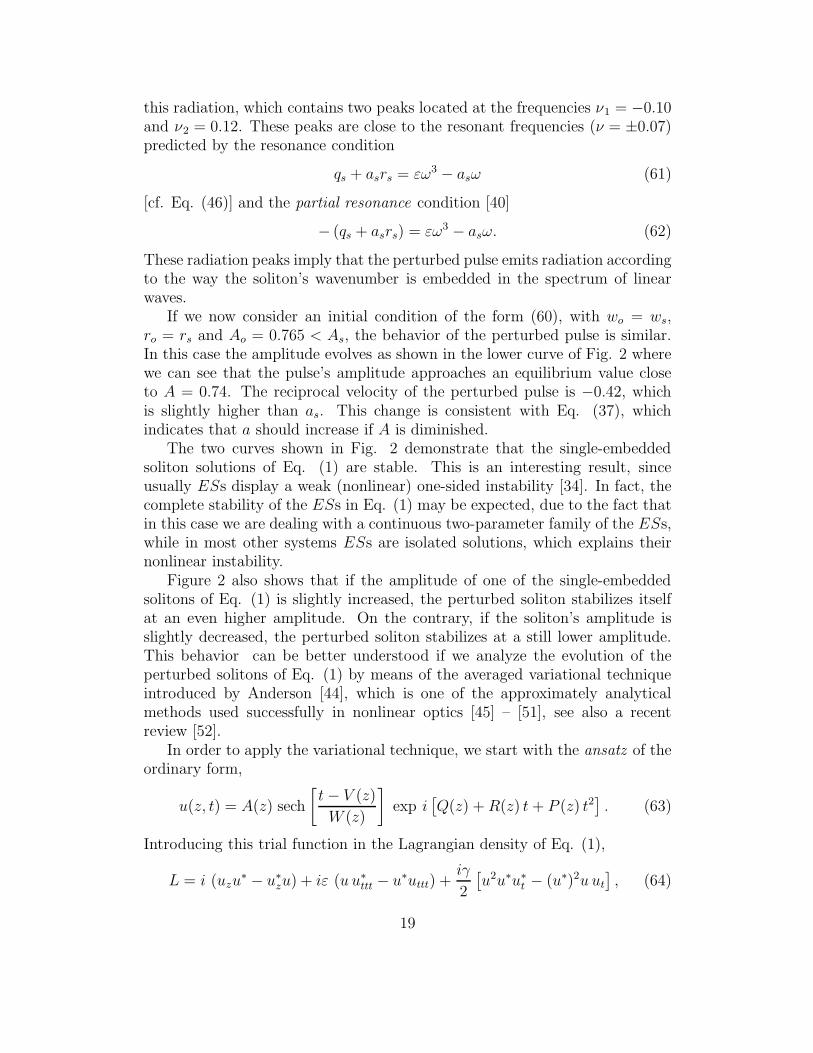
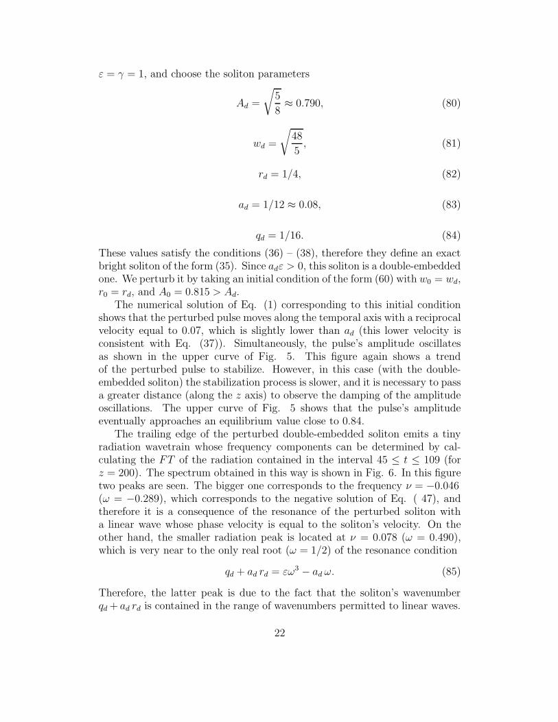
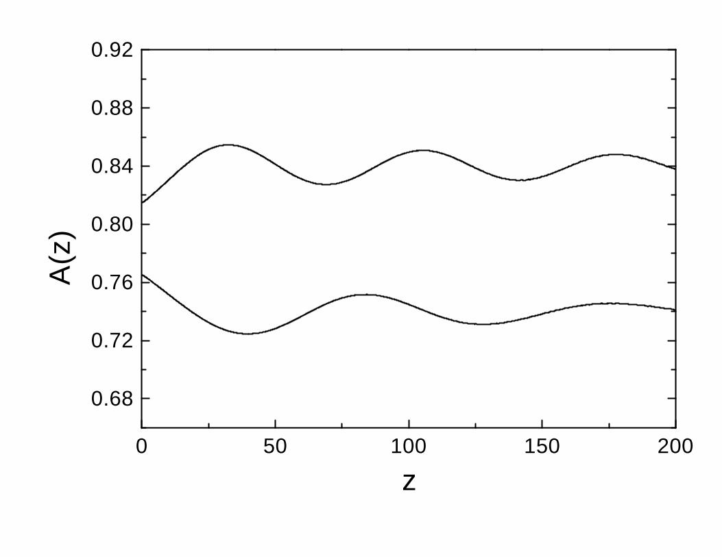
These values satisfy the conditions (36) – (38), therefore they define an exactbright soliton of the form (35). Since adε > 0, this soliton is a double-embeddedone. We perturb it by taking an initial condition of the form (60) with w0 = wd,r0 = rd, and A0 = 0.815 > Ad.
The numerical solution of Eq. (1) corresponding to this initial conditionshows that the perturbed pulse moves along the temporal axis with a reciprocalvelocity equal to 0.07, which is slightly lower than ad (this lower velocity isconsistent with Eq. (37)). Simultaneously, the pulse’s amplitude oscillatesas shown in the upper curve of Fig. 5. This figure again shows a trendof the perturbed pulse to stabilize. However, in this case (with the double-embedded soliton) the stabilization process is slower, and it is necessary to passa greater distance (along the z axis) to observe the damping of the amplitudeoscillations. The upper curve of Fig. 5 shows that the pulse’s amplitudeeventually approaches an equilibrium value close to 0.84.
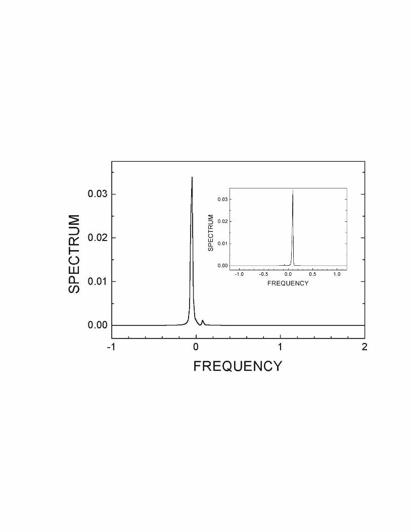
The trailing edge of the perturbed double-embedded soliton emits a tinyradiation wavetrain whose frequency components can be determined by cal-culating the FT of the radiation contained in the interval 45 ≤ t ≤ 109 (forz = 200). The spectrum obtained in this way is shown in Fig. 6. In this figuretwo peaks are seen. The bigger one corresponds to the frequency ν = −0.046(ω = −0.289), which corresponds to the negative solution of Eq. ( 47), andtherefore it is a consequence of the resonance of the perturbed soliton witha linear wave whose phase velocity is equal to the soliton’s velocity. On theother hand, the smaller radiation peak is located at ν = 0.078 (ω = 0.490),which is very near to the only real root (ω = 1/2) of the resonance condition
qd + ad rd = εω3 − ad ω. (85)
Therefore, the latter peak is due to the fact that the soliton’s wavenumberqd + ad rd is contained in the range of wavenumbers permitted to linear waves.
22
As the larger radiation peak (the one at ν = −0.046) exists due to thefact that the soliton is embedded according to the VE criterion, one couldassume that in this case (i.e., when a double-embedded soliton is perturbed)the radiation emitted by the pulse is mainly due to the VE embedding of thesoliton. However, such a conclusion would be wrong. The left radiation peakin Fig. 6 actually has a larger amplitude because the FT of the completesolution is slightly shifted to the left (as a consequence of r0 being positive),and it is this shift which enhances the left radiation peak.
To verify the latter point, one can consider a slightly different initial con-dition, characterized by the parameters A0 = 0.815, w0 = wd =
√48/5, and
r0 = −rd = −1/4. As in this case r0 is negative, the FT of the complete solu-tion will be shifted to the right, and this shift will enhance the right radiationpeak. At the insert in Fig. 6 we show the spectrum of the radiation emittedin this case by the perturbed double-embedded soliton (for z = 100). As ex-pected, in this case the radiation peak due to the wavenumber embedding ofthe soliton (i.e., the right peak) is much higher than the one existing due tothe velocity embedding (the very small peak on the left). We thus concludethat both embeddings, WN and VE, are important to explain the emission ofradiation by perturbed double-embedded solitons.
If we now consider an initial pulse of the form (60) with w0 = wd, r0 = rd
and A0 = 0.765 < Ad, the numerical solution of Eq. (1) shows that the pulse’samplitude again performs a damped oscillatory behavior, as shown in the lowercurve of Fig. 5. In this case, the pulse’s amplitude approaches an equilibriumvalue close to 0.74.
7 Concluding Remarks
In this work, using the multiple scales method, we have derived a model for thepropagation of a wavepacket of TM modes along a cylindrical liquid-crystalwaveguide beyond the usual weakly nonlinear limit of the Kerr medium. In thiscase, the amplitude of the wavepacket obeys a nonlinear equation, (1) or (32),which exhibits a derivative nonlinearity. This complex modified KdV equationgives rise to the two-parameter families of bright, Eqs. (35) – (38), and dark,Eqs. (39) – (42), solitons. The bright-soliton solutions of Eq. (1) are embeddedsolitons (ESs) (or sometimes double-embedded ones), i.e., they do not emitany radiation, in spite of the fact that their wavenumbers (and sometimes theirvelocities too) fall into the linear spectrum of the system. We have shown thatthe physical nature of the existence of the ESs inside the continuous spectrumis the balance between the dispersion and nonlinearity in Eq. (1). Moreover, itwas concluded that these ESs are completely stable solutions, while, in mostpreviously considered models, they are weakly unstable. It was observed that
23
perturbed single-embedded solitons relax to a new equilibrium state faster thandouble-embedded ones.
The coupled expansions for θ and Hφ in powers of q, that were introducedin Sec. 2, can be extended to higher orders. This leads to nonlinear equationswith the quintic i.e., O(q5), nonlinearity. Investigation of the correspondingmodel is currently in progress. Also, as discussed in Sec. 3, up to the orderO(q4) considered here, the same procedure to construct narrower (α = 2) orwider (α = 1/2) wavepackets of TM modes can also be carried out.
Another possible generalization of our model, not dealt with here, is apossibility to take into account hydrodynamic flows beyond the Kerr-mediumapproximation, that will inevitably couple to the reorientation dynamics ofthe liquid crystal. Actually, the inclusion of the flow is unavoidable owingto the fluid nature of the system. However, the consideration of the hydro-dynamical part of the system substantially complicates the problem. Someeffects produced by this generalization were considered, at the level of theNLS approximation, i.e., at order O(q3), in Ref. [13].
AcknowledgmentsWe acknowledge a partial financial support from DGAPA-UNAM IN105797,
from FENOMEC through the grant CONACYT 400316-5-G25427E and fromCONACYT 41035, Mexico. We also thank DGSCA-UNAM (Direccion Gen-eral de Servicios de Computo Academico de la UNAM) for their authorizationto use the computer Origin 2000 during this work.
24
References
[1] L. Lam and J. Prost, editors, Solitons in Liquid Crystals (Springer-Verlag,New York, 1992).
[2] W. Helfrich, Phys.. Rev. Lett. 21, 1518 (1968).
[3] P. G. de Gennes, J. Phys. (Paris) 32, 789 (1971).
[4] F. Brochard, J. Phys. (Paris) 33, 607 (1972).
[5] L. Lager, Solid State Commun. 10, 697 (1972).
[6] P. E. Cladis and M. Kleman, J. Phys (Paris) 33, 591 (1972).
[7] P. E. Cladis and S. Torza, Colloid Interface Sci. 4, 487 (1976).
[8] R. Ribotta, Phys. Rev. Lett. 42, 1212 (1979).
[9] R. K. Bullogh and P. J. Caudrey, editors, Solitons (Springer, New York,1980).
[10] E. Braun, L.P. Faucheux, A. Libchaber, D. W. McLaughlin, D. J. Murakiand M. J. Shelley, Europhys Lett. 23, 239 (1993).
[11] E. Braun, L. P. Faucheux and A. Libchaber, Phys.. Rev. A 48, 611 (1993).
[12] R. F. Rodriguez and J. A. Reyes, J. Mol. Liq. 71, 115 (1997).
[13] J. A. Reyes and R. F. Rodriguez, Phys. Rev E 65, 051701 (2002).
[14] J. A. Reyes and R. F. Rodriguez, Opt. Comm. 134, 349 (1997).
[15] R. F. Rodriguez and J. A. Reyes, Rev. Mex. Fis. 45, 254 (1999).
[16] Shu-Hsia Chen and Tien-Jung Chen, Appl. Phys. Lett. 64, 1893 (1994).
[17] A. V. Buryak, Phys. Rev. E 52, 1156 (1995).
[18] G. Assanto, M. Peccianti, C. Umeton, A. De Luca and I. C. Khoo, Mol.Cryst. Liq. Cryst. 375, 617 (2002).
[19] M. Peccianti and G. Assanto, Phys. Rev. E 65, 035603 (2000).
[20] M. A. Karpierz, Phys. Rev. E 66, 036603 (2002).
[21] M. Warenhem, J. F. Henninot, F. Derrien and G. Abbate, Mol. Cryst.Liq. Cryst. 373, 213-225 (2002).
25
[22] M. Peccianti, C. Conti, G. Assanto, A. De Luca and C. Umeton, Appl.Phys. Lett. 81, 3335-3337 (2002).
[23] J. Yang, B. A. Malomed and D. J. Kaup, Phys.. Rev. Lett.. 83, 1958(1999).
[24] J. A. Reyes and R. F. Rodriguez, Physica D 101, 333 (2000).
[25] A. C. Moloney and J. V. Newell, Nonlinear Optics (Addison Wesley, NewYork, 1992).
[26] D. Jackson, Classical Electrodynamics (Wiley, New York, 1984).
[27] D. Zwillinger, Handbook of Differential Equations, (Academic Press, NewYork, 1989)
[28] I. C. Khoo and S. T. Wu, Optics and Nonlinear Optics of Liquid Crystals(World Scientific, Singapore, 1993) Sec. 1.10.
[29] M. J. Ablowitz and H. Segur, Solitons and the Inverse Scattering Trans-form (SIAM, Philadelphia, 1981).
[30] V. I. Karpman, J. J. Rasmussen and A. G. Shagalov, Phys.. Rev E 64,026614 (2001).
[31] J. Fujioka and A. Espinosa, J. Phys. Soc. Japan 66, 2601 (1997).
[32] A. R. Champneys and B. A. Malomed, J. Phys. A 32, L547 (1999).
[33] A. R. Champneys and B. A. Malomed, Phys. Rev. E 61, 886 (2000).
[34] A. R. Champneys, B. A. Malomed, J. Yang and J. Kaup, Physica D152-153, 585 (2001).
[35] J. Yang, Stud. Appl. Math. 106, 337(2001).
[36] J. Yang, B. A. Malomed, D. J. Kaup and A. R. Champneys, Math. Com-put. Sim. 56, 585 (2001).
[37] K. Kolossovski, A. R. Champneys, A. Buryak, and R. A. Sammut, PhysicaD 171, 153 (2002).
[38] D. E. Pelinovsky and J. Yang, Proc. Roy. Soc. London A 458, 1469 (2002).
[39] T. Wagenknecht and A. R. Champneys, Physica D 177, 50 (2003).
[40] A. Espinosa-Ceron, J. Fujioka and A. Gomez-Rodriguez, Physica Scripta67, 314 (2003).
26
[41] A. N. Kosevich, Low Temp. Phys. 26, 453 (2000).
[42] R. Hirota, J. Math. Phys. 14, 805 (1973).
[43] N. Sasa and J. Satsuma, J. Phys. Soc. Japan 60, 409 (1991).
[44] D. Anderson, Phys. Rev. A 27, 3135 (1983).
[45] D. Anderson, M. Lisak and T. Reichel, J. Opt. Soc. Am. B 5, 207 (1988).
[46] B.A. Malomed, D.F. Parker and N.F. Smyth, Phys. Rev. E 48, 1418(1993).
[47] W.L. Kath and N.F. Smyth, Phys. Rev. E 51, 1484 (1995).
[48] S.L. Doty, J.W. Haus, Y. Oh and R.L. Fork, Phys. Rev. E 51, 709 (1995).
[49] C. Pare and M. Florjanczyk, Phys. Rev. A 41, 6287 (1990).
[50] B.A. Malomed and R.S. Tasgal, Phys. Rev. E 49, 5787 (1994).
[51] J. Fujioka and A. Espinosa, J. Phys. Soc. Japan 65, 2440 (1996).
[52] B.A. Malomed, Progr. Optics 43, 69 (2002).
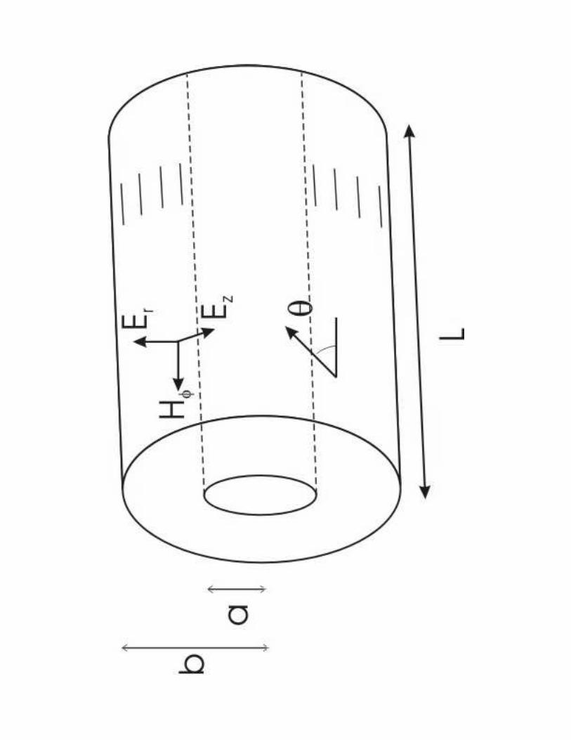
Figure CaptionsFig. 1. Schematic of a laser beam propagating through the nematic liquid-
crystal cylindrical guide. Transverse-magnetic (TM) modes are shown explic-itly.
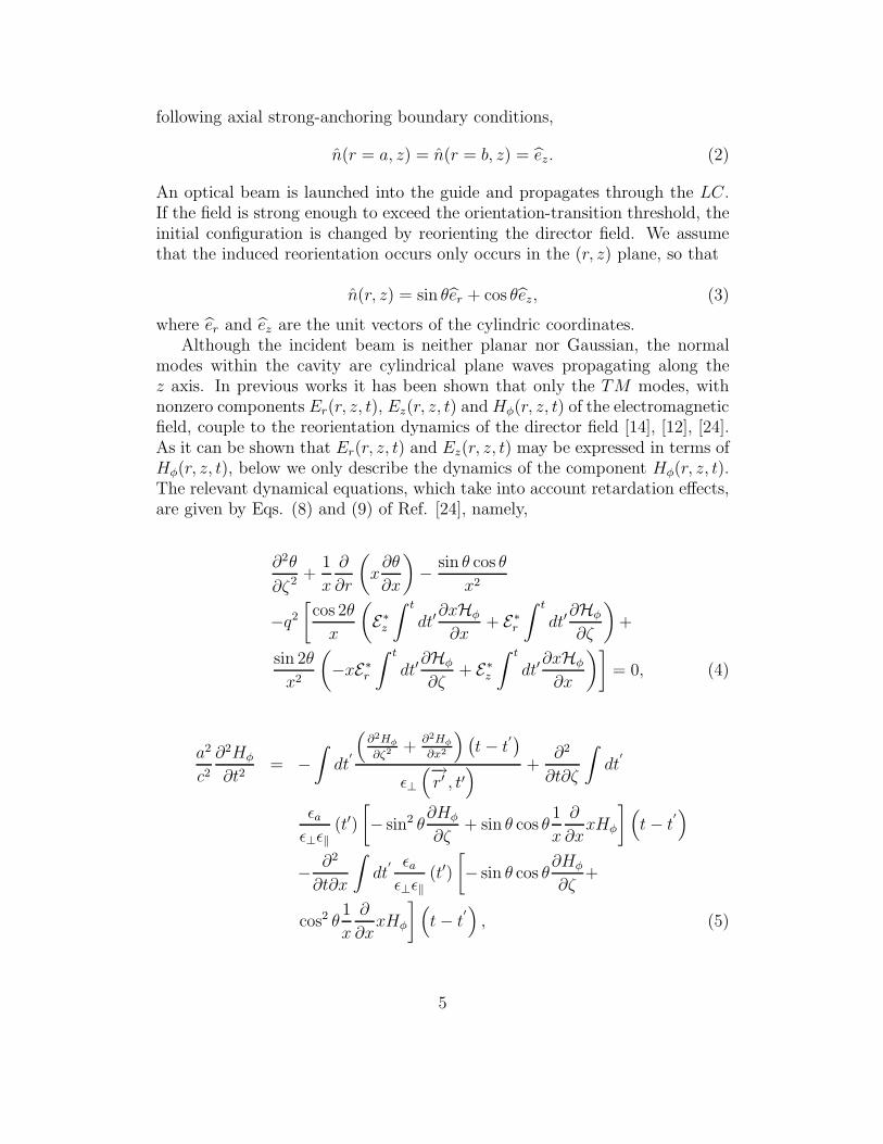
Fig. 2 Evolution of the amplitude of two perturbed single-embedded soli-tons of Eq. (1) (with ε = 1 and γ = 6). The upper curve corresponds tothe initial condition (60) with A0 = 0.815 > As, w0 = ws and r0 = rs, whereAs, ws and rs are the values (55) – (57). The lower curve corresponds to asimilar initial condition with A0 = 0.765 < As [A(z) and z are dimensionlessquantities].
Fig. 3. Temporal profile (at z = 50) of the perturbed single-embeddedsoliton of Eq. (1) whose amplitude (as a function of z is shown in the uppercurve of Fig. 2. The spectrum of this profile is shown in the insert [u and tare dimensionless quantities].
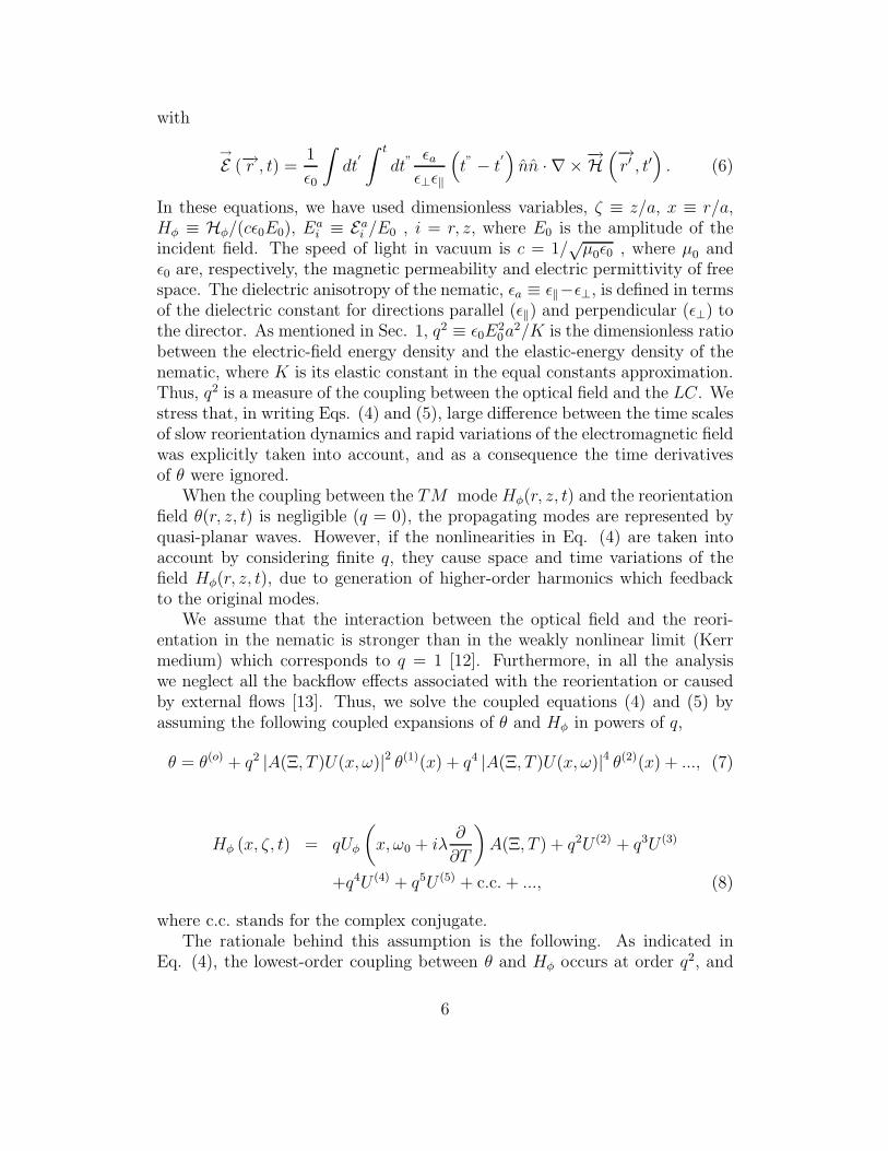
Fig. 4. The bold curve passing through the point E = (AE , WE) =(0.790, 2.192) is the plot of Eq. (75) with ε = 1 and γ = 6. The thinline passing through point 1 plots Eq. (78) with A(0) = 0.815 > AE andW (0) = WE . The thin line passing through point 3 is also a plot of Eq. (78),with A(0) = 0.765 < AE and W (0) = WE .
27
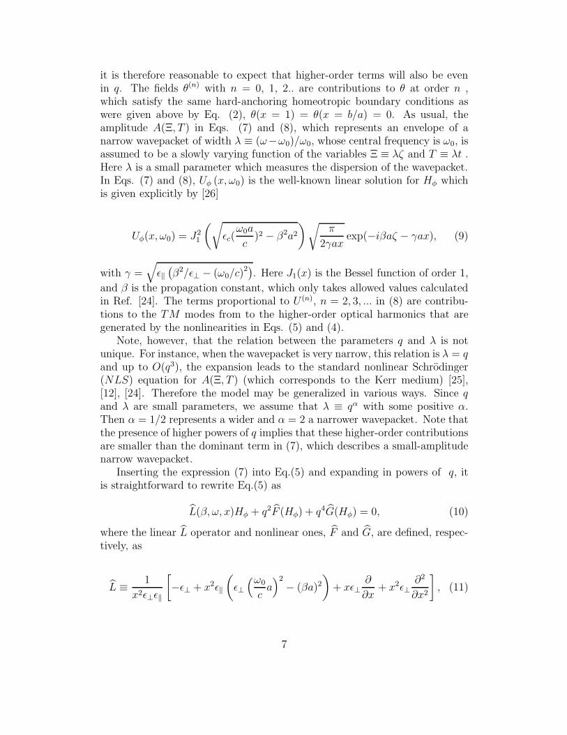
Fig. 5. Evolution of the amplitude of two perturbed double-embeddedsolitons of Eq. (1) (with ε = γ = 1). The upper curve corresponds to theinitial condition (60) with A0 = 0.815 > Ad, w0 = wd, and r0 = rd [where Ad,wd and rd are given by Eqs. (80) – (82)], and the lower curve corresponds to asimilar initial condition with A0 = 0.765 < Ad [A(z) and z are dimensionlessquantities].
Fig. 6. Spectrum (obtained at z = 200) of the radiation emitted by theperturbed double-embedded soliton whose amplitude (as a function of z) isshown in the upper curve of Fig. 5. The insert shows the spectrum (obtainedat z = 100) of the radiation emited when the sign of rd is reversed (i.e., whenrd = −1/4).
28
Appendix AExpressions for the coefficients A0, A1, A2, A3, A4, B0, B1, C0, C1, C2, C3
and C4, which appear in Eq. (17):
A0(a, b; γ, ǫ⊥) = 4a3b(a + b)γǫ⊥, (86)
A1(a, b; β, γ, µ, ǫa, ǫ⊥, k0) = a2{−24ab(a + b)[β2ǫa − ǫ⊥(ǫa + ǫ⊥)µk20] +
γ[16a(3a − b)b2β2ǫa − 2(a2 + ab + 8b2)ǫ⊥ +
16ab2(−3a + b)ǫ⊥(ǫa + ǫ⊥)µk20] −
ab(a + b)ǫ⊥γ2}, (87)
A2(a, b; β, γ, µ, ǫa, ǫ⊥, k0) = −12ab(a + b)γ[−ǫ⊥ + 4a2(β2ǫa − ǫ⊥(ǫa + ǫ⊥)µk20)],
(88)
A3(a, b; β, γ, µ, ǫa, ǫ⊥, k0) = a{24b(a + b)(β2ǫa − ǫ⊥(ǫa + ǫ⊥)µk20) +
2γ[32a2bβ2ǫa + 8ab2β2ǫa + 8b3β2ǫa +
aǫ⊥ − 7bǫ⊥ − 8b(4a2 + ab + b2)ǫ⊥(ǫa + ǫ⊥)µk20] +
γ2b(a + b)ǫ⊥}, (89)
A4(a, b; β, γ, µ, ǫa, ǫ⊥, k0) = 16ab(a + b)γ[−β2ǫa + ǫ⊥(ǫa + ǫ⊥)µk20], (90)
B0(a, b; γ, ǫ⊥) = −2ab(a − b)(a + b)2γǫ⊥, (91)
B1(a, b; β, γ, µ, ǫa, ǫ⊥, k0) = ab(a− b)(a+ b)2[24β2ǫa−24ǫ⊥(ǫa + ǫ⊥)µk20 +γ2ǫ⊥],
(92)
C0(a, b; γ, ǫ⊥) = 4ab3(a + b)γǫ⊥, (93)
C1(a, b; β, γ, µ, ǫa, ǫ⊥, k0) = b2{24ab(a + b)[β2ǫa − ǫ⊥(ǫa + ǫ⊥)µk20] +
γ[−16a2b(a − 3b)β2ǫa − 2(8a2 + 3ab + 3b2)ǫ⊥
+16a2b(a − 3b)ǫ⊥(ǫa + ǫ⊥)µk20
+ab(a + b)γǫ⊥}, (94)
29
C2(a, b; β, γ, µ, ǫa, ǫ⊥, k0) = −12ab(a + b)γ[−ǫ⊥ + 4b2(β2ǫa − ǫ⊥(ǫa + ǫ⊥)µk20)],(95)
C3(a, b; β, γ, µ, ǫa, ǫ⊥, k0) = b{24a(a + b)[−β2ǫa + ǫ⊥(ǫa + ǫ⊥)µk20] +
2γ(8a3β2ǫa + 8a2bβ2ǫa + 32ab2β2ǫa − 5aǫ⊥
+3bǫ⊥ − 8a(a2 + ab + 4b2)ǫ⊥(ǫa + ǫ⊥)µk20)
−a(a + b)ǫ⊥γ2}, (96)
C4(a, b; β, γ, µ, ǫa, ǫ⊥, k0) = 16ab(a + b)γ[−β2ǫa + ǫ⊥(ǫa + ǫ⊥)µk20] . (97)
An explicit form of θ(2)(x):
θ(2)(x) =βǫae
−(b+ax)γJ21 [√
ǫc(ω0ac
)2 − β2a2]
24x2a2b(a + b)2(b − a)π3γ2ǫ3⊥ǫ2
‖
[−a2e(1+x)aγ (1 − x)
(a2{24baxβ2ǫa
−48bxβ2γǫa(b − ax) + 2(xa − 2b)γǫ⊥ + baxǫ⊥γ2 + 24bxa(ω0a
c)2
(−1 + 2bγ − 2xaγǫ⊥ǫ‖)}
+ bxa{8baxβ2ǫa(3 + 2bγ − 2xaγ)
+2ǫ⊥γ(xa − 2b + γbax/2) − 8bxa(3 + 2bγ − 2xaγ)ǫ⊥ǫ‖(ω0a
c)2}
+ab(a − b)(a + b)2e−(b+a)γ[−2γǫ⊥ + xa
(24β2ǫa
+ǫ⊥(γ2 − 24ǫ‖(ω0a
c)2))]
+ b(xa − b)e(b+ax)γ (6baxγǫ⊥(b + xa)
+16a4x(b + xa)γ[β2ǫa − ǫ‖(
ω0a
c)2])
+ a2(−8ǫaxaβ2
[3b + 6b2γ
+xa(3 + 2xaγ)] − γǫ⊥ [4(b − 3xa) + xaγ(b + xa)] +
+8xa[3b + 6b2γ + xa(3 + 2xaγ)
]ǫ⊥ǫ‖(
ω0a
c)2)
+ a(−10x2a2γǫ⊥
+4b2[−6xaβ2ǫa + 12x2a2β2γǫa − γǫ⊥ − γ2xaǫ⊥/4
−6xa(2xaγ − 1)ǫ⊥ǫ‖(ω0a
c)2]
+ 4bxa[−6xaβ2ǫa − 4x2a2β2γǫa
+γǫ⊥/2 − γ2xaǫ⊥/4 + 2xa(2xaγ + 3)ǫ⊥ǫ‖(ω0a
c)2])]
. (98)
30
0 10 20 30 40 500.68
0.72
0.76
0.80
0.84
0.88
A(z
)
z
1.9
2
2.1
2.2
2.3
2.4
2.5
0.71 0.744 0.778 0.812 0.846 0.88
A
W
E1
2
3
4
0 50 100 150 200
0.68
0.72
0.76
0.80
0.84
0.88
0.92
A(z
)
z