Staging of Prostate Cancer Using Automatic Feature Selection, Sampling and Dempster-Shafer Fusion

Cancer Informatics 2009:7 57–73 57

ORIGINAL RESEARCH

Correspondence: Henry Leung, Department of Electrical and Computer Engineering, University of Calgary, ICT-402, 2500 University Drive NW, Calgary, Alberta, T2N 1N4 Canada. Email: [email protected].

Copyright in this article, its metadata, and any supplementary data is held by its author or authors. It is published under the Creative Commons Attribution By licence. For further information go to: http://creativecommons.org/licenses/by/3.0/.

Staging of Prostate Cancer Using Automatic Feature Selection, Sampling and Dempster-Shafer FusionSandeep Chandana1, Henry Leung1 and Kiril Trpkov2

1Department of Electrical and Computer Engineering, University of Calgary, ICT-402, 2500 University Drive NW, Calgary, Alberta, T2N 1N4 Canada. 2Department of Pathology and Laboratory Medicine, Calgary Laboratory Services, Calgary, Alberta T2V 1P9 Canada.

Abstract: A novel technique of automatically selecting the best pairs of features and sampling techniques to predict the stage of prostate cancer is proposed in this study. The problem of class imbalance, which is prominent in most medical data sets is also addressed here. Three feature subsets obtained by the use of principal components analysis (PCA), genetic algorithm (GA) and rough sets (RS) based approaches were also used in the study. The performance of under-sampling, synthetic minor-ity over-sampling technique (SMOTE) and a combination of the two were also investigated and the performance of the obtained models was compared. To combine the classifi er outputs, we used the Dempster-Shafer (DS) theory, whereas the actual choice of combined models was made using a GA. We found that the best performance for the overall system resulted from the use of under sampled data combined with rough sets based features modeled as a support vector machine (SVM).

Keywords: prostate cancer, staging, classifi er fusion

1. IntroductionProstate cancer is the leading type of cancer in men with a 27% incidence. The Canadian Cancer Society estimates about 72,700 cancer deaths, of which 3500 are in men with prostate cancer.1 There are several different types of treatments for prostate cancer, although some of the treatment techniques can substi-tute each other. The choice of a treatment is dependant upon the stage of the disease, i.e. the extent of cancer spread and whether the cancer has spread beyond the prostate. This information results in stag-ing the cancer. In essence, on the information gathered about the disease through biopsy and/or pros-tatectomy, staging categorizes a patient. Since different treatments result in variable outcomes, staging helps assess the risk of cancer progression and death based on the current extent of cancer, tumor char-acteristics, metastasis in the lymph nodes, and the spread of the disease to other parts of the body. Staging also helps in establishing a tradeoff between the risks of death due to cancer and death or medical complications due to treatment. This is particularly true for prostate cancer since a majority of men diagnosed with the disease are older adults, often suffering from multiple comorbidities.

Typically, medical doctors assess the clinical and the pathological data about the individual patient to assign a cancer stage and to choose the most appropriate treatment procedure. This is also known as clinical decision making and it is a complex process. Cancer staging performed by a doctor involves weighing multiple variables and processing information gathered by patient examination and by con-ducting various tests. However, this process may be subjective and therefore depends heavily on the doctor’s experience, skills and knowledge. Machine learning techniques can also be employed to learn and model the underlying theory when provided with relevant information and data. A variety of statistical, probabilistic and optimization tools under the umbrella of machine learning can be used to learn from past examples and a number of information systems have been developed to aid the clinical decision-making process.2

An automated cancer staging system was developed and is described in this paper. A classifi er based framework was used to draw a distinction between two primary stages of the disease: organ-confi ned disease and extraprostatic disease. The classifi er was modeled using past data from patients diagnosed with prostate cancer who are selected to undergo surgery (or prostatectomy). One of the key issues with such data sets is the class imbalance, resulting from the number of patients with organ-confi ned disease, which considerably exceeds the number of patients with extraprostatic disease. Data imbalances pose

58

Chandana et al

Cancer Informatics 2009:7

problems when less observed patterns are of higher relevance, because most of the machine learning techniques tend to generalize the patterns observed over the majority of data and ignore those observed over smaller portions of the data.3 Three approaches of dealing with the class imbalance problem were explored in this study. We also investigated the feature space reduction, because the data can potentially contain more information than required to perform the classifi cation.

There are a number of machine learning tech-niques that can be used to develop a classifi er, but it is well known that specifi c techniques are more suitable for certain domains. That is, for a particu-lar problem, specifi c techniques have superior performance, while other techniques are only able to produce mediocre or acceptable results. Even within one problem domain, different techniques can differ in the effi ciency for different (partial) ranges of the problem space. This leads to the conclusion that it is most appropriate when solving a problem, such as the one considered here, to primarily rely on actual data and information about the problem, rather than trying to generalize the performance of certain machine learning tech-niques in a generic manner.

Lately, a number of machine learning based tools have been developed for cancer diagnosis and prediction. And a majority of this work can be categorized into those which are heavily dependant upon expert domain knowledge or on extensive historic data. Garzotto et al.4 and Spurgeon et al.5 sequentially developed a decision tree approach, specifi cally CART (classifi cation and regression tree) to classify patients with aggressive prostate cancer based on ultrasound and biopsy markers. Sensitivity and specifi city were adopted as perfor-mance metrics in the study. Zlotta et al.6 developed a set of two artifi cial neural networks (ANN), where the fi rst ANN predicts the pathological stage of the patient and the second ANN classifies patients in groups based on cancer stage and the model performance was measured using the Receiver Operating Characteristic (ROC) curve. Veltri et al.7 favorably compared an ANN model to logistic regression for prostate cancer prediction and staging. Percentage of correctly classifi ed cases was adopted as the performance metric.

In this paper, we propose a novel system which selects the features automatically and couples appro-priate techniques in order to maximize the system performance. Specifi cally, performance of three

re-sampling techniques and three feature selection techniques were evaluated. A GA is used to search for optimal pairs of feature selection and sampling techniques; where optimality is based on the perfor-mance of the system. Once such pairs are identifi ed, respective classifiers are developed and a DS method8 is used to combine the component classifi er performances. The performance of such a system has been shown for two different types of classifi ers; the k-nearest neighbor (KNN) method and the sup-port vector machines (SVM). ROC curves9 are used as performance measures for the proposed cancer staging system. The next section describes the data used for this study and Section 3 provides justifi ca-tion for the use of ROC as a performance metric. Section 4 introduces the proposed method along with brief descriptions of the component classifi ers and feature extraction and sampling methods. Section 5 details the classifi er fusion and the obtained results. Section 6 provides details on the generic applicability of this method by validating it on a simulated prostate cancer dataset and on two pub-licly provided datasets of breast and lung cancer.

2. Study PopulationStaging and analysis of prostate cancer may be regarded as a function of the information (predic-tors) gathered during the diagnosis of every patient. Data from a total of 1174 patients with prostate cancer positive biopsies matched with their radical prostatectomies were used for this study. All specimens were processed in one labo-ratory between 07/2000 and 04/2005 and were reported using standard synoptic reports. The biopsy and the prostatectomy data were col-lected from the information system (Cerner) of the Calgary Laboratory Services. Various biopsy predictors that were considered are: Patient Age, Primary Gleason Grade, Secondary Gleason Grade, Biopsy Gleason Score, Prostate Specifi c Antigen (PSA), PSA Density (PSAD), Digital Rectal Exam (DRE), Transrectal Ultrasound (TRUS), Gland Volume, Number of Positive Cores, Total percent of Cores Involvement, and Total Cancer Length in mm. Prostatectomy data included: Disease Stage (pTNM), Primary Glea-son Grade, Secondary Gleason Grade, Prostatec-tomy Gleason Score, Tumor Volume, Seminal Vesicle Involvement, Surgical Resection Margin Status, and Pelvic Lymph Node Involvement. The prostate cancer dataset contained multiple stages

59

Prostate cancer staging using classifi er fusion


Table 1. Patient characteristics.

Clinical parameters Patients with Organconfi ned PCa

(n = 934)

Patients withExtraprostatic

extension(n = 120)

All patients(n = 1054)

Age (years):median (range)

59.9 (36.2–77.4) 63.4 (42.7–74.2) 60.4 (36.2–77.4)

Age categories (years): �50 (%) 103 (11) 5 (4.2) 108 (10.2) �50–60 (%) 368 (39.4) 34 (28.3) 402 (38.1) �60–70 (%) 404 (43.3) 67 (55.8) 471 (44.7) �70–80 (%) 59 (6.3) 14 (11.7) 73 (6.9)PSA (ng/ml): median (range)

5.7 (0.29–55) 6.9 (1.8–80) 5.8 (0.29–80)

PSA categories (ng/ml): �4 (%) 169 (18.1) 12 (10.0) 181 (17.2) �4–10 (%) 662 (70.9) 73 (60.8) 735 (69.7) �10–20 (%) 98 (10.5) 27 (22.5) 125 (11.9) �20–50 (%) 3 (0.3) 6 (5.0) 9 (0.9) �50–100 (%) 2 (0.2) 2 (1.7) 4 (0.4)Prostate Gland Volume (cc):median (range)

35.6 (7–193.2) 32.1 (10.02–176.6) 35.15 (7–193.2)

Prostate Gland Volume categories (cc): �25 (%) 188 (20.1) 33 (27.5) 221 (21.0) �25–50 (%) 503 (53.9) 61 (50.8) 564 (53.5) �50–100 (%) 243 (26.0) 26 (21.7) 269 (25.5)PSA Density:median (range)

0.15 (0.01–2.1) 0.22 (0.03–2.5) 0.16 (0.01–2.5)

(Continued)

for the disease, and thereby the stage data was converted into a binary format where extrapros-tatic disease represented by stages pT3 and pT4 was denoted by 1 and the organ-confi ned disease represented by stage pT2 was represented with a 0. Table 1 presents the statistical description of the data used in this study. Of the 1174 patient records, 1054 records were retained after remov-ing the ones with missing variables; 934 patients in the organ-confi ned stage and a 120 with an extra prostatic extension.

3. Performance MetricA classifi er’s performance typically refl ects how well it can discriminate between the objects belong-ing to different classes (two in this case). But the proposed system is expected to play a critical role,

particularly for patients where treatment modality may have a substantial impact on the post-treatment prognosis and survival. Therefore, in terms of the classifi cation performance, the cost of wrongly classifying a patient with extraprostatic disease is much higher than the cost of wrongly classifying one in the organ-confi ned stage. Conventional measures of performance therefore will not provide a relevant estimate of the classifi er performance; therefore an ROC curve and the area under the curve (AUC) were used as performance indices in this study.

An ROC curve is obtained by plotting the true positive rate (TPR) against the false positive rate (FPR) for varying decision thresholds. As shown in Table 2, TPR (and FPR) is representative of the number of positive (negative) examples correctly

60

Chandana et al


Table 1. (Continued)

Clinical parameters Patients with Organconfi ned PCa

(n = 934)

Patients withExtraprostatic

extension(n = 120)

All patients(n = 1054)

PSA Density categories: �0.10 (%) 231 (24.7) 18 (15.0) 249 (23.6) �0.10–0.25 (%) 535 (57.3) 49 (40.8) 584 (55.4) �0.25–0.50 (%) 139 (14.9) 38 (31.7) 177 (16.8) �0.50–1.0 (%) 25 (2.7) 11 (9.2) 36 (3.4) �1 (%) 4 (0.4) 4 (3.3) 8 (0.8)PCa Length (mm):Median (range)

5.25 (0–117) 19 (0.15–102.75) 6 (0–117)

PCa Length Categories: �10 (%) 615 (65.8) 41 (34.2) 656 (62.2) �10–20 (%) 174 (18.6) 25 (20.8) 199 (18.9) �20–40 (%) 107 (11.5) 37 (30.8) 144 (13.7) �40–60 (%) 31 (3.3) 12 (10.0) 43 (4.1) �60 (%) 7 (0.7) 5 (4.2) 12 (1.1)No. of cancer-positive cores:median (range)

2 (1–10) 4 (1–10) 2 (1–10)

No. of cancer-positive cores categories: �4 (%) 767 (82.1) 74 (61.7) 841 (79.8) �4–6 (%) 109 (11.7) 27 (22.5) 136 (12.9) �6 (%) 58 (6.2) 19 (15.8) 77 (7.3)Percent total core involvement on biopsy: median (range)

3.5 (0–78) 12.5 (0.1–68.5) 4 (0–78)

Percent core involvement categories: �3 (%) 441 (47.2) 20 (16.7) 461 (43.7) �3–10 (%) 280 (30.0) 30 (25.0) 310 (29.4) �10–20 (%) 140 (15.0) 42 (35.0) 182 (17.3) �20 (%) 73 (7.8) 28 (23.3) 101 (9.6)Biopsy Gleason Score: median (range)

6 (4–9) 7 (6–9) 6 (4–9)

Biopsy Gleason Score categories: �6 (%) 683 (73.1) 39 (32.5) 722 (68.5) 7–8 (%) 246 (26.3) 77 (64.2) 323 (30.6) �8 (%) 5 (0.5) 4 (3.3) 9 (0.9)

Abbreviations: PSA, prostate specifi c antigen; PCa, prostate cancer.

61



(incorrectly) classifi ed. They may be computed as follows,

TPRTP

TP FN

FPRFP

FP TN

=+

=+

;

;

The decision threshold or boundary for binary classifi cation refers to a threshold, below which the object is classifi ed as negative and above which it is classifi ed as positive. Such a threshold can be adjusted to trade off the cost of TP against the cost of FP, and each threshold setting provides a (FP, TP) pair. A series of such pairs produced by varying the decision threshold are used to plot the ROC curve. The ideal point on the ROC curve would be (0, 1) where all positive examples are classifi ed correctly and no negative examples are misclassified as positive. (0, 0) is the point where all the examples are predicted as negative. (1, 1) corresponds to clas-sifying all examples as positive.

One should note that, depending on the outcome of misclassifi cation, ideal decision thresholds may vary. For example, if the cost of misclassifying a patient with extraprostatic disease is lower than misclassifying a patient with organ-confi ned dis-ease, then a reciprocal ROC curve (to the one dis-cussed above) will be preferred. But in this study, a classifi er with an ROC tending towards the top-left of the graph indicates better performance than the ones with a lower ROC. In addition, ROC curves for different classifi ers tend to intersect each other; in which case AUC is used as an alternate metric. AUC ranges between the interval [0, 1] and greater the value of AUC, better is the technique. The AUC of a classifi er is equivalent to the probability that the classifi er will rank a randomly chosen positive example higher than a randomly chosen negative example. AUC as a measure has been proved to be equivalent of the Wilcoxon test statistic10 and the Gini Index11 i.e. unlike a typical measure of

classifi cation accuracy, the AUC quantifi es the likelihood that the underlying method will assign a higher probability of success to a patient having extraprostatic disease compared to a patient where the cancer is contained. Therefore such a measure will provide a true insight even in the case of imbal-anced data. Another important advantage is that the respective ROC is invariant to monotone transfor-mations of feature values,12 which renders fl exibil-ity in manipulating the feature set if necessary.

4. Proposed System and MethodologiesThe proposed system consists of four major parts: feature extraction, data sampling, classifi cation and classifi er fusion. Feature extraction helps identify the most prominent features in the search space thereby reducing the required computational and interpretational effort. Data sampling provides a mechanism to eliminate the bias or imbalance that exists in the data by over-sampling the minority class or under- sampling the majority class or a selective combination of both. Feature extraction and sampling enable the implementation of a clas-sifi er in order to model the class disparity in the data. A GA is then used to identify compatible sets of features, sampling techniques and classifi ers in order to maximize the performance of subsequent DS classifi er fusion. The adopted methods are indi-vidually described in the following subsections.

A. Feature selectionFeatures extracted or selected from the input data, can be categorized into continuous, discrete or projected features. Existing processes of selecting features can be classifi ed as: those based on sta-tistical information, those based on empirical information and those based on search in the sample space. Following this approach, three techniques associated with the major types of fea-tures have been adopted. Selection of RS based discretized features relies on empirical information about the system, PCA based transformed feature selection relies on the statistics of the data and GA based continuous feature selection relies on intel-ligent search through the sample space.

1. RS featuresRough Set Theory13 adopts an equivalence relation such that two objects (x, y) form an indiscernible

Table 2. ROC confusion matrix.

Predicted class Positive NegativeActual class Positive TP FN Negative FP TN

Abbreviations: TP, true positive; FN, false negative; FP, false positives; TN, true negatives.

62

Chandana et al


pair over the attribute a, only if a(x) = a( y); and assuming that (x, y) Є Ra, then Ra would be called the a-indiscernibility relation and denoted by the symbol INDa. Given that, a lower approximation set consists of all objects which can certainly be classifi ed as elements of X over an indiscernibility relation R, i.e.

R X Y U R Y X= ∈ ⊆∪{ : } (1)

The lower approximation set is also known as the Positive region i.e.

POS X R XR ( ) = (2)

The signifi cance of a variable is then expressed as a function of the dependency (γ) of a variable in classifying the objects into the classes of U IND D| ( ). The dependency of decision variable D on independent variable R is given as:

γ RRD

POS D

U( )

( )

| |=

(3)

where U denotes the cardinality of set U , i.e. the number of elements contained in that set. The signifi cance of a variable a is the increase of depen-dency between the independent variables and the decision variable after the addition of a, i.e.

SGF a R D Y D Y DR a R( , , ) ( ) ( ){ }= −+ (4)

Because dependency (defi ned by Equation 3) only considers the number of rules that cover various instances and not the number of instances that each of the rules represents, a parameterized average support heuristic method has been adopted to include both, the number of rules and the num-ber of instances supporting each rule in computing the average support function (similar to the mea-sure of dependency), given as:

F D POS D

nS R dR R

i

n

i( ) | ( ) | ( , )= ×=∑1

1

(5)

where di is a possible value of decision variable D, and S R d x X POSi IND R IND R R( , ) max{| [ ] |: [ ]( ) ( )= ⊂( )}D di= indicates the maximal size of the equivalence classes included in the positive region of { }D di= i.e. the support of the most signifi cant rule for the decision class { }D di= .

The signifi cance of a variable (Equation 4) is redefi ned as:

SGF a R D F D F DR a R( , , ) ( ) ( ){ }= −+ (6)

2. PCA featuresPCA14 reduces the feature space by projecting the complete feature set onto fewer variables known as the principal components with the objective of maximizing the variance in a least squares sense. This produces uncorrelated components with minimal information loss. X denotes a {n × p} matrix for n instances of a system represented through a p-dimensional feature space. Applying PCA begins by fi rst normalizing X into a feature set with zero mean and unit variance. PCA aims to transform this p-dimension into an m-dimensional feature space where m � p, but typically the fi rst few components represent the largest portion (~90%) of the original information, therefore effectively using only the fi rst m* (�� p) components. The correlation matrix SX of X is given as:

S

X X

nX

T

=−1

(7)

If Y represents the {n × m} matrix for n instances of a system represented through a reduced m-dimensional feature space, the transformation is achieved by weighting the original features using m number of principal components. The m com-ponents are identifi ed as the eigenvectors corre-sponding to the fi rst m largest eigenvalues of the correlation matrix SX. The transformation of the feature space is therefore given as:

Y V Xm= ⋅ (8)

where Vm is a { p × m} matrix made up of the m eigenvectors. Singular value decomposition of X is performed as:

X U L V T= ⋅ ⋅ (9)

where U is column-orthogonal matrix of size {n × p}, L is a square diagonal matrix of size { p × p} where the diagonal elements are square roots of the eigenvalues of the correlation matrix SX and V is also a square matrix of size { p × p} where the columns correspond to the eigenvectors of the correlation matrix. Vm consists of the fi rst

63



m eigenvectors in V. The number of principal components or eigenvectors (m) is determined as per a set threshold.

3. GA featuresGA15 based search depends on a user defi ned fi tness function; in this study, the product of the number of features and the average error in the predicted output class has been adopted as the fi tness func-tion. GA based search uses a chromosome repre-sentation of the solutions and a set of genetic manipulations in order to arrive at an optimum solution. First, a chromosome of the length equal to the total number of features in the input space is created. The value of the bit associated with a feature is set to 0 to indicate that the feature is not considered, whereas a bit value of 1 indicates that the feature will be considered. The search process begins with an initial generation where the population is generated randomly; all of the chromosomes in this generation are evaluated against the fi tness function and the best chromo-somes (representing better solutions) are chosen to propagate into the next generation. Through heuristic manipulation of the chromosome struc-tures in every generation, it is ensured that the newer generations always have an average fi tness higher than the previous generations. The search stops either when a fi tness threshold is achieved, or when the search runs out of the threshold on the number of generations. In this study, the population size per generation was set to 25 and the limit on the generations used in the search was set to 1000. These numbers were selected after a short sequence of random trials. Mutation and crossover operators were utilized to generate off springs for the next generation, and a simple natural selection based on the current fi tness values was used to identify potential parents.

B. Data samplingTwo re-sampling methods are often used in order to overcome an imbalance; one is to under-sample the majority class to match the size of the minority class and the other is to over-sample the minority class to match the size of the majority class. Over-sampling and under-sampling techniques have been previously evaluated for imbalanced datasets,16 and a conclusion that both meth-ods were effective was drawn. In one study,17 combined over-sampling of the minority class and

under-sampling of the majority class was used, but the combination did not provide significant improvement in the performance. Over-sampling in these cases was done by duplicating the original examples from the minority class, which does not cause minority class decision boundary to spread into the majority class region, but instead creates decision regions similar to those existing for the minority class. This shortfall may be overcome using an approach called SMOTE, as proposed in one study.18

SMOTE is an over-sampling of the minority class by creating “synthetic” examples. SMOTE is actually an interpolation approach where the synthetic examples are created along the line segments joining the example under consideration and any/all of its k nearest neighbors in the minority class. The synthetic examples are created in the following manner:1. For each minority class example, fi nd its k

nearest neighbors in the minority class.2. Randomly choose m (m � k) examples from the

k nearest neighbors depending upon the over-sampling amount. For instance, if the required over-sampling amount is 200%, then only 2 neighbors are randomly selected from the k nearest neighbors.

3. Calculate the differences between the minority class example under consideration and its m nearest neighbors, which are randomly chosen.

4. Multiply the differences by a random number between 0 and 1, and add the results to the minority class example under consideration to produce m synthetic examples for this minority class example.In this study, we used three re-sampling tech-

niques: 1) under-sampling 2) SMOTE and 3) combined under-sampling and SMOTE in the multi-classifi er fusion diagnosis system.

C. Classifi ersClassification, an operation of assigning an unknown sample to one of the output classes can typically be performed by either fi tting a model around the independent variables or through aver-aging or majority voting. In order to exemplify the proposed system for both types, we used SVM, which identifi es a nonlinear model of the input variables, and KNN, which is based on majority voting.

64

Chandana et al


1. Support vector machinesSVM19 is a supervised machine learning methodology used for classification and regression. Compared with the traditional statistical and neural net-work methods, SVM has the advantage to effec-tively avoid a local minimum due to its convexity property. On the other hand, SVM uses the kernel trick to apply linear classification techniques to nonlinear classification problems. When Gaussian kernels are used, the resulting SVM corresponds to a radial basis function (RBF) network with Gaussian radial basis func-tions. In comparison with traditional RBF net-work, SVM has the ability to automatically determine the model size by selecting the sup-port vectors based on quadratic programming (QP) procedure. Hidden neurons correspond to the support vectors. The support vectors serve as the centers of basis function in the RBF net-work. For linear SVM, the decision function is given in a linear form as:

f x w x b( ) = ⋅ + (10)

The decision value produced by SVM is not the estimate of posterior probability. Here, the binning technique is used to transform the output of the SVM into calibrated probability.19 The binning technique proceeds by fi rst sorting the training examples according to their decision values, and then dividing the value range into k equal sized intervals or bins. Given an exam-ple x, place it in a bin according to its decision value. The conditional probability of x is esti-mated as:

p c x x

m

n( ( ) | )=1

(11)

where n is the number of training examples that fall within the bin, m is the number of positive examples among these n training examples.

2. K-nearest neighborKNN20 is a statistical method for classifying objects based on their k nearest training examples in the feature space. KNN classifies a new example by fi rst calculating the distances of the new example from all other examples in the train-ing set, and then selects k nearest training exam-ples. The class of the new example is the most

frequent class label presented among the k nearest examples:

c x k km m is

i( ) ,= = =ω max 1 (12)

where s is the number of classes, ki is the number of examples belonging to class ωi among the k nearest examples, ∑ki = k; i = 1… s. The output of KNN classifi er is not probability. For the two-class problem, the conditional probability can be directly estimated as:

p c x x

k

k( ( ) | )=1 1

(13)

where k1 is the number of positive examples among the k nearest neighbors of x and SMOTE in the multi-classifi er fusion diagnosis system.

D. Classifi er fusionSuppose the universal set Θ = {A1… Am} is a set of all propositions under consideration and its power set 2Θ is formed by all possible subset of Θ, including the empty set ∅, a one-element subset {Ai} is called a singleton and a subset {Ak , Al} represents a proposition denoting the disjunction Ak ∪ Al (k, l ∈ {1, 2 … m}). DS theory assigns a numerical value to each subset of the power set 2Θ using mass function or basic probability assign-ment m: 2Θ → [0, 1]. The mass function has the following properties:

m m A

A( ) , ( )∅ = =

∈∑0 12Θ

(14)

Subsets A ∈ 2Θ that satisfy the condition m(A) � 0 are called the focal elements of mass function m. Since a subset A is the disjunction of all its elements. If the proposition B ⊆ A is true, then the proposition A is also true. Hence, given a subset A, the belief bel (A) is defi ned as the sum of all the masses of its subsets:

bel A m B

B A( ) ( )=

⊆∑ (15)

The belief value bel(A) indicates the degree that evidence supports the proposition A. When two evidences exist, there will be two different mass functions m1 and m2. If these two evidences are independent of each other, then the two mass

65



functions can be combined into a new mass function m using Dempster’s rule21:

m A m m A

Km A m A

m A m A

A A A

A

( ) ( ) ( )

( ) ( )

( ) ( )

= ⊕

=

=

∩ =∑1 2

1 1 2 2

1 1 2 2

11 2

whereΚ

11 2∩ =∅∑ A

(16)

=1 − m A m A

A A 1 1 2 21 2( ) ( )

∩ ≠ ∅∑

is a normalizing factor, which measures how much m1(A1) and m2 (A2) are in confl ict with each other. So K is also called the confl ict measure. If K = 0, the combination of m1 and m2 does not exist, it means m1 and m2 are totally contradictory. When more than two evidences exist, the mass function can be com-bined by sequentially using the formula:

m m m mk= ⊕ ⊕ ⊕1 2 � (17)

Multiple classifi er fusionFor the prostate cancer stage prediction problem, there are two exhaustive and mutually exclusive propositions Ai. Proposition A1 denotes that input example x is negative, and proposition A2 denotes that input example x is positive. The power set 2Θ = {Ø, {A1}, {A2}, {A1, A2}}. The key step in the DS fusion process is to assign a basic prob-ability assignment (BPA) to each subset of 2Θ. After calibrating, if the outputs of each of the classifi ers as conditional probabilities p (Ai|x), let D k (x) = [dk,1(x), dk,2(x)] denote the output of clas-sifi er ck, then dk,1(x) + dk,2(x) = 1; k = 1, 2. Given classifi er ck, assign the BPA values of subset {A1} and {A2} as:

m A d

m A d

k k

k k

( )

( )

,

,

1 1

2 2

=

= (18)

where mk(Ai) indicates the degree of belief that proposition Ai is true, provided by classifi er ck, k = 1, 2. Combining the evidence provided by the individual classifi ers, the belief value of each proposition is given as:

bel A m Ai i( ) ( )= (19)

where m is the combined mass function calculated by the sequential use equation (hello)

m m m m

m m m

= ⊕ ⊕

= ⊕ ⊕1 2 3

1 2 3( )

(20)

The fi nal decision is made according to the approach dealing with the imbalanced data. If re-sampling is used in the fused diagnosis system, the fi nal decision is made by assigning the label of the class with the largest belief value:

c x m m

bel A bel Am i i

( ) ; ,

( ) max ( )

= =

= =

1 2

12

(21)

If the imbalance is dealt with by changing the decision threshold, the class of the example is determined by changing the threshold on belief value of the positive class:

c x bel A T

c x else

( ) , ( )

( ) ,

= >=

⎧⎨⎩

1

01

(22)

where T is the threshold.

5. ResultsExperiments were done to assess the performance of all of the feature extractor-sampling-classifi er pairs. The available data set was divided into two: one for building the models and the other to test the developed models. Appropriate ratio of the training and testing data sizes for SVM was identifi ed by running differ-ent trials as shown in Figure 1. The best testing per-formance was observed when 70% of the total samples were used for training. The dip in the perfor-mance of the SVM beyond the training data size of 70% can be attributed to overfi tting, when the trained model lost its ability to generalize, and was rather rigid to the training data. As the performance of the KNN depends on the number of neighbors considered in the output class allocation, the optimum number of neighbors was identifi ed by running trials with different sizes, and 5 was the most optimal. Although higher number of neighbors may seem to have the ability to generalize, it is the separability of the data according to assigned classes that has the highest infl uence on the appropriate number of neighbors.

The AUC curves were generated for all of the feature-sample-classifi er sets by altering the decision

66

Chandana et al


4 6 8 10 12 14 16 18 2050

55

60

65

70

75

80

85

90

95

100Optimum number of naeighbors

Number of neighbors

AU

C (%

)

Figure 2. KNN performance for different number of neighbors.

0 0.1 0.2 0.3 0.4 0.5 0.6 0.7 0.8 0.9 10

0.1

0.2

0.3

0.4

0.5

0.6

0.7

0.8

0.9

1

UndersamplingSMOTESMOTE + Undersampling

False positive rate

True

pos

itive

rate

Figure 3. ROC curves of SVM and Rough Set Features.

0 0.1 0.2 0.3 0.4 0.5 0.6 0.7 0.8 0.9 10

0.1

0.2

0.3

0.4

0.5

0.6

0.7

0.8

0.9

1


False positive rate

True

pos

itive

rate

Figure 4. ROC curves of KNN and Rough Set Features.

30 40 50 60 70 80 9050

55

60

65

70

75

80

85

90

95

100Optimum training data size

AU

C (%

)

Training data size (%)

Figure 1. SVM performance for different training data sizes.

threshold. When the outputs of the classifi ers for all combinations were transformed into conditional probabilities, altering the decision threshold simply meant altering the respective probability threshold. By varying the probability threshold, the testing examples are re-labeled, giving out a series of (FP, TP) pairs. Each pair of (FP, TP) is a point on the ROC curve. For individual classifi ers, ROC curves are created by changing the threshold on conditional probability p (c(x) = 1|x). ROC curve for the fused classifi er is created by changing the threshold on belief value of the positive class. The outputs of SVM and KNN are then fused using DS fusion approach and ROC curves are plotted for the individual clas-sifi ers (Figures 3–14). AUC of the generated plots were tabled per classifi er in Tables 3 and 4.

To show the effect of combining multiple sets of features and the effect of combining different types of sampling, DS fusion of the classifi er outputs was performed over various combinations of sampling and feature selection methods. The following notation was adopted to refer to the clas-sifi ers developed in this study;

Notation: ‘C’ – ‘F’ – ‘S’.

where ‘C’ represents the type of classifi er used, i.e. {SVM, KNN}; ‘F’ represents the type of feature selection tool used, i.e. {R (rough sets), P (princi-pal component analysis), G (genetic algorithm)} and ‘S’ represents the type of data sampling adopted, i.e. {U (under sampling), S (SMOTE),

67



0 0.1 0.2 0.3 0.4 0.5 0.6 0.7 0.8 0.9 10

0.1

0.2

0.3

0.4

0.5

0.6

0.7

0.8

0.9

1


True

pos

itive

rate

False positive rate

Figure 5. ROC curves of SVM and PCA Features.

0 0.1 0.2 0.3 0.4 0.5 0.6 0.7 0.8 0.9 10

0.1

0.2

0.3

0.4

0.5

0.6

0.7

0.8

0.9

1


False positive rate

True

pos

itive

rate

Figure 6. ROC curves of KNN and PCA Features.

Figure 7. ROC curves of SVM and GA Features.

Figure 8. ROC curves of KNN and GA Features.

Figure 9. ROC curves of SVM and Under-sampling.

0 0.1 0.2 0.3 0.4 0.5 0.6 0.7 0.8 0.9 10

0.1

0.2

0.3

0.4

0.5

0.6

0.7

0.8

0.9

1

RSPCAGA

False positive rate

True

pos

itive

rate

Figure 10. ROC curves of SVM and SMOTE.

68

Chandana et al


0 0.1 0.2 0.3 0.4 0.5 0.6 0.7 0.8 0.9 10

0.1

0.2

0.3

0.4

0.5

0.6

0.7

0.8

0.9

1

True

pos

itive

rate

KNN with SMOTE data

RSPCAGA

False positive rate

Figure 13. ROC curves of KNN and SMOTE.

0 0.1 0.2 0.3 0.4 0.5 0.6 0.7 0.8 0.9 10

0.1

0.2

0.3

0.4

0.5

0.6

0.7

0.8

0.9

1

RSPCAGA

False positive rate

True

pos

itive

rate

Figure 14. ROC curves of KNN and combined sampling.

Table 3. AUC values with SVM for PCa.

Under Smote UnderSmote DSRST 0.8409 0.7223 0.8326 0.8611PCA 0.8075 0.7439 0.8334 0.8392GA 0.7704 0.7425 0.7112 0.7597DS 0.8313 0.7461 0.8420

Table 4. AUC values with KNN for PCa.


0 0.1 0.2 0.3 0.4 0.5 0.6 0.7 0.8 0.9 10

0.1

0.2

0.3

0.4

0.5

0.6

0.7

0.8

0.9

1

RSPCAGA

False positive rate

True

pos

itive

rate

Figure 11. ROC curves of SVM and combined sampling.

0 0.1 0.2 0.3 0.4 0.5 0.6 0.7 0.8 0.9 10

0.1

0.2

0.3

0.4

0.5

0.6

0.7

0.8

0.9

1

RSPCAGA

False positive rate

True

pos

itive

rate

Figure 12. ROC curves of KNN and Under-sampling.

US (under-sampling + SMOTE)}. Therefore SVM-P-S would imply the classifi er based on SVM trained over PCA features obtained from SMOTE sampled data.

It is evident in Table 3 that the SVM trained over RST based features had a superior perfor-mance. Similarly, under-sampling combined with SMOTE trained SVM had the best performance

among the types of sampling. DS fusion of SVM-R-[U, S, US] has 86.1% under favorable AUC. KNN performed poorly as a classifier over all sampling and features. Although much lower than average SVM, the combination of KNN-R-S has the highest favorable AUC at 80.9%, as illus-trated in Table 4. In general, DS fusion improved the performance over any single model. We also

69



note that under sampling proved a more efficient method of re-sampling the data than generating synthetic samples. As it has been observed pre-viously,18 generating synthetic samples can cause the decision boundary to spread, resulting in a poor performance. Despite the fact that fewer samples make parameter estimation dif-ficult in SVM and neural networks, under sam-pling of the data should be preferred, since performance degradation is higher when using synthetic sampling than using SVM trained over smaller data sets.

B. Comparison between different methodsMethodology proposed in this study relies on the use of GA to identify the most optimal set of classifi ers for fusion, where fi tness is defi ned as the overall fused performance. A total of 18 models (9 each for SVM and KNN with variations in the sampling method and features) were developed, and GA was used to choose the best set of fusion

classifi ers. Once an x set of classifi ers for best fused performance were identifi ed, the AUC (of ROC for changing thresholds) was determined for the test samples alone. The results for the overall performance from all model combinations obtained by fusing 2, 3, 4 and 5 models are shown in Table 5 (A) with the highest classification accuracy at 90.1% and a respective ROC AUC of 0.8640. Clearly, the number of fused models does not have a considerable impact on the perfor-mance, which is the reason why the trials were stopped after the fusion of 5 models. A combination of the outputs of 4 models has the best overall performance on the testing data. In this study, under sampling was observed to be the most effi cient for data sampling. KNN (with average performance for all models much lower than SVM) seems to have contributed equally in the best overall performance. As observed from Tables 3 and 4, overall effi ciency of rough sets based features was highest of all subsets. Rough sets based discretized features increase the dis-tance between different output classes, and thus

Table 5. Performance of GA optimized fusion for PCa.

2-models 3-models 4-models 5-modelsModels SVM-R-U SVM-R-U SVM-R-U SVM-R-U

SVM-R-US SVM-P-US SVM-P-U KNN-R-SSVM-R-US KNN-R-S SVM-P-US

KNN-G-U SVM-R-USKNN-G-U

AUC 0.8617 0.8626 0.8640 0.8631Accuracy 89.4% 89.7% 90.1% 89.8%

A. Comparison between different model combinations.

Proposed C4.5 ANN DS (C4.5 + ANN)AUC 0.8640 0.8049 0.8359 0.8580

Accuracy 90.1% 83.0% 86.0% 88.5%

Table 6. AUC values with SVM for SimPCa.


Table 7. AUC values with KNN for SimPCa.


70

Chandana et al


tend to impact the overall classifi cation performance in a favorable manner.

In order to contrast the performance of the proposed method with existing techniques, a C4.5 decision tree and a two-layer neural network have been additionally developed using the same data. C4.5, similar to the likes of expert systems and nomograms, is a simple and transparent technique which can also be regarded as means of knowledge representation. ANN, similar to the likes of SVM and nonlinear regression, on the other hand is a complex nonlinear model. These two models have been chosen to represent the majority of present day classifi ers. As can be observed from Table 5 (B), the proposed method fairs very well compared to the two other. Moreover, the performance of a 2-model combination (AUC: 0.8617, Accuracy: 89.4%) is better than that of the DS (C4.5 + ANN) method (AUC: 0.8580, Accuracy: 88.5%).

6. Validation with Other DatasetsA number of such techniques have been reported in the literature and these techniques perform very well for individual datasets that the techniques have been built for. Data used in the previous section is a large, unbiased and consecutive patient cohort originating from one institution. Therefore it should be comparable to other current patient data obtained

from patients who undergo prostatectomy in the larger North American centers. Although currently we have no access to data sets from different hos-pitals, we present the results of applying the pro-posed method to three different cancer datasets to testify that the proposed method is generic in appli-cability and that it outperforms other existing techniques, Firstly, we considered a simulated prostate cancer (SimPCa) dataset. 1000 patient records were synthetically generated using a com-bination of the under-sampling and SMOTE meth-ods. It was ensured that the overall statistics of the data remained consistent with the dataset reported in Table 1. In order to facilitate comparison, the same classifi ers, feature extractors and sampling techniques were adopted. ROC curves were gener-ated and the respective AUC given in Tables 6–8. The performance of the classifi er is very similar to the results in Section 5. SVM trained over RST identifi ed features had the best performance and KNN remained a weak classifi er for this dataset. Consistent with the other results, GA optimization identifi es the same four model fusion.

The other two datasets considered for this pur-pose have been adopted from the University of California-Irvine data repository. Using the two public datasets we demonstrate that the proposed method compares favorably to the existing techniques. The Wisconsin Breast Cancer (BCa)

Table 8. Performance of GA optimized fusion for SimPCa.

2-models 3-models 4-models 5-modelsModels SVM-R-U SVM-R-U SVM-R-U SVM-R-U

SVM-R-US SVM-P-US SVM-P-U KNN-R-SSVM-R-US KNN-R-S SVM-P-US

KNN-G-U SVM-R-USKNN-G-U

AUC 0.8596 0.8620 0.8632 0.8610Accuracy 88.8% 89.4% 89.8% 89.3%

Table 9. AUC values with SVM as the classifi er for BCa.


Table 10. AUC values with KNN as the classifi er for BCa.


71



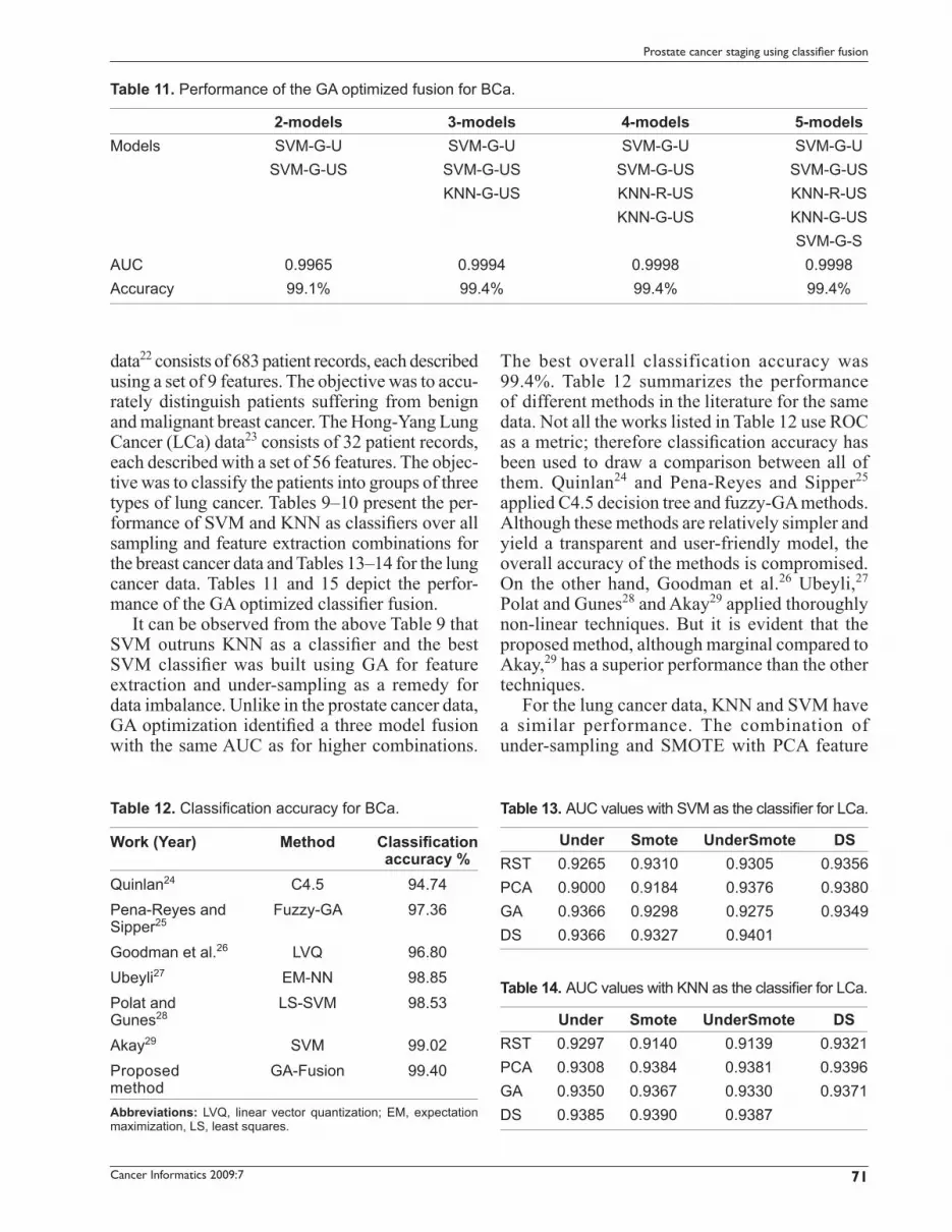
data22 consists of 683 patient records, each described using a set of 9 features. The objective was to accu-rately distinguish patients suffering from benign and malignant breast cancer. The Hong-Yang Lung Cancer (LCa) data23 consists of 32 patient records, each described with a set of 56 features. The objec-tive was to classify the patients into groups of three types of lung cancer. Tables 9–10 present the per-formance of SVM and KNN as classifi ers over all sampling and feature extraction combinations for the breast cancer data and Tables 13–14 for the lung cancer data. Tables 11 and 15 depict the perfor-mance of the GA optimized classifi er fusion.

It can be observed from the above Table 9 that SVM outruns KNN as a classifi er and the best SVM classifi er was built using GA for feature extraction and under-sampling as a remedy for data imbalance. Unlike in the prostate cancer data, GA optimization identifi ed a three model fusion with the same AUC as for higher combinations.

The best overall classification accuracy was 99.4%. Table 12 summarizes the performance of different methods in the literature for the same data. Not all the works listed in Table 12 use ROC as a metric; therefore classifi cation accuracy has been used to draw a comparison between all of them. Quinlan24 and Pena-Reyes and Sipper25 applied C4.5 decision tree and fuzzy-GA methods. Although these methods are relatively simpler and yield a transparent and user-friendly model, the overall accuracy of the methods is compromised. On the other hand, Goodman et al.26 Ubeyli,27 Polat and Gunes28 and Akay29 applied thoroughly non-linear techniques. But it is evident that the proposed method, although marginal compared to Akay,29 has a superior performance than the other techniques.

For the lung cancer data, KNN and SVM have a similar performance. The combination of under-sampling and SMOTE with PCA feature

Table 11. Performance of the GA optimized fusion for BCa.

2-models 3-models 4-models 5-modelsModels SVM-G-U SVM-G-U SVM-G-U SVM-G-U

SVM-G-US SVM-G-US SVM-G-US SVM-G-USKNN-G-US KNN-R-US KNN-R-US

KNN-G-US KNN-G-USSVM-G-S

AUC 0.9965 0.9994 0.9998 0.9998Accuracy 99.1% 99.4% 99.4% 99.4%

Table 12. Classifi cation accuracy for BCa.

Work (Year) Method Classifi cation accuracy %

Quinlan24 C4.5 94.74Pena-Reyes andSipper25

Fuzzy-GA 97.36

Goodman et al.26 LVQ 96.80Ubeyli27 EM-NN 98.85Polat andGunes28

LS-SVM 98.53

Akay29 SVM 99.02Proposedmethod

GA-Fusion 99.40

Abbreviations: LVQ, linear vector quantization; EM, expectation maximization, LS, least squares.

Table 13. AUC values with SVM as the classifi er for LCa.


Table 14. AUC values with KNN as the classifi er for LCa.


72

Chandana et al


extraction had the best performance for SVM as a standalone classifi er, whereas the combination of SMOTE and PCA feature extraction had the best performance for a single KNN based classi-fi er. GA optimization yielded a four model fusion as shown in Table 15 with an overall classifi cation accuracy of 97.5%. Table 16 compares the per-formance of the proposed method to two other methods from the existing literature. The proposed method has a much better performance when compared to that of Aeberhard’s30 RDA model and the neuro-fuzzy model adaptation used by Luukka.31 Although Luukka31 reports a 99.99% accuracy for a larger training-testing ratio, a per-formance of 65.48% is given for a 70:30 ratio, which is the same as used for this work. Therefore, it is concluded that the proposed GA based opti-mization of multiple model fusion is generically applicable across a wide range of data and in addition ensures better performance than most existing techniques.

7. ConclusionsA number of classifi er models based on KNN and SVM have been developed to test the automatic prediction of cancer stage using different features and data samples. We propose a novel approach of

using a GA to select the best models and to combine their outputs using the DS theory. Owing to DS fusion and GA optimization, the overall performance improved in all tested models. In particular, three sampling and three feature selection methods have been employed in this study. Under-sampling and rough sets based features were identifi ed to be most useful in improving overall performance of the system.

DisclosureThe authors report no confl icts of interest.

References 1. Canadian Cancer Society/National Cancer Institute of Canada.

Canadian Cancer Statistics. 2007;11–6. 2. Fieschi M, Coiera E, Li YCJ. Machine Learning in Clinical Decision

Making. Proceedings of 11th World Congress on Medical Informatics. 2004. p. 699–705.

3. Kubat M, Matwin S. Addressing the Curse of Imbalanced Training Sets: One Sided Selection. Proceedings of the 14th International Conference on Machine Learning. 1997. p. 179–86.

4. Garzotto M, Beer TM, Hudson RG, et al. Improved detection of pros-tate cancer using classifi cation and regression tree analysis. Journal of Clinical Oncology. 2005;23(19):4322–9.

5. Spurgeon SEF, Hsieh Y-C, Rivadinera A, et al. Classifi cation and Regression Tree Analysis for the Prediction of Aggressive Prostate Cancer on Biopsy. Journal of Urology. 2006;175:918–22.

6. Zlotta AR, Remzi M, Snow PB, et al. An Artifi cial Neural Network for Prostate Cancer Staging when Serum Prostate Specifi c Antigen is 10ng./ml. or less. Journal of Urology. 2003;169:1724–8.

7. Veltri RW, Chaudhari M, Miller MC, et al. Comparison of Logistic Regression and Neural Net Modeling for Prediction of Prostate Cancer Pathologic Stage. Clinical Chemistry. 2002;48(10):1828–34.

8. Shafer G. A Mathematical Theory of Evidence. New York: Princeton University Press; 1976.

9. Fawcett T. An introduction to ROC analysis. Pattern Recognition Letters. 2006;27:861–74.

10. Hanley JA, McNeil BJ. The Meaning and Use of the Area under a Receiver Operating Characteristic curve. Radiology. 1982;143:29–36.

11. Hand DJ, Till RJ. A simple generalization of the area under the roc curve for multiple class classifi cation problems. Machine Learning. 2001;45:171–86.

12. Gerds TA, Cai T, Schumacher M. The Performance of risk prediction models. Biometrical Journal. 2008;50(4):457–79.

Table 16. Classifi cation Accuracy for LCa.

Work (Year) Method Classifi cationaccuracy %

Aeberhard et al.30 RDA 62.5Luukka31 Yu-ANFIS 65.48Proposed method GA-Fusion 97.5

Abbreviations: RDA, regularized discriminant analysis; Yu, ANFIS- Yu norm ANFIS.

Table 15. Performance of the GA optimized fusion for LCa.

2-models 3-models 4-models 5-modelsModels KNN-P-S KNN-P-S KNN-P-S KNN-P-S

SVM-P-US SVM-P-US SVM-P-US SVM-P-USKNN-P-US KNN-P-US KNN-P-US

KNN-G-S KNN-G-SSVM-G-U

AUC 0.9410 0.9427 0.9451 0.9451Accuracy 96.6% 97% 97.5% 97.5%

73



13. Pawlak Z. Rough Sets: Theoretical Aspects of Reasoning about Data. Holland: Kluwer Academic Publishers; 1991.

14. Jolliffe IT. Principal Component Analysis. Berlin: Springer; 2002.15. Fogel DB. Evolutionary Computation. New York: IEEE Press; 2000.16. Lin Y, Lee Y, Wahba G. Support vector machines for classifi cation in

non-standard situation. Machine Learning. 2002;46:191–202.17. Ling C, Li C. Data Mining for Direct Marketing Problems and Solutions.

Proceedings of the 4th International Conference on Knowledge Discovery and Data Mining; 1998; p. 122–9.

18. Chawla N, Bowyer K, Hall L, et al. SMOTE: Synthetic Minority Over-sampling Technique. Journal of Artificial Intelligence Research. 2002;16:321–57.

19. Burges CJC. A tutorial on Support Vector Machines for pattern recognition. Knowledge Discovery and Data Mining. 1998;2:121–67.

20. Denoeux T. A K-nearest neighbour classification rule based on dempster-shafer theory. IEEE Trans On Systems, Man, and Cybernetics. 1995;25:804–13.

21. Furey TS, Cristianini N, Duffy N, et al. Support vector machine clas-sifi cation and validation of cancer tissue samples using microarray expression data. Bioinformatics. 2000;16:906–14.

22. Wolberg WH, Mangasarian OL. Multisurface method of pattern separation for medical diagnosis applied to breast cytology. Proceedings of the National Academy of Sciences. 1990;87:9193–6.

23. Hong ZQ, Yang JY. Optimal Discriminant Plane for a Small Number of Samples and Design Method of Classifi er on the Plane. Pattern Recognition. 1991;24 (4):317–24.

24. Quinlan JR. Improved use of continuous attributes in C4.5. Journal of Artifi cial Intelligence Research. 1996;4:77–90.

25. Pena-Reyes CA and Sipper M. A fuzzy-genetic approach to breast cancer diagnosis. Artifi cial Intelligence in Medicine. 1999;17:131–55.

26. Goodman DE, Boggess L, Watkins A. Artifi cial immune system clas-sifi cation of multiple-class problems. In Proceedings of the artifi cial neural networks in engineering; 2002; p.179–83.

27. Ubeyli ED. A Mixture of Experts Network Structure for Breast Cancer Diagnosis. Journal of Medical Systems. 2005;29(5):569–79.

28. Polat K, Gunes S. Breast cancer diagnosis using least square support vector machine. Digital Signal Processing. 2007;17(4):694–701.

29. Akay MF, 2008. Support vector machines combined with feature selec-tion for breast cancer diagnosis. Expert Systems with Applications. 2008;31:331–9.

30. Aeberhard S, Coomans D and De-Vel O. Comparative Analysis of Statistical Pattern Recognition Methods in High Dimensional Settings. Pattern Recognition. 1994;27(8):1065–77.

31. Luukka P. Similarity classifi er using similarity measure derived from Yu’s norm in classifi cation of medical data sets. Computers in Biology and Medicine. 2007;37:1133–40.

Documents

Staging of Prostate Cancer Using Automatic Feature Selection, Sampling and Dempster-Shafer Fusion