Springback prediction for sheet metal forming process using a 3D hybrid membrane/shell method

Available online at www.sciencedirect.com

International Journal of Mechanical Sciences 44 (2002) 2133–2153

Springback prediction for sheet metal forming processusing a 3D hybrid membrane/shell method

Jeong-Whan Yoona;b;∗, Farhang Pourboghratc, Kwansoo Chungd, Dong-Yol Yange

aMSC Software Corporation, 500 Arguello Street, Suite 200, Redwood City, CA 94063, USAbCenter for Mechanical Technology and Automation, University of Aveiro, P-3810 Aveiro, Portugal

cDepartment of Mechanical Engineering, Michigan State University, East Lansing, MI 48824-1226, USAdSchool of Materials Science and Engineering, Seoul National University, 56-1 Shinlim-Dong, Kwanak-Ku,

Seoul, 151-742, South KoreaeDepartment of Mechanical Engineering, KAIST, Kusung-Dong, Yusung-Ku, Taejon, 305-701, South Korea

Received 5 September 2001; received in revised form 2 October 2002; accepted 3 October 2002

Abstract

To reduce the computational time of 2nite element analyses for sheet forming, a 3D hybrid membrane/shellmethod has been developed and applied to study the springback of anisotropic sheet metals. In the hybridmethod, the bending strains and stresses were calculated as post-processing, considering the incremental changeof the sheet geometry obtained from the membrane 2nite element analysis beforehand. To calculate thespringback, a shell 2nite element model was used to unload the sheet. For veri2cation purposes, the hybridmethod was applied for a 2036-T4 aluminum alloy square blank formed into a cylindrical cup, in whichstretching is dominant. Also, as a bending-dominant problem, unconstraint cylindrical bending of a 6111-T4aluminum alloy sheet was considered. The predicted springback showed good agreement with experiments forboth cases.? 2002 Elsevier Science Ltd. All rights reserved.

Keywords: Hybrid membrane/shell method; Springback; Plasticity; Sheet metal forming

1. Introduction

In an e;ort to better understand sheet forming processes, various research works have been carriedout using diverse technologies involving experimental, analytical and computational methods. Amongthem, the computational method, especially the 2nite element method (FEM), has made signi2cant

∗Corresponding author. Tel.: +1-650-381-3343; fax: +1-866-743-3725.E-mail address: [email protected] (J.-W. Yoon).

0020-7403/02/$ - see front matter ? 2002 Elsevier Science Ltd. All rights reserved.PII: S0020-7403(02)00165-0

mailto:[email protected]

2134 J.-W. Yoon et al. / International Journal of Mechanical Sciences 44 (2002) 2133–2153

progress during the last two decades, partly because of the rapid development of computer capa-bilities. The 2nite element analyses of sheet metal processes can be classi2ed into three categoriesaccording to the element used in the analysis: membrane, continuum and shell elements. Amongthem, membrane and shell elements are considered eCcient for analyzing sheet metal stamping pro-cesses since the sheet metal is characterized by the relatively large ratio of surface area to volume.For processes in which stretching is dominant as in hydrostatic bulging and punch stretching, mem-brane elements are widely adopted and the membrane results were reported to be in good agreementwith the experimental results [1,2]. In the bending-dominant process such as U-draw bending andHanging, however, simulated results using membrane elements show some discrepancies from ex-perimental results. Especially, using membrane element is not proper to analyze the springback offormed parts since the membrane element does not account for stress variation in the thicknessdirection. In this case, using shell elements is appropriate, but they are computationally expensivecompared to membrane elements.In order to reduce the computational time for sheet forming simulations, a hybrid membrane/shell

method was previously developed by combining the shell and membrane elements and it was suc-cessfully applied to calculate springback of sheet metals under the plane strain and axisymmetricconditions [3–6]. In the hybrid method, membrane-element calculations are performed 2rst and thenthe through-thickness stresses are generated considering the mid-plane nodal solutions of the mem-brane code. For the springback analysis, shell-element calculations are performed after the wholestress information is passed on to shell elements. The springback analysis using the hybrid methodis possible when the mid-plane shape is well predicted by the membrane-element calculations withoutwrinkling. The previous results obtained for the plane strain and axisymmetric cases showed verygood agreement with the measured springback results while signi2cantly saving computational time.The time saving was much larger as the number of elements increased. The CPU savings of thehybrid membrane/shell method resulted from reduction in the number of degrees of freedom from6 to 3 when membrane elements are used instead of shell elements for the forming analysis.In this paper, the hydrid method is expanded and applied for general 3D cases. The theoretical

formulation for the 3D-hybrid membrane/shell method is rigorously provided. The through-thicknessstresses are generated under the framework of Kirchho; assumption and the normal vector of thesheet is calculated using Ferguson surface interpolation method. The stress integration method basedon the incremental deformation theory for elasto-plasticity is also introduced [7]. The theoreticalformulation of the 3D-hybrid membrane/shell method for anisotropic sheet metals is described inSection 2. The method was applied to predict the springback for two example cases: a punchstretching of a 2036-aluminum square blank and the unconstraint cylindrical bending of a 6111-T4aluminum alloy sheet. The results are discussed in Section 3. Finally, in Section 4, some conclusionsare drawn and technical issues to be considered to further improve the results of the hybrid methodare added.

2. Theory

The hybrid membrane/shell method is comprised of the following procedures (see Fig. 1):

(i) the calculation of the mid-plane nodal solution for all steps using a membrane code,(ii) through-thickness stress generation based on the step-by-step membrane solutions,

J.-W. Yoon et al. / International Journal of Mechanical Sciences 44 (2002) 2133–2153 2135

Post Processing

Through-Thickness Stress Generation

Loading Unloading

Shell Code

Spring-Back Analysis Membrane Code

Mid-Plane Solution

Fig. 1. The procedures of hybrid membrane/shell method (membrane calculation for mid-plane surfaces → through-thickness stress generation based on the membrane solutions → springback calculations using shell elements).

(iii) transferring the whole stress and strain information to a shell code,(iv) springback prediction using the shell code.

In the traditional shell theory, procedures (i) and (ii) are considered simultaneously during load-ing procedure. But, in order to reduce the computational time, the hybrid M/S method generatesthrough-thickness stresses as post-processing after membrane solutions for all steps are obtained.Therefore, the mid-plane solutions based on membrane elements are prerequisite for hybrid method.After stresses at all integration points are calculated, any shell codes could be used to unload thesheet for the springback analysis.

2.1. Mid-plane nodal solutions using a membrane code

In Fig. 2, a deformed sheet membrane is considered in the 3D space. The sheet is assumed tobe membrane under the plane stress condition. In analyzing the nonsteady deformation based onthe updated Lagrangian formulation, consider the deformation during one incremental step from t0to t0 + Jt. In the 2gure, � 1 and � 2 are de2ned as surface-convected coordinates and � 3-axis isaligned normal to the sheet surface. If natural convected coordinate system is employed, � 1 and � 2

coincide with � and � coordinates, respectively. Then, the covariant base vectors, the contravariantbase vectors and metric tensors at time t0 and t0 + Jt are given by

0b1 =9 LX9� ; 0b2 =

9 LX9� then 0bi · 0bj = �i

j;0gij = 0bi · 0bj (at time t0);

b2 =9 Lx9� ; b2 =

9 Lx9� then bi · bj = �i

j; gij = bi · bj (at time t0 + Jt);

(1)


Fig. 2. Schematic view of the membrane sheet with convected coordinate.

where the superscript ‘0’ denotes quantities at time t0; 0bi and bi are base vectors along the convectedcoordinate line at time t0 and t0+Jt, respectively. The mid-plane displacement Lu from t0 to t0+Jt is

Lu = Lx− LX = Lu i0bi; (2)

where LX and Lx are mid-plane position vectors at time t0 and t0 + Jt, respectively. The Green–Lagrange strain tensor components in the convected coordinate system are

E� = 12(b� · b − 0b� · 0b ): (3)

From the virtual work principle, the static weak form for the updated Lagrangian formulation becomes

t0+Jt�Wint =∫

t0+JtV� · �” dv= t0+Jt�Wout (4)

in which t0+JtV is the volume of the body at time t0 + Jt, � and �” are the Cauchy-stress tensorand the virtual strain tensor referred to the con2guration at time t0+Jt, respectively. The right-handside of Eq. (4) is an external virtual work. Since Eq. (4) includes the unknown volume t0+JtV , it


is convenient to transform Eq. (4) to the following equivalent form [8]; i.e.,

t0+Jt�Wint =∫

t0V

t0+Jtt0 S · �E dv= t0+Jt�Wout ; (5)

where t0V is the volume of the body at time t0;t0+Jt

t0 S and E are the 2nd Piola–Kirchho; stresstensor and the Green–Lagrange strain tensor referred to the con2guration at time t0, respectively.Here, t0+Jt

t0 S is the stress at t0 +Jt whose expression is based on the con2guration at t0. Therefore,the stress becomes the sum of the Cauchy stress tensor at time t0 and the increment of the 2ndPiola–Kirchho; stress tensor, t0S; i.e.,

t0+Jtt0 S=

t0� + t0S: (6)

Note that t0� is a known quantity and t0S is the unknown, which is dependent on the increment ofdisplacement. For the incompressible rigid plasticity, the necessary and suCcient condition for thestress 2eld to be in equilibrium at time t0 + Jt can be given as

t0+Jt�Wint =∫

t0V

t0+Jt L��(JL�) dv= t0+Jt�Wout : (7)

Now, consider the linearization of Eq. (5) or Eq. (7) with respect to Lu that enables the reduction ofthe nonlinear problem to the iterative sequence of a linear equation based on the Newton–Raphsonmethod. If Eq. (5) is linearized, membrane solutions based on elasto-plasticity are obtained [9]. Onthe other hand, if Eq. (7) is linearized, membrane solution based on rigid plasticity can be obtained[10]. The linearlized form of Eq. (5) or Eq. (7) becomes

9t0+Jt�Wint

9 Lu J Lu = t0+Jt�Wout − t0+Jt�Wint( Lu): (8)

Eq. (8) provides J Lu, which is used to update Lu until Lu satis2es the nonlinear equations at t0 +Jt.In this work, for the hybrid method the mid-plane shape was obtained from the membrane solutionbased on rigid plasticity [10].

2.2. Hybrid membrane/shell method

2.2.1. Kinematic hypothesesKinematics for the hybrid element is shown in Fig. 3 based on the coordinates �; �; �. In this work,

the reference surface Lx(�; �) is chosen to be the mid-surface which is designated by considering theaverage nodal positions of the top and bottom surfaces so that the generic position x on any pointat time t0 + Jt is given by

x(�; �; z) = Lx(�; �) + zn(�; �) where z = �h=2(−16 �6 1): (9)

In Eq. (9), h is shell thickness and n is the surface unit normal vector at mid-surface. Eq. (9)constrains the normal vector to remain straight. Here, transverse-shear deformations are not permittedin a manner that is analogous to the Kirchho; theory. When Eq. (9) is applied to the referencecon2guration at t=t0, it becomes

X(�; �; z) = LX(�; �) + ZN(�; �): (10)


Fig. 3. Kinematics of a shell element for the hybrid method.

From Eqs. (9) and (10), the incremental displacement then becomes

u(�; �; z) = Lu(�; �) + z(n(�; �)−N(�; �)) + (z − Z)N(�; �): (11)

By assuming that normals remain rigid; i.e., inextensible as well as straight, the quantity z − Z inEq. (11) vanishes and u becomes

u(�; �; z) = Lu(�; �) + z(n(�; �)−N(�; �)): (12)

Eq. (12) denotes displacement increments during each step with the thickness held constant. Infact, the element thickness change is updated independently at the end of each step considering theconstitutive equations (discussed later).

2.2.2. Globally smoothed normal vector to meet Kirchho= assumptionIn order to describe Kirchho; shell behavior, unit normal vector n in Eq. (9) must be obtained

geometrically. In this work, a global surface interpolation method is employed to obtain the sheetunit normal vector at the mid-plane nodal position. Then, the interpolated meshes are continuous tothe second-order accuracy (continuous in curvature) in order to meet Kirchho; assumption. NURBS(Non-Uniform Rational B-Spline Surface) or Ferguson surface 2tting algorithm can be used ininterpolating smooth rectangular curve nets from FEM meshes.A smooth surface of an arbitrary complex shape, which cannot be described with a single analytical

expression, can be represented in a piecewise continuous fashion using parametric patches. Eachsurface patch is a function of two parameters, u and v. Thus, in the Cartesian coordinate system, theposition of a point becomes r(u; v) = x(u; v)i + y(u; v)j + z(u; v)k, where x(u; v); y(u; v) and z(u; v)depend on the type of the surface patch used. Among the many types of parametric patches, theFerguson patch has been selected in this work since it is popular in CAD/CAM applications fordescribing arbitrary parts and tool surfaces. The parametric patch is considered to be more accurate


Fig. 4. schematic view of the globally smoothed sheet surface used to calculate sheet unit normal vectors at each nodalpoint.

than any tool description methods because the patch data is directly delivered from the CAD systemwithout any signi2cant changes. Yoo et al. [11] provide detailed descriptions about the parametricpatch and the Ferguson 2tting algorithm.In this work, Ferguson algorithm was introduced to obtain the exact normal to the deforming

sheet. As depicted in Fig. 4, all FEM meshes are globally smoothed into a continuous surface incurve-net form at each con2guration with Ferguson surface 2tting algorithm. A Ferguson surface iscompletely speci2ed by position vectors (P), tangent vectors on two directions (U′;V′) and twistvectors at the four corner points. A parametric patch is a function of two parameters u and v. Let usconsider FEM meshes, which are composed of m × n elements in u and v directions, respectively,as shown in Fig. 4. If one patch surrounded by 4 nodes ((i; j); (i+1; j); (i; j+1) and (i+1; j+1))is considered, the u-direction tangent vectors U′

(i; j) are evaluated from the following equation:

U′(i; j) = Ci(P(i+1; j) − P(i−1; j))=|P(i+1; j) − P(i−1; j)|; (13a)

where

Ci =min{|P(i; j) − P(i−1; j)|; |P(i+1; j) − P(i; j)|}; (16 i6m − 1; 06 j6 n): (13b)

The v-direction tangent vectors V′(i; j) are similarly determined. Then, the corner condition matrix of

a patch over the four data points (P(i; j);P(i+1; j);P(i; j+1);P(i+1; j+1)) is given by

Q=

P(i; j) P(i; j+1) U′(i; j) U′

(i; j+1)

P(i+1; j) P(i+1; j+1) U′(i+1; j) U′

(i+1; j+1)

V′(i; j) V′

(i; j+1) 0 0

V′(i+1; j) V(i+1; j+1) 0 0

; (14)

where the twist vectors at respective patch corners are assumed to be zero.


Fig. 5. Co-rotational coordinate system in the mid-plane.

Finally, the sheet unit normal vector n in Eq. (9) can be obtained from the following manner[11]; i.e.,

n =9 Lx=9u × 9 Lx=9v|9 Lx=9u × 9 Lx=9v| ; (15a)

where

Lx = [�0(u) �1(u) 0(u) 1(u)]Q

�0(v)

�1(v)

0(v)

1(v)

(15b)

and

�0(u) = 1− 3u2 + 2u3; �1(u) = 3u2 − 2u3; 0(u) = u − 2u2 + u3; 1(u) =−u2 + u3;

�0(v) = 1− 3v2 + 2v3; �1(v) = 3v2 − 2v3; 0(v) = v − 2v2 + v3; 1(v) =−v2 + v3:

(15c)

2.2.3. Kinematics of hybrid elementIn order to describe kinematics of hybrid element, as indicated in Fig. 5, the following co-rotational

system is introduced such that (i) el3 is normal to the mid-surface and (ii) such that el1 and e

l2 set

lie on a tangent plane of the mid-surface; i.e.,

el1 =9 Lx9�

/∣∣∣∣9 Lx9�∣∣∣∣ ;

el3 = el1 ×

(9 Lx9�

/∣∣∣∣9 Lx9�∣∣∣∣)

;

el2 = el3 × el1:

(16)


In the plane stress formulation, the deformation gradient (F) and the Cauchy strain tensor (C) forthe incremental deformation from t0 to t0 + Jt become

F= RU then C= FTF: (17)

Also,

F=9x9Xl =

9xi

9X ljei ⊗ 0elj (for i = 1–3; j = 1–2) (18)

where R and U are rotation tensor and right stretch tensor, respectively.In Eq. (18), ei and x are the base vector and the position vector based on the global Cartesian

coordinate system in the current con2guration, respectively. Also 0eli and Xl are the base vector and

the position vector based on the co-rotational axes in the reference con2guration, respectively. IfKirchho; assumption is applied after the substitution of the relation, x = Lx + zn into Eq. (18), thefollowing relation is obtained; i.e.,

F=9x9Xl =

9 Lx9Xl + z

9n9Xl : (19)

Then, the deformation gradient F can be approximated inside the element from nodal values byintroducing shape function (H) as follows:

F=9x9Xl =

nodes∑i

9Hi

9Xl ( Lxi + zni); (20)

where “nodes” is the number of nodes per element.Using the Cayley–Hamilton theorem [12], the following equation relating to the right-stretch tensor

U is obtained; i.e.,

U2 − IuU + IIuI = 0; (21a)

where

Iu =√IIc; IIu =

√Ic + 2

√IIc: (21b)

In Eq. (21b), Iu and IIu are the principal invariants of U, and Ic and IIc are the principal invariantsof C given by

Ic = C11 + C22; IIc = C11C22 − C12C21: (22)

Since U2 = C, Eq. (21a) leads to

U = I−1u (IIuI + C): (23)

2.2.4. Stress integration for elasto-plasticityIn the 2nite element formulation, it is necessary to assume the deformation paths of material

elements during a small time increment Jt. In this work, material elements are assumed to deform


following the minimum plastic work path in homogenous deformation (proportional logarithmic strainpath). Integration of the constitutive relations in the How theory following this speci2c deformationpath results in the incremental deformation theory. Details of minimum work paths can be found inthe works by Hill [13] and Chung and Richmond [14]. Now for an integration point of an element,the following relationship is obtained from Eq. (23) for the proportional logarithmic strain path: theprincipal material lines are 2xed and the ratios of the principal true strain rates are 2xed during eachdiscretized step; i.e.,

J”(≡

∫ t0+Jt

t0

D(t) dt)=J”L = lnU; (24)

where J” is the incremental logarithmic strain quantity. Note that the symbol ‘ˆ ’ denotes the quantityexpressed with respect to the materially embedded coordinate system (therefore, the quantity becomesLagrangian).The Cauchy stress increment becomes, under the plane stress condition,

J� = Ce J” e = Ce(J” −J”p); (25a)

where the superscript ‘e’ and ‘p’ refer to elastic and plastic deformations.In the matrix form,

J�11

J�22

J�12

= E

1− $2

1 $ 0

$ 1 0

0 0 1−$2

J”11

J”22

2J”12

−

J”p11

J”p22

2J”p12

: (25b)

where E and $ are Young’s modulus and Poisson’s ratio, respectively.The incremental relationship in Eq. (25) is all expressed in a materially embedded coordinate

system. Therefore, Eq. (25) is ‘objective’ with respect to material rotation. In order to follow theminimum plastic work path in the incremental deformation theory, the proportional logarithmic plasticstrain is assumed to remain normal to the yield surface at a representative stress, �n+� = �n+ �J�;i.e.,

J”p = JL�p9 L�9� (�n+�)(≡ %mn+�); (26)

where L� and JL�p(≡ ∫ t0+Jtt0

L�p dt) are the e;ective stress and the increment of e;ective plastic strain.Also, � is a numerical parameter (06 �6 1). In Eq. (26), mn+� is (9 L�=9�)(�n+�) and % is JL�p.Eq. (26) is obtained from the work-equivalence principle in the incremental deformation theory; i.e.,

JL�p =�n+�J”p

L�(�n+�)=�n+�%(9 L�=9�)(�n+�)

L�(�n+�)=

% L�(�n+�)L�(�n+�)

= %; (27)

where L� satis2es the relation L�(�n+�) = �n+�(9 L�=9�)(�n+�) as 2rst-order homogeneous function.


For the numerical implementation of Eq. (25), the general mid-point rule can be expressed asfollows:

�n+1 = �Tn+1 − %Cemn+� where �Tn+1 = �n + CeJ�; (28)

(case 1) if ’(�Tn+1)¡ 0; %= 0; �n+1 = �Tn+1;

(case 2) if ’(�Tn+1)¿ 0; %= L% such that ’(�n+1) = 0;

where the superscript ‘T’ stands for a trial state. For case 2, the condition that the updated stressstays on the work-hardening curve( L� = *( L�p)) provides the following condition:

’( L%) = L�(�Tn+1 − L%Cemn+�)− *( L�pn + L%) = 0: (29)

Eq. (29) is a nonlinear equation to solve for L%. Eq. (29) can be solved numerically by the schemesuch as the Euler backward method [7]. After Eq. (29) is solved, stresses at any integration pointin Fig. 1 can be obtained from Eq. (28).After the updated stresses caused by material deformation are calculated from Eq. (28), thickness

strains and element thickness are updated by the following relations; i.e.,

�33(l) =− $E(�11(n+1) + �22(n+1))− (�p11(n+1) + �p22(n+1)) (30a)

then,

(h)(n+1) = (h)(0) exp(�) where �(�; �) =∫

z�zz(l)(�; �; z) dz: (30b)

In Eq. (30b), (h)0 and (h)(n+1) are the element thickness in the initial and the current con2gurations,respectively.Also, the rotation e;ect is treated easily using the relation of R=eli ⊗ 0eli . Then, stresses at (n+1)

step can be obtained as follows:

�(n+1) = R�(n+1)RT then; �ij(n+1) = �ij(n+1); (31a)

where

�(n+1) = �ij(n+1)0eli ⊗ 0elj and �(n+1) = �ij(n+1) eli ⊗ elj: (31b)

3. Applications and discussions

3.1. Punch stretching and springback

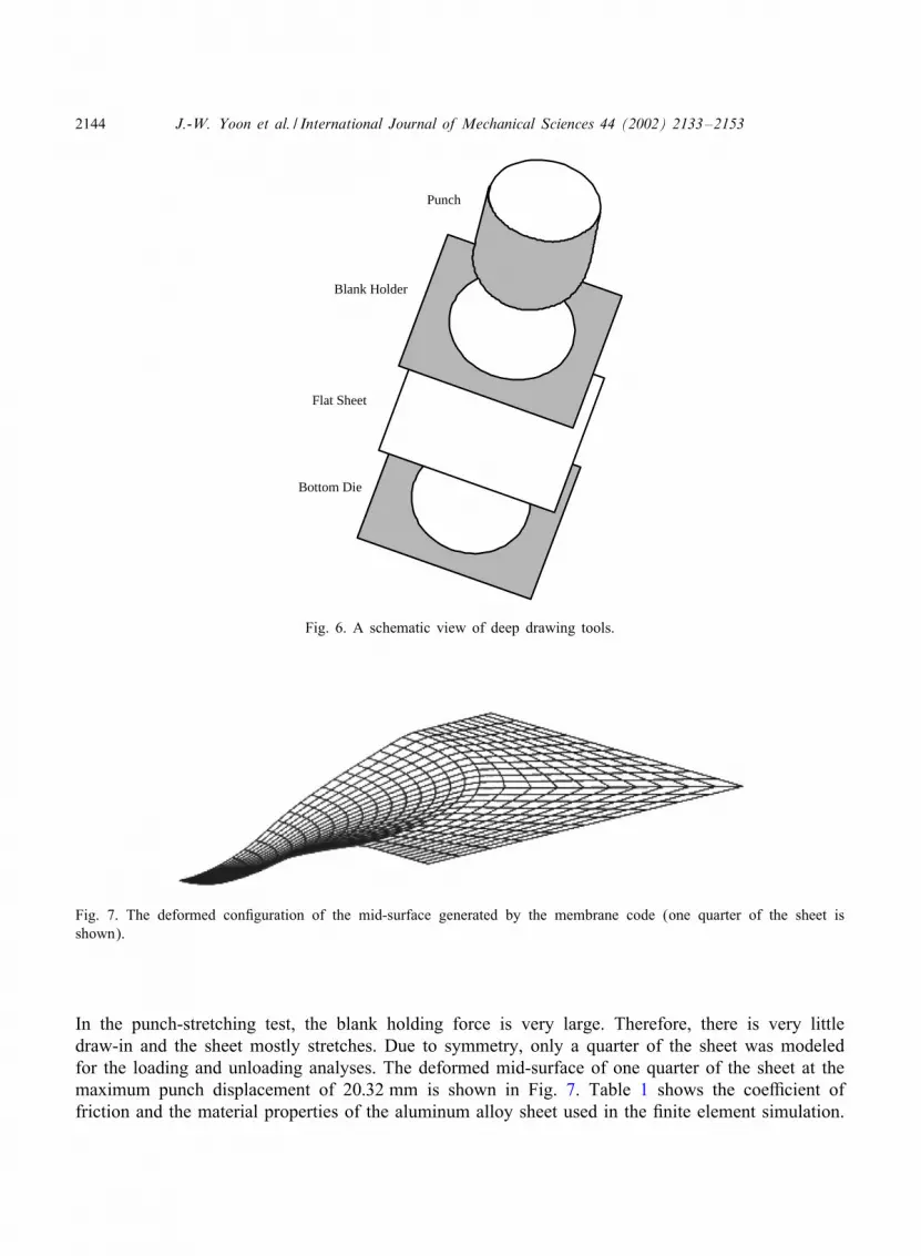
Fig. 6 shows a schematic view of forming tools used in the punch stretching of a squareblank sheet. The 3D hybrid membrane/shell method was applied to predict the springback of thispunch-stretched blank sheet. In the punch stretching test, a Hat square blank is initially clampedbetween a Hat blank holder (binder) and the bottom die with a speci2ed blank holding force. Then,the hemispherical punch bends and stretches the sheet by pushing the sheet into the die cavity.


Flat Sheet

Bottom Die

Blank Holder

Punch

Fig. 6. A schematic view of deep drawing tools.

Fig. 7. The deformed con2guration of the mid-surface generated by the membrane code (one quarter of the sheet isshown).

In the punch-stretching test, the blank holding force is very large. Therefore, there is very littledraw-in and the sheet mostly stretches. Due to symmetry, only a quarter of the sheet was modeledfor the loading and unloading analyses. The deformed mid-surface of one quarter of the sheet at themaximum punch displacement of 20:32 mm is shown in Fig. 7. Table 1 shows the coeCcient offriction and the material properties of the aluminum alloy sheet used in the 2nite element simulation.


Table 1Material properties of the sheet alloy and friction coeCcient used in the simulation ( L� = K( L�0 + L�)n)

Material K n E R Yield Poisson’s L�0 -(Mpa) (GPa) stress ratio Fric.

(MPa) coe;.

AL 2036-T4 604.0 0.214 69.0 0.84 196.0 0.33 0.0052 0.1

Table 2Tooling geometry and boundary conditions

Case Sheet Punch Die Die Punch Blank Holdingthickness radius radius cavity displacement force(mm) Rp Rd opening (mm) (KN)

(mm) (mm) (mm)

A 0.68 101.6 15.0 105.0 7.6 150B 0.68 101.6 15.0 105.0 20.3 150

Table 2 shows the tooling speci2cations, sheet dimensions and blank holding force used in thepunch-stretching experiment [15].

3.1.1. Comparison of springback predictions obtained from shell and hybrid methodsIn this paper, similar to the experiments performed by Stevenson [15], springback or the dis-

placement of the pole of the sheet after unloading was calculated in two steps using a full shellmodel by Yoon et al. [7] and the hybrid membrane/shell method. In the full shell model, bothloading and unloading of the sheet were simulated using shell elements with 2ve integration pointsthrough the thickness. In the hybrid method, loading was simulated using the membrane 2nite el-ement code [10], while unloading was done using a shell model [7]. In the 2rst step of the un-loading, the punch was removed and while the blank holder was still engaged, the springback ofthe sheet was calculated. In the second step of the unloading, initially the EDM cutting of thesheet in the experiment was simulated by 2xing the sheet nodes on the edges of the die open-ing and then removing all the sheet elements under the blank holder. Then, by 2xing the edgenodes and allowing the sheet to come to complete relaxation, the springback of the sheet wascalculated.Figs. 8–11 show loaded and unloaded shapes of the aluminum sheet predicted by the 3D hybrid

membrane/shell method for two di;erent punch displacements of 7.62 and 20:32 mm. Figs. 8 and10 represent the springback after the 2rst unloading step (SPB1) and Figs. 9 and 11 represent thespringback after the second unloading step (SPB2) with the Hange area removed. Table 3 showsthe measured springback results reported by Stevenson [15] after the two unloading steps and thenumerically predicted results by the full shell model and the hybrid membrane/shell method. The


Fig. 8. Unloaded shape of the sheet after the punch removal (before trimming) at the punch stroke of 7:62 mm (blankholderis still in place).

Fig. 9. Unloaded shape of the sheet after trimming at the punch stroke of 7:62 mm.

Fig. 10. Unloaded shape of the sheet after the punch removal (before trimming) at the punch stroke of 20.32 mm(blankholder is still in place).


Fig. 11. Unloaded shape of the sheet after trimming at the punch stroke of 20:32 mm.

Table 3Comparison of full shell, hybrid method and measured springback data

Max. SPB1 SPB1 SPB1 SPB2 SPB2 SPB2punch hybrid shell experiment hybrid Hmax shell Hmax experimentheight (mm) (mm) (mm) (mm) (mm) (mm)(mm)

−7.62 −5.69 −5.12 −5.23 −5.73 −5.15 −5.31−20.30 −19.48 −19.17 −19.38 −19.47 −19.41 −19.30

Table 4CPU time comparison of full shell and hybrid methods

Method CPU (s) CPU (s) hybrid Total CPU (s)stress cal.

loading unloading

Hybrid membrane/shell 1200 330 30 1560Full shell—5 intg. points 6000 180 0 6180

results shown in Table 3 indicate that a very good agreement exists between the measured and thenumerically predicted results.

3.1.2. Comparison of CPU time between shell and hybrid methodsTable 4 shows a comparison between the total CPU seconds taken by the hybrid membrane/shell

method and a full shell model to analyze the punch stretching and the two-step unloadingprocess. The hybrid method took a total of 1560 CPU seconds on a HP-755 workstation to


R3R2

R1

R1 = 23.5 mm, R2 = 25.0 mm, R3 = 4.0 mm

Fig. 12. Die geometry for unconstrained bending.

Table 5Material properties of the 6111-T4 aluminum alloy sheet used in the unconstrained bending example: L�=A−B exp(−C L�)

Material A (Mpa) B (Mpa) C (Mpa) E (GPa) R Poisson’s ratio

AL 6111-T4 429.8 237.7 8.504 70 0.6944 0.3

calculate the bending strains and stresses for 82 incremental membrane steps with 600 elementsand the unloading with the shell model. The full shell model, with one integration point on themid-surface and 2ve integration points through the thickness, required 6180 CPU time to analyzethe same problem. It can be seen that the hybrid membrane/shell model has at least a 75% advan-tage in CPU time over the conventional shell analyses for the same problem. It can be expectedto realize even better CPU time savings as the size of the problem (i.e., number of elements)increases.

3.2. Unconstrained cylindrical bending and springback

The example of a sheet undergoing unconstrained cylindrical bending and springback was modeledto demonstrate the robustness of the present method. Since the present method was successfullyapplied for a stretch-dominant problem in the previous section, a bending-dominant example wasconsidered here. As shown in Fig. 12, there is no blank holder in this example so that deformationis bending dominant. Besides, the example has complex contact boundary conditions during formingand the springback after forming is large, providing severe benchmark environment for the hybrid 3Dmethod. Experiment was also performed for comparison. The die geometry and dimensions shownin Fig. 12 are similar to the Numisheet 2002 benchmark example, with only a minor di;erence inthe die cavity radius, R2. The dimensions of the 6111-T4 aluminum alloy sheet are: 120 mm(L) ×30 mm(w)× 1 mm(t), and its properties are given in Table 5.


Fig. 13. Initial set-up for forming: (a) simulation; and (b) experiment.


(a)

(b)

Fig. 14. Deformed shapes before springback: (a) simulation; and (b) experiment.

Fig. 13 shows the views of the initial set-up for simulation and experiment. Bending aug-mented membrane element [11] was used for the calculation of membrane solution. Note thatfor this particular example, bending is dominant and it is almost impossible to obtain membranesolutions with conventional membrane elements without bending e;ects. Fig. 14, showing simu-lated and experimentally obtained deformed shapes at the punch stroke of 25 mm, demonstratesthat the deformation is bending dominant with large rotation and displacement. It took 100 stepsto complete the simulation with step size, 0:25 mm. The total number of iterations was 976 (lessthan 10 iteration per step) and the total analysis time was 3550 s. Relatively stable con-vergence was observed even though contact and geometry involved severe nonlinearity. In Fig. 14,the deformed shape obtained from the simulation is very similar to the experimentalone.Based on membrane solutions, through-thickness stresses were generated in a post-processing

fashion using the hybrid 3D method. The procedure took less than 1 min. The generated stresseswere then passed on to normal shell elements and springback analysis was performed. After contactconditions between the die and the sheet were removed and symmetric boundary conditions were


(a)

(b)

Fig. 15. Deformed shapes after springback: (a) simulation; and (b) experiment.

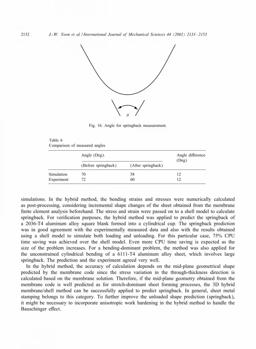
imposed for the sheet, springback was calculated with one step. Fig. 15 shows the simulated andexperimental results after springback. Fig. 16 shows the angles measured before and after spring-back, which are summarized in Table 6. As shown in Table 6, the di;erence between loaded andunloaded angles is exactly the same (i.e., 12◦), for both simulation and experiment, con2rmingthe excellent accuracy of the current method for springback prediction even in a bending-dominantproblem.

4. Conclusions

A 3D hybrid membrane/shell method was developed in order to perform springback analysisfrom the membrane mid-plane solution and also to reduce computational cost for sheet forming


�

Fig. 16. Angle for springback measurement.

Table 6Comparison of measured angles

Angle (Deg). Angle di;erence(Deg)

(Before springback) (After springback)

Simulation 70 58 12Experiment 72 60 12

simulations. In the hybrid method, the bending strains and stresses were numerically calculatedas post-processing, considering incremental shape changes of the sheet obtained from the membrane2nite element analysis beforehand. The stress and strain were passed on to a shell model to calculatespringback. For veri2cation purposes, the hybrid method was applied to predict the springback ofa 2036-T4 aluminum alloy square blank formed into a cylindrical cup. The springback predictionwas in good agreement with the experimentally measured data and also with the results obtainedusing a shell model to simulate both loading and unloading. For this particular case, 75% CPUtime saving was achieved over the shell model. Even more CPU time saving is expected as thesize of the problem increases. For a bending-dominant problem, the method was also applied forthe unconstrained cylindrical bending of a 6111-T4 aluminum alloy sheet, which involves largespringback. The prediction and the experiment agreed very well.In the hybrid method, the accuracy of calculation depends on the mid-plane geometrical shape

predicted by the membrane code since the stress variation in the through-thickness direction iscalculated based on the membrane solution. Therefore, if the mid-plane geometry obtained from themembrane code is well predicted as for stretch-dominant sheet forming processes, the 3D hybridmembrane/shell method can be successfully applied to predict springback. In general, sheet metalstamping belongs to this category. To further improve the unloaded shape prediction (springback),it might be necessary to incorporate anisotropic work hardening in the hybrid method to handle theBauschinger e;ect.


Acknowledgements

The authors are thankful to Mr. J.C. Brem at Alcoa Technical Center for performing the un-constrained cylindrical bending experiment. This work was partially supported by the Ministry ofScience and Technology in Korea through the National Research Laboratory for which the authorsare thankful.

References

[1] Wang NM, Budianski B. Analysis of sheet metal stamping by a 2nite element method. Journal of Applied MechanicTransactions ASME 1978;45:73.

[2] Chung WJ, Kim YJ, Yang DY. A rigid-plastic 2nite element calculation for the analysis of general deformation ofplanar anisotropic sheet metals and its application. International Journal of Mechanical Sciences 1986;28:825.

[3] Pourboghrat F, Chu E. Springback in plane strain stretch/draw sheet forming. International Journal of MechanicalSciences 1995;36(3):327–41.

[4] Pourboghrat F, Chung K, Richmond O. A hybrid membrane/shell method for rapid estimation of springback inanisotropic sheet metals. ASME Journal of Applied Mechanics 1998;65:671–84.

[5] Pourboghrat F, Yoon JW, Chung K, Barlat F. A 3D hybrid membrane/shell method with kinematic hardening topredict the springback of sheet metals, Seventh International Symposium on Plasticity and Its Current Applications,Cancun, Mexico January 5–13, 1999.

[6] Pourboghrat F, Karabin ME, Becker RC, Chung K. A hybrid membrane/shell method for calculating springback ofanisotropic sheet metals undergoing axisymmetric loading. International Journal of Plasticity 2000;16:677–700.

[7] Yoon JW, Yang DY, Chung K. Elasto-plastic 2nite element method based on incremental deformation theory andcontinuum based shell elements for planar anisotropic sheet materials. Computational Methods in Applied MechanicalEngineering 1999;174(1–2):23–56.

[8] Bathe KJ. Finite element procedures in engineering analysis. Englewood Cli;s, NJ: Prentice-Hall, 1982.[9] Yoon JW, Yang DY, Chung K, Barlat F. A general elasto-plastic 2nite element formulation based on incremental

deformation theory for planar anisotropy and its application to sheet metal forming. International Journal of Plasticity1999;15(1):35–68.

[10] Yoon JW, Song IS, Yang DY, Chung K, Barlat F. Finite element method for sheet forming based on an anisotropicstrain-rate potential and the convected coordinate system. International Journal of Mechanical Sciences 1995;37:733–52.

[11] Yoo DJ, Song IS, Yang DY, Lee JH. Rigid-plastic 2nite element analysis of sheet metal forming processesusing continuous contact treatment and membrane elements incorporating bending e;ects. International Journal ofMechanical Sciences 1994;36:513–46.

[12] Ting TC. Determination of C1=2;C−1=2 and more general isotropic tensor function of C. Journal of Elasticity1988;15:319–23.

[13] Hill R. External paths of plastic work and deformation. Journal of the Mechanics and Physics of Solids 1986;34:511–23.

[14] Chung K, Richmond O. A deformation theory of plasticity based on minimum work paths. International Journal ofPlasticity 1993;9:907–20.

[15] Stevenson R. Springback in simple axisymmetric stampings. Metallurgical Transactions A 1993;24A:925–34.

Documents

Springback prediction for sheet metal forming process using a 3D hybrid membrane/shell method