Spin-Yaw Lockin of an Elastic Finned Projectile - DTIC

Spin-Yaw Lockin of an Elastic Finned Projectile

by Charles H. Murphy and William H. Mermagen, Sr.

ARL-TR-3217 August 2004 Approved for public release; distribution is unlimited.

ARMY RESEARCH LABORATORY

NOTICES

Disclaimers The findings in this report are not to be construed as an official Department of the Army position unless so designated by other authorized documents. Citation of manufacturer’s or trade names does not constitute an official endorsement or approval of the use thereof. Destroy this report when it is no longer needed. Do not return it to the originator.

Army Research Laboratory Aberdeen Proving Ground, MD 21005-5066

ARL-TR-3217 August 2004


Charles H. Murphy and William H. Mermagen, Sr. Weapons and Materials Research Directorate, ARL

Approved for public release; distribution is unlimited.

ii

Report Documentation Page Form Approved OMB No. 0704-0188

Public reporting burden for this collection of information is estimated to average 1 hour per response, including the time for reviewing instructions, searching existing data sources, gathering and maintaining the data needed, and completing and reviewing the collection information. Send comments regarding this burden estimate or any other aspect of this collection of information, including suggestions for reducing the burden, to Department of Defense, Washington Headquarters Services, Directorate for Information Operations and Reports (0704-0188), 1215 Jefferson Davis Highway, Suite 1204, Arlington, VA 22202-4302. Respondents should be aware that notwithstanding any other provision of law, no person shall be subject to any penalty for failing to comply with a collection of information if it does not display a currently valid OMB control number. PLEASE DO NOT RETURN YOUR FORM TO THE ABOVE ADDRESS. 1. REPORT DATE (DD-MM-YYYY)

August 2004 2. REPORT TYPE

Final 3. DATES COVERED (From - To)

January–July 2003 5a. CONTRACT NUMBER

5b. GRANT NUMBER

4. TITLE AND SUBTITLE


5c. PROGRAM ELEMENT NUMBER

5d. PROJECT NUMBER

AH80 5e. TASK NUMBER

6. AUTHOR(S)

Charles H. Murphy and William H. Mermagen, Sr.

5f. WORK UNIT NUMBER

7. PERFORMING ORGANIZATION NAME(S) AND ADDRESS(ES)

U.S. Army Research Laboratory ATTN: AMSRD-ARL-WM-BC Aberdeen Proving Ground, MD 21005-5066

8. PERFORMING ORGANIZATION REPORT NUMBER

ARL-TR-3217

10. SPONSOR/MONITOR'S ACRONYM(S)

9. SPONSORING/MONITORING AGENCY NAME(S) AND ADDRESS(ES)

11. SPONSOR/MONITOR'S REPORT NUMBER(S)

12. DISTRIBUTION/AVAILABILITY STATEMENT

Approved for public release; distribution is unlimited. 13. SUPPLEMENTARY NOTES

14. ABSTRACT

Supersonic finned projectiles carrying very long dense metallic rods have been observed to have significantly large flexing motion. The appropriate Lagrangian for a pitching, yawing, rolling, and flexing missile is derived and the powerful finite element method used to construct differential equations for finite element parameters. These differential equations for constant spin are used to calculate frequencies and damping rates of transient motion and trim response motion to missile-fixed inertia and aerodynamic forcing terms associated with inelastic deformations. The results agree with earlier results based on a much more difficult iterative integration of a complex differential equation with unusual boundary conditions. Only three elements were necessary for reasonable accuracy, although codes for five and seven elements have been prepared and exercised. The finite element ordinary differential equations allowed calculation of the time history of missile motion with varying spin and demonstrated the occurrence of spin-yaw resonance at the aerodynamic frequency and at the lowest elastic frequency.

15. SUBJECT TERMS

aeroelastic, spin-yaw lockin, finned projectile

16. SECURITY CLASSIFICATION OF: 19a. NAME OF RESPONSIBLE PERSON Gene Cooper

a. REPORT UNCLASSIFIED

b. ABSTRACT UNCLASSIFIED

c. THIS PAGE UNCLASSIFIED

17. LIMITATION OF ABSTRACT

UL

18. NUMBER OF PAGES

64 19b. TELEPHONE NUMBER (Include area code)

410-278-3684 Standard Form 298 (Rev. 8/98) Prescribed by ANSI Std. Z39.18

iii

Contents

List of Figures v

List of Tables v

1. Introduction 1

2. Coordinate System 2

3. Motion of Central Disk 5

4. FEM 8

5. Flexing Motion 10

6. Special Solutions 12

7. Quadratic Roll Equation 13

8. Numerical Results 15

9. Summary 22

10. References 27

Appendix A. Integrals 29

Appendix B. Functions 31

Appendix C. Generalized Forces and Hermitian Polynomials 33

Appendix D. Connector Coefficients for Equations (39–41) 35

Appendix E. Connector Coefficients for Equations (42–44) 37

Appendix F. Differential Equations Coefficients 39

iv

Appendix G. Flexing Motion Finite Element Method (FEM) Quantities 41

Appendix H. Finned Missile Parameters 47

List of Symbols, Abbreviations, and Acronyms 49

Distribution List 52

v

List of Figures

Figure 1. X-Z coordinates of cross-sectional disk. .........................................................................3

Figure 2. X-Y coordinates of cross-sectional disk..........................................................................3

Figure 3. Sketch of finned missile. ...............................................................................................15

Figure 4. 1 R/φ ω vs. σ for finned missile. ......................................................................................16

Figure 5. fj vs. Rφ/ω for BF ss RΓ = 0, σ = 5, p = 6ω . ...................................................................18

Figure 6. R/ωφ vs. time for BF ss R 0 RΓ 0, 5, p 6.0ω , /ω 0, 5.4= σ = = φ = . ....................................19

Figure 7. fj vs. R/ωφ for BF ss RΓ = 0, σ = 5, p = 0.8ω ...................................................................19

Figure 8. R/ωφ vs. time for BF ss R 0Γ = 0, σ = 5, p = 0.8ω , ψ = 0, – 3 s-1. ..................................20

Figure 9. Angular motion (qb1y vs. qb1z) for BF ss R 0Γ 0, 5, p 0.8ω , ψ 0, 3= σ = = = − s-1. ........20

Figure 10. Rod forward tip motion (qb7y vs. qb7z) for –1

BF ss R 0 Γ 0, 5, p 0.8ω , ψ 0, 3 s= σ= = = − ...............................................................................21

Figure 11. Maximum strain ( Mε ) for BF ss R 0Γ 0, 5, p 0.8ω , ψ 0, 3= σ = = = − s-1. ...................22

Figure 12. 0ψ vs. 0θ showing regions of sse 1ep , p lockin BF ss RΓ = 0, σ = 5, p = 0.8ω .....................23

Figure 13. fj vs. Rφ/ω for BF ss RΓ = 0.02, σ= 5, p = 0.4ω ..............................................................23

Figure 14. R/ωφ vs. time for BF ss R 0Γ = 0.02, σ = 5, p = 0.4ω , θ = 0, 5 s-1.................................24

Figure 15. Angular motion (qb1y vs. qb1z) for BF ss R 0Γ = 0.02, σ = 5, p = 0.4ω , θ = 0, 5 s-1. ......24

Figure 16. Rod forward tip motion (qb7y vs. qb7z) for BF ss R 0Γ = 0.02, σ = 5, p = 0.4ω , θ = 0 s-1.................................................................................25

Figure 17. Rod forward tip motion (qb7y vs. qb7z) for BF ss R 0Γ = 0.02, σ= 5, p = 0.4ω , θ = 5 s-1.....25

Figure 18. Maximum strain ( )Mε for BF ss R 0Γ = 0.02, σ = 5, p = 0.4ω , θ = 0, 5 s-1. ...................26

Figure 19. 0ψ vs. 0θ showing regions of sse 2ep , p lockin BF ss RΓ = 0.02, σ = 5, p = 0.4ω . .............26

List of Tables

Table 1. Transient frequencies and damping rates........................................................................17 Table 2. Equilibrium spin rates.....................................................................................................18

vi

INTENTIONALLY LEFT BLANK.

1

1. Introduction

Very long finned projectiles carrying very dense metallic rods have been observed to be subjected to large inelastic deformations during hypersonic flight (1). Spark shadowgraphs of these projectiles have shown elastic bending motion with amplitudes as large as the rod’s radius (2). It has been conjectured that the cause of the inelastic deformation was the bending loads associated with pitching and yawing motion at resonant spin frequencies. These frequencies would be near to the aerodynamic frequency of a rigid projectile or the elastic frequencies of the rod.

Spinning motion at a resonant frequency can be caused by a nonlinear roll moment associated with the roll orientation of the fins or by mass asymmetry due to damage or poor construction of the projectile. This spin-yaw lockin mechanism has been discussed for a rigid missile by several authors (3–7).

The linear flight motion of an elastic missile has been considered in references (8–13). In reference (11), a very simple theoretical model of a projectile composed of three components connected by two bent mass-less elastic beams was used to approximate an elastic missile. For appropriate selection of beam parameters spin-yaw lockin was demonstrated and large amplitude oscillations occurred. In references (12) and (13), the correct linear partial-differential equation for a continuously elastic missile was derived, and special solutions for harmonic transient motion and trim motion were obtained. A nonlinear roll moment was shown to be capable of producing equilibrium spin near resonance. Although the lateral motion of the pitching and yawing missile was linearized, it was necessary to retain the quadratic terms in the roll equation. A time history of motion going to lockin was not obtained at that time. It is the purpose of this report to compute such a time history by use of the finite element method (FEM) (14).

The lateral motion of a symmetric rigid missile has often been described by complex variables (15), and complex variables were used in references (8) and (11–13) to describe the lateral flexing motion of the rotationally symmetric rod. The equations of motion of a spinning missile are usually derived by vector analysis and Newtonian mechanics, but FEM equations for elastic bodies require the use of the more sophisticated Lagrangian mechanics. The Lagrangian of a system must be stated in body-fixed coordinates. Separate differential equations in the two lateral directions can be obtained from the appropriate Lagrangian. Pairs of equations are combined and complex variables introduced to yield half as many complex equations.

If five elements are used to describe the pitching and flexing motion of the missile, 20 parameters, usually called connectors, are introduced and 25 second-order differential equations and one first order differential equation are required. The introduction of complex angles and complex connections reduce this system to 12 second-order complex differential equations and two real differential equations.

2

2. Coordinate System

The elastic missile is assumed to consist of a very heavy elastic circular rod of fineness ratio, L, and mass, m, embedded in a very light symmetric aerodynamic structure that may be longer than the rod. The rod’s axial moment of inertia is Ix and its transverse moment of inertia about its center is It0. The rod’s diameter can vary over its length, and its maximum diameter will be denoted by “d.” All distances will be expressed as multiples of the rod diameter and its length is Ld. A nose windshield of length 23x d may be attached to the forward end of the rod, and the fins may extend beyond the end of the rod at a distance of 01x d . Thus, the rod is located between 1x L 2= − and 2x L 2= , while the aerodynamic structure extends from 0 1 01x x x= − to 3 2 23x x x= + .

An earth-fixed coordinate system will be used with the Xe-axis oriented along the initial direction of the missile’s velocity vector. The Ze-axis is downward-pointing and the Ye-axis is determined by the right hand rule. A nonrotating coordinate system, XYZ is then defined with origin always at the center of the rod and the X-axis tangent there. The X-axis pitches through the angle,θ , and yaws through the angle,ψ , with respect to the Xe-axis. Body-fixed coordinates XYb-Zb are now defined for which the Yb-Zb axes rotate with the missile through the roll angle, φ , with respect to the Y-Z axes.

We will conceptually slice the missile into a large number of thin disks perpendicular to the X-axis with thickness, dx. When the rod flexes, the disks shift laterally perpendicular to the X-axis and cant to be perpendicular to the centerline of the disks. This canting action neglects the shear deformation of the rod, and this constraint is called the Bernoulli assumption (14). The lateral displacement of a disk has body-fixed coordinates by bzand δ δ , and the disk is canted at angles by bz and Γ Γ .

by bzby bz;

x x∂δ ∂δ

Γ = Γ =∂ ∂

. (1)

It important to note that at the central disk

( ) ( ) ( ) ( )by bz by bz0, t 0, t 0, t 0, t 0δ = δ = Γ = Γ = . (2)

Reference (12) used the nonspinning elastic coordinate system with XYZ axes ( )0φ = . The

lateral displacements of a disk in this elastic coordinate system are shown in figures 1 and 2 and can be computed from body-fixed quantities.

( ) iE Ey Ez by bzi i e φδ = δ + δ = δ + δ , (3)

and

3

VX

Xe

ZZe

α

θ

δEz Γz

Missile Centerline

Figure 1. X-Z coordinates of cross-sectional disk.

δEy

Γy

Y

Y

X

Missile Centerline

V

X

Xe

Y e

β

ψ

Figure 2. X-Y coordinates of cross-sectional disk.

4

( ) iy z by bzi i e φΓ = Γ + Γ = Γ + Γ . (4)

The earth-fixed coordinates of the central disk are e e ex , y , and z , and the earth-fixed coordinates of the other disks are computed in terms of the central disk earth-fixed coordinates, their body-fixed displacements, and the Euler angles , , and θ ψ φ .

( ) ( ){ } ( ){ }2 2 i ide e by bz by bzx x x 1 2 Re i e Im i eφ φ = + − ψ + θ −ψ δ + δ + θ δ + δ , (5)

( ){ }ide e by bzy y x Re i e φ= + ψ + δ + δ , (6)

and

( ){ }ide e by bzz z x Im i e φ= − θ+ δ + δ . (7)

ye, ze, by bz, , , θ ψ δ δ and their derivatives are assumed to be small quantities, but xe and ex are

not small. Lagrangian dynamics yields the correct linearized differential equations for these six variables when the kinetic energy expansion retains all quadratic terms in these variables. Thus, equations 6 and 7 consist of only linear terms, but equation 5, which contains xe, retains quadratic terms in these variables. The coefficient of x in equation 5, for example, is the quadratic form of the cosine of the angle between the Xe-axis and the X-axis.

The angular velocity of the central disk in the body-fixed coordinates is

p = φ−ψθ , (8)

( ){ }ibq Re i e− φ= θ + ψ , (9)

and

( ){ }ibr Im i e− φ= θ+ ψ . (10)

The angular velocity of any other disk along axes aligned with the disk’s axes of symmetry is

( ) ( ){ }d d by d bzp p 1 2 q r p Re i 2 i = −ΓΓ + Γ + Γ = + θ+ ψ −φΓ + Γ Γ , (11)

( ){ }id b bz byq q Re i i e− φ= −Γ −φΓ = θ+ ψ + Γ , (12)

and

( ){ }id b by bzr r Im i i e− φ= + Γ −φΓ = θ+ ψ + Γ . (13)

5

3. Motion of Central Disk

The mass of each circular disk is ( ) ( )1m L x dxρ ; its roll moment of inertia is ( ) ( )2

d 22a md x dxρ , and its transverse moment of inertia is ( ) ( )2d 2a md x dxρ , where da is

( ) 116L − . ( )1 xρ and ( )2 xρ describe the variation of mass and moments of inertia along the rod, and both become unity for a homogeneous rod with constant diameter. The kinetic energy of a disk is therefore

( )( ) ( )( )2 2 2 2 2 2 2 2d 1 de de de d 2 d d dT dx = md ρ 2L x + y + z + a md ρ 2 2p + q + r dx

. (14)

The total kinetic energy of the missile can be obtained by integrating dT over the length of the rod:

( ) ( )( )2

1

x2 2

d R 11 12 21 22x

T T dx T md T T md 2L T T= = + + + +∫ , (15)

( )( ) ( )( )

( ) ( ){ }( ) ( )( ){ }

( ) ( ) ( )

( )

2 2

1 1

2 2 2 2 2 2 2R e e e x t 0

2c e e e

11 e c c

12 e e c 6 8

x x2 2 2 2

21 Ey Ez 1 d y z 2x x

22 d

where T md 2 x y z I p 2 I 2

md x y z x ,

T x Re i i ,

T Re y iz i J J ,

T dx a L dx,

T 2 a L Re 2i

= + + + + ψ + θ

+ ψ − θ− ψψ + θθ

= − ψ + θ δ + ψ + θ δ

= − δ + ψ + θ +

= δ + δ ρ + Γ +Γ ρ

= φ Γ

∫ ∫

( )2

1

x

2x

dx , −φΓ Γρ ∫

and

( )2

1

x

c 1x

x 1 L x dx= ρ∫ .

The ey and ez components of the central disk velocity can be approximated by linear relations in angles of pitch and yaw with respect to inertia axes ( ),θ ψ and angles of attack and sideslip with respect to the velocity vector ( ),α β as shown in figures 1 and 2. The magnitude of the velocity vector is V.

( ) ( )ey V d = β+ψ , (16)

and

6

( ) ( )ez V d = α −θ . (17)

Equations 16 and 17 can be written as a single complex equation:

( ) ( )e e 1 1ey iz V d q q+ = + , (18)

where 1q i= β+ α and 1eq i= ψ − θ .

In reference (12), the linear aerodynamic force loading is expressed in terms of three force distribution functions, ( ) ( ) ( )D f1 f 2c x , c x , and c x and the base pressure coefficient, CDbp, plus a

body-fixed force associated with possible bent fins. Because the lateral motion of the missile is quite small, 1 1eq q≅ − and the aerodynamic damping force terms in the aerodynamic loading on the aerodynamic structure can be combined. This aerodynamic loading in nonrotating elastic coordinates is

( )x1 D

dF g c xdx

= − , (19)

( ) ( ) ( ) ( )

( ) ( )( ) ( )

if1 1 BF E 1y z

1 if 2 1 BF

c x q x e xq d VdF dFi gdx dx c x 2q i x e d V

φ

φ

−Γ −Γ + δ − + = − + −Γ − φΓ

, (20)

and

xbp 1 DpbF g C= − . (21)

The total aerodynamic force acting on the aerodynamic structure is given by the integrals of equations 19 and 20 and by adding the base drag of equation 21 to the axial force,

( )3

0

x

x 1 D 1 D Dbpx

F g C g c x dx C

= − = − + ∫ , (22)

and

( ) ( ) ( ) ( )i1 1 1 2 1 NBF 1 2F g c q c q d V C e J t J t d Vφ = − + − − − , (23)

where various functions are defined in appendices A and B.

The primary components of drag are head drag and base pressure drag. The third component is skin friction drag that is ~15% of the total drag and will be neglected in this report to simplify the FEM calculations.

Similarly, the total aerodynamic moment about the rod’s center can be computed from the transverse aerodynamic force and a small axial force contribution:

7

( ) ( ) ( ) ( )( ) ( )y z

i1 3 1 4 1 MBF 3 4 5

M M iM

i g d c q c q d V C e J t J t d V J tφ

= +

= − + − − − − . (24)

The motion of the central disk is described by the variables e e ex , y , z , , , and φ ψ θ . The motion of any other section on the aerodynamic structure located at x with thickness dx is the sum of this motion plus its motion relative to the central disk. The work done on any section caused by motion of the central disk is

( )cd 1x e 1y e 1z ex

2x 2y 1ey 2z 1ez

dW dx = dQ dx + dQ dy + dQ dz

+ dQ d + dQ dq + dQ dqφ , (25)

where the sectional generalized forces are defined in appendix B.

The total generalized forces can be obtained by integrating the sectional generalized forces and adding the work done by the base pressure drag. These are also given in appendix C.

The linearized Lagrangian differential equation for ex and φ gives the usual drag and spin equation,

e 1 DmV mx g C≅ = − , (26)

and

x xI Mφ = . (27)

The Lagrangian differential equation for ez can be multiplied by i and added to the Lagrangian differential equation for ye to yield a single second-order differential equation in complex variables. Next, the Lagrangian differential equation for θ can be multiplied by i and subtracted from the Lagrangian differential equation for ψ ,

( )1 2 1 c 2 cm V q q Vq d q x d F + + + δ + = (28)

and

( )2 2 2t0 c 2 x 2 6 8 c c cI md x q i I q md J J x iM x Fd + − φ + + + δ = − − , (29)

where ( )2

1

x

c 1x

x 1 L x dx= ρ∫ , ( )2

1

x

c E 1x

1 L dxδ = δ ρ∫ , and 2 1eq q= .

These differential equations for cx 0= are the same as those derived by Newtonian mechanics in reference (12). Equations 28 and 29 contain eight integrals of Eδ and Γ . Three of these are integrals of dynamics properties ( )c 6 8, J , Jδ over the rod ( )1 2x , x and five are integrals over aerodynamic properties ( )1 2 3 4 5J , J , J , J , J over the aerodynamic structure ( )0 3x , x .

8

For constant spin and velocity, a rigid unbent missile with its center of mass at the rod center, equations 28 and 29 predict a simple epicyclic angular motion:

1 1 2 2t i t i1 10 20q K e K eλ + φ λ + φ= + , (30)

where ( ) ( ) 2m x t 1 t 3 x tI 2I g d I c I 2Iφ = φ ± − + φ .

For zero spin, 1 2 Rφ = −φ = ω , where ( )R 1 t 3g d I cω = .

4. FEM

The rod is assumed to be represented by the sum of an inelastic bent component rotating with the missile and an elastic deformation,

( ) ( ) ( )iE EB E 1 2x, t x e x, t ; x x xφδ = δ + δ ≤ ≤ , (31)

and

( ) ( ) ( )b EB b 1 2x, t x x, t ; x x xδ = δ + δ ≤ ≤ , (32)

where ( ) ( )EBEB

d 00 0

dxδ

δ = = .

Because the aerodynamic structure is rigidly attached to the rod,

( ) ( ) ( ) ( )E E 1 1 1 0 1x, t x , t x x x , t ; x x xδ = δ + − Γ ≤ ≤ , (33)

and

( ) ( ) ( ) ( )E E 2 2 2 2 3x, t x , t x x x , t ; x x xδ = δ + − Γ ≤ ≤ . (34)

The motion of the elastic component of the rod is controlled by the elasticity of the rod and the aerodynamic force acting on it.

FEM is a very powerful method for calculating the time history of the elastic flexing motion. The rod is divided into nj elements of length e jL L n= . The shape of the j-th element is given

by a linear combination of third-order Hermitian polynomials (see appendix C).

( ) ( ) ( )4

by bpy p1

ˆx, t q t N zδ =∑ , (35)

and

9

( ) ( ) ( )4

bz bpz p1

ˆx, t q t N zδ =∑ , (36)

where ( )e j j 1 ex L z z ; z x L j 1 0 z 1= + = + − ≤ ≤ .

The coefficients of the polynomials are functions of time and are called connectors. The first two are the deflection and slope of the left end of the element and the third and fourth are the deflection and slope of the right end. To ensure continuity in deflection and slope at junction points, the corresponding pairs of connectors are equal. We will consider only an odd number of elements and require that the connecters of the central element satisfy equation 2.

b3 b1 e b2ˆ ˆ ˆq 5q L q= + , (37)

and

1b4 e b1 b2ˆ ˆ ˆq 24L q 5q−= + , (38)

where bq bqy bqzˆ ˆ ˆq q iq= + .

For jn elements, there are j2n independent complex connectors. It is convenient to let the index

for the connectors run from 3 to nt, where nt = 2nj + 2. The usual FEM procedure calculates the elastic parts of the integrals in equations 28 and 29 by first obtaining integrals over each element. These are linear functions of that element’s four connector functions. Due to equations 37 and 38, the central element has only two independent connector functions, and the next adjacent element connector functions are related to them. Integrals for these elements are specially computed. The desired elastic integrals are sums of these subintegrals and are linear combinations of the j2n complex connector functions. The three integrals can be written as

tn

1 ic 1n n cB

3L a q e− φδ = + δ∑ , (39)

tn

1 i6 2n n 6B

3J L a q J e− φ= +∑ , (40)

and

( )tn

i8 d 2n n n 8B1

3J a b q 2i q i J e φ= − φ − φ∑ , (41)

where in bnq q e φ= .

The five integrals have contributions from the aerodynamic structure extensions as well as from each element,

10

( ) ( ) ( ) ( )

( )

tn

1 2 1n a1n n 1n a1n n3

i1B 2B

J + J d V = f + f q + g + g q d V

+ J + i d V J e ,φ

φ

∑

(42)

( ) ( ) ( ) ( )

( )

tn

3 4 2n a2n n 2n a2n n3

i3B 4B

J + J d V = f + f q + g + g q d V

+ J + i d V J e ,φ

φ

∑

(43)

and

( )tn

1 i5 D 1n an n 5B

3J C a L h q J e− φ= − + +∑ . (44)

Expressions for cB kB an, J , hδ and all FEM coefficients in equations 39–44 for 1, 3, 5, and 7 elements are given in appendices A, D, and E.

Equations 39–44 can be used with equations 28 and 29 to write these two complex differential equations in a standard format:

( ) ( ) ( )tn

* *mn n mn mn n mn mn n m

n 1R q S i S q T i T q t exp i

=

+ + φ + + φ = φ ∑ . (45)

The coefficients for m = 1, 2 are given in appendix F.

5. Flexing Motion

In order to derive the equations for flexing motion, the kinetic energy given by equation 15 must be expressed in terms of the rigid-body parameters, plus the connector functions. The usual FEM process is used to express T2j in terms of two matrices, two vectors, and two constants.

t t tn n n

i 221 mn my ny mz zn Bm m xB1

3 3 3T k q q q q 2 Re i e k q I L− φ

= + − φ + φ

∑∑ ∑ , (46)

and

( ) ( )t t tn n n

i 222 d mn m m n Bm m m xB2

3 3 3T 2 a L Re b 2iq q q 2ie b q 2i q I L− φ

= φ − φ + + φ + φ ∑∑ ∑ , (47)

where xB1 xB2I , I are defined in appendix A and mn Bn mn Bnk , k , b , b are defined in Appendix G.

The potential energy stored by an elastic deformation is

11

( ) ( )2

1

2 2x 2 2by bz2 2

x

P.E. 1 2 EI d dxx x

∂ δ ∂ δ = + ∂ ∂ ∫ , (48)

where ( ) ( ) ( )0 0 3E x I x E I x= ρ .

0E and 0I are values of Young’s modulus and the area moment of inertia at the rod’s center.

( )3 xρ gives the variation of their product along the rod. For a homogeneous rod with constant

diameter, the product is E0I0. The potential energy integral can be replaced by a sum of integrals over each of the jn elements. After integrating over each element, the results can be summed to yield a linear combination of the j4n real connectors,

( ) ( )t tn n

2 20 bmy bny bmz bnz mn

m 3 n 3V md 2L q q q q c

= =

= ω +∑∑ , (49)

where 2 30 0 0E I md ,ω = mnc are defined in appendix G.

The work done on the rod by this elastic force can be expressed in terms of generalized force terms,

( )tn

2 2E 0 Emy bmy Emz bmz

m 3dW md L Q dq Q dq

=

= ω + ∑ , (50)

where tn

Emy Emz mn bnn 3

Q iQ c q=

+ = −∑ .

The Kelvin-Voight elastic damping force (16), which is proportional to the time derivative of the elastic shear force, has generalized force terms:

( )tn

2 2D 0 Dmy bmy Dmz bmz

m 3dW md L Q dq Q dq

=

= ω + ∑ , (51)

where )tn

Dmy Dmz 1 mn bnn 3

ˆQ iQ 2k c q=

+ = − ω ∑ , ( )21 04.730 Lω = ω .

The scale factor 112 −ω is selected so that k 1= corresponds to critical damping of the first elastic

mode.

The external aerodynamic force is divided between the force acting on the rod and the force acting on the aerodynamic structure extensions at the ends of the rod. The total work done on the missile is the sum of the work done by these forces.

12

( )

j

j

t

n

A Aj anj 1

n

1 Amy bmy Amz bmzm 3

dW dW dW

g d Q dq Q dq ,

=

=

= +

= +

∑

∑ (52)

where ( ) ( ) ( )tn

-iAmy Amz mn amn n mn amn n Bm aBm Bm aBm

n=3Q + iQ = f + f q + g + g q e + f + f + i g + gφ φ ∑

and mn mn amn amn Bm Bm aBm aBmf ,g , f ,g , f ,g , f ,g are defined in appendix G.

Equations 50–52, in conjunction with the kinetic energy defined by equations 15, 46, and 47, can be used to derive the j4n Lagrangian differential equations for the bmy bmzq ,q ’s for

jm 3, 4,...2n 2= + . The equation for bmzq should be multiplied by i and added to the corresponding equation for bmyq to yield j2n complex differential equations for the complex variables bm.q . If the bmq are replaced by mq in each equation, the result has the standard form given by equation 45, where the 14nj complex coefficients for jm 3, 4...2n 2= + are given in

appendix F.

6. Special Solutions

A rigid symmetric finned missile flying with constant spin has two natural frequencies: 1Rφ and

2Rφ , where 1R 2Rφ ≅ −φ . For zero spin, each of the flexure frequencies would give rise to two coning frequencies, K±ω . The frequencies present in the motion of an elastic projectile would form an infinite sequence, where the first two would be related to 1Rφ and 2Rφ , while the later ones would evolve from K±ω , i.e., 2K 1 K 2K 2 K;+ +φ ≅ ω φ ≅ −ω . The odd numbered modes have

positive frequencies and are called positive modes, while the even numbered modes are called negative modes. For nonzero spin, the pairs of frequencies would no longer be equal in magnitude.

Transient harmonic solutions of the homogeneous constant spin version of equation 45 have the form

( )iAtm mk k jq q e A A k 1, 2, 3,...2 2n 1= = = + . (53)

After substituting equation 53 into equation 45, a set of linear homogeneous algebraic equations is derived, which is specified by an tn × tn matrix,

13

( )2 * *mn mn mn mn mn mnu A R A S i S T i T= + + φ + + φ . (54)

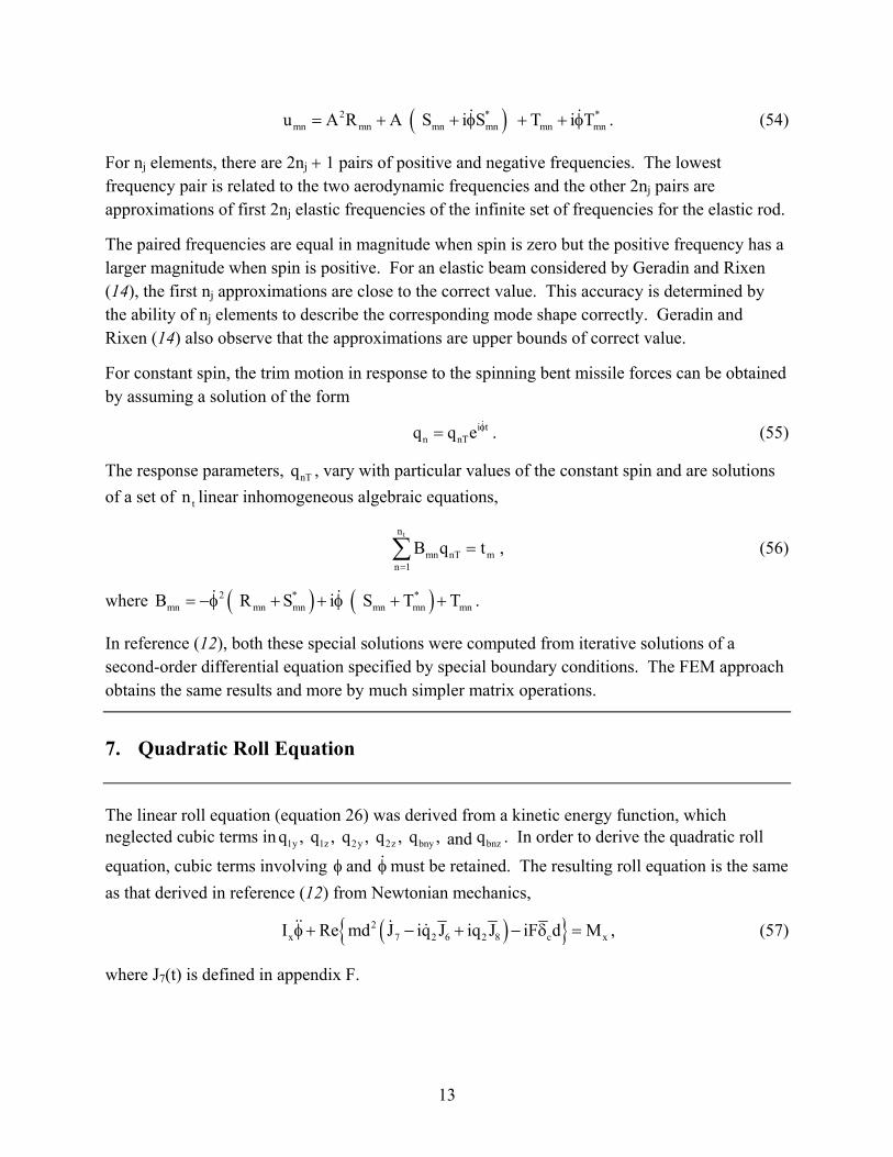
For nj elements, there are 2nj + 1 pairs of positive and negative frequencies. The lowest frequency pair is related to the two aerodynamic frequencies and the other 2nj pairs are approximations of first 2nj elastic frequencies of the infinite set of frequencies for the elastic rod.

The paired frequencies are equal in magnitude when spin is zero but the positive frequency has a larger magnitude when spin is positive. For an elastic beam considered by Geradin and Rixen (14), the first nj approximations are close to the correct value. This accuracy is determined by the ability of nj elements to describe the corresponding mode shape correctly. Geradin and Rixen (14) also observe that the approximations are upper bounds of correct value.

For constant spin, the trim motion in response to the spinning bent missile forces can be obtained by assuming a solution of the form

i tn nTq q e φ= . (55)

The response parameters, nTq , vary with particular values of the constant spin and are solutions of a set of tn linear inhomogeneous algebraic equations,

tn

mn nT mn 1

B q t=

=∑ , (56)

where ( ) ( )2 * *mn mn mn mn mn mnB R S i S T T= −φ + + φ + + .

In reference (12), both these special solutions were computed from iterative solutions of a second-order differential equation specified by special boundary conditions. The FEM approach obtains the same results and more by much simpler matrix operations.

7. Quadratic Roll Equation

The linear roll equation (equation 26) was derived from a kinetic energy function, which neglected cubic terms in 1y 1z 2y 2z bny bnzq , q , q , q , q , qand . In order to derive the quadratic roll

equation, cubic terms involving φ and φmust be retained. The resulting roll equation is the same as that derived in reference (12) from Newtonian mechanics,

( ){ }2x 7 2 6 2 8 c xI Re md J iq J iq J iF d Mφ+ − + − δ = , (57)

where J7(t) is defined in appendix F.

14

The aerodynamic roll moment is the X-component of the aerodynamic moment about the center of the central disk. The linear roll moment coefficient for a rigid finned projectile is usually expressed in terms of a roll-damping coefficient and a steady state spin,

( ) ( ) ( )p sslinearC C p d V= φ− . (58)

The steady state spin is usually determined by a differential canting of the fins caused either intentionally by the designer or unintentionally by damage to the projectile.

The roll moment of one of the projectile’s thin disks is the sum of the linear roll moment it has as part of a projectile and the quadratic roll moment induced by the transverse aerodynamic force acting on its lateral displacement relative to the center of the central disk. If we retain only the dominant cf1 term in equation 20, the quadratic roll moment has the form

( ) ( ) ( )

( ) ( ) ( ) ( ){ }x z Ey y Ezquadratic

i1 f1 1 BF E 1 E

dM dF dF

g d c Re i q e xq d V dx φ

= δ − δ = −Γ −Γ + δ − δ

. (59)

The total aerodynamic roll moment acting on the projectile, therefore,

( ) ( ) ( ){ }1x 1 A 1 clinear

M g d C Re Q t ig F − = + − δ , (60)

where ( ) ( ) ( ) ( ) ( )3

0

xi

A f1 1 BF E 1 E cx

Q t i c q e xq d V dxφ = −Γ −Γ + δ − δ − δ ∫ .

The nonlinear roll moment from equation 60 can be placed in the spin equation 57 to yield:

( ){ } ( )2X D 2 6 2 8 1 A 1 linear

I Re md Q iq J iq J g d Q g d Cφ+ − + − = , (61)

where the quadratic terms X DI .Q are defined in appendix F.

For trim motion, { } i tD 2 2TRe Q 0, q i q e φφ = = = φ and equation 61 become a simple equality of

two functions of p.

( ) ( )2 1f fφ = φ , (62)

where 1 ssf p= φ− , ( )( ){ }( )–1

2 AT 2T 1 6T 8T lpf = -R Q – q md g J + iJ C d Vφ , and

( ) ( )( )0

x3

AT f1 1T T BF ET 1T Tx

Q = i c q – Γ – Γ + i δ – xq d V δ dx φ ∫ .

ET T,δ Γ are computed from the solution to equation 56 and J6T, J8T are J6, J8 evaluated for

ET T,δ Γ . For moderate spin QAT is the dominant part of f2. Equilibrium values of spin are

determined by the intersection of these two curves. Lockin occurs at stable equilibrium spin.

15

Spin lockin can only occur when the missile has some rigid asymmetry such as that described by EBδ or BFΓ . For a rigid missile ETδ and TΓ are EBδ and BΓ . q1T is a function of spin which has

a large resonant amplitude when spin is near Rω . For an elastic missile 1T ET Tq , ,δ Γ are all functions of spin and have large resonant amplitudes when spin is near 2k 1−φ or near 2kφ for negative spin.

8. Numerical Results

In reference (12), calculations were made for a 20-cal. fin-stabilized rod, flying at 6000 ft/s. The finned missile has a 1-cal. nose extension and a 1-cal. fin extension (figure 3). The mass and aerodynamic parameters for the finned missile are given in appendix H. The bent rod will be described by a pair of quartic curves.

2 4

EB 11 212 4

12 22

δ = d x + d x 10 x 0

= d x + d x 0 x 10.

− ≤ ≤

≤ ≤ (63)

d 10d 10d

2d 2d

d

d/2

2d

Figure 3. Sketch of finned missile.

The rear of the rod is undeformed ( 11 21d d 0= = ), and the values of 12 22d , d are given in appendix G. Two values of BFΓ will be considered. These are unbent fins and the rear 1 cal. of fins bent uniformly to an angle of 0.02 radians.

A measure of the flight flexibility of a missile is the ratio of the first elastic frequency to the rigid missile aerodynamic frequency, 1 Rσ ≡ ω ω . Calculations of 1φ vs. σ have been made for the 1-, 3-, 5-, and 7-element rod. The results for all but the 1-element rod are practically identical, and the curve for a 3-element rod is given in figure 4. At 5σ = , the aerodynamic frequency is 60% of the rigid missile aerodynamic frequency; and even at 10σ = , it is 10% less than the rigid missile aerodynamic frequency.

16

Figure 4. 1 R/φ ω vs. σ for finned missile.

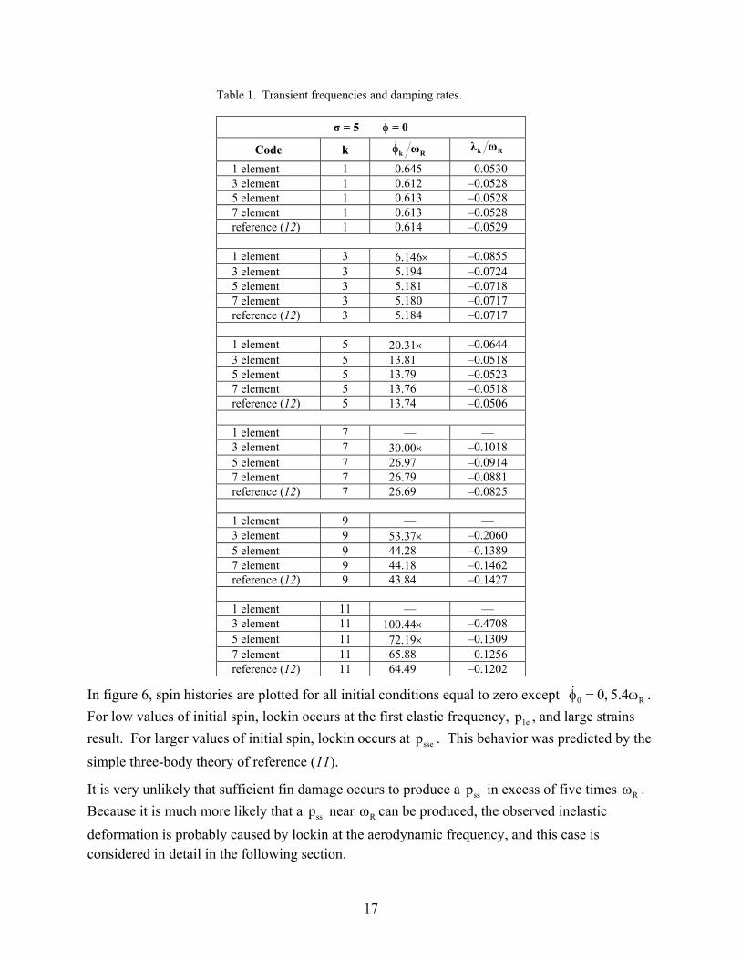
The first six positive frequencies and their damping rates for 5σ = have been calculated for a 1-, 3-, 5-, and 7-element rod. These results, together with calculations from the theory of reference (12), are tabulated in table 1. We identify frequencies which differ from the reference (12) value by >10% as poor values and mark them with x’s. Thus the 1-element rod yields one moderately good result while the 3-element and 5-element rods yield three and five good results, respectively. For this elastic problem, nj – 1, elastic frequencies are well calculated. For zero spin, the negative frequencies are the negatives of the positive frequencies.

Because the 3-element rod predicts the lower three frequencies quite well, all of the calculations given in this report are based on a 3-element rod. Most of these have been repeated for a 5-element rod, and almost identical results have been obtained.

In figure 5, 2f for BF5, 0σ = Γ = is plotted vs. Rφ ω for spin near the first elastic frequency. Large resonance values occur at R 5.1φ ω ≅ and an 1f line for ss Rp 6.0= ω is also shown. This

1f line has three intersections with the 2f curve, which are values of equilibrium spin. The intersection near ss Rp ω is denoted as ss Rp ω , while the other two are 1e R 2e Rp , p ,ω ω and all their numerical values are given in table 2.

1 R/φ ω

17

Table 1. Transient frequencies and damping rates.

σ = 5 = 0φ

Code k k Rωφ k Rλ ω

1 element 1 0.645 –0.0530 3 element 1 0.612 –0.0528 5 element 1 0.613 –0.0528 7 element 1 0.613 –0.0528 reference (12) 1 0.614 –0.0529

1 element 3 6.146× –0.0855 3 element 3 5.194 –0.0724 5 element 3 5.181 –0.0718 7 element 3 5.180 –0.0717 reference (12) 3 5.184 –0.0717

1 element 5 20.31× –0.0644 3 element 5 13.81 –0.0518 5 element 5 13.79 –0.0523 7 element 5 13.76 –0.0518 reference (12) 5 13.74 –0.0506

1 element 7 — — 3 element 7 30.00× –0.1018 5 element 7 26.97 –0.0914 7 element 7 26.79 –0.0881 reference (12) 7 26.69 –0.0825

1 element 9 — — 3 element 9 53.37× –0.2060 5 element 9 44.28 –0.1389 7 element 9 44.18 –0.1462 reference (12) 9 43.84 –0.1427

1 element 11 — — 3 element 11 100.44× –0.4708 5 element 11 72.19× –0.1309 7 element 11 65.88 –0.1256 reference (12) 11 64.49 –0.1202

In figure 6, spin histories are plotted for all initial conditions equal to zero except 0 R0, 5.4φ = ω . For low values of initial spin, lockin occurs at the first elastic frequency, 1ep , and large strains result. For larger values of initial spin, lockin occurs at ssep . This behavior was predicted by the simple three-body theory of reference (11).

It is very unlikely that sufficient fin damage occurs to produce a ssp in excess of five times Rω . Because it is much more likely that a ssp near Rω can be produced, the observed inelastic deformation is probably caused by lockin at the aerodynamic frequency, and this case is considered in detail in the following section.

18

Figure 5. fj vs. R/φ ω for BF ss RΓ = 0, σ = 5, p = 6ω .

Table 2. Equilibrium spin rates.

σ = 5 BFΓ 0 0 0.02

ss Rp ω 6.000 0.800 0.400

sse Rp ω 5.944 0.788 0.429

1e Rp ω 5.097 0.590 0.564

ss Rp ω 5.393 0.647 0.627 In figure 7, 2f is plotted for spins near the aerodynamic frequency, and 1f is shown for

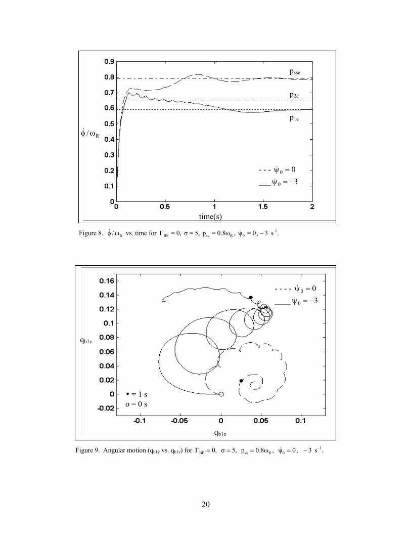
ss Rp 0.8= ω . The three intersection points are given in table 2. Spin histories are plotted in figure 8 for zero initial conditions except for 1

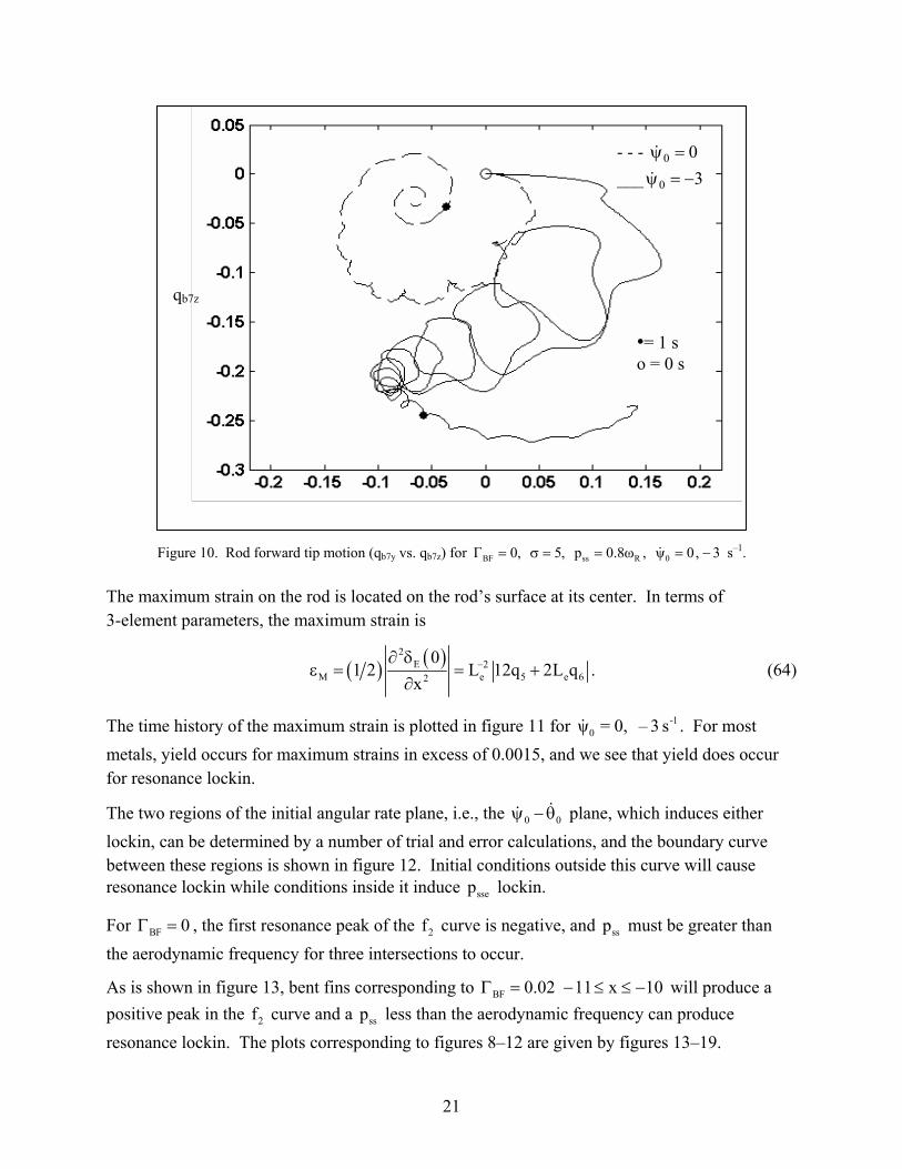
0 0, 3 s−ψ = − . Here, we see that ssep spin-yaw lockin occurs for zero initial angular velocity, and 1ep spin-yaw lockin for an initial yaw rate of –3 s–1. The angular motion in body-fixed coordinates is plotted in figure 9. For lockin at ssep , the motion is smaller than 0.09 rad, while for lockin at 1ep , it is as large as 0.15 rad. The motion of the forward end of the rod in body-fixed coordinates is given in figure 10. Motion for ssep lockin is <0.17 (0.7 in), and after 1 s, it is never >0.09 (0.4 in). For 1ep lockin, it exceeds 0.28 (1.2 in).

fj

19

Figure 6. R/φ ω vs. time for BF ss R 0 RΓ 0, 5, p 6.0ω , /ω 0, 5.4= σ = = φ = .

Figure 7. fj vs. R/φ ω for BF ss RΓ = 0, σ = 5, p = 0.8ω .

fj

R/ωφ

psse

p2e

p1e

R/ωφ

time(s)

20

Figure 8. R/φ ω vs. time for BF ss R 0Γ = 0, σ = 5, p = 0.8ω , ψ = 0, – 3 s-1.

Figure 9. Angular motion (qb1y vs. qb1z) for BF ss R 0Γ 0, 5, p 0.8ω , ψ 0, 3= σ = = = − s–1.

psse

p2e

p1e

R/ωφ

time(s)

- - - 00 =ψ ___ 30 −=ψ

qb1y

• = 1 s o = 0 s

qb1z

- - - - 00 =ψ ____ 30 −=ψ

21

Figure 10. Rod forward tip motion (qb7y vs. qb7z) for BF ss R 0 Γ 0, 5, p 0.8ω , ψ 0, 3= σ = = = − s–1.

The maximum strain on the rod is located on the rod’s surface at its center. In terms of 3-element parameters, the maximum strain is

( ) ( )2E 2

M e 5 e 62

01 2 L 12q 2L q

x−∂ δ

ε = = +∂

. (64)

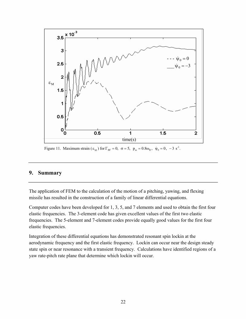
The time history of the maximum strain is plotted in figure 11 for -10ψ = 0, – 3 s . For most

metals, yield occurs for maximum strains in excess of 0.0015, and we see that yield does occur for resonance lockin.

The two regions of the initial angular rate plane, i.e., the 0 0ψ −θ plane, which induces either lockin, can be determined by a number of trial and error calculations, and the boundary curve between these regions is shown in figure 12. Initial conditions outside this curve will cause resonance lockin while conditions inside it induce ssep lockin.

For BF 0Γ = , the first resonance peak of the 2f curve is negative, and ssp must be greater than the aerodynamic frequency for three intersections to occur.

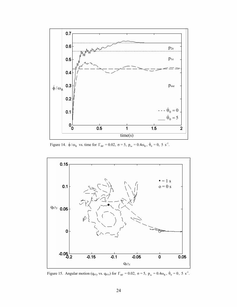
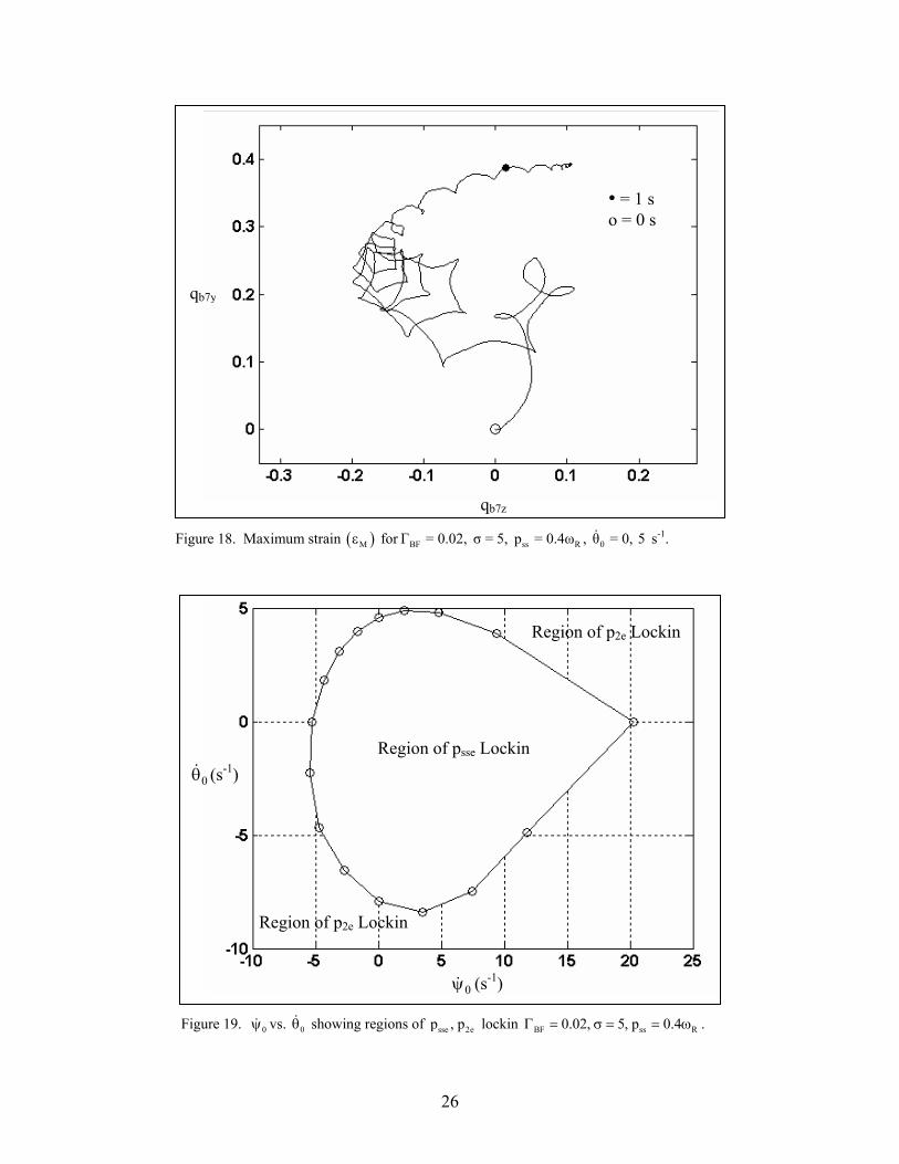
As is shown in figure 13, bent fins corresponding to BF 0.02 11 x 10Γ = − ≤ ≤ − will produce a positive peak in the 2f curve and a ssp less than the aerodynamic frequency can produce resonance lockin. The plots corresponding to figures 8–12 are given by figures 13–19.

- - - 00 =ψ ___ 30 −=ψ

•= 1 s o = 0 s

qb7z

22

Figure 11. Maximum strain ( Mε ) for BF ss R 0Γ 0, 5, p 0.8ω , ψ 0, 3= σ = = = − s-1.

9. Summary

The application of FEM to the calculation of the motion of a pitching, yawing, and flexing missile has resulted in the construction of a family of linear differential equations.

Computer codes have been developed for 1, 3, 5, and 7 elements and used to obtain the first four elastic frequencies. The 3-element code has given excellent values of the first two elastic frequencies. The 5-element and 7-element codes provide equally good values for the first four elastic frequencies.

Integration of these differential equations has demonstrated resonant spin lockin at the aerodynamic frequency and the first elastic frequency. Lockin can occur near the design steady state spin or near resonance with a transient frequency. Calculations have identified regions of a yaw rate-pitch rate plane that determine which lockin will occur.

- - - 00 =ψ ___ 30 −=ψ

Mε

time(s)

23

Figure 12. 0ψ vs. 0θ showing regions of sse 1ep , p lockin BF ss R0, 5, p 0.8Γ = σ = = ω .

Figure 13. fj vs. R/φ ω for BF ss R0.02, 5, p 0.4Γ = σ = = ω .

fj

R/ωφ

Region of p1e Lockin

0θ (s-1)

Region of psse Lockin


0ψ (s-1)

24

Figure 14. R/φ ω vs. time for BF ss R 0Γ = 0.02, σ = 5, p = 0.4ω , θ = 0, 5 s-1.

Figure 15. Angular motion (qb1y vs. qb1z) for BF ss R 0Γ = 0.02, σ = 5, p = 0.4ω , θ = 0, 5 s-1.

R/ωφ

- - - 00 =θ ___ 50 =θ

time(s)

p2e p1e psse

• = 1 s o = 0 s

qb7y

qb7z

25

Figure 16. Rod forward tip motion (qb7y vs. qb7z) for BF ss R 00.02, 5, p 0.4 , 0Γ = σ = = ω θ = s-1.

Figure 17. Rod forward tip motion (qb7y vs. qb7z) for BF ss R 0Γ = 0.02, σ = 5, p = 0.4ω , θ = 5 s-1.

qb1y

qb1z

• = 1 s o = 0 s

- - - 00 =θ ___ 50 =θ

- - - 00 =θ ___ 50 =θ

Mε

time (s)

26

Figure 18. Maximum strain ( )Mε for BF ss R 0Γ = 0.02, σ = 5, p = 0.4ω , θ = 0, 5 s-1.

Figure 19. 0ψ vs. 0θ showing regions of sse 2ep , p lockin BF ss R0.02, 5, p 0.4Γ = σ = = ω .

• = 1 s o = 0 s

qb7y

qb7z


Region of psse Lockin


0ψ (s-1)

0θ (s-1)

27

10. References

1. Mikhail, A. G. In-Flight Flexure and Spin Lock-in for Anti-Tank Kinetic Energy Projectiles. Journal of Spacecraft and Rockets 1996, 33, 657–664.

2. Guidos, B. J.; Garner, J. M.; Newill, J. F.; Livecchia, C. D. Measured In-Flight Rod Flexure of a 120-mm M829E3 Kinetic Energy (KE) Projectile Steel Model; ARL-TR-2820; U.S. Army Research Laboratory: Aberdeen Proving Ground, MD, 2002.

3. Peppitone, T. R.; Jacobson, J. D. Resonant Behavior of a Symmetric Missile Having Roll Orientation-Dependent Aerodynamics. Journal of Guidance and Control 1978, 1, 335–339.

4. Grover, L. S. Effects on Roll Rate of Mass and Aerodynamic Asymmetries On Ballistic Re-Entry Bodies. Journal of Spacecraft and Rockets 1965, 2, 220–225.

5. Price, D. A., Jr. Sources, Mechanisms, and Control of Roll Resonance Phenomena for Sounding Rockets. Journal of Spacecraft and Rockets 1967, 4, 1516–1525.

6. Price, D. A., Jr.; Ericsson, L. E. A New Treatment of Roll-Pitch Coupling for Ballistic Re-Entry Bodies. AIAA Journal 1970, 80, 1608–1615.

7. Murphy, C. H. Some Special Cases of Spin-Yaw Lock-In. Journal of Guidance, Control, and Dynamics 1989, 12, 771–776.

8. Platus, D. H. Aeroelastic Stability of Slender, Spinning Missiles. Journal of Guidance, Control, and Dynamics 1992, 15, 144–151.

9. Legner, H. H.; Lo, E. Y.; Reinecke, W. G. On the Trajectory of Hypersonic Projectiles Undergoing Geometry Changes. AIAA Aerospace Sciences Meeting, Reno, NV, 10–13 January 1994; AIAA 94-0719.

10. Heddadj, S.; Cayzac, R.; Renard, J. Aeroelasticity of High L/D Supersonic Bodies: Theoretical and Numerical Approach. AIAA Aerospace Sciences Meeting, Reno, NV, 10–13 January 2000; AIAA 2000-0390.

11. Murphy, C. H.; Mermagen, W. H. Flight Mechanics of an Elastic Symmetric Projectile. Journal of Guidance, Control, and Dynamics 2001, 24, 1125–1132.

12. Murphy, C. H.; Mermagen, W. H. Flight Motion of a Continuously Elastic Finned Missile. Journal of Guidance, Control, and Dynamics 2003, 26, 89–98.

13. Murphy, C. H.; Mermagen, W. H. Flight Motion of a Continuously Elastic Finned Missile; ARL-TR-2754; U.S. Army Research Laboratory: Aberdeen Proving Ground, MD, 2002.

28

14. Geradin, M.; Rixen, D. Mechanical Vibrations: Theory and Applications to Structural Dynamics; John Wiley & Sons: New York, 1994.

15. Murphy, C. H. Free Flight Motion of Symmetric Missiles; BRL-TR-1216; U.S. Army Ballistics Research Laboratory: Aberdeen Proving Ground, MD, 1963.

16. DeSilver, C. W. Vibration Fundamentals and Practice; CRC Press: New York, 2000; p 351.

29

Appendix A. Integrals

A.1 Aerodynamic Terms

( )

3 3

0 0

3 3

0 0

3 3

0 0

x x

1 N f1 3 M f1x x

x x

2 Nq N f 3 4 Mq M f 3x x

x x

NBF FB BF MBF BF BFx x

f 3 f 2 f1 BF f1 f 2

c C c dx c C c xdx

c C C c dx c C C c xdx

C c dx C c xdx

c 2c xc c c d V c .

α α

α α

= = = =

= + = = + =

= Γ = Γ

= − = + φ

∫ ∫

∫ ∫

∫ ∫

(A-1)

A.2 Boundary Terms

( )

( )

( )

( )

1

0

1

0

1

0

1

0

1

0

1

0

1

0

x

1 f1x

x

3 1 f1x

x

5 f 2x

x

7 1 f 2x

x2

9 1 f1x

11 5 3 1 1

13 7 9 1 3

x

1D D Dbpx

x

3D 1 Dx

I c dx

I x x c dx

I c dx

I x x c dx

I x x c dx

I 2I I x II 2I I x I

I c dx C

I x x c dx

=

= −

=

= −

= −

= − −= − −

= +

= −

∫

∫

∫

∫

∫

∫

∫

( )

( )

( )

( )

3

2

3

2

3

2

3

2

3

2

3

2

3

2

x

2 f1x

x

4 2 f1x

x

6 f 2x

x

8 2 f 2x

x2

10 2 f1x

12 6 4 2 2

14 8 10 2 4x

2D Dx

x

4D 2 Dx

I c dx

I x x c dx

I c dx

I x x c dx

I x x c dx

I 2I I x II 2I I x I

I c dx

I x x c dx

=

= −

=

= −

= −

= − −= − −

=

= −

∫

∫

∫

∫

∫

∫

∫

1

0

x

1BF BF BFx

I c dx= Γ∫ ( )1

0

x

3BF 1 BF BFx

I x x c dx= − Γ∫

1

0

x

5BF f 2 BFx

I c dx= Γ∫ ( )1

0

x

7BF 1 f 2 BFx

I x x c dx= − Γ∫ . (A-2)

30

A.3 Bent Missile Terms

( )

( )

( )

2

0

3

0

3

0

x

1B f1 B BFx

x

2B f 2 B BF f1 EBx

x

3B f1 B BFx

J c dx

J c c dx

J c xdx

= Γ +Γ

= Γ +Γ − δ

= Γ +Γ

∫

∫

∫

( )

( ) ( )

( )

3

0

3

0

2

1

x

4B f 2 B BF f1 EBx

x

5B D EB cB EB 1 cB Dbpx

x

6B B 1x

J c c xdx

J c dx x c

J 1 L x dx

= Γ +Γ − δ

= δ − δ + δ − δ

= δ ρ

∫

∫

∫

( )2 2

1 1

x x

cB B 1 8B1 d B 2x x

1 L dx J a dxδ = δ ρ = − Γ ρ∫ ∫

( ) ( )3

0

x

xB1 1 EB EB 2 d B Bx

I 1 L a L dx = ρ δ δ + ρ Γ Γ ∫ 3

0

x

xB2 d 2 B Bx

I 6a dx= − ρ Γ Γ ∫ . (A-3)

31

Appendix B. Functions

( )

( )

( ) ( )

( )

2

1

3

0

3

0

3

0

x

c E 1x

x

1 f1x

x

2 f 2 f1 Ex

x

3 f1x

1 L dx

J t c dx

J t c c dx

J t c xdx

δ = δ ρ

= Γ

= Γ − δ

= Γ

∫

∫

∫

∫

( ) ( )

( ) ( ) ( )

( ) ( )

( ) ( )

3

0

3

0

2

1

2

1

x

4 f 2 f1 Ex

x

5 D E c E 1 c Dbpx

x

6 E 1x

x

8 d 2x

J t c c xdx

J t c dx x c

J t 1 L x dx

J t a 2i dx.

= Γ − δ

= δ − δ + δ −δ

= δ ρ

= Γ − φΓ ρ

∫

∫

∫

∫ (B-1)

32


33

Appendix C. Generalized Forces and Hermitian Polynomials

( )

( )

x1x 1 D

y z x1y 1z

x2x

y z x x2y 2z E

dFdQ dx g c x dxdx

dF dF dFdQ idQ i i dxdx dx dx

dMdQ dxdx

dF dF dF dMdQ idQ x i dxdx dx dx dx

= = −

+ = + + −ψ + θ

=

+ = + − δ −θ

( )

( )2z

1x x

1y 1z y z x

2x x

2y y z x c x

Q FQ iQ F iF i F

Q M

Q iQ i M iM iF M

=

+ = + + −ψ + θ

=

+ = − + − δ −θ

( )( )( )

2 31

22 e

23

24 e

N 1 3z 2z

N L z 1 z

N z 3 2z

N L z z 1

= − +

= −

= −

= −

( )( )

( )( )

/ 21

/ 22 e

/ 23

/ 24 e

N 6 z z

N L 1 4z 3z

N 6 z z

N L 3z 2z .

= −

= − +

= −

= − (C-1)

34


35

Appendix D. Connector Coefficients for Equations (39–41)

D.1 Rod Parameters

( ) ( ) ( )

( ) ( ) ( )

( ) ( )

11qj e 1 q e j

01

2qj e 1 q j 1 e

01

2 'qj 2 q

0

a L x N z dz x L z z

a L x x N z dz z x L j 1

b x N z dz q 1, 2, 3, 4.

= ρ = +

= ρ = + −

= ρ =

∫

∫

∫ (D-1)

For central element jn 1r

2+

=

1 1 1 1 1 1 1 1 11c 1r 3r e 4r 2c 2r e 3r 4rˆ ˆ ˆ ˆ ˆ ˆ ˆ â a 5a 24L a a a L a 5a−= + + = + +

For adjacent element jn 3r

2+

=

1 1 1 1 1 1 11a 1r e 2r 2a e 1r 2r1 1 1 13a 3r 4a 4r

ˆ ˆ ˆ ˆ ˆ â 5a 24L a a L a 5aˆ ˆ ˆ â a a a ,

−= + = +

= =

2 2 2 2qc qa qc qa

ˆ ˆˆ â , a , b , and b are computed from 2 2qj qj

â and b in same manner as previously shown.

11 12a a 0= =

t e

113 14 2c

11c

n 4 L L

a aa a

= =

= =

t e

1 1 1 1 1 1 1 1 1 113 11 14 21 15 31 1c 1a 16 41 2c 2a 17 3a 18 4a

n 8 L L 3ˆ ˆ ˆ ˆ ˆ ˆ ˆ ˆ â a a a a a a a a a a a a aâ a

= =

= = = + + = + + = =

( ) ( ) ( )

t e1 1 1 1 1 1

13 11 14 21 15 31 12 16 41 22

1 1 1 1 1 1 1 117 32 1c 1a 18 42 2c 2a 19 3a 15

1 1 1 14a 25 35 451 10 1 11 1 12

n 12 L L 5ˆ ˆ ˆ ˆ ˆ â a a a a a a a a aˆ ˆ ˆ ˆ ˆ ˆ ˆ â a a a a a a a a a a

ˆ ˆ ˆ â a a a a a a

= =

= = = + = +

= + + = + + = +

= + = =

36

( ) ( )

( ) ( ) ( ) ( )

1 1 1 1 1 1 1 113 11 14 21 15 31 12 16 41 22 17 32 13

1 1 1 1 1 1 1 1 1 118 42 23 19 33 1c 1a 43 2c 2a 3a 161 10 1 11

1 1 1 1 1 14a 26 36 17 46 271 12 1 13 1 14 1 15a

n 16 L L 7etˆ ˆ ˆ ˆ ˆ ˆ ˆ â a a a a a a a a a a a aˆ ˆ ˆ ˆ ˆ ˆ ˆ ˆ ˆ â a a a a a a a a a a a a a

ˆ ˆ ˆ ˆ â a a a a a a a a

= =

= = = + = + = +

= + = + + = + + = +

= + = + = + = ( )1 137 471 16ˆ â a a=

2n 2na and b are computed from 2 2 2 2 2 2qj qc qa qj qc qa

ˆ ˆ ˆˆ ˆ â , a , a , b , b and b, in the same manner as previously

shown.

37

Appendix E. Connector Coefficients for Equations (42–44)

E.1 Rod Terms

( ) ( ) ( )

( ) ( ) ( ) ( ) ( )

( ) ( )

( ) ( ) ( ) ( )

11 /qj f1 q e j

0

11 /qj f 2 q f1 q e j 1 e

0

12 /qj f1 q

01

2 /qj f 2 q f1 q e

0

f c x N z dz x L z z

g c x N z c x N z L dz z x L j 1

f c x N z xdz q 1, 2, 3, 4

g c x N z c x N z L xdz,

= = +

= − = + −

= =

= −

∫

∫

∫

∫ (E-1)

1n 2n 1n 2nf , f , g and g, are computed from 1 2 1 2qj qj qj qj

ˆ ˆ ˆ ˆf , f , g and g, in the same manner as in appendix D.

E.2 Nonzero Aerodynamic Extension Terms

( ) ( )

t1

a13 e 2 a14 1 21

a 23 e 18 a 24 17 181

a13 1 2 e 6 4 a14 5 3 2 e 6 4

1a 23 17 18 e 16 a 24 15 18 e 16

1a3 ID 2D e 4D a 4 3DE e 2D 4D

n 4

f 24L I f I 5I

f 24L I f I 5I

g I 5I 24L I I g I I I L 5 I I

g I 5I 24L I g I I L 5I

h I 5I 24L I h I L I 5I

−

−

−

−

−

=

= = +

= = +

= − − + − = − − + −

= − − + = − +

= + + = + +

( )

( )

( )

t

t

tt

tt

tt

t

a14 1 a1n 2

a 24 17 a 2n 18

a13 1 a14 5 3 2 a1n 6 4a1 n 1

a 23 17 a 24 15 18 a1n 16a1 n 1

a3 ID a 4 3D 2D an 4Da n 1

n 4f I f I

f I f I

g I g I I g I g I I

g I g I g I g I

h I h I h I h I .

−

−

−

≠

= =

= =

= − = − = − = −

= − = = − =

= = = = (E-2)

38


39

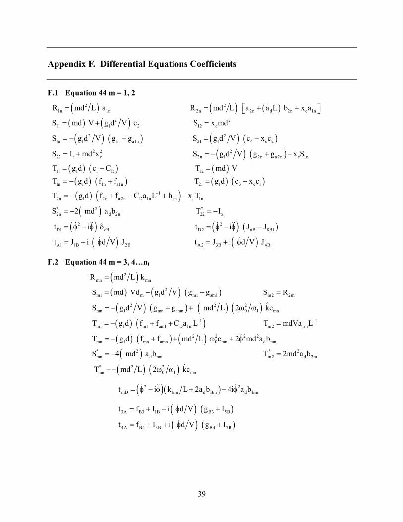
Appendix F. Differential Equations Coefficients

F.1 Equation 44 m = 1, 2

( ) ( ) ( )( ) ( )( ) ( ) ( ) ( )

( ) ( )( ) ( ) ( )( ) ( )

2 21n 1n 2n 2n d 2n c 1n

2 211 1 2 12 c

2 21n 1 1n a1n 21 1 4 c 2

2 2 222 t c 2n 1 2n a 2n c 1n

11 1 1 D 12

1n 1 1n a1n 21

R md L a R md L a a L b x a

S md V g d V c S x md

S g d V g g S g d V c x c

S I md x S g d V g g x S

T g d c C T md V

T g d f f T g

= = + +

= + =

= − + = −

= + = − + −

= − =

= − + = ( ) ( )( ) ( )( )

( ) ( ) ( )

( ) ( )

1 3 c 1

12n 1 2n a 2n D 1n an c 1n

* 2 *2n d 2n 22 x

2 2D1 cB D2 6B 8B1

A1 1B 2B A2 3B 4B

d c x c

T g d f f C a L h x T

S 2 md a b T I

t i t i J J

t J i d V J t J i d V J

−

−

= − + − + −

= − = −

= φ − φ δ = φ − φ −

= + φ = + φ

F.2 Equation 44 m = 3, 4…nt

( )( ) ( ) ( )

( ) ( ) ( ) ( )( ) ( )( ) ( ) ( )( )

2mn mn

2m1 m 1 m1 am1 m2 2m

2 2 2mn 1 mn amn 0 1 mn

1 1m1 1 m1 am1 D 1m m2 1m

2 2 2 2mn 1 mn amn 0 mn d mn

* 2 * 2mn d mn m2 d 2m

R md L k

S md Vd g d V g g S R

ˆ S g d V g g md L 2 kc

T g d f f C a L T mdVa L

T g d f f md L c 2 md a b

S 4 md a b T 2md a b

− −

=

= − + =

= − + + ω ω

= − + + =

= − + + ω + φ

= − =

( ) ( )* 2 2mn 0 1 mn

ˆ T md L 2 kc− − ω ω

( )( )2 2mD Bm d Bm d Bmt i k L 2a b 4i a b= φ − φ + − φ

( ) ( )

( ) ( )3A B3 1B B3 5B

4A B4 3B B4 7B

t f I i d V g I

t f I i d V g I

= + + φ +

= + + φ +

40

`

( )( ) ( ) ( ) ( ) ( ) ( )( )

( ) ( ) ( )( )t t t

t t t

mA Bm Bm t

2 B 2 6 B 2n 1 A B n 1 B n 1

n A Bn 4 B 2 Bn 8 B 2

t f i d V g 4 m n 1

t f I x i d V g I x

t f I x i d V g I x

− − −

= + φ < < −

= + Γ + φ + Γ

= + Γ + φ + Γ

( )( ) ( )

( ) ( ) ( )( )( ) ( )

( ) ( ) ( )( )

j t

2mD Bm

13A B1c 1B 2 B 2 e 4 B 2

1B1c 5B 6 B 2 e 8 B 2

4A B2c 3B e 2 B 2 4 B 2

B2c 7B e 6 B 2 8 B 2

For n 1 n 4 m 3, 4

t i k L

ˆt f I 5I x 24L I x

î d V g I 5I x 24L I x

ˆt f I L I x 5I x

î d V g I L I x 5I x .

−

−

= = =

= φ − φ

= + + Γ + Γ

+ φ + + Γ + Γ

= + + Γ + Γ

+ φ + + Γ + Γ (F-2)

F.3 Quadratic Spin Equation (61)

( ) ( )2

1

x

7 1 E E 2 d 2x

J i L a L 4i iq dx = − ρ δ δ −ρ Γ + φΓ + Γ ∫

( ) ( )

( ) ( ) ( )

( ) ( )( )

t t

t

t t t

n n

D mn d mn m n d mn m nm 3 n 3

ni 2

Bm d Bm m m d Bm n mm 3

n n n2 i

X x xB d mn m n Bm d Bm mm 3 n 3 m 3

2xB xB1

Q i L a a Lb q q 8i a Lb q q

i L e a a Lb q q 8i a Lb q i q

I I I md L Re 4a L b q q e a 3 a L b q

I md I

= =

− φ

=

− φ

= = =

= − − + φ

− − + φ + φ − φ

= + − + −

= +

∑∑

∑

∑∑ ∑

( )xB2I . (F-3)

41

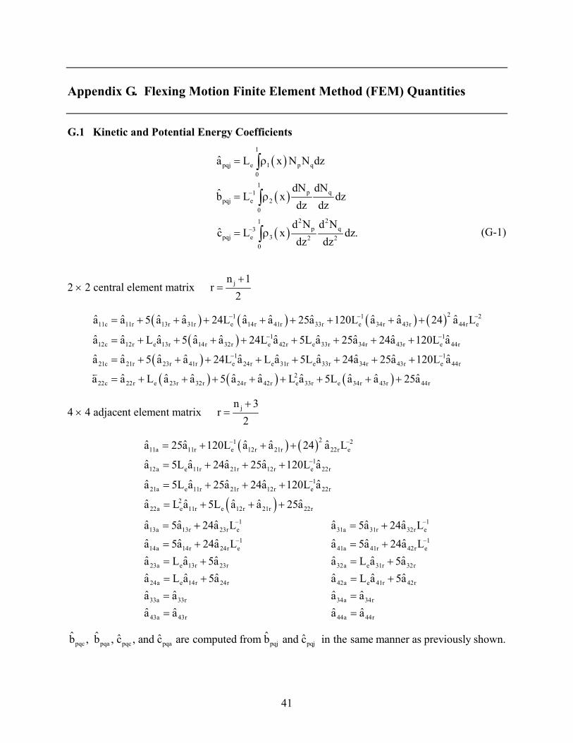
Appendix G. Flexing Motion Finite Element Method (FEM) Quantities

G.1 Kinetic and Potential Energy Coefficients

( )

( )

( )

1

pqj e 1 p q01

p q1pqj e 2

02 21

p q3pqj e 3 2 2

0

a L x N N dz

dN dNb L x dz

dz dz

d N d Nc L x dz.

dz dz

−

−

= ρ

= ρ

= ρ

∫

∫

∫ (G-1)

2 × 2 central element matrix jn 1r

2+

=

( ) ( ) ( ) ( )( )

( )

21 1 211c 11r 13r 31r e 14r 41r 33r e 34r 43r 44r e

1 112c 12r e 13r 14r 32r e 42r e 33r 34r 43r e 44r

121c 21r 23r 41r e 24r

ˆ ˆ ˆ ˆ ˆ ˆ ˆ ˆ ˆ â a 5 a a 24L a a 25a 120L a a 24 a L

ˆ ˆ ˆ ˆ ˆ ˆ ˆ ˆ ˆ â a L a 5 a a 24L a 5L a 25a 24a 120L a

ˆ ˆ ˆ ˆ â a 5 a a 24L a

− − −

− −

−

= + + + + + + + +

= + + + + + + + +

= + + +

( ) ( ) ( )

1e 31r e 33r 34r 43r e 44r

222c 22r e 23r 32r 24r 42r e 33r e 34r 43r 44r

ˆ ˆ ˆ ˆ ˆL a 5L a 24a 25a 120L a

ˆ ˆ ˆ ˆ ˆ ˆ ˆ ˆ â a L a a 5 a a L a 5L a a 25a

−+ + + + +

= + + + + + + + +

4 × 4 adjacent element matrix jn 3r

2+

=

( ) ( )

( )

21 211a 11r e 12r 21r 22r e

112a e 11r 21r 12r e 22r

121a e 11r 21r 12r e 22r

222a e 11r e 12r 21r 22r

113a 13r 23r e 31a

ˆ ˆ ˆ ˆ â 25a 120L a a 24 a L

ˆ ˆ ˆ ˆ â 5L a 24a 25a 120L a

ˆ ˆ ˆ ˆ â 5L a 25a 24a 120L a

ˆ ˆ ˆ ˆ â L a 5L a a 25a

ˆ ˆ ˆ ˆ â 5a 24a L a 5

− −

−

−

−

= + + +

= + + +

= + + +

= + + +

= + = 131r 32r e

1 114a 14r 24r e 41a 41r 42r e

23a e 13r 23r 32a e 31r 32r

24a e 14r 24r 42a e 41r 42r

33a 33r 34a 34r

43a 43r 44a 44r

â 24a Lˆ ˆ ˆ ˆ ˆ â 5a 24a L a 5a 24a Lˆ ˆ ˆ ˆ ˆ â L a 5a a L a 5aˆ ˆ ˆ ˆ ˆ â L a 5a a L a 5aˆ ˆ ˆ â a a aˆ ˆ ˆ â a a a

−

− −

+

= + = += + = +

= + = += == =

pqc pqa pqc pqa pqj pqjˆ ˆ ˆˆ ˆ ˆb , b , c , and c are computed from b and c in the same manner as previously shown.

42

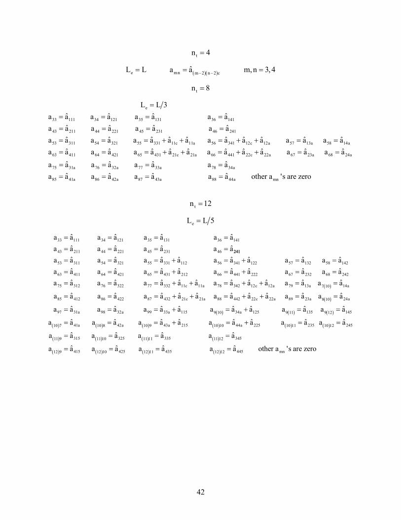
tn 4=

( )( )e mn m 2 n 2 cˆL L a a m,n 3, 4− −= = =

tn 8=

e

33 111 34 121 35 131 36 141

43 211 44 221 45 231 46 241

53 311 54 321 55 331 11c 11a 56 341 12c 12a 57 13a 58 14a

63 411 64 421 65 431 21c 21a 66

L L 3ˆ ˆ ˆ â a a a a a a aˆ ˆ ˆ â a a a a a a aˆ ˆ ˆ ˆ ˆ ˆ ˆ ˆ ˆ â a a a a a a a a a a a a a a aˆ ˆ ˆ ˆ ˆ â a a a a a a a a

=

= = = == = = =

= = = + + = + + = == = = + + = 441 22c 22a 67 23a 68 24a

75 31a 76 32a 77 33a 78 34a

85 41a 86 42a 87 43a 88 44a mn

ˆ ˆ ˆ â a a a a a aˆ ˆ ˆ â a a a a a a aˆ ˆ ˆ â a a a a a a a other a 's are zero

+ + = =

= = = == = = =

tn 12=

eL L 5=

33 111 34 121 35 131 36 141

43 211 44 221 45 231 46 224411

53 311 54 321 55 331 112 56 341 122 57 132 58 142

63 411 64 421 65 431 212 66 441 222 67 232 6

ˆ ˆ ˆ â a a a a a a aˆ ˆ ˆ â a a a a a a aˆ ˆ ˆ ˆ ˆ ˆ ˆ â a a a a a a a a a a a a aˆ ˆ ˆ ˆ ˆ ˆ â a a a a a a a a a a a a

= = = == = = =

= = = + = + = =

= = = + = + =

( )

( )

8 242

75 312 76 322 77 332 11c 11a 78 342 12c 12a 79 13a 14a7 10

85 412 86 422 87 432 21c 21a 88 442 22c 22a 89 23a 24a8 10

97 31a 98 32a 99 33a

aˆ ˆ ˆ ˆ ˆ ˆ ˆ ˆ ˆ â a a a a a a a a a a a a a a a

ˆ ˆ ˆ ˆ ˆ ˆ ˆ ˆ ˆ â a a a a a a a a a a a a a a a

ˆ ˆ ˆ â a a a a a

== = = + + = + + = =

= = = + + = + + = =

= = = + ( ) ( ) ( )

( ) ( ) ( ) ( ) ( ) ( )

( ) ( ) ( )

115 34a 125 135 1459 10 9 11 9 12

41a 42a 43a 215 44a 225 235 24510 7 10 8 10 9 10 10 10 11 10 12

315 32511 9 11 10 11 11

ˆ ˆ ˆ â a a a a a a a

ˆ ˆ ˆ ˆ ˆ ˆ ˆ â a a a a a a a a a a a a a

ˆ â a a a a

= + = =

= = = + = + = =

= = = ( )

( ) ( ) ( ) ( )

335 34511 12

415 425 435 445 mn12 9 12 10 12 11 12 12

ˆ â a a

ˆ ˆ ˆ â a a a a a a a other a 's are zero

=

= = = =

43

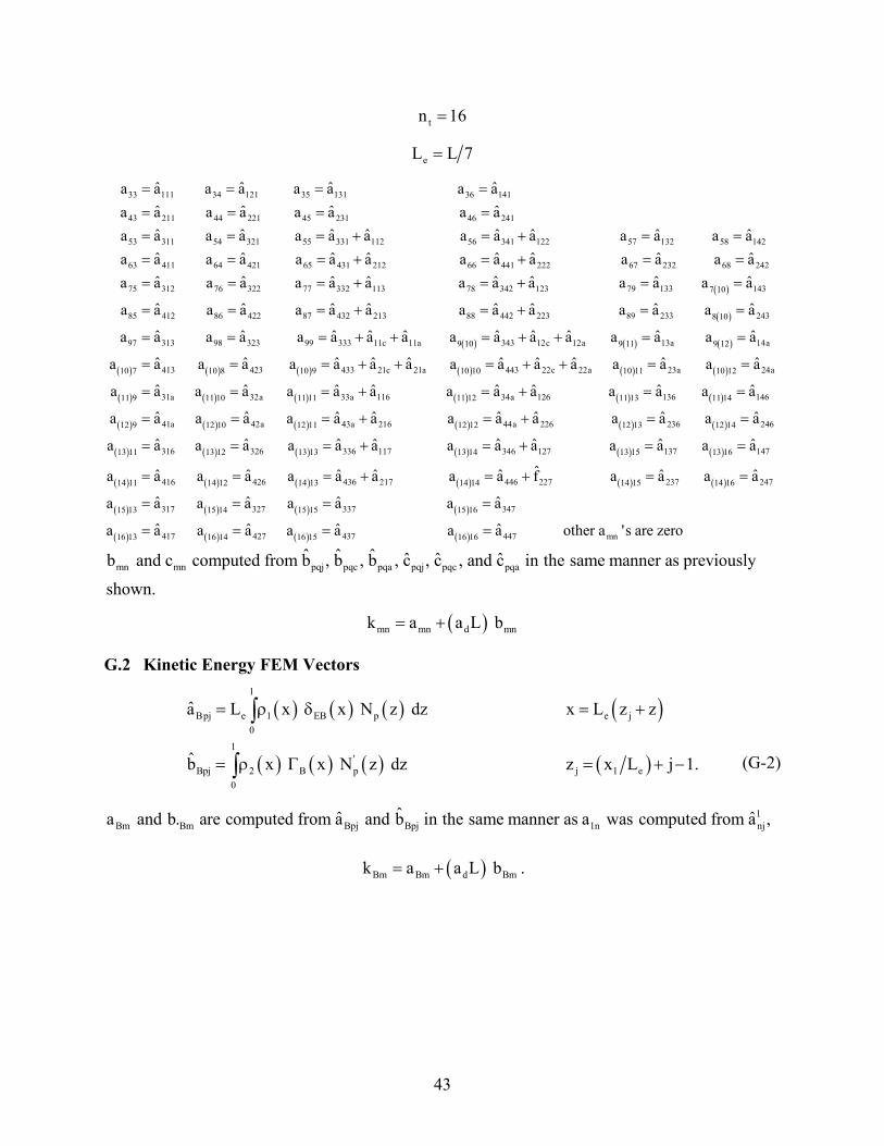
tn 16=

eL L 7=

33 111 34 121 35 131 36 141

43 211 44 221 45 231 46 241

53 311 54 321 55 331 112 56 341 122 57 132 58 142

63 411 64 421 65 431 212 66 441 222 6

ˆ ˆ ˆ â a a a a a a aˆ ˆ ˆ â a a a a a a aˆ ˆ ˆ ˆ ˆ ˆ ˆ â a a a a a a a a a a a a aˆ ˆ ˆ ˆ ˆ â a a a a a a a a a a

= = = == = = == = = + = + = == = = + = +

( )

( )

7 232 68 242

75 312 76 322 77 332 113 78 342 123 79 133 1437 10

85 412 86 422 87 432 213 88 442 223 89 233 2438 10

97 313 98 323 99 333 11c 11a

ˆ â a aˆ ˆ ˆ ˆ ˆ ˆ ˆ â a a a a a a a a a a a a a


ˆ ˆ ˆ ˆ â a a a a a a a a

= == = = + = + = =

= = = + = + = =

= = = + + ( ) ( ) ( )

( ) ( ) ( ) ( ) ( ) ( )

( ) ( ) ( ) ( ) ( )

343 12c 12a 13a 14a9 10 9 11 9 12

413 423 433 21c 21a 443 22c 22a 23a 24a10 7 10 8 10 9 10 10 10 11 10 12

31a 32a 33a 116 34a 126 1311 9 11 10 11 11 11 12 11 13

ˆ ˆ ˆ ˆ â a a a a a a

ˆ ˆ ˆ ˆ ˆ ˆ ˆ ˆ ˆ â a a a a a a a a a a a a a a a

ˆ ˆ ˆ ˆ ˆ ˆ â a a a a a a a a a a a

= + + = =

= = = + + = + + = =

= = = + = + = ( )

( ) ( ) ( ) ( ) ( ) ( )

( ) ( ) ( ) ( ) ( ) ( )

( ) ( )

6 14611 14

41a 42a 43a 216 44a 226 236 24612 9 12 10 12 11 12 12 12 13 12 14

316 326 336 117 346 127 137 14713 11 13 12 13 13 13 14 13 15 13 16

416 42614 11 14 12

â a



ˆ â a a a a

=

= = = + = + = =

= = = + = + = =

= = ( ) ( ) ( ) ( )

( ) ( ) ( ) ( )

( ) ( ) ( ) ( )

436 217 446 227 237 24714 13 14 14 14 15 14 16

317 327 337 34715 13 15 14 15 15 15 16

417 427 437 447 mn16 13 16 14 16 15 16 16

ˆˆ ˆ ˆ ˆ â a a a f a a a a

ˆ ˆ ˆ â a a a a a a a

ˆ ˆ ˆ â a a a a a a a other a 's are zero

= + = + = =

= = = =

= = = =

mn mn pqj pqc pqa pqj pqc pqaˆ ˆ ˆ ˆ ˆ ˆb and c computed from b , b , b , c , c , and c in the same manner as previously

shown.

( )mn mn d mnk a a L b= +

G.2 Kinetic Energy FEM Vectors

( ) ( ) ( ) ( )

( ) ( ) ( ) ( )

1

Bpj e 1 EB p e j0

1'

Bpj 2 B p j 1 e0

a L x x N z dz x L z z

b x x N z dz z x L j 1.

= ρ δ = +

= ρ Γ = + −

∫

∫ (G-2)

1Bm Bm Bpj Bpj 1n nj

ˆˆ â and b. are computed from a and b in the same manner as a was computed from a ,

( )Bm Bm d Bmk a a L b= + .

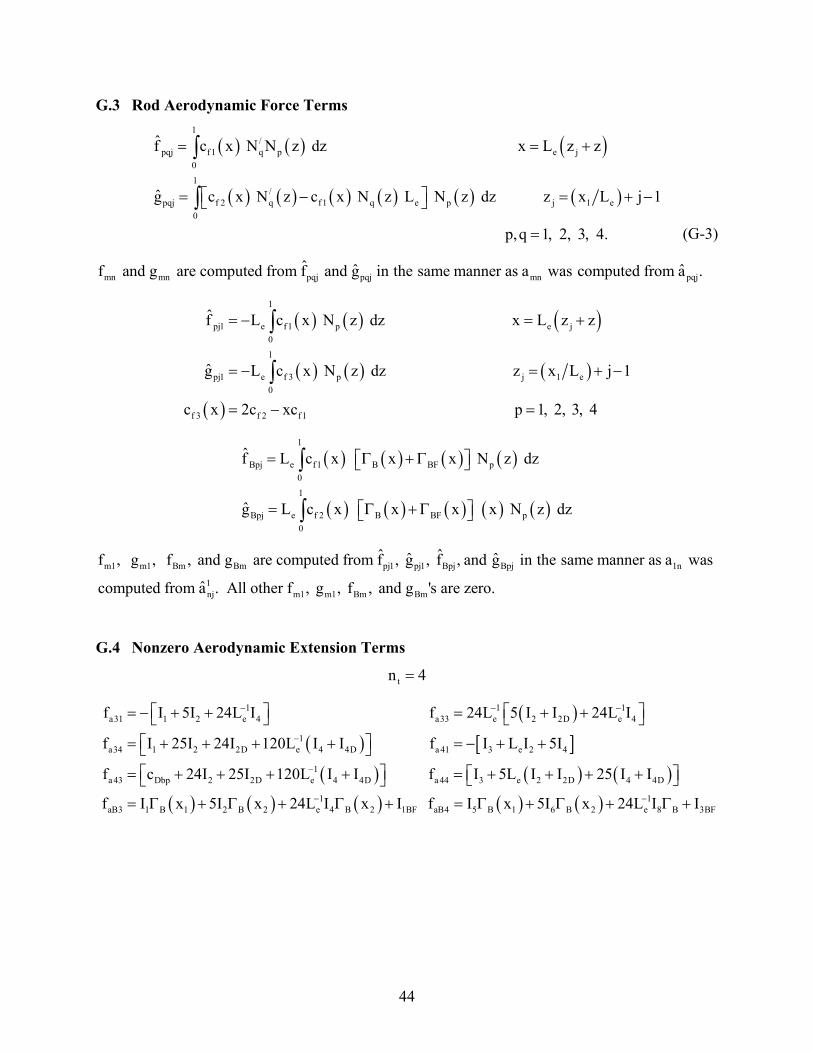
44

G.3 Rod Aerodynamic Force Terms

( ) ( ) ( )

( ) ( ) ( ) ( ) ( ) ( )

1/

pqj f1 q p e j0

1/

pqj f 2 q f1 q e p j 1 e0

f c x N N z dz x L z z

g c x N z c x N z L N z dz z x L j 1

p,q 1, 2, 3, 4.

= = +

= − = + −

=

∫

∫ (G-3)

mn mn pqj pqj mn pqjˆ ˆ ˆf and g are computed from f and g in the same manner as a was computed from a .

( ) ( ) ( )

( ) ( ) ( )

( )

1

pj1 e f1 p e j01

pj1 e f 3 p j 1 e0

f 3 f 2 f1

f L c x N z dz x L z z

g L c x N z dz z x L j 1

c x 2c xc p 1, 2, 3, 4

= − = +

= − = + −

= − =

∫

∫

( ) ( ) ( ) ( )

( ) ( ) ( ) ( ) ( )

1

Bpj e f1 B BF p0

1

Bpj e f 2 B BF p0

f L c x x x N z dz

g L c x x x x N z dz

= Γ +Γ

= Γ +Γ

∫

∫

m1 m1 Bm Bm pj1 pj1 Bpj Bpj 1n

1nj m1 m1 Bm Bm

ˆ ˆˆ ˆf , g , f , and g are computed from f , g , f , and g in the same manner as a was

ˆcomputed from a . All other f , g , f , and g 's are zero.

G.4 Nonzero Aerodynamic Extension Terms

tn 4=

( )( ) [ ]( ) ( ) ( )

( ) ( )

1 1 1a31 1 2 e 4 a33 e 2 2D e 4

1a34 1 2 2D e 4 4D a 41 3 e 2 4

1a 43 Dbp 2 2D e 4 4D a 44 3 e 2 2D 4 4D

aB3 1 B 1 2 B 2

f I 5I 24L I f 24L 5 I I 24L I

f I 25I 24I 120L I I f I L I 5I

f c 24I 25I 120L I I f I 5L I I 25 I I

f I x 5I x 24

− − −

−

−

= − + + = + + = + + + + = − + + = + + + + = + + + +

= Γ + Γ + ( ) ( ) ( )1 1e 4 B 2 1BF aB4 5 B 1 6 B 2 e 8 B 3BFL I x I f I x 5I x 24L I I− −Γ + = Γ + Γ + Γ +

45

tn 4≠

( ) ( ) ( ) ( )

( ) ( ) ( ) ( ) ( )t tt t t t t t

tt

a31 1 a34 1 a 43 Dbp a 41 3 a 44 3

2 2 2D 4 an n 4 4Da n 1 1 a n 1 n an n 1 a n 1

aB3 1 B 1 1BF aB4 3 B 1 3BF 2 B 2 aBn 4 B 2aB n 1

Amn

f I f I f c f I f I

f I f I f I f I f I I

f I x I f I x I f I x f I x

other f 's are zero

− − −

−

= − = = = − =

= − = = = − = +

= Γ + = Γ + = Γ = Γ

tn 4=

( ) ( ) ( )

( ) ( )[ ] ( ) ( )

( )

22 1 2a31 11 12 e 14 a33 1 2 e 4 6 e 10 8

a34 3 5 e 2 4 6 10 8

1a 41 13 e 12 14 a 43 3 e 2 4 6 e 10 8

2a 44 9 7 e 2 e 4 6

g I 5I 24L I g I 25I 120L 2I I 24 L I I

g I I 5L I 24 2I I 25 I I

g I L I 5I g I 5L I 24 2I I 120L I I

g I I L I 5L 2I I

− − −

−

= − + + = − + + − + − = − − + + − + −

= − + + = − + + − + −

= − − + + − ( )( ) ( ) ( )( ) ( ) ( )

10 8

1aB3 5 B 1 6 B 2 e 8 B 2 5BF

aB4 7 B 1 e 6 B 2 8 B 2 7BF

25 I I

g I x 5I x 24L I x I

g I x L I x 5I x I

−

+ − = Γ + Γ + Γ +

= Γ + Γ + Γ +

tn 4≠

( ) ( )( ) ( )( )

( ) ( )( ) ( )( )

( ) ( ) ( )

n n n n n

t t t t t

t

a31 11 a33 1 a34 5 3

a 41 13 a 43 3 a 44 7 9

12 2 6 4a n 1 1 a n 1 n 1 a n 1 n

14 4 8 10a n 1 a n n 1 a n n

aB3 5 B 1 5BF aB4 7 B 1 7BF aB n 1

g I g I g I Ig I g I g I I

g I I g I I

g I g I g I I

g I x I g I x I g

− − − −

−

−

= − = − = −= − = − = −= − = − = −

= − = − = −

= Γ + = Γ + ( ) ( )t6 B 2 aBn 8 B 2I x g I x= Γ = Γ

amnother g 's are zero . (G-4)

46


47

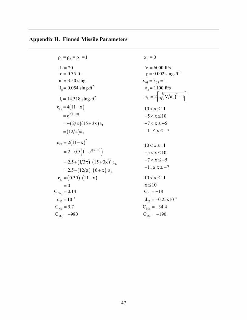
Appendix H. Finned Missile Parameters

1 2 3 cρ = ρ = ρ = 1 x = 0

L = 20 V = 6000 ft/s d = 0.35 ft. ρ= 0.002 slugs/ft3 m = 3.50 slug 01 23x x 1= = xI = 0.054 slug-ft2 sa = 1100 ft/s

tI = 14.318 slug-ft2 ( )1

2L sa 2 V a 1

− = −

( )( )

( ) ( )( )

f1

2 x 10

L

L

c 4 11 x

e2 15 3x a

12 a

−

= −

=

= − π +

= π

10 x 115 x 107 x 511 x 7

< ≤− < ≤− < ≤ −− ≤ ≤ −

( )( )( )

( ) ( )( ) ( )

2f 2

2 x 10

2L

L

c 2 11 x

2 0.5 1 e

2.5 1 3 15 3x a

2.5 12 6 x a

−

= −

= + −

= + π +

= − π +

10 x 115 x 107 x 511 x 7

< ≤− < ≤− < ≤ −− ≤ ≤ −

( ) ( )Dc 0.30 11 x0

= −

=

10 x 11x 10< ≤≤

DbpC 0.14= pC 18= − 3

12d 10−= 522d 0.25x10−= −

N M

Mq M

C 9.7 C 34.4C 980 C 190

α α

α

= = −

= − = −

48


49

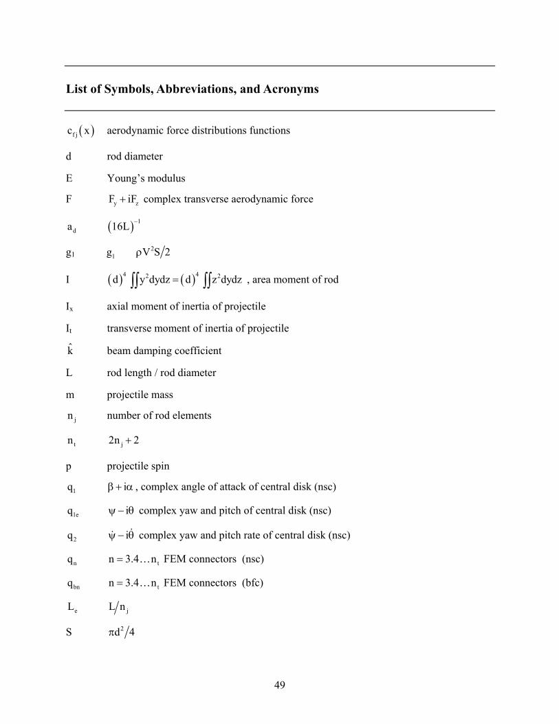
List of Symbols, Abbreviations, and Acronyms

( )f jc x aerodynamic force distributions functions

d rod diameter

E Young’s modulus

F y zF iF+ complex transverse aerodynamic force

da ( ) 116L −

g1 21g V S 2ρ

I ( ) ( )4 42 2d y dydz d z dydz=∫∫ ∫∫ , area moment of rod

Ix axial moment of inertia of projectile

It transverse moment of inertia of projectile

k beam damping coefficient

L rod length / rod diameter

m projectile mass

jn number of rod elements

tn j2n 2+

p projectile spin

1q iβ+ α , complex angle of attack of central disk (nsc)

1eq iψ− θ complex yaw and pitch of central disk (nsc)

2q iψ − θ complex yaw and pitch rate of central disk (nsc)

nq tn 3.4 n= … FEM connectors (nsc)

bnq tn 3.4 n= … FEM connectors (bfc)

eL jL n

S 2d 4π

50

T total kinetic energy

dT kinetic energy of disk at x with thickness dx

V magnitude of projectile velocity

1 2x , x location of beam ends

01 23x , x dimensionless length of fore and aft aerodynamic extensions

cx axial location of center of mass

α angle of attack of central disk

β angle of sideslip of central disk

Γ E

x∂δ∂

, complex cant of disk

Mε maximum strain of rod

2

1

x1

c Ex

L dx−δ δ∫ , lateral location of missile’s cm

E Ey Eziδ δ + δ , lateral displacement of disk (nsc)

φ roll angle

kφ frequency of k-th mode

kλ damping of k-th mode

ρ air density

jρ axial variation of mass, moment of inertia, elasticity

σ 1 Rω ω

( )20 0 0ω E I L md=

1ω lowest elastic frequency of beam in vacuum

Rω rigid projectile zero-spin frequency

( )x y zF F ,F ,F= , aerodynamic force exerted on missile (nsc)

( )x y zM M ,M ,M= , aerodynamic moment exerted on missile (nsc)

51

{ }Re z real part of z

{ }Im z imaginary part of z

Carat superscript denotes quantity for a single element

Tilde superscript denotes elastic parameter for bent missile

B subscript denotes parameter for bent projectile

BF subscript denotes bent fin parameter

E subscript denotes an elastic coordinate parameter (nsc)

T subscript denotes trim motion parameter

b subscript denotes an elastic coordinate parameter (bfc)

(bfc) body-fixed coordinates

(efc) earth-fixed coordinates

(nsf) non-spinning coordinates

NO. OF NO. OF COPIES ORGANIZATION COPIES ORGANIZATION

52

1 DEFENSE TECHNICAL (PDF INFORMATION CTR ONLY) DTIC OCA 8725 JOHN J KINGMAN RD STE 0944 FT BELVOIR VA 22060-6218 1 COMMANDING GENERAL US ARMY MATERIEL CMD AMCRDA TF 5001 EISENHOWER AVE ALEXANDRIA VA 22333-0001 1 INST FOR ADVNCD TCHNLGY THE UNIV OF TEXAS AT AUSTIN 3925 W BRAKER LN STE 400 AUSTIN TX 78759-5316 1 US MILITARY ACADEMY MATH SCI CTR EXCELLENCE MADN MATH THAYER HALL WEST POINT NY 10996-1786 1 DIRECTOR US ARMY RESEARCH LAB AMSRD ARL CS IS R 2800 POWDER MILL RD ADELPHI MD 20783-1197 3 DIRECTOR US ARMY RESEARCH LAB AMSRD ARL CI OK TL 2800 POWDER MILL RD ADELPHI MD 20783-1197 3 DIRECTOR US ARMY RESEARCH LAB AMSRD ARL CS IS T 2800 POWDER MILL RD ADELPHI MD 20783-1197

ABERDEEN PROVING GROUND 1 DIR USARL AMSRD ARL CI OK TP (BLDG 4600)


53

1 COMMANDER US ARMY ARDEC TECHNICAL LIBRARY PICATINNY ARSENAL NJ 07806-5000 1 COMMANDER US NAVAL SURFACE WEAPONS WARFARE CENTER T PEPITONE MS MC K21 DAHLGREN VA 22448 1 TECHNICAL DIRECTOR US ARMY ARDEC AMSTA AR TD PICATINNY ARSENAL NJ 07806-5000 1 HQ USAMC PRNCPL DPTY FOR TECHLGY ALEXANDRIA VA 22333-0001 12 COMMANDER US ARMY ARDEC AET A C NG J GRAU S KAHN H HUDGINS M AMORUSO E BROWN B WONG W TOLEDO S CHUNG C LIVECCHIA G MALEJKO J WHYTE PICATINNY ARSENAL NJ 07806-5000 3 COMMANDER US ARMY ARDEC SMCAR CCH V B KONRAD E FENNELL T LOUZERIO PICATINNY ARSENAL NJ 07806-5000

4 COMMANDER US ARMY ARDEC SMCAR FSE A GRAF D LADD E ANDRICOPOULIS K CHEUNG PICATINNY ARSENAL NJ 07806-5000 6 COMMANDER US ARMY ARDEC SMCAR CCL D F PUZYCKI D CONWAY D DAVIS K HAYES M PINCAY W SCHUFF PICATINNY ARSENAL NJ 07806-5000 3 DIRECTOR US ARMY RESEARCH OFC G ANDERSON K CLARK T DOLIGOWSKI PO BOX 12211 RESEARCH TRIANGLE PARK NC 27709-2211 2 COMMANDER US NAVAL SURFC WEAPONS CTR CODE DK20 MOORE CODE DK20 DEVAN DAHLGREN VA 22448-5000 2 COMMANDER WHITE OAK LABORATORY US NSWC APPLIED MATH BR CODE R44 PRIOLO CODE R44 WARDLAW SILVER SPRING MD 20903-5000 1 COMMANDER US ARMY AVN AND MIS CMND AMSAM RD SS AT W WALKER REDSTONE ARSENAL AL 35898-5010


54

4 COMMANDER US AIR FORCE ARMAMENT LAB AFATL FXA B SIMPSON G ASATE R ABELGREN G WINCHENBACK EGLIN AFB FL 32542-5434 2 DIRECTOR SANDIA NATIONAL LAB W OBERKAMPF W WOLFE DIVISION 5800 ALBUQUERQUE NM 87185 1 DIRECTOR LOS ALAMOS NATIONAL LAB MS G770 W HOGAN LOS ALAMOS NM 87545 1 DIRECTOR NASA AMES RESEARCH CTR MS 258 1 L SCHIFF MOFFETT FIELD CA 94035 1 DIRECTOR NASA LANGLEY RESEARCH CTR M HEMSCH LANGLEY STATION HAMPTON VA 23665 1 MASSACHUSETTS INST OF TECH DEPT OF AERONAUTICS AND ASTRONAUTICS E COVERT 77 MASSACHUSETTS AVE CAMBRIDGE MA 02139 1 ARROW TECHLGY ASSOC INC R WHYTE PO BOX 4218 BURLINGTON VT 05401-4218 2 C H MURPHY PO BOX 269 UPPER FALLS MD 21156 2 W H MERMAGEN 4149 U WAY HAVRE DE GRACE MD 21078

1 DR W STUREK 3500 CARSINWOOD DR ABERDEEN MD 21001-1412 1 OREGON STATE UNIV DEPT OF MECH ENGR DR M COSTELLO CORVALLIS OR 97331

ABERDEEN PROVING GROUND 4 COMMANDER US ARMY ARDEC SMCAR DSD T R LIESKE F MIRABELLE J WHITESIDE J MATTS APG MD 21005 26 DIR USARL AMSRD ARL CI H C NIETUBICZ AMSRD ARL HR SC D SAVICK AMSRD ARL SL BE A MIKHAIL AMSRD ARL WM E SCHMIDT AMSRD ARL WM B A HORST AMSRD ARL WM BA W D AMICO B DAVIS T HAWKINS AMSRD ARL WM BC M BUNDY G COOPER W DRYSDALE J GARNER B GUIDOS B OSKAY P PLOSTINS J SAHU K SOENCKSEN P WEINACHT S WILKERSON AMSRD ARL WM BD T MINOR

NO. OF COPIES ORGANIZATION

55

AMSRD ARL WM BF H EDGE AMSRD ARL WM T B BURNS AMSRD ARL WM TC R COATES W DE ROSSET R MUDD AMSRD ARL WM TD E RAPACKI

NO. OF COPIES ORGANIZATION

56

1 DEFENSE RESEARCH ESTABLISHMENT VALCARTIER DELIVERY SYSTEM DIVISION A D DUPUIS 2459 PIE XI NORD VAL BELAIR QUEBEC CANADA

Documents

Spin-Yaw Lockin of an Elastic Finned Projectile - DTIC