Spatio-temporal groundwater recharge assessment:

a data-integration and modelling approach

Alain Pascal Francés February, 2008

i

Spatio-temporal groundwater recharge assessment: a data-integration and modelling approach

by

Alain Pascal Francés Thesis submitted to the International Institute for Geo-information Science and Earth Observation in partial fulfilment of the requirements for the degree of Master of Science in Water Resources and Environmental Management, Specialisation Groundwater Assessment and Management Thesis Assessment Board Chairman : Prof. Dr. Z. Su External examiner : Prof. Dr. Okke Batelaan Supervisor : Dr. Ir. M.W. Lubczynski Member : Drs. R. Becht

INTERNATIONAL INSTITUTE FOR GEO-INFORMATION SCIENCE AND EARTH OBSERVATION ENSCHEDE, THE NETHERLANDS

iii

Disclaimer This document describes work undertaken as part of a programme of study at the International Institute for Geo-information Science and Earth Observation. All views and opinions expressed therein remain the sole responsibility of the author, and do not necessarily represent those of the institute.

v

Abstract

Groundwater fluxes can be highly variable in both space and time, which is a factor of uncertainty in groundwater flow modelling. This project aims to implement appropriate techniques to assess spatio-temporally groundwater recharge and thus improve the reliability and forecasting capabilities of groundwater flow models. The methodology is composed of the following steps: (i) design of field specific data acquisition schema to capture the spatial variability; (ii) intensive hydrological data monitoring to obtain the temporal variability of fluxes; (iii) development of a spatio-temporal recharge assessment protocol for its dynamic integration with numerical groundwater flow model. The recharge model is developed as a lumped parameter approach and requires a set of soil and aquifer parameters that can be obtained by standard field work and laboratory measurements.

The developed procedures are tested on the Pisoes catchment of the semi-arid zone of Alentejo province (Portugal). As the lateral heterogeneity of the clayey topsoil was considered crucial for the reliability of the recharge model, field data acquisition focused on: (i) apparent electrical conductivity measurements, using the GeonicsTM ground conductivity meter EM-31, to derive topsoil thickness and extrapolate it through kriging with external drift using high resolution multispectral images as auxiliary maps; (ii) drilling and augering, which allowed soil profiling observations and depth-sampling to determine vadose zone hydraulic properties in laboratory. Monitoring at strategic locations of the catchment provided the driving forces (rainfall and potential evapotranspiration) and the state variables (soil moisture and hydraulic heads) of the system.

Data integration determined the depth-wise discretization of the vadose zone and its parameterization. The developed recharge model (pyEARTH-2D) solves the water balance in the topsoil layer through linear relations between fluxes and soil moisture. pyEARTH-2D is coupled with flow model MODFLOW and its calibration is done against transient groundwater hydraulic heads. First results showed improvements of the groundwater flow model solution in the Pisoes catchment. Further work in this research direction will focus on developing the dynamic link involving simultaneous calibration of pyEARTH-2D and groundwater flow model MODFLOW through the PEST parameter estimation algorithm.

vii

Acknowledgements

I would like to express my gratitude to the Fundacao da Ciencia e Tecnologia to grant me with the scholarship that financed my participation to the WREM MSc degree programme. A grateful thank is due to my first supervisor Dr. Maciek W. Lubczynski for: (i) his enthusiasm in managing science activity; (ii) his permanent flux of ideas; (iii) his rigour and exigency on output quality. Many thanks to push and guide me into this adventure! I thank the Programme Director Ir. Arno van Lieshout for his flexibility, availability and creativity to find a special setup that allowed me to integrate the WREM course. I also really appreciated the dedication of the WREM course teachers and the quality of their lectures. A particular attention is due to my second supervisor Drs. Robert Becht for his unconventional comments, to MSc. Ir. Gabriel Norberto Parodi for his help in field work and data processing and to Dr. Ambro Gieske for his constructive criticism. I have been positively surprised by the availability and interest of ITC staff in giving support to the students in general and to my research in particular. I would thank Drs. Boudewijn de Smeth for his precious advices, assistance, tips and tricks in the laboratory world, Dr. David Rossiter for his attention and curiosity about students activity, Dr. Jean Roy, Dr. Mark van der Meijde and Drs. Rob Sporry for their valuable suggestions in setting the geophysical survey, Dr. Frank van Ruitenbeek and Dr. Harald van der Werff for their support in the acquisition and processing of the mineral spectra. I have to confess my saudade of the IGM-INETI-LNEG Hydrogeology Department staff: Doutor Augusto Costa for his friendship and his interest in my scientific activity, Eduardo Paralta that shared his data and knowledge of the Pisoes catchment, as well as the copos and petiscos do Pulo do Lobo, the amazing DH cachopas Carla, Carla and Judite, Eng. Alexandre, Dr Jose Sampaio and Dr. Manuel Morais. I also express my consideration to Prof. Luis Ribeiro of CVRM - Centro de Geo-Sistemas (Universidade Tecnica de Lisboa) for his helpful comments on my research topic. I am really grateful to Elsa Cristina Ramalho for her valuable help to the geophysical survey, as well as for her camaraderie. I also thank the INETI Beja staff, in particular his head Pedro Sousa and Senhores Joaquim Gomes and Manuel Silva for their sense of humour in early morning field work. The precious support offered by the Centro Operativo e de Tecnologia de Regadio staff and in particular his Director Técnico Isaurindo Oliveira, Jorge Maia and Marta Varela, has been essential to the success of the field campaign. Many thanks for their hospitality. I am thankful to Dr. Willem Vervoort from CSAM (University of Sidney) to share the R code for electromagnetic data inversion. I also thank Eng. Alexandre Leal from EMAS Beja for the information and data on public wells. To my colleagues Tanvir Hassan and Stephen Kiama, for the hard and nice time we had during the GB field work, I let this message: “A luta continua!”. To the WREM students, my companions of struggle, and to Diana Chavarro and Jamshid Farifteh, thank to share with me the life after ITC!

viii

I dedicate this work to my dear missing grand parents Jean, Odette, Angele and Louis that supported me during my childhood and study time with a special and sweet care. I will always have for them a deep tenderness. I also want to do homage to my mother, that always worried about me and my sister and struggled for our education, to my father that gave me the right suggestions, the inspiring readings and the freedom to choose my way, to my sister Helene and my nephew Tom with which we share a reciprocal affection. To Odete and Rose Marie for the precious support they gave to my family during the last two months of the thesis study (I think they also enjoyed!). And to Catarrina, to share with me this new life, to tolerate the demanding schedule of the Msc study and to have the surprising capacity in transforming this busy-stressed-exile period in a charming and pleasant lifetime! And to Alice, our lovely daughter, which deeply felt asleep many times with the boring reading of this thesis!

ix

Table of contents

1. Scope of the study ......................................................................................................................................... 1 1.1. Statement of the research problem ......................................................................................................... 1 1.2. State of the art......................................................................................................................................... 1 1.3. Objectives of the thesis........................................................................................................................... 3

1.3.1. Main objective ................................................................................................................................. 3 1.3.2. Specific objectives........................................................................................................................... 3 1.3.3. Research questions .......................................................................................................................... 3 1.3.4. Hypotheses ...................................................................................................................................... 3 1.3.5. Assumptions .................................................................................................................................... 4

2. Study area description ................................................................................................................................... 5 2.1. General settings / features of the catchment ........................................................................................... 5 2.2. Auxiliary maps and information............................................................................................................. 7

2.2.1. Soil and geology .............................................................................................................................. 7 2.2.2. Digital Elevation Model .................................................................................................................. 8 2.2.3. QuickBird image.............................................................................................................................. 8

3. Data integration ............................................................................................................................................. 9 3.1. Time-series ............................................................................................................................................. 9

3.1.1. Driving forces.................................................................................................................................. 9 3.1.2. State variables................................................................................................................................ 10

3.2. Soil spatial characterisation.................................................................................................................. 15 3.2.1. Electromagnetic survey and spatial assessment of topsoil thickness ............................................ 17 3.2.2. Soil moisture and soil electrical conductivity................................................................................ 27 3.2.3. Soil hydraulic parameters .............................................................................................................. 29 3.2.4. Mineral spectra analysis ................................................................................................................ 35

3.3. Summary............................................................................................................................................... 36 4. Recharge modelling..................................................................................................................................... 37

4.1. Recharge models concepts.................................................................................................................... 37 4.1.1. pyEARTH-1D model..................................................................................................................... 37 4.1.2. pyEARTH-2D model..................................................................................................................... 42

4.2. Well-hydrograph analysis..................................................................................................................... 47 4.2.1. Theory............................................................................................................................................47 4.2.2. Recession curve determination...................................................................................................... 49 4.2.3. Recharge assessment ..................................................................................................................... 49

5. Discussion and conclusions......................................................................................................................... 51 5.1. Data integration ....................................................................................................................................51 5.2. Recharge assessment ............................................................................................................................ 52 5.3. Follow-up research ............................................................................................................................... 53

6. References ................................................................................................................................................... 55 Appendix A – Study area maps ..........................................................................................................................a Appendix B - Field work and study area photographies ................................................................................... b Appendix C - Electromagnetic induction model: main equations......................................................................e Appendix D – Inverted electrical conductivity profiles ..................................................................................... i Appendix E – Water retention curves................................................................................................................ q

x

Appendix F – Linear models applied to topsoil thickness estimation ................................................................s Appendix G - Recession curve determination...................................................................................................w

xi

List of figures

Figure 1 – Actual evapotranspiration ET and percolation Rp as a linear function of soil moisture content

(Equation 1 and Equation 3). PET potential evapotranspiration; Ksat: saturated hydraulic conductivity; θfc:

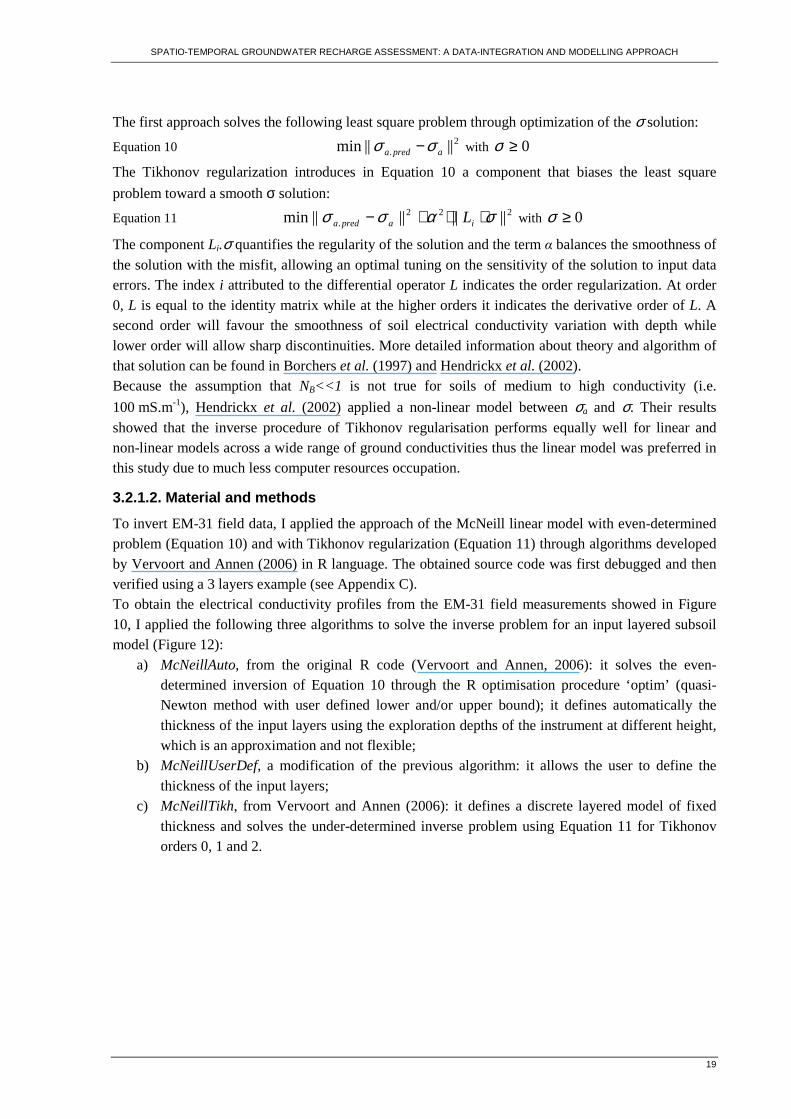
soil moisture at field capacity, θpwp: permanent wilting point; φ: porosity........................................................ 4 Figure 2 – Location of the Pisoes catchment..................................................................................................... 5 Figure 3 – Hyetograph, maximum and minimum temperatures. Monthly averages, period 1961-1990 (Beja meteorological station, Instituto de Meteorologia, www.meteo.pt) .................................................................. 6 Figure 4 - Conceptual model of the Pisoes catchment subsurface and location of the two main piezometers SDH1 and JK7 (Cortez, 2004)........................................................................................................................... 7 Figure 5 – Soil moisture time series at ITC station (ECHO sensor)................................................................ 11 Figure 6 – Soil matric pressure monitoring (CLAY – 20cm).......................................................................... 12 Figure 7 – Soil matric pressure monitoring (CALCRETE – 60cm)................................................................ 12 Figure 8 – Soil moisture time series at SDH1 piezometer (Steven Hydraprobe) ............................................ 13 Figure 9 - Meteorological and piezometric data.............................................................................................. 14 Figure 10 – Field data: apparent electrical conductivity (ECa) and drilling locations plotted on QuickBird image (natural colour). Higher values of ECa are related to higher thickness of clayey topsoil in the depressed drainage area of the catchment (measurements with EM31 device on the ground in vertical position)........................................................................................................................................................... 16 Figure 11 – Induced current flow by a ground conductivity meter (vertical dipoles) ..................................... 18 Figure 12 – Input models for the 3 inversion methods of σa measurements at 5 different heights (0,30 m increment) with EM-31 instrument in horizontal (H) and vertical (V) mode (T indicates thickness and Z depth of layers) using: a) McNeillAuto: thickness of layers is derived from the instrument depth exploration minus height of measurement; b) McNeillUserDef: user defined layer thickness; c) McNeillTikh: fixed thickness of discrete layers; d) hypothetic real case, in which Zi

* is the depth of homogeneous layers with

ground conductivity σi*. .................................................................................................................................. 20

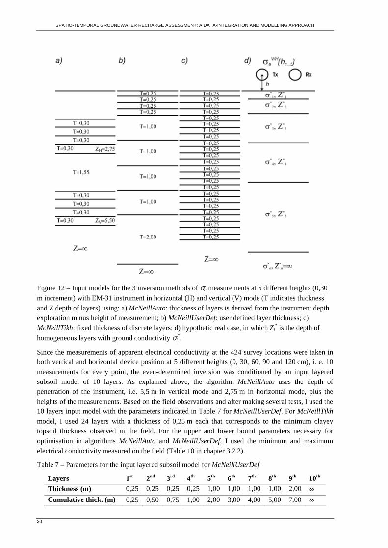
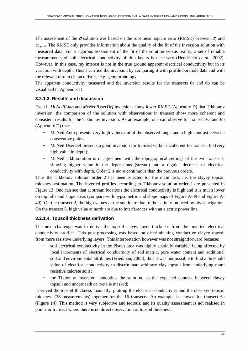
Figure 13 – Profiles of soil electrical conductivity obtained using Tikhonov inversion (order 2) for all transects (depth of 6 meters)............................................................................................................................22 Figure 14 – Topsoil thickness interpretation (green circles) from electrical conductivity profile and observed thickness values (yellow crosses) analysis (transect 6a) ................................................................................. 22 Figure 15 – Histogram of topsoil thickness in absolute values (left) and logarithm base 10 (right)............... 23 Figure 16 – Topsoil thickness relations with slope classes (left) and distance to stream (right)..................... 24 Figure 17 – Graphical assessment of the MLR model A*B*C ....................................................................... 25 Figure 18 - Dataset variogram compared to residuals variograms of linear model (left) Experimental and theoretical variogram of the residuals from the MLR A*B*C model (right).................................................. 25 Figure 19 – Topsoil thickness map obtained by KED..................................................................................... 26 Figure 20 – Steven Hydra Probe calibration curves for in-situ soil moisture measurements (left) and correlation between custom calibration curve and gravimetric measurements (right). CALCR: soil moisture determined by gravimetric method in CALCR soils. CLAY: soil moisture determined by gravimetric method in CLAY soils. Hydraprobe: soil moisture determined by Hydra Probe custom calibration. Others: standard calibration (Seyfried et al., 2005).................................................................................................................... 28 Figure 21 – Histograma and boxplot of soil conductivity measured by Hydra Probe (16 CALCR and 104 CLAY data) ..................................................................................................................................................... 29

xii

Figure 22 – Porosity φ, field capacity θfc, permanent wilting point θpwp and hygroscopic water content θhw (between brackets, depth of the sample in cm). Left: data obtained through water retention curve; Middle: data obtained by saturation/drainage method (Table 12); Right: data obtained by COTR (Table 11)............ 31 Figure 23 – Range of some soil hydraulic parameters for soils of various textures (Dingman, 2002) ........... 32 Figure 24 – Inverse augering graph at location COB9.................................................................................... 33 Figure 25 - Infiltration curve at site R8 ........................................................................................................... 34 Figure 26 –Spectra of samples at COB1 and R3 compared with USGS library mineral ................................ 35 Figure 27 - EARTH model schema ................................................................................................................. 37 Figure 28 – Soil reservoir model ..................................................................................................................... 38 Figure 29 – Results of pyEARTH-1D modelling (piezometer SDH1). From top to bottom, rainfall, potential evapotranspiration (dark curve) and evapotranspiration (clear curve), soil moisture, recharge, hydraulic heads................................................................................................................................................................ 41 Figure 30 – Results of pyEARTH-1D modelling (piezometer JK7). From top to bottom, rainfall, potential evapotranspiration (dark curve) and evapotranspiration (clear curve), soil moisture, recharge, hydraulic heads................................................................................................................................................................ 41 Figure 31 - Conceptual overview of the semi-distributed recharge model linked with MODFLOW model .. 43 Figure 32 – Meteorological and piezometric data of the modelled stress period............................................ 44 Figure 33 – Recharge zones map..................................................................................................................... 45 Figure 34 – Recharge rate map (time period between Sept. and Dec. 2002) .................................................. 45 Figure 35 – Soil evapotranspiration rate (ETu) map (time period between Sept. and Dec. 2002)................... 45 Figure 36 – Water budget for the different zones of the Pisoes model (Figure 33) and for the whole catchment......................................................................................................................................................... 46 Figure 37 – Diagram representing a section of an unconfined aquifer (see Equation 27 for keys)................. 48 Figure 38 - Conceptual scheme of the upgraded semi-distributed recharge model pyEARTH-..................... 54 Figure A-39 - Digital elevation model and soil thickness data (quartiles representation)..................................a Figure A-40 – Slope map (quartiles representation) and soil thickness data (quartiles representation).............a Figure A-41 – Geological map and soil thickness data (quartiles representation) ............................................ b Figure A-42 – Soil map and soil thickness data (quartiles representation) ....................................................... b Figure C-43 – McNeill layered subsoil model (see text for notation keys)........................................................e Figure C-44 – Relative sensitivity function for vertical (V) and horizontal (H) dipole orientation................... f Figure C-45 - Cumulative sensitivity function for vertical (V) and horizontal (H) dipole orientation .............. f Figure E-46 – Model A: slope classes............................................................................................................. 19 Figure E-47 – Model B: interactions between 4 QuickBird bands.................................................................. 19 Figure E-48 – Model C: log10(distance stream) ............................................................................................. 19 Figure E-49 – Multiple linear regression model A*B*C................................................................................. 19 Figure E-50 – Topsoil thickness differences between the KED model and the multiple linear regression model A*B*C (values showed in quartile classes)............................................................................................ u Figure E-51 – Quick Bird image, September 2006. .......................................................................................... u

xiii

List of tables

Table 1 – Main soil types in the study area ....................................................................................................... 8 Table 2 - Slope classes ...................................................................................................................................... 8 Table 3 – Characteristics of the studied meteorological station ........................................................................ 9 Table 4: Calibration equations for ECHO-20 sensor (x is voltage in millivolts, y is volumetric soil moisture)......................................................................................................................................................................... 11 Table 5: Calibration equations for Watermark and Gypsum sensors (x is voltage in millivolts, y is matric pressure in bars)............................................................................................................................................... 11 Table 6 – Characteristics of GeonicsTM ground conductivity meters .............................................................. 17 Table 7 – Parameters for the input layered subsoil model for McNeillUserDef.............................................. 20 Table 8 – Goodness of fit of the linear relations between soil thickness and ancillary variables ................... 24 Table 9 – Residuals statistics of MLR A*B*C model and KED models cross-validation (5 folders) ............ 26 Table 10 - Summary statistics of the bulk soil electrical conductivity measured by Hydra Probe Values in mS/m, except variance ([mS/m]2) ................................................................................................................... 28 Table 11 – Physical and hydraulic parameters of soil samples (COTR)......................................................... 30 Table 12 – Soils hydraulic parameters. ρ is soil density, φ is porosity, Sr is specific retention (field capacity), Sy is specific yield and Ksat is saturated hydraulic conductivity....................................................................... 32 Table 13 – Saturated hydraulic conductivity derived from inverse auger method (see locations on Figure 10)......................................................................................................................................................................... 33 Table 14 – Infiltration capacity derived from double ring infiltrometer test (see location on Figure 10)....... 35 Table 15 – pyEARTH-1D parameters ............................................................................................................. 40 Table 16 – pyEARTH-1D water balance at SDH1 and JK7........................................................................... 42 Table 17 – pyEARTH-2D parameters ............................................................................................................. 44 Table 18 – pyEARTH-2D results: flux and storage in percentage of rainfall (time period between September and December 2002, total rainfall 320 mm, total potential evapotranspiration 200 mm) ............................... 46 Table 19 – Results of recharge assessment based on well-hydrograph analysis. Results of pyEARTH-1D of Table 16 are also showed for comparison ....................................................................................................... 49 Table 20 – Hypothetic subsoil model and inversion models results used for R code validation ...................... h

SPATIO-TEMPORAL GROUNDWATER RECHARGE ASSESSMENT: A DATA-INTEGRATION AND MODELLING APPROACH

1

1. Scope of the study

1.1. Statement of the research problem

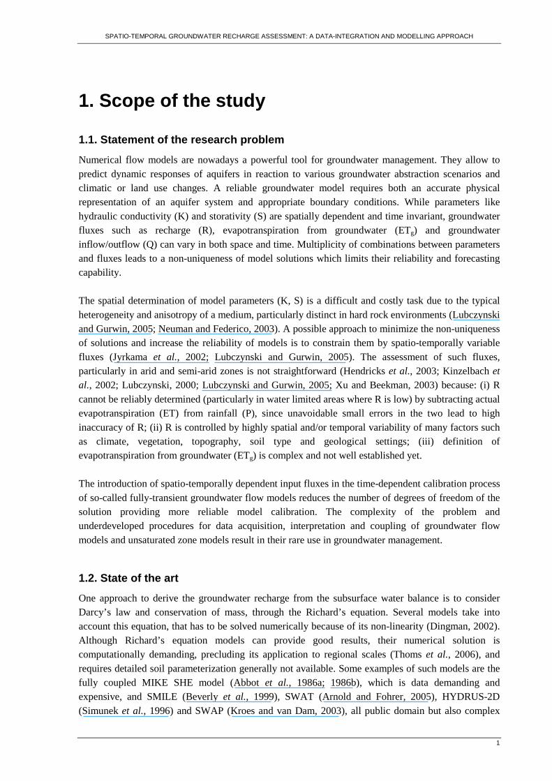
Numerical flow models are nowadays a powerful tool for groundwater management. They allow to predict dynamic responses of aquifers in reaction to various groundwater abstraction scenarios and climatic or land use changes. A reliable groundwater model requires both an accurate physical representation of an aquifer system and appropriate boundary conditions. While parameters like hydraulic conductivity (K) and storativity (S) are spatially dependent and time invariant, groundwater fluxes such as recharge (R), evapotranspiration from groundwater (ETg) and groundwater inflow/outflow (Q) can vary in both space and time. Multiplicity of combinations between parameters and fluxes leads to a non-uniqueness of model solutions which limits their reliability and forecasting capability. The spatial determination of model parameters (K, S) is a difficult and costly task due to the typical heterogeneity and anisotropy of a medium, particularly distinct in hard rock environments (Lubczynski and Gurwin, 2005; Neuman and Federico, 2003). A possible approach to minimize the non-uniqueness of solutions and increase the reliability of models is to constrain them by spatio-temporally variable fluxes (Jyrkama et al., 2002; Lubczynski and Gurwin, 2005). The assessment of such fluxes, particularly in arid and semi-arid zones is not straightforward (Hendricks et al., 2003; Kinzelbach et al., 2002; Lubczynski, 2000; Lubczynski and Gurwin, 2005; Xu and Beekman, 2003) because: (i) R cannot be reliably determined (particularly in water limited areas where R is low) by subtracting actual evapotranspiration (ET) from rainfall (P), since unavoidable small errors in the two lead to high inaccuracy of R; (ii) R is controlled by highly spatial and/or temporal variability of many factors such as climate, vegetation, topography, soil type and geological settings; (iii) definition of evapotranspiration from groundwater (ETg) is complex and not well established yet. The introduction of spatio-temporally dependent input fluxes in the time-dependent calibration process of so-called fully-transient groundwater flow models reduces the number of degrees of freedom of the solution providing more reliable model calibration. The complexity of the problem and underdeveloped procedures for data acquisition, interpretation and coupling of groundwater flow models and unsaturated zone models result in their rare use in groundwater management.

1.2. State of the art

One approach to derive the groundwater recharge from the subsurface water balance is to consider Darcy’s law and conservation of mass, through the Richard’s equation. Several models take into account this equation, that has to be solved numerically because of its non-linearity (Dingman, 2002). Although Richard’s equation models can provide good results, their numerical solution is computationally demanding, precluding its application to regional scales (Thoms et al., 2006), and requires detailed soil parameterization generally not available. Some examples of such models are the fully coupled MIKE SHE model (Abbot et al., 1986a; 1986b), which is data demanding and expensive, and SMILE (Beverly et al., 1999), SWAT (Arnold and Fohrer, 2005), HYDRUS-2D (Simunek et al., 1996) and SWAP (Kroes and van Dam, 2003), all public domain but also complex

SPATIO-TEMPORAL GROUNDWATER RECHARGE ASSESSMENT: A DATA-INTEGRATION AND MODELLING APPROACH

2

and data demanding. Besides, most of those models are not coupled with groundwater flow models, except of the very new package releases such as VSF (Thoms et al., 2006) and HYDRUS (Seo et al., 2007), both integrated with MODFLOW (Harbaugh et al., 2000). However, these packages coupled with MODFLOW inherited most of the typical disadvantages of the Richard’s equation models. Another approach is to develop models that simplify the representation of the physical processes and limits the number of parameters to commonly available field information (Finch, 2001; Rushton et al., 2006). One of such models is the lumped 1D EARTH approach that computes daily recharge based on deterministic methods that simulate soil physical processes. The EARTH model was widely tested and proved to be very successful in recharge assessment as indicated for example by its comparison with SWAP Richard’s equation model (Gehrels, 2000). The advantage of EARTH model is in its simplicity and reliability as confirmed by extensive verification (Kinzelbach et al., 2002; Lubczynski and Gurwin, 2005; Xu and Beekman, 2003). Its main disadvantages reside in its limitation in handling: (1) depth-wise heterogeneity – only one vertical layer is permitted; (2) lateral heterogeneity – current 1D structure does not account for lateral inflow/outflow; (3) separation of recharge from groundwater evapotranspiration. The spatial recharge assessment based on water balance in vadose reservoirs requires the development of methodologies that integrate the 1D in-situ measured data to the spatially discretized recharge model. Triantafilis et al. (2001) applied successfully geostatistical techniques that combine the spatial structure with ancillary variables, as electromagnetic (EM) measurements and remote sensing images, to estimate spatially soil properties. EM measurements already showed their applicability to map soil variability (Corwin and Lesch, 2005). Such techniques are fast and cost-effective, allowing to acquire the sufficient amount of data to obtain a reliable data integration by geostatistical interpolation (Borchers et al., 1997). Integration of large quantity of data from different sources is nowadays facilitated by developments in GIS software that integrate database management, as well as the progress of powerful and easy-to-learn programming languages that provide the user with a full set of tools to process, analyse, store and visualize data. Some examples are the R Project for Statistical Computing and the Python Programming Language, all public domain and open-source code. R is an environment (www.r-project.org) that provides a wide variety of statistical techniques in an integrated suite of software facilities for data manipulation, calculation and graphical display where the user has full control on the operation and output through a simple and effective programming language. Python (www.python.org) is a dynamic object-oriented programming language that can be used for many kinds of software developments. It has a very clear and readable syntax, associated with strong introspection capabilities that allow the users to produce quickly intelligible and maintainable code. Non linear parameter estimator such as PEST (Doherty, 2002) allows avoiding arduous, labour intensive and frustrating task of multi-parameter model calibration. Its recent development allows simultaneous calibration of multiple models.

SPATIO-TEMPORAL GROUNDWATER RECHARGE ASSESSMENT: A DATA-INTEGRATION AND MODELLING APPROACH

3

1.3. Objectives of the thesis

1.3.1. Main objective

The main objective of the thesis is to assess spatio-temporally the groundwater recharge, by the integration of several methods and techniques, to minimize the non-uniqueness of groundwater flow model solutions and to increase their reliability.

1.3.2. Specific objectives

Specific objectives are: (i) To select proper techniques and methods for data acquisition and data integration in order

to characterise spatially the topsoil and vadose zone properties (thickness and hydraulic characteristics) in most reliable way at the catchment scale;

(ii) To develop a semi-distributed recharge model and to couple it dynamically with numerical groundwater flow model;

(iii) To select proper data and methods for model calibration and validation; (iv) To use parameter estimation PEST algorithm for simultaneous calibration of models and

assessment of uncertainty and sensitivity analysis of the proposed procedure.

1.3.3. Research questions

1.3.3.1. Main research question

How to assess recharge spatio-temporally in efficient but reliable way?

1.3.3.2. Specific research questions

- Which processes, driving forces, state variables and parameters have to be considered in spatio-temporal recharge assessment?

- How to implement these processes in the model? - How to capture and retrieve the spatial and the temporal variability? - How to parameterise the different reservoirs of the model? - How to calibrate the model?

1.3.4. Hypotheses

1.3.4.1. Hypotheses on recharge model

Recharge can be efficiently and accurately assessed spatio-temporally through a semi-distributed lumped parameter model that solves the water balance in the unsaturated zone, simulated by overlaid homogeneous linear independent reservoirs, and that is coupled with MODFLOW groundwater model. Calibration of such distributed recharge model is done against (i) soil moisture of the recharge model; (ii) temporally variable hydraulic heads of the MODFLOW groundwater model.

1.3.4.2. Hypotheses on temporal variability

Temporal variability is captured through Automatic Data Acquisition System (ADAS) monitoring that provides state-variables and driving-forces time series.

1.3.4.3. Hypotheses on spatial variability

Inversion of apparent electrical conductivity measurements using the GeonicsTM ground conductivity meter EM-31 produces electrical conductivity soil profiles. The topsoil thickness is interpreted by the simultaneous visualisation/plotting of electrical conductivity profiles and measurements of layer thickness made by drilling and augering. The topsoil thickness can be mapped at catchment scale

SPATIO-TEMPORAL GROUNDWATER RECHARGE ASSESSMENT: A DATA-INTEGRATION AND MODELLING APPROACH

4

through kriging with external drift using high resolution multispectral images as auxiliary maps. The soil classification can be carried out by grouping soils in classes having the same or similar hydraulic properties. Thus soils profiling observations and depth-sampling through drilling and augering at representative sites allow to capture the spatial variability of vadose zone hydraulic properties.

1.3.5. Assumptions

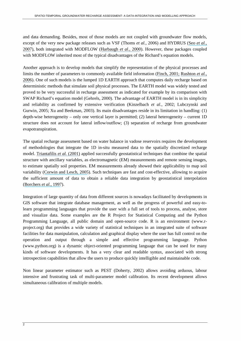
Fluxes (actual evapotranspiration and percolation) are assumed to be linear functions of soil moisture (Figure 1). Such approach is followed by van der Lee and Gehrels (1990) for the EARTH model (Equation 1 and Equation 3) and are also presented in Dingman (2002)(Equation 2 and Equation 4):

Equation 1 pwp

pwpPETETθφθθ

−−

⋅=

Equation 2 pwpfc

pwpPETETθθ

θθ−

−⋅=

Equation 3 fc

fcsatp KR

θφθθ

−−

⋅=

Equation 4 c

satp KR

⋅= φ

θ

where ET is actual evapotranspiration, PET is potential evapotranspiration, Rp is the percolation, Ksat is

the saturated hydraulic conductivity, θ is actual soil moisture, θfc, θpwp are respectively soil moisture at

field capacity and at permanent wilting point, φ is the porosity and c is the pore-disconnectedness index. Note that percolation is assumed to be equal to the unsaturated hydraulic conductivity. Application of these equations is detailed in chapter 4.

Figure 1 – Actual evapotranspiration ET and percolation Rp as a linear function of soil moisture content (Equation 1 and Equation 3). PET potential evapotranspiration; Ksat: saturated hydraulic

conductivity; θfc: soil moisture at field capacity, θpwp: permanent wilting point; φ: porosity.

SPATIO-TEMPORAL GROUNDWATER RECHARGE ASSESSMENT: A DATA-INTEGRATION AND MODELLING APPROACH

5

2. Study area description

The setup of a transient groundwater flow model integrated with spatio-temporal recharge model requires a test area with intensive spatio-temporal data coverage. The Pisoes catchment has been selected for such integration because of: (i) spatial data availability; (ii) temporal data availability and the status of monitoring network; (iii) the availability and reliability of groundwater use estimates and river discharges; (iv) well-defined boundary conditions; (v) lack of trees allowing to avoid complications related to estimates of transpiration from groundwater reservoir in groundwater balances.

2.1. General settings / features of the catchment

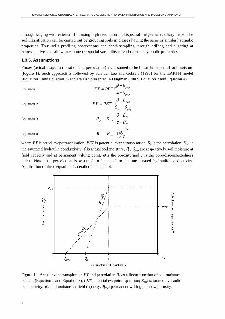
Pisoes catchment is located in the Alentejo region (Portugal), to the west of Beja city (Figure 2 and Figure A-39). Its position is peculiar since it is located on the top water divide of Guadiana and Sado watersheds, belonging to this latter one. Its area is ~19 km2 and is included in topographic sheet 521 of IGeoE (Continente 1/25 000 Série M888, www.igeoe.pt). The topography is smooth, with gentle slope and flat surface, since 75% of the area has slope lower than 4% (Figure A-39, Figure A-40 and Photos B-1). The catchment boundaries correspond to the basin water divide. The Ribeira da Chamine river drains the phreatic aquifer and consequently flows perennially, from east to west and south-west, where is located the Pisoes outlet. However, in some segments and at certain periods, the river can also be influent (Paralta, 2001). Groundwater recharge in the catchment occurs through direct infiltration of rainfall. The water table follows generally the topography, being deeper on top hills and shallower in the drainage area.

Figure 2 – Location of the Pisoes catchment

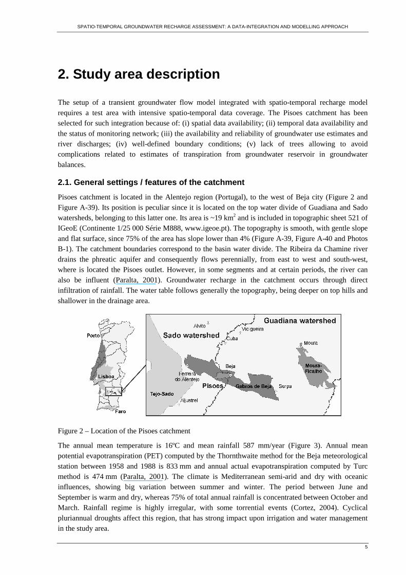
The annual mean temperature is 16ºC and mean rainfall 587 mm/year (Figure 3). Annual mean potential evapotranspiration (PET) computed by the Thornthwaite method for the Beja meteorological station between 1958 and 1988 is 833 mm and annual actual evapotranspiration computed by Turc method is 474 mm (Paralta, 2001). The climate is Mediterranean semi-arid and dry with oceanic influences, showing big variation between summer and winter. The period between June and September is warm and dry, whereas 75% of total annual rainfall is concentrated between October and March. Rainfall regime is highly irregular, with some torrential events (Cortez, 2004). Cyclical pluriannual droughts affect this region, that has strong impact upon irrigation and water management in the study area.

SPATIO-TEMPORAL GROUNDWATER RECHARGE ASSESSMENT: A DATA-INTEGRATION AND MODELLING APPROACH

6

Figure 3 – Hyetograph, maximum and minimum temperatures. Monthly averages, period 1961-1990 (Beja meteorological station, Instituto de Meteorologia, www.meteo.pt)

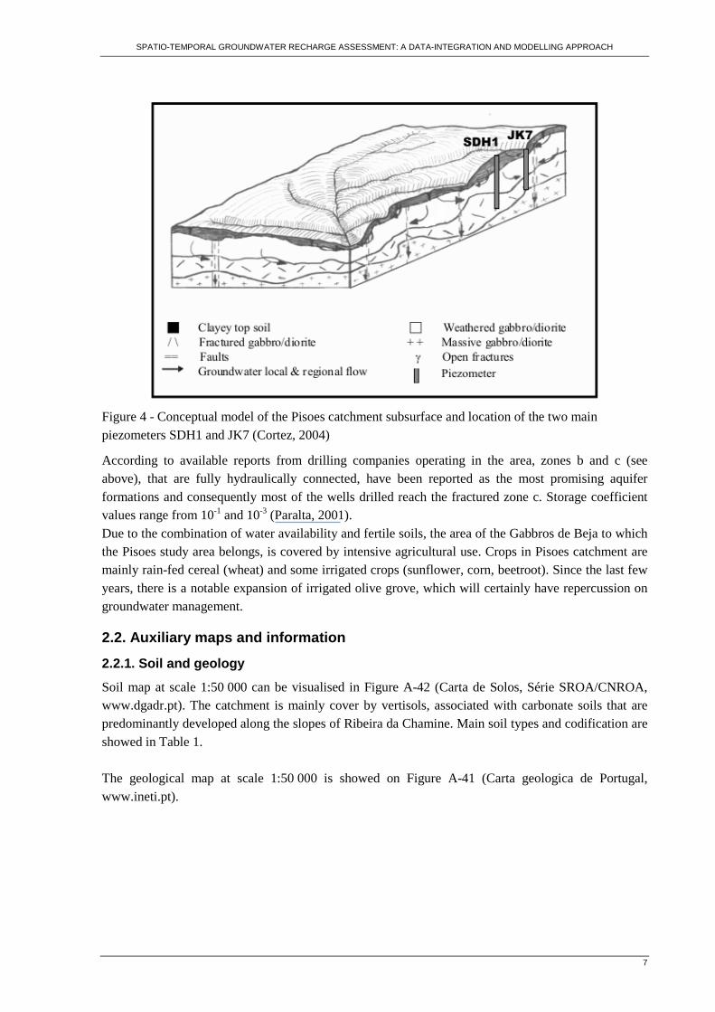
Hydrogeologically, the study area belongs to the fissured-porous “Gabro de Beja” aquifer that consists of two principal geological units: the Maphic and Ultramaphic Beja-Acebuches Complex and the Beja Gabbros Complex, mainly composed of gabbros and diorites (Figure A-41). Chemical weathering of the gabbro-dioritic rocks results in the neoformation of clay minerals, mainly montmorillonite (Vieira e Silva, 1991). This high content in swelling clay in the topsoil provokes in the dry season the opening of cracks (Photo B-2) that can have some influence in the recharge episodes. Calcrete outcrops are also frequent in the area (Photos B-1 and Photos B-3). Pimentel and Brum (1991) give them a pedologic and epigenetic origin and relate their formation with the combination of a semi-arid and warm paleoclimate activity, high evapotranspiration, deficient drainage due to a smooth topography, mobilization and re-precipitation of Ca2+ provided by the weathering of gabbroic and dioritic rocks and variations up to the surface of the water table level. The weathered upper zone of the gabbro-dioritic rocks has a thickness between 30 and 40 meters and it creates an unconfined aquifer that can be considered as porous. Its hydraulic properties are variable depth-wise. As the weathering intensity reduces progressively with depth, the groundwater storage and flow changes from porous to fractured. The typical profile and its associated hydraulic characteristics can be described as follow (Figure 4):

a. clayey topsoil, low hydraulic conductivity, with by-pass flow through crack in swelling clay during the first rainfall event after dry season;

b. weathered layers, with moderate to high hydraulic conductivity; c. fractured zone, hydraulic conductivity varying from very low to high; d. massive rock that constitute the base of the aquifer.

SPATIO-TEMPORAL GROUNDWATER RECHARGE ASSESSMENT: A DATA-INTEGRATION AND MODELLING APPROACH

7

Figure 4 - Conceptual model of the Pisoes catchment subsurface and location of the two main piezometers SDH1 and JK7 (Cortez, 2004)

According to available reports from drilling companies operating in the area, zones b and c (see above), that are fully hydraulically connected, have been reported as the most promising aquifer formations and consequently most of the wells drilled reach the fractured zone c. Storage coefficient values range from 10-1 and 10-3 (Paralta, 2001). Due to the combination of water availability and fertile soils, the area of the Gabbros de Beja to which the Pisoes study area belongs, is covered by intensive agricultural use. Crops in Pisoes catchment are mainly rain-fed cereal (wheat) and some irrigated crops (sunflower, corn, beetroot). Since the last few years, there is a notable expansion of irrigated olive grove, which will certainly have repercussion on groundwater management.

2.2. Auxiliary maps and information

2.2.1. Soil and geology

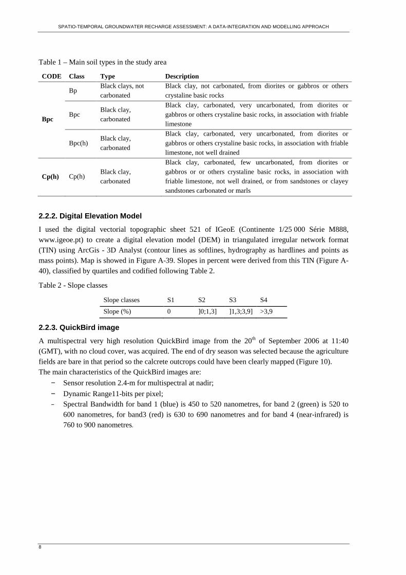
Soil map at scale 1:50 000 can be visualised in Figure A-42 (Carta de Solos, Série SROA/CNROA, www.dgadr.pt). The catchment is mainly cover by vertisols, associated with carbonate soils that are predominantly developed along the slopes of Ribeira da Chamine. Main soil types and codification are showed in Table 1. The geological map at scale 1:50 000 is showed on Figure A-41 (Carta geologica de Portugal, www.ineti.pt).

SPATIO-TEMPORAL GROUNDWATER RECHARGE ASSESSMENT: A DATA-INTEGRATION AND MODELLING APPROACH

8

Table 1 – Main soil types in the study area

CODE Class Type Description

Bp Black clays, not carbonated

Black clay, not carbonated, from diorites or gabbros or others crystaline basic rocks

Bpc Black clay, carbonated

Black clay, carbonated, very uncarbonated, from diorites or gabbros or others crystaline basic rocks, in association with friable limestone

Bpc

Bpc(h) Black clay, carbonated

Black clay, carbonated, very uncarbonated, from diorites or gabbros or others crystaline basic rocks, in association with friable limestone, not well drained

Cp(h) Cp(h) Black clay, carbonated

Black clay, carbonated, few uncarbonated, from diorites or gabbros or or others crystaline basic rocks, in association with friable limestone, not well drained, or from sandstones or clayey sandstones carbonated or marls

2.2.2. Digital Elevation Model

I used the digital vectorial topographic sheet 521 of IGeoE (Continente 1/25 000 Série M888, www.igeoe.pt) to create a digital elevation model (DEM) in triangulated irregular network format (TIN) using ArcGis - 3D Analyst (contour lines as softlines, hydrography as hardlines and points as mass points). Map is showed in Figure A-39. Slopes in percent were derived from this TIN (Figure A-40), classified by quartiles and codified following Table 2.

Table 2 - Slope classes

Slope classes S1 S2 S3 S4

Slope (%) 0 ]0;1,3] ]1,3;3,9] >3,9

2.2.3. QuickBird image

A multispectral very high resolution QuickBird image from the 20th of September 2006 at 11:40 (GMT), with no cloud cover, was acquired. The end of dry season was selected because the agriculture fields are bare in that period so the calcrete outcrops could have been clearly mapped (Figure 10). The main characteristics of the QuickBird images are:

− Sensor resolution 2.4-m for multispectral at nadir;

− Dynamic Range11-bits per pixel; − Spectral Bandwidth for band 1 (blue) is 450 to 520 nanometres, for band 2 (green) is 520 to

600 nanometres, for band3 (red) is 630 to 690 nanometres and for band 4 (near-infrared) is 760 to 900 nanometres.

SPATIO-TEMPORAL GROUNDWATER RECHARGE ASSESSMENT: A DATA-INTEGRATION AND MODELLING APPROACH

9

3. Data integration

The main objective of this chapter is to compile, process, interpret and synthesise the primary and secondary data collection in a coherent data set necessary to provide inputs (driving forces), to parameterise (topsoil properties) and to calibrate (state variables) the recharge models. Main tasks of the data integration focus on:

- Time series: (i) driving forces (rainfall and potential evapotranspiration); (ii) state variables (soil moisture and hydraulic heads);

- Spatial characterisation of the soil reservoir (thickness, hydraulic properties and mineralogical composition).

3.1. Time-series

3.1.1. Driving forces

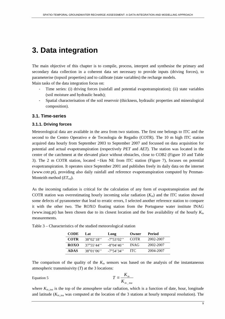
Meteorological data are available in the area from two stations. The first one belongs to ITC and the second to the Centro Operativo e de Tecnologia de Regadio (COTR). The 10 m high ITC station acquired data hourly from September 2003 to September 2007 and focussed on data acquisition for potential and actual evapotranspiration (respectively PET and AET). The station was located in the centre of the catchment at the elevated place without obstacles, close to COB2 (Figure 10 and Table 3). The 2 m COTR station, located ~1km NE from ITC station (Figure 7), focuses on potential evapotranspiration. It operates since September 2001 and publishes freely its daily data on the internet (www.cotr.pt), providing also daily rainfall and reference evapotranspiration computed by Penman-Monteith method (ETref). As the incoming radiation is critical for the calculation of any form of evapotranspiration and the COTR station was overestimating hourly incoming solar radiation (Kin) and the ITC station showed some defects of pyranometer that lead to erratic errors, I selected another reference station to compare it with the other two. The ROXO floating station from the Portuguese water institute INAG (www.inag.pt) has been chosen due to its closest location and the free availability of the hourly Kin measurements.

Table 3 – Characteristics of the studied meteorological station

CODE Lat Long Owner Period COTR 38°02’18’’ -7°53’02’’ COTR 2002-2007

ROXO 37°55’44’’ -8°04’46’’ INAG 2002-2007

ADAS 38°01’06’’ -7°54’34’’ ITC 2004-2007

The comparison of the quality of the Kin sensors was based on the analysis of the instantaneous atmospheric transmissivity (T) at the 3 locations:

Equation 5 toain

in

K

KT

_

=

where Kin_toa is the top of the atmosphere solar radiation, which is a function of date, hour, longitude and latitude (Kin_toa was computed at the location of the 3 stations at hourly temporal resolution). The

SPATIO-TEMPORAL GROUNDWATER RECHARGE ASSESSMENT: A DATA-INTEGRATION AND MODELLING APPROACH

10

principal assumption of that analysis was that with the same atmospheric conditions at nearby places, T should be similar. The results of this analysis confirmed that Kin values at COTR station were overestimated. To correct these values, daily data were multiplied by an Average Correction Factor (ACF) computed as follow:

Equation 6 ∑=n

i i

i

rT

Troxo

nACF

cot

1

where n is the number of observations, Troxo and Tcotr are the atmospheric transmissivity at Roxo and COTR stations respectively. The COTR station pyranometer was changed with a new one at 13th of January 2005 (information of COTR technical staff). Before this date, daily data were multiplied by an ACF of 0.84. After this date, as Kin values continue to show a slight overestimate, an ACF of 0.95 was applied. The imprecision of the new pyranometer was confirmed by COTR technical staff. The corrected hourly short incoming radiation, wind speed, relative humidity and temperature were used to calculate daily reference evapotranspiration (ETref) and daily potential evapotranspiration (PET; in this case the bulk surface resistance is set to 0) in AWSET software (Cranfield University, 2002) according to Penman-Monteith equation (Allen et al., 1998). The hourly rainfall data was also aggregated to daily data. As the Pisoes catchment is small and the differences in microclimatic data between ITC and COTR stations were negligible, the rainfall and potential evapotranspiration were considered spatially homogeneous. Data are showed graphically together with piezometric data in Figure 9 (chapter 3.1.2.2).

3.1.2. State variables

3.1.2.1. Soil moisture

The profile soil moisture was monitored at two locations, at the ITC station and close to piezometer SDH1 (Figure 10). At the ITC station soil moisture was monitored since October 2004 until September 2007 at the two depth levels (see Photos B-5 right): at 20 cm, in the clayey topsoil layer (CLAY), and at 60 cm, in weathered diorites (CALCR); next to soil moisture also matric potential monitoring was carried out in the same profile and at the same two levels. For soil moisture monitoring two ECHO 20 sensors (www.decagon.com) were used whereas for matric potential two gypsum blocks (www.eijkelkamp.com) and two Watermark ceramic blocks (www.specmeters.com) were installed. All the monitoring data was acquired hourly in mV and afterwards converted to physical units. The standard equation calibration of ECHO 20 gave incoherent results due to the conductive clayey soils. Therefore, a custom calibration equation had to be created for both clay and calcrete. Unfortunately, only one gravimetric field measurement of clay and calcrete soil moisture with corresponding ECHO 20 voltages were available for calibration. The ECHO 20 manufacturer relation between voltage output and volumetric soil moisture is linear and the slope is pretty stable with respect to various soil types. Therefore in the custom calibration the standard slope of 0.000695 was assumed and the offset was determined using field data (Table 4). The custom calibration characteristics were then used to convert monitored ECHO 20 sensor voltages into temporally variable soil moisture content of clay and calcrete soils as presented in Figure 5. It has to be pointed out that the absolute values of the soil moisture contents in Figure 5 are uncertain because they are derived on the base of 1 data per soil type only and also because applicability of

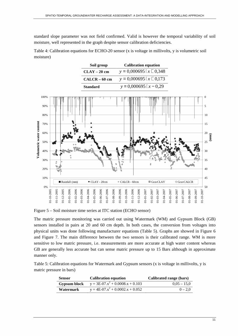
SPATIO-TEMPORAL GROUNDWATER RECHARGE ASSESSMENT: A DATA-INTEGRATION AND MODELLING APPROACH

11

standard slope parameter was not field confirmed. Valid is however the temporal variability of soil moisture, well represented in the graph despite sensor calibration deficiencies.

Table 4: Calibration equations for ECHO-20 sensor (x is voltage in millivolts, y is volumetric soil moisture)

Soil group Calibration equation

CLAY – 20 cm 348,0000695,0 +⋅= xy

CALCR – 60 cm 173,0000695,0 +⋅= xy

Standard 29,0000695,0 −⋅= xy

0%

10%

20%

30%

40%

50%

60%

70%

80%

90%

100%

01

-10

-200

5

01

-11

-200

5

01

-12

-200

5

01

-01

-200

6

01

-02

-200

6

01

-03

-200

6

01

-04

-200

6

01

-05

-200

6

01

-06

-200

6

01

-07

-200

6

01

-08

-200

6

01

-09

-200

6

01

-10

-200

6

01

-11

-200

6

01

-12

-200

6

01

-01

-200

7

01

-02

-200

7

01

-03

-200

7

01

-04

-200

7

01

-05

-200

7

01

-06

-200

7

01

-07

-200

7

01

-08

-200

7

01

-09

-200

7

01

-10

-200

7

Vo

lum

etric

wa

ter

cont

ent

0

5

10

15

20

25

30

35

40

45

50

(mm

)

Rainfall (mm) CLAY - 20cm CALCR - 60cm GravCLAY GravCALCR

Figure 5 – Soil moisture time series at ITC station (ECHO sensor)

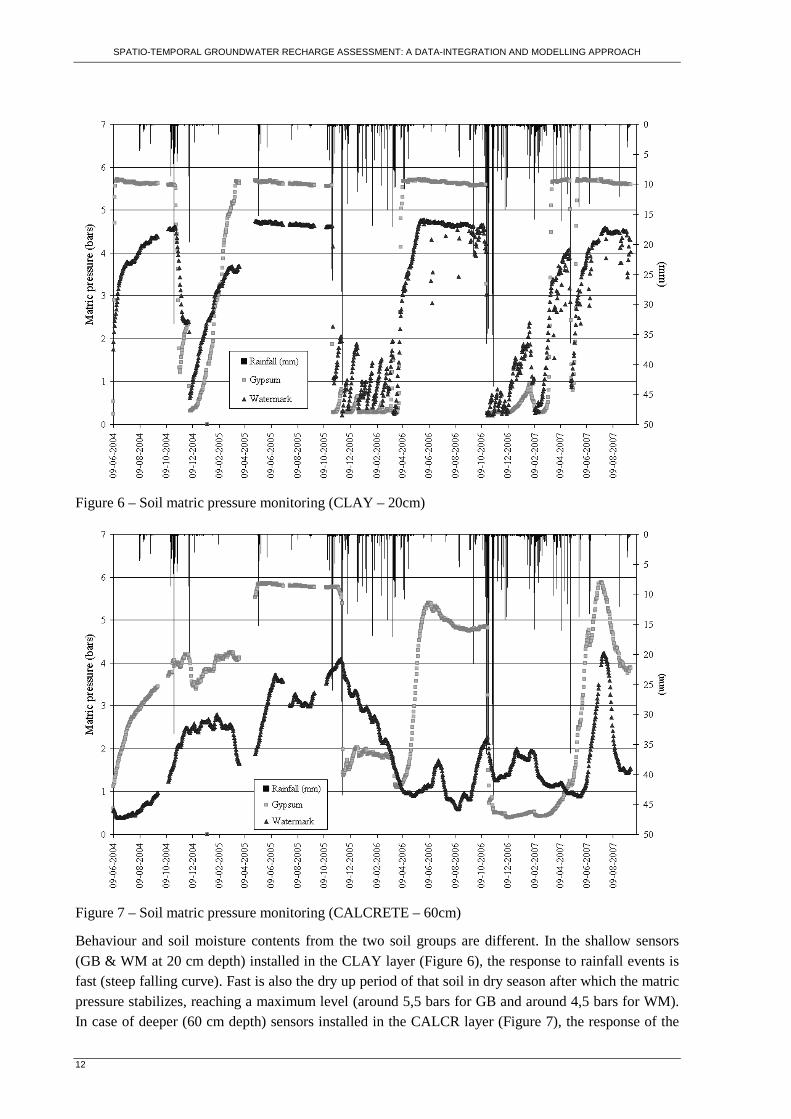
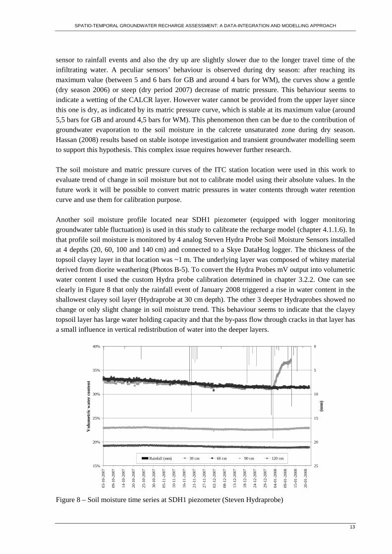
The matric pressure monitoring was carried out using Watermark (WM) and Gypsum Block (GB) sensors installed in pairs at 20 and 60 cm depth. In both cases, the conversion from voltages into physical units was done following manufacturer equations (Table 5). Graphs are showed in Figure 6 and Figure 7. The main difference between the two sensors is their calibrated range. WM is more sensitive to low matric pressure, i.e. measurements are more accurate at high water content whereas GB are generally less accurate but can sense matric pressure up to 15 Bars although in approximate manner only.

Table 5: Calibration equations for Watermark and Gypsum sensors (x is voltage in millivolts, y is matric pressure in bars)

Sensor Calibration equation Calibrated range (bars) Gypsum block y = 3E-07.x2 + 0.0008.x + 0.103 0,05 – 15,0

Watermark y = 4E-07.x2 + 0.0002.x + 0.052 0 – 2,0

SPATIO-TEMPORAL GROUNDWATER RECHARGE ASSESSMENT: A DATA-INTEGRATION AND MODELLING APPROACH

12

Figure 6 – Soil matric pressure monitoring (CLAY – 20cm)

Figure 7 – Soil matric pressure monitoring (CALCRETE – 60cm)

Behaviour and soil moisture contents from the two soil groups are different. In the shallow sensors (GB & WM at 20 cm depth) installed in the CLAY layer (Figure 6), the response to rainfall events is fast (steep falling curve). Fast is also the dry up period of that soil in dry season after which the matric pressure stabilizes, reaching a maximum level (around 5,5 bars for GB and around 4,5 bars for WM). In case of deeper (60 cm depth) sensors installed in the CALCR layer (Figure 7), the response of the

SPATIO-TEMPORAL GROUNDWATER RECHARGE ASSESSMENT: A DATA-INTEGRATION AND MODELLING APPROACH

13

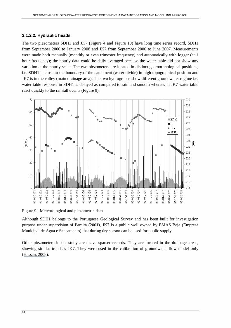
sensor to rainfall events and also the dry up are slightly slower due to the longer travel time of the infiltrating water. A peculiar sensors’ behaviour is observed during dry season: after reaching its maximum value (between 5 and 6 bars for GB and around 4 bars for WM), the curves show a gentle (dry season 2006) or steep (dry period 2007) decrease of matric pressure. This behaviour seems to indicate a wetting of the CALCR layer. However water cannot be provided from the upper layer since this one is dry, as indicated by its matric pressure curve, which is stable at its maximum value (around 5,5 bars for GB and around 4,5 bars for WM). This phenomenon then can be due to the contribution of groundwater evaporation to the soil moisture in the calcrete unsaturated zone during dry season. Hassan (2008) results based on stable isotope investigation and transient groundwater modelling seem to support this hypothesis. This complex issue requires however further research. The soil moisture and matric pressure curves of the ITC station location were used in this work to evaluate trend of change in soil moisture but not to calibrate model using their absolute values. In the future work it will be possible to convert matric pressures in water contents through water retention curve and use them for calibration purpose. Another soil moisture profile located near SDH1 piezometer (equipped with logger monitoring groundwater table fluctuation) is used in this study to calibrate the recharge model (chapter 4.1.1.6). In that profile soil moisture is monitored by 4 analog Steven Hydra Probe Soil Moisture Sensors installed at 4 depths (20, 60, 100 and 140 cm) and connected to a Skye DataHog logger. The thickness of the topsoil clayey layer in that location was ~1 m. The underlying layer was composed of whitey material derived from diorite weathering (Photos B-5). To convert the Hydra Probes mV output into volumetric water content I used the custom Hydra probe calibration determined in chapter 3.2.2. One can see clearly in Figure 8 that only the rainfall event of January 2008 triggered a rise in water content in the shallowest clayey soil layer (Hydraprobe at 30 cm depth). The other 3 deeper Hydraprobes showed no change or only slight change in soil moisture trend. This behaviour seems to indicate that the clayey topsoil layer has large water holding capacity and that the by-pass flow through cracks in that layer has a small influence in vertical redistribution of water into the deeper layers.

15%

20%

25%

30%

35%

40%

03-

10-2

007

09-

10-2

007

14-

10-2

007

20-

10-2

007

25-

10-2

007

30-

10-2

007

05-

11-2

007

10-

11-2

007

16-

11-2

007

21-

11-2

007

27-

11-2

007

02-

12-2

007

08-

12-2

007

13-

12-2

007

18-

12-2

007

24-

12-2

007

29-

12-2

007

04-

01-2

008

09-

01-2

008

15-

01-2

008

20-

01-2

008

Vol

umet

ric w

ater

con

tent

0

5

10

15

20

25

(mm

)

Rainfall (mm) 30 cm 60 cm 90 cm 120 cm

Figure 8 – Soil moisture time series at SDH1 piezometer (Steven Hydraprobe)

SPATIO-TEMPORAL GROUNDWATER RECHARGE ASSESSMENT: A DATA-INTEGRATION AND MODELLING APPROACH

14

3.1.2.2. Hydraulic heads

The two piezometers SDH1 and JK7 (Figure 4 and Figure 10) have long time series record, SDH1 from September 2000 to January 2008 and JK7 from September 2000 to June 2007. Measurements were made both manually (monthly or even trimester frequency) and automatically with logger (at 1 hour frequency); the hourly data could be daily averaged because the water table did not show any variation at the hourly scale. The two piezometers are located in distinct geomorphological positions, i.e. SDH1 is close to the boundary of the catchment (water divide) in high topographical position and JK7 is in the valley (main drainage area). The two hydrographs show different groundwater regime i.e. water table response in SDH1 is delayed as compared to rain and smooth whereas in JK7 water table react quickly to the rainfall events (Figure 9).

Figure 9 - Meteorological and piezometric data

Although SDH1 belongs to the Portuguese Geological Survey and has been built for investigation purpose under supervision of Paralta (2001), JK7 is a public well owned by EMAS Beja (Empresa Municipal de Agua e Saneamento) that during dry season can be used for public supply. Other piezometers in the study area have sparser records. They are located in the drainage areas, showing similar trend as JK7. They were used in the calibration of groundwater flow model only (Hassan, 2008).

SPATIO-TEMPORAL GROUNDWATER RECHARGE ASSESSMENT: A DATA-INTEGRATION AND MODELLING APPROACH

15

3.2. Soil spatial characterisation

A preliminary study showed that in the Pisoes study area there is a clear relation between the topsoil thickness and the topographical/geomorphological position, i.e. the clayey topsoil thickness is thinner on hilltops and slopes and thicker in valleys. This study was based on the topsoil lithological profile data (55 profiles) acquired from several sources (see Figure A-39 to Figure A-42 to visualise the spatial distribution):

- BH: borehole drilling report analysis (18 data points); - HA: hand augering (9 data points); - VES: vertical electrical soundings (20 data points); - PF: soil profiles analysis in a pitch (8 data points).

Details on the 3 first sources data can be found in Cortez (2004). The fourth was realized by the Centro Operativo e de Tecnologia de Regadio (COTR) in 2005 (see 3.2.3.1). The analysis of the 55 profile data indicated that the main spatial variability of soil composition is in the perpendicular direction to the main geomorphological features. This particular observation was further used as a guideline in the design of the follow up soil investigations. For example, to maximize the efficiency of information acquisition on soil thickness variability, transects of geophysical measurements from tophills to valleys were designed and realized (see below) to improve the available data base. The main characteristic of the area is a layering of vadose zone in two main soil types (Photos B-1, Photo B-2 to Photos B-5):

− topsoil composed of dark swelling clay (CLAY group);

− subsoil composed of whitey material derived from gabbroic and dioritic substratum, showing generally carbonate content (CALCR group).

To improve the database on spatial variability of the soil properties in the catchment area, the following tasks were done during field work in September 2007:

− geophysical measurements of the soil apparent conductivity using the GeonicsTM ground conductivity meter EM-31 to depict the topsoil clayey layer thickness;

− the percussion drilling to measure topsoil thickness and soil moisture with Hydra Probe soil sensor and to collect soil samples from different depths;

− inverse augering to derive lateral soil hydraulic conductivity;

− double ring infiltration tests to determine hydraulic conductivity of the shallow soil. The geophysical measurements are described in the section below. The percussion drilling was done with a COBRA gasoline powered percussion hammer (www.eijkelkamp.com/Portals/2/Eijkelkamp/Files/P1-21e.pdf) and was performed in 9 locations (see COB1 to COB9 in Figure 10). Soil samples were collected in the drilled boreholes and were analysed in the laboratory to obtain:

− actual soil moisture (gravimetric method);

− water retention curve;

− saturated hydraulic conductivity;

− mineral spectra for main minerals recognition; Samples for saturated hydraulic conductivity and actual soil moisture measurements (Photos B-4) were taken in metallic rings of 53 cm diameter and 100 cm3 volume with a closed ring holder (www.eijkelkamp.com/Portals/2/Eijkelkamp/Files/P1-31e.pdf).

SPATIO-TEMPORAL GROUNDWATER RECHARGE ASSESSMENT: A DATA-INTEGRATION AND MODELLING APPROACH

16

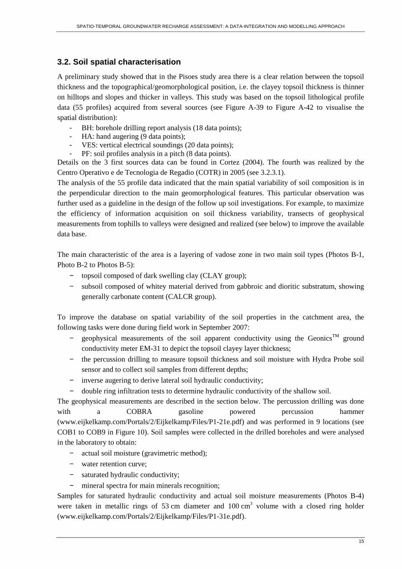
Figure 10 – Field data: apparent electrical conductivity (ECa) and drilling locations plotted on QuickBird image (natural colour). Higher values of ECa are related to higher thickness of clayey topsoil in the depressed drainage area of the catchment (measurements with EM31 device on the ground in vertical position)

SPATIO-TEMPORAL GROUNDWATER RECHARGE ASSESSMENT: A DATA-INTEGRATION AND MODELLING APPROACH

17

3.2.1. Electromagnetic survey and spatial assessment of topsoil thickness

Data acquisition of the vadose zone by non-invasive geophysical techniques allows to cover large area at lower cost than the common invasive sampling procedures such as for instance drilling. Electromagnetic techniques have been widely applied to a broad range of problems related to exploration of the vadose zone (Borchers et al., 1997; Corwin and Lesch, 2005). The ground conductivity meters of GeonicsTM (EM-31, EM-34, EM-38) are one-man portable instruments (two persons are needed for EM-34) that measure apparent conductivity of the subsurface, being particularly suitable to map quickly lateral variability of soils. These devices are constituted of two coils with a single frequency and a fixed spacing that define together the depth of penetration (Table 6 and Photos B-1).

Table 6 – Characteristics of GeonicsTM ground conductivity meters

Depth of penetration (m) GeonicsTM conductivity meters model

Coil spacing (m)

Frequency (Hz) Vert. dip. Hor. dip.

EM-38 1,00 14600 1,50 0,75

EM-31 3,66 9800 5,50 2,75

10,00 6400 15,00 7,50

20,00 1600 30,00 15,00 EM-34

40,00 400 60,00 30,00

I chose the EM-31 device to measure the soil apparent conductivity and to derive the topsoil thickness because: (i) measurements with horizontal and vertical orientation of the coils at different heights above the soil surface can be used to identify vertical changes in conductivity through the soil profiles and (ii) a pre-field study showed that clayey topsoil thickness is between 0,25 and 3,2 meters so that is within the range of the EM-31 penetration depth. The EM-31 measurements were done along transects perpendicular to the streams, allowing to depict the spatial variability of soil properties. Some transects were also measured in combination with EM-34 to derive aquifer layering (these data are not showed here but can be found in Hassan (2008)). The EM-31 field data acquisition was realised during September 2007 by Tanvir Hassan and me. At the end of the dry season soil moisture content was minimal thus its contribution to apparent electrical conductivity was minimized. We executed 6 transects constituted in total of 424 survey locations separated by a median distance of 21 m (Figure 10). Measurements of the apparent electrical conductivity at the 424 survey locations were acquired in both vertical and horizontal device positions at 5 different heights (0, 30, 60, 90 and 120 cm above the ground), i.e. in total 10 measurements for every survey location. Measurements at every point took few minutes, allowing to cover transect of 1 km length with spacing of ~20 m in ~2 hours. At some survey locations we also measured the in-phase to check consistency with quadrature phase. The EM-31 instrument was calibrated every 10 points during the survey progress.

3.2.1.1. Theory of EM data inversion

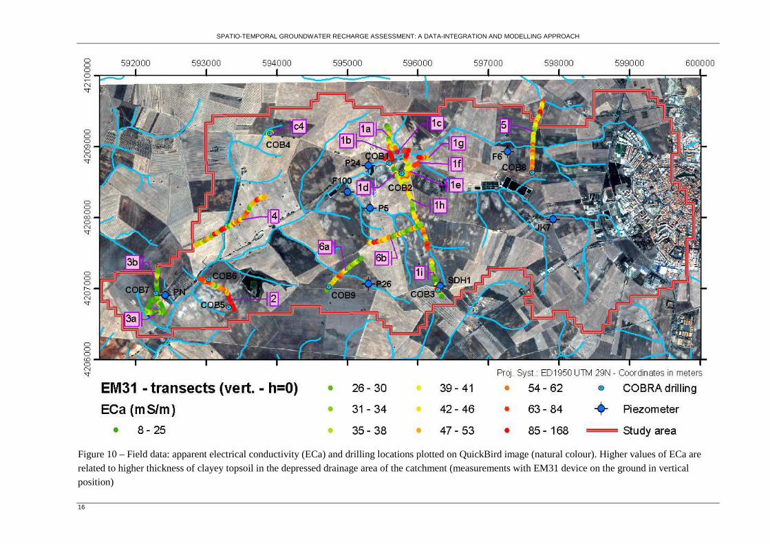
GeonicsTM instruments are constituted from 2 coils, one being the transmitter (Tx) and the other the receiver (Rx) (Figure 11). The injection of an alternating current in Tx generates a primary magnetic field (Hp) that propagates in the soil and induces very small electrical currents. These currents generate a secondary magnetic field (Hs) that is sensed, together with Hp, by Rx. At low induction number (NB),

and for an uniform ground conductivity (σu), Hs is approximated to the following function(McNeill, 1980):

SPATIO-TEMPORAL GROUNDWATER RECHARGE ASSESSMENT: A DATA-INTEGRATION AND MODELLING APPROACH

18

Equation 7 4

20 ri

H

H u

p

s ⋅⋅⋅⋅≈

σµω

where ω is the angular operating frequency ( f⋅⋅= πω 2 where f is the frequency in Hz), µ0 is the

magnetic permeability of free space ( 70 104 −⋅⋅= πµ H.m-1) and r is the coil spacing.

Figure 11 – Induced current flow by a ground conductivity meter (vertical dipoles)

NB is the ratio δr where δ is the skin depth, which is the depth at which Hp has been attenuated to

e1 (where e is the base of the natural system of logarithm) and is equal to (Hendrickx et al., 2002):

Equation 8 2

1

0 uσωµδ

⋅⋅=

From Equation 7, one can extract the uniform ground conductivity σu. For a stratified subsoil, where

every layer has its own thickness and its own electrical conductivity σ, σu corresponds to the apparent

conductivity σa, which is the bulk soil conductivity of the subsoil layers. McNeill (1980) describes a linear model that, under the assumption NB<<1, predicts the apparent

conductivity σa.pred of a layered subsoil. Assuming that the ground conductivity σ is constant within

discrete subsoil layers, the predicted ground conductivity σa.pred at different instrument heights h is expressed in its vectorial and matrixial expression as:

Equation 9 σσ ⋅= Kpreda.

where K is the matrix of the relative contribution to Hs of the discrete subsoil layers. The construction of this matrix is detailed in Appendix C.

The forward solution of this linear model for a given ground electrical conductivity profile σ is direct

(see Appendix C). The inverse problem of solving σ from measurements of apparent conductivity σa is

much more difficult since (Borchers et al., 1997): (i) there is only a finite set of measurements σa to

solve Equation 9; (ii) the inverse problem is ill-posed, i.e. small variations in σa observations, due to

common error in measurements, lead to large change in the σ solution. Hendrickx et al. (2002) showed however that the inverse problem applied to the linear model can be solved by the following two methods:

− Using an even-determined problem (i.e. a problem in which the number of equations is equal

to the number of unknowns) and minimizing the difference between observations σa and

predicted measurements σa.pred;

− Using an under-determined problem (number of equations less than number of unknowns), solving it by Tikhonov regularization.

SPATIO-TEMPORAL GROUNDWATER RECHARGE ASSESSMENT: A DATA-INTEGRATION AND MODELLING APPROACH

19

The first approach solves the following least square problem through optimization of the σ solution:

Equation 10 2. ||||min apreda σσ − with 0≥σ

The Tikhonov regularization introduces in Equation 10 a component that biases the least square

problem toward a smooth σ solution:

Equation 11 222. ||||||||min σασσ ⋅⋅+− iapreda L with 0≥σ

The component Li.σ quantifies the regularity of the solution and the term α balances the smoothness of the solution with the misfit, allowing an optimal tuning on the sensitivity of the solution to input data errors. The index i attributed to the differential operator L indicates the order regularization. At order 0, L is equal to the identity matrix while at the higher orders it indicates the derivative order of L. A second order will favour the smoothness of soil electrical conductivity variation with depth while lower order will allow sharp discontinuities. More detailed information about theory and algorithm of that solution can be found in Borchers et al. (1997) and Hendrickx et al. (2002). Because the assumption that NB<<1 is not true for soils of medium to high conductivity (i.e.

100 mS.m-1), Hendrickx et al. (2002) applied a non-linear model between σa and σ. Their results showed that the inverse procedure of Tikhonov regularisation performs equally well for linear and non-linear models across a wide range of ground conductivities thus the linear model was preferred in this study due to much less computer resources occupation.

3.2.1.2. Material and methods

To invert EM-31 field data, I applied the approach of the McNeill linear model with even-determined problem (Equation 10) and with Tikhonov regularization (Equation 11) through algorithms developed by Vervoort and Annen (2006) in R language. The obtained source code was first debugged and then verified using a 3 layers example (see Appendix C). To obtain the electrical conductivity profiles from the EM-31 field measurements showed in Figure 10, I applied the following three algorithms to solve the inverse problem for an input layered subsoil model (Figure 12):

a) McNeillAuto, from the original R code (Vervoort and Annen, 2006): it solves the even-determined inversion of Equation 10 through the R optimisation procedure ‘optim’ (quasi-Newton method with user defined lower and/or upper bound); it defines automatically the thickness of the input layers using the exploration depths of the instrument at different height, which is an approximation and not flexible;

b) McNeillUserDef, a modification of the previous algorithm: it allows the user to define the thickness of the input layers;

c) McNeillTikh, from Vervoort and Annen (2006): it defines a discrete layered model of fixed thickness and solves the under-determined inverse problem using Equation 11 for Tikhonov orders 0, 1 and 2.

SPATIO-TEMPORAL GROUNDWATER RECHARGE ASSESSMENT: A DATA-INTEGRATION AND MODELLING APPROACH

20

Figure 12 – Input models for the 3 inversion methods of σa measurements at 5 different heights (0,30 m increment) with EM-31 instrument in horizontal (H) and vertical (V) mode (T indicates thickness and Z depth of layers) using: a) McNeillAuto: thickness of layers is derived from the instrument depth exploration minus height of measurement; b) McNeillUserDef: user defined layer thickness; c) McNeillTikh: fixed thickness of discrete layers; d) hypothetic real case, in which Zi

* is the depth of

homogeneous layers with ground conductivity σi*.

Since the measurements of apparent electrical conductivity at the 424 survey locations were taken in both vertical and horizontal device position at 5 different heights (0, 30, 60, 90 and 120 cm), i. e. 10 measurements for every point, the even-determined inversion was conditioned by an input layered subsoil model of 10 layers. As explained above, the algorithm McNeillAuto uses the depth of penetration of the instrument, i.e. 5,5 m in vertical mode and 2,75 m in horizontal mode, plus the heights of the measurements. Based on the field observations and after making several tests, I used the 10 layers input model with the parameters indicated in Table 7 for McNeillUserDef. For McNeillTikh model, I used 24 layers with a thickness of 0,25 m each that corresponds to the minimum clayey topsoil thickness observed in the field. For the upper and lower bound parameters necessary for optimisation in algorithms McNeillAuto and McNeillUserDef, I used the minimum and maximum electrical conductivity measured on the field (Table 10 in chapter 3.2.2).

Table 7 – Parameters for the input layered subsoil model for McNeillUserDef

Layers 1st 2nd 3rd 4th 5th 6th 7th 8th 9th 10th Thickness (m) 0,25 0,25 0,25 0,25 1,00 1,00 1,00 1,00 2,00 ∞

Cumulative thick. (m) 0,25 0,50 0,75 1,00 2,00 3,00 4,00 5,00 7,00 ∞

SPATIO-TEMPORAL GROUNDWATER RECHARGE ASSESSMENT: A DATA-INTEGRATION AND MODELLING APPROACH

21

The assessment of the σ solution was based on the root mean square error (RMSE) between σa and

σa.pred. The RMSE only provides information about the quality of the fit of the inversion solution with measured data. For a rigorous assessment of the fit of the solution versus reality, a set of reliable measurements of soil electrical conductivity of thin layers is necessary (Hendrickx et al., 2002). However, in this case, my interest is not in the true ground apparent electrical conductivity but in its variation with depth. Thus I verified the inversion by comparing it with profile borehole data and with the relevant terrain characteristics, e.g. geomorphology. The apparent conductivity measured and the inversion results for the transects 6a and 6b can be visualized in Appendix D.

3.2.1.3. Results and discussion

Even if McNeillAuto and McNeillUserDef inversions show lower RMSE (Appendix D) that Tikhonov inversion, the comparison of the solution with observations in transect show more coherent and consistent results for the Tikhonov inversion. As an example, one can observe for transect 6a and 6b (Appendix D) that:

− McNeillAuto presents very high values out of the observed range and a high contrast between consecutive points;

− McNeillUserDef presents a good inversion for transect 6a but incoherent for transect 6b (very high value in depth);

− McNeillTikh solution is in agreement with the topographical settings of the two transects, showing higher value in the depressions (stream) and a regular decrease of electrical conductivity with depth. Order 2 is more continuous than the previous orders.

Thus the Tikhonov solution order 2 has been selected for the main task, i.e. the clayey topsoil thickness estimation. The inverted profiles according to Tikhonov solution order 2 are presented in Figure 13. One can see that at stream locations the electrical conductivity is high and it is much lower on top hills and slope areas (compare with hypsometric and slope maps of Figure A-39 and Figure A-40). On the transect 2, the high values at the south are due to the salinity induced by pivot irrigation. On the transect 5, high value at north are due to interferences with an electric power line.

3.2.1.4. Topsoil thickness derivation

The next challenge was to derive the topsoil clayey layer thickness from the inverted electrical conductivity profiles. This post-processing was based on discriminating conductive clayey topsoil from more resistive underlying layers. This interpretation however was not straightforward because:

− soil electrical conductivity in the Pisoes area was highly spatially variable, being affected by local increments of electrical conductivity of soil matric, pore water content and additional soil and environmental attributes (Friedman, 2005); thus it was not possible to find a threshold value of electrical conductivity to discriminate arbitrary clay topsoil from underlying more resistive calcrete soils;

− the Tikhonov inversion smoothes the solution, so the expected contrast between clayey topsoil and underneath calcrete is masked;

I derived the topsoil thickness manually, plotting the electrical conductivity and the observed topsoil thickness (28 measurements) together for the 16 transects. An example is showed for transect 6a (Figure 14). This method is very subjective and tedious, and its quality assessment is not realised in points or transect where there is no direct observation of topsoil thickness.

SPATIO-TEMPORAL GROUNDWATER RECHARGE ASSESSMENT: A DATA-INTEGRATION AND MODELLING APPROACH

22

Figure 13 – Profiles of soil electrical conductivity obtained using Tikhonov inversion (order 2) for all transects (depth of 6 meters)

Figure 14 – Topsoil thickness interpretation (green circles) from electrical conductivity profile and observed thickness values (yellow crosses) analysis (transect 6a)

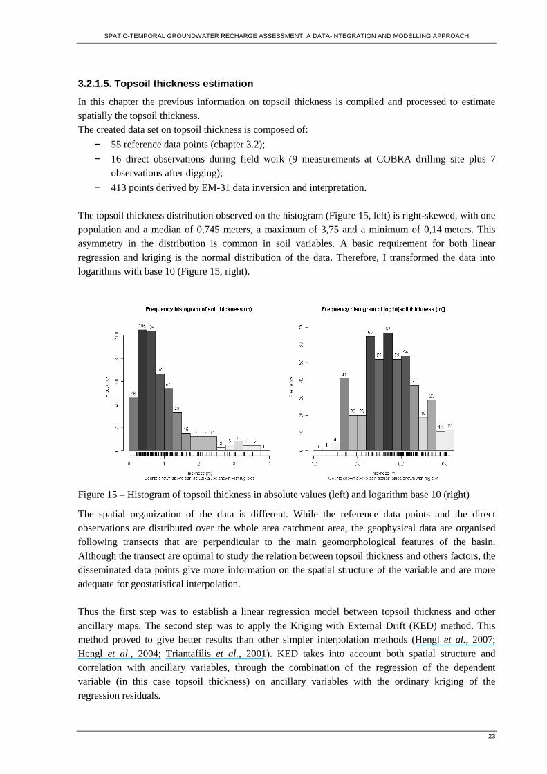
SPATIO-TEMPORAL GROUNDWATER RECHARGE ASSESSMENT: A DATA-INTEGRATION AND MODELLING APPROACH

23

3.2.1.5. Topsoil thickness estimation

In this chapter the previous information on topsoil thickness is compiled and processed to estimate spatially the topsoil thickness. The created data set on topsoil thickness is composed of:

− 55 reference data points (chapter 3.2);

− 16 direct observations during field work (9 measurements at COBRA drilling site plus 7 observations after digging);

− 413 points derived by EM-31 data inversion and interpretation. The topsoil thickness distribution observed on the histogram (Figure 15, left) is right-skewed, with one population and a median of 0,745 meters, a maximum of 3,75 and a minimum of 0,14 meters. This asymmetry in the distribution is common in soil variables. A basic requirement for both linear regression and kriging is the normal distribution of the data. Therefore, I transformed the data into logarithms with base 10 (Figure 15, right).

Figure 15 – Histogram of topsoil thickness in absolute values (left) and logarithm base 10 (right)

The spatial organization of the data is different. While the reference data points and the direct observations are distributed over the whole area catchment area, the geophysical data are organised following transects that are perpendicular to the main geomorphological features of the basin. Although the transect are optimal to study the relation between topsoil thickness and others factors, the disseminated data points give more information on the spatial structure of the variable and are more adequate for geostatistical interpolation. Thus the first step was to establish a linear regression model between topsoil thickness and other ancillary maps. The second step was to apply the Kriging with External Drift (KED) method. This method proved to give better results than other simpler interpolation methods (Hengl et al., 2007; Hengl et al., 2004; Triantafilis et al., 2001). KED takes into account both spatial structure and correlation with ancillary variables, through the combination of the regression of the dependent variable (in this case topsoil thickness) on ancillary variables with the ordinary kriging of the regression residuals.

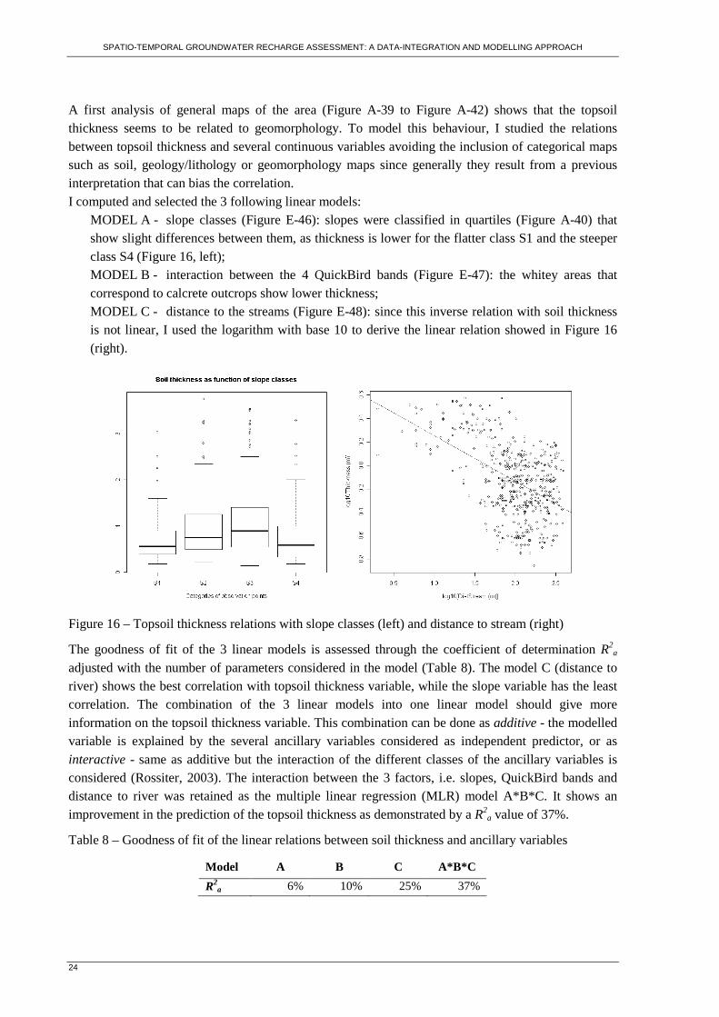
SPATIO-TEMPORAL GROUNDWATER RECHARGE ASSESSMENT: A DATA-INTEGRATION AND MODELLING APPROACH

24

A first analysis of general maps of the area (Figure A-39 to Figure A-42) shows that the topsoil thickness seems to be related to geomorphology. To model this behaviour, I studied the relations between topsoil thickness and several continuous variables avoiding the inclusion of categorical maps such as soil, geology/lithology or geomorphology maps since generally they result from a previous interpretation that can bias the correlation. I computed and selected the 3 following linear models:

MODEL A - slope classes (Figure E-46): slopes were classified in quartiles (Figure A-40) that show slight differences between them, as thickness is lower for the flatter class S1 and the steeper class S4 (Figure 16, left); MODEL B - interaction between the 4 QuickBird bands (Figure E-47): the whitey areas that correspond to calcrete outcrops show lower thickness; MODEL C - distance to the streams (Figure E-48): since this inverse relation with soil thickness is not linear, I used the logarithm with base 10 to derive the linear relation showed in Figure 16 (right).

Figure 16 – Topsoil thickness relations with slope classes (left) and distance to stream (right)

The goodness of fit of the 3 linear models is assessed through the coefficient of determination R2a

adjusted with the number of parameters considered in the model (Table 8). The model C (distance to river) shows the best correlation with topsoil thickness variable, while the slope variable has the least correlation. The combination of the 3 linear models into one linear model should give more information on the topsoil thickness variable. This combination can be done as additive - the modelled variable is explained by the several ancillary variables considered as independent predictor, or as interactive - same as additive but the interaction of the different classes of the ancillary variables is considered (Rossiter, 2003). The interaction between the 3 factors, i.e. slopes, QuickBird bands and distance to river was retained as the multiple linear regression (MLR) model A*B*C. It shows an improvement in the prediction of the topsoil thickness as demonstrated by a R2

a value of 37%.

Table 8 – Goodness of fit of the linear relations between soil thickness and ancillary variables

Model A B C A*B*C

R2a 6% 10% 25% 37%

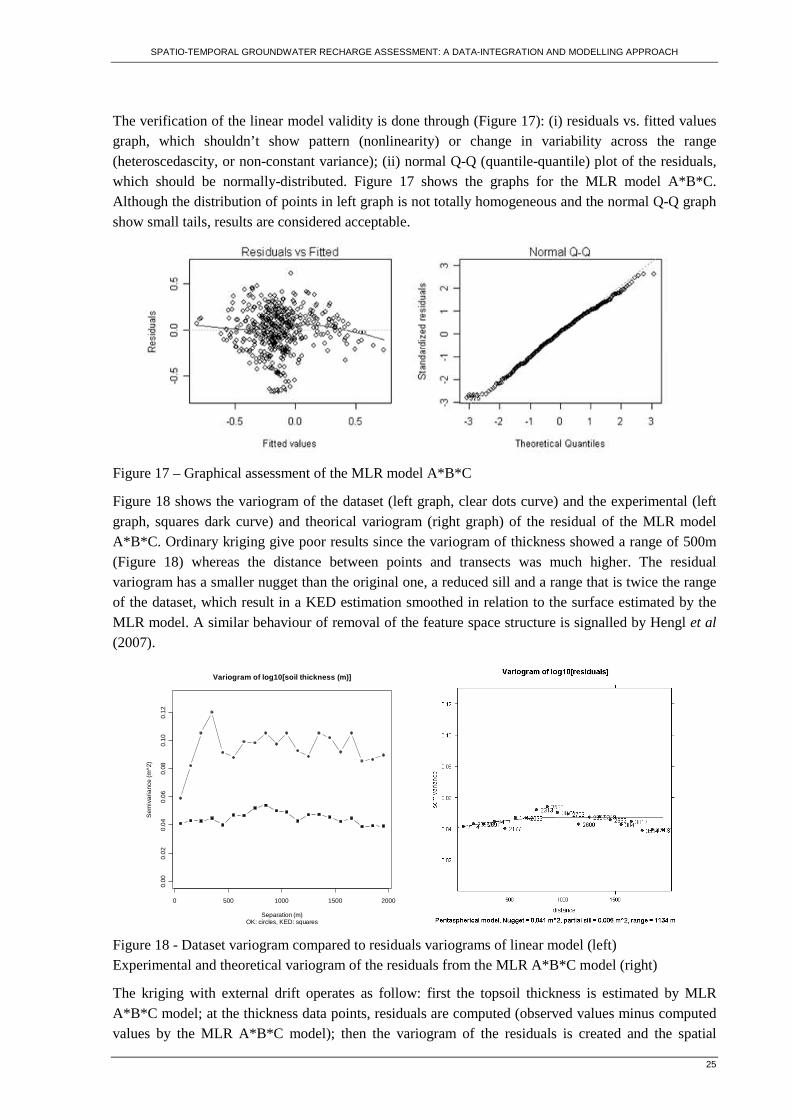
SPATIO-TEMPORAL GROUNDWATER RECHARGE ASSESSMENT: A DATA-INTEGRATION AND MODELLING APPROACH

25

The verification of the linear model validity is done through (Figure 17): (i) residuals vs. fitted values graph, which shouldn’t show pattern (nonlinearity) or change in variability across the range (heteroscedascity, or non-constant variance); (ii) normal Q-Q (quantile-quantile) plot of the residuals, which should be normally-distributed. Figure 17 shows the graphs for the MLR model A*B*C. Although the distribution of points in left graph is not totally homogeneous and the normal Q-Q graph show small tails, results are considered acceptable.

Figure 17 – Graphical assessment of the MLR model A*B*C

Figure 18 shows the variogram of the dataset (left graph, clear dots curve) and the experimental (left graph, squares dark curve) and theorical variogram (right graph) of the residual of the MLR model A*B*C. Ordinary kriging give poor results since the variogram of thickness showed a range of 500m (Figure 18) whereas the distance between points and transects was much higher. The residual variogram has a smaller nugget than the original one, a reduced sill and a range that is twice the range of the dataset, which result in a KED estimation smoothed in relation to the surface estimated by the MLR model. A similar behaviour of removal of the feature space structure is signalled by Hengl et al (2007).

0 500 1000 1500 2000

0.00

0.0

20

.04

0.06

0.08

0.10

0.12

Variogram of log10[soil thickness (m)]

OK: circles, KED: squaresSeparation (m)

Se

miv

aria

nce

(m^2

)

Figure 18 - Dataset variogram compared to residuals variograms of linear model (left) Experimental and theoretical variogram of the residuals from the MLR A*B*C model (right)

The kriging with external drift operates as follow: first the topsoil thickness is estimated by MLR A*B*C model; at the thickness data points, residuals are computed (observed values minus computed values by the MLR A*B*C model); then the variogram of the residuals is created and the spatial

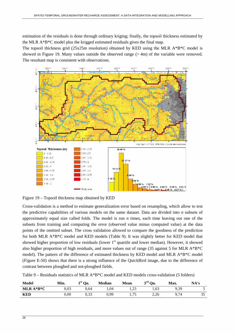
SPATIO-TEMPORAL GROUNDWATER RECHARGE ASSESSMENT: A DATA-INTEGRATION AND MODELLING APPROACH

26

estimation of the residuals is done through ordinary kriging; finally, the topsoil thickness estimated by the MLR A*B*C model plus the krigged estimated residuals gives the final map. The topsoil thickness grid (25x25m resolution) obtained by KED using the MLR A*B*C model is showed in Figure 19. Many values outside the observed range (> 4m) of the variable were removed. The resultant map is consistent with observations.

Figure 19 – Topsoil thickness map obtained by KED

Cross-validation is a method to estimate generalization error based on resampling, which allow to test the predictive capabilities of various models on the same dataset. Data are divided into n subsets of approximately equal size called folds. The model is run n times, each time leaving out one of the subsets from training and computing the error (observed value minus computed value) at the data points of the omitted subset. The cross validation allowed to compare the goodness of the prediction for both MLR A*B*C model and KED models (Table 9). It was slightly better for KED model that showed higher proportion of low residuals (lower 1st quartile and lower median). However, it showed also higher proportion of high residuals, and more values out of range (35 against 5 for MLR A*B*C model). The pattern of the difference of estimated thickness by KED model and MLR A*B*C model (Figure E-50) shows that there is a strong influence of the QuickBird image, due to the difference of contrast between ploughed and not-ploughed fields.

Table 9 – Residuals statistics of MLR A*B*C model and KED models cross-validation (5 folders)

Model Min. 1st Qu. Median Mean 3rd Qu. Max. NA's MLR A*B*C 0,03 0,64 1,04 1,23 1,63 9,39 5

KED 0,00 0,33 0,99 1,75 2,26 9,74 35

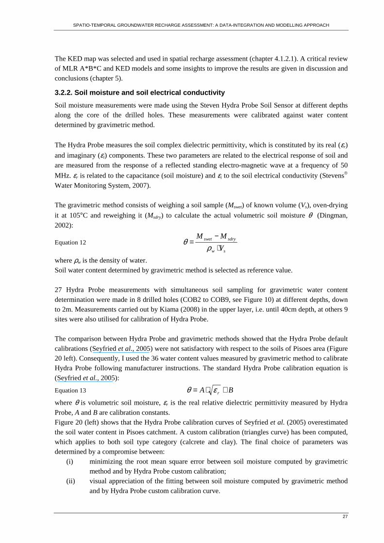
SPATIO-TEMPORAL GROUNDWATER RECHARGE ASSESSMENT: A DATA-INTEGRATION AND MODELLING APPROACH

27

The KED map was selected and used in spatial recharge assessment (chapter 4.1.2.1). A critical review of MLR A*B*C and KED models and some insights to improve the results are given in discussion and conclusions (chapter 5).

3.2.2. Soil moisture and soil electrical conductivity

Soil moisture measurements were made using the Steven Hydra Probe Soil Sensor at different depths along the core of the drilled holes. These measurements were calibrated against water content determined by gravimetric method.

The Hydra Probe measures the soil complex dielectric permittivity, which is constituted by its real (εr)

and imaginary (εi) components. These two parameters are related to the electrical response of soil and are measured from the response of a reflected standing electro-magnetic wave at a frequency of 50

MHz. εr is related to the capacitance (soil moisture) and εi to the soil electrical conductivity (Stevens Water Monitoring System, 2007). The gravimetric method consists of weighing a soil sample (Mswet) of known volume (Vs), oven-drying

it at 105°C and reweighing it (Msdry) to calculate the actual volumetric soil moisture θ (Dingman, 2002):

Equation 12 sw

sdryswet

V

MM

⋅−

=ρ

θ

where ρw is the density of water. Soil water content determined by gravimetric method is selected as reference value. 27 Hydra Probe measurements with simultaneous soil sampling for gravimetric water content determination were made in 8 drilled holes (COB2 to COB9, see Figure 10) at different depths, down to 2m. Measurements carried out by Kiama (2008) in the upper layer, i.e. until 40cm depth, at others 9 sites were also utilised for calibration of Hydra Probe. The comparison between Hydra Probe and gravimetric methods showed that the Hydra Probe default calibrations (Seyfried et al., 2005) were not satisfactory with respect to the soils of Pisoes area (Figure 20 left). Consequently, I used the 36 water content values measured by gravimetric method to calibrate Hydra Probe following manufacturer instructions. The standard Hydra Probe calibration equation is (Seyfried et al., 2005):

Equation 13 BA r +⋅= εθ

where θ is volumetric soil moisture, εr is the real relative dielectric permittivity measured by Hydra Probe, A and B are calibration constants. Figure 20 (left) shows that the Hydra Probe calibration curves of Seyfried et al. (2005) overestimated the soil water content in Pisoes catchment. A custom calibration (triangles curve) has been computed, which applies to both soil type category (calcrete and clay). The final choice of parameters was determined by a compromise between:

(i) minimizing the root mean square error between soil moisture computed by gravimetric method and by Hydra Probe custom calibration;

(ii) visual appreciation of the fitting between soil moisture computed by gravimetric method and by Hydra Probe custom calibration curve.

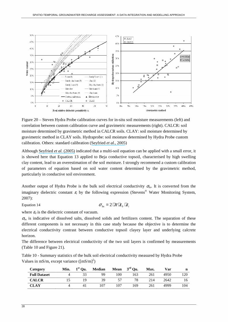
SPATIO-TEMPORAL GROUNDWATER RECHARGE ASSESSMENT: A DATA-INTEGRATION AND MODELLING APPROACH

28

Figure 20 – Steven Hydra Probe calibration curves for in-situ soil moisture measurements (left) and correlation between custom calibration curve and gravimetric measurements (right). CALCR: soil moisture determined by gravimetric method in CALCR soils. CLAY: soil moisture determined by gravimetric method in CLAY soils. Hydraprobe: soil moisture determined by Hydra Probe custom calibration. Others: standard calibration (Seyfried et al., 2005)

Although Seyfried et al. (2005) indicated that a multi-soil equation can be applied with a small error, it is showed here that Equation 13 applied to Beja conductive topsoil, characterised by high swelling clay content, lead to an overestimation of the soil moisture. I strongly recommend a custom calibration of parameters of equation based on soil water content determined by the gravimetric method, particularly in conductive soil environment.

Another output of Hydra Probe is the bulk soil electrical conductivity σbs. It is converted from the

imaginary dielectric constant εi by the following expression (Stevens Water Monitoring System, 2007):

Equation 14 ibs εεπσ ⋅⋅⋅= 02

where ε0 is the dielectric constant of vacuum.

σbs is indicative of dissolved salts, dissolved solids and fertilizers content. The separation of these different components is not necessary in this case study because the objective is to determine the electrical conductivity contrast between conductive topsoil clayey layer and underlying calcrete horizon. The difference between electrical conductivity of the two soil layers is confirmed by measurements (Table 10 and Figure 21).

Table 10 - Summary statistics of the bulk soil electrical conductivity measured by Hydra Probe Values in mS/m, except variance ([mS/m]2)

Category Min. 1st Qu. Median Mean 3rd Qu. Max. Var n Full Dataset 4 33 99 100 163 261 4950 120

CALCR 15 19 39 57 78 214 2642 16

CLAY 4 41 107 107 169 261 4999 104

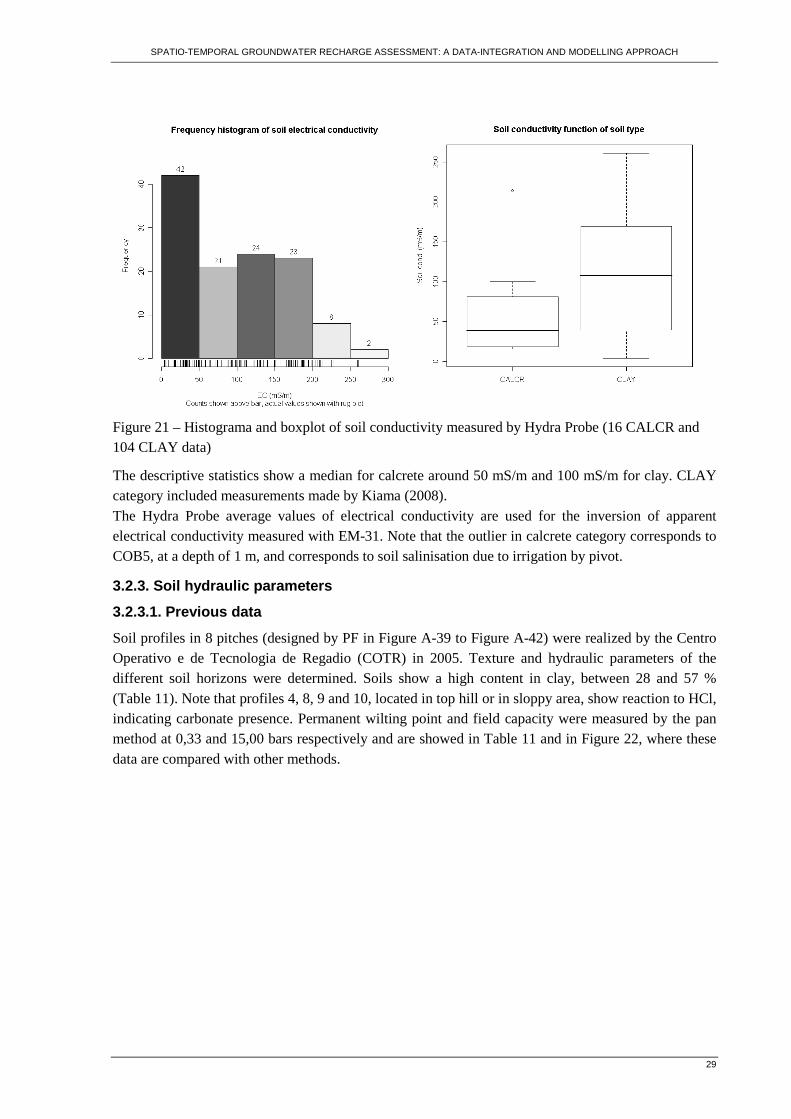
SPATIO-TEMPORAL GROUNDWATER RECHARGE ASSESSMENT: A DATA-INTEGRATION AND MODELLING APPROACH

29

Figure 21 – Histograma and boxplot of soil conductivity measured by Hydra Probe (16 CALCR and 104 CLAY data)

The descriptive statistics show a median for calcrete around 50 mS/m and 100 mS/m for clay. CLAY category included measurements made by Kiama (2008). The Hydra Probe average values of electrical conductivity are used for the inversion of apparent electrical conductivity measured with EM-31. Note that the outlier in calcrete category corresponds to COB5, at a depth of 1 m, and corresponds to soil salinisation due to irrigation by pivot.

3.2.3. Soil hydraulic parameters

3.2.3.1. Previous data

Soil profiles in 8 pitches (designed by PF in Figure A-39 to Figure A-42) were realized by the Centro Operativo e de Tecnologia de Regadio (COTR) in 2005. Texture and hydraulic parameters of the different soil horizons were determined. Soils show a high content in clay, between 28 and 57 % (Table 11). Note that profiles 4, 8, 9 and 10, located in top hill or in sloppy area, show reaction to HCl, indicating carbonate presence. Permanent wilting point and field capacity were measured by the pan method at 0,33 and 15,00 bars respectively and are showed in Table 11 and in Figure 22, where these data are compared with other methods.

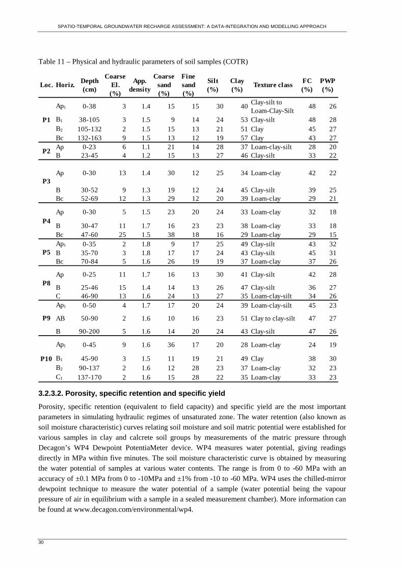
SPATIO-TEMPORAL GROUNDWATER RECHARGE ASSESSMENT: A DATA-INTEGRATION AND MODELLING APPROACH

30

Table 11 – Physical and hydraulic parameters of soil samples (COTR)

Loc. Horiz.Depth (cm)

Coarse El. (%)

App. density

Coarse sand (%)

Fine sand (%)

Silt (%)

Clay (%)

Texture classFC (%)

PWP (%)

Ap1 0-38 3 1.4 15 15 30 40Clay-silt to Loam-Clay-Silt

48 26

B1 38-105 3 1.5 9 14 24 53 Clay-silt 48 28B2 105-132 2 1.5 15 13 21 51 Clay 45 27Bc 132-163 9 1.5 13 12 19 57 Clay 43 27Ap 0-23 6 1.1 21 14 28 37 Loam-clay-silt 28 20B 23-45 4 1.2 15 13 27 46 Clay-silt 33 22

Ap 0-30 13 1.4 30 12 25 34 Loam-clay 42 22

B 30-52 9 1.3 19 12 24 45 Clay-silt 39 25Bc 52-69 12 1.3 29 12 20 39 Loam-clay 29 21

Ap 0-30 5 1.5 23 20 24 33 Loam-clay 32 18

B 30-47 11 1.7 16 23 23 38 Loam-clay 33 18Bc 47-60 25 1.5 38 18 16 29 Loam-clay 29 15Ap1 0-35 2 1.8 9 17 25 49 Clay-silt 43 32B 35-70 3 1.8 17 17 24 43 Clay-silt 45 31Bc 70-84 5 1.6 26 19 19 37 Loam-clay 37 26

Ap 0-25 11 1.7 16 13 30 41 Clay-silt 42 28

B 25-46 15 1.4 14 13 26 47 Clay-silt 36 27C 46-90 13 1.6 24 13 27 35 Loam-clay-silt 34 26Ap1 0-50 4 1.7 17 20 24 39 Loam-clay-silt 45 23

AB 50-90 2 1.6 10 16 23 51 Clay to clay-silt 47 27

B 90-200 5 1.6 14 20 24 43 Clay-silt 47 26

Ap1 0-45 9 1.6 36 17 20 28 Loam-clay 24 19

B1 45-90 3 1.5 11 19 21 49 Clay 38 30B2 90-137 2 1.6 12 28 23 37 Loam-clay 32 23C1 137-170 2 1.6 15 28 22 35 Loam-clay 33 23

P1

P2

P9

P10

P3

P4

P5

P8

3.2.3.2. Porosity, specific retention and specific yield

Porosity, specific retention (equivalent to field capacity) and specific yield are the most important parameters in simulating hydraulic regimes of unsaturated zone. The water retention (also known as soil moisture characteristic) curves relating soil moisture and soil matric potential were established for various samples in clay and calcrete soil groups by measurements of the matric pressure through Decagon’s WP4 Dewpoint PotentiaMeter device. WP4 measures water potential, giving readings directly in MPa within five minutes. The soil moisture characteristic curve is obtained by measuring the water potential of samples at various water contents. The range is from 0 to -60 MPa with an accuracy of ±0.1 MPa from 0 to -10MPa and ±1% from -10 to -60 MPa. WP4 uses the chilled-mirror dewpoint technique to measure the water potential of a sample (water potential being the vapour pressure of air in equilibrium with a sample in a sealed measurement chamber). More information can be found at www.decagon.com/environmental/wp4.

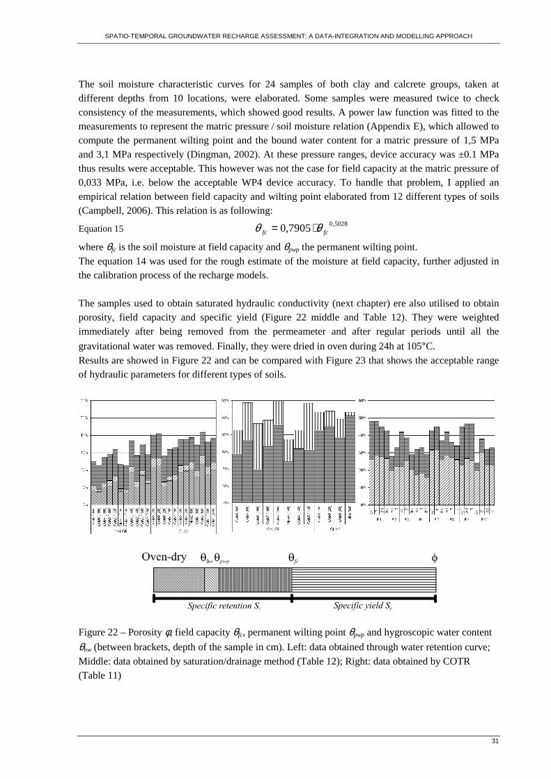
SPATIO-TEMPORAL GROUNDWATER RECHARGE ASSESSMENT: A DATA-INTEGRATION AND MODELLING APPROACH

31

The soil moisture characteristic curves for 24 samples of both clay and calcrete groups, taken at different depths from 10 locations, were elaborated. Some samples were measured twice to check consistency of the measurements, which showed good results. A power law function was fitted to the measurements to represent the matric pressure / soil moisture relation (Appendix E), which allowed to compute the permanent wilting point and the bound water content for a matric pressure of 1,5 MPa and 3,1 MPa respectively (Dingman, 2002). At these pressure ranges, device accuracy was ±0.1 MPa thus results were acceptable. This however was not the case for field capacity at the matric pressure of 0,033 MPa, i.e. below the acceptable WP4 device accuracy. To handle that problem, I applied an empirical relation between field capacity and wilting point elaborated from 12 different types of soils (Campbell, 2006). This relation is as following:

Equation 15 5028,07905,0 fcfc θθ ⋅=

where θfc is the soil moisture at field capacity and θpwp the permanent wilting point. The equation 14 was used for the rough estimate of the moisture at field capacity, further adjusted in the calibration process of the recharge models. The samples used to obtain saturated hydraulic conductivity (next chapter) ere also utilised to obtain porosity, field capacity and specific yield (Figure 22 middle and Table 12). They were weighted immediately after being removed from the permeameter and after regular periods until all the

gravitational water was removed. Finally, they were dried in oven during 24h at 105°C. Results are showed in Figure 22 and can be compared with Figure 23 that shows the acceptable range of hydraulic parameters for different types of soils.

Figure 22 – Porosity φ, field capacity θfc, permanent wilting point θpwp and hygroscopic water content

θhw (between brackets, depth of the sample in cm). Left: data obtained through water retention curve; Middle: data obtained by saturation/drainage method (Table 12); Right: data obtained by COTR (Table 11)

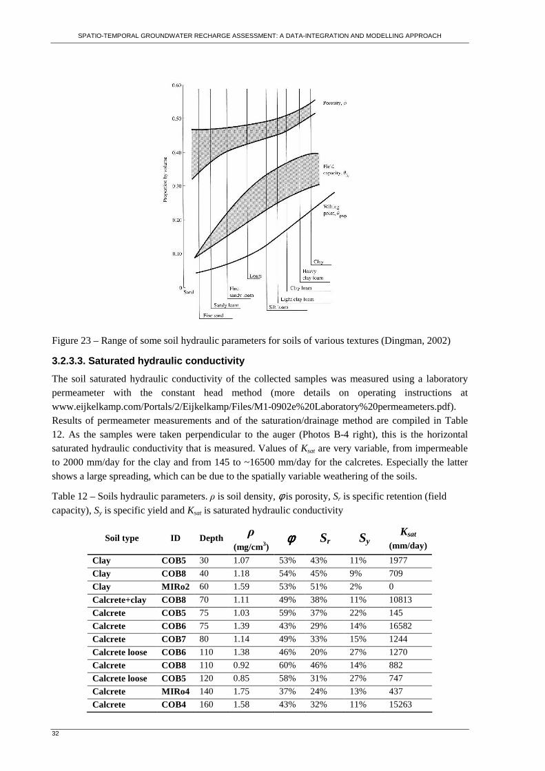
SPATIO-TEMPORAL GROUNDWATER RECHARGE ASSESSMENT: A DATA-INTEGRATION AND MODELLING APPROACH

32

Figure 23 – Range of some soil hydraulic parameters for soils of various textures (Dingman, 2002)

3.2.3.3. Saturated hydraulic conductivity

The soil saturated hydraulic conductivity of the collected samples was measured using a laboratory permeameter with the constant head method (more details on operating instructions at www.eijkelkamp.com/Portals/2/Eijkelkamp/Files/M1-0902e%20Laboratory%20permeameters.pdf). Results of permeameter measurements and of the saturation/drainage method are compiled in Table 12. As the samples were taken perpendicular to the auger (Photos B-4 right), this is the horizontal saturated hydraulic conductivity that is measured. Values of Ksat are very variable, from impermeable to 2000 mm/day for the clay and from 145 to ~16500 mm/day for the calcretes. Especially the latter shows a large spreading, which can be due to the spatially variable weathering of the soils.

Table 12 – Soils hydraulic parameters. ρ is soil density, φ is porosity, Sr is specific retention (field capacity), Sy is specific yield and Ksat is saturated hydraulic conductivity

Soil type ID Depth ρ

(mg/cm3) φφφφ Sr Sy

Ksat

(mm/day) Clay COB5 30 1.07 53% 43% 11% 1977

Clay COB8 40 1.18 54% 45% 9% 709

Clay MIRo2 60 1.59 53% 51% 2% 0

Calcrete+clay COB8 70 1.11 49% 38% 11% 10813

Calcrete COB5 75 1.03 59% 37% 22% 145

Calcrete COB6 75 1.39 43% 29% 14% 16582

Calcrete COB7 80 1.14 49% 33% 15% 1244

Calcrete loose COB6 110 1.38 46% 20% 27% 1270

Calcrete COB8 110 0.92 60% 46% 14% 882

Calcrete loose COB5 120 0.85 58% 31% 27% 747

Calcrete MIRo4 140 1.75 37% 24% 13% 437

Calcrete COB4 160 1.58 43% 32% 11% 15263

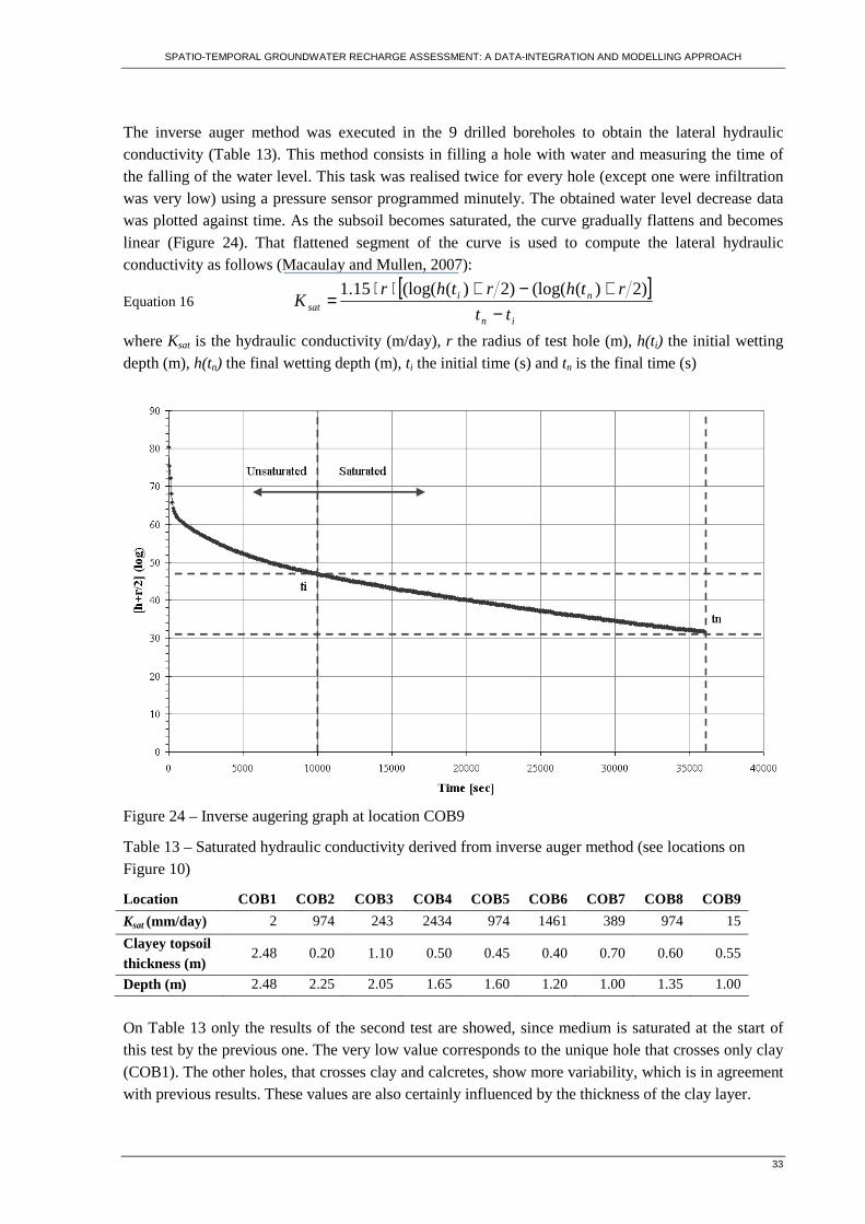
SPATIO-TEMPORAL GROUNDWATER RECHARGE ASSESSMENT: A DATA-INTEGRATION AND MODELLING APPROACH

33

The inverse auger method was executed in the 9 drilled boreholes to obtain the lateral hydraulic conductivity (Table 13). This method consists in filling a hole with water and measuring the time of the falling of the water level. This task was realised twice for every hole (except one were infiltration was very low) using a pressure sensor programmed minutely. The obtained water level decrease data was plotted against time. As the subsoil becomes saturated, the curve gradually flattens and becomes linear (Figure 24). That flattened segment of the curve is used to compute the lateral hydraulic conductivity as follows (Macaulay and Mullen, 2007):

Equation 16 [ ]

in

nisat tt

rthrthrK

−+−+⋅⋅

=)2)((log()2)((log(15.1

where Ksat is the hydraulic conductivity (m/day), r the radius of test hole (m), h(ti) the initial wetting depth (m), h(tn) the final wetting depth (m), ti the initial time (s) and tn is the final time (s)

Figure 24 – Inverse augering graph at location COB9

Table 13 – Saturated hydraulic conductivity derived from inverse auger method (see locations on Figure 10)

Location COB1 COB2 COB3 COB4 COB5 COB6 COB7 COB8 COB9

Ksat (mm/day) 2 974 243 2434 974 1461 389 974 15

Clayey topsoil thickness (m)

2.48 0.20 1.10 0.50 0.45 0.40 0.70 0.60 0.55

Depth (m) 2.48 2.25 2.05 1.65 1.60 1.20 1.00 1.35 1.00

On Table 13 only the results of the second test are showed, since medium is saturated at the start of this test by the previous one. The very low value corresponds to the unique hole that crosses only clay (COB1). The other holes, that crosses clay and calcretes, show more variability, which is in agreement with previous results. These values are also certainly influenced by the thickness of the clay layer.

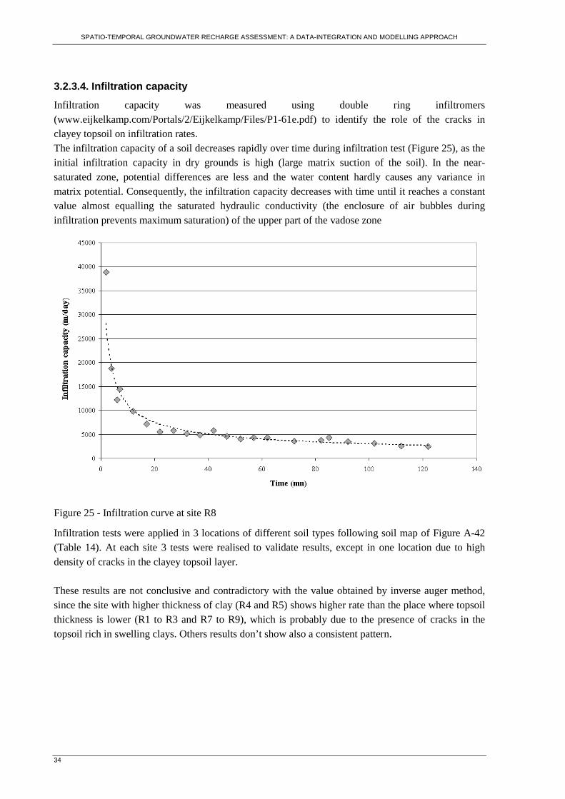
SPATIO-TEMPORAL GROUNDWATER RECHARGE ASSESSMENT: A DATA-INTEGRATION AND MODELLING APPROACH

34

3.2.3.4. Infiltration capacity

Infiltration capacity was measured using double ring infiltromers (www.eijkelkamp.com/Portals/2/Eijkelkamp/Files/P1-61e.pdf) to identify the role of the cracks in clayey topsoil on infiltration rates. The infiltration capacity of a soil decreases rapidly over time during infiltration test (Figure 25), as the initial infiltration capacity in dry grounds is high (large matrix suction of the soil). In the near-saturated zone, potential differences are less and the water content hardly causes any variance in matrix potential. Consequently, the infiltration capacity decreases with time until it reaches a constant value almost equalling the saturated hydraulic conductivity (the enclosure of air bubbles during infiltration prevents maximum saturation) of the upper part of the vadose zone

Figure 25 - Infiltration curve at site R8

Infiltration tests were applied in 3 locations of different soil types following soil map of Figure A-42 (Table 14). At each site 3 tests were realised to validate results, except in one location due to high density of cracks in the clayey topsoil layer. These results are not conclusive and contradictory with the value obtained by inverse auger method, since the site with higher thickness of clay (R4 and R5) shows higher rate than the place where topsoil thickness is lower (R1 to R3 and R7 to R9), which is probably due to the presence of cracks in the topsoil rich in swelling clays. Others results don’t show also a consistent pattern.

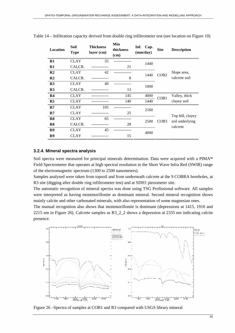
SPATIO-TEMPORAL GROUNDWATER RECHARGE ASSESSMENT: A DATA-INTEGRATION AND MODELLING APPROACH

35

Table 14 – Infiltration capacity derived from double ring infiltrometer test (see location on Figure 10)

Location Soil Type

Thickness layer (cm)

Min thickness (cm)

Inf. Cap. (mm/day)

Site Description

R1 CLAY 35 -------------

R1 CALCR. ------------- 21 1440

R2 CLAY 42 -------------

R2 CALCR. ------------- 8 1440

R3 CLAY 40 -------------

R3 CALCR. ------------- 13 1000

COB2 Slope area, calcrete soil

R4 CLAY ------------- 145 4000

R5 CLAY ------------- 140 1440 COB1

Valley, thick clayey soil

R7 CLAY 105 -------------

R7 CLAY ------------- 25 2160

R8 CLAY 65 -------------

R8 CALCR. ------------- 28 2500

R9 CLAY 45 -------------

R9 CLAY ------------- 15 4000

COB3 Top hill, clayey soil underlying calcrete

3.2.4. Mineral spectra analysis

Soil spectra were measured for principal minerals determination. Data were acquired with a PIMA Field Spectrometer that operates at high spectral resolution in the Short Wave Infra Red (SWIR) range of the electromagnetic spectrum (1300 to 2500 nanometers). Samples analysed were taken from topsoil and from underneath calcrete at the 9 COBRA boreholes, at R3 site (digging after double ring infiltrometer test) and at SDH1 piezometer site. The automatic recognition of mineral spectra was done using TSG Profissional software. All samples were interpreted as having montmorillonite as dominant mineral. Second mineral recognition shows mainly calcite and other carbonated minerals, with also representation of some magnesian ones. The manual recognition also shows that montmorillonite is dominant (depressions at 1415, 1910 and 2215 nm in Figure 26). Calcrete samples as R3_2_2 shows a depression at 2335 nm indicating calcite presence.

Figure 26 –Spectra of samples at COB1 and R3 compared with USGS library mineral

SPATIO-TEMPORAL GROUNDWATER RECHARGE ASSESSMENT: A DATA-INTEGRATION AND MODELLING APPROACH

36

This analysis confirmed the presence of swelling clay in all samples, even in calcrete layer, where the calcite signature is slight in the spectra curves. This method is qualitative, thus no conclusion can be made on minerals content.

3.3. Summary

The data acquired from primary and secondary collection were processed and organised in an intelligible data set that was used to provide inputs (driving forces), to parameterise (topsoil properties) and to calibrate (state variables) the recharge models described in chapter 4. The monitoring network composed by 2 main piezometers and one hydrometeorologic station gave insights on the temporal and spatial behaviour of recharge/discharge processes in the catchment. The design of sample/data acquisition scheme allowed to complement the previous information by spatial characterisation of the soil reservoir. The final data set is composed by:

- Driving forces time series (daily based, from January 2002 to January 2008): (i) reference evapotranspiration; (ii) rainfall;

- State variables time series (daily based): (i) piezometric time series (January 2002 to January 2008) that represent hydrogeological behaviour in the two distinct geomorphological positions of the catchment i.e. top-hill and drainage area; (ii) Soil moisture and matric pressure (October 2004 to January 2007);

- Soil hydraulic parameters in 18 sites distributed over the catchment (porosity, field capacity, permanent wilting point and saturated hydraulic conductivity at different depths were determined) that allow to differentiate two soil groups;

- Topsoil thickness map; - Soil and vadose zone main mineral composition.

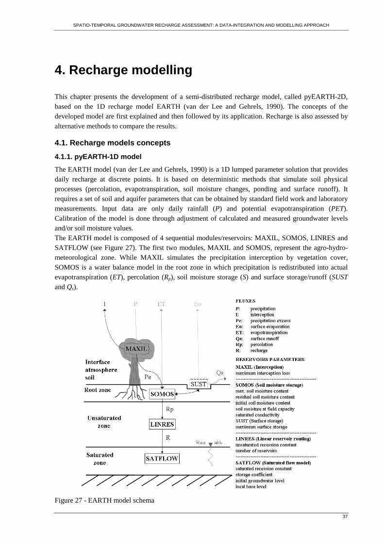
SPATIO-TEMPORAL GROUNDWATER RECHARGE ASSESSMENT: A DATA-INTEGRATION AND MODELLING APPROACH

37

4. Recharge modelling

This chapter presents the development of a semi-distributed recharge model, called pyEARTH-2D, based on the 1D recharge model EARTH (van der Lee and Gehrels, 1990). The concepts of the developed model are first explained and then followed by its application. Recharge is also assessed by alternative methods to compare the results.

4.1. Recharge models concepts

4.1.1. pyEARTH-1D model

The EARTH model (van der Lee and Gehrels, 1990) is a 1D lumped parameter solution that provides daily recharge at discrete points. It is based on deterministic methods that simulate soil physical processes (percolation, evapotranspiration, soil moisture changes, ponding and surface runoff). It requires a set of soil and aquifer parameters that can be obtained by standard field work and laboratory measurements. Input data are only daily rainfall (P) and potential evapotranspiration (PET). Calibration of the model is done through adjustment of calculated and measured groundwater levels and/or soil moisture values. The EARTH model is composed of 4 sequential modules/reservoirs: MAXIL, SOMOS, LINRES and SATFLOW (see Figure 27). The first two modules, MAXIL and SOMOS, represent the agro-hydro-meteorological zone. While MAXIL simulates the precipitation interception by vegetation cover, SOMOS is a water balance model in the root zone in which precipitation is redistributed into actual evapotranspiration (ET), percolation (Rp), soil moisture storage (S) and surface storage/runoff (SUST and Qs).

Figure 27 - EARTH model schema

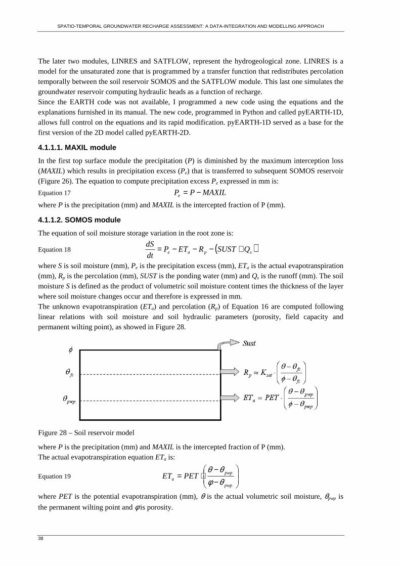
SPATIO-TEMPORAL GROUNDWATER RECHARGE ASSESSMENT: A DATA-INTEGRATION AND MODELLING APPROACH

38

The later two modules, LINRES and SATFLOW, represent the hydrogeological zone. LINRES is a model for the unsaturated zone that is programmed by a transfer function that redistributes percolation temporally between the soil reservoir SOMOS and the SATFLOW module. This last one simulates the groundwater reservoir computing hydraulic heads as a function of recharge. Since the EARTH code was not available, I programmed a new code using the equations and the explanations furnished in its manual. The new code, programmed in Python and called pyEARTH-1D, allows full control on the equations and its rapid modification. pyEARTH-1D served as a base for the first version of the 2D model called pyEARTH-2D.

4.1.1.1. MAXIL module

In the first top surface module the precipitation (P) is diminished by the maximum interception loss (MAXIL) which results in precipitation excess (Pe) that is transferred to subsequent SOMOS reservoir (Figure 26). The equation to compute precipitation excess Pe expressed in mm is:

Equation 17 MAXILPPe −=

where P is the precipitation (mm) and MAXIL is the intercepted fraction of P (mm).

4.1.1.2. SOMOS module

The equation of soil moisture storage variation in the root zone is:

Equation 18 ( )spae QSUSTRETPdt

dS +−−−=

where S is soil moisture (mm), Pe is the precipitation excess (mm), ETa is the actual evapotranspiration (mm), Rp is the percolation (mm), SUST is the ponding water (mm) and Qs is the runoff (mm). The soil moisture S is defined as the product of volumetric soil moisture content times the thickness of the layer where soil moisture changes occur and therefore is expressed in mm. The unknown evapotranspiration (ETa) and percolation (Rp) of Equation 16 are computed following linear relations with soil moisture and soil hydraulic parameters (porosity, field capacity and permanent wilting point), as showed in Figure 28.

Figure 28 – Soil reservoir model

where P is the precipitation (mm) and MAXIL is the intercepted fraction of P (mm). The actual evapotranspiration equation ETa is:

Equation 19

−−

⋅=pwp

pwpa PETET

θφθθ

where PET is the potential evapotranspiration (mm), θ is the actual volumetric soil moisture, θpwp is

the permanent wilting point and φ is porosity.

SPATIO-TEMPORAL GROUNDWATER RECHARGE ASSESSMENT: A DATA-INTEGRATION AND MODELLING APPROACH

39

The percolation equation is:

Equation 20

−−

⋅≈+⋅=fc

fcsat

pp K

dz

dhKR

θφθθ

1

where K is the unsaturated hydraulic conductivity, dhp/dz is the gradient of the hydraulic potential, Ksat

is the saturated hydraulic conductivity (mm.day-1), θ is the actual volumetric soil moisture, θfc is the

soil moisture at field capacity and φ is porosity. It is assumed in the simplification of Equation 20 that percolation is equal to the unsaturated hydraulic conductivity, i.e. the potential term K.dhp/dz is negligible in relation to the gravitational component. If the amount of water in SOMOS reaches saturation, and the infiltration rate exceeds percolation rate Rp, surface ponding may occur. In such case, the equation is:

Equation 21 ( )

opae ERETPdt

SUSTd −−−=

where SUST is the ponding water (mm) and E0 is the open water evaporation (mm). If the ponding water exceeds a threshold value (SUSTmax), that represents the maximum surface storage capacity, runoff (Qs) will occur. The equation is:

Equation 22 maxSUSTSUSTQs −=

4.1.1.3. LINRES module

The equations to delay Rp in recharge R are:

Equation 23 ( )∑=

−−+

+==

n

iin

in Yf

f

fYR

0

*11

Equation 24 pRf

fY

+= 10

where R is the recharge (mm day-1), f is the unsaturated recession constant, n is the number of reservoirs, Y* refers to the result from the previous time step, Y0 is the upper boundary condition and Rp is the percolation (mm).

4.1.1.4. SATFLOW module

The equation to determine groundwater level fluctuation is:

Equation 25 RC

h

STO

R

dt

dh −=

where R is the recharge (mm day-1), STO is storage coefficient (unitless), RC is the saturated recession constant (days) and h is the groundwater level above the local base level (m).

4.1.1.5. Python code

pyEARTH-1D is developed in Python 2.4 and is a stand-alone application with a graphical user interface (GUI) that allow the user to provide the model with the input data and parameters. It uses simple ASCII file as input/output (easy pre and pos-processing in MS Excel). One Python class has been developed for the GUI and another one for the recharge model processing. This setup allows the direct access to the model code, being independent of the GUI. This can be useful for optimization purpose with external code, for instance PEST (Doherty, 2002). The GUI has been developed using wxGlade allowing the implementation of the GUI in wxPython. The model class processes, exports and graphs the data. It uses the matplotlib graphical capabilities and its array functions to input and process the data in a very simple way. This class benefits of some

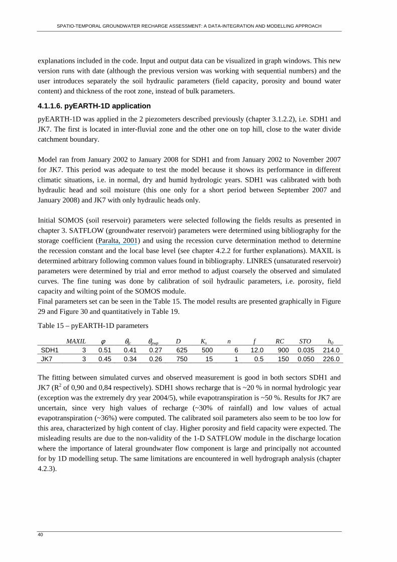
SPATIO-TEMPORAL GROUNDWATER RECHARGE ASSESSMENT: A DATA-INTEGRATION AND MODELLING APPROACH

40

explanations included in the code. Input and output data can be visualized in graph windows. This new version runs with date (although the previous version was working with sequential numbers) and the user introduces separately the soil hydraulic parameters (field capacity, porosity and bound water content) and thickness of the root zone, instead of bulk parameters.

4.1.1.6. pyEARTH-1D application

pyEARTH-1D was applied in the 2 piezometers described previously (chapter 3.1.2.2), i.e. SDH1 and JK7. The first is located in inter-fluvial zone and the other one on top hill, close to the water divide catchment boundary. Model ran from January 2002 to January 2008 for SDH1 and from January 2002 to November 2007 for JK7. This period was adequate to test the model because it shows its performance in different climatic situations, i.e. in normal, dry and humid hydrologic years. SDH1 was calibrated with both hydraulic head and soil moisture (this one only for a short period between September 2007 and January 2008) and JK7 with only hydraulic heads only. Initial SOMOS (soil reservoir) parameters were selected following the fields results as presented in chapter 3. SATFLOW (groundwater reservoir) parameters were determined using bibliography for the storage coefficient (Paralta, 2001) and using the recession curve determination method to determine the recession constant and the local base level (see chapter 4.2.2 for further explanations). MAXIL is determined arbitrary following common values found in bibliography. LINRES (unsaturated reservoir) parameters were determined by trial and error method to adjust coarsely the observed and simulated curves. The fine tuning was done by calibration of soil hydraulic parameters, i.e. porosity, field capacity and wilting point of the SOMOS module. Final parameters set can be seen in the Table 15. The model results are presented graphically in Figure 29 and Figure 30 and quantitatively in Table 19.

Table 15 – pyEARTH-1D parameters

MAXIL φ θfc θpwp D Ks n f RC STO h0 SDH1 3 0.51 0.41 0.27 625 500 6 12.0 900 0.035 214.0 JK7 3 0.45 0.34 0.26 750 15 1 0.5 150 0.050 226.0

The fitting between simulated curves and observed measurement is good in both sectors SDH1 and JK7 (R2 of 0,90 and 0,84 respectively). SDH1 shows recharge that is ~20 % in normal hydrologic year (exception was the extremely dry year 2004/5), while evapotranspiration is ~50 %. Results for JK7 are uncertain, since very high values of recharge (~30% of rainfall) and low values of actual evapotranspiration (~36%) were computed. The calibrated soil parameters also seem to be too low for this area, characterized by high content of clay. Higher porosity and field capacity were expected. The misleading results are due to the non-validity of the 1-D SATFLOW module in the discharge location where the importance of lateral groundwater flow component is large and principally not accounted for by 1D modelling setup. The same limitations are encountered in well hydrograph analysis (chapter 4.2.3).

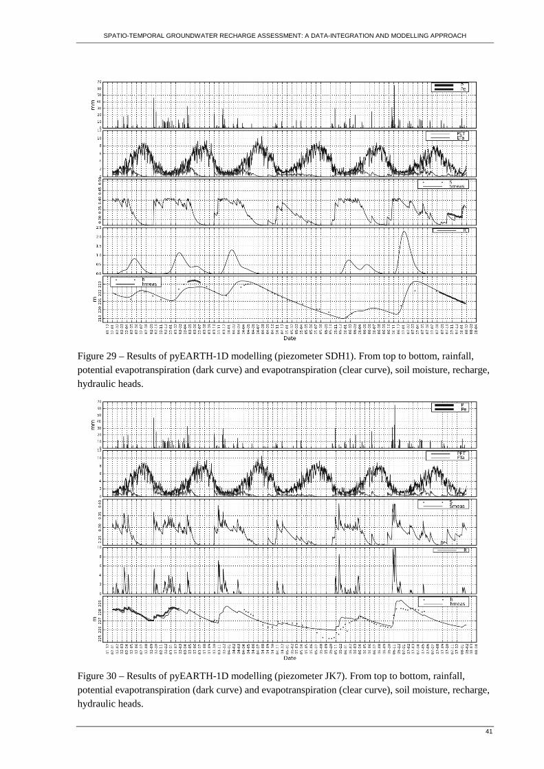
SPATIO-TEMPORAL GROUNDWATER RECHARGE ASSESSMENT: A DATA-INTEGRATION AND MODELLING APPROACH

41

Figure 29 – Results of pyEARTH-1D modelling (piezometer SDH1). From top to bottom, rainfall, potential evapotranspiration (dark curve) and evapotranspiration (clear curve), soil moisture, recharge, hydraulic heads.

Figure 30 – Results of pyEARTH-1D modelling (piezometer JK7). From top to bottom, rainfall, potential evapotranspiration (dark curve) and evapotranspiration (clear curve), soil moisture, recharge, hydraulic heads.

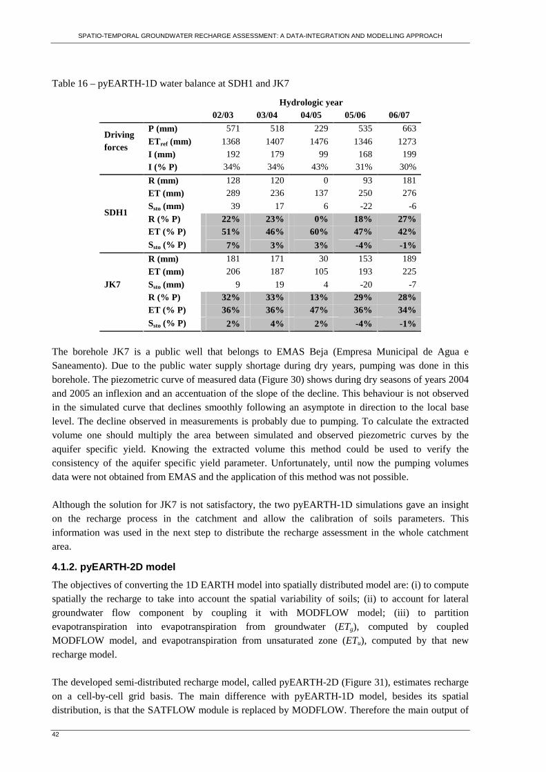
SPATIO-TEMPORAL GROUNDWATER RECHARGE ASSESSMENT: A DATA-INTEGRATION AND MODELLING APPROACH

42

Table 16 – pyEARTH-1D water balance at SDH1 and JK7

Hydrologic year 02/03 03/04 04/05 05/06 06/07

P (mm) 571 518 229 535 663

ETref (mm) 1368 1407 1476 1346 1273

I (mm) 192 179 99 168 199

Driving forces

I (% P) 34% 34% 43% 31% 30%

R (mm) 128 120 0 93 181

ET (mm) 289 236 137 250 276

Ssto (mm) 39 17 6 -22 -6

R (% P) 22% 23% 0% 18% 27% ET (% P) 51% 46% 60% 47% 42%

SDH1

Ssto (% P) 7% 3% 3% -4% -1%

R (mm) 181 171 30 153 189

ET (mm) 206 187 105 193 225

Ssto (mm) 9 19 4 -20 -7

R (% P) 32% 33% 13% 29% 28% ET (% P) 36% 36% 47% 36% 34%

JK7

Ssto (% P) 2% 4% 2% -4% -1%

The borehole JK7 is a public well that belongs to EMAS Beja (Empresa Municipal de Agua e Saneamento). Due to the public water supply shortage during dry years, pumping was done in this borehole. The piezometric curve of measured data (Figure 30) shows during dry seasons of years 2004 and 2005 an inflexion and an accentuation of the slope of the decline. This behaviour is not observed in the simulated curve that declines smoothly following an asymptote in direction to the local base level. The decline observed in measurements is probably due to pumping. To calculate the extracted volume one should multiply the area between simulated and observed piezometric curves by the aquifer specific yield. Knowing the extracted volume this method could be used to verify the consistency of the aquifer specific yield parameter. Unfortunately, until now the pumping volumes data were not obtained from EMAS and the application of this method was not possible. Although the solution for JK7 is not satisfactory, the two pyEARTH-1D simulations gave an insight on the recharge process in the catchment and allow the calibration of soils parameters. This information was used in the next step to distribute the recharge assessment in the whole catchment area.

4.1.2. pyEARTH-2D model

The objectives of converting the 1D EARTH model into spatially distributed model are: (i) to compute spatially the recharge to take into account the spatial variability of soils; (ii) to account for lateral groundwater flow component by coupling it with MODFLOW model; (iii) to partition evapotranspiration into evapotranspiration from groundwater (ETg), computed by coupled MODFLOW model, and evapotranspiration from unsaturated zone (ETu), computed by that new recharge model. The developed semi-distributed recharge model, called pyEARTH-2D (Figure 31), estimates recharge on a cell-by-cell grid basis. The main difference with pyEARTH-1D model, besides its spatial distribution, is that the SATFLOW module is replaced by MODFLOW. Therefore the main output of

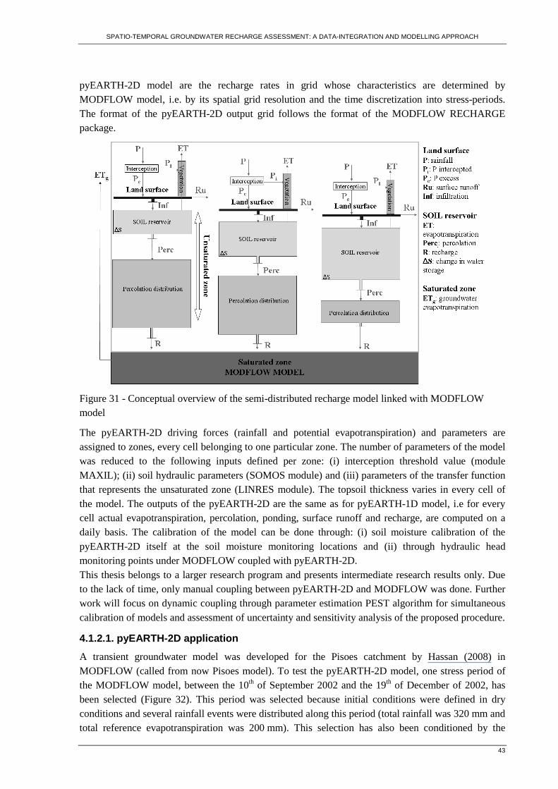
SPATIO-TEMPORAL GROUNDWATER RECHARGE ASSESSMENT: A DATA-INTEGRATION AND MODELLING APPROACH

43

pyEARTH-2D model are the recharge rates in grid whose characteristics are determined by MODFLOW model, i.e. by its spatial grid resolution and the time discretization into stress-periods. The format of the pyEARTH-2D output grid follows the format of the MODFLOW RECHARGE package.

Figure 31 - Conceptual overview of the semi-distributed recharge model linked with MODFLOW model

The pyEARTH-2D driving forces (rainfall and potential evapotranspiration) and parameters are assigned to zones, every cell belonging to one particular zone. The number of parameters of the model was reduced to the following inputs defined per zone: (i) interception threshold value (module MAXIL); (ii) soil hydraulic parameters (SOMOS module) and (iii) parameters of the transfer function that represents the unsaturated zone (LINRES module). The topsoil thickness varies in every cell of the model. The outputs of the pyEARTH-2D are the same as for pyEARTH-1D model, i.e for every cell actual evapotranspiration, percolation, ponding, surface runoff and recharge, are computed on a daily basis. The calibration of the model can be done through: (i) soil moisture calibration of the pyEARTH-2D itself at the soil moisture monitoring locations and (ii) through hydraulic head monitoring points under MODFLOW coupled with pyEARTH-2D. This thesis belongs to a larger research program and presents intermediate research results only. Due to the lack of time, only manual coupling between pyEARTH-2D and MODFLOW was done. Further work will focus on dynamic coupling through parameter estimation PEST algorithm for simultaneous calibration of models and assessment of uncertainty and sensitivity analysis of the proposed procedure.

4.1.2.1. pyEARTH-2D application

A transient groundwater model was developed for the Pisoes catchment by Hassan (2008) in MODFLOW (called from now Pisoes model). To test the pyEARTH-2D model, one stress period of the MODFLOW model, between the 10th of September 2002 and the 19th of December of 2002, has been selected (Figure 32). This period was selected because initial conditions were defined in dry conditions and several rainfall events were distributed along this period (total rainfall was 320 mm and total reference evapotranspiration was 200 mm). This selection has also been conditioned by the

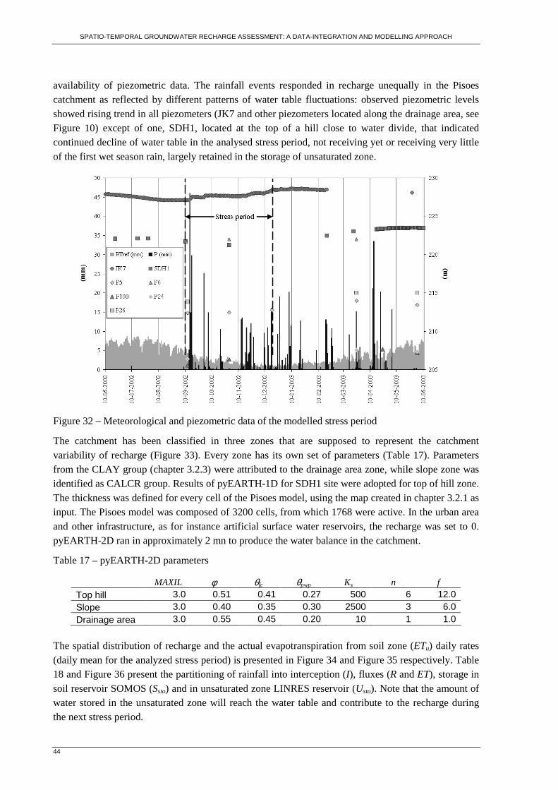
SPATIO-TEMPORAL GROUNDWATER RECHARGE ASSESSMENT: A DATA-INTEGRATION AND MODELLING APPROACH

44

availability of piezometric data. The rainfall events responded in recharge unequally in the Pisoes catchment as reflected by different patterns of water table fluctuations: observed piezometric levels showed rising trend in all piezometers (JK7 and other piezometers located along the drainage area, see Figure 10) except of one, SDH1, located at the top of a hill close to water divide, that indicated continued decline of water table in the analysed stress period, not receiving yet or receiving very little of the first wet season rain, largely retained in the storage of unsaturated zone.

Figure 32 – Meteorological and piezometric data of the modelled stress period

The catchment has been classified in three zones that are supposed to represent the catchment variability of recharge (Figure 33). Every zone has its own set of parameters (Table 17). Parameters from the CLAY group (chapter 3.2.3) were attributed to the drainage area zone, while slope zone was identified as CALCR group. Results of pyEARTH-1D for SDH1 site were adopted for top of hill zone. The thickness was defined for every cell of the Pisoes model, using the map created in chapter 3.2.1 as input. The Pisoes model was composed of 3200 cells, from which 1768 were active. In the urban area and other infrastructure, as for instance artificial surface water reservoirs, the recharge was set to 0. pyEARTH-2D ran in approximately 2 mn to produce the water balance in the catchment.

Table 17 – pyEARTH-2D parameters

MAXIL φ θfc θpwp Ks n f Top hill 3.0 0.51 0.41 0.27 500 6 12.0 Slope 3.0 0.40 0.35 0.30 2500 3 6.0 Drainage area 3.0 0.55 0.45 0.20 10 1 1.0

The spatial distribution of recharge and the actual evapotranspiration from soil zone (ETu) daily rates (daily mean for the analyzed stress period) is presented in Figure 34 and Figure 35 respectively. Table 18 and Figure 36 present the partitioning of rainfall into interception (I), fluxes (R and ET), storage in soil reservoir SOMOS (Ssto) and in unsaturated zone LINRES reservoir (Usto). Note that the amount of water stored in the unsaturated zone will reach the water table and contribute to the recharge during the next stress period.

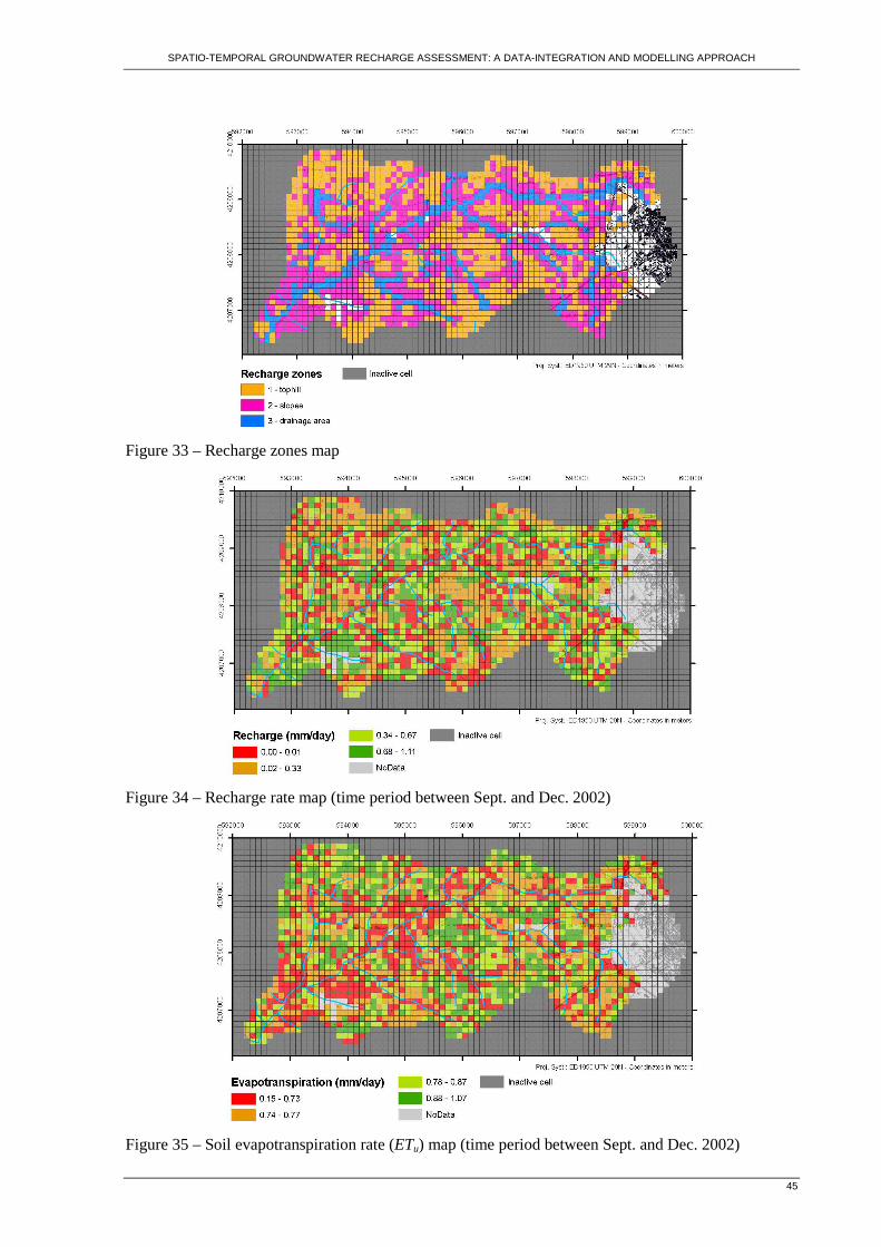
SPATIO-TEMPORAL GROUNDWATER RECHARGE ASSESSMENT: A DATA-INTEGRATION AND MODELLING APPROACH

45

Figure 33 – Recharge zones map

Figure 34 – Recharge rate map (time period between Sept. and Dec. 2002)

Figure 35 – Soil evapotranspiration rate (ETu) map (time period between Sept. and Dec. 2002)

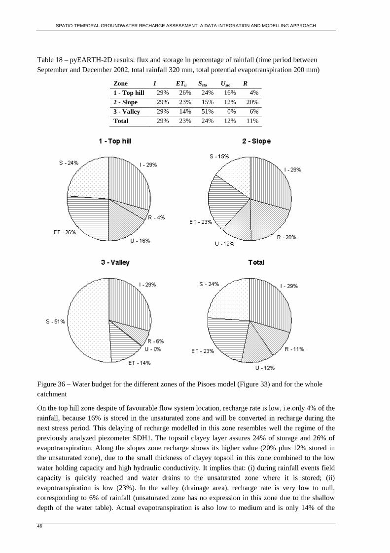
SPATIO-TEMPORAL GROUNDWATER RECHARGE ASSESSMENT: A DATA-INTEGRATION AND MODELLING APPROACH

46

Table 18 – pyEARTH-2D results: flux and storage in percentage of rainfall (time period between September and December 2002, total rainfall 320 mm, total potential evapotranspiration 200 mm)

Zone I ETu Ssto Usto R

1 - Top hill 29% 26% 24% 16% 4%

2 - Slope 29% 23% 15% 12% 20%

3 - Valley 29% 14% 51% 0% 6%

Total 29% 23% 24% 12% 11%

Figure 36 – Water budget for the different zones of the Pisoes model (Figure 33) and for the whole catchment

On the top hill zone despite of favourable flow system location, recharge rate is low, i.e.only 4% of the rainfall, because 16% is stored in the unsaturated zone and will be converted in recharge during the next stress period. This delaying of recharge modelled in this zone resembles well the regime of the previously analyzed piezometer SDH1. The topsoil clayey layer assures 24% of storage and 26% of evapotranspiration. Along the slopes zone recharge shows its higher value (20% plus 12% stored in the unsaturated zone), due to the small thickness of clayey topsoil in this zone combined to the low water holding capacity and high hydraulic conductivity. It implies that: (i) during rainfall events field capacity is quickly reached and water drains to the unsaturated zone where it is stored; (ii) evapotranspiration is low (23%). In the valley (drainage area), recharge rate is very low to null, corresponding to 6% of rainfall (unsaturated zone has no expression in this zone due to the shallow depth of the water table). Actual evapotranspiration is also low to medium and is only 14% of the

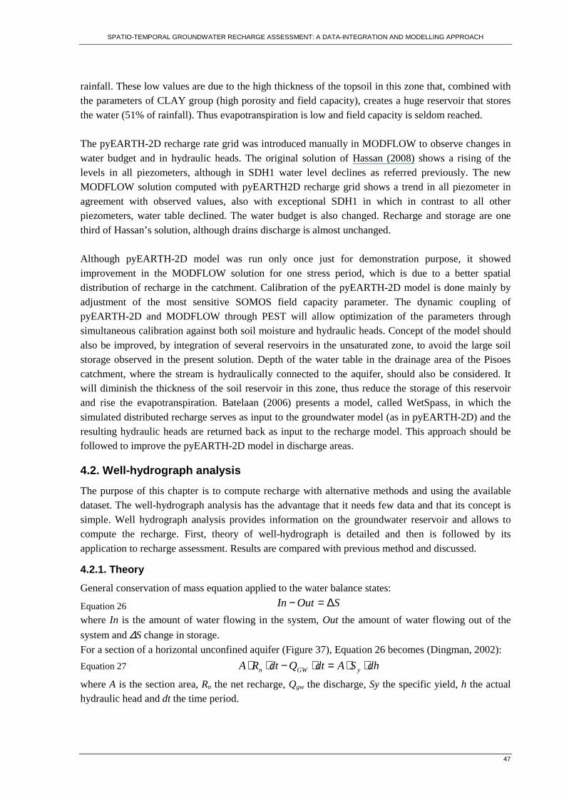
SPATIO-TEMPORAL GROUNDWATER RECHARGE ASSESSMENT: A DATA-INTEGRATION AND MODELLING APPROACH

47

rainfall. These low values are due to the high thickness of the topsoil in this zone that, combined with the parameters of CLAY group (high porosity and field capacity), creates a huge reservoir that stores the water (51% of rainfall). Thus evapotranspiration is low and field capacity is seldom reached. The pyEARTH-2D recharge rate grid was introduced manually in MODFLOW to observe changes in water budget and in hydraulic heads. The original solution of Hassan (2008) shows a rising of the levels in all piezometers, although in SDH1 water level declines as referred previously. The new MODFLOW solution computed with pyEARTH2D recharge grid shows a trend in all piezometer in agreement with observed values, also with exceptional SDH1 in which in contrast to all other piezometers, water table declined. The water budget is also changed. Recharge and storage are one third of Hassan’s solution, although drains discharge is almost unchanged. Although pyEARTH-2D model was run only once just for demonstration purpose, it showed improvement in the MODFLOW solution for one stress period, which is due to a better spatial distribution of recharge in the catchment. Calibration of the pyEARTH-2D model is done mainly by adjustment of the most sensitive SOMOS field capacity parameter. The dynamic coupling of pyEARTH-2D and MODFLOW through PEST will allow optimization of the parameters through simultaneous calibration against both soil moisture and hydraulic heads. Concept of the model should also be improved, by integration of several reservoirs in the unsaturated zone, to avoid the large soil storage observed in the present solution. Depth of the water table in the drainage area of the Pisoes catchment, where the stream is hydraulically connected to the aquifer, should also be considered. It will diminish the thickness of the soil reservoir in this zone, thus reduce the storage of this reservoir and rise the evapotranspiration. Batelaan (2006) presents a model, called WetSpass, in which the simulated distributed recharge serves as input to the groundwater model (as in pyEARTH-2D) and the resulting hydraulic heads are returned back as input to the recharge model. This approach should be followed to improve the pyEARTH-2D model in discharge areas.

4.2. Well-hydrograph analysis

The purpose of this chapter is to compute recharge with alternative methods and using the available dataset. The well-hydrograph analysis has the advantage that it needs few data and that its concept is simple. Well hydrograph analysis provides information on the groundwater reservoir and allows to compute the recharge. First, theory of well-hydrograph is detailed and then is followed by its application to recharge assessment. Results are compared with previous method and discussed.

4.2.1. Theory

General conservation of mass equation applied to the water balance states:

Equation 26 SOutIn ∆=−

where In is the amount of water flowing in the system, Out the amount of water flowing out of the

system and ∆S change in storage. For a section of a horizontal unconfined aquifer (Figure 37), Equation 26 becomes (Dingman, 2002):

Equation 27 dhSAdtQdtRA yGWn ⋅⋅=⋅−⋅⋅

where A is the section area, Rn the net recharge, Qgw the discharge, Sy the specific yield, h the actual hydraulic head and dt the time period.

SPATIO-TEMPORAL GROUNDWATER RECHARGE ASSESSMENT: A DATA-INTEGRATION AND MODELLING APPROACH

48

Figure 37 – Diagram representing a section of an unconfined aquifer (see Equation 27 for keys)

Assuming:

Equation 28 A

Qq GW

GW =

Equation 27 becomes:

Equation 29 dt

dhSqR yGWn ⋅=−

If we consider that the aquifer behaves as a linear reservoir, outflow rate is proportional to storage:

Equation 30 SkqGW ⋅= = ( )by hhSk −⋅⋅

where k is positive constant, S is the change in groundwater storage and hb is the local base level, i.e the level below which no discharge occurs (so-called drainage base). Combining Equation 29 and Equation 30 one obtains:

Equation 31 ( )dt

dhShhSkR ybyn ⋅=−⋅⋅−

If there is no recharge ( 0=nR ), Equation 31 becomes:

Equation 32 bhh

dhdtk

−=⋅−

Integrating Equation 32 gives:

Equation 33 ( ) Chhtk b +−=⋅− ln

At initial condition (i.e. 0hh = and 0=t ), ( )bhhC −−= 0ln and Equation 33 becomes:

Equation 34

−−=⋅−

b

b

hh

hhdtk

0

ln

or

Equation 35 ( ) tk

bb ehhhh ⋅−⋅−+= 0

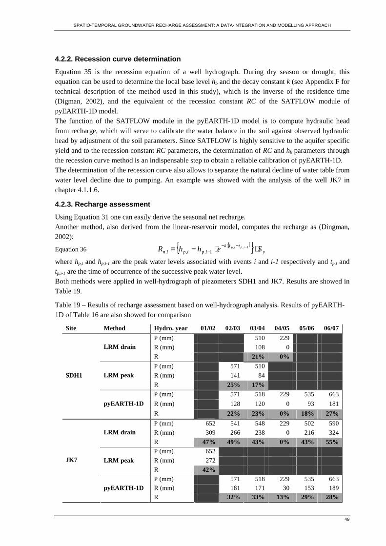
SPATIO-TEMPORAL GROUNDWATER RECHARGE ASSESSMENT: A DATA-INTEGRATION AND MODELLING APPROACH

49

4.2.2. Recession curve determination

Equation 35 is the recession equation of a well hydrograph. During dry season or drought, this equation can be used to determine the local base level hb and the decay constant k (see Appendix F for technical description of the method used in this study), which is the inverse of the residence time (Digman, 2002), and the equivalent of the recession constant RC of the SATFLOW module of pyEARTH-1D model. The function of the SATFLOW module in the pyEARTH-1D model is to compute hydraulic head from recharge, which will serve to calibrate the water balance in the soil against observed hydraulic head by adjustment of the soil parameters. Since SATFLOW is highly sensitive to the aquifer specific yield and to the recession constant RC parameters, the determination of RC and hb parameters through the recession curve method is an indispensable step to obtain a reliable calibration of pyEARTH-1D. The determination of the recession curve also allows to separate the natural decline of water table from water level decline due to pumping. An example was showed with the analysis of the well JK7 in chapter 4.1.1.6.

4.2.3. Recharge assessment

Using Equation 31 one can easily derive the seasonal net recharge. Another method, also derived from the linear-reservoir model, computes the recharge as (Dingman, 2002):

Equation 36 ( ){ } y

ttkipipin SehhR ipip ⋅⋅−= −−⋅−−

1,,

1,,,

where hp,i and hp,i-1 are the peak water levels associated with events i and i-1 respectively and tp,i and tp,i-1 are the time of occurrence of the successive peak water level. Both methods were applied in well-hydrograph of piezometers SDH1 and JK7. Results are showed in Table 19.

Table 19 – Results of recharge assessment based on well-hydrograph analysis. Results of pyEARTH-1D of Table 16 are also showed for comparison

Site Method Hydro. year 01/02 02/03 03/04 04/05 05/06 06/07

P (mm) 510 229

R (mm) 108 0 LRM drain

R 21% 0%

P (mm) 571 510

R (mm) 141 84 LRM peak

R 25% 17%

P (mm) 571 518 229 535 663

R (mm) 128 120 0 93 181

SDH1

pyEARTH-1D

R 22% 23% 0% 18% 27%

P (mm) 652 541 548 229 502 590

R (mm) 309 266 238 0 216 324 LRM drain

R 47% 49% 43% 0% 43% 55% P (mm) 652

R (mm) 272 LRM peak R 42%

P (mm) 571 518 229 535 663 R (mm) 181 171 30 153 189

JK7

pyEARTH-1D R 32% 33% 13% 29% 28%

SPATIO-TEMPORAL GROUNDWATER RECHARGE ASSESSMENT: A DATA-INTEGRATION AND MODELLING APPROACH

50

Values of recharge with the three methods are comparable and consistent for SDH1. At site JK7, results are overestimated, as already observed in pyEARTH-1D simulation, due to the high contribution of lateral groundwater flow in this part of the basin (draining area of the aquifer). The assumption that during recharge events other components of water balance should be null is not respected (Healy and Cook, 2002).

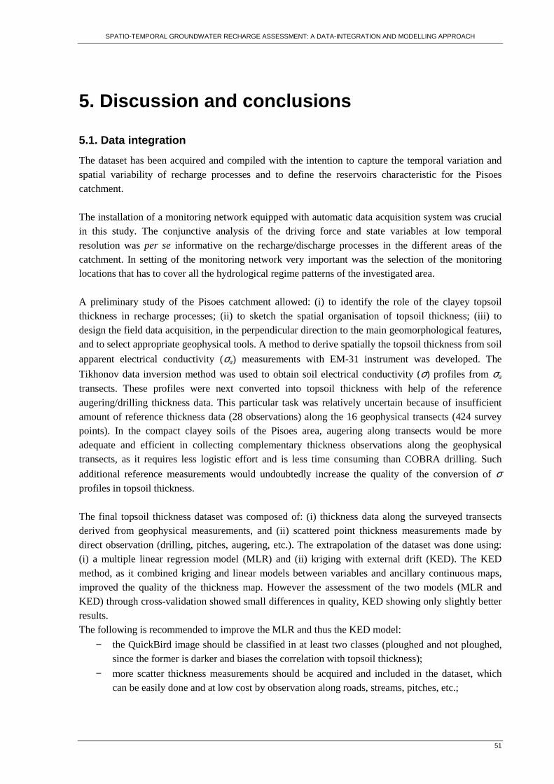
SPATIO-TEMPORAL GROUNDWATER RECHARGE ASSESSMENT: A DATA-INTEGRATION AND MODELLING APPROACH

51

5. Discussion and conclusions

5.1. Data integration

The dataset has been acquired and compiled with the intention to capture the temporal variation and spatial variability of recharge processes and to define the reservoirs characteristic for the Pisoes catchment. The installation of a monitoring network equipped with automatic data acquisition system was crucial in this study. The conjunctive analysis of the driving force and state variables at low temporal resolution was per se informative on the recharge/discharge processes in the different areas of the catchment. In setting of the monitoring network very important was the selection of the monitoring locations that has to cover all the hydrological regime patterns of the investigated area. A preliminary study of the Pisoes catchment allowed: (i) to identify the role of the clayey topsoil thickness in recharge processes; (ii) to sketch the spatial organisation of topsoil thickness; (iii) to design the field data acquisition, in the perpendicular direction to the main geomorphological features, and to select appropriate geophysical tools. A method to derive spatially the topsoil thickness from soil

apparent electrical conductivity (σa) measurements with EM-31 instrument was developed. The

Tikhonov data inversion method was used to obtain soil electrical conductivity (σ) profiles from σa transects. These profiles were next converted into topsoil thickness with help of the reference augering/drilling thickness data. This particular task was relatively uncertain because of insufficient amount of reference thickness data (28 observations) along the 16 geophysical transects (424 survey points). In the compact clayey soils of the Pisoes area, augering along transects would be more adequate and efficient in collecting complementary thickness observations along the geophysical transects, as it requires less logistic effort and is less time consuming than COBRA drilling. Such

additional reference measurements would undoubtedly increase the quality of the conversion of σ profiles in topsoil thickness.

The final topsoil thickness dataset was composed of: (i) thickness data along the surveyed transects derived from geophysical measurements, and (ii) scattered point thickness measurements made by direct observation (drilling, pitches, augering, etc.). The extrapolation of the dataset was done using: (i) a multiple linear regression model (MLR) and (ii) kriging with external drift (KED). The KED method, as it combined kriging and linear models between variables and ancillary continuous maps, improved the quality of the thickness map. However the assessment of the two models (MLR and KED) through cross-validation showed small differences in quality, KED showing only slightly better results. The following is recommended to improve the MLR and thus the KED model:

− the QuickBird image should be classified in at least two classes (ploughed and not ploughed, since the former is darker and biases the correlation with topsoil thickness);

− more scatter thickness measurements should be acquired and included in the dataset, which can be easily done and at low cost by observation along roads, streams, pitches, etc.;

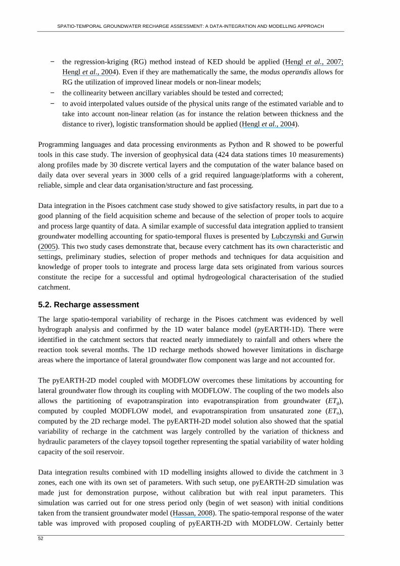
SPATIO-TEMPORAL GROUNDWATER RECHARGE ASSESSMENT: A DATA-INTEGRATION AND MODELLING APPROACH

52

− the regression-kriging (RG) method instead of KED should be applied (Hengl et al., 2007; Hengl et al., 2004). Even if they are mathematically the same, the modus operandis allows for RG the utilization of improved linear models or non-linear models;

− the collinearity between ancillary variables should be tested and corrected;

− to avoid interpolated values outside of the physical units range of the estimated variable and to take into account non-linear relation (as for instance the relation between thickness and the distance to river), logistic transformation should be applied (Hengl et al., 2004).

Programming languages and data processing environments as Python and R showed to be powerful tools in this case study. The inversion of geophysical data (424 data stations times 10 measurements) along profiles made by 30 discrete vertical layers and the computation of the water balance based on daily data over several years in 3000 cells of a grid required language/platforms with a coherent, reliable, simple and clear data organisation/structure and fast processing. Data integration in the Pisoes catchment case study showed to give satisfactory results, in part due to a good planning of the field acquisition scheme and because of the selection of proper tools to acquire and process large quantity of data. A similar example of successful data integration applied to transient groundwater modelling accounting for spatio-temporal fluxes is presented by Lubczynski and Gurwin (2005). This two study cases demonstrate that, because every catchment has its own characteristic and settings, preliminary studies, selection of proper methods and techniques for data acquisition and knowledge of proper tools to integrate and process large data sets originated from various sources constitute the recipe for a successful and optimal hydrogeological characterisation of the studied catchment.

5.2. Recharge assessment

The large spatio-temporal variability of recharge in the Pisoes catchment was evidenced by well hydrograph analysis and confirmed by the 1D water balance model (pyEARTH-1D). There were identified in the catchment sectors that reacted nearly immediately to rainfall and others where the reaction took several months. The 1D recharge methods showed however limitations in discharge areas where the importance of lateral groundwater flow component was large and not accounted for. The pyEARTH-2D model coupled with MODFLOW overcomes these limitations by accounting for lateral groundwater flow through its coupling with MODFLOW. The coupling of the two models also allows the partitioning of evapotranspiration into evapotranspiration from groundwater (ETg), computed by coupled MODFLOW model, and evapotranspiration from unsaturated zone (ETu), computed by the 2D recharge model. The pyEARTH-2D model solution also showed that the spatial variability of recharge in the catchment was largely controlled by the variation of thickness and hydraulic parameters of the clayey topsoil together representing the spatial variability of water holding capacity of the soil reservoir. Data integration results combined with 1D modelling insights allowed to divide the catchment in 3 zones, each one with its own set of parameters. With such setup, one pyEARTH-2D simulation was made just for demonstration purpose, without calibration but with real input parameters. This simulation was carried out for one stress period only (begin of wet season) with initial conditions taken from the transient groundwater model (Hassan, 2008). The spatio-temporal response of the water table was improved with proposed coupling of pyEARTH-2D with MODFLOW. Certainly better

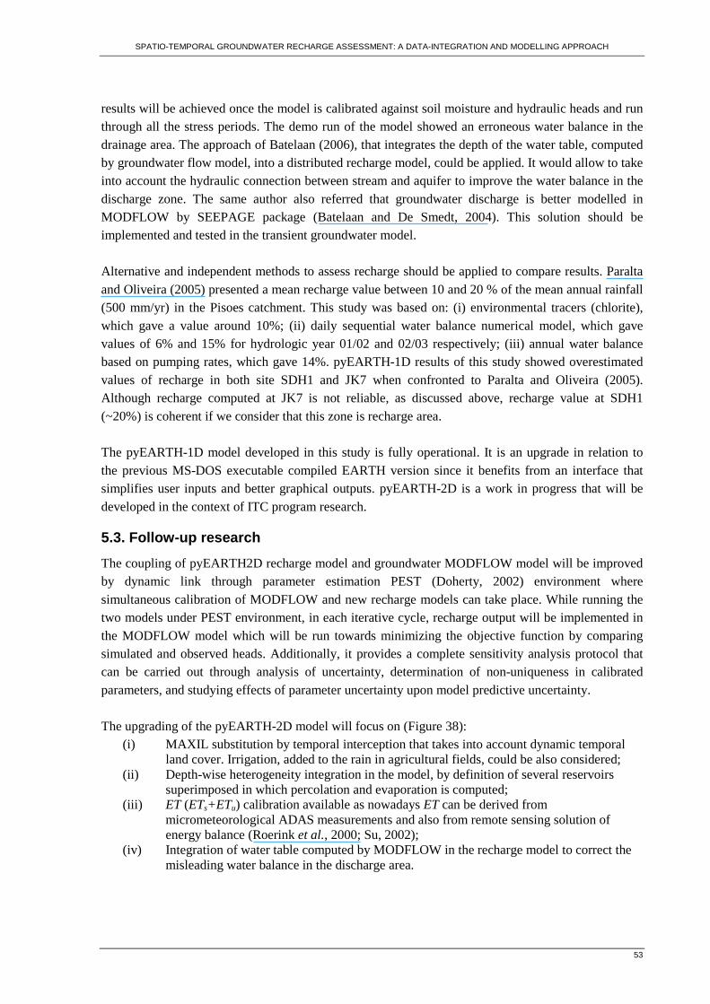
SPATIO-TEMPORAL GROUNDWATER RECHARGE ASSESSMENT: A DATA-INTEGRATION AND MODELLING APPROACH

53

results will be achieved once the model is calibrated against soil moisture and hydraulic heads and run through all the stress periods. The demo run of the model showed an erroneous water balance in the drainage area. The approach of Batelaan (2006), that integrates the depth of the water table, computed by groundwater flow model, into a distributed recharge model, could be applied. It would allow to take into account the hydraulic connection between stream and aquifer to improve the water balance in the discharge zone. The same author also referred that groundwater discharge is better modelled in MODFLOW by SEEPAGE package (Batelaan and De Smedt, 2004). This solution should be implemented and tested in the transient groundwater model. Alternative and independent methods to assess recharge should be applied to compare results. Paralta and Oliveira (2005) presented a mean recharge value between 10 and 20 % of the mean annual rainfall (500 mm/yr) in the Pisoes catchment. This study was based on: (i) environmental tracers (chlorite), which gave a value around 10%; (ii) daily sequential water balance numerical model, which gave values of 6% and 15% for hydrologic year 01/02 and 02/03 respectively; (iii) annual water balance based on pumping rates, which gave 14%. pyEARTH-1D results of this study showed overestimated values of recharge in both site SDH1 and JK7 when confronted to Paralta and Oliveira (2005). Although recharge computed at JK7 is not reliable, as discussed above, recharge value at SDH1 (~20%) is coherent if we consider that this zone is recharge area. The pyEARTH-1D model developed in this study is fully operational. It is an upgrade in relation to the previous MS-DOS executable compiled EARTH version since it benefits from an interface that simplifies user inputs and better graphical outputs. pyEARTH-2D is a work in progress that will be developed in the context of ITC program research.

5.3. Follow-up research

The coupling of pyEARTH2D recharge model and groundwater MODFLOW model will be improved by dynamic link through parameter estimation PEST (Doherty, 2002) environment where simultaneous calibration of MODFLOW and new recharge models can take place. While running the two models under PEST environment, in each iterative cycle, recharge output will be implemented in the MODFLOW model which will be run towards minimizing the objective function by comparing simulated and observed heads. Additionally, it provides a complete sensitivity analysis protocol that can be carried out through analysis of uncertainty, determination of non-uniqueness in calibrated parameters, and studying effects of parameter uncertainty upon model predictive uncertainty. The upgrading of the pyEARTH-2D model will focus on (Figure 38):

(i) MAXIL substitution by temporal interception that takes into account dynamic temporal land cover. Irrigation, added to the rain in agricultural fields, could be also considered;

(ii) Depth-wise heterogeneity integration in the model, by definition of several reservoirs superimposed in which percolation and evaporation is computed;

(iii) ET (ETs+ETu) calibration available as nowadays ET can be derived from micrometeorological ADAS measurements and also from remote sensing solution of energy balance (Roerink et al., 2000; Su, 2002);

(iv) Integration of water table computed by MODFLOW in the recharge model to correct the misleading water balance in the discharge area.

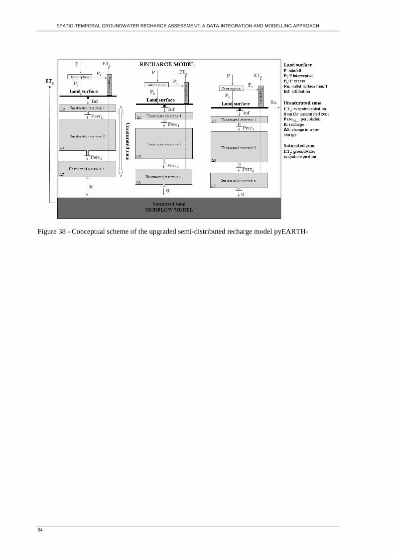
SPATIO-TEMPORAL GROUNDWATER RECHARGE ASSESSMENT: A DATA-INTEGRATION AND MODELLING APPROACH

54

Figure 38 - Conceptual scheme of the upgraded semi-distributed recharge model pyEARTH-

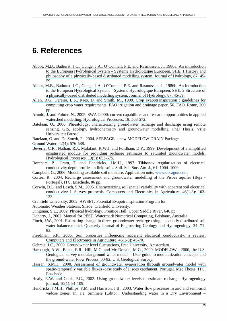
SPATIO-TEMPORAL GROUNDWATER RECHARGE ASSESSMENT: A DATA-INTEGRATION AND MODELLING APPROACH

55

6. References

Abbot, M.B., Bathurst, J.C., Cunge, J.A., O’Connell, P.E. and Rasmussen, J., 1986a. An introduction to the European Hydrological System – Systeme Hydrologique Europeen, SHE. 1 History and philosophy of a physically-based distributed modelling system. Journal of Hydrology, 87: 45-59.

Abbot, M.B., Bathurst, J.C., Cunge, J.A., O’Connell, P.E. and Rasmussen, J., 1986b. An introduction to the European Hydrological System – Systeme Hydrologique Europeen, SHE. 2 Structure of a physically-based distributed modelling system. Journal of Hydrology, 87: 45-59.

Allen, R.G., Pereira, L.S., Raes, D. and Smith, M., 1998. Crop evapotranspiration : guidelines for computing crop water requirements. FAO irrigation and drainage paper, 56. FAO, Rome, 300 pp.

Arnold, J. and Fohrer, N., 2005. SWAT2000: current capabilities and research opportunities in applied watershed modelling. Hydrological Processes, 19: 563-572.

Batelaan, O., 2006. Phreatology, characterizing groundwater recharge and discharge using remote sensing, GIS, ecology, hydrochemistry and groundwater modelling. PhD Thesis, Vrije Universiteit Brussel.

Batelaan, O. and De Smedt, F., 2004. SEEPAGE, a new MODFLOW DRAIN Package Ground Water, 42(4): 576-588. Beverly, C.R., Nathan, R.J., Malafant, K.W.J. and Fordham, D.P., 1999. Development of a simplified

unsaturated module for providing recharge estimates to saturated groundwater models. Hydrological Processes, 13(5): 653-675.

Borchers, B., Uram, T. and Hendrickx, J.M.H., 1997. Tikhonov regularization of electrical conductivity depth profiles in field soils. Soil. Sci. Soc. Am. J., 61: 1004–1009.

Campbell, G., 2006. Modeling available soil moisture, Application note, www.decagon.com. Cortez, R., 2004. Recharge assessment and groundwater modelling of the Pisoes aquifer (Beja -

Portugal), ITC, Enschede, 86 pp. Corwin, D.L. and Lesch, S.M., 2005. Characterizing soil spatial variability with apparent soil electrical

conductivity: I. Survey protocols. Computers and Electronics in Agriculture, 46(1-3): 103-133.

Cranfield University, 2002. AWSET: Potential Evapotranspiration Program for Automatic Weather Stations. Silsoe: Cranfield University. Dingman, S.L., 2002. Physical hydrology. Prentice Hall, Upper Saddle River, 646 pp. Doherty, J., 2002. Manual for PEST. Watermark Numerical Computing, Brisbane, Australia. Finch, J.W., 2001. Estimating change in direct groundwater recharge using a spatially distributed soil

water balance model. Quarterly Journal of Engineering Geology and Hydrogeology, 34: 71-83.

Friedman, S.P., 2005. Soil properties influencing apparent electrical conductivity: a review. Computers and Electronics in Agriculture, 46(1-3): 45-70.

Gehrels, J.C., 2000. Groundwater level fluctuations, Free University, Amsterdam. Harbaugh, A.W., Banta, E.R., Hill, M.C. and Mc Donald, M.G., 2000. MODFLOW - 2000, the U.S.

Geological survey modular ground-water model -- User guide to modularization concepts and the ground-water Flow Process. 00-92, U.S. Geological Survey.

Hassan, S.M.T., 2008. Assessment of groundwater evaporation through groundwater model with spatio-temporally variable fluxes -case study of Pisoes catchment, Portugal. Msc Thesis, ITC, Enschede.

Healy, R.W. and Cook, P.G., 2002. Using groundwater levels to estimate recharge. Hydrogeology journal, 10(1): 91-109.

Hendricks, J.M.H., Phillips, F.M. and Harrison, J.B., 2003. Water flow processes in arid and semi-arid vadose zones. In: I.e. Simmers (Editor), Understanding water in a Dry Environment –

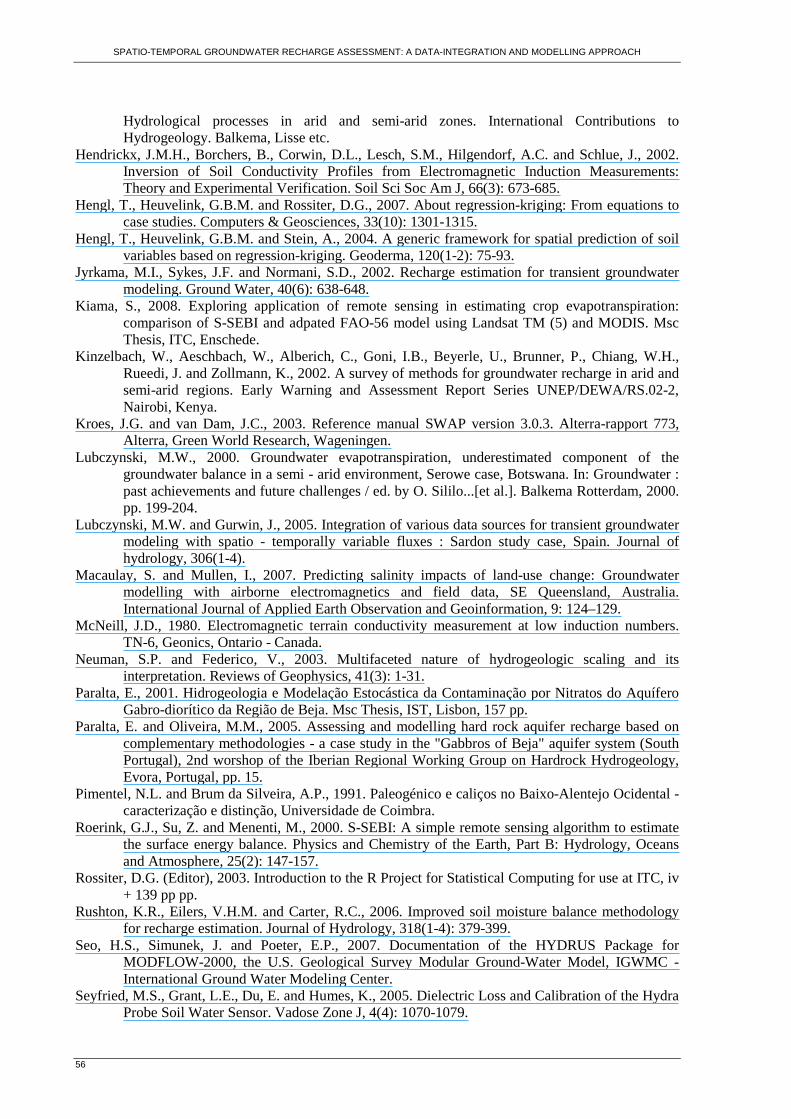
SPATIO-TEMPORAL GROUNDWATER RECHARGE ASSESSMENT: A DATA-INTEGRATION AND MODELLING APPROACH

56

Hydrological processes in arid and semi-arid zones. International Contributions to Hydrogeology. Balkema, Lisse etc.

Hendrickx, J.M.H., Borchers, B., Corwin, D.L., Lesch, S.M., Hilgendorf, A.C. and Schlue, J., 2002. Inversion of Soil Conductivity Profiles from Electromagnetic Induction Measurements: Theory and Experimental Verification. Soil Sci Soc Am J, 66(3): 673-685.

Hengl, T., Heuvelink, G.B.M. and Rossiter, D.G., 2007. About regression-kriging: From equations to case studies. Computers & Geosciences, 33(10): 1301-1315.

Hengl, T., Heuvelink, G.B.M. and Stein, A., 2004. A generic framework for spatial prediction of soil variables based on regression-kriging. Geoderma, 120(1-2): 75-93.

Jyrkama, M.I., Sykes, J.F. and Normani, S.D., 2002. Recharge estimation for transient groundwater modeling. Ground Water, 40(6): 638-648.

Kiama, S., 2008. Exploring application of remote sensing in estimating crop evapotranspiration: comparison of S-SEBI and adpated FAO-56 model using Landsat TM (5) and MODIS. Msc Thesis, ITC, Enschede.

Kinzelbach, W., Aeschbach, W., Alberich, C., Goni, I.B., Beyerle, U., Brunner, P., Chiang, W.H., Rueedi, J. and Zollmann, K., 2002. A survey of methods for groundwater recharge in arid and semi-arid regions. Early Warning and Assessment Report Series UNEP/DEWA/RS.02-2, Nairobi, Kenya.

Kroes, J.G. and van Dam, J.C., 2003. Reference manual SWAP version 3.0.3. Alterra-rapport 773, Alterra, Green World Research, Wageningen.

Lubczynski, M.W., 2000. Groundwater evapotranspiration, underestimated component of the groundwater balance in a semi - arid environment, Serowe case, Botswana. In: Groundwater : past achievements and future challenges / ed. by O. Sililo...[et al.]. Balkema Rotterdam, 2000. pp. 199-204.

Lubczynski, M.W. and Gurwin, J., 2005. Integration of various data sources for transient groundwater modeling with spatio - temporally variable fluxes : Sardon study case, Spain. Journal of hydrology, 306(1-4).

Macaulay, S. and Mullen, I., 2007. Predicting salinity impacts of land-use change: Groundwater modelling with airborne electromagnetics and field data, SE Queensland, Australia. International Journal of Applied Earth Observation and Geoinformation, 9: 124–129.

McNeill, J.D., 1980. Electromagnetic terrain conductivity measurement at low induction numbers. TN-6, Geonics, Ontario - Canada.

Neuman, S.P. and Federico, V., 2003. Multifaceted nature of hydrogeologic scaling and its interpretation. Reviews of Geophysics, 41(3): 1-31.

Paralta, E., 2001. Hidrogeologia e Modelação Estocástica da Contaminação por Nitratos do Aquífero Gabro-diorítico da Região de Beja. Msc Thesis, IST, Lisbon, 157 pp.

Paralta, E. and Oliveira, M.M., 2005. Assessing and modelling hard rock aquifer recharge based on complementary methodologies - a case study in the "Gabbros of Beja" aquifer system (South Portugal), 2nd worshop of the Iberian Regional Working Group on Hardrock Hydrogeology, Evora, Portugal, pp. 15.

Pimentel, N.L. and Brum da Silveira, A.P., 1991. Paleogénico e caliços no Baixo-Alentejo Ocidental - caracterização e distinção, Universidade de Coimbra.

Roerink, G.J., Su, Z. and Menenti, M., 2000. S-SEBI: A simple remote sensing algorithm to estimate the surface energy balance. Physics and Chemistry of the Earth, Part B: Hydrology, Oceans and Atmosphere, 25(2): 147-157.

Rossiter, D.G. (Editor), 2003. Introduction to the R Project for Statistical Computing for use at ITC, iv + 139 pp pp.

Rushton, K.R., Eilers, V.H.M. and Carter, R.C., 2006. Improved soil moisture balance methodology for recharge estimation. Journal of Hydrology, 318(1-4): 379-399.

Seo, H.S., Simunek, J. and Poeter, E.P., 2007. Documentation of the HYDRUS Package for MODFLOW-2000, the U.S. Geological Survey Modular Ground-Water Model, IGWMC - International Ground Water Modeling Center.

Seyfried, M.S., Grant, L.E., Du, E. and Humes, K., 2005. Dielectric Loss and Calibration of the Hydra Probe Soil Water Sensor. Vadose Zone J, 4(4): 1070-1079.

SPATIO-TEMPORAL GROUNDWATER RECHARGE ASSESSMENT: A DATA-INTEGRATION AND MODELLING APPROACH

57

Simunek, J., Sejna, M. and van Genuchten, M.T., 1996. The HYDRUS-2D software package for simulating water flow and solute transport in two-dimensional variably saturated media. Version 1.0. IGWMC – TPS – 53, International Ground Water Modeling Center, Colorado School of Mines, Golden, Colorado.

Stevens Water Monitoring System, I., 2007. Comprehensive Stevens Hydra Probe II Users Manual Su, Z., 2002. The surface energy balance system SEBS for estimation of turbulent heat fluxes.

Hydrology and Earth System Sciences, 6(1): 85-99. Thoms, R.B., Johnson, R.L. and Healy, R.W., 2006. User's Guide to the Variably Saturated Flow

(VSF) Process for MODFLOW. 6-A18, U.S. Geological Survey. Triantafilis, J., Huckel, A.I. and Odeh, I.O.A., 2001. Comparison of statistical prediction methods for

estimating field-scale clay content using different combinations of ancillary variables. Soil Science, 166(6): 415-427

van der Lee, J. and Gehrels, J.C., 1990. Modelling Aquifer Recharge– Introduction to the Lumped Parameter Model EARTH, Free University of Amsterdam, The Netherlands.

Vervoort, R.W. and Annen, Y.L., 2006. Palaeochannels in Northern New South Wales: Inversion of electromagnetic induction data to infer hydrologically relevant stratigraphy. Australian Journal of Soil Research, 44(1): 35-45.

Vieira e Silva, J.M., 1991. Alteração de uma rocha gabróica do Baixo Alentejo, Universidade de Coimbra.

Xu, Y.e. and Beekman, H.E.e., 2003. Groundwater recharge estimation in southern Africa. IHP Series, 64. United Nations Educational Scientific and Cultural Organization (UNESCO), Paris, 207 pp.

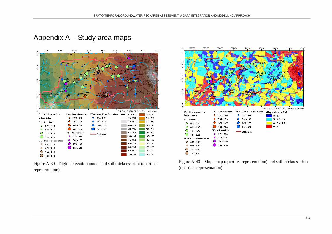
SPATIO-TEMPORAL GROUNDWATER RECHARGE ASSESSMENT: A DATA-INTEGRATION AND MODELLING APPROACH

A-a

Appendix A – Study area maps

Figure A-39 - Digital elevation model and soil thickness data (quartiles representation)

Figure A-40 – Slope map (quartiles representation) and soil thickness data (quartiles representation)

SPATIO-TEMPORAL GROUNDWATER RECHARGE ASSESSMENT: A DATA-INTEGRATION AND MODELLING APPROACH

A-b

Figure A-41 – Geological map and soil thickness data (quartiles representation)

Figure A-42 – Soil map and soil thickness data (quartiles representation)

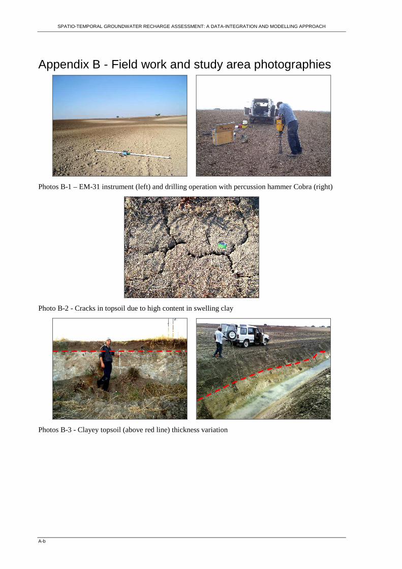
SPATIO-TEMPORAL GROUNDWATER RECHARGE ASSESSMENT: A DATA-INTEGRATION AND MODELLING APPROACH

A-b

Appendix B - Field work and study area photographies

Photos B-1 – EM-31 instrument (left) and drilling operation with percussion hammer Cobra (right)

Photo B-2 - Cracks in topsoil due to high content in swelling clay

Photos B-3 - Clayey topsoil (above red line) thickness variation

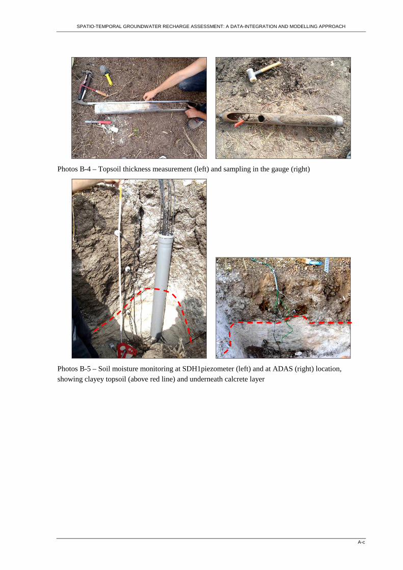
SPATIO-TEMPORAL GROUNDWATER RECHARGE ASSESSMENT: A DATA-INTEGRATION AND MODELLING APPROACH

A-c

Photos B-4 – Topsoil thickness measurement (left) and sampling in the gauge (right)

Photos B-5 – Soil moisture monitoring at SDH1piezometer (left) and at ADAS (right) location, showing clayey topsoil (above red line) and underneath calcrete layer

SPATIO-TEMPORAL GROUNDWATER RECHARGE ASSESSMENT: A DATA-INTEGRATION AND MODELLING APPROACH

A-e

Appendix C - Electromagnetic induction model: main equations The conceptual McNeill layered model is defined as (Figure C-43):

- (1…t) subsoil layers;

- electrical conductivity of each layer is σ1 to σt; - the depth of the base of the layers is designed as Z1 to Zt;

- n measurements of σa at heights h1 to hn in vertical and horizontal coil dipole orientation (superscripts H or V in the notations).

The predicted apparent conductivity σa.pred is:

Equation 37 ( ) ( ) dZZr

hZh VHVH

preda ⋅⋅

+= ∫∞

0. σφσ

where φH/V(Z) is the sensitivity function that reflects the relative contribution to Hs from a discrete layer of thickness dZ and is expressed as:

Equation 38 ( ) ( ) 232 144 +⋅⋅= zzzVφ

Equation 39 ( ) ( ) 212 1442 +⋅⋅−= zzzHφ

with r

hZz

+= (depth normalized by coil separation distance)

The cumulative response RH/V(Z) integrates the relative contribution to Hs of all layers between soil surface and Z and is given as:

Equation 40 ( ) dZr

hZhR

Z

VHVH ⋅

+= ∫∞φ

thus

Equation 41 ( ) ( ) 212 141 +⋅= zzRV

Equation 42 ( ) ( ) zzzRH 214212 −+⋅=

Figure C-43 – McNeill layered subsoil model (see text for notation keys)

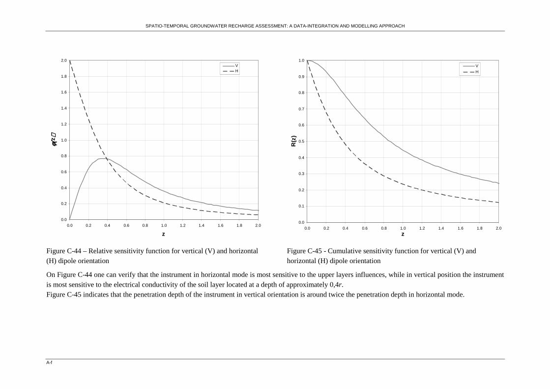
SPATIO-TEMPORAL GROUNDWATER RECHARGE ASSESSMENT: A DATA-INTEGRATION AND MODELLING APPROACH

A-f

0.0

0.2

0.4

0.6

0.8

1.0

1.2

1.4

1.6

1.8

2.0

0.0 0.2 0.4 0.6 0.8 1.0 1.2 1.4 1.6 1.8 2.0

z

φ(φ( φ(φ(z )) ))

VH

Figure C-44 – Relative sensitivity function for vertical (V) and horizontal (H) dipole orientation

0.0

0.1

0.2

0.3

0.4

0.5

0.6

0.7

0.8

0.9

1.0

0.0 0.2 0.4 0.6 0.8 1.0 1.2 1.4 1.6 1.8 2.0

z

R(z

)

V

H

Figure C-45 - Cumulative sensitivity function for vertical (V) and horizontal (H) dipole orientation

On Figure C-44 one can verify that the instrument in horizontal mode is most sensitive to the upper layers influences, while in vertical position the instrument is most sensitive to the electrical conductivity of the soil layer located at a depth of approximately 0,4r. Figure C-45 indicates that the penetration depth of the instrument in vertical orientation is around twice the penetration depth in horizontal mode.

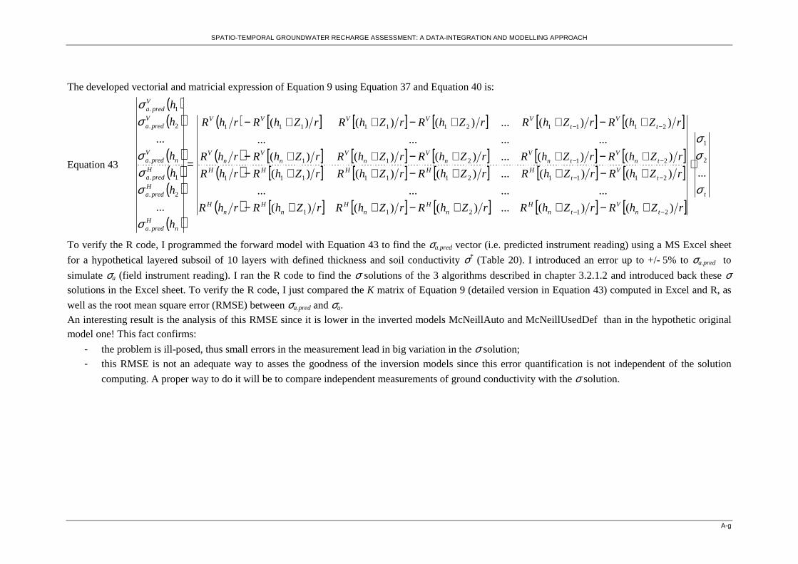
SPATIO-TEMPORAL GROUNDWATER RECHARGE ASSESSMENT: A DATA-INTEGRATION AND MODELLING APPROACH

A-g

The developed vectorial and matricial expression of Equation 9 using Equation 37 and Equation 40 is:

Equation 43

( )( )

( )( )( )

( )

=

nH

preda

Hpreda

Hpreda

nV

preda

Vpreda

Vpreda

h

h

h

h

h

h

.

2.

1.

.

2.

1.

...

...

σ

σσσ

σσ

( ) [ ] [ ] [ ] [ ] [ ]

( ) [ ] [ ] [ ] [ ] [ ]( ) [ ] [ ] [ ] [ ] [ ]

( ) [ ] [ ] [ ] [ ] [ ]t

tnV

tnH

nH

nH

nH

nH

tV

tHHHHH

tnV

tnV

nV

nV

nV

nV

tV

tVVVVV

rZhRrZhRrZhRrZhRrZhRrhR

rZhRrZhRrZhRrZhRrZhRrhR

rZhRrZhRrZhRrZhRrZhRrhR

rZhRrZhRrZhRrZhRrZhRrhR

σ

σσ

...

)()(...)()()(

............

)()(...)()()(

)()(...)()()(

............

)()(...)()()(

2

1

21211

21112111111

21211

21112111111

⋅

+−++−++−

+−++−++−+−++−++−

+−++−++−

−−

−−

−−

−−

To verify the R code, I programmed the forward model with Equation 43 to find the σa.pred vector (i.e. predicted instrument reading) using a MS Excel sheet

for a hypothetical layered subsoil of 10 layers with defined thickness and soil conductivity σ* (Table 20). I introduced an error up to +/- 5% to σa.pred to

simulate σa (field instrument reading). I ran the R code to find the σ solutions of the 3 algorithms described in chapter 3.2.1.2 and introduced back these σ solutions in the Excel sheet. To verify the R code, I just compared the K matrix of Equation 9 (detailed version in Equation 43) computed in Excel and R, as

well as the root mean square error (RMSE) between σa.pred and σa. An interesting result is the analysis of this RMSE since it is lower in the inverted models McNeillAuto and McNeillUsedDef than in the hypothetic original model one! This fact confirms:

- the problem is ill-posed, thus small errors in the measurement lead in big variation in the σ solution; - this RMSE is not an adequate way to asses the goodness of the inversion models since this error quantification is not independent of the solution

computing. A proper way to do it will be to compare independent measurements of ground conductivity with the σ solution.

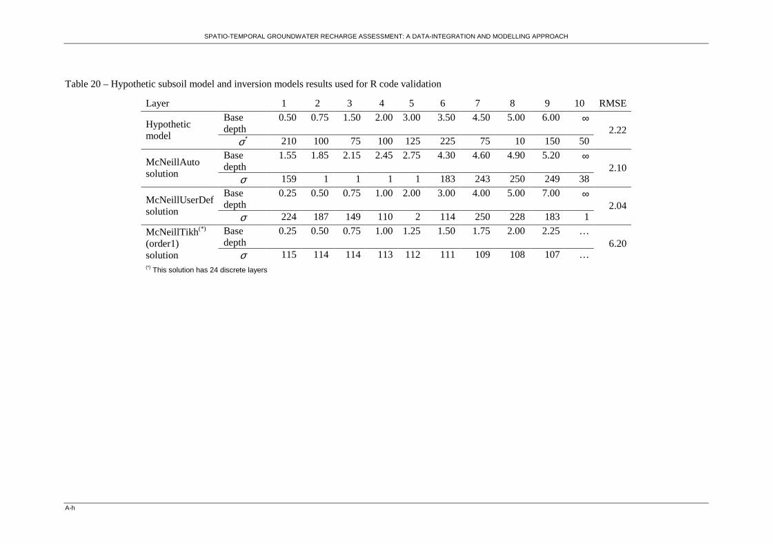
SPATIO-TEMPORAL GROUNDWATER RECHARGE ASSESSMENT: A DATA-INTEGRATION AND MODELLING APPROACH

A-h

Table 20 – Hypothetic subsoil model and inversion models results used for R code validation

Layer 1 2 3 4 5 6 7 8 9 10 RMSE

Base depth

0.50 0.75 1.50 2.00 3.00 3.50 4.50 5.00 6.00 ∞ Hypothetic model σ∗ 210 100 75 100 125 225 75 10 150 50

2.22

Base depth

1.55 1.85 2.15 2.45 2.75 4.30 4.60 4.90 5.20 ∞ McNeillAuto solution σ 159 1 1 1 1 183 243 250 249 38

2.10

Base depth

0.25 0.50 0.75 1.00 2.00 3.00 4.00 5.00 7.00 ∞ McNeillUserDef solution σ 224 187 149 110 2 114 250 228 183 1

2.04

Base depth

0.25 0.50 0.75 1.00 1.25 1.50 1.75 2.00 2.25 … McNeillTikh(*) (order1) solution σ 115 114 114 113 112 111 109 108 107 …

6.20

(*) This solution has 24 discrete layers

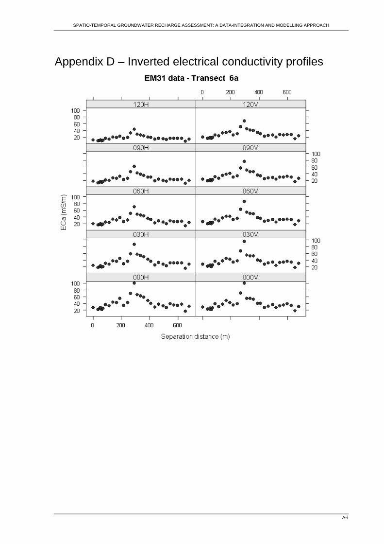
SPATIO-TEMPORAL GROUNDWATER RECHARGE ASSESSMENT: A DATA-INTEGRATION AND MODELLING APPROACH

A-i

Appendix D – Inverted electrical conductivity profiles

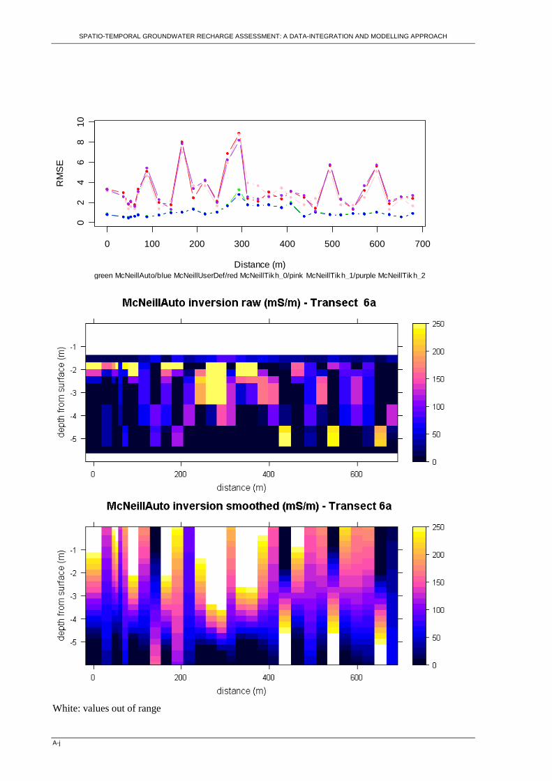
SPATIO-TEMPORAL GROUNDWATER RECHARGE ASSESSMENT: A DATA-INTEGRATION AND MODELLING APPROACH

A-j

0 100 200 300 400 500 600 700

02

46

810

Distance (m)

RM

SE

green McNeillAuto/blue McNeillUserDef/red McNeillTikh_0/pink McNeillTikh_1/purple McNeillTikh_2

White: values out of range

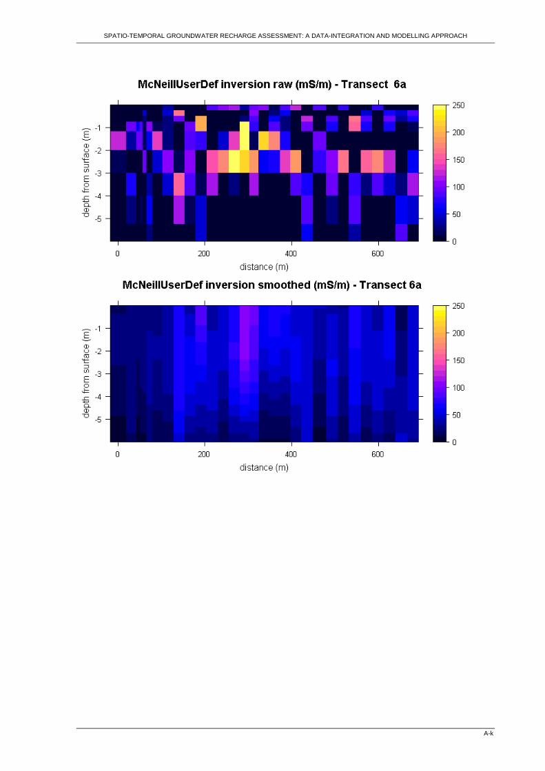
SPATIO-TEMPORAL GROUNDWATER RECHARGE ASSESSMENT: A DATA-INTEGRATION AND MODELLING APPROACH

A-k

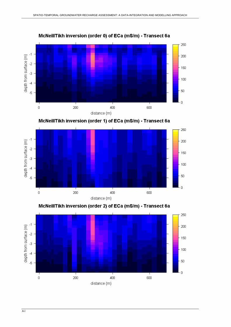
SPATIO-TEMPORAL GROUNDWATER RECHARGE ASSESSMENT: A DATA-INTEGRATION AND MODELLING APPROACH

A-l

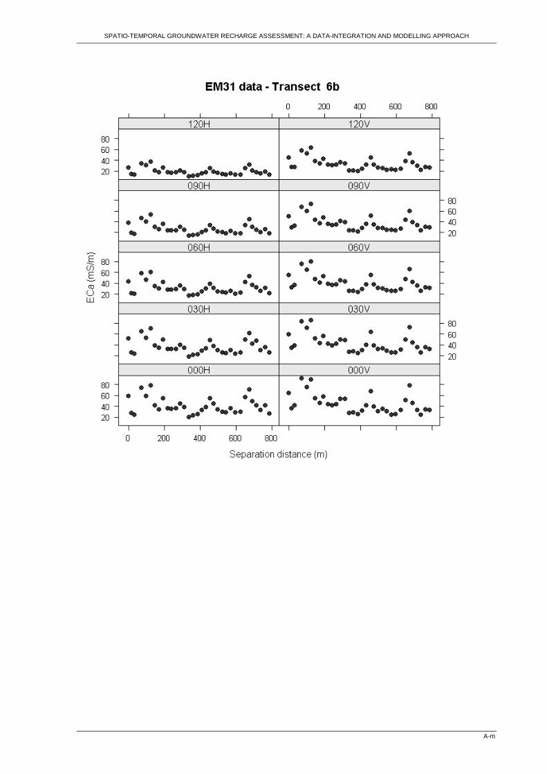
SPATIO-TEMPORAL GROUNDWATER RECHARGE ASSESSMENT: A DATA-INTEGRATION AND MODELLING APPROACH

A-m

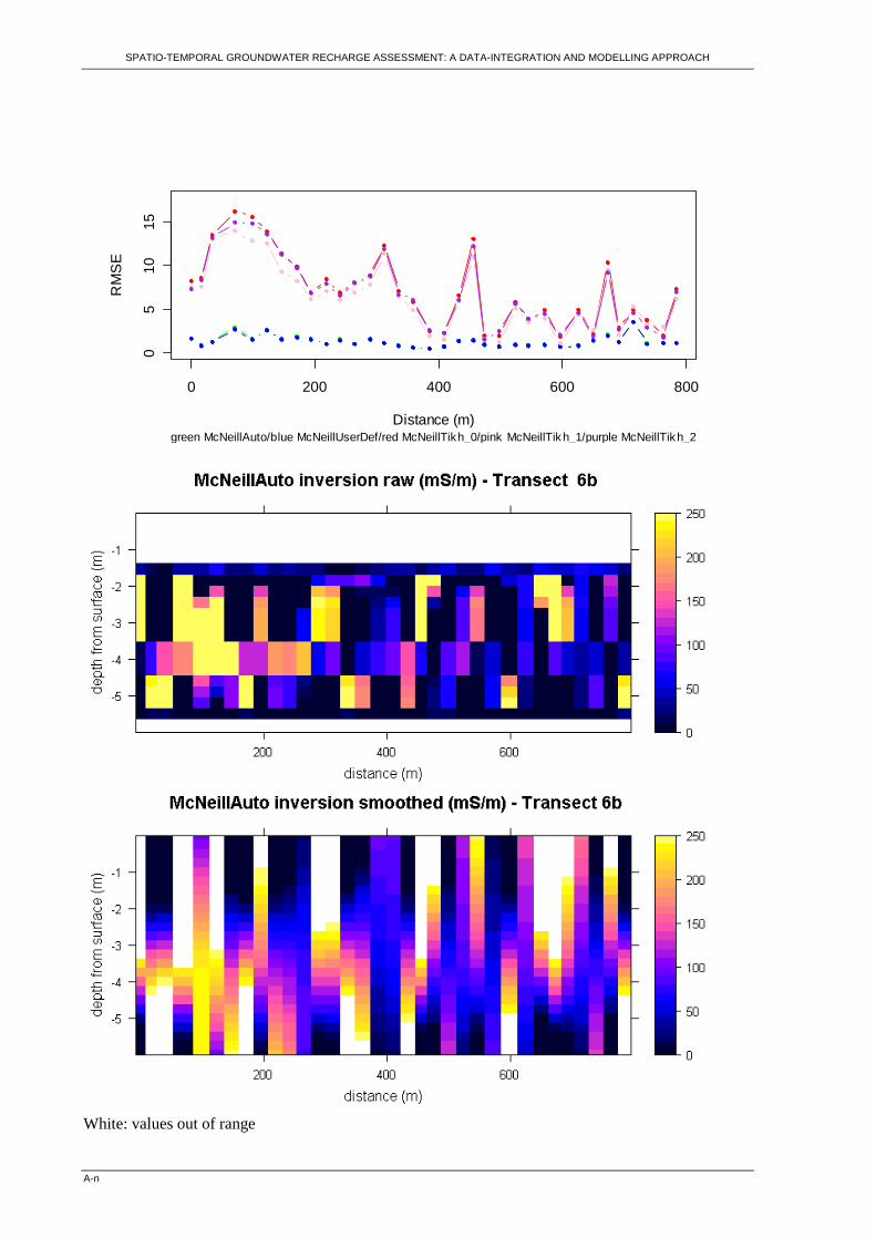
SPATIO-TEMPORAL GROUNDWATER RECHARGE ASSESSMENT: A DATA-INTEGRATION AND MODELLING APPROACH

A-n

0 200 400 600 800

05

1015

Distance (m)

RM

SE

green McNeillAuto/blue McNeillUserDef/red McNeillTikh_0/pink McNeillTikh_1/purple McNeillTikh_2

White: values out of range

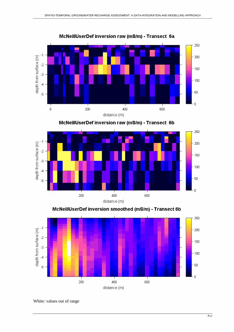
SPATIO-TEMPORAL GROUNDWATER RECHARGE ASSESSMENT: A DATA-INTEGRATION AND MODELLING APPROACH

A-o

White: values out of range

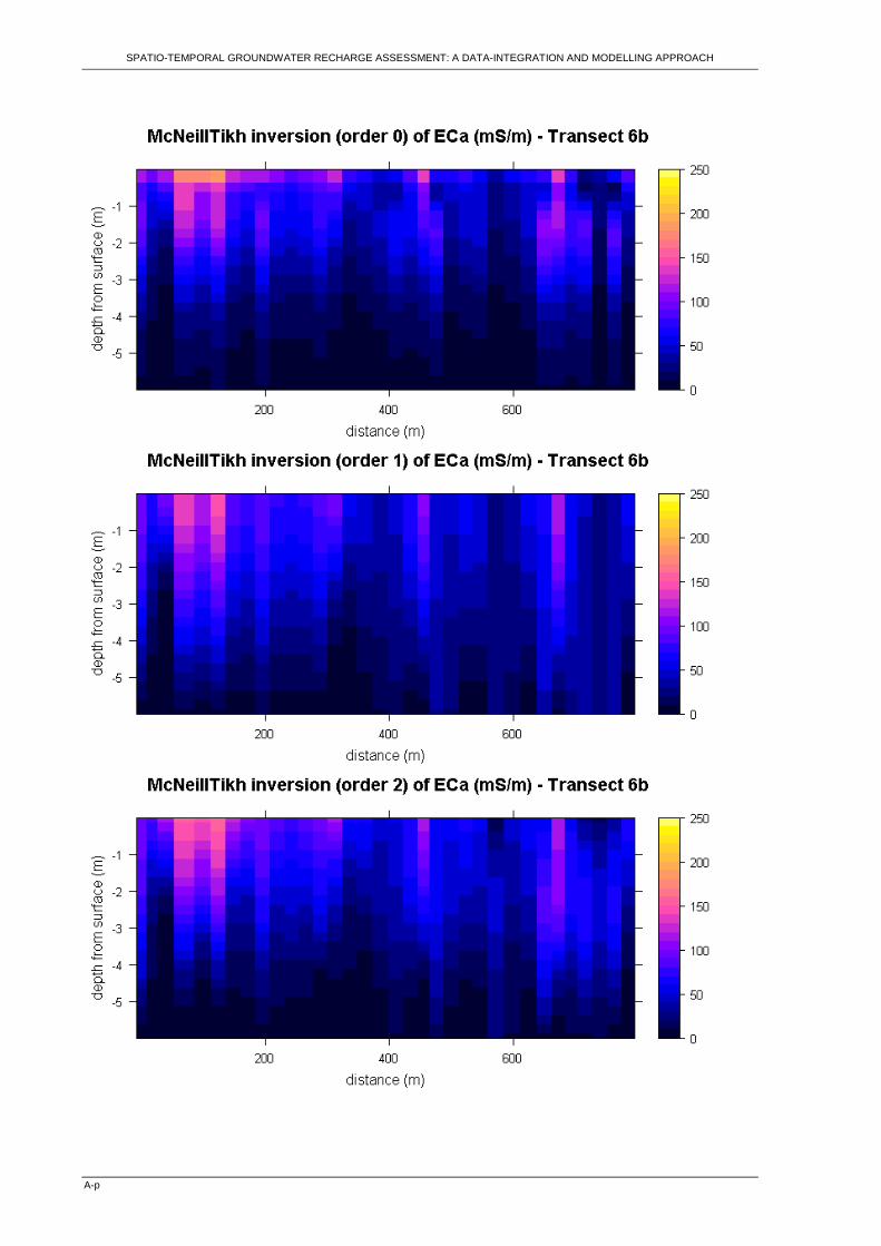
SPATIO-TEMPORAL GROUNDWATER RECHARGE ASSESSMENT: A DATA-INTEGRATION AND MODELLING APPROACH

A-p

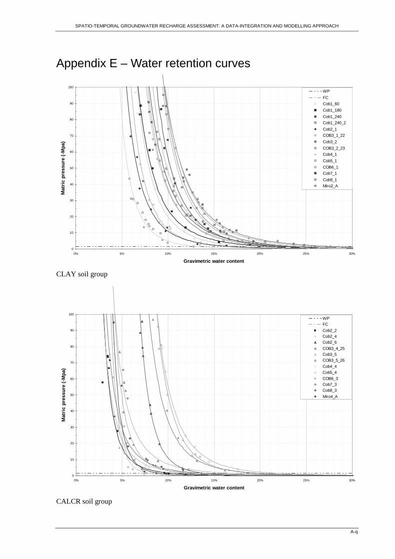
SPATIO-TEMPORAL GROUNDWATER RECHARGE ASSESSMENT: A DATA-INTEGRATION AND MODELLING APPROACH

A-q

Appendix E – Water retention curves

0

10

20

30

40

50

60

70

80

90

100

0% 5% 10% 15% 20% 25% 30%

Gravimetric water content

Mat

ric

pre

ssu

re (

-Mp

a)

WP

FC

Cob1_60

Cob1_180

Cob1_240

Cob1_240_2

Cob2_1

COB3_1_22

Cob3_2

COB3_2_23

Cob4_1

Cob5_1

COB6_1

Cob7_1

Cob8_1

Miro2_A

CLAY soil group

0

10

20

30

40

50

60

70

80

90

100

0% 5% 10% 15% 20% 25% 30%

Gravimetric water content

Mat

ric

pre

ssu

re (

-Mp

a)

WPFC

Cob2_2Cob2_4Cob2_6

COB3_4_25Cob3_5COB3_5_26

Cob4_4Cob5_4

COB6_3Cob7_3Cob8_3

Miro4_A

CALCR soil group

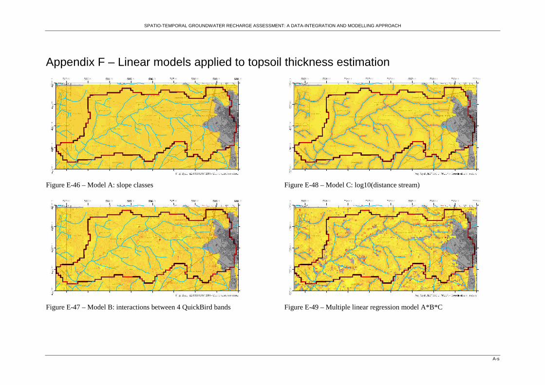
SPATIO-TEMPORAL GROUNDWATER RECHARGE ASSESSMENT: A DATA-INTEGRATION AND MODELLING APPROACH

A-s

Appendix F – Linear models applied to topsoil thickness estimation

Figure E-46 – Model A: slope classes

Figure E-47 – Model B: interactions between 4 QuickBird bands

Figure E-48 – Model C: log10(distance stream)

Figure E-49 – Multiple linear regression model A*B*C

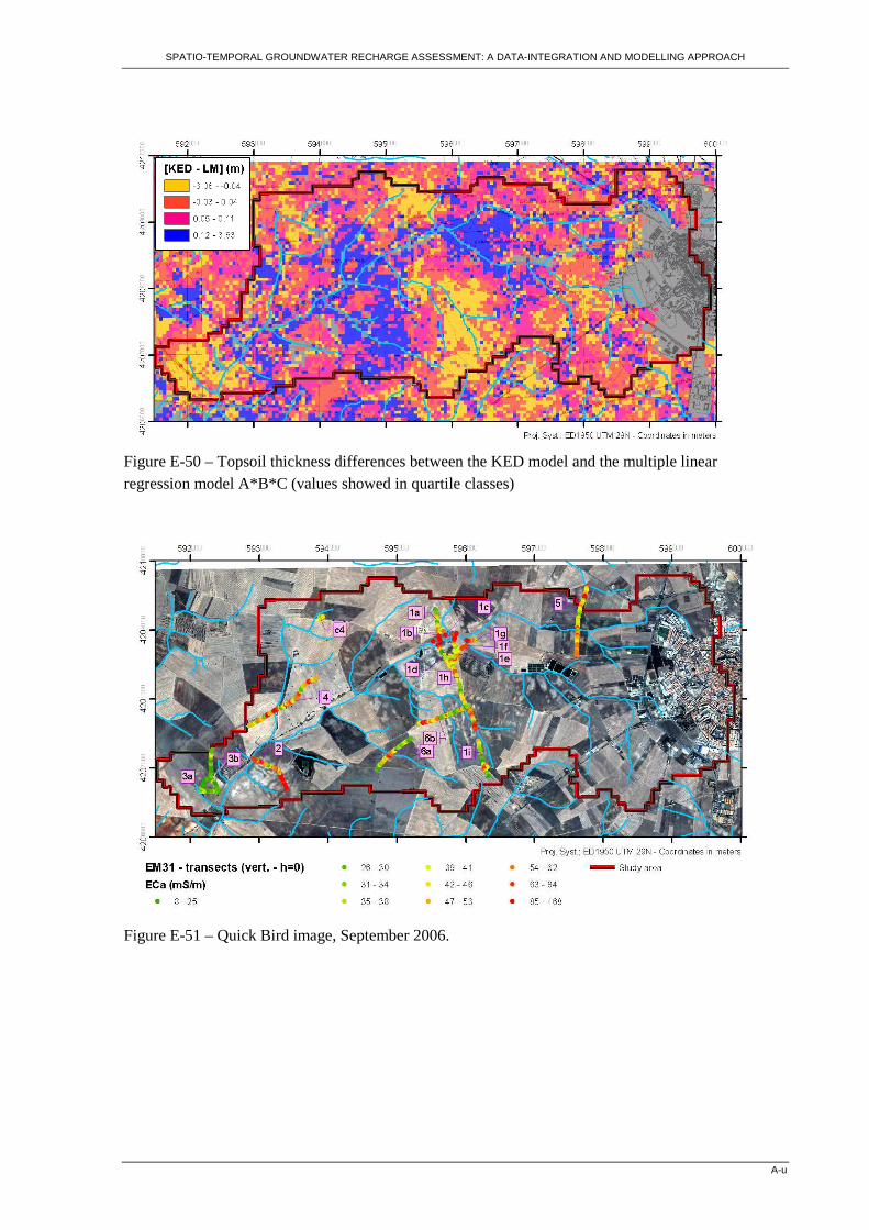
SPATIO-TEMPORAL GROUNDWATER RECHARGE ASSESSMENT: A DATA-INTEGRATION AND MODELLING APPROACH

A-u

Figure E-50 – Topsoil thickness differences between the KED model and the multiple linear regression model A*B*C (values showed in quartile classes)

Figure E-51 – Quick Bird image, September 2006.

SPATIO-TEMPORAL GROUNDWATER RECHARGE ASSESSMENT: A DATA-INTEGRATION AND MODELLING APPROACH

A-w

Appendix G - Recession curve determination The methodology to define the recession curve of a well-hydrograph is as following:

1. Display on a the same graph the hyetograph and the well-hydrograph versus time; 2. Identify on the graph periods of continuous groundwater table (GWT) decline with no rainfall. 3. Prolong these parts of the recession curves drawing it by hand, following approximately an

exponential decay. The asymptote of these curves corresponds to the local base level. Obviously this step is very suggestive. One should verify if the value found for the local base level has a physical meaning in relation to the local settings of the aquifer.

4. Plot on a semi-logarithmic graph (ordinates) time versus local actual level (the local actual level corresponds to the absolute actual level minus local base level). Since the recession curves correspond to straight lines (see Eq. 8), compute its slopes, which correspond to the

decay constant k of Equation 35. k should be approximately the same for all studied

recession periods. Choose a k value that fits better all GWT decline or choose the average of

the several recession curves.

5. Compute, for every period of the GWT decline, the simulated groundwater level h using in

Equation 35 the local base level from step 3 and k value from step 4 and compute root square

mean error (RSME) between measurements and simulated values.

6. Optimise k value with an objective function that minimizes the sum of the RSME of the

different recession curves (an easy way is to utilize SOLVER from Microsoft Excel). 7. Optimise local base level with the same objective function that in step 6. 8. Analyse results, particularly the fitting of simulated and measured groundwater levels, and

start again if not satisfactory. Cautions: In step 2, take care of change in slope of the hydrograph during dry period, since it can corresponds to pumping in the neighbourhood of the well. Others reasons are explained in Healy and Cook (2002).

The final value of k is generally different from the one computed for the several recession curves,

which is probably due to the determination of the specific yield Sy. The appropriate value of Sy is difficult to estimate due to (Dingman, 2002): (i) its high range of value for the same lithological material; (ii) Sy is not constant for the upper part of shallow aquifer, since the water content is a function of the depth of the water table that is itself a function of interactions between infiltration, percolation and capillary rise. This fact is responsible for the hysteresis of Sy in wetting soils: it is lower for a rising water table than for a falling water table, due to trapping of air bubbles in pores material.