Spatial-Temporal Motion Control via Composite Cam-follower

Spatial-Temporal Motion Control via Composite Cam-follower

Mechanisms

YINGJIE CHENG, University of Science and Technology of China, China and Singapore University of Technology and

Design, Singapore

YUCHENG SUN, University of Science and Technology of China, China and Singapore University of Technology and

Design, Singapore

PENG SONG∗, Singapore University of Technology and Design, Singapore

LIGANG LIU, University of Science and Technology of China, China

Fig. 1. We present a computational technique to model, design, and optimize composite cam-follower mechanisms for personalized automata, and showcase

our technique on a diverse set of examples including (from left to right): drawing on a non-planar surface, displaying realistic toy motion, and walking

according to a user-specified gait. Our technique enables users to control an automaton’s spatial-temporal motion by specifying the target trajectories and

timings (see the two spatial curves and corresponding time sliders in the right example).

Motion control, both on the trajectory and timing, is crucial for mechanical

automata to perform functionalities such as walking and entertaining. We

present composite cam-follower mechanisms that can control their spatial-

temporal motions to exactly follow trajectories and timings specified by

users, and propose a computational technique to model, design, and optimize

these mechanisms. The building blocks of our mechanisms are a new kind

of cam-follower mechanism with a modified joint, in which the follower

can perform spatial motion on a planar, cylindrical, or spherical surface

controlled by the 3D cam’s profile. We parameterize the geometry of these

cam-follower mechanisms, formulate analytical equations to model their

∗The corresponding author

Authors’ addresses: Yingjie Cheng, University of Science and Technology of China,

China and Singapore University of Technology and Design, Singapore, chengyj@mail.

ustc.edu.cn; Yucheng Sun, University of Science and Technology of China, China and

Singapore University of Technology and Design, Singapore, [email protected];

Peng Song, Singapore University of Technology and Design, Singapore, peng_song@

sutd.edu.sg; Ligang Liu, University of Science and Technology of China, China, lgliu@

ustc.edu.cn.

Permission to make digital or hard copies of all or part of this work for personal or

classroom use is granted without fee provided that copies are not made or distributed

for profit or commercial advantage and that copies bear this notice and the full citation

on the first page. Copyrights for components of this work owned by others than ACM

must be honored. Abstracting with credit is permitted. To copy otherwise, or republish,

to post on servers or to redistribute to lists, requires prior specific permission and/or a

fee. Request permissions from [email protected].

© 2021 Association for Computing Machinery.

0730-0301/2021/12-ART270 $15.00

https://doi.org/10.1145/3478513.3480477

kinematics and dynamics, and present a method to combine multiple cam-

follower mechanisms into a working mechanism. Taking this modeling

as a foundation, we propose a computational approach to designing and

optimizing the geometry and layout of composite cam-follower mechanisms,

with an objective of performing target spatial-temporal motions driving by

a small motor torque. We demonstrate the effectiveness of our technique by

designing different kinds of personalized automata and showing results not

attainable by conventional mechanisms.

CCS Concepts: • Computing methodologies → Shape modeling; Physicalsimulation.

Additional Key Words and Phrases: cam-follower mechanism, kinematic

modeling, computational design, 3D printing

ACM Reference Format:Yingjie Cheng, Yucheng Sun, Peng Song, and Ligang Liu. 2021. Spatial-

Temporal Motion Control via Composite Cam-follower Mechanisms. ACMTrans. Graph. 40, 6, Article 270 (December 2021), 15 pages. https://doi.org/

10.1145/3478513.3480477

1 INTRODUCTION

Mechanical automata have been created for many different pur-

poses since ancient times such as drawing machines and mechanical

toys [Peppé 2002]. Now, the increasing accessibility of rapid manu-

facturing devices makes it possible to fabricate mechanical automata

ACM Trans. Graph., Vol. 40, No. 6, Article 270. Publication date: December 2021.

https://doi.org/10.1145/3478513.3480477

https://doi.org/10.1145/3478513.3480477

https://doi.org/10.1145/3478513.3480477

270:2 • Yingjie Cheng, Yucheng Sun, Peng Song, and Ligang Liu

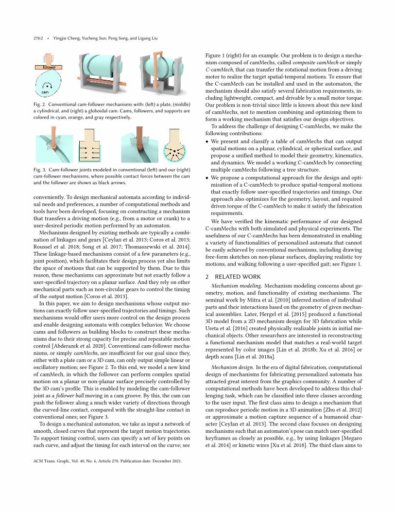
Fig. 2. Conventional cam-follower mechanisms with: (left) a plate, (middle)

a cylindrical, and (right) a globoidal cam. Cams, followers, and supports are

colored in cyan, orange, and gray respectively.

Fig. 3. Cam-follower joints modeled in conventional (left) and our (right)

cam-follower mechanisms, where possible contact forces between the cam

and the follower are shown as black arrows.

conveniently. To design mechanical automata according to individ-

ual needs and preferences, a number of computational methods and

tools have been developed, focusing on constructing a mechanism

that transfers a driving motion (e.g., from a motor or crank) to a

user-desired periodic motion performed by an automaton.

Mechanisms designed by existing methods are typically a combi-

nation of linkages and gears [Ceylan et al. 2013; Coros et al. 2013;

Roussel et al. 2018; Song et al. 2017; Thomaszewski et al. 2014].

These linkage-based mechanisms consist of a few parameters (e.g.,

joint position), which facilitates their design process yet also limits

the space of motions that can be supported by them. Due to this

reason, these mechanisms can approximate but not exactly follow a

user-specified trajectory on a planar surface. And they rely on other

mechanical parts such as non-circular gears to control the timing

of the output motion [Coros et al. 2013].

In this paper, we aim to design mechanisms whose output mo-

tions can exactly follow user-specified trajectories and timings. Such

mechanisms would offer users more control on the design process

and enable designing automata with complex behavior. We choose

cams and followers as building blocks to construct these mecha-

nisms due to their strong capacity for precise and repeatable motion

control [Abderazek et al. 2020]. Conventional cam-follower mecha-

nisms, or simply camMechs, are insufficient for our goal since they,

either with a plate cam or a 3D cam, can only output simple linear or

oscillatory motion; see Figure 2. To this end, we model a new kind

of camMech, in which the follower can perform complex spatial

motion on a planar or non-planar surface precisely controlled by

the 3D cam’s profile. This is enabled by modeling the cam-follower

joint as a follower ball moving in a cam groove. By this, the cam can

push the follower along a much wider variety of directions through

the curved-line contact, compared with the straight-line contact in

conventional ones; see Figure 3.

To design a mechanical automaton, we take as input a network of

smooth, closed curves that represent the target motion trajectories.

To support timing control, users can specify a set of key points on

each curve, and adjust the timing for each interval on the curve; see

Figure 1 (right) for an example. Our problem is to design a mecha-

nism composed of camMechs, called composite camMech or simply

C-camMech, that can transfer the rotational motion from a driving

motor to realize the target spatial-temporal motions. To ensure that

the C-camMech can be installed and used in the automaton, the

mechanism should also satisfy several fabrication requirements, in-

cluding lightweight, compact, and drivable by a small motor torque.

Our problem is non-trivial since little is known about this new kind

of camMechs, not to mention combining and optimizing them to

form a working mechanism that satisfies our design objectives.

To address the challenge of designing C-camMechs, we make the

following contributions:

• We present and classify a table of camMechs that can output

spatial motions on a planar, cylindrical, or spherical surface, and

propose a unified method to model their geometry, kinematics,

and dynamics. We model a working C-camMech by connecting

multiple camMechs following a tree structure.

• We propose a computational approach for the design and opti-

mization of a C-camMech to produce spatial-temporal motions

that exactly follow user-specified trajectories and timings. Our

approach also optimizes for the geometry, layout, and required

driven torque of the C-camMech to make it satisfy the fabrication

requirements.

We have verified the kinematic performance of our designed

C-camMechs with both simulated and physical experiments. The

usefulness of our C-camMechs has been demonstrated in enabling

a variety of functionalities of personalized automata that cannot

be easily achieved by conventional mechanisms, including drawing

free-form sketches on non-planar surfaces, displaying realistic toy

motions, and walking following a user-specified gait; see Figure 1.

2 RELATED WORK

Mechanism modeling. Mechanism modeling concerns about ge-

ometry, motion, and functionality of existing mechanisms. The

seminal work by Mitra et al. [2010] inferred motion of individual

parts and their interactions based on the geometry of given mechan-

ical assemblies. Later, Hergel et al. [2015] produced a functional

3D model from a 2D mechanism design for 3D fabrication while

Ureta et al. [2016] created physically realizable joints in initial me-

chanical objects. Other researchers are interested in reconstructing

a functional mechanism model that matches a real-world target

represented by color images [Lin et al. 2018b; Xu et al. 2016] or

depth scans [Lin et al. 2018a].

Mechanism design. In the era of digital fabrication, computational

design of mechanisms for fabricating personalized automata has

attracted great interest from the graphics community. A number of

computational methods have been developed to address this chal-

lenging task, which can be classified into three classes according

to the user input. The first class aims to design a mechanism that

can reproduce periodic motion in a 3D animation [Zhu et al. 2012]

or approximate a motion capture sequence of a humanoid char-

acter [Ceylan et al. 2013]. The second class focuses on designing

mechanisms such that an automaton’s pose canmatch user-specified

keyframes as closely as possible, e.g., by using linkages [Megaro

et al. 2014] or kinetic wires [Xu et al. 2018]. The third class aims to


Spatial-Temporal Motion Control via Composite Cam-follower Mechanisms • 270:3

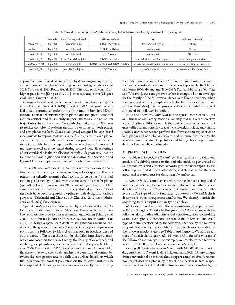
Table 1. Classification of our camMechs according to the follower motion type allowed by its support.

Example Follower-support joint Follower motion v𝑠 Follower Trajectory

camMech_1T Fig 4 (a) prismatic joint 1-DOF translation translation direction 3D line

camMech_1O Fig 4 (b) revolute joint 1-DOF oscillation rotation axis 3D arc

camMech_1R Fig 4 (c) revolute joint 1-DOF rotation rotation axis 3D circle

camMech_2T Fig 4 (d) (modified) sliding joint 2-DOF translation normal of the translation plane curve on a planar surface

camMech_1T1R Fig 4 (e) cylindrical joint 1-DOF translation & 1-DOF rotation translation direction & rotation axis curve on a cylindrical surface

camMech_2R Fig 4 (f) (modified) ball joint 2-DOF rotation axis of the motion cone curve on a spherical surface

approximate user-specified trajectories by designing and optimizing

different kinds of mechanisms with gears and linkages [Bächer et al.

2015; Coros et al. 2013; Roussel et al. 2018; Thomaszewski et al. 2014],

higher pair joints [Song et al. 2017], or compliant joints [Megaro

et al. 2017; Tang et al. 2020].

Compared with the above works, our work is most similar to [Zhu

et al. 2012] and [Coros et al. 2013]. Zhu et al. [2012] designedmechan-

ical toys to reproduce motion trajectories and timings in a 3D ani-

mation. Their mechanisms rely on plate cams for spatial-temporal

motion control, and thus mainly support linear or circular motion

trajectories. In contrast, our C-camMechs make use of 3D cams

to realize complex, free-form motion trajectories on both planar

and non-planar surfaces. Coros et al. [2013] designed linkage-based

mechanisms to approximate user-specified trajectories on a planar

surface while our camMechs can exactly reproduce these trajecto-

ries. Our camMechs also support both planar and non-planar spatial

motions, as well as allow exact timing control. One disadvantage

of our camMechs is their bulky and complex 3D geometry, leading

to more cost and higher demand on fabrication. See Section 7 and

Figure 18 for a comparison experiment with more discussions.

Cam-follower mechanisms. A cam-follower mechanism or cam-

Mech consists of a cam, a follower, and respective supports. The cam

rotates periodically around a fixed axis to drive a specific kind of

motion performed by the follower. A camMech can transfer planar

(spatial) motion by using a plate (3D) cam; see again Figure 2. Plate

cam mechanisms have been extensively studied and a variety of

methods have been proposed to optimize their design for various

purposes [Takahashi and Okuno 2018; Zhu et al. 2012]; see [Abder-

azek et al. 2020] for a review.

Spatial camMechs are characterized by a 3D cam and an ability

to transfer spatial motion in full 3D space. These mechanisms have

been successfully practiced in mechanical engineering [Chang et al.

2009] and robotics [Khan and Chen 2018; Koustoumpardis et al.

2017]. To design a spatial camMech, existing methods focus on con-

structing the groove surface of a 3D cam with analytical expressions

such that the follower (with a given shape) can produce desired

output motion. These methods can be classified into three classes,

which are based on the screw theory, the theory of envelopes, and

modeling swept surfaces, respectively. In the first approach [Chang

et al. 2009; Dhande et al. 1975; González-Palacios and Angeles 1994],

the screw theory is used to determine the condition of contact be-

tween the cam groove and the follower surface, based on which

the instantaneous contact point/line on the follower surface can

be computed. The cam groove surface is obtained by transforming

the instantaneous contact point/line within one motion period to

the cam’s coordinate system. In the second approach [Backhouse

and Jones 1990; Hwang and Tsay 2009; Tsay and Hwang 1994; Tsay

and Wei 1996], the cam groove surface is computed as an envelope

for the family of the follower surfaces in different positions when

the cam rotates for a complete cycle. In the third approach [Tsay

and Lin 1996, 2006], the cam groove surface is computed as a swept

surface of the follower in motion.

In all the above research works, the spatial camMechs output

only linear or oscillatory motions. We only realize a recent creative

work [Sugihara 2016] in which the spatial camMechs can output

quasi-elliptical motions. In contrast, we model, simulate, and classify

spatial camMechs that can perform free-form motion trajectories on

both planar and non-planar surfaces, and optimize these camMechs

to realize user-specified trajectories and timings for computational

design of personalized automata.

3 PROBLEM DEFINITION

Our problem is to design a C-camMech that transfers the rotational

motion of a driving motor to the periodic motions performed by

an automaton’s end-effectors according to the user input. In the

following, we first define C-camMech, and then describe the user

input and requirements for designing C-camMechs.

C-camMech. A C-camMech is a working mechanism composed of

multiple camMechs, driven by a single motor with a motion period

denoted as 𝑇 . A C-camMech can output multiple motions simulta-

neously. The type of output motions supported by C-camMechs is

determined by its component camMechs. We classify camMechs

according to this output motion type as below.

We focus on camMechs with the ball-move-in-groove joint shown

in Figure 3 (right). Thanks to this joint, the 3D cam can push the

follower along both radial and axial directions, thus controlling

at most 2 degrees of freedom (DOFs) of the follower. The actual

type of motion performed by the follower is defined by the follower

support. We classify the camMechs into six classes according to

the follower motion type; see Table 1 and Figure 4. We name each

class of camMechs as camMech_M, where𝑀 is the abbreviation of

the follower’s motion type. For example, camMechs whose follower

motion is 1-DOF translation are named camMech_1T.

Among all the six classes, camMechs with 2-DOF follower motion

(i.e., camMech_2T, camMech_1T1R, and camMech_2R) are unique

from conventional ones since they support complex, free-form mo-

tion trajectories on a planar, cylindrical, or spherical surface, respec-

tively. camMechs with 1-DOF follower motion (i.e., camMech_1T,



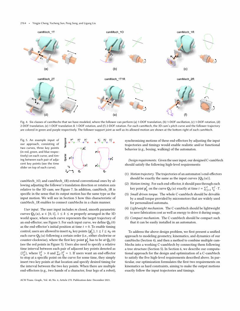
Fig. 4. Six classes of camMechs that we have modeled, where the follower can perform (a) 1-DOF translation, (b) 1-DOF oscillation, (c) 1-DOF rotation, (d)

2-DOF translation, (e) 1-DOF translation & 1-DOF rotation, and (f) 2-DOF rotation. For each camMech, the 3D cam’s pitch curve and the follower trajectory

are colored in green and purple respectively. The follower-support joint as well as its allowed motion are shown at the bottom right of each camMech.

Fig. 5. An example input of

our approach, consisting of

two curves, three key points

(in red, green, and blue respec-

tively) on each curve, and tim-

ing between each pair of adja-

cent key points (see the time

slider on top of each curve).

camMech_1O, and camMech_1R) extend conventional ones by al-

lowing adjusting the follower’s translation direction or rotation axis

relative to the 3D cam; see Figure 7. In addition, camMech_1R is

specific in the sense that its output motion has the same type as the

input motion. We will see in Section 5 how this characteristic of

camMech_1R enables to connect camMechs in a chain manner.

User input. The user input includes𝑚 closed, smooth parametric

curves Q𝑘 (𝑢), 𝑢 ∈ [0, 1], 1 ≤ 𝑘 ≤ 𝑚 properly arranged in the 3D

world space, where each curve represents the target trajectory of

an end-effector; see Figure 5. For each input curve, we define Q𝑘 (0)as the end-effector’s initial position at time 𝑡 = 0. To enable timing

control, users are allowed to insert𝑛𝑘 key points {p𝑙𝑘}, 1 ≤ 𝑙 ≤ 𝑛𝑘 on

each curve Q𝑘 (𝑢) following a certain order (i.e., either clockwise or

counter-clockwise), where the first key point p1𝑘has to be at Q𝑘 (0)

(see the red points in Figure 5). Users also need to specify a relative

time interval between each pair of adjacent key points denoted as

{𝑇 𝑙𝑘}, where 𝑇 𝑙

𝑘> 0 and

∑𝑙 𝑇

𝑙𝑘= 1. If users want an end-effector

to stop at a specific point on the curve for some time, they simply

insert two key points at that location and specify desired timing for

the interval between the two key points. When there are multiple

end-effectors (e.g., two hands of a character, four legs of a robot),

synchronizing motions of these end-effectors by adjusting the input

trajectories and timings would enable realistic and/or functional

behavior (e.g., boxing, walking) of the automaton.

Design requirements. Given the user input, our designed C-camMech

should satisfy the following high-level requirements:

(1) Motion trajectory. The trajectories of an automaton’s end-effectors

should be exactly the same as the input curves {Q𝑘 (𝑢)}.(2) Motion timing. For each end-effector, it should pass through each

key point p𝑙𝑘on the curve Q𝑘 (𝑢) exactly at time 𝑡 =

∑𝑙𝑗=1𝑇

𝑗

𝑘·𝑇 .

(3) Small driven torque. The whole C-camMech should be drivable

by a small torque provided by micromotors that are widely used

for personalized automata.

(4) Lightweight mechanism. The C-camMech should be lightweight

to save fabrication cost as well as energy to drive it during usage.

(5) Compact mechanism. The C-camMech should be compact such

that it can be easily installed in an automaton.

To address the above design problem, we first present a unified

approach to modeling geometry, kinematics, and dynamics of our

camMechs (Section 4), and then a method to combine multiple cam-

Mechs into a working C-camMech by connecting them following

a tree structure (Section 5). In Section 6, we describe our computa-

tional approach for the design and optimization of a C-camMech

to satisfy the five high-level requirements described above. In par-

ticular, our optimization formulates the first two requirements on

kinematics as hard constraints, aiming to make the output motions

exactly follow the input trajectories and timings.



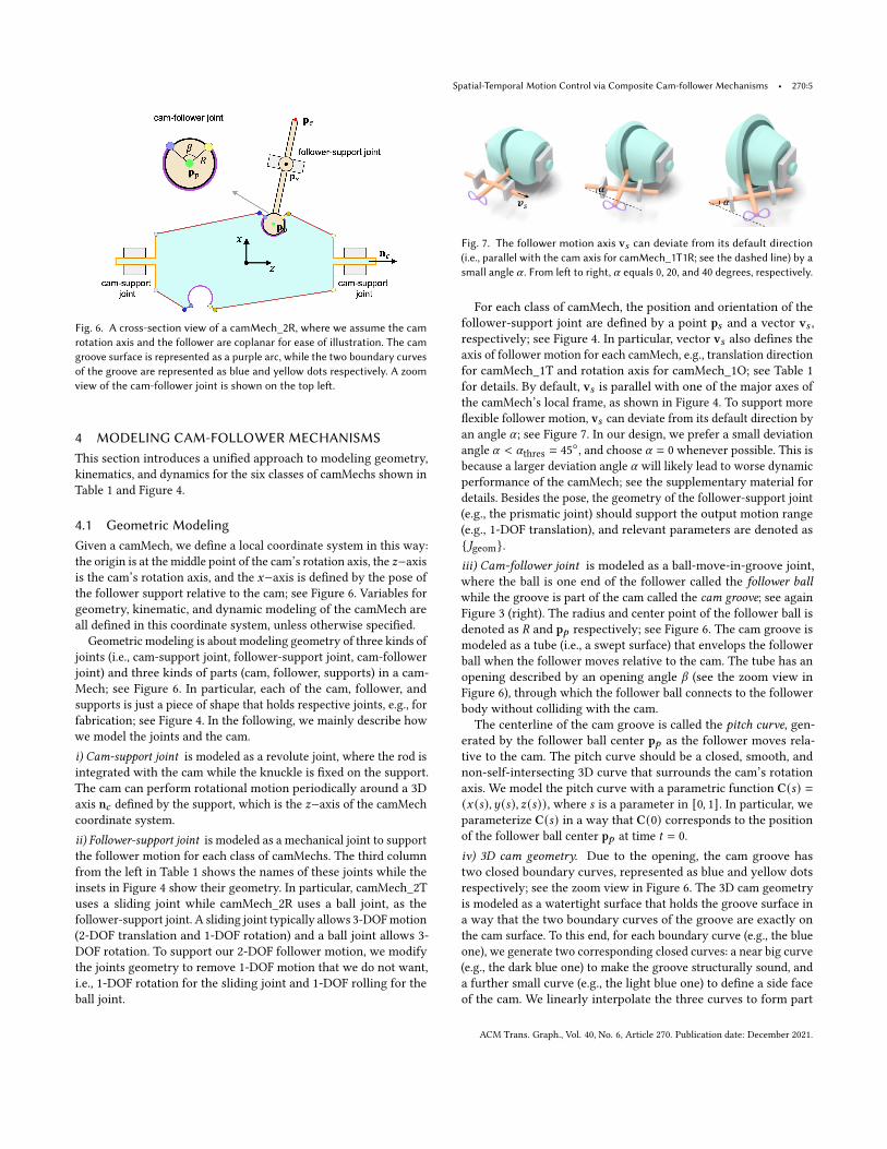
Fig. 6. A cross-section view of a camMech_2R, where we assume the cam

rotation axis and the follower are coplanar for ease of illustration. The cam

groove surface is represented as a purple arc, while the two boundary curves

of the groove are represented as blue and yellow dots respectively. A zoom

view of the cam-follower joint is shown on the top left.

4 MODELING CAM-FOLLOWER MECHANISMS

This section introduces a unified approach to modeling geometry,

kinematics, and dynamics for the six classes of camMechs shown in

Table 1 and Figure 4.

4.1 Geometric Modeling

Given a camMech, we define a local coordinate system in this way:

the origin is at the middle point of the cam’s rotation axis, the 𝑧−axisis the cam’s rotation axis, and the 𝑥−axis is defined by the pose of

the follower support relative to the cam; see Figure 6. Variables for

geometry, kinematic, and dynamic modeling of the camMech are

all defined in this coordinate system, unless otherwise specified.

Geometric modeling is about modeling geometry of three kinds of

joints (i.e., cam-support joint, follower-support joint, cam-follower

joint) and three kinds of parts (cam, follower, supports) in a cam-

Mech; see Figure 6. In particular, each of the cam, follower, and

supports is just a piece of shape that holds respective joints, e.g., for

fabrication; see Figure 4. In the following, we mainly describe how

we model the joints and the cam.

i) Cam-support joint is modeled as a revolute joint, where the rod is

integrated with the cam while the knuckle is fixed on the support.

The cam can perform rotational motion periodically around a 3D

axis n𝑐 defined by the support, which is the 𝑧−axis of the camMech

coordinate system.

ii) Follower-support joint is modeled as a mechanical joint to support

the follower motion for each class of camMechs. The third column

from the left in Table 1 shows the names of these joints while the

insets in Figure 4 show their geometry. In particular, camMech_2T

uses a sliding joint while camMech_2R uses a ball joint, as the

follower-support joint. A sliding joint typically allows 3-DOFmotion

(2-DOF translation and 1-DOF rotation) and a ball joint allows 3-

DOF rotation. To support our 2-DOF follower motion, we modify

the joints geometry to remove 1-DOF motion that we do not want,

i.e., 1-DOF rotation for the sliding joint and 1-DOF rolling for the

ball joint.

Fig. 7. The follower motion axis v𝑠 can deviate from its default direction

(i.e., parallel with the cam axis for camMech_1T1R; see the dashed line) by a

small angle 𝛼 . From left to right, 𝛼 equals 0, 20, and 40 degrees, respectively.

For each class of camMech, the position and orientation of the

follower-support joint are defined by a point p𝑠 and a vector v𝑠 ,respectively; see Figure 4. In particular, vector v𝑠 also defines the

axis of follower motion for each camMech, e.g., translation direction

for camMech_1T and rotation axis for camMech_1O; see Table 1

for details. By default, v𝑠 is parallel with one of the major axes of

the camMech’s local frame, as shown in Figure 4. To support more

flexible follower motion, v𝑠 can deviate from its default direction by

an angle 𝛼 ; see Figure 7. In our design, we prefer a small deviation

angle 𝛼 < 𝛼thres

= 45◦, and choose 𝛼 = 0 whenever possible. This is

because a larger deviation angle 𝛼 will likely lead to worse dynamic

performance of the camMech; see the supplementary material for

details. Besides the pose, the geometry of the follower-support joint

(e.g., the prismatic joint) should support the output motion range

(e.g., 1-DOF translation), and relevant parameters are denoted as

{𝐽geom}.iii) Cam-follower joint is modeled as a ball-move-in-groove joint,

where the ball is one end of the follower called the follower ballwhile the groove is part of the cam called the cam groove; see againFigure 3 (right). The radius and center point of the follower ball is

denoted as 𝑅 and p𝑝 respectively; see Figure 6. The cam groove is

modeled as a tube (i.e., a swept surface) that envelops the follower

ball when the follower moves relative to the cam. The tube has an

opening described by an opening angle 𝛽 (see the zoom view in

Figure 6), through which the follower ball connects to the follower

body without colliding with the cam.

The centerline of the cam groove is called the pitch curve, gen-erated by the follower ball center p𝑝 as the follower moves rela-

tive to the cam. The pitch curve should be a closed, smooth, and

non-self-intersecting 3D curve that surrounds the cam’s rotation

axis. We model the pitch curve with a parametric function C(𝑠) =(𝑥 (𝑠), 𝑦 (𝑠), 𝑧 (𝑠)), where 𝑠 is a parameter in [0, 1]. In particular, we

parameterize C(𝑠) in a way that C(0) corresponds to the position

of the follower ball center p𝑝 at time 𝑡 = 0.

iv) 3D cam geometry. Due to the opening, the cam groove has

two closed boundary curves, represented as blue and yellow dots

respectively; see the zoom view in Figure 6. The 3D cam geometry

is modeled as a watertight surface that holds the groove surface in

a way that the two boundary curves of the groove are exactly on

the cam surface. To this end, for each boundary curve (e.g., the blue

one), we generate two corresponding closed curves: a near big curve

(e.g., the dark blue one) to make the groove structurally sound, and

a further small curve (e.g., the light blue one) to define a side face

of the cam. We linearly interpolate the three curves to form part



of the cam surface. The 3D cam geometry is obtained by stitching

the two interpolated surfaces (in brown), the cam groove surface

(in purple), and the two side surfaces (in orange); see Figure 6.

4.2 Kinematic Modeling

Both the cam and the follower perform periodic motion, and we

denote their periods as 𝑇𝑐 and 𝑇𝑓 respectively. In this paper, we

assume 𝑇𝑐 = 𝑇𝑓 = 𝑇 for simplicity, where 𝑇 is the motion period of

the motor that drives the cam. The goal of kinematic modeling is to

determine the follower pose O𝑓 (𝑡) given the cam pose O𝑐 (𝑡) at anytime 𝑡 ∈ [0,𝑇 ].

The initial cam pose O𝑐 (0) and follower pose O𝑓 (0) are assumed

to be known.We rewriteO𝑐 (𝑡) = T𝑐 (𝑡) O𝑐 (0) andO𝑓 (𝑡) = T𝑓 (𝑡) O𝑓 (0),where T𝑐 (𝑡) and T𝑓 (𝑡) are transforms applied on the cam and fol-

lower respectively. Hence, the kinematics of a camMech can be

modeled as a transmission function:

T𝑓 (𝑡) = 𝐾 ( T𝑐 (𝑡) ), 𝑡 ∈ [0,𝑇 ] (1)

At time 𝑡 > 0, we assume that the cam has rotated around its

axis n𝑐 for \𝑐 degrees from its initial pose. Then we have T𝑐 (𝑡) =R(n𝑐 , \𝑐 (𝑡)). Since the pitch curve C(𝑠) rotates together with the

3D cam, any point on this rotating pitch curve can be represented as

T𝑐 (𝑡) C(𝑠). Since the follower ball center p𝑝 is a point on the pitch

curve, we have

p𝑝 (𝑡) = T𝑐 (𝑡) C(𝑠) (2)

In addition, the initial position of the follower ball center p𝑝 at time

𝑡 = 0 is known, i.e., p𝑝 (0) = C(0).Since the follower ball center p𝑝 is also a point on the follower,

p𝑝 (𝑡) and p𝑝 (0) have to satisfy the motion constraint enforced by

the follower support (e.g., equal distance to the rotation center p𝑠 forcamMech_2R; see Figure 6). This gives us the following equation:

𝐺 ( T𝑐 (𝑡) C(𝑠), C(0) ) = 0 (3)

Please refer to the supplementary material for a list of Equation 3

for each class of camMechs.

At any given time 𝑡 , we solve Equation 3 to obtain the parameter

𝑠 . By this, we obtain the follower ball center position p𝑝 (𝑡). Sincethe motion type of the follower is known, its transformation ma-

trix T𝑓 (𝑡) can be easily derived based on the position of a point

before and after the transform (i.e., p𝑝 (0) and p𝑝 (𝑡)). Once we havethe transformation matrix T𝑓 (𝑡), we could further compute the fol-

lower’s (angular) velocity and (angular) acceleration at time 𝑡 by

taking derivatives.

End-effector trajectory. Given the follower transformation matrix

T𝑓 (𝑡), the end-effector point p𝑒 ’s position at time 𝑡 can be repre-

sented as p𝑒 (𝑡) = T𝑓 (𝑡)p𝑒 (0); see Figure 6. However, this represen-tation does not explicitly show a relation between p𝑒 ’s trajectoryand the pitch curve C(𝑠). Hence, we choose another way to repre-

sent p𝑒 (𝑡). We know that the end-effector point p𝑒 and the followerball center p𝑝 are both on the follower, and p𝑝 ’s position at time 𝑡

can be obtained by Equation 2. Hence, p𝑒 (𝑡) can be represented as:

pe (𝑡) = L T𝑐 (𝑡) C(𝑠), 𝑡 ∈ [0,𝑇 ], 𝑠 ∈ [0, 1] (4)

where L is a constant matrix, and 𝑠 is a function of 𝑡 , i.e., 𝑠 = 𝑠 (𝑡),computed based on Equation 3. Note that 𝑠 (0) = 0 due to our way

of parameterizing C(𝑠).

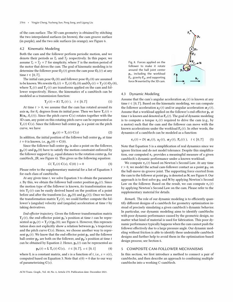
Fig. 8. Forces applied on the

follower to make it rotate

around the ball joint center

p𝑠 , including the workload

F𝑒 , gravity F𝑔 , and supporting

forceN exerted by the 3D cam.

4.3 Dynamic Modeling

Assume that the cam’s angular acceleration 𝜶𝑐 (𝑡) is known at any

time 𝑡 ∈ [0,𝑇 ]. Based on the kinematic modeling, we can compute

the follower acceleration a𝑓 (𝑡) and/or angular acceleration 𝜶 𝑓 (𝑡).Assume that a workload applied on the follower’s end-effector p𝑒 attime 𝑡 is known and denoted as F𝑒 (𝑡). The goal of dynamic modeling

is to compute a torque 𝝉𝑐 (𝑡) required to drive the cam (e.g., by

a motor) such that the cam and the follower can move with the

known accelerations under the workload F𝑒 (𝑡). In other words, the

dynamics of a camMech can be modeled as a function:

𝝉𝑐 (𝑡) = 𝐷 ( 𝜶𝑐 (𝑡), a𝑓 (𝑡), 𝜶 𝑓 (𝑡), F𝑒 (𝑡) ), 𝑡 ∈ [0,𝑇 ] (5)

Note that Equation 5 is a simplification of real dynamics since we

ignore friction and do not model tolerance. Despite this simplifica-

tion, our computed 𝝉𝑐 provides a meaningful measure of a given

camMech’s dynamic performance under a known workload.

We compute 𝝉𝑐 (𝑡) based on Newton’s Second Law. At any time

𝑡 > 0, we model the actual cam-follower contact as a point p𝑁 on

the ball-move-in-groove joint. The supporting force exerted from

the cam to the follower at point p𝑁 is denoted asN; see Figure 8. Ourapproach is to first solve p𝑁 and N by applying Newton’s Second

Law on the follower. Based on the result, we can compute 𝝉𝑐 (𝑡)by applying Newton’s Second Law on the cam. Please refer to the

supplementary material for details.

Remark. The role of our dynamic modeling is to efficiently quan-

tify different designs of a camMech for geometry optimization in-

stead of precisely simulating a given camMech’s dynamic behavior.

In particular, our dynamic modeling aims to identify camMechs

with poor dynamic performance caused by the geometric design, no

matter what kind of material is used for fabrication. This poor dy-

namic performance typically happenswhen the cam cannot push the

follower effectively due to a large pressure angle. Our dynamic mod-

eling without friction is able to identify these undesirable camMech

designs and further help to avoid them in the optimization-based

design process; see Section 6.

5 COMPOSITE CAM-FOLLOWER MECHANISMS

In this section, we first introduce a method to connect a pair of

camMechs, and then describe an approach to combining multiple

camMechs into a working C-camMech.



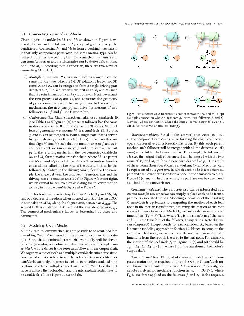
5.1 Connecting a pair of camMechs

Given a pair of camMechs 𝑀𝑖 and 𝑀𝑗 as shown in Figure 9, we

denote the cam and the follower of𝑀𝑖 as 𝑐𝑖 and 𝑓𝑖 respectively. The

condition of connecting𝑀𝑖 and𝑀𝑗 to form a working mechanism

is that only component parts with the same motion type can be

merged to form a new part. By this, the connected mechanism still

can transfer motion and its kinematics can be derived from those

of 𝑀𝑖 and 𝑀𝑗 . According to this condition, there are two ways of

connecting𝑀𝑖 and𝑀𝑗 :

(i) Multiple connection. We assume 3D cams always have the

same motion type, which is 1-DOF rotation. Hence, two 3D

cams, 𝑐𝑖 and 𝑐 𝑗 , can be merged to form a single driving part

denoted as 𝑝𝑘 . To achieve this, we first align𝑀𝑖 and𝑀𝑗 such

that the rotation axis of 𝑐𝑖 and 𝑐 𝑗 is co-linear. Next, we extract

the two grooves of 𝑐𝑖 and 𝑐 𝑗 , and construct the geometry

of 𝑝𝑘 as a new cam with the two grooves. In the resulting

mechanism, the new part 𝑝𝑘 can drive the motions of two

followers, i.e., 𝑓𝑖 and 𝑓𝑗 ; see Figure 9 (top).

(ii) Chain connection. Chain connectionmakes use of camMech_1R

(see Table 1 and Figure 4 (c)) since its follower has the same

motion type (i.e., 1-DOF rotation) as the 3D cams. Without

loss of generality, we assume 𝑀𝑖 is a camMech_1R. By this,

𝑓𝑖 and 𝑐 𝑗 can be merged to form a single part that is driven

by 𝑐𝑖 and drives 𝑓𝑗 ; see Figure 9 (bottom). To achieve this, we

first align𝑀𝑖 and𝑀𝑗 such that the rotation axes of 𝑓𝑖 and 𝑐 𝑗 is

co-linear. Next, we simply merge 𝑓𝑖 and 𝑐 𝑗 to form a new part

𝑝𝑘 . In the resulting mechanism, the two connected camMechs

𝑀𝑖 and𝑀𝑗 form a motion transfer chain, where𝑀𝑖 is a parent

camMech and 𝑀𝑗 is a child camMech. This motion transfer

chain allows adjusting the pose of the output motion by the

follower 𝑓𝑗 relative to the driving cam 𝑐𝑖 flexibly. For exam-

ple, the angle between the follower 𝑓𝑗 ’s motion axis and the

driving cam 𝑐𝑖 ’s rotation axis is 90◦in Figure 9 (bottom right),

which cannot be achieved by deviating the follower motion

axis v𝑠 in a single camMech; see also Figure 7.

In the both ways of connecting two camMechs 𝑀𝑖 and 𝑀𝑗 , 𝑀𝑗

has two degrees of freedom when aligned with𝑀𝑖 . The first DOF

is a translation of𝑀𝑗 along the aligned axis, denoted as 𝑑align

. The

second DOF is a rotation of𝑀𝑗 around the axis, denoted as 𝜙align

.

The connected mechanism’s layout is determined by these two

parameters.

5.2 Modeling C-camMechs

Multiple cam-follower mechanisms are possible to be combined into

a working C-camMech based on the above two connection strate-

gies. Since these combined camMechs eventually will be driven

by a single motor, we define a motor mechanism, or simply mo-torMech, whose driver is the rotor and follower is the output shaft.

We organize a motorMech and multiple camMechs into a tree struc-

ture, called camMech tree, in which each node is a motorMech or

camMech, each edge represents a chain connection, and a sibling

relation indicates a multiple connection. In a camMech tree, the root

node is always the motorMech and the intermediate nodes have to

be camMech_1R; see Figure 10 (a) and (b).

Fig. 9. Two different ways to connect a pair of camMechs𝑀𝑖 and𝑀𝑗 . (Top)

Multiple connection where a new cam 𝑝𝑘 drives two followers 𝑓𝑖 and 𝑓𝑗 .

(Bottom) Chain connection where the cam 𝑐𝑖 drives a new follower 𝑝𝑘 ,

which further drives another follower 𝑓𝑗 .

Geometric modeling. Based on the camMech tree, we can connect

all the component camMechs by performing the chain connection

operation iteratively in a breadth-first order. By this, each parent

mechanism’s follower will be merged with all the drivers (i.e., 3D

cams) of its children to form a new part. For example, the follower of

𝑀1 (i.e., the output shaft of the motor) will be merged with the two

cams of 𝑀2 and 𝑀3 to form a new part, denoted as 𝑝1. The result

of these connection operations is a working C-camMech that can

be represented by a part tree, in which each node is a mechanical

part and each edge corresponds to a node in the camMech tree; see

Figure 10 (c) and (d). In other words, the part tree can be considered

as a dual of the camMech tree.

Kinematic modeling. The part tree also can be interpreted as a

motion transfer tree since we can simply replace each node from a

part to its associated motion. Modeling kinematics of the resulting

C-camMech is equivalent to computing the motion of each leaf

node in the motion transfer tree, assuming the motion of the root

node is known. Given a camMech𝑀𝑖 , we denote its motion transfer

function as: T𝑓𝑖 = 𝐾𝑖 (T𝑐𝑖 ), where T𝑐𝑖 is the transform of the cam

and T𝑓𝑖 is the transform of the follower, at any time 𝑡 . Note that we

can compute 𝐾𝑖 independently for each camMech𝑀𝑖 based on the

kinematic modeling approach in Section 4.2. Hence, to compute the

motion of a leaf node, we can compose the involved motion transfer

functions from the root all the way to the leaf node. For example,

the motion of the leaf node 𝑓4 in Figure 10 (c) and (d) should be

T𝑓4 = 𝐾4 ( 𝐾2 ( 𝐾1 (T𝑑1 ) ) ), where T𝑑1 is the transform of the motor’s

output shaft.

Dynamic modeling. The goal of dynamic modeling is to com-

pute a motor torque required to drive the whole C-camMech un-

der known workloads at any time 𝑡 . Given a camMech 𝑀𝑖 , we

denote its dynamic modeling function as: 𝝉𝑐𝑖 = 𝐷𝑖 (F𝑓𝑖 ), whereF𝑓𝑖 is the force applied on the follower 𝑓𝑖 and 𝝉𝑐𝑖 is the required



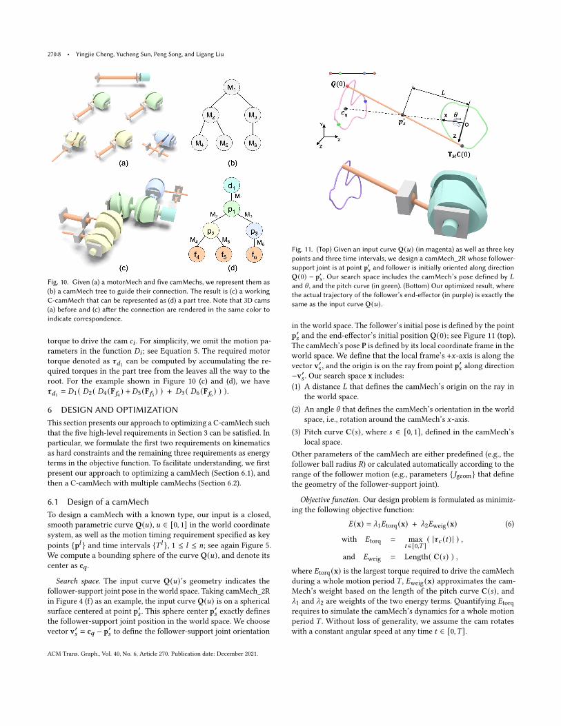
Fig. 10. Given (a) a motorMech and five camMechs, we represent them as

(b) a camMech tree to guide their connection. The result is (c) a working

C-camMech that can be represented as (d) a part tree. Note that 3D cams

(a) before and (c) after the connection are rendered in the same color to

indicate correspondence.

torque to drive the cam 𝑐𝑖 . For simplicity, we omit the motion pa-

rameters in the function 𝐷𝑖 ; see Equation 5. The required motor

torque denoted as 𝝉𝑑1 can be computed by accumulating the re-

quired torques in the part tree from the leaves all the way to the

root. For the example shown in Figure 10 (c) and (d), we have

𝝉𝑑1 = 𝐷1 ( 𝐷2 ( 𝐷4 (F𝑓4 ) + 𝐷5 (F𝑓5 ) ) + 𝐷3 ( 𝐷6 (F𝑓6 ) ) ).

6 DESIGN AND OPTIMIZATION

This section presents our approach to optimizing a C-camMech such

that the five high-level requirements in Section 3 can be satisfied. In

particular, we formulate the first two requirements on kinematics

as hard constraints and the remaining three requirements as energy

terms in the objective function. To facilitate understanding, we first

present our approach to optimizing a camMech (Section 6.1), and

then a C-camMech with multiple camMechs (Section 6.2).

6.1 Design of a camMech

To design a camMech with a known type, our input is a closed,

smooth parametric curve Q(𝑢), 𝑢 ∈ [0, 1] in the world coordinate

system, as well as the motion timing requirement specified as key

points {p𝑙 } and time intervals {𝑇 𝑙 }, 1 ≤ 𝑙 ≤ 𝑛; see again Figure 5.

We compute a bounding sphere of the curve Q(𝑢), and denote its

center as c𝑞 .

Search space. The input curve Q(𝑢)’s geometry indicates the

follower-support joint pose in the world space. Taking camMech_2R

in Figure 4 (f) as an example, the input curve Q(𝑢) is on a spherical

surface centered at point p′𝑠 . This sphere center p′𝑠 exactly defines

the follower-support joint position in the world space. We choose

vector v′𝑠 = c𝑞 − p′𝑠 to define the follower-support joint orientation

Fig. 11. (Top) Given an input curve Q(𝑢) (in magenta) as well as three key

points and three time intervals, we design a camMech_2R whose follower-

support joint is at point p′𝑠 and follower is initially oriented along direction

Q(0) − p′𝑠 . Our search space includes the camMech’s pose defined by 𝐿

and \ , and the pitch curve (in green). (Bottom) Our optimized result, where

the actual trajectory of the follower’s end-effector (in purple) is exactly the

same as the input curve Q(𝑢) .

in the world space. The follower’s initial pose is defined by the point

p′𝑠 and the end-effector’s initial position Q(0); see Figure 11 (top).The camMech’s pose P is defined by its local coordinate frame in the

world space. We define that the local frame’s +𝑥-axis is along the

vector v′𝑠 , and the origin is on the ray from point p′𝑠 along direction

−v′𝑠 . Our search space x includes:

(1) A distance 𝐿 that defines the camMech’s origin on the ray in

the world space.

(2) An angle \ that defines the camMech’s orientation in the world

space, i.e., rotation around the camMech’s 𝑥-axis.

(3) Pitch curve C(𝑠), where 𝑠 ∈ [0, 1], defined in the camMech’s

local space.

Other parameters of the camMech are either predefined (e.g., the

follower ball radius 𝑅) or calculated automatically according to the

range of the follower motion (e.g., parameters {𝐽geom} that definethe geometry of the follower-support joint).

Objective function. Our design problem is formulated as minimiz-

ing the following objective function:

𝐸 (x) = _1𝐸torq (x) + _2𝐸weig (x) (6)

with 𝐸torq = max

𝑡 ∈[0,𝑇 ]( |𝝉𝑐 (𝑡) | ) ,

and 𝐸weig = Length( C(𝑠) ) ,where 𝐸torq (x) is the largest torque required to drive the camMech

during a whole motion period 𝑇 , 𝐸weig (x) approximates the cam-

Mech’s weight based on the length of the pitch curve C(𝑠), and_1 and _2 are weights of the two energy terms. Quantifying 𝐸torqrequires to simulate the camMech’s dynamics for a whole motion

period 𝑇 . Without loss of generality, we assume the cam rotates

with a constant angular speed at any time 𝑡 ∈ [0,𝑇 ].



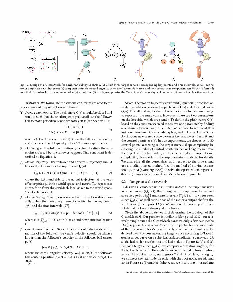
Fig. 12. Design of a C-camMech for a mechanical toy Scorpion. (a) Given three target curves, corresponding key points and time intervals, as well as the

motor output axis, we first select (b) component camMechs and organize them as (c) a camMech tree, and then connect the component camMechs to form (d)

an initial C-camMech that is represented as (e) a part tree. (f) Lastly, we optimize the C-camMech’s geometry and layout to minimize the objective function.

Constraints. We formulate the various constraints related to the

fabrication and output motion as follows:

(1) Smooth cam groove. The pitch curve C(𝑠) should be closed and

smooth such that the resulting cam groove allows the follower

ball to move periodically and smoothly in it (see Section 4.1):

C(0) = C(1)1/^ (𝑠) > Z 𝑅, 𝑠 ∈ [0, 1] (7)

where ^ (𝑠) is the curvature of C(𝑠), 𝑅 is the follower ball radius,

and Z is a coefficient typically set as 1.2 in our experiments.

(2) Motion type. The follower motion type should satisfy the con-

straint enforced by the follower support. This constraint is de-

scribed by Equation 3.

(3) Motion trajectory. The follower end-effector’s trajectory should

be exactly the same as the input curve Q(𝑢):

T𝑀 L T𝑐 (𝑡) C(𝑠) = Q(𝑢), 𝑡 ∈ [0,𝑇 ], 𝑠 ∈ [0, 1] (8)

where the left-hand side is the actual trajectory of the end-

effector point p𝑒 in the world space, and matrix T𝑀 represents

a transform from the camMech local space to the world space.

See also Equation 4.

(4) Motion timing. The follower end-effector’s motion should ex-

actly follow the timing requirement specified by the key points

{p𝑙 } and the time intervals {𝑇 𝑙 }:

T𝑀 L T𝑐 (𝑡𝑙 ) C(𝑠 (𝑡𝑙 )) = p𝑙 , for each 𝑙 ∈ [1, 𝑛] (9)

where 𝑡𝑙 =∑𝑙

𝑗=1𝑇𝑗 ·𝑇 , and 𝑠 (𝑡) is an unknown function of time

𝑡 .

(5) Cam-follower contact. Since the cam should always drive the

motion of the follower, the cam’s velocity should be always

larger than the follower’s velocity at the follower ball center

p𝑝 (𝑡):|𝝎𝑐 × p𝑝 (𝑡) | > |v𝑝 (𝑡) |, 𝑡 ∈ [0,𝑇 ]

where the cam’s angular velocity |𝝎𝑐 | = 2𝜋/𝑇 , the follower

ball center’s position p𝑝 (𝑡) = T𝑐 (𝑡) C(𝑠) and velocity v𝑝 (𝑡) =𝑑p𝑝 (𝑡 )𝑑𝑡

.

Solver. The motion trajectory constraint (Equation 8) describes an

analytical relation between the pitch curve C(𝑠) and the input curveQ(𝑢). The left and right sides of the equation are two different ways

to represent the same curve. However, there are two parameters

on the left side, which are 𝑠 and 𝑡 . To derive the pitch curve C(𝑠)based on the equation, we need to remove one parameter by finding

a relation between 𝑠 and 𝑡 , i.e., 𝑠 (𝑡). We choose to represent this

unknown function 𝑠 (𝑡) as a cubic spline, and initialize it as 𝑠 (𝑡) = 𝑡 .By this, our new search space becomes the parameters 𝐿 and \ , and

the control points of 𝑠 (𝑡). In our experiments, we choose 10 to 30

control points according to the target curve’s shape complexity. In-

creasing the number of control points further will slightly improve

the objective function value, at the cost of higher computational

complexity; please refer to the supplementary material for details.

We discretize all the constraints with respect to the time 𝑡 , and

use a gradient-based method (i.e., the method of moving asymp-

totes (MMA) [Svanberg 1987]) to solve the optimization. Figure 11

(bottom) shows an optimized camMech by our approach.

6.2 Design of a C-camMech

To design a C-camMech with multiple camMechs, our input includes

𝑚 target curves {Q𝑘 (𝑢)}, the timing control requirement specified

as 𝑛𝑘 key points {p𝑙𝑘} and time intervals {𝑇 𝑙

𝑘}, 1 ≤ 𝑙 ≤ 𝑛𝑘 for each

curve Q𝑘 (𝑢), as well as the pose of the motor’s output shaft in the

world space; see Figure 12 (a). We assume the motor performs a

rotational motion uniformly at any time 𝑡 .

Given the above inputs, we first determine the topology of the

C-camMechM. Our problem is similar to [Song et al. 2017] but rela-

tively simple since the C-camMech contains only a few camMechs

{M𝑖 }, represented as a camMech tree. In particular, the root node

of the tree is a motorMech and the type of each leaf node can be

derived from the corresponding target curve according to Table 1

(e.g., a target curve on a spherical surface indicates a camMech_2R

as the leaf node); see the root and leaf nodes in Figure 12 (b) and (c).

For each target curve Q𝑘 (𝑢), we compute a deviation angle 𝛼𝑘 for

the leaf node, which is the angle between the actual follower motion

axis and its default one; see Figures 7 and 12 (a). If 𝛼𝑘 < 𝛼thres

,

we connect the leaf node directly with the root node; see 𝑀2 and

𝑀3 in Figure 12 (b) and (c). Otherwise, we insert one intermediate



node (i.e., camMech_1R) between the root node and a leaf node to

form a chain connection, where the deviation angle 𝛼𝑘 is equally dis-

tributed to the intermediate and leaf nodes; see𝑀5 inserted between

𝑀1 and𝑀4 in Figure 12 (b) and (c).

Search space. The search space includes the parameters defined

for each camMech M𝑖 denoted as {𝐿𝑖 , \𝑖 ,C𝑖 (𝑠)} (see Section 6.1), as

well as parameters {𝑑align

, 𝜙align

} for aligning each child camMech

with its parent during the connection.

Objective function. Our design problem is formulated as minimiz-

ing the following objective function:

𝐸 (x) = _1𝐸torq (x) + _2𝐸weig (x) + _3𝐸dim (x) (10)

with 𝐸torq = max

𝑡 ∈[0,𝑇 ]( |𝝉𝑐 (𝑡) | ) ,

𝐸weig =∑︁𝑖

Length( C𝑖 (𝑠) ) ,

and 𝐸dim

= Volume(BBox({T𝑀𝑖C𝑖 (𝑠)}, {T𝑀𝑖

p𝑖𝑠 })),where 𝝉𝑐 (𝑡) is the motor torque required to drive the C-camMech

at time 𝑡 , 𝐸weig approximates the mechanism’s weight using the

pitch curves {C𝑖 (𝑠)}, 𝐸dim approximates the mechanism’s dimen-

sion using the pitch curves {C𝑖 (𝑠)} and the follower-support joint

positions {p𝑖𝑠 }, and _1, _2, and _3 are weights of the energy terms.

Constraints. Each camMechM𝑖 should satisfy the five constraints

described in Section 6.1. In addition, collision among different cam-

Mechs should be avoided when the C-camMechM is in motion at

any time 𝑡 ∈ [0,𝑇 ]. This constraint is satisfied by enforcing sufficient

distance among all pitch curves {C𝑖 (𝑠)} and all the follower-supportjoints centered at {p𝑖𝑠 } in the world space.

Solver. Solving Equation 10 requires optimizing not only the ge-

ometry but also layout of the C-camMech due to the energy term

𝐸dimen

. However, the collision-free constraint in the layout opti-

mization is not differentiable with respect to the design parameters

{𝑑align

, 𝜙align

}. Hence we use an iterative method to solve the opti-

mization problem.

We first fix the layout (i.e., {𝑑align

, 𝜙align

}), and use the above

gradient-based method to optimize each camMechM𝑖 (i.e., search

{𝐿𝑖 , \𝑖 ,C𝑖 (𝑠)}) to satisfy all the objectives in Equation 10 except

𝐸dim

. In case a camMechM𝑖 is connected with the motor through

a camMech_1R (see again Figure 10), both camMechs will be opti-

mized together to satisfy Equations 8 and 9. Next, we fix the geome-

try of each component camMech M𝑖 , and optimize the C-camMech

M’s layout by searching {𝑑align

, 𝜙align

} using a randomized algo-

rithm (i.e., improved stochastic ranking evolution strategy). Due to

the small search space, this randomized search can be performed

very efficiently. We iterate the above two steps until the decrease

of energy 𝐸 (x) is sufficiently small. Figure 12 shows an example of

our optimized C-camMech.

7 RESULTS

We implemented our tool in C++ and libigl [Jacobson et al. 2018]

on a MacBook with a 1.4GHz CPU and 4GB memory, and em-

ployed NLopt package [Johnson 2020] for solving our gradient-

based optimizations. We have conducted experiments to evaluate

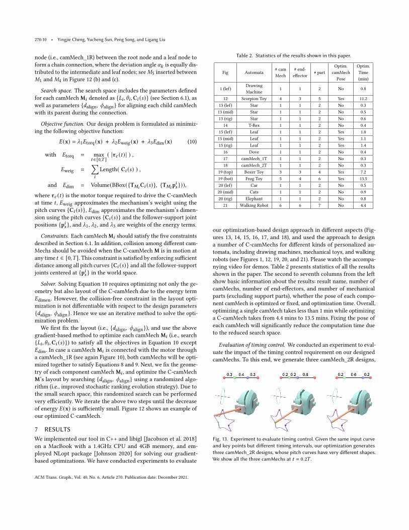
Table 2. Statistics of the results shown in this paper.

Fig Automata

# cam

Mech

# end-

effector

# part

Optim.

camMech

Pose

Optim.

Time

(min)

1 (lef)

Drawing

Machine

1 1 2 No 0.8

12 Scorpion Toy 4 3 5 Yes 11.2

13 (lef) Star 1 1 2 No 0.3

13 (mid) Star 1 1 2 No 0.5

13 (rig) Star 1 1 2 No 0.6

14 T-Rex 1 1 2 No 0.4

15 (lef) Leaf 1 1 2 Yes 1.0

15 (mid) Leaf 1 1 2 Yes 1.1

15 (rig) Leaf 1 1 2 Yes 1.4

16 Dove 1 1 2 No 0.4

17 camMech_1T 1 1 2 No 0.3

18 camMech_2T 1 1 2 No 0.3

19 (top) Boxer Toy 3 3 4 Yes 7.2

19 (bot) Frog Toy 5 4 6 Yes 13.5

20 (lef) Car 1 1 2 No 0.5

20 (mid) Cats 1 1 2 No 0.9

20 (rig) Elephant 1 1 2 No 0.8

21 Walking Robot 6 6 7 No 4.4

our optimization-based design approach in different aspects (Fig-

ures 13, 14, 15, 16, 17, and 18), and used the approach to design

a number of C-camMechs for different kinds of personalized au-

tomata, including drawing machines, mechanical toys, and walking

robots (see Figures 1, 12, 19, 20, and 21). Please watch the accompa-

nying video for demos. Table 2 presents statistics of all the results

shown in the paper. The second to seventh columns from the left

show basic information about the results: result name, number of

camMechs, number of end-effectors, and number of mechanical

parts (excluding support parts), whether the pose of each compo-

nent camMech is optimized or fixed, and optimization time. Overall,

optimizing a single camMech takes less than 1 min while optimizing

a C-camMech takes from 4.4 mins to 13.5 mins. Fixing the pose of

each camMech will significantly reduce the computation time due

to the reduced search space.

Evaluation of timing control. We conducted an experiment to eval-

uate the impact of the timing control requirement on our designed

camMechs. To this end, we generate three camMech_2R designs,

Fig. 13. Experiment to evaluate timing control. Given the same input curve

and key points but different timing intervals, our optimization generates

three camMech_2R designs, whose pitch curves have very different shapes.

We show all the three camMechs at 𝑡 = 0.2𝑇 .



Fig. 14. Experiment to evaluate the kinematic performance for realizing a target curve T-Rex. (a) The target curve; (b) our designed camMech_2R; (c) and (d)

3D printed camMech and its component parts, where a small green ball is used as the follower end-effector; (e) tracking the green ball in the video images (see

the green rectangles); and (f) comparing the tracked curve (in yellow) and the target curve projected onto the image (in magenta).

Fig. 15. Experiment to evaluate trajectory control. Given a target curve with

different levels of details, our optimization generates three camMech_2R

designs, whose pitch curves have very different sizes. We show all the three

camMechs at 𝑡 = 0.

taking as input the same curve Q(𝑢) and key points {p𝑙 } but dif-ferent time intervals {𝑇 𝑙 }; see Figure 13. We fix the pose of each

camMech and optimize the pitch curve to satisfy the timing re-

quirement. We observe that the timing requirement significantly

affects the pitch curve’s shape. In general, for a segment between

two key points on the input curve, shorter timing requires a shorter

segment on the pitch curve yet with high curvature to control the

motion. Our simulated result shows that the timing requirement

can be exactly satisfied by our designed camMechs. Please watch

the accompanying video for demos.

Evaluation of trajectory control. We conducted an experiment

to evaluate the impact of the trajectory control requirement on

our designed camMechs. Hence, we take a target curve with three

different levels of details as our input, and use our optimization

to generate three camMech_2R designs respectively; see Figure 15.

The timing requirement is ignored in this experiment. We observe

that the more geometric details the input curve has, the larger the

3D cam is (i.e., the longer the pitch curve is). This is because the

pitch curve needs to support reproducing geometric details in the

input curve (Equation 8) while maintaining low curvature at any

point (Equation 7).

Evaluation of kinematic performance. We conducted two phys-

ical experiments to evaluate the kinematic performance of our

camMechs. The first experiment takes a T-Rex curve while the

second one takes a Dove curve, as input; see Figures 14 and 16

and the accompanying video. For both experiments, we designed

a camMech_2R to realize the target curve without any timing con-

straint, and fabricated it using an FDM 3D printer with 0.1mm

accuracy, where the cam, follower, and support parts are 3D printed

separately and assembled to form the mechanism. Male and female

joints are constructed on the support parts for assembly purpose,

whose tolerance is set as 0.06mm such that the support parts can

be connected tightly. Tolerance of the cam-follower, cam-support,

and follower-support joints is set as 0.25mm to encourage the move-

ment of the cam and follower. A small opening is created on the

cam groove for assembling the follower ball; see the cyan square in

Figure 14 (d).

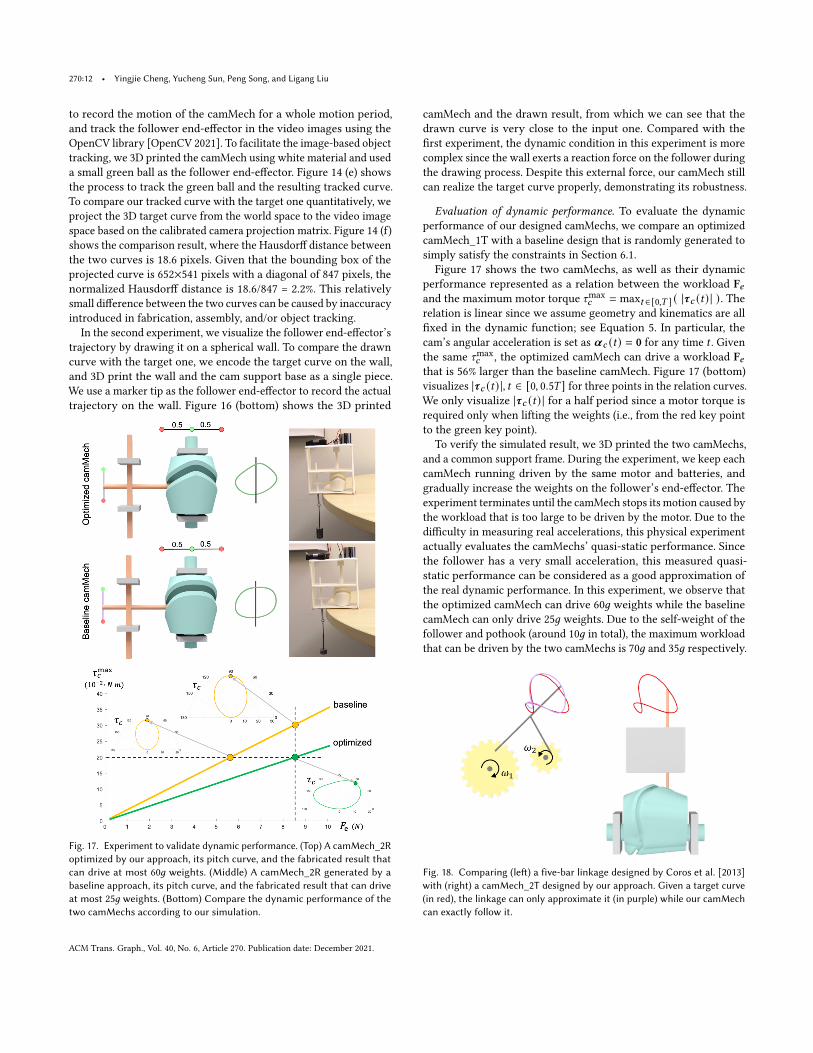
In the first experiment, we visualize the follower trajectory using

an image processing technique. In detail, we use a video camera

Fig. 16. Experiment to evaluate the kinematic performance for realizing a

target curve Dove. (Top) A camMech_2R optimized by our approach, and

the input curve. (Bottom) A 3D printed result, and the drawn curve.



to record the motion of the camMech for a whole motion period,

and track the follower end-effector in the video images using the

OpenCV library [OpenCV 2021]. To facilitate the image-based object

tracking, we 3D printed the camMech using white material and used

a small green ball as the follower end-effector. Figure 14 (e) shows

the process to track the green ball and the resulting tracked curve.

To compare our tracked curve with the target one quantitatively, we

project the 3D target curve from the world space to the video image

space based on the calibrated camera projection matrix. Figure 14 (f)

shows the comparison result, where the Hausdorff distance between

the two curves is 18.6 pixels. Given that the bounding box of the

projected curve is 652×541 pixels with a diagonal of 847 pixels, the

normalized Hausdorff distance is 18.6/847 = 2.2%. This relatively

small difference between the two curves can be caused by inaccuracy

introduced in fabrication, assembly, and/or object tracking.

In the second experiment, we visualize the follower end-effector’s

trajectory by drawing it on a spherical wall. To compare the drawn

curve with the target one, we encode the target curve on the wall,

and 3D print the wall and the cam support base as a single piece.

We use a marker tip as the follower end-effector to record the actual

trajectory on the wall. Figure 16 (bottom) shows the 3D printed

Fig. 17. Experiment to validate dynamic performance. (Top) A camMech_2R

optimized by our approach, its pitch curve, and the fabricated result that

can drive at most 60𝑔 weights. (Middle) A camMech_2R generated by a

baseline approach, its pitch curve, and the fabricated result that can drive

at most 25𝑔 weights. (Bottom) Compare the dynamic performance of the

two camMechs according to our simulation.

camMech and the drawn result, from which we can see that the

drawn curve is very close to the input one. Compared with the

first experiment, the dynamic condition in this experiment is more

complex since the wall exerts a reaction force on the follower during

the drawing process. Despite this external force, our camMech still

can realize the target curve properly, demonstrating its robustness.

Evaluation of dynamic performance. To evaluate the dynamic

performance of our designed camMechs, we compare an optimized

camMech_1T with a baseline design that is randomly generated to

simply satisfy the constraints in Section 6.1.

Figure 17 shows the two camMechs, as well as their dynamic

performance represented as a relation between the workload F𝑒and the maximum motor torque 𝜏max

𝑐 = max𝑡 ∈[0,𝑇 ] ( |𝝉𝑐 (𝑡) | ). Therelation is linear since we assume geometry and kinematics are all

fixed in the dynamic function; see Equation 5. In particular, the

cam’s angular acceleration is set as 𝜶𝑐 (𝑡) = 0 for any time 𝑡 . Given

the same 𝜏max

𝑐 , the optimized camMech can drive a workload F𝑒that is 56% larger than the baseline camMech. Figure 17 (bottom)

visualizes |𝝉𝑐 (𝑡) |, 𝑡 ∈ [0, 0.5𝑇 ] for three points in the relation curves.

We only visualize |𝝉𝑐 (𝑡) | for a half period since a motor torque is

required only when lifting the weights (i.e., from the red key point

to the green key point).

To verify the simulated result, we 3D printed the two camMechs,

and a common support frame. During the experiment, we keep each

camMech running driven by the same motor and batteries, and

gradually increase the weights on the follower’s end-effector. The

experiment terminates until the camMech stops its motion caused by

the workload that is too large to be driven by the motor. Due to the

difficulty in measuring real accelerations, this physical experiment

actually evaluates the camMechs’ quasi-static performance. Since

the follower has a very small acceleration, this measured quasi-

static performance can be considered as a good approximation of

the real dynamic performance. In this experiment, we observe that

the optimized camMech can drive 60𝑔 weights while the baseline

camMech can only drive 25𝑔 weights. Due to the self-weight of the

follower and pothook (around 10𝑔 in total), the maximum workload

that can be driven by the two camMechs is 70𝑔 and 35𝑔 respectively.

Fig. 18. Comparing (left) a five-bar linkage designed by Coros et al. [2013]

with (right) a camMech_2T designed by our approach. Given a target curve

(in red), the linkage can only approximate it (in purple) while our camMech

can exactly follow it.



The ratio between the two maximum workloads, which is 2.0, is

close to that (i.e., 1.56 ) predicted by our simulation. This result

verifies the effectiveness of our optimization to make the camMech

drivable by a small motor torque.

Comparison with Coros et al. [2013]. We compared our designed

camMechs with linkage-based mechanisms designed by Coros et

al. [2013]. To this end, we reproduced a five-bar linkage result shown

in [Coros et al. 2013], which can only approximate a target curve; see

Figure 18 (left). In contrast, our designed camMech_2T can exactly

follow the target curve; see Figure 18 (right). In addition, the linkage

has to be driven by two motors with synchronized angular speed

(i.e., 𝜔2 = −2𝜔1) while our camMech_2T can be driven by a single

motor. Our advantage comes from the larger design space, i.e., the

continuous pitch curve instead of a few joint parameters of the

linkage. However, the larger design space also results in more bulky

and complex geometry of the mechanism (i.e., the 3D cam), leading

to more cost and higher demand on the fabrication. For example,

the linkage can be fabricated cheaply and quickly with laser cutting

while our camMechs can only be fabricated with 3D printing.

Drawing machines. Our designed camMechs (i.e., camMech_2T,

camMech_1T1R, and camMech_2R) can be used as drawing ma-

chines. In Figure 16, we have used camMech_2R as a drawing ma-

chine to evaluate its kinematic performance. Figure 20 shows that

our camMechs are able to draw complex, free-form curves on a 3D

planar, cylindrical, or spherical surface, respectively. Our camMechs

are suitable for drawing shapes whose boundary can be represented

as a closed, smooth curve such as organic shapes. Our camMechs

are able to draw curves with intricate geometric details, but the

cost is that the 3D cam becomes larger; see again Figure 15. One

potential application of these camMechs is to automate the drawing

or painting on a cylindrical or spherical surface such as the interior

of containers; see Figure 1 (left) for an example. This task cannot

be achieved by conventional drawing machines based on gears and

linkages [Roussel et al. 2017] since they draw on planar surfaces.

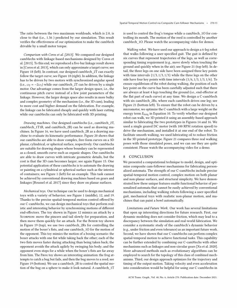
Mechanical toys. Our technique can be used to design mechanical

toys with a variety of behavior; see Figure 1 (middle), 12, and 19.

Thanks to the precise spatial-temporal motion control offered by

our C-camMechs, we can design mechanical toys that perform real-

istic and interesting behavior by synchronizing motions of different

end-effectors. The toy shown in Figure 12 mimics an attack by a

Scorpion: move the pincers and tail slowly for preparation, and

then move them quickly for an attack. For the Boxer toy shown

in Figure 19 (top), we use two camMech_2Rs for controlling the

motion of the boxer’s fists, and one camMech_1O for the motion of

the opponent. This toy mimics the motion of a boxing scenario: the

boxer attacks with one fist while taking back the other; each of the

two fists moves faster during attacking than being taken back; the

opponent avoids the attack agilely by swinging his body; and the

opponent even stops for a while when the boxer’s fists are far away

from him. The Frog toy shows an interesting animation: the frog at-

tempts to catch a bug but fails, and then the bug moves to a reed; see

Figure 19 (bottom). We use a camMech_2R to control the spatial mo-

tion of the bug on a sphere to make it look natural. A camMech_1T

is used to control the frog’s tongue while a camMech_1O for con-

trolling its mouth. The motion of the reed is controlled by another

camMech_1O. Please watch the accompanying video for demos.

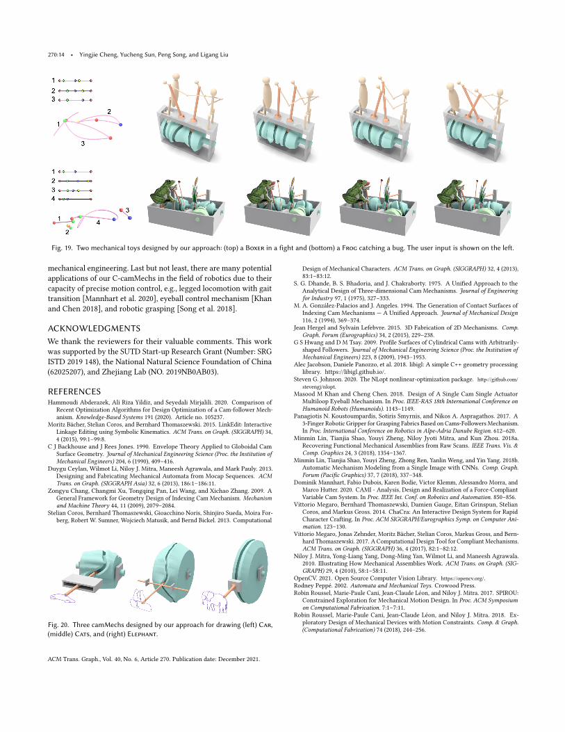
Walking robot. We have used our approach to design a 6-leg robot

that walks following a user-specified gait. The gait is defined by

six curves that represent trajectories of the legs, as well as corre-

sponding timing requirement (e.g., move slowly when touching the

ground and quickly when in the air); see Figure 21 (top left). In de-

tail, the three legs on one side have been assigned three key points

with time intervals {1/3, 1/3, 1/3} while the three legs on the other

side have four key points with time intervals {1/6, 1/3, 1/3, 1/6}. Toensure equilibrium of the robot during walking, the position of each

key point on the curve has been carefully adjusted such that there

are always at least 4 legs touching the ground (i.e., end-effector at

the flat part of each curve) at any time. We design a C-camMech

with six camMech_2Rs, where each camMech drives one leg; see

Figure 21 (bottom left). To ensure that the robot can be driven by a

micromotor, we optimize the C-camMech with a large weight on the

energy term 𝐸torq in Equation 10. To verify whether our designed

robot can walk, we 3D printed it using an assembly-based approach

similar to fabricating the two prototypes in Figures 14 and 16. We

used a single geared DC motor (with 100 RPM rotation speed) to

drive the mechanism, and installed it at one end of the robot. To

facilitate smooth walking, we used lubricating oil to reduce friction

in the 3D printed prototype. Figure 21 compares three real walking

poses with those simulated poses, and we can see they are quite

consistent. Please watch the accompanying video for a demo.

8 CONCLUSION

We presented a computational technique to model, design, and opti-

mize composite cam-follower mechanisms for fabricating person-

alized automata. The strength of our C-camMechs include precise

spatial-temporal motion control, complex motion on both planar

and non-planar surfaces, and structural simplicity. We have demon-

strated how these unique features enable functional behavior of per-

sonalized automata that cannot be easily achieved by conventional

mechanisms, including walking robots following a user-specified

gait, mechanical toys with realistic non-planar motion, and ma-

chines that can paint a bowl automatically.

Limitations and Future Work. Our work has several limitations

that open up interesting directions for future research. First, our

dynamic modeling does not consider friction, which may lead to a

discrepancy between the simulation and real-world fabrication. We

consider a systematic study of the camMech’s dynamic behavior

(e.g., under friction and even tolerance) as an important future work.

Second, we have shown that our C-camMechs can perform complex

spatial-temporal motion to achieve functional tasks. This capability

can be further extended by combining our C-camMechs with other

mechanisms such as linkages and non-circular gears [Xu et al. 2020].

More advanced methods such as evolutionary algorithms can be

employed to search for the topology of this class of combined mech-

anisms. Third, our design approach optimizes for the trajectory and

timing of the output motion. Taking velocity and even acceleration

into consideration would be helpful for using our C-camMechs in



Fig. 19. Two mechanical toys designed by our approach: (top) a Boxer in a fight and (bottom) a Frog catching a bug. The user input is shown on the left.

mechanical engineering. Last but not least, there are many potential

applications of our C-camMechs in the field of robotics due to their

capacity of precise motion control, e.g., legged locomotion with gait

transition [Mannhart et al. 2020], eyeball control mechanism [Khan

and Chen 2018], and robotic grasping [Song et al. 2018].

ACKNOWLEDGMENTS

We thank the reviewers for their valuable comments. This work

was supported by the SUTD Start-up Research Grant (Number: SRG

ISTD 2019 148), the National Natural Science Foundation of China

(62025207), and Zhejiang Lab (NO. 2019NB0AB03).

REFERENCES

Hammoudi Abderazek, Ali Riza Yildiz, and Seyedali Mirjalili. 2020. Comparison of

Recent Optimization Algorithms for Design Optimization of a Cam-follower Mech-

anism. Knowledge-Based Systems 191 (2020). Article no. 105237.Moritz Bächer, Stelian Coros, and Bernhard Thomaszewski. 2015. LinkEdit: Interactive

Linkage Editing using Symbolic Kinematics. ACM Trans. on Graph. (SIGGRAPH) 34,4 (2015), 99:1–99:8.

C J Backhouse and J Rees Jones. 1990. Envelope Theory Applied to Globoidal Cam

Surface Geometry. Journal of Mechanical Engineering Science (Proc. the Institution ofMechanical Engineers) 204, 6 (1990), 409–416.

Duygu Ceylan, Wilmot Li, Niloy J. Mitra, Maneesh Agrawala, and Mark Pauly. 2013.

Designing and Fabricating Mechanical Automata from Mocap Sequences. ACMTrans. on Graph. (SIGGRAPH Asia) 32, 6 (2013), 186:1–186:11.

Zongyu Chang, Changmi Xu, Tongqing Pan, Lei Wang, and Xichao Zhang. 2009. A

General Framework for Geometry Design of Indexing Cam Mechanism. Mechanismand Machine Theory 44, 11 (2009), 2079–2084.

Stelian Coros, Bernhard Thomaszewski, Gioacchino Noris, Shinjiro Sueda, Moira For-

berg, Robert W. Sumner, Wojciech Matusik, and Bernd Bickel. 2013. Computational

Fig. 20. Three camMechs designed by our approach for drawing (left) Car,

(middle) Cats, and (right) Elephant.

Design of Mechanical Characters. ACM Trans. on Graph. (SIGGRAPH) 32, 4 (2013),83:1–83:12.

S. G. Dhande, B. S. Bhadoria, and J. Chakraborty. 1975. A Unified Approach to the

Analytical Design of Three-dimensional Cam Mechanisms. Journal of Engineeringfor Industry 97, 1 (1975), 327–333.

M. A. González-Palacios and J. Angeles. 1994. The Generation of Contact Surfaces of

Indexing Cam Mechanisms — A Unified Approach. Journal of Mechanical Design116, 2 (1994), 369–374.

Jean Hergel and Sylvain Lefebvre. 2015. 3D Fabrication of 2D Mechanisms. Comp.Graph. Forum (Eurographics) 34, 2 (2015), 229–238.

G S Hwang and D M Tsay. 2009. Profile Surfaces of Cylindrical Cams with Arbitrarily-

shaped Followers. Journal of Mechanical Engineering Science (Proc. the Institution ofMechanical Engineers) 223, 8 (2009), 1943–1953.

Alec Jacobson, Daniele Panozzo, et al. 2018. libigl: A simple C++ geometry processing

library. https://libigl.github.io/.

Steven G. Johnson. 2020. The NLopt nonlinear-optimization package. http://github.com/

stevengj/nlopt.

Masood M Khan and Cheng Chen. 2018. Design of A Single Cam Single Actuator

Multiloop Eyeball Mechanism. In Proc. IEEE-RAS 18th International Conference onHumanoid Robots (Humanoids). 1143–1149.

Panagiotis N. Koustoumpardis, Sotiris Smyrnis, and Nikos A. Aspragathos. 2017. A

3-Finger Robotic Gripper for Grasping Fabrics Based on Cams-Followers Mechanism.

In Proc. International Conference on Robotics in Alpe-Adria Danube Region. 612–620.Minmin Lin, Tianjia Shao, Youyi Zheng, Niloy Jyoti Mitra, and Kun Zhou. 2018a.

Recovering Functional Mechanical Assemblies from Raw Scans. IEEE Trans. Vis. &Comp. Graphics 24, 3 (2018), 1354–1367.

Minmin Lin, Tianjia Shao, Youyi Zheng, Zhong Ren, Yanlin Weng, and Yin Yang. 2018b.

Automatic Mechanism Modeling from a Single Image with CNNs. Comp. Graph.Forum (Pacific Graphics) 37, 7 (2018), 337–348.

Dominik Mannhart, Fabio Dubois, Karen Bodie, Victor Klemm, Alessandro Morra, and

Marco Hutter. 2020. CAMI - Analysis, Design and Realization of a Force-Compliant

Variable Cam System. In Proc. IEEE Int. Conf. on Robotics and Automation. 850–856.Vittorio Megaro, Bernhard Thomaszewski, Damien Gauge, Eitan Grinspun, Stelian

Coros, and Markus Gross. 2014. ChaCra: An Interactive Design System for Rapid

Character Crafting. In Proc. ACM SIGGRAPH/Eurographics Symp. on Computer Ani-mation. 123–130.

Vittorio Megaro, Jonas Zehnder, Moritz Bächer, Stelian Coros, Markus Gross, and Bern-

hard Thomaszewski. 2017. A Computational Design Tool for Compliant Mechanisms.

ACM Trans. on Graph. (SIGGRAPH) 36, 4 (2017), 82:1–82:12.Niloy J. Mitra, Yong-Liang Yang, Dong-Ming Yan, Wilmot Li, and Maneesh Agrawala.

2010. Illustrating How Mechanical Assemblies Work. ACM Trans. on Graph. (SIG-GRAPH) 29, 4 (2010), 58:1–58:11.

OpenCV. 2021. Open Source Computer Vision Library. https://opencv.org/.

Rodney Peppé. 2002. Automata and Mechanical Toys. Crowood Press.

Robin Roussel, Marie-Paule Cani, Jean-Claude Léon, and Niloy J. Mitra. 2017. SPIROU:

Constrained Exploration for Mechanical Motion Design. In Proc. ACM Symposiumon Computational Fabrication. 7:1–7:11.

Robin Roussel, Marie-Paule Cani, Jean-Claude Léon, and Niloy J. Mitra. 2018. Ex-

ploratory Design of Mechanical Devices with Motion Constraints. Comp. & Graph.(Computational Fabrication) 74 (2018), 244–256.


http://github.com/stevengj/nlopt

http://github.com/stevengj/nlopt

https://opencv.org/


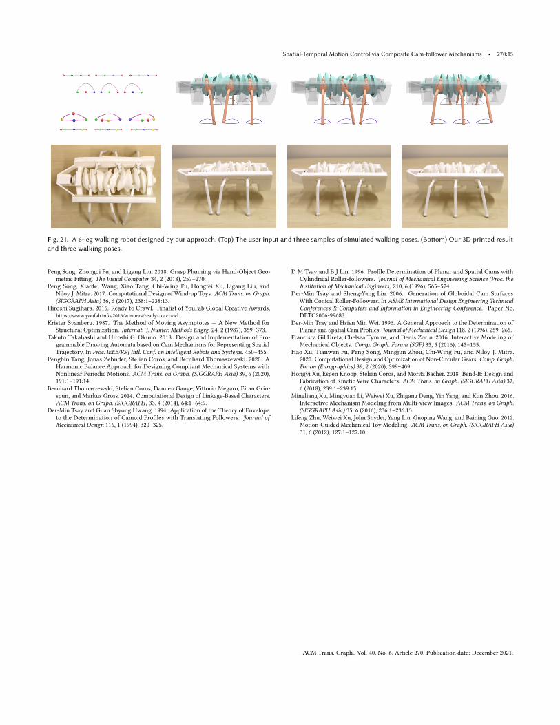
Fig. 21. A 6-leg walking robot designed by our approach. (Top) The user input and three samples of simulated walking poses. (Bottom) Our 3D printed result

and three walking poses.

Peng Song, Zhongqi Fu, and Ligang Liu. 2018. Grasp Planning via Hand-Object Geo-

metric Fitting. The Visual Computer 34, 2 (2018), 257–270.Peng Song, Xiaofei Wang, Xiao Tang, Chi-Wing Fu, Hongfei Xu, Ligang Liu, and

Niloy J. Mitra. 2017. Computational Design of Wind-up Toys. ACM Trans. on Graph.(SIGGRAPH Asia) 36, 6 (2017), 238:1–238:13.

Hiroshi Sugihara. 2016. Ready to Crawl. Finalist of YouFab Global Creative Awards,

https://www.youfab.info/2016/winners/ready-to-crawl.

Krister Svanberg. 1987. The Method of Moving Asymptotes — A New Method for

Structural Optimization. Internat. J. Numer. Methods Engrg. 24, 2 (1987), 359–373.Takuto Takahashi and Hiroshi G. Okuno. 2018. Design and Implementation of Pro-

grammable Drawing Automata based on Cam Mechanisms for Representing Spatial

Trajectory. In Proc. IEEE/RSJ Intl. Conf. on Intelligent Robots and Systems. 450–455.Pengbin Tang, Jonas Zehnder, Stelian Coros, and Bernhard Thomaszewski. 2020. A

Harmonic Balance Approach for Designing Compliant Mechanical Systems with

Nonlinear Periodic Motions. ACM Trans. on Graph. (SIGGRAPH Asia) 39, 6 (2020),191:1–191:14.

Bernhard Thomaszewski, Stelian Coros, Damien Gauge, Vittorio Megaro, Eitan Grin-

spun, and Markus Gross. 2014. Computational Design of Linkage-Based Characters.

ACM Trans. on Graph. (SIGGRAPH) 33, 4 (2014), 64:1–64:9.Der-Min Tsay and Guan Shyong Hwang. 1994. Application of the Theory of Envelope

to the Determination of Camoid Profiles with Translating Followers. Journal ofMechanical Design 116, 1 (1994), 320–325.

D M Tsay and B J Lin. 1996. Profile Determination of Planar and Spatial Cams with

Cylindrical Roller-followers. Journal of Mechanical Engineering Science (Proc. theInstitution of Mechanical Engineers) 210, 6 (1996), 565–574.

Der-Min Tsay and Sheng-Yang Lin. 2006. Generation of Globoidal Cam Surfaces

With Conical Roller-Followers. In ASME International Design Engineering TechnicalConferences & Computers and Information in Engineering Conference. Paper No.

DETC2006-99683.

Der-Min Tsay and Hsien Min Wei. 1996. A General Approach to the Determination of

Planar and Spatial Cam Profiles. Journal of Mechanical Design 118, 2 (1996), 259–265.Francisca Gil Ureta, Chelsea Tymms, and Denis Zorin. 2016. Interactive Modeling of

Mechanical Objects. Comp. Graph. Forum (SGP) 35, 5 (2016), 145–155.Hao Xu, Tianwen Fu, Peng Song, Mingjun Zhou, Chi-Wing Fu, and Niloy J. Mitra.

2020. Computational Design and Optimization of Non-Circular Gears. Comp. Graph.Forum (Eurographics) 39, 2 (2020), 399–409.

Hongyi Xu, Espen Knoop, Stelian Coros, and Moritz Bächer. 2018. Bend-It: Design and

Fabrication of Kinetic Wire Characters. ACM Trans. on Graph. (SIGGRAPH Asia) 37,6 (2018), 239:1–239:15.

Mingliang Xu, Mingyuan Li, Weiwei Xu, Zhigang Deng, Yin Yang, and Kun Zhou. 2016.

Interactive Mechanism Modeling from Multi-view Images. ACM Trans. on Graph.(SIGGRAPH Asia) 35, 6 (2016), 236:1–236:13.

Lifeng Zhu, Weiwei Xu, John Snyder, Yang Liu, Guoping Wang, and Baining Guo. 2012.

Motion-Guided Mechanical Toy Modeling. ACM Trans. on Graph. (SIGGRAPH Asia)31, 6 (2012), 127:1–127:10.


https://www.youfab.info/2016/winners/ready-to-crawl

Documents

Spatial-Temporal Motion Control via Composite Cam-follower