Embed Size (px)
Citation preview

Spatial interpolation of solar global radiation
C. Lussana(1), F. Uboldi(2) and C. Antoniazzi(1)
(1) ARPA Lombardia – Weather service, Milan, Italy(2) Consultant, Novate Milanese, Milan, Italy

22
Introduction
• Goal: analysis fields of hourly mean Solar Global Radiation – observations: mesoscale meteorological network– background: model of clear-sky solar global radiation,
incorporating the cover or shelter provided by interception by an object (mountain, building, tree) of the sun or its rays.
– method: Optimal Interpolation
13-17 September 201010th EMS/8th ECACSpatial Interpolation of solar global radiationLussana C., Uboldi F, and Antoniazzi C.

33
Introduction
• Goal: analysis fields of hourly mean Solar Global Radiation – observations: mesoscale meteorological network– background: model of clear-sky solar global radiation,
incorporating the cover or shelter provided by interception by an object (mountain, building, tree) of the sun or its rays.
– method: Optimal Interpolation
• Motivations:– In the last years, we have implemented robust and reliable OI-
based spatial interpolation schemes for several other variables (Uboldi et al, 2008; Lussana et al 2009):
• Testing the application of the OI to solar global radiation.
– (automated) Data quality control • Comparison with neighbouring observations
13-17 September 201010th EMS/8th ECACSpatial Interpolation of solar global radiationLussana C., Uboldi F, and Antoniazzi C.

44
Introduction
• Goal: obtain analysis fields of Solar Global Radiation – observations: observations from mesoscale meteorological network– background: model of clear-sky solar global radiation– method: Optimal Interpolation
• Motivations:– In the last years it has been developped and tested a robust and reliable
method tested on several other variables
13-17 September 201010th EMS/8th ECACSpatial Interpolation of solar global radiationLussana C., Uboldi F, and Antoniazzi C.
Temperature Relative humidity Precipitation
PressureP426 Lussana C., Uboldi F., Salvati M.R. and Ranci M.. Spatial interpolation of atmospheric pressure observations from automatic weather stations in complex alpine environmentAttendance: Thursday 1617
Wind

55
The Global Radiation Measurement Network
• Automatic stations
• Pyranometers spectral range 300-3000 nm
• Complex orography
• Hourly data
• Inhomogenous station density
• Station altitudes 10->3000 m amsl
13-17 September 201010th EMS/8th ECACSpatial Interpolation of solar global radiationLussana C., Uboldi F, and Antoniazzi C.

66
Background: SMARTS model
• SMARTS (the Simple Model of the Atmospheric Radiative Transfer of Sunshine,
www.nrel.gov/rredc/smarts, Gueymard, 1987, 1995, 1998, 2001):– spectral model that covers the whole shortwave solar spectrum (280 to
4000 nm)
• Outputs– direct radiation (on a horizontal surface)– diffuse radiation– Compute radiation on tilted sufaces (diffuse and reflected radiation)
• Main assumptions used for initialization– clear-sky conditions– reference vertical profiles for atmospheric composition (USSA)
• SOLPOS(http://rredc.nrel.gov/solar/codesandalgorithms/solpos/)– Solar Position and Intensity: routine used to compute the apparent solar
position based on the date, time and location on Earth.
13-17 September 201010th EMS/8th ECACSpatial Interpolation of solar global radiationLussana C., Uboldi F, and Antoniazzi C.

77
SMARTS model outputs
13-17 September 201010th EMS/8th ECACSpatial Interpolation of solar global radiationLussana C., Uboldi F, and Antoniazzi C.
Rad
iatio
n [W
/m^2
]
Blue: observation (1h average)
Green: SMARTS global radiation = direct + diffuse (+ reflected)
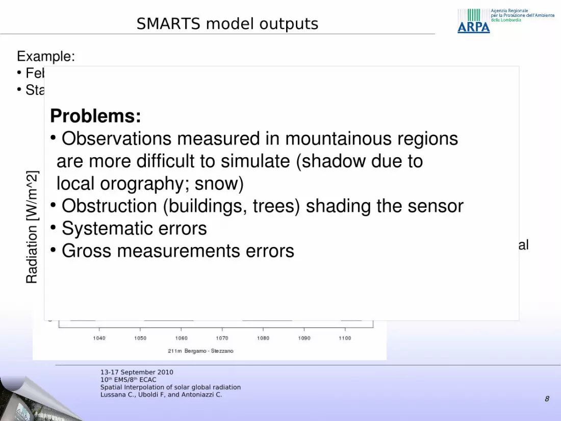
Example:● Feb 2009: 3 sunny days● Station located in the Plain (Bergamo, 211 m amsl)
88
SMARTS model outputs
13-17 September 201010th EMS/8th ECACSpatial Interpolation of solar global radiationLussana C., Uboldi F, and Antoniazzi C.
Rad
iatio
n [W
/m^2
]
Blue: observation
Green: SMART global radiation = direct + diffuse (+ reflected)
Example:● Feb 2009: 3 sunny days● Station located in the Plain (Bergamo, 211 m amsl)
Problems:● Observations measured in mountainous regions are more difficult to simulate (shadow due to local orography; snow)
● Obstruction (buildings, trees) shading the sensor● Systematic errors● Gross measurements errors

99
Shades
• Background field:– NO Shade
• Global radiation = direct + diffuse + reflected
– shade• Global radiation = direct + diffuse + reflected
• Grid points– automatic determination of orographic shadowing effects
• Station points– The dataset is divided in sub-datasets: station/season/hour of the day– Statistics analysis of innovation (= observation - SMARTS background)– subjective decision (though based on objective criteria)
• station/season/hour → Shade YES/NO
13-17 September 201010th EMS/8th ECACSpatial Interpolation of solar global radiationLussana C., Uboldi F, and Antoniazzi C.
1010
Orographic shading effect on grid points
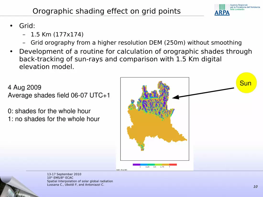
• Grid:– 1.5 Km (177x174)– Grid orography from a higher resolution DEM (250m) without smoothing
• Development of a routine for calculation of orographic shades through back-tracking of sun-rays and comparison with 1.5 Km digital elevation model.
13-17 September 201010th EMS/8th ECACSpatial Interpolation of solar global radiationLussana C., Uboldi F, and Antoniazzi C.
4 Aug 2009 Average shades field 0607 UTC+1
0: shades for the whole hour 1: no shades for the whole hour
Sun

1111
Orographic shading effect on station locations
● A station can be in the shadow of: orography, buildings, large trees, …● Comparison of statistical parameters (mean values, interquartile
range) derived from the distribution of observed values with the same parameters derived from SMARTS outputs
● Subjective decision: shades yes/no to a station/season/hour record
13-17 September 201010th EMS/8th ECACSpatial Interpolation of solar global radiationLussana C., Uboldi F, and Antoniazzi C.
daytime distribution of hourly mean solar global radiation values. JuneJulyAugust 2009. Station is located in the Plain.
Black: observations (continuous line median; dotted: 25 and 75 quantile)
Blue: direct/diffuse radiation (continuous line median; dotted: 25 and 75 quantile)

1212
Orographic shading effect on station locations
● A station can be in the shadow of: orography, buildings, large trees, …● Comparison of statistical parameters (mean values, interquartile
range) derived from the distribution of observed values with the same parameters derived from SMARTS outputs
● Subjective decision: shades yes/no to a station/season/hour record
13-17 September 201010th EMS/8th ECACSpatial Interpolation of solar global radiationLussana C., Uboldi F, and Antoniazzi C.
daytime distribution of hourly mean solar global radiation values. JuneJulyAugust 2009. Station is located in the Plain.
Black: observations (continuous line median; dotted: 25 and 75 quantile)
Blue: direct/diffuse radiation (continuous line median; dotted: 25 and 75 quantile)
1313
Data Quality Control
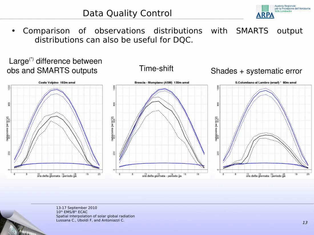
• Comparison of observations distributions with SMARTS output distributions can also be useful for DQC.
13-17 September 201010th EMS/8th ECACSpatial Interpolation of solar global radiationLussana C., Uboldi F, and Antoniazzi C.
Timeshift Shades + systematic error Large(*) difference between obs and SMARTS outputs

1414
Optimal Interpolation
• General scheme
13-17 September 201010th EMS/8th ECACSpatial Interpolation of solar global radiationLussana C., Uboldi F, and Antoniazzi C.
1515
Optimal Interpolation
• For each timestep, station locations/grid points are separated in 2 subsets– exposed to direct radiation– not exposed to direct radiation
• Background field is obtained using SMARTS– station/grid points exposed to direct radiation
• Background = direct + diffuse + reflected
– station/grid points not exposed to direct radiation• Background = diffuse + reflected
• Data Quality Control: plausibility check using the background field– Observation is flagged as supsect and not used in the analysis procedure if:
• observation > (direct + diffuse + reflected + 170 W/m2)• observation < (diffuse + reflected - 115 W/m2)
• OI is performed independently for the 2 different subsets– uncorrelated background errors between the 2 subsets– background error covariance specified by means of 3D Gaussian correlation
functions (horizontal decorrelation length scale=30Km; vertical = 600 m)– Ratio between obs and background variances = 0.5
13-17 September 201010th EMS/8th ECACSpatial Interpolation of solar global radiationLussana C., Uboldi F, and Antoniazzi C.
1616
Optimal Interpolation
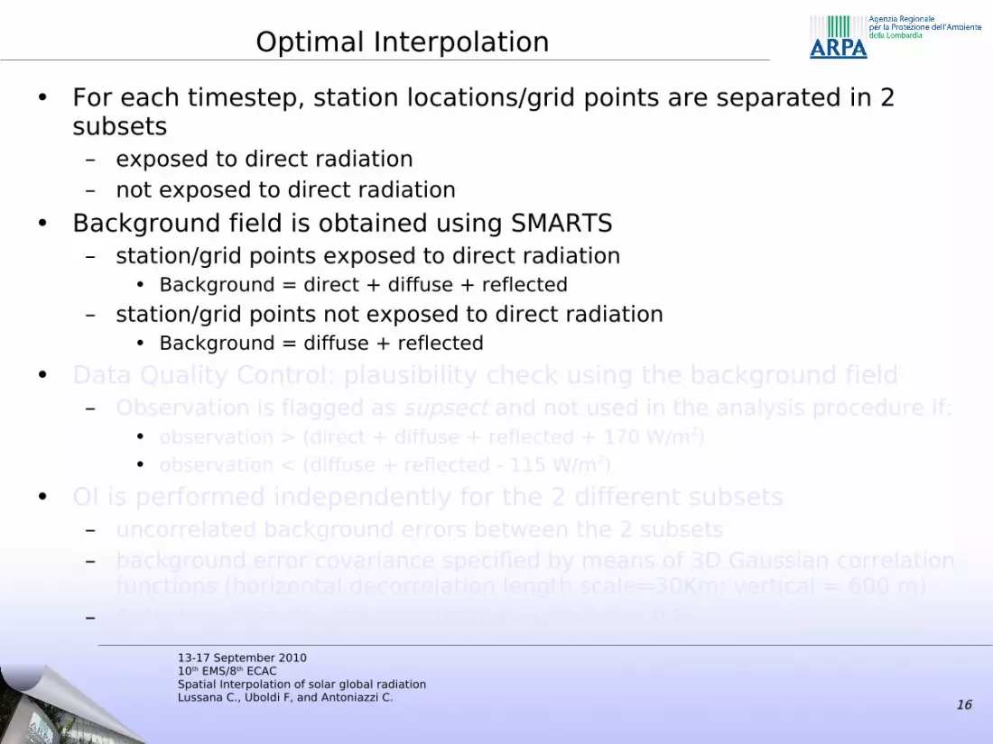
• For each timestep, station locations/grid points are separated in 2 subsets– exposed to direct radiation– not exposed to direct radiation
• Background field is obtained using SMARTS– station/grid points exposed to direct radiation
• Background = direct + diffuse + reflected
– station/grid points not exposed to direct radiation• Background = diffuse + reflected
• Data Quality Control: plausibility check using the background field– Observation is flagged as supsect and not used in the analysis procedure if:
• observation > (direct + diffuse + reflected + 170 W/m2)• observation < (diffuse + reflected - 115 W/m2)
• OI is performed independently for the 2 different subsets– uncorrelated background errors between the 2 subsets– background error covariance specified by means of 3D Gaussian correlation
functions (horizontal decorrelation length scale=30Km; vertical = 600 m)– Ratio between obs and background variances = 0.5
13-17 September 201010th EMS/8th ECACSpatial Interpolation of solar global radiationLussana C., Uboldi F, and Antoniazzi C.

1717
Optimal Interpolation
• For each timestep, station locations/grid points are separated in 2 subsets– exposed to direct radiation– not exposed to direct radiation
• Background field is obtained using SMARTS– station/grid points exposed to direct radiation
• Background = direct + diffuse + reflected
– station/grid points not exposed to direct radiation• Background = diffuse + reflected
• Data Quality Control: plausibility check using the background field– Observation is flagged as suspect and not used in the analysis procedure if:
• observation > (direct + diffuse + reflected + 170 W/m2)• observation < (diffuse + reflected - 115 W/m2)
• OI is performed independently for the 2 different subsets– uncorrelated background errors between the 2 subsets– background error covariance specified by means of 3D Gaussian correlation
functions (horizontal decorrelation length scale=30Km; vertical = 600 m)– Ratio between obs and background variances = 0.5
13-17 September 201010th EMS/8th ECACSpatial Interpolation of solar global radiationLussana C., Uboldi F, and Antoniazzi C.
1818
Optimal Interpolation
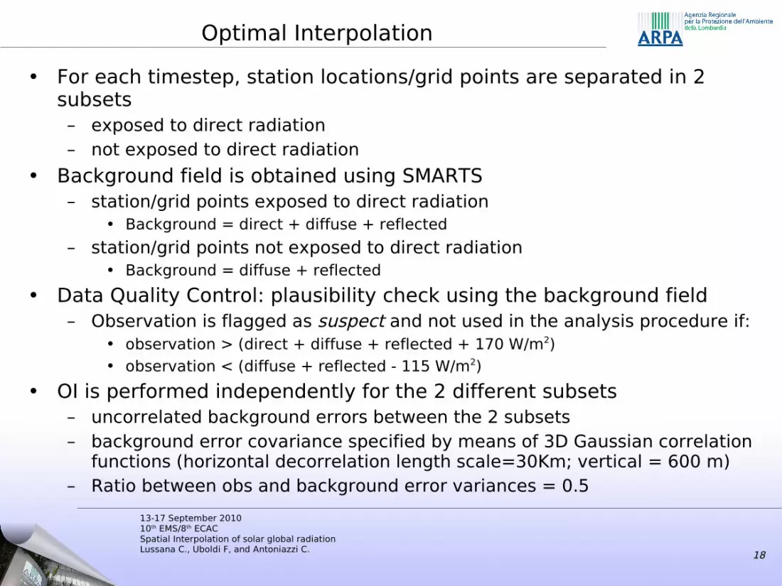
• For each timestep, station locations/grid points are separated in 2 subsets– exposed to direct radiation– not exposed to direct radiation
• Background field is obtained using SMARTS– station/grid points exposed to direct radiation
• Background = direct + diffuse + reflected
– station/grid points not exposed to direct radiation• Background = diffuse + reflected
• Data Quality Control: plausibility check using the background field– Observation is flagged as suspect and not used in the analysis procedure if:
• observation > (direct + diffuse + reflected + 170 W/m2)• observation < (diffuse + reflected - 115 W/m2)
• OI is performed independently for the 2 different subsets– uncorrelated background errors between the 2 subsets– background error covariance specified by means of 3D Gaussian correlation
functions (horizontal decorrelation length scale=30Km; vertical = 600 m)– Ratio between obs and background error variances = 0.5
13-17 September 201010th EMS/8th ECACSpatial Interpolation of solar global radiationLussana C., Uboldi F, and Antoniazzi C.

1919
Solar global radiation analysis: example 1
• d
13-17 September 201010th EMS/8th ECACSpatial Interpolation of solar global radiationLussana C., Uboldi F, and Antoniazzi C.
13 Jun 2009, 0700 UTC+1. Solar global radiation (W/m^2)Sunrise for a sunny day
2020
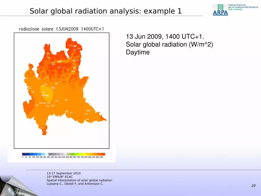
Solar global radiation analysis: example 1
• d
13-17 September 201010th EMS/8th ECACSpatial Interpolation of solar global radiationLussana C., Uboldi F, and Antoniazzi C.
13 Jun 2009, 1400 UTC+1. Solar global radiation (W/m^2) Daytime

2121
Solar global radiation analysis: example 1
• d
13-17 September 201010th EMS/8th ECACSpatial Interpolation of solar global radiationLussana C., Uboldi F, and Antoniazzi C.
13 Jun 2009, 2000 UTC+1. Solar global radiation (W/m^2)Sunset

2222
Solar global radiation analysis: example 1
• d
13-17 September 201010th EMS/8th ECACSpatial Interpolation of solar global radiationLussana C., Uboldi F, and Antoniazzi C.
8 Jun 2009, 10 UTC+1. Solar global radiation (W/m^2)Cloudy on the western part of the region

2323
Conclusions
• The analysis of solar global radiation using only pyranometers (with SMARTS providing the background field) can provide useful information about the solar global radiation field
• Data quality control procedure can benefit from solar global radiation analysis
• Further developments– Quantitative evaluations of the OI performance– Implementation of an automated routine to evaluate shades
on station location– Include satellite data in the statistical interpolation
procedure
13-17 September 201010th EMS/8th ECACSpatial Interpolation of solar global radiationLussana C., Uboldi F, and Antoniazzi C.

2424
13-17 September 201010th EMS/8th ECACSpatial Interpolation of solar global radiationLussana C., Uboldi F, and Antoniazzi C.


