Forest Ecology and Management 377 (2016) 170–181

Contents lists available at ScienceDirect

Forest Ecology and Management

journal homepage: www.elsevier .com/ locate/ foreco

Spatial distribution of forest biomass in Brazil’s state of Roraima,northern Amazonia

http://dx.doi.org/10.1016/j.foreco.2016.07.0100378-1127/� 2016 The Authors. Published by Elsevier B.V.This is an open access article under the CC BY-NC-ND license (http://creativecommons.org/licenses/by-nc-nd/4.0/).

⇑ Corresponding author at: Instituto Nacional de Pesquisas da Amazônia (INPA),Coordenação de Dinâmica Ambiental (CDAM), Av. André Araújo 2936, 69067-375Manaus, Amazonas, Brazil.

E-mail address: pmfearn@inpa.gov.br (P.M. Fearnside).1 Current address.

Paulo Eduardo Barni a, Antônio Ocimar Manzi b,c, Tiago Monteiro Condé a, Reinaldo Imbrozio Barbosa d,e,Philip Martin Fearnside b,e,⇑aUniversidade Estadual de Roraima (UERR), Campus Rorainópolis, Av. Senador Helio Campos, s/n�, 69375-000 Rorainópolis, Roraima, Brazilb Instituto Nacional de Pesquisas da Amazônia (INPA), Coordenação de Dinâmica Ambiental (CDAM), Av. André Araújo 2936, 69067-375 Manaus, Amazonas, Brazilc Instituto Nacional de Pesquisas Espaciais (INPE), Rodovia Presidente Dutra, Km 39, 12630-000 Cachoeira Paulista, São Paulo, Brazil1d Instituto Nacional de Pesquisas da Amazônia (INPA), Núcleo de Pesquisas de Roraima (NPRR), Rua Coronel Pinto 315, 69301-150 Boa Vista, Roraima, BrazileRede Brasileira de Pesquisas sobre Mudanças Climáticas Globais (Rede Clima), São José dos Campos, São Paulo, Brazil

a r t i c l e i n f o

Article history:Received 18 April 2016Received in revised form 30 June 2016Accepted 8 July 2016

Keywords:Carbon stockDeforestationGlobal warmingGreenhouse gas emissionsProtected areasREDD

a b s t r a c t

Forest biomass is an important variable for calculating carbon stocks and greenhouse gas emissions fromdeforestation and forest fires in Brazilian Amazonia. Its spatial distribution has caused controversy due todisagreements over the application of different calculation methodologies. Standardized networks of for-est surveys provide an alternative to solve this problem. This study models the spatial distribution andoriginal total stock of forest biomass (Aboveground + Belowground + Fine and coarse litter) in Brazil’sstate of Roraima, taking advantage of data from georeferenced forest surveys in the region.Commercial volume (bole volume) from surveys was expanded to total biomass. Kriging techniques wereused to model the spatial distribution of biomass stocks and generate a benchmark map. All results wereassociated with phytophysiognomic groups, climatic regions and land uses (protected areas; agriculturaluse). We estimate forest in the state of Roraima to have an original biomass stock of 6.32 � 109 Mg. Forestbiomasses in areas with shorter dry seasons were higher as compared to forests in regions with longerdry seasons. The original vegetation in protected areas, independent of phytophysiognomic group, hashigher biomass compared to areas currently under agricultural use. Protected areas support 65.8% ofRoraima’s stock of forest biomass, indicating an important potential role in REDD projects for conserva-tion of forest carbon. Information on spatial distribution of biomass stocks at a more refined scale isneeded to reduce uncertainties about the regional character of carbon pools in Amazonia.

� 2016 The Authors. Published by Elsevier B.V. This is an open access article under the CC BY-NC-NDlicense (http://creativecommons.org/licenses/by-nc-nd/4.0/).

1. Introduction

Forest biomass affects the calculation of carbon stocks andgreenhouse gas (GHG) emissions, this being a major source ofuncertainty regarding the climatic role of forests and their man-agement in Brazilian Amazonia (Fearnside, 1997a, 2000; Chaveet al., 2004, 2014; Houghton, 2010). Along with deforestation, bio-mass determines the potential for carbon emissions that can bereleased into the atmosphere when forests are cut (Houghtonet al., 2009; Harris et al., 2012; Song et al., 2015). Cutting and burn-ing of forest biomass in Amazonia are linked to expanding areas of

agriculture and pasture. The quickest and cheapest way to ‘‘clean”the deforested area is by burning. Accurate models of forest bio-mass distribution can reduce the uncertainties in carbon stocksbecause they are based on a consistent and spatially explicit setof observational data, enabling a better understanding of the envi-ronmental and human processes that determine GHG emissions(Harris et al., 2012), in addition to providing information neededfor projects for Reducing Emissions from Deforestation and Degra-dation (REDD) (e.g., Soares-Filho et al., 2010; Nepstad et al., 2011;Saatchi et al., 2011).

The first systematic attempt in Amazonia to obtain large-scaleforest biomass estimates was derived from studies of Brown andLugo (1992, 1994). These authors developed expansion factorsand adjustments from commercial volume equations derived fromforest inventories carried out by the Food and Agriculture Organi-zation of the United Nations (UN-FAO) in the late 1950s. In thespecific case of Amazonia, new adjustments were implemented

P.E. Barni et al. / Forest Ecology and Management 377 (2016) 170–181 171

by Fearnside (1992) with the correction or addition of other carbonpools (e.g., dead wood, lianas, understory plants) which had beenomitted by Brown and Lugo (1992). Adjustments derived fromFearnside (1992) were significantly improved by Nogueira et al.(2005, 2007, 2008) and have been applied to commercial volume(bole volume) values obtained by the RADAMBRASIL inventories(Brazil, RADAMBRASIL, 1973–1983) conducted in the entire Brazil-ian Amazon (Fearnside, 1994, 1996, 1997a). The bole volumes oftrees from the RADAMBRASIL inventories were calculated basedon diameter at breast height (DBH), or diameter 1.3 m above theground or above any buttresses. Only individuals with circumfer-ence at breast height P100 cm (i.e., 31.8 cm DBH) were includedin the inventory.

The values of commercial volume estimated by the RADAM-BRASIL Project for the whole of Brazilian Amazonia (Brazil, IBGE,2013) could then be expanded to total biomass (live biomass andnecromass; below- and aboveground) and used in regional spatialdistribution models or extrapolated in accord with physiognomieswithin each state (Fearnside, 2000; Sales et al., 2007; Brazil, MCT,2010; Nogueira et al., 2015). An advantage of using the RADAM-BRASIL database lies in its having been collected before the majordeforestation and forest degradation events currently observed inAmazonia, thus offering a unique opportunity to assess the ‘‘origi-nal” (pre-1970) biomass distribution.

Despite advances in reducing uncertainties, the spatial distribu-tion of Amazon forest biomass can be estimated based on land-cover maps and information on the biomasses of vegetation typesand the effects of environmental factors (e.g., physiognomies, cli-mate, soil) (Feldpausch et al., 2011; Baccini et al., 2012) andland-use history (e.g., agro-silvo-pastoral ‘‘use areas” and differenttypes of protected areas) (Malhi et al., 2006). This auxiliary infor-mation, when supported by forest inventories and remote-sensing data, brings great advantages for the construction of refer-ence maps (Saatchi et al., 2011; Harris et al., 2012; Baccini et al.,2012). This is due to the introduction of additional features thatassist in estimating mean biomass per unit area (Mg ha�1) anddelimiting the spatial distribution of the biomass and carbonstocks disturbed by deforestation. Given that large areas in theAmazon lack any direct measurement of biomass, this alternativeallows construction of spatially refined maps at local and regionalscales arranged in a georeferenced grid that may be reproducedunder varying temporal constraints (Nogueira et al., 2015;Saatchi et al., 2012). This is because the anthropogenic and envi-ronmental characteristics specific to each region (e.g., at the statelevel) can be analyzed separately under the same calculation basis,rather than being products of extrapolations to a less detailed scale(e.g., Saatchi et al., 2007, 2011; Baccini et al., 2012). Maps usingsatellite-derived data to extrapolate from a limited number ofground plots (e.g., Saatchi et al., 2011; Baccini et al., 2012) haveproduced inconsistent results, even though they have essentiallythe same data sources and methods (Mitchard et al., 2014). Pro-gress has been made in resolving differences (Avitabile et al.,2016), but the limited ground data remain as the principal sourceof uncertainty. The RADAMBRASIL dataset, not used in the Saatchiet al. (2011) and Baccini et al. (2012) studies, represents a muchlarger source of on-the-ground data (Nogueira et al., 2015).Large-scale approaches tend to have greater uncertainties thando those on smaller scales due to the different methods of data col-lection used and to environmental variability among macro-regions. Local and regional approaches are less subject to the prob-lems causing uncertainty. Use of smaller-scale procedures providesan alternate path for evaluations of the regional potential for stor-ing carbon and for emission of greenhouse gases.

We used the state of Roraima (northern Brazilian Amazonia) asa case study to model the spatial distribution of forest biomass and

to evaluate the original stock of biomass (live biomass and necro-mass; above- and belowground) considered here as undisturbedbiomass in pre-1970 period. This region of the Amazon has phyto-climatic zones represented by savannas, seasonal forests andombrophilous forests that are different from other Amazonianstates (Barni et al., 2015a). Analysis of the distribution of forest bio-mass in these areas permits a more realistic estimate of the originalforest biomass stocks, located in areas with different protectionstatus and climate type, providing the basis for more robust esti-mates of forest carbon stocks and GHG emissions from deforesta-tion. Our specific objectives were (i) estimate the total biomass(live biomass and necromass; below- and aboveground) based onforest volume inventories conducted in Roraima and its surround-ings mainly by the RADAMBRASIL project; (ii) generate a referencemap from the spatial modeling of forest biomass using geostatisti-cal techniques; (iii) determine the biomass (Mg ha�1) in each foresttype by phytoclimatic zone, and (iv) determine the original bio-mass stock in each phytoclimatic zone in areas with protection(IL = indigenous lands and CU = conservation units) and withoutlegal protection (UA = use areas). ‘‘Conservation units” refer tothe various types of areas, both ‘‘strictly protected” and for ‘‘sus-tainable use,” defined in Brazil’s National System of ConservationUnits (SNUC) (Brazil, MMA, 2000).

2. Materials and methods

2.1. Study area

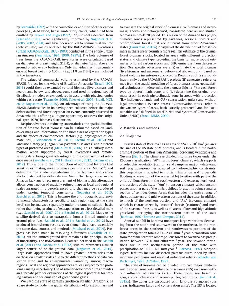
Brazil’s state of Roraima has an area of 224.3 � 103 km2 (an areathe size of the US state of Minnesota) and is located in the north-ernmost portion of Brazilian Amazonia, bordering Venezuela andGuyana (Fig. 1). The climate is divided into three types under theKöppen classification: ‘‘Af” (humid forest climate), which supportsoligotrophic vegetation (campina and campinarana) on white-sandsoil (phytophysionomies adapted to hydro-edaphic constraints;this vegetation is adapted to nutrient limitation and to periodicflooding or elevation of the water table) together with part of theombrophilous forest in the southwestern and extreme northwest-ern portions of the state; ‘‘Am” (monsoon climate), which encom-passes another part of the ombrophilous forest, this being a smallersection of semideciduous forest that includes the entire range ofthe southeastern and mid-western portions of the state, in additionto much of the northern portion, and ‘‘Aw” (savanna climate),which is characterized by ‘‘contact” forests (ecotones) and mostof the seasonal forests, as well as all areas of low and high altitudegrasslands occupying the northeastern portion of the state(Barbosa, 1997; Barbosa and Campos, 2011).

Annual rainfall in Roraima undergoes large variations, decreas-ing from the south and southwest to the northeast. In the rain-forest areas in the southern and southwestern portions of thestate, precipitation totals 2000–2300 mm�1 year. A transition zonefrommontane forest to ombrophilous forest to savanna has precip-itation between 1700 and 2000 mm�1 year. The savanna forma-tions are in the northeastern portion of the state withprecipitation of 1100–1400 mm year�1 (Barbosa, 1997). Morpho-logical features include dissected plateaus surrounded by intra-montane pediplains and residual individual reliefs (Schaefer andDarlymple, 1995; Ab’Saber, 1997).

The state of Roraima can be divided into two major phytocli-matic zones: zone with influence of savanna (ZIS) and zone with-out influence of savanna (ZOS). These zones are based ongeographical, climatic and geomorphological criteria (Barni et al.,2015a). The zones are associated with land-use categories (useareas, indigenous lands and conservation units). The ZIS is located

Fig. 1. Study area. The continuous solid line in the center of the figure divides thestudy area into two phytoclimatic zones (Barni et al., 2015a): ZIS = zone withsavanna influence; ZOS = Zone without savanna influence; SRTM = Shuttle RadarTopography Mission.

172 P.E. Barni et al. / Forest Ecology and Management 377 (2016) 170–181

in the northern and northeastern portions of Roraima (6–7 monthsdry), while the ZOS is located in the southern and southeastern andnorthwestern portions of the state where the dry period is shorter(1–5 months). Both zones are affected by deforestation, forest firesand selective logging.

2.2. Original boundaries of modeled physiognomies

The 17 forest physiognomies in Roraima were derived from avegetation map from the Program for Conservation and Sustain-able Use of Brazilian Biological Diversity (PROBio) at a scale of1:250,000 (Brazil, PROBio, 2013). Training operations were con-ducted to retrieve the original coverage of forests in the state usingmap algebra in a geographical information system (GIS): (1) allareas occupied by humans (deforested areas, grasslands and sec-ondary vegetation) were removed from the PROBio map andreplaced by the forest or non-forest physiognomies closest to theaffected area, assuming the original vegetation of Roraima withoutamendment; (2) the 17 physiognomies were condensed into fourmajor forest groups (Table 1): (i) Ombrophilous forests (all classesof open and dense forest); (ii) Ecotones (‘‘contact” physiognomies);(iii) Seasonal deciduous forests and semideciduous forest frag-ments, and (iv) Fragmented-physiognomies in oligotrophic ecosys-tems in the middle and lower Rio Branco. Savannas in thenortheastern portion of the state were also added.

2.3. Estimation of the original biomass

The original total forest biomass (live + dead, abovegroundand belowground) per unit area (Mg ha�1) was estimated frominventories (Brazil, RADAMBRASIL, 1973–1983) conducted inRoraima and in the surrounding region (Brazil, IBGE, 2013). These

inventories used commercial volume information on 296 plots(1 ha each), of which 119 were in Roraima, or within a range of100 km from the state’s borders, encompassing parts of Pará(5 plots) and Amazonas (172 plots) (Brazil, IBGE, 2013) in orderto soften the edge effect (Sales et al., 2007). To this database tworecently conducted forest inventories were added (Condé andTonini, 2013; Nascimento et al., 2014), bringing the total to 298sampling points (Supplementary Material, Fig. A.1; Table A.1).The data from these last two studies were used in the same wayas the RADAMBRASIL inventories (only individuals with circumfer-ence at breast height P100 cm, that is, diameter at breast heightP31.8 cm) in order to preserve the same criteria for biomassestimation throughout the spatial analysis.

The volume of each individual tree inventoried by the RADAM-BRASIL Project (in a tabulation at the level of species, genus or fam-ily) was converted to dry bole biomass (biomass of the trunk fromthe ground to the first significant branch) by multiplying by thebasic density (oven-dry weight divided by green volume; g cm�3)of the wood (Fearnside, 1992, 1997b). Expansion factors wereapplied to all 298 sampling points to convert bole biomass toexpanded aboveground biomass (Mg ha�1). These factors wereapplied (i) to expand from bole volume to represent the totalvolume of each individual tree for calculating the biomass, and(ii) to add the other components of forest biomass in order tocalculate the total biomass per hectare (Mg ha�1) for all points inthe BDG.

The volume expansion factor (VEF) adjusts for trees with DBH(diameter at breast height measured 1.3 m above the ground orabove any buttresses) between 10 cm and the minimum diametermeasured in the forest survey (the RADAMBRASIL database is fortrees with DBHP 31.8 cm). The values of VEF we used to correctfor the 10–31.7 cm DBH range were 1.537 for dense forest and1.506 for non-dense forest (Nogueira et al., 2008). These valuesinclude adjustments for hollow trees and irregularly shapedtrunks. The biomass expansion factor (BEF) adjusts for the treecrowns (the portion of the tree above and including the firstsignificant branch). The bole biomass was multiplied by the BEF,which has a value of 1.635 if bole biomass P190 Mg ha�1

(calculated by Nogueira et al. (2008) from data by Higuchi et al.(1998) normalized by diameter distribution in central Amazonia)and Exp (3.213 � (0.506 � Ln (bole biomass))) if bole biomass<190 Mg ha�1 (Brown and Lugo, 1992).

To convert the values for expanded biomass to total biomass,adjustments for inclusion or correction of other components ofthe forest (live and biomass and necromass, including the under-story and roots) were applied to the database. After the 298 com-mercial volume points for forest were converted to total biomass(Mg ha�1), additional 28 sampling points were included in theanalysis to estimate savanna biomass (Mg ha�1) in northern Ror-aima (Barbosa, 2001; Barbosa and Fearnside, 2005; Barbosa et al.,2012). Final sampling points totaled 326 (Supplementary Material,Table A.1). This dataset was called the ‘‘georeferenced database”(BDG) (Fig. 2).

2.4. Validation and the best model for interpolation

The georeferenced database was divided randomly into twosubsamples: (i) a set containing 33 sampling points (�10%), and(ii) another set containing 293 sampling points (�90%). The firstset (n1 = 33) was reserved for validation and determination of thebest interpolation model after obtaining the maps of biomass. Inorder to estimate each point not sampled in the execution of thethree Kriging techniques, five points were used that were nearneighbors to the location for which a value is to be estimated foreach quadrant. This is a standard procedure in ArcGIS software.

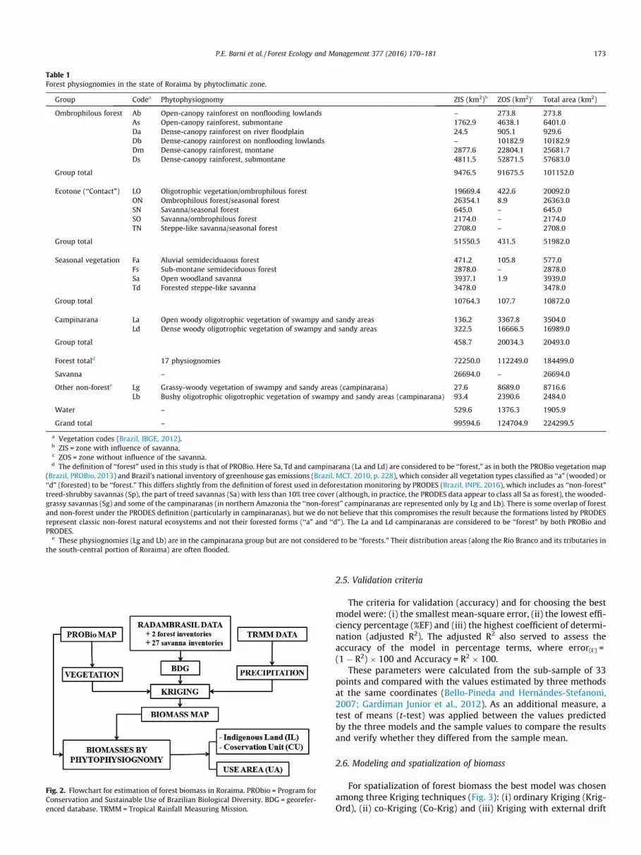
Table 1Forest physiognomies in the state of Roraima by phytoclimatic zone.

Group Codea Phytophysiognomy ZIS (km2)b ZOS (km2)c Total area (km2)

Ombrophilous forest Ab Open-canopy rainforest on nonflooding lowlands – 273.8 273.8As Open-canopy rainforest, submontane 1762.9 4638.1 6401.0Da Dense-canopy rainforest on river floodplain 24.5 905.1 929.6Db Dense-canopy rainforest on nonflooding lowlands – 10182.9 10182.9Dm Dense-canopy rainforest, montane 2877.6 22804.1 25681.7Ds Dense-canopy rainforest, submontane 4811.5 52871.5 57683.0

Group total 9476.5 91675.5 101152.0

Ecotone (‘‘Contact”) LO Oligotrophic vegetation/ombrophilous forest 19669.4 422.6 20092.0ON Ombrophilous forest/seasonal forest 26354.1 8.9 26363.0SN Savanna/seasonal forest 645.0 – 645.0SO Savanna/ombrophilous forest 2174.0 – 2174.0TN Steppe-like savanna/seasonal forest 2708.0 – 2708.0

Group total 51550.5 431.5 51982.0

Seasonal vegetation Fa Aluvial semideciduaous forest 471.2 105.8 577.0Fs Sub-montane semideciduous forest 2878.0 – 2878.0Sa Open woodland savanna 3937.1 1.9 3939.0Td Forested steppe-like savanna 3478.0 3478.0

Group total 10764.3 107.7 10872.0

Campinarana La Open woody oligotrophic vegetation of swampy and sandy areas 136.2 3367.8 3504.0Ld Dense woody oligotrophic vegetation of swampy and sandy areas 322.5 16666.5 16989.0

Group total 458.7 20034.3 20493.0

Forest totald 17 physiognomies 72250.0 112249.0 184499.0

Savanna – 26694.0 – 26694.0

Other non-foreste Lg Grassy-woody vegetation of swampy and sandy areas (campinarana) 27.6 8689.0 8716.6Lb Bushy oligotrophic oligotrophic vegetation of swampy and sandy areas (campinarana) 93.4 2390.6 2484.0

Water – 529.6 1376.3 1905.9

Grand total – 99594.6 124704.9 224299.5

a Vegetation codes (Brazil, IBGE, 2012).b ZIS = zone with influence of savanna.c ZOS = zone without influence of the savanna.d The definition of ‘‘forest” used in this study is that of PROBio. Here Sa, Td and campinarana (La and Ld) are considered to be ‘‘forest,” as in both the PROBio vegetation map

(Brazil, PROBio, 2013) and Brazil’s national inventory of greenhouse gas emissions (Brazil, MCT, 2010, p. 228), which consider all vegetation types classified as ‘‘a” (wooded) or‘‘d” (forested) to be ‘‘forest.” This differs slightly from the definition of forest used in deforestation monitoring by PRODES (Brazil, INPE, 2016), which includes as ‘‘non-forest”treed-shrubby savannas (Sp), the part of treed savannas (Sa) with less than 10% tree cover (although, in practice, the PRODES data appear to class all Sa as forest), the wooded-grassy savannas (Sg) and some of the campinaranas (in northern Amazonia the ‘‘non-forest” campinaranas are represented only by Lg and Lb). There is some overlap of forestand non-forest under the PRODES definition (particularly in campinaranas), but we do not believe that this compromises the result because the formations listed by PRODESrepresent classic non-forest natural ecosystems and not their forested forms (‘‘a” and ‘‘d”). The La and Ld campinaranas are considered to be ‘‘forest” by both PROBio andPRODES.

e These physiognomies (Lg and Lb) are in the campinarana group but are not considered to be ‘‘forests.” Their distribution areas (along the Rio Branco and its tributaries inthe south-central portion of Roraima) are often flooded.

Fig. 2. Flowchart for estimation of forest biomass in Roraima. PRObio = Program forConservation and Sustainable Use of Brazilian Biological Diversity. BDG = georefer-enced database. TRMM = Tropical Rainfall Measuring Mission.

P.E. Barni et al. / Forest Ecology and Management 377 (2016) 170–181 173

2.5. Validation criteria

The criteria for validation (accuracy) and for choosing the bestmodel were: (i) the smallest mean-square error, (ii) the lowest effi-ciency percentage (%EF) and (iii) the highest coefficient of determi-nation (adjusted R2). The adjusted R2 also served to assess theaccuracy of the model in percentage terms, where error(Ɛ) =(1 � R2) � 100 and Accuracy = R2 � 100.

These parameters were calculated from the sub-sample of 33points and compared with the values estimated by three methodsat the same coordinates (Bello-Pineda and Hernándes-Stefanoni,2007; Gardiman Junior et al., 2012). As an additional measure, atest of means (t-test) was applied between the values predictedby the three models and the sample values to compare the resultsand verify whether they differed from the sample mean.

2.6. Modeling and spatialization of biomass

For spatialization of forest biomass the best model was chosenamong three Kriging techniques (Fig. 3): (i) ordinary Kriging (Krig-Ord), (ii) co-Kriging (Co-Krig) and (iii) Kriging with external drift

Fig. 3. Flowchart for the application of Kriging to the georeferenced database and three auxiliary variables. (V) = Vegetation map; (P) = Precipitation map; (R) = Residualsmap; Krig-Ord = Ordinary Kriging; Co-Krig = Co-Kriging; KED = Kriging with external drift. In the case of co-Kriging two auxiliary variables were used (V and P) and in the KEDthree variables were used (V, P and R). BDG = georeferenced database.

174 P.E. Barni et al. / Forest Ecology and Management 377 (2016) 170–181

(KED). Kriging is used to estimate the value of a variable in a loca-tion that was not sampled, with the value calculated by interpola-tion using moving averages of sampling points. It is assumed thatthe values of the spatial variable are known in the vicinity of theunsampled location that will have its value estimated. To imple-ment Kriging one must first model the semivariogram, which asso-ciates the estimated variability between two sample points withthe distance that separates them. The influence will be larger orsmaller depending on how small or large the distance is betweenthe points. The semivariogram uses the following parameters: (i)the ‘‘nugget effect,” which evaluates the stability of the data orthe lack of change in their values as a function of the distance sep-arating neighboring points; in some cases the nugget effect can beattributed to measurement error or to the fact that the data havenot been collected at sufficiently close intervals; (ii) the ‘‘sill,” indi-cating the point of stabilization of the semivariogram curve; the sillrepresents the maximum variability between pairs of values (onthe y-axis, starting from the sill variation in the data is notobserved), and (iii) the ‘‘range,” which measures the distance (inthe units of the map on the x-axis) over which such variationsare observed in the data; the range indicates the distance afterwhich the samples are no longer spatially correlated and the rela-tionship between them becomes random (cf, Burrough andMcDonell, 1998; Landim and Sturaro, 2002). A conceptual modelof the semivariogram calculation is shown in Eq. (1):

Semivariogram ðcÞ ¼ Nugget þ ðSill� NuggetÞ � Range ð1ÞModeling of the semivariograms by the different Kriging tech-

niques was executed in ArcGIS software.In the case of Krig-Ord, the semivariogram was modeled from

sample points of a single variable (total biomass) as the input. Krig-ing produces a map of total biomass (Mg ha�1) with continuousvalues estimated from the sample data (Isaaks and Srivastava,1989; Bohling, 2005). In Co-Krig, in addition to the main variable(total biomass), two auxiliary variables were used: (i) the vegeta-tion map (V) from PROBio described earlier, with the four forestclasses plus the savanna class (converted to raster format with spa-tial resolution of 1 km2 per pixel, and (ii) the map of averageannual precipitation (P) retrieved from the NASA website (NASA-TRMM, 2013). After ordinary Kriging, this map was also convertedto raster format with 1-km2 resolution. The two maps were drawnin UTM/WGS 84 Zone 20 N. During the execution, auxiliary Krigvariables override the main variable in the prediction in the caseof locations that were not sampled or were poorly sampled. In thiscase the semivariogram is modeled for the primary variable andanother model is generated for each auxiliary variable. UnlikeKrig-Ord and Co-Krig, in KED the final map of biomass (Mg ha�1)was obtained by application of multiple linear regression to datafrom raster maps (grids of cells) of the auxiliary variables, withV, P and R (map) as independent variables (Eq. (2)). This mapwas created in three steps: (1) obtaining the residuals and the coef-

P.E. Barni et al. / Forest Ecology and Management 377 (2016) 170–181 175

ficients of the multiple linear regression by means of the least-squares method between the primary and the auxiliary variables(sampling points); (2) obtaining the raster map of the residuals(1 km2, UTM/WGS 84 Zone 20 N) through ordinary Kriging, and(3) execution of the multiple linear regression (Eq. (2)).

KED biomass ðYÞ ¼ �163:8823þ ð2:5535� VEGETATIONÞþ ð0:1403� PRECIPITATIONÞþ ð1� RESIDUALSÞ ð2Þ

where Y = dependent variable (TOTAL BIOMASS),VEGETATION = vegetation map, PRECIPITATION = precipitationmap and RESIDUALS = map of residuals.

2.7. Biomass maps by phytophysiognomy and forest group

To clarify the biomass content by forest physiognomy, binarymaps (0, 1) with 1-km2 spatial resolution were created for eachphytophysiognomy in the PROBio database and for the savanna.On each map that was created, pixels representing the domain orextension of the physiognomies were assigned a value of 1 (one)and the other pixels were assigned a value of 0 (zero). All mapswere created with the same number of rows (759) and columns(661). These maps were then crossed individually with the mapof forest biomass (MFB) (Mg ha�1) in a map-algebra operation(Eq. (3)) as follows:

BIOM:TYPEðiÞ ¼ Map:TypeðiÞ �MFB ð3Þ

where BIOM.TYPE(i) represents the biomass map for each forestphysiognomy; Map.Type(i) represents the map of each class gener-ated from the PROBio dataset and, i = 1–18 (including the savannaclass). Biomass maps for the forest group were created in the sameway as the maps of biomass by forest type (BIOM.Type) describedabove (Eq. (3), with i = 1–4).

2.8. Biomass in areas with and without legal protection

To assess biomass in protected areas, the binary maps of ILs andCUs using the ISA (2012) database were crossed with the maps ofbiomass generated for each forest group. The original biomass ofthe UA (agro-silvo-pastoral use area) group was determined bythe exclusion of IL, CU and savanna areas; the UA-group biomassmaps were also crossed with the maps of biomass by forest group.This protocol was applied to both phytoclimatic zones in Roraima.To evaluate and compare biomass between the use types (indige-nous lands, conservation units and use areas) a weighted averagewas applied that considered the area of each forest group in eachuse type.

2.9. Statistical analysis

Normality tests were applied to all datasets obtained by inter-sections of information between climatic zones (ZIS and ZOS), phy-tophysiognomic groups (ombrophilous forests, ecotones, seasonalvegetation and campinarana) and categories of land use: IL, CUand UA. In order to determine if the climatic areas explain the spa-tial distribution of forest biomass in Roraima nonparametric tests(Mann-Whitney; a = 0.05) were applied between the biomass val-ues for each forest group present in the two zones because the dataare not normally distributed.

To determine if the biomass per unit area (Mg ha�1) of the for-est groups differed among IL, CU and UA areas located in the samephytoclimatic zone, nonparametric tests (Kruskal Wallis, Mann-Whitney; a = 0.05) were applied to 100 pairs of biomass valueschosen randomly from each forest group in the ILs, CUs and UAs

present in both phytoclimatic areas. We used R software (RDevelopment Core Team, 2015) for testing.

3. Results

The KED model was chosen as having the best performance torepresent the total biomass of the state of Roraima (Table 2;Fig. 4). When Kriging was performed on the residuals the semivar-iogram showed no anisotropy (spatial trend in a given direction)and was therefore considered to be isotropic for the variability ofbiomass residuals. A variogram function composed of the nuggeteffect and the exponential structure (best fit to the data) was usedto fit the sample of residuals and to evaluate their variabilitydepending on the distance between sampling points. The finalsemivariogram fit this way had a total range of �120 km and anugget effect estimated at �20% in relation to the sill (8509.1),implying a spatial correlation between sample points. However,the spatial correlation of the residuals decreased rapidly between�73 km and 120 km, which was the maximum limit of variation.

The stock of total biomass in the state of Roraima, assuming theoriginal vegetation (without deforestation, forest fires and selec-tive logging), was estimated by the KED model at 6.32 � 109 Mg(184,499.0 km2 or 82.3% of the state area), of which live above-ground biomass represented 4.52 � 109 Mg (71.6%,), dead above-ground biomass (necromass) 0.83 � 109 Mg (13.1%), andbelowground biomass 0.97 � 109 Mg (15.3%) (Table 3). Consideringonly forest ecosystems, the weighted average per unit area, was345 Mg ha�1 (range 133–434 Mg ha�1). Ombrophilous forests werethe group with the largest weighted average for total biomass(404 Mg ha�1; range 189–488 Mg ha�1), while the seasonal-forestgroup had the smallest weighted average (182 Mg ha�1; range116–261 Mg ha�1).

Average biomass of the ZOS as a whole (357 Mg ha�1) wasgreater than that in the ZIS (302 Mg ha�1). Average total biomassin the ombrophilous group in the ZIS (385 ± 62 (±1 SD) Mg ha�1)was lower (Mann-Whitney: a = 0.05; p < 0.0000) than the biomassestimated for this group in the ZOS (406 ± 37 Mg ha�1), consideringthe pixel-by-pixel values established in the modeling (Fig. 5). Theother pairs of means tested for each forest group also showed sig-nificant differences between the two phytoclimatic zones.

The total biomass stock in protected areas (indigenous landsand conservation units) in Roraima was estimated at4.16 � 109 Mg (348 Mg ha�1) (Table 4). The largest stock was inindigenous lands (76%; 3.16 � 109 Mg), of which 16.3%(0.507 � 109 Mg) was in the ZIS and 83.7% (2.65 � 109 Mg) in theZOS. The area of the Indigenous lands in Roraima is greater thanthe total of all conservation units. Indigenous lands also have thelargest areas of dense and open ombrophilous forest in Roraima,stocking large amounts of biomass. Most of these forests arelocated in the area without savanna influence (ZOS). Most denseombrophilous forest is in the ZOS, while in the ZIS there is a greaterarea of lower-biomass forests (e.g., ecotones). Table 4 also indicatesthat Indigenous lands store large amounts of biomass in denseombrophilous forest, while conservation units stock more biomassin open forests or in less-dense forests (e.g., ecotones). In the caseof use areas, the percentages of biomass are more balanced, mean-ing that this use type is distributed evenly among the forest typesin the state.

The average original biomass of the use areas (UAs) was332 Mg ha�1, this being the largest stock in the ombrophilousgroup (0.96 � 109 Mg; 15.2%) in the ZOS, while the largest inven-tory of biomass in areas with some kind of legal protection (IL,CU) was also observed in the ombrophilous group in the ZOS(2.47 � 109 Mg; 39.1%). The mean (332 Mg ha�1) was weightedfor all biomass stocks covering all of the forest groups that had for-

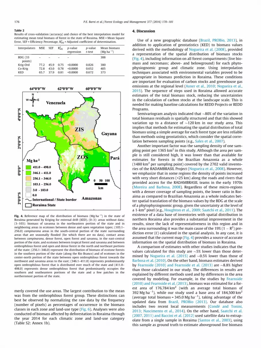
Fig. 4. Reference map of the distribution of biomass (Mg ha�1) in the state ofRoraima generated by Kriging for external drift (KED). (0–3): areas without data;(3–103): biomass of savanna in the northeastern portion of the state and inneighboring areas in ecotones between dense and open vegetation types; (103.1–256.0) campinarana areas in the south-central portion of the state surroundingareas that are seasonally flooded (for which there are no data), contact areasbetween campinarana, dense forest, open forest and savanna, in the east-centralportion of the state, and ecotones between tropical forest and savanna and betweenombrophilous forest and open and dense forest in the north and northeast portionsof the state; (256.1–346.0) represent the distribution of biomass of ecotone forestsin the southern portion of the state (along the Rio Branco) and of ecotones in thecenter-north portion of the state between open ombrophilous forest towards thenorthwest and savanna areas to the east; (346.1–411.0) represents predominantlyopen ombrophilous forest that is distributed over much of the state and (411.0–498.0) represents dense ombrophilous forest that predominantly occupies thesouthern and southeastern portions of the state and a few patches in thenorthernmost portion of the state.

Table 2Results of cross-validation (accuracy) and choice of the best interpolation model forestimating mean total biomass of forest in the state of Roraima. MSE = Mean SquareError, %EF = Efficiency Percentage, R2

adj = Adjusted coefficient of determination.

Interpolators MSE %EF R2adj p-value

regressionp-valuet-test

Mean biomass(Mg ha�1)

BDG (33points)

– – – – 388

Krig-Ord 77.2 45.9 0.75 <0.0000 0.826 380Co-Krig 72.8 43.0 0.78 <0.0000 0.652 405KED 65.7 37.9 0.81 <0.0000 0.672 373

176 P.E. Barni et al. / Forest Ecology and Management 377 (2016) 170–181

merly covered the use areas. The largest contribution to the meanwas from the ombrophilous forest group. These distinctions canbest be observed by normalizing the raw data by the frequency(number of pixels) as percentages of occurrence in the biomassclasses in each zone and land-use type (Fig. 6). Analyses were alsoconducted of biomass affected by deforestation in Roraima throughthe year 2014 for each climatic zone and land-use category(Table S2: Annex 1b).

4. Discussion

Use of a new geographic database (Brazil, PROBio, 2013), inaddition to application of geostatistics (KED) to biomass valuesderived with the methodology of Nogueira et al. (2008), provideda representation of the spatial distribution of biomass stocks(Fig. 4), including information on all forest compartments (live bio-mass and necromass; above- and belowground) for each phyto-physiognomic group and climatic zone. Using interpolationtechniques associated with environmental variables proved to beappropriate in biomass prediction in Roraima. These conditionsare important for evaluation of carbon stocks and greenhouse gasemissions at the regional level (Asner et al., 2010; Nogueira et al.,2015). The sequence of steps used in Roraima allowed accurateestimates of the total biomass stock, reducing the uncertaintiesin the calculation of carbon stocks at the landscape scale. This isneeded for making baseline calculations for REDD Projects or REDDPrograms.

Semivariogram analysis indicated that �80% of the variation intotal biomass residuals is spatially structured and that this showedvariation up to a distance of �120 km in our study area. Thisimplies that methods for estimating the spatial distribution of totalbiomass using a simple average for each forest type are less reliablethan methods using geostatistics, which consider the spatial corre-lation between sampling points (e.g., Sales et al., 2007).

Another important factor was the sampling density of one sam-pling point per 1365 km2 in this study. Although the area per sam-ple is still considered high, it was lower than that available forestimates for forests in the Brazilian Amazonia as a whole(1480 km2 per sampling point) covered by the 2702 valid invento-ries of the RADAMBRASIL Project (Nogueira et al., 2008). However,we emphasize that in some regions the density of points increasedwith very short distances (<25 km) along the roads and rivers thatprovided access for the RADAMBRASIL teams in the early 1970s(Moreira and Barbosa, 2008). Regardless of these micro-regionswith a denser coverage of sampling points, the lower ratio in Ror-aima as compared to Brazilian Amazonia as a whole indicates bet-ter spatial translation of the biomass values by the BDG at the scaleof a phytophysiognomic group, given the uncertainty at the level ofa 1-km2 pixel (e.g., Houghton et al., 2009; Saatchi et al., 2011). Theexistence of a data base of inventories with spatial distribution innorthern Roraima also provides a substantial improvement in theresults, since the lack of representativeness in this region and inthe area surrounding it was the main cause of the 19% (1 � R2) pre-diction error (Ɛ) calculated in the spatial analysis. In any case, it isassumed that the current map (Fig. 4) provides a source of accurateinformation on the spatial distribution of biomass in Roraima.

A comparison of estimates with other studies indicates that thevalues calculated for this study are �5% lower than those deter-mined by Nogueira et al. (2015) and �0.5% lower than those ofBarbosa et al. (2010). On the other hand, biomass estimates derivedby Fearnside (2010) and Fearnside et al. (2013) are �8.8% higherthan those calculated in our study. The differences in results areexplained by different methods used and by differences in the areacovered by modeling. For example, in the studies by Fearnside(2010) and Fearnside et al. (2013), biomass was estimated for a for-est area of 176,784 km2 (with an average total biomass of392 Mg ha�1), while our study used a base area of 184,500 km2

(average total biomass = 345.0 Mg ha�1), taking advantage of theupdated data from Brazil, PROBio (2013). Our database alsoincludes two recent local measurements (Condé and Tonini,2013; Nascimento et al., 2014). On the other hand, Saatchi et al.(2007, 2011) and Baccini et al. (2012) used satellite data to extrap-olate from a single sample in Roraima (Santos et al., 2003), usingthis sample as ground truth to estimate aboveground live biomass

Table 3Original stock of total biomass (live + dead; above- and belowground) and estimated weighted average per unit area of forest in the state of Roraima, representing biomasseswithout recent human impacts (deforestation, selective logging and forest fires).

Groupa Codeb Live aboveground (106

Mg)cDead aboveground(106 Mg)c

Live belowground(106 Mg)c

Total biomass stock(106 Mg)

% Mean(Mg ha�1)

Range(Mg ha�1)

Ombrophilousforest

Ab 8.3 1.5 1.8 11.6 0.2 432.1 402.4–445.1As 179.3 33.2 38.9 251.4 4.0 395.1 303.6–437.0Da 25.1 4.6 5.3 35.0 0.6 404.0 323.0–440.0Db 301.6 54.7 64.1 420.4 6.6 419.0 308.6–450.5Dm 728.2 132.1 154.9 1015.1 16.0 400.9 329.6–451.6Ds 1673.1 302.4 356.4 2331.8 36.8 404.2 291.5–445.0

Group total 2915.1 528.9 621.4 4065.3 64.3 404.3 304.3–446.7

Ecotone LO 474.7 87.9 103.1 665.7 10.5 331.3 233.3–405.3ON 594.9 110.1 129.2 834.2 13.2 318.8 238.2–390.6SN 9.6 1.8 2.1 13.4 0.2 230.2 189.3–293.6SO 42.3 7.8 9.2 59.3 0.9 277.3 218.6–341.6TN 35.9 6.6 7.8 50.3 0.8 191.8 137.8–229.6

Group Total 1157.3 214.3 251.3 1622.9 25.7 314.2 229.6–384.8

Seasonalvegetation

Fa 9.8 1.8 2.1 13.7 0.2 237.3 162.3–331.7Fs 31.3 5.8 6.8 43.9 0.7 171.4 111.5–252.5Sa 68.9 3.9 0.0 72.8 1.1 185.1 142.0–264.7Td 56.7 3.2 0.0 59.9 0.9 179.0 122.5–252.3

Group Total 136.9 24.7 28.7 190.3 3.0 182.3 128.8–261.1

Campinarana La 56.6 10.5 12.3 79.4 1.3 226.5 170.0–307.3Ld 259.6 48.1 56.4 364 5.7 214.2 182.5–343.8

Group total 316.2 58.6 68.7 443.4 7.0 216.3 180.4–337.6

Grand total 4525.4 826.4 970.1 6322.0 100 345.0 133.0–434.0

a The mean biomass stock of savannas was estimated at 14.7 � 106 Mg (5.5 Mg ha�1), or approximately 0.2% of the total biomass present in the state of Roraima.b Vegetation codes (Brazil, IBGE, 2012).c Percentages for calculation of biomass by forest compartment as in Nogueira et al. (2008).

Fig. 5. Total biomass (live + dead; above- and belowground) distinguished by forestgroup and climatic zone in Roraima (Mg ha�1 ± SD): ZIS = zone with influence ofsavanna (with shading); ZOS = zone without savanna influence (no shading).Different lowercase letters represent significant differences between means testedin the two zones (Mann-Whitney; 95%).

P.E. Barni et al. / Forest Ecology and Management 377 (2016) 170–181 177

and to represent the entire forest area. Although the Saatchi et al.(2011) and Baccini et al. (2012) maps can be considered valid forbiomass estimates at the pan-tropical scale, much larger numbersof ground-truth plots are needed at the level of the vegetationgroup and/or the local forest type for more detailed regional-scale estimates.

In terms of mean forest biomass per unit area, the results indi-cate that the modeled values (182–404 Mg ha�1) are contained inthe range established by Fearnside et al. (2013) for all forest typesin Roraima (392 Mg ha�1; range 240–513 Mg ha�1). The averagevalue (345 Mg ha�1) weighted by area suggests that the total forestbiomass per unit area in Roraima is less than that in the remainderof Brazilian Amazonia. This area in Roraima is largely located in an

ecotone with relatively dry climate, making it different from thehumid regions of the central Amazon. This condition is bestexplained by the distinction between the local climatic zonesbecause forests located close to savanna areas (ZIS) in most caseshave lower biomass than forests located in regions without longdry periods (ZOS) (Table 4 and Fig. 6). This result is consistent withother studies on biomass distribution considering the length of thedry season (Saatchi et al., 2007, 2011; Hirota et al., 2011; Bacciniet al., 2012), indicating that forests in Roraima also have an inverserelationship between biomass content and the length of the dryseason. Given these results, policies are necessary for the conserva-tion of carbon stocks in areas with longer dry periods in Roraima(ZIS), since the total area affected by deforestation in these regionsup to 2014 is 33% higher than that observed in the zone without asevere dry period (Table A.2: Annex 1b). This would have a directeffect in the reduction of the forest fires that negatively affect car-bon stocks in these regions (Barbosa and Fearnside, 1999; Xaudet al., 2013). Policy to conserve forest biomass in Roraima shouldinclude (i) regularization of land tenure; (ii) enforcement of thestate’s ecological-economic zoning (ZEE); (iii) creation of conserva-tion units, and (iv) increasing the government’s capacity to managethe protected areas (indigenous lands and conservation units) thatare already consolidated.

The distinction among the biomass stocks in different climaticzones and land-use categories was important in determining thedirect effect of these variables in the calculation of biomass andcarbon stocks. For example, a rough estimate based on the ratesof deforestation in Roraima up to 2014 indicated a disturbance in4.36% (0.276 � 109 Mg) of the original stock of total forest biomassin Roraima; ZIS = 1.95% and ZOS = 2.41% (Table S2: Annex 1b). Ofthis amount, IL and CU contributed little to disturbance of the orig-inal biomass stocks (6.8%), even though these institutional areasrepresent >65% of the total area of all of the forest physiognomies

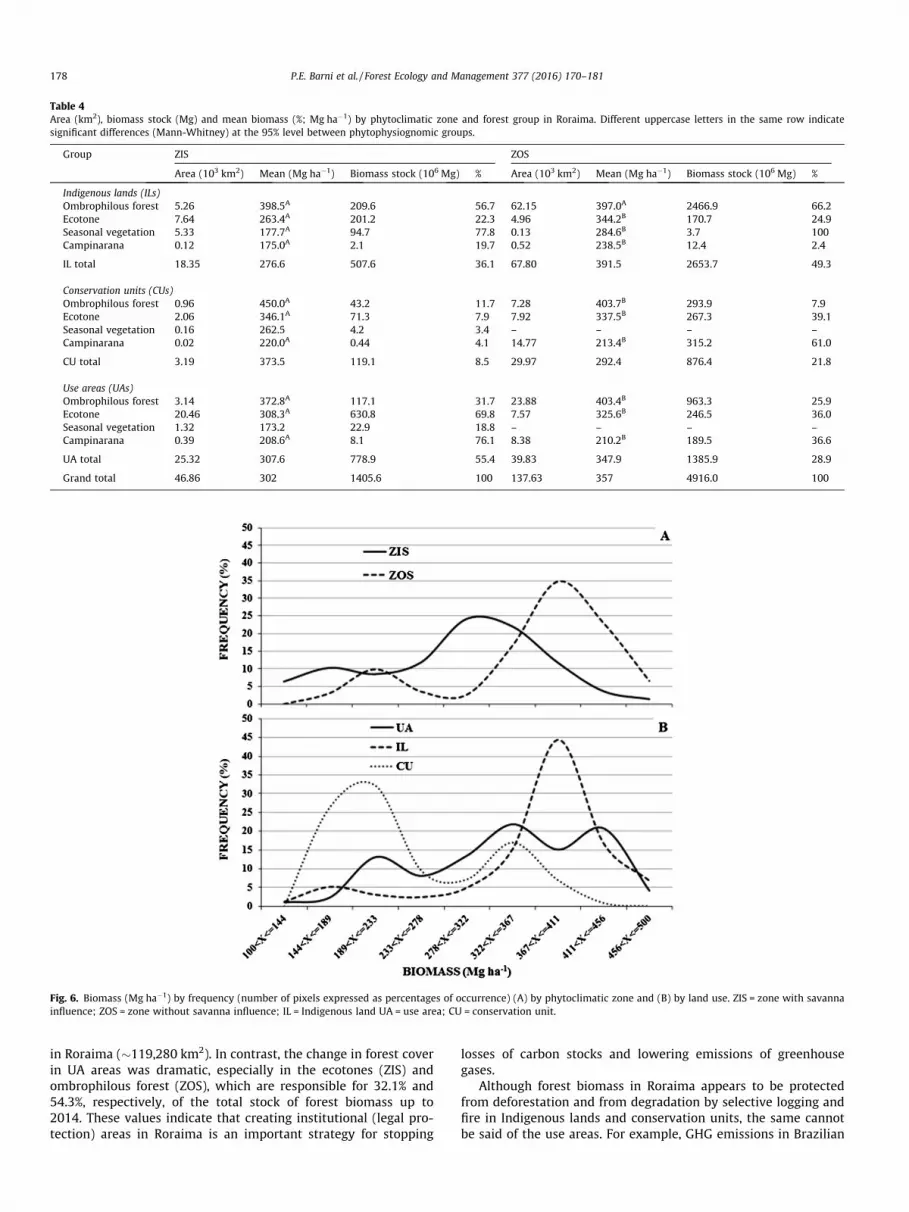
Table 4Area (km2), biomass stock (Mg) and mean biomass (%; Mg ha�1) by phytoclimatic zone and forest group in Roraima. Different uppercase letters in the same row indicatesignificant differences (Mann-Whitney) at the 95% level between phytophysiognomic groups.

Group ZIS ZOS

Area (103 km2) Mean (Mg ha�1) Biomass stock (106 Mg) % Area (103 km2) Mean (Mg ha�1) Biomass stock (106 Mg) %

Indigenous lands (ILs)Ombrophilous forest 5.26 398.5A 209.6 56.7 62.15 397.0A 2466.9 66.2Ecotone 7.64 263.4A 201.2 22.3 4.96 344.2B 170.7 24.9Seasonal vegetation 5.33 177.7A 94.7 77.8 0.13 284.6B 3.7 100Campinarana 0.12 175.0A 2.1 19.7 0.52 238.5B 12.4 2.4

IL total 18.35 276.6 507.6 36.1 67.80 391.5 2653.7 49.3

Conservation units (CUs)Ombrophilous forest 0.96 450.0A 43.2 11.7 7.28 403.7B 293.9 7.9Ecotone 2.06 346.1A 71.3 7.9 7.92 337.5B 267.3 39.1Seasonal vegetation 0.16 262.5 4.2 3.4 – – – –Campinarana 0.02 220.0A 0.44 4.1 14.77 213.4B 315.2 61.0

CU total 3.19 373.5 119.1 8.5 29.97 292.4 876.4 21.8

Use areas (UAs)Ombrophilous forest 3.14 372.8A 117.1 31.7 23.88 403.4B 963.3 25.9Ecotone 20.46 308.3A 630.8 69.8 7.57 325.6B 246.5 36.0Seasonal vegetation 1.32 173.2 22.9 18.8 – – – –Campinarana 0.39 208.6A 8.1 76.1 8.38 210.2B 189.5 36.6

UA total 25.32 307.6 778.9 55.4 39.83 347.9 1385.9 28.9

Grand total 46.86 302 1405.6 100 137.63 357 4916.0 100

Fig. 6. Biomass (Mg ha�1) by frequency (number of pixels expressed as percentages of occurrence) (A) by phytoclimatic zone and (B) by land use. ZIS = zone with savannainfluence; ZOS = zone without savanna influence; IL = Indigenous land UA = use area; CU = conservation unit.

178 P.E. Barni et al. / Forest Ecology and Management 377 (2016) 170–181

in Roraima (�119,280 km2). In contrast, the change in forest coverin UA areas was dramatic, especially in the ecotones (ZIS) andombrophilous forest (ZOS), which are responsible for 32.1% and54.3%, respectively, of the total stock of forest biomass up to2014. These values indicate that creating institutional (legal pro-tection) areas in Roraima is an important strategy for stopping

losses of carbon stocks and lowering emissions of greenhousegases.

Although forest biomass in Roraima appears to be protectedfrom deforestation and from degradation by selective logging andfire in Indigenous lands and conservation units, the same cannotbe said of the use areas. For example, GHG emissions in Brazilian

P.E. Barni et al. / Forest Ecology and Management 377 (2016) 170–181 179

Amazonia as a whole decreased from 2005 to 2010 due to thereduction in deforestation rates (Brazil, MCTI, 2015; Brazil, INPE,2016), deforestation in Roraima did not obey the same logic (Sup-plementary Material; Fig. A.2). Deforestation stabilized around anannual average of 241.1 km2 (2000–2015: Brazil, INPE, 2016),which is slightly less than the average of 277.0 km2 (1978–2006)observed by Barbosa et al. (2008) at the height of uncontrolleddeforestation. Although deforestation processes in Roraima aresimilar to those in other parts of Brazilian Amazonia (e.g.,Fearnside, 2008; Carrero and Fearnside, 2011; Barni et al., 2015a,2015b), they are also influenced by local factors. In the absenceof policy changes, deforestation and consequent greenhouse gasemissions in Roraima cannot be expected to decline soon in theuse area because of lax environmental surveillance and the preva-lence of land grabs (grilagem).

For example, in the use area in the ZIS, in addition to the forestbiomass having been degraded by logging as occurs throughoutBrazilian Amazonia (e.g., Nepstad et al., 1999; Asner et al., 2005;Broadbent et al. 2008), degradation of forest biomass is linked tothe deforestation process that is strongly related to climatic factorsand to vegetation types with open canopies (seasonal forests andecotones). These factors have influenced the occurrence of vastunderstory fires (Barbosa and Fearnside, 1999; Xaud et al., 2013;Barni et al., 2015a). Currently, some control over forest fires hasbeen achieved in this phytoclimatic zone, but higher humidity inthe ZOS seems to protect dense ombrophilous forest from fire.However, in January and February 2016, under the influence of astrong El Niño and due to the use of fire in land management(e.g., Alencar et al., 2004, 2006; Aragão and Shimabukuro, 2010),more than 1000 km2 of forest was affected by understory fires(unpublished remote-sensing data); most (84.5%) of the fires werein dense ombrophilous forest that had been subject to uncontrolledlogging (e.g., Barni et al., 2012).

5. Conclusions

Advances were made in quantifying stocks and in the spatial-ization of total original forest biomass in Roraima in relation toprevious studies that have used extrapolation to spatializebiomass in the state, thereby contributing to the reduction ofthe uncertainties in the spatial distribution of forest biomass. Thisindicates the need for spatialization of biomass stocks at amore-refined scale and making use of a greater number of plotsin order to reduce regional uncertainties about carbon pools inthe Amazon.

The reference map made available in this study provides aneasily used means of obtaining estimates at regional and localscales for studies of greenhouse-gas emissions. This map is alsoneeded for REDD projects and for public policies requiring a base-line for assessment of additionality and/or the impact of reductionsin deforestation and for assessing conservation of carbon stocks inareas under some kind of legal protection (IL and CU). The use areacovers the central portion of the state and accompanies the mainaccess highways (BR-174 and BR-210) that favor deforestation,selective logging and the invasion of public lands with consequentdegradation of forest biomass and carbon stocks. The original veg-etation in protected areas, independent of phytophysiognomicgroup, has higher biomass compared to the original vegetation inareas currently under agricultural use. Protected areas(119,310.0 km2 or 53.2% of the state) support 65.8% of Roraima’sstock of forest biomass, indicating an important potential role inREDD projects for conservation of forest carbon.

Our map of forest biomass provides an alternative reference forstudies on degradation of biomass and the emission of greenhouse

gas within the local and regional contexts and contributes informa-tion needed for the Brazilian inventory of greenhouse gasemissions.

Finally, the spatial analysis shows that, as compared to esti-mates in other studies, areas under some type of agro-silvo-pastoral use in Roraima had lower average biomass prior to defor-estation, indicating that greenhouse gas emissions from deforesta-tion and land-use change in Roraima may be lower than previouslycalculated.

Acknowledgements

This study was supported by the Universidade Estadual de Ror-aima (UERR), Instituto Nacional de Pesquisas da Amazônia (INPA-Roraima) and National Institute of Science & Technology for theEnvironmental Services of Amazonia (CNPq-INCT/SERVAMB). TheCoordenação de Aperfeiçoamento de Pessoal de Nível Superior(CAPES) provided P.E.B with a scholarship for the postgraduateprogram in climate and environment (CLIAMB). We thank the Con-selho Nacional de Desenvolvimento Científico e Tecnológico (CNPq303081/2011-2; 304020/2010-9/2008; 573810-7; 304020/2010-9)and the Brazilian Research Network on Climate Change (RedeClima). P.M.L.A. Graça, L. Nagy and two reviewers provided usefulsuggestions.

Appendix A. Supplementary material

Supplementary data associated with this article can be found, inthe online version, at http://dx.doi.org/10.1016/j.foreco.2016.07.010.

References

Ab’Saber, A.N., 1997. A Formação Boa Vista: O significado geomorfológico egeoecológico no contexto do relevo de Roraima. In: Barbosa, R.I., Ferreira, E.J.G., Castellon, E.G. (Eds.), Homem, Ambiente e Ecologia no Estado de Roraima.INPA, Manaus, Amazonas, Brazil, pp. 267–293.

Alencar, A., Nepstad, D., Diaz, M.C.V., 2006. Forest understory fire in the BrazilianAmazon in ENSO and non-ENSO years: area burned and committed carbonemissions. Earth Interact. 10, S139–S149.

Alencar, A.A., Solórzano, L.A., Nepstad, D.C., 2004. Modeling forest understory firesin an Eastern Amazonian landscape. Ecol. Appl. 14, 139–149.

Aragão, L.E.O.C., Shimabukuro, Y.E., 2010. The incidence of fire in Amazonian forestswith implications for REDD. Science 328, 1275–1278.

Asner, G.P., Powell, G.V.N., Mascaro, J., Knapp, D.E., Clark, J.K., Jacobson, J., Kennedy-Bowdoin, T., Balaji, A., Paez-Acosta, G., Victoria, E., Secada, L., Valqui, M., Hughes,R.F., 2010. High resolution forest carbon stock and emissions in the Amazon.Proc. Nat. Acad. Sci. USA 107, 16738–16742.

Asner, G.P., Knapp, D.E., Broadbent, E.N., Oliveira, P.J.C., Keller, M., Silva, J.N.M., 2005.Selective logging in the Amazon. Science 310, 480–482.

Avitabile, V., Herold, M., Heuvelink, G.B.M., Lewis, S.L., Phillips, O.L., Asner, G.P.,Armston, J., Ashton, P.S., Banin, L., Bayol, N., et al., 2016. An integrated pan-tropical biomass map using multiple reference datasets. Glob. Change Biol. 22(4), 1406–1420. http://dx.doi.org/10.1111/gcb.13139.

Baccini, A., Goetz, S.J., Walker, W.S., Laporte, N.T., Sun, M., Sulla-Menashe, D.,Hackler, J., Beck, P.S.A., Dubayah, R., Friedl, M.A., Samanta, S., Houghton, R.A.,2012. Estimated carbon dioxide emissions from tropical deforestation improvedby carbon-density maps. Nat. Clim. Change 2, 182–185.

Barbosa, R.I., 1997. Distribuição das chuvas em Roraima. In: Barbosa, R.I., Ferreira, E.J.G., Castellon, E.G. (Eds.), Homem, Ambiente e Ecologia no Estado de Roraima.Instituto Nacional de Pesquisas da Amazônia (INPA), Manaus, Amazonas, Brazil,pp. 325–335.

Barbosa, R.I., 2001. Estoque de Carbono e Emissão de CO2 e Gases-Traço pelaQueima e Decomposição da Biomassa Vegetal em Ecossistemas de Savana(Cerrado) de Roraima, Amazônia Brasileira Ph.D. thesis in ecology. InstitutoNacional de Pesquisas da Amazônia (INPA) and Universidade Federal doAmazonas (UFAM), Manaus, Amazonas, Brazil, 212 pp.

Barbosa, R.I., Campos, C., 2011. Detection and geographical distribution of clearingareas in the savannas (‘lavrado’) of Roraima using Google Earth web tool. J.Geogr. Reg. Plan. 4, 122–136.

Barbosa, R.I., Fearnside, P.M., 1999. Incêndios na Amazônia: estimativa da emissãode gases de efeito estufa pela queima de diferentes ecossistemas de Roraima napassagem do evento ‘‘El-Niño” (1997/1998). Acta Amazon. 29, 513–534.

180 P.E. Barni et al. / Forest Ecology and Management 377 (2016) 170–181

Barbosa, R.I., Fearnside, P.M., 2005. Aboveground biomass and the fate of carbonafter burning in the savannas of Roraima, Brazilian Amazonia. For. Ecol.Manage. 216, 295–316.

Barbosa, R.I., Pinto, F., Keizer, E., 2010. Ecossistemas terrestres de Roraima: Área emodelagem espacial da biomassa. In: Barbosa, R.I., Melo, V.F. (Eds.), Roraima:Homem, Ambiente e Ecologia. FEMACT, Boa Vista, Roraima, Brazil, pp. 347–368.

Barbosa, R.I., Santos, J.R.S., Cunha, M.S., Pimentel, T.P., Fearnside, P.M., 2012. Rootbiomass, root: shoot ratio and belowground carbon stocks in the opensavannahs of Roraima, Brazilian Amazonia. Aust. J. Bot. 60, 405–416.

Barbosa, R.I., Pinto, F.S., Souza, C.C., 2008. Desmatamento em Roraima: Dadoshistóricos e distribuição espaço-temporal Relatório Técnico. Ministério daCiência e Tecnologia, Instituto Nacional de Pesquisas da Amazônia – INPA,Núcleo de Pesquisas de Roraima, 10 pp.

Barni, P.E., Fearnside, P.M., Graça, P.M.L.A., 2012. Desmatamento no Sul do Estado deRoraima: padrões de distribuição em função de Projetos de Assentamento doINCRA e da distância das principais rodovias (BR-174 e BR-210). Acta Amazon.42, 195–204.

Barni, P.E., Pereira, V.B., Manzi, A.O., Barbosa, R.I., 2015a. Deforestation and forestfires in Roraima and their relationship with phytoclimatic regions in theNorthern Brazilian Amazon. Environ. Manage. 55, 1124–1138.

Barni, P.E., Fearnside, P.M., Graça, P.M.L.A., 2015b. Simulating deforestation andcarbon loss in Amazonia: impacts in Brazil’s Roraima state from reconstructingHighway BR-319 (Manaus-Porto Velho). Environ. Manage. 55, 259–278.

Bello-Pineda, J., Hernándes-Stefanoni, J.L., 2007. Comparing the performance of twospatial interpolation methods for creating a digital bathymetric model of theYucatan submerged platform. Pan-Am. J. Aquat. Sci. 2, 247–254.

Bohling, G., 2005. Introduction to Geostatistics and Variograms Analysis. KansasGeological Survey. Available at: <http://people.ku.edu/~gbohling/cpe940/>(accessed 29/07/2013).

Brazil, IBGE (Instituto Brasileiro de Geografia e Estatística), 2012. Manual Técnico daVegetação Brasileira – Manuais Técnicos em Geociências No 1. 2ª Edição Revistae Ampliada. IBGE, Rio de Janeiro, RJ, Brazil, 271 pp <ftp://geoftp.ibge.gov.br/documentos/recursos_naturais/manuais tecnicos/manual_tecnico_vegetacao_brasileira.pdf> (accessed 20/08/2013).

Brazil, IBGE (Instituto Brasileiro de Geografia e Estatística), 2013. Banco de DadosGeorreferenciado da Amazonia Legal Recursos Naturais, Vegetação. IBGE, Rio deJaneiro, RJ, Brazil <http://dados.gov.br/dataset/banco-de-dados-georreferenciado-da-amazonia-legal-recursos-naturais-vegetacao> (accessed12/05/2013).

Brazil, INPE (Instituto Nacional de Pesquisas Espaciais), 2016. Projeto PRODES –Monitoramento da Floresta Amazônica por Satélite. INPE, São José dos Campos,SP, Brazil <http://www.obt.inpe.br/prodes/index.html> (accessed 13/04/2016).

Brazil, MCT (Ministério da Ciência e Tecnologia), 2010. Segunda ComunicaçãoNacional do Brasil à Convenção-Quadro das Nações Unidas sobre Mudança doClima. MCT, Brasília, DF, Brazil, 280 pp.

Brazil, MCTI (Ministério da Ciência, Tecnologia e Inovação), 2015. TerceiraComunicação Nacional do Brasil à Convenção-Quadro das Nações Unidassobre Mudança do Clima. Setor Uso da Terra, Mudança do Uso da Terra eFlorestas. MCT, Brasília, DF, Brazil, 343 pp.

Brazil, MMA (Ministério do Meio Ambiente), 2000. Sistema Nacional de Unidades deConservação (SNUC), Lei No. 9985 de 18 de Julho de 2000. MMA, Brasília, DF,Brazil, 32 pp.

Brazil, PROBio, 2013. Mapas de Cobertura Vegetal dos Biomas Brasileiros <http://mapas.mma.gov.br/mapas/aplic/probio/datadownload.htm> (accessed 21/07/2013).

Brazil, RADAMBRASIL, 1973–1983. Levantamento dos Recursos Naturais (FolhasSA.20 Manaus; SA.21 Santarém; SB.19 Juruá; SB.20 Purus; SC.19 Rio Branco;SC.20 Porto Velho). Ministério das Minas e Energia, Rio de Janeiro, RJ, Brazil.

Broadbent, E.N., Asner, G.P., Keller, M., Knapp, D.E., Oliveira, P.J.C., Silva, J.N., 2008.Forest fragmentation and edge effects from deforestation and selective loggingin the Brazilian Amazon. Biol. Conserv. 141, 1745–1757.

Brown, S., Lugo, A.E., 1992. Biomass estimates for tropical moist forests of theBrazilian Amazon. Interciencia 17 (1), 8–18.

Brown, S., Lugo, A.E., 1994. Biomass of tropical forests: a new estimate based onforest volumes. Science 223, 1290–1293.

Burrough, P., McDonell, R., 1998. Principles of Geographical Information Systems.Oxford University Press, Oxford, UK. Available at: <http://www.rc.unesp.br/igce/ geologia/GAA01048/papers/Burrough_McDonnell-Two.pdf> (accessed 29/05/2013).

Carrero, G.C., Fearnside, P.M., 2011. Forest clearing dynamics and the expansion ofland holdings in Apuí, a deforestation hotspot on Brazil‘s TransamazonHighway. Ecol. Soc. 16 (2), 26 <http://www.ecologyandsociety.org/vol16/iss2/art26/>.

Chave, J., Condit, R., Aguilar, S., Hernandez, A., Lao, S., Perez, R., 2004. Errorpropagation and scaling for tropical forest biomass estimates. Philos. Trans. R.Soc. B 359, 409–420.

Chave, J., Réjou-Méchain, M., Búrquez, A., Chidumayo, E., Colgan, M.S., Delitti, W.B.C., Duque, A., Eid, T., Fearnside, P.M., Goodman, R.C., Henry, M., Martínez-Yrízar,A., Mugasha, W.A., Muller-Landau, H.C., Mencuccini, M., Nelson, B.W.,Ngomanda, A., Nogueira, E.M., Ortiz-Malavassi, E., Pélissier, R., Ploton, P.,Ryan, C.M., Saldarriaga, J.G., Vieilledent, G., 2014. Improved allometric modelsto estimate the aboveground biomass of tropical trees. Glob. Change Biol. 20(10), 3177–3190. http://dx.doi.org/10.1111/gcb.12629.

Condé, T.M., Tonini, H., 2013. Fitossociologia de uma Floresta Ombrófila Densa naAmazônia Setentrional, Roraima, Brasil. Acta Amazon. 43, 247–260.

Fearnside, P.M., 1992. Forest biomass in Brazilian Amazônia: comments on theestimate by Brown and Lugo. Interciencia 17 (1), 19–27.

Fearnside, P.M., 1994. Biomassa das florestas Amazônicas brasileiras. In: Bandeira,R.L., Reis, M., Borgonovi, M.N., Cedrola, S. (Eds.), Emissão � Seqüestro de CO2:Uma Nova Oportunidade de Negócios para o Brasil. Companhia Vale do Rio Doce(CVRD), Rio de Janeiro, RJ, Brazil, pp. 95–124.

Fearnside, P.M., 1996. Amazonia and global warming: annual balance of greenhousegas emissions from land-use change in Brazil’s Amazon region. In: Levine, J.(Ed.), Biomass Burning and Global Change, Biomass Burning in South America,Southeast Asia and Temperate and Boreal Ecosystems and the Oil Fires ofKuwait, vol. 2. MIT Press, Cambridge, Massachusetts, USA, pp. 606–617.

Fearnside, P.M., 1997a. Greenhouse gases from deforestation in Brazilian Amazonia:net committed emissions. Clim. Change 35 (3), 321–360.

Fearnside, P.M., 1997b. Wood density for estimating forest biomass in BrazilianAmazonia. For. Ecol. Manage. 90, 59–87.

Fearnside, P.M., 2000. Global warming and tropical land-use change: greenhousegas emissions from biomass burning, decomposition and soils in forestconversion, shifting cultivation and secondary vegetation. Clim. Change 46(1–2), 115–158.

Fearnside, P.M., 2008. The roles and movements of actors in the deforestation ofBrazilian Amazonia. Ecol. Soc. 13, 23 [Online] URL: <http://www.ecologyandsociety.org/vol13/iss1/art23/>.

Fearnside, P.M., 2010. Roraima e o aquecimento global: estimativa atualizada dobalanço anual das emissões de gases do efeito estufa provenientes da mudançade uso da terra. In: Barbosa, R.I., Melo, V.F. (Eds.), Roraima: Homem, Ambiente eEcologia. FEMACT, Boa Vista, Roraima, Brazil, pp. 369–389.

Fearnside, P.M., Barbosa, R.I., Pereira, V.B., 2013. Emissões de gases do efeito estufapor desmatamento e incêndios florestais em Roraima: Fontes e sumidouros.Revista Agroambiente 7, 95–111.

Feldpausch, T.R., Banin, L., Phillips, O.L., Lewis, S.L., Quesada, C.A., et al., 2011.Height-diameter allometry of tropical forest trees. Biogeosciences 8, 1081–1106.

Gardiman Junior, B.S., Magalhães, I.A.L., Freitas, C.A.A., Cecílio, R.A., 2012. Análise detécnicas de interpolação para espacialização da precipitação pluvial na bacia dorio Itapemirim (ES). Ambiência 8, 61–71.

Harris, N.L., Brown, S., Hagen, S.C., Saatchi, S.S., Petrova, S., Salas, W., Hansen, M.C.,Potapov, P.V., Lotsch, A., 2012. Baseline map of carbon emissions fromdeforestation in tropical regions. Science 336, 1573–1576.

Higuchi, N., dos Santos, J., Ribeiro, R.J., Minette, Y.B., 1998. Biomassa da parte aéreada vegetação da floresta tropical úmida de terra-firme da Amazônia brasileira.Acta Amazon. 28 (2), 153–166.

Hirota, M., Holmgren, M., Nes, E.H.V., Scheffer, M., 2011. Global resilience of tropicalforest and savanna to critical transitions. Science 234, 232–235.

Houghton, R.A., 2010. How well do we know the flux of CO2 from land-use change?Tellus 62B, 337–351.

Houghton, R.A., Hall, F., Goetz, S.J., 2009. Importance of biomass in the global carboncycle. J. Geophys. Res. 114, G00E03.

ISA (Instituto Socioambiental), 2012. Terras Indígenas do Brasil. ISA Roraima, BoaVista – RR (Compact Disc).

Isaaks, E., Srivastava, R., 1989. Applied Geostatistics. Oxford University Press, NewYork, USA.

Landim, P.M.B., Sturaro, J.R., 2002. Krigagem indicativa aplicada à elaboração demapas probabilísticos de riscos. Geomatematica, Texto didático, 6. DGA, IGCE,Universidade Estadual de São Paulo (UNESP), Rio Claro, São Paulo, Brazil.Available at: <http://www.rc.unesp.br/igce/aplicada/textodi.html>. Accessed25/05/13.

Malhi, Y., Wood, D., Baker, T.R., Wright, J., Phillips, O.L., Cochrane, T., Meir, P., Chave,J., Almeida, S., Arroyo, L., Higuchi, N., Killeen, T.J., Laurance, S.G., Laurance, W.F.,Lewis, S.L., Monteagudo, A., Neill, D.A., Vargas, P.N., Pitman, N.C.A., Quesada, C.A., Salomão, R., Silva, J.N.M., Lezama, A.T., Terborgh, J., Martinez, R.V., Vinceti, B.,2006. The regional variation of aboveground live biomass in old-growthAmazonian forests. Glob. Change Biol. 12, 1107–1138.

Moreira, J., Barbosa, R.I., 2008. Composição, riqueza e diversidade de árvorescomerciais inventariadas pelo Projeto RADAMBRASIL para Roraima e áreasadjacências. Mens Agitat 3 (2), 115–124.

Mitchard, E.T.A., Feldpausch, T.R., Brienen, R.J.W., Lopez-Gonzalez, G., et al., 2014.Markedly divergent estimates of Amazon forest carbon density from groundplots and satellites. Glob. Ecol. Biogeogr. 23, 935–946.

NASA-TRMM, 2013. TRMM level-3 monthly products <http://gdata1.sci.gsfc.nasa.gov/daac-binG3/gui.cgi?instance_id=TRMM_Monthly> (accessed 23/05/2013).

Nascimento, M.T., Carvalho, L.C.S., Barbosa, R.I., Villela, D.M., 2014. Variation infloristic composition, demography and above-ground biomass over a 20-yearperiod in an Amazonian monodominant forest. Plant Ecol. Divers. 7 (1–2), 293–303.

Nepstad, D.C., McGrath, D.G., Soares-Filho, B., 2011. Systemic conservation, REDD,and the future of the Amazon Basin. Conserv. Biol. 25, 1113–1116.

Nepstad, D.C., Veríssimo, A., Alencar, A., Nobre, C., Lima, E., Lefebvre, P., Schlesinger,P., Potter, C., Moutinho, P., Mendoza, E., Cochrane, M., Brooks, V., 1999. Large-scale impoverishment of Amazonian forests by logging and fire. Nature 398,505–508.

Nogueira, E.M., Nelson, B.W., Fearnside, P.M., 2005. Wood density in dense forest incentral Amazonia, Brazil. For. Ecol. Manage. 208, 261–286.

Nogueira, E.M., Fearnside, P.M., Nelson, B.W., Barbosa, R.I., Keizer, E.W.H., 2008.Estimates of forest biomass in the Brazilian Amazon: new allometric equations

P.E. Barni et al. / Forest Ecology and Management 377 (2016) 170–181 181

and adjustments to biomass from wood-volume inventories. For. Ecol. Manage.256, 1853–1867.

Nogueira, E.M., Fearnside, P.M., Nelson, B.W., França, M.B., 2007. Wood density inforests of Brazil’s ‘arc of deforestation’: implications for biomass and flux ofcarbon from land-use change in Amazonia. For. Ecol. Manage. 248, 119–135.

Nogueira, E.M., Yanai, A.M., Fonseca, F.O.R., Fearnside, P.M., 2015. Carbon stock lossfrom deforestation through 2013 in Brazilian Amazonia. Glob. Change Biol. 21,1271–1292.

R Development Core Team, 2015. R: A Language and Environment for StatisticalComputing. R Foundation for Statistical Computing, Vienna, Austria <http://www.R-project.org>.

Saatchi, S.S., Houghton, R.A., Dos Santos Alvalá, R.C., Soares, J.V., Yu, Y., 2007.Distribution of aboveground live biomass in the Amazon basin. Glob. ChangeBiol. 13, 816–837.

Saatchi, S.S., Harris, N.L., Brown, S., Lefsky, M., Mitchard, E.T.A., Salas, W., et al., 2011.Benchmark map of forest carbon stocks in tropical regions across threecontinents. Proc. Nat. Acad. Sci. USA 108, 9899–9904.

Saatchi, S., Ulander, L., Williams, M., Quegan, S., LeToan, T., Shugart, H., Chave, J.,2012. Forest biomass and the science of inventory from space. Nat. Clim. Change2 (12), 826–827.

Sales, M.H., Souza Jr., C.M., Kyriakidis, P.C., Roberts, D.A., Vidal, E., 2007. Improvingspatial distribution estimation of forest biomass with geostatistics: a case studyfor Rondônia, Brazil. Ecol. Model. 205, 221–230.

Santos, J.R., Freitas, C.C., Araujo, L.S., 2003. Airborne P-band SAR applied to the aboveground biomass studies in the Brazilian tropical rainforest. Remote Sens.Environ. 87, 482–493.

Schaefer, C., Darlymple, J., 1995. Landscape evolution in Roraima, North Amazonia:planation, paleosols and palioclimates. Zeitschrift für Geomorphologie 39, 1–28.

Soares-Filho, B., Moutinho, P., Nepstad, D., Anderson, A., Rodrigues, H., Garcia, R.,et al., 2010. Role of Brazilian Amazon protected areas in climate changemitigation. Proc. Nat. Acad. Sci. USA 107, 10821–10826.

Song, X.P., Huang, C., Saatchi, S.S., Hansen, M.C., Townshend, J.R., 2015. Annualcarbon emissions from deforestation in the Amazon Basin between 2000 and2010. PLoS ONE 10 (5), e0126754. http://dx.doi.org/10.1371/journal.pone.0126754.

Xaud, H.A.M., Martins, F.S.R.V., dos Santos, J.R., 2013. Tropical forest degradation bymega-fires in the northern Brazilian Amazon. For. Ecol. Manage. 294, 97–106.