Spatial competition between shopping centers

Antonio Brandao∗, Joao Correia-da-Silva† & Joana Pinho‡

CEF.UP and Faculdade de Economia. Universidade do Porto.

September 4th, 2013.

Abstract. We study competition between two shopping centers that sell the same set of

goods and are located at the extremes of a linear city, without restricting consumers to make

all their purchases at a single place. In the case of competition between a shopping mall (set

of independent single-product shops) and a department store (single multiproduct shop),

we find that: if the number of goods is low, all consumers shop at a single place; if it is

moderately high, some consumers travel to both shopping centers to buy each good where

it is cheaper (a single good is cheaper at the shopping mall). The shops at the mall, taken

together, obtain a lower profit than the department store. Nevertheless, two shopping malls

should be expected to appear endogenously.

Keywords: Multiproduct firms, Spatial competition, Two-stop shopping.

JEL Classification Numbers: D43, L13, R32.

The authors acknowledge financial support from CEF.UP, Fundacao para a Ciencia e Tecnologia andFEDER (PTDC/EGE-ECO/108331/2008, PTDC/EGE-ECO/111811/2009, PTDC/IIM-ECO/5294/2012and SFRH/BPD/79535/2011). We are grateful to Odd Rune Straume, Paul Belleflamme and Pedro PitaBarros for their useful comments, questions and suggestions. We are also grateful to Andres Carvajal (Editor)and two anonymous referees for their excellent reports, which allowed us to improve the paper substantially.One referee, in particular, provided very extensive and detailed comments, which were extremely useful. Wethank the participants in the CEFAGE Workshop on Industrial Economics in Evora, the 5th Meeting of thePortuguese Economic Journal, a seminar at U. Vigo, the 5th Economic Theory Workshop in Vigo, the 3rd

UECE Lisbon Meeting on Game Theory and Applications and the 2012 EARIE Conference in Rome.

∗abrandao@fep.up.pt†joao@fep.up.pt‡jpinho@fep.up.pt

1

1 Introduction

Shopping centers have existed for many centuries as galleries, market squares, bazaars or

seaport districts. Today, they are mainly organized in two alternative formats: shopping

malls and department stores. Both are spaces where consumers can buy a huge variety of

goods. But, while a department store can be seen as a multiproduct firm, a shopping mall

is constituted by independent shops.

Competition between shopping centers exists in most large cities, with physical distance

between them playing a relevant role.1 Even when they offer similar product lines, the fact

that they are spatially differentiated provides them with some market power that they can

exploit when setting prices.2 This market power is limited by the fact that some consumers

may find it worthwhile to visit more than one shopping center in order to purchase goods

where they are cheaper.

To study competition between shopping centers, one should take into account the demand

for multiple goods and also the cost of traveling to one or more shopping centers. Most of the

existing spatial competition models fail to do so, because they either restrict the analysis to

markets with a single good or assume that consumers make all their purchases at the same

place (Bliss, 1988; Beggs, 1994; Smith and Hay, 2005; Innes, 2006; Lahmandi-Ayed, 2010).

This “one-stop shopping” assumption is very convenient because it allows treating multiple

goods as a single bundled good.

We provide a study of competition between shopping centers by extending the standard

model of spatial competition (Hotelling, 1929; d’Aspremont, Gabszewicz and Thisse, 1979) to

the case of multiple goods, without assuming one-stop shopping. We consider the existence

of two shopping centers located at the extremes of a linear city, selling the same set of

goods. Consumers are uniformly spread across the city and buy exactly one unit of each

good.3 They may travel to a shopping center and buy all goods there, or travel to both

1Our hometown, Porto, having a metropolitan area with 1.3 million residents, is served by seven shop-ping centers with a commercial area above 39,000 m2: six shopping malls (ArrabidaShopping, Dolce Vita,GaiaShopping, MAR Shopping, NorteShopping and Parque Nascente), and one department store (El CorteIngles). They are more or less evenly distributed around the city, so that a car trip between two adjacentshopping centers can take around 10 minutes.

2In his empirical study on store choice in spatially differentiated markets, which uses data on store salesof packaged goods in Pittsfield (Massachusetts, U.S.A.), Figurelli (2013) reports that 99% of expenditure ison items for sale in more than one store and 96% in more than one chain of stores.

3Total demand is inelastic, as in the standard single-product model. It would undoubtedly be of interestto relax this simplifying assumption. A possible approach could be to maintain indivisibility, but introduceheterogeneous valuations for each good as in the multiproduct monopoly model of Rhodes (2012).

2

shopping centers and buy each good where it is cheaper.4

A shopping center may be either a shopping mall (where each good is sold by an inde-

pendent firm) or a department store (where a single firm sells all the goods).5 We solve for

equilibrium prices, market shares and profits in three scenarios: (i) competition between a

department store and a shopping mall; (ii) competition between two department stores; (iii)

competition between two shopping malls.

In the case of competition between a department store and a shopping mall, we find

that there may be consumers visiting the two extremes of the city or not, depending on

the number of goods that are sold by the shopping centers. If the number of goods is low,

all consumers make their purchases at a single place (one-stop shopping). If the number of

goods is moderately high, some consumers are willing to travel to both extremes of the city

to buy each good where it is cheaper (two-stop shopping). In this case, there is only one

good that is cheaper at the shopping mall than at the department store. However, its price

is low enough for some consumers to travel there just to buy this good. If the number of

goods is moderately low or very high, there is no price equilibrium in pure strategies.

Regardless of the number of goods, the equilibrium price of the bundle is lower at the

department store than at the shopping mall. This occurs because unrelated goods become

complements when they are sold at the same location (and substitutes when they are sold

at opposite extremes of the city).6 When a shop at the mall considers the possibility of

decreasing its price, it only cares about the increase of its own demand and not about the

increase of the demand of the other shops at the mall. In contrast, the department store

internalizes this effect, and takes into account that a decrease in the price of one good also

increases the demand for its other goods.7 In spite of charging a lower price for the bundle,

the department store obtains a higher profit than the shops at the mall taken together.

The scenario in which prices are lowest is that of competition between two department

stores. In this case, the price charged for the bundle of goods is equal to the price charged

4Consumers are assumed to be fully informed about the prices charged in each extreme of the city.Multiproduct pricing in the presence of search costs has been recently studied by Rhodes (2012). One of hismain conclusions is that a firm that sells more products attracts consumers that are less price-elastic and,therefore, has lower incentives to surprise customers with higher prices once they have visited the store.

5We rule out bundling strategies, i.e., we restrict the price of a bundle of goods to be equal to the sumof the prices of the individual goods. For an analysis of the bundle pricing problem in a related context, seeArmstrong and Vickers (2010). See also Hanson and Martin (1990).

6See Stahl (1987).

7Gould, Parshigian and Prendergast (2005) showed that rental contracts in shopping malls typicallyinclude incentives for an individual shop to act in a way that is beneficial for the other shops at the mall.Therefore, one should not expect a shopping mall to behave exactly as a set of independent shops.

3

in the single-good model (independently of the number of goods). The two department

stores obviously capture equal shares of the market and obtain equal profits. These are,

unsurprisingly, lower than the profits obtained when competing against a shopping mall.

Finally, in the scenario of competition between two shopping malls, we find that each

good is sold at the same price as in the single-good model. The shops behave as if consumers

only bought their good. This is the competitive scenario in which prices are highest. The

explanation is the same as before: the shops at the mall set the same price as in the single-

good model because they do not internalize the positive effect of a price decrease on the

other shops at the same mall.

After finding the equilibrium prices and profits in each of the three competitive scenarios,

it is straightforward to analyze whether it is more profitable to have a department store or

several independent shops at a mall.8 We answer this question by considering a two-stage

game in which the shopping centers start by acquiring land and then compete in prices.

We find that, if the number of goods is low, shopping malls are willing to bid higher for

the land. Therefore, the competitive scenario that appears in equilibrium is that of com-

petition between two shopping malls. However, if the number of goods is moderately high,

there is another self-fulfilling equilibrium, which is Pareto-inferior: competition between two

department stores.

As explained previously, a department store has stronger incentives to charge lower prices

than the independent shops at a mall. If the prices of the rival retailers remained the same,

the greater aggressiveness of the department store would be profitable. However, setting

lower prices induces the rivals to lower their prices as well. If the number of goods is low,

this effect dominates, leading to lower profits for everyone. The reason why both sides would

win if a department store separated itself into several independent shops was explained

by Innes (2006): “a multi-product retailer can effectively pre-commit to higher prices by

organizing itself as a mall of independent outlets”. If the number of goods is moderately

high, it becomes more profitable to compete against a department store by behaving as a

department store. But it is still better to compete against a shopping mall by behaving

as a shopping mall. This is why there are two scenarios that may emerge endogenously:

competition between two department stores or competition between two shopping malls.

We also compare the consumer surplus and the total surplus in the different competitive

scenarios. Since all consumers are assumed to buy exactly one unit of each good, a change

8Since otherwise unrelated goods become complements when they are sold at the same shopping center,this question is related to the literature on mergers between firms that sell complementary goods. See, forexample, Economides and Salop (1992), Matutes and Regibeau (1992) or Bart (2009).

4

in prices simply transfers surplus between consumers and stores. Therefore, total surplus

is maximized when consumers shop at the closest shopping center (transportation costs are

minimized).9 This occurs when there are either two department stores or two shopping

malls. Unsurprisingly, consumer surplus is maximal in the case of competition between two

department stores. Competition between two shopping malls is actually the worst scenario

for consumers. In spite of bearing a higher total transportation cost, consumers are better

off when there is competition between a department store and a shopping mall than when

there is competition between two shopping malls.

One possible policy implication of our work concerns the debate regarding the regulation

of big-box retail.10 According to Griffith, Harrison, Haskel and Sako (2003), the “wholesale

and retail” sector is responsible for 20% of the productivity gap between the U.K. and the

U.S.A.. This may partly be due to the stricter regulatory environment in the U.K., which

is restricting the development of large out-of-town retail stores.11 While the welfare-losses

associated with regulatory restrictions have been mainly focused on productivity losses due

to reduced store-size, the recent contribution of Schiraldi, Seiler and Smith (2011) focuses

on competition between large retailers and small stores with the objective of understanding

whether out-of-town big-box retail may have a predatory effect on small city centre stores

and, as a result, be detrimental to the vitality of the city centre.12 Our contribution seems

to be relevant for that discussion, as it provides a theoretical model of spatial competition

between a large retailer and a set of small independent stores. Despite the very stylized

nature of our model (in particular, the inelasticity of total demand and the absence of

substitution or complementarity between goods), which warns against taking our results

literally, we believe that our conclusions should not be readily dismissed.13

The remainder of the article is organized as follows. In Section 2, we briefly review the

9Under the assumption that total demand is inelastic, statements about total surplus should be takenwith a grain of salt. In more realistic settings, high prices entail a deadweight loss.

10We thank a referee for describing to us how our work could be meaningful to this policy issue.

11See Griffith and Harmgart (2008), Sadun (2011), Schiraldi, Seiler and Smith (2011), and Cheshire, Hilberand Kaplanis (2012). See also Bertrand and Kramarz (2002) and Schivardi and Viviano (2011) on the effectsof retail sector regulation in France and Italy, respectively.

12Using a model of consumer choice about which stores to visit and how much to spend in each store,Schiraldi, Seiler and Smith (2011) address the conflict that seems to exist between: environmental policyauthorities, according to whom out-of-town big-box stores lead to the shutdown of small downtown stores;and competition policy authorities, which view big-box stores as mainly competing among themselves. Thesettlement of this issue crucially depends on the extent to which consumers view the two types of stores assubstitutes. According to Schiraldi, Seiler and Smith (2011), two-stop shoppers are an important consumersegment for such an analysis.

13The recent contribution of Sloev, Thisse and Ushchev (2013) also seems very relevant for that discussion.

5

existing literature. In Section 3, we setup the model and obtain the demand and profit

functions. In Section 4, we find the equilibrium prices, demand and profits in each of the

three different competitive scenarios. We obtain endogenous modes of retail in Section 5, and

dedicate Section 6 to a welfare analysis. Section 7 concludes the article with some remarks.

Most of the proofs are collected in the Appendix.

2 Literature review

Our model extends the standard duopoly model of spatial competition to analyze multi-

product competition between department stores and shopping malls. To the best of our

knowledge, Lal and Matutes (1989) were the first to present a multiproduct version of the

linear city model of Hotelling (1929). Their objective was to study price discrimination

between two types of consumers.14 Building on this contribution, Lal and Matutes (1994)

and Lal and Rao (1997) introduced imperfect information about prices and the possibility

of firms announcing the prices that they charge for one or more goods (with advertising

acting as a commitment device).15 In all these works, the analysis is restricted to the case of

competition between two department stores that sell two goods. We allow a finite number

of goods and an alternative mode of retail: the shopping mall.16

Other authors have analyzed multiproduct price competition, but did not use the spatial

competition model. Moreover, most of them based the analysis on the assumption that

consumers make all their purchases at the same shopping center (Bliss, 1988; Beggs, 1994;

Smith and Hay, 2005; Innes, 2006). The empirical evidence regarding this assumption is

mixed. On the one hand, consumers concentrate most of their expenditure in a single

store. Rhee and Bell (2002) estimated that consumers make 94% of their weekly groceries

expenditures at the same supermarket, while Schiraldi, Seiler and Smith (2011) estimated

this fraction to be 86%. On the other hand, a large fraction of consumers engages in multi-

14In the model of Lal and Matutes (1989), there are two types of consumers: poor and rich. The poorhave low reservation prices and do not bear transportation costs. Therefore, they buy each good where itis cheaper (one-stop shopping is not assumed). In contrast, the rich have high reservation prices and beartransportation costs. In equilibrium, these consumers are not interested in shopping around.

15This line of research has been recently developed by Rhodes (2012). His model is quite general in thatagents have heterogeneous valuations for a finite number of indivisible goods. But, contrarily to us, he doesnot build upon the linear city model. Instead, he assumes that agents have homogeneous search costs.

16There are other extensions of the spatial competition model that allow for multiproduct firms, but inwhich consumers only buy one of the goods that are available (Giraud-Heraud, Hammoudi and Mokrane,2003; Laussel, 2006). In such settings, goods available in a shopping center are substitutes instead ofcomplements. This is also the case in the model of Gehrig (1998).

6

store shopping. Schiraldi, Seiler and Smith (2011) found that, in an average week, 39% of

shoppers visit more than one store. Stassen, Mittelstaedt and Mittelstaedt (1999) estimated

a much higher fraction, 75%. Figurelli (2013) estimated that 95% of consumers visit three

or more retail stores over a year.

A quite general multiproduct duopoly model in which consumers decide whether to buy

goods from a single seller or to bear an additional cost to buy goods from two sellers was pro-

posed by Klemperer (1992). This is a notable exception to the one-stop shopping assumption.

He analysed two cases: one in which the two department stores offer differentiated product

lines; and another in which they offer the same product line. In the first scenario, some

consumers make two-stop shopping to benefit from a greater variety of goods.17 When the

product lines are identical, the motive for two-stop shopping disappears. Consumers never

make two-stop shopping to take advantage of price differences (as they do in our model).18

There are other studies of multiproduct competition with spatial differentiation in which

two-stop shopping emerges because firms offer different sets of goods. In the model of Thill

(1992), a firm that sells two goods competes against a firm that sells only one of the goods.

He concluded that some of the consumers that need to buy both goods choose to make two-

stop shopping.19 In a recent contribution, Chen and Rey (2012a) also considered competition

between a firm that sells two goods and a firm (or a fringe of firms) that offers only one of

the goods. They show that heterogeneity in consumers’ shopping costs makes it profitable

for the multiproduct firm to price below cost the good in which it faces competition. This

loss-leading strategy allows it to discriminate two-stop shoppers from one-stop shoppers.

Interestingly, they conclude that the multiproduct firm can actually obtain a higher profit

in the presence of competition than if it were a monopolist in the sale of the two goods.

Another multiproduct duopoly model with spatial differentiation and two-stop shopping

was also recently developed by Chen and Rey (2012b). Two department stores sell the

same pair of goods, but each of them has a competitive advantage in the supply of one of the

goods. Consumers are heterogeneous in the additional cost of buying goods from both sellers

instead of a single seller. As a result, some consumers buy both goods at a single store, while

17In the contributions of Kim and Serfes (2006) and Anderson, Foros and Kind (2012), where each firmoffers a single product, consumers may also engage in two-stop shopping in order to consume both goodsinstead of a single good. This kind of setup is related to the literature on two-sided markets where multi-homing is permitted. Our contribution diverges from this strand of literature because our focus is on theinteraction between multiproduct competition and multi-stop shopping.

18The main point of the contribution of Klemperer (1992) is that the two firms may choose to offer thesame product line to decrease the level of competition.

19For a similar reason, some consumers make two-stop shopping in the model of Zhu, Singh and Dukes(2011). There, two firms sell goods 1 and 2, while a third firm sells goods 2 and 3.

7

the others buy each good where the difference between utility and price is greater. Chen

and Rey (2012b) concluded that fierce competition for one-stop shoppers dissipates profits

in this segment, but firms still earn positive profits from two-stop shoppers. This contrasts

with the results of our model, where the one-stop shoppers are the high-value segment.20

Armstrong and Vickers (2010) also studied competition between two department stores

that sell two horizontally differentiated goods, but with consumers located in a square ac-

cording to their preferences for the different varieties of the two types of goods. In their

model, some consumers make two-stop shopping because they prefer the variety of good A

that is sold by one firm and the variety of good B that is sold by the other firm.21

Regarding the comparison between the behavior of department stores and shopping malls,

the first result in the literature was presented by Edgeworth (1925), who found that it is

better, for consumers, to have a single monopolist selling two complementary goods than

to have two separate monopolists. Salant, Switzer and Reynolds (1983) arrived at a similar

conclusion, but in a model of Cournot competition. Using a framework that is closer to ours,

Bertrand competition with linear demand, Beggs (1994) concluded that it may be desirable

for a department store to separate into several shops or not, depending on the degree of

substitutability between goods. As a result, either two department stores or two shopping

malls emerge in equilibrium. Innes (2006) studied the effect of entry and concluded that

only department stores survive in equilibrium because they compete more aggressively and,

therefore, are more effective in deterring entry. Shopping malls would be driven out of the

market by department stores because when there is competition between department stores

and shopping malls, the former have higher profits.22

20In the work of Shelegia (2012), there are also two firms offering the same pair of goods, but consumersdo not necessarily buy the two goods (which may be complements or substitutes). In his model, there is nohorizontal differentiation between firms. Instead, some consumers only have access to a single firm (captives),while others have access to both firms without incurring in an additional cost (shoppers).

21The contribution of Armstrong and Vickers (2010) has also the notable feature of addressing the bundlepricing problem (they allow the price of the bundle to be lower than the sum of the prices of the individualgoods), in contrast to the existing literature on spatial multiproduct competition.

22Smith and Hay (2005) have also studied price competition under alternative modes of retail organization(shopping streets, shopping malls and department stores), but did not consider two-stop shopping norcompetition between different modes of retail.

8

3 The model

3.1 Basic setup

We consider a multiproduct version of the model of Hotelling (1929). There is a continuum

of consumers uniformly distributed across a linear city, [0, 1]. Each consumer buys one unit

of each of the products, i ∈ I ≡ {1, ..., n}, which are sold at both extremes of the city (x = 0

and x = 1).23 The price of good i at the left extreme (L) is denoted by piL and the price of

good i at the right extreme (R) is denoted by piR .

The reservation price for each good is assumed to be high enough for the market to be

fully covered. Thus, total demand is perfectly inelastic and the only decision of consumers

is where to buy each product. Each consumer chooses among three possibilities:

(L) to buy all the goods at the left extreme;

(R) to buy all the goods at the right extreme;

(LR) to travel to both extremes and buy each good where it is cheaper.

We denote by PL and by PR the price that a consumer pays for all the goods at L and

at R, respectively (PL =∑n

i=1 piL and PR =∑n

i=1 piR). By PLR, we denote the price

that a consumer pays for all the goods if she buys each good where it is cheaper (PLR =∑ni=1 min{piL , piR}).

To make their decision, consumers take into account not only the prices of the goods,

but also the transportation costs that they must bear to acquire them. We assume that

transportation costs are linear in distance.24 Let uL(x), uR(x) and uLR(x) denote the utility

attained by an agent located at x ∈ [0, 1] who chooses to purchase, respectively: all the

23As mentioned by Lal and Rao (1997), to assume that the same goods are sold at both extremes hasthe advantage of focusing the analysis on price competition. A possible interpretation is that the goods aresupplied by manufacturers that are common to both stores.

24Using data from the motion picture exhibition market in the U.S.A., Davis (2006) concluded that themarginal transportation cost is decreasing in distance, ranging from 31 cents for the first mile to 19 cents forthe 15th mile (which he refers as being the maximum distance that consumers are willing to travel). Figurelli(2013) arrived at similar conclusions for the supermarket industry, having found that the average distanceof a trip to a supermarket is 3.1 miles, and that the shopping cost ranges from 12 cents for the first mileto 10 cents for the 7th mile. In spite of this empirical evidence, we consider linear transportation costs forreasons of tractability.

9

goods at L; all the goods at R; each good where it is cheaper. Then:

uL(x) = V − PL − tx,uR(x) = V − PR − t(1− x),

uLR(x) = V − PLR − t,

where V denotes the reservation price of the bundle of goods and t > 0 denotes the trans-

portation cost per unit of distance.

It is important to keep in mind that if a consumer travels to both extremes, she bears

higher transportation costs than if she purchases all the goods at the same location. For

this reason, the demand for each product at a certain location is related to the demand for

all the other products at the same and at the other location. Products sold at the same

location are complementary goods, while products sold at different locations are substitutes.

3.2 Demand and profit functions

The consumers that are most likely to purchase a good that is sold at one extreme are those

who are located closer to that extreme. When all the goods have strictly positive demand

at both locations, the consumers near the left extreme are surely buying all the goods at L,

while those near the right extreme are surely buying all the goods at R.

Depending on the prices charged for each good at each location, some consumers may find

it worthwhile to travel to both extremes of the city, to buy each good where it is cheaper. This

occurs if some goods are sufficiently cheaper at L while other goods are sufficiently cheaper

at R. On the contrary, if the price differences across locations are relatively small, then

all the consumers make their purchases at a single location (at L or at R). These possible

demand scenarios (one-stop shopping and two-stop shopping) are illustrated in Figure 1.

0 x 1

L R

0 xL xR 1

L LR R

Figure 1: Possible demand scenarios.

To obtain the demand for each good at each location, it is useful to find the location of the

10

consumer that is indifferent between each pair of choices (among L, R and LR). Accordingly,

we use some additional notation.

By xL, we denote the location of the consumer that is indifferent between L and LR:

uL (xL) = uLR (xL) ⇔ xL = 1− PL − PLR

t.

We denote by xR the consumer that is indifferent between R and LR:

uR (xR) = uLR (xR) ⇔ xR =PR − PLR

t.

Finally, we denote by x the consumer that is indifferent between L and R. It is clear from

the expression below that x = xL+xR

2:

uL (x) = uR (x) ⇔ x =1

2+PR − PL

2t. (1)

Consumers located in x ∈ (xL, xR) choose LR. Hence, there are consumers traveling to both

extremes of the city if xL < xR, which is equivalent to∑

i∈I |piL − piR | > t. Otherwise, all

consumers make their purchases at a single place. It is easy to verify that∑

i∈I |piL−piR | ≤ t

implies that 0 ≤ x ≤ 1.25 Therefore, in this case, the demand for each good sold at L is x

and the demand for each good sold at R is 1− x.

It is convenient to denote the vector of prices of all the goods at both locations by p ∈ IR2n+

and to consider the following sets:

P1 ≡{p ∈ IR2n

+ :∑

i∈I |piL − piR | ≤ t}

;

P2 ≡{p ∈ IR2n

+ :∑

i∈I |piL − piR | > t}.

If there are consumers that travel to both extremes, the demand for a good depends on

whether this good is cheaper at L or at R. Denoting by IL and IR the sets of goods that

are strictly cheaper at L and R, respectively, we can write the expressions for the indifferent

consumers as follows:26

xL = 1− 1

t

∑i∈IR

(piL − piR) (2)

25There are prices for which the location of the consumer that is indifferent between L and R is outside theinterval [0, 1]. Precisely, this occurs when |PL−PR| > t. But

∑i∈I |piL−piR | ≤ t implies that |PL−PR| ≤ t,

which guarantees that x ∈ [0, 1].

26Formally, IL ≡ {i ∈ I : piL < piR} and IR ≡ {i ∈ I : piR < piL}.

11

and

xR =1

t

∑i∈IL

(piR − piL) . (3)

If piL = piR , consumers that travel to both extremes may either buy good i at L or at R.

We can assume, for example, that half of the consumers buys good i at L and the other half

buys it at R. Any other tie-breaking assumption would lead to the same results.

The demand for good i at L is:

qiL =

x if p ∈ P1

min {xR, 1} if p ∈ P2 ∧ piL < piR12

(min {xR, 1}+ max {0, xL}) if p ∈ P2 ∧ piL = piR

max {0, xL} if p ∈ P2 ∧ piL > piR

,

while the demand for the same good at x = 1 is qiR = 1− qiL .

The marginal cost of producing one unit of each of the goods is assumed to be zero.27

Therefore, profits coincide with sales revenues.

The profit that results from selling good i at L is:

ΠiL =

piL(

12

+ PR−PL

2t

)if p ∈ P1

piL min{

PR−PLR

t, 1}

if p ∈ P2 ∧ piL < piRpiL2

(min

{PR−PLR

t, 1}

+ max{

0, 1− PL−PLR

t

})if p ∈ P2 ∧ piL = piR

piL max{

0, 1− PL−PLR

t

}if p ∈ P2 ∧ piL > piR

.

By symmetry, the profit that results from selling good i at the right extreme of the city is:

ΠiR =

piR(

12

+ PL−PR

2t

)if p ∈ P1

piR min{

PL−PLR

t, 1}

if p ∈ P2 ∧ piR < piLpiR2

(min

{PL−PLR

t, 1}

+ max{

0, 1− PR−PLR

t

})if p ∈ P2 ∧ piR = piL

piR max{

0, 1− PR−PLR

t

}if p ∈ P2 ∧ piR > piL

.

Before moving on to study the profit-maximizing behavior of firms, it is worth making a

remark on the characteristics of the demand and profit functions.

Observe that, under two-stop shopping, the slope of the functions that give the indifferent

consumers (xL and xR) as a function of prices is 1t, whereas the slope for the indifferent

27The introduction of strictly positive marginal costs would add an unnecessary confounding factor.

12

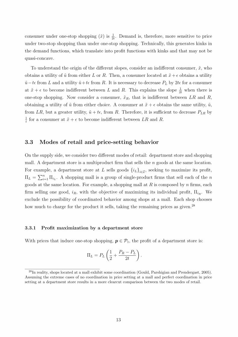
consumer under one-stop shopping (x) is 12t

. Demand is, therefore, more sensitive to price

under two-stop shopping than under one-stop shopping. Technically, this generates kinks in

the demand functions, which translate into profit functions with kinks and that may not be

quasi-concave.

To understand the origin of the different slopes, consider an indifferent consumer, x, who

obtains a utility of u from either L or R. Then, a consumer located at x+ ε obtains a utility

u− tε from L and a utility u+ tε from R. It is necessary to decrease PL by 2tε for a consumer

at x + ε to become indifferent between L and R. This explains the slope 12t

when there is

one-stop shopping. Now consider a consumer, xR, that is indifferent between LR and R,

obtaining a utility of u from either choice. A consumer at x+ ε obtains the same utility, u,

from LR, but a greater utility, u+ tε, from R. Therefore, it is sufficient to decrease PLR by1t

for a consumer at x+ ε to become indifferent between LR and R.

3.3 Modes of retail and price-setting behavior

On the supply side, we consider two different modes of retail: department store and shopping

mall. A department store is a multiproduct firm that sells the n goods at the same location.

For example, a department store at L sells goods {iL}i∈I , seeking to maximize its profit,

ΠL =∑n

i=1 ΠiL . A shopping mall is a group of single-product firms that sell each of the n

goods at the same location. For example, a shopping mall at R is composed by n firms, each

firm selling one good, iR, with the objective of maximizing its individual profit, ΠiR . We

exclude the possibility of coordinated behavior among shops at a mall. Each shop chooses

how much to charge for the product it sells, taking the remaining prices as given.28

3.3.1 Profit maximization by a department store

With prices that induce one-stop shopping, p ∈ P1, the profit of a department store is:

ΠL = PL

(1

2+PR − PL

2t

).

28In reality, shops located at a mall exhibit some coordination (Gould, Parshigian and Prendergast, 2005).Assuming the extreme cases of no coordination in price setting at a mall and perfect coordination in pricesetting at a department store results in a more clearcut comparison between the two modes of retail.

13

The bundle price, PL, that maximizes profits in this domain is:

PL =PR

2+t

2. (4)

It is always possible for the department store to set prices that add up to this PL and induce

one-stop shopping. For example, by setting piL = PL

PRpiR ,∀i ∈ I.

With prices that induce two-stop shopping, p ∈ P2, the profit of the department store is

given by:

ΠL =1

t

∑i∈IL

piL∑j∈IL

(pjR − pjL) +∑i∈IR

piL

[1− 1

t

∑j∈IR

(pjL − pjR)

]. (5)

For the choice of any piL such that i ∈ IL, the first-order condition is:

∂ΠL

∂piL= 0 ⇔

∑i∈IL

piL =1

2

∑i∈IL

piR . (6)

While, for the choice of any piL such that i ∈ IR, the first-order condition is:

∂ΠL

∂piL= 0 ⇔

∑i∈IR

piL =1

2

∑i∈IR

piR +t

2. (7)

We need to check that these candidate profit-maximizing prices are inside the domain, i.e.,

that they induce two-stop shopping. Otherwise, there are no profit-maximizing prices in the

interior of P2, which, in turn, means that the profit-maximizing prices are in P1.

The prices that satisfy the first-order conditions (6) and (7) are inside the domain of the

objective function (5) if and only if:∑i∈IL

piR −∑i∈IR

piR > t. (8)

This is actually a necessary and sufficient condition for the department store to be interested

in inducing two-stop shopping.

Lemma 1. Let PR−mini∈I {piR} ≤ 2t. A department store located at L prefers to induce two-

stop shopping with a given partition instead of one-stop shopping if and only if:∑

i∈IL piR −∑i∈IR piR > t.

Proof. See the Appendix.

14

Adding (6) and (7), we obtain (4). This means that the department store charges the same

price for the bundle of n goods regardless of whether it induces two-stop shopping or not.

Underlying this result is the fact that, while under one-stop shopping the demand of a

department store located at L is linear with reservation price equal to PR + t, under two-stop

shopping the department store faces two linear demand functions whose reservation prices

add up to PR + t.29 The bundle composed by the goods that are more expensive at L than

at R, which is only demanded by the one-stop shoppers at L, has a reservation price given

by∑

i∈IR piR + t. The bundle composed by the goods that are cheaper at L than at R is

also demanded by the two-stop shoppers, with a reservation price given by∑

i∈IL piR .

Lemma 2. Let PR − mini∈I {piR} ≤ 2t. A department store located at L sets the price of

the bundle of n goods to: PL = PR

2+ t

2.

A department store that induces two-stop shopping always finds it optimal to set prices such

that a single good is more expensive there than at the other shopping center (all the other

goods are cheaper).

Lemma 3. Let PR − mini∈I {piR} ≤ 2t. When a department store located at L induces

two-stop shopping, it sets prices pL so that the set IR contains a single element, j ∈argmini∈I {piR}. The only exception is when there is more than one good i with piR = 0. In

this case, IR can be any non-empty subset of those goods.

Proof. See the Appendix.

Given that the two-stop shoppers pay 12

∑i∈IL piR , while the one-stop shoppers pay 1

2(PR + t),

it is not surprising that a department store that induces two-stop shopping always finds it

optimal to choose the partition of goods that maximizes∑

i∈IL piR . In fact, besides being the

partition that maximizes the price paid by the two-stop shoppers, it is also the partition that

maximizes the mass of this segment. Having more two-stop shoppers is an additional advan-

tage because an increase of this segment is associated with equal decreases of the masses of

one-stop shoppers at L and at R (because we are keeping PL fixed), and a two-stop shopper

is more than half as profitable than a one-stop shopper (otherwise, two-stop shopping would

not be preferred to one-stop shopping).

Our result is related to the well-known loss leader marketing strategy, in which a single

product is sold at a low price to attract customers to the store. However, what we find is

29When a firm’s demand is linear and costs are null, the profit-maximizing price is half of the reservationprice. Therefore, in both cases, the profit-maximizing price for the bundle is PL = PR

2 + t2 .

15

that the department store should follow a pricing strategy in which all products except one

are leaders. It should set low prices for all goods except one, to attract customers, and a

very high price for a single good, to cream-skim the consumers that live nearby (who are

less willing to travel to the opposite extreme of the city).

The profit-maximizing behavior of a department store is summarized in Proposition 1.

Proposition 1. Let PR ≤ 2t and j ∈ argmini∈I {piR}. If∑

i 6=j piR − pjR ≤ t, a de-

partment store located at L induces one-stop shopping, setting prices that are such that:∑i |piL − piR | ≤ t and PL = PR

2+ t

2. If

∑i 6=j piR − pjR > t, the department store induces

two-stop shopping, setting∑

i 6=j piL = 12

∑i 6=j piR (with piL < piR ,∀i 6= j) and pjL = 1

2pjR + t

2.

3.3.2 Profit maximization by the shops at the mall

In this subsection, we consider the profit-maximization problem of an individual shop located

at the right extreme of the city.

To study the behavior of ΠiR as a function of piR , it is convenient to define a partition of

the domain of piR and consider separately the cases in which: (D1) all consumers buy good

i at R; (D2) there is two-stop shopping with i ∈ IR; (D3) there is one-stop shopping; (D4)

there is two-stop shopping with i ∈ IL; (D5) no consumer buys good i at R:

D1 = [0 , −t+ piL + sRi]

D2 = (−t+ piL + sRi , −t+ piL + sLi + sRi)

D3 = [−t+ piL + sLi + sRi , t+ piL − sLi − sRi]

D4 = (t+ piL − sLi − sRi , t+ piL − sLi)D5 = [t+ piL − sLi , +∞) ,

where sLi =∑

j∈IL\{i} (pjR − pjL) and sRi =∑

j∈IR\{i} (pjL − pjR). The above partition is

valid as long as sLi + sRi ≤ t. Otherwise, D3 becomes empty and the transition between D2

and D4 occurs at piR = piL .

16

Accordingly, the demand for good iR, as a function of piR , is:30

qiR =

1, piR ∈ D1

1t

∑j∈IR (pjL − pjR) , piR ∈ D2

12

+ 12tPL − 1

2tPR, piR ∈ D3

1− 1t

∑j∈IL (pjR − pjL) , piR ∈ D4

0, piR ∈ D5

. (9)

If D3 is not empty (sLi + sRi ≤ t), demand and profit are globally continuous functions of

piR . Otherwise (sLi + sRi > t), they exhibit a downwards jump at the transition between D2

and D4 (i.e., at piR = piL), which is the point at which the shop loses the two-stop shoppers.

In this subsection, we will not provide a complete characterization of the price-setting

behavior of the shops at a mall. We only report, for later use, the profit function in the

relevant branches (D2, D3 and D4) and the corresponding first-order conditions.

In D2, the profit of the shop is:

ΠiR =1

tpiR∑j∈IR

(pjL − pjR) ,

which leads to the following first-order condition:

piR =∑j∈IR

(pjL − pjR) ⇔ piR =1

2

∑j∈IR

pjL −1

2

∑j∈IR\{i}

pjR . (10)

In D3, the profit of the shop is:

ΠiR = piR

(1

2+PL − PR

2t

).

The corresponding first-order condition is:

piR = PL − PR + t ⇔ piR =PL

2− 1

2

∑j∈I\{i}

pjR +t

2. (11)

30The demand function is continuous and piecewise linear. Its derivative is initially zero (in D1), then it is− 1

t (in D2), changes to − 12t (in D3), becomes − 1

t again (in D4) and, finally, vanishes (in D5). Accordingly,the profit function is concave in each branch. It starts at zero (for piR = 0) and ends at zero (for piR ∈ D5).

17

Finally, in D4, the profit of the shop is:

ΠiR =piRt

[t−

∑j∈IL

(pjR − pjL)

],

and the first-order condition is given by:

piR = t−∑j∈IL

(pjR − pjL) ⇔ piR =t

2+

1

2

∑j∈IL

pjL −1

2

∑j∈IL\{i}

pjR . (12)

4 Competitive scenarios

In the previous section, we have studied the profit-maximizing behavior of the department

store and of an individual shop at a mall. In this section, we will characterize the equilibrium

prices, demand and profits in three possible competitive scenarios:

– a department store at L and a shopping mall at R;

– two department stores, one at L and another at R;

– two shopping malls, one at L and another at R.

We will show that, when a department store competes against a shopping mall, existence

and characteristics of pure strategy equilibrium crucially depend on the number of goods.

If n ≤ 4, there is a unique equilibrium in which all consumers make one-stop shopping. If

n > 4, a one-stop shopping equilibrium does not exist because the department store would

deviate and induce two-stop shopping by setting low prices for n− 1 goods and a high price

for a single good. Such a strategy allows the department store to profit the most from

two-stop shoppers, who demand the cheap goods, while maintaining the surplus extracted

from one-stop shoppers, who also buy the expensive good. If 7 ≤ n ≤ 11, there is a unique

equilibrium in which some consumers make two-stop shopping to buy n − 1 goods at the

department store and the other good at the shopping mall. If n ≤ 6 or n ≥ 12, a two-stop

shopping equilibrium cannot exist. If n ≤ 6, there are very few two-stop shoppers in the

candidate equilibrium. Thus, the single shop at the mall that is setting a low price and

capturing the two-stop shoppers prefers to set a higher price to profit more from one-stop

shoppers, and this deviation from the candidate equilibrium eliminates the reason for two-

stop shopping. If n ≥ 12, the opposite occurs. There are so many two-stop shoppers that

the shops at the mall which are setting high prices and selling only to one-stop shoppers

prefer to undercut the price set by the department store, in order to capture the two-stop

shoppers.

18

The analysis of the symmetric scenarios is more straightforward. Under competition

between two department stores, the equilibrium is identical to that of the single-product

model. The n goods are treated as a single bundled good. In the case of competition between

two shopping malls, the equilibrium corresponds to a n times replicated equilibrium of the

single-product model. Each pair of shops that sell the same good in opposite locations

behaves as in the single-product duopoly model.

4.1 Competition between a department store and a shopping mall

We start by considering the case in which there is a department store located at L and a

shopping mall located at R. The department store chooses the prices of the n goods with

the objective of maximizing its total profit (∑n

i=1 ΠiL), while each shop at the mall seeks to

maximize its individual profit (ΠiR).

4.1.1 Equilibria with one-stop shopping

In an equilibrium with one-stop shopping, the first-order conditions for profit-maximization

by the shops at the mall (11) imply that:

piR = PL − PR + t ⇒ PR = npiR = nPL − nPR + nt ⇒ PR =n

n+ 1(PL + t) . (13)

Combining this condition with the first-order condition for profit-maximization by the de-

partment store (4), we obtain the candidate equilibrium prices (see Figure 2):{PL = PR

2+ t

2

PR = nn+1

(PL + t)⇒

{PL = 2n+1

n+2t

PR = 3nn+2

t with piR = 3n+2

t, ∀i ∈ I. (14)

0 2n+ 1

2n+ 4

1

L R

Figure 2: Candidate equilibrium with one-stop shopping.

By Lemmata 1 and 3, we know that the department store prefers to deviate from this

19

candidate equilibrium and set prices that induce two-stop shopping if and only if:

∑i∈IL

piR −∑i∈IR

piR > t ⇔ 3(n− 2)

n+ 2t > t ⇔ n > 4.

This means that the candidate (14) can only be an equilibrium for n ≤ 4. As the number

of goods increases, individual prices at R decrease while the total price at R increases. For

n > 4, it becomes possible to form two bundles whose prices are sufficiently different at

R for the department store to prefer two-stop shopping. More precisely, as the number of

goods increases, good j becomes cheaper (pjR = 3n+2

t) while the bundle composed by the

remaining goods becomes more expensive (∑

i 6=j piR = 3n−3n+2

t). At n = 5, the threshold

in Proposition 1 is attained, and it becomes profitable for the department store to induce

two-stop shopping in order to exploit the greater market power it enjoys in the segment of

one-stop shoppers (consumers that are nearer) relatively to two-stop shoppers (consumers

that are more distant).

To better understand why there is no equilibrium with one-stop shopping if n ≥ 5, see

the comparison (for n = 5) between the equilibrium candidate and the profit-maximizing

deviation by the department store in Figure 3.

PL =11

7t

ΠL =121

98t

11

14PR =

15

7t

L R

4∑i=1

piL =6

7t ; p5L =

5

7t

ΠL =122

98t

5

7

6

7PR =

15

7t

L LR R

Figure 3: Comparison between the candidate one-stop shopping equilibrium (top)and the optimal deviation by the department store (bottom) when n = 5.

The shops at the mall do not deviate to a situation with two-stop shopping as long as the

20

prices at the department store satisfy the following condition:31

n∑i=1

∣∣∣∣piL − 3

n+ 2t

∣∣∣∣ ≤ n+ 6√

2− 7

n+ 2t < t.

Proposition 2. In the case of competition between a department store and a shopping mall,

there is an equilibrium with one-stop shopping if and only if n ≤ 4. It is such that:

(1) It is cheaper to buy the n goods at the department store than at the shopping mall:{PL =

∑ni=1 piL = 2n+1

n+2t, with

∑ni=1

∣∣piL − 3n+2

t∣∣ ≤ n+6

√2−7

n+2t < t

PR =∑n

i=1 piR = 3nn+2

t, with piR = 3n+2

t, ∀i ∈ I.

(2) The demand is greater at the department store:{qiL = 2n+1

2n+4

qiR = 32n+4

.

(3) The department store earns more profits than the shops at the mall taken together: ΠL =∑n

i=1 ΠiL = (2n+1)2

2(n+2)2t

ΠR =∑n

i=1 ΠiR = 9n2(n+2)2

t.

Proof. See the Appendix.

The department store does not care about how much to charge for each individual good

because all of its customers buy the entire bundle of goods. What matters for the department

store is the price of the bundle.

The department store charges a lower price for the bundle of n goods, because, when

compared with the shops at the mall, it has an additional incentive to set low prices. By

decreasing the price of one good (for example, the price of books), the department store

increases the demand for all the goods that are sold there (books, groceries, etc.). At

the shopping mall, the bookshop, when choosing the price to set for books, only takes into

account the effect on its own demand, ignoring the effect of the price of books on the demand

for groceries and the remaining goods.

31This is shown in the proof of Proposition 2. See the Appendix.

21

As a result of setting lower prices, the department store captures more than half of the

market. It does not capture the whole market because the customers that are closer to

the shopping mall weigh the price advantage of the department store against the proximity

advantage of the shopping mall. In equilibrium, the shopping mall retains the consumers

that are sufficiently close.

Comparing the joint profit at each extreme of the city, we find that the department store

earns more than the shops at the mall taken together.

4.1.2 Equilibria with two-stop shopping

In an equilibrium with two-stop shopping, by Lemma 3, the department store must be selling

n− 1 goods at a lower price than the shopping mall and a single good at a higher price.

Adding the first-order conditions for profit-maximization by the n− 1 shops at the mall

that sell goods in IL, given by (12), we obtain the following best-response function:

∑i∈IL

piR = (n− 1)t− (n− 1)∑i∈IL

(piR − piL) ⇔∑i∈IL

piR =n− 1

n

(t+

∑i∈IL

piL

).

Combining it with the first-order condition for profit-maximization by the department store

(6), we obtain: { ∑i∈IL piR = 2n−2

n+1t, with piR = 2

n+1t,∀i ∈ IL∑

i∈IL piL = n−1n+1

t.

For the single shop at the mall that sells a good i ∈ IR, the first-order condition for profit-

maximization is (10):

piR =piL2.

While the corresponding first-order condition for profit-maximization by the department

store is (7):

piL =piR2

+t

2.

Combining the two conditions, we obtain:

piR =t

3and piL =

2t

3.

In spite of charging a higher price, the department store has a greater demand because many

22

of its customers do not find it profitable to make two-stop shopping:

qiR =1

3and qiL =

2

3.

The candidate equilibrium with two-stop shopping is represented in Figure 4.

PL =5n− 1

3n+ 3t

2

3

n− 1

n+ 1PR =

7n− 5

3n+ 3t

L LR R

Figure 4: Candidate equilibrium with two-stop shopping.

The department store is only interested in setting prices that induce two-stop shopping if

condition (8) is satisfied. Substituting the expressions for the candidate equilibrium prices,

this condition becomes:

2n− 2

n+ 1t− t

3> t ⇔ n > 5.

For n ≤ 5, the candidate equilibrium is upset because the department store prefers to set

prices that induce one-stop shopping.32

We must also verify that the shop at the mall that is setting the low price does not deviate

to a price that induces one-stop shopping. From, the first-order condition (11), we find the

following candidate deviation (which induces one-stop shopping for n ≤ 8):

piR =PL

2− 1

2

∑j∈I\{i}

pjR +t

2=

n− 1

2(n+ 1)t+

t

3− n− 1

n+ 1t+

t

2=

n+ 4

3(n+ 1)t.

The corresponding profit is:

ΠiR = piR (1− x) =(n+ 4)2

18(n+ 1)2t.

32Recall that in the candidate equilibrium with one-stop shopping, the department store preferred todeviate and induce two-stop shopping for n ≥ 5. It is not contradictory that, for n = 5: the departmentstore prefers to induce two-stop shopping when facing the one-stop shopping candidate equilibrium; andprefers to induce one-stop shopping when facing the two-stop shopping equilibrium. This behavior prevents,however, the existence of an equilibrium when n = 5.

23

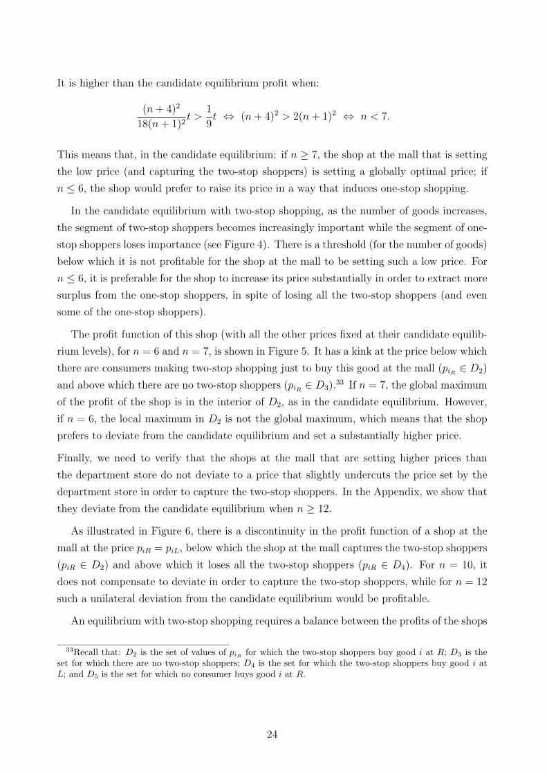
It is higher than the candidate equilibrium profit when:

(n+ 4)2

18(n+ 1)2t >

1

9t ⇔ (n+ 4)2 > 2(n+ 1)2 ⇔ n < 7.

This means that, in the candidate equilibrium: if n ≥ 7, the shop at the mall that is setting

the low price (and capturing the two-stop shoppers) is setting a globally optimal price; if

n ≤ 6, the shop would prefer to raise its price in a way that induces one-stop shopping.

In the candidate equilibrium with two-stop shopping, as the number of goods increases,

the segment of two-stop shoppers becomes increasingly important while the segment of one-

stop shoppers loses importance (see Figure 4). There is a threshold (for the number of goods)

below which it is not profitable for the shop at the mall to be setting such a low price. For

n ≤ 6, it is preferable for the shop to increase its price substantially in order to extract more

surplus from the one-stop shoppers, in spite of losing all the two-stop shoppers (and even

some of the one-stop shoppers).

The profit function of this shop (with all the other prices fixed at their candidate equilib-

rium levels), for n = 6 and n = 7, is shown in Figure 5. It has a kink at the price below which

there are consumers making two-stop shopping just to buy this good at the mall (piR ∈ D2)

and above which there are no two-stop shoppers (piR ∈ D3).33 If n = 7, the global maximum

of the profit of the shop is in the interior of D2, as in the candidate equilibrium. However,

if n = 6, the local maximum in D2 is not the global maximum, which means that the shop

prefers to deviate from the candidate equilibrium and set a substantially higher price.

Finally, we need to verify that the shops at the mall that are setting higher prices than

the department store do not deviate to a price that slightly undercuts the price set by the

department store in order to capture the two-stop shoppers. In the Appendix, we show that

they deviate from the candidate equilibrium when n ≥ 12.

As illustrated in Figure 6, there is a discontinuity in the profit function of a shop at the

mall at the price piR = piL, below which the shop at the mall captures the two-stop shoppers

(piR ∈ D2) and above which it loses all the two-stop shoppers (piR ∈ D4). For n = 10, it

does not compensate to deviate in order to capture the two-stop shoppers, while for n = 12

such a unilateral deviation from the candidate equilibrium would be profitable.

An equilibrium with two-stop shopping requires a balance between the profits of the shops

33Recall that: D2 is the set of values of piR for which the two-stop shoppers buy good i at R; D3 is theset for which there are no two-stop shoppers; D4 is the set for which the two-stop shoppers buy good i atL; and D5 is the set for which no consumer buys good i at R.

24

0 D2 D3 D5 piR

ΠiR

(n=6)

0 D2 D3 D5 piR

ΠiR

(n=7)

Figure 5: Profit function of the shop that sells the cheap good at the mall, given that the otherstores are charging the prices of the candidate equilibrium with two-stop shopping.

at the mall that are setting high prices and the profits of the shop that is setting a low price,

so that neither wishes to change its pricing strategy. When the number of goods is low

(n ≤ 6), the two-stop shopping segment is small, therefore, the shop that is setting a low

price deviates. When the number of goods is high (n ≥ 12), it is the one-stop shopping

segment that is small. As a result, a shop that is setting a high price prefers to deviate and

lower its price substantially, in order to capture all the two-stop shoppers. It is only when

the number of goods is intermediate (7 ≤ n ≤ 11) that none of the shops deviates from the

two-stop shopping equilibrium.

Proposition 3. In the case of competition between a department store and a shopping mall,

there is an equilibrium with two-stop shopping if and only if 7 ≤ n ≤ 11. It is such that:

(1) It is cheaper to buy n − 1 of the n goods at the department store than at the shopping

mall: #IL = n− 1 and #IR = 1.

(2) The prices of the goods that are cheaper at the department store, i ∈ IL, are such that:{ ∑i∈IL piL = n−1

n+1t, with piL ≤ 12

(n+1)2t,∀i ∈ IL∑

i∈IL piR = 2(n−1)n+1

t, with piR = 2n+1

t,∀i ∈ IL,

and the corresponding demands are:

qiL =n− 1

n+ 1and qiR =

2

n+ 1.

25

0 D2 D4 D5 piR

ΠiR

(n=10)

0 D2 D4 D5 piR

ΠiR

(n=12)

Figure 6: Profit function of a shop that sells an expensive good at the mall, given that theother stores are charging the prices of the candidate equilibrium with two-stop shopping.

(3) The prices of the only good that is cheaper at the shopping mall, i ∈ IR, are:

piL =2

3t and piR =

1

3t,

and the demands are:

qiL =2

3and qiR =

1

3.

(4) The department store earns more profits than the shops at the mall taken together:{ΠL = (n−1)2

(n+1)2t+ 4t

9

ΠR = 4(n−1)(n+1)2

t+ t9

.

Curiously, independently of the number of goods, exactly two thirds of the consumers buy

all the products at the department store. For the remaining, which are located at x ∈(

23, 1],

the cost of visiting the shopping mall is smaller than t3. However, the difference in the price

of good i ∈ IR is: piL − piR = t3. Thus, for all these consumers, it is worthwhile to buy

the good i ∈ IR at the shopping mall. As the number of goods increases, there are more

consumers willing to make their purchases at both extremes of the city.

When the number of goods is low (n ≤ 6), the shop that sells the cheap good at the

mall is not capturing (in the candidate equilibrium) much more consumers than the shops

that sell the expensive goods (see Figure 4). It prefers to deviate and set a higher price,

which induces one-stop shopping. As the number of goods increases, to sell a cheap good

becomes more profitable, because the two-stop shopping segment, x ∈(

23, n−1n+1

), increases.

26

As a result, when the number of goods is high (n ≥ 12), the shops that sell the expensive

goods at the mall prefer to deviate and set a lower price, to capture the customers that make

two-stop shopping.

There only exists equilibrium with one-stop shopping when n ≤ 4 and with two-stop

shopping when 7 ≤ n ≤ 11. Therefore, there is no equilibrium (in pure strategies) when the

number of goods is 5 ≤ n ≤ 6 or n ≥ 12.

4.2 Competition between two department stores

Now, we consider the case in which there are two department stores, one at each extreme

of the city. Each department store chooses the price to charge for each of the n goods, with

the objective of maximizing its profit, taking as given the prices set by its competitor.

Proposition 4. In the case of competition between two department stores:

(1) The price of the bundle is equal to the transportation cost parameter:

PL = PR = t, withn∑

i=1

|piL − piR | ≤ t.

(2) Consumers make all their purchases at the closest department store:

qiL = qiR =1

2.

(3) The resulting profits are also independent of the number of goods:

ΠL = ΠR =t

2.

Proof. See the Appendix.

In equilibrium, the department stores charge the same price for the bundle of n goods (there

is, once more, some indeterminacy regarding the split of the bill between the goods). No

consumer is willing to travel to both extremes of the city. All consumers buy the n goods

at the closest department store.

What may be surprising is that the margin (difference between price and marginal cost)

with n goods is the same as in the standard Hotelling model, in which a single good is

27

sold. The reason why the margin is not greater with n goods is related to the fact that the

reservation utility of the customer is not relevant for the pricing decisions of the firms (as

long as it is high enough, as it is typically assumed). With one-stop shopping, the n goods

are equivalent to a single bundled good. Therefore, even if customers attribute a higher

utility to the n goods than to a single good, the margin remains constant and equal to the

transportation cost parameter.34

4.3 Competition between two shopping malls

In the case of competition between two shopping malls (one at each extreme of the city), the

shops that sell the same good at different locations are direct competitors. However, their

demand also depends on the prices of the other goods. This interdependence across shops

selling different goods exists because, when deciding where to buy each good, consumers

take into account not only the price but also the transportation costs that they have to bear.

A shop benefits from having low prices for the goods sold at the same location (since this

attracts customers to its location); and high prices for the goods sold at the other location

(since this repels customers from the other location). But since this externality has no

influence on the pricing decisions of the shops, the equilibrium of the model replicates that

of the single-product model.

Proposition 5. In the case of competition between two shopping malls:

(1) The price of each good is equal to the transportation cost parameter:

piL = piR = t, ∀i ∈ I.

(2) Consumers make all their purchases at the closest shopping mall:

qiL = qiR =1

2, ∀i ∈ I.

(3) The profit of each firm is also independent of the number of goods:

ΠiL = ΠiR =t

2, ∀i ∈ I.

Proof. See the Appendix.

34The same occurs in the case of Bertrand competition with homogeneous products. Independently of thenumber of products that firms sell, their equilibrium margin is always null.

28

Notice that the joint profit of the n shops located at a shopping mall is greater than the

profits obtained in any of the alternative scenarios that we have considered.

5 Endogenous modes of retail

Until now, we have assumed that the organization of each shopping center was exogenous.

In this section, we analyze whether one should expect department stores or shopping malls

to appear endogenously.

More precisely, we consider a two-stage game in which two land owners (one at L and

another at R) start by simultaneously auctioning their land for the construction of depart-

ment stores or shopping malls.35 Price competition as studied in the previous section takes

place afterwards.

We assume that land is allocated to the form of retail that is more profitable, because

managers of more profitable projects are willing to bid higher. Therefore, what we need is

to compare the profit of a department store with the joint profit of the shops that constitute

a shopping mall.36

For n ≤ 4, the profits of the shopping centers in each competitive scenario are shown in

Table 1.

Department Store Shopping Mall

Department Store(

12t , 1

2t) (

(2n+1)2

2(n+2)2t , 9n

2(n+2)2t)

Shopping Mall(

9n2(n+2)2

t , (2n+1)2

2(n+2)2t) (

n2t , n

2t)

Table 1: Profits of the competing shopping centers if n ≤ 4.

Proposition 6. If n ≤ 4, a shopping mall is more profitable than a department store,

regardless of whether its competitor is a department store or a shopping mall.

35What we designate by shopping mall is simply a co-located group of independent shops. In reality, sucha group may constitute a shopping street instead of a mall. In that case, there would be many independentshops bidding for fractions of land.

36As in the previous section, we do not consider the possible combination of a smaller department store(selling a subset of the existing goods, Ids ⊂ I) with several independent shops (each selling one of theremaining goods, i ∈ I \Ids). This could change the outcome of the game, as suggested by the contributionsof Salant, Switzer and Reynolds (1983) and Kamien and Zang (1990).

29

We expect, therefore, that the land is allocated to the development of shopping malls or

shopping streets and not to the development of department stores.

For 7 ≤ n ≤ 11, the payoff matrix is given in Table 2.

Department Store Shopping Mall

Department Store(

12t , 1

2t) (

(n−1)2

(n+1)2t+ 4

9t , 4(n−1)

(n+1)2t+ 1

9t)

Shopping Mall(

4(n−1)(n+1)2

t+ 19t , (n−1)2

(n+1)2t+ 4

9t) (

n2t , n

2t)

Table 2: Profits of the competing shopping centers if 7 ≤ n ≤ 11.

Proposition 7. If 7 ≤ n ≤ 11, a shopping mall is more profitable than a department store

when competing against a shopping mall, while a department store is more profitable than a

shopping mall when competing against a department store.

If the land at L and at R is auctioned simultaneously, there are two equilibrium outcomes.

If department stores are expected to form, department stores will bid higher than shopping

malls; if the opening of shopping malls is expected, shopping malls will bid higher.

Of course, the retailers will prefer to coordinate on the equilibrium with two shopping

malls. Therefore, we should expect to have shopping malls at both extremes of the city.

This would also be the case if the allocation of land at L and R were sequential instead of

simultaneous.

Our results are robust to a variation of the first-stage game in which there is a single

owner of land or, equivalently, there is collusion between the two owners. It is clear that two

shopping malls emerge in equilibrium.

We have implicitly assumed that the regulatory environment does not allow a retailer to

own both shopping centers. If that was possible, a single retailer would be the highest bidder

for the two pieces of land - as it would, then, enjoy monopoly profits.37

37In this model, since total demand is inelastic, a monopolist would be able to raise prices up to thereservation price of the consumer located in the middle of the city.

30

6 Welfare analysis

6.1 Total surplus

In this model, the total demand is assumed to be perfectly inelastic (each consumer buys one

unit of each good that is available in the market, independently of the prices of the goods).

Therefore, a change in prices only leads to a transfer of surplus between consumers and firms.

The total surplus remains constant. In this context, the maximization of total surplus is

equivalent to the minimization of total transportation costs incurred by consumers.

Total transportation costs are minimized when each consumer shops at the closest shop-

ping center. This occurs in the case of competition between two department stores and in

the case of competition between two shopping malls. When there is a department store

competing with a shopping mall, the indifferent consumer is no longer located at the middle

of the city. If n ≤ 4, there are more consumers shopping at the department store than at the

shopping mall (x > 12). If 7 ≤ n ≤ 11, there are consumers who shop at both extremes of

the city. Total transportation costs are even higher in such a situation. Thus, the existence

of different modes of retail diminishes total surplus.

The assumption of inelastic demand seems to be crucial for the conclusion that total

surplus is higher when there are two shopping malls than when there is one shopping mall

and one department store. With elastic demand, since production costs are null, the so-

cial optimum would consist in having null prices (with inelastic demand, symmetric prices

suffice). It seems, therefore, that in the presence of a significant level of demand elasticity,

the deadweight loss due to high prices and low demand would render the scenario with two

shopping malls the least desirable from a social point of view.

Given the limitations of our model, it seems preferable to focus the attention on consumer

surplus rather than total surplus as a guide for policy design.

6.2 Consumer surplus

Let CSDD, CSMM and CSDM denote the consumer surplus in each of the three scenarios:

(DD) competition between two department stores; (MM) competition between two shopping

malls; and (DM) competition between a department store and a shopping mall.

If the shopping centers are organized in the same way, they charge the same price for the

bundle of goods. As a result, the indifferent consumer is located at the middle of the city

31

and the total transportation cost is minimized. We have:

CSDD = x (V − t) + x (V − t)− t∫ x

0

x dx− t∫ 1

x

(1− x) dx = V − 5

4t;

CSMM = x (V − nt) + x (V − nt)− t∫ x

0

x dx− t∫ 1

x

(1− x) dx = V − 4n+ 1

4t.

When a department store competes with a shopping mall and n ≤ 4 (equilibrium with

one-stop shopping), consumer surplus is:

CSDM =

∫ x

0

(V − PL − tx) dx+

∫ 1

x

[V − PR − t(1− x)] dx = V − 10n2 + 28n+ 7

4(n+ 2)2t.

When 7 ≤ n ≤ 11 (equilibrium with two-stop shopping), it is given by:

CSDM =

∫ xL

0

(V − PL − tx) dx+

∫ xR

xL

(V − PLR − t) dx+

∫ 1

xR

[V − PR − t(1− x)] dx

= V − 19n2 + 20n− 17

9(n+ 1)2t.

For consumers, competition between department stores is the most favorable scenario. Prices

are lower than in the other scenarios, and transportation costs are minimized. It is not

so straightforward to compare the case of competition between two shopping malls (lower

transportation costs) with the case of competition between a shopping mall and a department

store (lower prices). We find that the price effect dominates. Consumers prefer competition

between a shopping mall and a department store rather than competition between two

shopping malls.

Proposition 8. Comparing the consumer’ surplus in the three competitive scenarios, for

2 ≤ n ≤ 4 and for 7 ≤ n ≤ 11, we obtain:

CSDD > CSDM > CSMM .

Proof. Straightforward from the above expressions for CSDD, CSDM and CSMM .

It is somewhat surprising that the lower is the number of independent stores in the market,

the higher is the consumer surplus. This result contradicts the typical intuition, according to

which as the number of firms in the market increases, competition becomes stronger, leading

to lower prices. In our model, this is not the case, since the price for the bundle of goods is

cheaper when there are only two department stores.

32

7 Conclusions

We have developed a multiproduct version of the model of Hotelling (1929) to study compe-

tition between shopping centers that can be organized as department stores or as shopping

malls. In particular, we analyzed how the modes of retail affect prices, market shares and

profits, and which retail structure is more likely to emerge endogenously.

Relatively to the existing theoretical literature, our focus was on relaxing the one-stop

shopping assumption.38 For the model to remain tractable, we have maintained the hypothe-

ses of the model of Hotelling (1929): inelasticity of total demand, linearity of transportation

costs and uniform distribution of consumers. In addition, we have assumed that the two com-

peting shopping centers are exogenously located at opposite extremes of the city and that

they offer the same exogenous product line. Our stylized model has, therefore, limitations

that advise against taking our results literally.

A department store competes more aggressively than a shopping mall, because it takes

into account that a decrease of the price of one good increases the demand for all its goods.

In contrast, a shop at a mall only takes into account its individual demand when setting the

price of its good.

As a result, when a department store competes with a shopping mall, the bundle of goods

is cheaper at the department store than at the shopping mall. The greater demand more

than compensates the lower price, hence, the department store obtains higher profits than

the shops at the mall taken together. In spite of having higher profits, the department store

has incentives to separate itself into a shopping mall. In fact, the competitive scenario that

is expected to emerge endogenously is competition between two shopping malls.

When the mode of retail is the same in the two shopping centers, our results are identical

to those of the single-product model. In the case of competition between department stores,

multiple goods are treated as a single bundled good. In the case of competition between

shopping malls, multiple goods originate replicas of the single-product model. In these cases,

no consumer finds it worthwhile to shop at both shopping centers.

It is when a department store competes with a shopping mall that our results are more

interesting. If the number of goods is low, there is one-stop shopping in equilibrium, but,

if the number of goods is moderately high, some consumers travel to both extremes of the

city to buy each product where it is cheaper. In this case, the department store sells all

38The empirical contributions of Stassen, Mittelstaedt and Mittelstaedt (1999), Schiraldi, Seiler and Smith(2011) and Figurelli (2013) suggest that assuming one-stop shopping would be too restrictive.

33

goods except one at a low price, to attract and profit the most from two-stop shoppers, and

a single good at a high price, to cream-skim the customers who live nearer to the store.

It would be of interest to investigate whether this pricing strategy remains optimal without

the assumption that total demand is inelastic. With elastic demand, concentrating the

upward distortion on a single good and distributing the downward distortions among all

the remaining goods may not be the most profitable way to induce two-stop shopping. The

demand for the single expensive good could become too reduced.

If the number of goods is moderately low or very high, there is no equilibrium in pure

strategies for the case of competition between a department store and a shopping mall.

Therefore, a natural extension of this work would be to allow mixed strategies. The shops

would set prices simultaneously and irreversibly, and then consumers would observe the prices

and decide their purchases. An alternative would be to consider that consumers would have

to travel to a shopping center to observe the prices that were actually set, and then decide

whether to travel to the other shopping center or not. We leave this extension for future

work.

The dependence of results on the number of goods is one of the most peculiar aspects of

our model. In order to have some intuition for the impact of the number of goods, we may

view the shopping mall as becoming less coordinated when the number of goods increases.

This, given the discontinuities and failures of quasi-concavity of the profit functions of the

department store and of the shops at the mall, originates the qualitative changes on the

existence of one-stop shopping or two-stop shopping equilibria.

In reality, the number of goods is an endogenous variable. Unfortunately, our model is not

appropriate to account for this endogeneity. In the case of competition between shopping

malls, profits are proportional to the number of goods. Therefore, the shopping mall would

like the number of goods to be as high as possible. However, increasing the number of goods

indefinitely strains the assumption that consumers are willing to buy one unit of each good.

We believe that our conclusions show that reducing the research on multiproduct compe-

tition to the case of two goods may be restrictive. In the specific case of our stylized model,

more than two goods are necessary to generate two-stop shopping. Moreover, in a model

with only two goods, the strategy of setting a high price for a single good and low prices for

the remaining goods would be undistinguishable from a strategy of selling a single good at

a low price and the remaining at a high price.

34

8 Appendix

Proof of Lemma 1.

(⇒) Let us start by showing that if the department store prefers to induce two-stop shopping,

then∑

i∈IL piR −∑

i∈IR piR > t.

Suppose, by way of contradiction, that∑

i∈IL piR −∑

i∈IR piR ≤ t. In this case, to induce

two-stop shopping, the department store has to sell the bundle of goods IL at a lower price

than the bundle IR:{ ∑i∈IL piR −

∑i∈IR piR ≤ t∑

i∈IL (piR − piL) +∑

i∈IR (piL − piR) > t⇒

∑i∈IL

piL <∑i∈IR

piL .

From the expressions that yield the indifferent consumers, (1)-(3), for any given PL (the

same with one-stop shopping and two stop-shopping), the indifferent consumer with one-

stop shopping is at the midpoint between the indifferent consumers with two-stop shopping:

xR − x = x− xL.

This implies that, for any given PL, the one-stop shopping scenario is more profitable

than the two-stop shopping scenario:∑i∈IL

piL <∑i∈IR

piL ⇔ (xR − x)∑i∈IL

piL < (x− xL)∑i∈IR

piL

⇔ xR∑i∈IL

piL + xL∑i∈IR

piL < xPL. (15)

This contradicts our hypothesis. Therefore,∑

i∈IL piR −∑

i∈IR piR > t is a necessary condi-

tion for the department store to prefer two-stop shopping.

(⇐) Let us now show that if∑

i∈IL piR −∑

i∈IR piR > t, then the department store prefers

to induce two-stop shopping.

We start by showing that, under the current hypotheses and with the piL given by the

first-order conditions (6) and (7), we have: (i) xR ∈ [0, 1]; (ii) xL ∈ [0, 1]; (iii) p ∈ P2; (iv)∑i∈IL piL <

∑i∈IL piR ; and (v)

∑i∈IR piL >

∑i∈IR piR .

Conditions (i) and (ii) ensure that the indifferent consumers are inside the interval [0, 1],

and condition (iii) ensures that xL < xR. This implies that the demand for goods in IL is xR

and the demand for goods in IR is xL. From conditions (iv) and (v), the individual prices

are not incompatible with the partitions. More precisely, there exist prices pL that induce

35

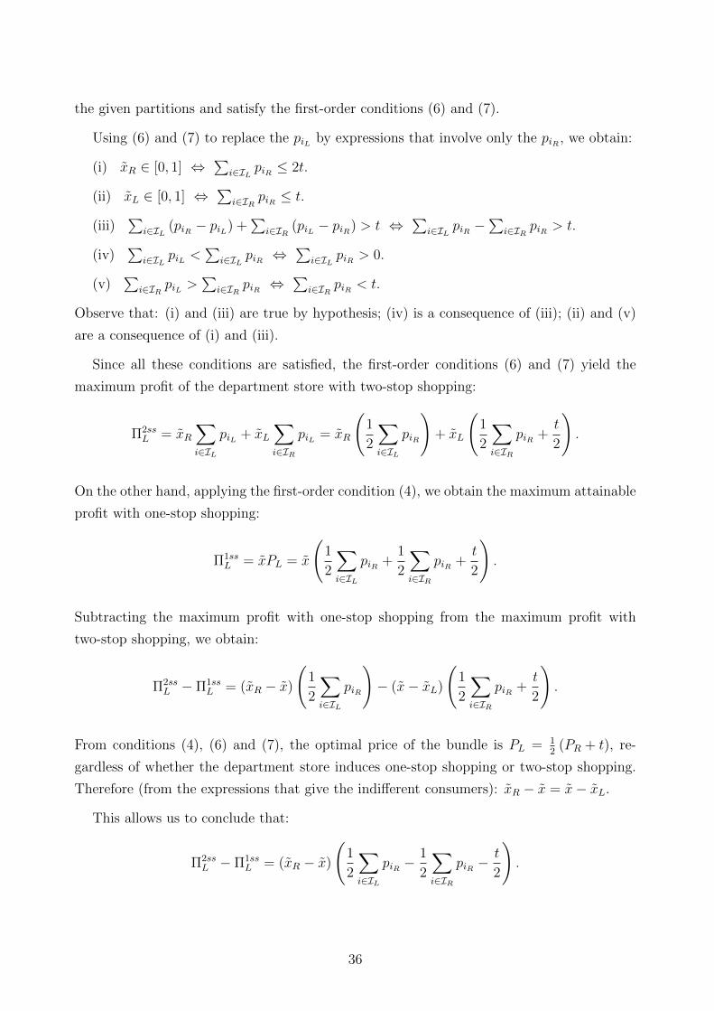
the given partitions and satisfy the first-order conditions (6) and (7).

Using (6) and (7) to replace the piL by expressions that involve only the piR , we obtain:

(i) xR ∈ [0, 1] ⇔∑

i∈IL piR ≤ 2t.

(ii) xL ∈ [0, 1] ⇔∑

i∈IR piR ≤ t.

(iii)∑

i∈IL (piR − piL) +∑

i∈IR (piL − piR) > t ⇔∑

i∈IL piR −∑

i∈IR piR > t.

(iv)∑

i∈IL piL <∑

i∈IL piR ⇔∑

i∈IL piR > 0.

(v)∑

i∈IR piL >∑

i∈IR piR ⇔∑

i∈IR piR < t.

Observe that: (i) and (iii) are true by hypothesis; (iv) is a consequence of (iii); (ii) and (v)

are a consequence of (i) and (iii).

Since all these conditions are satisfied, the first-order conditions (6) and (7) yield the

maximum profit of the department store with two-stop shopping:

Π2ssL = xR

∑i∈IL

piL + xL∑i∈IR

piL = xR

(1

2

∑i∈IL

piR

)+ xL

(1

2

∑i∈IR

piR +t

2

).

On the other hand, applying the first-order condition (4), we obtain the maximum attainable

profit with one-stop shopping:

Π1ssL = xPL = x

(1

2

∑i∈IL

piR +1

2

∑i∈IR

piR +t

2

).

Subtracting the maximum profit with one-stop shopping from the maximum profit with

two-stop shopping, we obtain:

Π2ssL − Π1ss

L = (xR − x)

(1

2

∑i∈IL

piR

)− (x− xL)

(1

2

∑i∈IR

piR +t

2

).

From conditions (4), (6) and (7), the optimal price of the bundle is PL = 12

(PR + t), re-

gardless of whether the department store induces one-stop shopping or two-stop shopping.

Therefore (from the expressions that give the indifferent consumers): xR − x = x− xL.

This allows us to conclude that:

Π2ssL − Π1ss

L = (xR − x)

(1

2

∑i∈IL

piR −1

2

∑i∈IR

piR −t

2

).

36

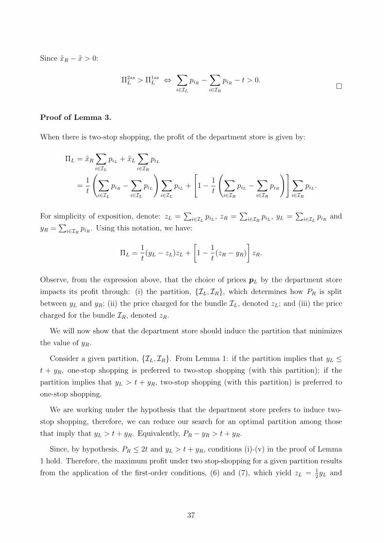
Since xR − x > 0:

Π2ssL > Π1ss

L ⇔∑i∈IL

piR −∑i∈IR

piR − t > 0.�

Proof of Lemma 3.

When there is two-stop shopping, the profit of the department store is given by:

ΠL = xR∑i∈IL

piL + xL∑i∈IR

piL

=1

t

(∑i∈IL

piR −∑i∈IL

piL

)∑i∈IL

piL +

[1− 1

t

(∑i∈IR

piL −∑i∈IR

piR

)]∑i∈IR

piL .

For simplicity of exposition, denote: zL =∑

i∈IL piL , zR =∑

i∈IR piL , yL =∑

i∈IL piR and

yR =∑

i∈IR piR . Using this notation, we have:

ΠL =1

t(yL − zL)zL +

[1− 1

t(zR − yR)

]zR.

Observe, from the expression above, that the choice of prices pL by the department store

impacts its profit through: (i) the partition, {IL, IR}, which determines how PR is split

between yL and yR; (ii) the price charged for the bundle IL, denoted zL; and (iii) the price

charged for the bundle IR, denoted zR.

We will now show that the department store should induce the partition that minimizes

the value of yR.

Consider a given partition, {IL, IR}. From Lemma 1: if the partition implies that yL ≤t + yR, one-stop shopping is preferred to two-stop shopping (with this partition); if the

partition implies that yL > t + yR, two-stop shopping (with this partition) is preferred to

one-stop shopping.

We are working under the hypothesis that the department store prefers to induce two-

stop shopping, therefore, we can reduce our search for an optimal partition among those

that imply that yL > t+ yR. Equivalently, PR − yR > t+ yR.

Since, by hypothesis, PR ≤ 2t and yL > t+ yR, conditions (i)-(v) in the proof of Lemma

1 hold. Therefore, the maximum profit under two stop-shopping for a given partition results

from the application of the first-order conditions, (6) and (7), which yield zL = 12yL and

37

zR = 12(t+ yR):

ΠL =1

4ty2L +

[1− 1

2t(t− yR)

]1

2(t+ yR)

=1

4t(PR − yR)2 +

1

4t(t+ yR)2.

The value of PR is not affected by the partition, but yR is. Thus, the resulting partition

impacts the attainable profit through the value of yR that results. When choosing the price

vector pL, besides satisfying the first-order conditions, the department store wishes to induce

a profit-maximizing value of yR:

maxyR

{1

4t(PR − yR)2 +

1

4t(t+ yR)2

}.

Under the restriction PR−yR > t+yR, the objective function is decreasing in yR. Therefore,

the maximum occurs when yR is minimum.

We conclude, then, that it is in the interest of the department store to choose a price

vector pL such that zL = 12yL, zR = 1

2(t + yR) and yR is minimized. To minimize yR, the

department store should induce IR to contain only the good j that is the cheapest at R.39

The department will set pjL = 12(t+ pjR) and, for example, set piL = 1

2piR , ∀i 6= j. �

Proof of Proposition 2.

To finish the proof, we must verify that piR = 3n+2

t maximizes the profit of the shop at the

mall that sells good iR. So far, we only know that it maximizes profit in D3, as long as∑ni=1 |piL −

3n+2

t| ≤ t (which implies that piR ∈ D3 and, thus, p ∈ P1).

With PL = 2n+1n+2

t and pjR = 3n+2

t, ∀j 6= i, the profit function has a local maximum in

D3, attained at p∗iR = 3n+2

t. The derivative of the demand with respect to price is − 12t

in

D3 and −1t

in D4. Therefore, if a marginal price increase is not profitable, it is also not

profitable to make a greater price increase to D4, where the demand is more price-sensitive.

The maximum is either p∗iR = 3n+2

t or attained in D2.

In D2, the demand for good iR is qiR = 1t

(sRi + piL − piR) and the corresponding profit

is ΠiR = 1t

(sRipiR + piLpiR − p2

iR

). The first-order condition is satisfied at p∗∗iR = sRi

2+

piL2

.

39Unless there is more than one good with null price at R. In that case, it is optimal for the departmentstore to induce any set IR ⊆ {i ∈ I : piR = 0}.

38

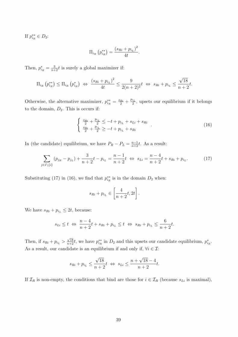
If p∗∗iR ∈ D2:

ΠiR

(p∗∗iR)

=(sRi + piL)2

4t.

Then, p∗iR = 3n+2

t is surely a global maximizer if:

ΠiR

(p∗∗iR)≤ ΠiR

(p∗iR)⇔ (sRi + piL)2

4t≤ 9

2(n+ 2)2t ⇔ sRi + piL ≤

√18

n+ 2t.

Otherwise, the alternative maximizer, p∗∗iR = sRi

2+

piL2

, upsets our equilibrium if it belongs

to the domain, D2. This is occurs if:{sRi

2+

piL2≤ −t+ piL + sLi + sRi

sRi

2+

piL2≥ −t+ piL + sRi

. (16)

In (the candidate) equilibrium, we have PR − PL = n−1n+2

t. As a result:

∑j∈I\{i}

(pjR − pjL) +3

n+ 2t− piL =

n− 1

n+ 2t ⇔ sLi =

n− 4

n+ 2t+ sRi + piL . (17)

Substituting (17) in (16), we find that p∗∗iR is in the domain D2 when:

sRi + piL ∈[

4

n+ 2t, 2t

].

We have sRi + piL ≤ 2t, because:

sLi ≤ t ⇔ n− 4

n+ 2t+ sRi + piL ≤ t ⇔ sRi + piL ≤

6

n+ 2t.

Then, if sRi + piL >√

18n+2

t, we have p∗∗iR in D2 and this upsets our candidate equilibrium, p∗iR .

As a result, our candidate is an equilibrium if and only if, ∀i ∈ I:

sRi + piL ≤√

18

n+ 2t ⇔ sLi ≤

n+√

18− 4

n+ 2t.

If IR is non-empty, the conditions that bind are those for i ∈ IR (because sLi is maximal),

39

which can be written as:

∑i∈IL

|piR − piL| ≤n+√

18− 4

n+ 2t.

If IR is empty, then all the above conditions are satisfied because, in this case:

∑i∈IL

|piR − piL| =∑i∈I

(piR − piL) = PR − PL =n− 1

n+ 2t <

n+√

18− 4

n+ 2t.

To obtain a more elegant condition, notice that (in the candidate equilibrium):

PR − PLR − PL + PLR =n− 1

n+ 2t ⇔

∑i∈IR

|piL − piR | =∑i∈IL

|piR − piL| −n− 1

n+ 2t ⇔

⇔∑i∈I

|piL − piR | = 2∑i∈IL

|piR − piL| −n− 1

n+ 2t.

Therefore, the equilibrium condition can be written as:

∑i∈I

|piL − piR | ≤2(n+√

18− 4)

n+ 2t− n− 1

n+ 2t =

n+ 6√

2− 7

n+ 2t.

�

Proof of Proposition 3.

To finish the proof, we need to check that the shops at the mall that are selling goods at a

higher price than the department store do not wish to deviate as long as 7 ≤ n ≤ 11. The

candidate equilibrium maximizes their profits in the domain D4, but we must guarantee that

the shops do not prefer to choose prices in D3 (if it exists) or in D2.

It is convenient to start with some preliminary calculations. In the candidate equilibrium,

for the shop that sells good i ∈ IL, we have:

sLi =∑

j∈IL\{i}

(pjR − pjL) =n− 3

n+ 1t+ piL ;

sRi =∑

j∈IR\{i}

(pjL − pjR) =t

3.

We know that D3 is empty if and only if:

sLi + sRi > t ⇔ n− 3

n+ 1t+ piL +

t

3> t ⇔ piL >

11− n3(n+ 1)

t.

40

For n ≥ 12, the domain D3 is empty (for n = 11 it is either empty or a singleton).

Let us start by considering the case in which D3 is empty and study whether a deviation

to D2 is profitable. From (10), the interior maximizer in D2 is:

p∗∗iR =piL2

+t

6. (18)

This alternative only belongs to D2 if p∗∗iR < piL . Equivalently, if:

piL2

+t

6< piL ⇔ piL >

t

3. (19)

But since piL < 2n+1

t, condition (19) cannot hold for n ≥ 7. This means that the optimal

choice in D2 is at the frontier (piR → piL). The resulting profit is ΠiR =piL3

. We conclude

that the shop gains with this deviation if:

piL3>

4

(n+ 1)2t ⇔ piL >

12

(n+ 1)2t.

It is straightforward to confirm that piL > 12(n+1)2

t implies that piL > 11−n3(n+1)

t, which was a

prerequisite (for D3 to be empty).

Notice that if piL ≤ 12(n+1)2

t,∀i ∈ IL, then:

∑i∈IL

piL ≤12(n− 1)

(n+ 1)2t ⇔ n− 1

n+ 1t ≤ 12(n− 1)

(n+ 1)2t ⇔ n ≤ 11.

For n ≥ 12, the candidate is not an equilibrium because at least one of the shops deviates.

Now suppose that D3 is not empty. We must have piL ≤ 11−n3(n+1)

t and piL <2

n+1t. The first

condition can only hold for n ≤ 11, while the second is implied by the first. In this case, we

must consider deviations to D3 and also to D2.

The interior maximum in D2, given by (18), is again outside the domain because:

piL ≤11− n

3(n+ 1)t ⇒ piL

2+t

6> −t+ piL + sLi + sRi.

The candidate deviation is, therefore, at the frontier. But if it is profitable to increase the

price until the frontier of D2 it is surely profitable to keep increasing the price after entering

D3 because the price-sensitivity of demand is lower in D3. It is enough to consider deviations

in D3.

41

From (11), the candidate deviation is:

piR =PL

2− 1

2

∑j∈I\{i}

pjR +t

2=

n+ 13

6(n+ 1)t.

This deviation is outside D3, because:

n+ 13

6(n+ 1)t ≤ t+ piL − sLi − sRi ⇔

n+ 13

6(n+ 1)t ≤ 11− n

3(n+ 1)t ⇔ n ≤ 3,

which is false.

Therefore, the maximum in D3 is at the frontier with D4. Global continuity of the profit

function (satisfied as long as D3 is not empty) and concavity in D4 imply that the local

maximum at D4 is actually the global maximum. �

Proof of Proposition 4.

We start by showing that an equilibrium with two-stop shopping is not possible.

With n = 2, one of the goods must be cheaper at x = 0 and the other must be cheaper

at x = 1. Combining the first-order conditions, (6) and (7), we obtain, for i ∈ IL:{piL =

piR2

piR =piL2

+ t2

⇔

{piL = 1

3t

piR = 23t.

.

For j ∈ IR, we obtain pjL = 23t and pjR = 1

3t. This is an equilibrium, but no consumer

gains by shopping at both extremes (only the consumer in the middle, x = 12, is indifferent

between one-stop shopping and two-stop shopping).

For n > 2, both department stores wish to have a single good that is more expensive than

at the other extreme. From Proposition 1, the profit-maximizing behavior of the department

store located at L implies that there is a single good j for which pjL > pjR . Simultaneously,

the profit-maximizing behavior of the department store located at R implies that there is

a single good j′ for which pj′R > pj′L . For these behaviors to be compatible, we must have,

∀i /∈ {j, j′} , piL = piR . Actually, we must have piL = piR = 0,∀i /∈ {j, j′}, otherwise the

department stores would gain by undercutting each other’s prices (so capture the demand of

all the two-stop shoppers). Since, from Proposition 1, j′ is one of the cheapest goods at L,

we also have pj′L = 0. It follows that the department store at L (resp. R) is setting a strictly

positive price for good j (resp. j′), pjR = t2

(resp. pj′R = t2) and offering all the remaining

goods for free. This is neither optimal nor induces two-stop shopping.

42

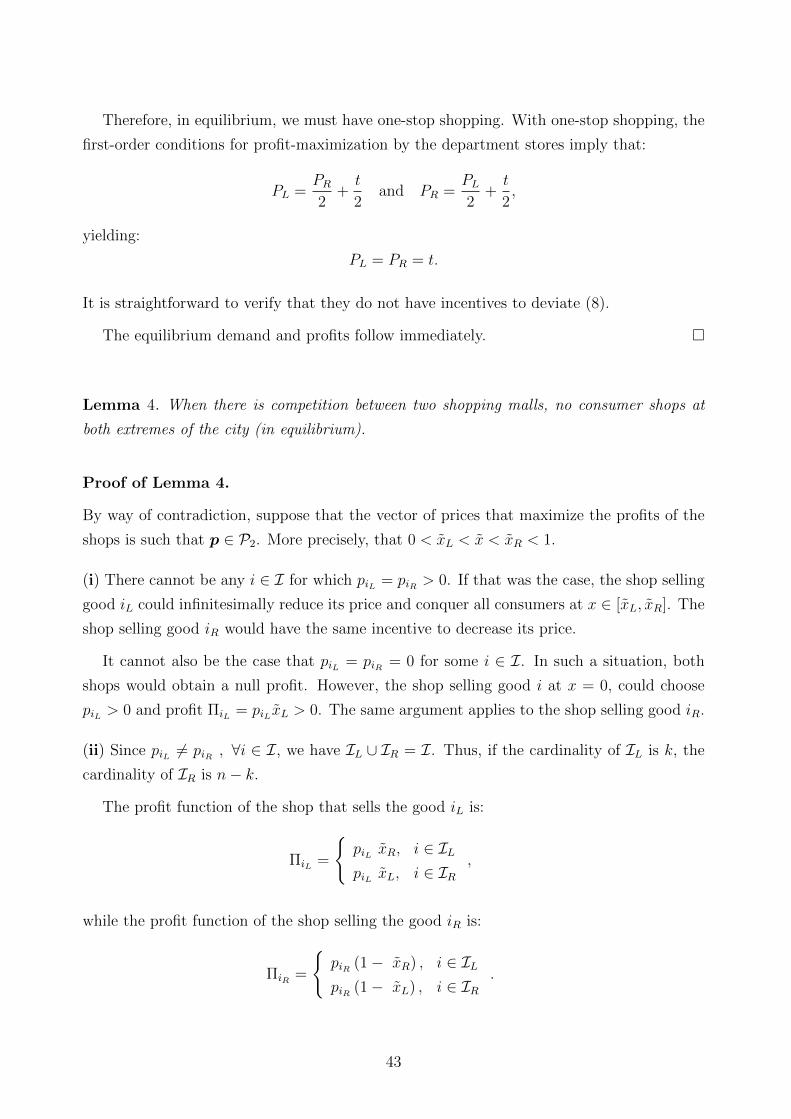
Therefore, in equilibrium, we must have one-stop shopping. With one-stop shopping, the

first-order conditions for profit-maximization by the department stores imply that:

PL =PR

2+t

2and PR =

PL

2+t

2,

yielding:

PL = PR = t.

It is straightforward to verify that they do not have incentives to deviate (8).

The equilibrium demand and profits follow immediately. �

Lemma 4. When there is competition between two shopping malls, no consumer shops at

both extremes of the city (in equilibrium).

Proof of Lemma 4.

By way of contradiction, suppose that the vector of prices that maximize the profits of the

shops is such that p ∈ P2. More precisely, that 0 < xL < x < xR < 1.

(i) There cannot be any i ∈ I for which piL = piR > 0. If that was the case, the shop selling

good iL could infinitesimally reduce its price and conquer all consumers at x ∈ [xL, xR]. The

shop selling good iR would have the same incentive to decrease its price.

It cannot also be the case that piL = piR = 0 for some i ∈ I. In such a situation, both

shops would obtain a null profit. However, the shop selling good i at x = 0, could choose

piL > 0 and profit ΠiL = piLxL > 0. The same argument applies to the shop selling good iR.

(ii) Since piL 6= piR , ∀i ∈ I, we have IL ∪ IR = I. Thus, if the cardinality of IL is k, the

cardinality of IR is n− k.

The profit function of the shop that sells the good iL is:

ΠiL =

{piL xR, i ∈ ILpiL xL, i ∈ IR

,

while the profit function of the shop selling the good iR is:

ΠiR =

{piR (1− xR) , i ∈ ILpiR (1− xL) , i ∈ IR

.

43

If i ∈ IL, the first-order conditions are:∂ΠiL

∂piL= 0

∂ΠiR

∂piR= 0

⇔

{piL = PR − PLR

piR = t− PR + PLR

⇒ piR = t− piL .

The expressions above imply that ∀i, j ∈ IL: piL = pjL and piR = pjR . Moreover:

piL =∑j∈IL

(pjR − pjL) = k (t− 2piL) ⇔ piL =k

2k + 1t

and

piR =k + 1

2k + 1t.

Analogously, if i ∈ IR, then:

piL =n− k + 1

2n− 2k + 1t and piR =

n− k2n− 2k + 1

t.

The expressions for the marginal consumers, xL and xR, follow immediately:

xL =n− k + 1

2n− 2k + 1and xR =

k

2k + 1.

It is straightforward to see that xL > xR. Contradiction. �

Proof of Proposition 5.

By Lemma 4 (in this Appendix), there is no equilibrium with prices in P2. Therefore, we

must seek prices satisfying the condition∑n

i=1 |piL − piR | ≤ t.

As obtained in (13), the first-order conditions of the n shops at the malls imply that:

PL =n

n+ 1(t+ PR) and PR =

n

n+ 1(t+ PL) .

Therefore:

PL = PR = nt.

Using (11), we obtain the individual prices:

piL = piR = t,∀i ∈ I.

To complete the proof, we must verify that these local maxima are global maxima. We need

44

to check if each shop chooses the price t, when the remainders charge t for their products.

Without loss of generality, we consider the shop that sells good iR.

Substituting pjL = pjR = t, ∀j 6= i and piL = t in the demand for good iR, given in (9):

qiR =

{1− piR

2t, piR ∈ [0, 2t]

0, piR ∈ (2t,+∞)

and

ΠiR =

{piR(1− piR

2t

), piR ∈ [0, 2t]

0, piR ∈ (2t,+∞).

The profit function is globally concave and continuous. Therefore, the local maximum is

also the global maximum. The equilibrium demand and profits follow immediately. �

45

References

Anderson, S.P., Ø. Foros and H.J. Kind (2012): “Product quality, competition and multi-

purchasing”, CEPR Discussion Paper No. 8923 (April 2012).

Armstrong, M. and J. Vickers (2010): “Competitive non-linear pricing and bundling”, Re-

view of Economic Studies, 77 (1), pp. 30-60.

Bart, Y. (2009): “Multiproduct competition with demand complementarity”, Ph.D. disser-

tation, University of California, Berkeley.

Beggs, A.W. (1994): “Mergers and malls”, Journal of Industrial Economics, 44 (4), pp. 419-

428.

Bertrand, M. and F. Kramarz (2002): “Does entry regulation hinder job creation? Evidence

from the French retail industry”, Quarterly Journal of Economics, 117 (4), pp. 1369-1413.

Bliss, C. (1988): “A theory of retail pricing”, Journal of Industrial Economics, 36 (4),

pp. 375-391.

Chen, Z. and P. Rey (2012a): “Loss leading as an exploitative practice”, American Economic

Review, 102 (7), pp. 3462-3482.

Chen, Z. and P. Rey (2012b): “Shopping patterns and cross subsidization”, mimeo.

Cheshire, P., C.A.L. Hilber and I. Kaplanis (2012): “Land use regulation and productivity

- land matters: Evidence from a UK supermarket chain”, Document de treball de la IEB

2012/15.

D’Aspremont, C., J.J. Gabszewicz and J.-F. Thisse (1979): “On Hotelling’s ‘Stability in

competition’ ”, Econometrica, 47, pp. 1145-1150.

Davis, P. (2006): “Spatial competition in retail markets: movie theaters”, RAND Journal

of Economics, 37 (4), pp. 964-982.

Economides, N. and S.C. Salop (1992): “Competition and integration among complements,

and network market structure”, Journal of Industrial Economics, 40 (1), pp. 105-133.

Edgeworth, F.Y. (1925): “Papers relating to political economy”, London: MacMillan.

Figurelli, L. (2013): “Store choice in spatially differentiated markets”, mimeo (January 24,

2013).

Gehrig, T. (1998): “Competing markets”, European Economic Review, 42, pp. 277-310.

46

Giraud-Heraud, E., H. Hammoudi and M. Mokrane (2003): “Multiproduct firm behaviour

in a differentiated market”, Canadian Journal of Economics, 36 (1), pp. 41-61.

Gould, E.D., B.P. Pashigian and C.J. Prendergast (2005): “Contracts, externalities, and

incentives in shopping malls”, Review of Economics and Statistics, 87 (3), pp. 411-422.

Griffith, R. and H. Harmgart (2008): “Supermarkets and planning regulation,” CEPR Dis-

cussion Paper No. 6713.

Griffith, R., R. Harrison, J. Haskel and M. Sako (2003): “The UK productivity gap & the

importance of the service sectors”, AIM Briefing Note, Advanced Institute for Management

Research.

Hanson, W. and R.K. Martin (1990): “Optimal bundle pricing”, Management Science, 36

(2), pp. 155-174.

Hotelling, H. (1929): “Stability in competition”, Economic Journal, 39, pp. 41-57.

Innes, R. (2006): “Entry deterrence by non-horizontal merger”, Journal of Industrial Eco-

nomics, 54, pp. 369-395.

Kamien, M.I. and I. Zang (1990): “The limits of monopolization through acquisition”, Quar-

terly Journal of Economics, 105 (2), pp. 465-499.

Kim, H. and K. Serfes (2006): “A location model with preference for variety”, Journal of

Industrial Economics, 54 (4), pp. 569-595.

Klemperer, P. (1992): “Equilibrium product lines: competing head-to-head may be less

competitive”, American Economic Review, 82 (4), pp. 740-755.

Lahmandi-Ayed, R. (2010): “Spatial differentiation, divisible consumption and the pro-

competitive effect of income”, Journal of Mathematical Economics, 46 (1), pp. 71-85.

Lal, R. and C. Matutes (1989): “Price competition in multimarket duopolies”, RAND Jour-

nal of Economics, 20 (4), pp. 516-537.

Lal, R. and C. Matutes (1994): “Retail pricing and advertising strategies”, Journal of Busi-

ness, 67 (3), pp. 345-370.

Lal, R. and R. Rao (1997): “Supermarket competition: the case of everyday low pricing”,

Marketing Science, 16 (1), pp. 60-80.

Laussel, D. (2006): “Are manufacturers competing through or with supermarkets? A theo-

retical investigation”, B.E. Journal of Theoretical Economics - Contributions, 6 (1), pp. 1-18.

47

Matutes, C. and P. Regibeau (1992): “Compatibility and bundling of complementary goods

in a duopoly”, Journal of Industrial Economics, 40 (1), pp. 37-54.

Rhee, H. and D.R. Bell (2002): “The inter-store mobility of supermarket shoppers”, Journal

of Retailing, 78 (4), pp. 225-237.

Rhodes, A. (2012): “Multiproduct retailing”, mimeo.

Sadun, R. (2011): “Does planning regulation protect independent retailers?”, Working Pa-

per, Harvard Business School.

Salant, S., S. Switzer and R. Reynolds (1983): “Losses from horizontal merger: the effects of

an exogenous change in industry structure on Cournot-Nash equilibrium”, Quarterly Journal

of Economics, 98 (2), pp. 185-199.

Schiraldi, P., S. Seiler and H. Smith (2011): “Supermarket choice with multi-store shopping:

measuring the effect of format regulation”, mimeo.

Schivardi, F. and E. Viviano (2011): “Entry barriers in retail trade”, Economic Journal, 121

(551), pp. 145-170.

Shelegia, S. (2012): “Multiproduct pricing in oligopoly”, International Journal of Industrial

Organization, 30, pp. 231-242.

Sloev, I., J.-F. Thisse and P. Ushchev (2013): “Do We Go Shopping Downtown or in the

Burbs? Why Not Both?”, CEPR Discussion Paper No. 9604, August 2013.

Smith, H. and D. Hay (2005): “Streets, malls and supermarkets”, Journal of Economics and

Management Strategy, 14 (1), pp. 29-59.

Stahl, K. (1987): “Theories of urban business location”, Handbook of Regional and Urban

Economics (edited by E.S. Mills), Vol. 2, Chapter 19, pp. 759-820.

Stassen, R.E., J.D. Mittelstaedt and R.A. Mittelstaedt (1999): “Assortment overlap: its

effect on shopping patterns in a retail market when the distributions of prices and goods are

known”, Journal of Retailing, 75 (3), pp. 371-386.

Thill, J.-C. (1992): “Spatial duopolistic competition with multipurpose and multistop shop-

ping”, Annals of Regional Science, 26, pp. 287-304.

Zhu, T., V. Singh and A. Dukes (2011): “Local competition, entry, and agglomeration”,

Quantitative Marketing and Economics, 9 (2), pp. 129-154.

48