Spatial and temporal controls on watershed ecohydrologyin the northern Rocky Mountains

Ryan E. Emanuel,1,2 Howard E. Epstein,3 Brian L. McGlynn,4 Daniel L. Welsch,5

Daniel J. Muth,3 and Paolo D’Odorico3

Received 16 November 2009; revised 26 August 2010; accepted 3 September 2010; published 24 November 2010.

[1] Vegetation water stress plays an important role in the movement of waterthrough the soil!plant!atmosphere continuum. However, the effects of water stress onevapotranspiration (ET) and other hydrological processes at the watershed scale remainpoorly understood due in part to spatially and temporally heterogeneous conditions withinthe watershed, especially in areas of mountainous terrain. We used a spatially distributedmodel to understand and evaluate the relationship between water stress and ET in aforested mountain watershed during the snow!free growing season. Vegetation waterstress increased as the growing season progressed, due to continued drying of soils, andpersisted late into the growing season, even as vapor pressure deficit decreased withlower temperatures. As a result, ET became decoupled from vapor pressure deficit andbecame increasingly dependent on soil moisture later in the growing season, shiftingfrom demand limitation to supply limitation. We found water stress and total growingseason ET to be distributed nonuniformly across the watershed due to interactions betweentopography and vegetation. Areas having tall vegetation and low topographic indexexperienced the greatest water stress, yet they had some of the highest evapotranspirationrates in the watershed.

Citation: Emanuel, R. E., H. E. Epstein, B. L. McGlynn, D. L. Welsch, D. J. Muth, and P. D’Odorico (2010), Spatialand temporal controls on watershed ecohydrology in the northern Rocky Mountains, Water Resour. Res., 46, W11553,doi:10.1029/2009WR008890.

1. Introduction

[2] Evapotranspiration is the major flux of water andenergy from vegetated land surfaces, and it is closely linkedto carbon cycling and vegetation characteristics in terrestrialecosystems due to the biophysical link between transpirationand CO2 assimilation [e.g., Eagleson, 1982; Rodriguez!Iturbe and Porporato, 2004]. Evapotranspiration is alsoan important sink for soil moisture within the root zone[Albertson and Kiely, 2001]. When soil moisture falls belowa critical level (whether by ET or other means), vegetationexperiences water stress, the result of which is a reducedability to assimilate atmospheric CO2 [e.g., Guswa, 2005;Detto et al., 2006; Emanuel et al., 2007a]. Since currentcarbon stores and CO2 assimilation rates are dictated in partby past rates of CO2 uptake [Kozlowski, 1992], the verystructure and organization of a vegetated landscape includ-ing both above and belowground vegetation contain informa-tion about historical patterns of water stress and ET. Thus,

the ability to quantify and understand water stress and itseffects on ET within terrestrial ecosystems is important forunderstanding not only hydrological processes but also thehydrological controls on carbon cycling and on the structureand distribution of vegetation. In areas such as the subalpineforests of the northern Rocky Mountains, understanding howwater stress functions and affects carbon and water cycles isvery important in light of the climate!driven trend towardearlier snowmelts and reduced snowpacks in this region [e.g.,Fyfe and Flato, 1999; Stewart et al., 2004;Mote et al., 2005;Barnett et al., 2008].[3] At larger spatial scales, water stress and ET are depen-

dent on topography and vegetation. Topographic control ofsoil moisture through patterns of drainage and connectivity[e.g., Grayson et al., 1997;Mohanty and Skaggs, 2001] mayextend to ET and vegetation water stress through the water!limited processes described above. Vegetation may controlET directly through scaling by leaf area [Zhang et al., 2001]or it may operate on ET indirectly by affecting the aero-dynamic properties of canopies [Anderson et al., 2003].Additionally, vegetation type influences the degree of waterstress experienced by plants under a particular set of atmo-spheric and soil moisture conditions [Emanuel et al., 2007a].Topography and vegetation thus interact to influence thespatial variability of both water stress and ET, and it isimportant to characterize (i.e., quantify) the spatial hetero-geneity of these processes and their controls to better under-stand carbon and water cycling at the landscape scale.[4] For watershed scale studies, ET has traditionally been

calculated as the residual unknown in the annual water

1Department of Geology, Appalachian State University, Boone, NorthCarolina, USA.

2Now at Department of Forestry and Environmental Resources,North Carolina State University, Raleigh, North Carolina, USA.

3Department of Environmental Sciences, University of Virginia,Charlottesville, Virginia, USA.

4Department of Land Resources and Environmental Sciences,Montana State University, Bozeman, Montana, USA.

5Canaan Valley Institute, Davis, West Virginia, USA.

Copyright 2010 by the American Geophysical Union.0043!1397/10/2009WR008890

WATER RESOURCES RESEARCH, VOL. 46, W11553, doi:10.1029/2009WR008890, 2010

W11553 1 of 14

balance [Dingman, 2002]. Although useful for low!resolutionstudies, such estimates of ET are of little help to under-standing controls on ET that act at time scales shorter than1 year or spatial scales smaller than the watershed as awhole. For studies over shorter time scales, flux towers havebecome a common method for measuring ET directly usingtechniques such as eddy covariance; however, the arealextent of a tower footprint may or may not represent ade-quately the heterogeneity of topography and vegetationwithin a watershed. Even where a flux tower footprint canbe assumed to approximate watershed!wide conditions, mea-surements of ET will reflect average conditions within thefootprint, homogenizing the spatial variability caused by dif-ferences in topography and vegetation. Although flux towersprovide relatively reliable measurements of ET at the land-scape scale (typically on the order of 1 km2 or more forforest ecosystems, depending on vegetation height, surfaceroughness, and stability of the atmospheric boundary layer),investigations of the spatial and temporal heterogeneity ofecohydrological processes at finer spatial scales within thewatershed (approximately 1 m2 to 1 ha) require estimates ofET at the resolution of topographic and vegetation featureswithin the watershed. Moreover, whereas tree level measure-ments of transpiration (i.e., sap flux measurements) addressthe spatial heterogeneity over subwatershed areas, scaling ofthese measurements to the entire watershed remains difficult[Ford et al., 2007; Kumagai et al., 2008], particularly inthe absence of concurrent surface evaporation measurements.[5] Despite the important role played by ET in land sur-

face hydrology, plant physiology, and climate dynamics, itis unclear how interactions between plant ecophysiologyand watershed processes determine the spatial and temporalvariability of ET across multiple scales. The purpose of thisstudy is to understand controls on the spatial and temporalvariability of ET within a forested watershed. Specifically,we couple a point!based ecohydrological model of vegeta-tion water stress with a spatially distributed hydrologicalmodel to provide spatial and temporal descriptions of veg-

etation water stress within a catchment that allow us todetermine (1) what factors contribute to the development ofcatchment!wide water stress during the growing season in asemiarid, montane forest and (2) what factors cause waterstress and ET to evolve and behave differently across avegetated watershed. By investigating the physical andbiological controls on the temporal and spatial heterogeneityof ET during the course of a growing season, we also usethis framework to evaluate the impacts of micrometeorol-ogy, topography, and vegetation on streamflow.[6] To investigate these controls we consider as a case

study the ecohydrologic dynamics in a subalpine forest of theRocky Mountains. These forests are important sinks foratmospheric CO2 in North America [Schimel et al., 2002] andare affected by hydrologic controls, as they lie in semiaridclimates, where spring snowmelt provides ecosystems withmost of their annual influx of water [Running, 1980; Baleset al., 2006]. As a result these forests experience a seasonaldecline in soil moisture and, frequently, extended water stressduring the growing season. Thus, in these forests CO2 uptakeand ET are closely coupled. This coupling, combined withseasonal patterns of moisture availability as well as mountaintopography, make these systems ideal for studying coupledhydrological and ecological processes in a watershed context.

2. Methods

2.1. Site Description and Field Methods[7] Data were collected during the snow!free portion

of the 2006 growing season (22 June through 4 September2006) within the upper Stringer Creek watershed, a heavilyinstrumented, 300 ha subcatchment located in the TenderfootCreek Experimental Forest (TCEF,Montana, USA; Figure 1).The study site is a forested, subalpine watershed ranging inelevation from 2090 to 2430 m. The watershed is dominatedby lodgepole pine (Pinus contorta) forest, but it also con-tains small areas (9% of the watershed) of riparian and uplandmeadows and isolated areas of subalpine fir (Abies lasiocarpa)

Figure 1. Map of the Stringer Creek watershed showing (a) topographic index TI and (b) distribution ofvegetation heights Zveg derived from 1 m ALSM data. White circle shows location of flux tower and whitesquares show locations of ancillary meteorological stations.

EMANUEL ET AL.: WATERSHED ECOHYDROLOGY IN THE ROCKY MOUNTAINS W11553W11553

2 of 14

and Engelmann spruce (Picea engelmannii). In general, how-ever, the watershed has been characterized as even!aged,low!diversity lodgepole forest [Mincemoyer and Birdsall,2006]. The soils are cryoboralfs with a sandy loam texture.[8] On average, TCEF receives more than 70% of its

880 mm of mean annual precipitation as snow [McCaughey,1996], and it experiences a relatively steady drying of soilsthroughout the growing season [Riveros!Iregui et al., 2007].As a result, the temporal dynamics of soil moisture at TCEFare relatively simple; the seasonal dry!down is the domi-nant trend in soil moisture time series. Soils throughout thewatershed transition from relatively wet at the beginning ofthe growing season to relatively dry at the end. This trend,combined with the relatively simple and uniform ecologi-cal structure of the site, makes TCEF well suited for ourinvestigation.[9] Long!term measurements at this site include snow

depth, snow water equivalent, and streamflow [McCaughey,1996; Woods et al., 2006], and since 2005, tower!basedmeasurements of ecosystem fluxes and micrometeorologyover the lodgepole forest (measured at 30 m) and separatelyover a riparian meadow (measured at 1.5 m). Tower!basedmeasurements of interest to this study include ET mea-sured by eddy covariance using a triaxial sonic anemometer(CSAT3, Campbell Scientific, Logan, UT) and open!pathinfrared gas analyzer (LI7500, Licor Biosciences, Lincoln,NE), air temperature and relative humidity (HMP45C,Campbell Scientific), photosynthetically active radiation(PAR, LI190, Licor Biosciences), net radiation (CNR1, Kippand Zonen, Delft, Netherlands), and precipitation (tippingbuckets, TE525, Texas Electronics, Dallas, TX). Standard tiltcorrection, spike filtering, sonic anemometer virtual tem-perature correction, and Webb correction were performedon half!hourly eddy covariance fluxes [Webb et al., 1980;Schotanus et al., 1983; Kaimal and Finnegan, 1994; Paw Uet al., 2000]. Tower!based micrometeorological measure-ments were complemented by nests of soil instruments (threeper tower) measuring soil temperature at 2.5 and 7.5 cm(Thermocouple, Omega Engineering, Stamford, Conn.), soilheat flux at 5 cm (HFT3, Radiation and Energy BalanceSystems, Inc., Seattle, WA), and soil moisture integrated over0–30 cm using time domain reflectometry (CS616, CampbellScientific). Separate CS616 probes were also used to measuresoil moisture near each tower at 20 cm below ground.[10] At the beginning of the study period and approx-

imately 3 weeks after snowmelt ended five weather sta-tions (HOBO Micro Station, Onset Computer Corporation,Bourne, MA) were installed in the watershed to provideadditional input data for the watershed model. These weatherstations measured air temperature and relative humidity at1 m above the ground surface. Two of the five weather sta-tions measured precipitation using additional tipping buckets.In addition tometeorological data, leaf level ecophysiologicaldata were collected at regular intervals (two to three times perweek) from 30 m ! 30 m sampling plots surrounding eachstation using a portable photosynthesis system (LI6400, LicorBiosciences) following the methods of Norman et al. [2006].Leaf chamber measurements (3157 total measurements)collected from the plots were used to estimate parameters forthe leaf level ecophysiological model (section 2.3) for twogeneral vegetation types in the watershed, namely conifersand grasses/forbs using nonlinear regression as described byEmanuel et al. [2007a]. Leaf chamber measurements were

accompanied by shallow (0–20 cm) soil moisture measure-ments using a handheld TDR probe (HydroSense, CampbellScientific). Together, these seven stations (two flux towersand five weather stations) cover the major combinations ofelevation, aspect, and vegetation type present in the StringerCreek watershed (Figure 1).

2.2. Remote Sensing of Topography and Vegetation[11] In September 2005, airborne light detection and

ranging (lidar) measurements were collected over approxi-mately 50 km2 of the TCEF, including the upper StringerCreek watershed by the National Center for Airborne LaserMapping (NCALM, Berkeley, CA). First return (canopy top)and last return (bare earth) elevations were recorded as dis-crete point data and interpolated to 1 m2 digital elevationmodels (DEMs) in postprocessing. Two model inputs werederived from the lidar data: a topographic index and an indexof vegetation height. The topographic index (TI) was cal-culated from the bare earth DEM (Figure 1a). The digitalelevation model was coarsened from 1 to 5 m2 hori-zontal resolution using bilinear interpolation, and TI wascomputed as

TI ! lnaDI

! "; "1#

where a is the specific area contributing to flow through apoint in the watershed computed following the algorithm ofSeibert and McGlynn [2007], and DI is the downhill index,an alternative to the local slope that considers topographicconcavity downhill of each point by determining how fardownhill a parcel of water must travel to lose a certain amountof potential energy [Hjerdt et al., 2004]. In this watershed, themain advantage of DI over local slope is the ability to use ahigh resolution DEM without introducing unrealistic sen-sitivity of flow to microtopography. Thus, DI provides animproved representation of topographic influences on flow inthis watershed over the local slope.[12] In addition to TI, an index of vegetation height Zveg

was calculated as the difference in elevation between thefirst and last lidar returns (i.e., the difference between thecanopy top elevation and the ground surface elevation),which was coarsened from 1 to 5 m2 using bilinear inter-polation (Figure 1b). Similar lidar!derived vegetation heightindices have been shown to accurately represent ground!based measurements of vegetation height [Dubayah andDrake, 2000; Lefsky et al., 2002]. Spectral data were notavailable to discriminate between vegetation types (treesversus grasses/forbs); thus grid cells having Zveg > 0.5 mwere classified as conifers, and cells having Zveg ! 0.5 mwere classified as grasses/forbs. In addition to classification,Zveg was used to derive leaf area index (LAI), a neces-sary model input, using site!specific allometric relationshipsgiven by Keane et al. [2005] for lodgepole pine at TCEF. Forgrass/forb grid cells, we estimated LAI to be 1.0 m2 m"2. Wetreated LAI as static through the model simulation period.

2.3. Model Framework[13] Amodel of land!atmosphere exchange was developed

to simulate coupled hydrological and ecological processesthrough time as functions of spatially heterogeneous soil,vegetation, and micrometeorological conditions. The model

EMANUEL ET AL.: WATERSHED ECOHYDROLOGY IN THE ROCKY MOUNTAINS W11553W11553

3 of 14

simulated soil moisture as well as water fluxes from thecatchment, including evapotranspiration and runoff.[14] For the spatially distributed modeling of water fluxes

through the soil!plant!atmosphere continuum, we developedand used a spatially extended Soil!Vegetation!Atmosphere!Transfer (SVAT) model. This type of model can providereliable estimates of ET because it can account for hetero-geneity of ET at spatial scales below that of the footprint offlux towers typically used to measure surface water vaporand energy fluxes; however, spatially distributed informa-tion about land cover and hydrometeorological conditions isrequired. This type of model has seen broad use in recentyears [e.g. Famiglietti and Wood, 1994; Houser et al., 1998;Boegh et al., 2004; Scanlon et al., 2005; Detto et al., 2006].Detailed SVAT models may scale ET from leaf to landscapescale by applying spatially distributed data to biophysicaland energy balance calculations that determine evaporationand transpiration separately. Tower!based measurements ofET may then serve to constrain and validate spatially aver-aged model estimates. Our SVAT modeling frameworkincludes a TOPMODEL!based subsurface flow and runoffcomponent [Beven and Kirkby, 1979] adapted from Scanlonet al. [2005] coupled with an ecohydrological model of sto-matal conductance. Together, TOPMODEL and the eco-hydrological model are used to determine the water balancefor each grid cell in the watershed

d!dt

! 1drz

I $ ET $ qv $ q1" #; "2#

where ! is root zone soil moisture, drz is the depth of the rootzone, I is infiltration, ET is evapotranspiration, qv is verticalsoil water drainage, and ql is lateral soil water drainage.TOPMODEL estimates groundwater discharge, root zone(unsaturated) discharge, and overland flow based on a con-ceptual framework of topographic similarity as defined by thetopographic index (equation (1)), and these discharges maybe combined to simulate total runoff from the watershed [e.g.,Scanlon et al., 2005].[15] The ecohydrological model calculates vegetation sto-

matal conductance and transpiration based on a frameworkfor modeling the dynamic threshold for water stress pre-sented by Emanuel et al. [2007a]. Calculating the dynamicthreshold for water stress requires that stomatal conductancebe modeled as two separate processes, a soil moisture!independent process where stomatal conductance is a functionof the biochemical demand for carbon (i.e., photosynthesis),and a soil moisture!dependent process where stomatal con-ductance responds to plant hydrodynamics.[16] We derived a moisture!independent, biochemical

model of stomatal conductance by combining a Farquhar!type photosynthesis model [Farquhar et al., 1980; Collatzet al., 1991] with a modified Ball!Woodrow!Berry modelof stomatal conductance [Ball et al., 1987; Leuning, 1995].This model assumes similarity among biochemical processesof C3 plants and is also based on a semiempirical relationshipbetween photosynthetic assimilation rate and stomatal con-ductance. The resulting model of stomatal conductance doesnot account for the effect of water stress induced by soil waterdeficit.[17] For the hydrodynamicmodel of stomatal conductance,

we selected a steady state model of soil!plant water transfer

with four physiological parameters [Gao et al., 2002]. Thismodel considers transpiration as the steady state balancebetween two diffusion processes: transpiration is expressed asdiffusion of water vapor between the water!saturated sto-matal cavity and the atmosphere, and soil to leaf water fluxis expressed as a laminar flow driven by water potentialgradients between the soil and leaf. Leaf water potential isrelated to stomatal conductance by assuming a linear (elastic)dependence of guard cell deformation on leaf water poten-tial, where osmotic potential is expressed as a semiempiricalfunction of PAR [Gao et al., 2002; Buckley et al., 2003;Emanuel et al., 2007a]. Although this semiempirical rela-tionship between PAR and conductance has been criticizedfor lack of causality [Buckley et al., 2003], the model isparsimonious compared to other hydrodynamic models ofstomatal conductance, which may include 20 or more para-meters, and it captures the main factors and processes thatdetermine moisture controls on stomatal function.[18] Using the framework by Emanuel et al. [2007a], sto-

matal conductance is calculated as the minimum between thevalues obtained with the moisture!independent biochemicalmodel and with the hydrodynamic model. This approachaccounts for limitations arising both from soil water avail-ability and photosynthetic capacity, and for the switchingbetween these two controls. We used model values of sto-matal conductance to calculate transpiration, which was, inturn, included in the calculation of soil moisture availabilityfor the next time step. This approach also facilitates calcu-lation of the dynamic threshold of vegetation water stress(y*), which is the soil water potential where switching occursbetween biochemical and hydrodynamic stomatal control.The water stress threshold is calculated following Emanuelet al. [2007a] as

y* !gs 1% k"gdv# $

$ g0m $ k#"Qky

; "3#

where dv and Q are vapor pressure deficit and PAR, respec-tively, gs is biochemically limited stomatal conductance, andthe remaining terms (kbg, g0m, kab, and ky) are parametersfrom a hydrodynamic model of stomatal conductance. Thestatus of vegetation water stress may be determined bycomparing y* to actual soil water potential, ys (i.e., vegeta-tion is stressed if y* exceeds ys).[19] The combined SVAT model simulates volumetric

soil water content in the root zone (estimated to be 60 cmdeep based on observations from soil pits and from exca-vations for the flux tower foundation in 2005) by solving thesoil water balance equation for every 5 m grid cell at 30 mintime steps. Given micrometeorological inputs and initialstates of root zone soil water content and catchment dis-charge (determined from field observations of soil moistureand discharge), the model estimates discharge (groundwater,root zone, and overland flow discharges) and transpirationusing the previously described ecological and hydrologicalmodeling frameworks. The model calculates evaporationof canopy and litter interception and litter moisture (froma single, lumped pool at each grid cell) using the directPriestley!Taylor method [Priestley and Taylor, 1972] ofdetermining potential evapotranspiration (PET) and con-sidering evaporation to be the minimum of PET and avail-able water from this pool.

EMANUEL ET AL.: WATERSHED ECOHYDROLOGY IN THE ROCKY MOUNTAINS W11553W11553

4 of 14

[20] This modeling framework makes a few assumptionsand simplifications concerning homogeneity of soil texture,soil thickness, and rooting depth, with important implica-tions for the texture!based relationships between volumetricsoil water content and actual soil water potential ys, thecalculation of soil moisture dynamics, and water controlledstomatal conductance (hydrodynamic submodel). Moreover,by assuming static ecological structure (e.g., no biomassaccumulation, litterfall, nutrient cycling), we ignore seasonalchanges as plants allocate carbon to new growth or experi-ence senescence. This assumption is reasonable based onthe short length of this study (72 days) relative to the slowgrowth of lodgepole pines in subalpine ecosystems [see Ryanand Waring, 1992]. Finally, ET modeled at any individualpoint is subject to uncertainty because we assume simplecanopy aerodynamics by calculating both the canopy bound-ary layer resistance and aerodynamic resistance (to watervapor) based on spatial interpolation over complex terrainof wind velocity measurements collected at two points.[21] Of the model parameters, drz was estimated by direct

observation of soil depths from excavated pits. Other soilparameters, including field capacity and porosity were esti-mated from the time series of soil moisture measured at theforest flux tower. The TOPMODEL groundwater recessionparameter was determined using the recession curve analy-sis of Scanlon et al. [2000], applied to the Stringer Creekhydrograph during the study period. Surface interceptionstorage was approximated based on leaf area index. All ofthe stomatal conductance model parameters were estimatedusing nonlinear regression analysis applied to leaf chambermeasurements described in section 2.1. Three remainingTOPMODEL parameters (saturated hydraulic conductivity,fraction of root zone discharge lost as vertical drainage,and a soil!specific decay constant for unsaturated hydraulicconductivity) [see Scanlon et al., 2005] were calibrated byminimizing the squared error between observed and modeledstream discharge during the study period.

2.4. Atmospheric Data[22] We framed this model in a spatially explicit fashion,

meaning that all atmospheric, soil, topographic, and vege-tation inputs were distributed over the entire watershed at5 m2 resolution (for a total of 2.4 ! 105 grid cells), and modelalgorithms were evaluated for each grid cell rather than forbins of similar grid cells. Others [Famiglietti and Wood,1994; Houser et al., 1998] have adopted this approachwhen considering spatial heterogeneity of multiple environ-mental factors. Precipitation, air temperature, relative humid-ity, and horizontal wind speed measurements from the fluxtowers and weather stations, spanning ranges of elevation,aspect and vegetation cover within the Stringer Creek water-shed, were interpolated to a 10 m2 grid using the SpatialObservation Gridding System (SOGS) [Jolly et al., 2005].These grid cells were subdivided to match the resolution ofthe 5 m2 topographic and vegetation inputs. This interpola-tion scheme was designed to be independent of the spatialscale of the input data, and it was found to have an absoluteuncertainty of less than 2.0°C for temperature and less than3 mb for atmospheric vapor pressure for continental scalemeasurements interpolated to a few kilometers [Jolly et al.,2005]. Prior to using the SOGS input variables we verifiedthe accuracy of this interpolation method by removing,

individually, each of the two flux towers (forest tower andriparian tower) from the SOGS processing and comparingtime series of atmospheric measurements from the removedtower to time series data for the tower’s location interpolatedfrom the remaining six weather stations. In each case, wefound that SOGS, even when reduced by one input station,was at least as accurate as and typicallymore accurate than thenearest weather station at reproducing air temperature, rela-tive humidity, and atmospheric vapor pressure deficit at thetower. Precipitation and horizontal wind speed interpolationswere not assessed because these input variables were notmeasured at all seven sites. Additional details of the SOGSverification are found in section 3.1 of this paper.[23] Photosynthetically active radiation and net radiation

were assumed spatially homogeneous at the top of thevegetation canopy; however, we approximated the effectsof topography on these variables using a terrain!based hills-hading algorithm [Kumar et al., 1997; Pierce et al., 2005] toscale radiation and account for differential topographicshading during morning and afternoon hours. We also useda simplified two big!leaf approximation [Dai et al., 2004]based on lidar!derived vegetation heights to simulate theeffects of shading and attenuation of radiation verticallywithin the canopy.[24] We also simplified the complex relationships among

surface heat fluxes, air temperature, and canopy temperature[Campbell and Norman, 1998] after comparing measure-ments of air temperature to canopy surface skin temperaturetaken at the forest and meadow flux towers with temperature!corrected infrared thermometers (IRTS!P, Apogee Instru-ments, Logan, UT). For both sites, regressions between30 min averages of air and surface temperatures were highlycorrelated (R2 = 0.91 for forest, R2 = 0.82 for meadow),their slopes were statistically indistinguishable from unity(P < 0.05), and their intercepts were statistically indistin-guishable from 0 (P < 0.05). For this reason, we used airtemperature to represent average canopy temperature for eachhalf hour of the study period.[25] We used friction velocity (u*), derived from turbu-

lence measurements at the 30 m forest flux tower to estimatethe canopy boundary layer resistance to water vapor (rb)following Hicks et al. [1987] and Fuentes et al. [1994] as

rb !2ku*

ScPr

% &2=3

; "4#

where k is the von Kármán number, Sc is the Schmidt numberfor water vapor in air, and Pr is the Prandtl number. Aero-dynamic resistance to water vapor transfer was calculated byapplying flux tower!based stability corrections for the loga-rithmic wind profile to neutrally stable wind profiles com-puted from interpolated wind velocity data [see Emanuelet al., 2007a].[26] Key features of this SVAT model include (1) cal-

culation and incorporation of a dynamic threshold for veg-etation water stress, (2) use of lidar!derived topographicaland vegetation structure information, (3) use of the down-stream index in the calculation of TI, and (4) spatial inter-polation of point!based meteorological variables using SOGS.This modeling strategy makes a number of common assump-tions and simplifications, yet assimilates a wide rangeof spatially distributed environmental data to characterize

EMANUEL ET AL.: WATERSHED ECOHYDROLOGY IN THE ROCKY MOUNTAINS W11553W11553

5 of 14

ecological and hydrological responses to environmentalcontrols at high temporal resolution.

3. Assessment of Model Performance

3.1. Assessment Methods[27] Since nomethod exists for measuring vegetation water

stress directly at the spatial or temporal scales represented bythemodel, we assessed the validity of themodel using outputsthat could be measured directly (ET and stream discharge),and we also considered these validation results to representthe model’s ability to track vegetation water stress. We val-idated the model at two time scales using three differentapproaches, each utilizing independent measures of hydro-logic conditions within the watershed. At the 30 min timescale, we compared watershed!averaged ET to eddy covari-ance measurements of ET above the lodgepole forest. Thisvalidation method assumes that the flux footprint of thetower is large enough to represent the variability of ET acrossthe study watershed. A conservative estimate of the upwindextent of the flux footprint of 3 km, based on an instrumentheight of 30 m and a general southerly wind direction, sug-gests that, in general, the area contributing to the measuredflux contains the study site and similar forested areas andterrain. This method tests the ability of the model to cap-ture the short!term response of vegetation to fluctuations inatmospheric and soil conditions. Also at the 30 min timescale, we compared simulated soil moisture in the root zone(0–60 cm) to actual measurements of root zone soil moisturecollected from the moisture probes buried near each fluxtower at 20 cm below the surface. For each set of observed Oand simulated S variables, we used two measures of modelperformance. First, the mean absolute error (MAE) was cal-culated for the time series of length N as

MAE ! N$1XN

i!1

Oi $ Sij j; "5#

following Legates and McCabe [1999]. This measure pro-vides an estimate of model performance in absolute units thathave relevance to the system under consideration. Second,a comparative measure of model performance, the adjustedcoefficient of efficiency, "1" was calculated as

"01 ! 1$

PN

i!1Oi $ Sij j

PN

i!1Oi $ O 0'' ''

; "6#

where O 0 may be either the mean of observations or a timetrend of observations (which could also be another modelsimulation) with 95% confidence intervals for the statisticderived from percentile method bootstrapping using 100realizations [Legates and McCabe, 1999]. A value of 0 for"1" means that the model performed equally as well (i.e.,explained as much variation) as O 0. Positive values of "1"indicate improvements over, O 0 and negative values of "1"indicate that the model performed worse than O 0. In anapplication such as this one, comparison of modeled residualto time trend residuals provides a more powerful indicator ofmodel performance than comparison against residuals fromthe mean observed value. For example, observed dischargedecreases almost monotonically through the growing season;substitution of a parametric trend forO 0 in equation (6) yieldsa more meaningful measure of the model’s performanceversus that trend rather than versus mean discharge.[28] As another example, when verifying the accuracy of

the SOGS weather interpolation, we compared a time seriesof observations from the riparian flux tower (O) to a timeseries at this site based on SOGS interpolation of data fromthe remaining six sites (S ). Table 1 shows mean absoluteerrors for each tower site and adjusted coefficients of effi-ciency for each tower site, compared to baselines (O 0) ofboth the observational mean and a time series of data fromthe other flux tower. For each variable tested (air tempera-ture, relative humidity, and atmospheric vapor pressure def-icit) "1" reveals that SOGS interpolation is (1) significantlybetter at predicting each variable than the mean observedvalue from each site (with the exception of RH at the forestflux tower, where SOGS was not significantly better thanmean observed RH from this site) and (2) at least as accurateas using data from one flux tower to represent another loca-tion within the watershed. The SOGS algorithm performedbetter for the riparian tower than for the forest tower becausethe riparian tower was surrounded bymeteorological stations,whereas the forest tower had nometeorological stations to thenorth or west to bound the interpolation (Figure 1). Thesecomparisons are based on SOGS interpolation from onlysix of the meteorological stations; for the full simulation, allsevenmeteorological stations were used (five HOBOweatherstations and two flux towers).[29] We used MAE and "1" to compare model simulations

of half!hourly and total stream discharge during the studyperiod to actual stream discharge measured by a U.S. ForestService stream gage at the watershed outlet. We also com-pared the model estimate of total ET during the study periodto actual ET measured by the forest flux tower. These com-parisons assess the ability of the model to represent accu-rately the seasonal hydrologic balance of the watershed,and they provide an estimate of closure between observationsand simulations of the major terms in the catchment waterbalance.[30] We expressed vegetation water stress for average

watershed conditions and for individual grid cells as a prob-ability that y* would exceed the soil water potential (ys)derived from modeled soil moisture using the Clapp andHornberger [1978] relationship

y s ! ySat!

n

% &$b

; "7#

Table 1. Assessment of SOGS Interpolation of MeteorologicalVariables for the Two Flux Tower Sites

MAE"1" (Baseline: Mean

Observation)"1" (Baseline:Other Tower)

Forest TowerTair 3.84°C 0.07 (±0.05) "0.02 (±0.02)RH 14.50% 0.02 (±0.07) 0.13 (±0.02)VPD 4.42 mb 0.13 (±0.05) 0.00 (±0.02)

Riparian TowerTair 1.96°C 0.68 (±0.01) 0.48 (±0.02)RH 10.30% 0.55 (±0.02) 0.37 (±0.02)VPD 2.40 mb 0.65 (±0.02) 0.43 (±0.02)

EMANUEL ET AL.: WATERSHED ECOHYDROLOGY IN THE ROCKY MOUNTAINS W11553W11553

6 of 14

where ySat is the saturation soil water potential, n is porosity,and b is a soil!specific parameter. To account for uncertaintyin both the TOPMODEL!derived soil moistures and theconversion from soil moisture to water potential, we used a500!iteration Monte Carlo simulation to determine a rangeof likely soil water potential values for average watershedconditions and for each grid cell. For each iteration, the threeparameters of equation (7) were selected from uniform dis-tributions based on the range of variability for sandy loamsoils documented by Clapp and Hornberger [1978]. Theprobability of water stress for a grid cell during a particularhalf!hour was calculated as the fraction of the 500 iterationsin which y* exceeded ys or P(y* > ys). This value representsthe likelihood that water stress occurs at each point in thewatershed under present soil and atmospheric conditions,given uncertainty in our estimate of ys. For the analysis oftemporal controls on watershed ecohydrology, we consideredP(y* > ys) for the average, watershed!wide soil moisture ateach time step, P"y* > ys#. We also computed P(y* > ys)for the 25th and 75th percentiles of soil moisture at time stepto determine a realistic range of variability for P"y* > y s#.For the analysis of spatial controls on watershed ecohydrol-ogy, we considered P(y* > ys) for the time!averaged soilmoisture conditions at each grid cell in the model, hP(y* >ys)i. Finally, we evaluated the statistical significance ofcomparisons between water stress conditions using two!sampled Kolmogorov!Smirnov tests to evaluate differencesamong cumulative probability distributions and Wilcoxonrank!sum tests to evaluate differences among group medians.Both tests provide P values (PKS and PW) useful for assessingstatistical significance.

3.2. Model Performance and Hydrologic Balance[31] For the entire time series, "1" for modeled ET was

0.44 (±0.04) when compared to a baseline of mean observedET (Figure 2), meaning that at the half!hourly time scale the

model significantly outperformed the mean value of ET.Furthermore, the MAE between observed and simulatedhalf!hourly ET was 0.06 mm h"1, or 1.5 mm d"1. For theentire study period, our SVAT model estimated a totalET loss of 215 mm (46 mm of which was evaporation and169 mm of which was transpiration), and the forest fluxtower measured 213 mm of total ET during the same period.During the 72 day study period, 60 mm of precipitation fellover the study site (Figure 2a), most of which was evapo-rated from interception storage or litter before infiltratinginto the soil. Very little precipitation infiltrated into the rootzone relative to the amount of water removed from the rootzone by transpiration, which is consistent with earlier find-ings that snowmelt is the only significant source of soilmoisture recharge in subalpine forests of the western UnitedStates [Running, 1980].[32] We also compared simulated half!hourly runoff,

Qsim, with half!hourly observations of runoff, Qobs, at thewatershed outlet and found that the model simulated theobserved hydrograph rather well (Figure 2b). For the entiretime series, "1" for Qsim was 0.69 (±0.02) when comparedto the mean of half!hourly Qobs. The MAE between Qsimand Qobs during the study period was 0.002 mm h"1 or0.04 mm d"1. For the entire study period, our SVAT modelestimated total runoff to be 16 mm, whereas measured run-off totaled 18 mm. Thus, for the Stringer Creek watershedrunoff is an order of magnitude smaller than ET during thegrowing season. Observations of ET and stream dischargecorroborate these model results. Clearly, ET is the dominantwatershed scale hydrological flux during the snow!freegrowing season.[33] Assessing the validity of simulated soil moisture

(Figure 2c) is difficult due to spatial variability inherent inthis variable [Western et al., 1999]. We selected two pointswithin the watershed to compare time series of simulatedand observed soil moisture. The two points, correspondingto a forested hillslope and a relatively flat riparian meadow,

Figure 2. (a) Precipitation observed during the 2006 growing season within the Stringer Creek water-shed. (b) Observed (solid line) and modeled (dashed line) stream discharge at the outlet of Stringer Creek.(c) Observed soil moisture at 20 cm depth on a forested hillslope (solid line) and modeled, watershed!average soil moisture ! (dashed line). (d) Observed (solid line) and modeled (dashed line) evapotranspi-ration within the watershed.

EMANUEL ET AL.: WATERSHED ECOHYDROLOGY IN THE ROCKY MOUNTAINS W11553W11553

7 of 14

were selected for comparison because they represent the twopredominant ecosystems within the Stringer Creek water-shed. We compared simulated soil moisture ! at the forestedgrid cell to moisture probe measurements at 20 cm belowthe surface and found "1" to be 0.28 (±0.04) compared toa baseline of mean observed soil moisture at this site andMAE of 0.03 m3 m"3. Simulated soil moisture at this gridcell declined nearly twice as much (0.28 m3 m"3) during thestudy period as observed soil moisture (0.16 m3m"3). Despitea low coefficient of efficiency for simulated soil moistureat this forested hillslope location, simulated and measuredsoil moistures are highly correlated over time (R2 = 0.97).[34] We also compared simulated ! for a grid cell rep-

resenting a portion of the riparian meadow to measurementsfrom a moisture probe buried at 20 cm. Here we found, "1" tobe 0.61 (±0.02) compared to a baseline of mean observed !at this site, and MAE of 0.03 m3 m"3. Simulated and mea-sured ! were highly correlated at this site as well (R2 = 0.95).For the meadow site, we also found that the model provided amarginally better estimate of ! than simply using observa-tions of ! from another site ("1"was 0.05 ± 0.04 compared to abaseline of soil moisture from the forested hillslope location).In other words, modeled !was, in general, more realistic thanextrapolating forested hillslope ! across the entire watershed.[35] To understand how well TOPMODEL represented

soil moisture dynamics across the watershed in general, wecombined shallow soil moisture measurements from five ofour seven sampling plots with shallow soil moisture mea-surements from 53 additional sites collected during the samegrowing season for a separate study (D. A. Riveros!Iregui,B. L. McGlynn, L. A. Marshall, D. L. Welsch, R. E.Emanuel, and H. E. Epstein, A watershed!scale assessmentof a process soil CO2 production and transport model,submitted to Water Resources Research, 2010) to create a

data set of shallow soil moisture statistics from 58 samplingsites distributed throughout the upper Stringer Creek water-shed. We compared the mean and interquartile range ofgrowing season soil moisture (as a conservative measure oftotal growing season soil drainage) at each site to lidar!derived TOPMODEL variables a, DI, and TI (equation (1)).We found significant pairwise correlations betweenmean soilmoisture and TI, and mean soil moisture and DI for the dataset (Spearman’s r = 0.45, p < 0.01 for TI; Spearman’s r =0.47, p < 0.01 for DI ). We also found significant pairwisecorrelations between the interquartile range of soil moistureand both TI and DI (Spearman’s r = 0.41, p < 0.01 for TI;Spearman’s r = 0.41, p < 0.01 for DI ). These results, alongwith observed correlations between actual and simulated soilmoistures at both the forested hillslope and riparian meadowsites, indicate that TOPMODEL characterizes the seasonaldynamics of the soil water balance in this system and thespatial heterogeneity of soil moisture, suggesting that our soilmoisture model provides a useful basis for further analysis ofspatial and temporal controls on watershed ecohydrology.

4. Results and Discussion

4.1. Temporal Controls on Watershed Ecohydrology[36] Here we investigate temporal controls on average

vegetation water stress conditions within the watershed andprovide a context for evaluating controls on average ETwithin the watershed. The average grid cell within the water-shed did not experience water stress, for approximately thefirst half of the study period (Figure 3). Beginning aroundday 209 P"y* > ys# began to rise, indicating a gradualincrease in vegetation water stress throughout the entirewatershed. Thus, the growing season may be separated intotwo regimes: one characterized by a general absence of veg-etation water stress within the watershed (P"y* > y s# # 0)and the other characterized by gradually increasing waterstress (P"y* > ys# > 0). The pattern of P"y* > y s# inFigure 3 does not mirror that of watershed!averaged !,suggesting that soil moisture alone does not fully repre-sent and explain the emergence of water stress conditionsP"y* > ys#; rather, some combination of ! and atmosphericcontrols (represented in Figure 3 by VPD) are acting on veg-etation to create a watershed scale stress response manifestedas two distinct regimes. Indeed, by definition P"y* > ys# isdetermined both by soil moisture (because of its direct rela-tionship to ys) and by atmospheric controls, which com-bine with vegetation!specific characteristics to determine y*[Emanuel et al. 2007a].[37] Evaluating differences in hydrologic and atmospheric

conditions between the two regimes helps to reveal the pro-cesses responsible for determining the status of the water-shed with respect to vegetation water stress. Two!sampledKolmogorov!Smirnov (KS) tests and Wilcoxon rank!sumtests indicate that distributions and median values of mod-eled ET, !, VPD, PAR, and air temperature are all signifi-cantly different between the unstressed and stressed regimes(Table 2). Differences are reported in standard deviation unitsfor each flux and state variable. The decrease in modeled ETmay be considered the response of the watershed to the onsetof vegetation water stress, whereas changes in other variablesare due to the dependence of y* on soil moisture, lightand VPD, and the direct effect of ! on ys. As Figure 3 indi-

Figure 3. Daytime mean of watershed!averaged probabil-ity of water stress P(y* > ys) (open circles) shown withdaytime means of vapor pressure deficit (triangles) and volu-metric soil moisture (squares). Vapor pressure deficit andvolumetric soil moisture have been rescaled from 0 to 1for plotting on a single axis. Gray area shows range ofP(y* > ys) calculated from 25th and 75th percentile of !at each time step.

EMANUEL ET AL.: WATERSHED ECOHYDROLOGY IN THE ROCKY MOUNTAINS W11553W11553

8 of 14

cates, ! (and thus ys) is most different between stressed andunstressed regimes. However, differences in atmosphericvariables are also important when defining these two regimesconsidering the definition of y* as the soil water potentialrequired to balance the atmospheric demand for watervapor with the rate of CO2 uptake prescribed by atmosphericconditions [Emanuel et al., 2007a]. Although decreasing airtemperature and PAR decrease the capacity for CO2 uptakeby vegetation late in the growing season, continued increasesin VPD offset the effect of PAR and air temperature on sto-matal conductance and result in an overall rise in y* duringthe growing season. Continually decreasing ys combined withincreasing y* results in an overall increase in P"y* > y s#late in the growing season.[38] Another difference between the unstressed and stressed

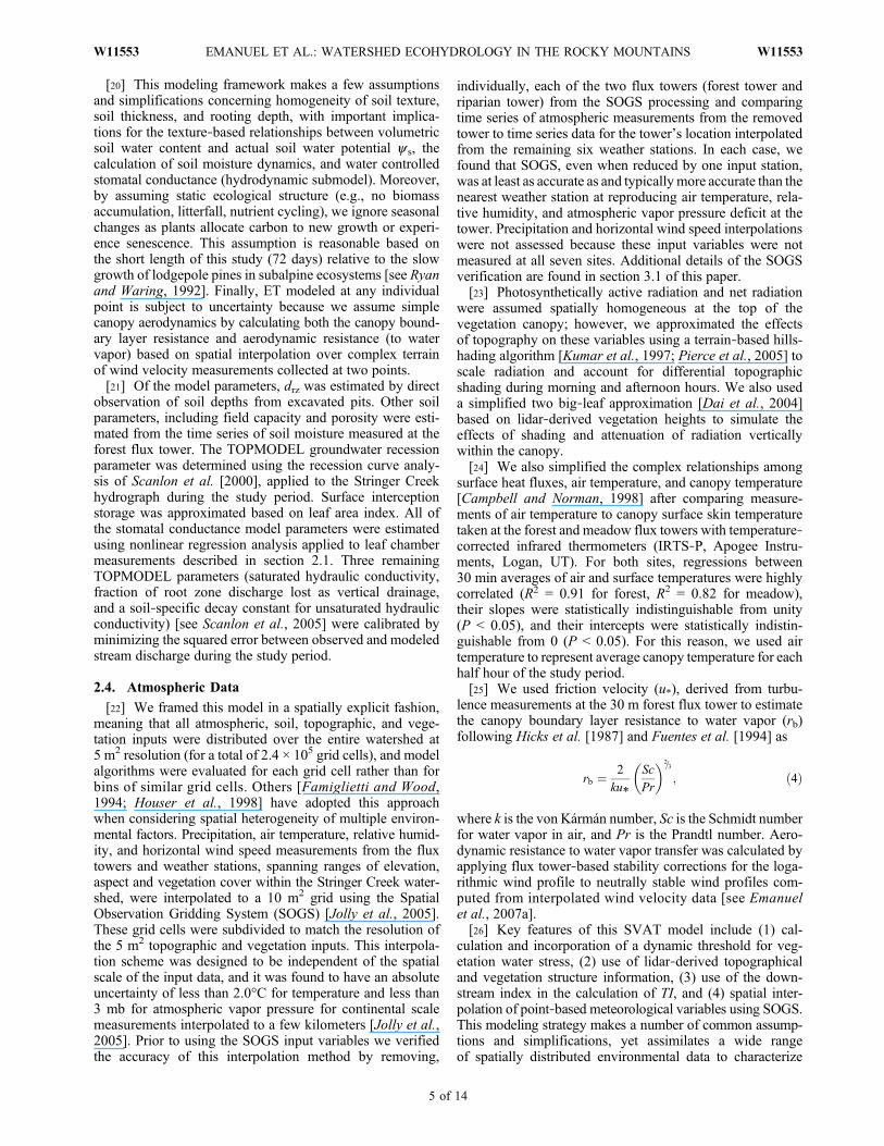
regimes is the correlation between watershed!average ETand micrometeorological variables (Table 2). The correla-tion between ET and ! increases from unstressed to stressedconditions within the watershed, whereas the correlationbetween ET and atmospheric variables (i.e., VPD and Tair)decreases from conditions of no water stress to conditions ofstress. Thus the transition from unstressed to stressed veg-etation is marked by a shift in the functional control of ETfrom predominantly atmospheric factors and no significantsoil moisture control (representing capacity for CO2 uptakeand atmospheric demand for water) to reduced atmosphericcontrol and significant soil moisture control. Not only doesthe correlation between ET and ! appear at the onset of waterstress, but it also strengthens with P"y* > y s# (Figure 4),accompanied by a decrease in correlation between ETand atmospheric demand (represented by VPD) decreases(Figure 4). We emphasize here that these correlations are basedon observations from the forest flux tower that have been par-titioned using modeled levels of catchment!wide water stress.[39] These patterns of changing correlation suggest that

during the growing season, watershed!averaged water stress,and thus watershed!averaged ET are subject to a shift fromdemand!limitation (controlled by atmospheric variables) tosupply limitation (controlled by !) as the soil water supplydecreases relative to the atmospheric demand. As a resultET, which is not limited by ! early in the season, increaseswith VPD even as ! declines during the unstressed regime.However, once ! is insufficient to meet the atmosphericdemand for moisture when stomatal conductance is maxi-mized for CO2 uptake (a definition of vegetationwater stress),ET declines as stomatal conductance is reduced to maintain asustainable flow of water through the soil!plant!atmospherecontinuum. Indeed, watershed!averaged, modeled stomatal

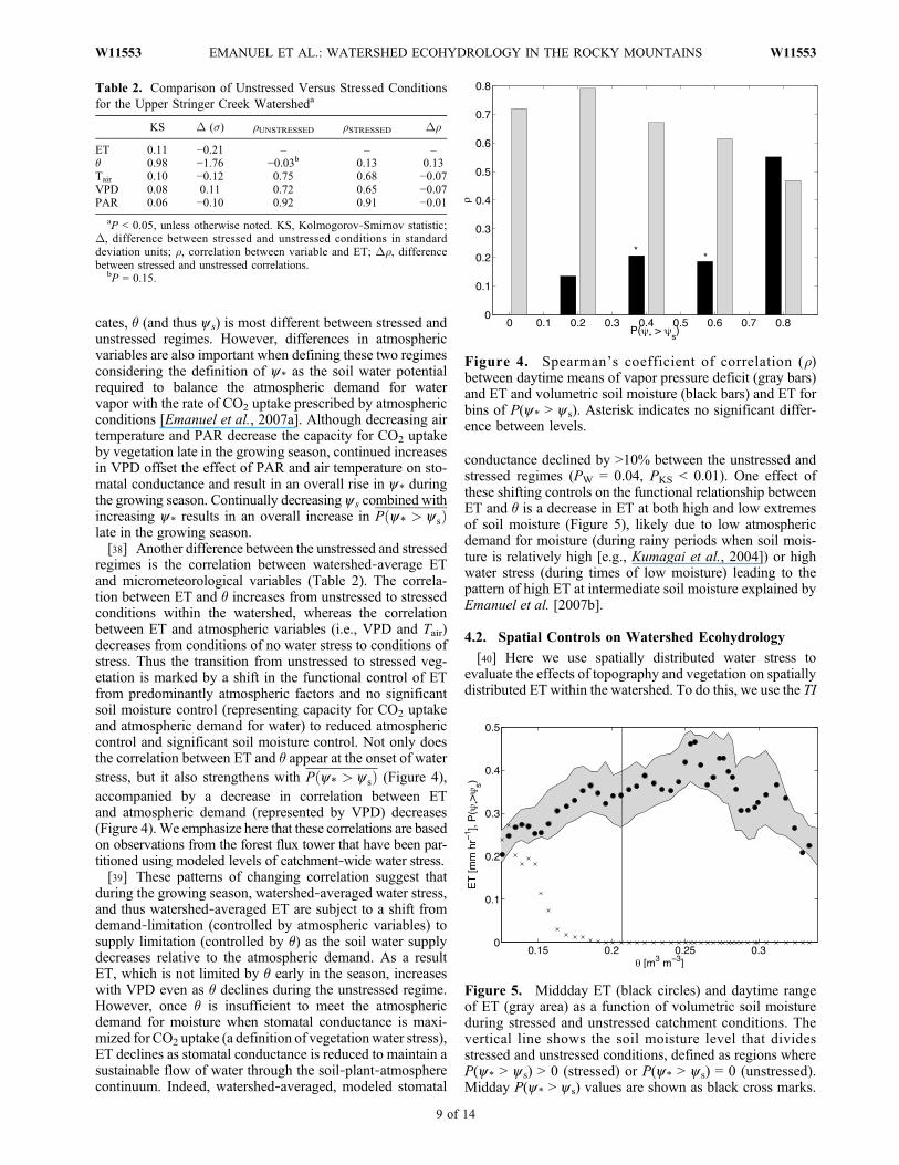
conductance declined by >10% between the unstressed andstressed regimes (PW = 0.04, PKS < 0.01). One effect ofthese shifting controls on the functional relationship betweenET and ! is a decrease in ET at both high and low extremesof soil moisture (Figure 5), likely due to low atmosphericdemand for moisture (during rainy periods when soil mois-ture is relatively high [e.g., Kumagai et al., 2004]) or highwater stress (during times of low moisture) leading to thepattern of high ET at intermediate soil moisture explained byEmanuel et al. [2007b].

4.2. Spatial Controls on Watershed Ecohydrology[40] Here we use spatially distributed water stress to

evaluate the effects of topography and vegetation on spatiallydistributed ET within the watershed. To do this, we use the TI

Table 2. Comparison of Unstressed Versus Stressed Conditionsfor the Upper Stringer Creek Watersheda

KS D (s) rUNSTRESSED rSTRESSED Dr

ET 0.11 "0.21 – – –! 0.98 "1.76 "0.03b 0.13 0.13Tair 0.10 "0.12 0.75 0.68 "0.07VPD 0.08 0.11 0.72 0.65 "0.07PAR 0.06 "0.10 0.92 0.91 "0.01

aP < 0.05, unless otherwise noted. KS, Kolmogorov!Smirnov statistic;D, difference between stressed and unstressed conditions in standarddeviation units; r, correlation between variable and ET; Dr, differencebetween stressed and unstressed correlations.

bP = 0.15.

Figure 4. Spearman’s coefficient of correlation (r)between daytime means of vapor pressure deficit (gray bars)and ET and volumetric soil moisture (black bars) and ET forbins of P(y* > ys). Asterisk indicates no significant differ-ence between levels.

Figure 5. Middday ET (black circles) and daytime rangeof ET (gray area) as a function of volumetric soil moistureduring stressed and unstressed catchment conditions. Thevertical line shows the soil moisture level that dividesstressed and unstressed conditions, defined as regions whereP(y* > ys) > 0 (stressed) or P(y* > ys) = 0 (unstressed).Midday P(y* > ys) values are shown as black cross marks.

EMANUEL ET AL.: WATERSHED ECOHYDROLOGY IN THE ROCKY MOUNTAINS W11553W11553

9 of 14

and Zveg as indicators of topography and local vegetationconditions at each 5 m ! 5 m grid cell, respectively. Meangrowing season soil moisture (!, Figure 6a) and total growingseason ET (SET, Figure 6b) appear to follow the spatialorganization of TI (Figure 1a) and Zveg (Figure 1b), respec-tively. At first glance, the difference between the spatialorganization of these two variables across the watershedsuggests that soil moisture does not control ET and that waterstress is not a controlling factor. However, despite the highcorrelation between SET and Zveg (due to leaf!to!canopyscaling based on Zveg), many forested grid cells (Zveg > 0.5 m)have values of SET below the maximum value predictedby Zveg!scaling alone. In fact, the MAE between SET and alinear regression model (c) based solely on Zveg is 51 mm, orapproximately 20% of total ET averaged across the water-shed. Because the simple model c considers only tree heightand ignores the impact of soil moisture on SET, the model’sresiduals (c " SET) represent, in part, the degree to whichsoil moisture, and thereby water stress, control ET within thewatershed.[41] By plotting residuals (c " SET) as a function of

topography (i.e., TI) and vegetation (i.e., Zveg), the twomain sources of spatial heterogeneity within the watershed,areas having low TI and high Zveg emerge as portions of thewatershed where ET is controlled by factors other than treeheight (Figure 7). These areas, which make up approxi-mately 10% of the watershed and are characterized by rel-atively tall trees (high Zveg) and relatively dry soils (low TI),have lower evapotranspiration than predicted by c (i.e.,larger residuals). However, this does not mean that theseareas necessarily have low SET compared to the rest ofthe watershed. On the contrary, because these areas containsome of the tallest trees and greatest leaf area within thewatershed, average SET for these grid cells (330 mm) isnearly double the average SET for the rest of the watershed(180 mm). If not for water stress, the preceding analysis ofresiduals suggests that these areas of the watershed wouldcontribute even more to total watershed ET. We evaluate

water stress in this portion of Figure 7 (i.e., areas with lowc " SET) by considering two spatially distributed metrics,time!averaged probability of water stress and the date ofwater stress onset. This analysis highlights the importance ofconsidering water stress when using LAI or vegetation heightto scale ET between leaf and canopy scales. By scalingmodeled ET based on LAI, vegetation height or other struc-tural variables without considering the soil and atmosphericfactors contributing to water stress, one runs the risk ofoverestimating ET. In other words, any univariate relation-ship between ET and a structural scaling variable should beconsidered an upper bound to the actual relationship betweenET and vegetation structure, made nonlinear by water stress.[42] The time!averaged probability of vegetation water

stress for each grid cell, hP(y* > ys)i, is correlated primarilywith soil moisture or, more precisely, with the sensitivityof modeled ! to TI (Figure 8a, note similarity to Figure 1a).In contrast, the date of water stress onset for each gridcell Dstress is correlated primarily with Zveg (Figure 8b, notesimilarity to Figure 1b). The correlation between Dstress andZveg may result from the tendency of taller trees to have

Figure 6. Model simulations of the (a) average soil moisture and (b) total ET distributed throughout theStringer Creek watershed.

Figure 7. Residuals of linear model c ! SET as a functionof TI and Zveg for the Stringer Creek watershed.

EMANUEL ET AL.: WATERSHED ECOHYDROLOGY IN THE ROCKY MOUNTAINS W11553W11553

10 of 14

more leaf area and transpire more water, thus depleting soilmoisture earlier in the season.[43] Both hP(y* > ys)i and Dstress are useful for inter-

preting the overall impact of vegetation water stress on ETand other hydrological processes within the watershed, par-ticularly in the low!TI, high!Zveg region defined in Figure 7,because these parts of the watershed contribute, on aver-age, more evapotranspiration than the rest of the watershed(Figure 9a). However, this region experiences significantlyhigher hP(y* >ys)i than the rest of the watershed (Figure 9b).Similarly, this region experiences significantly earlier Dstressthan the rest of the watershed (Figure 9c). This result con-firms that tall trees on relatively dry hillslopes experiencemore water stress than vegetation in other parts of the water-shed, and they also encounter water stress at an earlier date.Increased stress occurs in part because these trees transpiremore soil water than other vegetation in the watershed, andalso because the hillslopes on which they are located have, onaverage, only 14% of the uphill contributing area of the rest ofthe watershed. Thus, small contributing areas combine withtall trees to create water stress, the result of which is to reducelocal evapotranspiration in areas of the watershed that alreadycontribute substantially to the water balance of this water-shed. These results add to the growing body of evidence fortopographic control over vegetation water stress [e.g. Cayloret al., 2005; Jasper et al., 2006] by introducing an eco-physiological basis for modeling spatially distributed waterstress and using these model results to interpret flux towerobservations.

4.3. Interaction of Temporal and Spatial Controls[44] Model results and flux tower measurements indicate

that ET is the dominant watershed scale flux during boththe unstressed and stressed periods defined in section 4.1,

Figure 8. Model simulations of (a) the average probability of water stress during the 2006 growing sea-son and (b) the onset date of water stress for the Stringer Creek watershed.

Figure 9. Differences in (a) total ET and (b) average waterstress and (c) onset date of water stress for locations whereZveg > 5 m and TI < 8.5 (black line) and for the rest of thewatershed (gray line).

EMANUEL ET AL.: WATERSHED ECOHYDROLOGY IN THE ROCKY MOUNTAINS W11553W11553

11 of 14

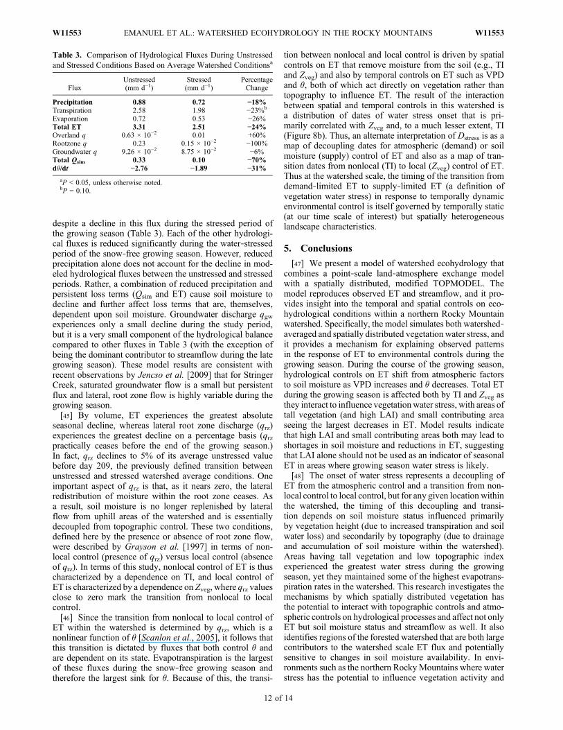
despite a decline in this flux during the stressed period ofthe growing season (Table 3). Each of the other hydrologi-cal fluxes is reduced significantly during the water!stressedperiod of the snow!free growing season. However, reducedprecipitation alone does not account for the decline in mod-eled hydrological fluxes between the unstressed and stressedperiods. Rather, a combination of reduced precipitation andpersistent loss terms (Qsim and ET) cause soil moisture todecline and further affect loss terms that are, themselves,dependent upon soil moisture. Groundwater discharge qgwexperiences only a small decline during the study period,but it is a very small component of the hydrological balancecompared to other fluxes in Table 3 (with the exception ofbeing the dominant contributor to streamflow during the lategrowing season). These model results are consistent withrecent observations by Jencso et al. [2009] that for StringerCreek, saturated groundwater flow is a small but persistentflux and lateral, root zone flow is highly variable during thegrowing season.[45] By volume, ET experiences the greatest absolute

seasonal decline, whereas lateral root zone discharge (qrz)experiences the greatest decline on a percentage basis (qrzpractically ceases before the end of the growing season.)In fact, qrz declines to 5% of its average unstressed valuebefore day 209, the previously defined transition betweenunstressed and stressed watershed average conditions. Oneimportant aspect of qrz is that, as it nears zero, the lateralredistribution of moisture within the root zone ceases. Asa result, soil moisture is no longer replenished by lateralflow from uphill areas of the watershed and is essentiallydecoupled from topographic control. These two conditions,defined here by the presence or absence of root zone flow,were described by Grayson et al. [1997] in terms of non-local control (presence of qrz) versus local control (absenceof qrz). In terms of this study, nonlocal control of ET is thuscharacterized by a dependence on TI, and local control ofET is characterized by a dependence on Zveg, where qrz valuesclose to zero mark the transition from nonlocal to localcontrol.[46] Since the transition from nonlocal to local control of

ET within the watershed is determined by qrz, which is anonlinear function of ! [Scanlon et al., 2005], it follows thatthis transition is dictated by fluxes that both control ! andare dependent on its state. Evapotranspiration is the largestof these fluxes during the snow!free growing season andtherefore the largest sink for !. Because of this, the transi-

tion between nonlocal and local control is driven by spatialcontrols on ET that remove moisture from the soil (e.g., TIand Zveg) and also by temporal controls on ET such as VPDand !, both of which act directly on vegetation rather thantopography to influence ET. The result of the interactionbetween spatial and temporal controls in this watershed isa distribution of dates of water stress onset that is pri-marily correlated with Zveg and, to a much lesser extent, TI(Figure 8b). Thus, an alternate interpretation of Dstress is as amap of decoupling dates for atmospheric (demand) or soilmoisture (supply) control of ET and also as a map of tran-sition dates from nonlocal (TI) to local (Zveg) control of ET.Thus at the watershed scale, the timing of the transition fromdemand!limited ET to supply!limited ET (a definition ofvegetation water stress) in response to temporally dynamicenvironmental control is itself governed by temporally static(at our time scale of interest) but spatially heterogeneouslandscape characteristics.

5. Conclusions

[47] We present a model of watershed ecohydrology thatcombines a point!scale land!atmosphere exchange modelwith a spatially distributed, modified TOPMODEL. Themodel reproduces observed ET and streamflow, and it pro-vides insight into the temporal and spatial controls on eco-hydrological conditions within a northern Rocky Mountainwatershed. Specifically, the model simulates both watershed!averaged and spatially distributed vegetationwater stress, andit provides a mechanism for explaining observed patternsin the response of ET to environmental controls during thegrowing season. During the course of the growing season,hydrological controls on ET shift from atmospheric factorsto soil moisture as VPD increases and ! decreases. Total ETduring the growing season is affected both by TI and Zveg asthey interact to influence vegetationwater stress, with areas oftall vegetation (and high LAI) and small contributing areaseeing the largest decreases in ET. Model results indicatethat high LAI and small contributing areas both may lead toshortages in soil moisture and reductions in ET, suggestingthat LAI alone should not be used as an indicator of seasonalET in areas where growing season water stress is likely.[48] The onset of water stress represents a decoupling of

ET from the atmospheric control and a transition from non-local control to local control, but for any given location withinthe watershed, the timing of this decoupling and transi-tion depends on soil moisture status influenced primarilyby vegetation height (due to increased transpiration and soilwater loss) and secondarily by topography (due to drainageand accumulation of soil moisture within the watershed).Areas having tall vegetation and low topographic indexexperienced the greatest water stress during the growingseason, yet they maintained some of the highest evapotrans-piration rates in the watershed. This research investigates themechanisms by which spatially distributed vegetation hasthe potential to interact with topographic controls and atmo-spheric controls on hydrological processes and affect not onlyET but soil moisture status and streamflow as well. It alsoidentifies regions of the forested watershed that are both largecontributors to the watershed scale ET flux and potentiallysensitive to changes in soil moisture availability. In envi-ronments such as the northern Rocky Mountains where waterstress has the potential to influence vegetation activity and

Table 3. Comparison of Hydrological Fluxes During Unstressedand Stressed Conditions Based on Average Watershed Conditionsa

FluxUnstressed(mm d"1)

Stressed(mm d"1)

PercentageChange

Precipitation 0.88 0.72 !18%Transpiration 2.58 1.98 "23%b

Evaporation 0.72 0.53 "26%Total ET 3.31 2.51 !24%Overland q 0.63 ! 10"2 0.01 +60%Rootzone q 0.23 0.15 ! 10"2 "100%Groundwater q 9.26 ! 10"2 8.75 ! 10"2 "6%Total Qsim 0.33 0.10 !70%d!/dt !2.76 !1.89 !31%

aP < 0.05, unless otherwise noted.bP = 0.10.

EMANUEL ET AL.: WATERSHED ECOHYDROLOGY IN THE ROCKY MOUNTAINS W11553W11553

12 of 14

where ET is a dominant watershed scale flux, the spatialdistribution of vegetation is an important characteristic withimplications for other watershed scale fluxes.[49] Acknowledgments. This research was funded by NSF grants

EAR!0236621, EAR!0403924, and EAR!0838193 and a Moore ResearchAward from the Department of Environmental Sciences, University ofVirginia. We thank W. Matt Jolly (U.S. Forest Service) for provid-ing SOGS code and Todd Scanlon (University of Virginia) for providingTOPMODEL code. We are grateful to the U.S. Forest Service RockyMountain Research Station, especially Ward McCaughey, for extensivelogistical support. Kelly Caylor (Princeton University), Pat Yeh (Universityof Tokyo), and an anonymous reviewer provided helpful comments on themanuscript.

ReferencesAlbertson, J. D., and G. Kiely (2001), On the structure of soil moisture

time series in the context of land surface models, J. Hydrol., 243(1–2),101–119.

Anderson, M. C., W. P. Kustas, and J. M. Norman (2003), Upscaling anddownscaling—A regional view of the soil!plant!atmosphere continuum,Agron. J., 95(6), 1408–1423.

Bales, R. C., N. P. Molotch, T. H. Painter, M. D. Dettinger, R. Rice, andJ. Dozier (2006), Mountain hydrology of the western United States,Water Resour. Res., 42, W08432, doi:10.1029/2005WR004387.

Ball, J. T., I. E. Woodrow, and J. A. Berry (1987), A model predicting sto-matal conductance and its contribution to the control of photosynthesisunder different environmental conditions, Prog. Photosynth. Res., 4,221–224.

Barnett, T. P., et al. (2008), Human!induced changes in the hydrology ofthe western United States, Science, 319, 1080–1083.

Beven, K. J., and M. J. Kirkby (1979), A physically based, variable contrib-uting area model of basin hydrology, Hydrol. Sci. Bull., 24(1) 43–69.

Boegh, E., M. Thorsen, M. B. Butts, S. Hansen, J. S. Christiansen,P. Abrahamsen, C. B. Hasager, N. O. Jensen, P. Van der Keur, and J. C.Refsgaard (2004), Incorporating remote sensing data in physically baseddistributed agro!hydrological modelling, J. Hydrol., 287(1–4), 279–299.

Buckley, T. N., K. A. Mott, and G. D. Farquhar (2003), A hydromechanicaland biochemical model of stomatal conductance, Plant Cell Environ.,26(10), 1767–1785.

Campbell, G. S., and J. M. Norman (1998), An Introduction to Environ-mental Biophysics, 2nd ed., Springer, New York.

Caylor, K. K., S. Manfreda, and I. Rodriguez!Iturbe (2005), On the coupledgeomorphological and ecohydrological organization of river basins, Adv.Water Res., 28, 69–86, doi:10.1016/j.advwatres.2004.08.013.

Clapp, R. B., and G. M. Hornberger (1978), Empirical equations forsome soil hydraulic properties, Water Resour. Res., 14(4) 601–604,doi:10.1029/WR014i004p00601.

Collatz, G. J., J. T. Ball, C. Grivet, and J. A. Berry (1991), Physiologicaland environmental regulation of stomatal conductance, photosynthesisand transpiration: A model that includes a laminar boundary layer, Agric.Forest Meteorol., 54(2–4), 107–136.

Dai, Y., R. E. Dickinson, and Y. P. Wang (2004), A two!big!leaf model forcanopy temperature, photosynthesis, and stomatal conductance, J. Clim.,17(12), 2281–2299.

Detto, M., N. Montaldo, J. D. Albertson, M. Mancini, and G. Katul (2006),Soil moisture and vegetation controls on evapotranspiration in a hetero-geneous Mediterranean ecosystem on Sardinia, Italy, Water Resour.Res., 42, W08419, doi:10.1029/2005WR004693.

Dingman, S. L. (2002), Physical Hydrology, 2nd ed., 646 p., Prentice Hall,Upper Saddle River, N. J.

Dubayah, R. O., and J. B. Drake (2000), Lidar remote sensing for forestry,J. For., 98, 44–46.

Eagleson, P. (1982), Ecological optimality in water!limited natural soil!vegetation systems: 1. Theory and hypothesis, Water Resour. Res.,18(2), 325–340, doi:10.1029/WR018i002p00325.

Emanuel, R. E., P. D’Odorico, and H. E. Epstein (2007a), A dynamicsoil water threshold for vegetation water stress derived from stomatalconductance models, Water Resour. Res., 43, W03431, doi:10.1029/2005WR004831.

Emanuel, R. E., P. D’Odorico, and H. E. Epstein (2007b), Evidence of opti-mal water use among a range of north american ecosystems, Geophys.Res. Lett., 34, L07401, doi:10.1029/2006GL028909.

Famiglietti, J. S., and E. F. Wood (1994), Application of multiscale waterand energy balance models on a tallgrass prairie, Water Resour. Res.,30(11), 3079–3094, doi:10.1029/94WR01499.

Farquhar, G. D., S. Von Caemmerer, and J. A. Berry (1980), A biochemicalmodel of photosynthetic CO2 in leaves of C3 species., Planta, 149, 78–90.

Ford, C. R., R. M. Hubbard, B. D. Kloeppel, and J. M. Vose (2007), Acomparison of sap flux!based evapotranspiration estimates withcatchment!scale water balance, Agric. Forest Meteorol., 145, 176–185.

Fuentes, J. D., T. J. Gillespie, and N. J. Bunce (1994), Effects of foliagewetness on the dry deposition of ozone onto red maple and poplar leaves,Water Air Soil Pollut., 74(1–2), 189–210.

Fyfe, L. C., and J. M. Flato (1999), Enhanced climate change and its detec-tion over the Rocky mountains, J. Clim., 12(1), 230–243.

Gao, Q., P. Zhao, X. Zeng, X. Cai, and W. Shen (2002), A model ofstomatal conductance to quantify the relationship between leaf transpira-tion, microclimate and soil water stress, Plant Cell Environ., 25(11),1373–1381.

Grayson, R. B., A. W. Western, F. H. S. Chiew, and G. Bloschl (1997),Preferred states in spatial soil moisture patterns: Local and nonlocal con-trols, Water Resour. Res., 33(12), 2897–2908, doi:10.1029/97WR02174.

Guswa, A. J. (2005), Soil!moisture limits on plant uptake: An upscaled rela-tionship for water!limited ecosystems, Adv. Water Res., 28(6), 543–552.

Hicks, B. B., D. D. Baldocchi, T. Meyers, R. P. Hosker, and D. R. Matt(1987), A preliminary multiple resistance routine for deriving dry depo-sition velocities from measured quantities, Water Air Soil Pollut., 36,311–330.

Hjerdt, K. N., J. J. McDonnell, J. Seibert, and A. Rodhe (2004), A newtopographic index to quantify downslope controls on local drainage,Water Resour. Res., 40, W05602, doi:10.1029/2004WR003130.

Houser, P. R., W. J. Shuttleworth, J. S. Famiglietti, H. V. Gupta, K. H.Syed, and D. C. Goodrich (1998), Integration of soil moisture remotesensing and hydrologic modeling using data assimilation, Water Resour.Res., 34(12), 3405–3420, doi:10.1029/1998WR900001.

Jasper, K., P. Calanca, and J. Fuhrer (2006) Changes in summertime soilwater patterns in complex terrain due to climatic change, J. Hydrol.,327, 550–563, doi:10.1016/j.jhydrol.2005.11.061.

Jencso, K. G., B. L. McGlynn, M. N. Gooseff, S. M. Wondzell, K. E.Bencala, and L. A. Marshall (2009), Hydrologic connectivity betweenlandscapes and streams: Transferring reach! and plot!scale understandingto the catchment scale, Water Resour. Res., 45, W04428, doi:10.1029/2008WR007225.

Jolly, W. M., J. M. Graham, A. Michaelis, R. Nemani, and S. W. Running(2005), A flexible, integrated system for generating meteorologicalsurfaces derived from point sources across multiple geographic scales,Environ. Modell. Software, 20(7), 873–882.

Kaimal, J. C., and J. J. Finnegan (1994) Atmospheric Boundary LayerFlows, 289 pp., Oxford Univ. Press, New York.

Keane, R. E., E. D. Reinhardt, J. Scott, K. Gray, and J. Reardon (2005),Estimating forest canopy bulk density using six indirect methods, Can.J. For. Res., 35(3), 724–739.

Kozlowski, T. T. (1992), Carbohydrate sources and sinks in woody plants,Bot. Rev., 82(2), 107–222.

Kumagai, T., G. G. Katul, T. M. Saitoh, Y. Sato, O. J. Manfroi, T. Morooka,T. Ichie, K. Kuraji, M. Suzuki, andA. Porporato (2004),Water cycling in aBornean tropical rain forest under current and projected precipitation sce-narios, Water Resour. Res., 40, W01104, doi:10.1029/2003WR002226.

Kumagai, T., M. Tateishi, T. Shimizu, and K. Otsuki (2008), Transpirationand canopy conductance at two slope positions in a Japanese cedar forestwatershed, Agric. For. Meteorol., 148, 1444–1455.

Kumar, L., A. K. Skidmore, and E. Knowles (1997), Modelling topo-graphic variation in solar radiation in a GIS environment, Int. J. Geogr.Info. Sci., 11(5), 475–497.

Lefsky, M. A., W. B. Cohen, G. G. Parker, and D. J. Harding (2002), Lidarremote sensing for ecosystem studies, Bioscience, 52(1), 19–30.

Legates, D. R., and G. J. McCabe (1999), Evaluating the use of “goodness!of!fit” measures in hydrologic and hydroclimatic model validation,Water Resour. Res., 35(1), 233–241, doi:10.1029/1998WR900018.

Leuning, R. (1995), A critical appraisal of a combined stomatal!photosynthesismodel for C3 plants, Plant Cell Environ., 18(4), 339–355.

McCaughey, W. W. (1996), Tenderfoot creek experimental forest, inExperimental Forests, Ranges, and Watersheds in the Northern RockyMountains: A Compendium of Outdoor Laboratories in Utah, Idaho,and Montana, edited by W. C. Schmidt and J. L. Friede, U.S. Dep. ofAgriculture, Forest Service, Utah.

Mincemoyer, S. A., and J. L. Birdsall (2006), Vascular flora of the Tender-foot Creek Experimental Forest, Little Belt Mountains, Montana,Madroño, 53(3), 211–222.

Mohanty, B. P., and T. H. Skaggs (2001), Spatio!temporal evolution andtime!stable characteristics of soil moisture within remote sensing foot-

EMANUEL ET AL.: WATERSHED ECOHYDROLOGY IN THE ROCKY MOUNTAINS W11553W11553

13 of 14

prints with varying soil, slope, and vegetation, Adv. Water Res., 24(9–10),1051–1067.

Mote, P. W., A. F. Hamlet, M. P. Clark, and D. P. Lettenmaier (2005),Declining mountain snowpack in western North America, Bull. Am.Meteorol. Soc, 86(1), 39–49.

Norman, J. M., J. M. Welles, and D. K. McDermitt (2006), Estimatingcanopy light!use and transpiration efficiencies from leaf measurements,Appl. Note 105, LI!COR Biosci., Lincoln, Nebr.

Paw U., K. T., D. D. Baldocchi, T. P. Meyers, and K. B. Wilson (2000),“Correction of eddy!covariance measurements incorporating both advec-tive effects and density fluxes,” Boundary Layer Meteorol., 97, 487–511.

Pierce, K. B., T. Lookingbill, and D. Urban (2005), A simple method forestimating potential relative radiation (PRR) for landscape!scale vegeta-tion analysis, Landscape Ecol., 20(2), 137–147.

Priestley, C. H. B., and R. J. Taylor (1972), On the assessment of surfaceheat flux and evaporation using large!scale parameters, Mon. WeatherRev., 100, 81–92.

Riveros!Iregui, D. A., R. E. Emanuel, D. J. Muth, B. L. McGlynn, H. E.Epstein, D. L. Welsch, V. J. Pacific, and J. M. Wraith (2007), Diurnalhysteresis between soil temperature and soil CO2 is controlled by soilwater content, Geophys. Res. Lett., 34, L17404, doi:10.1029/2007GL030938.

Rodriguez!Iturbe, I., and A. Porporato (2004), Ecohydrology of Water!Controlled Ecosystems, 442 pp., Cambridge Univ. Press, New York.

Running, S. W. (1980), Relating plant capacitance to the water relationsof pinus contorta, For. Ecol. Manage., 2(4), 237–252.

Ryan, M. G., and R. H. Waring (1992), Maintenance respiration andstand development in a subalpine lodgepole pine forest, Ecology, 73(6),2100–2108.

Scanlon, T. M., J. P. Raffensperger, G. M. Hornberger, and R. B. Clapp(2000), Shallow subsurface stormflow in a forested headwater catch-ment: Observations and modeling using a modified TOPMODEL, WaterResour. Res., 36(9) 2575–2586, doi:10.1029/2000WR900125.

Scanlon, T. M., G. Kiely, and R. Amboldi (2005), Model determination ofnonpoint source phosphorus transport pathways in a fertilized grasslandcatchment, Hydrol. Processes, 19(14), 2801–2814.

Schimel, D., T. G. F. Kittel, S. Running, R. Monson, A. Turnispeed, andD. Anderson (2002), Carbon sequestration studied in western U.S.

mountains, Eos Trans. AGU , 83(40), 445–449, doi:10.1029/2002EO000314.

Schotanus, P., F. T. M. Nieuwstadt, and H. A. R. De Bruin (1983), Tem-perature measurement with a sonic anemometer and its application toheat and moisture fluxes, Boundary Layer Meteorol., 26, 81–93.

Seibert, J., and B. L. McGlynn (2007), A new triangular multipleflow direction algorithm for computing upslope areas from gridded dig-ital elevation models, Water Resour. Res., 43, W04501, doi:10.1029/2006WR005128.

Stewart, I. T., D. R. Cayan, and M. D. Dettinger (2004), Changes in snow-melt runoff timing in western North America under a ‘business as usual’climate change scenario, Clim. Change, 62(1–3), 217–232.

Webb, I. K., G. I. Pearman, and R. Leuning (1980), Correction of fluxmeasurements for density effects due to heat and water vapour transfer,Q. J. R. Meteorol. Soc., 106, 85–100.

Western, A. W., R. B. Grayson, G. Bloschl, G. R. Wilgoose, and T. A.McMahon (1999), Observed spatial organization of soil moisture andits relation to terrain indices, Water Resour. Res., 35(3), 797–810,doi:10.1029/1998WR900065.

Woods, S. W., R. Ahl, J. Sappington, and W. McCaughey (2006), Snowaccumulation in thinned lodgepole pine stands, Montana, USA, ForestEcol. Manage., 235(1–3), 202–211.

Zhang, L., W. R. Dawes, and G. R. Walker (2001), Response of meanannual evapotranspiration to vegetation changes at catchment scale,Water Resour. Res., 37(3), 701–708, doi:10.1029/2000WR900325.

R. E. Emanuel, Department of Forestry and Environmental Resources,North Carolina State University, PO Box 8008, Raleigh, NC 27695,USA. (ryan_emanuel@ncsu.edu)P. D’Odorico, H. E. Epstein, and D. J. Muth, Department of

Environmental Sciences, University of Virginia, 291 McCormick Rd,Charlottesville, VA 22904, USA.B. L. McGlynn, Department of Land Resources and Environmental

Sciences, Montana State University, Bozeman, MT 59716, USA.D. L. Welsch, Canaan Valley Institute, Davis, WV 26260, USA.

EMANUEL ET AL.: WATERSHED ECOHYDROLOGY IN THE ROCKY MOUNTAINS W11553W11553

14 of 14