Space-time precipitation reflecting climate change

Hydrological Sciences -Journal- des Sciences Hydrologk[ues,38,6, December 1993 5 3 9

Space-time precipitation reflecting climate change

ISTVAN MATYASOVSZKY* & ISTVAN BOGARDI Department of Civil Engineering, University of Nebraska-Lincoln, Lincoln, Nebraska 68588-0531, USA

ANDRAS BARDOSSY Institut fur Hydrologie und Wasserwirtschaft, University of Karlsruhe, Kaiserstrasse 12, D-7500 Karlsruhe 1, Germany

LUCIEN DUCKSTEIN Systems and Industrial Engineering Department, University of Arizona, Tucson, Arizona 85721, USA

Abstract A methodology has been developed and applied to an eastern Nebraska, USA, case study to estimate the space-time distribution of daily precipitation under climate change. The approach is based on the analysis both of the type and of the Markov properties of atmospheric circulation patterns (CPs), and a stochastic linkage between daily (here 500 hPa) CP types and daily precipitation events. Historical data and General Circulation Model (GCM) output of daily CPs corresponding to 1 X CO ?

and 2 X C 0 2 are considered. Time series of both local and regional precipitation corresponding to each of those cases were simulated and their statistical properties were compared. Under the dry continental climate of eastern Nebraska, a highly variable spatial response to climate change was obtained. Most of the local and the regional average precipitation values reflect, under 2 X C 0 2 , a somewhat wetter and a more variable precipitation regime in eastern Nebraska. The sensitivity of the results to the GCM utilized should be considered.

Estimation spatiale des précipitations journalières en cas de modification climatique Résumé Une méthode d'estimation de la distribution spatiale et temporelle des précipitations journalières en cas de modification climatique a été développée et appliquée au cas d'espèce du Nebraska oriental. L'approche consiste à analyser au pas de temps journalier la circulation atmosphérique (CA) puis à modéliser la dépendance stochastique entre les types de CA (caractérisés ici par la courbe des 500 hPA) et les données pluviométriques. La série chronologique des données historiques et celles obtenues par des modèles de circulation générale (MCG) ont été comparées pour les scénarios 1 X C 0 2 et 2 x C 0 2 . Les séries de pluies ponctuelles et régionales correspondant à chacun des scénarios précités ont été simulées et leurs propriétés statistiques ont été comparées. Dans les conditions continentales sèches du Nebraska oriental, la réponse spatiale à une modification climatique semble être très variable. D'une façon générale, les précipitations moyennes

*On leave from Department of Meteorology, Eôtvôs Lorând University, Ludovika ter, 1083 Budapest, Hungary. Open for discussion until I June 1994

540 Istvan Matyasovsky et al.

ponctuelles et régionales deviennent, pour le cas étudié et pour le scénario 2 X C02 , quelque peu plus fortes et plus variables. Une étude de sensibilité de ces résultats au type de MCG utilisé doit être envisagée.

INTRODUCTION

The purpose of this paper is to develop a stochastic space-time model for estimating the effect of climate change scenarios on regional and local precipitation. The methodology is applied under the dry continental climate of eastern Nebraska, USA.

The magnitude and consequences of regional response to anticipated climatic changes are uncertain (Houghton et al., 1990). Possible sustained regional droughts, excessive floods, multi-year shortage of water in reservoirs, excessive water levels in natural lakes and other hydrological events pose considerable social concern. A typical question to be answered is: can time series of hydrological events be conditioned on scenarios of future climate change, and if so, how can this be implemented?

The proposed approach is an extension of the usual analysis of regional hydrological impacts of climate change. Often, the quite uncertain hydrological outputs of atmospheric global circulation models (GCM) are disaggregated to calculate regional hydrological events. This study proposes to examine the more accurate and verifiable time series of daily GCM-produced atmospheric circulation patterns (CPs) to estimate local precipitation. The approach is based on an analysis of daily CPs defined as pressure surfaces using available and reliable data.

The paper is organized as follows. First the space-time precipitation model is described. Then, daily CPs are classified and analysed statistically, first for historical and then for GCM produced data. Next, the height of the 500 hPa pressure field within each CP type is introduced as an additional variable influencing daily precipitation. 1 x C02 and 2 x C02 scenarios result in similar CP types and frequencies but, as can be expected, in different average pressure heights. This fact is utilized to estimate the regional and local effects of climate change. The methodology section is followed by a case study application. A discussion and conclusions section describing results and experiences of this study close the paper.

PRECIPITATION MODEL

Space-time approach

For hydrological application, precipitation is usually modelled as a stochastic process. The resulting (usually point-process) models describe precipitation occurrence (Chang et al., 1984a; 1984b; Foufoula-Georgiou & Lettenmaier, 1987; Small & Morgan, 1986), or occurrence and amount (Duckstein et al.,

Space-time precipitation reflecting climate change 541

1972; Bogardi et al., 1988; Kavvas & Delleur, 1981) at selected locations. Spatial characteristics of precipitation are usually analysed for selected events (Chua & Bras, 1982). Space-time models for the spatial and time distribution of precipitation over a region (for example a basin) are usually models for single events, based on some general physical considerations and several stochastic assumptions (Rodriguez-Iturbe & Eagleson, 1987). A model for simultaneous multi-site generation of daily precipitation was developed by Binark et al. (1976) and Binark (1979). In the present paper, a modified version of the space-time precipitation model developed in Bardossy & Plate (1992) is used. This model makes it possible to distribute a given precipitation amount over a basin.

Univariate autoregressive (AR) processes represent a well developed and commonly used technique to model time series (Box & Jenkins, 1970). Here, the time series of daily precipitation at spatially correlated locations would need to be modelled as a multivariate AR process that is a natural generalization to vector time series.

The main difficulty of modelling the precipitation is its space-time intermittence. The precipitation occurrence at a given location must be conditioned on precipitation at other locations; then the precipitation amount (if it exists) is conditioned on occurrence and amount at other locations. This approach requires the estimation of a lot of parameters. Another difficulty is that time series models have been principally developed for Gaussian processes but conditional probability distributions of precipitation are far from normal. Therefore, there is a need to develop a transformation that establishes a relationship between precipitation and the normal distribution.

Bardossy & Plate (1992) presented a stochastic model to incorporate the occurrence of daily precipitation and its spatially correlated and highly skewed time series. Intermittence in both time and space and skewness are modelled analytically as a power-transformed normally distributed random vector. This approach, however, does not appear to be applicable to modelling daily precipitation under dry continental climates since no appropriate exponent can be found to describe the distribution of daily precipitation (Bogardi et al., 1992). Instead of this technique a nonparametric approach was used to simulate daily precipitation based on the empirical distribution given by Bogardi et al. (1992). However, such an approach cannot be used to estimate the effect of global climate change because empirical distributions of regional and local precipitation reflecting climate change are not available.

Consider the transformation Z(t, u) = T\W(t, u)) in a general non-analytical form, where Z(t, u) represents the daily precipitation amount at time t and location u, and W(t, u) is a normal random function. A natural way to represent Tis a series expansion of given functions. Specifically, let W(t, u)—V for each t and u, where V is the standard normal random variable. The standard normal random variable defined on the interval (— °°, oo) may be considered on an interval ( -L, L) since the probability of lying outside this region is negligible if L is sufficiently large. Then a finite Fourier series expansion of T may be


established in the following manner. (For the sake of simplicity, arguments of Zwill be omitted; each location is handled separately as discussed below). Let z and v be realizations of Z and V, respectively. Then a finite approximation of T corresponding to z and v is given by:

n n

z _ j^v) = a0 + ^2 akcos(—kv) + ^2 bksm(—kv) (1) *=i L k=1 L

where: L

a° = i ! r ( v ) d v (2a)

L

ak = - [ T(v)co$(-kv)dv (2b)

bk= - \ T{v)sm{-kv)àv (2c)

The integrations (2a)-(2c) can be approximated numerically by appropriate summations based on quantiles of the standard normal distribution and an empirical distribution of the precipitation as follows. Quantiles zp, vp corresponding to probability p are defined by:

P{Z<zp) = * ^ ) = p

P(V<vp) = *(vp) = p

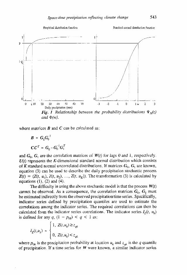
wherep> 1 — p0 and p0 is the precipitation probability, ¥N is the empirical distribution function of the precipitation and $ is the standard normal distribution function. The transformation Tcan be rewritten as:

Z=JXV) = I 0 ' F ^ ° (3) { ' \T(V), V>0

and T(V) for v is given by:

Zp=r(vpMrN\vp)) W

(Fig. 1). The value L = 3 may be used in equations (l)-(2). To reproduce the space-time statistical structure of precipitation at

locations uk, k = 1, 2, ..., K a suitable model should be chosen for the vector Wdefined at time t as W(t) = (W(t, ux), W(t, u2), ..., W(t, uK)). Note that the components of the vector W(f) are correlated normal random variables with zero expectation and unit variance. The time dependence is described using a first order autoregressive (AR(1)) process:

W(t) = BW(t-l) + CV(t)


Empirical distribution function Standard normal distribution function

H

70 0 zlO 20 30 40 50 60 Daily precipitation (mm)

Fig. 1 Relationship between the probability distributions ^^z) and 3>(w).

where matrices B and C can be calculated as:

B = Gfiô1

CC = GQ-G0 GJ

and G0, GY are the correlation matrices of W(t) for lags 0 and 1, respectively. U(t) represents the isT-dimensional standard normal distribution which consists of i£ standard normal uncorrelated distributions. If matrices GQ, G, are known, equation (3) can be used to describe the daily precipitation stochastic process Z(t) = (Z(t, Mj), Z(t, Uj), ..., Z(t, %)). The transformation (3) is calculated by equations (1), (2) and (4).

The difficulty in using the above stochastic model is that the process W(t) cannot be observed. As a consequence, the correlation matrices G0, Gx must be estimated indirectly from the observed precipitation time series. Specifically, indicator series defined by precipitation quantiles are used to estimate the correlations among the indicator series. The required correlations can then be calculated from the indicator series correlations. The indicator series Iz(t, uk) is defined for any q, (1 - p0k) < q < 1 as:

Iz(t,uk) 1, Z(t,uk)>z •qk

0, Z(t,uk)<zqk

where p0k is the precipitation probability at location uk and zqk is the q quantile of precipitation. If a time series for W were known, a similar indicator series


Iy^t, uk) could be defined and each element of G0 could be calculated using equation (5). However, the indicator series Iy/f, uk) and Iz(t, uk) are the same because of the correspondence between the quantiles of W and Z, so that Iz{t, uk) may be used instead of Iy^t, uk). The required correlation g(i,j), the (/, j)th element of G0, is related to the correlation of the indicator series g^9\i,f) through the relationship (Abramowitz & Stegun, 1965):

sin-'feO',/)]

g(q\ij) = n ,} , \ exp

This equation can be solved for g(i,f) using a simple numerical algorithm. The elements of Gx are derived in a similar way.

Linkage of daily CPs with daily space-time precipitation

Daily circulation patterns are characterized by the daily spatial distribution of sea level pressure or of a given low or middle tropospheric pressure height. The regional and local hydrological variables at a given time and location are strongly influenced by atmospheric circulation patterns, hence climatic variability may be related to changes in atmospheric circulation (Lamb, 1977).

The task here is to extend the mathematical model described in the previous section by conditioning on daily CP types. As proposed in Bardossy & Plate (1992), this can be done by considering each circulation type separately and defining the multivariate normal process W(t) in the following way. If the

j'th CP type persists at days t and t — 1, W(t) is given by:

W(t) = BjW(t -1) + CjU(f) (6)

However, if thej'th CP type just changes to the ith type at time t the precipitation process will have no "memory" at that time:

W(t) = Dp(f) (7)

where DDT = G0.

DAILY CIRCULATION PATTERNS AND CLIMATE CHANGE SCENARIOS

Three types of daily CP data are used here: (a) historical data are represented by the National Meteorological Center

(NMC) grid point analyses of the height of 500 hPa pressure fields, available from the National Center for Atmospheric Research (NCAR). The analysis is based on daily values (1200 h) at 40 points on a diamond grid covering the sector 25°-60°N, 80°-125°W for the period January

l+sin(s) ds (5)


1948-June 1989; (b) a 10-year long data series for the same pressure level has been obtained

from the outputs of the Canadian Climate Centre (CCC) GCM (Boer et al., 1984) corresponding to the 1 x COj scenario; and

(c) an analogous series has been obtained from the 2 x C02 scenario. There are several possibilities combined with considerable experience for

classifying daily CPs. A brief review of classification techniques for precipitation modelling purposes can be found in Matyasovszky et al. (1992a). In the present paper, the three data sets are classified using the &-means clustering method (MacQueen, 1967) combined with a principal component analysis described in detail in Matyasovszky et al. (1992a). The periods from 1 April to 30 September and from 1 October to 31 March were examined separately. Defining nine types for both periods seems to be a good compromise between the increasing number of types and decreasing distances of pressure fields within types.

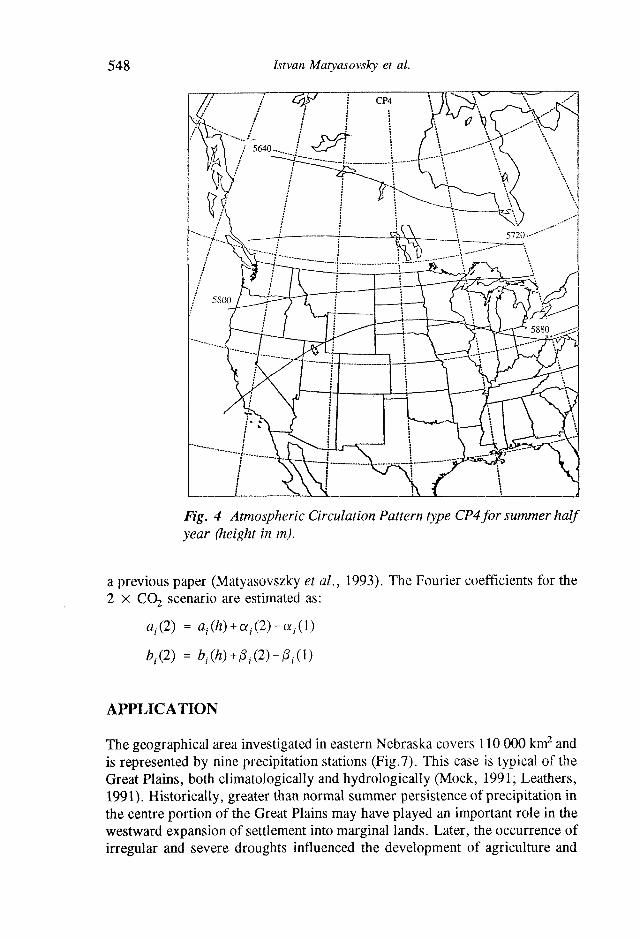
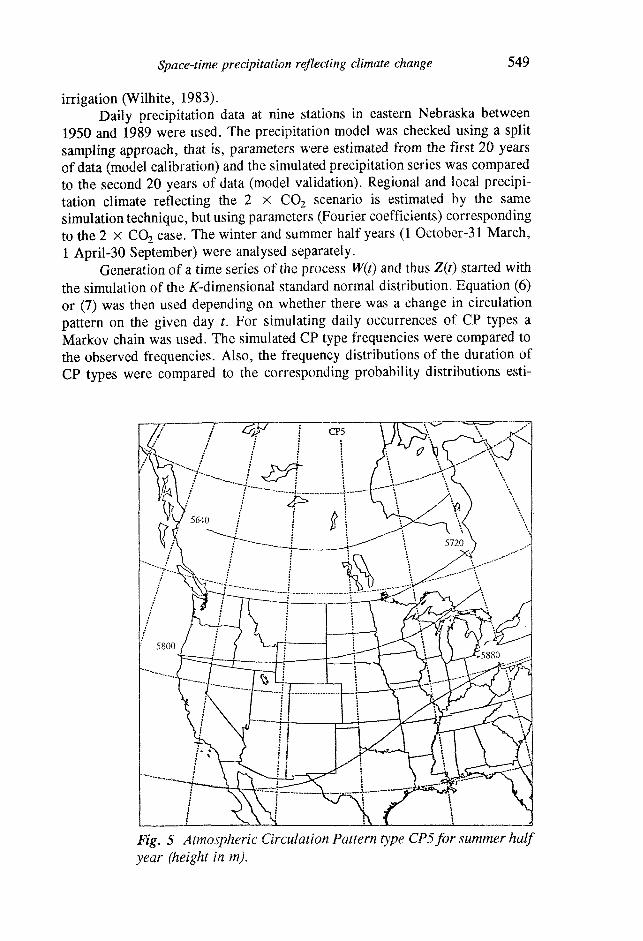
Two examples are given for the winter and summer seasons, respectively. In winter, CP1 (the "wettest" type) is characterized by southwesterly flows in central and eastern USA. Warm and wet air masses advected from the subtropics cause large amounts of precipitation (Fig. 2). CP3, the "driest" type, is a pattern with strong northwesterly flows (Fig. 3). Cold air masses are dry due to the passage over the mountainous west. The summer season is illustrated in Figs 4 and 5. CP4 is a type without considerable flows in central and southern USA (Fig. 4). Precipitation is governed by local effects which can cause intensive but very infrequent precipitation. CP5 advects warm and moist conditionally unstable air masses from the subtropics, in which case convective activity can occur over Nebraska (Fig. 5).

The persistence of CP types is described by a Markov chain model. Such a model is characterized by a transition probability matrix which is, in the present case, the matrix of transition probabilities from one CP type to another. Figure 6 illustrates, as an example, how such a Markov model can describe statistically the duration of CP types, and shows a good fit between the observed and GCM produced CP type durations in the 1 x CO2 case. However, the 2 x C02 case appears to yield very similar relative frequencies of CP type duration. Originally, it was intended to use this approach to simulate space-time series of local climatic variables reflecting climate change. However, the difference between the frequencies of CP types corresponding to the 1 x C02 and 2 x C02 cases is relatively small compared to the difference between the frequencies of the 1 x C02 case and historical data (Table 1). Some authors argue that, within a CP type, atmospheric conditions influencing precipitation may change, which means that knowledge of the type of CP alone is not enough and additional parameters have to be introduced to describe CPs under climate change. Since CPs in the 2 x C02 case are characterized in general by larger pressure level heights it is reasonable to link meteorological variables to the type and height of CPs. The height is an indicator of the atmospheric pressure (high or low) and temperature (warm or cold). The basic idea is that the annual cycle of the pressure height is considered as an analogy


Fig. 2 Atmospheric Circulation Pattern type CP1 for winter half year (height in m).

of the difference between present and the warmer 2 x CO, climates.

CONSIDERATION OF THE PRESSURE FIELD HEIGHT

Within each CP type daily precipitation depends on the actual spatial average height z of the 500 hPa pressure field. This relationship can be used to estimate the effect of climate change on regional and local precipitation.

The basic idea is to include die spatially averaged pressure height into the analysis; the annual cycle of the pressure height is considered as an analogy of the difference between present and 2 x COj climates. The relationship between the probability distribution of daily precipitation and spatial average height is described using historical data. Table 2 shows the heights spatially averaged over each CP type separately for the winter and summer and the three CP data sets. Two important facts should be noted in Table 2. Firstly, the average heights of the 1 x C02 and 2 x C02 cases are significantly different for every type. Secondly, the average heights of the historical and 1 x CQ2


CPs are significantly different for several CP types. The direction of differences in heights suggests that the GCM used in this paper systematically underestimates the pressure height.

Because of these facts, regional and local precipitation statistics reflecting the 2 x C02 scenario were estimated in two steps: (a) the differences of the Fourier coefficients between 1 x C02 and 2 x C02 cases were calculated; and (b) Fourier coefficients obtained from the historical data were corrected using the above differences to arrive at a probability distribution reflecting the 2 x C02 scenario. Denote {affi), b/Ji}} as the Fourier coefficients computed from the whole historical data series and denote {a,(l), «,(1)}, {$(2), jS,(2)} as sequences of the Fourier coefficients corresponding to 1 x CO2 and 2 x C02

average pressure heights (zl5 z2), respectively. These two sequences are also determined from the historical data series using precipitation data only from an interval around Zj and z2- The widths of these two intervals are chosen to be equal to the bandwidth used for a nonparametric regression technique developed for estimating the precipitation probability for the 2 x C02 case in

Fig. 3 Atmospheric Circulation Pattern type CP3 for winter half year (height in m).

Istvan Matyasovsky et al.

Fig. 4 Atmospheric Circulation Pattern type CP4for summer half year (height in m).

a previous paper (Matyasovszky et al., 1993). The Fourier coefficients for the 2 x C02 scenario are estimated as:

û.(2) =û,.(a) + a,.(2)-a,.(l)

b{(2) = bt(h) +0,(2)-0,(1)

APPLICATION

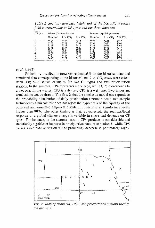
The geographical area investigated in eastern Nebraska covers 110 000 km2 and is represented by nine precipitation stations (Fig.7). This case is typical of the Great Plains, both climatologically and hydrologically (Mock, 1991; Leathers, 1991). Historically, greater than normal summer persistence of precipitation in the centre portion of the Great Plains may have played an important role in the westward expansion of settlement into marginal lands. Later, the occurrence of irregular and severe droughts influenced the development of agriculture and


irrigation (Wilhite, 1983). Daily precipitation data at nine stations in eastern Nebraska between

1950 and 1989 were used. The precipitation model was checked using a split sampling approach, that is, parameters were estimated from the first 20 years of data (model calibration) and the simulated precipitation series was compared to the second 20 years of data (model validation). Regional and local precipitation climate reflecting the 2 x C02 scenario is estimated by the same simulation technique, but using parameters (Fourier coefficients) corresponding to the 2 x C02 case. The winter and summer half years (1 October-31 March, 1 April-30 September) were analysed separately.

Generation of a time series of the process W(t) and thus Z(t) started with the simulation of the ^-dimensional standard normal distribution. Equation (6) or (7) was then used depending on whether there was a change in circulation pattern on the given day t. For simulating daily occurrences of CP types a Markov chain was used. The simulated CP type frequencies were compared to the observed frequencies. Also, the frequency distributions of the duration of CP types were compared to the corresponding probability distributions esti-

Fig. 5 Atmospheric Circulation Pattern type CP5for summer half year (height in m).


0 . 6

0.5 \-

0.4

0.3

0.2

0.1

Observed Simulated(l) Simulated(2)

3 4 5 6 7 8 9 Duration (days)

Fig. 6 Duration of CP3 in winter calculated from observed and simulated data corresponding to 1 x C02 (simulated (1)) and 2 x C02 (simulated (2)) cases.

mated from the Markov model. The fitting was satisfactory for each CP type (BogMdiet ah, 1992).

Daily precipitation in eastern Nebraska is quite variable both in time and space: it is characterized by a relatively high probability of zero precipitation, a skewed distribution and spatial dependency. The hydro-climatological model can reproduce these characteristics. Also, the occurrence of different CP types has a substantial influence on space-time precipitation. For instance, there is a sixteen-fold difference between means of daily precipitation conditioned on the wettest and the driest CPs. The simulated frequency distributions obtained from the stochastic model were close to the observed frequencies. Precipitation statistics conditioned on CP types were also quite well reproduced, but to save space these results will not be discussed here; for further details see Bogardi

Table 1 Relative frequency ofCP types corresponding to the three data sets

CP type Winter (October-March)

Historical 1 X C0 2 2 X C0 2

Summer (April-September)

Historical 1 X CO, 2 X C0 2

1 1

3 4 5 6 7 8 9

0.082 0.134 0.122 0.112 0.082 0.124 0.089 0.134 0.120

0.065 0.186 0.113 0.127 0.086 0.082 0.092 0.162 0.086

0.070 0.189 0.108 0.106 0.088 0.080 0.152 0.123 0.085

0.126 0.067 0.097 0.102 0.130 0.121 0.104 0.134 0.119

0.122 0.062 0.060 0.173 0.093 0.134 0.115 0.156 0.083

0.103 0.097 0.056 0.076 0.093 0.074 0.167 0.246 0.088


Table 2 Spatially averaged height (m) of the 500 hPa pressure field corresponding to CP types and the three data sets

CP type

1 2 3 4 5 6 7 8 9

Winter (October-March)

Historical

5566 5529 5521 5541 5550 5582 5565 5590 5490

1 x CO,

5536 5528 5528 5525 5527 5527 5520 5533 5527

2 x C 0 2

5613 5598 5616 5620 5608 5603 5610 5606 5614


Historical

5725 5737 5738 5748 5720 5707 5731 5681 5705

1 x C 0 2

5691 5677 5671 5683 5686 5691 5679 5684 5695

2 x C 0 2

5752 5766 5762 5777 5773 5755 5756 5762 5773

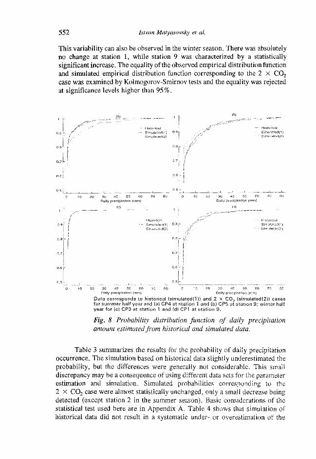
et al. (1992). Probability distribution functions estimated from the historical data and

simulated data corresponding to the historical and 2 x CO, cases were calculated. Figure 8 shows examples for two CP types and two precipitation stations. In the summer, CP4 represents a dry type, while CP5 corresponds to a wet one. In the winter, CP3 is a dry and CP1 is a wet type. Two important conclusions can be drawn. The first is that the stochastic model can reproduce the probability distribution of daily precipitation amount since a two sample Kolmogorov-Smirnov test does not reject the hypothesis of the equality of the observed and simulated empirical distribution functions at significance levels higher than 90%. The other finding is that, as expected, the regional/local response to a global climate change is variable in space and depends on CP types. For instance, in the summer season, CP4 produces a considerable and statistically significant increase in precipitation amount at station 1, while CP5 causes a decrease at station 9 (the probability decrease is particularly high).

WY

N E B R A

CO

O 50 scale miles

S K A

!100 KA

Fig. 7 Map of Nebraska, USA, and precipitation stations used in the analysis.


This variability can also be observed in the winter season. There was absolutely no change at station 1, while station 9 was characterized by a statistically significant increase. The equality of the observed empirical distribution function and simulated empirical distribution function corresponding to the 2 x C02

case was examined by Kolmogorov-Smirnov tests and the equality was rejected at significance levels higher than 95%.

f Historical Simu!ated(1) 0-9 Simu!ated(2)

— Historical - Simu?ated(1)

Stmu!at©d(2)

10 20 30 40 50 60 70 80 Daiiy precipitation (mm)

(c)

Simulated(l) °-9

Simu!ated<2)

20 30 10 SO 60 70 80 Daisy precipitation (mm)

Histories! Simuiated(l) Simulated(2)

>0 30 40 50 60 70 80 0 10 20 30 40 50 60 70 80 Daily precipitation (mm) Daiiy precipitation (mm)

Data corresponds to historical (s imulatedd )) and 2 x C 0 2 !simulated(2)) cases for summer half year and (a) CP4 at station 1 and (b) CP5 at stat ion 9 ; winter half year for (c) CP3 at stat ion 1 and (d) CP1 at stat ion 9.

Fig. 8 Probability distribution Junction of daily precipitation amount estimated from historical and simulated data.

Table 3 summarizes the results for the probability of daily precipitation occurrence. The simulation based on historical data slightly underestimated the probability, but the differences were generally not considerable. This small discrepancy may be a consequence of using different data sets for the parameter estimation and simulation. Simulated probabilities corresponding to the 2 x C02 case were almost statistically unchanged, only a small decrease being detected (except station 2 in the summer season). Basic considerations of the statistical test used here are in Appendix A. Table 4 shows that simulation of historical data did not result in a systematic under- or overestimation of the


Table 3 Probability of daily precipitation occurrence estimated from historical data and simulated data corresponding to historical and 2 x C02 cases

Precipitation station

Winter (October-March) Summer (April-September)

Historical Simulated (historical)

Simulated (2 X CCy

Historical Simulated (historical)

Simulated (2 X CCy

1 2 3 4 5 6 7 8 9

0.38 0.15 0.27 0.19 0.20 0.20 0.31 0.32 0.27

0.32* 0.13 0.21* 0.19 0.17 0.19 0.28* 0.29 0.24

0.28** 0.11* 0.21* 0.18 0.18 0.19 0.26** 0.27* 0.23*

0.42 0.25 0.36 0.26 0.32 0.29 0.37 0.39 0.37

0.38* 0.25 0.30* 0.25 0.28* 0.29 0.36 0.38 0.34

0.45 0.60** 0.30* 0.26 0.29 0.30 0.35 0.38 0.29*

* significant difference between historical and simulated cases at 95% level; ficant difference between historical and both simulated cases at 95% level.

signi-

Table 4 Mean of daily positive precipitation amount (mm) estimated from historical data and simulated data corresponding to historical and 2 x C02 cases

Precipitation Winter (October-March)

i 2 3 4 5 6 7 8 9

Historical

2.4 5.7 3.0 4.6 4.0 5.1 3.5 3.7 4.4

Simulated (historical)

2.5 5.1* 3.2 4.7 3.9 5.2 3.2 3.4 4.2

Simulated (2 x COj)

3.7** 6.0** 4.1** 5 7** 5.0** 5.5** 4 1** 4.6** 5.9**


Historical

5.9 9.9 7.0 9.4 7.8 9.4 7.8 7.4 7.9

Simulated (historical)

6.4* 10.1 6.9 9.2 7.7 9.9* 7 ?» 7.5 8.4*

Simulated (2 x CCy 6.1? 11.3** 9.2** 9.3 10.2** 10.0* 7.7? 7.8* 10.5**

* significant difference between historical and simulated cases at 95% level; ** significant difference between historical and both simulated cases at 95 % level, ? significant difference between the two simulated cases, but there is no difference between the

level.

daily mean precipitation, while 2 x C02 simulation produced a considerable increase. The test for significance is summarized in Appendix B.

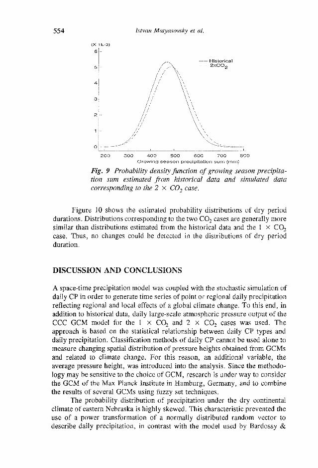
To smooth the large spatial variability, daily regional mean precipitation amounts were calculated using the external drift kriging interpolation method (Bardossy & Muster, 1992). The daily values were summarized for summer half years (growing season). Figure 9 contains the probability density functions corresponding to the historical data and the 2 x COj scenario. The density functions were obtained after simulating 1000 summer half years and checking the hypothesis of normality. Since the normality was not rejected using even a small acceptance interval the normal densities are shown instead of the corresponding histograms. The means (474.6 and 492.0 mm) and standard deviations (72.2 and 75.4 mm) show that the 2 x C02 case is characterized by a slightly and statistically significant larger mean and standard deviation of the precipitation amount, which means that not only the average precipitation but also the variability increases.

Istvan Matyasovsky et al.

2O0 300 400 500 600 700 800 Growing s e a s o n precip i tat ion sunn (mm)

Fig. 9 Probability density function of growing season precipitation sum estimated from historical data and simulated data corresponding to the 2 x C02 case.

Figure 10 shows the estimated probability distributions of dry period durations. Distributions corresponding to the two C02 cases are generally more similar than distributions estimated from the historical data and the 1 x COj case. Thus, no changes could be detected in the distributions of dry period duration.

DISCUSSION AND CONCLUSIONS

A space-time precipitation model was coupled with the stochastic simulation of daily CP in order to generate time series of point or regional daily precipitation reflecting regional and local effects of a global climate change. To this end, in addition to historical data, daily large-scale atmospheric pressure output of the CCC GCM model for the 1 x CO, and 2 x C02 cases was used. The approach is based on the statistical relationship between daily CP types and daily precipitation. Classification methods of daily CP cannot be used alone to measure changing spatial distribution of pressure heights obtained from GCMs and related to climate change. For this reason, an additional variable, the average pressure height, was introduced into the analysis. Since the methodology may be sensitive to the choice of GCM, research is under way to consider the GCM of the Max Planck Institute in Hamburg, Germany, and to combine the results of several GCMs using fuzzy set techniques.

The probability distribution of precipitation under the dry continental climate of eastern Nebraska is highly skewed. This characteristic prevented the use of a power transformation of a normally distributed random vector to describe daily precipitation, in contrast with the model used by Bardossy &


Plate (1992). The transformation used in this paper is based on a Fourier series expansion. The application results indicate a spatially variable but considerable effect of climate change on the distribution of daily precipitation in eastern Nebraska.

The following conclusions may be made: (a) a Fourier series expansion technique can be used to express the relation

ship between the standard normal random vector and daily space-time precipitation;

(b) a stochastic linkage can be established between the daily circulation pattern types and daily precipitation;

(c) the classification techniques do not detect differences in daily atmospheric circulation pattern types obtained from 1 x C02 and 2 x C02

GCM outputs; (d) using the differences between spatially averaged pressure heights corres

ponding to the 1 x CO2 and 2 x C02 cases the regional and local effects of climate change scenarios can be estimated;

0.5

0,4

0.3

0.2

0.1

0

• \ \

"A \ -v ^

( 0 !

^=^.

— Historical —• Slmu!ated(1) • - SImu!ated(2)

i i i i

— Historical — Slmulated( l ) • • Slmulated(2)

0 1 2 3 4 5 6 7 0 9 10 0 1 2 3 4 5 6 7 Duration (days)

Historical Simulaîed(l) Simulated(2) OA

Historical StmulatedO) Slmulaied(2)

10 11 12 10 11 12 Duration (days) Durat ion (days)

Data used corresponds to the historical (simulated (1)) and 2 x C 0 2 (simulated

(2)) cases for summer half year and (a) CP4 at stat ion 1 and (b) CP5 at stat ion 9;

winter half year for (c) CP3 at stat ion 1 and (d) CP1 at stat ion 9.

Fig. 10 Probability distribution of dry period duration estimated from historical and simulated data.


(e) Fourier coefficients for the 2 x C02 scenario can be estimated and these coefficients can be used to generate time series of space-time daily precipitation reflecting climate change;

(f) the regional and local response to a global climate change is variable in space and depends on CP types in eastern Nebraska;

(g) time series of regional precipitation under climate change can also be generated. The growing season precipitation amount is characterized by a slightly larger mean and standard deviation;

(h) no changes can be detected in the probability distribution of dry period duration; and

(i) for the region considered here a more variable precipitation climate is detected for the 2 x CO> scenario.

Acknowledgements The authors would like to thank the reviewers for their helpful criticism and useful comments. Research leading to this paper has been partly supported by grants from the US National Science Foundation, BCS-9016462/9016556, EAR-9205717/9217818 and the Great Plains Regional Center of the National Institute for Global Environmental Change. The additional support of the Center for Infrastructure Research of the University of Nebraska is also acknowledged.

REFERENCES

Abramowitz, M. & Stegun, I. (1965) Handbook of Mathematical Functions. Dover Publications, New York, USA.

Bardossy, A. & Muster, H. (1992) Spatial interpolation of daily rainfall amounts under different meteorological conditions Working paper, Institut fiir Hydrologie und Wasserwirtschaft, UniversMt Karlsruhe, 7500 Karlsruhe, Germany.

Bardossy, A. & Plate, E. (1990) Modeling daily rainfall using a semi-Markov representation of circulation pattern occurrence. J. Hydrol. 66, 33-47.

Bardossy, A. & Plate, E. (1992) Space-time model for daily rainfall using atmospheric circulation patterns. Wit. Resour. Res. 28, 1247-1260.

Binark, A. M. (1979) Simultané Niederschlagsgenerierung an mehreren Stationen eines Einzugs-gebietes. Mitteilungen, Heft 16, Institut wasserbau III Universitat Karlsruhe, 1979.

Binark, A. M. Duckstein, L. & Plate, E. (1976) Multi-site rainfall generation for multi-site flood simulation. AGU Fall Meeting, San Francisco, California, USA.

Boer, G. J., McFarlane, N. A., Laprise, R., Henderson, J. D. & Blanchet, J. P. (1984) The Canadian Climate Centre spectral atmospheric General Circulation Model. Atrnos. Ocean 22, 397-429.

Bogardi, I., Matyasovszky, I., Bardossy, A. & Duckstein, L. (1992) Estimating space-time local hydrological quantities under climate change. Proc. 5th International Meeting on Statistical Climatology, Toronto, Canada, 22-26 June 1992.

Bogardi, J. J., Duckstein, L. & Rumambo, O. (1988) Practical generation of synthetic rainfall event time series in a semiarid climatic zone. J. Hydrol. 103, 357-363.

Box, G. E. P. & Jenkins, G.M. (1970) Time Series Analysis, Forecasting and Control. Holden Day, San Francisco, USA.

Chang, T. J., Kavvas, M. L. & Delleur, J. W. (1984a) Daily precipitation modeling by discrete auto-regressive moving average. H6f. Resour. Res. 20, 565-580.

Chang, T. J. Kawas, M. L. & Delleur, J. W. (1984b) Modeling of sequences of wet and dry days by binary discrete autoregressive moving average processes. / . Clim. Appl. Met. 23, 1367-1378.

Chua, S. H. & Bras, R. L. (1982) Optimal estimators of mean areal precipitation in regions of orographic influence. / . Hydrol. 57, 23-48.

Duckstein, L., Fogel, M. & Kisiel, C. C. (1972) A stochastic model of runoff producing rainfall for summer type storms, Wit. Resour. Res. 8, 410-421.

Foufoula-Georgiou, E. & Lettenmaier, D. P. (1987) A Markov renewal model for rainfall occurrences. Wht. Resour. Res. 23, 875-884.


Houghton, J. T., Jenkins, G. J. & Ephraums, J. J. (eds) (1990) Climate change: the IPCC scientific assessment. Intergovernmental Panel on Climate Change, Cambridge University Press, New York, USA.

Kawas, M. L. & Delleur, J. W. (1981) A stochastic cluster model for daily rainfall sequences Wit. Resour.Res. 17, 1151-1160.

Lamb, H. H. (1977) Climate, Present, Past and Future. Vol. 2: Climatic History and the Future. Methuen, London, UK.

Leathers, D. J. (1991) Relationship between 700 mb circulation variation and Great Plains climate. Great Plain Res. 1, 58-76.

MacQueen, J. (1967) Some methods for classification and analysis of multivariate observations. Proc. 5th Berkeley Symp. on Mathematics, Statistics and Probability 1, 281-297.

Matyasovszky, I., Bogardi, I., Bardossy, A. &. Duckstein, L. (1992) Évaluation of historical and GCM produced atmospheric circulation patterns. Working Paper, Department of Civil Engineering, University of Nebraska-Lincoln, Lincoln, Nebraska 68588, USA.

Matyasovszky, I., Bogardi, I., Bardossy, A. & Duckstein, L. (1993) Estimation of local precipitation statistics reflecting climate change. Working Paper, Department of Civil Engineenrg, University of Nebraska-Lincoln, Lincoln, Nebraska 68588, USA; Wit. Resour. Res. 19 (in press).

Mock, C. J. (1991) Drought and precipitation fluctuations in the Great Plains during the late nineteenth century. Great Plains R^s. 1,26-57.

Rodriguez-Iturbe, I. & Eagleson, P. S. (1987) Mathematical models of rainstorm events in space and time. Wit. Resour. Res. 23, 181-190.

Small, M. J. & Morgan, D. J. (1986) The relationship between a continuous-time renewal model and a discrete Markov chain model of precipitation occurrence. Wit. Resour. Res. 22, 1420-1430.

Wilhite, D. A. (1983) Government response to drought in the United States: with particular reference to the Great Plains. J. Clim. 4, 297-310.

APPENDIX A: TEST FOR PROBABILITY O F PRECIPITATION OCCURRENCE

Letx i ; i = 1, ..., n, andj-, i = 1, ..., «2 be two statistically independent time series of daily precipitation amount and let px, p2 be the probabilities of positive daily precipitation amount. Since the relative frequency p calculated from a sample of size n has a normal limiting distribution with expected value p and variance p(l — p)ln, a statistical test can be constructed as follows. If Pi ~ Pii t n e random variable:

A _ A 0,(1-AW* lAa-AtW''4

has normal limiting distribution with zero expected value and unit variance, and then the acceptance interval of the hypothesis px — p2 is:

(-xa<Q<xa) xa = *-\l-Z) 0 < a < l (Al)

where $ is the standard normal distribution function and (1 — a)100% is the significance level.

APPENDIX B: TEST FOR MEAN O F POSITIVE DAILY PRECIPITATION AMOUNT

Let ml and m^ be the expectations of positive values of time series {*,•}, {yt}. Using the central limit theorem the means ml, fhj have normal limiting distributions with expected value mx and % , and variance vl/hl and v2//i2, respectively,

Q (2)'


where hu h^ represent the numbers of positive daily precipitation amounts and v1? v2 correspond to their variances. If mx = m^ the random variable:

Q l

(2)v

mx ffh

{yhj* (D2//g*

has a normal limiting distribution with zero expected value and unit variance, and then the acceptance interval of the hypothesis ml = n^ is given by equation (Al).

Received 12 January 1993; accepted 4 August 1993

Documents

Space-time precipitation reflecting climate change