Integr. equ. oper. theory 42 (2002) 1-21 0378-620X/02/010001-21 $1.50+0.20/0 �9 Birkh~iuser Verlag, Basel, 2002

I Integral Equations and Operator Theory

S O M E F I N I T E - D I M E N S I O N A L B A C K W A R D - S H I F T - I N V A R I A N T S U B S P A C E S IN T H E BALL AND A R E L A T E D I N T E R P O L A T I O N

P R O B L E M

DANIEL ALPAY* and H. TURGAY KAPTANOGLU

We solve Gleason's problem in the reproducing kernel Hilbert space with repro- ducing kernel 1 / ( 1 - ~ zjw~). We define and study some finite-dimensional resolvent-invariant subspaces that generalize the finite-dimensional de Branges- Rovnyak spaces to the setting of the ball.

1 I n t r o d u c t i o n

In this paper we study a family of finite-dimensional Hilbert spaces of rational functions analytic in the ball

= ( z l , . . . , z N ) l lzjl 2 < 1 , (1.1) 1

whose reproducing kernel is of the form

I,~ - B ( z )S (w)* (1.2) 1 -- ZW*

In this expression, z and w are in the unit ball, zw* = ~ z~w;, and the function B is rational and matrix-valued. To provide motivation and set the framework, we first consider the case N = 1, that is, the case of the open unit disk D. First recall that the Hardy space of the open unit disk H2(D) consists of power series f ( z ) = ~ o fn zn with complex coefficients such that

[Ifll~I2(D) def. f i lfnl 2 < (:~ (1.3) 0

*This research was supported by a grant from the United States-Israel Binational Science Foundation (BSF), Jerusalem, Israel, and by the Israeli Academy of Sciences.

2 Alpay, Kaptano~lu

1 We recall that and is the reproducing kernel Hilbert space with reproducing kernel 1--G~w." 1 belongs to H2(D) and this means the following: For every w 6 ]3 the function z ~-+

f ( z ) , 1 - z w * H2(ID)

for every f E H2(D). The space H2(D) is invariant under the backward shift (also called resolvent-like) operators Ra defined as

Raf (Z) = f ( z ) - f ( a ) , z E D. (1.4) z - - a

We recall that these operators satisfy the resolvent equation

Ra - Rb = (a - b)R~Rb, a, b E D, (1.5)

hence their name. Furthermore, the adjoint of the operator Ra in H2(D) is given by

<:(z) = zf(z), (1.6) 1 - za "

In particular, R~ is the shift operator:

R ; f ( z ) = z f ( z ) . (1.7)

The finite-dimensional Ra-invariant subspaces of He(D) are exactly the spaces of the form H2(D) (9 bH2(•), where b(z) is a finite Blaschke product, that is,

f i z - a j b(z) = l ~ za--~' a l , . . . , a m 6 D (1.8) 1

(see [20, Lemma 7.35, p. 189]). The space H2(D) @ bH2(D) has reproducing kernel

1 -

1 - zw* ' (1.9)

and more generally, any Ra-invariant reproducing kernel Hilbert space A/I contract ive ly included in H2(D) has a reproducing kernel of the form (1.9), where b(z) is now allowed to be a row vector. If A4 is finite-dimensional, then b is rational; see [8, Theorem 3.1.2, p. 18].

When one leaves the open unit disk and goes to the setting of several complex variables, at least two choices for the domain are possible, the polydisk and the ball. For the polydisk D N, the Hardy space H2(D N) is the reproducing kernel Hilbert space with reproducing kernel

N 1

]~1 1- z j w ; ' (1.10)

Alpay, Kaptano~lu 3

where (zl , . . . , ZN) and (Wl, . . . , wN) E D N. In this case there are N families of resolvent operators

TlOa)f(z ) = f ( z ) - f ( z i , . . . , z j - i , a , z j+i , . . . ,zlv), a E ]}. (1.11) zi - a

Resolvent-invariant subspaces of He(D N) were studied in [6] for N = 2. Reproducing kernel Hilbert spaces with reproducing kernel of the form

1 - (1.12) 1-I (1 - z y ; ) '

where S is 1 x m-valued with m possibly oo, are R(/)-invariant and are contractively included in H2(DN). One of the main conclusions of [6] is that when N > 1, there is no finite- dimensional nontrivial reproducing kernel Hilbert space with reproducing kernel of the form (1.12). It is also worth noting that the common eigenvectors in H2(]]]) N) are exactly the kernels (1.10).

In this paper we consider the case of the ball ]By. The function 1 (with zw* =

~ N ZjW~) is positive in ]~N and we will denote by S ( ~ g ) the corresponding reproducing kernel Hilbert space (definitions are reminded at the end of the Introduction). Note that this is not the classical Hardy space associated to ~y, which has reproducing kernel

and which we will denote by H2(~N). On the other hand, since we have the inequality

1 1 , ) ( 1 - zw*) g 1 - zw ~ w (1 - zw*) N-k >_ 0

in the sense of reproducing kernel spaces, the space S(~y) is contractively included in the Hardy space of the ball H2(]~N). As is well known, the inclusion is strict; see [1] and Lemma 2.2 below.

The space H(]BN) (even for N = 0% that is, when one considers the unit ball of ~2) has been considered by Agler and McCarthy in [1] in the study of Nevanlinna-Pick interpolation. Operator-valued functions for which the kernel (1.2) is positive have been studied by Ball, Trent, and Vinnikov in [17], and some of our formulas are special cases of the general representation formulas obtained in [17], but the starting point and emphasis in [17] and in the present paper are different. It is easy to check (see Lemma 2.1) that the operators (1.11) are unbounded in H(~N). On the other hand, the operators of multiplication by the variables zj are bounded in H(~N), and we define the backward shift operators as their adjoints in H(BN). This provides the appropriate definition of backward-shift- invariant subspaces of H(~N), which is our starting point. It appears that these backward shift operators are exactly the operators considered in the solution of Gleason's problem by Ahern and Schneider [2] and by Leibenson [23]. See [29] and Section 3 for the definitions. We refer the reader to [24] (in particular Theorem 5.14, p. 67) for more background material on division theorems. We also note the following: The kernel k(z, w) = 1 is a complete 1---:7g:w- Nevanllnna-Pick kernel, i.e., is such that 1/k(z, w) has one positive square. Let H(k) be

4 Alpay, Kaptanoglu

the reproducing kernel Hilbert space associated to such a kernel. One knows (see [22], [25]) that subspaces of H(k) invariant under multiplication by the independent variables are of the form BH(k) TM, where n can be co, and B is an inner function in some sense. These

1 results are due to Arveson [16] for the kernel 1---:-7~-" Complete Nevanlinna-Pick kernels have been characterized to be those kernels for which Pick's interpolation theorem holds; see [28]. This aspect plays an important role in the preprint [7] where we develop the counterpart of the Schur algorithm for Schur multipliers.

The outline of the paper is as follows: In Section 2 we study some properties of the space H(~N). In Section 3 we consider the resolvent operators, and in Section 4 we define Blaschke factors. Section 5 is devoted to homogeneous interpolation in the space H(~N) and in Section 6 we consider homogeneous interpolation in the Hardy space of the ball. Finally in the last section we study finite-dimensional resolvent-invariant spaces of H(~N). Some of the results presented in this paper have been announced in [10].

Some words on notation and definitions. C denotes the complex numbers, and C p• denotes the set o fp • q matrices with complex entries. By a matrix-valued rational function we mean a matrix-valued function whose entries are rational functions, tha t is, quotients of polynomials in the variables z i , . . . , zN. We denote by H(]3N) TM the Hilbert space of matrix-valued functions F = (re,j) with entries in H(]~N) and with norm

/

Usually we have p or q equal to 1. We denote by the symbol T* the adjoint of a bounded operator T between Hilbert spaces, or the adjoint of a matrix, or complex conjugation. Finally, we note that the paper relies heavily on the theory of positive functions and of the associated reproducing kernel Hilbert spaces. We refer to [15], [31], [32] for the main definitions and theorems. We use the noation K(z, w) >_ 0 for the fact that a function

K ( z , w) : ~ • B~v - -+ C ~•

is positive; tha t is, it satisfies K(z, w) = If(w, z)* (i.e., it is hermitian), and it is such tha t for all m C N and all choices of w l , . . . ,wm E ~N the m x m block hermitian matr ix with g, j block K(wj, wt) is nonnegative (i.e., has all its eigenvalues positive or equal to 0). Associated to such a function is a unique reproducing kernel Hilbert space of functions ~N --+ C re• which we will denote by H( / ( ) , that is characterized by the following properties: For every vector ~ E C m• and every point w e BN, the function z ~-+ K(z,w)~ belongs to H(K) and

(f(z)~ K(z,w)~>H(K) : ~*f(w) for all f E H ( K ) .

2 The space H(BN)

Since tile kernel 1 . is analytic in each zj and each wj, it follows from a general theorem (see e.g. [14, p. 43]) that the elements of H(~N) are analytic in ~N- We now give an explicit

Alpay, Kaptano~lu 5

description of the elements of H(BN). We first remark that

1 - zw* n: !n2! . . .n lv ! ( z lwl ) 0 0 (h i ,... ,nN) EI~ g

n l q - . . . + n N = n

Thus #

(2.1) H(]~N) . ~ = a n , , n 2 ~ . . . , n N Z l Z 2 " Z N

t (m,... ,nN)~N N J n l + . . . + n N = n

with norm

(2.2) n!

(nl , . . . ,nlv)EN N n l !ne! ' . .nN[ nl~-...+nNmn

and inner product

f n~!~!..-~N! if .. mN n! ' nj = mj , j = 1, . , N, <z[~...ZNnN,Z lm: . . . Z g >H~t~N)= ~0, otherwise. (2.3)

To prove these, we just verify that the Hilbert space defined by (2.1) and inner product associated to the norm (2.2) has indeed reproducing kernel : Specializing for simplicity to N = 2, this characterization allows us to show the following.

L e m m a 2.1 The operator that associates to f the funct ion

f ( z , , z2) - f ( zx , O)

Z2

is unbounded in H(]t~2).

P r o o f : Take the function f ( z : , z2) = z'~z2. Then

f ( z : , z2) - f ( z t , O) n -~ Zl ~

Z2

and using (2.3),

z2 I]tt(~) 1 = ~ = n + l - - + o c

[If(z:, z2)lI~(~) (n+:):

as n -+ oc. []

Another consequence of (2.2) and (2.3) is:

L e m m a 2.2 The space H(~N) is strictly included in the Hardy space of the ball.

6 Alpay, Kaptano~lu

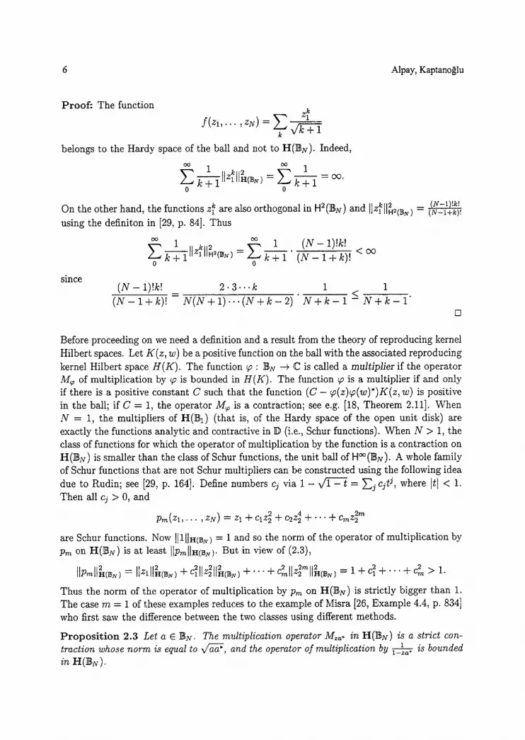
Proof : The function zt

f ( Z l ' ' ' " ' ZN) = E ~/]C -[- 1 k

belongs to the Hardy space of the ball and not to H(]~N). Indeed,

f i 1 2 1 Z k 1 I~(~) = ~.~ k + l co, 0 0

On the other hand, the functions z~ are also orthogonal in H2(BN) and []Z lkl[H~(]~_ ) 2 = (N-l+k)!(N-1)!k!

using the definiton in [29, p. 84]. Thus

f i 1 z k 2 1 1 H 2 ( ~ u ) = ~ k + l

0 0

since

( N - 1)!k! < O O

( N - 1 + k)!

( N - 1 ) ! k ! _ 2 . 3 . . . k . 1 < 1

( N - 1 + k)! N ( N + I ) . . . ( N + k - 2 ) g + k - l - g + k - l " []

Before proceeding on we need a definition and a result from the theory of reproducing kernel Hilbert spaces. Let K(z, w) be a positive function on the ball with the associated reproducing kernel Hilbert space H(K). The function T : BN --+ C is called a multiplier if the operator M~ of multiplication by ~ is bounded in H(K). The function ~ is a multiplier if and only if there is a positive constant C such that the function (C - T(z)~(w)*)K(z, w) is positive in the ball; if C = 1, the operator M~ is a contraction; see e.g. [18, Theorem 2.11]. When N = 1, the multipliers of H(BI) (that is, of the Hardy space of the open unit disk) are exactly the functions analytic and contractive in D (i.e., Schur functions). When N > 1, the class of functions for which the operator of multiplication by the function is a contraction on H(~N) is smaller than the class of Schur functions, the unit ball of H~ A whole family of Schur functions that are not Schur multipliers can be constructed using the following idea due to Rudin; see [29, p. 164]. Define numbers cj via 1 - ~ = Y~j cjt j, where It I < 1. Then all cj > 0, and

;re(z , , . . , z ~ ) = zl + clz~ + c2z~ + - . . + cmz~ ~

are Schur functions. Now ]]I[]H(~N) = 1 and so the norm of the operator of multiplication by Pm on H(B~) is at least ][Pm[]H(~). But in view of (2.3),

= IIz~llH(~,,) + ClllZ211H(~,,) + " " + emllz2 Ila(B,~) 1 + c m > 1.

Thus the norm of the operator of multiplication by Pm on H(BN) is strictly bigger than 1. The case m = 1 of these examples reduces to the example of Misra [26, Example 4.4, p. 834] who first saw the difference between the two classes using different methods.

P r o p o s i t i o n 2.3 Let a E ]~N" The multiplication operator Mz~. in H(~N) is a strict con- traction whose norm is equal to ~ , and the operator of multiplication by 1 is bounded in H(By ).

Alpay, Kaptano~Iu 7

Proof : We first write

aa* - (za*)(aw*) z ((aa*)IN - a'a) w* = a a * +

1 - z w * 1 - zw*

Note that the matrix (aa*)IN -- a*a is positive, and so the function z ((aa*)I~r - a'a) w* is positive in the ball. Since a product or a sum of positive functions is positive, we have

z ((aa*)rn -- a'a) ~* _>0 1 - - W Z *

By a result on multipliers mentioned above, it follows that ]tM~.]] _< x/'a-~. To see that the norm is exactly ~/aa*, notice that the constants belong to H(B~) since they are just multiples of the function identically equal to 1, which is the kernel corresponding to w = 0. Thus by (2.2),

IIM=o-(1)II~(B~) = II ~'~ * zjajlIH(~,,) = ~ lajl = = aa* 1 j

The second claim drops from the inequality I]Mf_~a. [] -< 1-1Pq=o.II'I which in turn follows from the power series expansion

o o

1 =~(za,)~ 1 - - z a *

D

[]

For related computations we refer to [11]. As a corollary, we have the following.

Coro l la ry 2.4 Let a E •tr The operators Tj(a) defined by

z j f ( z ) (Tj(a)) f ( z ) = 1 - za*

are bounded.

(2.4)

Using the theory of Hilbert spaces of analytic functions on bounded symmetric domains, one can find integral formulas for the inner product of H(]~N). They are presented in [9].

3 T h e r e s o l v e n t o p e r a t o r s

When N = 1, that is, in the case of the disk, the adjoint of the operator TI(0) (defined by (2.4)) is just the backward shift operator (1.4). When N > 1, the natural analogues of these operators would seem to be the operators (1.11), but they are unbounded, as we showed above. On the other hand, the adjoints of the operators Tj(a) are of course bounded. These will be our backward shift operators here.

Def ini t ion 3.1 The operator Tj(a)* will be called the j - th backward shift operator in H(I~N) at the point a.

8 Alpay, Kaptanoglu

These operators in general do not satisfy the resolvent equation (1.5). They do when one restricts a to have only one fixed nonzero component. We cannot give a closed-form expres- sion for the backward shift operators acting on arbitrary f E H(~N). On the other hand, as is usual in reproducing kernel spaces, we can compute the adjoint on the kernels. This is a special case of a general theorem oa multipliers in reproducing kernel Hilbert spaces (see e.g. [4, formula (2.3.5), p. 34]), but we give a proof for completeness.

L e m m a 3.2 We have

1 , ) w; 1 (Tj(a)*) 1 --'z-~-w* -- 1 - aw* I - zw*

Proof : Let v be in the ball. Then

(Tj(a). 1 1 ) (;) - - Z W *

(Tj( 1 1 } = a ) * l _ z w , , l _ z v , H(S~)

1 -- ZW* ~I(BN)

= 1 - zw* ' 1 - za* 1 -- ' zv H(e~) ,)" 1 - wv* 1 - wa*

w j

( I - vw*)(1 - aw*)"

(3.1)

[]

The main result of this section is the following.

T h e o r e m 3.3 Let f E H(BN). Then there exist funct ions g l ( z ) , . . . , g ~ ( z ) E H(BN) such that

N

f(z) - f ( a ) = ~ ( z j - a j ) a ( z ) . (3.2) 1

We define the functions gj(z) in a unique way by the formula gj(z) = T j (a )* f . The decom- position is not unique in general if one does not impose further restrictions on the gj(z) , as is illustrated by the example

1 = I + zl(0) + z~(0) = 1 + zl(z2) + z2(-zl),

which holds since the functions zl and z2 and the constant functions belong to H(BN).

Alpay, Kaptano~lu 9

P r o o f o f T h e o r e m 3.3: We first consider f ( z ) to be a kernel, i.e., f ( z ) = 1

gj = T j ( a ) * f . Then

1 1 f ( z ) -- f(a) =

1 - zw* 1 - aw* 1 .

= E . (1 - zw*)(1 - aw*) (zj - a j )w j 3

Thus the equality

= ~ ( z ~ - ~ ) g ~ ( z ) .

Let

f ( z ) = f ( a ) + ~ '~(z j - a j ) ( T j ( a ) * f ) ( z ) (3.3) J

holds on the linear span of the kernel functions, and hence on all of H(]~N) by continuity. []

We can rewrite (3.3) as

M=j_ajT~(a)* = • - c o (3.4) J

where Ca is the evaluation at the point a. The problem of existence of such functions gj in a given domain and m a given class of functions is called Gleason's problem. See [29, p. 116] for a list of spaces where this problem has a solution. Rudin gives two formulas for the gj(z ) in various spaces, and in particular in the Hardy space of the ball. The first formula is due to Ahem and Schneider (see [2]) and is valid in the space HI(~N) associated to the ball, and is equal to

C(z, ~) - C(a, ~) gj(z) = f~ U--~)-~ ~;f(~)~~ (3.5)

In this expression, C(z , u) = (1 - ZU*) -N is the Cauchy kernel, S is the boundary of the ball and a is the Lebesgue measure on S such that ~r(S) -- 1; see [29, pp. 12-13]. The second formula holds for a = 0, is valid for functions analytic in the ball and continuous up to the boundary (i.e., in the ball algebra), and is due to Leibenson (see [23]). The gj(z ) are now given (when a = 0) by

9j(z)= / t ~---~jf(tz)d~. (3.6)

A long computat ion using Propositions 1.4.8 and 1.4.9 of [29] shows that the Ahem-Schneider solution coincides with our solution for any a E ] ~ N for N = 2. The computat ions for N > 2 and a ~ 0 seem similar but longer. On the other hand, for a --- 0 the situation is simpler and we have the following.

i 0 Alpay, Kaptano~lu

L e m m a 3.4 Let N > 1 and a = O. The operator Tj(0)* coincides with the formulas of Ahem and Schneider and of Leibenson on H ( ~ . ) .

P r o o f : We first consider an element of the form f (z) = 1 Since it is in the ball algebra, 1--=7-~w- �9 it follows tha t the formulas of Ahem and Schneider and of Leibenson coincide; see [29, w

p. 117]. We now check that for such f

f ( tz)dt = w~ . 1 - zw*

But

~ z j 1 - z w (1 - t z w * ) 2 '

and so

fol O@j fo ~ W~w,)2d t wj* f( tz)dt = ( 1 - t = 1 - zw*"

The result follows by continuity.

We conclude with some further properties of the operators Tj(a)*.

P r o p o s i t i o n 3.5 / t holds that Tj(a)*(1) = 0 and

r~(~)*z~ = 5~,

where 5ij denotes the Kronecker symbol.

P r o o f : Let v and w in the ball. We have

(Tj(a)*l)(v) = a ) * l ' l - zv* H(~)

= (1 , ( I_za , )Z l I_zv , ) )H(~N)

( )" = zj = 0 . ( 1 - z a * ) ( 1 - zv*) z:O

Similarly,

(rj(a)* z~)(v)

and the result follows.

/ 1) = Tj(a)*ze, 1 - zv* H(~)

= {ze , ( l_za , )Z i l_zv , ) }H(~N)

= ~ 1 - zw* ' (1 - za*)(1 - zv*) . ~

= ~ze (1 - za*)(1 - zv*)

[]

Alpay, Kaptano~lu 11

Proposition 3.6 The operators Tj(a)* commute.

Proof : It is enough to prove that their adjoints commute on a dense set, but this is clear from

f(z Tj'(a)Tj2(a)f = (1 - za*) 2 "

for f ( z ) = 1 I=1 1--zw*

Propos i t i on 3.7 The common eigenvectors of the resolvent operators Tj(a)* in H(~N) are

exactly the kernels 1 1--Z~* "

Proof : Let ] �9 H(]BN) such that Tj(a)*f = Aj f for possibly different complex numbers hi. Then it follows from (3.3) that f(z)(1 - ~-~.j Aj(zj - aj)) = f(a), that is,

f(a)

As already remarked, f is analytic in the ball and in particular in a neighborhood of the c f(a) and origin, and so 1 + ~j Ajaj ~ O. Thus f(z) = 1-z~= with c -- I+Ej ~

1 w*= l + ~.~jAjaj( A1 )~2 "'" AN ).

If [wl _> 1, the function f would not be in H(~N)- So ]w I < 1 and f is a kernel. []

We have already remarked that a similar result holds in the setting of the polydisk. It is of interest to note that it also holds in the setting of de Branges-Rovnyak spaces defined on compact real Riemann surfaces (see [13], [12]).

4 B l a s c h k e factors

It is well known that one can extract zeros of functions in H2(D) via Blaschke factors. The counterpart here is the following.

P r o p o s i t i o n 4.1 Let a E ]BN. Then the cl• function

satisfies

b~(z) = (1 - aa*'l/2~ (z - a)(Iiv - a'a) -1/2 (4.1) 1 - - z a *

1 - ba(z)ba(w)* 1 - aa* 1 - z w * = ( 1 - z a * ) ( 1 - w * a ) ' z, we]Blv . (4.2)

In particular,

bo(z)bo(z)" < 1, if zz* < 1, [= 1, if z z * = l.

Lastly, b~ belongs to H(]~N) l•

(4.3)

12 Alpay, Kaptano~lu

Formula (4.2) appears in Rudin's book on the ball [29, Theorem 2.2.2, p. 261 (with an apparently different choice of b,, but in fact, up to sign, the same; see Lemma 4.2). It expresses the fact that the one-dimensional vector space spanned by the function z ~+ 1 1--Za*

endowed with the metric of H(BN) has reproducing kernel of the form 1-bo(z)b~(~)" That 1--Z~t]*

formula in Rudin's book was the trigger that made us understand that par t of the analysis of H2(D) could be extended to the space H(BN). We also note that (4.1) can be rewritten

aS

bo(z) = bo(o) + b (z) - b (o) Z

= - ( 1 - aa*)l/2a(I,~ - a 'a ) < / 2 -+ 1 - za* ((1 - aa*) l /2( IN - a ' a ) -1/2 - a ' a )

= - a + (1 - aa*)l /2z(1 - z a * ) - l ( I N - a 'a ) 1/2. (4.4)

To get to this last formula we first use that

( 1 - aa*)l /2a =- a ( I g -- a 'a ) I/~,

and so (1 - aa*) I /2a ( I y -- a ' a ) -1/2 = a. Next we have to check that

( 1 - aa*) l l2( Im - a 'a ) -I /2 - a* a = (1 - aa*) l /2(IN -- a ' a ) 1/2.

This is readily done by multiplying both sides of this equality by ( IN -- a ' a ) 1/2 on the right and making use of

( 1 - aa ' ) ' / 2 a* a = a*(1 - aa*)l /2a = a* a(XN - a 'a ) 112. (4.5)

The matrix

(1 - aa*) I/2 - a

is unitary and formula (4.4) is the dimension-one ease of the general representation formula (2.3) in [17, ~2].

P r o o f of P r o p o s i t i o n 4.1: For a E B~, let H ( a ) denote the Halmos extension of a, that is, let H ( a ) be the matrix

( ) H(a) ---- ~ i n --a(IN-- a'a) -I/2 ( i -a , ' ) '~ ' ( IN -- a 'a ) -1/2 " (4.6)

(1

Then

z ) H(a) = (l_~.)l/,l-za" (z - a ) ( IN -- aa*) -1/2 )

l -- z a * - ( 1 o(z) )

(4.7)

Alpay, Kaptano~lu 13

Let

J - - 0 - - IN "

One has H ( a ) J H ( a ) * = J (see [21, Theorem 1.2, p. 17]) and therefore, for any choice of z, w E ]By, we have

1 - z w * = ( 1 z ) J ( 1

= ( 1 z ) H ( a ) J H ( a ) * ( 1 ) w *

= (1 - z a * ) ( 1 - a w * ) ( 1 - M z ) b o ( w ) ' ) 1 - aa*

and hence the result. The last claim follows from the fact that 1 belongs to H(~N) and tha t multiplication by the independent variables are bounded operators in H(]~N). []

The function b~(z) is the counterpart in the setting of ]~N of the Blaschke factor ~-a We now give another expression for b~(z) which appears in [29].

L e m m a 4.2 The func t ion ba(z) can be wri t ten as

~ . a ) b,~(z) a - ~ a ' a - (1 - aa*)ll2(z - z,~" = ~" (4.9) 1 - - z a *

P r o o f : We rewrite the right side of (4.9) as

a'___~ + (1 - aa*)l/2(IN - a'a ~ . ) - aa* aa" - a + z

1 - - z a *

So, in view of formula (4.4), we have to check that

. . . . a*a. (4.10) aa* aa*

Taking into account (4.5), we see that (4.10) is equivalent to

( 1 - aa*) 1/2 ( ( I N - - a'a) 1/2 - IN) -- a*a a*a. aa* ~ a , ( I N - - a 'a) 1/2 a*a. (4.11)

By looking at the power series expansion in powers of a*a of (IN -- a 'a) 1/2, we see tha t both sides of (4.11) are multiples of a* and so it is legitimate to multiply both sides of (4.11) by a on the left and get the equivalent expression

( a* a a* a a'a) 1/' a ' a } a(1 - aa*) 1/2 ((IN - a 'a) 1/2 - IN) = a \ aa* ~a *(IN -

= a - a(IN - a'a) 1/2 - (aa*)a. (4.12)

14 Alpay, Kaptano(~lu

This in turn is readily seen after remarking that

a ( l _ a a * ) i / 2 ( I N - - a * a)I/2 = ( l - -aa ' ) I / 2a ( IN- -a * a)i/2 = a ( I N - a * a ) I / 2 ( I N - a * a) V2 = a ( IN- -a* a)

and that a(1 - aa*) I/2 = ( I - aa*)V2a = a(1N - a 'a) U2.

[]

The right-side of (4.9) is an automorphism of the ball, and is the expression used in [29] to prove (4.2). In fact, Lemma 4.2 implies equation (4.2) by Theorem 2.2.5 of [29]. This result is also the case M = 1 of the structure Theorem 7.2.

The analogy of ha(z) with Blaschke factors is also stressed by the following result.

P r o p o s i t i o n 4.3 Let a E ]~N and let f 6 H(BN). Then

f (a) = 0 r f ( z ) = ba(z)u(z)

for some u E H(BN) g•

Proof : The ~ direction is trivial. Conversely, assume that f (a ) = O. By Theorem 3.3 we can write

N

f ( z ) - f (a) = f ( z ) = E ( z j - aj)gj(z) = (z - a)g(z), 1

where

So

f(z) - -

with

( gl(z) ) g(z) = ! e H(BN) N•

gN(z)

I -- za* (11-_aa*)I/2za, (z - a ) ( IN -- a* a l - I / 2 ( IN -- a" a) I/2 (1 -- aa*) I /2g(z) = bo(z)u(z)

has reproducing kernel of the form

Is - B(z)B(w)* (4.14) 1 -- ZW*

where B(z ) is a rational C "• function taking coisometric values on the bound- ary of the ball. Here coisometric means B(z)B(z)* = Is for zz* = 1.

i - ~a ~ _ ~*~)V~g(z) e HI~)N• (I - a~*)v ~(I~

since by Proposition 2.3 the function (za*)g(z) belongs to H(]~N) N• []

P r o p o s i t i o n 4.4 Let n E IN, let d E C ~xl and let a ~ By . The one-dimensional subspace of H(]~N) TM spanned by the function

d z ~+ ~ (4.13)

1 - za*

Alpay, Kaptano~lu 15

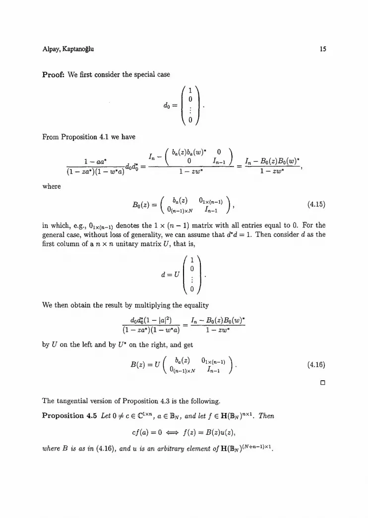
Proof." We first consider the special case

d O =

From Proposition 4.1 we have

where

(I (bo(z)b~(~) * 0 )

1 - aa* I~ - 0 In-1 In - Bo(z )Bo(w)*

(1 - za*)(1 - w'a ) d~176 = 1 - zw* 1 - zw*

( b a ( z ) 01• ) (4.15) Bo(z) = O(~-l)• I n - i '

in which, e.g., 01x(,~-l) denotes the 1 x (n - 1) matrix with all entries equal to 0. For the general case, without loss of generality, we can assume that d*d = 1. Then consider d as the first column of a n x n unitary matrix U, that is,

We then obtain the result by multiplying the equality

eoe;(1 - la?) • - Bo(z)Bo(~)* m m (i - za*)(i - ~*a)

by U on the left and by U* on the right, and get

= u ( b o ( z ) B ( z ) \ O(n-l)xN

1 - - Z~D*

Ol• ) . ( 4 . 1 6 )

[]

The tangential version of Proposition 4.3 is the following.

P r o p o s i t i o n 4.5 Let 0 # c E C lxn, a E BN, and let f E H(B~) TM. Then

c f ( a ) = 0 ~ f ( z ) = B ( z ) u ( z ) ,

where B is as in (4.16), and u is an arbitrary e lement of H(~N) T M .

i 6 Alpay, Kaptanoglu

Before turning to the proof, we recall some facts on the sum of positive functions and on the associated reproducing kernel Hilbert spaces. If Kl(z, w) and K2(z , w) are two C~• functions positive in the ball, their sum is of course still positive. The associated reproducing kernel Hilbert spaces of Cn• functions satisfy

H ( K ) --- H(K1) + H(K2),

but this decomposition is not in general orthogonal. The spaces H ( K 1 ) and H ( K 2 ) are contractively included in H(K); see [19]. When H ( K 1 ) is isometrically included in H(K), so is H(K2), and the sum is an orthogonal sum. One can see this, if need be, from e.g. [4, (2.3.s), p 36]

P r o o f of P ropos i t i on 4.5: We first check the ~ direction. We construct U from c as in the proof of Proposition 4.4. By the choice of U we have cU = ( 1 0 .-- 0 ), and so

c f ( a ) = c B ( a ) u ( a )

= ( 1 0 . . .

( lO

ba(a) 01• ) 0 ) 0(n-1)xN In-1

( 0 0~• ) "'" 0 ) O(n_l)xN I,~-I = 0.

Conversely, assume that c f (a ) = O. Thus the function f is orthogonal in H(]N) ~• to the function (4.13). Let M denote the subspace of H(BN) T M spanned by the function (4.13). The reproducing kernel of M is, as already seen, of the form Z~-B(z)S(~)" where B

I--ZW*

is defined by (4.16). Since

I~ I~ - B ( z ) B ( w ) * B ( z ) B ( w ) *

1 - zw* 1 - zw* 1 - zw*

it follows from the discussion before the beginning of the proof that the orthogonal comple- ment of M has reproducing kernel B(z)B(w)" But this means that the elements of AA ~- are

1 - - Z W * "

of the form B ( z ) u ( z ) , where u belongs to the closed linear span of the functions ~ in l--Z~g*

H(BN) T M as w runs through the ball and ~ runs through C n+N-1. []

When N = 1, the function B ( z ) is square and B(z )U* reduces to the matrix-valued Blaschke factor

c*c~ c*c z - a el• ~ I~ - - - / , c ~ a ~ D

co* 1 - za*

introduced by Potapov; see [27], [21].

5 H o m o g e n e o u s i n t e r p o l a t i o n in H(~N) n•

We wish to solve the following interpolation problem.

Alpay, Kaptano~lu 17

P r o b l e m 5.1 Given a l , . . . ,aM E ~N and vectors e l , . . . ,CM E C lxn different from 0i• find all f E H(~lv) T M such that

cj f (aj)=O, j = I , . . . , M .

T h e o r e m 5.2 The set of solutions of Problem 5.1 is of the form

f(z) = B(z)u(z)

where B(z) is a rational C ~• function for some integer k < M taking coiso- metric values on the boundary Of ~y , and u is an arbitrary element in H(~N) (n+k(~-l))•

Proof : We solve the problem by induction. First let M = 1. We use Proposition 4.5 and find that f (z) = Bl(z) f l (z) where Bi(z) is given by (4.16) and fl is an arbitrary function in H ( ~ ) (N+~-i)• Assume now the result proved up to M0. So all the solutions are of the form f (z ) = SMo(Z)U(Z), where BM0(Z) is rational with coisometric values on the boundary of the ball and is C~• for some nMo. If CMo+IBMo(aMo+I) : 0, the next interpolation condition is empty. Otherwise, the next interpolation condition becomes

(CMo+IBMo(aMo+I)) u(aMo+l) = O,

and the set of all solutions u is given by

u(z) = gMo+~(z)v(z),

where BMo+I (Z) is C~Mo • and given by (4.16). This concludes the induction with BMo+l(Z) = BMo(Z)BMo+I(Z). []

One could in the same way handle tangential interpolation problems with derivatives, i.e., problems of the type

cof(ao) = 0 o f C07z (a0)+clf(a0) = o

0 ~ f [ x CO~z~ao) + " ' + c n f ( a o ) = O,

where the cj are in C lxm and f E H(HN) lxm. When N = 1, i.e., in the case of the disk, the function B(z) is square and one recovers part of the results of [5].

6 Homogeneous interpolation in the Hardy space of the ball

In this section we only remark that the analysis in the previous section holds in fact in the Hardy space (H2(]BN)) T M of the ball; the gj(z) are now given by the formulas of Ahern and

18 Alpay, Kaptano~lu

Schneider or of Leibenson. The Blaschke factor ha(z) is in the ball algebra A(]By), and in particular is a multiplier of the Hardy space. There is an important difference between the case of the space H(BN) and of the Hardy space. In (H(BN)) TM we saw in the previous section that the decomposition

I~ I,~ - S ( z )B (w)* B(z )B(w)*

1 - zw* 1 - zw* 1 - zw*

leads to an orthogonal decomposition of the space (H(BN)) TM. Now in the Hardy space, the corresponding decomposition

In In - B(z )B(w)* B( z )B(w)* (6.1) (1 - zw*) N = (1 - zw*)N + (1 -- zw*)N

does not lead in general to an orthogonal decomposition in the Hardy space. Indeed, take n = 1 and B(z ) = b,(z). The orthogonal complement of the set of functions in the Hardy space that vanish at the point a is spanned by the function 1/ (1-za*) N and has reproducing

kernel (l_z~.)X0_w.~)u, which is equal to

( 1 - - ba(z)ba(w)*) N

(1 - zw*) u

Thus the decomposition of the kernel 1/(1 - zw*) N which leads to an orthogonal decompo- sition of the Hardy space is

In ( I , - B(z )B(w)*) N I , - ( I , - B ( z )B(w)*) N (6.2) (1 - zw*) N = (1 - zw*) N + (1 - zw*) N

and not (6.1). Finally we remark that for an inner function B of the ball (which exists; see [30],

[3]), multiplication by B is an isometry form the Hardy space of the ball into itself and we have the orthogonal decomposition

H2(~N) = (H2(]~N) (9 BH2(~N)) (9 -~H2(]~N),

corresponding to the decomposition (6.2). On the other hand, we do not know if inner functions of the ball are multipliers of the space H(BN).

7 S o m e f i n i t e - d i m e n s i o n a l r e s o l v e n t - i n v a r i a n t s u b s p a c e s

The structure of general Tj(a)*-invariant subspaces of S(ISy) seems at present elusive. In this section we present some partial results. We begin with the following.

P ropos i t i on 7.1 Assume M is a finite-dimensionaI resolvent-invariant subspace of H(]~y ). Then there exist matrices C, A t , . . . , AN such that the columns of the matrix-valued rational

function

C ( I - E z j A j ) - ' (7.1) J

form a basis of A t .

Alpay, Kaptaao~lu 19

Proof : Let f l , . . . , fM be a basis of 3 / /and set

F(z) = ( f l ( z ) f2(z) ".. fM(Z) ) .

Then there exist matrices rnl , . . . ,rr~M E C MxM Such that

Tj(a)*(F(z)~) = F(z)mj~, ~ e C ::xl, j = 1, . . . ,N.

Hence using (3.3), we get F(z) - F(a) = ~N(z j -- aj)F(z)mj; so

N

F ( z ) ( I M - (zj - aj)mj) = f (a ) , 1

and the result follows. []

The condition in the lemma is only necessary and is not sufficient as illustrated by the

example

when N = 2. The corresponding space 34 is spanned by the functions 1 and z~ One 1-- ~-~ "

checks readily that

and thus the space is not T1 (0)*-invariant. We do not know how to characterize general Tj(a)*-invariant subspaces of H(~N).

Here is a partial result.

T h e o r e m 7.2 Let Ad be a finite-dimcnsional resolvent-invariant subspace of H(I~N ) spanned by M distinct kernel functions 1 7 ' j = 1, . . . , M. Then there exists a row-valued function

B such that the reproducing kernel of 3/[ is

1 - B(z)B(w)* (7.2) I - - Z W *

Proof : It suffices to note that the elements of A4 • satisfy the interpolation conditions

f (w j )=O, j = I , . . . , M

and apply Theorem 5.2. []

A c k n o w l e d g m e n t s : The first author thanks TUBITAK of Turkey for supporting a visit of Daniel Alpay to Middle East Technical University, Ankara, and to Professor Hayri KSrezlio~lu for initiating the visit. The second author wishes to thank Middle East Technical University and Ben-Gurion University for supporting a visit to Ben-Gurion University, Beer-Sheva, and to Daniel Alpay for initiating this joint project. It is also a pleasure to thank Professor Szafraniec for pointing out to us G. Misra's paper [26].

20 Alpay, Kaptano~lu

References [1] J. Agler and J. E. McCarthy, Complete Nevanlinna-Pick kernels, J. Funct. Anal. 175

(2000), 111-124.

[2] P. R. Ahern and R. Schneider, Isometrics of H ~176 Duke Math. J. 42 (1975), 321-326.

[3] A. B. Aleksandrov, The existence of inner functions in a ball, Mat. Sb. (N.S.) 118(160) (1982), 147-163, 287.

[4] D. Alpay, Algorithme de Schur, espaees d noyau reproduisant et thdorie des syst~mes, Panor. Syntheses, vol. 6, Soe. Math. France, Paris, 1998.

[5] D. Alpay and V. Bolotnikov, Two-sided interpolation for matrix functions with entries in the Hardy space, Linear Algebra Appl. 223/224 (1995), 31-56.

[6] D. Alpay, V. Bolotnikov, A. Dijksma, and C. Sadosky, Hilbert spaces contractively included in the Hardy space of the bidisk, Positivity 5 (2001), 25-50.

[7] D. Alpay, V. Bolotnikov, and H. T. Kaptano~lu. The Schur algorithm and reproducing kernel Hilbert spaces in the ball, preprint, 2001.

[8] D. Alpay, A. Dijksma, J. Rovnyak, and H. de Shoo. Sehur functions, operator colli- gations, and reproducing kernel Pontryagin spaces, Oper. Theory: Adv. Appl., vol. 96, Birkhs Basel, 1997.

[9] D. Alpay and H. T. Kaptano~lu. Integral formulas for a sub-Hardy Hilbert space on the ball with complete Nevanlinna-Pick reproducing kernel, preprint, 2001.

[10] D. Alpay and H. T. Kaptano~lu, Sous espaces de codimension finie dans la boule unit6 et un probl6me de factorisation, C. R. Acad. Sei. Paris Sdr. I Math. 331 (2000), 947-952.

[11] D. Alpay and V. Khatskevich, Linear fractional transformations: basic properties, applications to spaces of analytic functions and Schroeder's equation, Int. J. Appl. Math. 2 (2000), 459-476.

[12] D. Alpay and V. Vinnikov, de Branges spaces on real Riemann surfaces, to appear in Y. Funct. Anal. (2001).

[13] D. Alpay and V. Vinnikov, Analogues d'espaces de de Branges sur des surfaces de Riemann, C. R. Acad. Sci. Paris Sdr. I Math. 318 (1994), 1077-1082.

[14] T. And6, Reproducing kernel spaces and quadratic inequalities, lecture notes, Hokkaido Univ., Sapporo, 1987.

[15] N. Aronszajn, Theory of reproducing kernels, Trans. Amer. Math. Soc. 68 (1950), 337-404.

[16] W. Arveson, The curvature invariant of a Hilbert module over C[zz,-" , Zd], J. Reine Angew. Math. 522 (2000), 173-236.

[17] J. Ball, T. Trent, and V. Vinnikov, Interpolation and commutant lifting for multipliers on reproducing kernel Hilbert spaces, in Proceedings of the conference in honor of the 60th birthday of M. A. Kaashoek, pp. , Birkhs Basel, 2001.

[18] F. Beatrous and J. Burbea, Positive-definiteness and its applications to interpolation problems for holomorphic functions, Trans. Amer. Math. Soc. 284 (1984), 247-270.

Alpay, Kaptano~lu 21

[19] L. de Branges, Complementation in Krdn spaces, Trans. Amer. Math. Soc. 305 (1988), 277-291.

[20] R. G. Douglas, Banach algebra techniques in operator theory, Academic, New York, 1972.

[21] H. Dym, J contractive matrix functions, reproducing kernel Hilbert spaces and inter- polation, CBMS Regional Conf. Set. in Math., vol. 71, Amer. Math. Soc., Providence, 1989.

[22] D. Greene, S. Richter, and C. Sundberg, The structure of inner multipliers on spaces with complete Nevanlinna-Pick kernels, preprint.

[23] G. M. Henkin, The approximation of functions in pseudo-convex domains and a theorem of Z. L. Le~enzon, Bull. Acad. Polon. Sei. Sdr. Sci. Math. Astronom. Phys. 19 (1971), 37-42.

[24] G. M. Henkin, The method of integral representations in complex analysis, in Current problems in mathematics. Fundamental directions, vol. 7, pp. 23-124, Itogi Nauki i Tekhniki, Akad. Nauk SSSR Vsesoyuz. Inst. Nauchn. i Tekhn. Inform., Moscow, 1985.

[25] S. McCullough and T. T. Trent, Invariant subspaces and Nevanlinna-Pick kernels, preprint.

[26] G. Misra, Pick-Nevanlinna interpolation theorem and multiplication operators on func- tional Hilbert spaces, Integral Equations Operator Theory 14 (1991), 825-836.

[27] V. P. Potapov, The multiplicative structure of J-contractive matrix-functions, Trudy Moskow. Mat. Obs. 4 (1955), 125-236. English translation in Amer. Math. Soc. Transl. Set. 2, vol. 15, pp. 131-243 (1960).

[28] P. Quiggin, For which reproducing kernel Hilbert spaces is Pick's theorem true?, Integral Equations Operator Theory 16 (1993), 244-266.

[29] W. Rudin, Function theory in the unit ball of C ~, Grundlehren Math. Wiss., vol. 241, Springer, New York, 1980.

[30] W. Rudin, New constructions of functions holomorphic in the unit ball of C ~, CBMS Regional Conf. Set. in Math., vol. 63, Amer. Math. Soc., Providence, 1986.

[31] S. Saitoh, Theory of reproducing kernels and its applications, Pitman Res. Notes Math. Ser., vol. 189, Longman, Harlow, 1988.

[32] L. Schwartz, Sous espaces hilbertiens d'espaces vectoriels topologiques et noyaux as- soci~s (noyaux reproduisants), J. Analyse Math. 13 (1964), 115-256.

Daniel Alpay Department of Mathematics Ben-Gurion University of the Negev Beer-Sheva 84105, Israel

H. Turgay Kaptano~lu Mathematics Department Middle East Technical University Ankara 06531, Turkey

2000 Mathematics Subject Classification. Primary: 47A57; Secondary: 32A70.

Submitted: September 7, 2000