Software Defined Radiofrequency signal processing (SDR)

Software Defined Radiofrequency signal processing (SDR) – GNURadio

J.-M Friedt, January 26, 2022

1 First steps with GNURadio

GNURadio [1] provides a set of digital signal processing blocks as well as a scheduler taking care of data flow. Signal processingblocks are written in C++ or in Python. Assembling blocks as a processing chain is defined by a Python script. A graphical userinterface is not mandatory, making GNURadio well suited for embedded environments not fitted with graphical displays (e.g.Redpitaya board).

A tool helps in assembling blocks – which actually happens to be a Python code generator from the processing chain graph-ically defined – named GNURadio Companion. We shall use this tool, called gnuradio-companion from the command lineinterface, for this introduction to software defined radio (SDR) digital signal processing.

Be aware that since GNU Radio 3.8, a flowchart cannot be executed unless you define the Id: double click on “Options” andset the Id to anything other than “default”. This will defined the name of the Python3 script that will be generated by GNU RadioCompanion.

1.1 Sound card output

We can test basic – yet fundamental – signal processing algorithms such as filters. A Finite Impulse Filter (FIR) is designed toprocess synthetic data. In order to characterize the spectral characteristics of the filter, we feed it with a white noise source, andobserve the spectrum at the input and the output of the filter.

In order to become familiar with GNURadio-companion, a first example aims at generating a processing flow fed by a noisesource, a band-pass filter of varying central frequency and bandpass, and a display of the resulting spectrum (Fig. 1)

sampling rateselect a sampling ratecompatible with sound card

Options

Title: lab1

Output Language: Python

Generate Options: QT GUI

QT GUI Range

Id: b

Default Value: 1k

Start: 0

Stop: 10k

Step: 1

QT GUI Range

Id: f

Default Value: 5k

Start: 0

Stop: 10k

Step: 1

Variable

Id: samp_rate

Value: 96k

Noise Source

Noise Type: Gaussian

Amplitude: 1

Seed: 0

Audio Sink

Sample Rate: 96kBand Pass Filter

Decimation: 1

Gain: 1

Sample Rate: 96k

Low Cutoff Freq: 4k

High Cutoff Freq: 6k

Transition Width: 200

Window: Hamming

Beta: 6.76

QT GUI Frequency Sink

FFT Size: 1.024k

Center Frequency (Hz): 0

Bandwidth (Hz): 96k

Figure 1: Characterizing a (real) bandpass filter and playing its output on the sound card.

In this example, the data sink is a sound card. The sampling rate along the whole flowgraph is defined with the variablesamp_rate which must be set to one of the sampling rates supported by the hardware, in this case 96 kHz. Making sure thesampling rate is consistent along the processing chain must be taken care of by the designer and will not be handled by GNURadio: most specifically, interpolation will increase the sampling rate and decimation will reduce the sampling rate. In thisexample, decimation is set to 1 and there is no interpolation, so the sampling rate remains constant throughout the flowchart.

1. Find, on the GNURadio website, the API describing the signal processing blocks, and the methods associated to the“band pass filter” object.

2. Add to the Python script generated by GNURadio-companion an output printing the length of the filter.

3. Output the processed signal on the sound card: listen at the impact of the bandwidth and central frequency of the filter.

1.2 How to handle data-flow when lacking input or output hardware

When the signal is emitted by the sound card, the data-rate is defined by the sampling rate of the sound card. If a signal issampled from an acquisition card, here again the sampling rate is defined. But if we only perform signal processing on syntheticdata or data stored in a file to display its characteristics, no sampling rate is imposed in the processing flowchart by a hardware

1

interface. We must tell the scheduler to wait between two processing steps to comply with the expected sampling rate definedby the samp_rate variable: the throttle bloc is in charge of such an operation.

4. Remove the audio output and display on a virtual oscilloscope the output of the filtered output.

Let us demonstrate the flexibility of GNURadio-companion to address and prototype signal processing concepts by printingthe filter coefficients. A FIR (Finite Impulse Response) filter generates an output yn as weighted combination of past inputs xk

following

yn =N∑0

bk · xn−k

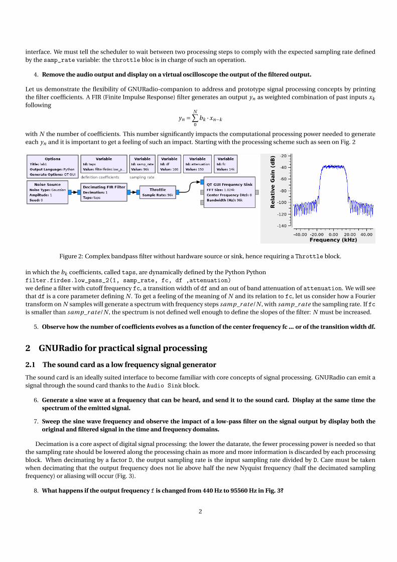
with N the number of coefficients. This number significantly impacts the computational processing power needed to generateeach yn and it is important to get a feeling of such an impact. Starting with the processing scheme such as seen on Fig. 2

Figure 2: Complex bandpass filter without hardware source or sink, hence requiring a Throttle block.

in which the bk coefficients, called taps, are dynamically defined by the Python Pythonfilter.firdes.low_pass_2(1, samp_rate, fc, df ,attenuation)we define a filter with cutoff frequency fc, a transition width of df and an out of band attenuation of attenuation. We will seethat df is a core parameter defining N . To get a feeling of the meaning of N and its relation to fc, let us consider how a Fouriertransform on N samples will generate a spectrum with frequency steps samp_r ate/N , with samp_r ate the sampling rate. If fcis smaller than samp_r ate/N , the spectrum is not defined well enough to define the slopes of the filter: N must be increased.

5. Observe how the number of coefficients evolves as a function of the center frequency fc ... or of the transition width df.

2 GNURadio for practical signal processing

2.1 The sound card as a low frequency signal generator

The sound card is an ideally suited interface to become familiar with core concepts of signal processing. GNURadio can emit asignal through the sound card thanks to the Audio Sink block.

6. Generate a sine wave at a frequency that can be heard, and send it to the sound card. Display at the same time thespectrum of the emitted signal.

7. Sweep the sine wave frequency and observe the impact of a low-pass filter on the signal output by display both theoriginal and filtered signal in the time and frequency domains.

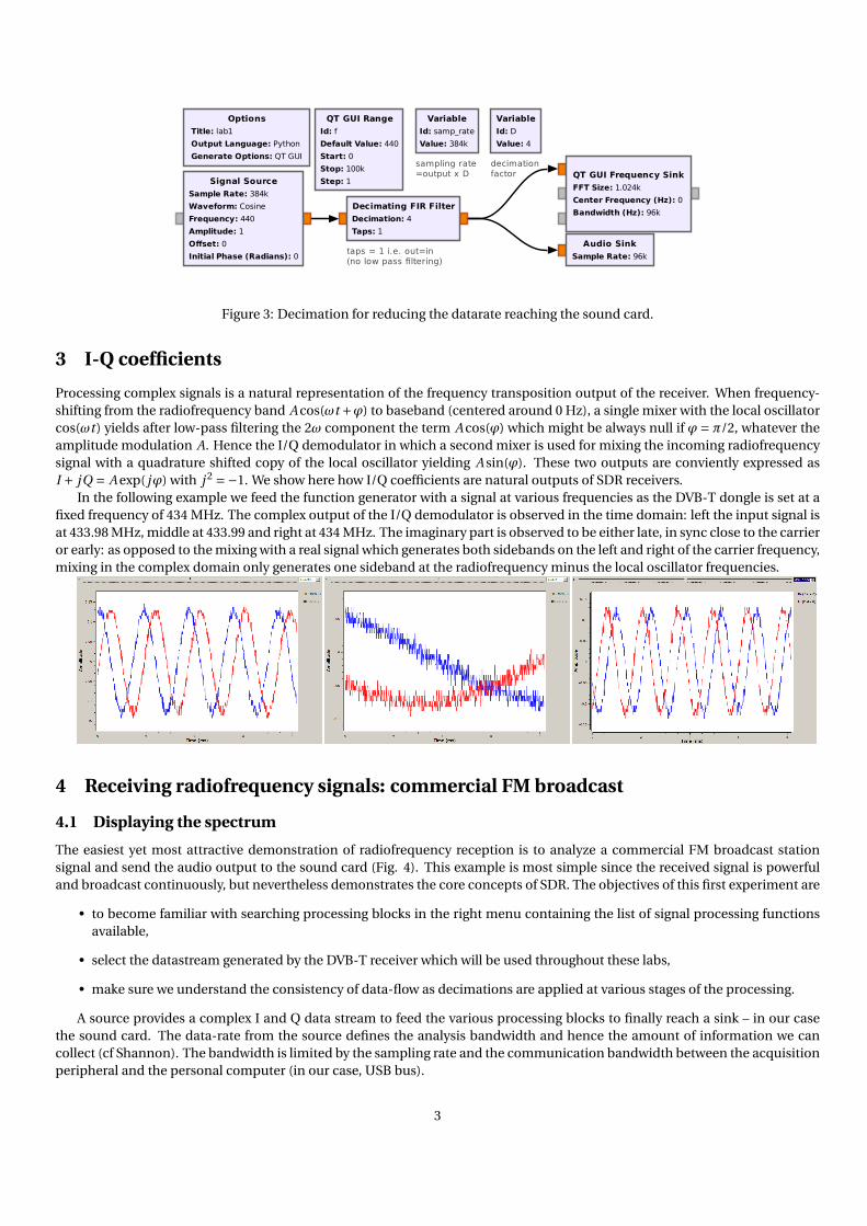
Decimation is a core aspect of digital signal processing: the lower the datarate, the fewer processing power is needed so thatthe sampling rate should be lowered along the processing chain as more and more information is discarded by each processingblock. When decimating by a factor D, the output sampling rate is the input sampling rate divided by D. Care must be takenwhen decimating that the output frequency does not lie above half the new Nyquist frequency (half the decimated samplingfrequency) or aliasing will occur (Fig. 3).

8. What happens if the output frequency f is changed from 440 Hz to 95560 Hz in Fig. 3?

2

decimationfactor

sampling rate=output x D

taps = 1 i.e. out=in(no low pass filtering)

Options

Title: lab1



Variable

Id: D

Value: 4

QT GUI Range

Id: f

Default Value: 440

Start: 0

Stop: 100k

Step: 1

Variable

Id: samp_rate

Value: 384k

Signal Source

Sample Rate: 384k

Waveform: Cosine

Frequency: 440

Amplitude: 1

Offset: 0

Initial Phase (Radians): 0

Audio Sink

Sample Rate: 96k

Decimating FIR Filter

Decimation: 4

Taps: 1


FFT Size: 1.024k


Bandwidth (Hz): 96k

Figure 3: Decimation for reducing the datarate reaching the sound card.

3 I-Q coefficients

Processing complex signals is a natural representation of the frequency transposition output of the receiver. When frequency-shifting from the radiofrequency band A cos(ωt +ϕ) to baseband (centered around 0 Hz), a single mixer with the local oscillatorcos(ωt ) yields after low-pass filtering the 2ω component the term A cos(ϕ) which might be always null if ϕ= π/2, whatever theamplitude modulation A. Hence the I/Q demodulator in which a second mixer is used for mixing the incoming radiofrequencysignal with a quadrature shifted copy of the local oscillator yielding A sin(ϕ). These two outputs are conviently expressed asI + jQ = A exp( jϕ) with j 2 =−1. We show here how I/Q coefficients are natural outputs of SDR receivers.

In the following example we feed the function generator with a signal at various frequencies as the DVB-T dongle is set at afixed frequency of 434 MHz. The complex output of the I/Q demodulator is observed in the time domain: left the input signal isat 433.98 MHz, middle at 433.99 and right at 434 MHz. The imaginary part is observed to be either late, in sync close to the carrieror early: as opposed to the mixing with a real signal which generates both sidebands on the left and right of the carrier frequency,mixing in the complex domain only generates one sideband at the radiofrequency minus the local oscillator frequencies.

4 Receiving radiofrequency signals: commercial FM broadcast

4.1 Displaying the spectrum

The easiest yet most attractive demonstration of radiofrequency reception is to analyze a commercial FM broadcast stationsignal and send the audio output to the sound card (Fig. 4). This example is most simple since the received signal is powerfuland broadcast continuously, but nevertheless demonstrates the core concepts of SDR. The objectives of this first experiment are

• to become familiar with searching processing blocks in the right menu containing the list of signal processing functionsavailable,

• select the datastream generated by the DVB-T receiver which will be used throughout these labs,

• make sure we understand the consistency of data-flow as decimations are applied at various stages of the processing.

A source provides a complex I and Q data stream to feed the various processing blocks to finally reach a sink – in our casethe sound card. The data-rate from the source defines the analysis bandwidth and hence the amount of information we cancollect (cf Shannon). The bandwidth is limited by the sampling rate and the communication bandwidth between the acquisitionperipheral and the personal computer (in our case, USB bus).

3

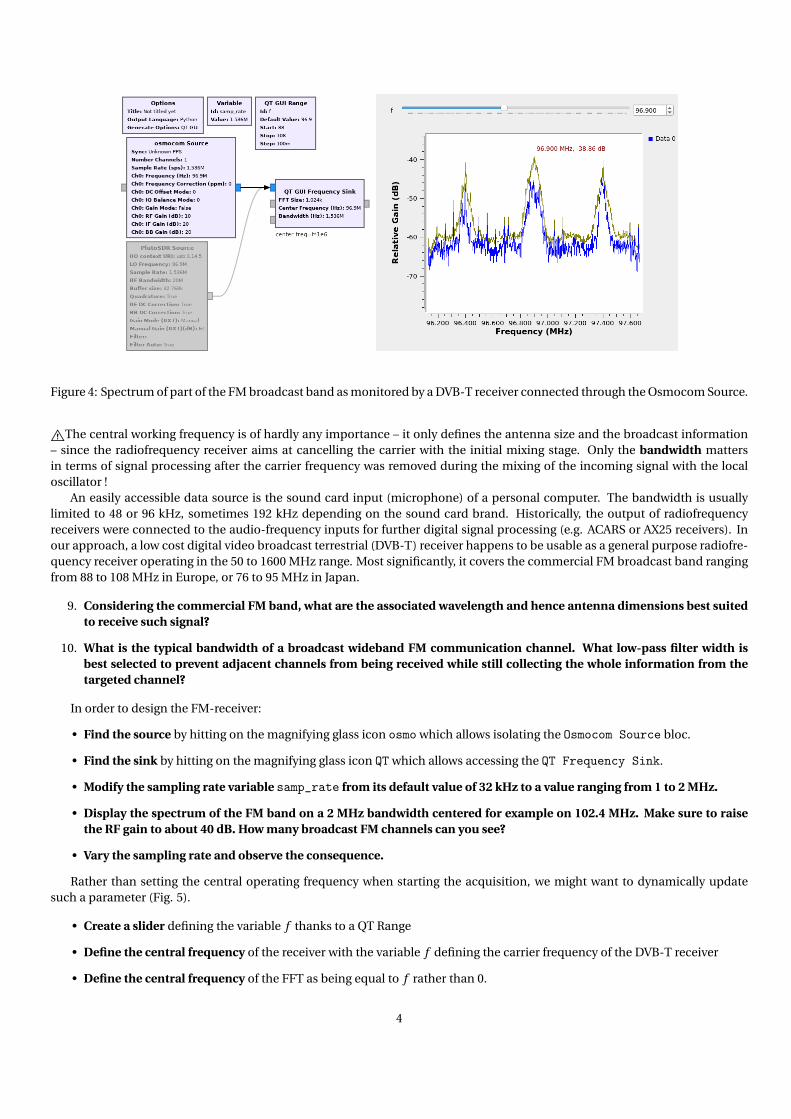
Figure 4: Spectrum of part of the FM broadcast band as monitored by a DVB-T receiver connected through the Osmocom Source.

"The central working frequency is of hardly any importance – it only defines the antenna size and the broadcast information– since the radiofrequency receiver aims at cancelling the carrier with the initial mixing stage. Only the bandwidth mattersin terms of signal processing after the carrier frequency was removed during the mixing of the incoming signal with the localoscillator !

An easily accessible data source is the sound card input (microphone) of a personal computer. The bandwidth is usuallylimited to 48 or 96 kHz, sometimes 192 kHz depending on the sound card brand. Historically, the output of radiofrequencyreceivers were connected to the audio-frequency inputs for further digital signal processing (e.g. ACARS or AX25 receivers). Inour approach, a low cost digital video broadcast terrestrial (DVB-T) receiver happens to be usable as a general purpose radiofre-quency receiver operating in the 50 to 1600 MHz range. Most significantly, it covers the commercial FM broadcast band rangingfrom 88 to 108 MHz in Europe, or 76 to 95 MHz in Japan.

9. Considering the commercial FM band, what are the associated wavelength and hence antenna dimensions best suitedto receive such signal?

10. What is the typical bandwidth of a broadcast wideband FM communication channel. What low-pass filter width isbest selected to prevent adjacent channels from being received while still collecting the whole information from thetargeted channel?

In order to design the FM-receiver:

• Find the source by hitting on the magnifying glass icon osmo which allows isolating the Osmocom Source bloc.

• Find the sink by hitting on the magnifying glass icon QT which allows accessing the QT Frequency Sink.

• Modify the sampling rate variable samp_rate from its default value of 32 kHz to a value ranging from 1 to 2 MHz.

• Display the spectrum of the FM band on a 2 MHz bandwidth centered for example on 102.4 MHz. Make sure to raisethe RF gain to about 40 dB. How many broadcast FM channels can you see?

• Vary the sampling rate and observe the consequence.

Rather than setting the central operating frequency when starting the acquisition, we might want to dynamically updatesuch a parameter (Fig. 5).

• Create a slider defining the variable f thanks to a QT Range

• Define the central frequency of the receiver with the variable f defining the carrier frequency of the DVB-T receiver

• Define the central frequency of the FFT as being equal to f rather than 0.

4

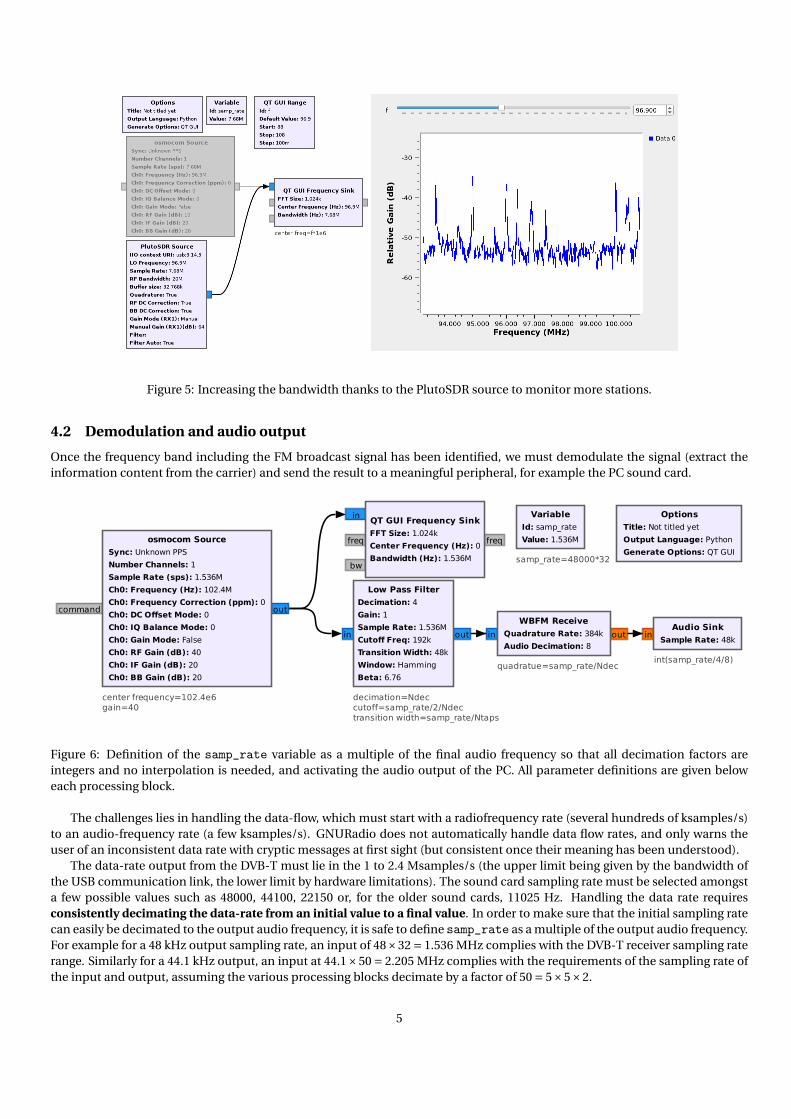
Figure 5: Increasing the bandwidth thanks to the PlutoSDR source to monitor more stations.

4.2 Demodulation and audio output

Once the frequency band including the FM broadcast signal has been identified, we must demodulate the signal (extract theinformation content from the carrier) and send the result to a meaningful peripheral, for example the PC sound card.

samp_rate=48000*32

quadratue=samp_rate/Ndecint(samp_rate/4/8)

center frequency=102.4e6gain=40

decimation=Ndeccutoff=samp_rate/2/Ndectransition width=samp_rate/Ntaps

Options

Title: Not titled yet



Variable

Id: samp_rate

Value: 1.536M

outin

WBFM Receive

Quadrature Rate: 384k

Audio Decimation: 8in

Audio Sink

Sample Rate: 48k

outcommand

osmocom Source

Sync: Unknown PPS

Number Channels: 1

Sample Rate (sps): 1.536M

Ch0: Frequency (Hz): 102.4M

Ch0: Frequency Correction (ppm): 0

Ch0: DC Offset Mode: 0

Ch0: IQ Balance Mode: 0

Ch0: Gain Mode: False

Ch0: RF Gain (dB): 40

Ch0: IF Gain (dB): 20

Ch0: BB Gain (dB): 20

freq

in

freq

bw


FFT Size: 1.024k


Bandwidth (Hz): 1.536M

outin

Low Pass Filter

Decimation: 4

Gain: 1

Sample Rate: 1.536M

Cutoff Freq: 192k

Transition Width: 48k

Window: Hamming

Beta: 6.76

Figure 6: Definition of the samp_rate variable as a multiple of the final audio frequency so that all decimation factors areintegers and no interpolation is needed, and activating the audio output of the PC. All parameter definitions are given beloweach processing block.

The challenges lies in handling the data-flow, which must start with a radiofrequency rate (several hundreds of ksamples/s)to an audio-frequency rate (a few ksamples/s). GNURadio does not automatically handle data flow rates, and only warns theuser of an inconsistent data rate with cryptic messages at first sight (but consistent once their meaning has been understood).

The data-rate output from the DVB-T must lie in the 1 to 2.4 Msamples/s (the upper limit being given by the bandwidth ofthe USB communication link, the lower limit by hardware limitations). The sound card sampling rate must be selected amongsta few possible values such as 48000, 44100, 22150 or, for the older sound cards, 11025 Hz. Handling the data rate requiresconsistently decimating the data-rate from an initial value to a final value. In order to make sure that the initial sampling ratecan easily be decimated to the output audio frequency, it is safe to define samp_rate as a multiple of the output audio frequency.For example for a 48 kHz output sampling rate, an input of 48×32 = 1.536 MHz complies with the DVB-T receiver sampling raterange. Similarly for a 44.1 kHz output, an input at 44.1×50 = 2.205 MHz complies with the requirements of the sampling rate ofthe input and output, assuming the various processing blocks decimate by a factor of 50 = 5×5×2.

5

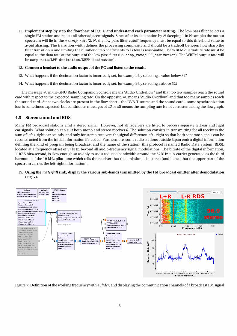
11. Implement step by step the flowchart of Fig. 6 and understand each parameter setting. The low-pass filter selects asingle FM station and rejects all other adjacent signals. Since after its decimation by N (keeping 1 in N sample) the outputspectrum will lie in the ±samp_r ate/2/N , the low pass filter cutoff frequency must be equal to this threshold value toavoid aliasing. The transition width defines the processing complexity and should be a tradeoff between how sharp thefilter transition is and limiting the number of tap coefficients to as few as reasonable. The WBFM quadrature rate must beequal to the data rate at the output of the low pass filter (i.e. samp_rate/LPF_decimation). The WBFM output rate willbe samp_rate/LPF_decimation/WBFM_decimation).

12. Connect a headset to the audio output of the PC and listen to the result.

13. What happens if the decimation factor is incorrectly set, for example by selecting a value below 32?

14. What happens if the decimation factor is incorrectly set, for example by selecting a above 32?

The message aU in the GNU Radio Companion console means “Audio Underflow” and that too few samples reach the soundcard with respect to the expected sampling rate. On the opposite, aO means “Audio Overflow” and that too many samples reachthe sound card. Since two clocks are present in the flow chart – the DVB-T source and the sound card – some synchronizationloss is sometimes expected, but continuous messages of aU or aO means the sampling rate is not consistent along the flowgraph.

4.3 Stereo sound and RDS

Many FM broadcast stations emit a stereo signal. However, not all receivers are fitted to process separate left ear and rightear signals. What solution can suit both mono and stereo receivers? The solution consists in transmitting for all receivers thesum of left + right ear sounds, and only for stereo receivers the signal difference left - right so that both separate signals can bereconstructed from the initial information if needed. Furthermore, some radio stations outside Japan emit a digital informationdefining the kind of program being broadcast and the name of the station: this protocol is named Radio Data System (RDS),located at a frequency offset of 57 kHz, beyond all audio-frequency signal modulations. The bitrate of the digital information,1187.5 bits/second, is slow enough so as only to use a reduced bandwidth around the 57 kHz sub-carrier generated as the thirdharmonic of the 19 kHz pilot tone which tells the receiver that the emission is in stereo (and hence that the upper part of thespectrum carries the left-right information).

15. Using the waterfall sink, display the various sub-bands transmitted by the FM broadcast emitter after demodulation(Fig. 7).

Figure 7: Definition of the working frequency with a slider, and displaying the communication channels of a broadcast FM signal

6

5 Spectral occupation of the various modulation schemes

5.1 AM v.s FM

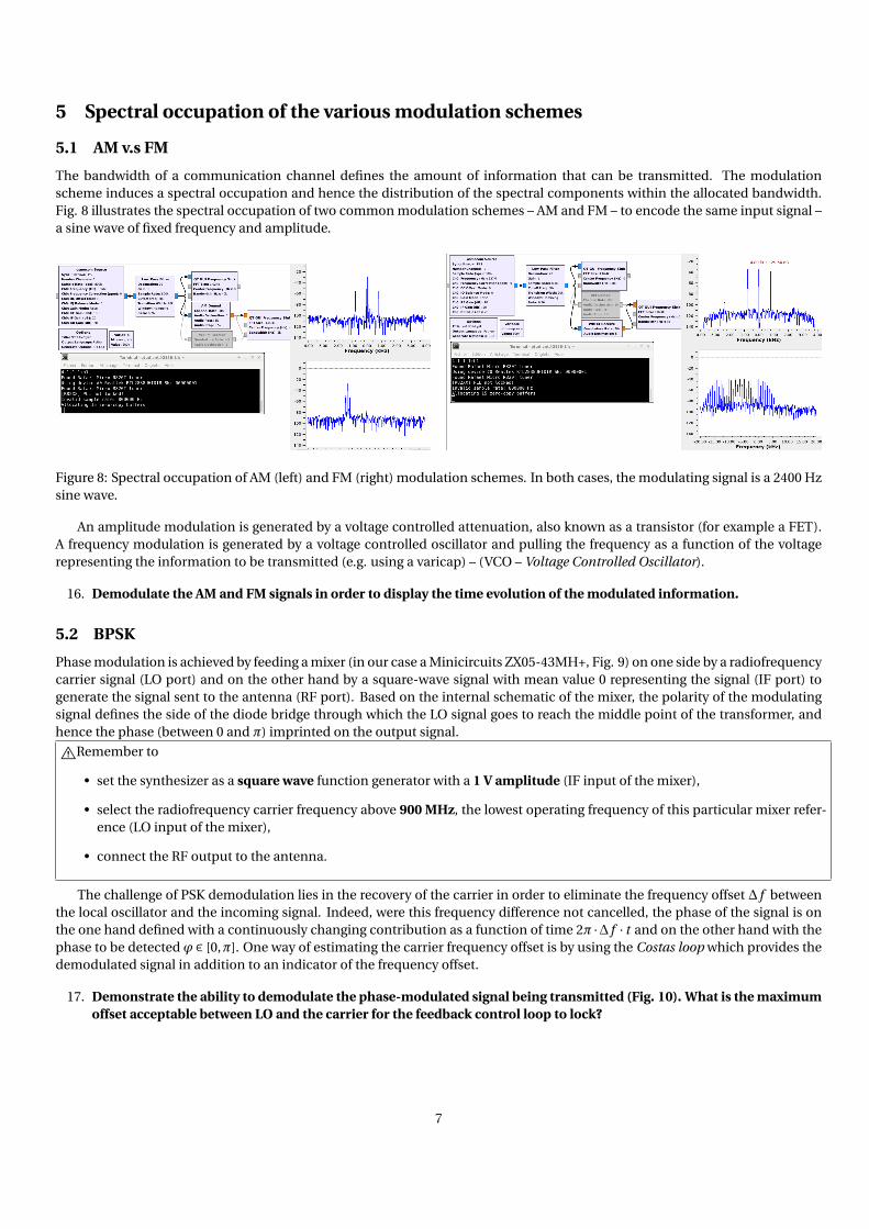
The bandwidth of a communication channel defines the amount of information that can be transmitted. The modulationscheme induces a spectral occupation and hence the distribution of the spectral components within the allocated bandwidth.Fig. 8 illustrates the spectral occupation of two common modulation schemes – AM and FM – to encode the same input signal –a sine wave of fixed frequency and amplitude.

Figure 8: Spectral occupation of AM (left) and FM (right) modulation schemes. In both cases, the modulating signal is a 2400 Hzsine wave.

An amplitude modulation is generated by a voltage controlled attenuation, also known as a transistor (for example a FET).A frequency modulation is generated by a voltage controlled oscillator and pulling the frequency as a function of the voltagerepresenting the information to be transmitted (e.g. using a varicap) – (VCO – Voltage Controlled Oscillator).

16. Demodulate the AM and FM signals in order to display the time evolution of the modulated information.

5.2 BPSK

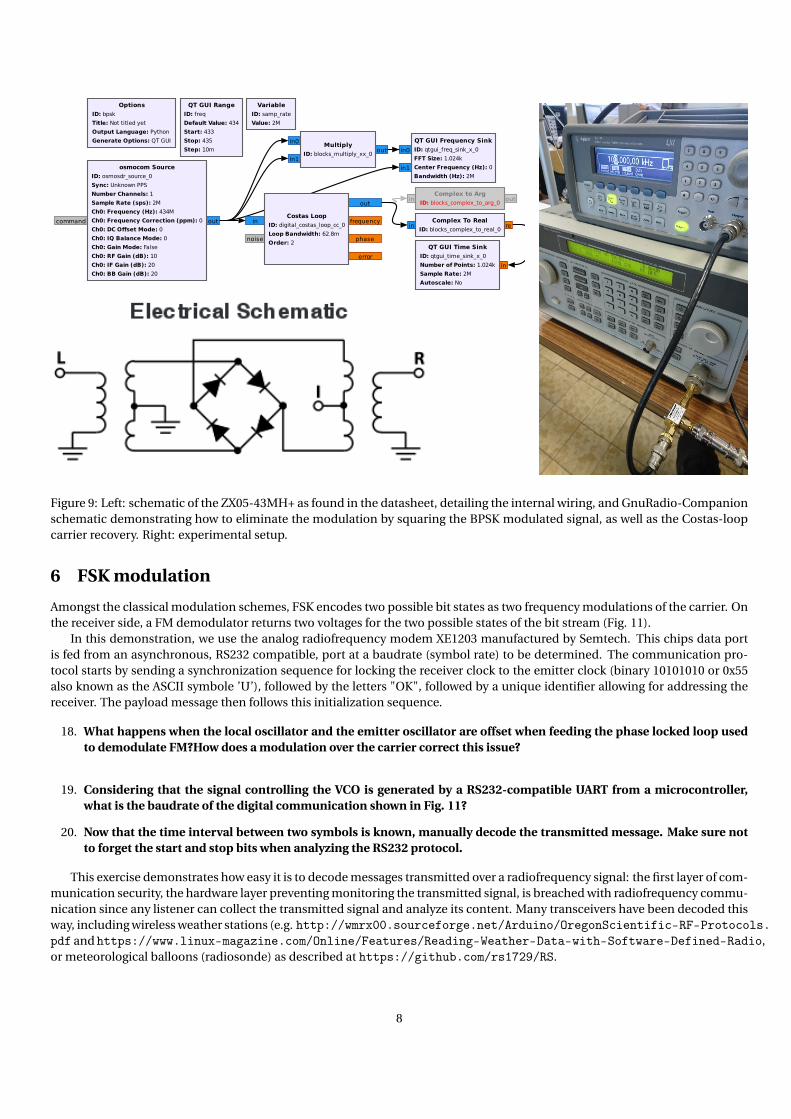
Phase modulation is achieved by feeding a mixer (in our case a Minicircuits ZX05-43MH+, Fig. 9) on one side by a radiofrequencycarrier signal (LO port) and on the other hand by a square-wave signal with mean value 0 representing the signal (IF port) togenerate the signal sent to the antenna (RF port). Based on the internal schematic of the mixer, the polarity of the modulatingsignal defines the side of the diode bridge through which the LO signal goes to reach the middle point of the transformer, andhence the phase (between 0 and π) imprinted on the output signal.

"Remember to

• set the synthesizer as a square wave function generator with a 1 V amplitude (IF input of the mixer),

• select the radiofrequency carrier frequency above 900 MHz, the lowest operating frequency of this particular mixer refer-ence (LO input of the mixer),

• connect the RF output to the antenna.

The challenge of PSK demodulation lies in the recovery of the carrier in order to eliminate the frequency offset ∆ f betweenthe local oscillator and the incoming signal. Indeed, were this frequency difference not cancelled, the phase of the signal is onthe one hand defined with a continuously changing contribution as a function of time 2π ·∆ f · t and on the other hand with thephase to be detected ϕ ∈ [0,π]. One way of estimating the carrier frequency offset is by using the Costas loop which provides thedemodulated signal in addition to an indicator of the frequency offset.

17. Demonstrate the ability to demodulate the phase-modulated signal being transmitted (Fig. 10). What is the maximumoffset acceptable between LO and the carrier for the feedback control loop to lock?

7

outinComplex to Arg

ID: blocks_complex_to_arg_0

Options

ID: bpsk




QT GUI Range

ID: freq

Default Value: 434

Start: 433

Stop: 435

Step: 10m

Variable

ID: samp_rate

Value: 2M

reinComplex To Real

ID: blocks_complex_to_real_0

out

in0

in1

Multiply

ID: blocks_multiply_xx_0

out

frequency

phase

error

in

noise

Costas Loop

ID: digital_costas_loop_cc_0

Loop Bandwidth: 62.8m

Order: 2

outcommand

osmocom Source

ID: osmosdr_source_0

Sync: Unknown PPS

Number Channels: 1

Sample Rate (sps): 2M

Ch0: Frequency (Hz): 434M








in0

in1


ID: qtgui_freq_sink_x_0

FFT Size: 1.024k


Bandwidth (Hz): 2M

in

QT GUI Time Sink

ID: qtgui_time_sink_x_0

Number of Points: 1.024k

Sample Rate: 2M

Autoscale: No

Figure 9: Left: schematic of the ZX05-43MH+ as found in the datasheet, detailing the internal wiring, and GnuRadio-Companionschematic demonstrating how to eliminate the modulation by squaring the BPSK modulated signal, as well as the Costas-loopcarrier recovery. Right: experimental setup.

6 FSK modulation

Amongst the classical modulation schemes, FSK encodes two possible bit states as two frequency modulations of the carrier. Onthe receiver side, a FM demodulator returns two voltages for the two possible states of the bit stream (Fig. 11).

In this demonstration, we use the analog radiofrequency modem XE1203 manufactured by Semtech. This chips data portis fed from an asynchronous, RS232 compatible, port at a baudrate (symbol rate) to be determined. The communication pro-tocol starts by sending a synchronization sequence for locking the receiver clock to the emitter clock (binary 10101010 or 0x55also known as the ASCII symbole ’U’), followed by the letters "OK", followed by a unique identifier allowing for addressing thereceiver. The payload message then follows this initialization sequence.

18. What happens when the local oscillator and the emitter oscillator are offset when feeding the phase locked loop usedto demodulate FM?How does a modulation over the carrier correct this issue?

19. Considering that the signal controlling the VCO is generated by a RS232-compatible UART from a microcontroller,what is the baudrate of the digital communication shown in Fig. 11?

20. Now that the time interval between two symbols is known, manually decode the transmitted message. Make sure notto forget the start and stop bits when analyzing the RS232 protocol.

This exercise demonstrates how easy it is to decode messages transmitted over a radiofrequency signal: the first layer of com-munication security, the hardware layer preventing monitoring the transmitted signal, is breached with radiofrequency commu-nication since any listener can collect the transmitted signal and analyze its content. Many transceivers have been decoded thisway, including wireless weather stations (e.g. http://wmrx00.sourceforge.net/Arduino/OregonScientific-RF-Protocols.pdf andhttps://www.linux-magazine.com/Online/Features/Reading-Weather-Data-with-Software-Defined-Radio,or meteorological balloons (radiosonde) as described at https://github.com/rs1729/RS.

8

http://wmrx00.sourceforge.net/Arduino/OregonScientific-RF-Protocols.pdf

http://wmrx00.sourceforge.net/Arduino/OregonScientific-RF-Protocols.pdf

https://www.linux-magazine.com/Online/Features/Reading-Weather-Data-with-Software-Defined-Radio

https://github.com/rs1729/RS

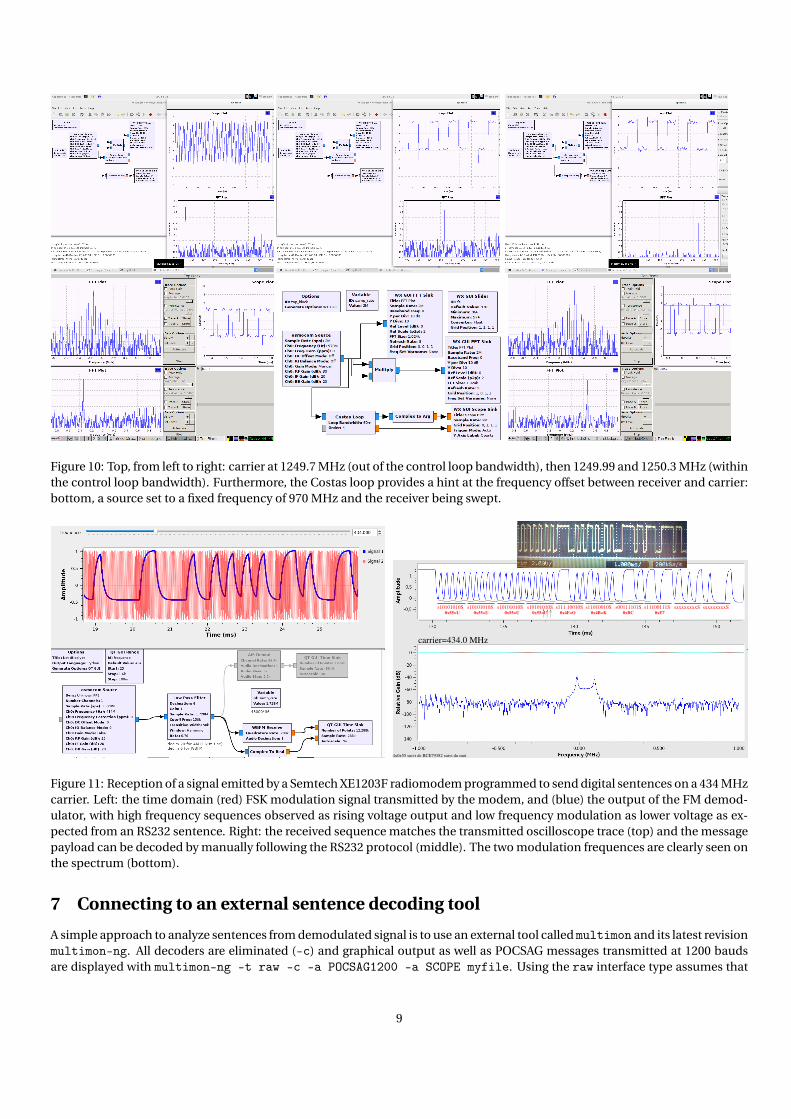
Figure 10: Top, from left to right: carrier at 1249.7 MHz (out of the control loop bandwidth), then 1249.99 and 1250.3 MHz (withinthe control loop bandwidth). Furthermore, the Costas loop provides a hint at the frequency offset between receiver and carrier:bottom, a source set to a fixed frequency of 970 MHz and the receiver being swept.

s10101010S s10101010S s10101010S s10101010S s111 10010S s11010010S s00111101S s11100111S sxxxxxxxxS sxxxxxxxxS

0x55=U 0x55=U 0x55=U0x55=U 0x4F=O 0x4B=K 0xBC 0xE7

4x0x55 suivi de BCE79382 suivi du mot

carrier=434.0 MHz

Figure 11: Reception of a signal emitted by a Semtech XE1203F radiomodem programmed to send digital sentences on a 434 MHzcarrier. Left: the time domain (red) FSK modulation signal transmitted by the modem, and (blue) the output of the FM demod-ulator, with high frequency sequences observed as rising voltage output and low frequency modulation as lower voltage as ex-pected from an RS232 sentence. Right: the received sequence matches the transmitted oscilloscope trace (top) and the messagepayload can be decoded by manually following the RS232 protocol (middle). The two modulation frequences are clearly seen onthe spectrum (bottom).

7 Connecting to an external sentence decoding tool

A simple approach to analyze sentences from demodulated signal is to use an external tool called multimon and its latest revisionmultimon-ng. All decoders are eliminated (-c) and graphical output as well as POCSAG messages transmitted at 1200 baudsare displayed with multimon-ng -t raw -c -a POCSAG1200 -a SCOPE myfile. Using the raw interface type assumes that

9

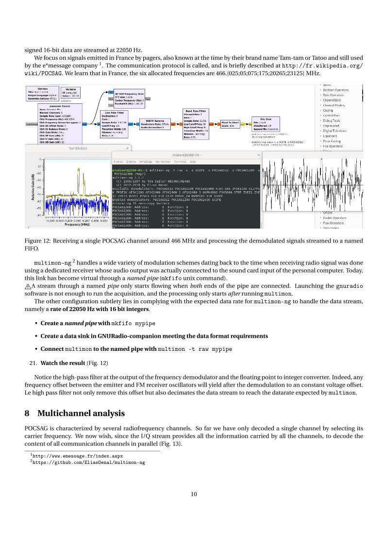
signed 16-bit data are streamed at 22050 Hz.We focus on signals emitted in France by pagers, also known at the time by their brand name Tam-tam or Tatoo and still used

by the e*message company 1. The communication protocol is called, and is briefly described at http://fr.wikipedia.org/wiki/POCSAG. We learn that in France, the six allocated frequencies are 466.{025;05;075;175;20265;23125} MHz.

Figure 12: Receiving a single POCSAG channel around 466 MHz and processing the demodulated signals streamed to a namedFIFO.

multimon-ng 2 handles a wide variety of modulation schemes dating back to the time when receiving radio signal was doneusing a dedicated receiver whose audio output was actually connected to the sound card input of the personal computer. Today,this link has become virtual through a named pipe (mkfifo unix command)."A stream through a named pipe only starts flowing when both ends of the pipe are connected. Launching the gnuradiosoftware is not enough to run the acquisition, and the processing only starts after running multimon.

The other configuration subtlety lies in complying with the expected data rate for multimon-ng to handle the data stream,namely a rate of 22050 Hz with 16 bit integers.

• Create a named pipe with mkfifo mypipe

• Create a data sink in GNURadio-companion meeting the data format requirements

• Connect multimon to the named pipe with multimon -t raw mypipe

21. Watch the result (Fig. 12)

Notice the high-pass filter at the output of the frequency demodulator and the floating point to integer converter. Indeed, anyfrequency offset between the emitter and FM receiver oscillators will yield after the demodulation to an constant voltage offset.Le high pass filter not only remove this offset but also decimates the data stream to reach the datarate expected by multimon.

8 Multichannel analysis

POCSAG is characterized by several radiofrequency channels. So far we have only decoded a single channel by selecting itscarrier frequency. We now wish, since the I/Q stream provides all the information carried by all the channels, to decode thecontent of all communication channels in parallel (Fig. 13).

1http://www.emessage.fr/index.aspx2https://github.com/EliasOenal/multimon-ng

10

http://fr.wikipedia.org/wiki/POCSAG

http://fr.wikipedia.org/wiki/POCSAG

http://www.emessage.fr/index.aspx

https://github.com/EliasOenal/multimon-ng

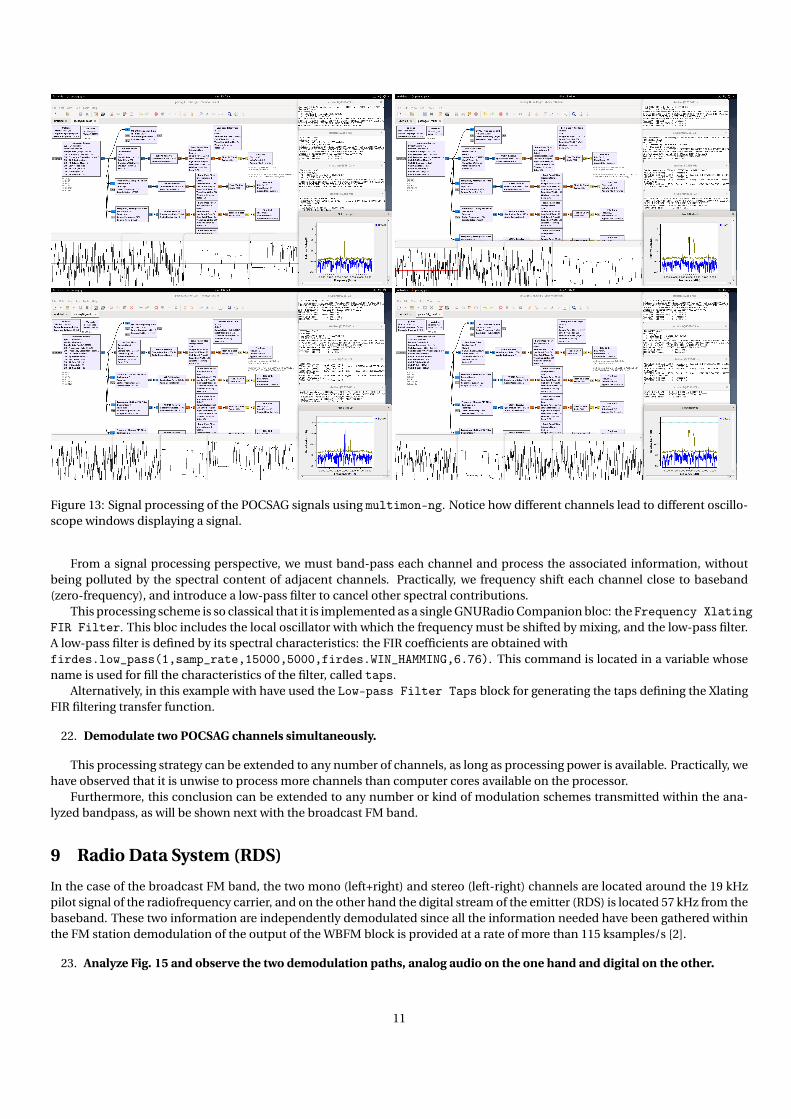
Figure 13: Signal processing of the POCSAG signals using multimon-ng. Notice how different channels lead to different oscillo-scope windows displaying a signal.

From a signal processing perspective, we must band-pass each channel and process the associated information, withoutbeing polluted by the spectral content of adjacent channels. Practically, we frequency shift each channel close to baseband(zero-frequency), and introduce a low-pass filter to cancel other spectral contributions.

This processing scheme is so classical that it is implemented as a single GNURadio Companion bloc: theFrequency XlatingFIR Filter. This bloc includes the local oscillator with which the frequency must be shifted by mixing, and the low-pass filter.A low-pass filter is defined by its spectral characteristics: the FIR coefficients are obtained withfirdes.low_pass(1,samp_rate,15000,5000,firdes.WIN_HAMMING,6.76). This command is located in a variable whosename is used for fill the characteristics of the filter, called taps.

Alternatively, in this example with have used the Low-pass Filter Taps block for generating the taps defining the XlatingFIR filtering transfer function.

22. Demodulate two POCSAG channels simultaneously.

This processing strategy can be extended to any number of channels, as long as processing power is available. Practically, wehave observed that it is unwise to process more channels than computer cores available on the processor.

Furthermore, this conclusion can be extended to any number or kind of modulation schemes transmitted within the ana-lyzed bandpass, as will be shown next with the broadcast FM band.

9 Radio Data System (RDS)

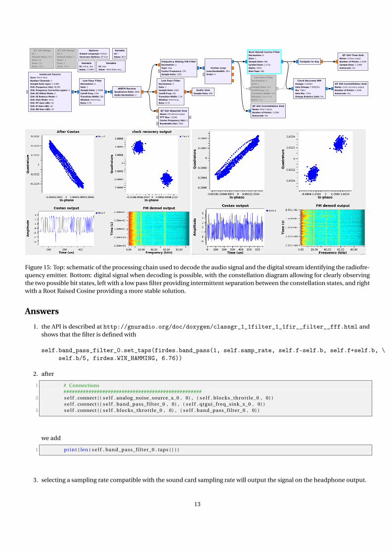
In the case of the broadcast FM band, the two mono (left+right) and stereo (left-right) channels are located around the 19 kHzpilot signal of the radiofrequency carrier, and on the other hand the digital stream of the emitter (RDS) is located 57 kHz from thebaseband. These two information are independently demodulated since all the information needed have been gathered withinthe FM station demodulation of the output of the WBFM block is provided at a rate of more than 115 ksamples/s [2].

23. Analyze Fig. 15 and observe the two demodulation paths, analog audio on the one hand and digital on the other.

11

22050*64

multimon-ng assumes 22050 Hz, 16-bit signed stream

multimon-ng -t raw -c -a SCOPE -a POCSAG512 \-a POCSAG1200 -a POCSAG2400 /tmp/1

466.025466.050466.075466.175466.20625466.23125

Options




Variable

Id: samp_rate

Value: 1.4112M

Low-pass Filter Taps

Id: taps

Gain: 1

Sample Rate (Hz): 1.4112M

Cutoff Freq (Hz): 15k

Transition Width (Hz): 5k

Window: Hamming

Beta: 6.76

outin

WBFM Receive

Quadrature Rate: 176.4k

Audio Decimation: 8

outin

WBFM Receive


Audio Decimation: 8

outin

WBFM Receive


Audio Decimation: 8

outin

WBFM Receive


Audio Decimation: 8

outin

Band Pass Filter

Interpolation: 1

Gain: 1

Sample Rate: 22.05k

Low Cutoff Freq: 50



Window: Hamming

Beta: 6.76

outin

Band Pass Filter

Interpolation: 1

Gain: 1

Sample Rate: 22.05k

Low Cutoff Freq: 50



Window: Hamming

Beta: 6.76

outin

Band Pass Filter

Interpolation: 1

Gain: 1

Sample Rate: 22.05k

Low Cutoff Freq: 50



Window: Hamming

Beta: 6.76

outin

Band Pass Filter

Interpolation: 1

Gain: 1

Sample Rate: 22.05k

Low Cutoff Freq: 50



Window: Hamming

Beta: 6.76

in

File Sink

File: /tmp/1

Unbuffered: Off

Append file: Overwrite

in

File Sink

File: /tmp/2

Unbuffered: Off


in

File Sink

File: /tmp/3

Unbuffered: Off


in

File Sink

File: /tmp/4

Unbuffered: Off


outinFloat To Short

Scale: 300k

outinFloat To Short

Scale: 300k

outinFloat To Short

Scale: 300k

outinFloat To Short

Scale: 300k

out

in

freq

Frequency Xlating FIR Filter

Decimation: 8

Taps: taps

Center Frequency: -25k

Sample Rate: 1.4112M

out

in

freq


Decimation: 8

Taps: taps

Center Frequency: 125k


out

in

freq


Decimation: 8

Taps: taps



outin

Low Pass Filter

Decimation: 8

Gain: 1


Cutoff Freq: 15k


Window: Hamming

Beta: 6.76

outcommand

osmocom Source

Sync: Unknown PPS

Number Channels: 1










freq

in

freq

bw


FFT Size: 1.024k


Bandwidth (Hz): 1.4112M

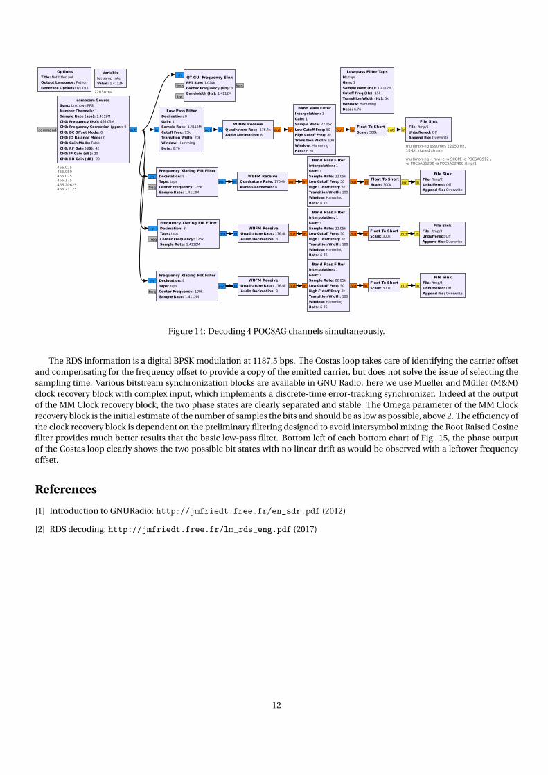
Figure 14: Decoding 4 POCSAG channels simultaneously.

The RDS information is a digital BPSK modulation at 1187.5 bps. The Costas loop takes care of identifying the carrier offsetand compensating for the frequency offset to provide a copy of the emitted carrier, but does not solve the issue of selecting thesampling time. Various bitstream synchronization blocks are available in GNU Radio: here we use Mueller and Müller (M&M)clock recovery block with complex input, which implements a discrete-time error-tracking synchronizer. Indeed at the outputof the MM Clock recovery block, the two phase states are clearly separated and stable. The Omega parameter of the MM Clockrecovery block is the initial estimate of the number of samples the bits and should be as low as possible, above 2. The efficiency ofthe clock recovery block is dependent on the preliminary filtering designed to avoid intersymbol mixing: the Root Raised Cosinefilter provides much better results that the basic low-pass filter. Bottom left of each bottom chart of Fig. 15, the phase outputof the Costas loop clearly shows the two possible bit states with no linear drift as would be observed with a leftover frequencyoffset.

References

[1] Introduction to GNURadio: http://jmfriedt.free.fr/en_sdr.pdf (2012)

[2] RDS decoding: http://jmfriedt.free.fr/lm_rds_eng.pdf (2017)

12

http://jmfriedt.free.fr/en_sdr.pdf

http://jmfriedt.free.fr/lm_rds_eng.pdf

QT GUI Range

Id: df

Default Value: 0

Start: -5

Stop: 5

Step: 100m

QT GUI Range

Id: f

Default Value: 96.9

Start: 88

Stop: 108

Step: 100m

Low Pass Filter

Decimation: 8

Gain: 1

Sample Rate: 96k

Cutoff Freq: 10k


Window: Hamming

Beta: 6.76

Options



Variable

Id: f

Value: 96.9

Variable

Id: samp_rate

Value: 1.536M

Variable

Id: taps

Value: filter.firdes.low_...

WBFM Receive

Quadrature Rate: 384k

Audio Decimation: 2

Audio Sink

Sample Rate: 48k

Complex to Arg

Clock Recovery MM

Omega: 5.05263

Gain Omega: 7.65625m

Mu: 700m

Gain Mu: 175m

Omega Relative Limit: 5m

Costas Loop

Loop Bandwidth: 20m

Order: 4


Decimation: 2

Taps: taps


Sample Rate: 192k

Low Pass Filter

Decimation: 4

Gain: 1

Sample Rate: 1.536M

Cutoff Freq: 130k


Window: Hamming

Beta: 6.76

Low Pass Filter

Decimation: 4

Gain: 1

Sample Rate: 192k

Cutoff Freq: 20k

Transition Width: 1.5k

Window: Hamming

Beta: 6.76

osmocom Source

Sync: Don't Sync

Number Channels: 1










QT GUI Constellation Sink

Name: After Costas


Autoscale: Yes

QT GUI Constellation Sink

Name: clock recovery output


Autoscale: Yes

QT GUI Time Sink

Name: Costas output


Sample Rate: 1.536M

Autoscale: Yes

QT GUI Waterfall Sink

Name: FM demod output

FFT Size: 1.024k


Bandwidth (Hz): 192k

Root Raised Cosine Filter

Decimation: 8

Gain: 1

Sample Rate: 96k

Symbol Rate: 2.371k

Alpha: 350m

Num Taps: 48k

Figure 15: Top: schematic of the processing chain used to decode the audio signal and the digital stream identifying the radiofre-quency emitter. Bottom: digital signal when decoding is possible, with the constellation diagram allowing for clearly observingthe two possible bit states, left with a low pass filter providing intermittent separation between the constellation states, and rightwith a Root Raised Cosine providing a more stable solution.

Answers

1. the API is described at http://gnuradio.org/doc/doxygen/classgr_1_1filter_1_1fir__filter__fff.html andshows that the filter is defined with

self.band_pass_filter_0.set_taps(firdes.band_pass(1, self.samp_rate, self.f-self.b, self.f+self.b, \self.b/5, firdes.WIN_HAMMING, 6.76))

2. after

1 # Connections##################################################

3 s e l f . connect ( ( s e l f . analog_noise_source_x_0 , 0) , ( s e l f . blocks_thrott le_0 , 0) )s e l f . connect ( ( s e l f . band_pass_filter_0 , 0) , ( s e l f . qtgui_freq_sink_x_0 , 0) )

5 s e l f . connect ( ( s e l f . blocks_thrott le_0 , 0) , ( s e l f . band_pass_filter_0 , 0) )

we add

1 print ( len ( s e l f . band_pass_fi lter_0 . taps ( ) ) )

3. selecting a sampling rate compatible with the sound card sampling rate will output the signal on the headphone output.

13

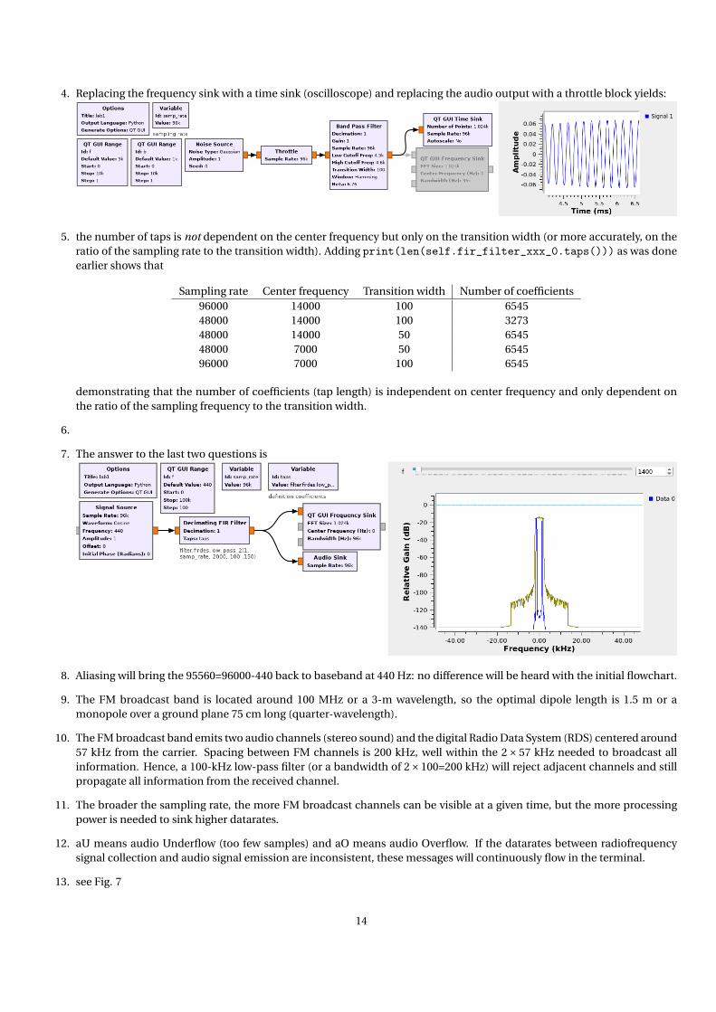
http://gnuradio.org/doc/doxygen/classgr_1_1filter_1_1fir__filter__fff.html

4. Replacing the frequency sink with a time sink (oscilloscope) and replacing the audio output with a throttle block yields:

5. the number of taps is not dependent on the center frequency but only on the transition width (or more accurately, on theratio of the sampling rate to the transition width). Adding print(len(self.fir_filter_xxx_0.taps())) as was doneearlier shows that

Sampling rate Center frequency Transition width Number of coefficients96000 14000 100 654548000 14000 100 327348000 14000 50 654548000 7000 50 654596000 7000 100 6545

demonstrating that the number of coefficients (tap length) is independent on center frequency and only dependent onthe ratio of the sampling frequency to the transition width.

6.

7. The answer to the last two questions is

8. Aliasing will bring the 95560=96000-440 back to baseband at 440 Hz: no difference will be heard with the initial flowchart.

9. The FM broadcast band is located around 100 MHz or a 3-m wavelength, so the optimal dipole length is 1.5 m or amonopole over a ground plane 75 cm long (quarter-wavelength).

10. The FM broadcast band emits two audio channels (stereo sound) and the digital Radio Data System (RDS) centered around57 kHz from the carrier. Spacing between FM channels is 200 kHz, well within the 2× 57 kHz needed to broadcast allinformation. Hence, a 100-kHz low-pass filter (or a bandwidth of 2×100=200 kHz) will reject adjacent channels and stillpropagate all information from the received channel.

11. The broader the sampling rate, the more FM broadcast channels can be visible at a given time, but the more processingpower is needed to sink higher datarates.

12. aU means audio Underflow (too few samples) and aO means audio Overflow. If the datarates between radiofrequencysignal collection and audio signal emission are inconsistent, these messages will continuously flow in the terminal.

13. see Fig. 7

14

14. The frequency synthetisizer generates either 400 Hz or 1 kHz AM or FM modulated signals.

15. Squaring the BPSK signal will shift the squared signal frequency offset to twice the offset value, and this doubled frequencyoffset must remain within the sampling band of the receiver.

16. DC offset since the FM demodulator acts as a frequency to voltage converter. Adding a modulation, e.g. AFSK (AudioFrequency Shift Keying) on NOAA satellites, cancels this offset.

17. 0.4 ms peak-to-peak period, i.e. for transmitting two symbols (0 and 1) so 1000/0.4=2500 which is most certainly a2400 baud transmission for two symbols, or 4800 bauds which is indeed the configuration of the XE1203 we used.

18. see Fig. 12

19. see Fig. 13

20. see Fig. 15

15

Documents

Software Defined Radiofrequency signal processing (SDR)