Small-x behaviour of initial state radiation in perturbative QCD

Nuclear Physics B336 (1990) 18-85North-Holland

SMALL-x BEHAVIOUR OF INITIAL STATE RADIATION INPERTURBATIVE QCD*

S. CATANI

Dipartimento di Fisica, Università di Firenze, INFN, Sezione di Firenze, Italy

F. FIORANI and G. MARCHESINI

Dipartimento di Fisiea, Università di Parma, INFN, Gruppo Collegato di Parma, Italy

Received 17 July 1989

We analyze in perturbative QCD the asymptotic behaviour of deep inelastic processes in thesemi-hard region x - 0. The study is done by extending the soft gluon insertion techniques. Weconfirm and extend the analysis recently performed by Ciafaloni. The main results are thefollowing: (i) Soft gluon emission from the incoming parton takes place in a region where theangles between incoming and outgoing partons are ordered. This is due to coherent effects similarto the ones in the x - 1 region . (ii) Virtual corrections involving an internal line with energyfraction x give rise, for x -0, to a new form factor of non-Sudakov type . This regularizes

collinear singularities when an emitted gluon is parallel to the incoming parton . (iii) At the

complete inclusive level, the new form factor plays the same role as the virtual corrections in the

Lipatov equation for the Regge regime . We show that, in the semi-hard regime, the gluonanomalous dimension coincides with the Lipatov ansatz . (iv) We identify the branching structure

of initial-state radiation including the semi-hard regime . The branching is formulated as aprobability process given in terms of Sudakov and non-Sudakov form factors . This process. inprinciple, can be used to extend the existing simulations of QCD cascades to the semi-hardregime .

1 . Introduction

One of the most arduous problems in perturbative QCD is the analysis ofprocesses involving incoming hadrons in the regime

0550-3213/90/$03 .50 T~ Elsevier Science Publishers B.V .(North-Holland)

A<<Q«~_s_ ,

(1 .1)

where V~s_ is the energy, Q is the hard scale of the process and A the QCD scale.This regime has been the subject of intensive studies in perturbative QCD [1-6] buta general theoretical understanding is still lacking .

*Research supported in part by the Italian Ministero della Pubblica Istruzione .

S . Catani et al. / Perturbative QCD

19

The extension of the QCD analysis to the semi-hard regime (1.1) is becomingcrucial for the interpretation of a large set of high energy data from hadron-hadronand hadron-lepton collisions .At the inclusive level we have, for instance, the cross sections and the distribu-

tions of semi-hard jets with ET << vfs- (minijets), and the emission of heavy particleswith mass M << ~s_ . Such quantities crucially depend on the behaviour of the quarkand gluon structure functions for small x - Q/ 6_. In perturbative QCD thesefunctions grow rapidly for x - 0 (see refs . [1-3,6]) so that semi-hard jet eventsprovide a large contribution to the total cross section .At the semi-inclusive level the structure of the emitted radiation is characterized

by the soft gluon interference effect (coherence) . In the hard regime x - 1 or in thetimelike processes of final state emission (e.g . in e + e- annihilation) we have a quitesatisfactory understanding of this phenomenon, at least to leading order (see refs .[1, 2,6,7]) . In the regime x - 0, instead, the QCD coherence of the radiation emittedby the incoming parton is not completely known.Monte Carlo simulations of hard events are important tools both for theoretical

and phenomenological study of QCD. At least to leading order, coherence of thesoft gluon radiation in hard processes can be described by a Markov process . Areliable description of coherence in the initial state radiation is already implementedin one of the existing Monte Carlo program [7] . However in regime (1 .1), asatisfactory description is still lacking.On the theoretical point of view, the analysis of the phase space region (1 .1) is

quite interesting . Let us recall some of the known results .(i) On the basis of the analysis of soft emission amplitudes at tree level, it has

been suggested [6] that the initial state soft gluon radiation is emitted within anangular ordered region . Outside this region, destructive interference takes place andthe distribution vanishes to leading order. In this spacelike process for x - 0, thestructure of soft gluon coherence is the same for x - 1 or in the timelike processes(e.g . in e'e - annihilation) .

(ü) On the contrary, virtual corrections to the initial state radiation in thesemi-hard regime (1.1) are expected to be quite different from virtual corrections tothe final state radiation of a soft gluon . Consider for instance the timelike andspacelike gluon anomalous dimension yx, for N - 1, with N the energy-momentindex . In the timelike case we have the known result [81

N4

1

~~N4

1_

_

\2

âs ~s(

l

2

s + . . ._1N_11 (N_1~

a5_

a,CA,

(1 .2)

which shows that, at the perturbative order as, the leading singularity as N - 1 isas(N_ 1) î _ 2n

.

20

S. Catani et aL / Perturbatiue QCD

The structure of the spacelike anomalous dimension for N - 1 is quite different .From two-loop calculations [14] it is known that

Accordingexpansion

YN(as) =

+ a

+ . . . ,

(1 .3)N-1 N-1

with a a known number . In contrast with the timelike case the leading as/(N - 1)3and the next to leading as/(N - 1) 2 singularities are absent .

(iii) From the analysis of the complete two-loop calculation it has been shown[2,4,6] that the absence of the leading as/(N - 1)3 singularity of YN is the result ofa cancellation between real emission contributions and virtual corrections of non-Sudakov type . The virtual correction of Sudakov type regularizes the soft emissionsingularity 1/(1 - z) in the Altarelli-Parisi splitting function, while this non-Suda-kov virtual correction regularizes the collinear singularity present when an addi-tional emitted gluon becomes parallel to the incoming parton . Such a cancellation ofcollinear singularities is also present in the equation which Lipatov [3] obtained longtime ago in his investigation of Regge behaviour in gauge theories . Although thesemi-hard regime is different from the Regge regime, one may try to translate theLipatov equation in terms of a gluon anomalous dimension ansatz and obtainthe following equation involving the Euler function (see e.g . ref. [2])

Nasl= [2~(1) - (YN) - (1-YN)~-1

f(YN) .

to this ansatz, YN(as) is a function of as/(N- 1) with perturbative

a s00

asa sYN(as) = y-gj ( N-1

)~= N-1

j=i

+O(( N-llal,

which is consistent with the two-loop result in eq . (1 .3) .(iv) According to this ansatz, the first correction to the one-loop result is of order

as and therefore one could think that the one-loop anomalous dimension couldprovide a reliable approximation to the structure function for small x . However thisis not the case since expansion (1.5) generates a square-root singularity in themoment index N for N = N* given by

N* =1+'is f(2)=1+iis 41n2 .

(1 .6)

The presence of this singularity at N* > 1 implies that the actual behaviour of thestructure function is much more singular than the one-loop expression : the structurefunction diverges as x-N ' for x -). 0, thus yielding a violation of the Froissart

q

where q is the hard probe

S. Catani et al. / Perturbative QCD

21

qn

q

P

Fig . 1 . The deep inelastic parton scattering . Here and in the following figures all solid lines indicategluons.

bound . In refs . [1, 5] it has been shown that such a violation could be overcome by aconsistent unitarization procedure .

(v) No real proof of the Lipatov ansatz (1 .4) still exists . A sizable step in thisdirection has been made in ref . [6] in which a method is suggested to factorize andresum higher order QCD corrections . Here a new form factor of non-Sudakov typeis introduced to regularize to all orders the real emission collinear singularities andthe Lipatov ansatz is obtained . However, in that paper there is not a real proof offactorization, especially at the virtual level, or of exponentiation of loop corrections .One of the aims of the present paper is to obtain such a proof .

In this paper we study the process of parton deep inelastic scattering (see fig . 1)

p+q~p'+qt+q2+ . . . +qn,

q 2=-Q 2 <0 and x=Q 2/2pq,

and p' represents the recoiling parton . Since gluons provide the most singularcontributions for x - 0, we focus our attention on deep inelastic scattering in pureYang-Mills theory . We consider a hard probe generated by the gauge-invariantcolour-singet source current (Ft°v)2 . However we will point out the generalizationwhen quarks are also included (see appendix B) .We study this process in the phase space region

qit < Q,

(1 .9)

with qit the transverse momentum of gluon i . It is only within this region that thecross section for the process (1 .7) admits a parton interpretation in terms of a single

22

S. Catani et al. / Perturbatioe QCD

incoming parton structure function. Note that for x - 0 values of q; t >> Q areallowed, since the kinematical boundary is q < QZ1x . Processes with q » QZ

correspond to the Drell-Yan emission of jets which are harder then the probe Q.

These processes have two hard scales and have to be analyzed independently . Ouranalysis in the region (1.9) provides, via the factorization theorem, a completedescription of jet emission in pp collisions with E t = Q « r .

Before explaining the results of this paper we describe the method we use .To compute the multi-gluon amplitudes in fig . 1, we follow the method of ref. [6]

which consists in generalizing to semi-hard processes the soft gluon insertiontechnique which has been extensively used [2,11-13] for the study of infraredsingularities in hard processes .The leading infrared singularities in hard processes are obtained by studying the

process of fig . 1 in the energy ordered region

Yn« * . . «Y2 «Y1 «x - 1,

(l .10)

where Yk is the energy fraction of the emitted gluon k . The soft gluon insertiontechnique [2] consists in factorizing the emission of the softest gluon n in terms of asoft current . In the region (1 .10) this is given by the eikonal current of all externalharder gluons

P P 1 " - 1 q,k

Tp

+ Tp,; + Y, Te

(l .11)Pqn

P qn

t=1

q,,q�

where the T's are the colour charges of emitting partons . Virtual corrections aretreated in a similar way [11,12] by factorizing the contributions with the softestgluon in the loop . This technique allows one to obtain a recurrence relation whichenables one to compute the leading infrared contributions to the multi-gluonamplitudes and to exponentiate the virtual corrections giving the proper Sudakovform factors .The x - 0 leading contributions of the multi-gluon amplitudes of fig. 1 are

obtained by studying the energy region

x«Yn« "'« «Y2 «Y1 -- .

(l .12)

The main difficulty in the study of this region is the presence of an internal line withenergy fraction x, which for x - 0 may be less energetic than the softest emittedgluon . This implies that insertions on this internal line cannot be described by eq .(1 .11) and one has to generalize the form of the soft current . A similar difficultyappears in the evaluation of virtual corrections involving this less energetic internalline. We shall show that all these complications can be overcome by appealing to theproperties of soft gluon coherence .

S. Catani et al. / Perturbatiue QCD

23

Our calculations are done in the axial gauge with the gauge vector essentiallyparallel to the recoiling gluon p' . We check the gauge invariance of final results tothe extent of current conservation . Let us list the results obtained in this paper .

(i) We show that, in the semi-hard regime (1.12), the emission of the softest gluonn can be factorized in terms of the total current (see eqs . (3.4) and (3 .5))

Jto~t -1) 1gn) - Je(, k- ')(q,) + Jne(Q, , qn) ,

where the additional current J�e is a non-eikonal current which corresponds to thesoft gluon emission from the softest internal line with momentum Qn =p - ql

- - - - - q» . This factorization gives a recurrence relation (see eq . (3 .3)) which allowsus to compute the multi-gluon amplitude at tree level in the phase space region(1 .12) .

(ii) We solve the recurrence relation and compute the leading contribution to themulti-gluon distributions at tree level (see eq . (4.16)) . Mass singularities related tospacelike internal lines are present in individual graphs but they are cancelled in thefinal result due to a coherence effect (see eq . (4.2)) . We confirm that there areleading collinear singularities only for 011h, 0, eg,g,

- 0 and BP , g, __' 0, where Bkk,are the angles between parton k and k' . As a consequence one obtains that the softgluon emission from the incoming parton p takes place within the angular orderedregion

0PP > BPgrz >. . . > BPV2 > BPgt

(iii) We show that the softest virtual correction to the multi-gluon amplitudesfactorizes and gives two contributions of different origin (see eq. (5.29)) . The first isthe usual one of eikonal type and the second one is of non-eikonal type and relatedto the non-eikonal current in eq . (1.13), (see eq . (3.5)) . This factorization provides away to exponentiate both types of virtual corrections (see eq . (5 .2)) . The completeform factor is given by the usual Sudakov one (see eq . (5.3)) and by a non-Sudakovform factor (see eq . (5 .4)) which is similar to the one suggested in ref . [6] . This lastone is relevant only for x - 0.

(iv) We write a recurrence relation for the complete multi-gluon amplitudes (seeeqs . (5 .2) and (5.5)) . By solving this recurrence relation (see eq . (6.14)) andintegrating over final state emission we compute the initial state multi-gluondistribution (see eq. (6.25)) . This distribution takes into account only the contribu-tions with collinear singularities for 9,g, 0 and includes the corresponding virtualcorrections . The structure function is obtained by integrating this initial statedistribution (see eq . (6.26)) .

(v) If we extrapolate the multi-gluon distributions, computed for x - 0, into thecomplementary region x - 1 we find that, apart from contributions which aresubleading, they match with those already known in the latter region (see ref . [2]) .

24


Therefore we can assume the distribution (6 .25) to be valid for any values of x . Inthis way we neglect only subleading singularities for finite x which contribute in theintermediate regions y; << x << y and give the finite terms for z - 0,1 of theAltarelli-Parisi splitting functions .

(vi) For x - 0 we obtain an equation for the structure function at fixed totaltransverse momentum similar to the one in refs . [2,61 (see eq. (7.28)) . This can besolved by the diagonalization of the energy N moments (see eq . (7.31)) . We confirmthe Lipatov ansatz (1.4) for the N - 1 anomalous dimension .

(vii) We cast the initial state multi-gluon distribution in terms of a spacelikebranching process and give the branching distribution (see eqs . (7.54) and (7 .55)) .The branching takes place within the angular ordered region (1.14), and thebranching probability contains two form factors : the usual Sudakov one (see eq .(7.48)) and a non-Sudakov form factor (see eq . (7.17)) . The last form factor isrelevant only when the emitted gluon is fast and therefore it is important only inpresence of the 1/z term in the Altarelli-Parisi splitting function .The paper is organized as follows . In sect . 2 we set the notations and recall some

of the general results on the soft gluon insertion techniques which are needed in thefollowing . In sect . 3 we analyze the factorization of softest gluon emission for x - 0and we give the general recurrence relation at tree level for the multi-gluonamplitudes . In sect . 4 we solve the previous recurrence relation and compute thegeneral multi-gluon distributions at tree level . We discuss also the structure of softgluon interference (coherence) . In sect . 5 we perform a detailed analysis of virtualcorrections at the same level of accuracy as in the calculation of real emission andwe prove the exponentiation of these virtual corrections . We deduce also therecurrence relation for the multi-gluon amplitude including the appropriate formfactor . In sect . 6 we solve the above relation and compute the initial state multi-gluondistributions . In sect . 7 we discuss the coherence of multi-gluon emission, wecompute the anomalous dimension for N - 1 and we deduce the branching struc-ture of initial state emission . The paper is completed by two appendices . Inappendix A the two-gluon emission amplitude is evaluated in a general axial gaugeand we check the gauge invariance of the total soft gluon emission current . Inappendix B we discuss deep inelastic scattering with incoming quarks . By usingcoherent state techniques we extend the results obtained in the pure Yang-Millstheory .

2. General features

For the kinematics of the process in fig . 1 we introduce two lightlike vectors

p=E(1,0,0,1), p=E(1,0,0,-1), 2pp=4E2 . (2.1)

The other momenta in eq . (1.7) can be written as

Q2 Pq =- xp +--x

2pp

S. Catani et al. / Perturhative QCD

25

where 2pq i = q /yi for qi massless and x = QZ/2pq . For large QZ we have

x=xn-(1-Y,- . . . - ya ),

P,-p,

where y i is essentially the energy fraction of qi and -- stands for almost parallel . Inthe deep inelastic process of fig. 1 the kinematical boundary for the total squaredtransverse momentum Qnt=(E"-lgit)2 is of order 2pp' and for small x we haveQnt <

Q2/x.As already mentioned, in this paper we limit our analysis to simpledeep inelastic process in which the only hard scale is Q and we consider the phasespace region QI « Q.As mentioned in the introduction, since only gluons are relevant for x - 0, we

focus our attention on deep inelastic scattering in Yang-Mills theory. The case witha quark in the initial state will be discussed in appendix B . For the hard probe wetake the simple gauge invariant current (F,,", ) 2 . To first order it gives rise to thetwo-gluon vertex

V"'(P, P') = - gtiw(PP) + (P"'P" ' ),

with [t and ,u' the Lorentz indices of gluons p and p' respectively. In addition tothis we have a contribution of order gs with three-gluon vertex . The four-gluoncoupling can be neglected in our approximation .

For x - 0 the dominant part of the multi-gluon amplitude is obtained bystudying the process of fig. 1 in the phase space with strongly ordered energies . Forthe emitted gluons which are softer than x the soft emission factorization works asin the case of x - 1 . We then focus our attention on the phase space in which x issofter than the emitted gluons

x«y� «Y� -1« . . . «y1-1 .

2.1 . GAUGE FRAME AND STRUCTURE OF LEADING DIAGRAMS

We work in axial gauge and introduce the polarization projection vector

qi =yP+(Pqi)P +qit,

(2 .2)PP

(2 .3)

(2 .4)

(2.5)

(2 .6)

26

S. Catani et a1. / Perturhatiue QCD

so that

and the gluon polarization sum is

We choose the gauge

k'E(~)(q)=0- kg 1lx

,

E(X)(q)gx=q'E(X)(q)=0,

(2 .7)q ,q

du°(q) = -EpX)(q)E(a)°(q),

n"dl,v(q) =0 .

(2 .8)

in which the gauge vector rl is essentially parallel to the recoiling momentum p' .The topological and Lorentz structure of the dominant Feynman diagrams forx - 0 greatly simplify in this gauge . Let us list the main simplifications :

(i) First we can neglect the Feynman diagrams in which the gluons qt,..., q� areemitted by the recoiling parton p' . This is due to the fact that in the phase space(2.5) soft gluon emission from p' can be approximated by the eikonal vertex2pw --- 2pw which is orthogonal to the polarization vector in our gauge rl =p.

In our gauge we need to consider only the contributions of the hard current (Fw,) 2

coming from the two-gluon coupling in eq . (2 .4) . This is due to the same reasondescribed above . The contribution from this current with three-gluon coupling givesrise to two terms . The first is of order ytpa with respect to the one corresponding toeq. (2 .4) and gives a nonleading infrared contribution . The second is proportional to

p, - ptl and does not contribute in our gauge . As a result we limit our analysis to thediagrams with the structure in fig . 2 . For the analysis in a general gauge we refer toappendix A.

9

,1=P-p',

(2 .9)

Fig. 2. Structure of diagrams for the leading infrared contribution in the gauge (2 .9). The full circlecorresponds to the effective vertex in eq . (2 .11) .


27

(ii) A further important simplification comes from the structure of the followingeffective hard vertex

1

( V ",(Q", P') ) 1 )Ve(fpt(Q, P')

d~v(Qrr)n

P'L~l

n

where V "(Qn , p') is given by eq . (2.4) and corresponds to the vertex Q n + q -> p' infig . 2 . Eq. (2.10) can be rewritten as

Ve(f é,) (Qn , P') - rcxl (Qn, P')

pQrr (

d(QQ) . P)(Q,r'

((X,)(P')),

(2 .11)n

where

X) (Qn , P') - (1/Q2) dw(Qn)E~x)(P') .

(2 .12)

In our gauge q - p', the second term can be neglected and the effective hard vertexis just given by F(Q � , p') which for x = x � - 0 is essentially parallel to the gaugevector 71

1

rit',,)(Qn,P')-

Qz~

p

~P(Qn-x� P),E(x,)(P')-x � /E (~)(P')-

p~P .EW)(p')J~x n

rn

PP

2(Qr,- x,P)*E(X' ) (P') pl~ 1 .

The neglected term of order xn is a purely transverse vector .(iii) The fact that for x - 0 the effective hard vertex

Veff (Q, , p') becomesproportional to the gauge vector P provides a further simplification in the relevantLorentz index flow in the Feynman diagrams . Let us illustrate this for the case offig . 3 in which we represent the three polarization flow contributions to the

(2 .10)

(2 .13)

Fig. 3 . The three polarization flow contributions in the three-gluon vertex . In our gauge, the leadingcontribution is given only by the diagram (a).

28


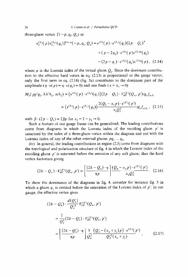
three-gluon vertex I'(-p, q 1 , Qj as

E(À)(P)E,(,~1)(Rl)rvvlp(-P, Rl , Q1) = E (À) (P) * E(~1)(gl)(2P -QI) p

(2k - Qn) 'd(Qn)Q 1 z

Ve(fé')(Qn> P')n

1-

2 (2k - Qn) ' Vefé') (Qn> P')

+ ( P - 2q1) - E ( ~' ) ( P)E(~")P(g1)

- (2P-gl)'E(~')(ql)E( ~')p(P), (2 .l4)

where p is the Lorentz index of the virtual gluon Q1 . Since the dominant contribu-tion to the effective hard vertex in eq . (2.13) is proportional to the gauge vector,only the first term in eq . (2.14) (fig. 3a) contributes to the dominant part of theamplitude (rt - E(p) = ,q - E(q,) = 0) and one finds (x _ x1 - 0)

Mj(PP'g1, NX'X 1 , aeb l ) = (E(")( P) . E(x`)(gl))(2P - Q1) - V,~f,)(Q, P ')igjaeb1

= (E(a)( P) ' E(~')(R1))2(Ql - x, p) ' E(~/)(P')

1SsÎacb l ,

(2 .15)

with p . (2 p - Q1)=2pp for xl =I-y1 -0.Such a feature of our gauge frame can be generalized . The leading contributions

come from diagrams in which the Lorentz index of the recoiling gluon p' issaturated by the index of a three-gluon vertex within the diagram and not with theLorentz index of any of the other external gluons pql . . . qn .

(iv) In general, the leading contributions in region (2.5) come from diagrams withthe topological and polarization structure of fig. 4 in which the Lorentz index of therecoiling gluon p' is saturated before the emission of any soft gluon ; thus the hardvertex factorizes giving

(2k- Qj - Vecé") (Qn , p') -

(2k ~Qn)

(Q, -x PQ �E(~'

~(P') .

(2.l6)

To show the dominance of the diagrams in fig. 4, consider for instance fig . 5 inwhich a gluon qj is emitted before the saturation of the Lorentz index of p' . In ourgauge, the effective vertex gives

_ [ (2k - Qn)-n

_1

(Q~'- (xn +yj)P) . E (X,)(P')

(2.17)7%P

] Qn

Qnz ( xn + yj)

2 .2 . COLOUR NOTATIONS

S . Catani et ai . / Perturbative QCD

29

qa2

qa2

Fig . 4 . Structure of diagrams giving, in our gauge, the dominant contribution in the region (2 .5) . Thepolarization flow is also indicated .

Fig . 5 . Emission of soft gluon q, gives a subleading contribution in the region (2 .5) .

with Q' = Qn + q. . The 1/x � singularity in eq . (2.16) is replaced in eq . (2.17) by1/(x � + yj ) . The singularity is then screened by yj and one obtains a nonleadingcontribution .

The n-gluon emission amplitude M� for process (1 .7) is a function of the externalmomenta p, p', q . . . . . . q n , the corresponding Lorentz indices X, X', X1, . . . , a � andthe colour indices a, c, b l , . . . , b� (see fig . 2) . For each process with a given numberof emitted gluons we introduce a space of colour indices (I acb l . . . b� )) and write

30


the amplitude as a representative state in this space

M� _(acbl . . .b� lMn(PP'gi . . .gn ;AX'A1 . . .Q) . (2 .18)

As shown in a previous analysis [13] of the infrared structure of deep inelasticscattering for x - 1 or of final state emission processes as e + e- annihilation, thisnotation not only simplifies the Feynman diagram calculations but also helps ingrasping the consequences of colour conservation and the physical properties ofcoherence of QCD radiation .

In the colour space for n emitted gluons we introduce SU(N) colour chargematrices Tp , T, Tl , . . . , T� for each external gluon p, p', ql , . . . , qn acting as follows

2 .3 . SOFT GLUON EMISSION FOR x -> I

This condition is satisfied by Mo and Ml (see eq . (2.15)) .

Before analyzing the x -> 0 case we recall here the results of soft gluon factoriza-tion in the case x - 1 . This will help in describing the general method and inunderstanding the physical differences between x - 1 and x -> 0 cases.

For x - 1 the leading infrared structure of M� is obtained by studying theprocess of fig . 1 in the strongly ordered energy region for the emitted gluons

Y� «Yn-1« . . . «Y,«x-1 .

(2.21)

As well known [2], the emission of the softest gluon qn can be factorized in termsof the eikonal current and, in the colour notations of the previous subsections, onehas

(acbl . . . b� IMn) - (acbl . . .b�-1IJe(ik-1)b

"(gj IM,,(2.22)

P Pf n-1 gtwhere

J;"-1)(q) = - Tp- + Tp ,; + Y, T,- ,

(2 .23)Pg

p'q

t=1

grg

is the classical current for the emission of the soft gluon by the other harder charges .This current is conserved due to the vanishing of the total charge (see eq. (2.20)) .

T,61acbl =. . . b�) ifbb,b, l acbl . . . b, . . . b�) , (2 .19)

and similarly for TP and Tn , . The charge conservation condition is

-Tp +T',+ T,) l m�)=0 . (2 .20)l=1

S. Catani et ai. / Perturbatiue QCD

3 1

The fact that, after the factorization of qn emission, one is able to reconstruct theamplitude Mn - I , is crucial in order to provide a recurrence relation which allowsone to construct the dominant part of Mn in the phase space (2.21) .

3 . Factorization of soft emission current for x ---> 0

For x - 0 the dominant part of Mn is obtained by studying the process of fig . 1in the phase space region (2 .5) . In this section we extend the method of soft gluonfactorization extensively used [2] in the region x - 1 . We prove that this factoriza-tion is possible in general and we construct the corresponding soft current . We areable to obtain a recurrence relation which allows one to evaluate the leading x - 0contributions to all amplitudes Mn at tree level .Due to the form (2.13) of the effective hard vertex Veff(Q,, p') in our gauge, we

factorize in all M� the following subamplitude

2(Q,, - xnp) - E (À' ) (p')M� -

2

(acb l . . . bn1hn(pp'g1 . . . qni,

(3 .1)xQn

where h� corresponds to the diagram in fig . 4 in which the hard vertex Qn + q -p'is replaced by gl2 rlp (see eq . (2.13)) . We have already found this structure in thecase of n = 1 (see eq . (2.15)) in which the subamplitude h l is

(acbljhI(pp'g1)) = ' (A) (p) - E (~' )(g1)Igsfaeb, *

(3 .2)

In the following we show that the soft gluon factorization and the correspondingrecurrence relation hold not for the full amplitude Mn but for the subamplitude hnin the form

(acbl . . .bnjhn(pp'qj . . .qn) ) = gs(acbl . . .bn-IlJtoi -1>b"(gn)Ihn-1(Pp'gj . . .qn 1)i

We show also that the soft emission current Jc(,t-')(q.) is given by the following twocontributions

with Q�_1-Q,,+q, xn-I-xn+Yn'

Jt("-I)(q,,) = Jeik- ')(qn) + Jne(Qn, qn) ,

where Jerk-1)(q.) is the eikonal current in eq . (2.22) and Jne(Q � , qn) is a non-eikonalcurrent given by

__ 2(Qn- , - xn-IP)' E (gn)Jne(Qn~gn)

Q2

rP',

n-1

(3 .3)

(3 .4)

(3 .5)

3 2


This result is obtained as follows . The emission of the softest gluon n from theharder external and internal lines can be factorized as usual [2] and is described bythe eikonal part of the current . In the phase space (2.5) only the internal line Qn issofter than the emitted gluon . In this case the emission of the softest gluon n from

Qn cannot be evaluated by the eikonal approximation . However we are able tofactorize also this contribution by taking into account the property of coherence ofthe radiation and obtain the non-eikonal current Je .

This additional non-eikonal contribution to the total soft current for x - 0 hasbeen introduced also in ref . [6] in a one-loop calculation . In this section we presentthe generalization to all loops.We shall present in subsect . 3 .3 the general proof by induction of eqs . (3 .3) and

(3.4) . To this purpose we first analyze in detail the case with n = 2 and some generalfeatures of the case n = 3 .

3 .1 . SOFT EMISSION FOR n = 2

The leading contributions to M2 in the phase space

come, in our gauge, from the diagrams in fig . 6 (see sect . 2) .Consider first the two diagrams (figs . 6a, b) which correspond to the usual eikonal

emission of the softest gluon q2 from the hard external gluons p and qt . In thesetwo diagrams the soft emission can be factorized giving the usual result [2]

with

J;"(q2) _ ( -P

Tp+

ql

Tl) . E(q2)

(3 .8)Pq2 glq2

x«y2 «y 1 =1,

(3 .6)

4z '" L-~-

uz_p

~Q

p

Q2 Qi

P

Fig . 6 . Diagrams for n = 2 giving the leading contribution in (3 .6) .

(acblb2 j h( a +b)) g s(acb j jJ~,1 (g2)jhl) , (3 .7)

We consider now the last graph of fig . 6 and show that also in this case the softgluon q2 can be factorized . Notice that in diagram of fig . 6c, the gluon q2 is emittedwith the same effective vertex r(Qj, q2 ) we have introduced in the previous section(eq . (2.13))

1

2(Ql__

x1P) . E ( ~ 2) (g2)

qwTtX z ) (Q1, qz) - Qi-d (Q,) ' E~~ 2) (gz) -

x1Qi

2qP

(acblb2 ~h2`))=gs q . (2Q1-Q2) [(2p_Qi)'r(~ Z) (Qi,9z) ] ~ acb1 1 TP? ihi)2qP

= gs(acbl~2(Q1 - x1 P ) 'E (

ÀZ) (gz )l

T,21h1)QI

P

3.2 . CASE n = 3 AND THE STRUCTURE OF GENERAL SOFT INSERTIONS

(3 .12)

We have neglected a contribution regular as x = xl = 1 -yl -> 0 and purely trans-verse .As in the case of the hard vertex, in this gauge the saturation of the Lorentz index

with external gluon polarizations gives only a nonleading contribution of order xl .By using the approximation in eq. (2 .13), the diagram of fig . 6c gives

= gs(acb1 1 JeX2) (Q2, gAhl) ,

(3 .13)

where the factor (2Q1 - Q2) (q/2qp) = xl - zx2 = xl has canceled the 1/xl sin-gular factor in the effective vertex r(Q,, q2).

The features of the calculations for n = 2 can be generalized to higher n . Howeverthe generalization requires some new features which we want to illustrate by


Since in this gauge q - p' we have

33

_P P~ qi qi.E (q2) -

_P _E( q2)

=

_ _P~(3 .9)

Pq2 Pq2 P'q2 glq2 glg2 P'qz

and the hard probe is a colour singlet

(- Tp + TI + Tp , )I hl) = 0, (3 .10)

and the eikonal current can be written as follows

Je(i k)(g2 )P ql

= Tp+pi

Tp,+ Tl . (3.11)-Pq2 P'q2 gigz

34

S. Catani et at. / Perturbative QCD

qs q3 q2

analyzing the case n = 3 in the region

q2 qs qr

Fig . 7 . Example of diagrams for n = 3 . (a) Diagram with a leading contribution . (b) Diagram with anonleading contribution .

X«y3«y2«yl=1 .

(3 .14)

In our gauge the subamplitude h 3 can be obtained by considering all possibleinsertions of the softest gluon q3 on the diagrams of fig. 6 . These insertions can bedivided into four general categories :(i) non-eikonal insertion on the softest internal line Q2,(ii) non-eikonal insertion on harder lines,(iii) eikonal insertion on harder lines emitted from eikonal vertices,(iv) eikonal insertion on harder lines emitted from non-eikonal vertices

(1) Non-eikonal insertion on the softest internal line Qz .

This gives a new vertexQz --* Q3 + q3, with the Lorentz index structure of fig . 4 . For example, in the case offig . 6a this type of insertion gives the diagram of fig . 7a . For all diagrams of fig. 6this will contribute to the subamplitude h 3 with the momentum factor

2(Q2 - X 2 P ) . E (N3, (g3 ) 71P21P ' (2Q2 - Q3) rw~3) (Qz, q3) =

Qzz

2,qP(3 .15)

where we have replaced the effective hard vertex V,,(fX)(Q3,P') by q/2qp andapproximated the effective vertex rO31(Qz, q3) for the emission of q3 according toeq. (2.13) .From eq . (3.15) we have the following factorized contribution to the soft gluon

emission

2(Qz - X2P)'E03)(g3)(acb 1b2 b3 1h 3) =gs(acblb2l

Q2

Tp%~h2) + . . . .

(3 .16)

(ii) Non-eikonal insertion on hard lines . An example is given in fig . 7b . Allinsertions of this type give nonleading contributions.

(iii) Eikonal insertion on harder lines emitted from eikonal vertices .

This refers tothe insertions into figs . 6a, b in which qz is emitted from an eikonal vertex . Let us

consider for instance the diagram of fig. 6a, in which this type of insertion can befactored out and gives the following soft emission current (k 2 =p - q2, k2 = k2 - q3)

j(a)(g3) ---


35

kgl2 P gzTl + 2 -

Tp+

T2glg3 k2 P93 g2g3

2

+

I

1-k2 z )kg3 (-Tp+T2) E(q3)* (3 .17)

The first term is the eikonal emission from ql . The second term with the bracketscorresponds to the emission from external gluons p, qz and the factor k2 k2z isneeded in order to reconstruct the original subamplitude h~) in fig . 6a . The thirdterm corresponds to insertion of q3 on the internal line k 2 which, according tocharge conservation, has the colour charge Tkz = - Tp + T2 . As shown in ref. [13], atthe leading collinear level, the last two contributions can be replaced just by the sumof the eikonal currents for the emission of q3 from external gluons p and q2 with noresealing of internal momenta . We have then

j(a)(g2) = Je(i k)(g3)

qzP -4- q,Tl +

pq3 p glg3

g2g3- E(q3)* (3 .18)

The reason for the above approximation is a coherent effect . When q3 is parallel tok2 we have k2z = kz since q3 is the softest gluon . In this case the last term in eq .(3.17) can be neglected, the factor of momentum resealing in the second term is 1and we obtain eq . (3.18) . In the opposite case p and q2 can be considered nearlyparallel at the leading collinear level and we have l k2z 1 >> I k2 1 = 0. It follows thatthe second term in eq . (3.17) can be neglected and the last one becomes

k2( -Tp+T2)=~-

PTp+

gz T2 ~

(3 .19)k2g3

pq3 g2g3

thus leading again to eq . (3.18) . A similar result holds also for fig . 6b .(iv) Eikonal insertions on harder lines emitted from non-eikonal vertices .

Thisrefers to insertions on fig . 6c in which q2 is emitted from non-eikonal vertex .Considering the soft emission of q3 from all harder lines in fig . 6c we can factorizethe following expression (Qi = Ql - q3)

d(Ql) - E(g2)

z+

Q12

_pTp+

il,Tl

.E(q3)Ql [ M

M3 ]

,

+~(1

- Q1z) Q1

.Q1'73 )

(-Tp + T1)~

d(Q1)'E(g2)

d(Q1)'E(gz) (3 .20)

36

S. Catani et at. / Perturbative QCD

Qh�,

Qh,,._i

qhl

3.3 . GENERAL LEADING AMPLITUDES

Fig . 8 . Structure of diagrams giving the leading contributions to the general amplitude .

The first term corresponds to the emission from qZ ; the second one to the emissionfrom p and q, and the last one corresponds to the emission from the internal hardline Q, with colour charge TQ, = - Tp + T, . The expression in eq . (3 .20) is similar tothe one in eq . (3.17) . We can apply the same analysis and by coherence we obtain

F(c) = Jeik) (g3)d(Qi) ' E(qz) ,

(3 .21)

where the quantity d(Q,) - E(q2) is needed to reconstruct the original subamplitudeh2(c) of fig . 6c .Combining all these contributions we obtain the soft emission formulae (3.3) and

(3.4) for the n = 3 case .

Here we give the general proof by iteration of eqs . (3.3) and (3.4) . First we showthat in the phase space region (2.5) the leading diagrams have the structure in fig . 8 .In this figure we denote by q,, the hardest gluon emitted within the subgraph Aj .Other specific features are the following :(i) As indicated, the Lorentz index of qt, is saturated by the Lorentz index of p .(ii) The Lorentz index of the gluon q,, . is saturated within the vertex pf , -~ p/ +kj _, .(iii) The soft emission from the various subamplitudes Ao . . . A m is of eikonal typeonly .The above helicity structure can be proved by an iterative method. We suppose

that this structure holds for a graph with a given number (n - 1) of emitted gluonsand then we analyze all possible insertions of a softer gluon qn (xn << yn << y,) .Due to the simplifications discussed in the n = 2,3 cases, we have to consider only

the following categories of insertions :(i) Non-eikonal insertions on the softest internal line Q n _, .

In this case we canfollow the calculation for n = 3 in eq. (3 .15) and reconstruct the original subampli-

S. Catani et at. / Perturbatiue QCD

37

tude h n , by factorizing the soft current contribution of non-eikonal type Jne(Q,, q� )given in eq . (3 .5) .(ii) Non-eikonal insertions on harder lines .

These are of the type of fig . 7b and canbe neglected in general .(iii) Eikonal insertion on harder lines .

Consider first the eikonal insertions of thesoftest gluon n on the last subgraph A m . It is known [13] that all these insertionscan be factorized in terms of eikonal current emission

_ _ gi (gn)J~An>>(gn) Jeik (qn) - L

T.

(3 .22)iEA �, giqn

Consider now the sum of the insertions on the line p, pm

k,,,

and on thenext eikonal subgraph A m - 1 . For insertions on Am _ 1 and km - 1 we can use theapproximations in the previous subsection . As in eq. (3.20) we can factorizethe expression

F

-

I 1

P;n2 )

-

TPm j ( d l Pm ) ' E l gh,� ) )Pm 1q �

X(d(Pm)'E(ghm)),

where Tpm_ , and Tpm are the colour charges of lines p._iPm-i = pm-i - qn . Using colour conservation we have

F (A,, 1)-(d(Pm)'E(gh~))

Pm-l' E(gn)TP~, -, - Jeik ",

-1) (gn )Pm- lgn

Tpm-1 = Tpm +

Y"

T, .iEA~-1

(3 .23)

and pm , and p;� = p n - qn,

(3 .24)

The factors ph,/Pn,2 and (1 - pn/pm2), etc. are set in order to reconstruct the fullsubamplitude h._1 (apart from the factor d(pm) E(qh,) which is included in eq .(3.23)) .Eq . (3.23) has the same structure of eq . (3 .20) and as in the previous case, we have

Pm-i Pm-l'El gn)J(ikm-1~(9n) -

I1 -

,2

TP-1}

(3 .25)PM

) P»'-lgn

where the factor d(p.) - E (qh-) allows one to complete the reconstruction of the full

3 8


original subamplitude hn - 1 . The current J,;km-t)(qn) contributes to the eikonal partof the total current . The remaining soft current contribution,

Pmz-1

Pm-1 " E(gn)

1I

Pm 1 )

Pn,-lqn

r°-'

can be added to the insertion of gluon n on p,n _z, km _z and Am-2 to obtainPA-2) given by eq . (3 .25) with m - m - 1 . Continuing this procedure down theladder of fig . 8 we always reconstruct the original amplitude hn - 1 and factor out theeikonal emission current Jé~')(gn) from all eikonal subgraphs Am, Ao'The remaining term in eq. (3.26) for m = 0 is now the contribution from theinsertion of gluon n on the incoming gluon p .In conclusion from the iterative analysis of all these insertions we have shown

that (i) the structure of the dominant diagrams (in our gauge) is given in fig . 8, (u)the factorization of soft emission gives the recurrence relation (3 .3), (iii) the softcurrent has the form (3 .4) .As shown in ref . [13] one can explicitly check that, in our approximation, charge

and current are conserved .

4 . Soft gluon coherence for x -> 0 : tree level distributions

In this section we solve the recurrence relation as in eqs . (3 .1) and (3 .3) andcompute the leading contribution of I Mn`ree) I z, the spin and colour average squareamplitude at tree level . We then analyze the structure of coherence of soft gluonradiation emitted in initial jets for small x and compute the gluon structurefunction at tree level .Let us recall the main differences between the two cases x - 0 and x - 1. First

we have that in the case x - 0 the total soft current (3.4) contains an additionalcontribution of non-eikonal type . The second difference is in the recurrence rela-tion : for x - 1, it holds directly for the full amplitude Mn (see eq . (2.22)) ; while forx -> 0 it holds for the subamplitude h n (see (3.3)) . This subamplitude is obtained byfactorizing the effective hard vertex in eq . (2.10) and therefore the multi-gluondistribution for x -> 0 is given by

1 4

r

\IMhi tree)I2=

Xz Qn~h"~PP~gl " ' . qn)Ih n\PP/gl " . . qn)/

2

xz Q z \ h n-ll`Jtot -1) ( gn))Z l hn

n

(3 .26)

We shall show that the role of these differences is the following :(i) The factor 1/x 2 from the hard vertex gives rise to the contribution in theAltarelli-Parisi splitting function which becomes singular as a fast gluon is emitted .( 11) The non-eikonal term in the total soft current has the role of compensating thesingular factor 1/Q,' from the effective vertex . In general we find that there are noleading mass singularities in spacelike momenta . This fact, as pointed out in ref .[2,61 from a one-loop analysis, is an important consequence of coherence in theregion x - 0 . As we shall see, this cancellation is based on the remarkable result

valid in the energy ordered region (2.5) .By iterating eq . (4.2), all mass singularities of spacelike legs Qk = p - ql - - - -

- qk , k >_ 2 are cancelled and the recurrence relation for the squared amplitudes(4.1) involves only the eikonal currents . Therefore we find the important result that,to leading order, the structure of coherence in initial jets for the two regions x - 0and x - 1 is similar . In particular, as we shall explicitly show, the soft gluonemission takes place in the angular ordered region

where Bpv ; is the angle between p and q i .The disappearance of all 1/Qj (j >_ 2) pole contributions in

Mnz has been

observed [15] in the exact calculations up to n = 3 . Beside extending this feature forany values of n to leading order, our analysis provides an insight into the physicalorigin of this cancellation : soft gluon coherence .

4 .1 . SQUARED AMPLITUDES

Because of eq. (4 .2), the multi-gluon distribution for the x - 0 case can becomputed by the same techniques used for the x - 1 case .We start by proving eq . (4.2) . The total soft current in eq . (3 .4) can be written as

with

S. Catani et al. / Perturhatioe QCD

39

z(n-1)

\ 2

Qn

(n_1)

2(Jtot

(gnl) -Qn-1

(Jeik

(gn)) ,

Op q, >> . . .

> Bpq2 >> 0pgt '

(4 .3)

(4 .2)

n-1Jtôi-1'(qn) _ - (jp(gn) -jQJgn))TP + Y (jl(gn) -jQ�(gn))T1, (4 .4)

l=1

jp (qn)P gl= = =

P,, jl(gn), jp, (gn) , (4 .5)

pqn glgn p gn

1JQJ gn)

r-

z +Qn-1 p'gn

(Qn 2pgnxn-1) + 2(Qn-1 xn-lp) (4.6)

40

S. Catani et al. / Perturhatiue QCD

The current jQ,r(q � ) is obtained from

with Qn = Qn-1 - qn, xn = xn-1 - Yn and we used the charge conservation in eq .(2.20) .Eq. (4.2) can be obtained by using the following two results :

(i) In the semi-hard phase space region (2.5), the first term of the quantity

(jt(gn)-jQ�(q,,))2

1 2- -

2

{YtQn + 2Yngt (Qn-1 - xn-1P) + 2Pgnxn-IYI - 2 gtgnYn } ,Q»-1 Y,,gtgn

dominates and we obtain

Jne(Qn , qn) +jp'(gn) rp' _jQn(gn) Tp' I

(j1 -jQn ) 2= -Qn 2 Yt Qn

22

2

( il

jp')

,Qn-1 Yngtgn

Qn-1

where, in the currents, the qn dependence is understood .(ii) Moreover for x ~ 0 we have

(jt - jQn)(jt' -jQn) = 1 {(jt - jQn) 2

+(jt' - jQn) 2- (jt - jt') 2 }

(4.7)

(4 .8)

(4.9)

(4 .10)

This is due to the fact that in the region (2.5) the coefficient of the Qn -> 0singularity vanishes for qn --P or qn -- qr and one has Qn - Qn-1.By using eqs . (4.9) and (4.10) we get

- (`GQn-1)(jt jp')(jt'

jp') .

(4.11)V

At this point we insert eqs . (4.9), (4.10) and (4.11) into the square of J,(r-')(q,)given in eq . (4.4) and obtain the result in eq . (4.2) .

In view of the discussion in sect. 6 it is useful to recall here the main pointsneeded to obtain the multi-gluon distributions and to prove the coherence propertyleading to eq . (4.3) . We follow the method of ref . [13] . In general the colour

S. Catani et aL / Perturbative QCD

41

amplitudes can be written as follows (see also ref . [15])

(acbl . . . bnlhni =

Y, hn( Pgl( , . . . gt~)2Tr(A°Àblo . . . Xb'") ,

(4.12)

where the sum is over permutations 10 , . . . ' I n with q0 = p', bo = c. By performing thecolour algebra one has (uo = (N2 - 1))

with the initial condition

The

(h,,Ihn % =ao(2A)n

~. Ih,,(Pglo . . .qtn ) I 2 ,

CA=Ne .

(4.13)+1

Here we have neglected terms which are doubly suppressed (see ref. [13]) since theyare nonleading collinear and nonplanar (suppressed by 1/N,2 ) . These terms areabsent up to n = 3 . One uses eqs . (3 .3) and (4.2) to obtain a recurrence relation forthe colour component in eq. (4.12)

1

z gs-_ Ihn( . . .glq,,gl- .)(

=- ~ 2

Ihn-1( . . .glgl' .n

`Ln-1

1

z_ 1

z g_zQi

Ih1(PP'g1)I

QiIh1(Pg1P')

= 4 (Jp(gl)-Jp,(g1))

(4.15)

solution of this equation is obtained in ref. [13] . We find

n(tree) 2 _

(gs CAI Mn - QO x 2 Wn(Pgl o . . . gt

n ~n+t

where W� is the multi-eikonal distribution

)12(Jl(gn) -Jr(gn))2 (4 .14)

(4.16)

(PP~)2Wn(Pglo . . .glR ) =

(Pglo) . . .(qhP)'

(4.17)

introduced in ref. [2].The multi-gluon distribution (4.16) although computed for x - 0, can be assumed

to be valid also for x - 1 . As previously mentioned, this is due to the observationthat if we extrapolate (4.16) into the region x - 1, the resulting distributions matchthe ones obtained here (see ref. [2]) . We then assume eq . (4.16) to be valid for anyvalue of x . In the resulting multi-gluon distributions we do not take into account ina reliable way the intermediate regions y; << x << y; 1 which, however, are nonlead-ing both for x - 0 and x - 1 .

42

S. Catani et aL / Perturhatiue QCD

The expression in eq . (4.16) has been obtained in the y-ordered region yi << yi_ 1 .

Notice however that jM� "ee> 12 is symmetric with respect to the emitted gluons .Therefore, eq . (4.16) is valid in any y-ordered region and, as in the x - 1 case, thespacelike branching takes place in the ordered angular region (4.3) . To show thisone has to discuss the structure of collinear singularities of M� tree) 2 . The collinearsingularities in op ' gk = 0 and Bgk9k , = 0 are relevant for the analysis of final statebranching . Since we are interested in the initial state branching, we limit ourfollowing analysis to the BPgk = 0 singular terms.

It is convenient to express the multi-eikonal distribution in the following form

Wn(P11 . . . 1kP'1k+l* . .ln) = WPP,

where WPQ (q!,) is the usual eikonal distribution for the emission of q!' from the twocharges p and ql

By introducing the angular variables

we can write

WPq,(gl') = (Pgl)l(Pql')(ql'ql) .

giqj

_ 12

wiwj

i i'

pqj

(1 - cos 0P9r ) = 2102P9;

q2_

_

2w2

~ 4.20i

'

it =

i iEw i

1

1ca1,WP9,(q!') -

t 1

+

(4 .21)

where the last expression is obtained by performing the azimuthal integrations (seerefs . [8,101) . The initial state singularities are then given by

-(

n

1Wn(P 11 . . . 1kp'1k+1' . . 1n)

1

where W are angular ordering theta-functions

k-1

n

(glk)WPP , (qlk +,) Fl WP9t; +t (ql;) H WP9r;_1(q!;),i=1

i=k+2

k-1

eIk . . . = M 194l;+, - ti;) ~1

(4.18)

(4.19)

19i . . .r~k+t . . .l � + . .

(4.22)

(4.23)

and the dots in eq . (4.22) correspond to collinear singular terms for Bp,q, - 0 and0q,q - 0 .

Finally, summing over all permutations in eq . (4.16), we obtain the initial stateradiation distribution

4 .2 . THE STRUCTURE FUNCTION (TREE LEVEL)


43

2 \2ôsCA)n n 1M(tree)

- 00 -n

2

Y_ 1_1

2

0t � . . .ll

+

. . .

.xn ,_ 1 W%

We compute here the contributions to the structure function obtained from eq .(4.24) . For a given distribution IMn 12 we have

n

ao F(Q,x) = QO8(I-x)+r 1, f II(dgi)0(Q - git)IMnI2s(1-x

)> (4.25)n n . i=1

xn

where

(dq,) =

d 3 q'

3 ,

(4 .26)2co;(27)

and, as discussed in the introduction, we integrate over the region qi t < Q only .Taking into account only the initial state collinear singularities in eq . (4.24), we have

we obtain

F 00(tree)tQ,x)- S(1-x)+ Y, f

d e dYial

s»=1 i=1 ~i Yi

x0(Q-git)xns(1-nlOn. . . .,2,i>

where ii, = Ca,,/7T and x � = 1 - yl - - - - - yn . Introducing the energy fractions

xj = ZIZ2 . . . zj ,

xn = ZI Z 2 . . . Z n

Yi = xi-i(1 - zi) ,

(4 .28)

F(tree)(Q x ) = 8(1 _ x) + Eoc

ilf FI di dz;a,

P(zi)O(Q - qit)n=1 1=1 ei 27

(4.24)

(4.27)

x8(x-zl . . .zn)0n_ .,2,i,

(4.29)

2C, 1 1where

P(Z) =

=2C, ( - +

) ,

(4 .30)z(1-z) z 1-z

is the sum of the two singular contributions for z -> 0,1 of the Altarelli-Parisi

44


splitting function for gluon emission

1 1P,(z) = 2C,,(+-

z 1-z

The finite terms in Pg , i .e . -2 + z(1 - z), are not obtained in our analysis . As notedbefore this is due to the fact that we do not take reliably into account the subleadingenergy regions with y; « x «y.The tree approximation (4.29) of the structure function contains infrared singular-

ities for z - 1 which should be regularized by appropriate virtual correctionscorresponding to the Sudakov form factor . Moreover, as recalled in the introduc-tion, the anomalous dimension for N -> 1 computed from this tree expression showsleading singularities of the type as/(N-1)Z"-1 which should be cancelled byvirtual corrections . The virtual contributions are computed in the next section.

5 . Virtual contributions and form factors

-2+z(1-z)) . (4 .31)

In the present section we show that, as in the soft emission current for x - 0, inthe virtual corrections there are two types of contributions as well, the eikonal andthe non-eikonal one . The eikonal one leads to the Sudakov form factor which, asusual, regularizes the soft gluon emission singularities. The non-eikonal one leads toa non-Sudakov form factor which regularizes the collinear singularities when arelatively fast gluon is emitted parallel to the incoming parton .We compute virtual corrections by using the method of refs . [11,12] . In each

virtual loop one of the integrals is evaluated by the residue theorem, i .e . by puttingon-shell a gluon in the loop . The complex plane contours can be selected in such away that the on-shell gluon corresponds to the soft momentum in the loop . Thismethod is equivalent to compute the virtual corrections by considering all possiblediagrams in which an on-shell soft gluon is emitted and absorbed. In this way thevirtual corrections are evaluated by a technique which is very similar to the onepreviously used to compute the real emission diagrams. We have the advantage thatthe approximations we use in the evaluation of real and virtual contributions are thesame.

Before entering into technical details, it may be useful to summarize here themain points of the method and the main results. We consider the virtual correctionsto the multi-gluon amplitude M.1tree) obtained in sect . 3 in the semi-hard y-orderedregion relevant for the x -> 0 analysis

x«yn «yn 1 « --- «yi -1 .

(5 .1)

We divide the phase space of momenta q of the on-shell virtual gluons in tworegions, of which (i) q is softer (0 < y « y,) or (ii) q is harder (y, « y) than thesoftest external gluon n . We consider separately these regions .

(1) On-shell virtual gluons softer than all external gluons .

We show that all thesecorrections factorize and they can be summed by exponentiation as follows

where h n is the subamplitude with all virtual corrections included to leading order.In the subamplitude hn we include all virtual corrections which are in region (ii) .The two form factors are obtained from eikonal and non-eikonal virtual contribu-tions .The Sudakov form factor S(jk ) ( yn,0) is given by the following y-ordered colour

matrix function

This form factor is well known from the analysis of the region x - 1 (see forinstance refs . [11,12]) : it sums all virtual corrections in which gluons q" are emittedand absorbed from harder external and internal lines with eikonal vertices . They-range of integration implies that this form factor sums any number of virtualon-shell gluons in region (i) .The non-Sudakov form factor Sne(yn , xn > Qnt) sums all virtual corrections in

which the on-shell gluons q" are emitted from the internal line Qn which is softerthan q for x n < y. This contribution is analogous to the non-eikonal real emissiondescribed by the soft current Jne . Actually we find that this virtual correction can beexpressed in terms of a product of Jne(Q., 4) (emission from Qn) and Je;k'(4)(emission from harder external partons) . Also these corrections factorize and can besummed by exponentiation . By using colour conservation we show that the corre-sponding non-Sudakov form factor is diagonal in colour and given by

Sne(Yn, xn, Qnt) = CXp


45

I hni = S~k'(Yn, 0)Sne(Yn , xn , Qnt)Ihn% 1

(5 .2)

(

vSZ(Yn,0) =Py(exp 2 s

(dq) ( Jé

2;

0

=1+ Zgsfy( d9)(JU'(4))zs~k'(Y,0)-

(s.3)

/' vrt dy dq~In

y

qI

O(qt - Qnt)a'C'

(5 .4)

where Qnt is the total transverse momentum of emitted gluons .(ii) On-shell virtual gluons harder than the softest external gluon .

Since qn is thesoftest momentum, before computing the virtual corrections to the subamplitude hnin eq . (5.2), we evaluate the contribution from the emission of the external gluon n.This is achieved by factorizing the total emission current Jc(.i-1)(qn) as in sect . 3 .After the emission of gluon n the virtual corrections due to gluons q with y << yn _ ican be computed as in the previous region (i) and one obtains the following

46


recurrence relation

(acb1 . . . b� 1h n )

- S,(acbl . . . bn_1lJtôt-1)b- (gn)`Seik-1) ( .yn-1,yn)Sne( .yn-1~ .yn 5 Qn-lt)Ihn-1)

(5 .5)

where by definition 4, = hit...) as given in eq. (3.2) . The Sudakov and non-Sudakovform factors in eq. (5 .5) are defined as in eqs . (5 .3) and (5.4) .

Before proving the general results in eqs . (5 .2) and (5.5) we describe the mainfeatures of the virtual corrections for n = 1, 2 .

5.1 . VIRTUAL CORRECTIONS IN h1

We evaluate here the leading order virtual corrections to h 1 by starting with adetailed discussion of the one-loop contribution . Then the resummation of thevirtual corrections for all loops will be performed by showing their exponentiation .

5.1 .1 . One-loop corrections .

As previously discussed, the order as virtual correc-tions to the diagram in fig. 3a are given by the insertion of an on-shell soft gluon ofmomentum q, with y = (qp)/(pp) and qi = 2pqy . The leading contribution isobtained for q soft (0 <y << y1 -- 1) and we have to consider the diagrams of fig . 9 .We divide them into two groups : diagrams in which the soft gluon q is emitted andabsorbed from two eikonal vertices (figs . 9a-f) and diagrams with one eikonal andone non-eikonal vertex (figs . 9g-h) . Notice that the non-eikonal soft energy diagramof fig . 91 is nonleading . Let us discuss them separately .

(a) Eikonal-eikonal contributions . The diagrams of figs . 9a-c, in which onlyharder lines are involved, give leading contributions in the full region 0 <y << y1 = 1 .The corresponding corrections to the tree subamplitude h (tree) can be computed asin sect . 3 and they factorize in the form

d 3

Ihi1) )eik =

zgsfout(dq) ~J~k)(q)) Z1 lhitree) (1>> tll)> >

(dq) ° 2w(2?t)3 '

(5 .6)

where J(jk)(q) is the eikonal current in eq . (3.8) for the emission of the soft gluon qfrom p and q,

Eikonal diagrams of fig . 9d-f, in which the soft gluon is emitted from the internalline Q1 , give a nonleading collinear contribution . This is due to coherence : asQi ~ 0 the external gluons p and q l become parallel and eikonal insertions on pand ql become the same as the insertion on Q1 .

(b) Non-eikonal-eikonal contributions .

The diagrams of figs . 9g-h, in which q isemitted from the internal line Ql with non-eikonal vertex, give leading contribu-tions only in the region xl << y << y1 - 1 . The virtual corrections to the subampli-

S . Catani et al. / Perturbative QCD

47

qt

qt

qi

~q

l

1

~4

OO _ -

OO-~

q1

Qt

Qß-1 ~_,-)4 P

Q1

P

(d)

(e)

(.f)

qt

qt

f

~1(2q+ Qi)~hill )ne = ~ gsJ , ' (dq~

x,

2 ,1p

Q1

qt

Fig . 9 . Diagrams of one-loop virtual corrections to the diagram in fig. 3a. The gluon Q in the virtualloop is on-shell and soft . See discussion in the text and in refs . [11,12] .

tude h (tree) from figs . 9g, h can be computed as in sect . 3 . They factorize in the form

X

2QiQt

)d(Qi)d ( q)IPq

Tb

+ qt4 TibJ

T''~Ihltree> ~

(5 .7)

where Qi = Ql - q and we have substituted the effective hard vertex with n/(2,1p) .In order to find the way to generalize this result it is useful to notice that this

expression can be written in terms of the effective vertex T(Qi, q), hence in terms of

48


the soft non-eikonal current introduced in sect. 3 . This is obtained by writing thegluon polarization d(q) as in eq . (2 .8) and by taking the leading term of F(Qi, q)

(see eq . (2.13)) . We have then

where

is

the non-eikonal soft current we have introduced in sect .

3 (Qi = Q i - q,

xi = xl - Y) .To evaluate eq . (5 .8), notice that for xl << y << yl -- 1 we have

Finally

where qt is the transverse momentum of q with respect to p, and q' is the transversemomentum of q with respect to q l

qt'- qt - yqu ,

qi = 2 pgy ,,

q12= 2 giqy

Y~

Yi

Q12 = (Qt+q)2 =- (QIt+qt)2+q2 -- (QIt-q')2+qt2 . (5 .12)

We find therefore that the two contributions of figs . 9g, h give approximately thesame functions of q t and q' respectively . We get

a s

vt_

dy

d 2gt

(Qit - qt) - qt 1 (T+T1 )

Tp'fxt

Y

f7Tq~

( Qlc - q,) 2 _qt

p

d 2gt

(Qic - qt) - qt

1

dqt o(qt - Qj t )f 7Tgi

( Q1t - qt) 2 - qi

- 2 f q t

2

Ihil)ine= zis

v, dY

dqtp(qt - Qjc)Ih (tree) if- 1 Yfgt

a s =a,CA

I h (tree) \ .

(5 .13)

By using the colour singlet condition Tp = Ti - Tp, this contribution is diagonal incolour (p2 = CA) . Performing the angular integration we obtain

(5 .14)

1 p _-

QI77,2--(2p QI~) d(Qi' )d(q)

pq

4 ( Qit + qt) - qt

qi (Qlt,

+ qt)2- qt

1Qi2(2p-Qi)d(Qi)d(q)giq

_ql _ 4 ( Qlc + 9i) - qi_qt 2 (Qit+qi) 2- q 12, (5 .10)

I a1 =ne

gs f

yt (dq)(Jne (Q1 , q)J (jeikl)(q))}Ih (tree)\1 , (5 .8)l

xt

2(Qi - xip)E(q)Jne(Q1, q) = Q,2 Tp , ,

i(5 .9)

In conclusion the complete one-loop virtual correction to leading order is

5.1.2 Exponentiation . In order to compute virtual corrections to order as wehave to consider the diagram of fig . 3a in which n on shell virtual gluons, 4142 . . . 4,are emitted-absorbed in all possible ways . To evaluate the leading contributions ofthese we study the following strongly ordered integration region in the virtual loops

q1

q1

S . Catani et al . / Perturbative QCD

49

s fl1t(dq)\Jik)(~11)2+2asJ_

YtdyJ

qqtO(qt-Qlt)

0

xt

Yn«Yn-1« - . . «Y1«YI-I,-2where

(4;p)/(pp) and 4t = 2(4;p)yj . Note that for the case of h l , all virtualon-shell gluons are in region (i) previously introduced . In the ordered region (5 .17)we can recursively apply the soft gluon technique [2,13] to obtain the exponentia-tion of (5 .16) . We start from the softest gluon 4. and consider all possible diagramsin which 4,, can be emitted and absorbed. As in the previous subsection, the leadingdiagrams can be divided into two groups : (a) Eikonal-eikonal diagrams in which 4nis emitted and absorbed with eikonal vertices only (see figs . 9a-f and 10a, b), (b)Non-eikonal-eikonal diagrams in which 4,, is emitted from Q1 with non-eikonalvertex and absorbed from harder lines with eikonal vertices (see figs . 9g-,.' and fig .10c) .

41

0

O___w- i .

Q1 +~Î2 P C

q1

I h (tree)) .

(516)

qt

(5 .17)

Fig . 10 . Examples of two-loop virtual corrections to the diagram in fig . 3a . The on-shell gluons in thevirtual loops are ordered in energy .

50


By using the soft gluon technique of sect . 3, we obtain that both virtualcorrections factorize and, as in eqs . (5.6) and (5.8), we find

z

l5fw~~- ' (dqn) (Jeik) (~ln)) 2 + zas.f in-1

dY f qqt0 (qc - Qit) t1hin-1)i .

(5 .18)

This equation has a recurrence structure which allows us to sum all leading virtualcorrections by exponentiation of the one-loop result [11,12] . The complete leadingvirtual contributions to h l are then given by

I hi) - aS (1) (Yi, O)Sae(Yi , xv Qlt) Ihhltree)

eik

\ . (5 .19)

Here Se is the non-Sudakov form factor in eq . (5.4), which is obtained byexponentiation of one-loop correction in eq . (5 .15) and S (yi, 0) is Sudakov form1

factor given by the y-ordering colour matrix function in eq . (5 .3) .At the end of this section we explicitly evaluate the full amplitude h l by

diagonalizing the eikonal form factor .

5.2 . VIRTUAL CORRECTIONS TO h z

In order to develop the method to compute the complete leading virtual correc-tion to the general amplitude h � we analyze here the case of h 2 which, in theordered region

X«Y2«y1=1,

(5 .20)

is given, at tree level, by the diagrams in fig. 6 .As in the previous subsection we consider on-shell virtual gluons emitted and

absorbed in all possible ways . In order to apply the soft gluon techniques for eachvirtual gluon q, we have to consider the following two regions

R(2) :

y «y 2 ,

R(l ) : Y2«Y«yl=1, (5.21)

with y=(gP)l(PP) and q2 = 2(Pq)Y .5.2.1 . Region R( 2 ) . Let us consider first the one-loop corrections in which the

on-shell virtual gluon q is softer than q2 . As before, we have diagrams witheikonal-eikonal or non-eikonal-eikonal types of vertices . Both contributions factor-ize giving

Ih21)~ - {zg5f v (dq)(J,ii) (q)) 2 +gsfY2(dq)(Jek(q)Jne(QZ>q))

11h2`ree) ) .0

XZ

(5 .22)


51

The first term corresponds to the eikonal emission of soft gluon q from the harderexternal lines p, ql and q2 . The second term corresponds to the non-eikonalemission from the internal leg Q2 and takes contribution only for x2 <Y' It can beexplicitly evaluated by using the approximation in eq . (5 .11) and gives

S gs f (dq) (Je(i k) (q)Jne(Q2, q)) }jh2ree))x

1llz

- ~«sf

t'zdy fd2gt ~ (Q2t+gt)'gt

)

z(Tn_Tl_Tz)'Tp,77

sY

77qz

t

(Q2t + qt

- qt ]

where Q2t - - 91 t - qzt . As in the case of h l , the eikonal emission of q from theexternal legs p, ql and q2 gives, after integration, the same momentum factor . Byusing the colour singlet condition Tp = Tp , + Ti + T2 , (5 .23) is diagonal in colour .The final one-loop result for the virtual correction in the region R( 2 ) is

-d

d z~h21))

~gsf1z(dq)(Jeizk(q))z+ ZâsfVZ

Yfqt

~(qt-Qzt)0

xz Y

qt

Consider now the contributions with n on-shell virtual gluons ql . . . qn all in theregion R(2) (yi «Y2). The leading terms can be summed by exponentiating theone-loop result in eq. (5 .24) and the complete virtual corrections in region R(2) aregiven by

jh2) - `Se(2) (Y2 ,0)Sne(Y2, x2, Q2t)1hz) ,

1h (tree))

(5 .23)

Ih (2tree)) .

(5 .24)

(5 .25)

The form factors are given in eqs . (5 .3) and (5.4) . In eq . (5 .25) the subamplitude h zinvolves virtual corrections only in the harder region of phase space Rcl) we are nowgoing to compute .5.2.2 . Region Rcl) .

In order to evaluate the virtual corrections to h2 we considerthe case in which the on-shell virtual gluons ql . . . q""� are all in region RM, i .e.Y2 << Y`; << yi , In this case the emitted gluon q2 is the softest one and has to befactorized before computing the harder virtual corrections . This can be achieved byusing the recurrence relation of sect . 3 which at tree level is

(acblb21h (2ttee) (Pglq2)) - gs( acbllJtoli~Z (gz)Ihltree)(Pql))

(5 .26)

The virtual corrections in the region y2 << Y`; << yl affect only the subamplitudehlt"e) and are given by eq . (5.19) . In conclusion the complete virtual corrections inthe region R(1) are given by the recurrence relation

(acblb2 1 hz) = gs< acbl1 Jt(I )bz (g2)Sik)(Y>, Yz)Sne(Yl, Yz> Qlt) j h ( tree) (P, ql)) >

(5 .27)

52


where Qlt is the transverse momentum of Q 1 = p - q, Notice the arguments of thematrix eikonal form factor which implies that virtual corrections here take placeonly in the region y2 << yl << yl . This form factor is then given by eq . (5 .3) with yrestricted to the interval (y l , y2) .

5 .3 . VIRTUAL CORRECTIONS TO THE GENERAL AMPLITUDE

By generalizing the analysis of the case h2, one can develop a method to computethe leading virtual corrections for the general case . The strategy is the one antici-pated at the beginning of this section . We consider the multi-gluon amplitude hn inthe energy ordered region (5.1) . As in the case n = 2 we consider the various phasespace regions for on-shell gluons q in the virtual loops

R(n) :

0<y«yn ,

R(i): yj +1 «y« yJ ,

j=1,2, . . .,n-1 .

(5 .28)

Let us start from the one-loop virtual correction . When q E R(n ) all external gluonsare harder than gluon q . The eikonal and non-eikonal contributions factorize as inthe cases n = 1,2 and one obtains

Ih i7 ) i - l2 sfv~~(dq)(Jk

2+gs f

y'(d9)(Jeik ) (q)Jne(Qn>q)lll hntree) ) .J0

x �

As before the non-eikonal contribution can be written in the

h(~)

as y,dy

d2_qt

(Qnt+qt) - qtn

ne

I n

y

qt

2

2

Tp - Tl_

l

- .-

Ir x

~

I (Qnt + qt) -qt I\

2la

y"dy

dqt0(qt-Qnt)'Ihntree>2

)slxn y qt

form

. . _Tn) ' Tp " Ihn(tree)

77

(5 .29)

(5 .30)

where Qnt is the transverse momentum of the spacelike gluon Qn . Again thenon-eikonal term is diagonal in colour due to charge conservation .We then consider the contribution from any number of on-shell virtual gluons in

region R(n ) . All these contributions exponentiate as in the n = 1, 2 cases and weobtain the general expression (5 .2) .The virtual corrections to h n involve only on-shell virtual gluons which are harder

than qn . Therefore the real emission of gluon n can be factorized as in sect . 3 interms of the total soft current Jtot-1)(qn) in eq. (5 .2) .

The virtual corrections to h � are then obtained iteratively . We consider theon-shell virtual gluons in region R(" -1 ) . These contributions can be factorized andwe find the general recurrence relation in eq . (5 .5) which involves hn 1 . To computethe virtual corrections in the subamplitude 4.- 1 we iterate the previous procedure.This iteration stops at ßh 1) =

Ihitree)) .

In conclusion eqs. (5.2) and (5.5) are the recurrence relations for the completemulti-gluon amplitudes . Virtual corrections and real emission are computed at thesame level of infrared and collinear accuracy . In the next section we perform thecolour algebra and we evaluate the general multi-gluon distributions .We conclude this section by explicitly evaluating the complete subamplitude h1 .

This requires the diagonalization of the colour matrix eikonal form factor .

5 .4 . COLOUR DIAGONALIZATION OF h 1

By using the fact that the hard probe is a colour singlet we can diagonalize thematrix Silk) (y, 0) .

Let us start from the one-loop eikonal contribution in eq . (5.6) . By introducing

All virtual corrections to hltree) are diagonal and obtained by exponentiating (5.32) .To evaluate this more explicitly we introduce the usual angular variables of sect . 4 :1

---SPgi,

e --SPq,

e' -5gtq

and --_ APP , . Neglecting contributions from collinearsingularities when the soft gluon becomes parallel to the recoiling gluon p', weobtain

Ih1a))eik -

Je(il)(q) = -JP(q)TP +J1(q)Ti+JP, (q)TP, , Jk(q) = klkq, (5 .31)

and by using the colour singlet condition (T. - T1 - TP ,) I hl("")) = 0 we find

I h(1)-

1 )eik -

S. Catanî et al. / Perturbatiue QCD

53

gs4A f"'(dq)[(J'P(q)-.î1(q))2+ ( .î1(q) -jP-(q))z

+(JP'(q) IP(q))2]

CA

2 1

1

1 1s4

f (dq)W2 [_o(e1 -

) + -O( 1 -

') + ~ +

,

Ihitree)) . (5 .32)

I h (tree) )1

(5 .33)

where we have taken into account that, after taking the average in the azimuthal

54


direction we have

For the one-loop virtual corrections we then have

z9s?~t~'(dq)(Jéj1) (q)) Z~Ihi

tree))

where 0 + indicates the infrared and collinear cutoff .In conclusion the full virtual correction to h(tree) is given by

Ih() = Seik(Y(> 4) Seik(Y( , e()Sae(Y(, x, Q(t)Ih (tree) (P,q())

(5 .36)

where the eikonal form factors are now diagonal in colour and obtained byexponentiating the result in eq . (5.35)

0(~(-0+ ' 19(~i - ~)

(dy' t de'Seik(y ,

) = exp{ - 2

f

y,

f

, ~ .

(5 .37)

The two form factors Seik(Y(, ~) and Seik(Y(, ~() in eq . (5.36) are the Sudakov formfactors for the incoming and outgoing gluons p and q( respectively . The Sudakovform factor for gluon q( is integrated with ~ < ~( -_ pgl , This constraint is due tocoherence of QCD radiation and corresponds to the fact that the emission fromgluon q( is bounded into a cone centered around q( with aperture given by ~ < ~( .

6. The initial state radiation distribution

Ih(( tree) )

(5 .34)

(5 .35)

In this section, extending the calculation of sect . 4, we solve the recursive relationsfor I M� 1 2 given in eqs . (5.2) and (5.5) . The main new complication is that theeikonal form factors S(jk) are nondiagonal in colour . However, the colour algebra ofvirtual corrections can be performed by the same technique used for the realemission . We focus our attention on the initial state radiation distributions whichare obtained when one inclusively sums over final state emission . In this way thesingularities for eq,q - 0 and 0,, q - 0 cancel with the corresponding Sudakov formfactors. Therefore we are left only with the singular contributions for Bpq __" 0together with the corresponding Sudakov and non-Sudakov form factors .The Sudakov form factors are obtained by recurrent diagonalization of the

various colour matrix eikonal form factors S,k ), k = 1, 2, . . ., n . We will show that


55

their contribution to the initial state radiation distribution is very simple and givenby

z l

r

1 dy_

'P de

_

CAasSeik\ 1, 4) = expl - asf

y

J

T

1

as =

,

(6 .1)

where t corresponds to the maximum available phase space (t- 1) . In the nextsection we will show that this form factor regularizes the infrared singularities of thevarious emitted gluons .

The non-Sudakov form factors Sne are already diagonal in colour . They dependon the particular energy ordered region . In the energy ordered region

the full non-eikonal form factor is

x«yn « yn_ 1 « . . . «y 1 -1,

(6.2)

_

n

Sne(12 . . .n)= Il S,(yi> .yi+1>Qit), y"+1-x,i=1

6 .1 . THE SOLUTION OF THE RECURRENCE RELATION FOR THE AMPLITUDE

(6.3)

with Qit the transverse momentum of Qi =p- q1 - - - - - qi .The complete result for the initial state radiation distribution in the phase space

(6.2), is presented in eq. (6.25) . Integrating these distributions, we obtain thestructure function (see eq. (6 .26)).

In contrast with the tree level case, the distribution in eq . (6.25) is not symmetricunder the exchange of emitted gluons . The analysis of coherence of radiation, i.e.the angular ordering structure, is then more complex than in the tree approximation .This analysis is performed in the next section .We refer to appendix B for the case of a quark in the initial state .

As for the tree amplitude in sect . 4 we introduce the following ansatz for thecolour decomposition of the partial subamplitude h � defined in eq. (5.2)

(acb1 . . . bjhn) = Y_ hn( p, 10 . . . 1� )2Tr(XaÀbto . . . Xb'°) ,

(6 .4)+t

with the notation of sect . 4 (q o = p',

bo = c) . This ansatz can be proved byinduction .We want to show that, to leading collinear order, this decomposition diagonalizes

the colour matrix eikonal form factors . The key feature is that, to leading collinear

56


and 1/N,2 order, one has (ao = N2 - 1, CA = Ne)

where

n

< hn I (Jélk ) (R))2,hn%=ao(

2A)

Ihn (P,lo . . .l n )I 2In (P,lo . . .l n ),

(6.5)+1

z

In (P, lo . . . ln) = 2CA{(Jp(R) -Jt o(R))

+

_P

_Rt

_ PJP (R) =

PR

JI(R) =R1R '

JP'

p'q.

projection of the colour matrix eikonal form factor and is given by

. . +( j,n (R) -Jp(R))21 ,

(6 .6)

\ ( n

2Ch nl hn/ - a0`2CA)

(hn(P, lo . . . ln) I Sne Yn , xn> Qnt)

(6 .7)

The proof of eq . (6 .5) is just the same as that of eq . (4 .14) in sect . 4 and correspondsto the fact (see ref. [13]) that nonplanar corrections are also nonleading collinear.From eq . (5 .2) we then obtain

x ~S;k)(Yn,0, P, lo - ln)]2 ,

(6.8)

where Soe is the non-eikonal form factor already diagonal in colour and S k~ is the

S k)(Yn~o; P"o . . . ln ) = exp

1Zg,fvn(dq) In(PJO . . . ln)J .

(6.9)

From eq. (6 .8) and from the recurrence relation for h n in eq. (5 .5), we obtain nowthe corresponding relation for the colour components h n(p, to . . . ln) . From eq . (5 .5)we have

\ hnl hrt/ -9SSe(Yn-1, Yn, Q(n-l ) t) ( hn-1 I [S~k-1 )(Yn-1, Y")~tJtôi-1 ) (Rn)

XJtôi -1) (Rn)L`ik -1 ) (Yn- 1 , Yn)~ lhn-~%

(6 .10)

To evaluate this we recall that, in eq . (6 .2), the total emission current Jt(Y -1)(qn) isproportional to Je(ik -1)(qn) (cf . eq . (4 .2)) . The colour matrix in eq. (6.10) is then afunctional only of Jerk-1)(qn) . We can repeatedly use eq . (6 .5) to obtain the final

S. Catani et a7. / Perturbatiue QCD

57

recurrence relation for the colour components (cf. eq . (4.14) to tree level)

2

2

hn( . . .lnl' . . .)1 --~n

ôs1hn-1( . . .11' . . .)12( .%/(qn).%/'(q,) )2

Qn-1

where

Y"-,Seik -1) (Yn-1,Yn ; . . . Il ' . . . ) = expl2Ssf (dq)In-1( . . .ll' . . .)l . (6 .12)

By ( . . . ll' . . .) we represent the ordered set of momenta obtained from the originalset ( . . . lnl' . . .) by removing the softest momentum qn . The function In - 1 ( . . . ll' . . . )is obtained from In ( . . . lnl' . . .) in eq. (6 .6) by the replacement

(jl(q) ->� (q))2 + (jn(q) -il'(q))2-.> (jl(q) - Jl'(q)) 2 .

The resealing factor Q21Qn_1 in eq. (6.11) is due to the replacement of Jtot -1) withJeik-1) (cf . eq. (4.2)) .By using the solution of the recurrence relation at tree level in sect . 4 we can solve

(6.11) and obtain the full amplitude (yn+1 -- x)

hn(P ,1 0 . . .ln) = h /7tree) (p ,1 0 . . . ln)IISne(Y/,Y/ +1,Qtt )séi Lot)k (Yn--Yl ;P,10 . . .ln) .1

The total eikonal form factor is given by

Sr~k`)(Yn, . . . . Yl ; P, lo . . . In)

_ Sek)=expzgslfv,(dq)In+

XSne(Yn-1,Yn,Q(n-1)t)[Seik-1)(Yn-1,Yn> . . .11' . . .), 2,

(6 .11)

(6 .13)

(6 .14)

(dq) In-1 + . . . +f

,(dq)Ii ,

(6 .l5)Yz J

where Ik is a function of the hardest k + 2 momenta p, p', ql, . . . , q k which isobtained from In in eq . (6 .6) by successively removing the softest gluonsqn, q n -1, . . ., qk+1 according to eq . (6.13) .The total eikonal form factor can be further simplified by using the identity

f",(dq) In ( p, 10 . . . I n ) + . . . + fv' (dq) h(P91P') _

J f vk(dq) Ik ,

(6.l6)0

Yz

k-1 0

58


where 10' = 0 and Ik = Ik - Ik_ 1 . We have then that Ik involves only the softemission currents of the three gluons qk, q1k and q,k, where q,k (q,k) is the nextgluon harder than q k to the right (left) of q k in the considered permutation . Wehave then h= h and for k >, 2

6 .2 . DISTRIBUTIONS

Ik -2A l (Jtk -Jk

)2 + (Jk-Jtk)2 _ (Jrk _Jrk)

2}

Introducing the angular variable ~ of sect . 4 we have

igsf vk(dq)Ik = - '2asf_

vkdYf-

{19\Sktk-

+0(~k,k_

~ - 0 (~ikik -~~0

0+ Y 0+

,

and we recover the result of subsect . 5 .4 .

(6 .17)

The calculation at tree level in sect . 4 can now be extended to obtain the completedistributions. From eq. (6 .14), in the energy ordered region (6.2), we obtain

IM. I 2 =Cr0(gsCAJn

x2

YL Wn(P, I 0 . . . In )n

n

(

2X IlSé(Yk , Yk+r, Qkt) L`Sé t) (Yn> . . ., Yi

;P, 1 0 . . . l n )~

(6.21)

where W,(P, 1 0 . . . 1 n ) is the multi-eikonal distribution in eq . (4.17) .To analyze the initial state branching and to compute the structure function we

integrate over the final state evolution and we are left only with the singularities for

engk~0, k=1,2, . . .,n .Recall that in each multi-eikonal distribution W,(p, 10 . . .1 n ) in eq. (4.17) the

initial branching angular variables Bpgk are ordered (cf . eq . (4 .3)) . In each one of

(6.18)

where - =Sk,l = 1 cos B9kgk , etc. For the case k 1 we have instead

1i =I1=2A {(Jp -Ji) z + (Ji -Jp-)2 + (JP._

Jn)2} (6 .19)

By integration we obtain

zgsfvl(dq)I, = - z«sfvldy f - t19(~,-0+1 }, (6 .20)0 0+ Y 0+


59

these ordered regions the generic term in eq . (6 .16) becomes (k > 2)

_

fvk d y

~k dezgs

(dd) Ik - - z«SJO ,y

f0

+

This is due to the fact that since gtk(gtk ) are to the right (left) of qk in thepermutation one has either the ordering ep% << op

q'

< Bp9 , k or the opposite one . Inthe first case one has Sktk =

tktk = t- 1 . Similarly for the other case .From eqs . (6.20) and (6.22) we have that in each angular ordered region the total

eikonal form factor assumes the symmetric form

_

_ nSék t) (Yn~ . . .

.yl> p, 10 . . . In) = Seik(Y1,

) ~Seik(Yk , ek) >1

where Seik(Y, e) is given by

Finally the gluon structure function is

_

(~v dy'

e de'Seik(Y,

) - exp~- 2CYsJ+

y'J +

ek = 1 - COS BP9k .

(6 .22)

(6 .23)

(6 .24)

The various eikonal form factor in eq . (6 .23) have a simple interpretation : the firstone is the Sudakov form factor which will regularize the infrared singularities for thesoft gluon emission of the incoming gluon p (yl - 1) . The form factor Seik(Yk, Sk)instead regularizes the final state soft emission from gluon qk . Because of coherencethis emission takes place within a cone centered around qk with aperture e < ek . Inthe study of initial state branching, we integrate over the successive branching ofemitted gluons k = 1, . . . , n . In this way all the Sudakov form factors Seik(Yk , ek) arecancelled by the final state singularities for ekj = 0 . In the energy ordered phasespace region (6.2) the distribution of initial state radiation is given by

- ao(2g,CA),

n

1z

Y-Oi . . .t, 11 z

Sne(12 . . . n)S?k (1, ~) +

(6 .25)x �

Wn

1 co kek

" d, d,

1F(Q ,x)=

00

Y a5

~(y.

)Oz . . ."EOi . . .tzt1HO(Q-qit)-s(xn-x)� =1 1 Yr r

1

x

x Seik(1 , ~)Sné(12 . . . n),

(6 .26)

where Oiz . .,n is the energy ordering theta-function corresponding to the region (6.2)and W is the angular ordering theta-function in the region

>> etrt >> . . . >> e ll,

(6 .27)

60


where

is the maximum available phase space value

- 1 . As discussed in theintroduction we define the structure function by integrating qit up to Q, where qit isthe transverse momentum of gluon i and is given by

q =2(EYi)z~i

(6 .28)it

*

Recall that in the total cross section of deep inelastic process, the kinematicalboundary for qit is given by q< < Q Z1x. In defining the structure function we donot include the region of qit in the range (Q z, QZ/x), which corresponds to aDrell-Yan emission of hard jets with transverse momentum larger than the probeQ. Such processes with two different hard scales have to be analyzed in anindependent way . Notice that, from the factorization theorem, the structure func-tion here defined, i .e . with the transverse momenta restricted to qit < ET, provides acomplete description of high ET jet emission in pp collisions .

7 . The structure function and initial state branching

In this section we analyze the initial state radiation distribution (6.25) given insect . 6 by stressing the following points .

(i) The coherence structure of the initial state emission .

We generalize the analysisdone in sect . 4 at tree level and find that the soft gluon emission takes place withinan angular ordered region . As we shall discuss, although the distributions in eq .(6.25) have been computed in the semi-hard region x - 0, they can be assumed tobe valid in any region of x. This is due to the fact that extrapolating (6.25) into theregion x ---> 1, the resulting distributions match the ones in this latter region (see ref.[2]) . By assuming the distributions in eq . (6.25) to be valid in any region of x, wehave under control all the singular terms for z ---> 0,1 in the Altarelli-Parisi distribu-tion .

(ii) The spacelike gluon anomalous dimension for N -4 1 .

This is obtained byfollowing the method of refs . [2,61, i .e . from the multi-gluon distribution for x - 0we deduce an equation for the structure function with fixed total transversemomentum of emitted gluons . By diagonalizing such equation we obtain an anoma-lous dimension which for N - 1 coincides with the Lipatov ansatz discussed in thesect . 1 . As suggested in refs . [2,6], this is a consequence of a cancellation of collinearsingularities due to coherence .

(iii) The initial state branching structure .

From the multi-gluon distributions ineq. (6.25) we find the probability for the emission of soft and fast gluons . Atinclusive level, the infrared singularities in the soft gluon emission are properlyregularized by the appropriate Sudakov form factor . In the case of a fast emittedgluon we identify a non-Sudakov form factor to be responsible for the cancellationof too singular contributions in the anomalous dimension .

7 .1 . ANGULAR ORDERED DISTRIBUTION AND COHERENCE

In order to see more clearly and exploit the structure of coherence of initial stateradiation we consider the integral structure function in eq . (6.26) and we exchangethe sum over ~-ordering permutation with the sum over y-ordering permutation. Inthe integrand of eq. (6.26), we make the substitution

19iz . . . ., Y 0i, . . .t2t,Se(12 . . . n) -> en . . .21EO;t2 . . .trtSé( 1112 . . .1n),

~n

7n

so that n gluons are now emitted in the ~-ordered phase space

where

is the maximum available value fixed by coherence (

1). The non-eikonalform factor in eq . (6 .3) is not symmetric under permutation and this exchange isquite laborious . Given the permutation corresponding to the energy ordered region

we want now to obtain a simple expression for Se(11 1 2 . . . ln ) . We first identify theset of m harder gluons qh, , qh 2 , . . . , qh,� and (m + 1) clusters C,, C2, ., ., Cn, +' ofrelatively softer gluons as indicated in fig . 11 . In this kinematical configuration, allemitted gluons are ordered according to increasing angles moving from right to left .We have then h, < h 2 < . . . < h, n corresponding to

Each gluon h k is harder than the gluons within the cluster C k . A gluon 1 belongs tocluster Ck when the following property is satisfied

S . Catani et ai. / Perturbative QCD

61

>> ~n >>~n-1

>> . . . >>~2

>> ~1

(7 .2)

Yt, «Y,,-, « . . . «Y/, «Y/, -1,

>>~hm » . . . »~h2»~

hl .

(7.3)

(7 .4)

%

Xn3

22

X1

X0 = 1

Fig. 11 . Kinematical configurations for initial state emission . The angles between the emitted gluons andthe incoming one increase from right to left. The energy of emitted gluons are specified in eqs. (7 .3) and

(7 .5) . Note that this is not a Feynman diagram .

1 E Ck if Yt <Yhk , ~hk < <1 ~t ~h, ,

1 E C"+1 if y/ < x , eh- < et < e , (7 .5)

qh � , qh z qh,

62


where Sh, = 0 . We have then h k _ 1 < 1 < hk , for 1 E Ck, and the m harder gluons areordered also in energies

Yh�, <<Yh �,_t« . . . «yh2«yht-1 .

Notice that in the phase space (7 .5) we have

1ECk qrt << ghkt,

1ECn,+1 qrt<<Q .

In the kinematical configuration of fig . 11 we can greatly simplify the non-eikonalform factor S;(1112 . . . 1n) . Due to the fact that Se(yt , yt+l, Qrt) = 1 when gluon 1 issoft, we have that only fast gluons h1 , h 2 , . ._ h n, contribute significatively to

Sné( 11 1 2 " . . 1n)

m

`sne1 1 1 12 " . . ln) = ~Se(Yhk, Yhk+t' Qhkt)1

(7 .6)

(7 .7)

(7 .8)

The total transverse momentum Qhkt is given by the sum of the transverse momentaof all gluons which are harder than h k (see sect . 5) . However, due to eq . (7.7), wecan neglect the contributions of all gluons within the soft clusters . Hence we canapproximate

Qhkt-ghtt+gh2t+. . .

+ghkt* (7 .9)

We are now ready to express the structure function in eq . (6.26) as an integral overthe angular ordered region in (7.2) as follows

F(Q2, x) =n~ I_((('''

dYh k dehk

2

_as

I

J

t

Sne(Yh k1 Yhk+1' Qh k t) 0 (Q

ghk t) J~h, . . .h2hl

ni=l 1 Yhk Sh k

ni+1 oo nk

k on,~ dyi d~ i

x Sc~k( 1 > t ) ~

. . .211C-1 n k =~

Ck 1

Yt

i )

The transverse momentum qjt of the emitted gluon j is given by eq . (6.28) and thephase space integration over the cluster Ck is defined in eq . (7.5)

~ dy dei

_fCk l l(Yi

e` ) 19nek . . .21

(7.10)

nk

nkrekk

dJ enk . . .21f hk1

1

d.vj .

(7 .l1)en k- 1 j

0+ 1 Yj

S . Catani et al . / Perturbatioe QCD

63

Notice that, since gluons within the soft clusters have transverse momenta smallerthan the ones of fast gluons (see eq . (7.7)), in the phase space we have included thetransverse momentum limitation only for the m fast gluons .From the integrand of eq . (7 .10) we obtain the structure of initial state radiation .

Before discussing in details the structure of this emission, we first perform allintegrations in eq . (7.10) and compute the behaviour of F(Q 2 , x) for x - 0 .

7 .2 . THE STRUCTURE FUNCTION FOR x - 0

For x - 0, essentially all the energy is taken by emitted hard gluons h . . . . . . h k sothat we can approximate x � = 1 -Yh, - -Yhk . In this case there are no energyconstraints in the range of integration within the soft clusters and we can performthe corresponding integrals . Summing over any number of gluons in Ck, we have

k

~ âs'kJ

~

dYi d `O

21 = expl â,J

k'"'

d

J" hk dY

.

(7 .l2)Ck 1

Y~

~;

k .

~ti

~ o~

Y

In this real emission contributions, the infrared singularities for y - 0 are regular-ized by the Sudakov form factor Sék(l, 0. Combining all soft cluster emission in eq .(7.12) with the Sudakov form factor, we have

r

( d Y

f~,

d

dY tn~+1

nt

Sék (l, 0

exPl ayJ

-J

` -~ _

exPl-«_s r .

f

>

(7 .13)1

01 Y

1

!ha Y Sli k

which is infrared finite .In the energy ordering (7.6) we introduce the energy fraction

Zhkrelated to the

emission of the harder gluons

Y/~k _1 = zhkyhk ,Yh,- 1,

We obtain the following result for x - 0

x =Z11zhz . . .

ix,nt .de(F(Q 2, X) =S(1 - X) +

fn [dZr

s rQne(Zr, Qrt , grt) O lQ

qrt)~n,=1 1

Zr er

(7 .14)

XOni . . .21s(X - z1 . . .zm),

(7 .15)

where the index r stands for h k . We have introduced a new non-eikonal form factor4 ne(Z rI Qrt , q,.t) which is obtained by combining Sé with the part of the eikonal

64


form factor which remains after the soft cluster integration in (7 .13)

v, dY ~d~ane( Z r , Qrt+ grt) _ Ste(Yr , Yr+1 , Qrt)exp~ -a s .f

- fV,11 Y

where we have introduced k' = 2E 2y2~ and q2 is defined in eq . (6.28) . Notice thecancellation of the dependence on the phase space boundary ~ < t and k< < 2(yE)2~ .By rescaling Yr+1 = ZrY, we obtain

Sf1

dz

(Qr

d42 I .dne(Zr+ QrW grt) = eXp -CY

~

(7 .17)°r Z (zgrt) 2 qt

This form factor is analogous to the one introduced in ref . [6] .Before performing the calculation of the anomalous dimension we consider some

terms of the perturbative expansion in as of the structure function in eq. (6.26) andits energy moments

_ V, d y dk2eXp asf

-~k2 O(kt-Qrt)V1t Y

t

2xexp -as

//''~ `, dY

dktO kt-grty

(7 .16)"_Y,+t Y

kt

Yr )

FN(Q 2)

= fldxXN-1F(Q2, x) = [Q211,2]YN

(7 .18)

where [t is the factorization scale and yN is the anomalous dimension . The term oforder ay in the expansion of eq. (7.15), is given by

F(1)( Q2 x) -

âs f,)2dqt = âs

Qx

wz

q 22

xlx1(

7 ~

,

.FN1)

(QZ)

s Q=

1In 2

N-

The order a2 contribution is

F(2)(Q2, x) = asf

1dz1 fQ2dgi f fQ2

dgzt - f gi,

dg2tz 2 zx

x

zl

Wz

q1t

(ztgtc)Z

g2t

(ztgit)z

g2t

1 âslnx

Qr

~i2)

J

l 2[In

2 xF()(Q 2 ) =

SI

In2 NIX 1

(7 .19)

Qz I12,(7 .20)

F~

F( Q 2 ^ X)

1x f d2Qt F(Qt, X)

S . Catani et al . / Perturhatiue QCD

65

which is just the exponentiation of FNI)(Q2) . Therefore the N ---> 1 anomalousdimension is

a sYN= N-1

+O(is),

(7 .21)

which agrees with the exact result [14] .The first term in the integrand of eq . (7.20) is the contribution from two gluon

emission . We have introduced the transverse momenta qtt and q2t defined by eq .(6 .28) . The angular ordering S2 > ~ t gives q2t > zlglt . The negative term in theintegrand comes from the order as virtual correction to the emission of gluon ql .

Notice that the real and virtual contributions in eq . (7.20) are individually moresingular than the final expression . In the two contributions the q2t integrationdiverges for zl - 0 and then give terms of order as 1n2 (x)/x . Summing the realemission and the virtual corrections, the q2t --* 0 singularities cancel and one obtainsthe less singular result in eq . (7.20) . This cancellation has been already noticed [2,6] .In the following we shall see its generalization to all orders .We now explicitly evaluate the structure function and the anomalous dimension

for N - l. This is obtained by transforming eq . (7.15) in the form of a recurrencerelation . Following the method of ref . [2,6], we introduce the total transversemomentum distribution F(Q,, x) and the unintegrated distribution 5w- (x, Q, z, q t )defined by

= S(1 -x)+ x f d2Qt fQZ d~gt fl-~(x, Qt, z, qt) .

(7 .22)wz ~gt x z

In these unintegrated distributions the dependence on y and Q is understood . Thedistribution .f(x, Qt, z, qt) is obtained from eq . (7.15) by setting Qt = Q, z = zn,

and qt = qi»t . Hence Qt is the total transverse momentum of the emitted gluons,(1 - z) and qt are the energy fraction and transverse momentum of the last harderemitted gluon . Note that Qt and qt are constrained* by the kinematical boundaryQM < zQ~,_t, which essentially gives

Q 2 2t > zqt

* We are grateful to Marcello Ciafaloni for drawing our attention on this boundary .

(7.23)

66

S. Catani et aL / Perturhatioe QCD

From eq . (7.15) we deduce the following integral equation

( x, Qt, z, qt) = 0(Qt - zgt) l ass 2 ( Qc + qt) s (1 - Z),3.,(x, Qt l qt)

1

dz'

2d2gi x+as f

,f2

12 0 (gt - z'gt') I .,(z,Q,gt) `~( Z ,Qt+qt , z~,gi)J,

(7.24)al~ z IL ~qt

where the transverse momentum constraint z'q' < qt is obtained from angularordering .We now transform eq . (7.24) into a differential equation : first we integrate eq .

(7.24) over z and q t and then we differentiate over x . We can write

where

A, (Q" x) = -

f2 (Qt, x)

X_x

[ F(Qt, x) - s(1 - x)s 2 (Qt)] = Fi (Qt, x) + FZ (Q" X),

(7 .25)

as

j dz

Q2 dq2Z8(1-x)+ii, f

f,2 2~Qt

x z w` qt

d2qt'Q_

z o(q' - zqt)~ (x, Qt, z, qt)f2

qTgt

_

Q , dq= as

fQt gzt

(Q_

1d2g2~(qt-zgt)~(x,Qt+9i>z,gt)j , (7.26)-f' '7Tgt

xF(Qt + qt , x) - F( Qt + qt, -~ZO

t2Z O = Qc .

(7 .27)

The contribution f2 embodies the constraints from the kinematical boundariesz = 1 and z = zp in eq . (7.23) . We shall show that F2 gives a nonleading contribu-tion to the structure function for N - 1 .The two terms in Fi come by differentiating the virtual and real emission

contributions in eq . (7.24) . We explicitly see that the singularity in q t" for z - 0 iscancelled . This is the generalization to all order of the cancellation of collinearsingularities in the two-loop case (see (7 .20)) . We can neglect in eq . (7.26) the boundfrom the angular ordering qt > zq t which corresponds to neglect terms of order z . In

this way we can perform the integration over z and q, and obtain

Fi (Qt , x) =

By integrating eq. (7.25) we obtain

,dzF(Qt, x) - S(1 - x) s 2 (Qt) - f

(Fi(Qt, z) + Fz (Qt, z » ,

(7 .29)x z

with f, and F2' given in eqs . (7.27) and (7.28) . This equation for the structurefunction at fixed Q, is equivalent, at the leading order level, to the equationobtained by Ciafaloni [6] from his analysis mainly done at the one-loop level .We can now diagonalize (7.29) by introducing the energy moment distribution FN

defined by

FN(Q2, It

2) = f d 2Qt FN (Qt, [1),

where the Q-dependence is understood . We obtain

and eq . (7.31) becomes


67

QA2,7

`

z d2gcf

zF(Qt,z) - fv zF(Q,+q�z)I

(7 .28)wz ~gt

wz ~gt

â5 rQz d2gtFN(Qt,l

t) =

8 2 (Qt) + N_1 ~J~2

~giFN(Qt+qt,l-~)

Qzd2

as

1 _ ZN_i

fQ~ 7g~FN(Qt+qt,ft )(

N~1~,

~ frt~ ` 7gtFN (Qt,[L) 19 (Qt - qt)

(7 .30)

(7 .31)

where the last term, coming from eq . (7 .27) can be neglected since it is less singularfor N- 1 than the first term . In terms of anomalous dimension, we have

Q t

YN

FN(Qt,

SZ (QJ + Qr ( ~ 21

'

(7 .32)

il,,

YN -1 -- YN -

1 =Nas

1

el-

+ f l d q

1 -

1 1 + f 1 d q ~_1 1 -

1 ~~ + 0(âç) , (7 .33)~ YN

Et

r1

'2

'n

68


with E1 =,u2/Q2, e 2 = Q2/Q2. For 0 < Y,, < 1 we can take the asymptotic limitet 0 and e 2 - 0 and obtain a relation for the anomalous dimension. The O(as)contribution in eq. (7.33) comes from kinematical constraints in eq . (7 .23) and givesa non-leading contribution for N- 1. The anomalous dimension YN is given by theLipatov ansatz discussed in the introduction

which gives

N - 1= asf21G( 1) - ~(YN) - ~(1- YN)] = asf(YN), (7 .34)

00

YN=N-S1

~1+2 Y_ «3+2k)YN+ zk ~,

(7 .35)ti=o

where ~(j) are the Riemann zeta-functions . By expanding we have*

YN (as) =

E9i(Nas 1 ) J ,

as =

7T,

(7 .36)=1

and the first few coefficients are

91 = I, 92 =0 > 93 =0 ,

94 = 2~(3) = 2 .401736 . . . ,

95 =0 ,

96 =2~(5) = 2 .073853 . . . ,

97 =12 2(3) = 17.305004 . . . ,

98 = 2~(7) = 2 .016698 . . . ,

g9 = 32~(5)~(3) = 39 .846771 . . . ,

glo = 2f48~ 3 (3) + ~(9) } = 168 .252213 . . . ,

911= 2{20~(7)~(3) + lg2(5)} = 69.940094 . . . ,

912 = 2{220~(5)~2(3) + x(11)} = 659.948242 . . . ,

913 = 2{440 4(3) + 24~(9)~(3) + 24~(7)~(5)) = 1937 .998169 . . .,

914= 2{312(7)~ 2(3) + 312 2 (5)x(3) + x(13)} = 1715 .077881 . . . .

(7.37)

As mentioned in the introduction, the fact that the two- and three-loop correctionsgives zero contribution, does not imply that the one-loop result (YN = ix,/(N - 1))gives a good approximation to the structure function for x --> 0. As indicated by the

*We are grateful to Enrico Onofri for discussing the most efficient way to obtain these coefficients .

growth of the coefficients in eq . (7.37), yN has a singularity for N above 1 . To seethis, notice [2, 3] that f(y,) in eq . (7.34) is symmetric for YN ___' 1 - 1'N and has aminimum at 'YN = 12, As a result yN has a square root singularity at N = N* given byN* = 1 + &J;), and the structure function grows as F(Q, x) - x-N'.

7.3 . INITIAL STATE BRANCHING

The initial state branching is described by the integrand of the structure functionin eq. (7.10) . We introduce the spacelike momenta Qi with the relative energyfractions (xj = (PQj)l(pp))

Qi=p- q, - . . . -qj ,

and the energy fraction (1 - zj) for the emitted gluons (xo = 1)

contributions in eq. (7.10) in the form

S. Catani et al. / Perturbatiûe QCD

69

xi=1-Y1- . . . -Yi (7.38)

Yi = (1 - zj )xj-1,

xi = xozlz2 . . . zj .

(7 .39)

In eq. (7 .10) one sums over all possible ordering in the energy of the emitted gluons .This is obtained by considering all kinematical configurations of fig . 11 . Here oneidentifies the fast gluons h l , h2,...,h�, corresponding to (r = hk)

Zr «1,

Y. = (1-Zr)xr-l -xr-1,

(7 .40)

and the soft gluons emitted within clusters C1 , C2 , . . . , Cm+1 corresponding to

1-z,«1,

y,=(1-zr)xl-1« x,- 1 .

(7 .41)

In this kinematical configuration one has

x n =z1Z 2 . . . zn = zh zhz . . . Zh �~ .

(7 .42)

From the analysis in the previous subsection we find useful to write the virtual

m

Seik( l,

)~Se(Yhk ' Yhk+1' Qhkt)1

_

~

e_ de xh,_ , dY- ~a ne( Zhk , Qhk t , ghkt)111 eXpl -aSI

Y

I'

(7 .43)eh, 1

where we have introduced the non-Sudakov form factor A n, defined in eq . (7 .17) .The remaining form factors, as shown in the previous subsection, regularize theinfrared divergences of soft gluons within Cl , . . ., C, 1 . By using eq . (7.43) and the

70


previous variables, the structure function in eq . (7.10) can be cast in the form

x

F(Q 2 , x) _m=1

m(M+1)soft

1

a d hs k

kdZ hk Zhk

ShkA ne( Zhk , Qhkt~ gh kt)~sof

)t

m

X 19 h�' . . .h 2ht 11 19 (Qgh k t) 8(-X-ZIZ2 . . . Zn),

(7 .44)1

where _qset corresponds to the emission of soft gluons in cluster Ck and is given by

r

~de �_ ('x'dy

~

n

n«t

., nkdyl

co t --- expl -as f ,

~~

-]

as kf, On k . . .211 1-f

H

,

(7.45)o+ Y �4=0

1 t o+ 1 Yl

where xhk =

, 'hk- _ ' and xhk-1 =x' . This part of the branching includes theappropriate virtual corrections which cancel the infrared singularities for y-0'

(see previous subsection) .Since we want to study the initial state radiation at the (partially) exclusive level,

we need to regularize these infrared divergences . As usual we assume a lower cutoffin the transverse momenta of the emitted gluons . From eqs . (6.28) and (7.39) we set

and the cluster emission -5ôi becomes

(1-Z/)>Ei-QOI( Ex, 1 Zl),

0,0

~~k

det(k)

r

r

n_

, 1-,,dz,

soft = 3 eik(x ,

>

)

askf,Onk . . .21 Il ,nk=0

~

l=1

~t

0

1 - Z,

where we have introduced the Sudakov form factor

t t

r _ OV 1 ,-_E dz l

V,0

nk

l

'~' eik(x ', ~,0 - ~ eik(x% ~, ~nk) ~H aeik(x '+ Sl, 51-1)

)]k

- deik\xnk , ~, ~,7k)~1 1 ~eik(xl-1I 5l, Sl-1)~ .J1

(7.46)

(7 .47)

E" = Qo/( Ex ~" ) .

(7 .48)

The cluster .2sét contribution can be written as a branching process for the softgluon emission . Taking into account that for the soft emission within the cluster Ckwe have x, = x' = xhk-t, we obtain Q0 = ~')

(7 .49)

The cluster emission can be written as

(k) -_

~yyy-~~~soft

Y_

f ~elk(x,,4,, ~,

,,4nk =0

S . Catani et al . / Perturhative QCD

71

Ji

l

X

"119 (

r-

t-1)dzt 1a,s

0(1- Et - Zt) aeik(xt-1, ~t , ~t-1) t

(7 .50)t=t

~t

- zt

The quantity in the braces can be interpreted as probability distribution [7] for thesoft gluon emission . Note that deik(xt-1, fit, ~t-1) has the correct relation with thereal emission distribution function and the phase space in eq. (7.50) .

If we insert eq. (7.50) in (7.44) we obtain the general branching process with twotypes of probabilities : the fast and the soft one given respectively by Mast and _Opsof,

The soft one is obtained from eq . (7.50)

d~soft( 1 ) = Ztt0(et-Zt-1) dzt 1 aszt 0(1 -.EI- zt) aeik(xt-1, Zt , el-1) *

(7 .51)

The branching distribution for fast gluons h k is given by (hk = r)

'r

a sd~9fast(r)

~r0(Q

grt)0 (er - er-1) dZrZr

4 ne( Zr , Qrt , qrt)

Xa eik( xr-1 , ~r , ~r-1)'

It corresponds to the contributions of gluon hk in the integrand of eq . (7 .44) andincludes the form factor '~leik in the left-hand side of eq. (7 .50) .In terms of these two quantities, the structure function has the simple form

F(QZ,x)= Y- f aeik(xn,4,Zn)rld°2(i)s(x-Z1zz . . .z � ),

(7 .53)n=1

1

with

d-q(i) = dgfast( i ) + dg~soft(i) .

(7 .54)

The two distributions in eq. (7.54) can be combined more systematically. Observethat the non-Sudakov form factor dne(z, Qt, qt) -~ 1 for z -> 1 . Therefore, to doublelogarithmic accuracy, we can multiply d9soft by the non-Sudakov form factor andwe obtain

'o(Q-git)0( i- ; i-)dzia P(Z)0(I- Ei -Zi)

X ane(Zi , Qit , qit) aeik(xi-1 , ~ i , ~i-1),

(7 .52)

(7 .55)

72

S. Catani et al. / Perturhative QCD

where1 1

P(z) = 2C,(+-z 1-z

is the singular part for z -> 1,0 of the Altarelli-Parisi gluon distribution P,(z) in eq.(4.31) . The finite terms -2 + z(1 + z) in Pg are not obtained from our analysis atthe leading infrared accuracy .From eqs . (7.52) and (7.51) or (7.55) we can define a Markov process for the

initial state branching . Due to the fact that the non-Sudakov form factor for theemission of gluon i depends on Qit, we have that the Markov process involvesthe variables qit, zi, Qit and xi . From the distribution (7.54) or (7.55) one obtainsqi+1t and zi+1 while Q(i+1)t and xi+1 are determined by momentum conservation .

It is a pleasure to acknowledge many helpful discussions over some years on thetopics of this paper with Marcello Ciafaloni . Discussions with Al Mueller and BryanWebber are also acknowledged .

Appendix A

(7 .56)

In this appendix we outline the calculation of the two-gluon emission amplitudein a general axial gauge . Our purpose is to explicitly check the gauge invariance ofthe results in subsect. 3 .1 . We consider the amplitude for the process

p+q --* p'+q1+q2>

(A.1)

where q is the hard spacelike momentum carried by the gauge invariant current(Fu,)

2 and p, p', q 1 , q 2 , are incoming and outgoing gluon momenta . The generaliza-tion to incoming quark, which is straightforward, will not be considered in thefollowing . We refer to sect . 2 for our notational conventions .We use a general axial gauge 11 - A = 0 and evaluate the amplitude (A.1) at tree

level . By performing a graph by graph calculation, spurious gauge poles of type(rl - Q1) -1 and (71 * Q 2 ) -1 will appear in intermediate results . We may introduce arelevant simplification by using Feynman polarization tensors g" for internal gluonlines . This follows from the fact that external gluons are on mass shell and havephysical polarization ; then Ward identities automatically guarantee that, at treelevel, only transverse polarizations propagates in internal legs .

Since external gluons are physical ones, the use of the eikonal approximation forsoft gluon emission by external lines is still allowed . Therefore, in the stronglyordered region

x=1-v1-v2«v2«v1--1, (A .2)

we limit ourselves to evaluate the leading x - 0 diagrams in fig . 12, with theincoming gluon helicity conserved along the line p, q1 .

P

S . Catani et al. / Perturbatiue QCD

73

P

Fig . 12 . Feynman diagrams for n = 2 amplitude in a general axial gauge .

As usual, the first two diagrams figs . 12a, b can be evaluated in terms of eikonalemission of the softest gluon q 2 from the harder external ones p and ql . Theamplitude MZa+b) has the factorized form

M(a+b) - 2(Q2-xz2Qâ E(X'

) (P ' )(acblb2 j hza+b>)

(A.3)

where

(acb lb2 lh(a+b ) ) -g s(acbl j - TI,

P+ Tl

qiIh,) .

(A.4)Pq2 giq2

Eq. (A .4) is normalized according to eq . (3 .3) and hl is the analogue of eq. (3.2)with e(X)(P), et~>>(g l ) replaced by the polarization vectors in our axial gauge.

74


We come now to the diagram in fig . 12f . The corresponding amplitude MzO is

given by

where VIV(Q,, p') denotes the hard vertex in eq . (2 .4) .Since we have introduced eikonal vertices for the emission of Ql and q2 , eq . (A.5)

is valid up to terms of relative order x l, y2 . Expression (A.5) can be simplified withthe following approximations . Firstly we replace p' by p and secondly, by using theconservation property

we have

2pM2f

x(pP')Qi ~ V(Q1I P') E`X')(P')gs(acbjI TP,P~

jh j ),p'q2

Qiv"(Q" P) = 0,

(A.6)

2(Qi - x1P )2 p - V(Q, p)-E`~~'(p') =-

1 _ y1

'(P')

= -2Pp(Qi - xip) -

By inserting eq . (A.7) into eq . (A .5) we get

2(x,P - Qjl~

1 -Y,

(A.5)

(A.7)

Mz0- - 2(Q1 - x,P)Z E`~")(P')gs(acb1

1 TP, P j hl) .

(A .8)XQ1

Pq2

Let us consider now the diagrams in figs . 12c-e . It is simple to check that, for thesubprocess Ql + q - p' + q2 in these graphs, the current Ql is conserved apart fromcontributions of relative order Y2 . Therefore, analogously to eqs . (A.6) and (A.7) wecan approximate the eikonal vertex 2pß` for the Ql emission with

(A.9)

By introducing this approximation in individual diagrams and using eikonal verticesfor soft gluon emission, we see that the diagram in fig . 12d vanishes in the leadinginfrared order whilst that of fig . 12e gives a contribution

M2(e)- 2(Ql -x1p)zE`À~)(p') gs(acbl1Tp,

p

lh l ) .

(A.10)XQ1

(1 -y,) PP

Since for x - 0 we have pq2 = Y2PP = (1 - YOPP, the contribution in eq . (A.10)completely cancels the contribution in eq. (A.8) .

The evaluation of the diagram in fig. 12c is less simple because in the vertexQi --> q2 + Q2 the gluon q2 is not the softest one and we cannot use the eikonalapproximation . In particular we can check that the eikonal contribution is infraredsubleading and the dominant terms are the remaining ones. We get

M2(C)A2 -2(Ql - x1P)"

S. Catani et aL / Perturbatioe QCD

75

XPP(1- Yl)Q2Q2 `gf`2(P

gi+q2)P+(P-

X VPV(Q2 , P)E,(~" ,(Y/)OS(acbll (Tp- T, ) Ihl)

2(Ql - XiP) "

XPP(1_Y1)QiQ2[g~22(1

Yi)PP+(P - g, -

qi - 2g2)wgA2 I

2q2)"P A2 1

X (QZ - X2P) - E( ~")(PZ)gs(acblj (Tp - Tj )jhi) ,

(A.11)

where the two contributions in the square brackets come respectively from the termswith helicity conservation along the lines (Ql , q 2 ) and (Qz, q2 ) . Performing theLorentz algebra in eq . (A.11) we obtain

where

M2(c)-2(Q2 - X2P)Z E(')(PZ) (acblb2 1 h2e)),

(A.12)XQ2

(acb b ~h~`~)

2(Qi - XiP)

2(Qi - XiP) ' q2

P

+

1 +y

Pi 2

2

-

_1

Qi

Qi

(1 - y') pp

2(1 - Yi) PP

X g s(acb1 j Tp, jh 1 ) .

(A.13 )

Here we have used the colour conservation (see eq . (3.10)) . Recalling the approxima-tions

we can identify eq . (A.13) with

1+y1-2, ( 1- YI)PP - Y2PP, PZ- P,

(acb162 l h(c))=gs(acbl jjne(Q2 ,g 2 )+Tp" P;g2 jh1), (A .14)

where J,, e is given in eq . (3 .5) . The sum of eqs . (A.3) and (A.14) reproduces thefactorized result in eq . (3.1) and (3.3) thus showing explicitly its gauge indepen-dence .

76


The gauge invariant analysis we have performed in this appendix for the n = 2emission amplitude is quite complicated and makes clear the difficulties one meetsin trying to generalize to higher values of n . In particular, the computation of thediagram in fig . 12c shows the complication related to the evaluation of thecontributions with gluon emission by soft internal lines . In this case the usualeikonal coupling is infrared subleading and both the other two helicity flows have totake into account . Let us stress once more the important simplification due to thechoice of the axial gauge with 11 =P. In this latter case, as discussed in subsect . 2.1,the introduction of the effective hard vertex (2.11) automatically selects a singleleading helicity flow .

Appendix B

The deep inelastic scattering process involving the hard current (F,",)2 is exam-ined in this appendix by including quark contributions . Since, as discussed in theintroduction, only exchanged and radiated gluons give the leading behaviour forx - 0, we limit ourselves in considering the case with a quark in the initial state . Byreferring to the notations in eq. (1 .7) (see fig. 1), p and ql will denote respectivelythe momenta of the incoming and outgoing quarks and p', q2, . . . . qn are gluonmomenta.We introduce an amplitude Mn4)( pp'g lg2 . . . qn ; SX'sl~2 . . . � n) and a space of

colour vectors { I acalb2 . . . bn)) . Here s and sl are the helicity indices for the quarksp and ql with colours a, al and A', X i denote the polarizations of the gluons p', qrwith colours c, b; . The analogous of eq . (2 .18) is now

Mn 9) _ (aca,b2 . . . bnI M;,g)(PP,91R2

. . qn ; s'~ 'S1'~ 2 . . . ~n))

The gluons charges T,. (i >_ 2) act on the colour space as in eq . (2 .19), whilst for thequark charges t l and tp we have

ti I acalb2 . . . b,,) = tßl « I acßlb2 . . . bn) ,

(B.2a)

tP I acalb2 . . . bn) = tbß I ßcßlb2 . . . bn) ,

(B .2b)

where t«ß are SU(N) generators in the fundamental representation (Vt' = CF) .

Note the transposition of the colour indices in eqs. (B.2a) and (B.2b) due to the factthat ql and p are outgoing and incoming quarks respectively .The analysis of the x - 0 leading diagrams contributing in the energy ordered

regionx«yn «yn 1« . . . «y2«y1--1 (B.3)

goes along the same lines of sects . 2-4. The reason for this fact is that soft gluonemission by the fast quarks p and ql can be again evaluated by using the eikonal


77

approximation . Therefore the soft gluon factorization theorems in sects . 3 and 4 arestill valid . The only differences arise from the underlying spin and colour indexspace on which soft gluon factorization takes place . For the present case we have tointroduce the subamplitude h,R)(tree) given by

(acal I h,R)(tree) ( PP / ql)) = u(s't)(ql) u (S) (P)gsta ,

where it, u are quark spinors . The amplitude Mn(q) for the emission of n - 1 gluonsincluding virtual corrections is given by the recurrence relations (3.1), (5 .2), (5.5)which we rewrite for sake of completeness

I h(nR) > = Se(i n)

o)sne(Yn> Xn> Qnt)I hn4) ) ,

(acat . . . b� Ihn(R) )

(B.4)

= 2(Qn-XnP)'E( XI)(P ' )Mn(')

(acalb2 . . . bnI h R) (PP'g1qz

. . qniz

n

(B .5)XQn

(B .6)

- gc_(aca1 . . . bn IJtot

n(n-1)b"(q )S(eilcn-1) (Yn-11 Yn)Sne(Yn-11 Yn~ Qn-lt

n)Ih(R)-1 -1~

(B .7)

In eq . (B.7), the current Jtot and the form factors Se;k , Sne are given respectively byeqs . (3.4), (5 .3) and (5.4) and the initial condition is hi q) = hiq)(tree) as given in eq.(B.4) .As in the pure Yang-Mills case, the coherence property (4.2) for the square of the

total soft insertion current Jtot allows us to express I MR) Iz� in terms of eikonal

currents . Starting from eqs. (B.5), (B.6) and (B .7) we get

4 2 n-1

Mn(')12 __

g2Q2 )

[ FISne(Yi, Yi+l, Qit) l Z(hn9 )R IhnR)R)

(B.8)X l i=1

where we have defined the reduced subamplitude hnq)R as follows (note that colourindices are understood)

Ih(4)R>=S(n)( o) J(n-1) (q)Stn -1)(Y ) . . .J(1) ( )S(1)( Y )Ih(R)(tree)>

.n

eilt

Yn

tot

n

eilt

n-1> Yn

tot q2

eilt Yl

2

1

(B .9)

Eqs . (B.8) and (B.9) are formally equivalent to those for the pure Yang-Mills case.With respect to this latter case the only differences arise in computing the colouralgebra for (hn9)R Ihn9)R i since in eq . (B.9) colour charges in both the adjoint andfundamental representations are present . This fact prevents us in using the tech-niques of ref . [13] to evaluate the multi-gluon squared amplitudes IMnR)I

z .

78


In order to explain more clearly colour charge effects, let us consider the casewith n = 1, 2 at tree level . For n = 1 we get (aô = Ne)

where the eikonal distribution WPP ,(gl) is defined in eq. (4.19) .Eq . (13.10) coincides with (4.16) for the pure Yang-Mills case apart for the

obvious replacements ao - aô and CA --> CF respectively due to the sum over thefinal state colours and to the different colour charge of the incoming parton.However it is important to note that eq. (13.10) cannot be extrapolated in the x - 1region . All the amplitudes Mnq)(tree) vanish in the leading order for this latter regionsince soft quark radiation is not infrared singular . It follows that the constraintx << yl -- 1 cannot be released for the incoming quark case .

Performing the azimuthal integration of eq. (13.10) as in eq . (4.21) and by takinginto account only the initial state collinear singularity we obtain the quark structurefunction contribution

For n = 2 we have

M(q)(tree) 1 2 =

1 9sx2CzF

lao WPP (gl),

F(1)(tree)(Q2 x) - I

11dyl

CFas12 8(1 - i ~ 0(Q-ql,)q

7r x

x

Eq. (13.11) differs from eq . (4.27) for the absence of the factor 1/y,. This is due tothe constraint y l - 1 which, by introducing the energy fraction zl = xl = I - ylleads to the appearance in eq . (13.11) of the Altarelli-Parisi probability splittingfunction Pgq for the process quark - gluon

4CFM(q)(tree) 12 =

gs2

aoix2

WPP ' (ql )

(B .10)

fdZl

CFas 1= J

ldz,

77

zlS(x-zl)O(Q-qlt) .

(B .11)

Pgq (z) = 2CF/z .

(B.12)

X {2CFWPgc (q 2) + CA [ WP 'ql (g2) + WP,P (g2) - WPgi(q2)]) > (B.13)

which correctly reduces itself to (4.16) for aô - co and CF -). CA . Performingazimuthal averages of the eikonal distributions [13] or equivalently by introducing


79

strong ordering in angles [11], eq . (B.13) gives

2 2 ) 2C 2 12(q)(tree 2 =

, ~ gs

FM

)

Qo

2

fi 2e [CFOi2 + CAOil] + . . .x

i-1 col

where the ellipses stands for contributions with final state or subleading initial statecollinear singularities .We stress the presence in eq . (B.14) of the colour factor CA associated with the

angular ordering s2 > S1 . When S2 > ~1 the q2 gluon is radiated coherently by theincoming and outgoing quarks p and ql so that its radiation pattern measures theirtotal colour charge (-tp + t 1)2= CA . This coherent effect is similar [8-10] to thecelebrated string effect for final state radiation .

It is important to note that expression (B.14) is a leading collinear one . For theincoming quark case this statement is very different from "leading in the number ofcolours Ne " . In this latter approximation eq . (B.13) should lead to a differentradiation pattern .

In recovering from eq . (B .14) the structure function we must remember theconstraint w l - E (e.g. yl - 1) . Moreover we can release the constraint x << y2 sinceeq . (B.14) coincides with I M(q)(tree)I 2 evaluated in the complementary region y2 « x[11,12] . We obtain the result

F(2)(tree)(Q2 X) -J~

Id 77

?rdy,O(Q-git)J(

s)2q

t=1 ~i

which, by referring to a single overall angular ordering OZl and introducing thecorresponding energy fractions (4.28), gives

where

Fq(2)(tree)(Q2 x)- f ~ [dSj dz i O(Q -git)l( ~ 12i=1 Si ,,

XY2

(CFOi2+CAOz1)x2s( 1- 2),

(B .15)

CF CFCA X2(X> Z1> Z2) -(1- Zl)Z2 + ZIZ2(1 - Z2))

S 1 -Z1Z2

(B .14)

(X, Zl, Z2)021, (B.16)

- [pq(Zl)pgq(Z2)+p8q(Zl)p(Z2)] 8(1

x~,

(B .17)Z1Z2

80

S. Catani et aL / Perturbatioe QCD

and we have introduced the z - 1 Altarelli-Parisi probability splitting functionP9(z) for the process quark - quark

� (q)R> = OY . . .

;

. . .(q)(tree)~U(P,)(E ; z, o )I ht )gs

(b2 . . . bIh �

t2n(g2 . . . qnb2bn

Pi

(B .19)

where p, = p, q l , p', and U (P) is the QCD coherent state operator defined by therecurrence relation

U(P)(E ; ~, ~0) = P� exp

P,(z) = 2CF/(1 -Z)'

(B.18)

Eq. (B.16) admits a simple interpretation in terms of an angular ordered branchingprocess with probabilities given by the Altarelli-Parisi splitting functions .

Obviously, in the leading infrared order we are working, the quark splittingprobabilities (B.12) and (B .18) we obtain, contain only the z - 1,0 singular part ofthe full Altarelli-Parisi distributions .

After this detailed discussion of the n = 1, 2 cases at tree level, we come back tothe general multi-gluon distribution (B.8) . The colour algebra complications encoun-tered in performing the evaluation of eq. (B.8) for n = 1, 2 can be overcome bynoting the close resemblance between eq . (B.9) and matrix elements obtained withinthe QCD coherent state framework [11,12] . Actually, eq. (B.9) can be expressed inthe following way

gs f(dg) O(E -Wq) O ( ~ - SPq) 19 \~Pq -W

wX (A'(q) +Awt(q))

[ e(q)(Wq; Z, Z0)1 abfv pg )'

(B.20)

where Gh is the analogue of U, but in the adjoint representation of the colour groupA0, Aot are annihilation and creation operators for the gluon free field andßq2 . . . qn ; b 2 . . . b�) is a vector in the colour and Fock space of the gluon field .By substituting eq . (B.19) into eq . (B.8), the multi-gluon distribution I Mn(q) 2

turns out to be equivalent to that for the region x -- 1 [111 apart from the factors Snewhich however are infrared subleading in this latter region . As for the pureYang-Mills case, we can therefore assume eq . (B.8) to be valid for any x value. Weshall see that this approximation is equivalent to neglect nonsingular terms forz - 0,1 in the Altarelli-Parisi splitting functions .Eq . (B.19) allows to evaluate the reduced subamplitude lh ;,q)R ) in the leading

infrared and collinear order by using the techniques presented in ref. [111 to whichwe refer for further details .

driven by the eikonal current


gl

We start by introducing two angular cones with maximum aperture Smax - ~

around the directions of the incoming and outgoing parton p and p'. Gluonradiation takes place in the leading collinear order within such cones . Then in theleading collinear approximation, the energy ordered coherent state (B.20) can bereplaced by an angular ordered coherent state [11] . The recurrence relation satisfiedby this latter is similar to eq. (B.20) with Py replaced by fit . At this point angularordering is implemented .The coherent state operator o&(P')(E ; ~,~o ), takes into account collinear singulari-

ties for ~P,r--> 0 and gives rise to the contributions known [2,13] from the analysis of

final state soft radiation . As done for the pure Yang-Mills case in sects . 4,6 and 7,we neglect these standard contributions and analyze the initial state collinearsingularities .

Large and small angle initial state radiation with respect to ~i can be factorized inoperator form by using (p i = p, q l )

U(P;)(E ; ~, ~o) = U(P,)(E ; t, ~1)U(Pi)(E ;~1, ~o) .

(B.21)

By inserting eq . (B.21) into (B.19) and collecting large angle coherent state operatorson the right (we recall that the coherent state operators (B.21) commute each otherin the Fock space), we get

gs -1(b2, . . b� l h(aq)R ) _ Oiz_ . . n(q2 . . . qn ; b2 . . . b� l [rI U(P,)(E ; e,, eo)

J

X [Il U(Pi)(E ; 4, e 1 )llhiq)(tree)% + . . . ,

(B.22)P

,I

l

where the dots correspond to terms with collinear singularities for~P,7

- 0 . Eq.(B.22) shows that large angle radiation is described by the coherent state operator

U(P;)(E ; ~, ~i) =Pt exp( gsJ (dq) O(E-Wq)o(t-~)0(~-0Pr -P " q

1,

X(A;l(q)+A~~(q))[°h(q)(wq ; , o~~unjnit(q)}, (B .23)

w

r'X'(q) _ -t p + tl

q~ _

(B.24)Ppq

qiq

Since in the large angle region i; >> ~1, p and q l can be considered essentiallyparallel, we can replace q l by p in eq . (B.24) and then use the colour charge

82


conservation (- tP + tl + TP, ) I h (q)(tree)%- 0 in eq . (B.22) to obtain

fj U(P , )(E ; ~ e11lh1g)(vee)) =au(P)(E ; t, Sl ) Ihiq)(Vee)) .

P;

The appearance of the coherent state operator Gh in the adjoint representationclearly shows the coherent effect of the large angle gluon emission : the combinedradiating action of the incoming and outgoing quarks simulates radiation by agluon.

Inserting eq . (B.25) into eq. (B.22) one obtainsRgs-1(b2-bnlhnq) =012 . . .n( g2 " . .qn ;b2 . . .bnl

X U(P)(E ; 1,

0)Gh(P)(E ;

>tl )lhigxtree)\

(B .26)

where we have again neglected the terms with final state collinear singularities

eli -> 0, due to the coherent state operator U(q,)( E; el, ~0).We are now ready to compute the multi-gluon distribution (B.8) . Let us start for

notational simplicity from the tree level distribution . In this case the form factorsSne in eq . (B.8) reduce themselves to unity and the matrix element on the right-handside in eq. (B.26) is completely symmetric with respect to q2,, . . , qn . It follows thatby summing over all permutations {2, . . ., n ), the constraint 012 . . . n can be released .The square of the matrix element in eq . (B.26) can be simply evaluated as in ref. [11]because, due to the angular ordering, interference terms are automatically sup-pressed . The initial state contribution to the multi-gluon distribution which weobtain, is the following

M(q)(tree) 12- aàn

(B .25)

to be compared with eq . (4.22) after summing over all permutations . We recall thatthe constraint W 1 = E is understood into (B.27) . The two terms i >_ k + 1 and j < k

in (B.27) are due respectively to coherent large angle emission and incoherent smallangle radiation .Eq . (B.27) gives the following contribution to the structure function

~-,oc

il

n

CAas de i d_yi CFas de,q

(E

fi

- dy,F(tree)(~2, X) -

L2

=l

Q>qn[i=k l

ei

yi ]

e1(~

k

CFas dej d y~

1

XX

t

On, . . .,k+1 ~k+l,l,k~k, . . .,1Z S

1 -~J =2 77 Sl yJ

Xn ~ Xrn

(B .28)

(2 gsZ) n

Xn2

n

k=10£n, . . . . k+l k+l,l,k O ¬k, . . .,2

[i n

Il1 CA

2CF

k

2t~FI

CF

2e.1-(B .27)

we obtain


83

where the absence of the 1/y, factor is due to the constraint yl - 1 for IMnq) 2 .

Introducing into eq . (B.28) energy fractions defined with respect to the angularordering as follows

x i=ZIz2 . . . zi ,

(i >_ k + 1),

x; +Y, = z2z3 . . .

P(zi)~ Pgq(Z1)I l lk l1i= +

=2

(J < k), (B .29)

OG JJ k(tree)

2

_x

a_}

r

detd z O

lO

O

O9

(Q

)

J7=2k=2_ [ù 2~ St

t (Q gtt)I 9 n, . . .,k+1 k+1,1,k k, . . . .1

x

Pq (z j)I8(x-z 1 . . .z n ) I (B.30)

where the splitting functions P(z), Pgq(z) and Pq(z) are defined in eqs . (4.30),(B .12) and (B.18) and turn out to coincide with the z --->0,1 limit of theAltarelli-Parisi splitting probabilities. Note that the absence of the singular factor1/yl in eq . (B.28) has led to the appearance of Pgq and Pq into eq . (B.30).We now come back to include virtual corrections . For this case the nonsymmetric

non-eikonal form factor

JJ`Sne(1,2, . .,n)= H Sne(Yi , yi+1 , Qit) ,yn+1-x,

i=1(B.31)

appearing in eq . (B.8) does not allow to eliminate the energy ordering Oi 2, . . .,n bysumming over the permutations . In order to proceed, we divide the gluonsq2, q31' . ., q� in two subsets according to whether their emission angle ei is larger orsmaller than e1 . In this configuration we have qit << qlt for every gluon qi such thatei < e1 . It follows that the non-eikonal form factor (B.31) which turns out, does notdepend on the kinematical variables of the gluons qi emitted at small angles . Thesum over the permutations allows therefore to eliminate the energy orderingbetween the gluons emitted at large and small angles . We obtain

(9) 2

42M(q)

-2Q2Y_ §,12,(1, k+ 1, . . , n) Oi,k+1_ .,nOY.2, ._kx ~1 k=1

x I((qk+1 . . . qnIOZ/(P)(E ; t, S1/

t l

2®~q2 . . . qk I U(P)(E ; el, eo)llhlq)(tree)% I

+ . . . . (B .32)

At this point the virtual corrections in eq . (B.32) can be evaluated in the leadingorder as in ref. [111 . The small angle coherent state U(P) gives rise to a form factor

84


Sék) (1, e1) similar to Seik in eq. (6.24) apart from the replacement ii, = (CAas)/7r

(CFas)/7r . The large angle coherent state °u(p) yields the form factorSeik(1, S1)Seik(1, 0. In order to replace energy ordering with angular ordering weproceed as in subsect . 7 .1 and we arrive to the final result

k

I Mn(q) IZ - a0

IM(e>t~)I2 (2gs) CFet

n-k

2

1, kr 60 k=1

(01 1

Okt.2 [Sefk) (1 ~ e1), 2 . (B .33)

In eq . (B.33) IM�tkt1)1 2 is the multi-gluon amplitude we have computed in sect. 7for the pure Yang-Mills case . The superscript (e > e1) mean that the angularvariables e for both real and virtual emission in Mn - k are constrained by e > e1 .

Starting from eq . (B .33), the evaluation of the quark structure function for x - 0is straightforward . It amounts to note that the integration over the soft gluonradiation incoherently emitted at small angles e < e1 completely cancels the eikonalform factor Sé,k)(1, ~1) in eq . (B.33). As a result of this cancellation, only coherentsoft gluon radiation for angles larger than e1 is left . This contribution is exactly thesame computed in subsect . 7.2 for the pure Yang-Mills case and we obtain

FgN(Q Z ) = CF[FN

( Q 2 ) - 1l ,(B .34)A

where FN is the gluon structure function whose anomalous dimension are given bythe Lipatov ansatz.We conclude this appendix by discussing the structure of the initial state branch-

ing with incoming quark. A simple analysis of the multi-gluon distribution (B.33)along the lines of subsect . 7 .3 yields the following branching distributions

de t

dz . ad~gg (i) _

(r O(Q - qit) ~( i - Si-1) Zif 2 ,ff

X pgg(Zi) A.e(zi , Qit> qit) Aegk(xi-1> ei , Si-1

deitdzi asd .9g (i) =

! O(Q-19(Q 0(ei-Si-1) zr -

(B .35)

Xpq( Zi) Ane( Z i , Qit , qit) ,A(9k(xi-1 , ~ i, Si-1) O(I - Ei - Zi) ,

(B.36)

respectively for the quark - gluon and quark - quark splitting . In eqs . (B.35) and

S. Catani et al / Perturbative QCD

85

(B.36) we have used the same notations as for (7.55) and

I

a.CF

z de�

1 - E�

dz,A(9)ei k (x,

>

') - eXpL-

-

rr

f

1-

z

En - Qol(Ex

Ü)

(B.37)

is the Sudakov form factor for the quark .

References[1] For a review see : L .A . Gribov, E.M . Levin and M.G . Ryskin, Phys . Rep . 100 (1983) 1[2] For a review see : A . Bassetto, M . Ciafaloni and G . Marchesini, Phys . Rep . 100 (1983) 201[3] L.N . Lipatov, Yad . Fiz . 23 (1976) 642 [Sov . J . Phys. 23 (1976) 338] ;

E.A . Kuraev, L.N . Lipatov and V.S . Fadin, Zh . Eksp. Teor . Fiz. 7 2 (1977) 373 [Sov . Phys. JETP 45(1977) 199] ;Ya. Balitskii and L.N . Lipatov, Sov . J . Nucl. Phys . 2 8 (1978) 6 ;T . Jaroszewicz, Acta Phys . Pol. 1311 (1980) 965 ; Phys. Lett . B116 (1982) 291 ;AN . Kisselev, Phys . Lett . B214 (1988) 434

[4] N . Mitra, Nucl . Phys . B218 (1983) 145[5] A.H . Mueller and J . Qiu, Nucl . Phys . B268 (1986) 427 ;

A.H . Mueller and H . Navelet, Nucl . Phys. B282 (1987) 727 ;A.H . Mueller, Self-consistent small-x behaviour in QED, Columbia preprint CU-TP-409

[6] M . Ciafaloni, Nucl. Phys . B296 (1987) 249[7] G . Marchesini and B.R . Webber, Nucl . Phys . B310 (1988) 461[8] A.H . Mueller, Phys . Lett. B104 (1981) 161 ;

A. Bassetto, M. Ciafaloni, G . Marchesini and A.H . Mueller, Nuel . Phys . B207 (1982) 189 ;B .I . Ermolaev and V.S. Fadin, JETP Lett . 33 (1981) 285 ;Yu .l . Dokshitzer, V.S . Fadin and V.A . Khoze, Z . Phys . C15 (1983) 325 ; C18 (1983) 37

[9] Yu .I . Dokshitzer, V.A . Khoze and S .I . Troyan, in Perturbative QCD, ed . A.H . Mueller (WorldScientific, Singapore, 1989), to be published ;L .V . Gribov, Yu.I . Dokshitzer, S .I . Troyan and V.A . Khoze, Sov . Phys . JETP 68 (1988) 1 ;R.K . Ellis, G . Marchesini and B.R . Webber, Nucl . Phys. B286 (1987) 643

[10] Yu.I . Dokshitzer, V.A . Khoze, S.L. Troyan and A.H . Mueller, Rev . Mod . Phys . 60 (1988) 373[ll] S . Catani and M . Ciafaloni, Nucl . Phys . B236 (1984) 61 ; B249 (1985) 301[12] S . Catani, M. Ciafaloni and G . Marchesini, Nucl . Phys . B264 (1986) 588[13] F . Fiorani, G. Marchesini and L . Reina, Nucl . Phys . B309 (1988) 439[14] G . Curci, W . Furmanski and R . Petronzio, Nucl . Phys . B175 (1980) 27 ;

W . Furmanski and R. Petronzio, Z . Phys . C11 (1982) 293 ;J . Kalinowski, K . Konishi, P.N . Scharbach and T.R . Taylor, Nucl . Phys. B181 (1981) 253 ;E.G . Floratos, C . Kounnas and R . Lacaze, Phys . Lett . B98 (1981) 89 ;I. Antoniadis and E.G . Floratos, Nucl . Phys . B191 (1981) 217

[15] S. Parke and T. Taylor, Phys . Lett . B157 (1985) 81 ;M . Mangano, S . Parke and Z . Xu, in Proc. Les Rencontres de Physique de la Vallée d'Aoste, LaThuile, Italy, 1987, ed . M . Greco (Editions Frontières, Gip- sur-Yvettte) p . 513 ;M . Mangano, S . Parke and Z . Xu, Nucl . Phys . B298 (1988) 653 ;M . Mangano, Nucl . Phys . B309 (1988) 461

Documents

Small-x behaviour of initial state radiation in perturbative QCD