Embed Size (px)
Citation preview
Small Worlds
Bruno Codenotti*
Luca Foschini †
* Istituto di Informatica e Telematica del CNR, Area della Ricerca San Cataldo† Scuola Superiore S.Anna
2002/11 Maggio 2002
LLEEMM
Laboratory of Economics and ManagementSant’Anna School of Advanced StudiesPiazza dei Martiri della Libertà 33- I-56127 PISA (Italy)Tel. +39-050-883-341 Fax +39-050-883-344Email: [email protected] Web Page: http://www.sssup.it/~LEM/
Working Paper Series

Small Worlds
Bruno Codenotti�, Luca Foschiniy
May 23, 2002
Abstract
In this tutorial we present some basic ideas behind the notion of Small World. We
review the state-of-the-art in the �eld, and put emphasis on some recent developments,
in connection with analyzing the structure of the Web.
1 Introduction
The small world phenomenon formalizes the anecdotal notion that \you are only ever six de-
grees of separation away from anybody else on the planet." Almost everyone is familiar with
the experience of running into a complete stranger at a party or in some public arena and,
after a short conversation, discovering to have some unexpected mutual acquaintanceship.
\Well, it's a small-world!" one would exclaim.
The small-world phenomenon is a generalized version of this experience, the claim being that
even when two people do not have much in common, only a short chain of intermediaries
separates them.
We will illustrate this phenomenon, and analyze its potential impact on computational issues
related to Web crawling and searching. We will start our review from folklore examples, and
from experiments done in the sixties in the social sciences [13, 14] which gave rise to the (by
now popular) expression \six degrees of separation".
We will then see how this pervasive notion later got the attention of the exact sciences and
�nally of computer science. We will especially focus on:
� the background in graph theory which must guide our understanding of the main issues
concerning small worlds;
�Istituto di Informatica e Telematica del CNR, Area della Ricerca di S.Cataldo, 56010-Ghezzano, Pisa
(Italy). e-mail: [email protected] ordinario del settore di ingegneria, Scuola Superiore Sant'Anna, Piazza dei Martiri 33, 56100,
Pisa (Italy). e-mail: [email protected].
1
� the latest developments in the context of \decentralized" algorithms [9];
� applications to the Web [3].
2 Graph Theory and Real Networks
Networks are ubiquitous. The brain is a network of neurons; organizations are networks
of people; the global economy is a network of national economies, which are networks of
markets, which in turn are networks of producers and consumers. Diseases and rumors
both transmit themselves through social networks, and computer viruses propagate via the
Internet, which is a prime example of a network across which an increasing amount of our
daily business is conducted.
Any kind of network can be described in terms of a graph, composed of nodes (or vertices)
and a set of lines, edges, joining the nodes. The nodes could represent, e.g., members of a
population, and the edges their interpersonal ties, business ties, friendships, etc.
2.1 Distance
As creatures living in a three-dimensional world, we have historically tended to think of
distance as determined by separation in space. In problems dominated by geography, such
as deciding where to live in relation to work, this conception of distance often makes a lot
of sense. On the other hand, there are di�erent de�nitions of distance that may turn out
to be just as sensible and relevant in the modern world. Sociologists, for instance, think
about social distance which, crudely speaking, is a measure of how much individuals have
in common, for example in terms of wealth, nationality, religion, and/or profession. In
these settings, two individuals on opposite sides of the planet may turn out to be closer
to one another than two people who live in the same neighborhood. In a world of rapid
transport and even more rapid communications, it often turns out that social distance is
more important than geographical distance in determining who we interact with and what
factors in uence the decisions we make.
It is now quite natural to ask ourselves how should we measure distance on networks.
Actually, it can be done quite simply. If node A is connected to node B, then regardless
of the particular nature of the connection (which could be a hardware connection, like an
Ethernet cable, as well as something quite intangible, like a friendship) and regardless of
what sort of geographical and social terrain that connection traverses, we can say that the
distance between A and B is just one. If A and B are not connected, but are both connected
to a third node, then the distance is two, and so on.
In the context of social networks, the above notion of distance corresponds to saying that
any two people in a (social) network are separated by so many degrees of separation, where
the degrees are given by the length of the chain of intermediaries (number of edges necessary
to connect the two people).
2
3 An Introduction to Small Worlds: Milgram's Exper-
iment.
As mentioned above, we talk of a social network whenever we have a (typically large) number
of people, each corresponding to a node in a network, and we represent the presence of a
relationship (which could be acquaintanceship, friendship, etc.) between any two people by
an edge connecting the two nodes. We say that a social network exhibits the small world
property if, roughly speaking, any two individuals in the network are likely to be connected
through a short sequence of intermediaries.
This has long been the subject of anecdotal observation and folklore. It has since grown into
a signi�cant area of study in the social sciences, in large part through a series of striking
experiments conducted by Stanley Milgram and his co-workers in the 60's.
Recent work has suggested that the phenomenon is pervasive in networks arising in nature
and technology, and a fundamental ingredient in the structural evolution of the World Wide
Web1.
3.1 The Idea
Milgram's basic small-world experiment remains one of the most compelling ways to think
about the problem. The goal of the experiment was to �nd short chains of acquaintances
linking pairs of people in the United States who did not know one another. In a typical
instance of the experiment, a source person in Nebraska or Kansas would be given a letter
to deliver to a target person in Massachusetts. The source would initially be told basic
information about the target, including address and occupation; the source would then be
instructed to send the letter to someone she knew on a �rst-name basis in an e�ort to
transmit the letter to the target as rapidly as possible. Anyone subsequently receiving the
letter would be given the same instructions, and the chain of communication would continue
until the target were reached.
Over many trials, the average number of intermediate steps in a successful chain was found
to lie between �ve and six, a quantity that has since entered popular culture as the \six
degrees of separation" principle.
4 Beyond Milgram's Experiment
Why should there exist short chains of acquaintances linking together arbitrary pair of
strangers?
1See for example, the paper [2] by Lada A. Adamic, who has shown that the Web �ts the small-world
model
3
In order to answer this question, certain structural properties of social networks have to be
analyzed.
There is a wide spectrum of possibilities for modeling real networks, the two extreme options
being an ordered network (exhibiting a very regular structure) and a completely random
network (characterized by the lack of any structure).
In an ordered network, like a crystal lattice, each node has the same number of edges that join
a small number of neighboring nodes in a tightly clustered pattern. In a random network,
each node is connected to any other node with some �xed probability.
Although ordered and random networks are in a very precise sense extreme opposites, they
share the common feature of uniformity,i.e., locally the network looks the same everywhere,
a fact that signi�cantly simpli�es the analysis.
4.1 Random Networks
The graphs in this class were �rst studied in the 60's by the Hungarian mathematicians Paul
Erd�os and Alfred R�enyi. [5] To build one of their graphs, one starts with a collection of nvertices and no edges. Then one has to make a sweep through the graph, considering every
possible pairing of vertices, and in each case either draw an edge with probability p or do
nothing with probability 1�p. The outcome of this process is easy to predict in the extreme
cases: if p = 0, the graph remains edgeless, while, if p = 1, the graph becomes a clique, i.e., a
complete graph. Between the extremes, one can expect the graph to have about pn(n�1)=2edges, placed randomly and independently.
Erd�os and R�enyi proved a number of interesting results about these graphs. Most of the
proofs are statements about \almost every" random graph; this sounds like a strangely vague
manner of speaking for a mathematical discourse, but it has a precise meaning. Saying that
almost every random graph has some property Q means that as the size of the graph n goes
to in�nity, the probability of Q being true approaches 1.
For example, a famous theorem by Erd�os and R�enyl (1959) guarantees that \almost any"
random graphs with at least n
2lnn2 edges will be connected. Note that the above density
requirement for edges is equivalent to saying that k > lnn, where k is the average degree of
the graph, i.e., the average number of edges connected to a node.
The above theorem does not imply that one cannot construct disconnected graphs for k >
lnn, but rather that the random process has a vanishing chance of producing them when n
approaches in�nity.
It is important to notice that, for k < lnn, the graph will not be connected with high
probability, while, when k approaches lnn, the graph becomes suddenly connected with
high probability. This phenomenon of sudden change is called phase transition.
2The notation ln is used for the natural logarithm, while log will be used for the logarithm to the base 2.
4
Size
ClusterLargestof
1.51.00.50.0
Ratio of Edges to Nodes
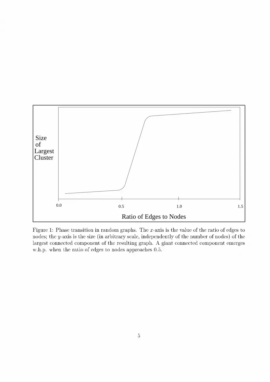
Figure 1: Phase transition in random graphs. The x-axis is the value of the ratio of edges tonodes; the y-axis is the size (in arbitrary scale, independently of the number of nodes) of the
largest connected component of the resulting graph. A giant connected component emerges
w.h.p. when the ratio of edges to nodes approaches 0:5.
5
As a model of small-world networks, the Erd�os-R�enyi random graph has some strengths. It
can be made as dense or as sparse as necessary just by adjusting the edge probability p.
The diameter (i.e. the longest shortest path across it) tends to be small (in some cases too
small). On the other hand Erd�os-R�enyi graphs show no tendency to form clusters. This
follows from the fact that the edges are placed independently, and neighbors of neighbors
are no more likely to be linked than any other randomly chosen vertices.
4.2 Not So Much Random!
Therefore random networks are not the right model to explain most small world phenomena
occurring in practice. Small world properties appear to fall somewhere in between the
ordered and random extremes. Friendship networks are a good example of this in-between
state. Since people meet most new friends through existing friends, the networks are locally
ordered. (Here order means that if A knows B and B knows C, then A is more likely to
know C than some other random element.)
Local ordering in such a network implies that one individual's friends are more likely than not
to know one another: a characteristic that is called clustering. Many real-world networks,
including friendship networks, tend to be highly clustered, but they are not entirely so. If
a person joins a club and meets new people or moves to a di�erent city, new connections
can form that prevent the existing network to become just a collection of (almost) disjoint
clusters.
4.2.1 Weak vs Strong Ties
M.S. Granovetter [6] argued that what holds a society together are not the strong ties within
clusters but rather the weak ones between people who span two or more communities.
Speci�cally, Granovetter analyzes social ties as follows:
\Consider, now, any two arbitrarily selected individuals, call them A and B, and the set,
S = C; D; E; : : : ; of all persons with ties to at least one of them. The hypothesis which
enable us to relate dyadic ties to larger structures is: the stronger the ties between A and
B, the larger the proportion of individuals in S to whom they will both be tied, that is,
connected by a weak or strong tie. This overlap in their friendship circle is predicted to be
least when their tie is absent, most when is strong and intermediate when it is weak."
In [7] Granovetter emphasizes the fact that weak ties are more signi�cant in a social network
than their strong counterparts; indeed weak ties are crucial bridges between pairs of closely
knit communities.
6
5 Small Worlds and Graph Theory
We can now work out a general characterization of small world networks, taking advantage
of some properties encountered analyzing social networks.
� They tend to be sparse. The graphs have relatively few edges, compared with the
large number of vertices. In a graph with n vertices, the maximum number of edges isn(n�1)
2. In large size small-world graphs, the number of edges is generally closer to n
than ton(n�1)
2.
� They tend to be clustered. As we mentioned above in the context of social networks,
they have the following property: if two people share an acquaintance, there is a higher-
than-normal chance they also know each other. Thus the edges of the graph are not
distributed uniformly but are likely to form clumps or knots.
� They tend to have a small diameter.
A connected graph must have at least n � 1 edges, and its largest possible diameter3
is n � 1. At the opposite extreme, a complete graph, with n(n�1)
2edges, has diameter
1, since one can get from any vertex to any other one in a single step. Graphs nearer
to the minimum than to the maximum number of edges might be expected to have a
large diameter.
Once �xed the number of edges, the clustering property could increase the diameter
further still, since edges used to creating local clumps leave fewer edges available for
long-distance connections.
Despite the above arguments, there are sparse and clustered graphs with small diam-
eter; in particular the diameter of the Web and other graphs describing, e.g., social
netowrks, seems to grow only logarithmically with the number of vertices.
Graphs with the above three properties (sparseness, clustering, and small diameter) have
been called \small world" graphs.
5.1 Small Worlds around us
Idealized models like the one just described suggest that the small-world phenomenon might
be common in sparse networks with many vertices. This leads to the question of whether
or not they arise in the real world. Actually, there are many real-world networks which
have been recognized to show the small-world properties listed above. Let us look at some
examples.
3Recall that the diameter of a graph is the longest shortest path across it, or, in other words, the length
of the most direct route between the most distant vertices. Diameter is �nite only for connected graphs, i.e.,
those that are all in one piece.
7
� The electric power grid of Southern California, the vertices being generators, trans-
formers, and substations, and the links being high-voltage transmission lines. The
structure of the graph of the power grid is relevant to the eÆciency and robustness of
power networks.
� The neuronal network of the worm Caenorhabditis Elegans (C. Elegans, for short), the
vertices being the individual neurons and the links being connections between neurons.
(C.Elegans is the sole example of a completely mapped neuronal network.)
� The conformation space of a lattice polymer chain, where the vertices of the network
are in a one-to-one correspondence to the conformations of the chain, and an edge
between two vertices indicates the possibility of switching from one conformation to
the other by a single move of the chain.
� The Hollywood graph. The graph of actors is a particular social network, with the
advantage of being much more easily speci�ed; the vertices of the graph represent
actors, and links between vertices are present if the two corresponding actors have
been in a movie together4. A popular case study, based on this graph, consists of
starting with actor Kevin Bacon. Any actor is assigned a Bacon Number, measuring
how many links must be traversed to get back to Bacon. Bacon himself has Bacon
Number zero; anyone who has acted with him in a movie has Bacon Number one;
anyone who has acted with somebody in the group of people with Bacon Number one
(but not with Bacon himself) has Bacon Number two; and so on.
It turns out that of the 225; 000 actors listed in the Internet Movie Database as of
April 1997, only about 1; 300 have a Bacon Number of one, but nearly 80; 000 have a
Bacon Number of two. (Marilyn Monroe, for instance, is in that group. She was in
\Some Like it Hot" with Jack Lemmon, who in turn was in JFK with Kevin Bacon.)
No American actor, living or dead, has a Bacon Number greater than four. Even more
surprosingly is the fact that, although there are about 20; 000 non American actors
who cannot be connected to Bacon and therefore with Bacon number \in�nity", if we
restrict ourselves to those who can be linked to him, none of them has a Bacon number
higher than eight.
� The call graph. An interesting example of a very large graph comes from telephone
billing records.
In the following, we mainly follow [8], which contains a popularized presentation of the
main properties of the call graph.
The vertices of this graph are telephone numbers, and the edges are calls made from
one number to another. In [1] James M. Abello et al. have studied the evolution of the
graph as calls accumulate over a period of days. In one 20-day period, they observed
that the graph grew to have 290 million vertices and 4 billion edges. The call graph is
4It is akin to the graph of mathematical collaborations centered, traditionally, on P. Erd�os.
8
actually a directed multigraph5. For ease of analysis, however, they collapsed multiple
edges into a single edge, and treated the graph as if it were undirected.
The �rst challenge in studying the call graph is that it is not possible to keep it in main
memory, even using a computer with six gigabytes of memory. Therefore portions of
the graph have to be repeatedly shuttled between memory and disk storage, and thus
most algorithms are extremely ineÆcient. For this reason, the call graph has become
a testbed for algorithms designed to run quickly on data held in external storage.
A one-day call graph analyzed by Abello and his colleagues has 53,767,087 vertices and
170 million edges. Although it is not connected (it actually has 3.7 million separate
components), it contains one giant connected component with 44,989,297 vertices, i.e.,
more than 80 percent of the total.
The diameter of the giant component is 20, which implies that any telephone in the
component can be linked to any other through a chain of no more than 20 calls. The
emergence of a giant component is characteristic of Erd�os-R�enyi random graphs, but
the pattern of connections in the call graph is surely not random.
� Last but not least: the Web. Studies have estimated that the Web has a diameter of
19 [3]. This means that to get from one randomly selected Web page to another one, it
takes an average of 19 clicks; this property makes the Web another example of a small
world graph.
6 Watts Strogatz model
Using a combination of results and techniques from graph theory, computer simulations,
and non-linear dynamics, Strogatz and Watts [15, 16, 17] proposed a model to explain the
small-world phenomenon.
6.1 Rewiring the Lattice
It is not surprising that both the lattice model and Erd�os-R�enyi model fail to reproduce some
features of networks such as the human friendship graph or the World Wide Web. After all,
these real-world networks are neither strongly regular nor fully random. People generally
know their neighbors, but their circle of acquaintances is not con�ned to those who live next
door, as the lattice model would imply. Conversely, links between, e.g., pages on the Web
are not created at random, as the Erd�os-R�enyi process requires. Watts and Strogatz deal
with these failures by employing the following simple strategy: they interpolate between the
above two models.
5directed because the two ends of a call can be distinguished as originator and receiver, a multigraph
because a pair of telephones can exchange more than one call
9
Increasing randomnessp = 0 p = 1
Regular Small world Random
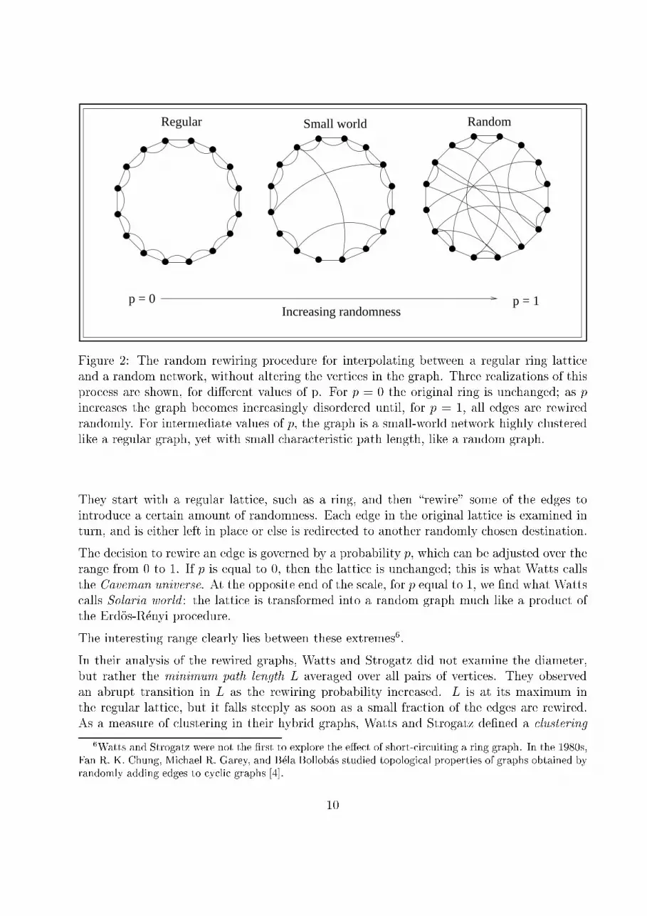
Figure 2: The random rewiring procedure for interpolating between a regular ring lattice
and a random network, without altering the vertices in the graph. Three realizations of this
process are shown, for di�erent values of p. For p = 0 the original ring is unchanged; as pincreases the graph becomes increasingly disordered until, for p = 1, all edges are rewired
randomly. For intermediate values of p, the graph is a small-world network highly clustered
like a regular graph, yet with small characteristic path length, like a random graph.
They start with a regular lattice, such as a ring, and then \rewire" some of the edges to
introduce a certain amount of randomness. Each edge in the original lattice is examined in
turn, and is either left in place or else is redirected to another randomly chosen destination.
The decision to rewire an edge is governed by a probability p, which can be adjusted over the
range from 0 to 1. If p is equal to 0, then the lattice is unchanged; this is what Watts calls
the Caveman universe. At the opposite end of the scale, for p equal to 1, we �nd what Watts
calls Solaria world : the lattice is transformed into a random graph much like a product of
the Erd�os-R�enyi procedure.
The interesting range clearly lies between these extremes6.
In their analysis of the rewired graphs, Watts and Strogatz did not examine the diameter,
but rather the minimum path length L averaged over all pairs of vertices. They observed
an abrupt transition in L as the rewiring probability increased. L is at its maximum in
the regular lattice, but it falls steeply as soon as a small fraction of the edges are rewired.
As a measure of clustering in their hybrid graphs, Watts and Strogatz de�ned a clustering
6Watts and Strogatz were not the �rst to explore the e�ect of short-circuiting a ring graph. In the 1980s,
Fan R. K. Chung, Michael R. Garey, and B�ela Bollob�as studied topological properties of graphs obtained by
randomly adding edges to cyclic graphs [4].
10
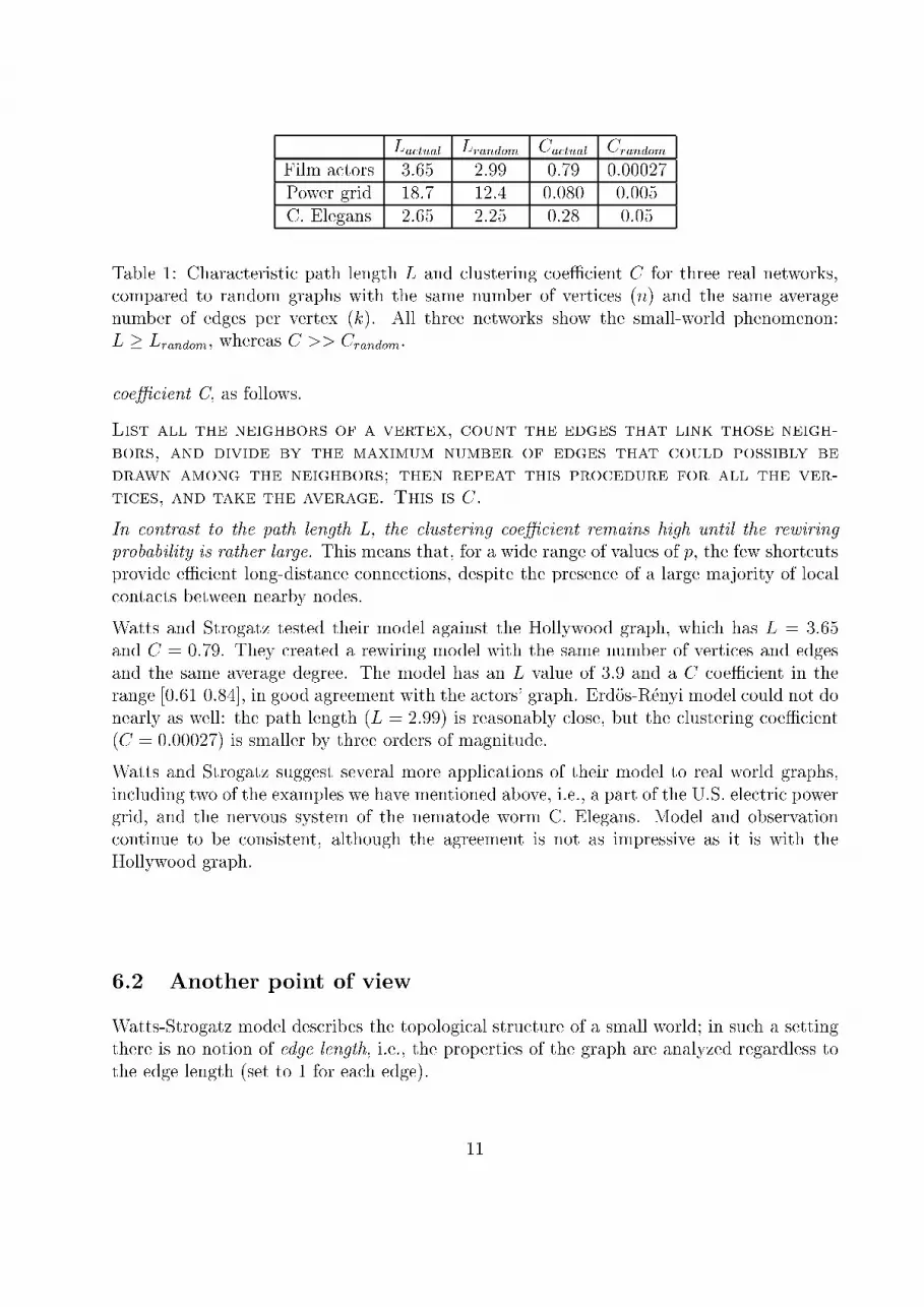
Lactual Lrandom Cactual Crandom
Film actors 3.65 2.99 0.79 0.00027
Power grid 18.7 12.4 0.080 0.005
C. Elegans 2.65 2.25 0.28 0.05
Table 1: Characteristic path length L and clustering coeÆcient C for three real networks,
compared to random graphs with the same number of vertices (n) and the same average
number of edges per vertex (k). All three networks show the small-world phenomenon:
L � Lrandom, whereas C >> Crandom.
coeÆcient C, as follows.
List all the neighbors of a vertex, count the edges that link those neigh-
bors, and divide by the maximum number of edges that could possibly be
drawn among the neighbors; then repeat this procedure for all the ver-
tices, and take the average. This is C.
In contrast to the path length L, the clustering coeÆcient remains high until the rewiring
probability is rather large. This means that, for a wide range of values of p, the few shortcuts
provide eÆcient long-distance connections, despite the presence of a large majority of local
contacts between nearby nodes.
Watts and Strogatz tested their model against the Hollywood graph, which has L = 3:65and C = 0:79. They created a rewiring model with the same number of vertices and edges
and the same average degree. The model has an L value of 3:9 and a C coeÆcient in the
range [0:61 0:84], in good agreement with the actors' graph. Erd�os-R�enyi model could not do
nearly as well: the path length (L = 2:99) is reasonably close, but the clustering coeÆcient
(C = 0:00027) is smaller by three orders of magnitude.
Watts and Strogatz suggest several more applications of their model to real world graphs,
including two of the examples we have mentioned above, i.e., a part of the U.S. electric power
grid, and the nervous system of the nematode worm C. Elegans. Model and observation
continue to be consistent, although the agreement is not as impressive as it is with the
Hollywood graph.
6.2 Another point of view
Watts-Strogatz model describes the topological structure of a small world; in such a setting
there is no notion of edge length, i.e., the properties of the graph are analyzed regardless to
the edge length (set to 1 for each edge).
11
We now describe a new approach, suggested by Marchiori and Latora [12], according to
which the metrical nature of small world networks comes into play, determined by the so
called physical distance between vertices (edge length).
The set-up consists of a generic metrical graph G, that in principle, does not need be con-
nected. N will denote the number of vertices and k the overall number of edges. Two nodes
i and j connected by an edge are at a certain physical distance, which can be, for exam-
ple, the real distance between the two nodes or a measure of the strength of their possible
interaction. The distance on the graph d(i; j) is instead de�ned as the smallest sum of the
physical distances throughout all the possible paths in the graph from i to j.
If every node sends information along the network through its edges and every node in the
network propagates information concurrently, the amount of information sent from node
i to node j per unit of time is v=d(i; j), where v is the speed at which the information
travels over the network. When there is no path in the network between i and j, we say
that d(i; j) = +1, and consistently, that the amount of exchanged information is 0. The
performance of G can be de�ned as the total amount of information propagated over the
network per unit of time:
P =Xi;j2G
v=d(i; j):
(Every sum here and in the following is intended for i 6= j.)
In order to quantify the typical separation between two vertices in the graph, it is convenient
to introduce the connectivity length D(G), de�ned as the �xed distance at which to set every
two vertices in the graph in order to maintain its performance. Interestingly enough, the
connectivity length of the graph turns out to be not the arithmetic mean but the harmonic
mean of all the distances:
D(G) = Hfd(i; j); i; j 2 Gg =N(N � 1)Pi;j2G 1=d(i; j)
:
As we have seen before, the de�nition of small-world proposed by Watts and Strogatz is
based on two di�erent quantities, L and C. L, the characteristic path length, is a measure of
a global property of the graph L, while C, the clustering coeÆcient, is obtained by averaging
over local quantities. The main reason to introduce C is because L, de�ned as the simple
arithmetic mean of d(i; j), applies only to connected graphs.
Marchiori-Latora model provides a uniform description of both global and local properties
of the network by means of the single measure D.
Indeed, let us de�ne
1. Dglob as the connectivity length for the global graph G, i.e., Dglob = D(G), and
12

2. Dloc as the average connectivity length of the graphs of neighbors of any given vertex.
Then we can de�ne small-worldness for networks: a network is a small world (or, in equivalent
terms, the network performance is locally and globally high) if and only if it has small D at
global and local scale, i.e., if Dglob and Dloc are both small.
The connectivity length D gives harmony to the whole theory of small-world networks, since:
� It is not just a generic intuitive notion of average distance in a network, but has a
precise meaning in terms of network eÆciency.
� It describes in a uni�ed way the system at both global and local scale.
� It applies to topological as well as metrical networks.
� It applies to any graph, not only to connected graphs as was the case for the original
theory.
� It describes structural as well as dynamical features of a network.
6.3 What are Small Worlds for?
The small world phenomenon suggests a fundamentally new way of looking at our world,
and might shed some light on a plethora of interesting questions:
� How do diseases spread?
� Can an accident at a single power station bring down the rest of the power grid?
� How does a joke spread across the Internet?
� How are the neurons of the brain connected?
� Can one prevent a crowd from panicking?
� How do you design the most eÆcient oÆce building?
The global and local scales at which social networks can be analyzed provide di�erent view-
points to observe the world in which we live:
1. At the global scale, we can appreciate the fact that we are all very closely connected;
this may have all sorts of consequences for phenomena like the spread of diseases, the
growth of fads, and the cascades of failures in the world's �nancial markets, none of
which are currently well-understood.
13
2. At a local scale, it is very diÆcult for us to appreciate this relatively recent feature of
the world, con�ned as we are to our own highly clustered local environments.
The above observations put into evidence that there might be a subtle di�erence between
small-worldness per se, and the ability of taking advantage of it.
Understanding how small worlds a�ect issues like the di�usion of information, the coordi-
nation of distributed activities, and strategies for searching out speci�c information, are all
problems at the frontier of research.
In the next section, we come to terms with the di�erence between networks which are small
worlds only in a global sense, and networks further characterized by properties which make
it possible to exploit small-worldness using only local information.
7 Finding the Way in a Small World: Kleinberg Re-
sults
Kleinberg [9] comments on the success of Milgram's experiment, saying that it \suggests a
source of latent navigational cues embedded in the underlying social network, by which a
message could implicitly be guided quickly from source to target".
And also: \Existing models are insuÆcient to explain the striking algorithmic component
of Milgram's original �ndings: that individuals using local information are collectively very
e�ective at actually constructing short paths between two points in a social network".
The presence of a large number of short paths in a network (for instance, in a highly connected
random graph) does not imply that an agent using only local information can actually �nd
the right shortcuts which would let her traverse the network at a speed reasonably related
to the lengths of the short paths. In other words \one can imagine networks in which short
chains exists but no mechanism based on purely local information is able to �nd them."
As an example of the fact that existing models are insuÆcient to explain the success of
decentralized algorithms, Kleinberg [10, 11] �nds a counterexample for Watts-Strogatz (WS)
model, and introduces a family of models generalizing WS.
More precisely, he proves that:
(1) for one of these models there is a decentralized algorithm capable of �nding short paths
with high probability, and
(2) there exists only a unique model within the family such that (1) holds.
Kleinberg de�nes a simple framework that encapsules the paradigm of Watts and Strogatz.
The model is given by a lattice (grid) with the addition of a few randomly chosen long range
connections.
The basic ingredients are the following:
14
A) B)
u
v w
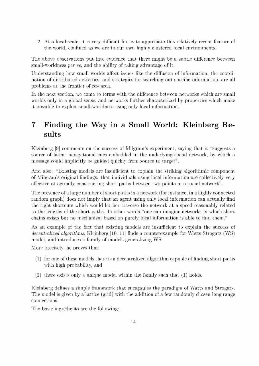
Figure 3: (A) A two-dimensional lattice grid network with n = 6, p = 1, and q = 0. (B) The
contacts of a node u with p = 1 and q = 2. (u; v) and (u; w) are the long range contacts.
� Lattice distance between u = (i; j) and v = (k; l):
d(u; v) = jk � ij+ jl � jj :
� Universal constant p � 1 such that each node has a directed edge to every other node
at distance at most p (local contacts). For the 2-dimensional grid, p = 1.
� Universal constants q , r � 0 such that each node u has directed edges to q other nodes(long range contacts), where the i-th edge from u has endpoint v with probability
proportional to [d(u; v)]�r.
The model de�ned above is rich in local connection, with a few range connections; it gener-
alizes the paradigm of Watts and Strogatz and satis�es the basic features of a small world.
In the following we outline the main di�erences w.r.t. Watts and Strogatz model.
� Watts and Strogatz proposed a model constructed starting with a set V of n points
uniformly spaced on a circle; each point is then connected to each of its k nearest
neighbors, for a small constant k, and �nally a small fraction of the edges is rewired.
Kleinberg model is based on a k-dimensional grid.
� In Watts and Strogatz model, edges are not directed, while Kleinberg's grid is directed.
The model proposed by Kleinberg has a simple geographic interpretation: individuals live on
a grid and know their neighbors for some number of steps in all directions; they also have
some acquaintances distributed more broadly on the grid.
Viewing p and q as �xed constants, he obtains a \one-parameter family of network" models
by tuning the value of the exponent r. When r=0, we have the uniform distribution over
15
����
����
���
���
����
���
���
���
���
��������
��������
���
���
����
������
������
��������
����
����
����
��������
���
���
����
���
���
������
������
��������
����
��������
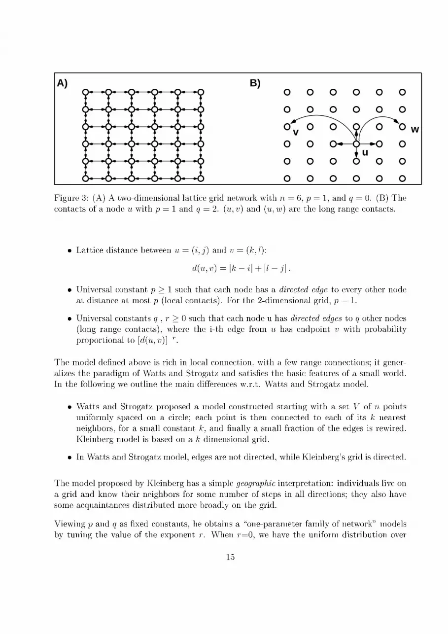
Figure 4: Three grids with di�erent long-range edge distribution (A) r = 0 (B) r > 2, (C)
r < 2.
long-range contacts, the distribution used in the basic network model of Watts and Strogatz,
according to which one's long range contacts are chosen independently of their position on the
grid. As r increases, the long-range contacts of a node become more and more clustered in its
vicinity on the grid. Thus, r describes how the underlying society of nodes is \networked".
Kleinberg's model allows us to give a solid foundation to Milgram's original �ndings; let us
consider a message which has to go from a source to a target. The message holder at any
given step has knowledge of:
a. underlying grid structure;
b. location of the target on the grid;
c. location of long range contacts of all the nodes that have been involved with the
message.
REMARKS:
� (c) is used only for lower bounds; upper bounds use only (a) and (b).
� Constraining the algorithm to use only local information is crucial; otherwise it is easy
to �nd the shortest path between any two nodes by, e.g., breadth-�rst seaarch.
The expected delivery time of a decentralized algorithm is the primary �gure of merit in
Kleinberg's analysis; it represents the expected number of steps taken by the algorithm to
deliver a message over a network from a source to a target chosen uniformly at random from
the set of nodes.
In Kleinberg model a message traveling on an edge across two connected nodes takes always
a unit of time, regardless to the lattice distance (as de�ned above) between the two nodes.
16
In other words, long range and local contacts are traversed in the same amount of time,
i.e., the network is analyzed under a topological, rather than metrical, viewpoint. We could
interpret this from a physical standpoint saying that the speed V the message travels on the
network on an edge u is proportional to the length of u.
The expected delivery time as de�ned by Kleinberg makes sense when the goal is to analyze
information transfer processes in which the delivery time of a generic message is roughly
proportional to the number of steps (edges covered) taken by the message to move from the
source to the target.
7.0.1 Kleinberg Theorems
Kleinberg proves that the (topological) structure of the network deeply a�ects the ability of
a decentralized algorithm to �nd a short path.
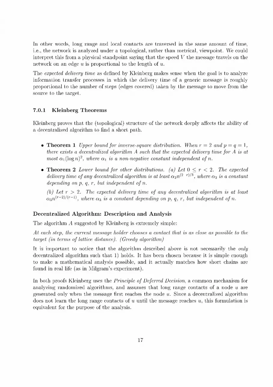
� Theorem 1 Upper bound for inverse-square distribution. When r = 2 and p = q = 1,
there exists a decentralized algorithm A such that the expected delivery time for A is at
most �1(logn)2, where �1 is a non-negative constant independent of n.
� Theorem 2 Lower bound for other distributions. (a) Let 0 � r < 2. The expected
delivery time of any decentralized algorithm is at least �2n(2�r)=3, where �2 is a constant
depending on p; q; r, but independent of n.
(b) Let r > 2. The expected delivery time of any decentralized algorithm is at least
�3n(r�2)=(r�1), where �3 is a constant depending on p, q, r, but independent of n.
Decentralized Algorithm: Description and Analysis
The algorithm A suggested by Kleinberg is extremely simple:
At each step, the current message holder chooses a contact that is as close as possible to the
target (in terms of lattice distance). (Greedy algorithm)
It is important to notice that the algorithm described above is not necessarily the only
decentralized algorithm such that 1) holds. It has been chosen because it is simple enough
to make a mathematical analysis possible, and it actually matches how short chains are
found in real life (as in Milgram's experiment).
In both proofs Kleinberg uses the Principle of Deferred Decision, a common mechanism for
analyzing randomized algorithms, and assumes that long range contacts of a node u are
generated only when the message �rst reaches the node u. Since a decentralized algorithm
does not learn the long range contacts of u until the message reaches u, this formulation is
equivalent for the purpose of the analysis.
17
������
������
tA0
A1
A2
A3
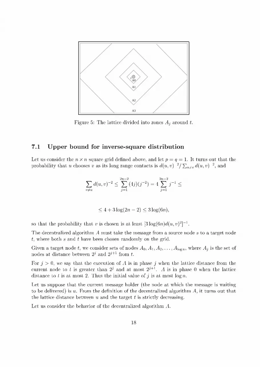
Figure 5: The lattice divided into zones Aj around t.
7.1 Upper bound for inverse-square distribution
Let us consider the n�n square grid de�ned above, and let p = q = 1. It turns out that the
probability that u chooses v as its long range contacts is d(u; v)�2=P
u6=v d(u; v)�2, and
Xv 6=u
d(u; v)�2 �2n�2Xj=1
(4j)(j�2) = 42n�2Xj=1
j�1 �
� 4 + 3 log(2n� 2) � 3 log(6n);
so that the probability that v is chosen is at least [3 log(6n)d(u; v)2]�1.
The decentralized algorithm A must take the message from a source node s to a target nodet, where both s and t have been chosen randomly on the grid.
Given a target node t, we consider sets of nodes A0; A1; A2; : : : ; Alog n, where Aj is the set of
nodes at distance between 2j and 2j+1 from t.
For j > 0, we say that the execution of A is in phase j when the lattice distance from the
current node to t is greater than 2j and at most 2j+1. A is in phase 0 when the lattice
distance to t is at most 2. Thus the initial value of j is at most logn.
Let us suppose that the current message holder (the node at which the message is waiting
to be delivered) is u. From the de�nition of the decentralized algorithm A, it turns out thatthe lattice distance between u and the target t is strictly decreasing.
Let us consider the behavior of the decentralized algorithm A.
18

� log logn � j < logn. The message will leave phase j when the distance between the
current message holder u and the target t will become less than 2j. Let Bj be the set
of nodes within lattice distance 2j from t. It is easy to see that there are at least
1 +2jXi=1
i =1
222j +
1
22j + 1 > 22j�1
nodes in Bj. Each node in Bj is within lattice distance 2j�1 of u; hence each has a
probability at least (3 log(6n)22j+4)�1 of being the long range contact of u.
Since the probability P of A to leave phase j depends only on the number of nodes in
Bj and on the distance between u and these nodes, we have that
P �22j�1
3 log(6n)22j+4=
1
96 log(6n):
Thus the total number of steps spent in phase j is at most
EXj =1Xi=1
Pr[Xj > i] �1Xi=1
(1�1
96 log(6n))i�1 = 96 log(6n):
� 0 � j � logn. In this case, it is simple to prove that the arithmetic mean of the total
number of steps is at most 96 log(6n). This follows from the fact that the algorithm
can spend at most logn steps in phase j even if all the nodes pass the message to a
local contact.
Since the maximum number of phases is logn, then the mean of the total number of
steps (expected delivery time) is at most
X =log nXj=0
Xj:
Thus the expected delivery time is at most �1 log2 n, for a suitable choice of �1.
The proofs of the theorems reveal a general structural property that implies the optimality
of the exponent r = 2 for the two-dimensional lattice: it is the unique exponent at which a
node's long-range contacts are nearly uniformly distributed over all \distance scales".
Speci�cally, given any node u, we can partition the remaining nodes of the lattice into sets
A0; A1; A2; : : : ; Alog n, where Aj consists of all nodes whose lattice distance to u is between
2j and 2j+1. These sets naturally correspond to di�erent levels of \resolution" as we move
away from u; all nodes in each Aj are at approximately the same distance (to within a factor
of 2) from u. At exponent r = 2, each long-range contact of u is nearly equally likely to
belong to any of the sets Aj; when r < 2, there is a bias toward sets Aj at greater distances,
and when r > 2, there is a bias toward sets Aj at nearer distances.
19
������
������
������
������
���
���
������
������
s
t����
s
t
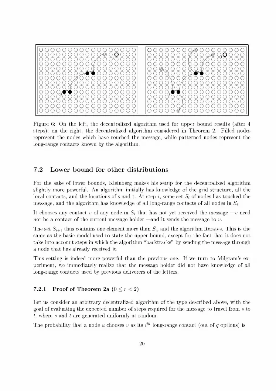
Figure 6: On the left, the decentralized algorithm used for upper bound results (after 4
steps); on the right, the decentralized algorithm considered in Theorem 2. Filled nodes
represent the nodes which have touched the message, while patterned nodes represent the
long-range contacts known by the algorithm.
7.2 Lower bound for other distributions
For the sake of lower bounds, Kleinberg makes his setup for the decentralized algorithm
slightly more powerful. An algorithm initially has knowledge of the grid structure, all the
local contacts, and the locations of s and t. At step i, some set Si of nodes has touched the
message, and the algorithm has knowledge of all long-range contacts of all nodes in Si.
It chooses any contact v of any node in Si that has not yet received the message { v need
not be a contact of the current message holder { and it sends the message to v.
The set Si+1 thus contains one element more than Si, and the algorithm iterates. This is the
same as the basic model used to state the upper bound, except for the fact that it does not
take into account steps in which the algorithm \backtracks" by sending the message through
a node that has already received it.
This setting is indeed more powerful than the previous one. If we turn to Milgram's ex-
periment, we immediately realize that the message holder did not have knowledge of all
long-range contacts used by previous deliverers of the letters.
7.2.1 Proof of Theorem 2a (0 � r < 2)
Let us consider an arbitrary decentralized algorithm of the type described above, with the
goal of evaluating the expected number of steps required for the message to travel from s to
t, where s and t are generated uniformly at random.
The probability that a node u chooses v as its ith long-range contact (out of q options) is
20
d(u; v)�r=P
v 6=u d(u; v)�r.
We have:
Xv 6=u
d(u; v)�r �n=2Xj=1
(j)(j�r) =n=2Xj=1
j1�r �Z
n=2
1x(1�r)dx �
� (2� r)�1((n=2)2�r � 1) �1
(2� r)2(3�r)� n(2�r);
where in the last line we assume that n � 23�r. Let Æ = (2� r)=3, and let U denote the set
of nodes within lattice distance pnÆ from t. Note that
jU j � 1 +pnÆXj=1
4j � 4p2n2Æ:
Assume that n is large enough so to satisfy pn� 2, and de�ne � = ((2� r)27�rqp2)�1.
Let "0 be the event that within �nÆ steps the message reaches a node other than t using a
long-range contact in U . Let "0ibe the event that at step i, the message reaches a node other
than t using a long-range contact in U . We have that "0 =S
i��nÆ "0
i.
The node reached at step i has q long-range contacts that are generated at random when it
is encountered (for the Principle of Deferred Decision), so that
Pr["0i] �
qjU j1
(2�r)2(3�r) � n2�r
�(2� r)23�rq � 4p2n2Æ
n2�r
=(2� r)2(5�r)qp2n2Æ
n2�r:
Since the probability of a union of events is bounded by the sum of their probabilities, we
have
Pr["0] �X
i��nÆ
Pr["0i]
21
�(2� r)25�r�qp2n3Æ
n2�r
= (2� r)25�r�qp2 �1
4:
Let � denote the event that the chosen source s and target t are separated by a lattice
distance of at least n=4. One can verify that Pr[�] � 12.
Since Pr[� _ "0] � 12+ 1
4, we obtain Pr[� ^ "0] � 1
4.
Finally, let X denote the random variable equal to the number of steps taken by the message
to reach t, and let " denote the event that the message reaches t within �nÆ steps.
If � occurs and "0 does not occur, then " cannot occur. In fact, if � occurs, then the distance
d(u; v) satis�es d(u; v) � n=4 > p�nÆ. Therefore in any s� t path of at most �nÆ steps the
message must have used at least once a long-range contact; furthermore the last time this
happened, the message must have used a long range contact in U , so that the event "0 must
occur. Otherwise, if "0 does not occur, the message can not reach the target t in at most �nÆ
steps.
This means that
EX �1
4�0nÆ;
where EX stands for the mathematical expected value of the random variable X.
Part (a) of the theorem now follows.
7.2.2 Proof of Theorem 2b (r > 2).
In this section we consider the same decentralized algorithm analyzed in the proof of Theorem
2(a).
Let � = r� 2. We consider a node u, and let v be a randomly generated long-range contact
of u. The normalizing constant for the inverse rth-power distribution is at least 1, and so,
for any m, we have
Pr[d(u; v) > m] �2n�2X
j=m+1
(4j)(j�r) = 42n�2X
j=m+1
j1�r �
�
Z1
m
x(1�r)dx � (r � 2)�1m2�r = ��1m��:
22
We now de�ne � = �
1+�, � = 1
1+�, and �0 = min(�;1)
8q.
Let "0 be the event that in step i the message reaches a node u 6= t that has a long-range
contact v satisfying d(u; v) > n�.
Let also "0 =S
i��0n� "0
ibe the event that this happens during the �rst �0n� steps.
We have:
Pr["0] �X�0n�
Pr["0i] � �0n�
� q��1n��� = �0q��1 �1
4:
Let � be the event that s and t are separated by a lattice distance of at least n=4. We observe
that Pr[� ^ "0] � 14. Let X denote the random variable equal to the number of steps taken
by the message to reach t, and let " denote the event that the message reaches t within �0n�
steps. If "0 does not occur, then the message can move to a lattice distance of at most n� in
each of its �rst �0n� steps. This leads to a total lattice distance of at most
�0n�+� = �0n � n=4 ;
and so if � occurs (i.e., if s and t are separated by a lattice distance greater than n=4), then
the message will not reach t.
This implies the inequality
EX �1
4�0n�:
Therefore part (b) of the Theorem follows.
Let us now take into special account the case r = 0. The following happens:
� the long-range contacts are uniformly distributed, as in the basic network model of
Watts and Strogatz, where long-range contacts are in fact chosen independently of
their position;
� there exist short paths with high probability, but there is no way for a decentralized
algorithm to �nd them; indeed the expected delivery time turns out to be about n2=3.
As anticipated before, this shows that Watts and Strogatz models are insuÆcient to explain
the success of decentralized algorithms in �nding short paths through a social network.
23
source
target
Distance ~ n^(2/3)
R
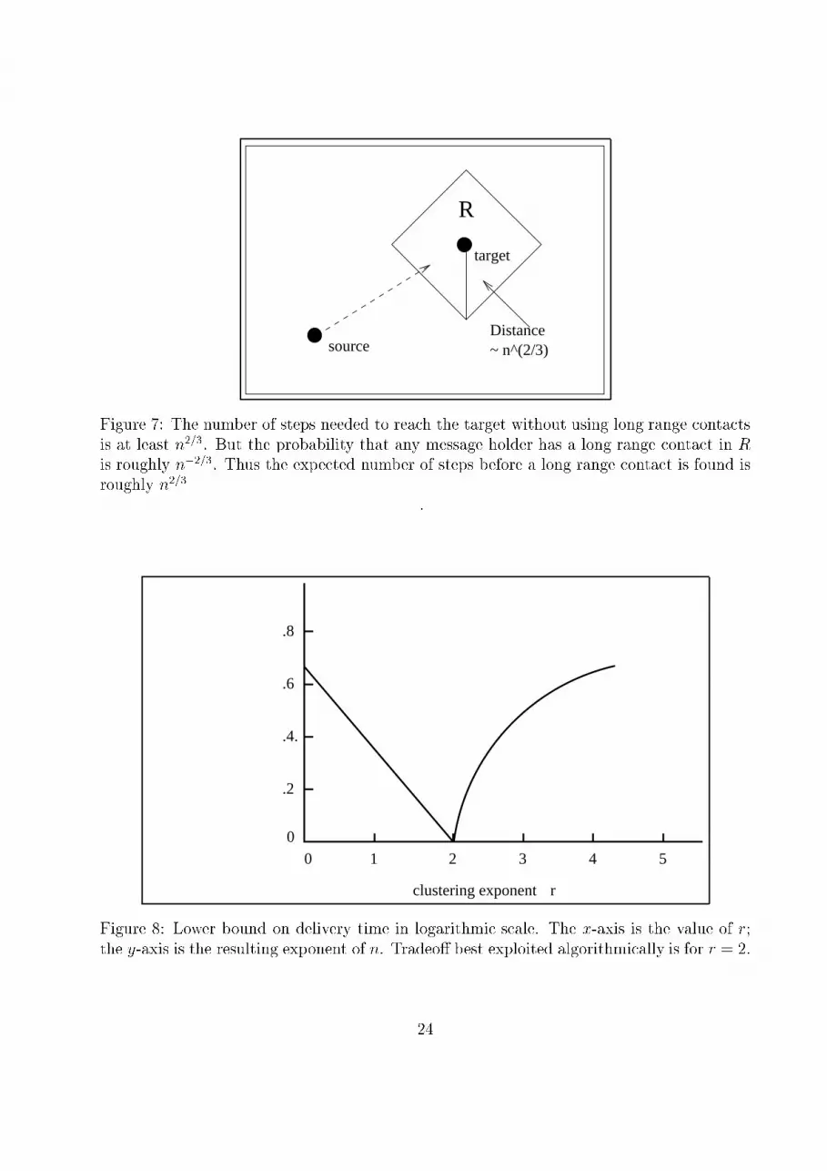
Figure 7: The number of steps needed to reach the target without using long range contacts
is at least n2=3. But the probability that any message holder has a long range contact in Ris roughly n�2=3. Thus the expected number of steps before a long range contact is found is
roughly n2=3
.
00 1 2 3 4 5
.4.
.6
.2
.8
clustering exponent r
Figure 8: Lower bound on delivery time in logarithmic scale. The x-axis is the value of r;
the y-axis is the resulting exponent of n. Tradeo� best exploited algorithmically is for r = 2.
24
7.3 Conclusion
The correlation between local structure and long-range connections provides fundamental
cues for �nding short paths through the network.
� When this correlation is near a critical threshold, the structure of the long-range con-
nections forms a sort of \gradient" that allows individuals to guide a message eÆciently
towards a target.
� As the correlation drops below this critical value and the social network becomes more
homogeneous, these cues begin to disappear.
� In the limit, when long-range connections are generated uniformly at random, Klein-
berg model describes a world in which short chains exist but individuals, faced with a
disorienting array of social contacts, are unable to �nd them.
8 Small World Wide Web
Nowhere is the breakdown in the barriers posed by physical distance more dramatic than
in the rise of the Internet and the World Wide Web. In the past ten years, the Internet
has gone from an academic and military tool, unknown to the general public except as
a curiosity, to a social, technological and economic presence that a�ects everything from
personal communications to business practice, and even the US stock market. In so doing,
the Internet (in conjunction with an increasingly information-based economy and services
like rapid, world-wide delivery) has made physical distance increasingly irrelevant to the
retrieval of information, access to services, formation of organisations, and even the purchase
of material products ranging from cars to groceries.
Despite its increasing role in communication, the Web remains the least controlled medium:
any individual or institution can create websites with an essentially unrestricted number
of documents and links. This unregulated growth leads to a huge and complex Web graph,
which is a large directed graph, whose vertices are documents, and edges are the links (URLs)
pointing from one document to another. The topology of this graph describes the Web
connectivity and, consequently, our e�ectiveness in locating information.
Our knowledge of the Web topology is however partial. Due to its large size, estimated to
be of at least 8 � 108 documents, and the continuous change of documents and hyperlinks,
it is impossible to catalogue all vertices and edges. The challenge in obtaining a reasonably
accurate topological map of the Web is illustrated by the limitations of the commercial search
engines: Northern Light, the search engine with the largest coverage, is estimated to index
only about 38 % of the Web [3].
25
8.1 Low Diameter and Power Law
Sparseness, clustering, and small diameter are not the only properties of large real-world
graphs that have been extensively studied. Another characteristic that has attracted notice
is the degree sequence d0; d1; : : : ; dn�1, where dj is the number of vertices which have degree
j.
As an example, a lattice has a very simple degree sequence: all the vertices have the same
number of edges, and so a plot of the degree sequence consists of a single sharp spike. Any
randomness in the graph broadens this peak.
In the case of an Erd�os- R�enyi graph, the degree sequence has a Poisson distribution, which
falls o� exponentially away from the peak value. Because of this exponential decline, the
probability of �nding a vertex with k edges becomes negligibly small for large k. There
is evidence that certain real graphs, among which the Web is the most popular example,
behave di�erently. The distribution of degrees is described by a power law rather than an
exponential. This means that the fraction of vertices of degree k is not given by e�k (an
exponential function) but by k�� (a polynomial function).
The power-law distribution falls o� more gracefully than an exponential, allowing for vertices
of very large degree. Several research groups have independently found evidence of this
property for the degree sequence of the Web graph7.
Barab�asi et al. [3] set out to estimate the diameter of the Web (or, strictly speaking, its
characteristic path length), and found that two randomly chosen pages are about 19 mouse-
clicks apart. In the course of their analysis they sampled the degree sequence, observing
that the probability that a page has links to k other pages is approximately k�2:45, and that
the probability that k pages point to a given page is k�2:1. To explain the power-law degree
sequence, they have proposed a new random graph model. They argue that other models
fail to take into account the two following attributes of the Web.
� The Web is continually sprouting new pages, but most models are static: although
edges can be added or rearranged, the number of vertices never changes.
� Both Erd�os-R�enyi and Watts-Strogatz processes assume uniform probabilities when
creating new edges, but this is not very realistic. Barab�asi et al. note that Web pages
that already have many links are more likely to acquire still more links.
Like Erd�os-R�enyi model, Barab�asi et al. model starts with n vertices and no edges, but the
evolution is di�erent.
1. At every step, we add to the existing graph a single new vertex and m edges; all the
new edges link the new vertex to some of the vertices already present in the graph.
7A group that includes Kleinberg and several scientists from the IBM Almaden Research Center found
evidence of a power law in the Web, and so did Adamic and Bernardo A. Huberman of the Xerox Palo
Alto Research Center, as well as Albert-L�aszl�o Barab�asi, R�eka Albert and Hawoong Jeong of Notre Dame
University.
26

2. The probability that a given vertex will receive a new edge is proportional to the share
of the total set of edges that the vertex already has; hence well-connected nodes become
better-connected.
3. After t steps, the graph has n+ t vertices and m � t edges.
Upon growing according to these rules, the graph achieves a statistical steady state: the
shape of the distribution of node degrees does not change over time. The distribution is
described by a power law with an exponent of 3; in other words, the probability of �nding a
vertex with k edges is proportional to k�3.
Barab�asi et al. have tested their model on several large graphs, including those discussed by
Watts and Strogatz { the Hollywood graph, an electric power grid, and the neural network
of C. Elegans. They found that both of the novel features of the model are essential to
its success; eliminating either growth in the vertex set or preferential attachment of edges
impairs the model's performance. The straightforward way according to which Barab�asi
et al. model mimics the dynamics of the Web evolution gives the model strong intuitive
appeal. Nevertheless it turns out that the correspondence between theory and observation
is not quite as good as one might hope.
As noted above, the actual exponents for the Web are about 2:45 for outward links and
2:1 for inward links, and thus signi�cantly di�erent from the model's prediction of 3. For
some other graphs, such as the C. Elegans network, the discrepancy is even larger. Various
adjustments could tune the model for a better match, but they inevitably sacri�ce some of
its simplicity.
8.1.1 Small Diameter, High Resources
The relatively small value of the characteristic path length d suggests the possibility that
an intelligent agent (someone who can make some sense out of the links and follow only the
relevant one), could in principle �nd in a short time the desired information by navigating
the Web.
However, this is for sure not the case of a robot that tries to locate information based on
purely syntactic rules, like matching strings: Barab�asi et al. have shown that such a robot,
aiming at identifying a document at distance d , needs to search M ' 0:53N0:92 documents.
For N = 8 � 108, this leads to a �gure of M = 8 � 107, i.e., 10% of the whole Web.
This indicates that robots cannot take much advantage of the highly connected nature of the
Web, their only successful strategy being indexing as large a fraction of the Web as possible.
A better understanding of the Web topology, aided by modeling e�orts, will be instrumental
to developing search algorithms or designing strategies for eÆciently accessing information.
The good news is that, due to the surprisingly small diameter of the Web, all that information
is just a few clicks away.
27

References
[1] Abello, J., P. M. Pardalos and M. G. C. Resende. On maximum clique problems in very
large graphs. In External Memory Algorithms (J. Abello and J. Vitter, eds.), AMS-
DIMACS Series on Discrete Mathematics and Theoretical Computer Science, Vol. 50
(1999).
[2] L. Adamic. The Small World Web. Proc. 3rd European Conf. Research and Advanced
Technology for Digital Libraries, ECDL (1999).
[3] R. Albert, H. Jeong, and A.-L. Barabasi. Diameter of the world wide web. Nature,
401:130{131 (1999).
[4] B. Bollob�as, and F.R.K. Chung. The diameter of a cycle plus a random matching.
SIAM Journal on Discrete Mathematics 1:328-333 (1988).
[5] P. Erd�os, and A. R�enyi. On the evolution of random graphs. Publications of the Math-
ematical Institute of the Hungarian Academy of Sciences 5:17-61 (1960).
[6] M. Granovetter. The strength of weak ties, American Journal of Sociology, 78:1360{
1380 (1973).
[7] M. Granovetter. The strength of weak ties: A network theory revisited. In N. Lin and
P. V. Marsden (Eds.), Social structure and network analysis (pp. 105-130). Beverly
Hills, CA: Sage (1983).
[8] B. Hayes. Computing Science: Graph Theory in Practice: Part I. American Scientist,
Vol. 88(1):9-13 (2000).
[9] J. Kleinberg. Navigation in a Small World. Nature 406:845 (2000).
[10] J. Kleinberg. The small-world phenomenon: An algorithmic perspective. Cornell Com-
puter Science Technical Report 99-1776, October 1999. (This is an extended version
of the Nature paper.)
[11] J. Kleinberg. The small-world phenomenon: an algorithmic perspective, Thirty-Second
Annual ACM Symposium on Theory of Computing, May 21-23, 2000 (conference ver-
sion).
[12] M. Marchiori, L. Latora. Harmony in the small-world, Physica A 285:539-546 (2000).
[13] S. Milgram. The small-world problem. Psychology Today, 1(1), 62-67 (1967).
[14] S. Milgram. The small world problem. In \The Individual in a Social World: Essays
and Experiments", 281-295. Addison-Wesley 1977.
[15] D. J. Watts. Small Worlds: The Dynamics of Networks between Order and Random-
ness, Princeton Univ. Press (1999).
28
[16] D. J. Watts. Networks, dynamics and the small-world phenomenon. American Journal
of Sociology 105(2):493-527 (1999).
[17] D. J. Watts, and S. H. Strogatz. Collective dynamics of 'small-world' networks. Nature
393:440-442 (1998).
29


