SlopeHelp Guide

13 Fitzroy StreetLondonW1T 4BQTelephone: +44 (0) 20 7755 3302Facsimile: +44 (0) 20 7755 3720

Central SquareForth StreetNewcastle Upon TyneNE1 3PLTelephone: +44 (0) 191 238 7559Facsimile: +44 (0) 191 238 7555

e-mail: oasys@arup.comWebsite: http://www.oasys-software.com

© O as ys Ltd. 2021

All rights reserved. No parts of this work may be reproduced in any form or by any means - graphic, electronic, ormechanical, including photocopying, recording, taping, or information storage and retrieval systems - without thewritten permission of the publisher.

Products that are referred to in this document may be either trademarks and/or registered trademarks of therespective owners. The publisher and the author make no claim to these trademarks.

While every precaution has been taken in the preparation of this document, the publisher and the author assume noresponsibility for errors or omissions, or for damages resulting from the use of information contained in thisdocument or from the use of programs and source code that may accompany it. In no event shall the publisher andthe author be liable for any loss of profit or any other commercial damage caused or alleged to have been causeddirectly or indirectly by this document.

Printed: June 2021

Slope

© Oasys Ltd. 2021

Slope

4 © O as ys Ltd. 2021

Table of Contents

Part I About Slope 21.0 7

Part II What's New 9

Part III Theory 11

................................................................................................................................... 111 Method of Slices

................................................................................................................................... 122 Governing Equations

................................................................................................................................... 133 Bishop's Methods

......................................................................................................................................................... 14Iteration procedure

................................................................................................................................... 154 Morgenstern-Price Method

......................................................................................................................................................... 16Iteration procedure

................................................................................................................................... 175 Janbu's Methods

................................................................................................................................... 186 Interlock

................................................................................................................................... 197 Positioning of Slices

................................................................................................................................... 198 Reinforcement Calculations

Part IV Getting Started 25

Part V Entering Data 29

................................................................................................................................... 291 Defining Analysis Options

......................................................................................................................................................... 29Titles

......................................................................................................................................................... 30Units

......................................................................................................................................................... 31Specif ication

................................................................................................................................... 322 Defining the Ground Model

......................................................................................................................................................... 33Material Properties

......................................................................................................................................................... 36Soil Layers

......................................................................................................................................................... 40Water Data

......................................................................................................................................................... 44Graphical Input

................................................................................................................................... 463 Slip Surface Definition

......................................................................................................................................................... 46Circular Slip Definition

......................................................................................................................................................... 49Non-circular Slip Definition

................................................................................................................................... 504 Surface Loads

................................................................................................................................... 515 Reinforcement

................................................................................................................................... 536 Importing previous format Slope fi les

Part VI Analysis and Results 57

................................................................................................................................... 571 Analysis and Data Checking

................................................................................................................................... 572 Tabular Output

......................................................................................................................................................... 58Summary of Results

......................................................................................................................................................... 59Full Results

................................................................................................................................... 613 Graphical Output

5© O as ys Ltd. 2021

Slope

................................................................................................................................... 634 Edit Slips Shown

Part VII Programming Interface 66

................................................................................................................................... 661 COM function l isting

Part VIII References 72

Part I

Slope

© O as ys Ltd. 2021 7

1 About Slope 21.0

Slope 21.0 is a development of Oasys Slope which includes the option of finite elementsteady state seepage analysis or defined pore pressure distribution, with analysis of slopestability by traditional limit equilibrium methods. Soil reinforcement can be included. The main features are:

The ground section is built up by drawing lines to form polygons representing soil strata. Data files from previous versions of Oasys Slope, in which the strata were represented bypolylines from left to right of the problem, can also be imported and the program willgenerate the 2D polygons. A new feature for importing 3D TIN files from GIS systems, anddefining a plane across which to cut the 3D surface, is also available.

Pore pressures can be specified by the coordinates of one or more water tables, levels ofwater in piezometers, or an Ru value (pore pressure as a proportion of overburden). Porepressures may optionally be generated instead, using groundwater boundary conditionsspecified on the mesh boundary lines. For this option, material permeabilities are requiredas well as material strength data. The 2D problem domain is used to create the finiteelement mesh for steady state seepage analysis .

The strength of the materials is represented by specifying cohesion and an angle ofshearing resistance. Linear variations of cohesion with depth can also be entered.

Slopes which are submerged or partially submerged can be analysed.

The location of circular slip surfaces is defined using a rectangular grid of centres (optionallyinclined) and then either a number of different radii, a common point through which allcircles must pass or a tangential surface which the circle almost touches.

Any combination of reinforcement, consisting of horizontal geotextiles or horizontal orinclined soil nails, rock bolts or ground anchors, can be specified. The restoring momentcontributed by the reinforcement is calculated according to BS8006.

External forces can be applied to the ground surface to represent building loads or strutforces in excavations.

Analysis first carries out a steady state seepage analysis or calculates pore pressures fromthe specified water data, then uses the result as input to a method of slices limitequilibrium slope stability analysis.

Output includes plotting of pore pressures and other water data, and display of theanalysed slip circles with their factors of safety against failure.

Part II

Slope

© O as ys Ltd. 2021 9

2 What's New

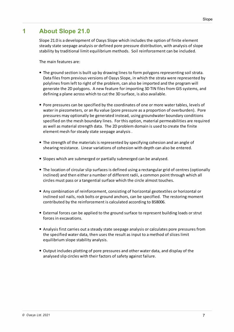
The program introduces a new user interface with a ribbon menu and windows which can bedocked, floated on screen or minimised to the edge of the screen.

The ribbon contains all the commands available in the program, organised into tabbed groups. The most frequently used commands are on the Home tab. Opening some viewsautomatically switches to show the tab most applicable to that view, but the tab can alwaysbe manually changed by the user. Some overall problem data (general specification such asanalysis method, slip circle definition) is shown on "property grids" to the right of the mainscreen. Again, these views can be floated and docked in different positions if required.

The Data Explorer navigation view has links to the various data entry screens and outputviews. It is “docked” to the left of the main view, but can be moved to another location,closed, or set to auto-hide if required. Setting auto-hide is done using the push-pin symbol atthe top of the Data Explorer. It will then minimise to the side of the main window unless youhover over the minimised view title bar. The Data Explorer can also be closed or re-openedusing a check box on the Home tab of the ribbon.

The “application button” at the top left of the main window takes the place of the File menu. Clicking this button opens a menu with access to file operation commands (New, Open, Saveetc.), some view commands (Export, Print etc.) and quick access to recently opened files.

This version of Slope introduces a new file extension for Slope files which is .sbd. Files withthe suffix .sld, from previous versions of Slope, may also be opened.

Part III

Slope

© O as ys Ltd. 2021 11

3 Theory

3.1 Method of Slices

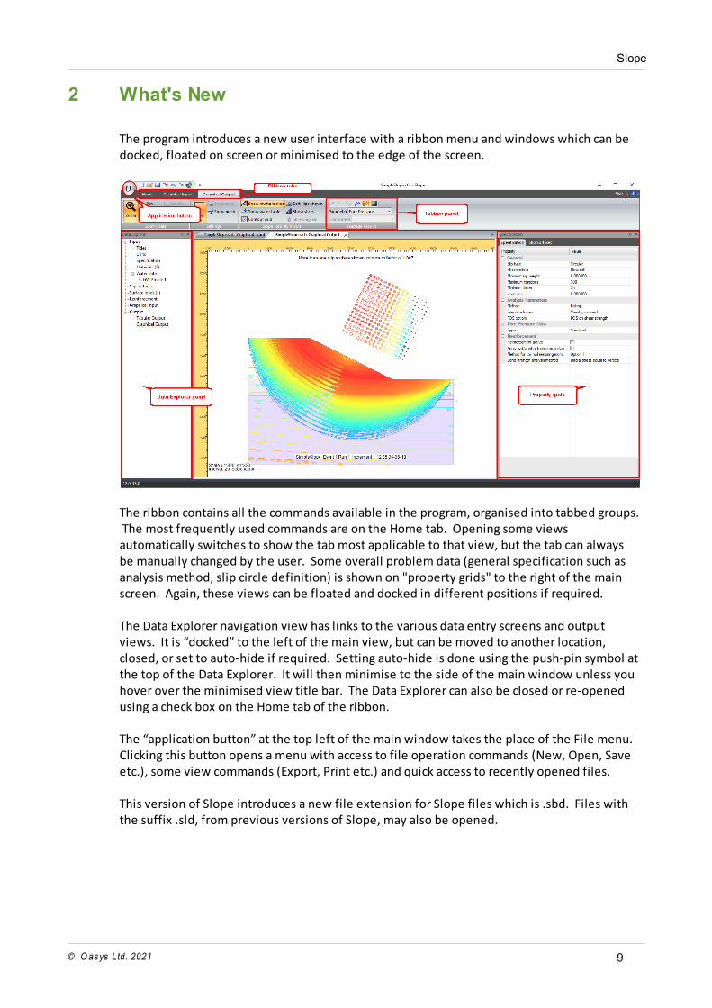
Slope analyses slope stability using the method of slices, in which the slipping mass is dividedinto a number of vertical slices and various equations of static equilibrium are applied eitherto each slice or to the slipping mass as a whole.

The annotation and sign convention for the method of slices is as follows:

All forces are given as total forces (i.e. including water pressure). F - Factor of Safety Ph - Horizontal component of external loads Pv - Vertical component of external loads E - Horizontal Interslice Force X - Vertical Interslice Force W - Total weight of soil = γbh N - Total normal force acting along slice base R - Distance from slice base to moment centre S - Shear force acting along slice base

Slope

© O as ys Ltd. 202112

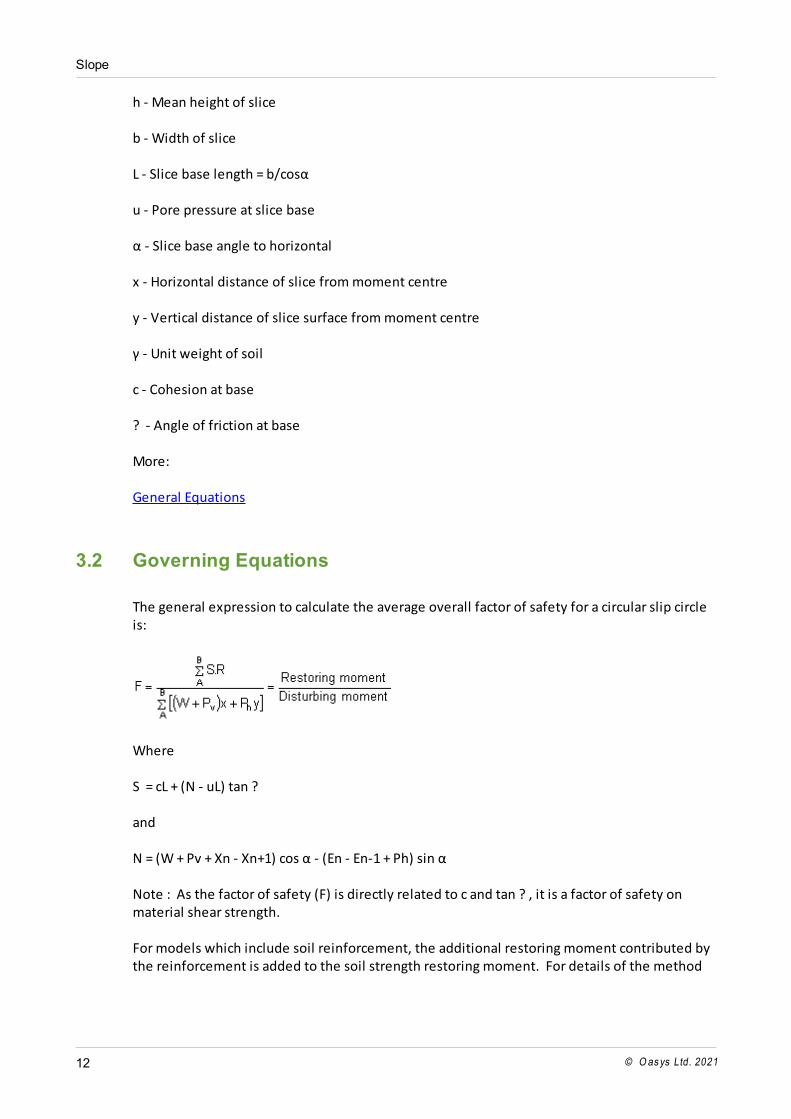
h - Mean height of slice b - Width of slice L - Slice base length = b/cosα u - Pore pressure at slice base α - Slice base angle to horizontal x - Horizontal distance of slice from moment centre y - Vertical distance of slice surface from moment centre γ - Unit weight of soil c - Cohesion at base ? - Angle of friction at base More: General Equations

3.2 Governing Equations

The general expression to calculate the average overall factor of safety for a circular slip circleis:

Where S = cL + (N - uL) tan ? and N = (W + Pv + Xn - Xn+1) cos α - (En - En-1 + Ph) sin α Note : As the factor of safety (F) is directly related to c and tan ? , it is a factor of safety onmaterial shear strength. For models which include soil reinforcement, the additional restoring moment contributed bythe reinforcement is added to the soil strength restoring moment. For details of the method

Slope

© O as ys Ltd. 2021 13

of calculation, see Reinforcement Calculations. In addition other expressions for equilibrium are as follows: For vertical equilibrium: N cos α = W + Pv + (Xn - Xn+1) - (S sin α) / F For horizontal equilibrium: N sin α = (En+1 - En) – Ph + (S cos α) / F For full details of notation see Method of Slices.

3.3 Bishop's Methods

Bishop's method (Bishop AW, 1955) is applicable to circular slip surfaces. There are three methods of Bishop solution available in Slope. These differ only in thedirection of the interslice forces. Horizontal interslice forces

In this method, the interslice shear forces are assumed to sum to zero. This satisfies verticalequilibrium, but not horizontal equilibrium. This leads to errors in the calculated factors ofsafety, but these are usually small and on the safe side (Spencer 1967). The method satisfiesoverall moment equilibrium. The limitations of the method have been investigated by Whitman and Bailey (1967). Theyconcluded that the method can occasionally give misleading answers particularly in the caseof Interlock. If it is suspected that this may be a problem then the user should select themethod with variably inclined interslice forces.

Parallel inclined interslice forces

This method (also known as Spencer's Method) is a refinement of the horizontal forcesmethod, and satisfies conditions of horizontal, vertical and moment equilibrium for the slip asa whole. The program assumes that all the interslice forces are parallel and at a constantinclination throughout the slope.

This method was assessed by Spencer (1967). He has shown that in most cases the resultsdiffer only slightly from those obtained by the simplified method, which assumes onlyhorizontal interslice forces. The differences between the two methods increase with slopeangle. For steep slopes Spencer's method is more accurate, but some slip circles may haveproblems with interlock and so the final method with variably inclined interslice forces is theprogram default.

Slope

© O as ys Ltd. 202114

Variably inclined interslice forces

In this method the program calculates the interslice forces to maintain horizontal and verticalequilibrium of each slice. The inclinations of the interslice forces are then varied in eachiteration until overall horizontal, vertical and moment equilibrium is also achieved.

3.3.1 Iteration procedure

Slope uses iteration to reach convergence for each of the Bishop methods as follows: Factors of safety For each iteration i, Slope calculates a new factor of safety Fi using the ratio of restoring

moment to disturbing moment (which is a function of F i-1). When the difference between Fi

and F i-1 is within the specified tolerance, the calculation is complete.

The factor of safety, F, is the ratio of restoring moment to disturbing moment. However, thisratio is itself a function of F, (except in the Swedish circle method) so an iterative solution isnecessary. Horizontal interslice forces

1.Slope starts at slice 1 (Note : Slices are numbered from left to right) and, by maintainingvertical equilibrium it calculates the resultant horizontal force.

2.The program then uses this as the interslice force with slice 2. The process continuesuntil the last slice which ends up with a resultant horizontal force.

In this method each slice and the slope as a whole is in vertical equilibrium, with zero verticalinterslice forces. Horizontal equilibrium is not achieved within each slice or the slope as awhole. Therefore the only force check within each slice is for vertical equilibrium. Constant inclined interslice forces In this method Slope varies the ratio (which is constant), between the vertical and horizontalinterslice forces, until the resultant of each is reduced to zero. For this method each slice is not in equilibrium, only the slope as a whole. In the calculationequilibrium is effectively maintained for each slice in the direction normal to the intersliceforces. Variably inclined interslice forces The variably inclined method is usually preferable, as it keeps every slice in horizontal and

Slope

© O as ys Ltd. 2021 15

vertical equilibrium at all times. However, it can exceed the soil strength along the sliceinterface as it does not check the vertical interslice forces against the shear strength of thematerial. The results should therefore be checked for this criterion. The interslice force is adjusted separately, for both the vertical and horizontal direction, byadding the fraction of the residual values from the previous iteration. The fraction isdetermined by the horizontal length of the slip surface represented by that slice. Theinterslice force direction can vary by this method, but each slice is in equilibrium at all timesas is the slope as a whole.

3.4 Morgenstern-Price Method

Morgenstern and Price's method (1965) is similar to the Bishop's method with parallel inclinedinterslice forces, but uses a function to express a varying ratio between the normal and shearinterslice forces from left to right across the slip circle. (If this function is constant, themethod produces the same result as the Bishop method with parallel inclined intersliceforces.)

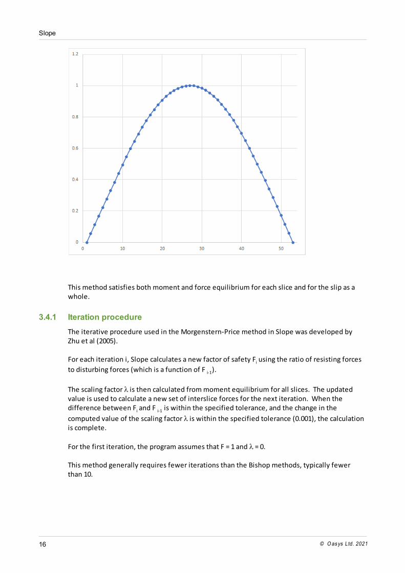
The choice of interslice function can be a constant ratio or a half-sine function, scaled by a

factor , which is printed in the detailed results output. The shear interslice force at a sliceboundary is calculated as:

X = E f(x)

where f(x) is either constant or the half-sine function, which has the same shape as a sinecurve and varies from 0 at the left end of the slip to 1 halfway across the slip, reducing to 0 atthe right end of the slip:

Slope

© O as ys Ltd. 202116

This method satisfies both moment and force equilibrium for each slice and for the slip as awhole.

3.4.1 Iteration procedure

The iterative procedure used in the Morgenstern-Price method in Slope was developed byZhu et al (2005).

For each iteration i, Slope calculates a new factor of safety Fi using the ratio of resisting forces

to disturbing forces (which is a function of F i-1).

The scaling factor is then calculated from moment equilibrium for all slices. The updatedvalue is used to calculate a new set of interslice forces for the next iteration. When thedifference between Fi and F i-1 is within the specified tolerance, and the change in the

computed value of the scaling factor is within the specified tolerance (0.001), the calculationis complete.

For the first iteration, the program assumes that F = 1 and = 0.

This method generally requires fewer iterations than the Bishop methods, typically fewerthan 10.

Slope

© O as ys Ltd. 2021 17

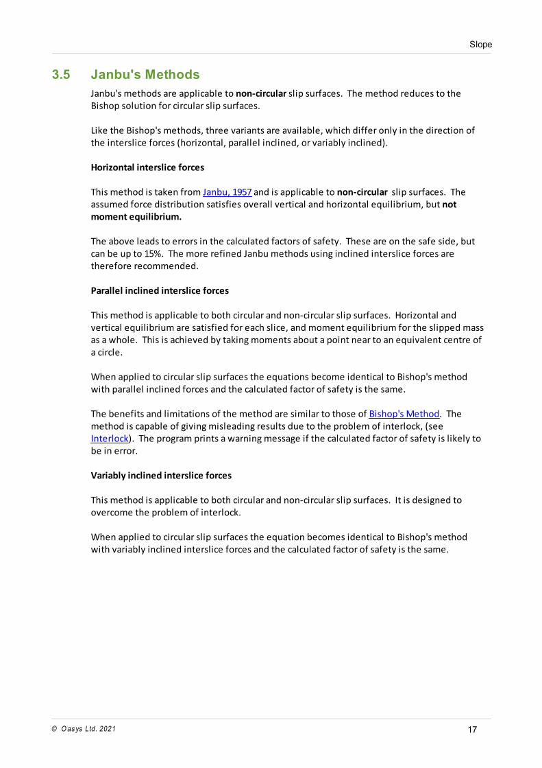
3.5 Janbu's Methods

Janbu's methods are applicable to non-circular slip surfaces. The method reduces to theBishop solution for circular slip surfaces.

Like the Bishop's methods, three variants are available, which differ only in the direction ofthe interslice forces (horizontal, parallel inclined, or variably inclined).

Horizontal interslice forces

This method is taken from Janbu, 1957 and is applicable to non-circular slip surfaces. Theassumed force distribution satisfies overall vertical and horizontal equilibrium, but notmoment equilibrium.

The above leads to errors in the calculated factors of safety. These are on the safe side, butcan be up to 15%. The more refined Janbu methods using inclined interslice forces aretherefore recommended.

Parallel inclined interslice forces

This method is applicable to both circular and non-circular slip surfaces. Horizontal andvertical equilibrium are satisfied for each slice, and moment equilibrium for the slipped massas a whole. This is achieved by taking moments about a point near to an equivalent centre ofa circle.

When applied to circular slip surfaces the equations become identical to Bishop's methodwith parallel inclined forces and the calculated factor of safety is the same.

The benefits and limitations of the method are similar to those of Bishop's Method. Themethod is capable of giving misleading results due to the problem of interlock, (see Interlock). The program prints a warning message if the calculated factor of safety is likely tobe in error.

Variably inclined interslice forces

This method is applicable to both circular and non-circular slip surfaces. It is designed toovercome the problem of interlock. When applied to circular slip surfaces the equation becomes identical to Bishop's methodwith variably inclined interslice forces and the calculated factor of safety is the same.

Slope

© O as ys Ltd. 202118

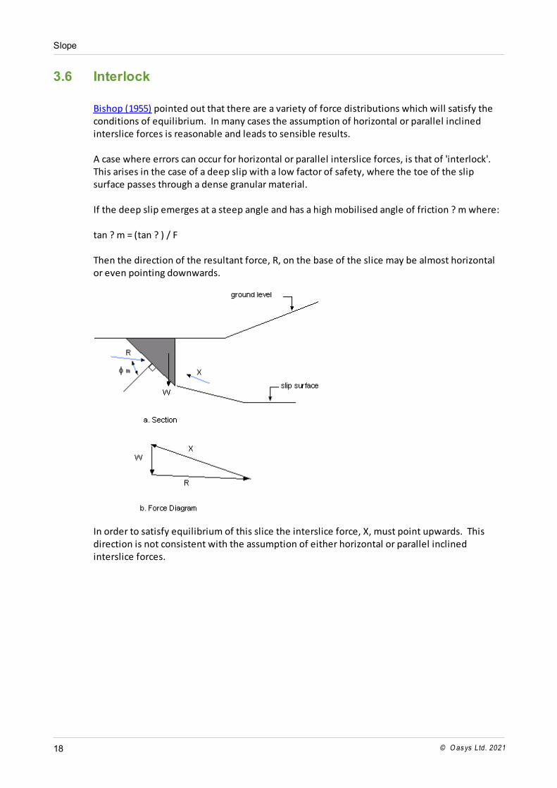
3.6 Interlock

Bishop (1955) pointed out that there are a variety of force distributions which will satisfy theconditions of equilibrium. In many cases the assumption of horizontal or parallel inclinedinterslice forces is reasonable and leads to sensible results. A case where errors can occur for horizontal or parallel interslice forces, is that of 'interlock'. This arises in the case of a deep slip with a low factor of safety, where the toe of the slipsurface passes through a dense granular material. If the deep slip emerges at a steep angle and has a high mobilised angle of friction ? m where: tan ? m = (tan ? ) / F Then the direction of the resultant force, R, on the base of the slice may be almost horizontalor even pointing downwards.

In order to satisfy equilibrium of this slice the interslice force, X, must point upwards. Thisdirection is not consistent with the assumption of either horizontal or parallel inclinedinterslice forces.

Slope

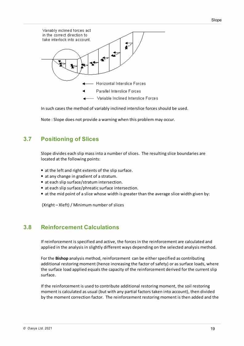
© O as ys Ltd. 2021 19

In such cases the method of variably inclined interslice forces should be used. Note : Slope does not provide a warning when this problem may occur.

3.7 Positioning of Slices

Slope divides each slip mass into a number of slices. The resulting slice boundaries arelocated at the following points:

at the left and right extents of the slip surface.

at any change in gradient of a stratum.

at each slip surface/stratum intersection.

at each slip surface/phreatic surface intersection.

at the mid point of a slice whose width is greater than the average slice width given by: (Xright – Xleft) / Minimum number of slices

3.8 Reinforcement Calculations

If reinforcement is specified and active, the forces in the reinforcement are calculated andapplied in the analysis in slightly different ways depending on the selected analysis method.

For the Bishop analysis method, reinforcement can be either specified as contributingadditional restoring moment (hence increasing the factor of safety) or as surface loads, wherethe surface load applied equals the capacity of the reinforcement derived for the current slipsurface. If the reinforcement is used to contribute additional restoring moment, the soil restoringmoment is calculated as usual (but with any partial factors taken into account), then dividedby the moment correction factor. The reinforcement restoring moment is then added and the

Slope

© O as ys Ltd. 202120

factor of safety calculated.

For the Morgenstern-Price method, the calculated forces are either applied through the baseof the slices where the reinforcing elements cross the slip surface, or as surface loads. Thedifference to the factor of safety in many cases will be small, but the normal and shear forcesat the base will tend to show more "spikes" in the former method than in the surface loadmethod.

Calculation of design capacity of reinforcing elements where they cross the slip surface For end anchored elements (rockbolts Type B): Tj = T/S For ground anchors without pre-stress or soil nails, capacity is the minimum of design pulloutforce, tensile force and stripping force, so Tj = min{T/S, BLO/S,(P+BLi)/S} For ground anchors with prestress, the applicable prestress cannot exceed this value. Theinput prestress is reduced in proportion to the amount of fixed length outside the slipsurface. In the output, the applicable prestress and any additional capacity are shownseparately. The applicable prestress per m run of slope is: Tpj = min{Tj, (Tp/S x LO/L)} and the additional capacity is (Tj - Tpj). For geotextiles, capacity is the minimum of design tensile force and pullout force, so Tj =min{T, 2LOτ} where T is design tensile capacity per m run of slope (Tult x fcr/(fm11 x fm12 x fm21 x fm22 x fn x fs)) where fcr is the partial factor for creep reduction fm11 is the partial factor for manufacture fm12 is the partial factor for extrapolation of test data fm21 is the partial factor for damage fm22 is the partial factor for environment fn is the partial factor for economic ramification of failure fs is the partial factor for material strength Tp is input prestress per anchor S is out-of-plane spacing B is bond strength (force per unit length of anchor/nail) P is design surface plate capacity Li is bonded length within the slip circle LO is bonded length or length outside the slip circle

Slope

© O as ys Ltd. 2021 21

L is total bonded length The calculation of pullout and stripping forces are mentioned above. To calculate them theshear / bond strength of the appropriate soil strength model has to be applied to the materialthe reinforcement is in (linear, hyperbolic etc). B is bond strength (force per unit length of anchor/nail), which can be calculated or specifiedby the user. If calculated, the value is based on equation 12 from BS8081 or section 4.3.2 ofBS8006-2. For BS8081 the equation to calculate bond strength is: πD(σν'tanδ + ca)/(fp x fn) where σv' = γh + wvertical h is vertical distance between reinforcement and slope surface For BS8006-2 the equation to calculate bond strength is: πD(σr'tanδ + ca)/(fp) where σr'=σν'(1 + KL)/2 and KL= (1 + Ka)/2 Shear strength of soil = τ = (σν' .a. tanδ + ca)/(fp x fn) (for drained linear strength model). Itshould be noted that a reduced pullout factor is adopted in this analysis as the factoredstrength and friction angle are used.

δ is factored soil friction angle (tan-1(tan ? '/fmsphi)) where fmsphi is factor on frictionangle

ca is factored soil cohesion ( ( ac c)/fmsc )

γh is weight of soil above the reinforcement behind the slip surface - soil unit weight ismultiplied by the applicable partial factor

w is surcharge on the surface above reinforcement behind the slip surface - with factorson dead and live load applied, so w = (dead load x dead load factor)+(live load x liveload factor)

a is coefficient of interaction between reinforcement and soil relating to the φ' of soil

ac is coefficient of interaction between reinforcement and soil relating to the c' of soil

Ka is the Rankine active earth pressure coefficient

fp is partial factor on pull-out (BS8006 =1.3)

fn is partial factor for structure importance (BS8006 =1-1.1)

Slope

© O as ys Ltd. 202122

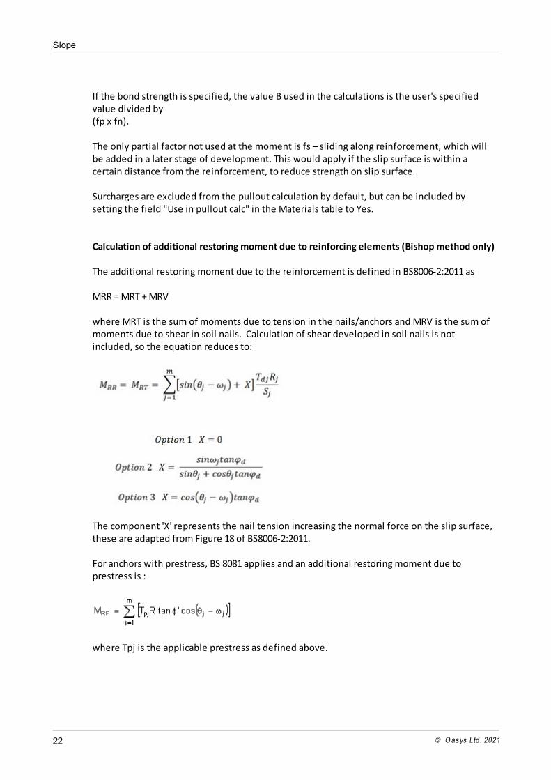
If the bond strength is specified, the value B used in the calculations is the user's specifiedvalue divided by(fp x fn). The only partial factor not used at the moment is fs – sliding along reinforcement, which willbe added in a later stage of development. This would apply if the slip surface is within acertain distance from the reinforcement, to reduce strength on slip surface. Surcharges are excluded from the pullout calculation by default, but can be included bysetting the field "Use in pullout calc" in the Materials table to Yes. Calculation of additional restoring moment due to reinforcing elements (Bishop method only) The additional restoring moment due to the reinforcement is defined in BS8006-2:2011 as MRR = MRT + MRV where MRT is the sum of moments due to tension in the nails/anchors and MRV is the sum ofmoments due to shear in soil nails. Calculation of shear developed in soil nails is notincluded, so the equation reduces to:

The component 'X' represents the nail tension increasing the normal force on the slip surface,these are adapted from Figure 18 of BS8006-2:2011. For anchors with prestress, BS 8081 applies and an additional restoring moment due toprestress is :

where Tpj is the applicable prestress as defined above.

Slope

© O as ys Ltd. 2021 23

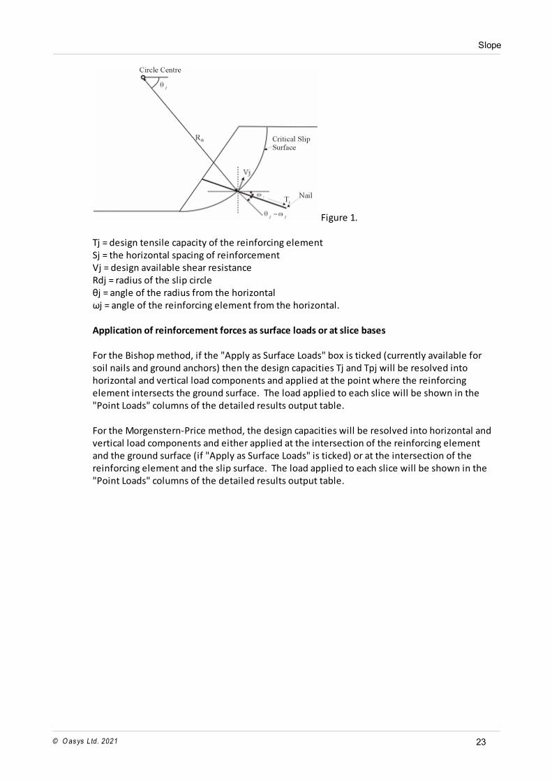
Figure 1. Tj = design tensile capacity of the reinforcing elementSj = the horizontal spacing of reinforcementVj = design available shear resistanceRdj = radius of the slip circleθj = angle of the radius from the horizontalωj = angle of the reinforcing element from the horizontal. Application of reinforcement forces as surface loads or at slice bases For the Bishop method, if the "Apply as Surface Loads" box is ticked (currently available forsoil nails and ground anchors) then the design capacities Tj and Tpj will be resolved intohorizontal and vertical load components and applied at the point where the reinforcingelement intersects the ground surface. The load applied to each slice will be shown in the"Point Loads" columns of the detailed results output table.

For the Morgenstern-Price method, the design capacities will be resolved into horizontal andvertical load components and either applied at the intersection of the reinforcing elementand the ground surface (if "Apply as Surface Loads" is ticked) or at the intersection of thereinforcing element and the slip surface. The load applied to each slice will be shown in the"Point Loads" columns of the detailed results output table.

Part IV

Slope

© O as ys Ltd. 2021 25

4 Getting Started

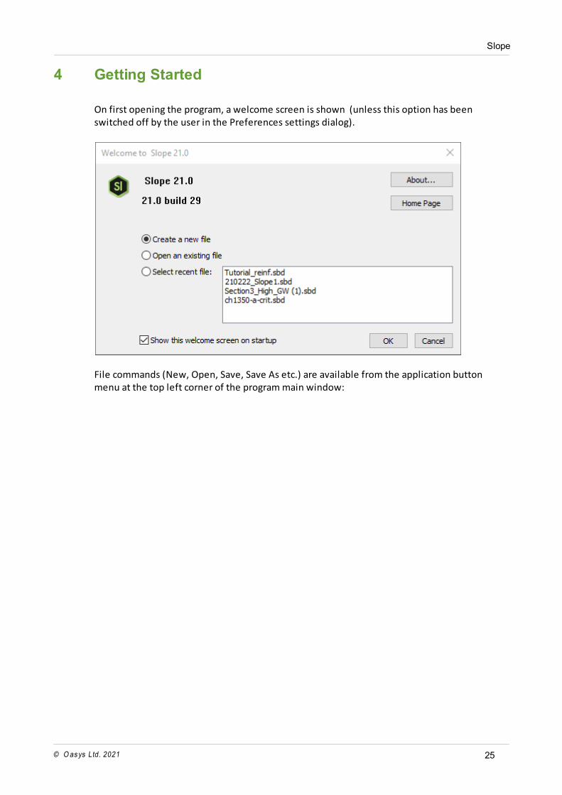
On first opening the program, a welcome screen is shown (unless this option has beenswitched off by the user in the Preferences settings dialog).

File commands (New, Open, Save, Save As etc.) are available from the application buttonmenu at the top left corner of the program main window:

Slope

© O as ys Ltd. 202126

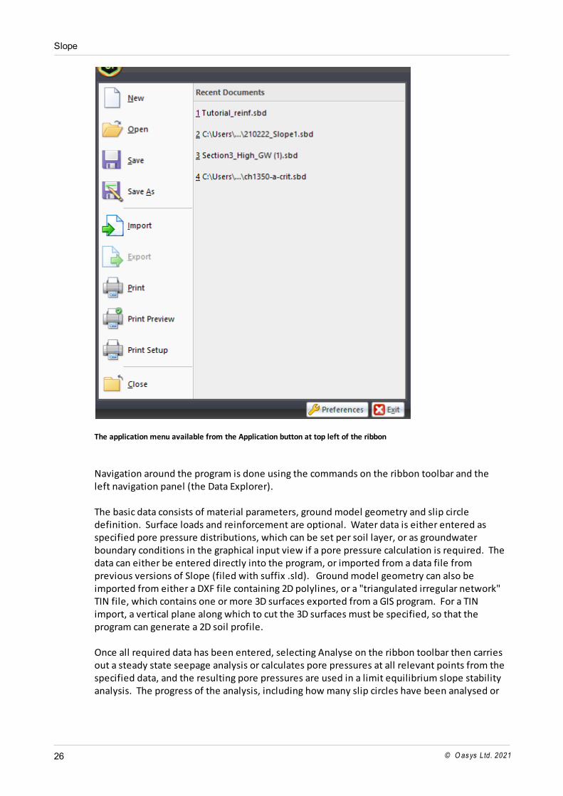
The application menu available from the Application button at top left of the ribbon

Navigation around the program is done using the commands on the ribbon toolbar and theleft navigation panel (the Data Explorer). The basic data consists of material parameters, ground model geometry and slip circledefinition. Surface loads and reinforcement are optional. Water data is either entered asspecified pore pressure distributions, which can be set per soil layer, or as groundwaterboundary conditions in the graphical input view if a pore pressure calculation is required. Thedata can either be entered directly into the program, or imported from a data file fromprevious versions of Slope (filed with suffix .sld). Ground model geometry can also beimported from either a DXF file containing 2D polylines, or a "triangulated irregular network"TIN file, which contains one or more 3D surfaces exported from a GIS program. For a TINimport, a vertical plane along which to cut the 3D surfaces must be specified, so that theprogram can generate a 2D soil profile. Once all required data has been entered, selecting Analyse on the ribbon toolbar then carriesout a steady state seepage analysis or calculates pore pressures at all relevant points from thespecified data, and the resulting pore pressures are used in a limit equilibrium slope stabilityanalysis. The progress of the analysis, including how many slip circles have been analysed or

Slope

© O as ys Ltd. 2021 27

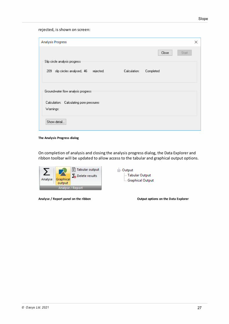
rejected, is shown on screen:

The Analysis Progress dialog

On completion of analysis and closing the analysis progress dialog, the Data Explorer andribbon toolbar will be updated to allow access to the tabular and graphical output options.

Analyse / Report panel on the ribbon Output options on the Data Explorer

Part V

Slope

© O as ys Ltd. 2021 29

5 Entering Data

5.1 Defining Analysis Options

5.1.1 Titles

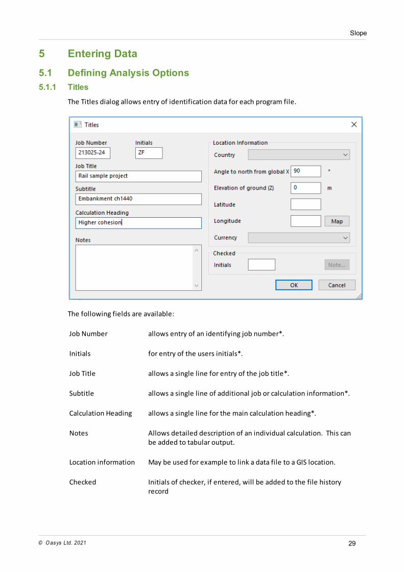
The Titles dialog allows entry of identification data for each program file.

The following fields are available:

Job Number allows entry of an identifying job number*.

Initials for entry of the users initials*.

Job Title allows a single line for entry of the job title*.

Subtitle allows a single line of additional job or calculation information*.

Calculation Heading allows a single line for the main calculation heading*.

Notes Allows detailed description of an individual calculation. This canbe added to tabular output.

Location information May be used for example to link a data file to a GIS location.

Checked Initials of checker, if entered, will be added to the file historyrecord

Slope

© O as ys Ltd. 202130

*These fields will be reproduced in the title block at the head of printed information usingthe "Calculation Sheet" layout.

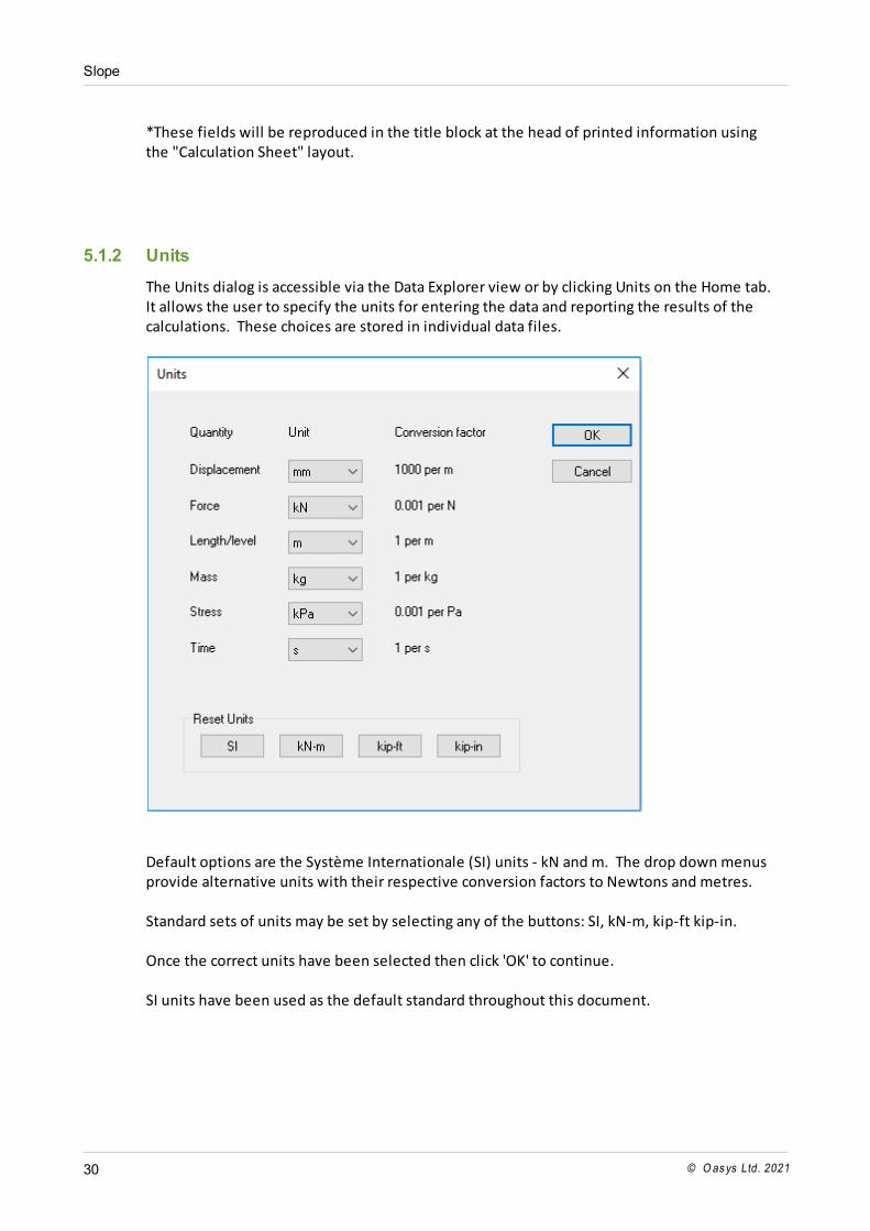
5.1.2 Units

The Units dialog is accessible via the Data Explorer view or by clicking Units on the Home tab. It allows the user to specify the units for entering the data and reporting the results of thecalculations. These choices are stored in individual data files.

Default options are the Système Internationale (SI) units - kN and m. The drop down menusprovide alternative units with their respective conversion factors to Newtons and metres. Standard sets of units may be set by selecting any of the buttons: SI, kN-m, kip-ft kip-in. Once the correct units have been selected then click 'OK' to continue. SI units have been used as the default standard throughout this document.

Slope

© O as ys Ltd. 2021 31

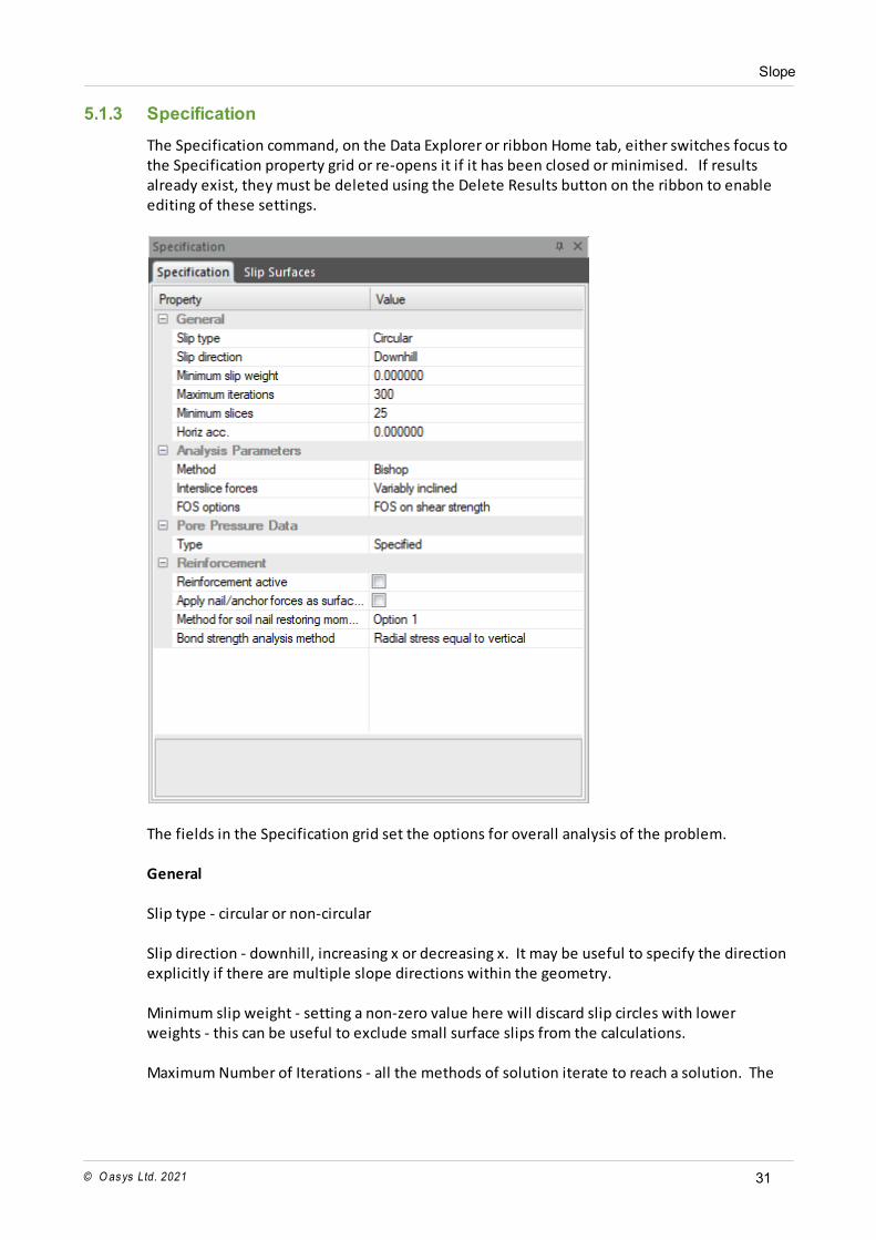
5.1.3 Specification

The Specification command, on the Data Explorer or ribbon Home tab, either switches focus tothe Specification property grid or re-opens it if it has been closed or minimised. If resultsalready exist, they must be deleted using the Delete Results button on the ribbon to enableediting of these settings.

The fields in the Specification grid set the options for overall analysis of the problem.

General

Slip type - circular or non-circular

Slip direction - downhill, increasing x or decreasing x. It may be useful to specify the directionexplicitly if there are multiple slope directions within the geometry. Minimum slip weight - setting a non-zero value here will discard slip circles with lowerweights - this can be useful to exclude small surface slips from the calculations. Maximum Number of Iterations - all the methods of solution iterate to reach a solution. The

Slope

© O as ys Ltd. 202132

program defaults to 300 iterations, but the user can specify any number. Minimum Number of Slices - the program requires the minimum number of slices for each slipsurface to be specified. The default value is 25. Analysis Parameters

For the Bishop or Janbu analysis methods, the direction of interslice forces (horizontal,parallel or variably inclined) must also be selected. The default is variably inclined forces. For the Morgenstern-Price method, there are two options for the interslice force function,constant or a half-sine function. For circular slips, the constant interslice force function isequivalent to the Bishop method with parallel inclined interslice forces.

For all methods including Bishop, Janbu and Morgenstern-Price, choose between FoS on shearstrength (the default), FoS on disturbing or restoring loads, or a partial factor analysis. If partial factor analysis is specified, the visible fields will expand to allow selection of apartial factor set to apply to the input data. The results will be reported as an "over-designfactor" rather than a factor of safety.

Pore Pressure Data

Choose between specified pore pressures for each soil layer, which can be hydrostatic,defined by piezometers or a single Ru value (see Water Data), or generated pore pressures. IfGenerated is selected, then permeabilities should be added for each soil material andgroundwater boundary conditions must be set to enable a steady state seepage analysis to berun. See Groundwater boundary conditions for details.

Reinforcement Check boxes are available to set whether reinforcement is active and whether to apply nail/anchor forces as surface loads. These apply to all reinforcement defined in the data file. Theremaining options allow the user to specify the method for calculating the bond stress andrestoring moment attributable to soil nails. Details of these methods are included in the Reinforcement Calculations section.

5.2 Defining the Ground Model

The ground model to be analysed consists of a 2D section through the slope, divided intoconnected polygons of different soil strata.

The material parameters for each stratum are entered in a table (see Material Properties ),but the geometry of the slope and many of the other properties are entered and accessed viathe Graphical Input view.

The following sections give details of the data input for the ground model and a summary ofthe features available in the graphical input. Detailed tutorials and videos on the methodsdescribed are available on the web site.

Slope

© O as ys Ltd. 2021 33

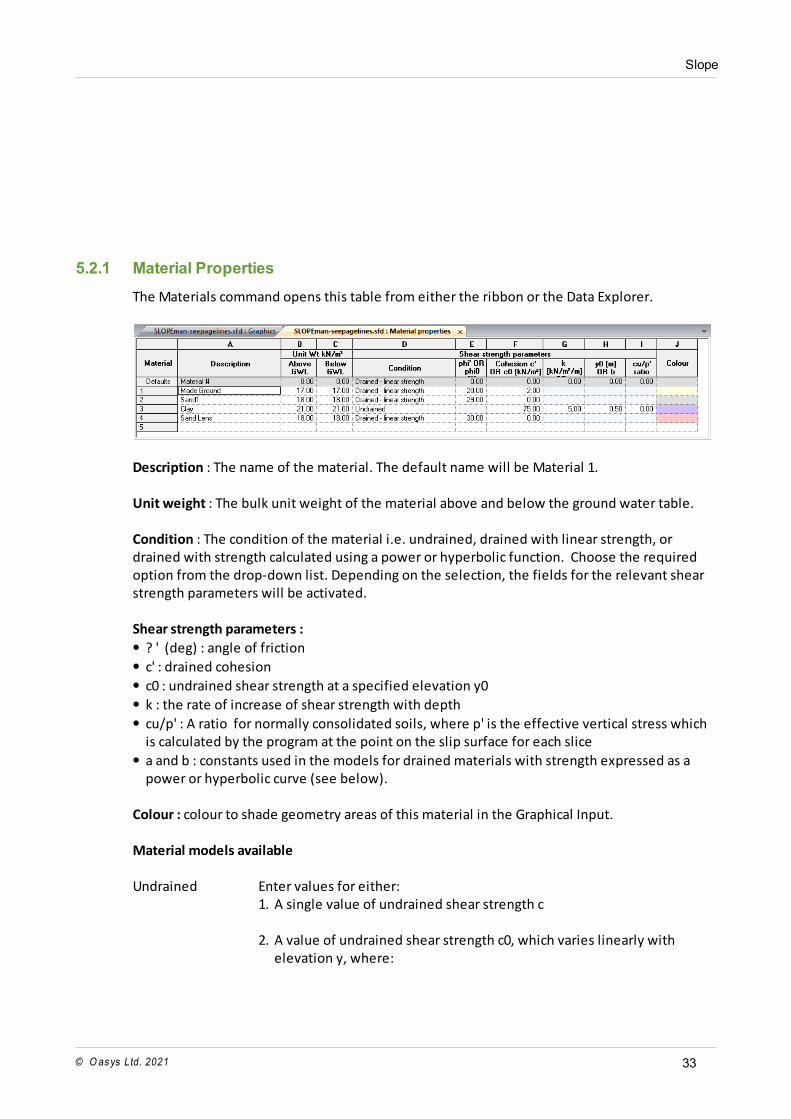
5.2.1 Material Properties

The Materials command opens this table from either the ribbon or the Data Explorer.

Description : The name of the material. The default name will be Material 1. Unit weight : The bulk unit weight of the material above and below the ground water table. Condition : The condition of the material i.e. undrained, drained with linear strength, ordrained with strength calculated using a power or hyperbolic function. Choose the requiredoption from the drop-down list. Depending on the selection, the fields for the relevant shearstrength parameters will be activated. Shear strength parameters :

? ' (deg) : angle of friction

c' : drained cohesion

c0 : undrained shear strength at a specified elevation y0

k : the rate of increase of shear strength with depth

cu/p' : A ratio for normally consolidated soils, where p' is the effective vertical stress whichis calculated by the program at the point on the slip surface for each slice

a and b : constants used in the models for drained materials with strength expressed as apower or hyperbolic curve (see below).

Colour : colour to shade geometry areas of this material in the Graphical Input.

Material models available

Undrained Enter values for either:1. A single value of undrained shear strength c

2. A value of undrained shear strength c0, which varies linearly withelevation y, where:

Slope

© O as ys Ltd. 202134

c = c0 + k(y0 - y)

c = undrained shear strength at any elevation yc0 = undrained shear strength at a specified elevation y0k = rate of increase of shear strength with depth

3. A ratio of cu/p' for normally consolidated soils, where p' is theeffective vertical stress calculated at the point on the slip surface foreach slice

4. A combination of 2 and 3. If both are selected, the higher value ofstrength is used.

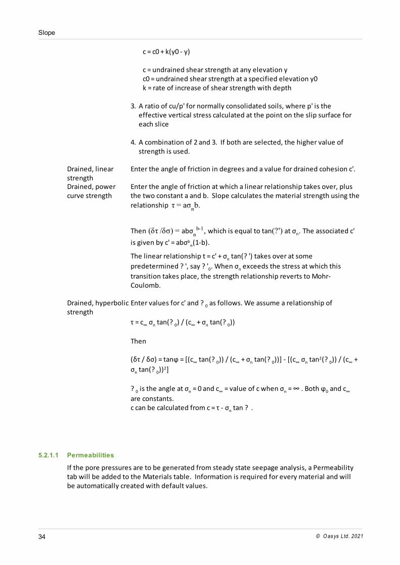
Drained, linearstrength

Enter the angle of friction in degrees and a value for drained cohesion c'.

Drained, powercurve strength

Enter the angle of friction at which a linear relationship takes over, plusthe two constant a and b. Slope calculates the material strength using the

relationship τ = aσnb.

Then (δτ /δσ) = abσn

b-1, which is equal to tan(?') at σn. The associated c'

is given by c' = abσbn(1-b).

The linear relationship t = c' + σn tan(? ') takes over at some

predetermined ? ', say ? '0. When σn exceeds the stress at which this

transition takes place, the strength relationship reverts to Mohr-Coulomb.

Drained, hyperbolicstrength

Enter values for c' and ? 0 as follows. We assume a relationship of

τ = c σn tan(? 0) / (c + σn tan(? 0))

Then

(δτ / δσ) = tan = [(c tan(? 0)) / (c + σn tan(? 0))] - [(c σn tan2(? 0)) / (c +

σn tan(? 0))2]

? 0 is the angle at σn = 0 and c = value of c when σn 0 and c

are constants. c can be calculated from c = τ - σn tan ? .

5.2.1.1 Permeabilities

If the pore pressures are to be generated from steady state seepage analysis, a Permeabilitytab will be added to the Materials table. Information is required for every material and willbe automatically created with default values.

Slope

© O as ys Ltd. 2021 35

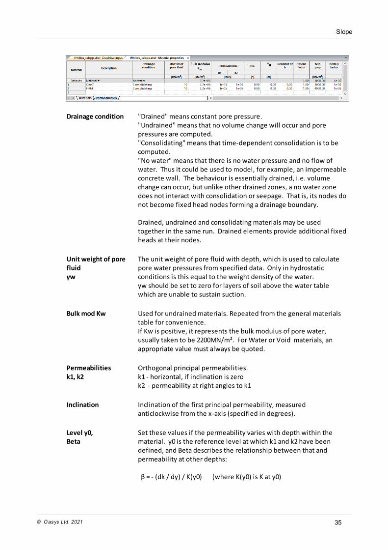
Drainage condition "Drained" means constant pore pressure."Undrained" means that no volume change will occur and porepressures are computed."Consolidating" means that time-dependent consolidation is to becomputed."No water" means that there is no water pressure and no flow ofwater. Thus it could be used to model, for example, an impermeableconcrete wall. The behaviour is essentially drained, i.e. volumechange can occur, but unlike other drained zones, a no water zonedoes not interact with consolidation or seepage. That is, its nodes donot become fixed head nodes forming a drainage boundary. Drained, undrained and consolidating materials may be usedtogether in the same run. Drained elements provide additional fixedheads at their nodes.

Unit weight of porefluidγw

The unit weight of pore fluid with depth, which is used to calculatepore water pressures from specified data. Only in hydrostaticconditions is this equal to the weight density of the water.γw should be set to zero for layers of soil above the water tablewhich are unable to sustain suction.

Bulk mod Kw Used for undrained materials. Repeated from the general materialstable for convenience.If Kw is positive, it represents the bulk modulus of pore water,usually taken to be 2200MN/m². For Water or Void materials, anappropriate value must always be quoted.

Permeabilitiesk1, k2

Orthogonal principal permeabilities.k1 - horizontal, if inclination is zerok2 - permeability at right angles to k1

Inclination Inclination of the first principal permeability, measuredanticlockwise from the x-axis (specified in degrees).

Level y0,Beta

Set these values if the permeability varies with depth within thematerial. y0 is the reference level at which k1 and k2 have beendefined, and Beta describes the relationship between that andpermeability at other depths: β = - (dk / dy) / K(y0) (where K(y0) is K at y0)

Slope

© O as ys Ltd. 202136

Desensitising factor F This must be set to 1.0 for all materials for which an accurateconsolidation analysis is required. However, it will sometimes bethe case that the problem involves low cv materials, for whichaccurate consolidation is required, and high cv materials whichprovide boundary conditions to the others, and for which some errorin pore pressure could be tolerated. In this case, it is desirable thatthe time steps are suited to the low permeability materials, and thedesensitising factor is used to keep the high permeability materialsin a stable state.In effect, for each iteration, the coefficient of consolidation of thehigh cv materials is decreased by this factor; however the overalleffect is made less severe as iterations proceed within each timeincrement. Users must inspect the results for materials with valuesof F greater than 1.0, and satisfy themselves that they areappropriate for the problem.

Min pwp Minimum pore water pressure attainable by the material. This is thepressure at which the material becomes unsaturated; it will generallybe zero or negative, representing suction. For unlimited suction,leave blank.

Permeability factor If the pore pressure in the element tends to fall even lower than thatspecified above, it will be held at the specified minimum, and thepermeability of the element will also be reduced by this user-specified factor. This represents conditions in a non-saturated zone. In simple cases, the factor should be set very low: the default is 10E-6meaning that the permeability of the unsaturated material is onemillionth of the saturated value. Other values could be used, given aproper understanding of unsaturated flow.

5.2.2 Soil Layers

Soil layers are created in the Graphical Input view. The 2D section through the ground to beanalysed should be defined as a set of 2D polygons.

Lines to construct the polygons can be imported from DXF or 3D TIN files, or drawn directly inthe 2D graphical input view using the drawing tools.

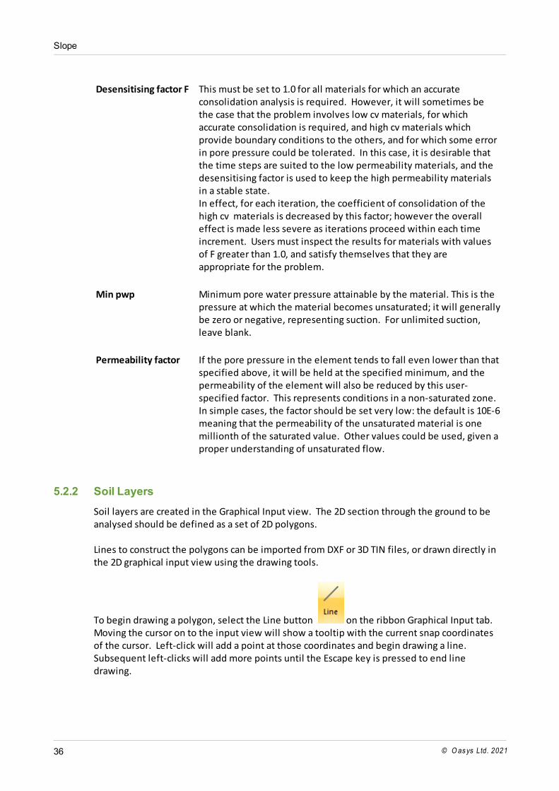
To begin drawing a polygon, select the Line button on the ribbon Graphical Input tab. Moving the cursor on to the input view will show a tooltip with the current snap coordinatesof the cursor. Left-click will add a point at those coordinates and begin drawing a line. Subsequent left-clicks will add more points until the Escape key is pressed to end linedrawing.

Slope

© O as ys Ltd. 2021 37

If a point at exact coordinates is required, including a point off the current screen limits, right-click and the tooltip coordinates will become editable. Enter the required coordinates withthe x and y coordinates separated by a comma, and press the Enter key. The next point will beadded at the coordinates typed in, and the screen limits reset to include it in the drawingarea.

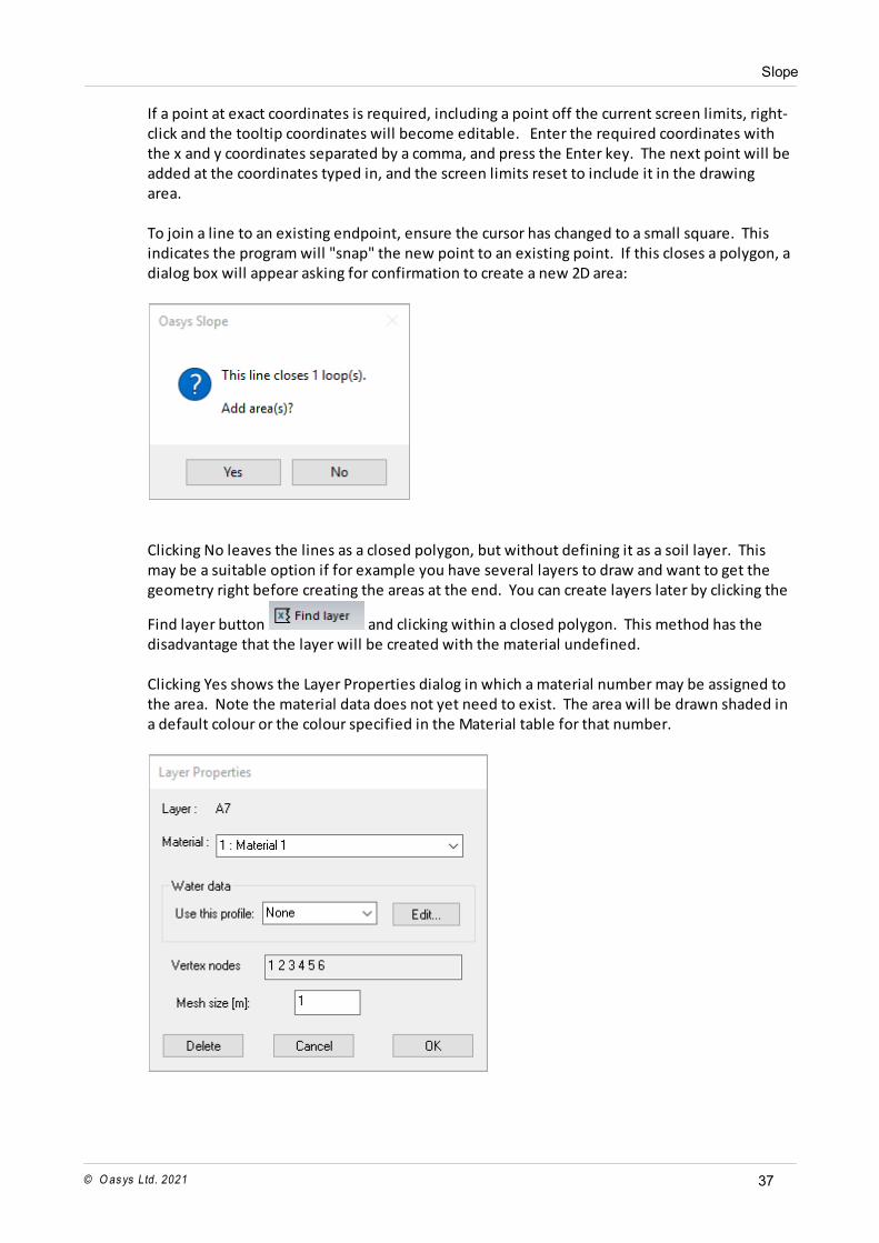
To join a line to an existing endpoint, ensure the cursor has changed to a small square. Thisindicates the program will "snap" the new point to an existing point. If this closes a polygon, adialog box will appear asking for confirmation to create a new 2D area:

Clicking No leaves the lines as a closed polygon, but without defining it as a soil layer. Thismay be a suitable option if for example you have several layers to draw and want to get thegeometry right before creating the areas at the end. You can create layers later by clicking the

Find layer button and clicking within a closed polygon. This method has thedisadvantage that the layer will be created with the material undefined.

Clicking Yes shows the Layer Properties dialog in which a material number may be assigned tothe area. Note the material data does not yet need to exist. The area will be drawn shaded ina default colour or the colour specified in the Material table for that number.

Slope

© O as ys Ltd. 202138

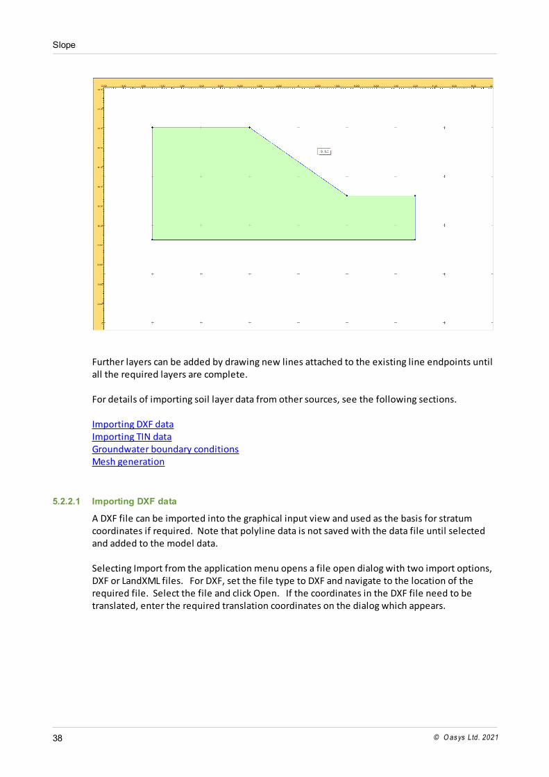
Further layers can be added by drawing new lines attached to the existing line endpoints untilall the required layers are complete.

For details of importing soil layer data from other sources, see the following sections.

Importing DXF dataImporting TIN dataGroundwater boundary conditionsMesh generation

5.2.2.1 Importing DXF data

A DXF file can be imported into the graphical input view and used as the basis for stratumcoordinates if required. Note that polyline data is not saved with the data file until selectedand added to the model data. Selecting Import from the application menu opens a file open dialog with two import options,DXF or LandXML files. For DXF, set the file type to DXF and navigate to the location of therequired file. Select the file and click Open. If the coordinates in the DXF file need to betranslated, enter the required translation coordinates on the dialog which appears.

Slope

© O as ys Ltd. 2021 39

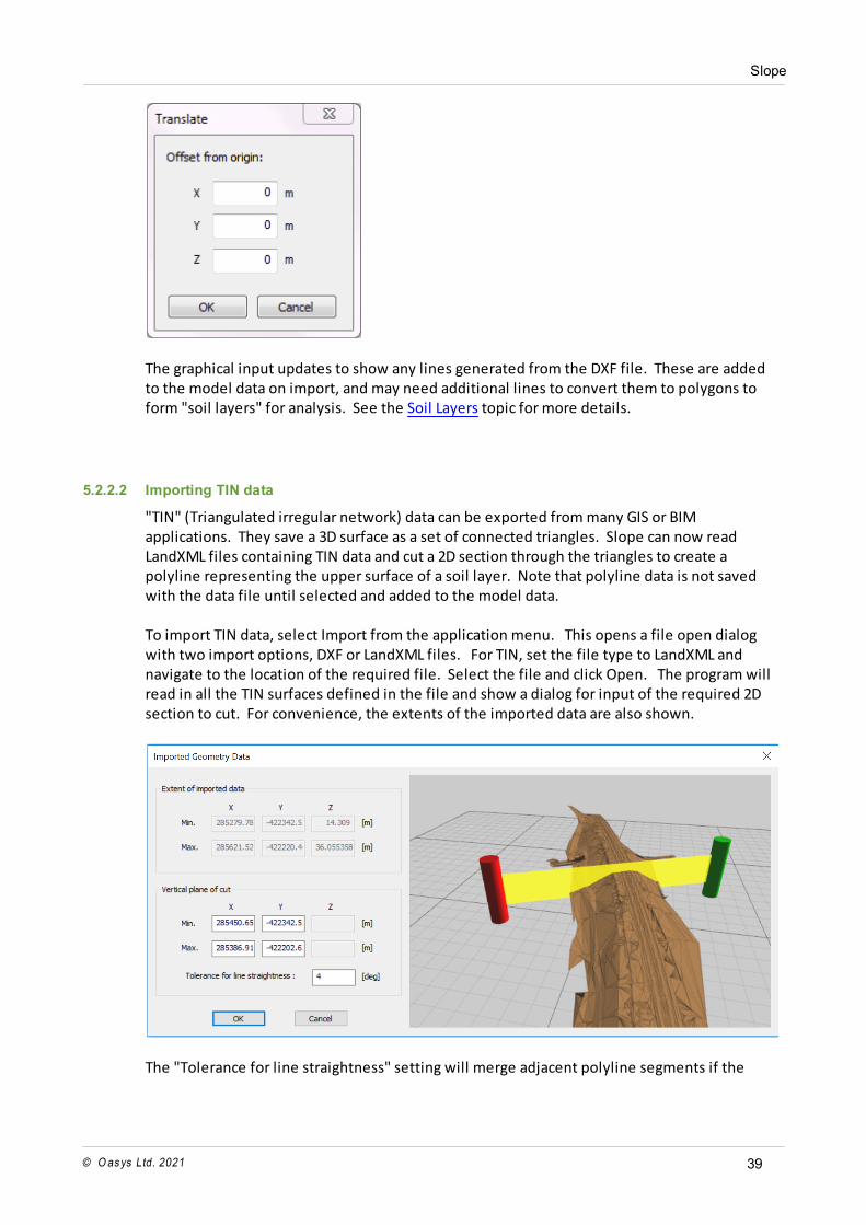
The graphical input updates to show any lines generated from the DXF file. These are addedto the model data on import, and may need additional lines to convert them to polygons toform "soil layers" for analysis. See the Soil Layers topic for more details.

5.2.2.2 Importing TIN data

"TIN" (Triangulated irregular network) data can be exported from many GIS or BIMapplications. They save a 3D surface as a set of connected triangles. Slope can now readLandXML files containing TIN data and cut a 2D section through the triangles to create apolyline representing the upper surface of a soil layer. Note that polyline data is not savedwith the data file until selected and added to the model data.

To import TIN data, select Import from the application menu. This opens a file open dialogwith two import options, DXF or LandXML files. For TIN, set the file type to LandXML andnavigate to the location of the required file. Select the file and click Open. The program willread in all the TIN surfaces defined in the file and show a dialog for input of the required 2Dsection to cut. For convenience, the extents of the imported data are also shown.

The "Tolerance for line straightness" setting will merge adjacent polyline segments if the

Slope

© O as ys Ltd. 202140

angle between them is less than this value in degrees, i.e. if the two line segments are almostparallel.

The graphical pane shows an image of the 3D surface, and the highlighted section theproposed cutting plane. This can be moved to the required position by dragging the end"goalposts" shown, or by revising the coordinates in the edit boxes.

Clicking OK on this dialog will add any imported data within the range of the specified verticalplane to the model data as lines. These may need additional lines to be drawn, to specify thepolygons to form "soil layers" for analysis. See the Soil Layers topic for more details.

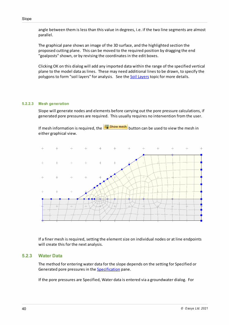
5.2.2.3 Mesh generation

Slope will generate nodes and elements before carrying out the pore pressure calculations, ifgenerated pore pressures are required. This usually requires no intervention from the user.

If mesh information is required, the button can be used to view the mesh ineither graphical view.

If a finer mesh is required, setting the element size on individual nodes or at line endpointswill create this for the next analysis.

5.2.3 Water Data

The method for entering water data for the slope depends on the setting for Specified orGenerated pore pressures in the Specification pane.

If the pore pressures are Specified, Water data is entered via a groundwater dialog. For

Slope

© O as ys Ltd. 2021 41

Generated pore pressures, material permeabilities must be defined (see Permeabilities ) ,and groundwater boundary conditions added to the model in the Graphical Input view.

5.2.3.1 Specified Pore Pressures

To enter or edit specified pore pressure, select Water Data on the ribbon Home tab or doubleclick the Water Data item in the Data Explorer, or one of its sub-items if any water profilesalready exist

The water data dialog shows a single water data specification at a time, so the availablespecifications are expanded in the Data Explorer so that any individual one may be edited.

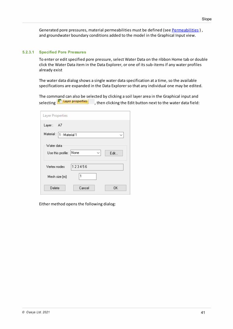
The command can also be selected by clicking a soil layer area in the Graphical input and

selecting , then clicking the Edit button next to the water data field:

Either method opens the following dialog:

Slope

© O as ys Ltd. 202142

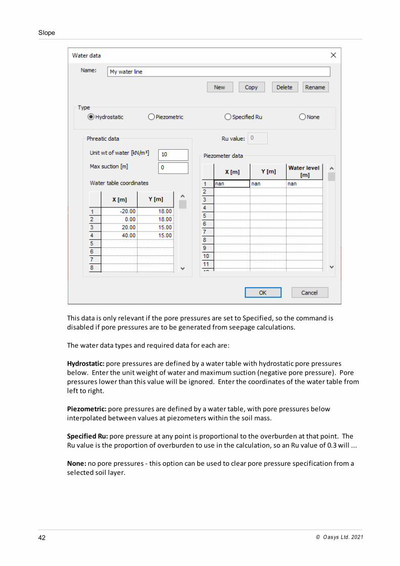
This data is only relevant if the pore pressures are set to Specified, so the command isdisabled if pore pressures are to be generated from seepage calculations.

The water data types and required data for each are:

Hydrostatic: pore pressures are defined by a water table with hydrostatic pore pressuresbelow. Enter the unit weight of water and maximum suction (negative pore pressure). Porepressures lower than this value will be ignored. Enter the coordinates of the water table fromleft to right.

Piezometric: pore pressures are defined by a water table, with pore pressures belowinterpolated between values at piezometers within the soil mass.

Specified Ru: pore pressure at any point is proportional to the overburden at that point. TheRu value is the proportion of overburden to use in the calculation, so an Ru value of 0.3 will ...

None: no pore pressures - this option can be used to clear pore pressure specification from aselected soil layer.

Slope

© O as ys Ltd. 2021 43

5.2.3.2 Generated Pore Pressures

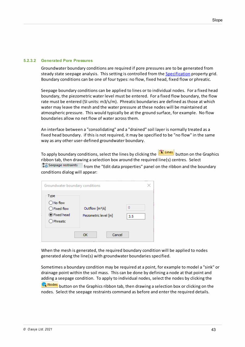
Groundwater boundary conditions are required if pore pressures are to be generated fromsteady state seepage analysis. This setting is controlled from the Specification property grid. Boundary conditions can be one of four types: no flow, fixed head, fixed flow or phreatic. Seepage boundary conditions can be applied to lines or to individual nodes. For a fixed headboundary, the piezometric water level must be entered. For a fixed flow boundary, the flowrate must be entered (SI units: m3/s/m). Phreatic boundaries are defined as those at whichwater may leave the mesh and the water pressure at these nodes will be maintained atatmospheric pressure. This would typically be at the ground surface, for example. No flowboundaries allow no net flow of water across them. An interface between a "consolidating" and a "drained" soil layer is normally treated as afixed head boundary. if this is not required, it may be specified to be "no flow" in the sameway as any other user-defined groundwater boundary.

To apply boundary conditions, select the lines by clicking the button on the Graphicsribbon tab, then drawing a selection box around the required line(s) centres. Select

from the "Edit data properties" panel on the ribbon and the boundaryconditions dialog will appear:

When the mesh is generated, the required boundary condition will be applied to nodesgenerated along the line(s) with groundwater boundaries specified. Sometimes a boundary condition may be required at a point, for example to model a "sink" ordrainage point within the soil mass. This can be done by defining a node at that point andadding a seepage condition. To apply to individual nodes, select the nodes by clicking the

button on the Graphics ribbon tab, then drawing a selection box or clicking on thenodes. Select the seepage restraints command as before and enter the required details.

Slope

© O as ys Ltd. 202144

5.2.4 Graphical Input

There are many data entry and editing options available in the Graphical Input view. Fordetails specific to each type of data entry, see the main topic for that data.

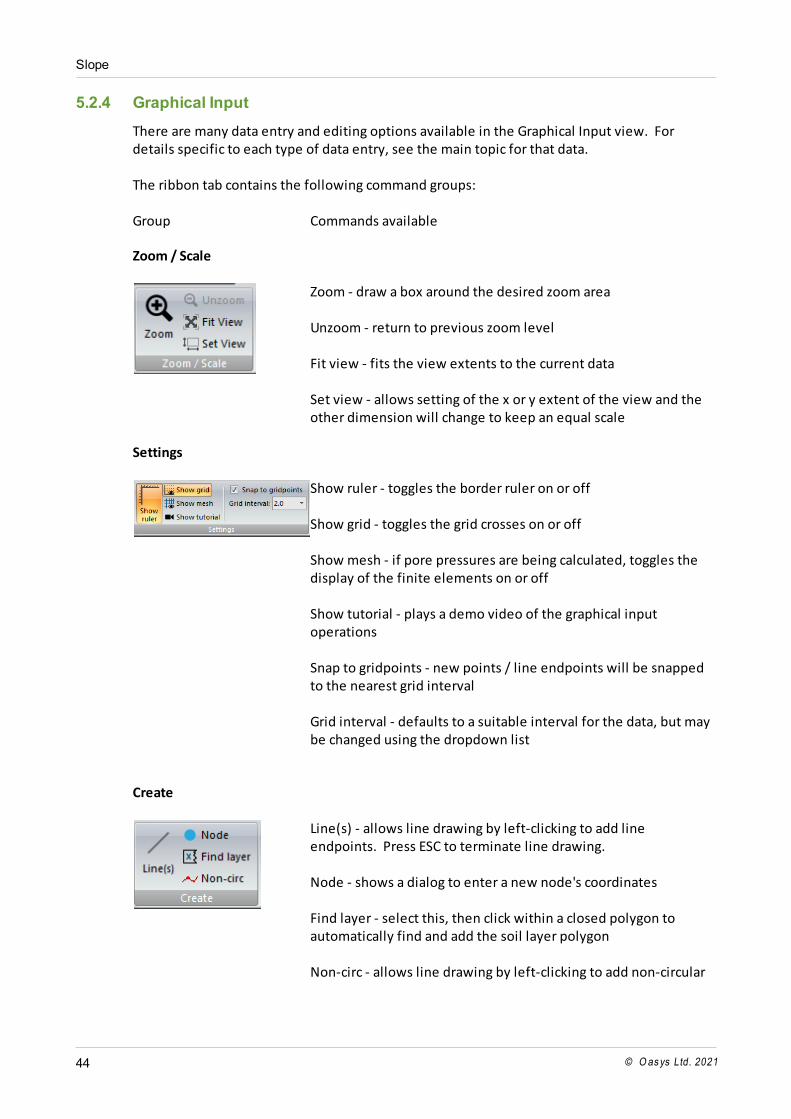
The ribbon tab contains the following command groups:

Group Commands available

Zoom / Scale

Zoom - draw a box around the desired zoom area

Unzoom - return to previous zoom level

Fit view - fits the view extents to the current data

Set view - allows setting of the x or y extent of the view and theother dimension will change to keep an equal scale

Settings

Show ruler - toggles the border ruler on or off

Show grid - toggles the grid crosses on or off

Show mesh - if pore pressures are being calculated, toggles thedisplay of the finite elements on or off

Show tutorial - plays a demo video of the graphical inputoperations

Snap to gridpoints - new points / line endpoints will be snappedto the nearest grid interval

Grid interval - defaults to a suitable interval for the data, but maybe changed using the dropdown list

Create

Line(s) - allows line drawing by left-clicking to add lineendpoints. Press ESC to terminate line drawing.

Node - shows a dialog to enter a new node's coordinates

Find layer - select this, then click within a closed polygon toautomatically find and add the soil layer polygon

Non-circ - allows line drawing by left-clicking to add non-circular

Slope

© O as ys Ltd. 2021 45

slip coordinates. Pressing the ESC key terminates drawing andclips the slip surface to the section boundaries. This will only beenabled if the non-circular slip type is selected.

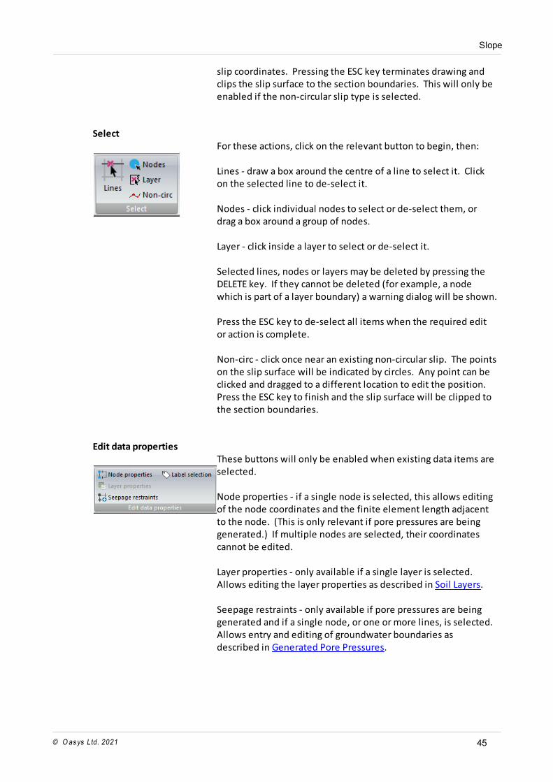
SelectFor these actions, click on the relevant button to begin, then:

Lines - draw a box around the centre of a line to select it. Clickon the selected line to de-select it.

Nodes - click individual nodes to select or de-select them, ordrag a box around a group of nodes.

Layer - click inside a layer to select or de-select it.

Selected lines, nodes or layers may be deleted by pressing theDELETE key. If they cannot be deleted (for example, a nodewhich is part of a layer boundary) a warning dialog will be shown.

Press the ESC key to de-select all items when the required editor action is complete.

Non-circ - click once near an existing non-circular slip. The pointson the slip surface will be indicated by circles. Any point can beclicked and dragged to a different location to edit the position. Press the ESC key to finish and the slip surface will be clipped tothe section boundaries.

Edit data propertiesThese buttons will only be enabled when existing data items areselected.

Node properties - if a single node is selected, this allows editingof the node coordinates and the finite element length adjacentto the node. (This is only relevant if pore pressures are beinggenerated.) If multiple nodes are selected, their coordinatescannot be edited.

Layer properties - only available if a single layer is selected. Allows editing the layer properties as described in Soil Layers.

Seepage restraints - only available if pore pressures are beinggenerated and if a single node, or one or more lines, is selected. Allows entry and editing of groundwater boundaries asdescribed in Generated Pore Pressures.

Slope

© O as ys Ltd. 202146

5.3 Slip Surface Definition

Selecting the Slip Surfaces command in either the Data Explorer or the ribbon home tab willeither:

open the Slip Surfaces property grid, for circular slips

open the Slip Surfaces tabular input, for non-circular slips

5.3.1 Circular Slip Definition

For circular slips, the Slip Surfaces command, on the Data Explorer or ribbon Home tab, eitherswitches focus to the Slip Surface property grid or re-opens it if it has been closed orminimised. If results already exist, they must be deleted using the Delete Results button onthe ribbon to enable editing of these settings. The fields in the property grid will appear asrequired by other settings, i.e. changing the radius type from "Defined radii" to "Tangent tostratum" will cause the remaining fields in that section to be re-drawn to show the relevantoptions for the tangent stratum.

Slope

© O as ys Ltd. 2021 47

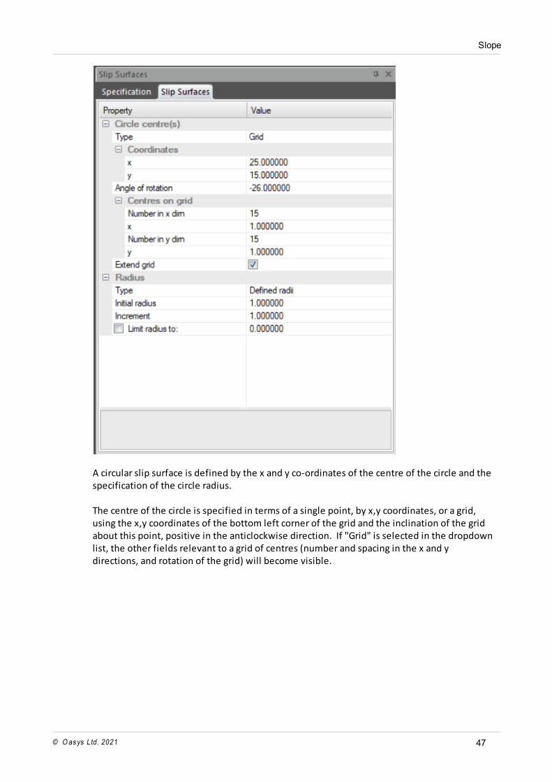
A circular slip surface is defined by the x and y co-ordinates of the centre of the circle and thespecification of the circle radius. The centre of the circle is specified in terms of a single point, by x,y coordinates, or a grid,using the x,y coordinates of the bottom left corner of the grid and the inclination of the gridabout this point, positive in the anticlockwise direction. If "Grid" is selected in the dropdownlist, the other fields relevant to a grid of centres (number and spacing in the x and ydirections, and rotation of the grid) will become visible.

Slope

© O as ys Ltd. 202148

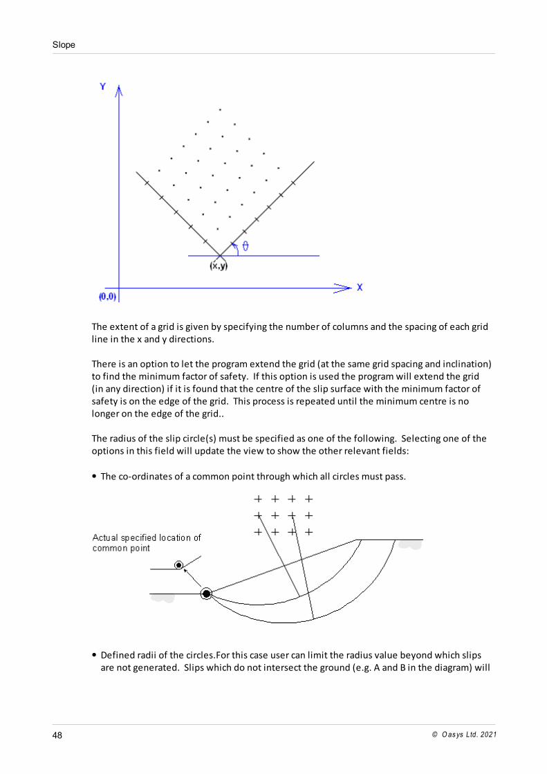
The extent of a grid is given by specifying the number of columns and the spacing of each gridline in the x and y directions. There is an option to let the program extend the grid (at the same grid spacing and inclination)to find the minimum factor of safety. If this option is used the program will extend the grid(in any direction) if it is found that the centre of the slip surface with the minimum factor ofsafety is on the edge of the grid. This process is repeated until the minimum centre is nolonger on the edge of the grid.. The radius of the slip circle(s) must be specified as one of the following. Selecting one of theoptions in this field will update the view to show the other relevant fields:

The co-ordinates of a common point through which all circles must pass.

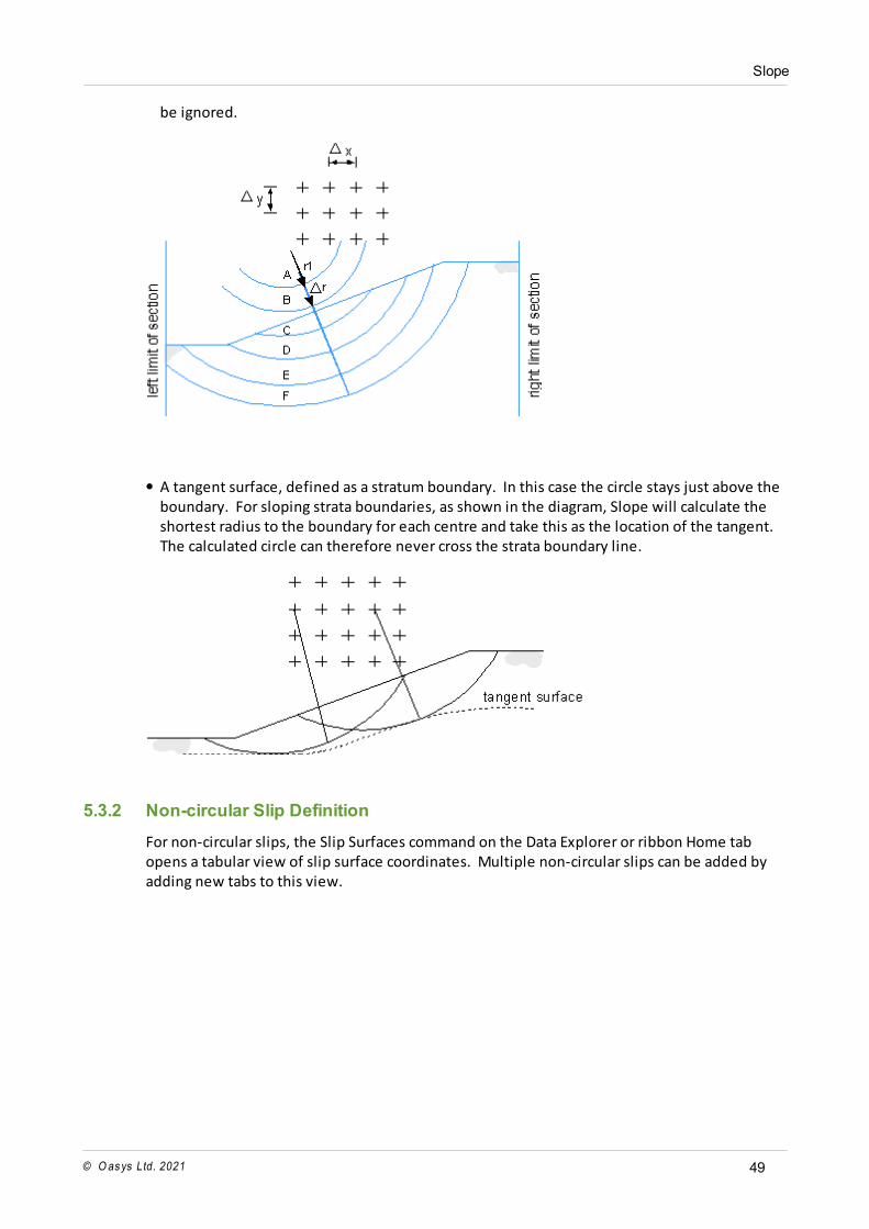
Defined radii of the circles.For this case user can limit the radius value beyond which slipsare not generated. Slips which do not intersect the ground (e.g. A and B in the diagram) will

Slope

© O as ys Ltd. 2021 49

be ignored.

A tangent surface, defined as a stratum boundary. In this case the circle stays just above theboundary. For sloping strata boundaries, as shown in the diagram, Slope will calculate theshortest radius to the boundary for each centre and take this as the location of the tangent. The calculated circle can therefore never cross the strata boundary line.

5.3.2 Non-circular Slip Definition

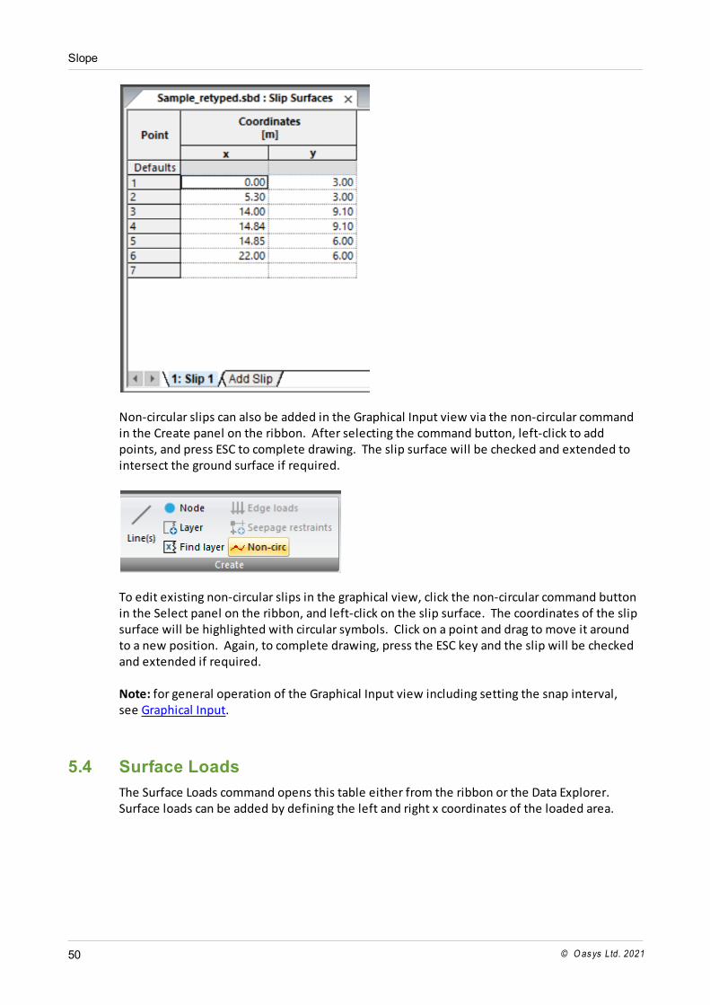
For non-circular slips, the Slip Surfaces command on the Data Explorer or ribbon Home tabopens a tabular view of slip surface coordinates. Multiple non-circular slips can be added byadding new tabs to this view.

Slope

© O as ys Ltd. 202150

Non-circular slips can also be added in the Graphical Input view via the non-circular commandin the Create panel on the ribbon. After selecting the command button, left-click to addpoints, and press ESC to complete drawing. The slip surface will be checked and extended tointersect the ground surface if required.

To edit existing non-circular slips in the graphical view, click the non-circular command buttonin the Select panel on the ribbon, and left-click on the slip surface. The coordinates of the slipsurface will be highlighted with circular symbols. Click on a point and drag to move it aroundto a new position. Again, to complete drawing, press the ESC key and the slip will be checkedand extended if required.

Note: for general operation of the Graphical Input view including setting the snap interval,see Graphical Input.

5.4 Surface Loads

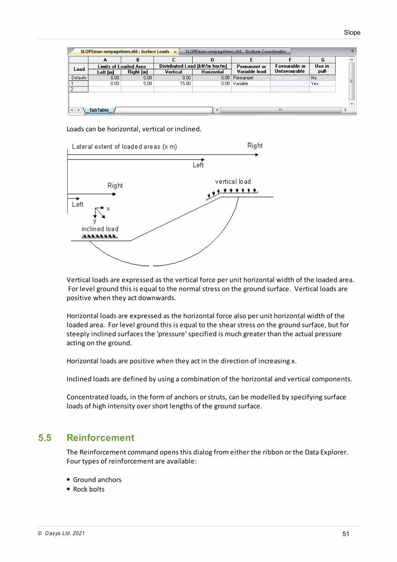
The Surface Loads command opens this table either from the ribbon or the Data Explorer. Surface loads can be added by defining the left and right x coordinates of the loaded area.

Slope

© O as ys Ltd. 2021 51

Loads can be horizontal, vertical or inclined.

Vertical loads are expressed as the vertical force per unit horizontal width of the loaded area. For level ground this is equal to the normal stress on the ground surface. Vertical loads arepositive when they act downwards. Horizontal loads are expressed as the horizontal force also per unit horizontal width of theloaded area. For level ground this is equal to the shear stress on the ground surface, but forsteeply inclined surfaces the 'pressure' specified is much greater than the actual pressureacting on the ground. Horizontal loads are positive when they act in the direction of increasing x. Inclined loads are defined by using a combination of the horizontal and vertical components. Concentrated loads, in the form of anchors or struts, can be modelled by specifying surfaceloads of high intensity over short lengths of the ground surface.

5.5 Reinforcement

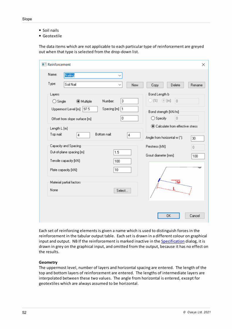
The Reinforcement command opens this dialog from either the ribbon or the Data Explorer.Four types of reinforcement are available:

Ground anchors

Rock bolts

Slope

© O as ys Ltd. 202152

Soil nails

Geotextile The data items which are not applicable to each particular type of reinforcement are greyedout when that type is selected from the drop-down list.

Each set of reinforcing elements is given a name which is used to distinguish forces in thereinforcement in the tabular output table. Each set is drawn in a different colour on graphicalinput and output. NB If the reinforcement is marked inactive in the Specification dialog, it isdrawn in grey on the graphical input, and omitted from the output, because it has no effect onthe results. GeometryThe uppermost level, number of layers and horizontal spacing are entered. The length of thetop and bottom layers of reinforcement are entered. The lengths of intermediate layers areinterpolated between these two values. The angle from horizontal is entered, except forgeotextiles which are always assumed to be horizontal.

Slope

© O as ys Ltd. 2021 53

CapacityOut-of-plane spacing, tensile capacity and plate capacity (if applicable) are entered. Platecapacity must be at least 50% of tensile capacity. The tensile capacity should represent theallowable capacity if BS8081 is used or ultimate capacity if EC3 is used. Bond details and prestressBond length can be entered for ground anchors and rock bolts Type B. Soil nails are assumedto be 100% bonded along their length.Bond strength can be specified or calculated from effective stress.Prestress can be entered for ground anchors and can not exceed the tensile capacity. Material partial factorsClick the Select button to set material partial factors for each set of reinforcing elements. Thisis optional - all partial factors will be set to 1.0 if no selection is made.

See Reinforcement Calculations for details of the calculations used to derive the forces andmoments from reinforcing elements.

5.6 Importing previous format Slope files

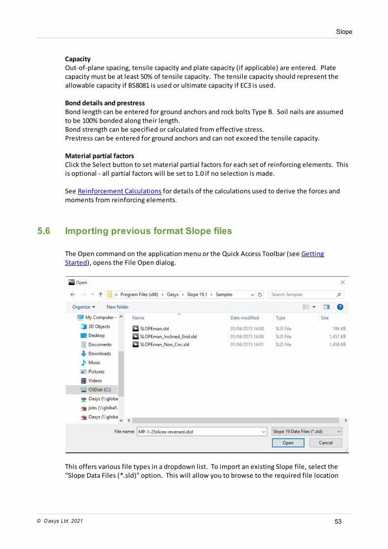
The Open command on the application menu or the Quick Access Toolbar (see GettingStarted), opens the File Open dialog.

This offers various file types in a dropdown list. To import an existing Slope file, select the"Slope Data Files (*.sld)" option. This will allow you to browse to the required file location

Slope

© O as ys Ltd. 202154

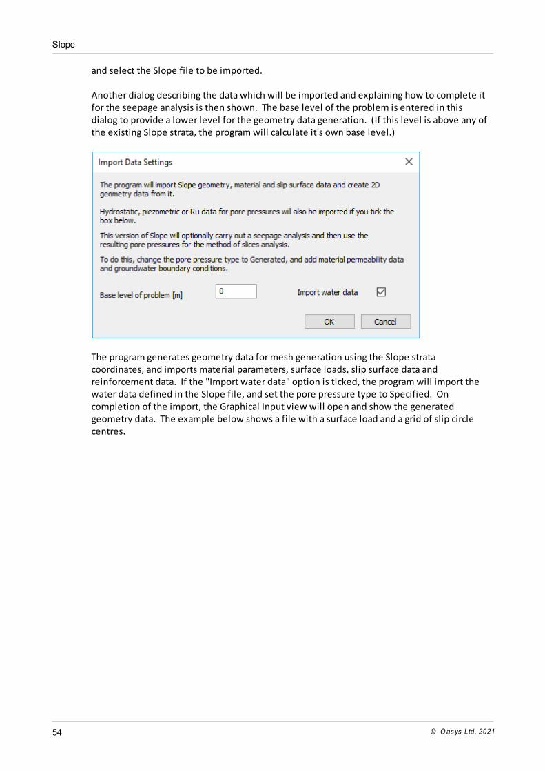
and select the Slope file to be imported. Another dialog describing the data which will be imported and explaining how to complete itfor the seepage analysis is then shown. The base level of the problem is entered in thisdialog to provide a lower level for the geometry data generation. (If this level is above any ofthe existing Slope strata, the program will calculate it's own base level.)

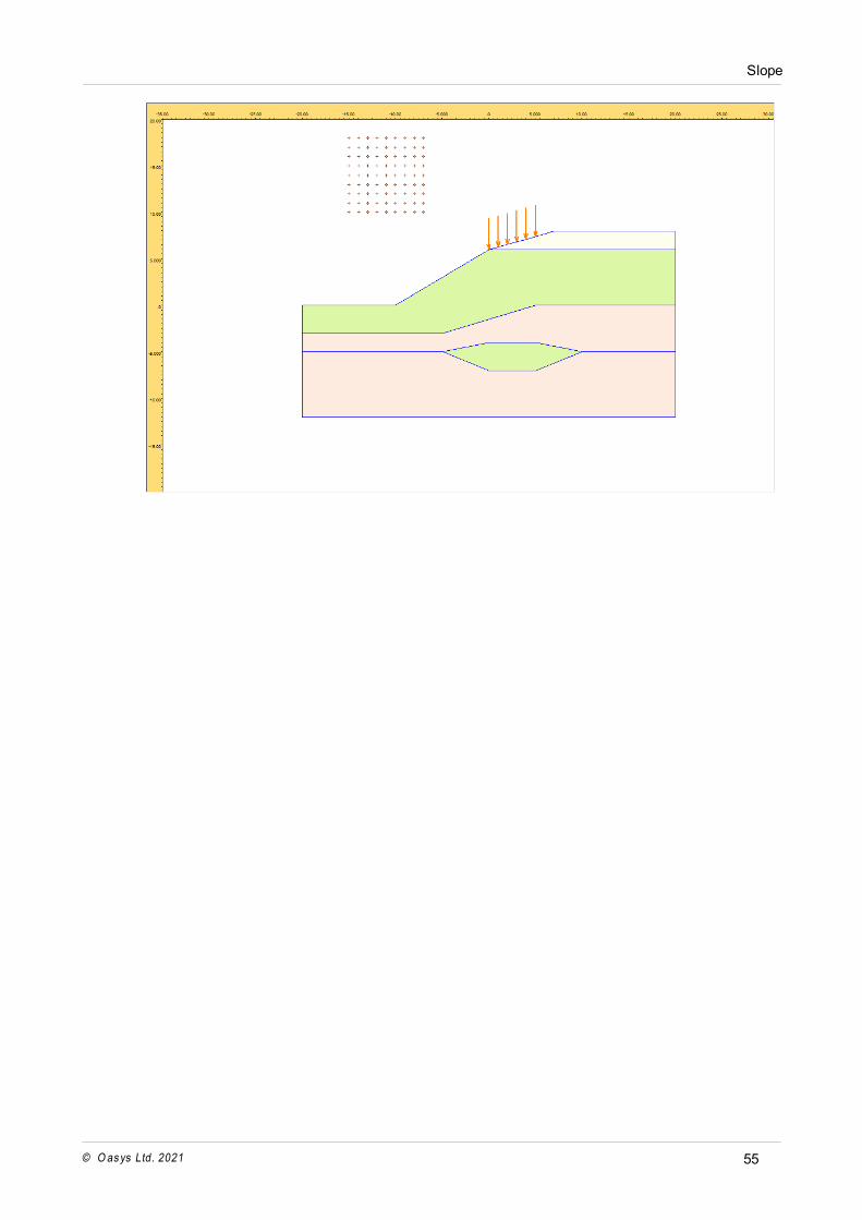
The program generates geometry data for mesh generation using the Slope stratacoordinates, and imports material parameters, surface loads, slip surface data andreinforcement data. If the "Import water data" option is ticked, the program will import thewater data defined in the Slope file, and set the pore pressure type to Specified. Oncompletion of the import, the Graphical Input view will open and show the generatedgeometry data. The example below shows a file with a surface load and a grid of slip circlecentres.

Slope

© O as ys Ltd. 2021 55

Part VI

Slope

© O as ys Ltd. 2021 57

6 Analysis and Results

6.1 Analysis and Data Checking

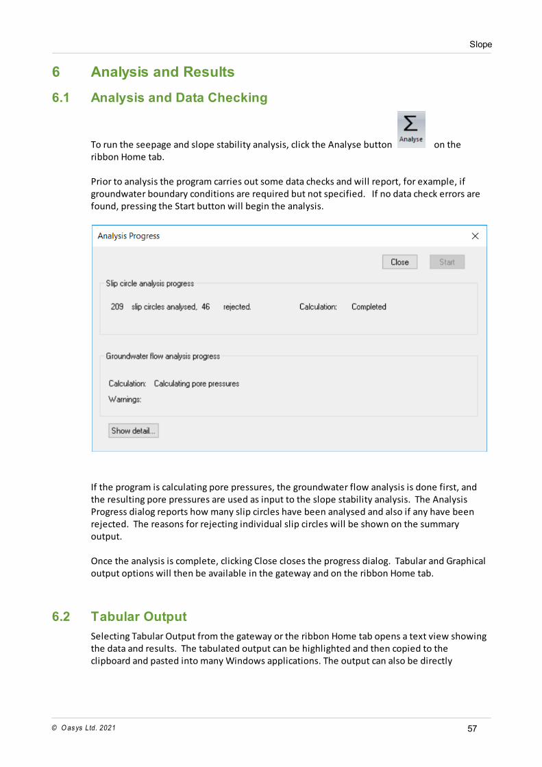
To run the seepage and slope stability analysis, click the Analyse button on theribbon Home tab. Prior to analysis the program carries out some data checks and will report, for example, ifgroundwater boundary conditions are required but not specified. If no data check errors arefound, pressing the Start button will begin the analysis.

If the program is calculating pore pressures, the groundwater flow analysis is done first, andthe resulting pore pressures are used as input to the slope stability analysis. The AnalysisProgress dialog reports how many slip circles have been analysed and also if any have beenrejected. The reasons for rejecting individual slip circles will be shown on the summaryoutput. Once the analysis is complete, clicking Close closes the progress dialog. Tabular and Graphicaloutput options will then be available in the gateway and on the ribbon Home tab.

6.2 Tabular Output

Selecting Tabular Output from the gateway or the ribbon Home tab opens a text view showingthe data and results. The tabulated output can be highlighted and then copied to theclipboard and pasted into many Windows applications. The output can also be directly

Slope

© O as ys Ltd. 202158

exported to various text or HTML formats by selecting Export from the Application buttonmenu.

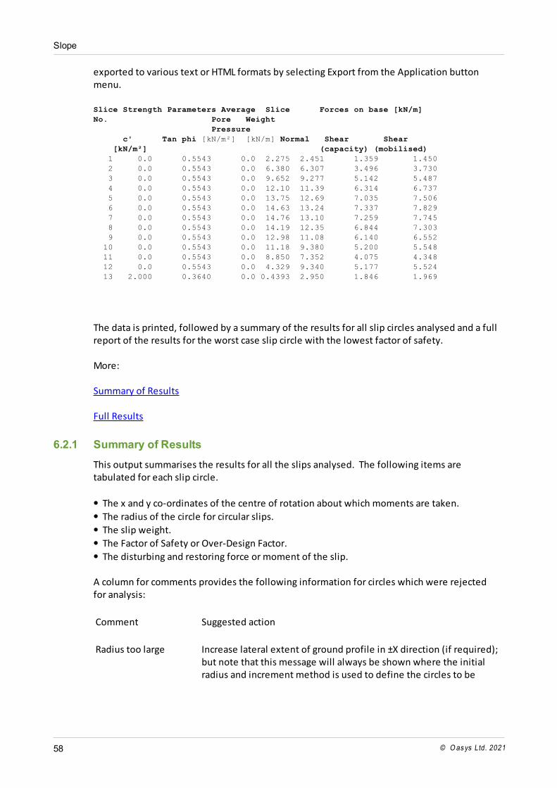
Slice Strength Parameters Average Slice Forces on base [kN/m]

No. Pore Weight

Pressure

c' Tan phi [kN/m²] [kN/m] Normal Shear Shear

[kN/m²] (capacity) (mobilised)

1 0.0 0.5543 0.0 2.275 2.451 1.359 1.450

2 0.0 0.5543 0.0 6.380 6.307 3.496 3.730

3 0.0 0.5543 0.0 9.652 9.277 5.142 5.487

4 0.0 0.5543 0.0 12.10 11.39 6.314 6.737

5 0.0 0.5543 0.0 13.75 12.69 7.035 7.506

6 0.0 0.5543 0.0 14.63 13.24 7.337 7.829

7 0.0 0.5543 0.0 14.76 13.10 7.259 7.745

8 0.0 0.5543 0.0 14.19 12.35 6.844 7.303

9 0.0 0.5543 0.0 12.98 11.08 6.140 6.552

10 0.0 0.5543 0.0 11.18 9.380 5.200 5.548

11 0.0 0.5543 0.0 8.850 7.352 4.075 4.348

12 0.0 0.5543 0.0 4.329 9.340 5.177 5.524

13 2.000 0.3640 0.0 0.4393 2.950 1.846 1.969

The data is printed, followed by a summary of the results for all slip circles analysed and a fullreport of the results for the worst case slip circle with the lowest factor of safety. More: Summary of Results Full Results

6.2.1 Summary of Results

This output summarises the results for all the slips analysed. The following items aretabulated for each slip circle.

The x and y co-ordinates of the centre of rotation about which moments are taken.

The radius of the circle for circular slips.

The slip weight.

The Factor of Safety or Over-Design Factor.

The disturbing and restoring force or moment of the slip. A column for comments provides the following information for circles which were rejectedfor analysis:

Comment Suggested action

Radius too large Increase lateral extent of ground profile in ±X direction (if required);but note that this message will always be shown where the initialradius and increment method is used to define the circles to be

Slope

© O as ys Ltd. 2021 59

analysed, unless a limiting radius is also defined.

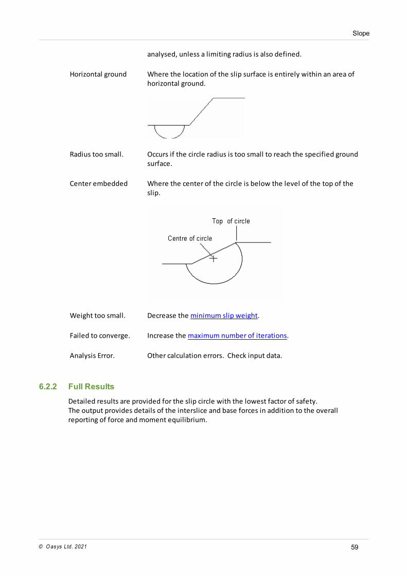
Horizontal ground

Where the location of the slip surface is entirely within an area ofhorizontal ground.

Radius too small. Occurs if the circle radius is too small to reach the specified groundsurface.

Center embedded

Where the center of the circle is below the level of the top of theslip.

Weight too small. Decrease the minimum slip weight.

Failed to converge. Increase the maximum number of iterations.

Analysis Error. Other calculation errors. Check input data.

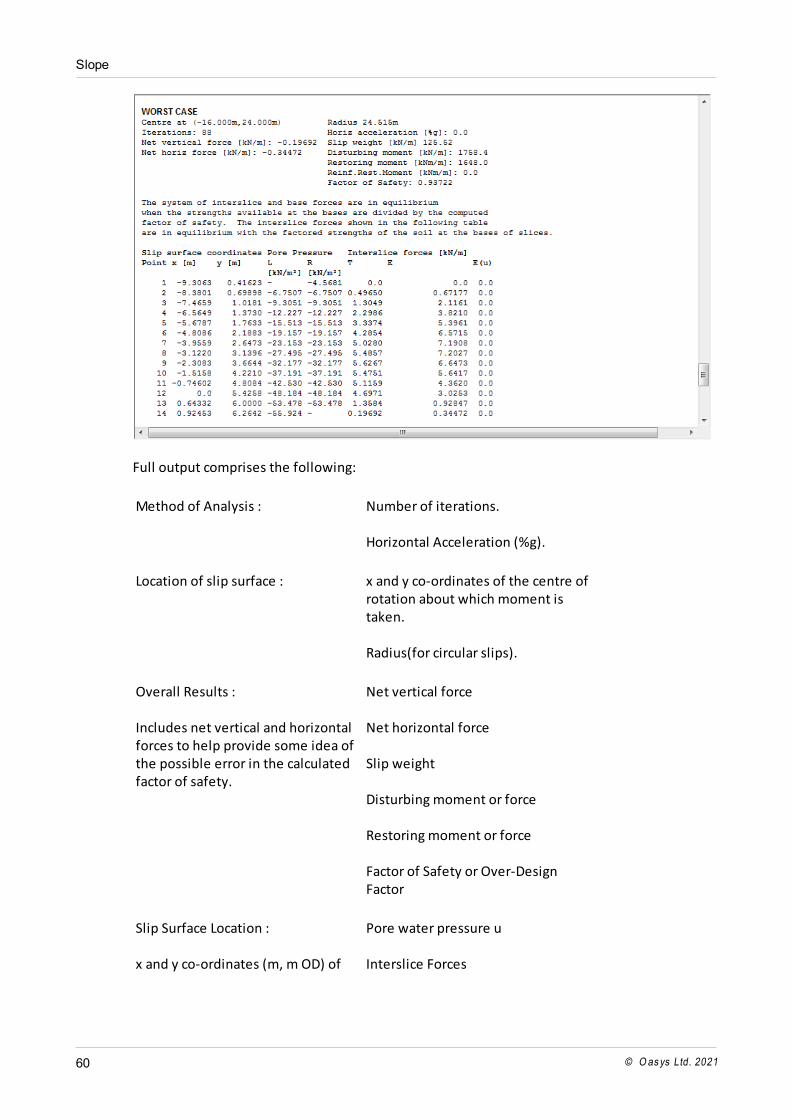
6.2.2 Full Results

Detailed results are provided for the slip circle with the lowest factor of safety.The output provides details of the interslice and base forces in addition to the overallreporting of force and moment equilibrium.

Slope

© O as ys Ltd. 202160

Full output comprises the following:

Method of Analysis : Number of iterations. Horizontal Acceleration (%g).

Location of slip surface : x and y co-ordinates of the centre ofrotation about which moment istaken. Radius(for circular slips).

Overall Results : Includes net vertical and horizontalforces to help provide some idea ofthe possible error in the calculatedfactor of safety.

Net vertical force Net horizontal force Slip weight Disturbing moment or force Restoring moment or force Factor of Safety or Over-DesignFactor

Slip Surface Location : x and y co-ordinates (m, m OD) of

Pore water pressure u Interslice Forces

Slope

© O as ys Ltd. 2021 61

the base of the LEFT side of eachslice are used to define the locationof the slip surface.

Vertical Shear T Horizontal Normal E Horizontal Water Pressure E(u)

Slices : Slices are numbered from left toright.

Strength Parameters Cohesion c' tan ? ' (degrees) Pore Pressure Slice weight Forces on the base Normal N Shear S

General Slice Information : Surface Loads - vertical andhorizontal Water pressure on ground surface -Vertical and horizontal

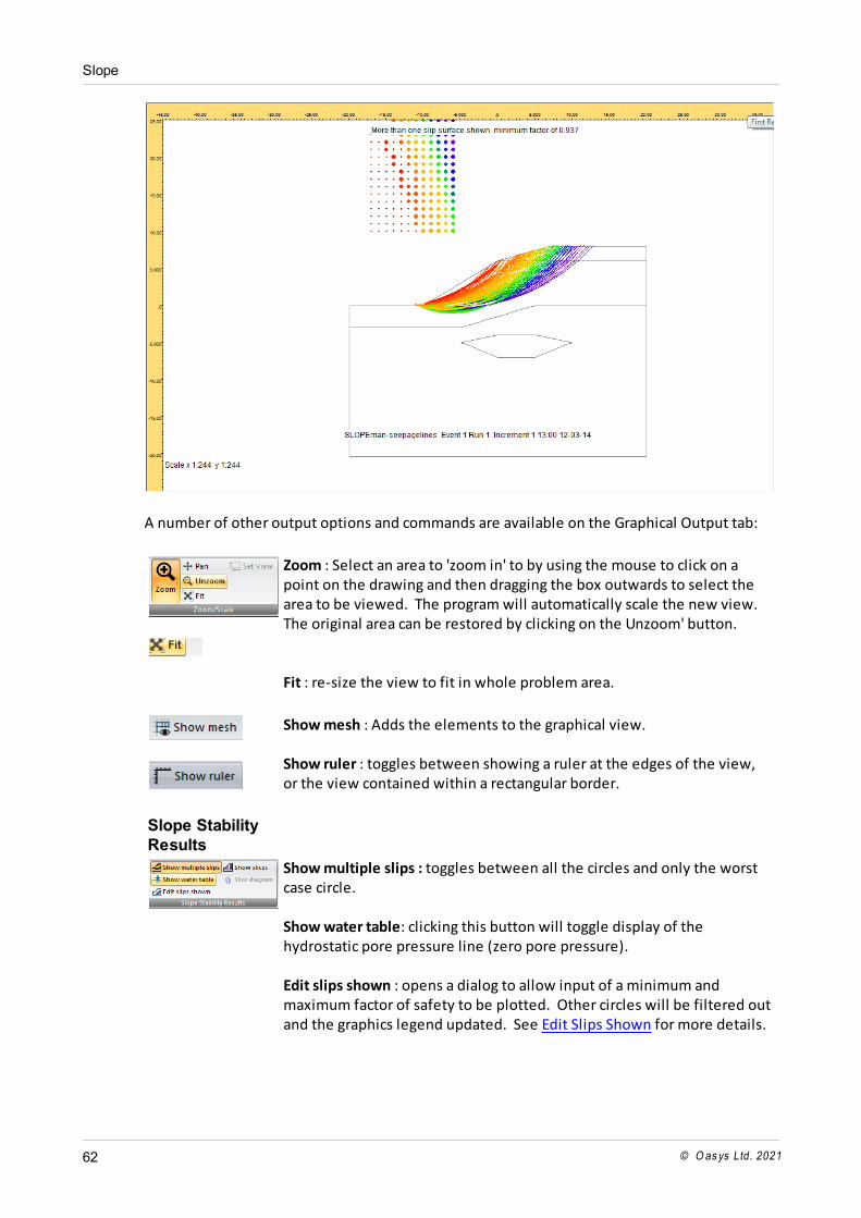
6.3 Graphical Output

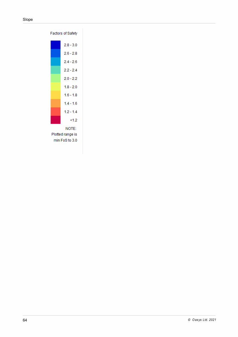
The ribbon command or the Gateway item "Graphical output" open the graphical output view. The program defaults to show all slip circles with a factor of safety below 3, or, if there are nocircles with FoS less than 3, any with less than 10. The slip circles will be coloured inaccordance with their factor of safety. To change the currently plotted circle when a grid of centres has been analysed, move thecursor into the grid and right-click on the required centre. The circle with the lowest factor ofsafety for that centre will be plotted.

Slope

© O as ys Ltd. 202162

A number of other output options and commands are available on the Graphical Output tab:

Zoom : Select an area to 'zoom in' to by using the mouse to click on apoint on the drawing and then dragging the box outwards to select thearea to be viewed. The program will automatically scale the new view. The original area can be restored by clicking on the Unzoom' button. Fit : re-size the view to fit in whole problem area.

Show mesh : Adds the elements to the graphical view. Show ruler : toggles between showing a ruler at the edges of the view,or the view contained within a rectangular border.

Slope StabilityResults

Show multiple slips : toggles between all the circles and only the worstcase circle.

Show water table: clicking this button will toggle display of thehydrostatic pore pressure line (zero pore pressure).

Edit slips shown : opens a dialog to allow input of a minimum andmaximum factor of safety to be plotted. Other circles will be filtered outand the graphics legend updated. See Edit Slips Shown for more details.

Slope

© O as ys Ltd. 2021 63

Show slices : draws the slices within the slipping mass of soil. If only onecircle is plotted, the Slice diagram command then becomes available,and clicking it followed by any slice on the view opens a separatewindow showing the slice force polygon.

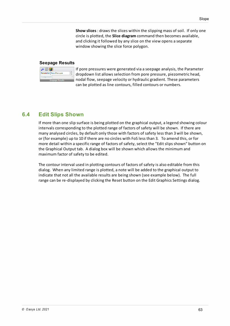
Seepage Results

If pore pressures were generated via a seepage analysis, the Parameterdropdown list allows selection from pore pressure, piezometric head,nodal flow, seepage velocity or hydraulic gradient. These parameterscan be plotted as line contours, filled contours or numbers.

6.4 Edit Slips Shown

If more than one slip surface is being plotted on the graphical output, a legend showing colourintervals corresponding to the plotted range of factors of safety will be shown. If there aremany analysed circles, by default only those with factors of safety less than 3 will be shown,or (for example) up to 10 if there are no circles with FoS less than 3. To amend this, or formore detail within a specific range of factors of safety, select the "Edit slips shown" button onthe Graphical Output tab. A dialog box will be shown which allows the minimum andmaximum factor of safety to be edited. The contour interval used in plotting contours of factors of safety is also editable from thisdialog. When any limited range is plotted, a note will be added to the graphical output toindicate that not all the available results are being shown (see example below). The fullrange can be re-displayed by clicking the Reset button on the Edit Graphics Settings dialog.

Slope

© O as ys Ltd. 202164

Part VII

Slope

© O as ys Ltd. 202166

7 Programming Interface

Slope now includes a COM (Component Object Model) interface. This enables externalprograms to pass information and instructions to and from the program, via a "data object". COM objects can be used by many other programs, including Excel, MATLAB and Python. Slope 21.0 has a lot of code in common with the Oasys Geotechnical finite element programSafe, so the COM interface library is shared between them, and the COM object name andreferences are based on Safe.Excel(VBA) and Python sample files to demonstrate the use of the COM API is provided withthe program. They are installed in the folder C:\Program Files\Oasys\Slope\Samples.

Using the COM interface in Excel

Click the Developer tab and click on the "Visual Basic" button to open the VBA window. In theVBA window, click on "Tools" in the menu bar and select "References". Check the list for theentry "safeLib" and make sure it is ticked. If the type library is not listed, add it as a new reference. The file is "safe.tlb" and is availablein the program installation folder.

Using the COM interface in Python

In a Python script, or the interactive window, create the COM object as follows:Import win32com.clientslp = win32com.client.Dispatch(“safeLib.SafeAuto”)The first line imports the Python library which supports COM. The second line creates theCOM object and associates it with the published COM interface, which has the nameSafeAuto, contained in the type library safeLib.

7.1 COM function listing

The following functions are available in the COM interface. Note that the first function that

should be used is ‘Open’. Functions return either a number value (e.g. node level or

displacement) or an integer return code so that success or failure can be tested if required.

The Analyse function needs to be run before using any of the functions which retrieve results,

to ensure that there are results available.

The units of the various parameters are as defined in the current data file. The default unit

system is kN for force, metres for length and millimetres for displacement.

Show

This function has no input/output variables. It opens Slope and shows the main programwindow.

Open(String sPathName) - returns an integer

Slope

© O as ys Ltd. 2021 67

This function opens a saved file. sPathName is a string giving the file path. If the file isopened successfully the function will return 0, or if it was unsuccessful it will return -1.

Analyse(Integer iStage) – returns an integer

This is a function instructing Slope to analyse the currently open file, up to the stage numberiStage.

Save – returns an integer

Saves the currently open file.

SaveAs(String sPathName) – returns an integer

Saves the currently open file with a different name.

Close – returns an integer

Closes the current file.

Material functions

GetNumMaterial – returns the number of materials as an integer

CreateMaterial(String name) – creates a blank material record with the name specified

SetUnitWtAbove(integer imat, float value) – sets material “imat”’s unit weight above thewater table to the value specified

SetUnitWtBelow(integer imat, float value) – sets material “imat”’s unit weight below thewater table to the value specified

SetDrainageType(integer imat, integer type) – sets the material imat to be undrained, drainedwith linear strength, drained with a power curve or hyperbolic strength relationship (values 0to 3 respectively)

SetPhi(integer imat, float value) – sets the friction angle of the material

SetCohesion(integer imat, float value) – sets the cohesion value for the material

SetCohesionRefLevel(integer imat, float value) – sets the level at which the cohesion valueapplies. This need not be specified unless the material has varying cohesion with depth.

SetCohesionGradient(integer imat, float value) – sets the gradient of cohesion. Need not bespecified if the material has constant cohesion.

SetPowerCurveParams(integer imat, float value1, float value2) – sets the values of the two

Slope

© O as ys Ltd. 202168

parameters for use in drained materials with a power curve relationship (see MaterialProperties for details)

SetCupRatio(integer imat, float value) – sets the Cu/p ratio for an undrained material. If thisis set as well as the cohesion gradient, the lower of the two values will be used.

GetUnitWtAbove(integer imat) – returns the unit weight above the water table

GetUnitWtBelow(integer imat) – returns the unit weight below the water table

GetDrainageType(integer imat) – returns the material drainage setting

GetPhi(integer imat) – returns the friction angle of the material

GetCohesion(integer imat) – returns the cohesion value for the material

GetCohesionRefLevel(integer imat) – returns the level at which the cohesion value applies

GetCohesionGradient(integer imat) – returns the gradient of cohesion.

GetPowerCurveParamA(integer imat) – returns the first parameter for use in drainedmaterials with a power curve relationship (see manual for details)

GetPowerCurveParamB(integer imat) – returns the second parameter for use in drainedmaterials with a power curve relationship (see manual for details)

GetCupRatio(integer imat) – returns the Cu/p ratio for an undrained material

Geometry functions

DefineCutPlane(float xmin, float ymin, float xmax, float ymax) – define a vertical plane from(xmin, ymin) to (xmax, ymax) along which to cut a 3D surface. The 3D surface can be importedfrom a TIN surface contained in an XML file.

SetStraightnessTol(float tol) – sets a straightness tolerance, in degrees. Two adjacent lines ona polyline will be treated as one line (middle point will be omitted) if their angles are withinthis tolerance of each other, i.e. if the lines are near-parallel.

ImportXml(String path) – reads the specified XML file, imports the 3D data contained in it, andgenerates polylines where the 3D surface cuts the previously specified cutting plane

SetStratum(integer is, string name, string matname) – creates a “blank” stratum (no pointsyet) with the specified name. The integer should be the stratum number. The first stratumshould have the number 1.

SetStratumPoint(integer is, integer ip, float xp, float yp) – set point ‘ip’ in stratum ‘is’ to thevalue (xp, yp)

NumStrata – returns the number of strata as an integer

Slope

© O as ys Ltd. 2021 69

GetStratumPointX(integer is, integer ip) - returns the X coordinate of point 'ip' in stratum'is' (zero-based point counter)

GetStratumPointY(integer is, integer ip) - returns the Y coordinate of point 'ip' in stratum'is' (zero-based point counter)

Create2DSection() - creates a 2D section from the existing strata information

NumNodes() - returns the number of "nodes" (vertices of the soil layer polygons)

NodeX(integer inode) - returns the X coordinate of node 'inode' (1-based node counter)

NodeY(integer inode) - returns the Y coordinate of node 'inode' (1-based node counter)

SetNodeX(integer inode, float xnode) - sets the X coordinate of node inode. Caution requirednot to set invalid data.

SetNodeY(integer inode, float ynode) - sets the Y coordinate of node inode.

Water data functions

SetWaterTable(integer iref, float dX1, float fY1, float dX2, float dY2) - sets water table "iref" tohave 2 points at (dX1, dY1) and (dX2, dY2). "iref" is a 1-based counter. If "iref" equals zero oris greater than the current number of water tables, a new one will be added.

SetWaterPoint(integer iref, float dX, float dY) - inserts the point (dX, dY) in x-coordinate orderinto the water table "iref" (1-based counter)

SetStratumWater(integer istratum, integer iref) - sets stratum "istratum" to have the watertable "iref"

Slip circle functions

SetSingleOrGrid(integer i) – set 0 for a single circle or 1 for a grid of circle centres

SetPosition(float x, float y) – Coordinates of lower left corner of grid

SetNumXCentresAndSpacing(integer nx, float dx) – set the grid to have nx centres in the xdirection at dx distance apart

SetNumYCentresAndSpacing(integer ny, float dy) – set the grid to have ny centres in the ydirection at dy distance apart

SetGridAngle(float angle) – set the grid to an angle of inclination (positive in theanticlockwise direction from the bottom left of the grid)

SetRadSpec(integer itype) – which radius option - set

Slope

© O as ys Ltd. 202170

SetCommonPoint(float x, float y) – set the coordinates of the common point through which allslip circles will pass

SetRadius(float rad) – set the initial radius

SetRadInc(float rinc) – set the radius increment. Slip circles will be increased from the initialradius by this increment, until the maximum possible radius has been analysed

Results functions

CriticalCircleRef – returns an integer corresponding to the position, in the results set, of thecircle with the lowest factor of safety

GetMinFoS(integer iref) – returns the factor of safety. Iref should be the previously obtainedcritical circle reference.

GetCriticalCentreX(integer iref) – returns the x coordinate of the circle centre iref

GetCriticalCentreY(integer iref) – returns the y coordinate of the circle centre iref

GetCriticalCircleRadius(integer iref) – returns the radius of the slip circle iref

Load functions

NumLoads - returns the number of loads

GetXminLoad(integer iload) - returns the minimum X coordinate of load 'iload' (1-based loadcounter)

GetXmaxLoad(integer iload) - returns the maximum X coordinate of load 'iload'

SetXminLoad(integer iload, float xmin) - sets the minimum X coordinate of load 'iload'

SetXmaxLoad(integer iload, float xmax) - sets the maximum X coordinate of load 'iload'

SetVertLoadIntensity(integer iload, float vP) - sets the vertical load intensity of load 'iload' to'vP'

Reinforcement functions

SetReinfActive(bool b) - set reinforcement active if b is non-zero, or inactive if b is zero

Part VIII

Slope

© O as ys Ltd. 202172

8 References

BSI (2010 / 2011). Code of practice for strengthened/reinforced soils and other fills. BS 8006-1:2010 and BS 8006-2:2011. Bishop A W (1955). The use of the Slip Circle in the Stability Analysis of Earth Slopes. Géotechnique Vol.5 No.1 pp 7-17.

Fredlund D G and Krahn J (1977). Comparison of slope stability methods of analysis. CanadianGeotechnical Journal Vol 14 p.429-439. Janbu N (1957). Earth Pressures and Bearing Capacity Calculations by Generalized Procedure ofSlices. Proc. 4th International Conference Soil Mech. Fdn. Engng. Vol.2 pp 207-212.

Morgenstern N R and Price V E (1965) The Analysis of the Stability of General Slip Surfaces. Geotechnique, Vol. 15, pp. 79-93. Nash D (1987). A comparative review of limit equilibrium methods of stability analysis inslope stability. Anderson and Richards (eds), John Wiley & Sons. Spencer E (1967). A Method of Analysis of Embankments ensuring Parallel Interslice Forces. Géotechnique Vol.77 pp 11.26. Whitman R V, and Bailey W A (1967). Use of Computers for Slope Stability Analysis. International Soil Mech. Fdns. Div. Am. Soc, Civ. Engrs Vol.93 SM4 pp 475 - 498.

Zhu D Y et al (2005) A concise algorithm for computing the factor of safety using theMorgenstern-Price method. Canadian Geotechnical Journal Vol. 42 p.272-278.

Endnotes 2... (after index)

73

© Oasys Ltd. 2021

Back Cover