Simulation of vortex sheet roll-up by vortex methods

JOURNAL OF COMPUTATIONAL PHYSICS 80, l-16 (1989)

Simulation of Vortex Sheet Roil-up by Vortex Methods

GRBTAR TRYGGVASON Department of Mechanical Engineering and Applied Mechanics,

The University of Michigan, Ann Arbor, Michigan 48109

Received February 20, 1987; revised February 16, 1988

The vortex sheet roll-up characteristic of large amplitude Kelvin-Helmholtz instability is simulated by vortex-in-cell methods and a vortex blob method. Both methods regularize the problem and prevent the irregular motion found in many previous simulations. The regularization properties of the methods are compared and discussed. 0 1989 Academic Press, Inc.

1. INTRODUCTION

The idealization of a shear layer as a vortex sheet separating two regions of potential flow is an old and often used approximation. Although this model has an appealing simplicity, complete understanding of its properties has not yet been achieved, in spite of the considerable attention the model has received. Analytical investigations are limited to linear or weakly nonlinear studies of the small amplitude stage, so numerical methods were applied quite early to this problem. Rosenhead [27] modelled the vortex sheet as a row of point vortices and was able to simulate the motion up to relatively large amplitudes. Rosenhead’s calculation, done in the precomputer years of the early thirties, used only a modest number of points and a large time step. Nevertheless, the calculations clearly showed the expected roll-up of the vortex sheet. When computers became available, these calculations were repeated with a larger number of points by Birkhoff and Fisher [9], who found that instead of a more accurate solution, the increased number of points led to irregular motion of the points and early deterioration of the computations. Later efforts by other investigators confirmed these disappointing result. Birkhoff [S] pointed out that the vortex sheet problem does not contain a physical mechanism that stabilizes small-scale motion and that the model is subject to a short wave instability with the growth rate increasing with wave number. The problem is therefore formally ill-posed, and extreme care must be taken not to introduce short wave disturbances as the resolution is increased. Finite numerical resolution, however, provides an artifical short wave stabilitzation, and since early calculations generally used rather modest resolution, this rapid growth of short waves during the initial stages of the evolution was not as serious of a problem as one might suspect. However, even when calculations proceeded beyond the linear

OO21-9991/89 $3.00 Copyright (0 1989 by Academic Press, Inc.

All nghtn of reproduction in any form reserved.

2 GRhTAR TRYGGVASON

stage, the vortices close to the center of the roll-up eventually moved in an irregular manner. During the last decade or so, studies by several investigators have shed considerable light on the problem. Careful asymptotic and numerical studies (see, e.g., Moore [23], Meiron et al. t-213, Krasny [ 171) have provided strong evidence for the formation of a curvature singularity of the sheet after a finite, but short, time, and before any roll-up has taken place.

The consequences of the singularity formation both for the relevance of the model to physical phenomena and for numerical simulations remain somewhat uncertain at the present time. Some investigators seem to believe that the singularity limits the usefulness of the model, and it should therefore be abandoned. Another possibility is that after the critical time (when the singularity forms) a “weak” solution of physical relevance still exists, which may be obtained with the proper regularization. Weak solutions to the Euler equations are well known, point vortices perhaps being the one that first comes to mind. Indeed, most “classical” solutions are “weak” in the sense that although the velocity may be continuous, the vorticity is not. Various methods have been suggested to regularize the vortex sheet problem, including replacing the innermost parts of the rolled up vortex by a single large vortex [22], smoothing the vortex sheet strength by redistributing the interface points [14], and replacing the point vortices by vortex blobs [ 111. Most of these modifications allow the computations to continue past the critical time and to predict the development of a smooth, rolled-up vortex, although some irregularities often appear at the end of the calculations. For further discussions on weak solutions to the vortex sheet problem, and the relation between solutions to a “regularized” model and the original equations, the reader is referred to Krasny C181.

In this paper we report on some recent studies using the blob regularization. We compare simulations of a large amplitude Kelvin-Helmholtz instability by the well- known vortex-in-cell (VIC) method with simulations by a vortex blob method previously used by Krasny [ 181 to study the same problem. We emphasize that the VIC method is properly classified as a (grid-based) vortex blob method and possesses similar regularization properties. This is not a completely new observation, although not all researchers have explicitly recognized the similarity. Generally, the VIC method is presented only as a device to speed up the calculation of the velocities from the vorticity, and the smoothing of the short-scale interactions is regarded as a nuisance. It is possible to separate the grid smoothing and smoothing needed to stabilize point vortex calculations, but since the VIC method is fairly widely used without any such local corrections it seems useful to record its properties and compare it with the more expensive vortex blob methods.

The motivation for this study comes from our simulations of stratified flow, where we have used a method that is based on the VIC technique. The blob regularization appears to be the regularization that extends most easily to stratified flows, and in order to implement the regularization from our VIC method for stratified flow into a traditional vortex blob method (described in Tryggvason [303), it was important to understand in some detail the relation between vortex

VORTEX SHEETROLL-UP 3

blobs and the VIC method for simulations of vortex sheets. An additional reason for undertaking this comparison is the concern raised by some proponents of vortex blob methods about the accuracy of WC methods (see, e.g., Beale and Majda [7]). Our study indicates that for the most part such worries are without reason.

2. NUMERICAL METHODS

The starting point for two-dimensional vortex methods is the Euler equation in the vorticity form:

do Z’O’ V’$ = -0, u=vx ($k).

Here, w is the vorticity, + is the stream function, and

$=$+u.v is the Lagrangian time derivative. Vortex methods assume that the vorticity field consists of an assembly of discrete point vortices, each with circulation fi. By (1) the circulation of each vortex remains constant, and since they are material points, their motion can by found by integrating

i&. dt ”

(2)

To find the velocity from the vorticity, that is, to solve the Poisson equation for the stream function, several methods are possible. Traditional vortex methods use the fact that the solution can be written as a sum over the singular point sources:

u(x) = 1 K(x, Xi) f;

where K is a kernel whose form depends on the boundary conditions. For unbounded flow

1 /Gx(x-Xi) K(x, xi) = -

27c Jx-xp . (4)

Although the above equations can be integrated with any degree of accuracy to study the motion of point vortices, implementations aimed at modelling some smoother vorticity distributions generally lead to disappointing results. Some success can be claimed when the point vortices are used to model vortex sheets in those case where a singularity does not form (or for the short time before a singularity forms) (see Baker et al. [S], and Krasny [ 173). However, for vortex sheets in homogeneous fluids, singularity formation is apparently the rule and not

4 GRhTAR TRYGGVASON

the exception. When point vortices are used to model a smooth vorticity field, the vortices usually move in a chaotic manner and their motion diverges from the motion of the smooth vorticity field they were supposed to approximate. If the smooth vorticity field is modelled by smooth vortex “blobs,” the field can be approximated much better than by the point vortices, but the equations are now only approximately satisfied. The use of blobs suppresses the chaotic motion, and by assuming sufficient smoothness, it can be shown that by increasing the number of blobs and decreasing their size (in the proper order) the solution will converge to a solution of the Euler equations (see, e.g., the discussion in [6]).

An alternative to the direct summation methods just described are grid-based methods that work directly with the Poisson equation. The singular point vortex distribution is approximated by a smoother grid vorticity, the elliptic equation in (1) is solved, and the grid velocity is found by numerical differentiation of II/. The velocity of the point vortices is found by interpolating from the grid. Such grid- based methods are generally referred to as vortex-in-cell (or cloud-in-cell) methods, although that name is sometimes reserved for the original version introduced by Christiansen [ 12). We will adopt the growing convention of assigning the VIC name to any grid-based vortex method that combines explicit tracking of vortex points with a fixed Eulerian grid to evaluate the velocities. By calculating the velocity field from a smooth grid vorticity, vortex-in-cell methods are inherently a type of vortex blob method. Recently, Cottet [ 131 presented a VIC method that he was able to show convergent under similar conditions as the blob methods.

In Christiansen’s original VIC method, the vorticity of the point vortices is assigned to the corners of the mesh block that each vortex is in at each time step by the so-called area-weight rule. This corresponds to giving each vortex an effective area of the order of one mesh block. However, since only the nearest four grid nodes are involved, a somewhat uneven distribution results. The resulting blob is more like a square, and therefore, anisotropic, rather than symmetric, as the blobs in the vortex blob methods. If the problem being simulated is sensitive to small- scale disturbances, this anisotropy may have adverse effects on the results. For vortex sheets, the grid scale anisotropy can trigger small-scale Kelvin-Helmholtz instability, and in the past this small-scale instability has severely limited investigations of the effects of grid refinements [4]. However, several ways are known to reduce this problem. By making the blob slightly larger and spreading the vorticity over a larger area on the grid, the small-scale anisotropy can be made significantly smaller. Many such improvements have been presented (see, e.g., [lo], [ 161, and [20]). All of these improvements will presumably have similar effects, and we have used an interpolation function suggested by Peskin [25] in a slightly different context. This conversion of the singular point vortex into a smooth grid vorticity can be vpwed as approximating the d-function representing the point vortex by a smoother function, whose grid values are denoted by 6,. Here, the value at the grid point (i,j) is written as a product of two one-dimensional functions:

6, = d(x - ih) d(y - jh)

VORTEX SHEET ROLL-UP 5

where

(1/4h)( 1 + cos(?rr/2h)), b-1 < 34

2 lrl 2 2h, (6)

h is the mesh size, and the point vortex is located at (x, y). The various properties of this approximation are discussed in detail by Peskin [25]. We have also used the original method (with the four-point area-weighting rule) and find that for problems that have physical stabilizing of the smallest scales accurate results can be obtained [28]. For problems where small-scale stabilizing comes from the finite blob size, as in the simulations presented here, the more isotropic method gives superior results. An additional improvement implemented in our code is that the number of point vortices is increased as the vortex sheet is stretched, and the points redistributed when the spacing becomes too uneven. A “smart” redistributing routine written for the calculations in Tryggvason [29] accomplishes both tasks, and determines when those actions are needed. As in previous calculations with this code, we generally maintain about three to four vortices on the interface per length equal to the mesh size and use a high-order predictor-corrector time integration method.

All convergence proofs for vortex blob methods assume a rather smooth vorticity field, and although the results are presumably valid under much less stringent conditions, there is no a priori reason to believe that the results apply to such singular distributions as a vortex sheet. Furthermore, when vortex sheets roll up, the curve itself may form a singularity and the very meaning of a converged solution is somewhat obscure. The vortex blob regularization for vortex sheets has recently been reexamined by Krasny [18], who replaces K in (4) by K,, defined as

1 /2x(x-xxi) K,(x, xi) = -

27c (Ix-xil*+6*) (7)

where the 6 is a numerical parameter that, in effect, converts a singular point vortex into a smooth vortex blob. Krasny’s calculations, and earlier calculations by Anderson [ 1 ] for weakly stratified flow, have given convincing evidence indicating that (a) for any finite blob size, sufficiently accurate calculations will produce regular and smooth roll up, and (b) as the regularization parameter is reduced, the solution appears to converge in the sense that the part of the interface away from the vortex center becomes independent of the regularization parameter. The distance from the center out to where independence of 6 is observed also decreases as 6 + 0. That the convergence is toward some solution of the Euler equation is only a conjecture as of yet. The emphasis in (a) is on the phrase “sufficiently accurate.” Earlier calculations produced results past the critical time, but generally the calculations eventually deteriorated, even if blobs were used. Krasny has shown that it is important to take the limit of N + co and 6 -+ 0 in the right order, namely, first increase N, then reduce 6. We may note that this is precisely the required order under which vortex blob approximations to a smooth vorticity field converge.

6 GRl?TAR TRYGGVASON

For a general review of vortex methods, including vortex blobs and VIC, the reader is referred to Leonard [20].

3. NUMERICAL RESULTS AND DISCUSSIONS

Computations of a roll-up of a periodic vortex sheet calculated by both a vortex blob method, using (7) modified for periodic boundaries, and a VIC method, using the isotropic interpolation described by (5) and (6), are shown in Fig. 1. The VIC simulation (Fig. la) was on a grid with 32 meshes per wavelength; the vortex blob simulation (Fig. lb) used 200 points and 6 = 0.2. The vertical dimension of the computational box in the VIC simulation was four times the horizontal one to keep the

\

FIG. 1. The roll-up of a vortex sheet. The nondimensional times are 0.0, 0.5, 1.0, 1.5, and 2.0. (a) Calculation with an isotorpic vortex-in-cell method. The grid is 32 by 128 meshes. (b) Calculations with a vortex blob method with 200 points and 6 = 0.2.


top and bottom boundaries well away from the interface. The initial conditions were

27ri x,=l- +0.05 sin N ,

N ( > yi= -0.05 sin X ( )

03)

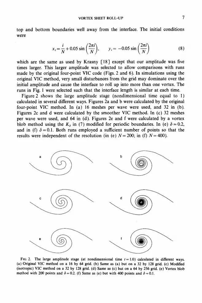
which are the same as used by Krasny [18] except that our amplitude was live times larger. This larger amplitude was selected to allow comparisons with runs made by the original four-point VIC code (Figs. 2 and 6). In simulations using the original WC method, very small disturbances from the grid may dominate over the initial amplitude and cause the interface to roll up into more than one vortex. The runs in Fig. 1 were selected such that the interface length is similar at each time.

Figure 2 shows the large amplitude stage (nondimensional time equal to 1) calculated in several different ways. Figures 2a and b were calculated by the original four-point VIC method. In (a) 16 meshes per wave were used, and 32 in (b). Figures 2c and d were calculated by the smoother VIC method. In (c) 32 meshes per wave were used, and 64 in (d). Figures 2e and f were calculated by a vortex blob method using the K6 in (7) modified for periodic boundaries. In (e) 6 = 0.2, and in (f) S =O.l. Both runs employed a sufficient number of points so that the results were independent of the resolution (in (e) N = 200; in (f) N = 400).

FIG. 2. The large amplitude stage (at nondimensional time t = 1.0) calculated in different ways. (a) Original WC method on a 16 by 64 grid. (b) Same as (a) but on a 32 by 128 grid. (c) Modified (isotropic) VIC method on a 32 by 128 grid. (d) Same as (c) but on a 64 by 256 grid. (e) Vortex blob method with 200 points and 6 = 0.2. (f) Same as (e) but with 400 points and 6 = 0.1.

8 GRkTAR TRYGGVASON

The run in Fig. 2 by the original VIC code shows slight waves in the “braid” region. For the more finely resolved run, some smoothing (a live-point weighted average) for the first 40 time steps (up to time 1.0) was applied. The coarser run was smoothed for the first 20 steps. Slight smoothing was also applied to the first few steps in the runs by the modified VIC code but much less than was needed for the original method. In general, the results obtained by the modified VIC method are superior to those obtained by the original method, but the effective blob size is larger for the latter, so a finer grid is needed. For many purposes the original method gives quite satisfactory results. When no smoothing was applied, small vortices sometimes formed during the early stages of the evolution and subsiquently merged into a large vortex with a complicated rolled-up region. Otherwise the interface generally had a structure very similar to when smoothing was applied and the roll-up was regular. It therefore seems that maintaining regular roll-up may be only of minor importance if the goal is to study the behavior of the large scales (such as the interaction of many large vortices). This is presumably the reason for the success of previous applications of the VIC method (i.e., Aref and Siggia [3]; Baker [4]; Murman and Stremel [24]) where no redistribution or smoothing was applied. Of course, when the detailed structure of the roll-up is the object under investigation, these secondary instabilities, although not completely nonphysical, are totally unacceptable.

To test for some kind of convergence in his simulations of the same problem, Krasny [ 181 recorded the location of points on the curve where its slope is vertical. In Fig. 3 we present a similar test by plotting the vertical position of the curve

l/l6 1132 l/64 .l .2 .4 Ah 6

FIG. 3. Convergence of the position of the outer spirals as the regularization is reduced. Calculations by the modified WC method are on the left-hand side of the graph; calculations by the vortex blob method of Krasny [18] are to the right.


directly above the vortex (see the top part of the figure) at time equal to one. To the right of the vertical axis we plot results from the vortex blob calculations, and to the left results from calculations by the smoother VIC method. Although three points are somewhat few, these results indicate that the outer spirals of the vortex converge to the same position for both methods. Notice that the result from the VIC method corresponding to the finest grid seem to be slightly better converged than the result from the vortex blob method with smallest blob. Furthermore, the difference between the VIC results is slightly less than between the vortex blob results.

For a different test of convergence we have also chosen to monitor the low-order moments of the vorticity distribution. The motivation for our choice is, of course, that the flow away from the vorticity region is controlled by the moments, and the first few are most important. Furthermore, for comparisons with calculations that do not use a sharp vortex sheet but allow the vorticity to diffuse slightly (or use a vortex sheet of finite thickness), the moments may be more relevant. Figure 4a is a plot of the second moments

,*=XK=I (Yi-Yc)2ri Y cy=“=, ri ’

M2 = CL 1 txiexc)’ ri -x CYz 1 ri (9)

for runs by the vortex blob method and three values of 6. Here, (x,, y,) is the location of the center of vorticity:

0.10

a 5.80

5.00 t

b

0.00 0.40 0.80 1.20 1.60 2.00 2.40 0.00 0.40 0.60 1.20 1.60 2.00 2.40

Time Time

FIG. 4. The moments as a function of time for three runs by the vortex blob method. (a) Second order moments. (b) Fourth order moments. (i) 6 = 0.4, 100 points. (ii) 6 = 0.2, 200 points. (iii) 6 = 0.1, 400 points.

10 CRl?TAR TRYGGVASON

Figure 4b is a plot of the fourth moments

normalized by the square of the second moments to give a flatness factor, or kurtosity. (Notice that D2 = Mz+ M:, which is a constant of motion for an unbounded system, is not constant for periodic boundaries, since the system is not invariant to rotations. x, and yc are, however, constants.) Figures 5a and b give similar information from runs by the modified VIC method (using the interpolation described by (5) and (6)) and Fig. 6 was obtained by the original VIC method (using the four-point area-weighting rule of Christiansen [ 121). For the graphs of the moments from the VIC simulations we have also plotted the corresponding curve from the blob simulations with 6 = 0.2 (dashed curve). This is curve (b) in Fig. 4.

The shapes of these graphs have an obvious physical interpretation. The second moment is a measure of the spread of the vorticity, and the graph shows how the vorticity is compressed along the horizontal axis, decreasing Mz, while the increase in amplitude of the initial wave causes a slight increase in M.t. Similarly, the fourth moment normalized by the second moment is a measure of how flat the vorticity distribution is. Initially, both Mf, and i$ are close to 1.8, indicating an almost uniform distribution. As the sheet is compressed, the vorticity becomes more “peaked’ in the horizontal direction and M4, rises sharply. Once the interface has rolled up, the “ellipticity” of the vortex increases as it is stretched in the horizontal direction. This reduces the peakness of the distribution and therefore n/r:,.

All methods predict that the initial horizontal vorticity compression is faster as the regularization is decreased. The second moments, particularly from the calcula-

Time

2.40

Time

FIG. 5. Same as Fig. 4, but calculations by the modified WC method. (i) 16 by 64 grid. (ii) 32 by 128 grid. (iii) 64 by 256 grid. For reference the result obtained by the vortex blob method with 6 = 0.2 is also drawn (dashed line).


0.12

I a 5.60,

~ b

0.00 0.00 0.40 0.60 1.20 1.60 2.00 2.40 0.40 0.60 1.20 1.60 2.00 2.40

Time Time

FIG. 6. Same as Fig. 4, but calculations by the original VIC method. (i) 16 by 64 grid. (ii) 32 by 128 grid. For reference the result obtained by the vortex blob method with 6 = 0.2 is also drawn (dashed line).

tions by the modified WC method, are virtually “fully converged.” The convergence for the fourth moments is not quite as fast as that of the second moments. Nevertheless, agreement is quite good, and the vortex blob method and the modified VIC method give very similar results. The original VIC method gives reasonably good results for early time, but near the end of the calculations the results show some deviation from the other methods. This is presumably an indica- tion of growth of secondary grid-generated instabilities. Notice that the calculations from the VIC method agree well with the result from the vortex blob methods with the smallest 6. A comparison of Figures 2c,d and 2e,f actually shows better agreement between (c) (the coarse VIC run) and (f) (the vortex blob with small 6), as far as the outer shape of the curve goes, than between (c) and (e), even though (c) and (e) have a more equal interface length. The same is true for the moments. This observation, and the one made for the position of the outer turns in Fig. 3, suggests that the compact “blob” in the VIC method leads to fatter convergence than the blob described by (7) for a given length of the interface. In the VIC method the computational time depends only weakly on the number of interface points, so a very long interface causes no particular difficulties. However, in the vortex blob method the computational time is proportional to N*, so longer interfaces are much more expensive to simulate. The blob described by (7) may therefore not be optimum in the sense of leading to the most rapid convergence of the outer shape of the curve and the moments for a given N.

As an additional check of convergence, and also to learn something about the structure of the vortex core, the radial distance of the interface points is plotted versus T(s) in Fig. 7 for runs by the vortex blob method. Here T(s) is a circulation coordinate defined as the integral of the vortex sheet strength from the center of the vortex along the interface to point S. A particularly striking feature is that, except for the initial conditions (t =O.O), the curves are virtually identical, close to the

12 GRiiTAR TRYGGVASON

0.0 1.0

Circulation

FIG. 7. The radial distance of a point on the vortex sheet from the center of the vortex versus the circulation of the interface segment from the vortex center to this point. Calculations by the vortex blob method. (a) 6 = 0.4, (b) 6 = 0.2, (c) 6 = 0.1. The curves are plotted for I = 0.0, 0.5, 1.0, 1.5, and 2.0, except in (c), which was only run up to t = 1.0.

vortex center. Furthermore, this shape appears to be very insenstive to the desingularization parameter. This core contains a large fraction of the circulation; approximately half of the total circulation is within g of the wavelength from the center. The core of the vortex, that is, the region mostly unaffected by the evolution, is somewhat smaller. Figure 8 shows the same information for the runs done with the modified VIC method. Again, the behavior of both methods is nearly identical, and the best agreement is between the vortex blob run with the smallest 6 and the VIC run using 32 meshes per wavelength.

Preliminary results indicate that the vortex sheet strength in the center of the vortex reaches a constant value after a critical time, and that this constant value increases as the blob size is decreased. This suggests that the vortex sheet strength may “blow up” (become infinitely large) as the regularization parameter is reduced. However, the circulation (f) in the eye of the vortex appears to decrease faster than y increases.

Although the VIC method is fairly simple, as far as programming is concerned, it is considerably more involved than the vortex blob method, which produces the velocities from the vorticity in only a few lines of code. The advantages of the VIC method, therefore, must be considerable to warrant its use. Unfortunately, a direct comparison of the efficiency of these two methods is not completely straightforward. Several numerical parameters must be selected, and this may affect the relative performance of the methods. The number of points (N) needed to repre- sent the vortex sheet is the most important parameter in the vortex blob methods,


c

b 0.0

Circulation 1.0 0.0 1.0

FIG. 8. Same as Fig. 7, but calculations by the modified WC method. (a) 16 by 64 grid, (b) 32 by 128 grid, (c) 64 by 256 grid. Times as in Fig. 7.

since the computational time is directly proportional to N2. But in the VIC method the main cost is associated with solving Poisson’s equation on the grid and a relatively large number of points can be used at little additional cost. In the vortex blob calculations presented here, N was selected such that the results appeared fairly smooth and were clearly superior to results with half that number of points. No redistribution or addition of points was used. Such dynamic regridding, while adding to the complexity of the method, could clearly increase its efficiency. The vortex blob simulations assume unbounded flow, and to mimic that, we have taken the horizontal boundaries in the VIC simulations quite far away from the vortex sheet. Large regions of potential flow generally reduce the efficiency of the VIC method. However, even under these conditions the VIC method on a 16 by 64 grid ran about as fast as the vortex blob method with 100 points and 6 = 0.4, and the VIC run on a 64 by 256 grid (up to t = 1.0) was two and a half times faster than the vortex blob run (also t = 1.0) with 400 points and 6=0.1. As pointed out earlier, the vortex blob run with the smallest blob actually agrees better with the VIC run on a 32 by 128 grid, which ran to a time slightly larger than 2.0 in less than one-sixth the time it took the vortex blob method (400 points and 6 = 0.1) to run up to time 1.0. Therefore, the VIC method was more efficient for the calculations presented here, although the relative advantage of the VIC method is definitely somewhat problem dependent. The major saving though is in larger problems such as the interactions and, say, pairing of two or more rolled-up vortices. To simulate two vortices the vortex blob method requires a fourfold increase in computing time, whereas the VIC method requires only slightly more than twice the time of a single vortex simulation.

Sal/so/l-2

14 GRbTAR TRYGGVASON

As the regularization is reduced, whether blob or mesh size, the growth rate of small-scale disturbances increases. Krasny [ 181 actually found it necessary to use double precision on a VAX computer for very small 6 to reduce round-off errors. In the VIC method, small-scale grid disturbances are alway present (although smoother interpolation reduces them), and for fine grids, slight smoothing may be necessary to dissipate these short waves. As the grid is made finer, the short wave grows faster and this problem is likely to become worse. Therefore, we do not believe that the VIC method is the ideal tool to study senstive issues such as the detailed shape of the spiral in the limit of vanishing regularization. However, calculations aimed at capturing the motion of several vortex regions are likely to be performed at relatively large 6 (see, e.g., Krasny [ 191); for such calculations the VIC method offers the distinct advantage of efficiency with no loss of accuracy.

4. CONCLUSION

The main attraction of the VIC method is its computational efficiency. We have discussed here its desingularization property, which is similar to vortex blob methods.

The desingularization of vortex sheets may be divided roughly into two classes: those that seek to incorporate more of the physics of “real” vortex sheets (such as viscosity, finite thickness, and surface tension) and those that are motivated purely by numerical considerations. The vortex blob and VIC methods clearly belong to the latter class. However, often the distinction is only superficial. Pullin [26], for example, studied the inclusion of surface tension for vortex sheets between fluids of different densities, where it is physically meaningful, and for “ordinary” vortex sheets, where it must be considered an artificially introduced desingularization parameter. A finite thickness vortex layer, although having the attractive feature of being presumably well posed for all time, is also somewhat artificial, since usually there is nothing in the problem to determine a priori the correct thickness.

The application of regularization to the vortex sheet problem must be regarded at present as a somewhat ad hoc procedure. No rigorous proof has shown that a “weak” solution exists at all times, and even the existence of a singularity is not rigorously established. The hope is, of course, that the exact nature of the regularization is of minor importance, and as the controlling parameter (be it blob radius, thickness, or surface tension) is reduced, the vortex sheet rolls up in some universal manner. Detailed comparisons between the various approaches are still quite limited. However, even if it should turn out that a “weak” solution to the vortex sheet model does not exist, it is quite possible that a finite blob size approximates some other physically plausible regularization such as, say, finite thickness. It may be necessary to use slightly different blobs than used here to make the connection rigorously and possibly blobs whose shape varies in space and time. For large-scale effects such as interactions of rolle-up vortex sheets, the detailed


vortex structure may be unimportant and any regularization may give “physical” results.

We conclude by noting that refinements of both the VIC method and the direct summation method have recently been introduced. Anderson [2] has recently introduced a grid-based (VIC) vortex method that solves two Poisson equations for each velocity component, rather than one Poisson equation for the stream function, and corrects for the grid effects on close interactions. Although this method seems to be more expensive (requiring solutions of two elliptic equations), higher accuracy may offset that drawback. Apart from some test cases presented in [a], no applications are yet available. Similar comment applies to the fast summation method proposed by Rokhlin and his students (Greengard and Rokhlin [15]); although highly promising, it has only recently been implemented in an actual vortex calculation.

ACKNOWLEDGMENTS

This work was partly motiva!ed by discussions with R. Krasny. I also thank H. Aref for illuminating discussions on all aspects of vortex methods and N. J. Zabusky for constructive interactions. This work has been supported by a Rackham faculty grant from the University of Michigan and by a grant from the Naval Research Laboratory (contract NOOO14-83-C-2006) to Fluid Sciences, Inc. The computations were done on the computers at the San Diego Supercomputer Center (SDSC). SDSC is sponsored by the NSF.

REFERENCES

1. C. R. ANDERSON, J. Compur. Phys. 61, 417 (1985) 2. C. R. ANDERSON, J. Comput. Phys. 62, 111 (1986). 3. H. AREF AND E. D. SIGGIA, J. Fluid Mech. 100, 705 (1980). 4. G. R. BAKER, J. Comput. Phys. 31, 76 (1979). 5. G. R. BAKER, D. I. MEIRON, AND S. A. ORSZAG, Phys. Fluids 23, 1485 (1980). 6. J. T. BEALE AND A. MAJDA, 1. Comput. Phys. 58, 188 (1985). 7. J. T. BEALE AND A. MAJDA, Contemp. Math. 28, 221 (1986). 8. G. BIRKHOFF, Proceedings, Symp. Appl. Math., 13th (Amer. Math. Sot., Providence, RI, 1962) p. 55. 9. G. BIRKHOFF AND J. FISHER, Rend. Circ. Math. Palmero, Ser. 2 8, 77 (1959).

10. 0. BUNEMAN, J. Comput. Phys. 11, 250 (1973). 11. A. J. CHORIN AND P. S. BERNARD, J. Comput. Phys. 13, 423 (1973). 12. J. P. CHRISTIANSEN, J. Comput. Phys. 13, 363 (1973). 13. G. H. COVET, Math. Compur. 49, 407 (1987). 14. P. T. FINK AND W. K. SOH, Proc. R. Sot. London, Ser. A 362, 195 (1978). 15. L. GREENGARD AND V. ROKHLIN, J. Comput. Phys. 73, 325 (1987). 16. R. W. HOCKNEY, S. P. GOEL, AND J. W. EASTWARD, J. Compuf. Phys. 14, 148 (1974). 17. R. KRASNY, J. Fluid Mech. 167, 65 (1986). 18. R. KRASNY, J. Comput. Phys. 65, 292 (1986). 19. R. KRASNY, J. Fluid Mech. 184, 123 (1987).

16 GRbTAR TRYGGVASON

20. A. LEONARD, J. Comput. Phys. 37, 289 (1980). 21. D. I. MEIRON, G. R. BAKER, AND S. A. ORSZAG, J. Fluid Mech. 114, 283 (1982). 22. D. W. MOORE, J. Fluid Mech. 63, 225 (1974). 23. D. W. MOORE, Proc. R. Sot. London, Ser. A 365, 105 (1979). 24. E. M. MURMAN AND P. M. STREMEL, AIAA paper 82-0947, June 1982. 25. C. S. PFSKIN, J. Comput. Phys. 25, 220 (1977). 26. D. I. PULLIN, J. Fluid Mech. 119, 507 (1982). 27. L. ROSENHEAD, Proc. R. Sot. London, Ser. A 134, 170 (1931). 28. G. TRYGGVASIN AND H. AREF, J. Fluid Mech. 154, 287 (1985). 29. G. TRYGGVA~~N, J. Comput. Phys. 75, 253 (1988). 30. G. TRYGGVA~~N, “Vortex Methods for Stratitied Flow,” Proceedings, UC Davis INLS Workshop on

Computational Fluid Dynamics, June 1986.

Documents

Simulation of vortex sheet roll-up by vortex methods