Modeling

490 Agronomy Journa l • Volume 100 , I s sue 3 • 2008

Published in Agron. J. 100:490–501 (2008).doi:10.2134/agronj2007.0156

Copyright © 2008 by the American Society of Agronomy, 677 South Segoe Road, Madison, WI 53711. All rights reserved. No part of this periodical may be reproduced or transmitted in any form or by any means, electronic or mechanical, including photocopying, recording, or any information storage and retrieval system, without permission in writing from the publisher.

The calculation of LAR is an important part of

many crop simulation models (Hodges, 1991), including

those computing development and growth of rice (Gao et al.,

1992; Lee et al., 2001). Th e integration of LAR over time gives

the number of accumulated or emerged leaves (NL) on a stem.

Vegetative development of plants, especially in small grains, is

defi ned by main stem NL (Haun, 1973). Th e main stem NL in

rice is related to the timing of several plant development stages

such as tillering (Tivet et al., 2001; Jaff uel and Dauzat, 2005;

Watanabe et al., 2005), panicle initiation (Ellis et al., 1993;

Lee et al., 2001; Watanabe et al., 2005), booting and anthesis

(Counce et al., 2000; Watanabe et al., 2005). Leaf area that

intercepts and absorbs photosynthetically active radiation for

canopy photosynthesis, which impacts dry matter production

and crop yield, is also related to the main stem NL (Amir and

Sinclair, 1991; McMaster et al., 1991; Tivet et al., 2001). In

small grains, NL if oft en represented by the HS, which is the

number of fully expanded leaves plus a ratio of the length of the

expanding leaf to the penultimate leaf (Haun, 1973).

Temperature is a major factor that drives leaf appearance in

rice (Gao et al., 1992; Ellis et al., 1993; Sié et al., 1998). One

approach to predict the appearance of individual leaves is to use

the phyllochron concept, defi ned as the time interval between

the appearance of successive leaf tips (Klepper et al., 1982;

Kirby, 1995; Wilhelm and McMaster, 1995). Th e time needed

for the appearance of one leaf can be expressed in thermal

time (TT), with units of °C day. In this case, the phyllochron

has units of °C day leaf−1. However, the TT approach may be

subject to criticism because there are diff erent ways to calcu-

late TT, which can cause diff erent results from the same data

(McMaster and Wilhelm, 1997), and because of the assump-

tion of a linear response of development to temperature, which

is not biologically sound (Shaykewich, 1995; Xue et al., 2004).

One way to overcome some of the disadvantages of the TT

approach is to use nonlinear temperature response functions

and multiplicative models. An example of the latter is the WE

model (Wang and Engel, 1998). Xue et al. (2004) demon-

strated that the predictions of leaf appearance in several winter

wheat cultivars were improved with the WE model compared

to the phyllochron concept.

Although temperature is the major factor that drives LAR

in rice, results from growth chamber experiments showed that

LAR is not constant with time when rice plants are grown at

constant temperature and light (Yin and Kropff , 1996). Th ese

results suggest age eff ects on LAR in rice. Streck et al. (2003a)

modifi ed the WE model for simulating LAR in wheat, a spe-

cies similar to rice in morphology and growth habit, by incor-

porating age eff ects through a chronology response function

that takes into account the eff ect of seed reserves for the fi rst

two leaves and a decrease in LAR with increase in leaf number.

Hereaft er this model will be referenced as the Streck model.

Th e chronology response function in the Streck model has

two stages. Th e fi rst stage is when HS < 2, and the assump-

tion during this stage is that seed reserves represent a plentiful

source of carbohydrates and nutrients for growth and therefore

ABSTRACTMost rice (Oryza sativa L.) simulation models assume that only temperature aff ects leaf appearance rate (LAR). Th is assumption

ignores results from controlled environment studies that show that LAR in rice is not constant with time (calendar days) under

constant temperature. Th e Streck model, which takes into account age eff ects on LAR, improved the prediction of leaf appear-

ance in winter wheat (Triticum aestivum L.) cultivars compared with the Wang and Engel (WE) model and the phyllochron

model but has not been evaluated in rice. Th e objective of this study was to adapt and evaluate the Streck model to simulate main

stem LAR and leaf number in rice. A 4-yr experiment with several sowing dates from 2003–2004 to 2006–2007 was performed at

Santa Maria, RS, Brazil. Seven rice cultivars were used: IRGA 421, IRGA 420, IRGA 417, IRGA 416, BRS 7 (TAIM), BR-IRGA

409, and EPAGRI 109. Plants were grown in 12-L pots during the 4 yr, and in a paddy rice fi eld during the 2006–2007 growing

season. Coeffi cients necessary to run the Streck model, the WE model, and the phyllochron model were estimated with data from

fi ve sowing dates of the 2003–2004 growing season and the models were evaluated with independent data from the other three

growing seasons. Predictions of the main stem leaf number, represented by the Haun Stage (HS), were better with the Streck

model. Th e RMSE was 0.7, 1.0, and 1.8 leaves, for the Streck model, the WE model, and the phyllochron model, respectively.

Simulating Leaf Appearance in Rice

Nereu Augusto Streck,* Leosane Cristina Bosco, and Isabel Lago

N.A. Streck, Dep. de Fitotecnia, Centro de Ciências Rurais, and L.C. Bosco and I. Lago, Programa de Pós-graduação em Agronomia, Univ. Federal de Santa Maria, 97105-900, Santa Maria, RS, Brazil. Received 8 May 2007. *Corresponding author (nstreck2@yahoo.com.br).

Abbreviations: NL, number of leaves; LAR, leaf appearance rate; WE, Wang and Engel (model); HS, Haun Stage; TT, thermal time; ATT, accumulated thermal time.

Agronomy Journa l • Volume 100, Issue 3 • 2008 491

the fi rst two leaves have the highest LAR. Th is assumption

was based on results from wheat, but in rice the main source

of energy and nutrients up to the time the fi rst two leaves

are fully expanded also comes from seed reserves (Stansel,

1975; Hoshikawa, 1993). Th e second stage of the chronology

response function in the Streck model is when HS ≥ 2, and the

assumption during this stage is a decrease in LAR with time

following a power law due to the fact that higher leaves take

more time to appear because the distance that each leaf tip

has to traverse from the apical meristem to the whorl increases

for each subsequent leaf. Th e Streck model improved the pre-

diction of leaf appearance in several winter wheat genotypes

compared with the WE model. Similarities in plant morphol-

ogy and growth habit between rice and wheat and the fact that

the Streck model has not been evaluated in rice constituted

the rationale for this research eff ort. In this study we hypoth-

esized that the chronology response function is appropriated

for LAR in rice and that the Streck model is better than other

approaches to simulate the main stem LN in rice. Th e objec-

tive of this study was to adapt and evaluate the Streck model

(Streck et al., 2003a) for simulating main stem LAR and LN

in rice.

MATERIALS AND METHODS

Streck ModelTh e Streck model (Streck et al., 2003a), adapted for simulat-

ing leaf appearance in rice, combines nonlinear temperature

and age eff ects on LAR in a multiplicative fashion, and has the

general form

LAR = LARmax12 f(T) f(C) [1]

where LAR is measured in leaves d−1, LARmax12 is the maxi-

mum daily leaf appearance rate (leaves d−1) of the fi rst two

leaves under optimum temperature, f(T) and f(C) are dimen-

sionless temperature and chronology response functions

(varying from 0–1) for LAR, respectively. Th e f(T) is a beta

function:

f(T) = [2(T – Tmin)α(Topt – Tmin)α – (T – Tmin)2α]/

(Topt – Tmin)2α [2]

for Tmin ≤ T ≤ Tmax

f(T) = 0

for T < Tmin or T > Tmax

α = ln(2)/ln[(Tmax – Tmin)/(Topt – Tmin)] [3]

where Tmin, Topt, and Tmax are the cardinal (minimum, opti-

mum, and maximum) temperatures for LAR and T is the mean

daily air temperature calculated from the average of minimum

and maximum air temperatures. Th e cardinal temperatures

for LAR in rice are 11°C (Ellis et al., 1993; Infeld et al., 1998),

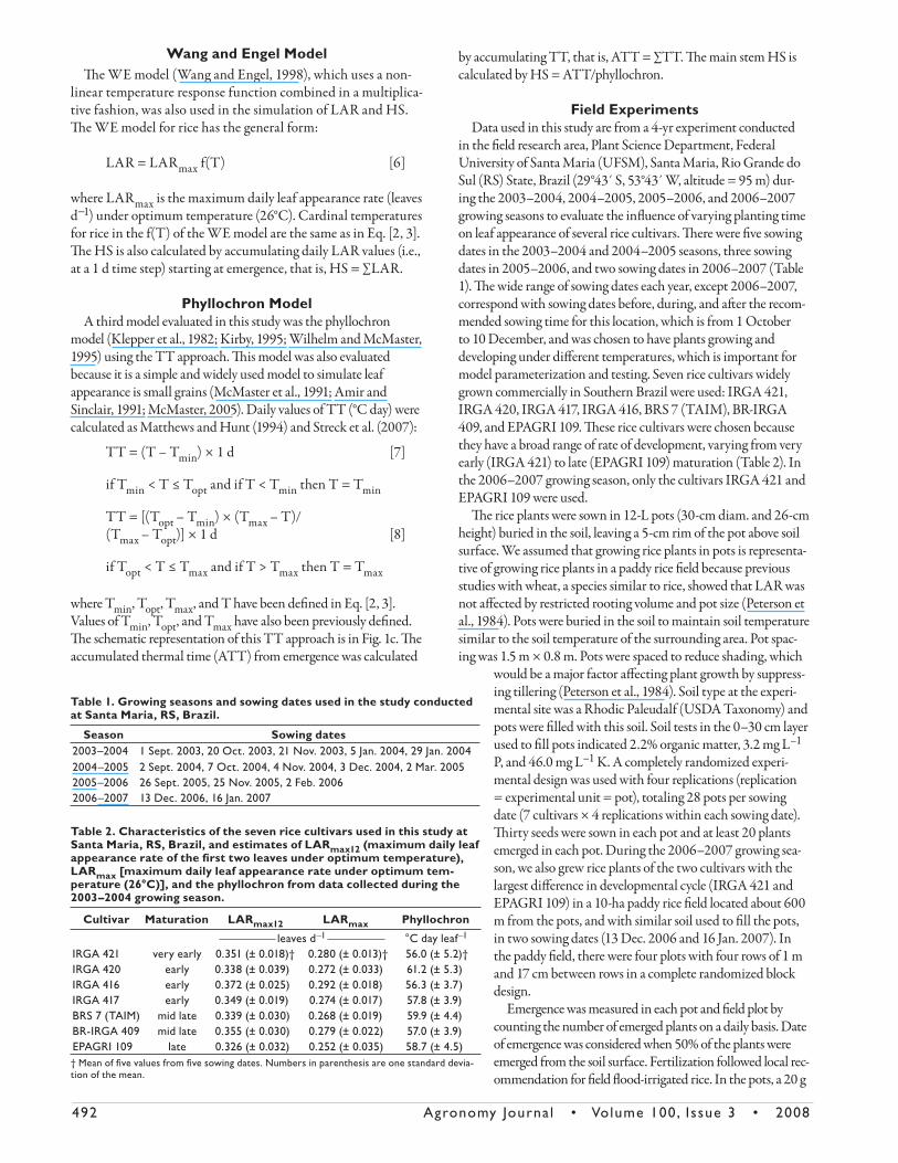
26°C (Ellis et al., 1993) and 40°C (Gao et al., 1992). Th e curve

generated by Eq. [2, 3] with these cardinal temperatures for

LAR is shown in Fig. 1a.

Th e f(C) is given as

f (C) = 1 if HS < 2 [4]

f (C) = (HS/2)b if HS ≥ 2 [5]

where b is a sensitivity coeffi cient and has a value of –0.3

(Streck et al., 2003a). Th e curve generated by Eq. [4, 5] is

shown in Fig. 1b.

Th e main stem number of emerged leaves, represented by the

HS, is calculated by accumulating daily LAR values (i.e., at a

daily time step) starting at emergence, that is, HS = ∑LAR.

Fig. 1. (a) The temperature response function (Eq. [2, 3]) in the Wang and Engel (WE) and Streck leaf appearance models with cardinal temperatures for rice of 11, 26, and 40°C; (b) the chronology response function (Eq. [4, 5]) used in the Streck leaf appearance model; (c) method of calculating daily values of thermal time (TT; Eq. [7, 8]) for leaf appearance in rice with cardinal temperatures of 11, 26, and 40°C.

492 Agronomy Journa l • Volume 100, Issue 3 • 2008

Wang and Engel ModelTh e WE model (Wang and Engel, 1998), which uses a non-

linear temperature response function combined in a multiplica-

tive fashion, was also used in the simulation of LAR and HS.

Th e WE model for rice has the general form:

LAR = LARmax f(T) [6]

where LARmax is the maximum daily leaf appearance rate (leaves

d−1) under optimum temperature (26°C). Cardinal temperatures

for rice in the f(T) of the WE model are the same as in Eq. [2, 3].

Th e HS is also calculated by accumulating daily LAR values (i.e.,

at a 1 d time step) starting at emergence, that is, HS = ∑LAR.

Phyllochron ModelA third model evaluated in this study was the phyllochron

model (Klepper et al., 1982; Kirby, 1995; Wilhelm and McMaster,

1995) using the TT approach. Th is model was also evaluated

because it is a simple and widely used model to simulate leaf

appearance is small grains (McMaster et al., 1991; Amir and

Sinclair, 1991; McMaster, 2005). Daily values of TT (°C day) were

calculated as Matthews and Hunt (1994) and Streck et al. (2007):

TT = (T – Tmin) × 1 d [7]

if Tmin < T ≤ Topt and if T < Tmin then T = Tmin

TT = [(Topt – Tmin) × (Tmax – T)/

(Tmax – Topt)] × 1 d [8]

if Topt < T ≤ Tmax and if T > Tmax then T = Tmax

where Tmin, Topt, Tmax, and T have been defi ned in Eq. [2, 3].

Values of Tmin, Topt, and Tmax have also been previously defi ned.

Th e schematic representation of this TT approach is in Fig. 1c. Th e

accumulated thermal time (ATT) from emergence was calculated

by accumulating TT, that is, ATT = ∑TT. Th e main stem HS is

calculated by HS = ATT/phyllochron.

Field ExperimentsData used in this study are from a 4-yr experiment conducted

in the fi eld research area, Plant Science Department, Federal

University of Santa Maria (UFSM), Santa Maria, Rio Grande do

Sul (RS) State, Brazil (29°43́ S, 53°43́ W, altitude = 95 m) dur-

ing the 2003–2004, 2004–2005, 2005–2006, and 2006–2007

growing seasons to evaluate the infl uence of varying planting time

on leaf appearance of several rice cultivars. Th ere were fi ve sowing

dates in the 2003–2004 and 2004–2005 seasons, three sowing

dates in 2005–2006, and two sowing dates in 2006–2007 (Table

1). Th e wide range of sowing dates each year, except 2006–2007,

correspond with sowing dates before, during, and aft er the recom-

mended sowing time for this location, which is from 1 October

to 10 December, and was chosen to have plants growing and

developing under diff erent temperatures, which is important for

model parameterization and testing. Seven rice cultivars widely

grown commercially in Southern Brazil were used: IRGA 421,

IRGA 420, IRGA 417, IRGA 416, BRS 7 (TAIM), BR-IRGA

409, and EPAGRI 109. Th ese rice cultivars were chosen because

they have a broad range of rate of development, varying from very

early (IRGA 421) to late (EPAGRI 109) maturation (Table 2). In

the 2006–2007 growing season, only the cultivars IRGA 421 and

EPAGRI 109 were used.

Th e rice plants were sown in 12-L pots (30-cm diam. and 26-cm

height) buried in the soil, leaving a 5-cm rim of the pot above soil

surface. We assumed that growing rice plants in pots is representa-

tive of growing rice plants in a paddy rice fi eld because previous

studies with wheat, a species similar to rice, showed that LAR was

not aff ected by restricted rooting volume and pot size (Peterson et

al., 1984). Pots were buried in the soil to maintain soil temperature

similar to the soil temperature of the surrounding area. Pot spac-

ing was 1.5 m × 0.8 m. Pots were spaced to reduce shading, which

would be a major factor aff ecting plant growth by suppress-

ing tillering (Peterson et al., 1984). Soil type at the experi-

mental site was a Rhodic Paleudalf (USDA Taxonomy) and

pots were fi lled with this soil. Soil tests in the 0–30 cm layer

used to fi ll pots indicated 2.2% organic matter, 3.2 mg L–1

P, and 46.0 mg L–1 K. A completely randomized experi-

mental design was used with four replications (replication

= experimental unit = pot), totaling 28 pots per sowing

date (7 cultivars × 4 replications within each sowing date).

Th irty seeds were sown in each pot and at least 20 plants

emerged in each pot. During the 2006–2007 growing sea-

son, we also grew rice plants of the two cultivars with the

largest diff erence in developmental cycle (IRGA 421 and

EPAGRI 109) in a 10-ha paddy rice fi eld located about 600

m from the pots, and with similar soil used to fi ll the pots,

in two sowing dates (13 Dec. 2006 and 16 Jan. 2007). In

the paddy fi eld, there were four plots with four rows of 1 m

and 17 cm between rows in a complete randomized block

design.

Emergence was measured in each pot and fi eld plot by

counting the number of emerged plants on a daily basis. Date

of emergence was considered when 50% of the plants were

emerged from the soil surface. Fertilization followed local rec-

ommendation for fi eld fl ood-irrigated rice. In the pots, a 20 g

Table 1. Growing seasons and sowing dates used in the study conducted at Santa Maria, RS, Brazil.

Season Sowing dates2003–2004 1 Sept. 2003, 20 Oct. 2003, 21 Nov. 2003, 5 Jan. 2004, 29 Jan. 20042004–2005 2 Sept. 2004, 7 Oct. 2004, 4 Nov. 2004, 3 Dec. 2004, 2 Mar. 20052005–2006 26 Sept. 2005, 25 Nov. 2005, 2 Feb. 20062006–2007 13 Dec. 2006, 16 Jan. 2007

Table 2. Characteristics of the seven rice cultivars used in this study at Santa Maria, RS, Brazil, and estimates of LARmax12 (maximum daily leaf appearance rate of the fi rst two leaves under optimum temperature), LARmax [maximum daily leaf appearance rate under optimum tem-perature (26°C)], and the phyllochron from data collected during the 2003–2004 growing season.

Cultivar Maturation LARmax12 LARmax Phyllochron

leaves d−1 °C day leaf−1

IRGA 421 very early 0.351 (± 0.018)† 0.280 (± 0.013)† 56.0 (± 5.2)†IRGA 420 early 0.338 (± 0.039) 0.272 (± 0.033) 61.2 (± 5.3)IRGA 416 early 0.372 (± 0.025) 0.292 (± 0.018) 56.3 (± 3.7)IRGA 417 early 0.349 (± 0.019) 0.274 (± 0.017) 57.8 (± 3.9)BRS 7 (TAIM) mid late 0.339 (± 0.030) 0.268 (± 0.019) 59.9 (± 4.4)BR-IRGA 409 mid late 0.355 (± 0.030) 0.279 (± 0.022) 57.0 (± 3.9)EPAGRI 109 late 0.326 (± 0.032) 0.252 (± 0.035) 58.7 (± 4.5)† Mean of fi ve values from fi ve sowing dates. Numbers in parenthesis are one standard devia-tion of the mean.

Agronomy Journa l • Volume 100, Issue 3 • 2008 493

pot−1 of a 7–11–9 N–P–K fertilizer was used at sowing. Additional

nitrogen was added as a side-dress application at beginning of tiller-

ing (V4 stage; Counce et al., 2000) and at panicle diff erentiation

(R1 stage; Counce et al., 2000) with urea at a rate of 8.5 g of urea

pot−1. Th e same fertilizer rates at sowing and side-dressings were

used in the fi eld plots, corresponding to 300 kg ha−1 of 7–11–9

N–P–K fertilizer and 222 kg ha−1 of urea. At the V3 stage (three

fully expanded leaves) of the Counce et al. (2000) scale, plants

were thinned to 15 plants per pot, resulting in a plant density of

about 200 plant m−2, which is a plant density commonly found in

commercial rice fi elds in southern Brazil. Th e same plant density

was used in the fi eld plots. Irrigation in both pots and fi eld plots

was performed to keep a continuous 5- to 7-cm water layer above

the soil surface (fl ooded soil) from V3 to R9 (physiological matu-

rity) Counce stages.

Five plants per pot and fi ve plants in the central row of the fi eld

plots were tagged with colored wires 1 wk aft er emergence. In the

pots, plants located in the central part of the pot were tagged. In

doing so, a red–far red balance similar to the one found in a rice fi eld

was attempted to achieve, as such balance is aff ected by the proxim-

ity of nearest neighbor and it is known to aff ect development in

small grains (Wilhelm and McMaster, 1995). Tagged plants were

used to measure the NL on the main stem. A leaf was counted when

the tip had visibly emerged from the whorl, independent of ligule

formation. Th e NL, the blade length of the expanding leaf (Ln), and

the penultimate leaf (Ln–1) on the main stem were measured once a

week throughout the experiment. Th e Haun Stage (leaves) was cal-

culated as follows (Haun, 1973; Wilhelm and McMaster, 1995):

HS = (NL – 1) + Ln/Ln–1 [9]

Daily minimum and maximum air temperatures were mea-

sured by a standard meteorological station located at about 200

m from the pots and about 500 m from the fi eld plots. Mean

daily air temperature (T) used in the temperature response

functions (Eq. [2, 3, 7, 8]) was calculated as the average of daily

minimum and maximum temperatures.

Estimates of Coeffi cients of the ModelsCoeffi cients LARmax12 (Eq. [1]), LARmax (Eq. [6]), and the

phyllochron are genotype dependent. Th ese coeffi cients were esti-

mated for each cultivar using HS data collected from the fi ve sowing

dates of the 2003–2004 growing season. Coeffi cients LARmax12

and LARmax were estimated by changing (increasing and decreas-

ing) an initial value (0.3 leaves d–1) by a 1% step until obtaining the

best fi t between observed and estimated HS values by minimizing

the RMSE, calculated as (Janssen and Heuberger, 1995):

RMSE = [Σ(p – o)2/N]0.5 [10]

where p = predicted HS values, o = observed HS values, and N =

number of observations. Th e unit of RMSE is the same as p and o,

that is, leaves.

Th e phyllochron was estimated by the inverse of the slope

of the linear regression of HS against ATT (Klepper et

al., 1982; Kirby, 1995; Xue et al., 2004). Th e estimates of

LARmax12, LARmax, and phyllochron for each cultivar were

the average of the fi ve sowing dates (Table 2). We averaged

the estimates over the fi ve sowing dates because an ANOVA

analysis revealed no signifi cant interaction between sowing

date and genotypes for the variable phyllochron (inverse of

leaf appearance) during the 2003–2004 growing season and

because of the low values of the standard deviations of the

mean values (Table 2).

Evaluation of ModelsTh e values of main stem HS predicted by the Streck model,

the WE model, and the phyllochron model were compared

with the observed HS values for each cultivar during the sow-

ing dates of the 2004–2005, 2005–2006, and 2006–2007

growing seasons, which were all independent data sets. Models

performance was evaluated with the RMSE statistic (Eq. [10]).

Better predictions result in smaller RMSE. Systematic and

unsystematic errors of models predictions was calculated for

each model by the MSE, that is, RMSE2, and decomposing the

MSE into systematic and unsystematic (random) components

(systematic + unsystematic = 100%) according to Willmott

(1981). A good model has low systematic and high unsystem-

atic error.

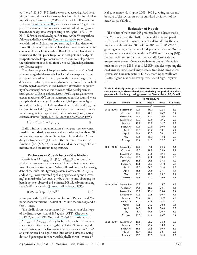
Table 3. Monthly average of minimum, mean, and maximum air temperature, and sunshine duration during the period of leaf ap-pearance in the four growing seasons at Santa Maria, RS, Brazil.

Season MonthTemperature

SunshineMin. Mean Max.°C h d−1

2003–2004 September 10.9 16.7 22.6 5.2October 14.9 20.9 26.9 6.9

November 16.6 22.3 28.0 7.3December 17.3 22.5 27.6 9.0

January 19.8 25.7 31.7 8.8February 17.9 23.9 30.0 9.5

March 17.3 23.7 30.1 7.2April 16.4 22.2 28.1 6.0May 10.6 15.3 19.8 5.9

Average 15.7 21.5 27.2 7.3

2004–2005 September 13.8 19.1 24.5 4.4October 12.2 18.9 25.6 8.7

November 15.7 21.6 27.4 7.0December 17.8 24.1 30.4 9.0

January 19.8 26.6 33.4 9.0February 19.1 25.0 31.0 7.1

March 18.0 24.5 31.0 6.5April 15.1 20.1 25.1 4.4May 13.8 18.5 23.2 4.2

Average 16.1 22.0 27.9 6.7

2005−2006 September 10.9 15.3 19.7 4.6October 14.5 18.8 23.1 4.4

November 15.7 22.6 29.4 8.4December 17.3 23.8 30.3 9.4

January 20.7 26.3 31.9 7.7February 19.0 25.1 31.2 8.5

March 18.1 24.2 30.3 7.4April 14.2 20.1 26.0 6.8May 9.4 14.9 20.5 5.2

Average 15.5 21.2 26.9 6.9

2006–2007 December 19.6 25.9 32.2 8.5January 20.5 25.7 30.8 7.5

February 19.5 25.1 30.8 8.2March 20.4 25.3 30.1 5.2

Average 20.0 25.5 31.0 7.3

494 Agronomy Journa l • Volume 100, Issue 3 • 2008

RESULTSTh ere was variation in meteorological conditions during the

period of leaf appearance of the four growing seasons (Table

3). Th e 2004–2005 growing season was the warmest, with the

highest average monthly mean (26.6°C) and maximum (33.4°C) air

temperatures, which occurred in January 2005. Th e lowest average

monthly minimum air temperature was in May 2006 (9.4°C). On

the other hand, sunshine duration was greater in the 2003–2004

and in the 2005–2006 growing seasons, with the highest average

monthly values in February 2004 (9.5 h d−1) and December 2005

(9.4 h d−1). Th e distinct meteorological conditions in the diff erent

sowing dates during each year provide a rich data set to calibrate

and evaluate the diff erent LAR models.

An analysis of the HS data of cultivars IRGA 421 and EPAGRI

109 grown in the 2006–2007 growing season showed HS diff er-

ence between plants grown in the pots and plants grown in the

paddy rice fi eld less than 0.6 leaves. Th ese small diff erences in HS

indicate that results from the potted plants can be extrapolated to a

rice fi eld. In addition, they are consistent with the results presented

in Peterson et al. (1984) with wheat that LAR is not aff ected by

restricted rooting volume and pot size.

Predicted vs. observed values for main stem HS for the inde-

pendent data (pooling data for diff erent cultivars, sowing dates

and years) are presented in Fig. 2 (plants grown in pots) and Fig.

3 (plants grown in the paddy rice fi eld). We pooled cultivar, sow-

ing date, and year data, and separated results from pots (Fig. 2)

and from the paddy rice fi eld (Fig. 3) in our fi rst data analysis to

present an overall RMSE, and for better visualizing data, making

results interpretation easier. In panels a, b, and c of Fig. 2 and 3,

models were run from emergence, whereas panels d, e, and f show

the results when models were run starting at the day of fi rst HS

measurement. Th e predicted HS at this day was set equal to the

observed HS. We also started the simulation at the day of fi rst

HS measurement because on closer inspection of Fig. 2c and 3c,

it is clear that the phyllochron approach misses the fi rst and two

leaves. In doing so, we removed this initial error and all three mod-

els started running from the same initial condition, which from

a modeling perspective can be interpreted as a fairer comparison

amongst them.

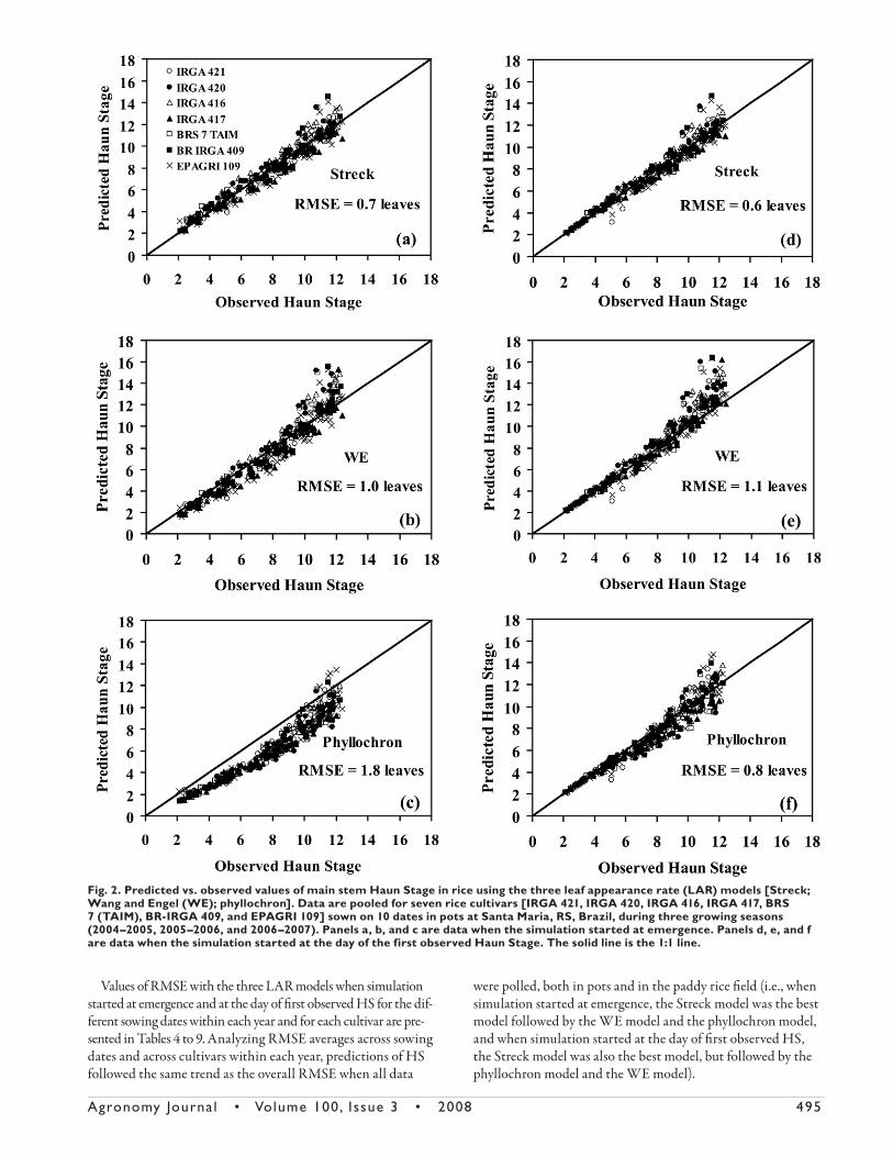
From Fig. 2 and 3, the accuracy of the HS predictions decreased

in the sequence Streck model > WE model > phyllochron model

when the simulation started at emergence and Streck model > phyl-

lochron model > WE model when the simulation started at the day

of fi rst observed HS. For the pot experiment, the overall RMSE was

0.7 leaves, 1.0 leaves, and 1.8 leaves when the simulation started at

emergence and 0.6 leaves, 1.1 leaves, and 0.8 leaves when the simula-

tion started at the day of fi rst observed HS with the Streck model,

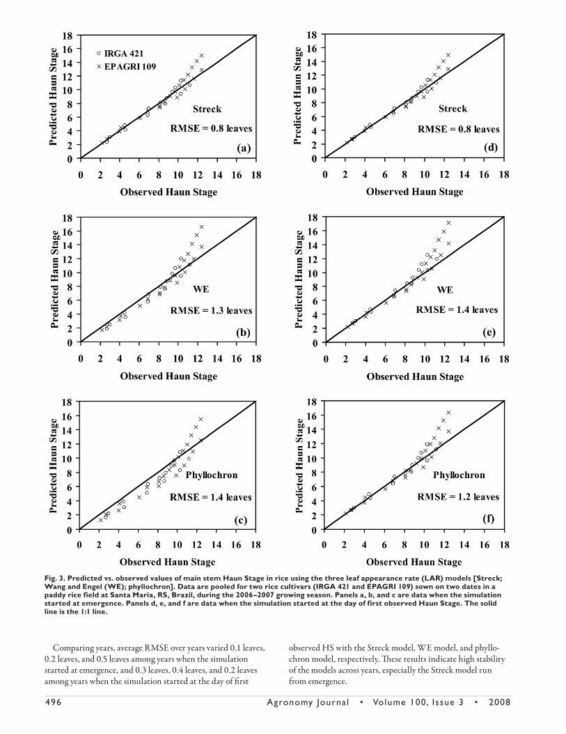
WE model, and phyllochron model, respectively. For the paddy rice

fi eld experiment, RMSE was 0.8 leaves, 1.3 leaves, and 1.4 leaves

when the simulation started at emergency, and 0.8 leaves, 1.4 leaves,

and 1.2 leaves when the simulation started at the day of fi rst HS

measurement.

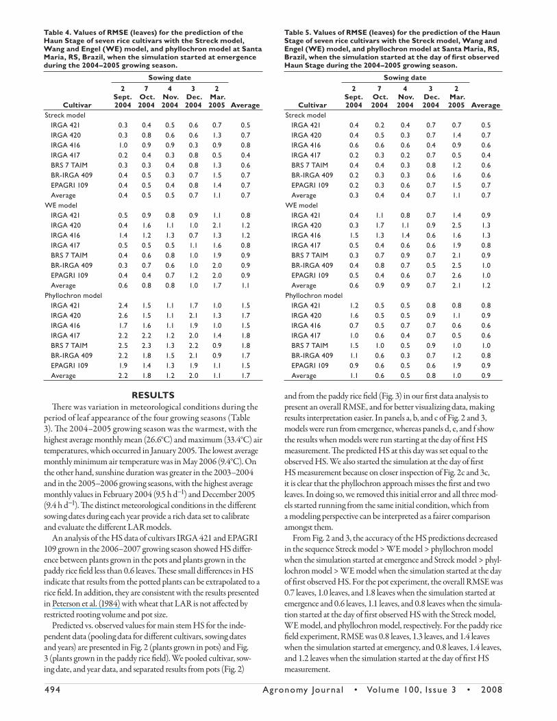
Table 4. Values of RMSE (leaves) for the prediction of the Haun Stage of seven rice cultivars with the Streck model, Wang and Engel (WE) model, and phyllochron model at Santa Maria, RS, Brazil, when the simulation started at emergence during the 2004–2005 growing season.

Cultivar

Sowing date

Average

2 Sept. 2004

7 Oct. 2004

4 Nov. 2004

3 Dec. 2004

2 Mar. 2005

Streck model IRGA 421 0.3 0.4 0.5 0.6 0.7 0.5 IRGA 420 0.3 0.8 0.6 0.6 1.3 0.7 IRGA 416 1.0 0.9 0.9 0.3 0.9 0.8 IRGA 417 0.2 0.4 0.3 0.8 0.5 0.4 BRS 7 TAIM 0.3 0.3 0.4 0.8 1.3 0.6 BR-IRGA 409 0.4 0.5 0.3 0.7 1.5 0.7 EPAGRI 109 0.4 0.5 0.4 0.8 1.4 0.7 Average 0.4 0.5 0.5 0.7 1.1 0.7WE model IRGA 421 0.5 0.9 0.8 0.9 1.1 0.8 IRGA 420 0.4 1.6 1.1 1.0 2.1 1.2 IRGA 416 1.4 1.2 1.3 0.7 1.3 1.2 IRGA 417 0.5 0.5 0.5 1.1 1.6 0.8 BRS 7 TAIM 0.4 0.6 0.8 1.0 1.9 0.9 BR-IRGA 409 0.3 0.7 0.6 1.0 2.0 0.9 EPAGRI 109 0.4 0.4 0.7 1.2 2.0 0.9 Average 0.6 0.8 0.8 1.0 1.7 1.1Phyllochron model IRGA 421 2.4 1.5 1.1 1.7 1.0 1.5 IRGA 420 2.6 1.5 1.1 2.1 1.3 1.7 IRGA 416 1.7 1.6 1.1 1.9 1.0 1.5 IRGA 417 2.2 2.2 1.2 2.0 1.4 1.8 BRS 7 TAIM 2.5 2.3 1.3 2.2 0.9 1.8 BR-IRGA 409 2.2 1.8 1.5 2.1 0.9 1.7 EPAGRI 109 1.9 1.4 1.3 1.9 1.1 1.5 Average 2.2 1.8 1.2 2.0 1.1 1.7

Table 5. Values of RMSE (leaves) for the prediction of the Haun Stage of seven rice cultivars with the Streck model, Wang and Engel (WE) model, and phyllochron model at Santa Maria, RS, Brazil, when the simulation started at the day of fi rst observed Haun Stage during the 2004–2005 growing season.

Cultivar

Sowing date

Average

2 Sept. 2004

7 Oct. 2004

4 Nov. 2004

3 Dec. 2004

2 Mar. 2005

Streck model IRGA 421 0.4 0.2 0.4 0.7 0.7 0.5 IRGA 420 0.4 0.5 0.3 0.7 1.4 0.7 IRGA 416 0.6 0.6 0.6 0.4 0.9 0.6 IRGA 417 0.2 0.3 0.2 0.7 0.5 0.4 BRS 7 TAIM 0.4 0.4 0.3 0.8 1.2 0.6 BR-IRGA 409 0.2 0.3 0.3 0.6 1.6 0.6 EPAGRI 109 0.2 0.3 0.6 0.7 1.5 0.7 Average 0.3 0.4 0.4 0.7 1.1 0.7WE model IRGA 421 0.4 1.1 0.8 0.7 1.4 0.9 IRGA 420 0.3 1.7 1.1 0.9 2.5 1.3 IRGA 416 1.5 1.3 1.4 0.6 1.6 1.3 IRGA 417 0.5 0.4 0.6 0.6 1.9 0.8 BRS 7 TAIM 0.3 0.7 0.9 0.7 2.1 0.9 BR-IRGA 409 0.4 0.8 0.7 0.5 2.5 1.0 EPAGRI 109 0.5 0.4 0.6 0.7 2.6 1.0 Average 0.6 0.9 0.9 0.7 2.1 1.2Phyllochron model IRGA 421 1.2 0.5 0.5 0.8 0.8 0.8 IRGA 420 1.6 0.5 0.5 0.9 1.1 0.9 IRGA 416 0.7 0.5 0.7 0.7 0.6 0.6 IRGA 417 1.0 0.6 0.4 0.7 0.5 0.6 BRS 7 TAIM 1.5 1.0 0.5 0.9 1.0 1.0 BR-IRGA 409 1.1 0.6 0.3 0.7 1.2 0.8 EPAGRI 109 0.9 0.6 0.5 0.6 1.9 0.9 Average 1.1 0.6 0.5 0.8 1.0 0.9

Agronomy Journa l • Volume 100, Issue 3 • 2008 495

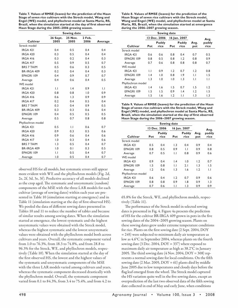
Values of RMSE with the three LAR models when simulation

started at emergence and at the day of fi rst observed HS for the dif-

ferent sowing dates within each year and for each cultivar are pre-

sented in Tables 4 to 9. Analyzing RMSE averages across sowing

dates and across cultivars within each year, predictions of HS

followed the same trend as the overall RMSE when all data

were polled, both in pots and in the paddy rice fi eld (i.e., when

simulation started at emergence, the Streck model was the best

model followed by the WE model and the phyllochron model,

and when simulation started at the day of fi rst observed HS,

the Streck model was also the best model, but followed by the

phyllochron model and the WE model).

Fig. 2. Predicted vs. observed values of main stem Haun Stage in rice using the three leaf appearance rate (LAR) models [Streck; Wang and Engel (WE); phyllochron]. Data are pooled for seven rice cultivars [IRGA 421, IRGA 420, IRGA 416, IRGA 417, BRS 7 (TAIM), BR-IRGA 409, and EPAGRI 109] sown on 10 dates in pots at Santa Maria, RS, Brazil, during three growing seasons (2004–2005, 2005–2006, and 2006–2007). Panels a, b, and c are data when the simulation started at emergence. Panels d, e, and f are data when the simulation started at the day of the first observed Haun Stage. The solid line is the 1:1 line.

496 Agronomy Journa l • Volume 100, Issue 3 • 2008

Comparing years, average RMSE over years varied 0.1 leaves,

0.2 leaves, and 0.5 leaves among years when the simulation

started at emergence, and 0.3 leaves, 0.4 leaves, and 0.2 leaves

among years when the simulation started at the day of fi rst

observed HS with the Streck model, WE model, and phyllo-

chron model, respectively. Th ese results indicate high stability

of the models across years, especially the Streck model run

from emergence.

Fig. 3. Predicted vs. observed values of main stem Haun Stage in rice using the three leaf appearance rate (LAR) models [Streck; Wang and Engel (WE); phyllochron]. Data are pooled for two rice cultivars (IRGA 421 and EPAGRI 109) sown on two dates in a paddy rice field at Santa Maria, RS, Brazil, during the 2006–2007 growing season. Panels a, b, and c are data when the simulation started at emergence. Panels d, e, and f are data when the simulation started at the day of first observed Haun Stage. The solid line is the 1:1 line.

Agronomy Journa l • Volume 100, Issue 3 • 2008 497

Among sowing dates, RMSE averages over cultivars indi-

cate, in general, better predictions in the earliest sowing date

and worst predictions in the latest sowing dates with the

Streck model and the WE model, except for the WE model

prediction when the simulation started at emergence in the

2006–2007 season (Table 8). For the phyllochron model,

predictions were better in the latest sowing date and worst

in the earliest sowing date when simulations started at

emergence (Tables 4, 6, 8). When simulation started at the

first observed HS, the phyllochron model performed better

in the intermediate sowing dates of the 2004–2005 growing

season (Table 5), in the latest sowing date of the 2005–2006

growing season (Table 7), and in the earliest sowing date

of the 2006–2007 growing season (Table 9). These results

indicate greater stability of the Streck model and lower stabil-

ity of the phyllochron model among sowing dates.

Among cultivars, no clear trend could be detected from the

RMSE data presented in Tables 4 to 9 in terms of HS predic-

tion (i.e., models performed better for some cultivars in some

sowing dates and years and for the same cultivars models per-

formed not as good in other sowing dates and years). In the

2004–2005 and 2005–2006 growing seasons, which included

all seven cultivars, and considering simulations starting both

at emergence and at the day of fi rst observed HS, the diff erence

between the cultivars with the lowest RMSE and the cultivars

with the highest RMSE (average over sowing dates, Tables 4–7)

varied from 0.2 to 0.5 leaves with the Streck model, 0.1 to 0.7

leaves with the WE model, and the 0.2 to 0.8 leaves with the

phyllochron model. Th ese results again favor the Streck model,

which had greater stability of the predictions across cultivars.

When the simulation started at emergence, the WE model

had systematic errors, with underpredictions at low HS (HS

< 4) and overpredictions at high HS (HS > 10) (Fig. 2b, 3b).

Th e phyllochron model had even greater systematic errors,

and most of the HS values were underpredicted (Fig. 2c, 3c).

Systematic errors were smallest with the Streck model, with

data scattered around the 1:1 line (Fig. 2a, 3a), with somewhat

wider scatter above the 1:1 line than below. As expected, scat-

tering decreased when the simulation started at the day of fi rst

Table 6. Values of RMSE (leaves) for the prediction of the Haun Stage of seven rice cultivars with the Streck model, Wang and Engel (WE) model, and phyllochron model at Santa Maria, RS, Brazil, when the simulation started at emergence during the 2005–2006 growing season.

Cultivar

Sowing date

Average26 Sept.

200525 Nov.

20052 Feb. 2006

Streck model IRGA 421 0.5 0.5 0.5 0.5 IRGA 420 0.4 0.4 0.6 0.5 IRGA 416 0.4 0.2 0.4 0.3 IRGA 417 0.5 1.2 0.9 0.9 BRS 7 TAIM 0.6 0.8 0.3 0.6 BR-IRGA 409 0.3 0.6 0.6 0.5 EPAGRI 109 0.3 1.1 1.0 0.8 Average 0.4 0.7 0.6 0.6WE model IRGA 421 0.9 1.1 0.9 1.0 IRGA 420 0.6 0.7 0.9 0.7 IRGA 416 0.4 0.9 0.8 0.7 IRGA 417 0.4 1.4 1.2 1.0 BRS 7 TAIM 0.3 1.1 0.8 0.7 BR-IRGA 409 0.2 0.9 0.9 0.7 EPAGRI 109 0.6 1.6 1.4 1.2 Average 0.5 1.1 1.0 0.9Phyllochron model IRGA 421 1.6 1.2 1.2 1.3 IRGA 420 2.0 1.9 1.8 1.9 IRGA 416 2.2 1.5 1.3 1.7 IRGA 417 2.2 2.2 1.8 2.1 BRS 7 TAIM 2.2 2.2 1.4 1.9 BR-IRGA 409 2.1 2.0 1.7 1.9 EPAGRI 109 2.0 2.2 1.8 2.0 Average 2.0 1.9 1.6 1.8

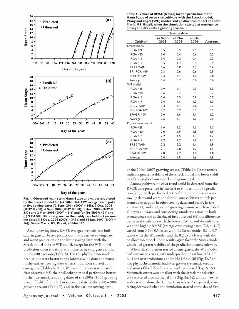
Fig. 4. Observed main stem Haun Stage and values predicted by the Streck model for (a) ‘BR-IRGA 409’ rice grown in pots in five sowing dates [2 Sept. 2004 (DOY = 245), 7 Oct. 2004 (DOY = 280), 4 Nov. 2004 (DOY = 308), 3 Dec. 2004 (DOY = 337) and 2 Mar. 2005 (DOY = 61)] and for (b) ‘IRGA 421’ and (c) ‘EPAGRI 109’ rice grown in the paddy rice field in two sow-ing dates [13 Dec. 2006 (DOY = 347), and 16 Jan. 2007 (DOY = 16)]. Santa Maria, RS, Brazil, 2004–2007.

498 Agronomy Journa l • Volume 100, Issue 3 • 2008

observed HS for all models, but systematic errors still appear

more evident with WE and the phyllochron models (Fig. 2d,

2e, 2f, 3d, 3e, 3f). Predictive accuracy of all models declined

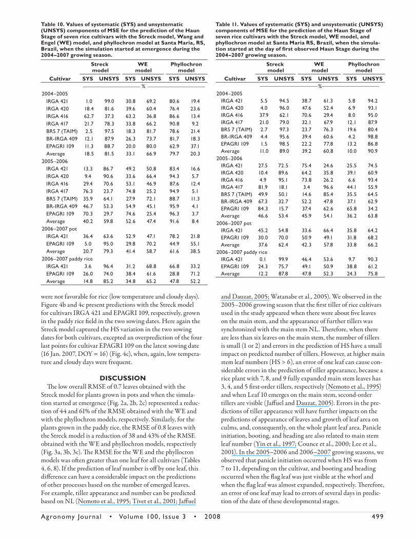
as the crop aged. Th e systematic and unsystematic (random)

components of the MSE with the three LAR models for each

cultivar (average of sowing dates) within each year are pre-

sented in Table 10 (simulation starting at emergence) and in

Table 11 (simulation starting at the day of fi rst observed HS).

We pooled the data of diff erent sowing dates presented in

Tables 10 and 11 to reduce the number of tables and because

of similar results among sowing dates. When the simulation

started at emergence, the lowest systematic and the highest

unsystematic values were obtained with the Streck model,

whereas the highest systematic and the lowest unsystematic

values were obtained with the phyllochron model both across

cultivars and years. Overall, the systematic component varied

from 1.0 to 76.3%, from 18.3 to 74.8%, and from 28.8 to

96.3% for the Streck, WE, and phyllochron models, respec-

tively (Table 10). When the simulation started at the day of

the fi rst observed HS, the lowest and the highest values of

the systematic and unsystematic components of the MSE

with the three LAR models varied among cultivars and years,

whereas the systematic component decreased drastically with

the phyllochron model. Overall, the systematic component

varied from 0.1 to 84.3%, from 3.4 to 75.4%, and from 4.2 to

65.8% for the Streck, WE, and phyllochron models, respec-

tively (Table 11).

Th e performance of the Streck model in selected sowing

dates is presented in Fig. 4. Figure 4a presents the prediction

of HS for the cultivar BR-IRGA 409 grown in pots in the fi ve

sowing dates of the 2004–2005 growing season. Plants on

these sowing dates grew under extreme temperature conditions

for rice. Plants on the fi rst sowing date (2 Sept. 2004, DOY

= 245) were subjected to minimum daily air temperature as

low as 4.6°C in September 2004, whereas plants on the fourth

sowing date (3 Dec. 2004, DOY = 337) where exposed to

maximum daily air temperature as high as 38.2°C in January

2005. Th e third sowing date (4 Nov. 2004, DOY = 308) rep-

resents a normal sowing date for local conditions. On the fi ft h

sowing date (2 Mar. 2005, DOY = 61) plants died by middle

June 2005 due to low temperatures and cloudy days before the

fl ag leaf emerged from the whorl. Th e Streck model captured

the HS variation quite well in the fi ve sowing dates, except an

overprediction of the last two observed data of the fi ft h sowing

date collected in end of May and early June, when conditions

Table 7. Values of RMSE (leaves) for the prediction of the Haun Stage of seven rice cultivars with the Streck model, Wang and Engel (WE) model, and phyllochron model at Santa Maria, RS, Brazil, when the simulation started at the day of fi rst observed Haun Stage during the 2005–2006 growing season.

Cultivar

Sowing date

Average26 Sept.

200525 Nov.

20052 Feb. 2006

Streck model IRGA 421 0.4 0.5 0.4 0.4 IRGA 420 0.3 0.5 0.4 0.4 IRGA 416 0.3 0.2 0.4 0.3 IRGA 417 0.5 0.9 0.5 0.7 BRS 7 TAIM 0.5 0.6 0.3 0.5 BR-IRGA 409 0.2 0.4 0.4 0.3 EPAGRI 109 0.4 0.9 0.7 0.7 Average 0.4 0.6 0.4 0.5WE model IRGA 421 1.1 1.4 0.9 1.1 IRGA 420 0.8 0.8 1.0 0.9 IRGA 416 0.6 1.3 0.9 0.9 IRGA 417 0.2 0.4 0.5 0.4 BRS 7 TAIM 0.3 0.4 0.9 0.5 BR-IRGA 409 0.3 0.3 0.6 0.4 EPAGRI 109 0.4 0.5 0.5 0.5 Average 0.5 0.7 0.8 0.8Phyllochron model IRGA 421 0.5 1.1 0.6 0.7 IRGA 420 0.9 0.3 0.5 0.6 IRGA 416 0.9 0.6 0.4 0.6 IRGA 417 1.0 0.3 0.4 0.6 BRS 7 TAIM 1.3 0.5 0.4 0.7 BR-IRGA 409 1.0 0.1 0.3 0.5 EPAGRI 109 1.1 0.5 0.4 0.7 Average 1.0 0.5 0.4 0.7

Table 8. Values of RMSE (leaves) for the prediction of the Haun Stage of seven rice cultivars with the Streck model, Wang and Engel (WE) model, and phyllochron model at Santa Maria, RS, Brazil, when the simulation started at emergence during the 2006–2007 growing season.

Cultivar

Sowing date

Avg. pot

Avg. paddy rice

13 Dec. 2006 16 Jan. 2007

PotPaddy

rice PotPaddy

riceStreck model IRGA 421 0.6 0.6 0.8 0.4 0.7 0.5 EPAGRI 109 0.8 0.5 0.8 1.2 0.8 0.9 Average 0.7 0.6 0.8 0.8 0.8 0.7WE model IRGA 421 1.1 0.9 1.2 0.7 1.2 0.8 EPAGRI 109 1.4 1.0 0.8 1.9 1.1 1.5 Average 1.3 1.0 1.0 1.3 1.1 1.1Phyllochron model IRGA 421 1.4 1.6 1.5 0.7 1.5 1.2 EPAGRI 109 1.5 1.5 0.9 1.4 1.2 1.5 Average 1.5 1.6 1.2 1.1 1.3 1.3

Table 9. Values of RMSE (leaves) for the prediction of the Haun Stage of seven rice cultivars with the Streck model, Wang and Engel (WE) model, and phyllochron model at Santa Maria, RS, Brazil, when the simulation started at the day of fi rst observed Haun Stage during the 2006–2007 growing season.

Cultivar

Sowing date

Avg. pot

Avg. paddy rice

13 Dec. 2006 16 Jan. 2007

PotPaddy

rice PotPaddy

riceStreck model IRGA 421 0.5 0.4 1.3 0.4 0.9 0.4 EPAGRI 109 0.8 0.5 0.9 1.1 0.9 0.8 Average 0.7 0.5 1.1 0.8 0.9 0.6WE model IRGA 421 0.9 0.4 1.4 1.0 1.2 0.7 EPAGRI 109 1.5 0.8 1.1 2.1 1.3 1.5 Average 1.2 0.6 1.3 1.6 1.2 1.1Phyllochron model IRGA 421 0.6 0.4 1.2 0.7 0.9 0.6 EPAGRI 109 0.8 0.8 0.9 1.8 0.9 1.3 Average 0.7 0.6 1.1 1.3 0.9 0.9

Agronomy Journa l • Volume 100, Issue 3 • 2008 499

were not favorable for rice (low temperature and cloudy days).

Figure 4b and 4c present predictions with the Streck model

for cultivars IRGA 421 and EPAGRI 109, respectively, grown

in the paddy rice fi eld in the two sowing dates. Here again the

Streck model captured the HS variation in the two sowing

dates for both cultivars, excepted an overprediction of the four

last points for cultivar EPAGRI 109 on the latest sowing date

(16 Jan. 2007, DOY = 16) (Fig. 4c), when, again, low tempera-

ture and cloudy days were frequent.

DISCUSSIONTh e low overall RMSE of 0.7 leaves obtained with the

Streck model for plants grown in pots and when the simula-

tion started at emergence (Fig. 2a, 2b, 2c) represented a reduc-

tion of 44 and 61% of the RMSE obtained with the WE and

with the phyllochron models, respectively. Similarly, for the

plants grown in the paddy rice, the RMSE of 0.8 leaves with

the Streck model is a reduction of 38 and 43% of the RMSE

obtained with the WE and phyllochron models, respectively

(Fig. 3a, 3b, 3c). Th e RMSE for the WE and the phyllocron

models was oft en greater than one leaf for all cultivars (Tables

4, 6, 8). If the prediction of leaf number is off by one leaf, this

diff erence can have a considerable impact on the predictions

of other processes based on the number of emerged leaves.

For example, tiller appearance and number can be predicted

based on NL (Nemoto et al., 1995; Tivet et al., 2001; Jaff uel

and Dauzat, 2005; Watanabe et al., 2005). We observed in the

2005–2006 growing season that the fi rst tiller of rice cultivars

used in the study appeared when there were about fi ve leaves

on the main stem, and the appearance of further tillers was

synchronized with the main stem NL. Th erefore, when there

are less than six leaves on the main stem, the number of tillers

is small (1 or 2) and errors in the prediction of HS have a small

impact on predicted number of tillers. However, at higher main

stem leaf numbers (HS > 6), an error of one leaf can cause con-

siderable errors in the prediction of tiller appearance, because a

rice plant with 7, 8, and 9 fully expanded main stem leaves has

3, 4, and 5 fi rst-order tillers, respectively (Nemoto et al., 1995)

and when Leaf 10 emerges on the main stem, second-order

tillers are visible (Jaff uel and Dauzat, 2005). Errors in the pre-

dictions of tiller appearance will have further impacts on the

predictions of appearance of leaves and growth of leaf area on

culms, and, consequently, on the whole plant leaf area. Panicle

initiation, booting, and heading are also related to main stem

leaf number (Yin et al., 1997; Counce et al., 2000; Lee et al.,

2001). In the 2005–2006 and 2006–2007 growing seasons, we

observed that panicle initiation occurred when HS was from

7 to 11, depending on the cultivar, and booting and heading

occurred when the fl ag leaf was just visible at the whorl and

when the fl ag leaf was almost expanded, respectively. Th erefore,

an error of one leaf may lead to errors of several days in predic-

tion of the date of these developmental stages.

Table 11. Values of systematic (SYS) and unsystematic (UNSYS) components of MSE for the prediction of the Haun Stage of seven rice cultivars with the Streck model, WE model, and phyllochron model at Santa Maria RS, Brazil, when the simula-tion started at the day of fi rst observed Haun Stage during the 2004–2007 growing season.

Cultivar

Streck model

WE model

Phyllochron model

SYS UNSYS SYS UNSYS SYS UNSYS%

2004–2005 IRGA 421 5.5 94.5 38.7 61.3 5.8 94.2 IRGA 420 4.0 96.0 47.6 52.4 6.9 93.1 IRGA 416 37.9 62.1 70.6 29.4 8.0 95.0 IRGA 417 21.0 79.0 32.1 67.9 12.1 87.9 BRS 7 (TAIM) 2.7 97.3 23.7 76.3 19.6 80.4 BR-IRGA 409 4.4 95.6 39.4 60.6 4.2 98.8 EPAGRI 109 1.5 98.5 22.2 77.8 13.2 86.8 Average 11.0 89.0 39.2 60.8 10.0 90.92005–2006 IRGA 421 27.5 72.5 75.4 24.6 25.5 74.5 IRGA 420 10.4 89.6 64.2 35.8 39.1 60.9 IRGA 416 4.9 95.1 73.8 26.2 6.6 93.4 IRGA 417 81.9 18.1 3.4 96.6 44.1 55.9 BRS 7 (TAIM) 49.9 50.1 14.6 85.4 35.5 64.5 BR-IRGA 409 67.3 32.7 52.2 47.8 37.1 62.9 EPAGRI 109 84.3 15.7 37.4 62.6 65.8 34.2 Average 46.6 53.4 45.9 54.1 36.2 63.82006–2007 pot IRGA 421 45.2 54.8 33.6 66.4 35.8 64.2 EPAGRI 109 30.0 70.0 50.9 49.1 31.8 68.2 Average 37.6 62.4 42.3 57.8 33.8 66.22006–2007 paddy rice IRGA 421 0.1 99.9 46.4 53.6 9.7 90.3 EPAGRI 109 24.3 75.7 49.1 50.9 38.8 61.2 Average 12.2 87.8 47.8 52.3 24.3 75.8

Table 10. Values of systematic (SYS) and unsystematic (UNSYS) components of MSE for the prediction of the Haun Stage of seven rice cultivars with the Streck model, Wang and Engel (WE) model, and phyllochron model at Santa Maria, RS, Brazil, when the simulation started at emergence during the 2004–2007 growing season.

Cultivar

Streck model

WE model

Phyllochron model

SYS UNSYS SYS UNSYS SYS UNSYS%

2004–2005 IRGA 421 1.0 99.0 30.8 69.2 80.6 19.4 IRGA 420 18.4 81.6 39.6 60.4 76.4 23.6 IRGA 416 62.7 37.3 63.2 36.8 86.6 13.4 IRGA 417 21.7 78.3 33.8 66.2 90.8 9.2 BRS 7 (TAIM) 2.5 97.5 18.3 81.7 78.6 21.4 BR-IRGA 409 12.1 87.9 26.3 73.7 81.7 18.3 EPAGRI 109 11.3 88.7 20.0 80.0 62.9 37.1 Average 18.5 81.5 33.1 66.9 79.7 20.32005–2006 IRGA 421 13.3 86.7 49.2 50.8 83.4 16.6 IRGA 420 9.4 90.6 33.6 66.4 94.3 5.7 IRGA 416 29.4 70.6 53.1 46.9 87.6 12.4 IRGA 417 76.3 23.7 74.8 25.2 94.9 5.1 BRS 7 (TAIM) 35.9 64.1 27.9 72.1 88.7 11.3 BR-IRGA 409 46.7 53.3 54.9 45.1 95.9 4.1 EPAGRI 109 70.3 29.7 74.6 25.4 96.3 3.7 Average 40.2 59.8 52.6 47.4 91.6 8.42006–2007 pot IRGA 421 36.4 63.6 52.9 47.1 78.2 21.8 EPAGRI 109 5.0 95.0 29.8 70.2 44.9 55.1 Average 20.7 79.3 41.4 58.7 61.6 38.52006–2007 paddy rice IRGA 421 3.6 96.4 31.2 68.8 66.8 33.2 EPAGRI 109 26.0 74.0 38.4 61.6 28.8 71.2 Average 14.8 85.2 34.8 65.2 47.8 52.2

500 Agronomy Journa l • Volume 100, Issue 3 • 2008

Th e phyllochron model gave the poorest predictions of HS

when the simulation started at the day of fi rst observed HS,

with predictions oft en being off by at least 1.5 leaves (Tables 4,

6, 8), and with high values of systematic component of MSE

(Table 10). Th is model uses the TT approach as a measure of

time. Th e TT approach has the assumption of a linear rela-

tionship between temperature and development, which is not

completely realistic from a biological viewpoint. Biological

processes, including plant development, respond to tempera-

ture in a nonlinear fashion (Yin et al., 1995; Granier and

Tardieu, 1998; Bonhomme, 2000), with only a small portion

of the response being linear (Wang and Engel, 1998; Streck

et al., 2003b; Streck et al., 2007). Th e predictions of HS with

the WE model were better than with the phyllochron model

(Table 4, 6, 8), confi rming previous results that LAR response

to temperature in rice is nonlinear (Gao et al., 1992; Ellis et

al., 1993; Sie et al., 1998). Similar results with the WE model

gave better predictions of main stem HS than the phyllochron

model, as reported by Xue et al. (2004) in winter wheat.

It is evident that the phyllochron model misses the fi rst and

second leaves, but the scattering of points around the 1:1 is

less than for the other two models at higher HS (Fig. 2c, 3c).

Considering the simplicity and wide use of the phyllochron

model, we tested the removal of this initial error by setting the

fi rst estimated HS value equal to the observed HS value. If the

predictions were improved by removing the initial error, then a

reason for the large error in predicting the time of appearance

of the fi rst and second leaves with the phyllochron model could

be found. Th e results of these simulations showed a consider-

able reduction in the RMSE with the phyllochron model and

little or no change in the RMSE with the Streck and the WE

models, resulting in a lower RMSE with the phyllochron model

compared with the WE model, but still greater RMSE than the

Streck model, both in the pot experiment (Fig. 2d, 2e, 2f) and

the paddy rice experiment (Fig. 3d, 3e, 3f).

Th e predictive accuracy for HS declined for all models as

plants aged (Fig. 2, 3), with the Streck model showing the

smallest decline in the predictions. Small errors from the

beginning of the simulations added up throughout the period

of leaf appearance contributed to the decline in the predictions

late in the growing season. However, decline in the predictions

with the Streck model were found due to overpredictions at

the end of the latest sowing date with cultivars BR-IRGA 409

and EPAGRI 109, mainly the latter (Fig. 2a, 2d, 3a, 3d). Two

aspects are important here. First, in all 3 yr used as indepen-

dent data sets to evaluate the models, the last sowing dates (2

Mar. 2005, 2 Feb. 2006, and 16 Jan. 2007) were late and out of

the recommended sowing date for this location. Second, these

two cultivars are mid late and late cultivars, respectively, and

had the lowest LARmax12 and LARmax (Table 2). Th e combi-

nation of late sowing date and low LAR resulted in plants of

these two cultivars growing leaves in May and early June, when

temperatures and solar radiation were low as a result of the Fall

in the Southern Hemisphere, and did not fl ower because of

low temperatures in the weeks aft er (winter). For this location,

paddy rice is harvested in late February and March, so the over-

predictions of HS observed for these two cultivars in the latest

sowing dates (Fig. 2a, 2d, 3a, 3d) do not represent a signifi cant

problem from a practical fi eld perspective.

Most rice simulation models assume that only temperature

aff ects LAR (Alocilja and Ritchie, 1991; Gao et al., 1992;

Horie, 1994; Sié et al., 1998). If this assumption is correct, then

the NL (at HS) should increase linearly as a function of time

(calendar days) under constant temperature or as a function

of TT in the fi eld (Streck et al., 2003a). Results from growth

chamber experiments with rice at constant temperature show

that this assumption is not correct—as time progresses, LAR

in rice decreases (Baker et al., 1990; Yin and Kropff , 1996).

Results presented in Fig. 2b, 2c, 2e, 2f, 3b, 3c, 3e, 3f also show

that this assumption is not correct and support the hypothesis

that LAR in rice decreases as a plant ages. Predictions with

the WE model (Fig. 2b, 2c, 3b, 3c) and with the phyllochron

model (Fig. 2e, 2f, 3e, 3f) were curvilinear upward because of

a constant LARmax and phyllochron assumed in the models,

respectively, and because of a decreasing observed LAR as time

progresses, resulting in underprediction early in the growing

season and overprediction late in the growing season. Th e

under- and overpredictions with the WE and phyllochron

models increased the systematic errors of the predictions with

these two models (Table 10). In the Streck model, LAR is

assumed aff ected by seed reserves and plant age, represented by

accumulated leaf number, through a chronology response func-

tion [f(C)]. Th e fi rst two leaves have the highest LAR due to

seed reserves. As the number of emerged leaves increases, LAR

decreases because the distance that each leaf primordium must

extend to appear at the whorl increases for each subsequent

leaf. Th is assumption was proposed for wheat (Streck et al.,

2003a) and predictions with the Streck model (Fig. 2a, 2d, 3a,

3d) showing no curvilinear response, at least for HS < 10, dem-

onstrating that this assumption is also valid for rice.

Th e decrease in LAR as a plant ages results from an increas-

ing time required for leaf tips to grow from the apical meristem

to the whorl for each successive leaf; it is accounted for by the

decreasing f(C) in the Streck model (Fig. 1b). Th is approach is

biologically and mathematically sound. Biologically, as more

leaves are produced and successive leaves have longer sheaths,

each additional leaf must grow longer and takes more time before

the tip is visible at the whorl, which decreases LAR with time.

Mathematically, this decrease in LAR is represented by a decreas-

ing time response function [f(C)] that multiplies LARmax12. Th e

scatter of points curving upward from the 1:1 line in Fig. 2b, 2c,

2e, and 2f, with underpredictions at lower HS and overpredic-

tions at higher HS, can be attributed to the absence of an age fac-

tor decreasing LAR in the WE model and phyllchron model. If

the very few points at the highest HS values in Fig. 2a and 2d are

excluded (as discussed above, these points probably are off due

to low temperature and cloudy days as results of plants growing

late in Fall), then no upward or downward trend in the points is

evident in the simulations with the Streck model.

Th e strength of a crop simulation model is how well it works

under a wide range of diff erent environmental conditions and

diff erent genotypes. Th e greatest stability of the Streck model,

characterized by the lowest RMSE across cultivars, sowing

dates, and years (Tables 4–9) and the lowest systematic compo-

nent of MSE (Tables 10 and 11) both when simulations started

at emergence and at the day of fi rst observed HS, compared

with the other two LAR models, indicates high robustness of

this model. Th e predictions with the phyllochron model were

Agronomy Journa l • Volume 100, Issue 3 • 2008 501

greatly improved when the simulations started at the day of

fi rst observed HS, but were the worst when the simulation

started at plant emergence. We seek a model that performs

well with simulations starting as early as possible, so we can

predict events as soon as the plant emerges. If we are interested

in tracking leaf area from leaf number, predictions of the fi rst

leaves impacts greatly on leaf area. Th ese results highlight some

limitations of the phyllochron model.

In this application of the Streck model, there was only one

coeffi cient that is genotype dependent: LARmax12. Th e tempera-

ture [f(T)] and the chronology [f(C)] response functions were

assumed genotype independent. Th ese assumptions worked well

for the seven genotypes used in this study, with no additional

input being necessary to run the Streck model compared with

the WE and the phyllochron models. Th ese results and the fact

that the chronology response function has worked with wheat

and rice indicate two important features of the Streck model

that are sought for any crop simulation model—generality and

robustness—while maintaining accurate predictions.

AKNOWLEDGMENTSTo the Instituto Rio Grandense do Arroz (IRGA) for providing

the seeds, and to Dr. Albert Weiss at the University of Nebraska-

Lincoln (USA) and anonymous peer reviewers for valuable comments

on early versions of the manuscript. The authors gratefully thank the

students Simone Michelon, Lidiane Cristine Walter, Hamilton Telles

Rosa, Cátia Camera, Gizelli Moiano de Paula, and Flávia Kaufmann

Samboranha for their assistance in collecting data and technical sup-

port during the four years of experiments, and Dr. Luis Antonio de

Avila for the facilities of the paddy rice field experiment. Funding

to N.A. Streck through Conselho Nacional de Desenvolvimento

Científico e Tecnológico- CNPq (Bolsa de Produtividade em Pesquisa)

at the Ministry of Science and Technology of Brazil and to L.C. Bosco

and I. Lago through Fundação CAPES (Bolsa de Mestrado) at the

Ministry of Education of Brazil are greatly acknowledged.

REFERENCESAlocilja, E.C., and J.T. Ritchie. 1991. A model for the phenology of rice. p.

181–189. In T. Hodges (ed.) Predicting crop phenology. CRC Press, Boston.

Amir, J., and T.R. Sinclair. 1991. A model of the temperature and solar radiation eff ects on spring wheat growth and yield. Field Crops Res. 28:47–58.

Baker, J.T., L.H. Allen, Jr., K.J. Boote, P. Jones, and J.W. Jones. 1990. Developmental responses of rice to photoperiod and carbon dioxide con-centration. Agric. For. Meteorol. 50:201–210.

Bonhomme, R. 2000. Bases and limits to using ‘degree.day’ units. Eur. J. Agron. 13:1–10.

Counce, P., T.C. Keisling, and A.J. Mitchell. 2000. A uniform, objetive, and adaptive system for expressing rice development. Crop Sci. 40:436–443.

Ellis, R.H., A. Qi, R.J. Summerfi eld, and E.H. Roberts. 1993. Rates of leaf appearance and panicle development in rice (Oryza sativa L.): A compari-son at three temperatures. Agric. For. Meteorol. 66:129–138.

Gao, L.Z. Jun, Y. Huang, and L. Zhang. 1992. Rice clock model—A computer model to simulate rice development. Agric. For. Meteorol. 60: 1–16.

Granier, C., and F. Tardieu. 1998. Is thermal time adequate for expressing the eff ects of temperature on sunfl ower leaf development? Plant Cell Environ. 21:695–703.

Haun, J.R. 1973. Visual Quantifi cation of wheat development. Agron. J. 65:116–119.

Hodges, T. 1991.Crop growth simulation and the role of phenological models. p. 3–5. In T. Hodges (ed.) Predicting crop phenology. CRC Press, Boston.

Horie, T. 1994. Crop ontogeny and development. p. 153–180. In Physiology and determination of crop yield. ASA, CSSA, and SSSA, Madison, WI.

Hoshikawa, K. 1993. Seedlings. p. 110–118. In T. Matsuo, and K. Hoshikawa (ed.) Science of the rice plant. Food and Agriculture Policy Res. Center, Tokyo.

Infeld, J.A., J.B. Silva, and F.N. Assis. 1998. Temperatura base e graus-dia durante o período vegetativo de três grupos de cultivares de arroz irri-gado (in Portuguese with Abstract in English). Rev. Bras. Agrometeorol. 6:187–191.

Jaff uel, S., and J. Dauzat. 2005. Syncrhonism of leaf and tiller emergence relative to position and to main stem development stage in a rice cultivar. Ann. Bot. (Lond.) 95:401–412.

Janssen, P.H.M., and P.S.C. Heuberger. 1995. Calibration of process-oriented models. Ecol. Modell. 83:55–56.

Kirby, E.J. 1995. Factors aff ecting rate of leaf emergence in barley and wheat. Crop Sci. 35:11–19.

Klepper, B., R.W. Rickman, and C.M. Peterson. 1982. Quantitative char-acterization of vegetative development in small cereal grains. Agron. J. 74:789–792.

Lee, C.K., B.W. Lee, J.C. Shin, and Y.H. Yoon. 2001. Heading date and fi nal leaf number as aff ected by sowing date and prediction of heading date based on leaf appearance model in rice. Korean J. Crop Sci. 46:195–201.

Matthews, R.B., and L.A. Hunt. 1994. GUMCAS: A model describing the growth of cassava (Manihot esculenta L. Crantz). Field Crops Res. 39:69–84.

McMaster, G.S. 2005. Phytomers, phyllochrons, phenology and temperate cereal development. J. Agric. Sci. (Cambridge) 143:137–150.

McMaster, G.S., B. Keppler, R.W. Rickman, W.W. Wilhelm, and W.O. Willis. 1991. Simulation of shoot vegetative development and growth of unstressed winter wheat. Ecol. Modell. 53:189–204.

McMaster, G.S., and W.W. Wilhelm. 1997. Growing degree-days: One equa-tion, two interpretations. Agric. For. Meteorol. 87:291–300.

Nemoto, K., S. Morita, and T. Bata. 1995. Shoot and root development in rice related to the phyllochron. Crop Sci. 35:24–29.

Peterson, C.M., B. Klepper, F.V. Pumphrey, and R.W. Rickman. 1984. Restricted rooting decreases tillering and growth of winter wheat. Agron. J. 76:861–863.

Shaykewich, C.F. 1995. An appraisal of cereal crop phenology modeling. Can. J. Plant Sci. 75:329–341.

Sié, M., M. Dingkuhn, M.C.S. Wopereis, and K.M. Miezan. 1998. Rice crop duration and leaf appearance rate in a variable thermal environment. I. Development of an empirically based model. Field Crops Res. 57:1–13.

Stansel, J.W. 1975. Th e rice plant—Its development and yield. p. 9–21. In Six decades of rice research in Texas. Res. Monogr. 4. Texas A&M Univ., College Station.

Streck, N.A., A. Weiss, Q. Xue, and P.S. Baenziger. 2003a. Incorporating a chronology response into the prediction of leaf appearance rate in winter wheat. Ann. Bot. (London) 92:181–190.

Streck, N.A., A. Weiss, Q. Xue, and P.S. Baenziger. 2003b. Improving predic-tions of developmental stages in winter wheat: A modifi ed Wang and Engel model. Agric. For. Meteorol. 115:139–150.

Streck, N.A., F.L.M. Paula, D.A. Bisognin, A.B. Heldwein, and J. Dellai. 2007. Simulating the development of fi eld grown potato (Solanum tuberosum L.). Agric. For. Meteorol. 142:1–11.

Tivet, F., B.S. Pinheiro, M. Raissac, and M. Dingkuhn. 2001. Leaf blade dimen-sions of rice (Oryza sativa L. and Oryza glaberrima Stend.). Relationship between tillers and the main stem. Ann. Bot. (London) 88:507–511.

Wang, E., and T. Engel. 1998. Simulation of phenological development of wheat crops. Agric. Syst. 58:1–24.

Watanabe, T., P.M.R. Hanan, T. Hazegawa, H. Nakagawa, and W. Takahashi. 2005. Rice morphogenesis and plant architecture: Measurement, specifi -cation and the reconstruction of structural development by 3D architec-tural modeling. Ann. Bot. (London) 95:1131–1143.

Wilhelm, W.W., and G.S. McMaster. 1995. Importance of the phyllochron in studying development and growth in grasses. Crop Sci. 35:1–3.

Willmott, C.J. 1981. On the validation of models. Phys. Geogr. 2:184–194.

Xue, Q., A. Weiss, and P.S. Baenziger. 2004. Predicting leaf appearance in fi eld grown winter wheat: Evaluating linear and non-linear models. Ecol. Modell. 175:261–270.

Yin, X., M.J. Kropff , G. Mclaren, and R.M. Visperas. 1995. A nonlinear model for crop development as a function of temperature. Agric. Forest Meteorol. 77:1–16.

Yin, X., and M.J. Kropff . 1996. Th e eff ect of temperature on leaf appearance in rice. Ann. Bot. (London) 77:215–221.

Yin, X., M.J. Kropff , and M.A. Ynalvez. 1997. Photoperiodically sensitive and insensitive phases of prefl owering development in rice. Crop Sci. 37:182–190.