HAL Id: tel-03662449https://tel.archives-ouvertes.fr/tel-03662449

Submitted on 9 May 2022

HAL is a multi-disciplinary open accessarchive for the deposit and dissemination of sci-entific research documents, whether they are pub-lished or not. The documents may come fromteaching and research institutions in France orabroad, or from public or private research centers.

L’archive ouverte pluridisciplinaire HAL, estdestinée au dépôt et à la diffusion de documentsscientifiques de niveau recherche, publiés ou non,émanant des établissements d’enseignement et derecherche français ou étrangers, des laboratoirespublics ou privés.

Signal processing and analysis of PTR-TOF-MS datafrom exhaled breath for biomarker discovery

Camille Roquencourt

To cite this version:Camille Roquencourt. Signal processing and analysis of PTR-TOF-MS data from exhaled breath forbiomarker discovery. Statistics [math.ST]. Université Paris-Saclay, 2022. English. NNT : 2022UP-ASG024. tel-03662449

THESE

DEDO

CTORAT

NNT:2

022UPA

SG024

Signal processing and analysis ofPTR-TOF-MS data from exhaled breath

for biomarker discoveryTraitement du signal et analyse des données PTR-TOF-MS de l’air

expiré pour la découverte de biomarqueurs

Thèse de doctorat de l’université Paris-Saclay

École doctorale n 580 Sciences et technologies de l’information et de lacommunication (STIC)

Spécialité de doctorat: Mathématiques et InformatiqueGraduate School : Informatique et sciences du numérique

Référent : Faculté des sciences d’Orsay

Thèse préparée à l’Institut LIST (Université Paris-Saclay, CEA), sous la direction deStanislas Grassin Delyle, professeur des universités - praticien hospitalier, et le

co-encadrement d’Etienne Thévenot, ingénieur chercheur.

Thèse soutenue à Paris-Saclay, le 25 mars 2022, par

Camille ROQUENCOURT

Composition du jury

Karine Bennis Zeitouni PrésidenteProfesseure des universités, Université deVersailles-Saint-Quentin-en-YvelinesFrédéric Bertrand Rapporteur & ExaminateurProfesseur des universités, Université de Technolo-gie de TroyesThomas Burger Rapporteur & ExaminateurDirecteur de recherche, HDR, CNRS, UniversitéGrenoble AlpesWolfram Miekisch ExaminateurSenior researcher, University of RostockStanislas Grassin-Delyle Directeur de thèseProfesseur des universités - praticien hospitalier ,Université de Versailles-Saint-Quentin-en-Yvelines

Titre: Traitement du signal et analyse des données PTR-TOF-MS à partir de l’expiration pour la découvertede biomarqueursMots clés: Traitement du signal, logiciel, air expiré, PTR-TOF-MSRésumé: L’analyse des composés organiques volatils(COVs) dans l’air expiré est une méthode non invasiveprometteuse en médecine pour le diagnostic précoce,le phénotypage, le suivi de la maladie et du traite-ment et le dépistage à grande échelle. La spectrométriede masse à temps de vol par réaction de transfert deprotons (PTR-TOF-MS) présente un intérêt majeur pourl’analyse en temps réel des COVs et la découverte denouveaux biomarqueurs. Le manque de méthodes etd’outils logiciels pour le traitement des données PTR-TOF-MS provenant de cohortes représente actuellement unverrou pour le développement de ces approches.Nous avons ainsi développé une suite d’algorithmespermettant le traitement des données brutes jusqu’autableau des intensités des molécules détectées, grâce àla détection des expirations et des pics dans les spec-tres de masse, la quantification dans la dimension tem-porelle, l’alignement entre les échantillons et l’imputationdes valeurs manquantes. Nous avons notamment misau point un modèle innovant de déconvolution des picsen 2 dimensions reposant sur une régression du signalpar splines pénalisées, ainsi qu’une méthode permettantde sélectionner spécifiquement les COVs dans l’air expiré.L’ensemble du processus est implémenté dans le paquetR/Bioconductor ptairMS, disponible en ligne. Nous avonsvalidé notre approche à la fois sur des données expéri-

mentales (mélange de COVs à des concentrations stan-dardisées) et par simulation. Les résultats montrent quel’identification des COVs provenant de l’air expiré à partirdu modèle proposé atteint une sensibilité de 99 ‘%. Uneinterface graphique a également été développée pour fa-ciliter l’analyse des données et l’interprétation des résul-tats par les expérimentateurs (les cliniciens notamment).Nous avons appliqué notre méthodologie à la caractéri-sation de l’air expiré d’adultes sous ventilationmécaniqueatteints de l’infectionCOVID-19. Les analyses de l’air expiréde 40 patients atteints d’un syndrome de détresse respi-ratoire aiguë (SDRA) ont été effectuées quotidiennement,de l’entrée à la sortie de l’hôpital. Nous avons d’abordréalisé un modèle de classification pour prédire le statutde l’infection, en utilisant l’acquisition disponible la plusproche de l’admission à l’hôpital. Ce modèle permet deprédire le statut de l’infection avec une précision de 93%.Ensuite, nous avons utilisé toutes les données disponiblespour une analyse longitudinale de l’évolution des COVsen fonction de la durée de l’hospitalisation, en utilisantun modèle à effets mixtes. Après sélection de variables,quatre biomarqueurs de l’infection par le COVID-19 ontpu être identifiés. Ces résultats soulignent la valeur desdonnées PTR-TOF-MS et du logiciel ptairMS pour la décou-verte de biomarqueurs dans l’air expiré.

Title: Signal processing and analysis of PTR-TOF-MS data from exhaled breath for biomarker discoveryKeywords: Signal processing, Sotfware, Exhaled breath, PTR-TOF-MSAbstract: The analysis of Volatile Organic Compounds(VOCs) in exhaled breath is a promising non-invasive ap-proach in medicine for early diagnosis, phenotyping, dis-ease and treatmentmonitoring and large-scale screening.Proton Transfer Reaction Time-Of-Flight Mass Spectrom-etry (PTR-TOF-MS) is of major interest for the real timeanalysis of VOCs and the discovery of new biomarkers inthe clinics. However, there is currently a lack of methodsand software tools for the processing of PTR-TOF-MS datafrom cohorts.We therefore developed a suite of algorithms that pro-cess raw data from the patient acquisitions, and buildthe table of feature intensities, through expiration andpeak detection, quantification, alignment between sam-ples, and missing value imputation. Notably, we devel-oped an innovative 2D peak deconvolution model basedon penalized splines signal regression, and a method tospecifically select the VOCs from exhaled breath. The fullworkflow is implemented in the freely available ptairMSR/Bioconductor package. Our approach was validatedboth on experimental data (mixture of VOCs at standard-ized concentrations) and simulations, which showed that

the sensitivity for the identification of VOCs from exhaledbreath reached 99%. A graphical interfacewas also devel-oped to facilitate data analysis and result interpretationby experimenters (e.g., clinicians).We applied our methodology to the characterization ofexhaled breath from mechanically ventilated adults withCOVID-19 infection. Analysis of exhaled breath from28 pa-tients with an acute respiratory distress syndrome (ARDS)andCOVID-19 infection, and 12 patientswith non-COVID-19ARDS were performed daily from the hospital admissionto the discharge. First, classification models were built topredict the status of the infection, using the closest avail-able acquisition to the entry into hospital, and achievedhigh prediction accuracies (93 %). Then, all the avail-able data acquired during the hospital stay were used forthe longitudinal analysis of the VOCs evolution as a func-tion of the hospitalization timebymixed-effectsmodeling.Following feature ranking and selection, four biomarkersof COVID-19 infection were identified. Altogether, theseresults highlight the value of the PTR-TOF-MS data andthe ptairMS software for biomarker discovery in exhaledbreath.

2

Acknowledgements

First of all I would like to express my sincere gratitude to my two supervisors, Mr Eti-enne Thévenot and Mr Stanislas Grassin Delyle, for proposing this thesis subject, trustingme and providing the best supervision possible, both on the human and scientific levels.Many thanks to Etienne for his benevolence, kindness and involvement throughout thePhD, as well as during the review of this manuscript, and to Stanislas for his availability,reactivity and his confidence for a future collaboration.I would like to thank my rapporteurs Mr Thomas Burger and Mr Frédéric Bertrand for

kindly agreeing to evaluate this thesis, aswell as the examinersMrs Karine Bennis Zeitouniand Mr Wolfram Miekisch.I thank the CEA and more particularly the Data Intelligence Unit (SID), for the optimal

working conditions. I would also like to thank all the bioinformatics team, Alyssa, Camilo,Sylvain, Eric, Pierrick and Krystyna, for all the constructive discussions and advice, and allthe other colleagues of the SID that I met during those three years, for the good atmo-sphere and the unfailing support.I would also like to thank the Exhalomics team and the pneumology department at the

Foch Hospital, Prof. Philippe Devillier, Prof. Antoine Magnan, Prof. Louis-Jean Couderc,Dr. Hélène Salvator, Dr. Emmanuel Naline, for their excellent welcome and scientificexpertise, it is a pleasure to work with them.Finally, I would like to thank my parents and my brother for their constant help and

support, my boyfriend Imad and my friends who have been my crutch for these years,Manel, Ines, Margot, Karim, Ruana, Nabila, and the two best flatmates ever during thelockdown: Joana, who helped me prepare my English orals, and Célia, with whom I haveshared every step of our lives for 26 years.

1

Preface

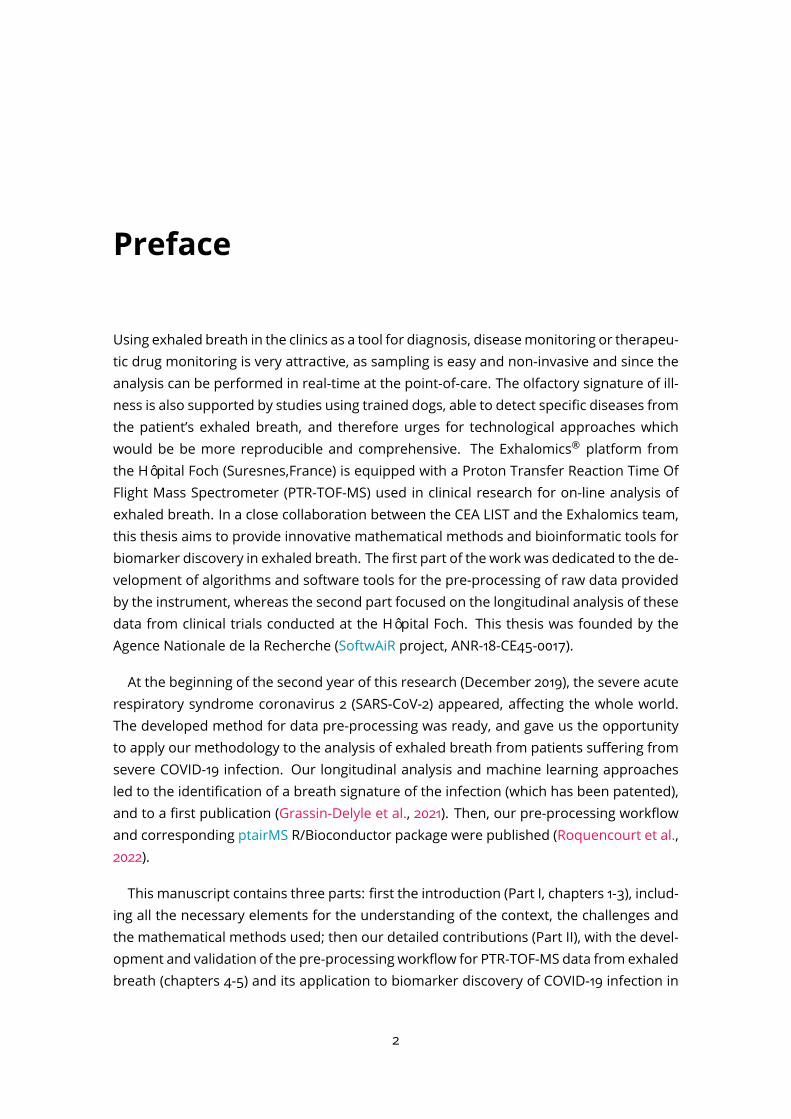
Using exhaled breath in the clinics as a tool for diagnosis, diseasemonitoring or therapeu-tic drug monitoring is very attractive, as sampling is easy and non-invasive and since theanalysis can be performed in real-time at the point-of-care. The olfactory signature of ill-ness is also supported by studies using trained dogs, able to detect specific diseases fromthe patient’s exhaled breath, and therefore urges for technological approaches whichwould be be more reproducible and comprehensive. The Exhalomics® platform fromthe Hôpital Foch (Suresnes,France) is equipped with a Proton Transfer Reaction Time OfFlight Mass Spectrometer (PTR-TOF-MS) used in clinical research for on-line analysis ofexhaled breath. In a close collaboration between the CEA LIST and the Exhalomics team,this thesis aims to provide innovative mathematical methods and bioinformatic tools forbiomarker discovery in exhaled breath. The first part of the work was dedicated to the de-velopment of algorithms and software tools for the pre-processing of raw data providedby the instrument, whereas the second part focused on the longitudinal analysis of thesedata from clinical trials conducted at the Hôpital Foch. This thesis was founded by theAgence Nationale de la Recherche (SoftwAiR project, ANR-18-CE45-0017).At the beginning of the second year of this research (December 2019), the severe acute

respiratory syndrome coronavirus 2 (SARS-CoV-2) appeared, affecting the whole world.The developed method for data pre-processing was ready, and gave us the opportunityto apply our methodology to the analysis of exhaled breath from patients suffering fromsevere COVID-19 infection. Our longitudinal analysis and machine learning approachesled to the identification of a breath signature of the infection (which has been patented),and to a first publication (Grassin-Delyle et al., 2021). Then, our pre-processing workflowand corresponding ptairMS R/Bioconductor package were published (Roquencourt et al.,2022).This manuscript contains three parts: first the introduction (Part I, chapters 1-3), includ-

ing all the necessary elements for the understanding of the context, the challenges andthe mathematical methods used; then our detailed contributions (Part II), with the devel-opment and validation of the pre-processing workflow for PTR-TOF-MS data from exhaledbreath (chapters 4-5) and its application to biomarker discovery of COVID-19 infection in

2

intubated, mechanically ventilated patients (chapter 6); and finally the conclusion andperspectives (Part III). The two articles are shown in appendix B.

Notation

Bold-face, lower-case letters refer to vectors x; italic lower-case letters refer to vectorelements xi or scalars a. Bold-face, capital letters refer to matrices X , and special frontparam to software parameters.

Valorisation and teaching activities

Publications

• Stanislas Grassin-Delyle, Camille Roquencourt, PierreMoine, Gabriel Saffroy, Stanis-las Carn, NicholasHeming, Jérôme Fleuriet, Hélène Salvator, EmmanuelNaline, Louis-JeanCouderc, PhilippeDevillier, EtienneA. Thévenot, andDjillali Annane (2021). Metabolomicsof exhaledbreath in critically ill COVID-19 patients: A pilot study. EBioMedicine, 63:103154,doi:10.1016/j.ebiom.2020.103154.

• Camille Roquencourt, StanislasGrassinDelyle, and EtienneA. Thévenot (2022). ptairMS:real-time proces sing and analysis of PTR-TOF-MS data for biomarker discovery in-exhaled breath. Bioinformatics, doi:10.1093/bioinformatics/btac031.

Patent

• EP20306170.0 European patentOral communications (online)

• Metabolomics Society 2021; Signal processing and data analysis of mass spectrometrydata from exhaled breath for biomarker discovery; Early career member best abstractaward

• JOBIM 2021 (Journées Ouvertes en Biologie, Informatique et Mathématiques); Pro-cessing of Proton Transfer Reaction Time-of Flight Mass Spectrometry (PTR-TOF-MS) datafor untargeted biomarker discovery in exhaled breath: application to COVID-19 intubatedventilated patient; Best presentation award

• ECCB 2021 (European Conference on Computational Biology); ptairMS: processingand analysis of PTR-TOF-MS data for biomarker discovery in exhaled breath

• ICFSP 2021 (International Conference Frontier Signal Processing); Innovative methodsbased on 2D penalized regression for the processing and analysis of mass spectrometry

3

data from exhaled breath• ASMS 2021 (American Society for Mass Spectrometry); Processing and analysis of PTR-TOF mass spectrometry data for biomarker discovery in exhaled breath; switched to aposter presentation as US borders were closed due to health restrictions

Monitorat (1st and 2nd year of the PhD; 64h/year)

• Introduction to databases; Licence 2; Université Paris-Saclay• Introduction to databases; 2nd year; Polytech Paris-Saclay• Introduction to the C++ language; Licence 1; Université Paris-Saclay

4

Résumé

La ’volatolomique’, analyse globale des composés organiques volatils (COV) dans l’air ex-piré, est une approche prometteuse pour la médecine personnalisée. En effet, l’air quenous expirons est composé à 1%de ces COVs, qui proviennent directement dumétabolisme.Des signatures volatolomiques caractéristiques de maladies (biomarqueurs) pourraientdonc être identifiées dans l’air expiré. De récents travaux ont ainsi mis en avant l’étudedes COVs pour la détection de plusieurs pathologies, dont le cancer, l’asthme, la cirrhose,ou la mucoviscidose (Einoch Amor et al., 2019; Pereira et al., 2015; Feil et al., 2021; Guiraoet al., 2019).L’avantagemajeur de la volatolomique par rapport aux examens biologiques classiques

est que le prélèvement est complètement non-invasif, simple et rapide. De plus, certainsinstruments permettent une analyse en temps réel de l’air expiré, tel que la spectrométriede masse par réaction de transfert de protons (PTR-TOF-MS, Jordan et al. 2009). L’analysese fait par introduction directe, l’ionisation des COVs a lieu en temps réel, par transfertd’un proton à partir d’un ion primaire (généralement H3O+). Les ions ainsi formés (COV+ H+) sont ensuite analysés par un spectromètre de masse à temps de vol.Le traitement des données brutes issues des instruments PTR-TOF-MS représente un

enjeu majeur pour la recherche de biomarqueurs dans l’air expiré. Les principaux dé-fis sont la détection et la déconvolution des pics dans la dimension de masse, ainsi quel’estimation de leurs intensités tout au long de l’acquisition (dans l’échelle temporelle), afind’identifier les molécules provenant uniquement de l’air expiré. Au démarrage de cettethèse, deux logiciels existaient pour le traitement des données PTR-TOF-MS (Holzinger,2015;Müller et al., 2013), dont l’un seulement était en libre accès. Ces logiciels sont générale-ment utilisés pour l’analyse de l’air atmosphérique, et se focalisent sur la détection despics dans la dimension de masse. Ils ne prennent pas en compte les expirations pour fil-trer les variables provenant explicitement de l’air expiré, et ne sont pas adaptés à l’analysede cohortes (e.g. traitement des fichiers en parallèle).Nous avons ainsi développé une suite d’algorithmes permettant le traitement des don-

nées brutes jusqu’au tableau des intensités des molécules détectées, grâce à la détec-tion des expirations et des pics dans les spectres de masse, la quantification dans la di-

5

mension temporelle, l’alignement entre les échantillons et l’imputation des valeurs man-quantes (Roquencourt et al., 2022). Nous avons notamment mis au point un modèle in-novant de déconvolution des pics en 2 dimensions reposant sur une régression du sig-nal par splines pénalisées, ainsi qu’une méthode permettant de sélectionner spécifique-ment les COVs dans l’air expiré. L’ensemble du traitement est implémenté dans le paquetR/Bioconductor ptairMS, disponible en ligne. Une interface graphique a également étédéveloppée pour faciliter l’analyse des données et l’interprétation des résultats par lesexpérimentateurs (les cliniciens notamment).Nous avons d’abord validé notre approche sur des données expérimentales (mélange

de COVs à des concentrations standardisées). Après traitement des fichiers par ptairMS,tous les composés attendus ont été détectés, ainsi que leurs isotopes, avec une erreur enmasse inférieure à 20 ppm, et une erreur de quantification inférieure à 8%.Afin de comparer les performances de ptairMS aux deux logiciels existants, nous avons

développé un algorithme de simulation de données PTR-TOF-MS issus de l’air expiré,disponible en ligne dans le paquet R ptairData. ptairMS a obtenu lameilleure précision dedétection des pics parmi les trois logiciels (99.99%). L’erreur absoluemoyenne (MAPE) en-tre l’évolution temporelle estimée et l’entrée de la simulation est de 4,96% pour ptairMS,contre 14,65% et 5,38% pour les deux autres logiciels. Enfin, nous avons comparé la ca-pacité à discriminer les composés spécifiques de l’air expiré, en utilisant deux t-tests uni-latéraux comparant les intensités entre les phases d’expiration et d’air ambiant. ptairMSs’est avéré capable de détecter l’origine des VOCs avec une précision de 99%.Nous avons ensuite appliqué notre méthodologie à la caractérisation de l’air expiré

d’adultes sous ventilationmécanique atteints de l’infection COVID-19. Les analyses de l’airexpiré de 40 patients atteints d’un syndromede détresse respiratoire aiguë (SDRA) ont étéeffectuées quotidiennement, de l’entrée à la sortie de l’hôpital. Nous avons d’abord réal-isé unmodèle de classification pour prédire le statut de l’infection, en utilisant l’acquisitiondisponible la plus proche de l’admission à l’hôpital. Ce modèle permet de prédire lestatut de l’infection avec une précision de 93%. Ensuite, nous avons utilisé toutes lesdonnées disponibles pour une analyse longitudinale de l’évolution des COVs en fonctionde la durée de l’hospitalisation, en utilisant un modèle à effets mixtes. Après sélectionde variables, quatre biomarqueurs de l’infection par le COVID-19 ont pu être identifiés(Grassin-Delyle et al., 2021).

6

Contents

I Introduction 13

1 Context 141.1 Biomarker discorvery in exhaled breath . . . . . . . . . . . . . . . . . . . . 14

1.1.1 Metabolomic biomarkers . . . . . . . . . . . . . . . . . . . . . . . . . 141.1.2 Volatolomics: analysis of exhaled breath for personalised medicine 151.1.3 Mass spectrometry approaches for VOC analysis . . . . . . . . . . . 17

1.2 Signal processing of mass spectrometry-based data . . . . . . . . . . . . . 191.2.1 Peak detection and quantification . . . . . . . . . . . . . . . . . . . . 211.2.2 Alignment . . . . . . . . . . . . . . . . . . . . . . . . . . . . . . . . . . 251.2.3 Identification . . . . . . . . . . . . . . . . . . . . . . . . . . . . . . . . 25

1.3 Online exhaled breath data processing . . . . . . . . . . . . . . . . . . . . . 251.3.1 Expiration phases detection . . . . . . . . . . . . . . . . . . . . . . . 261.3.2 Ambient inhaled air . . . . . . . . . . . . . . . . . . . . . . . . . . . . 26

2 Current processing of PTR-TOF-MS data 292.1 Data acquisition . . . . . . . . . . . . . . . . . . . . . . . . . . . . . . . . . . 292.2 Data pre-processing . . . . . . . . . . . . . . . . . . . . . . . . . . . . . . . . 30

2.2.1 Calibration of the mass axis . . . . . . . . . . . . . . . . . . . . . . . 302.2.2 Dead time correction . . . . . . . . . . . . . . . . . . . . . . . . . . . 332.2.3 Peak detection on the mass spectra . . . . . . . . . . . . . . . . . . . 332.2.4 Temporal estimation . . . . . . . . . . . . . . . . . . . . . . . . . . . 362.2.5 Normalisation and quantification . . . . . . . . . . . . . . . . . . . . 37

2.3 Software . . . . . . . . . . . . . . . . . . . . . . . . . . . . . . . . . . . . . . 373 Mathematical approaches for classification and longitudinal analysis 39

3.1 Penalised spline regression . . . . . . . . . . . . . . . . . . . . . . . . . . . . 393.1.1 Penalised smooth regression . . . . . . . . . . . . . . . . . . . . . . . 393.1.2 P-splines . . . . . . . . . . . . . . . . . . . . . . . . . . . . . . . . . . 413.1.3 Penalty, knots location and basis dimension . . . . . . . . . . . . . . 423.1.4 Multidimensional penalised regression . . . . . . . . . . . . . . . . . 45

3.2 Statistical learning for biomarker discovery . . . . . . . . . . . . . . . . . . . 467

3.2.1 Classification . . . . . . . . . . . . . . . . . . . . . . . . . . . . . . . . 463.2.2 Feature selection . . . . . . . . . . . . . . . . . . . . . . . . . . . . . . 533.2.3 Time-course modelling . . . . . . . . . . . . . . . . . . . . . . . . . . 56

II Results 63

4 Design and implementation of innovativemethods for the processing of PTR-TOF-MS data: ptairMS 644.1 Pre-processing for each file . . . . . . . . . . . . . . . . . . . . . . . . . . . . 65

4.1.1 Calibration . . . . . . . . . . . . . . . . . . . . . . . . . . . . . . . . . 654.1.2 Expiration detection . . . . . . . . . . . . . . . . . . . . . . . . . . . . 674.1.3 Peak detection and quantification on the Total Ion Spectrum (TIS) . 674.1.4 Estimating the temporal evolution for each peak . . . . . . . . . . . 694.1.5 Quantification . . . . . . . . . . . . . . . . . . . . . . . . . . . . . . . 734.1.6 Statistical testing of intensity differences between expiration and am-

bient air phases . . . . . . . . . . . . . . . . . . . . . . . . . . . . . . 744.2 Alignment between samples followed by quality control . . . . . . . . . . . 74

4.2.1 Peak matching . . . . . . . . . . . . . . . . . . . . . . . . . . . . . . . 744.2.2 Quality control . . . . . . . . . . . . . . . . . . . . . . . . . . . . . . . 74

4.3 Imputation of missing values . . . . . . . . . . . . . . . . . . . . . . . . . . . 754.4 Putative annotation (including isotopes) . . . . . . . . . . . . . . . . . . . . 754.5 ptairMS software . . . . . . . . . . . . . . . . . . . . . . . . . . . . . . . . . . 76

5 Application to simulated and real datasets 795.1 Quantification and detection in a standardised gas mixture . . . . . . . . . 79

5.1.1 Standardised gas mixture data set . . . . . . . . . . . . . . . . . . . . 795.1.2 Results . . . . . . . . . . . . . . . . . . . . . . . . . . . . . . . . . . . 79

5.2 Temporal profile classification and comparison to existing software on sim-ulated data . . . . . . . . . . . . . . . . . . . . . . . . . . . . . . . . . . . . . 815.2.1 Simulated data . . . . . . . . . . . . . . . . . . . . . . . . . . . . . . . 815.2.2 Software parameters . . . . . . . . . . . . . . . . . . . . . . . . . . . 835.2.3 Results . . . . . . . . . . . . . . . . . . . . . . . . . . . . . . . . . . . 84

5.3 Application to real datasets . . . . . . . . . . . . . . . . . . . . . . . . . . . . 855.4 Discussion . . . . . . . . . . . . . . . . . . . . . . . . . . . . . . . . . . . . . 86

6 Application tobiomarker discovery in the clinic: intubated,mechanically ven-tilated COVID-19 patients 916.1 Study participants . . . . . . . . . . . . . . . . . . . . . . . . . . . . . . . . . 926.2 Data collection and processing . . . . . . . . . . . . . . . . . . . . . . . . . 926.3 Data analysis . . . . . . . . . . . . . . . . . . . . . . . . . . . . . . . . . . . . 94

6.3.1 Classification for early diagnosis . . . . . . . . . . . . . . . . . . . . . 948

6.3.2 Time course modelling . . . . . . . . . . . . . . . . . . . . . . . . . . 1006.4 Evaluation of potential interfering factors . . . . . . . . . . . . . . . . . . . . 1046.5 Discussion . . . . . . . . . . . . . . . . . . . . . . . . . . . . . . . . . . . . . 105

III Conclusion and perspectives 111

A Characteristic of sech2 functions 117

B Articles 118

Bibliography 135

9

List of Figures

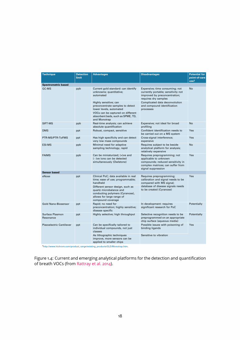
1.1 Metabolomics among the main omics approaches . . . . . . . . . . . . . . 151.2 Pathways of exhaled molecules in the human body . . . . . . . . . . . . . . 161.3 Schematic representation of the PTR-TOF-MS system . . . . . . . . . . . . . 171.4 Current and emerging analytical platforms for the detection and quantifica-

tion of breath VOCs (from Rattray et al. 2014). . . . . . . . . . . . . . . . . . 181.5 Processing workflow for biomarker discovery with MS . . . . . . . . . . . . 201.6 Mass spectrum decomposition . . . . . . . . . . . . . . . . . . . . . . . . . . 211.7 Peak shape parameters . . . . . . . . . . . . . . . . . . . . . . . . . . . . . . 232.1 PTR-Qi-TOFMSwith a buffered-end tidal device (BETmed, Herbig et al. 2008),

Exhalomics, Foch Hospital. . . . . . . . . . . . . . . . . . . . . . . . . . . . . 302.2 PTR-TOF-MS raw data and nomenclature . . . . . . . . . . . . . . . . . . . . 312.3 PTR-TOF-MS data processing software: PTRwid . . . . . . . . . . . . . . . . 382.4 PTR-TOF-MS data processing software: IDA . . . . . . . . . . . . . . . . . . . 383.1 B-spline basis . . . . . . . . . . . . . . . . . . . . . . . . . . . . . . . . . . . . 413.2 Penalised spline regression with P-spline . . . . . . . . . . . . . . . . . . . . 433.3 2-dimensional B-spline basis . . . . . . . . . . . . . . . . . . . . . . . . . . . 463.4 Linear model and linear mixed effect model comparison . . . . . . . . . . . 573.5 Example of F-test for linear mixed effect model . . . . . . . . . . . . . . . . 593.6 Non linear mixed effect model . . . . . . . . . . . . . . . . . . . . . . . . . . 614.1 Expiration phases and ambient air detection . . . . . . . . . . . . . . . . . . 664.2 Peak detection on the Total Ion Spectrum (TIS) around nominal masses . . 684.3 Asymmetric peak shape functions . . . . . . . . . . . . . . . . . . . . . . . . 694.4 Different step of the temporal estimation . . . . . . . . . . . . . . . . . . . . 714.5 Knots location . . . . . . . . . . . . . . . . . . . . . . . . . . . . . . . . . . . 724.6 Alignment with kernel Gaussian density . . . . . . . . . . . . . . . . . . . . . 754.7 The ptairMS workflow . . . . . . . . . . . . . . . . . . . . . . . . . . . . . . . 764.8 ptairMS graphical interface . . . . . . . . . . . . . . . . . . . . . . . . . . . . 78

10

5.1 List of the compounds and their absolute concentrations in the TO-14 gasmixture, as provided by the manufacturer (Restek) . . . . . . . . . . . . . . 80

5.2 ptairMS analysis of a reference VOC mixture . . . . . . . . . . . . . . . . . . 805.3 Peak shape computation on a simulated file for the three software . . . . . 845.4 Simulated data . . . . . . . . . . . . . . . . . . . . . . . . . . . . . . . . . . . 855.5 Application to the truffle biological matrix (Vita et al., 2015) . . . . . . . . . . 876.1 PCA and OPLS-DA . . . . . . . . . . . . . . . . . . . . . . . . . . . . . . . . . 966.2 ROC curve . . . . . . . . . . . . . . . . . . . . . . . . . . . . . . . . . . . . . . 976.3 Quality plots for the p-value from the Wilcoxon-Mann-Whitney test . . . . . 986.4 Feature selection methods comparison . . . . . . . . . . . . . . . . . . . . . 996.5 Longitudinal analysis of VOCs in expired breath . . . . . . . . . . . . . . . . 1026.6 Analysis of four covariates . . . . . . . . . . . . . . . . . . . . . . . . . . . . 1036.7 Study of the impact of the positive end-expiratory pressure (PEEP), respira-

tory rate, and serum C-reactive protein (CRP), on the relationship betweeneach of the four VOC biomarkers and the COVID-19 status. . . . . . . . . . . 107

11

List of Tables

3.1 Elastic net summary . . . . . . . . . . . . . . . . . . . . . . . . . . . . . . . . 483.2 Random forest summary . . . . . . . . . . . . . . . . . . . . . . . . . . . . . 483.3 SVM summary . . . . . . . . . . . . . . . . . . . . . . . . . . . . . . . . . . . 503.4 PLS summary . . . . . . . . . . . . . . . . . . . . . . . . . . . . . . . . . . . . 514.1 Comparison of knots location . . . . . . . . . . . . . . . . . . . . . . . . . . 724.2 ptairMS parameters . . . . . . . . . . . . . . . . . . . . . . . . . . . . . . . . 775.1 Mean absolute percentage error (MAPE) and coefficient of variation (CV) be-

tween replicates of the ptairMS processed data from the reference gas mix-ture acquisitions. . . . . . . . . . . . . . . . . . . . . . . . . . . . . . . . . . . 81

5.2 Comparison of peak detection and quantification by ptairMS, PTRwid, andIDA on 10 simulated files . . . . . . . . . . . . . . . . . . . . . . . . . . . . . 86

6.1 Patient characteristics and treatments. . . . . . . . . . . . . . . . . . . . . . 936.2 Summary of the statistical methods used . . . . . . . . . . . . . . . . . . . . 956.3 Comparison of model performances . . . . . . . . . . . . . . . . . . . . . . 976.4 Putative annotation of features selected . . . . . . . . . . . . . . . . . . . . 100

12

Part I

Introduction

13

Chapter 1

Context

1.1 Biomarker discorvery in exhaled breath

1.1.1 Metabolomic biomarkers

Metabolomics is the study of chemical processes involving small molecule (metabolites,with a molecular weight <1,500 Dalton (Da) ) that are intermediates and products of life-sustaining chemical reactions in organisms (Oliver et al., 1998). These metabolites, whichare the end products of regulatory processes in the organism (Figure 1.1), are importantindicators of physiological or pathological states (Wishart, 2019). Targetedmetabolomicsrefers to the (usually absolute) quantification of knownmetabolites in a biological sample(saliva, urina, blood; Roberts et al. 2012). In contrast, untargeted metabolomics aimsat detecting and providing a (usually relative) quantification of all metabolites present inthe sample. Since the majority of the detected compounds are not known a priori in anuntargeted metabolomics experiment, additional experiments are usually required forthe structural characterisation and identification of the compounds of interest (e.g. thosehighlighted by the statistical analysis).Biomakers are indicators of a specific biological state, particularly one relevant to the

risk of the contraction, the presence or the stage of a disease, or the response to thera-peutics (Rifai et al., 2006; Johnson et al., 2016). The full validation of a biomarker usuallyinvolves three mains steps:

• Discovery: Using an untargetedmetabolomics approach, samples from a cohort ofpatients are collected and analysed. Thanks to statistical learning methods, candi-datemetabolites providing classificationmodelswith a high prediction performance(e.g. for diagnosis, prognosis, or response to treatment are then identified) are de-tected.

14

• Identification: Chemical identification of the selected metabolites is then neces-sary for further clinical validation, through both computational (e.g., matching within-house or public databases), and additional experimental approaches (e.g. tan-dem mass spectrometry).

• Validation: The key step to confirm or refute the candidates metabolites utility inclinical diagnostics is their validation with a second, usually larger, independent co-hort.

Figure 1.1: Metabolomics among the main omics approaches

1.1.2 Volatolomics: analysis of exhaled breath for personalised medicine

Volatolomics is the analysis of Volatile Organic Compounds (VOCs), which can be foundin several human matrices such as saliva, urine, skin, blood, and exhaled breath (Amannet al., 2014). More specially, breathomics (breath-based metabolomics) focuses on thecapture, identification, and quantification of VOCs in human breath, and their use astools in medicine (Rattray et al., 2014). Over the past few years, a thousand of individ-ual VOCs have been detected and identified in the human body (Drabińska et al., 2021;de Lacy Costello et al., 2014; Kuo et al., 2020). VOCs may be directly derived from pul-monary metabolism (and thus reflect the metabolic state of the lungs), but they may alsobe derived from all other organs by being transported through the bloodstream to thelungs, and then into the exhaled breath (Figure 1.2).Recently, many studies have highlighted the potential of VOC analysis from exhaled

breath for early diagnosis and phenotyping of several diseases, such as lung diseases(asthma, cancer, acute respiratory distress syndrome ), cardiovascular diseases, cancer(breast, ovarian and liver; Einoch Amor et al. 2019; Pereira et al. 2015), therapeutic drug

15

was developed by Lavoisier during the time of the Frenchrevolution when he described breath as a chemical reaction ofrespirable air (O2) producing acid forming fixed air (CO2).

7 In1971 Linus Pauling analyzed frozen breath with gas chromatog-raphy and could differentiate more than 250 volatile features.8

Today he is considered the father of modern breath analysis. Gaschromatography coupled to mass spectrometry in turn allowedmuch higher selectivity and compound identification. It iscurrently the most frequently used breath analysis method.However, it is limited because it is an off-line method, which canlead to sample loss and degradation during storage andtransport.9

The three main mass spectrometry methods for on-lineanalysis of volatile organic compounds and later breath analysisare SIFT-MS and PTR-MS andmore recently SESI-MS (section2). The coupling with state-of-the-art high-resolution massspectrometers opened up new possibilities with a much highernumber of several thousand detected features and the capabilityfor unknown identification.10

Portable breath analyzers are also considered important; thischallenge has mainly been addressed by chemical sensors.However, sensors can currently only detect a very limitednumber of compounds in simple gas mixtures (section 2.5).Only a limited number of breath analysis tests are currently

used in patients and recognized by international guidelines.These include the ethanol breath test,11 the nitric oxide breathtest developed by Gustafsson et al.12 for the monitoring ofasthma,13 the hydrogen breath test to diagnose small intestinalbacterial overgrowth,14 and the urea breath test for Helicobacterpylori infection.15 At present, there is not a single exhaled breathtest that is capable of diagnosing a disease as a stand-alone test.1.2. Volatile Organic Compounds and the RespiratorySystem

The human respiratory system emits a vast number of volatileorganic compounds (VOCs) of different origin (see Figure 1).VOCs can either be endogenous, i.e., they arise from therespiratory tract or they are of systemic origin after passing theblood−air barrier, or VOCs can be of exogenous origin, in which

case they originate from the environment and are inhaled andexhaled without alteration. Whether VOCs from the gastro-intestinal tract (e.g., limonene), which often origin fromsymbiotic bacteria, are considered exogeneous or endogenousis currently a matter of debate. The exogenous VOCs from theenvironment in exhaled breath outnumber the endogenous onesby far;16 however, the small number of endogenous VOCsincluding the ones from the gastrointestinal tract are of highinterest in the field of medicine.The pulmonary alveolus represents the smallest unit of the

respiratory tract where molecules pass the blood−air barrier (35to 200 nm thick) via diffusion.17 Estimations of the total areasurface of alveoli range from 75 to 150 m2. Currently, on-linebreath analysis is capable of detecting >500 VOCs in exhaledbreath, with different origins.16

Recently, the identification and quantification of airway andsystemic biomarkers have been of particular interest, to gaininsight into airway physiology and human metabolism in anoninvasive fashion.18 Typically, the end-tidal phase of anexhalation is analyzed when the flow reaches a plateau withVOCs at their high concentrations. While VOCs from theairways are constantly emitted, a wide range of factors contributeto the ability of a VOC to reach a phase equilibrium on bothsides of the blood−air barrier: polarity, solubility in fat, Henry’spartition constant, and volatility, to list the important ones. It istherefore understandable that different classes of molecules inthe blood (e.g., hydrophilic molecules) display a uniquediffusion pattern when it comes to crossing the blood−airbarrier.19,20 Furthermore, the concentrations of the exhaledVOC in the environment should be taken into account (i.e.,ambient air). Under ideal conditions, the concentration ofcertain VOCs (e.g., acetone, acetonitrile or plasma free aminoacids) is directly proportional to their respective concentrationin blood or urine.21−23 Smoking behavior, age, body-mass-index,and biological sex can affect the concentration of certain exhaledbreath components by a cumulative factor of up to 10.24,25Whilethere is a guideline from the American Thoracic Society/European Respiratory Society Task Force on methodologicalissues regarding exhaled breath condensate collection,26 thereare no recommendations or guidelines for exhaled breathanalysis yet. However, the standardization focus group chairedby J. Beauchamp and W. Miekisch of the InternationalAssociation for Breath Research (IABR) is working ondeveloping guidelines for this purpose.

1.3. Reported Volatile Organic Compounds Detected byOn-Line Breath Analysis

In 2014, de Lacy Costello et al. reviewed volatiles detected inexhaled breath.16 They reported 872 VOCs in breath, amongthem alkanes, alkenes, alkynes, benzyl, and phenyl hydro-carbons, alcohols, ethers, aldehydes, acids, esters, ketones,nitrogen containing volatiles, sulfur-containing volatiles, andhalogen-containing volatiles. However, only a small subgroup ofthem has also been monitored on-line. Most of the reportedcompounds were detected off-line, by GC-MS, and often samplepreconcentration steps such as thermal desorption tubes orSolid-Phase Microextraction (SPME) were required.9 In thisreview, we focus on on-line monitoring of molecules in exhaledbreath. Based on a literature search, we have compiled a table ofthe compounds and compound classes which have beenreported in breath by on-line analysis of exhaled breath. Theanalytical methods, level of identification, and literaturereferences are listed for each compound (Supporting

Figure 1. Pathway of exhaled molecules in the human body. A smallproportion of exhaled molecules originate from the airways, gastro-intestinal tract, and the organism (i.e., systemic molecules passing theblood−air barrier in the lungs). Themajority of molecules in exhaled airis of environmental origin. Due to the maximal relative humidity andbody temperature of 37 °C, the MS-analysis of exhaled breath may onlybe compared to a limited extend.

Chemical Reviews Review

DOI: 10.1021/acs.chemrev.9b00005Chem. Rev. 2019, 119, 10803−10828

10805

Figure 1.2: Pathways of exhaled molecules in the human body (Bruderer et al., 2019). En-dogenous VOCs are excreted through the red and blue pathways.

monitoring (Chen et al., 2021; Boots et al., 2015), and infectious diseases, as tuberculosis,bacterial colonisation of the airways (Koo et al., 2014; Nakhleh et al., 2014; Suarez-Cuartinet al., 2018), ventilator-associated pneumonia in intensive care patients (Schnabel et al.,2015; Bos et al., 2014a), or viral infections (Traxler et al., 2018). In the infectious diseasescontext, the detected "breathprint" is a mixture of metabolites from microbial origin (i.e.direct biomarkers of the presence of pathogens), and metabolites generated by the hostin response to the infection. The existence of the olfactory fingerprints is corroborated byworks with dogs, showing the remarkable ability of canine olfaction to identify patientswith specific cancer or infectious diseases based on the sniffingof exhaled breath or sweatsamples (Feil et al. 2021; Guirao et al. 2019; Vesga et al. 2021; ten Hagen et al. 2021; see alsothe KDOG project from the Curie Institute).Breath analysis offers several advantages, the most important being its non-invasive

nature and the simplicity of collection, in contrast to biopsy or nasopharyngeal swabs,the current gold standard for the diagnosis of cancer and COVID-19 respectively, whichare highly invasive and not risk free. Secondly, recent analytical technologies enable realtime analysis and sample collection at the point of care, which is a major asset for largepopulating screening and personalised (or precision) medicine (which refers to the tai-loring ofmedical treatments to the individual characteristics of each patient; Devillier et al.2017; Martinez-Lozano Sinues et al. 2013). Finally, breath is available in nearly unlimitedquantities.While the discovery of VOC biomarkers is a very promising approach, their detection

and identification remain challenging. First, VOCs present in the exhaled breath may beeither endogenous (internal metabolic production), or exogenous (current or previousenvironmental exposures), as illustrated on Figure 1.2, where the exogenous VOCs out-number the endogenous ones (de Lacy Costello et al., 2014). Second, measurement of

16

proceeds along the drift tube. The drift tube is typically operatedat E/N of 190 Td, where E is the electric field across the drifttube and N is the gas number density. Figure 2 shows thepercentage contribution of H3O+‚(H2O)1-2 clusters to the total ioncounts with varying values of E/N; at the operating field strengthof 190 Td, the cluster formation is relatively minor. Furtherexperiments have demonstrated that at an operating field strengthof 190 Td cluster formation is relatively insensitive to samplehumidity.

The gas exits the drift tube via a 200-µm orifice in a stainlesssteel plate and enters a short differentially pumped chamber (notshown in Figure 1) before passing through a second (3 mm)orifice into the transfer ion optics and pulsed extraction unit ofthe TOF-MS. Using a Faraday cup arrangement, the ion currenthas been measured to be ∼500 pA or 3 × 109 ions s-1. This ioncurrent is comparable to that obtained by Hanson et al.,5

demonstrating that the two ion sources have comparable perfor-mance. The ion-transfer optics consist of a three-element Einzel

lens, which focuses the ions into a narrow beam between thebackplate and extraction grid of the TOF-MS. The potential onthe grid is rapidly switched to drive ions into the flight tubethrough a set of spatial focusing electrodes and steering platesbefore the ions enter a large-bore reflectron equipped with a dualmicrochannel plate (MCP) detector.

The anode of the MCP detector is connected to a purpose-built preamplifier with a built-in discriminator that generates anECL logic pulse whenever the preselected signal threshold isexceeded. The output is sent to a time-to-digital converter (TDC)with 2-ns time bins, and this constructs an arrival time histogram.The TDC also provides the trigger pulse to the extraction gridfor initiating the flight time sequence. Repetitive scans areessential to attain meaningful ion count statistics and for a scanrange of 0-300 Da we can accumulate 104 scans/s-1. The transferoptics, the TOF-MS, and the TDC were all supplied by KoreTechnology (Ely, U.K.).

Pumping in the first differential pumping region, the transferoptics chamber, and the TOF-MS is carried out using separateturbomolecular pumps. The downstream end of the drift tube isevacuated by a small mechanical pump.

Gas Delivery. High-purity deionized water (15 MΩ) was usedas the source of water vapor. This was purged before use andwas bubbled into the ion source using N2 carrier gas at a flowrate of 12-15 sccm. Zero grade nitrogen (BOC, 99.998%) wasemployed after having been passed through an Alltech activatedcharcoal hydrocarbon trap. Zero air (BOC, BTCA 178 grade)scrubbed through a self-indicating hydrocarbon trap was used forsome calibration scans.

Determining Absolute Concentrations. Absolute concentra-tions of trace gas R are determined in PTR-MS via the steady-state expression

Figure 2. Experimentally determined percentage formation asfunction of total ion counts of H3O+ and H3O+. (H2O)1-2 with varyingelectric field (E/N). The sample gas had a dew point temperature ofTd ) 6 °C. The arrow indicates typical operating conditions.

Figure 1. Schematic representation of the PTR-TOF-MS system.

[R] ) 1kt

[RH+]

[H3O+]

(1)

3842 Analytical Chemistry, Vol. 76, No. 13, July 1, 2004

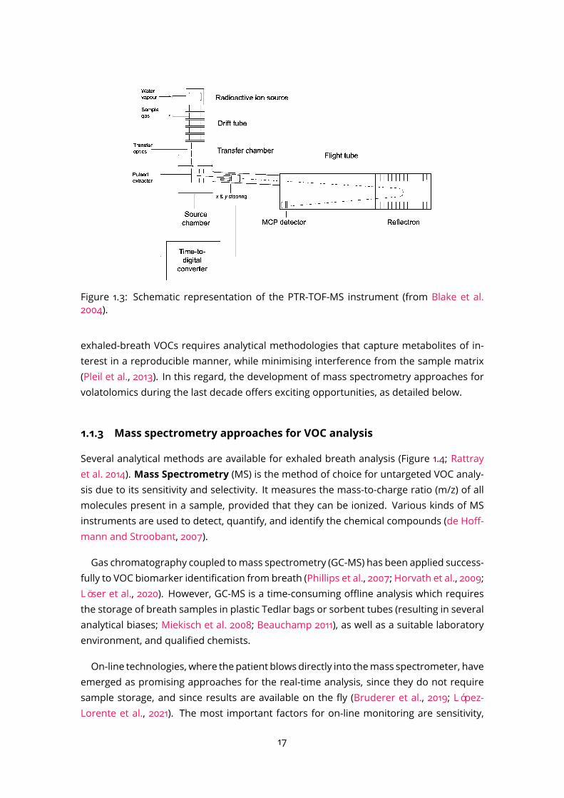
Figure 1.3: Schematic representation of the PTR-TOF-MS instrument (from Blake et al.2004).

exhaled-breath VOCs requires analytical methodologies that capture metabolites of in-terest in a reproducible manner, while minimising interference from the sample matrix(Pleil et al., 2013). In this regard, the development of mass spectrometry approaches forvolatolomics during the last decade offers exciting opportunities, as detailed below.

1.1.3 Mass spectrometry approaches for VOC analysis

Several analytical methods are available for exhaled breath analysis (Figure 1.4; Rattrayet al. 2014). Mass Spectrometry (MS) is the method of choice for untargeted VOC analy-sis due to its sensitivity and selectivity. It measures the mass-to-charge ratio (m/z) of allmolecules present in a sample, provided that they can be ionized. Various kinds of MSinstruments are used to detect, quantify, and identify the chemical compounds (de Hoff-mann and Stroobant, 2007).Gas chromatography coupled tomass spectrometry (GC-MS) has been applied success-

fully to VOC biomarker identification from breath (Phillips et al., 2007; Horvath et al., 2009;Löser et al., 2020). However, GC-MS is a time-consuming offline analysis which requiresthe storage of breath samples in plastic Tedlar bags or sorbent tubes (resulting in severalanalytical biases; Miekisch et al. 2008; Beauchamp 2011), as well as a suitable laboratoryenvironment, and qualified chemists.On-line technologies, where the patient blowsdirectly into themass spectrometer, have

emerged as promising approaches for the real-time analysis, since they do not requiresample storage, and since results are available on the fly (Bruderer et al., 2019; López-Lorente et al., 2021). The most important factors for on-line monitoring are sensitivity,

17

Clinical applications of breathomicsBreath analysis offers the potential for biomarker discov-ery in an almost unlimited variety of clinical circum-stances, ranging from disease diagnosis to stratificationto treatment monitoring or prognosis (Table 3). Likewise,the breadth of disease groups would include airway andlung diseases, and even distal single-organ or systemic andmultiorgan diseases that transmit VOC byproducts intothe blood stream. Challenges that must always beaddressed and accounted for in breath sampling for clinicalstudies include environmental contamination, patientcomfort and safety, and infection control. Study-specificissues relate to the desire to sample preferentially theportion of the breath that arises from the area of interest

(e.g., the mouth, airways, or alveoli). The study of volatilesarising in the mouth principally relates to the study ofhalitosis and is reviewed elsewhere [37].

The aspect of breath analysis that relates to metabo-lomics is unlikely to reveal any single, unique biomarkerspertaining to particular diseases, organisms, or process.Specific combinations or classes of compounds (i.e., fin-gerprints) are more likely to form the basis of a ‘compoundbiomarker panel’ for a disease, as established from pre-vious work in obstructive airway diseases. For example,in chronic obstructive pulmonary disease (COPD), a mod-el VOC panel comprising 11 volatile compounds discrimi-nated COPD from healthy controls, of which nine VOCswere aldehydes [19]. Similarly, the model that could

Table 2. Current and developing analytical platforms for detecting breath VOCs

Technique Detection

limit

Advantages Disadvantages Potential for

point-of-care

use?

Refs

Spectrometric based

GC-MS ppb Current gold standard: can identify

unknowns; quantitative;

automated

Expensive; time consuming; not

currently portable; sensitivity not

improved by preconcentration;

requires dry samples

No [37,38,62]a

Highly sensitive; can

preconcentrate samples to detect

lower levels, automated

Complicated data deconvolution

and compound identification

processes

VOCs can be captured on different

absorbent beds, such as SPME, TD,

and Monotrap

SIFT-MS ppb Real-time analysis; can achieve

absolute quantification

Expensive; not ideal for broad

profiling

No [25,27]

DMS ppt Robust, compact, sensitive Confident identification needs to

be carried out on a MS system

Yes [63]

PTR-MS/PTR-ToFMS ppt Has high specificity and can detect

very low mass compounds

Cross-signal interference;

expensive

Yes [18,59]

ESI-MS ppb Minimal need for adaptive

sampling technology, rapid

Requires subject to be beside

analytical platform for analysis;

relatively expensive

No [64,65]

FAIMS ppb Can be miniaturized; (+)ve and

()ve ions can be detected

simultaneously (Owlstone)

Requires preprogramming; not

applicable to unknown

compounds; reduced sensitivity in

complex matrices; can suffer from

signal suppression

Yes [66]

Sensor based

eNose ppt Clinical PoC; data available in real

time; ease of use; programmable;

handheld

Requires preprogramming;

calibration and signal needs to be

compared with MS signal;

database of disease signals needs

to be created (Cyranose)

Yes [67]

Different sensor design, such as

quartz microbalance and

conducting polymers (Cyranose),

allows for large range of

compound coverage

Gold Nano-Biosensor ppt Rapid; no need for

preconcentration; highly sensitive;

disease specific

In development: requires

significant research for PoC

Potentially [68]

Surface Plasmon

Resonance

ppt Highly selective; high throughput Selective recognition needs to be

preprogrammed on an appropriate

chip surface (aqueous media)

Potentially [69]

Piezoelectric Cantilever ppt Can be specifically tailored to

individual compounds, not just

classes

Possible issues with poisoning of

binding ligands

Yes [70]

As lithographic techniques

improve, more sensors can be

applied to smaller chips

Sensitive to vibration

ahttp://www.hichrom.com/product_range/existing_products/GLS/Monotrap.htm.

Review Trends in Biotechnology October 2014, Vol. 32, No. 10

542

Figure 1.4: Current and emerging analytical platforms for the detection and quantificationof breath VOCs (from Rattray et al. 2014).

18

selectivity, scan speed, and robustness. Different variants of MS techniques enable directsampling and ionisation, including Selected Ion Flow Tube Mass Spectrometry (SIFT-MS,Španěl and Smith 2011), which provides absolute quantification but with low resolution,Secondary Electrospray Ionization (SESI -MS, Wu et al. 2000), which achieves the highestmass resolution reported to date (>140,000) but requires laboratory analytical platformfor analysis, and Proton Transfer Reaction (PTR-MS; Ellis and Mayhew 2014), which pro-vides both high specificity and the possibility to collect breath at the point of care.When coupled to Time-of-Flight (TOF) Mass Spectrometry, PTR-TOF-MS (Blake et al.,

2004; Herbig et al., 2009; Jordan et al., 2009) has emerged as a promising approach withhigh sensitivity and specificity for VOC analysis in a wide range of applications (includingenvironment, food quality, biology). Ionisation is based on proton transfer from a reagention, most commonlyH3O

+:V OC +H3O

+ → (V OC)H+ +H2O

As a result, only molecules with a relatively higher proton affinity than water are ionised,excluding the major components of air (N2,O2, and CO2). Furthermore, fragmentation isminimal since proton transfer is a relatively soft ionisation technique. Protonated VOCsare then focused by a lens system and detected in a high resolution reflectron time-of-flight mass spectrometer, according to their mass/charge (m/z) ratio (Figure 1.3). Finally,real-time quantification of VOCs is achieved by ion counting and normalisations based onreaction rates and transmission factors (Cappellin et al., 2012b).In the area of health and care, PTR-TOF-MS opens up unique opportunities for real-

time analysis at the point of care (Smith et al., 2014). Its potential for bio-medicine hasbeen shown in applications such as emphysema, liver cirrhosis, chronic kidney diseaseand diabetes (Cristescu et al., 2011; Fernández del Río et al., 2015; Obermeier et al., 2017;Pleil et al., 2019; Trefz et al., 2013). However, there is currently a lack of numerical methodsand efficient, user-friendly software tools for the processing of PTR-TOF-MS data in theclinics.

1.2 Signal processing of mass spectrometry-based data

The processing of mass spectrometry (MS)-based data consists in transforming the rawdata files generated by the mass spectrometer instrument into a representation that fa-cilitates access to characteristics of each observed ion (Katajamaa and Orešič, 2007). Itincludes the pre-processing of each file (one file per biological sample), by listing the m/zvalue and quantity of all detected ions (peak picking), followed by the alignment betweenthe samples to generate the sample by variable table of intensities (i.e. the peak table).Finally, additional information about the ions is added (such as the isotope distribution

19

Peak

list

Peak

list

Peak

list

Collection of sample

Alignment between sample

Control Interest

Patients

Feat

ures

Peak matchingComplete missing valueIsotope Identification

SmoothingBaseline estimationPeak findingQuantification

Pre-processing of each file

Peak table

Statistical analysisClassificationTime course modellingTesting hypothesisBiomarkers

Peak

list

Peak

list

Peak

list

Peak

list

Peak

list

Peak

list

Peak

list

Peak

list

Peak

list

Peak

list

Peak

list

m/z

inte

nsi

ty

Mass sepctrum

Raw Data

Inte

nsity

m/z

inte

nsi

ty

x

y

time

Figure 1.5: Processing workflow for biomarker discovery with MS

20

m/z

inte

nsity

True signal

m/z

Baseline

m/z

Noise

m/z

Mass sepctrum

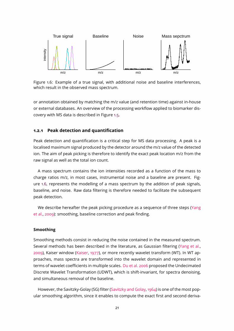
Figure 1.6: Example of a true signal, with additional noise and baseline interferences,which result in the observed mass spectrum.

or annotation obtained by matching the m/z value (and retention time) against in-houseor external databases. An overview of the processing workflow applied to biomarker dis-covery with MS data is described in Figure 1.5.

1.2.1 Peak detection and quantification

Peak detection and quantification is a critical step for MS data processing. A peak is alocalisedmaximum signal produced by the detector around them/z value of the detectedion. The aim of peak picking is therefore to identify the exact peak location m/z from theraw signal as well as the total ion count.A mass spectrum contains the ion intensities recorded as a function of the mass to

charge ratios m/z, in most cases, instrumental noise and a baseline are present. Fig-ure 1.6, represents the modelling of a mass spectrum by the addition of peak signals,baseline, and noise. Raw data filtering is therefore needed to facilitate the subsequentpeak detection.We describe hereafter the peak picking procedure as a sequence of three steps (Yang

et al., 2009): smoothing, baseline correction and peak finding.

Smoothing

Smoothing methods consist in reducing the noise contained in the measured spectrum.Several methods has been described in the literature, as Gaussian filtering (Yang et al.,2009), Kaiser window (Kaiser, 1977), or more recently wavelet transform (WT). In WT ap-proaches, mass spectra are transformed into the wavelet domain and represented interms of wavelet coefficients in multiple scales. Du et al. 2006 proposed the UndecimatedDiscrete Wavelet Transformation (UDWT), which is shift-invariant, for spectra denoising,and simultaneous removal of the baseline.However, the Savitzky-Golay (SG) filter (Savitzky and Golay, 1964) is one of themost pop-

ular smoothing algorithm, since it enables to compute the exact first and second deriva-21

tive at each point of the signal, which is very useful to detect local maxima. It consists ina moving average filter that performs independent polynomial regression of degree d ona subset of consecutive data points of odd size 2m + 1 (windows), and takes the centralpoint of the fitted polynomial curve as output.The choice of the windows size and degree d is then important, since too large win-

dows (or small degree) leads to underestimation and too small windows (or large degree)leads to over fitting and doesn’t smooth enough (bias-variance trade-off). An optimal win-dows selection algorithm has been proposed by Vivo Truyols and Schoenmakers (2006),which minimise the difference between auto-correlation of the fitting residuals (i.e., thedifferences between the input signal and the smoothed signal) and the auto-correlationof blank signal. More recently, John et al. (2021) also proposed an adaptive method forboth degree and windows size choice, based on minimising a generalised unbiased es-timation of Mean Squares Error (GUE-MSE) between the true signal and the smoothedoutput, without any specific distributional assumption on noise.

Baseline correction

After denoising, the baseline needs to be removed from the spectrum before proceedingto peak finding. It classically consists in estimating the baseline before subtracting it.Many iterative algorithms have been proposed in the literature for baseline correction,

including polynomial fitting (the signal is iteratively cut off above the fitted curve; Ganet al. 2006), reweighted penalized least squares (at each iteration, the signal above thefitted curve is assigned a lower weight than signal below; Zhang et al. 2010; Baek et al.2015; Ruckstuhl et al. 2001), quantile regression (the 0.01 quantile of the signal is estimatedinstead of the mean Komsta 2011), mixture probabilistic modeling (by computing at eachiteration the probability of each point to belong to the baseline; de Rooi and Eilers 2012),and the sensitive nonlinear iterative peak algorithm (SNIP), based on a low statistics digitalfilter (Ryan et al., 1988; Morháč and Matoušek, 2008). All of these algorithms depend onparameters (such as the degree of the polynomial regression), and require a convergencecriterion. The choice of algorithm depends mainly on the type of baseline observed in thedata, and thus the type of MS instrument.

Peak finding

The main step of peak picking is the determination of peak locations. A peak can be de-fined by the m/z centre µ, width σ, and height h or area under the curve A. The widthσ is usually defined as the full width of the peak at half maximum (FWHM) (Figure 1.7).The resolution of an instrument corresponds to the separation capability between twopeaks, and is defined as R = m

∆m, where ∆m is usually the FWHM. Several methods of

peak finding are available:22

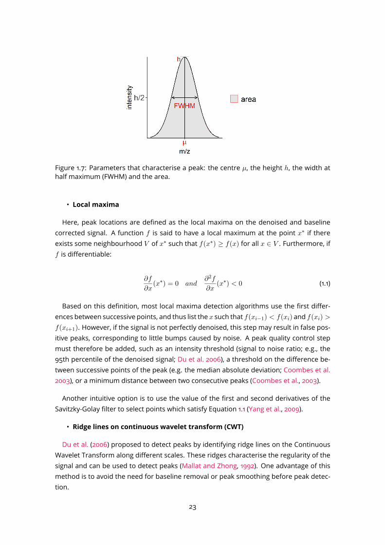
Figure 1.7: Parameters that characterise a peak: the centre µ, the height h, the width athalf maximum (FWHM) and the area.

• Local maxima

Here, peak locations are defined as the local maxima on the denoised and baselinecorrected signal. A function f is said to have a local maximum at the point x∗ if thereexists some neighbourhood V of x∗ such that f(x∗) ≥ f(x) for all x ∈ V . Furthermore, iff is differentiable:

∂f

∂x(x∗) = 0 and

∂2f

∂x(x∗) < 0 (1.1)

Based on this definition, most local maxima detection algorithms use the first differ-ences between successive points, and thus list the x such that f(xi−1) < f(xi) and f(xi) >f(xi+1). However, if the signal is not perfectly denoised, this step may result in false pos-itive peaks, corresponding to little bumps caused by noise. A peak quality control stepmust therefore be added, such as an intensity threshold (signal to noise ratio; e.g., the95th percentile of the denoised signal; Du et al. 2006), a threshold on the difference be-tween successive points of the peak (e.g. the median absolute deviation; Coombes et al.2003), or a minimum distance between two consecutive peaks (Coombes et al., 2003).Another intuitive option is to use the value of the first and second derivatives of the

Savitzky-Golay filter to select points which satisfy Equation 1.1 (Yang et al., 2009).• Ridge lines on continuous wavelet transform (CWT)

Du et al. (2006) proposed to detect peaks by identifying ridge lines on the ContinuousWavelet Transform along different scales. These ridges characterise the regularity of thesignal and can be used to detect peaks (Mallat and Zhong, 1992). One advantage of thismethod is to avoid the need for baseline removal or peak smoothing before peak detec-tion.

23

• Deconvolution with a model peak function

Medium or low resolution mass analysers generate overlapping peaks. In such a case,a deconvolution method must be used to separate and quantify each peak. An approachis to use a model of the peak function, denoted pθ(t) with θ = (µ, σ, h), and to applya regression algorithm minimising a loss function between the denoised and baselinecorrected observed signal y, and the mixture of peak functions:

minθ

||y −P∑i=1

pθi(m)||2 (1.2)

with m the vector of m/z values and P the number of overlapping peaks. This can beachievedwith standardnonlinear optimisation algorithms, such as the Levenberg-Marquardtalgorithm (Lange et al., 2006), particle swarm optimization (PSO; Wijetunge et al. 2015) orExpectation-Maximization (EM; Yu and Peng 2010). The number of peaks P and the initialvalues of θmust be defined, e.g. by using local maximumdetectionmethods as describedbefore.Asymmetric peak functions are usually needed, due to imperfections of the mass anal-

yser. Several asymmetric peak shapes have been described in the literature, includingbi-gaussian (Yu and Peng, 2010), mixture of gaussians (Leptos et al., 2006), Lorentzian,sech2 (Lange et al., 2006; Stancik and Brauns, 2008), or combination of these (Wijetungeet al., 2015).To select the best number of peaks P and the best fit function, model selection based

on the Bayesian Information Criterion (BIC) or R2 criteria are used (Lange et al., 2006; Yuand Peng, 2010):

BIC = −2 ln((

n∑i

yi − yi)2)+ P · ln(n) (1.3)

R2 = 1−∑n

i (yi − yi)2∑n

i (yi − y)2(1.4)

with yi = ∑Pj=1 pθj (mi), θj the solution of equation 1.2 and y the average of the denoised

and baseline corrected observed signal .The last step of peak picking is to provide the total ion count for each detected peak. It

is usually computed as the area under the curve of the fitted peak shape, or the sum ofthe raw signal between the peak boundaries if there was no peak deconvolution.

24

1.2.2 Alignment

Once the peaks have been detected in the individual sample files, a matching (i.e. align-ment of m/z values) across the samples is required to generate a single matrix of inten-sities for the whole experiment, where each row corresponds to one ion and each col-umn contains the quantities of these ions (e.g., peak area) in one sample. Regarding thePTR-MS instrument, the internal mass calibration (section 2.1) enables to perform an ini-tial alignment between the mass spectra by using reference peaks (Jeffries, 2005; Frenzelet al., 2003). Then, since the mass shift error is non-linear, additional methods are re-quired to group masses corresponding to the same ion. Instead of using fixed intervalmatching (i.e. binning), Smith et al. (2006); Delabrière et al. (2017) proposed a kernel den-sity estimator to compute the overall distribution of peaksm/z, and to dynamically identifyboundaries of regions where many peaks have similar m/z.

1.2.3 Identification

At that stage, the detected features (ions) are defined by their mass. Two kinds of addi-tional information are sought to provide further chemical insight. First, the identificationof isotopepairs among the features canbedetected by looking formass differences corre-sponding to one neutron and by checking the correlations between the intensity profilesamong the samples (Treutler and Neumann, 2016). Second, the mass can be matched todatabases of metabolites, or the chemical formula, to suggest candidates. The key pa-rameters for a successful match are the mass accuracy of the instrument, its resolution(i.e. its ability to separate neighbouring peaks), and the content of available databases.For further characterisation (e.g. distinction between isomers), complementary analyticalapproaches are required, such as one- or two-dimensional gas chromatography (Phillipset al. 2013; see the discussion in section III).

1.3 Online exhaled breath data processing

The principal challenge of exhaled breath analysis is to differentiate between VOCs com-ing from the body and the external environment (endogenous vs exogenous). Indeed,real time analysis method continuously records spectra during the acquisition, the ambi-ent air of the room is analysed during the intervals between two expirations (e.g. when thepatient inhales). Furthermore, Miekisch et al. (2008) showed that alveolar samples (whichcorrespond to the end tidal of expiration, coming from alveoli, see Figure 1.2) showedthe highest concentrations of endogenous and lowest concentration of exogenous sub-stances. It is therefore important to detect the alveolar expiration phases and discardcompounds that do not originate from exhaled breath.

25

1.3.1 Expiration phases detection

During real-time breath acquisitions, several exhalations are usually recorded. As ex-plained in section 1.1.2, gas exchanges take place in the alveoli: as a result, VOCs producedby the metabolism are present in the alveolar air, which represent the end tidal of expira-tion. Herbig et al. (2009) therefore suggested to identify breath phases by using the signalof tracer compounds that originate from the blood–gas exchange in the alveoli and arepresent in high concentration in a breath sample, such as acetone (m/z 59.049), CO2 (m/z44.997) or humidity with the water dimer isotope (m/z 39.033).Schwoebel et al. (2011) used the water dimer signal (m/z 37.028) to distinguish between

inspiratory and alveolar air. An algorithm was designed to automatically detect thosephases using the signal trace around m/z 37, with a threshold on the intensity and thestability of cycle. Points greater (respectively, lower) than the mean of the whole trace areconsidered as expirations (respectively inspirations), and the gradient signals (differencebetween successive points) from the same expiration cycle (respectively inspiration) hasto be less than a fixed value (2.5%).This method was further generalised by Trefz et al. (2013), who set two percentage

thresholds texp and tinh, and defined expiration (respectively inhalation) as the part ofthe trace where the intensity is higher (respectively lower) than texp% (respectively tinh%)of the signal trace maximum. This approach was used in several studies from the samegroup: using isoprene as breath tracer (Sukul et al., 2014) , on ventilated patients (Brocket al., 2017), or using acetone (Trefz et al., 2019b; Sukul et al., 2021).1.3.2 Ambient inhaled air

During online acquisition of exhaled breath, the ambient air of the room is both analysedby the instrument and inhaled by the patient. Compound from ambient air can thus be asignificant source of confounding variables. It has been demonstrated that for the com-pounds present in ambient air, their concentration in exhaled breath is related to theirconcentration in the ambient inhaled air (Phillips, 1997; Beauchamp, 2011; Filipiak et al.,2012; Španěl et al., 2013; Pleil et al., 2013; Smith et al., 2014). Phillips (1997) therefore in-troduced the concept of "alveolar gradient", which corresponds to the concentration inbreath minus the concentration in inhaled air. If the gradient is positive, the VOCs is con-sidered from exhaled breath, and if it is negative or close to zero, it is considered as anambient air pollutant. This method assumes that the subject is in equilibrium with roomair before the sampling (in practice, the patient is allowed to breath quietly in the roomfor a few minutes).The quantitative analysis of seven VOCs present in ambient air showed that all these

compounds were partially retained in the exhaled breath, and that there was a linearrelationship between the exhaled and inhaled air concentrations (Španěl et al., 2013). A

26

correctionwhich is specific to each compoundmay therefore be applied for targeted stud-ies.In the more general case of untargeted approaches, the ambient air intensity is usu-

ally subtracted from the averaged expiration intensity (van den Velde et al., 2007; Zhouet al., 2017). Alternatively, breath-specific compounds are selected by thresholding theexpiration intensity as a function of ambient air (Bajtarevic et al., 2009; Wehinger et al.,2007).

27

28

Chapter 2

Current processing of PTR-TOF-MSdata

2.1 Data acquisition

MS instruments consist of an ion source, a mass analyser, and a detector (Gross, 2011). InPTR-TOF-MS instruments (section 1.1.3), chemical ionisation is achieved by proton transfer,usually from a source of hydronium ions (H3O

+, called primary ions). In addition, the TOFanalyser provides high sensitivity and resolving power (Jordan et al., 2009). Finally, ioncounting is performed by using a microchannel plate detector.During data acquisition, which is very fast, the instrument continuously analyses the

air flowing through a buffer tube (i.e. ambient air by default) and the patient is asked toexpire a few times into the tube. A buffered-end tidal systemmay be used to prolong theend of expirations and to achieve efficient breath capture (Herbig et al., 2008), shown inFigure 2.1.Raw data are provided in the form of a numerical matrix, where the indices of the rows

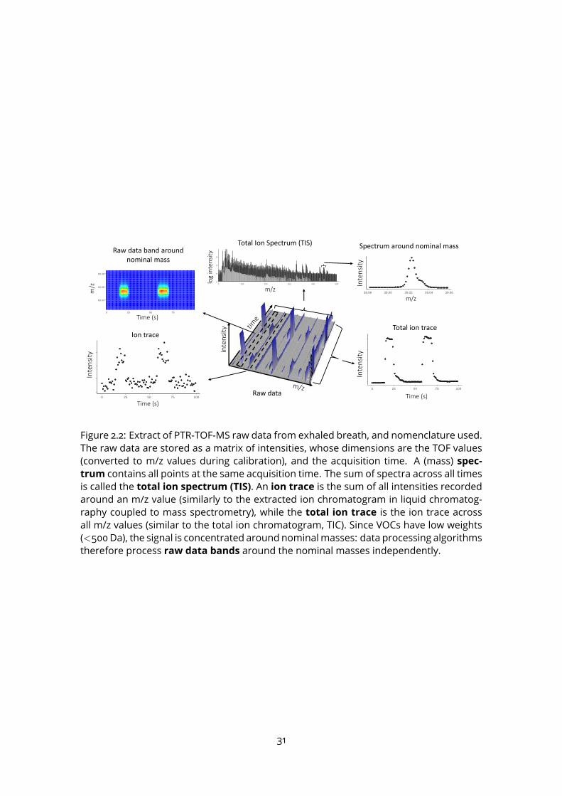
are the TOF bins (which will be converted into m/z values during the calibration step ofdata processing), and the column indices are the acquisition times (in seconds). A binj is a time interval of duration tbin (in ns), during which the ions arriving between ](j −1)× tbin, j× tbin] are counted by the detector. The resulting intensities for all bins form anextraction, or spectrum: spectramay be averaged by the processing algorithms to reducethe signal/noise ratio (see the nomenclature on Figure 2.2).Raw files may be large (∼ 50 MB); they are generally stored in the HDF5 open format

(Koziol, 2011), which allows direct access to specific blocks of data of interest if necessary(e.g. during imputation of missing values, when a refined analysis of the raw data withinthe region of interest is required). The raw files also contain themetadata collected during

29

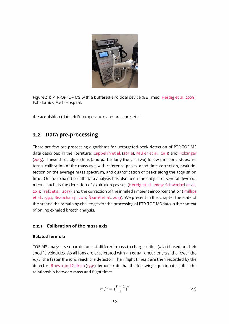
Figure 2.1: PTR-Qi-TOF MS with a buffered-end tidal device (BET med, Herbig et al. 2008),Exhalomics, Foch Hospital.

the acquisition (date, drift temperature and pressure, etc.).

2.2 Data pre-processing

There are few pre-processing algorithms for untargeted peak detection of PTR-TOF-MSdata described in the literature: Cappellin et al. (2011a), Müller et al. (2011) and Holzinger(2015). These three algorithms (and particularly the last two) follow the same steps: in-ternal calibration of the mass axis with reference peaks, dead time correction, peak de-tection on the average mass spectrum, and quantification of peaks along the acquisitiontime. Online exhaled breath data analysis has also been the subject of several develop-ments, such as the detection of expiration phases (Herbig et al., 2009; Schwoebel et al.,2011; Trefz et al., 2013), and the correction of the inhaled ambient air concentration (Phillipset al., 1994; Beauchamp, 2011; Španěl et al., 2013). We present in this chapter the state ofthe art and the remaining challenges for the processing of PTR-TOF-MS data in the contextof online exhaled breath analysis.

2.2.1 Calibration of the mass axis

Related formula

TOF-MS analysers separate ions of different mass to charge ratios (m/z) based on theirspecific velocities. As all ions are accelerated with an equal kinetic energy, the lower them/z, the faster the ions reach the detector. Their flight times t are then recorded by thedetector. Brown and Gilfrich (1991) demonstrate that the following equation describes therelationship between mass and flight time:

m/z =( t− a

b

)2 (2.1)30

inte

nsi

ty

0

5

10

15

0 100 200 300 400 500

m/z

log-I

nte

nsiti

es

TIS

m/z

log

inte

nsi

ty

Total Ion Spectrum (TIS)

Total ion trace

Time (s)400

800

1200

1600

0 25 50 75 100

x

y

1.5e+07

2.0e+07

2.5e+07

3.0e+07

3.5e+07

0 25 50 75 100

x

y

Ion trace

60.04

60.06

60.08

0 25 50 75

time (s)

m/z

Time (s)

m/z

Time (s)

Raw data band around nominal mass

0

500000

1000000

1500000

2000000

38.98 39.00 39.02 39.04 39.06

x

y

m/z

Spectrum around nominal mass

Inte

nsi

ty

Inte

nsi

tyIn

ten

sity

Raw data

Figure 2.2: Extract of PTR-TOF-MS raw data from exhaled breath, and nomenclature used.The raw data are stored as a matrix of intensities, whose dimensions are the TOF values(converted to m/z values during calibration), and the acquisition time. A (mass) spec-trum contains all points at the same acquisition time. The sum of spectra across all timesis called the total ion spectrum (TIS). An ion trace is the sum of all intensities recordedaround an m/z value (similarly to the extracted ion chromatogram in liquid chromatog-raphy coupled to mass spectrometry), while the total ion trace is the ion trace acrossall m/z values (similar to the total ion chromatogram, TIC). Since VOCs have low weights(<500Da), the signal is concentrated around nominalmasses: data processing algorithmstherefore process raw data bands around the nominal masses independently.

31

where (a, b) are calibration constants which depend on the distance travelled to the de-tector and the the accelerating voltage, and can be determined from the flight times of atleast two ions of known m/z.Experimentally, however, the linear relationship between t and √

m/z does not crossthe origin (Guilhaus et al., 2000). This is a relatively minor effect that can be only observedon high resolution TOF instruments or at very low m/z. Cappellin et al. (2010) thereforeproposed to add a third coefficient to Equation 2.1:

m/z = a+ bt+ ct2 (2.2)

Alternatively, Holzinger (2015) suggests to improve themass accuracy by optimising theexponent parameter q:

m/z = (t− a

b)q (2.3)

In practice, the Formula 2.1 remains the most used, especially by manufacturers forexternal calibration.

Choice of the reference peak

The first external calibration used to convert the TOF axis tom/z values usually does notprovide sufficient accuracy. The parameters of the previous equation are then updatedby selecting reference peaks with knownm/z, called calibration peaks. Themass accuracytherefore depends on the choice of those peaks: they should be i) well distributed alongthe whole axis, ii) without neighbours at the same nominal mass, iii) present in all scans,and iv) not saturated. The following optimisation problem is then solved with non-linearoptimisation algorithms:

minθ

∑i

((m/z)i − fθ(ti)

)2where fθ is one of the equations linkingm/z and time of flight tof (i.e. Equation 2.1, 2.2, or2.3), θ the two or three parameters to be estimated, (m/z)i the exact mass to charge ratioof the calibration peaks, and ti the observed tof of this compound in the mass spectrum.Note that a precise determination of the calibration peak centroids ti is therefore criticalto achieve a good mass accuracy (see the peak detection section).The most often used reference peak in the literature is the isotope of the primary ion

(since the primary ion itself is saturated), i.e. H183 O+ at m/z 21.022 when the reagent ion

32

is H3O+. Additional ions have been used as calibration references, depending on thesample analysed (exhaled breath, atmospheric air, food etc.), including nitric oxide NO+

(m/z 29.998), dioxygen O+2 (m/z 31.999), the isotope of water cluster (m/z 39.0326), or

acetone H7C3O+ (m/z 59.0491) (Müller et al., 2013; Cappellin et al., 2011a; Herbig et al.,2009; Trefz et al., 2018). Finally, the instrument itself continuously produces external ions(generally with highm/z) aimed at improving the calibration accuracy.An alternative strategy avoiding theneed for calibration peakswas proposedbyHolzinger

(2015), by determining an autonomous mass scale calibration based on the matching to alibrary of compound formulae generated in silico. The full calibration procedure relies onthree evaluations: a first calibration is performed by combining any two of the largest 16peaks and assumes that these peaks correspond to a pair of primary ions. For the stan-dard operation mode based on proton transfer from H3O

+, the pair of primary ions isH3O

+ (m/z 19.018) and H2O.H3O+ (m/z 37.028). The second step performs a variation

of constants on the previous parameter values, by maximising the number of matches tothe compound library. The third calibration computes parameters according to the "clas-sical" user-specified m/z values. Among the three sets of parameters obtained, the onewhich maximises the matches to the library compounds is selected.

Calibration shift

Due to low changes of temperature and small variations of the PTR-TOF instrumental pa-rameters, a drift of the mass accuracy over the acquisition time is observed (Cappellinet al., 2010; Müller et al., 2011; Holzinger, 2015). To correct this effect (especially for longterm acquisitions), several calibrations are performed periodically to update the parame-ters values. Then, an interpolation of the time bins of each mass spectrum is performed.

2.2.2 Dead time correction

Instrumental dead times are caused by the finite time response of themulti-channel plate(MCP) detector and the amplifier–discriminator, when two or more ions arrive at the de-tector within a single data acquisition time bin of the time-to-digital converter (TDC;Mülleret al. 2013). It can therefore lead to an underestimation of high-intensity ion signals andlimit the dynamic range of the measurements. Titzmann et al. (2010) proposed to use aPoisson counting to correct this effect.

2.2.3 Peak detection on the mass spectra

The main challenge of peak detection for PTR-TOF-MS data is the presence of severalpeaks at one nominalmass (multiple peaks), aswell as the asymmetric shape of the peaks.Based on thework by Titzmann et al. (2010), Müller et al. (2011) proposed a cumulative peakshape function computed from the data (which was later improved by Holzinger 2015) as

33

well as an iterative residual analysis algorithm. We will now present these peak detectionalgorithms according to the three steps described in Section 1.2.1: smoothing, baselinecorrection and peak finding.

Denoising and baseline correction

PTR-TOF-MS spectra are affected by two main sources of error: electronic random noiseand saturation effects. The first issue is addressed by detecting the peaks on the TIS. De-noising is therefore not a critical point of PTR-TOF-MS processing: Holzinger (2015) andCappellin et al. (2011a) use a smoothing filter (Savitzky-Golay filtering and Wavelet denois-ing, respectively; 1.2.1) to facilitate the subsequent peak detection.The baseline in PTR-TOF-MS spectra especially affects those peaks that are close to sat-

uration. Müller et al. (2013) and Cappellin et al. (2011a) thus used a local baseline correctionat each unit m/z interval, by subtracting a linear fit (respectively, polynomial) computedbetween the upstreamanddownstream signal points. Holzinger (2015) also applied a localbaseline algorithm, but on each 90 ns partition (1 bin corresponding generally to 0.2 ns).The algorithm consists of a 7-fold iteration of the two steps: localise the position of thehighest signal and remove the signal located ± 9 ns around this position. The baseline isfinally set to the mean of the remaining data.

Peak finding

Since several peaks may be present at one nominal mass, and since the mass resolutionof the instrument is not always sufficient to separate them, a deconvolution step is re-quired (see the section 2.2.3). The three algorithms described in the literature all use thesame method: 1) detect local maxima on the average spectrum (i.e. average of all spec-tra acquired during the acquisition), and 2) use a peak model function to separate andquantify the peaks.

• Detection of local maximaSince volatile organic compounds are molecules with a low weight (< 500 Da), the sig-

nal is expected to be close to nominal masses (note that since most of the ions detectedby the PTR-TOF-MS technology carry a single charge z=1, the measuredm/z value there-fore corresponds to the ion mass). Müller et al. (2011) thus propose to reduce the peaksearch to windows around each nominal massm± 0.3Da. Peak detection then relies ona classical algorithm for the detection of local maxima (2.2.3), with two additional qual-ity controls: a minimum distance of 1000 ppm between 2 peaks, and an adaptive noisethreshold corresponding to the maximum of the signal around the nominal mass (i.e. in[(m− 1) + 0.3;m− 0.3[∪]m+ 0.3; (m+ 1)− 0.3]).Holzinger (2015) used the first and second derivatives of the Savitzky-Golay filter to de-

34

tect localmaxima. Twoquality controlswere also added: the signal at each localmaximummust exceed the noise by 8 times the variability of the noise, and the ratio between themaximum and the full width of the peak (end− start) must be in [20; 10000]. The noise isdefined here as the median of the signal around the nominal mass ±1Da.

• Peak separation with the model peak functionIn the case of signals based on counting, Titzmann et al. (2010) proposed to improve

the peak analysis by using the cumulative signal for the fit. Indeed, for TOF data, theith data point of the spectrum represents the number of ions which arrived within theith time bin, and not exactly at this time bin. Thus the cumulative signal, correspondingto the cumulative distribution function (CDF), is more appropriate than the probabilitydistribution function (PDF) of the ion (the latter corresponding to the classical peak shape).Furthermore, Müller et al. (2011) proposed a peak shape function computed from the

data for each single acquisition. It first derives a referencePeak, which corresponds to theaverage normalised cumulative signal of the calibration peaks (section 2.2.1) after baselinecorrection, and a normalised TOF rangeTOF∆ = tof−t

∆ , where tof is the TOF axis obtainedby converting the mass axis with the external calibration coefficient, t is the peak centreand∆ is the FWHM. The peak function is then defined as:

peaki(tof,∆i, ti, Ai) = interpolation(tof, TOF∆ ×∆i + ti, referencePeak ×Ai) (2.4)

with ∆i the peak width, ti the peak centre, Ai the area, and interpolation the cubic in-terpolation function. Müller et al. (2013) also proposed the following initial values andboundaries for the parameters:

• ∆i = a(t2ib2

+ 1)0.5, where (a, b) are the calibration coefficients determined in sec-tion 2.2.1 (this formula was introduced by Coles and Guilhaus 1994). The fitting con-straints are empirically set to ± 6% of∆i

• Ai: sum of all data bins within an interval of 10×∆i

• ti: apex of the detected local maximum, with boundaries set to ±∆i/5

Holzinger (2015) further improved the reference peak shape, by using all the peaks (i.e.not only the calibration peaks) with a maximum signal in the following range: (a) a prede-finedminimum (the default value is 800 counts), and (b) a maximumwhich is the larger ofeither 10 times the minimum signal or 1% of the maximum signal of the entire spectrum.This allows for a better generalisation of the peak function. The final peak shape func-tion is obtained by computing the 10% quantile of all the selected peaks, which is further

35

smoothed by using a Savitzky–Golay filter.Of note, a Gaussian peak function has been proposed by Cappellin et al. (2011a): despite

its agreement with the data on the top part of the peak and its reduced computing time,Gaussian models cannot fit well the asymmetric tails of the peaks.

• Iterative residual analysisTo improve the peak separation of PTR-TOF-MS spectra, Müller et al. (2010) proposed an

iterative residual analysis. Following the detection of the first local maxima and the fittingof the peak model, the smoothed fit residual is analysed for additional peak maxima. Theprocedure for the detection of local maxima is identical to the previous one, except thatsofter thresholds are applied: intensity higher than 8 times the standard deviation of theresidual for intensity threshold and ∆i/3 for the minimum peak separation. If maximaare detected in the residual, they are added to the sum of model peaks for a second fiton the spectrum. This step is repeated until one of the following criteria is satisfied: theR2 criteria of the residuals is greater that 0.995, the total number of peaks reaches 5, thenumber of iterations reaches 3, or there is no new peak in the residuals.

2.2.4 Temporal estimation

PTR-TOF-MS instruments not only record the mass of the compounds, but also their evo-lution with time. In fact, during an acquisition, PTR-TOF-MS instruments continuouslyrecord mass spectra along time (e.g. 1 mass spectrum per second). Consequently, PTR-TOF-MS data from one acquisition (i.e. in one file) consists in a matrix of TOF counts withmass and time as dimensions.In the previous sections, we reviewed the processing along the mass axis (applied to

the sum of the mass spectra). Existing software further perform the global compoundquantification during the whole acquisition by integrating the signal between the m/zboundaries along the time dimension.More precisely, Holzinger (2015) integrates the raw signal contained within 2 standard

deviations around the peakm/z apex. In case of overlapping integration boundaries, thecommon boundary is set at an equal distance between the neighbouring peak apexes,and a correction factor is applied to take into account the overlap (Holzinger, 2015).Alternatively, Müller et al. (2011) computes specific intervals for each peak, and a super-

position of the “model peaks” is fitted with the tight fitting constraints described above foreach single spectrum. Finally, peak areas are TOF-MS duty corrected and saved togetherwith additional peak information. Ultimately, signal counts in the resulting temporal evo-lution are scaled-up with a correction factor to match the intensities in the integratedspectrum.

36

2.2.5 Normalisation and quantification

An interesting property of the ionisation by PTR is the conversion of ion intensities intoabsolute quantities. This is achieved by normalising the ion intensities by the reagention (e.g. H3O

+) intensities (Vlasenko et al., 2010; warneke et al., 2001), the reaction ratecoefficient k between the VOC and the reagent ion (Hartungen et al., 2004; Cappellin et al.,2011b), and the residence time of the primary ions in the drift tube (Cappellin et al., 2012b).When a k for a specific VOC was not available, a standard value of 2×10−9cm3s−1 is used(Sekimoto et al., 2017). The final normalisation by the density of the air in the reactionchamber gives the absolute concentration of the VOC, expressed in part per billion (ppb).

2.3 Software

Twoprocessing software tools for PTR-TOF-MSdata have beendescribed, the open-sourcePTRwid tool, developed by Holzinger (2015) in IDL language (Figure 2.3), and the commer-cial Ionicon Data Analyzer (IDA) released in 2020, based on the algorithms developed byMüller et al. (2013) (Figure 2.4). These software tools allow for the analysis of single filesfrom high-resolution, TOF-MS acquisition, with the automatic calibration for PTRwid (seesection 2.2.1). Both propose a csv file output, with the list of the peakm/z centres and theirquantification in ppb or cps at each time point from the acquisition. They also suggest aputative chemical formula for each detected peak, by generating all possible chemicalformulae CaC

13b HcOdNe, with a ∈ [1, 40], b ∈ 0, 1, c ∈ [max(1, a− 9), a], d ∈ [0, 5] .

To address the issue of the analysis of multiple files, Holzinger (2015) proposed the"unifiedmass list" tool, that enables to align peaks fromdifferent samples: peaks detectedin each individual file are first counted by bin, of width equal to the maximum between1 mDa and 8 ppm; the corresponding histogram is then analysed for each nominal mass(smoothing with a running mean of 5 points, detection of local maxima and Gaussianfitting of 11 data points). The peak centre estimated on this histogram provides the so-called "unified peak list". For IDA, the analysis of multiple files consists in merging thefiles and analysing the total spectrum.

37

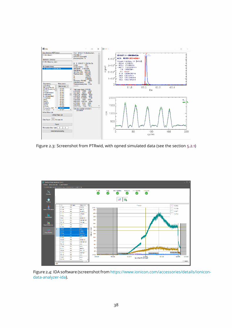
Figure 2.3: Screenshot from PTRwid, with opned simulated data (see the section 5.2.1)

Figure 2.4: IDA software (screenshot fromhttps://www.ionicon.com/accessories/details/ionicon-data-analyzer-ida).

38

Chapter 3

Mathematical approaches forclassification and longitudinalanalysis

3.1 Penalised spline regression

In this section, wepresent penalised spline regression, (Marx and Eilers, 2005;Wood, 2006;Bollaerts et al., 2006; Ruppert et al., 2009), which permits to estimate any shape of functionwithout parametric assumptions and generalising well to multi-dimensions. In particular,the P-spline approach introduced by Eilers and Marx (1996) is very powerful to model anyprofile without a priori knowledge on the data and to provide interpretive coefficients andpenalisation.

3.1.1 Penalised smooth regression

Let some data be (yi, xi)ni=1, we want to estimate a smooth function f , without any para-

metric assumption such that:yi = f(xi) ∀i ∈ 1, ..., n

f may then be expressed as a linear combination of K basis functions (b1(x), ..., bK(x)):f(x) =

∑Kj=1 βjbj(x). We thus come back to a parametric linear model:

yi =k∑

j=1

βjbj(xi) + ϵi ϵi ∼ N (0, σ2) (3.1)

39

The parameter β is then estimated by the least squares method:

β = argminβ

n∑i=1

(yi −k∑

j=1

βjbj(xi))2

= argminβ

||y −Xβ||2

= (XTX)−1XTy

where the ith row of the (n × k) matrix X, Xi = (b1(xi), b2(xi), ..., bk(xi)), and y =

(y1, ..., yn).It then remains to choose the basis and the dimension k. Several basis of smooth func-

tions could be used, for instance polynomial, Gaussian or spline. Grenn and Silverman(1994) demonstrate that splines are the best interpolators function in the sense of min-imising the integrated squared second derivative of f on [x1, xn]. So, in order to estimateany shape of function, splines present themselves as ideal candidates.Then to select the best dimension k, oneway is to start with a large dimension, and then

use hypothesis testing methods or AIC criteria to select K by backward selection. How-ever such an approach is problematic since the fit of the model tends to depend on thebasis function locations. An alternative to controlling smoothness is to add a “wiggliness”penalty to the least squares optimisation problem (Ramsay et al., 1996):

minβ

||y −Xβ||2 + λ

∫ xn

x1

f ′′(x)2dx

where λ is the smooth coefficient. Because f is linear in the parameters β, the penaltycan always be written as a quadratic form in β : βTSβ, where S is a matrix of knowncoefficients (Wood, 2006). The optimisation problem (Equation 3.3) become:

β =argminβ

||Y −Xβ||2 + λβTSβ

β =(XTX + λS)−1XTY

(3.2)

If λ→ ∞, the fitted curve f approaches the standard linear regression to the observeddata. In contrary, where λ → 0 the curve will tend to become more and more variable,and at 0, f will approach an interpolant to the data, satisfying f(xi) = yi ∀i.

40

0.00

0.25

0.50

0.75

1.00

0 1x

d= 1 k= 5

0.00

0.25

0.50

0.75

1.00

0 1x

d= 3 k= 7

internal knots outer knots

Figure 3.1: B-spline functions spread over a set of 5 equidistant knots for data between 0and 1, with degree d = 1 (top panel) and d = 3 (bottom panel). This results in a basis ofdimension 5 for d = 1 and 7 for d = 3.

3.1.2 P-splines

P-splines (penalised B-splines) are B-splines to which the penalty added corresponds tothe difference between successive parameters βi, to control the smoothness of the es-timated function f . It has been used in many applications and theoretical works (Eilerset al., 2015) such as data smoothing (Currie and Durban, 2002), Bayesian statistics (Gres-sani and Lambert, 2021), and machine learning with generalised additive models (GAM;Brezger and Lang 2006; Wood 2006). Let us first introduce B-splines.Basis splines (B-splines) are polynomial functions with a minimal compact support, intro-duced by de Boor (1978). To construct a B-spline basis of dimension k, (b1, ..., bk), we firstdefine a degree d and a set of knots k1, ..., kq such that k1 < k2 < ... < kq , and q = k+d+1.The first and last d knots are called outer knots, and the k + 1− d central knots are inter-nal knots and must be located within [xmin, xmax]. Only the position of the internal knotsimpacts the estimation of the function f . Then each element bdi is a polynomial functiona of degree d over the interval [ki, ki+d+1], and zero otherwise:

bdi (x) =x− kiki+d − ki

bd−1i (x) +

ki+d+1 − x

ki+d+1 − ki+1bd−1i+1 (x)

∀i ∈ 1, ...,K and b0i (x) =

1 if ki < x < ki+1

0 otherwise

41

A examples of B-splines basis with fives knots distributed between [0, 1] are shown in Fig-ure 3.1. B-splines were developed as a very stable basis for large scale spline interpolation(Unser et al., 1993), but the real statistical interest in B-splines has resulted from the workof Eilers andMarx (1996), by using them to develop P-splines. We add to the least squaresregression a penalty on the difference between successive parameters βi of order b:

minβ

||Y −Xβ||2 + λk∑

j=b+1

∆b(βj)2 (3.3)

where ∆b(βj) = ∆(∆(b−1)(βj)) and ∆(βj) = βj − βj−1. For instance, if b = 1 and k = 3,the penalty could be written as follow:

P =

3∑j=2

(βj − βj−1)2 = β21 − 2β1β2 + 2β22 − 2β2β3 + β23

P =βT

1 −1 0

−1 2 −1

0 −1 1

β

P =βT

1 0

1 −1

0 1

[−1 1 0

0 −1 1

]β

P =βTDTDβ

where the (k − b) × k matrix D corresponds to the difference of successive row of theidentity matrix of dimension k: ∆bIk. For practical computation, the problem can be re-formulated as follows (Eilers and Marx, 1996):

||Y −Xβ||2 + λβTSTSβ =

∥∥∥∥∥[Y

0

]−

[X√λS

]β

∥∥∥∥∥2

It simply corresponds to the unpenalised least squares problem, hence the model can befitted by standard linear regression. An example of spline regression with B-spline andpenalised spline regressionwith P-spline are shown on Figure 3.2. P-splines are extremelyeasy to set up and use, and allow a good deal of flexibility, in that any order of penaltycan be combined with any order of B-spline basis.

3.1.3 Penalty, knots location and basis dimension

We now discuss the choice of the penalty parameter λ, the knot location and the dimen-sionK.

42

0.0

0.4

0.8

1.2

0 10 20 30x

λ = 0

0.0

0.4

0.8

1.2

0 10 20 30x

λ = 1

0.0

0.4

0.8

1.2

0 10 20 30x

λ = 10

0.0

0.4

0.8

1.2

0 10 20 30x

λ selected with GCV criteria

data fitted line P−splines

Figure 3.2: Example of penalised spline regression with a P-spline basis of dimension 15with a penalty difference of order 2, for different values of the penalisation parameter λ.We observe that too high penalties lead to underfitting, and the contrary to overfitting.

43

The knots canbedistributed equidistantly over the data interval, or concentrated aroundthe information in the case of unequal distribution (by using quantiles for instance). ForP-splines, the choice of the knots location is generally equidistant in order to make thepenalty interpretive, since the penalty parameter is the same for the difference of all suc-cessive knots.Regarding penalty and dimension, a too high penalty and a too small basis dimension

result to underfitting, whereas a too small penalty and a too large basis lead to overfitting.It is therefore important to find a trade-off between bias and variance. Kim and Gu (2004)showed that the basis size should scale as 10n 2

9 , where n is the number of observation.However, it is important to note that the exact size of the basis dimension is not reallycritical, since the smoothing parameter controls the actual effective degrees of freedom.The basis dimension is a mere upper bound to the flexibility of the function.

Generalized Cross Validation (GCV)

The smooth penalty parameter λ can be estimated by cross validation. This method con-sists in separating the data into k sub-parts, and successively using one part for testingand the others for training. The error metric of each sub-model on the test data are thenaveraged to get the Cross Validation (CV) criterion. In case k is equal to the number ofdata n, the Leave One Out Cross Validation (LOOCV) is computed as:

LOOCV =1

n

n∑i=1

L(yi, f−i

β(xi))

where f−i

βis the function estimated on all the data excepted xi and L is a loss function

(e.g. squared error loss, absolute error, indicator function). To get the best parameterλ, the simplest way is to compute the LOOCV on a grid of λ values, and choose theone which gives the lowest LOOCV error. But this method can be very time consuming,since it requires the training of n × the size of the grid search models. However, in caseof penalised regression, calculating CV by performing n model fits is unnecessary. TheGCV criterion can be used, which is approximately equivalent to LOOCV and can bederived from the model fit and the whole data set (proof in Golub et al. 1979) :

GCV =n||Y −Xβ||2

(n− tr(A))2

whereA is the influencematrix (or hatmatrix) of themodel (Equation 3.2): A = X(XTX+

λS)−1XT . An example of the influence of the λ parameter is show in Figure 3.2.44

3.1.4 Multidimensional penalised regression

The penalised spline regression theory can be generalised to multidimensional smooth-ing. Here, we illustrate the two-dimensional case (Marx and Eilers, 2005; Wood, 2006;Dierckx, 1995; Durban et al., 2002). The objective now is to estimate a function f suchthat:

yij = f(xi, zj) ∀i ∈ 1, ..., n1 and ∀j ∈ 1, ..., n2

To do so, we choose a basis for each axis (not necessary the same) (b1(x), .., bKx(x)) and(a1(z), .., aKz(z)):

fδ(x) =

Kx∑i=1

δibi(x) fα(z) =

Kz∑j=1

αjaj(z)

A two dimensional function is then obtained by multiplying each coefficient of each basisterm to term (tensor product):

fβ(x, z) =

Kx∑i=1

Kz∑j=1

βijbi(x)aj(z) with βij = δi × αj

This function can be written in a matrix format: fβ((x1, ..., xn1), (z1, ..., zn2)) = Xβ

with: β ∈ R(Kx×Kz), X ∈ R(n1×n2)×(Kx×Kz)

Xi = Xxi ⊗Xzi, where ⊗ represent the kronecker product, and Xi the ith row of X

Xxi = (b1(xi), ..., bKx(xi)), Xzi = (a1(zi), ..., aKz(zi))

A specific penalty may be applied to each axis:

minβ

||Y −Xβ||2 + λxβTPxβ + λzβ

TPzβ

minβ

||Y −Xβ||2 + βTSβ with S = λxβT Pxβ + λzβ

T Pzβ

and Px = Px ⊗ IKz Pz = IKx ⊗ Pz , where IK is the identity matrix of dimension K.This brings us back to a similar 1D optimisation problem as in Equation 3.2. Examples of2-dimensional B-spline basis built with the tensor product are shown in Figure 3.3.

45

x

0.0

0.5

1.0z

0.0

0.5

1.0

0.0

0.2

0.4

x

0.0

0.5

1.0

z

0.0

0.5

1.0

0.0

0.2

0.4

Figure 3.3: 2D B-spline consisting of a single (left) or 9 (right) basis functions, with equidis-tant knots between 0 and 1.

3.2 Statistical learning for biomarker discovery

The objective of biomarker discovery is to find a significant feature subset with optimalpredictive properties (see the section 1.1.1). The pre-processing of data from volatolomics,or more generally metabolomics, usually provides hundreds of features for one sample,resulting in a data table with a high feature over sample ratio, and incomplete, noisy, andcollinear data structures (Trygg et al., 2007a). Classification methods with feature selec-tion and reduction of dimension are therefore needed to avoid over-fitting and predictionvariability. In addition, clinical studies are often designed as longitudinal data, with multi-ple measurements of the same individual over time, to increase the statistical power.We therefore present in this section state of the art methods to address these three is-

sues: classificationmodels in the case of dimensions greater than the number of samples,feature selection methods and time course modelling.

3.2.1 Classification

We denote the random variables Y ∈ 0, 1 andX = (X1, ..., Xp), and their observationsy = (y1, ..., yn)

T a n× 1 vector andX = (x1, ...,xp) a n× pmatrix with xi = (x1i , ..., xni )

T ,where X are the predictor variables and y the response. We suppose that p > n. Wewant to construct a decision rule from the observations that enables to predict Y . To doso, we search for a prediction function Y (x) that minimises the risk function for classifi-cation P (Y (X) = Y ). We describe hereafter four reference supervised machine learningapproaches adapted to high dimension, namely Elastic Net, Random Forest, Support Vec-tor Machine (SVM) and Partial Least Squares - Discriminant Analysis (PLS-DA). In addition,we present associated feature selectionmethods, either based on the ranking of featuresaccording to their contribution to the prediction (Random Forest, PLS-DA, SVM), or basedon integrated sparse constraints (Elastic-Net). Furthermore, hypothesis testing to discrim-

46

inate two classes are introduced.

Elastic Net

The Elastic Net model, developed by Zou and Hastie (2005), is a regularised logistic re-gression that linearly combines the L1 and L2 penalties of the lasso (Tibshirani, 1996) andridge (Hoerl and Kennard, 1988) regression. It is particularly useful when the number ofpredictors is much larger than the number of observations, because it includes variableselection within the model-building procedure by setting the smallest coefficients to zero(unlike ridge regression). In addition, if a group of variables is highly correlated, and oneof the variables is selected, the whole group is automatically included (see below), whichis not the case in the lasso approach.The model assumes that Y follows a Bernoulli distribution conditional toX , and that:

P (Y = 1|X) =1

1 + e−(β0+Xβ)(3.4)

The p + 1 coefficients (β0, β) are then estimated by maximising the (or minimising thenegative) penalised log-likelihood function of the model L(β0, β|y,X) with the LARS-ENalgorithm proposed by Zou and Hastie (2005) based on the Least Angle Regression, whichis similar to forward stepwise regression (see the section 3.2.2), but instead of includingvariables at each step, the estimated parameters are increased in a direction equiangularto each one’s correlations with the residual (Efron et al., 2004):

β = argminβ

−L(β0, β|y,X) + λ1||β||1 + λ2||β||2

(3.5)

Features which are not selected by themodel get their coefficients set to zero. Interest-ingly, Zou and Hastie (2005) demonstrate that the two penalties L1 and L2 lead to selecting‘grouped’ correlated variables, since if two variables i and j have a correlation ρ close to1, the difference between the coefficient βi and βj is bounded by (1− ρ).The parameters (λ1, λ2) are usually tuned by cross validation, in order to find the right

balance between the bias and variance, and to minimise the miss-classification error.The Elastic Net produces a sparsemodel with a good prediction accuracy, while encour-

aging a grouping effect.

Random Forest

Random forests, introduced by Breiman (2001), are a combination of decision tree predic-tors, such that each tree is built with a bootstrap sampling of observations and a random

47

Predictor Regularisationparameters Ranking featuremetricsY (X) =

1 if 1

1+e−(β0+βX)> 0.5

0 otherwisepenalty coefficients λ1and λ2

absolute values ofnon-zero β coefficientsTable 3.1: Elastic net summary

subset of features, independently and with the same distribution for all trees. The pre-dicted class is then assigned by a majority vote: each tree provides a class according to itsown classifier, and then the most frequent class from the ensemble of trees is returned.Random forest is reported as an excellent and fast classifier, with simple theory. Over-

fitting in the case of a higher number of features than observation is prevented by usingdifferent subsets of the training data and different subsets of features for training the in-dividual trees (Biau and Scornet, 2015). It has already been applied tomanymetabolomicsdata in clinical studies aiming at biomarker discovery (Touw et al., 2012; Chen et al., 2013).Two methods have been proposed to measure the feature importance in the model,

namely the Gini importance (Breiman, 2001) and the permutation accuracy importance(Seoane et al., 2014). The latter estimates the decrease of the prediction performancewhen the values of that variable are randomly permuted within the out-of-bag observa-tions.Predictor Regularisationparameters RankingfeaturemetricsY (X) =

1 if

∑Ki=1 1Y Ti=1 >

∑Ki=1 1Y Ti=0

0 otherwisewhere Y Ti is the prediction of the ith tree of theforest andK is the number of trees

maximum depth of atree in the forest;maximum number offeatures in the leaf(last node of the tree)and number ofvariables to berandomly drawn foreach individual tree

Featureimportance

Table 3.2: Random forest summary

Support Vector Machine

Support Vector Machine (SVM), introduced by Boser et al. (1996); Vapnik (1995), maximisethe distance between the training data set and the decision boundary between two dif-ferent classes. The underlying hypothesis is that the larger this marge is, the better thegeneralisation error of the classifier will be.

48

SVMworks well both in situations when the separation between classes is linear or not,and is effective in cases where the number of dimensions is greater than the number ofsamples. Many studies have already demonstrated the potential of SVM for biomarkerdiscovery in metabolomics and mass spectrometry data (Marchiori et al., 2006; Mahade-van et al., 2008; Heinemann et al., 2014).In this section, the observed responses yi will be assumed to be in −1, 1. The sepa-

rating hyperplane (or decision function)D(x) is formulated as a function of a KernelK:

D(x) =n∑

j=1

αjK(xj , x) + b (3.6)

Kernel functions represent dot products in the feature space. They enable the algo-rithms to be used in a feature space without explicitly carrying out computations withinthat space. According toAronszajn (1950), kernels canbewrittenK(x, x′) =

∑Ni=1 ψi(x)ψi(x

′),with ψ any function of an Hilbert space andN the kernel dimension. Equation 3.6 is thusequivalent to:

D(x) =n∑

j=1

N∑i=1

αjψi(xj)ψi(x) + b

D(x) =

N∑i=1

wiψi(x) + b with wi =

n∑j=1

αjψi(xj)

(3.7)

α are called dual parameters, w direct parameters, and b the bias. To estimate them, themargin between the class boundary and the training points is formulated in the directspace of Equation 3.7, by maximising the normalised distance of any training point x tothe hyperspace: d(x,D) = D(x)

||w|| . This is equivalent tominimising ||w|| under the constraintthat the observation x is assigned to the good class, i.e. sign(D(xi)) = sign(yi):

min ||w||2

s.t. yiD(xi) ≥ 1 ∀i(3.8)

This problem is then transformed into the dual space by using the Lagrange multipliermethod. This results in a quadratic optimisation problem with linear constraints. The lat-ter can be easily resolved by numeric optimisation algorithms such as descent methods.A regularisation parameter λ may be added to the dual optimisation problem on the

α coefficient. This approach, called Kernel Ridge Regression (Saunders et al., 1998), wasdesigned to reduce over-fitting resulting from the “curse of dimensionality”.

49

Predictor Regularisation parameters Ranking feature metricsY (X) = sign(wTψ(X) + b) regularisationparameter λ values of w incase of a linearkernel

Table 3.3: SVM summary

Partial Least Square - Discriminant Analysis (PLS-DA)

Partial Least Squares regression (PLS) is a dimension reduction technique based on latentvariables that maximises the covariance with the response (in contrast to principle com-ponent analysis, which maximises the variance of the components; Wold et al. 2001). Itwas developed in the late 60s by Herman Wold, and later applied by his son Svante Woldto high dimension andmulti-collinear datasets (Wold et al., 1984; Brereton and Lloyd, 2014;Fordellone et al., 2018). It finds a linear regression model by projecting the predicted vari-ables and the observed variables into a new space. PLSwas later extended to classificationproblems by using a dummy matrix Y as the response (Barker and Rayens, 2003).In parallel, Trygg and Wold (2002) proposed to include within the PLS algorithm an or-

thogonal signal correction filter to remove systematic variation in the predictors (i.e. vari-ation from X that is not correlated to Y). The resulting model, called Orthogonal PartialLeast Squares (OPLS), has similar performances compared to PLS, but facilitates interpre-tation. In particular, OPLS models of a 1-dimension y response have a single predictivecomponent (Trygg and Wold, 2002). Due to its ability to perform well with high dimensionand multi-collinear datasets, the PLS approach is very popular in metabolomics (Trygget al., 2007b), e.g. for mass spectrometry, nuclear magnetic resonance, or near-infrareddata.In the classical multi-linear modelling Y = Xβ + ϵ, the least square solution is β =

(XTX)−1XTy. In cases where the number of predictors is larger than the number ofobservations, or when multi-collinearity is present, theXTXmatrix becomes singular.PLS solves this problem by decomposing the data matrix X and the response y into

k orthogonal scores (components) in the form of a (n × k) matrix T, and two loadingmatrices P andQ, of respective dimensions (p× k) and (1× k):

X = TPT + ϵ

y = TQT + ν(3.9)

where ϵ and ν are error vectors of independent and identically distributed random nor-mal variables. A weight matrixW (p× k) is then defined as:

50

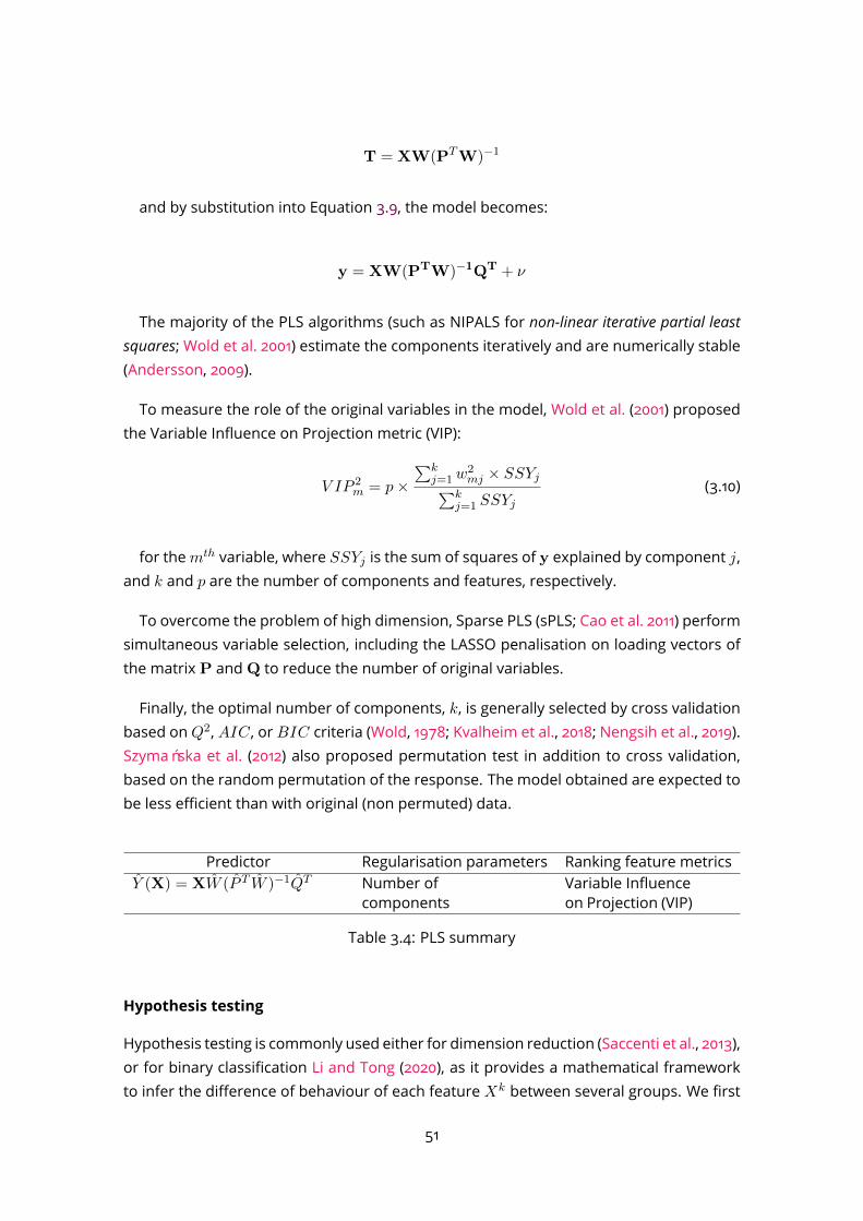
T = XW(PTW)−1

and by substitution into Equation 3.9, the model becomes:

y = XW(PTW)−1QT + ν

The majority of the PLS algorithms (such as NIPALS for non-linear iterative partial leastsquares; Wold et al. 2001) estimate the components iteratively and are numerically stable(Andersson, 2009).To measure the role of the original variables in the model, Wold et al. (2001) proposed

the Variable Influence on Projection metric (VIP):

V IP 2m = p×

∑kj=1w

2mj × SSYj∑k

j=1 SSYj(3.10)

for themth variable, where SSYj is the sum of squares of y explained by component j,and k and p are the number of components and features, respectively.To overcome the problem of high dimension, Sparse PLS (sPLS; Cao et al. 2011) perform

simultaneous variable selection, including the LASSO penalisation on loading vectors ofthe matrix P andQ to reduce the number of original variables.Finally, the optimal number of components, k, is generally selected by cross validation

based onQ2, AIC , orBIC criteria (Wold, 1978; Kvalheim et al., 2018; Nengsih et al., 2019).Szymańska et al. (2012) also proposed permutation test in addition to cross validation,based on the random permutation of the response. The model obtained are expected tobe less efficient than with original (non permuted) data.

Predictor Regularisation parameters Ranking feature metricsY (X) = XW (P T W )−1QT Number ofcomponents Variable Influenceon Projection (VIP)

Table 3.4: PLS summary

Hypothesis testing

Hypothesis testing is commonly used either for dimension reduction (Saccenti et al., 2013),or for binary classification Li and Tong (2020), as it provides a mathematical frameworkto infer the difference of behaviour of each feature Xk between several groups. We first

51

present Hypothesis testing as a classification method.Let Xk

0 = Xk ∩ (Y = 0) (respectively, Xk1 ) the kth explanatory feature when Y = 0

(respectively, Y = 1). The test is called parametric if a probabilistic law is used for Xk1and Xk

0 , and non-parametric if there is no assumption of such a law. A statistical test isdefined by two opposite hypothesesH0 (null hypothesis) andH1 (alternative hypothesis).The critical region Rα(x), a sub-set of observations leading to the H0 to be rejected, isdefined for a significance level α such that: PH0(X ∈ Rα(x)) ≤ α, where PH0(X ∈ Rα)

is the probability to reject H0 under the H0 hypothesis (Type 1 error; Taeger and Kuhnt2014).The p-value is then defined as the minimum probability to reject wronglyH0:

p = infα; s.t x ∈ Rα

The smaller the p-value, the higher the evidence against H0 (conversely, however, a p-value close to 1 does not mean that there is strong evidence in favour ofH0). The p-valuethus reflects only the non-matching toH0 (Thiese et al., 2016). We describe here two tests:

• Student’s t-test:The t-test (Student, 1908) is a parametric test, with assumption of normality: Xk

0 ∼N (µ0, σ

2) andXk1 ∼ N (µ1, σ

2). The test is then formulated as follows :

H0 : µ0 = µ1 vs H1 :

µ0 = µ1 bilateralµ0 > µ1 unilateralµ0 < µ1

Let us denote X the empiric mean of theXki underH0: we have√n X−µ0

σ ∼ N (0, 1),and, according to Cochran theorem, (n−1) σ

2

σ2 ∼ χ2n−1 with the estimator of variance

σ2 = 1n−1

∑ni=1(Xi − X)2. We end up comparing the t-statistic to the T (n − 1)

Student’s law with n− 1 degree of freedom:

Z =√nX − µ0√

σ∼ T (n− 1) (3.11)

• Wilcoxon-Mann-Whitney testA commonly used non-parametric counterpart of the t-test is the Wilcoxon - Mann-Whitney test (or Mann – Whitney U test; Wilcoxon 1945), which is based on ranks.

52

Under the null hypothesisH0, the distributions of both populations are equal:

H0 : P (Xk0 < Xk

1 ) = P (Xk1 < Xk

0 ) =1

2vs

H1 :

P (Xk

0 < Xk1 ) = 1

2 bilateralP (Xk

0 < Xk1 ) >

12 unilateral: Xk

1 greater thanXk0

P (Xk0 < Xk

1 ) <12 unilateral: Xk

1 lower thanXk0

No assumption of the probabilistic law for Xki is required: only the ordered values

of the observations (xk1, ..., xkn) are used. Let us note the statistic U0 =∑ri the sum

of ranks of the xki for yi = 0, and U1 the sum of ranks for yi = 1. UnderH0, Xk0 and

Xk1 have the same distribution, as well as U0 and U1. The distribution of the sum of

ranks can then be asymptotically approximated by a normal distribution (Mann andWhitney, 1947; Iman, 1974). This test can be used even if the observations of the twoclasses are of different sizes, and it can be also adapted to paired data (Wilcoxon,1945).

To select features with a significant difference in means (or medians) between thetwo groups, all features are first tested independently, resulting in a vector of p-values(p1, ..., pp). A correctionmust then be applied to the results of thesemultiple tests (Burger,2017), since using the α threshold directly for each pj would result in a global increase offalse positives: in the case of p independent comparisons, the number of false positives,or Family-Wise Error Rate (FWER) is 1 − (1 − α)p. A mean of controlling the FWER (i.e. ofcontrolling the probability of at least one Type 1 error) is to use the α/p threshold for eachtest (Bonferroni correction).A less stringent criterion is usually applied in omics studies, which focuses on controlling

the False Discovery Rate (FDR), i.e. the expected proportion of "discoveries" (rejected nullhypotheses) that are false. In particular, Benjamini and Hochberg (1995) demonstratedthat selecting features such that p(i) < i

pα∗ controls the FDR to α∗ (where p(i) are the

ordered p-values, i the rank, and p the number of features).

3.2.2 Feature selection

Feature selection consists in selecting a subset of relevant features used for a predictivemodel. A high number of features in a data set, larger than the number of samples, leadsto model over fitting. Furthermore, selecting themost promising candidates between thefirst untargeted step and the subsequent validation phases is critical in the biomarkerpipeline (section 1.1.1).Methods for features selection can be classified in three categories (Jović et al., 2015):

53

• Filtermethods: select variables before building themodel, based on a criterion inde-pendent from the performance of the classification algorithm, such as the p-valuefrom statistical hypothesis tests (correlation, Chi-square), or multivariate metrics(e.g., Variable Importance), and a fixed threshold

• Embedded methods: select features during the building of the model; examplesinclude regularisation models (Lasso, Elastic Net), or variant algorithms from SVM(Weston et al., 2000), and RF (Genuer et al., 2010).

• Wrapper methods: train a model iteratively with several subsets of features, andselect the one that gives the best predictive performance. The most known sub-setting strategies are: (i) forward selection, starting with an empty feature set, andthen adding one or more features at each iteration, (ii) backward elimination, start-ing with the whole feature set, and removing one or more features, (iii) bidirectionalselection (stepwise), from an empty set or from the whole set, simultaneously con-sidering larger and smaller feature subsets, or (iv) heuristic selection, that generatesa starting subset based on a heuristic (e.g. a genetic algorithm), and then exploresit further.

On the one hand, filter methods are the fastest and the simplest approaches. However,since the filtering is performed before the training of themodel, the selected featuresmaynot be optimal for the classifier performance. In addition, the choice of the threshold isarbitrary. On the other hand, embedded methods usually achieve good prediction per-formances, while still being computationally efficient. They are, however, specific to asingle type of classifier, which may be a limitation when one wants to compare severalapproaches with distinct mathematical backgrounds (to maximise the chance of findingan optimal classification).Thewrapper feature selectionmethods are then a good trade-off. One of them is recur-

sive feature elimination (RFE). It has been applied successfully to severalmachine learningalgorithms, including SVM (Guyon et al., 2002; Sanz et al., 2018), RF (Granitto et al., 2006),and PLS (Sahran et al., 2018). It is a backward recursive process, which iteratively ranksfeatures according to a measure of their importance (related to the algorithm used) andremoves the weakest one(s). There are several possible stopping criteria, such as: rununtil the feature subset is empty, or until the model performance reaches a threshold, oruntil the performance does not improve from one iteration to the next.A limitation of RFE is that the selection criterion is based on the classifier performance

only: the added-value of including a particular group of features instead of noise into themodel (i.e. the statistical significance of the selection for the model performance) is notevaluated. Rinaudo et al. (2016) therefore proposed a wrapper algorithm based on ran-dom permutation of feature intensities within the test subsets (obtained by resampling),

54

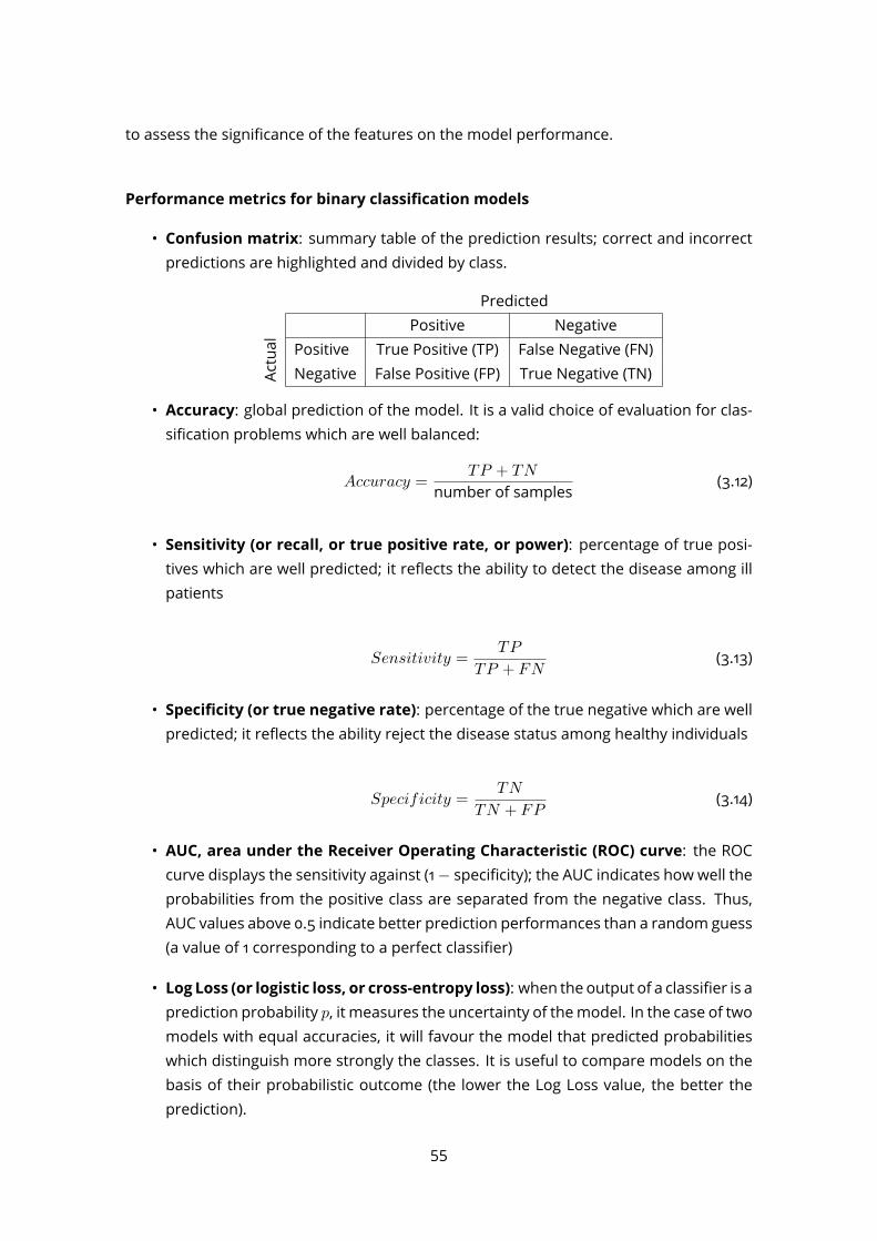
to assess the significance of the features on the model performance.

Performance metrics for binary classification models

• Confusion matrix: summary table of the prediction results; correct and incorrectpredictions are highlighted and divided by class.

PredictedPositive Negative

Actual Positive True Positive (TP) False Negative (FN)

Negative False Positive (FP) True Negative (TN)• Accuracy: global prediction of the model. It is a valid choice of evaluation for clas-sification problems which are well balanced:

Accuracy =TP + TN

number of samples (3.12)

• Sensitivity (or recall, or true positive rate, or power): percentage of true posi-tives which are well predicted; it reflects the ability to detect the disease among illpatients

Sensitivity =TP

TP + FN(3.13)

• Specificity (or true negative rate): percentage of the true negative which are wellpredicted; it reflects the ability reject the disease status among healthy individuals

Specificity =TN

TN + FP(3.14)

• AUC, area under the Receiver Operating Characteristic (ROC) curve: the ROCcurve displays the sensitivity against (1− specificity); the AUC indicates how well theprobabilities from the positive class are separated from the negative class. Thus,AUC values above 0.5 indicate better prediction performances than a random guess(a value of 1 corresponding to a perfect classifier)

• Log Loss (or logistic loss, or cross-entropy loss): when the output of a classifier is aprediction probability p, it measures the uncertainty of themodel. In the case of twomodels with equal accuracies, it will favour the model that predicted probabilitieswhich distinguish more strongly the classes. It is useful to compare models on thebasis of their probabilistic outcome (the lower the Log Loss value, the better theprediction).

55

Log loss = −n∑i

(yilog(pi) + (1− yi)log(1− pi)) (3.15)

3.2.3 Time-course modelling

In this section we seek for modelling longitudinal data, where individuals are measuredrepeatedly thought time, in contrast to cross-sectional data where only a single responseis available for each person. This is a common problem in clinical analysis, when we wantto study the effect of a pathology or a treatment over time.Let y(tij) be a response variable obtained for an individual i at different time levels j

and possibly under changing experimental conditions (eg. treatment administered froma date, change of climatic conditions), and ci be a categorical variable (we restrict our-selves here to the number of 2 classes of patients). We want i) to model y as a functionof time by taking into account the individual effects, and ii) to test if there is a differentevolution between the two groups in time. This could results in unbalanced data sets,and general multivariate models are not suitable for this analysis due to the covariancestructure between individual measurement (all observations are not independent).Mixed-effectmodels (Harville, 1977; Laird andWare, 1982; Demidenko, 2004; Galecki and

Burzykowski, 2013; Pinheiro andBates, 2000) arewell suited for the analysis of longitudinaldata, because they include multilevel random effects (which allow data from the sameindividual to be combined) and explicit modelling and analysis of between and withinindividual variation. Thesemodels are primarily used to describe relationships between aresponse variable and some covariates in data that are grouped according to one ormoreclassification factors. Examples of such grouped data include longitudinal data, repeatedmeasures data, multilevel data, and block designs.

Mixed effect model

Mixed-effects model are defined as follows:y(tij) = f(tij)︸ ︷︷ ︸fixed effect

+ gi(tij)︸ ︷︷ ︸random effect+ ϵij , ϵij ∼ N (0, σ2) iid

This means that there is a common mean longitudinal response across all individuals(fixed effect f ) and an individual-specific deviation from this mean curve (random effectgi). To illustrate and demonstrate the proprieties ofmixed-effectsmodels, let us start withthe linear case.

56

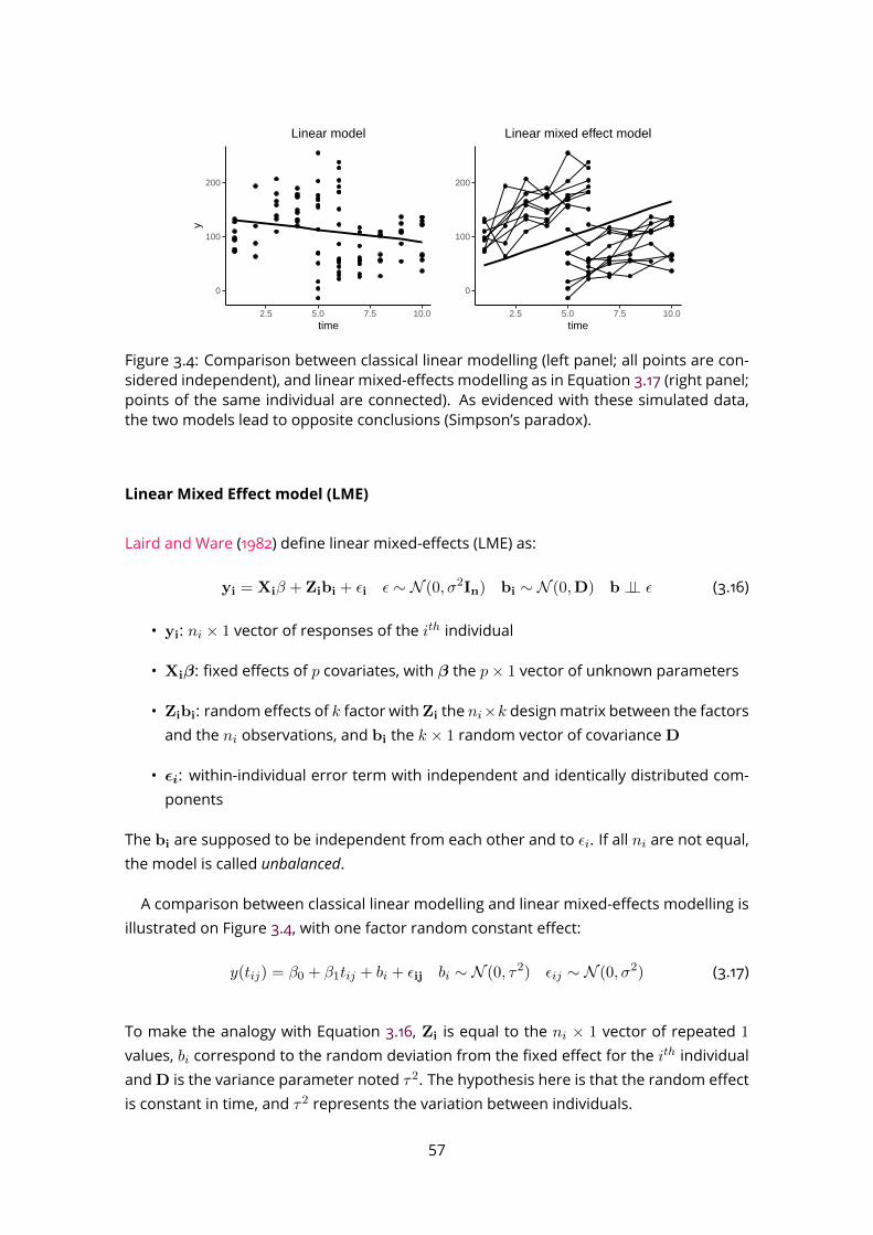
0

100

200

2.5 5.0 7.5 10.0time

y

Linear model

0

100

200

2.5 5.0 7.5 10.0time

Linear mixed effect model

Figure 3.4: Comparison between classical linear modelling (left panel; all points are con-sidered independent), and linear mixed-effects modelling as in Equation 3.17 (right panel;points of the same individual are connected). As evidenced with these simulated data,the two models lead to opposite conclusions (Simpson’s paradox).

Linear Mixed Effect model (LME)

Laird and Ware (1982) define linear mixed-effects (LME) as:yi = Xiβ + Zibi + ϵi ϵ ∼ N (0, σ2In) bi ∼ N (0,D) b ⊥⊥ ϵ (3.16)

• yi: ni × 1 vector of responses of the ith individual• Xiβ: fixed effects of p covariates, with β the p× 1 vector of unknown parameters• Zibi: random effects of k factor withZi the ni×k designmatrix between the factorsand the ni observations, and bi the k × 1 random vector of covarianceD

• ϵi: within-individual error term with independent and identically distributed com-ponents

The bi are supposed to be independent from each other and to ϵi. If all ni are not equal,the model is called unbalanced.A comparison between classical linear modelling and linear mixed-effects modelling is

illustrated on Figure 3.4, with one factor random constant effect:y(tij) = β0 + β1tij + bi + ϵij bi ∼ N (0, τ2) ϵij ∼ N (0, σ2) (3.17)

To make the analogy with Equation 3.16, Zi is equal to the ni × 1 vector of repeated 1

values, bi correspond to the random deviation from the fixed effect for the ith individualandD is the variance parameter noted τ2. The hypothesis here is that the random effectis constant in time, and τ2 represents the variation between individuals.

57

Estimation of parameters

Parameters of Equation 3.16 (β, b, θ) with θ = (σ2, D) could then be estimated by max-imising the likelihood L(β, b, θ) of the model 3.16, which can be written as follows:

yi = Xiβ + νi νi = Zbi + ϵi ∼ N (0,Σθ) Σθ = ZiDZTi + Iσ2 (3.18)

Parameters are then be estimated iteratively with either the EM (Expectation - Max-imisation) or the Newton–Raphson algorithm. But since the ML variance estimator σ2 isbiased, Patterson and Thompson (1971) and Harville (1977) have proposed to reduce thisbias with the Restricted Maximum Likelihood (REML) estimators. The latter is obtainedby maximising the likelihood, not of all the data, but rather by the average of the like-lihood over all the possible values of β : ∫ L(β, b, θ)dβ. This method could also have aBayesian interpretation, corresponding to assuming a locally uniform prior distributionfor the fixed effects β (Laird and Ware, 1982). This method provides estimations for the θand β(θ), b(θ). The derivation of ML and REML estimators are detailed and discussed byLaird and Ware (1982).

Testing hypotheses for the fixed effects

To assess the significance of longitudinal evolution between two groups of individuals, abinary variable c is added to the fixed effects, and we test if the related β coefficient(s)are different from zero. Using the formulation of model in Equation 3.16, it is equivalentto testing:

H0 : Gβ = 0 H1 : Gβ = 0 (3.19)

where G is a r×pmatrix and r is the number of coefficients tested as different from zero.The Likelihood Ratio test compares the log likelihood of the both models (H0 and H1).

However, as explained by Pinheiro and Bates (2000), likelihood ratio tests are not validwhen comparing LME models with different fixed effects fitted using REML, since there isa term in the REML criterion that changeswith the change in the fixed-effects specification.In contrast, the F-test, which is similar to likelihood ratio test, relies on a single model

for comparison (assuming that the variables not common to bothmodels are zero). In theclassical linear model, we have the following results which follows from the Wald statistic(Galecki and Burzykowski, 2013; Scheipl et al., 2008):

F =(Gβ)T (G ˆVar(β)GT )−1Gβ

r∼ F(r, df)

58

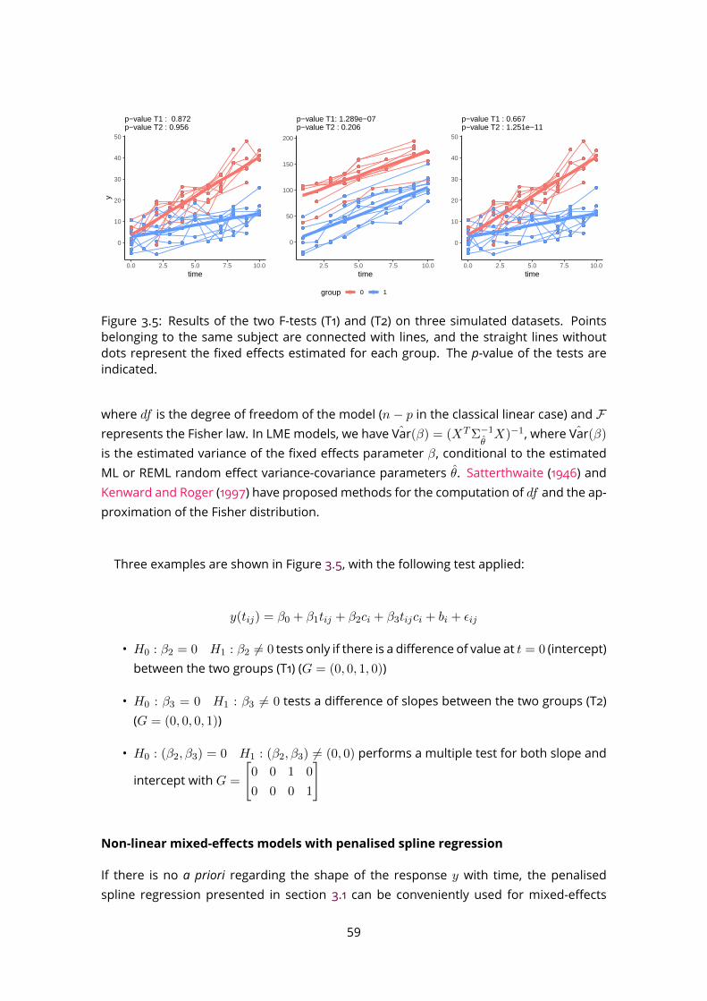
0

10

20

30

40

50

0.0 2.5 5.0 7.5 10.0time

y

p−value T1 : 0.872 p−value T2 : 0.956

0

50

100

150

200

2.5 5.0 7.5 10.0time

p−value T1: 1.289e−07 p−value T2 : 0.206

0

10

20

30

40

50

0.0 2.5 5.0 7.5 10.0time

p−value T1 : 0.667 p−value T2 : 1.251e−11

group 0 1

Figure 3.5: Results of the two F-tests (T1) and (T2) on three simulated datasets. Pointsbelonging to the same subject are connected with lines, and the straight lines withoutdots represent the fixed effects estimated for each group. The p-value of the tests areindicated.

where df is the degree of freedom of the model (n− p in the classical linear case) and Frepresents the Fisher law. In LME models, we have ˆVar(β) = (XTΣ−1

θX)−1, where ˆVar(β)

is the estimated variance of the fixed effects parameter β, conditional to the estimatedML or REML random effect variance-covariance parameters θ. Satterthwaite (1946) andKenward and Roger (1997) have proposed methods for the computation of df and the ap-proximation of the Fisher distribution.

Three examples are shown in Figure 3.5, with the following test applied:

y(tij) = β0 + β1tij + β2ci + β3tijci + bi + ϵij

• H0 : β2 = 0 H1 : β2 = 0 tests only if there is a difference of value at t = 0 (intercept)between the two groups (T1) (G = (0, 0, 1, 0))

• H0 : β3 = 0 H1 : β3 = 0 tests a difference of slopes between the two groups (T2)(G = (0, 0, 0, 1))

• H0 : (β2, β3) = 0 H1 : (β2, β3) = (0, 0) performs a multiple test for both slope andintercept with G =

[0 0 1 0

0 0 0 1

]

Non-linear mixed-effects models with penalised spline regression

If there is no a priori regarding the shape of the response y with time, the penalisedspline regression presented in section 3.1 can be conveniently used for mixed-effects

59

modelling, thereby connecting non parametric mixed-effects modelling and linear mixed-effects modelling. Let us note (B1, ..., BK) a base of smooth functions of dimension K;the following model is equivalent to model 3.16:

yi =

K∑k=1

βkBk(ti) + bi + ϵi

yi = Xiβ + bi + ϵi

whereXi is a ni×Kmatrix corresponding to (B1(ti), ..., BK(ti)), and ti the ni×1 vectorof time points for individual i.A penalisation may be applied to the smooth fixed coefficient β:

P = λβTSβ

with S a positive semi-definite matrix. The least square problem then becomes:

||y −Xβ − Zb||+ λβTSβ

The S for P-splines is explained in section 3.1.2. By using the eigen-decomposition, S =

UDUT , where U is an orthogonal matrix of eigenvectors, andD is a diagonal matrix, themodel can be re-parameterised (Wood, 2006; Lee et al., 2013) to get to amodel of the format equation 3.16. Estimation of parameters is then equivalent.Testing hypotheses on the fixed effect can then be performed using a Fisher test as

described above (an example of a non-linear mixed model is shown on Figure 3.6):

y(tij) = β0 +

K∑k=1

βkbk(tij) + (α0 +

K∑k=1

αkbk(tij))× ci + bi + ϵij

• H0 : (α1, ..., αK) = 0 vs. H1 : (α1, ..., αK) = 0 tests if the two groups have the sametrend in time or not, without any a priori knowledge on this trend (T3)

60

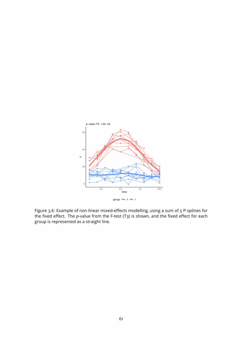
0

20

40

60

2.5 5.0 7.5 10.0time

y

group 0 1

p−value T3 : <2e−16

Figure 3.6: Example of non linear mixed-effects modelling, using a sum of 5 P-splines forthe fixed effect. The p-value from the F-test (T3) is shown, and the fixed effect for eachgroup is represented as a straight line.

61

62

Part II

Results

63

Chapter 4

Design and implementation ofinnovative methods for theprocessing of PTR-TOF-MS data:ptairMS

Existing PTR-TOF-MS pre-processing tools are particularly suited for the analysis of verylarge files resulting from continuous environmental monitoring, including robust pic pick-ing methods in the m/z dimension, but poor temporal signal treatment as described insection 2.2.4. Furthermore, there are specific needs for breath research in patient cohortswhich have to be covered, for instance, the simultaneous analysis of multiple samplesrequires that peak lists from different samples may be aligned; in addition, the parallelprocessing of several files would be a time-sparing capability; furthermore, a correct dis-tinction of the signals coming from the background and the expiratory phases is needed;finally, implementing a background correction of the ambient air composition as a func-tion of time would be an asset for accurate peak detection and quantification.We therefore developed a suite of algorithms for the processing of PTR-TOF-MS data

fromexhaled breath, based on an innovative 2Dmodel based on P-splines regression thatenables a precise estimation of the peak evolution over the acquisition time, and integrat-ing several tools for cohort management in an R package, called ptairMS. It takes as inputthe name of the directory containing the raw files in HDF5 format and ultimately gener-ates the samples by variables table of peak intensities. The main steps of the workfloware summarised below (Algorithm 1) and detailed in the following section:

1. Processing of each file

64

1.1 Internal calibration of the m/z axis1.2 Determination of expiration limits1.3 Detecting peaks on the TIS1.4 Estimating the temporal evolution for each peak1.5 Quantifying1.6 Statistical testing of intensity differences between ambient air and expiration

phases2. Alignment between samples followed by quality control

2.1 Peak matching between samples2.2 Filtering features based on reproducibility within the whole cohort or sample

classes and on the p-value from the test in 1.63. Imputation of missing values4. Putative annotation (including isotopes)5. Peak table update when new files are included in the input directory

4.1 Pre-processing for each file

4.1.1 Calibration

Calibration converts the Time-of-Flight (TOF) values recorded by the mass spectrometerinto m/z values (see section 2.2.1). We used the formula proposed by Brown and Gilfrich(1991):

m/z =(tof − b)2

a

To estimate the parameters (a, b), the Levenberg-Marquardt algorithm is used, with cou-ples (tof,m/z) of reference peaks without overlap. For exhaled breath, we suggest touse the following peaks: the primary ion isotope (m/z 21.022), nitrogen (m/z 29.013), theacetone isotope (m/z 60.053), and the two external calibration ions from the instrument:(iodobenzene m/z 203.943, and diiodobenzene m/z 330.850).As a drift over time is observed due to low changes of temperature, calibration is per-

formed periodically (e.g. every minute) to update the (a, b) values. The shift is subse-quently estimated for eachm/z as a function of time by linear interpolation, and correctedlocally (for each nominal mass ±0.4) before peak detection.

65

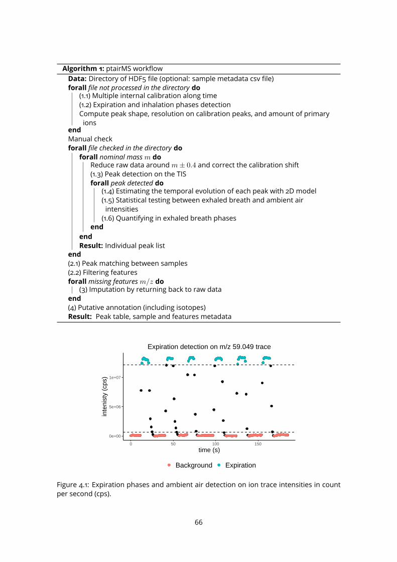
Algorithm 1: ptairMS workflowData: Directory of HDF5 file (optional: sample metadata csv file)forall file not processed in the directory do(1.1) Multiple internal calibration along time(1.2) Expiration and inhalation phases detectionCompute peak shape, resolution on calibration peaks, and amount of primaryionsendManual checkforall file checked in the directory do

forall nominal massm doReduce raw data aroundm± 0.4 and correct the calibration shift(1.3) Peak detection on the TISforall peak detected do(1.4) Estimating the temporal evolution of each peak with 2D model(1.5) Statistical testing between exhaled breath and ambient airintensities(1.6) Quantifying in exhaled breath phasesend

endResult: Individual peak list

end(2.1) Peak matching between samples(2.2) Filtering featuresforallmissing featuresm/z do(3) Imputation by returning back to raw dataend(4) Putative annotation (including isotopes)Result: Peak table, sample and features metadata

0e+00

5e+06

1e+07

0 50 100 150

time (s)

inte

nist

y (c

ps)

Background Expiration

Expiration detection on m/z 59.049 trace

Figure 4.1: Expiration phases and ambient air detection on ion trace intensities in countper second (cps).

66

4.1.2 Expiration detection

Determination of expiration limits and background (ambient air) is a very important stepfor the analysis, as boundaries will be used for quantification and for the statistical test forfeature selection in section 4.1.5. A raw data ion trace is used to automatically detect expi-rations, using the same method as described by Schwoebel et al. (2011); Trefz et al. (2013):after a polynomial baseline removal, the signal above fracMaxTIC×max(trace) is consid-ered as expiration (Figure 4.1). Conversely, the signal below fracMaxTICBg ×max(trace)is considered as background (inhalation phases). In addition, differences between succes-sive points in expiration (respectively, inhalation) phasesmust be lower than derivThresholdExp(respectively, derivThresholdBg). All parameters from theptairMS software are describedin Table 4.2.Finally, to assist the user in this important step, we have designed a specific panel from

the graphical interface of our software tool to the visualisation (and possiblemanualmod-ification) of the expiration limits (Figure 4.8).

4.1.3 Peak detection and quantification on the Total Ion Spectrum (TIS)

The peak picking (section 1.2.1) algorithm in the m/z dimension is mainly based on Mülleret al. 2013. Since VOCs have low weights (< 500 Da), we detect peaks on the TIS aroundnominal masses (±0.4Da). The successive steps are (see Figure 4.2):

1. Baseline removal using the SNIP algorithm (Ryan et al., 1988)2. Estimation of the noise threshold and auto-correlation within the “off-peak” interval

[m− 0.6,m− 0.4] ∪ [m+ 0.4,m+ 0.6] (Müller et al., 2011)3. SavitzkyGolay (SG) signal filtering by using optimalwindows (Vivo Truyols and Schoen-

makers, 2006; Savitzky and Golay, 1964)4. Detection of localmaxima by using the first and second derivatives of SG smoothing,

followed by quality control on peak separation (in ppm) and intensity threshold setto the maximum between a) the noise threshold, b) min intensity parameter, and c)1% of the signal maximum

5. Peak deconvolution, by using a peak function depending on the vector parametersµ (peak centre), σl, σr (peak widths at half maximum, left and right from the peakcentre), and h (peak height):

minµ,σl,σr ,h

||y −P∑i=1

hi × peakµi,σli,σ

ri(m)||2 (4.1)

67

noise noise

0

300

600

900

1200

37.6 38.0 38.4

mz

inte

nsity

baselineRaw data

Baseline correction and noise estimation around m/z 38

1−2

0

100

200

300

400

78.95 79.00 79.05 79.10 79.15

mz

inte

nsity

Noise thresholdSG smoothing

Local maximaRaw data

SG smoothing and local maxima around m/z 79 3−4

R2= 0.992

0

100

200

300

400

78.95 79.00 79.05 79.10 79.15

mz

inte

nsity

Local Maxima residualPeak centerPeak sumPeaksRaw dataResidual

De−convolution and residual anlaysis iteration 15R2= 0.999

0

100

200

300

400

78.95 79.00 79.05 79.10 79.15

mz

inte

nsity

Peak centerPeak sumPeaksRaw dataResidual

Residual anlaysis iteration 26

Figure 4.2: Peak detection on the Total Ion Spectrum (TIS) around nominal masses. Forillustrative purposes, we focus on m/z 38 for baseline correction (1-2) and m/z 79 for de-convolution (3-6). We used the sech2 function for deconvolution at steps 5 and 6.

with y the baseline corrected and smoothed signal, and P the number of detectedlocal maxima. The optimisation is done with the Levenberg-Marquardt algorithm,with the following initialisation and constraints: σl = σr = σ/2withσ = m/resmean ∈[m/resmax;m/resmin], µ the local maxima detected at the step 4 above ±σ× 4Da,and h the values of the spectrum at mass(es) µ (always positive).

6. Iterative peak detection on the residuals (Müller et al., 2011), using the samemethodas described above, with a decreased noise threshold of 20%. Iterations stop assoon as one of the following criteria is met: R2 > R2min (default: 0.995), noise auto-correlation < autocorMax , the maximum number of iterations is reached (default:4), the maximum number of detected peaks is reached (default: 7).

Peak shape

To find the most suitable peak shape, four asymmetric functions are evaluated on thecalibration peaks, and the one providing the best R2 value is selected: average calibrationpeak shape used by Müller et al. (2010) and Holzinger (2015) (see section 2.2.3), the sech2function (Equation 4.2; Lange et al. 2007), Bi-Gaussian (Equation 4.3), and Lorentzian func-tions (Equation 4.4; Lange et al. 2007). An example of the peak shape selection is shownin Figure 4.3.

68

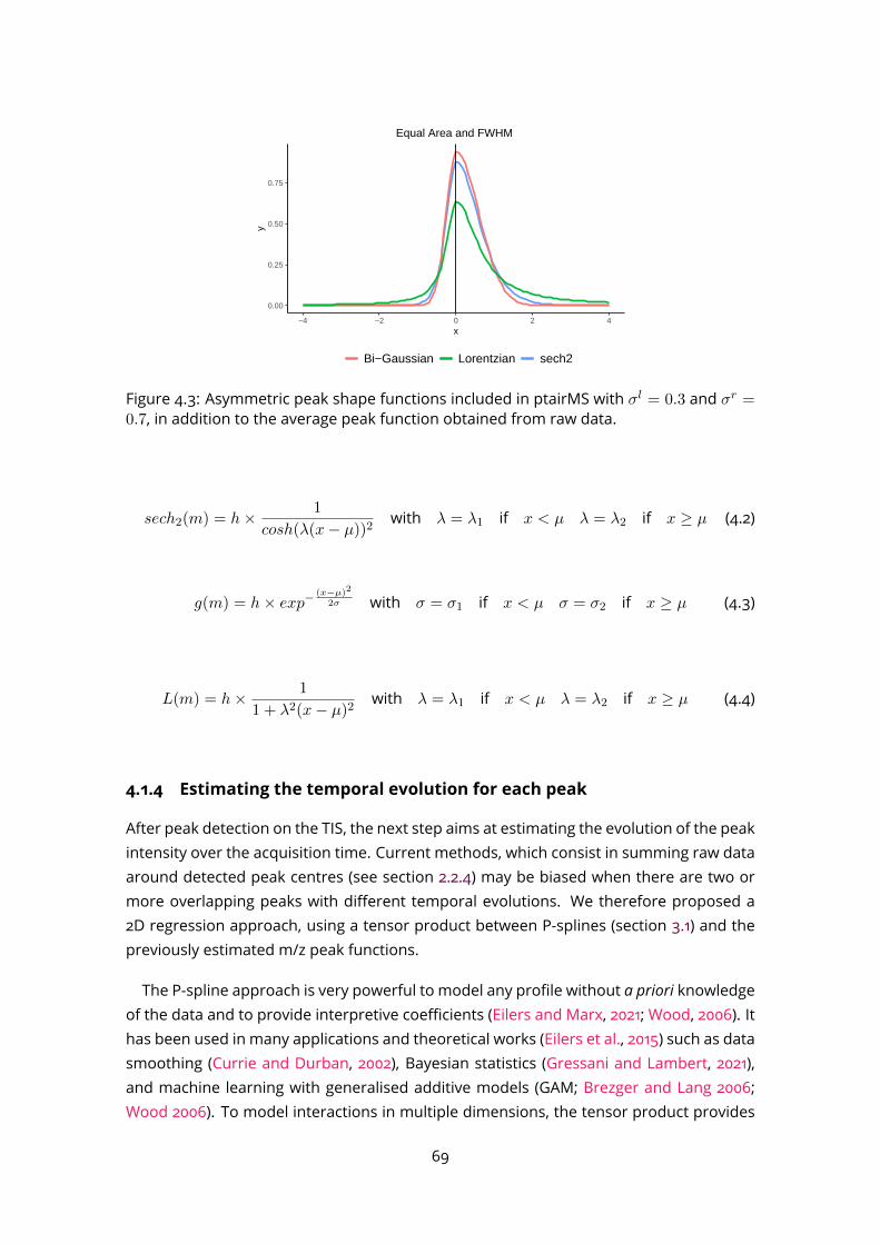
0.00

0.25

0.50

0.75

−4 −2 0 2 4x

y

Bi−Gaussian Lorentzian sech2

Equal Area and FWHM

Figure 4.3: Asymmetric peak shape functions included in ptairMS with σl = 0.3 and σr =0.7, in addition to the average peak function obtained from raw data.

sech2(m) = h× 1

cosh(λ(x− µ))2with λ = λ1 if x < µ λ = λ2 if x ≥ µ (4.2)

g(m) = h× exp−(x−µ)2

2σ with σ = σ1 if x < µ σ = σ2 if x ≥ µ (4.3)

L(m) = h× 1

1 + λ2(x− µ)2with λ = λ1 if x < µ λ = λ2 if x ≥ µ (4.4)

4.1.4 Estimating the temporal evolution for each peak

After peak detection on the TIS, the next step aims at estimating the evolution of the peakintensity over the acquisition time. Current methods, which consist in summing raw dataaround detected peak centres (see section 2.2.4) may be biased when there are two ormore overlapping peaks with different temporal evolutions. We therefore proposed a2D regression approach, using a tensor product between P-splines (section 3.1) and thepreviously estimated m/z peak functions.The P-spline approach is very powerful to model any profile without a priori knowledge

of the data and to provide interpretive coefficients (Eilers and Marx, 2021; Wood, 2006). Ithas been used in many applications and theoretical works (Eilers et al., 2015) such as datasmoothing (Currie and Durban, 2002), Bayesian statistics (Gressani and Lambert, 2021),and machine learning with generalised additive models (GAM; Brezger and Lang 2006;Wood 2006). To model interactions in multiple dimensions, the tensor product provides

69

a straightforward generalisation of the P-spline basis (Sidiropoulos et al., 2017). Here, wethus used tensor product modelling to achieve a fast deconvolution of peaks in both m/zand time dimensions simultaneously, as described below (see Figure 4.4):

1. Raw data are processed sequentially within bands around the detected peaks (the1% quantile of the estimated mixture of peak functions is used to define the m/zbounds) and covering the full acquisition time

2. The baseline in the m/z dimension is estimated at each time point by linear regres-sion between the two m/z boundaries and is subsequently removed

3. The calibration shift estimated in section 4.1.1 is corrected by linear interpolation4. The modelling of peak evolution with time is performed by using a two dimensional

model:Let us denote the functions representing the acquisition time g(t) and the m/z pro-file h(m), respectively:

g(t) =K∑j=1

αjbj(t) h(m) =

npeak∑i=1

hipeaki(m) (4.5)

with peaki(m) being the function of peak i estimated in the previous step (equa-tion 4.1), npeak the number of detected peaks, and (b1, . . . bK) the cubic B-splinefunctions for the set of K knots. The 2D model is obtained by writing each peakcoefficient hi in the B-spline basis (tensor product, section 3.1.4):

fβ(t,m) =

npeak∑i=1

K∑j=1

βijbj(t)× peaki(m) (4.6)

The βij coefficients are estimated according to the P-spline theory by minimisingthe following penalised regression, where the penalty λ is applied only to the timedimension:

minβ

T∑t=1

M∑m=1

(Ymt − fβ(m, t))2 + λ

npeak∑i=1

K∑j=3

(∆2βij)2 (4.7)

where ∆2βij = β(i,j) − 2β(i,j−1) + β(i,j−2) is the second order difference betweensuccessive coefficients in the time dimension, i (respectively, j) represents the knotslocation on themass (respectively, time) axis,m (respectively, t) represents the indexon the mass (respectively, time) axis, and Y is the raw data matrix of dimensionsM × T after baseline removal and correction of the calibration shift.

70

0

2000

4000

6000

8000

lower bound

m/z 39.02

m/z 39.03

upper bound

inte

nsity

Peak 1 Peak 2 Peak center

Peak sum Raw data

1− Define limits around peakslower bound

39.02

39.03

upper bound

0 50 100 150time (s)

m/z

Raw data

2− Calibration shift correction 3− Baseline correction

Estimated P−splines

lower bound

39.02

39.03

upper bound

0 50 100 150time (s)

m/z

Fitted data

0.00 0.25 0.50 0.75 1.00

Peak functions

.

Peak 1 Peak 2 knots

4− 2D modeling

cps

Peak 1 m/z 39.02

0 50 100 150time (s)

cps

ambient air expiration

Peak 2 m/z 39.03

5− Temporal estimation

Figure 4.4: Modelling of the VOC temporal evolution, starting from the peaks detected inthe total ion spectrum (1), and resulting in the estimation of a temporal series for each ofthem (5).

5. Quantification (in counts per spectrum) is then performed at each time point t bysumming the previous estimated 2D model along the m/z dimension

cit =

M∑m=1

K∑j=1

βij × sj(t)× peaki(m)

This results in a temporal series of intensities for each peak (ci1, ..., ciT ).The choice of the knot locations and the penalty coefficient λ are very important, since

too many knots may lead to over fitting and too few knots may result in under fitting.

Knots location

Classically, knots are uniformly distributed over the data range in order to facilitate theinterpretation of the penalty applied to the successive knot differences (Eilers and Marx,1996). In our case, however, i) exhaled breath phases are the main focus of our quantifi-cation, and ii) inhaled air phases are generally constant. We therefore propose to targetthe knot locations mainly around the expiration phases: knots are spread uniformly ev-ery 3 seconds, except for inhalation phases longer than 3 seconds, where only the first,middle and last points of the phase are used as knots (Figure 4.5). This allows to reducethe dimension of the model, and thus the computational time, while maintaining a goodfit (Table 4.1). Alternatively, a uniform distribution of the knots along the time axis is alsoavailable in the ptairMS software, in case the user has no a priori knowledge about thetemporal profile of the compound.

71

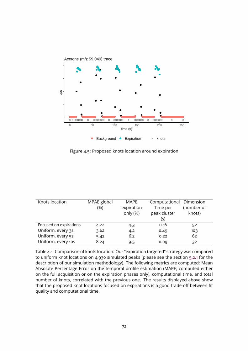
0 50 100 150 200 250time (s)

cps

Background Expiration knots

Acetone (m/z 59.049) trace

Figure 4.5: Proposed knots location around expiration

Knots location MPAE global(%) MAPEexpirationonly (%)ComputationalTime perpeak cluster(s)

Dimension(number ofknots)Focused on expirations 4.22 4.3 0.16 52Uniform, every 3s 3.62 4.2 0.49 103Uniform, every 5s 5.42 6.2 0.22 62Uniform, every 10s 8.24 9.5 0.09 32Table 4.1: Comparison of knots location: Our “expiration targeted” strategy was comparedto uniform knot locations on 4,930 simulated peaks (please see the section 5.2.1 for thedescription of our simulation methodology). The following metrics are computed: MeanAbsolute Percentage Error on the temporal profile estimation (MAPE; computed eitheron the full acquisition or on the expiration phases only), computational time, and totalnumber of knots, correlated with the previous one. The results displayed above showthat the proposed knot locations focused on expirations is a good trade-off between fitquality and computational time.

72

Penalty coefficient

The optimal penalty coefficient λ is selectedwith a grid search using the generalised cross-validation criterion (GCV; section 3.1.3). Since the penalty is set only to the time dimension,the GCV criterion is not computed from the 2D model, but from the 1D spline regressionon the total time trace of the raw data band (containing the mixture of peaks), to reducecomputational time.

4.1.5 Quantification

As presented in the introduction, PTR ionisation enables to compute "absolute" quanti-ties. Here, we thus describe how the times series for each peak i, (ci1, ..., ciT ), are nor-malised and converted to absolute quantities (Qi

1, ..., QiT ). First, since the intensities pro-vided by the instrument at each time point are in fact the sum of a fixed number of in-

ternal acquisitions, the cit are normalised (as counts of ions per second; cps) by dividingby the integrated internal time period and by multiplying by the single ion pulse voltage(Müller et al., 2014). To obtain the concentration, the latter values are then normalisedby the reagent ion (H3O

+) intensities, the reaction rate coefficient between the VOC andH3O

+, and the residence time of the primary ions in the drift tube (normalized cps, ncps)(Cappellin et al., 2012a). The final normalisation by the density of the air in the reactionchamber (ideal gas law) gives the absolute concentration of the VOC, expressed in partper billion (ppb) (section 2.2.5).The final absolute concentration of each VOC i in exhaled breath is obtained by aver-

aging absolute quantities in the expiration phases:

Qi =

∑t∈expQ

it

|exp|

where |exp| corresponds to the number of expiration points.

Ambient inhaled air correction

As discussed in section 1.3.2, inhaled air may impact exhaled breath concentrations. Tocorrect the ambient inhaled air level in exhaled breath, we thus propose to subtract theambient air baseline from the temporal profile (Qi

1, ..., QiT ) of each detected VOC beforeaveraging in exhaled breath phases: to do so, a polynomial fit of default degree 3 com-

puted on the ambient air time points is used. Note that the subtraction step may beomitted in particular cases, as detailed in the discussion.

73

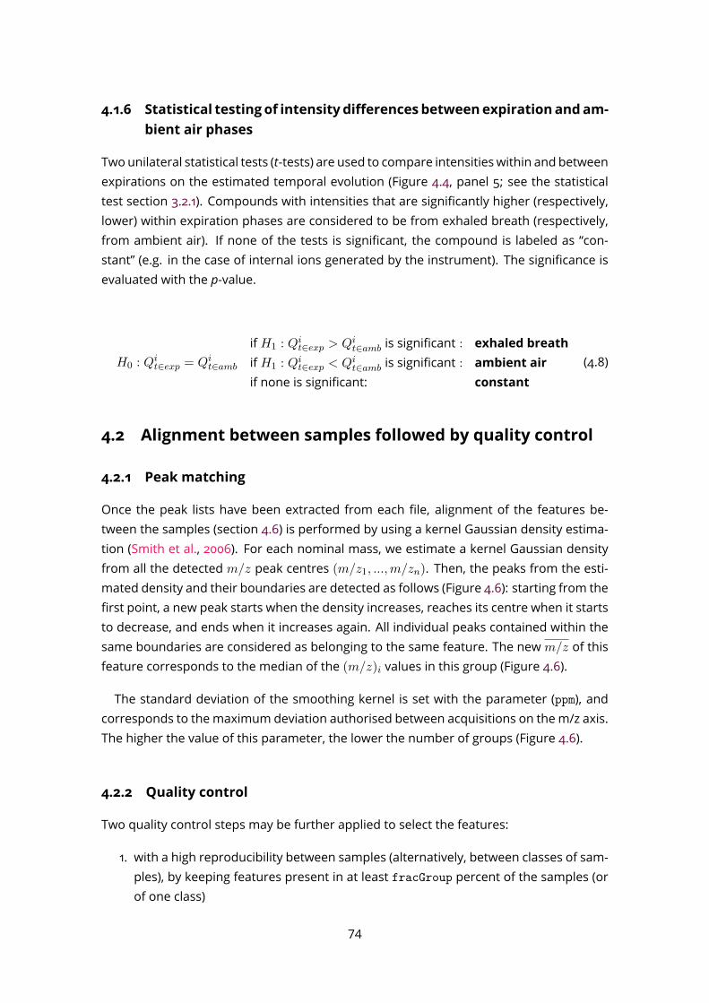
4.1.6 Statistical testingof intensity differencesbetweenexpirationandam-bient air phases

Twounilateral statistical tests (t-tests) are used to compare intensities within and betweenexpirations on the estimated temporal evolution (Figure 4.4, panel 5; see the statisticaltest section 3.2.1). Compounds with intensities that are significantly higher (respectively,lower) within expiration phases are considered to be from exhaled breath (respectively,from ambient air). If none of the tests is significant, the compound is labeled as “con-stant” (e.g. in the case of internal ions generated by the instrument). The significance isevaluated with the p-value.

H0 : Qit∈exp = Qi

t∈amb

ifH1 : Qit∈exp > Qi

t∈amb is significant : exhaled breathifH1 : Q

it∈exp < Qi

t∈amb is significant : ambient airif none is significant: constant

(4.8)

4.2 Alignment between samples followed by quality control

4.2.1 Peak matching

Once the peak lists have been extracted from each file, alignment of the features be-tween the samples (section 4.6) is performed by using a kernel Gaussian density estima-tion (Smith et al., 2006). For each nominal mass, we estimate a kernel Gaussian densityfrom all the detected m/z peak centres (m/z1, ...,m/zn). Then, the peaks from the esti-mated density and their boundaries are detected as follows (Figure 4.6): starting from thefirst point, a new peak starts when the density increases, reaches its centre when it startsto decrease, and ends when it increases again. All individual peaks contained within thesame boundaries are considered as belonging to the same feature. The newm/z of thisfeature corresponds to the median of the (m/z)i values in this group (Figure 4.6).The standard deviation of the smoothing kernel is set with the parameter (ppm), and

corresponds to themaximum deviation authorised between acquisitions on them/z axis.The higher the value of this parameter, the lower the number of groups (Figure 4.6).

4.2.2 Quality control

Two quality control steps may be further applied to select the features:1. with a high reproducibility between samples (alternatively, between classes of sam-ples), by keeping features present in at least fracGroup percent of the samples (orof one class)

74

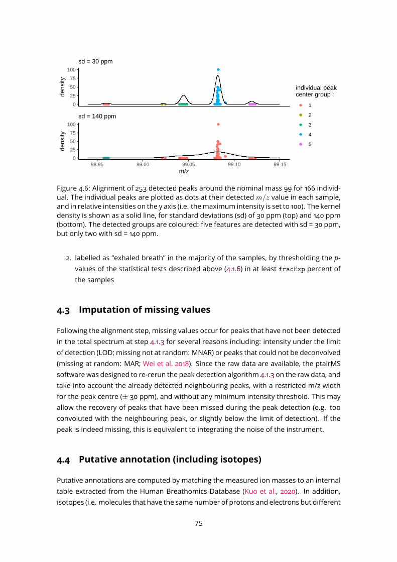
0

25

50

75

100

dens

itysd = 30 ppm

0

25

50

75

100

98.95 99.00 99.05 99.10 99.15m/z

dens

ity

sd = 140 ppm

individual peak center group :

1

2

3

4

5

Figure 4.6: Alignment of 253 detected peaks around the nominal mass 99 for 166 individ-ual. The individual peaks are plotted as dots at their detectedm/z value in each sample,and in relative intensities on the y axis (i.e. themaximum intensity is set to 100). The kerneldensity is shown as a solid line, for standard deviations (sd) of 30 ppm (top) and 140 ppm(bottom). The detected groups are coloured: five features are detected with sd = 30 ppm,but only two with sd = 140 ppm.

2. labelled as “exhaled breath” in the majority of the samples, by thresholding the p-values of the statistical tests described above (4.1.6) in at least fracExp percent ofthe samples

4.3 Imputation of missing values

Following the alignment step, missing values occur for peaks that have not been detectedin the total spectrum at step 4.1.3 for several reasons including: intensity under the limitof detection (LOD; missing not at random: MNAR) or peaks that could not be deconvolved(missing at random: MAR; Wei et al. 2018). Since the raw data are available, the ptairMSsoftwarewas designed to re-rerun the peak detection algorithm 4.1.3 on the raw data, andtake into account the already detected neighbouring peaks, with a restricted m/z widthfor the peak centre (± 30 ppm), and without any minimum intensity threshold. This mayallow the recovery of peaks that have been missed during the peak detection (e.g. tooconvoluted with the neighbouring peak, or slightly below the limit of detection). If thepeak is indeed missing, this is equivalent to integrating the noise of the instrument.

4.4 Putative annotation (including isotopes)

Putative annotations are computed by matching the measured ion masses to an internaltable extracted from the Human Breathomics Database (Kuo et al., 2020). In addition,isotopes (i.e. molecules that have the samenumber of protons and electrons but different

75

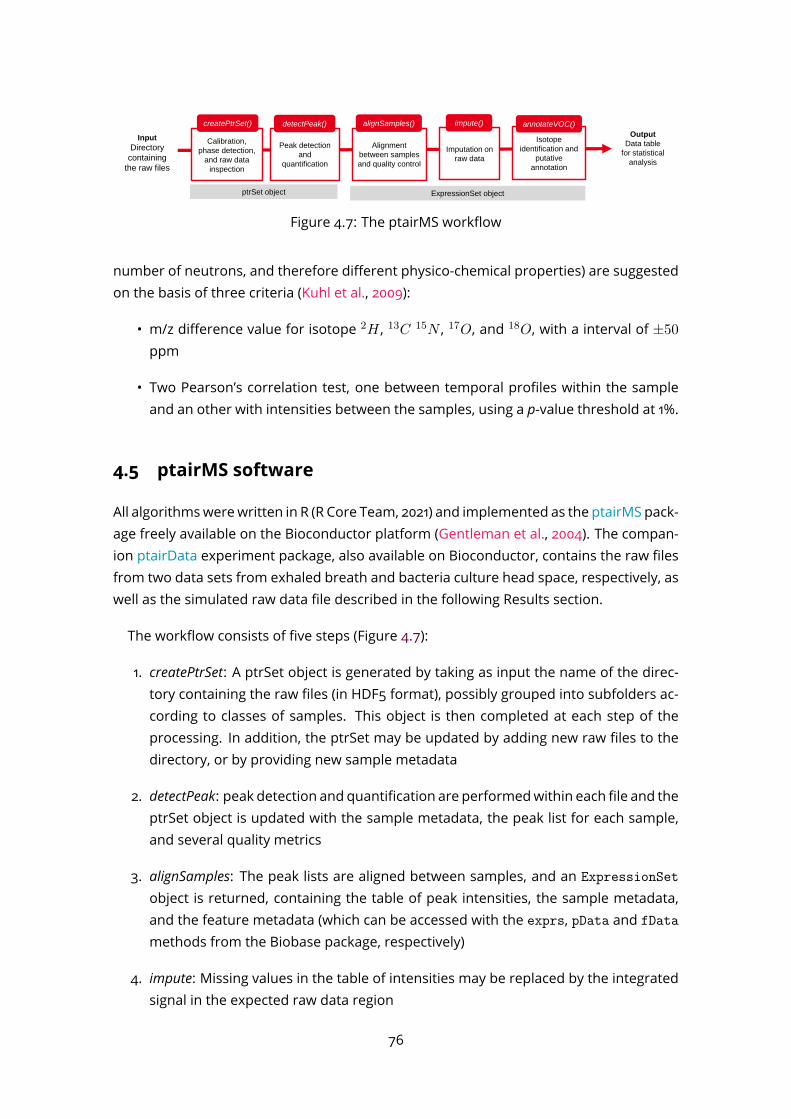
Input

Directory

containing

the raw files

Peak detection

and

quantification

Alignment

between samples

and quality control

Isotope

identification and

putative

annotation

Calibration,

phase detection,

and raw data

inspection

Output

Data table

for statistical

analysis

createPtrSet() detectPeak() alignSamples() annotateVOC()

Imputation on

raw data

impute()

ptrSet object ExpressionSet object

Figure 4.7: The ptairMS workflow

number of neutrons, and therefore different physico-chemical properties) are suggestedon the basis of three criteria (Kuhl et al., 2009):

• m/z difference value for isotope 2H , 13C 15N , 17O, and 18O, with a interval of ±50

ppm• Two Pearson’s correlation test, one between temporal profiles within the sampleand an other with intensities between the samples, using a p-value threshold at 1%.

4.5 ptairMS software

All algorithmswerewritten in R (R Core Team, 2021) and implemented as the ptairMS pack-age freely available on the Bioconductor platform (Gentleman et al., 2004). The compan-ion ptairData experiment package, also available on Bioconductor, contains the raw filesfrom two data sets from exhaled breath and bacteria culture head space, respectively, aswell as the simulated raw data file described in the following Results section.The workflow consists of five steps (Figure 4.7):1. createPtrSet: A ptrSet object is generated by taking as input the name of the direc-tory containing the raw files (in HDF5 format), possibly grouped into subfolders ac-cording to classes of samples. This object is then completed at each step of theprocessing. In addition, the ptrSet may be updated by adding new raw files to thedirectory, or by providing new sample metadata

2. detectPeak: peak detection and quantification are performedwithin each file and theptrSet object is updated with the sample metadata, the peak list for each sample,and several quality metrics

3. alignSamples: The peak lists are aligned between samples, and an ExpressionSet

object is returned, containing the table of peak intensities, the sample metadata,and the feature metadata (which can be accessed with the exprs, pData and fData

methods from the Biobase package, respectively)4. impute: Missing values in the table of intensities may be replaced by the integrated

signal in the expected raw data region76

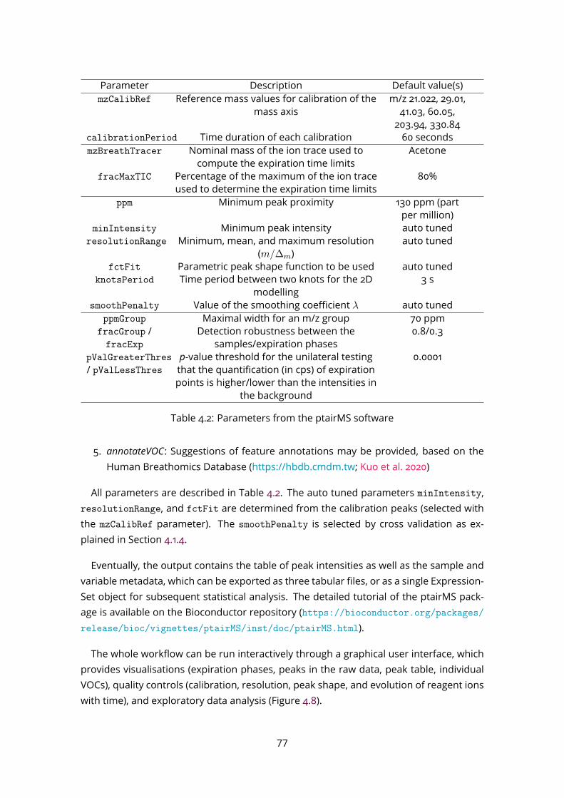
Parameter Description Default value(s)mzCalibRef Reference mass values for calibration of themass axis m/z 21.022, 29.01,41.03, 60.05,203.94, 330.84

calibrationPeriod Time duration of each calibration 60 secondsmzBreathTracer Nominal mass of the ion trace used tocompute the expiration time limits Acetone

fracMaxTIC Percentage of the maximum of the ion traceused to determine the expiration time limits 80%ppm Minimum peak proximity 130 ppm (partper million)

minIntensity Minimum peak intensity auto tunedresolutionRange Minimum, mean, and maximum resolution(m/∆m)

auto tunedfctFit Parametric peak shape function to be used auto tuned

knotsPeriod Time period between two knots for the 2Dmodelling 3 ssmoothPenalty Value of the smoothing coefficient λ auto tuned

ppmGroup Maximal width for an m/z group 70 ppmfracGroup /fracExp

Detection robustness between thesamples/expiration phases 0.8/0.3pValGreaterThres/ pValLessThres p-value threshold for the unilateral testingthat the quantification (in cps) of expirationpoints is higher/lower than the intensities inthe background

0.0001

Table 4.2: Parameters from the ptairMS software5. annotateVOC: Suggestions of feature annotations may be provided, based on the

Human Breathomics Database (https://hbdb.cmdm.tw; Kuo et al. 2020)All parameters are described in Table 4.2. The auto tuned parameters minIntensity,

resolutionRange, and fctFit are determined from the calibration peaks (selected withthe mzCalibRef parameter). The smoothPenalty is selected by cross validation as ex-plained in Section 4.1.4.Eventually, the output contains the table of peak intensities as well as the sample and

variable metadata, which can be exported as three tabular files, or as a single Expression-Set object for subsequent statistical analysis. The detailed tutorial of the ptairMS pack-age is available on the Bioconductor repository (https://bioconductor.org/packages/release/bioc/vignettes/ptairMS/inst/doc/ptairMS.html).The whole workflow can be run interactively through a graphical user interface, which

provides visualisations (expiration phases, peaks in the raw data, peak table, individualVOCs), quality controls (calibration, resolution, peak shape, and evolution of reagent ionswith time), and exploratory data analysis (Figure 4.8).

77

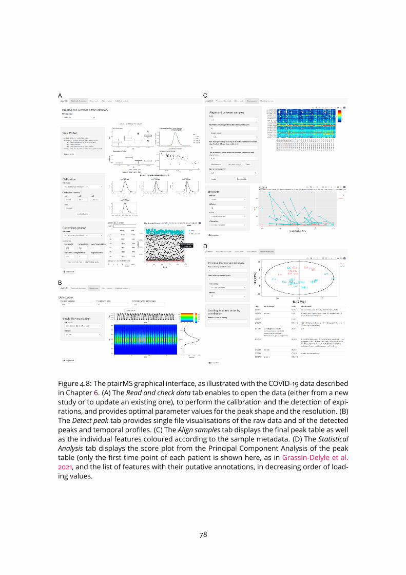
Figure 4.8: The ptairMS graphical interface, as illustratedwith the COVID-19 data describedin Chapter 6. (A) The Read and check data tab enables to open the data (either from a newstudy or to update an existing one), to perform the calibration and the detection of expi-rations, and provides optimal parameter values for the peak shape and the resolution. (B)The Detect peak tab provides single file visualisations of the raw data and of the detectedpeaks and temporal profiles. (C) The Align samples tab displays the final peak table as wellas the individual features coloured according to the sample metadata. (D) The StatisticalAnalysis tab displays the score plot from the Principal Component Analysis of the peaktable (only the first time point of each patient is shown here, as in Grassin-Delyle et al.2021, and the list of features with their putative annotations, in decreasing order of load-ing values.

78

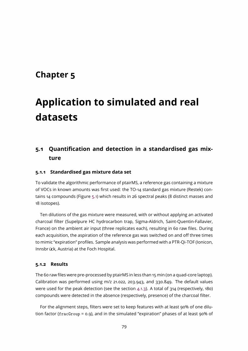
Chapter 5

Application to simulated and realdatasets

5.1 Quantification and detection in a standardised gas mix-ture

5.1.1 Standardised gas mixture data set

To validate the algorithmic performance of ptairMS, a reference gas containing a mixtureof VOCs in known amounts was first used: the TO-14 standard gas mixture (Restek) con-tains 14 compounds (Figure 5.1) which results in 26 spectral peaks (8 distinct masses and18 isotopes).Ten dilutions of the gas mixture were measured, with or without applying an activated

charcoal filter (Supelpure HC hydrocarbon trap, Sigma-Aldrich, Saint-Quentin-Fallavier,France) on the ambient air input (three replicates each), resulting in 60 raw files. Duringeach acquisition, the aspiration of the reference gas was switched on and off three timestomimic “expiration” profiles. Sample analysis was performedwith a PTR-Qi-TOF (Ionicon,Innsbrück, Austria) at the Foch Hospital.

5.1.2 Results

The 60 rawfileswere pre-processed by ptairMS in less than 15min (on a quad-core laptop).Calibration was performed using m/z 21.022, 203.943, and 330.849. The default valueswere used for the peak detection (see the section 4.1.3). A total of 314 (respectively, 180)compounds were detected in the absence (respectively, presence) of the charcoal filter.For the alignment steps, filters were set to keep features with at least 90% of one dilu-

tion factor (fracGroup = 0.9), and in the simulated “expiration” phases of at least 90% of79

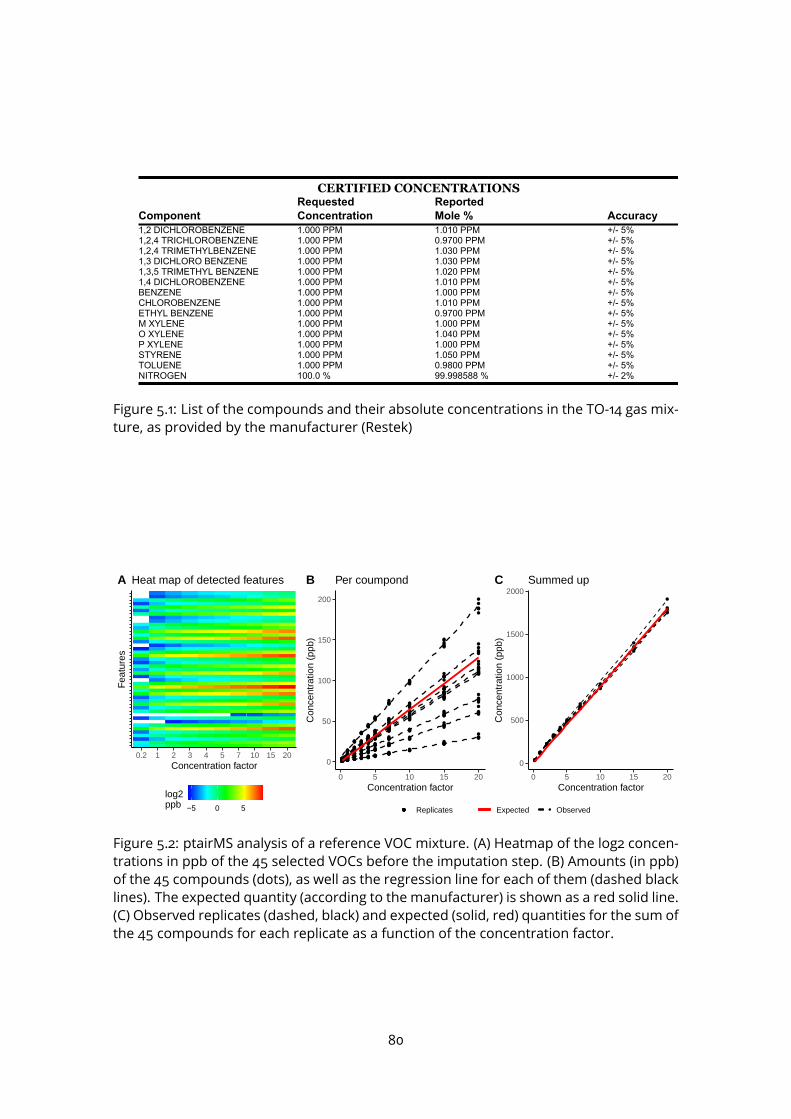
CERTIFICATE OF ANALYSISGrade of Product: CERTIFIED HYDROCARBON

Part Number: X15NI99CHPIC004 Reference Number: 160-401455492-1Cylinder Number: ST0000197547 Cylinder Volume: 110.0 LGLaboratory: 124 - Plumsteadville - PA Cylinder Pressure: 1800 PSIGAnalysis Date: Apr 03, 2019 Valve Outlet: 180Lot Number: 160-401455492-1 Expiration Date: Apr 03, 2021

Traceability Statement: Hydrocarbon Process standards are NIST traceable either directly by weight or by comparison toAirgas laboratory standards that are directly NIST traceable by weight.

CERTIFIED CONCENTRATIONSRequested Reported

Component Concentration Mole % Accuracy1,2 DICHLOROBENZENE 1.000 PPM 1.010 PPM +/- 5%1,2,4 TRICHLOROBENZENE 1.000 PPM 0.9700 PPM +/- 5%1,2,4 TRIMETHYLBENZENE 1.000 PPM 1.030 PPM +/- 5%1,3 DICHLORO BENZENE 1.000 PPM 1.030 PPM +/- 5%1,3,5 TRIMETHYL BENZENE 1.000 PPM 1.020 PPM +/- 5%1,4 DICHLOROBENZENE 1.000 PPM 1.010 PPM +/- 5%BENZENE 1.000 PPM 1.000 PPM +/- 5%CHLOROBENZENE 1.000 PPM 1.010 PPM +/- 5%ETHYL BENZENE 1.000 PPM 0.9700 PPM +/- 5%M XYLENE 1.000 PPM 1.000 PPM +/- 5%O XYLENE 1.000 PPM 1.040 PPM +/- 5%P XYLENE 1.000 PPM 1.000 PPM +/- 5%STYRENE 1.000 PPM 1.050 PPM +/- 5%TOLUENE 1.000 PPM 0.9800 PPM +/- 5%NITROGEN 100.0 % 99.998588 % +/- 2%

Permanent Notes:RESTEK P/N 34404-PI

Airgas Specialty GasesAirgas USA, LLC6141 Easton RoadBldg 2Plumsteadville, PA 18949Airgas.com

Signature on file

Approved for Release Page 1 of 160-401455492-1

Figure 5.1: List of the compounds and their absolute concentrations in the TO-14 gas mix-ture, as provided by the manufacturer (Restek)

0.2 1 2 3 4 5 7 10 15 20Concentration factor

Fea

ture

s

−5 0 5

log2ppb

Heat map of detected featuresA

0

50

100

150

200

0 5 10 15 20Concentration factor

Con

cent

ratio

n (p

pb)

Per coumpondB

0

500

1000

1500

2000

0 5 10 15 20Concentration factor

Con

cent

ratio

n (p

pb)

Summed upC

Replicates Expected Observed

Figure 5.2: ptairMS analysis of a reference VOC mixture. (A) Heatmap of the log2 concen-trations in ppb of the 45 selected VOCs before the imputation step. (B) Amounts (in ppb)of the 45 compounds (dots), as well as the regression line for each of them (dashed blacklines). The expected quantity (according to the manufacturer) is shown as a red solid line.(C) Observed replicates (dashed, black) and expected (solid, red) quantities for the sum ofthe 45 compounds for each replicate as a function of the concentration factor.

80

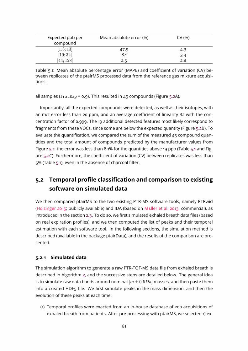
Expected ppb percompound Mean absolute error (%) CV (%)[1.3; 13] 47.9 4.3[19; 32] 8.1 3.4[44; 128] 2.5 2.8

Table 5.1: Mean absolute percentage error (MAPE) and coefficient of variation (CV) be-tween replicates of the ptairMS processed data from the reference gas mixture acquisi-tions.

all samples (fracExp = 0.9). This resulted in 45 compounds (Figure 5.2A).Importantly, all the expected compounds were detected, as well as their isotopes, with

an m/z error less than 20 ppm, and an average coefficient of linearity R2 with the con-centration factor of 0.999. The 19 additional detected features most likely correspond tofragments from these VOCs, since some are below the expected quantity (Figure 5.2B). Toevaluate the quantification, we compared the sum of the measured 45 compound quan-tities and the total amount of compounds predicted by the manufacturer values fromFigure 5.1: the error was less than 8.1% for the quantities above 19 ppb (Table 5.1 and Fig-ure 5.2C). Furthermore, the coefficient of variation (CV) between replicates was less than5% (Table 5.1), even in the absence of charcoal filter.

5.2 Temporal profile classification and comparison to existingsoftware on simulated data

We then compared ptairMS to the two existing PTR-MS software tools, namely PTRwid(Holzinger 2015; publicly available) and IDA (based on Müller et al. 2013; commercial), asintroduced in the section 2.3. To do so, we first simulated exhaled breath data files (basedon real expiration profiles), and we then computed the list of peaks and their temporalestimation with each software tool. In the following sections, the simulation method isdescribed (available in the package ptairData), and the results of the comparison are pre-sented.

5.2.1 Simulated data

The simulation algorithm to generate a raw PTR-TOF-MS data file from exhaled breath isdescribed in Algorithm 2, and the successive steps are detailed below. The general ideais to simulate raw data bands around nominal [m± 0.5Da]masses, and then paste theminto a created HDF5 file. We first simulate peaks in the mass dimension, and then theevolution of these peaks at each time:(1) Temporal profiles were exacted from an in-house database of 200 acquisitions of

exhaled breath from patients. After pre-processing with ptairMS, we selected 1) ex-81

Algorithm 2: Simulation of PTR-TOF MS data from exhaled breathData: Library of exhaled breath temporal profiles extracted from several rawfiles, and then smoothed and normalised (1)Data: List of chemical formulae used by PTRwid for calibration matches (2)Randomly draw a file j from the library, and extract the mass and time axes.forall nominal massm doGenerate random background noise (3)

if there is a compound in the chemical formula list of nominal massm thenRandom draw of the parameters from the (mixture of)m/z peaks (4)Given a temporal profile (q1, ..., qT ) from the file j:Compute the number of ions n (area of the peak) for a given peak height h(5)forall t in time axis [1, .., T ] doDraw n× ratio× qt random variable of sech2 lawWrite the histogram as a spectrum in the data matrixendResult: Simulated peak(s) + background noise

elseResult: Background noise

endend

piration profiles (with intensities significantly greater in expirations than ambientair; p−value < 2×10−20 ), and 2) ambient air profiles (with the p-value of the oppo-site test< 10−10) . The profiles were then normalised (mean set to 1) and smoothedwith the Savitzky-Golay filter. This resulted in approximately 12,800 expiration pro-files and 11,000 ambient air profiles.

(2) m/z values were generated from the library of compound formulae used by PTRwidfor calibration matching CaC

13b HcOdNe, with a ∈ [1, 40], b ∈ 0, 1, c ∈ [max(1, a −

9), a], d ∈ [0, 5] and e ∈ [0, 2]. We included only masses between 15 and 400 Da(corresponding to a total of 9,114 formulae).

(3) The Background noise was generated using a Poisson stochastic process (Gundlach-Graham et al., 2018), with λ=0.1 and a Gaussian distribution N (11, 3) to model thesingle ion Pulse-Height.

(4) Random drawing of them/z peak parameters for nominal masses distinct from 19,21, 29, 30, 32, 59, 204, and 331:

• number of overlapping peaks set to 1, 2, and 3, with probabilities (0.4, 0.5, 0.1)• class of temporal profile set to “expiration”, “ambient air”, or “constant”, withprobabilities (0.4, 0.4, 0.2)

• intensity of the highest peak on the average total spectrum: uniform distribu-82

tion U(50, 500) for multiple peaks, and Gaussian distribution N (1500, 100) forsingle peaks (most of the peaks used to compute the peak shape are singlepeaks; see Figure 5.3)

• intensity ratio of the neighbouring peaks: U(0.5, 1)• peak width set tom/resolution, where resolution is drawn from N (5000, 500)

• sech2 skewness: U(−0.3, 0.3)

• asymmetry coefficient: U(0.4, 0.6)• peak proximity (in ppm): U(190, 230)

(5) The relation between the peak height h and the peak area of the sech2 function isdetailed in appendix A.2

To get closer to exhaled breath raw data, and enables PTRwid to finds peaks for itscalibration, the following peaks were simulated without overlap: primary ion and waterdimerm/z 19.017 andm/z 37.0284 with the highest intensity (200,000), their isotopesm/z21.022, m/z 38.033 with the corresponding ratio of intensities, m/z 59.049 with intensityset to 20,000, and the calibration peaksm/z 203.943 andm/z 330.84 with intensity set to1,000.Parameters have been selected based on raw data observation, especially for the peak

width, asymmetry coefficient, and number of overlapping peaks. Then, peak proximityand ratio were set on a reasonable range, in order to challenge the peak deconvolution.No baseline nor calibration shift were added in the mass and time dimensions, the

focus of the simulation is the estimation of the temporal evolution. The code used forthe simulation, as well as a representative simulated data file in the HDF5 format areincluded in the ptairData companion package, also available in Bioconductor. An exampleof simulation is shown in Figure 5.4.

5.2.2 Software parameters

The simulated files were processed with ptairMS (version 0.1), PTRwid (version 002 IDL),and IDA (version beta 0.9.4.8). Mass calibration was performed using the features atm/z21.022, 203.943 and 330.84 for the three software, intentionally simulated without overlapat the exactm/z. The calibration stability period (calibrationPeriod for ptairMS and Timmingwindow for IDA) was set to the acquisition duration, since no calibration shift was added.To ensure a good estimation of the peak shape for the three software, we simulatedmoresingle peaks in the intensity range used for the calculation of the peak shape : between20 and 200 cps for IDA, and minSig set to 300 for PTRwid (see Figure 5.3). Note that, for

83

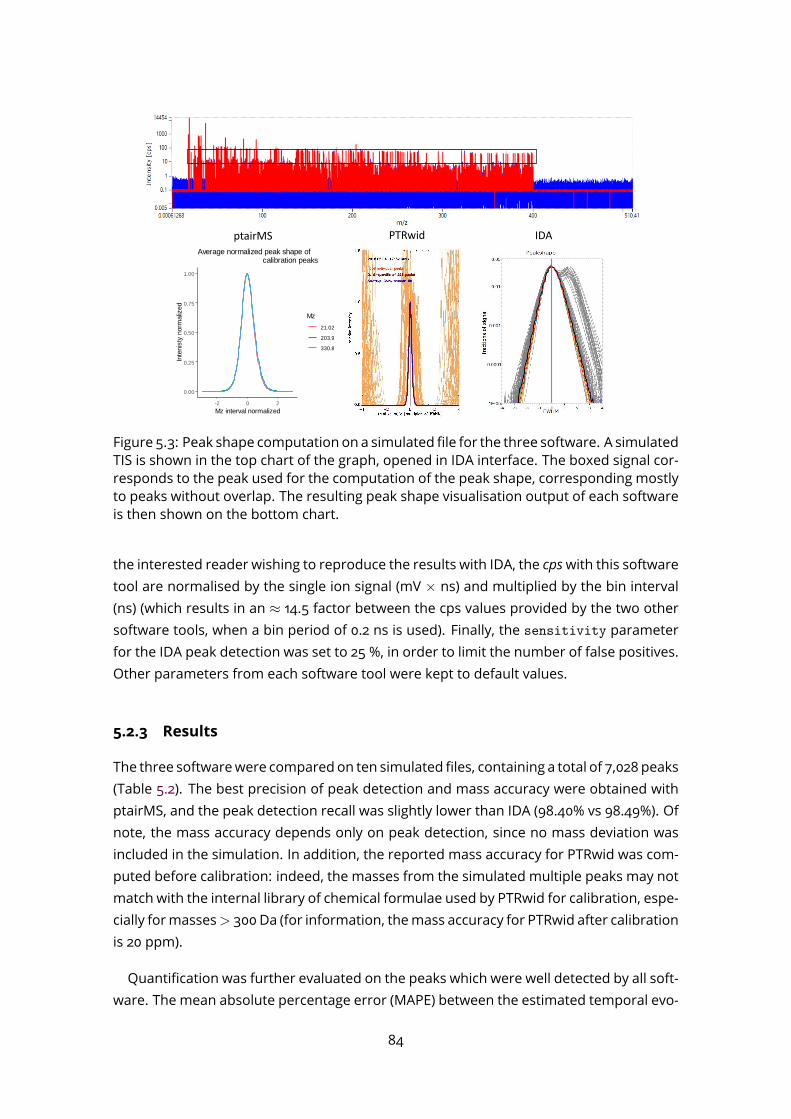
0.00

0.25

0.50

0.75

1.00

-2 0 2

Mz interval normalized

Inte

nis

ty n

orm

aliz

ed

Mz

21.022

203.943

330.849

Average normalized peak shape of calibration peaks

ptairMS PTRwid IDA

Figure 5.3: Peak shape computation on a simulated file for the three software. A simulatedTIS is shown in the top chart of the graph, opened in IDA interface. The boxed signal cor-responds to the peak used for the computation of the peak shape, corresponding mostlyto peaks without overlap. The resulting peak shape visualisation output of each softwareis then shown on the bottom chart.

the interested reader wishing to reproduce the results with IDA, the cpswith this softwaretool are normalised by the single ion signal (mV × ns) and multiplied by the bin interval(ns) (which results in an ≈ 14.5 factor between the cps values provided by the two othersoftware tools, when a bin period of 0.2 ns is used). Finally, the sensitivity parameterfor the IDA peak detection was set to 25 %, in order to limit the number of false positives.Other parameters from each software tool were kept to default values.

5.2.3 Results

The three softwarewere comparedon ten simulated files, containing a total of 7,028 peaks(Table 5.2). The best precision of peak detection and mass accuracy were obtained withptairMS, and the peak detection recall was slightly lower than IDA (98.40% vs 98.49%). Ofnote, the mass accuracy depends only on peak detection, since no mass deviation wasincluded in the simulation. In addition, the reported mass accuracy for PTRwid was com-puted before calibration: indeed, the masses from the simulated multiple peaks may notmatch with the internal library of chemical formulae used by PTRwid for calibration, espe-cially formasses> 300Da (for information, themass accuracy for PTRwid after calibrationis 20 ppm).Quantification was further evaluated on the peaks which were well detected by all soft-

ware. The mean absolute percentage error (MAPE) between the estimated temporal evo-84

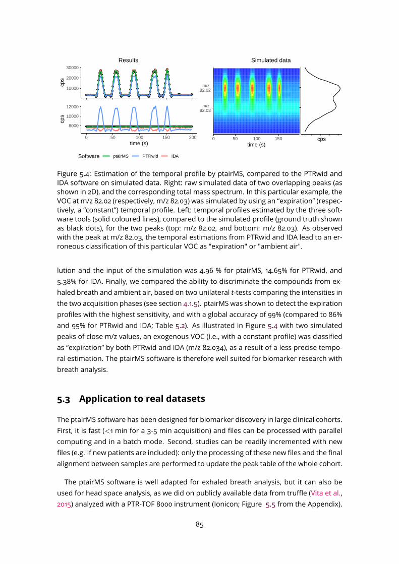
10000

20000

30000cp

s

8000

10000

12000

0 50 100 150 200time (s)

cps

Software ptairMS PTRwid IDA

Results

m/z 82.02

m/z 82.03

0 50 100 150time (s)

cps

Simulated data

Figure 5.4: Estimation of the temporal profile by ptairMS, compared to the PTRwid andIDA software on simulated data. Right: raw simulated data of two overlapping peaks (asshown in 2D), and the corresponding total mass spectrum. In this particular example, theVOC at m/z 82.02 (respectively, m/z 82.03) was simulated by using an “expiration” (respec-tively, a “constant”) temporal profile. Left: temporal profiles estimated by the three soft-ware tools (solid coloured lines), compared to the simulated profile (ground truth shownas black dots), for the two peaks (top: m/z 82.02, and bottom: m/z 82.03). As observedwith the peak at m/z 82.03, the temporal estimations from PTRwid and IDA lead to an er-roneous classification of this particular VOC as "expiration" or "ambient air".

lution and the input of the simulation was 4.96 % for ptairMS, 14.65% for PTRwid, and5.38% for IDA. Finally, we compared the ability to discriminate the compounds from ex-haled breath and ambient air, based on two unilateral t-tests comparing the intensities inthe two acquisition phases (see section 4.1.5). ptairMS was shown to detect the expirationprofiles with the highest sensitivity, and with a global accuracy of 99% (compared to 86%and 95% for PTRwid and IDA; Table 5.2). As illustrated in Figure 5.4 with two simulatedpeaks of close m/z values, an exogenous VOC (i.e., with a constant profile) was classifiedas “expiration” by both PTRwid and IDA (m/z 82.034), as a result of a less precise tempo-ral estimation. The ptairMS software is therefore well suited for biomarker research withbreath analysis.

5.3 Application to real datasets

The ptairMS software has been designed for biomarker discovery in large clinical cohorts.First, it is fast (<1 min for a 3-5 min acquisition) and files can be processed with parallelcomputing and in a batch mode. Second, studies can be readily incremented with newfiles (e.g. if new patients are included): only the processing of these new files and the finalalignment between samples are performed to update the peak table of the whole cohort.The ptairMS software is well adapted for exhaled breath analysis, but it can also be

used for head space analysis, as we did on publicly available data from truffle (Vita et al.,2015) analyzed with a PTR-TOF 8000 instrument (Ionicon; Figure 5.5 from the Appendix).

85

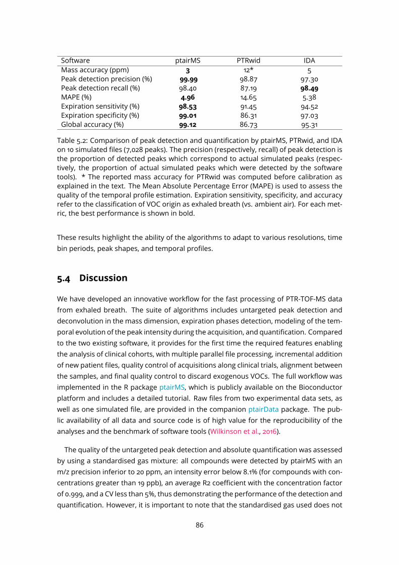
Software ptairMS PTRwid IDAMass accuracy (ppm) 3 12* 5Peak detection precision (%) 99.99 98.87 97.30Peak detection recall (%) 98.40 87.19 98.49MAPE (%) 4.96 14.65 5.38Expiration sensitivity (%) 98.53 91.45 94.52Expiration specificity (%) 99.01 86.31 97.03Global accuracy (%) 99.12 86.73 95.31Table 5.2: Comparison of peak detection and quantification by ptairMS, PTRwid, and IDAon 10 simulated files (7,028 peaks). The precision (respectively, recall) of peak detection isthe proportion of detected peaks which correspond to actual simulated peaks (respec-tively, the proportion of actual simulated peaks which were detected by the softwaretools). * The reported mass accuracy for PTRwid was computed before calibration asexplained in the text. The Mean Absolute Percentage Error (MAPE) is used to assess thequality of the temporal profile estimation. Expiration sensitivity, specificity, and accuracyrefer to the classification of VOC origin as exhaled breath (vs. ambient air). For each met-ric, the best performance is shown in bold.

These results highlight the ability of the algorithms to adapt to various resolutions, timebin periods, peak shapes, and temporal profiles.

5.4 Discussion

We have developed an innovative workflow for the fast processing of PTR-TOF-MS datafrom exhaled breath. The suite of algorithms includes untargeted peak detection anddeconvolution in the mass dimension, expiration phases detection, modeling of the tem-poral evolution of the peak intensity during the acquisition, and quantification. Comparedto the two existing software, it provides for the first time the required features enablingthe analysis of clinical cohorts, with multiple parallel file processing, incremental additionof new patient files, quality control of acquisitions along clinical trials, alignment betweenthe samples, and final quality control to discard exogenous VOCs. The full workflow wasimplemented in the R package ptairMS, which is publicly available on the Bioconductorplatform and includes a detailed tutorial. Raw files from two experimental data sets, aswell as one simulated file, are provided in the companion ptairData package. The pub-lic availability of all data and source code is of high value for the reproducibility of theanalyses and the benchmark of software tools (Wilkinson et al., 2016).The quality of the untargeted peak detection and absolute quantification was assessed

by using a standardised gas mixture: all compounds were detected by ptairMS with anm/z precision inferior to 20 ppm, an intensity error below 8.1% (for compounds with con-centrations greater than 19 ppb), an average R2 coefficient with the concentration factorof 0.999, and a CV less than 5%, thus demonstrating the performance of the detection andquantification. However, it is important to note that the standardised gas used does not

86

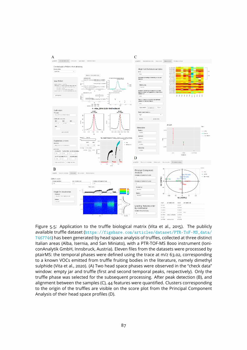
6

A C

D

B

Figure S5: Application to the truffle biological matrix (Vita et al., 2015). The publicly available truffle dataset (https://figshare.com/articles/dataset/PTR-ToF-MS_data/7467746) has been generated by head space analysis of truffles, collected at three distinct Italian areas (Alba, Isernia, and San Miniato), with a PTR-TOF-MS 8000 instrument (IoniconAnalytik GmbH, Innsbruck, Austria). Eleven files from the datasets were processed by ptairMS: the temporal phases were defined using the trace at m/z 63.02, corresponding to a known VOCs emitted from truffle fruiting bodies in the literature, namely dimethyl sulphide (Vita et al., 2020). (A) Two head space phases were observed in the “check data” window: empty jar and truffle (first and second temporal peaks, respectively). Only the truffle phase was selected for the subsequent processing. After peak detection (B), and alignment between the samples (C), 44 features were quantified. Clusters corresponding to the origin of the truffles are visible on the score plot from the Principal Component Analysis of their head space profiles (D).

Figure 5.5: Application to the truffle biological matrix (Vita et al., 2015). The publiclyavailable truffle dataset (https://figshare.com/articles/dataset/PTR-ToF-MS_data/7467746) has been generated by head space analysis of truffles, collected at three distinctItalian areas (Alba, Isernia, and San Miniato), with a PTR-TOF-MS 8000 instrument (Ioni-conAnalytik GmbH, Innsbruck, Austria). Eleven files from the datasets were processed byptairMS: the temporal phases were defined using the trace at m/z 63.02, correspondingto a known VOCs emitted from truffle fruiting bodies in the literature, namely dimethylsulphide (Vita et al., 2020). (A) Two head space phases were observed in the “check data”window: empty jar and truffle (first and second temporal peaks, respectively). Only thetruffle phase was selected for the subsequent processing. After peak detection (B), andalignment between the samples (C), 44 features were quantified. Clusters correspondingto the origin of the truffles are visible on the score plot from the Principal ComponentAnalysis of their head space profiles (D).

87

reflect breath matrices. In practice, humidity saturation of exhaled breath biases the VOCquantification in PTR-MS instruments, with divergent behaviour for different substanceclasses (Trefz et al., 2018). This effect also impacts the proposed correction of the am-bient air level (which consists in subtracting the ambient air baseline from the temporalprofile estimated for each VOC). Since the exhaled breath and ambient air have differentconcentrations of humidity, O2, and CO2, the direct subtraction should not therefore beconsidered as an absolute quantification, but rather as a relative concentration, whichcan be used to compare patients. To further compute accurate concentration differencesbetween inspiratory and expiratory phases, adequate humidity-adapted calibrations arerequired (Trefz et al., 2018).A simulation algorithmof PTR-TOF-MSdata has beendeveloped for the software perfor-

mance comparison. It used both real data for the temporal evolution of exhaled breathVOCs, and theoretical modelling for peak shape and noise. It is available on the ptair-Data Bioconductor package, making possible further comparison and bench marking forexhaled breath PTR-TOF-MS data processing. Parameters of this simulation have beenchosen to challenge more the temporal estimation of each peak than the peak picking orthe mass axis calibration, which is quite similar for the three software (e.g. stable peakshape, peak separation of at least 150 ppm, no mass deviation and baseline). However,the simulation code may be easily modified to extend the focus of the benchmark.Since the estimation of temporal profile is a key aspect of breath analysis to determine

the VOC origin (i.e. exhaled breath vs. ambient air), we have developed a 2Dmodel basedon P-splines regression. Compared to the existing software IDA (Müller et al., 2013) andPTRwid (Holzinger, 2015), which are well suited for single-file, large data from environ-mental monitoring, we demonstrate that ptairMS is very convenient for breath analysis,achieving highest sensitivity and accurate quantification with an accuracy up to 99%. Itshould be noted that the temporal estimation of the peak intensities relies on the m/zvalues previously computed on the total ion spectrum (i.e. these m/z values are not re-evaluated at each time point) which allows a fast computation, but the time deconvolutiondepends then crucially on the mass detection. The ptairMS algorithms provides precisem/z and intensity estimations, in a computation time (< 1 min) which is compatible withthe real-time patient analysis.Since the resolution of the PTR-TOF-MS does not always allow complete peak separa-

tion in the mass dimension, the peak picking algorithm relies on the subsequently steps:denoising, baseline correction, detection of local maxima, and finally deconvolution us-ing parametric peak shape. Since peak shapes observed in TOF analysers are asymmetric,and may change according to the resolution (Müller et al., 2011), we proposed to test boththeoretic model functions and estimated shapes from the raw data, and select the mostappropriate for each dataset according to the R2 criterion. This method yielded goodestimations and facilitates visualisation and interpretation of the signals. Interestingly,

88

some recently described algorithms simultaneously perform the three processing steps(denoising, baseline correction and detection of local maxima; Picaud et al. 2018), withthe aim to reduce the potential unrecoverable artefacts introduced by the sequential ap-proach.To impute missing values, ptairMS returns back to the raw data, and re-runs the pro-

cessing algorithmwith flexible parameter settings to extract the raw signals. This methodis relatively fast since subsets of the raw data are easily accessible with the HDF5 hierar-chical format, and is assumed to be as close as possible to the raw signals. Alternatively,methods based on the table of intensities are also used in metabolomics and in otheromics data (Wei et al., 2018). These methods borrow information from features withsimilar profiles, assuming that values are missing (completely) at random, and includek-nearest neighbours (kNN; Troyanskaya et al. 2001), random forest (RF; Stekhoven andBühlmann 2011), or singular value decomposition (SVD; Hastie et al. 2001) imputations. Totake into account the stochastic process underlyingmissingness and imputation, multipleimputation approaches are also of interest: such methods perform repeated imputationto generate multiple datasets, which are subsequently used to estimate the mean andthe variance of the parameter of interest (e.g. the test statistic; Chion et al. 2021).Putative annotation is finally performed, based on the matching with a database of

1,488 exhaled breath compound (∼ 400 isotopic masses; Kuo et al. 2020; Drabińska et al.2021). We observed that about 60% of the detected VOCs have a suggested annotationby ptairMS. The database may be easily updated by the user with the annotateVOC func-tion. An alternative approach based on the generation and matching of elemental for-mulae is used by the PTRwid software (Holzinger, 2015). However, the formula databaseincludes several endogenous compounds that are not found in the exhaled air, andmanyof the corresponding masses are too close to be distinguished by PTR-TOF-MS. Beyondmass library search and isotope detection, complementary experiments with hyphenatedtechniques such as GC-MS are required to achieve higher structural identification levels(Sumner et al., 2007) for the most interesting VOCs (Ibrahim et al., 2019; Nardi-Agmonet al., 2016; Wilde et al., 2019).Importantly, ptairMS automatically suggests optimal values for the parameters, such

as the resolution and the peak shape (as evaluated on the calibration peaks), but alsothe location of spline knots (at higher densities within the expiration phases) and the pe-nalisation for the 2D regression (based on generalised cross validation). This enables toadapt the processing to specific instruments (e.g. with distinct resolutions) but also tovarious biological matrices (e.g. with different time profiles). As an example, ptairMS wasused to process files from both PTR-TOF 8000 and PTR-Qi-TOF instruments (Ionicon). Filesfrom other vendors (e.g. Tofwerk) should be processed accordingly, since they are in thesame open source HDF5 format, which is a data storage format of choice within the MScommunity (Askenazi et al., 2017). Beyond exhaled breath, ptairMS was successfully ap-

89

plied to atmospheric air data (hospital room and corridor air), headspace analysis frommycobacteria (see the package tutorial) and truffles (Vita et al. 2015; Figure 5.5).A graphical interface was developed to facilitate data analysis and result interpreta-

tion by experimenters (e.g. clinicians). It covers the processing of raw data up to theexploratory data analysis of the cohort, with interactive tables and graphics. Since clinicalstudies may last several months, or even years, the interface includes a dedicated panelfor the real time control of instrument parameters to avoid unwanted effects resultingfrom drift in temperature, pressure, or variations in the amount of reagent ion. Incre-mental addition of new patient files is also possible without the need to reprocess all ofthe previous acquisitions. New features in future implementations will include visualisa-tions (such as the superposition of multiple temporal profiles for several patients), andstatistical testing of clinical metadata for each detected VOC.Altogether, these results demonstrate the value of the ptairMS software as a key re-

source in breathomics for real-time analysis at the point of care and in biomarker dis-covery studies, with a high clinical potential for the phenotyping of health and disease,therapeutic drug monitoring, toxicological studies and precision medicine (Fernández delRío et al., 2015; Ibrahim et al., 2021; Löser et al., 2020; Zhou et al., 2017).

90

Chapter 6

Application to biomarker discoveryin the clinic: intubated,mechanically ventilated COVID-19patients

As of December 2021, about 280 million of people worldwide had been infected with se-vere acute respiratory syndrome coronavirus 2 (SARS-CoV-2), and about 5 million haddied from coronavirus disease 2019 (COVID-19; coronavirus.jhu.edu). Approximately 5%of patients with COVID-19 will develop acute respiratory distress syndrome (ARDS), septicshock, or multiple organ dysfunction. Around the world, unprecedented research effortsare being focused on the prevention, early detection, diagnosis and management of thislethal disease.In this context, our breathomics approachwith the PTR-TOF-MS technology andptairMS

software tool was ideally suited for the rapid and non-invasive diagnosis of COVID-19 in-fection. The suitability of this approach was investigated as a part of a research projectdevoted to severe infections (Rapid rEcognition of Corticostroid sensitive or resistant Sep-sis, RHU RECORDS, lead investigator: Prof. Djillali Annane, Intensive Care Unit, RaymondPoincaré hospital). Exhaled breath frommechanically ventilated adults was analysed dur-ing the first wave of COVID-19 to assess diagnosic performance in this patient population(Grassin-Delyle et al., 2021).

91

6.1 Study participants

Forty adults with ARDS were included between March 25th and June 25th, 2020, of whom28 had proven COVID-19. This prospective study was part of the observational phase ofthe ongoing RECORDS trial (NCT04280497).Sample metadata (Table 6.1) included patient demographics (sex, age, body weight,

height, and body mass index), clinical and laboratory data (body temperature, Simpli-fied Acute Physiology Score (SAPS II) and SOFA scores (Le Gall et al., 1993; Force, 2012), andserum CRP and creatinine levels), comorbidities (high blood pressure, chronic obstructivepulmonary disease, ischemic cardiac disease, and cancer), ventilation parameters (respi-ratory rate, positive end-expiratory pressure, and tidal volume) and treatments unrelatedto COVID-19 (catecholamines, renal replacement, glucocorticoids, and fludrocortisone).

6.2 Data collection and processing

Each patient’s exhaled breath was analysed daily in the morning, from the hospital entryuntil discharge (death or recover). Measurements weremade with a PTR-TOF-MS (IoniconAnalytik GmbH, Innsbruck, Austria) placed outside the patient room, and samples wereobtained via a heated transfer line (length: 1.6 m) connected directly to the end of theendotracheal tube (i.e., without disconnection from the mechanical ventilator), with anair flow of 50 mL/min.Importantly, ventilated patient acquisition presents some differences from classical ex-

haled breath obtained by direct introduction. First, the air phases between the expirationphases are from medical air (not the usual ambient air), composed of oxygen, in a per-centage defined according to the patient’s health status (FiO2, from 22% to 100%), andnitrogen. The room or corridor air should not impact the exhaled breath. Second, pre-vious studies have shown that exhaled VOC concentrations determined with online PTR-TOF-MS may be influenced through distribution of pulmonary ventilation, as the positiveend expiratory pressure (PEEP), and fraction of inspired dioxygen (Brock et al., 2017; Trefzet al., 2019a).To eliminate the dependency on the oxygen concentration in the samplematrix, record-

ings were performed in patients with a fraction of inspired oxygen set to 100% for at least3 min, and the acquisition duration was set to 2 min, with an acquisition time unit of 0.1 s.H3O

+ was used as the primary ion and the instrument settings were as follows: sourcevoltage 120 V; drift tube pressure, 3.8 mbar.Data were processed daily with the ptairMS software, with a calibration every minute

based on the peaks at m/z 21.022, 60.05, 203.94 and 330.8495. The expiration phaseswhere detectedusing the ions trace ofCO2H

+ (m/z 44.99). Peak detectionwasperformed92

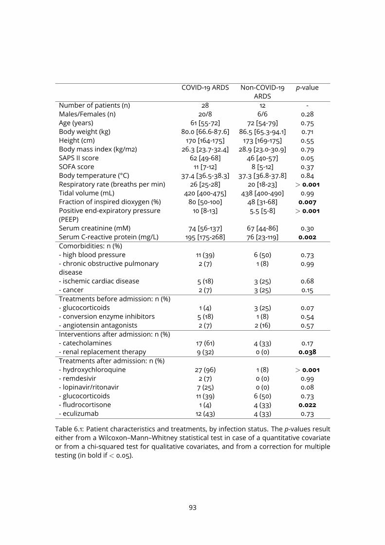
COVID-19 ARDS Non-COVID-19ARDS p-valueNumber of patients (n) 28 12 -Males/Females (n) 20/8 6/6 0.28Age (years) 61 [55-72] 72 [54-79] 0.75Body weight (kg) 80.0 [66.6-87.6] 86.5 [65.3-94.1] 0.71Height (cm) 170 [164-175] 173 [169-175] 0.55Body mass index (kg/m2) 26.3 [23.7-32.4] 28.9 [23.0-30.9] 0.79SAPS II score 62 [49-68] 46 [40-57] 0.05SOFA score 11 [7-12] 8 [5-12] 0.37Body temperature (°C) 37.4 [36.5-38.3] 37.3 [36.8-37.8] 0.84Respiratory rate (breaths per min) 26 [25-28] 20 [18-23] > 0.001Tidal volume (mL) 420 [400-475] 438 [400-490] 0.99Fraction of inspired dioxygen (%) 80 [50-100] 48 [31-68] 0.007Positive end-expiratory pressure(PEEP) 10 [8-13] 5.5 [5-8] > 0.001

Serum creatinine (mM) 74 [56-137] 67 [44-86] 0.30Serum C-reactive protein (mg/L) 195 [175-268] 76 [23-119] 0.002Comorbidities: n (%)- high blood pressure 11 (39) 6 (50) 0.73- chronic obstructive pulmonarydisease 2 (7) 1 (8) 0.99- ischemic cardiac disease 5 (18) 3 (25) 0.68- cancer 2 (7) 3 (25) 0.15Treatments before admission: n (%)- glucocorticoids 1 (4) 3 (25) 0.07- conversion enzyme inhibitors 5 (18) 1 (8) 0.54- angiotensin antagonists 2 (7) 2 (16) 0.57Interventions after admission: n (%)- catecholamines 17 (61) 4 (33) 0.17- renal replacement therapy 9 (32) 0 (0) 0.038Treatments after admission: n (%)- hydroxychloroquine 27 (96) 1 (8) > 0.001- remdesivir 2 (7) 0 (0) 0.99- lopinavir/ritonavir 7 (25) 0 (0) 0.08- glucocorticoids 11 (39) 6 (50) 0.73- fludrocortisone 1 (4) 4 (33) 0.022- eculizumab 12 (43) 4 (33) 0.73Table 6.1: Patient characteristics and treatments, by infection status. The p-values resulteither from a Wilcoxon–Mann–Whitney statistical test in case of a quantitative covariateor from a chi-squared test for qualitative covariates, and from a correction for multipletesting (in bold if < 0.05).

93

with default values (section 4.1.3), and knots where placed every 0.5 second. An overviewof the data with the ptairMS graphical interface is shown in Figure 4.8. After alignment(with a standard deviation of the kernel density set to 40 ppm; section 4.2.1) the followingsteps were applied:

• Only ions detected in more than 70% of at least one group (COVID vs. non-COVID-19ARDS) and significantly greater in the expiration phases of at least 5% of the sampleswere kept, resulting in 81 features

• Missing values were imputed with the ptairMS package (section 4.3)• Data were log2-transformed• Outliers (patients with a z-score >3 for at least five features) were discarded• Saturated ions (acetone,H3O

+,H2O−H3O+, oxygen) and isotopes were removed,

resulting in a final table of 65 features

6.3 Data analysis

In the context of biomarker discovery, we first used an untargeted metabolomic strategyto discover the signature associated with COVID-19 ARDS, using the first breath sampleavailable after the admission (section 6.3.1). We then investigated the evolution of eachVOC during the hospitalisation time, to validate the results obtained at the first day andto further analyse the difference of VOC concentration evolution between each groups(COVID +/-; section 6.3.2).

6.3.1 Classification for early diagnosis

To build a predictive model for early diagnosis of COVID-19 infection, we used the firstbreath sample collected for each patient after admission. Ten of the 40 participants hadbeen hospitalised for more than 10 days at the start of the sampling period, and werethus excluded from this first part of the study. Then two outliers where excluded (oneCOVID-19 negative admitted to the ICU for attempted suicide with medication, and theother COVID-19 positive with very saturated peaks for unknown reasons). This resulted ina subset of 28 patients (18 COVID-19 positive and 10 COVID-19 negative patients), and 65features. In such a case where the number of features exceeds the number of samples,a particular attention should be paid to the multivariate modelling and to the featureselection methods to avoid over fitting. A summary of all the methods and software toolsused in this section is provided in Table 6.2.

94

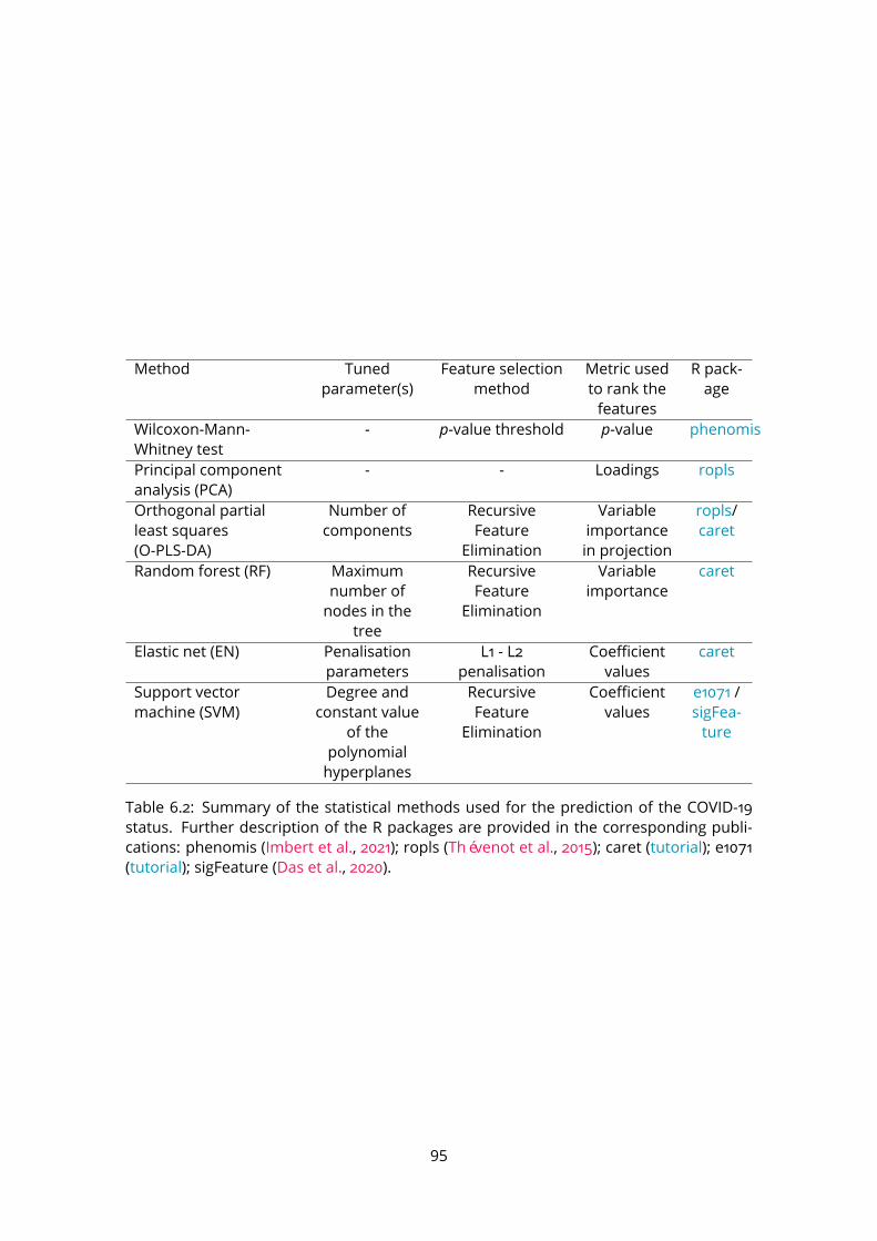
Method Tunedparameter(s) Feature selectionmethod Metric usedto rank thefeaturesR pack-age

Wilcoxon-Mann-Whitney test - p-value threshold p-value phenomisPrincipal componentanalysis (PCA) - - Loadings roplsOrthogonal partialleast squares(O-PLS-DA)

Number ofcomponents RecursiveFeatureEliminationVariableimportancein projection

ropls/caretRandom forest (RF) Maximumnumber ofnodes in thetree

RecursiveFeatureEliminationVariableimportance caret

Elastic net (EN) Penalisationparameters L1 - L2penalisation Coefficientvalues caretSupport vectormachine (SVM) Degree andconstant valueof thepolynomialhyperplanes

RecursiveFeatureEliminationCoefficientvalues e1071 /sigFea-ture

Table 6.2: Summary of the statistical methods used for the prediction of the COVID-19status. Further description of the R packages are provided in the corresponding publi-cations: phenomis (Imbert et al., 2021); ropls (Thévenot et al., 2015); caret (tutorial); e1071(tutorial); sigFeature (Das et al., 2020).

95

+

−+

+

−

+

++

−

−

+++

+

++

−

+

+

−− −−

+

−

++ +

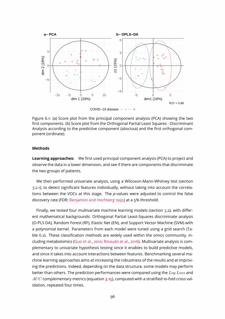
−5

0

5

−10 −5 0 5 10dim 1 (33%)

dim

2 (

18%

)

a− PCA

+

−

+

+−

+

+

+

−

−

+++

+

+

+−

+

+

−

−

−

−

+−

+

++

−6

−3

0

3

6

−5 0 5dim1 (16%)

o1 (

15%

)

R2Y = 0.88

b− OPLS−DA

COVID−19 disease − +

Figure 6.1: (a) Score plot from the principal component analysis (PCA) showing the twofirst components. (b) Score plot from the Orthogonal Partial Least Squares - DiscriminantAnalysis according to the predictive component (abscissa) and the first orthogonal com-ponent (ordinate).

Methods

Learning approaches: We first used principal component analysis (PCA) to project andobserve the data in a lower dimension, and see if there are components that discriminatethe two groups of patients.We then performed univariate analysis, using a Wilcoxon-Mann-Whitney test (section

3.2.1), to detect significant features individually, without taking into account the correla-tions between the VOCs at this stage. The p-values were adjusted to control the falsediscovery rate (FDR; Benjamini and Hochberg 1995) at a 5% threshold.Finally, we tested four multivariate machine learning models (section 3.2), with differ-

ent mathematical backgrounds: Orthogonal Partial Least-Squares discriminate analysis(O-PLS DA), Random Forest (RF), Elastic Net (EN), and Support Vector Machine (SVM) witha polynomial kernel. Parameters from each model were tuned using a grid search (Ta-ble 6.2). These classification methods are widely used within the omics community, in-cluding metabolomics (Guo et al., 2010; Rinaudo et al., 2016). Multivariate analysis is com-plementary to univariate hypothesis testing since it enables to build predictive models,and since it takes into account interactions between features. Benchmarking several ma-chine learning approaches aims at increasing the robustness of the results and at improv-ing the predictions. Indeed, depending on the data structure, some models may performbetter than others. The prediction performances were compared using the Log Loss andAUC complementary metrics (equation 3.15), computed with a stratified 10-fold cross val-idation, repeated four times.

96

Model

ElasticNet

AUC

Random Forest

SVM

OPLS

0.95

0.98

0.95

0.980.00

0.25

0.50

0.75

1.00

0.00 0.25 0.50 0.75 1.00

1 − specificity

sens

itivi

ty

ElasticNet RF SVM OPLS

ROC Curve

Figure 6.2: ROC curves from the the four complementary machine learning approaches(EN, RF, SVM, and OPLS-DA).

Model Accuracy Sensitivity Specificity AUC LogLossmeanLogLosssd

NumberoffeaturesElastic Net 0.93 0.90 0.94 0.95 7.45 0.54 22Random Forest 0.93 0.90 0.94 0.98 7.38 0.21 16SVM 0.93 0.90 0.94 0.95 7.68 0.48 22O-PLS-DA 0.93 0.90 0.94 0.98 11.77 0.10 12

Table 6.3: Comparison of model performances. The accuracy, sensitivity, specificity, AUCand Log Loss were computed using a 10-fold cross-validation, repeated 4 times (metricsdefined in the section 3.2.2). The standard deviation (sd) across the cross-validation foldsis also indicated, and provides information about the prediction variance. RF proved tobe the best performingmodel, according to the Log Loss metric, with the same AUC valueas O-PLS-DA. O-PLS-DA selected the lowest subset of features (12), which provided highaccuracy (93%), with the lowest variance of prediction (Log Loss sd of 0.1).

97

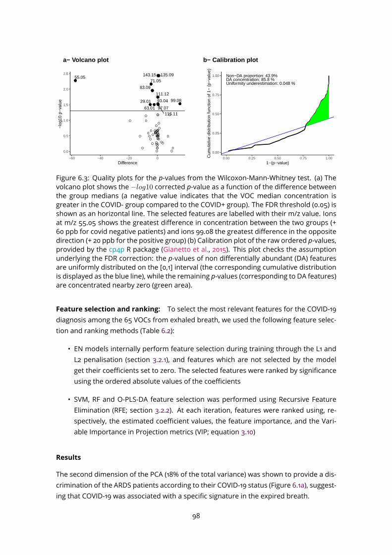
29.01

55.05

63.01

71.05

83.09

93.04

97.07

99.08

111.12

115.11

135.09143.15

0.0

0.5

1.0

1.5

2.0

2.5

−60 −40 −20 0Difference

−lo

g10

p−va

lue

a− Volcano plot

Non−DA proportion: 43.9%DA concentration: 85.8 % Uniformity underestimation: 0.048 %

0.00

0.25

0.50

0.75

1.00

0.00 0.25 0.50 0.75 1.001−(p−value)

Cum

ulat

ive

dist

ribut

ion

func

tion

of 1

− (

p−va

lue)

b− Calibration plot

Figure 6.3: Quality plots for the p-values from the Wilcoxon-Mann-Whitney test. (a) Thevolcano plot shows the −log10 corrected p-value as a function of the difference betweenthe group medians (a negative value indicates that the VOC median concentration isgreater in the COVID- group compared to the COVID+ group). The FDR threshold (0.05) isshown as an horizontal line. The selected features are labelled with their m/z value. Ionsat m/z 55.05 shows the greatest difference in concentration between the two groups (+60 ppb for covid negative patients) and ions 99.08 the greatest difference in the oppositedirection (+ 20 ppb for the positive group) (b) Calibration plot of the raw ordered p-values,provided by the cp4p R package (Gianetto et al., 2015). This plot checks the assumptionunderlying the FDR correction: the p-values of non differentially abundant (DA) featuresare uniformly distributed on the [0,1] interval (the corresponding cumulative distributionis displayed as the blue line), while the remaining p-values (corresponding to DA features)are concentrated nearby zero (green area).

Feature selection and ranking: To select the most relevant features for the COVID-19diagnosis among the 65 VOCs from exhaled breath, we used the following feature selec-tion and ranking methods (Table 6.2):

• EN models internally perform feature selection during training through the L1 andL2 penalisation (section 3.2.1), and features which are not selected by the modelget their coefficients set to zero. The selected features were ranked by significanceusing the ordered absolute values of the coefficients

• SVM, RF and O-PLS-DA feature selection was performed using Recursive FeatureElimination (RFE; section 3.2.2). At each iteration, features were ranked using, re-spectively, the estimated coefficient values, the feature importance, and the Vari-able Importance in Projection metrics (VIP; equation 3.10)

Results

The second dimension of the PCA (18% of the total variance) was shown to provide a dis-crimination of the ARDS patients according to their COVID-19 status (Figure 6.1a), suggest-ing that COVID-19 was associated with a specific signature in the expired breath.

98

OPLS

RF

SVM

EN

Wilcoxon

0

2

3

5

0

0

0

0

0

1

0

0

40

0

1

0 0

00

0

1

0

0

0

0

00

1

1

10

a− Venn diagram

0.84 0.8 0.68 0.51 0.98

0.72 0.72 0.2 0.88

0.38 0.43 0.88

0.22 0.68

0.47

Wilcoxon test

OPLS−DA

Random Forest

SVM

Elastic Net

OPLS−D

A

Rando

m F

ores

tSVM

Elastic

Net

Aggre

gate

d ra

nk

−1.0

−0.5

0.0

0.5

1.0

Spearman's rank correlation

b− Rank aggregation

Figure 6.4: Comparison of feature selection methods. (a) Venn diagram comparing thefeatures selected by eachmethod: Wilcoxon test, RF, SVM, EN andO-PLS-DA. Ten featureswere common to all selections, and 29 were selected in at least one model. (b) Matrix ofthe Spearman correlations between the ranks of the 10 common features selected byeach classifier (Table 6.2). The ranks were then aggregated by maximising the sum of theSpearman correlations with each classifier ranking (RankAggreg R package; Pihur et al.2009). RF, OPLS-DA and Wilcoxon test metrics proved to be the most correlated.

The univariate analysis (Wilcoxon-Mann-Whitney test) highlighted 12 significant VOCsat an FDR threshold of 5% (quality plots showed that the p-values were moderately wellcalibrated for the FDR correction; Figure 6.3).The use of four complementary machine learning algorithms enabled to achieve an ac-

curacy of 93% for all four classifiers, based on the selection of 22, 16, 22 and 12 featuresfor the EN, RF, SVM, and OPLS-DA, respectively (Figure 6.2 and Table 6.3). Although themodels gave quite similar performances, RF was shown to be the best performing modelaccording to the Log Loss criterion. Ten VOCs were common to all selection approaches(Figure 6.4a), and 29 were selected by at least one method. Of note, the OPLS-DA mod-elling, which is very popular in metabolomics, yielded a robust (1 orthogonal componentonly) and significant model (as assessed by permutation testing of the response labels;Szymańska et al. 2012) with good predictive performances (Q2= 0.69; Figure 6.1b).Finally, the ranks of the 10 features selected by the five methods were aggregated ac-

cording to their rankings by the specific metrics (Table 6.2), by maximising the sum of theSpearman correlations with each of the model rankings (RankAggreg R package; Pihuret al. 2009). The correlation matrix is shown in Figure 6.4b, and the putative VOC annota-tions provided by ptairMS are shown in Table 6.4.

99

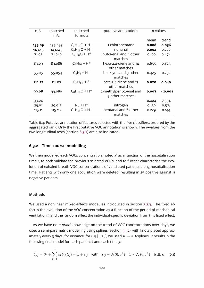
m/z matchedm/z matchedformula putative annotations p-valuesmean trend

135.09 135.093 C7H15Cl + H+ 1-chloroheptane 0.008 0.036143.15 143.143 C9H18O + H+ nonanal 0.002 0.20071.05 71.049 C4H6O + H+ but-2-enal and 4 othermatches 0.100 0.47483.09 83.086 C6H10 + H+ hexa-2,4-diene and 14other matches 0.655 0.82555.05 55.054 C4H6 + H+ but-1-yne and 3 othermatches 0.425 0.232111.12 111.117 C8H14+H+ octa-2,4-diene and 17other matches 0.020 0.040

99.08 99.080 C6H10O + H+ 2-methylpent-2-enal and9 other matches 0.007 <0.001

93.04 - - - 0.404 0.33429.01 29.013 N2 + H+ nitrogen 0.139 0.518115.11 115.112 C7H14O + H+ heptanal and 6 othermatches 0.229 0.144

Table 6.4: Putative annotation of features selected with the five classifiers, ordered by theaggregated rank. Only the first putative VOC annotation is shown. The p-values from thetwo longitudinal tests (section 6.3.2) are also indicated.

6.3.2 Time course modelling

We then modelled each VOCs concentration, noted Y as a function of the hospitalisationtime t, to both validate the previous selected VOCs, and to further characterise the evo-lution of exhaled breath VOC concentrations of ventilated patients along hospitalisationtime. Patients with only one acquisition were deleted, resulting in 25 positive against 11negative patients.

Methods

We used a nonlinear mixed-effects model, as introduced in section 3.2.3. The fixed ef-fect is the evolution of the VOC concentration as a function of the period of mechanicalventilation t, and the random effect the individual-specific deviation from this fixed effect.As we have no a priori knowledge on the trend of VOC concentrations over days, we

used a semi-parametric modelling using splines (section 3.1.2), with knots placed approx-imately every 3 days: for instance, for t ∈ [1, 10], we usedK = 4 B-splines. It results in thefollowing final model for each patient i and each time j:

Yij = β0 +K∑k=1

βkbk(tij) + bi + ϵij with ϵij ∼ N (0, σ2) bi ∼ N (0, τ2) b ⊥⊥ ϵ (6.1)

100

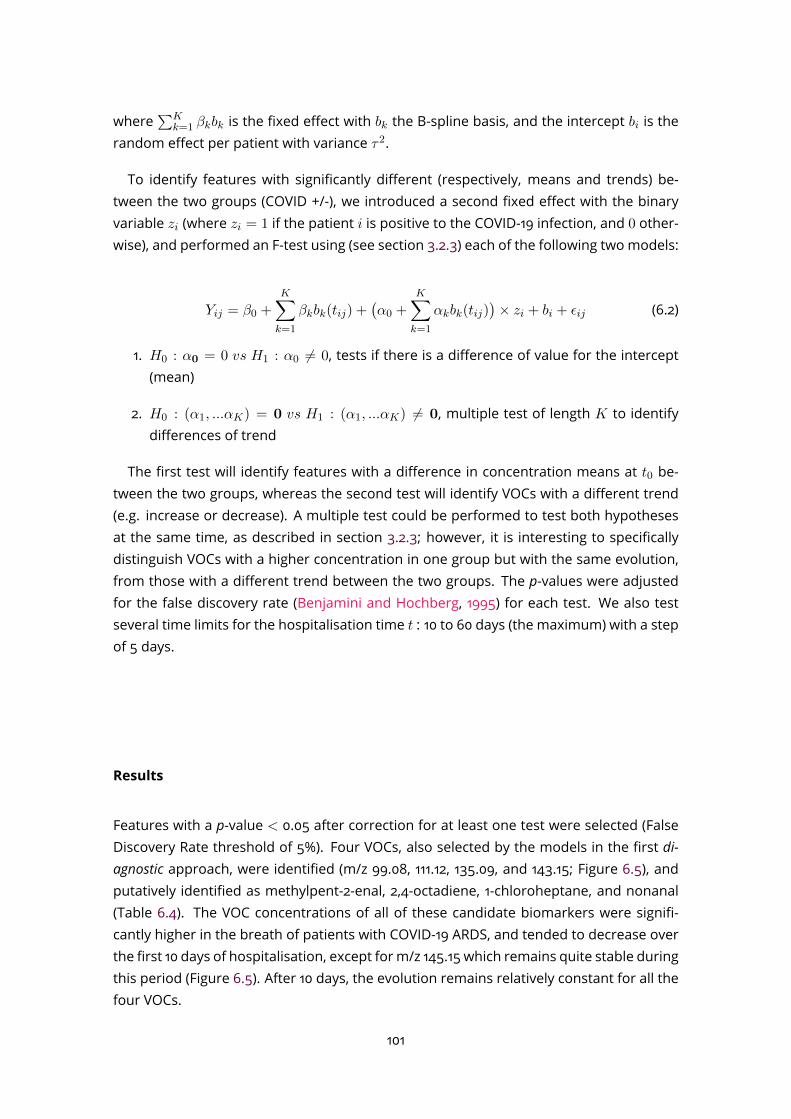
where ∑Kk=1 βkbk is the fixed effect with bk the B-spline basis, and the intercept bi is the

random effect per patient with variance τ2.To identify features with significantly different (respectively, means and trends) be-

tween the two groups (COVID +/-), we introduced a second fixed effect with the binaryvariable zi (where zi = 1 if the patient i is positive to the COVID-19 infection, and 0 other-wise), and performed an F-test using (see section 3.2.3) each of the following two models:

Yij = β0 +K∑k=1

βkbk(tij) +(α0 +

K∑k=1

αkbk(tij))× zi + bi + ϵij (6.2)

1. H0 : α0 = 0 vs H1 : α0 = 0, tests if there is a difference of value for the intercept(mean)

2. H0 : (α1, ...αK) = 0 vs H1 : (α1, ...αK) = 0, multiple test of length K to identifydifferences of trend

The first test will identify features with a difference in concentration means at t0 be-tween the two groups, whereas the second test will identify VOCs with a different trend(e.g. increase or decrease). A multiple test could be performed to test both hypothesesat the same time, as described in section 3.2.3; however, it is interesting to specificallydistinguish VOCs with a higher concentration in one group but with the same evolution,from those with a different trend between the two groups. The p-values were adjustedfor the false discovery rate (Benjamini and Hochberg, 1995) for each test. We also testseveral time limits for the hospitalisation time t : 10 to 60 days (the maximum) with a stepof 5 days.

Results

Features with a p-value < 0.05 after correction for at least one test were selected (FalseDiscovery Rate threshold of 5%). Four VOCs, also selected by the models in the first di-agnostic approach, were identified (m/z 99.08, 111.12, 135.09, and 143.15; Figure 6.5), andputatively identified as methylpent-2-enal, 2,4-octadiene, 1-chloroheptane, and nonanal(Table 6.4). The VOC concentrations of all of these candidate biomarkers were signifi-cantly higher in the breath of patients with COVID-19 ARDS, and tended to decrease overthe first 10 days of hospitalisation, except form/z 145.15 which remains quite stable duringthis period (Figure 6.5). After 10 days, the evolution remains relatively constant for all thefour VOCs.

101

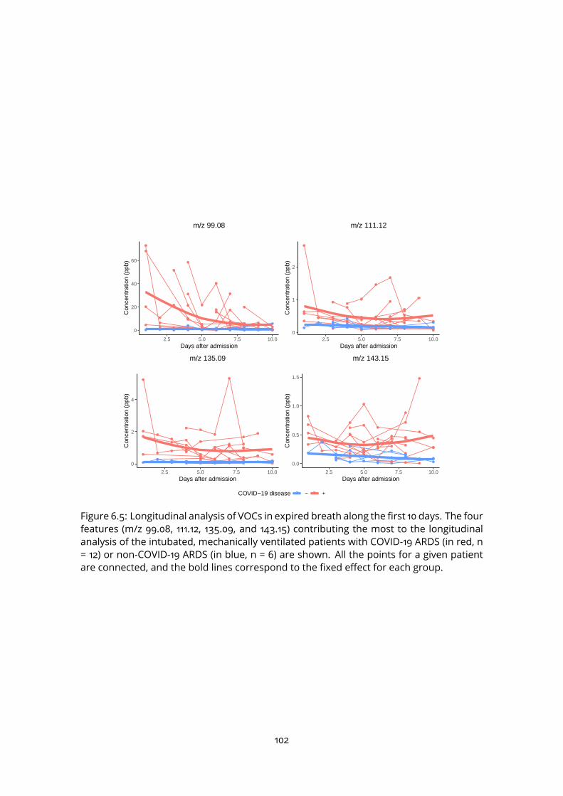
0

20

40

60

2.5 5.0 7.5 10.0Days after admission

Con

cent

ratio

n (p

pb)

m/z 99.08

0

1

2

2.5 5.0 7.5 10.0Days after admission

Con

cent

ratio

n (p

pb)

m/z 111.12

0

2

4

2.5 5.0 7.5 10.0Days after admission

Con

cent

ratio

n (p

pb)

m/z 135.09

0.0

0.5

1.0

1.5

2.5 5.0 7.5 10.0Days after admission

Con

cent

ratio

n (p

pb)

m/z 143.15

COVID−19 disease − +

Figure 6.5: Longitudinal analysis of VOCs in expired breath along the first 10 days. The fourfeatures (m/z 99.08, 111.12, 135.09, and 143.15) contributing the most to the longitudinalanalysis of the intubated, mechanically ventilated patients with COVID-19 ARDS (in red, n= 12) or non-COVID-19 ARDS (in blue, n = 6) are shown. All the points for a given patientare connected, and the bold lines correspond to the fixed effect for each group.

102

+

−+

+−

++

−

−

++ ++

+ +

−

+

+

−−−

−

+

−

++ +

−10

−5

0

5

10

−10 −5 0 5 10dim 1 (32%)

dim

2 (

20%

)

400

450

500

550

600

p−value: dim 1 = 0.38, dim 2 = 0.27, dim 3 = 0.29

Tidal volume

+

−+

+−

++

−

−

++ ++

+ +

−

+

+

−−−

−

+

−

++ +

−10

−5

0

5

10

−10 −5 0 5 10dim 1 (32%)

dim

2 (

20%

)

100

200

300

400

500

p−value: dim 1 = 0.45, dim 2 = 0.33, dim 3 = 0.47

CRP

+

−+

+−

++

−

−

++ ++

+ +

−

+

+

−−−

−

+

−

++ +

−10

−5

0

5

10

−10 −5 0 5 10dim 1 (32%)

dim

2 (

20%

)

35

36

37

38

p−value: dim 1 = 0.52, dim 2 = 0.40, dim 3 = 0.22

Body temperature

+

−+

+−

++

−

−

++ ++

+ +

−

+

+

−−−

−

+

−

++ +

−10

−5

0

5

10

−10 −5 0 5 10dim 1 (32%)

dim

2 (

20%

)

0.0

2.5

5.0

7.5

10.0

p−value: dim 1 = 0.16, dim 2 = 0.87, dim 3 = 0.64

Number of day in ICU

Figure 6.6: Analysis of potential relationships between clinical covariates and the COVID-19 status. The results for four covariates, namely the tidal volume, the serum C-reactiveprotein level (CRP), the body temperature, and the number of days in the ICU, are shownas a score plot from the principal component analysis, coloured according to the covariatevalues. The p-values from the Pearson test of the correlation between the covariate andthe three principal components is shown at the top of each plot. +: positive COVID-19status; -: negative COVID-19 status.

103

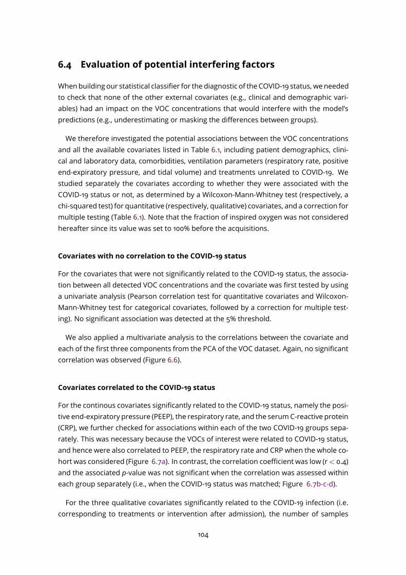
6.4 Evaluation of potential interfering factors

Whenbuilding our statistical classifier for the diagnostic of theCOVID-19 status, weneededto check that none of the other external covariates (e.g., clinical and demographic vari-ables) had an impact on the VOC concentrations that would interfere with the model’spredictions (e.g., underestimating or masking the differences between groups).We therefore investigated the potential associations between the VOC concentrations

and all the available covariates listed in Table 6.1, including patient demographics, clini-cal and laboratory data, comorbidities, ventilation parameters (respiratory rate, positiveend-expiratory pressure, and tidal volume) and treatments unrelated to COVID-19. Westudied separately the covariates according to whether they were associated with theCOVID-19 status or not, as determined by a Wilcoxon-Mann-Whitney test (respectively, achi-squared test) for quantitative (respectively, qualitative) covariates, and a correction formultiple testing (Table 6.1). Note that the fraction of inspired oxygen was not consideredhereafter since its value was set to 100% before the acquisitions.

Covariates with no correlation to the COVID-19 status

For the covariates that were not significantly related to the COVID-19 status, the associa-tion between all detected VOC concentrations and the covariate was first tested by usinga univariate analysis (Pearson correlation test for quantitative covariates and Wilcoxon-Mann-Whitney test for categorical covariates, followed by a correction for multiple test-ing). No significant association was detected at the 5% threshold.We also applied a multivariate analysis to the correlations between the covariate and

each of the first three components from the PCA of the VOC dataset. Again, no significantcorrelation was observed (Figure 6.6).

Covariates correlated to the COVID-19 status

For the continous covariates significantly related to the COVID-19 status, namely the posi-tive end-expiratory pressure (PEEP), the respiratory rate, and the serumC-reactive protein(CRP), we further checked for associations within each of the two COVID-19 groups sepa-rately. This was necessary because the VOCs of interest were related to COVID-19 status,and hence were also correlated to PEEP, the respiratory rate and CRP when the whole co-hort was considered (Figure 6.7a). In contrast, the correlation coefficient was low (r< 0.4)and the associated p-value was not significant when the correlation was assessed withineach group separately (i.e., when the COVID-19 status was matched; Figure 6.7b-c-d).For the three qualitative covariates significantly related to the COVID-19 infection (i.e.

corresponding to treatments or intervention after admission), the number of samples104

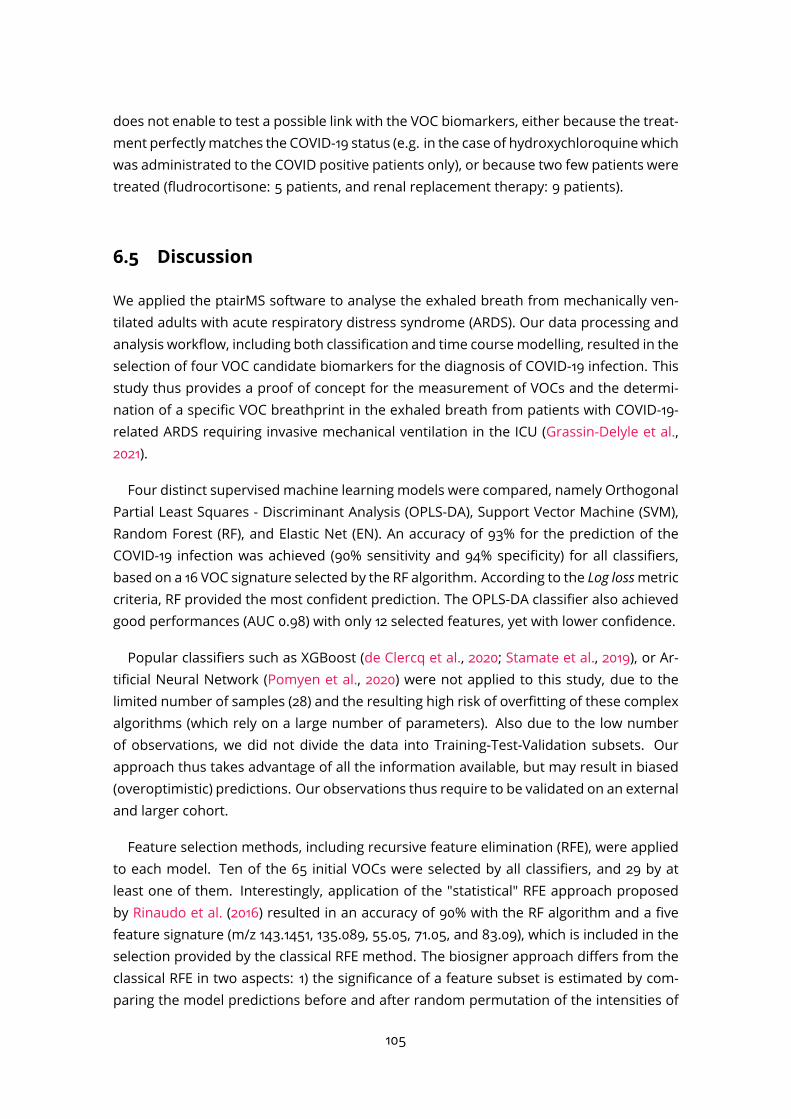
does not enable to test a possible link with the VOC biomarkers, either because the treat-ment perfectlymatches the COVID-19 status (e.g. in the case of hydroxychloroquinewhichwas administrated to the COVID positive patients only), or because two few patients weretreated (fludrocortisone: 5 patients, and renal replacement therapy: 9 patients).

6.5 Discussion

We applied the ptairMS software to analyse the exhaled breath from mechanically ven-tilated adults with acute respiratory distress syndrome (ARDS). Our data processing andanalysis workflow, including both classification and time coursemodelling, resulted in theselection of four VOC candidate biomarkers for the diagnosis of COVID-19 infection. Thisstudy thus provides a proof of concept for the measurement of VOCs and the determi-nation of a specific VOC breathprint in the exhaled breath from patients with COVID-19-related ARDS requiring invasive mechanical ventilation in the ICU (Grassin-Delyle et al.,2021).Four distinct supervised machine learning models were compared, namely Orthogonal

Partial Least Squares - Discriminant Analysis (OPLS-DA), Support Vector Machine (SVM),Random Forest (RF), and Elastic Net (EN). An accuracy of 93% for the prediction of theCOVID-19 infection was achieved (90% sensitivity and 94% specificity) for all classifiers,based on a 16 VOC signature selected by the RF algorithm. According to the Log lossmetriccriteria, RF provided the most confident prediction. The OPLS-DA classifier also achievedgood performances (AUC 0.98) with only 12 selected features, yet with lower confidence.Popular classifiers such as XGBoost (de Clercq et al., 2020; Stamate et al., 2019), or Ar-

tificial Neural Network (Pomyen et al., 2020) were not applied to this study, due to thelimited number of samples (28) and the resulting high risk of overfitting of these complexalgorithms (which rely on a large number of parameters). Also due to the low numberof observations, we did not divide the data into Training-Test-Validation subsets. Ourapproach thus takes advantage of all the information available, but may result in biased(overoptimistic) predictions. Our observations thus require to be validated on an externaland larger cohort.Feature selection methods, including recursive feature elimination (RFE), were applied

to each model. Ten of the 65 initial VOCs were selected by all classifiers, and 29 by atleast one of them. Interestingly, application of the "statistical" RFE approach proposedby Rinaudo et al. (2016) resulted in an accuracy of 90% with the RF algorithm and a fivefeature signature (m/z 143.1451, 135.089, 55.05, 71.05, and 83.09), which is included in theselection provided by the classical RFE method. The biosigner approach differs from theclassical RFE in two aspects: 1) the significance of a feature subset is estimated by com-paring the model predictions before and after random permutation of the intensities of

105

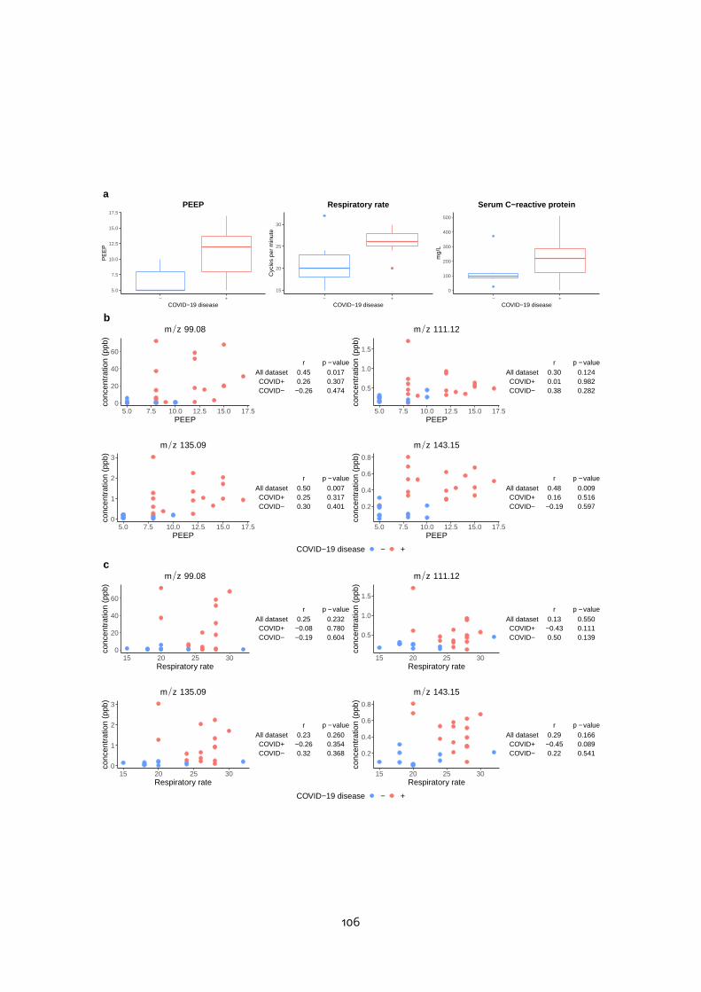
5.0

7.5

10.0

12.5

15.0

17.5

− +COVID−19 disease

PE

EP

PEEPa

15

20

25

30

− +COVID−19 disease

Cyc

les

per

min

ute

Respiratory rate

0

100

200

300

400

500

− +COVID−19 disease

mg/

L

Serum C−reactive protein

0

20

40

60

5.0 7.5 10.0 12.5 15.0 17.5PEEP

conc

entr

atio

n (p

pb)

m z 99.08b

All datasetCOVID+COVID−

0.450.26

−0.26

0.0170.3070.474

r p − value

0.5

1.0

1.5

5.0 7.5 10.0 12.5 15.0 17.5PEEP

conc

entr

atio

n (p

pb)

m z 111.12

All datasetCOVID+COVID−

0.300.010.38

0.1240.9820.282

r p − value

0

1

2

3

5.0 7.5 10.0 12.5 15.0 17.5PEEP

conc

entr

atio

n (p

pb)

m z 135.09

All datasetCOVID+COVID−

0.500.250.30

0.0070.3170.401

r p − value

0.2

0.4

0.6

0.8

5.0 7.5 10.0 12.5 15.0 17.5PEEP

conc

entr

atio

n (p

pb)

m z 143.15

All datasetCOVID+COVID−

0.480.16

−0.19

0.0090.5160.597

r p − value

COVID−19 disease − +

0

20

40

60

15 20 25 30Respiratory rate

conc

entr

atio

n (p

pb)

m z 99.08c

All datasetCOVID+COVID−

0.25−0.08−0.19

0.2320.7800.604

r p − value

0.5

1.0

1.5

15 20 25 30Respiratory rate

conc

entr

atio

n (p

pb)

m z 111.12

All datasetCOVID+COVID−

0.13−0.430.50

0.5500.1110.139

r p − value

0

1

2

3

15 20 25 30Respiratory rate

conc

entr

atio

n (p

pb)

m z 135.09

All datasetCOVID+COVID−

0.23−0.260.32

0.2600.3540.368

r p − value

0.2

0.4

0.6

0.8

15 20 25 30Respiratory rate

conc

entr

atio

n (p

pb)

m z 143.15

All datasetCOVID+COVID−

0.29−0.450.22

0.1660.0890.541

r p − value

COVID−19 disease − +

106

0

20

40

60

0 100 200 300 400 500Serum C−reactive protein

conc

entr

atio

n (p

pb)

m z 99.08d

All dataset

COVID+

COVID−

0.25

−0.08

−0.19

0.232

0.780

0.604

r p − value

0.5

1.0

1.5

0 100 200 300 400 500Serum C−reactive protein

conc

entr

atio

n (p

pb)

m z 111.12

All dataset

COVID+

COVID−

0.13

−0.43

0.50

0.550

0.111

0.139

r p − value

0

1

2

3

0 100 200 300 400 500Serum C−reactive protein

conc

entr

atio

n (p

pb)

m z 135.09

All dataset

COVID+

COVID−

0.23

−0.26

0.32

0.260

0.354

0.368

r p − value

0.2

0.4

0.6

0.8

0 100 200 300 400 500Serum C−reactive protein

conc

entr

atio

n (p

pb)

m z 143.15

All dataset

COVID+

COVID−

0.29

−0.45

0.22

0.166

0.089

0.541

r p − value

COVID−19 disease − +

Figure 6.7: Study of the impact of the positive end-expiratory pressure (PEEP), the respira-tory rate, and the serum C-reactive protein (CRP), on the relationship between each of thefour VOC biomarkers and the COVID-19 status. a. PEEP, respiratory rate, and CRP valuesaccording to the COVID-19 status. b-d. VOC concentrations as a function of PEEP (b), therespiratory rate (c), and CRP (d). The Pearson correlation coefficients (r) and the p-valuesfrom the correlation tests (either computed on the whole dataset or for each COVID-19subset separately) are indicated.

these features in test subsets generated by resampling, and 2) the whole feature selec-tion procedure is repeated recursively until all features of the selected subset are foundsignificant, or until there is no feature left to be tested (Rinaudo et al., 2016). Its applicationto the COVID-19 study highlighted very short signatures which still provide high predictionperformances.A time course analysis, using mixed effect models across the hospitalisation time and

a Fisher test, was also used. It confirmed that four of the selected features had a signifi-cantly different behaviour between the two groups (m/z 99.08, 111.12, 135.09, and 143.15),with a significantly higher concentration in the breath of patients with COVID-19 infection,and a tendency to decrease over the first 10 days of hospitalisation. The fact that somefeatures were selected only by the classification approach at t0 but not by the longitudinalanalysis may be explained by the fact that these features are only observed at the begin-ning of the infection. Interestingly, themajority of these VOCs have higher concentrationsin the breath of COVID-19 negative patients (m/z 71.05, 83.09, 55.05 and 29.01), in contrastto the four biomarkers confirmed by the longitudinal analysis.The time course methodology used may be easily extended to more than two classes

(e.g. in the case of multiple levels of infection severity), by transforming the categoricalresponse z with Q levels in (Q− 1) binary (dummy) variables : zq = 1 for the presence of

107

the category q. Then, the variables are include in the mixed effect model :

Yij = fβ(tij)︸ ︷︷ ︸effect of the first class+

Q∑q=2

fαq(tij)× zqi︸ ︷︷ ︸shift for each other class q+bi + ϵij

with ϵij ∼ N (0, σ2), bi ∼ N (0, τ2), b ⊥⊥ ϵ, for patient i and time point j. Then to test ifthere is at least one category that differ from the first, we performmultiple Fisher tests ofdimension (q − 1) for intercept test, and (q − 1)× (number of parameters of the functionf ) for trend test (e.g number of knots) on multiplying coefficients α : H0 : (α2...αQ) =

0 vs H1 : (α2...αQ) = 0.

We investigated potential interfering factors (i.e. covariates with significant median dif-ferences between the COVID-19 and non-COVID-19 subgroups). In particular, COVID-19infected patients had a higher respiratory rate, fraction of inspired oxygen (FiO2), PEEP,and CRP values on admission. The respiratory rate, PEEP and CRP, however, were notfound to interfere with the VOC predictive signature. Furthermore, FiO2 was set to 100%during all acquisitions to avoid any impact of dioxygen variations on PTR ionisation (Trefzet al., 2019a). The hydroxychloroquine treatment may also be a potential confounder,since it was administrated specifically to the patients with COVID-19 ARDS. However, nocorrespondence was observed between the VOCs described in the present study and themolecular masses of the known metabolites of hydroxychloroquine. In addition, the ob-served concentrations of the VOC biomarkers decreased with time, whereas the hydrox-ychloroquine dosage was constant during hospitalisation.In line with a previous report on ARDS analysis by GC-MS (Bos et al., 2014b), the VOC

concentrations described in our study were not correlated with the severity of illness (asjudged by the SAPS II and the SOFA scores). This finding suggests that the exhaled breathsignature is a marker of COVID-19 per se, rather than a marker of the severity of illness.Likewise, the VOC concentrationswere not correlatedwith the viral load (as independentlydetermined by Polymerase Chain Reaction, PCR), suggesting that this signature may be amarker of the disease related to SARS-CoV-2 rather than of the virus carriage.Two of the four prominent VOCs (with putative annotation: methylpent-2-enal and

nonanal) are aldehydes, while 2,4-octadiene is an alkadiene. These three compounds areknown to be expressed in breath (van de Kant et al., 2013; Corradi et al., 2004). Nonanalis a sub-product of the destruction of the cell membrane as a result of oxidative stress;reactive oxygen speciesmay be generated by various types of inflammatory, immune andstructural cell in the airways (Rahman, 2003).A critical issue in breath analysis is the standardisation, to make results from indepen-

dent studies comparable (Miekisch et al., 2012; Herbig and Beauchamp, 2014; Bruderer

108

et al., 2019; Henderson et al., 2020). Indeed, breath composition is influenced not only byambient inhaled air, but also by many external factors, as shown in several studies of theRostock Medical Breath Research Analytics and Technologies (ROMBAT) team: the bodyposition (Sukul et al., 2015), exhalation strength (Sukul et al., 2016), upper-airway restric-tions (Sukul et al., 2017), menstrual cycles (Sukul et al., 2018), medication, specific dietary,or even sampling procedures (e.g. the use of Tedlar bags; Miekisch et al. 2008). Impor-tantly, a particular attention should be paid during the design of the study to thematchingof patients and sampling conditions between the groups of interest. Finally, a validationstudy using similar samplingmethods and processing parameters is of critical importancefor the clinical use of the candidate biomarkers.Since the end of 2020, other studies were performed for the early diagnosis of COVID-19

infection fromexhaled breath onnonARDSpatients, with differentMSmethods, includingGC coupled to ionmobility (GC-IMS; 98 patients, sensitivity and specificity: 82.4% and 75%;Ruszkiewicz et al. 2020), PTR-TOF-MS (340 patients, accuracy: 81.2%; Liangou et al. 2021),GC-MS (81 patients, sensitivity and specificity: 68% and 85%; Ibrahim et al. 2021); GCxGC-TOF-MS on exhaled breath condensate (EBC; 37 patients, AUC=0.98, accuracy: 100%; Bar-beris et al. 2021). The VOCs selected by these studies differ from our 4 biomarkers, whichmay be explained by the fact that the progression of the physiologic response of nonARDS patients is different compared to severely ill and mechanically ventilated patients.The differences between the resultsmay also result fromdistinct sampling procedures, orspecific ionisation selectivity and sensitivity from the MS instruments. Altogether, thesecandidates provide a broader picture of the COVID-19 physio-pathology, and the resultsfrom these studies highlight the potential of exhaled breath for early and non invasivediagnosis.

109

110

Part III

Conclusion and perspectives

111

Conclusion

In this thesis, we have developed innovative tools and methods for biomarker discoveryin exhaled breath by means of Proton Transfer Reaction Time-of-Flight Mass Spectrom-etry (PTR-TOF-MS), from the raw data processing up to the statistical analysis for clinicalapplications.We have developed the first freely available workflow for the PTR-TOF-MS data pre-

processing from exhaled breath (Chapter 4), starting from the raw data files, and provid-ing as output the sample by variable table of intensities. Compared to existing software,it provides new features for the monitoring of cohorts from exhaled breath. Especially,an innovative 2D model based on P-splines regression enables a precise estimation ofthe peak evolution over the acquisition time. The comparison on simulated data showedthat the developed methods clearly improve the classification of the VOC origin (exhaledbreath or ambient air), which is of critical interest for biomarker discovery. The developedworkflow has been implemented in the R package ptairMS, which is publicly availableon the Bioconductor platform, and includes a detailed tutorial and a graphical interface,which makes it easy for clinicians to use. Our software is already used in routine at theExhalomics platform located within the pneumology department from the Hôpital Foch(Suresnes, France), to process the acquisitions from breathing patients. Several clinicalstudies are currently underway, mainly in pneumology, infectious diseases and oncology.Our methodology then allowed the longitudinal analysis of intubated, mechanically

ventilated patients in record time (less than 6 months between the inclusion of the firstpatient and the submission of the manuscript), and enabled to discover a biomarker sig-nature of four VOCs for the diagnosis of COVID-19 infection (Chapter 6; Grassin-Delyleet al. 2021). The currently most usedmethod for the diagnosis of COVID-19 is nasopharyn-geal swab collection followed by reverse transcriptase-polymerase chain reaction analysis(RT-PCR): this approach is invasive, requires instrumentation in laboratories, and has veryhigh specificity but moderate sensitivity (Zitek, 2020). Diagnosis with exhaled breath anal-ysis is thereby of major interest for high-throughput population testing, since it is totallynon-invasive, painless, and gives the diagnosis in real-time. The design and commerciali-sation of a breath test for COVID-19 infection is currently a very competitive field aroundthe world. Our VOCs signature is therefore the subject of a European patent, and a vali-dation on a larger and independent cohort is in progress.

Our work therefore provides the scientific community with the computational methodsand tools to conduct clinical studies on exhaled breath through the PTR-TOF-MS technol-ogy. It paves the way for new rapid and non-invasive tests at the patient bedside fordiagnostic purposes, monitoring of treatment response, or high-throughput populationscreening.

112

Perspectives

Bayesian deconvolution

Our proposed method for 2D peak deconvolution involves sequential steps, starting withthe detection of peaks in the mass dimension and followed by the building of the 2Dmodel. This is therefore an approximation since we perform the peak detection in a singledimension once all mass spectra have been summed. Bayesian deconvolution methodsmay therefore be a valuable alternative, since they include i) combined estimation of peaklocations and intensities, ii) denoising, and iii) baseline removal in 2D. In particular, non-parametric Bayesian approaches allow to separate the baseline component from the setof peaks, without using a parametricmodel for the baseline, and to deconvolute the peakswithout imposing a total number of peaks a priori.The Bayesian approach considers each of the unknown quantities that we want to esti-

mate as random variables, with a prior probability law. These quantities are then updatedfrom the observations, through the Bayes’ rule (Gelman et al., 2004). This approach hasthe advantage to provide knowledge of uncertainties and credibles intervals. In our case,the model for peak detection would thus be written as:

(xi, yi)|(P,B,wi) ∼ wiP + (1− wi)B

with (xi, yi) the observed spectrum in 2D (i.e. m/z and time dimensions), P the mixtureof peaks, B the baseline, and wi the probability of belonging to peak or baseline. Theposterior law y|(P,B,w) would then estimated by Markov Chain Monte Carlo methods(Grenn, 1995).Barat et al. (2007a,b) proposed non parametric prior laws for P and B, respectively

the Dirichlet Process Mixture (DPM; Antoniak 1974) and 2D Polya Trees (PT; Mauldin et al.1992), and aBeta distribution forw. Their SINBADalgorithmshows great performances forpeak location and quantification on gamma-ray spectra, especially for highly convolutedpeaks (Rohée et al., 2015; Rohée et al., 2016). Applying such an approach to PTR-TOF-MSdata would require new developments to adapt the priors and to ensure that the MCMCframework converges rapidly.

Deep learning

Deep Learning (DL) has become one of the most active fields in artificial intelligence, withhigh performances in a broad area of applications, especially for image classification usingConvolutional Neural Networks (CNN; Rawat and Wang 2017).Applying DL to the 2DMS data considered as images, is therefore appealing: this would

eliminate the need for feature-engineering (peak detection and deconvolution). DLmeth-113

ods have already be applied to Imaging Mass Spectrometry (IMS; Behrmann et al. 2017)and tandemmass spectrometry (Data Independent Analysis; Tran et al. 2019; Cadow et al.2021. In case of PTR-TOF-MS data, a pixel would correspond to the count of ions withinan m/z bin and a time acquisition period. Since the duration of acquisition is differentbetween patients, the images would have to be resized (Siu and Hung, 2012).DL offers a fast and accurate prediction, having a more global view of the data than

classical feature extraction methods. However, it presents two main limitations: the lim-ited amount of labelled data for training and the lack of interpretability (e.g the m/z valueof the discriminant metabolites). To overcome the former issue, Cadow et al. (2021) useda collection of publicly available DL models already trained for the task of natural im-age classification. To address the interpretability of DL models, Behrmann et al. (2017)proposed a strategy to interpret the learned model in the spectral domain, based on asensitivity analysis between the predicted class probabilities and each spectrum input.Nevertheless, interpretability remains an open challenge for clinical applications (Chinget al., 2018).Instead of using DL on the whole raw data for direct prediction, the learning may be

restricted to the pre-processing workflow. Kantz et al. (2019) decreased the number offalse positive peak detection by 90% by training CNNmodels on manually labelled LC-MSraw data subsets around detected peaks in the m/z and RT dimensions. In the contextof exhaled breath analysis, one could think to learn the VOC origin (exhaled breath orexternal contamination) by training DLmodels on the raw data bands obtained after peakdetection in the mass dimension (instead of relying on statistical tests to discriminatebetween exhaled and ambient phases).

Varying-coefficient models using P-splines

P-splines were used in both parts of this thesis, as they are particularly interesting flex-ible tools for nonlinear smooth modelling without any parametric assumption. In thepre-processing part, P-splines were used with a tensor product for 2D signal regressionto model the evolution of peaks during the acquisition time. In the longitudinal analysispart, they were used within a mixed-effect modelling of the evolution of VOC concentra-tions during hospitalisation time for each patient. In the latter case, however, we only per-formed univariate time course modelling analysis. An alternative multivariate approach,to take into account the interactions between the VOCs, is provided by varying coefficientregression.Varying-coefficientmodels (VCM;Hastie and Tibshirani 1993) are predictivemodelswhere

coefficients are allowed to change smoothly with the value of other variables, called "ef-fect modifiers" (e.g. time, age). Let us denote tij the time-points at which the measure-ments for the ith patient were recorded, yij the response, and Xij = (x1ij , ...x

pij) the p

114

predictor values. In the case of a generalised linear model, the model is written as follow(Hoover et al., 1998):

g(yij) = XTijβ(tij) + ϵ(tij)

where g is a link function (e.g. logit for binary variable or identity for regression), β(t) =(β1(t), ..., βp(t)) are smooth functions, and ϵ(t) is a zero-mean stochastic process. Theβ(t) smooth functions would then be estimated with P-splines: β(t) =

∑Kk=1 γkbk(t),where (b1(t), ..., bK(t)) are B-splines function, and a difference penalisation is applied to

the optimisation least squares problem, according to the P-spline theory (Marx, 2010; Liand Zhang, 2010). This model has been used in several applications including economics,spatialmodelling and epidemiology, and has been generalised to the Bayesian framework(Franco-Villoria et al., 2019; Heuclin et al., 2021).

Electronic noses

The Exhalomics platform is also equipped with several electronic noses (eNose; Gardnerand Bartlett (1994); Devillier et al. (2017)). eNose technologies have already been applied toclinical applications (Di Natale et al., 2014; Farraia et al., 2019). It is a portable and low costtechnology, using an array of sensors that are relatively selective for different families ofVOCs, and is compatible with online acquisitions (Bruderer et al., 2019). PTR-TOF-MS andeNoses are therefore two complementary technologies which are evaluated in parallel foreach patient at the Hôpital Foch. In particular, coupling eNose with PTR-TOF-MS may beuseful to support the development of optimised sensors, as recently explored by otherteams for malaria transmissible stage prediction (Capuano et al., 2019).

VOCs identification with GCxGC MS

We have shown that the PTR-TOF-MS instrument is a method of choice for biomarker dis-covery, due to its fast response time, its high sensitivity (limits of detection in the pptvrange), and since it can be operated readily at the point of care. However, this approachonly provides information on the mass/charge ratio of the compound, which is limitingfor the structural identification of themetabolite (and hence for the characterisation of itsbiological role). Additional MS technologies offering higher mass resolution, chromato-graphic separation, and fragmentation, are thus required for metabolite identification.The Exhalomics platform recently acquired a two-dimensional gas chromatography TOFmass spectrometer (GCxGC-TOF-MS; Liu and Phillips 1991; Phillips et al. 2013), a power-ful tool for multidimensional analysis of complex samples with the potential to identify agreater number of VOCs.Comprehensive two-dimensional GC (GCxGC) extends the chromatographic separation

115

by pairing two columns with complementary stationary phases. Therefore, compoundsthat would co-elute in conventional GC may be separated by the GCxGC system. Theresulting data contain three dimensions: two retention times (one from each chromato-graphic separation) and amass spectrum that is relatively unique to each compound. Veryfew open source tools for the pre-processing of such data already exist (Ramaker et al.,2017; Quiroz-Moreno et al., 2020; Wilde et al., 2020), and focus on baseline correction,denoising, peak alignment using correlation optimised warping with a reference chro-matogram (Zhang et al., 2008), and identification by matching mass spectral signatures toa library of mass spectra. Peak detection and deconvolution in 2D, however, remain to bedeveloped, and will benefit from the rich datasets currently analysed on the Exhalomicsplatform.

116

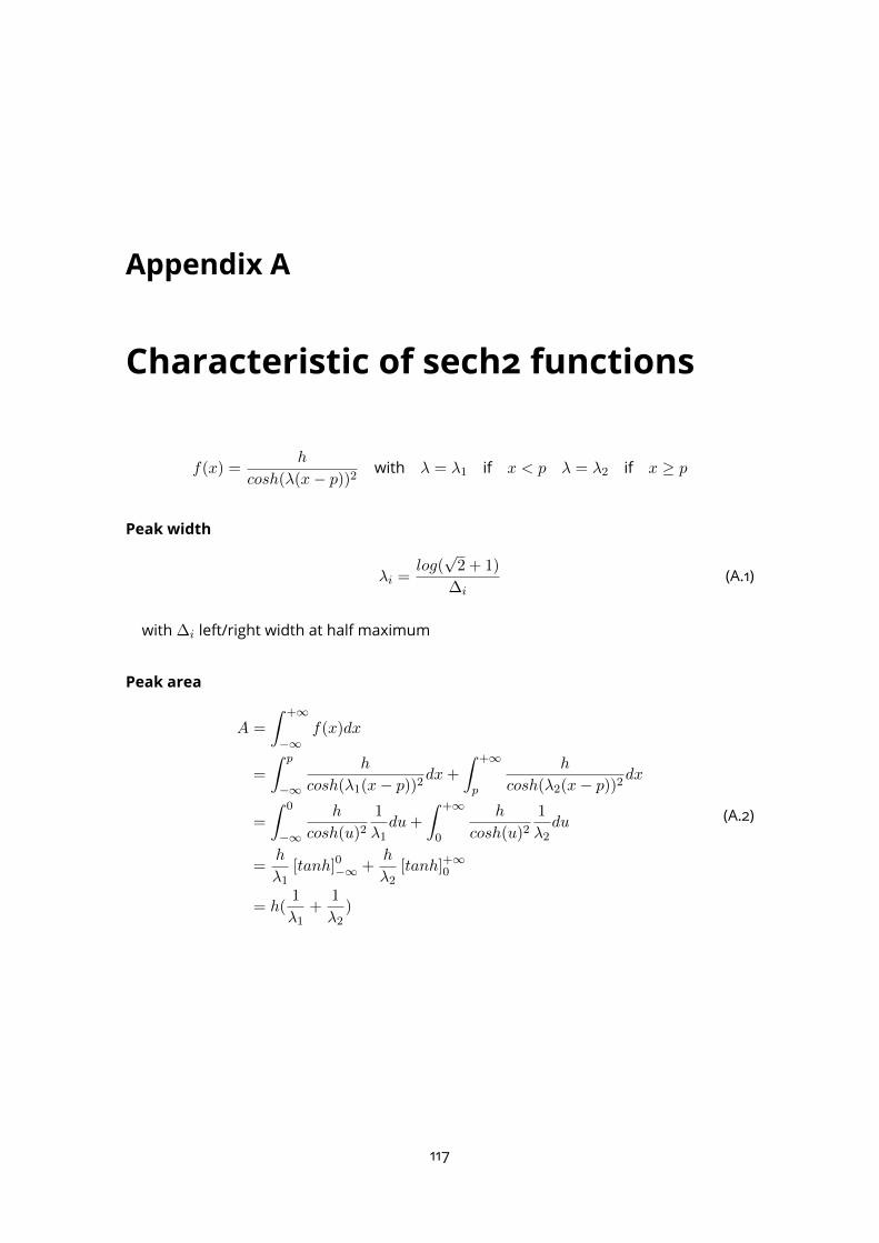
Appendix A

Characteristic of sech2 functions

f(x) =h

cosh(λ(x− p))2with λ = λ1 if x < p λ = λ2 if x ≥ p

Peak width

λi =log(

√2 + 1)

∆i(A.1)

with∆i left/right width at half maximumPeak area

A =

∫ +∞

−∞f(x)dx

=

∫ p

−∞

h

cosh(λ1(x− p))2dx+

∫ +∞

p

h

cosh(λ2(x− p))2dx

=

∫ 0

−∞

h

cosh(u)21

λ1du+

∫ +∞

0

h

cosh(u)21

λ2du

=h

λ1[tanh]0−∞ +

h

λ2[tanh]+∞

0

= h(1

λ1+

1

λ2)

(A.2)

117

Appendix B

Articles

118

Gene expression

ptairMS: real-time processing and analysis of PTR-TOF-MS

data for biomarker discovery in exhaled breath

Camille Roquencourt 1,*, Stanislas Grassin-Delyle2,3,4 and Etienne A. Thevenot 5

1Departement Metrologie Instrumentation & Information (DM2I), CEA, LIST, Laboratoire Sciences des Donnees et de la Decision, F-

91191 Gif-Sur-Yvette, France, 2Departement des maladies des voies respiratoires, Hopital Foch, Exhalomics, Suresnes 92150, France,3Departement de Biotechnologie de la Sante, Universite Paris-Saclay, UVSQ, INSERM, Infection et inflammation, Montigny le

Bretonneux 78180, France, 4FHU SEPSIS (Saclay and Paris Seine Nord Endeavour to PerSonalize Interventions for Sepsis), Garches

92380, France and 5Departement Medicaments et Technologies pour la Sante (MTS), Universite Paris-Saclay, CEA, INRAE,

MetaboHUB, F-91191 Gif sur Yvette, France

*To whom correspondence should be addressed.

Associate Editor: Olga Vitek

Received on September 29, 2021; revised on December 24, 2021; editorial decision on December 27, 2021; accepted on January 16, 2022

Abstract

Motivation: Analysis of volatile organic compounds (VOCs) in exhaled breath by proton transfer reaction time-of-flight mass spectrometry (PTR-TOF-MS) is of increasing interest for real-time, non-invasive diagnosis, phenotypingand therapeutic drug monitoring in the clinics. However, there is currently a lack of methods and software tools forthe processing of PTR-TOF-MS data from cohorts and suited for biomarker discovery studies.

Results: We developed a comprehensive suite of algorithms that process raw data from patient acquisitions andgenerate the table of feature intensities. Notably, we included an innovative two-dimensional peak deconvolutionmodel based on penalized splines signal regression for accurate estimation of the temporal profile and feature quan-tification, as well as a method to specifically select the VOCs from exhaled breath. The workflow was implementedas the ptairMS software, which contains a graphical interface to facilitate cohort management and data analysis.The approach was validated on both simulated and experimental datasets, and we showed that the sensitivity andspecificity of the VOC detection reached 99% and 98.4%, respectively, and that the error of quantification was below8.1% for concentrations down to 19 ppb.

Availability and implementation: The ptairMS software is publicly available as an R package on Bioconductor (doi:10.18129/B9.bioc.ptairMS), as well as its companion experiment package ptairData (doi: 10.18129/B9.bioc.ptairData).

Contact: camille.roquencourt@hotmail.fr

Supplementary information: Supplementary data are available at Bioinformatics online.

1 Introduction

Volatolomics is the study of volatile organic compounds (VOCs)emitted by a biological system (Amann et al., 2014), which can befound in several human matrices such as saliva, urine, skin, bloodand exhaled breath. Recently, many studies have highlighted the po-tential of VOC analysis from exhaled breath for early diagnosis, dis-ease phenotyping, therapeutic drug monitoring or toxicologicalanalysis (Boots et al., 2015; Bruderer et al., 2019; Einoch Amoret al., 2019; Pereira et al., 2015; Rattray et al., 2014). One of themain advantages of breath analysis is its non-invasive nature(Devillier et al., 2017).

Mass spectrometry is a powerful method for the study of smallvolatile molecules (Rattray et al., 2014). Recently, ‘on-line’

technologies, where the patient blows directly into the mass spec-trometer, have emerged as promising approaches for the real-timeanalysis at the point of care (Bruderer et al., 2019; Devillier et al.,2017). Such strategies are of major interest for the screening andmonitoring of individual patients or cohorts (Trefz et al., 2013). Thepotential of proton transfer reaction coupled to time-of-flight massspectrometry (PTR-TOF-MS; Blake et al., 2009; Herbig et al., 2009;Jordan et al., 2009) for biomedicine has been shown in applicationssuch as emphysema, liver cirrhosis, chronic kidney disease and dia-betes (Cristescu et al., 2011; Fernandez del Rıo et al., 2015;Obermeier et al., 2017; Pleil et al., 2019). PTR-TOF-MS spectrome-ters provide limits of detection in the parts per billion by volume(ppbv) range and rely on VOCs ionization with a transfer of protonfrom a reagent ion (usually H3Oþ), then subsequent detection of the

VC The Author(s) 2022. Published by Oxford University Press. 1

This is an Open Access article distributed under the terms of the Creative Commons Attribution-NonCommercial License (https://creativecommons.org/licenses/by-nc/4.0/),

which permits non-commercial re-use, distribution, and reproduction in any medium, provided the original work is properly cited. For commercial re-use, please contact

journals.permissions@oup.com

Bioinformatics, 2022, 1–8

https://doi.org/10.1093/bioinformatics/btac031

Advance Access Publication Date: 19 January 2022

Original Paper

Dow

nloaded from https://academ

ic.oup.com/bioinform

atics/advance-article/doi/10.1093/bioinformatics/btac031/6511435 by U

niversite De Versailles Saint-Q

uentin-En-Yvelines user on 15 March 2022

resulting ions with time-of-flight (TOF)-MS. During data acquisi-tion, which is very fast, the instrument continuously analyzes the airflowing through a buffer tube (i.e. ambient air by default) and thepatient is asked to expire a few times into the tube. Each data file (inthe HDF5 open format; Koziol, 2011) contains the ion intensitiesstored as a numerical matrix whose dimensions are the TOF bins(which can be converted to m/z values) and the acquisition time.

Two processing software are currently available for PTR-TOF-MS data, the commercial Ionicon Data Analyzer (IDA) released in2020 based on the algorithms by Muller et al. (2013) and the open-source PTRwid (Holzinger, 2015). These software tools allow theanalysis of high-resolution, TOF-MS data with the following char-acteristics: (i) single (or multiple for PTRwid) file analysis, (ii) in-ternal m/z calibration, (iii) untargeted peak detection anddeconvolution and (iv) quantification and suggestion of elementalcomposition. They are particularly suited for the analysis of verylarge files resulting from continuous environmental monitoring.However, there are specific needs for breath research in patientcohorts which have to be covered. For instance, the simultaneousanalysis of multiple samples requires that peak lists from differentsamples may be aligned; in addition, the parallel processing of sev-eral files would be a time-sparing capability; furthermore, a correctdistinction of the signals coming from the background and the ex-piratory phases is needed; finally, implementing a background cor-rection of the ambient air composition as a function of time wouldbe an asset for accurate peak detection and quantification(Beauchamp, 2011; Filipiak et al., 2012; Spanel et al., 2013).

We have therefore developed a suite of algorithms for the proc-essing and analysis of PTR-TOF-MS data for untargeted breath ana-lysis and biomarker discovery in patient cohorts. In particular, thepenalized regression on a B-spline basis (P-splines) was used foradaptive temporal modeling (Eilers and Marx, 1996), and the coeffi-cients in both m/z and time dimensions were jointly estimated with atwo-dimensional (2D) tensor product. This approach enables to esti-mate all temporal trends without any parametric hypothesis, and toprecisely separate peaks in the m/z dimension at each time. The tem-poral profiles are then used to correct the external contamination,using linear ambient air baseline removal and statistical testing ofmean intensity in ambient air versus exhaled breath.

The whole workflow from the raw data files up to the table ofpeak intensities is implemented as the ptairMS package (doi:10.18129/B9.bioc.ptairMS) available on Bioconductor (Gentlemanet al., 2004). It includes specific features to facilitate routine clinicalanalysis (e.g. graphical user interface, quality control checks, samplemetadata management, iterative inclusion of new acquisitions). Inthe following, we will first describe the methods used for each stepof the workflow, and then present the results obtained with simu-lated, experimental, and clinical datasets.

2 Materials and methods

The suite of algorithms developed for the processing of PTR-TOF-MS data from exhaled breath, and implemented in the ptairMS Rpackage, takes as input the name of the directory containing the rawfiles in HDF5 format, and ultimately generates the samples by varia-bles table of peak intensities. The main steps of the workflow aresummarized below and detailed in the following of Section 2. Thisworkflow proposes innovative developments for the breathomicsanalysis of cohorts, including 2D processing and ambient air quanti-fication and correction methods, which were implemented to previ-ous literature on breath analysis.

1. Processing of each file

a. Internal calibration of the m/z axis

b. Determination of expiration limits

c. Untargeted peak detection and quantification in exhaled

breath• Detecting peaks on the average total ion spectrum• Estimating the temporal evolution for each peak

• Quantifying• Ambient inhaled air correction• Statistical testing of intensity differences between ambi-

ent air and expiration phases

2. Alignment between samples followed by quality control• Aligning features between samples• Filtering features based on reproducibility within the whole

cohort or sample classes• Filtering features based on the P-value from the test in (1.c)

3. Imputation of missing values

4. Putative annotation (including isotopes)

5. Export of the peak table and metadata

6. Peak table update when new files are included in the input directory

2.1 Processing of each file2.1.1 Calibration

Calibration converts the TOF values recorded by the mass spectrom-eter into m/z values: m=z ¼ ðtofbÞ2

a (Brown and Gilfrich, 1991). Toestimate the parameters (a, b), the Levenberg–Marquardt algorithmis used, with couples (tof, m/z) of reference peaks without overlap(Cappellin et al., 2010; Muller et al., 2013). For exhaled breath,we suggest using the following peaks: the primary ion isotope(m/z 21.022), dinitrogen (m/z 29.013) and the acetone isotope(m/z 60.053). External calibration ions such as iodobenzene(m/z 203.943), and diiodobenzene (m/z 330.850) can also be usedfor calibration in instruments with internal permeation devices. As adrift over time is observed due to low changes of temperature, cali-bration is performed periodically (e.g. every minute) to update the(a, b) values. The shift is subsequently estimated for each m/z as afunction of time by linear interpolation.

2.1.2 Expiration detection

Determination of expiration limits and background (ambient air) isa very important step for the analysis, as boundaries will be used forquantification and for the statistical test for features selection inSection 2.1.3. Classically, a raw data ion trace is used to automatic-ally detect expiration. Herbig et al. (2009) propose to use acetone(m/z 59.049), CO2 (m/z 44.997) or humidity with the water clusterisotope (m/z 39.033) as ion traces. We used the same method asdescribed by Schwoebel et al. (2011) and Trefz et al. (2013), to auto-matically detect expiration and inhalation phases on an ion trace. Inaddition, we designed a specific panel from our graphical interfaceto the visualization (and possible manual modification) of the expir-ation limits (as described in Section 3.3 below).

2.1.3 Untargeted peak detection and quantification in exhaled

breath

Raw data consist in a numerical matrix of TOF counts, whosedimensions are 105 bins (m/z between 0 and 500 Da), and 102 s(depending on the acquisition time). After m/z calibration, data areprocessed sequentially within bands centered at each nominal masswithin an interval of 60.6 Da (since VOCs are of low molecularweight, <500 Da, peak m/z are clustered around nominal masses;Cappellin et al., 2011; Muller et al., 2011), and covering the fulltime range. The following steps are then applied: (i) peaks aredetected in the mass axis on the sum spectrum, (ii) their temporalevolution is estimated by a tensor product with P-splines, (iii) statis-tical tests are performed to identify if VOCs come from exhaledbreath or ambient air and (iv) their average intensity in expirationphases are quantified in ppb (Fig. 1).

Peak detection on the average spectrum in 1D: The peak pickingalgorithm in the m/z dimension is mainly based on Muller et al.(2013). Due to the medium resolution of the instrument (5000 to10 000), a parametric peak function is required for peak separation.The described estimation of the peak shape starts from the 10% en-velop quantile of the normalized and filtered raw spectrum between

2 C.Roquencourt et al.

Dow

nloaded from https://academ

ic.oup.com/bioinform

atics/advance-article/doi/10.1093/bioinformatics/btac031/6511435 by U

niversite De Versailles Saint-Q

uentin-En-Yvelines user on 15 March 2022

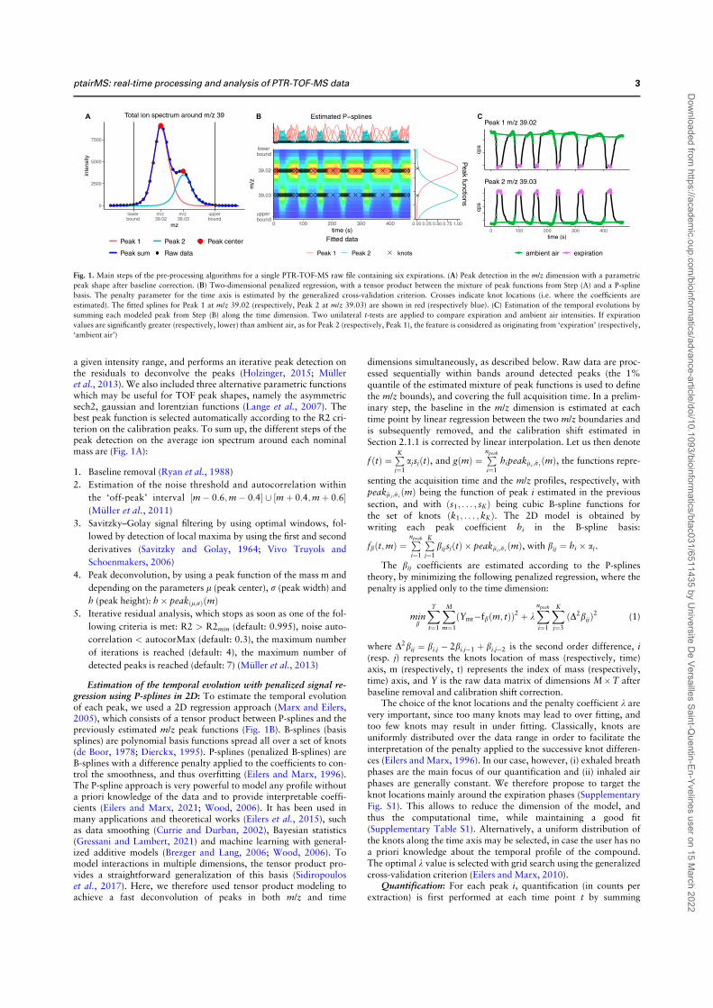
a given intensity range, and performs an iterative peak detection onthe residuals to deconvolve the peaks (Holzinger, 2015; Mulleret al., 2013). We also included three alternative parametric functionswhich may be useful for TOF peak shapes, namely the asymmetricsech2, gaussian and lorentzian functions (Lange et al., 2007). Thebest peak function is selected automatically according to the R2 cri-terion on the calibration peaks. To sum up, the different steps of thepeak detection on the average ion spectrum around each nominalmass are (Fig. 1A):

1. Baseline removal (Ryan et al., 1988)

2. Estimation of the noise threshold and autocorrelation within

the ‘off-peak’ interval ½m 0:6;m 0:4 [ ½mþ 0:4;mþ 0:6(Muller et al., 2011)

3. Savitzky–Golay signal filtering by using optimal windows, fol-

lowed by detection of local maxima by using the first and second

derivatives (Savitzky and Golay, 1964; Vivo Truyols and

Schoenmakers, 2006)

4. Peak deconvolution, by using a peak function of the mass m and

depending on the parameters l (peak center), r (peak width) and

h (peak height): h peakðl;rÞðmÞ5. Iterative residual analysis, which stops as soon as one of the fol-

lowing criteria is met: R2 > R2min (default: 0.995), noise auto-

correlation < autocorMax (default: 0.3), the maximum number

of iterations is reached (default: 4), the maximum number of

detected peaks is reached (default: 7) (Muller et al., 2013)

Estimation of the temporal evolution with penalized signal re-gression using P-splines in 2D: To estimate the temporal evolutionof each peak, we used a 2D regression approach (Marx and Eilers,2005), which consists of a tensor product between P-splines and thepreviously estimated m/z peak functions (Fig. 1B). B-splines (basissplines) are polynomial basis functions spread all over a set of knots(de Boor, 1978; Dierckx, 1995). P-splines (penalized B-splines) areB-splines with a difference penalty applied to the coefficients to con-trol the smoothness, and thus overfitting (Eilers and Marx, 1996).The P-spline approach is very powerful to model any profile withouta priori knowledge of the data and to provide interpretable coeffi-cients (Eilers and Marx, 2021; Wood, 2006). It has been used inmany applications and theoretical works (Eilers et al., 2015), suchas data smoothing (Currie and Durban, 2002), Bayesian statistics(Gressani and Lambert, 2021) and machine learning with general-ized additive models (Brezger and Lang, 2006; Wood, 2006). Tomodel interactions in multiple dimensions, the tensor product pro-vides a straightforward generalization of this basis (Sidiropouloset al., 2017). Here, we therefore used tensor product modeling toachieve a fast deconvolution of peaks in both m/z and time

dimensions simultaneously, as described below. Raw data are proc-essed sequentially within bands around detected peaks (the 1%quantile of the estimated mixture of peak functions is used to definethe m/z bounds), and covering the full acquisition time. In a prelim-inary step, the baseline in the m/z dimension is estimated at eachtime point by linear regression between the two m/z boundaries andis subsequently removed, and the calibration shift estimated inSection 2.1.1 is corrected by linear interpolation. Let us then denote

f ðtÞ ¼PK

j¼1

ajsjðtÞ, and gðmÞ ¼Pnpeak

i¼1

hipeakl i ;r iðmÞ, the functions repre-

senting the acquisition time and the m/z profiles, respectively, withpeakl i ;r i

ðmÞ being the function of peak i estimated in the previous

section, and with ðs1; . . . ; sKÞ being cubic B-spline functions forthe set of knots ðk1; . . . ; kKÞ. The 2D model is obtained bywriting each peak coefficient hi in the B-spline basis:

fbðt;mÞ ¼Pnpeak

i¼1

PK

j¼1

bijsjðtÞ peakl i ;r iðmÞ, with bij ¼ hi aj.

The bij coefficients are estimated according to the P-splinestheory, by minimizing the following penalized regression, where thepenalty is applied only to the time dimension:

minb

XT

t¼1

XM

m¼1

ðYmtfbðm; tÞÞ2 þ kXnpeak

i¼1

XK

j¼3

ðD2bijÞ2 (1)

where D2bij ¼ bi;j 2bi;j1 þ bi;j2 is the second order difference, i(resp. j) represents the knots location of mass (respectively, time)axis, m (respectively, t) represents the index of mass (respectively,time) axis, and Y is the raw data matrix of dimensions MT afterbaseline removal and calibration shift correction.

The choice of the knot locations and the penalty coefficient k arevery important, since too many knots may lead to over fitting, andtoo few knots may result in under fitting. Classically, knots areuniformly distributed over the data range in order to facilitate theinterpretation of the penalty applied to the successive knot differen-ces (Eilers and Marx, 1996). In our case, however, (i) exhaled breathphases are the main focus of our quantification and (ii) inhaled airphases are generally constant. We therefore propose to target theknot locations mainly around the expiration phases (SupplementaryFig. S1). This allows to reduce the dimension of the model, andthus the computational time, while maintaining a good fit(Supplementary Table S1). Alternatively, a uniform distribution ofthe knots along the time axis may be selected, in case the user has noa priori knowledge about the temporal profile of the compound.The optimal k value is selected with grid search using the generalizedcross-validation criterion (Eilers and Marx, 2010).

Quantification: For each peak i, quantification (in counts perextraction) is first performed at each time point t by summing

0

2500

5000

7500

lower bound

m/z39.02

m/z39.03

upperbound

mz

inte

nsity

Peak 1 Peak 2 Peak center

Peak sum Raw data

Total ion spectrum around m/z 39A Estimated P−splines

lower bound

39.02

39.03

upperbound

0 100 200 300 400time (s)

m/z

Fitted data

0.00 0.25 0.50 0.75 1.00

Peak functions

.

Peak 1 Peak 2 knots

B

cps

Peak 1 m/z 39.02

0 100 200 300 400time (s)

cps

ambient air expiration

Peak 2 m/z 39.03

C

Fig. 1. Main steps of the pre-processing algorithms for a single PTR-TOF-MS raw file containing six expirations. (A) Peak detection in the m/z dimension with a parametric

peak shape after baseline correction. (B) Two-dimensional penalized regression, with a tensor product between the mixture of peak functions from Step (A) and a P-spline

basis. The penalty parameter for the time axis is estimated by the generalized cross-validation criterion. Crosses indicate knot locations (i.e. where the coefficients are

estimated). The fitted splines for Peak 1 at m/z 39.02 (respectively, Peak 2 at m/z 39.03) are shown in red (respectively blue). (C) Estimation of the temporal evolutions by

summing each modeled peak from Step (B) along the time dimension. Two unilateral t-tests are applied to compare expiration and ambient air intensities. If expiration

values are significantly greater (respectively, lower) than ambient air, as for Peak 2 (respectively, Peak 1), the feature is considered as originating from ‘expiration’ (respectively,

‘ambient air’)

ptairMS: real-time processing and analysis of PTR-TOF-MS data 3

Dow

nloaded from https://academ

ic.oup.com/bioinform

atics/advance-article/doi/10.1093/bioinformatics/btac031/6511435 by U

niversite De Versailles Saint-Q

uentin-En-Yvelines user on 15 March 2022

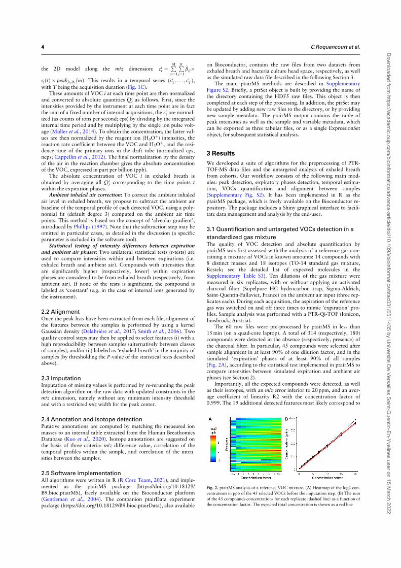
the 2D model along the m/z dimension: cit ¼

PM

m¼1

PK

j¼1

bij

sjðtÞ peakl i ;r iðmÞ. This results in a temporal series ðci

1; . . . ; ciTÞ,

with T being the acquisition duration (Fig. 1C).These amounts of VOC i at each time point are then normalized

and converted to absolute quantities Qit as follows. First, since the

intensities provided by the instrument at each time point are in factthe sum of a fixed number of internal acquisitions, the ci

t are normal-ized (as counts of ions per second; cps) by dividing by the integratedinternal time period and by multiplying by the single ion pulse volt-age (Muller et al., 2014). To obtain the concentration, the latter val-ues are then normalized by the reagent ion (H3Oþ) intensities, thereaction rate coefficient between the VOC and H3Oþ, and the resi-dence time of the primary ions in the drift tube (normalized cps,ncps; Cappellin et al., 2012). The final normalization by the densityof the air in the reaction chamber gives the absolute concentrationof the VOC, expressed in part per billion (ppb).

The absolute concentration of VOC i in exhaled breath isobtained by averaging all Qi

t corresponding to the time points twithin the expiration phases.

Ambient inhaled air correction: To correct the ambient inhaledair level in exhaled breath, we propose to subtract the ambient airbaseline of the temporal profile of each detected VOC, using a poly-nomial fit (default degree 3) computed on the ambient air timepoints. This method is based on the concept of ‘alveolar gradient’,introduced by Phillips (1997). Note that the subtraction step may beomitted in particular cases, as detailed in the discussion (a specificparameter is included in the software tool).

Statistical testing of intensity differences between expirationand ambient air phases: Two unilateral statistical tests (t-tests) areused to compare intensities within and between expirations (i.e.exhaled breath and ambient air). Compounds with intensities thatare significantly higher (respectively, lower) within expirationphases are considered to be from exhaled breath (respectively, fromambient air). If none of the tests is significant, the compound islabeled as ‘constant’ (e.g. in the case of internal ions generated bythe instrument).

2.2 AlignmentOnce the peak lists have been extracted from each file, alignment ofthe features between the samples is performed by using a kernelGaussian density (Delabriere et al., 2017; Smith et al., 2006). Twoquality control steps may then be applied to select features (i) with ahigh reproducibility between samples (alternatively between classesof samples), and/or (ii) labeled as ‘exhaled breath’ in the majority ofsamples (by thresholding the P-value of the statistical tests describedabove).

2.3 ImputationImputation of missing values is performed by re-rerunning the peakdetection algorithm on the raw data with updated constraints in them/z dimension, namely without any minimum intensity thresholdand with a restricted m/z width for the peak center.

2.4 Annotation and isotope detectionPutative annotations are computed by matching the measured ionmasses to an internal table extracted from the Human BreathomicsDatabase (Kuo et al., 2020). Isotope annotations are suggested onthe basis of three criteria: m/z difference value, correlation of thetemporal profiles within the sample, and correlation of the inten-sities between the samples.

2.5 Software implementationAll algorithms were written in R (R Core Team, 2021), and imple-mented as the ptairMS package (https://doi.org/10.18129/B9.bioc.ptairMS), freely available on the Bioconductor platform(Gentleman et al., 2004). The companion ptairData experimentpackage (https://doi.org/10.18129/B9.bioc.ptairData), also available

on Bioconductor, contains the raw files from two datasets fromexhaled breath and bacteria culture head space, respectively, as wellas the simulated raw data file described in the following Section 3.

The main ptairMS methods are described in SupplementaryFigure S2. Briefly, a ptrSet object is built by providing the name ofthe directory containing the HDF5 raw files. This object is thencompleted at each step of the processing. In addition, the ptrSet maybe updated by adding new raw files to the directory, or by providingnew sample metadata. The ptairMS output contains the table ofpeak intensities as well as the sample and variable metadata, whichcan be exported as three tabular files, or as a single ExpressionSetobject, for subsequent statistical analysis.

3 Results

We developed a suite of algorithms for the preprocessing of PTR-TOF-MS data files and the untargeted analysis of exhaled breathfrom cohorts. Our workflow consists of the following main mod-ules: peak detection, expiratory phases detection, temporal estima-tion, VOCs quantification and alignment between samples(Supplementary Fig. S2). It has been implemented in R as theptairMS package, which is freely available on the Bioconductor re-pository. The package includes a Shiny graphical interface to facili-tate data management and analysis by the end-user.

3.1 Quantification and untargeted VOCs detection in a

standardized gas mixtureThe quality of VOC detection and absolute quantification byptairMS was first assessed with the analysis of a reference gas con-taining a mixture of VOCs in known amounts: 14 compounds with8 distinct masses and 18 isotopes (TO-14 standard gas mixture,Restek; see the detailed list of expected molecules in theSupplementary Table S3). Ten dilutions of the gas mixture weremeasured in six replicates, with or without applying an activatedcharcoal filter (Supelpure HC hydrocarbon trap, Sigma-Aldrich,Saint-Quentin-Fallavier, France) on the ambient air input (three rep-licates each). During each acquisition, the aspiration of the referencegas was switched on and off three times to mimic ‘expiration’ pro-files. Sample analysis was performed with a PTR-Qi-TOF (Ionicon,Innsbruck, Austria).

The 60 raw files were pre-processed by ptairMS in less than15 min (on a quad-core laptop). A total of 314 (respectively, 180)compounds were detected in the absence (respectively, presence) ofthe charcoal filter. In particular, 45 compounds were selected aftersample alignment in at least 90% of one dilution factor, and in thesimulated ‘expiration’ phases of at least 90% of all samples(Fig. 2A), according to the statistical test implemented in ptairMS tocompare intensities between simulated expiration and ambient airphases (see Section 2).

Importantly, all the expected compounds were detected, as wellas their isotopes, with an m/z error inferior to 20 ppm, and an aver-age coefficient of linearity R2 with the concentration factor of0.999. The 19 additional detected features most likely correspond to

Fig. 2. ptairMS analysis of a reference VOC mixture. (A) Heatmap of the log2 con-

centrations in ppb of the 45 selected VOCs before the imputation step. (B) The sum

of the 45 compounds concentrations for each replicate (dashed line) as a function of

the concentration factor. The expected total concentration is shown as a red line

4 C.Roquencourt et al.

Dow

nloaded from https://academ

ic.oup.com/bioinform

atics/advance-article/doi/10.1093/bioinformatics/btac031/6511435 by U

niversite De Versailles Saint-Q

uentin-En-Yvelines user on 15 March 2022

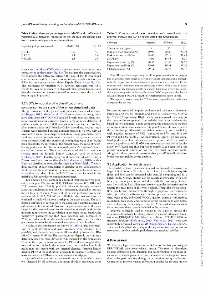
fragments from these VOCs, since some are below the expected con-centration (Supplementary Fig. S3). To evaluate the quantification,we computed the difference between the sum of the 45 compoundconcentrations and the expected concentration, which was less than8.1% for the concentrations above 19 ppb (Table 1 and Fig. 2B).The coefficient of variation (CV) between replicates was <5%(Table 1), even in the absence of charcoal filter, which demonstratesthat the ambient air intensity is well subtracted from the exhaledbreath signal in ptairMS.

3.2 VOCs temporal profile classification and

comparison to the state of the art on simulated dataThe performance of the present and previously described software(Holzinger, 2015; Muller et al., 2013) were compared using simu-lated data from PTR-TOF-MS exhaled breath analysis. First, tem-poral evolutions were extracted from a large in-house database ofpatient acquisitions (>10 000 expiration and ambient air profiles),after normalization and Savitzky–Golay smoothing. Second, peakclusters were generated around nominal masses 21 to 400, with anasymmetric sech2 peak shape distribution. Peaks parameters wererandomly selected for each nominal mass: i.e. the asymmetry coeffi-cient the peak width, the number of overlapping peaks (1 to 3), thepeak proximity, the intensity of the highest peak, the ratio of neigh-boring peaks, and the class of temporal profile (‘expiration’, ‘ambi-ent air’ or ‘constant’). The exact m/z value of the first peak wasselected from the formula library CxHyOzNt used by PTRwid(Holzinger, 2015). Finally, background noise was added by using aPoisson stochastic process (Gundlach-Graham et al., 2018), with aGaussian distribution to model the single ion Pulse-Height. The ran-dom drawing of each parameters is detailed in the SupplementaryTable S2, and the code used for the simulation, as well as a represen-tative simulated data file in the HDF5 format, are included in theptairData R/Bioconductor companion package.

Ten simulated files, containing a total of 7028 peaks, were proc-essed with ptairMS (version 0.1), PTRwid (version 002 IDL) andIDA (version beta 0.9.4.8). ptairMS, which is the only softwareallowing simultaneous multiple file processing, enabled to processthe 10 files in <10 min. Mass calibration was performed using thepeaks at m/z 21.022, 203.943 and 330.84 for the three software, in-tentionally simulated without overlap at the exact masses. The cali-bration stability period was set to the acquisition duration, since nocalibration shift was added. To ensure a good estimation of the peakshape for the three software, we simulated more single peaks in theintensity range set for the calculation of the peak shape. Finally, the‘sensitivity’ parameter for IDA peak detection was decreased to25%, in order to limit the number of false positives. The otherparameters from each software tool were kept to default values.

Results of the comparison are shown in Table 2. The best preci-sion of peak detection and mass accuracy were obtained withptairMS, and the peak detection recall was slightly lower than IDA(98.40% versus 98.49%). The mass accuracy depends only on peakdetection, since no mass deviation was included in the simulation.Of note, the reported mass accuracy for PTRwid was computed be-fore calibration: indeed, the masses from the simulated multiplepeaks may not match with the internal chemical formula libraryused by PTRwid for calibration, especially for masses >300 Da (themass accuracy for PTRwid after calibration was 20 ppm).

Quantification was further evaluated on the peaks which werewell detected by all software. The mean absolute percentage error

between the estimated temporal evolution and the input of the simu-lation was 4.96% for ptairMS and 14.65% (respectively, 5.38%)for PTRwid (respectively, IDA). Finally, we compared the ability todiscriminate the compounds from exhaled breath and ambient air,based on two unilateral t-tests comparing the intensities in the twoacquisition phases (see Section 2.1.3). ptairMS was shown to detectthe expiration profiles with the highest sensitivity and specificity,with a global accuracy of 99% (compared to 87% and 95% forPTRwid and IDA; Table 2). As illustrated in Figure 3 on two simu-lated peaks with close m/z values, an exogenous VOC (i.e. with aconstant profile) at m/z 82.034 was erroneously classified as ‘expir-ation’ by PTRwid and IDA but not by ptairMS, as a result of a lessprecise temporal estimation of the two first software tools.Altogether, these results demonstrate that ptairMS is well suited forbiomarker research by breath analysis.

3.3 Application to real datasetsThe ptairMS software has been designed for biomarker discovery inlarge clinical cohorts. First, it is fast (<1 min for a 3–5 min acquisi-tion), and files can be processed with parallel computing and in abatch mode. Second, studies can be readily incremented with newfiles (e.g. if new patients are included): only the processing of thesenew files and the final alignment between samples are performed toupdate the peak table of the whole cohort. Third, the whole work-flow can be run interactively through a graphical user interface,which provides visualizations (expiration phases, peaks in the rawdata, peak table, individual VOCs), quality controls (calibration,resolution, peak shape and evolution of the reagent ions with time),and exploratory data analysis (Fig. 4). A detailed documentationincluding several use cases is included in the package.

ptairMS is already used in routine in the clinic to process theacquisitions from freely breathing patients in some breath research cen-ters using PTR-Qi-TOF MS. Files from a distinct PTR-TOF 8000 in-strument (Ionicon) (Trefz et al., 2013; Vita et al., 2015) were alsosuccessfully processed with ptairMS (Supplementary Figs S4 and S5).These results highlight the ability of the algorithms to adapt to variousresolutions, time bin periods, peak shapes and temporal profiles.

4 Discussion

We have developed an innovative workflow for the fast processing ofPTR-TOF-MS data from exhaled breath. The suite of algorithmsincludes untargeted peak detection and deconvolution in the mass di-mension, expiration phases detection, estimation of the temporal evolu-tion of the peak intensity during the acquisition and quantification.Compared to the two existing software, it enables for the first time to

Table 1. Mean absolute percentage error (MAPE) and coefficient of

variation (CV) between replicates of the ptairMS processed data

from the reference gas mixture acquisitions

Expected ppb per compound MAPE (%) CV (%)

½1:3; 13 47.9 4.3

½19; 32 8.1 3.4

½44; 128 2.5 2.8

Table 2. Comparison of peak detection and quantification by

ptairMS, PTRwid and IDA on 10 simulated files (7028 peaks)

Software ptairMS PTRwid IDA

Mass accuracy (ppm) 3 12a 5

Peak detection precision (%) 99.99 98.87 97.30

Peak detection recall (%) 98.40 87.19 98.49

MAPE (%) 4.96 14.65 5.38

Expiration sensitivity (%) 98.53 91.45 94.52

Expiration specificity (%) 99.01 86.31 97.03

Global accuracy (%) 99.12 86.73 95.31

Note: The precision (respectively, recall) of peak detection is the propor-

tion of detected peaks which correspond to actual simulated peaks (respect-

ively, the proportion of actual simulated peaks which were detected by the

software tools). The mean absolute percentage error (MAPE) is used to assess

the quality of the temporal profile estimation. Expiration sensitivity, specifi-

city and accuracy refer to the classification of VOC origin as exhaled breath

(vs. ambient air). For each metric, the best performance is shown in bold.aThe reported mass accuracy for PTRwid was computed before calibration

as explained in the text.

ptairMS: real-time processing and analysis of PTR-TOF-MS data 5

Dow

nloaded from https://academ

ic.oup.com/bioinform

atics/advance-article/doi/10.1093/bioinformatics/btac031/6511435 by U

niversite De Versailles Saint-Q

uentin-En-Yvelines user on 15 March 2022

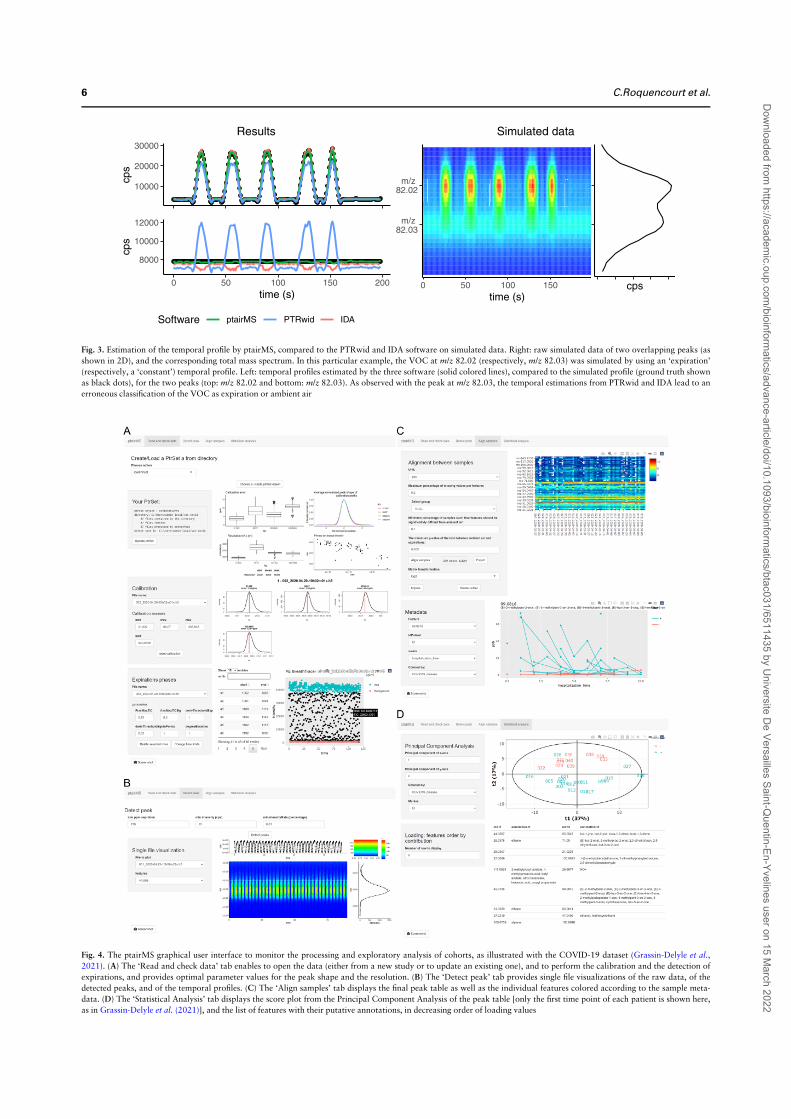
10000

20000

30000

cps

8000

10000

12000

0 50 100 150 200time (s)

cps

Software ptairMS PTRwid IDA

Results

m/z82.02

m/z82.03

0 50 100 150time (s)

cps

Simulated data

Fig. 3. Estimation of the temporal profile by ptairMS, compared to the PTRwid and IDA software on simulated data. Right: raw simulated data of two overlapping peaks (as

shown in 2D), and the corresponding total mass spectrum. In this particular example, the VOC at m/z 82.02 (respectively, m/z 82.03) was simulated by using an ‘expiration’

(respectively, a ‘constant’) temporal profile. Left: temporal profiles estimated by the three software (solid colored lines), compared to the simulated profile (ground truth shown

as black dots), for the two peaks (top: m/z 82.02 and bottom: m/z 82.03). As observed with the peak at m/z 82.03, the temporal estimations from PTRwid and IDA lead to an

erroneous classification of the VOC as expiration or ambient air

Fig. 4. The ptairMS graphical user interface to monitor the processing and exploratory analysis of cohorts, as illustrated with the COVID-19 dataset (Grassin-Delyle et al.,

2021). (A) The ‘Read and check data’ tab enables to open the data (either from a new study or to update an existing one), and to perform the calibration and the detection of

expirations, and provides optimal parameter values for the peak shape and the resolution. (B) The ‘Detect peak’ tab provides single file visualizations of the raw data, of the

detected peaks, and of the temporal profiles. (C) The ‘Align samples’ tab displays the final peak table as well as the individual features colored according to the sample meta-

data. (D) The ‘Statistical Analysis’ tab displays the score plot from the Principal Component Analysis of the peak table [only the first time point of each patient is shown here,

as in Grassin-Delyle et al. (2021)], and the list of features with their putative annotations, in decreasing order of loading values

6 C.Roquencourt et al.

Dow

nloaded from https://academ

ic.oup.com/bioinform

atics/advance-article/doi/10.1093/bioinformatics/btac031/6511435 by U

niversite De Versailles Saint-Q

uentin-En-Yvelines user on 15 March 2022

conduct the analysis of clinical cohorts, with parallel file processing, in-cremental addition of new patient files, quality control of the acquisi-tions along clinical trials, alignment between the samples, and finalstatistical tests to discard exogenous VOCs. The full workflow wasimplemented in the R package ptairMS which is publicly available onthe Bioconductor repository and includes a detailed tutorial. Raw filesfrom two experimental datasets, as well as one simulated file, are pro-vided in the companion ptairData package. The public availability ofall data and source code will therefore be of high value for the reprodu-cibility of the analyzes, and the benchmark of software tools(Wilkinson et al., 2016).

The quality of the untargeted peak detection and absolute quantifi-cation was assessed by using a standardized gas mixture: all com-pounds were detected by ptairMS with an m/z precision lower than20 ppm, an intensity error below 8.1% (for compounds with concen-trations >19 ppb), an average R2 coefficient with the concentrationfactor of 0.999, and a CV <5%, thus demonstrating the performanceof the detection and quantification. However, it is important to notethat the standardized gas used does not reflect breath matrices. In prac-tice, humidity saturation of exhaled breath biases the VOC quantifica-tion in PTR-MS instruments, with divergent behavior for differentsubstance classes (Trefz et al., 2018). This effect also impacts the pro-posed correction of the ambient air level (which consists in subtractingthe ambient air baseline from the temporal profile estimated for eachVOC). Since the exhaled breath and ambient air have different concen-trations of humidity, O2, and CO2, the direct subtraction should nottherefore be considered as an absolute quantification, but rather as arelative concentration, which can be used to compare patients. To fur-ther compute accurate concentration differences between inspiratoryand expiratory phases, adequate humidity-adapted calibrations arerequired (Trefz et al., 2018).

Since the estimation of the temporal profiles is a key aspect ofbreath analysis, we have developed a 2D model based on P-spline re-gression. Compared to the existing software which are well suitedfor single-file, large data from environmental monitoring, we dem-onstrate that ptairMS is very convenient for breath analysis, achiev-ing highest sensitivity and accurate quantification. It should benoted that the temporal estimation of the peak intensities relies onthe m/z values previously computed on the total ion spectrum (i.e.these m/z values are not re-evaluated at each time point) whichallows a fast computation. While alternative approaches may beconsidered for the combined estimation of location and intensity ofthe peaks in 2D (such as Bayesian methods or non-linear optimiza-tion; Barat et al., 2007; Binette et al., 2020; He et al., 2014), theptairMS algorithms already provides precise m/z and intensity esti-mations, in a computation time (<1 min) which is compatible withthe real-time patient analysis.

The classification of the VOC origin between exhaled breath andambient air was shown to be improved with ptairMS (due to the 2Dmodeling), with an accuracy up to 99%. The control of external fac-tors such as the ambient air (Trefz et al., 2013), but also the dioxygenconcentration (Trefz et al., 2019), the patient medication, or specificdiets, is of critical importance in breath analysis (Hanna et al., 2019).ptairMS therefore checks the sample reproducibility after alignment toavoid some of these unwanted variations. In all cases, attention shouldbe paid during the design of the study to the matching of patients andsampling conditions between the groups of interest.

Importantly, ptairMS automatically suggests optimal values forthe parameters, such as the resolution and the peak shape (as eval-uated on the calibration peaks), but also the location of spline knots(at higher densities within the expiration phases) and the penaliza-tion for the 2D regression (based on generalized cross-validation).This enables to adapt the processing to specific instruments (e.g.with distinct resolutions) but also to various biological matrices (e.g.with different time profiles). As an example, ptairMS was used toprocess files from both PTR-TOF 8000 and PTR-Qi-TOF instru-ments (Ionicon Analytik). Files from other vendors (e.g. Tofwerk)should be processed accordingly, since they are in the same opensource HDF5 format, which is a data storage format of choice with-in the MS community (Askenazi et al., 2017). Beyond exhaledbreath, ptairMS was successfully applied to atmospheric air data

(hospital room and corridor air), headspace analysis from mycobac-teria (see the package tutorial) and truffles (Vita et al., 2015;Supplementary Fig. S5).

A graphical interface was developed to facilitate data analysisand result interpretation by experimenters (e.g. clinicians). It coversthe processing of raw data up to the exploratory data analysis of thecohort, with interactive tables and graphics. Since clinical studiesmay last several months, or even years, the interface includes a dedi-cated panel for the real-time control of instrument parameters toavoid unwanted effects resulting from drift in temperature, pressure,or variations in the amount of reagent ion. Incremental addition ofnew patient files is also possible without the need to reprocess all ofthe previous acquisitions. New features in future implementationswill include visualizations (such as the superposition of multipletemporal profiles for several patients), and statistical testing of clin-ical metadata for each detected VOC. Finally, a putative annotationof the compounds and their isotopes based on the m/z values is pro-vided to facilitate interpretation. To achieve higher confidence levelsof 2 or 1 for the most interesting VOCs, complementary experi-ments with hyphenated techniques such as GC-MS are required(Ibrahim et al., 2019; Nardi-Agmon et al., 2016; Wilde et al., 2019).

Recently, ptairMS was successfully applied to intubated, mech-anically ventilated patients, and enabled to discover a biomarker sig-nature of four VOCs for the diagnosis of coronavirus disease-19infection (Grassin-Delyle et al., 2021). In addition, it is routinelyused for clinical trials in centers performing exhaled breath research,not only for online patient analysis, but also for the off-line analysisof breath collected in sampling bags, allowing the analysis of sam-ples from multisite patients.

Altogether, these results demonstrate the value of the ptairMSsoftware as a key resource in breathomics for real-time analysis atthe point of care and in biomarker discovery studies, with a highclinical potential for the phenotyping of health and disease, thera-peutic drug monitoring, toxicological studies and precision medicine(Fernandez del Rıo et al., 2015; Ibrahim et al., 2019; Jung et al.,2021; Loser et al., 2020; Zhou et al., 2017).

Acknowledgements

We thank all the staff from the Exhalomics platform (Foch Hospital,

Suresnes) for providing PTR-MS data. We thank Pierrick Roger and Paul

Zheng for their help with the volatolomics database, the raw data format and

the package design. We thank Dr Phillip Trefz for kindly providing acquisi-

tion files for the PTR-TOF-MS 8000 instrument. We also thanks Dr Vincent

Le Moine and Pr Jean-Louis Herrmann for providing bacteria cultures.

Funding

The study was funded by the Agence Nationale de la Recherche (SoftwAiR

project, ANR-18-CE45-0017).

Conflict of Interest: none declared.

References

Amann,A. et al. (2014) The human volatilome: volatile organic compounds

(VOCs) in exhaled breath, skin emanations, urine, feces and saliva. J.

Breath Res., 8, 034001.

Askenazi,M. et al. (2017) The arc of Mass Spectrometry Exchange Formats is

long, but it bends toward HDF5: plain HDF5 as a mass spectrometry ex-

change format. Mass Spectrom. Rev., 36, 668–673.

Barat,E. et al. (2007). A nonparametric bayesian approach for PET reconstruc-

tion. In: 2007 IEEE Nuclear Science Symposium Conference Record. IEEE,

Honolulu, HI, USA, pp. 4155–4162.

Beauchamp,J. (2011) Inhaled today, not gone tomorrow: pharmacokinetics

and environmental exposure of volatiles in exhaled breath. J. Breath Res., 5,

037103.

Binette,O. et al. (2020) Bayesian Closed Surface Fitting Through Tensor

Products. J. Mach. Learn. Res., 26.

Blake,R.S. et al. (2009) Proton-transfer reaction mass spectrometry. Chem.

Rev., 109, 861–896.

ptairMS: real-time processing and analysis of PTR-TOF-MS data 7

Dow

nloaded from https://academ

ic.oup.com/bioinform

atics/advance-article/doi/10.1093/bioinformatics/btac031/6511435 by U

niversite De Versailles Saint-Q

uentin-En-Yvelines user on 15 March 2022

Boots,A.W. et al. (2015) Exhaled molecular fingerprinting in diagnosis and

monitoring: validating volatile promises. Trends Mol. Med., 21, 633–644.

Brezger,A. and Lang,S. (2006) Generalized structured additive regression

based on Bayesian P-splines. Comput. Stat. Data Anal., 50, 967–991.

Brown,R. and Gilfrich,N. (1991) Design and performance of a matrix-assisted

laser desorption time-of-flight mass spectrometer utilizing a pulsed nitrogen

laser. Anal. Chim. Acta, 248, 541–552.

Bruderer,T. et al. (2019) On-line analysis of exhaled breath: focus review.

Chem. Rev., 119, 10803–10828.

Cappellin,L. et al. (2010) Improved mass accuracy in PTR-TOF-MS: another

step towards better compound identification in PTR-MS. Int. J. Mass

Spectrom., 290, 60–63.

Cappellin,L. et al. (2011) On data analysis in PTR-TOF-MS: from raw spectra

to data mining. Sens. Actuators B Chem., 155, 183–190.

Cappellin,L. et al. (2012) On quantitative determination of volatile organic

compound concentrations using proton transfer reaction time-of-flight mass

spectrometry. Environ. Sci. Technol., 46, 2283–2290.

Cristescu,S.M. et al. (2011) Screening for emphysema via exhaled volatile or-

ganic compounds. J. Breath Res., 5, 046009.

Currie,I.D. and Durban,M. (2002) Flexible smoothing with P-splines: a unified

approach. Stat. Modelling, 2, 333–349.

de Boor,C. (1978) A Practical Guide to Splines. Applied Mathematical

Sciences, Springer, New York.

Delabriere,A. et al. (2017) proFIA: a data preprocessing workflow for flow in-

jection analysis coupled to high-resolution mass spectrometry.

Bioinformatics, 33, 3767–3775.

Devillier,P. et al. (2017) Metabolomics in the diagnosis and pharmacotherapy

of lung diseases. Curr. Pharm. Des., 23,

Dierckx,P. (1995) Curve and Surface Fitting with Splines. Monographs on nu-

merical analysis p. 5.

Eilers,P. and Marx,B. (2021). Practical Smoothing: The Joys of P-Splines.

Cambridge University Press, Cambridge.

Eilers,P.H.C. and Marx,B.D. (1996) Flexible smoothing with B-splines and

penalties. Stat. Sci., 11, 89–121.

Eilers,P.H.C. and Marx,B.D. (2010) Splines, knots, and penalties. Wiley

Interdiscip. Rev. Comput. Stat., 2, 637–653.

Eilers,P.H.C. et al. (2015) Twenty Years of P-Splines. SORT (Statistics and

Operations Research Transactions). 39. 149–186.

Einoch Amor,R. et al. (2019) Breath analysis of cancer in the present and the

future. Eur. Respir. Rev., 28, 190002.

Fernandez del Rıo,R. et al. (2015) Volatile biomarkers in breath associated

with liver cirrhosis—comparisons of pre- and post-liver transplant breath

samples. EBioMedicine, 2, 1243–1250.

Filipiak,W. et al. (2012) Dependence of exhaled breath composition on ex-

ogenous factors, smoking habits and exposure to air pollutants. J Breath

Res, 6, 036008.

Gentleman,R.C. et al. (2004) Bioconductor: open software development for

computational biology and bioinformatics. Genome Biol., 5, R80.

Grassin-Delyle,S. et al. (2021) Metabolomics of exhaled breath in critically ill

COVID-19 patients: a pilot study. EBioMedicine, 63, 103154.

Gressani,O. and Lambert,P. (2021) Laplace approximations for fast Bayesian

inference in generalized additive models based on P-splines. Comput. Stat.

Data Anal., 154, 107088.

Gundlach-Graham,A. et al. (2018) Monte Carlo simulation of low-count sig-

nals in time-of-flight mass spectrometry and its application to single-particle

detection. Anal. Chem., 90, 11847–11855.

Hanna,G.B. et al. (2019) Accuracy and methodologic challenges of volatile or-

ganic compound-based exhaled breath tests for cancer diagnosis: a system-

atic review and meta-analysis. JAMA Oncol., 5, e182815.

He,X. et al. (2014) A spline filter for multidimensional nonlinear state estima-

tion. Signal Process., 102, 282–295.

Herbig,J. et al. (2009) On-line breath analysis with PTR-TOF. J. Breath Res.,

3, 027004.

Holzinger,R. (2015) PTRwid: a new widget tool for processing PTR-TOF-MS

data. Atmos. Meas. Tech., 8, 3903–3922.

Ibrahim,W. et al. (2019) Assessment of breath volatile organic compounds in

acute cardiorespiratory breathlessness: a protocol describing a prospective

real-world observational study. BMJ Open, 9, e025486.

Jordan,A. et al. (2009) A high resolution and high sensitivity

proton-transfer-reaction time-of-flight mass spectrometer (PTR-TOF-MS).

Int. J. Mass Spectrom., 286, 122–128.

Jung,Y.J. et al. (2021) Advanced diagnostic technology of volatile organic

compounds real time analysis from exhaled breath of gastric cancer patients

using proton-transfer-reaction time-of-flight mass spectrometry. Front.

Oncol., 11, 560591.

Koziol,Q. (2011). HDF5. In: Padua D. (ed.) Encyclopedia of Parallel

Computing. Springer US, Boston, MA, pp. 827–833.

Kuo,T.-C. et al. (2020) Human breathomics database. Database (Oxford),

2020, baz139.

Lange,E. et al. (2007) A geometric approach for the alignment of liquid chro-

matography—mass spectrometry data. Bioinformatics, 23, i273–i281.

Loser,B. et al. (2020) Changes of exhaled volatile organic compounds in post-

operative patients undergoing analgesic treatment: a prospective observa-

tional study. Metabolites, 10, 321.

Marx,B.D. and Eilers,P.H. (2005) Multidimensional penalized signal regres-

sion. Technometrics, 47, 13–22.

Muller,M. et al. (2011) Enhanced spectral analysis of C-TOF aerosol mass

spectrometer data: iterative residual analysis and cumulative peak fitting.

Int. J. Mass Spectrom., 306, 1–8.

Muller,M. et al. (2013) A new software tool for the analysis of high resolution

PTR-TOF mass spectra. Chemom. Intell. Lab. Syst., 127, 158–165.

Muller,M. et al. (2014) Detector aging induced mass discrimination and

non-linearity effects in PTR-TOF-MS. Int. J. Mass Spectrom., 365–366,

93–97.

Nardi-Agmon,I. et al. (2016) Exhaled breath analysis for monitoring response

to treatment in advanced lung cancer. J. Thorac. Oncol., 11, 827–837.

Obermeier,J. et al. (2017) Exhaled volatile substances mirror clinical condi-

tions in pediatric chronic kidney disease. PLoS One, 12, e0178745.

Pereira,J. et al. (2015) Breath analysis as a potential and non-invasive frontier

in disease diagnosis: an overview. Metabolites, 5, 3–55.

Phillips,M. (1997) Method for the collection and assay of volatile organic

compounds in breath. Anal. Biochem., 247, 272–278.

Pleil,J.D. et al. (2019) Advances in proton transfer reaction mass spectrometry

(PTR-MS): applications in exhaled breath analysis, food science, and atmos-

pheric chemistry. J. Breath Res., 13, 039002.

R Core Team (2021) R: A language and environment for statistical computing.

R Foundation for Statistical Computing, Vienna, Austria. URL https://

www.R-project.org/.

Rattray,N.J. et al. (2014) Taking your breath away: metabolomics breathes

life in to personalized medicine. Trends Biotechnol., 32, 538–548.

Ryan,C.G. et al. (1988) SNIP, A Statistics Sensitive Background Treatment for

the Quantitative Analysis of the Pixe Spectra in Geoscience

Application. Nucl. Instrum. Methods. Phys. Res. B., 34, 396–402.

Savitzky,A. and Golay,M.J.E. (1964) Smoothing and differentiation of data by

simplified least squares procedures. Anal. Chem., 36, 1627–1639.

Schwoebel,H. et al. (2011) Phase-resolved real-time breath analysis during ex-

ercise by means of smart processing of PTR-MS data. Anal. Bioanal. Chem.,

401, 2079–2091.

Sidiropoulos,N.D. et al. (2017) Tensor decomposition for signal processing

and machine learning. IEEE Trans. Signal Process., 65, 3551–3582.

Smith,C.A. et al. (2006) XCMS: processing mass spectrometry data for metab-

olite profiling using nonlinear peak alignment, matching, and identification.

Anal. Chem., 78, 779–787.Spanel,P. et al. (2013) A quantitative study of the influence of inhaled com-

pounds on their concentrations in exhaled breath. J. Breath Res., 7, 017106.

Trefz,P. et al. (2013) Continuous real time breath gas monitoring in the clinic-

al environment by proton-transfer-reaction-time-of-flight-mass spectrom-

etry. Anal. Chem., 85, 10321–10329.

Trefz,P. et al. (2018) Effects of humidity, CO2 and O2 on real-time quantita-

tion of breath biomarkers by means of PTR-ToF-MS. J. Breath Res., 12,

026016.

Trefz,P. et al. (2019) Effects of elevated oxygen levels on VOC analysis by

means of PTR-ToF-MS. J. Breath Res., 13, 046004.

Vita,F. et al. (2015) Volatile organic compounds in truffle (Tuber magnatum

Pico): comparison of samples from different regions of Italy and from differ-

ent seasons. Sci. Rep., 5, 12629.

Vivo Truyols,G. and Schoenmakers,P.J. (2006) Automatic selection of optimal

savitzky golay smoothing. Anal. Chem., 78, 4598–4608.

Wilde,M.J. et al. (2019) Breath analysis by two-dimensional gas chromatog-

raphy with dual flame ionisation and mass spectrometric detection—method

optimisation and integration within a large-scale clinical study. J.

Chromatogr. A, 1594, 160–172.

Wilkinson,M.D. et al. (2016) The FAIR Guiding Principles for scientific data

management and stewardship. Sci. Data, 3, 160018.

Wood,S.N. (2006) Generalized Additive Models: an introduction with R.

Chapman & Hall/CRC, Boca Raton, FL. p. 397.

Zhou,W. et al. (2017) Exhaled breath online measurement for cervical cancer

patients and healthy subjects by proton transfer reaction mass spectrometry.

Anal. Bioanal. Chem., 409, 5603–5612.

8 C.Roquencourt et al.

Dow

nloaded from https://academ

ic.oup.com/bioinform

atics/advance-article/doi/10.1093/bioinformatics/btac031/6511435 by U

niversite De Versailles Saint-Q

uentin-En-Yvelines user on 15 March 2022

Research paper

Metabolomics of exhaled breath in critically ill COVID-19 patients:A pilot study

Stanislas Grassin-Delyle, Ph.D.a,b,f,#,*, Camille Roquencourt, M.S.c,#, Pierre Moine, M.D.b,e,Gabriel Saffroye, Stanislas Carne, Nicholas Heming, M.D.b,e, Jerome Fleuriet, Ph.D.e,Helene Salvator, M.D.a,f, Emmanuel Naline, Ph.D.a,f, Louis-Jean Couderc, M.D.a,f,Philippe Devillier, M.D.a,f, Etienne A. Thevenot, Ph.D.d,f, Djillali Annane, M.D.b,e,f, for the GarchesCOVID-19 Collaborative Group RECORDS Collaborators and Exhalomics CollaboratorsaHopital Foch, Exhalomics , Departement des maladies des voies respiratoires, Suresnes, France (S.G.D., H.S., E.N., L-J.C., P.D.)b Universite Paris-Saclay, UVSQ, INSERM, Infection et inflammation, Montigny le Bretonneux, France (S.G.D., P.M., N.H., D.A.)c CEA, LIST, Laboratoire Sciences des Donnees et de la Decision, Gif-sur-Yvette, France (C.R.)d Departement Medicaments et Technologies pour la Sante (DMTS), Universite Paris-Saclay, CEA, INRAE, MetaboHUB, Gif-sur-Yvette, France (E.T.)e Intensive Care Unit, Raymond Poincare Hospital, Assistance Publique-Hopitaux de Paris, Garches, France (P.M., G.S., S.C., N.H., J.F., D.A.)f FHU SEPSIS (Saclay and Paris Seine Nord Endeavour to PerSonalize Interventions for Sepsis) (S.G.D., H.S., E.N., L-J.C., P.D., E.T., D.A.).

A R T I C L E I N F O

Article History:Received 14 September 2020Revised 6 November 2020Accepted 17 November 2020Available online 4 December 2020

A B S T R A C T

Background: Early diagnosis of coronavirus disease 2019 (COVID-19) is of the utmost importance but remainschallenging. The objective of the current study was to characterize exhaled breath from mechanicallyventilated adults with COVID-19.Methods: In this prospective observational study, we used real-time, online, proton transfer reaction time-of-flight mass spectrometry to perform a metabolomic analysis of expired air from adults undergoing invasivemechanical ventilation in the intensive care unit due to severe COVID-19 or non-COVID-19 acute respiratorydistress syndrome (ARDS).Findings: Between March 25th and June 25th, 2020, we included 40 patients with ARDS, of whom 28 hadproven COVID-19. In a multivariate analysis, we identified a characteristic breathprint for COVID-19. Wecould differentiate between COVID-19 and non-COVID-19 ARDS with accuracy of 93% (sensitivity: 90%, speci-ficity: 94%, area under the receiver operating characteristic curve: 0¢94-0¢98, after cross-validation). The fourmost prominent volatile compounds in COVID-19 patients were methylpent-2-enal, 2,4-octadiene 1-chloro-heptane, and nonanal.Interpretation: The real-time, non-invasive detection of methylpent-2-enal, 2,4-octadiene 1-chloroheptane,and nonanal in exhaled breath may identify ARDS patients with COVID-19.Funding: The study was funded by Agence Nationale de la Recherche (SoftwAiR, ANR-18-CE45-0017 andRHU4 RECORDS, Programme d’Investissements d’Avenir, ANR-18-RHUS-0004), Region Ile de France (SESAME2016), and Fondation Foch.© 2020 The Author(s). Published by Elsevier B.V. This is an open access article under the CC BY-NC-ND license

(http://creativecommons.org/licenses/by-nc-nd/4.0/)

Keywords:COVID-19Intensive careMechanical ventilationBreath analysisMetabolomics

Introduction

As of November 21st, 2020, about 57 million of people worldwidehad been infected with severe acute respiratory syndrome coronavi-rus 2 (SARS-CoV-2), and about 1¢4 million had died from coronavirusdisease 2019 (COVID-19) [1]. Approximately 5% of patients with

COVID-19 will develop acute respiratory distress syndrome (ARDS),septic shock, or multiple organ dysfunction [2]. Around the world,unprecedented research efforts are being focused on the prevention,early detection, diagnosis and management of this lethal disease. Todate, only one antiviral drug (remdesivir) has been approved for thetreatment of patients hospitalized for COVID-19 [3]. More recently, alarge trial showed that dexamethasone at a daily dose of 6 mg for10 days substantially reduced the risk of 28 day death (age-adjustedrate ratio [95% confidence interval (CI)]: 0¢83 [0¢75 to 0¢93], particu-larly in patients with severe disease requiring invasive mechanicalventilation (rate ratio: 0¢64 [0¢51 to 0¢81]) [4]. Although the early

* Corresponding author.E-mail address: stanislas.grassin-delyle@uvsq.fr (S. Grassin-Delyle).

# contributed equally to this work

https://doi.org/10.1016/j.ebiom.2020.1031542352-3964/© 2020 The Author(s). Published by Elsevier B.V. This is an open access article under the CC BY-NC-ND license (http://creativecommons.org/licenses/by-nc-nd/4.0/)

EBioMedicine 63 (2021) 103154

Contents lists available at ScienceDirect

EBioMedicine

journal homepage: www.elsevier.com/locate/ebiom

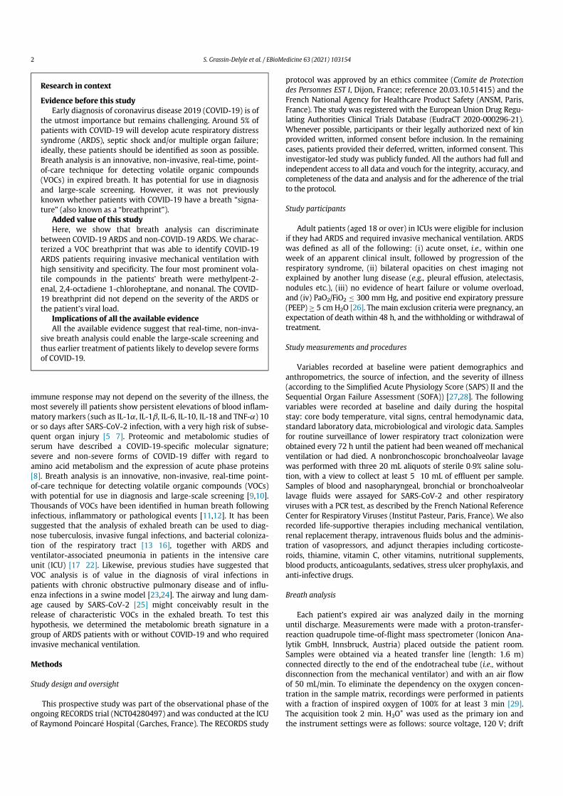
immune response may not depend on the severity of the illness, themost severely ill patients show persistent elevations of blood inflam-matory markers (such as IL-1a, IL-1b, IL-6, IL-10, IL-18 and TNF-a) 10or so days after SARS-CoV-2 infection, with a very high risk of subse-quent organ injury [57]. Proteomic and metabolomic studies ofserum have described a COVID-19-specific molecular signature;severe and non-severe forms of COVID-19 differ with regard toamino acid metabolism and the expression of acute phase proteins[8]. Breath analysis is an innovative, non-invasive, real-time point-of-care technique for detecting volatile organic compounds (VOCs)with potential for use in diagnosis and large-scale screening [9,10].Thousands of VOCs have been identified in human breath followinginfectious, inflammatory or pathological events [11,12]. It has beensuggested that the analysis of exhaled breath can be used to diag-nose tuberculosis, invasive fungal infections, and bacterial coloniza-tion of the respiratory tract [1316], together with ARDS andventilator-associated pneumonia in patients in the intensive careunit (ICU) [1722]. Likewise, previous studies have suggested thatVOC analysis is of value in the diagnosis of viral infections inpatients with chronic obstructive pulmonary disease and of influ-enza infections in a swine model [23,24]. The airway and lung dam-age caused by SARS-CoV-2 [25] might conceivably result in therelease of characteristic VOCs in the exhaled breath. To test thishypothesis, we determined the metabolomic breath signature in agroup of ARDS patients with or without COVID-19 and who requiredinvasive mechanical ventilation.

Methods

Study design and oversight

This prospective study was part of the observational phase of theongoing RECORDS trial (NCT04280497) and was conducted at the ICUof Raymond Poincare Hospital (Garches, France). The RECORDS study

protocol was approved by an ethics commitee (Comite de Protectiondes Personnes EST I, Dijon, France; reference 20.03.10.51415) and theFrench National Agency for Healthcare Product Safety (ANSM, Paris,France). The study was registered with the European Union Drug Regu-lating Authorities Clinical Trials Database (EudraCT 2020-000296-21).Whenever possible, participants or their legally authorized next of kinprovided written, informed consent before inclusion. In the remainingcases, patients provided their deferred, written, informed consent. Thisinvestigator-led study was publicly funded. All the authors had full andindependent access to all data and vouch for the integrity, accuracy, andcompleteness of the data and analysis and for the adherence of the trialto the protocol.

Study participants

Adult patients (aged 18 or over) in ICUs were eligible for inclusionif they had ARDS and required invasive mechanical ventilation. ARDSwas defined as all of the following: (i) acute onset, i.e., within oneweek of an apparent clinical insult, followed by progression of therespiratory syndrome, (ii) bilateral opacities on chest imaging notexplained by another lung disease (e.g., pleural effusion, atelectasis,nodules etc.), (iii) no evidence of heart failure or volume overload,and (iv) PaO2/FiO2 300 mm Hg, and positive end expiratory pressure(PEEP) 5 cm H2O [26]. The main exclusion criteria were pregnancy, anexpectation of death within 48 h, and the withholding or withdrawal oftreatment.

Study measurements and procedures

Variables recorded at baseline were patient demographics andanthropometrics, the source of infection, and the severity of illness(according to the Simplified Acute Physiology Score (SAPS) II and theSequential Organ Failure Assessment (SOFA)) [27,28]. The followingvariables were recorded at baseline and daily during the hospitalstay: core body temperature, vital signs, central hemodynamic data,standard laboratory data, microbiological and virologic data. Samplesfor routine surveillance of lower respiratory tract colonization wereobtained every 72 h until the patient had been weaned off mechanicalventilation or had died. A nonbronchoscopic bronchoalveolar lavagewas performed with three 20 mL aliquots of sterile 0¢9% saline solu-tion, with a view to collect at least 510 mL of effluent per sample.Samples of blood and nasopharyngeal, bronchial or bronchoalveolarlavage fluids were assayed for SARS-CoV-2 and other respiratoryviruses with a PCR test, as described by the French National ReferenceCenter for Respiratory Viruses (Institut Pasteur, Paris, France). We alsorecorded life-supportive therapies including mechanical ventilation,renal replacement therapy, intravenous fluids bolus and the adminis-tration of vasopressors, and adjunct therapies including corticoste-roids, thiamine, vitamin C, other vitamins, nutritional supplements,blood products, anticoagulants, sedatives, stress ulcer prophylaxis, andanti-infective drugs.

Breath analysis

Each patient’s expired air was analyzed daily in the morninguntil discharge. Measurements were made with a proton-transfer-reaction quadrupole time-of-flight mass spectrometer (Ionicon Ana-lytik GmbH, Innsbruck, Austria) placed outside the patient room.Samples were obtained via a heated transfer line (length: 1.6 m)connected directly to the end of the endotracheal tube (i.e., withoutdisconnection from the mechanical ventilator) and with an air flowof 50 mL/min. To eliminate the dependency on the oxygen concen-tration in the sample matrix, recordings were performed in patientswith a fraction of inspired oxygen of 100% for at least 3 min [29].The acquisition took 2 min. H3O+ was used as the primary ion andthe instrument settings were as follows: source voltage, 120 V; drift

Research in context

Evidence before this studyEarly diagnosis of coronavirus disease 2019 (COVID-19) is of

the utmost importance but remains challenging. Around 5% ofpatients with COVID-19 will develop acute respiratory distresssyndrome (ARDS), septic shock and/or multiple organ failure;ideally, these patients should be identified as soon as possible.Breath analysis is an innovative, non-invasive, real-time, point-of-care technique for detecting volatile organic compounds(VOCs) in expired breath. It has potential for use in diagnosisand large-scale screening. However, it was not previouslyknown whether patients with COVID-19 have a breath “signa-ture” (also known as a “breathprint”).

Added value of this studyHere, we show that breath analysis can discriminate

between COVID-19 ARDS and non-COVID-19 ARDS. We charac-terized a VOC breathprint that was able to identify COVID-19ARDS patients requiring invasive mechanical ventilation withhigh sensitivity and specificity. The four most prominent vola-tile compounds in the patients’ breath were methylpent-2-enal, 2,4-octadiene 1-chloroheptane, and nonanal. The COVID-19 breathprint did not depend on the severity of the ARDS orthe patient’s viral load.

Implications of all the available evidenceAll the available evidence suggest that real-time, non-inva-

sive breath analysis could enable the large-scale screening andthus earlier treatment of patients likely to develop severe formsof COVID-19.

2 S. Grassin-Delyle et al. / EBioMedicine 63 (2021) 103154

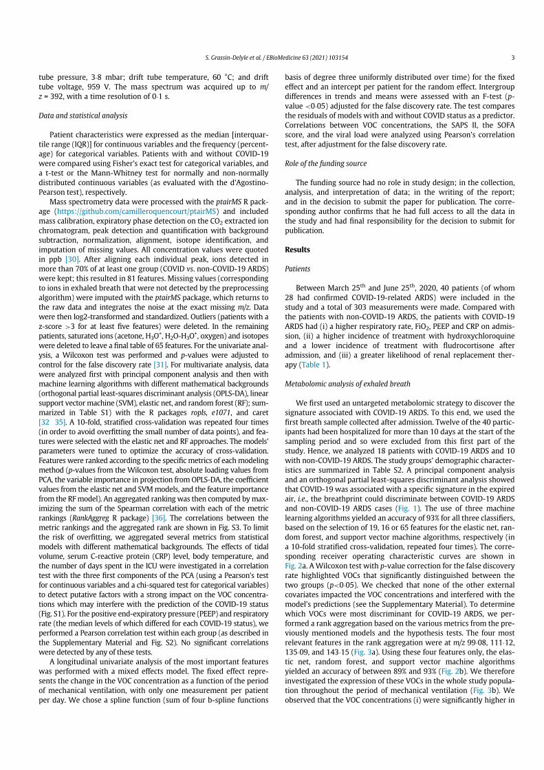
tube pressure, 3¢8 mbar; drift tube temperature, 60 °C; and drifttube voltage, 959 V. The mass spectrum was acquired up to m/z = 392, with a time resolution of 0¢1 s.

Data and statistical analysis

Patient characteristics were expressed as the median [interquar-tile range (IQR)] for continuous variables and the frequency (percent-age) for categorical variables. Patients with and without COVID-19were compared using Fisher’s exact test for categorical variables, anda t-test or the Mann-Whitney test for normally and non-normallydistributed continuous variables (as evaluated with the d'Agostino-Pearson test), respectively.

Mass spectrometry data were processed with the ptairMS R pack-age (https://github.com/camilleroquencourt/ptairMS) and includedmass calibration, expiratory phase detection on the CO2 extracted ionchromatogram, peak detection and quantification with backgroundsubtraction, normalization, alignment, isotope identification, andimputation of missing values. All concentration values were quotedin ppb [30]. After aligning each individual peak, ions detected inmore than 70% of at least one group (COVID vs. non-COVID-19 ARDS)were kept; this resulted in 81 features. Missing values (correspondingto ions in exhaled breath that were not detected by the preprocessingalgorithm) were imputed with the ptairMS package, which returns tothe raw data and integrates the noise at the exact missing m/z. Datawere then log2-transformed and standardized. Outliers (patients with az-score >3 for at least five features) were deleted. In the remainingpatients, saturated ions (acetone, H3O+, H2O-H3O+, oxygen) and isotopeswere deleted to leave a final table of 65 features. For the univariate anal-ysis, a Wilcoxon test was performed and p-values were adjusted tocontrol for the false discovery rate [31]. For multivariate analysis, datawere analyzed first with principal component analysis and then withmachine learning algorithms with different mathematical backgrounds(orthogonal partial least-squares discriminant analysis (OPLS-DA), linearsupport vector machine (SVM), elastic net, and random forest (RF); sum-marized in Table S1) with the R packages ropls, e1071, and caret[3235]. A 10-fold, stratified cross-validation was repeated four times(in order to avoid overfitting the small number of data points), and fea-tures were selected with the elastic net and RF approaches. The models’parameters were tuned to optimize the accuracy of cross-validation.Features were ranked according to the specific metrics of eachmodelingmethod (p-values from the Wilcoxon test, absolute loading values fromPCA, the variable importance in projection fromOPLS-DA, the coefficientvalues from the elastic net and SVMmodels, and the feature importancefrom the RFmodel). An aggregated rankingwas then computed bymax-imizing the sum of the Spearman correlation with each of the metricrankings (RankAggreg R package) [36]. The correlations between themetric rankings and the aggregated rank are shown in Fig. S3. To limitthe risk of overfitting, we aggregated several metrics from statisticalmodels with different mathematical backgrounds. The effects of tidalvolume, serum C-reactive protein (CRP) level, body temperature, andthe number of days spent in the ICU were investigated in a correlationtest with the three first components of the PCA (using a Pearson’s testfor continuous variables and a chi-squared test for categorical variables)to detect putative factors with a strong impact on the VOC concentra-tions which may interfere with the prediction of the COVID-19 status(Fig. S1). For the positive end-expiratory pressure (PEEP) and respiratoryrate (the median levels of which differed for each COVID-19 status), weperformed a Pearson correlation test within each group (as described inthe Supplementary Material and Fig. S2). No significant correlationswere detected by any of these tests.

A longitudinal univariate analysis of the most important featureswas performed with a mixed effects model. The fixed effect repre-sents the change in the VOC concentration as a function of the periodof mechanical ventilation, with only one measurement per patientper day. We chose a spline function (sum of four b-spline functions

basis of degree three uniformly distributed over time) for the fixedeffect and an intercept per patient for the random effect. Intergroupdifferences in trends and means were assessed with an F-test (p-value <0¢05) adjusted for the false discovery rate. The test comparesthe residuals of models with and without COVID status as a predictor.Correlations between VOC concentrations, the SAPS II, the SOFAscore, and the viral load were analyzed using Pearson’s correlationtest, after adjustment for the false discovery rate.

Role of the funding source

The funding source had no role in study design; in the collection,analysis, and interpretation of data; in the writing of the report;and in the decision to submit the paper for publication. The corre-sponding author confirms that he had full access to all the data inthe study and had final responsibility for the decision to submit forpublication.

Results

Patients

Between March 25th and June 25th, 2020, 40 patients (of whom28 had confirmed COVID-19-related ARDS) were included in thestudy and a total of 303 measurements were made. Compared withthe patients with non-COVID-19 ARDS, the patients with COVID-19ARDS had (i) a higher respiratory rate, FiO2, PEEP and CRP on admis-sion, (ii) a higher incidence of treatment with hydroxychloroquineand a lower incidence of treatment with fludrocortisone afteradmission, and (iii) a greater likelihood of renal replacement ther-apy (Table 1).

Metabolomic analysis of exhaled breath

We first used an untargeted metabolomic strategy to discover thesignature associated with COVID-19 ARDS. To this end, we used thefirst breath sample collected after admission. Twelve of the 40 partic-ipants had been hospitalized for more than 10 days at the start of thesampling period and so were excluded from this first part of thestudy. Hence, we analyzed 18 patients with COVID-19 ARDS and 10with non-COVID-19 ARDS. The study groups’ demographic character-istics are summarized in Table S2. A principal component analysisand an orthogonal partial least-squares discriminant analysis showedthat COVID-19 was associated with a specific signature in the expiredair, i.e., the breathprint could discriminate between COVID-19 ARDSand non-COVID-19 ARDS cases (Fig. 1). The use of three machinelearning algorithms yielded an accuracy of 93% for all three classifiers,based on the selection of 19, 16 or 65 features for the elastic net, ran-dom forest, and support vector machine algorithms, respectively (ina 10-fold stratified cross-validation, repeated four times). The corre-sponding receiver operating characteristic curves are shown inFig. 2a. AWilcoxon test with p-value correction for the false discoveryrate highlighted VOCs that significantly distinguished between thetwo groups (p<0¢05). We checked that none of the other externalcovariates impacted the VOC concentrations and interfered with themodel’s predictions (see the Supplementary Material). To determinewhich VOCs were most discriminant for COVID-19 ARDS, we per-formed a rank aggregation based on the various metrics from the pre-viously mentioned models and the hypothesis tests. The four mostrelevant features in the rank aggregation were at m/z 99¢08, 111¢12,135¢09, and 143¢15 (Fig. 3a). Using these four features only, the elas-tic net, random forest, and support vector machine algorithmsyielded an accuracy of between 89% and 93% (Fig. 2b). We thereforeinvestigated the expression of these VOCs in the whole study popula-tion throughout the period of mechanical ventilation (Fig. 3b). Weobserved that the VOC concentrations (i) were significantly higher in

S. Grassin-Delyle et al. / EBioMedicine 63 (2021) 103154 3

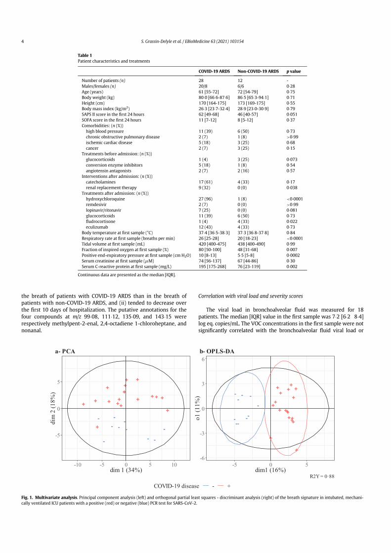
the breath of patients with COVID-19 ARDS than in the breath ofpatients with non-COVID-19 ARDS, and (ii) tended to decrease overthe first 10 days of hospitalization. The putative annotations for thefour compounds at m/z 99¢08, 111¢12, 135¢09, and 143¢15 wererespectively methylpent-2-enal, 2,4-octadiene 1-chloroheptane, andnonanal.

Correlation with viral load and severity scores

The viral load in bronchoalveolar fluid was measured for 18patients. The median [IQR] value in the first sample was 7¢2 [6¢28¢4]log eq. copies/mL. The VOC concentrations in the first sample were notsignificantly correlated with the bronchoalveolar fluid viral load or

Table 1Patient characteristics and treatments

COVID-19 ARDS Non-COVID-19 ARDS p value

Number of patients (n) 28 12 -Males/females (n) 20/8 6/6 0¢28Age (years) 61 [55-72] 72 [54-79] 0¢75Body weight (kg) 80¢0 [66¢6-87¢6] 86¢5 [65¢3-94¢1] 0¢71Height (cm) 170 [164-175] 173 [169-175] 0¢55Body mass index (kg/m2) 26¢3 [23¢7-32¢4] 28¢9 [23¢0-30¢9] 0¢79SAPS II score in the first 24 hours 62 [49-68] 46 [40-57] 0¢051SOFA score in the first 24 hours 11 [7-12] 8 [5-12] 0¢37Comorbidities: (n (%))high blood pressure 11 (39) 6 (50) 0¢73chronic obstructive pulmonary disease 2 (7) 1 (8) >0¢99ischemic cardiac disease 5 (18) 3 (25) 0¢68cancer 2 (7) 3 (25) 0¢15

Treatments before admission: (n (%))glucocorticoids 1 (4) 3 (25) 0¢073conversion enzyme inhibitors 5 (18) 1 (8) 0¢54angiotensin antagonists 2 (7) 2 (16) 0¢57

Interventions after admission: (n (%))catecholamines 17 (61) 4 (33) 0¢17renal replacement therapy 9 (32) 0 (0) 0¢038

Treatments after admission: (n (%))hydroxychloroquine 27 (96) 1 (8) <0¢0001remdesivir 2 (7) 0 (0) >0¢99lopinavir/ritonavir 7 (25) 0 (0) 0¢081glucocorticoids 11 (39) 6 (50) 0¢73fludrocortisone 1 (4) 4 (33) 0¢022eculizumab 12 (43) 4 (33) 0¢73

Body temperature at first sample (°C) 37¢4 [36¢5-38¢3] 37¢3 [36¢8-37¢8] 0¢84Respiratory rate at first sample (breaths per min) 26 [25-28] 20 [18-23] <0¢0001Tidal volume at first sample (mL) 420 [400-475] 438 [400-490] 0¢99Fraction of inspired oxygen at first sample (%) 80 [50-100] 48 [31-68] 0¢007Positive end-expiratory pressure at first sample (cm H2O) 10 [8-13] 5¢5 [5-8] 0¢0002Serum creatinine at first sample (mM) 74 [56-137] 67 [44-86] 0¢30Serum C-reactive protein at first sample (mg/L) 195 [175-268] 76 [23-119] 0¢002

Continuous data are presented as the median [IQR].

Fig. 1. Multivariate analysis. Principal component analysis (left) and orthogonal partial least squares - discriminant analysis (right) of the breath signature in intubated, mechani-cally ventilated ICU patients with a positive (red) or negative (blue) PCR test for SARS-CoV-2.

4 S. Grassin-Delyle et al. / EBioMedicine 63 (2021) 103154

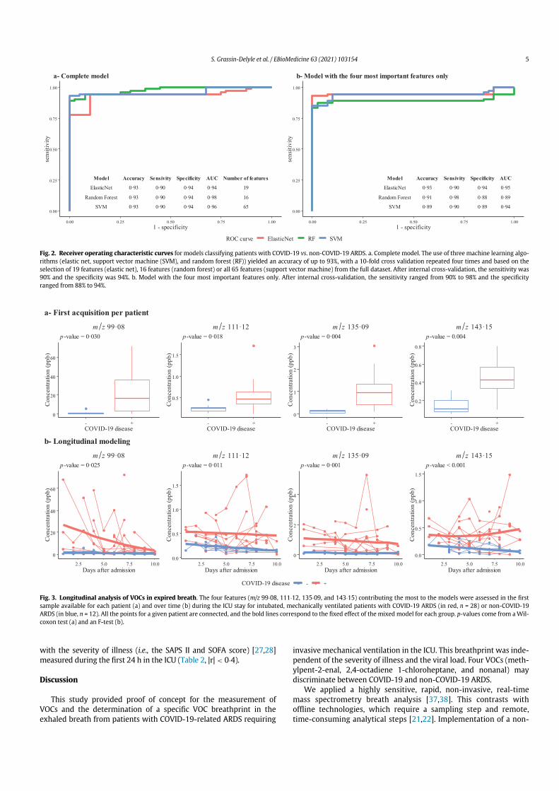
with the severity of illness (i.e., the SAPS II and SOFA score) [27,28]measured during the first 24 h in the ICU (Table 2, |r|< 0¢4).

Discussion

This study provided proof of concept for the measurement ofVOCs and the determination of a specific VOC breathprint in theexhaled breath from patients with COVID-19-related ARDS requiring

invasive mechanical ventilation in the ICU. This breathprint was inde-pendent of the severity of illness and the viral load. Four VOCs (meth-ylpent-2-enal, 2,4-octadiene 1-chloroheptane, and nonanal) maydiscriminate between COVID-19 and non-COVID-19 ARDS.

We applied a highly sensitive, rapid, non-invasive, real-timemass spectrometry breath analysis [37,38]. This contrasts withoffline technologies, which require a sampling step and remote,time-consuming analytical steps [21,22]. Implementation of a non-

Fig. 2. Receiver operating characteristic curves for models classifying patients with COVID-19 vs. non-COVID-19 ARDS. a. Complete model. The use of three machine learning algo-rithms (elastic net, support vector machine (SVM), and random forest (RF)) yielded an accuracy of up to 93%, with a 10-fold cross validation repeated four times and based on theselection of 19 features (elastic net), 16 features (random forest) or all 65 features (support vector machine) from the full dataset. After internal cross-validation, the sensitivity was90% and the specificity was 94%. b. Model with the four most important features only. After internal cross-validation, the sensitivity ranged from 90% to 98% and the specificityranged from 88% to 94%.

Fig. 3. Longitudinal analysis of VOCs in expired breath. The four features (m/z 99¢08, 111¢12, 135¢09, and 143¢15) contributing the most to the models were assessed in the firstsample available for each patient (a) and over time (b) during the ICU stay for intubated, mechanically ventilated patients with COVID-19 ARDS (in red, n = 28) or non-COVID-19ARDS (in blue, n = 12). All the points for a given patient are connected, and the bold lines correspond to the fixed effect of the mixed model for each group. p-values come from aWil-coxon test (a) and an F-test (b).

S. Grassin-Delyle et al. / EBioMedicine 63 (2021) 103154 5

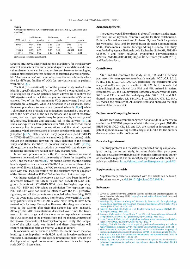
targeted strategy (as described here) is mandatory for the discoveryof novel biomarkers. The subsequent diagnostic validation and clini-cal implementation can be based on less cumbersome technologies,such as mass spectrometers dedicated to targeted analyses or porta-ble “electronic noses” with a set of sensors that are relatively selec-tive for different families of VOCs (as previously used in patientswith ARDS) [20].

The first (cross-sectional) part of the present study enabled us toidentify a specific signature. We then performed a longitudinal analy-sis of expired air in ARDS patients, which allowed us to confirm theVOC signature and to track the changes over time in the VOC concen-trations. Two of the four prominent VOCs (methylpent-2-enal andnonanal) are aldehydes, while 2,4-octadiene is an alkadiene. Thesethree compounds are known to be expressed in breath [39,40], while1-chloroheptane is probably not endogenous. Nonanal is a sub-prod-uct of the destruction of the cell membrane as a result of oxidativestress; reactive oxygen species may be generated by various type ofinflammatory, immune and structural cell in the airways [41]. Instudies of expired air from patients with ARDS, Schubert et al. foundabnormally low isoprene concentrations and Bos et al. reportedabnormally high concentrations of octane, acetaldehyde and 3-meth-ylheptane [21,22]. Differences in study populations (non-COVID-19vs. COVID-19 ARDS) and analytical methods (offline vs. online) mightexplain the differences between the VOCs identified in the presentstudy and those identified in previous studies of ARDS [21,22].Although there may be an association between VOCs and disease, theunderlying biochemistry has not been fully characterized.

In line with previous reports, the VOC concentrations measuredhere were not correlated with the severity of illness (as judged by theSAPS II and the SOFA score) [21]. This finding suggest that the exhaledbreath signature is a marker of COVID-19 per se, rather than of theseverity of illness. Likewise, the VOC concentrations were not corre-lated with viral load, suggesting that this signature may be a markerof the disease related to SARS-CoV-2 rather than of virus carriage.

Our interpretation of the present data may have been limited bydifferences between the COVID-19 and non- COVID-19 ARDS sub-groups. Patients with COVID-19 ARDS cohort had higher respiratoryrate, FiO2, PEEP and CRP values on admission. The respiratory rate,PEEP and CRP were not found to interfere with the VOC predictivesignature, and all the patients were sampled when breathing 100%FiO2 (to avoid mass spectrometry interference by oxygen) [29]. Simi-larly, patients with COVID-19 ARDS were more likely to have beentreated with hydroxychloroquine. However, this drug was adminis-tered to the patients after their first sample had been analyzed.Although the VOC concentrations decreased over time, the treat-ments did not change, and there was no correspondence betweenthe VOCs described in the present study and the molecular masses ofthe known metabolites of hydroxychloroquine. Lastly, the samplesize of this pilot study was limited and these observations willrequire confirmation with an external validation cohort.

In conclusion, we determined a COVID-19-specific breath metabo-lomic signature in patients with ARDS requiring invasive mechanicalventilation. Knowledge of this specific breathprint might enable thedevelopment of rapid, non-invasive, point-of-care tests for large-scale COVID-19 screening.

Acknowledgements

The authors would like to thank all the staff members at the inten-sive care unit at Raymond Poincare Hospital for their collaboration,Professor Marie-Anne Welti and Professor Elyanne Gault for provid-ing virological data, and Dr David Fraser (Biotech CommunicationSARL, Ploudalmezeau, France) for copy-editing assistance. The studywas funded by Agence Nationale de la Recherche (SoftwAiR, ANR-18-CE45-0017 and RHU4 RECORDS, Programme d’Investissementsd’Avenir, ANR-18-RHUS-0004), Region Ile de France (SESAME 2016),and Fondation Foch.

Contributors

S.G.D. and D.A. conceived the study. S.G.D., P.M. and C.R. definedparameters for mass spectrometry breath analysis. S.G.D., G.S., S.C., J.F., H.S., E.N., L-J.C., P.D., P.M., D.A. performed the experiments andanalyzed and/or interpreted results. S.G.D., P.M., N.H., D.A. collectedepidemiological and clinical data. P.M. and N.H. assisted in patientrecruitment. C.R. and E.T. developed software and analyzed the data.S.G.D. and C.R. checked the underlying data. S.G.D., C.R. and D.A.drafted the manuscript. E.T., P.M., P.D., L-J.C., H.S, E.N., G.S., S.C., N.H.,J.F. revised the manuscript. All authors read and approved the finalversion of the manuscript.

Declaration of Competing Interests

DA has received a grant from Agence Nationale de la Recherche toconduct the RECORDS program, of which this study is part (ANR-18-RHUS-0004). S.G.D, C.R., E.T. and D.A. are named as inventors on apatent application covering breath analysis in COVID-19. The authorsdeclare no other conflicts of interest.

Data sharing statement

The study protocol and the datasets generated during and/or ana-lysed during the current study, including deidentified participantdata will be available with publication from the corresponding authoron reasonable request. The ptairMS R package used for data analysis ispublicly available at https://github.com/camilleroquencourt/ptairMS

Supplementary materials

Supplementary material associated with this article can be found,in the online version, at doi:10.1016/j.ebiom.2020.103154.

References

1 COVID-19 Dashboard by the Center for Systems Science and Engineering (CSSE) atJohns Hopkins University (JHU). https://coronavirus.jhu.edu/map.html (accessedOctober 19th, 2020).

2 Wiersinga WJ, Rhodes A, Cheng AC, Peacock SJ, Prescott HC. Pathophysiology,transmission, diagnosis, and treatment of coronavirus disease 2019 (COVID-19): areview. JAMA 2020;324(8):782–93.

3 Beigel JH, Tomashek KM, Dodd LE, et al. Remdesivir for the treatment of COVID-19 -final report. N Engl J Med 2020.

4 Recovery_Collaborative_Group, Horby P, LimWS, et al. Dexamethasone in hospital-ized patients with COVID-19 - preliminary report. N Engl J Med 2020.

5 Lucas C, Wong P, Klein J, et al. Longitudinal analyses reveal immunological misfir-ing in severe COVID-19. Nature 2020;584(7821):463–9.

6 Hadjadj J, Yatim N, Barnabei L, et al. Impaired type I interferon activity and inflam-matory responses in severe COVID-19 patients. Science 2020;369(6504):718–24.

7 Kuri-Cervantes L, Pampena MB, Meng W, et al. Comprehensive mapping ofimmune perturbations associated with severe COVID-19. Sci Immunol 2020;5(49).

8 Shen B, Yi X, Sun Y, et al. Proteomic and metabolomic characterization of COVID-19patient sera. Cell 2020;182(1) 59-72 e15.

9 Kataoka H, Saito K, Kato H, Masuda K. Noninvasive analysis of volatile biomarkersin human emanations for health and early disease diagnosis. Bioanalysis 2013;5(11):1443–59.

Table 2Correlations between VOC concentrations and the SAPS II, SOFA score andviral load.

SAPS II score SOFA score Viral loadVOC (m/z) r p-value r p-value r p-value

99¢08 0¢04 0¢88 0¢36 0¢13 0¢08 0¢70111¢12 0¢02 0¢93 0¢28 0¢25 -0¢14 0¢48135¢09 0¢05 0¢85 0¢35 0¢14 -0¢0004 1¢00143¢15 0¢12 0¢62 0¢27 0¢25 -0¢23 0¢24

r: Pearson's correlation coefficient.

6 S. Grassin-Delyle et al. / EBioMedicine 63 (2021) 103154

10 Rattray NJ, Hamrang Z, Trivedi DK, Goodacre R, Fowler SJ. Taking your breath away:metabolomics breathes life in to personalized medicine. Trends Biotechnol 2014;32(10):538–48.

11 Amann A, de Lacy Costello B, Miekisch W, et al. The human volatilome: volatileorganic compounds (VOCs) in exhaled breath, skin emanations, urine, feces andsaliva. J Breath Res 2014;8(3):034001.

12 de Lacy Costello B, Amann A, Al-Kateb H, et al. A review of the volatiles from thehealthy human body. J Breath Res 2014;8(1):014001.

13 Koo S, Thomas HR, Daniels SD, et al. A breath fungal secondary metabolite signa-ture to diagnose invasive aspergillosis. Clin Infect Dis 2014;59(12):1733–40.

14 Nakhleh MK, Jeries R, Gharra A, et al. Detecting active pulmonary tuberculosiswith a breath test using nanomaterial-based sensors. Eur Respir J 2014;43(5):1522–5.

15 Coronel Teixeira R, Rodriguez M, Jimenez de Romero N, et al. The potential of a por-table, point-of-care electronic nose to diagnose tuberculosis. J Infect 2017;75(5):441–7.

16 Suarez-Cuartin G, Giner J, Merino JL, et al. Identification of pseudomonas aerugi-nosa and airway bacterial colonization by an electronic nose in bronchiectasis.Respir Med 2018;136:111–7.

17 Schnabel R, Fijten R, Smolinska A, et al. Analysis of volatile organic compounds inexhaled breath to diagnose ventilator-associated pneumonia. Sci Rep 2015;5:17179.

18 Filipiak W, Beer R, Sponring A, et al. Breath analysis for in vivo detection of patho-gens related to ventilator-associated pneumonia in intensive care patients: a pro-spective pilot study. J Breath Res 2015;9(1):016004.

19 Schnabel RM, BoumansML, Smolinska A, et al. Electronic nose analysis of exhaled breathto diagnose ventilator-associated pneumonia. Respir Med 2015;109(11):1454–9.

20 Bos LD, Schultz MJ, Sterk PJ. Exhaled breath profiling for diagnosing acute respira-tory distress syndrome. BMC Pulm Med 2014;14:72.

21 Bos LD, Weda H, Wang Y, et al. Exhaled breath metabolomics as a noninvasivediagnostic tool for acute respiratory distress syndrome. Eur Respir J 2014;44(1):188–97.

22 Schubert JK, Muller WP, Benzing A, Geiger K. Application of a new method for anal-ysis of exhaled gas in critically ill patients. Intensive Care Med 1998;24(5):415–21.

23 van Geffen WH, Bruins M, Kerstjens HA. Diagnosing viral and bacterial respiratoryinfections in acute COPD exacerbations by an electronic nose: a pilot study. J BreathRes 2016;10(3):036001.

24 Traxler S, Bischoff AC, Sass R, et al. VOC breath profile in spontaneously breathingawake swine during Influenza A infection. Sci Rep 2018;8(1):14857.

25 Ackermann M, Verleden SE, Kuehnel M, et al. Pulmonary vascular endothelialitis,thrombosis, and angiogenesis in COVID-19. N Engl J Med 2020;383(2):120–8.

26 Force ADT, Ranieri VM, Rubenfeld GD, et al. Acute respiratory distress syndrome:the Berlin definition. JAMA 2012;307(23):2526–33.

27 Le Gall JR, Lemeshow S, Saulnier F. A new simplified acute physiology score (SAPSII) based on a European/North American multicenter study. JAMA 1993;270(24):2957–63.

28 Vincent JL, Moreno R, Takala J, et al. The SOFA (sepsis-related organ failure assess-ment) score to describe organ dysfunction/failure. On behalf of the working groupon sepsis-related problems of the european society of intensive care medicine.Intensive Care Med 1996;22(7):707–10.

29 Trefz P, Pugliese G, Brock B, Schubert JK, Miekisch W. Effects of elevated oxygenlevels on VOC analysis by means of PTR-ToF-MS. J Breath Res 2019;13(4):046004.

30 Hansel A, Jordan A, Holzinger R, Prazeller P, Vogel W, Lindinger W. Proton transferreaction mass spectrometry: on-line trace gas analysis at the ppb level. Int J MassSpectrom Ion Process 1995;149-150:609–19.

31 Benjamini Y, Hochberg Y. Controlling the false discovery rate: a practical and pow-erful approach to multiple testing. J R Stat Soc Ser B 1995;57(1):289–300.

32 Breiman L. Random forests. Machine Learning 2001;45(1):5–32.33 Thevenot EA, Roux A, Xu Y, Ezan E, Junot C. Analysis of the human adult urinary

metabolome variations with age, body mass index, and gender by implementing acomprehensive workflow for univariate and OPLS statistical analyses. J ProteomeRes 2015;14(8):3322–35.

34 Weston J, Mukherjee S, Chapelle O, Pontil M, Poggio T, Vapnik V. Feature selectionfor SVMs. Adv Neural Inform Process Syst 2000;13.

35 Zou H, Hastie T. Regularization and variable selection via the elastic net. J R Stat SocSer B 2005;67(2):301–20.

36 Pihur V, Datta S, Datta S. RankAggreg, an R package for weighted rank aggregation.BMC Bioinformatics 2009;10:62.

37 Trefz P, Schmidt M, Oertel P, et al. Continuous real time breath gas monitoring inthe clinical environment by proton-transfer-reaction-time-of-flight-mass spec-trometry. Anal Chem 2013;85(21):10321–9.

38 Brock B, Kamysek S, Silz J, Trefz P, Schubert JK, Miekisch W. Monitoring of breathVOCs and electrical impedance tomography under pulmonary recruitment inmechanically ventilated patients. J Breath Res 2017;11(1):016005.

39 van de Kant KD, van Berkel JJ, Jobsis Q, et al. Exhaled breath profiling in diagnosingwheezy preschool children. Eur Respir J 2013;41(1):183–8.

40 Corradi M, Pignatti P, Manini P, et al. Comparison between exhaled and sputumoxidative stress biomarkers in chronic airway inflammation. Eur Respir J 2004;24(6):1011–7.

41 Rahman I. Oxidative stress, chromatin remodeling and gene transcription ininflammation and chronic lung diseases. J BiochemMol Biol 2003;36(1):95–109.

S. Grassin-Delyle et al. / EBioMedicine 63 (2021) 103154 7

134

Bibliography

Anton Amann, Ben de Lacy Costello, Wolfram Miekisch, Jochen Schubert, Bogusław Buszewski,Joachim Pleil, Norman Ratcliffe, and Terence Risby. The human volatilome: volatile or-ganic compounds (VOCs) in exhaled breath, skin emanations, urine, feces and saliva.Journal of Breath Research, 8(3):034001, June 2014. ISSN 1752-7155, 1752-7163. doi: 10.1088/1752-7155/8/3/034001. URL http://stacks.iop.org/1752-7163/8/i=3/a=034001?key=crossref.6e7280a35b5e0d4fb0ad16f618f47439.

Martin Andersson. A comparison of nine pls1 algorithms. Journal of Chemometrics, 23:518 – 529,10 2009. doi: 10.1002/cem.1248.Charles E Antoniak. Mixtures of dirichlet processes with applications to bayesian nonparametricproblems. The annals of statistics, pages 1152–1174, 1974.N. Aronszajn. Theory of reproducing kernels. Transactions of the American Mathematical Society,68(3):337–404, 1950. ISSN 00029947. URL http://www.jstor.org/stable/1990404.Manor Askenazi, Hisham Ben Hamidane, and Johannes Graumann. The arc of Mass Spectrom-etry Exchange Formats is long, but it bends toward HDF5: plain HDF5 as amass spectrometryexchange format. Mass Spectrometry Reviews, 36(5):668–673, September 2017. ISSN 02777037.doi: 10.1002/mas.21522. URL https://onlinelibrary.wiley.com/doi/10.1002/mas.21522.Sung-June Baek, Aaron Park, Young-Jin Ahn, and Jaebum Choo. Baseline correction using asym-metrically reweighted penalized least squares smoothing. The Analyst, 140(1):250–257, 2015.ISSN 0003-2654, 1364-5528. doi: 10.1039/C4AN01061B. URL http://xlink.rsc.org/?DOI=C4AN01061B.

Amel Bajtarevic, Clemens Ager, Martin Pienz, Martin Klieber, Konrad Schwarz, Magdalena Ligor,Tomasz Ligor, Wojciech Filipiak, Hubert Denz, Michael Fiegl, Wolfgang Hilbe, Wolfgang Weiss,Peter Lukas, Herbert Jamnig, Martin Hackl, Alfred Haidenberger, Bogusław Buszewski, Wol-fram Miekisch, Jochen Schubert, and Anton Amann. Noninvasive detection of lung cancerby analysis of exhaled breath. BMC Cancer, 9(1):348, December 2009. ISSN 1471-2407. doi:10.1186/1471-2407-9-348. URL http://bmccancer.biomedcentral.com/articles/10.1186/1471-2407-9-348.

Eric Barat, Claude Comtat, Thomas Dautremer, Thierry Montagu, and Regine Trebossen. A non-parametric bayesian approach for PET reconstruction. In 2007 IEEE Nuclear Science Sympo-sium Conference Record, pages 4155–4162, Honolulu, HI, USA, 2007a. IEEE. ISBN 978-1-4244-0922-8. doi: 10.1109/NSSMIC.2007.4437035. URL http://ieeexplore.ieee.org/document/4437035/.

135

Eric Barat, Thomas Dautremer, and Thierry Montagu. Nonparametric bayesian inference in nu-clear spectrometry. In 2007 IEEE Nuclear Science Symposium Conference Record, pages 880–887,Honolulu, HI, USA, October 2007b. IEEE. ISBN 978-1-4244-0922-8 978-1-4244-0923-5. doi: 10.1109/NSSMIC.2007.4436469. URL http://ieeexplore.ieee.org/document/4436469/. ISSN:1082-3654.

Elettra Barberis, Elia Amede, Shahzaib Khoso, Luigi Castello, Pier Paolo Sainaghi, Mattia Bellan,Piero Emilio Balbo, Giuseppe Patti, Diego Brustia, Mara Giordano, Roberta Rolla, AnnalisaChiocchetti, Giorgia Romani, Marcello Manfredi, and Rosanna Vaschetto. Metabolomics di-agnosis of covid-19 from exhaled breath condensate. Metabolites, 11(12), 2021. ISSN 2218-1989.doi: 10.3390/metabo11120847. URL https://www.mdpi.com/2218-1989/11/12/847.Matthew Barker and William Rayens. Partial least squares for discrimination. Journal ofChemometrics, 17(3):166–173, 2003. doi: https://doi.org/10.1002/cem.785. URL https://analyticalsciencejournals.onlinelibrary.wiley.com/doi/abs/10.1002/cem.785.

J Beauchamp. Inhaled today, not gone tomorrow: pharmacokinetics and environmental expo-sure of volatiles in exhaled breath. 5(3):037103, jun 2011. doi: 10.1088/1752-7155/5/3/037103.URL https://doi.org/10.1088/1752-7155/5/3/037103.Jens Behrmann, Christian Etmann, Tobias Boskamp, Rita Casadonte, Jörg Kriegsmann, and PeterMaab. Deep learning for tumor classification in imaging mass spectrometry. Bioinformatics,34(7):1215–1223, 11 2017. ISSN 1367-4803. doi: 10.1093/bioinformatics/btx724. URL https://doi.org/10.1093/bioinformatics/btx724.

Yoav Benjamini and Yosef Hochberg. Controlling the false discovery rate - a practical and pow-erful approach to multiple testing. J. Royal Statist. Soc., Series B, 57:289 – 300, 11 1995. doi:10.2307/2346101.

Gérard Biau and Erwan Scornet. A random forest guided tour. TEST, 25, 11 2015. doi: 10.1007/s11749-016-0481-7.

Robert S. Blake, ChristopherWhyte, Ceri O. Hughes, AndrewM. Ellis, and Paul S. Monks. Demon-stration of Proton-Transfer Reaction Time-of-Flight Mass Spectrometry for Real-Time Analysisof Trace Volatile Organic Compounds. Analytical Chemistry, 76(13):3841–3845, July 2004. ISSN0003-2700, 1520-6882. doi: 10.1021/ac0498260. URL https://pubs.acs.org/doi/10.1021/ac0498260.

Kaatje Bollaerts, Paul H. C. Eilers, and Iven Mechelen. Simple and multiple P-splines regressionwith shape constraints. British Journal of Mathematical and Statistical Psychology, 59(2):451–469,November 2006. ISSN00071102. doi: 10.1348/000711005X84293. URL http://doi.wiley.com/10.1348/000711005X84293.

Agnes W. Boots, Lieuwe D. Bos, Marc P. van der Schee, Frederik-Jan van Schooten, andPeter J. Sterk. Exhaled Molecular Fingerprinting in Diagnosis and Monitoring: Validat-ing Volatile Promises. Trends in Molecular Medicine, 21(10):633–644, October 2015. ISSN14714914. doi: 10.1016/j.molmed.2015.08.001. URL https://linkinghub.elsevier.com/retrieve/pii/S1471491415001574.

Lieuwe Bos, Marcus Schultz, and Peter Sterk. Exhaled breath profiling for diagnosing acuterespiratory distress syndrome. BMC pulmonary medicine, 14:72, 04 2014a. doi: 10.1186/

136

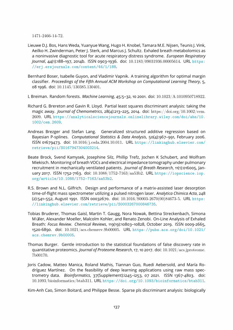
1471-2466-14-72.Lieuwe D.J. Bos, HansWeda, YuanyueWang, Hugo H. Knobel, TamaraM.E. Nijsen, Teunis J. Vink,Aeilko H. Zwinderman, Peter J. Sterk, and Marcus J. Schultz. Exhaled breath metabolomics asa noninvasive diagnostic tool for acute respiratory distress syndrome. European RespiratoryJournal, 44(1):188–197, 2014b. ISSN 0903-1936. doi: 10.1183/09031936.00005614. URL https://erj.ersjournals.com/content/44/1/188.

Bernhard Boser, Isabelle Guyon, and Vladimir Vapnik. A training algorithm for optimal marginclassifier. Proceedings of the Fifth Annual ACM Workshop on Computational Learning Theory, 5,08 1996. doi: 10.1145/130385.130401.L Breiman. Random forests. Machine Learning, 45:5–32, 10 2001. doi: 10.1023/A:1010950718922.Richard G. Brereton and Gavin R. Lloyd. Partial least squares discriminant analysis: taking themagic away. Journal of Chemometrics, 28(4):213–225, 2014. doi: https://doi.org/10.1002/cem.

2609. URL https://analyticalsciencejournals.onlinelibrary.wiley.com/doi/abs/10.1002/cem.2609.

Andreas Brezger and Stefan Lang. Generalized structured additive regression based onBayesian P-splines. Computational Statistics & Data Analysis, 50(4):967–991, February 2006.ISSN 01679473. doi: 10.1016/j.csda.2004.10.011. URL https://linkinghub.elsevier.com/retrieve/pii/S0167947304003214.

Beate Brock, Svend Kamysek, Josephine Silz, Phillip Trefz, Jochen K Schubert, and WolframMiekisch. Monitoring of breath VOCs and electrical impedance tomography under pulmonaryrecruitment in mechanically ventilated patients. Journal of Breath Research, 11(1):016005, Jan-uary 2017. ISSN 1752-7163. doi: 10.1088/1752-7163/aa53b2. URL https://iopscience.iop.org/article/10.1088/1752-7163/aa53b2.

R.S. Brown and N.L. Gilfrich. Design and performance of a matrix-assisted laser desorptiontime-of-flight mass spectrometer utilizing a pulsed nitrogen laser. Analytica Chimica Acta, 248(2):541–552, August 1991. ISSN 00032670. doi: 10.1016/S0003-2670(00)84673-5. URL https://linkinghub.elsevier.com/retrieve/pii/S0003267000846735.

Tobias Bruderer, Thomas Gaisl, Martin T. Gaugg, Nora Nowak, Bettina Streckenbach, SimonaMüller, Alexander Moeller, Malcolm Kohler, and Renato Zenobi. On-Line Analysis of ExhaledBreath: Focus Review. Chemical Reviews, 119(19):10803–10828, October 2019. ISSN 0009-2665,1520-6890. doi: 10.1021/acs.chemrev.9b00005. URL https://pubs.acs.org/doi/10.1021/acs.chemrev.9b00005.

Thomas Burger. Gentle introduction to the statistical foundations of false discovery rate inquantitative proteomics. Journal of Proteome Research, 17, 10 2017. doi: 10.1021/acs.jproteome.7b00170.

Joris Cadow, Matteo Manica, Roland Mathis, Tiannan Guo, Ruedi Aebersold, and María Ro-dríguez Martínez. On the feasibility of deep learning applications using raw mass spec-trometry data. Bioinformatics, 37(Supplement):i245–i253, 07 2021. ISSN 1367-4803. doi:10.1093/bioinformatics/btab311. URL https://doi.org/10.1093/bioinformatics/btab311.

Kim-Anh Cao, Simon Boitard, and Philippe Besse. Sparse pls discriminant analysis: biologically

137

relevant feature selection and graphical displays for multiclass problems. BMC bioinformatics,12:253, 06 2011. doi: 10.1186/1471-2105-12-253.Luca Cappellin, Franco Biasioli, Alessandra Fabris, Erna Schuhfried, Christos Soukoulis,Tilmann D. Märk, and Flavia Gasperi. Improved mass accuracy in PTR-TOF-MS: Anotherstep towards better compound identification in PTR-MS. International Journal of Mass Spec-trometry, 290(1):60–63, February 2010. ISSN 13873806. doi: 10.1016/j.ijms.2009.11.007. URLhttps://linkinghub.elsevier.com/retrieve/pii/S1387380609003571.

Luca Cappellin, Franco Biasioli, Pablo M. Granitto, Erna Schuhfried, Christos Soukoulis, Fab-rizio Costa, Tilmann D. Märk, and Flavia Gasperi. On data analysis in PTR-TOF-MS: Fromraw spectra to data mining. Sensors and Actuators B: Chemical, 155(1):183–190, July 2011a.ISSN 09254005. doi: 10.1016/j.snb.2010.11.044. URL https://linkinghub.elsevier.com/retrieve/pii/S0925400510009135.

Luca Cappellin, Michael Probst, Limtrakul Jumras, Franco Biasioli, Schuhfried Erna, ChristosSoukoulis, Tilmann Märk, and Flavia Gasperi. Proton transfer reaction rate coefficients be-tween h3o+ and some sulphur compounds. International Journal of Mass Spectrometry, 295:43–48, 07 2011b. doi: 10.1016/j.ijms.2010.06.023.Luca Cappellin, Eugenio Aprea, Pablo Granitto, RonWehrens, Christos Soukoulis, Roberto Viola,Tilmann D. Märk, Flavia Gasperi, and Franco Biasioli. Linking GC-MS and PTR-TOF-MS fin-gerprints of food samples. Chemometrics and Intelligent Laboratory Systems, 118:301–307, Au-gust 2012a. ISSN 01697439. doi: 10.1016/j.chemolab.2012.05.008. URL https://linkinghub.elsevier.com/retrieve/pii/S0169743912001219.

Luca Cappellin, Thomas Karl, Michael Probst, Oksana Ismailova, Paul M. Winkler, ChristosSoukoulis, Eugenio Aprea, Tilmann D. Märk, Flavia Gasperi, and Franco Biasioli. On Quan-titative Determination of Volatile Organic Compound Concentrations Using Proton Trans-fer Reaction Time-of-Flight Mass Spectrometry. Environmental Science & Technology, 46(4):2283–2290, February 2012b. ISSN 0013-936X, 1520-5851. doi: 10.1021/es203985t. URL https://pubs.acs.org/doi/10.1021/es203985t.

Rosamaria Capuano, Iuliia Khomenko, Felicia Grasso, Valeria Messina, Anna Olivieri, Luca Cap-pellin, Roberto Paolesse, Alexandro Catini, Marta Ponzi, Franco Biasioli, and Corrado Natale.Simultaneous proton transfer reaction-mass spectrometry and electronic nose study of thevolatile compounds released by plasmodium falciparum infected red blood cells in vitro. Sci-entific Reports, 9, 08 2019. doi: 10.1038/s41598-019-48732-x.Tian-Lu Chen, Yu Cao, Yinan Zhang, Jiajian Liu, Yuqian Bao, Congrong Wang, Wei Jia, and AihuaZhao. Random forest in clinical metabolomics for phenotypic discrimination and biomarkerselection. Evidence-based complementary and alternative medicine : eCAM, 2013:298183, 02 2013.doi: 10.1155/2013/298183.Xing Chen, Keda Zhang, Zhihong Yin, Mingliang Fang, Weidan Pu, Zhening Liu, Lei Li, PabloSinues, Robert Dallmann, Zhen Zhou, and Xue Li. Online real-time monitoring of exhaledbreath particles reveals unnoticed transport of nonvolatile drugs from blood to breath. An-alytical Chemistry, 93(12):5005–5008, 2021. doi: 10.1021/acs.analchem.1c00509. URL https://doi.org/10.1021/acs.analchem.1c00509. PMID: 33724781.

Travers Ching, Daniel S. Himmelstein, Brett K. Beaulieu-Jones, Alexandr A. Kalinin, Brian T. Do,

138

Gregory P.Way, Enrico Ferrero, Paul-Michael Agapow,Michael Zietz, MichaelM. Hoffman,WeiXie, Gail L. Rosen, Benjamin J. Lengerich, Johnny Israeli, Jack Lanchantin, StephenWoloszynek,Anne E. Carpenter, Avanti Shrikumar, Jinbo Xu, Evan M. Cofer, Christopher A. Lavender, Srini-vas C. Turaga, Amr M. Alexandari, Zhiyong Lu, David J. Harris, Dave DeCaprio, Yanjun Qi,Anshul Kundaje, Yifan Peng, Laura K. Wiley, Marwin H. S. Segler, Simina M. Boca, S. JoshuaSwamidass, Austin Huang, Anthony Gitter, and Casey S. Greene. Opportunities and obsta-cles for deep learning in biology and medicine. Journal of The Royal Society Interface, 15(141):20170387, 2018. doi: 10.1098/rsif.2017.0387. URL https://royalsocietypublishing.org/doi/abs/10.1098/rsif.2017.0387.

Marie Chion, Christine Carapito, and Frédéric Bertrand. Accounting for multiple imputation-induced variability for differential analysis inmass spectrometry-based label-free quantitativeproteomics. 2021. URL https://arxiv.org/abs/2108.07086.J. N. Coles and M. Guilhaus. Resolution limitations from detector pulse width and jitter in a lin-ear orthogonal-acceleration time-of-flight mass spectrometer. Journal of the American Societyfor Mass Spectrometry, 5(8):772–778, August 1994. ISSN 1044-0305, 1879-1123. doi: 10.1016/

1044-0305(94)80010-3. URL http://link.springer.com/10.1016/1044-0305(94)80010-3.Kevin R Coombes, Jr Fritsche, Herbert A, Charlotte Clarke, Jeng-neng Chen, Keith A Baggerly,Jeffrey S Morris, Lian-chun Xiao, Mien-Chie Hung, and Henry M Kuerer. Quality Control andPeak Finding for Proteomics Data Collected from Nipple Aspirate Fluid by Surface-EnhancedLaser Desorption and Ionization. Clinical Chemistry, 49(10):1615–1623, 10 2003. ISSN 0009-9147.doi: 10.1373/49.10.1615. URL https://doi.org/10.1373/49.10.1615.M. Corradi, P. Pignatti, P. Manini, R. Andreoli, M. Goldoni, M. Poppa, G. Moscato, B. Balbi, andA. Mutti. Comparison between exhaled and sputum oxidative stress biomarkers in chronicairway inflammation. European Respiratory Journal, 24(6):1011–1017, 2004. ISSN 0903-1936. doi:

10.1183/09031936.04.00002404. URL https://erj.ersjournals.com/content/24/6/1011.S M Cristescu, H A Gietema, L Blanchet, C L J J Kruitwagen, P Munnik, R J van Klaveren, J W J Lam-mers, L Buydens, F J M Harren, and P Zanen. Screening for emphysema via exhaled volatileorganic compounds. Journal of Breath Research, 5(4):046009, December 2011. ISSN 1752-7155,1752-7163. doi: 10.1088/1752-7155/5/4/046009. URL http://stacks.iop.org/1752-7163/5/i=4/a=046009?key=crossref.c32325fed4ac4e42a95c31b898674471.

I D Currie and M Durban. Flexible smoothing with P-splines: a unified approach. Statis-tical Modelling, 2(4):333–349, December 2002. ISSN 1471-082X, 1477-0342. doi: 10.1191/1471082x02st039ob. URL http://journals.sagepub.com/doi/10.1191/1471082x02st039ob.

Pijush Das, Anirban Roychowdhury, Subhadeep Das, Susanta Roychoudhury, and Sucheta Tri-pathy. sigfeature: Novel significant feature selectionmethod for classification of gene expres-sion data using support vector machine and t statistic. Frontiers in Genetics, 11:247, 2020. ISSN1664-8021. doi: 10.3389/fgene.2020.00247. URL https://www.frontiersin.org/article/10.3389/fgene.2020.00247.

Carl de Boor. A practical guide to splines. 1978.Nicolien C. de Clercq, Tom van den Ende, Andrei Prodan, Mark I. van Berge Henegouwen,Suzanne S. Gisbertz, Sybren L. Meijer, Sandor Schokker, Jacques J.G.H.M. Bergman, Na-dia Haj Mohammad, Jelle P. Ruurda, Richard van Hillegersberg, Stella Mook, Nicole C.T.

139

van Grieken, Tanja D. de Gruijl, Mark Davids, Maarten F. Bijlsma, Maarten C.C.M. Hulshof,Hanneke W.M. Van Laarhoven, and Max Nieuwdorp. Intestinal and tumor microbiomeanalysis combined with metabolomics of the anti-pd-l1 phase ii perfect trial for resectableesophageal adenocarcinoma. Journal of Clinical Oncology, 38(15_suppl):4556–4556, 2020.doi: 10.1200/JCO.2020.38.15\_suppl.4556. URL https://doi.org/10.1200/JCO.2020.38.15_suppl.4556.

E. de Hoffmann and V. Stroobant. Mass Spectrometry: Principles and Applications. Wiley, 2007.ISBN 9780470512135. URL https://books.google.fr/books?id=6D_Zz2cvgvUC.B de Lacy Costello, A Amann, H Al-Kateb, C Flynn, W Filipiak, T Khalid, D Osborne,and N M Ratcliffe. A review of the volatiles from the healthy human body. Jour-nal of Breath Research, 8(1):014001, January 2014. ISSN 1752-7155, 1752-7163. doi: 10.

1088/1752-7155/8/1/014001. URL http://stacks.iop.org/1752-7163/8/i=1/a=014001?key=crossref.b6b6a6911efb2c74c533c2e3a6bae189.

Johan J. de Rooi and Paul H.C. Eilers. Mixture models for baseline estimation. Chemometrics andIntelligent Laboratory Systems, 117:56–60, August 2012. ISSN 01697439. doi: 10.1016/j.chemolab.2011.11.001. URL https://linkinghub.elsevier.com/retrieve/pii/S0169743911002292.

Alexis Delabrière, Ulli M Hohenester, Benoit Colsch, Christophe Junot, François Fenaille, and Eti-enne A Thévenot. proFIA: a data preprocessingworkflow for flow injection analysis coupled tohigh-resolution mass spectrometry. Bioinformatics, 33(23):3767–3775, December 2017. ISSN1367-4803, 1460-2059. doi: 10.1093/bioinformatics/btx458. URL https://academic.oup.com/bioinformatics/article/33/23/3767/3965327.

Eugene Demidenko. Mixed models: Theory and applications. Mixed Models: Theory and Applica-tions, 01 2004. doi: 10.1002/0471728438.Philippe Devillier, Helene Salvator, Emmanuel Naline, Louis-Jean Couderc, and StanislasGrassin-Delyle. Metabolomics in the Diagnosis and Pharmacotherapy of Lung Dis-eases. Current Pharmaceutical Design, 23(14), May 2017. ISSN 13816128. doi: 10.2174/

1381612823666170130155627. URL http://www.eurekaselect.com/149636/article.Corrado Di Natale, Roberto Paolesse, Eugenio Martinelli, and Rosamaria Capuano. Solid-stategas sensors for breath analysis: A review. Analytica chimica acta, 824:1–17, 2014.Paul Dierckx. Curve and Surface Fitting with Splines. page 5, 1995.Natalia Drabińska, Cheryl Flynn, Norman Ratcliffe, Ilaria Belluomo, Antonis Myridakis, OliverGould, Matteo Fois, Amy Smart, Terry Devine, and Benjamin De Lacy Costello. A literaturesurvey of volatiles from the healthy human breath and bodily fluids: the human volatilome.Journal of Breath Research, 15, 03 2021. doi: 10.1088/1752-7163/abf1d0.P. Du, W. A. Kibbe, and S. M. Lin. Improved peak detection in mass spectrum by incor-porating continuous wavelet transform-based pattern matching. Bioinformatics, 22(17):2059–2065, September 2006. ISSN 1367-4803, 1460-2059. doi: 10.1093/bioinformatics/

btl355. URL https://academic.oup.com/bioinformatics/article-lookup/doi/10.1093/bioinformatics/btl355.

Maria Durban, Iain Currie, and Paul Eilers. Using P-splines to smooth two-dimensional Poisson

140

data. page 8, 2002.Bradley Efron, Trevor Hastie, Iain Johnstone, and Rob Tibshirani. Least angle regression” (withdiscussions). The Annals of Statistics, 32, 01 2004.P. Eilers and B Marx. Practical Smoothing: The Joys of P-splines. Cambridge, cambridge universitypress. edition, 2021. URL doi:10.1017/9781108610247.Paul H. C. Eilers and Brian D. Marx. Flexible smoothing with B -splines and penalties. StatisticalScience, 11(2):89–121, May 1996. ISSN 0883-4237. doi: 10.1214/ss/1038425655. URL http://projecteuclid.org/euclid.ss/1038425655.

Paul H C Eilers, Brian D Marx, and Maria Durban. Twenty years of P-splines. page 38, 2015.Reef EinochAmor,MoradK.Nakhleh, OrnaBarash, andHossamHaick. Breath analysis of cancerin the present and the future. European Respiratory Review, 28(152):190002, June 2019. ISSN0905-9180, 1600-0617. doi: 10.1183/16000617.0002-2019. URL http://err.ersjournals.com/lookup/doi/10.1183/16000617.0002-2019.

Andrew M. Ellis and Christopher A. Mayhew. Background, chapter 1, pages 1–23. John Wiley andSons, Ltd, 2014. ISBN 9781118682883. doi: https://doi.org/10.1002/9781118682883.ch1. URLhttps://onlinelibrary.wiley.com/doi/abs/10.1002/9781118682883.ch1.

Mariana Valente Farraia, João Cavaleiro Rufo, Inês Paciência, Francisca Mendes, Luís Delgado,and André Moreira. The electronic nose technology in clinical diagnosis: A systematic review.Porto biomedical journal, 4(4), 2019.Charlotte Feil, Frank Staib, Martin R. Berger, Thorsten Stein, Irene Schmidtmann, Andrea Forster,and Carl Christoph Schimanski. Sniffer dogs can identify lung cancer patients frombreath andurine samples. BMC Cancer, 21, 2021.R. Fernández del Río, M.E. O’Hara, A. Holt, P. Pemberton, T. Shah, T. Whitehouse, and C.A.Mayhew. Volatile Biomarkers in Breath Associated With Liver Cirrhosis — Comparisons ofPre- and Post-liver Transplant Breath Samples. EBioMedicine, 2(9):1243–1250, September 2015.ISSN 23523964. doi: 10.1016/j.ebiom.2015.07.027. URL https://linkinghub.elsevier.com/retrieve/pii/S2352396415300797.

W Filipiak, V Ruzsanyi, P Mochalski, A Filipiak, A Bajtarevic, C Ager, H Denz, W Hilbe, H Jamnig,M Hackl, A Dzien, and A Amann. Dependence of exhaled breath composition on exogenousfactors, smoking habits and exposure to air pollutants. 6(3):036008, aug 2012. doi: 10.1088/1752-7155/6/3/036008. URL https://doi.org/10.1088/1752-7155/6/3/036008.

The ARDS Definition Task Force. Acute Respiratory Distress Syndrome: The Berlin Definition.JAMA, 307(23):2526–2533, 06 2012.Mario Fordellone, Andrea Bellincontro, and Fabio Mencarelli. Partial least squares discriminantanalysis: A dimensionality reduction method to classify hyperspectral data. 06 2018.Maria Franco-Villoria, Massimo Ventrucci, and Håvard Rue. A unified view on bayesian varyingcoefficient models. Electronic Journal of Statistics, 13(2):5334–5359, 2019.Thomas Frenzel, Andreas Miller, and Karl-Heinz Engel. A methodology for automated com-

141

parative analysis of metabolite profiling data. European Food Research and Technology, 216:335–342, 04 2003. doi: 10.1007/s00217-002-0659-y.Andrzej Galecki and Tomasz Burzykowski. Linear Mixed Effects Models Using R. : A Step-by-StepApproach. 03 2013. ISBN 978-1-4614-3899-1. doi: 10.1007/978-1-4614-3900-4.Feng Gan, Guihua Ruan, and Jinyuan Mo. Baseline correction by improved iterative polyno-mial fitting with automatic threshold. Chemometrics and Intelligent Laboratory Systems, 82(1-2):59–65, May 2006. ISSN 01697439. doi: 10.1016/j.chemolab.2005.08.009. URL https://linkinghub.elsevier.com/retrieve/pii/S0169743905001589.

Julian W Gardner and Philip N Bartlett. A brief history of electronic noses. Sensors and ActuatorsB: Chemical, 18(1-3):210–211, 1994.Andrew Gelman, John B. Carlin, Hal S. Stern, and Donald B. Rubin. Bayesian Data Analysis. Chap-man and Hall/CRC, 2nd ed. edition, 2004.Robert C Gentleman, Vincent J Carey, Douglas M Bates, Ben Bolstad, Marcel Dettling, SandrineDudoit, Byron Ellis, Laurent Gautier, Yongchao Ge, Jeff Gentry, Kurt Hornik, Torsten Hothorn,Wolfgang Huber, Stefano Iacus, Rafael Irizarry, Friedrich Leisch, Cheng Li, Martin Maechler,Anthony J Rossini, Gunther Sawitzki, Colin Smith, Gordon Smyth, Luke Tierney, Jean YH Yang,and Jianhua Zhang. Bioconductor: open software development for computational biologyand bioinformatics. Genome Biology, page 16, 2004.Robin Genuer, Jean-Michel Poggi, and Christine Tuleau-Malot. Variable selection using randomforests. Pattern Recognition Letters, 31(14):2225–2236, 2010. ISSN 0167-8655. doi: https://doi.

org/10.1016/j.patrec.2010.03.014. URL https://www.sciencedirect.com/science/article/pii/S0167865510000954.

Quentin Gianetto, Florence Combes, Claire Ramus, Christophe Bruley, Yohann Coute, andThomas Burger. Technical brief calibration plot for proteomics (cp4p): A graphical tool to vi-sually check the assumptions underlying fdr control in quantitative experiments. Proteomics,16, 11 2015. doi: 10.1002/pmic.201500189.Gene H. Golub, Michael Heath, and Grace Wahba. Generalized cross-validation as a methodfor choosing a good ridge parameter. Technometrics, 21(2):215–223, 1979. doi: 10.1080/

00401706.1979.10489751. URL https://www.tandfonline.com/doi/abs/10.1080/00401706.1979.10489751.

Pablo M. Granitto, Cesare Furlanello, Franco Biasioli, and Flavia Gasperi. Recursive featureelimination with random forest for PTR-MS analysis of agroindustrial products. Chemo-metrics and Intelligent Laboratory Systems, 83(2):83–90, September 2006. ISSN 01697439.doi: 10.1016/j.chemolab.2006.01.007. URL https://linkinghub.elsevier.com/retrieve/pii/S0169743906000232.

Stanislas Grassin-Delyle, Camille Roquencourt, Pierre Moine, Gabriel Saffroy, Stanislas Carn,Nicholas Heming, Jérôme Fleuriet, Hélène Salvator, Emmanuel Naline, Louis-Jean Coud-erc, Philippe Devillier, Etienne A. Thévenot, and Djillali Annane. Metabolomics of exhaledbreath in critically ill COVID-19 patients: A pilot study. EBioMedicine, 63:103154, January 2021.ISSN 23523964. doi: 10.1016/j.ebiom.2020.103154. URL https://linkinghub.elsevier.com/retrieve/pii/S2352396420305302.

142

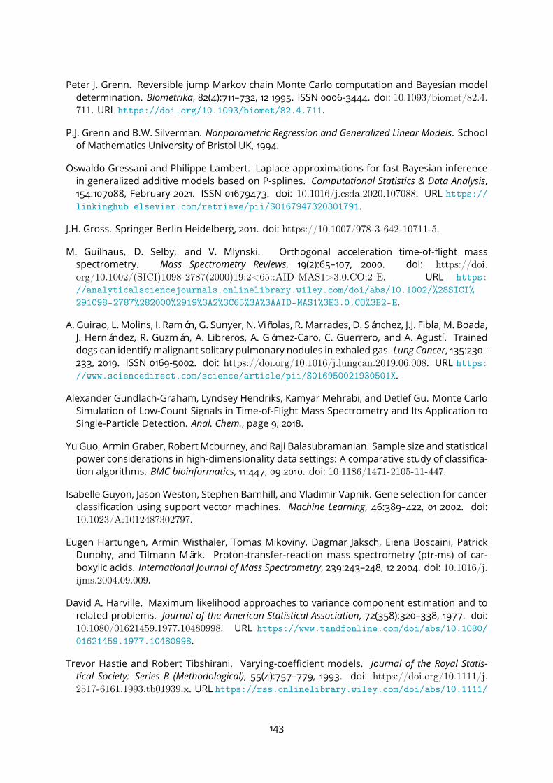
Peter J. Grenn. Reversible jump Markov chain Monte Carlo computation and Bayesian modeldetermination. Biometrika, 82(4):711–732, 12 1995. ISSN 0006-3444. doi: 10.1093/biomet/82.4.711. URL https://doi.org/10.1093/biomet/82.4.711.

P.J. Grenn and B.W. Silverman. Nonparametric Regression and Generalized Linear Models. Schoolof Mathematics University of Bristol UK, 1994.Oswaldo Gressani and Philippe Lambert. Laplace approximations for fast Bayesian inferencein generalized additive models based on P-splines. Computational Statistics & Data Analysis,154:107088, February 2021. ISSN 01679473. doi: 10.1016/j.csda.2020.107088. URL https://linkinghub.elsevier.com/retrieve/pii/S0167947320301791.

J.H. Gross. Springer Berlin Heidelberg, 2011. doi: https://10.1007/978-3-642-10711-5.M. Guilhaus, D. Selby, and V. Mlynski. Orthogonal acceleration time-of-flight massspectrometry. Mass Spectrometry Reviews, 19(2):65–107, 2000. doi: https://doi.

org/10.1002/(SICI)1098-2787(2000)19:2<65::AID-MAS1>3.0.CO;2-E. URL https://analyticalsciencejournals.onlinelibrary.wiley.com/doi/abs/10.1002/%28SICI%291098-2787%282000%2919%3A2%3C65%3A%3AAID-MAS1%3E3.0.CO%3B2-E.

A. Guirao, L. Molins, I. Ramón, G. Sunyer, N. Viñolas, R. Marrades, D. Sánchez, J.J. Fibla, M. Boada,J. Hernández, R. Guzmán, A. Libreros, A. Gómez-Caro, C. Guerrero, and A. Agustí. Traineddogs can identify malignant solitary pulmonary nodules in exhaled gas. Lung Cancer, 135:230–233, 2019. ISSN 0169-5002. doi: https://doi.org/10.1016/j.lungcan.2019.06.008. URL https://www.sciencedirect.com/science/article/pii/S016950021930501X.

Alexander Gundlach-Graham, Lyndsey Hendriks, Kamyar Mehrabi, and Detlef Gu. Monte CarloSimulation of Low-Count Signals in Time-of-Flight Mass Spectrometry and Its Application toSingle-Particle Detection. Anal. Chem., page 9, 2018.Yu Guo, Armin Graber, Robert Mcburney, and Raji Balasubramanian. Sample size and statisticalpower considerations in high-dimensionality data settings: A comparative study of classifica-tion algorithms. BMC bioinformatics, 11:447, 09 2010. doi: 10.1186/1471-2105-11-447.Isabelle Guyon, JasonWeston, Stephen Barnhill, and Vladimir Vapnik. Gene selection for cancerclassification using support vector machines. Machine Learning, 46:389–422, 01 2002. doi:

10.1023/A:1012487302797.Eugen Hartungen, Armin Wisthaler, Tomas Mikoviny, Dagmar Jaksch, Elena Boscaini, PatrickDunphy, and Tilmann Märk. Proton-transfer-reaction mass spectrometry (ptr-ms) of car-boxylic acids. International Journal of Mass Spectrometry, 239:243–248, 12 2004. doi: 10.1016/j.

ijms.2004.09.009.David A. Harville. Maximum likelihood approaches to variance component estimation and torelated problems. Journal of the American Statistical Association, 72(358):320–338, 1977. doi:

10.1080/01621459.1977.10480998. URL https://www.tandfonline.com/doi/abs/10.1080/01621459.1977.10480998.

Trevor Hastie and Robert Tibshirani. Varying-coefficient models. Journal of the Royal Statis-tical Society: Series B (Methodological), 55(4):757–779, 1993. doi: https://doi.org/10.1111/j.2517-6161.1993.tb01939.x. URL https://rss.onlinelibrary.wiley.com/doi/abs/10.1111/

143

j.2517-6161.1993.tb01939.x.Trevor Hastie, Robert Tibshirani, Gavin Sherlock, Michael Eisen, Patrick Brown, and David Bot-stein. Imputing missing data for gene expression arrays. Technical report, Stanford StatisticsDepartment, 1, 12 2001.Joshua Heinemann, Aurélien Mazurie, Monika Tokmina-Lukaszewska, Greg Beilman, and BrianBothner. Application of support vector machines to metabolomics experiments with limitedreplicates. Metabolomics, 10, 12 2014. doi: 10.1007/s11306-014-0651-0.Ben Henderson, Dorota Ruszkiewicz, Maxim Wilkinson, Jonathan Beauchamp, S.M. Cristescu,Stephen Fowler, Dahlia Salman, Fabio Di Francesco, Gudrun Koppen, Jens Langejuergen, OlafHolz, Andria Hadjithekli, Sergi Moreno, Michele Pedrotti, Pablo Sinues, Gitte Slingers, MichaelWilde, Tommaso Lomonaco, Delphine Zanella, and Charles Thomas. A benchmarking proto-col for breath analysis: The peppermint experiment. Journal of Breath Research, 14, 06 2020.doi: 10.1088/1752-7163/aba130.Jens Herbig and Jonathan Beauchamp. Towards standardization in the analysis of breath gasvolatiles. Journal of Breath Research, 8(3):037101, September 2014. ISSN 1752-7155, 1752-7163. doi: 10.1088/1752-7155/8/3/037101. URL http://stacks.iop.org/1752-7163/8/i=3/a=037101?key=crossref.4e3bdba7f2701356e225d9050ae0ae5e.

Jens Herbig, Thorsten Titzmann, Jonathan Beauchamp, Ingrid Kohl, and Armin Hansel. Bufferedend-tidal (BET) sampling—a novel method for real-time breath-gas analysis. Journal ofBreath Research, 2(3):037008, September 2008. ISSN 1752-7155, 1752-7163. doi: 10.1088/1752-7155/2/3/037008. URL http://stacks.iop.org/1752-7163/2/i=3/a=037008?key=crossref.6c1463e66d0714dce9de2a6cfe05bf66.

Jens Herbig, Markus Müller, Simon Schallhart, Thorsten Titzmann, Martin Graus, andArmin Hansel. On-line breath analysis with PTR-TOF. Journal of Breath Research,3(2):027004, June 2009. ISSN 1752-7155, 1752-7163. doi: 10.1088/1752-7155/3/2/027004. URL http://stacks.iop.org/1752-7163/3/i=2/a=027004?key=crossref.cd366040f247a8c9557af6c2233e90f2.

Benjamin Heuclin, Frédéric Mortier, Catherine Trottier, and Marie Denis. Bayesian varying co-efficient model with selection: An application to functional mapping. Journal of the Royal Sta-tistical Society: Series C (Applied Statistics), 70(1):24–50, 2021. doi: https://doi.org/10.1111/rssc.12447. URL https://rss.onlinelibrary.wiley.com/doi/abs/10.1111/rssc.12447.

A. Hoerl and R. Kennard. Ridge regression. In Encyclopedia of Statistical Sciences, 8:129–136, 1988.R. Holzinger. PTRwid: A new widget tool for processing PTR-TOF-MS data. AtmosphericMeasurement Techniques, 8(9):3903–3922, September 2015. ISSN 1867-8548. doi: 10.5194/

amt-8-3903-2015. URL https://www.atmos-meas-tech.net/8/3903/2015/.DONALD R. Hoover, JOHN A. Rice, COLIN O. WU, and LI-PING YANG. Nonparametric smoothingestimates of time-varying coefficient models with longitudinal data. Biometrika, 85(4):809–822, 12 1998. ISSN 0006-3444. doi: 10.1093/biomet/85.4.809. URL https://doi.org/10.1093/biomet/85.4.809.

I. Horvath, Z. Lazar, N. Gyulai, M. Kollai, and G. Losonczy. Exhaled biomarkers in lung cancer.

144

European Respiratory Journal, 34(1):261–275, July 2009. ISSN 0903-1936, 1399-3003. doi: 10.1183/09031936.00142508. URL http://erj.ersjournals.com/cgi/doi/10.1183/09031936.00142508.

Wadah Ibrahim, Michael Wilde, Rebecca Cordell, Dahlia Salman, Dorota Ruszkiewicz, LukeBryant, Matthew Richardson, Robert C Free, Bo Zhao, Ahmed Yousuf, Christobelle White,Richard Russell, Sheila Jones, Bharti Patel, Asia Awal, Rachael Phillips, Graham Fowkes, TeresaMcNally, Clare Foxon, Hetan Bhatt, Rosa Peltrini, Amisha Singapuri, Beverley Hargadon, ToruSuzuki, Leong L Ng, Erol Gaillard, Caroline Beardsmore, Kimuli Ryanna, Hitesh Pandya, TimCoates, Paul S Monks, Neil Greening, Christopher E Brightling, Paul Thomas, and Salman Sid-diqui. Assessment of breath volatile organic compounds in acute cardiorespiratory breath-lessness: a protocol describing a prospective real-world observational study. BMJ Open, 9(3):e025486, March 2019. ISSN 2044-6055, 2044-6055. doi: 10.1136/bmjopen-2018-025486. URLhttps://bmjopen.bmj.com/lookup/doi/10.1136/bmjopen-2018-025486.

Wadah Ibrahim, Rebecca L. Cordell, Michael J. Wilde, Matthew Richardson, Liesl Carr, AnangaSundari Devi Dasi, Beverley Hargadon, Robert C. Free, Paul S. Monks, Christopher E.Brightling, Neil J. Greening, and Salman Siddiqui. Diagnosis of covid-19 by exhaled breathanalysis using gas chromatography–mass spectrometry. ERJ Open Research, 7(3), 2021.doi: 10.1183/23120541.00139-2021. URL https://openres.ersjournals.com/content/7/3/00139-2021.

Ronald Iman. Use of a t-statistic as ah approximation to the exact distribution of the wilcoxonsigned ranks test statistic. Communications in Statistics - Theory and Methods, 3:795–806, 011974. doi: 10.1080/03610927408827178.Alyssa Imbert, Magali Rompais, Mohammed Selloum, Florence Castelli, Emmanuelle Mouton-Barbosa, Marion Brandolini, Emeline Chu-Van, Charlotte Joly, Aurélie Hirschler, PierrickRoger, Thomas Burger, Sophie Leblanc, Tania Sorg, Sadia Ouzia, Yves Vandenbrouck, Clau-dine Médigue, Christophe Junot, Myriam Ferro, Estelle Pujos-Guillot, and Etienne Thévenot.Prometis, deep phenotyping of mouse models by combined proteomics and metabolomicsanalysis. Scientific Data, 8, 12 2021. doi: 10.1038/s41597-021-01095-3.Neal Jeffries. Algorithms for alignment of mass spectrometry proteomic data. Bioinformatics(Oxford, England), 21:3066–73, 08 2005. doi: 10.1093/bioinformatics/bti482.Arlene John, Jishnu Sadasivan, and Chandra Sekhar Seelamantula. Adaptive savitzky-golay fil-tering in non-gaussian noise. IEEE Transactions on Signal Processing, 69:5021–5036, 2021. doi:

10.1109/TSP.2021.3106450.Caroline Johnson, Julijana Ivanisevic, and Gary Siuzdak. Metabolomics: Beyond biomarkers andtowards mechanisms. Nature Reviews Molecular Cell Biology, 17, 03 2016. doi: 10.1038/nrm.

2016.25.A. Jordan, S. Haidacher, G. Hanel, E. Hartungen, L. Märk, H. Seehauser, R. Schottkowsky,P. Sulzer, and T.D. Märk. A high resolution and high sensitivity proton-transfer-reactiontime-of-flight mass spectrometer (PTR-TOF-MS). International Journal of Mass Spectrometry,286(2-3):122–128, September 2009. ISSN 13873806. doi: 10.1016/j.ijms.2009.07.005. URLhttps://linkinghub.elsevier.com/retrieve/pii/S1387380609002371.

A. Jović, K. Brkić, and N. Bogunović. A review of feature selection methods with applications.

145

pages 1200–1205, 2015. doi: 10.1109/MIPRO.2015.7160458.J. Kaiser. Nonrecursive digital filter design using the i-sinh window function. Proceedings of theIEEE, 1977.Edward D. Kantz, Saumya Tiwari, Jeramie D.Watrous, Susan Cheng, andMohit Jain. Deep neuralnetworks for classification of lc-ms spectral peaks. Analytical Chemistry, 91(19):12407–12413,2019. doi: 10.1021/acs.analchem.9b02983. URL https://doi.org/10.1021/acs.analchem.9b02983. PMID: 31483992.

Mikko Katajamaa and Matej Orešič. Data processing for mass spectrometry-basedmetabolomics. Journal of Chromatography A, 1158(1-2):318–328, July 2007. ISSN 00219673.doi: 10.1016/j.chroma.2007.04.021. URL https://linkinghub.elsevier.com/retrieve/pii/S0021967307006966.

Michael G. Kenward and JamesH. Roger. Small sample inference for fixed effects from restrictedmaximum likelihood. Biometrics, 53(3):983–997, 1997. ISSN 0006341X, 15410420. URL http://www.jstor.org/stable/2533558.

Young-Ju KimandChongGu. Smoothing spline gaussian regression: more scalable computationvia efficient approximation. Journal of the Royal Statistical Society: Series B (Statistical Methodol-ogy), 66(2):337–356, 2004. doi: https://doi.org/10.1046/j.1369-7412.2003.05316.x. URL https://rss.onlinelibrary.wiley.com/doi/abs/10.1046/j.1369-7412.2003.05316.x.

Ł. Komsta. Comparison of Several Methods of Chromatographic Baseline Removal with a NewApproach Based on Quantile Regression. Chromatographia, 73(7-8):721–731, April 2011. ISSN0009-5893, 1612-1112. doi: 10.1007/s10337-011-1962-1. URL http://link.springer.com/10.1007/s10337-011-1962-1.

Sophia Koo, Horatio Thomas, S Daniels, Robert Lynch, Sean Fortier, Margaret Shea, PreshiousRearden, James Comolli, Lindsey Baden, and Francisco Marty. A breath fungal secondarymetabolite signature to diagnose invasive aspergillosis. Clinical infectious diseases : an officialpublication of the Infectious Diseases Society of America, 59, 10 2014. doi: 10.1093/cid/ciu725.Quincey Koziol. HDF5. In David Padua, editor, Encyclopedia of Parallel Computing, pages 827–833.Springer US, Boston, MA, 2011. ISBN 978-0-387-09766-4. doi: 10.1007/978-0-387-09766-4_44.URL https://doi.org/10.1007/978-0-387-09766-4_44.Carsten Kuhl, Ralf Tautenhahn, and Steffen Neumann. LC-MS Peak Annotation and Identifica-tion with CAMERA. page 15, 2009.Tien-Chueh Kuo, Cheng-En Tan, San-Yuan Wang, Olivia A Lin, Bo-Han Su, Ming-Tsung Hsu, Jes-sica Lin, Yu-YenCheng, Ciao-Sin Chen, Yu-Chieh Yang, Kuo-Hsing Chen, Shu-Wen Lin, Chao-ChiHo, Ching-Hua Kuo, and Yufeng Jane Tseng. Human Breathomics Database. 2020:8, 2020.Olav Kvalheim, Reidar Arneberg, Bjørn Grung, and Tarja Rajalahti Kvalheim. Determination ofoptimum number of components in partial least squares regression from distributions of theroot-mean-squared error obtained by monte carlo resampling: Determination of optimumnumber of components in pls regression. Journal of Chemometrics, 32:e2993, 01 2018. doi:

10.1002/cem.2993.Nan M. Laird and James H. Ware. Random-Effects Models for Longitudinal Data. Biometrics, 38

146

(4):963, December 1982. ISSN 0006341X. doi: 10.2307/2529876. URL https://www.jstor.org/stable/2529876?origin=crossref.

Eva Lange, Clemens Gröpl, Reinert Knut, Oliver Kohlbacher, and Andreas Hildebrandt. High-accuracy peak picking of proteomics data using wavelet techniques. Pacific Symposiumon Biocomputing. Pacific Symposium on Biocomputing, 11:243–54, 02 2006. doi: 10.1142/9789812701626_0023.

Eva Lange, Clemens Gröpl, Ole Schulz-Trieglaff, Andreas Leinenbach, Christian Huber, and KnutReinert. A geometric approach for the alignment of liquid chromatography—mass spectrom-etry data. Bioinformatics, 23(13):i273–i281, July 2007. ISSN 1460-2059, 1367-4803. doi: 10.1093/bioinformatics/btm209. URL https://academic.oup.com/bioinformatics/article/23/13/i273/233877.

Jean-Roger Le Gall, Stanley Lemeshow, and Fabienne Saulnier. A New Simplified Acute Physi-ology Score (SAPS II) Based on a European/North American Multicenter Study. JAMA, 270(24):2957–2963, 12 1993.Dae-Jin Lee, María Durbán, and Paul Eilers. Efficient two-dimensional smoothing with p-splineanova mixed models and nested bases. Computational Statistics and Data Analysis, 61:22–37,2013. ISSN 0167-9473. doi: https://doi.org/10.1016/j.csda.2012.11.013. URL https://www.sciencedirect.com/science/article/pii/S016794731200415X.

Kyriacos Leptos, David Sarracino, Jacob Jaffe, Bryan Krastins, and George Church. Mapquant:Open-source software for large-scale protein quantification. Proteomics, 6:1770–82, 03 2006.doi: 10.1002/pmic.200500201.Jianbo Li and Riquan Zhang. Penalized spline varying-coefficient single-index model. Communi-cations in Statistics—Simulation and Computation®, 39(2):221–239, 2010.Jingyi Jessica Li and Xin Tong. Statistical hypothesis testing versus machine learning binary clas-sification: Distinctions and guidelines. Patterns, 1(7):100115, 2020.Aikaterini Liangou, Antonios Tasoglou, Heinz J. Huber, Christopher Wistrom, Kevin Brody,Prahlad G Menon, Thomas Bebekoski, Kevin Menschel, Marlise Davidson-Fiedler, Karl De-Marco, Harshad Salphale, Jonathan Wistrom, Skyler Wistrom, and Richard J. Lee. A methodfor the identification of covid-19 biomarkers in human breath using proton transfer reac-tion time-of-flight mass spectrometry. eClinicalMedicine, 42:101207, 2021. ISSN 2589-5370.doi: https://doi.org/10.1016/j.eclinm.2021.101207. URL https://www.sciencedirect.com/science/article/pii/S2589537021004880.

Zaiyou Liu and John B Phillips. Comprehensive two-dimensional gas chromatography using anon-column thermal modulator interface. Journal of Chromatographic Science, 29(6):227–231,1991.Celia Isabel López-Lorente, Mo Awchi, Pablo Sinues, and Diego García-Gómez. Real-time phar-macokinetics via online analysis of exhaled breath. Journal of Pharmaceutical and BiomedicalAnalysis, 205:114311, 2021. ISSN 0731-7085. doi: https://doi.org/10.1016/j.jpba.2021.114311.URL https://www.sciencedirect.com/science/article/pii/S0731708521004222.Benjamin Löser, Alina Grabenschröer, Giovanni Pugliese, Pritam Sukul, Phillip Trefz, Jochen K

147

Schubert, and Wolfram Miekisch. Changes of Exhaled Volatile Organic Compounds in Post-operative Patients Undergoing Analgesic Treatment: A Prospective Observational Study.Metabolites, 10(8):321, August 2020. ISSN 2218-1989. doi: 10.3390/metabo10080321. URLhttps://www.mdpi.com/2218-1989/10/8/321.

Sankar Mahadevan, Sirish L. Shah, Thomas J. Marrie, and Carolyn M. Slupsky. Analysis ofmetabolomic data using support vector machines. Analytical Chemistry, 80(19):7562–7570,2008. doi: 10.1021/ac800954c. URL https://doi.org/10.1021/ac800954c. PMID: 18767870.S. Mallat and S. Zhong. Characterization of signals from multiscale edges. IEEE Transactions onPattern Analysis and Machine Intelligence, 14(7):710–732, 1992. doi: 10.1109/34.142909.H. B. Mann and D. R. Whitney. On a Test of Whether one of Two Random Variables is Stochas-tically Larger than the Other. The Annals of Mathematical Statistics, 18(1):50 – 60, 1947. doi:

10.1214/aoms/1177730491. URL https://doi.org/10.1214/aoms/1177730491.Elena Marchiori, Connie R. Jimenez, Mikkel West-Nielsen, and Niels H. H. Heegaard. Robustsvm-based biomarker selection with noisy mass spectrometric proteomic data. pages 79–90,2006.Pablo Martinez-Lozano Sinues, Malcolm Kohler, and Renato Zenobi. Human breath analysismay support the existence of individual metabolic phenotypes. PLOS ONE, 8(4):1–5, 04 2013.doi: 10.1371/journal.pone.0059909. URL https://doi.org/10.1371/journal.pone.0059909.Brian D Marx. P-spline varying coefficient models for complex data. In Statistical modelling andregression structures, pages 19–43. Springer, 2010.Brian DMarx and Paul H.C Eilers. Multidimensional Penalized Signal Regression. Technometrics,47(1):13–22, February 2005. ISSN 0040-1706, 1537-2723. doi: 10.1198/004017004000000626. URLhttp://www.tandfonline.com/doi/abs/10.1198/004017004000000626.

R Daniel Mauldin, William D Sudderth, and Stanley C Williams. Polya trees and random distri-butions. The Annals of Statistics, pages 1203–1221, 1992.Wolfram Miekisch, Sabine Kischkel, Annika Sawacki, Tina Liebau, Maren Mieth, and Jochen KSchubert. Impact of sampling procedures on the results of breath analysis. Jour-nal of Breath Research, 2(2):026007, June 2008. ISSN 1752-7155, 1752-7163. doi: 10.

1088/1752-7155/2/2/026007. URL http://stacks.iop.org/1752-7163/2/i=2/a=026007?key=crossref.8604809836ce670fcb15d956965e8a96.

WolframMiekisch, Jens Herbig, and Jochen K Schubert. Data interpretation in breath biomarkerresearch: pitfalls and directions. Journal of Breath Research, 6(3):036007, September 2012.ISSN 1752-7155, 1752-7163. doi: 10.1088/1752-7155/6/3/036007. URL http://stacks.iop.org/1752-7163/6/i=3/a=036007?key=crossref.05eaf83b4b4b20424c143d1a0c6701b3.

Miroslav Morháč and Vladislav Matoušek. Peak clipping algorithms for background esti-mation in spectroscopic data. Applied Spectroscopy, 62(1):91–106, 2008. doi: 10.1366/000370208783412762. URL https://doi.org/10.1366/000370208783412762. PMID: 18230214.

M. Müller, M. Graus, T. M. Ruuskanen, R. Schnitzhofer, I. Bamberger, L. Kaser, T. Titzmann,L. Hörtnagl, G. Wohlfahrt, T. Karl, and A. Hansel. First eddy covariance flux measure-ments by ptr-tof. Atmospheric Measurement Techniques, 3(2):387–395, 2010. doi: 10.5194/

148

amt-3-387-2010. URL https://amt.copernicus.org/articles/3/387/2010/.M. Müller, T. Mikoviny, and A. Wisthaler. Detector aging induced mass discrimination and non-linearity effects in PTR-ToF-MS. International Journal of Mass Spectrometry, 365-366:93–97, May2014. ISSN 13873806. doi: 10.1016/j.ijms.2013.12.008. URL https://linkinghub.elsevier.com/retrieve/pii/S1387380613004338.

Markus Müller, Christian George, and Barbara D’Anna. Enhanced spectral analysis of C-TOF Aerosol Mass Spectrometer data: Iterative residual analysis and cumulative peak fit-ting. International Journal of Mass Spectrometry, 306(1):1–8, September 2011. ISSN 13873806.doi: 10.1016/j.ijms.2011.04.007. URL https://linkinghub.elsevier.com/retrieve/pii/S1387380611001576.

Markus Müller, Tomáš Mikoviny, Werner Jud, Barbara D’Anna, and Armin Wisthaler. A newsoftware tool for the analysis of high resolution PTR-TOF mass spectra. Chemometrics and In-telligent Laboratory Systems, 127:158–165, August 2013. ISSN 01697439. doi: 10.1016/j.chemolab.2013.06.011. URL https://linkinghub.elsevier.com/retrieve/pii/S0169743913001275.

Morad Nakhleh, Raneen Jeries Zaher, A’laa Gharra, Anke Binder, Yoav Broza, Mellissa Pascoe,Keertan Dheda, and Hossam Haick. Detecting active pulmonary tuberculosis with a breathtest using nanomaterial-based sensors. The European respiratory journal, 43:1522–1525, 052014. doi: 10.1183/09031936.00019114.Inbar Nardi-Agmon, Manal Abud-Hawa, Ori Liran, Naomi Gai-Mor, Maya Ilouze, Amir Onn, JairBar, Dekel Shlomi, Hossam Haick, and Nir Peled. Exhaled Breath Analysis for MonitoringResponse to Treatment in Advanced Lung Cancer. Journal of Thoracic Oncology, 11(6):827–837, June 2016. ISSN 15560864. doi: 10.1016/j.jtho.2016.02.017. URL https://linkinghub.elsevier.com/retrieve/pii/S1556086416004408.

Titin Agustin Nengsih, Frédéric Bertrand, Myriam Maumy-Bertrand, and Nicolas Meyer. Deter-mining the number of components in pls regression on incomplete data set. Statistical Applica-tions in Genetics andMolecular Biology, 18(6):20180059, 2019. doi: doi:10.1515/sagmb-2018-0059.URL https://doi.org/10.1515/sagmb-2018-0059.Juliane Obermeier, Phillip Trefz, Josephine Happ, Jochen K. Schubert, Hagen Staude, Dagmar-Christiane Fischer, and Wolfram Miekisch. Exhaled volatile substances mirror clinical condi-tions in pediatric chronic kidney disease. PLOS ONE, 12(6):e0178745, June 2017. ISSN 1932-6203. doi: 10.1371/journal.pone.0178745. URL https://dx.plos.org/10.1371/journal.pone.0178745.

Stephen G. Oliver, Michael K. Winson, Douglas B. Kell, and Frank Baganz. Systematic functionalanalysis of the yeast genome. Trends in Biotechnology, 16(9):373–378, 1998. ISSN 0167-7799.doi: https://doi.org/10.1016/S0167-7799(98)01214-1. URL https://www.sciencedirect.com/science/article/pii/S0167779998012141.

H. D. Patterson and R. Thompson. Recovery of inter-block information when block sizes areunequal. Biometrika, 58(3):545–554, 12 1971. ISSN 0006-3444. doi: 10.1093/biomet/58.3.545.URL https://doi.org/10.1093/biomet/58.3.545.Jorge Pereira, Priscilla Porto-Figueira, Carina Cavaco, Khushman Taunk, Srikanth Rapole, RahulDhakne, Hampapathalu Nagarajaram, and José Câmara. Breath Analysis as a Potential and

149

Non-Invasive Frontier in Disease Diagnosis: An Overview. Metabolites, 5(1):3–55, January 2015.ISSN 2218-1989. doi: 10.3390/metabo5010003. URL http://www.mdpi.com/2218-1989/5/1/3.Michael Phillips. Method for the collection and assay of volatile organic compounds inbreath. Analytical Biochemistry, 247(2):272–278, 1997. ISSN 0003-2697. doi: https://doi.

org/10.1006/abio.1997.2069. URL https://www.sciencedirect.com/science/article/pii/S0003269797920698.

Michael Phillips, Joel Greenberg, and Marilu Sabas. Alveolar gradient of pentane in normalhuman breath. Free Radical Research, 20(5):333–337, 1994. doi: 10.3109/10715769409145633.URL https://doi.org/10.3109/10715769409145633. PMID: 8069391.Michael Phillips, Nasser Altorki, John H.M. Austin, Robert B. Cameron, Renee N. Cataneo,Joel Greenberg, Robert Kloss, Roger A. Maxfield, Muhammad I. Munawar, Harvey I. Pass,Asif Rashid, William N. Rom, and Peter Schmitt. Prediction of lung cancer using volatilebiomarkers in breath1. Cancer Biomarkers, 3(2):95–109, April 2007. ISSN 18758592, 15740153.doi: 10.3233/CBM-2007-3204. URL http://www.medra.org/servlet/aliasResolver?alias=iospress&doi=10.3233/CBM-2007-3204.

Michael Phillips, Renee N. Cataneo, Anirudh Chaturvedi, Peter D. Kaplan, Mark Libardoni,Mayur Mundada, Urvish Patel, and Xiang Zhang. Detection of an extended human volatomewith comprehensive two-dimensional gas chromatography time-of-flightmass spectrometry.PLOS ONE, 8(9):null, 09 2013. doi: 10.1371/journal.pone.0075274. URL https://doi.org/10.1371/journal.pone.0075274.

Vincent Picaud, Jean-Francois Giovannelli, Caroline Truntzer, Jean-Philippe Charrier, AudreyGiremus, Pierre Grangeat, and Catherine Mercier. Linear MALDI-ToF simultaneous spectrumdeconvolution and baseline removal. BMC Bioinformatics, 19(1), December 2018. ISSN 1471-2105. doi: 10.1186/s12859-018-2116-3. URL https://bmcbioinformatics.biomedcentral.com/articles/10.1186/s12859-018-2116-3.

Vasyl Pihur, Susmita Datta, and Somnath Datta. Rankaggreg, an r package for weighted rankaggregation. BMC bioinformatics, 10:62, 03 2009. doi: 10.1186/1471-2105-10-62.Pinheiro and Bates. Mixed-Effects Models in S and S-PLUS. 2000.Joachim Pleil, Matthew Stiegel, and Terence Risby. Clinical breath analysis: Discriminatingbetween human endogenous compounds and exogenous (environmental) chemical con-founders. Journal of breath research, 7:017107, 03 2013. doi: 10.1088/1752-7155/7/1/017107.Joachim D Pleil, A Hansel, and Jonathan D Beauchamp. Advances in proton transfer reac-tion mass spectrometry (PTR-MS): applications in exhaled breath analysis, food science,and atmospheric chemistry. Journal of Breath Research, May 2019. ISSN 1752-7155, 1752-7163. doi: 10.1088/1752-7163/ab21a7. URL http://iopscience.iop.org/article/10.1088/1752-7163/ab21a7.

Yotsawat Pomyen, Kwanjeera Wanichthanarak, Patcha Poungsombat, Johannes Fahrmann,Dmitry Grapov, and Sakda Khoomrung. Deep metabolome: Applications of deep learn-ing in metabolomics. Computational and Structural Biotechnology Journal, 18:2818–2825,2020. ISSN 2001-0370. doi: https://doi.org/10.1016/j.csbj.2020.09.033. URL https://www.sciencedirect.com/science/article/pii/S2001037020304177.

150

Cristian Quiroz-Moreno, Mayra Furlan, Joao Belinato, Fabio Augusto, Guilherme Alexandrino,and Noroska Mogollón. Rgcxgc toolbox: An r-package for data processing in comprehensivetwo-dimensional gas chromatography-mass spectrometry.Microchemical Journal, 156:104830,03 2020. doi: 10.1016/j.microc.2020.104830.Irfan Rahman. Oxidative stress, chromatin remodeling and gene transcription in inflammationand chronic lung diseases. Journal of biochemistry and molecular biology, 36:95–109, 02 2003.doi: 10.5483/BMBRep.2003.36.1.095.Ryne C Ramaker, Emily R Gordon, and Sara J Cooper. R2DGC: threshold-free peak alignmentand identification for 2D gas chromatography-mass spectrometry in R. Bioinformatics, 34(10):1789–1791, 12 2017. ISSN 1367-4803. doi: 10.1093/bioinformatics/btx825. URL https://doi.org/10.1093/bioinformatics/btx825.

James Ramsay, Nancy Heckman, and Bernard Silverman. Spline smoothing with model-basedpenalties. Behavior Research Methods, Instruments, Computers, 29:99–106, 01 1996. doi: 10.3758/BF03200573.

Nicholas J.W. Rattray, Zahra Hamrang, Drupad K. Trivedi, Royston Goodacre, and Stephen J.Fowler. Taking your breath away: metabolomics breathes life in to personalized medicine.Trends in Biotechnology, 32(10):538–548, October 2014. ISSN 01677799. doi: 10.1016/j.tibtech.2014.08.003. URL https://linkinghub.elsevier.com/retrieve/pii/S0167779914001632.

Waseem Rawat and Zenghui Wang. Deep convolutional neural networks for image classifica-tion: A comprehensive review. Neural Computation, 29(9):2352–2449, 2017. doi: 10.1162/neco_a_00990.

Nader Rifai, Michael Gillette, and Steven Carr. Protein biomarker discovery and validation: Thelong and uncertain path to clinical utility. Nature biotechnology, 24:971–83, 09 2006. doi: 10.1038/nbt1235.

Philippe Rinaudo, Samia Boudah, Christophe Junot, and Etienne A. Thévenot. biosigner: A NewMethod for the Discovery of Significant Molecular Signatures from Omics Data. Frontiers inMolecular Biosciences, 3, June 2016. ISSN 2296-889X. doi: 10.3389/fmolb.2016.00026. URLhttp://journal.frontiersin.org/Article/10.3389/fmolb.2016.00026/abstract.

LeeD. Roberts, Amanda L. Souza, Robert E. Gerszten, andClary B. Clish. Targetedmetabolomics.Current Protocols in Molecular Biology, 98(1):30.2.1–30.2.24, 2012. doi: https://doi.org/10.1002/0471142727.mb3002s98. URL https://currentprotocols.onlinelibrary.wiley.com/doi/abs/10.1002/0471142727.mb3002s98.

E Rohée, R Coulon, F Carrel, T Dautremer, E Barat, T Montagu, S Normand, and C Jammes.Benchmark of the non-parametric bayesian deconvolution method implemented in the sin-bad code for x/γ rays spectra processing. Nuclear Instruments and Methods in Physics ResearchSection A: Accelerators, Spectrometers, Detectors and Associated Equipment, 836:91–97, 2016.E. Rohée, R. Coulon, F. Carrel, T. Dautremer, E. Barat, T. Montagu, S. Normand, and C. Jammes.Qualitative and quantitative validation of the sinbad code on complex hpge gamma-ray spec-tra. In 2015 4th International Conference on Advancements in Nuclear Instrumentation Measure-ment Methods and their Applications (ANIMMA), pages 1–6, 2015. doi: 10.1109/ANIMMA.2015.

7465517.

151

Camille Roquencourt, Stanislas Grassin Delyle, and Etienne Thévenot. ptairMS: real-time pro-cessing and analysis of PTR-TOF-MS data for biomarker discovery in exhaled breath. Bioinfor-matics, January 2022. doi: 10.1093/bioinformatics/btac031. URL https://doi.org/10.1093/bioinformatics/btac031.

Andreas F. Ruckstuhl, Matthew P. Jacobson, Robert W. Field, and James A. Dodd. Baseline sub-traction using robust local regression estimation. Journal of Quantitative Spectroscopy andRadiative Transfer, 68(2):179–193, January 2001. ISSN 00224073. doi: 10.1016/S0022-4073(00)00021-2. URL http://linkinghub.elsevier.com/retrieve/pii/S0022407300000212.

David Ruppert, M.P. Wand, and Raymond J. Carroll. Semiparametric regression during2003–2007. Electronic Journal of Statistics, 3(0):1193–1256, 2009. ISSN 1935-7524. doi: 10.1214/09-EJS525. URL https://projecteuclid.org/euclid.ejs/1259944245.

Dorota Ruszkiewicz, Daniel Sanders, Rachel o’Brien, Frederik Hempel, Matthew Reed, AnsgarRiepe, J. Baillie, Emma Brodrick, Kareen Darnley, Richard Ellerkmann, Oliver Mueller, Ange-lika Skarysz, Michael Truss, Thomas Wortelmann, Simeon Yordanov, Charles Thomas, Bern-hard Schaaf, and Michael Eddleston. Diagnosis of covid-19 by analysis of breath with gaschromatography-ion mobility spectrometry: A feasibility study. SSRN Electronic Journal, 012020. doi: 10.2139/ssrn.3675407.C G Ryan, E Clayton, W L Griffin, and S H Sie. SNIP, a statistics sensitive background treatmentfor the quantitative analysis of the pixe spectra in geoscience application. page 7, 1988.Edoardo Saccenti, Huub Hoefsloot, Age Smilde, Johan Westerhuis, and Margriet Hendriks. Re-flections on univariate and multivariate analysis of metabolomics data. Metabolomics, 10, 122013. doi: 10.1007/s11306-013-0598-6.Shahnorbanun Sahran, Dheeb Albashish, Azizi Abdullah, Nordashima Abd Shukor, and SuriaPauzi. Absolute cosine-based svm-rfe feature selectionmethod for prostate histopathologicalgrading. Artificial Intelligence in Medicine, 87, 04 2018. doi: 10.1016/j.artmed.2018.04.002.Hector Sanz, Clarissa Valim, Esteban Vegas, Josep Oller, and Ferran Reverter. Svm-rfe: Selectionand visualization of the most relevant features through non-linear kernels. BMC Bioinformat-ics, 19, 11 2018. doi: 10.1186/s12859-018-2451-4.F. E. Satterthwaite. An approximate distribution of estimates of variance components. Biomet-rics Bulletin, 2(6):110–114, 1946. ISSN 00994987. URL http://www.jstor.org/stable/3002019.Craig Saunders, Alexander Gammerman, and Volodya Vovk. Ridge regression learning algo-rithm in dual variables. pages 515–521, 01 1998.Abraham. Savitzky and M. J. E. Golay. Smoothing and Differentiation of Data by Simplified LeastSquares Procedures. Analytical Chemistry, 36(8):1627–1639, July 1964. ISSN 0003-2700, 1520-6882. doi: 10.1021/ac60214a047. URL http://pubs.acs.org/doi/abs/10.1021/ac60214a047.Fabian Scheipl, Sonja Greven, and Helmut Küchenhoff. Size and power of tests for a zerorandom effect variance or polynomial regression in additive and linear mixed models.Computational Statistics & Data Analysis, 52(7):3283–3299, March 2008. ISSN 01679473.doi: 10.1016/j.csda.2007.10.022. URL https://linkinghub.elsevier.com/retrieve/pii/S0167947307004306.

152

R. Schnabel, Rianne Fijten, Agnieszka Smolinska, Jan Dallinga, Marie-Louise Boumans, Ellen Sto-bberingh, Agnes Boots, Paul Roekaerts, Dennis Bergmans, and Frederik Van Schooten. Anal-ysis of volatile organic compounds in exhaled breath to diagnose ventilator-associated pneu-monia. Scientific reports, 5:17179, 11 2015. doi: 10.1038/srep17179.Henny Schwoebel, Roland Schubert, Martin Sklorz, Sabine Kischkel, Ralf Zimmermann, Jochen K.Schubert, and Wolfram Miekisch. Phase-resolved real-time breath analysis during exerciseby means of smart processing of PTR-MS data. Analytical and Bioanalytical Chemistry, 401(7):2079–2091, October 2011. ISSN 1618-2642, 1618-2650. doi: 10.1007/s00216-011-5173-2. URLhttp://link.springer.com/10.1007/s00216-011-5173-2.

Kanako Sekimoto, Shao-Meng Li, Bin Yuan, Abigail Koss, Matthew Coggon, Carsten Warneke,and Joost de Gouw. Calculation of the sensitivity of proton-transfer-reaction mass spectrom-etry (ptr-ms) for organic trace gases using molecular properties. International Journal of MassSpectrometry, 421:71–94, 2017. ISSN 1387-3806. doi: https://doi.org/10.1016/j.ijms.2017.04.006.URL https://www.sciencedirect.com/science/article/pii/S1387380616302494.Jose A Seoane, Ian N M Day, Colin Campbell, Juan P Casas, and Tom R Gaunt. Using a RandomForest proximity measure for variable importance stratification in genotypic data. page 12,2014.Nicholas D. Sidiropoulos, Lieven De Lathauwer, Xiao Fu, Kejun Huang, Evangelos E. Papalexakis,and Christos Faloutsos. Tensor Decomposition for Signal Processing and Machine Learning.IEEE Transactions on Signal Processing, 65(13):3551–3582, July 2017. ISSN 1053-587X, 1941-0476.doi: 10.1109/TSP.2017.2690524. URL http://ieeexplore.ieee.org/document/7891546/.Wan-Chi Siu and Kwok-Wai Hung. Review of image interpolation and super-resolution. In Pro-ceedings of The 2012 Asia Pacific Signal and Information Processing Association Annual Summitand Conference, pages 1–10, 2012.Colin A. Smith, Elizabeth J. Want, Grace O’Maille, Ruben Abagyan, and Gary Siuzdak. XCMS:Processing Mass Spectrometry Data for Metabolite Profiling Using Nonlinear Peak Align-ment, Matching, and Identification. Analytical Chemistry, 78(3):779–787, February 2006. ISSN0003-2700, 1520-6882. doi: 10.1021/ac051437y. URL https://pubs.acs.org/doi/10.1021/ac051437y.

David Smith, Patrik Španěl, Jens Herbig, and Jonathan Beauchamp. Mass spectrometry for real-time quantitative breath analysis. Journal of Breath Research, 8(2):027101, March 2014. ISSN1752-7155, 1752-7163. doi: 10.1088/1752-7155/8/2/027101. URL http://stacks.iop.org/1752-7163/8/i=2/a=027101?key=crossref.947798b7ff37f376a62a261671408ec5.

Patrik Španěl, Kseniya Dryahina, and David Smith. A quantitative study of the influence of in-haled compounds on their concentrations in exhaled breath. Journal of breath research, 7(1):017106, 2013.Daniel Stamate, Min Kim, Petroula Proitsi, Sarah Westwood, Alison Baird, Alejo Nevado-Holgado, Abdul Hye, Isabelle Bos, Stephanie Vos, Rik Vandenberghe, Charlotte Teunissen,Mara Kate, Philip Scheltens, Silvy Gabel, Karen Meersmans, Olivier Blin, Jill Richardson, EllenDeroeck, Sebastiaan Engelborghs, and Cristina Legido-Quigley. A metabolite-based machinelearning approach to diagnose alzheimer-type dementia in blood: Results from the euro-pean medical information framework for alzheimer disease biomarker discovery cohort.

153

Alzheimer’s and Dementia: Translational Research and Clinical Interventions, 5:933–938, 12 2019.doi: 10.1016/j.trci.2019.11.001.Aaron L. Stancik and Eric B. Brauns. A simple asymmetric lineshape for fitting infraredabsorption spectra. Vibrational Spectroscopy, 47(1):66–69, May 2008. ISSN 09242031.doi: 10.1016/j.vibspec.2008.02.009. URL https://linkinghub.elsevier.com/retrieve/pii/S0924203108000453.

Daniel J. Stekhoven and Peter Bühlmann. MissForest—non-parametric missing value impu-tation for mixed-type data. Bioinformatics, 28(1):112–118, 10 2011. ISSN 1367-4803. doi:10.1093/bioinformatics/btr597. URL https://doi.org/10.1093/bioinformatics/btr597.

Student. The probable error of a mean. Biometrika, 6(1):1–25, 1908. ISSN 00063444. URL http://www.jstor.org/stable/2331554.

Guillermo Suarez-Cuartin, Jordi Giner, José Merino, Ana Rodrigo-Troyano, Anna Feliu, LidiaPerea, Ferran Sanchez-Reus, Diego Castillo, Vicente Plaza, James Chalmers, and Oriol Sibila.Identification of pseudomonas aeruginosa and airway bacterial colonization by an electronicnose in bronchiectasis. Respiratory Medicine, 136, 02 2018. doi: 10.1016/j.rmed.2018.02.008.Pritam Sukul, Phillip Trefz, Jochen Schubert, andWolframMiekisch. Immediate effects of breathholding maneuvers onto composition of exhaled breath. Journal of Breath Research, 8:037102,09 2014. doi: 10.1088/1752-7155/8/3/037102.Pritam Sukul, Phillip Trefz, Svend Kamysek, Jochen K Schubert, and Wolfram Miekisch.Instant effects of changing body positions on compositions of exhaled breath. Jour-nal of Breath Research, 9(4):047105, November 2015. ISSN 1752-7163. doi: 10.1088/

1752-7155/9/4/047105. URL http://stacks.iop.org/1752-7163/9/i=4/a=047105?key=crossref.b3a3e383ff839d9cb9e5669d99853c04.

Pritam Sukul, Jochen K. Schubert, Peter Oertel, Svend Kamysek, Khushman Taunk, Phillip Trefz,and Wolfram Miekisch. FEV manoeuvre induced changes in breath VOC compositions: anunconventional view on lung function tests. Scientific Reports, 6(1):28029, June 2016. ISSN2045-2322. doi: 10.1038/srep28029. URL http://www.nature.com/articles/srep28029.Pritam Sukul, Jochen K. Schubert, Svend Kamysek, Phillip Trefz, and Wolfram Miekisch. Ap-plied upper-airway resistance instantly affects breath components: a unique insight into pul-monary medicine. Journal of breath research, 11 4:047108, 2017.Pritam Sukul, Jochen Schubert, Phillip Trefz, and Wolfram Miekisch. Natural menstrual rhythmand oral contraception diversely affect exhaled breath compositions. Scientific Reports, 8:10838, 07 2018. doi: 10.1038/s41598-018-29221-z.Pritam Sukul, Anna Richter, Jochen K. Schubert, and Wolfram Miekisch. Deficiency and ab-sence of endogenous isoprene in adults, disqualified its putative origin. Heliyon, 7(1):e05922,2021. ISSN 2405-8440. doi: https://doi.org/10.1016/j.heliyon.2021.e05922. URL https://www.sciencedirect.com/science/article/pii/S240584402100027X.

Lloyd W Sumner, Alexander Amberg, Dave Barrett, Michael H Beale, Richard Beger, Clare ADaykin, Teresa W-M Fan, Oliver Fiehn, Royston Goodacre, Julian L Griffin, et al. Proposedminimum reporting standards for chemical analysis. Metabolomics, 3(3):211–221, 2007.

154

Ewa Szymańska, Edoardo Saccenti, Age Smilde, and JohanWesterhuis. Double-check: Validationof diagnostic statistics for pls-da models in metabolomics studies. Metabolomics : Officialjournal of the Metabolomic Society, 8:3–16, 06 2012. doi: 10.1007/s11306-011-0330-3.Dirk Taeger and Sonja Kuhnt. Statistical hypothesis testing with sas and r. Statistical HypothesisTesting with SAS and R, 02 2014. doi: 10.1002/9781118762585.Nele Alexandra ten Hagen, Friederike Twele, Sebastian Meller, Paula Jendrny, Claudia Schulz,Maren von Köckritz-Blickwede, Ab Osterhaus, Hans Ebbers, Isabell Pink, Tobias Welte,Michael Peter Manns, Thomas Illig, Anahita Fathi, Marylyn Martina Addo, Andreas Nitsche,Andreas Puyskens, Janine Michel, Eva Krause, Rosina Ehmann, Albrecht von Brunn, Chris-tiane Ernst, Katrin Zwirglmaier, Roman Wölfel, Alexandra Nau, Eva Philipp, Michael Engels,Esther Schalke, and Holger Andreas Volk. Discrimination of sars-cov-2 infections from otherviral respiratory infections by scent detection dogs. Frontiers in Medicine, 8:2245, 2021. ISSN2296-858X. doi: 10.3389/fmed.2021.749588. URL https://www.frontiersin.org/article/10.3389/fmed.2021.749588.

Matthew Thiese, Brenden Ronna, and Ulrike Ott. P value interpretations and considerations.Journal of Thoracic Disease, 8:E928–E931, 09 2016. doi: 10.21037/jtd.2016.08.16.Etienne A. Thévenot, Aurélie Roux, Ying Xu, Eric Ezan, and Christophe Junot. Analysis of thehuman adult urinary metabolome variations with age, body mass index, and gender byimplementing a comprehensive workflow for univariate and opls statistical analyses. Jour-nal of Proteome Research, 14(8):3322–3335, 2015. doi: 10.1021/acs.jproteome.5b00354. URLhttps://doi.org/10.1021/acs.jproteome.5b00354. PMID: 26088811.

Robert Tibshirani. Regression shrinkage and selection via the lasso. Journal of the Royal StatisticalSociety. Series B (Methodological), 58(1):267–288, 1996. ISSN 00359246. URL http://www.jstor.org/stable/2346178.

Thorsten Titzmann, Martin Graus, Markus Müller, Armin Hansel, and Alexander Ostermann.Improved peak analysis of signals based on counting systems: Illustrated for proton-transfer-reaction time-of-flight mass spectrometry. International Journal of Mass Spectrometry, 295(1-2):72–77, July 2010. ISSN 13873806. doi: 10.1016/j.ijms.2010.07.009. URL https://linkinghub.elsevier.com/retrieve/pii/S1387380610002459.

Wouter Touw, Jumamurat Bayjanov, LexOvermars, Lennart Backus, Jos Boekhorst, MichielWels,and Sacha van Hijum. Data mining in the life sciences with random forest: a walk in the parkor lost in the jungle? Briefings in bioinformatics, 14, 07 2012. doi: 10.1093/bib/bbs034.Ngoc Hieu Tran, Rui Qiao, Lei Xin, Xin Chen, Chuyi Liu, Xianglilan Zhang, Baozhen Shan,Ali Ghodsi, and Ming Li. Deep learning enables de novo peptide sequencing from data-independent-acquisition mass spectrometry. Nature methods, 16(1):63–66, 2019.Selina Traxler, Ann-Christin Klemenz, Radost Saß, Phillip Trefz, Peter Gierschner, Beate Brock,Theresa Schwaiger, Claudia Karte, Ulrike Blohm, Charlotte Schröder, Wolfram Miekisch, andJochen Schubert. Voc breath profile in spontaneously breathing awake swine during influenzaa infection. Scientific Reports, 8:14857, 10 2018. doi: 10.1038/s41598-018-33061-2.Phillip Trefz, Markus Schmidt, Peter Oertel, Juliane Obermeier, Beate Brock, Svend Kamysek,Jürgen Dunkl, Ralf Zimmermann, Jochen K. Schubert, andWolframMiekisch. Continuous Real

155

Time Breath Gas Monitoring in the Clinical Environment by Proton-Transfer-Reaction-Time-of-Flight-Mass Spectrometry. Analytical Chemistry, 85(21):10321–10329, November 2013. ISSN0003-2700, 1520-6882. doi: 10.1021/ac402298v. URL https://pubs.acs.org/doi/10.1021/ac402298v.

Phillip Trefz, Jochen K Schubert, and Wolfram Miekisch. Effects of humidity, CO 2 and O 2on real-time quantitation of breath biomarkers by means of PTR-ToF-MS. Journal of BreathResearch, 12(2):026016, March 2018. ISSN 1752-7163. doi: 10.1088/1752-7163/aa9eea. URLhttps://iopscience.iop.org/article/10.1088/1752-7163/aa9eea.

Phillip Trefz, Giovanni Pugliese, Beate Brock, Jochen K Schubert, and Wolfram Miekisch. Ef-fects of elevated oxygen levels on VOC analysis by means of PTR-ToF-MS. Journal of BreathResearch, 13(4):046004, July 2019a. ISSN 1752-7163. doi: 10.1088/1752-7163/ab28ec. URLhttps://iopscience.iop.org/article/10.1088/1752-7163/ab28ec.

Phillip Trefz, Sibylle C. Schmidt, Pritam Sukul, Jochen K. Schubert, Wolfram Miekisch, andDagmar-Christiane Fischer. Non-Invasive Assessment of Metabolic Adaptation in Paedi-atric Patients Suffering from Type 1 Diabetes Mellitus. Journal of Clinical Medicine, 8(11):1797,October 2019b. ISSN 2077-0383. doi: 10.3390/jcm8111797. URL https://www.mdpi.com/2077-0383/8/11/1797.

Hendrik Treutler and Steffen Neumann. Prediction, Detection, and Validation of Isotope Clus-ters in Mass Spectrometry Data. Metabolites, 6(4):37, October 2016. ISSN 2218-1989. doi:10.3390/metabo6040037. URL http://www.mdpi.com/2218-1989/6/4/37.

Olga Troyanskaya, Michael Cantor, Gavin Sherlock, Pat Brown, Trevor Hastie, Robert Tibshirani,David Botstein, and Russ B. Altman. Missing value estimation methods for DNA microarrays. Bioinformatics, 17(6):520–525, 06 2001. ISSN 1367-4803. doi: 10.1093/bioinformatics/17.6.520.URL https://doi.org/10.1093/bioinformatics/17.6.520.Johan Trygg and Svante Wold. Orthogonal projections to latent structures (o-pls). Journalof Chemometrics, 16(3):119–128, 2002. doi: https://doi.org/10.1002/cem.695. URL https://analyticalsciencejournals.onlinelibrary.wiley.com/doi/abs/10.1002/cem.695.

Johan Trygg, Elaine Holmes, and Torbjörn Lundstedt. Chemometrics in metabonomics. Journalof proteome research, 6 2:469–79, 2007a.Johan Trygg, Elaine Holmes, and Torbjörn Lundstedt. Chemometrics in metabonomics. Journalof Proteome Research, 6(2):469–479, 2007b. doi: 10.1021/pr060594q. URL https://doi.org/10.1021/pr060594q. PMID: 17269704.

M. Unser, A. Aldroubi, and M. Eden. B-spline signal processing. I. Theory. IEEE Transactions onSignal Processing, 41(2):821–833, February 1993. ISSN 1053587X. doi: 10.1109/78.193220. URLhttp://ieeexplore.ieee.org/document/193220/.

Kim D.G. van de Kant, Joep J.B.N. van Berkel, Quirijn Jöbsis, Valéria Lima Passos, Ester M.M.Klaassen, Linda van der Sande, Onno C.P. van Schayck, Johan C. de Jongste, Frederik Jan vanSchooten, Eduard Derks, Edward Dompeling, and Jan W. Dallinga. Exhaled breath profiling indiagnosing wheezy preschool children. European Respiratory Journal, 41(1):183–188, 2013. ISSN0903-1936. doi: 10.1183/09031936.00122411. URL https://erj.ersjournals.com/content/41/1/183.

156

Sandra van den Velde, Marc Quirynen, Paul van Hee, and Daniel van Steenberghe. Differencesbetween Alveolar Air and Mouth Air. Analytical Chemistry, 79(9):3425–3429, May 2007. ISSN0003-2700, 1520-6882. doi: 10.1021/ac062009a. URL https://pubs.acs.org/doi/10.1021/ac062009a.

Vladimir N. Vapnik. The nature of statistical learning theory. Springer-Verlag New York, Inc., 1995.ISBN 0-387-94559-8.Omar Vesga, Maria Agudelo, Andres Valencia-Jaramillo, Alejandro Mira-Montoya, Ivan Ossa-Ospina, Esteban Ocampo, Karl Ciuoderis, Laura Perez, Andres Cardona, Yudy Aguilar, YuliAgudelo, Juan Hernández-Ortiz, and Jorge Osorio. Highly sensitive scent-detection of covid-19patients in vivo by trained dogs, 06 2021.Federico Vita, Cosimo Taiti, Antonio Pompeiano, Nadia Bazihizina, Valentina Lucarotti, StefanoMancuso, and Amedeo Alpi. Volatile organic compounds in truffle (Tuber magnatum Pico):comparison of samples from different regions of Italy and from different seasons. ScientificReports, 5(1):12629, October 2015. ISSN 2045-2322. doi: 10.1038/srep12629. URL http://www.nature.com/articles/srep12629.

Gabriel Vivo Truyols and Peter J. Schoenmakers. Automatic selection of optimal savitzky golaysmoothing. Analytical Chemistry, 78(13):4598–4608, July 2006. ISSN 0003-2700, 1520-6882. doi:10.1021/ac0600196. URL https://pubs.acs.org/doi/10.1021/ac0600196.

A. Vlasenko, A. M. Macdonald, S. J. Sjostedt, and J. P. D. Abbatt. Formaldehyde measurementsby proton transfer reaction – mass spectrometry (ptr-ms): correction for humidity effects. At-mospheric Measurement Techniques, 3(4):1055–1062, 2010. doi: 10.5194/amt-3-1055-2010. URLhttps://amt.copernicus.org/articles/3/1055/2010/.

Carsten warneke, C. Veen, Stefan Luxembourg, Joost de Gouw, and A. Kok. Measurementsof benzene and toluene in ambient air using proton-transfer-reaction mass spectrometry:Calibration, humidity dependence, and field intercomparison. International Journal of MassSpectrometry, 207:167–182, 05 2001. doi: 10.1016/S1387-3806(01)00366-9.Andreas Wehinger, Alex Schmid, Sergei Mechtcheriakov, Maximilian Ledochowski, ChristophGrabmer, Guenther A. Gastl, and Anton Amann. Lung cancer detection by proton transfer re-action mass-spectrometric analysis of human breath gas. International Journal of Mass Spec-trometry, 265(1):49–59, August 2007. ISSN 13873806. doi: 10.1016/j.ijms.2007.05.012. URLhttps://linkinghub.elsevier.com/retrieve/pii/S1387380607002382.

Runmin Wei, Jingye Wang, Mingming Su, Erik Jia, Shaoqiu Chen, Tian-Lu Chen, and Yan Ni. Miss-ing value imputation approach for mass spectrometry-based metabolomics data. ScientificReports, 8, 01 2018. doi: 10.1038/s41598-017-19120-0.Jason Weston, Sayan Mukherjee, Olivier Chapelle, Massimiliano Pontil, Tomaso Poggio, andVladimir Vapnik. Feature selection for svms. Advances in Neural Information Processing Sys-tems, 13:668–674, 01 2000.Chalini DWijetunge, Isaam Saeed, Berin A Boughton, Ute Roessner, and Saman K Halgamuge. Anew peak detection algorithm for MALDI mass spectrometry data based on amodified Asym-metric Pseudo-Voigt model. BMC Genomics, 16(S12):S12, December 2015. ISSN 1471-2164. doi:

10.1186/1471-2164-16-S12-S12. URL https://bmcgenomics.biomedcentral.com/articles/

157

10.1186/1471-2164-16-S12-S12.Frank Wilcoxon. Individual comparisons by ranking methods. Biometrics Bulletin, 1(6):80–83,1945. ISSN 00994987. URL http://www.jstor.org/stable/3001968.Michael J. Wilde, Rebecca L. Cordell, Dahlia Salman, Bo Zhao, Wadah Ibrahim, Luke Bryant,Dorota Ruszkiewicz, Amisha Singapuri, Robert C. Free, Erol A. Gaillard, Caroline Beardsmore,C.L. Paul Thomas, Chris E. Brightling, Salman Siddiqui, and Paul S. Monks. Breath analysisby two-dimensional gas chromatography with dual flame ionisation and mass spectrometricdetection – Method optimisation and integration within a large-scale clinical study. Journal ofChromatography A, 1594:160–172, June 2019. ISSN 00219673. doi: 10.1016/j.chroma.2019.02.001.URL https://linkinghub.elsevier.com/retrieve/pii/S0021967319301311.Michael J. Wilde, Bo Zhao, Rebecca L. Cordell, Wadah Ibrahim, Amisha Singapuri, Neil J. Green-ing, Chris E. Brightling, Salman Siddiqui, Paul S. Monks, and Robert C. Free. Automating andextending comprehensive two-dimensional gas chromatography data processing by inter-facing open-source and commercial software. Analytical Chemistry, 92(20):13953–13960, 2020.doi: 10.1021/acs.analchem.0c02844. URL https://doi.org/10.1021/acs.analchem.0c02844.PMID: 32985172.Mark D. Wilkinson, Michel Dumontier, IJsbrand Jan Aalbersberg, Gabrielle Appleton, Myles Ax-ton, Arie Baak, Niklas Blomberg, Jan-Willem Boiten, Luiz Bonino da Silva Santos, Philip E.Bourne, Jildau Bouwman, Anthony J. Brookes, TimClark, Mercè Crosas, Ingrid Dillo, Olivier Du-mon, Scott Edmunds, Chris T. Evelo, Richard Finkers, Alejandra Gonzalez-Beltran, Alasdair J.G.Gray, Paul Groth, Carole Goble, Jeffrey S. Grethe, Jaap Heringa, Peter A.C ’t Hoen, Rob Hooft,Tobias Kuhn, Ruben Kok, Joost Kok, Scott J. Lusher, Maryann E. Martone, Albert Mons, Abel L.Packer, Bengt Persson, Philippe Rocca-Serra, Marco Roos, Rene van Schaik, Susanna-AssuntaSansone, Erik Schultes, Thierry Sengstag, Ted Slater, George Strawn, Morris A. Swertz, MarkThompson, Johan van der Lei, Erik van Mulligen, Jan Velterop, Andra Waagmeester, PeterWittenburg, Katherine Wolstencroft, Jun Zhao, and Barend Mons. The FAIR Guiding Princi-ples for scientific data management and stewardship. Scientific Data, 3(1):160018, December2016. ISSN 2052-4463. doi: 10.1038/sdata.2016.18. URL http://www.nature.com/articles/sdata201618.

David Wishart. Metabolomics for investigating physiological and pathophysiological processes.Physiological reviews, 99:1819–1875, 10 2019. doi: 10.1152/physrev.00035.2018.S. Wold, A. Ruhe, H. Wold, and W. J. Dunn, III. The collinearity problem in linear regression. thepartial least squares (pls) approach to generalized inverses. SIAM J. Sci. Stat. Comput., 5(3):735–743, sep 1984. ISSN 0196-5204. doi: 10.1137/0905052. URL https://doi.org/10.1137/0905052.

Svante Wold. Cross-validatory estimation of the number of components in factor and prin-cipal components models. Technometrics, 20(4):397–405, 1978. doi: 10.1080/00401706.1978.10489693. URL https://www.tandfonline.com/doi/abs/10.1080/00401706.1978.10489693.

Svante Wold, Michael Sjöström, and Lennart Eriksson. PLS-regression: a basic tool of chemo-metrics. Chemometrics and Intelligent Laboratory Systems, 58(2):109–130, October 2001. ISSN01697439. doi: 10.1016/S0169-7439(01)00155-1. URL http://linkinghub.elsevier.com/retrieve/pii/S0169743901001551.

158

Simon N Wood. Generalized Additive Models: an introduction with R. page 397, 2006.Ching Wu, William F. Siems, and Herbert H. Hill. Secondary electrospray ionization ion mobilityspectrometry/mass spectrometry of illicit drugs. Analytical Chemistry, 72(2):396–403, 2000.doi: 10.1021/ac9907235. URL https://doi.org/10.1021/ac9907235. PMID: 10658336.Chao Yang, Zengyou He, and Weichuan Yu. Comparison of public peak detection algorithmsfor MALDI mass spectrometry data analysis. BMC Bioinformatics, 10(1), December 2009. ISSN1471-2105. doi: 10.1186/1471-2105-10-4. URL https://bmcbioinformatics.biomedcentral.com/articles/10.1186/1471-2105-10-4.

Tianwei Yu and Hesen Peng. Quantification and deconvolution of asymmetric LC-MS peaksusing the bi-Gaussian mixture model and statistical model selection. BMC Bioinformatics,11(1):559, December 2010. ISSN 1471-2105. doi: 10.1186/1471-2105-11-559. URL https://bmcbioinformatics.biomedcentral.com/articles/10.1186/1471-2105-11-559.

Dabao Zhang, Xiaodong Huang, Fred E. Regnier, and Min Zhang. Two-dimensional correlationoptimizedwarping algorithm for aligning gcxgc-ms data. Analytical Chemistry, 80(8):2664–2671,2008. doi: 10.1021/ac7024317. URL https://doi.org/10.1021/ac7024317. PMID: 18351753.Zhi-Min Zhang, Shan Chen, and Yi-Zeng Liang. Baseline correction using adaptive iterativelyreweighted penalized least squares. The Analyst, 135(5):1138, 2010. ISSN 0003-2654, 1364-5528.doi: 10.1039/b922045c. URL http://xlink.rsc.org/?DOI=b922045c.Wenzhao Zhou, Chaoqun Huang, Xue Zou, Yan Lu, Chengyin Shen, Xiping Ding, Hongzhi Wang,Haihe Jiang, and Yannan Chu. Exhaled breath online measurement for cervical cancer pa-tients and healthy subjects by proton transfer reaction mass spectrometry. Analytical andBioanalytical Chemistry, 409(23):5603–5612, September 2017. ISSN 1618-2642, 1618-2650. doi:

10.1007/s00216-017-0498-0. URL http://link.springer.com/10.1007/s00216-017-0498-0.Tony Zitek. The appropriate use of testing for covid-19. Western Journal of Emergency Medicine,21, 04 2020. doi: 10.5811/westjem.2020.4.47370.Hui Zou and Trevor Hastie. Regularization and variable selection via the elastic net. Journal of theRoyal Statistical Society. Series B (Statistical Methodology), 67(2):301–320, 2005. ISSN 13697412,14679868. URL http://www.jstor.org/stable/3647580.Patrik Španěl and David Smith. Progress in sift-ms: Breath analysis and other applica-tions. Mass Spectrometry Reviews, 30(2):236–267, 2011. doi: https://doi.org/10.1002/mas.

20303. URL https://analyticalsciencejournals.onlinelibrary.wiley.com/doi/abs/10.1002/mas.20303.

159