Shape Dynamics and The Universe:Foundations and Implications

Pooya Farokhi1

Bachelor Thesis

Department of Physics, Sharif University of Technology, Tehran, Iran

Winter 2022

1pooyafarokhi.p@gmail.com

arX

iv:2

201.

0797

9v1

[gr

-qc]

19

Jan

2022

Abstract

Shape dynamics is an alternative background-independent approach to classical dy-namics that implements Leibnizian philosophy and Mach’s Principles. It is a formu-lation of the dynamics of the universe in terms of the intrinsic and relational degreesof freedom which are objectively observable and not properties defined with respectto an external frame of reference. Shape dynamics is not a very old field of study.Although it was already gradually coming alive out of Julian Barbour’s early workson Mach’s Principle back in the 1980s, it was invigorated by a series of rigorousworks in the last decade.

This work is an exhaustive review of the historical and conceptual underpinningof the theory that extends to Leibniz and Newton’s philosophy, and the currentlyestablished formulation of the theory, together with some of the major results ofits cosmological applications. The structure of this work consists of two parts: Inthe first one we cover the foundations and the formulation of the theory (both thefield and particle ontology), and in the second one we study its applications andreflect on the resolution of the problem of the arrow of time. We end our journey bycontemplating some recent ideas and prospects for further developing the theory.

i

Dedication

I dedicate this work to all those who have pondered the mysteries of nature... sincethe time immemorial that man portrayed his inner wonder at the veiled secrets ofnature on the walls of the caves hidden and protected at the heart of nature, untilnow that we have ink and paper, chalks and blackboards all over the world and dothe same thing... extending this precious lineage.

ii

Acknowledgment

There are a lot of people to whom I would like to express my gratitude.I started my research independently and worked mostly on my own, but then I

found my way to Julian Barbour’s research group and since then, started writingthis thesis. I can hardly find any words to convey my gratitude to Julian Barbourfor many valuable and insightful discussions, his unconditional support and constantsupervision and guidance. His unwavering dedication to understanding nature fun-damentally and sincere curiosity are truly phenomenal. I was very lucky to conductmy research on shape dynamics with the help of the founder of it, which presentedto me an opportunity to think deeply and critically and develop the courage to askand ponder really fundamental questions, as well as a valuable source of constantinspiration for being a harmonious human being.

I would like to thank Adam Fountain and Kartik Tiwari for many interestingdiscussions. Also, thank you very much to Bahram Shakerin for his helpful remarksand heartening support.

During my undergraduate program, I greatly benefited from studying physicswith some of my classmates, and the discussions I had with them played a major rolein helping me learn to think more deeply and rigorously. I would like to thank KuroshAllame, Mohammadamin Sadeghian, Mobin Moradi, and Hossein Mohammadi.

Finally, thank you to my family for providing for me and their support.

iii

Contents

1 Introduction 11.1 What is shape dynamics? . . . . . . . . . . . . . . . . . . . . . . . . 11.2 The structure of this work . . . . . . . . . . . . . . . . . . . . . . . . 41.3 A note on the symbols and notation . . . . . . . . . . . . . . . . . . . 5

I The Foundations of Shape Dynamics 7

2 Relationalism: A Philosophical-Historical Prelude 82.1 Newton’s notion of absolute space and absolute time . . . . . . . . . 82.2 Leibniz’s relationalism . . . . . . . . . . . . . . . . . . . . . . . . . . 122.3 Mach’s critique . . . . . . . . . . . . . . . . . . . . . . . . . . . . . . 142.4 Lange and Tait’s contributions . . . . . . . . . . . . . . . . . . . . . . 162.5 The contemporary relational physics . . . . . . . . . . . . . . . . . . 192.6 Why relationalism? . . . . . . . . . . . . . . . . . . . . . . . . . . . . 22

3 Best-Matching and Relational Particle Mechanics 263.1 Building the intuition behind best-matching . . . . . . . . . . . . . . 263.2 Best-matching is minimizing the incongruence . . . . . . . . . . . . . 28

3.2.1 Jacobi’s action . . . . . . . . . . . . . . . . . . . . . . . . . . 283.2.2 Introducing the best-matching . . . . . . . . . . . . . . . . . . 293.2.3 The best-matching constraints . . . . . . . . . . . . . . . . . . 323.2.4 The solution to Newton’s bucket problem . . . . . . . . . . . . 333.2.5 Mach-Poincare Principle . . . . . . . . . . . . . . . . . . . . . 34

3.3 Best-matching: the general approach . . . . . . . . . . . . . . . . . . 363.3.1 Action principle and the best-matching . . . . . . . . . . . . . 373.3.2 Mach-Poincare Principle revisited . . . . . . . . . . . . . . . . 41

3.4 Best-matching and reparametrization invariance . . . . . . . . . . . . 423.5 Equivariant best-matching . . . . . . . . . . . . . . . . . . . . . . . . 44

iv

3.5.1 Lagrangian formulation . . . . . . . . . . . . . . . . . . . . . . 453.5.2 From the Lagrangian to the Hamiltonian formulation . . . . . 473.5.3 Best-matching conditions in the Hamiltonian formulation . . . 493.5.4 The equations of motion . . . . . . . . . . . . . . . . . . . . . 50

3.6 Non-equivariant best-matching . . . . . . . . . . . . . . . . . . . . . . 523.6.1 The Lagrangian point of view . . . . . . . . . . . . . . . . . . 533.6.2 The Hamiltonian formulation and symmetry trading algorithm 563.6.3 Symmetry trading . . . . . . . . . . . . . . . . . . . . . . . . 583.6.4 Solving the constraints and the explicit form of the equations

of motion . . . . . . . . . . . . . . . . . . . . . . . . . . . . . 603.7 Canonical best-matching: An independent approach . . . . . . . . . . 63

4 Shape Dynamics of Geometry and Fields 694.1 The historical evolution of shape dynamics . . . . . . . . . . . . . . . 69

4.1.1 Einstein and Mach’s Principle . . . . . . . . . . . . . . . . . . 694.1.2 Mach-Poincare Principle and general relativity . . . . . . . . . 734.1.3 Towards a theory of geometrodynamics on conformal superspace 75

4.2 The formulation of shape dynamics . . . . . . . . . . . . . . . . . . . 804.2.1 Enlarging the phase space . . . . . . . . . . . . . . . . . . . . 824.2.2 Introducing the VPCTs . . . . . . . . . . . . . . . . . . . . . 824.2.3 Shape dynamics is gauge-fixing of the Linking theory . . . . . 844.2.4 Shape dynamics is a dual theory to GR . . . . . . . . . . . . . 874.2.5 Deparametrizing shape dynamics and Mach-Poincare Principle 89

II The Cosmological Application 91

5 The Solutions of The Particle Shape Dynamics and The Arrow ofTime 925.1 The solutions of the theory . . . . . . . . . . . . . . . . . . . . . . . . 93

5.1.1 The generic solutions of the 3-body problem . . . . . . . . . . 935.1.2 Complexity and a measure of structure formation . . . . . . . 955.1.3 The structure and topography of shape space . . . . . . . . . 975.1.4 Back to the 3-body problem: the complete solution . . . . . . 985.1.5 Deparametrization and the equations of motion . . . . . . . . 1035.1.6 The mysterious issue of absolute size! . . . . . . . . . . . . . . 1055.1.7 Einstein’s sin (!) . . . . . . . . . . . . . . . . . . . . . . . . . 107

5.2 Time’s arrow . . . . . . . . . . . . . . . . . . . . . . . . . . . . . . . 1105.2.1 Reflection on the problem of the arrow of time . . . . . . . . . 111

v

5.2.2 The solution of the problem in shape dynamics . . . . . . . . 113

6 Conclusion and Outlook 116

A Reparametrization Invariant Lagrangian Systems and Jacobi’s ac-tion 119

B Lie Groups and Lie Algebras 123B.1 Lie groups and their Lie algebras . . . . . . . . . . . . . . . . . . . . 123B.2 Group action . . . . . . . . . . . . . . . . . . . . . . . . . . . . . . . 125B.3 Examples: T (3), SO(3), and R+ . . . . . . . . . . . . . . . . . . . . . 127

C Constrained Hamiltonian Systems and Dirac’s Approach 131C.1 Singular Lagrangians and primary constraints . . . . . . . . . . . . . 131C.2 Consistency conditions . . . . . . . . . . . . . . . . . . . . . . . . . . 134C.3 First-class constraints as gauge generators . . . . . . . . . . . . . . . 136C.4 Elimination of the second-class constraints . . . . . . . . . . . . . . . 137C.5 Reparametrization invariant theories . . . . . . . . . . . . . . . . . . 139

D ADM Formalism 141D.1 Breaking up the 4-dimensional spacetime . . . . . . . . . . . . . . . . 141D.2 ADM action . . . . . . . . . . . . . . . . . . . . . . . . . . . . . . . . 143D.3 The Hamiltonian of GR . . . . . . . . . . . . . . . . . . . . . . . . . 145D.4 BSW action . . . . . . . . . . . . . . . . . . . . . . . . . . . . . . . . 149

vi

List of Figures

1.1 Janus depicted on a Roman coin . . . . . . . . . . . . . . . . . . . . . 4

2.1 Newton’s bucket thought experiment . . . . . . . . . . . . . . . . . . 102.2 Mind map of concepts in relationalism . . . . . . . . . . . . . . . . . 25

3.1 Illustration of the symmetry trading procedure . . . . . . . . . . . . . 68

4.1 Illustration of the symmetry trading procedure (shape dynamics) . . 88

5.1 The formation of a Kepler pair and a singleton in a 3-body system inSD . . . . . . . . . . . . . . . . . . . . . . . . . . . . . . . . . . . . . 95

5.2 The shape sphere of the 3-body problem . . . . . . . . . . . . . . . . 995.3 Complexity growth in both directions in a solution . . . . . . . . . . 1155.4 Janus depicted on a Roman coin . . . . . . . . . . . . . . . . . . . . . 115

C.1 Geometrical intuition of guage fixation . . . . . . . . . . . . . . . . . 137

D.1 Geometrical representation of the lapse and the shift . . . . . . . . . 143

vii

List of Tables

B.1 The generators of the rotation, translation, and dilatation group . . . 130

viii

Symbols

QN Configuration spaceQR Relational configuration spaceCSV Conformal superspace plus volumeSup SuperspaceRiem3 Space of three-dimensional Riemannian metricsG Lie groupg Lie algebraE(N) Euclidean group (in N dimensions)R+ Scale transformationsSim(N) Similarity group, i.e., Sim(N) = R+ n E(N)I, J,K, · · · Indices of particlesa, b, c, · · · Spatial indicesµ, ν, ρ, · · · Spatio-temporal indicesqaI generalized coordinates (particle mechanics)pJb Conjugate momentum (particle mechanics)Tφq

aI Transformation of the qI ’s under a Lie group

taαb Elements of the generators of a Lie groupDφq

aI denotes T−1

φddλTφq

aI

gab 3D Riemannian metricpab Momentum conjugate to metricKab Extrinsic curvature·, ·· Poisson bracket·, ··DB Dirac bracketf(x) Real-valued function defined on a manifoldF [g] Functional defined on the space of functions on a manifoldf · g Smearing, i.e., f · g =

∫d3x√gf(x)g(x)

F [g, k, l, · · · , x) Functional F depending on x through the functions g, k, l, · · ·

ix

Chapter 1

Introduction

1.1 What is shape dynamics?

Shape dynamics starts with an urge to find an answer to the question of how wecan locate ourselves and other entities in the universe. In other words, what dowe mean when we talk about location, position, motion, or more broadly, space ortime? Shape dynamics strives to provide a meanigful, objective, and epistemolog-ically sound answers to this question within a dynamical framework. As opposedto the Newtonian way of thinking about these questions, shape dynamics adopts amuch simpler and intuitively more tangible point of view, from which we think aboutpositions as ‘relative’. Ironically, shape dynamics presents a very childlike picture ofthe whole universe, in which everything is meaningfully defined in terms of how itis seen from each points of view. The whole reality is nothing but what is reflectedin the views of all the entities within the universe. Following Leibniz, our anthem inshape dynamics is that ‘each part [of the universe] is a living mirror of the whole’1, and shape dynamics is the physical theory that describes the dynamics of thewhole universe in terms of the totality of those intrinsic pictures that each individualentity possesses of what the whole universe looks like, i.e., in terms of the relationalproperties.

And this childlike picture might ultimately turn out to be the key to unlock thedeep puzzles of nature that have kept the adults in physics occupied for nearly acentury. Shape dynamics provides a uniquely simple understanding of the arrow oftime, and it seems to have the potential to tackle the most fundamental issues ofcosmology and quantum gravity. At the moment, shape dynamics has been richlydeveloped with both particle ontology and field ontology, and as an alternative theory

1The Monadology [1], part 56.

1

of Newtonian mechanics and Einstein’s relativity, it tells the story of classical physicsin another way, much more illuminating and elegant, filled with many colorful insightsthat are normally hidden in the absolutist attitude towards physics which has workedquite satisfactorily in the laboratory, but not so much for unraveling the history ofthe whole universe.

To share with you more of the interesting story that follows in the next chapters,I clarify the relational properties and the underlying ontology of shape dynamics.All the objective information of the whole universe eventually boils down to the‘angles’ we observe in the universe. As I look around, I see dozens of differentobjects together forming complicated and intricate structures, all definable in termsof the pure angles I see as I look at them. The same thing follows for all the otherentities of the universe, and these vast structures constitute what we consider to bethe ontology of the whole universe: The totality of all the angles within the universe.Shape dynamics is a theory of the evolution of the shape of the universe, expressedthrough these pure angles.

In the standard Newtonian mechanics, the dynamical equations of motion aregiven with respect to a certain frame of reference (or as Newton himself originallysaid, motion is defined with respect to the absolute space). An intrinsic descriptionof the evolution of the whole universe requires a different mathematical formulation.Julian Barbour and Bruno Bertotti found such a procedure in 1982. The key idea isto define an intrinsic ‘measure’ on the relational shapes of the whole universe. Theirmethod is to calculate the standard Euclidean distance between two specific shapes inthe absolute Euclidean space, and then move the shapes relative to one another underany Euclidean transformation to minimize this distance. This minimized distance,the ‘best-matched’ one, is identified as the intrinsic distance defined on the relationalstate space. We merely use Newton’s absolute space to calculate all the possibledistances between two shapes, but after finding out the minimum, we can simplycast it aside and work in the reduced relational configuration space. More explicitly,one might actually define the best-matched distance directly in terms of the relationaldegrees of freedom (the angles).

With a notion of relational distance at our disposal, we can take one step furtherand posit an action principle to find the dynamics of the whole universe given only theinitial data: The solution curve is the one that extremizes the total path-dependentbest-matched distance between an initial and final shape. This total distance is thesum of the distances between all successive shapes.

Time in this relational picture is nothing but the successive changes of the shapeswhich follow one another. Time has no fundamental role. Leibniz said that ‘timeis the order of succession’. There is no gigantic divine metronome somewhere in

2

the universe that synchronizes the universe. The evolving universe, along with itsperiodic subsystems, is its own clock and keeps everything synchronized. The ideathat the flow of time is just the observable change of some system was more explicitlyand clearly enunciated by Ernst Mach. It is not a challenge to sympathize with thisidea. After all, we all use our wristwatches and wall clocks in our daily life. Theway these clocks tell us the time is a clear order expressed in terms of the relativepositions of the hands of the clocks, which can be read off. The relational status ofthe hands of these clocks and their change, encode what is interpreted as the passageof time. This idea is also true in a much broader sense about the whole universe. Thewhole universe, with its complicated structures and innumerable entities, records thepassage of time.

In this sense, our relational theory of the whole universe does not implement abackground notion of time. Mathematically, this means that the action of the theoryis reparametrization invariant and the passage of time can be defined through gaugefixing.

More importantly, the solutions of the equations of shape dynamics tell us a veryrich and profoundly simple story about the whole universe. To see that, we willdefine a mathematical quantity that measures the ‘amount’ of structure formationin the whole universe in terms of the relational properties, called complexity. Whatwe ultimately aim for is to decree that complexity is the origin of the arrow of time.The richness of the structure of the whole universe defines both a measure and anarrow of time. This will clearly show why the universe is as it is: The dynamicsof the shape dynamics pushes any typical universe into increasing its complexity,and hence structure formation, as regions of higher complexity are the valleys of the‘shape potential’ which steers the dynamics in shape space. Hence, the history ofthe universe is one of more and more creation and formation of an increasing varietyof structures. In this spirit, shape dynamics provides a sufficient reason for the wayour universe works, the question that Leibniz was too concerned about.

The final plot is that our own universe we find ourselves in might be just one‘branch’ of a bi-universe. The point is that there is no reason to consider only anextendable solution curve in the configuration space, and we can in principle continuethe curve representing the evolution of our universe in the other direction smoothly,and this takes us to another region of high complexity on the other side of shapespace. The other universe also started at the same big bang that gave birth to ourown universe, but its complexity (and hence time) flows in the other direction. Thebig bang, in this picture, resembles the Roman God ‘Janus’, with its two protectivefaces looking at both of the universes in both directions, see Fig. 1.1.

3

Figure 1.1: The picture of a Roman coin with a depiction of the God‘Janus’. Picture taken from Wikipedia

1.2 The structure of this work

My work has two major parts. The first part is on the foundations of shape dynamicsand contains 3 chapters. I first start with a philosophical-historical account of theevolution of relational physics and the birth of shape dynamics in contemporaryphysics. I then move to the mathematical formulation of best-matching in the nextchapter which is the procedure for purifying absolutist physical theories and distillingtheir inner relational core. Chapter 3 is the longest chapter of my work. I have verymuch cared about being rigorous and constructing a powerful mathematical skeletonfor the theory that supports the heavy conceptual body of it that will form in parallel.

Chapter 4 is on the formulation of shape dynamics in the context of geometro-dynamics, and this ultimately leads to an alternative geometrical theory of gravitywhich is equivalent to the standard theory of general relativity for globally hyper-bolic and CMC foliable spacetimes. The role of these conditions will be clarifiedmore properly. What is noteworthy at this stage, however, is the important role thisalternative theory plays in laying bare the shiny Machian core of general relativityand sheds light on the decades-old problem of the status of Mach’s Principle in Ein-stein’s general relativity which left even Einstein, the prime figure behind Mach’sPrinciple in a quandary.

The fifth chapter is on the cosmological applications of the theory and the res-olution of the arrow of time. In this chapter, I give an account of the implicationsof the particle toy model as it is more maturely developed, and do not include theresults of shape dynamics of geometry. There is still a long way to fully develop

4

shape dynamics, and my focus in this work is to give a thorough review of whatwe are currently sure of. However, I will mention several ideas and prospects forresearch on shape dynamics in the last chapter.

This work might be useful to anyone, whether student or researcher, who isinterested in learning the foundations of shape dynamics and being prepared to doresearch on the topic. This is meant to be a somewhat miniature textbook. No priorknowledge of shape dynamics and relational physics is assumed, but familiarity withclassical dynamics, Lagrangian and Hamiltonian formulations, differential geometryand manifolds, and general relativity are needed. Knowing Lie groups, constrainedHamiltonian systems, and ADM formalism can be definitely beneficial and facilitatelearning shape dynamics, but I have included a brief introduction to those topics inthe appendices for possible readers who might need some help with them.

1.3 A note on the symbols and notation

Throughout this thesis, I have used many symbols and conventions for differentpurposes, many of which are not standard and common in physics but are relevantfor the formulation of shape dynamics. Some of the symbols I use might be new andnot conventionally used even in the literature on shape dynamics. I personally foundthese symbols a lot more succinct and hope that they facilitate following this work.The complete list of the symbols, along with their definition was presented on pagevii before this chapter. Note that some of the symbols might not be familiar at thisstage and will be defined properly in the body of the text. There are some commentson some conventions I have made in the work:

1. In all the calculations Einstein summation convention has been used for thespatial and spatio-temporal indices, but not for the particle indices, meaningthat repeated spatial indices are summed over implicitly. For example, theexpression

qaIpJaq

cJ

means

∑a

qaIpJaq

cJ

but there is no sum over J , and as another example we have

5

T abcl glsparvr =

∑a,l,r

T abcl glsparvr.

2. The boundaries of the action integrals are often omitted for brevity. I hopethis information can be understood and hence, it does not lead to confusion.

3. Functions or functional like S[q] depend on all of the configuration space vari-ables and the individual indices are not explicitly written. Thus, S[q] meansS[q1

1, · · · ].

4. I use ‘S’ to refer to the shape space of both particle ontology and field ontology.For particle model, it is simply the quotient of the Newtonian configurationspace with respect to the similarity group, S = QN/Sim(3). In geometrody-namics, it is the conformal superspace, i.e., the space of all Riemannian metricsdefined up to a diffeomorphism and a conformal transformation.

5. I use the symbol ‘≡’ to denote an identity based on definition.

6

Part I

The Foundations of ShapeDynamics

7

Chapter 2

Relationalism: APhilosophical-Historical Prelude

2.1 Newton’s notion of absolute space and abso-

lute time

Back in 1687, Issac Newton formulated his novel theory. Aristotelian dynamicswas already on the wane for centuries. Johannes Kepler had called for a new anddifferent way of philosophizing1 , Galileo Galilei had started taking the first steps inthis direction and formulated a new law of inertia. Issac Newton, a genius with aprofound understanding of mathematics and philosophy as well as physical intuition,completed this feat.

In doing so, Newton faced a problem in establishing a notion of equilocality.In order to have a sensible theory of dynamics, we must have a clear definition of‘motion’ and ‘rest’. The problem is to meaningfully talk of the same place at differenttimes. How do we determine if a particle has remained in the ‘same’ position if welook at it one hour later?

Newton, as sharp as he was, certainly anticipated this problem and addressed itin the Scholium. His solution was to reify space and time. In Newton’s eyes, even ifthe universe is empty, still there exists the space of a translucent structure, and theflow of time as the tickings of an invisible clock resonate through nothingness. In

1Following an important observation by Tycho Brahe of a comet, Johannes Kepler drew thefar-reaching conclusion that crystalline spheres could not have existed, otherwise the comet wouldhave gone through them. He said: “From henceforth the planets follow their paths through the etherlike the birds in the air. We must therefore philosophize about these things differently.”

8

Newton’s words:

Absolute space, in its own nature, without relation to anything external,remains always similar and immovable. Relative space is some movabledimension or measure of the absolute spaces; which our senses determineby its position to bodies; and which is commonly taken for immovablespace...

Absolute, true, and mathematical time, of itself, and from its own nature,flows equably without relation to anything external, and by another nameis called duration: relative, apparent, and common time, is some sensibleand external (whether accurate or unequable) measure of duration by themeans of motion, which is commonly used instead of true time; such asan hour, a day, a month, a year.

Following these principles, Newton proposed his three laws of motion. He tiedthe concepts of motion and rest to absolute space and absolute time and managed toconsistently state his principles. For instance, Newton’s first law which states thata body continues in its state of rest, or of uniform motion in a straight line, unlessit is subject to a force, should be understood in the context in which state of rest oruniform motion is defined with respect to the absolute space.

Newton could see a difficulty in this approach. How do we determine the kine-matical state of bodies in absolute space if we can only know the relative distancesbetween bodies? Analogously, how can we hear the tickings of Newton’s absolutetime in this noisy universe full of mechanical clocks surrounding us? Newton’s ab-solute space and absolute time are utterly beyond our observations. Ratios of therelative distances, angles between the objects, planetary motions, and the movementsof the hands of the clocks are what we can directly observe.2

In Newton’s own words in the Scholium, this problem, known as the Scholiumproblem is:

It is indeed a matter of great difficulty to discover, and effectually to dis-tinguish, the true motions of particular bodies from the apparent; becausethe parts of that immovable space, in which those motions are performed,do by no means come under the observation of our senses.

2Actually, relative distances alone are also unobservable. In fact, ratios of distances are theultimate reality we observe. In other words, we can only see the angles between objects. Therelationality of size is a subtle issue that was not investigated by the earlier relationalists. We willcome back to this issue for many times in this work and discuss that in detail.

9

And he continues to comfort himself and also the worried reader3:

Yet the thing is not altogether desperate; for we have some arguments toguide us, partly from the apparent motions, which are the differences ofthe true motions; partly from the forces, which are the causes and effectsof the true motions.

One such argument is the well-known Newton’s bucket thought experiment illus-trated in the Fig. 2.1.

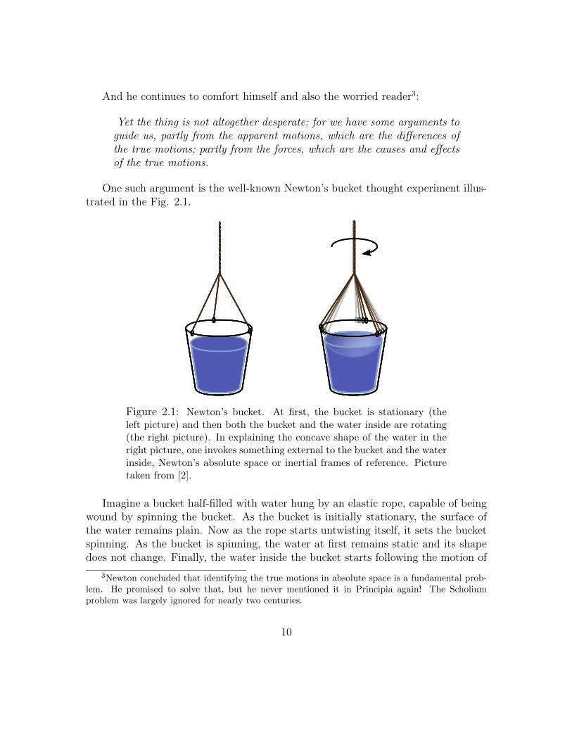
Figure 2.1: Newton’s bucket. At first, the bucket is stationary (theleft picture) and then both the bucket and the water inside are rotating(the right picture). In explaining the concave shape of the water in theright picture, one invokes something external to the bucket and the waterinside, Newton’s absolute space or inertial frames of reference. Picturetaken from [2].

Imagine a bucket half-filled with water hung by an elastic rope, capable of beingwound by spinning the bucket. As the bucket is initially stationary, the surface ofthe water remains plain. Now as the rope starts untwisting itself, it sets the bucketspinning. As the bucket is spinning, the water at first remains static and its shapedoes not change. Finally, the water inside the bucket starts following the motion of

3Newton concluded that identifying the true motions in absolute space is a fundamental prob-lem. He promised to solve that, but he never mentioned it in Principia again! The Scholiumproblem was largely ignored for nearly two centuries.

10

the vessel and then its surface gradually becomes concave upwards. If we suddenlystop the rotation of the bucket the water continues its circular rotation and retainsits concave shape. If we wait for long enough, the water gradually becomes stagnant.

What this thought experiment shows is a phenomenon (change in the shape ofthe surface of the water) that needs explanation. From the experiment it follows thatthis phenomenon cannot depend upon the relative motion of the vessel and the waterinside it: We see that the water does not immediately respond to the rotation of thevessel as the vessel is set in its motion and then later stopped, the water retainsits previous shape. Thus what is the reason? What lies behind this observablephenomenon? According to Newton, the rotation of the water with respect to theabsolute space is the reason. In this way, Newton hopes to convince us to endorsethe reality of absolute time, even though it remains outside the domain of our directempirical knowledge.

This sounds quite suspicious. Certainly, no wise man would doubt the reality ofthe change in the surface of the water. The problem is linking a ‘visible’ phenomenonto something ‘invisible’ and external. Should this phenomenon not be explainedbased on the relations between the observable entities within the universe? We sawthat the relative state of the water and the sides of the bucket cannot be the cause,but this does not indicate that such a relational cause cannot exist at all. This willbe addressed later in this and the next chapter. We may in fact say that this thesisexplores this possibility and provides a review of what has been developed in thatdirection.

Newton, however, was satisfied and could carry on with developing his theory ofmotion withstood for more than two centuries. This conceptual flaw of his theorydid not impede the ever-increasing practical usage of Newton’s equations. After allthe distant stars determined a proper reference system and the rotation of the earthwith respect to them, a good measure of absolute time (called sidereal time). It isusually the case in the history of physics (and probably other fields) that when thegeneration of revolutionaries who establish a new paradigm grow older, the youngerones who come next are more practical and pragmatic and do not engage in theserather philosophical discussions.4

This is perhaps why the conceptual defect of Newton’s theory went largely un-

4The same thing happened in the development of quantum mechanics to some extent. Afterthe development of the Copenhagen interpretation, between the years 1930 and 1970, except forEPR paper and Schrodinger’s reaction to it, as well as Everett’s 1957 paper and Bohm’s approachin 1952, until the full implications of Bell’s theorems and Aspect’s experiment, many youngerphysicists had no interest in the conceptual problems of the theory. However, unlike Newton’stheory, the foundational problems of quantum mechanics are still unsolved.

11

noticed for nearly two centuries until Ernst Mach revived this debate in the secondhalf of the 19th century.

2.2 Leibniz’s relationalism

Gottfried Wilhelm Leibniz, a prominent figure in the history of philosophy and math-ematics, as well as the debates on Newtonian mechanics, was one of the first whocriticized Newton’s concepts of absolute space and time. In a heated exchange withNewton’s representative, Samuel Clarke [3], he mounted a condemnation of Newto-nian philosophy. Leibniz advocated a relational understanding of space and time:Space is nothing but an order of co-existence of bodies, and time is a similar orderof succession of events.

Leibniz was epistemologically a rationalist and believed that ‘reason’ is our reli-able main source of gaining knowledge. He then based his philosophy on his greatPrinciple of Sufficient Reason. Understanding this principle and Leibniz’s philoso-phy, in general, helps us to lay a solid background of relationalism that proves to beof value in our future discussions. Leibniz’s pivotal principle is:

The Principle of Sufficient Reason (PSR): ...no fact can ever betrue or existent, no statement correct, unless there is a sufficient reasonwhy things are as they are and not otherwise - even if in most cases wecan’t know what the reason is. [1]

In a nutshell, this principle encourages us to keep searching and do not easilycontent ourselves by taking things for granted. The term ‘sufficient reason’ definitelyneeds more clarification. In the context of relationalism, a reason must be given interms of the inner relations between the elements of the universe. In that respect,invoking external causes to explain the phenomena that we directly observe in theuniverse, violates this principle. In the example of Newton’s bucket, we have anunsolved phenomenon, the concave shape of the water in the rotating bucket, andthere must be a sufficient reason behind that.

Newton’s absolute space and absolute time are similarly in direct opposition tothe above principle: Why is the universe located at a certain point in absolute spaceand not anywhere else? Why are the physical processes of the universe unfolding at‘this’ moment and not any moment sooner or later? Absolute space and time promptus to ask these questions but render any possible solution unattainable. The Principleof Sufficient Reason points out this very flaw in the Newtonian understanding of theuniverse.

12

The Principle of Sufficient Reason is at the heart of relationalism from whichvarious other principles stem. A direct consequence of the PSR was stated by Leibnizas the Principle of the Identity of Indiscernibles (PII). PII states that if two elementsshare the same set of features such that there are completely indistinguishable, theyare in fact identical : There are not two elements but only one. Discernibility is tobe stated in terms of all the relations of the elements to other entities. What thisprinciple suggests is that in the entire history of the universe, no two things have thesame set of relations to the rest of the universe. In other words, every event, everystructure in the vast expanse of the whole universe is unique. Entities of the universemight be similar, but never identical, as they are always distinguished based on theirtotality of relations to the whole.

Another major consequence of PII is that it undermines the concept of ‘symme-try’. Physical symmetries are widely used in theories, from Galilean symmetry inclassical mechanics to Poincare symmetry in relativity and supersymmetry in highenergy physics. The key picture behind symmetries is to change the physical systemssuch that the dynamics of the system does not alter. An example is the translationof a closed system in space. However, it is very suspicious: we claim to change thephysical state of the system while not changing anything observable! In the spiritof PII, how can we even say we have transformed anything if all properties of thesystem remain indistinguishable and unchanged? We will elaborate on this remarklater and see that in relational physics the concept of physical symmetries of thistype is simply meaningless. Physical symmetries of this type can only be ‘emer-gent’ and defined with respect to the whole universe. The only symmetry we haveis gauge symmetry or rather, gauge freedom. Some even use the term gauge redun-dancy5. These symmetries are mathematical in nature and reflect our mere freedomin choosing physically equivalent, but mathematically distinct variables to describenature. Gauge transformations are not tied to any physical interpretation like thosewe mentioned in the case of physical symmetries.

Despite his deeply suggestive principles, we can say that Leibniz lost the argu-ment to Newton and Clarke. Mere philosophical reasoning could not be convincingwhile Newton had already developed a theory based on his standpoint. A relationalphysical theory requires a more sophisticated mathematical machinery that Leibnizcould never have dreamed of. We will see that a relational theory of mechanics ispossible using the language of gauge theories which is much more advanced than

5This expression can be problematic because of the negative connotation of “redundancy”.Some argue that gauge is more than just a mathematical redundancy [4]. While I personally agreeto that, I think that the concept of gauge eventually boils down to just a valuable mathematicallanguage for describing nature. It is empty of any observational content or physical interpretation.

13

the mathematics available at that time. Although being a great mathematician,the co-founder of calculus could not cast his profound philosophical insights intomathematical expressions and build a theory upon them. Fortunately, that feat wasfinally completed a little more than two centuries later, the story of which is themain content of this thesis.

2.3 Mach’s critique

Following Ernst Mach’s demise in 1916 only a few months after the completion ofthe general theory of relativity in Berlin, in his obitary Einstein wrote:

It is a fact that Mach has had tremendous impact upon our generation ofnatural scientists, in particular with his historical-critical writings wherehe follows the evolution of individual sciences with so much love, wherehe probes practically the most remote brain cells of researchers who brokenew paths in their fields. [5]

Ernst Mach was a 19th-century eminent experimental physicist as well as a keyphilosopher behind the second wave of positivism. He is considered to be one ofthe most influential critics of Newton’s absolute space and time. In 1883 he wroteThe Science of Mechanics, a book on the history of mechanics which immenselyinfluenced Einstein’s pursuit of general relativity. This book is also an importantcritique of Newtonian space and time.

Starting with the problem of time, we find these words:

It is utterly beyond our power to measure the changes of things by time.Quite the contrary, time is an abstraction at which we arrive by meansof the changes of things; made because we are not restricted to any onedefinite measure, all being interconnected.

This is very suggestive. What do we really refer to when talking of time? Afterreflecting on the concept of time and freeing ourselves from the deep-rooted New-tonian absolute time, we find Mach’s view quite tenable. It is always the changeof some thing that we identify as the passage of time, never the other way around.Look at the wristwatches we use all over the world. It is the change in the positionof the hands of the clock that tells the time. The days and nights are in turn therotation of the earth around its axix and years and seasons are its rotation aroundthe sun, all of which are essentially the change in the earth’s position.

14

If we lay bare the core of our usual way of formulating the laws of nature withrespect to an external time, we will see that we are actually formulating the changesof some physical system with respect to the changes of some clock (which is alsoa physical system). Time, at least in the domain of classical physics6, is a non-existent imaginary entity, resting on the changes in the real observable entities, ormore appropriately, relations.

Therefore, time should be understood as the total change in the whole universe.As Julian Barbour puts it, the universe is its own clock. It is absolutely meaning-less to say how fast the whole universe is evolving. The universe determines time.However, this question is meaningful if we talk of a certain subsystem in the wholeuniverse. This is why we can tell the difference if we watch a movie in slow-motion:We compare the rate at which the changes unfold on the screen with the changes ofother parts of the universe, i.e., our watch, our personal sense of the flow of time,etc.

It should be noted that there are two aspects to the concept of time: durationand direction. So far, our analysis has addressed the former. Duration is the measureof the passage of the time we attribute to physical processes. The latter is relatedto the direction along which the universe evolves and changes. In the Newtonianframework, absolute time determines both of these aspects. The second aspect ismuch more delicate and is tightly bound to the problem of time’s arrow(s). Theproblem and its possible resolution in relational physics will be explained in thesecond part of this work.

Accompanying Leibniz and other advocates of relationalism, Mach was opposedto the concept of absolute space as an invisible container. Everything must becharacterized in terms of the visible entities of the universe, in terms of the relationsbetween parts of the whole universe. However, unlike Leibniz, Mach did not attemptto base his view on some rich metaphysical foundation. Instead, being an influentialfigure in the development of positivism, as well as a competent experimentalist, Machproposed that we stay within the boundaries of observables and do not rush into goingbeyond what observations grant us in hope of finding a better explanation. Mach’santhem is that we have a phenomenon at our disposal, and as scientists, we have toproceed to explain that phenomenon in terms of the internal structures rather than

6The status of time as an independent concept is likely to be elevated in passing from classicalphysics to quantum mechanics. We will touch on this delicate matter (of which we have yet noproper understanding) in the second part of this thesis.

15

external causes. In his words on the relational understanding of space:

When we say that a body K alters its direction and velocity solely throughthe influence of another body K ′, we have inserted a conception that isimpossible to come at unless other bodies A,B,C, · · · are present withreference to which the motion of the body K has been estimated.

What would Mach say as regards the bucket thought experiment by which Newtonfelt that he had cleared up all these suspicions? Mach remarked that Newton’smechanics has always been put to test by relying on fixed stars to represent absolutespace and sidereal time as the measure of absolute time. Thus, why not consider thepossibility that the concave shape of the water in Newton’s bucket is the result ofbackground stars, or in general, all the other masses in the universe? This is indeeda radical proposal. In another well-known quote from Mach we read:

No one is competent to say how the experiment would turn out if thesides of the vessel increased in thickness and mass till they were ultimatelyseveral leagues thick.

What can we make of all these audacious, but not entirely clear remarks? Thehonest answer is that it is not very clear. Unfortunately, Mach never stated his ideasprecisely enough and it did led to some confusions. Anyway, the correct and precisecriterion was found about one century later by Julian Barbour which will be coveredin Sec. 2.5. What is worth noting, however, is that Mach did tentatively suggest thatwe include the whole universe in our considerations. We will see that this insight isexactly what we have to do if we aspire to have a relational understanding of theuniverse: a relational theory must necessarily be a theory of the whole universe.

Einstein definitely played a significant role in popularizing Mach’s ideas. Havingread his works as a young man, Mach’s critical thinking made a significant impact onEinstein’s perspective. Even it was Einstein who dubbed the term Mach’s Principlein his 1918 paper, On the Foundations of the General Theory of Relativity [6]. Wewill come back to the story of Einstein and Mach’s Principle later. It is fascinatingand deserves some detailed remarks in its proper place.

2.4 Lange and Tait’s contributions

Mach’s critique captured Lang and Tait’s attention to ponder the Scholium problemin a new light [7]. Lange considered three freely-moving particles and took their

16

successive positions to define a frame of reference based on the material particlesalone. He called it an inertial system. Ever since this term has become standardand replaced Newton’s absolute space and time. But the point is that in the text-books an inertial frame of reference is defined as a frame in which Newton’s firstlaw holds. But unfortunately, they do not get into the details of their constructionbased on only observational information (which are relational). After all, the coreof the Scholium problem is exactly about determining the state of motion and restof particles given only the observational data. Lange’s work was an important steptowards the resolution of the problem. We will see that the problem can be solvedin this way, but only partially.

A cleaner procedure for the determination of inertial frames had been proposedby Peter Guthrie Tait in 1883 Tait.1883. A generalization of his work in a moreilluminating context can be found in Barbour’s 2010 paper on Mach’s Principle [7].

Tait assumed that size is given. Alhough we essentially follow his approach,we take size relational. Suppose a system of N point particles. The observationalinformation is encoded in ‘snapshots’ of the configuration of particles at certainunspecified instants. In accord with relationalism, only relational data are physicallymeaningful, i.e, only ratios matter. These ratios are between separations of particles,or in other words, the angles between particles as seen from other ones. These anglesdefine the ‘shapes’. Only shapes observed within the whole system can be physicallyallowed.

Now we do some counting. In an arbitrary Cartesian system, we can assign3N coordinates to the N particles in three-dimensional space. However, three ofthem determine the system’s center of mass position which is unobservable from therelational point of view, 3 more are related to the total orientation of the systemwhich is also unphysical. One last number determines the total scale of the system.As ratios are only relevant, this too must be omitted. In fact, translating, rotating,and rescaling the total system does not change the relational data. The 3+3+1 datawe arrived at are exactly linked to the action of these groups on the configurationspace. Thus, we are eventually left with 3N−3−3−1 = 3N−7 observable data.7 Forinstance, if there are three particles, the relational data can only be the two anglesthat define the triangular shape of the system which is indeed correct: 3× 3− 7 = 2.If this three-body system is the entire universe, the size, place, and orientation of

7One might say that for the N -body system there are N(N−1)2 possible numbers for each pairs

of the particles. This counting, however, neglects the certain constraints that the configuration ofthe particles must satisfy. The simplest one is the triangle inequality for three particles. If N > 5,then there are also equalities they have to satisfy which greatly reduces the number of independentnumbers.

17

the triangle in the three-dimensional space are not observable.Now Tait’s problem is that how many snapshots are needed to determine the

inertial motion of the particles. More generally, we can ask the same questionsfor determining the motion of particles according to Newton’s law for a certaininteraction.

The answer is not that hard. Given the configuration of the particles, we canchoose one of them (particle 1) to be perpetually at rest. This fixes the origin ofthe frame. We need a standard rod to define distance. We can take the separationbetween an arbitrary particle (particle 2) and particle 1 at that specific instant tobe of distance 1 by definition.8 To define an orientation, we can take the directionof the second particle from the first one at that instant to be one of the axes (x),and the direction of the motion of the particle 2 the other one (z). With these twoaxes, an orthogonal coordinate system is defined. Finally, the motion of particle 2 canmeasure the time. Based on our construction, in this frame the coordinate of particle1 is (0, 0, 0), and that of particle 2 is (1, 0, t). Now all that is left is the informationof the rest N − 2 particles. To determine their trajectories completely, we need 6numbers for their positions and velocities with respect to the frame of reference webuilt with the other two particles. The coordinates of the other particles are of theform (xI , yI , zI) + (uI , vI , wI)t. Thus 6(N − 2) = 6N − 12 data are needed.

It follows that given only two snapshots is not enough to determine the evolutionof the system. For each snapshot provides 3N−7 data. Also, we do not know ‘when’these two snapshots were taken. Thus, each of them contains 3N − 8 usable dataand there are 6N − 16 data in two snapshots. We are short of 4 more numbers todetermine the entire dynamics in the frame we constructed from the particles. Threeof the lacking data are related to the angular momentum of the system, one of them isthe value of the overall expansion and contraction of the system, called dilatationalmomentum9. These conserved quantities cannot be determined by the observablerelational data alone. In the standard Newtonian mechanics, we determine them inan inertial frame of reference. Here, however, our frame is the N -particle systemitself. Angular momentum measures the change in the total orientation. As totalorientation is completely unobservable from the relational point of view, its changeis also irrelevant. The same thing holds for the dilatational momentum.

This is very significant. If we insist on only using the available data in the entiresystem (which is in fact a reasonable expectation), two snapshots are not enough for

8We assume that the two particles never collide.9The dilatational momentum in an inertial frame of reference is D =

∑NI=1 ~rI .~pI . This quantity

is the momentum conjugate to the total size of the system. We will define and clarify its role indetail in the next chapter.

18

solving the simplest inertial motion of the non-interacting particles. If the numberof particles is large enough (N > 5), three snapshots will be enough.

We could have left the size of the system untouched (as Tait did). Assuming thatan external rod exists, each snapshot contains 3N−6 data (only the total orientationand the location of the system remain undetermined). We can still use two particlesto construct a frame. This time, however, the distance between particles 1 and 2 isphysically relevant and is to be determined. Thus, we would need 6(N − 2) + 1 =6N − 11 data. Two snapshots contain 2(3N − 6) − 2 = 6N − 14. Now there is a3-number shortfall which is contained in the angular momentum of the system.

Although we only considered the inertial motion, an analogous calculation canbe carried out for a system of interacting particles. But it is more complicated as wecannot simply fix the motion of the particles to define an inertial frame of referencedue to the particles’ non-inertial motion.

The important lesson we must take from Tait and Lange’s work is that Newtonianmechanics can be made relational, but at the cost of needing more than two sets ofdata. This is a matter of causality, not epistemology. Newton’s absolute spaceand absolute time were indeed plagued with an epistemological defect. But whatwe learned from the above discussion is that the concept of an inertial frame ofreference can be built on only the observational data and it can take the place ofabsolute space and time. What we lose in taking this step forward is the predictivepower of the theory: We would be needing more initial information to solve theequations of motion.

2.5 The contemporary relational physics

Before we proceed to today’s relational physics, there is an important link in thechain of the works done on relationalism and that is Henri Poincare’s contribution tothe discussion. He was sympathetic to the critique of Newton’s absolute space andtime and pointed out the repugnancy of attributing states of motion to the wholeuniverse in invisible space. He asked an illuminating question: What precise defect,if any, arises within Newtonian dynamics from its use of absolute space?

Based on our discussion in the previous section, the answer should be clear:Newton’s absolute space gives the theory an artificial predictive power, without whichmore information would be needed for predicting the evolution of the system if weinsist on only the physical information.

Poincare too noted that the separations between the particles in aN -body system,

19

rij and their rates of change, rij are the physically meaningful data.10 He thenpointed out that those are not enough to determine the evolution uniquely. Aswe discussed, the information of the total angular momentum of the system is notencoded in the relational data. We did the counting in the previous section. Wequickly recap our result by giving the simple example of a two-body Kepler system,like the motion of earth and sun. Let the initial change in their separation be zero,that is r = 0. But this does not determine the evolution of the system uniquely.All possible motions can follow: the two particles collide, or they orbit around eachother in a circular or elliptical motion. We could solve the equations of motion inthis way, however, by knowing some of the second derivatives of the separations rijas well. This unpredictability rests exclusively on the difference between relativequantities and those with respect to an inertial frame of reference. This is the defectof Newton’s mechanics.

What is worth emphasizing is Poincare’s insight that helped to identify the precisemanner in which Newton’s theory fails to be relational. It is about the amount ofobservable information needed for the evolution to be determined uniquely.

Despite being on the right track to formulating relational physics, Poincare waspessimistic about the prospect of finding a relational description of nature. Thefailure of Newtonian mechanics to be relational for subsystems led him to regretfullyconclude that nature does not respect our philosophical aspirations.

But there is no reason for hopelessness. Mach already told us to look at thewhole universe. Following this intuition, it is possible to find a relational theory ofthe whole universe, which is precisely what Barbour and Bertotti showed in theirseminal paper [8]. The method they discovered, now called best-matching, is a math-ematical procedure that helps to construct relational dynamics irrespective of theconfiguration space. Best-matching and relational particle mechanics will be coveredin the next chapter extensively and in detail. After nearly three hundred years, fi-nally a consistent relational framework was found that captured the core philosophyof Leibniz, the critique of Mach, and works of all the others who pondered relation-alism. Relational field theory was also developed later in the early 2000s [9]. We willcover them in this first part.

Finally, we state what we believe to be the precise statement of Mach’s Principleas formulated by Julian Barbour. The starting point is to identify the true physicalconfiguration space. It is done by finding the underlying symmetry group of thetheory. For instance, for the N -particle system in three-dimensional Euclidean space,

10In Poincare’s approach, an external clock and a measuring rod are taken for granted. But thisdoes not affect the conclusion he arrived at. One could also take the time and size to be relational,as in our account of Tait’s problem.

20

in the absence of external orientation, size, and spatial specification, the symmetrygroup is the similarity group Sim(3) which is the semidirect product of the rotationgroup SO(3), the translation group T (3), and the rescaling group which is simplythe set of the positive numbers that rescale the total size of the system, denoted byR+: Sim(3) = R+nE(3), where E(3) is the Euclidean group: E(3) = SO(3)nT (3).The symmetry group is mostly determined based on empirical considerations. Thegoal is to identify the directly observable quantities and satisfy the Principle of theIdentity of Indiscernibles.

The next step is to quotient the initial configuration space in which we do thecalculations by the symmetry group. The result is the relational configuration space.In the N -body system the configuration space can initially be taken to be R3N : 3coordinates for each of particles. But due to the redundancy of this space, orientation,size, and positions of the particles in the space must be eliminated by quotienting.

Finally, for the theory to have maximal predictive power, we demand that only aninitial point and its change in the reduced (quotiented) configuration space suffice todetermine the evolution of the system uniquely. Hence, we define the Mach-PoincarePrinciple 11:

Mach-Poincare Principle: Given the configuration space Q, and theunderlying symmetry group G, we identify the quotient of the configu-ration space with respect to the group G as the relational configurationspace: QR = Q/G. Then the following are respectively the strong and weakform of Mach’s Principle [7]:

1. Specification of an initial point q ∈ QR together with a direction δqin QR at q defines a unique curve in QR.

2. Specification of an initial point q ∈ QR together with a tangent vectorq in QR at q defines a unique curve in QR.

Some remarks should be made on the distinction between the strong and the weakform. The distinction is made based on Mach’s philosophy of time as a measureof change. In this light, the strong form of the principle respects the relationalunderstanding of time as well as the relational structure of the configuration space.12

Explicitly, the set of admissible initial conditions in the first principle has one lessdatum: the directions in the configuration space provide us with one less piece of

11As Poincare’s illuminating discussions are of significant relevance to our criterion of Machianity,we included his name in the principle, in accord with the terminology of [2].

12Some refer to Mach’s temporal relationalism as Mach’s second principle, and his spatial rela-tionalism as Mach’s first principle.

21

information. For instance, if the relational configuration space is represented by atwo-dimensional sphere, as in the case of 3-body system, a direction at each pointis determined only by one number. A tangent vector, or in other words, the rate ofchange of a point, is determined by two numbers. As the result, an initial tangentvector provides us with more information, but at the cost of positing an externalclock with respect to which the magnitude of the tangent vector can be physicallymeaningful.

Although the concept of relational time is very precious to us from the relationalpoint of view, nature is unfortunately not sympathetic to us. There are some diffi-culties in constructing a totally relational physics. We cannot have both a relationaltime and a relational size. One solution could be to eliminate size by using thechange of which to define an external time. The downside is that only the weak formof the principle would be satisfied. We will discuss this problem more properly laterin the second part.

2.6 Why relationalism?

Should we take relationalism seriously? If yes, why?First of all, I believe one should not dismiss metaphysical thinking and trying

too much to find objective reasons for proceeding in science can be detrimental to itsprogress.13 I do not mean to suggest that any personal preference and philosophicalview can be blindly allowed to contribute to science. But if we study the historyof science and the great men behind the great discoveries, it becomes quite hardto separate logical objective reasoning from personal views. Newton’s advocacy ofabsolute space and absolute time, Nils Bohr’s background and its influence on hisapproach to quantum mechanics, and Einstein’s critique of quantum mechanics aresome examples. Einstein’s enthusiasm for Mach’s ideas - which is in fact relevant toour discussion - is also a revealing example. After Einstein found the correct fieldequations in November 1915, the non-Machian nature of his theory based on hisdefinition of Mach’s principle bothered him so much that he set out to modify histheory to incorporate Mach’s principle. He worked for some years on this programuntil he gradually became disappointed with it. Why would Einstein do that in thefirst place if it were not for his ingrained passion for Mach’s ideas? Nevertheless, itis noteworthy that one must be very cautious in indulging in subjective thinking inscience. After all, the outcome of science must be based on objective facts.

Thus, one support for relationalism has certainly been the personal ‘caring’ about

13We should criticize the “Shut up and Calculate!” attitude in this regard.

22

understanding the universe as a whole without reference to something external; auniverse as a totality which includes its causes effects altogether.

It is not the only thing we can hope for. Shape dynamics as a successful classicalrelational theory, although a very young field, has already brought us many inter-esting facts and there are many hopes that it gives us some hints on the problem ofquantum gravity. One notable success of the theory is the possible resolution of theold problem of the origin of the arrow of time which will be discussed in the secondpart of this work.

Philosophically, there are some reasons for taking relationalism as a guiding prin-ciple seriously. First of all, as relationalism describes nature in terms of the innerrelations between its constituents, not against a background structure, it is morerestrictive and hence more predictive. We will see that both in the case of particledynamics and geometrodynamics, implementing Mach-Poincare Principle imposessome restrictive constraints on the whole system. In the case of particle dynamics,these are the vanishing of the total angular momenta and linear momenta. Similarly,relational geometrodynamics demands the whole spacetime be globally hyperbolic,CMC foliable, and spatially closed which renders the theory more restrictive (thusmore predictive) than the standard general relativity.

Predictive power is an important feature in science, the lack of which leads sci-entific pursuit astray. Some suggest it is exactly one of the reasons for the currentstagnancy of the foundations of physics in the past decades [10].

Finally, I would like to elaborate on the strong bond between relationalism andthe aspiration for a theory of the whole universe. We saw that how including thewhole universe helped to state the Machian criterion more precisely. The point isthat a relational theory must be a theory of the whole by nature: all relations play adynamical role in such a theory and restricting the scope of our investigation to partsof the universe can only be approximate. This is very illuminating. In the standardNewtonian paradigm14 the theory is for subsystems only and then we extrapolate it tolarger and larger systems in our attempt to have a theory of the whole. This method- which is only possible because we posit an external background against which westudy a certain system by neglecting the environment - has led to some difficulties insearching a fundamental theory of the whole Smolin.2015. Relationalism is quitethe opposite to that: we start with a theory of the whole and under certain conditions,we can study subsystems of the universe approximately. The whole universe is itsown background ; relational physics describes the systems within the universe against

14Newtonian paradigm is different from Newtonian physics. Newtonian physics was overthrownby the advent of modern physics in the 20th-century. But Newtonian paradigm as a general wayof doing science still lives on.

23

this background.It is also true the other way around. If a fundamental theory is to apply to

the whole universe, it must be background independent and relational, otherwisethe theory would include some concomitant external causes and elements. Thiscontradicts the fundamentality of such a theory since a fundamental theory mustexplain all causes by definition.

The distinction between physics of the whole universe and physics in laboratorycannot be overemphasized. Relationalism is the portal of a theory of the whole.

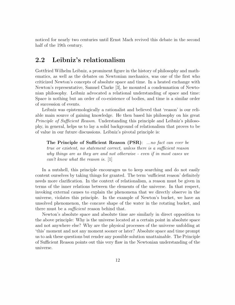
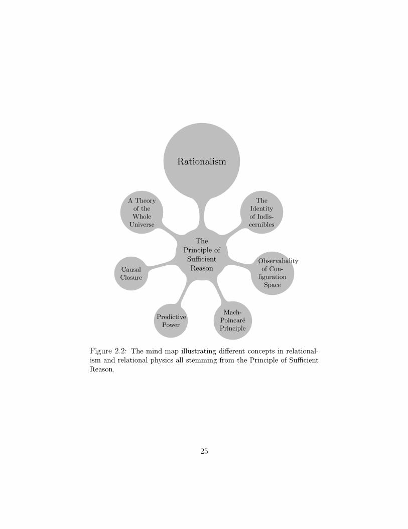
All the results that follow from relationalism are shown in Fig. 2.2. They allemanate from the cornerstone of relationalism, the Principle of Sufficient Reason.15

We summarize the key features that make a compelling case for relationalism:

1. Relational physics is more restrictive and hence more predictively powerful.

2. Relational physics describes the universe in terms of the directly observablereal quantities. Moreover, the nexus of causal relations between the entitiesstays within the observable universe.

3. Relational physics is by construction applicable to the whole universe andmakes it possible to have a fundamental theory of the whole.

4. Relational physics has thus far led us to many enthralling results which spureven more studies.

15Julian Barbour suggested to me to call this illustration ‘the map of God’s mind’. We may sayit is how Leibniz’s God might have thought when creating the universe.

24

Rationalism

ThePrinciple ofSufficientReason

TheIdentityof Indis-cernibles

Observabalityof Con-

figurationSpace

Mach-PoincarePrinciple

PredictivePower

CausalClosure

A Theoryof theWhole

Universe

Figure 2.2: The mind map illustrating different concepts in relational-ism and relational physics all stemming from the Principle of SufficientReason.

25

Chapter 3

Best-Matching and RelationalParticle Mechanics

3.1 Building the intuition behind best-matching

In the last chapter, we tracked the story of relationalism and found our way to theMach-Poincare Principle. We must now proceed with constructing a proper mathe-matical framework for implementing that principle in various dynamical theories.

As we mentioned, Barbour and Bertotti came up with a novel approach in 1982[8]. Their method is now called best-matching. The idea behind that is rather simple.It is about finding the quantitative ‘difference’ between certain configurations interms of their innate properties without referring to anything external. We illustratethe procedure with a simple 3-particle model in two-dimensional space. We assumethat the particles are distinguishable and label them with some distinct numbers.Consider two snapshots of a 3-particle system, represented by two different trianglesin space. For the moment, we assume that an external size is given and that onlythe separations between the particles are observable. How do we compare thesetwo configurations with one another without locating them in a fictional backgroundspace?

Given the two configurations located arbitrarily in the Euclidean space, a naturalmeasure of the ‘distance’ between them can be defined to be simply the sum of theEuclidean distances between each particle of the configurations (each vertex of thetriangles in our illustration). What best-matching does is to use one of the trianglesas the reference, and then transform the other one all over an imaginary space1

1It might seem that we are implicitly using the redundant Newtonian absolute space here. Thepoint is that the best-matched difference that is established in this method is completely indepen-

26

and rotate it under all arbitrary rotations until the Euclidean distance between thetwo configurations is minimized. This distance is the best-matched distance and theresultant configuration in this procedure is called the best-matched configuration.

Interestingly, this method solves the Scholium problem by establishing the con-cept of equilocality in an alternative way. The dynamical history of the whole uni-verse is nothing but a succession of the relational configurations in the correspondingconfiguration space. The significance of best-matching is that it determines exactlyhow the configurations must follow one another. We no longer need to worry aboutthe location of a certain system at different times and try to conceive that in absolutespace (or an inertial frame of reference). Best-matching requires all the successiveconfigurations to be the best-matched ones.2

Several remarks follow. First, we should note that this method is defined forthe whole universe. The ‘snapshots’ of the whole universe are to be compared toone another and then best-matched. Second, best-matching kills two birds with onestone.3 All possible motions, from inertial ones to those under different interactions,are all different manifestations of the best-matching procedure carried out with dif-ferent metrics (as hinted in the footnote 2. And finally, the third remark is thatbest-matching imposes certain conditions on the evolution of the whole universe inconfiguration space (or equivalently on the phase space). For instance, best-matchingwith respect to translations results in the vanishing of the total linear momenta. In-cluding the rotation group, in turn, enforces the vanishing of the angular momentumof the whole universe.

Mach said that it is meaningless to talk of a spinning universe. We are now inthe position to endorse that: The total angular momentum of the whole universe iszero according to our relational approach based on best-matching. The same is truefor the vanishing of the total linear momenta which renders the motion of the wholeuniverse hollow, as it should be.

Leibniz’s God is without a doubt more rational than to flaunt his mighty powerto set the entire universe in motion. The rationality behind nature decrees that the

dent of the initial space and is only dependent on the relational properties of the two configurations.Mathematically, we use this background space to define the gauge variables. Eventually, all thephysical evolutions and the ontological configurations reside in the reduced space we defined in Sec.2.5.

2There are some subtleties here. We use the Euclidean distance between the particles in theprocedure. However, in general, the dynamics of the configurations can be more complicated thanthat as there might be some interactions between particles. This does not affect our intuitiveapproach however, as we shall see below that interactions can be implemented through the ‘metric’we define on the configuration space for defining distance.

3Actually, we may say it kills infinitely many birds!

27

momenta of the whole universe vanish! Relational physics is the rational naturalists’religion that rests on Leibniz’s great metaphysical Principle of Sufficient Reason, andbest-matching is its ritual. Now we proceed with learning best-matching in detail.

3.2 Best-matching is minimizing the incongruence

3.2.1 Jacobi’s action

We now take the first steps to formulate best-matching mathematically. We firstconsider the simple N -body problem and then develop this technique more abstractlyin a general case for any given configuration space with a certain symmetry group.

Following William Rowan Hamilton’s great principle (1834), known as Hamilton’sprinciple, we know that the Newtonian evolution of the N -body dynamical systemscan be formulated as the following action:

S[q] =

∫ qaIi,tf

qaIi,ti

dt (T (qaI , · · · )− V (qaI , · · · )) ≡∫ qaIi,tf

qaIi,ti

dt L. (3.1)

Here ti and tf refer to the initial and final Newtonian absolute time respectively,V is the potential energy dependent on the particle coordinates, and T is the Kinetic

energy of the system, i.e., T = 12

I=N∑I=1

mI q2I , and L = T − V is the Lagrangian. The

dots denote the derivatives with respect to the Newtonian time, and by q2I we mean∑

a

(qaI )2 by virtue of Einstein’s summation convention for the spatial indices a.

There is a rather less known method, called Routhian reduction procedure, bywhich we can transform the above action into a dynamically equivalent action withan explicit timeless character. See Appx. A. The result, known as Jacobi’s action,is of utmost importance in relational physics and is very suitable for formulatingbest-matching. Jacobi’s action is4

SJ [q] =

∫dλ√

(E − V (q))T (q′), (3.2)

where T = 12

I=N∑I=1

mIq′2I , and E is a constant. The role of E is different here

from its role in our derivation in Appx. A. In the latter derivation, it serves as asupplementing condition and is equal to the momentum conjugate to the Newtonian

4The boundaries of the integral - which are simply the initial and final configurations - are notshown for simplicity.

28

time. Here, there is no ‘time’ at all, and our starting point is Jacobi’s action, notthe standard Newtonian action. E is simply a constant that is to be determinedexperimentally. However, best-matching may restrict this constant term, as we willsee. We say more about E in the theory in Sec. 3.4. Jacobi’s action can be expressedin the following suggestive way which manifests the timeless nature of the action moreexplicitly:

SJ [q] =

∫ √(E − V (q))

∑I

dq2I . (3.3)

This action is the sacred mantra we keep chanting throughout this thesis. Wewill see how all our classical dynamical theories, from particle mechanics to generalrelativity, can be conceived and born from a simple Jacobi’s action through best-matching with respect to the corresponding symmetry group. I doubt if Carl GustavJacob Jacobi ever thought of the profound significance behind this action and theremarkable role it would play in relational physics one day.

3.2.2 Introducing the best-matching

Let qaI represents the coordinates of the Ith particle in three-dimensional Euclideanspace, where a runs from 1 to 3 and I takes the numbers 1, 2, · · · , N . Under thetranslation group T (3) acting on the whole system, the coordinates transform asqaI → qaI + αa, where αa is an arbitrary vector belonging to the three-dimensionalspace. The action of the rotation group is given by 3 × 3 rotation matrices Ωa

b (ωc)

parameterized by three variables denoting the axis and the angles of rotation: qaI →Ωab q

bI , where the summation over the repeated index b is omitted according to our

convention. Hence, under the Euclidean group5 the coordinates transform as

qaI → qaI = Ωab q

bI + αa. (3.4)

Following our intuitive account of best-matching in Sec. 3.1, we ‘shift’ the vari-ables in Jacobi’s action (3.2) and replace them with the transformed ones (3.4):

SJ [q, α, ω] =

∫dλ√

(E − V (q))T (q′). (3.5)

5For the moment, we restrict our attention to the Euclidean group instead of the similarity groupfor the sake of simplicity. We will shortly develop the best-matching procedure more generally andthe relationality of scale can be easily included.

29

The important point is that the action is now a functional depending on ‘both’the trajectories in configuration space and the group parameters αa(λ). Note thatthe action (3.5) is not ‘derived’ but rather ‘proposed’ as a principle underpinning therelational physics. Its role in satisfying the Mach-Poincare Principle will be shortlyclarified.

First of all, we look at the potential term in the action (3.5). In general, thepotentials used in Newtonian physics are translationally and rotationally invariant,such as the Newtonian potential V = −

∑I<J

mImJrIJ

, where rIJ is the separation between

the particle I and J .6 As a result, we need to only calculate the kinetic term.

T (q′2I ) =

1

2

∑I

mI q′2I =

1

2

∑I

mI

(Ωq′I + Ω′qI + α

′

I

)2

, (3.6)

where by Ω′, the derivative of the rotation matrix Ω (α(λ), β(λ), γ(λ)) with respectto λ is meant.

Because of the invariance of the Euclidean inner product, we can write the squaredterm in the above expression in the following way

(Ωq′I + Ω′qI + α′)2

=(q′I + ΩTΩ′qI + ΩTα′

)2. (3.7)

The operator ΩTΩ′ appearing in this term is related to ‘Lie algebra’ of the rotationgroup.7 Working with the matrix representation of the group elements, we canrepresent the group elements as the exponent of an element of the algebra and thenumbers ωa which can be identified as the components of that specific element:

Ω = exp (ωaOa). (3.8)

Thus,

ΩTΩ′ =d

dλlog (Ω) =

d

dλ(ωaOa) = ω

′aOa (3.9)

Where Oa is the matrix representation of the elements of the Lie algebra. Ex-plicitly, Oa’s can be taken to be the matrices

O1 =

0 0 00 0 10 −1 0

, O2 =

0 0 −10 0 01 0 0

, O3 =

0 1 0−1 0 00 0 0

. (3.10)

6We omitted the Newtonian gravitational constant for simplicity. Anyway, it is not importantand it can be eliminated by simply redefining our unit of time.

7For a brief account of Lie groups and Lie algebras see the Appx. B

30

If we first extremize8 the action (3.2) with respect to the parameters ωa and αa,it will do exactly what we described in Sec. 3.1: it aligns the successive snapshotsof the whole universe in a such a way that the difference between them (given byJacobi’s action) is minimized. However, because of the invariance of Euclidean innerproduct with respect to Euclidean group, and our assumption that the potentialdepends on only separations and thus also invariant under Euclidean group, onlythe derivatives of the group parameters appear in the action. As the result, we varythe action with respect to the parameters ω

′a and α′a directly.9 Thus, we have the

following ‘best-matched action’.

SbmJ [q] = SJ [q, ω′, α′]|ω′a=ω′a0 ,α

′a=α′a0

=

∫dλ√

(E − V (q))T (q′2),

δSJδω′a

∣∣∣∣ω′a0

=δSJδα′a

∣∣∣∣α′a0

= 0.(3.11)

The parameters ωa0 , αa0 are the ones that minimize the previous action (3.5), and

qaI (λ) is the ‘best-matched’ trajectory: qaI (λ) = Ω(ω0(λ))qaI (λ) + αa0(λ). Thus, theaction (3.11) depends on the trajectories in the configuration space for any of which,we must first solve the two conditions in (3.11) and then insert the ‘refined’ trajectory(the one transformed with the variables ω0 and α0) back into the action.

Best-matching introduces a gauge symmetry in the action. For any given tra-jectory, the best-matched action is ‘gauge invariant’ and the gauge group is simplythe Euclidean group with respect to which we carried out the best-matching. To seethat, the reader can easily verify that

SJ [q, ω, α] = SJ [q, ω, α], (3.12)

where the transformed variables q, ω, α are given by the transformation

q = Ω(ω)q + α

Ω(ω) = Ω(ω)ΩT (ω)

α = α− Ω(ω)ΩT (ω)α.

(3.13)

8Actually, we are effectively ‘minimizing’ the action with respect to the group parameters. Itis easy to show that the transformation (3.4) increases the value of the action. After all, it takessome effort to set the entire universe in a certain translational or rotational motion!

9The sharp-witted reader can certainly spot a loophole here. Since when do we vary the action(or any other functional) with respect to only the derivative of a function appearing inside it? Thisis not what ‘variation’ means in the calculus of variations. I ask the readers to be a bit patient andlet me continue with this procedure to arrive at some illuminating results. I will address this issueat length in the following section.

31

for arbitrary smooth functions ωa(λ) and αa(λ)’s.Hence, Jacobi’s action (3.5) is gauge-invariant under the above parameter-dependent

(local) transformation.

3.2.3 The best-matching constraints

We now see what best-matching really implies. For this, we explicitly calculate thetwo conditions we derived in (3.11). For translations, we have

δSJδα′a

=∑I

ΩT δSJδq

′aI

=∑I

ΩTpIa. (3.14)

Thus, best-matching with respect to translations enforces the vanishing of thetotal momentum:

P a ≡∑I

pIa = 0. (3.15)

It means that the parameters αa’s must be chosen in such a way that the totalmomentum vanishes. Of course, this condition fixes only the derivative of αa’s andtheir initial value, i.e., their global value remains arbitrary. But the essential pointis that they can be solved in terms of the qaI ’s.

Regarding the second condition, in light of (3.7) we have

δSJδω′a

=∑I

δSJδq

′bI

(OaqI)b =∑I

(Oa)bcqcIpIb . (3.16)

Based on (3.10), the matrix representations of the elementsOas are all asymmetricand are indeed the Levi-Civita symbol. Thus, the condition (3.16) is equivalent tothe vanishing of the total angular momentum.

Ja =∑I

εabcqbIpIc = 0. (3.17)

So it follows that best-matching with respect to rotations demands the totalangular momentum of the whole universe vanishes. Again, we can use this conditionto solve for the parameters ωa (up to their initial value).

The above calculations have revealed what best-matching essentially does: italigns the succession of configuration states of the whole universe by making thetranslational and rotational momenta vanish. More strikingly, the best-matching

32

conditions we derived are the vanishing of the momenta that generate the very trans-formations used in the procedure. There is a bigger and more general picture behindthis observation which will be developed in Sec. 3.3.

From these conditions, we see that relational particle physics is not so foreignto Newtonian mechanics. We already know that for rotationally and translationallyinvariant potentials the total momentum P and total angular momentum J are con-stant. Now best-matching requires them to vanish. Thus, we can say that relationalphysics is ‘part of’ Newtonian mechanics, with only the difference that the value ofthe constants of motion, the total conjugate momenta, is set to zero. In other words,relational particle mechanics is equivalent to Newtonian mechanics, provided thatthe total momenta vanish.

What is striking is the relevance these constraints bear to Tait’s problem. Aswe saw, to completely solve the Scholium problem, i.e., to determine the Newtonianevolution of a system based on the observable data encoded in the configuration ofparticles, we needed more than two snapshots. The constraints imposed on the pos-sible solution curves in the configuration space exactly compensate for those missingdata. Given that the total linear and angular momentum of the whole universe mustvanish, the two snapshots representing the initial configuration and its change shouldbe enough to determine the evolution of the system. This hint is in the direction ofthe Mach-Poincare Principle as will be discussed in the following part.

3.2.4 The solution to Newton’s bucket problem

As best-matching is the key to relational physics, we can see how it provides a betterexplanation of Newton’s bucket thought experiment. We can think of the wholeuniverse as being composed of the bucket, the water, and the distant stars. Thebest-matching condition corresponding to the rotational group is the vanishing ofthe total angular momentum. Thus, as the water is spinning, the distant stars mustbe rotating in the opposite direction to ensure that condition holds. However, dueto their large mass and distance, the contribution of the motion of the stars to thetotal angular momentum is extremely more significant, and thus, their rotation isnegligible. Even with a tiny amount of rotation which is unnoticeable, the totalangular momentum can vanish in accord with the best-matching condition. Thisleads to the resolution of the problem: the rotation of the water is indeed meaningfulwith respect to distant stars. The distant stars create a background with respect towhich the bucket and the water inside rotate, resulting in the change in the surfaceof the water.

There is no need to posit an absolute space or a background inertial frame of

33

reference. Best-matching ensures that the whole universe provides the background.It is tempting to think about the scenario in which there are no distant stars

and there is only a bucket filled with water. Best-matching implies that there areonly two acceptable possibilities: either the bucket and water are not rotating andthe surface of the water is flat or the bucket and water are rotating in oppositedirections and the surface of the water is concave. Unlike the results of Newtonianmechanics, there are no further possibilities. This highlights the restrictive characterof relational physics and also emphasizes the role of the whole universe in providinga background for motion.

3.2.5 Mach-Poincare Principle

The content of the Mach-Poincare Principle is to first quotient the redundant New-tonian configuration space with respect to the relevant symmetry group, and thenconstruct a theory that uniquely evolves the whole universe given only the initialconfiguration and its change (tangent vector or the direction of change). We consid-ered N particles in the three-dimensional Euclidean space. Hence, the initial crudeconfiguration space is R3N : one assigns three coordinates to each particle in the Eu-clidean space that plays the role of Newton’s absolute space. Assuming that the sizeis given by some external measuring rod, the symmetry group of Euclidean space,i.e., the group of transformations that leave the distinguishable states of the wholeuniverse untouched, is the Euclidean group. Thus, the real relational configurationspace is QR = R3N/E(3). Moreover, the action we arrived at after best-matching (3.11)is defined on this reduced configuration space. The distinct trajectories that give riseto different values for this action are the ones that are distinguishable in the reducedconfiguration space.

We can picture the way best-matching affects the configuration space in thefollowing way. The Euclidean group slices the initial configuration space R3N intoorbits10. We surely cannot visualize the 3N -dimensional configuration space. But wecan proceed with the simpler example of a two-dimensional space and the rotationgroup SO(2) playing the role of the symmetry group. The group orbits are thecentered circles around the origin. What the Mach-Poincare Principle demands is atheory defined in the reduced configuration space that consists of only these circles,described by a positive number denoting the radius. Best-matching smoothly movesany trajectory in R2 along those circles so that the action is minimized. The curveswhich minimize the action ‘cut through’ the orbits. Hence, the best-matched actionis an action defined in terms of the trajectories in the quotiented configuration space.

10For the definition of group orbits see Appx. B.

34

The same scenario plays out in the general case of N particles in the three-dimensional space. The orbits of the Euclidean group are the true degree of freedomon which the best-matched action is defined: The best-matched trajectories cutthrough the gauge orbits. The Euler-Lagrange equations for this action give theequations of motion.

Hence, we infer that spatial relationalism is embodied in this method. We nowturn our attention to temporal relationalism.

With a glance at the action (3.5), we notice its timeless character as we explainednear the end of Sec. 3.2.1. Moreover, we know that an action theory admits a uniquesolution given any initial data comprising of an initial point and an initial tangentvector. Because of the reparametrization invariance of the action (3.5) only the initial‘directions’ are relevant. It is impossible to meaningfully talk about the tangentvectors as their magnitude can change under a simple change of the parameter:

q′aI =

dqaIdλ

=dλ′

dλ

dqaIdλ′≡ ζq

′aI . (3.18)

Where qa′I is another equally acceptable tangent vector.

There is a more illuminating way of seeing how Mach’s relational understandingof time is embodied in the theory. The Euler-Lagrange equations for the action (3.5)are

d

dλ

(√(E − V )

TmI q

a′

I

)= −

√T

(E − V )

dV

dqaI. (3.19)

Now we fix the parametrization of the equations of motion such that E = V +T .Thus, by definition

V (q) +1

2

∑I

mI ˙q2I = E. (3.20)

Where ˙qaI =dqaIdt

and t is the parameter that satisfies the above condition, calledephemeris time. More explicitly,

dt =

√√√√ ∑I

mIdqa2I

2 (E − V (q)). (3.21)

With resepect to this time variable, the equation (3.19) turns into the familiarNewton’s 2nd law:

35

mI ¨qaI = −dVdqaI

. (3.22)

Take another look at the definition (3.21). It does exactly entail what Machmeant when he said ‘time is an abstraction we arrive at by means of changes’. TheLHS of the equation is a measure of time, while the RHS is solely dependent on thechanges of the best-matched variables, and (3.21) defines the former in terms of thelatter. This is a suitable choice of gauge which leads to formally simple equations ofmotion.

We learned the rudiments of best-matching and saw how it embodies the strongversion of the Mach-Poincare Principle. From the mathematical point of view, how-ever, our account is not thorough. We now plunge into the mathematical details ofthis procedure and lay a solid foundation to dispel any confusion and unclear pointwe glossed over in this section.

3.3 Best-matching: the general approach

To my knowledge, the best modern and thorough account of best-matching in ageneral theory with all the details is given by Sean Gryb in his doctoral thesis [11].We basically give a distillation of his work with some minor changes here.

Let Q be the differentiable manifold representing the configuration space of aN -body system11 with the elements denoted by qaI representing the ath coordinate ofthe Ith particle. Let G denote the underlying symmetry group. In accord with Sec.B.2, we represent the action of the symmetry group on qaI by Tφq

aI where φα denotes

a specific element of G. Based on our discussion of the action of the Lie group on amanifold, we can write the transformation in the following way

TφqaI ≡ exp (φαtaαb) q

bI , (3.23)

where taαb is the elements of the generator of the Lie group and is generally asmooth function on the configuration space manifold, depending on the points itacts on as explained in Sec. B.2.

We can define the trajectories in Q and their transformation under G analogously.For the trajectory qaI (λ), we have

11Although we develop this general approach in particle mechanics, the method can be easilygeneralized to other configuration spaces. In particular, relational field theory and Einstein’s generalrelativity will be developed in the next chapter with this method.

36

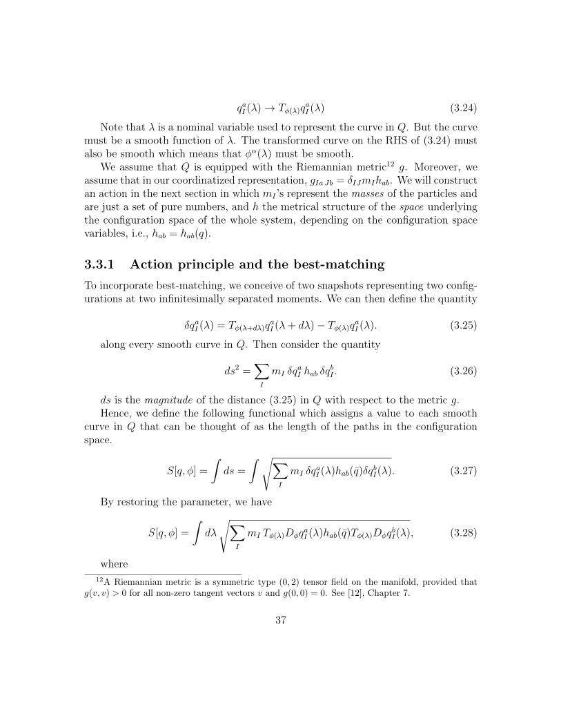
qaI (λ)→ Tφ(λ)qaI (λ) (3.24)

Note that λ is a nominal variable used to represent the curve in Q. But the curvemust be a smooth function of λ. The transformed curve on the RHS of (3.24) mustalso be smooth which means that φα(λ) must be smooth.

We assume that Q is equipped with the Riemannian metric12 g. Moreover, weassume that in our coordinatized representation, gIa Jb = δIJmIhab. We will constructan action in the next section in which mI ’s represent the masses of the particles andare just a set of pure numbers, and h the metrical structure of the space underlyingthe configuration space of the whole system, depending on the configuration spacevariables, i.e., hab = hab(q).

3.3.1 Action principle and the best-matching

To incorporate best-matching, we conceive of two snapshots representing two config-urations at two infinitesimally separated moments. We can then define the quantity

δqaI (λ) = Tφ(λ+dλ)qaI (λ+ dλ)− Tφ(λ)q

aI (λ). (3.25)

along every smooth curve in Q. Then consider the quantity

ds2 =∑I

mI δqaI hab δq

bI . (3.26)

ds is the magnitude of the distance (3.25) in Q with respect to the metric g.Hence, we define the following functional which assigns a value to each smooth

curve in Q that can be thought of as the length of the paths in the configurationspace.

S[q, φ] =

∫ds =

∫ √∑I

mI δqaI (λ)hab(q)δqbI(λ). (3.27)

By restoring the parameter, we have

S[q, φ] =

∫dλ

√∑I

mI Tφ(λ)DφqaI (λ)hab(q)Tφ(λ)DφqbI(λ), (3.28)

where

12A Riemannian metric is a symmetric type (0, 2) tensor field on the manifold, provided thatg(v, v) > 0 for all non-zero tangent vectors v and g(0, 0) = 0. See [12], Chapter 7.

37

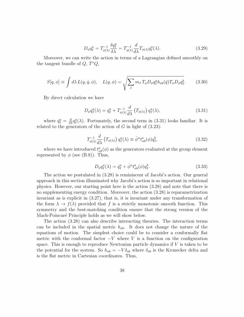
DφqaI = T−1

φ(λ)

δqaIδλ

= T−1φ(λ)

d

dλTφ(λ)q

aI (λ). (3.29)

Moreover, we can write the action in terms of a Lagrangian defined smoothly onthe tangent bundle of Q, T ∗Q,

S[q, φ] ≡∫dλL(q, q, φ), L(q, φ) =

√∑I

mI TφDφqaIhab(q)TφDφqbI . (3.30)

By direct calculation we have

DφqaI (λ) = qaI + T−1

φ(λ)

d

dλ

(Tφ(λ)

)qaI (λ), (3.31)

where qaI = ddλqaI (λ). Fortunately, the second term in (3.31) looks familiar. It is

related to the generators of the action of G in light of (3.23):

T−1φ(λ)

d

dλ

(Tφ(λ)

)qaI (λ) ≡ φαtaαb(φ)qbI , (3.32)

where we have introduced taαb(φ) as the generators evaluated at the group elementrepresented by φ (see (B.8)). Thus,

DφqaI (λ) = qaI + φαtaαb(φ)qbI . (3.33)

The action we postulated in (3.28) is reminiscent of Jacobi’s action. Our generalapproach in this section illuminated why Jacobi’s action is so important in relationalphysics. However, our starting point here is the action (3.28) and note that there isno supplementing energy condition. Moreover, the action (3.28) is reparametrizationinvariant as is explicit in (3.27), that is, it is invariant under any transformation ofthe form λ → f(λ) provided that f is a strictly monotonic smooth function. Thissymmetry and the best-matching condition ensure that the strong version of theMach-Poincare Principle holds as we will show below.

The action (3.28) can also describe interacting theories. The interaction termscan be included in the spatial metric hab. It does not change the nature of theequations of motion. The simplest choice could be to consider a conformally flatmetric with the conformal factor −V where V is a function on the configurationspace. This is enough to reproduce Newtonian particle dynamics if V is taken to bethe potential for the system. So hab = −V δab where δab is the Kronecker delta andis the flat metric in Cartesian coordinates. Thus,

38

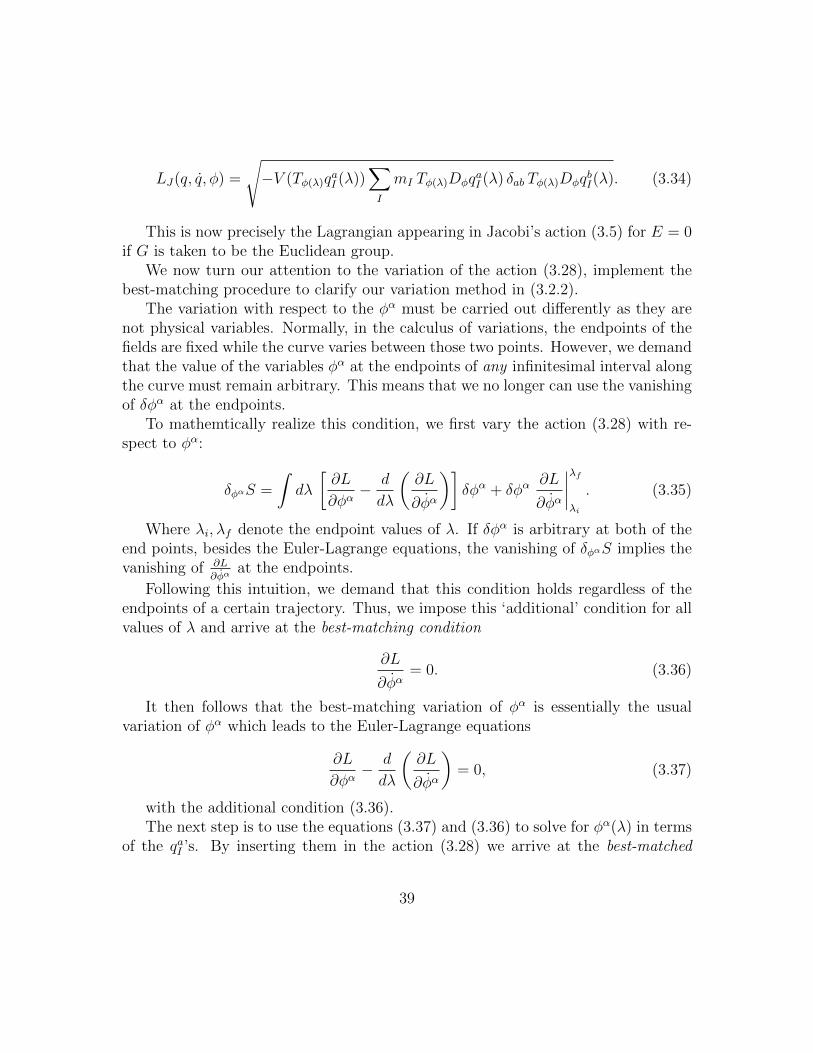
LJ(q, q, φ) =

√−V (Tφ(λ)q

aI (λ))

∑I

mI Tφ(λ)DφqaI (λ) δab Tφ(λ)DφqbI(λ). (3.34)

This is now precisely the Lagrangian appearing in Jacobi’s action (3.5) for E = 0if G is taken to be the Euclidean group.

We now turn our attention to the variation of the action (3.28), implement thebest-matching procedure to clarify our variation method in (3.2.2).

The variation with respect to the φα must be carried out differently as they arenot physical variables. Normally, in the calculus of variations, the endpoints of thefields are fixed while the curve varies between those two points. However, we demandthat the value of the variables φα at the endpoints of any infinitesimal interval alongthe curve must remain arbitrary. This means that we no longer can use the vanishingof δφα at the endpoints.

To mathemtically realize this condition, we first vary the action (3.28) with re-spect to φα:

δφαS =

∫dλ

[∂L

∂φα− d

dλ

(∂L

∂φα

)]δφα + δφα

∂L

∂φα

∣∣∣∣λfλi

. (3.35)

Where λi, λf denote the endpoint values of λ. If δφα is arbitrary at both of theend points, besides the Euler-Lagrange equations, the vanishing of δφαS implies thevanishing of ∂L

∂φαat the endpoints.

Following this intuition, we demand that this condition holds regardless of theendpoints of a certain trajectory. Thus, we impose this ‘additional’ condition for allvalues of λ and arrive at the best-matching condition

∂L

∂φα= 0. (3.36)

It then follows that the best-matching variation of φα is essentially the usualvariation of φα which leads to the Euler-Lagrange equations

∂L

∂φα− d

dλ

(∂L

∂φα

)= 0, (3.37)

with the additional condition (3.36).The next step is to use the equations (3.37) and (3.36) to solve for φα(λ) in terms

of the qaI ’s. By inserting them in the action (3.28) we arrive at the best-matched

39

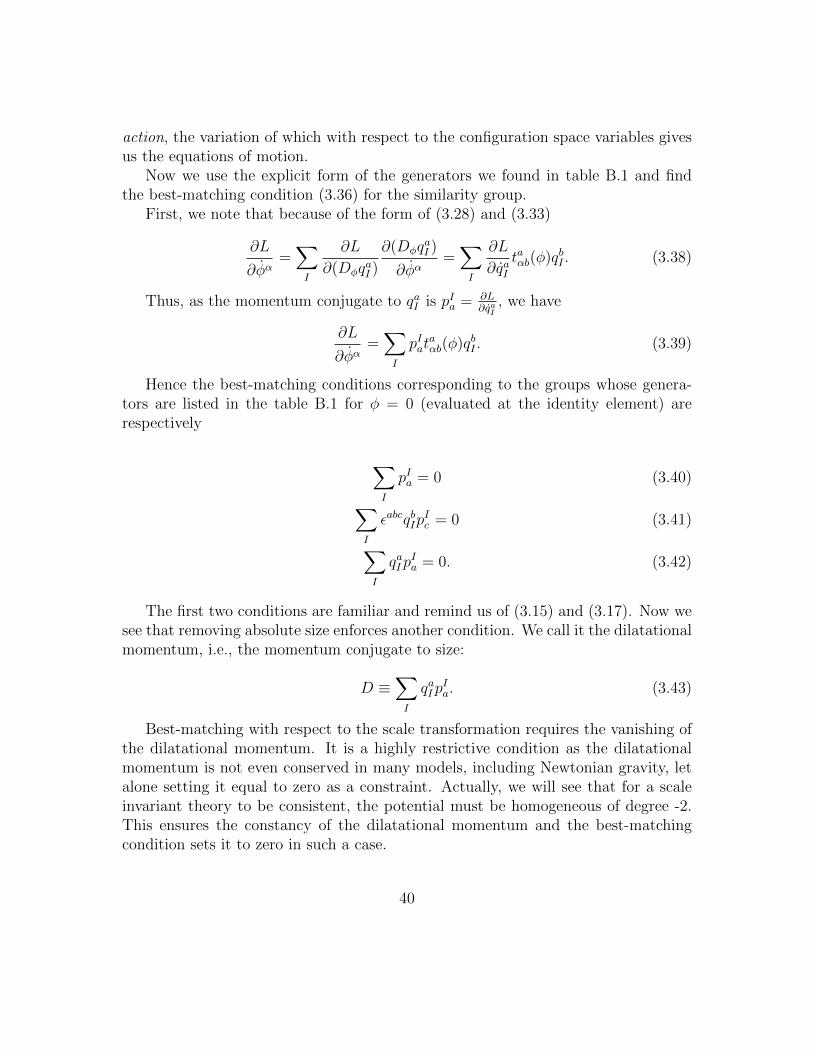
action, the variation of which with respect to the configuration space variables givesus the equations of motion.

Now we use the explicit form of the generators we found in table B.1 and findthe best-matching condition (3.36) for the similarity group.

First, we note that because of the form of (3.28) and (3.33)

∂L

∂φα=∑I

∂L

∂(DφqaI )

∂(DφqaI )

∂φα=∑I

∂L

∂qaItaαb(φ)qbI . (3.38)

Thus, as the momentum conjugate to qaI is pIa = ∂L∂qaI

, we have

∂L

∂φα=∑I

pIataαb(φ)qbI . (3.39)

Hence the best-matching conditions corresponding to the groups whose genera-tors are listed in the table B.1 for φ = 0 (evaluated at the identity element) arerespectively

∑I

pIa = 0 (3.40)∑I

εabcqbIpIc = 0 (3.41)∑

I

qaIpIa = 0. (3.42)

The first two conditions are familiar and remind us of (3.15) and (3.17). Now wesee that removing absolute size enforces another condition. We call it the dilatationalmomentum, i.e., the momentum conjugate to size:

D ≡∑I

qaIpIa. (3.43)

Best-matching with respect to the scale transformation requires the vanishing ofthe dilatational momentum. It is a highly restrictive condition as the dilatationalmomentum is not even conserved in many models, including Newtonian gravity, letalone setting it equal to zero as a constraint. Actually, we will see that for a scaleinvariant theory to be consistent, the potential must be homogeneous of degree -2.This ensures the constancy of the dilatational momentum and the best-matchingcondition sets it to zero in such a case.

40

3.3.2 Mach-Poincare Principle revisited

The action (3.28) is invariant under the double gauge transformation

qaI (λ)→ Tω(λ)qaI (λ),

φα(λ)→ φα(λ)− ζα(λ),(3.44)

for any ω, where ζα satisfies the condition Tφ−ζTω = Tφ. This double gaugesymmetry is named banal transformation in [13].

Thus, the action (3.28) is practically defined on the orbits of Sim(3) in Q. Moreprecisely, after choosing the initial conditions in Q/Sim(3), in light of our discussionthat the best-matched curves in the configuration space cut through the orbits, therewill be only one curve in the quotiented space extremizing the action and given theinitial condition in the reduced space. This is essentially the first main content ofthe Mach-Poincare Principle.

As regards the second principle, the reparametrization invariance of the action(3.28) ensures that the directions are only relevant. This action is a geodesic principleand only requires an initial point in Q and a direction in the corresponding tangentspace as the initial conditions, for the magnitude of the initial vector is redundantdue to the arbitrariness of the parameter.

More strikingly, we can choose the ephemeris time as the parameter with respectto which the equations of motion take the familiar form of Newton’s equations (in thecase that interaction is also included in the metric, i.e., hab = −V δab. The variationof the action (3.28) with respect to the best-matched coordinates, qaI = Tφq

aI , where

φα is the solution of the best-matching conditions, leads to the equation of motion

d

dλ

(−V (q)

L(q, q, φ)mI ˙qbI(λ)δab

)= − T ( ˙q)

L(q, q, φ)

∂V (q)

∂qaI. (3.45)

With the choice of the parameter such that√− TV

= 1, we have

mI ¨qaI = −∂V (q)

∂qaI. (3.46)

This specific time parameter is the ephemeris time (3.47) and its definition isbased on the change of the variables of the entire island universe:

dt =

√√√√∑I mIdq2I

−2V (q). (3.47)

We recapitulate the best-matching procedure in the Lagrangian formulation:

41

1. First, we begin with a well-defined configuration space Q endowed with a dif-ferentiable manifold and a metric g.

2. We identify the symmetry group G on empirical grounds, consider its actionon Q, and make the substitution qaI → Tφαq

aI .

3. We posit a geodesic principle in the configuration space of the form

S =

∫dλ√g(TφDφq, TφαDφq).

4. Finally, we perform the best-matching variation of φα by imposing the Euler-Lagrange equations and the additional condition

∂L

∂φα= 0.

5. We solve the above equations, find the best-matched coordinates, vary theaforementioned action with respect to them, and arrive at the relational equa-tions of motion.

Depending on the nature of the metric, there are in principle two different typesof best-matching. One is equivariant best-matching which is the case that the metricg remains invariant under the group transformation Tφ, i.e., this transformation isan isometry of g. More precisely, it means that T−1∗

φ g = g where T−1∗φ is the pullback

corresponding to the diffeomorphism T−1φ on Q. The second type is non-equivariant

best-matching, corresponding to the case that the group transformation is not anisometry of the configuration space metric.

As these two types can differ in many respects, we study them in the followingsections separately.

3.4 Best-matching and reparametrization invari-

ance

In our general approach, we posited an action defined in terms of the trajectories inthe configuration space equipped with a metric:

S[q] =

∫dλ

√∑I

mI habqaI qbI .

42

We saw that with a particular choice of a conformally flat metric the actionbecomes Jacobi’s action (3.2). In fact, what is striking is that one can look at thereparametrization invariance of Jacobi’s action in light of best-matching with respectto time. To see that, let us assume hab = −V δab. It is easy to check that the action

S[q,N ] =

∫dλ

(1

N

∑I

mI qI qI −NV

)(3.48)

also reproduces the same equations of motion and is equivalent to the aboveaction provided that we identify N as

N =

√∑I

mI qI qJ

V. (3.49)

In general, N is an additional variable in the action (3.48) and should be variedindependently. If we extermize (3.48) with respect to N , we arrive at the abovecondition.

Action (3.48) resembles the reparametrization invariant form of the Newtonianaction we have introduced in Appx. A:

S[q, t] =

∫dλ

(1

t

∑I

mI qI qJ − tV

)(3.50)

We should just take N = t to make them identical. For this reason, we mightsay that the action (3.48) performs best-matching with respect to time: We havean initial action written in terms of an external time t, we give it an arbitraryparametrization, i.e., t → t(λ), we eventually vary the action with respect to t andimpose the best-matching condition

∂L

∂t= 0. (3.51)

This condition ensures that we could have made the identification N = t = dtdλ

and vary the action with respect to N , in accord with what we did with the action(3.48).

Overall, what it all means is that mathematically, Jacobi’s action is effectivelythe standard Newtonian action best-matched with respect to the time that is used inits formulation. It should be emphasized that this is only a mathematical analogy,and not as part of the procedure developed in relational physics. Time is essentially

43

different from the configuration space variables, and using the term ‘best-matching’for reparametrization invariant theories, as we did, has merely a heuristic meaning.

One last note should be made regarding the status of E which we identifiedas the energy in Jacobi’s action. In general, one can conceive of a conformallyflat metric with an additional constant added to the potential term, hab = (E −V )δab. In this approach, E is a universal constant existing originally in the action.Also, as we discuss in Appx. A, in the Routhian reduction procedure for time-independent Newtonian potentials, we can set the momentum conjugate to timeequal to a constant value, e.g., −E. This again adds a constant term to the potentialterm in Jacobi’s action. Here, unlike the above case, E is a constant of motion thatis only meaningful in the case that Newtonian external time is posited. In relationalphysics, the momentum conjugate to time is essentially set to zero and is a constraintby virtue of the best-matching condition (3.51). The point is that both of the aboveapproaches result in the same action and in both cases, E can be seen as the energyof the system. In Newtonian physics, E = −pt is the energy by definition, while inrelational physics, if we introduce the ephemeris time we have

E = T + V, T =∑I

1

2mI

dqIdt

dqJdt, (3.52)

where t is the ephemeris time again by definition.The above discussion shows that at least in classical physics, as far as the evolution

of the relational degrees of freedom of the system is concerned, these two ways ofdefining E result in the same thing. However, in the spirit of Leibniz’s Principle ofSufficient Reason, we may not want to introduce an arbitrary universal constant inthe action and set E equal to zero. It should be noted that in quantum mechanicsthese two ways do not remain equivalent, the discussion of which goes beyond thescope of this work. See Section 3.5 of [11].

3.5 Equivariant best-matching

The focus of this chapter is the equivariant actions. We recap the Lagrangian for-mulation of equivariant actions, perform the best-matching, and finally analyze theimplications of equivariance best-matching for interaction potentials. Then we willdevelop the Hamiltonian formulation.

The Hamiltonian formulation is a lot more powerful than the Lagrangian formu-lation in many respects. The most significant aspect is the elegantly clear perspectiveit provides on the concept of gauge transformations as we will see.

44

3.5.1 Lagrangian formulation

Our starting point is the action (3.28) we found in the last section

S[q, φ] =

∫dλ

√∑I

mI Tφ(λ)DφqaI (λ)habTφ(λ)DφqbI(λ).

Based on definition, the equivariance condition means that T−1∗φ h = h, implying

that

hab(q) ≡ (T−1φ )ca(T

−1φ )db hcd(q) = hab(q), (3.53)

where (T−1φ )ca denotes the matrix elements of the inverse of the diffeomorphism

induced by the action of the symmetry group G on Q, i.e.,

(Tφ)ab ≡ ∂qbITφqaI =

∂qaI∂qbI

, (3.54)

where φ(q) is a smooth function defined on Q. Thus, the equivariance conditionleads to the action

S[q, φ] =

∫dλ

√∑I

mI DφqaI (λ)hab(q)DφqbJ(λ). (3.55)

The equations of motion can be determined by performing the best-matchingvariation with respect to φα’s and then qaI ’s. For equivatiant theories, what best-matching variation essentially does is that it elevates the role of the parameters αα’sas a cyclic variable to a Lagrange multiplier. In an equivariant action of the form(3.55), φα’s drops out of the theory completely. Formally,

∂L

∂φα= 0. (3.56)

This means that the variables φα’s are cyclic and the momentum conjugate tothem is a constant of motion. Now the best-matching condition (3.36) is effectivelyequivalent to varying the action (3.55) with respect to the variable Nα = φα. In lightof this consideration, we can say that φα’s appearing in the term Dαq

aI in (3.55) act

as Lagrange multipliers, enforcing the best-matching conditions.We know that every isometry like (3.53) leads to the existence of some global

Killing vectors in Q, for the Lie derivative of the metric in the direction of theflow of the symmetry group vanishes, i.e., Lvh = 0, where v is the vector field

45

associated with the infinitesimal group transformation. As to the first degree wehave qaI → φαtaαbq

bI , v

a = φαtaαbqbI .

Consequently, the equivariance condition explicitly implies13

Lvhab =∑I

φα(tcαdq

dI∂qcIhab + hcb∂qaI (tcαdq

dI ) + hac∂qbI (t

cαdq

dI ))

= 0, (3.57)

for all φα’s. When exponentiated, the above condition yields the global isometry(3.53). In fact, (3.57) is the infinitesimal form of the aforementioned condition.

Now we turn our attention to the implications for particle dynamics of the equiv-ariance condition with respect to the similarity group.

As we explained in the previous section, one can choose a conformally flat metricand arrive at the standard Newtonian mechanics given by Jacobi’s action (3.34).For brevity, we drop the constant term E and take the factor to be proportional toonly the potential. With this choice, hab = −V δab. In light of the above discussion,the equivariance condition (3.57) with respect to translations, rotations, and scaletransformation implies the conditions

∑I

∂qaIV (q) = 0, (3.58)∑I

εartqrI∂qtIV (q) = 0, (3.59)∑I

qaI∂qaIV (q) + 2NV (q) = 0. (3.60)

for φ = 0 respectively.The significance of the first two conditions is quite clear. It means that the

total potential of the island universe (the whole system) must be translationallyand rotationally invariant, as they should be if we want a relational theory of thewhole. The third condition, however, is new. Using Euler’s theorem, it meansthat the potential is homogeneous of degree -2 in the variables, i.e., V (q) ∝ 1/q2.Unfortunately, the Newtonian gravitational potential is of degree -1 and does notsatisfy this condition. This is an issue if we want to include the standard gravitationalinteraction in a relational theory of the whole universe. This shakes our hope foran empirically valid consistent scale-free theory. We will come back to this issuein the second part of this work. For now, we just stay focused on developing themathematics of best-matching.

13We drop the φ dependence of the generators in this section for brevity.

46

3.5.2 From the Lagrangian to the Hamiltonian formulation

To make the transition to the Hamiltonian formulation, our starting point in thecanonical formulation of the equivariant action (3.55). We can then find the momen-tum conjugate to the variables qaI ’s and φα’s:

pIa ≡∂L

∂qaI=

mIhabDφqbI√∑

I

mI DφqaI (λ)habDφqbJ(λ),

πα ≡∂L

∂φα=

∑I

mIhabDφqbJ t

aαc(φ)qcI√∑

I

mI DφqaI (λ)habDφqbJ(λ).

(3.61)

Then the phase space Γ can be coordinatized by the variables (qaI , paI , φ

α, πα).Also, as the fundamental and essential structure of phase space, we posit the Poissonbrackets

qaI , pJb = δab δJI , φα, πβ = δαβ . (3.62)

From the definitions of the conjugate momenta in (3.61), it can be easily verifiedthat the constraints

H =∑I

habpIapIb

mI

− 1 ≈ 0, (3.63)

Hα = πα −∑I

pIataαbq

bI ≈ 0. (3.64)

immediately follow, where hab is the inverse of hab.The first constraint is the Hamiltonian constraint as the result of the reparametriza-

tion invariance. This quadratic constraint arises from the fact that only the directionsof the variables qaI matter. From the definition of pIa in (3.61) we see that it is a unitvector on phase space. These are all consistent and ultimately come down to tem-poral relationalism and Mach’s second principle. The vector constraints (3.64) arerelated to the symmetries of the configurations and Mach’s first principle.

Thus, H reflects the physically insignificant magnitude of qaI , meaning that theevolution of the whole universe can be parametrized arbitrarily. Hα’s reflect thegauge invariance of the action with respect to the symmetry of the configurationspace expressed by G.

47

Hence, as the Hamiltonian corresponding to the Lagrangian (3.55) vanished, wefollow Dirac’s approach (see Appx. C), and write total Hamiltonian as

HT = NH +NαHα, (3.65)

with N and Nα as some arbitrary coefficients. Following the standard terminol-ogy used in ADM formalism, we call them the lapse function and the shift vectorrespectively.

It is very important to calculate the Poisson brackets between the constraintsand see that they are all first-class:14 15

Hα,Hβ = 0,

H,Hα =

(∑I

mIpIapJb

)(∑K

tcαdqdK∂qcKh

ab − hcb∂qcI taαdq

dI − hac∂qcI t

bαdq

dI

).

(3.66)

The first relation merely reflects the structure of the Lie algebra and clearly showsthat Hα’s are first-class with respect to one another. The second relation is also zeroin light of the equivariance condition (3.57).16

As we know from Dirac’s formulation of constrained Hamiltonian systems, first-class constraints generally generate gauge transformations in the phase space. Thestatus of the single scalar constraint H is clear: In light of [14] and our account of itin Sec. C.5, it generates true evolution but with an arbitrary parametrization. Theparametrization, expressed through N in (3.65), is the gauge. The vector constraintsHα’s generate the transformations

δqaI ≡ NαqaI ,Hα = −NαtaαbqbI ,

δpIa ≡ NαpIa,Hα = NαpIb∂qaI tbαcq

cI .

(3.67)

When exponentiated, these infinitesimal transformations yield the banal trans-formation (3.44) we noted in the Lagrangian formulation. This ensures that Mach’sfirst principle is satisfied in the theory.

14One has to use (B.9) for calculating the Poisson brackets between the vector constraints.Thanks to Sean Gryb for the discussion and the clarification of this point.

15In working our the second bracket note that ∂qcJ taαbq

bI = δJI ..., as is clear from the fact that G

acts non-trivially only on the spatial part of Q and treats all particle on the same footing.16Note that contrary to (3.57), in (3.66) the inverse of the spatial metric appears, resulting in a

relative minus sign between the first term and the other two. It can be easily verified by multiplying(3.57) by haehbf and using Leibniz rule.

48

3.5.3 Best-matching conditions in the Hamiltonian formula-tion

Apart from the standard variation with respect to qaI ’s and the equations of motion,we posited the additional condition (3.36) by which the best-matching variation wasdefined. So far, in our analysis of the canonical formulation of best-matching, wehave not addressed this condition. It can be done analogously to the Lagrangianformulation through the phase space action.

The phase space action which gives the correct equations of motion of the phasespace variables is

SPS[q, p, φ, π,N,Nα] =

∫dλ

(∑I

pIaqaI + παφ

α −HT (q, p, φ, π,N,Nα)

). (3.68)

As we discussed in the previous section, the best-matching variation means tovary the fields φα’s freely on the endpoints of any interval along the trajectory. In(3.68) only the in the variation of φ and πα this method becomes relevant, sinceonly these two are the parameters associated with the action of the symmetry group.Following the condition of the vanishing of the variation with respect to the πα, wefind out that the values of the field at the endpoints do not appear and there wouldbe no best-matching condition for them.

However, the variation of (3.68) with respect to φ is

δφS = −∫dλ

(∂HT

∂φα+ πα

)δφα + παδφ

α|λfλi . (3.69)

The vanishing of the first term is simply the Euler-Lagrange equation for the φα

field. However, δφα is not equal to zero at the endpoints and if we demand that theabove variation vanishes irrespective of the endpoints along any trajectory, we arriveat the canonical best-matching condition

πα ≈ 0. (3.70)

It is the counterpart of the best-matching condition in the Hamiltonian formu-lation. This condition is new and actually changes the Poisson structure. UsingDirac’s terminology, it is a constraint to be enforced weakly, same as H,Hα. Thisconstraint is first-class in the equivariant best-matching.

This condition leads to a remarkable conclusion in its connection with the vectorconstraints Hα. The two of them lead to the first-class constraint

49

Cα ≡∑I

pIataαbq

bI ≈ 0 (3.71)

This constraint is also first-class as it is the offspring of two first-class constraints.The meaning of this constraint is evident: It generates a gauge transformation in-duced by the symmetry group G on the (qaI , p

Ia) variables alone. The best-matching

condition breaks the banal symmetry (3.44) in two parts, throws the transformationof the unphysical field φ away, and keeps the other part which corresponds to thetransformation of the configurations.

3.5.4 The equations of motion

We can now work out the equations of motion.In light of the best-matching condition and that the constraint (3.71) is first-

class, Dirac’s conjecture is applicable here and we define the extended Hamiltonianas (C.21):

HE = NH +NαCα + ζαπα. (3.72)

The equations of motion are

qaI = 2Nhab

mI

pIb +NαtaαbqbI ,

pIa = −N∑J

1

mJ

∂qaI hbcpJb p

Jc −NαpIb∂qaI t

bαcq

cI ,

φα = ζα,

πα = 0.

(3.73)

The last equation is obvious. As we noted, the constraints are first-class and theconsistency conditions ensure that the constraint πα remains zero. The third equationmerely reflects the arbitrariness of φα in light of the best-matching condition. Thefirst two equations govern the evolution of the configurations. We find the equationof motion of qaI ’s alone and make sure that it is in accord with our results in theLagrangian formulation. First, we rewrite the equations of motion for qaI and pIamore concisely in the form17

17Strictly speaking, the equations (3.74) with −Nα follow from (3.73). But this is not importantdue to arbitrariness of Nα.

50

T−1N

d

dλTNq

aI = −2N

hab

mI

pIb ,

TNd

dλT−1N pIa = N

∑J

1

mJ

∂qaI hbcpJb p

Jc .

(3.74)

We can inverse the first equation in (3.74) and find the conjugate momentum:

pIa = − 1

2NmIhab(q) ˙qbI , (3.75)

where qaI = TNqaI and pIa = T−1

N pIa = (T−1N )bap

Ib , and we also used (3.53).

And the second equation can be rewritten as

˙pIa = N∑J

1

mJ

pJb pJc ∂qaI h

bc(q). (3.76)

Thus, the equations of motion for ˙qaI is

1

N

d

dλ

(1

2NmIhab(q) ˙qbI

)= −

∑J

1

mJ

pJb pJc ∂qaI h

bc(q). (3.77)

It becomes more familiar if we take hab = −2V δab. Moreover, the Hamiltonianconstraint H = 0 given in (3.63) gives∑

I

pIapIa

2mI

+ V = 0. (3.78)

Hence,

− V

N

d

dλ

(−VNmIδab ˙qbI

)= −∂qaIV. (3.79)

By using the reparametrization freedom and identifying

− N

Vdλ ≡ dt, (3.80)

we fix N , and arrive at Newton’s 2nd law:

mId2

dt2qaI = −∂qaIV (q). (3.81)

By using (3.75) and (3.78), it is straightforward to see that

51

N2

V 2= −T

V. (3.82)

Therefore, this reparametrization fixing condition is in accord with the result wearrived at Sec. 3.3.2 and (3.80) actually defines the ephemeris time (3.47).

Hence, compatibly with the results we derived in the Lagrangian formulation,from the point of view of relational particle physics, Newtonian mechanics is bornwhen a particular conformally flat metric, and a specific time gauge are chosen. Wemust not forget the constraints Hα. From this perspective, we could say relationalphysics is more fundamental.

3.6 Non-equivariant best-matching

In the last section, we explored the best-matching technique for equivariant metrics,i.e., those which are invariant under the action of the symmetry group:

T ∗φh = h. (3.83)

We saw that best-matching elevates the global symmetry of such theories to agauge symmetry in a larger configuration space. This mathematical ‘transfiguration’turned the standard Newtonian mechanics into a Machian theory. In this chapter,we consider non-equivariant metrics which are by definition, not invariant under theaction of the group. They do not even respect the symmetry induced by the groupas a global symmetry. If we insist on performing best-matching, we will have thebest-matching constraint to be satisfied, same as before. However, the conservationof such constraint is not even assured in the first place, let alone its vanishing. Thisis the issue: best-matching with respect to a group that is not a symmetry group ofthe action results in an inconsistency.

This can be quite disheartening, especially in light of its connection with ourown universe. So far, our attempts in this first part of the thesis have been in thedirection of developing the theory mathematically and we keep the physical applica-tion of relational physics to our universe for the second part. But the point is thatthe Newtonian 1/r potential - which is strongly supported by observational evidence- renders the configuration space metric non-invariant under scale transformation.However, from the relational point of view, we resolutely need scale invariance if weaspire to have a relational theory of the whole, i.e., to satisfy the Mach-Poincareprinciple for the group Sim(3). What can we do?

52

I think it is safe to say that a completely scale-free theory compatible with obser-vations is nearly unobtainable if not entirely impossible. We will discuss this issuein more detail later in part II. For now, the matter is fortunately not that hopeless.A partially scale-free theory can be constructed - even if the underlying metric isnot equivariant - which is the main focus of this section. The physical intuition ofthis approach was first realized by Julian Barbour, et al. in [15] in its application togeneral relativity and was later developed more mathematically by Tim Koslowski,Sean Gryb, and Henrique Gomes at Perimeter Institute [16].

To give an intuitive picture of how it can be done, suppose N particles in thethree-dimensional Euclidean space. Scaling means changing the positions of theparticles by a factor. If best-matching with respect to this transformation does notwork, why do we not weaken the symmetry? We can conceive of a transformationthat changes the ‘local’ scale while being subject to a global restriction. As we will seein the next chapter, In geometrodynamics, this translates into working with volumepreserving conformal transformations. We can then proceed with implementing thebest-matching and Mach-Poincare principle for that weaker symmetry.

There is a price to pay in the course of this procedure. The metric remainsnon-equivariant under this weaker symmetry. In order to resolve the inconsistencythat might follow from enforcing the best-matching condition, we strengthen thereparametrization invariance of the theory, making it possible to fit the best-matchingconstraint into the theory consistently as we have now more freedom in fixing theparametrization. There is a deeper picture behind this procedure, called symmetrytrading, that essentially captures the mathematical essence of what we are doing here:We trade a larger reparametrization invariance for a symmetry in configuration spacewe would like to have.

In other words, we must ‘bribe’ a non-equivariant theory into accepting a morehumble symmetry as its gauge freedom. If we accept that compromise, we can havea partially scale-free theory.

We now proceed to formulate this intuition mathematically. We use a particle toymodel in this section to sharpen our technique, leaving the more physically profoundcase of general relativity for the next chapter.

3.6.1 The Lagrangian point of view

The procedure we outlined above can be developed more powerfully and clearly inthe Hamiltonian formulation. it is nevertheless insightful to see how it generallyworks in the Lagrangian picture.

53

The toy model we work with comprises N independent harmonic oscillators.18 Inlight of (3.48), the reparametrization invariant action is

S[q,N ] =

∫dλ

N∑I=1

(q2I

2NI

+NIk

2q2I

), (3.84)

where the masses of the particles are set to one for convenience. The metric thatis used for the Kinetic term is the Euclidean metric. We dealt with a general confor-mally flat metric on configuration space before and for now, we focus on a simpler toymodel. The quadratic potential and its negative sign are also for simplicity purposes.As we will see, what is most important is that the N systems must be independentand in other words, ‘local’. The reader might spot something conspicuously non-relational about the action (3.84). The concept of an independent system does havea non-relational aura indeed. Nonetheless, this is a good toy model for studyingbest-matching and scale transformations. Note that this approach serves solely aheuristic role as a toy model for working with general relativity later. The NI ’s aremeant to model the local nature of time in general relativity. Here, the concept oflocality is modeled by working with the individual particles. We are effectively usinga theory with a finite number of degrees of freedom as a ‘naive’ model of field theories(general relativity in particular) with continuous degrees of freedom.

Now we define the symmetry to best-match. We are looking for a scale transfor-mation of the form

qaI → eφIqaI , (3.85)

where φI ’s are arbitrary conformal factors for each I. However, this is not goingto work as it is equivalent to scale transformation of the N independent systemsseparately and in light of our above discussion this leads to an inconsistency. Wedefine the mean operator:

〈·〉 ≡ 1

N

∑I

·I , (3.86)

and restrict the scale transformation parameters to obey the condition

〈φ〉 = 0. (3.87)

We can satisfy this identity by writing φ as

18There is nothing special about harmonic oscillators in this approach. It is just for making thecalculations simpler.

54

φI = φI − 〈φ〉. (3.88)

This explicitly reduces the number of independent φI ’s to N − 1. We can stillwork with the parameters φI ’s but use the transformation eφI . This weakens thescale transformation as promised.

We now turn our attention to best-matching with respect to the parameters φI .The action (3.84) changes to

S[q,N, φ] =

∫dλ

N∑I=1

(1

2NI

(d

dλ

(eφIqI

))2

+NIk

2e2φIq2

I

), (3.89)

Using the notation we introduced in (3.29), we have

˙qaI ≡d

dλ

(eφIqaI

)= eφIDφq

aI = eφI

(qaI +

˙φIq

aI

)(3.90)

If the action (3.89) is to be best-matched, we have to impose the best-matchingcondition

πIφ ≡∂L

∂φI=

˙qI · qINI

− 〈˙q · qN〉 = 0 (3.91)

as can be simply checked.The remarkable aspect of (3.91) is that it does not impose the vanishing of the

total dilatational momentum. It only requires them to be the same:

DI(λ) = DJ(λ) = C(λ) (3.92)

at each instant for all I, J , where DI is the dilatational momentum of the systemI and C is a function of λ, independent of the configuration space variables.

The vanishing of the dilatational momentum is a restrictive condition that is notsatisfied in a non-equivariant theory, whereas the above condition can in principlebe satisfied by fixing the lapse functions NI . (3.91) enforces only N − 1 independentconstraints. Thus, N − 1 lapses can be fixed, and one global lapse remains thatevolves the whole system. More significantly, the solutions of (3.91) are in generalnon-local, meaning that the NI satisfying (3.91) would be generally dependent onthe variables qJ .

This is what happens in the Lagrangian formulation. N independently evolvingsystems ‘link up’ together and evolve in a universal manner to keep up a local scalesymmetry. Of course, this is only an intuitive picture of what happens in our abstract

55

mathematical description of the system. Neither of the NI is physical or related tosomething inherently observable.

We leave out the complete calculations of NI here. More rigorous calculationsand details will be given in the Hamiltonian formulation. This section is to only givean overview of how to deal with non-equivariant actions.

3.6.2 The Hamiltonian formulation and symmetry tradingalgorithm

The Hamiltonian formulation provides a remarkably deeper perspective into whathappens in a non-equivariant model by using Dirac’s approach and the languageof constraints. Our starting point is to perform the Legendre transform of the La-grangian in (3.84). The momentum conjugate to qaI is

pIa =qaINI

. (3.93)

Because of the local reparametrization invariance of each system, there are Nconstraints associated with the variation of lapse functions,

∂L

∂NI

= − q2I

2N2I

+k

2q2I = 0. (3.94)

Thus, we identify the Hamiltonian constraints19

χI =1

2

(p2I − kq2

I

)≈ 0. (3.95)

The Hamiltonian constraints are all first-class. The total Hamiltonian is20

H =N∑I=1

N IχI . (3.96)

19We have deviated from our notation convention here and used the subscript I for the squareof pIa to make the expression neater.

20Strictly speaking, we should have also considered the variables NI and the momenta conjugateto them (which vanish as some constraints) in the Hamiltonian formulation. This only complicatesthe procedure and does not change the final Hamiltonian, as those momenta simply generate gaugetransformations, rendering the NI ’s arbitrary. This is already respected in the Hamiltonian wearrived at.

56

This theory is defined on the original phase space Γ(q, p) labeled by (qaI , pJb ).

To implement canonical best-matching, we enlarge the phase space by adding theconformal factors φI ’s and their conjugate momenta πIφ’s.

From (3.89), the conjugate momenta are

pIa =1

NI

e2φIDφqaI . (3.97)

Moreover, a straightforward calculation shows that the momentum conjugate toφI is

πIφ = qI · pI − 〈q · p〉. (3.98)

The Hamiltonian constraints associated with the theory (3.89) are

χI =1

2

(e−2φIp2

I − e2φIkq2I

)(3.99)

Thus, we have a theory in the extended phase space ΓE(q, p, φ, π). In this theory,the following constraints have to be satisfied:

χI =1

2

(e−2φIp2

I − e2φIkq2I

)≈ 0

CI = πIφ −(qI · pI − 〈q · p〉

)≈ 0

(3.100)

This is reminiscent of the constraints in the equivariant case (3.63). The totalHamiltonian is

H =N∑I=1

(N IχI + θICI

). (3.101)

It can be checked that the constraints χI ’s and CI ’s are first-class. It should notbe a surprise. We have not done anything suspicious beyond the ‘tame’ extendedaction (3.89). As CI ’s are first-class, they generate gauge transformations. Theinfinitesimal gauge transformations are easy to calculate:

δθqaI = −θIqaI δθp

Ia = θIp

Ia

δθφI = θI δθπIφ = 0,

(3.102)

where δθ· = ·,∑I

θICI. We can easily fix this gauge freedom by imposing the

condition φI = 0 and go back to the reduced phase space Γ(q, p) with the Hamiltonian

57

(3.96). However, we bravely tread forward and perform the best-matching in theextended phase space. The best-matching condition implies

πIφ ≈ 0. (3.103)

The point is that this constraint is not in general first-class with respect to χI ’sand hence, it does not propagate. This is what we did not face in the equivariantbest-matching and is now solely the result of non-equivariance. This is the mainissue, the solution of which is the focus of the next section.

We should note that the constraints πIφ’s are redundant and this reflects the lackof complete independence of φI ’s from one another. It is easy to see

〈C〉 = 〈πφ〉 ≈ 0. (3.104)

are satisfied in the original theory regardless of best-matching. In fact, the con-straint 〈πφ〉 acts trivially on phase space. Following (3.102), one can show that the

change of qaI , pIa, φI , π

Iφ under the transformation generated by 〈πφ〉 vanish.

This is actually a blessing! Had we insisted on the full scale transformation withrespect to φI , we would have had a problem: The theory would be inconsistent andlead to ‘frozen’ dynamics as we will shortly see.

For now, the lesson we learn from the above consideration is that only N − 1 ofthe CI ’s are some non-trivial constraints to be satisfied. It is reasonable to simplyignore 〈C〉.

3.6.3 Symmetry trading

In the spirit of Dirac’s approach, all constraints on phase space must propagateaccording to the Hamiltonian evolution. This is the consistency condition. Thebest-matching condition we imposed is first-class with respect to CI ’s as can beeasily checked. It is intuitively clear why this should be the case: The CI ’s aremanifestly φI independent and πIφ essentially generates translations in φI . Hence,our focus should be the Hamiltonian constraints. We have the following condition:

N∑I=1

N IχI , πJφ =[〈N(p2 + kq2)〉 −NJ(p2

J + kq2J)]

= 0. (3.105)

We must solve this condition for N I . Although the expression in the bracket isgenerally non-zero, we can be sure that a solution exists. The reason is that the rankof the matrix χI , πJφ is not N . We must not forget about the 〈πφ〉 and that it acts

58

trivially on χI . Thus, there is in principle a one-dimensional Kernel and a uniquelapse function N I

0 that satisfies the above constraint.21 Therefore, the constraint

χf.c. ≡∑I

N I0χI (3.106)

is first class and propagates the best-matching constraint, leading to a consistentpartially scale-free theory. It is now clear why we had to weaken the symmetrygroup in the context of the Hamiltonian formulation. If φI had not been restricted,the rank of the aforementioned matrix would have been N , leading to the trivialsolution N I = 0 for (3.105). This is the ‘frozen’ dynamics we mentioned before.By restricting the symmetry group, we made room for the existence of a non-trivialsolution to evolve the system.

It is worthwhile to note that αN I0 for any α also satisfies (3.105). Thus, one

global freedom is still left for the lapse function which reflects Mach’s temporalrelationalism. The local direction of time is only fixed by (3.105). Time as anexternal entity has not come into existence. Time is still a measure of change, butnow it is the global change of the N independent systems linked together.

We can redefine the remaining second-class Hamiltonian cosntraints by usingsome arbitrary numbers αIi where i = 1, 2, · · · , N − 1:

χi ≡∑I

αIiχI . (3.107)

αIi are chosen in such a way that the N − 1 constraints χi are linearly indepen-dent, provided that the complete set χf.c., χi includes all of the original N linearlyindependent Hamiltonian constraints.

The constraints CI are still first-class. All πIφ are also second-class, apart fromone corresponding to 〈πφ〉. In the same way, we introduce some numbers to defineN − 1 linearly independent constraints πiφ. Thus, the final theory we arrived at,defined on ΓE(q, p, φ, πφ), is characterized by the first-class constraints

χf.c. ≈ 0, CI ≈ 0, (3.108)

along with the second-class constraints

χi ≈ 0, πiφ ≈ 0. (3.109)

21There is a mathematical subtlety here. The ‘matrix’ appearing in the LHS of (3.105) is definedover the phase space and its rank is in principle non-constant and it might be N . However, for all ofthe physically interesting states, our argument is valid and we can find a non-trivial lapse functionas the solution.

59

The total Hamiltonian is

HT = χf.c. +N∑I=1

θICI . (3.110)

We can now use the method we explained in Sec. C.4 to eliminate the second-classconstraints of the theory by using the Dirac bracket and imposing the second-classconstraints strongly. First of all, note that

HT = HT |χi=0,πiα=0 = χf.c.(q, p, φ0(q, p)) + θICI , (3.111)

where

CI =N∑I=1

θI(pIaq

aI − 〈p · q〉

), (3.112)

and φi0(q, p)’s are the solutions of χi = 0’s. It then follows that if we have afunction F of the variables (q, p), its evolution is given by

F ≈ F, HTDB ≈ F, HT, (3.113)

as the Dirac bracket and the usual Poisson bracket give the same equations ofmotion here.22 We now find the explicit form of the first-class Hamiltonian and theequations of motion.

3.6.4 Solving the constraints and the explicit form of theequations of motion

The toy model we used in developing non-equivariant best-matching is fortunatelysimple enough to solve the constraints and derive the equations of motion explicitly.This will also enable us to construct a dictionary between the best-matched theoryand the original theory. We saw that in the non-equivariant case, best-matchingcan be consistently performed by trading part of the gauge symmetry of the originaltheory. Thus, at the level of the equations of motion for the physical variables, thetwo theories must match.

We have the constraints χi ≈ 0’s to be satisfied. Using the explicit expression(3.100) we can solve the first set for φi0:

22It is always the case if the second-class constraints are functions of an equal number of some ofthe configuration space variables and their conjugate momenta. Thanks to Mohammad Khorramifor that observation.

60

e2φi0 =

√p2i

kq2i

. (3.114)

These N − 1 solutions together with the condition∑I

φI0 = 0 determine all the

φI0’s. We now proceed to work out the first-class Hamiltonian. Solving the lapse-fixing equation (3.105) can be quite complicated. But it is easy to use φi0’s we foundand find the general form of χf.c.:

χf.c. =∑I

N I0χI =

∑I

N I0

(e−2φI0p2

I − ke2φI0q2I

)=∑I

N I0

(exp

(2∑J 6=I

φJ0

)p2I − exp

(−2∑J 6=I

φJ0

)kq2

I

)

∝N∏I=1

p2I − kN

N∏I=1

q2I .

(3.115)

Thus, in general, we can write the first-class Hamiltonian as

χf.c. = N

(N∏I=1

p2I − kN

N∏I=1

q2I

)(3.116)

for the arbitrary lapse function N which reflects the reparametrization invarianceof the theory.

Two points follow. First of all, note that the explicit expression for χf.c. is φinvariant as expected. The whole procedure we followed was to ensure that the best-matching constraint, πIφ ≈ 0 propagates and the invariance of χf.c. under translations

in φ ensures that.The next point is that we could have started with a certain initial condition in

phase space that satisfies the second-class constraints. This essentially means thatφI0 = 0 in this approach. Consistent propagation of the constraints then ensuresthat φI0 remains zero under the evolution of the system. This method is completelyequivalent to the above one and is more suitable when an explicit solution for φI0is difficult to find. The drawback, however, is that in this method the lapse fixingequation must be explicitly solved. Otherwise, the complete expression for χf.c.cannot be found. In the case of a system with three particles, this method can befollowed quite easily. See [11], Sec. 4.2.4 for the calculations.

61

The dictionary

We can now compare the two theories we have. One is the original theory withlocal reparametrization invariant. The other one, the dual theory, is a theory withlocal conformal symmetry but a fixed local parametrization. The two theories areessentially defined on the same configuration space with the following Hamiltonians:

H0 =N∑I=1

N IχI ,

Hdual = N

(N∏I=1

p2I − kN

N∏I=1

q2I

)+

N∑I=1

θI(pIaq

aI − 〈p · q〉

).

(3.117)

We see more explicitly how the symmetry of the original theory has been traded:ThoseN I ’s generate local reparametrization transformations for each of the variables,N − 1 of which have been traded for the independent θI ’s that generate local scaletransformations. The non-local nature of the dual Hamiltonian is also note-worthy.

We complete the construction of the dictionary between the two theories byfinding the equations of motion for both of them. Those of the original theoryare

qaI = 2N IpIa,

pIa = 2N IkqaI ,(3.118)

and those of the latter are

qaI =

(2N

∏J 6=I

p2J

)pIa +

N − 1

NθIqaI ,

pIa =

(2N

∏J 6=I

kq2J

)kqaI +

1−NN

θIpIa.

(3.119)

Now we see that the non-local dependence of the evolution of the phase spacevariables is the result of the gauge freedom and is not physically relevant. Finally,we see that the equations (3.119) turn into (3.118) with the gauge choice

N I = N∏J 6=I

p2J ,

θI = 0.

(3.120)

62

By virtue of the constraints χI ≈ 0, we have N I ≈ N∏J 6=I

kq2J as well and with

this gauge fixing, the two sets of equations of motion would be identical.This establishes a complete connection between the two theories. Thus, non-

equivariant actions can in principle be best-matched (at least for the simple modelwe considered) and the resultant theory is equivalent to the original one in a specificgauge.

3.7 Canonical best-matching: An independent ap-

proach

Both in equivariant and non-equivariant best-matching, we started with a geodesicprinciple on configuration space and then made the transition to the Hamiltonianformulation. However, although less intuitive, one can literally start independentlyin the canonical formulation and implement best-matching. Configuration space isa more tangible structure as it by definition consists of the ontological states thatcan be realized in nature. In this particular sense, phase space might be to someextent less comprehensible but it is mathematically more powerful. The importanceof considering canonical best-matching more deeply and independently was mostlyinvigorated by [16], [17] which is the subject of the next chapter.

We recapitulate the canonical best-matching in this section by constructing analgorithmic procedure for both equivariant and non-equivariant metrics. For sim-plicity, we set the masses of all particles to one. We can easily include the masses bytensor producing the metric by the mass tensor as we did before.

Equivariant canonical best-matching

1. We posit the phase space Γ(q, p) coordinatized by the conjugate variables qaIand pIa. Γ is equipped with the Poisson brackets

qaI , pJb = δJI δab . (3.121)

To satisfy temporal relationalism (Mach’s second principle), we need a geodesictheory in the configuration space. In phase space, this translates into theHamiltonian constraint H that renders the magnitude of the momenta irrele-vant. We can define the Hamiltonian constraint by using a metric defined forthe variables q:

63

H =∑I

gab(q)pIapIb ≈ 0. (3.122)

2. We trivially extend the phase space to a larger one by adding the conjugatevariables (φα, πα) where α runs from 1 to the dimension of the symmetry groupG. The larger phase space is denoted by ΓE(q, p, φ, π) = Γ(q, p)×T ∗(φ) and isequipped with the new Poisson bracket

φα, πβ = δαβ . (3.123)

To ensure that φα is non-physical and arbitrary, we impose the primary con-straint

πα ≈ 0. (3.124)

Thus, we have a Hamiltonian theory on the extended phase space with thetotal Hamiltonian

HT = NH + ζαπα. (3.125)

3. We have to apply the group of transformations - which necessarily leaves themetric g invariant - to the phase space variables. This can be done by per-forming a canonical transformation (q, φ, p, π) → (q, φ, p, π) generated by thegenerating function

F (q, φ, p, π) =∑I

pIaTφqaI + φαπα, (3.126)

Under this canonical transformation, we have

qaI =∂F

∂pIa= Tφq

aI ,

φα =∂F

∂πα= φα,

pIa =∂F

∂qaI= T ba(φ)pIb ,

πα =∂F

∂φα= πα +

∑I

pIataαb(φ)qbI .

(3.127)

64

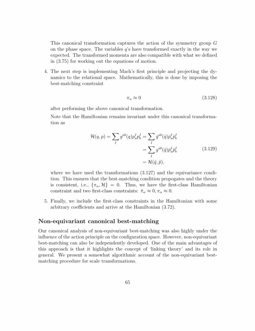
This canonical transformation captures the action of the symmetry group Gon the phase space. The variables q’s have transformed exactly in the way weexpected. The transformed momenta are also compatible with what we definedin (3.75) for working out the equations of motion.

4. The next step is implementing Mach’s first principle and projecting the dy-namics to the relational space. Mathematically, this is done by imposing thebest-matching constraint

πα ≈ 0 (3.128)

after performing the above canonical transformation.

Note that the Hamiltonian remains invariant under this canonical transforma-tion as

H(q, p) =∑I

gab(q)pIapIb =

∑I

gab(q)pIapIb

=∑I

gab(q)pIapIb

= H(q, p),

(3.129)

where we have used the transformations (3.127) and the equivariance condi-tion. This ensures that the best-matching condition propogates and the theoryis consistent, i.e., πα,H = 0. Thus, we have the first-class Hamiltonianconstraint and two first-class constraints: πα ≈ 0, πα ≈ 0.

5. Finally, we include the first-class constraints in the Hamiltonian with somearbitrary coefficients and arrive at the Hamiltonian (3.72).

Non-equivariant canonical best-matching

Our canonical analysis of non-equivariant best-matching was also highly under theinfluence of the action principle on the configuration space. However, non-equivariantbest-matching can also be independently developed. One of the main advantages ofthis approach is that it highlights the concept of ‘linking theory’ and its role ingeneral. We present a somewhat algorithmic account of the non-equivariant best-matching procedure for scale transformations.

65

1. Similarly to equivariant best-matching, we start with a phase space Γ(q, p)equipped with the corresponding Poisson structure. We posit N Hamiltonianconstraints χI on the phase space. We then extend the phase space of thetheory by introducing the non-physical variable φI along with the constraintπI ≈ 0. So we have a theory on the extended phase space ΓE = Γ×T ∗(φ) withthe following first-class constraints:

χI ≈ 0, πI ≈ 0. (3.130)

We call this extended theory a linking theory. The reason is that this broad the-ory links two theories with smaller gauge groups: one with local reparametriza-tion invariance expressed through χI ’s, and another one with local scale invari-ance but with a fixed local direction of time.

2. We introduce the symmetry by performing the canonical transformation gen-erated by the generator

F (q, φ, p, π) =∑I

(qaI e

φαI pIa + φI πI), (3.131)

Under this transformation, we have the following trivial constraint:

TφπI ≡ πI = πI −(qaIp

Ia − 〈q · p〉

)≡ CI ≈ 0, (3.132)

and the constraints

TφχI ≈ 0. (3.133)

3. We impose the best-matching condition

πI ≈ 0. (3.134)

In non-equivariant best-matching, the constraint πI is generally not first-classwith respect to the transformed constraints TφχI ’s which might potentiallylead to an inconsistency. However, provided that the symmetry group is notso large, under certain conditions there might exist a lapse function such that∑

I

N I0 TφχI , πJ ≈ 0. (3.135)

66

If such N0 exists, then πI ’s can be treated as special gauge fixing conditionsfor the local reparametrization invariance generated by χI ’s. We call this step‘symmetry trading’. In this case, N0 • Tφ ≡

∑I

N I0TφχI is the first-class Hamil-

tonian constraint. πI ’s and the rest of the Hamiltonian constraints, representedby χi’s, are the second-class constraints.

4. Elimination of the second-class constraints by defining Dirac bracket and im-posing them strongly. Hence, we find φI0 by solving Tφχi = 0 and arrive at thedual Hamiltonian

HT = N0 • Tφ0 +N∑I=1

θI(pIaq

aI − 〈p · q〉

), (3.136)

in accord with (3.111).

5. Finally, one can construct the explicit dictionary which relates the two phys-ically equivalent theories with different underlying gauge groups. It must bechecked that there exists a particular gauge in both theories that lead to equiv-alent equations of motion. This completes the construction of the dual theoryas a consistent theory with the desired gauge group.

Thus, the linking theory is the progenitor of two theories with two different gaugegroups. Both of them are the result of a particular gauge fixing of the linking theory.In the non-equivariant theory we studied, the local reparametrization invariant the-ory is born by imposing the gauge condition φI ≈ 0 in the linking theory, while itslocal scale invariant twin (the dual theory) is the result of the gauge fixing conditionπI ≈ 0. In the case of particle dynamics, both of these theories are physically equiva-lent in the sense that for any solution in one of them there exists a corresponding onein the other. It should be noted that both of these theories are also gauge theories.The gauge freedom of both of them can be fixed in a particular way and one arrivesat one single ‘isolated’ theory with physically realizable solutions: the dictionary.

Fig. 3.1 illustrates the structure of non-equivariant canonical best-matching andsymmetry trading more clearly.

67

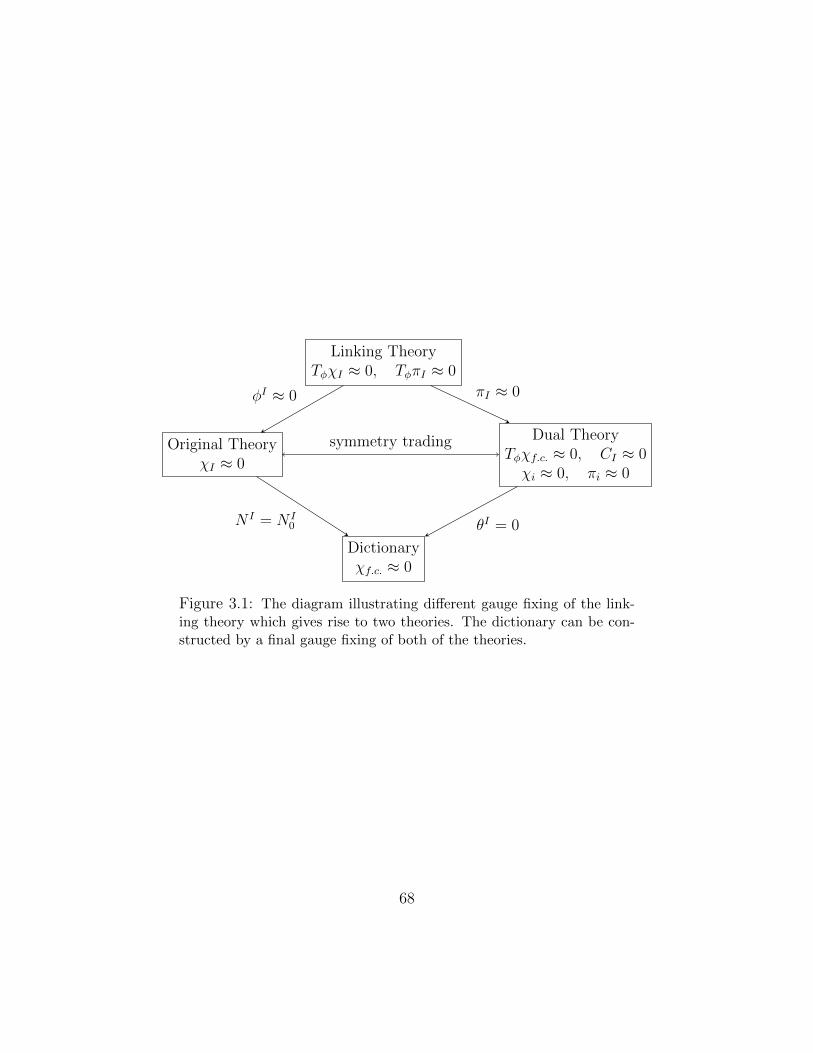
Linking TheoryTφχI ≈ 0, TφπI ≈ 0

Dual TheoryTφχf.c. ≈ 0, CI ≈ 0χi ≈ 0, πi ≈ 0

Original TheoryχI ≈ 0

Dictionaryχf.c. ≈ 0

πI ≈ 0φI ≈ 0

θI = 0N I = N I0

symmetry trading

Figure 3.1: The diagram illustrating different gauge fixing of the link-ing theory which gives rise to two theories. The dictionary can be con-structed by a final gauge fixing of both of the theories.

68

Chapter 4

Shape Dynamics of Geometry andFields

4.1 The historical evolution of shape dynamics

4.1.1 Einstein and Mach’s Principle

The story of Mach’s Principle began with Einstein who picked up the idea from anearly age and kept considering it as an important guiding principle until several yearsafter the devlopment of his great theory of general relativity. It was actually Einsteinwho dubbed the term ‘Mach’s Principle’, a phrase which has stood with us for morethan a century. Einstein’s advocacy of Mach’s Principle, however, was not that plainand simple. He repeatedly changed his attitude towards the principle, used differentformulations over the course of his work on what later became general relativity, andfinally dismissed the idea altogether and considered it obsolete. The lack of clarity ofEinstein’s formulations and understanding of the principle, along with Mach’s ownvague statements did inflict some lasting negative connotations even on the phraseitself.1

Many historians have analyzed the historical evolution and the role of Mach’sideas in Einstein’s works and have come up with many interesting insights.

To see clearly why Einstein could not fit his understanding of Mach’s Principleinto the framework of his theory, which led to even more misunderstanding, weshould start with the development of special relativity and Hermann Minkowski’scontribution to it shortly afterwards, and pinpoint the source of the problem.

1I personally think this is another strong reason to refer to this principle as the ‘Mach-PoincarePrinciple’ !

69

Einstein’s 1905 discovery of special relativity was the result of his long-standingdiscontent with Newton’s absolute notion of space and time, and in particular, thedisturbing discrepancy between Newtonian mechanics and electromagnetism. Hesolved the problem by putting the constancy of speed of light which is at the heart ofMaxwell’s equations first, and modify the theory of mechanics. His physical intuitionwas sound and valid. Shortly after that in 1908, Hermann Minkowski, Einstein’sformer teacher at Zurich polytechnic2 put the theory in a concise mathematicalformulation by constructing a mathematical structure, now known as the ‘Minkowskispacetime’ [18].

The key thing about Minkowski spacetime is the unification of time and spaceinto a single structure called spacetime. Time is considered as another physical di-mension, same as space, and this way one formulates the dynamical laws of physicsin a ‘timeless’ manner. Einstein at first dismissed this idea, calling it a ‘a pointlessmathematical complication’, but soon he changed his mind and used Minkowski’smathematical spacetime as his starting point to unify gravity with his special rela-tivity.

Einstein frequently talked about his three guiding principles in developing histheory: the relativity principle or the principle of general covariance, the equivalenceprinciple, and what later became known as Mach’s principle. I will focus on thestatus of Mach’s Principle and how it shaped Einstein’s thinking over time here.3

Einstein’s earliest expression of what he later called Mach’s Principle was theidea that the whole inertia of any material point should be an effect of the presenceof all other masses, depending on a kind of interaction with them. At the time,Einstein had not started to use tensor calculus and geometry to develop his theory,and he still had the intuition behind Newtonian particle ontology in mind. Later inthe period in which he was working on the first formulation of his theory in light ofhis equivalence principle, he equated general covariance, Mach’s Principle, and theequivalence principle.

As regards the connection between the equivalence principle and Mach’s Principle,Einstein argued that by virtue of the equilvalence principle, one cannot differentiatea centrifugal force from a gravitational field in the case of a rotating object (likeNewton’s bucket). In this way, one may regard a rotating system as at rest and thecentrifugal field as a gravitational field. He also wanted his theory to be generallycovariant. This, according to Einstein, would ensure that Mach’s Principle holds.

2Interestingly, Minkowski once called Einstein ‘a lazy dog’ for not attending his lectures as astudent!

3There are very valuable papers in [19] which came out of a conference on Mach’s Principle inJuly 1993. I mostly rely on Hoefer’s contribution [20] for my historical account here.

70

He regarded the principle of general covariance as the generalization of his previousrelativity principle and that would make the apparently priviledging role of uniformtransformations disappear, and the lack of existence of any priviledged referenceframe would incorporate and vindicate Mach’s critique of Newton’s absolute motion.

Furthermore, in the 1913-1915 period that Einstein was vigorously working on histheory, he also articulated Mach’s ideas as the demand that the metric field shouldbe fully determined by the material distribution, in other words, in the absence ofany matter there should not be any solution for the metric. Minkowski spacetimedefinitely posed a serious challenge for this way of understanding Mach’s Principle,as it is a vacuum solution.

Einstein published his first formulation of his theory, the Entwurf theory in thesummer of 1913, and maintained that the theory is Machian. This is very strange!Entwurf theory lacked general covariance, to which Einstein referred as an ‘uglydark spot’ in his letter to Lorentz in August 1913. But Einstein had equated Mach’sideas with the covariance principle! What is more striking, is that the Minkowskispacetime was a valid vacuum solution of the Entwurf equations, and this is in directcontradiction with his understanding of Mach’s Principle.

The problem of the general covariance of the Entwurf theory was resolved whenEinstein finally found general relativity in November 1915. But the problem withthe Minkowski spacetime solution remained. Einstein tried to solve this problemby imposing some suitable boundary conditions to rule out ‘non-Machian solutions’such as the empty Minkowski spacetime. He had begun working on this conditionsby May 1916 as a letter to Besso indicates, but as Hoefer suggests, he might have hadthe idea much further back in the period in which he was working on the Entwurftheory.

Until December 1916, Einstein kept working on ‘Machian boundary conditions’,but gradually became disappointed with this approach. By that time, he had alreadyfocused on the cosmological solutions of his theory and tried to implement Mach’sPrinciple by considering a topologically closed universe.

In the 1917-1918 period, Einstein formulated Mach’s Principle as the requirementfor a closed and finite universe with no boundary, and that there should be no matter-free and singularity-free solutions. He kept emphasizing that the gµν field should bedetermined by the matter alone both in his letter to de Sitter of March 24, 1917, andmore explicitly in his 1918 review paper [21] in which he dubbed the phrase ‘Mach’sPrinciple’.

However, de Sitter found a matter-free solution to the new field equations withthe cosmological constant in early 1917. Einstein struggled to show that either thissolution had a singularity and was physically unacceptable, or not matter-free at all.

71

He failed. Eventually, he gave up his attempts in June 1918 and this marks the endof Einstein’s strong advocacy of Mach’s Principle.

After 1918, Einstein kept referring to some Machian ideas in his writings occa-sionally. He mostly cited certain Machian phenomena, such as the frame draggingeffect, which were implemented in his theory, but not the full principle itself in arigorous and mathematical manner.

Ultimately, a letter to Felix Pirani in 1954 indicates Einstein’s complete repudi-ation of the principle:

One should not talk at all any longer of Mach’s principle, in my opinion.It arose at a time when one thought that ‘ponderable bodies’ were the onlyphysical reality and that in a theory all elements that are fully determinedby them should be conscientiously avoided. I am quite aware of the factthat for a long time, I, too, was influenced by this fixed idea.

But why did Einstein have such a complicated attitude towards Mach’s Principle?It seems that there are two main reasons behind it: one is the spacetime approach

which was initiated by Minkowski, the other is Einstein’s confusion and misunder-standing of the underlying ontology of his own theory.

Space and time are inherently different entities, especially from the relationalpoint of view. They should not be treated on the same footing. Space emergesfrom the relational states of the universe, and time emerges from the change ofthose relations. From this perspective, it must be the configuration space of therelational states that comes first. Unifying space and time goes against the relationalunderstanding of either one of them, and obscures the essence of what we formulatedas the Mach-Poincare Principle. We will see how clearly relational ideas can beimplemented in a dynamical theory of geometry and fields, and how spacetime canemerge from such a Machian approach.

Moreover, in judging the value and usefulness of Mach’s Principle near the end ofhis life, Einstein confused the matter of ontology with the true criterion of Machianity.The resolution of this conundrum has been the privotal matter in the contemporaryrelational physics project.

To make the matter more clear, consider Einstein’s field equations:

Rµν −1

2gµνR = kTµν . (4.1)

This equation is not for determining the metric gµν from the matter fields on theRHS. Actually, both the LHS and the RHS do in principle contain derivatives of the

72

metric and the matter fields with respect to time and space in parallel. Einstein’sfield equations govern the evolution of the matter and the metric.

In light of this note and the above realization that the spacetime approach is theculprit behind the obscure status of Machianity of GR, we take a step forward toidentify an alternative way of understanding the Machian core of Einstein’s theory.Fortunately, we already have a formal definition of Mach’s Principle. We should nowdiscuss its application to general relativity.

4.1.2 Mach-Poincare Principle and general relativity

We should begin this section with an important question: What is the configurationspace of GR?

John Wheeler asked this question. The dynamical core of Einstein’s theory isveiled behind the spacetime structure. If we think about this question, Einstein’stheory describes the evolution of the geometry and the matter fields in a spatial extentthrough time. Hence, we can start with a Riemannian manifold, representing ouruniverse, and introduce the metrical structure and the matter fields. Now we see thatgeometry has its own ontological status in the theory. Focusing on only geometry, wecan identify the configuration space as ‘the space of all possible Riemannian metricson a certain manifold with a given topology’, denoted by Riem3.

Now we can apply the Mach-Poincare Principle to such a configuration space. Theingredient we need is the symmetry group of this configuration space. The observablerole of the metric is that we can define ‘length’ with it. Now let us assume we haveidentified the points of a manifold, and have set an arbitrary coordinate system andassigned some coordinates to each point, e.g xa(P ). What we can do is to measurethe angles between lines in different directions each point, i.e., quantities like

g(X, Y )√g(X,X)

√g(Y, Y )

(4.2)

at each point of the space. We can therefore measure the angles between thelines emerging along the coordinate basis vectors ∂a at each point and this gives uscertain ratios between the components of the metric. In the three-dimensional space,there are 2 measurable numbers at each point. So two of the total 6 components ofa three dimensional Riemannian metric actually represent the observable content ofthe metric. This is in accord with the field-theoretic approach to gravity as a spin-2field. The massless spin-2 field has 2 polarizations.

The other 4 components of the metric are redundant and are the handles ofgauge transformation. Three of them correspond to diffeomorphisms. The coordinate

73

system we considered was arbitrary and one could write the components of themetric in any other smooth coordinate system. The transformed metric under adiffeomorphism ψ from the manifold to the manifold, ψ∗gij is as good as gij. Thisintroduces a local three-parameter group of transformations, the diffeomorphismgroup. Morover, in considering only the ratios (4.2) we removed the local scale ofthe metric. This corresponds to the action of the conformal group. The conformalgroup of transformations comprise of any smooth, positive definite function φ(x)which transforms the metric as gij → φgij. This transformation also leaves theobservable content of the metric invariant.

Hence, the symmetry group should be Conf nDiff , the group of all conformaland diffeomorphism transformations on a certain manifold with a given topology.

The quotient of Riem3 by diffeomorphisms was called the superspace by Wheeler,denoted by Sup. We can construct the conformal superspace (the shape space) CS,by quotienting superspace by the conformal transformations.

Einstein’s theory satisfies the criterion of Machianity in superspace. The BSWaction

SBSW [g,Na] =

∫dtd3x

√g√RGabcd (gab − 2∇aNb) (gcd − 2∇cNd), (4.3)

derived in Appx. D, is equivalent to Einstein-Hilbert action for globally hyper-bolic spacetimes and as we soon will see more clearly, implements best-matchingwith respect to diffeomorphisms through the shift vector Na. Einstein was confusedabout the Machian nature of his theory, but his theory was certainly not! Withouteven having the formulation of the Mach-Poincare Principle in mind, he created atheory that not only satisfies that principle to some extent, but also embodies thebest-matching procedure in a natural way!

We are now in the position to dispell some of the conceptual difficulties Ein-stein faced in implementing Mach’s Principle. First of all, by virtue of describingthe universe as an evolution of geometry unfolding in the configuration space, wedo not need to look for Machian ideas in spacetime. Machianity translates into therequirement for the dynamics of the universe to take place in the relational configu-ration space. Moreover, this prompts us to look at certain seemingly non-Machiansolutions, e.g., the Minkowski spacetime, in a new light. If we remember that thetheory is a dynamical one of both the geometry and the matter fields, the Minkowskispacetime should not be considered as an absolute and rigid structure. It is justone particular ‘dynamical’ solution to the equations. As Julian Barbour put it more

74

clearly in [22],4

Any solution of pure geometrodynamics, i.e., any Ricci-flat spacetime, isnot to be analyzed as a matter-free structure in which test particles haveinertia or as a structure that has a disconcerting resemblance to Newton’sabsolute space and time but as a dynamical history of 3-geometries. TheMachian requirements apply to the structure of such a dynamical history,not the behavior of test particles within it... The real difference betweenthe Newtonian absolute structures and all Einsteinian spacetimes is thatthe former are a rigid kinematic framework for dynamics, whereas thelatter arise as a result of Machian dynamical evolution in a situation inwhich there are no preexisting frameworks at all.

4.1.3 Towards a theory of geometrodynamics on conformalsuperspace

Just a few years after the Tubingen conference on Mach’s Principle, Julian Barbourwith the help of his collaborators set out to implement the relationality of size andmoved towards a completely relational description of the universe both in the particlemodel and geometrodynamics. This task was not inherently unattainable from thetechnical point of view, as in 1982 Barbour and Bertotti already found a correctmathematical procedure to construct a relational dynamical theory with respect toany Lie group. The matter was actually more conceptually challenging.

The first attempt to include the conformal transformations in geometrodynamicswas Barbour and O Murchadha’s joint paper [23]. In that paper, they tried todevelop a scale-invariant theory that satisfies the strong version of the Mach-PoincarePrinciple in the conformal superspace. In a nutshell, what they did was to includethe conformal transformations

gab → e4φgab, (4.4)

for an arbitrary smooth function φ defined on a closed Riemannian manifold inan action for geometrodynamics and perform the best-matching variation.

But one cannot use the standard BSW action (4.3) for that. The reason is that theBSW action is not invariant under a global rescaling of the metric in the first place,and performing best-matching with respect to the local form of this transformation

4Note that at the time of writing that paper the role of scale and conformal transformationswas not clearly understood. Therefore, the claim made in that paper must be moderated, and aswe will see, general relativity is equivalent to an almost Machian theory.

75

would lead to inconsistency.5 They proposed the following simple modification of aBSW-type action:

S[g] =

∫dt

∫d3x√g√RGabcd (gab) (gcd)

V 2/3, (4.5)

where V =∫d3x√g is the volume and we ignored the shift vector Na for brevity.

The action (4.5) is invariant under the global scaling gab → α gab (R transforms toαR). But to implement best-matching with respect to the full local scale transforma-tion, we add the φ(x) field to the action and perform the transformation gab → e4φgaband write

S[g, φ] =

∫dt

∫d3x√ge4φ

√R− 8∇2eφ

eφ

√T(∫

d3x e6φ√g)2/3

, (4.6)

where the transformed kinetic term is

T = Gabcd(gab + 4φgab

)(gcd + 4φgcd

). (4.7)

Performing the best-matching variation leads to the condition

p ≡ Tr pab = gabpab = 0, (4.8)

in other words, the trace of the extrinsic curvature must vanish identically at eachinstant. This condition also fixes the lapse function. The Hamiltonian constraint ofthis theory has only a solution if and only if the initial metric belongs to the Yamabe-non-negative class (see [2], Chapter 8). This condition is overly restrictive.

Hence, a completely scale-free theory of geometry is mathematically possible, butis highly restrictive. Moreover, one has to modify the standard BSW action and usea globally scale-invariant action such as (4.6). It could be very hard to reconcile the‘global’ coupling that the volume term in the denominator induces with the verifiedcosmological predictions of GR.

Scale-invariant particle mechanics was also developed in [13]. But it too hadsome deep issues with observations. In particular, such a toy particle model cannotexplain the structure formation that has happened in our universe and explains onlya short range of the redshift we observe.

5In the canonical formulation, this means that the best-matching constraint would not propagateto close the constraint algebra.

76

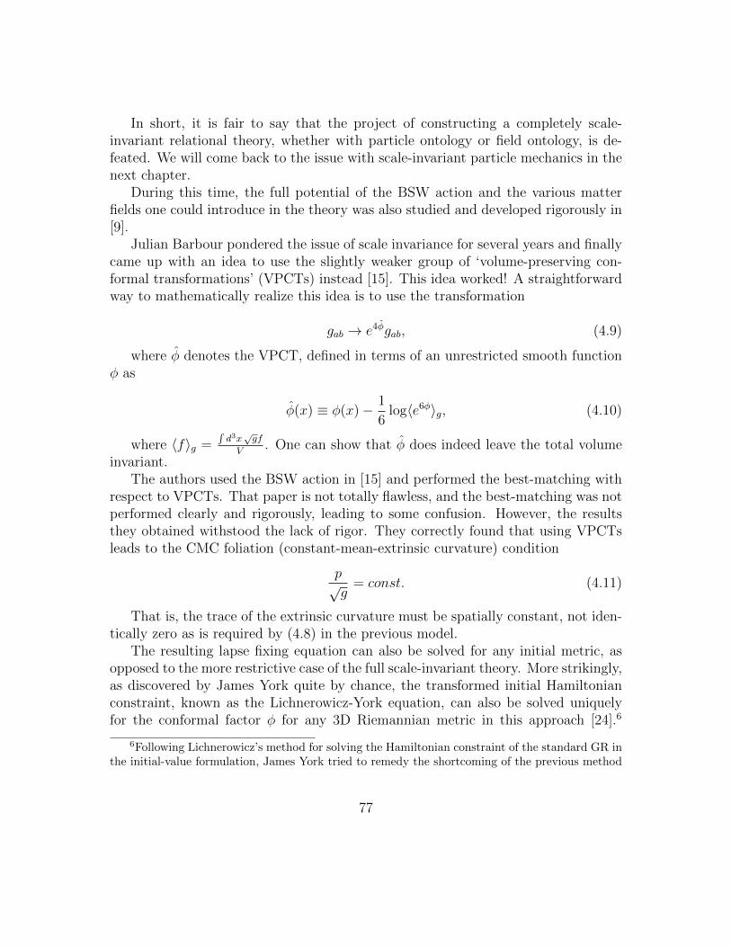
In short, it is fair to say that the project of constructing a completely scale-invariant relational theory, whether with particle ontology or field ontology, is de-feated. We will come back to the issue with scale-invariant particle mechanics in thenext chapter.

During this time, the full potential of the BSW action and the various matterfields one could introduce in the theory was also studied and developed rigorously in[9].

Julian Barbour pondered the issue of scale invariance for several years and finallycame up with an idea to use the slightly weaker group of ‘volume-preserving con-formal transformations’ (VPCTs) instead [15]. This idea worked! A straightforwardway to mathematically realize this idea is to use the transformation

gab → e4φgab, (4.9)

where φ denotes the VPCT, defined in terms of an unrestricted smooth functionφ as

φ(x) ≡ φ(x)− 1

6log〈e6φ〉g, (4.10)

where 〈f〉g =∫d3x√gf

V. One can show that φ does indeed leave the total volume

invariant.The authors used the BSW action in [15] and performed the best-matching with

respect to VPCTs. That paper is not totally flawless, and the best-matching was notperformed clearly and rigorously, leading to some confusion. However, the resultsthey obtained withstood the lack of rigor. They correctly found that using VPCTsleads to the CMC foliation (constant-mean-extrinsic curvature) condition

p√g

= const. (4.11)

That is, the trace of the extrinsic curvature must be spatially constant, not iden-tically zero as is required by (4.8) in the previous model.

The resulting lapse fixing equation can also be solved for any initial metric, asopposed to the more restrictive case of the full scale-invariant theory. More strikingly,as discovered by James York quite by chance, the transformed initial Hamiltonianconstraint, known as the Lichnerowicz-York equation, can also be solved uniquelyfor the conformal factor φ for any 3D Riemannian metric in this approach [24].6

6Following Lichnerowicz’s method for solving the Hamiltonian constraint of the standard GR inthe initial-value formulation, James York tried to remedy the shortcoming of the previous method

77

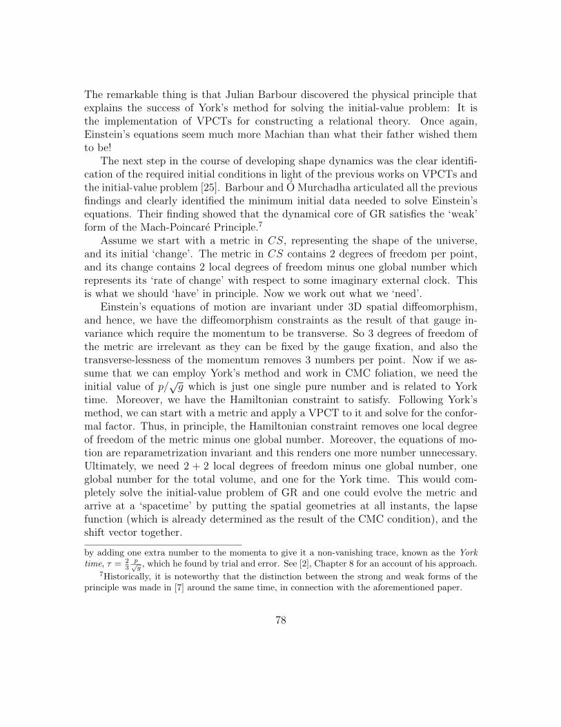
The remarkable thing is that Julian Barbour discovered the physical principle thatexplains the success of York’s method for solving the initial-value problem: It isthe implementation of VPCTs for constructing a relational theory. Once again,Einstein’s equations seem much more Machian than what their father wished themto be!

The next step in the course of developing shape dynamics was the clear identifi-cation of the required initial conditions in light of the previous works on VPCTs andthe initial-value problem [25]. Barbour and O Murchadha articulated all the previousfindings and clearly identified the minimum initial data needed to solve Einstein’sequations. Their finding showed that the dynamical core of GR satisfies the ‘weak’form of the Mach-Poincare Principle.7

Assume we start with a metric in CS, representing the shape of the universe,and its initial ‘change’. The metric in CS contains 2 degrees of freedom per point,and its change contains 2 local degrees of freedom minus one global number whichrepresents its ‘rate of change’ with respect to some imaginary external clock. Thisis what we should ‘have’ in principle. Now we work out what we ‘need’.

Einstein’s equations of motion are invariant under 3D spatial diffeomorphism,and hence, we have the diffeomorphism constraints as the result of that gauge in-variance which require the momentum to be transverse. So 3 degrees of freedom ofthe metric are irrelevant as they can be fixed by the gauge fixation, and also thetransverse-lessness of the momentum removes 3 numbers per point. Now if we as-sume that we can employ York’s method and work in CMC foliation, we need theinitial value of p/

√g which is just one single pure number and is related to York

time. Moreover, we have the Hamiltonian constraint to satisfy. Following York’smethod, we can start with a metric and apply a VPCT to it and solve for the confor-mal factor. Thus, in principle, the Hamiltonian constraint removes one local degreeof freedom of the metric minus one global number. Moreover, the equations of mo-tion are reparametrization invariant and this renders one more number unnecessary.Ultimately, we need 2 + 2 local degrees of freedom minus one global number, oneglobal number for the total volume, and one for the York time. This would com-pletely solve the initial-value problem of GR and one could evolve the metric andarrive at a ‘spacetime’ by putting the spatial geometries at all instants, the lapsefunction (which is already determined as the result of the CMC condition), and theshift vector together.

by adding one extra number to the momenta to give it a non-vanishing trace, known as the Yorktime, τ = 2

3p√g , which he found by trial and error. See [2], Chapter 8 for an account of his approach.

7Historically, it is noteworthy that the distinction between the strong and weak forms of theprinciple was made in [7] around the same time, in connection with the aforementioned paper.

78

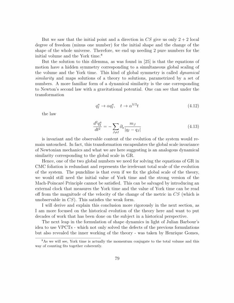
But we saw that the initial point and a direction in CS give us only 2 + 2 localdegree of freedom (minus one number) for the initial shape and the change of theshape of the whole universe. Therefore, we end up needing 2 pure numbers for theinitial volume and the York time.8

But the solution to this dilemma, as was found in [25] is that the equations ofmotion have a hidden symmetry corresponding to a simultaneous global scaling ofthe volume and the York time. This kind of global symmetry is called dynamicalsimilarity and maps solutions of a theory to solutions, parametrized by a set ofnumbers. A more familiar form of a dynamical similarity is the one correspondingto Newton’s second law with a gravitational potential. One can see that under thetransformation

qaI → αqaI , t→ α3/2t (4.12)

the law

d2qaIdt2

= −∑J 6=I

∂amJ

|qI − qJ |(4.13)

is invariant and the observable content of the evolution of the system would re-main untouched. In fact, this transformation encapsulates the global scale invarianceof Newtonian mechanics and what we are here suggesting is an analogous dynamicalsimilarity corresponding to the global scale in GR.

Hence, one of the two global numbers we need for solving the equations of GR inCMC foliation is redundant and represents the irrelevant total scale of the evolutionof the system. The punchline is that even if we fix the global scale of the theory,we would still need the initial value of York time and the strong version of theMach-Poincare Principle cannot be satisfied. This can be salvaged by introducing anexternal clock that measures the York time and the value of York time can be readoff from the magnitude of the velocity of the change of the metric in CS (which isunobservable in CS). This satisfies the weak form.

I will derive and explain this conclusion more rigorously in the next section, asI am more focused on the historical evolution of the theory here and want to putdecades of work that has been done on the subject in a historical perspective.

The next leap in the formulation of shape dynamics in light of Julian Barbour’sidea to use VPCTs - which not only solved the defects of the previous formulationsbut also revealed the inner working of the theory - was taken by Henrique Gomes,

8As we will see, York time is actually the momentum conjugate to the total volume and thisway of counting fits together coherently.

79

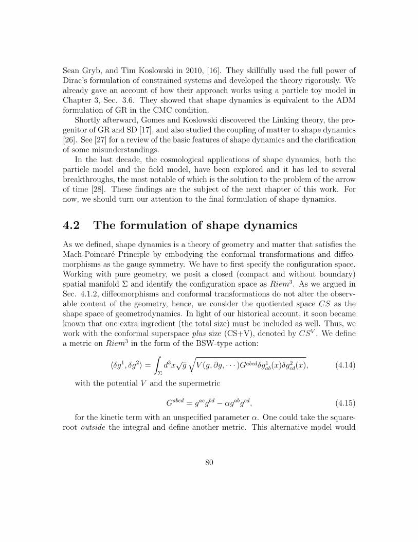
Sean Gryb, and Tim Koslowski in 2010, [16]. They skillfully used the full power ofDirac’s formulation of constrained systems and developed the theory rigorously. Wealready gave an account of how their approach works using a particle toy model inChapter 3, Sec. 3.6. They showed that shape dynamics is equivalent to the ADMformulation of GR in the CMC condition.

Shortly afterward, Gomes and Koslowski discovered the Linking theory, the pro-genitor of GR and SD [17], and also studied the coupling of matter to shape dynamics[26]. See [27] for a review of the basic features of shape dynamics and the clarificationof some misunderstandings.

In the last decade, the cosmological applications of shape dynamics, both theparticle model and the field model, have been explored and it has led to severalbreakthroughs, the most notable of which is the solution to the problem of the arrowof time [28]. These findings are the subject of the next chapter of this work. Fornow, we should turn our attention to the final formulation of shape dynamics.

4.2 The formulation of shape dynamics

As we defined, shape dynamics is a theory of geometry and matter that satisfies theMach-Poincare Principle by embodying the conformal transformations and diffeo-morphisms as the gauge symmetry. We have to first specify the configuration space.Working with pure geometry, we posit a closed (compact and without boundary)spatial manifold Σ and identify the configuration space as Riem3. As we argued inSec. 4.1.2, diffeomorphisms and conformal transformations do not alter the observ-able content of the geometry, hence, we consider the quotiented space CS as theshape space of geometrodynamics. In light of our historical account, it soon becameknown that one extra ingredient (the total size) must be included as well. Thus, wework with the conformal superspace plus size (CS+V), denoted by CSV . We definea metric on Riem3 in the form of the BSW-type action:

〈δg1, δg2〉 =

∫Σ

d3x√g√V (g, ∂g, · · · )Gabcdδg1

ab(x)δg2cd(x), (4.14)

with the potential V and the supermetric

Gabcd = gacgbd − αgabgcd, (4.15)

for the kinetic term with an unspecified parameter α. One could take the square-root outside the integral and define another metric. This alternative model would

80

be highly non-local, coupling all the distant points in Σ.9

Using the above metric, we can define the action

S[g] =

∫Σ

d3x√gV Gabcdgabgcd (4.16)

on Riem3. The conjugate momenta are

pab(x) ≡ δLδgab

=

√gV

TGabcdgcd(x) (4.17)

which immediately leads to a primary constraint corresponding to the reparametriza-tion invariance of (4.16):

H[g, x) =Gabcdp

abpcd√g

−√gV. (4.18)

We call this the Hamiltonian constraint. Now, if we take one further step andimplement best-matching with respect to diffeomorphisms, we see that diffeomor-phisms leave the kinetic term invariant, provided that the potential V is scalar.Hence, this procedure would be an equivariant best-matching. Under infinitesimaldiffeomorphisms xa → xa + ξa , the metric transforms as

gab(x)→ gab(x) = gab(x)− (∂aξc)gbc − (∂bξ

c)gac

=⇒ gab(x) = gab(x)− Lξgab(x) = gab(x)− 2∇(aξb).(4.19)

Thus, under best-matching, the gab term in (4.16) transforms as10

gab → gab − 2∇(aξb). (4.20)

As the best-matching variation requires that we vary the action with respect to ξdirectly, putting (4.20) in (4.16) effectively leads to the BSW action (4.3), providedthat V = R[g] and α = 1 to ensure that the theory would be consistent and the best-matching constraint propagates. Best-matching with respect to diffeomorphismsleads to the familiar momentum constraints

Ha = −2∇bpab (4.21)

9See Chapter 5 in [11] for further details.10In light of our discussion near the end of Sec. B.2, we should note that for simplicity, we are here

using the generators of the diffeomorphisms evaluated at the identity element for lifting the metric.It does not change the essence of equivariant best-matching with respect to diffeomorphisms.

81

we have derived in Appx. D.As we intuitively indicated, to construct an almost scale-free consistent theory,

we have to perform best-matching with respect to VPCTs. The action (4.16) is notinvariant under the global form of these transformations, meaning that we have toperform non-equivariant best-matching. Fortunately, we already have a strong localgauge invariance by virtue of the Hamiltonian constraint, and we see the possibilityof symmetry trading on the horizon. Thus, we construct canonical formulation ofshape dynamics following our non-equivariance best-matching procedure outlined inSec. 3.7.

4.2.1 Enlarging the phase space

The phase space Γ of ADM formulation of general relativity on Σ is coordinatizedby 3-dimensional Riemannian metrics gab and its conjugate momenum density pab ofdensity weight 1.11 Γ(gab, p

ab) is equipped with the fundamental Poisson bracket

Aab • gab, Bcd • pcd = Aab •Bab =

∫Σ

d3x√g Aab(x)Bab(x), (4.22)

for any smooth square-integrable scalars A and B. The dynamics on Γ is givenby the first-class constraints

H =1√g

(pabpab −

1

2p2

)−√gR,

Ha = −2∇bpab,

(4.23)

where p = gabpab. We have used the DeWitt supermetric (D.18).

We extend the phase space to ΓE(gab, pab, φ, πφ) by adding the scalar field φ and

its conjugate momentum πφ defined on Σ and impose the first-class constraint

πφ ≈ 0. (4.24)

to ensure that φ is redundant and a gauge variable.

4.2.2 Introducing the VPCTs

We now perform a canonical transformation that implements VPCT’s on the ex-tended phase space. The total volume is by definition

11It means that pab/√g transforms as a 2-tensor.

82

Vg ≡∫

Σ

d3x√g. (4.25)

We define the restricted field φ to apply a VPCT, as opposed to the unrestrictedoriginal φ in the following way:

φ = φ− 1

6log〈e6φ〉g, (4.26)

where 〈f〉g = 1Vg

∫Σd3x√gf for any smooth function f on Σ. One can then see

that the conformal transformation e4φ leaves Vg invariant.The functional

F [gab, Pab, φ,ΠΦ] =

∫Σ

d3x(gabe

4φP ab + φΠΦ

)(4.27)

generates the canonical transformation corresponding to the VPCT. More explic-itly,

Gab ≡δF

δP ab= e4φgab, pab ≡ δF

δgab= e4φP ab − 1

3

(e6φ − 1

)〈e4φgcdP

cd〉g√ggab,

Φ ≡ δF

δΠΦ

= φ, πφ ≡δF

δφ= ΠΦ + 4

(e4φgabP

ab − 〈e4φgcdPcd〉g√ge6φ

).

(4.28)These relations imply the transformations

Gab = e4φgab, P ab = e−4φ

(pab +

1

3

(e6φ − 1

)〈p〉g√ggab

),

Φ = φ, ΠΦ = πφ − 4 (p− 〈p〉g√g) .

(4.29)

A long and careful calculation shows that the transformed constraints are weaklyequivalent to

TφH =e−6φ

√g

(pabpab −

p2

2+

1

3

√g(1− e6φ)〈p〉gp−

1

6g(1− e6φ)2〈p〉2g

)−√g

(Re2φ − 8eφ4 eφ

),

TφHa ≈ −2∇bp

ab + πφ∇aφ,

C ≡ Tφπφ = πφ − 4 (p− 〈p〉g√g) ,

(4.30)

83

where 4 denotes the invariant Laplacian, i.e., 4 = ∇a∇a. These constraintsare of course first-class, as the cannonical transformation we performed does notchange the Poisson brackets. The theory on ΓE(gab, p

ab, φ, πφ), characterized by theconstraints (4.30), is called the Linking theory with the total Hamiltonian

HT = N • TφH +Na • TφHa + ρ • Tφπφ. (4.31)

Note that∫

Σd3xTφπφ acts trivially on the phase space, just as in the toy particle

model. Its Poisson bracket with gab,pab, φ, and πφ vanish. This is the direct conse-

quence of weakening the symmetry group and reducing it to only VPCTs, and is thekey behind the success of shape dynamics as a consistent theory.

4.2.3 Shape dynamics is gauge-fixing of the Linking theory

The gauge-fixing φ ≈ 0 fixes the ρ = 0 in (4.31) and gives us the standard ADMformalism of GR. However, if we impose the best-matching condition

πφ ≈ 0, (4.32)

it would give us shape dynamics as an alternative gauge-fixing of the Linkingtheory. πφ is first-class with respect to C and TφH

a, as

πφ(x), Na • TφHa ≈ √g∇a

(Naπφ√

g

)(x) ≈ 0. (4.33)

But it has a non-vanishing Poisson bracket with TφH and except for a specialchoice of N , it does not propagate under the Hamiltonian evolution. Thus, wecalculate

N • TφH, πφ(x) = SN(x)− 〈SN〉g√ge6φ(x), (4.34)

where

SN(x) =δ(N •H)

δφ(x)≈ √geφ

(56N 4 (eφ) + 84 (eφN)− 2N

(4Reφ + e5φ〈p〉2g

)).

(4.35)The lapse-fixing equation

SN(x)− 〈SN〉g√ge6φ(x) = 0 (4.36)

84

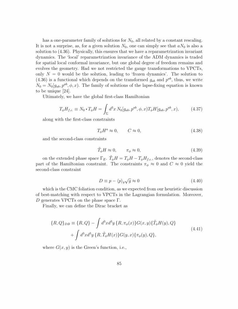
has a one-parameter family of solutions for N0, all related by a constant rescaling.It is not a surprise, as, for a given solution N0, one can simply see that aN0 is also asolution to (4.36). Physically, this ensures that we have a reparametrization invariantdynamics. The ‘local’ reparametrization invariance of the ADM dynamics is tradedfor spatial local conformal invariance, but one global degree of freedom remains andevolves the geometry. Had we not restricted the gauge transformations to VPCTs,only N = 0 would be the solution, leading to ‘frozen dynamics’. The solution to(4.36) is a functional which depends on the transformed gab and pab, thus, we writeN0 = N0[gab, p

ab, φ, x). The family of solutions of the lapse-fixing equation is knownto be unique [24].

Ultimately, we have the global first-class Hamiltonian

TφHf.c. ≡ N0 • TφH =

∫Σ

d3xN0[gab, pab, φ, x)TφH[gab, p

ab, x), (4.37)

along with the first-class constraints

TφHa ≈ 0, C ≈ 0, (4.38)

and the second-class constraints

TφH ≈ 0, πφ ≈ 0, (4.39)

on the extended phase space ΓE. TφH = TφH−TφHf.c., denotes the second-classpart of the Hamiltonian constraint. The constraints πφ ≈ 0 and C ≈ 0 yield thesecond-class constraint

D ≡ p− 〈p〉g√g ≈ 0 (4.40)

which is the CMC foliation condition, as we expected from our heuristic discussionof best-matching with respect to VPCTs in the Lagrangian formulation. Moreover,D generates VPCTs on the phase space Γ.

Finally, we can define the Dirac bracket as

R,QDB ≡ R,Q −∫d3xd3y R, πφ(x)G(x, y)TφH(y), Q

+

∫d3xd3y R, TφH(x)G(y, x)πφ(y), Q,

(4.41)

where G(x, y) is the Green’s function, i.e.,

85

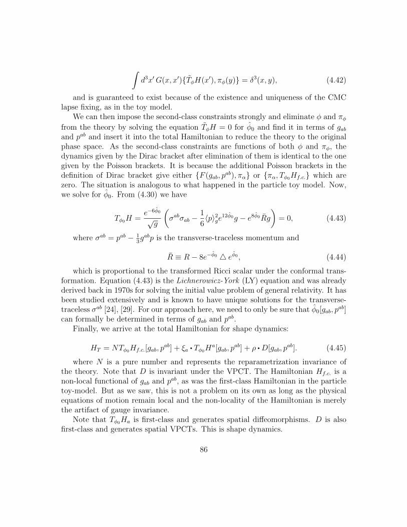
∫d3x′G(x, x′)TφH(x′), πφ(y) = δ3(x, y), (4.42)

and is guaranteed to exist because of the existence and uniqueness of the CMClapse fixing, as in the toy model.

We can then impose the second-class constraints strongly and eliminate φ and πφfrom the theory by solving the equation TφH = 0 for φ0 and find it in terms of gaband pab and insert it into the total Hamiltonian to reduce the theory to the originalphase space. As the second-class constraints are functions of both φ and πφ, thedynamics given by the Dirac bracket after elimination of them is identical to the onegiven by the Poisson brackets. It is because the additional Poisson brackets in thedefinition of Dirac bracket give either F (gab, p

ab), πα or πα, Tφ0Hf.c. which arezero. The situation is analogous to what happened in the particle toy model. Now,we solve for φ0. From (4.30) we have

Tφ0H =e−6φ0

√g

(σabσab −

1

6〈p〉2ge12φ0g − e8φ0Rg

)= 0, (4.43)

where σab = pab − 13gabp is the transverse-traceless momentum and

R ≡ R− 8e−φ0 4 eφ0 , (4.44)

which is proportional to the transformed Ricci scalar under the conformal trans-formation. Equation (4.43) is the Lichnerowicz-York (LY) equation and was alreadyderived back in 1970s for solving the initial value problem of general relativity. It hasbeen studied extensively and is known to have unique solutions for the transverse-traceless σab [24], [29]. For our approach here, we need to only be sure that φ0[gab, p

ab]can formally be determined in terms of gab and pab.

Finally, we arrive at the total Hamiltonian for shape dynamics:

HT = NTφ0Hf.c.[gab, pab] + ξa • Tφ0H

a[gab, pab] + ρ •D[gab, p

ab]. (4.45)

where N is a pure number and represents the reparametrization invariance ofthe theory. Note that D is invariant under the VPCT. The Hamiltonian Hf.c. is anon-local functional of gab and pab, as was the first-class Hamiltonian in the particletoy-model. But as we saw, this is not a problem on its own as long as the physicalequations of motion remain local and the non-locality of the Hamiltonian is merelythe artifact of gauge invariance.

Note that Tφ0Ha is first-class and generates spatial diffeomorphisms. D is alsofirst-class and generates spatial VPCTs. This is shape dynamics.

86

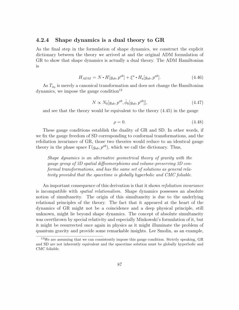
4.2.4 Shape dynamics is a dual theory to GR

As the final step in the formulation of shape dynamics, we construct the explicitdictionary between the theory we arrived at and the original ADM formulation ofGR to show that shape dynamics is actually a dual theory. The ADM Hamiltonianis

HADM = N •H[gab, pab] + ξa •Ha[gab, p

ab]. (4.46)

As Tφ0 is merely a canonical transformation and does not change the Hamiltoniandynamics, we impose the gauge condition12

N ∝ N0[gab, pab, φ0[gab, p

ab]], (4.47)

and see that the theory would be equivalent to the theory (4.45) in the gauge

ρ = 0. (4.48)

These gauge conditions establish the duality of GR and SD. In other words, ifwe fix the gauge freedom of SD corresponding to conformal transformations, and therefoliation invariance of GR, those two theories would reduce to an identical gaugetheory in the phase space Γ(gab, p

ab), which we call the dictionary. Thus,

Shape dynamics is an alternative geometrical theory of gravity with thegauge group of 3D spatial diffeomorphisms and volume-preserving 3D con-formal transformations, and has the same set of solutions as general rela-tivity provided that the spacetime is globally hyperbolic and CMC foliable.

An important consequence of this derivation is that it shows refoliation invarianceis incompatible with spatial relationalism. Shape dynamics possesses an absolutenotion of simultaneity. The origin of this simultaneity is due to the underlyingrelational principles of the theory. The fact that it appeared at the heart of thedynamics of GR might not be a coincidence and a deep physical principle, stillunknown, might lie beyond shape dynamics. The concept of absolute simultaneitywas overthrown by special relativity and especially Minkowski’s formulation of it, butit might be resurrected once again in physics as it might illuminate the problem ofquantum gravity and provide some remarkable insights. Lee Smolin, as an example,

12We are assuming that we can consistently impose this gauge condition. Strictly speaking, GRand SD are not inherently equivalent and the spacetime solution must be globally hyperbolic andCMC foliable.

87

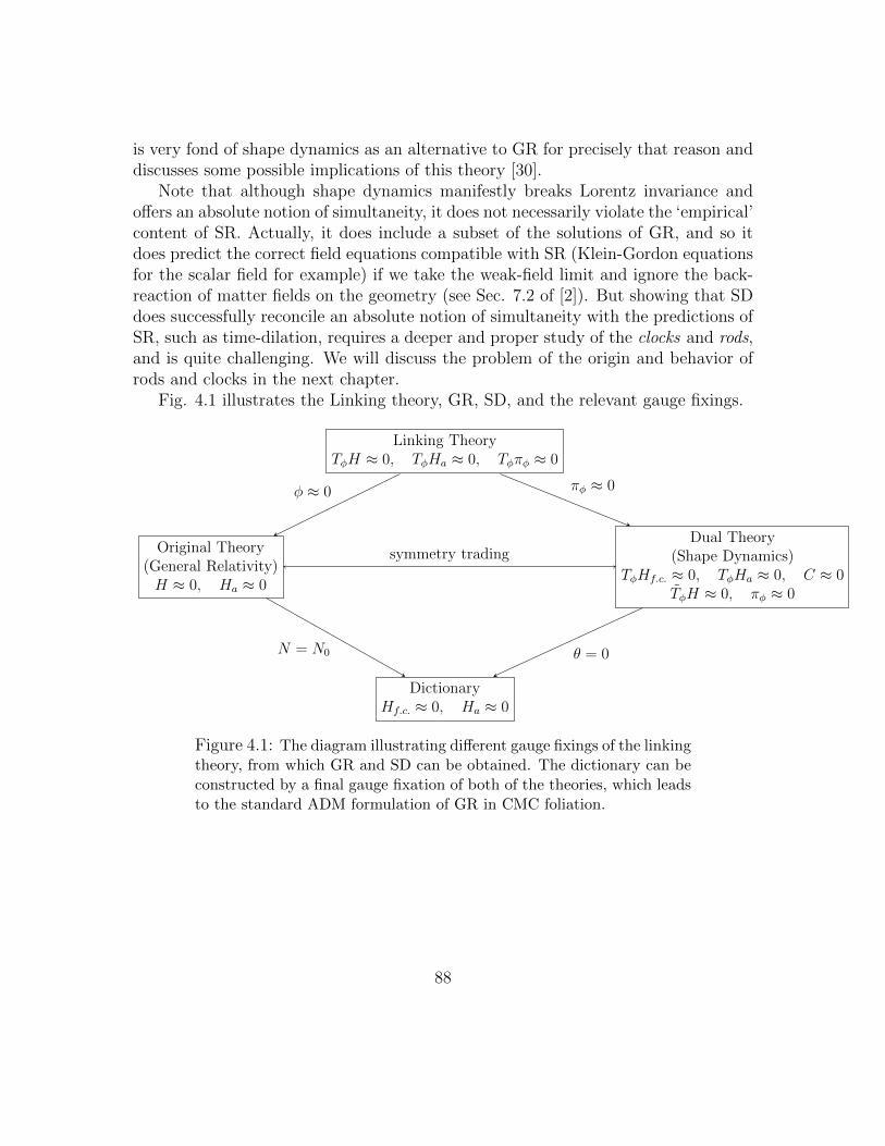
is very fond of shape dynamics as an alternative to GR for precisely that reason anddiscusses some possible implications of this theory [30].

Note that although shape dynamics manifestly breaks Lorentz invariance andoffers an absolute notion of simultaneity, it does not necessarily violate the ‘empirical’content of SR. Actually, it does include a subset of the solutions of GR, and so itdoes predict the correct field equations compatible with SR (Klein-Gordon equationsfor the scalar field for example) if we take the weak-field limit and ignore the back-reaction of matter fields on the geometry (see Sec. 7.2 of [2]). But showing that SDdoes successfully reconcile an absolute notion of simultaneity with the predictions ofSR, such as time-dilation, requires a deeper and proper study of the clocks and rods,and is quite challenging. We will discuss the problem of the origin and behavior ofrods and clocks in the next chapter.

Fig. 4.1 illustrates the Linking theory, GR, SD, and the relevant gauge fixings.

Linking TheoryTφH ≈ 0, TφHa ≈ 0, Tφπφ ≈ 0

Dual Theory(Shape Dynamics)

TφHf.c. ≈ 0, TφHa ≈ 0, C ≈ 0TφH ≈ 0, πφ ≈ 0

Original Theory(General Relativity)H ≈ 0, Ha ≈ 0

DictionaryHf.c. ≈ 0, Ha ≈ 0

πφ ≈ 0φ ≈ 0

θ = 0N = N0

symmetry trading

Figure 4.1: The diagram illustrating different gauge fixings of the linkingtheory, from which GR and SD can be obtained. The dictionary can beconstructed by a final gauge fixation of both of the theories, which leadsto the standard ADM formulation of GR in CMC foliation.

88

4.2.5 Deparametrizing shape dynamics and Mach-PoincarePrinciple

We should do the counting of the degrees of freedom of shape dynamics once againand clarify the status of the Mach-Poincare Principle in the theory. In the canonicalformulation of the theory, we constructed a theory with gauge groups correspondingto global reparametrization invariance, spatial diffeomorphisms, and spatial VPCTs.Thus, if we make the transition to the configuration space, we have a geodesic theoryon conformal superspace plus volume, CSV ≡ CS × R+: an initial point and adirection in CSV determines the future evolution uniquely, and the theory satisfiesthe strong version of the Mach-Poincare Principle on CSV . However, the criterionof Machianity requires that we take CS alone as the relational configuration space.Given the initial point and a direction in CS, it seems that we need two additionalnumbers: the initial volume and its conjugate momentum. We can see that Yorktime, τ = 2/3〈p〉g, is actually the momentum conjugate to volume, as

V, τ =2

3V, 〈p〉g = 1. (4.49)

The situation is a bit more hopeful as the initial volume V is conventional andirrelevant to the dynamics. As Barbour and O Murchadha noticed in [25], the lawsof shape dynamics are invariant under the dynamical similarity, expressed as

(gab, pab)→ (α2gab, p

ab), (4.50)

and if we transform N to N/α. The reason is that the Lichnerowicz-York equation(4.43), and the diffeomorphism and conformal constraints remain invariant under thistransformation and H transforms to αH.

This transformation maps solutions in CSV to other solutions, but they all de-scribe the same curve when projected down to CS. Moreover, note that this transfor-mation is not a VPCT. In this way, one can employ the dynamical similarity and setthe value of the initial total size arbitrarily, and would actually need only one purenumber in addition to shape degrees of freedom. Julian Barbour calls it anomaly.One way to include this single parameter into the equations of motion is to definean external clock by deparametrizing the theory with respect to York time [31].

In fact, any reparametrization invariant theory can be deparametrized by usingone of the variables (or a monotonic function of it) as the parameter, provided thatit is monotonic. To outline the procedure, assume we have a constrained Hamil-tonian system with the constraint H(q0, p0, · · · , qn, pn) ≈ 0 and that the evolu-tion of q0 is monotonic. We deparametrize the theory with respect to it by solv-

89

ing H = 0 and find the conjugate momentum p0 in terms of other variables, i.e.,p0 = h(q0, q1, p1, · · · , qn, pn). Then, by using the implicit function theorem one canwrite

dqi

dq0= h, qi, dpj

dq0= h, pj. (4.51)

York time is also known to be monotonic in CMC gauge [28], therefore, it canbe used as an external measure of time and we can parameterize the solutions of SDwith respect to it. In the deparametrized theory, one needs to know the ‘velocity’of the change of the initial shape degrees of freedom. It means that SD satisfies the‘weak’ Mach-Poincare Principle in CS.

90

Part II

The Cosmological Application

91

Chapter 5

The Solutions of The ParticleShape Dynamics and The Arrowof Time

In the last part, we cast the charming philosophical intuitions into rigorous mathe-matical forms and developed a relational theory of particle mechanics and geometro-dynamics by carrying out the best-matching. Our job to show that relational physicsis mathematically viable and has the potential to illuminate some of the conceptualdifficulties of the standard classical physics is done. But we, philosophers of nature,ought to ultimately contemplate the natural order of things and phenomena, andreason why they are as they are and not otherwise.

So the next step we have to take is to probe the solutions of equations of motionof shape dynamics, find the general features of them, and clearly contrast themwith those of the standard Newtonian mechanics. The equations of motion of shapedynamics in the case of geometrodynamics are a lot more complicated. Althoughsome the solutions in some simple models have been found with striking results, suchas the possibility of continuous continuation of the dynamics of the shape of the wholeuniverse through the big bang [32], we focus only on the solutions of the particle toymodel here1. Much further work needs to be done to make the field ontology clear.Nevertheless, particle ontology has already presented us with many profound resultsto ponder and develop, which is one of the main points of this chapter.

Next, we move to the issue of the arrow of time. We talked at length about therelational understanding of the passage of time, and that it is just a succession ofshapes. Back in Chapter 1, we indicated that there is another aspect to the notion

1See Chapter 13 of [2] for a thorough analysis of the solutions of SD.

92

of time, its ‘direction’, of which we have not yet spoken at all. What we aim for, isa ‘relational understanding of the arrow of time’, in parallel with Mach’s temporalPrinciple which captures the relationality of the duration of time. Next, we probe theemergence of the arrow of time in the solutions of the theory and will see that shapedynamics does not need any past hypothesis at all: The emergence of the arrow oftime in the universe is typical and one does not need to posit some special initialstate with high entropy to account for the asymmetry we observe in our universe.Moreover, the concept of entropy - which is drastically problematic when applied tothe whole universe - can be discarded and replaced with a quantity, called complexitywhich is a natural measure of the amount of structure of the universe, and this tellsus that a story of the universe which is the one of more and more creation and ‘order’,as opposed to the standard narrative loosely based on the thermodynamic conceptsthat the universe tends to more and more ‘disorder’.

These two steps are not disjointed. Actually, we will see the complexity whichnarrates the story of the universe is related to the very potential which controls thedynamics of the whole universe. We now move to the mathematics of the solutionsof shape dynamics.

5.1 The solutions of the theory

5.1.1 The generic solutions of the 3-body problem

As we saw in Chapter 3, the particle mechanics is normally constructed in the New-tonian configuration space, R3N , coordinatized by the variables qaI , denoting thecomponent a of the position of the particle I. We identify the quotiented spaceR3N/Sim(3) as the shape space, the arena in which the relational dynamics of thewhole universe unfolds.

The best-matching procedure demands the vanishing of the momentum associ-ated with the group of transformations. We perform best-matching with respect tothe Euclidean group which results in the vanishing of the translational and angularmomenta,2

P a =∑I

pIa = 0

Ja =∑I

εabcqbIpIc = 0

(5.1)

2We will shortly explain why we do not perform best-matching with respect to dilatations, aswe have already promised.

93

as some constraints. Moreover, in the spirit of Leibniz’s Principle of SufficientReason, we also set the energy constant E which appears in the Jacobi’s action(3.2) to zero. Hence, we can say that the relational solutions of the particle shapedynamics are equivalent to those of the Newtonian mechanics provided that P andJ and E vanish identically. In this sense, shape dynamics is equivalent to a smaller‘subset’ of Newtonian mechanics. The first condition does not take anything fromthe dynamical core of Newtonian mechanics, as the Galilean symmetry of Newton’stheory already grants us to take a reference frame with respect to which P vanishes.However, the other 4 constraints do indeed change the nature of the solutions ofshape dynamics.

To see more directly the effect of best-matching on the possible solutions of thetheory, we consider the simplest case, the 3-body system. Almost all 3-body solutionswith the constraints E = 0 and J = 0 have a period of rather irregular interactionand then develop asymptotically in both directions into a hyperbolic-elliptic escapein which a pair of particles separates from the third one and forms an ellipticalKeplerian motion, while the third one escapes to infinity and asymptotically tendsto an increasingly accurate inertial motion away from the pair. The pair of particlesin Keplerian motion on each side is not necessarily the same. Fig. 5.1 illustrates theusual Newtonian way of looking at this solution with respect to an external time.

This is the typical behavior of the 3-body system as we will see. But numericalworks have established that it is actually typical of any system in particle shapedynamics! We will mention the results shortly and see why this should be the case.

The important point at this stage is that we have narrated the typical 3-bodydynamics with respect to an external time. Just to sow the seeds of what will follow,I give the reader a glimpse of the explanation of the arrow of time that we will givein light of the point I mentioned: What we ultimately aim for is to narrate the 3-body particle exchange described above, in a way that the central irregular motionbecomes the start of the flow of time and that time flows in both of the direction asthe Kepler pair and the distant particle (called singleton) emerge. The reason is thatthe only objectively valid basis to posit the passage of time (or any other physicalproperty) is the arena of shape space and the relational dynamics of the system. Thedynamics we saw is vigorously presenting us with a ‘relational notion’ of direction:The formation of the Kepler pair. Hence, we extend the principles of the doctrine ofrelationalism and base the emergence of the arrow of time on structure formation.

Before we do that, we quantify what we mean by structure formation, and thendevelop the mathematics of the three-body system and get to become more familiarwith shape space in which all possible motions play out.

94

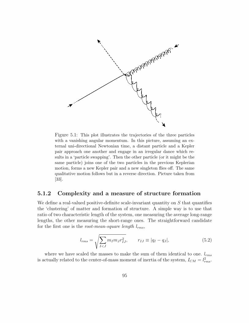
Figure 5.1: This plot illustrates the trajectories of the three particleswith a vanishing angular momentum. In this picture, assuming an ex-ternal uni-directional Newtonian time, a distant particle and a Keplerpair approach one another and engage in an irregular dance which re-sults in a ‘particle swapping’. Then the other particle (or it might be thesame particle) joins one of the two particles in the previous Keplerianmotion, forms a new Kepler pair and a new singleton flies off. The samequalitative motion follows but in a reverse direction. Picture taken from[33].

5.1.2 Complexity and a measure of structure formation

We define a real-valued positive-definite scale-invariant quantity on S that quantifiesthe ‘clustering’ of matter and formation of structure. A simple way is to use thatratio of two characteristic length of the system, one measuring the average long-rangelengths, the other measuring the short-range ones. The straightforward candidatefor the first one is the root-mean-square length lrms,

lrms =

√∑I<J

mImJr2IJ , rIJ ≡ |qI − qJ |, (5.2)

where we have scaled the masses to make the sum of them identical to one. lrmsis actually related to the center-of-mass moment of inertia of the system, ICM = l2rms.

95

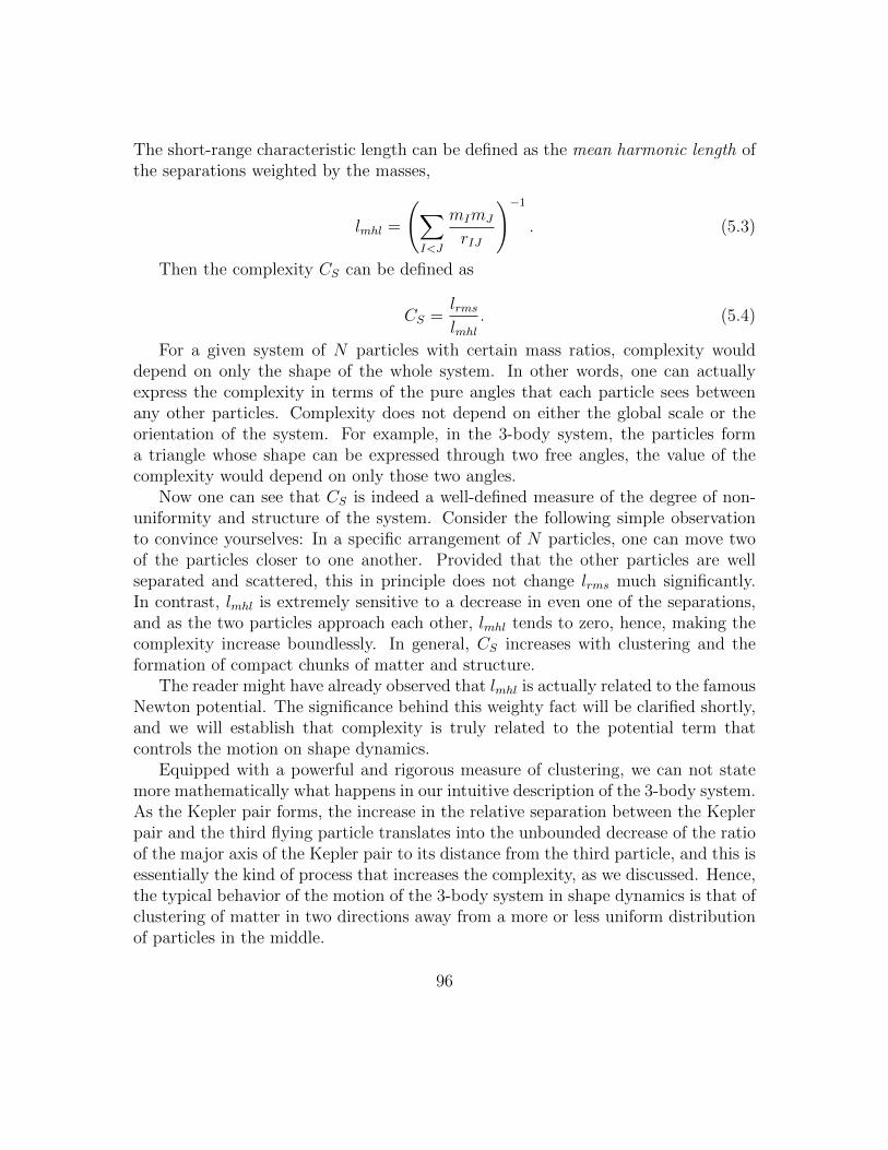
The short-range characteristic length can be defined as the mean harmonic length ofthe separations weighted by the masses,

lmhl =

(∑I<J

mImJ

rIJ

)−1

. (5.3)

Then the complexity CS can be defined as

CS =lrmslmhl

. (5.4)

For a given system of N particles with certain mass ratios, complexity woulddepend on only the shape of the whole system. In other words, one can actuallyexpress the complexity in terms of the pure angles that each particle sees betweenany other particles. Complexity does not depend on either the global scale or theorientation of the system. For example, in the 3-body system, the particles forma triangle whose shape can be expressed through two free angles, the value of thecomplexity would depend on only those two angles.

Now one can see that CS is indeed a well-defined measure of the degree of non-uniformity and structure of the system. Consider the following simple observationto convince yourselves: In a specific arrangement of N particles, one can move twoof the particles closer to one another. Provided that the other particles are wellseparated and scattered, this in principle does not change lrms much significantly.In contrast, lmhl is extremely sensitive to a decrease in even one of the separations,and as the two particles approach each other, lmhl tends to zero, hence, making thecomplexity increase boundlessly. In general, CS increases with clustering and theformation of compact chunks of matter and structure.

The reader might have already observed that lmhl is actually related to the famousNewton potential. The significance behind this weighty fact will be clarified shortly,and we will establish that complexity is truly related to the potential term thatcontrols the motion on shape dynamics.

Equipped with a powerful and rigorous measure of clustering, we can not statemore mathematically what happens in our intuitive description of the 3-body system.As the Kepler pair forms, the increase in the relative separation between the Keplerpair and the third flying particle translates into the unbounded decrease of the ratioof the major axis of the Kepler pair to its distance from the third particle, and this isessentially the kind of process that increases the complexity, as we discussed. Hence,the typical behavior of the motion of the 3-body system in shape dynamics is that ofclustering of matter in two directions away from a more or less uniform distributionof particles in the middle.

96

5.1.3 The structure and topography of shape space

The story of the universe plays out in the space of all possible relational degreesof freedom, the shape space. The shape space is the quotient of the Newtonianconfiguration space with respect to translations, rotations, and dilatations. Theinitial configuration space is R3N and comes with 3N degrees of freedom, some ofwhich are redundant. The similarity group is a 3 + 3 + 1 = 7 dimensional Lie groupand removes 7 degrees of freedom of the configuration space. Thus, we end up withthe 3N − 7 dimensional shape space, S = R3N/Sim(3). For the 3-body problem,the shape space is 2 dimensional. This agrees with our expectation, as the shapeof a triangle can be expressed by two angles. Hence, it can be represented by a2-dimensional ‘sphere’. Shape space is always compact.

In particle shape dynamics, we use the Newton potential3

V = −∑I<J

mImJ

rIJ(5.5)

and perform the best-matching with respect to translations and rotations.Naturally, we define the scale-invariant version of the potential by multiplying the

square root of the center-of-mass moment of inertia and arrive at the shape potential

VS ≡√ICMV, (5.6)

introduced in [31].We will see more clearly how VS controls the dynamics in shape space, neverthe-

less, it is clear at this point that VS captures the qualitative dynamical features ofthe potential on shape space, as shape space is scale-free and its degrees of freedomare defined up to a redundant scale.

The profound and yet, straightforward observation is that VS is actually thenegative of the complexity. This clearly means that the valleys of the shape potentialare in regions with higher complexity, which means that shape dynamics typicallysteers almost any system towards becoming more clustered and structured: Structureformation is typical in shape dynamics. This is already compatible with the intuitionwe gave about the generic 3-body solutions, but it is true for any other number ofparticles. Structure formation is the signature of the dynamics in shape space.

We state some commonly used concepts and definitions. First of all, the shapepotential is not a monotonic function in any sense and introduces non-trivial ripples

3G has been set to one by defining a unit of time in terms of that of the length. Moreover, allthe masses have been scaled so that the total mass equals one. These conventions do not changethe dynamics, as will become more clear when we introduce the dynamical similarity.

97

in the topographic map of shape space. The stationary points of VS are called centralconfigurations.

Moreover, notice that the shape potential is always negative and unbounded frombelow, as we discussed that complexity is unbounded from above. This means thatVS must have at least one maximum for it is a continuous function defined on shapespace which is compact. In the 3-body problem with equal masses, the maximumcorresponds to the uniform equilateral triangle. All non-maximal stationary pointsare saddles, as there are no local minima apart from the infinitely deep wells of VSassociated with the infinitely structured configurations.

In the 3-body problem, these non-maximal stationary points are the collinearshapes, those with the three particles lined up. The saddles are the collinear shapeswith one of the particles placed exactly between the other ones, while the minima ofVS are the collinear shapes in which two of the particles coincide.

The number of saddles, deep wells, and in general the non-uniformities of thetopographic features of VS increase with the number of particles. But the pivotalfact that the potential is bounded from above, but with infinitely deep wells at shapeswith infinitely high complexity remains valid, and this is exactly what explains whyour universe is as it is. Shape space is highly asymmetric. What we ultimately aimfor is to base the asymmetrical behavior of our universe on this asymmetry of theshape space, but maintain the time-symmetrical (or better, timeless) laws of motion.

There are still a few more technical terms we should cover. There are a zero-measure set of solutions, called homothetic solutions, in which a system is held at acentral configuration and its shape does not change, and then ‘explode’ and then comeout again. In Newton’s absolute space, such a system follows a uniform contractionuntil all of the particles collide in a way that does not change the shape. Thesesolutions in which the size of the system reaches zero (in Newtonian sense) are knownas central collisions. Central collisions can only occur if the solution terminates at acentral configuration.

Excluding a zero-measure subset of asymptotically homothetic solutions, all theother solutions can be extended so that they fall into the infinitely deep wells of thepotential asymptotically at both ends. This is the key result we should bear in mind.

See Fig. 5.2 for an illustration of the shape sphere of the 3-body system with aplot of the shape potential.

5.1.4 Back to the 3-body problem: the complete solution

We now investigate the mathematical structure of the shape space of the 3-bodysystem and find the equations of motion. Using good coordinates to satisfy the

98

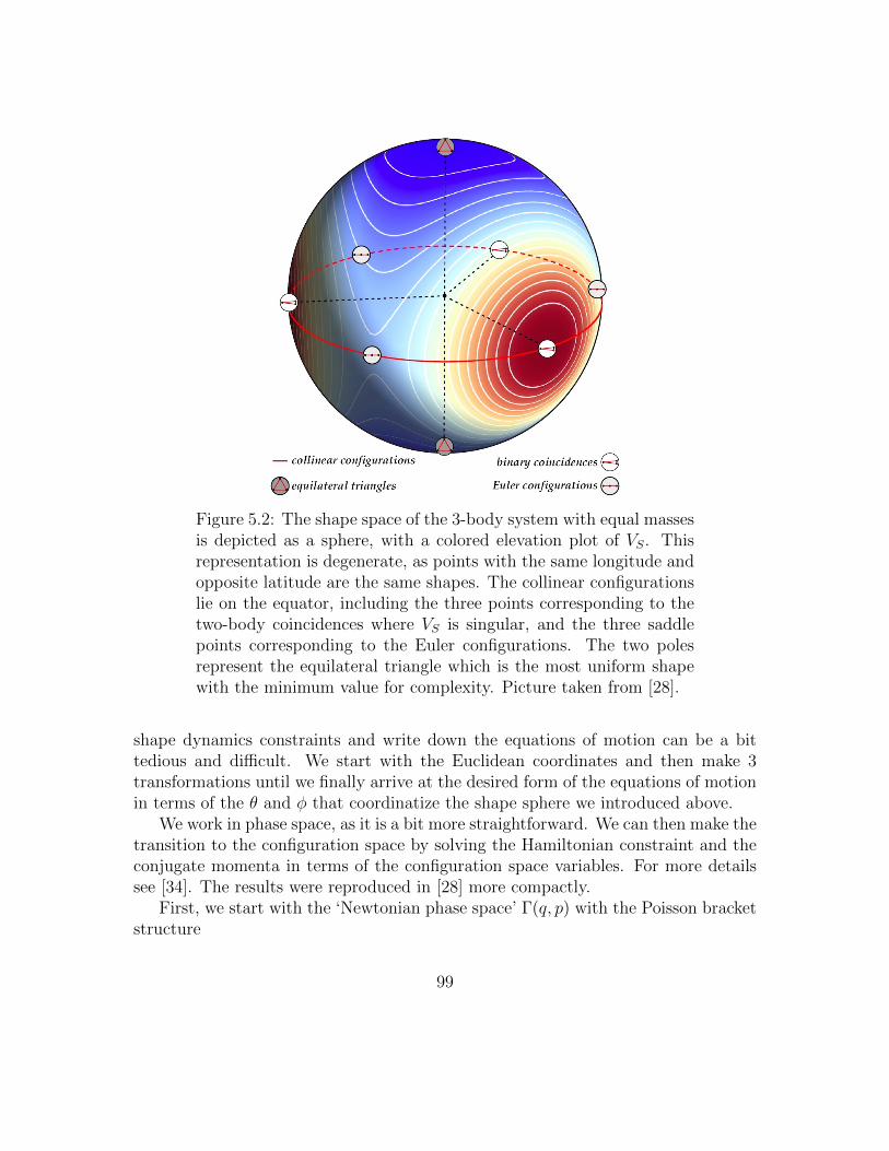
Figure 5.2: The shape space of the 3-body system with equal massesis depicted as a sphere, with a colored elevation plot of VS. Thisrepresentation is degenerate, as points with the same longitude andopposite latitude are the same shapes. The collinear configurationslie on the equator, including the three points corresponding to thetwo-body coincidences where VS is singular, and the three saddlepoints corresponding to the Euler configurations. The two polesrepresent the equilateral triangle which is the most uniform shapewith the minimum value for complexity. Picture taken from [28].

shape dynamics constraints and write down the equations of motion can be a bittedious and difficult. We start with the Euclidean coordinates and then make 3transformations until we finally arrive at the desired form of the equations of motionin terms of the θ and φ that coordinatize the shape sphere we introduced above.

We work in phase space, as it is a bit more straightforward. We can then make thetransition to the configuration space by solving the Hamiltonian constraint and theconjugate momenta in terms of the configuration space variables. For more detailssee [34]. The results were reproduced in [28] more compactly.

First, we start with the ‘Newtonian phase space’ Γ(q, p) with the Poisson bracketstructure

99

qaI , pJb = δab δIJ . (5.7)

Now we make the following three canonical transformations:

1. The transformation4

qaI ≡∑J

MIJqaJ

pIa ≡∑J

pJaM−1JI ,

(5.8)

with the invertible matrix

MIJ =

−√

m1m2

m1+m2

√m1m2

m1+m20

−m1

√m3(m1+m2)

m1+m2−m2

√m3(m1+m2)

m1+m2

√m3(m1 +m2)

m1 m2 m3

, (5.9)

andm1+m2+m3 = 1 by convention is a canonical transformation and leaves thePoisson structure unchanged. The reason that this particular transformationis useful, is that we can see that the third new momenta are the total momentathat vanish as the result of best-matching. To see that, we calculate the inverseof M :

M−1IJ =

−

√m1m2m1+m2

m1− m3√

(m1+m2)m3

1√m1m2m1+m2

m2− m3√

(m1+m2)m3

1

0

√(m1+m2)m3

m31

(5.10)

and hence, we have

p3a =

∑I

pIa ≈ 0. (5.11)

4Note that q and p’s here are not the same ‘transformed’ variables we used in Chapter 3 forbest-matching.

100

This helps us to apply the best-matching constraint corresponding to the trans-lational group directly and set p3

a weakly equal to zero. This makes sense, as q3

denotes the center of mass of the system and it should not be dynamical fromthe relational point of view.

Another important result is that the kinetic term in terms of the new momentais

T =∑I

pIapIa

2mI

=1

2

∑I

pIapIa ≈

1

2

((p1)2 + (p2)2

), (5.12)

as can be checked directly by using (5.10).

The center-of-mass moment of inertia is also diagonal in the new coordinates:

ICM =∑I<J

mIr2IJ = q2

1 + q22 (5.13)

Now we have 6 + 6 variables and only the angular momentum constraint todeal with,

Ja =∑I

εabcqbIpIc ≈

∑I=1,2

εabcqbI pIc ≈ 0. (5.14)

2. We introduce another set of conjugate variables:

w1 =1

2

(q2

1 − q22

), w2 = q1 · q2 ≡ qa1 q

a2 , w3 = |q1 × q2|,

z1 =(q1 · p1 − q2 · p2)

ICM, z2 =

(q2 · p1 + q1 · p2)

ICM, z3 =

(|q1 × p2| − |q2 × p1|)ICM

.

(5.15)

These variables are rotationally invariant, and hence completely decouple therotational degrees of freedom. This is the way we enforce the angular momen-tum constraint and remove 3 + 3 degrees of freedom and cover the reducedphase space by the three pairs of variables in (5.15).

A rather long calculation can show that the only non-trivial Poisson bracketsare

101

wI , zJ = δIJ . (5.16)

The ‘magnitude’ of w, i.e., w21 + w2

2 + w23 equals to

I2CM4

. Moreover, the kineticterm has the same simple form:

T =1

2

(ICM |z|2 +

|J |ICM

)≈ ICM

2|z|2, (5.17)

where |z| and |J | are the magnitude of z, and J respectively.

3. The final canonical transformation takes us to shape sphere, or more precisely,the phase space associated with the shape sphere parametrized by θ and φ andtheir conjugate momenta.

For that, we introduce the variable R =√ICM and write w’s in the form

w1 = R2 sin θ cosφ, w2 = R2 sin θ sinφ, w3 = R2 cos θ. (5.18)

The dimensionless variables θ and φ coordinatize the shape sphere Fig. 5.2.Following the usual transformation to polar coordinates, we introduce the con-jugate momenta pθ, pφ, and pr, and arrive at5

T =1

2

R4p2r + p2

θ + sin−2 θp2φ

R2, (5.19)

where pr is the momentum conjugate to r ≡ R2 and is

pr =r

R2=

2

RR. (5.20)

Moreover, R is related to the dilatational momentum, as

R =1

2RICM =

1

2R(2D − 2qCM · P ) ≈ D

R. (5.21)

Thus,

5An easy way to see that is to write the kinetic term of the Lagrangian. Following (5.17) wededuce that w = R2z and therefore, Lkin =

∑I

12R2 w

2I . Thus, in polar coordinates the kinetic term

would be (5.19).

102

T =1

2

p2θ + sin−2 θp2

φ + 4D2

R2. (5.22)

We should not neglect the potential term. The Newton potential is homo-geneous of degree -1, and hence shape potential VS =

√ICMV is scale-free.

Therefore, in principle, we can write VS in terms of θ and φ. The details offinding the explicit form are in [34]. The Hamiltonian is

H =1

2

p2θ + sin−2 θp2

φ + 4D2

R2+

1

RVS(θ, φ). (5.23)

The theory is reparametrization invariant and (5.23) weakly vanishes. Hence, thisHamiltonian gives us a geodesic theory of the shape variables, and also the total size ofthe system expressed by R. It does not satisfy the strong-version of Mach’s Principle,as we did not implement best-matching with respect to dilatations. However, inparallel with our discussion in Sec. 4.2.5, we can follow the same procedure here anduse the dilatational momentum as the time variable to satisfy the weak version ofMach’s Principle, as in [31].

It should be stressed that the H = NH is the total Hamiltonian and should notbe accompanied by first-class constraints. The three steps we took to enforce shapedynamics constraints already restricted the variables to the gauge-invariant ones,i.e., wI and zI ’s. Of course, they are not subject to any gauge transformation. Thefirst-class Hamiltonian (5.23) gives us the complete equations of motion.

5.1.5 Deparametrization and the equations of motion

The dilatational momentum is monotonic, and therefore, a good candidate for parametriza-tion of the theory. Too see its monotonicity, we derive what is known as the Euler-Lagrange equation:

D =∑I

(qI · pI + qI · pI

)= 2T −

∑I

qI ·∂V

∂qI

= 2T − kV,(5.24)

where k is the degree of homogeneity of V and we have used Euler’s theorem inthe last line. For Newon potential k = −1. Assuming T + V = E, we have

D = 2E − (2 + k)V. (5.25)

103

In shape dynamics, we normally do not introduce any constant E into Jacobi’saction which means that in ephemeris time, T + V = 0 and D = −V for Newtonpotential and is always positive (V is negative). Hence, D is monotonic and we candeparametrize the theory with respect to it. As we discussed in Sec. 4.2.5, we haveto find the variable conjugate to D, solve the Hamiltonian constraint, and use theresult as the Hamiltonian for the reduced variables. In light of (5.21) and (5.22), weshould posit the fundamental Poisson bracket

logR,D =1

4. (5.26)

which means that we should solve (5.23) for 4 logR:

h = 4 logR = 4 log

(1

2

p2θ + sin−2 θp2

φ

CS+

2D2

CS

). (5.27)

This gives us a ‘time’-dependent evolution of the shape degrees of freedom withrespect to D. To make the Hamiltonian evolution more clear, we make the variablesand the time parameter completely dimensionless. We introduced only a dimensionof length to the initial Newtonian configuration variables. This induces dimensionto all the other variables:

= length2, [z] = length−3/2,

[pθ] = [pφ] = [D] = length1/2.(5.28)

We can rescale the momenta π = p/D0 where D0 can be taken to be the initialdilatational momentum. We define the parameter ζ = D/D0. Although the rescalingwe introduced is not a canonical transformation, the accompanying change in theparametrization leaves the equations of motion unchanged. The equations of motionin terms of the complexity are

dθ

dζ=

8πθπ2θ + sin−2 θπ2

φ + 4ζ2,

dφ

dζ=

8 sin−2 θπφπ2θ + sin−2 θπ2

φ + 4ζ2,

dπθdζ

=8 sin−3 θ cos θπ2

φ

π2θ + sin−2 θπ2

φ + 4ζ2+ 4

∂ logCS∂θ

,dπφdζ

= 4∂ logCS∂φ

.

(5.29)

We see that complexity actually controls the dynamics, as we expected. A lotcan be said about these equations of motion. First, we start with the explicit ‘timedependence’ of these equations. This is the price we had to pay to have a manifestly

104

Machian theory. We did not implement best-matching with respect to dilatations(and we will soon explain why) and the theory is not geodesic. The amount ofchange of the variables with respect to ζ is dynamically relevant, and this is theonly ‘absolute’ extra ingredient we need to solve the equations of motion. (5.29)completely determine the equations of motion if we specify the initial shape and theinitial velocity. Thus, the theory satisfied the weak version of Mach’s Principle.

The time-dependence of the equations has another notable consequence. It vi-olates the Poincare recurrence theorem. The recurrence theorem states that underany invertible Hamiltonian evolution in bounded phase space, an initial state re-turns arbitrarily close to itself after some long but finite time. The shape dynamicsequations of motion, being explicitly time-dependent, do not satisfy the condition ofinvertibility and hence, the dynamics is not recurrent. This means that the evolutionis ‘dissipative’. This dissipative aspect of the dynamics is behind the typical behaviorof the trajectories of motion as they spiral and get drawn deeper and deeper into thepotential wells, and lead to the formation of Kepler pair.

The dependence of the equations of motion can be eliminated by applying thenon-canonical transformation

ωθ =πθζ, ωφ =

πφζ, (5.30)

and use the parameter

λ = log ζ. (5.31)

This results in manifestly time-independent equations of motion, but with theextra terms −ωθ and −ωφ on the right hand side of the equations for dωθ

dλand

dωφdλ

.This transformation does not change the qualitative behavior of the trajectories,as the resulting equations of motion are not measure-preserving, and hence, wouldfortunately (!) not resurrect the recurrence theorem as one might think.

5.1.6 The mysterious issue of absolute size!6

At the very moment we introduced best-matching in Chapter 3, it was obvious thatone could implement this technique with respect to any Lie group. There is nothingsacred about the Euclidean group. Of course, we do not care about all the other Liegroups, but as far as the observational content of the configuration space leads us,

6A philosopher would object to my use of the word ‘mysterious’. If we are to be precise,mystery applies to an unknowable unknown. I do certainly hope that the issue of size is in principleknowable! Maybe I should use the word ‘puzzling’ instead.

105

we should have included the dilatational group. We briefly commented on this inSec. 3.5.1, and showed that the best-matching condition would be the vanishing ofthe dilatational momentum D. This condition is consistent only with a homogeneouspotential of degree -2. The easiest candidate could be VS/R

2. Introducing this ‘new’potential into the Hamiltonian results in the Hamiltonian constraint

H =1

2

(p2θ + sin−2 θp2

φ

)− VS. (5.32)

One can indeed show that the equations of motion, in this case, are equivalent tothe geodesics of the conformally flat metric

gab =

(CS 00 sin2 θCS

)(5.33)

defined on shape space in terms of θ and φ. In other words, the completelyscale-free equations of motion follow from the action

S =

∫ds

√2gab

dqa

ds

dqb

ds. (5.34)

The reason is that this action gives the Hamiltonian constraint (5.32). Thisgeodesic principle gives rise to equations of motion fundamentally different fromthose of (5.27), and to put it very succinctly, it does not conform to observations.There is no longer any dissipative evolution, and the solutions curves would not bedragged inescapably into the holes of wells of structure creation, and matter couldavoid getting clumpy and clustered well enough.

Another major drawback of the model (5.32) is that it does not lead to Newtonianequations of motion asymptotically. Newton potential has been tested for centuriesand has been known to give valid results for weakly bounded isolated subsystems.Insisting on a V ∝ 1/r2 potential leads to potential experimental discrepancies foreven trivial systems like our own solar system.

Absolute size is a tricky subject. We all hear cosmologists talk about the ‘expan-sion’ of the universe. Julian Barbour once said ‘the idea of an expanding universestinks! it’s not expanding... it’s changing its shape’.

The point is that expansion is not empirically verifiable at all, and does not haveany role in our relational physics. The major phenomenon cosmologists point out tosupport our description of the expansion of the universe is the cosmological redshifts.Of course, those redshifts are real, but the point is that the standard FLRW metricexplains them by presupposing some background clocks (which measure the cosmo-logical time) and an external rod (which measures the expansion of the universe),

106

and relates the redshift of a photon as measured by those clocks to an expansionwith respect to the external rod. This story ‘stinks’ because it takes a roundaboutroute and avoids the objectively real phenomenon (the redshift) and explains that interms of some absolute structure. The alternative shape dynamic description of theredshifts involves a direct explanation of the change in the frequency of a photon asmeasured by certain ‘physical’ clocks within the universe between two points.

Although this issue is still open in shape dynamics (see next subsection), it isin principle feasible to give a relational account of the redshift (and all the otherevidence for an expanding universe). For that, matter must get clustered well enoughand certain physical clocks must form. As the structure gets more and more compact,the time that it measures as compared to the external Newtonian time gets slowerand slower, making it possible to account for the redshift of a photon as it makesits way from one of these structures (consider a galaxy) to another one. But (5.32)would give us only a very limited range of redshifts, as Barbour and his collaboratorsalready found out in the early 2000s. This is the last nail in the coffin.

This is why we cannot rely on a completely scale-free theory and had to leavethe absolute size untouched. Instead, we used the dynamical similarity and de-parametrization to get rid of it at the price of losing the geodesic equations of motion.

But why? Why does nature not respect a relational theory? Does it meanthat nature wants us to keep a bit of the absolute structures? This may not bethe case. Although the present state of this issue is hidden in deep mist, it mightbe eventually quantum mechanics that dispels the aura of mystery surrounding theapparent ‘expansion’ of the universe, and the failure of shape dynamics as a classicaltheory to make sense of it.

5.1.7 Einstein’s sin (!)

In all successful theories in physics, whether Newtonian mechanics or relativity oreven quantum field theory and string theory, we posit a spacetime and a frame ofreference constructed by putting myriads of ‘imaginary’ clocks and rods at each pointto record the physical processes. But throughout this work, we have kept preachingthat clocks are nothing but physical systems using the change included in a physicalprocess as a measure of time, and clarified and defined this philosophical intuitionin Chapter 2. If our physical theory is to be an inclusive and complete theory of thewhole universe, and if we agree on saying that clocks and rods are themselves subjectto the laws of physics, then it would be contradictory to formulate the fundamentallaws of physics with respect to a reference frame outside our domain of description.As long as one clings to the ‘laboratory picture’ of the laws of physics, this does not

107

pose a serious challenge, but as a theory of the whole universe, this would certainlybe a conceptual flaw and should be subject to meticulous scrutiny.

Einstein himself admitted that this is an issue back in 1949 in his autobiography[35]:

It is striking that the theory [of special relativity] (except for four-dimensionalspace) introduces two kinds of physical things, i.e. (1) measuring rods andclocks, (2) all other things, e.g., the electromagnetic field, material point,etc. This, in a certain sense, is inconsistent; strictly speaking, measur-ing rods and clocks would have to be represented as solutions of the basicequations... not, as it were, as theoretically self-sufficient entities. Theprocedure justifies itself, however, because it was clear from the very be-ginning that the postulates of the theory are not strong enough to deducefrom them equations for physical events sufficiently complete and suffi-ciently free from arbitrariness to base upon such a foundation a theory ofmeasuring rods and clocks. If one did not wish to forego a physical inter-pretation of the coordinates in general (something that, in itself, would bepossible), it was better to permit such inconsistency – with the obligation,however, of eliminating it at a later stage of the theory.

But Einstein never attempted to eliminate them and base them on the underlyinglaws of physics, and this problem was largely neglected afterward.

I think that there are two aspects to this problem:

1. First, a working physical model of a clock and rod must be proposed in termsof the intrinsic dynamical variables, subject to laws of physics.

2. The behavior of these physical clocks and rods must be deduced from the lawsgoverning the whole universe and must conform to the corresponding standardprinciples of physics, e.g., absolute simultaneity in Newtonian mechanics andtime dilation in relativity.

Shape dynamics can potentially put this matter in a new light, as its startingpoint is not the spacetime, but a notion of the relational configuration of the wholeuniverse. We will see that the particle shape dynamics we developed does providea convincing resolution of this problem. Shape dynamics of geometry and fields,although being a more accurate physical theory of the whole universe that embodiesthe core of Einstein’s relativity, does not solve this problem. We can address the firstaspect by using the simple model in which a light ray bounces between two parallel

108

mirrors. But the main issue is the second step, and to rigorously show that theproper distance the spacetime metric gives is the measure of the proper time thatany clock records. This is an assumption we take for granted in relativity, and itsagreement with observations has enticed most physicists into accepting that as it is,without considering it critically.

But the problem can be more challenging than that. To ‘derive’ the behavior ofclocks and rods in any motion and show that they conform to the laws of relativity,requires an extra ingredient: the initial conditions. One must unambiguously specifywhat conditions correspond to an initial state of a clock (or a rod) in a certain motion.Normally, we do not care about this issue as we work with idealized ‘point-clocks’ inrelativity, and only the initial direction of motion is enough. But in light of the aboveconsideration, in a more physical model of a clock, the inner structure of the clockis an essential ingredient and it requires the specification of the initial conditions forthe substructure of the clock, meaning that only the initial direction of motion wouldnot suffice.7

We now proceed to the problem of rods and clocks in particle mechanics. We sawthat the dynamical laws of shape dynamics for three particles lead to the formation ofa Kepler pair and a singleton. These Kepler pairs grant us the pass to the first (andeasy) step of the ordeal. Each Kepler pair forms a clock, and the relative motion ofone of the particles against the background that the singleton puts up measures thepassage of time, exactly in the same way that solar time is defined. Moreover, theratio of the semi-major axis of the Kepler pair and the distance from the singletondefines a measuring rod.

The formation of Kepler pairs and a singleton is typical in the solutions of shapedynamics with any number of particles. Hence, the whole universe in this picturebreaks into myriads of clocks and rods, all in effective isolation from the others. Thewhole universe is a gigantic clock and rod factory.

More strikingly, these rods and clocks maintain their relations with one anothermore and more accurately as the universe evolves. The clocks ‘march in steps’ withone another, and the rods become congruent. This is ensured in shape dynamics,following a major result in N -body problem [36]. It can be shown that as the New-tonian time t approaches the infinity, each subsystem (a Kepler pair and a singleton)develops the conserved quantities

7Thanks to Mohammad Khorrami for pointing that out and a thorough discussion.

109

EI(t) = EI +O(t−5/3),

JaI (t) = JaI +O(t−2/3),

XaI (t)/t = V a

I +O(t−1/2),

(5.35)

where here, EI(t), JaI (t), Xa

I (t) are respectively the energy, angular momentum,and the distance of the subsystem from the center of the mass of the whole universe.I denotes the subsystems, not an individual particle.

It means that asymptotically, each substem would have constant energy and an-gular momentum. As these quantities encode the information of the clocks and rods,this ensures that the clocks and rods maintain their mutual relations to increasinglygreater accuracy.

The complete resolution of Einstein’s sin, especially in the context of geometrody-namics and field theory, requires much more sophisticated arguments and deductions,and more study and research.

5.2 Time’s arrow

The arrow of time conventionally refers to the irreversible process we observe allaround us: our house tends to become more disorderly, coffee spills on the groundand spreads out, we leave a bottle of ink in the open and the ink dries out, etc.Imagining the reversed processes of either one of these examples would be utterlystrange: We have not experienced anything of this sort in nature. One might createthese processes artificially in a laboratory, but it requires a tremendous amount ofresources.

The most evident arrow of time that we observe, which is the figures prominentlyin all of the above examples, is the thermodynamic arrow, defined as the growth ofentropy. There are two other observed arrows in the physical realm: The electro-magnetic arrow, and the arrow in quantum mechanics. The first one corresponds tothe propagation of the retarded waves, and not the ‘advanced’ waves. The third oneis related to the collapse of the wavefunction in the standard formulation.

Regardless of some proposed possible connections between them, these three ar-rows ground what we experience and identify as the arrow of time.

The existence of the arrow of time is not dubious of course, reconciling it with theknown laws of physics is the problem, known as the problem of the arrow of time.

110

5.2.1 Reflection on the problem of the arrow of time

There are in fact two problems. The first problem is the conventional problem of thearrow of time:

I. Given that the fundamental laws of physics, apart from the weak theory thatdoes not make a huge contribution to the evolution of the universe, are alltime-symmetric, how is it that we observe an asymmetry in time? In otherwords, how is this symmetry of the laws of nature broken and not realized inthe evolution of nature?

This question (problem) is a logical question and points out a meaningful apparentcontradiction, but there is also a presumption at the heart of the question that thelaws of nature are time-symmetric.

This might be one way to dodge the inconsistency: There might be yet-to-be-found laws of nature that inherently distinguish an arrow of time.

But if we accept the laws of nature as they are, there would be one way to solvethe problem: To postulate some non-symmetric initial conditions that break thetime symmetry of the underlying physics at the level of the solution. One thus has toposit an initial state with extremely low entropy and then allows the laws of natureto evolve the state and increase the entropy and lead to the emergence of an arrowof time. David Albert calls this the ‘Past Hypothesis’.

The general consensus among most physicists is that the Past Hypothesis isneeded to solve the version of the problem of the arrow of time presented above.

But there are some concerns on both Past Hypothesis and also the generally ac-cepted approach to this problem. First, in the known frameworks of physics, an initialcondition that accounts for the qualitative behavior of our universe is extremely spe-cial and requires fine-tuning, making the Past Hypothesis very suspicious. This isthe main issue, which will be addressed in relational physics.

Moreover, there are some critical remarks on the usual approach, as given in [28],[33], [37], [38]:

1. The concept of entropy that is widely used in the literature on the arrow of time,just like any other thermodynamic concept, is applicable to confined systemsin a box which makes it possible for the system to equilibrate. However, thewhole universe is not in a box, and defining entropy for it is problematic in thefirst place. The walls of a box that confine a system play an essential role inpushing a system of particles to equilibrium: The particles keep bouncing offone another and the walls.

111

2. Gravitational systems are anti-thermodynamic and they lead to more cluster-ing, rather than spreading of matter. This fact is already acknowledged inshape dynamics quantitatively as complexity generally increases along the so-lution curves. Hence, self-gravitating systems cannot and do not equilibratethermodynamically.

3. It is not clear how to define entropy in general relativity, and repeating thethermodynamic arguments in the context of general relativity remains highlyproblematic.

This is not to overthrow thermodynamics at all. Thermodynamics remains anincredibly powerful theory within its domain of application, as Einstein said8, butthe point is that the whole universe is definitely not in that domain. The universeis not a steam engine, or some gas in a container hovering in the vast absolutespace. By thinking out of the box and going beyond the thermodynamic concepts,we can more appropriately discuss the dynamics of the whole universe in terms of itsintrinsic degrees of freedom, the relational quantities we have been using in this work.Moreover, contrary to entropy, complexity is a well-defined quantity and applicableto the whole universe, on which we rely to understand the arrow of time.

A brief review of the discussions of the arrow of time can be found in [39].There is another question, more metaphysical, that can be put in connection with

the arrow of time:

II. What grounds the arrow of time? In other words, what is it from which thearrow of time emerges?

Not all people would even accept this question as meaningful, especially in to-day’s pragmatic era. The problem of the arrow of time arises naturally within thecontext of time-symmetric fundamental laws, and one can easily convince himself byinvoking Past Hypothesis. But this second question is metaphysical and demandsa metaphysical basis for the arrow of time. Yet, any solution to this question mustalso show that all of the arrows of time we observe can be ‘deduced’ from what onesuggests as the origin of time’s arrow.

8Einstein said of thermodynamics: “It is the only physical theory of universal content, whichI am convinced, that within the framework of applicability of its basic concepts will never beoverthrown”.

112

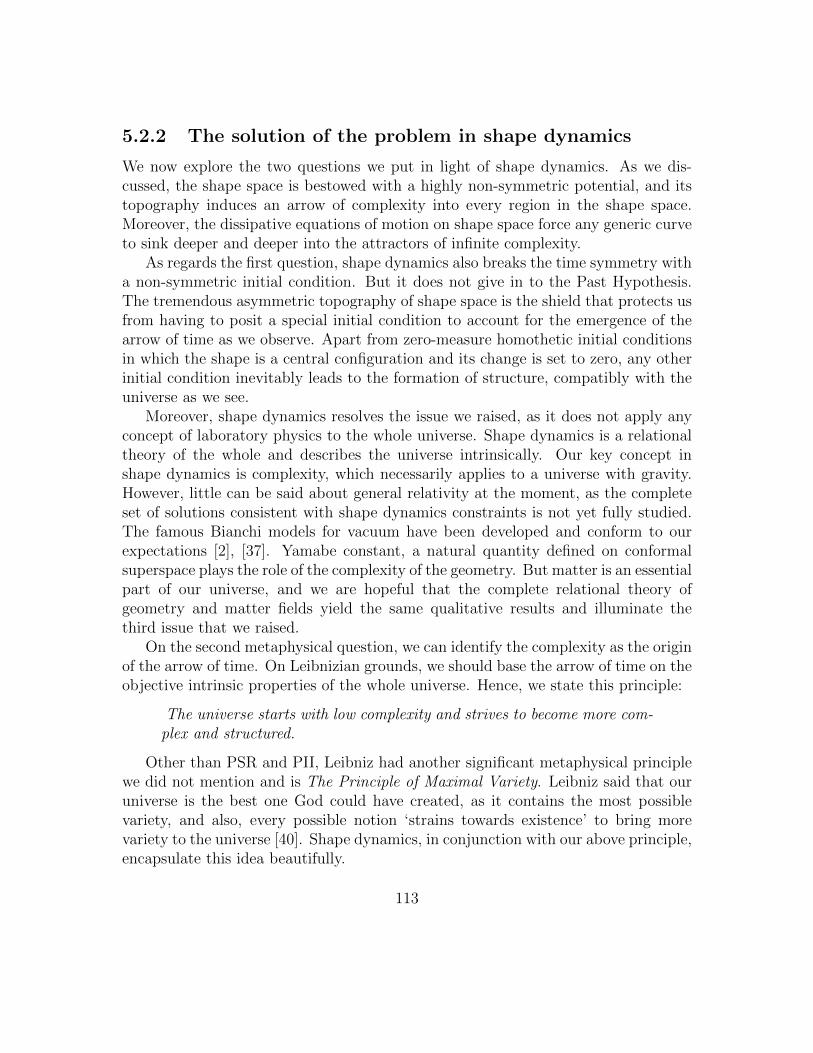
5.2.2 The solution of the problem in shape dynamics

We now explore the two questions we put in light of shape dynamics. As we dis-cussed, the shape space is bestowed with a highly non-symmetric potential, and itstopography induces an arrow of complexity into every region in the shape space.Moreover, the dissipative equations of motion on shape space force any generic curveto sink deeper and deeper into the attractors of infinite complexity.

As regards the first question, shape dynamics also breaks the time symmetry witha non-symmetric initial condition. But it does not give in to the Past Hypothesis.The tremendous asymmetric topography of shape space is the shield that protects usfrom having to posit a special initial condition to account for the emergence of thearrow of time as we observe. Apart from zero-measure homothetic initial conditionsin which the shape is a central configuration and its change is set to zero, any otherinitial condition inevitably leads to the formation of structure, compatibly with theuniverse as we see.

Moreover, shape dynamics resolves the issue we raised, as it does not apply anyconcept of laboratory physics to the whole universe. Shape dynamics is a relationaltheory of the whole and describes the universe intrinsically. Our key concept inshape dynamics is complexity, which necessarily applies to a universe with gravity.However, little can be said about general relativity at the moment, as the completeset of solutions consistent with shape dynamics constraints is not yet fully studied.The famous Bianchi models for vacuum have been developed and conform to ourexpectations [2], [37]. Yamabe constant, a natural quantity defined on conformalsuperspace plays the role of the complexity of the geometry. But matter is an essentialpart of our universe, and we are hopeful that the complete relational theory ofgeometry and matter fields yield the same qualitative results and illuminate thethird issue that we raised.

On the second metaphysical question, we can identify the complexity as the originof the arrow of time. On Leibnizian grounds, we should base the arrow of time on theobjective intrinsic properties of the whole universe. Hence, we state this principle:

The universe starts with low complexity and strives to become more com-plex and structured.

Other than PSR and PII, Leibniz had another significant metaphysical principlewe did not mention and is The Principle of Maximal Variety. Leibniz said that ouruniverse is the best one God could have created, as it contains the most possiblevariety, and also, every possible notion ‘strains towards existence’ to bring morevariety to the universe [40]. Shape dynamics, in conjunction with our above principle,encapsulate this idea beautifully.

113

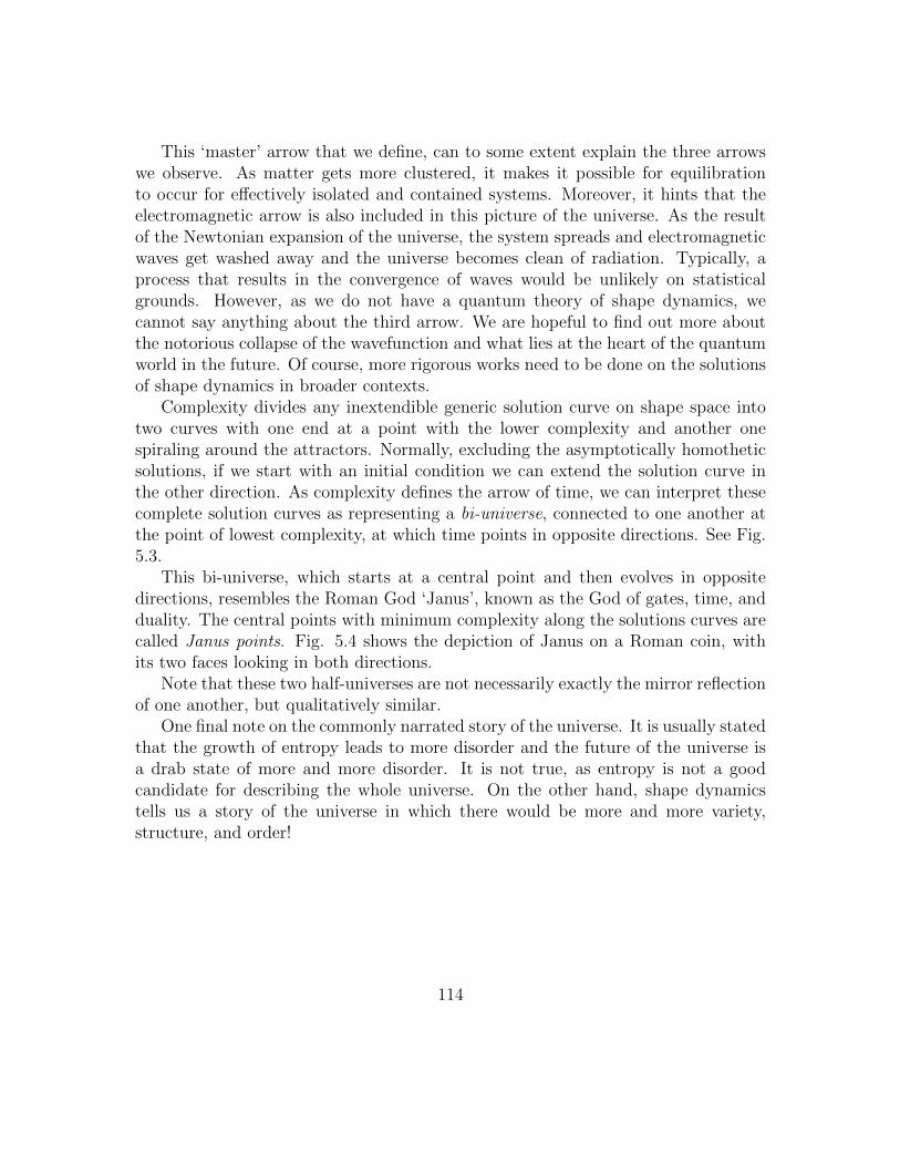
This ‘master’ arrow that we define, can to some extent explain the three arrowswe observe. As matter gets more clustered, it makes it possible for equilibrationto occur for effectively isolated and contained systems. Moreover, it hints that theelectromagnetic arrow is also included in this picture of the universe. As the resultof the Newtonian expansion of the universe, the system spreads and electromagneticwaves get washed away and the universe becomes clean of radiation. Typically, aprocess that results in the convergence of waves would be unlikely on statisticalgrounds. However, as we do not have a quantum theory of shape dynamics, wecannot say anything about the third arrow. We are hopeful to find out more aboutthe notorious collapse of the wavefunction and what lies at the heart of the quantumworld in the future. Of course, more rigorous works need to be done on the solutionsof shape dynamics in broader contexts.

Complexity divides any inextendible generic solution curve on shape space intotwo curves with one end at a point with the lower complexity and another onespiraling around the attractors. Normally, excluding the asymptotically homotheticsolutions, if we start with an initial condition we can extend the solution curve inthe other direction. As complexity defines the arrow of time, we can interpret thesecomplete solution curves as representing a bi-universe, connected to one another atthe point of lowest complexity, at which time points in opposite directions. See Fig.5.3.

This bi-universe, which starts at a central point and then evolves in oppositedirections, resembles the Roman God ‘Janus’, known as the God of gates, time, andduality. The central points with minimum complexity along the solutions curves arecalled Janus points. Fig. 5.4 shows the depiction of Janus on a Roman coin, withits two faces looking in both directions.

Note that these two half-universes are not necessarily exactly the mirror reflectionof one another, but qualitatively similar.

One final note on the commonly narrated story of the universe. It is usually statedthat the growth of entropy leads to more disorder and the future of the universe isa drab state of more and more disorder. It is not true, as entropy is not a goodcandidate for describing the whole universe. On the other hand, shape dynamicstells us a story of the universe in which there would be more and more variety,structure, and order!

114

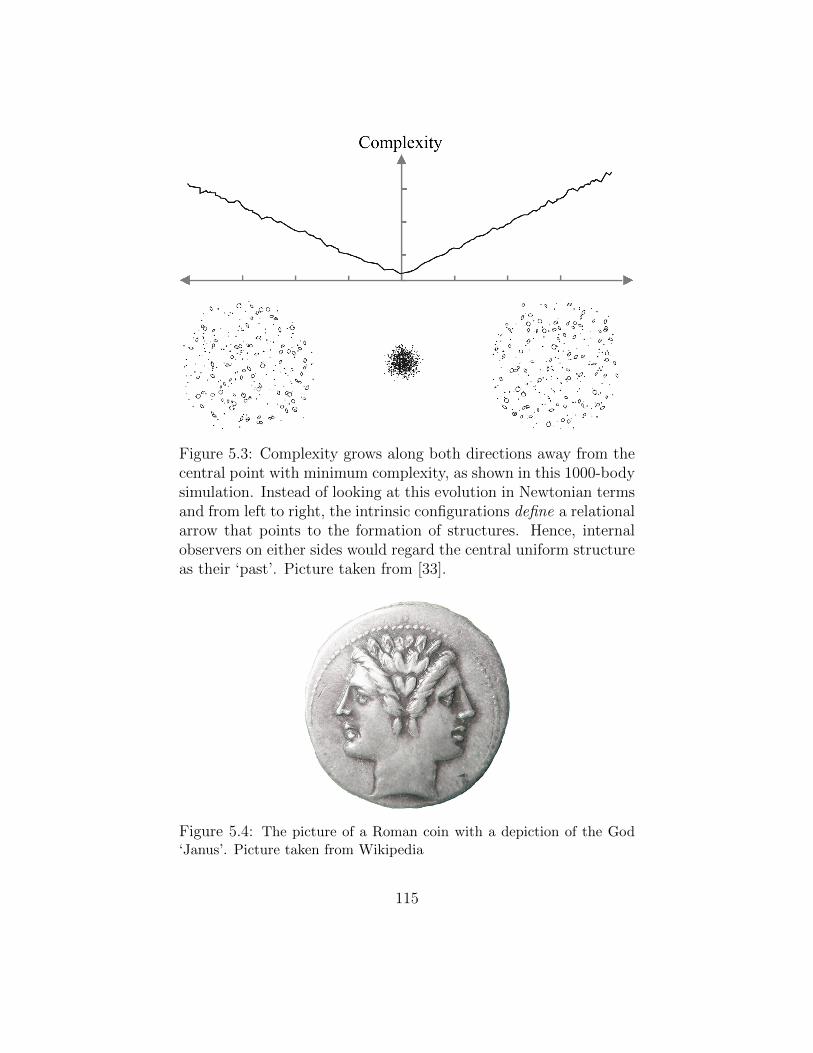
Figure 5.3: Complexity grows along both directions away from thecentral point with minimum complexity, as shown in this 1000-bodysimulation. Instead of looking at this evolution in Newtonian termsand from left to right, the intrinsic configurations define a relationalarrow that points to the formation of structures. Hence, internalobservers on either sides would regard the central uniform structureas their ‘past’. Picture taken from [33].

Figure 5.4: The picture of a Roman coin with a depiction of the God‘Janus’. Picture taken from Wikipedia

115

Chapter 6

Conclusion and Outlook

Our focus in this work has been to

1. Clarify the foundations and underlying principles of relationalism and delin-eate what exactly separates relational physics from the standard Newtonian orEinsteinian classical physics.

2. Give a rigorous and thorough formulation of shape dynamics, as the alternativerelational theory in both particle mechanics and geometrodynamics.

3. Explore the implications of the particle toy model for the whole universe andreflect on the origin of time.

Although this work presented the established results of shape dynamics, shapedynamics is a young field of study and a lot more research should be done, whichmight change some of these results, especially those of the third one we developed inChapter 5.

At the moment, there are three active lines of research on shape dynamics. Oneof them is in the direction of doing more numerical works on the solutions of shapedynamics to reveal more elements of the potentials of shape dynamics as a theory ofthe whole. Some central configurations with a large number of particles have recentlybeen simulated, with some possible interesting implications for quantum mechanics.These numerical works can suggest very valuable ideas for developing the theory.

Another research area is developing the field ontology. As I mentioned briefly, thesimple Bianchi IX model of shape dynamics leads to the continuation of shape degreesof freedom of the universe through the big bang singularity [32]. Flavio Mercati andhis research group, and David Sloan have been working on further developing this to

116

both generalize their results and include other singularities, such as the gravitationalsingularity.

Lastly, let us not forget about the holy grail of modern physics, the problem ofquantum gravity and quantum foundations! Very little can be said about quantummechanics, or what I call quantum shape dynamics. But there are some deeplyinsightful ideas in that direction too.

Before I mention two major guiding ideas, I recap the open questions we faced inthe development of the theory in our work:

1. Shape dynamics is not perfectly Machian, and there is one single remnant of theabsolute structures we removed: the dilatational momentum or ‘anomaly’ asJulian Barbour calls it. How do we make sense of this non-relational variable?

2. Shape dynamics does not completely solve the problem of the rods and clocks.

3. The field ontology is not fully developed and the status of the arrow of time isstill not known in that context.

4. Quantum mechanics is not taken into account.

We are very hopeful that shape dynamics might solve these issues in the nearfuture. We may need some new ideas for developing the theory if we are to tacklethese fundamental problems.

There are two ideas, among many other ones, which are very suggestive, simple,and well-formed as compared to others.

1. Tim Koslowski suggests that shape dynamics should not be limited to a fixednumber of particles. The number of particles might change under some lawthat is not yet found. This allows for particle creation and annihilation whichis the key phenomenon in quantum field theory.

2. Julian Barbour suggests that complexity is literally the time.

The first idea is very powerful, as it opens up a possibility to reconcile quantummechanics with shape dynamics. It makes ‘creation of structure’ possible in shapedynamics. The second idea is also radical, especially in conjunction with the firstone.

We already discussed the role of complexity as the origin of the arrow of time,and that the time all internal clocks measure are related to the global increase ofcomplexity. But if complexity is to be the time, it means that it controls the ‘du-ration’ of time as well as its direction. By looking at the mathematical expression

117

of complexity, one sees that adding more particles generically leads to an increase incomplexity. Therefore, the first idea together with the second one, if they are true,indicates that nature highly controls and constrains creation. A large number ofparticles cannot pop into existence right away, as it would require an infinite amountof time which is not accessible! This might solve the cosmological constant problem.

More strikingly, it might also solve the problem of gravitational collapse andsingularities at the classical level! The collapse of matter increases the complexitydrastically. If it is true that in a fundamental law of the whole universe complexityplays the role of time, then no gravitational singularity would form in the first place.

These are certainly worth pondering, but require more research and study to bedone.

In short, now is a great time for developing shape dynamics, especially in lightof the open questions we summarized, and the interesting ideas we mentioned. Thecurrent results indicate that shape dynamics might be on the right track as a theoryof the whole.

118

Appendix A

Reparametrization InvariantLagrangian Systems and Jacobi’saction

We start with the standard Newtonian action defined on the configuration space ofN particles represented by the variables qaI where I denotes the particles and a standsfor the spatial dimensions:

S[q] =

∫ qaIi,tf

qaIi,ti

dt (T (qaI , · · · )− V (qaI , · · · )) ≡∫ qaIi,tf

qaIi,ti

dt L, (A.1)

where T is the Kinetic term ∑I

1

2mI q

2I , (A.2)

and V is an arbitrary time-independent potential.In general, there is a procedure called Routhian reduction procedure that expur-

gates the action from the cyclic variables, those which only enter the action withderivatves.1 One can apply this procedure to time-independent lagrangian systemsand arrive at a less known, but powerful action called Jacobi’s action. Before weproceed with that procedure, we note that the standard Newtonian action can beturned into an action to which this procedure would be applicable by elevating therole of the Newtonian time and treating it as a dynamical variable. Thus, along any

1For a more detailed account of the procedure see parts 9 and 10 of Chapter VI of [41], or theentry on it in Wikipedia.

119

trajectory, we can take t to be a function of an arbitrary parameter t = t(λ). Thenthe above action can be written as the following integral with the same boundaries:

S =

∫dλ

dt

dλ

(1

2

∑I

mIq′2I

(dλ

dt

)2

− V (qaI , · · · )

)≡∫dλ L(q, q′, t, t′) (A.3)

where q′aI is the derivative of the qaI (t(λ)) with respect to the new parameter.L is the ‘new’ Lagrangian that generates the same trajectories in the ‘extended’configuration space which includes time as an independent variable, and is equal tothe original Lagrangian by a factor of t′: L = t′L.

This theory if reparametrization invariant, meaning that we can use any param-eter to describe the system. In other words, action is invariant under the transfor-mation λ→ λ′ = λ′(λ) where λ′(λ) is a strictly monotonic smooth function of λ 2 ascan be checked simply. Actually, it is not a surprise as we found the action (A.3) byintroducing an ‘arbitrary’ parameter into the original action (A.1).

If we calculate the momentum conjugate to this ‘new’ dynamical variable, t, wefind

pt =∂L

∂t′= −

(dλ

dt

)21

2

I=N∑I=1

mIq′2I − V. (A.4)

What is interesting is that pt is exactly the same as the Hamiltonian functionone derives from the Lagrangian in (A.1). Moreover, the conjugate momenta to thevariables qaI denoted by pIa remain the same:

pIa =∂L

∂q′aI=

1

t′mIq

′aI = pIa. (A.5)

It suggests that the Hamiltonian for the action (A.3) vanishes:

H = ptt′ +

N∑I=1

pIaq′aI − L = ptt

′ + t′

(N∑I=1

pIaqaI − L

)= (pt +H)t′ = 0. (A.6)

This is the price we have to pay for adding a new artificially dynamical variable tothe configuration space. It means the Hamiltonian for this new theory is a constraint.

2This smoothness condition is to assure that the derivatives of the configuration space variableswith respect to the new parameter exist to any arbitrary order. The requirement of monotonicity isnecessary, otherwise, two different states may be assigned to one ‘instant’ of the new time parameter.

120

This, however, does not mean that there is no evolution in phase space. If theHamiltonian had vanished ‘identically’ in the phase space, it would have meant thatthere is no evolution and the variables remain constant. But here, the Hamiltonianis a constraint and vanishes on only a ‘part’ of the phase space that includes the truephysical variables, i.e., it is a constraint. For the constrained Hamiltonian systemsrefer to Appx. C in which we apply Dirac’s approach to reparametrization invarianttheories of this type and discuss them at length.

There is an important thing to note about the reparametrization invariant action(A.3). The new variable, the Newtonian time, is a cyclic variable if the originalLagrangian in (A.1) is not explicitly time-dependent. For closed systems, this isalways the case. Thus, for these systems the new Lagrangian L does not dependon t. This means that its conjugate momentum, pt is constant. We now apply theRouthian reduction procedure to the time variable. The Routhian is

R(qaI , q′aI , t, pt) = L− ptt′ = t′L(qaI , q

′aI)− ptt′ = t′(T − V − pt). (A.7)

Because of the Legendre transformation, t′ is a function of other variables andwe need to replace it with its explicit form. We can do that by noting that pt isconstant according to the equations of motion. Let pt = −E. E is the total energyof the system (as we will see) and the minus sign is for later convenience. From the

above calculation we saw that pt = −H where H = T + V = 12

I=N∑I=1

mI q2I + V . After

rewriting the above expression, we have

pt = −1

2

∑I

mIq′2I

(dλ

dt

)2

− V (qaI ) = −E, (A.8)

thus,

t′ =

√T

(E − V ), (A.9)

where T = 12

∑I

mIq′2I . Hence,

R(qaI , qa′

I , t, pt) = 2√

(E − V )T . (A.10)

As the result, we have the following action which in principle, is equivalent to theabove action we started from

121

SJ = 2

B∫A

dλ√

(E − V (qaI ))T (A.11)

This action, called Jacobi’s action, is reparametrization invariant and time doesnot play any role in it. The A and B represent the fixed initial and final configurationsin the configuration space. Again, time does not have any role to play in theseboundaries. Minimizing this action with respect to qaI ’s determines the trajectoriesof motion in the configuration space.

But we should need more information to find the Newtonian trajectories becausethe above procedure removed time completely. What happened to the dynamicalrole of Newtonian time now?

This one last datum is encoded in the condition pt = −E. This condition deter-

mines ‘how fast’ the system should evolve with respect to t. As pt = 12

I=N∑I=1

mI q2I +V ,

we can now parametrize the trajectory we find from (A.11) with t such that theabove condition holds for a specific value for E.

The punchline is that Jacobi’s action determines the timeless ‘frozen’ trajectoryof motion, e.g., the path of planets around the sun, and the supplementing energycondition determines how fast the planets must dance around the sun with respectto Newtonian time.

122

Appendix B

Lie Groups and Lie Algebras

Lie Groups, Lie algebras, and their actions on manifolds, are all of utmost importanceto relational physics and shape dynamics. The language of relational physics is thelanguage of gauge theories. This was clear as early as we introduced Mach-PoincarePrinciple. Hence, we first review all the primary definitions and concepts in Lie groupand Lie algebra theory, and then we discuss the Euclidean group in more detail asit is the cornerstone of relational particle physics.1

B.1 Lie groups and their Lie algebras

Definition B.1. A Lie group G is a differentiable manifold endowed with a groupstructure such that the group multiplication G× G → G and the inverse map ()−1 :G→ G are smooth.

If the Lie group manifold is r-dimensional, we say that G is a r-parameter Liegroup.

Hence, a Lie group is basically a group of continuous elements which is alsomanifold in itself. It means that any concept in group theory is relevant for Liegroups, such as group multiplication, inverse, and a unique identity element denotedby e.

There are many examples of Lie groups. The general Linear group GL(V ) is aLie group with a well-defined multiplication law (multiplication of the operators).

1For more details, see the Chapter 29,30 of the book [42] and Chapter 2 of [43]. I assume thatthe reader is familiar with the formal definition of group and representation. For that, see Chapter1 of [43].

123

The translation group T (3), the rotation group SO(3), the gauge group of electro-magnetism, U(1) are some other examples.

These groups are all finite-dimensional. There are also more abstract infinite-dimensional Lie groups such as the group of conformal transformations in a Rieman-nian manifold, the group of diffeomorphisms, etc that are of relevance to geometro-dynamics.

Lie group manifolds can have various topological shapes. For instance, U(1) issimply a circle, T (3) is diffeomorphic to R3. SO(3) has a more non-trivial topologyand is a compact non-simply connected manifold. It has the shape of a sphere withthe two points on its surface identified with one another.

We now proceed to define Lie algebra. The concept of Lie algebra can be visu-alized as the tangent vector space at a point in the Lie group manifold, usually theidentity element for simplicity. Intuitively, elements of the Lie algebra (which is avector space as we will see) are vectors in all possible directions along the Lie groupmanifold. You may have seen elsewhere that elements of Lie algebra are defined byconsidering group elements infinitesimally close to the identity. We follow a ratherabstract way that ultimately leads us to a proper mathematical definition of Liealgebra. First, we have to start with the definition of left translation:

Definition B.2. Let G be a Lie group and g ∈ G. The left translation by g is thediffeomorphism Lg : G→ G defined by Lgh = gh for all h ∈ G where by gh the groupmultiplication of g and h is meant.

A vector field v defined on G is called left-invariant if for each g ∈ G, v is relatedto itself under the pushforward induced by Lg. Formally, this means

Lg∗v|h = v|gh (B.1)

for all h ∈ G.We denote the set of all left-invariant vector fields on G by g. In general, the

space of all vector fields defined on a manifold, i.e., the vector bundle, is an infinite-dimensional vector space. We have also the Lie bracket structure defined on themanifold which is the Lie derivative of one vector field with respect to the other,[v, w](f) = v(w(f)) − w(v(f)), the output of which is also another vector field.Hence, we can say that the vector bundle defined on a manifold is a Lie algebraunder the Lie bracket ‘multiplication’.2

The same thing can be constructed for Lie groups by virtue of being manifold.However, a more restricted and useful structure can be defined for left-invariant

2For a brief and formal account of Lie algebra theory see Sec. 29.2 of [42].

124

vector fields. It can be proved that the left-invariant vector fields form a Lie algebrathemselves. We have the following theorem:

Theorem B.1. Let G be a Lie group and g the set of its left-invariant vector fields.Then g is a real vector space of the same dimension as G. Moreover, g is closedunder Lie brackets. Hence, g is a Lie algebra.

Being left-invariant, it does not make any substantial difference whether we con-sider the elements of the vector field at the identity or any other element. Usually,we associate the Lie algebra with the tangent vector space at e. Thus, we have thefollowing definition:

Definition B.3. The Lie algebra of the Lie group G is the Lie algebra g of the left-invariant vector fields on G. Conventionally, we think of v ∈ g as a vector in Te(G),the tangent vector space at e. Then we can denote the corresponding vector field byXv, i.e., Xv|e = v.

As we discussed, the Lie algebra comes with an algebraic structure, called theLie bracket. In other words, the objects [Xv, Xw] are also left-invariant and thereforebelong to g. If we introduce the basis vi for the Lie algebra g, then we have

[Xvi , Xvj ] =∑k

fkijXvk , (B.2)

where fkij are some constant numbers independent of the group element at whichthe commutator has been evaluated, called the structure constants of G.

Although our formal definition of Lie group and Lie algebra may seem abstract,we can study the action of the Lie groups on other more physical manifolds, such asthe configuration space, and infer many useful things from that. This is the contentof the next section. We will see that it is easier to conceive the action of a grouprather than the abstract group itself.

B.2 Group action

We start with the formal definition of the action of a Lie group:

Definition B.4. Let M be a manifold. A local group of transformations correspond-ing to a Lie group G acting on M is a smooth map3 T : G×M →M satisfying thefollowing condition:

3In some mathematical literature the action of a group is not defined for all members of thegroup and only an open subset of it is considered. This does not quite matter at this level for theexamples and physical applications we consider.

125

1. g · (h · P ) = (gh) · P ∀g, h ∈ G,P ∈M ,

2. e · P = P ∀P ∈M ,

3. g−1 · (g · P ) = P ∀g ∈ G,P ∈M ,

where g · P ≡ T (g, P ).

There is an important concept regarding the Mach-Poincare Principle called theorbit of a Lie group. The formal definition is

Definition B.5. The orbit of an element P ∈M , denoted by OP , is a set of pointsin M obtained from g by the action of G on M4

OP = g · P |g ∈ G. (B.3)

Based on the definition of the action of a group Def. B.4 and the orbit of itDef. B.5, it immediately follows that ‘belonging to the same orbit’ is an equivalencerelation on M . The reflexivity, symmetry, and transitivity conditions follow fromthe 2nd, 3rd, and 1st conditions in Def. B.4 respectively.

Hence, we can conceive of the quotient of M with respect to the group G, the setof the orbits of M , denoted by M/G.

Our definition of the Mach-Poincare Principle in Sec. 2.5 manifestly makes use ofthe concept of orbit. In relational physics, the configuration space Q plays the roleof the manifold M , and the spatial symmetry group is the corresponding Lie group.Then, we defined the relational configuration space as the quotiented space and gotrid of the redundant degrees of freedom.

The action of a group on a manifold can also be defined infinitesimally. This, inturn, induces a homomorphism between the Lie algebra and the vector bundle of M .Given v ∈ g, one can consider the flow of v on G, Fv(t), parametrized by t. Then weconsider the map T (Fv(t), ·) as a function of t on M . The following function definesa vector field over M :

Xv|P ≡d

dtT (Fv(t), P )|t=0 . (B.4)

One can show that [Xv, Xw] = X[v,w] where [·, ·] is the commutation of vectorfields. Hence, the function does indeed define the promised homomorphism.

4Some define the concept of orbit in a different way. However, this given definition is clear, byfollowing which we arrive at the standard known results.

126

In a particular coordinate system, we can assign the numbers ai’s to the groupelements and also coordinatize M by xi’s. Then the group action would have theform

x′i = T(α1, · · · , αr, x1, · · · , xn

), (B.5)

where r denotes the dimension of the Lie group G while n is the dimension ofM . Here i runs from 1 to n. Based on definition, if αi = 0 then x′i = x. Therefore,we can consider the following infinitesimal changes of the coordinates in response toinfinitesimal changes of the group parameters in a specific direction away from e:

δφatiajxj ≡ δxi = T

(δφ1, · · · , δφr, x1, · · · , xn

)− xi = δφa

∂T

∂αa

∣∣∣∣αa=0

. (B.6)

tiaj’s are called the infinitesimal generators as they generate the transformationson the manifold corresponding to the action of G. Explicitly,

tiajxj =

∂T

∂αa

∣∣∣∣αa=0

(B.7)

The generators can in principle be evaluated at an arbitrary φ, not necessarilythe identity. In that case we have

ta(φ) ≡ T−1∂aT, (B.8)

where we have suppressed the indices. An important and useful relation is

∂atb(φ)− ∂bta(φ) = −f cabtc(φ), (B.9)

where f cab are the structure constants. This can be proved by using the definition(B.8):

∂atb(φ)− ∂bta(φ) = (∂aT−1)∂bT − (∂bT

−1)∂aT

= −T−1(∂aT )T−1∂bT + T−1(∂bT )T−1∂aT

= − (tatb(φ)− tbta(φ)) = −f cabtc(φ).

(B.10)

B.3 Examples: T (3), SO(3), and R+

So far, our discussion of Lie groups and Lie algebras has been precise but not veryphysically oriented. We have used abstract mathematical structures. For physical

127

purposes, we have to work with specific groups and a certain coordinate system. Wecan proceed to calculate the components of the generators and the explicit form ofthe action of the groups on a manifold.

For particle mechanics, we consider the translation, rotation, and dilatationgroups as they are the building blocks of the similarity group. We assume that themanifold is the configuration space of N particles in the three-dimensional Euclideanspace, parametrized by the variables qaI ’s. Hence, M = R3N .

T (3)

The group T (3) is isomorphic to R3. It is a three-dimensional Lie group. We cancoordinatize it by assigning the numbers (α1, α2, α3) to every element of it. Theproduct of two elements is represented by the sum of their coordinates. It thenfollows that the action of T (3) on M is given by

T((α1, α2, α3), qaI

)= qaI + αa. (B.11)

Thus, in this particular coordinate system, we can work out the generators onT (3) by noting that

taibqbI = δai . (B.12)

Thus, the generators are

taib = δab∂i (B.13)

Note that we have suppressed the index I in the above expressions. All the groupswe study in this section act non-trivially on the spatial part of the configuration space.Therefore, the generators are dependent on the spatial indices, and not those thatrepresent the particles. This is only a physical requirement and not a mathematicalnecessity. It is to only ensure that all of the particles are subject to the sametransformation.

SO(3)

The three-dimensional rotation group, characterized by the orthogonal matrices withdeterminant one and hence the name SO(3), rotate the spatial components of qaI . Thegroup manifold of SO(3) is topologically compact and non-simply connected. Wecannot cover the whole group with one coordinate system. One way is to work withEuler parameters to represent different rotations. However, as we are more curious

128

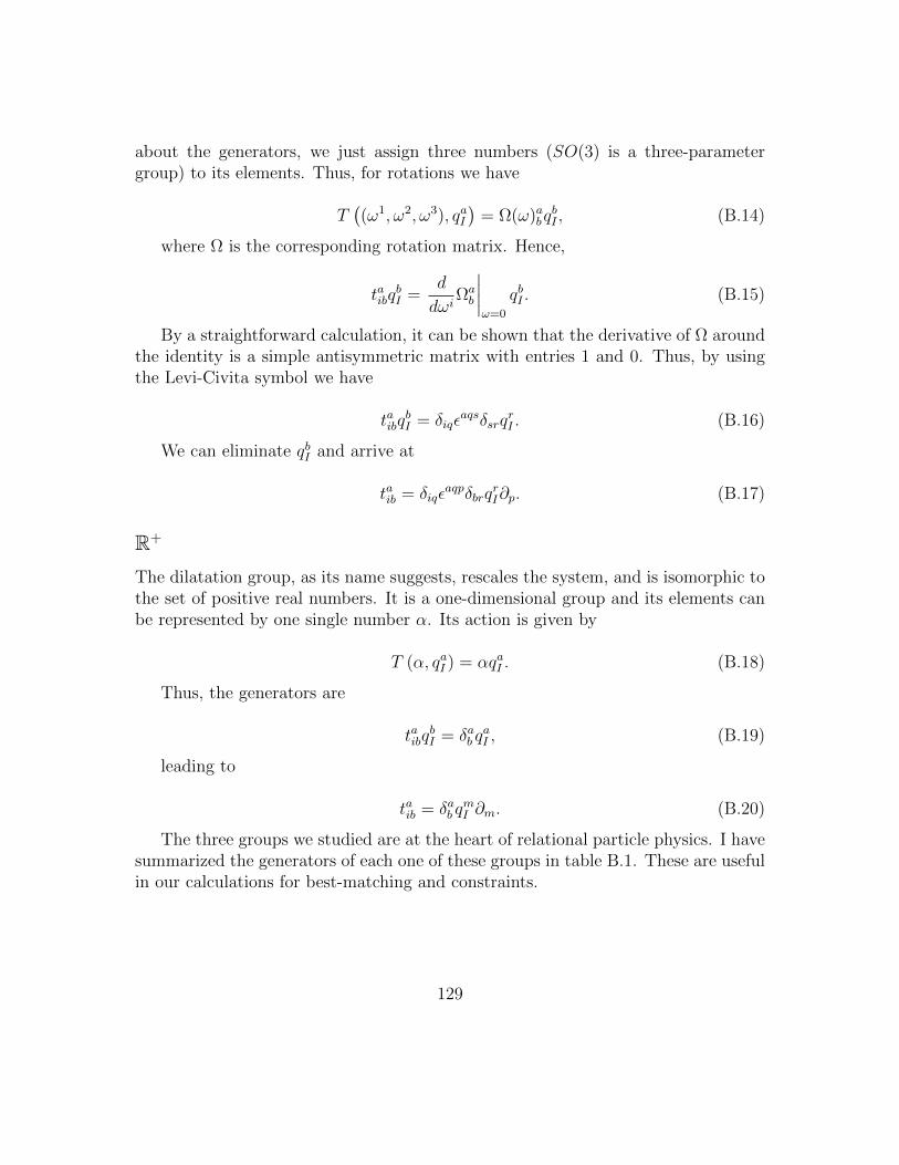
about the generators, we just assign three numbers (SO(3) is a three-parametergroup) to its elements. Thus, for rotations we have

T((ω1, ω2, ω3), qaI

)= Ω(ω)abq

bI , (B.14)

where Ω is the corresponding rotation matrix. Hence,

taibqbI =

d

dωiΩab

∣∣∣∣ω=0

qbI . (B.15)

By a straightforward calculation, it can be shown that the derivative of Ω aroundthe identity is a simple antisymmetric matrix with entries 1 and 0. Thus, by usingthe Levi-Civita symbol we have

taibqbI = δiqε

aqsδsrqrI . (B.16)

We can eliminate qbI and arrive at

taib = δiqεaqpδbrq

rI∂p. (B.17)

R+

The dilatation group, as its name suggests, rescales the system, and is isomorphic tothe set of positive real numbers. It is a one-dimensional group and its elements canbe represented by one single number α. Its action is given by

T (α, qaI ) = αqaI . (B.18)

Thus, the generators are

taibqbI = δab q

aI , (B.19)

leading to

taib = δab qmI ∂m. (B.20)

The three groups we studied are at the heart of relational particle physics. I havesummarized the generators of each one of these groups in table B.1. These are usefulin our calculations for best-matching and constraints.

129

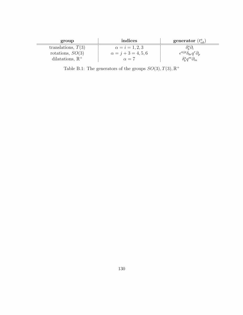
group indices generator (taαb)

translations, T (3) α = i = 1, 2, 3 δab∂irotations, SO(3) α = j + 3 = 4, 5, 6 εajpδbrq

r∂pdilatations, R+ α = 7 δab q

m∂m

Table B.1: The generators of the groups SO(3), T (3),R+

130

Appendix C

Constrained Hamiltonian Systemsand Dirac’s Approach

In his wonderful lectures on constraints and quantization of the constrained systems[44], Paul Dirac wrote

I feel that there will always be something missing from [alternative meth-ods] which we can only get by working from a Hamiltonian.

So do I... at least as far as shape dynamics and relational physics are concerned.The language of constrained systems is very important in relational physics. Thewhole point of relational physics is that we have a gauge theory in an extendedconfiguration space or phase space. As we will prove in this appendix, whenever wehave gauge theories, we have constraints. Thus, the natural language for describingthe mathematical formulation of the theory is that of the constrained systems. Inthis appendix, we give a rather brief account of the Hamiltonian constrained systems.Lagrangian systems can also be studied deeply, but for developing relational physics -even though it is also a constrained Lagrangian system - the Hamiltonian formulationis more important.1

C.1 Singular Lagrangians and primary constraints

Constrained Hamiltonian systems can be considered completely independently. How-ever, for the sake of more clarity, we start with an action in the Lagrangian form:

1This approach was first developed and explained very well by Dirac in [44]. Among majorreferences on this topic, I find [45] clear and thorough.

131

S[q] =

∫dt L(qi, qi, t), (C.1)

where qi’s belong to a N -dimensional configuration space and t is a time param-eter, not necessarily with a physical meaning at this point.

Demanding the action to be stationary along the space of all trajectories betweentwo fixed points, gives us the Euler-Lagrange equations:

d

dt

(∂L

∂qi

)− ∂L

∂qi= 0. (C.2)

The above equations can be written more explicitly by separating different ordersas

qj∂2L

∂qj∂qi+ qj

∂2L

∂qj∂qi− ∂L

∂qi= 0, (C.3)

where we have used Einstein’s summation convention. The point of Eq. (C.3)is that it directly shows the necessary and sufficient condition for writing the accel-erations qi in terms of the positions and velocities, which is the invertibility of thematrix appearing next to the accelerations, i.e.,

det

(∂2L

∂qj∂qi

)6= 0. (C.4)

If this determinant vanishes, we say the Lagrangian is singular. One case of such afailure is the existence of gauge freedom in the Lagrangian formulation. In this case,one can show that the Lagrangian is singular and the equations of motion do notdetermine the solution uniquely.2 This is actually what Noether’s second theoremshows.

Singular Lagrangians, in turn, are also relevant to the Hamiltonian formulation.The starting point is the definition of the conjugate momenta

pi ≡∂L

∂qi. (C.5)

By virtue of the implicit function theorem, we know that the relations (C.5) canbe used to solve for qi in terms of the momenta if and only if (C.4) holds. Wefirst assume that the rank of ∂2L

∂qj∂qiis constant throughout the tangent bundle of

the configuration space. The failure of this matrix to be of maximal rank, i.e., (C.4)

2See [46], Sec. 3.5 for the details.

132

fails, means that the momenta (C.5) are not all independent and must satisfy certainrelations of the form

φa(q, p) = 0, a = 1, · · · ,M. (C.6)

These constraints are solely the result of the definition (C.5) and reflect thestructure of the phase space. Using the standard terminology of constrained systemsDirac proposed, we call (C.6) primary constraints. If we assume that the rank of∂2L∂qj∂qi

is N −M , then M independent primary constraints would be found.The canonical Hamiltonian function is by definition

H = piqi − L, (C.7)

but now that we are dealing with a constrained phase space, one wonders how toconstruct the Hamiltonian as a function on phase space and write down the equationsof motion. For that, we state a theorem, the proof of which can be found in Chapter1 of [45].

Theorem C.1. If a smooth phase space function F vanishes on the surface φa = 0,then it follows that F = uaφa for some smooth functions ua(q, p). Furthermore, ifwe have λiδq

i + µiδpi = 0 for variations tangent to the constrained surface, then

λi = ua∂φa∂qi

, µi = ua∂φa∂pi

, (C.8)

for arbitrary smooth functions ua’s.

This should be intuitively clear. The second part of the theorem is especiallyused for finding Hamilton’s equations of motion. Following the definition of theHamiltonian, we vary it with respect to the parameters qi, qi independently:

δH = δpiqi + piδq

i − δqi∂qiL− δqi∂qiL= δpiq

i − δqi∂qiL.(C.9)

Because of the existence of certain constraints, the variations appearing in thesecond line are tangent to the constraint surface. Thus, along the constraint surface,we have (

∂H

∂pi− qi

)δpi +

(∂H

∂qi+ ∂qiL

)δqi = 0, (C.10)

and by using the theorem (C.1) and Euler-Lagrange equation (C.2) we have thefollowing equations of motion

133

qi =∂H

∂pi+ ua

∂φa∂pi

,

pi = −∂H∂qi− ua∂φa

∂qi,

(C.11)

for some phase space functions ua. But we will see that certain consistencyconditions may restrict them.

The above equations of motion can be derived from the phase space action

SP [q, p, u] =

∫dt (pnq

n − (H + uaφa)) . (C.12)

Following Dirac, we introduce the concept of weak equality, denoted by ≈, whichmeans that a certain function is equal to another function on the constrained surface.For example, for all constraints, we have φa ≈ 0. This is particularly useful for havinga notion of equality restricted to the constraint surface.

C.2 Consistency conditions

The constrained system is consistent if the constraints ‘propagate’ under the Hamil-tonian evolution, meaning that φa = 0. Using the above equations of motion, thiscondition is

φa = φa, H+ ua′φa, φa′ = 0. (C.13)

(C.13) can result in three scenarios: either it reduces to a relation independentof the ua

′’s involving only the q’s and p’s, or it may impose a restriction on some

of the ua′’s (or all of them), or it may actually lead to an inconsistency! The last

case is the least attractive one, but in the first case, the resultant relation - which isindependent of the primary constraints - is called a secondary constraint, because theequations of motion have been used for arriving at them. We can then continue theprocess with the secondary constraints and check the consistency conditions. Finally,if the system is consistent, this approach should come to an end and we should havea number of primary and secondary constraints

φα ≈ 0, α = 1, · · · ,M +K, (C.14)

with K secondary constraints that have been added. Once again, we assume thatthese constraints are all independent, and hence, the above set is minimal.

134

Now that we have found the complete set of constraints (C.14), we can study theimplication of their propagation for the ua’s, as

φα = φα, H+ uaφα, φa ≈ 0 (C.15)

should hold. In order to find the general form of ua’s, we define another classifi-cation of constraints Dirac proposed.

Again, we assume the rank of φα, φβ is constant along the surface constraintsto avoid certain mathematical problems. We call a constraint first-class if its Poissonbracket with every other constraint vanishes weakly, and second-class if it does not.We denote the first-class constraints by

γα ≈ 0, α = 1, · · · , f (C.16)

and second-class constraints by

χβ ≈ 0, β = 1, · · · , g. (C.17)

It is clear that f + g = M + K. One can define a first-class function in general,meaning a function whose Poisson bracket with any other constraint vanishes weakly.We have defined two classifications. But we will see that the first-class versus second-class distinction is more meaningful and fundamental in the Hamiltonian formulationthan the primary versus secondary one.

For solving (C.15) in light of this analysis, we see that the coefficients of thefirst-class primary constraints in the Hamiltonian remain unrestricted and arbitrary,and those corresponding to the second-class primary constraints would be solved interms of q’s and p’s. Therefore, we arrive at the total first-class Hamiltonian

HT = Hc + ub0χb + vaγa, (C.18)

where Hc is the original canonical Hamiltonian, ub0(q, p) is the solution of (C.15),va’s are abitrary, and the indices a and b represent the primary constraints here, asopposed to α and β. Therefore, we have the final form of the equations of motionfor an arbitrary phase space function:

F (q, p) ≈ F,HT. (C.19)

There is something interesting about the first-class primary constraints in thetotal Hamiltonian. Their coefficients are arbitrary, meaning that for any given initialcondition on the constraint surface, we can vary va smoothly and generate a family ofsolutions. This ‘local freedom’, in turn, signals the concept of gauge transformation.

135

C.3 First-class constraints as gauge generators

To clarify the role of the first-class primary constraints as gauge generators, weassume that the time parameter with respect to which we wrote (C.19) represents aphysically measurable quantity, like time measured by a specific clock.

Hence, if we start with a given initial point s on phase space satisfying φα = 0,evolve that for an infinitesimal amount of time from t to t+ δt, and change va to va,the change of the evolved point becomes

δs = δt(va − va)s, γa ≡ δvas, γa. (C.20)

Hence, if the time parameter is physical (observable), and according to our expec-tation that the equations of motion should completely determine the evolution of thephysical (observable) points, we deduce that the first-class primary constraints gener-ate gauge transformations of the form (C.20). It can be also proved that the Poissonbracket between the first-class primary constraints and those between one first-classprimary constraint and the total Hamiltonian also generate gauge transformations(see [45]).

Although the above argument works essentially for first-class primary constraints,it is reasonable to say that all first-class constraints generate gauge transformations.This was conjectured by Dirac. Although some counterexamples can be proposed,in our physical applications it remains completely valid and consistent to includeall the other first-class constraints in the Hamiltonian. This is exactly what hap-pens in ADM formalism and shape dynamics. Hence, we may define the extendedHamiltonian:

HE = Hc + ub0χb + vαγα, (C.21)

where γα represents all the first-class constraints. Now that we have gauge free-dom, we may conceive of ‘gauge fixation’. It is physically desirable to fix the freedomof the theory and establish a one-to-one correspondence between the physical statesand the phase space variables. The gauge freedom can be fixed by imposing a numberof constraints on the phase space which are second-class with the original first-classprimary constraints, i.e.,

Gc(q, p) ≈ 0, Gc, γa 6≈ 0. (C.22)

If one wants to fix the gauge freedom completely, one in principle needs f inde-pendent gauge conditions in the above form. Imposing more constraints restricts thephysical part of the phase space, and is not admissible. Fig. C.1 clearly illustrates

136

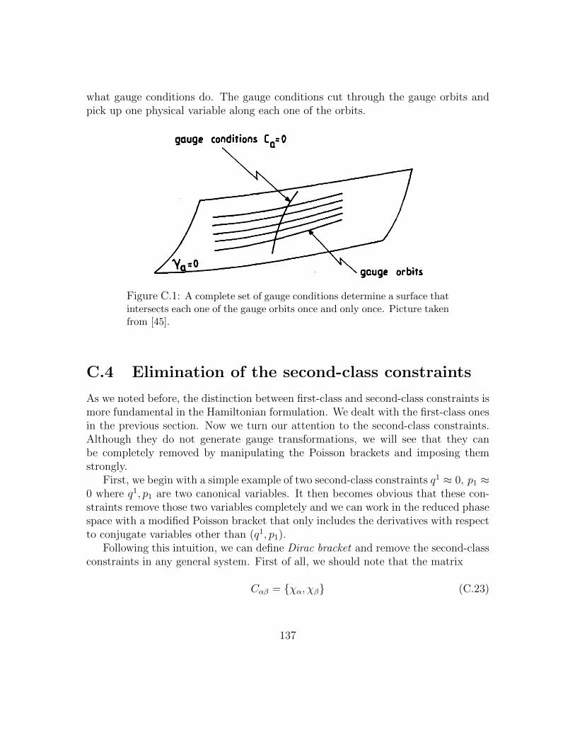
what gauge conditions do. The gauge conditions cut through the gauge orbits andpick up one physical variable along each one of the orbits.

Figure C.1: A complete set of gauge conditions determine a surface thatintersects each one of the gauge orbits once and only once. Picture takenfrom [45].

C.4 Elimination of the second-class constraints

As we noted before, the distinction between first-class and second-class constraints ismore fundamental in the Hamiltonian formulation. We dealt with the first-class onesin the previous section. Now we turn our attention to the second-class constraints.Although they do not generate gauge transformations, we will see that they canbe completely removed by manipulating the Poisson brackets and imposing themstrongly.

First, we begin with a simple example of two second-class constraints q1 ≈ 0, p1 ≈0 where q1, p1 are two canonical variables. It then becomes obvious that these con-straints remove those two variables completely and we can work in the reduced phasespace with a modified Poisson bracket that only includes the derivatives with respectto conjugate variables other than (q1, p1).

Following this intuition, we can define Dirac bracket and remove the second-classconstraints in any general system. First of all, we should note that the matrix

Cαβ = χα, χβ (C.23)

137

is of maximal rank, and hence, invertible. Otherwise, in case that there existswα such that wαCαβ ≈ 0, we can identify the constraint wαCα as another first-classconstraint which is incompatible with our basic postulate that we classified all theconstraints. From Cαβ being invertible and asymmetric, it then follows that thenumber of the second-class constraints must be even.3

Finally, we define the Dirac bracket as

·, ··DB ≡ ·, ·· − ·, χαC−1αβ χβ, ··. (C.24)

It is easy to show that

1. The Dirac bracket of any function with a first-class function, in particular, thetotal Hamiltonian, is weakly equal to the result of the Poisson bracket,

F,HTDB ≈ F,HT. (C.25)

2. The Dirac bracket of any second-class constraint with any other function van-ishes weakly,

χα, · ≈ 0. (C.26)

So, in light of the second property, we see that in evaluating the Dirac bracketwe can set the second-class constraints equal to zero even before calculating thebracket. Furthermore, because of the first property, we can determine the evolutionof the system with respect to the Dirac bracket. Hence, we deduce

F ≈ F,HT ≈ F,HTDB ≈ F , HTDB, (C.27)

where F and HT are F |χα=0 and HT |χα=0 respectively.In this way, we can eliminate all the second-class constraints by modifying the

Poisson bracket. This has a far-reaching conclusion, especially for shape dynamicsand non-equivariant best-matching.

We should make one final remark before ending this section. Let us count thenumber of degrees of freedom that are left. We started with a 2N -dimensional phasespace and found f first-class constraints and g second-class constraints. We notedthat g = 2k. Moreover, each first-class constraint removes 2 degrees of freedom, oneof which is because of the constraint itself, the other one because of gauge fixation

3The proof follows from the consideration that detC = detCT = −detC if C is of odd dimen-sion, implying detC = 0.

138

corresponding to that.4 Hence, we are left with 2N−2f−2k = 2(N−f−k) degreesof freedom, i.e., N − f − k pairs of conjugate variables.

There is a caveat, however, regarding the constrained field theories. In thatcontext, we should talk about the number of degrees of freedom ‘per point’, as thephase space is infinite-dimensional in such theories.

C.5 Reparametrization invariant theories

One particular example of a constrained system is reparametrization invariant sys-tems. There are basically two forms of such systems. One is those systems that areinitially formulated with respect to a time parameter, and then the time is takento be a dynamical variable. This was our approach in Appx. A. However, thereare also reparametrization invariant dynamical theories that are written on a well-defined configuration space that does not include any separate time parameter likethe latter case. Here, we focus on general reparametrization invariant theories. AnyLagrangian theory of this sort can be subject to our analysis here.

We start with a phase space action,

SP =

∫dλ (pnq

n −H) . (C.28)

Assuming that the phase space variables are scalar functions of λ, we see thatthe first term in the action respects the reparametrization invariance. If the actionis to have this symmetry, we see that the Hamiltonian must vanish. If the Hamil-tonian vanishes as a primary constraint and not identically, based on our previousanalysis, the total Hamiltonian would be something like H ≡ NH0, with the arbi-trary function N . Thus, by demanding that N transforms as a scalar density underreparametrization, i.e.,

N ′(λ′) = N(λ)dλ

dλ′(C.29)

the resultant phase space action would be reparametrization invariant.Hence, we see that there is a strong connection between reparametrization invari-

ance and the vanishing of the Hamiltonian as a constraint. In fact, this is the resultwe got to in (A.6) for a system with a dynamical time.

Therefore, we can generally write reparametrization invariant Hamiltonian sys-tems as

4There is this famous saying “the gauge always hits twice” attributed to Teitelboim.

139

HT = NH + vaγa, (C.30)

with arbitrary scalar densities N and va, and the first-class constraints H and γa.This opens up an important conceptual issue: What is the status of the Hamil-

tonian as a first-class constraint in reparametrization invariant theories in light ofour observation that first-class constraints generate gauge transformations? Therehas been quite a lot of debate over this issue in the literature. Some talk about theabsence of true dynamics in such theories and that “evolution is nothing but theunfolding of a gauge transformation”.

But there is a clearer approach to understanding the meaning of the Hamilto-nian constraint proposed by Barbour and Foster [14]. The starting point in thisapproach is to note that the interpretation of first-class constraints as generatorsof gauge transformation rested on the presumption that the time parameter itselfis physical. This is obviously not the case in reparametrization invariant theories!Hence, it is reasonable to modify our original interpretation than try to apply it toa case with completely different underlying presumptions. We say that the Hamil-tonian constraint generates ‘true’ motion, but with a non-physical parameter. Thegauge aspect of such theories is that we can change the N , resulting in a differentparametrization of the solution curves.

In other words, the change in the parameter is the gauge transformation theHamiltonian generates, not the change in the configuration space variables. Inreparametrization invariant theories, the Hamiltonian generates true dynamics withrespect to an arbitrary parameter in parallel.

140

Appendix D

ADM Formalism

One of the most influential works on classical general relativity is the Hamiltonianformulation of Einstein’s general relativity, known as the ADM formalism, developedin 1960s.1 ADM formalism has the merit of describing the core dynamics underlyingthe theory of general relativity and melts the frozen spacetime picture of the theory,provides an initial-value formulation of the theory suitable for numerical calculations,brings many insights into quantum gravity, and builds a framework to meaningfullydefine energy and radiation.

It also plays a profound role in developing shape dynamics, as shape dynamicsis an alternative dual theory with a different constraint algebra and its connectionwith the Hamiltonian formulation of the standard general relativity makes the innerworking of the theory remarkably clear. We give a rather brief account of thisformalism and derive the key results, starting with the standard Einstein-Hilbertaction and using the Gauss-Codazzi equations.

D.1 Breaking up the 4-dimensional spacetime

We assume that spacetime M equipped with the Lorentzian metric g(4)µν is globally

hyperbolic, hence, foliable to spacelike hypersurfaces with a common topology, andthat there exists a time parameter t that labels the ‘leaves’ Σt.

2 Thus, M = ∪tΣt 'Σ× R, where Σ denotes the topology of the hypersurfaces.

1See the 1962 review of the work by its founders, republished in [47]. Chapter 4 of [46] andSection 21 of [48] are also very thorough.

2See theorem 8.3.14 in [49]. The requirement of global hyperbolicity is very important andthe Hamiltonian formulation works if and only if the spacetime associated with the solution of theequations is globally hyperbolic.

141

Now we consider a coordinate system that includes the parameter t as the timecoordinate. For the sake of simplicity, we assume that each one of the Σt’s canbe covered with a single coordinate system (x1, x2, x4). Therefore, the (x1, x2, x4, t)constitutes a well-behaved coordinate system on the entire M .

For our analysis, we consider a general coordinate system yα(t, xa). Then, thevector field ∂αt ≡

∂yα

∂tgives us the flow of time, and the vectors Eα

a ≡∂yα

∂xa

∣∣t

representthree tangent vectors belonging to T (Σt). Moreover, The existence of foliation en-sures that there is a globally well-defined unit timelike normal vector n for each Σt.Hence, in our arbitrary coordinate system we can decompose the ‘time vector field’∂t as

∂µt = Nnµ +Nµ, (D.1)

where Nµ is a vector field orthogonal to nµ, i.e., g(4)µν nµN ν = 0. Note that Nµ is

tangent to the leaves and can be written as Nµ = EµaN

a for the vector fields Na inthe tangent bundle of the Σt’s. N(xi, t) is called the lapse function and Na(xi, t) theshift vector. Their geometrical meaning will signify these names.

In the suitable coordinate system (x1, x2, x4, t) we constructed, we can use theabove relations and decompose the 4D Lorentzian metric:

ds2 ≡ g(4)µν dy

µdyν

= g(4)µν (Nnµdt+ Eµ

aNadt+ Eµ

adxa)(Nnνdt+ Eν

aNadt+ Eν

adxa)

= −(N2 − gabNaN b)dt2 + 2gabNadtdxb + gabdx

adxb,

(D.2)

where gab denotes the induced 3D Riemannian metric on Σ. (D.2) is called theADM decomposition of the metric and is the departure point for deriving the ADMaction and then pursuing the Hamiltonian formulation.

Thus, The components of the metric and its inverse in the coordinate system(xa, t) are

g(4)00 = −N2 + gabN

aN b, g(4)0a = gabN

b, g(4)ab = gab,

g(4)00 = − 1

N2, g(4)a0 =

Na

N2, g(4)ab = gab − NaN b

N2.

(D.3)

Another relation that becomes useful in the next section is

g(4) ≡ det g(4)µν = Ng, (D.4)

where g is the determinant of the induced Riemannian metric.

142

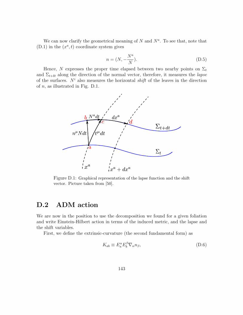
We can now clarify the geometrical meaning of N and Na. To see that, note that(D.1) in the (xa, t) coordinate system gives

n = (N,−Na

N). (D.5)

Hence, N expresses the proper time elapsed between two nearby points on Σt

and Σt+δt along the direction of the normal vector, therefore, it measures the lapseof the surfaces. N i also measures the horizontal shift of the leaves in the directionof n, as illustrated in Fig. D.1.

Figure D.1: Graphical representation of the lapse function and the shiftvector. Picture taken from [50].

D.2 ADM action

We are now in the position to use the decomposition we found for a given foliationand write Einstein-Hilbert action in terms of the induced metric, and the lapse andthe shift variables.

First, we define the extrinsic-curvature (the second fundamental form) as

Kab ≡ EαaE

βb∇αnβ, (D.6)

143

where ∇α denotes the covariant derivative with respect to the metric g(4)µν . Using

the ADM decomposition, it can be shown that Kab is related to the time derivativeof the induced metric:

Kab =1

2N(gab − LNgab) . (D.7)

LN denotes the Lie derivative with respect to the shift vector.Using the Gauss-Codazzi equations, we can write the 4D Ricci scalar R(4)[g

(4)µν ] in

terms of the 3D intrinsic scalar curvature R[gab] and the extrinsic curvature:

R(4) = R +KabKab −K2 + 2∇α

(nβ∇βn

α − nα∇βnβ). (D.8)

We ignore the last term in the action which is a total derivative.3

Thus, in light of (D.4) and (D.8), one can write the Einstein-Hilbert action

SEH [g(4)µν ] =

∫d4y R(4) (D.9)

purely in terms of the spatial structures gab and Kab, referred to as the ADMaction:

SADM [gab, N,Na] =

∫dtd3xLADM =

∫dtd3x

√gN(R +KabKab −K2

), (D.10)

where we have introduced the ADM Lagrangian density. This action includesfirst-order time derivatives of the metric (expressed through Kab) and its spatialderivatives. The Ricci scalar plays the role of the ‘potential term’ and KabKab −K2

the ‘kinetic term’. We will see that more clearly when we introduce the BSW actionat the end of this appendix. The kinetic term can be written as

KabKab −K2 = GabcdKabKcd, (D.11)

where Gabcd is called the DeWitt supermetric and is

Gabcd =1

2

(gacgbd + gadgbc

)− gabgcd. (D.12)

3We assume that the space is topologically closed, i.e., compact and without boundary, to avoidcertain mathematical complications. This assumption is justifiable in shape dynamics. Moreover,the temporal boundary terms can also be ignored when performing fixed-end-point variation.

144

DeWitt supermetric plays the role of a metric in the space of spatial metrics.Formally, for metric deformations δgab at a specific spatial metric, we can define thefollowing ‘inner product’:

〈δ1g, δ2g〉 ≡∫d3x√gGabcdδ1gabδ2gcd. (D.13)

The space of metrics is very important in shape dynamics, as the configurationspace is the pivotal structure in the theory.

As that the extrinsic curvature is related to the time derivative of the metric(D.7). Hence, the ADM action is the suitable action for performing the Legendretransformation and writing general relativity in the Hamiltonian formulation.

D.3 The Hamiltonian of GR

From (D.10), the momenta conjugate to gab are

pab =δLADMδgab

=√gGabcdKcd =

√g(Kab −Kgab

). (D.14)

We see that pab is a tensor-density of weight 1, i.e., pab√g

is a tensor.

Moreover, we define the momenta conjugate to N and Na which result in fourprimary constraints:

pN =δLADMδN

≈ 0, pNa =δLADMδNa

≈ 0. (D.15)

It should not be a surprise. After all, the lapse function and the shift vectorappear in the ADM action as some Lagrange multipliers.

We can proceed to work out the canonical Hamiltonian. The Hamiltonian densityis

HADM = pabgab − LADM . (D.16)

We can use (D.7) and (D.14) to fine gab in terms of the conjugate momenta:

gab = 2NKab + 2∇(aNb) =2N√gGabcdp

cd + 2∇(aNb), (D.17)

where Gabcd is the inverse of the DeWitt supermetric, i.e.,

145

Gabcd =1

2(gacgbd + gadgbc − gabgcd) , GabcdGcdef =

1

2

(δ(ae δ

b)f

). (D.18)

Thus, the Hamiltonian density is

HADM =N√gGabcdp

abpcd −√gNR + 2pab∇aNb. (D.19)

The Hamiltonian density is a density of weight 1. Thus, when integrated all overthe space, the Hamiltonian would be a scalar. We have

HADM [g, p,N,Na] ≡∫d3xHADM =

∫d3x

(N(x)H[gab, p

ab, x) +Na(x)Ha[gab, pab, x)

)≡ N •H +Na •H

a,(D.20)

where

H =1√gGabcdp

abpcd −√gR (D.21)

is called the Hamiltonian constraint and

Ha = −2∇bpab (D.22)

is the momentum (or diffeomorphism) constraint (these names will be clarified shorlty). Note that we have omitted the total derivative 2∇a

(pabNb

)in the integral. More-

over, based on convention, ∇apab actually means

√g∇a

pab√g, as follows from a general

convention for writing the covariant derivative of densities more succinctly. Thebullets in the last line denote smearing.

The Hamiltonian is a functional of the metric and its conjugate momenta, thelapse function, and the shift vector. These variables along with pN and pNa constitutethe phase space. We have also the following non-zero Poisson brackets:

gab(x), pcd(y) =(δ(ca δ

d)b

)δ3(x− y)

N(x), pN(y) = δ3(x− y)

Na(x), pNb(y) = δab δ3(x− y).

(D.23)

We have calculated the canonical Hamiltonian. But general relativity is a con-strained system and Dirac’s approach is applicable here. We have the primary con-straints (D.15). Hence, we have the total Hamiltonian

146

HT = N •H +Na •Ha + ξ • pN + ξa • pNa . (D.24)

The consistency conditions for the propagation of pN and pNa give the secondaryconstraints

pN(x), HT = H(x) ≈ 0, pNa(x), HT = Ha(x) ≈ 0. (D.25)

Hence, the ADM Hamiltonian is a linear combination of 4 constraints. In fact,it can be shown that H = G00 and Ha = G0a where G is the Einstein tensor writtenin the (xa, t) coordinates. This makes sense, as we know that Einstein’s equationsare not all dynamical and 4 of them represent certain constraints. This is what theabove constraints show for pure geometry, i.e., vacuum solutions.

Before moving to the interpretation of these cosntraints, we note that all theseconstraints are first-class.One can show that the Hamiltonian and the momentumconstraints satisfy the following relations, known as surface deformation algebra:

N1 •H,N2 •H = (N1∇aN2 −N2∇aN1) •Ha

Ma •Ha, N •H = (LMN) •H

Na •Ha,Mb •H

b = (LNM) •Ha.

(D.26)

As all of these constraints are first-class, and pN and pNa generate ‘gauge’ trans-formations’ N → N + ξ, Na → Na + ξa. Hence, the lapse function and the shiftvector are arbitrary. Therefore, without loss of generality, we can effectively workwith the ADM Hamiltonian instead and take N and Na to be some arbitrary coeffi-cients, i.e., remove (N, pN) and (Na, pNa) from the phase space. Hence, we have theHamiltonian

HT [gab, pab] = N •H +Na •H

a. (D.27)

and the constraints

H ≈ 0, Ha ≈ 0. (D.28)

This completes the analysis of ADM formalism.The physical interpretation of the constraints and the surface deformation algebra

is remarkable. As these constraints are first-class, they generate gauge transforma-tions. But what do they generate?

Ha generates 3D spatial diffeomorphisms. We can see that by directly calculatingthe transformation

147

δgab(x) ≡ gab(x), δva •Ha = 2∇(aδvb)(x) = Lδvgab(x), (D.29)

which is indeed the transformation of the metric under a diffeomorphism corre-sponding to the vector field δva.

The interpretation of the Hamiltonian constraint is a bit more nuanced. First,it clearly shows that GR is a reparametrization invariant theory. In light of ourdiscussion in Sec. C.5, it generates true evolution in the phase space, but alsogenerates gauge transformation corresponding to the arbitrary parameterization ofthe dynamics. Geometrically, we saw that N represents the embedding of the spatialleaves along the direction of time. Changing N changes the temporal alignment ofthe leaves ‘locally’, that is, it changes the foliation. Time in general relativity is alocal entity. It is commonly known as ‘many-fingered time’.

In reparametrization invariant particle mechanics, we saw that the Hamilto-nian constraint with an arbitrary coefficient generates evolution with an arbitraryparametrization. Fixing the lapse function in those models amounted to defining a‘duration’. But in ADM formalism, time is local and we have to fix a local lapsefunction. Its local nature means that we can define a ‘local duration’: Each point inthe spatial manifold evolves at its own arbitrary speed.

Hence, N(x) represents the foliation of the spacetime and signifies the local du-ration of the evolution of 3D metrics in a spatial manifold.

Another important point is that the Hamiltonian constraint does not generate anypoint transformation in the space of metrics (Riem3), as it mixes the metric and themomenta. But it does map certain curves in the Riem3 to other curves. Each curvein the configuration space represents a spacetime. What the Hamiltonian constraintdoes is change the foliation of the spacetime and map that curve to another validsolution.

Finally, H and Ha together generate 4D diffeomorphisms. Although this is notvery clear in ADM formalism, as we have broken the spacetime structure, one canobserve that by writing the ADM action (D.10) as the phase space action

SP [gab, pab, N,Na] =

∫dtd3x

(pabgab −

(N(x)H[gab, p

ab, x) +Na(x)Ha[gab, pab, x)

)).

(D.30)By extremizing this action with respect to pab and putting the solution back in

the action, SP would be identical to SADM . Therefore, we see that the gauge groupof the two actions must be equivalent, i.e., for every gauge transformation of anycurve gab(t), N(t), Na(t), there exists a corresponding gauge transformation of thecurve in phase space. Noting that the gauge group of SADM is that of SEH , the

148

4D diffeomorphisms, We then see that H,Ha are indeed the generators of the 4Ddiffeomorphisms in phase space.

D.4 BSW action

BSW action, carrying the three names Baierlein, Sharp, and Wheeler, is Jacobi’saction for GR, found in 1962 [51]. It manifests the local reparametrization invarianceof the theory more clearly. We can simply derive it from the decomposed Einstein-Hilbert action, SADM . First, note that (D.10) can be written as

SADM [gab, N,Na] =

∫dtd3x

√g

(1

4NT +NR

), (D.31)

where T is the kinetic term

T = Gabcd (gab − 2∇aNb) (gcd − 2∇cNd) . (D.32)

Extremizing (D.31) with respect to the lapse function N gives

N =1

2

√T

R. (D.33)

Substituting this expression in the action, eliminates the lapse function and givesthe BSW action:

SBSW [gab, Na] =

∫dtd3x

√gRT . (D.34)

This formally elegant and simple action is Jacobi’s action for GR, and gives thesame equations of motion as SEH action, provided that the original spacetime isglobally hyperbolic. −R plays the role of the potential here.

BSW action is manifestly reparametrization invariant. If we use that as thedeparture point for the Hamiltonian formulation, instead of the ADM action, wearrive at the canonical Hamiltonian Na •H

a and the primary constraints

H ≈ 0, pNa =δLADMδNa

≈ 0. (D.35)

As compared to the standard ADM formalism, we see that the Hamiltonianconstraint appears as a primary constraint here, but the diffeomorphism constraintis still secondary. On the whole, one can perform the Legendre transformation andarrive at the total Hamiltonian (D.27). BSW action does not change that.

149

Bibliography

[1] G. W. Leibniz, Monadology, 1714. [Online]. Available: https://www.earlymoderntexts.com/assets/pdfs/leibniz1714b.pdf.

[2] F. Mercati, Shape dynamics: Relativity and relationalism, First edition. Ox-ford, United Kingdom: Oxford University Press, 2018, isbn: 978-0198789475.[Online]. Available: https://arxiv.org/abs/1409.0105.

[3] G. W. Leibniz and S. Clarke, Leibniz’s exchange of papers with clarke, 1715-6.[Online]. Available: https://www.earlymoderntexts.com/assets/pdfs/leibniz1715.pdf.

[4] C. Rovelli, “Why gauge?” Foundations of Physics, vol. 44, no. 1, pp. 91–104,2014, issn: 1572-9516. doi: 10.1007/s10701-013-9768-7. [Online]. Available:https://arxiv.org/abs/1308.5599.

[5] A. Einstein, The Collected Papers of Albert Einstein, Volume 6: The BerlinYears: Writings, 1914-1917 (Collected Papers of Albert Einstein, 7), trans. byA. Engel. Princeton University Press. [Online]. Available: https://einsteinpapers.press.princeton.edu/vol6-trans/.

[6] ——, The Collected Papers of Albert Einstein, Volume 7: The Berlin Years:Writings, 1918-1921 (Collected Papers of Albert Einstein, 11), trans. by A. En-gel. Princeton University Press. [Online]. Available: https://einsteinpapers.press.princeton.edu/vol7-trans/.

[7] J. Barbour, “The definition of mach’s principle,” Foundations of Physics, vol. 40,no. 9, pp. 1263–1284, 2010, issn: 1572-9516. doi: 10.1007/s10701-010-9490-7. [Online]. Available: https://arxiv.org/abs/1007.3368.

[8] J. Barbour and B. Bertotti, “Mach’s principle and the structure of dynamicaltheories,” Proceedings of the Royal Society of London. A. Mathematical andPhysical Sciences, vol. 382, no. 1783, pp. 295–306, 1982, issn: 0080-4630. doi:10.1098/rspa.1982.0102. [Online]. Available: http://www.platonia.com/barbour_bertotti_prs1982_scan.pdf.

150

[9] J. Barbour, B. Z. Foster, and N. O Murchadha, “Relativity without relativity,”Classical and Quantum Gravity, vol. 19, no. 12, pp. 3217–3248, 2002, issn:02649381. doi: 10.1088/0264-9381/19/12/308. [Online]. Available: https://arxiv.org/abs/gr-qc/0012089.

[10] L. Smolin, The trouble with physics: The rise of string theory, the fall of ascience, and what comes next / Lee Smolin. Boston: Houghton Mifflin, 2007,2006, isbn: 978-0618918683.

[11] S. Gryb, “Shape dynamics and mach’s principles: Gravity from conformal ge-ometrodynamics,” [Online]. Available: http://arxiv.org/pdf/1204.0683v1.

[12] M. Nakahara, Geometry, topology, and physics, 2nd ed., ser. Graduate stu-dent series in physics. Bristol: Institute of Physics Publishing, 2003, isbn:9780750306065.

[13] J. Barbour, “Scale-invariant gravity: Particle dynamics,” Classical and Quan-tum Gravity, vol. 20, no. 8, pp. 1543–1570, 2003, issn: 02649381. doi: 10.1088/0264-9381/20/8/310. [Online]. Available: arxiv.org/abs/gr-qc/0211021.

[14] J. Barbour and B. Z. Foster, “Constraints and gauge transformations: Dirac’stheorem is not always valid,” [Online]. Available: http://arxiv.org/pdf/0808.1223v1.

[15] E. Anderson, J. Barbour, B. Z. Foster, B. Kelleher, and N. O Murchadha, “Thephysical gravitational degrees of freedom,” Classical and Quantum Gravity,vol. 22, no. 9, pp. 1795–1802, 2005, issn: 02649381. doi: 10.1088/0264-9381/22/9/020. [Online]. Available: https://arxiv.org/abs/gr-qc/0407104.

[16] H. Gomes, S. Gryb, and T. Koslowski, “Einstein gravity as a 3d conformallyinvariant theory,” Classical and Quantum Gravity, vol. 28, no. 4, p. 045 005,2011, issn: 02649381. doi: 10.1088/0264- 9381/28/4/045005. [Online].Available: https://arxiv.org/abs/1010.2481.

[17] H. Gomes and T. Koslowski, “The link between general relativity and shapedynamics,” Classical and Quantum Gravity, vol. 29, no. 7, p. 075 009, 2012,issn: 02649381. doi: 10.1088/0264-9381/29/7/075009. [Online]. Available:https://arxiv.org/abs/1101.5974.

[18] H. Minkowski, “Space and time,” he Principle of Relativity: a Collection ofOriginal Memoirs on the Special and General Theory of Relativity, pp. 73–91,1923.

151

[19] J. B. Barbour and H. E. Pfister, Mach’s principle: From Newton’s bucket toquantum gravity : Conference : Revised papers and discussions, ser. Einsteinstudies. Boston: Birkhauser, 1995, vol. v. 6, isbn: 978-0817638238.

[20] C. Hoefer, “Einstein’s formulations of mach’s principle,” Mach’s principle:From Newton’s bucket to quantum gravity, vol. 6, pp. 67–87, 1995.

[21] A. Einstein, “On the foundations of the general theory of relavitiy,” 1918.[Online]. Available: https://einsteinpapers.press.princeton.edu/vol7-trans/49.

[22] J. Barbour, “General relativity as a perfectly machian theory,” Mach’s princi-ple: From Newton’s bucket to quantum gravity, vol. 6, pp. 214–231, 1995.

[23] J. Barbour and N. O Murchadha, “Classical and quantum gravity on conformalsuperspace,” 1999. [Online]. Available: https://arxiv.org/abs/gr- qc/

9911071.

[24] N. O’Murchadha and J. W. York, “Existence and uniqueness of solutions of thehamiltonian constraint of general relativity on compact manifolds,” Journal ofMathematical Physics, vol. 14, no. 11, pp. 1551–1557, 1973, issn: 0022-2488.doi: 10.1063/1.1666225.

[25] J. Barbour and N. O Murchadha, “Conformal superspace: The configurationspace of general relativity,” 2010. [Online]. Available: http://arxiv.org/pdf/1009.3559v1.

[26] H. Gomes and T. Koslowski, “Coupling shape dynamics to matter gives space-time,” General Relativity and Gravitation, vol. 44, no. 6, pp. 1539–1553, 2012,issn: 0001-7701. doi: 10.1007/s10714- 012- 1355- 2. [Online]. Available:https://arxiv.org/abs/1110.3837.

[27] ——, “Frequently asked questions about shape dynamics,” Foundations ofPhysics, vol. 43, no. 12, pp. 1428–1458, 2013, issn: 1572-9516. doi: 10.1007/s10701-013-9754-0. [Online]. Available: https://arxiv.org/abs/1211.5878.

[28] J. Barbour, T. Koslowski, and F. Mercati, “A gravitational origin of the arrowsof time,” 2013. [Online]. Available: https://arxiv.org/abs/1310.5167.

[29] N. O Murchadha, “Readings of the lichnerowicz-york equation,” 2005. [Online].Available: https://arxiv.org/abs/gr-qc/0502055.

[30] R. M. Unger and L. Smolin, The Singular Universe and the Reality of Time:A Proposal in Natural Philosophy. Untied Kingdom and New York: CambridgeUniversity Press, 2015, isbn: 978-1107074064.

152

[31] J. Barbour, T. Koslowski, and F. Mercati, “The solution to the problem of timein shape dynamics,” Classical and Quantum Gravity, vol. 31, no. 15, p. 155 001,2014, issn: 02649381. doi: 10.1088/0264- 9381/31/15/155001. [Online].Available: arxiv.org/abs/1302.6264.

[32] T. A. Koslowski, F. Mercati, and D. Sloan, “Through the big bang: Continu-ing einstein’s equations beyond a cosmological singularity,” Physics Letters B,vol. 778, pp. 339–343, 2018, issn: 03702693. doi: 10.1016/j.physletb.2018.01.055. [Online]. Available: https://arxiv.org/abs/1607.02460.

[33] J. Barbour, The Janus point: A new theory of time, First edition. New York:Basic Books, 2020, isbn: 978-0465095469.

[34] R. Montgomery, “Infinitely many syzygies,” Archive for Rational Mechanicsand Analysis, vol. 164, no. 4, pp. 311–340, 2002, issn: 0003-9527. doi: 10.1007/S00205-002-0211-Z.

[35] P. A. Schilpp, Albert Einstein: Philosopher-Scientist, 3rd ed., ser. Library of liv-ing philosophers. S.l.: Open Court, 1969-1970, vol. v. 7, isbn: 979-0875482865.

[36] C. Marchal and D. G. Saari, “On the final evolution of the n-body prob-lem,” Journal of Differential Equations, vol. 20, no. 1, pp. 150–186, 1976, issn:00220396. doi: 10.1016/0022-0396(76)90101-7.

[37] J. Barbour, T. Koslowski, and F. Mercati, “Identification of a gravitationalarrow of time,” Physical review letters, vol. 113, no. 18, p. 181 101, 2014. doi:10.1103/PhysRevLett.113.181101. [Online]. Available: https://arxiv.org/abs/1409.0917.

[38] J. Barbour, “Arrows of time in unconfined systems,” 2016. [Online]. Available:https://arxiv.org/abs/1602.08019.

[39] C. Callender, “Thermodynamic asymmetry in time,” in The Stanford Ency-clopedia of Philosophy, E. N. Zalta, Ed., Summer 2021, Metaphysics ResearchLab, Stanford University, 2021. [Online]. Available: \urlhttps://plato.

stanford.edu/archives/sum2021/entries/time-thermo/.

[40] G. W. Leibniz, The ultimate origin of things, 1697. [Online]. Available: https://www.earlymoderntexts.com/assets/pdfs/leibniz1697b.pdf.

[41] C. Lanczos, The variational principles of mechanics, 4th ed. New York: Dover,1986, isbn: 978-0486650678.

[42] S. Hassani, Mathematical physics: A modern introduction to its foundations,2nd edition. New York: Springer, 2013, isbn: 3319011944.

153

[43] H. Georgi, Lie algebras in particle physics, 2nd ed., ser. Frontiers in physics.Reading, Mass.: Perseus Books, 1999, vol. v.54, isbn: 0738202339.

[44] P. A. M. Dirac, Lectures on quantum mechanics. New York: Dover Publications,Yeshivea University, 1964.

[45] M. Henneaux and C. Teitelboim, Quantization of gauge systems. Princeton,N.J.: Princeton University Press, 1992, isbn: 0691037698.

[46] C. Kiefer, Quantum gravity, 3rd ed., ser. International series of monographs onphysics. Oxford: Oxford University Press, 2012, vol. 155, isbn: 0199585202.

[47] R. Arnowitt, S. Deser, and C. W. Misner, “Republication of: The dynamics ofgeneral relativity,” General Relativity and Gravitation, vol. 40, no. 9, pp. 1997–2027, 2008, issn: 0001-7701. doi: 10.1007/s10714-008-0661-1. [Online].Available: https://arxiv.org/abs/gr-qc/0405109.

[48] M. Blau, Lecture notes on general relativity. [Online]. Available: http://www.blau.itp.unibe.ch/GRLecturenotes.html.

[49] R. M. Wald, General relativity. Chicago and London: University of ChicagoPress, 1984, isbn: 0226870332.

[50] A. Barrau, T. Cailleteau, J. Grain, and J. Mielczarek, “Observational issuesin loop quantum cosmology,” Classical and Quantum Gravity, vol. 31, no. 5,p. 053 001, 2014, issn: 02649381. doi: 10.1088/0264-9381/31/5/053001.[Online]. Available: arxiv.org/abs/1309.6896.

[51] R. F. Baierlein, D. H. Sharp, and J. A. Wheeler, “Three-dimensional geometryas carrier of information about time,” Physical Review, vol. 126, no. 5, pp. 1864–1865, 1962, issn: 0031-899X. doi: 10.1103/PhysRev.126.1864.

154