Embed Size (px)
Citation preview

SELF-SERVING DICTATORS AND ECONOMIC GROWTH
DANIEL HAILE ABDOLKARIM SADRIEH HARRIE A. A. VERBON
CESIFO WORKING PAPER NO. 1105 CATEGORY 1: PUBLIC FINANCE
DECEMBER 2003
An electronic version of the paper may be downloaded • from the SSRN website: www.SSRN.com • from the CESifo website: www.CESifo.de

CESifo Working Paper No. 1105
SELF-SERVING DICTATORS AND ECONOMIC GROWTH
Abstract A new line of theoretical and empirical literature emphasizes the pivotal role of fair institutions for growth. We present a model, a laboratory experiment, and a simple cross-country regression supporting this view. We model an economy with an unequal distribution of property rights, in which individuals can free-ride or cooperate. Experimentally we observe a dramatic drop in cooperation (and growth), when inequality is increased by a selfserving dictator. No such effect is observed when the inequality is increased by a fair procedure. Our regression analysis provides basic macroeconomic support for the adverse growth effect of the interaction between the degree and the genesis of inequality. We conclude that economies giving equal opportunities to all are not likely to suffer retarded growth due to inequality in the way economies with self-serving dictators will.
JEL Classification: C91, D60, K40, O40, P51.
Keywords: inequality, corruption, weak institutions, growth, intentions, dynamic public goods.
Daniel Haile Department of Economics
Tilburg University P.O. Box 90153 5000 LE Tilburg The Netherlands
Abdolkarim Sadrieh Department of Economics
Tilburg University P.O. Box 90153 5000 LE Tilburg The Netherlands [email protected]
Harrie A. A Verbon
Department of Economics Tilburg University
P.O. Box 90153 5000 LE Tilburg The Netherlands
[email protected] We are grateful for helpful comments from conference and seminar audiences at the ESA international meetings in Pittsburgh, the European Public Choice Society meeting at Aarhus, the Maastricht University, the University of Innsbruck, and at the Max-Planck Institute for Research in Economic Systems in Jena. Part of this paper was written when the last author was at the CESifo Institute in Munich.

1
1. Introduction
The growth of an economy depends – amongst other factors – also on the amount of effort
that the individuals provide in the production and development processes. When individual
effort contributions create positive externalities for the entire economy (e.g. through
technological spillover, increased tax income, etc.), the added benefit typically is divided up
according to the distribution of property rights in the economy. Since the provision of effort is
costly and to some extent non-observable (or not easily verifiable), there is usually scope both
for cooperative behavior that enhances economic output and for free-riding behavior that
hampers it. If individuals in this framework condition their effort choices on social parameters
– such as the level or the genesis of income inequality –, the societal configuration may have
a significant impact on economic growth.
In fact, Knack and Keefer (1998) find empirical evidence for a negative correlation between
income inequality and growth. They conjecture that inequality harms growth, because it
impairs “social capital,” i.e. trust in people and institutions.1 Glaeser, Scheinkman, and
Schliefer (2003), however, argue that inequality is not harmful for social capital per se, but
only in connection with some form of “institutional weakness”. They model a society with a
weak legal system and show that inequality may substantially reduce the level of investments,
because investors fear the expropriation of their expected returns by the rich who can bribe
their way out of the prosecution by the corrupt courts. Hence, the combination of inequality
and corruption impedes efficient investments, thus leading to low levels of economic growth.
1 Although the cross-section studies provide empirical insights on the macro level, they are bound to leave questions concerning the microeconomic foundations unanswered. For a critical assessment of the cross-section analyses and an overview of possible channels of interaction between inequality and growth see Aghion, Caroli, and García-Peñalosa (1999) as well as Barro (2000).

2
This link between inequality, corruption, and growth finds support in the numerous surveys in
which business people sound their concern for corruption and preferential treatment
(Lambsdorff 2002).
Without contesting the link suggested by Glaeser et al. (2003), we propose another channel
for the negative effect of the interaction of injustice and corruption on growth. Our idea is that
the same level of inequality can affect cooperation behavior in different ways, depending on
the circumstances under which it has historically emerged. When inequality is perceived as
resulting from the unfair actions of a few powerful agents, the level of trust in the society
deteriorates, free-riding increases and the willingness of individuals to cooperate declines.
But, when inequality is perceived as resulting from a fair procedure (e.g. competition on free
markets), we conjecture that trust and cooperation are unaffected. We take three steps to find
evidence for our conjecture: We first introduce and analyze a dynamic game that captures the
main features of the situation that we have in mind. Next, we report a laboratory experiment
of that game, comparing the degree of cooperation in the case when inequality is a
consequence of unfair actions to the opposite case. Finally, we run a few simple regression
analyses of macro data in the search of some basic empirical support for our main hypothesis.
While close in spirit, there are two key differences between our approach and that of Glaeser
et al. (2003). On the one hand, Glaeser et al. compare equilibrium behavior in the different
settings, showing that equilibrium investments are lowest in the case with corruption and
inequality. In contrast, we compare out-of-equilibrium behavior by measuring the extent of
cooperation in laboratory experiments of the different settings. We observe significantly
lower levels of cooperation when self-serving dictators choose high inequality than otherwise.
On the other hand, while the poor in the Glaeser et al. model withdraw their investments,
because they fear that a part of their investment returns may be expropriated, the poor in our

3
model withdraw their effort, because they feel that they have been treated unfairly. Hence,
while the poor in the Glaeser et al. model act in anticipation of future unfair events, our poor
react to past unfair events.
The game we introduce is a dynamic 3-person 2-period game with one “rich” and two “poor”
individuals. In each period, individuals choose either to cooperate (i.e. increase the total social
product), to free-ride (i.e. increase the own relative payoff), or to destroy the current period’s
payoffs of all the individuals in the economy, including the own. Free-riding is the
individually optimal action, while mutual cooperation leads to the efficient outcome. The
destruction action is clearly dominated, but provides a strong means of punishment.
There is inequality in the model, because the individual earnings from the social product are
proportional to individual endowments, i.e. they are greater for the rich than for the poor.
Hence, being poor in this game means having a smaller share of the property rights to the
social output than the rich. Just as in Sadrieh and Verbon (2002), the degree of inequality is
varied. The important new feature of this study is that, in one treatment, the degree of
inequality is chosen by the rich individual (the dictator) before the interaction starts. Hence,
in our dictator treatment we sometimes observe a high inequality economy DicHi (Gini-
coefficient .6) and sometime a low inequality economy DicLo (Gini-coefficient .1), depending
on the choice made by the rich individual. Our experimental control treatment consists of two
settings where the inequality is fixed by nature: in NatHi the high inequality economy and in
NatLo the low inequality economy are implemented at random by the experimenter.
Our main hypothesis is that the cooperation by the poor is on a much lower level when the
high inequality setting is chosen by the rich (the dictator) than when it is implemented by the
experimenters (by nature). In contrast, when the rich deliberately choose the low inequality
setting, we expect that the poor engage in even more cooperation than in a low inequality

4
setting fixed by nature. Hence, we expect the reciprocal behavior of the poor in the dictator
treatment to lead to a clear negative effect of inequality choice on growth, while in the nature
treatment we expect to replicate the neutrality finding of Sadrieh and Verbon (2002).
The experimental results are in line with our three hypotheses: When implemented by nature
(i.e a random draw), inequality has no effect whatsoever on the level of cooperation. In
contrast, when implemented by the choice of the rich dictator, choosing high (low) inequality
leads to a significantly lower (higher) level of cooperation by the poor than in the nature
treatment. Hence, we find a strong and significantly negative effect of inequality on growth,
but only when inequality results from deliberate actions of the rich dictator.2
Our experimental results suggest that the willingness to initiate and sustain cooperation in a
society crucially depends on the historic process that created the distribution of wealth. This
means that simply correlating inequality to growth may miss out on an important aspect of the
issue, namely the genesis of inequality. We expect to find a negative correlation between
inequality and growth only when inequality has emerged due to discriminating and corrupt
actions of the rich and powerful, but not when it is the result of differences in capabilities and
preferences in an otherwise just society. Thus, inequality that arises in free market economies
where the political systems are perceived as fair has a different effect on the economic
development than inequality that arises in corrupt and politically biased societies. We provide
basic empirical support for this hypothesis in a simple regression analysis in section 5. Before
that, we introduce our model in section 2 and report on the experiment in sections 3 and 4.
2 Our results seem related to the literature on reciprocal responses that asserts that an agent’s response not only depends on the consequences, but also on the intentions of other agents’ actions. Rabin (1993) introduces a first formal model that is enhanced by Dufwenberg and Kirchsteiger (1998). Blount (1995) and Falk, Fehr and Fischbacher (2000) find more reciprocation to human than to the randomized first movers. Fehr and Rockenbach (2003) show that the level of positive reciprocity is higher when punishment is possible, but deliberately not chosen, than when punishment is not possible in the first place.

5
2. The Model
We assume there are n individuals i = 1,...,n with capital endowments, 0>iω . All capital is
productive, and individuals can generate a return on the total capital available by exerting
effort iσ ( .,...,1 ni = ). Effort can be interpreted as the time or attention an individual
contributes to the production process. All individual’s efforts are perfect substitutes in
generating returns on capital, i.e. the marginal productivity of effort is the same for every
individual. The efforts iσ that are exerted by the individuals ( .,...,1 ni = ) are aggregated to
form total labor input in production. Total output iif ωσσω ΣΣ=),( is distributed in
proportion to the capital endowments (i.e. the endowments are ownership rights to society’s
return on efforts). The individual’s effort involves a cost (e.g. a decrease in utility due to the
loss of leisure) that is borne by the individual himself. As in Aghion et al. (1999) the cost
incurred by individual i is proportional to total capital accumulated in the economy and the
squared individual efforts, 2/),( 2iic ωσσω Σ= .3 The payoff of individual i at the end of a
period is equal to his share ii ωω Σ/ of the total product minus effort cost:
2/),(),()/( 2
1j
1ii
n
ji
n
jjii cf ωσσωσωσωωωπ Σ−=−= ∑∑
== (1)
Notice that the individual effort choices have the character of voluntary contributions to a
public good: All members of the society gain when an individual exerts productive effort, but
the cost of exerting the effort is borne by the individual alone. Moreover, if no individual
contributes to the generation of a return on investment (i.e. nj ,...,1,0j ==σ ) everyone’s
3 We introduce this cost function because it generates a convenient description of Nash behavior. The interpretation for this specification, apart from the familiar U-shaped form, is that as the economy becomes more prosperous the utility loss of providing a certain amount of effort increases.

6
gross and net return will be zero. It can readily be calculated that for any vector of
contributions jσ by the other individuals, the Nash equilibrium strategy of player i is:
∑=
=n
ji
1ji / ωωσ (2)
Notice that, according to equation (2), it will always be optimal to contribute towards the
public good, i.e. 0>iσ , irrespective of the contributions by the others. Thus, the Nash
equilibrium will not be at a corner of the action space. In our experiment, subjects had to
choose between playing Nash or playing cooperatively. As is well-known, the literature has
not arrived at a unique objective function for cooperation in games like this. This left it up to
us to choose a cooperative structure, so we picked a structure that was simple to implement
experimentally and led to substantial payoff differences compared to Nash. The following
specification, in which a constant amount of effort (.25) is added to every player’s Nash
equilibrium effort, satisfied these criteria:
25.0+= iCi σσ (3)
Next period’s endowment is the discounted sum of this period’s endowment and payoff that is
defined by (1), i.e. )(1 tii
ti ωπρω +=+ where ρ is a discount factor. (For the experiment, we
set 3/2=ρ ). In the next period, with the updated wealth levels, the individual again must
decide whether to play Nash, as defined by (2), or to play cooperatively, as defined by (3).
The payoff of the new period is again determined by (1), but now for the updated values of
the individual endowments. The total payoff of each individual is obtained by adding up all
period payoffs. The total payoff, thus, indicates the absolute growth an individual has realized
on his initial endowment. The individual rate of growth can then be obtained by simply
dividing the total payoff by the initial endowment.

7
After each period of the game, every individual has the option to destroy the entire current
production of the economy. If destruction is chosen by any single individual, the payoffs of
all individuals for the current round are zero and the endowments retain the original previous
period size. In particular, if in all periods at least one member chooses the destruction option,
perfect income equality is established, because the total payoff of every individual is zero.4
3. Experimental Conditions and Procedures
The dynamic public goods game described in the previous section was played in four
experimental conditions. In every condition, an observation consisted of 3 players (that are
called “an economy” in the following) with a total endowment of 300. In the low inequality
setting, the rich had an endowment of 120, while the endowment of the poor was 90. In the
high inequality setting, the endowments were 220 for the rich and 40 for the poor. In each
session of the nature treatment, the experimenter determined one of the two possible
distributions of endowments and informed the subjects before the game started. In the dictator
treatment, the experimenter informed the subjects that the rich individual will choose one of
the two possible distributions before the game starts. After this choice was made the subjects
were informed on the chosen distribution of endowments and the game started. This method
of determining the initial endowments was the only difference between the treatments.
Combining the method of distribution selection (nature vs. dictator) with the two possible
outcomes (low inequality vs. high inequality) gives us the four experimental conditions
NatLo, NatHi, DicLo, DicHi that are summarized in table 1.
4 A number of experimental studies have shown that subjects are willing to incur a substantial loss, if necessary, in order to avoid a large income inequality. E.g. in ultimatum games (Güth 1995; Roth 1995), responders reject up to 40% of the benefits of trade, just to avoid an unfair 40%-60% division of the surplus. The phenomenon that subjects are willing to pay a high price to reduce income inequality is not only observed in the ultimatum game, but also in other games (see e.g. Abbink, Irlenbusch, and Renner 2000; Bosman and van Winden 2002).

8
In all conditions, a two-period version of the dynamic public goods game was played. In each
period, players first chose their effort levels. They could choose to act cooperatively or to
free-ride (i.e. play Nash equilibrium strategy). After all effort choices were made, subjects
received feedback on all choices and payoff consequences in their economy. Then, each
subject was given the opportunity to destroy the period’s payoffs of all individuals in the
economy (including their own payoff). In the second period of the game, the same decisions
had to be taken. After the second period had been completed, subjects received their final
payoffs. All actions were presented to the subjects in neutral terms: the free-riding and
cooperative actions were called “A” and “B,” respectively, and the payoff destruction action
was called “reset.”
Table 1 – Experimental Conditions
Treatment Distribution is
determined Inequality level
(Gini coefficient) endowments
(rich, poor, poor) number of subjects
Number of independent observations
NatLo by nature Low (.10) (120, 90, 90) 21 7
NatHi by nature High (.60) (220, 40, 40) 24 8
DicLo by dictator Low (.10) (120, 90, 90) 24 8
DicHi by dictator High (.60) (220, 40, 40) 24 8
.
All sessions took place at the CentERlab, at Tilburg University. The subjects were student
volunteers that were hired via public recruitment on campus. Most of them were first year
students in economics, business, and social sciences. Upon entering the laboratory, subjects
were asked to draw a card from a covered deck. The randomly drawn card determined the
table number at which they were seated. The matching of the tables into economies and the
roles of the players had been randomly determined before the experiment started.
The game was extensively explained to the subjects. After subjects had read the instructions
(reproduced in Appendix A), they were asked to answer two guided practice questions that

9
tested their understanding of the game. All subjects successfully solved the control questions.
In total, 93 subjects (forming 31 economies) participated in the experiment. The distribution
of economies over the treatments is given in Table 1. Incidentally, exactly one half of the rich
subjects in the dictator treatment opted for the low inequality and one half opted for the high
inequality distribution. Each subject participated only in one session. All sessions were held
in May, June, and September 2002.
The experiment was run with paper and pencil. Students were seated in cubicles and were
asked not to communicate. The payoff information was presented to subjects in tables (see
Appendix B). The tables were organized so that each subject saw the own payoffs in the first
column and the payoffs of the other players in the other two columns. Using the tables, the
subjects could quickly “look forward” through both periods of the dynamic game.
Subjects did not know the identity of the other subjects in their economy, but they were fully
informed of the contribution history in their economy. No explicit time limit was given to
subjects. Nevertheless, the duration of no session exceeded the two hours that had been
announced on the posters. The average duration of a session was about one hour and twenty
minutes. At the end of the experiment, subjects received a monetary payment consisting of a
show-up fee of 3 Euros plus the experimental payoff that was converted at a rate of 20
Eurocents per point. Payments to the subjects, including show-up fee, ranged from 4 to 44.6
Euros, with an average of 10.10 Euros (1 Euro exchanged at the rate of about $1 at the time).
4. Experimental Evidence
Table 2 contains information on the individual choices regarding cooperative effort and
destruction in both periods of the game. In the first part of the table, the cooperative effort
choices of rich and poor individuals are given for the first period.

10
We first check whether the neutrality result found by Sadrieh and Verbon (2002) is replicated,
i.e. whether the inclination to cooperate by rich and poor individuals is neutral to the degree
of inequality in the nature treatment. According to Table 2, in the nature treatment, 3 out of 7
low inequality economies show cooperative effort choices by the rich, while cooperation is
exhibited for the high inequality economies in 5 out of 8 cases. This small difference
obviously is not statistically significant. Likewise, the difference in cooperative efforts
provided by the poor (5 out of 14 in NatLo and 7 out of 16 in NatHi economies) is not
significantly different. This gives support to the finding that inequality – when it emerges
from a fair, but random process – is neutral and does not have any growth-enhancing or
growth-decreasing effects. This leads to our first result:
Result 1: Inequality given by nature (a fair, but random process) does not have an effect on
the level of cooperation by rich and poor individuals
Let us now turn to the dictator treatment. Remember that in that case the rich individual
determines which distribution should be put in place before effort choices are made. Notice
from table 2 that the rich are not much affected by their own choice of inequality: Only 2 of
the 8 rich, who choose low inequality as dictators, also choose the cooperative action. This
ratio is not significantly different from the ratio of one out of the 8 rich dictators, who chooses
high inequality and cooperation. The behavior of the poor, however, is significantly affected
by the distribution that the dictator chooses: While 10 of 16 poor provide cooperatively high
effort, when low inequality has been chosen, only 2 of 16 cooperate, when high inequality has
been chosen. This difference in the number of cooperative plays is highly significant (α ≤ .01;
two-tailed). Thus, if the rich dictator chooses low inequality, the poor reciprocate by putting
more effort into generating returns on the capital stock. Hence, if the poor and powerless in an
economy know that those who are in power have actively reduced the inequality, then they

11
provide more effort to the benefit of the entire economy. On the other hand, dictators
choosing high inequality seem to signal a self-serving attitude that induces a large majority of
the poor to behave non-cooperatively. This is laid down in our second result:
Result 2: In the dictator treatment the poor will provide more cooperative effort under low
inequality than under high inequality.
Table 2: Individual choices in the 1st and 2nd periods a)
1. First period cooperative effort choices
Rich Poor
Treatments Dictator Nature Fisher b) Dictator Nature Fisher
Low inequality 2 (0.25) 3 (0.43) .33 10 (0.63) 5 (0.36) .10
High inequality 1 (0.13) 5 (0.63) .06 2 (0.13) 7 (0.44) .05
Fisher .40 .30 .00 .27
2. First period destruction choices
Low inequality 0 (0.00) 0 (0.00) 0 (0.00) 0 (0.00)
High inequality 0 (0.00) 1 (0.13) 1 (0.06) 1 (0.06)
3. Second period cooperative effort choices
Low inequality 2 (0.25) 1 (0.14) .43 3 (0.19) 4 (0.29) .28
High inequality 1 (0.13) 3 (0.38) .25 1 (0.06) 6 (0.38) .04
Fisher .40 .29 .25 .27
4. Second period destruction choices
Low inequality 1 (0.13) 0 (0.00) 1 (0.06) 1 (0.07)
High inequality 0 (0.00) 0 (0.00) 2 (0.13) 1 (0.06)
5. Pay-off points
Low inequality 73.57 77.50 55.06 60.50
High inequality 43.13 86.13 21.94 27.50 a) The entries indicate the frequency of cooperative effort choices (sections 1 and 3) or destruction choices (sections 2 and 4). The relative frequencies are given in parentheses. Section 5 indicates average total payoff. b) “Fisher” stands for the Fisher’s exact probability test for two independent samples. The entries in the “Fisher” columns (rows) indicate the two-tailed error probability for rejecting the Null hypothesis (H0 = no treatment differences). A value at or below .10 is considered to indicate a significant treatment difference.
A key issue in this paper is the question whether the way inequality arises has an effect on
individual behavior. We can analyze this issue by comparing the effort choices in the dictator

12
settings to the effort choices in the corresponding nature settings. Comparing across columns
in Table 2 shows that under low inequality, the behavior of the rich is the same, no matter
whether the distribution was randomly selected or was an explicit own choice: 3 of 7 rich in
NatLo and 2 of 8 rich in DicLo provide cooperative efforts. In the case of high inequality,
however, the rich are significantly (α ≤ .10; two-tailed) more cooperative in NatHi, where the
income distribution is set by nature (5 out of 8), than in DicHi, where the chose high
inequality distribution themselves (1 out of 8). But, of course, there may be a selection bias
here, because the rich, who choose high inequality, can be expected to be less cooperative.
For the poor the picture is even clearer. Under high inequality, the poor are significantly less
cooperative (α ≤ .05; two-tailed), if the distribution has come about by willful choice of the
rich dictator than if the distribution has been determined by nature: 2 of 16 poor cooperate in
DicHi, while 7 of 16 do so in NatHi. Under low inequality we find the reverse: the poor are
significantly (α ≤ .10; two-tailed) more cooperative when the rich choose the low inequality
distribution than when it is put in place by nature (10 of 16 poor cooperate in DicLo, but only
5 of 14 poor cooperate in NatLo). This leads to our third result:
Result 3a: The poor are more cooperative when low inequality has been set by the dictator
instead of by nature.
Result 3b: The poor are less cooperative when high inequality has been set by the dictator
instead of by nature.
Notice that result 3b survives in the second period, but result 3a does not. As can be seen in
the third part of Table 2, the case of poor in the DicLo treatment is the only case in which the
general level of cooperation actually changes dramatically in the second period. In all other
cases, we observe about the same level of cooperation in the second period as we had
observed in the first period. Thus, we have no indication of a general “end effect” (i.e.

13
increased free-riding at the end of a finitely repeated game). The negative effect of a
deliberate choice of high inequality on the poor players’ willingness to cooperate is so strong
that result 3b persists in the second period at the same significance level as in the first: the
poor in DicHi economies exert significantly lower cooperative effort than in NatHi
economies, both in the first and in the second period. In contrast, the positive effect of a
deliberate choice of low inequality on the poor players’ propensity to be cooperative is not
strong enough to influence behavior in both periods: the frequency of cooperation by poor in
DicLo is significantly greater than in NatLo in the first period, but drops to the same level in
the second period.
Result 3 makes clear that poor individuals reciprocate the “kind” act of a dictator choosing
low inequality by exerting high productive efforts, but punish the “unkind” act of choosing
high inequality by exerting low productive efforts. Note that the “punishment” by providing
uncooperative efforts is not costly to the punisher, because it is the best response strategy. The
destruction option that all individuals in the economy have at the end of each period provides
a quite different – and very costly – punishment possibility. If any individual chooses this
option the current period payoffs will be lost for all individuals. From the second part of
Table 2 it is clear that this option is used rarely. Only 3 of the 93 individuals use this option in
the first period and they are dispersed over all treatments.5 In the fourth part of Table 2, we
see that one rich and 5 poor individuals choose to destroy the returns of the second period.
Obviously, destruction in this stage has no “educational” effect anymore, but it may be used
5 Looking at the individual choices in the cases in which destruction took place in the first period, we see the following. The case where the rich individual chose destruction, the first period choice was BAA (where B indicates cooperation, A indicates Nash effort, and the choice of the rich is given first). Apparently the rich was disappointed that both poor chose A. In another case, one of the poor chose destruction, even though the dictator, who had chosen high inequality, showed “remorse” by choosing B in the first period. In the third case, the cooperating poor chose destruction apparently to punish the other poor, who had chosen to free-ride in a NatHi session, in which the rich had also chosen to cooperate.

14
as punishment, because it affects the final payoffs.6 Apparently, almost all rich individuals
choose to safeguard the payoff that they have generated, while some of the poor individuals
care less for their final payoffs and remain willing to punish others.7 Finally, it seems
interesting that in three of the five DicHi economies, in which one of the subjects chooses the
cooperative effort level, a destruction of the returns occurs. Apparently, when the dictator opts
for high inequality, cooperation frequently is followed by destruction, because cooperation by
one player tends to stay an isolated act.
Figure 1 shows the observed growth rate of every economy in every treatment normalized to
equilibrium growth. To derive the normalized growth rates, we subtract the equilibrium
payoff of each individual from the total payoff obtained in the experiment and express the
result as a percentage of their endowment (see the fifth part of Table 2). The resulting number
indicates to what degree the individuals have been able to realize a higher than equilibrium
growth. Figure 1 shows the average normalized growth rates of all economies.
In the dictator treatments positive growth rates are obtained in 2 high inequality economies
and 5 low inequality economies. In 3 high inequality economies sizable negative growth rates
are observed, while this is the case in only 1 low inequality economy. As a result of these
differences the average growth rate over all economies is clearly positive in the low inequality
setting, while it is negative in the high inequality setting. In the nature treatments positive
growth rates are obtained in 6 low inequality economies and 5 high inequality economies; in 3
high inequality economies negative growth rates are observed, while this is the case in 1 low
6 It might be noticed here that in no economy the destruction option was chosen twice. 7 The one rich individual that chose to destroy was a very cooperative one. He opted for the equal distribution first and then chose the cooperative B twice. After he saw that neither of the two poor subjects chose to cooperate in the second period, he decided to destroy their (and his own) returns.

15
inequality economy. Apparently, in the nature treatment the effect of inequality on growth is
inconclusive, although average growth is somewhat higher in the low inequality setting.
Figure 1 – Total growth for each economy and each treatment* *) Each bar represents an independent observation of growth per economy, sorted in a descending order.
Comparing the nature and dictator treatments, it appears that the differences in growth for
given low inequality are only minor: in the nature treatment 6 out of 7 economies realize
positive growth rates, while this holds for 5 out of 8 economies in the dictator treatment. As a
result, the average growth rate is slightly higher in the nature treatment (0.16 versus 0.13). In
the high inequality setting, however, the differences are clearly discernible: 5 out of 8
economies in the nature treatment realize positive growth rates while in the dictator treatment
2 out of 8 economies realize positive but small growth rates, leading to a sizable difference in
the average growth rate. This leads to:
Result 4: Low inequality leads to higher growth than high inequality in the dictator
treatment. No such effect can be observed in the nature treatment.
-0.4
-0.2
0
0.2
0.4
0.6
DicLo (average growth = 0.13)
Ob
serv
ed g
row
th -
Nas
h
gro
wth
-0.4
-0.2
0
0.2
0.4
0.6
NatLo (average growth = 0.16)
Ob
serv
ed g
row
th -
Nas
h
gro
wth
-0.4
-0.2
0
0.2
0.4
0.6
DicHi (average grow th = -0.07)
Ob
serv
ed g
row
th -
Nas
h
gro
wth
-0.4
-0.2
0
0.2
0.4
0.6
NatHi (average grow th = 0.11)
Ob
serv
ed g
row
th -
nas
h
gro
wth

16
5. Empirical evidence on the growth-inequality relationship
Our experimental results suggest that when free-riding behavior can harm economic
development, the adverse effect of inequality on growth depends on the interaction of the
degree and the genesis of inequality. In this section, we present very simple cross-section
regression analyses that provide some rather basic evidence for the external validity of our
experimental finding. Checking our main hypothesis requires a measure of the genesis of
inequality to be included in a standard regression of inequality on growth. In principle, the
required parameter should represent an evaluation of the “fairness” of the procedure (or the
institutions) that historically led to the observed degree of inequality. If the procedure was
fair, then we expect growth to be unaffected by inequality. If it was unfair, we expect to
observe a strong negative correlation between inequality and growth.
Obviously, there is no simple way to assess the genesis of inequality across countries. The
closest (accessible) proxy that we can think of is corruption. It seems straightforward to
assume that people perceive the genesis of inequality as especially unfair in societies in which
a high degree of corruption governs economic activities. If corruption is a good proxy, then
we should observe that the adverse effect of inequality on growth mainly runs through the
interaction of inequality and corruption. This is exactly what we find.
The effect of corruption on growth was first measured by Mauro (1995), who finds an adverse
effect of corruption. Ehrlich and Lui (1999), in a somewhat more elaborate model, also find
significant adverse effects of corruption variables on growth. Neither paper, however,
includes an inequality measure in the analysis and neither examines the interaction between
inequality and corruption that is necessary for testing our hypothesis.

17
The analysis that comes closest to ours is provided by Glaeser et al. (2003), who regress GDP
growth on inequality and on a binary variable indicating whether a country has a “strong legal
system” or not. They find that: “Inequality is bad for growth, but only in countries with poor
rule of law.” (p. 215). This result is in line with our experimental results and with the cross-
country evidence we provide below, which shows that inequality is bad for growth, but much
more so when corruption is high. In this sense, our analysis complements the findings of
Glaeser et al. (2003) and extends these to a richer measure of institutional fairness.
The corruption index that we use is constructed by Transparency International.8 The index
describes the level of perceived corruption in each country using of a collection of corruption
and political risk indexes for the 1990’s. We transfer the originally negative score into the
range from 0 (low corruption) to 10 (high corruption). As a measure of inequality we use the
Gini coefficients reported by Deininger and Squire (1996). The measure ranges from 0
(complete equality) to 100 (complete inequality). Our dependent variable is the GDP growth
per capita over the period 1991-2001 and is taken from the World Bank’s “World
Development Indicators”.9 We use an average over a relatively long period (ten years) to
capture the long-run characteristics of the economies and to avoid cyclic short term effects as
far as possible. We were able to construct a full data set for 49 countries.
Before reporting the results, we must note, that we are fully aware of the of econometric
difficulties that plague such an analysis (e.g. endogeneity biases, omitted-variable biases, and
measurement errors). We therefore see the evidence provided here only as indicative for the
empirical prevalence of the conjectured effect. In this sense, our analysis is along the same
8 For details see the website: http://www.transparency.org/cpi/2002/cpi2002.en.html 9 For details see the website: www.worldbank.orghttp://www.worldbank.org/data/countrydata/countrydata.html
18
lines as the one provided by Glaeser et al. (2003, p. 214), who caution that their cross-country
regression evidence should be interpreted as being “only suggestive.”
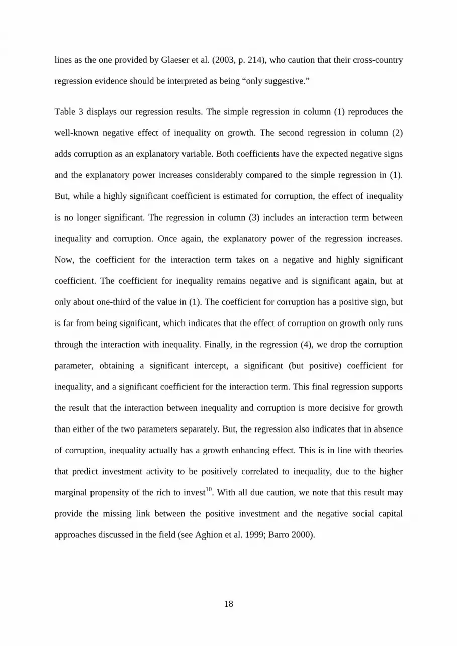
Table 3 displays our regression results. The simple regression in column (1) reproduces the
well-known negative effect of inequality on growth. The second regression in column (2)
adds corruption as an explanatory variable. Both coefficients have the expected negative signs
and the explanatory power increases considerably compared to the simple regression in (1).
But, while a highly significant coefficient is estimated for corruption, the effect of inequality
is no longer significant. The regression in column (3) includes an interaction term between
inequality and corruption. Once again, the explanatory power of the regression increases.
Now, the coefficient for the interaction term takes on a negative and highly significant
coefficient. The coefficient for inequality remains negative and is significant again, but at
only about one-third of the value in (1). The coefficient for corruption has a positive sign, but
is far from being significant, which indicates that the effect of corruption on growth only runs
through the interaction with inequality. Finally, in the regression (4), we drop the corruption
parameter, obtaining a significant intercept, a significant (but positive) coefficient for
inequality, and a significant coefficient for the interaction term. This final regression supports
the result that the interaction between inequality and corruption is more decisive for growth
than either of the two parameters separately. But, the regression also indicates that in absence
of corruption, inequality actually has a growth enhancing effect. This is in line with theories
that predict investment activity to be positively correlated to inequality, due to the higher
marginal propensity of the rich to invest10. With all due caution, we note that this result may
provide the missing link between the positive investment and the negative social capital
approaches discussed in the field (see Aghion et al. 1999; Barro 2000).

19
Table 3. Inequality, Corruption, and Growth
Dependent variable: Ten year average GDP growth per capita (1991-2001)
(1) (2) (3) (4)
Constant 3.065 (0.642) 0.607 (0.856) 3.622 (1.380) 2.007 (0.581)
Gini – 0.031 (0.016) – 0.006 (0.015) – 0.088 (0.034) 0.047 (0.021)
Corruption – 0.295 (0.077) 0.300 (0.233)
Corruption*Gini/100 – 1.740 (0.648) – 0.948 (0.203)
Adjusted R2 0.058 0.270 0.357 0.348
Standard errors in parentheses.
Based on the regression (4) in table 3, we estimate growth for the lowest level (corruption
index = 0) and the highest level (corruption index = 10) of corruption combined with the low
(Gini = 20) and the high (Gini = 60) income inequality used in our experiment. The result of
this estimation is displayed in table 4. Comparing across lines it becomes evident that high
inequality can be growth enhancing without corruption, but it is detrimental for the economic
development when it goes hand in hand with high levels of corruption.
Table 4. Estimated Effect of Inequality and Corruption on Growth
per capita GDP growth low corruption (index = 0) high corruption (index = 10)
low inequality (Gini = 10) 2.48 1.53
high inequality (Gini = 60) 4.83 – 0.86
6. Conclusions
Both the empirical and the theoretical research on the relationship between inequality and
growth have come to ambiguous results, sometimes finding a positive, sometimes a negative,
and sometimes varying correlations (Aghion et al. 1999; Barro 2000). It seems that more
theoretical and experimental work on the behavioral micro-foundations will be necessary to
10 Our experiment was not designed to check for this effect, because investment decision are not modeled.

20
untangle the complicated mechanisms that govern the relationship between inequality and
growth. In a first paper, we put Knack and Keefer’s (1997) conjecture that inequality destroys
“social capital” to a direct experimental test, but found no evidence whatsoever in support of
it: the observed level of cooperation was independent of the implemented degree of inequality
(Sadrieh and Verbon 2002). Given the clear result, it seems evident that something more than
inequality by itself is needed to observe the collapse of societal cooperation.
The hypothesis we started this paper with is that the degree of cooperation not only depends
on the degree of inequality, but also on its genesis. To be able to examine this hypothesis, we
first introduce a model that allows for out-of-equilibrium, but efficient, mutual cooperation in
an unequal income setting. We then conduct laboratory experiments using this model in two
variants. In the nature variant, the degree of inequality – either high or low inequality – is
selected by the experimenter at random. In the dictator variant, the degree of inequality is
selected by the only “rich” individual in the 3-person economy. The results of the experiment
are as conjectured: Inequality is only detrimental to cooperation and, thus, to growth, when it
is deliberately chosen by the rich dictator. As in the previous experiment, inequality has no
effect when it is brought on by a random draw, i.e. by a “fair procedure”.
In an attempt to give this micro-foundations result some macroeconomic substance, we run
simple regressions of cross-country data on per-capita growth, inequality (Gini coefficients),
and corruption (“corruption perception index” of Transparency International). With all due
caveats in interpreting such simple regression models, the effect seems to be strong enough to
allow confidence in its support for our hypothesis. The adverse effect on growth is entirely
captured by the interaction term of inequality and corruption, leaving inequality with a small
positive coefficient and corruption without a significant coefficient.

21
Our result strongly supports the spreading view that the real output effects of inequality are
linked to the institutions governing the economy (see Glaeser et al. 2003). The special
contribution of our paper is to show a new channel through which this interaction may be
effective. The channel we suggest and examine is that of voluntary cooperation in a social
dilemma type situation. The idea is that a substantial part of the effort that is put into
production by the labor force is non-verifiable and, hence, will dependent on the individual’s
trust and emotional attachment to the society. Clearly, these may both be severely damaged
by inequality that results from the actions of a self-serving dictator, but not by inequality
emerging from a fair competition.
References
Abbink, Klaus, Bernd Irlenbusch, and Elke Renner (2000): “The Moonlighting Game - An Experimental Study
on Reciprocity and Retribution,” Journal of Economic Behavior and Organization, 42, 265-277.
Aghion, Philippe, Eve Caroli, and Cecilia García-Peñalosa (1999): “Inequality and Economic Growth: The
Perspective of the New Growth Theories,” Journal of Economic Literature, 37 (4), 1615-1660.
Barro, Robert J. (2000): “Inequality and Growth in a Panel of Countries,” Journal of Economic Growth 5, 5-32.
Blount, Sally (1995): “When Social Outcomes Aren’t Fair: The Effect of Causal Attributions on Preferences,”
Organizational Behavior and Human Decision Processes, 63, 131-144.
Bosman, Ronald, and Frans van Winden (2002): “Emotional hazard in a power-to-take game experiment,”
Economic Journal, 112, 147-169.
Deininger, Klaus, and Lynn Squire (1996): “A New Data Set Measuring Income Inequality,” World Bank
Economic Review, 10 (3), 565-591.
Dufwenberg, Martin, and Georg Kirchsteiger (1998): “A Theory of Sequential Reciprocity,” CentER discussion
paper, 9837, Tilburg University.
Ehrlich, Isaac and Francis T. Lui, (1999): “Bureaucratic Corruption and Endogenous Economic Growth,”
Journal of Political Economy, 107 (6), S270-S293.
Falk, Armin, Ernst Fehr, and Urs Fischbacher (2000): “Testing Theories of Fairness,” Working paper 63,
University of Zurich.
Fehr, Ernst, and Bettina Rockenbach (2003): “Detrimental Effects of Sanctions on Human Altruism,” Nature,
422, 137-140.
Glaeser, Edward, Jose Scheinkman, and Andrei Schleifer (2003): “The Injustice of Inequality,” Journal of
Monetary Economics, 50, 199-222.

22
Güth, Werner (1995): ”An Evolutionary Approach to Explaining Cooperative Behavior by Reciprocal
Incentives,” International Journal of Game Theory, 24, 323 - 344.
Knack, Stephen, and Philip Keefer (1997): “Does Social Capital Have an Economic Payoff,” Quarterly Journal
of Economics, 112 (4), 213-214.
Lambsdorff, Johann Graf (2002): “Background Paper to the 2002 Corruption Perceptions Index – Framework
Document 2002,” Transparency International and University of Göttingen. (http://www.transparency.org)
Mauro, Paolo, (1995): “Corruption and Growth,” Quarterly Journal of Economics, 110 (4), 681-712.
Rabin, Matthew (1993): “Incorporating Fairness into Game Theory and Economics,” American Economic
Review, 83, 1281-1302.
Roth, Alvin E. (1995): “Bargaining Experiments,” in Kagel, John and Alvin E. Roth (eds): Handbook of
Experimental Economics. Princeton, NJ: Princeton University Press.
Sadrieh, Abdolkarim, and Harrie A.A. Verbon (2002): “Inequality Trust and Growth,” CentER discussion Paper,
Tilburg University.

23
Appendix A – Instructions
This is an experiment on economic decision-making within groups over 2 periods. These instructions explain the
workings of the experiment and if you follow them carefully, you may earn a considerable amount of money,
which will be paid to you in cash. You are expected to make decisions on your own without consulting other
participants. So, please, do not communicate with the other participants. Otherwise, we might have to stop the
experiment.
How does this experiment work? Each group consists of 3 participants, so you are in a group with 2 others in
the room but you will not be able to identify your group members. The group members will be indicated by a
color: Red, Blue, and Green. For the purposes of this instruction we will just talk of “your group members”. At
the beginning of period 1, each group member has some amount of start capital. At least one of your group
members will have a start capital that differs from yours. The start capital that you get can be relatively low, or
it can be relatively high. Which of the two will hold for you will be decided by the Red player, who in both cases
will have the highest start capital in your group. Of course, if you happen to be the Red player you will decide on
your own and the others’ start capital.
Whatever your start capital may be you can enlarge your start capital over two periods by making a decision
each period. These decisions determine the return that you are earning on your capital. The development of your
capital does not only depend on your own decisions, but also on the decisions of the other members of your
group. Based on these decisions, at the end of the 2nd period you will have accumulated a certain amount of final
capital. From this final capital the start capital will be subtracted resulting in the payoffs that determine your
earnings out of this experiment.
In each period, each group member chooses simultaneously one of two options: A or B. As will become clear
from the payoff sheets to be discussed in a moment, if all group members choose B, the capital of all group
members will grow more than if all choose A. However, if you choose B alone, while the other group members
choose A, your capital will grow less while the others’ capital will grow more, than if you had chosen A.
Consider the 2 payoff sheets on your desk. These sheets contain important information on your payoff during the
experiment. However, if we start playing the experiment, only 1 of the two payoff sheets are relevant for your
decisions. Which payoff tables that will be, depends on the Red player’s decision. If the Red player chooses the
start capital of 220 for him- or herself and 40 for Blue and Green, payoff sheet 1 is relevant to all of you. But if
the Red player chooses the start capital of 120 for him- or herself and 90 for Blue and Green, payoff sheets 2 is
relevant to all of you.
Let us assume that a payoff sheet 1 is relevant. But, the same reasoning applies if payoff sheet 2 is relevant. For
that case, just change in the following, payoff sheet 1 into payoff sheet 2. When you decide on A or B in the 1st
period, you do not know your group members’ 1st period choices. However, if you choose A in the 1st period,
then, whatever the choices of your group members, payoff sheet 1 LEFT is from then on relevant for you. On the
other hand, if you choose B in the 1st period, payoff sheet 1 RIGHT is relevant. So, a choice between A or B is a
choice between payoff sheets 1 LEFT and 1 RIGHT. The structure of payoff sheets 1 LEFT and 1 RIGHT is

24
identical. It suffices, therefore, to consider one of those payoff sheets only. Let us look at payoff sheet 1 LEFT,
where your 1st period decision is A. Omit for a moment the table at the center of the page, saying, “If 1st period
choice was Reset”.
Payoff sheet 1 LEFT shows 4 payoff tables. These tables give the possible payoff you and your group members
will generate, depending on you and your group members’ 2nd period choices. The letters in the rows of those
tables show the decisions of your group (including yourself) in period 2 and the numbers show the final payoff
for you and your group members corresponding to these decisions. The first of those numbers is always your
final payoff, while the next two numbers are those of your group members. Which of these four tables is relevant
for you will depend on the 1st period choice of your group members. If they both choose A, then the first table
saying “If 1st period choice was (A, A, A)” is relevant, but if the first other group member chooses A and the
other one chooses B the second table saying “If 1st period choice was (A, A, B)” is relevant. The other two tables
will be relevant, if the first other group member chooses B, and the other chooses A, or when they both choose
B, respectively. In payoff sheet 1 RIGHT you will notice that the first letter in the headings of the payoff tables
is not A, but B, corresponding with a 1st period decision of yours of B instead of A.
Once all 1st period decisions on A or B are made, the experimenter will collect all the decision sheets, and return
them with the decisions of your group members on A or B included. Then you will know exactly which payoff
table on the left-hand side of the payoff sheet is relevant for you. Notice that in your payoff table the payoffs of
your group members are shown as well. To help you the experimenter will mark this table with a cross.
After all group members know their payoff table, each group member is given a reset option. If one group
member chooses to reset, then the capital of every group member after the 1st period will be reset to the start
capital. What this implies for the payoff is shown by the “Reset” table at CENTER of Payoff sheet 1. You or one
of your group members might prefer the Reset option over and above the relevant table at the left-hand side of
the Payoff sheet.
The experimenter will communicate to all group members whether there has been a reset, or not. If not, then the
table at the left-hand side that was marked with a cross will be the table that is decisive for your final payoff.
But, if there has been a reset, table CENTER on the page is decisive.
After the decision whether or not to reset, the 2nd period starts. In the 2nd period again each group member
chooses simultaneously from one of two options: A or B. Like in the 1st period, when you decide on A or B, you
do not know your group members’ 2nd period choices. If you choose A, then the first four rows in your relevant
table shows you the possible payoffs for you and your group members. If you choose B, then the last four rows
in your relevant table show you the possible payoffs for you and your group members. Which of those four rows
is decisive for your final payoff depends on your group members.
After everyone has decided on A or B, the experimenter will collect the decision sheets and return them with the
decision of your group members. Then you will know exactly which row in your payoff table is relevant for you.
To help you the experimenter will mark this row with a cross. Again, after all group members have decided for
A or B in the 2nd period, each group member is given a reset option. If one group member chooses to reset, then
the capital of every group member after the 2nd period will be reset to the start capital of the 2nd period. What this
implies for the final payoff is shown by the bottom row of the table saying, “Reset”. You or one of your group

25
members might prefer the Reset option over and above the relevant rows in your payoff table. Notice that if you
are already in the Reset table, a reset choice in your group will lead to zero final payoffs for all group members.
This is due to a choice for reset in the 1st and the 2nd period, which implies that the final capital for you and your
group members equals the start capital. As a result the payoff for any of your group members, including
yourself, equals the show-up fee.
The experimenter will collect all decisions on the reset option and thereafter communicate to all group members
whether there has been a reset, or not. If not, then the row in the table that was marked with a cross will be
decisive for your final payoff. But, if there has been a reset, the bottom row of the table is decisive for your final
payoff.
The final payoff will be exchanged into earnings at the rate of 20 cent per point. Your total earnings from the
experiment are paid to you at the end of the experiment in cash. Additionally, each of you will receive a fixed
payment of 3 Euro for participation in the experiment.
Summarizing. First the Red player decides on the distribution of capital. That choice determines whether the
Payoff sheet 1 or Payoff sheet 2 is used. Your own 1st period choice determines whether sheet 1 LEFT or sheet 1
RIGHT (or, sheet 2 LEFT or sheet 2 RIGHT) is decisive for your and the others’ payoff. The 1st period choices
of your group members fix the table on the left/right-hand side of the relevant payoff sheet. However, if you or
one of your group members chooses to reset in the 1st period, the “Reset” table on the center of the sheet is
decisive. The 2nd period choices of you and your group members determine which row in the chosen table is
going to be decisive for the payoffs. However, if any one in your group (including yourself) has opted for a reset
in the 2nd period, the bottom row in the chosen table sets the payoffs for all group members.
Practice rounds. Before running the actual experiments, we give you the opportunity to have some practice. For
these practice rounds you can use the payoff sheets on your desk, which are also used for the actual experiment.
Moreover, you can use the practice sheets, which are handed out to you now. You will not be paid for the results
of these rounds, these rounds are only meant to let you become acquainted with the structure of the experiment.
First, we play two practice rounds together for payoff sheets 1. After that, we play two practice rounds together
for payoff sheets 2.
During these rounds I announce what you and your group members are hypothetically doing. This information is
indicated on your group-practice sheets by A1.1, etc. You indicate on your guided-practice sheets which payoff
sheets, tables, or payoffs are relevant behind the questions Q1.1. etc.

26
Appendix B – Payoff Sheets
Payoff sheet of the rich in the high inequality treatment (Gini = .6).
The other payoff sheets contained exactly the same information, but the columns of the tables were sorted in a way that had each subject’s own payoff in the first column.
PAYOFF SHEET LEFT
START CAPITAL (220, 40, 40) Payoff tables, if your 1st choice was A
PAYOFF SHEET CENTER
START CAPITAL (220, 40, 40) If 1st period choice was Reset
PAYOFF SHEET RIGHT
START CAPITAL (220, 40, 40) Payoff tables, if your 1st choice was B
If 1st period choice was (A, A, A) If 1st period choice was (B, A, A) Red Green Blue Red Green Blue Red Green Blue Red Green Blue
A A A 44 26 26 A A A 39 34 34 A A B 84 35 19 A A B 78 44 27 A B A 84 19 35 A B A 78 27 44
A B B 123 28 28 A B B 117 37 37 B A A 36 35 35 B A A 32 44 44 B A B 76 43 28 B A B 71 54 37
B B A 76 28 43 B B A 71 37 54 B B B 116 36 36 B B B 110 47 47 Reset 20 12 12 Reset 13 18 18
If 1st period choice was (A, A, B) If 1st period choice was Reset If 1st period choice was (B, A, B) Red Green Blue Red Green Blue Red Green Blue Red Green Blue Red Green Blue Red Green Blue A A A 81 35 19 A A A 20 12 12 A A A 77 43 27
A A B 127 44 11 A A B 56 18 5 A A B 122 54 19 A B A 127 27 26 A B A 56 5 18 A B A 122 35 36 A B B 173 36 18 A B B 93 12 12 A B B 167 46 28
B A A 73 44 26 B A A 13 18 18 B A A 69 54 36 B A B 119 54 18 B A B 50 25 12 B A B 114 65 28 B B A 119 36 34 B B A 50 12 25 B B A 114 46 44
B B B 165 46 26 B B B 87 19 19 B B B 159 56 36 Reset 56 18 5 Reset 0 0 0 Reset 50 25 12
If 1st period choice was (A, B, A) If 1st period choice was (B, B, A) Red Green Blue Red Green Blue Red Green Blue Red Green Blue A A A 81 19 35 A A A 77 27 43
A A B 127 26 27 A A B 122 36 35 A B A 127 11 44 A B A 122 19 54 A B B 173 18 36 A B B 167 28 46
B A A 73 26 44 B A A 69 36 54 B A B 119 34 36 B A B 114 44 46 B B A 119 18 54 B B A 114 28 65
B B B 165 26 46 B B B 159 36 56 Reset 56 5 18 Reset 50 12 25
If 1st period choice was (A, B, B) If 1st period choice was (B, B, B) Red Green Blue Red Green Blue Red Green Blue Red Green Blue
A A A 119 27 27 A A A 115 35 35
A A B 171 36 18 A A B 166 45 27
A B A 171 18 36 A B A 166 27 45
A B B 223 27 27 A B B 217 36 36
B A A 110 36 36 B A A 106 45 45
B A B 162 44 27 B A B 157 55 36
B B A 162 27 44 B B A 157 36 55
B B B 215 36 36 B B B 208 46 46
Reset 93 12 12
The tables on the left and right -hand side are decisive for your payoff if there has been no reset in the 1st period. If there has been a reset, the CENTER table determines your payoff. The last row of any table will be the payoff if there has been a reset in the 2nd period. Letters in the rows are 2nd-period choices of you and your group members Green and Blue; Numbers are the corresponding payoffs for you, Green and Blue. Reset 87 19 19

27
Payoff sheet of the rich in the low inequality treatment (Gini = .1).
The other payoff sheets contained exactly the same information, but the columns of the tables were sorted in a way that had each subject’s own payoff in the first column.
PAYOFF SHEET LEFT START CAPITAL (120, 90, 90)
Payoff tables, if your 1st choice was A
PAYOFF SHEET CENTER START CAPITAL (120, 90, 90)
If 1st period choice was Reset
PAYOFF SHEET RIGHT START CAPITAL (120, 90, 90)
Payoff tables, if your 1st choice was B
If 1st period choice was (A, A, A) If 1st period choice was (B, A, A) Red Green Blue Red Green Blue Red Green Blue Red Green Blue A A A 53 47 47 A A A 47 64 64
A A B 77 65 39 A A B 70 85 56 A B A 77 39 65 A B A 70 56 85 A B B 101 58 58 A B B 93 77 77
B A A 45 65 65 B A A 39 85 85 B A B 69 84 58 B A B 62 106 77 B B A 69 58 84 B B A 62 77 106
B B B 93 76 76 B B B 85 98 98 Reset 24 21 21 Reset 18 36 36 If 1st period choice was (A, A, B) If 1st period choice was Reset If 1st period choice was (B, A, B)
Red Green Blue Red Green Blue Red Green Blue Red Green Blue Red Green Blue Red Green Blue A A A 76 65 40 A A A 24 21 21 A A A 71 82 58 A A B 103 86 32 A A B 44 36 15 A A B 97 106 50
A B A 103 56 58 A B A 44 15 36 A B A 97 73 78 A B B 131 77 50 A B B 64 30 30 A B B 123 97 69 B A A 68 86 58 B A A 18 36 36 B A A 62 106 78
B A B 95 107 50 B A B 38 51 30 B A B 88 129 69 B B A 95 77 75 B B A 38 30 51 B B A 88 97 98 B B B 122 98 67 B B B 58 45 45 B B B 114 120 89
Reset 44 36 15 Reset 0 0 0 Reset 38 51 30 If 1st period choice was (A, B, A) If 1st period choice was (B, B, A)
Red Green Blue Red Green Blue Red Green Blue Red Green Blue A A A 76 40 65 A A A 71 58 82 A A B 103 58 56 A A B 97 78 73
A B A 103 32 86 A B A 97 50 106 A B B 131 50 77 A B B 123 69 97 B A A 68 58 86 B A A 62 78 106
B A B 95 75 77 B A B 88 98 97 B B A 95 50 107 B B A 88 69 129 B B B 122 67 98 B B B 114 89 120
Reset 44 15 36 Reset 38 30 51 If 1st period choice was (A, B, B) If 1st period choice was (B, B, B)
Red Green Blue Red Green Blue Red Green Blue Red Green Blue
A A A 99 58 58 A A A 93 76 76
A A B 129 78 50 A A B 123 99 67
A B A 129 50 78 A B A 123 67 99
A B B 160 70 70 A B B 153 89 89
B A A 90 78 78 B A A 84 99 99
B A B 121 98 70 B A B 114 121 89
B B A 121 70 98 B B A 114 89 121
B B B 151 89 89 B B B 143 112 112
Reset 64 30 30
The tables on the left and right -hand side are decisive for your payoff if there has been no reset in the 1st period. If there has been a reset, the CENTER table determines your payoff. The last row of any table will be the payoff if there has been a reset in the 2nd period. Letters in the rows are 2nd-period choices of you and your group members Green and Blue; Numbers are the corresponding payoffs for you, Green and Blue. Reset 58 45 45

CESifo Working Paper Series (for full list see www.cesifo.de)
________________________________________________________________________ 1040 Michele Moretto, Paolo M. Panteghini, and Carlo Scarpa, Investment Size and Firm’s
Value under Profit Sharing Regulation, September 2003 1041 A. Lans Bovenberg and Peter Birch Sørensen, Improving the Equity-Efficiency Trade-
off: Mandatory Savings Accounts for Social Insurance, September 2003 1042 Bas van Aarle, Harry Garretsen, and Florence Huart, Transatlantic Monetary and Fiscal
Policy Interaction, September 2003 1043 Jerome L. Stein, Stochastic Optimal Control Modeling of Debt Crises, September 2003 1044 Thomas Stratmann, Tainted Money? Contribution Limits and the Effectiveness of
Campaign Spending, September 2003 1045 Marianna Grimaldi and Paul De Grauwe, Bubbling and Crashing Exchange Rates,
September 2003 1046 Assar Lindbeck and Dennis J. Snower, The Firm as a Pool of Factor Complementarities,
September 2003 1047 Volker Grossmann, Firm Size and Diversification: Asymmetric Multiproduct Firms
under Cournot Competition, September 2003 1048 Dan Anderberg, Insiders, Outsiders, and the Underground Economy, October 2003 1049 Jose Apesteguia, Steffen Huck and Jörg Oechssler, Imitation – Theory and
Experimental Evidence, October 2003 1050 G. Abío, G. Mahieu and C. Patxot, On the Optimality of PAYG Pension Systems in an
Endogenous Fertility Setting, October 2003 1051 Carlos Fonseca Marinheiro, Output Smoothing in EMU and OECD: Can We Forego
Government Contribution? A Risk Sharing Approach, October 2003 1052 Olivier Bargain and Nicolas Moreau, Is the Collective Model of Labor Supply Useful
for Tax Policy Analysis? A Simulation Exercise, October 2003 1053 Michael Artis, Is there a European Business Cycle?, October 2003 1054 Martin R. West and Ludger Wößmann, Which School Systems Sort Weaker Students
into Smaller Classes? International Evidence, October 2003 1055 Annette Alstadsaeter, Income Tax, Consumption Value of Education, and the Choice of
Educational Type, October 2003

1056 Ansgar Belke and Ralph Setzer, Exchange Rate Volatility and Employment Growth:
Empirical Evidence from the CEE Economies, October 2003 1057 Carsten Hefeker, Structural Reforms and the Enlargement of Monetary Union, October
2003 1058 Henning Bohn and Charles Stuart, Voting and Nonlinear Taxes in a Stylized
Representative Democracy, October 2003 1059 Philippe Choné, David le Blanc and Isabelle Robert-Bobée, Female Labor Supply and
Child Care in France, October 2003 1060 V. Anton Muscatelli, Patrizio Tirelli and Carmine Trecroci, Fiscal and Monetary Policy
Interactions: Empirical Evidence and Optimal Policy Using a Structural New Keynesian Model, October 2003
1061 Helmuth Cremer and Pierre Pestieau, Wealth Transfer Taxation: A Survey, October
2003 1062 Henning Bohn, Will Social Security and Medicare Remain Viable as the U.S.
Population is Aging? An Update, October 2003 1063 James M. Malcomson , Health Service Gatekeepers, October 2003 1064 Jakob von Weizsäcker, The Hayek Pension: An efficient minimum pension to
complement the welfare state, October 2003 1065 Joerg Baten, Creating Firms for a New Century: Determinants of Firm Creation around
1900, October 2003 1066 Christian Keuschnigg, Public Policy and Venture Capital Backed Innovation, October
2003 1067 Thomas von Ungern-Sternberg, State Intervention on the Market for Natural Damage
Insurance in Europe, October 2003 1068 Mark V. Pauly, Time, Risk, Precommitment, and Adverse Selection in Competitive
Insurance Markets, October 2003 1069 Wolfgang Ochel, Decentralising Wage Bargaining in Germany – A Way to Increase
Employment?, November 2003 1070 Jay Pil Choi, Patent Pools and Cross-Licensing in the Shadow of Patent Litigation,
November 2003 1071 Martin Peitz and Patrick Waelbroeck, Piracy of Digital Products: A Critical Review of
the Economics Literature, November 2003

1072 George Economides, Jim Malley, Apostolis Philippopoulos, and Ulrich Woitek, Electoral Uncertainty, Fiscal Policies & Growth: Theory and Evidence from Germany, the UK and the US, November 2003
1073 Robert S. Chirinko and Julie Ann Elston, Finance, Control, and Profitability: The
Influence of German Banks, November 2003 1074 Wolfgang Eggert and Martin Kolmar, The Taxation of Financial Capital under
Asymmetric Information and the Tax-Competition Paradox, November 2003 1075 Amihai Glazer, Vesa Kanniainen, and Panu Poutvaara, Income Taxes, Property Values,
and Migration, November 2003 1076 Jonas Agell, Why are Small Firms Different? Managers’ Views, November 2003 1077 Rafael Lalive, Social Interactions in Unemployment, November 2003 1078 Jean Pisani-Ferry, The Surprising French Employment Performance: What Lessons?,
November 2003 1079 Josef Falkinger, Attention, Economies, November 2003 1080 Andreas Haufler and Michael Pflüger, Market Structure and the Taxation of
International Trade, November 2003 1081 Jonas Agell and Helge Bennmarker, Endogenous Wage Rigidity, November 2003 1082 Fwu-Ranq Chang, On the Elasticities of Harvesting Rules, November 2003 1083 Lars P. Feld and Gebhard Kirchgässner, The Role of Direct Democracy in the European
Union, November 2003 1084 Helge Berger, Jakob de Haan and Robert Inklaar, Restructuring the ECB, November
2003 1085 Lorenzo Forni and Raffaela Giordano, Employment in the Public Sector, November
2003 1086 Ann-Sofie Kolm and Birthe Larsen, Wages, Unemployment, and the Underground
Economy, November 2003 1087 Lars P. Feld, Gebhard Kirchgässner, and Christoph A. Schaltegger, Decentralized
Taxation and the Size of Government: Evidence from Swiss State and Local Governments, November 2003
1088 Arno Riedl and Frans van Winden, Input Versus Output Taxation in an Experimental
International Economy, November 2003 1089 Nikolas Müller-Plantenberg, Japan’s Imbalance of Payments, November 2003

1090 Jan K. Brueckner, Transport Subsidies, System Choice, and Urban Sprawl, November 2003
1091 Herwig Immervoll and Cathal O’Donoghue, Employment Transitions in 13 European
Countries. Levels, Distributions and Determining Factors of Net Replacement Rates, November 2003
1092 Nabil I. Al-Najjar, Luca Anderlini & Leonardo Felli, Undescribable Events, November
2003 1093 Jakob de Haan, Helge Berger and David-Jan Jansen, The End of the Stability and
Growth Pact?, December 2003 1094 Christian Keuschnigg and Soren Bo Nielsen, Taxes and Venture Capital Support,
December 2003 1095 Josse Delfgaauw and Robert Dur, From Public Monopsony to Competitive Market.
More Efficiency but Higher Prices, December 2003 1096 Clemens Fuest and Thomas Hemmelgarn, Corporate Tax Policy, Foreign Firm
Ownership and Thin Capitalization, December 2003 1097 Laszlo Goerke, Tax Progressivity and Tax Evasion, December 2003 1098 Luis H. B. Braido, Insurance and Incentives in Sharecropping, December 2003 1099 Josse Delfgaauw and Robert Dur, Signaling and Screening of Workers’ Motivation,
December 2003 1100 Ilko Naaborg,, Bert Scholtens, Jakob de Haan, Hanneke Bol and Ralph de Haas, How
Important are Foreign Banks in the Financial Development of European Transition Countries?, December 2003
1101 Lawrence M. Kahn, Sports League Expansion and Economic Efficiency: Monopoly Can
Enhance Consumer Welfare, December 2003 1102 Laszlo Goerke and Wolfgang Eggert, Fiscal Policy, Economic Integration and
Unemployment, December 2003 1103 Nzinga Broussard, Ralph Chami and Gregory D. Hess, (Why) Do Self-Employed
Parents Have More Children?, December 2003 1104 Christian Schultz, Information, Polarization and Delegation in Democracy, December
2003 1105 Daniel Haile, Abdolkarim Sadrieh and Harrie A. A. Verbon, Self-Serving Dictators and
Economic Growth, December 2003


