Self-organizing mixture models

ARTICLE IN PRESS

Neurocomputing 63 (2005) 99–123

0925-2312/$ -

doi:10.1016/j

�Correspo

Amsterdam,

E-mail a

krose@scienc

www.elsevier.com/locate/neucom

Self-organizing mixture models

J.J. Verbeek�, N. Vlassis, B.J.A. Krose

Faculty of Science, Informatics Institute, University of Amsterdam, Kruislaan 403, 1098 SJ Amsterdam,

The Netherlands

Received 21 October 2003; received in revised form 23 February 2004; accepted 23 April 2004

Available online 20 August 2004

Abstract

We present an expectation-maximization (EM) algorithm that yields topology preserving

maps of data based on probabilistic mixture models. Our approach is applicable to any

mixture model for which we have a normal EM algorithm. Compared to other mixture model

approaches to self-organizing maps (SOMs), the function our algorithm maximizes has a clear

interpretation: it sums data log-likelihood and a penalty term that enforces self-organization.

Our approach allows principled handling of missing data and learning of mixtures of SOMs.

We present example applications illustrating our approach for continuous, discrete, and mixed

discrete and continuous data.

r 2004 Elsevier B.V. All rights reserved.

Keywords: Self-organizing maps; Mixture models; EM algorithm

1. Introduction

The self-organizing map, or SOM for short, was introduced by Kohonen in theearly 1980s and it combines clustering of data with topology preservation. Theclusters found in the data are represented on a, typically two dimensional, grid, suchthat clusters with similar content are nearby in the grid. The representation thus

see front matter r 2004 Elsevier B.V. All rights reserved.

.neucom.2004.04.008

nding author. Intelligent Autonomous Systems, Computer Science Institute, University of

Kruislaan 403, 1098 SJ Amsterdam, The Netherlands.

ddresses: [email protected] (J.J. Verbeek), [email protected] (N. Vlassis),

e.uva.nl (B.J.A. Krose).

www.elsevier.com/locate/neucom

ARTICLE IN PRESS

J.J. Verbeek et al. / Neurocomputing 63 (2005) 99–123100

preserves topology in the sense that it keeps similar cluster nearby. The SOM allowsone to visualize high-dimensional data in two dimensions, e.g. on a computer screen,via a projection that may be a nonlinear function of the original features in which thedata was given. The clusters are sometimes also referred to as ‘nodes’, ‘neurons’ or‘prototypes’. Since their introduction, SOMs have been applied in many engineeringproblems, see e.g. the list of over 3000 references on applications of SOM in [15].Some examples of applications include visualization and browsing of large imageand document databases, where similar database items are projected to nearbyneurons of the SOM.

Probabilistic mixture models are densities (or distributions) that can be written asa weighted sum of component densities, where the weighting factors are all non-negative and sum to one [19]. By using weighted combinations of simple componentdensities a rich class of densities is obtained. Mixture models are used in a wide rangeof settings in machine-learning and pattern recognition. Examples includeclassification, regression, clustering, data visualization, dimension reduction, etc. Amixture model can be interpreted as a model that assumes that there are, say k,sources that generate the data: each source is selected to generate data with aprobability equal to its mixing weight and it generates data according to itscomponent density. Marginalizing over the components, we recover the mixturemodel as the distribution over the data. With a mixture model we can associate aclustering of the data, by assigning each data item to the source that is most likely tohave generated the data item. The expectation-maximization (EM) algorithm [7] is asimple and popular algorithm to fit the parameters of a mixture to given data.

Several variations of the original SOM algorithm have been proposed in theliterature, they can be roughly divided into two groups. First, different divergencemeasures have been proposed, suitable to assign data points to clusters when usingdifferent types of data. Second, alternative learning algorithms for SOMs have beenproposed. In this paper, we show how to combine the benefits of SOMs and mixturemodels. We present a general learning algorithm, similar to Kohonen’s originalSOM algorithm, that can, in principle, be applied to any probabilistic mixturemodel. The algorithm is the standard EM learning algorithm using a slightlymodified expectation-step (E-step). Our contribution can be considered as one in thecategory of SOM papers presenting new learning algorithms. However, since ourmodified EM algorithm can be applied to any mixture model for which we have anormal EM algorithm, it can be applied to a wide range of data types. Priorknowledge or assumptions about the data can be reflected by choosing anappropriate mixture model. The mixture model will, implicitly, provide thecorresponding divergence measure. We can thus state that our work also gives acontribution of the first type: it helps to design divergence measures implicitly byspecifying a generative model for the data.

The main merits of our work are the following. First, we have a SOM-likealgorithm with the advantages of probabilistic models, like principled handling ofmissing data values, the ability to learn mixtures of SOMs, etc. Second, compared toother mixture model like approaches to SOMs, the objective function the algorithmoptimizes has a clear interpretation: it sums the data log-likelihood and a penalty

ARTICLE IN PRESS

J.J. Verbeek et al. / Neurocomputing 63 (2005) 99–123 101

term which enforces the topology preservation. Finally, since we merely modify theE-step, we can directly make a SOM version of any mixture model for which we havea normal EM algorithm. We only need to replace normal E-step with the modified E-step presented here to obtain a SOM version of the given mixture model.

The rest of the paper is organized as follows: first we briefly review SOMs andmotivate our work. Then, in Section 3, we review the EM algorithm. In Section 4, weshow how a modified E-step can be used to enforce self-organization in any mixturemodel. Two extensions of the basic idea are presented in Section 5. Related work onSOMs is discussed in Section 6. In Section 7, we provide examples of applying themodified EM algorithm to several different mixture models. Conclusions areprovided in Section 8.

2. Self-organizing maps

SOMs are used for different purposes, however their main application is datavisualization. If the data are high dimensional or non-numerical, a SOM can be usedto represent the data in a two-dimensional space, often called ‘latent’ space. Nearbylocations in the latent space represent similar data. For example, the SOM can beused to represent images in a two-dimensional space, such that similar images arenearby. This latent representation can then be used to browse a large image data-base.

Another application of SOMs to image data is the PICSOM system1 [18] forcontent-based image retrieval. The system provides a search mechanism that allows auser to find images of interest through several interactions with the system. First, thePICSOM system presents some random images from the data-base to the user andthen the user identifies relevant images: i.e. images that are (most) similar to thetarget. Alternatively, the user could directly provide some relevant images to thesystem. The system uses a SOM to find similar pictures and presents those to theuser. The process can then be iterated by letting the user add new images (from thepresented ones) to the set of relevant images. The system uses several differentrepresentations of the images, among others color and texture content are used. Asthe user adds more images to the set of relevant images, it may become apparent thatthey are all similar in respect to their texture content but not in their color content,the system identifies that mainly texture content matters and will present new imagesmainly on the basis of similar texture content.

The basic SOM algorithm assumes that the data are given as vectors. Thealgorithm then fits a set of reference vectors or prototypes to the data. We use thevariable s throughout to index the prototypes. With each prototype s a location inthe latent space gs is associated. The latent space is typically two dimensional invisualization applications of the SOM. The prototypes are fitted in such a way thatnearby prototypes in the latent space will also be nearby in the data space. There aretwo ways to fit the prototypes, we can process data items one-by-one, referred to as

1An online demo of the system can be found at http://www.cis.hut.fi/picsom/.

http://www.cis.hut.fi/picsom/

ARTICLE IN PRESS


online, and all-at-once, referred to as batch. The online algorithm is useful when thedata items cannot be stored because that might take too much storage.

Both batch and online algorithm make use of a so-called ‘neighborhood’ functionthat will encode the spatial relationships of the prototypes in the latent space. Theneighborhood function is a function that maps the indices of two prototypes to a realnumber. Typically the neighborhood function is a positive function which decreasesas the distance between two prototypes in the latent space increases. Often, theexponent of the negative-squared distance between the two prototypes in the latentspace is used as neighborhood function, i.e. a Gaussian centered at one prototypeevaluated at the other. In that case, having fixed the locations of the prototypes inthe latent space at gs for prototype s, the neighborhood function evaluated atprototypes r and s is given by

hrs ¼ expð�lkgr � gsk2Þ;

where l controls the width of the neighborhood function. Sometimes, theneighborhood function is considered a function of one argument fixing one of theprototypes. We will use the following notation to reflect this:

hrðsÞ ¼ expð�lkgr � gsk2Þ; ð1Þ

The online SOM training algorithm can be summarized as follows:

Basic online SOM algorithm

Initialize the prototype vectors as randomly selected data points.Iterate these steps:
� Assignment: Assign the current data item to its nearest (typically in terms ofEuclidean distance) prototype r� in the data space, this prototype is called the‘winner’. � Update: Move the each prototype s towards the data vector by an amountproportional to hr� ðsÞ: the value of the neighborhood function evaluated at thewinner r� and prototype s.
Thus a prototype is moved towards the data that is assigned to it, but also towardsdata that is assigned to prototypes nearby in the latent space. Fig. 1 illustrates theupdate for a point indicated with x. Alternatively, the prototypes can be initializedby linearly mapping the gs to the subspace spanned by the principal components ofthe data, such that the covariance of the mapped gs matches the covariance of thedata in the principal components subspace.

The batch version of the SOM algorithm processes all data at once in each step byfirst doing the assignment for all data vectors. In the update step, each prototype s isthen placed at the weighted average of all data, where each data vector is weighted bya factor proportional to the neighborhood function evaluated at s and the winner forthat data vector. If we use lr to denote prototype r and sn to indicate the winner for

ARTICLE IN PRESS

Fig. 1. The update of the online algorithm. The small dots are data points and the big dots are the

prototype vectors. The ordering of the prototypes in the latent space is indicated by the bars connecting

them. The size of the arrows indicates the force by which the nodes are attracted towards the point x.


data point xn, the batch algorithm sets

lr ¼

PNn¼1hsn

ðrÞxnPNn¼1hsn

ðrÞ:

The Euclidean distance used in the assignment step of the SOM algorithm is notalways appropriate, or even not applicable, e.g. for data that is not expressed as real-valued vectors. For example, consider data that consists of vectors with binaryentries. Then, we might still use the Euclidean distance, but how will we represent theprototypes? As binary vectors as well? Or should we allow for scalars in the interval½0; 1? In general, it is not always clear to decide whether Euclidean distance isappropriate and if it is not it may be hard to come up with a divergence measure thatis appropriate. Moreover, it is not clear whether the ‘prototypes’ should be the sametype of object as the data vectors (e.g. binary vs. real-valued vectors).

Hence, an ongoing issue in research on SOMs is to find appropriate distancemeasures, or more generally divergence measures, for different types of data.However, there are no general ways to translate prior knowledge about the data intodistance measures. The EM algorithm we present in the subsequent sections doesprovide us with a simple way to encode prior knowledge about the data into a SOMalgorithm. The mixture model can be designed based on our assumptions or priorknowledge on how the data is generated. Hence, we can separate the designof the model from the learning algorithm. For example, for binary vectors we mightwant to use a mixture of Bernoulli distributions to model their probability ofoccurrence.

Furthermore, in some applications some values in the data might be missing, e.g. asensor on a robot brakes down or an entry in a questionnaire was left unanswered. Insuch cases, it is common practice when applying Kohonen’s SOM algorithm, see e.g.[15], to simply ignore the missing values and use an adapted divergence measure inorder to compute the winning unit and to update the prototypes. The EM algorithmfor SOMs, just as the normal EM algorithm, provides a simple and justified way todeal with missing data for many types of mixtures.

ARTICLE IN PRESS


In Section 3, we review the standard EM algorithm for mixture models and inSection 4 we show how the EM algorithm can be modified to produce SOMs.

3. Mixtures models and the EM algorithm

As stated in the introduction, mixture models are densities of the form:

pðxÞ ¼Xk

s¼1

pspðx j sÞ;

where the ps are the non-negative mixing weights that sum to one. The pðxjsÞ arecalled the component densities, parameterized by hs. The model thus makes theassumption that the data is generated by first selecting with probability ps a mixturecomponent s and then drawing a data item from the corresponding distributionpð�jsÞ.

Given data X ¼ fx1; . . . ;xNg, and initial parameters, collectively denoted as:h ¼ fh1; . . . ; hk;p1; . . . ;pkg, the EM algorithm finds a local maximizer h of the datalog-likelihood LðhÞ. Assuming data are independent and identically distributed (iid)

LðhÞ ¼ log pðX ; hÞ ¼XN

n¼1

log pðxn; hÞ:

Learning is facilitated by introducing N ‘hidden’ variables z1; . . . ; zN , collectivelydenoted as Z. Hidden variable zn indicates which of the k mixture componentsgenerated the corresponding data point xn. The zn are called hidden variables sincewe are only given X and do not know the ‘true’ values of the zn. Intuitively, the EMalgorithm [7] iterates between (E-step) guessing the values of the zn based on the dataand the current parameters, and (M-step) updating the parameters accordingly.

The EM algorithm maximizes a lower bound F on the data log-likelihood LðhÞ.The lower-bound is known as the negative free-energy because of its analogy withthe free-energy in statistical physics [20]. The lower-bound F on LðhÞ is a function ofh and also depends on some distribution Q over the hidden variables Z, and isdefined as

F ðQ; hÞ ¼ EQ log pðX;Z; hÞ þHðQÞ ¼ LðhÞ �DKLðQkpðZjX; hÞÞ:

In the above, we used H and DKL to denote, respectively, Shannon entropy andKullback–Leibler (KL) divergence [6]. The EM algorithm consists of coordinateascent on F, iterating between steps in h and steps in Q.

The two forms in which we expanded F are associated with the M-step and the E-step of EM. In the M-step we change h as to maximize, or at least increase, F ðQ; hÞ.The first decomposition includes HðQÞ which is a constant w.r.t. h, so we essentiallymaximize the expected joint log-likelihood in the M-step. In the E-step we maximizeF w.r.t. Q. Since, the second decomposition includes LðhÞ which is constant w.r.t. Q,what remains is a KL divergence which is the effective objective function in the

ARTICLE IN PRESS


E-step of EM. Note that, due to the non-negativity of the KL-divergence, for any Q

we have F ðQ; hÞpLðhÞ.For iid data the Q that maximizes F factors over the individual hidden variables

and using such a factored distribution we can decompose the lower-bound, just likethe log-likelihood, as a sum over data points:

F ðQ; hÞ ¼X

n

Fnðqn; hÞ; ð2Þ

Fnðqn; hÞ ¼ Eqnlog pðxn; zn ¼ s; hÞ þHðqnÞ ð3Þ

¼ log pðxn; hÞ �DKLðqnkpðzn j xn; hÞÞ: ð4Þ

In the above, we wrote qn for the distribution on the mixture components for datapoint n. Sometimes, we will also simply write pðsjxnÞ to denote pðzn ¼ sjxn; hÞ andsimilarly qns for qnðzn ¼ sÞ.

In standard applications of EM (e.g. mixture modeling) Q is unconstrained, whichresults in setting qn ¼ pðzn j xn; hÞ in the E-step since the non-negative KL divergenceequals zero if and only if both arguments are equal. Therefore, after each E-stepF ðQ; hÞ ¼ LðhÞ and it follows immediately that the EM iterations can never decreasethe data log-likelihood. Furthermore, to maximize F w.r.t. hs and ps, the parametersof component s, the relevant terms in F, using (2) and (3), are

Xn

qns log pðsÞ þ logðxnjsÞ½ :

Thus hs is updated as to maximize a weighted sum of the data log-likelihoods. Theqns are therefore also referred to as ‘responsibilities’, since each component is tunedtoward data for which it is ‘responsible’ (large qns) in the M-step.

For some probabilistic models it is not feasible to store the distribution pðZjXÞ,e.g. in a hidden Markov random field [5] where the posterior has to be representedusing a number of values that is exponential in the number of variables. In such casesvariational methods [12] can be used: instead of allowing any distribution Q

attention is restricted to a certain class Q of distributions allowing for tractablecomputations. In the hidden Markov random field example, using a factoreddistribution over the states would make computations tractable and the correspond-ing lower-bound on the data log-likelihood is also known as the mean-fieldapproximation. Variational EM maximizes F instead of L, since we can no longerguarantee that F equals LðhÞ after each E-step. The function F can be interpreted assumming log-likelihood and a penalty which is high if the true posterior is far fromall members of Q. Thus, applying the algorithm will find us models that (a) assignhigh likelihood to the data and (b) have posteriors pðZjXÞ that are similar to somemember of Q. In the next section, we show how we can constrain the distributions Q,not to achieve tractability, but to enforce self-organization.

ARTICLE IN PRESS


4. Self-organization in mixture models

In this section, we describe how we can introduce the self-organizing quality ofSOMs in the mixture modeling framework. First, we will explain the idea in generaland then give a simple example for modeling data with a Gaussian mixture. In thelast two sections we discuss algorithmic issues.

4.1. The neighborhood function as a distribution

Suppose, we have found an appropriate class of component densities for our data,either based on prior knowledge or with an educated guess, for which we have anEM algorithm. By appropriately constraining the set Q of allowed distributions qn inthe E-step we can enforce a topological ordering of the mixture components, as weexplain below. This is much like the approach taken in [23,26], where constraints onthe qn are used to globally align the local coordinate systems of the components of aprobabilistic mixture of factor analyzers. The latter works actually inspired thematerial presented here.

Here, we consider the neighborhood function of Kohonen’s SOM as a function ofone component index by fixing the other component index. If we constrain theneighborhood function to be non-negative and sum to unity, it can be interpreted asa distribution over the components. We refer to such neighborhood functions as‘normalized’ neighborhood functions. Thus, using the notation of (1), we have

hrðsÞ / expð�lkgr � gsk2Þ;

Xs

hrðsÞ ¼ 1:

In order to obtain the self-organizing behavior in the mixture model learning weconstrain the qn to be normalized neighborhood functions. Thus, for fixed shape ofthe neighborhood function, the E-step will consist of selecting for each data item n

the component r� such that Fn is maximized if we use qn ¼ hr� . As before, we will callr� the ‘winner’ for data item n. Below, we will analyze the consequences ofconstraining the qn in this way.

What happens in the M-step if the qn in the EM algorithm are normalizedneighborhood functions? Similar as with Kohonen’s SOM, if a specific component isthe winner for xn it receives most responsibility and will be forced to model xn, butalso its neighbors in the latent space will be forced, but to a lesser degree, to modelxn. So by restricting the qn in the EM-algorithm to be a normalized neighborhoodfunction centered on one of the units we thus force the components with largeresponsibility for a data point to be close in the latent space. In this manner, weobtain a training algorithm for mixture models similar to Kohonen’s SOM.

The same effect can also be understood in another way: consider thedecomposition (4) of the objective function F, and two mixtures, parameterized byh and h0, that yield equal data log-likelihood LðhÞ ¼ Lðh0Þ. The objective function F

prefers the mixture for which the KL-divergences are the smallest, i.e. the mixture forwhich the posterior on the mixture components looks the most like the normalizedneighborhood function. If the posteriors are truly close to the normalized

ARTICLE IN PRESS


neighborhood function then this implies that nearby components in the latentspace model similar data. If the penalty term is large, this indicates that theposteriors do not resemble the neighborhood function and that the mixture is poorly‘organized’.

Note that these observations hold for any mixture model and that the algorithm isreadily generalized to any mixture model for which we have a maximum-likelihoodEM algorithm.

Since the E-step is constrained, in general the objective function F does not equallog-likelihood after the E-step. Instead, the objective function sums data log-likelihood and a penalty term which measures the KL divergence between the (bestmatching, after the E-step) neighborhood function and the true posteriors for eachdata point. The modified EM algorithm can be summarized as follows:

EM algorithm for SOM

Initialize the parameters of the mixture model.Iterate these steps:
� E: Determine for each xn the distribution q� 2 Q that maximizes F n, i.e.q� ¼ arg minq2QDKLðqkpðsjxnÞÞ, and set qn ¼ q�. � M: perform the normal M-step for the mixture, using the qn computed in the E-step.
In fact, in the M-step we do not need to maximize F with respect to the parameters h.As long as we can guarantee that the M-step does not decrease F, we are guaranteedthat the iterations of the (modified) EM algorithm will never decrease F.

Finally, in order to project the data to the latent space, we average over the latentcoordinates of the mixture components. Let gs denote the latent coordinates of thesth mixture component and let gn denote the latent coordinates for the nth data item.We then define gn as

gn ¼X

s

pðsjxnÞgs: ð5Þ

4.2. Example with Gaussian mixture

Next, we consider an example of this general algorithm for a Mixture of Gaussians(MoG). A mixture giving a particularly simple M-step is obtained by using equalmixing weights ps ¼ 1=k for all components and using isotropic Gaussians ascomponent densities

pðxjsÞ ¼Nðx; ls; s2IÞ:

For this simple MoG, the Fn can be rewritten up to some constants as

Fnðqn; hÞ ¼ �1

2D log s2 �

Xs

qns s�2kxn � lsk2=2þ log qns

� �:

ARTICLE IN PRESS


The parameters of the mixture are h ¼ fs2;l1; . . . ;lkg: The parameters h maximizingF for given q1; . . . ; qN are obtained easily through differentiation of F and thecomplete algorithm for D-dimensional data reads:

EM algorithm for SOM for simple MoG

Iterate these steps:
� E: Determine for each xn the distribution q� 2 Q that maximizes Fn, set qn ¼ q�.P P P � M: Set: ls ¼ nqnsxn= nqns and s2 ¼ nsqnskxn � lsk
2=ðNDÞ.

A Matlab implementation of SOMM for the isotropic MoG is available at: http://www.science.uva.nl/�jverbeek/software/.

Note that the update for the means ls coincides with that of Kohonen’s batchSOM algorithm when using the Euclidean distance: it places each prototype at theweighted average of all data, where each data vector is weighted proportionally tothe neighborhood function centered at the winning prototype for that data vectorand evaluated at the prototype s. Only definition of the winner is different in thiscase: instead of the minimizer of kxn � lrk

2 we select the minimizer ofPs hrðsÞkxn � lrk

2. Hence, the selection of the winner also takes into account theneighborhood function, whereas this is not the case in the standard Kohonen SOM.

4.3. Shrinking the neighborhood function

A particular choice for the normalized neighborhood function is obtained byassociating with each mixture component s a latent coordinate gs. It is convenient totake the components as located on a regular grid in the latent space. We then set thenormalized neighborhood functions to be discretized isotropic Gaussians in thelatent space, centered on one of the components. Thus, for a given set of latentcoordinates of the components fg1; :::; gkg, we set Q to be the set of distributions ofthe form:

qðsÞ ¼expð�lkgs � grk

2ÞPt expð�lkgt � grk

2Þwith r 2 f1; . . . kg:

A small l corresponds to a broad distribution, and for large l the distribution q

becomes more peaked.Since, the objective function might have local optima and EM is only guaranteed

to give a local optimizer of F, good initialization of the parameters of the mixturemodel is essential to finding a good solution. Analogous to the method of shrinkingthe extent of the neighborhood function with the SOM, we can start with a small l(broad neighborhood function) and increase it iteratively until a desired value of l(i.e. the desired width of the neighborhood function) is reached. In implementationswe started with l such that the q are close to uniform over the components, then werun the EM algorithm until convergence. Note that if the q are almost uniform theinitialization of h becomes irrelevant, since the responsibilities will be approximately

http://www.science.uva.nl/jverbeek/software/



ARTICLE IN PRESS


uniform over all components. The subsequent M step will give all componentssimilar parameters. After convergence we set lnew Zlold with Z41 (typically Z isclose to unity). In order to initialize the EM procedure with lnew, we initialize h withthe value found in running EM with lold.

Note that in the limit of l!1 it is not the case that we recover the usual EMalgorithm for mixtures. Instead, a ‘winner-take-all’ (WTA) algorithm is obtainedsince in the limit the distributions in Q tend to put all mass on a single mixturecomponent. The WTA algorithm tends to find more heterogeneous mixturecomponents than the usual EM algorithm [14]. Arguably, this can be an advantagefor visualization purposes.

4.4. Sparse winner search

The computational cost of the E-step is OðNk2Þ, a factor k slower than SOM and

prohibitive in large-scale applications. However, by restricting the search for awinner in the E-step to a limited number of candidate winners we can obtain anOðNkÞ algorithm. A straightforward choice is to use the l components with thelargest joint likelihood pðxn; sÞ as candidates, corresponding for our simple exampleMoG to smallest Euclidean distances to the data point. If none of the candidatesyields a higher value of Fnðqn; hÞ we keep the winner of the previous step, in this waywe are guaranteed never to decrease the objective in every step. We found l ¼ 1 towork well and fast in practice, in this case we only check whether the winner from theprevious round should be replaced with the node with highest joint-likelihoodpðs;xnÞ.

Note that in the l ¼ 1 case our algorithm is very similar to Kohonen’s batch SOMalgorithm for the simple MoG model. We will return to this issue in Section 6.

5. Extensions of the basic framework

In this section, we describe two extensions of the basic framework for self-organization in mixture models. In Section 5.1, we consider how data with missingvalues can be dealt with and in Section 5.2, we consider how the adaptive-subspaceSOM can be fitted in the proposed framework.

5.1. Modeling data with missing values

When the given data has missing values the EM algorithm can still be used to traina mixture on the incomplete data [8]. The procedure is more or less the same as withthe normal EM algorithm to train a mixture model. The missing data are now alsohandled as ‘hidden’ variables. Below, we consider the case for iid data.

Let us use xon to denote the observed part of xn and xh

n to denote the missing or‘hidden’ part. The distributions qn now range over all the hidden variables of xn: thegenerating component zn, and possibly xh

n if there are some unobserved values for xn.We can now again construct a lower-bound on the (incomplete) data log-likelihood

ARTICLE IN PRESS


as follows:

F ðQ; hÞ ¼X

n

F nðqn; hÞ;

Fnðqn; hÞ ¼ log pðxon ; hÞ �DKLðqnkpðzn; x

hn jx

onÞÞ

¼ Eqnlog pðxo

n ;xhn ; zn; hÞ þHðqnÞ: (6)

The EM algorithm then iterates between setting in the E-step: qn ¼ pðzn;xhnjx

onÞ.

The M-step updates h to maximize (or at least increase) the expected joint log-likelihood:

Pn Eqn

log pðxon ;x

hn ; zn; hÞ. After each E-step F equals the (incomplete)

data log-likelihood, so we see that the EM iterations can never decrease the log-likelihood.

Now consider the decomposition: qnðzn;xhnÞ ¼ qnðznÞqnðx

hnjznÞ. We can re-

write (6) as

Fnðqn; hÞ ¼ HðqnðznÞÞ þ EqnðznÞ Hðqnðxhn jznÞÞ þ Eqnðx

hn jznÞ

log pðzn; xhn ;x

onÞ

h i: ð7Þ

Just as before, we can now constrain the qnðznÞ to be a normalized neighborhoodfunction. We then find that in order to maximize F w.r.t. Q in the E-step we have toset qnðx

hn jsÞ ¼ pðxh

n jxon ; sÞ. The optimization of F w.r.t. qnðznÞ is then achieved by

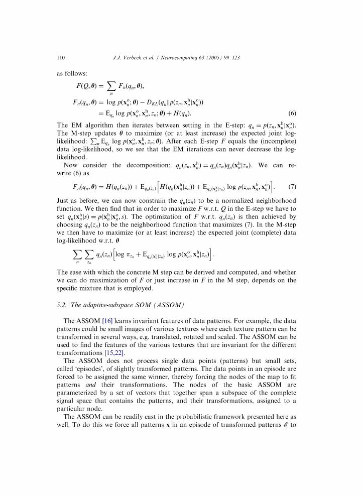
choosing qnðznÞ to be the neighborhood function that maximizes (7). In the M-stepwe then have to maximize (or at least increase) the expected joint (complete) datalog-likelihood w.r.t. h

Xn

Xzn

qnðznÞ log pznþ Eqnðx

hn jznÞ

log pðxon ;x

hnjznÞ

h i:

The ease with which the concrete M step can be derived and computed, and whetherwe can do maximization of F or just increase in F in the M step, depends on thespecific mixture that is employed.

5.2. The adaptive-subspace SOM (ASSOM)

The ASSOM [16] learns invariant features of data patterns. For example, the datapatterns could be small images of various textures where each texture pattern can betransformed in several ways, e.g. translated, rotated and scaled. The ASSOM can beused to find the features of the various textures that are invariant for the differenttransformations [15,22].

The ASSOM does not process single data points (patterns) but small sets,called ‘episodes’, of slightly transformed patterns. The data points in an episode areforced to be assigned the same winner, thereby forcing the nodes of the map to fitpatterns and their transformations. The nodes of the basic ASSOM areparameterized by a set of vectors that together span a subspace of the completesignal space that contains the patterns, and their transformations, assigned to aparticular node.

The ASSOM can be readily cast in the probabilistic framework presented here aswell. To do this we force all patterns x in an episode of transformed patterns E to

ARTICLE IN PRESS


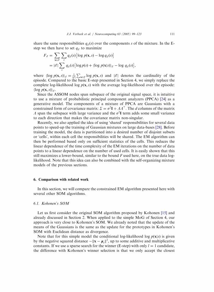
share the same responsibilities qEðsÞ over the components s of the mixture. In the E-step we then have to set qE to maximize

FE ¼Xx2E

Xs

qEðsÞ log pðx; sÞ � log qEðsÞ� �

¼ jEjX

s

qEðsÞ log pðsÞ þ hlog pðxjsÞiE � log qEðsÞ� �

;

where hlog pðx; sÞiE ¼1jEj

Px2E log pðx; sÞ and jEj denotes the cardinality of the

episode. Compared to the basic E-step presented in Section 4, we simply replace thecomplete log-likelihood log pðx; sÞ with the average log-likelihood over the episode:hlog pðx; sÞiE.

Since the ASSOM nodes span subspace of the original signal space, it is intuitiveto use a mixture of probabilistic principal component analyzers (PPCA) [24] as agenerative model. The components of a mixture of PPCA are Gaussians with aconstrained form of covariance matrix: S ¼ s2Iþ LL>. The d columns of the matrixL span the subspace with large variance and the s2I term adds some small varianceto each direction that makes the covariance matrix non-singular.

Recently, we also applied the idea of using ‘shared’ responsibilities for several datapoints to speed-up the training of Gaussian mixtures on large data-bases [28]. Beforetraining the model, the data is partitioned into a desired number of disjoint subsetsor ‘cells’, within each cell the responsibilities will be shared. The EM algorithm canthen be performed based only on sufficient statistics of the cells. This reduces thelinear dependence of the time complexity of the EM iterations on the number of datapoints to a linear dependence on the number of used cells. It is easily shown that thisstill maximizes a lower-bound, similar to the bound F used here, on the true data log-likelihood. Note that this idea can also be combined with the self-organizing mixturemodels of the previous sections.

6. Comparison with related work

In this section, we will compare the constrained EM algorithm presented here withseveral other SOM algorithms.

6.1. Kohonen’s SOM

Let us first consider the original SOM algorithm proposed by Kohonen [15] andalready discussed in Section 2. When applied to the simple MoG of Section 4, ourapproach is very close to Kohonen’s SOM. We already noted that the update of themeans of the Gaussians is the same as the update for the prototypes in Kohonen’sSOM with Euclidean distance as divergence.

Note that for this simple model the conditional log-likelihood log pðxjsÞ is givenby the negative squared distance �kx� lsk

2; up to some additive and multiplicativeconstants. If we use a sparse search for the winner (E-step) with only l ¼ 1 candidate,the difference with Kohonen’s winner selection is that we only accept the closest

ARTICLE IN PRESS


node, in terms of Euclidean distance, as a winner when it increases F, and keep theprevious winner otherwise.

In comparison to the standard Kohonen SOM, we presented a SOM algorithmapplicable to any type of mixture model. We can use prior knowledge of the data todesign a specific generative mixture model for given data and then train it with theconstrained EM algorithm. Also, the probabilistic formulation of the SOMpresented here allows us to handle missing data in a principled manner and tolearn mixtures of SOMs. Furthermore, the probabilistic framework helps us designSOM algorithms for data types which were difficult to handle in the original SOMframework, e.g. data that consists of variable-size trees or sequences, data thatcombines numerical with categorical features, etc.

6.2. Soft topographic vector quantization

Soft topographic vector quantization (STVQ) [10,11], is a SOM-like algorithmsimilar to the one presented here. Given some divergence measure dðxn; sÞ betweendata items and neurons, the following error function is minimized by STVQ:

ESTVQ ¼ bX

ns

pns

Xr

hsðrÞdðxn; sÞ þX

ns

pns log pns;

with all pnsX0 andP

s pns ¼ 1. The error function sums an error term based on d

(which could for example be based on squared Euclidean distance, but other errorsbased on the exponential family can be easily plugged in) and an entropy term. Theneighborhood function, implemented by the hsðrÞ, is fixed, but the winnerassignment, given by the pns, is soft. Instead of selecting a single ‘winner’ as in ourwork, an (unconstrained) distribution pns over the units is used. Since we use acomplete distribution over the units, we cannot apply the speed-up of ‘sparse’ searchfor the winning neuron here. However, speed-ups can be obtained by using a ‘sparse’EM algorithm [20] in which the pns a adapted only for a few components s (differentones for each data item) and freezing the values pns for other components.

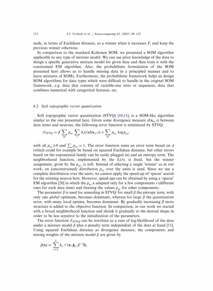
The parameter b is used for annealing in STVQ: for small b the entropy term, withonly one global optimum, becomes dominant, whereas for large b the quantizationerror, with many local optima, becomes dominant. By gradually increasing b morestructure is added to the objective function. In comparison, in our work we startedwith a broad neighborhood function and shrink it gradually to the desired shape inorder to be less sensitive to the initialization of the parameters.

The error function ESTVQ can be rewritten as a sum of log-likelihood of the dataunder a mixture model ~p plus a penalty term independent of the data at hand [11].Using squared Euclidean distance as divergence measure, the components andmixing weights of the mixture model ~p are given by

~pðxÞ ¼Xk

s¼1

~psNðx; ~ls; b�1IÞ;

ARTICLE IN PRESS


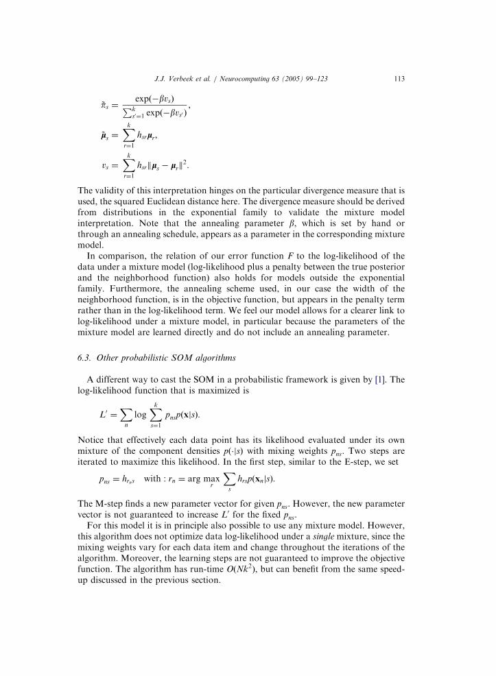
~ps ¼expð�bvsÞPk

s0¼1 expð�bvs0 Þ;

~ls ¼Xk

r¼1

hsrlr;

vs ¼Xk

r¼1

hsrkls � lrk2:

The validity of this interpretation hinges on the particular divergence measure that isused, the squared Euclidean distance here. The divergence measure should be derivedfrom distributions in the exponential family to validate the mixture modelinterpretation. Note that the annealing parameter b, which is set by hand orthrough an annealing schedule, appears as a parameter in the corresponding mixturemodel.

In comparison, the relation of our error function F to the log-likelihood of thedata under a mixture model (log-likelihood plus a penalty between the true posteriorand the neighborhood function) also holds for models outside the exponentialfamily. Furthermore, the annealing scheme used, in our case the width of theneighborhood function, is in the objective function, but appears in the penalty termrather than in the log-likelihood term. We feel our model allows for a clearer link tolog-likelihood under a mixture model, in particular because the parameters of themixture model are learned directly and do not include an annealing parameter.

6.3. Other probabilistic SOM algorithms

A different way to cast the SOM in a probabilistic framework is given by [1]. Thelog-likelihood function that is maximized is

L0 ¼X

n

logXk

s¼1

pnspðxjsÞ:

Notice that effectively each data point has its likelihood evaluated under its ownmixture of the component densities pð�jsÞ with mixing weights pns. Two steps areiterated to maximize this likelihood. In the first step, similar to the E-step, we set

pns ¼ hrns with : rn ¼ arg maxr

Xs

hrspðxnjsÞ:

The M-step finds a new parameter vector for given pns. However, the new parametervector is not guaranteed to increase L0 for the fixed pns.

For this model it is in principle also possible to use any mixture model. However,this algorithm does not optimize data log-likelihood under a single mixture, since themixing weights vary for each data item and change throughout the iterations of thealgorithm. Moreover, the learning steps are not guaranteed to improve the objectivefunction. The algorithm has run-time OðNk2

Þ, but can benefit from the same speed-up discussed in the previous section.

ARTICLE IN PRESS


In [17] a probabilistic model is given based on isotropic Gaussian components.The maximum-likelihood estimation procedure of the means of the Gaussianscoincides with the estimation of the vector quantizers with the batch version ofKohonen’s SOM algorithm. There are, however, some difficulties with thisapproach. The density is Gaussian in each of the Voronoi regions associated withthe vector quantizers and thus not smooth in the data space as a whole. Second, theestimation of the variance of the Gaussians needs to be done by numericaloptimization techniques. Third, to evaluate the likelihood a normalization constanthas to be computed. The constant is defined in terms of integrals that can not beanalytically computed and therefore sampling techniques are needed to approximateit. Furthermore, the density model seems to be restricted to Gaussian mixtures withthe corresponding squared Euclidean distance as divergence measure.

Other maximum-likelihood approaches for mixture models achieve topographicorganization by a smoothness prior [25] on the parameters. For this method is it notclear whether it generalizes directly to mixture models outside the exponential familyand whether speed-ups can be applied to avoid Oðnk2

Þ run-time.

6.4. Generative topographic mapping

Generative topographic mapping (GTM) [3] achieves topographic organization ina quite different manner than the SOM. GTM fits a constrained probabilisticmixture model to given data. With each mixture component s a latent coordinate gs

is associated, like in our approach. The mixture components are parameterized as alinear combination of a fixed set of smooth nonlinear basis functions of the fixedlocations of the components in the latent space. Due to the smooth mapping fromlatent coordinates of the mixture components to their parameters, nearbycomponents in the latent space will have similar parameters. The parameters ofthe linear map are fitted by the EM algorithm to maximize the data log-likelihood.Although originally presented for Gaussian mixtures, the GTM can be extended tomixtures of members of the exponential family [9,13]. To our knowledge it is notknown how to extend the GTM to mixtures of component densities outside theexponential family.

The main benefit of GTM over SOMM is that the parameter fitting can be donedirectly in the maximum-likelihood framework. For SOMM we need to specify thenumber of mixture components and a desired shape and width of the neighborhoodfunction. For GTM we also need to set parameters: the number of mixturecomponents, the number of basis functions, their smoothness and their shape. ForGTM these parameters can be dealt with in a Bayesian manner, by specifyingappropriate priors for these parameters. Optimal parameter settings can then befound by inferring their values using approximate inference techniques if enoughcomputational resources are available [2]. For the SOMM approach it is not clearwhether such techniques can be used to set the parameters of the algorithm. Thismay be considered a drawback of the SOMM approach, however in situations withlimited computational resources the SOMM has fewer parameters to be set and maytherefore be preferred.

ARTICLE IN PRESS


7. Example applications

In this section we illustrate the modified EM algorithm with some examples. Westart with a more extensive treatment of the example already used in Section 4. Thesecond example uses a mixture of (products of) discrete Bernoulli distributions. Inthe third example, we use mixtures for data that has both nominal and continuousvariables.

In all experiments we used discretized Gaussians as neighborhood function andthe same scheme to shrink the neighborhood function. The mixture componentswere arranged as (i) a regular rectangular grid on the unit square for a two-dimensional latent space or (ii) at regular intervals on the real line between zero andone for a one-dimensional latent space. At initialization we set the neighborhoodfunction width as that of a isotropic Gaussian with unit variance, i.e. l ¼ 1

2. After the

algorithm converges with a particular l we increase it with a factor Z ¼ 1110. The

algorithm halts if a winning node receives more than 90% of the mass of itsneighborhood function.

7.1. The simple Gaussian mixture

In the first example we show the configurations of the means of the simple MoGmodel used in Section 4. We generated a data set by drawing 500 point uniformlyrandom in the unit square. We trained two SOMM models on the data.

First, we used 49 nodes on a 7� 7 grid in a two-dimensional latent space. In Fig. 2we show the means of the Gaussians, connected according to the grid in the latentspace. Configurations after each 10 EM iterations are shown for the first 60iterations. It can be clearly seen how the SOMM spreads out over the data as theneighborhood function is shrunk until it has about 80% of its mass at the winner atiteration 60.

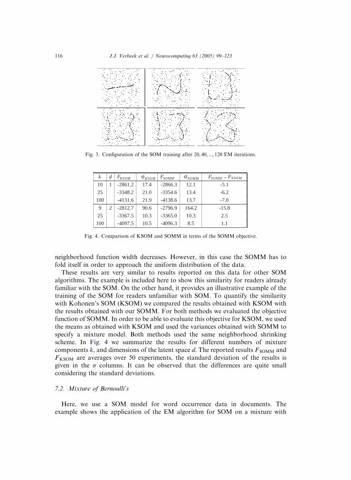
Fig. 3 shows the same experiment but with 50 Gaussians placed at a regularintervals in a 1d latent space. Here, we showed the configuration after each 20iterations. Again, we can observe the SOMM spreading out over the data as the

Fig. 2. Configuration of the SOM training after 10; 20; :::; 60 EM iterations.

ARTICLE IN PRESS

Fig. 3. Configuration of the SOM training after 20; 40; :::; 120 EM iterations.

k d FKSOM σKSOM σSOMMFSOMM FSOMM_ FKSOM

10 1 -2861.2 17.4 -2866.3 12.1 -5.1

25 -3348.2 21.0 -3354.6 13.4 -6.2

100 -4131.6 21.9 -4138.6 13.7 -7.0

9 2 -2812.7 90.6 -2796.9 164.2 -15.8

25 -3367.5 10.3 -3365.0 10.3 2.5

100 -4097.5 10.5 -4096.3 8.5 1.1

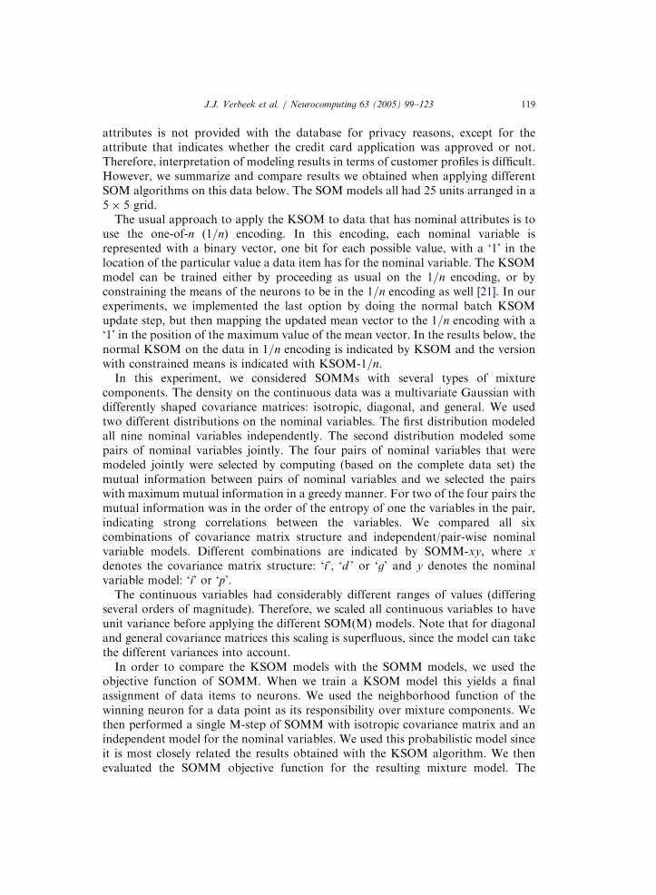
Fig. 4. Comparison of KSOM and SOMM in terms of the SOMM objective.


neighborhood function width decreases. However, in this case the SOMM has tofold itself in order to approach the uniform distribution of the data.

These results are very similar to results reported on this data for other SOMalgorithms. The example is included here to show this similarity for readers alreadyfamiliar with the SOM. On the other hand, it provides an illustrative example of thetraining of the SOM for readers unfamiliar with SOM. To quantify the similaritywith Kohonen’s SOM (KSOM) we compared the results obtained with KSOM withthe results obtained with our SOMM. For both methods we evaluated the objectivefunction of SOMM. In order to be able to evaluate this objective for KSOM, we usedthe means as obtained with KSOM and used the variances obtained with SOMM tospecify a mixture model. Both methods used the same neighborhood shrinkingscheme. In Fig. 4 we summarize the results for different numbers of mixturecomponents k, and dimensions of the latent space d. The reported results FSOMM andFKSOM are averages over 50 experiments, the standard deviation of the results isgiven in the s columns. It can be observed that the differences are quite smallconsidering the standard deviations.

7.2. Mixture of Bernoulli’s

Here, we use a SOM model for word occurrence data in documents. Theexample shows the application of the EM algorithm for SOM on a mixture with

ARTICLE IN PRESS


non-Gaussian components. The data consists of a matrix with entries that are eitherzero or one. Each row represents a word and each column represents a document. Aone indicates that the specific word occurs in a specific document. Thus, the wordsare the data items and the occurrence in documents are the features. The wordoccurrence data were obtained from the 20 newsgroup dataset.2 The data setcontains occurrence of 100 words in 16 242 newsgroup postings.

We use very simple mixture components that assume independence between all thefeatures and each feature is Bernoulli distributed. We use N to indicate the numberof words and D to denote the number of documents. Words are indexed by n and weuse xd

n 2 f0; 1g to denote the value of the dth feature (presence in document d) of thenth word xn. The probability of the dth feature being ‘1’ according to the sth mixturecomponent is denoted psd . Formally, we have

pðxnjsÞ ¼YD

d¼1

pxd

n

sd ð1� psd Þð1�xd

n Þ:

The mixing weights of all k ¼ 25 components were taken equal.The EM algorithm to train this model is particularly simple. For the E-step we

need the posteriors pðsjxnÞ which can be computed using Bayes rule

pðsjxÞ ¼pðxjsÞpsPs pðxjsÞps

:

In the M-step we have to maximize the expected joint log-likelihood w.r.t. theparameters psd . Which yields:

psd ¼

Pnqnsx

dnP

nqns

;

which is simply the relative frequency of the occurrence of the words in document d

where all the words are weighted by the responsibility qns.Due to the huge dimensionality of this data, the posteriors are quite peaked,

i.e. the posteriors have very low entropy resulting in gn almost equal to one of the gs.Although the obtained assignment of words to components is sensible, the latentcoordinates obtained with (5) are less useful. This is because peaked posteriors willdrive the gn close to one of the gs, and thus plotting the words at the correspondingcoordinates gn will result in plotting the words with high posterior for the samecomponent on top of each other. In order to reduce this problem, for visualizationwe did not use the actual posterior but the distribution p0ðsjxnÞ / pðsjxnÞ

a for ao1such that the entropies of the p0ðsjxnÞ were close to two bits.3 In Fig. 5 we plotted thewords at their expected latent coordinate, the bottom plot zooms in on areaindicated by the box in the top plot.

2The 20-newsgroup dataset is available through the internet at: http://www.ai.mit.edu/�jrennie/

20Newsgroups/.3The justification for using the normalized exponentiated posteriors is that if we have a distribution and

want the distribution that is closest in Kullback–Leiber sense to the original under a constraint on the

entropy, then we should use the normalized exponentiated distribution.

http://www.ai.mit.edu/jrennie/20Newsgroups/



ARTICLE IN PRESS

aids

baseball

bmw

cancer

car

dealerengine

fans

games

hit

hockey

honda launch

league

lunar

marsmission moon

msg

nasa

nhl

oil

orbit

players

puck

satellite

season

shuttle

solar

team

vitamin

win

won

Fig. 5. Self-organizing Bernoulli models, k ¼ 25. Bottom plot displays area in the box in the top plot.

Note that the ambiguous word ‘win’ (referring to the operating system ‘windows’ and to ‘winning’ a game)

is located between the computer terms (lower and middle right area) and the sports terms (upper right

area).


7.3. Modeling credit card application data

In this section we consider a self-organizing mixture model for data of 690 creditcard applications. The data set is available from the UCI machine learningrepository [4]. The data has six numerical features and nine nominal attributes. Forsome records the values of one or more attributes are missing, in the example belowwe removed these cases from the data set for simplicity. The meaning of the

ARTICLE IN PRESS


attributes is not provided with the database for privacy reasons, except for theattribute that indicates whether the credit card application was approved or not.Therefore, interpretation of modeling results in terms of customer profiles is difficult.However, we summarize and compare results we obtained when applying differentSOM algorithms on this data below. The SOM models all had 25 units arranged in a5� 5 grid.

The usual approach to apply the KSOM to data that has nominal attributes is touse the one-of-n (1=n) encoding. In this encoding, each nominal variable isrepresented with a binary vector, one bit for each possible value, with a ‘1’ in thelocation of the particular value a data item has for the nominal variable. The KSOMmodel can be trained either by proceeding as usual on the 1=n encoding, or byconstraining the means of the neurons to be in the 1=n encoding as well [21]. In ourexperiments, we implemented the last option by doing the normal batch KSOMupdate step, but then mapping the updated mean vector to the 1=n encoding with a‘1’ in the position of the maximum value of the mean vector. In the results below, thenormal KSOM on the data in 1=n encoding is indicated by KSOM and the versionwith constrained means is indicated with KSOM-1=n.

In this experiment, we considered SOMMs with several types of mixturecomponents. The density on the continuous data was a multivariate Gaussian withdifferently shaped covariance matrices: isotropic, diagonal, and general. We usedtwo different distributions on the nominal variables. The first distribution modeledall nine nominal variables independently. The second distribution modeled somepairs of nominal variables jointly. The four pairs of nominal variables that weremodeled jointly were selected by computing (based on the complete data set) themutual information between pairs of nominal variables and we selected the pairswith maximum mutual information in a greedy manner. For two of the four pairs themutual information was in the order of the entropy of one the variables in the pair,indicating strong correlations between the variables. We compared all sixcombinations of covariance matrix structure and independent/pair-wise nominalvariable models. Different combinations are indicated by SOMM-xy, where x

denotes the covariance matrix structure: ‘i’, ‘d ’ or ‘g’ and y denotes the nominalvariable model: ‘i’ or ‘p’.

The continuous variables had considerably different ranges of values (differingseveral orders of magnitude). Therefore, we scaled all continuous variables to haveunit variance before applying the different SOM(M) models. Note that for diagonaland general covariance matrices this scaling is superfluous, since the model can takethe different variances into account.

In order to compare the KSOM models with the SOMM models, we used theobjective function of SOMM. When we train a KSOM model this yields a finalassignment of data items to neurons. We used the neighborhood function of thewinning neuron for a data point as its responsibility over mixture components. Wethen performed a single M-step of SOMM with isotropic covariance matrix and anindependent model for the nominal variables. We used this probabilistic model sinceit is most closely related the results obtained with the KSOM algorithm. We thenevaluated the SOMM objective function for the resulting mixture model. The

ARTICLE IN PRESS

method F D

KSOM _6070.0 443.1

KSOM-1/n _6389.8 532.5

SOMM-ii _5678.8 297.2

SOMM-di _1481.3 380.3

SOMM-gi _1398.3 411.7

SOMM-ip _5147.2 232.1

SOMM-dp _1001.9 342.8

SOMM-gp _1096.4 342.5

Fig. 6. Comparison in terms of the SOMM objective F and the penalty term D.


resulting averages of the SOMM objective function F and the penalty term D for thedifferent models are presented in Fig. 6. Averages were taken over 20 experiments,each time selecting a random subset of 620 of the total 653 records. The resultssupport two conclusions.

First, when using independent distributions for the nominal and isotropiccovariance matrix for the continuous variables, we see that the SOMM-ii algorithmobtains higher objective values than the KSOM algorithms. The KSOM yields betterresults than the KSOM-1=n algorithm. Also taking into account the differences inthe penalty terms, we can conclude that on average the SOMM models yield both ahigher likelihood and better topology preservation.

Second, using models that use more expressive component densities we can obtainconsiderably higher scores of the objective function. In particular the models that donot assume equal variance in all continuous variables (isotropic covariance) obtainrelatively high scores. This indicates that these models give a much better fit on thedata and thus that they can provide more realistic descriptions of the customers inthe clusters.

8. Conclusions

We showed how we can change any mixture model for which we have an EMalgorithm into a SOM version by a simple modification of the E-step of the EMalgorithm. The use of mixture models as basis for SOMs allows for easy design ofdivergence measures by designing a generative model for the data based on priorknowledge and/or assumptions. The EM framework allows one to deal with missingdata in a principled way, by estimating in each EM iteration the missing values basedon the current parameters of the mixture model. The objective function is in a clearmanner related to the data log-likelihood under the mixture model. In our view, themodified EM algorithm for SOM does not come with any drawbacks as compared toexisting SOM algorithms. In our approach, it is not obvious how hyperparameterssuch as the neighborhood width or the number of components could be set in anautomatic manner. For the GTM, Bayesian techniques can be used to set

ARTICLE IN PRESS


hyperparameters, such as a penalty term on the smoothness of the nonlinear basisfunctions. However, such Bayesian techniques are computationally expensive. Insome applications, the simplicity of the SOMM might therefore be preferred,depending on the computational resources.

Acknowledgements

This research is supported by the Technology Foundation STW (Project No.AIF4997) applied science division of NWO and the technology program of theDutch Ministry of Economic Affairs. We like to thank the organizers of ESANN2003 for inviting us to submit this extended version of our paper [27] toNeurocomputing. We would also like to thank the reviewers for their detailedcomments and suggestions.

References

[1] F. Anouar, F. Badran, S. Thiria, Probabilistic self-organizing map and radial basis function

networks, Neurocomputing 20 (1–3) (1998) 83–96.

[2] C.M. Bishop, M. Svensen, C.K.I. Williams, Developments of the generative topographic mapping,

Neurocomputing 21 (1998) 203–224.

[3] C.M. Bishop, M. Svensen, C.K.I. Williams, GTM: the generative topographic mapping, Neural

Comput. 10 (1998) 215–234.

[4] C.L. Blake, C.J. Merz, UCI repository of machine learning databases, hhttp://www.ics.uci.edu/

�mlearn/MLRepository.htmli 1998.

[5] G. Celeux, F. Forbes, N. Payrard, EM procedures using mean field-like approximations for Markov

model-based image segmentation, Pattern Recognition 36 (2003) 131–144.

[6] T. Cover, J. Thomas, Elements of Information Theory, Wiley, New York, 1991.

[7] A.P. Dempster, N.M. Laird, D.B. Rubin, Maximum likelihood from incomplete data via the EM

algorithm, J. Roy. Statist. Soc. 39 (1) (1977) 1–38.

[8] Z. Ghahramani, M.I. Jordan, Supervised learning from incomplete data via an EM approach, in: J.D.

Cowan, G. Tesauro, J. Alspector (Eds.), Advances in Neural Information Processing Systems, vol. 6,

Morgan Kaufmann, Los Altos, CA, 1994, pp. 120–127.

[9] M. Girolami, The topographic organisation and visualisation of binary data using multivariate-

Bernoulli latent variable models, IEEE Trans. Neural Networks 12 (6) (2001) 1367–1374.

[10] T. Graepel, M. Burger, K. Obermayer, Self-organizing maps: generalizations and new optimization

techniques, Neurocomputing 21 (1998) 173–190.

[11] T. Heskes, Self-organizing maps, vector quantization, and mixture modeling, IEEE Trans. Neural

Networks 12 (2001) 1299–1305.

[12] M.I. Jordan, Z. Ghahramani, T. Jaakola, L.K. Saul, An introduction to variational methods for

graphical models, Mach. Learn. 37 (1999) 183–233.

[13] A. Kaban, M. Girolami, A combined latent class and trait model for the analysis and visualization of

discrete data, IEEE Trans. Pattern Anal. Mach. Intell. 23 (2001) 859–872.

[14] M.J. Kearns, Y. Mansour, A.Y. Ng, An information-theoretic analysis of hard and soft assignment

methods for clustering, in: M.I. Jordan (Ed.), Learning in Graphical Models, Kluwer, Dordrecht,

1998, pp. 495–520.

[15] T. Kohonen, Self-organizing Maps, Springer, Berlin, 2001.

[16] T. Kohonen, S. Kaski, H. Lappalainen, Self-organized formation of various invariant-feature filters

in the adaptive subspace SOM, Neural Comput. 9 (6) (1997) 1321–1344.

http://www.ics.uci.edu/mlearn/MLRepository.html

http://www.ics.uci.edu/mlearn/MLRepository.html

ARTICLE IN PRESS


[17] T. Kostiainen, J. Lampinen, On the generative probability density model in the self-organizing map,

Neurocomputing 48 (2002) 217–228.

[18] J. Laaksonen, K. Koskela, S. Laakso, E. Oja, Self-organizing maps as a relevance feedback technique

in content-based image retrieval, Pattern Anal. Appl. 4 (2+3) (2001) 140–152.

[19] G.J. McLachlan, D. Peel, Finite Mixture Models, Wiley, New York, 2000.

[20] R.M. Neal, G.E. Hinton, A view of the EM algorithm that justifies incremental, sparse, and other

variants, in: M.I. Jordan (Ed.), Learning in Graphical Models, Kluwer, Dordrecht, 1998, pp.

355–368.

[21] S. Negri, L. Belanche, Heterogeneous Kohonen networks, in: Connectionist Models of Neurons,

Learning Processes and Artificial Intelligence: Sixth International Work Conference on Artificial and

Natural Neural Networks, Lecture Notes in Computer Science, vol. 2084, Springer, Berlin, 2001, pp.

243–252.

[22] D. De Ridder, J. Kittler, O. Lemmers, R.P.W. Duin, The adaptive subspace map for texture

segmentation, in: A. Sanfeliu, J.J. Villanueve, M. Vanrell, R. Alquezar, J.O. Eklundh, Y. Aloimonos

(Eds.), Proceedings of the 15th IAPR International Conference on Pattern Recognition, IEEE

Computer Society Press, Silver Spring, MD, 2000, pp. 216–220.

[23] S.T. Roweis, L.K. Saul, G.E. Hinton, Global coordination of local linear models, in: T.G. Dietterich,

S. Becker, Z. Ghahramani (Eds.), Advances in Neural Information Processing Systems 14, MIT

Press, Cambridge, MA, 2002.

[24] M.E. Tipping, C.M. Bishop, Mixtures of probabilistic principal component analysers, Neural

Computation 11 (2) (1999) 443–482.

[25] A. Utsugi, Density estimation by mixture models with smoothing priors, Neural Comput. 10 (8)

(1998) 2115–2135.

[26] J.J. Verbeek, N. Vlassis, B.J.A. Krose, Coordinating principal component analyzers, in: J.R.

Dorronsoro (Ed.), Proceedings of the International Conference on Artificial Neural Networks,

Madrid, Spain, Springer, Berlin, 2002, pp. 914–919.

[27] J.J. Verbeek, N. Vlassis, B.J.A. Krose, Self-organization by optimizing free-energy, in: M. Verleysen

(Ed.), Proceedings of European Symposium on Artificial Neural Networks, D-side, Evere, Belgium,

2003.

[28] J.J. Verbeek, N. Vlassis, J.R.J. Nunnink, A variational EM algorithm for large-scale mixture

modeling, in: Proceedings of the Eighth Annual Conference of the Advanced School for Computing

and Imaging (ASCI 2003), Het Heijderbos, Heijen, 2003.

Jakob Verbeek received a cum laude Masters degree in Artificial Intelligence

(1998) and a cum laude Master of Logic degree (2000), both at the University

of Amsterdam, The Netherlands. Since 2000 he is a Ph.D. student in the

Advanced School for Computing and Imaging, working in the Intelligent

Autonomous Systems group at the University of Amsterdam. His research

interests include nonlinear feature extraction, density estimation and machine

learning in general.

Nikos Vlassis received a M.Sc. in Electrical and Computer Engineering in 1993

and a Ph.D. in Artificial Intelligence in 1998, both from the National

Technical University of Athens, Greece. In 1998 he joined the Intelligent

Autonomous Systems Group at the Department of Computer Science of the

University of Amsterdam, The Netherlands, where he is currently holding an

assistant professor position. In 1998, he received the Dimitris Chorafas

Foundation prize (Luzern, Switzerland) for young researchers in Engineering

and Technology. His current research interests are in machine learning,

multiagent systems, and autonomous robots.

ARTICLE IN PRESS


Ben Krose graduated at the Technical University Delft in the Applied Physics

Department on the subject of Statistical Pattern Recognition and Image

Processing. He obtained his Ph.D. from the same university, but in the

Department of Industrial Design Engineering, in a project on human

perception. From 1986 to 1988 he stayed as a postdoc at Caltech, Pasadena,

in the laboratory of Bela Julesz, where he did more psychophysics and worked

on artificial neural networks. In his current position as Associate Professor at

the University of Amsterdam he leads a group on learning in autonomous

systems. He published numerous papers in the fields of psychophysics,

learning and autonomous systems.

Documents

Self-organizing mixture models