Selecting Design Objectives for an Integrated Guidance System of a Commercial Launch Vehicle with Application of GPS Technologies

Send Orders for Reprints to [email protected]

6 The Open Aerospace Engineering Journal, 2013, 6, 6-19

1874-1460/13 2013 Bentham Open

Open Access

Selecting Design Objectives for an Integrated Guidance System of a Commercial Launch Vehicle with Application of GPS Technologies

Nickolay Zosimovych*

Mechanical and Automobile Department, School of Engineering and Technology, Sharda University, Greater Noida,

Uttar Pradesh, 201301, India

Abstract: In this article have been proposed the design objectives for an integrated guidance system of a commercial launch vehicle with application of GPS technologies and has been set a technical problem of the

conceptual design of an integrated navigation system for the space launch vehicle qualified to inject small artificial

Earth satellites into low and medium circular orbits. The conceptual design of the integrated navigation system based on GPS technology involves determination of its structure, models and algorithms, providing the

required accuracy and reliability in injecting payloads with due regard to restrictions on weight and dimensions of the system.

Keywords: A gimbaled inertial navigation system (GINS), global positioning system (GPS), an inertial navigation

system (INS), mathematical model (MM), navigation, pseudo-range, pseudo-velocity, the launch vehicle.

1. INTRODUCTION

A key tendency in the development of affordable modern

navigation systems is displayed by the use of integrated

GPS/INS navigation systems consisting of a gimbaled

inertial navigation system (GINS) and a multichannel GPS

receiver [1]. The investigations show [2, 3], that such

systems of navigation sensors with their relatively low cost

are able to provide the required accuracy of navigation for a

wide range of highly maneuverable objects, such as

airplanes, helicopters, airborne precision-guided weapons,

spacecrafts, launch vehicles and recoverable orbital carriers.

The study of applications of GPS navigation technologies

for highly dynamic objects ultimately comes to solving the

following problems [4]:

1. Creation of quality standards (optimality criteria) for

solving the navigation task depending on the type of

an object, its trajectory characteristics and restrictions

on the weights, dimensions, costs, and reliability of

the navigation system.

2. Selection and justification of the system interconnect-

ing the GPS-receiver and GINS: uncoupled, loosely

coupled, tightly coupled (ultra-tightly coupled).

3. Making mathematical models (MM) of an object's

motion, including models of external factors beyond

control influencing object (disturbances). This

requires to make two types of object models: the most

detailed and complete one, which will be later

*Address correspondence to this author at the Mechanical and Automobile

Department, School of Engineering and Technology, Sharda University,

Greater Noida, Uttar Pradesh, 201301, India; Tel: +91 956 055 8421;

E-mail: [email protected]

included in the model of the environment when

simulating the operation of an integrated system, and

a so-called on-board model, which is much simpler

and more compact than the former one, and will be

used in the future to solve the navigation problem

being a part of the on-board software.

4. Making MM for GINS considering the use of

gyroscopes and accelerometers (i.e. it is required to

make a model for navigation measurements supplied

by GINS, taking into account systematic (drift) and

random measurement errors).

5. Making a model of the navigation field of GPS,

including system architecture, a method of calculating

ephemeris of navigation satellites in consideration of

possible errors, clock drifts on board the navigation

satellites, and taking into account the conditions of

geometric visibility of a navigation satellite on

different parts of the trajectory of a highly dynamic

object.

6. Making a model of a multichannel GPS receiver,

including models of code measurements (pseudo-

range and pseudo-velocity) and, if necessary, phase

measurements, including the whole range of chance

and indeterminate factors beyond control, existing

when such measurements are conducted (such as

multipath effect).

7. Choosing an algorithm to process measured data in an

integrated system in agreement with the speed-of-

response requirement (the possibility to process data

in real time) and demand accuracy in solving a

navigation task.

Selecting Design Objectives for an Integrated Guidance System The Open Aerospace Engineering Journal, 2013, Volume 6 7

8. Creating an object-oriented computer complex for the

implementation of the above models and algorithms

with the objective to model the process of functioning

of the integrated navigation system of a highly

dynamic object.

Let's consider the above objectives, regarding the

peculiarities of the subject of inquiry, namely a commercial

launch vehicle, designed to launch payloads into low Earth

orbit (LEO) or geostationary orbit (GSO), in more details.

Fig. (1). Launch vehicle Vega (Vettore Europeo di Generazione Avanzata, ASI&ESA) [5].

Within the framework of this study, we shall consider a

light launch vehicle which has been jointly developed by the

European Space Agency (ESA) and the Italian Space

Agency (ASI) since 1998 (Fig. 1). It is qualified to launch

satellites ranging from 300 kg to 2000 kg into low circular

polar orbits. As a rule, these are low cost projects conducted

by research organizations and universities monitoring the

Earth in scientific missions as well as spy satellites, scientific

and amateur satellites. The main characteristics of the launch

vehicle are given in Table 1. The launch vehicle Vega [5] is

the prototype of the vehicle under development.

The planned payload to be delivered by the launch

vehicle to a polar orbit at an altitude of ~700 km shall be

1500 kg. The launch vehicle is tailored for missions to low

Earth and Sun-synchronous orbits. During the first mission,

the light class launch vehicle is to launch the main payload, a

satellite weighing 400 kg, to an altitude of 1450 km with an

inclination of the orbit 71050

m. Unlike most single-body

launchers, this vehicle is to launch several spacecrafts. Here

are the main types of spacecrafts that can be a potential

payload [1]:

• microsatellites — up to 300 kg;

• mini satellites — between 300 and 1000 kg;

• small satellites —between 1000 and 2000 kg.

The launch vehicle under consideration is the smallest

one developed by ESA. We assume that the new launch

vehicle will be able to meet the demands of the market for

launching small research satellites and will enable

universities to conduct research in space. The launcher will

be primarily used for satellites that monitor the Earth

surface. The injection is conducted according to the most

popular and simplest (and the cheapest) scenario [6], more

specifically: the instrument unit and the navigation system

ride atop the 3rd stage of the launch vehicle.

Thus, launching until separation of the 4th stage carrying

payload is conducted in accordance with the data provided

by the navigation system which estimates 12 components of

the launcher state vector, including position, velocity,

orientation angles and angular velocities. Basically,

launching may be done upon implementation of any of the

possible algorithms, for example, a terminal one, that

provides accuracy of the 3rd stage launching to the

calculated point of separation of the 4th stage or the

traditional algorithm which minimizes the deviation of the

center of mass of the launcher from the preselected

programmed trajectory [5].

able 1. Key Specifications of the Vega Launch Vehicle [5]

Specification Values

Main technical specifications

Number of stages 4

Length 30 m

Diameter 3 m

First stage – 80

Length 10.5 m

Diameter 3.0 m

Sustainer Engine RDTT (solid fuel rocket engine)

Thrust 3040 k N

Burn time 107 s

Fuel Solid

Second stage – Zefiro 23

Length 7.5 m

Diameter 1.9 m


Thrust 1200 kN

Burn time 71.6 s

Fuel Solid

Third stage – Zefiro 9

Length 3.85 m

Diameter 1.9 m


Thrust 214 kN

Burn time 117 s

Fuel Solid

Fourth stage – AVUM

Length 1.74 m

Diameter 1.9 m

Sustainer Engine LRE AVUM

Thrust 2.45 kN

Burn time 315.2 s

Fuel UDMH

Oxidizer

The injection sequence which is being described here

supposes conducting the following procedures at peak

altitude reached by the 3rd stage, namely the computation of

the required orientation of the 4th stage and the computation

of the required impulse to transfer the payload carried by the

8 The Open Aerospace Engineering Journal, 2013, Volume 6 Nickolay Zosimovych

4th stage to an orbit of an artificial satellite of the Earth from

the final point reached by the 3rd stage. Thus, the transfer of

the 4th stage from the end-point of lifting the 3rd stage to an

orbit of injecting the payload is performed by the software,

i.e. without the use of navigation data, and thus the accuracy

of injection of the payload into the required orbit is

determined by two factors: the accuracy of lifting the 3rd

stage in the predetermined terminal point and the accuracy of

the program control in the 4th stage [5].

2. PROBLEM SETTING

From the standpoint of the problem concerned, namely

the synthesis of the navigational algorithm of the space

launcher in the proposed injection sequence we are interested

only in the first factor, i.e. accuracy of lifting of the 3rd stage

to the point of separation of 4th stage. This accuracy, other

conditions being equal, is determined by the precision of

solving a navigation task in lifting the 3rd stage in

consideration of both components: the center of mass and the

velocity of the stage. They predetermine the required

impulse for the 4th stage [7].

Thus, we may determine the main criterion of the

accuracy of the navigation task in relation to the integrated

inertial navigation system of the space launch vehicle: we

need to ensure maximum accuracy in determining the

position and velocity vectors of the 3rd stage of the launch

vehicle in the exo-atmospheric phase of the mission for the

selection of navigation coordinate system. Clearly, this

accuracy, in its turn, other things being equal, depends upon

the accuracy of the initial conditions of travel of the 3rd

stage, or in other words, the accuracy of navigation on the

previous atmospheric phase of the mission [1].

Consequently, in the case of the proposed injection

sequence, the simplest and most obvious criterion for

evaluation of the accuracy of the synthesized system should

be adopted. It is required to ensure maximum accuracy in

determining the vectors of position and the center of mass

velocity of the launcher during the flight of the1st-3rd stages,

i.e. in atmospheric and exo-atmospheric phases of the

mission. This accuracy can be characterized by the value of

the dispersions posteriori of the corresponding components

of the mentioned vectors [8]. Now let's consider the possible

integration schemes for GINS and GPS receiver with respect

to this technical problem. As it has been aforementioned,

currently we can think of three possible integration schemes

as follows [9-13]:

• uncoupled (separated subsystems);

• loosely coupled;

• tightly coupled (ultra-tightly coupled).

Let's consider the peculiarities of these systems.

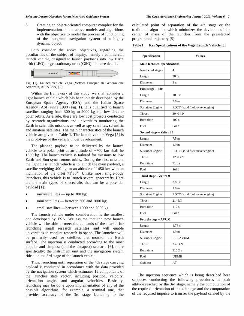
Uncoupled systems are the simplest option for

simultaneous use of INS and GPS receiver (Fig. 2) [14].

Both systems operate independently. But, as INS errors

constantly accumulate, it is eventually necessary to make

correction of INS according to data provided by the GPS

receiver. Creating such architecture requires minimal

changes to the hardware and the software.

Fig. (2). Uncoupled system with simultaneous use of INS and GPS receiver.

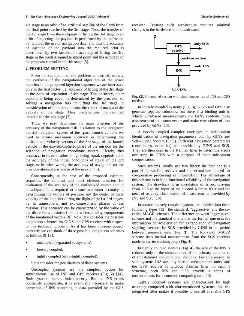
In loosely coupled systems (Fig. 3), GINS and GPS also

generate separate solutions, but there is a binding unit in

which GPS-based measurements and GINS readouts make

assessment of the status vector and make corrections of data

provided by GINS [14].

A loosely coupled complex envisages an independent

identification of navigation parameters both by GINS and

Self-Guided System (SGS). Different navigation parameters

(coordinates, velocities) are provided by GINS and SGS.

They are then used in the Kalman filter to determine errors

occurring in GINS with a purpose of their subsequent

compensation.

Such systems usually use two filters: the first one is a

part of the satellite receiver and the second one is used for

co-operative processing of information. The advantage of

this scheme is in high functional reliability of the navigation

system. The drawback is in correlation of errors, arriving

from SGS to the input of the second Kalman filter and the

need of strict synchronization of measurements provided by

INS and SGS [14].

In sources loosely coupled systems are divided into three

following types [12]: the standard, "aggressive" and the so-

called MAGR schemes. The difference between "aggressive"

scheme and the standard one is that the former one uses the

information on acceleration for extrapolation of navigation

sighting executed by SGS provided by GINS in the period

between measurements (Fig. 3). The Rockwell MAGR

scheme uses inertial measurement from the SGS receiver

made in carrier tracking loop (Fig. 4).

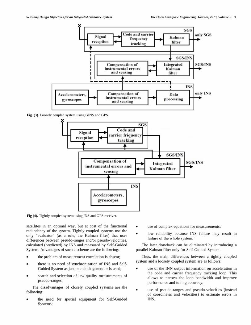
In tightly coupled systems (Fig. 4), the role of the INS is

reduced only to the measurement of the primary parameters

of translational and rotational motions. For this reason, in

such systems INS are only inertial measurement units, and

the GPS receiver is without Kalman filter. In such a

structure, both INS and SGS provide a series of

measurements for a common computing unit [14].

Tightly coupled systems are characterized by high

accuracy compared with aforementioned systems, and the

integrated filter makes it possible to use all available GPS


satellites in an optimal way, but at cost of the functional

redundancy of the system. Tightly coupled systems use the

only "evaluator" (as a rule, the Kalman filter) that uses

differences between pseudo-ranges and/or pseudo-velocities,

calculated (predicted) by INS and measured by Self-Guided

System. Advantages of such a scheme are the following:

• the problem of measurement correlation is absent;

• there is no need of synchronization of INS and Self-

Guided System as just one clock generator is used;

• search and selection of law quality measurements of

pseudo-ranges.

The disadvantages of closely coupled systems are the

following:

• the need for special equipment for Self-Guided

Systems;

• use of complex equations for measurements;

• low reliability because INS failure may result in

failure of the whole system.

The later drawback can be eliminated by introducing a

parallel Kalman filter only for Self-Guided System.

Thus, the main differences between a tightly coupled

system and a loosely coupled system are as follows:

• use of the INN output information on acceleration in

the code and carrier frequency tracking loop. This

allows to narrow the loop bandwidth and improve

performance and tuning accuracy;

• use of pseudo-ranges and pseudo-velocities (instead

of coordinates and velocities) to estimate errors in

INS.

Fig. (3). Loosely coupled system using GINS and GPS.

Fig (4). Tightly coupled system using INS and GPS receiver.


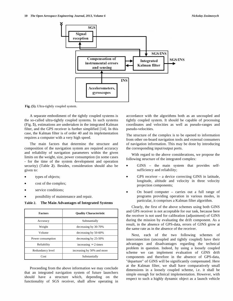
A separate embodiment of the tightly coupled systems is

the so-called ultra-tightly coupled systems. In such systems

(Fig. 5), estimations are undertaken in the integrated Kalman

filter, and the GPS receiver is further simplified [14]. In this

case, the Kalman filter is of order 40 and its implementation

requires a computer with a very high speed.

The main factors that determine the structure and

composition of the navigation system are required accuracy

and reliability of navigation parameters within the given

limits on the weight, size, power consumption (in some cases

- for the time of the system development and operation

security) (Table 2). Besides, consideration should also be

given to:

• types of objects;

• cost of the complex;

• service conditions;

• possibility of maintenance and repair.

Table 2. The Main Advantages of Integrated Systems

Factors Quality Characteristic

Accuracy Substantially

Weight decreasing by 30-70%

Volume decreasing by 50-60%

Power consumption decreasing by 25-50%

Reliability increasing 2 times

Redundancy level increasing by 50% and more

Cost Substantially

Proceeding from the above information we may conclude

that an integrated navigation system of future launchers

should have a structure which, depending on the

functionality of SGS receiver, shall allow operating in

accordance with the algorithms both as an uncoupled and

tightly coupled system. It should be capable of processing

coordinates and velocities as well as pseudo-ranges and

pseudo-velocities.

The structure of the complex is to be opened to information

from other on-board navigation tools and external consumers

of navigation information. This may be done by introducing

the corresponding input/output ports.

With regard to the above considerations, we propose the

following structure of the integrated complex:

• GINS – the main system that provides self-

sufficiency and reliability;

• GPS receiver – a device correcting GINS in latitude,

longitude, altitude and velocity in three velocity

projection components;

• On board computer – carries out a full range of

programs providing operation in various modes, in

particular, it comprises a Kalman filter algorithm.

Clearly, the first of the above schemes using both GINS

and GPS receiver is not acceptable for our task, because here

the receiver is not used for calibration (adjustment) of GINS

during the mission by evaluating the drift component. As a

result, in the absence of GPS-data, errors of GINS grow at

the same rate as in the absence of the receiver.

Next, each of the two following schemes of

interconnection (uncoupled and tightly coupled) have their

advantages and disadvantages regarding the technical

problem in question. Indeed, by using a loosely coupled

scheme we can implement evaluation of GINS drift

components and therefore in the absence of GPS-data,

"departure" of GINS will be significantly compensated. Here

at the Kalman filter, we shall have comparatively small

dimensions in a loosely coupled scheme, i.e. it shall be

simple enough for technical implementation. However, with

respect to such a highly dynamic object as a launch vehicle

Fig. (5). Ultra-tightly coupled system.


in the end it turns out that the accuracy of executing a

navigation task is determined by errors of a multi-channel

receiver. But with regard to peculiarities of object's motions

and flight time limitations, this accuracy may not be

sufficient to provide the required accuracy of the payload

injection because in loosely coupled scheme receiver errors

are not evaluated. Which means that the apriori rejection of a

tightly coupled scheme as the most challenging to implement

is not a sufficient reason? Indeed, if the flight conditions

allow us to estimate the actual values of systematic errors in

measurement of pseudo-range and pseudo-velocity, the

tightly coupled scheme allows us obtain the highest possible

accuracy of navigation.

Here, certainly appear additional problems with the big

Kalman filter and mathematical models of systematic

measurements of pseudo-range and pseudo-velocity caused

by atmospheric delays, receiver clock drifts, multipath, etc.

Thus, we conclude that in the present study it is

appropriate to examine both schemes of interconnection:

tightly and loosely coupled, and based on the results of

simulation, conclusions are drawn in favor of one of the

possible solutions. Let us briefly examine the

scientific and technical problems arising when making the

corresponding models and algorithms.

MM of spatial motion of center of mass and relative to

center of mass of a solid launch vehicle is well known and

widely described in sources. The greatest difficulty in the

implementation of such a model as a part of the model of the

environment, represents a model of a solid-propellant rocket

engine with thrust distribution in respect to the nominal

model in mind and the model of stage separation from the

point of view of the influence of disturbing moments that

arise when dividing into initial conditions of the motion of

the next stage.

The key question here is the question of the appropriate

level of complexity of the "on-board" model of launcher

movement used in the Kalman filter to predict its movement.

The answer to this question can also be obtained by

simulation of the navigation process.

Mathematical models of GINS are currently also well

described in sources, e.g. [15-18]. At the same time MM of

GINS drift depends essentially on the type of gyro units and

accelerometers used in GINS. In other words, a so-called

non-modelable constant is always present in the drift model.

It ultimately determines the possibility of GINS alignment

during flight. Because of apriori uncertainty of this

component, it is appropriate to select the parameters of the

shaping filter in such a way as to ensure the least impact on

the accuracy of estimation. In other words, it is advisable in

this case to receive a guaranteed result.

MM of the navigation field created by the GPS and

GLONASS systems, including the visibility of individual

satellites during the flight is also well characterized and can

be implemented as it is described in the source [14, 19].

With the implementation of this model, as well as with the

implementation of the receiver model, we shall further

assume that we may use only code measurements: pseudo-

range and pseudo-velocity. Next we shall assume a

possibility to use dual-frequency measurements to practically

exclude ionospheric and tropospheric delays, and the lack of

selective access. With this approach, the main factor

determining the possibility of GPS-navigation for the

problem in question is the analysis of geometric visibility

conditions of navigation satellites with the possible loss of

communication, which is determined by the specific

dynamics of the object. In this case, we shall assume that the

uncertainty in searching a navigation constellation due to the

Doppler shift of the carrier has already been overcome, and

the receiver is synchronized in frequency, phase and code

[1].

Now we shall move on to the analysis of the possible

algorithms for processing navigation information. Due to the

specific nature of the set task that requires processing of

navigational measurements as soon as they are received, we

will consider only the recursive modification of the

following algorithms: Bayesian (and Kalman filter) or

recurrent modification of the least square method, is not

required as we know an additional apriori information about

the state vector of the object. Thus, attention should be paid

to the fact that an appropriate algorithm is to be implemented

by the on board computer (OC) and, consequently, such

operations as matrix inversion, summing of numbers with

significantly different orders, etc should be excluded.

Existing experience in this field [20, 21] suggests that the

most appropriate modification of recursive algorithm for this

task is one that will allow measurements as if bound to a

definite time point by components. In this case, the result of

processing the regular components of the measurement,

"tied" to a given point in time, is seen as an apriori estimate

in the processing of a subsequent component. Another

important aspect in developing the processing algorithm is

different speed with which navigation measurements enter.

Thus, measurements generated in GINS enter with a

relatively high frequency (200 Hz) while the code

measurements from the receiver generally enter with a

frequency of 1 Hz and the fact that GPS delays

measurements may require special modifications of the

recursive information algorithm. Finally, essential is the

choice of a model predicting object's motion in the onboard

algorithm. Moreover, generally there can be several different

prediction models which will be used for different phases of

flight: atmospheric and exo-atmospheric.

Next, the different prediction models can be used when

using loosely coupled scheme of interconnection with the

different rates of data entry from the GINS and GPS

receiver.

Finally, the last aspect that we need to consider in setting

the technical problem in the present paper is the selection of

an approach to the shaping of an integrated navigation

system for a space launch vehicle with GPS technology. It is

important to stress once again, as mentioned earlier that the

term "shape" will encompass the structure, composition,

models and algorithms for integrated navigation system [1].

Obviously that with regard to the variety of different

physical nature of uncontrolled factors having an effect


within the framework of this problem, the nonlinear nature

of MM of subject's motion and nonlinear relationship

between the results of measurements and navigation

components of the state vector, the only reasonable approach

for solving the technical problems stated above is the

simulation of the operation of the system to be shaped.

The above statement makes it necessary to create a

special "tool" that shall ensure the implementation of the

chosen approach to the solution of the technical problem set.

This tool is a computer system with a fairly simple interface

allowing, nevertheless varying interactively source data and

parameters of the models and algorithms for analyzing and

modeling results presented in graphic and numeric forms.

Generally such a system must include two models: a model

of the environment and a model of a launcher board.

In more detail, this problem will be discussed later in the

chapter on modeling. Here we merely note that the model of

a launcher board should include in addition to the model

made by the navigation system, a model of the control

channel, including steering signal formation and an actuating

mechanism with the necessary detail level allowing the

exploration of the impact of errors on the accuracy of the

navigation controls.

For its part, a model of the environment should include as

much detailed model of the object, disturbances, and natural

and artificial navigation fields.

3. A MODEL OF GUIDED MOTION OF A LAUNCH VEHICLE DURING THE POWERED PORTION OF

FLIGHT

This section presents developed models, algorithms and

methods underlying the mathematical software designed for

simulation of guided flight during the powered portion of the

mission performed by a launch vehicle equipped with

various navigation systems. The need to introduce the

following material is determined, on the one hand, by

peculiarities of the main power and disturbing factors of

reducible models (operation of control loop by angular

motion, calculation of the mass and inertial characteristics,

modeling of thrust distribution), and, on the other hand, the

detailed elaboration of a model to provide solution to the

following tasks:

1. Simulation of the motion of the launch vehicle as a

rigid body in space with 6 degrees of freedom, taking

into account all the external disturbances.

2. The implementation of the control loop of the launch

vehicle with engines having fixed and rotary nozzles

which together with the drives are treated as dynamic

systems.

3. Simulation of the work of measuring equipment and

the on-board computer with regard to specific

character of their operation as digital devices.

4. Operation of programs and algorithms developed to

solve the target task by the launch vehicle (terminal

control algorithms, navigation algorithm) in the

framework of a model of the on-board computer.

5. Simulation of operation of the on-board integrated

navigation system, taking into account a wide range

of disturbing factors and errors made by measuring

equipment.

In accordance with the above information for the sake of

completeness further we shall give a brief, systematic

description of coordinate systems, mathematical models of

the launch vehicle's motion and disturbing factors, as well as

of the algorithms used for complex simulation of the guided

flight of the launch vehicle, will describe in detail

peculiarities of methods and numerical procedures suitable

for the specified objectives set before the development of

mathematical software.

Structurally, the chapter consists of descriptions of

movement patterns (unperturbed and perturbed motion) and

loop control system that ensures fulfillment of program

control on the basis of measurement and navigation data.

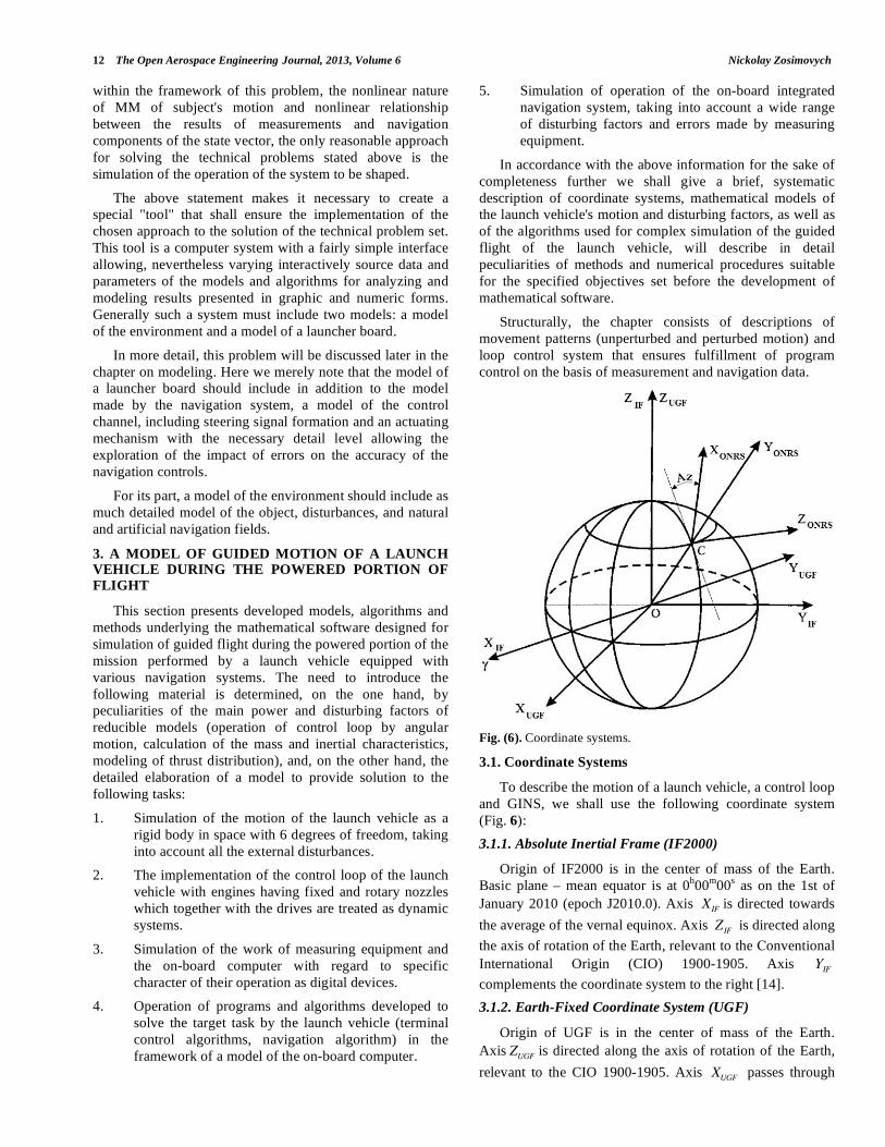
Fig. (6). Coordinate systems.

3.1. Coordinate Systems

To describe the motion of a launch vehicle, a control loop

and GINS, we shall use the following coordinate system

(Fig. 6):

3.1.1. Absolute Inertial Frame (IF2000)

Origin of IF2000 is in the center of mass of the Earth.

Basic plane – mean equator is at 0h00

m00

s as on the 1st of

January 2010 (epoch J2010.0). Axis XIF is directed towards

the average of the vernal equinox. Axis ZIF is directed along

the axis of rotation of the Earth, relevant to the onventional

International Origin (CIO) 1900-1905. Axis YIF

complements the coordinate system to the right [14].

3.1.2. Earth-Fixed Coordinate System (UGF)

Origin of UGF is in the center of mass of the Earth.

Axis ZUGF is directed along the axis of rotation of the Earth,

relevant to the CIO 1900-1905. Axis XUGF passes through


the Greenwich meridian, relevant to the CIO. Axis YUGF

complements the coordinate system to the right [21].

3.1.3. Inertial Navigation Reference System (INRS)

Origin of INRS is in the point of launching a launch

vehicle. Axis Y is directed along local vertical line. Axis X

makes an angle AZ with the direction to the north (azimuth

of launch angle). Axis Z complements the coordinate system

to the right [22].

3.1.4. Onboard Navigation Reference System (ONRS)

This reference system (RS) must coincide with INRS at

the moment of launching the launch vehicle and has to be

kept to the selected axis directions during its flight.

Sensitivity axes of accelerometers that measure the apparent

velocity increment of the launch vehicle (basic information

for INS) lie in the direction of the axes of the simulated RS

[21].

3.1.5. Body Frame (BF)

Origin BF for a target flying vehicle is in its center of

mass. Axes BF (XC ,YC ,ZC ) are axes of symmetry of the

flying vehicle [21].

We shall present equations describing transitions

between the Coordinate Systems used. With this purpose, we

introduce operator matrices of rotation around each axis at an

angle :

RX ( ) =1 0 00 cos( ) sin( )

0 sin( ) cos( )

,

RY ( ) =cos( ) 0 sin( )

0 1 0sin( ) 0 cos( )

,

RZ ( ) =cos( ) sin( ) 0

sin( ) cos( ) 0

0 0 1

.

Then the matrix of transition from the inertial to the

Greenwich Coordinate System AIFUGF

is written as follows

[3]:

AIFUGF

= RZ (GST ), (1)

where GST is Greenwich Sidereal Time.

Coordinates of the navigation satellites used by the

system GPS, as well as navigational estimates of the launch

vehicle's position and velocity supplied by the multi-channel

GPS receiver are set in one of the World Geodetic Systems:

WGS-84 or PP-90. To move from Greenwich Coordinate

System to the Coordinate System, the following equation is

used:

XWGS 84 = AUGFWGS 84XUGF , (2)

where the matrix of transition from the Greenwich

Coordinate System to the Coordinate System WGS-84

AUGFWGS 84

is written as follows [23]:

AUGFWGS 84

=

1 0 xp

0 1 yp

xp yp 1

,

xp , yp are the current coordinates of a pole .

Transition from INRS to WGS-84 is described by the

following equation:

XWGS 84*

= A X HCK + XWGS 84LP ,

AT= RY ( (90 + Az))RX ( )RZ ( 90),

XWGS 84 = AWGS 84WGS 84 XWGS 84

* ,

WGS 84WGS 84

= RZ ( Earth t),

(3)

where XWGS 84*

is a launch vehicle's state vector in "the

frozen" at the moment of start Coordinate System WGS-84;

XWGS 84LP

is the position of the launch point in WGS-84.

The matrix of transition from INRS to the Body Frame

AHCK

BF is written as follows [3]:

AHCK

BF= AX ( ) RZ ( ) RY ( ), (4)

where , , are Euler angles of launch vehicle's

orientation.

3.2. The Model of the Unperturbed Motion

In order to give a systematic presentation below we shall

give a full MM of unperturbed motion of the center of mass

of the launch vehicle and angular motion the launch vehicle

in an active phase. When considering the unperturbed

motion, we take into account the following power factors:

1. the attracting force of the Earth, taking into account

the non-spherical potential up to the 4th degree and

order including;

2. thrust of the launch vehicle according to the thrust

nominal profile and fuel mass flow;

3. aerodynamic force in accordance with the parameters

of the dynamic environment and coefficients of drag

force and lift specified in a table.

Furthermore when considering the unperturbed motion of

a launch vehicle we assume that the assembly of the launch

vehicle has been carried out without errors. All angular and

linear parameters correspond to the nominal levels and there

are no disturbing moments during separation of the stages.

3.3. The Equations of Motion of the Center of Mass

We shall use the MM of the launch vehicle's center mass

motion based on the laws of Newtonian mechanics,

according to which the model of the motion of a point

particle in INRS is written as follows [3]:


mX = Fii

, (5)

where m is the mass of the launcher;

X is the launcher position of the vector;

Fi are the forces acting on the launcher.

In the above models the accuracy of the motion of the

center of mass of the launch vehicle is determined by a

composition of forces to be taken into account during the

simulation on the basis of the duration of the active phase

and the need of the simulation accuracy. As it was noted

above, when considering the unperturbed motion we take

into account the following power factors:

• the attracting force of the Earth, taking into account

the non-spherical potential up to the 4th order

including;

• thrust of the propulsion system of the launch vehicle

according to the thrust nominal profile and fuel mass

flow;

• aerodynamic force in accordance with the parameters

of the dynamic environment and coefficients of drag

force and lift specified in a table.

Let us consider each of these factors separately.

3.3.1. Gravity

For representation let's expand the geo-potential into

spherical functions [24]:

U =μ

r1+

Cn0

a3r

n

Pn sin +

a3r

n

+ Pnm sin Cnm cosmL + dn sinmL( )

m=1

n

n=2

n=2

, (6)

where μ = fM is a product of gravitation constant by

terrestrial mass;

r,L, are respectively the geocentric radius, longitude and

latitude of the considered point in WGS-84;

Pn sin is Legendre polynomial of order n;

Pnm sin are associated spherical functions;

Cn0 ,Cnm ,dnm are dimensionless constants which characterize

the form and the gravitational field of the Earth.

Radial, meridional and normal components of the

acceleration of gravity can be calculated according to the

following formulae:

gr =UT

r, g =

1

r

UT , gL =1

r cos

UT

L. (7)

It should be noted that the integration of the equations of

motion of the center of mass in the launch vehicle is done in

INRS, while the calculation of the acceleration conditioned

by the gravity of the Earth is conducted in WGS-84 in

spherical coordinates. Accordingly, in order to determine the

projection of the acceleration on the axis of INRS we must

[25]:

1. Determine the coordinates of the center of mass of the

launcher in UGF in accordance with equations (3).

2. Calculate the spherical coordinates of the center of

mass of the launch vehicle in UGF:

r = x2 + y2 + z2 ,

L = arctgy

x,

= arctgz

x2 + y2.

(8)

1. Determine projection of the acceleration of the

spherical WGS-84, using the following equation:

x = r cosL cos

y = r sin L cos

z = r sin

2. Get the projections of acceleration in INRS, in

accordance with equations (3).

3.3.2. Thrust

Rocket thrust is generated on account of combustion of

fuel with mass flow rate ms and discharge of combustion

products through the nozzles at flow rate W .

Thrust at a certain altitude h is determined by the

following subjection [7]:

P(h) = msW + Sa (pa ph ), (9)

where pa is pressure at the nozzle exit; ph is pressure at a

given height h; Sa is nozzle exit area.

At sea level where ph = po , thrust is minimal:

P(0) = P0 = msW + Sa (pa ph ).

In vacuum where ph = 0, thrust reaches its maximum:

PV = msW + Sa pa .

Then the expression for P(h) shall be rewritten as

follows:

P(h) = PV Sa ph . (10)

The difference between thrusts at sea level and in

vacuum shall be PV P0 = Sa p0 dependent on nozzle exit

Sa , determining the engine critical altitude, i.e. its ability to

most effectively work in a rarefied atmosphere. The value

Sa determines the expansion ratio of a jet of flowing through

the nozzle gases and, consequently, the pressure pa in the

nozzle exit.

An important characteristic of the efficiency of the

engine is the specific thrust, i.e. a ratio of thrust to fuel

consumption per second [14]:


Py (h) =P(h)

mSg0= Py

pbSamSg0

,

where specific thrust in «vacuum»: Py =W

g0+p0SamSg0

.

The so-called "earth" specific thrust is always less than

the specific thrust in vacuum:

Py 0= Py

p0SamSg0

.

Attractive force direction is determined in Body Frame

related to a coordinate system independent of the orientation

of the longitudinal axis of the nozzle relative to the

longitudinal axis of the engine of the launch vehicle. When

considering the unperturbed motion of the launch vehicle,

angles of incidence of the engine are considered nominal and

the direction is determined only by the nozzle deflection

angles resulting from tracking.

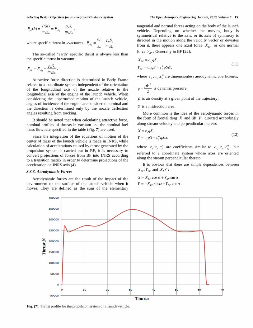
It should be noted that when calculating attractive force,

nominal profiles of thrusts in vacuum and the nominal fuel

mass flow rate specified in the table (Fig. 7) are used.

Since the integration of the equations of motion of the

center of mass of the launch vehicle is made in INRS, while

calculation of accelerations caused by thrust generated by the

propulsion system is carried out in BF, it is necessary to

convert projections of forces from BF into INRS according

to a transition matrix in order to determine projections of the

acceleration on INRS axis (4).

3.3.3. Aerodynamic Forces

Aerodynamic forces are the result of the impact of the

environment on the surface of the launch vehicle when it

moves. They are defined as the sum of the elementary

tangential and normal forces acting on the body of the launch

vehicle. Depending on whether the moving body is

symmetrical relative to the axis, or its axis of symmetry is

directed in the motion along the velocity vector or deviates

from it, there appears one axial force XBF or one normal

force YBF . Generally in BF [22]:

XBF = cxi qS,

YBF = cyi qS = cyi qS , (11)

where cxi ,cyi ,cyi are dimensionless aerodynamic coefficients;

q =V 2

2 is dynamic pressure;

is air density at a given point of the trajectory;

S is a midsection area.

More common is the idea of the aerodynamic forces in

the form of frontal drag X and lift Y , directed accordingly

along stream velocity and perpendicular thereto:

X = cxqS,

Y = cyqS = cy qS , (12)

where cx ,cy ,cy are coefficients similar to cxi ,cyi ,cyi , but

referred to a coordinate system whose axes are oriented

along the stream perpendicular thereto.

It is obvious that there are simple dependences between

XBF ,YBF and X,Y :

X = XBF cos +YBF sin ,

Y = XBF sin +YBF cos ,

Fig. (7). Thrust profile for the propulsion system of a launch vehicle.


or

XBF = X cos Y sin ,

YBF = X sin +Y cos .

These formulas are valid for small angles of attack, which

are present during the flight of the launch vehicle in the dense

layers of the atmosphere. Therefore, if we suggest

sin = , cos = 1, the dependence can be simplified:

X = XBF +YBF = XBF +YBF ,

XBF = X Y ,YBF = X +Y .

It must be noted that when calculating the aerodynamic

forces we use nominal coefficients of drag and lift specified in a

table.

Furthermore, since the projections of the aerodynamic

forces are calculated in a coordinate system connected with the

air speed of the launch vehicle, it is necessary to determine a

single vector of air speed of the launch vehicle VB0

in INRS.

Since the launch vehicle performs its mission in the dense layers

of the atmosphere which rotates with the Earth, the air velocity

vector in INRS is defined as follows [22]:

VB0= V + AUGF84

INRS3 R[ ],

where V is the launcher's velocity vector in INRS; 3

angular velocity vector of rotation of the Earth in WGS 84; R

radius vector of the launch vehicle; AUGF84INRS

is a matrix for

conversion from WGS 84 into INRS.

To describe the unperturbed motion of the center of mass of

the launch vehicle besides equations (5), it is necessary to use an

equation of launcher mass change during the flight m = M (t).

However, due to table dependence of the propulsion

system's fuel mass flow per second and spasmodic changes in

the mass during the separation of stages of the launch vehicle,

the launch vehicle's full weight is calculated as the sum of all

current stages with fuel in operating engines, determined in

accordance with the current propulsion system's profile of

thrust.

3.4. The Equations of Rotational Motion of the Launch Vehicle

The spatial angular motion of the center of mass of the

launcher is described by the following equations projected on

the axes BF [14, 26]:

x =Mx

Ix;

Y =(IZ IX ) x Z

IZ+

MY

IY;

Z =(IZ IX ) x Y

IZ+

MZ

IZ.

(13)

In these equations: x , Y , Z are components of the

angular velocity vector of the launch vehicle relative to axes

BF; Mx , MY , MZ components of the sum vector of

moments M , acting on the launch vehicle during the

mission projected on axes BF; Ix , IY , IZ are axial moments of

inertia of the launch vehicle (the launch vehicle's centrifugal

moments of inertia are equal to zero because of symmetry of the

object).

It should be noted that in order to connect angular motion

parameters, i.e. a component of angular velocity vector in BF

with the parameters of the center of mass of the launch vehicle

(i.e. determining the orientation angles of the launch vehicle) we

shall use an approach based on the Rodrigues-Hamilton

parameters instead of the standard kinematic equations [7]

= x + tg ( y sin + z cos ),

= y sin + z sin( )1

cos

= y cos z sin

(14)

This approach is based on the idea of finite rotation of a

rigid body within its own quaternion of conversion between

coordinate systems whose components are called the

Rodrigues-Hamilton parameters.

In line with this approach, the Rodrigues-Hamilton

parameters are connected with the Euler angles via the

following relations [20]:

Q =

cos2

00

sin2

cos2

0

sin2

0

cos2

sin2

00

, (15)

where Q is own quaternion of conversion between INRS and

BF; is quaternion multiplication sign.

Transition matrix AINRSBF

between INRS and BF is made on

the basis of its own quaternion of conversion in accordance with

the following formulae:

AIFBF

=

q02+ q1

2 q22 q3

2

Q

2(q1 q2 + q0 q3 )

Q

2(q1 q3 q0 q2 )

Q

2(q1 q2 q0 q3 )

Q

q02+ q2

2 q12 q3

2

Q

2(q2 q3 + q0 q1 )

Q

2(q1 q3 + q0 q2 )

Q

2(q2 q3 q0 q1 )

Q

q02+ q3

2 q12 q2

2

Q

, (16)

where q1,q2 ,q3,q4 , Q are components and a module of its

own quaternion of conversion Q.

Traditional Euler angles can be defined on the basis of

the present transition matrix [20] as follows


= arctga12a11

,

= arctga13

a112+ a12

2,

= arctga23a33

, (17)

where aij is the component of the matrix AIFBF .

Then the kinematic equations, i.e. equations relating to

the angular velocity vector of a rigid body with time

derivatives of the kinematic parameters shall be written as

follows [20]:

Q =1

2Q (18)

This approach, compared with classical kinematic

equations (14), due to linearity of equations (18) allows

obtaining a high-precision stable numerical solution devoid

of singular points.

Thus, the complete system of differential equations that

describe the spatial motion of a flying vehicle, consists of 6

equations of the center of mass motion (5), 3 equations of an

aircraft's angular motion (13) and 4 kinematic equations (18)

describing the dynamics of the Rodrigues-Hamilton

parameters.

Let us consider the method of generation of the total

moment relative to the center of gravity acting on the launch

vehicle. Obviously, the total moment is the vector sum of the

moments created by active and passive forces acting on the

launch vehicle. Let's begin with gravity.

Designers of a launch vehicle try to position the center of

mass at its geometrical axis in such a way that thrust does

not create disturbing moment about the center of mass. We

shall assume that the center of mass lies exactly on the

longitudinal axis of the launch vehicle at a distance xЦM

from the top. However, since fuel mass flow per second of

the propulsion system depends on values specified in a table

as well as on abrupt changes in the mass and length during

the separation stages with the current engine, operating fuel

mass is determined in accordance with the current thrust

profile and stage joint angles [21].

Since gravity always acts along a straight line passing

through the center of mass, it does not create a moment.

3.4.1. Aerodynamic Moments

Since force along its line of action can be moved to any

point, we shall agree to assume aerodynamic force applied in

the center of pressure of the launch vehicle. In this case, the

force components acting along the axes XBF ,YBF of BF or

along the axes X,Y of velocity system can also be

considered to be applied in the center of pressure. Force XBF

acts along the longitudinal axis of the launch vehicle and

does not create a moment about the center of mass. Force

YBF creates a moment about the center of mass [22]:

MZAD

= YBF (xЦД xЦM ) = cy1qS(xЦД xЦM ) . (19)

It must be noted as well that the position of the center of

pressure is specified in a table in accordance with the current

flight time and abruptly changes during separation of stages

of the launch vehicle.

3.4.2. Thrust Moment of the Engine

Control moments must provide the ability to control the

longitudinal motion of the vehicle and angular movements

about axes of BF ( 0x rolling, 0y yaw, 0z pitching

motion).

The launch vehicle under consideration has no velocity

control due to the peculiarities of the propulsion system and

control algorithms, i.e. amount of engine thrust is realized

"in fact" without affecting the control system. In this case,

the main means of control is to change the direction of the

thrust vector to generate thrust moment about the center of

mass of the launch vehicle in one of the following channels

[21]:

• roll channel is a channel to control angular motion

about body axis 0x;

• yaw channel is a channel to control angular motion

about the body axis 0y;

• pitch channel is a channel to control angular motion

about the axis 0z.

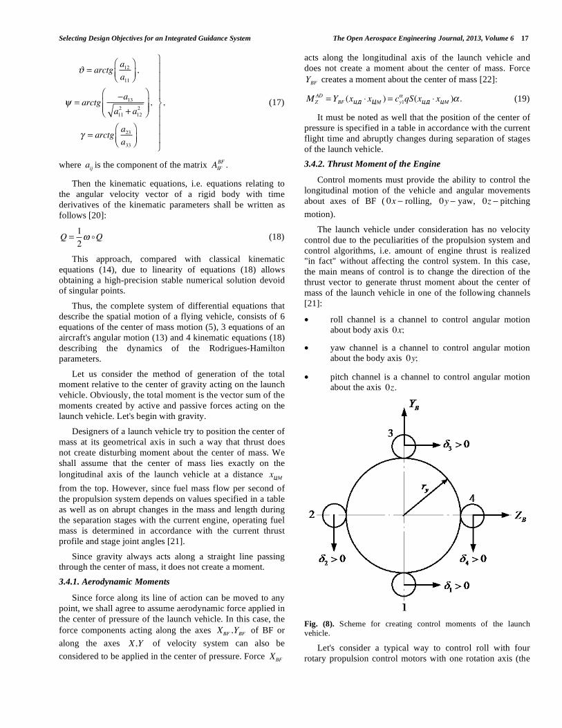
Fig. (8). Scheme for creating control moments of the launch vehicle.

Let's consider a typical way to control roll with four

rotary propulsion control motors with one rotation axis (the


so-called stage I boosters). The positive direction of rotation

about the roll axis is determined by the mark of the control

moment. It creates a positive rolling control moment:

Mx = Pry (cos 1 + cos 2 sin 3 sin 4 ), (20)

where P is the thrust of one engine; ry is an arm of engines

thrust about the center of mass.

To create yaw control moments, engines situated in

planes 1-3 (Fig. 8) synchronously deviate at angles 1, 3 :

My = Ply (sin 1 + sin 3 ), (21)

where ly is a distance from the center of mass to the axis of

engine rotation.

To create pitch control moments, engines situated in

planes 2-4 (Fig. 8) synchronously deviate at angles 2 , 4 :

Mz = Ply (sin 2 + sin 4 ). (22)

It should be noted that the calculation of arms of force,

i.e. a distance from the center of mass to the axis of rotation

of the engine, the current position of the center of mass and

the arm is determined based on the current angles of stages

and the engine setting.

4. CONCLUSIONS

1. Based on the above, we have set a technical problem

of the conceptual design of an integrated navigation

system for the space launch vehicle qualified to inject

small artificial Earth satellites into low and medium

circular orbits.

2. The conceptual design of the integrated navigation

system based on GPS technology involves

determination of its structure, models and algorithms,

providing the required accuracy and reliability in

injecting payloads with due regard to restrictions on

weight and dimensions of the system.

3. We have defined the sequence of essential scientific

and technical problems that lead to the solution of the

major technical problem. This sequence includes:

) selection of quality (accuracy) criteria for solving

the navigation task;

b) selection of a method for integration of

navigation information;

c) making a model of an object's motion, GINS,

navigation field, GPS receiver, taking into

account all uncontrolled factors;

d) making a "tool" to simulate functioning of the

system involved.

4. It has been demonstrated that it is appropriate to take

a posteriori accuracy dispersion of the position and

velocity vectors of the launch vehicle in phases of

flight of I-III stages as a criterion of accuracy of

solving a navigation task.

5. We have made an analysis of possible models of

flight and navigation measurements and identified

key potential difficulties in the process of their

creation.

CONFLICT OF INTEREST

The author confirms that this article content has no

conflict of interest.

ACKNOWLEDGEMENTS

Declared none.

REFERENCES

[1] Z. Nickolay, “Integrated navigation system for prompting of the commersial carrier rocket”, In: Information Technology Conference

for Academia and Professionals (ITC-AP 2013), Sharda University, India, 19-21 April, 2013.

[2] Flight instruments and navigation systems/ Politecnico di Milano - Dipartimento di Ingegneria Aerospaziale, Aircraft systems (lecture

notes), version, 2004. [3] G. M. Siouris, Aerospace Avionics Systems. Academic Press: INC,

1993. [4] K-S. Choi, “Development of the commercial launcher integrated

navigation system the mathematical model, using GPS/GLONASS technique”, In: 52nd International Astronautical Congress, France,

Toulouse, 2001. [5] Available at: http://ru.wikipedia.org/wiki/ - Vega launcher (

- ), (in Russian). [6] G. Siharulidze Yu, Flying vehicles ballistics, Nauka Publisher,

Russia, 1982, p. 351, ( . . . .: , 351 ., 1982).

[7] A. A. Lebedyev, G. G. Adzhimamudov, V. N. Baranov, and V. T. Bobronnikov, Fundamentals of flying vehicles systems synthesis,

Moscow Aviation Institute MAI: Moscow, 1996, p. 224, ( . ., . ., . ., . . .

. .: , 224 c., 1996).

[8] D. J. Bayley, Design optimization of space launch vehicles using a genetic algorithm, Auburn University, Alabama, 2007, p. 196.

[9] B. Scherzinger, “Precise Robust Positioning with Inertial/GPS RTK”, In: Proceedings of ION-GPS-2000, Salt Lake City UH,

September 20-23, 2000. [10] C. Urmson, C. Ragusa, and D. Ray, “A robust approaches to high

speed navigation for unrehearsed Desert Terrain”, J. Field. Rebot., vol. 23, no. 8, August, 2006, pp. 467-508, 2006.

[11] W. Whittaker and L. Nastro, “Utilization of position and orientation data for preplanning and real time autonomous vehicle

navigation”, GPS World, Sept 1, 2006. [12] J. Daniel, Biezad integrated navigation and guidance systems,

AIAA Education Series, American Institute of Aeronautics and Astronautics : USA, 1999.

[13] J. F. Hanaway and R. W. Moorehead, Space shuttle avionics system, National Aeonatics ans Space Administration Office of

Management, Scientific and Technical Information Division: USA, p. 505, 1989.

[14] M. N. Krasilshikov, and G. G. Serebryakov, Control and guidance of unmanned flying vehicles on the basis of modern information

technologies, Fizmatlit Publisher: Moscow, 2003, p. 280. (

/ . . .

. . . – .: , 280 ., 2003). [15] A.J. Kelly, “A 3D state space formulation of a navigation Kalman

filter for autonomous vehicles”, Report CMU-RI-TR-94-19, CMU Robotics Institute Technical, PA, USA, 1994.

[16] A. Kelly, “Modern inertial and satellite navigation systems”. Technical Rep, CMU-RI-TR-94-15, The Robotics Institute

Carnegie Mellon University, USA, 1994. [17] M. Horemu, Integrated Navigation. Royal Institute of Technology,

Stocholm, 2006.


[18] D. B. Cox Jr., Integration of GPS with inertial navigation systems,

Institute of Navigation, USA, pp. 144-153, 1978. [19] Available at: http://satellite-monitoring.atcommunication. com/en/s

ecure/seu8800.pdf - Satellite Monitoring and Intercept System SEU 8800.

[20] E. A. Fedosov, V. T. Bobrronnikov, M. N. Krasilshikov, and V. I. Kuhtenko, Dynamical design of automatic control systems of flying

vehicles, Mashinostroyeniye Publisher: Moscow, 1977, p. 336, ( . ., . ., . .,

. . .

. .: , 336 ., 1977). [21] V. V. Malyshev, M. N. Krasilshikov, V. T. Bobronnikov, and V. D.

Dishel, Aerospace vehicle control, 1996. [22] T. R. Kane, P. W. Likins, and D. A. Levinson, Spacecraft

Dynamics, The Internet-First University Press: Cornell University, p. 454, 2005.

[23] C. L. Botasso, “Solution procedures for maneuvering multibody

dynamics problems for vehicle models of varying complexity”, Multibody Dyn. Comput. Methods Appl. Sci., vol. 12, pp. 57-79,

2008. [24] A. Prati, S. Calderara, and R. Cuccira, Using circular statistics for

trajectory shape analysis, University of Modena and Reggio Emilia: Italy. Available at: http://mplab.ucsd.edu/wp-content/uploa

ds/cvpr2008/ conference/data/papers/497.pdf [25] B. F. Zhdanyuk, Fundamentals of statistical processing of

trajectory measurements, Mashinostroyeniye Publisher: Moscow, p. 384, 1978 ( . .

. .: , 384 ., 1978). [26] H. S. Tsien, T. C. Adamson, and E. L Knuth, “Automatic rocket

navigation of a long range rocket vehicles”, J. Am. Soc., July-August, 1952.

Received: May 31, 2013 Revised: June 13, 2013 Accepted: August 15, 2013

© Nickolay Zosimovych; Licensee Bentham Open.

This is an open access article licensed under the terms of the Creative Commons Attribution Non-Commercial License (http: //creativecommons.org/licenses/by-nc/3.0/) which permits unrestricted, non-commercial use, distribution and reproduction in any medium, provided the work is properly cited.

Documents

Selecting Design Objectives for an Integrated Guidance System of a Commercial Launch Vehicle with Application of GPS Technologies