DEGREE PROJECT IN ENERGY AND ENVIRONMENT, SECOND CYCLE, 30 CREDITS

STOCKHOLM, SWEDEN 2021

Seawater heat recovery by the

utilisation of phase change heat of

freezing

Technical feasibility study of a system for District Heating in the city of Helsinki

RAKESH RAMESH

KTH ROYAL INSTITUTE OF TECHNOLOGY

SCHOOL OF INDUSTRIAL ENGINEERING AND MANAGEMENT

Master of Science Thesis

Department of Energy Technology

KTH 2021

Seawater heat recovery by the utilisation of phase

change heat of freezing

TRITA: TRITA-ITM-EX 2021:589

Rakesh Ramesh

Approved

Date

Examiner

Justin NingWei Chiu

Supervisor

Justin NingWei Chiu

Aalto University Supervisor

Annukka Santasalo-Aarnio

Contact person

Annukka Santasalo-Aarnio

2

Abstract

With the Paris agreement calling to limit global warming to 2°C below pre-industrial levels,

with further efforts to ensure it stays below 1.5°C, the Finnish government passed the Laki

hiilen energiakäytön kieltämisestä (416/2019), i.e., Act of Prohibition of Coal Energy,

which stipulates that the use of coal as a fuel for heat/electricity production to be banned

from 1 May 2029. This affects Helsinki’s energy industry and a key concern to this work is

the Salmisaari Combined Heat and Power plant, which is set to be decommissioned. This

plant currently generates heat and electricity by using wood pellets and coal to cater to

around 25-45% of the District Heating consumption of the city of Helsinki.

To compensate for this decommissioning, there arises a need for more heat production,

around 300-500MW of capacity. One alternative is the heat recovery of seawater by

utilising the phase change heat of freezing. The present project investigates a technical

feasibility study of a system to generate ice slurry, which is then used to extract heat from

seawater at ~0°C via a heat pump. The competitiveness of an ice-slurry based system to

state-of-the-art water or ice-based storage is analysed as well. The proposed system is then

modelled in Aspen Plus, and the pressure drop characteristics of the generated ice slurry

are studied. Finally, a sensitivity analysis of the pressure ratio of the compressor on the

performance of the system is studied.

Based on prior works, level of commercialisation and technical feasibility, it was found that

a vacuum ice generation method, in combination with heat pumps, is a viable solution to

cater to the district heating demand of the city. Further, it is concluded that the pressure

drop occurring during transport of the ice slurry is quite minimal – less than 0.5% of the

total power consumed whilst producing 300MW of district heat. The COP of the system

varies between 2.6-2.8 depending on the pressure ratio of the compressor and thus is

energy efficient. Overall, the proposed solution seems to be promising and with further

socio-techno-economic analysis, this could be the potential alternative to bridge the deficit.

Keywords District heating, Seawater, Ice slurry, Aspen Plus, Pressure drop

3

Abstrakt

Med Parisavtalet som kräver att den globala uppvärmningen ska begränsas till 2 °C under

förindustriella nivåer, med ytterligare ansträngningar för att säkerställa att den håller sig

under 1,5 °C, antog den finska regeringen Laki hiilen energiakäytön kieltämisestä

(416/2019), dvs. Förbud mot kolenergi, som föreskriver att användningen av kol som

bränsle för värme-/elproduktion ska förbjudas från och med den 1 maj 2029. Detta

påverkar Helsingfors energiindustri och en central fråga för detta arbete är Salmisaari

kraftvärmeverk, som är planlagt på att avvecklas. Denna anläggning genererar för

närvarande värme och elektricitet genom att använda träpellets och kol för att tillgodose

cirka 25–45 % av Helsingfors stads fjärrvärmeförbrukning.

För att kompensera för denna avveckling uppstår ett behov av mer värmeproduktion, cirka

300-500MW kapacitet. Ett alternativ är värmeåtervinning från havsvatten genom att

utnyttja fasförändringsvärmen från frysning. Detta projekt skall undersöka genom en

teknisk förstudie olika system för att generera isslurry (en blandning av is och vatten), som

sedan används för att utvinna värme från havsvatten vid ~0°C med hjälp av en värmepump.

Konkurrenskraften hos ett isslurrybaserat system jämfört mot toppmoderna vatten- eller

isbaserad lagrings system analyseras också. Det föreslagna systemet modelleras sedan i

Aspen Plus, och tryckfallsegenskaperna hos den genererade isslurryn studeras. Slutligen

görs en känslighetsanalys av kompressorns tryckförhållande och dess påverkan på

systemets prestanda.

Baserat på tidigare arbeten, kommersialiseringsnivå och teknisk genomförbarhet fann

denna rapport att genom en metod för att generera vakuumis, i kombination med

värmepumpar att en hållbar lösning för att tillgodose stadens fjärrvärmebehov finns.

Vidare dras slutsatsen att tryckfallet som inträffar under transport av isslurryn är minimalt

- mindre än 0,5 % av den totala energiförbrukningen samtidigt som den producerar

300MW fjärrvärme. Systemets COP varierar mellan 2,6–2,8 beroende på kompressorns

tryckförhållande och är därmed energieffektivt. Sammantaget verkar den föreslagna

lösningen vara lovande och med ytterligare socio-teknoekonomisk analys kan detta vara ett

potentiellt alternati för att brygga underskottet av fjärrvärme.

Nyckelord: Fjärrvärme, Havsvatten, Isslurry, Aspen Plus, Tryckfall

4

Table of Contents

Abstract ................................................................................................................. 2

Preface ................................................................................................................. 6

Abbreviations and Symbols ................................................................................... 7

1. Introduction .................................................................................................. 8

1.1 Carbon Neutrality goals of Helsinki ......................................................... 8

1.2 Problem Definition ................................................................................. 12

1.3 Research Question ............................................................................... 12

1.4 Methodology ......................................................................................... 13

1.5 Thesis Outline ....................................................................................... 13

2. Theoretical Background ............................................................................... 15

2.1 Water vs ice slurry ..................................................................................... 15

2.2 Theory of Crystallisation, Ice slurry formation and Melting ......................... 16

2.2.1 Supersaturation ................................................................................... 17

2.2.2 Nucleation ........................................................................................... 17

2.2.3 Growth ................................................................................................ 18

2.2.4 Attrition ................................................................................................ 18

2.2.5 Agglomeration ..................................................................................... 18

2.2.6 Ostwald ripening.................................................................................. 19

2.2.7 Spheroidization ................................................................................... 19

2.2.8 Heat transfer rate and Crystal morphology .......................................... 19

2.2.9 Melting ................................................................................................ 20

2.3 Baltic Seawater properties ......................................................................... 20

2.3.1 Salinity ................................................................................................ 21

2.3.2 Oxygen Content .................................................................................. 23

3. Methods of Ice Slurry Generation ................................................................ 26

3.1 Scraped-Surface Ice Slurry Generator ....................................................... 26

3.2 Direct Contact Ice Slurry Generators with Immiscible Primary Refrigerant .. 30

3.3 Direct Contact Generators with Immiscible Secondary Refrigerant ............. 32

3.4 Supercooled Method .................................................................................. 33

3.5 Hydro-Scraped Ice Slurry Generator ........................................................... 35

3.6 Fluidised Bed Crystalliser ........................................................................... 36

3.7 High-Pressure Ice Slurry Generator ............................................................ 38

5

3.8 Recuperative Ice Making ............................................................................ 40

3.9 Vacuum Ice Generation ............................................................................. 41

4. Modelling in Aspen Plus ............................................................................... 47

4.1 Introduction to Aspen Plus ......................................................................... 47

4.2 Choice of Refrigerant - R1234ze ................................................................ 47

4.3 The Aspen Plus Model ............................................................................... 48

4.3.1 Overview ............................................................................................. 48

4.3.2 Components and Setup parameters .................................................... 49

4.3.3 Model Validation .................................................................................. 52

5. Pressure drop analysis of ice slurry during transport ............................ 53

5.1 Pressure loss evaluation based on laboratory-scale experimental data ..... 53

5.2 Viscosity based pressure drop calculation ................................................. 55

6. Results and Discussions .............................................................................. 57

6.1 Selection of Ice Slurry Generation method ................................................. 57

6.2 Pressure Drop Analysis ............................................................................. 59

6.3 Performance of the system ........................................................................ 65

6.4 Contribution to SDG ................................................................................... 66

6.5 Future Work ............................................................................................... 67

7. Conclusion..................................................................................................... 69

8. Bibliography .................................................................................................. 70

Appendix ............................................................................................................ 81

A1 – Augustenborg District Heating Plant ........................................................ 81

A2 – Refrigerant R-1234ze .............................................................................. 83

A3 – Experimental values used in Pressure drop studies ................................ 84

A4 – Extension of Pressure Drop studies ......................................................... 85

6

Preface

Throughout the writing of this thesis, I have received a great deal of support

and assistance.

Firstly, I would first like to thank my supervisor, Dr. Annukka Santasalo-

Aarnio and advisor Dr. Ari Seppälä for helping in setting up an interview for

this position and whose expertise was invaluable in formulating the research

questions. I am extremely grateful to Ari and Aleksi Barsk, without whom

this work would not have been possible. Their insightful feedback pushed me

to sharpen my thinking and helped me improve the quality of my work. I

would like to thank Judit Nyári and Shouzhuang Li for their guidance in

developing the Aspen model. I would like to acknowledge my other

supervisor, Dr Justin Ning-Wei Chiu, for his astute comments and help in

the shaping up of my thesis.

I would particularly like to express my gratitude to Jaakko Nummelin and

Laura Korhonen of Helen Oy, for offering me this position. I want to thank

you for your patient support and for all the opportunities I was given to

further my research.

In addition, I would like to thank my parents, and my brother for everything.

Finally, I could not have completed this thesis without the support of my

friends who provided happy distractions in these testing COVID times.

Otaniemi, 27th October 2021

Rakesh Ramesh

7

Abbreviations and Symbols

Abbreviations

BAU - Business-as-usual

CHP - Combined heat and power

CO2e - Carbon-dioxide equivalent

COP - Coefficient of Performance

DC - District cooling

DH - District Heating

DTI - Danish Technological

Institute

EU - European Union

F-gas - Fluorinated gas

GHG - Greenhouse gas

GWP - Global Warming Potential

HCl - Hydrogen chloride

HF - Hydrogen fluoride

HFC - Hydrofluorocarbons

HFO - Hydrofluoro-olefins

HPAF - High-pressure assisted

freezing

HPSF - High-pressure shift

freezing

HSY - Helsingin seudun

ympäristöpalvelut

I/O - Input/output

IEA - International Energy Agency

IPCC - Intergovernmental Panel

on Climate Change

ISG - Ice slurry generator

LNG - Liquefied natural gas

NaCl - Sodium Chloride

NH3 - Ammonia

NOx - Nitrogen Oxides

O&M - Operation and

Maintenance

O2 - Oxygen

ODP - Ozone Depletion Potential

ORE - Orbital rod evaporators

R12 - Dichlorodifluoromethane

R1234ze - 1,3,3,3-

tetrafluoropropene

R143a - 1,1,1-Trifluoroethane

R717 - Refrigerant grade Ammonia

rpm - revolutions per minute

SDG - Sustainable Development

Goals

USD - United States Dollar

VIH – Vacuum Ice Heat Pump

VIM - Vacuum Ice Maker

Symbols in equations

A - cross-sectional area (m2)

D – Diameter (m)

f - friction factor

g - gravitational acceleration

constant (m/s2)

L - length

Lwater → ice - specific latent heat of

fusion of water (kJ/kg)

ṁ - mass flow rate (kg/s)

P - Pumping power (kW)

Pt - Triple point pressure (bar)

Q - Flow rate (m3/s)

Re - Reynolds number

S - salinity of water (‰, per mille)

v - flow velocity (m/s)

vmin - Minimum velocity (m/s)

x- ice fraction

ΔG - Gibbs free energy state

ΔP - Pressure Drop (Pa)

ηpump - efficiency of pump

μ - Dynamic viscosity (kg/ms)

ρ – density (kg/m3)

ρcf - Carrier fluid density (kg/m3)

ρi - Density of ice (kg/m3)

8

1. Introduction

Ever since the Industrial revolution 350 years ago, anthropogenic

greenhouse gas (GHG) emissions have put our planet on the pathway to a

climate catastrophe. Human activities are estimated to have triggered

approximately 1.0°C of global warming above pre-industrial levels, with the

figure expected to reach 1.5°C between 2030 and 2050 if it continues to

increase at the current pace [1].

Immediate and collective action by all of mankind towards lowering the

levels of it in the atmosphere is the only way to avoid such a disaster. Decades

of global co-operation amongst the 196 countries bore fruit in 2015 in the

form of the Paris agreement, which aims at significantly cutting down on the

emissions of the greenhouse gases and thereby limiting the global

temperature rise to 2°C, with further efforts to keep the temperature rise to

below 1.5° [2, 3].

The member states of the European Union (EU) are legally bound to the

policy decisions agreed upon on climate issues. This includes the EU’s

commitment to achieving zero net anthropogenic greenhouse gas emissions

by the year 2050, in addition to individual targets for each sector. The

objective is to cut greenhouse gas emissions by at least 40% to 2030 from the

1990 levels. Other means of mitigating the emissions are by improving the

energy efficiency and the share of renewables in electricity generation; this

has been an important cornerstone in the EU’s quest for a greener world. In

numbers, a target of improved energy efficiency by at least 32.5% by 2030,

with an improvement of 0.8% per year in the current decade. and share of

renewable energy to 32% by the end of this decade. [4, 5, 6].

In addition to the above-mentioned, every country has their national targets

that they strive to achieve for a cleaner future. Of particular interest to this

work, is the city of Helsinki in Finland, which is discussed in detail

subsequently.

1.1 Carbon Neutrality goals of Helsinki

Carbon neutrality is defined as a state of having net-zero CO2 emissions. This

could be achieved by either carbon offsetting or balancing the emitted and

removed emissions. For the City of Helsinki to become carbon-neutral by

2035, it requires that GHG emissions are reduced by at least 80% from the

levels 30 years back, with further increase of carbon sinks. The remaining 20

percent will be compensated for by Helsinki taking care of implementing

9

emission reductions outside the city or, for example, increasing the number

of carbon sinks. [7, 8]

Figure 1: An infographic depicting the energy, emission levels and targets forHelsinki [9]

In 2002, Helsinki’s Sustainability Action Plan, comprising its objectives for

GHG emissions, was approved, and the city became the first European capital

with an all-inclusive sustainable development pathway. This plan, which

turned out to be successful, called for emissions in 2010 to be at the same

level as it was in 1990 [10].

So far, there has been steady progress, with some significant milestones. In

2018, Helsinki's total GHG emissions were about 27% lower than in 1990.

Per capita emissions are 45% lower than in 1990. Despite population growth

by 150,000, the total energy consumption in urban areas remains

unchanged, which speaks volumes about the development of energy

efficiency. As of 2018, renewable energy accounts for 12% of the city's total

output [9].

Helen Oy, owned 100% by the city of Helsinki, is one of Finland's largest

energy companies and caters to the district heating (DH), cooling (DC) and

electricity demand in Helsinki. Helen Oy was the first energy company in

Finland that was dedicated to setting an emissions reduction target, not just

for CO2, but for the other GHG gases as well based on their entire life cycle

[11]. In accordance with the 2035 plan to achieving carbon neutrality, Helen

Oy fulfils its obligation through measures that would reduce the DH

emissions of the population of Helsinki by ~75% by 2035. The measures

include phasing out of fossil fuel-based generation, uptake of renewable

10

energy sources, especially in electricity production, introducing Demand side

response measures, storage measures to name a few [12].

Figure 2: The development of Helsinki’s emissions from 1990 to 2015, the BAU scenario for 2035

and the target scenario for 2035 [8] .

Helen Oy is analysing several scenarios to provide sustainable fossil-free

power. As compared to the BAU scenario, the target scenario for 2035

includes an assumption that clean energy sources would make up around

70% of heat produced (Figure 2). Further, usage of natural gas produces

emissions that must be balanced by development of carbon sinks. In 2017, in

Salmisaari and Hanasaari alone, burning a mixture of wooden pellets and

coal instead of only coal diminished the GHG emissions by almost 80kt of

CO2e [8]. The city of Helsinki and Helen Oy have developed a strategy to

decommission the coal-based powerplants during this decade [8, 13].

The Salmisaari CHP plant is completely owned by Helen Oy. Salmisaari A

commenced producing electricity in 1953, and four years later became the

first plant to produce DH in Helsinki. Salmisaari B, its coal fired counterpart,

produces 300MW of DH and 160 MW of electricity. The 65m x 40m silos

present in the premises, 120m below the surface ground can store up to

250000 tons of coal [14]. The A plant, these days, is used to generate heat

when DH from cogeneration is not adequate. Heavy fuel oil, stored in a rock

storage in the site, acts as the backup fuel for A and B power. In summer, in

addition to DH and electricity, the B-plant also generates energy for district

cooling purposes. It is complemented by the Kellosaari reserve power plant,

operated on light fuel oil, and ensures there is no dearth of demand [15, 16,

17, 18, 19].

11

Figure 3: Salmisaari B power plant, located at Porkkalankatu 9–11 in Helsinki [20]

Table 1: Technical datasheet of Salmisaari – B (coal/pellet boiler) [21]

Intended use Base load boiler

Year of introduction 1984

Main Fuel Coal, Pellet

Auxiliary/Backup fuel Heavy fuel oil

Burners Coal burners – 16

Oil burners - 12

Rated Power

- Electricity

- District Heating

160MW

300MW

Running time 5000-7800h/a

Chimney height 153m

Gross electricity production 962.4 GWh/a

Thermal energy production 1741.5 GWh/a

Fuel consumption, as of 2017

- Coal

- Pellets

- Heavy fuel oil

418980 t

8692 t

350.5 t

With demands for increased share of renewables rising, a pellet system,

including the receiving, preparation, storage and feeding of the fuel, was built

in 2014, ensuring greener energy [21]. Further, in 2018, Helen Oy

12

inaugurated a 92MW wood pellet-fired boiler in Salmisaari, with it providing

enough heat for a town the size of Savonlinna, Finland [22, 23].

1.2 Problem Definition

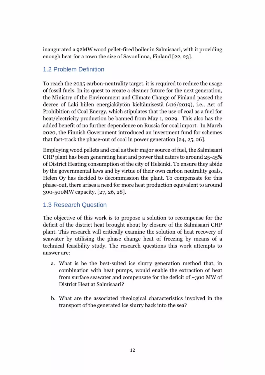
To reach the 2035 carbon-neutrality target, it is required to reduce the usage

of fossil fuels. In its quest to create a cleaner future for the next generation,

the Ministry of the Environment and Climate Change of Finland passed the

decree of Laki hiilen energiakäytön kieltämisestä (416/2019), i.e., Act of

Prohibition of Coal Energy, which stipulates that the use of coal as a fuel for

heat/electricity production be banned from May 1, 2029. This also has the

added benefit of no further dependence on Russia for coal import. In March

2020, the Finnish Government introduced an investment fund for schemes

that fast-track the phase-out of coal in power generation [24, 25, 26].

Employing wood pellets and coal as their major source of fuel, the Salmisaari

CHP plant has been generating heat and power that caters to around 25-45%

of District Heating consumption of the city of Helsinki. To ensure they abide

by the governmental laws and by virtue of their own carbon neutrality goals,

Helen Oy has decided to decommission the plant. To compensate for this

phase-out, there arises a need for more heat production equivalent to around

300-500MW capacity. [27, 26, 28].

1.3 Research Question

The objective of this work is to propose a solution to recompense for the

deficit of the district heat brought about by closure of the Salmisaari CHP

plant. This research will critically examine the solution of heat recovery of

seawater by utilising the phase change heat of freezing by means of a

technical feasibility study. The research questions this work attempts to

answer are:

a. What is be the best-suited ice slurry generation method that, in

combination with heat pumps, would enable the extraction of heat

from surface seawater and compensate for the deficit of ~300 MW of

District Heat at Salmisaari?

b. What are the associated rheological characteristics involved in the

transport of the generated ice slurry back into the sea?

13

1.4 Methodology

For the current work of heat recovery from seawater using the phase change

heat of ice slurry, there is a critical examination of the literature to analyse

the various ice slurry generation methods. A method suitable for the current

application, in integration with heat pumps, and based on previous large-

scale works is then selected and studied further. The system is then modelled

in Aspen Plus, a process simulation software package and the mass flow rate

of the ice slurry is determined. The system is designed in such a way that the

DH water temperature is raised from 45°C to 90°C, to cater to the demand in

the winter. This is followed by a study of the pressure drop during ice slurry

flow, that is characteristic of transport of fluids. Since, the physics of ice

slurry transport and its rheological characteristics is not well-defined, a

sensitivity analysis for the friction factor models and viscosities are

performed and the changes in pressure drop are observed.

1.5 Thesis Outline

The thesis is structured as follows: it progresses from initially presenting the

objectives and literature review of ice slurries, with particular focus on its

application in integration with the District Heating system of the city of

Helsinki, followed by modelling in Aspen Plus and culminated with the

conclusions based on the results and subsequent discussions.

Firstly, an overlook of the Carbon Neutrality goals of the city of Helsinki and

Helen Oy is presented. The current situation of the Salmisaari CHP plant is

then briefly described. Section 2 introduces a theoretical framework used in

this paper that could serve as the basis of further developments. It further

discusses the chemistry of latent heat storage, its advantages, and the

selection of ice-water slurry for this work. The science of crystal formation is

also communicated in this section. Since this work is centred around

Salmisaari, the properties of seawater at Länsi-Tonttu monitoring station,

15kms from the focal area of this work, was analysed and the results conclude

this section. The potential applications and previous research on ice slurry

generation methods, including large-scale systems were studied deeply and

the findings are put forth in Section 3. A model of a vacuum ice generation

system based on the application for the current work is developed and is

presented in Section 4. The definitive aim of the thesis is to identify the best

suited method of ice slurry generation for this case and attempt to model it

and calculate the pressure drop that occurs during its transport. The pressure

drop studies are explained in Section 5. The results are presented in Section

14

6 along with some suggestions for future work, while the conclusions are

drawn in Section 7.

This work would then serve as one of the underlying support materials for

the construction of a seawater-based DH system by Helen Oy in the near

future. This field of study, being relatively unexplored, also helps in

identifying important areas for future work.

15

2. Theoretical Background

2.1 Water vs ice slurry

Water, owing to its superior properties of neither having global warming

potential (GWP) or ozone depletion potential (ODP) nor being flammable or

toxic, is a suitable candidate for being a refrigerant from an environmental

point of view. In the earlier days, due to risk of freezing, surface waters of

seas, rivers etc. exhibiting near zero temperatures, were not extensively used

as heat sources for heat pumps. With the advent of ice slurry systems, this

could be made possible in a cascade of heat pumps [29]. Among the different

states of water, the advantages of a two-phase fluid (ice slurry) over a single-

phase liquid (water/ice) are plentiful. Ice slurries, double up as storage

medium and a transportation fluid, both of which are explained below.

In sensible thermal energy storage, energy is stored by changing the

temperature of the material, without it undergoing phase change. The total

energy stored is dependent on the mass of the storage material, the specific

heat capacity, and the change in temperature. The inherent disadvantages

associated with sensible heat storage are low storage density per degree

temperature change and large temperature range for storing the energy.

Latent heat thermal energy storage systems can store the latent heat of fusion

in an isothermal process which corresponds to phase transition temperature

of the phase change material. The enthalpy (334kJ/kg at 0°C) associated with

the phase change of water [30] corresponds to a high energy storage density

and thus, it requires lesser space, and the system becomes compact.

Figure 4: Transport capacity in pipe having inner diameter 16-50mm [31]

16

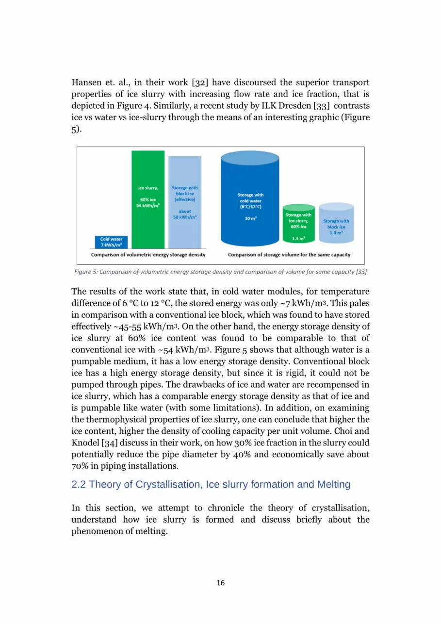
Hansen et. al., in their work [32] have discoursed the superior transport

properties of ice slurry with increasing flow rate and ice fraction, that is

depicted in Figure 4. Similarly, a recent study by ILK Dresden [33] contrasts

ice vs water vs ice-slurry through the means of an interesting graphic (Figure

5).

Figure 5: Comparison of volumetric energy storage density and comparison of volume for same capacity [33]

The results of the work state that, in cold water modules, for temperature

difference of 6 °C to 12 °C, the stored energy was only ~7 kWh/m3. This pales

in comparison with a conventional ice block, which was found to have stored

effectively ~45-55 kWh/m3. On the other hand, the energy storage density of

ice slurry at 60% ice content was found to be comparable to that of

conventional ice with ~54 kWh/m3. Figure 5 shows that although water is a

pumpable medium, it has a low energy storage density. Conventional block

ice has a high energy storage density, but since it is rigid, it could not be

pumped through pipes. The drawbacks of ice and water are recompensed in

ice slurry, which has a comparable energy storage density as that of ice and

is pumpable like water (with some limitations). In addition, on examining

the thermophysical properties of ice slurry, one can conclude that higher the

ice content, higher the density of cooling capacity per unit volume. Choi and

Knodel [34] discuss in their work, on how 30% ice fraction in the slurry could

potentially reduce the pipe diameter by 40% and economically save about

70% in piping installations.

2.2 Theory of Crystallisation, Ice slurry formation and Melting

In this section, we attempt to chronicle the theory of crystallisation,

understand how ice slurry is formed and discuss briefly about the

phenomenon of melting.

17

2.2.1 Supersaturation

The generation of ice crystals involves several steps, the first of which is need

for the solution to be supersaturated. This is necessitated because

crystallisation occurs only if sufficient driving force is applied. [35]. A

saturated solution is in thermodynamic equilibrium with the solid phase and

contains maximum amount of solute that could be dissolved at the specified

temperature and pressure. A supersaturated solution contains more

dissolved solid than that maximum as characterised by the equilibrium

saturation [36]. In other words, the solution is said to be in a metastable

state.

Supersaturation can be brought about by either changing the pressure and

thus, shifting the equilibrium temperature or by supercooling the solution at

the equilibrium temperature or by changing the concentration of the additive

[31]. In the case of ice, when water is maintained at triple point conditions,

evaporation of water (partial) creates the potential difference, making way

for the formation of ice crystals. The ice crystals continue to form till the

equilibrium is attained and saturation is ensured.

2.2.2 Nucleation

Okolieocha et. al. define nucleation in the following manner:

“Nucleation is simply defined as the first random formation of

a distinct thermodynamic new phase (daughter phase or

nucleus) that have the ability to irreversibly grow into larger

sized nucleus within the body of a metastable parent phase.”

[37].

As defined above, in a supersaturated solution, molecules congregate and

form stable clusters, thus ensuing the formation of the initial nuclei. This can

transpire in two ways: homogeneously or heterogeneously.

In the former mechanism, ‘statistical fluctuation’ of the aggregated molecules

results in the formation of the initial nuclei. This is difficult to control owing

to the low temperature levels and the high crystal formation rate. In the case

of water-ice, this happens at very low temperatures and with the Baltic

seawater having foreign objects that act as nucleation spots, homogeneous

nucleation is not likely to occur in our application. In heterogeneous primary

nucleation, which is expected to occur, the initial nuclei are formed with the

aid of extraneous particles or foreign surfaces. These occur at relatively

18

higher temperatures as compared to homogeneous nucleation and the

orientation of molecules in the crystal lattice is controlled to an extent by the

surface of foreign particles. Heterogeneous nucleation can be further divided

into two mechanism: primary and secondary nucleation. [31, 35].

Primary nucleation is the direct materialisation of ice crystals from the

solution, while secondary nucleation is the realisation of ice crystals from

already existing ice crystals in the solution [38].

2.2.3 Growth

The final step is the growth phase, where the crystals get bigger till the

desired size is attained. Crystal growth follows three basic steps: initially,

there is a mass transfer across the boundary layer from the bulk of the

solution by means diffusion of molecules. These molecules are then

assimilated into the surface, and finally, phase change heat transfer occurs

from the crystal to the bulk. The rate of crystal growth is influenced by either

of these three stages, the driving force, the remaining supersaturation of the

solution and the residence times in the crystalliser. Ice slurry removed from

an ice slurry generator (ISG) do not necessarily maintain the same shape and

texture as it did in the generator, owing to a few pertinent processes like

attrition, agglomeration, Ostwald ripening etc [31, 39]. These processes are

described in detail in the following chapters.

2.2.4 Attrition

The process of a crystal breaking off on being subject to stress and forming

fragments is termed attrition [35]. The shear stress of fluids while mixing,

particle collisions with each other, with pumps, walls, other components are

some examples of stresses the crystals are subjected to. The fragments thus

formed act as secondary nuclei. The attributes of attrition happening could

be due to a variety of factors. The texture of the original crystal affects the

amount of fragments, with ice crystals having a rougher surface producing a

larger number of fragments as compared to smooth crystals. In addition,

smaller crystals tend to display less attrition. Attrition is considered either

desired or detrimental depending on the application and the choice of ice

slurry generator used.

2.2.5 Agglomeration

The process of crystals colliding with one another, adhering to them, and

coalescing together to form a crystal larger in size and more stable is termed

19

agglomeration [35]. The higher the level of supersaturation of the solution,

the higher the rate of agglomeration. Additionally, as the slurry is disturbed

with growing intensity, the degree of agglomeration decreases. Although it

might mildly influence the size of crystals formed in the ISGs, agglomeration

is a side effect and not a primary process.

2.2.6 Ostwald ripening

The phenomenon of Ostwald ripening affects the distribution of crystal size

in a solution. Owing to the solubility difference amongst the different crystals

formed and, in a quest, to attain the most stable minimum Gibbs free energy

state (ΔG), smaller crystals tend to dissolve and are assimilated on to the

larger ones [35]. This effect is slow and is prominent only in systems over a

long period of time (ex. ice slurry storage systems, ice creams stored in

freezer etc.) and thus, are not so relevant in our application.

2.2.7 Spheroidization

Spheroidization is a process germane to crystal formation. Ice crystals on exiting the

ISG try to attain the thermodynamically favourable least energy state. Amongst the

shapes, a sphere has the least surface area to volume ratio and is considered to be

the most stable [40]. As a result, the dendritic crystals try to attain spheroidal shape

to minimise its energy during the transport, just as the name suggests.

2.2.8 Heat transfer rate and Crystal morphology

Continuing on the theory of crystallisation, it is important to discuss other issus

related to ice slurry generation. Amongst them, two things are of high importance:

high heat transfer rate and ideal crystal shape and size. When ice crystals are

formed, they tend to adhere to the heat exchanging surfaces. As a result, a layer of

ice is built up on the walls. Ice has a low thermal conductivity (2.22 W/mK at 0°C)

and thus, this impedes the heat transfer rates. Thus, for high heat transfer rates

and indirectly, lower O&M costs, one needs to remove the layers of ice either

mechanically or by defrosting it at regular intervals using a recuperative heat

exchanger. An ideal size and shape of ice crystals are to be generated by the ISGs

for optimal functioning of the system. Typically, in several applications, round and

small crystals are preferred. A larger crystal usually exhibits a dawdling melt-off

rate and requires more power to pump. As a result, proper research of the

morphology of the crystals must be done to find the shape and size, and

subsequently the method best suited for the application [41].

20

2.2.9 Melting

The process involving phase change of an object from a solid to liquid state is

defined as melting [42]. When heat is supplied to ice crystals, the thermal driving

force causes the atoms to move faster and break the chemical hydrogen bonds to

form water, in a liquid state [43]. Since the surface atoms have relatively fewer

bonds as compared to the atoms at the centre, energy of the atoms is transferred

from the surface to the bulk and thus, melting usually initiates from the surface

[44]. One major difference between crystallisation and melting of ice is - in the

former, there is a metastable supercooled state observed (discussed earlier in this

section) [31], whereas in the latter, there is no associated metastable effect

(superheating). But since this work entails the use of the heat released when water

crystallises and not the heat gained while melting, we do not explore the

mechanism of melting any further.

2.3 Baltic Seawater properties

In this work, an attempt is made to utilise the latent heat of seawater for

district heating. The proposed plant is likely to be located in the Salmisaari

area, in the current premises of the CHP plant [45]. The Salmisaari plant is

surrounded by Lapinlahti and Lauttasaarensalmi on either side, as it can be

seen from the Figure 6. The Gulf of Finland, which is a part of the Baltic Sea

serves as the base for extracting heat during the winter. This will be looked

into in detail in the following sections.

Figure 6: A map of the Salmisaari B powerplant (denoted by the red pin) [46]

Since the propositioned plant is in the same site as Salmisaari A and B, the

water source would be the from the Baltic Sea. The generation of ice slurry is

21

inherently determined by the quality of the water, its salinity, temperature,

and other properties.

Figure 7: (left) Länsi-Tonttu monitoring station in the Baltic Sea, denoted by a red dot [47]; (right)

15km – the distance between the proposed plant at Salmisaari and Länsi-Tonttu monitoring station

in West Tukan [48]

The two major properties – salinity and dissolved oxygen of the water at the

target site are ascertained using relevant literature and other available

sources. Amongst them, the Länsi-Tonttu station is 15kms away to the south

of Salmisaari at a depth of 53m (Figure 7). Being located at the outer edge of

the archipelago, beyond the islands of Vallisaari and Isosaari, it is linked to

the open sea and the properties of seawater here closely resemble to what

Helen Oy’s seawater-based DH plant would be operating with.

2.3.1 Salinity

The Baltic Sea is typified by low-salinity brackish water. The Gulf of Finland

is an estuarine sea in the north-eastern part of Baltic sea, encompassing

Finland to the north and Estonia to the south, to St. Petersburg in Russia to

the east, lying between 59°11´N, 22°50´E and 60°46´N, 30°20´E. It receives

briny water from the Baltic Sea Proper in the west, while it receives huge

influx of fresh water from the east, majorly (~15% of total flow) from River

Neva. As a result, there occurs a salinity gradient in both ways. The salinity

increases from north to south and from east to west. The surface salinity

varies from 5–7‰ in the western Gulf of Finland to about 0–3‰ in the east.

At the bottom of the sea, the salinity varies from 8-10‰ in the western Gulf

of Finland. Salinity affects the freezing point of the surface water, typified by

varying the freezing point of –0.17 °C in the east to –0.33 °C in the west [49].

22

Figure 8: Map of the Baltic Sea and its easternmost arm - the Gulf of Finland [50]

As depicted in Figure 9, the salinity of the water around the Länsi-Tonttu

station is quite steady (5-6‰) and does not fluctuate much across seasons

[51]. This is well in synergy with other literature on the salinity of the Gulf of

Finland, as it can be seen from Figure 10. Although the salinity is relatively

low, this serves the purpose of being a freezing point depressant. The reason

behind the requirement of a minimum level of salinity for this work is

explained in the subsequent chapters [52].

Figure 9: Seasonal variation of salinity of seawater at the Länsi-Tonttu station [53]

As salinity of water increases, the electrical conductivity of water increases

while the oxygen content decreases. The presence of salt indicates the

presence of chloride ions that have the potential to destroy the oxide layer on

the metal surface and as a result, corrosion happens [54]. In a system like the

one proposed in this thesis, a lot of components and pipes contain metal and

so, there arises a need to give a protective layer of coating and prevent

corrosion. This should be studied in detail.

23

Figure 10: Vertical salinity gradient across the Gulf of Finland and Northern Baltic Sea. (the

numbers indicating each location, with 54 corresponding to the region off Helsinki, 61 – Hanko, 81

– east of Gotland [49]

2.3.2 Oxygen Content

In any water body, oxygen is present in a dissolved form. Due to seawater

pulses and ocean-warming driven deoxygenation, the oxygen levels are

relatively low. Because of seawater pulses, oxygen-scant water from deep

parts of the Baltic sea flow into Gulf of Finland, lowering its oxygen levels,

while a warmer sea increases the oxygen demand of the organisms present,

thereby depleting the oxygen content available [55].

At the bottom of the Gulf of Finland, it is almost completely anoxic; bereft of

oxygen, while in the surface near Länsi-Tonttu, it fluctuates between 6.5-13

mg/L depending on the season as it can be seen from the Figure 11.

Figure 11: Seasonal variation of oxygen levels of the seawater at Länsi-Tonttu station [56]

24

This is corroborated with the data available in other literature as it could be

observed in distribution of oxygen concentration data in Figure 12 [57].

Figure 12: Oxygen concentrations, 2001–2006. They greyness indicates the lack of oxygen, with the

darker the shade, the more it lacks in oxygen.

The amount of oxygen present in dissolved form in seawater determines the

rate of corrosion. The higher the O2 levels of the sea, the greater the electrode

potential of the metal, which in turn causes the rate of corrosion to be more

rapid [54, 58]. If the piping of the system is to be placed on or near the

surface, it must be ensured that the oxygen doesn’t attack the metal since the

proposed system would be vital to the functioning of the city and cannot fail.

The temperature levels of the seawater determine the energy required to

bring it down to triple point. The closer it is to the triple point temperature,

the less energy required and as it can be observed from Figure 13 (d), the

temperature in the winter is close to 0°C. In addition, as the temperature

increases, the solubility of oxygen decreases, and corrosion slows down.

Other properties like the amount of turbidity, chlorophyll-α [59, 60],

phosphorous content [61, 62]) also affect the crystallisation of water

particles and the corrosion rate and these are exhibited in Figure 13 (a), (b),

(c). These are outside the scope of this work.

25

Figure 13: Seasonal variation of (a) amount of algae [63] (b) turbidity [64] (c) phosphorous content

[62] (d) temperature levels of the seawater at Länsi-Tonttu station [65]

26

3. Methods of Ice Slurry Generation

Archaeological findings have suggested that mankind has been using ice to

preserve food since over 5000 years ago. The first patent for producing ice

slurry was done in 1935 to shave peak loads in dairies in Sweden [66]. The

70s and the 80s saw a plethora of patent applications being filed for ice slurry

generators. Since then, ice slurry has developed from being a niche product into

an applied science being used across the world in various disciplines. However, the

pursuit for an efficient ISG, subsequent storage and crystal measurements has

been never-ending for the scientists. There is no silver bullet when deciding what

ice slurry generator to use for a certain application. Different ice slurry generators

are used for different purposes. Some methods are developed at a laboratory

scale, while others have been fully commercialised. This section reports the

different types of ISGs, their merits and demerits and their suitability for our

application.

3.1 Scraped-Surface Ice Slurry Generator

Over the last three decades ice slurry generation has garnered the interest of

thousands of scientists and no other technique in this field has been more widely

acknowledged and scientifically developed than the scraped surface ice slurry

generator. The generator comprises of a circular shell-and-tube heat exchanger, a

rotating scraping device on the inner side, a refrigerant stream and a process fluid

stream.

It is a double pipe element, with the process fluid flowing through the inner pipe

while coolant flows in the annulus between inner and outer pipe. The coolant is a

refrigerant that evaporates and is usually present on the shell side. Crystals are

formed on the cold inner pipe wall. Inner pipe scraping assembly, usually consisting

of spring-loaded rotating blades or orbital rods or brushes, prevents the deposit of

crystals on the surface by scraping between the pipe walls (see Figure 14). The

absence of scraping would result in a sheet of ice forming on the walls of the pipe,

affecting the heat transfer rate and over a period of time this might result in

blockages. Therefore, to reduce the probability of formation of ice layers on the wall,

there is a requirement of a minimum amount of freezing point depressant

(like NaCl) to be added to the water. [31]

27

Figure 14: (a) Scraped-surface ice slurry generator (b) Orbital rod ice slurry generator (c)

Scraped-surface ice slurry – top view (d) Scraped-surface ice slurry with a helical screw– cross

section [31]

In addition to reducing the thermal resistance and increasing the heat transfer rate

through agitation, the scraping action also enables the crystals to flow axially. These

crystals, in turn act as a seed and acts as a nucleation spot and creates more crystals.

Thus, the scraped surface ice slurry generator produces a mixture of small ice

crystals and water (i.e., ice-water slurry) from a binary solution.

Figure 15: Schematic diagram of an ice slurry generation system [31]

28

As Figure 15 depicts, a refrigerating unit, typically consisting of a compressor,

condenser, and an expansion valve, delivers the refrigerant to the shell-side of the

ISG. The refrigerant evaporates at low pressure through the outer pipe of the

ISG, withdrawing heat from its surroundings, and thus, cools the incoming

solution that flows through the inner pipe. Here, cooling is done indirectly,

and ice slurry is generated on the tube side. At the evaporator exit, the

superheated refrigerant vapour is sent through a compressor and condenser

at high pressure and the cycle continues.

Figure 16: Working of a scraped-surface ice slurry generator with rotating blades [67]

As Russell et.al state in their work [68], the rate of nucleation chiefly depends on

the degree of supercooling at the wall, which in turn is inherently dependent

on the refrigerant temperature. Therefore, by operating the units at high

temperature difference between the refrigerant and ice slurry flows, one can

obtain improved heat transfer rates. However, as the refrigerant temperature

is lowered below a certain limit, the heat duty is reduced owing to a low

thermal length [69]. Although the addition of a freezing point depressant

innately drives down the temperature driving force, it helps in reducing the

probability of ice formation in the heat exchanger and hence a trade-off must

be made to ensure efficient functioning of the scraped surface ISG [31].

29

Figure 17 summarises the typical specifications of the scraped surface ISGs and

OREs. Depending on the application, one chooses either the scraped-surface ISG

or the orbital rod evaporators (ORE). The former uses an electric motor to propel

the scraper blades at speeds of ~450 rpm. A higher rotational speed results in

a higher heat transfer rate, but this comes at the cost of increased power

requirements. They have a wide range of refrigerant capacity (10-1400kW)

and are available in both horizontal and vertical setups, with the tubes being

around 2m long and the ice slurry generation side having a diameter of about

15cm. They provide the benefit of being modular, making the expansion of

such a system straightforward, while this is the not the case with the OREs.

Figure 17: Specifications for ice slurry generator – scraped-surface and OREs [31]

On the other hand, OREs are falling-film type ISG and are essentially assembled

in a vertical orientation to accommodate the vertical spinning rods [70]. The effect

of this rod is to agitate by creating a turbulent flow of fluid around tube,

thereby enhancing the tube side film coefficient. Thus, the agitated flow also

prevents the ice crystals from sticking to the surface. The falling film liquid

performs the role of a lubricant and thereby minimises wear and tear and along

with the centrifugal force, this ensures that the rods do not come in contact with

the walls [70]. They require lesser power per m2 (~0.2 kW/m2) as compared

to scraped surface ISG (~1.2-1.8 kW/m2) [31].

From an economic standpoint, the scraped-surface ISG are more expensive,

costing between 300-600 USD/kW. As Gladis et al., stipulate in their work [70],

OREs are one of the most economical methods of generating ice slurry, with a

capital cost of about 160 USD/kW and a cost of ~USD 550 per ton of ice produced.

Even though they have a high capital cost, the scraped-surface ISGs are

available in all sizes, with smaller units requiring less power and this results

30

in shorter payback periods [71, 70]. One thing to consider while doing a cost-

benefit analysis before investing in ISGs is the wear of rods and blades over

time and their replacement cost and duration.

The ice fraction to be generated by the ISG is dependent on the application and the

scraped surface ISG has an upper limit of 35%. On further recirculation of streams

and cascading heat exchangers, one could achieve higher ice fractions as well. The

size of the crystals generated is dependent on the agitating speed and the additive

added. Studies have shown that the scraped-surface ISG produces homogeneous

ice slurry with crystal size ranging from 25-250μm, while OREs could

produce ice crystals of sizes between 50-100 μm [71, 31].

Since our application entails using the Baltic seawater, which is less saline,

from an additive concentration viewpoint, this is less likely to be feasible. A

lower concentration of freezing point depressant results in increased freezing

up of walls and thereby resulting in higher scraper power requirements. In

addition, the high investment costs and the constant need for maintenance

and replacement of the rotating blades and rods because of wear [31] makes

this system not suitable for our purpose.

3.2 Direct Contact Ice Slurry Generators with Immiscible Primary

Refrigerant

One method of ice slurry generation is by using direct contact generator with

immiscible refrigerant. This has been in the works since the late 80s, with some

works focussing on its application of desalination of sea water [31]. As the name

suggests, the immiscible refrigerant is expanded and then infused into a tank

where it vaporises. Thus, on evaporation, the water cools and is in a

supersaturated state and ice crystals are formed which are then dispersed.

An additional equipment in the form of injection devices is required in the

tank where evaporation occurs to distribute the primary refrigerant to ensure

a homogeneous slurry formation throughout and to induce turbulence that aids in

slurry formation. A schematic diagram is shown in Figure 18.

31

Figure 18: Schematic illustration of a direct contact ice slurry generator [72]

As depicted in Figure 19, in the COLDECO-process, the refrigerant is

expanded and then injected into the evaporating tank and mixed with the

water [73]. The refrigerant, being immiscible, evaporates, while the water

cools down and transitions to a well- circulated ice slurry. Since there is no

intervening heat transfer surface between water and the refrigerant, attrition

of ice on a solid does not occur. As it was the case with the scraped-surface

ISG, the components must ensure smooth slurry transport and blockages

should be avoided.

Figure 19: Schematic representation of the COLDECO process [73]

32

The absence of any physical boundary between the refrigerant and the ice

slurry is the major advantage in this system and this results in reduced power

requirements, reduced investments (no heat transfer surface) and increased

heat transfer rates. The evaporator tank doubles up as a storage tank, and

this is an added benefit as well [72]. Scaling up is not straightforward as

several of these generators should be assembled in parallel and this reduces

the economic benefits usually associated with scaling up of systems [31].

However, due to the pressure differential between the system and the

atmosphere, possible withdrawal of the slurry formed in the tank might pose

an issue [31]. It should be ensured that the injecting devices, which add to

the investment cost and reduces the efficiency of the system, should be

fabricated in such a manner that there is no threat of ice formation on

themselves and should ensure uniform distribution.

The maximum ice fraction realised in a direct contact ISG, as reported by

Fukusako et al. is 40% [74]. At 40%, the flow is hindered due to the high

viscosity and thus, flow of it is challenging. Another issue that is encountered

in this system is the refrigerant – even if it is immiscible with water, they are

trapped in the ice slurry when they crystallise. Now, in our application, we do

not utilise the slurry for any purpose and pump it back into the sea and

consequently, these potentially unsafe refrigerant-trapped ice crystals pose a

threat to the aquatic life and a serious impact on the environment. There are

a few direct contact generators with immiscible primary refrigerant built on

a laboratory scale [32, 72, 73], and with the usage of an environment friendly

refrigerant, this method for our application might be a feasible choice, but

they are yet to be commercialised and hence, are not pursued further for this

study.

3.3 Direct Contact Generators with Immiscible Secondary

Refrigerant

Another variant of the direct contact heat exchanger was reported by Fukusako et

al. in their work [74]. The schematic of such a direct contact ice slurry generator is

illustrated in Figure 20. Here the primary refrigerant cools down an immiscible

liquid, which is then sprayed into the feed water, using injectors for direct

evaporation. In contrast to the previous method, the advantage here is that the

miscibility of the primary refrigerant with water is immaterial. However, the non-

soluble liquid must have a higher density and a lower freezing point than

water.

33

Figure 20: Schematic diagram of a direct contact liquid coolant type ISG [31]

Another difference is that, in this system, there is an additional cycle in which a

heavy, non-soluble liquid transfers heat amid the ice slurry loop and the

primary refrigeration cycle. This results in increased investment costs and

energy consumption. This liquid is cooled by the evaporator of the primary

cycle and is mixed with water/ice solution in the ejector. Ice crystals begin to

form in the generator owing to the lower temperature of liquid, which is

below the freezing point of the solution. And as a result, due to density

difference, the crystals rise upward and the liquid settles to the bottom and

the cycle continues. Some applications of this system could be found in the

referenced literature [74, 75, 76].

In this system as well, some portion of the heavy, non-miscible liquid is

trapped in the crystals and when it is pumped back to the sea, it becomes an

environmental hazard. As stated in the previous chapter, utilising an eco-

friendly refrigerant might make it viable from a safety viewpoint, but owing

to high investment and energy costs [31] and lack of commercialisation, the

suitability of this method for our application is not investigated any further.

3.4 Supercooled Method

Another approach in generating ice slurry is using the supercooled technique

(Figure 21). In this mechanism, the water is supercooled to a temperature below

the freezing point. The water is then ‘released’ from this state, undergoing phase

change as it flows. This slurry is then fed to an ice slurry storage tank where due to

density differential, water, and ice separates. It should be ensured that the water

sent to the supercooler is free of ice crystals that could bring about secondary

nucleation. There are different variants of this method, with the differing

characteristic being the type of supercooler (Shell & Tube type/ Plate-type) and the

type of releaser (Falling to pipe/ Falling to tank/ Ultrasonic waves/ Mechanical

vibration). [31, 77].

34

Figure 21: Supercooled large-scale on-site-type system by Takasago Thermal Engineering Co., Ltd

[78]

Figure 22: Schematic diagram of an experimental setup of a supercooled ice slurry generator [77]

35

One specific work [77] is studied further to understand the working in detail.

In a supercooled ISG, the system usually consists of a refrigeration circuit

and an ice slurry flow circuit. The former consists of components depicted in

grey in Figure 22 and is used to cool down the water exiting the first

evaporator. In their work, Bedecarrats et.al used R134a as the refrigerant

[77]. This loop is in charge to cool down the water passing through the first

evaporator and the second evaporator ensures complete phase change of

refrigerant. The components in the ice slurry loop are illustrated in black

colour in Figure 22. The tank receives the supercooled water from the

evaporator, and as it exits the heat exchanger, ice slurry is formed. Water and

ice crystals later separate due to difference in density.

This technique uses exclusively pure water for the generation of ice slurry. As a

result, in our application, where we use seawater directly, this would not be

suitable. Seawater from the Baltic sea without filtration, contains α-chlorophyll,

impurities and other inorganic salts that would result in crystallisation of the

water at an undesired location, and this might lead to blockage of pipes. As a result,

this approach is not investigated any further.

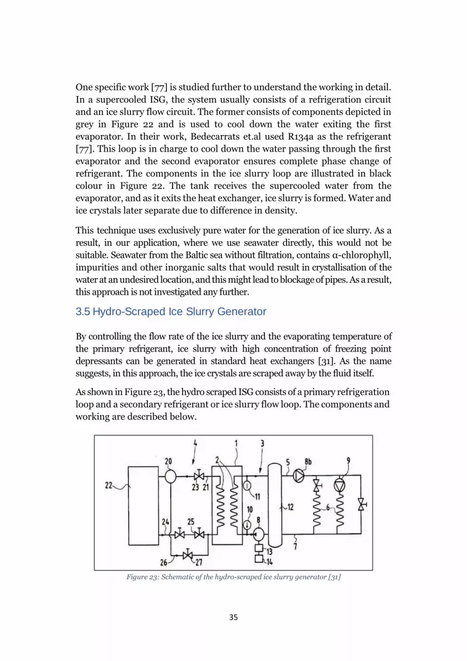
3.5 Hydro-Scraped Ice Slurry Generator

By controlling the flow rate of the ice slurry and the evaporating temperature of

the primary refrigerant, ice slurry with high concentration of freezing point

depressants can be generated in standard heat exchangers [31]. As the name

suggests, in this approach, the ice crystals are scraped away by the fluid itself.

As shown in Figure 23, the hydro scraped ISG consists of a primary refrigeration

loop and a secondary refrigerant or ice slurry flow loop. The components and

working are described below.

Figure 23: Schematic of the hydro-scraped ice slurry generator [31]

36

Primary refrigeration cycle: Evaporator (1), Compressor (20), Condenser

(22), Regulation valves (23, 27), Expansion valve (25)

Ice slurry loop: Pump (8), Temperature gauge (10, 11), Storage tank (12),

Variable speed motor (13), Control box (14)

Distribution of ice slurry: Distribution line (5), Heat exchangers to

melt ice slurry (6), Return line (7), Pump (8b)

The parameters determining the formation of crystals in the evaporator are

temperature and pressure of the slurry loop. The increase in pressure difference

between the input and output stream of the refrigerant and the decrease of the

temperature difference is an indicator of formation of ice crystals. Then, the

electronic controller increases the flow rate of the ice slurry because of which,

turbulence is created, and the crystals start to disengage from the surface of the

evaporator. The increase in velocity accompanying the increase in flow rate helps

in removal of the forming ice crystals. Simultaneously, the refrigeration

capacity is decreased and this aids in the removal as well. Ice slurry is then

formed by the removed crystals in the secondary refrigerant flow. Now, the

flow rate and the associated properties return to nominal conditions and the

cycle resumes.

One could also apply special coating, like sol-gel, on the surface of the

evaporator to avoid the adhesion of ice [31]. The absence of no moving parts

like rods or blades, reduces the investment costs and the O&M costs.

Nonetheless, salt-based solutions for ice slurry generation are inclined to

present greater adhesiveness, and thus, are less suited for this type of ISG,

unless a suitable coating material that solves this issue is developed.

3.6 Fluidised Bed Crystalliser

Klaren’s work paved the way for ice slurry generation by the fluidised bed

crystalliser method [31]. In this system, the primary refrigerant (for instance,

ammonia) evaporates on the shell side, while ice crystals are formed on or

near the inner periphery of the tubes. A fluidised bed, comprising of little

steel or glass elements, with a radius of 0.5-2.5mm, is present within the

tubes. As the ice slurry feed flow flows upwards in a liquid state, the particle

beds are fluidised. This is followed by a constant impingement of the solid

particles on the inner walls of the tubes, preventing a build-up of a layer of

ice on the heat transfer surface and improved heat transfer rates. This

mechanism is displayed in Figure 24.

37

Figure 24: Ice Removal Mechanism in a Fluidised bed crystalliser [31]

Figure 25: Schematic – Fluidised bed heat exchanger

A major advantage of this method is the low investment and O&M costs, because

of no complex moving mechanical components, except for the pump [79]. Ice

fractions up to 30% could be generated in a single pass, while multiple passes

could be employed to generate a higher fraction of ice particles in the slurry.

Although this system has the above-mentioned benefits, certain limitations

prevent it from being utilised for our application. Even though this has been

working well in a laboratory scale, its commercial viability has not been

tested. Since the current work calls for a district heat of ~300MW, scaling up

without prior studies is not feasible. Since seawater is the fluid being used to

generate ice slurry, the salt present in it might corrode the components. So,

38

components having materials like stainless steel, for example, should be

coated with a non-corrosive layer. This increases the expenditure of the

system. The vertical layout of the beds poses a space issue, requiring a lot of

floor space and very high ceilings. With the proposed system planned to be

built underground [46], this limitation makes it almost infeasible to consider

this option. The trade-off between the allowable temperature difference

between the refrigerant and the working fluid, and its relationship with the

freezing up of the heat exchanging walls rounds up the reasons behind the

non-pursual of this method for this work [79]. As a result, further attributes of

the system, including the rate of residence, the velocity, circulation, presence of a

cyclone etc., are not explored any further.

3.7 High-Pressure Ice Slurry Generator

As the term ‘high-pressure ice slurry generator’ implies, this technique employs

the application of high-pressure to generate ice/ice-slurry. Otero et. al., in their

work have described two high-pressure freezing processes that are described

in brief below [80]:

High-pressure assisted freezing (HPAF)

In this process, ice or associated polymorphs are obtained by applying a constant

high pressure and simultaneously reducing the temperature to the corresponding

freezing point. Governed by thermal gradient, the cooling of the process fluid

follows from the surface to the centre, with the nucleation of ice occurring in the

outer periphery of the surface with the crystals growing in a dendritic manner

towards the centre radially.

High-pressure shift freezing (HPSF)

Pascal’s principle states that a pressure change at any point in an enclosed

incompressible fluid is transferred throughout the fluid such that the change is

reflected everywhere else. In accordance with this principle, a pressure release

takes place almost spontaneously upon expansion throughout the entire sample

and, consequently, a decrease in the temperature corresponding to the pressure

drop is produced. This in turn results in a high degree of supercooling, and

subsequently, higher nucleation rates [80].

There is another high-pressure freezing process known as high-pressure induced

freezing wherein, phase transition is instigated by a rise in pressure and is

sustained at the same pressure. This method has not been studied in detail and

hence is not explored further [81].

39

In HPSF method, the transition of phase is induced due to a change in pressure

that fosters metastable conditions and spontaneous ice generation. The change in

pressure could be gradual, over several minutes, or rapid, within a couple of

seconds. The kinetics of the freezing process depends on the level of supercooling

attained, which in turn depends on the manner of release of pressure. Usually,

water is compressed and then pre-cooled to a temperature close to its freezing

point, where it remains in a liquid state. The pressure is then released, which

causes uniform supercooling, which in turn causes uniform nucleation, which

ensues the release of latent heat. This heat is absorbed, and the temperature rises

to the freezing point and crystals are formed, the fraction being determined by the

pressure and temperature before the expansion.

Figure 26: High-pressure freezing processes inserted on the phase diagram of water. (a) HPAF (b)

HPSF with phase transition at atmospheric conditions (c) HPSF with phase transition under

pressure [81]

One of the drawbacks of this process is the high economic cost of high-pressure

equipment as compared to other ISGs. Also, it is common knowledge that the

dendritic particles, characteristically elongated and rough in texture tend to

form large, entangled clusters which results in plugging and hence, are

considered far from optimal for ice slurry generation [82]. In addition, the

current level of knowledge of high-pressure equipments for continuous

processes also deters the author from exploring this technique any further.

40

3.8 Recuperative Ice Making

Contrary to other commercially available ISGs, wherein supercooling of a

secondary fluid occurs in the evaporator with ice crystals forming on the

surface and then later scraped off, in the recuperative ice slurry system, the ice

formation on the cold surface i.e., ice buildup is reduced and it is removed at

regular intervals through a recuperative heat exchanger.

Figure 27: Refrigeration circuit for recuperative ice slurry generator [31]

As depicted in the Figure 27, the pair of heat exchangers (4a, 4b) act as the

interface between the refrigeration loop and the ice-generating loop. Other

numbered components include compressor (1), air-cooled condenser (2),

reversible 4-way valve (3), heat exchangers (4a), (4b), check valves (5a), (5b),

accumulator with heat exchange coil (7), expansion valve (8), check valves (9a),

(9b).

The refrigerant flows from the condensing pack [consisting of a compressor and

air-cooled condenser] and is fed to a reversible 4-way valve, which regulates the

flow of refrigerant to either of the heat exchangers. Firstly, the hot exhaust

gas from the compressor passes through the condenser and condenses in the

heat exchanger (4a), releasing ice and raising the temperature. As the

temperature increases, approaching that of ambient air, condensation starts

happening in the condenser, with the warmer liquid flowing to (4a) at a

controlled temperature. The sub-cooled liquid refrigerant then exits (4a) is

then directed by check valves (5a, b) to an accumulator, and is then expanded at

(8), resulting in wet vapour. This is then sent via the second set of check

valves (9a, b) to the second heat exchanger (4b), which, takes up the role of

an evaporator and acts as the site for generating ice crystals. The amount of

flash gas formed is small because of the relatively low temperature change of

41

the refrigerant between the two heat exchangers, owing to the falling film.

[31].

After a certain time, de-icing is done by reversing the refrigerant flow. Since,

this process is done in a cyclical manner, this method is aptly termed recuperative.

The corrugated/grooved surface of the turbo-chiller plate, creates a highly

turbulent flow, leading to higher heat transfer rates.

One chief advantage of this system is its ability to generate ice slurry continuously

without utilising moving components like scrapers or orbital rods. This reduces

the investment costs and the O&M costs as well [31]. Further, since the evaporator

operates at a higher temperature, this reduces the amount of freezing point

depressant required. But the cost of the additional evaporator surface, difficulty in

maintaining the cooling capacity of the refrigerant and lack of commercialisation

at large scale dissuades us from actively investigating this method for our

application.

3.9 Vacuum Ice Generation

The most efficient method of producing ice slurry using water utilises a direct

contact heat transfer vacuum freeze process. Figure 28 shows the phase

diagram for the three phases of water – vapour, liquid and solid. The idea

behind this mechanism is that, at triple point, all three phases co-exist. As

water molecules (maintained at triple point in vacuum) are evaporated,

energy is removed from the neighbouring liquid particles, causing them to

freeze and form ice particles [83]. Let us now delve deep into the system.

Figure 28: Phase diagram of water indicating the triple point [33]

42

Figure 29 depicts the schematic illustration of a vacuum ice generator. The

numbered components relevant to the ice slurry generation are evaporator

(1), compressor (2), heat exchanger (3), ice slurry pumped out (4,5)

Figure 29: Vacuum ice generation with water as refrigerant [31]

The evaporator contains a pure water or saltwater solution and is maintained

at near the triple point conditions. The water is evaporated in the evaporator

(1) and compressed to condenser pressure at (2). Owing to the low pressure

and correspondingly, low density of water vapour, compression of it is a

cause of concern. However, some institutions have developed solutions in the

form of centrifugal compressors and turbo compressors. Since seawater

contains dissolved gases that are non-condensable, over a period of time,

they start to build up, leading to increased pressure on the condenser side.

To avoid it, and thereby, reduce the work done by the compressor, a vacuum

pump is required on the condenser side. [32].

If pure water is used, freezing up of the walls of the evaporator might occur

and defrosting cycles become necessary. When used in combination with

seawater, the vacuum ice generator partly freezes the water, leading to larger

enthalpies being removed (latent heat) as compared to sensible cooling of sea

water in conventional heat pumps [31]. For our specific application, we need

to utilise seawater in the winter, exhibiting temperatures just above freezing

point, as a heat source.

A similar system was in operation from 1986 till it was decommissioned in

2005 in Denmark. In addition, ILK Dresden are attempting to establish a

similar system as well. The two systems are studied in detail subsequently.

43

Augustenborg DH system [83, 84]

This sub-section describes the vacuum ice generator pilot plant, used as a

heat pump, with seawater as source for the Augustenborg District Heating

Plant. For this process to be continuous and functioning over long periods of

time, the water vapour needs to be extracted continuously. For pure water, at

triple point, the pressure is 6.103 mbar abs, and the temperature is 0.01°C.

But since, seawater is being utilised, the triple point pressure depends on the

salinity of water (S) as well in the following manner:

𝑃𝑡 = 6.103 − 0.246 𝑆 (𝑚𝑏𝑎𝑟) (1)

Since the pressure is very low, at around 6mbar, the density of the water

vapour is low as well. This poses a problem while compressing it owing to the

large required swept volume, but some establishments such as IDE, Solid

Energy etc., have developed solutions to combat this cause of concern. This

vacuum ice maker (VIM) works well with all water temperatures and is

therefore suited for being used in a DH plant.

Figure 30: Schematic illustration of the vacuum ice generation system for Augustenborg DH plant

[83]

Figure 30 displays the schematic diagram of the plant in Augustenborg. Sea

water was initially fed to the evaporator, which was maintained at triple point

condition of 5 mbar, -1°C for the corresponding salinity level of around 4.5‰.

As the vapour evaporated, it passed through a turbo compressor (swept

volume of ~75 m3/s) and a pressure ratio of 1: 1.45, corresponding to a

temperature increase of about 5°C. The refrigerant cycle employed R12 as the

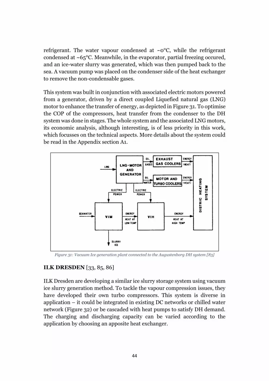
44

refrigerant. The water vapour condensed at ~0°C, while the refrigerant

condensed at ~65°C. Meanwhile, in the evaporator, partial freezing occured,

and an ice-water slurry was generated, which was then pumped back to the

sea. A vacuum pump was placed on the condenser side of the heat exchanger

to remove the non-condensable gases.

This system was built in conjunction with associated electric motors powered

from a generator, driven by a direct coupled Liquefied natural gas (LNG)

motor to enhance the transfer of energy, as depicted in Figure 31. To optimise

the COP of the compressors, heat transfer from the condenser to the DH

system was done in stages. The whole system and the associated LNG motors,

its economic analysis, although interesting, is of less priority in this work,

which focusses on the technical aspects. More details about the system could

be read in the Appendix section A1.

Figure 31: Vacuum Ice generation plant connected to the Augustenborg DH system [83]

ILK DRESDEN [33, 85, 86]

ILK Dresden are developing a similar ice slurry storage system using vacuum

ice slurry generation method. To tackle the vapour compression issues, they

have developed their own turbo compressors. This system is diverse in

application – it could be integrated in existing DC networks or chilled water

network (Figure 32) or be cascaded with heat pumps to satisfy DH demand.

The charging and discharging capacity can be varied according to the

application by choosing an apposite heat exchanger.

45

Figure 32: Integration of vacuum ice slurry generation with a chilled water network [33]

A pilot plant with 90m3 slurry storage unit has been designed to operate in

operation at the Westsächsische Hochschule Zwickau. A maximum of

~500kW of refrigerating capacity/ice slurry generation could be achieved by

utilising a single compressor [87]. The storage unit allows for flexibility in

operations and reduces the discrepancy between the supply and demand,

along with a reduced fiscal strain, if charged during low tariff periods. In

addition, the stored ice slurry, which is pumpable as well, can also be utilised

for process cooling as a coolant.

This system uses R717 as a refrigerant. Refrigerant grade Ammonia is

commonly used in industrial refrigeration plants and is of safety class B

(toxic). However, since ammonia is hazardous and a leak could potentially

cause severe injuries to those handling it in the plant, intensive safety

regulations are to be met [88]. A 3D illustration of a water vapour compressor

in the vacuum ice slurry generation system of the experimental plant is

displayed in Figure 33.

Figure 33: Design of the experimental plant in ILK Dresden presented at the ATMOsphere Europe

2013 conference [29]

46

It is now observed how this system could be used in heating applications.

Integration of heat pumps in DH systems is a chief contributor towards

increased cleaner energy shares. This system developed at ILK Dresden

enables the use of water, even during winter, as source of heat without the

risk of frosting. This makes this system and the one in Augustenborg ideal

‘prototypes’ for our application. The system could be used to generate heat in

the following manner, as depicted in Figure 34.

Figure 34: Cascading of heat pumps enabling the use of water at ~0°C as a heat source [33]

Water is initially taken from a water source (at temperatures close to 0°C)

and fed to an evaporator. The evaporator is maintained at triple point and

the vapour is compressed by a specially designed turbo-compressor that

raises its temperature by a small value. This in turn, causes the partial

freezing of water and ice-slurry is formed that could be either stored or

pumped away. The vapour is then passed through a heat exchanger

(condenser), with heat being transferred to a refrigerant. The heated

refrigerant, then transfers the heat to the water to be heated through a

conventional heat pump cycle. Thus, the temperature of the hot water is

raised to the desired levels. This is how this vacuum ice generation system

designed by ILK Dresden could be integrated with heat pumps for heating

purposes.

The above two large-scale applications of using ice slurry in DH played a

pivotal role in the selection of vacuum ice generation method for our work.

We then proceed to model the vacuum ice generator, in combination with a

heat pump to produce the necessary District heating in Aspen Plus.

47

4. Modelling in Aspen Plus

This section includes all the aspects regarding the modelling of the vacuum

ice generation + District Heating system. Moreover, upstream and

downstream system characteristics, choice of refrigerant, heat exchangers,

ice slurry pumping are also described to get a better understanding of the

system level design.

4.1 Introduction to Aspen Plus

Aspen Plus is a product of Aspen Technologies, which was founded in 1981.

It is a process simulation software package, i.e., it is a modelling tool that

enables the user to design a process and select suitable thermodynamic

models and it simulates it using appropriate mathematical models and

envisages the performance of the process. It is further used to optimise a

process from a technical and economic standpoint, perform sensitivity

analysis, maximise, and minimise functions. Despite being a sequential

modular simulator, Aspen Plus has multiple functionalities and could be

used to simulate complex processes involving reactors, compressors, pumps,

distillation columns, flash system, electrolytes, crystallisers, heat exchangers

etc., and it finds its application in chemical process, oil, and gas,

pharmaceutical, food and beverage industries, to name a few. Owing to the

above-mentioned reasons, it was chosen to model the vacuum ice system in

Aspen Plus and analyse the technical viability of it. [89, 90, 91].

4.2 Choice of Refrigerant - R1234ze

HFCs (Hydrofluorocarbons) like R134a, R404a are one of the most used

refrigerants across the globe. But, due to rising environmental concerns,

HFCs are being phased out and being replaced by alternatives having lower

GWP and ODP levels. With the advent of HFOs (Hydrofluoro-olefins), a class

of environment-friendly refrigerants having low GWP values and abiding by

Kigali amendment of the Montreal Protocol, this certainly seems to be

beginning of the end for HFCs. With desirable GWP, ODP values and good

thermodynamic properties, HFOs have already been adopted in several parts

of Western Europe, while other countries are following suit [92].

One among the HFO refrigerants - 1,3,3,3-tetrafluoropropene, commonly

known as R1234ze, was developed to adhere to the F-gas regulation laid

down by the European Union [93] to control emissions from fluorinated

greenhouse gases. R1234ze, being more energy efficient than conventional

refrigerant like R404A, is utilised in several medium temperature

48

applications such as heat pumps, chillers and in industrial cooling [94]. It

has a boiling point at 0 bar (g) of -18.95°C and thus, it is similar to R134A in

this sense [95]. The physical properties of R1234ze are displayed in in Table

A. 2 in the appendix. Further, an EIA report in 2021 [96] recommends the

use of R1234ze as the refrigerant for the seawater heat recovery project

(“Lämpöpumppujen kylmäaineista todennäköisin on HFO-yhdiste R1234ze

(GWP100a=0”). Owing to the aforementioned reasons, the refrigerant

R1234ze is considered to be the refrigerant for our work.

4.3 The Aspen Plus Model

4.3.1 Overview

Let us look at the overview of the system that has been modelled in Aspen

Plus to produce 300MW of district heat (Figure 35). The components and the

parameters are explained in detail later. As we can see, seawater initially

enters the evaporator (EVAP) and as mentioned in the preceding section, it

is maintained at triple point. The triple point pressure is calculated according

to equation 1. Now, on the application of very small amount of heat, a

molecule of water turns into vapour and travels to the water vapour

compressor (H2O-COMP), while due to removal of heat, ice is generated at

the slurry generator. In this work, the vacuum ice slurry generator is

modelled in two stages and the heat duties are set to be the same. The two

components include the evaporator from which the supercooled liquid exits

and the cooler (ISG) which produces ice slurry at desired fraction.

The compressed water vapour (S4) exchanges heat with the cold refrigerant

(R1234ze) flowing through a heat exchanger (HEATX-1). Once heat has been

exchanged, the water vapour stream, in a liquid state (indicated in green

colour), is recirculated back to mixer (B8) where it is mixed at atmospheric

pressure along with incoming seawater and enters the evaporator.

The refrigerant which is now in a vapour state (S7) is raised to a higher

pressure by means of a compressor (REF-COMP). Now, this refrigerant is fed

into a heat exchanger (HEATX-DH) where it condenses, releasing heat and

raising the temperature of the DH water from 45°C to 90°C. This heat

exchange is an integral component of the system and serves to recompense

the ~300MW lost due to the retiring of the Salmisaari CHP plant. The

refrigerant now, after the exchange of heat is now in a cooled state (COOL-

REF) and is now reduced to the initial pressure by means of an expansion

valve. The refrigerant is then re-circulated back to HEATX-1 and the cycle

continues.

49

Figure 35: Process Flowsheet of the simulated model in Aspen Plus

On the other hand, the ice slurry generated by the generator is now

discharged back into the sea. But since there will be a pressure loss

accompanying the transport of ice slurry through long distances (in this case,

about 500m [45]), this necessitates the involvement of a pump. The pump

then increases the pressure by an amount equal to the drop incurred by the

transport of ice slurry, and thus, the ice slurry is pumped back into the sea.

4.3.2 Components and Setup parameters

The challenging part here is the determination of mass flow of input (mass

flow of seawater). It should be fixed such that the ice slurry generated is of

desired ice fraction and the district heat produced is what is required. For

this purpose, a Design-spec is used (B6 in Figure 35). It is similar to a

feedback controller, wherein the desired value for a variable is specified and

another variable is manipulated to obtain it. In this case, the mass flow rate

was varied such that the ice slurry generated has a liquid fraction of 80%

(LFRAC = 0.8) and thereby, ice fraction of 20%. This is illustrated in Figure

36. The reasoning behind utilising slurry having 20% ice fraction is explained

in the next section.

Figure 36: Design specification to set the liquid fraction of the generated slurry as 0.8.

50

For the Mixer, it is set such that the incoming seawater and the recirculated

water are combined into a single stream at atmospheric pressure.

The inlet seawater properties are as illustrated in the Figure 37. The

temperature and pressure were set to ~0°C and 1 bar respectively to model

conditions during winter [45]. Further, the 0.6% saline seawater [51] was

modelled as water + sodium chloride proportionately. The mass flow

calculations are initialised at 3000kg/s and based on the design-spec are

iterated till the desired value is reached.

Figure 37: Inlet seawater properties in Aspen Plus

As mentioned earlier, the evaporator is set to triple point conditions as

depicted in the Figure 38. Here, in Aspen Plus, the evaporator is modelled

using separator Flash2, which determines the thermal and phase conditions

of the inlet stream on specifying the outlet conditions. In this case, we specify

the triple point pressure (equation 13) and the heat duty [97]. The valid

phases are set to be vapour-liquid.

Figure 38: Evaporator specifications in Aspen Plus

51

The Flash2, in conjunction with the cooler (model Heater in Aspen Plus,

denoted by ISG in Figure 35), constitutes the ice slurry generator. The heat

duty and the pressure of the ISG was set to be the same as the evaporator.

The slurry coming out of the ISG is to be pumped to a distance of about

1000m. The hydraulic and driver efficiency of the pump as set to be 75% and

90% respectively [98]. The pump outlet specification is set to ‘Pressure

increase’ and the value is set based on calculations in the Section 6 and can

be varied as per the requirement.

The water vapour compressor was set to type ‘isentropic’ and the pressure

ratio was adjusted according to the condensor pressure. The efficiencies were

set to be the default values [97].

The refrigerant used, R1234ze, acquires its properties from REFPROP in the

Aspen physical property system. It provides thermodynamic and transport

properties of fluids predominantly utilised in the industries, with particular

focus on refrigerants and hydrocarbons [99]. It is ensured that the streams

REF-IN and REF-IN-O have the same stream properties. The mass flow here

is obtained on adjustment to ensure ~300MW of DH is produced. The input

data of the refrigerant is displayed in Figure 39.

Figure 39: Input specifications for the refrigerant R1234ze

For the input parameters of the heat exchanger (HEATX-1), the model

fidelity is set to ‘Shortcut’, which performs simple material and energy

balance calculations. The flow direction is set to ‘countercurrent’ for optimal

output and the exchanger specification for the cold stream output vapour

fraction is set to be 1, meaning the refrigerant on passing through the heat

exchanger should completely change into vapour phase.

The pressure ratio of REF-COMP is varied to a value slightly less than the

critical pressure of the fluid [95] to have a high COP. The efficiencies are set

to the default values [97].

52

The other heat exchanger, HEATX-DH, is designed in a similar way as

HEATX-1, with only the exchanger specification being different. In this case,

the cold stream output temperature is set to 90°C, which is the intended

target [45]. The inlet temperature of the DH water (DHW-IN) is set at 45°C,

based on Helen Oy’s usual practice [45]. The expansion valve (B7) is set to

release the fluid at its initial pressure of 1.5 bar.

One shortcoming of Aspen Plus is its inability to model closed loops. To work

around it, the recirculating water stream (RECIRC-O & RECIRC) and the

refrigerant stream (REF-IN-O & REF-IN) are split and the inlet values are

set the same as the output values.

Prior to all this modelling in the simulation part, we need to define the

properties and the materials in the Properties part. Since saltwater

transforming into ice involves electrolytes, the base method was set as

‘ELECNRTL’ and the method filter ‘COMMON’. Similar to REFPROP for the

refrigerant, we use ‘STEAM-TA’ for District water properties. The model is

then simulated by pressing the ▶️ symbol or the functional key F5.

A parametric study was done to determine the mass flows that would aid in

the designing of a flexible system. And for this reason, the model was

simulated for three cases by fixing the ice slurry generator capacity to 3 MW,

200MW, 300MW. The reasoning behind these numbers was 3 MW was the

biggest ISG currently in commercial use [31, 100], while 200MW and

300MW were chosen with the idea that the ensuing DH produced would be

comparable to what the city of Helsinki would require. Lastly, the pressure

ratio of the water vapour compressor is varied to study how it affects the COP

of the system. The results of this are then utilised in the next section to

calculate the pressure drop for the resulting ice slurry generated.

4.3.3 Model Validation

The pressure drop values obtained in the model developed in this work has

been validated with the results obtained by IDE’s ice slurry generator. The

ice slurry generated at IDE’s plant had a flow rate of 240 m3/h (1057 gpm).

The pressure drop values in the system and the model developed were in

agreement [45] and hence the work proceeded in this direction.

53

5. Pressure drop analysis of ice slurry during

transport

Prior experiments have led to researchers concluding that ice slurry behaves

as a Newtonian fluid at lower ice fraction (~20%) and as a non-Newtonian

fluid at higher concentrations [101]. A Newtonian fluid is a fluid whose ratio

of shear stress to that of shear strain (i.e., viscosity) is independent of the rate

of shear [102]. In our case, the flow is assumed to be isothermal. For

isothermal ice-slurry flow, the pressure drop could be calculated by means of

Darcy-Weisbach equation:

∆𝑃

𝐿=

𝑓 ∗ 𝜌 ∗ 𝑣2

2 ∗ 𝐷 (2)

where the notations are as described in section Symbols and abbreviations

5.1 Pressure loss evaluation based on laboratory-scale

experimental data

In this method, the pressure drop is expressed in terms of the diameter and

mass flow. Subsequently, it would then be able to evaluate the pressure drop

for our application by utilising pressure drop data from previous experiments

for a certain mass flow and diameter.

We know the formula for pressure loss per length (equation 2). Here, one of

the friction factor models is substituted for f and the velocity is written in

terms of mass flow.

Mass flow rate, m:

�̇� = 𝜌𝐴𝑣 (3)

𝑣 = 4 �̇�

𝜌 𝜋 𝐷2 (4)

Blasius friction factor model for turbulent flow [103],

𝑓 = 0.316. 𝑅𝑒−0.25 (5)

f = 0.316 ∗ 𝜌−0.25 ∗ 𝑣−0.25 ∗ 𝐷−0.25 ∗ 𝜇0.25 (6)

Substituting the above two into equation 2,

54

∆𝑃

𝐿=

0.316 ∗ 𝜌−0.25 ∗ 𝑣−0.25 ∗ 𝐷−0.25 ∗ 𝜇0.25 ∗ 𝜌 ∗ (4 ∗ �̇�

𝜌 ∗ 𝜋 ∗ 𝐷2)2

2 ∗ 𝐷

∆𝑃

𝐿= 0.158 ∗ (

4

𝜋)

1.75

∗ 𝜌−1 ∗ 𝐷−4.75 ∗ 𝜇0.25 ∗ �̇�1.75 (7)

Now, on dividing the pressure loss per length for our case and the values

obtained from an experimental work, we obtain the below mentioned ratio.

∆𝑃𝐿

(∆𝑃𝐿 )𝑒𝑥𝑝

=0.158 ∗ (

4𝜋)

1.75

∗ 𝜌−1 ∗ 𝐷−4.75 ∗ 𝜇0.25 ∗ �̇�1.75

(0.158 ∗ (4𝜋)

1.75

∗ 𝜌−1 ∗ 𝐷−4.75 ∗ 𝜇0.25 ∗ �̇�1.75)𝑒𝑥𝑝

The subscript exp stands for the experimental value of the parameter. Now,

the constants get cancelled out and there will be a minimal difference in the

density (~2.8%) and viscosity (~3%) between our case and the experimental

case, owing to the difference in salinity in the experiments performed that we

would be using as a reference. When the ratio of the product of μ, ρ were

calculated and raised to respective powers, it was found out that they were

found to be close to 1 (~1.04 for 20% ice fraction) and therefore, the product

of ratio of density and viscosity raised to the respective powers were

approximated to 1.

Subsequently, the above equation is now reduced to:

∆𝑃𝐿

(∆𝑃𝐿 )𝑒𝑥𝑝

= 𝐷−4.75 ∗ �̇�1.75

(𝐷−4.75 ∗ �̇�1.75)𝑒𝑥𝑝 (8)

In addition to Blasius friction factor, the friction factor proposed by Knodel

et. al, was also considered [34].

𝑓 = 0.174064 ∗ 𝑅𝑒−0.2 (9)

Doing a reduction for Knodel’s friction factor as done previously results in

the pressure loss per metre length in the following manner:

∆𝑃𝐿

(∆𝑃𝐿 )𝑒𝑥𝑝

= 𝐷−4.8 ∗ �̇�1.8

(𝐷−4.8 ∗ �̇�1.8)𝑒𝑥𝑝 (10)

55

So, now we get an equation where pressure drop per length is dependent on

mass flow rate and diameter. We fix mass flow rate and vary the diameter (in

steps of 0.025m) and observe the pressure losses.

The experimental values obtained in Meewisse et. al [104], Lee et. al [105]

and Grozdek et. al [106] (presented in Appendix A3) were utilised and were

substituted in the above equations and the pressure drops were

comparatively studied.

5.2 Viscosity based pressure drop calculation

Although the above method provides us with a rough approximation of the

pressure drops, these values cannot be used in critical applications. The

difference between the actual values and the ones calculated from the method

mentioned above arises from a combination of factors - the density and

viscosity differences that are inherent of the fluid used (varying degrees of

freezing point depressant used, as compared to 0.6% salinity we use for this

work), experimental inaccuracies, instrumentation errors and since the

friction factor model is highly sensitive (raised to power of 4.75-4.80), this

has a magnifying effect on the error as well. As a result, we estimate the

pressure drop using equation 2, that couples the measured ice slurry viscosity

values and the various friction factor models found in the literature.

The friction factor models utilised are the earlier discussed Blasius [103],

Knodel [34] and Petukhov [31].

𝑓 = (0.79 𝑙𝑛 𝑅𝑒 − 1.64)−2 (11)

3000 ≤ 𝑅𝑒 ≤ 5 × 106

The viscosity measurements used in the calculation were UASCS (Rot visc in

1996, hereafter referred to as Rot96), UASCS (Rot visc in small storage,

hereafter referred to as UASCS), Cemagref (Online visc) [107], as depicted in

Figure 40. The experiments done at the University of Applied Sciences of

Central Switzerland (UASCS) were done with a Haake Type-RV 20 rheometer

with 10% mass fraction of talin and a small storage tank (Rot96) and a

relatively larger tank (UASCS), while those done by CEMAGREF were

performed with 11% mass fraction of ethanol in an Ostwald rheometer and

no storage.

56

Figure 40: Measured dynamic viscosities of ice slurries by DTI, UASCS and Cemagref [107]. The

ones indicated by red arrows are utilised in this study.

The mass flows of the ice slurry generated when the Aspen simulation is run

for the ISG capacity of 3 MW, 200 MW and 300 MW (discussed in section

6.2) are 50 kg/s, 3236.75 kg/s, 4799.47 kg/s. For these mass flows, we

calculate the pressure drop using equation 2. Since we know the mass flow,

we increase the diameter in steps of 0.025m and the velocity is automatically

adjusted (equation 4). The pressure loss per length values obtained are

compared with the experimental papers mentioned earlier.

In addition, a ratio of pump power to latent heat released by ice was

calculated to get an idea of how much power would be required as compared

to the heat released by the phase change. The length of the pipe has been

assumed to be 1000m for pumping purposes. The formulas used are:

Pumping Power,

𝑃 (𝑖𝑛 𝑊) =𝑄 ∗ ∆𝑝

𝜂𝑝𝑢𝑚𝑝 (12)

Q = Flow rate of slurry (m3/s)

∆p = pressure drop (Pa)

ηpump = efficiency of pump

Latent heat released,

𝑄𝑤𝑎𝑡𝑒𝑟 → 𝑖𝑐𝑒 (𝑖𝑛 𝑊) = �̇� ∗ 𝐿𝑤𝑎𝑡𝑒𝑟 →𝑖𝑐𝑒 ∗ 𝑥 (13)

�̇�= mass flow rate (in kg/s)

Lwater →ice = latent heat of fusion of water (334 kJ/kg)

x= ice fraction

57

6. Results and Discussions

6.1 Selection of Ice Slurry Generation method

The ice slurry generation methods and their suitability for our application are

analysed and summarised in Table 2.

Table 2: Ice slurry generation methods and its suitability for current work

Method Suitability

Scraped-surface ice slurry

generator

Not likely

- Continual freezing up of heat exchanging

surfaces on utilisation of low salinity water

- High power requirements

- Need for frequent maintenance

- Large space requirement (for vertical

configuration)

Direct contact ice slurry

generator with immiscible

refrigerant

Not likely

- Possibility of refrigerant being trapped in the

slurry, thus posing an environmental threat

when pumped back to the sea.

- Threat of ice formation on the injectors

Direct contact ice slurry

generator with an

immiscible secondary

refrigerant

Not likely

- The additional cycle results in increased

investment cost and energy consumption

- Possibility of an environment hazard when

the immiscible liquid-trapped crystals are

pumped back into the sea

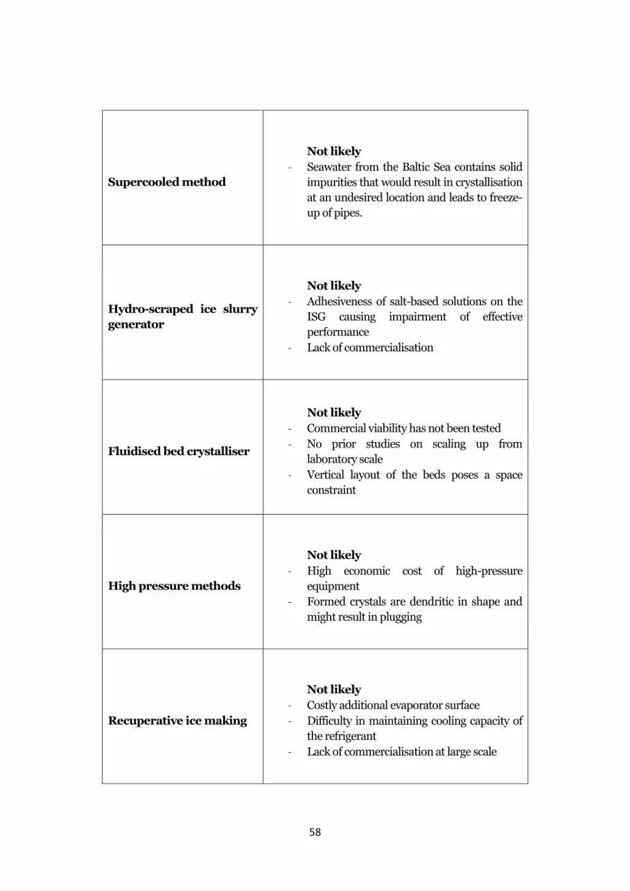
58

Supercooled method

Not likely

- Seawater from the Baltic Sea contains solid

impurities that would result in crystallisation

at an undesired location and leads to freeze-

up of pipes.

Hydro-scraped ice slurry

generator

Not likely

- Adhesiveness of salt-based solutions on the

ISG causing impairment of effective

performance

- Lack of commercialisation

Fluidised bed crystalliser

Not likely

- Commercial viability has not been tested

- No prior studies on scaling up from

laboratory scale

- Vertical layout of the beds poses a space

constraint

High pressure methods

Not likely

- High economic cost of high-pressure

equipment

- Formed crystals are dendritic in shape and

might result in plugging

Recuperative ice making

Not likely

- Costly additional evaporator surface

- Difficulty in maintaining cooling capacity of

the refrigerant

- Lack of commercialisation at large scale

59

Vacuum Ice Method

Seemingly feasible

- Previous similar application at Augustenborg

DH plant, Denmark

- A scaled-up system from laboratory scale has

been fabricated and operated, so seems

technically viable.

Thus, vacuum ice method is chosen to generate ice slurry as the proposed

solution in this work and this is followed by further studies of the system. The

following sections deal with the pressure drop evaluations and the

performance of the system.

6.2 Pressure Drop Analysis

As discussed earlier, the Aspen Plus model was simulated for three cases by

fixing the ice slurry generator capacity to 3 MW, 200 MW, 300 MW. The

corresponding DH produced, and the mass flow of the generated ice slurry

are tabulated in Table 3.

Table 3: District Heating produced and Ice slurry flow rate for fixed duty of the ice slurry

generator

Case Ice Slurry Generator

Duty (MW)

District Heating

produced (MW)

Ice slurry flow

rate (kg/s)

1 3 5.18 50

2 200 320.46 3240

3 300 518.39 4800

The mass flow of 3240 kg/s, i.e., ~3.24 m3/s for a DH capacity of 320MW is

in agreement with the preliminary estimates of Helen Oy [28]. Further, for

each diameter for each mass flow, the corresponding minimum velocity

required to ensure no phase separation occurs was calculated using the

following formula [31, 101] and if flow velocity is less than minimum velocity,

the diameters were not subsequently studied:

𝑣𝑚𝑖𝑛 = 1.4 ∗ √𝑔 ∗ 𝐷 ∗ (1 − 𝜌𝑖

𝜌𝑐𝑓) (14)

It was later proposed by Guilpart et. al. [108], for safety purposes, the

minimum velocity be twice of 𝑣𝑚𝑖𝑛 and this is what is used in our work. For

instance, as we can deduce from Figure 41, for a mass flow of 3240kg/s, the

60

upper limit on diameter, in accordance with Guilpart’s minimum velocity

formula, is 1.725 m.

Figure 41: Velocity vs Diameter plot for mass flow of 3240kg/s. The blue line denotes the minimum

velocity, based on Guilpart's formula, while the orange line indicates the flow velocity.

A comparative plot between the pressured drop per length of the three mass

flow rates against the viable diameters for 20% ice fraction is illustrated in

Figure 42 below. The pressure drop in the graph was deduced from the

pressure ratio analysis (Chapter 5.1), using Blasius friction factor and

experimental work [104]. Since the decommissioning of the Salmisaari CHP

plant creates a paucity of ~300MW of DH, case 2 (ice slurry flow rate of 3240

kg/s) alone is presented in detail in this report. The data for the other two

cases can be found in the appendix section A4.

Figure 42: Comparison of Pressure Drops per length of the three mass flows for an ice fraction of

20%

0

1

2

3

4

5

6

7

8

9

10

0 0.5 1 1.5 2 2.5

Vel

oci

ty (

m/s

)

Diameter (m)

Minimum Velocity Corresponding Velocity

0

0.05

0.1

0.15

0.2

0.25

0.3

0 0.2 0.4 0.6 0.8 1 1.2 1.4 1.6 1.8 2 2.2

Pre

ssu

re D

rop

per

len

gth

(kP

a/m

)

Diameter (m)

mass flow = 50kg/s mass flow = 3240 kg/s mass flow = 4800kg/s

61

Further, it was found out that the ratio of pump work to latent heat was the

least in case of ice fraction of 20%, irrespective of mass flow of the ice slurry.

A lower ratio implies that the work done by the pump is less as compared to

the energy released during the phase transition. This is validated by

evaluating the ratio using both pressure ratio analysis and viscosity-based

pressure drop calculations. Due to discrepancies in experimental

measurements of viscosity and pressure drop in the literature, we have

selected the values in a way so as to evaluate the best- and worst-case

pressure drop for our application. As it can be observed from the figure, a

system having 20% ice fraction offers the best benefit from an energy

expenditure point of view.

Figure 43: Pumping power/Latent heat vs Diameter for varying ice fractions for worst-case pressure drop

scenario.

In addition, although all diameters up to 1.725 m are technically possible

without phase separation, from a practical point of view, it need not be the

case. For instance, for a mass flow of 3240 kg/s, a diameter of 0.5 m

corresponds to a velocity of 16.88 m/s. In real-world situations, ice slurries

are pumped at much lower rates, with Snoek et.al, in their work, specifying a

value of 0.5-2.5 m/s in District cooling networks [109]. As a result, we

consider diameters having reasonable velocities (> 0.9 m, <1.725 m). Now,

let us look at the results obtained using pressure ratio analysis.

0

0.2

0.4

0.6

0.8

1

1.2

0.9 1 1.1 1.2 1.3 1.4 1.5 1.6 1.7 1.8

Pu

mp

ing

po

wer

/Lat

ent

hea

t (%

)

Diameter (m)

Blasius + Cemagref

5% 10% 15% 20%

62

Figure 44: Pressure drop vs diameter using pressure ratio analysis for a mass flow rate of 3240

kg/s. The first word in the legend (e.g., knodel) is the friction factor model, while the other one (e.g.,

lee) is the experimental paper used as reference

Figure 44 depicts the results of the pressure ratio analysis for 20% ice slurry

and a mass flow rate of 3240 kg/s. As we can see, the pressure drop

experienced in ice slurries is greater than that of water (blue), albeit not so

much. The pressure drop of water was calculated using Colebrook’s friction

factor [110] and using the pressure ratio analysis method (Knodel’s friction

factor) and the results were found to be in agreement. The small difference

could be attributed to the difference in additive concentration as stated

earlier. Hence, we also try to compare this with the results obtained using

viscosity-based pressure drop calculation.

0

0.05

0.1

0.15

0.2

0.25

0.9 1 1.1 1.2 1.3 1.4 1.5 1.6 1.7 1.8

Pre

ssu

re D

rop

(kP

a/m

)

Diameter (m)

knodel + meewise knodel + grozdek knodel + lee

blasius + grozdek blasius + meewise Water

63

Figure 45: Pressure drop vs diameter using viscosity-based pressure drop calculation for a mass

flow rate of 3240 kg/s. The first word in the legend (e.g., knodel) is the friction factor model, while

the other one (e.g., Rot96) is the viscosity used as reference

As we can see from Figure 45, the relative increase in pressure drop between

water and ice slurry is much more pronounced. When determining the

pressure drop for critical applications, it is advisable to align with the worst-

case scenario. Even though this might seem like a bit of overdesign, a safer

design is better than one that fails. We observe that when Blasius’ friction

factor is used in combination with the viscosity values obtained at Cemagref,

the pressure drop values are the highest. As a result, when deciding the pump

specifications, one should base it on these values.

For this mass flow, and an arbitrary diameter of 1.5m (based on realistic

velocity estimates), plotted friction factor vs ice fraction to get an idea of how

the ice fraction and the various viscosity values used influences the friction

0

0.05

0.1

0.15

0.2

0.25

0.3

0.35

0.9 1 1.1 1.2 1.3 1.4 1.5 1.6 1.7 1.8

Pre

ssu

re D

rop

(kP

a/m

)

Diameter (m)

petukhov cemagref blasius cemagref knodel cemagref

petukhov uascs blasisus uascs knodel uascs

petukhov Rot96 blasius Rot96 knodel Rot96

Water

64

factor (Figure 46). We realise that the viscosity values used (based on the

experiment) has a bigger role than the friction factor model, with the values

presented by Cemagref resulting in the highest pressure drop values.

Figure 46: Calculated friction factor plotted against ice fraction (in %) for a mass flow of 3240kg/s

and a diameter of 1.5m. The first word in the legend (e.g., Knodel) is the friction factor model, while

the other one (e.g., Rot96) is the viscosity used as reference

Since we have determined that the desired ice fraction for pumping for our

application is 20%, a graph is plotted between the pumping power required

in three different cases depending on the viscosity values used. The pump

power was calculated using equation 12 and the efficiency of the pump was

set to 0.8, which is subject to change, depending on the supplier. The length

of the pipe was assumed to be 1000m, based on discussions with the

concerned people [45]. The power required to pump the same volume of pure

water is also calculated and is provided as a baseline. The highest pressure

drop, which is observed when using Blasius friction factor model in

conjunction with the viscosity values we termed as ‘Rot96’, is almost twice of

what is required to pump water.

0.01

0.012

0.014

0.016

0.018

0.02

0.022

0 5 1 0 1 5 2 0 2 5

Fric

tio

n F

acto

r

Ice Fraction (%)

Blasius + UASCS

Knodel + UASCS

Petukhov + UASCS

Blasius + Rot96

Knodel + Rot96

Petukhov + Rot96

Blasius + Cemagref

Knodel + Cemagref

Petukhov + Cemagref

Water

65

Figure 47: Pumping power vs diameter - a comparison between water and ice slurry (20% ice

fraction) based on the viscosity models. Pump efficiency = 0.8.

6.3 Performance of the system

Once the pressure drop was calculated, for a mass flow of 3240 kg/s, ice

fraction of 20% and a pipe diameter of 1.5 m, a pump was appended to the

Aspen model, and it was made to raise the pressure equivalent to what is lost

while pumping it for a distance of 1000 m. This corresponded to a pump work

of about 106 kW, as it can be observed from Figure 48.

Figure 48: Summary of the results of working of the pump.

0

200

400

600

800

1000

1200

1400

0.9 1 1.1 1.2 1.3 1.4 1.5 1.6 1.7

Pu

mp

ing

Po

wer

(in

kW

)

Diameter (in m)

Blasius + Cemagref Blasius + UASCS Knodel + Rot96 Water

66

The pressure ratio of the water vapour compressor was varied and the

influence of it on the COP was studied. This is presented in the graph below.

We can see that as the pressure ratio is increased, there is a drop in the overall

performance of the system. The COP is calculated as the ratio of the useful

energy produced (District Heating) to the energy required (sum of pump and

compressor work). It was discovered that the pump work is relatively small

compared to the work done by the compressor on the fluid and its effect on

the COP of the system is minimal.

Figure 49: Plot of COP vs Pressure ratio of the water vapour compressor.

However, it should be noted that the actual COP values of the system in

operation might be lower than the theoretical COP values obtained above.

Since the water compressors must operate at very low-pressure levels

(around 6 mbar), they are subject to high mechanical losses [97]. However,

since no definite data was available on the efficiency of the water vapour

compressors, the efficiencies of standard compressors are instead used in

this work and this incongruity gives raise to potential difference in the COP

of the system.

6.4 Contribution to SDG

The 2030 Agenda for Sustainable Development, adopted by the member

states of the United Nations in 2015, introduces 17 Sustainable Development

Goals (SDGs) with 169 targets [111, 112]. The present thesis contributes

chiefly to 5 of the SDGs and has an impact on the others as well. The main

synergies are presented in Figure 50.

2.6

2.65

2.7

2.75

2.8

2.85

1 1.2 1.4 1.6 1.8 2 2.2 2.4

Co

effi

cien

t o

f P

erfo

rman

ce

Pressure Ratio of the Water vapor compressor

67

Figure 50: United Nations Sustainable Development Goals that are in synergy with the current

work

By means of this work, we attempt to suggest a cleaner alternative to the

existing coal CHP plant in Salmisaari. This decarbonised alternative would

lead to lesser pollution and thus, would have a positive interaction with SDG

3 (Ensure healthy lives and promote well-being for all at all ages), SDG 7

(Ensure access to affordable, reliable, sustainable, and modern energy for all)

and SDG 13 (Take urgent action to combat climate change and its impacts).

Further, the construction of such a seawater-based DH system, is a step

further in achieving SDG 9 (Build resilient infrastructure, promote inclusive

and sustainable industrialization and foster innovation). In addition,

extracting the refrigerant from naturally available seawater, and disposing

the generated slurry back into the sea ensures that we are on track to achieve

SDG 12 (Ensure sustainable consumption and production patterns).

6.5 Future Work

The present work is set to serve as one of the baseline support material for

Helen Oy in their continued work and materialisation of this project. In

addition to what has been done in the timeframe for this thesis, the following

will help in getting a better understanding of the subject and would impact

the work in a positive manner.

Before the construction of a 300 MW DH plant is constructed, a pilot plant

based on the current model and the corresponding pressure drop studies

68

could be built and its functioning studied, and shortcomings rectified. The

model could be improved in later works to enable the selection of multiple

pipelines for flow of slurry based on the amount of DH produced. The size of

the pipes should factor in the effect of elbows at the conjunction, and

minimum slurry velocities to avoid phase separation. In addition, the

performance of the water vapour compressor could be modelled more

accurately. In the current work, the particle size of ice slurry is assumed to be

constant and is considered to be the same as the experimental papers that

were referenced. The referenced papers did not employ the same method of

ISG as our application and hence, this variation should be factored in and

analysed further. A back-up plan (green and clean) must be worked out in

case of the plant fails before a major share of Helsinki’s citizens starts to rely

solely on this plant.

When the seawater from the Baltic Sea is used, it should initially be filtered

using a rough filter to keep away substances like fish, rocks that might

damage the system. From a manufacturing point of view, Solid Energy has

the design for a 2.6 MW compressor, but since the company has been

liquidated, they no longer manufacture compressors [97]. But the design is

ready and hence, with the help of suitable manufacturers, it could be built. A

team at DTI are trying to develop a 100 kW unit that is tentatively set to start

operating by next autumn. If the results are successful, a possible

collaboration could be considered. A vacuum pump must be used to

continuously remove the dissolved gases in water, as it was the case with the

Augustenborg DH plant [97].

Further, it would also be interesting to study is the ice slurry generated could

be utilised for some purpose, as it was done in Denmark, where they stored

it and used for district cooling in Copenhagen during the summer months

[97]. But since Helsinki’s district cooling requirements are not so high, the

slurry could be used in other applications, like for example, a ski hill in

Helsinki. Another important thing would be the selection of the location in

the sea to dump the ice slurry. An extensive EIA should be performed to study

how the ice slurry dissolves, and it should be ensured that there is a constant

current to prevent disastrous environmental consequences. Lastly, this work

is a part of a collaboration between Helen Oy, AFRY, Aalto University, VTT

and Luode Consulting and thus, the results of the individual works should be

compared and discussed in detail before proceeding further.

69

7. Conclusion

In this work, an attempt was made to identify the best-suited ice slurry

generation method that, on integration with heat pumps, would enable the

extraction of heat from surface seawater. All viable ice slurry generation

methods were analysed, and the chosen method of vacuum ice generation

was found likely to work for our application and has the potential to provide

~300 MW of District Heating capacity for the city of Helsinki. Prior

applications similar to ours (Augustenborg DH, ILK Dresden) point to

vacuum ice generation system being a promising alternative for Helen Oy’s

future.

A model of the proposed system was developed, with the incorporation of a

refrigerant/heat pump cycle, in Aspen Plus. The system was modelled to

cater to three different district heating demands, with one of the cases

(~300MW) explored in detail in the main report and the rest in the appendix.

The later part of the study, involving pressure drop analysis, attempts to

answer the second research question. Two methods of pressure drop studies

are carried out, utilising previously performed experiments on ice slurry, and

the scenario having the largest pressure drop is studied further. It is

concluded that the pressure drop, characterisitic of transport of ice slurry, is

quite minimal in the overall scheme of things, being less than 0.5% of the

total power consumed.

This is further complemented by a study of performance of the system and a

sensitivity analysis of the pressure ratio of the water vapour compressor on

the COP of the system. It is advisable to keep the pressure ratio of the water

vapour compressor slightly greater than 1 to prevent any loss in performance

of the system.

To sum up, this solution seems promising for the city of Helsinki and Helen

Oy to adopt such an alternative for district heating to realise its carbon-

neutrality goals before the proposed timeline. Although this model should

not be taken at its face value and the assumptions and limitations are to be

addressed, it however acts as a blueprint and a supporting document in

bringing such a clean source of district heating to fruition.

70

8. Bibliography

[1] IPCC, “Global Warming of 1.5°C: An IPCC Special Report on the impacts of

global warming of 1.5°C above pre-industrial levels and related global

greenhouse gas emission pathways,” 2018.

[2] United Nations, “Paris Agreement,” United Nations Framework

Convention on Climate Change, Paris, 2015.

[3] European Commission, “Paris Agreement,” European Union, [Online].

Available:

https://ec.europa.eu/clima/policies/international/negotiations/paris_en.

[Accessed 20 September 2021].

[4] European Council, “Climate change: what the EU is doing,” European

Union, [Online]. Available:

https://www.consilium.europa.eu/en/policies/climate-change/. [Accessed

06 July 2021].

[5] General Secretariat of the Council, “Proposal for a Regulation of the

European Parliament and of the Council establishing the framework for

achieving climate neutrality and amending Regulation (EU) 2018/1999

(European Climate Law),” Council of the European Union, Brussels, 2020.

[6] Ympäristöministeriö, “Finland's national climate change policy,” Ministry

of the Environment, [Online]. Available: https://ym.fi/en/finland-s-

national-climate-change-policy. [Accessed 15 July 2021].

[7] City of Helsinki, “Making Helsinki carbon-neutral,” My Helsinki, [Online].

Available: https://www.myhelsinki.fi/en/think-sustainably/making-

helsinki-carbon-neutral. [Accessed 15 July 2021].

[8] City of Helsinki, “The Carbon-neutral Helsinki 2035 Action Plan,” City of

Helsinki, Helsinki, 2018.

[9] Carbon Neutral Cities Alliance, “Helsinki, Finland,” CNCA, [Online].

Available: https://carbonneutralcities.org/cities/helsinki/. [Accessed 17

July 2021].

[10] City of Helsinki, “Environmental Sustainability Issues and Challenges in

Helsinki 2010,” Kopio Niini Oy, Helsinki, 2010.

[11] Helen Oy, “Carbon-Neutral Energy,” Helen Oy, [Online]. Available:

https://www.helen.fi/en/company/responsibility/responsibility-

71

report/environmental-responsibility/carbon-neutral-energy. [Accessed 18

July 2021].

[12] City of Helsinki, “Carbon-neutral Helsinki 2035: Summary,” City of

Helsinki, Helsinki, 2019.

[13] Helen Oy, “Helsinki closes Hanasaari power plant almost two years ahead

- carbon storage disappears from street view,” Helen Oy, 22 June 2021.

[Online]. Available: https://www.helen.fi/uutiset/2021/helsinki-sulkee-

hanasaaren-voimalaitoksen-lahes-kaksi-vuotta-etuajassa. [Accessed 12

November 2021].

[14] Rockplan, ”Salmisaaren hiilivarastot,” Rockplan, [Online]. Available:

https://www.rockplan.fi/referenssit/salmisaaren-hiilivarastot/. [Haettu

20 July 2021].

[15] Helen Oy, ”Salmisaaren Voimalaitosten Turvallisuustiedote,” Helen Oy,

Helsinki, 2016.

[16] ”Salmisaaren voimalaitos,” Wikipedia, [Online]. Available:

https://fi.wikipedia.org/wiki/Salmisaaren_voimalaitos. [Haettu 23 July

2021].

[17] Helen Oy, “Salmisaari power plant,” Helen Oy, [Online]. Available:

https://www.helen.fi/en/company/energy/energy-production/power-

plants/salmisaari-power-plant. [Accessed 18 July 2021].

[18] Helen Oy, “Kellosaari reserve power plant,” Helen Oy, [Online]. Available:

https://www.helen.fi/en/company/energy/energy-production/power-

plants/kellosaari-stand-by-power-plant. [Accessed 19 July 2021].

[19] Helen Oy, ”Kierrätyspesulla Tehoa Merivesi-lämmönvaihtimiin,” Motiva,

Helsinki, 2016.

[20] A. Fin, “Salmisaari B powerplant in Helsinki, Finland. Built 1984,

Architects: Timo Penttilä, Heikki Saarela and Kai Lind.,” Wikimedia

Commons, 2007.

[21] BMH Technology, “Bioflame solution in Salmisaari Power Plant, Helsinki,

Finland,” BMH, [Online]. Available:

https://www.bmh.fi/references/bioflame-solution-in-salmisaari-power-

plant-helsinki-finland/. [Accessed 20 July 2021].

[22] A. Sherrard, “Helen inaugurate Finland's largest pellet-fired boiler,”

Bioenergy International, 21 February 2018. [Online]. Available:

https://bioenergyinternational.com/heat-power/helen-inaugurate-

finlands-largest-pellet-fired-boiler.

[23] Helen, “First bioenergy heating plant in Helsinki inaugurated,” Euroheat &

Power, 14 February 2018. [Online]. Available:

72

https://www.euroheat.org/news/first-bioenergy-heating-plant-helsinki-

inaugurated/.

[24] S. Morgan, “Finland confirms coal exit ahead of schedule in 2029,”

Euractiv, 12 April 2018. [Online]. Available:

https://www.euractiv.com/section/energy/news/finland-confirms-coal-

exit-ahead-of-schedule-in-2029/.

[25] Ministry of Economic Affairs and Employment, “Investment incentives to

promote rapid phase-out of coal in energy production,” Suomen

valtioneuvosto, 27 March 2020. [Online]. Available:

https://valtioneuvosto.fi/en/-/1410877/investment-incentives-to-

promote-rapid-phase-out-of-coal-in-energy-production.

[26] Finlex, ”Laki hiilen energiakäytön kieltämisestä,” Suomen

oikeusministeriö, 16 April 2019. [Online]. Available:

https://www.finlex.fi/fi/laki/alkup/2019/20190416.

[27] Eduskunta, “Hallituksen Esitys eduskunnalle laeiksi hiilen energiakäytön

kieltämisestä ja oikeudenkäynnistä markkinaoikeudessa annetun lain 1

luvun 2 §:n muuttamisesta,” Eduskunta, Helsinki, 2018.

[28] Helen Oy, Sea water heat recovery, Helsinki: Personal communication,

2021.

[29] ILK Dresden, “Energy efficient vacuum freezing ice slurry generation using

a R718 compressor,” ATMOsphere, Brussels, 2013.

[30] D. R. Legates, “Latent Heat,” in Encyclopedia of World Climatology,

Encyclopedia of Earth Sciences Series, Dordrecht, Springer, 2005.

[31] Michael Kauffeld, Masahiro Kawaji, Peter W. Egolf, Handbook on Ice

Slurries: Fundamentals and Engineering, Paris: International Institute of

Refrigeration, 2005.

[32] T. M. Hansen, E. Noergaard and B. Frei, “Transport,” in Handbook on Ice

Slurries, Paris, International Institute of Refrigeration, 2005, pp. 167-201.

[33] ILK Dresden, “Ice Slurry: For Refrigeration and Heat supply,” Institute for

Air Handling and Refrigeration, Dresden, 2016.

[34] B. Knodel, D. France, U. Choi and M. Wambsganss, “Heat transfer and

pressure drop in ice-water slurries,” Applied Thermal Engineering, vol.

20, no. 7, pp. 671-685, 2000.

[35] E. Stamatiou, J. Meewisse and M. Kawajia, “Ice slurry generation

involving moving parts,” International Journal of Refrigeration, vol. 28,

no. 1, pp. 60-72, 2005.

73

[36] J. W. Mullin, Crystallization, Butterworth-Heinemann, 2001, p. 600.

[37] C. Okolieocha, D. Raps, K. Subramaniam and V. Altstädt, “Microcellular to

nanocellular polymer foams: Progress (2004–2015) and future directions

– A review,” European Polymer Journal, vol. 73, pp. 500-519, 2015.

[38] Hydrology and Atmospheric Sciences - University of Arizona, “Formation

and Growth of Ice Crystals,” 2011. [Online]. Available:

http://www.atmo.arizona.edu/students/courselinks/fall11/atmo551a/AT

MO_451a_551a_files/ColdClouds.pdf. [Accessed 15 May 2021].

[39] P. Pronk, J. Meewisse and C. Infante Ferreira, “Fluidized bed for ice slurry

production,” Delft University of Technology WbMT, Delft, 2002.

[40] Ishita Gupta, “Why sphere minimizes surface area for a given volume?,”

Physics Stack Exchange, 29 November 2015. [Online]. Available:

https://physics.stackexchange.com/questions/221210/why-sphere-

minimizes-surface-area-for-a-given-volume.

[41] X. Liu, K. Zhuang, S. Lin, Z. Zhang and X. Li, “Determination of

Supercooling Degree, Nucleation and Growth Rates, and Particle Size for

Ice Slurry Crystallization in Vacuum,” Crystals, vol. 7, no. 5, 2017.

[42] A. M. Helmenstine, “Melting Definition in Chemistry,” Thought Co., 05

June 2019. [Online]. Available: https://www.thoughtco.com/definition-of-

melting-604568.

[43] C. Huber, “What Makes an Ice Cube Melt?,” sciencing.com, [Online].

Available: https://sciencing.com/ice-cube-melt-7485740.html. [Accessed

15 November 2021].

[44] L. Makkonen, “Surface melting of ice,” The Journal of Physical Chemistry

B, vol. 101, no. 32, pp. 6196 - 6200, 1997.

[45] J. Nummelin and L. Korhonen, Interviewees, Personal Communication.

[Interview]. 2021.

[46] “Helen Oy, Salmisaaren voimalaitos,” Google, [Online]. Available:

https://www.google.com/maps/place/Helen+Ab,+Sundholmens+kraftver

k/@60.1652638,24.9034219,17z/data=!3m1!4b1!4m5!3m4!1s0x46920a48

92065ccd:0x7895f728616ec0a1!8m2!3d60.1652638!4d24.9056106.

[Accessed 05 April 2021].

[47] Marine Finland, “Water Quality,” 04 June 2021. [Online]. Available:

https://marinefinland.fi/en-US/The_Baltic_Sea_now/Water_quality.

[48] “Distance from West Tukan to Helen Ab, Sundholmens kraftverk,” Google,

[Online]. Available:

https://www.google.com/search?rlz=1C1GCEU_enFI961FI962&sxsrf=AO

aemvKWa5p-

74

mgOZLPAlZxIoaHEOBgwN4A:1632386427736&q=lansitoukki+to+helen+

salmisaari+distance&spell=1&sa=X&ved=2ahUKEwiF0KSp2ZTzAhUCyos

KHQpDBN4QBSgAegQIARAx&biw=1536&bih=722&dpr=1.25#. [Accessed

10 June 2021].

[49] Pekka Alenius, Kai Myrberg, Alexei Nekrasov, “The physical oceanography

of the Gulf of Finland: A review,” Boreal Environment Research, vol. 3,

no. 2, pp. 97-125, 1998.

[50] D. Ghosh, “Gulf Of Finland,” World Atlas, 01 April 2021. [Online].

Available: https://www.worldatlas.com/gulfs/gulf-of-finland.html.

[51] “Salinity,” Marine Finland, [Online]. Available:

https://www.marinefinland.fi/en-

US/The_Baltic_Sea_now/Water_quality/Salinity. [Accessed 05 May

2021].

[52] CK-12 Foundation, “Freezing Point Depression and Boiling Point

Elevation,” LibreTexts, 20 February 2021. [Online]. Available:

https://chem.libretexts.org/@go/page/47559.

[53] Marine Finland, “Salinity,” [Online]. Available:

https://www.marinefinland.fi/en-

US/The_Baltic_Sea_now/Water_quality/Salinity. [Accessed 11 June

2021].

[54] Xiangyu Hou, Lili Gao, Zhendong Cui, Jianhua Yin, “Corrosion and

Protection of Metal in the Seawater Desalination,” in IOP Conference

Series: Earth and Environmental Science, 2017.

[55] City of Helsinki, “Baltic Sea,” City of Helsinki, 06 December 2019.

[Online]. Available:

https://www.hel.fi/helsinki/en/housing/nature/waters/baltic/.

[56] Marine Finland, “Water quality: Oxygen,” [Online]. Available:

https://www.marinefinland.fi/en-

US/The_Baltic_Sea_now/Water_quality/Oxygen_conditions. [Accessed

12 June 2021].

[57] HELCOM, “Eutrophication in the Baltic Sea – An integrated thematic

assessment of the effects of nutrient enrichment in the Baltic Sea region,”

Baltic Sea Environment Proceedings No. 115B, Helsinki, 2009.

[58] P. R. Roberge, “Corrosion Basics—Water Constituents,” Materials

Performance, 05 April 2020. [Online]. Available:

https://www.materialsperformance.com/articles/corrosion-

basics/2018/07/corrosion-basicswater-constituents.

75

[59] Hayden Allwright, Hossein Enshaei, “Investigation of the Impact of

Marine Algae on the Corrosion of Mild Steel,” Journal of Basic and

Applied Scientific Research, vol. 6, no. 3, pp. 28-37, 2016.

[60] City of Helsinki, “Sea water temperature and amount of algae,” City of

Helsinki, 06 December 2019. [Online]. Available:

https://www.hel.fi/helsinki/en/housing/nature/waters/baltic/algae.

[61] Jeffrey Poon, David C. Madden, Rebecca J.L. Welbourn, Finian J. Allen,

Fahmida Khan, Hans Sonke, Stuart M. Clarke, “Corrosion inhibition of

steel in seawater through surface phosphate formed from oil,” Surface and

Coatings Technology, vol. 410, 2021.

[62] Marine Finland, “Nutrients: Phosphorous,” Marine Finland, [Online].

Available: https://www.marinefinland.fi/en-

US/The_Baltic_Sea_now/Water_quality/Phosphorus. [Accessed 10 May

2021].

[63] Marine Finland, “Water quality: Amount of algae,” [Online]. Available:

https://www.marinefinland.fi/en-

US/The_Baltic_Sea_now/Water_quality/Amount_of_algae. [Accessed 13

June 2021].

[64] Marine Finland, “Water quality: Turbidity,” [Online]. Available:

https://www.marinefinland.fi/en-

US/The_Baltic_Sea_now/Water_quality/Turbidity. [Accessed 13 June

2021].

[65] Marine Finland, “Water temperature,” [Online]. Available:

https://www.marinefinland.fi/en-

US/The_Baltic_Sea_now/Water_quality/Water_temperature. [Accessed

13 June 2021].

[66] Michael Kauffeld, Sebastian Gund , “Ice slurry – History, current

technologies and future developments,” International Journal of

Refrigeration , vol. 99, pp. 264-271, 2019.

[67] Armstrong Chemtec Group, “Scraped Surface Heat Exchangers,” 23 May

2017. [Online]. Available: https://www.armstrong-

chemtec.com/products/scraped-surface-heat-exchangers.html.

[68] A. Russell, P. Cheney and S. Wantling, “Influence of freezing conditions on

ice crystallisation in ice cream,” Journal of Food Engineering, vol. 39, no.

2, pp. 179-191, 1999.

[69] Alfa Laval, “The theory behind heat transfer,” 2004. [Online]. Available:

https://www.alfalaval.com/globalassets/documents/microsites/heating-

and-cooling-

76

hub/alfa_laval_heating_and_cooling_hub_the_theory_behind_heat_tra

nsfer.pdf. [Accessed 18 October 2021].

[70] S. P. Gladis, M. J. Marciniak, P. Joseph B. O'Hanlon and P. and Brad

Yundt, “Ice Crystal Slurry Tes System Using The Orbital Rod Evaporator,”

2006. [Online]. Available: http://www.icesynergy.com/L3-8-

PDFlibrary/Ice%20Crystal%20Slurry%20Tes%20System%20Using%20Th

e%20Orbital%20Rod%20Evaporator.pdf.

[71] M. Wang and N. Kusumoto, “Ice slurry based thermal storage in

multifunctional buildings,” Heat and Mass Transfer, vol. 37, pp. 597-604,

2001.

[72] Wobst Eberhard, Vollmer Dietrich, “Ice Slurry Generation by Direct

Evaporating of Refrigerant,” in First IIR Workshop on Ice Slurries,

Yverdon-les-Bains Switzerland, 1999.

[73] M. Chuard and J. P. Fortuin, “COLDECO - A New Technology System for

Production and Storage of Ice,” in First Workshop on Ice Slurries of the

International Institute of Refrigeration, Yverdon-les-Bains, Switzerland,

1999.

[74] S. Fukusako, Y. Kozawa, M. Yamada and M. Tanino, “Research and

Development Activities on Ice Slurries in Japan,” in First IIR Workshop

on Ice Slurries, Yverdon-les-Bains, Switzerland, 1999.

[75] H. Inaba, “Fundamental Research and Development of Ice slurry for Its

Cooling System Design in Japan,” in Fourth IIR Workshop on Ice Slurries,

Osaka, Japan, 2001.

[76] U. Z, “Slurry ice based cooling systems.,” in CIBSE National Conference

1997. Proceedings, London, United Kingdom, 1997.

[77] Jean-Pierre Bédécarrats, Thomas David, Jean Castaing-Lasvignottes, “Ice

slurry production using supercooling phenomenon,” International

Journal of Refrigeration, vol. 33, pp. 196-204, 2010.

[78] Masayuki Tanino, Yoshiyuki Kozawa, “Ice-water two-phase flow behavior

in ice heat storage systems,” International Journal of Refrigeration, vol.

24, no. 7, pp. 639-651, 2001.

[79] J. Meewisse and C. Infante Ferreira, “Ice Slurry Production with a

Fluidised Bed Heat Exchanger,” in Second IIR Workshop on Ice Slurries,

Paris, France, 2000.

[80] Laura Otero, Pedro D. Sanz, “High-Pressure Shift Freezing. Part 1. Amount

of Ice Instantaneously Formed in the Process,” Biotechnology Progress,

vol. 16, pp. 1030-1036, 2000.

77

[81] P. Fernández, L. Otero, B. Guignon and P. Sanz, “High-pressure shift

freezing versus high-pressure assisted freezing: Effects on the

microstructure of a food model,” Food Hydrocolloids, vol. 20, no. 4, pp.

510-522, 2006.

[82] S. Zhu, H. Ramaswamy and A. Le Bail, “Ice-crystal formation in gelatin gel

during pressure shift versus conventional freezing,” Journal of Food

Engineering, vol. 66, pp. 69-76, 2005.

[83] Knud Andersen, Flemming V. Boldvig, “Large Capacity Heat Pump Using

Vacuum Ice Production as Heat Source,” in Proceedings of the XVIIth

international Congress of Refrigeration, Vienna, Austria, 1987.

[84] Hans Madsbøll, Gunnar Minds, Jesper Nyvad, Frank Elefsen, “The State of

Art for Water Vapour Compressors and Cooling Plants Using Water as

Refrigerant,” in Proceedings of the third International Symposium on the

Large Scale Applications of Heat Pumps, Oxford, England, 1987.

[85] M. Honke, “Ice Slurry Generation,” ILK Dresden, [Online]. Available:

https://www.ilkdresden.de/en/project/ice-slurry-generation/. [Accessed

20 March 2021].

[86] F. Hückelheim, “Heizen mit Eis,” Handelsblatt Media Group, 27

November 2014. [Online]. Available:

https://www.handelsblatt.com/technik/das-technologie-

update/nachgeforscht/v-wie-vakuum-fluessigeis-technologie-heizen-mit-

eis-seite-2/10951156-2.html?ticket=ST-639511-

HItWgWuyBqQRTZQEBhew-ap2.

[87] WindNODE, SINTEG, “Showcasing Smart Energy Systems from

Northeastern Germany,” WindNODE, Berlin, 2020.

[88] United National Environmental Protection Agency, “Hazards of Ammonia

Releases at Ammonia Refrigeration Facilities,” US EPA, Washington D.C,

2001.

[89] E. Ortega, “What is Aspen Plus?,” ChemEngGuy, [Online]. Available:

https://www.chemicalengineeringguy.com/the-blog/process-

simulation/what-is-aspen-plus/. [Accessed 15 April 2021].

[90] C. T. Lira, “ASPEN Tutorial,” Michigan State University, [Online].

Available: https://www.chems.msu.edu/resources/tutorials/ASPEN.

[Accessed 07 April 2021].

[91] R. Schefflan, “Introduction to Aspen Plus,” in Teach Yourself the Basics of

Aspen Plus, John Wiley and Sons, 2016.

78

[92] V. Nair, “HFO refrigerants: A review of present status and future

prospects,” International Journal of Refrigeration, vol. 122, pp. 156-170,

2021.

[93] European Commission, “EU legislation to control F-gases,” European

Union, [Online]. Available: https://ec.europa.eu/clima/policies/f-

gas/legislation_en. [Accessed 25 April 2021].

[94] “The advantages of R1234ZE refrigerant,” Daikin Applied Europe S.p.A.,

15 April 2020. [Online]. Available: https://www.daikinapplied.eu/news-

center/the-advantages-of-r1234ze-refrigerant/.

[95] Darment Oy, “R1234ze egological option for many medium temperature

applications,” Darment Oy, [Online]. Available:

https://darment.eu/refrigerant/r1234ze/. [Accessed 27 April 2021].

[96] Helen Oy and AFRY Finland Oy, ”Meriveden lämmöntalteenottohanke,

Helsinki: Ympäristövaikutusten arviointiohjelma,” AFRY Finland Oy,

Helsinki, 2021.

[97] H. Madsbøll, Interviewee, Personal Communication. [Interview]. 21 May

2021.

[98] Page Bloomer Associates, “Pump Efficiency Guidelines,” [Online].

Available: http://www.landwise.org.nz/wp-content/uploads/EEC1427-

Pump-Efficiency-Guidelines-2_0.pdf. [Accessed 28 July 2021].

[99] Aspen Technology Inc., “Aspen Physical Property System,” Aspen

Technology Inc., Massachusetts, 2013.

[100] I. Bellas and S. Tassou, “Present and future applications of ice slurries,”

International Journal of Refrigeration, vol. 28, pp. 115-121, 2005.

[101] Andrej Kitanovski, Christian Doetsch, Torben Hansen, Patrick Reghem,

Beat Frei, Didier, “Fluid Dynamics: Pressure Drop,” in Handbook on Ice

Slurries: Fundamentals and Engineering, Paris, International Institute of

Refrigeration, 2005.

[102] A. Yahia, S. Mantellato and R. Flatt, “7 - Concrete rheology: A basis for

understanding chemical admixtures,” in Science and Technology of

Concrete Admixtures, P. Aïtcin and R. J. Flatt, Eds., Woodhead

Publishing, 2016, pp. 97-127.

[103] M. Awad, “Two-Phase Flow,” in An Overview of Heat Transfer

Phenomena, IntechOpen, 2012.

[104] J. W. Meewisse and F. Infante, “Freezing point depression of various ice

slurries,” in Thermophysical properties and transfer processes of new

79

refrigerants, Paris, International Institute of Refrigeration, 2001, pp. 166-

174.

[105] D. Lee, C. Yoon, E. Yoon and M. Joo, “Experimental study on flow and

pressure drop of ice slurry for various pipes,” in Proceedings of 5th

Workshop on Ice Slurries, Stockholm, 2003.

[106] M. Grozdek, R. Khodabandeh and P. Lundqvist, “Experimental

investigation of ice slurry flow pressure drop in horizontal tubes,”

Experimental Thermal and Fluid Science, vol. 33, no. 2, pp. 357-370,

2009.

[107] P. Frei and P. Egolf, “Viscometry applied to the Bingham substance ice

slurry,” in Proceedings of the second Workshop on Ice Slurries of the IIR,

Paris, 2000.

[108] J. Guilpart, E. Stamatiou and L. Fournaison, “The control of ice slurry

systems: an overview,” International Journal of Refrigeration, vol. 28, no.

1, pp. 98-107, 2005.

[109] C. W. Snoek, S. Walosik, R. P. Gupta and B. G. Ltd., “Ice slurry transport

for district cooling networks,” in Slurry handling and pipeline transport,

Brugge, 1993.

[110] Engineering-abc, “Pipe Flow pressure drop,” [Online]. Available:

https://www.tribology-abc.com/calculators/pipeflow_fluid.htm.

[Accessed 01 September 2021].

[111] Francesco Fuso Nerini, Julia Tomei, Long Seng To, Iwona Bisaga, Priti

Parikh, Mairi Black, Aiduan Borrion, Catalina Spataru, Vanesa Castán

Broto, Gabrial Anandarajah, Ben Milligan, Yacob Mulugetta , “Mapping

synergies and trade-offs between energy and the Sustainable Development

Goals,” Nature Energy, vol. 3, pp. 10-15, 2018.

[112] Division for Sustainable Development Goals, “The 17 Goals,” United

Nations Department of Economic and Social Affairs (UNDESA), [Online].

Available: https://sdgs.un.org/goals. [Accessed 28 April 2021].

[113] H. Madsbøll, Development of Water Vapor Compressors and future

market implementation, IEA Heat Pump Workshop: Danish

Technological Institute, 2015.

[114] The Engineering Mindset, “R1234ze (E) Pressure Enthalpy Chart,”

Danfoss, [Online]. Available:

https://theengineeringmindset.com/r1234ze-e-pressure-enthalpy-chart/.

[Accessed 03 July 2021].

[115] Gas Servei, “R1234-ze Technical Data sheet,” Gas Servei, Barcelona.

80

[116] Honeywell Belgium N.V., “Low GWP Hydrofluoroolefins (HFO): The

Environmental Alternative to Traditional Refrigerants,” Honeywell,

Heverlee, Belgium, 2015.

[117] Helen Oy, ”Salmisaaren voimalaitokset: Ympäristölupahakemus

lupamääräysten tarkistamiseksi suurten polttolaitosten BAT- päätelmien

julkaisun takia,” Helen Oy, Helsinki, 2018.

[118] D. Patience, J. B. Rawlings and H. A. Mohameed, “Crystallization of para-

xylene in scraped-surface crystallizers,” American Institute of Chemical

Engineers, vol. 47, no. 11, pp. 2441-2451, 2001.

[119] Yle, “Surprise rise in Helsinki carbon emissions, coal main culprit,” Yle, 28

December 2017. [Online]. Available:

https://yle.fi/uutiset/osasto/news/surprise_rise_in_helsinki_carbon_em

issions_coal_main_culprit/9996445.

[120] M. Kauffeld, K. G. Christensen, S. Lund and T. M. Hansen, “Experience

with ice slurry,” in Proceedings of the First Workshop on Ice Slurries,

Yverdon-les-Bains, Switzerland, 1999.

[121] A. A. Sonin, “The physical basis of Dimensional Analysis,” Massachusetts

Institute of Technology, Cambridge, 2001.

81

Appendix

A1 – Augustenborg District Heating Plant

A 1.1. Water Vapour compressor

Figure A. 1: DTI’s Water vapour compressor for Augustenborg District Heating plant [113]

A 1.2. Operation Data of Heat Pump System

Figure A. 2: Supply diagram of share of Thermal energy sale over an average of 3 years [83]

Figure A. 2 indicates that VIH condensers expel 1687 kW of thermal energy,

while the LNG motor cooling (incl. exhaust gas cooling) expel 1021 kW.

Regarding the operating time, it was noted that the VIH ran at 100% load for

4250 h/a, and at a partial load for 3750 h/a. The relationship between the

load and the consumption could be studied more in detail in this paper [83].

82

Table A. 1: Process data for heat pump of Augustenborg DH plant [84]

Time period

Heat

Production

(MWh)

Power

consumed

(MWh)

COP

Operating

time

(h)

Operating

time

(%)

3rd quarter 1991 1151.2 332.03 3.47 1704 78.9

4th quarter 1991 2665.5 791.15 3.37 2116 98.0

1st quarter 1992 2657.4 758.75 3.50 2114 97.9

2nd quarter 1992 2008.5 575.11 3.49 1974 91.4

3rd quarter 1992 1258.0 349.76 3.60 1831 84.8

4th quarter 1992 2819.5 781.11 3.61 2193 99.3

1st quarter 1993 2357.4 627.2 3.76 2052 95.0

The numbers in Table A. 1 show the average values for an operating interval

of around 21 months. It is serviced in the summer when the demand is low,

and it is praiseworthy that the plant had been operating with a high COP

value.

83

A2 – Refrigerant R-1234ze

Figure A.3: Mollier diagram of the refrigerant R1234ze [114]

Table A. 2: Physical properties of the refrigerant R1234ze [115, 116]

Properties Value Units

Molecular weight 114 g/mol

Boiling Point (at 101.3 kPa) -18.95 °C

Freezing Point (at 101.3 kPa) 156 °C

Critical Pressure 36.36 bar

Critical Temperature 109.4 °C

Critical Density 489 kg/m3

Vapour pressure (at 20°C) 4.27 bar

Solubility in water 0.037 wt%

Heat of vaporisation at boiling point 195.4 kJ/kg

Liquid heat capacity at 25°C 1.383 kJ/kg °C

84

Vapour heat capacity at 25°C 0.9822 kJ/kg °C

Safety classification A2L -

GWP

(according to IPCC AR4/CIE)

(according to revised 5th IPCC)

7

< 1

-

-

ODP 0 -

A3 – Experimental values used in Pressure drop studies

Meewise et. al., in their experiments used a tube having a diameter of 20 mm

and a mass flow of 0.96454 kg/s [104]. The pressure drop values

corresponding to the ice fraction are extracted from the paper and tabulated

in the table below.

Table A. 3: Measured pressure drop and corresponding ice fraction based on experiments by Meewise et. al.

Ice Fraction Pressure Drop Pa per length (Pa/m)

5% 6336.6

10% 6579.2

15% 6905.1

20% 7220.0

Lee et. al., in their experiments used a tube having a diameter of 24 mm and

a velocity of 2 m/s [105]. The pressure drop values corresponding to the ice

fraction are extracted from the paper and tabulated in the table below.

Table A. 4: Measured pressure drop and corresponding ice fraction based on experiments by Lee et. al.

Ice Fraction Pressure Drop Pa per length (Pa/m)

5% 2059.3

10% 2157.4

15% 2255.5

20% 2402.6

85

Grozdek et. al., in their experiments used a tube having a diameter of 9 mm

and a velocity of 1.8 m/s [106]. The pressure drop values corresponding to the ice fraction are extracted from the paper and tabulated in the table below.

Table A. 5: Measured pressure drop and corresponding ice fraction based on experiments by Grozdek et. al.

Ice Fraction Pressure Drop Pa per length (Pa/m)

5% 6925.5

10% 7024.1

15% 7268.5

20% 7786.2

A4 – Extension of Pressure Drop studies

The main body of the report discusses in detail the pressure drop studies for

mass flow rate of 3240 kg/s. This corresponds to a DH capacity of ~300MW.

But, in real life, the demand will not be fixed and there will be variations on

either side. As a result, two other cases were also studied – for mass flow rates

of 50kg/s and 4800 kg/s, that corresponded to DH capacity of ~5 MW and

~500 MW respectively.

Figure A. 4: Plot of Velocity vs Diameter for mass flow of 50kg/s. The blue line denotes the minimum

velocity required according to Guilpart's work, while the orange line indicates the corresponding

velocity for the diameter.

0

0.5

1

1.5

2

2.5

3

3.5

4

4.5

5

0.05 0.15 0.25 0.35 0.45 0.55 0.65

Vel

oci

ty (

m/s

)

Diameter (m)

Minimum Velocity Corresponding velocity

86

As it can be observed from the plot above, for mass flow of 50kg/s, the

diameters that do not allow for phase separation are up to 0.325m. Although,

diameters 0f 0.05m, 0.1m are viable, the corresponding velocities are not

practically possible. Hence, this study covers the diameter range from 0.15 m

to 0.325m. For 20% ice fraction, for this mass flow, the pressure drop vs

diameter characteristics is plotted in Figure A. 5.

Figure A. 5: Pressure drop vs diameter for a mass flow rate of 50 kg/s, for 20% ice fraction

When selecting the pump and the pipe, care should be taken care to ensure

that the worst-case scenario (Blasius + Cemagref) is used to base the design

on to avoid any disastrous consequences. For this case, the ratio of pumping

power to latent heat released is plotted in Figure A. 6. It can be observed that

irrespective of the mass flow, a 20% ice fraction is the most desirable in terms

of energy consumed.

Figure A. 6: Ratio of Pumping power to latent heat released (in %) vs diameter for various ice

fractions for a mass flow rate of 50 kg/s.

0

0.2

0.4

0.6

0.8

1

0.15 0.175 0.2 0.225 0.25 0.275 0.3 0.325

Pre

ssu

re D

rop

per

len

gth

(k

Pa/

m)

Diameter (m)

Blasius + cemagref Knodel + grozdek Petukhov + Rot96

0

1

2

3

4

5

6

0.15 0.175 0.2 0.225 0.25 0.275 0.3 0.325

Pu

mp

ing

po

wer

/Lat

ent

hea

t (%

)

Diameter (m)

5% 10% 15% 20%

87

Similarly, we repeat the same for ice slurry mass flow rate of 4800 kg/s. For this

flow rate, up to a diameter of 2.025 m, the flow velocity is greater than the minimum

velocity required, according to Guilpart, and hence, no phase separation occurs. But,

owing to practical reasons, viable diameters less than 1.5 m are not studied (the

velocities are too high) and hence, the graph plotted here if for diameters ranging

from 1.5 m to 2.025 m (Figure A. 7).

Figure A. 7: Plot of Velocity vs Diameter for mass flow of 4800kg/s. The blue line denotes the

minimum velocity required according to Guilpart's work, while the orange line indicates the

corresponding velocity for the diameter.

Figure A.8: Pressure drop vs diameter using pressure ratio analysis for mass flow of 4800 kg/s.

For 20% ice fraction, for this mass flow, the pressure drop vs diameter

characteristics is plotted in Figure A.8. Also, since we have already established that

a 20% ice fraction is the most ideal for our application, regardless of the mass flow

rate, a graph is plotted between the pumping power and the diameter in the Figure

1

1.5

2

2.5

3

1.5 1.6 1.7 1.8 1.9 2 2.1 2.2 2.3

Vel

oci

ty (

m/s

)

Diameter (m)

Minimum Velocity Corresponding Velocity

0

0.005

0.01

0.015

0.02

0.025

0.03

0.035

0.04

0.045

1.5 1.6 1.7 1.8 1.9 2 2.1Pre

ssu

re D

rop

per

len

gth

(kP

a/m

)

Diameter (m)

Blasius + Cemagref Knodel + Grozdek Petukhov + Rot96

88

A.9. This done using the values calculated for the worst-case scenario (Blasius

friction factor model, used alongside Cemagref viscosity values).

Figure A.9: Pumping power vs diameter - a comparison between different ice slurry fractions

based on the viscosity models. Pump efficiency = 0.8.

One interesting thing that could be observed is that the pumping power required is

almost similar for both 5% and 20%. What leads us to opt for the latter is the latent

heat released when 20% of water turns to ice is four times that of 5% ice fraction.

This leads to significant reduction in extra energy spent, thereby being energy

efficient and hence is best suited for our application.

20

40

60

80

100

120

140

160

1.5 1.6 1.7 1.8 1.9 2 2.1

Pu

mp

ing

po

wer

(in

kW

)

Diameter (in m)

20% 15% 10% 5%

89

www.kth.se