Sea surface temperature patterns and air-sea fluxes in the German Bight during MARSEN 1979, Phase 1

JOURNAL OF GEOPHYSICAL RESEARCH, VOL. 88, NO. C14, PAGES 9871-9882, NOVEMBER 20, 1983

Sea Surface Temperature Patterns and Air-Sea Fluxes in the German Bight During MARSEN 1979, Phase 1

KRISTINA B. KATSAROS

Department of Atmospheric Sciences, University of Washin•lton

ARMANDO FII•IZA AND F,•TIMA SOUSA

Grupo de Oceanografia, Departamento de Fisica, Universidade de Lisboa

VOLKER AMANN

Institut fiir Nachrichtentechnik, Deutsche Forschun•ls-und Versuchsanstalt flit Luft-und Raumfahrt

An analysis was made of remotely sensed sea surface temperatures (SST) obtained from aircraft and satellites and of data from hydrological surveys conducted in the German Bight during the Marine Remote Sensing Experiment (MARSEN) phase 1, in the North Sea August 15 to September 15, 1979. The signature of a thermal double frontal structure associated with a coastal front resulting from freshwater runoff and extending along the 30-m bottom contour at the northeastern edge of the sub- marine glacial valley of the Elbe river was the most prominent feature in the SST field. Air-sea fluxes of heat and momentum were computed for the same period from field observations by using recently developed parameterization schemes. It was possible to group the SST patterns according to the intensity of the wind stress and of the net heat gain or loss by the sea. It was found that the thermal signal of the front is more evident at the surface when the wind stress is greater than about 0.5 N m-2. In the summer of 1979 these occasions were also associated with weak heating or with a net cooling of the sea. During periods of weaker wind stress and strong solar heating, a shallow thermocline develops which tends to isolate the frontal cold water from the interface and the SST pattern becomes less organized. Frontal eddies related to the baroclinicity and to the current shear at the frontal zone were visible in the surface distributions of density and on the satellite infrared imagery.

INTRODUCTION

The Marine Remote Sensing (MARSEN) experiment 1979 had as one of its objectives to demonstrate the use of remotely sensed data in scientific investigations. The proper interpretation of the remotely sensed data was ensured by simultaneous conventional observations.

The study reported here concerns sea surface temperature (SST) patterns observed in the German Bight during phase 1 of the MARSEN experiment, August 15 to September 15, 1979. This period of time fell within the "Year of the German Bight," when a detailed oceanographic measurement program was carried out in this area. We, therefore, have much supporting information on the hydrographic structure which sub- •tantially aids interpretation of the SST patterns.

There exist in the literature some examples where remotely sensed SST's have been successfully merged with hydrographic data. Good examples are the Grand Banks Experiment [La- Violette, 1981] and a study of the California current [Bern- stein et al., 1977].

The stimulus for the detailed study of the German Bight in late summer was the hint of a thermal front in the area during that season. A double thermal frontal structure was in fact

seen to be present during 1979 with varying sharpness strongly dependent on the meteorological conditions.

In interpreting the SST patterns, we started out with many hypotheses as to what causes the observed features and their changes, including advection, upwelling, tidal mixing, and

Copyright 1983 by the American Geophysical Union.

Paper number 3Cl181. 0148-0227/83/003C- 1181 $05.00

forcing by wind and surface fluxes. The dynamics of how the front is formed is, however, not the central part of this study. The water masses that constitute its structure are described

and discussed in Becker et al. [this issue] (hereinafter referred to as BFJ). What we are demonstrating with this contribution is the importance of the meteorological forcing for the thermal signature of the front at the sea surface. The meteorological forcing includes wind mixing and heating or cooling by radiation and turbulent surface fluxes.

SEA SURFACE TEMPERATURE DATA

Aircraft and Satellite Data

Remotely sensed SST patterns in the German Bight consisted of the results obtained with an infrared radiometer (a Barnes PRT-5 operating in the wavelength band 9.5-11.5 #m), flown at altitudes of 300-450 m on a Dornier 28 aircraft of the

Deutsche Forschungs-und Versuchsanstalt fiir Luft-und Raumfahrt e.V. (DFVLR) during 11 missions.

The procedures for evaluating the surface temperatures are summarized in Figure 1. The airborne radiometer readings were corrected for effects of sky reflection (Ar) and of atmospheric interference (Aa), respectively, by using simultaneous readings from an auxiliary zenith looking radiometer mounted on the top of the aircraft and by flying repeatedly over the same portion of the sea at different altitudes, generally over the forschungs-plattform Nordsee (FPN) and/or over the research vessel Tabasis, from where synchronous SST measurements were conducted. The details of this procedure follow Kraan's [1977] review.

In-flight calibrations of the PRT-5 were conducted with a portable blackbody during aircraft turns between the legs of

9871

9872 KATSAROS ET AL.' SST PATTERNS IN GERMAN BIGHT

PRT2

PRT I • I

BLACKBODY SOURCE

-½

TpR T , MEASURED UNCORRECTED

t "'- RADIATION TEMPERATURE AC.*--•.IN FLIGHT CALIBRATION CORRECTION

• :.-T R (h), RAD. TEMP. AT ALTITUDE h

ao ATMOSPHERIC ABSORPTION AND • EMISSION CORRECTION

I • T R (O), RAD. TEMP. AT SEA LEVEL AF-----SKY REFLECTING CORRECTION EFFECT

•i • Ts ' SKIN TEMP. • INTERFACE EFFECT

=- TB, BULK TEMP.

T B= TpR T + AC + Aa+Ar +Ai

with self-recording current meters were maintained in the area. The Friedrich Heincke covered the area with stations made

with a conductivity-temperature-depth (CTD) system from August 14 to 20. An almost simultaneous cruise was conducted with the Gauss (August 16-20) along a much narrower sampling grid. The grid points are indicated in Plate 1 and 4. The Gauss again covered part of the study area August 21-23, and John Murray made a CTD cruise immediately afterward (August 23-26). The Tabasis also conducted some hydrologic observations during August 24-26, while moving slowly through a large sampling grid. The John Murray made an- other cruise between August 31 and September 3, following almost the same pattern as in its previous cruise. The Tabasis operated in the area between September 4 and 9.

The ship data were used to produce surface maps of temperature, salinity, and density. The Tabasis charts show very little detail and will not be used here. The other distributions are

displayed and discussed below. Vertical sections of hydrological parameters corresponding

to the same data base are found in the companion paper (BFJ) where the water masses in the German Bight are analyzed. Mittelstaedt and Soetje [1982] described the residual currents measured during MARSEN phase 1 with the moored current meters.

AIR SEA FLUXES

OBSERVED

CO RRECT I ON METHOD MAGN I TUDES

ac PORTABLE BLACKBODY SOURCE Ac • 0.1' ATom b ao VERTICAL PROFILES AF ZENITH VIEWING PRT2 Ar '- O.l,...,O.6øC

aj SURFACE OBSERVATIONS Ai • 0.2eC

Fig. 1. Scheme of sea surface temperature evaluation by airborne radiometry on the Dornier 28 aircraft; Ar is the correction for the sky radiance reflected by the sea into the radiometer, Aa is the correction for atmospheric absorption and emission, Ac is the correction for chopper emission, Ai is the correction for the interfacial boundary layer temperature gradient, and AT am b is the change in ambient temperature of the radiometer.

the flight pattern. These were later used for correcting the radiometer readings for the effect of the ambient temperature change; this occurs because the reflection coefficient of the PRT-5 golden chopper is only about 90% [Lorenz, 1973], and, as it is located outside the temperature controlled refer- ence chamber of the radiometer, it offsets the calibration by a factor (Ac) of 0.1 times the ambient temperature change (AT•mb) [Kraan, 1977]. The interfacial effect (skin temperature being different from bulk temperature) was removed from the airborne records by using the FPN or Tabasis measurements contemporary with the overflights; this effect (Ai) amounted to about 0.2øC.

The corrected records were then divided in 0.25øC ranges, starting from the lowest observed temperature in each flight, and hand-contoured SST charts were drawn from them.

Thermal infrared images (AVHRR) obtained at the Univer- sity of Dundee ground receiving station, both with the NOAA 6 and TIROS N satellites, were also available for a few occasions when cloud-free conditions prevailed over the study area.

Ship Data

During MARSEN phase 1, several research vessels conducted hydrological surveys in the German Bight and moorings

Calculations of Momentum, Heat, and Vapor Fluxes Through the Surface Layer

Direct measurements of turbulent surface layer fluxes were not made during phase 1 of MARSEN. However, the formulae below (which include the bulk aerodynamic formulae) express the fluxes of momentum, heat, and vapor'

• -/5•oU, 2 (la)

•: = ,6,oCD(ff, o -- a,) 2 (lb)

H = IS•oevu,O , (2a)

H = lS,oe•,Cn(t2,o - t2,X0, - 0,o) (2b)

E = IS•oU,q, (3a)

E = lS,oCe(t2, o - as)[Os(T•)- ,•,o(Y,o)] (3b)

where z is the momentum flux (or surface stress), H is the heat flux, E is the vapor flux, tS•o is the air density 10 m above the sea surface, u, is the friction or scaling velocity, 0, is the scaling potential temperature, q, is the scaling specific humidity, t2•o is the wind speed at 10 m, as is the sea surface current speed (in the direction of the wind speed), 6•, is the specific heat

_

of moist air at constant pressure, 0s is the potential temperature of air at the sea surface, 0xo is the potential temperature of air at 10 m, qs(T•) is the specific humidity of air at the sea surface at temperature •, and tho(T•o ) is the specific humidity of air at 10 m at temperature T•o. Overbars denote hourly means. Co is the drag coefficient or bulk momentum transfer coefficient, and Cn and Cs are the bulk heat and vapor transfer coefficients, respectively.

Hourly observations of the bulk sea temperature at 7 m depth and of wind speed, air temperature, relative humidity, and air pressure at 46 m were recorded at the Nordsee research platform (FPN) at 54ø42.5'N, 7ø10.YE. To adapt these observations to the requirements of the above formulae (namely, that the mean quantities apply at 10 m height in a

KATSAROS ET AL.' SST PATTERNS IN GERMAN BIGHT 9873

neutrally stratified atmosphere), the following assumptions are made:

1. The logarithmic, stability adjusted, surface layer flux- profile relations [Businger et al., 1971] hold for mean wind, mean potential temperature, and mean specific humidity as follows:

fiz-- fis 1

u, - k [ln(z/Zo) - ½•(z/Lv) ] (4) Oz--Os 1 O, - Ekk [ln(z/zr) - tP2(J/Lv)] (5)

c]z- Cjs 1

q, - Ek k [ln(z/za) - ½2(z/L•)] (6) where the subscript z refers to height z above the sea surface; subscript s refers to the sea surface; k is the von K/•rm/•n constant; Zo is the roughness length, or the intercept of the wind profile; Zr is the intercept of the potential temperature profile; za is the intercept of the specific humidity profile; En is the ratio of eddy diffusivity of momentum to eddy diffusivity of heat, K•t/Kn; tp• and ½2 are the Businger-Dyer stability functions discussed by Businger et al. [1971]; and L,is the virtual Monin-Obukhov length. The Monin-Obukhov length is a height scaling parameter which depends on the balance between buoyancy and shear-produced turbulence. It changes sign from positive for stable to negative for unstable conditions.

2. Here, zo can be parameterized by Charnock's relation, Zo = •u,2/g, where g is the acceleration due to gravity and •--Charnock's constant--is chosen as follows:

Under neutral conditions (so that ½• =0), combine Charnock's relation and (la), (lb), and (4) to get

log exp(_ k/x• (7) •z = CD(fiio- ds) 2 smith [1980] gives a regression formula for CD on fi•o for neutral conditions of CD = (0.61 + 0.63 fi•o)x 10 -3. Substi- tuting this regression into the expression for • gives • as a weak function of a•o and ds. For a representative selection of values for ff•o and ds (see assumption 8 also), a mean value for • can. be computed and used in CharnoCk's relation. The mean • used was consistent with Smith's expression for neutral CD. One must also choose a value for k' 0.4 was used in these

calculations.

3. Either Zr is set equal to z o, and Ca is given by (2)-(6) or ca is specified from experiments, 0, is found from {2b), and Zr is found from (5). For example, Smith [1980] found Ca = 0.00083 under stable conditions and Cr = 0.0011 under unstable conditions. These values were used under assumption (3b) for the MARSEN flux calculations.

4. Here, z a is equal to Zr. 5. The air temperature at the sea surface is assumed equal

to the bulk sea temperature at 7 m depth. 6. The air at the sea surface is saturated.

ß

7. The air above the sea surface is not saturated (so that rising and falling air parcels change temperature dry adia- batically).

8. The sea surface current speed (fis) in the direction of the wind is 3% of the wind speed at 10 m. (This assumption is an approximation in view of the relatively strong tidal flows in the study area but is adequate in comparison to the overall accuracy of the present bulk parameterization scheme [see further Geernaert, 1983].)

9. The hourly observations at FPN represent hourly means.

Though the bulk sea temperature is measured to _+0.05øC, assumption 5 may be reasonable because the air temperature is measured only to _+0.5øC. Assumption 8 is made on the basis of wind tunnel studies.

With FPN observations, Charnock's relation, expressions for the virtual Monin-Obukhov length and the Businger-Dyer stability functions, and (2b) for 0,, (4)-(6) represent three simultaneous nonlinear equations in u,, 0•o, and q,. These equations can be solved iteratively by repeated substitution given first guesses for u,, 0•o, and q,. Except under stable conditions with low wind speeds, the iterations converge nicely almost regardless of the first guesses. Given the iterated solutions for u,, 0,, and q,, the momentum, heat, and vapor fluxes can be computed from (la)-(3a). Details of the algorithm can be found in Katsaros and Dempsey [1983].

Calculation of the Radiative Heat Fluxes

The radiative heat fluxes were calculated from hourly observations at Helgoland Island (54ø25'N, 7ø50'E) and synoptic upper level data as follows' For insolation the scheme of Lumb [1964] was used. This empirical formulation was developed with measurements and cloud observations from the weather ship Juliette at 52ø30'N, 20øW and tested with data from Alfa (62øN, 33øW). One might expect these two stations to have a somewhat similar radiation climate as the Helgol- and station. Direct measurements of short-wave irradiance

made on the John Murray, August 20 to September-3 were about 30-40 W m-2 lower in the daily average. However, on some days (August 30, September 3) when the ship operated in the vicinity of Helgoland, the agreement is within 1 W m -2. The high incidence of cloudiness in the German Bight would make insolation very variable over the area. Shortwave albedo was considered by applying an analytical expression fitted to Payhe's [1972] data [see Lind et al., 1983].

The longwave eXitance was simply calculated by using the Stefan-Boltzmann equation with infrared emittance of water taken as 0.97. The longwave irradiance scheme is that of Lind and Katsaros [ 1982]. This is a physical model essentially with- out empirical constants although a somewhat subjective choice of the value of cloud emittance is made. This scheme

employs the World Meteorological Organization (WMO) hourly observations at surface stations. Upper level synoptic charts are used to develop vertical temperature profiles, which are used in esti__m_ati_n_g cloud base temperatures, and the irradiance from the moist atmospheric boundary layer. The infrared irradiance parameterization was tested against measurements obtained in the Joint Air Sea Interaction (JASIN) experiment off Scotland in the same season as MARSEN, phase 1, and is therefore expected to provide a reasonable estimate for the conditions existing in the German Bight.

The net radiative balance Ene t is obtained from

Enet = Esl - o•Esl - Mt y + aEtl (8) Es• is solar irradiance, • is albedo, Mr, is longwave exitance and equals eats '•, where Ts is the interface temperature and a is the Stefan-Boltzmann constant; e is emittance of the sea surface taken as 0.985, and a is the sea surface absorptance of longwave irradiance from the sky Et taken as 0.964 (from spectral measurements by Mikhaylov and Zolotarev [1970]). Here, e and a are slighly different from each other because of the different wavelength regions in which the sea surface and sky radiate due to different absolute temperatures.


AUGUST 1979 SEPTEMBER

'• 14 15 16 17 18 19 20 2l 22 23 24 25 26 27 28 29 30 31 I 2 3 4 5 6 7 8 9 IO I I 12 13 14 15 16

Fig. 2a. Wind speed and direction at the Nordsee Platform in the middle of the study area displayed as a "stick" diagram with the meteorological convention (i.e, the sticks extend toward where the wind comes from).

Since the radiative fluxes are calculated by using parameterization schemes with mean parameters from one station only, the results will not be representative of the fluxes oc- curring from hour to hour at any particular location in the area. However, by taking daily averages, discrepancies are expected to be reduced. In this study it is the relative magnitudes and the sign of the net heat flux which is of interest.

METEOROLOGICAL CONDITIONS

During the first phase of MARSEN weak atmospheric pressure gradients, typical of summer conditions, prevailed over the German Bight, the area being on the average inside the northernmost extension of the subtropical high. This pattern was broken by the passage of an intense low pressure center, August 26-29, with WNW winds as high as 20 m s-• (see Figure 2a). From September 10 the Icelandic low was the prominent feature controlling the atmospheric circulation over the North Sea, bringing a sequence of frontal systems with strong winds over the area.

During the period of August 15 to September 10 there were several intervals of relative calm and strong net heat flux into the ocean alternating with windier periods when the heating was much less or the net heat flux resulted in some cooling of the sea. The calculated wind stress and net heat flux, sea to air,

300

i i i---.i •t•1 i i

200

W

'•-2 EAT FLUX

IC) I ......... -•oot

-2001 N

rn2 .2

.31

I'1 I v I I

.I

5 AUGUST 30 I SEPTEMBER 15

Fig. 2b. Calculated daily averages of wind stress and net heat flux across the air-sea interface for the period August 15 to September 15, 1979, in the German Bight central region. Positive net heat flux indi- cates cooling of the sea.

averaged over the day are plotted in Figure 2b. The following discussion of the SST patterns will focus on a few periods of time when the meteorological conditions remained approxi- mately constant. These periods are marked on Figure 2b. August 16-20 was characterized by weak wind stress and strong solar heating. The period August 21-26 had a moderate wind stress and much less net heating, < 100 W/m e. A third period is the stormy period during August 27 and 28 when strong wind stress nearly 0.3 W/m e, and over 100 W/m e of net cooling occurred. The fourth period is August 29 to September 2 which has extremely light winds with strong solar heating. During the fifth period, September 3-12, variable conditions prevailed.

ATMOSPHERIC FORCING OF SEA SURFACE TEMPERATURE PAT-

TERNS AND ASSOCIATED HYDROGRAPHIC STRUCTURE

The thermal surface features observed in the German Bight during MARSEN phase 1 showed essentially two different patterns which were related to air-sea fluxes. During periods of light winds (wind stress under 0.05 N m- 2, say), which were generally related to clearer skies and to a net heat gain by the sea (heat fluxes into the sea exceeding about 100 Wm-2), a patchy structure tended to prevail in the SST field, with patch dimensions of 20-50 km and with some tendency for zonal patterns to dominate Plates 1 and 3b and 5b). On the other hand, under moderate to strong winds (wind stresses of 0.1 N m-2 or greater), corresponding to weak net heat gains by the sea or to heat losses, a more organized SST pattern was observed' this consisted of a NNW-SSE oriented band of low

temperatures a few tens of kilometers wide, extending from the northern limit of the area under study, up to the vicinity of Helgoland Island (Plates 2a, 2b, and 3a). On both sides of this feature relatively strong thermal gradients of the order of 1øC/5 km characterize this feature as a double thermal front. This front was very nearly aligned with the 30-m bottom contour line defining the northern limit of the glacial Elbe river estuary, thus indicating topographic control. (The topography is mapped in Figure 4.)

From the vertical cross sections of hydrologic parameters presented by BFJ one can conclude that the SST front is a surface manifestation of a frontal structure which separates coastal fresher and lighter water, with a strong influence from the discharge of the Elbe river, from saltier and heavier offshore North Sea water. The water of the frontal zone is itself

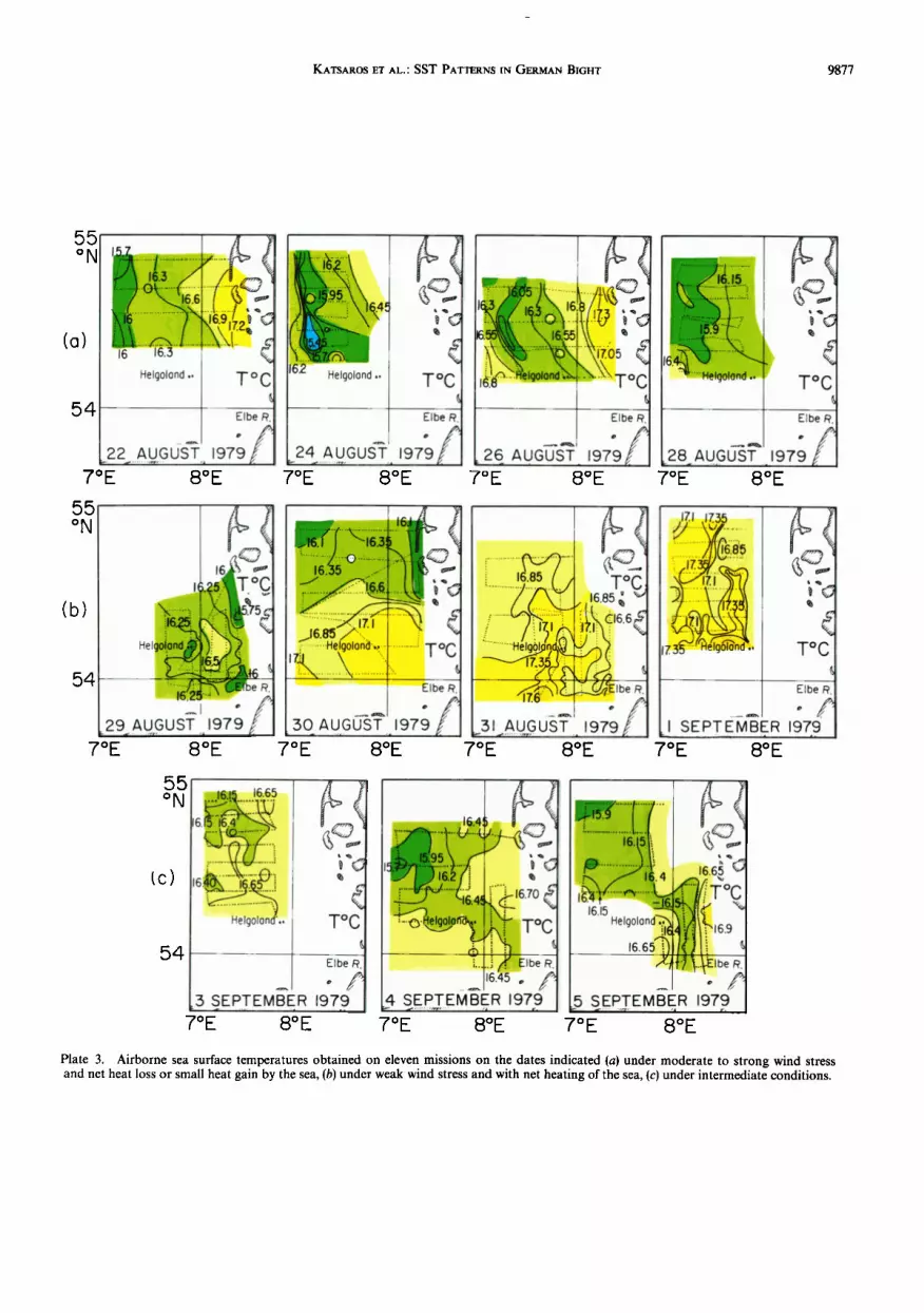
colder and has an intermediate salinity relative to inshore and offshore waters and, as was shown by BFJ, constitutes a separ- ate water mass which is formed by mixing of Elbe estuary water with North Sea deep water. In the period August 16-20 when there was a net heat gain by the sea (Figure 2b), the thermal signal of the front at the surface weakens and almost disappears (Plates 1 and 3b) due to the formation of a shallow thermocline only about 10 m deep. During subsequent events of moderate to strong net heat loss periods (Figure 2b), the thermal stratification eroded and the front extended to the

surface in full strength (Plates 2 and 3b).

KATSAROS ET AL.: SST PATTERNS IN GERMAN BIGHT 9875

55 o N

54

16.5 17.5

6..•. Helg010nd ,.

(a) FR. I:IEINCKE •?-' ' 14-g•O A•U_G.,.,1979•,;] o- T øC r/

7øE 8øE

55 o N

54

7øE 8øE

7øE 8øE 7OE 8øE

7OE 8øE 7øE 8øE

55 o N

54

I I

Elbe R

7øE 8øE 7OE 8øE

Plate 1. Sea surface temperature, salinity, and density (in sigma t units) distributions obtained in the German Bight during the summer of 1979 under conditions of weak wind stress and net heating of the sea.


.-% • ---: : :• ....

LOZ •

w

KATSAROS ET AL.' SST PATTERNS IN GERMAN BIGHT 9877

55 o N

(a)

54

Helgoland .. T o C

Elbe R.

22 AUGUST 1979

•-: ( 162

Helg010nd .. T øC

Elbe R.

24 AUGUST 1979

I( ..'•.•e Igola nd';'•,- 5TO Elbe R.

•26• AUGUST 1979 f .

ß

Helgøland Toc

Elbe R.

•28_ AU...GU ST., 1979 7øE 8øE 7øE 8øE 7øE 8øE 7øE 8øE

55, o N

(b)

54

.:. .... '(•,•.,-..l.t:

,•"•"¸,,•., • ,•< .... :.-H,•0,;;,.-.,. ............. •ToC '•..• ....... .• ......... ':-:,::..

Elbe R.

30 AUGUST 1979

....... i/•.•.•'• -.•...•C. E lbe R.

•31 AUGUST 1979

•.•.z I .1•_35

......... •'"'i'•' ........

Toc

Elbe R

o/• .I SE.PT. EMBE, R 197.,9

7øE 8øE 7øE 8øE 7øE 8øE 7øE 8øE

55 o N

•c)

54

16.15 16.65 .."•/ ....

.... ii'!!:.•...:..::.•i' Helgoland'.. Toc

Elbe R.

oœ SEPTEMBER 1979

•..,..i • Elbe R. 16.45 o •

• S•.E...P.•EMBER 1979

...T ø ,•-•• .... ....... -•,•! c• Helgoland ,?l •

16.65•':.. 169 • •, , '• •...••,be•

,• •EPTEMBER 1979 7øE 8øE 7OE 8øE 7øE 8OE

Plate 3. Airborne sea surface temperatures obtained on eleven missions on the dates indicated (a) under moderate to strong wind stress and net heat loss or small heat gain by the sea, (b) under weak wind stress and with net heating of the sea, (c) under intermediate conditions.


(a)

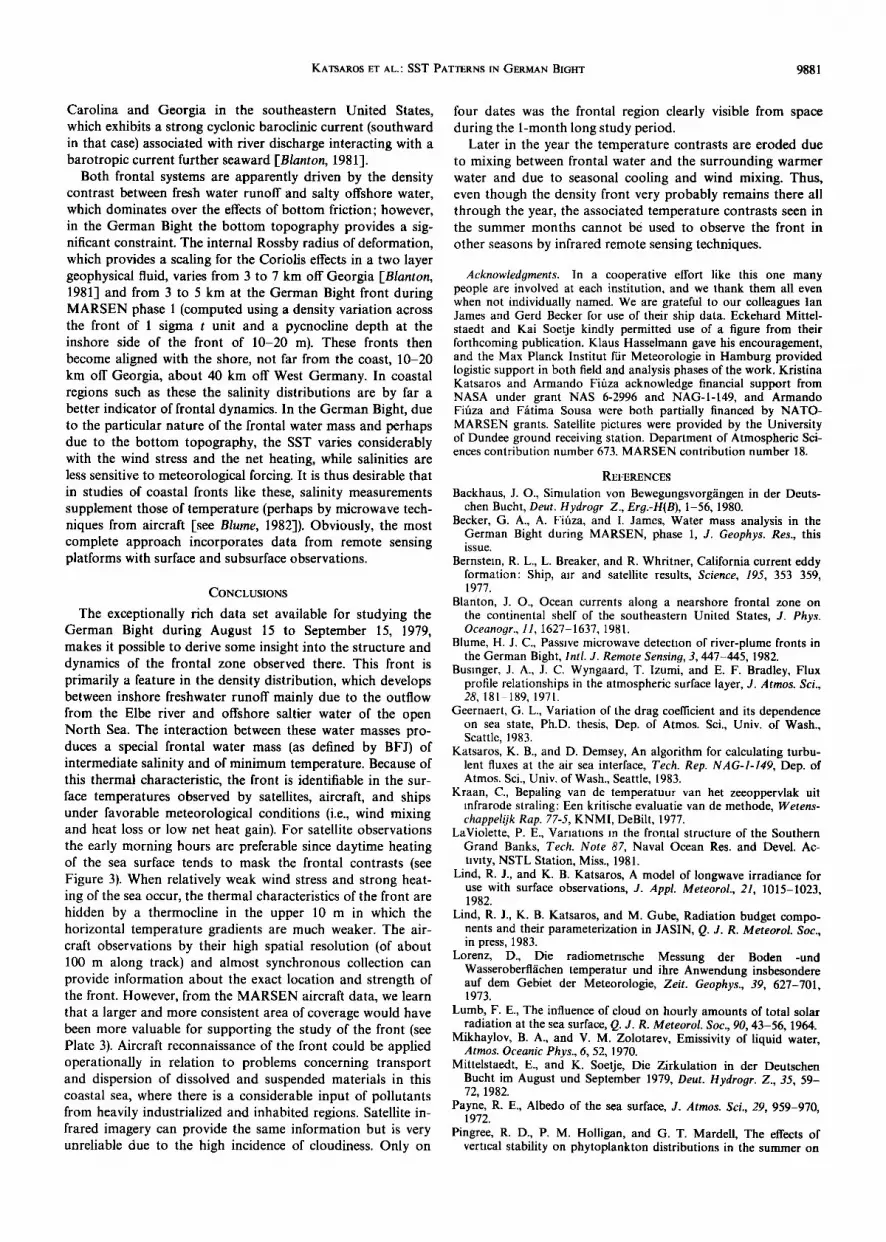
Fig. 3.

,---'TIROS-N" '18 AUG

......... ::.?" 4 -MT Infrared images obtained on NOAA 6 and TIROS N satellites. (a) Examples of the signature of the German

Bight front missing. (b) Examples of the German Bight front being recognizable.

Owing to the strong salinity contrast between the main water masses in presence (Elbe estuary water and North Sea water), the field of mass in the German Bight is essentially determined by the salinity distribution. The density field was thus almost insensitive to the thermal evolution of the upper layers of this coastal sea during the study period. Indeed, and as Plates 1 and 2 illustrate clearly, the surface salinity and sigma t distributions did not present any major variations for the duration of the experiment; their main feature consisted in a strong, one-sided front coinciding with the thermal front described above.

From the vertical sections presented by BFJ, it is obvious that the frontal zone separates inshore and offshore waters both with little or no stratification. However, the frontal zone corresponds itself to strong vertical and horizontal gradients in the analyzed fields of temperature, salinity, and density. The band of stronger density gradients, defined by the layer con- tained between the isopycnals of 23.0 and 23.5 sigma t units (bright blue in Plates 1 and 2)coincides with the inshore half of the core of colder temperatures of the thermal double frontal structure. This peculiar thermal structure is due to the "frontal water" mass being colder but of intermediate salinity relative to the neighboring water masses as defined by BFJ, who also discuss the stratification in the frontal zone.

The individual SST distributions show some interesting features. As mentioned above, the calm wind, net heat gain by the sea situation was characterized by mesoscale patchiness in the SST fields; this designation should perhaps be clarified by some examples. Comparing the SST charts in Plate I (low wind stress) with those in Plate 2 (moderate to high wind stress), one could imagine that a uniform heating of 1ø-2øC of the structure shown in the latter would lead to distributions

not too dissimilar from those in Plate 1. Indeed, bands of lower surface temperatures still can be identified both in Plates l a and lb in the area of the front, and in Plate 3c the cold patch near Helgoland corresponds to a local maximum of frontal water, as can be seen in the percentage distributions

of water masses presented by BFJ. Lower temperatures were also observed at that same location during situations of strong wind stress and net heat loss from the sea (Plates 2b and 3b). The tendency for zonal patterns noted in the ship's SST charts under calm wind conditions may result to some extent from the east-west orientation of the lines of stations occupied during all of the cruises.

An interesting pattern, observed in the surface density fields shown in Plates 1 and 2 (particulary in those obtained with the high resolution grid of the Gauss) is apparently due to the presence of frontal eddies with individual sizes of the order of 10 km and with a separation scale of 20-40 km. One might argue that these features could result from tidal fluctuations of the frontal structure between consecutive sampling lines; however, the infrared satellite pictures of Figure 3b also show frontal eddies with the same spatial scales. These suggest that the frontal structure observed in the German Bight during the summer is affected by baroclinic instabilities. The frontal eddies may also contribute to the observed thermal patchiness.

The airborne SST maps shown in Plate 3 illustrate in some detail the day-to-day variability that took place within periods with different meteorological forcing in spite of the reduced area covered in each flight and of their somewhat irregular coverage. The sequence in Plate 3b shows the progressive warming of the sea surface under persistently calm winds right after the isolated storm of August 27 and 28. A considerable amount of small-scale structure is observed in the aircraft-

produced charts, which is apparently related to the almost continuous sampling along the flight lines; these structures are very similar to those obtained with the fine resolution of the Gauss data (Plates lb and 2a) and thus do not seem to result from a possible residual influence of differential atmospheric interference or scattered cloud reflection in the radiometric

records. The sequence of SST charts in Plate 5a shows the evolution of the intensity of the double thermal front northwest of Helgoland under moderate to strong wind conditions.


(b) '0 '•'.i•,,....L•y:/.o.,.jttine of dou-.b!e thermal

:;'.6 SEP'79 -

Fig. 3. (continued)

front


The potential of airborne infrared radiometery is quite well demonstrated here, particularly when comparing the detail and the strength of the frontal structure observed in the airborne SST chart of August 24 with the coarse resolution of the corresponding John Murray SST map shown on Plate 2b. The last three flights provided the sequence in Plate 3c and illustrate a transitional situation during a 3-day cycle of intensi- fication and decay in wind stress and of a slight increase of the heat gain by the sea (Figure 2b). Because of the general trend observed in the three SST charts, we conclude that vertical mixing induced by the wind stress prevailed during this particular period.

In Figure 3 the TIROS N and NOAA 6 infrared pictures available for the MARSEN phase 1 period are shown. The two typical situations characterized above are clearly illustrated with the satellite imagery. The pictures obtained on August 18 and on September 9, both corresponding to very similar situations of light winds and with net heat fluxes into the sea, show no trace of the thermal front. However, the images obtained on August 29, right after the summer storm, and on September 6, under a pulse of moderate wind stress, show clearly the thermal front as a meridional band of cooler water about 50 km wide, with its sides distorted by the small scale eddies already described. The morning images (NOAA 6, around 0830 GMT) show the front somewhat better than those obtained in the early afternoon (TIROS N, around 1430 GMT); this may be due to instrumental differences or to skin effects related to the solar warming during those relatively cloud-free days.

RESIDUAL CIRCULATION

The dynamical interpretation of the frontal structure cannot be sought in models based on tidally induced mixing on the shallow water side of stratified waters [e.g., Simpson and Hunter, 1974; Pingree et al., 1978], as in the area under study the water column was essentially unstratified on both sides of the frontal zone. Instead, the gravitational circulation induced by the salinity-density gradients deriving from land runoff, coupled with the topographic control of the residual (i.e., non- tidal) circulation, apparently determine the dynamics of the front. Other mechanisms due to upwelling, mesoscale eddies, long waves, internal tides, and waves are ruled out because of the vertical homogeneity away from the front and the re- strictive configuration of the coastline. The diret action of the wind stress or the resulting effects of wind setup also do not appear to determine the strength of the front, which remained essentially unchanged for the duration of the MARSEN phase 1 experiment (as exemplified by the sigma t fields in Figures. 3 and 4) under fairly large variations of wind direction and intensity. A description of the residual circulation in the German Bight as observed during the experiment is given below in an attempt to contribute to the understanding of the dynamics of the front.

All the charts of residual currents in the North Sea, based on observations or on numerical models, show a northerly coastal flow in the German Bight area [see, for example, the review by Backhaus, 1980]. The current measurements conducted during MARSEN phase 1, with two moorings located near the coast in depths of 10 and 20 m, provided the residuals illustrated for positions WT and ST in Figure 4, which show some variability. This may be due to strong dependence of the circulation in such shallow areas on the wind. The results

obtained by Backhaus [1980] with a wind-driven multilayer

model including tidal and density induced flows indicate that northerly winds of 10 m s -• are capable of reversing the whole residual circulation in the German Bight. Although winds of such an intensity were only observed for a short time during the study period (Figure 2a), the shallow areas are certainly more sensitive to the mechanical forcing by the wind and the variability observed there is not surprising. Figure 4 shows that the residual currents near the surface and close to

the bottom were consistently northward and had almost no vertical shear at the moorings installed in total depths of 40 m or more to the west of the front (positions PU, WB, A). How- ever, the current meters located in the central part of the area, between depths of 30 and 40 m in the glacial Elbe river valley to the west and northwest of Helgoland (positions FDB, ZE, and BG), displayed strong shears between near surface and bottom residuals, the FDB position even providing a near- bottom southward flow, while near the surface the current was predominantly to the north. These observations generally agree with the tide and density-induced residual currents obtained by Backhaus [1980] with his multilayer numerical model. He shows a strong shear between a general cyclonic near surface flow and a deep southward circulation, stronger near the northern margin of the submerged valley and weak- ening offshore. The currents measured at locations B and FPN (Figure 4) corresponding to the position of the core of the frontal zone, showed vertical speed shear (at B) or strong variability in direction (at FPN). These confirm the baroclinic character of the front as opposed to the pronounced baro- tropy of the offshore northward residual flow (as observed at positions PU, WB, A).

The mechanisms maintaining this front appear to have some similarity with those producing a coastal front off South

6øE 7øE 8øE 9øE

Fig. 4. Residual currents measured near the bottom (solid curve) and near the surface (dashed curve) with self recording current meters during August and September 1979. Each segment shows a 10-day vector average of the current direction and the numbers indicate the corresponding mean speed (cm s -•) beginning on August 18, 1979 (after Mittelstaedt and Soetje [1982], except moorings A and B which are based on measurements of Institute of Oceanographic Sciences, Bidston, United Kingdom). The shaded area is the envelope of the density fronts colored bright blue in Plates 1 and 2.


Carolina and Georgia in the southeastern United States, which exhibits a strong cyclonic baroclinic current (southward in that case) associated with river discharge interacting with a barotropic current further seaward [Blanton, 1981].

Both frontal systems are apparently driven by the density contrast between fresh water runoff and salty offshore water, which dominates over the effects of bottom friction; however, in the German Bight the bottom topography provides a sig- nificant constraint. The internal Rossby radius of deformation, which provides a scaling for the Coriolis effects in a two layer geophysical fluid, varies from 3 to 7 km off Georgia [Blanton, 1981] and from 3 to 5 km at the German Bight front during MARSEN phase 1 (computed using a density variation across the front of 1 sigma t unit and a pycnocline depth at the inshore side of the front of 10-20 m). These fronts then become aligned with the shore, not far from the coast, 10-20 km off Georgia, about 40 km off West Germany. In coastal regions such as these the salinity distributions are by far a better indicator of frontal dynamics. In the German Bight, due to the particular nature of the frontal water mass and perhaps due to the bottom topography, the SST varies considerably with the wind stress and the net heating, while salinities are less sensitive to meteorological forcing. It is thus desirable that in studies of coastal fronts like these, salinity measurements supplement those of temperature (perhaps by microwave techniques from aircraft [see Blume, 1982]). Obviously, the most complete approach incorporates data from remote sensing platforms with surface and subsurface observations.

CONCLUSIONS

The exceptionally rich data set available for studying the German Bight during August 15 to September 15, 1979, makes it possible to derive some insight into the structure and dynamics of the frontal zone observed there. This front is primarily a feature in the density distribution, which develops between inshore freshwater runoff mainly due to the outflow from the Elbe river and offshore saltier water of the open North Sea. The interaction between these water masses pro- duces a special frontal water mass (as defined by BFJ) of intermediate salinity and of minimum temperature. Because of this thermal characteristic, the front is identifiable in the surface temperatures observed by satellites, aircraft, and ships under favorable meteorological conditions (i.e., wind mixing and heat loss or low net heat gain). For satellite observations the early morning hours are preferable since daytime heating of the sea surface tends to mask the frontal contrasts (see Figure 3). When relatively weak wind stress and strong heating of the sea occur, the thermal characteristics of the front are hidden by a thermocline in the upper 10 m in which the horizontal temperature gradients are much weaker. The aircraft observations by their high spatial resolution (of about 100 m along track) and almost synchronous collection can provide information about the exact location and strength of the front. However, from the MARSEN aircraft data, we learn that a larger and more consistent area of coverage would have been more valuable for supporting the study of the front (see Plate 3). Aircraft reconnaissance of the front could be applied operationally in relation to problems concerning transport and dispersion of dissolved and suspended materials in this coastal sea, where there is a considerable input of pollutants from heavily industrialized and inhabited regions. Satellite infrared imagery can provide the same information but is very unreliable due to the high incidence of cloudiness. Only on

four dates was the frontal region clearly visible from space during the 1-month long study period.

Later in the year the temperature contrasts are eroded due to mixing between frontal water and the surrounding warmer water and due to seasonal cooling and wind mixing. Thus, even though the density front very probably remains there all through the year, the associated temperature contrasts seen in the summer months cannot be used to observe the front in

other seasons by infrared remote sensing techniques.

Acknowledgments. In a cooperative effort like this one many people are involved at each institution, and we thank them all even when not individually named. We are grateful to our colleagues Ian James and Gerd Becker for use of their ship data. Eckehard Mittel- staedt and Kai Soetje kindly permitted use of a figure from their forthcoming publication. Klaus Hasselmann gave his encouragement, and the Max Planck Institut ffir Meteorologie in Hamburg provided logistic support in both field and analysis phases of the work. Kristina Katsaros and Armando Fifiza acknowledge financial support from NASA under grant NAS 6-2996 and NAG-l-149, and Armando Fifiza and Ffitima Sousa were both partially financed by NATO- MARSEN grants. Satellite pictures were provided by the University of Dundee ground receiving station. Department of Atmospheric Sci- ences contribution number 673. MARSEN contribution number 18.

REFERENCES

Backhaus, J. O., Simulation yon Bewegungsvorg//ngen in der Deuts- chen Bucht, Deut. Hydrogr. Z., Erg.-H(B), 1-56, 1980.

Becker, G. A., A. Fifiza, and I. James, Water mass analysis in the German Bight during MARSEN, phase 1, J. Geophys. Res., this issue.

Bernstein, R. L., L. Breaker, and R. Whritner, California current eddy formation: Ship, air and satellite results, Science, 195, 353-359, 1977.

Blanton, J. O., Ocean currents along a nearshore frontal zone on the continental shelf of the southeastern United States, J. Phys. Oceanogr., 11, 1627-1637, 1981.

Blume, H. J. C., Passive microwave detection of river-plume fronts in the German Bight, Intl. J. Remote Sensing, 3, 447-445, 1982.

Businger, J. A., J. C. Wyngaard, T. Izumi, and E. F. Bradley, Flux profile relationships in the atmospheric surface layer, J. Atmos. Sci., 28, 181-189, 1971.

Geernaert, G. L., Variation of the drag coefficient and its dependence on sea state, Ph.D. thesis, Dep. of Atmos. Sci., Univ. of Wash., Seattle, 1983.

Katsaros, K. B., and D. Demsey, An algorithm for calculating turbulent fluxes at the air sea interface, Tech. Rep. NAG-l-149, Dep. of Atmos. Sci., Univ. of Wash., Seattle, 1983.

Kraan, C., Bepaling van de temperatuur van het zeeoppervlak uit infrarode straling: Een kritische evaluatie van de methode, Wetens- chappelijk Rap. 77-5, KNMI, DeBilt, 1977.

LaViolette, P. E., Variations in the frontal structure of the Southern Grand Banks, Tech. Note 87, Naval Ocean Res. and Devel. Ac- tivity, NSTL Station, Miss., 1981.

Lind, R. J., and K. B. Katsaros, A model of longwave irradiance for use with surface observations, J. Appl. Meteorol., 21, 1015-1023, 1982.

Lind, R. J., K. B. Katsaros, and M. Gube, Radiation budget compo- nents and their parameterization in JASIN, Q. J. R. Meteorol. Soc., in press, 1983.

Lorenz, D., Die radiometrische Messung der Boden -und Wasseroberfl/ichen temperatur und ihre Anwendung insbesondere auf dem Gebiet der Meteorologie, Zeit. Geophys., 39, 627-701, 1973.

Lumb, F. E., The influence of cloud on hourly amounts of total solar radiation at the sea surface, Q. J. R. Meteorol. $oc., 90, 43-56, 1964.

Mikhaylov, B. A., and V. M. Zolotarev, Emissivity of liquid water, Atmos. Oceanic Phys., 6, 52, 1970.

Mittelstaedt, E., and K. Soetje, Die Zirkulation in der Deutschen Bucht im August und September 1979, Deut. Hydrogr. Z., 35, 59- 72, 1982.

Payne, R. E., Albedo of the sea surface, J. Atmos. $ci., 29, 959-970, 1972.

Pingree, R. D., P.M. Holligan, and G. T. Mardell, The effects of vertical stability on phytoplankton distributions in the summer on

9882 KATSAROS ET AL.: SST PATTERNS IN GERMAN BIGHT

the northwest European Shelf, Deep Sea Res., 25, 1011-1028, 1978. Simpson, J. H., and J. R. Hunter, Fronts in the Irish Sea, Nature, 250,

404-406, 1974. Smith, S. D., Wind stress and heat flux over the ocean in gale force

winds, J. Phys. Oceanogr. 10, 709-726, 1980.

V. Amann, Institut f/Jr Nachrichtentechnik, Deutsche Forschungs- und Versuchsanstalt f/Jr Luft-und Raumfahrt e.v. (DFVLR), 8031 Oberpfaffenhofen, Federal Republic of Germany.

A. Fi6za and F. Sousa, Grupo de Oceanografia, Departamento de Ffsica, Universidade de Lisboa, Rua de Escola Polit6cnica 58, 1200 Lisboa, Portugal.

K. B. Katsaros, Department of Atmospheric Sciences, University of Washington, Seattle, WA 98195.

(Received June 21, 1982; revised July 11, 1983;

accepted July 14, 1983;

Documents

Sea surface temperature patterns and air-sea fluxes in the German Bight during MARSEN 1979, Phase 1