P2.12 Sampling Errors of Climate Monitoring Constellations

Renu Joseph1*, Daniel B. Kirk-Davidoff1 and James G. Anderson2

1University of Maryland, College Park, Maryland, 2Harvard University, Cambridge, Massachusetts

1. INTRODUCTION

Satellites need to observe the earth with great accuracy to capture the long-term trends in climate. As part of an effort to design a constellation of low earth orbiting satellites to benchmark climate observations, we explore the impact of imperfect sampling of satellites on the effort to monitor mean radiance on a variety of spatial and temporal scales. Our aims are (1) to find those orbits which provide an accuracy of at least 0.1 K in brightness temperatures at different temporal and spatial resolutions, and (2) to look for alternate ways of calibrating existing and future satellites like NPOESS. The 0.1 K level of accuracy in brightness temperature was chosen to agree with the expected magnitude of decadal trends in temperature forced by changes in greenhouse gas concentration.

Sampling studies are carried out at different frequencies representative of the lower, middle and upper troposphere. Model generated radiances rather than observed radiances are used for this study, since a good representation of diurnal variability in the original data is essential; polar orbiters don't have enough observation times, and geostationary orbiters don't cover enough of the world, and have problems because of high observing angles. The brightness temperatures are obtained by using MODTRAN on the archived simulations from the GFDL coupled model. These are then sub-sampled along the paths traversed by the satellite footprint for various potential orbits at different inclinations. Maps of retrieval accuracy for annual mean radiance are presented for single satellites and for a constellation of satellites. Also, the errors of single and multiple precessing satellites are examined with the underlying motive of understanding whether these errors can be predicted.

* Corresponding author address: Renu Joseph, Department of Atmospheric and Oceanic Science and Earth System Science Interdisciplinary Center, University of Maryland, College Park, MD 20742-2425

2. DATA AND METHODOLOGY

The study consists of one in which satellite orbits for single and multiple platforms will sample MODTRAN brightness temperatures along the lines of the work done by Kirk-Davidoff et. al (2005) and Lin et al.(2002) and the resulting errors between the model derived brightness temperatures and the output the satellite sampled output are quantified. The equations for the trajectories for the simulated satellites trajectories are similar to those described in Kirk-Davidoff et al. (2005), in which the longitude and latitude are obtained once the inclination, the height and the initial equator crossing time of the satellites are known.

The brightness temperatures from the MODTRAN output provide the “observed value” at the instances sampled by the satellite. They are then grouped together by location and averaged together at the appropriate temporal resolution. The averaged brightness temperatures from the MODTRAN output over the same period provides the “true value”. Analysis of differences between the true and “observed” establishes the accuracy of the retrieval. The accuracy of the satellite sampled data can then be assessed on global scales and local scales at different spatial and temporal resolution in terms of absolute and root mean square errors. Brightness temperatures at four different frequencies representative of vertical heights in the atmosphere are chosen based on the results of Haskins et. al. (1997) and is shown in Figure 1. The 909 cm-1 or the window channel represents the surface of the earth or the surface of the highest cloud layer of the earth since it is minimally affected by water vapor or carbon dioxide. Other frequencies, which mostly represent emission by water vapor or carbon dioxide high in the atmosphere, have much smaller variances and hence sampling at this frequency indicates the worst case. The other frequencies chosen are the 465, 700 and 660 cm-1 representing the mid-troposphere to stratosphere region.

3. RESULTS

The orbits used for sampling studies include (a) 90° inclination “true” polar orbits at various initial longitudes in which observations

rotate through 24 hours of local time twice over the year, (b) Sun-synchronous polar orbits at a range of equator crossing times and (c) 60° inclination orbits with more rapid precession. Figure 2 represents the errors in brightness temperatures obtained by single satellites for the 909 cm-1 channel at a 2°x2.5° grid resolution. These clearly indicate that sun-synchronous satellites with different equator crossing times produces a distribution of errors that are totally different from each other highlighting the importance of choosing the appropriate equator crossing times. The truly polar orbits have the least amount of error. Figure 3 shows the errors for the various combinations of satellites. Examining the spatial distribution of errors for the various constellations of satellites, the errors from the three-polar combination is comparable to that of the three-sun-synchronous orbits. Removing one of the satellites from a 3 sun-synchronous satellite constellation however produces a larger error than removing any one satellite from a 3-polar satellite combination. Also a two-polar satellite combination appears superior to any of the other possible two sun-synchronous combinations.

To obtain smaller errors, we increase the averaging area to be sampled to a 15°x15° area-averaged region. The random errors from weather noise are essentially defeated for yearly means since there are ~9000 observations per grid square for a single 90° orbiter. The error distribution for the combination of satellites at the 15°x15° is shown in Figure 4 for the brightness temperatures at the four different frequency channels. For the window channel, accuracy of the satellite constellation improves to 0.1K for the 3 satellite combinations. It can be clearly seen that in the lower troposphere, the combination of satellites produce errors of the order of 0.1K (909 cm-1 and 465 cm-1) while in the upper troposphere of 0.04K (660 cm-1 and 700 cm-1).

In Figures 3 and 4, we also noticed that the inclusion of a precessing satellite to a 3-satellite combination did not necessarily always reduce the total error. To understand the errors of precessing orbits we look at sampling errors at 2°x2.5° resolution, for a range of orbit altitudes, holding inclination constant. The first column of Figure 5 shows the spatial distribution of sampling errors for different heights at the same inclination of 52.5°. We notice that higher precession rates do not necessarily imply lower values of errors. Standard deviations of the errors of the corresponding figures are shown at the top of each figure. The second column of Figure 5

indicates the number of times each grid box is sampled in a year. This appears fairly constant. The first and second columns of Figure 6 show the errors in sampling of the average time of day in hours and the average day of the year in days. Ideally the satellites over the course the year should sample all hours of the diurnal cycle and all days of the year. Therefore the ideal values of the errors should be 12 hours and 182.5 days. However there is a spread in these values at different orbital parameters (inclination and heights). We notice that certain orbit parameters appear to have some beat frequencies that cause the sampling to be very inhomogeneous.

To predict the errors of brightness temperatures indicated in the first column of Figure 5 we use the standard deviation of those errors as a measure of the total error at a given satellite inclination and height. The top panel in Figure 7 contains the standard deviation of the error in brightness temperature as a function of height and inclination for the brightness temperature at window channel (909 cm-1) channel as an example. The orbital parameters of satellites where the errors are larger are immediately visible. In order to predict these errors, we have examined similar plots of standard deviation of the time of day (indicator of the diurnal sampling), the standard deviation of the day of year and the standard deviation of the day of half year (indicators of the seasonal cycle). Their inclination-height plots are shown in the three lower panels of Figure 7. The correspondence between the sampling of the seasonal cycle, diurnal cycle and the errors in brightness temperatures are immediately visible. Scatter plots of these with the observed error are shown in first column of Figure 8. If the fields were homogeneously sampled at the different resolutions the standard deviations would be small. Attempt to model the standard deviations of brightness temperatures based on these values showed that the errors are dependant on the time of day, the time of the semiannual year. The right panels of Figure 9 show the predicted versus the observed error and its correlations. This highlights the importance of capturing the dominant temporal frequencies of brightness temperature.

4. SUMMARY

Results for the annual mean indicate that: It is possible to attain 0.1 K accuracy in long-term climate averages with a reasonable number of satellites; For a single satellite, the preferred orbit

for climate monitoring is a true polar (precessing) orbit, as this substantially reduces errors in mean brightness temperatures, and creates a climate record that is independent of orbital parameters; A single satellite in a precessing orbit can achieve sampling errors in 15 degree grid boxes less than 0.1 K for brightness temperatures in the spectral regions that mostly sample the lower and the upper troposphere and the lower stratosphere; In the mid-troposphere channels and in the window channel, a single precessing orbiter requires zonal averaging to reliably attain errors of less than 0.1 K; Since the primary source of sampling bias arises due to inadequate sampling of the diurnal and semidiurnal cycle, a constellation of satellites surely reduces the errors considerably and combinations with precessing polar orbits normally fare better than their sun-synchronous counterparts; For multiple orbiters, precession has large advantages in establishing accurate mean radiances, because a configuration of several sun-synchronous orbiters must sample the diurnal cycle evenly. For instance, if there are initially three orbiters separated by 8 hours in equator crossing time, the loss of a single orbiter will greatly reduce the accuracy of the remaining two

orbiters, assuming they maintain their station; It is possible to predict the errors of brightness temperatures at different frequencies if the dominant temporal cycles prevalent in them are known. For instance, in the window channel (909 cm-1) if the diurnal cycle and seasonal cycle are captured, there can be a reasonable expectation of capturing the temperature.

5. REFERENCES

Haskins, R. D., R. M. Goody, and L. Chen, 1997: A statistical method for testing a general circulation model with spectrally resolved satellite data, J. Geophys. Res., 102(D14), 16,563–16,581.

Kirk-Davidoff, D. B., R. M. Goody, and J. G. Anderson, 2005: Analysis of sampling errors for climate monitoring satellites. J. Clim., 18, 810-822.

Lin, X., L. D. Fowler, and D. A. Randall, 2002: Flying the TRMM satellite in a general circulation model, J. Geophys. Res., 107, 4281.

Figure 1: Pressure level of maximum emission to space for each wavenumber calculated using a MODTRAN output for a tropical atmosphere adapted from Haskins et. al. (1997)

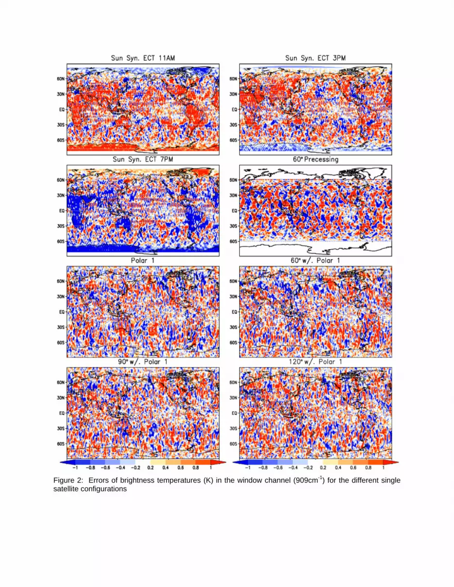
Figure 2: Errors of brightness temperatures (K) in the window channel (909cm-1) for the different single satellite configurations

Figure 3: Errors of brightness temperatures (K) in the window channel (909cm-1) for several combinations of satellites (errors of the individual satellites are provided in Figure 2).

Error Distribution for Satellite Combinations

Figure 4: Error distributions of the brightness temperatures at the (a) 909 cm-1 (b) 465 cm-1 (c) 660 cm-1 and (d) 700 cm-1 frequencies for the different satellite constellations. In the lower troposphere, a combination of satellites can produce errors of the order of 0.1K while in the upper troposphere it is in the order of 0.04K.

Figure 5: The first column shows the errors in brightness temperatures (K) for the window channel (909 cm-1) for precessing satellites for different orbital parameters when the inclination is kept fixed and the height of the satellite is varied. The second column shows the number of times in a year that the points are sampled to obtained the errors shown in the first column. The standard deviation of the errors and the number of points are printed on top of each panel.

Figure 6: The first column shows the time of day (hours) for precessing satellites for different orbital parameters when the inclination is kept fixed and the height of the satellite is varied. The second column shows the average day of the year that the satellite sample to obtained the errors shown in the first column of Figure 5. The standard deviation of the spatial distribution of time of day and day of year are printed on top of each panel.

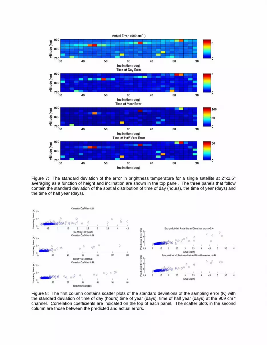
Figure 7: The standard deviation of the error in brightness temperature for a single satellite at 2°x2.5° averaging as a function of height and inclination are shown in the top panel. The three panels that follow contain the standard deviation of the spatial distribution of time of day (hours), the time of year (days) and the time of half year (days).

Figure 8: The first column contains scatter plots of the standard deviations of the sampling error (K) with the standard deviation of time of day (hours),time of year (days), time of half year (days) at the 909 cm-1 channel. Correlation coefficients are indicated on the top of each panel. The scatter plots in the second column are those between the predicted and actual errors.