Runge-Kutta-Nystr�om-type parallel blockpredictor-corrector methods �Nguyen Huu Cong, Karl Strehmel and R�udiger WeinerAbstractThis paper describes the construction of block predictor-corrector methods based onRunge-Kutta-Nystr�om correctors. Our approach is to apply the predictor-correctormethod not only with stepsize h, but, in addition (and simultaneously) with stepsizesaih; i = 1; : : : ; r. In this way, at each step, a whole block of approximations to the ex-act solution at o�-step points is computed. In the next step, these approximations areused to obtain a high-order predictor formula using Lagrange or Hermite interpolation.Since the block approximations at the o�-step points can be computed in parallel, thesequential costs of these block predictor-corrector methods are comparable with thoseof a conventional predictor-corrector method. Furthermore, by using Runge-Kutta-Nystr�om corrector methods, the computation of the approximation at each o�-steppoint is also highly parallel. By a number of widely-used test problems, a class ofthe resulting block predictor-corrector methods is compared with both sequential andparallel RKN methods available in the literature and is shown to demonstrate superiorbehaviour.Key words: Runge-Kutta-Nystr�om methods, predictor-corrector methods, stability, parallelism.AMS(MOS) subject classi�cations (1991): 65M12, 65M20CR subject classi�cations: G.1.71 IntroductionConsider the numerical solution of nonsti� initial value problems (IVPs) for systems of specialsecond-order, ordinary di�erential equations (ODEs)y00(t) = f(t;y(t)); y(t0) = y0; y0(t0) = y00; t0 � t � T; (1.1)where y : R! Rd, f : R� Rd ! Rd. Problems of the form (1.1) are encountered in e.g.,celestial mechanics. A (simple) approach for solving this problem is to convert it into a system�This work was supported by a three-month DAAD research grant1

of �rst-order ODEs with double dimension and to apply e.g., a (parallel) Runge-Kutta-type method (RK-type method), ignoring the special form of (1.1) (the indirect approach).However, taking into account the fact that f does not depend on the �rst derivative, theuse of a direct method tuned to the special form of (1.1) is usually more e�cient (thedirect approach). Such direct methods are generally known as Runge-Kutta-Nystr�om-typemethod (RKN-type method). Sequential explicit RKN methods up to order 10 can be foundin [11, 12, 16, 19]. The performance of the tenth-order explicit RK method requiring 17sequential f -evaluations in [17] and the tenth-order explicit RKN method requiring only 11sequential f-evaluations in [19] is an example showing the advantage of the direct approachfor sequential explicit RK and RKN methods. It is highly likely that in the class of parallelmethods, the direct approach also leads to an improved e�ciency.In the literature, several classes of parallel explicit RKN-type methods have been investigatedin [5, 4, 7, 8, 25]. A common challenge in these papers is to reduce, for a given order,the required number of sequential f -evaluations per step, using parallel processors. In thepresent paper, we investigate a particular class of explicit RKN-type block predictor-correctormethods (PC methods) for use on parallel computers. Our approach consists of applyingthe PC method not only at step points, but also at o�-step points (block points), so that,in each step, a whole block of approximations to the exact solutions is computed. Thisapproach was �rstly used in [10] for increasing reliability in explicit RK methods. It was alsosuccessfully applied in [21] for improving e�ciency of RK-type PC methods. We shall usethis approach to construct PC methods of RKN-type requiring few numbers of sequentialf -evaluations per step with acceptable stability properties. In this case as in [21], the blockof approximations is used to obtain a highly accurate predictor formula in the next step byusing Lagrange or Hermite interpolation. The precise location of the o�-step points can beused for minimizing the interpolation errors and also for developing various cheap strategiesfor stepsize control. Since the approximations to the exact solutions at o�-step points tobe computed in each step can be obtained in parallel, the sequential costs of the resultingRKN-type block PC methods are equal to those of conventional PC methods. Furthermore,by using Runge-Kutta-Nystr�om corrector methods, the PC iteration method computing theapproximation to the exact solution at each o�-step point, itself is also highly parallel (cf.[5, 25]). The parallel RKN-type PC methods investigated in this paper may be considered asblock versions of the parallel-iterated RKN methods (PIRKN methods) in [5, 25], and willtherefore be termed block PIRKN methods (BPIRKN methods). Moreover, by using directRKN correctors, we have obtained BPIRKNmethods possessing both faster convergence andsmaller truncation error resulting in better e�ciency than by using indirect RKN correctors(cf. e.g., [5]).In the next section, we shall formulate the block PIRKN methods. Furthermore, we considerorder conditions for the predictor, convergence and stability boundaries, and the choice ofblock abscissas. In Section 3, we present numerical e�ciency tests and comparisons withparallel and sequential explicit RKN methods available in the RKN literature.In the following sections, for the sake of simplicity of notation, we assume that the IVP (1.1)is a scalar problem. However, all considerations below can be straightforwardly extended toa system of ODEs, and therefore, also to nonautonomous equations.2

1.1 Direct and indirect RKN methodsA general s-stage RKN method for numerically solving the scalar problem (1.1) is de�nedby (see e.g., [22, 25], and also [1, p. 272])Un = une+ hu0nc+ h2Af(Un);un+1 = un + hu0n + h2bTf(Un);u0n+1 = u0n + hdTf(Un); (1.2)where un � y(tn), u0n � y0(tn), h is the stepsize, s� s matrix A, s-dimensional vectors b; c;dare the method parameters matrix and vectors, e being the s-dimensional vector with unitentries (in the following, we will use the notation e for any vector with unit entries, and ej forany jth unit vector, however, its dimension will always be clear from the context). VectorUndenotes the stage vector representing numerical approximations to the exact solution vectory(tne+ch) at the nth step. Furthermore, in (1.2), we use for any vector v = (v1; : : : ; vs)T andany scalar function f , the notation f(v) := (f(v1); : : : ; f(vs))T . Similarly to a RK method,the RKN method (1.2) is also conveniently presented by the Butcher array (see e.g., [25], [1,p. 272]) c AbTdTThis RKN method will be referred to as the corrector method. We distinguish two types ofRKN methods: direct and indirect. Indirect RKN methods are derived from RK methods for�rst-order ODEs. Writing (1.1) in �rst-order form, and applying a RK method with Butcherarray c ARKbTRKyield the indirect RKN method de�ned byc [ARK]2bTRKARKbTRKIf the originating implicit RK method is of collocation type, then the resulting indirect im-plicit RKN will be termed indirect collocation implicit RKN method. Direct implicit RKNmethods are directly constructed for second-order ODEs of the form (1.1). A �rst familyof these direct implicit RKN methods is obtained by means of collocation technique (see[22]) and will be also called direct collocation implicit RKN method. In this paper, we willcon�ne our considerations to collocation high-order implicit RKN methods that is the Gauss-Legendre and Radau IIA methods (brie y called direct or indirect Gauss-Legendre, Radau3

IIA). This class contains methods of arbitrarily high order. Indirect collocation uncondition-ally stable methods can be found in [18]. Direct collocation conditionally stable methodswere investigated in [22, 5]1.2 Parallel explicit RKN methodsA �rst class of parallel explicit RKN methods called PIRKN is considered in [25]. ThesePIRKN methods are closely related to the block PIRKN methods to be considered in thenext section. Using indirect collocation implicit RKN of the form (1.2) as corrector method,a general PIRKN method of [25] assumes the following form (see also [5])U(0)n = yne+ hy0nc;U(j)n = yne+ hy0nc+ h2Af(U(j�1)n ); j = 1; : : : ;m;yn+1 = yn + hy0n + h2bTf(U(m)n );y0n+1 = y0n + hdTf(U(m)n ); (1.3)where, yn � y(tn), y0n � y0(tn). Let p be the order of the corrector (1.2), by setting m =[(p� 1)=2], [�] denoting the integer function, the PIRKN method (1.3) is indeed an explicitRKN method of order p with the Butcher array (cf. [5, 25])0 Oc A Oc O A O... ... . . . . . .c O : : : O A O0T : : : 0T 0T bT0T : : : 0T 0T dT (1.4)where, O and 0 denote s� s matrix and s-dimensional vector with zero entries, respectively.From the Butcher array (1.4), it is clear that the PIRKN method (1.3) has the number ofstages equal to (m + 1) � s. However, in each iteration, the evaluation of s components ofvector f(U(j�1)n ) can be obtained in parallel, provided that we have an s-processor com-puter. Consequently, the number of sequential f -evaluations equals s� = m + 1. This classalso contains the methods of arbitrarily high order and belongs to the set of e�cient paral-lel methods for nonsti� problems of the form (1.1). For the detailed performance of thesePIRKN methods, we refer to [25]. A further development of parallel RKN-type methods wasconsidered in e.g., [4, 5, 7, 8]. Notice that for the PIRKN method, apart from parallelismacross the methods and across the problems, it does not have any further parallelism. InSection 3 the PIRKN methods will be used in the numerical comparisons with the new blockPIRKN methods. 4

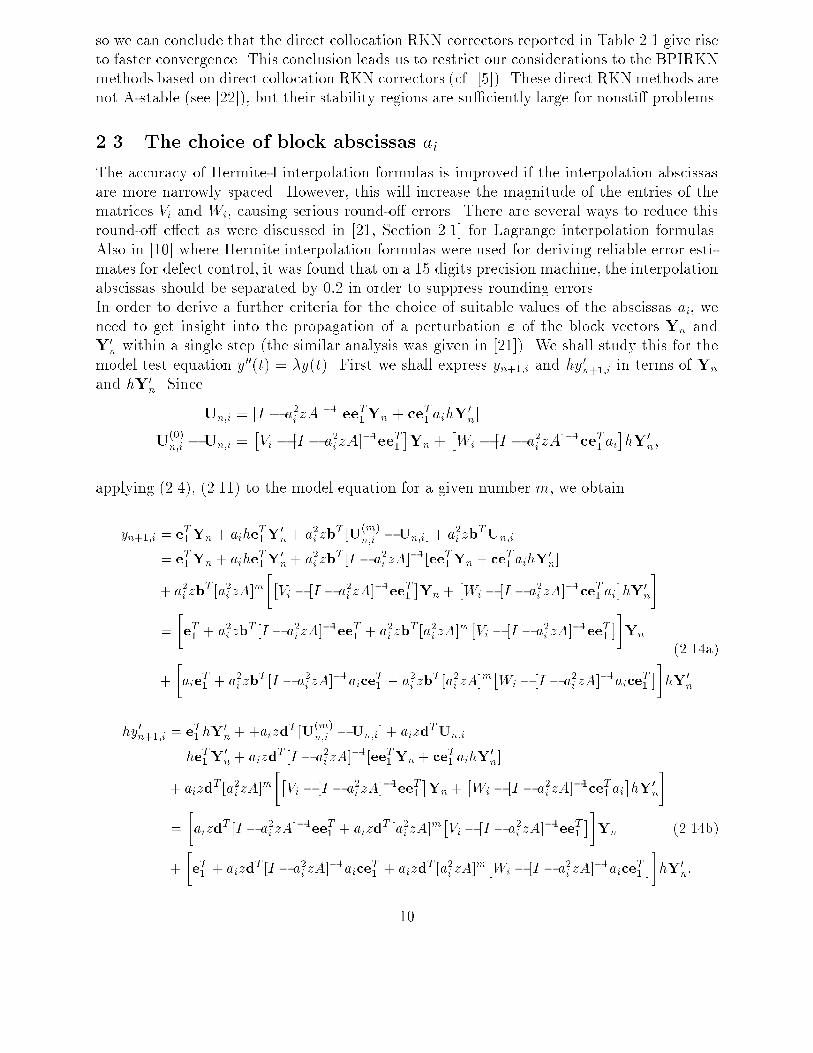
2 Block PIRKN methodsApplying the RKN method (1.2) at tn with r distinct stepsizes aih, where i = 1; : : : ; r anda1 = 1, we have Un;i = une+ aihu0nc+ a2ih2Af(Un;i);un+1;i = un + aihu0n + a2ih2bTf(Un;i);u0n+1;i = u0n + aihdTf(Un;i); i = 1; : : : ; r: (2.1)Let us suppose that at (n� 1)th step, a block of predictions U(0)n�1;i; i = 1; : : : ; r, and the ap-proximations yn�1 � y(tn�1), y0n�1 � y0(tn�1) are given. We shall compute r approximationsyn;i to the exact solutions y(tn�1 + aih); i = 1; : : : ; r, de�ned byU(j)n�1;i = yn�1e+ aihy0n�1c+ a2ih2Af(U(j�1)n�1;i); j = 1; : : : ;mb;yn;i = yn�1 + aihy0n�1 + a2ih2bTf(U(mb)n�1;i);y0n;i = y0n�1 + aihdTf(U(mb)n�1;i); i = 1; : : : ; r:In the next step, these r approximations are used to create high-order predictors. By denotingYn := (yn;1; : : : ; yn;r)T ; yn;1 = yn;Y0n := (y0n;1; : : : ; y0n;r)T ; y0n;1 = y0n; (2.2)we can construct the following predictor formulasU(0)n;i = ViYn; (2.3a)U(0)n;i = ViYn + hWiY0n (2.3b)U(0)n;i = ViYn + hWiY0n + h2�if(Yn); i = 1; : : : ; r: (2.3c)where Vi,Wi and �i are s�r extrapolation matrices which will be determined by order condi-tions (see Section 2.1). The predictors (2.3a), (2.3b) and (2.3c) are referred to as Lagrange,Hermite-I and Hermite-II, respectively. Apart from (2.3), we can construct predictors ofother types like e.g., Adam type (cf. [21]). Regarding (2.1) as block corrector methods and(2.3) as block predictor methods for the stage vectors, we leave the class of one-step methodsand arrive at a block PC methodU(0)n;i = ViYn + h�2WiY0n + h2[�2(1� �)=2]�if(Yn) (2.4a)U(j)n;i = eeT1Yn + aihceT1Y0n + a2ih2Af(U(j�1)n;i ); j = 1; : : : ;m;yn+1;i = eT1Yn + aiheT1Y0n + a2ih2bTf(U(m)n;i );y0n+1;i = eT1Y0n + aihdTf(U(m)n;i ); i = 1; : : : ; r; � 2 f0; 1;�1g: (2.4b)Notice that for a general presentation, in (2.4), the three di�erent predictor formulas (2.3)have been combined in a common one (2.4a), where, � = 0, 1 and �1 respectively indicate5

Lagrange, Hermite-I and Hermite-II predictor. With � = �1 the block PC method (2.4) isin PE(CE)mE mode and, with � = 0 or 1, the PE(CE)mE mode is reduced to P (CE)mEmode.It can be seen that the block PC method (2.4) consists of a block of PIRKN-type correctionsusing a block of predictions at the o�-step points (block points) (cf. Section 1.2). Therefore,we call the method (2.4) the r-dimensional block PIRKN method (BPIRKN method) (cf.[21]). In the case of Hermite-I predictor (2.3b), for r = 1, the BPIRKN method (2.4) reallyreduces to a PIRKN method of the form (1.3) studied in [5, 25].Once the vectors Yn and Y0n are given, the r values yn;i can be computed in parallel and,on a second level, the components of the ith stage vector iterate U(j)n;i can also be evaluatedin parallel (cf. also Section 1.2). Hence, the r-dimensional BPIRKN methods (2.4) basedon s-stage RKN correctors can be implemented on a computer possessing r � s parallelprocessors. The number of sequential f -evaluations per step of length h in each processorequals s� = m+ �2(1� �)=2 + 1, where � 2 f0; 1;�1g.2.1 Order conditions for the predictorIn this section we consider order conditions for the predictors. For �xed stepsize h, the qth-order conditions for (2.4a) are derived by replacing U(0)n;i and Yn by the exact solution valuesy(tne+aihc) = y(tn�1e+h(aic+e)) and y(tn�1e+ha), respectively, with a = (a1; : : : ; ar)T .On substitution of these exact values into (2.4a) and by requiring that the residue is of orderq + 1 in h, we are led toy(tn�1e+ h(aic+ e))� Viy(tn�1e+ ha)� �2hWiy0(tn�1e+ ha)� [�2(1� �)=2]h2�iy00(tn�1e+ ha) = O(hq+1)i = 1; : : : ; r: (2.5)Using Taylor expansions, we can expand the left-hand side of (2.5) in powers of h and obtain�exp�h(aic+e) ddt�� �Vi + �2hWi ddt + [�2(1� �)=2]h2�i d2dt2�exp�ha ddt��y(tn�1)= qXj=0C(j)i �h ddt�jy(tn�1) +C(q+1)i �h ddt�q+1y(t�i ) = O(hq+1);i =1; : : : ; r; (2.6)where, t�i is a suitably chosen point in the interval [tn�1; tn�1 + (1 + ai)h], andC(j)i = 1j!�(aic+ e)j � Viaj � j�2Wiaj�1 � j(j � 1)[�2(1� �)=2]�iaj�2�;j = 0; : : : ; q; i = 1; : : : ; r: (2.7a)The vectors C(j)i , i = 1; : : : ; r represent the error vectors of the block predictors (2.4a). From(2.6), we obtain the order conditionsC(j)i = 0; j = 0; 1; : : : ; q; i = 1; : : : ; r: (2.7b)6

The vectors C(q+1)i , i = 1; : : : ; r, are the principal error vectors of the block predictors. Theconditions (2.7), imply thatUn;i �U(0)n;i = O(hq+1); i = 1; : : : ; r: (2.8)Since each iteration raises the order of the iteration error by 2, the following order relationsare obtained Un;i �U(m)n;i = O(h2m+q+1);un+1;i � yn+1;i = a2ih2bT�f(Un;i)� f(U(m)n;i )� = O(h2m+q+3);u0n+1;i � y0n+1;i = aihdT �f(Un;i)� f(U(m)n;i )� = O(h2m+q+2);i = 1; : : : ; r:Furthermore, for the local truncation error of the BPIRKN method (2.4), we may writey(tn+1)� yn+1 = �y(tn+1)� un+1�+ �un+1 � yn+1� = O(hp+1) +O(h2m+q+3);y0(tn+1)� y0n+1 = �y0(tn+1)� u0n+1�+ �u0n+1 � y0n+1� = O(hp+1) +O(h2m+q+2);where, p is the order of the generating RKN corrector (1.2). Thus, we have the theoremTheorem 2.1 If the conditions (2.7) are satis�ed and if the generating RKN corrector (1.2)has order p, then the BPIRKN method (2.4) has the order p� = minfp; piterg, where piter =2m+ q + 1.In order to express Vi;Wi and �i explicitly in terms of vectors a and c, we suppose thatq = [1 + �2 + �2(1� �)=2]r � 1, � 2 f0; 1;�1g, and for i = 1; : : : ; r, de�ne the matricesPi :=�e; (aic+ e); (aic+ e)2; : : : ; (aic+ e)r�1�;Q :=�e;a;a2;a3; : : : ;ar�1�;R :=�0; e; 2a; 3a2; : : : ; (r � 1)ar�2�;S :=�0;0; 2e; 6a; 12a2; : : : ; (r � 1)(r � 2)ar�3�;P �i :=�(aic+ e)r; (aic+ e)r+1; : : : ; (aic+ e)2r�1�;Q� :=�ar;ar+1;ar+2; : : : ;a2r�1�;R� :=�rar�1; (r + 1)ar; : : : ; (2r � 1)a2r�2�;S� :=�r(r � 1)ar�2; (r + 1)rar�1; : : : ; (2r � 1)(2r � 2)a2r�3�;7

P ��i :=�(aic+ e)2r; (aic+ e)2r+1; : : : ; (aic+ e)q�;Q�� :=�a2r;a2r+1;a2r+2; : : : ;aq�;R�� :=�2ra2r�1; (2r + 1)a2r; : : : ; qaq�1�;S�� :=�2r(2r � 1)a2r�2; (2r + 1)2ra2r�1; : : : ; q(q � 1)aq�2�;where, for � = 0, the matrices P �i ; Q�; R�; S�; P ��i ; Q��; R��; S�� are assumed to be zero, andfor � = 1, only P ��i ; Q��; R��; S�� are assumed to be zero matrices. Then the order conditions(2.7) can be presented in the formPi � ViQ� �2WiR � [�2(1� �)=2]�iS = O;P �i � ViQ� � �2WiR� � [�2(1� �)=2]�iS� = O;P ��i � ViQ�� � �2WiR�� � [�2(1� �)=2]�iS�� = O: (2.9)Since the components ai are assumed to be distinct implying that Q is nonsingular, and from(2.9), for i = 1; : : : ; r, we may writeVi = �Pi � �2WiR� [�2(1� �)=2]�iS�Q�1�2Wi = �[�2(1� �)=2]�i(S� � SQ�1Q�) + (PiQ�1Q� � P �i )� (2.10)� �RQ�1Q� �R���1[�2(1� �)=2]�i = �(P ��i � PiQ�1Q��) + (PiQ�1Q� � P �i )(RQ�1Q� �R�)�1(RQ�1Q�� �R��)�� �(SQ�1Q� � S�)(RQ�1Q� �R�)�1(RQ�1Q�� �R��) + (S��� SQ�1Q��)��1;where the matrices (SQ�1Q� � S�)(RQ�1Q� � R�)�1(RQ�1Q�� � R��) + (S�� � SQ�1Q��)and RQ�1Q� �R� are assumed to be nonsingular. In view of Theorem 2.1 and the explicitexpressions of the predictor matrices Vi,Wi and �i, in (2.10), we have the following theorem:Theorem 2.2 If q = [1 + �2 + �2(1 � �)=2]r � 1, and the predictor matrices Vi;Wi;�i,i = 1; : : : ; r satisfy the relations (2.10), then for the BPIRKN methods (2.4), piter = [1 +�2 + �2(1� �)=2]r + 2m, p� = minfp; piterg and s� = m+ �2(1� �)=2 + 1, � 2 f0; 1;�1g.In the application of BPIRKN methods, we have some natural combinations of the predic-tors (2.4a) with Gauss-Legendre and Radau IIA correctors. Using Lagrange and Hermite-Ipredictors has the advantage of possessing no additional f -evaluations in the predictor. Animportant disadvantage of using Lagrange predictor is that, for a given order q of predictorformulas, its block dimension is two times larger than that of using Hermite-I, yielding adouble number of processors needed for the implementation of BPIRKN methods. However,recent developments indicate that the number of processors is no longer an important issue.In this paper, we concentrate our considerations on the Hermite-I predictors. In the nearfuture, we intend to compare BPIRKN methods employing Lagrange and Hermite-II predic-tors. 8

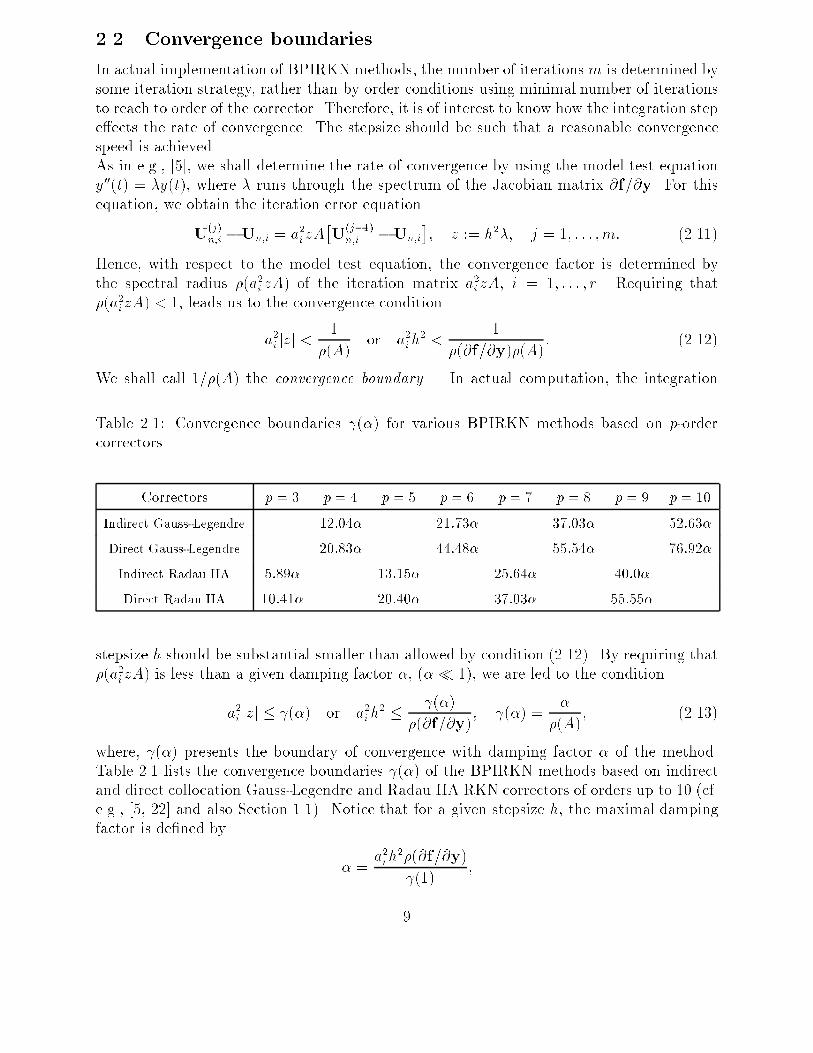
2.2 Convergence boundariesIn actual implementation of BPIRKN methods, the number of iterations m is determined bysome iteration strategy, rather than by order conditions using minimal number of iterationsto reach to order of the corrector. Therefore, it is of interest to know how the integration stepe�ects the rate of convergence. The stepsize should be such that a reasonable convergencespeed is achieved.As in e.g., [5], we shall determine the rate of convergence by using the model test equationy00(t) = �y(t), where � runs through the spectrum of the Jacobian matrix @f=@y. For thisequation, we obtain the iteration error equationU(j)n;i �Un;i = a2i zA�U(j�1)n;i �Un;i�; z := h2�; j = 1; : : : ;m: (2.11)Hence, with respect to the model test equation, the convergence factor is determined bythe spectral radius �(a2i zA) of the iteration matrix a2i zA, i = 1; : : : ; r. Requiring that�(a2i zA) < 1, leads us to the convergence conditiona2i jzj < 1�(A) or a2ih2 < 1�(@f=@y)�(A): (2.12)We shall call 1=�(A) the convergence boundary. In actual computation, the integrationTable 2.1: Convergence boundaries (�) for various BPIRKN methods based on p-ordercorrectorsCorrectors p = 3 p = 4 p = 5 p = 6 p = 7 p = 8 p = 9 p = 10Indirect Gauss-Legendre 12:04� 21:73� 37:03� 52:63�Direct Gauss-Legendre 20:83� 44:48� 55:54� 76:92�Indirect Radau IIA 5:89� 13:15� 25:64� 40:0�Direct Radau IIA 10:41� 20:40� 37:03� 55:55�stepsize h should be substantial smaller than allowed by condition (2.12). By requiring that�(a2i zA) is less than a given damping factor �, (�� 1), we are led to the conditiona2i jzj � (�) or a2ih2 � (�)�(@f=@y); (�) = ��(A); (2.13)where, (�) presents the boundary of convergence with damping factor � of the method.Table 2.1 lists the convergence boundaries (�) of the BPIRKN methods based on indirectand direct collocation Gauss-Legendre and Radau IIA RKN correctors of orders up to 10 (cf.e.g., [5, 22] and also Section 1.1). Notice that for a given stepsize h, the maximal dampingfactor is de�ned by � = a2ih2�(@f=@y) (1) ;9

so we can conclude that the direct collocation RKN correctors reported in Table 2.1 give riseto faster convergence. This conclusion leads us to restrict our considerations to the BPIRKNmethods based on direct collocation RKN correctors (cf. [5]). These direct RKNmethods arenot A-stable (see [22]), but their stability regions are su�ciently large for nonsti� problems.2.3 The choice of block abscissas aiThe accuracy of Hermite-I interpolation formulas is improved if the interpolation abscissasare more narrowly spaced. However, this will increase the magnitude of the entries of thematrices Vi and Wi, causing serious round-o� errors. There are several ways to reduce thisround-o� e�ect as were discussed in [21, Section 2.1] for Lagrange interpolation formulas.Also in [10] where Hermite interpolation formulas were used for deriving reliable error esti-mates for defect control, it was found that on a 15 digits precision machine, the interpolationabscissas should be separated by 0:2 in order to suppress rounding errors.In order to derive a further criteria for the choice of suitable values of the abscissas ai, weneed to get insight into the propagation of a perturbation " of the block vectors Yn andY0n within a single step (the similar analysis was given in [21]). We shall study this for themodel test equation y00(t) = �y(t). First we shall express yn+1;i and hy0n+1;i in terms of Ynand hY0n. SinceUn;i = [I � a2i zA]�1[eeT1Yn + ceT1 aihY0n]U(0)n;i �Un;i = �Vi � [I � a2i zA]�1eeT1 �Yn + �Wi � [I � a2i zA]�1ceT1 ai�hY0n;applying (2.4), (2.11) to the model equation for a given number m, we obtainyn+1;i = eT1Yn + aiheT1Y0n + a2i zbT [U(m)n;i �Un;i] + a2i zbTUn;i= eT1Yn + aiheT1Y0n + a2i zbT [I � a2i zA]�1[eeT1Yn + ceT1 aihY0n]+ a2i zbT [a2i zA]m��Vi � [I � a2i zA]�1eeT1 �Yn + �Wi � [I � a2i zA]�1ceT1 ai�hY0n�= �eT1 + a2i zbT [I � a2i zA]�1eeT1 + a2i zbT [a2i zA]m�Vi � [I � a2i zA]�1eeT1 ��Yn (2.14a)+ �aieT1 + a2i zbT [I � a2i zA]�1aiceT1 + a2i zbT [a2i zA]m�Wi � [I � a2i zA]�1aiceT1 ��hY0nhy0n+1;i = eT1 hY0n ++aizdT [U(m)n;i �Un;i] + aizdTUn;i= heT1Y0n + aizdT [I � a2i zA]�1[eeT1Yn + ceT1 aihY0n]+ aizdT [a2i zA]m��Vi � [I � a2i zA]�1eeT1 �Yn + �Wi � [I � a2i zA]�1ceT1 ai�hY0n�= �aizdT [I � a2i zA]�1eeT1 + aizdT [a2i zA]m�Vi � [I � a2i zA]�1eeT1 ��Yn (2.14b)+ �eT1 + aizdT [I � a2i zA]�1aiceT1 + aizdT [a2i zA]m�Wi � [I � a2i zA]�1aiceT1 ��hY0n:10

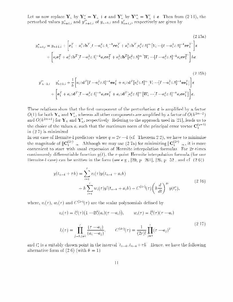
Let us now replace Yn by Y�n = Yn + " and Y0n by Y0�n = Y0n + ". Then from (2.14), theperturbed values y�n+1;i and y0�n+1;i of yn+1;i and y0n+1;i, respectively are given by (2.15a)y�n+1;i = yn+1;i + �eT1 + a2i zbT [I � a2i zA]�1eeT1 + a2i zbT [a2i zA]m�Vi � [I � a2i zA]�1eeT1 ��"+ �aieT1 + a2i zbT [I � a2i zA]�1aiceT1 + a2i zbT [a2i zA]m�Wi � [I � a2i zA]�1aiceT1 ��h"(2.15b)y0�n+1;i = y0n+1;i + 1h�aizdT [I � a2i zA]�1eeT1 + aizdT [a2i zA]m�Vi � [I � a2i zA]�1eeT1 ��"+ �eT1 + aizdT [I � a2i zA]�1aiceT1 + aizdT [a2i zA]m�Wi � [I � a2i zA]�1aiceT1 ��":These relations show that the �rst component of the perturbation " is ampli�ed by a factorO(1) for both Yn andY0n, whereas all other components are ampli�ed by a factor of O(h2m+2)and O(h2m+1) for Yn and Y0n, respectively. Refering to the approach used in [21], leads us tothe choice of the values ai such that the maximum norm of the principal error vector C(q+1)1in (2.7) is minimized.In our case of Hermite-I predictors where q = 2r� 1 (cf. Theorem 2.2), we have to minimizethe magnitude of kC(2r)1 k1. Although we may use (2.7a) for minimizing kC(2r)1 k1, it is moreconvenient to start with usual expression of Hermite interpolation formulas. For 2r-timescontinuously di�erentiable function y(t), the r-point Hermite interpolation formula (for ourHermite-I case) can be written in the form (see e.g., [20, p. 261], [26, p. 52], and cf. (2.6))y(tn�1 + �h) = rXi=1 vi(� )y(tn�1 + aih)+ h rXi=1 wi(� )y0(tn�1 + aih) + C(2r)(� )�h ddt�2ry(t��); (2.16)where, vi(� ), wi(� ) and C(2r)(� ) are the scalar polynomials de�ned byvi(� ) = l2i (� )�1 � 2l0i(ai)(� � ai)�; wi(� ) = l2i (� )(� � ai)li(� ) = rYj=1;j 6=i (� � aj)(ai � aj) ; C(2r)(� ) = 1(2r)! rYj=1(� � aj)2 (2.17)and t�� is a suitably chosen point in the interval [tn�1; tn�1+�h]. Hence, we have the followingalternative form of (2.6) (with � = 1) 11

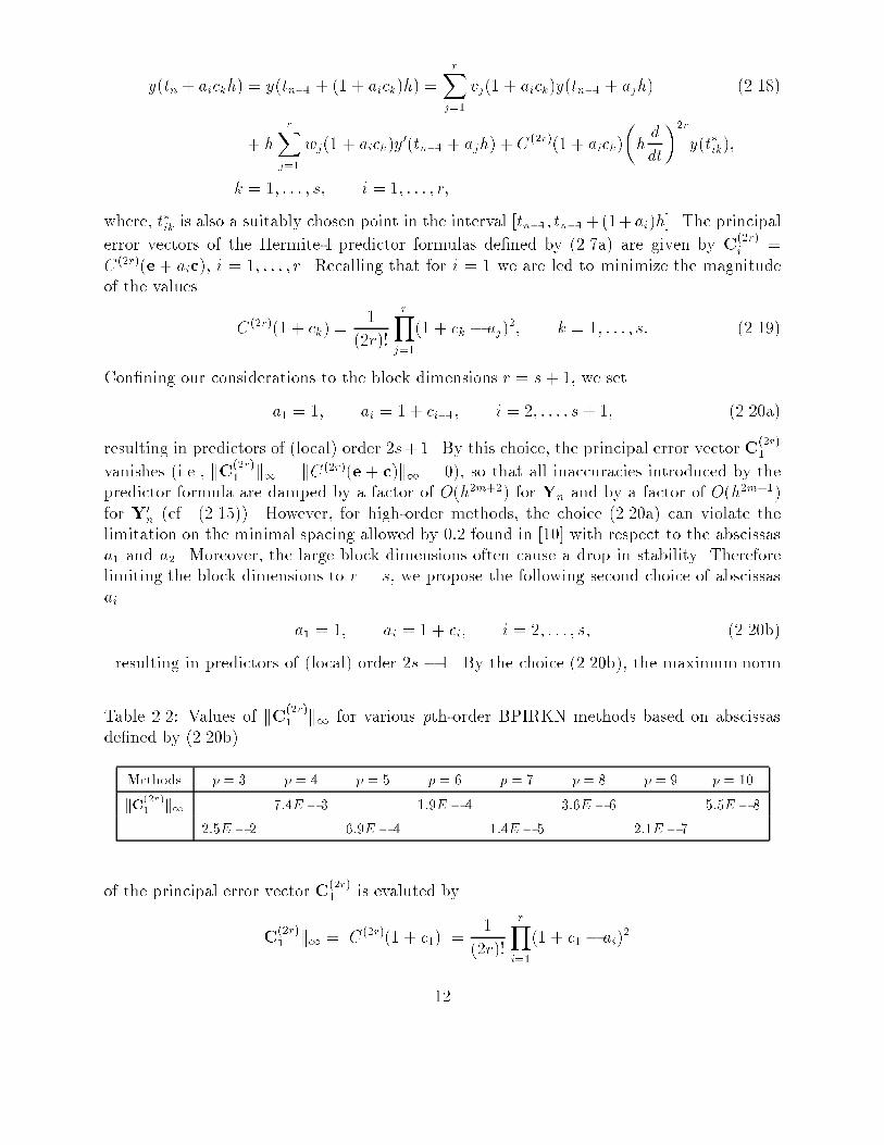
y(tn + aickh) = y(tn�1 + (1 + aick)h) = rXj=1 vj(1 + aick)y(tn�1 + ajh) (2.18)+ h rXj=1 wj(1 + aick)y0(tn�1 + ajh) + C(2r)(1 + aick)�h ddt�2ry(t�ik);k = 1; : : : ; s; i = 1; : : : ; r;where, t�ik is also a suitably chosen point in the interval [tn�1; tn�1+(1+ai)h]. The principalerror vectors of the Hermite-I predictor formulas de�ned by (2.7a) are given by C(2r)i =C(2r)(e+ aic), i = 1; : : : ; r. Recalling that for i = 1 we are led to minimize the magnitudeof the values C(2r)(1 + ck) = 1(2r)! rYj=1(1 + ck � aj)2; k = 1; : : : ; s: (2.19)Con�ning our considerations to the block dimensions r = s+ 1, we seta1 = 1; ai = 1 + ci�1; i = 2; : : : ; s+ 1; (2.20a)resulting in predictors of (local) order 2s+1. By this choice, the principal error vector C(2r)1vanishes (i.e., kC(2r)1 k1 = kC(2r)(e+ c)k1 = 0), so that all inaccuracies introduced by thepredictor formula are damped by a factor of O(h2m+2) for Yn and by a factor of O(h2m+1)for Y0n (cf. (2.15)). However, for high-order methods, the choice (2.20a) can violate thelimitation on the minimal spacing allowed by 0:2 found in [10] with respect to the abscissasa1 and a2. Moreover, the large block dimensions often cause a drop in stability. Thereforelimiting the block dimensions to r = s, we propose the following second choice of abscissasai a1 = 1; ai = 1 + ci; i = 2; : : : ; s; (2.20b)resulting in predictors of (local) order 2s � 1. By the choice (2.20b), the maximum normTable 2.2: Values of kC(2r)1 k1 for various pth-order BPIRKN methods based on abscissasde�ned by (2.20b)Methods p = 3 p = 4 p = 5 p = 6 p = 7 p = 8 p = 9 p = 10kC(2r)1 k1 7:4E � 3 1:9E � 4 3:6E � 6 5:5E � 82:5E � 2 6:9E � 4 1:4E � 5 2:1E � 7of the principal error vector C(2r)1 is evaluted bykC(2r)1 k1 = jC(2r)(1 + c1)j = 1(2r)! rYi=1(1 + c1 � ai)212

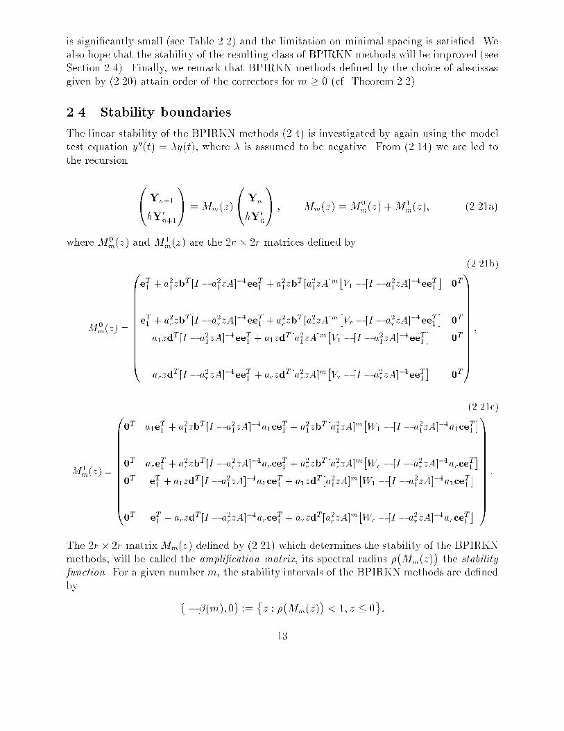
is signi�cantly small (see Table 2.2) and the limitation on minimal spacing is satis�ed. Wealso hope that the stability of the resulting class of BPIRKN methods will be improved (seeSection 2.4). Finally, we remark that BPIRKN methods de�ned by the choice of abscissasgiven by (2.20) attain order of the correctors for m � 0 (cf. Theorem 2.2).2.4 Stability boundariesThe linear stability of the BPIRKN methods (2.4) is investigated by again using the modeltest equation y00(t) = �y(t), where � is assumed to be negative. From (2.14) we are led tothe recursion 0@ Yn+1hY0n+11A =Mm(z)0@ YnhY0n1A ; Mm(z) = M0m(z) +M1m(z); (2.21a)where M0m(z) and M1m(z) are the 2r � 2r matrices de�ned by (2.21b)M0m(z) = 0BBBBBBBBBBBB@eT1 + a21zbT [I � a21zA]�1eeT1 + a21zbT [a21zA]m�V1 � [I � a21zA]�1eeT1 � 0T... ...eT1 + a2rzbT [I � a2rzA]�1eeT1 + a2rzbT [a2rzA]m�Vr � [I � a2rzA]�1eeT1 � 0Ta1zdT [I � a21zA]�1eeT1 + a1zdT [a21zA]m�V1 � [I � a21zA]�1eeT1 � 0T... ...arzdT [I � a2rzA]�1eeT1 + arzdT [a2rzA]m�Vr � [I � a2rzA]�1eeT1 � 0T1CCCCCCCCCCCCA ;(2.21c)M1m(z) = 0BBBBBBBBBBBB@0T a1eT1 + a21zbT [I � a21zA]�1a1ceT1 + a21zbT [a21zA]m�W1 � [I � a21zA]�1a1ceT1 �... ...0T areT1 + a2rzbT [I � a2rzA]�1arceT1 + a2rzbT [a2rzA]m�Wr � [I � a2rzA]�1arceT1 �0T eT1 + a1zdT [I � a21zA]�1a1ceT1 + a1zdT [a21zA]m�W1 � [I � a21zA]�1a1ceT1 �... ...0T eT1 + arzdT [I � a2rzA]�1arceT1 + arzdT [a2rzA]m�Wr � [I � a2rzA]�1arceT1 � 1CCCCCCCCCCCCA :The 2r � 2r matrix Mm(z) de�ned by (2.21) which determines the stability of the BPIRKNmethods, will be called the ampli�cation matrix, its spectral radius ��Mm(z)� the stabilityfunction. For a given number m, the stability intervals of the BPIRKN methods are de�nedby �� �(m); 0� := �z : ��Mm(z)� < 1; z � 0:13

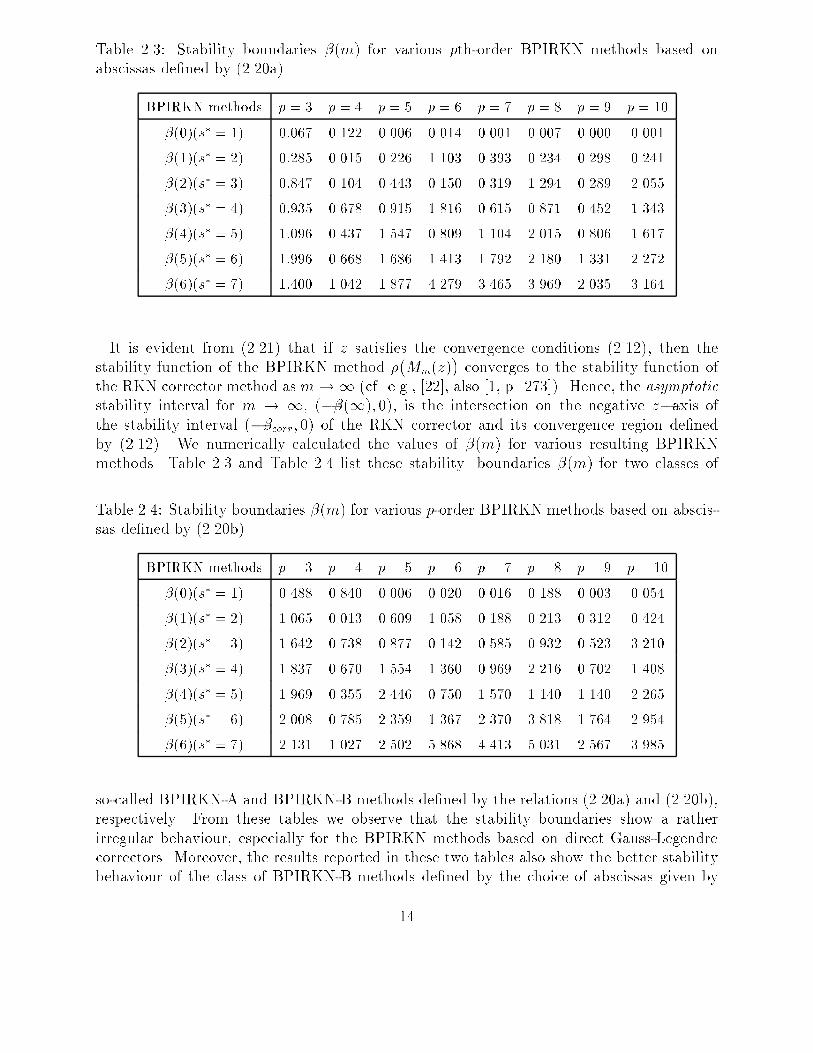
Table 2.3: Stability boundaries �(m) for various pth-order BPIRKN methods based onabscissas de�ned by (2.20a)BPIRKN methods p = 3 p = 4 p = 5 p = 6 p = 7 p = 8 p = 9 p = 10�(0)(s� = 1) 0:067 0.122 0.006 0.014 0.001 0.007 0.000 0.001�(1)(s� = 2) 0:285 0.015 0.226 1.103 0.393 0.234 0.298 0.241�(2)(s� = 3) 0:847 0.104 0.443 0.150 0.319 1.294 0.289 2.055�(3)(s� = 4) 0:935 0.678 0.915 1.816 0.615 0.871 0.452 1.343�(4)(s� = 5) 1:096 0.437 1.547 0.809 1.104 2.015 0.806 1.617�(5)(s� = 6) 1:996 0.668 1.686 1.413 1.792 2.180 1.331 2.272�(6)(s� = 7) 1:400 1.042 1.877 4.279 3.465 3.969 2.035 3.164It is evident from (2.21) that if z satis�es the convergence conditions (2.12), then thestability function of the BPIRKN method ��Mm(z)� converges to the stability function ofthe RKN corrector method as m!1 (cf. e.g., [22], also [1, p. 273]). Hence, the asymptoticstability interval for m ! 1, (��(1); 0), is the intersection on the negative z�axis ofthe stability interval (��corr; 0) of the RKN corrector and its convergence region de�nedby (2.12). We numerically calculated the values of �(m) for various resulting BPIRKNmethods. Table 2.3 and Table 2.4 list these stability boundaries �(m) for two classes ofTable 2.4: Stability boundaries �(m) for various p-order BPIRKN methods based on abscis-sas de�ned by (2.20b)BPIRKN methods p = 3 p = 4 p = 5 p = 6 p = 7 p = 8 p = 9 p = 10�(0)(s� = 1) 0.488 0.840 0.006 0.020 0.016 0.188 0.003 0.054�(1)(s� = 2) 1.065 0.013 0.609 1.058 0.188 0.213 0.312 0.424�(2)(s� = 3) 1.642 0.738 0.877 0.142 0.585 0.932 0.523 3.210�(3)(s� = 4) 1.837 0.670 1.554 1.360 0.969 2.216 0.702 1.408�(4)(s� = 5) 1.969 0.355 2.446 0.750 1.570 1.140 1.140 2.265�(5)(s� = 6) 2.008 0.785 2.359 1.367 2.370 3.818 1.764 2.954�(6)(s� = 7) 2.131 1.027 2.502 5.868 4.413 5.031 2.567 3.985so-called BPIRKN-A and BPIRKN-B methods de�ned by the relations (2.20a) and (2.20b),respectively. From these tables we observe that the stability boundaries show a ratherirregular behaviour, especially for the BPIRKN methods based on direct Gauss-Legendrecorrectors. Moreover, the results reported in these two tables also show the better stabilitybehaviour of the class of BPIRKN-B methods de�ned by the choice of abscissas given by14

(2.20b). The stability regions of this class are also su�ciently large for nonsti� problems.From Table 2.4, we can select a whole set of BPIRKN-B methods of order p up to 10 (exceptfor p = 4) using only 1 correction with acceptable stability regions for nonsti� problems (cf.Theorem 2.2). In the next section we shall compare the e�ciency of BPIRKN-A methodswith that of BPIRKN-B methods by numerical tests. In all numerical experiments, we shallcon�ne our considerations to the BPIRKN methods using Radau IIA correctors.3 Numerical experimentsIn this section we report numerical results obtained by the BPIRKN methods (2.4). Asit was mentioned in the previous sections, we con�ne our considerations to the BPIRKNmethods based on Hermite-I predictor and direct Radau IIA corrector pairs with blockpoints de�ned by (2.20) (cf. Sections 2.2 and Section 2.3). First, we test the e�ciency oftwo classes of BPIRKN-A and BPIRKN-B methods (cf. Section 2.4). Next, we compare thebest resulting class of BPIRKN methods with parallel and sequential explicit RKN methodsfrom the literature. In order to see the e�ciency (partly) de�ned by convergence behaviourof the various PC methods, we applied a dynamical strategy for determining the number ofiterations in the successive steps as it was applied in [5, 7, 8]. So that we can reproduce thebest numerical results in those papers of the PC methods to be compared with our BPIRKNmethods. The discussion on the error propagation in Section 2.3 suggests the followingstopping criterion (cf. [5, 7, 8])kU(m)n;1 �U(m�1)n;1 k1 � TOL = Chp�1; (3.1)where p is the order of the corrector method, and C is a parameter depending on themethod and on the problem. To have a comparison with the numerical results for thePIRKN methods reported in [7, 8], we used the same constant C as in [7, 8]. Notice that bythis criterion, the iteration error for yn+1;1 = yn+1 and y0n+1;1 = y0n+1 is of the same order inh as the underlying corrector. In the �rst step, we always use the trivial predictors U(0)n;i =yne + aihy0nc, i = 1; : : : ; r. The absolute error obtained at the end point of the integrationinterval is presented in the form 10�NCD (NCD may be interpreted as the number of correctdecimal digits). The computational e�orts are measured by Nseq denoting the total numberof sequential f -evaluations required over the whole integration interval. Furthermore, in thetables of results, Nsteps denotes the total number of integration steps. All the computationswere carried out on a computer with 28 digits precision. An actual implementation on aparallel machine is a subject of further research.3.1 E�ciency of BPIRKN-A and BPIRKN-B methodsSection 2.4 compared the stability properties of the two classes of BPIRKN-A and BPIRKN-B methods. This section is devoted to mutually numerical comparison of e�ciency of thesemethods. For that purpose, we apply the BPIRKN-A and BPIRKN-B methods to a selectionof two test problems found in the literature. 15

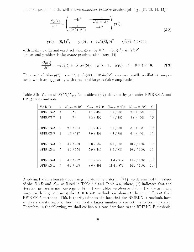
The �rst problem is the well-known nonlinear Fehlberg problem (cf. e.g., [11, 12, 14, 15])d2y(t)dt2 =0B@ �4t2 � 2py21(t)+y22(t)2py21(t)+y22(t) �4t2 1CAy(t);y(0) = (0; 1)T ; y0(0) = (�2p�=2; 0)T p�=2 � t � 10; (3.2)with highly oscillating exact solution given by y(t) = (cos(t2); sin(t2))T .The second problem is the scalar problem taken from [14]d2y(t)dt2 = �25y(t) + 100cos(5t); y(0) = 1; y0(0) = 5; 0 � t � 10: (3.3)The exact solution y(t) = cos(5t) + sin(5t)+ 10tsin(5t) possesses rapidly oscillating compo-nents which are appearing with small and large variable amplitudes.Table 3.5: Values of NCD/Nseq for problem (3.2) obtained by pth-order BPIRKN-A andBPIRKN-B methodsMethods p Nsteps = 100 Nsteps = 200 Nsteps = 400 Nsteps = 800 CBPIRKN-A 3 (*) 1.1 / 439 1.9 / 800 2.8 / 1600 102BPIRKN-B 3 (*) 1.2 / 400 1.9 / 800 2.8 / 1600 102BPIRKN-A 5 2.0 / 464 3.4 / 479 4.8 / 801 6.4 / 1601 103BPIRKN-B 5 1.9 / 317 3.0 / 401 4.8 / 801 6.4 / 1601 103BPIRKN-A 7 4.2 / 403 6.0 / 507 8.0 / 802 10.2 / 1602 103BPIRKN-B 7 4.1 / 354 5.9 / 440 8.0 / 833 10.2 / 1602 103BPIRKN-A 9 6.0 / 482 8.7 / 579 11.4 / 912 14.2 / 1604 103BPIRKN-B 9 6.0 / 435 8.6 / 494 11.4 / 879 14.2 / 1604 103Applying the iteration strategy using the stopping criterion (3.1), we determined the valuesof the NCD and Nseq as listed in Table 3.5 and Table 3.6, where, (*) indicates that theiteration process is not convergent. From these tables we observe that in the low accuracyrange (with large stepsizes) the BPIRKN-B methods are shown to be more e�cient thanBPIRKN-A methods. This is (partly) due to the fact that the BPIRKN-A methods havesmaller stability regions, they may need a larger number of corrections to become stable.Therefore, in the following, we shall con�ne our considerations to the BPIRKN-B methods.16

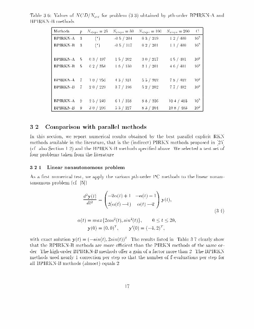
Table 3.6: Values of NCD/Nseq for problem (3.3) obtained by pth-order BPIRKN-A andBPIRKN-B methodsMethods p Nsteps = 25 Nsteps = 50 Nsteps = 100 Nsteps = 200 CBPIRKN-A 3 (*) -0.5 / 204 0.3 / 219 1.2 / 400 102BPIRKN-B 3 (*) -0.5 / 117 0.2 / 201 1.1 / 400 102BPIRKN-A 5 0.3 / 497 1.5 / 202 3.0 / 217 4.5 / 401 102BPIRKN-B 5 0.2 / 358 1.6 / 150 3.1 / 201 4.6 / 401 102BPIRKN-A 7 1.0 / 256 4.3 / 231 5.5 / 202 7.8 / 402 102BPIRKN-B 7 2.0 / 229 3.7 / 196 5.2 / 202 7.7 / 402 102BPIRKN-A 9 2.5 / 249 6.1 / 258 8.8 / 236 10.4 / 403 102BPIRKN-B 9 3.0 / 206 5.3 / 227 8.3 / 204 10.8 / 403 1023.2 Comparison with parallel methodsIn this section, we report numerical results obtained by the best parallel explicit RKNmethods available in the literature, that is the (indirect) PIRKN methods proposed in [25](cf. also Section 1.2) and the BPIRKN-B methods speci�ed above. We selected a test set offour problems taken from the literature.3.2.1 Linear nonautonomous problemAs a �rst numerical test, we apply the various pth-order PC methods to the linear nonau-tonomous problem (cf. [5])d2y(t)dt2 = 0@�2�(t) + 1 ��(t) + 12(�(t) � 1) �(t)� 2 1Ay(t);�(t) = maxf2cos2(t); sin2(t)g; 0 � t � 20;y(0) = (0; 0)T ; y0(0) = (�1; 2)T ; (3.4)with exact solution y(t) = (�sin(t); 2sin(t))T . The results listed in Table 3.7 clearly showthat the BPIRKN-B methods are more e�cient than the PIRKN methods of the same or-der. The high-order BPIRKN-B methods o�er a gain of a factor more than 2. The BPIRKNmethods used nearly 1 correction per step so that the number of f -evaluations per step forall BPIRKN-B methods (almost) equals 2. 17

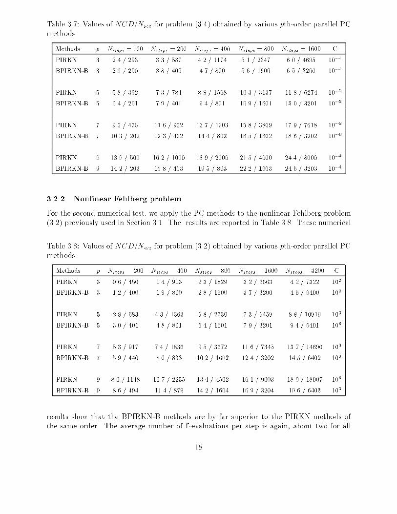
Table 3.7: Values of NCD=Nseq for problem (3.4) obtained by various pth-order parallel PCmethodsMethods p Nsteps = 100 Nsteps = 200 Nsteps = 400 Nsteps = 800 Nsteps = 1600 CPIRKN 3 2.4 / 293 3.3 / 587 4.2 / 1174 5.1 / 2347 6.0 / 4695 10�1BPIRKN-B 3 2.9 / 200 3.8 / 400 4.7 / 800 5.6 / 1600 6.5 / 3200 10�1PIRKN 5 5.8 / 392 7.3 / 784 8.8 / 1568 10.3 / 3137 11.8 / 6274 10�2BPIRKN-B 5 6.4 / 201 7.9 / 401 9.4 / 801 10.9 / 1601 13.0 / 3201 10�2PIRKN 7 9.5 / 476 11.6 / 952 13.7 / 1903 15.8 / 3809 17.9 / 7618 10�3BPIRKN-B 7 10.3 / 202 12.3 / 402 14.4 / 802 16.5 / 1602 18.6 / 3202 10�3PIRKN 9 13.9 / 500 16.2 / 1000 18.9 / 2000 21.5 / 4000 24.4 / 8000 10�4BPIRKN-B 9 14.2 / 203 16.8 / 403 19.5 / 803 22.2 / 1603 24.6 / 3203 10�43.2.2 Nonlinear Fehlberg problemFor the second numerical test, we apply the PC methods to the nonlinear Fehlberg problem(3.2) previously used in Section 3.1. The results are reported in Table 3.8. These numericalTable 3.8: Values of NCD=Nseq for problem (3.2) obtained by various pth-order parallel PCmethodsMethods p Nsteps = 200 Nsteps = 400 Nsteps = 800 Nsteps = 1600 Nsteps = 3200 CPIRKN 3 0.6 / 450 1.4 / 913 2.3 / 1829 3.2 / 3663 4.2 / 7322 102BPIRKN-B 3 1.2 / 400 1.9 / 800 2.8 / 1600 3.7 / 3200 4.6 / 6400 102PIRKN 5 2.8 / 683 4.3 / 1363 5.8 / 2730 7.3 / 5459 8.8 / 10919 103BPIRKN-B 5 3.0 / 401 4.8 / 801 6.4 / 1601 7.9 / 3201 9.4 / 6401 103PIRKN 7 5.3 / 917 7.4 / 1836 9.5 / 3672 11.6 / 7345 13.7 / 14690 103BPIRKN-B 7 5.9 / 440 8.0 / 833 10.2 / 1602 12.4 / 3202 14.5 / 6402 103PIRKN 9 8.0 / 1148 10.7 / 2255 13.4 / 4502 16.1 / 9003 18.9 / 18007 103BPIRKN-B 9 8.6 / 494 11.4 / 879 14.2 / 1604 16.9 / 3204 19.6 / 6403 103results show that the BPIRKN-B methods are by far superior to the PIRKN methods ofthe same order. The average number of f -evaluations per step is again, about two for all18

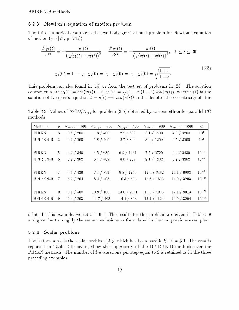
BPIRKN-B methods.3.2.3 Newton's equation of motion problemThe third numerical example is the two-body gravitational problem for Newton's equationof motion (see [24, p. 245]).d2y1(t)dt2 = � y1(t)�py21(t) + y22(t)�3 ; d2y2(t)d2t = � y2(t)�py21(t) + y22(t)�3 ; 0 � t � 20;y1(0) = 1� "; y2(0) = 0; y01(0) = 0; y02(0) =r1 + "1� ": (3.5)This problem can also found in [15] or from the test set of problems in [23]. The solutioncomponents are y1(t) = cos(u(t)) � ", y2(t) = p(1 + ")(1� ") sin(u(t)), where u(t) is thesolution of Keppler's equation t = u(t) � " sin(u(t)) and " denotes the eccentricity of theTable 3.9: Values of NCD=Nseq for problem (3.5) obtained by various pth-order parallel PCmethodsMethods p Nsteps = 100 Nsteps = 200 Nsteps = 400 Nsteps = 800 Nsteps = 1600 CPIRKN 3 0.5 / 200 1.3 / 400 2.2 / 800 3.1 / 1600 4.0 / 3200 101BPIRKN-B 3 0.9 / 200 1.8 / 400 2.7 / 800 3.6 / 1600 4.5 / 3200 101PIRKN 5 3.0 / 340 4.5 / 680 6.0 / 1361 7.5 / 2720 9.0 / 5439 10�1BPIRKN-B 5 3.7 / 202 5.1 / 402 6.6 / 802 8.1 / 1602 9.7 / 3202 10�1PIRKN 7 5.6 / 436 7.7 / 873 9.8 / 1745 12.0 / 3492 14.1 / 6983 10�2BPIRKN-B 7 6.3 / 204 8.4 / 403 10.5 / 803 12.6 / 1603 14.9 / 3203 10�2PIRKN 9 8.2 / 500 10.9 / 1000 13.6 / 2001 16.3 / 4006 19.1 / 8013 10�2BPIRKN-B 9 9.4 / 203 11.7 / 403 14.4 / 803 17.1 / 1604 19.9 / 3204 10�2orbit. In this example, we set " = 0:3. The results for this problem are given in Table 3.9and give rise to roughly the same conclusions as formulated in the two previous examples.3.2.4 Scalar problemThe last example is the scalar problem (3.3) which has been used in Section 3.1. The resultsreported in Table 3.10 again, show the superiority of the BPIRKN-B methods over thePIRKN methods. The number of f -evaluations per step equal to 2 is retained as in the threepreceding examples. 19

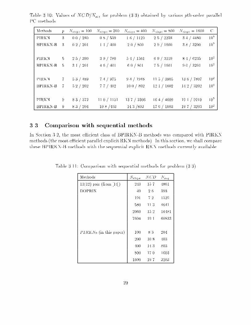
Table 3.10: Values of NCD=Nseq for problem (3.3) obtained by various pth-order parallelPC methodsMethods p Nsteps = 100 Nsteps = 200 Nsteps = 400 Nsteps = 800 Nsteps = 1600 CPIRKN 3 0.0 / 280 0.8 / 559 1.6 / 1120 2.5 / 2238 3.4 / 4480 102BPIRKN-B 3 0.2 / 201 1.1 / 400 2.0 / 800 2.9 / 1600 3.8 / 3200 102PIRKN 5 2.5 / 390 3.9 / 780 5.4 / 1561 6.9 / 3119 8.4 / 6235 102BPIRKN-B 5 3.1 / 201 4.6 / 401 6.0 / 801 7.5 / 1601 9.0 / 3201 102PIRKN 7 5.3 / 489 7.4 / 975 9.4 / 1948 11.5 / 3905 13.6 / 7807 102BPIRKN-B 7 5.2 / 202 7.7 / 402 10.0 / 802 12.1 / 1602 14.2 / 3202 102PIRKN 9 8.3 / 572 11.0 / 1151 13.7 / 2306 16.4 / 4609 19.1 / 9210 102BPIRKN-B 9 8.3 / 204 10.8 /403 14.3 /803 17.0 / 1603 19.7 / 3203 1023.3 Comparison with sequential methodsIn Section 3.2, the most e�cient class of BPIRKN-B methods was compared with PIRKNmethods (the most e�cient parallel explicit RKN methods). In this section, we shall comparethese BPIRKN-B methods with the sequential explicit RKN methods currently available.Table 3.11: Comparison with sequential methods for problem (3.3)Methods Nsteps NCD Nseq11(12) pair (from [14]) 243 15.7 4861DOPRIN 49 2.6 393191 7.2 1529580 11.3 46412060 15.2 164817604 19.1 60833PIRKN9 (in this paper) 100 8.3 204200 10.8 403400 14.3 803800 17.0 16031600 19.7 320320

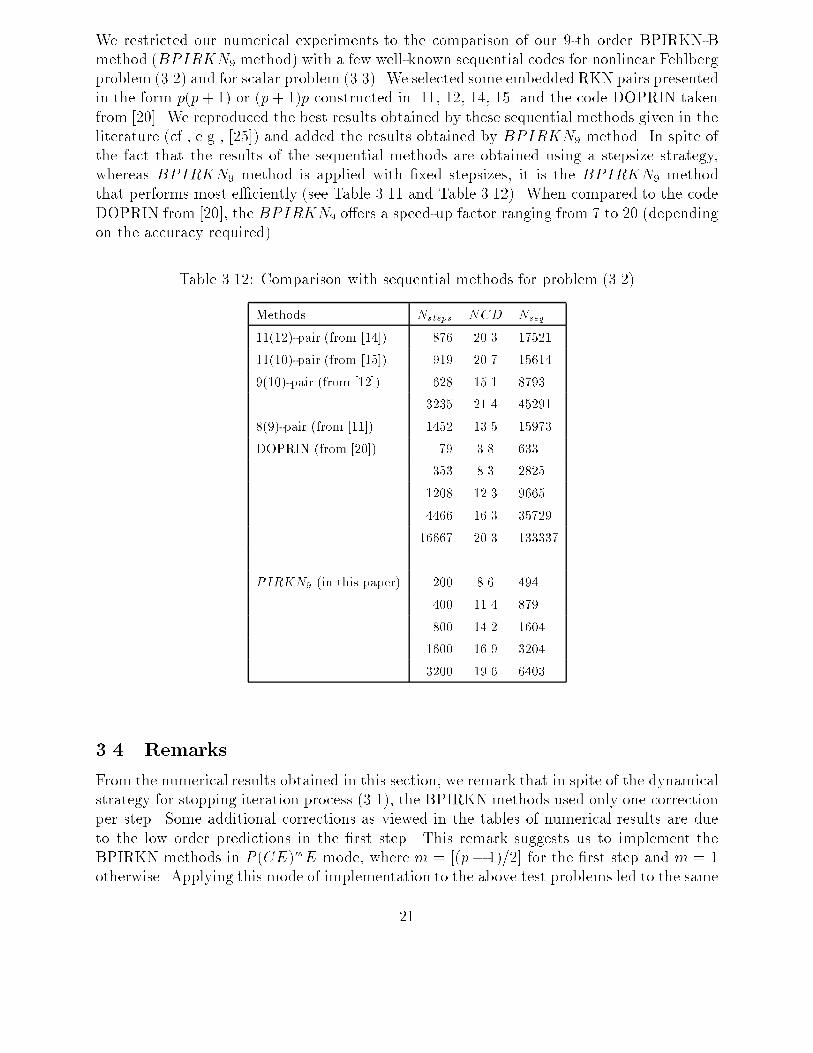
We restricted our numerical experiments to the comparison of our 9-th order BPIRKN-Bmethod (BPIRKN9 method) with a few well-known sequential codes for nonlinear Fehlbergproblem (3.2) and for scalar problem (3.3). We selected some embedded RKN pairs presentedin the form p(p+ 1) or (p+ 1)p constructed in [11, 12, 14, 15] and the code DOPRIN takenfrom [20]. We reproduced the best results obtained by these sequential methods given in theliterature (cf., e.g., [25]) and added the results obtained by BPIRKN9 method. In spite ofthe fact that the results of the sequential methods are obtained using a stepsize strategy,whereas BPIRKN9 method is applied with �xed stepsizes, it is the BPIRKN9 methodthat performs most e�ciently (see Table 3.11 and Table 3.12). When compared to the codeDOPRIN from [20], the BPIRKN9 o�ers a speed-up factor ranging from 7 to 20 (dependingon the accuracy required).Table 3.12: Comparison with sequential methods for problem (3.2)Methods Nsteps NCD Nseq11(12)-pair (from [14]) 876 20.3 1752111(10)-pair (from [15]) 919 20.7 156149(10)-pair (from [12]) 628 15.1 87933235 21.4 452918(9)-pair (from [11]) 1452 13.5 15973DOPRIN (from [20]) 79 3.8 633353 8.3 28251208 12.3 96654466 16.3 3572916667 20.3 133337PIRKN9 (in this paper) 200 8.6 494400 11.4 879800 14.2 16041600 16.9 32043200 19.6 64033.4 RemarksFrom the numerical results obtained in this section, we remark that in spite of the dynamicalstrategy for stopping iteration process (3.1), the BPIRKN methods used only one correctionper step. Some additional corrections as viewed in the tables of numerical results are dueto the low order predictions in the �rst step. This remark suggests us to implement theBPIRKN methods in P (CE)mE mode, where m = [(p� 1)=2] for the �rst step and m = 1otherwise. Applying this mode of implementation to the above test problems led to the same21

performance of BPIRKN-B methods. In the forthcoming paper, we shall apply this mode ofimplementation for BPIRKN methods with stepsize control.4 Concluding remarksThis paper described an algorithm to obtain Runge-Kutta-Nystr�om-type parallel block PCmethods (BPIRKN methods) requiring (almost) 2 sequential f -evaluations per step for anyorder of accuracy. The structure of BPIRKN methods also enables us to obtain variouscheap error estimates for stepsize control. The sequential costs of a resulting class of theseBPIRKN methods (BPIRKN-B methods) implemented with �xed stepsize strategy are al-ready considerably less than those of the best parallel and sequential methods available inthe literature. These conclusions encourage us to pursue the study of BPIRKN methods. Inparticular, we will concentrate on performance analysis of other predictor methods and onstepsize control that exploit the special structure of BPIRKN methods.References[1] K. Burrage, Parallel and Sequential Methods for Ordinary Di�erential Equations, (ClarendonPress, Oxford, 1995).[2] J.C. Butcher, Implicit Runge-Kutta processes, Math. Comp. 18, (1964), 50-64.[3] J.C. Butcher, The Numerical Analysis of Ordinary Di�erential Equations, Runge-Kutta andGeneral Linear Methods, (Wiley, New York, 1987).[4] N.H. Cong, An improvement for parallel-iterated Runge-Kutta-Nystr�om methods, Acta Math.Viet. 18 (1993), 295-308.[5] N.H. Cong, Note on the performance of direct and indirect Runge-Kutta-Nystr�om methods, J.Comput. Appl. Math. 45 (1993), 347-355.[6] N.H. Cong, Direct collocation-based two-step Runge-Kutta-Nystr�om methods, SEA Bull. Math.19 (1995), 49-58.[7] N.H. Cong, Explicit symmetric Runge-Kutta-Nystr�om methods for parallel computers, Comput.Math. Appl. 31 (1996), 111-122.[8] N.H. Cong, Explicit parallel two-step Runge-Kutta-Nystr�om methods, Comput. Math. Appl.32 (1996), 119-130.[9] N.H. Cong, Parallel Runge-Kutta-Nystr�om-type PC methods with stepsize control, in prepara-tion.[10] W.H. Enright and D.J. Highman, Parallel defect control, BIT 31 (1991), 647-663.[11] E. Fehlberg, Klassische Runge-Kutta-Nystr�om-Formeln mit Schrittweitenkontrolle f�ur Di�e-rentialgleichungen x00 = f(t; x), Computing 10 (1972), 305-315.[12] E. Fehlberg, Eine Runge-Kutta-Nystr�om-Formel 9-ter Ordnung mit Schrittweitenkontrolle f�urDi�erentialgleichungen x00 = f(t; x), Z. Angew. Math. Mech. 61 (1981), 477-485.22

[13] E. Fehlberg, S. Filippi und J. Gr�af, Ein Runge-Kutta-Nystr�om-Formelpaar der Ordnung 10(11)f�ur Di�erentialgleichungen y00 = f(t; y), Z. Angew. Math. Mech. 66 (1986), 265-270.[14] S. Filippi und J. Gr�af, Ein Runge-Kutta-Nystr�om-Formelpaar der Ordnung 11(12) f�ur Di�e-rentialgleichungen der Form y00 = f(t; y), Computing 34 (1985), 271-282.[15] S. Filippi and J. Gr�af, New Runge-Kutta-Nystr�om formula-pairs of order 8(7), 9(8), 10(9) and11(10) for di�erential equations of the form y00 = f(t; y), J. Comput. Appl. Math. 14 (1986),361-370.[16] E. Hairer, Methodes de Nystr�om pour l'�equations di�erentielle y00(t) = f(t; y), Numer. Math.27 (1977), 283-300.[17] E. Hairer, A Runge-Kutta method of order 10, J. Inst. Math. Appl. 21 (1978), 47-59.[18] E. Hairer, Unconditionally stable methods for second order di�erential equations, Numer. Math.32 (1979), 373-379.[19] E. Hairer, A one-step method of order 10 for y00(t) = f(t; y), IMA J. Numer. Anal. 2 (1982),83-94.[20] E. Hairer, S.P. N�rsett and G. Wanner, Solving Ordinary Di�erential Equations, I. Nonsti�Problems, (second revised edition, Springer-Verlag, Berlin, 1993).[21] P.J. van der Houwen and N.H. Cong, Parallel block predictor-corrector methods of Runge-Kuttatype, Appl. Numer. Math. 13 (1993), 109-123.[22] P.J. van der Houwen, B.P. Sommeijer and N.H. Cong, Stability of collocation-based Runge-Kutta-Nystr�om methods, BIT 31 (1991), 469-481.[23] T.E. Hull, W.H. Enright, B.M. Fellen and A.E. Sedgwick, Comparing numerical methods forordinary di�erential equations, SIAM J. Numer. Anal. 9 (1972), 603-637.[24] L.F. Shampine and M.K. Gordon, Computer Solution of Ordinary Di�erential Equations, TheInitial Value Problems, (W.H. Freeman and Company, San Francisco, 1975).[25] B.P. Sommeijer, Explicit, high-order Runge-Kutta-Nystr�om methods for parallel computers,Appl. Numer. Math. 13 (1993), 221-240.[26] J. Stoer and R. Bulirsch, Introduction to Numerical Analysis, (Springer-Verlag, New York,1983).Nguyen Huu CongFaculty of MathematicsMechanics and InformaticsHanoi University of Sciences90 Nguyen TraiDong Da, HanoiVietnam Karl Strehmel, R�udiger WeinerFB Mathematik und InformatikMartin-Luther-Universit�atHalle-WittenbergPostfachD-06099 Halle/SaaleGermanye-mail: rw@mail.mathematik.uni-halle.de23