Robust net present value

Mathematical and Computer Modelling 54 (2011) 233–242

Contents lists available at ScienceDirect

Mathematical and Computer Modelling

journal homepage: www.elsevier.com/locate/mcm

Robust net present valuePayam Hanafizadeh a,∗, Vahideh Latif ba Department of Industrial Management, School of Management and Accountancy, Allameh Tabataba’i University, Tehran, Iranb Department of Industrial Engineering, School of Industrial and Mechanical Engineering, Qazvin Islamic Azad University, Qazvin, Iran

a r t i c l e i n f o

Article history:Received 22 May 2009Received in revised form 3 February 2011Accepted 3 February 2011

Keywords:Net present valueRobust approachFuture cash flows

a b s t r a c t

Considering the variance and correlation of uncertain parameters, this study presentsa new approach to computing net present value (NPV) of the financial processes. Thechanges of the uncertain parameters are postulated in a closed and convex region calledthe uncertainty region. The size and shape of the uncertainty region is selected based onthe historical data and risk-taking or risk-aversion of the investor. The variance of cashflows is of high significance in analyzing the sensitivity of NPV. The model proposed in thisstudy is highly reliable because of entering the covariance of historical data.

In this study, using the robust approach, the mathematical formulation computingthe robust NPV is presented. Programming of the presented robust NPV was done in C++programming environment. The robust NPV is analyzed through presenting numericalexamples. Simulating 10,000 random scenarios of uncertain parameters demonstratesthat in circumstances where the traditional approach to computing NPV is doomed toa percentage of failure to make decisions, the robust approach never faces failure. Themore positive the skewness in the scenarios produced, the higher is the probability ofencountering failure in the traditional approach; whereas the robust approach still doesnot fail.

© 2011 Elsevier Ltd. All rights reserved.

1. Introduction

One of the most important and frequent decisions managers have to make is the selection of new industrial projects.One of the most fundamental criteria for financial measurement of projects is their net Present Value (NVP) defined as thesum of present values of annual net incomes earned in the period of the project exploitation [1]. Most firms undertakeprojects with the goal of making profit, and profitability is often measured as the discounted value of a project’s cash flows.It is very important to use precise data in calculating NPV, for the feasibility of a project may change by fluctuation of thedata. For financial decision making, it is quite clear that dependence on such uncertain criteria may bring about unpleasantconsequences. According to Ingersoll [2], in the presence of uncertainty, the expected NPV of the investment, rather thanthe point estimate, has to be used. Point estimates are not consistent with the decision makers’ state-of-belief. In this study,it is attempted to find a relation to calculate NPV, in which, considering uncertainty, the covariance of uncertain parameterscan be used in calculations in addition to the mean value of uncertain parameters. It is also tried to determine the region ofchanges of uncertain parameters so that the NPV obtained is better and more reliable for decision making.

2. Literature review

In this section, a review of the literature related to the importance of NPV, its applications, and different ways ofcalculation from some scientists’ point of views is presented. Regarding the use of NPV, Sobel et al. [3] argue that in addition

∗ Corresponding author.E-mail address: [email protected] (P. Hanafizadeh).

0895-7177/$ – see front matter© 2011 Elsevier Ltd. All rights reserved.doi:10.1016/j.mcm.2011.02.005

http://dx.doi.org/10.1016/j.mcm.2011.02.005

http://www.elsevier.com/locate/mcm

http://www.elsevier.com/locate/mcm

mailto:[email protected]

http://dx.doi.org/10.1016/j.mcm.2011.02.005

234 P. Hanafizadeh, V. Latif / Mathematical and Computer Modelling 54 (2011) 233–242

to comparing several economical proposals, NPV is an appropriate criterion which can be employed to plan the projects.Ross [4] points to the inefficiency of traditional NPV method for economically assessing the projects, and stresses thatif this criterion is ever to be used, it should be modified. Highlighting the weaknesses of NPV, Berkovitch and Israel [5]assert that firms indeed use criteria like internal rate of return (IRR), payback period, and profitability index (PI) moreoften than the NPV criterion in selecting projects. Magni [6] also refers to the inefficiency of the NPV method and statesthat the use of this criterion in decision making leads to some conflicts. In a review of Magni’s (2002) article [6], Reyck [7]comments that the main thesis of that paper was incorrect, and finance theory, when correctly applied, can be used to valueinvestment projects by comparing assets of equivalent risk. In addition, he points to the fallacies in the author’s reasoning.To encounter future ambiguities, scholars exploited the historical data about uncertain parameters. For example, it is acommon practice to replace the nominal mean as the expected value in the future with uncertain parameters. The pastapproaches suffered from some limitations; that is to say, the variance and mean of the data as well as their correlationwere not taken into account in those methods, and in most cases the nominal mean could not appropriately representthe introduced value expected in the future. In order to encounter the effect of changes of uncertain parameters fromestimated values, researchers consider the uncertain causes. For dealing with uncertainty, a variety of techniques havebeen presented which are generally divided into two main groups, namely passive and proactive approaches [8]. Passiveapproaches usually enter the data obtained from uncertain parameters pointwise, and after the problem is solved, thesensitivity of the solution to uncertain parameters is measured. Sensitivity analysis is one of the methods used for assessingsensitivity to uncertain parameters. This method considers the effect of the changes of one entry parameter on the outputparameter. For instance, Jovanovic [9] uses sensitivity analysis to study the interval of NPV changes while the inputs of theproblem change in assumed intervals. In this method, each entry parameter is given a correction coefficient and the effect ofchanges of correction coefficients on the estimated NPV is taken into account. This approach considers the same coefficientsfor a certain variable in all periods of the project; nevertheless, these changes indeedwill vary in different years. For example,in the near future the coefficients are expected to be smaller but in the distant future, they are supposed to be greater. Aswas mentioned by Willem and Groenendaal [10] in practice, the changes of entry variables occur simultaneously althoughthe analysis of the variability is usually restricted to deterministic sensitivity analysis, such as ‘one-factor-at-a-time’, andscenario analysis. These deterministic analyses, however, do not account for the total variability in the NPV. Accordingly, thismethod is not so efficient and might mislead the decision makers. Xu and Gertner [11] stress that the variability of outputsof a model varies according to the effect of uncertainty of independent, and dependent inputs. That is, the correlation ofinputs to the model should be separately taken into account in the sensitivity analysis of the outputs, despite the fact that,in this approach, the correlation between inputs is not considered.

Another group of approaches for dealing with uncertainty is proactive ones. Proactive approaches require moreinformation about uncertain parameters in the process of modeling and problem-solving and consequently their resultingsolution is of higher quality in uncertain conditions. In fact, in proactive approaches, the solution is already prepared to dealwith uncertainty. Scenario analysis belongs to this group. In analyzing scenarios, each scenario is a description of qualitativeand quantitative values of uncertain data of a problem. In uncertain circumstances where there is no statistical informationavailable, this approach is appropriate since it can predict the future use of experts’ opinions [12]. One drawback of thisapproach is that it is almost impossible to count and examine all possible scenarios [13]. Therefore, in this approach, itsuffices to predict the best, the worst, and the mean scenarios which neither consider the correlation between the data, norprovide the proper information for decision making. Employing approaches based on Monte Carlo simulation are amongother proactive approaches. Willem and Groenendaal [10] argue that the analysis of the variability is usually restrictedto deterministic sensitivity analysis, such as ‘one-factor-at-a-time’ and scenario analysis. These deterministic analyses,however, do not account for the total variability in the NPV. Coates and Kuhl [14] point out that simulation software such asSLAMII (based onMonte Carlo) can be used to estimate the NPV distribution. Using themean and standard deviation of cashflows of different years and considering their normal distribution, they simulatemany random scenarios thereby estimatingtheNPVdistribution. Due to consideration of the information on the standarddeviation of uncertain variables, their approachis more reliable than traditional approaches. Besides, they take simultaneous changes of uncertain parameters into accountin computing NPV. However, since no certain NPV is predicted for the future in this approach and only the NPV statisticaldistribution is estimated, it is quite difficult to compare projects for choosing the most economical project. In other words,this approach utilizes the point estimation of the difference between the means of the two projects’ NPV to compare thetwo projects at disposal. In this approach, the comparison of n projects leads to 2n two-by-two comparisons of NPV meansof the projects, which is complex and cumbersome.

Another proactive approach is the real option approach proposed by Dixit and Pindyck [15]. In this approach, decisionmaking about the economical projects consists of a flexible process. Each project is divided into several decision-makingphases. After finishing each phase, entering certain information obtained from the market conditions, the discount rateand the amount of expenses and revenues, a new decision is made. When a decision is to be made, options which mightoccur for the life cycle of a project are taken into account and their effect on estimating the discount rate of the project andcomputing the NPV are considered. Lin [16] states, ‘‘the decision-making process based on the Real Option Approach (ROA)is more realistic than that based on the NPV rule since it considers the uncertainty regarding future costs and output prices,investment irreversibility, and managerial flexibility, meaning the decision is not ‘now or never’ but rather ‘now or later’’’.Reyck, et al. [17] stress the above-mentioned point and argue that in fact, even if a project has a positive NPV, this doesnot necessarily mean that the project should be taken on immediately. Sometimes postponing a positive NPV project can

P. Hanafizadeh, V. Latif / Mathematical and Computer Modelling 54 (2011) 233–242 235

further improve the value of the project. Types of possible options are introduced by Campbell and Harvey [18] including:Input Mix Options or Process Flexibility, Output Mix Options or Product Flexibility, Abandonment or Termination Options,Temporary Stop Options, Growth Options, Switching Options, etc.

It is claimed that in this approach, when the real options are taken into consideration, the project is less risky becausethe probability of the negative big output is removed. In addition, since the project is less risky, a discount rate lower thanthe one common in the economical market should be considered for the valuation of the project. It can be indicated thatconsideration of this option may lead to the adoption of projects that would otherwise have been overlooked as too risky oroffering too low a return [19]. The value of a project estimated by the ROA is greater than that estimated by the NPVmethod.In other words, the NPV tends to undervalue investments [20]. Moreover, this method creates a formal appeal for entering aproject. Furthermore, as Ross [4]mentions, since the project can be delayed indefinitely, the OANPV (option adjusted NPV) isnever zero no matter how large the interest rate and how negative the NPV. However, abandoning a project after acceptingit or waiting for conditions expected to occur involve expenses such as losing the opportunity to invest on other projects,and the expenses of capital stagnation which are not taken into account in this method.

Kunsch, et al. [21] observe, ‘‘the choice of a discount rate for comparing environmental costs distributed over time is adifficult task, because of themulti-generational impacts of long-termexternalities’’ and certainmethods should be employedin this regard. Samis, et al.’s [22] recognizes that in the real optionsmethod it is sometimes essential to consider twodifferentdiscount rates, namely time discount rate and risk discount rate for an asset (especially assets of natural resources, such asmining or swamp exploitation, etc.). Usually the time discount rate is determined in terms of the type of asset and how itis eroded or devastated; meanwhile, the risk discount rate is computed by the available economy market. To compute theNPV of the asset, time and risk discount rates are added up while there is no strong mathematical argument for adding upthese two discount rates.

There seems to be two statuses about uncertain parameters; first, probable status, i.e. knowing the probable statisticaldistribution of the uncertain parameter; and second, uncertain status where there is no information available about thewayuncertain parameters are probably distributed. In this article, the decision is made under probable conditions. It is obviousthat the only resource to future uncertainty is historical information, and the more information is involved in calculations,the more reliable solutions will be gained.

It was mentioned at the beginning of the literature review that traditionally, the nominal mean of uncertain parametersare used as the expected value in the future. If the transgression from the mean value is considered for each parameter,more reliable results will be obtained. Borgonovo and Peccati [23] have conducted sensitivity analysis of NPV by followingmethods:

Sobol total indices (ST (xi))

Sobol Global sensitivity indices of order 1 (S1(xi))

Standardized regression coefficient (SRC(xi)2)

Pearson correlation coefficient (PEAR2(xi)).

They suggested that NPV changes are independent of chosen distribution for cash flows; rather, they depend upon thevariance of uncertain parameters. Emphasizing the significance of entering the variance of cash flows in NPV calculation,the robust approach presented in this study considers variance and covariance of uncertain parameters in calculating robustnet present value (RNPV). Deviations of uncertain parameters are postulated in a closed and convex space as U. Uncertaintyregion U is a unit ball centered by a nominal value of uncertain parameter. Radius of the uncertainty region changes byexerting coefficient r , according to the expected risk for the investor. Themeaning of the unit ball differs in various structuresdefined by norms and the appropriate norm is chosen according to the statistical distribution of the historical data [24].Such uncertainty region can be considered for all uncertain parameters as cash flows, the discount rate and the lifetimeof the project. In this study, the uncertainty has been considered only for future cash flows to keep the formula simple.After determining the uncertainty region, considering the worst-case behavior for the uncertain parameter (for example‘‘a’’ which is defined as the equal annual outcome of an assumed project) in uncertainty region U, a model is introducedto calculate RNPV. Being robust for NPV means that with deviations of uncertain parameters (for example ‘‘a’’) from theirnominal value in the region U, the calculated NPV preserves its characteristics (to be positive or negative). It is obvious thatdecisionmakers need tomake sure of the robustness of a project throughout the reasoned changes of uncertain parameters.Referring to the literature, the advantages and disadvantages of approaches for adequately dealing with uncertainty incalculating the NPV of the project are presented in Table 1:

The rest of the paper is structured as follows: In Section 3, the uncertainty region is investigated and the robust NPV isformulated. Themathematical model of robust NPV is analyzed in Section 4. Simulation of the robust NPV is run in Section 5and in the next section the results are discussed. Conclusions are presented in the last section.

3. Robust net present value

In the robust approach, the changes of the uncertain parameters are postulated in a continuous, closed, convex, boundedand non-null region. The concept of norm function is applied to make U uncertainty region. This article applies only to


Table 1The summary of advantages and disadvantages of approaches for dealing with uncertainty in calculating NPV of economic projects.

Approach Advantages Disadvantages

Sensitivity analysis (1) Since little information is needed, it is suitable foruncertainty conditions where there is no statistical informationavailable about the parameters [10]; (2) Identifies the factors onwhich to focus managerial attention during implementation[25].

(1) Evaluating simultaneous changes ofuncertain parameters is very complicated [10].(2) It is not appropriate when there isstatistical dependence between variables [26].

Scenario analysis (1) It is suitable for uncertainty conditions where there is nostatistical information available about the parameters [14].

(1) It does not properly use historical data likedata covariance, if available [14]. (2) Using thisapproach, it is difficult to investigate allscenarios and find out the worst and the bestscenario [27].

Monte Carlo simulation (1) It takes historical data of parameters into account [14]. (2) Itconsiders simultaneous changes of uncertain parameters [14].

(1) Distribution of NPV is obtainable but not avalue [14]. (2) Comparing economical plans isvery difficult in terms of calculation [14]. (3) Itdoes not consider the variance of uncertainparameters in NPV calculation [14].

Real option approach (1) Decision making is flexible [17]. (2) It contemplates theprobability of scenarios happening in calculating NPV [18]. (3)It considers certain information obtained from past phases inthe next decision stages [19].

(1) It ignores expenditures of delay or quittingthe project [19]. (2) It does not consider thevariance of uncertain parameters in NPVcalculation [18].

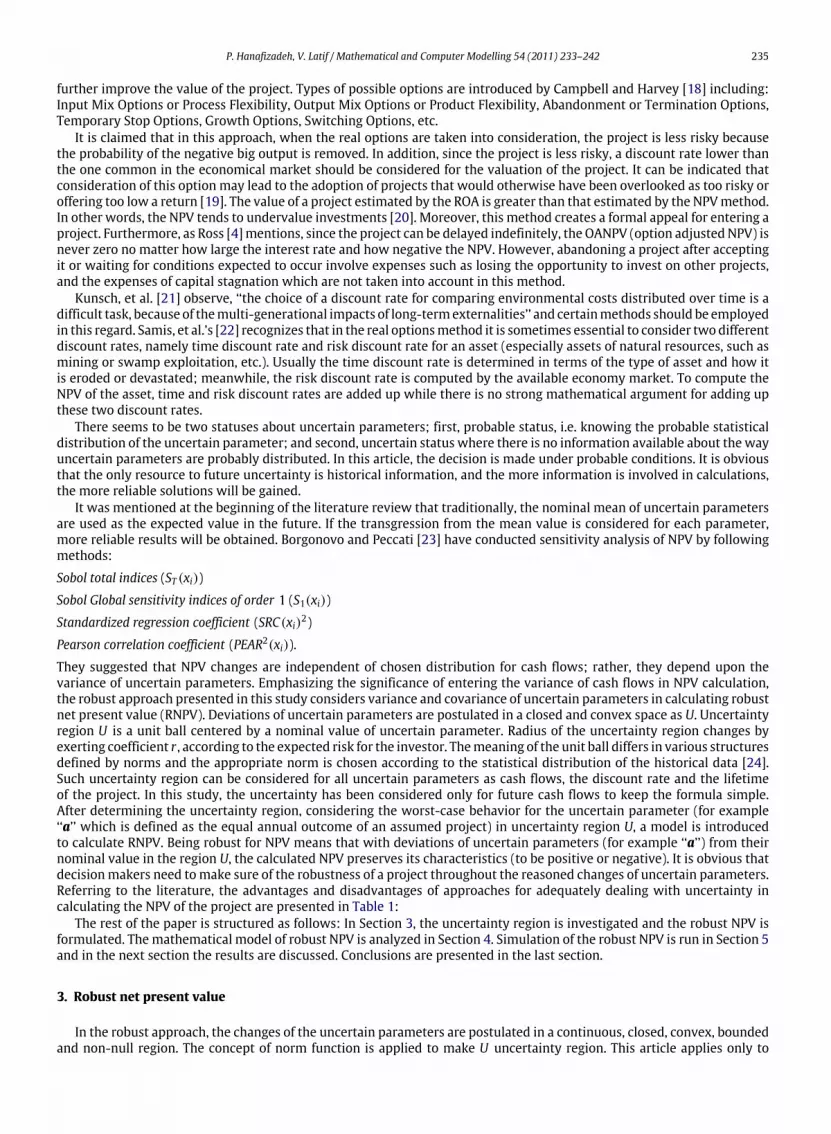
Fig. 1. Various norm bodies in two-dimensional space and their comparison ([8]).

symmetric distributions whose contours can be approximated by a convex norm body. The following relationship exist forl1, l2 and l∞ norm bodies:

‖ν‖1 ≥ ‖ν‖2 ≥ ‖ν‖∞. (1)

For more information, see [28,29].Various norm bodies in two-dimensional spaces and their comparison are sketched out as follows in [8] (see Fig. 1):The Chebyshev norm (infinity norm body) is a rectangular cube associated with a joint uniform distribution with

independent random parameters. The Euclidean l2 norm body is a ball characterizing the level sets of a standard normaldistribution for independent random parameters.

The standard equation to calculate NPV is:

NPV = −c0 + aTx (2)

where,c0 is initial investment valuei is discount rate,n is period of the project exploitationaj: is net cash flow of the j-th year of the period of project exploitation which occurs at the end of j-th period.

xj =

1

1 + i

j

.

In this paper, small bold letters and capital letters are used to show vectors and matrices, respectively.It is assumed that the changes of uncertain parameter ‘‘a’’ occur in the closed, convex and continuous region U. U is

defined as:

U(q, r) = {a : a = µa + Wu | u ∈ Bq(r)} (3)


where, Eq. (3) µa is the mean value of parameter ‘‘a’’. Bq(r) is lq norm body which is built by the following definition:

Bq(r) = {u ∈ Rn| ‖u‖q ≤ r}. (4)

W is an n × n symmetric positive definite matrix.W is the matrix square root of covariance matrix of uncertain parameter‘‘a’’. It is calculated as:

W = C1/2, C1/2= V D1/2 V T . (5)

In Eq. (5) ‘‘C ’’ is the covariancematrix of uncertain parameter ‘‘a’’. (For more information about ‘‘C’’ refer to [30].) In practice,the uncertainty region defined in (3), describes the changes of stochastic parameter ‘‘a’’ from its mean value µa. Thesechanges are affected by the change slope ofW matrix and are defined as the disorders occurring in Bq(r).

Applying the worst case in (2) (here the worst case for a, means choosing the infimum of a vector which can occur inU(q, r)), we have:

RNPV = infa∈U(q,r)

(−c0 + aTx) = −c0 + infa∈U(q,r)

aTx. (6)

Using definition (3) we have:

RNPV = −c0 + µaTx + inf

‖u‖q≤r(Wu)Tx. (7)

For each arbitrary x, we have inf(x) = − sup(−x), therefore:

RNPV = −c0 + µTax − sup

‖−u‖q≤r(−uTWx). (8)

According to norm function properties in [24,29], the following relation exists:

‖ − u‖q = | − 1|‖u‖q = ‖u‖q (9)

relation (8) can be obtained as:

RNPV = −c0 + µTax − sup

‖u‖q≤r(uTWx). (10)

Based on the definition of the dual norm [29], the dual of the lq norm is the lp norm where q satisfies 1/p + 1/q = 1, so it isconcluded that:

RNPV = −c0 + µTax − r‖W Tx‖p; 1/p + 1/q = 1. (11)

A robust model is proposed in (11) which obtains robust amounts of NPV by selecting various norm bodies and radiuses forthe U uncertainty region. Considering the definition of NPV in (2), robust formulation can be summarized as follows:

RNPV(q, r) = NPV0− r‖W Tx‖p; 1/p + 1/q = 1 (12)

(12) is final definition of RNPV.

4. Robust net present value analysis

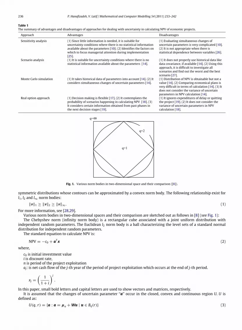
Based onwhat is defined in (12), r‖W T x‖p is subtracted fromNPV0 to calculate the robust NPV. The amplitude of r‖W T x‖pis dependent on the form and chosen radius of the uncertainty region as well as the size of the W matrix. r (the radius ofthe uncertainty region) is a positive real number. ‖W T x‖p is always a non-negative real number based on norm functionproperties. Hence the robust NPV formulation always obtains an NPV which is smaller than NPV0. To better understand thisconcept, see Fig. 2.1

In this figure, the quality of NPV and RNPV variations in relation to i, is monitored. By increasing the discount rate on thehorizontal axis, x decreases according to xj = (1/(1 + i))j. Decrease in x results in a reduction in the difference betweenNPV and RNPV, and at i = ∞where the elements of x approach zero; this difference is getting close to zero, and both curvesapproach c0 (initial investment that is $100 million in this example). In other words, −c0 is the asymptote of 2 curves. The

1 In this article, data of an assumed project is used for numerical examples and sketching graphs.

c0 = 100 million $ n = 4

W =

3.90 −1.75 −3.60 −2.67−1.75 8.22 3.15 −1.74−3.60 3.15 8.88 4.32−2.67 −1.74 4.32 5.81

µa =

17.233.8260.284.2

.


Fig. 2. Comparison of RNPV and NPV0 for U(2,3).

rate of return (ROR) is attained fromNPV = 0,which, according to the figure, is 25.3%,whereas robust rate of return (RROR) is14%. Now, if theminimum attractive rate of return (MARR) is less than 14% for an investor, considering both approaches, theproject is attractive to invest on. If the investor’s MARR is more than 25.3%, then considering both approaches the project isuneconomical; but if the investor’s MARR is between 14% and 25.35%, then being attractive or not, depends on the investor’sown characteristics, i.e. how risk-taking or risk-aversive they are. Selecting an appropriate approach is discussed in detail inthe simulating section. Another impressive element in the difference between NPV and RNPV is selecting the q normwhoseeffects are summarized in the following observations:Observation 1: choosing a greater q in RNPV(q, r) = NPV0

− r‖W T x‖p leads to a greater uncertainty region. Based on dualnorm definition, greater q results in a smaller p and according to (1), the smaller p, the greater lp norm. In other words, itmakes a greater uncertainty region: U(∞, r) > U(2, r) > U(1, r).

Proposition 1. A greater uncertainty region obtains a smaller RNPV:

RNPV(1, r) ≥ RNPV(2, r) ≥ RNPV(∞, r). (13)

Proof. From (1) we have:

‖W Tx‖1 ≥ ‖W Tx‖2 ≥ ‖W Tx‖∞. (14)

If both sides of the above relation are multiplied by −r which is a negative real number, we will have:

− r‖W Tx‖1 ≤ −r‖W Tx‖2 ≤ −r‖W Tx‖∞ (15)

adding NPV0 to both sides of the above equation

NPV0− r‖W Tx‖1 ≤ NPV0

− r‖W Tx‖2 ≤ NPV0− r‖W Tx‖∞. (16)

According to robust relation definition (13), it follows that:

RNPV(∞, r) ≤ RNPV(2, r) ≤ RNPV(1, r). � (17)

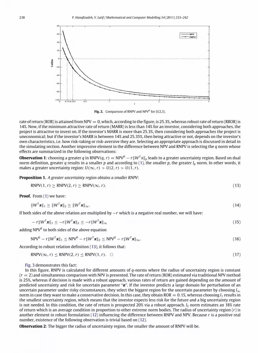
Fig. 3 demonstrates this fact:In this figure, RNPV is calculated for different amounts of q-norms where the radius of uncertainty region is constant

(r = 2) and simultaneous comparisonwith NPV is presented. The rate of return (ROR) estimated via traditional NPVmethodis 25%, whereas if decision is made with a robust approach, various rates of return are gained depending on the amount ofpredicted uncertainty and risk for uncertain parameter ‘‘a’’. If the investor predicts a large domain for perturbation of anuncertain parameter under risky circumstances, they select the biggest region for the uncertain parameter by choosing l∞norm in case they want tomake a conservative decision. In this case, they obtain ROR = 0.15, whereas choosing l1 results inthe smallest uncertainty region, which means that the investor expects less risk for the future and a big uncertainty regionis not needed. In this condition, the rate of return is prospected 20% via a robust approach. l2 norm estimates an 18% rateof return which is an average condition in proportion to other extreme norm bodies. The radius of uncertainty region (r) isanother element in robust formulation (12) influencing the difference between RNPV and NPV. Because r is a positive realnumber, existence of the following observation is trivial based on (12).Observation 2: The bigger the radius of uncertainty region, the smaller the amount of RNPV will be.


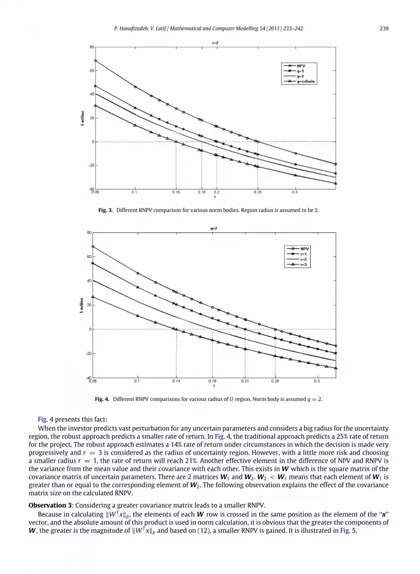
Fig. 3. Different RNPV comparison for various norm bodies. Region radius is assumed to be 2.

Fig. 4. Different RNPV comparisons for various radius of U region. Norm body is assumed q = 2.

Fig. 4 presents this fact:When the investor predicts vast perturbation for any uncertain parameters and considers a big radius for the uncertainty

region, the robust approach predicts a smaller rate of return. In Fig. 4, the traditional approach predicts a 25% rate of returnfor the project. The robust approach estimates a 14% rate of return under circumstances in which the decision is made veryprogressively and r = 3 is considered as the radius of uncertainty region. However, with a little more risk and choosinga smaller radius r = 1, the rate of return will reach 21%. Another effective element in the difference of NPV and RNPV isthe variance from the mean value and their covariance with each other. This exists in W which is the square matrix of thecovariance matrix of uncertain parameters. There are 2 matrices W1 and W2. W2 < W1 means that each element of W1 isgreater than or equal to the corresponding element of W2. The following observation explains the effect of the covariancematrix size on the calculated RNPV.

Observation 3: Considering a greater covariance matrix leads to a smaller RNPV.Because in calculating ‖W T x‖p, the elements of each W row is crossed in the same position as the element of the ‘‘x’’

vector, and the absolute amount of this product is used in norm calculation, it is obvious that the greater the components ofW , the greater is the magnitude of ‖W T x‖p and based on (12), a smaller RNPV is gained. It is illustrated in Fig. 5.


Fig. 5. Different RNPV comparisons for variousW sizes considering U(2, 2) in (12).

Table 2Comparison of traditional and robust approach results, MARR ≤ RROR.

ROR interval occurred in the scenario Percentage of simulatedscenarios in this interval (%)

Results of the traditionalapproach

Results of therobustapproach

0 < ROR < MARR 0.06 Failure FailureMARR ≤ ROR 99.94 Success Success

Fig. 6. Interpretation of failure and success percentages for traditional and robust approach while the investor’s MARR is less than RROR.

Since higher variance and covariance of parameters lead to higher risk in decision conditions, it gives a less robustROR. Among the effective components on RNPV mentioned above, selecting a radius and norm for the uncertain region isdependent on the investor’s characteristics, their expected risk, and further historical data. However, the size of covariancematrix is just under the influence of existing historical data of uncertain parameters rather than the investor’s characteristics.

5. Simulation of the robust net present value

Many people find the percentages of ROR easier to understand than NPV [31], especially, when investors use bank-loanswith fixed interest rates. So ROR and RROR are calculated (simply from NPV = 0 and RNPV = 0) in this study to compareprojects. Nominal and robust NPV relations are programmed by C++ and it has run for 10,000 stochastic scenarios of ai foran assumed project. The rate of return for the 10,000 scenarios is calculated and the results are proposed as follows. Therate of return for the traditional approach is calculated as 25.31%. The robust approach gives this rate as 14.23% consideringr = 2 and q = 2. Suppose that an investor wants to decide about selecting traditional or robust approach for a suggestedproject. The investor’s criterion for decision making is the minimum attractive rate of return (MARR). Three situations mayoccur:

A: If the investor’sMARR ismore than 25.31%; because both approaches calculate the project’sMARR less than or equal to25.31%, they will suggest the investor not to accept the project. So there is no discussion on choosing the suitable approach.

B: If the investor’s MARR is less than or equal to RROR; then both approaches encourage the investor to accept the projectand failure of approaches occur when the scenario obtained ROR is less than investor’s MARR. For example, if MARR = 13%,the prediction failure means that the project had been predicted as profitable but practically, the project’s ROR is less thanthe investor’s MARR. The summary of this situation is presented in Table 2 and Fig. 6.

C: If the investor’s MARR is between ROR0 and RROR (e.g. 22%), then the traditional approach which obtains 25.31%,renders the project attractive. The robust approach forecasts 14.23% for ROR and suggests avoiding entering the project.What occurred in simulation is that 1564 cases of 10,000 scenario encountered an ROR less than 22% (so the project does


Fig. 7. Interpretation of failure percentages for traditional approach while the investor’s MARR is between NPV0 and RNPV.

not seem economical for investors and in fact the traditional approach has encountered failure in 15.64% of times) whereas,the robust approach does not face any failures.

As shown in Fig. 7, the more investor’s MARR is close to the traditional ROR and far from RROR, the more the traditionalapproach faces failure in the case that when MARR < 25.31% – the worst case – 4965 scenarios out of 10,000 confrontedfailure, which means about 50% !

6. Discussion

In the example studied, simulation is conducted producing 10,000 stochastic scenarios of nominal cash flows with anarbitrary mean value and covariance matrix. The traditional approach uses a mean value of parameters to calculate NPV.Therefore, there is a high chance of occurring in equal numbers at both sides of ROR0. Now, the normal distribution ofscenarios is assumed to have skewness. For instance, in a situation where the investor’s MARR is placed between ROR0 andRROR –with a pessimistic approach – the number of scenarios, whose ROR is less than themean value aremore than 50%. Inother words, the percentage of failure for the traditional approach increases, and the percentage of good projects which therobust approachmaymiss, decreases. Conversely, with an optimistic approach inwhich the normal distribution of scenarioshas a negative skewness, more than 50% of scenarios occur with an ROR higher than the mean value. The failure percentageof the traditional approach decreases and the robust approach remains with no failure in forecasting. Hence, choosing anappropriate approach depends on the investor’s information about the probability of occurrence of each scenario in additionto being pessimistic or optimistic about future scenarios.

7. Conclusion

When the cash flows of the period of project exploitation are random and dependent, calculating NPV is an importantpractical problem. In this study, the robust approach was presented for dealing with random and dependent net income ofa cash flow. The robust approach has high reliability because it considers the information about variance and correlation ofhistorical data in calculating NPV. In this approach, the changes of the uncertain parameters are postulated in a closed andconvex region called the uncertainty region. The size and shape of the uncertainty region is selected based on the historicaldata and risk-taking or risk-aversion characteristics of the investor [24]. A mathematical relation for calculating NPV wasacquired from the robust approach and the quality of the solutions was evaluated using simulation in a C++ programmingenvironment. The analysis of robust relation was done through numerical examples. These examples show that the robustapproach always results in a lower NPV than the traditional approach. The more risky circumstances the investor predictsfor the future and the more conservatively they may decide, the bigger the uncertainty region they would consider forthe changes of uncertain parameters. A smaller robust NPV is acquired as the uncertainty region gets bigger and bigger. Acomparison was presented using the robust approach versus the traditional approach for calculating NPV. This comparisonwas done with the help of 10,000 stochastic normal scenarios. As a result of this simulation, when the traditional approachfails by 15.64% probability, the robust approach does not face any failures. If stochastic distribution of scenarios has a positiveskewness (while pessimistic scenarios are more probable), the percentage of failure of the traditional approach increasesand in the worst conditions; it reaches 50% yet the robust approach remains with no failure.

References

[1] R. Stone, Management of Engineering Projects, Macmillan Education, London, 1988.[2] E. Jonathan Jr., Ingersoll, Theory of Financial Decision Making, Yale University press, New Haven, 1987.[3] M.J. Sobel, J.G. Szmerekovsky, V. Tilson, Scheduling projects with stochastic activity duration to maximize expected net present value, European

Journal of Operational Research 198 (2009) 697–705.[4] S.A. Ross, Uses, abuses, and alternatives to the net-present-value rule, Financial Management 24 (3) (1995) 96–102.[5] E. Berkovitch, R. Israel, Why the NPV criterion does not maximize NPV, The Review of Financial Studies 17 (1) (2004) 239–255.[6] C.A. Magni, Investment decisions in the theory of finance: some antinomies and inconsistencies, European Journal of Operational Research 137 (2002)

206–217.[7] B.D. Reyck, On investment decision in the theory of finance: some antinomies and inconsistencies, European Journal of Operational Research 161

(2005) 499–504.[8] P. Hanafizadeh, A. Seifi, A unified model for robust optimization of linear programs with uncertain parameters, Transactions on Operational Research

16 (2004) 20–45.[9] P. Jovanovic, Application of sensitivity analysis in investment project evaluation under uncertainty and risk, International Journal of Project

Management 17 (1999) 217–222.[10] J.H. Willem, V. Groenendaal, Estimating NPV variability for deterministic models, European Journal of Operational Research 107 (1998) 202–213.


[11] C. Xu, G.Z. Gertner, Uncertainty and sensitivity analysis for models with correlated parameters, Computational Statistics and Data Analysis 51 (2007)5579–5590.

[12] P. Hanafizadeh, A. Kazazi, A. Jalili Bolhasani, Portfolio design for investment companies through scenario planning, Management Decision 49 (4)(2011).

[13] D. Bertsimas, D. Pachamanova, M. Sim, Robust linear optimization under general norms, Opeations Research Letters 32 (2004) 510–516.[14] E.R. Coates, M.E. Kuhl, Using simulation software to solve engineering economy problems, Computers and Industrial Engineering 45 (2003) 285–294.[15] A.K. Dixit, R.S. Pindyck, Investment Under Uncertainty, Princeton University Press, Princeton, 1994.[16] T.T. Lin, Applying the maximum NPV rule with discounted/growth factors to a flexible production scale model, European Journal of Operational

Research 196 (2009) 628–634.[17] B.D. Reyck, Z. Degraeve, R. Vandenborre, Project options valuation with net present value and decision tree analysis, European Journal of Operational

Research 184 (2008) 341–355.[18] R. Campbell, F. Harvey, School of Business, Duke university, NC, National Bureau of economic research, Cambridge, MA, December, 1999.[19] A. Keswani, M.B. Shackleton, How real option disinvestment flexibility augments project NPV, European Journal of Operational Research 168 (2006)

240–252.[20] R.G. Dimitrakopoulos, A. Sabry, A. Sabour, Evaluating mine plans under uncertainty: can the real options make a difference?, Resources Policy 32

(2007) 116–125.[21] P.L. Kunsch, A. Ruttiens, A. Chevalier, A methodology using option pricing to determine a suitable discount rate in environmental management,

European Journal of Operational Research 185 (2008) 1674–1679.[22] M. Samis, G. Davis, D. Laughton, R. Poulin, Valuing uncertain asset cash flows when there are no options: a real option approach, Resources Policy 30

(2006) 285–298.[23] E. Borgonovo, L. Peccati, Uncertainty and global sensitivity analysis in the evaluation of investment projects, International Journal of Production

Economics 104 (2006) 62–73.[24] P. Hanafizadeh, A. Seifi, Tuning the unified robust model of uncertain linear programs, IUST International Journal of Engineering Science 17 (2006)

49–54.[25] E. Borgonovo, L. Peccati, Sensitivity analysis in investment project evaluation, International Journal of Production Economics 90 (2004) 17–25.[26] T.G. Eschenbach, R.J. Gimple, Stochastic sensitivity analysis, The Engineering Economist 35 (4) (1990) 305–321.[27] C.S. Park, Contemporary Engineering Economics, 2nd ed., Addison-Wesly, Menlo Park, CA, 1997.[28] N. Bourbaki, Topological vector spaces, in: Elements of Mathematics, Springer, New York, 1987, Chapters 1–5.[29] S. Boyd, L. Vandenberghe, Convex Optimization, Cambridge University Press, Cambridge, 2004.[30] P. Hanafizadeh, A. Seifi, k. Ponnambalam, Primal and dual robust counterparts of uncertain linear programs: an application to portfolio selection,

Journal of Industrial Engineering International 2 (1) (2006) 38–52.[31] A. Damodaran, Investment Valuation: Tools and Techniques for Determining the Value of Any Asset, 2nd ed., John Wiley and Sons, Hoboken, 2002.

Documents

Robust net present value