Embed Size (px)
Citation preview

1
Right Sizing Safety Stock and Effectively Managing Inventory using Forecastability
by
Ni Pan
Bachelor of Science, Mechanical Engineering, Worcester Polytechnic Institute, 2015
and
Jamie Sweeney Bachelor of Science, Industrial Engineering, Pennsylvania State University, 2015
SUBMITTED TO THE PROGRAM IN SUPPLY CHAIN MANAGEMENT
IN PARTIAL FULFILLMENT OF THE REQUIREMENTS FOR THE DEGREE OF
MASTER OF APPLIED SCIENCE IN SUPPLY CHAIN MANAGEMENT AT THE
MASSACHUSETTS INSTITUTE OF TECHNOLOGY
May 2020
© 2020 Ni Pan and Jamie Sweeney. All rights reserved. The authors hereby grant to MIT permission to reproduce and to distribute publicly paper and electronic
copies of this capstone document in whole or in part in any medium now known or hereafter created.
Signature of Author: ____________________________________________________________________ Department of Supply Chain Management
May 8, 2020
Signature of Author: ____________________________________________________________________ Department of Supply Chain Management
May 8, 2020
Certified by: __________________________________________________________________________ Tim Russell
Research Engineer, MIT Humanitarian Supply Chain Lab Capstone Advisor
Accepted by: __________________________________________________________________________ Prof. Yossi Sheffi
Director, Center for Transportation and Logistics Elisha Gray II Professor of Engineering Systems Professor, Civil and Environmental Engineering

2
Right Sizing Safety Stock and Effectively Managing Inventory using Forecastability
by
Ni Pan
and
Jamie Sweeney
Submitted to the Program in Supply Chain Management on May 2020 in Partial Fulfillment of the
Requirements for the Degree of Master of Applied Science in Supply Chain Management
ABSTRACT
In a commodity consumer product business, such as bottled water, the customer has the power. Therefore, the business incurs whatever cost necessary to meet demand. To reduce the cost of fulfilling demand and of stockout, businesses must thoughtfully set inventory safety stock levels to compensate for potential spikes in demand. The purpose of this capstone is to analyze the current inventory strategy and its effectiveness of the sponsor, a bottled water company. The team worked to explore the drivers of supply and demand variability to identify potential improvements in inventory management, which could reduce cost while maintaining service levels. The team analyzed the customer demand, production demand, strategic forecast, and inventory on hand for over 100 stock keeping units (SKUs) in a specific geographic region over the last three years. As a result of the analysis, the team proposes SKU segmentation by forecastability and appropriate safety stock calculation using the standard deviation of forecast errors. This method of calculating safety stock, as compared to the sponsor’s current approach, reveals a clear opportunity to reduce the inventory by 28% for SKUs with predictable and positive demand. Another key finding is the opportunity to reduce the order quantities when the annual forecasted demand of a SKU is below an identified threshold. Lastly, the team recommends increasing the inventory level kept at supplier consignment to further minimize the risk of stockout at low cost due to consignment agreements. To further and continuously improve inventory position and service levels, the team recommends a quarterly strategic inventory review to adapt strategy as business needs and requirements shift.
Capstone Advisor: Tim Russell Title: Research Engineer, MIT Humanitarian Supply Chain Lab

3
ACKNOWLEDGMENTS
We would like to thank our Capstone advisor, Tim Russell, for his time and endless support during the completion of this research. Thank you for always encouraging us to pause, recognize our progress, and celebrate the ‘small wins’.
We also would like to thank our writing instructor, Pamela Siska, for providing meaningful advice to help us perfect this capstone report.
Special thanks to Mathew Weber, Raymond Heath, Kishore Adiraju, Bruce Kaabipour, Hongfei He, Jesus Valentin and the entire Niagara team for your key insights, support and constant efforts to help us collect, clean and make sense of the data.
Ni Pan would like to thank her family back in China for the tremendous support throughout this MIT journey. She would also like to thank all the SCM faculty and staff members for their hard work on providing a seamless program experience especially during such a challenging time. Lastly, she is grateful for meeting every amazing classmate in the cohort. This lifelong friendship will be the most precious treasure for her.
Jamie Sweeney would like to thank her parents for instilling the value of education and for giving her every opportunity to be independent, successful, and happy. She would also like to thank her siblings for always being there to support her, no matter what. Lastly, she would like to thank every member of the SCM family for their friendship and encouragement (especially Ni (Penny) for being an incredible collaborator on this project).

4
Table of Contents
1 List of Figures ........................................................................................................................................ 6
2 List of Tables ......................................................................................................................................... 7
3 Introduction .......................................................................................................................................... 8
3.1 Problem Motivation ...................................................................................................................... 8
3.1.1 Demand Seasonality and Volatility ....................................................................................... 8
3.1.2 Short Customer Lead Times .................................................................................................. 9
3.1.3 One Rule-of-Thumb Inventory Ordering Strategy for all Stock Keeping Units (SKUs) .......... 9
3.1.4 Current Challenges .............................................................................................................. 10
3.2 Problem Statement ..................................................................................................................... 11
4 Literature Review ................................................................................................................................ 13
4.1 Vendor Consignment Inventory .................................................................................................. 14
4.2 Safety Stock ................................................................................................................................. 15
4.2.1 Seasonal Demand ................................................................................................................ 15
4.2.2 Forecast Bias ....................................................................................................................... 17
4.3 Raw Material Ordering Policy ..................................................................................................... 18
4.4 Demand Classification ................................................................................................................. 20
5 Data and Methodology ....................................................................................................................... 23
5.1 Analysis Scope ............................................................................................................................. 23
5.2 Current Raw Material Inventory Strategy ................................................................................... 24
5.3 SKU Classification Using Customer Demand ............................................................................... 26
5.4 SKU Forecast Bias ........................................................................................................................ 28
5.5 Inventory on Hand Analysis ........................................................................................................ 29
5.6 Safety Stock Calculation .............................................................................................................. 31
5.6.1 Standard Deviation Using Customer Demand for Traditional Strategy .............................. 32
5.6.2 Standard Deviation Using Forecast Errors for Forecast Error Strategy .............................. 32
5.6.3 Demand Simulation ............................................................................................................. 33
5.7 Minimum Order Quantity (MOQ) vs. Full Pallet Analysis ........................................................... 35
6 Results and Analysis ............................................................................................................................ 36
6.1 Safety Stock Simulation Results .................................................................................................. 36
6.1.1 Traditional vs. Forecast Error Safety Stock Strategy ........................................................... 36
6.2 Recommended Inventory Level Comparison .............................................................................. 39

5
6.2.1 Opportunity in Inventory Level Reduction for Smooth SKUs .............................................. 39
6.2.2 Opportunity in Ordering Minimum Order Quantity ........................................................... 42
6.2.3 Summary ............................................................................................................................. 43
6.3 Limitations................................................................................................................................... 44
7 Conclusion ........................................................................................................................................... 45
7.1 Recommended Safety Stock Strategy ......................................................................................... 45
7.2 Safety Stock Strategy Implementation ....................................................................................... 46
7.3 Insights for General Management .............................................................................................. 47
7.4 Future Research Recommendations ........................................................................................... 49
References .................................................................................................................................................. 50
6
1 List of Figures
Figure 1: Standard Purchasing Guidelines (J. Valentin, personal communication, Oct.22, 2019) ................ 9 Figure 2: Inventory Network ....................................................................................................................... 11 Figure 3: Forecast-based Classification Categories (Engelmeyer, 2016) .................................................... 22 Figure 4: SKU Distribution per Classification Approach .............................................................................. 26 Figure 5: SKU Segmentation Comparison: ABC vs. Forecastability ............................................................. 27 Figure 6: NE SKU Forecast Bias Histogram .................................................................................................. 28 Figure 7: Forecast Error % vs. Forecast Bias ............................................................................................... 29 Figure 8: Segment A Smooth Forecastability SKU ...................................................................................... 30 Figure 9: Safety Stock Approach for Segment A Smooth Forecastability SKU ............................................ 37 Figure 10: Potential IOH Pallet Savings ....................................................................................................... 40 Figure 11: IOH Potential Pallet Savings per SKU ......................................................................................... 41 Figure 12: SKU with Low Demand Volume MOQ Example ......................................................................... 42 Figure 13: MOQ Breakeven Model ............................................................................................................. 43

7
2 List of Tables
Table 1: Common Inventory Ordering Policies Summarized ...................................................................... 19 Table 2: Cycle Service Level ........................................................................................................................ 31 Table 3: Lead Time ...................................................................................................................................... 31 Table 4: Example SKU Using Customer Demand ........................................................................................ 32 Table 5: Example SKU’s Forecast Error ....................................................................................................... 32 Table 6: Example SKU Using Forecast Error ................................................................................................ 33 Table 7: Demand Simulation Parameters ................................................................................................... 33 Table 8: Demand Simulation Example ........................................................................................................ 34 Table 9: Service Level Results from Simulation per Forecastability Category ............................................ 36 Table 10: Potential Cost Reduction using Forecast Error Safety Stock Approach ...................................... 41 Table 11: Operationalized Strategy Template ............................................................................................ 46

8
3 Introduction
The bottled water market has shown continuous strong demand growth year after year. Our
sponsor Niagara Bottling LLC (Niagara), the largest bottled water manufacturer in the United States, has
significantly grown its sales year over year for the past 5 years and foresees a similar growth rate
continuing in the next few years. Niagara has grown its footprint in the United States and improved
production efficiency through investment in automation technology. While Niagara is optimizing its
production as much as possible, the availability of raw materials is crucial for the sponsor to operate in
an environment where the customers’ demand must always be met. For Niagara, raw materials are
categorized as flexibles (labels and stretch film), corrugate, resin (used for plastic injection molding of
bottles), and caps.
3.1 Problem Motivation
Niagara schedules its production with the assumption of 100% raw material availability, and it is
experiencing challenges in ensuring raw material availability.
3.1.1 Demand Seasonality and Volatility
Niagara faces a seasonal distribution of demand for bottled water. Typically, sales double in the
summer (Chua and Heyward, 2017), especially around the holidays, and dip significantly in the winter.
Demand is also very volatile due to customer-driven promotions throughout the year. Niagara follows a
traditional strategy to meet over-capacity peak demand, prebuilding inventory during the low season
and storing finished goods in a third-party warehouse (3PL). In addition, Niagara is adding new
production lines within existing plants to expand capacity and meet growing demand.
9
3.1.2 Short Customer Lead Times
Similar to most consumer-packaged goods (CPG) companies, Niagara is facing pressure from its
customers to shorten its lead times. Niagara’s typical customer lead time is 5-10 days; however, Niagara
also accommodates customer orders with lead times as short as 24 hours. From conversations with the
Niagara production planning team, the probability of production schedule changes 3 to 7 days out is as
high as 40% (I. Liang, personal communication, Oct. 15, 2019). This variability imposes great challenges
for Niagara to meet customer orders because of the large gap between raw material lead time (30 days)
and potential customer lead time (24 hours).
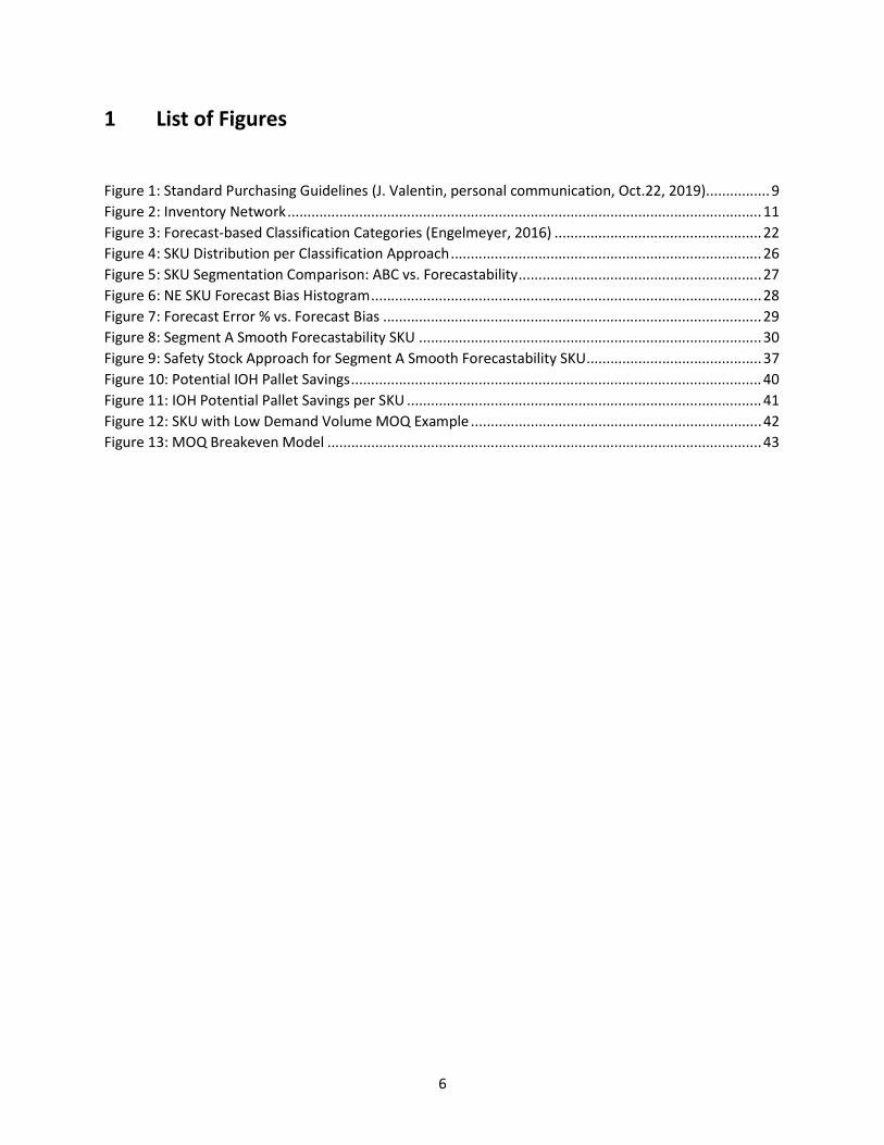
3.1.3 One Rule-of-Thumb Inventory Ordering Strategy for all Stock Keeping Units (SKUs)
Niagara’s strategic buying group relies on legacy day-on-hand (DOH) numbers to set its
inventory target at their suppliers. Currently, a 90-DOH inventory target is applied to all stock keeping
units (SKUs). When DOH for each SKU dips to 60 days, the buyer places an order for an additional 60
days of supply to bring DOH level back to 90 days, as illustrated in Figure 1.
Figure 1: Standard Purchasing Guidelines (J. Valentin, personal communication, Oct.22, 2019)
This one-size-fits-all strategy for ordering raw materials is not optimal as each SKU has different
demand volume and distribution. Optimizing inventory ordering policy after SKUs are classified and
10
grouped has the potential to minimize inventory holding cost, reduce costs of expediting materials, and
maintain high customer service levels.
3.1.4 Current Challenges
Niagara has vertically integrated its supply chain and manufactures its own plastic bottles. This
allows Niagara to be more agile under volatile demand. However, our sponsor is continuously facing
challenges in raw material availability specifically in one category: Flexibles. The Flexibles category
consists of shrink film and labels, which are purchased under bill-and-hold arrangements with suppliers.
Flexibles stay at a supplier consignment facility until Niagara releases the material to a plant.
The complexity of the Flexibles category is high and is driven by bottle/pack size, product type,
marketing promotions, and traceability legal requirements in certain geographic areas. Moreover, the
long lead time of these raw materials (30 days) creates challenges when not available at the supplier
consignment facility. When Flexibles are not available at supplier consignment facility, the tactical
material buying group at Niagara has to seek the following costly solutions:
Finding Flexibles substitutions at plant
Expedite Flexibles from suppliers
Transshipment in network
Dynamic sourcing (move production to another plant)
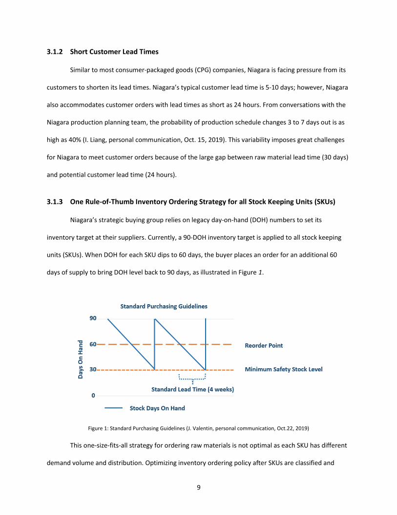
To buffer against demand volatility and shorter customer lead time, Niagara utilizes safety stock
to cover demand uncertainty. Niagara holds safety stock in two physical forms: raw materials and
finished goods. Safety stocks are held at multiple locations in the Niagara network. Finished good safety
stocks are stored at Niagara plants and at third party warehouses (3PL). Raw material safety stocks are
held at the raw material suppliers, as consignment inventory, and at Niagara plants as shown in Figure 2.

11
Figure 2: Inventory Network
Currently, Niagara determines safety stock levels with various measures. Customer demand
variability is used in calculating required finished goods safety stock to be held at the plant, this
approach is already deployed and used within Niagara network. However, raw material safety stock
levels at plant and supplier consignment are driven by generic inventory DOH rules without clear SKU
classifications. Niagara has been working on utilizing production plan variability to calculate required
raw material safety stock needed at the plant, but this approach has not been fully validated and
deployed.
3.2 Problem Statement
Niagara sees the need to improve its inventory positions to achieve lower cost without
damaging customer service levels. Specifically, the team is interested in applying a data-driven approach
to set safety stock inventory targets to optimize raw materials at supplier consignment locations and at
Niagara plants.
The team believes the statistical approach of calculating inventory position by SKU classification
could benefit Niagara’s supply chain by eliminating additional effort spent on ensuring raw material
availability. This approach will demonstrate the benefits of applying a data-driven approach to inventory

12
decisions which could be leveraged across industries to companies facing similar inventory optimization
problems.

13
4 Literature Review
Regardless of the product, market, or industry, supply chain costs often represent a significant
portion of the price of a good or service. Businesses, therefore, dedicate significant time and energy to
evaluating their own supply chains to become more efficient and ultimately improve profitability.
The fundamental question firms struggle to answer is how much and when to order raw
materials in order to achieve the highest level of service at the lowest cost. The underlying drivers of
inventory levels, demand, and supply variability, are common to all supply chains, making inventory
optimization applicable to every industry (Willems, 2011).
The team reviewed information from two theses completed with Niagara: one is by V. Chandra
and M. Tully (2016), which provides lead time and legacy inventory DOH targets that are still being used
at Niagara today; the other is by I. Chua and T. Heyward (2017), which provides the economic
production quantity (EPQ) model that is widely adopted at Niagara today. Both provided key insights to
Niagara’s past supply chain challenges and contributed to the potential approaches considered by the
team along with the other high level concepts outlined within this Literature Review.
Topics on vendor consignment inventory, safety stock calculations, raw material ordering
policies are explained and explored further in this section as applicable to the key research question of
this capstone: how a consumer-packaged goods company, Niagara LLC, can optimize its inventory
position to better buffer against demand volatility and shortened customer lead times, at low cost,
without damaging customer service levels.
14
4.1 Vendor Consignment Inventory
Finding the correct inventory management policy to balance demanded high service level at low
cost is often made easier with increased transparency and collaboration between supplier and buyer.
Collaboration could range from straightforward information sharing, where a buyer will share the
forecasted demand with supplier to inform the supplier’s production planning, or a more formal
commitment or partnership, where a supplier holds and manages inventories until the buyer withdraws
them for use (Battini, 2010). This formal partnership is an example of a consignment inventory policy.
Consignment inventory can be implemented differently depending on the needs of the business.
Recent literature explores minimizing the joint total expected cost (JTEC) also known as the total supply
chain management cost, for both partners involved, supplier and buyer. Piplani and Viswanathan (2003)
prove lower JTEC through a cycle time reduction when inventory is kept at the buyer’s plant location
which virtually eliminates procurement lead time.
Considerable work over the past decade has used mathematical models with inputs to account
for factors such as demand variability, obsolescence cost, demand variation, and space limitations to
quantify the optimal ordering policy for a buyer to order raw materials (Braglia and Zavanella, 2003;
Valentini and Zavanella, 2003; Srinivas and Rao, 2004; Battini, Gunasekaran; Faccio, Persona and
Sgarbossa, 2010). These models have demonstrated the applicability and attractiveness of consignment
inventory policies in many different business environments and demand circumstances.
Niagara is not unique in struggling to balance competing priorities of high service levels and low
total inventory cost. The consignment inventory policy agreements developed with raw materials
suppliers allow Niagara more flexibility and absorbs demand fluctuation at lower overall cost due to a
reducing in inventory holding costs. Due to Niagara’s network for suppliers and plants, as well as space

15
constraints at plant locations, all consignment inventory is kept at the supplier’s location. While this
shortens raw material lead time from lead time of producing and shipping the material (30 days) to lead
time from supplier consignment warehouse to plant (seven days), the procurement lead time does not
completely disappear as noted in many of the above studies. Moreover, while this strategic inventory
approach has been proven effective, the effectiveness of consignment inventory is heavily impacted by
variation in demand and ordering policies, both of which will be described below.
4.2 Safety Stock
4.2.1 Seasonal Demand
Safety stock is the level of extra stock maintained by a company to prevent stockouts. It is
important to understand that the goal of having safety stock is to eliminate the majority of stockouts,
not intended to remove all stockouts. Although this is not an exhaustive list of all possible drivers that
can cause stockouts, typical influencing factors are customer demand variations, forecasting errors, and
variability in lead times for raw material or manufacturing (King, 2011). Theoretical safety stock
calculations can be in different forms, depending on which one of the following sources of variability is
the primary concern: demand, lead time, or a combination of both, as illustrated in equation (1) - (4)
(King, 2011). Equation (3) is used when both variability in demand and lead time are present,
independent and normally distributed. Otherwise, equation (4) is used.
SS = Z × (√LT × 𝜎 ) (1)
SS = Z × (𝐷 × 𝜎 ) (2)
SS = Z × (LT × 𝜎 ) + (𝐷 × 𝜎 ) (3)
𝑆𝑆 = Z × √LT × 𝜎 + Z × (𝐷 × 𝜎 ) (4)
16
Demand fluctuation and seasonality is a common problem faced by many consumer goods
companies. As most companies work diligently to improve their forecasting accuracy by using well-
prepared data sources, they are often challenged to predict the impact of demand seasonality patterns
on forecasts. The even more challenging task is how to strategically plan and place inventory physically
in the supply chain to accommodate seasonal demand.
Neale, Willems, and Beyl (2012) explore a forward-coverage planning approach to safety stock
policy. Common industry practice has been to set and adjust safety stock levels through analyzing at a
targeted number of periods of future demand. However, the study identified that companies may
experience “landslide effects” under seasonal demand, showing a significant drop in inventory and
service levels as they transition out of peak seasons (Neale, Willems, and Beyl, 2012). Safety stock levels
can drop prematurely prior to a low demand season, because low demand forecasts were used to set
safety stock levels during high seasons under the forward-coverage planning approach.
To prevent this “landslide effect” and ensure correct timing used in inventory planning, Neale,
Willems, and Beyl (2012) recommend a “backward-coverage” strategy when setting safety stock targets.
Instead of using the forecasts in the future replenishment lead time periods, safety stock targets should
be calculated using the preceding time periods (including the current period). Therefore, companies will
not experience significant drops in inventory when transitioning from a high season to low season,
avoiding increased stockouts and decreased customer service levels. This theory also applies when
companies transition from a low season to high season. Although the effect is less damaging to costs, it
can result in safety stock targets prematurely raising inventory levels while companies are still in the low
demand season. As a result, companies would unnecessarily inflate inventory levels, thus increasing
total inventory cost.
17
This study was of particular interest due to the extreme seasonality in Niagara’s demand as their
product demand doubles in the summer months. Moreover, current safety stock calculations at Niagara
use forward-looking forecasts. If supported by internal data, this research could be directly applicable to
Niagara’s safety stock calculation and prevent additional costs associated with raw material shortages. It
is important to recognize seasonality and trend in demand so that it can factor into inventory decisions
and inform ordering policy.
4.2.2 Forecast Bias
Traditionally, as described above, the variability input to the safety stock equation is variation in
historical demand, see Equations (1-4). This approach to calculating variability and, by extension, safety
stock is effective for stationary demand and scenarios where past demand is a better predictor of future
demand than the forecasted demand. However, to better capture deviation in demand caused by
seasonality and life cycles, Manary and Willems (2008) propose calculating the variation using the
difference between the forecasted demand and the real demand instead of variation in historical
demand. Manary and Willems (2008) propose that characterization of demand is the most significant
input to determine proper safety stock levels because the most appropriate safety stock equation can
be identified only once the demand characterization is understood.
The variation between forecast and demand can be calculated using the Equation (5) to
calculate the standard deviation of forecast errors (SDFE) for each SKU where Fi denotes the forecasted
demand for period i, Di denotes actual demand in period i and n is the number of period of data which
are being analyzed (Manary and Willems, 2008).
𝜎 =( )
(5)
18
Equation (6) is used to test for bias, that is to understand if there are any trends to historically
over or under forecast a specific SKU. The ratio can be calculated for each period I to compute the
relative forecast accuracy. A collection of 𝜃s across time centered around 0.5 for a specific SKU
demonstrated unbiased forecasting (Manary and Willems, 2008).
𝜃 =
(6)
Manary and Willems’ (2008) method of approximating variation while accounting for deviation
in demand due to seasonality was extremely valuable to this team due to the seasonal nature of
Niagara’s products. This model and these calculations were further explored to better identify the best
policy for Niagara’s specific demand pattern. Moreover, this research led the team to focus on first
characterizing demand for Niagara’s products.
4.3 Raw Material Ordering Policy
The fundamental purpose of an inventory replenishment system is to resolve the following
three inquiries: i) when should an order be placed? ii) how large should the order be? iii) how often
should the inventory status be reviewed? Inventory ordering policies work to minimize the total cost
equation, the sum of purchasing, ordering, holding, and shortage costs. Inherent to every purchasing
model is many assumptions, most significantly, assumptions on the form of demand for the good or
service. Under the conditions of deterministic demand, the above three questions become
straightforward and economic order quantity (EOQ) principles can easily be applied to determine
optimal order size (Silver, Pyke, and Thomas, 2017).
Under probabilistic demand, answering the above three questions becomes much more
complex. Silver, Pyke, and Thomas (2017) recommend managers ask themselves additional questions to

19
best establish the appropriate inventory policy (Silver, Pyke, and Thomas, 2017). First, how important is
the good or service? Second, does the inventory level of the product require constant attention, in other
words, should it be continuously reviewed? Third, what form should the inventory policy take? Fourth,
what are the specific cost and service goals set by the company?
The importance of the good or service can be determined by SKU segmentation or A, B, C
classification. Niagara implements a volume-based segmentation policy currently on all raw materials
and identifies A SKUs as those with highest volume consumption and therefore highest priority. Niagara
currently employs a continuous review policy. At Niagara, buyers monitor inventory levels of all SKUs
daily. A major advantage of continuous review ordering policy as compared to periodic review is that the
same level of customer service can be achieved with less safety stock and, therefore, lower carrying
costs (Silver, Pyke, and Thomas, 2017). However, continuous review policies are generally more
expensive in terms of inventory reviewing costs and errors. Due to the volatility of demand and variation
in forecast accuracy at Niagara, a continuous review policy is optimal to achieve the desired high service
levels.
To answer the question: what form inventory policy is optimal for a given scenario, Table 1
summarizes the four most common ordering strategies as well as the best applications of each.
Table 1: Common Inventory Ordering Policies Summarized
Inventory Policy
Review Period Description Advantages Disadvantages
Order-Point, Order Quantity (s, Q) system
Continuous
Fixed quantity Q ordered when inventory position drops to the reorder point, s, or below
Simple to understand; Errors unlikely to occur; Production requirements for supplier predictable
Ineffective for individual large transactions
Order-Point, Order-Up-to-Level (s,S) System
Continuous
When inventory levels reach the reorder point, s, an order must be placed to
Optimal (s,S) system has lower total relevant cost than the optimal (s,Q) system
Resources required to find optimal (s, S) pair;

20
achieve the order-up-to inventory level, S
Variable order quantity cause more frequent errors
Periodic-Review, Order-Up-to-Level (R,S) System
Periodic
Every R units of time enough is ordered to raise inventory position to level S
Does not require sophisticated computer control; Coordination of orders can provide significant savings
Replenishment quantities vary; Carrying costs higher than continuous review systems
(R,s,S) System Periodic
Every R units of time if inventory position is at or below re-order point, s, order enough to raise it to S
Optimal (R, s,S) system produces lower total relevant cost than any other system (under demand assumptions)
Requires significant resources to obtain best values of control parameters
Note. Data from Silver Pyke and Thomas (2017).
After review of various inventory ordering policies and best applications, the team believes the
Order-Point, Order-Up-to-Level (s, S) System provides inherent advantages when applied to Niagara’s
dynamic operating environment. This ordering policy has been proven optimal for dynamic inventory
models with fixed ordering costs and stochastic demand (Sethi and Cheng 1995). Moreover, raw
material SKU segmentation can be utilized to help Niagara define re-order points and order-up-to levels
appropriate to the specific SKUs to mitigate risk of stockout while minimizing cost.
4.4 Demand Classification
When determining safety stock, demand-side variation is one of the most influential
parameters. To set safety stock targets and reorder points, it is important to understand not only the
historical demand for products, but also the forecasted demand. However, widely accepted forecasting
truisms are that the forecast is always wrong and improving it dramatically could be a daunting task.
High forecast error can result in either excess inventory within the supply chain network or lost sales for
businesses. Understanding the forecastability of products can provide companies ways to efficiently
allocate efforts and manage inventory.
21
There are multiple ways for demand classifications to help one understand the forecastability of
products. ABC classification is the most widely used SKU classification approach in businesses (Babai,
Ladhari, and Lajili, 2015). Following the 80/20 Pareto principle, this classification method uses a single-
criteria, normally revenue (‘ABC’), price (‘HIL’) or demand volatility (‘XYZ’) (Gudehus, 2005). For ABC
classification, SKUs with cumulative revenue reaching specified thresholds will be grouped into
corresponding A, B and C categories.
K-means clustering is another technique that can be used for demand classifications. Different
from traditional ABC classification by specifying exogenous thresholds, k-means clustering uses machine
learning algorithms to group SKUs by minimizing the squared distance between the SKUs within a cluster
and the cluster centers (Hastie, Tibshirani, and Friedman, 2009) to determine the best number of SKU
clusters.
Instead of using a single-criteria, forecast-based classification uses two different dimensions, the
probability of positive demand and the variation of the positive demand to distinguish four demand
profiles: smooth, intermittent, erratic and lumpy (Boylan, Syntetos, and Karakostas, 2008). The two
criteria for forecast-based classification is illustrated in equation (7) and (8) (Engelmeyer, 2016).
Moreover, the relationship between the two equations and the four demand profiles is outlined in
Figure 3.
𝜋 =
(7)
𝐶𝑉 = ( ) (8)

22
Figure 3: Forecast-based Classification Categories (Engelmeyer, 2016)
Similar to other businesses, Niagara struggles to produce accurate forecasts. The current generic
forward-looking safety stock strategy, which is largely based on forecasted demand, may pose greater
challenges for Niagara to ensure raw material availability when product forecastability is poor. In
addition to traditional single-criteria SKU classification based on product demand, Niagara could benefit
from classification techniques such as k-means clustering and forecast-based classifications to cluster
SKUs with similar characteristics and manage SKUs based on their forecastability.

23
5 Data and Methodology
The team reviewed Niagara’s legacy inventory targets and safety stock calculations to
understand differences, sensitivities and drivers of safety stock inventory levels. Available data was
analyzed to identify optimal strategies to reduce inventory levels and save cost while achieving target
service levels.
5.1 Analysis Scope
Niagara manages inventory for five different types of raw materials: caps, labels, stretch film,
corrugate and resin. For this safety stock analysis, the scope only includes labels. Niagara identified this
material group as the most poorly managed with the most opportunity for improvement due to the
volume of SKUs and custom nature of the material.
Moreover, the analysis focused specifically on production in a specific region of the United
States. This specific region was chosen because there are additional regulatory requirements within the
region that increase the SKU complexity. For example, regulations require any bottle that is shipping
into a certain state to have a certification for that specific state listed on the label. Only a few Niagara
plants in this region are cleared to produce bottles with these certifications. Therefore, Niagara must
hold label SKUs for both state specific certified and non-state specific certified bottles in the region.
These requirements limit Niagara’s ability to shift raw material label resources among plants to support
spikes in demand or production schedule changes. Due to the decreased flexibility in this region, it is
even more critical for Niagara to properly manage inventory and set safety stock levels.
Throughout the project, the team dedicated a lot of time to cleaning and manipulating the data
to identify the most meaningful and accurate way to aggregate the label SKUs. Many of Niagara’s labels

24
have multiple versions due to necessary and frequent artwork changes and updates. Additionally, two
labels can be identical in every way except for the address listed as the production plant due to the
regulatory requirements discussed above. The team decided it was important to aggregate labels that
were interchangeable on the production floor, i.e. could be swapped out for each other during any given
production run. However, care was taken to ensure the aggregated SKU groups were plant specific.
5.2 Current Raw Material Inventory Strategy
Niagara’s current raw material inventory strategy can be broken into two policies: i) policy for
inventory at the supplier and ii) policy for inventory at the plant. As mentioned in the Introduction
(1.1.3), Niagara’s current ordering and safety stock policy is a one size fits all approach meaning the
same policy is applied to all SKUs. The raw material team responsible for inventory at the supplier works
to ensure there is 75- 90 days of supply at the supplier site. When the inventory level of a particular SKU
drops to 60 days of supply, the team places an order for an additional 60 days of supply to bring the
inventory level back to 90 days. This stock sits at the supplier in consignment inventory until Niagara
requests for it to be transferred to their plant locations. This ordering policy is driven by the three-week
lead time for label production at the supplier.
Niagara’s ordering policy for plant inventory is to ensure 14 days of forecasted production
demand for each SKU on hand as safety stock. This safety stock is reserved to cover demand variation
over the 1-week lead time from supplier to a specific plant location. In addition to this safety stock
inventory, Niagara orders to the next 14 days of forecasted and firmed production demand to be held at
the plant. Therefore, in total, Niagara aims to have 28 days of supply for each SKU at the plant. Again,
the plant raw material ordering policy is a one size fits all approach applied to all SKUs.
25
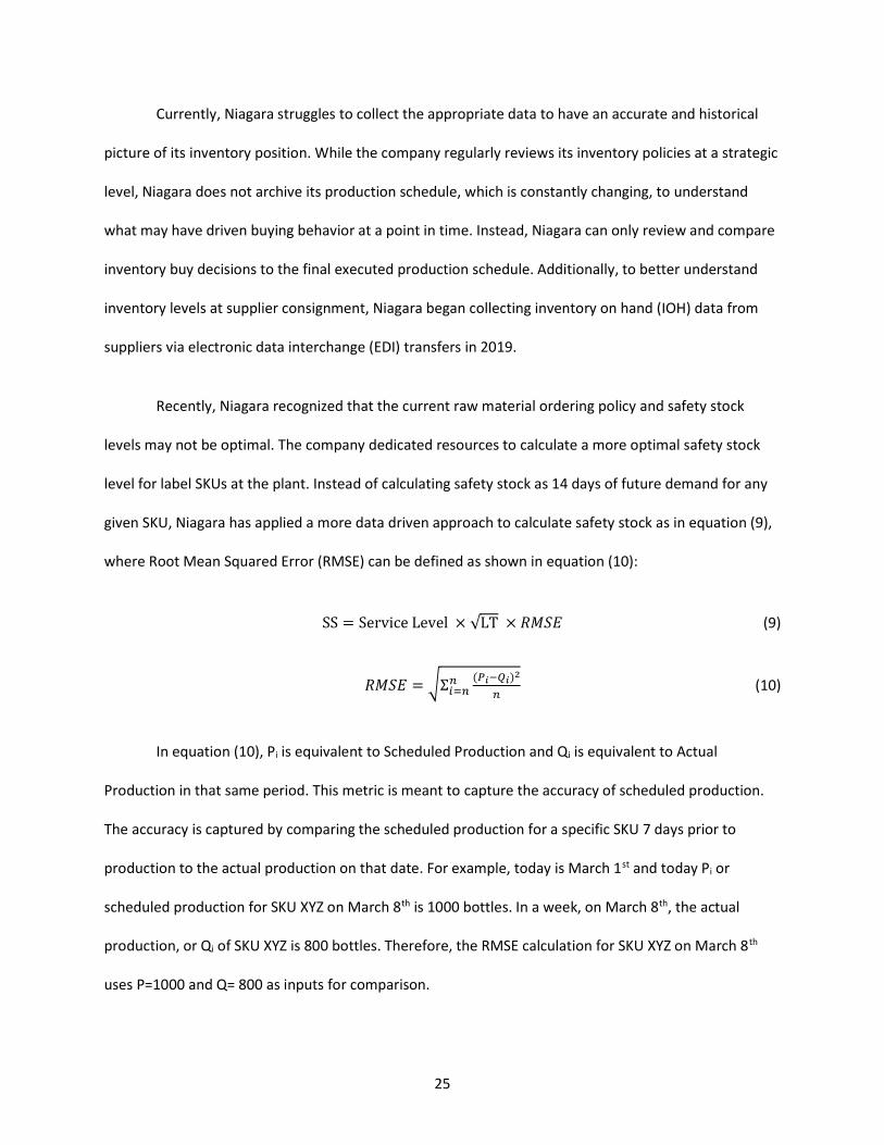
Currently, Niagara struggles to collect the appropriate data to have an accurate and historical
picture of its inventory position. While the company regularly reviews its inventory policies at a strategic
level, Niagara does not archive its production schedule, which is constantly changing, to understand
what may have driven buying behavior at a point in time. Instead, Niagara can only review and compare
inventory buy decisions to the final executed production schedule. Additionally, to better understand
inventory levels at supplier consignment, Niagara began collecting inventory on hand (IOH) data from
suppliers via electronic data interchange (EDI) transfers in 2019.
Recently, Niagara recognized that the current raw material ordering policy and safety stock
levels may not be optimal. The company dedicated resources to calculate a more optimal safety stock
level for label SKUs at the plant. Instead of calculating safety stock as 14 days of future demand for any
given SKU, Niagara has applied a more data driven approach to calculate safety stock as in equation (9),
where Root Mean Squared Error (RMSE) can be defined as shown in equation (10):
SS = Service Level × √LT × 𝑅𝑀𝑆𝐸 (9)
𝑅𝑀𝑆𝐸 = Σ( ) (10)
In equation (10), Pi is equivalent to Scheduled Production and Qi is equivalent to Actual
Production in that same period. This metric is meant to capture the accuracy of scheduled production.
The accuracy is captured by comparing the scheduled production for a specific SKU 7 days prior to
production to the actual production on that date. For example, today is March 1st and today Pi or
scheduled production for SKU XYZ on March 8th is 1000 bottles. In a week, on March 8th, the actual
production, or Qi of SKU XYZ is 800 bottles. Therefore, the RMSE calculation for SKU XYZ on March 8th
uses P=1000 and Q= 800 as inputs for comparison.

26
Niagara believes this RMSE approach is a more appropriate method of calculating safety stock
using SKU specific data to set safety stock levels as compared to the previous Niagara method. The new
safety stock values have not yet been implemented due to organizational challenges. For example, the
RMSE method of calculating safety stock results in a higher total level of safety stock in pallets which
would require additional space at the plants which cannot always be accommodated.
5.3 SKU Classification Using Customer Demand
Niagara currently segments SKUs based on sales volume. Category A SKUs cover 70% of the total
volume. B and C categories cover the remaining 20% and 10% of total volume respectively. The team
performed another SKU classification based on coefficient of variation and positive demand probability,
as explained in literature review section, to segment SKUs into four sections that indicate forecastability
level. An overview of the SKU distribution per segment with Niagara ABC and forecastability approach is
shown in Figure 4. From ABC analysis, 14% of SKUs are category A, which covers 70% of the total sales
volume. From forecastability analysis, 40% of SKUs are categorized as Smooth, which indicates high
forecastability.
Figure 4: SKU Distribution per Classification Approach
Are SKUs that show high forecastability primarily in category A? A comparison of these two
classification approaches was conducted, and the result is shown in Figure 5. Quite a few SKUs from
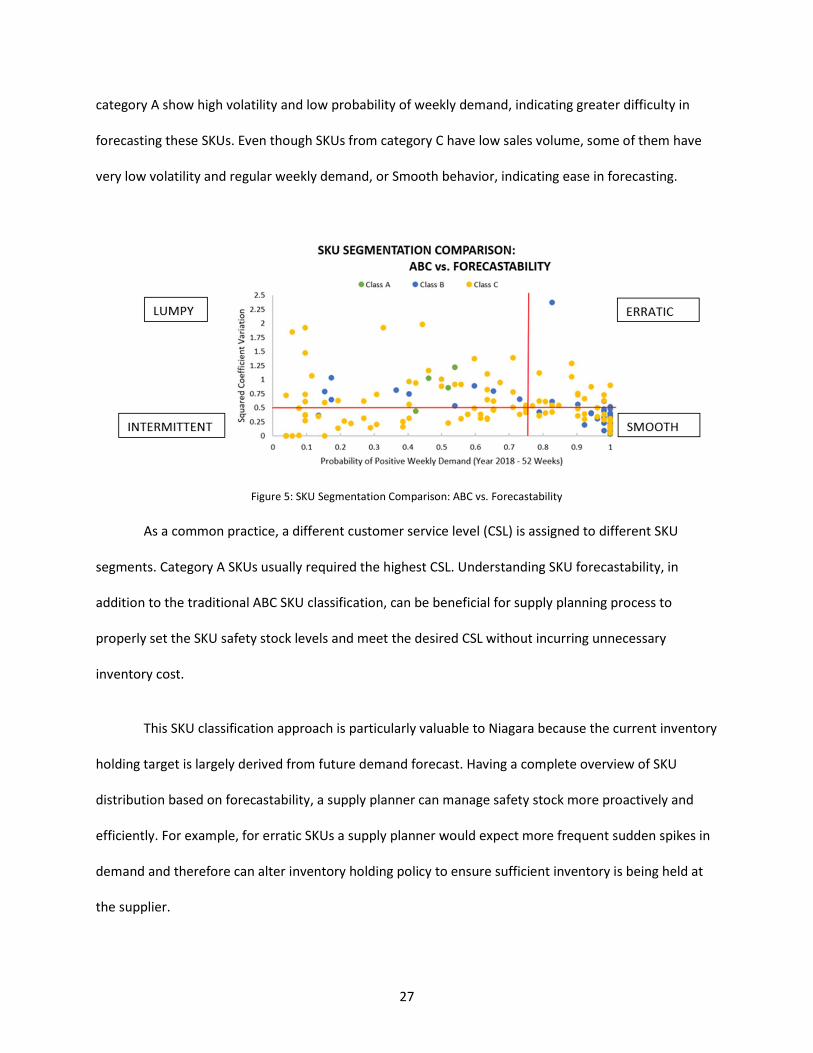
27
category A show high volatility and low probability of weekly demand, indicating greater difficulty in
forecasting these SKUs. Even though SKUs from category C have low sales volume, some of them have
very low volatility and regular weekly demand, or Smooth behavior, indicating ease in forecasting.
Figure 5: SKU Segmentation Comparison: ABC vs. Forecastability
As a common practice, a different customer service level (CSL) is assigned to different SKU
segments. Category A SKUs usually required the highest CSL. Understanding SKU forecastability, in
addition to the traditional ABC SKU classification, can be beneficial for supply planning process to
properly set the SKU safety stock levels and meet the desired CSL without incurring unnecessary
inventory cost.
This SKU classification approach is particularly valuable to Niagara because the current inventory
holding target is largely derived from future demand forecast. Having a complete overview of SKU
distribution based on forecastability, a supply planner can manage safety stock more proactively and
efficiently. For example, for erratic SKUs a supply planner would expect more frequent sudden spikes in
demand and therefore can alter inventory holding policy to ensure sufficient inventory is being held at
the supplier.

28
5.4 SKU Forecast Bias
The team utilized the approach presented in section 4.2.2 (Forecast Bias) to evaluate the
forecast bias for each raw material SKU with data from customer demand and strategic forecast of 2018.
A SKU with a forecast bias at 0.5 is considered unbiased in forecasting due to forecasted demand the
same as the actual demand. When forecast bias is below 0.5, a SKU is considered underforecasted, and
it is considered overforecasted when the forecast bias is above 0.5. A forecast bias distribution for raw
material SKUs in the identified region is shown in Figure 6.
Figure 6: NE SKU Forecast Bias Histogram
The data shown in forecast bias histogram is left-skewed, which indicates more SKUs are
overforecasted. If we drill down to see how SKUs behave on forecasting bias in each forecastability
category, we found in intermittent and lumpy categories all the SKUs that we analyzed are
overforecasted (larger than 0.5 forecasting bias). This data insight matches the current behavior of
material buyer, who usually tends to stock up when SKUs demand are highly volatile or with high
forecasting error.
It is not intuitively easy to interpret the forecast bias and see how it relates to forecast error.
The relationship between these two is shown in Figure 7. Forecast bias changes faster when forecast
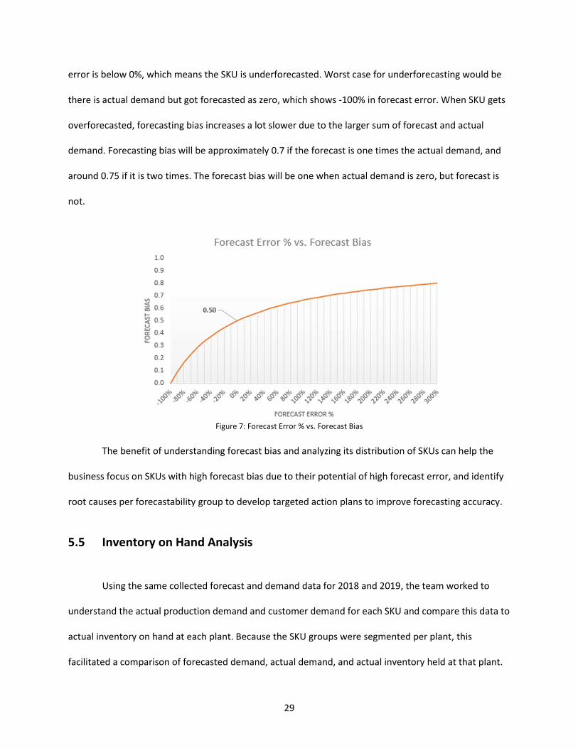
29
error is below 0%, which means the SKU is underforecasted. Worst case for underforecasting would be
there is actual demand but got forecasted as zero, which shows -100% in forecast error. When SKU gets
overforecasted, forecasting bias increases a lot slower due to the larger sum of forecast and actual
demand. Forecasting bias will be approximately 0.7 if the forecast is one times the actual demand, and
around 0.75 if it is two times. The forecast bias will be one when actual demand is zero, but forecast is
not.
Figure 7: Forecast Error % vs. Forecast Bias
The benefit of understanding forecast bias and analyzing its distribution of SKUs can help the
business focus on SKUs with high forecast bias due to their potential of high forecast error, and identify
root causes per forecastability group to develop targeted action plans to improve forecasting accuracy.
5.5 Inventory on Hand Analysis
Using the same collected forecast and demand data for 2018 and 2019, the team worked to
understand the actual production demand and customer demand for each SKU and compare this data to
actual inventory on hand at each plant. Because the SKU groups were segmented per plant, this
facilitated a comparison of forecasted demand, actual demand, and actual inventory held at that plant.

30
This was a good opportunity for the team to understand if Niagara’s purchasing policy was actually being
implemented at the plants and to identify current inventory levels at the plants.
For example, Figure 8 demonstrates the significant variance in actual inventory on hand (IOH) at
the plant for a category A SKU.
Figure 8: Segment A Smooth Forecastability SKU
The figure shows that the production demand and customer demand throughout 2019 are
relatively similar and stable, with an average weekly demand of 10.2 million labels and a maximum
weekly demand of 17.1 million labels. On the other hand, the actual IOH at the plant is extremely
variable and erratic. According to Niagara purchasing policy, the plant should always have 14 days, or
two weeks, of forecasted demand on hand at the plant as safety stock. Therefore, the inventory on hand
should not dip below about 20 million labels. Nevertheless 13 weeks, or 25% of the year, the number of
labels on hand at the plant is below the designated safety stock level. Moreover, based on the figure it
seems as though the plant is holding much more inventory than needed during other weeks of the year.
0
10,000
20,000
30,000
40,000
50,000
60,000
70,000
1 3 5 7 9 11 13 15 17 19 21 23 25 27 29 31 33 35 37 39 41 43 45 47 49 51 53
Num
ber o
f Lab
els
(tho
usan
ds)
Week of 2019
Production Demand Customer Demand Plant Actual IOH

31
The team aimed to further analyze what was causing these discrepancies and the best way to improve
Niagara’s inventory position.
5.6 Safety Stock Calculation
Two safety stock calculation approaches are explored and explained separately in this section.
These two approaches differ on the standard deviation used in the safety stock equation: one is defined
as the traditional strategy, using standard deviation of customer demand as explained under section
4.2.1. The other is defined as the forecast error strategy, using standard deviation of forecast error as
explained under section 4.2.2. With the understanding of Niagara’s pain points of demand volatility and
struggles in forecasting accuracy, the team seeks to compare these two approaches and determine the
most suitable one for Niagara business situation.
The common parameters used for these two safety stock approaches are cycle service level and
lead time, as shown in Table 2 and Table 3. The calculation methods will be explained in detail under
section 3.6.1 and 3.6.2.
Table 2: Cycle Service Level
Cycle Service Level ABC Category Cycle Service Level Z-score
A 99.8% 2.88
B 99.0% 2.33
C 97.0% 1.88
Table 3: Lead Time
Lead Time
Replenishment Process Net Replenishment Lead Time
Supplier consignment to plant 1 week
Supplier to supplier consignment 4 weeks

32
5.6.1 Standard Deviation Using Customer Demand for Traditional Strategy
Historical customer demand data from 2018 is used when calculating standard deviation. The
customer demand is segmented into weekly buckets and a simple standard deviation formula in Excel is
applied to calculate the customer demand standard deviation among one year of weekly demand data.
One raw material SKU from category A is used to illustrate the calculation results as shown in
Table 4. Average demand, standard deviation of customer demand and safety stock are in Thousands of
Labels. To convert the safety stock target into number of pallets, the team used: 3 million labels = 1
pallet. Number of pallets is rounded up as the final result.
Table 4: Example SKU Using Customer Demand
ABC Category
Forecastability Avg. Demand
SD Customer Demand
Z-score
Lead Time
Safety Stock Target
Round up Pallets
A Smooth 5136 1429 2.88 1 Week 4116 2
5.6.2 Standard Deviation Using Forecast Errors for Forecast Error Strategy
To calculate standard deviation using forecast error, both historical customer demand and
strategic forecast data from 2018 are used. The customer demand and strategic forecast are segmented
into weekly buckets. One raw material SKU from category A is used to illustrate the calculation result of
forecast error for week 1 of 2018, as shown in Table 5. All data in Table 5 are shown in Thousands of
Labels.
Table 5: Example SKU’s Forecast Error
Week 1 Forecast Demand Week 1 Customer Demand Forecast Error
1747 2162 - 415
33
Weekly forecast error for each SKU is calculated, and then a simple standard deviation formula
in Excel is applied to calculate the standard deviation of forecast errors among one year of weekly
forecast error data.
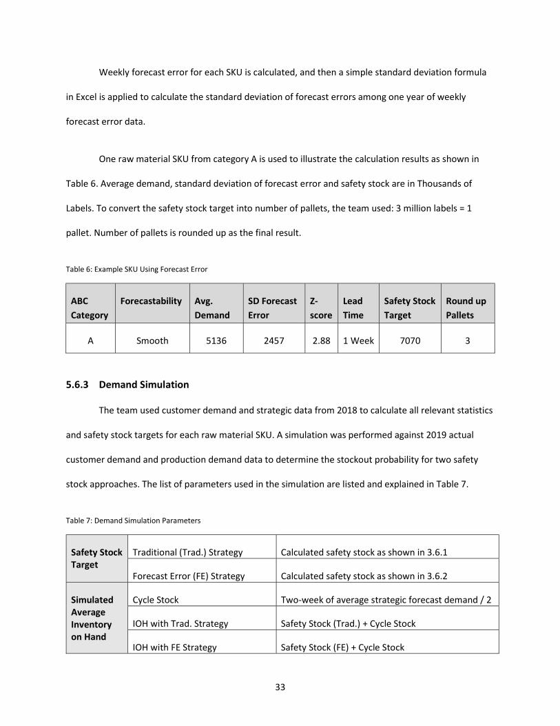
One raw material SKU from category A is used to illustrate the calculation results as shown in
Table 6. Average demand, standard deviation of forecast error and safety stock are in Thousands of
Labels. To convert the safety stock target into number of pallets, the team used: 3 million labels = 1
pallet. Number of pallets is rounded up as the final result.
Table 6: Example SKU Using Forecast Error
ABC Category
Forecastability Avg. Demand
SD Forecast Error
Z-score
Lead Time
Safety Stock Target
Round up Pallets
A Smooth 5136 2457 2.88 1 Week 7070 3
5.6.3 Demand Simulation
The team used customer demand and strategic data from 2018 to calculate all relevant statistics
and safety stock targets for each raw material SKU. A simulation was performed against 2019 actual
customer demand and production demand data to determine the stockout probability for two safety
stock approaches. The list of parameters used in the simulation are listed and explained in Table 7.
Table 7: Demand Simulation Parameters
Safety Stock Target
Traditional (Trad.) Strategy Calculated safety stock as shown in 3.6.1
Forecast Error (FE) Strategy Calculated safety stock as shown in 3.6.2
Simulated Average Inventory on Hand
Cycle Stock Two-week of average strategic forecast demand / 2
IOH with Trad. Strategy Safety Stock (Trad.) + Cycle Stock
IOH with FE Strategy Safety Stock (FE) + Cycle Stock

34
2019 Actual Demand
Customer Demand Actual customer demand data in weekly buckets
Production Demand Actual production demand data in weekly buckets
End IOH for Traditional Strategy
Compare w/ Customer Demand Simulated IOH (Trad.) – Customer Demand (2019)
Compare w/ Production Demand Simulated IOH (Trad.) – Production Demand (2019)
End IOH for FE Strategy
Compare w/ Customer Demand Simulated IOH (FE) – Customer Demand (2019)
Compare w/ Production Demand Simulated IOH (FE) – Production Demand (2019)
For cycle stock, the team followed the current buying practice at Niagara, which uses two weeks
of forecasted demand of a SKU. The weekly average demand from the 2019 strategic forecast was used
in cycle stock calculation for the demand simulation. For calculating stockout probability, after
comparing with either customer or production demand, a stockout event is occurred when the end IOH
is less than 0. To help illustrate this demand simulation process, the calculation of one raw material SKU
from category A is presented in Table 8.
Table 8: Demand Simulation Example
In the example shown in Table 8, the stockout probability for forecast error method while
simulating against customer and production demand is 0%, since the end IOH are all above zero. The
stockout probability for traditional safety stock strategy while simulating against production demand is
35
0%. However, while simulating against customer demand, the stockout probability is 8.3%. When
stockout probability is 0%, the cycle service level is 100% since all demand is fulfilled within the
replenishment cycle. Otherwise, the cycle service level would be the stockout probability subtracted
from 100%. In this example, the cycle service level is 91.7% while using traditional safety stock strategy
and simulating against customer demand.
5.7 Minimum Order Quantity (MOQ) vs. Full Pallet Analysis
Figure 8 in Section 5.5, which displays Niagara’s current state inventory position for a category A
SKU over 2019 illustrates erratic inventory holding quantities. One explanation for extreme spikes in
inventory on hand at Niagara is the current policy to order only full pallets of labels. While not all label
SKUs hold identical quantities on a pallet the difference is insignificant, so the team agreed on the
generally true assumption that one pallet holds 3 million labels. The team expected this full pallet
ordering behavior would have a clear negative impact on inventory holding for low volume SKUs with
Smooth demand behavior. Therefore, the team decided to further explore the relevant costs to
ordering, transporting, holding, and potentially scrapping raw material to understand if there was any
justification for Niagara to order less than pallet quantities as detailed in Section 6.2.2.

36
6 Results and Analysis
Using the available 2018 data for customer demand, production demand and strategic forecast,
the team calculated recommended safety stock levels using two different approaches as described in
section 5.6 and compared to 2019 actual customer demand and production demand data. The
simulation results revealed that the forecast error safety stock strategy resulted in fewer stockouts and
higher cycle service levels as compared to the traditional safety stock strategy. Moreover, the analysis
revealed that when compared with the actual IOH at Niagara plants, there is an opportunity for savings
through lower safety stock inventory levels. While there are several limitations to our analysis, such as
limited data, the team’s findings suggest Niagara could significantly reduce inventory levels for SKUs in
Smooth forecastability category while keeping the same high cycle service levels.
6.1 Safety Stock Simulation Results
6.1.1 Traditional vs. Forecast Error Safety Stock Strategy
After calculating the recommended safety stock level for each SKU with appropriate data
available, 110 SKUs, using both approaches, the simulation was executed as described in section 5.6.3.
Table 9 summarizes the cycle service level, or probability of fulfilling all demand during replenishment
cycle, averaged across each week in 2019 per forecastability category. Each forecastability category
consists of 5 representative SKUs chosen at random.
Table 9: Service Level Results from Simulation per Forecastability Category
SKU Forecastability
Group
Traditional Strategy Forecast Error Strategy Production
Demand Customer Demand
Production Demand
Customer Demand
Erratic 91% 96% 96% 99%
37
Intermittent 79% 90% 83% 92% Lumpy 90% 91% 94% 89%
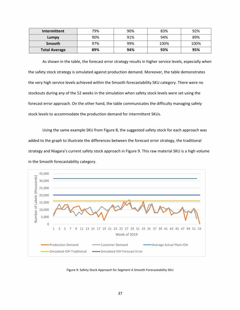
Smooth 97% 99% 100% 100% Total Average 89% 94% 93% 95%
As shown in the table, the forecast error strategy results in higher service levels, especially when
the safety stock strategy is simulated against production demand. Moreover, the table demonstrates
the very high service levels achieved within the Smooth forecastability SKU category. There were no
stockouts during any of the 52 weeks in the simulation when safety stock levels were set using the
forecast error approach. On the other hand, the table communicates the difficulty managing safety
stock levels to accommodate the production demand for intermittent SKUs.
Using the same example SKU from Figure 8, the suggested safety stock for each approach was
added to the graph to illustrate the differences between the forecast error strategy, the traditional
strategy and Niagara’s current safety stock approach in Figure 9. This raw material SKU is a high volume
in the Smooth forecastability category.
Figure 9: Safety Stock Approach for Segment A Smooth Forecastability SKU
0
5,000
10,000
15,000
20,000
25,000
30,000
35,000
1 3 5 7 9 11 13 15 17 19 21 23 25 27 29 31 33 35 37 39 41 43 45 47 49 51 53
Num
ber o
f Lab
els
(tho
usan
ds)
Week of 2019
Production Demand Customer Demand Average Actual Plant IOH
Simulated IOH Traditional Simulated IOH Forecast Error
38
The figure shows that the safety stock recommendation based on the forecast error approach
results in a higher volume of raw material on hand at the plant as compared to the traditional safety
stock approach. Moreover, because the customer or production demand is never higher than the
‘Simulated IOH Forecast Error’, it is clear the inventory policy developed using forecast error results in
zero stockout. The same is not true for the inventory policy developed from the traditional safety stock
formula or ‘Simulation IOH Traditional’ in Figure 9.
The team noticed the differences between traditional and forecast error inventory policies were
generally attributable to the forecast bias as defined in Equation 6. When the forecast bias is close to
0.5, the forecast is not biased, and, therefore, the safety stock calculated using the two different
methods will be very similar. On the other hand, when the bias is greater than 0.5 or less than 0.5 this
suggests an overforecasting or underforecasting of demand. Therefore, the standard deviation of
forecast errors will be greater, which will drive up the safety stock of these SKUs. Moreover, when a SKU
is overforecasted, the inventory on hand will be greater not just due to higher standard deviation of
forecast errors but also due to the higher than necessary cycle stock as cycle stock is based on the
forecast for the next 14 days.
Lastly, the inventory position of the example SKU graphed in Figure 9 shows a clear disconnect
between the suggested future inventory position and the current strategy. For the lower volume SKUs,
this disconnect is driven by Niagara’s minimum ordering policy of one full pallet or three million labels,
however, for this high-volume SKU it suggests erratic ordering frequency and volume. This erratic
ordering could be due to various factors such as infrequent review of inventory on hand, discrepancies
between forecast and actual demand, or attempt to utilize the full capacity of trucks in transporting raw
materials. Regardless, this erratic behavior represents an opportunity to smooth out raw material

39
holding quantities to match demand trends and potentially save money depending on implications to
transportation and ordering costs.
Ultimately, the team identified the forecast error safety stock method as the optimal strategy
due to Niagara’s seasonal demand, ability to continuously review inventory levels, the service levels
generated from the simulation shown in Table 9. For the 110 SKUs analyzed, this approach resulted in a
higher total number of pallets of safety stock at the plant when compared with the traditional safety
stock approach, 143 pallets as compared with 118 pallets. However, when comparing total pallets of
inventory on hand required at the plant for the 101 SKUs with available data, the number of pallets
using the forecast error safety stock method, 165 pallets, was significantly less than the current state,
209 pallets. For all these calculations, labels were rounded up to order in full pallet as is Niagara’s
current practice. In the next section, the team will further explore trends in opportunities for reduced
safety stock pallets at the plants using a forecast error approach to set safety stock levels.
6.2 Recommended Inventory Level Comparison
When further comparing the current state to suggested inventory levels by forecastability
category, the team noticed that a majority of the inventory reduction opportunity was among SKUs
within the Smooth forecastability category. Moreover, the team conducted an analysis to prove that
depending on key assumptions regarding cost of obsolescence and cost to order, there are
circumstances in which ordering less than a pallet is a more cost-effective inventory policy.
6.2.1 Opportunity in Inventory Level Reduction for Smooth SKUs
Figure 10 illustrates the potential change in pallets held at the plant when the forecast error
approach of calculating safety stock is applied. In total, 47 pallets could be removed from the specific

40
region network from the raw material inventory held for around 100 SKUs. As is obvious from Figure 10,
a majority of the pallet reduction is from the SKUs within the Smooth forecastability category. It is
important to note, that the 100% cycle service levels for the Forecast error approach and Smooth
category SKUs shown in Table 9 were achieved in the simulation with this reduced number of SKUs. This
demonstrates negligible impact on the customer and associated service levels, yet savings in inventory
holding and additional space availability at the plants.
Figure 10: Potential IOH Pallet Savings
Figure 11 shows this change in pallets held at the plant per SKU. Again, it is clear the SKUs with
the most obvious reduction in pallets all belong to the Smooth forecastability category, yet there are
also some within this SKU segment that require additional pallets. A majority of the SKUs, over 60%,
have no change in raw material holding volume using the new forecast error method of calculating
safety stock and rounding all recommended volumes up to the next full pallet.

41
Figure 11: IOH Potential Pallet Savings per SKU
This reduction in pallets in the network results in potential cost savings for Niagara. Table 10
shows the difference in holding costs per pallet per plant as applied to the reduction in pallets due to
the new forecast error approach of calculating safety stock. Using the assumptions listed, the total
potential savings in the specific region’s network is around $225,000. The team estimates if this policy is
rolled across the entire Niagara network and all SKU groups, this has the potential to be increased to
10X this savings, or $2.25 million.
Table 10: Potential Cost Reduction using Forecast Error Safety Stock Approach
Cost Reduction
Plant Annual Holding
Cost/Pallet Pallets
Reduction Number of
Labels (Thou) Raw Material
Cost Holding
Cost Total
Savings
P1 366 22 66000 99000 8051 107051 P2 33 5 15000 22500 163 22663 P3 313 1 3000 4500 313 4813 P4 410 13 39000 58500 5326 63826 P5 17 6 18000 27000 102 27102
Consignment 90
Total 225456
-5
-4
-3
-2
-1
0
1
2
3
0 10 20 30 40 50 60 70 80 90 100
Palle
tsChange in IOH per SKU when Forecast Error Approach Applied
erratic intermittent lumpy smooth
42
6.2.2 Opportunity in Ordering Minimum Order Quantity
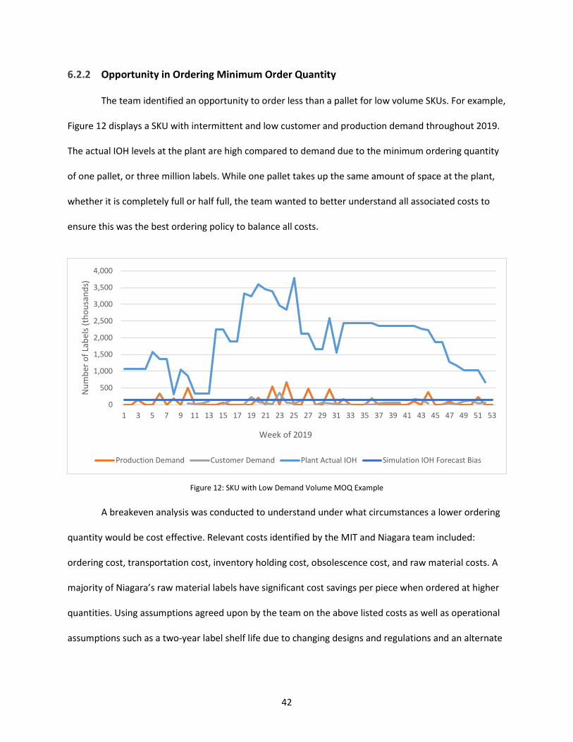
The team identified an opportunity to order less than a pallet for low volume SKUs. For example,
Figure 12 displays a SKU with intermittent and low customer and production demand throughout 2019.
The actual IOH levels at the plant are high compared to demand due to the minimum ordering quantity
of one pallet, or three million labels. While one pallet takes up the same amount of space at the plant,
whether it is completely full or half full, the team wanted to better understand all associated costs to
ensure this was the best ordering policy to balance all costs.
Figure 12: SKU with Low Demand Volume MOQ Example
A breakeven analysis was conducted to understand under what circumstances a lower ordering
quantity would be cost effective. Relevant costs identified by the MIT and Niagara team included:
ordering cost, transportation cost, inventory holding cost, obsolescence cost, and raw material costs. A
majority of Niagara’s raw material labels have significant cost savings per piece when ordered at higher
quantities. Using assumptions agreed upon by the team on the above listed costs as well as operational
assumptions such as a two-year label shelf life due to changing designs and regulations and an alternate
0
500
1,000
1,500
2,000
2,500
3,000
3,500
4,000
1 3 5 7 9 11 13 15 17 19 21 23 25 27 29 31 33 35 37 39 41 43 45 47 49 51 53
Num
ber o
f Lab
els
(tho
usan
ds)
Week of 2019
Production Demand Customer Demand Plant Actual IOH Simulation IOH Forecast Bias

43
MOQ of 500,000 labels as inputs. The Figure 13 breakeven model was created based on forecasted
annual demand of SKUs.
Figure 13: MOQ Breakeven Model
The MOQ breakeven excel model helped to illustrate to the team and the sponsor that in some
circumstances, such as when the forecasted annual demand of a SKU is less than 1 million, it is more
cost effective to order a MOQ of 500,000 labels. In operation, this only impacts around 13% of SKUs in
the specific region. However, this was a learning to be passed on to buyers and potential cost savings,
especially if rolled out across the entire Niagara network. The excel MOQ breakeven analysis tool is
dynamic so that the sponsoring company can continue to change assumptions and costs to make
effective and appropriate conclusions as needed in their changing business environment.
6.2.3 Summary
After a deep dive into the selected safety stock strategy, trends were revealed around the
negative impact of Niagara’s current inventory policy leading to excess inventory for SKUs with
$0
$2,000
$4,000
$6,000
$8,000
$10,000
$12,000
$14,000
$16,000
010
020
030
040
050
060
070
080
090
010
0011
0012
0013
0014
0015
0016
0017
0018
0019
0020
0021
0022
0023
0024
0025
0026
0027
0028
0029
0030
00
Cost
Forecasted Annual Demand of SKU (thousands)
MOQ vs. Full Pallet Breakeven Analysis
MOQ Full Pallet
44
predictable and stable demand. The team identified the opportunity to apply the new safety stock
approach and reduce pallets of these SKUs at the plant while keeping high service levels, 100%, as
indicated through the simulation. The team also came to the conclusion that it is appropriate to have
different ordering strategies for different SKU classification categories to capture the cost savings
opportunities presented.
6.3 Limitations
Niagara is aware of the high volatility in its production demand, especially between day three
and day seven during the seven-day firm production demand window. Both the team and Niagara are
interested in learning how production demand variation, comparing planned production demand sent
prior seven days with the actual production demand, would effect safety stock target and stockout
probability. However, due to the difficulty of acquiring planned production data, the team was not able
to conduct this analysis and analyze the results.
45
7 Conclusion
7.1 Recommended Safety Stock Strategy
Based on the analysis and results presented in the previous sections, the team recommends the
forecast error approach as the optimal safety stock strategy for Niagara. During simulation against
seasonal actual customer and production demand, this strategy demonstrates satisfactory cycle service
levels on top of a reduction of current raw material inventory levels. Coupling with the recommended
forecast error safety stock strategy, a new classification method to segment SKUs into different
forecastability categories is also recommended to help Niagara target the right SKUs for the right
corrective actions.
It is clear from our analysis that there should not be a one-size-fits-all safety stock strategy
across all SKUs. Due to different demand characteristics and forecastability in SKUs, it is recommended
to segment these SKUs into different forecastability categories that share similar demand patterns in
order to efficiently review and drive inventory improvement. For Niagara, the biggest inventory
reduction opportunity is in the Smooth forecastability category, which includes SKUs with lower demand
volatility and better forecastability. Right sizing the inventory levels for these SKUs brings significant
inventory reductions and cost savings.
For SKUs that are difficult to forecast and show high demand volatility, such as those in the
intermittent and lump forecastability categories, the team recommends to right size the ordering
quantity to improve inventory levels while maintaining the same or better cycle service levels. Niagara
can choose to order in minimum order quantity when the annual forecasted demand of a SKU is under
the threshold recommended from the analytical model.
46
Last but not least, ensuring the input data accuracy and integrity and establishing a periodic
review practice are also the keys to a good safety stock strategy. Raw material SKU lists are dynamic due
to new product introduction or obsolescence annually. Therefore, it is important to proactively manage
these SKUs and preprocess the data before interpreting the results from the models.
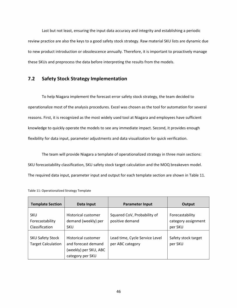
7.2 Safety Stock Strategy Implementation
To help Niagara implement the forecast error safety stock strategy, the team decided to
operationalize most of the analysis procedures. Excel was chosen as the tool for automation for several
reasons. First, it is recognized as the most widely used tool at Niagara and employees have sufficient
knowledge to quickly operate the models to see any immediate impact. Second, it provides enough
flexibility for data input, parameter adjustments and data visualization for quick verification.
The team will provide Niagara a template of operationalized strategy in three main sections:
SKU forecastability classification, SKU safety stock target calculation and the MOQ breakeven model.
The required data input, parameter input and output for each template section are shown in Table 11.
Table 11: Operationalized Strategy Template
Template Section Data Input Parameter Input Output
SKU Forecastability Classification
Historical customer demand (weekly) per SKU
Squared CoV, Probability of positive demand
Forecastability category assignment per SKU
SKU Safety Stock Target Calculation
Historical customer and forecast demand (weekly) per SKU, ABC category per SKU
Lead time, Cycle Service Level per ABC category
Safety stock target per SKU

47
MOQ Breakeven Model
Historical forecast demand annually per SKU
Raw material price (UOM), Ordering/holding/ obsolescence cost, time to obsolescence
List of SKUs that are recommended ordering in MOQ
7.3 Insights for General Management
One of the first opportunities identified by the team was to take advantage of supplier
consignment inventory contracts. All label suppliers hold raw material inventory for 90 days free of
charge. The more the team dug into the data, the more the team realized the extreme upside of these
agreements, which essentially offer free inventory holding to buffer risk of potential spikes in demand
with low downside due to low cost of obsolescence. Moreover, after the 90 days, suppliers charge a
relatively small amount per pallet per month, less than the annual holding cost at three of the five plants
in the specific region network. This early win has “already shifted our buying practices,” according to
Niagara team members.
Additionally, the team identified an opportunity for better data collection and review to inform
the inventory strategy and buying practices of Niagara. For example, as mentioned previously, the
Niagara team uses planned production data as compared to actual production data to calculate the root
mean square error as a potential alternative method to calculate safety stock. However, this planned
production data is not archived. The only accessible historical data related to production data is the
actual production data. This presents an opportunity for further data archiving to better understand the
planned production, which is driving buying requirements and the inconsistencies as compared to what
is executed on the production floor.
48
Additionally, while Niagara receives daily EDI transmissions from the supplier as of the past year
to understand inventory position, there is an opportunity to more frequently aggregate and review this
data on the strategic level. By collecting the data and filtering by plant, SKU classification, and supplier,
this data can be compared to inventory on hand at the plant to identify trends and opportunities for
potential inventory savings or service level improvements proactively. The team recommends a bi-
annual or quarterly review of the inventory picture at both the supplier and the plant to ensure current
inventory policies are being implemented and ensure the approach makes sense given the business
environment.
When reviewing and evaluating inventory positions, the team recommends Niagara bucket
inventory into safety stock and cycle stock and examine separately. Currently, all inventory is lumped
together and not categorized or classified to clearly identify what volume is being held as safety stock
and which is being ordered to future demand. By better categorizing the intent or purpose of the raw
material inventory, it will be easier to make conclusions about whether adequate inventory levels are
being held in each bucket and where adjustments might need to be made. This will allow Niagara to
derive actionable items to address the real drivers of excess or shortages in inventory for the different
inventory classes. Other potential classifications of inventory are pre-build stock and promotional stock.
These classifications should be separated from actual demand so that the team has a better picture and
understanding of the actual drivers and urgency of production demand. Furthermore, when reviewing
inventory levels and stockouts from a strategic level, better conclusions can be drawn to address the
root cause and continuously improve Niagara’s inventory position and service levels.
As alluded to above, these bi-annual or quarterly inventory reviews should also include a review
of specific high impact stockout events. By performing a detailed root cause analysis with the key
stakeholders, the team can make valuable conclusions about what is working in the system and where
49
additional opportunity for improvement is present. The SKU segmentation based on forecastability as
recommended should also be reviewed to ensure SKUs are properly classified and to ensure newly
added SKUs are appropriately added to the classification structure.
One final recommendation from the team is to ensure that actual customer demand is driving
inventory levels as opposed to production demand. While it is true, production demand could be
accounting for pre-stock buildup and other one-off events, the ultimate goal should be to order to
customer demand and ensure customer demand is driving all associated production activities.
7.4 Future Research Recommendations
While the team’s research focused specifically on raw material safety stock, future potential
research could extend this analysis to create an optimization model for inventory levels within the plant
between both the raw materials and the finished goods safety stock. Moreover, the team presented an
alternate SKU classification method using the forecastability of the SKUs, but there is a further
opportunity to segment SKUs based on profitability. This would allow Niagara to differentiate its service
to ensure customers who provide the most profit receive the best service. It would also allow the
sponsor company to identify customers with low profitability as potential clients to work to renegotiate
prices and terms. Lastly, as the recommended safety stock strategy is based on forecastability, it is
important to dedicate adequate resources to frequently review, revise, and update the forecast of
finished goods and raw materials. While the forecast will always be wrong, when it’s very wrong, it will
have a significant impact on cycle service levels and raw material inventory across the network.

50
References
Babai, M. Z., T. Ladhari, and I. Lajili (2015). “On the Inventory Performance of Multi-Criteria Classification Methods: Empirical Investigation”. In: International Journal of Production Research 53, pp. 279–290.
Battini, D., Gunasekaran, A., Faccio, M., Persona, A., & Sgarbossa, F. (2010). Consignment stock inventory model in an integrated supply chain. International Journal of Production Research, 48(2), 477–500. https://doi.org/10.1080/00207540903174981
Bollapragada, S., & Morton, T. E. (1999). A Simple Heuristic for Computing Nonstationary (s, S) Policies. Operations Research, 47(4), 576–584. https://doi.org/10.1287/opre.47.4.576
Boylan, J. E., A. A. Syntetos, and G. C. Karakostas (2008). “Classification for Forecasting and Stock Control: a Case Study”. In: The Journal of the Operational Research Society 59.4, pp. 473–481.
Braglia, M., & Zavanella, L. (2003). Modelling an industrial strategy for inventory management in supply chains: The “Consignment Stock” case. International Journal of Production Research, 41(16), 3793–3808. https://doi.org/10.1080/0020754031000138330
Chandra, V., & Tully, M. (n.d.). Raw Material Inventory Strategy for Make-to-Order Manufacturing. 64.
Clark, A. J., & Scarf, H. (1960). Optimal Policies for a Multi-Echelon Inventory Problem. Management Science (Pre-1986); Linthicum, 6(4), 475.
de Kok, T., Grob, C., Laumanns, M., Minner, S., Rambau, J., & Schade, K. (2018). A typology and literature review on stochastic multi-echelon inventory models. European Journal of Operational Research, 269(3), 955–983. https://doi.org/10.1016/j.ejor.2018.02.047
Engelmeyer, T. (2016). Managing Intermittent Demand. Springer Fachmedien Wiesbaden.
Graves, S. C., & Willems, S. P. (2000). Optimizing Strategic Safety Stock Placement in Supply Chains. Manufacturing & Service Operations Management, 2(1), 68–83. https://doi.org/10.1287/msom.2.1.68.23267
Graves, S. C., & Willems, S. P. (2003). Supply Chain Design: Safety Stock Placement and Supply Chain Configuration. In Handbooks in Operations Research and Management Science (Vol. 11, pp. 95–132). https://doi.org/10.1016/S0927-0507(03)11003-1
Gudehus, T. (2005). Logistik. Grundlagen - Strategien - Anwendungen. Berlin/Heidelberg: Springer.
Hastie, T., R. Tibshirani, and J. Friedman (2009). The Elements of Statistical Learning. Data Mining, Inference, and Prediction, Second Edition. Springer.
Karlin, S. (1960). Dynamic Inventory Policy with Varying Stochastic Demands. Management Science, 6(3), 231–258. https://doi.org/10.1287/mnsc.6.3.231
King, P. L. (2011). Understanding safety stock and mastering its equations. 4.
51
Manary, M.P., & Willems, S.P. (2008). Setting Safety-Stock Targets at Intel in the Presence of Forecast Bias. Interfaces, 38, 112-122.
Morton, T. E., & Pentico, D. W. (1995). The Finite Horizon Nonstationary Stochastic Inventory Problem: Near-myopic Bounds, Heuristics, Testing. Management Science, 41(2), 334–343. https://doi.org/10.1287/mnsc.41.2.334
Neale, J. J., & Willems, S. P. (2009). Managing Inventory in Supply Chains with Nonstationary Demand. Interfaces, 39(5), 388–399. https://doi.org/10.1287/inte.1090.0442
Neale, J., Willems, S., & Beyl, J. C. (2012). Misalignment in the Timing of Seasonal Demand and Supply: The Landslide Effect. SSRN Electronic Journal. https://doi.org/10.2139/ssrn.2029509
Piplani, R., & Viswanathan, S. (2003). A model for evaluating supplier-owned inventory strategy. International Journal of Production Economics, 81–82, 565–571. https://doi.org/10.1016/S0925-5273(02)00298-0
Sethi, Suresh and Cheng, Feng, Optimality of (s, S) Policies in Inventory Models with Markovian Demand (1995). Operations Research, Vol. 45, No. 6, pp. 931-939. https://ssrn.com/abstract=1126048 or http://dx.doi.org/10.2139/ssrn.1126048
Silver, E. A., Pyke, D. F., & Thomas, D. J. (2017). Inventory and production management in supply chains.
Srinivas, Ch., & Rao, C. S. P. (2004). An improved consignment stock policy under stochastic lead times for effective inventory management in supply chains. 2004 IEEE International Engineering Management Conference (IEEE Cat. No.04CH37574), 3, 1222–1225. https://doi.org/10.1109/IEMC.2004.1408888
Valentini, G., & Zavanella, L. (2003). The consignment stock of inventories: Industrial case and performance analysis. International Journal of Production Economics, 81–82, 215–224. https://doi.org/10.1016/S0925-5273(02)00300-6
Willems, S. (2011). How Inventory Optimization Opens Pathways To. Supply Chain Management Review, March/April 2011, 30-36.


