Embed Size (px)
Citation preview
UNIVERSITA’ DEGLI STUDI DI PADOVA
DIPARTIMENTO DI INGEGNERIA INDUSTRIALE DII
CORSO DI LAUREA MAGISTRALE IN INGEGNERIA CHIMICA E DEI PROCESSI INDUSTRIALI
TREATMENT OF GREYWATER USING SUSPENDED AND IMMOBILIZED BIOMASS IN SEQUENTIAL BATCH REACTORS
Relatore: Prof. Alberto Bertucco
Correlatori: Dr. Rafael Gonzáles Olmos, Dr.ssa Maria Auset Vallejo
Laureando: RICCARDO TOMBOLA 1106633
Anno Accademico 2016/2017

Abstract
Water scarcity has become one of the main problems to face in the XXI century. Greywater
treatment and reuse can be a promising option for reducing potable water consumption and the
volumetric load on wastewater treatment plants.
The aim of this thesis work was to study the performance of SBBR technology in greywater
treatment, comparing it with SBR technology.
Four reactors have been operated: a SBBR with additional suspended biomass, run with carriers
made of waste material; a SBR, so with suspended biomass only; two SBBRs with immobilized
biomass only, one with the repurposed carriers, the other with commercial carriers, run for
comparing the performances of the different carrier media. The pollutants that were monitored
are COD, ammonium, total nitrogen, nitrites and nitrates.
Two reactors, the SBBRs equipped with the carriers made of recovered material, achieved good
removal percentage of the pollutants, results that show that SBBR is a suitable technology for
greywater treatment.
Experimental data collected during the thesis work was fitted with two kinetic models, the
power law and a Monod-type model. The parameters obtained can be useful tools in reactor
design, using them with caution being the kinetics of nitrogen removal connected to the C:N
ratio.

Riassunto
La carenza d’acqua è diventata uno dei principali problemi da affrontare nel XXI secolo. Il
trattamento e il riutilizzo delle acque grigie possono essere delle promettenti opzioni per
limitare il consumo di acqua potabile e ridurre il carico volumetrico sugli impianti di
trattamento di acque reflue.
Lo scopo di questo lavoro di tesi è stato lo studio delle prestazioni, nel trattamento di acque
grigie, della tecnologia SBBR, confrontandola con la tecnologia SBR.
Sono stati utilizzati Quattro reattori: un SBBR con biomassa sospesa addizionale, operato con
carrier costituiti da materiale di scarto; un SBR, dotato solamente di biomassa sospesa; due
SBBR provvisti solamente della biomassa supportata, uno utilizzato con i carrier di materiale
di recupero, l’altro con carrier commerciali, operato con lo scopo di comparare le prestazioni
dei diversi carrier. Gli inquinanti che sono stati analizzati sono COD, ammonio, azoto totale,
nitriti e nitrati.
Con i due reattori SBBR operati con i carrier costruiti con materiale di scarto sono state ottenute
buone percentuali di rimozione degli inquinanti, risultati che mostrano come la tecnologia
SBBR sia adeguata nel trattamento delle acque grigie.
I dati sperimentali raccolti durante il lavoro di tesi sono stati modellati tramite due modelli
cinetici, la legge di potenza e un modello di Monod. I parametri ottenuti con i calcoli possono
essere strumenti utili nel design dei reattori, ponendo attenzione nel loro utilizzo, essendo la
cinetica di rimozione dell’azoto strettamente legata al rapporto C:N.

Resumen
La falta de agua es uno de los mayores problemas que el mundo tiene que enfrentar en el siglo
XXI. El tratamiento y el reúso de agua gris pueden ser una opción prometedora para reducir el
consumo de agua potable y la carga volumétrica en las plantas de tratamiento de agua.
El objetivo de este trabajo de tesis ha sido estudiar el rendimiento de la tecnología SBBR en
el tratamiento de las aguas grises, comparándola con la tecnología SBR.
Cuatro reactores fueron utilizados: un SBBR con biomasa colgada adicional, utilizado con
carriers hechos de material sobrante; un SBR con solamente biomasa colgada; dos SBBR con
solamente biomasa pegada, uno con los carriers hechos de material desperdiciado, el otro con
carriers comerciales, operado para comparar el rendimiento de los carriers distintos. Los
contaminantes que fueron analizados son DQO, nitrógeno total, amonio, nitritos y nitratos.
Dos reactores, los SBBR utilizados con los carriers hechos de material sobrante, han
conseguido buenos porcentajes de eliminación de contaminantes, resultados que enseñan que
SBBR es una tecnología adecuada para el tratamiento de las aguas grises.
Los datos experimentales que se han recogido durante el trabajo de tesis se han modelado
utilizando dos modelos cinéticos, la ley de potencia y un modelo de Monod. Los parámetros
conseguidos pueden ser herramientas útil para desarrollar reactores, utilizándolos cuidados,
siendo la cinética de la eliminación del nitrógeno relacionada con el ratio C:N.

Table of contents
INTRODUCTION ................................................................................................................................................ 1
STATE OF THE ART ............................................................................................................................................ 3
1.1 PHYSICAL TREATMENTS ....................................................................................................................................... 3 1.2 CHEMICAL TREATMENTS ...................................................................................................................................... 6 1.3 BIOLOGICAL TREATMENTS .................................................................................................................................... 7
1.3.1 SBR technology .................................................................................................................................... 10 1.3.2 SBBR technology .................................................................................................................................. 11
1.4 AIM OF THE THESIS ........................................................................................................................................... 12
MATERIALS AND METHODS ........................................................................................................................... 13
2.1 MATERIALS ..................................................................................................................................................... 13 2.1.1 Greywater ............................................................................................................................................ 13 2.1.2 Carriers ................................................................................................................................................ 14 2.1.3 AnoxKaldnes K3 Carriers ...................................................................................................................... 15
2.2 EQUIPMENT .................................................................................................................................................... 16 2.2.1 Reactor I .............................................................................................................................................. 16
2.2.1.1 Tempering media ........................................................................................................................................... 17 2.2.1.2 Gas supply ...................................................................................................................................................... 17 2.2.1.3 Correction media ........................................................................................................................................... 17 2.2.1.4 Calibration of the dissolved oxygen probe..................................................................................................... 17 2.2.1.5 Calibration of the pH probe ........................................................................................................................... 18 2.2.1.6 Peristaltic pumps ........................................................................................................................................... 18 2.2.1.7 Tuning of the temperature controller ............................................................................................................ 19 2.2.1.8 Tuning of the pH controller ............................................................................................................................ 20 2.2.1.9 Operative conditions...................................................................................................................................... 20
2.2.2 Reactor II-a .......................................................................................................................................... 21 2.2.2.1 Operative conditions...................................................................................................................................... 22
2.2.3 Reactor II-b .......................................................................................................................................... 22 2.2.3.1 Operative conditions...................................................................................................................................... 23
2.2.4 UV 1280 – UV-VIS Spectrophotometer ................................................................................................ 23 2.2.5 Thermoreactor RD 125 - Digester reactor ........................................................................................... 24 2.2.6 ISENH418101 - Ammonium probe ....................................................................................................... 24 2.2.7 ICS-2000 - Ion chromatography system ............................................................................................... 25 2.2.8 JEOL 5310 – Scanning Electron Microscope......................................................................................... 26
2.3 OPERATIVE PROCEDURE .................................................................................................................................... 27 2.3.1 Inoculation and operation of Reactor I-a ............................................................................................ 27 2.3.2 Operation of Reactor I-b ...................................................................................................................... 28 2.3.3 Operation of Reactor II-a ..................................................................................................................... 28 2.3.4 Operation of Reactor II-b ..................................................................................................................... 29
2.4 ANALYSIS OF POLLUTANTS .................................................................................................................................. 30 2.4.1 Chemical Oxygen Demand ................................................................................................................... 30 2.4.2 Total Nitrogen ..................................................................................................................................... 32 2.4.3 Ammonium .......................................................................................................................................... 33
2.4.4 Nitrates and Nitrites ............................................................................................................................ 34
EXPERIMENTAL RESULTS AND DISCUSSION .................................................................................................... 37
3.1 REACTOR I-A ................................................................................................................................................... 37 3.1.1 COD ...................................................................................................................................................... 37 3.1.2 N species .............................................................................................................................................. 38 3.1.3 Cycle behaviour ................................................................................................................................... 41
3.2 REACTOR I-B ................................................................................................................................................... 42 3.2.1 COD ...................................................................................................................................................... 42 3.2.2 N species .............................................................................................................................................. 43 3.2.3 Cycle behaviour ................................................................................................................................... 45
3.3 REACTOR II-A .................................................................................................................................................. 47 3.3.1 COD ...................................................................................................................................................... 47 3.3.2 N species .............................................................................................................................................. 48 3.3.3 Cycle behaviour ................................................................................................................................... 50
3.4 REACTOR II-B .................................................................................................................................................. 52 3.4.1 COD ...................................................................................................................................................... 52 3.4.2 N species .............................................................................................................................................. 53
3.5 DISCUSSION .................................................................................................................................................... 55
KINETICS AND MODELING .............................................................................................................................. 59
4.1 KINETICS ........................................................................................................................................................ 59 4.1.1 Monod-type equations ........................................................................................................................ 60
4.2 MODELING ..................................................................................................................................................... 60 4.2.1 COD Modeling ..................................................................................................................................... 61
4.2.1.1 Reactor I-a ...................................................................................................................................................... 61 4.2.1.2 Reactor I-b ..................................................................................................................................................... 63
4.2.2 N-species Modeling ............................................................................................................................. 65 4.2.2.1 Reactor I-a ...................................................................................................................................................... 66 4.2.2.2 Reactor I-b ..................................................................................................................................................... 68 4.2.2.3 Reactor II-a ..................................................................................................................................................... 70
4.3 DISCUSSION .................................................................................................................................................... 73
CONCLUSIONS ................................................................................................................................................ 75
APPENDIX....................................................................................................................................................... 77
NOMENCLATURE ............................................................................................................................................ 79
REFERENCES ................................................................................................................................................... 81
ACKNOWLEDGEMENT .................................................................................................................................... 87
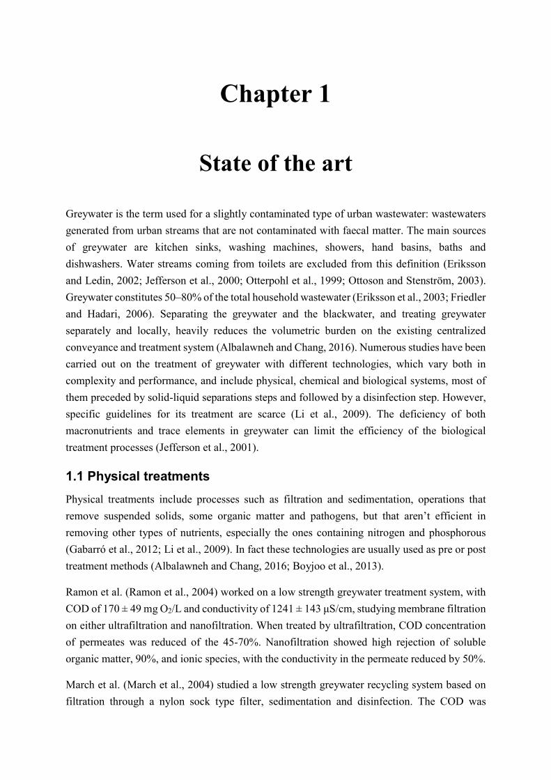
Introduction
Water is an essential resource for living organisms. Its scarcity, that is the lack of sufficient
available water resources, has become one of the main problems to face in the XXI century.
There is enough fresh water, but it is distributed unevenly and too much of it is wasted, polluted
and unsustainably managed. Wastewater treatment and reuse are becoming an essential field of
research. The treatment of greywater, the term used for a slightly polluted urban wastewater,
originating for example from showers, kitchen sinks and washing machines, is getting more
and more attention: separate it from blackwater, and treat it locally, can significantly reduce the
volumetric load on wastewater plants and its reuse for non-potable purpose can heavily reduce
potable water consumption. The small load of nutrients of greywater often cause difficulties in
their removal, especially for the nitrogen species and phosphorous.
This thesis is based on the study of two treatment technologies, in order to develop a process
suitable in treating greywater: the sequential batch reactor, studied in various project, and the
sequential batch biofilm reactor, that has never been used alone for this issue. In this project,
the main pollutants that were monitored are chemical oxygen demand (COD), total nitrogen,
ammonium, nitrates and nitrites. Parameters as pH and conductivity were monitored as well.
The experiments were performed in the laboratories of Institut Químic de Sarrià (IQS), a
department of the University Ramón Llull in Barcelona. The modeling was performed in the
Industrial Engineering department of the University of Padova.
The thesis is structured in four chapters.
The first chapter is a review of the main technologies used nowadays in order to treat greywater,
lingering on biological processes. Numerous literature articles are quoted and illustrated, in
order to obtain a smattering on this subject.
In the second chapter, it is listed the equipment employed in the thesis, the analytical methods
performed, the biological reactors operated and the operative procedures used in order to carry
out the experiments.
The third chapter presents the experimental results, showing the trends of the different reactors
run, analysing them, and comparing their different behaviours.
The fourth chapter is about modeling. Using the experimental data collected during the
treatment cycles, the rates of the reaction involved in the treatment processes have been
modelled using Matlab.

Chapter 1
State of the art
Greywater is the term used for a slightly contaminated type of urban wastewater: wastewaters
generated from urban streams that are not contaminated with faecal matter. The main sources
of greywater are kitchen sinks, washing machines, showers, hand basins, baths and
dishwashers. Water streams coming from toilets are excluded from this definition (Eriksson
and Ledin, 2002; Jefferson et al., 2000; Otterpohl et al., 1999; Ottoson and Stenström, 2003).
Greywater constitutes 50–80% of the total household wastewater (Eriksson et al., 2003; Friedler
and Hadari, 2006). Separating the greywater and the blackwater, and treating greywater
separately and locally, heavily reduces the volumetric burden on the existing centralized
conveyance and treatment system (Albalawneh and Chang, 2016). Numerous studies have been
carried out on the treatment of greywater with different technologies, which vary both in
complexity and performance, and include physical, chemical and biological systems, most of
them preceded by solid-liquid separations steps and followed by a disinfection step. However,
specific guidelines for its treatment are scarce (Li et al., 2009). The deficiency of both
macronutrients and trace elements in greywater can limit the efficiency of the biological
treatment processes (Jefferson et al., 2001).
1.1 Physical treatments
Physical treatments include processes such as filtration and sedimentation, operations that
remove suspended solids, some organic matter and pathogens, but that aren’t efficient in
removing other types of nutrients, especially the ones containing nitrogen and phosphorous
(Gabarró et al., 2012; Li et al., 2009). In fact these technologies are usually used as pre or post
treatment methods (Albalawneh and Chang, 2016; Boyjoo et al., 2013).
Ramon et al. (Ramon et al., 2004) worked on a low strength greywater treatment system, with
COD of 170 ± 49 mg O2/L and conductivity of 1241 ± 143 μS/cm, studying membrane filtration
on either ultrafiltration and nanofiltration. When treated by ultrafiltration, COD concentration
of permeates was reduced of the 45-70%. Nanofiltration showed high rejection of soluble
organic matter, 90%, and ionic species, with the conductivity in the permeate reduced by 50%.
March et al. (March et al., 2004) studied a low strength greywater recycling system based on
filtration through a nylon sock type filter, sedimentation and disinfection. The COD was
4 Chapter 1
reduced from 171 ± 130 to 78 ± 30 mg O2/L, and the total nitrogen was reduced from 11.4 ±
9.4 to 7.1 ± 2.99 mg N/L with average removal percentages, respectively, of 54.4% and 37.7%.
Gross et al. (Gross et al., 2008) tested the performance of seven commercial greywater
treatment systems, three of them being filtration systems: treatment of laundry effluent by
filtration with a 130 μm net, treatment of bath and shower effluent by tuff filter, treatment of
greywater by sand filtration and electrolysis. Total nitrogen was removed from 18, 16 and 10
mg N/L to 10, 15 and 5.7 mg N/L, with average removal percentages of 44.44%, 6.25% and
43% respectively.
Li et al. (Li et al., 2008) evaluated the performance and suitability of a submerged spiral wound
module system, equipped with a ultrafiltration membrane. This study showed that with a
permeate flux between 6 and 10 L/m2h the total organic carbon was reduced from 161 to 28.6
mg/L, but soluble nutrients like ammonia totally passed through the membrane, thus remaining
in the permeate.
Finley et al. (Finley et al., 2009) performed a study on the filtration of shower and washing
machine greywater. A primary settling stage with a hydraulic retention time of 8 h was followed
by a coarse filtration and a slow sand filtration, with a retention time of 24 h. The influent COD
concentration, range 278–435 mg O2/L, was changed to a range of 161–348 mg O2/L in the
influent, while the ammonia-N concentration passed from 1.2–6.2 to 4.1–5.1 mg NH4+-N/L.
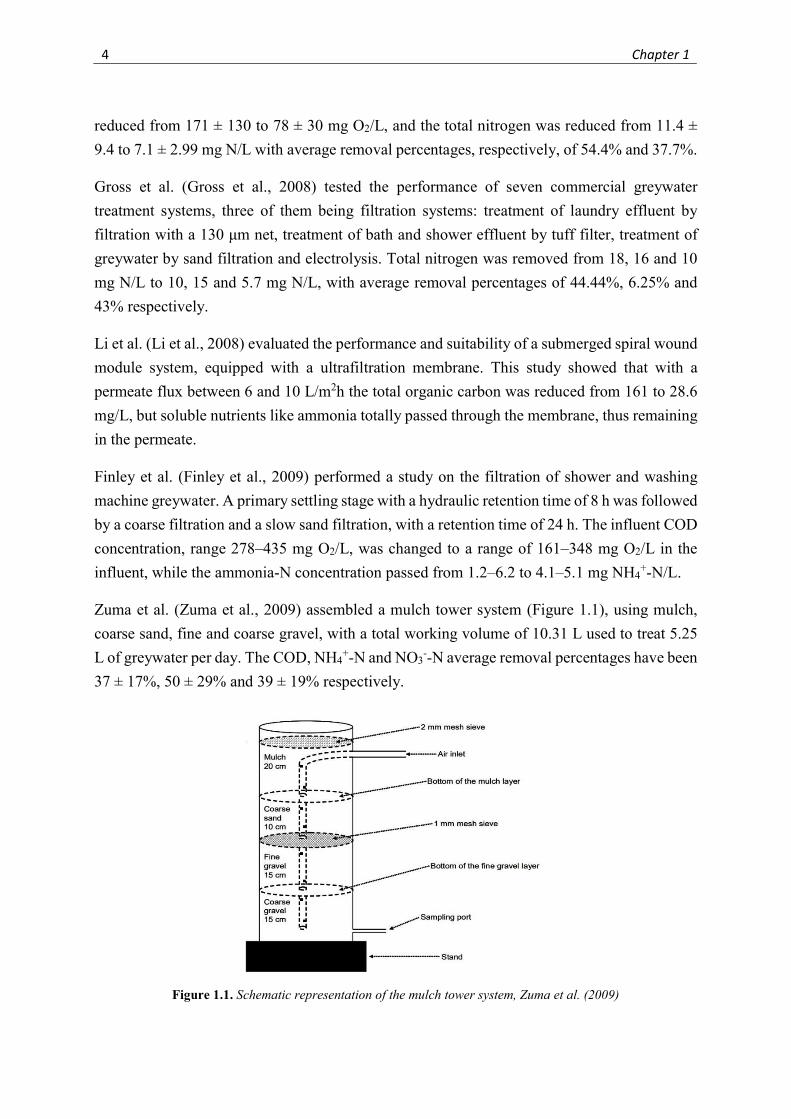
Zuma et al. (Zuma et al., 2009) assembled a mulch tower system (Figure 1.1), using mulch,
coarse sand, fine and coarse gravel, with a total working volume of 10.31 L used to treat 5.25
L of greywater per day. The COD, NH4+-N and NO3
--N average removal percentages have been
37 ± 17%, 50 ± 29% and 39 ± 19% respectively.
Figure 1.1. Schematic representation of the mulch tower system, Zuma et al. (2009)
State of the art 5
Al-Hamaideh and Bino (Al-hamaiedeh and Bino, 2010) studied a four barrels filtration unit in
order to treat greywater rich of organic matter. The average COD, total nitrogen and
conductivity of the influent was respectively 1712 ± 592 mg O2/L, 52 ± 30 mg N/L and 1830
μS/cm. These values were reduced in the effluent to respectively 489 ± 124 mg O2/L, 11 ± 3
mg N/L and 1760 μS/cm with average removals percentages of 71.44% for the COD and
78.85% for the total nitrogen.
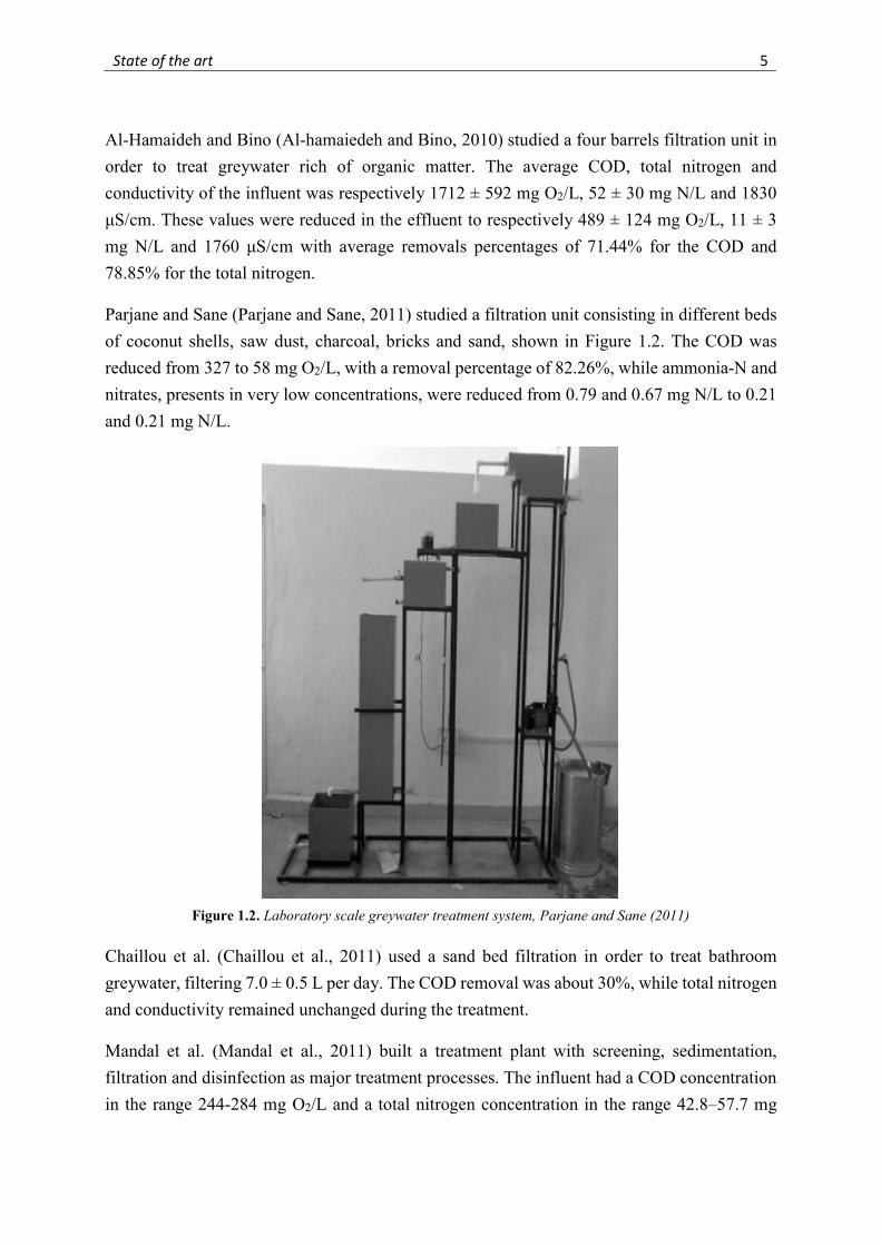
Parjane and Sane (Parjane and Sane, 2011) studied a filtration unit consisting in different beds
of coconut shells, saw dust, charcoal, bricks and sand, shown in Figure 1.2. The COD was
reduced from 327 to 58 mg O2/L, with a removal percentage of 82.26%, while ammonia-N and
nitrates, presents in very low concentrations, were reduced from 0.79 and 0.67 mg N/L to 0.21
and 0.21 mg N/L.
Figure 1.2. Laboratory scale greywater treatment system, Parjane and Sane (2011)
Chaillou et al. (Chaillou et al., 2011) used a sand bed filtration in order to treat bathroom
greywater, filtering 7.0 ± 0.5 L per day. The COD removal was about 30%, while total nitrogen
and conductivity remained unchanged during the treatment.
Mandal et al. (Mandal et al., 2011) built a treatment plant with screening, sedimentation,
filtration and disinfection as major treatment processes. The influent had a COD concentration
in the range 244-284 mg O2/L and a total nitrogen concentration in the range 42.8–57.7 mg
6 Chapter 1
N/L. The removal percentage of COD and total nitrogen varied respectively in a range between
50–70% and 9–35%.
Albalawneh et al. (Albalawneh et al., 2017) studied the performance of various granular
filtration systems, using volcanic tuff and gravel. The average COD removal percentage was
65% for the tuff filtration and 51 % for the gravel filtration, but with both technologies there
was a significant increase in the electrical conductivity, due to the dissolution of various ions.
1.2 Chemical treatments
The chemical treatment of greywater is getting more and more attention (Boyjoo et al., 2013).
Chemical processes used include coagulation, ion exchange, flocculation, absorption using
granular activated carbon and natural zeolites, and oxidation processes such as ozonation,
photocatalysis and ultraviolet C combined with H2O2. These processes, followed by a filtration
and/or a disinfection stage, can reduce the suspended solids, organic substances and surfactants
in low strength greywater to an acceptable level, which can meet non-potable urban reuse needs
(Albalawneh and Chang, 2016; Lin et al., 2005; Pidou et al., 2008). For medium and high
strength greywater, the chemical-treated water is not always able to meet the standards, unless
these processes are combined with other ones (Albalawneh and Chang, 2016; Li et al., 2009;
Pidou et al., 2008), for example as a final treatment step, following biological treatment (Boyjoo
et al., 2013).
Sostar-Turk et al. (Sostar-Turk et al., 2005) used coagulation followed by adsorption on
granular activated carbon in order to treat laundry greywater. The influent was flocculated with
Al3+ and filtered through a sand bed, with the COD concentration reduced from 280 to 180 mg
O2/L. After passing through the adsorption column the effluent COD was 20 mg O2/L, with a
total treatment time of 38 minutes. The content of ammonia and total nitrogen remained the
same during the treatment.
Friedler et al. (Friedler et al., 2008) used a combination of coagulation and chlorination as a
pre-treatment step for low strength greywater treatment with ultrafiltration and reverse osmosis,
with a reduction of the total organic carbon of 24% and the total nitrogen of 2%.
Pidou et al. (Pidou et al., 2008) studied coagulation, magnetic ion exchange resin and
combinations between these technologies in the treatment of low strength and medium strength
greywater for reuse. The results obtained revealed that such systems were suitable for low
strength greywater sources. However, they were unable to achieve the required level of
treatment of medium to high strength greywaters. Treating shower greywater with average
COD of 791 mg O2/L, total nitrogen concentration of 18 mg N/L, ammonia concentration of
1.2 mg NH4+-N/L and nitrates concentration of 6.7 mg NO3
--N/L, the resulting effluent of the
State of the art 7
optimum combination of magnetic ion exchange membrane with coagulation using Al3+, had
average COD of 247 mg O2/L, total nitrogen concentration of 15.3 mg N/L, ammonia
concentration of 1.2 mg NH4+-N/L and nitrates concentration of 4.4 mg NO3
--N/L, reaching
average removal percentage of respectively 69%, 15%, 0% and 34%.
Ciabatti et al. (Ciabatti et al., 2009) experimented a system consisting of coagulation,
flocculation, sand filtration, ozonation, granular activated carbon filtration and cross-flow
ultrafiltration, in order to purify the low strength greywater from an industrial laundry. The
outlet of the granular activated carbon filter in the combined system had an average COD of
140 mg O2/L, ammonia nitrogen of 0.13 mg NH4+-N/L and conductivity of 1275 μS/cm. With
average influent values of 602 mg O2/L, 1.8 mg NH4+-N/L and 1342 μS/cm, an average removal
of 77% for the COD, 93% for the ammonia and a reduction of 5% for the conductivity was
achieved.
Photocatalytic oxidation with titanium dioxide has been used in various studies, especially as a
post-treatment step after biological treatments (Gulyas, 2007; Li et al., 2003). Sanchez et al.
(Sanchez et al., 2010) used this technology in order to treat low strength hotel greywater, low
and high strength laundry greywater, monitoring the dissolved organic carbon. The average
reduction of the dissolved organic carbon of the hotel greywater was 65%, with an effluent
concentration of 10.31 mg/L, while for the high strength laundry greywater it was 44%, with
an effluent concentration of 709.5 mg/L, showing that this technology alone is not sufficient.
1.3 Biological treatments
Several biological treatment systems have been applied for greywater treatment, including
constructed wetland (CW), up-flow anaerobic sludge blanket (UASB), membrane bioreactor
(MBR), rotating biological contactor (RBC), moving bed bioreactor (MBBR), sequencing batch
reactor (SBR).
CW is a technology designed to exploit ecological processes found in natural wetland
ecosystems (Ghaitidak and Yadav, 2013). These systems utilize wetland plants, soil, and
associated microorganisms to remove contaminants from wastewater, a removal which occurs
by physical, chemical and biological processes. Gross et al. (Gross et al., 2007) developed a
system based on a combination of a vertical flow constructed wetland with water recycling and
trickling filter. The greywater COD and total nitrogen concentration were reduced from 839 ±
47 mg O2/L and 34.3 ± 2.6 mg N/L to 157 ± 62 mg O2/L and 10.8 ± 3.4 mg N/L, reaching
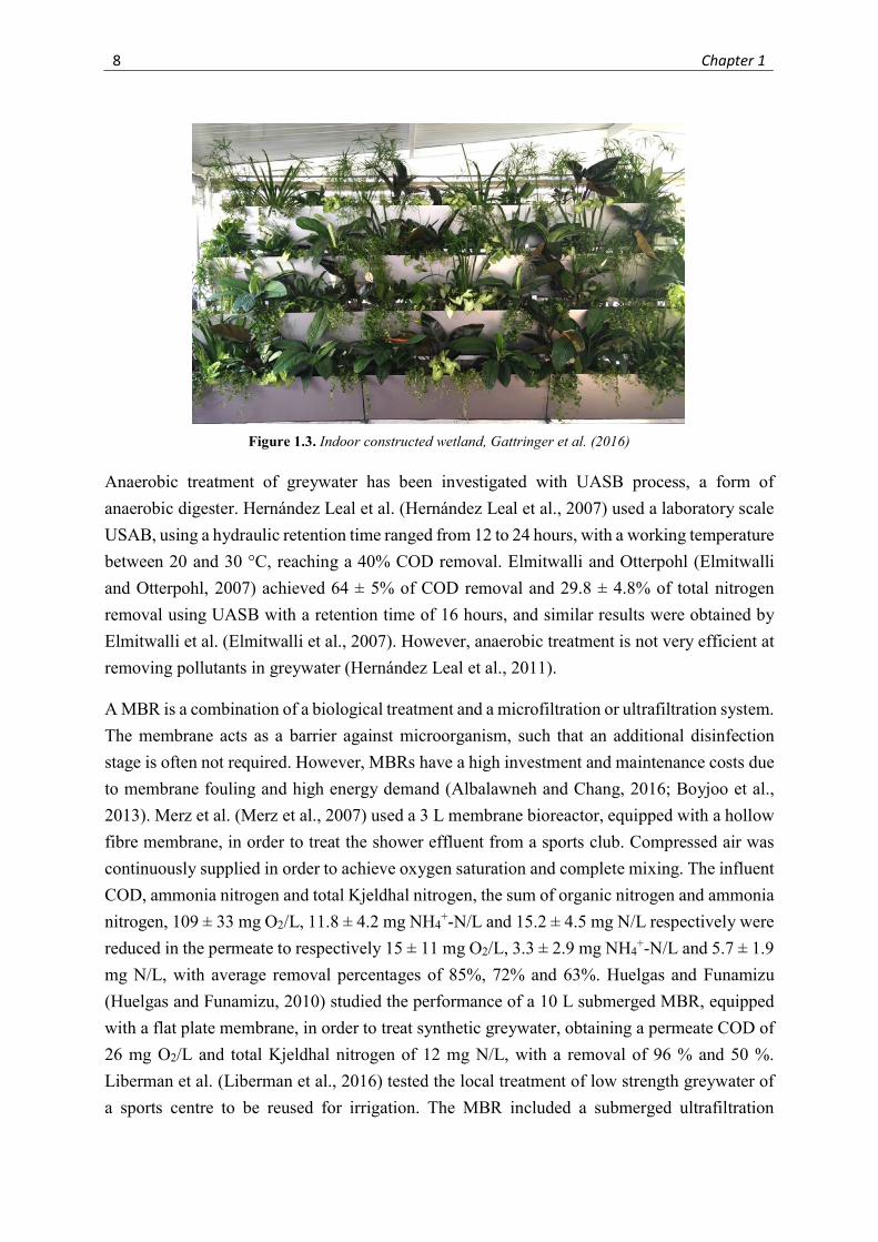
average removal percentages of 81% and 69% respectively in a 12 h treatment cycle. Gattringer
et al. (Gattringer et al., 2016) studied an indoor constructed wetland (Figure 1.3) in order to
treat 1 cubic meter per day of greywater from a hotel. The average removal percentage have
been 96.6% for COD, 96.6% for ammonium and 74.0% for total nitrogen.
8 Chapter 1
Figure 1.3. Indoor constructed wetland, Gattringer et al. (2016)
Anaerobic treatment of greywater has been investigated with UASB process, a form of
anaerobic digester. Hernández Leal et al. (Hernández Leal et al., 2007) used a laboratory scale
USAB, using a hydraulic retention time ranged from 12 to 24 hours, with a working temperature
between 20 and 30 °C, reaching a 40% COD removal. Elmitwalli and Otterpohl (Elmitwalli
and Otterpohl, 2007) achieved 64 ± 5% of COD removal and 29.8 ± 4.8% of total nitrogen
removal using UASB with a retention time of 16 hours, and similar results were obtained by
Elmitwalli et al. (Elmitwalli et al., 2007). However, anaerobic treatment is not very efficient at
removing pollutants in greywater (Hernández Leal et al., 2011).
A MBR is a combination of a biological treatment and a microfiltration or ultrafiltration system.
The membrane acts as a barrier against microorganism, such that an additional disinfection
stage is often not required. However, MBRs have a high investment and maintenance costs due
to membrane fouling and high energy demand (Albalawneh and Chang, 2016; Boyjoo et al.,
2013). Merz et al. (Merz et al., 2007) used a 3 L membrane bioreactor, equipped with a hollow
fibre membrane, in order to treat the shower effluent from a sports club. Compressed air was
continuously supplied in order to achieve oxygen saturation and complete mixing. The influent
COD, ammonia nitrogen and total Kjeldhal nitrogen, the sum of organic nitrogen and ammonia
nitrogen, 109 ± 33 mg O2/L, 11.8 ± 4.2 mg NH4+-N/L and 15.2 ± 4.5 mg N/L respectively were
reduced in the permeate to respectively 15 ± 11 mg O2/L, 3.3 ± 2.9 mg NH4+-N/L and 5.7 ± 1.9
mg N/L, with average removal percentages of 85%, 72% and 63%. Huelgas and Funamizu
(Huelgas and Funamizu, 2010) studied the performance of a 10 L submerged MBR, equipped
with a flat plate membrane, in order to treat synthetic greywater, obtaining a permeate COD of
26 mg O2/L and total Kjeldhal nitrogen of 12 mg N/L, with a removal of 96 % and 50 %.
Liberman et al. (Liberman et al., 2016) tested the local treatment of low strength greywater of
a sports centre to be reused for irrigation. The MBR included a submerged ultrafiltration
State of the art 9
module, supplied with air in steps of 1 minute every 6 minutes. The percentages of COD and
ammonium removal were respectively 97% and 98%, but only low degree of denitrification
could be achieved. Atanasova et al. (Atanasova et al., 2017) study on a MBR showed a high
removal percentage of COD from hotel greywater but poor ammonium and total nitrogen
reductions.
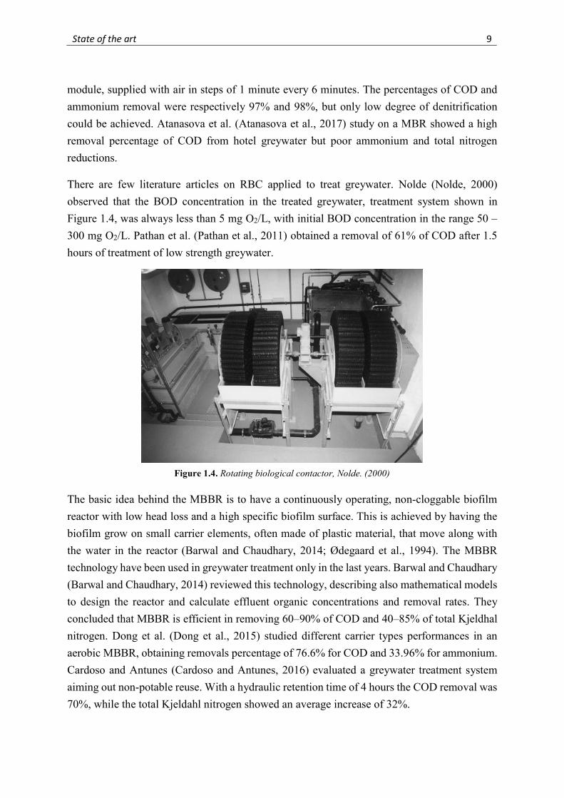
There are few literature articles on RBC applied to treat greywater. Nolde (Nolde, 2000)
observed that the BOD concentration in the treated greywater, treatment system shown in
Figure 1.4, was always less than 5 mg O2/L, with initial BOD concentration in the range 50 –
300 mg O2/L. Pathan et al. (Pathan et al., 2011) obtained a removal of 61% of COD after 1.5
hours of treatment of low strength greywater.
Figure 1.4. Rotating biological contactor, Nolde. (2000)
The basic idea behind the MBBR is to have a continuously operating, non-cloggable biofilm
reactor with low head loss and a high specific biofilm surface. This is achieved by having the
biofilm grow on small carrier elements, often made of plastic material, that move along with
the water in the reactor (Barwal and Chaudhary, 2014; Ødegaard et al., 1994). The MBBR
technology have been used in greywater treatment only in the last years. Barwal and Chaudhary
(Barwal and Chaudhary, 2014) reviewed this technology, describing also mathematical models
to design the reactor and calculate effluent organic concentrations and removal rates. They
concluded that MBBR is efficient in removing 60–90% of COD and 40–85% of total Kjeldhal
nitrogen. Dong et al. (Dong et al., 2015) studied different carrier types performances in an
aerobic MBBR, obtaining removals percentage of 76.6% for COD and 33.96% for ammonium.
Cardoso and Antunes (Cardoso and Antunes, 2016) evaluated a greywater treatment system
aiming out non-potable reuse. With a hydraulic retention time of 4 hours the COD removal was
70%, while the total Kjeldahl nitrogen showed an average increase of 32%.
10 Chapter 1
1.3.1 SBR technology
The sequencing batch reactor is a batch fill-and-draw activated sludge system, that can be
composed of one or more tanks. Each vessel has five basic operating modes, that are fill, react,
settle, draw, and idle (Irvine and Busch, 1979; Puig Broch, 2008). This permits to avoid settling
tanks, an equipment that needs a large surface for being operated (Barwal and Chaudhary, 2014)
and is necessary in generic activated sludge processes, saving space and decreasing installation
cost. In addition, this type of reactor allows the use of sequencing anoxic, anaerobic and aerobic
phases, that are usually consecutive but can also be alternated in cycles, in order to perform the
removal of different pollutants in the same tank (Sowinska and Makowska, 2016). The time for
a complete treatment cycle is the total time between the beginning of fill to the end of the idle.
Lee et al. (Lee et al., 2001) used an anaerobic-aerobic-anoxic-aerobic SBR in order to study the
biological nitrogen removal in high C:N ratio synthetic wastewater, in cycles of 8 hours,
obtaining average removal percentages of 92% for COD and 88% for the total nitrogen.
Lamine et al. (Lamine et al., 2007) is one of the first studies on greywater treatment using a
SBR. The low strength greywater, with COD 102 ± 86 mg O2/L, ammonium nitrogen 6.7 ± 5.6
mg NH4+-N/L and total Kjeldahl nitrogen 8.1 ± 3.7 mg N/L, was treated with an SBR with
cycles consisting in 30 minutes of feed, 5 hours of anoxic phase, 5 hours of aerobic phase, 1
hour of settling and 30 minutes of draw. The removal of ammonium was poor, 7.5%, so the
hydraulic retention time was increased to 2.5 days, obtaining removal percentages of 80% for
the COD and 95% for the ammonium, but with no denitrification.
Blackburne et al. (Blackburne et al., 2008) studied the performance of a SBR with 3 hours of
cycle length, consisting in 80 minutes anoxic fill, 105 minutes aerobic react, settling and
discharge, treating high strength domestic greywater with a mean C:N ratio of 9. An average
removal percentage of 77.5% for the total nitrogen was achieved, together with an ammonium
removal over 95%.
Gabarró et al. (Gabarró et al., 2012) investigated the applicability of SBR technology to on-site
greywater treatment in a sports centre for reuse in irrigation. Two 500 L SBR working in
parallel were used, one seeded with sludge from an urban wastewater treatment plant, the
second one not seeded. The low strength greywater, 110 ± 58 mg O2/L of COD, 20.95 ± 10.05
mg NH4+-N/L of ammonium and 27.17 ± 10.04 mg N/L of total Kjeldhal nitrogen, was treated
using 24 hours cycles. In the first part of the study a sequence of anaerobic and aerobic phases
of 1 hour each were applied in both reactors, as long as a step-feed strategy, feeding 50% of the
water at the beginning of the cycle and 50% after 2 hours. After nitrification had been fully
achieved in both reactors the cycle was modified, starting with 5 hours of anoxic phase, in order
to improve denitrification efficiency. A removal of 60% of organic matter and 89% of
State of the art 11
ammonium was obtained in both reactors, while a poor denitrification caused the effluent to
remain above the limit of 15 mg N/L during most of the experimental run.
1.3.2 SBBR technology
Combining the SBR and the MBBR technology, another type of reactor can be implemented,
called sequencing batch biofilm reactor (SBBR). This technology combines the possibility of
sequential aerobic, anoxic and anaerobic phases, as long with the possibility of achieving a
treatment cycle in one vessel, with the biomass attached to carrier mediums. If the suspended
biomass is completely absent from the system, the settle phase is no longer needed (Hwang et
al., 2015). Guo et al. (Guo et al., 2014) studied a combination of a SBBR with a vertical
constructed wetland for the treatment of synthetic domestic wastewater. The SBBR was filled
with fibrous packing made from PVC, soft polyethylene and porous aggregates. The operation
cycle of 12 hours was divided into intermittent aeration and anaerobic period, that varied
through the experimental period from 1 to 2 hours each. The temperature was controlled at 30
°C. The effluent of the SBBR was fed to the CW, with another 12 hours treatment time. The
concentration changes of each parameter in the SBBR were as follows: COD from 276.20 to
50.89 mg O2/L, ammonium nitrogen from 79.25 to 13.10 mg NH4+-N/L and total nitrogen from
79.25 to 24.76 mg N/L with average removal percentages of 81%, 83% and 68%. At the end of
the treatment, at the outlet of the constructed wetland, the discharge concentration was 15.37
mg O2/L for COD, 1.85 mg NH4+-N/L for ammonium nitrogen and 9.90 mg N/L for the total
nitrogen, with average total removal percentages of respectively 94%, 98% and 87%. Other
studies on nutrients removal via SBBR are the one by Hai et al. (Hai et al., 2014), who treated
swine wastewater, C:N ratio of 11, using a SBBR with 3 hours of anaerobic phase and 7 hours
of aerobic phase cycling in a 24 hours cycle. The removals of COD, ammonia nitrogen and total
nitrogen obtained were respectively 98.2%, 95.7% and 95.6%, with effluent concentrations of
85.6 mg O2/L, 35.22 mg NH4+-N/L and 44.64 mg N/L. Hwang et al. (Hwang et al., 2015) used
an SBBR with 8 hours cycle time in order to treat the high ammonium containing filtrate
generated from the dewatering process in a wastewater treatment plant, helping the removal of
nitrogen with the addition of methanol and alkalinity. A removal percentage of nitrogen of 90%
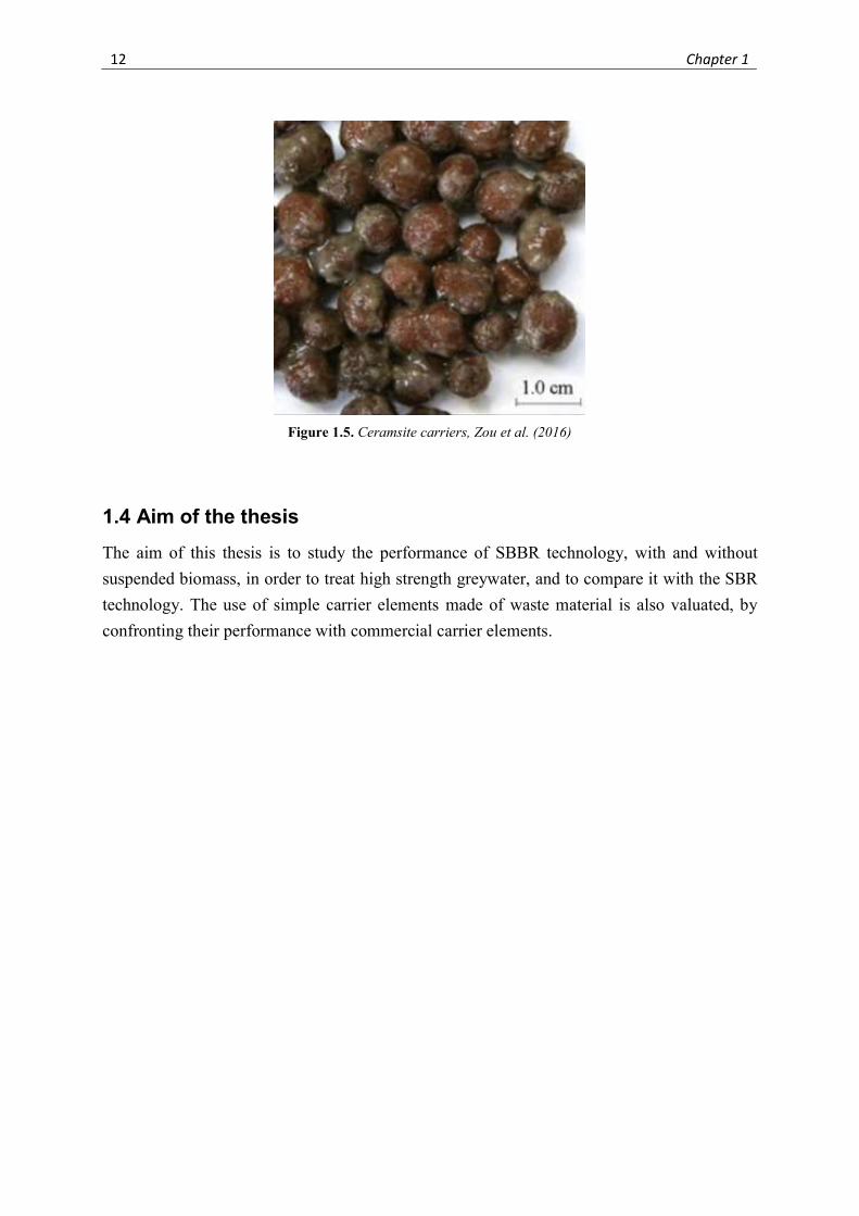
has been obtained during the experimental period. Zou et al. (Zou et al., 2016) tested a novel
SBBR in order to treat different C:N ratios, using ceramsite made of river sediment as biomass
carriers (Figure 1.5). The reactor was separated by a vertical clapboard in two parts. The
removals percentage for total nitrogen were 76.8%, 44.5% and 10.4% at C:N ratios respectively
of 9, 4.8 and 2.5.
12 Chapter 1
Figure 1.5. Ceramsite carriers, Zou et al. (2016)
1.4 Aim of the thesis
The aim of this thesis is to study the performance of SBBR technology, with and without
suspended biomass, in order to treat high strength greywater, and to compare it with the SBR
technology. The use of simple carrier elements made of waste material is also valuated, by
confronting their performance with commercial carrier elements.
Chapter 2
Materials and methods
2.1 Materials
2.1.1 Greywater
The greywater used in this work was prepared daily using tap water. The recipe was based on
previous literature (Abed and Scholz, 2016; Eriksson et al., 2009; Hernández Leal et al., 2007;
Hourlier et al., 2010; Jefferson et al., 2001), taking into account the great variability of the
composition of greywater, depending on the living habits of the people involved, the products
used and the nature of the installation (Eriksson and Ledin, 2002; Li et al., 2009). The
ingredients with their concentration are reported in the Table 2.1. As previous studies have
shown (J E Burgess et al., 1999; J. E. Burgess et al., 1999; Jefferson et al., 2001),
microorganisms in wastewater treatment require macronutrients for metabolic processes such
as carbon sources, oxygen, nitrogen, phosphorous, sulphur. They also need trace elements, for
example potassium and copper, that have an active role on the growth and activity of the
microorganisms. Deficiencies of micronutrients may be alleviated using supplements of the
required ionic species, to avoid the stoppage of the process that they activate, but an excess
dosage is also self-defeating, inhibiting the treatment of the wastewater (J. E. Burgess et al.,
1999) and causing toxicity to the cells (Jefferson et al., 2001). Studies stated that the
concentration of nutrients don’t show apparent limitation for the growth and proliferation of
microorganisms (Hernández Leal et al., 2007; Palmquist and Hanæus, 2005). In this study, a
concentrated solution of trace elements was added to the greywater, having into account
exceeding the typical concentrations found in greywater (J. E. Burgess et al., 1999; Hernández
Leal et al., 2007; Jefferson et al., 2001; Palmquist and Hanæus, 2005). The concentration of
microelements in the synthetic greywater is reported in Table 2.1. The main parameters of the
greywater are summarized in the Table 2.2.
14 Chapter 2
Table 2.1. Composition of the greywater
Parameter Source Unit Mean Standard deviation
Range
- Yeast extract mg/L 100.4 1.2 98.9-104.9 - Peptone mg/L 101.3 2.4 98.3 – 109.2
COD Fructose mg/L 78.0 131.8 28.7-604.5 P Sodium dihydrogen phosphate mg/L 15.7 43.7 0 – 165.3
NH4+-N Ammonium sulphate mg/L 183.7 2.0 178.2 – 188.4
NO3--N Sodium nitrate mg/L 42.43 1.7 38.8 – 47.7
- Vegetal oil μL/L 20.0 - - Ca Tap water mg/L >3 - - K KNO3 - KAl(SO4)2·12H2O mg/L 6 - - Fe Fe2(SO4)3 mg/L 0.2 - - Mg Tap water mg/L >5 - - Mn MnCl2·4H2O mg/L 0.02 - - Cu CuSO4·5H2O mg/L 0.02 - - Al KAl(SO4)2·12H2O mg/L 0.02 - - Zn ZnCl2 mg/L 0.2 - -
Table 2.2. Influent characteristics of the greywater
Parameter Unit Mean Standard deviation Range
COD mg/L 327.41 143.57 196.92 – 788.11 Total nitrogen mg/L 80.48 4.33 73.83 – 88.09
NH4+-N mg/L 40.85 5.78 31.60 – 51.30
NO3-N mg/L 21.18 2.94 15.98 - 23.97 NO2-N mg/L 1.87 1.86 0 – 5.53
pH - 7.52 0.13 7.30 – 7.72
Conductivity μS/cm 2118 21 2075 - 2150
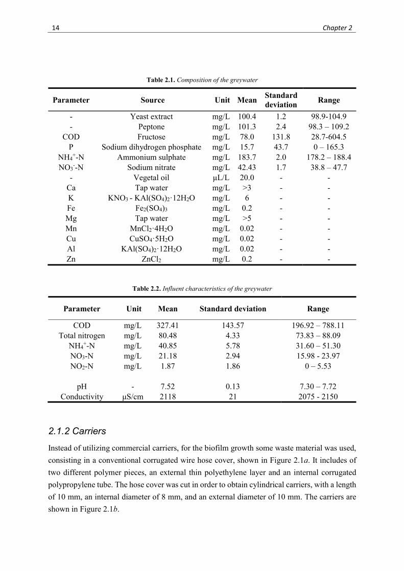
2.1.2 Carriers
Instead of utilizing commercial carriers, for the biofilm growth some waste material was used,
consisting in a conventional corrugated wire hose cover, shown in Figure 2.1a. It includes of
two different polymer pieces, an external thin polyethylene layer and an internal corrugated
polypropylene tube. The hose cover was cut in order to obtain cylindrical carriers, with a length
of 10 mm, an internal diameter of 8 mm, and an external diameter of 10 mm. The carriers are
shown in Figure 2.1b.
Materials and methods 15
(a)
(b)
Figure 2.1. (a) Corrugated wire hose cover (b) Carriers
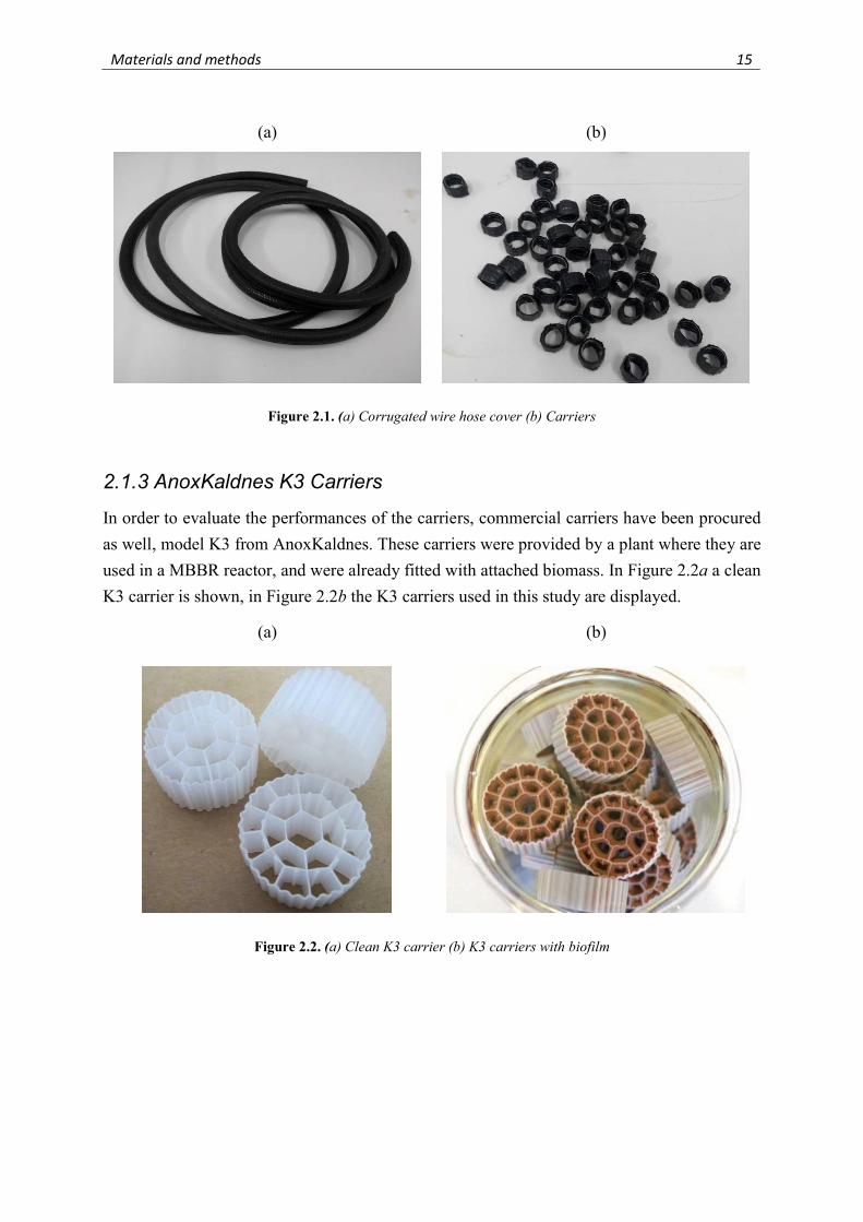
2.1.3 AnoxKaldnes K3 Carriers
In order to evaluate the performances of the carriers, commercial carriers have been procured
as well, model K3 from AnoxKaldnes. These carriers were provided by a plant where they are
used in a MBBR reactor, and were already fitted with attached biomass. In Figure 2.2a a clean
K3 carrier is shown, in Figure 2.2b the K3 carriers used in this study are displayed.
(a)
(b)
Figure 2.2. (a) Clean K3 carrier (b) K3 carriers with biofilm
16 Chapter 2
2.2 Equipment
2.2.1 Reactor I
(a)
(b)
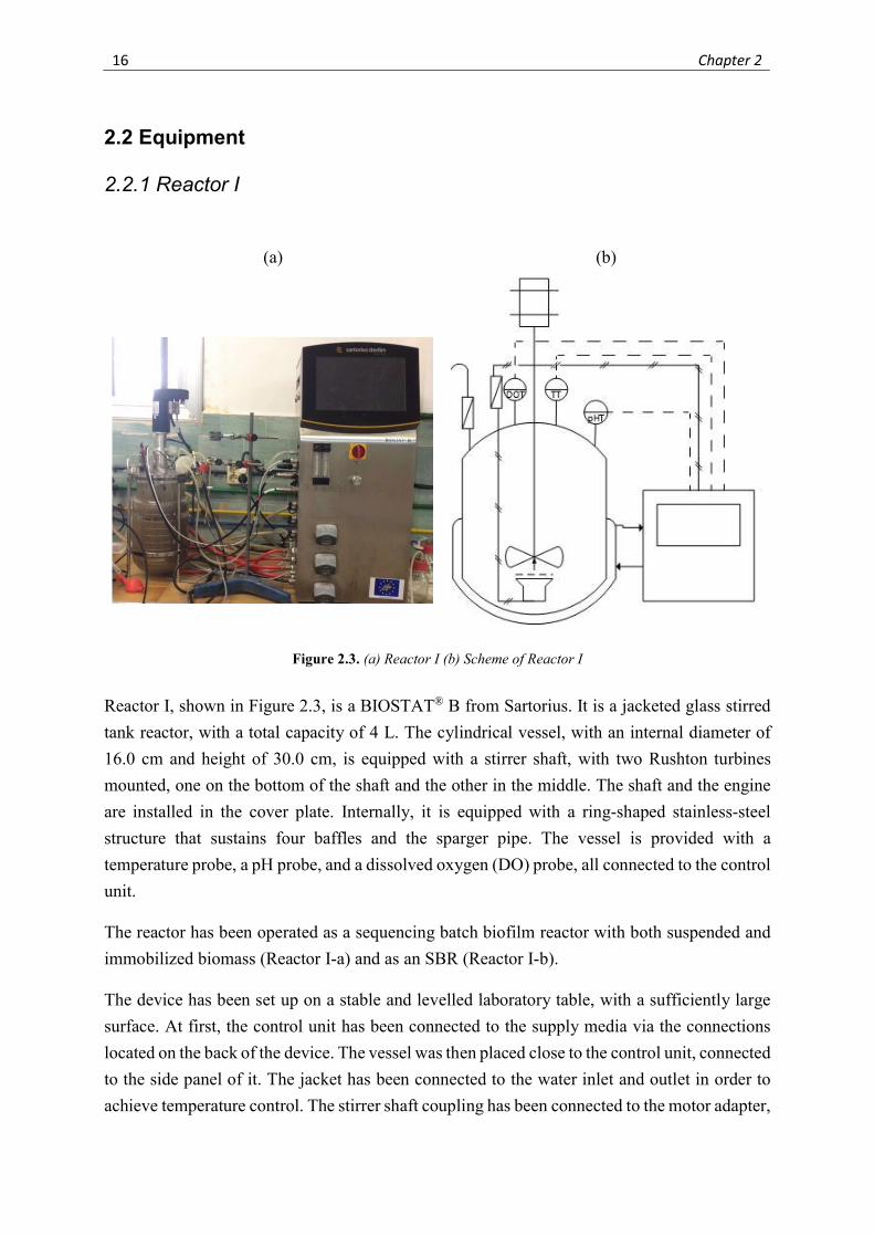
Figure 2.3. (a) Reactor I (b) Scheme of Reactor I
Reactor I, shown in Figure 2.3, is a BIOSTAT® B from Sartorius. It is a jacketed glass stirred
tank reactor, with a total capacity of 4 L. The cylindrical vessel, with an internal diameter of
16.0 cm and height of 30.0 cm, is equipped with a stirrer shaft, with two Rushton turbines
mounted, one on the bottom of the shaft and the other in the middle. The shaft and the engine
are installed in the cover plate. Internally, it is equipped with a ring-shaped stainless-steel
structure that sustains four baffles and the sparger pipe. The vessel is provided with a
temperature probe, a pH probe, and a dissolved oxygen (DO) probe, all connected to the control
unit.
The reactor has been operated as a sequencing batch biofilm reactor with both suspended and
immobilized biomass (Reactor I-a) and as an SBR (Reactor I-b).
The device has been set up on a stable and levelled laboratory table, with a sufficiently large
surface. At first, the control unit has been connected to the supply media via the connections
located on the back of the device. The vessel was then placed close to the control unit, connected
to the side panel of it. The jacket has been connected to the water inlet and outlet in order to
achieve temperature control. The stirrer shaft coupling has been connected to the motor adapter,
Materials and methods 17
and the motor to the control unit. The pressurized air was distributed by a sparger, connected
using a silicon hose, placing a PTFE filter before the sparger. Temperature, dissolved oxygen
and pH probes have been located in the cover plate and linked to the control unit.
2.2.1.1 Tempering media
Water is used as tempering medium for the device for the temperature control of the vessel and
as cooling liquid of the exhaust cooler. The unit has been connected to the water line of the
laboratory. The jacket of the vessel was then filled activating the temperature control.
2.2.1.2 Gas supply
The device has been connected to the pressurized air line located in the laboratory. A
manometer and a valve have been installed before the connection, to ensure that the pressure
did not pass the maximum pressure suggested in the device manual, 1.5 barg.
2.2.1.3 Correction media
The vessel has been connected to two correction medium bottles, one filled with a solution of
NaOH 1 N, the other one with a solution of H2SO4 1 N, used to control the pH of the vessel.
These are glass bottles, with a stainless-steel top with hose couplings and seal, located in the
top of the storage bottle and held in place by a screw cap. A PTFE riser pipe works as barrel
sampler, a filter is placed on the cap to allow ventilation and equalizing the pressure when the
correction medium is removed. A silicon hose was then used to connect the bottles to the
vessel, fitting them into the peristaltic pumps located in the front of the control unit.
2.2.1.4 Calibration of the dissolved oxygen probe
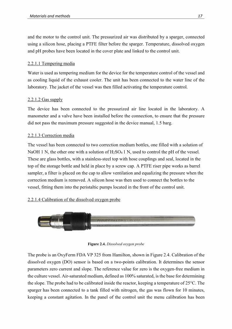
The probe is an OxyFerm FDA VP 325 from Hamilton, shown in Figure 2.4. Calibration of the
dissolved oxygen (DO) sensor is based on a two-points calibration. It determines the sensor
parameters zero current and slope. The reference value for zero is the oxygen-free medium in
the culture vessel. Air-saturated medium, defined as 100% saturated, is the base for determining
the slope. The probe had to be calibrated inside the reactor, keeping a temperature of 25°C. The
sparger has been connected to a tank filled with nitrogen, the gas was flown for 10 minutes,
keeping a constant agitation. In the panel of the control unit the menu calibration has been
Figure 2.4. Dissolved oxygen probe
18 Chapter 2
selected, then the zero has been determined while nitrogen was still flowing through the vessel.
The determination was stopped when the measurement reached a stable value of current. The
vessel was then connected to the air outlet of the control unit, and was aerated for 15 minutes
more. The saturation value, and so the slope, was then measured with the same procedure.
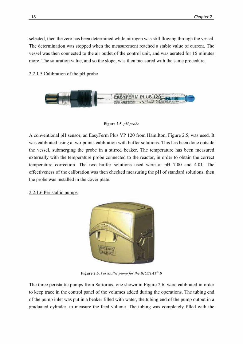
2.2.1.5 Calibration of the pH probe
A conventional pH sensor, an EasyFerm Plus VP 120 from Hamilton, Figure 2.5, was used. It
was calibrated using a two-points calibration with buffer solutions. This has been done outside
the vessel, submerging the probe in a stirred beaker. The temperature has been measured
externally with the temperature probe connected to the reactor, in order to obtain the correct
temperature correction. The two buffer solutions used were at pH 7.00 and 4.01. The
effectiveness of the calibration was then checked measuring the pH of standard solutions, then
the probe was installed in the cover plate.
2.2.1.6 Peristaltic pumps
The three peristaltic pumps from Sartorius, one shown in Figure 2.6, were calibrated in order
to keep trace in the control panel of the volumes added during the operations. The tubing end
of the pump inlet was put in a beaker filled with water, the tubing end of the pump output in a
graduated cylinder, to measure the feed volume. The tubing was completely filled with the
Figure 2.5. pH probe
Figure 2.6. Peristaltic pump for the BIOSTAT® B
Materials and methods 19
water, switching on the pump manually. The calibration mode was then selected, leaving the
pump working for 5 minutes and entering the feed volume at the end. The DCU system
calculated the pumping rate automatically from the internally recorded pump run time and the
pumped amount measured.
2.2.1.7 Tuning of the temperature controller
The temperature controller from Sartorius, integrated in the BIOSTAT® B, is implemented as a
cascade system: the master controller, TEMP, receives the signal from the temperature probe
in the reactor, the set-point being given by the operator. The slave controller. JTEMP, receives
the signal from the temperature transmitter inside the control unit, that measures the temperature
of the water outlet of the jacket, the set-point is given by the master controller, or by the user if
TEMP is in manual mode.
The first tuning operation was done on the slave controller, operating the master controller in
manual mode. It was chosen to maintain only a proportional action and the tuning was done
directly on-field. A positive step-change of 5°C in the set-point was applied, returning to the
original one as soon as a new steady state was reached. The operation was repeated changing
the value of the controller gain, expressed in the control panel as proportional band (PB). The
default PB value was 4%, and it was slowly decreased to speed up the control loop, choosing
the value of the PB that gave the faster but still stable response, PB = 2%.
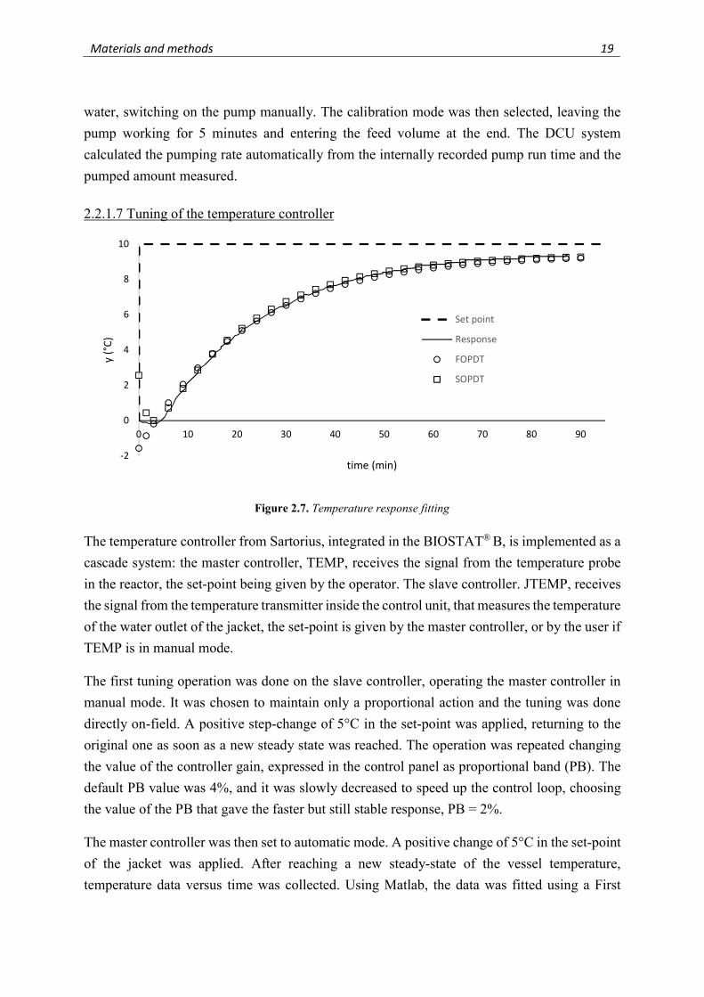
The master controller was then set to automatic mode. A positive change of 5°C in the set-point
of the jacket was applied. After reaching a new steady-state of the vessel temperature,
temperature data versus time was collected. Using Matlab, the data was fitted using a First
Figure 2.7. Temperature response fitting
-2
0
2
4
6
8
10
0 10 20 30 40 50 60 70 80 90
y (°
C)
time (min)
Set point
Response
FOPDT
SOPDT
20 Chapter 2
Order Plus Dead Time (FOPDT) model and a Second Order Plus Dead Time (SOPDT) model.
The FOPDT model was enough representative for the process and has been chosen. The
resulting plot is shown in Figure 2.7. The values of the process gain KT, of the dead time θT and
of the process time constant τT have been used in the Internal Model Control (IMC) model, in
order to obtain the parameters of a PID controller with an assigned tuning, so the values of the
controller gain, expressed as PB, the integral time τI and the derivative time τD were set. These
values, using a rule of thumb, were reduced to the 75% of the initial value due to the presence
of the cascade loop that makes the system more stable and fast, then they were slightly adjusted
on-field, obtaining final values of PB = 15.0 %, τI = 600 s, τD = 200 s.
2.2.1.8 Tuning of the pH controller
The pH controller from Sartorius is a simple feedback controller. It controls correction medium
pumps for acid and bases, using pulse-width modulated outputs. It doesn’t activate the control
signal until the control deviation is located outside of a configurable dead band, preventing
unnecessary electrolytes proportioning. For the tuning, a PI action was chosen. The proportional
band and the integral time suggested in the reactor manual were too aggressive for the desired
tuning, so their values for the first trial were selected consulting the literature and entered as PB
= 100 % and τI = 100 s, setting a dead band of 0.50 pH units. The correction medium bottles
were filled, one with a solution of NaOH 1 N, one with a solution of H2SO4 1 N. The aeration
was then activated, in order to perturbate the pH of the water in the vessel. The pH controller
was turned in automatic mode. On the first hour of operation the controller response was
satisfying, then it started to show an oscillatory behaviour with increasing amplitude. The gain
was then slowly reduced, without obtaining the stabilization of the system. The buffer solutions
were then diluted 1:10, in order to avoid sharp changes of the pH. With a trial and error
procedure, with positive and negative step-changes to the set-point, the final values of the
parameters were obtained, keeping a slow but smooth response: PB = 200 %, τI = 150 s.
2.2.1.9 Operative conditions
Biological processes in SBR and SBBR technologies are conducted following a sequence of
different conditions. Common practice is executing a predefined cycle over time. In this study,
a cycle duration of 24 hours has been chosen, due to the limitations of the type of wastewater
treated, with a carbon-nitrogen ratio not optimal for the removal of nitrogen (Puig Broch, 2008).
The bioreactor has a programmable aeration profile, with a maximum of 30 different set-points
that can be entered. It was chosen to work alternating aerobic and anaerobic phases, each one
of 1.5 hour, in order to obtain both nitrification and denitrification. Air was supplied in the
vessel through a 2-way solenoid valve. The valve opening indicates the percentage of time in
which it remains opened; in the aerobic phases, it was set to 100%. The cycles started feeding
Materials and methods 21
the reactor in aerobic condition, ending with an anaerobic phase, that includes also the settling
and the draw of the effluent.
The reactor was operated under temperature control at 25°C, in order to neglect the temperature
dependence of the biological reaction rate was neglected.
The pH control was initially disabled, in order to observe the pH trend during the cycles. As
some studies shown, the range in which a wastewater treatment should take place is between 6
and 8.5 pH units (Puig Broch, 2008; Sowinska and Makowska, 2016).
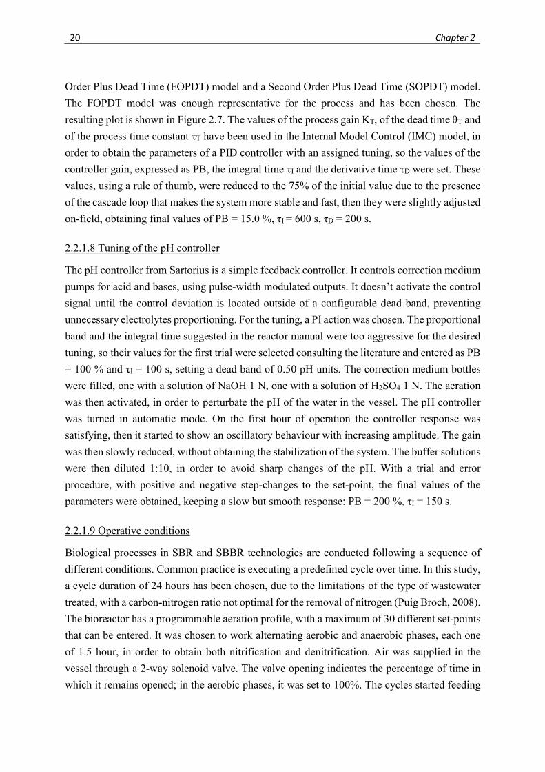
2.2.2 Reactor II-a
(a)
(b)
Figure 2.8. (a) Reactor II-a (b) Scheme of Reactor II-a
Reactor II-a, shown in Figure 2.8, is a tubular flat-bottom glass reactor, 7.0 cm of diameter,
30.0 cm of height and a total capacity of 1154 mL. The top and the bottom of the vessel are
stainless-steel plates, provided with holes and connections. A peristaltic pump recirculates the
water, while the aeration, connected to the bottom of the reactor, is provided with a small air
compressor, connected to an on-off switch.
The reactor has been operated as an SBBR with only immobilized biomass, using the carriers
made with the waste material.
The reactor was devoid of controllers on purpose, in order to simulate the conditions of a real
treatment plant. The empty vessel has been installed on a stable and levelled laboratory table.
22 Chapter 2
The bottom and the top of the vessel have been connected to a peristaltic pump using silicone
rubber tubes, in order to recirculate the greywater from the bottom to the top during the
treatment. A second hole in the bottom was connected to a Danner air pump AP8, linked to the
power line through a programmable plug-in timer switch.
2.2.2.1 Operative conditions
The duration of the predefined cycles and of the aerobic and anaerobic sequential phases was
set to 24 hours and 1.5 hours respectively. This was obtained programming the plug-in timer
switch, which simply blocked the electrical power while in the anaerobic stage. The lack of
suspended biomass allowed the removal of the settling phase.
The reactor was always operated at room temperature.
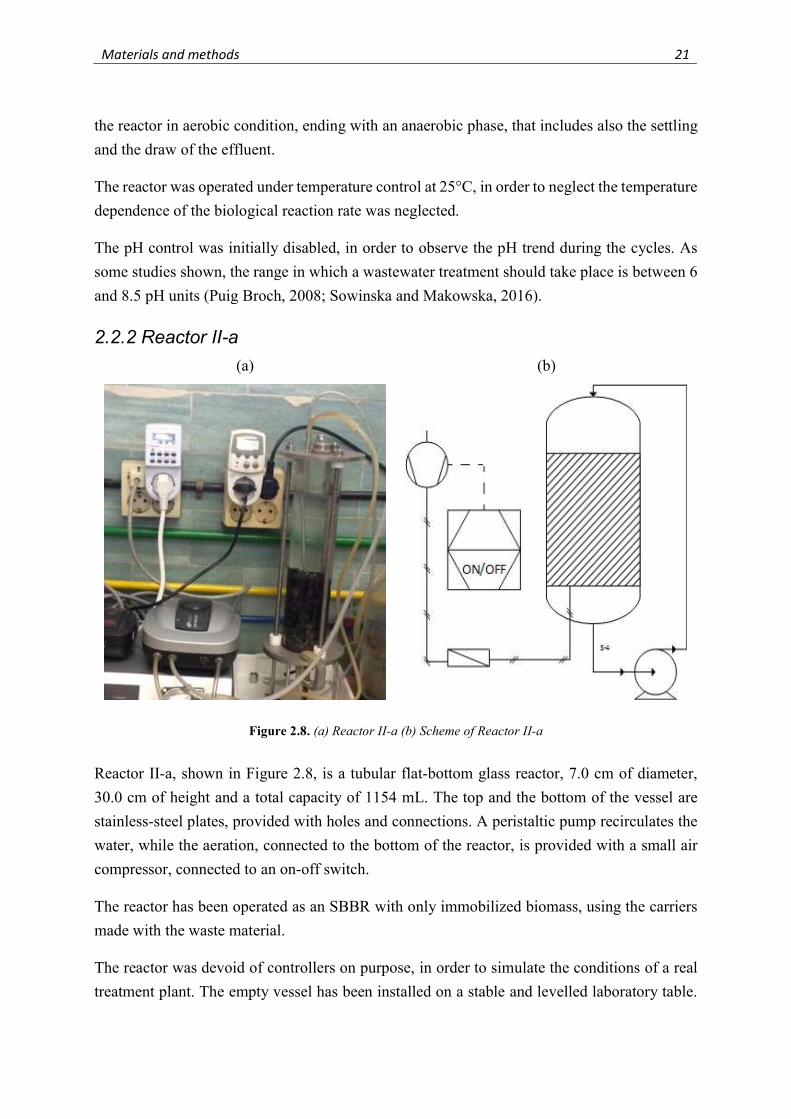
2.2.3 Reactor II-b
(a)
(b)
Figure 2.9. (a) Reactor II-b (b) Scheme of Reactor II-b
Reactor II-b, shown in Figure 2.9, is a tubular flat-bottom polymethyl methacrylate (PMMA)
reactor, 19.0 cm of diameter, 55 cm of height and a total capacity of 15.6 L. The flat bottom of
the reactor is equipped with four stone spargers, connected to an air compressor provided with
an on-off switch. The recirculation of the greywater during the treatment cycle is done with a
peristaltic pump.
Materials and methods 23
The reactor has been operated as an SBBR with only immobilized biomass, supported on the
commercial K3 carriers.
This reactor was used in order to compare the performance of the carriers derivate from waste
material and the ones of commercial origin. The set-up has been done in order to recreate the
conditions as close as possible to the Reactor II-a. The bottom of the reactor was connected to
the top through a peristaltic pump, using silicone rubber tubes. The aeration system, a PMMA
tube connected to four porous stone spargers, installed on the bottom of the vessel, is operated
by a Danner air pump AP8, connected to the power line through a different programmable plug-
in switch.
2.2.3.1 Operative conditions
The cycles were 24 hours long, 1.5 hours long every aerobic and anaerobic stage. This has been
obtained using the same type of plug-in timer switch of Reactor II-a.
The reactor was always operated at room temperature.
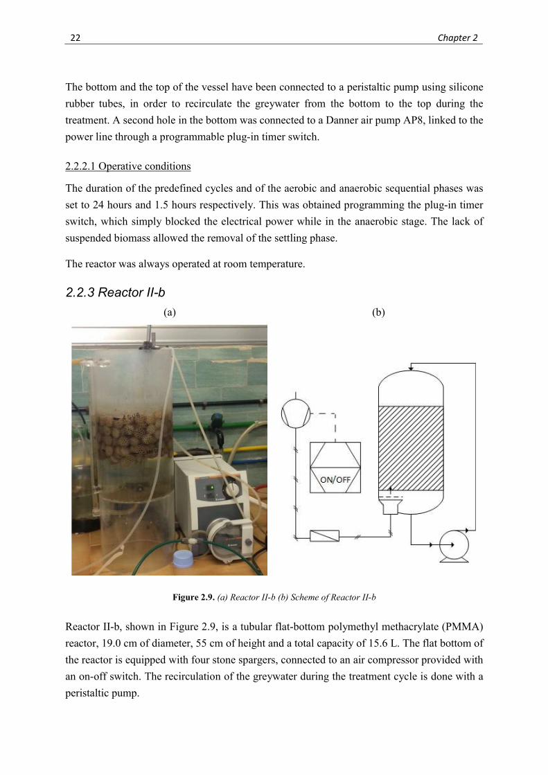
2.2.4 UV 1280 – UV-VIS Spectrophotometer
The spectrophotometer used, shown in Figure 2.10, is an UV 1280 from Shimadzu. It allows
wavelength scanning from 190 to 1100 nm. It was run in photometric mode, a function that
measures the absorbance (ABS) at a single wavelength or multiple, up to eight, wavelengths
(Shimadzu, 2010). This instrument has been used in order to measure the absorbance of the test
tubes for the analysis of COD, total nitrogen and ammonium.
Figure 2.10. UV 1280
24 Chapter 2
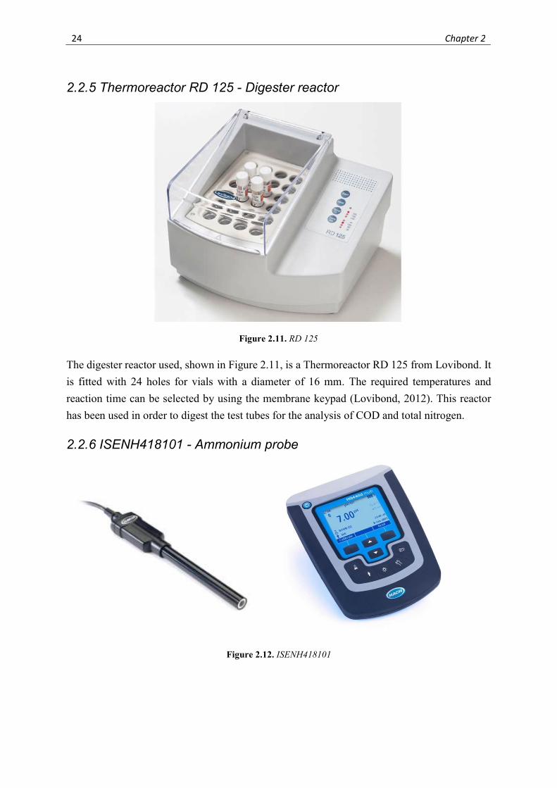
2.2.5 Thermoreactor RD 125 - Digester reactor
The digester reactor used, shown in Figure 2.11, is a Thermoreactor RD 125 from Lovibond. It
is fitted with 24 holes for vials with a diameter of 16 mm. The required temperatures and
reaction time can be selected by using the membrane keypad (Lovibond, 2012). This reactor
has been used in order to digest the test tubes for the analysis of COD and total nitrogen.
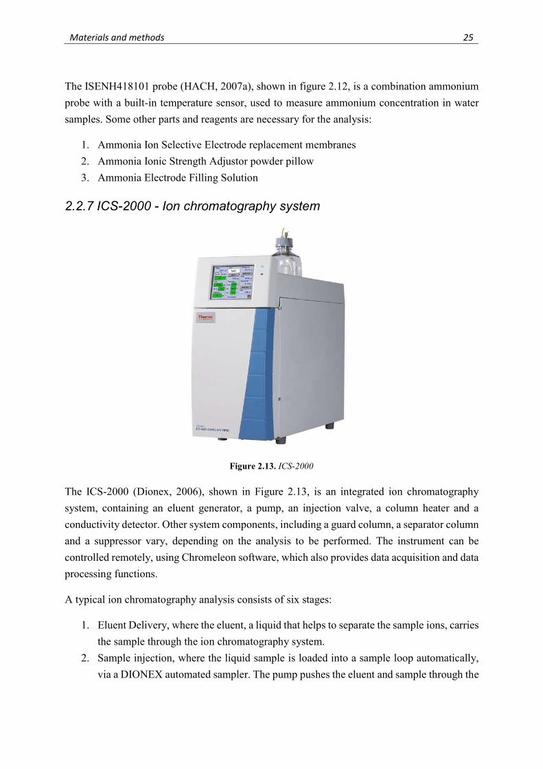
2.2.6 ISENH418101 - Ammonium probe
Figure 2.12. ISENH418101
Figure 2.11. RD 125
Materials and methods 25
The ISENH418101 probe (HACH, 2007a), shown in figure 2.12, is a combination ammonium
probe with a built-in temperature sensor, used to measure ammonium concentration in water
samples. Some other parts and reagents are necessary for the analysis:
1. Ammonia Ion Selective Electrode replacement membranes
2. Ammonia Ionic Strength Adjustor powder pillow
3. Ammonia Electrode Filling Solution
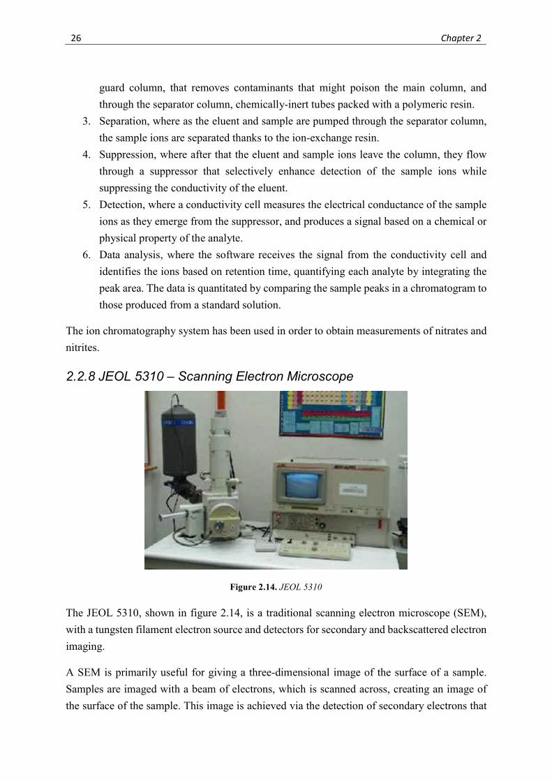
2.2.7 ICS-2000 - Ion chromatography system
The ICS-2000 (Dionex, 2006), shown in Figure 2.13, is an integrated ion chromatography
system, containing an eluent generator, a pump, an injection valve, a column heater and a
conductivity detector. Other system components, including a guard column, a separator column
and a suppressor vary, depending on the analysis to be performed. The instrument can be
controlled remotely, using Chromeleon software, which also provides data acquisition and data
processing functions.
A typical ion chromatography analysis consists of six stages:
1. Eluent Delivery, where the eluent, a liquid that helps to separate the sample ions, carries
the sample through the ion chromatography system.
2. Sample injection, where the liquid sample is loaded into a sample loop automatically,
via a DIONEX automated sampler. The pump pushes the eluent and sample through the
Figure 2.13. ICS-2000
26 Chapter 2
guard column, that removes contaminants that might poison the main column, and
through the separator column, chemically-inert tubes packed with a polymeric resin.
3. Separation, where as the eluent and sample are pumped through the separator column,
the sample ions are separated thanks to the ion-exchange resin.
4. Suppression, where after that the eluent and sample ions leave the column, they flow
through a suppressor that selectively enhance detection of the sample ions while
suppressing the conductivity of the eluent.
5. Detection, where a conductivity cell measures the electrical conductance of the sample
ions as they emerge from the suppressor, and produces a signal based on a chemical or
physical property of the analyte.
6. Data analysis, where the software receives the signal from the conductivity cell and
identifies the ions based on retention time, quantifying each analyte by integrating the
peak area. The data is quantitated by comparing the sample peaks in a chromatogram to
those produced from a standard solution.
The ion chromatography system has been used in order to obtain measurements of nitrates and
nitrites.
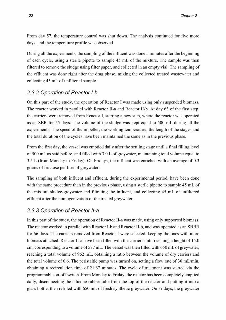
2.2.8 JEOL 5310 – Scanning Electron Microscope
The JEOL 5310, shown in figure 2.14, is a traditional scanning electron microscope (SEM),
with a tungsten filament electron source and detectors for secondary and backscattered electron
imaging.
A SEM is primarily useful for giving a three-dimensional image of the surface of a sample.
Samples are imaged with a beam of electrons, which is scanned across, creating an image of
the surface of the sample. This image is achieved via the detection of secondary electrons that
Figure 2.14. JEOL 5310

Materials and methods 27
are released from the sample as a result of it being scanned by very high energy electrons. As
most biological samples are made up of non-dense material, the number of secondary electrons
produced is too low to be useful in creating an image. Therefore, biological samples are usually
coated with a very thin layer of metals such palladium and gold (JeolUSA, 1995).
The SEM has been used to observe and capture surface images of the biofilm on the carriers.
2.3 Operative procedure
2.3.1 Inoculation and operation of Reactor I-a
The first step of this study was the inoculation of the carriers with biomass collected from the
recirculation of the activated sludge process of an urban wastewater treatment plant. The
bioreactor was operated as an SBBR with both suspended and attached biomass during 62 days.
The first day of operations, 2 litres of the vessel were filled with the carriers, and 2.5 L of mixed
liquor were inoculated in the vessel, resulting in a total reaction volume of 3.5 L, in order to
obtain a ratio between the volume of the dry carriers and the total volume of 0.57, close to the
suggested ratio range of 0.60 – 0.70 (Leiknes and Ødegaard, 2000; Ødegaard, 1999). The cycle
was started, with an impeller speed of 150 rpm, monitoring in the control panel the dissolved
oxygen, expressed as percentage of saturation, the temperature inside the vessel and the pH.
The second day of operation the reactor was emptied after the settling phase, using a peristaltic
pump to remove the treated wastewater until a reactor filling level of 2.5 L, replacing it with 1
L of greywater, enriched with 1 g of fructose. The operation was followed by the removal of
the excess biomass, done while the vessel was mixed, in order to maintain the same solids
retention time and the same ratio between activated sludge and treated water (Puig Broch,
2008). This procedure was kept during the first two weeks of treatment. On Fridays, the amount
of fructose added was higher, an average of 2.5 g per batch, then the reactor wasn’t emptied
until Monday. The steps were also changed, due the limitation gave by the control panel; the
duration of each phase was increased to 4 hours.
On day 15, the end of the start-up, the final filling level of the reactor reached was 2 L, obtained
by removing 0.5 L of sludge, in order to start treating more greywater, 1.5 L per day, and
observing the behaviour of the system with less suspended biomass. The carriers started to
break, due to phenomena caused by the collisions between them and with the impeller and
baffles. The intensity of the agitation was reduced, lowering it to 100 rpm, limiting the air
mixing during the aerobic phase. Small dead zones in the bottom of the vessel and near the
baffles were noticed.
28 Chapter 2
From day 57, the temperature control was shut down. The analysis continued for five more
days, and the temperature profile was observed.
During all the experiments, the sampling of the influent was done 5 minutes after the beginning
of each cycle, using a sterile pipette to sample 45 mL of the mixture. The sample was then
filtered to remove the sludge using filter paper, and collected in an empty vial. The sampling of
the effluent was done right after the drag phase, mixing the collected treated wastewater and
collecting 45 mL of unfiltered sample.
2.3.2 Operation of Reactor I-b
On this part of the study, the operation of Reactor I was made using only suspended biomass.
The reactor worked in parallel with Reactor II-a and Reactor II-b. At day 63 of the first step,
the carriers were removed from Reactor I, starting a new step, where the reactor was operated
as an SBR for 55 days. The volume of the sludge was kept equal to 500 mL during all the
experiments. The speed of the impeller, the working temperature, the length of the stages and
the total duration of the cycles have been maintained the same as in the previous phase.
From the first day, the vessel was emptied daily after the settling stage until a final filling level
of 500 mL as said before, and filled with 3.0 L of greywater, maintaining total volume equal to
3.5 L (from Monday to Friday). On Fridays, the influent was enriched with an average of 0.3
grams of fructose per litre of greywater.
The sampling of both influent and effluent, during the experimental period, have been done
with the same procedure than in the previous phase, using a sterile pipette to sample 45 mL of
the mixture sludge-greywater and filtrating the influent, and collecting 45 mL of unfiltered
effluent after the homogenization of the treated greywater.
2.3.3 Operation of Reactor II-a
In this part of the study, the operation of Reactor II-a was made, using only supported biomass.
The reactor worked in parallel with Reactor I-b and Reactor II-b, and was operated as an SBBR
for 66 days. The carriers removed from Reactor I were selected, keeping the ones with more
biomass attached. Reactor II-a have been filled with the carriers until reaching a height of 15.0
cm, corresponding to a volume of 577 mL. The vessel was then filled with 650 mL of greywater,
reaching a total volume of 962 mL, obtaining a ratio between the volume of dry carriers and
the total volume of 0.6. The peristaltic pump was turned on, setting a flow rate of 30 mL/min,
obtaining a recirculation time of 21.67 minutes. The cycle of treatment was started via the
programmable on-off switch. From Monday to Friday, the reactor has been completely emptied
daily, disconnecting the silicone rubber tube from the top of the reactor and putting it into a
glass bottle, then refilled with 650 mL of fresh synthetic greywater. On Fridays, the greywater
Materials and methods 29
content of fructose was increased from 0.16 g/L to 0.85 g/L, in order to supply more organic
matter during the two following days, when the greywater wasn’t renewed.
A volume of 45 mL of the synthetic greywater was sampled for before the fill-in of the reactor,
as the reactor was completely empty at the end of each cycle, and it wasn’t diluted as in Reactor
I by the amount of water that remained in the vessel after the drag phase. So, he treated water
was homogenized and 45 mL were sampled using a sterile pipette. Measures of conductivity,
pH and temperature were done using a multiparameter probe before the fill-in phase and after
the drag phase.
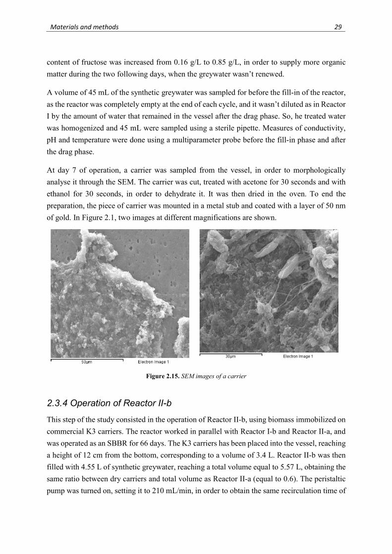
At day 7 of operation, a carrier was sampled from the vessel, in order to morphologically
analyse it through the SEM. The carrier was cut, treated with acetone for 30 seconds and with
ethanol for 30 seconds, in order to dehydrate it. It was then dried in the oven. To end the
preparation, the piece of carrier was mounted in a metal stub and coated with a layer of 50 nm
of gold. In Figure 2.1, two images at different magnifications are shown.
Figure 2.15. SEM images of a carrier
2.3.4 Operation of Reactor II-b
This step of the study consisted in the operation of Reactor II-b, using biomass immobilized on
commercial K3 carriers. The reactor worked in parallel with Reactor I-b and Reactor II-a, and
was operated as an SBBR for 66 days. The K3 carriers has been placed into the vessel, reaching
a height of 12 cm from the bottom, corresponding to a volume of 3.4 L. Reactor II-b was then
filled with 4.55 L of synthetic greywater, reaching a total volume equal to 5.57 L, obtaining the
same ratio between dry carriers and total volume as Reactor II-a (equal to 0.6). The peristaltic
pump was turned on, setting it to 210 mL/min, in order to obtain the same recirculation time of
30 Chapter 2
Reactor II-a. Via the on-off timer switch the cycle was started, following the same daily
procedure as for Reactor II-a.
The synthetic greywater was the same prepared for Reactor II-a, so it was analysed once for
both reactors. The treated water was sampled after the homogenization of the dragged effluent.
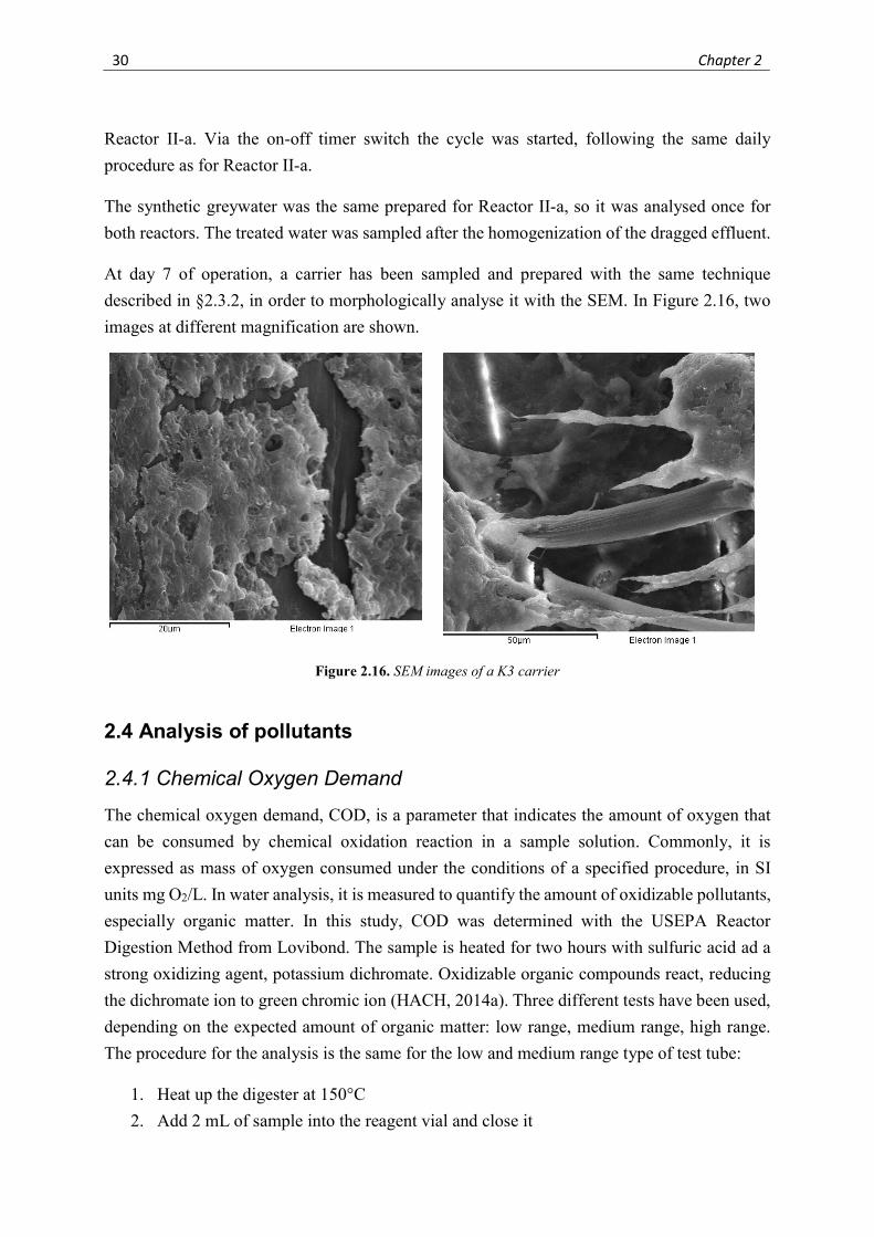
At day 7 of operation, a carrier has been sampled and prepared with the same technique
described in §2.3.2, in order to morphologically analyse it with the SEM. In Figure 2.16, two
images at different magnification are shown.
Figure 2.16. SEM images of a K3 carrier
2.4 Analysis of pollutants
2.4.1 Chemical Oxygen Demand
The chemical oxygen demand, COD, is a parameter that indicates the amount of oxygen that
can be consumed by chemical oxidation reaction in a sample solution. Commonly, it is
expressed as mass of oxygen consumed under the conditions of a specified procedure, in SI
units mg O2/L. In water analysis, it is measured to quantify the amount of oxidizable pollutants,
especially organic matter. In this study, COD was determined with the USEPA Reactor
Digestion Method from Lovibond. The sample is heated for two hours with sulfuric acid ad a
strong oxidizing agent, potassium dichromate. Oxidizable organic compounds react, reducing
the dichromate ion to green chromic ion (HACH, 2014a). Three different tests have been used,
depending on the expected amount of organic matter: low range, medium range, high range.
The procedure for the analysis is the same for the low and medium range type of test tube:
1. Heat up the digester at 150°C
2. Add 2 mL of sample into the reagent vial and close it
Materials and methods 31
3. Shake vigorously for 15 seconds and put it into the digester
4. Digest for two hours
5. Remove immediately the vial, invert it carefully two-three times and let it cool down to
ambient temperature
6. Transfer the content of the vial in a cuvette and analyse it into the spectrophotometer at
a wavelength of 605 nm
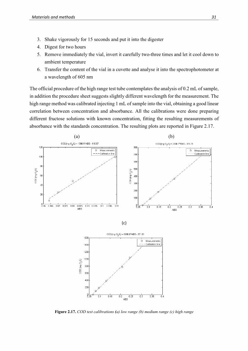
The official procedure of the high range test tube contemplates the analysis of 0.2 mL of sample,
in addition the procedure sheet suggests slightly different wavelength for the measurement. The
high range method was calibrated injecting 1 mL of sample into the vial, obtaining a good linear
correlation between concentration and absorbance. All the calibrations were done preparing
different fructose solutions with known concentration, fitting the resulting measurements of
absorbance with the standards concentration. The resulting plots are reported in Figure 2.17.
(a) (b)
(c)
Figure 2.17. COD test calibrations (a) low range (b) medium range (c) high range
32 Chapter 2
2.4.2 Total Nitrogen
Nitrogen is an essential nutrient for plants and animals. However, an excess amount of nitrogen
in a waterway may lead to low levels of dissolved oxygen and negatively alter various plant life
and organisms. Three forms of nitrogen are commonly measured, ammonia, nitrates, and
nitrites. Total nitrogen is the sum of all the forms of nitrogen contained in a solution, including
organic and reduced nitrogen (Environmental Protection Agency, 2013). In this project, total
nitrogen was determined using the Persulfate Digestion Method from HACH (HACH, 2014b):
an alkaline persulfate digestion converts all forms of nitrogen to nitrate. Sodium metabisulfite
is added after the digestion to eliminate halogen oxide interferences. Nitrates than react with
chromotropic acid under strongly acidic conditions to give a yellow coloration. Two types of
test tubes have been used, low range and high range kits. Here is reported the procedure for the
low range tubes:
1. Heat up the digester at 105°C
2. Add the persulfate reagent powder pillow to the hydroxide reagent vial
3. Add 2 mL of sample to the vial
4. Close the vial and shake vigorously for at least 30 seconds
5. Put the vial in the digester and digest for 30 minutes
6. Remove immediately the vial from the digester reactor and let it cool down to ambient
temperature
7. Add the reagent A powder pillow to the vial
8. Close the vial and shake for 15 seconds, then wait for 3 minutes
9. After the time expires, add the reagent B powder pillow to the vial
10. Close the vial, shake for 15 seconds, then wait for two minutes
11. When the time expires, use a pipet to transfer 2 mL of the digested, treated prepared
sample into a reagent C vial
12. Close the vial, then invert it 10 times to mix, using slow, deliberation inversion
13. Wait 5 minutes for the completion of the reaction
14. Transfer the content of the vial in a cuvette, then analyse with the spectrophotometer at
a wavelength of 404 nm.
The high range test has a slightly different procedure, being the volume of sample 0.5 mL (point
3), the mixing time 30 seconds (point 8), and the wavelength 410 nm (point 14).
The calibration lines were obtained preparing different solutions of ammonium sulphate with
known concentrations, interpolating them with the measured values of absorbance. Figure 2.18
shows the plots.
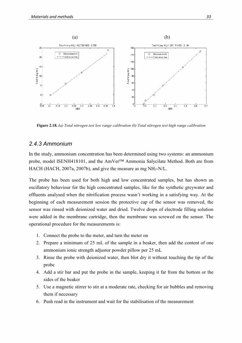
Materials and methods 33
(a) (b)
Figure 2.18. (a) Total nitrogen test low range calibration (b) Total nitrogen test high range calibration
2.4.3 Ammonium
In the study, ammonium concentration has been determined using two systems: an ammonium
probe, model ISENH418101, and the AmVer™ Ammonia Salycilate Method. Both are from
HACH (HACH, 2007a, 2007b), and give the measure as mg NH3-N/L.
The probe has been used for both high and low concentrated samples, but has shown an
oscillatory behaviour for the high concentrated samples, like for the synthetic greywater and
effluents analysed when the nitrification process wasn’t working in a satisfying way. At the
beginning of each measurement session the protective cap of the sensor was removed, the
sensor was rinsed with deionized water and dried. Twelve drops of electrode filling solution
were added in the membrane cartridge, then the membrane was screwed on the sensor. The
operational procedure for the measurements is:
1. Connect the probe to the meter, and turn the meter on
2. Prepare a minimum of 25 mL of the sample in a beaker, then add the content of one
ammonium ionic strength adjustor powder pillow per 25 mL
3. Rinse the probe with deionized water, then blot dry it without touching the tip of the
probe
4. Add a stir bar and put the probe in the sample, keeping it far from the bottom or the
sides of the beaker
5. Use a magnetic stirrer to stir at a moderate rate, checking for air bubbles and removing
them if necessary
6. Push read in the instrument and wait for the stabilisation of the measurement
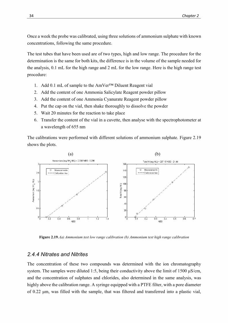
34 Chapter 2
Once a week the probe was calibrated, using three solutions of ammonium sulphate with known
concentrations, following the same procedure.
The test tubes that have been used are of two types, high and low range. The procedure for the
determination is the same for both kits, the difference is in the volume of the sample needed for
the analysis, 0.1 mL for the high range and 2 mL for the low range. Here is the high range test
procedure:
1. Add 0.1 mL of sample to the AmVer™ Diluent Reagent vial
2. Add the content of one Ammonia Salicylate Reagent powder pillow
3. Add the content of one Ammonia Cyanurate Reagent powder pillow
4. Put the cap on the vial, then shake thoroughly to dissolve the powder
5. Wait 20 minutes for the reaction to take place
6. Transfer the content of the vial in a cuvette, then analyse with the spectrophotometer at
a wavelength of 655 nm
The calibrations were performed with different solutions of ammonium sulphate. Figure 2.19
shows the plots.
(a) (b)
Figure 2.19. (a) Ammonium test low range calibration (b) Ammonium test high range calibration
2.4.4 Nitrates and Nitrites
The concentration of these two compounds was determined with the ion chromatography
system. The samples were diluted 1:5, being their conductivity above the limit of 1500 μS/cm,
and the concentration of sulphates and chlorides, also determined in the same analysis, was
highly above the calibration range. A syringe equipped with a PTFE filter, with a pore diameter
of 0.22 μm, was filled with the sample, that was filtered and transferred into a plastic vial,
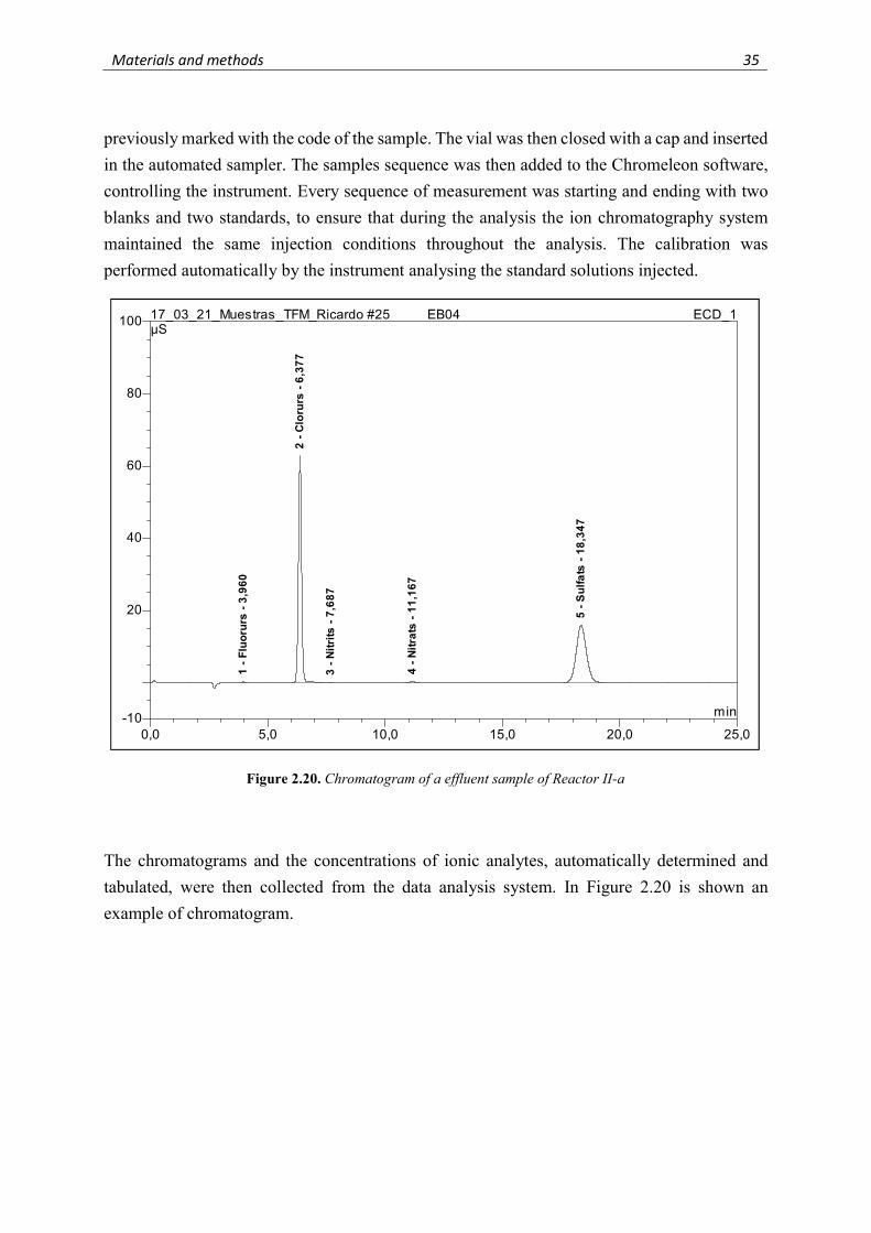
Materials and methods 35
previously marked with the code of the sample. The vial was then closed with a cap and inserted
in the automated sampler. The samples sequence was then added to the Chromeleon software,
controlling the instrument. Every sequence of measurement was starting and ending with two
blanks and two standards, to ensure that during the analysis the ion chromatography system
maintained the same injection conditions throughout the analysis. The calibration was
performed automatically by the instrument analysing the standard solutions injected.
The chromatograms and the concentrations of ionic analytes, automatically determined and
tabulated, were then collected from the data analysis system. In Figure 2.20 is shown an
example of chromatogram.
Figure 2.20. Chromatogram of a effluent sample of Reactor II-a
0,0 5,0 10,0 15,0 20,0 25,0-10
20
40
60
80
100 17_03_21_Muestras_TFM_Ricardo #25 EB04 ECD_1µS
min
1 -
Flu
oru
rs -
3,9
60
2 -
Clo
rurs
- 6
,37
7
3 -
Nit
rits
- 7
,68
7
4 -
Nit
rats
- 1
1,1
67
5 -
Su
lfa
ts -
18
,34
7

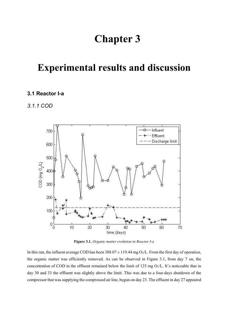
Chapter 3
Experimental results and discussion
3.1 Reactor I-a
3.1.1 COD
In this run, the influent average COD has been 388.07 ± 119.44 mg O2/L. From the first day of operation,
the organic matter was efficiently removed. As can be observed in Figure 3.1, from day 7 on, the
concentration of COD in the effluent remained below the limit of 125 mg O2/L. It’s noticeable that in
day 30 and 33 the effluent was slightly above the limit. This was due to a four-days shutdown of the
compressor that was supplying the compressed air line, begun on day 23. The effluent in day 27 appeared
Figure 3.1. Organic matter evolution in Reactor I-a
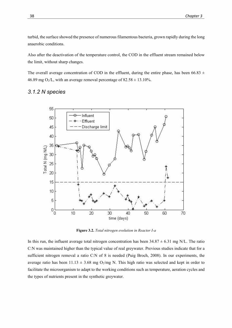
38 Chapter 3
turbid, the surface showed the presence of numerous filamentous bacteria, grown rapidly during the long
anaerobic conditions.
Also after the deactivation of the temperature control, the COD in the effluent stream remained below
the limit, without sharp changes.
The overall average concentration of COD in the effluent, during the entire phase, has been 66.83 ±
46.89 mg O2/L, with an average removal percentage of 82.58 ± 13.10%.
3.1.2 N species
In this run, the influent average total nitrogen concentration has been 34.87 ± 6.31 mg N/L. The ratio
C:N was maintained higher than the typical value of real greywater. Previous studies indicate that for a
sufficient nitrogen removal a ratio C:N of 8 is needed (Puig Broch, 2008). In our experiments, the
average ratio has been 11.13 ± 3.68 mg O2/mg N. This high ratio was selected and kept in order to
facilitate the microorganism to adapt to the working conditions such as temperature, aeration cycles and
the types of nutrients present in the synthetic greywater.
Figure 3.2. Total nitrogen evolution in Reactor I-a
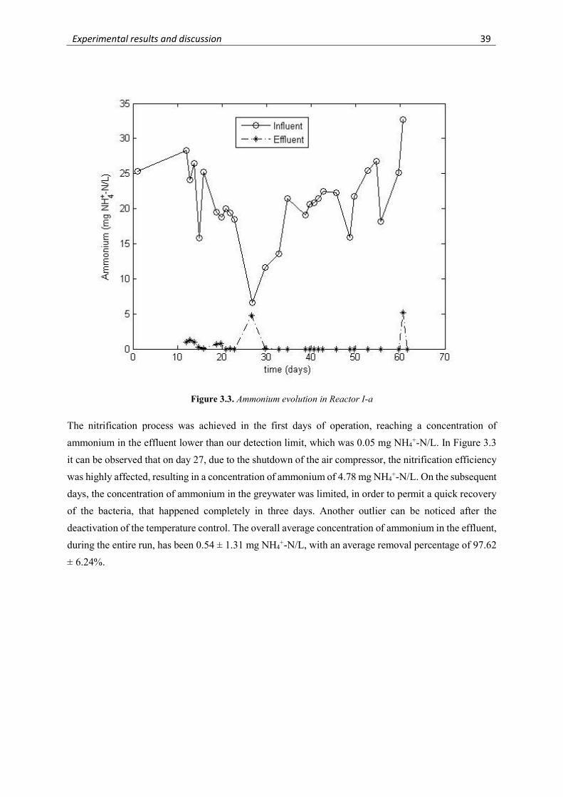
Experimental results and discussion 39
The nitrification process was achieved in the first days of operation, reaching a concentration of
ammonium in the effluent lower than our detection limit, which was 0.05 mg NH4+-N/L. In Figure 3.3
it can be observed that on day 27, due to the shutdown of the air compressor, the nitrification efficiency
was highly affected, resulting in a concentration of ammonium of 4.78 mg NH4+-N/L. On the subsequent
days, the concentration of ammonium in the greywater was limited, in order to permit a quick recovery
of the bacteria, that happened completely in three days. Another outlier can be noticed after the
deactivation of the temperature control. The overall average concentration of ammonium in the effluent,
during the entire run, has been 0.54 ± 1.31 mg NH4+-N/L, with an average removal percentage of 97.62
± 6.24%.
Figure 3.3. Ammonium evolution in Reactor I-a
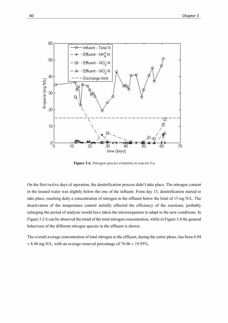
40 Chapter 3
On the first twelve days of operation, the denitrification process didn’t take place. The nitrogen content
in the treated water was slightly below the one of the influent. From day 13, denitrification started to
take place, reaching daily a concentration of nitrogen in the effluent below the limit of 15 mg N/L. The
deactivation of the temperature control initially affected the efficiency of the reactions, probably
enlarging the period of analysis would have taken the microorganism to adapt to the new conditions. In
Figure 3.2 it can be observed the trend of the total nitrogen concentration, while in Figure 3.4 the general
behaviour of the different nitrogen species in the effluent is shown.
The overall average concentration of total nitrogen in the effluent, during the entire phase, has been 8.94
± 8.48 mg N/L, with an average removal percentage of 76.06 ± 19.95%.
Figure 3.4. Nitrogen species evolution in reactor I-a
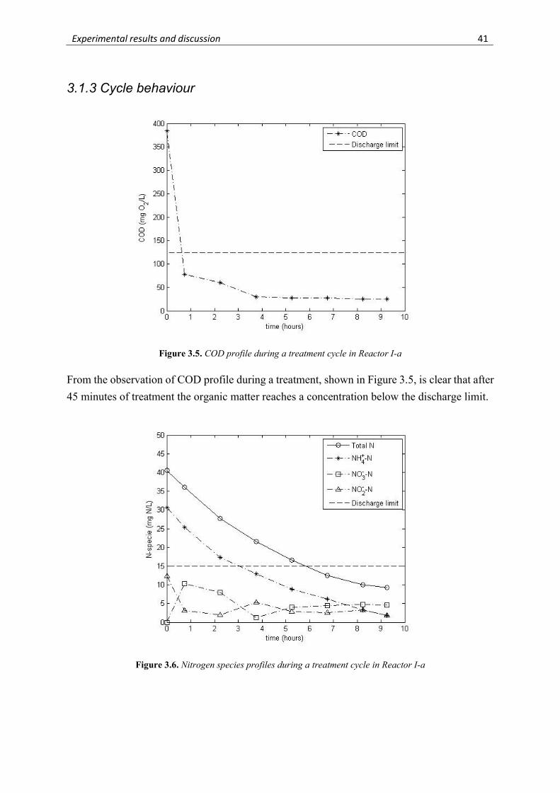
Experimental results and discussion 41
3.1.3 Cycle behaviour
From the observation of COD profile during a treatment, shown in Figure 3.5, is clear that after
45 minutes of treatment the organic matter reaches a concentration below the discharge limit.
Figure 3.5. COD profile during a treatment cycle in Reactor I-a
Figure 3.6. Nitrogen species profiles during a treatment cycle in Reactor I-a
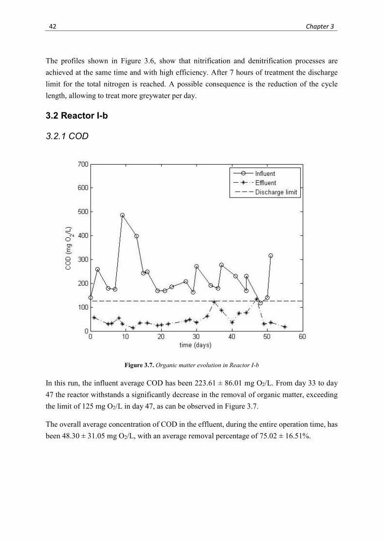
42 Chapter 3
The profiles shown in Figure 3.6, show that nitrification and denitrification processes are
achieved at the same time and with high efficiency. After 7 hours of treatment the discharge
limit for the total nitrogen is reached. A possible consequence is the reduction of the cycle
length, allowing to treat more greywater per day.
3.2 Reactor I-b
3.2.1 COD
In this run, the influent average COD has been 223.61 ± 86.01 mg O2/L. From day 33 to day
47 the reactor withstands a significantly decrease in the removal of organic matter, exceeding
the limit of 125 mg O2/L in day 47, as can be observed in Figure 3.7.
The overall average concentration of COD in the effluent, during the entire operation time, has
been 48.30 ± 31.05 mg O2/L, with an average removal percentage of 75.02 ± 16.51%.
Figure 3.7. Organic matter evolution in Reactor I-b
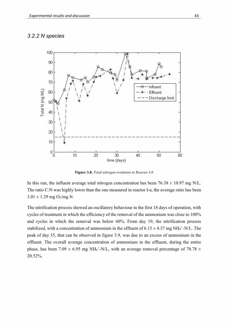
Experimental results and discussion 43
3.2.2 N species
In this run, the influent average total nitrogen concentration has been 76.38 ± 10.97 mg N/L.
The ratio C:N was highly lower than the one measured in reactor I-a, the average ratio has been
3.01 ± 1.29 mg O2/mg N.
The nitrification process showed an oscillatory behaviour in the first 18 days of operation, with
cycles of treatment in which the efficiency of the removal of the ammonium was close to 100%
and cycles in which the removal was below 60%. From day 19, the nitrification process
stabilized, with a concentration of ammonium in the effluent of 6.15 ± 4.37 mg NH4+-N/L. The
peak of day 35, that can be observed in figure 3.9, was due to an excess of ammonium in the
effluent. The overall average concentration of ammonium in the effluent, during the entire
phase, has been 7.09 ± 6.95 mg NH4+-N/L, with an average removal percentage of 78.78 ±
20.52%.
Figure 3.8. Total nitrogen evolution in Reactor I-b
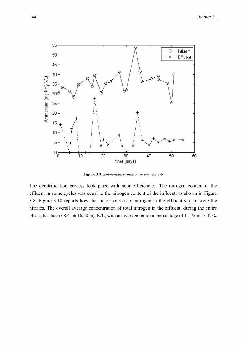
44 Chapter 3
The denitrification process took place with poor efficiencies. The nitrogen content in the
effluent in some cycles was equal to the nitrogen content of the influent, as shown in Figure
3.8. Figure 3.10 reports how the major sources of nitrogen in the effluent stream were the
nitrates. The overall average concentration of total nitrogen in the effluent, during the entire
phase, has been 68.41 ± 16.50 mg N/L, with an average removal percentage of 11.75 ± 17.42%.
Figure 3.9. Ammonium evolution in Reactor I-b
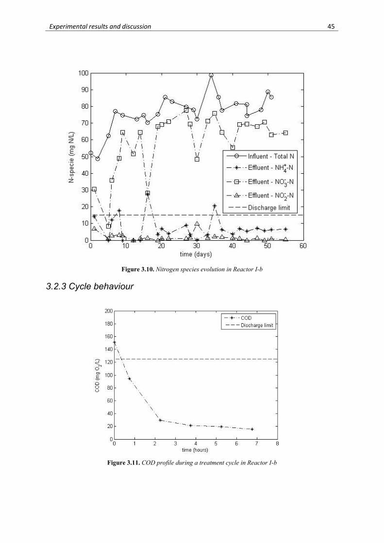
Experimental results and discussion 45
3.2.3 Cycle behaviour
Figure 3.10. Nitrogen species evolution in Reactor I-b
Figure 3.11. COD profile during a treatment cycle in Reactor I-b
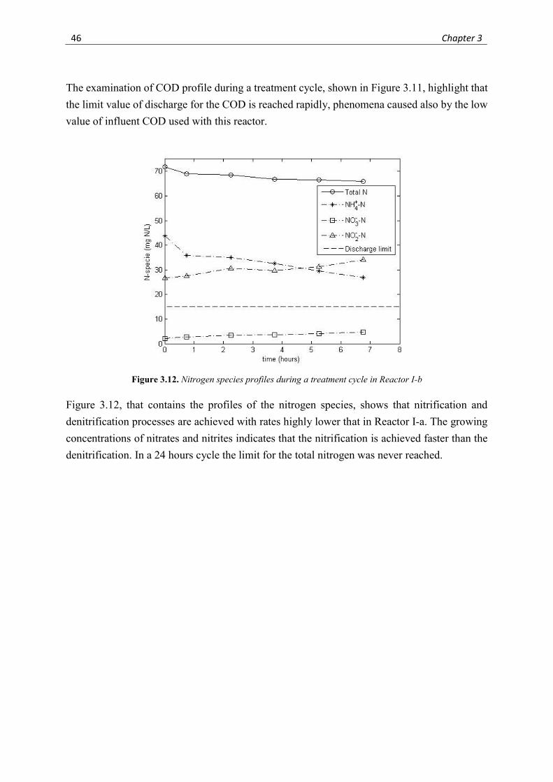
46 Chapter 3
The examination of COD profile during a treatment cycle, shown in Figure 3.11, highlight that
the limit value of discharge for the COD is reached rapidly, phenomena caused also by the low
value of influent COD used with this reactor.
Figure 3.12, that contains the profiles of the nitrogen species, shows that nitrification and
denitrification processes are achieved with rates highly lower that in Reactor I-a. The growing
concentrations of nitrates and nitrites indicates that the nitrification is achieved faster than the
denitrification. In a 24 hours cycle the limit for the total nitrogen was never reached.
Figure 3.12. Nitrogen species profiles during a treatment cycle in Reactor I-b
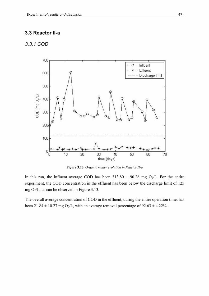
Experimental results and discussion 47
3.3 Reactor II-a
3.3.1 COD
In this run, the influent average COD has been 313.80 ± 90.26 mg O2/L. For the entire
experiment, the COD concentration in the effluent has been below the discharge limit of 125
mg O2/L, as can be observed in Figure 3.13.
The overall average concentration of COD in the effluent, during the entire operation time, has
been 21.84 ± 10.27 mg O2/L, with an average removal percentage of 92.63 ± 4.22%.
Figure 3.13. Organic matter evolution in Reactor II-a
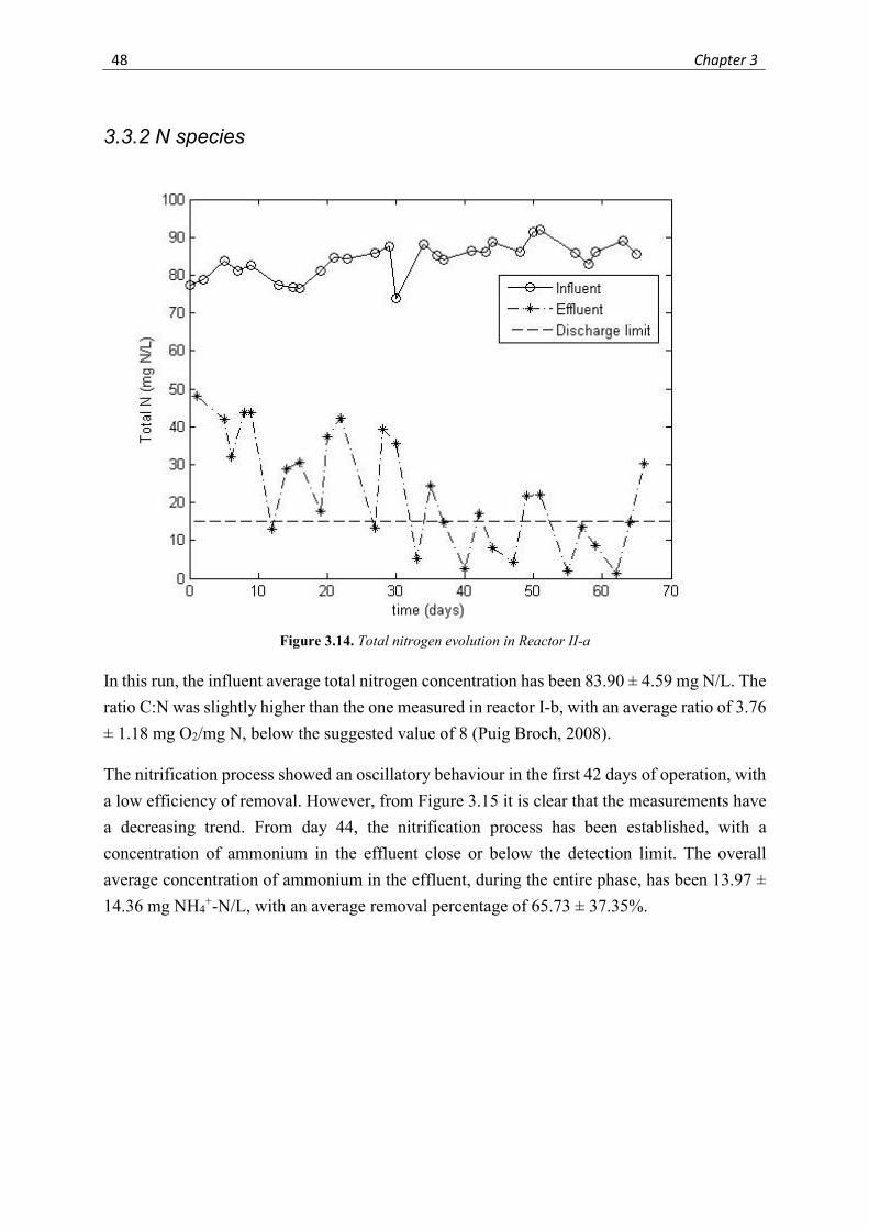
48 Chapter 3
3.3.2 N species
In this run, the influent average total nitrogen concentration has been 83.90 ± 4.59 mg N/L. The
ratio C:N was slightly higher than the one measured in reactor I-b, with an average ratio of 3.76
± 1.18 mg O2/mg N, below the suggested value of 8 (Puig Broch, 2008).
The nitrification process showed an oscillatory behaviour in the first 42 days of operation, with
a low efficiency of removal. However, from Figure 3.15 it is clear that the measurements have
a decreasing trend. From day 44, the nitrification process has been established, with a
concentration of ammonium in the effluent close or below the detection limit. The overall
average concentration of ammonium in the effluent, during the entire phase, has been 13.97 ±
14.36 mg NH4+-N/L, with an average removal percentage of 65.73 ± 37.35%.
Figure 3.14. Total nitrogen evolution in Reactor II-a
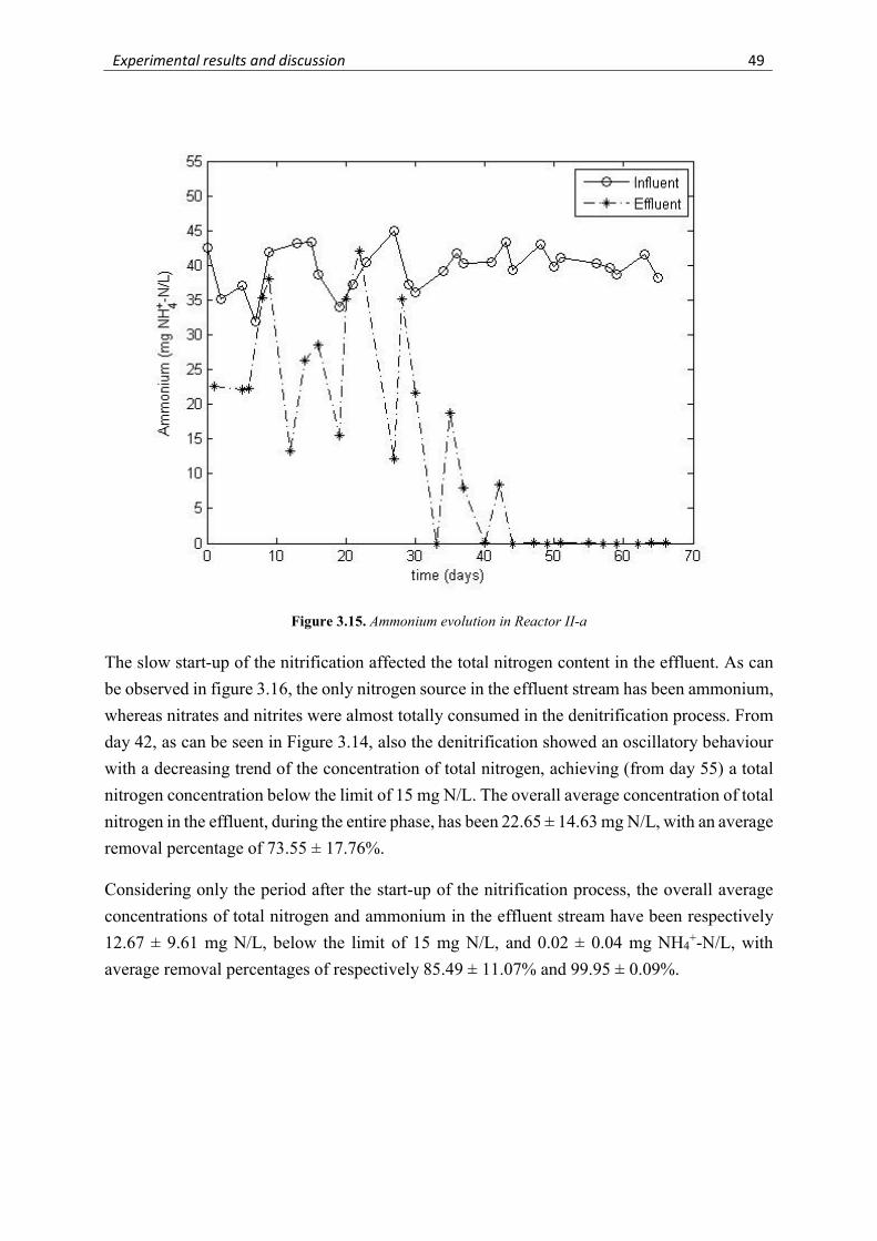
Experimental results and discussion 49
The slow start-up of the nitrification affected the total nitrogen content in the effluent. As can
be observed in figure 3.16, the only nitrogen source in the effluent stream has been ammonium,
whereas nitrates and nitrites were almost totally consumed in the denitrification process. From
day 42, as can be seen in Figure 3.14, also the denitrification showed an oscillatory behaviour
with a decreasing trend of the concentration of total nitrogen, achieving (from day 55) a total
nitrogen concentration below the limit of 15 mg N/L. The overall average concentration of total
nitrogen in the effluent, during the entire phase, has been 22.65 ± 14.63 mg N/L, with an average
removal percentage of 73.55 ± 17.76%.
Considering only the period after the start-up of the nitrification process, the overall average
concentrations of total nitrogen and ammonium in the effluent stream have been respectively
12.67 ± 9.61 mg N/L, below the limit of 15 mg N/L, and 0.02 ± 0.04 mg NH4+-N/L, with
average removal percentages of respectively 85.49 ± 11.07% and 99.95 ± 0.09%.
Figure 3.15. Ammonium evolution in Reactor II-a
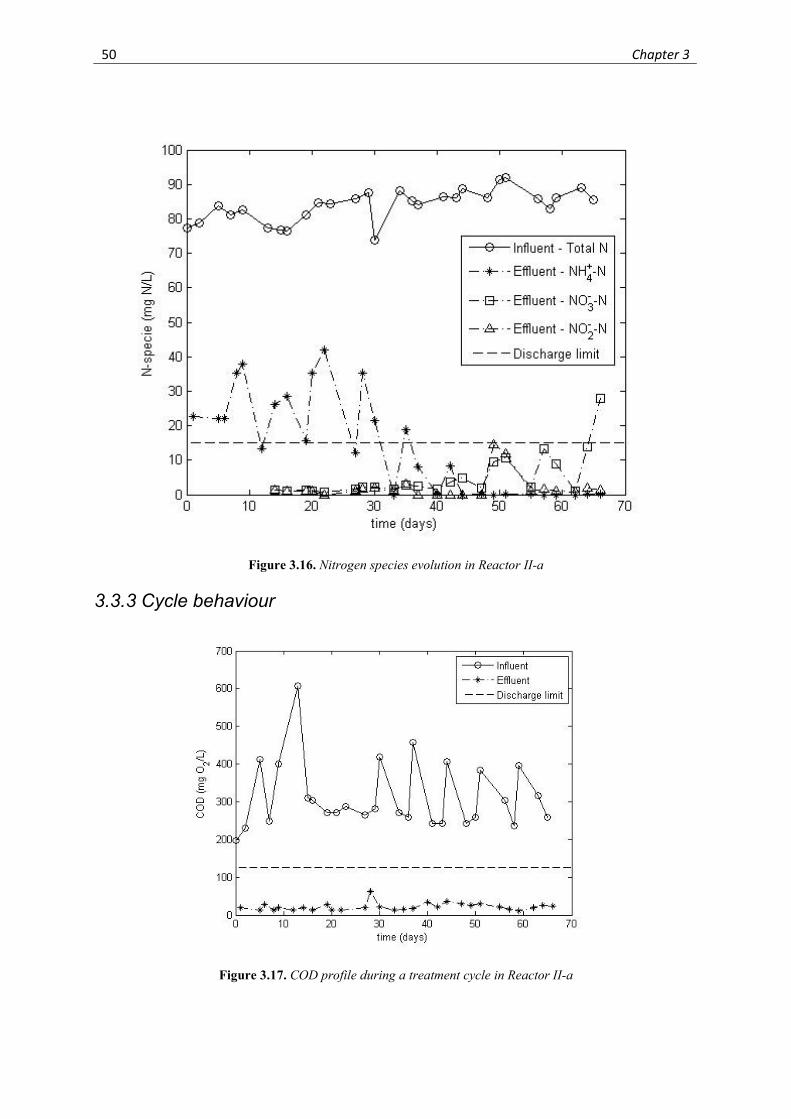
50 Chapter 3
3.3.3 Cycle behaviour
Figure 3.16. Nitrogen species evolution in Reactor II-a
Figure 3.17. COD profile during a treatment cycle in Reactor II-a
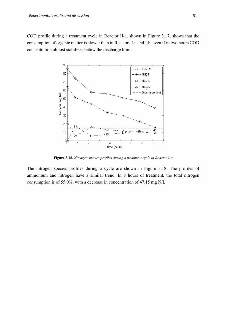
Experimental results and discussion 51
COD profile during a treatment cycle in Reactor II-a, shown in Figure 3.17, shows that the
consumption of organic matter is slower than in Reactors I-a and I-b, even if in two hours COD
concentration almost stabilizes below the discharge limit.
The nitrogen species profiles during a cycle are shown in Figure 3.18. The profiles of
ammonium and nitrogen have a similar trend. In 8 hours of treatment, the total nitrogen
consumption is of 55.0%, with a decrease in concentration of 47.15 mg N/L.
Figure 3.18. Nitrogen species profiles during a treatment cycle in Reactor I-a
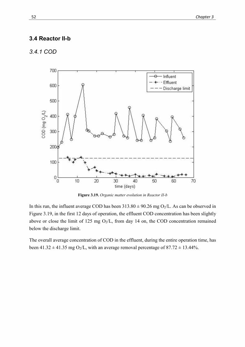
52 Chapter 3
3.4 Reactor II-b
3.4.1 COD
In this run, the influent average COD has been 313.80 ± 90.26 mg O2/L. As can be observed in
Figure 3.19, in the first 12 days of operation, the effluent COD concentration has been slightly
above or close the limit of 125 mg O2/L, from day 14 on, the COD concentration remained
below the discharge limit.
The overall average concentration of COD in the effluent, during the entire operation time, has
been 41.32 ± 41.35 mg O2/L, with an average removal percentage of 87.72 ± 13.44%.
Figure 3.19. Organic matter evolution in Reactor II-b
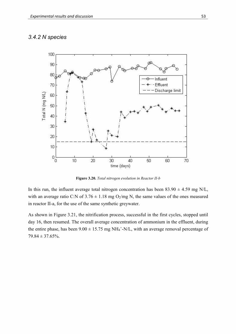
Experimental results and discussion 53
3.4.2 N species
In this run, the influent average total nitrogen concentration has been 83.90 ± 4.59 mg N/L,
with an average ratio C:N of 3.76 ± 1.18 mg O2/mg N, the same values of the ones measured
in reactor II-a, for the use of the same synthetic greywater.
As shown in Figure 3.21, the nitrification process, successful in the first cycles, stopped until
day 16, then resumed. The overall average concentration of ammonium in the effluent, during
the entire phase, has been 9.00 ± 15.75 mg NH4+-N/L, with an average removal percentage of
79.84 ± 37.65%.
Figure 3.20. Total nitrogen evolution in Reactor II-b
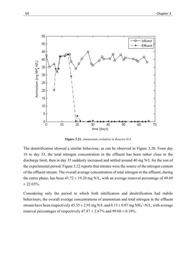
54 Chapter 3
The denitrification showed a similar behaviour, as can be observed in Figure 3.20. From day
16 to day 33, the total nitrogen concentration in the effluent has been rather close to the
discharge limit, then in day 35 suddenly increased and settled around 40 mg N/L for the rest of
the experimental period. Figure 3.22 reports that nitrates were the source of the nitrogen content
of the effluent stream. The overall average concentration of total nitrogen in the effluent, during
the entire phase, has been 43.72 ± 19.20 mg N/L, with an average removal percentage of 49.69
± 22.03%.
Considering only the period in which both nitrification and denitrification had stabile
behaviours, the overall average concentrations of ammonium and total nitrogen in the effluent
stream have been respectively 45.35 ± 2.95 mg N/L and 0.13 ± 0.07 mg NH4+-N/L, with average
removal percentages of respectively 47.87 ± 2.67% and 99.68 ± 0.19%.
Figure 3.21. Ammonium evolution in Reactor II-b
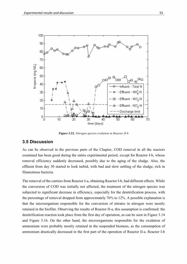
Experimental results and discussion 55
3.5 Discussion
As can be observed in the previous parts of the Chapter, COD removal in all the reactors
examined has been good during the entire experimental period, except for Reactor I-b, whose
removal efficiency suddenly decreased, possibly due to the aging of the sludge. Also, the
effluent from day 30 started to look turbid, with bad and slow settling of the sludge, rich in
filamentous bacteria.
The removal of the carriers from Reactor I-a, obtaining Reactor I-b, had different effects. While
the conversion of COD was initially not affected, the treatment of the nitrogen species was
subjected to significant decrease in efficiency, especially for the denitrification process, with
the percentage of removal dropped from approximately 76% to 12%. A possible explanation is
that the microorganism responsible for the conversion of nitrates in nitrogen were mostly
retained in the biofilm. Observing the results of Reactor II-a, this assumption is confirmed: the
denitrification reaction took place from the first day of operation, as can be seen in Figure 3.14
and Figure 3.16. On the other hand, the microorganisms responsible for the oxidation of
ammonium were probably mostly retained in the suspended biomass, as the consumption of
ammonium drastically decreased in the first part of the operation of Reactor II-a. Reactor I-b
Figure 3.22. Nitrogen species evolution in Reactor II-b
56 Chapter 3
achieved poorer performances than the other ones, showing that SBBR is a more suitable
technology in treating greywater.
The oscillatory behaviour of both nitrification and denitrification processes in Reactor II-a,
shown in Figures 3.14, 3.15 and 3.16 was probably due to the lack of nutrients during the
weekend, that caused some type of stress in the microorganisms in the biofilm. In fact, the first
day of operation of the week always registered the lower efficiency for both processes. The
slow start-up of Reactor II-a, due to the grown of nitrifying bacteria, slow-growing (Sowinska
and Makowska, 2016), could probably be reduced significantly if the reactor is operated
continuously, feeding new wastewater every day.
The comparison between Reactor II-a and Reactor II-b, the two SBBRs without suspended
biomass, returns various considerations. The COD removal, slightly higher in Reactor II-a, have
been closer to 90 % for both reactors in the entire experimental period, as shown in Figure 3.16
and Figure 3.19. Reactor II-a showed a slower start-up with an intermittent efficiency for the
nitrification, Figure 3.15, but both reactors achieved ammonium removals higher than 99% after
the start-up, with effluent concentration often under the detection limits. The removal of
nitrogen is the main difference between the two reactors. Reactor II-b stabilized behaviour
achieved a consumption around 48%, Figure 3.20, while Reactor II-a showed a decreasing
trend, achieving effluent concentration below the limit of 15 mg N/L. A longer observation
period could probably show a stabilization of the effluent quality of this SBBR.
The observation of the concentration profiles during a cycle in Reactor I-a and Reactor II-a
indicates that the length of the cycle can be highly reduced for both reactor, Reactor I-a at about
8 hours, Reactor II-a at about 12-13 hours, allowing the treatment of larger amount of greywater
per day. Even if the C:N ratios of the influent treated in the two reactors are too different to
perform a comparison of the performances of nitrogen removal, is clear that in Reactor II-a the
denitrification process was achieved with higher efficiency despite the unfavourable ratio. Also,
the effluent of Reactor II-a appeared clearer than the one of Reactor I-a, probably only a
disinfection step is needed in order to achieve a complete treatment. The effluent of Reactor I-
a, even if the settling phase was achieved rapidly and satisfactorily, needed also a post treatment
step of filtration.
Reactor II-a can be compared with the SBBR used by Guo et al. (Guo et al., 2014), mentioned
in §1.3.2, being the greywater treated with similar characteristics and similar ratio carbon-
nitrogen. Guo et al. achieved, in a 12 hours treatment, an average removal percentage of 81%
for COD, 83% for ammonium and 68% for the total nitrogen. In 8 hours, the removal
percentages of Reactor II-a were 93.0%, 61.0% and 55.0% respectively, while the average
removal percentages in a 24 hours cycle after the start-up were 92.63 ± 4.22% for COD, 85.49

Experimental results and discussion 57
± 11.07% for total nitrogen and 99.95 ± 0.09% for ammonium. Therefore, our method returned
positive results, as projecting the concentration profiles the removal percentages can possibly
match or exceed the ones achieved by Guo et al.

Chapter 4
Kinetics and Modeling
4.1 Kinetics
Kinetics means velocity. When studying chemical reactions, measure the involved compounds
is necessary in order to describe the rates of transformations of chemical species among each
other [book]. The rate of production of a specie can be defined as the time derivative of the
amount of the specie in the system. Using moles to quantify a compound, the rate of production
of a generic specie i is:
𝑑𝑁
𝑑𝑡= 𝑟𝑎𝑡𝑒 𝑜𝑓 𝑝𝑟𝑜𝑑𝑢𝑐𝑡𝑖𝑜𝑛 𝑜𝑓 𝑖 (4.1)
where Ni is the number of moles of the specie i. If the rate value is negative, it can be defined
as the rate of consumption. To obtain the intensive value, in homogeneous systems the rate of
production is divided for the volume in which the reaction occurs, VR. Dividing also for the
stoichiometric coefficient νi, the rate of reaction is obtained:
𝑑𝑁
𝑑𝑡∗
1
𝑉∗
1
𝜈= 𝑟𝑎𝑡𝑒 𝑜𝑓 𝑟𝑒𝑎𝑐𝑡𝑖𝑜𝑛 (𝑅) (4.2)
In a single, elementary, irreversible reaction, the reaction rate can usually be divided in two
parts, one temperature-dependent (kT) and the other composition-dependent. The composition
dependence must show that the higher is the concentration of a reagent, the higher will be the
reaction rate. This can be obtained with the product of the concentrations of the reagents to the
power of the module of the stoichiometric coefficient. This equation time is called power law,
the sum of the modules is called reaction order. For non-elementary reactions, the exponents of
the concentrations that appear in the reaction rate are usually different from the stoichiometric
coefficient, and they can be whole and negative numbers. In this case, they are called partial
orders of reaction αi.
Using material balances, is possible to obtain the time function of the composition of the
system. In a batch reactor with constant volume, the intensive rate of production of i (ri), calling
Ci the concentration of i, the is:
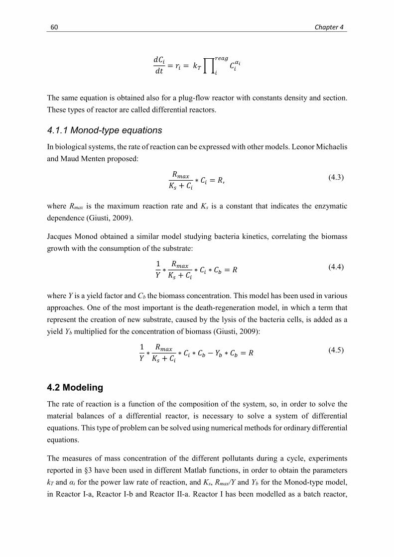
60 Chapter 4
𝑑𝐶
𝑑𝑡= 𝑟 = 𝑘 𝐶
The same equation is obtained also for a plug-flow reactor with constants density and section.
These types of reactor are called differential reactors.
4.1.1 Monod-type equations
In biological systems, the rate of reaction can be expressed with other models. Leonor Michaelis
and Maud Menten proposed:
𝑅
𝐾 + 𝐶∗ 𝐶 = 𝑅, (4.3)
where Rmax is the maximum reaction rate and Ks is a constant that indicates the enzymatic
dependence (Giusti, 2009).
Jacques Monod obtained a similar model studying bacteria kinetics, correlating the biomass
growth with the consumption of the substrate:
1
𝑌∗
𝑅
𝐾 + 𝐶∗ 𝐶 ∗ 𝐶 = 𝑅 (4.4)
where Y is a yield factor and Cb the biomass concentration. This model has been used in various
approaches. One of the most important is the death-regeneration model, in which a term that
represent the creation of new substrate, caused by the lysis of the bacteria cells, is added as a
yield Yb multiplied for the concentration of biomass (Giusti, 2009):
1
𝑌∗
𝑅
𝐾 + 𝐶∗ 𝐶 ∗ 𝐶 − 𝑌 ∗ 𝐶 = 𝑅 (4.5)
4.2 Modeling
The rate of reaction is a function of the composition of the system, so, in order to solve the
material balances of a differential reactor, is necessary to solve a system of differential
equations. This type of problem can be solved using numerical methods for ordinary differential
equations.
The measures of mass concentration of the different pollutants during a cycle, experiments
reported in §3 have been used in different Matlab functions, in order to obtain the parameters
kT and αi for the power law rate of reaction, and Ks, Rmax/Y and Yb for the Monod-type model,
in Reactor I-a, Reactor I-b and Reactor II-a. Reactor I has been modelled as a batch reactor,
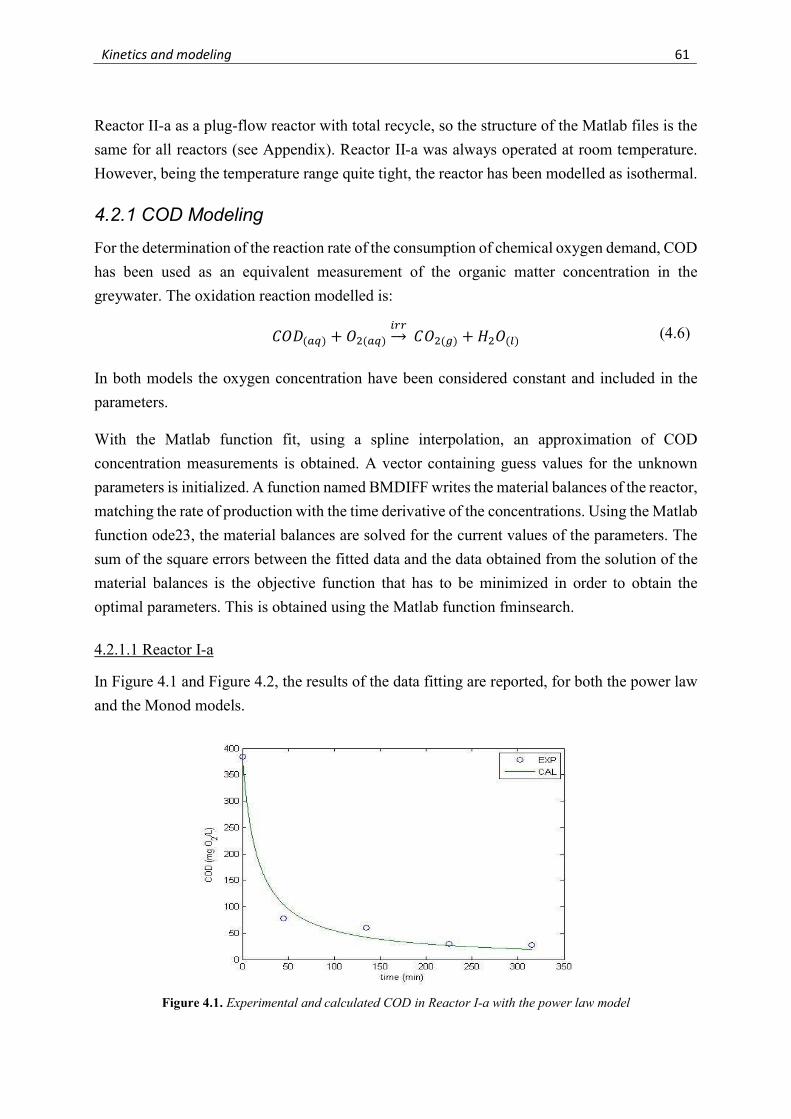
Kinetics and modeling 61
Reactor II-a as a plug-flow reactor with total recycle, so the structure of the Matlab files is the
same for all reactors (see Appendix). Reactor II-a was always operated at room temperature.
However, being the temperature range quite tight, the reactor has been modelled as isothermal.
4.2.1 COD Modeling
For the determination of the reaction rate of the consumption of chemical oxygen demand, COD
has been used as an equivalent measurement of the organic matter concentration in the
greywater. The oxidation reaction modelled is:
𝐶𝑂𝐷( ) + 𝑂 ( ) 𝐶𝑂 ( ) + 𝐻 𝑂( ) (4.6)
In both models the oxygen concentration have been considered constant and included in the
parameters.
With the Matlab function fit, using a spline interpolation, an approximation of COD
concentration measurements is obtained. A vector containing guess values for the unknown
parameters is initialized. A function named BMDIFF writes the material balances of the reactor,
matching the rate of production with the time derivative of the concentrations. Using the Matlab
function ode23, the material balances are solved for the current values of the parameters. The
sum of the square errors between the fitted data and the data obtained from the solution of the
material balances is the objective function that has to be minimized in order to obtain the
optimal parameters. This is obtained using the Matlab function fminsearch.
4.2.1.1 Reactor I-a
In Figure 4.1 and Figure 4.2, the results of the data fitting are reported, for both the power law
and the Monod models.
Figure 4.1. Experimental and calculated COD in Reactor I-a with the power law model
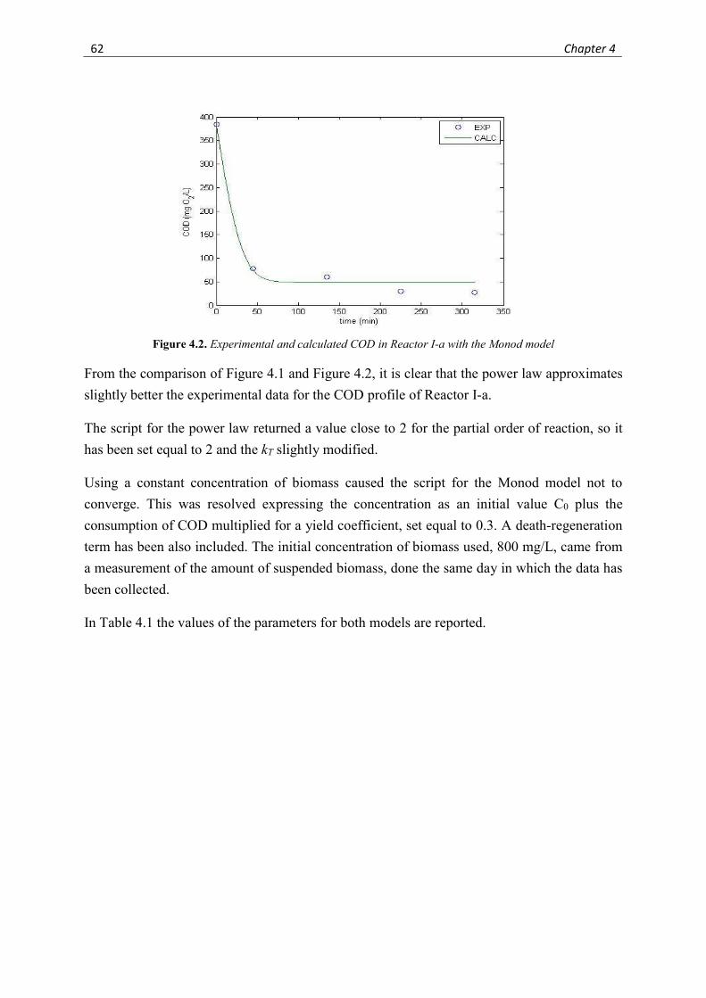
62 Chapter 4
Figure 4.2. Experimental and calculated COD in Reactor I-a with the Monod model
From the comparison of Figure 4.1 and Figure 4.2, it is clear that the power law approximates
slightly better the experimental data for the COD profile of Reactor I-a.
The script for the power law returned a value close to 2 for the partial order of reaction, so it
has been set equal to 2 and the kT slightly modified.
Using a constant concentration of biomass caused the script for the Monod model not to
converge. This was resolved expressing the concentration as an initial value C0 plus the
consumption of COD multiplied for a yield coefficient, set equal to 0.3. A death-regeneration
term has been also included. The initial concentration of biomass used, 800 mg/L, came from
a measurement of the amount of suspended biomass, done the same day in which the data has
been collected.
In Table 4.1 the values of the parameters for both models are reported.
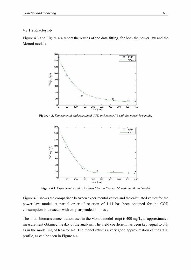
Kinetics and modeling 63
4.2.1.2 Reactor I-b
Figure 4.3 and Figure 4.4 report the results of the data fitting, for both the power law and the
Monod models.
Figure 4.3. Experimental and calculated COD in Reactor I-b with the power law model
Figure 4.4. Experimental and calculated COD in Reactor I-b with the Monod model
Figure 4.3 shows the comparison between experimental values and the calculated values for the
power law model. A partial order of reaction of 1.44 has been obtained for the COD
consumption in a reactor with only suspended biomass.
The initial biomass concentration used in the Monod model script is 400 mg/L, an approximated
measurement obtained the day of the analysis. The yield coefficient has been kept equal to 0.3,
as in the modelling of Reactor I-a. The model returns a very good approximation of the COD
profile, as can be seen in Figure 4.4.
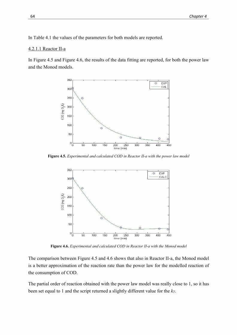
64 Chapter 4
In Table 4.1 the values of the parameters for both models are reported.
4.2.1.1 Reactor II-a
In Figure 4.5 and Figure 4.6, the results of the data fitting are reported, for both the power law
and the Monod models.
Figure 4.5. Experimental and calculated COD in Reactor II-a with the power law model
Figure 4.6. Experimental and calculated COD in Reactor II-a with the Monod model
The comparison between Figure 4.5 and 4.6 shows that also in Reactor II-a, the Monod model
is a better approximation of the reaction rate than the power law for the modelled reaction of
the consumption of COD.
The partial order of reaction obtained with the power law model was really close to 1, so it has
been set equal to 1 and the script returned a slightly different value for the kT.
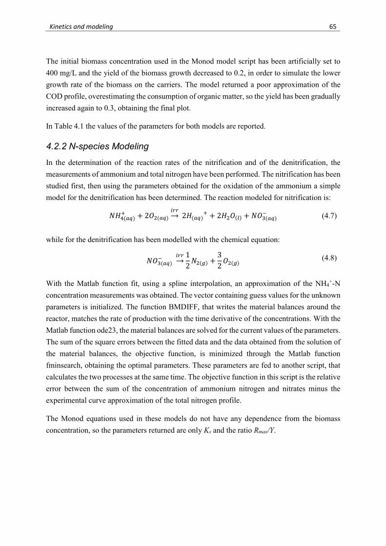
Kinetics and modeling 65
The initial biomass concentration used in the Monod model script has been artificially set to
400 mg/L and the yield of the biomass growth decreased to 0.2, in order to simulate the lower
growth rate of the biomass on the carriers. The model returned a poor approximation of the
COD profile, overestimating the consumption of organic matter, so the yield has been gradually
increased again to 0.3, obtaining the final plot.
In Table 4.1 the values of the parameters for both models are reported.
4.2.2 N-species Modeling
In the determination of the reaction rates of the nitrification and of the denitrification, the
measurements of ammonium and total nitrogen have been performed. The nitrification has been
studied first, then using the parameters obtained for the oxidation of the ammonium a simple
model for the denitrification has been determined. The reaction modeled for nitrification is:
𝑁𝐻 ( ) + 2𝑂 ( ) 2𝐻( ) + 2𝐻 𝑂( ) + 𝑁𝑂 ( ) (4.7)
while for the denitrification has been modelled with the chemical equation:
𝑁𝑂 ( ) 1
2𝑁 ( ) +
3
2𝑂 ( )
(4.8)
With the Matlab function fit, using a spline interpolation, an approximation of the NH4+-N
concentration measurements was obtained. The vector containing guess values for the unknown
parameters is initialized. The function BMDIFF, that writes the material balances around the
reactor, matches the rate of production with the time derivative of the concentrations. With the
Matlab function ode23, the material balances are solved for the current values of the parameters.
The sum of the square errors between the fitted data and the data obtained from the solution of
the material balances, the objective function, is minimized through the Matlab function
fminsearch, obtaining the optimal parameters. These parameters are fed to another script, that
calculates the two processes at the same time. The objective function in this script is the relative
error between the sum of the concentration of ammonium nitrogen and nitrates minus the
experimental curve approximation of the total nitrogen profile.
The Monod equations used in these models do not have any dependence from the biomass
concentration, so the parameters returned are only Ks and the ratio Rmax/Y.
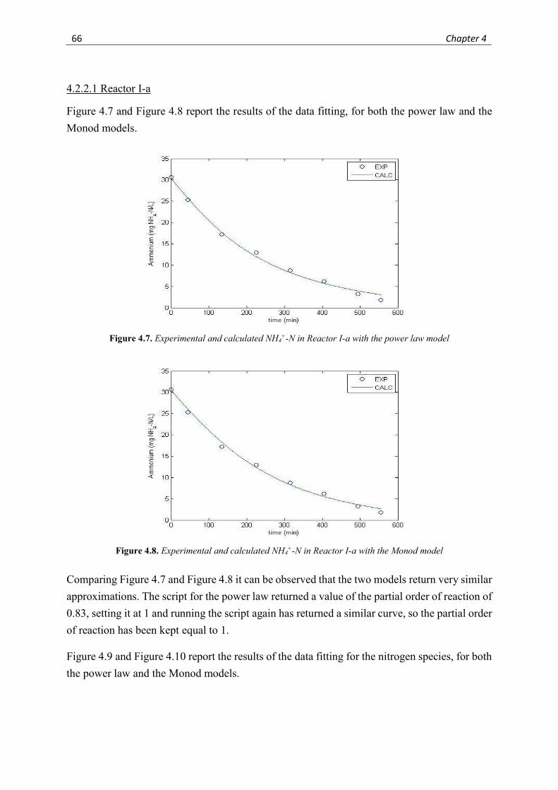
66 Chapter 4
4.2.2.1 Reactor I-a
Figure 4.7 and Figure 4.8 report the results of the data fitting, for both the power law and the
Monod models.
Figure 4.7. Experimental and calculated NH4+-N in Reactor I-a with the power law model
Figure 4.8. Experimental and calculated NH4+-N in Reactor I-a with the Monod model
Comparing Figure 4.7 and Figure 4.8 it can be observed that the two models return very similar
approximations. The script for the power law returned a value of the partial order of reaction of
0.83, setting it at 1 and running the script again has returned a similar curve, so the partial order
of reaction has been kept equal to 1.
Figure 4.9 and Figure 4.10 report the results of the data fitting for the nitrogen species, for both
the power law and the Monod models.
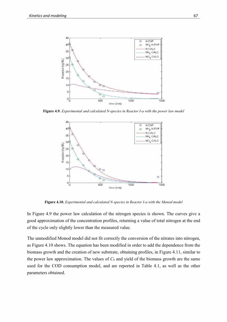
Kinetics and modeling 67
Figure 4.9. Experimental and calculated N-species in Reactor I-a with the power law model
Figure 4.10. Experimental and calculated N-species in Reactor I-a with the Monod model
In Figure 4.9 the power law calculation of the nitrogen species is shown. The curves give a
good approximation of the concentration profiles, returning a value of total nitrogen at the end
of the cycle only slightly lower than the measured value.
The unmodified Monod model did not fit correctly the conversion of the nitrates into nitrogen,
as Figure 4.10 shows. The equation has been modified in order to add the dependence from the
biomass growth and the creation of new substrate, obtaining profiles, in Figure 4.11, similar to
the power law approximation. The values of Cb and yield of the biomass growth are the same
used for the COD consumption model, and are reported in Table 4.1, as well as the other
parameters obtained.
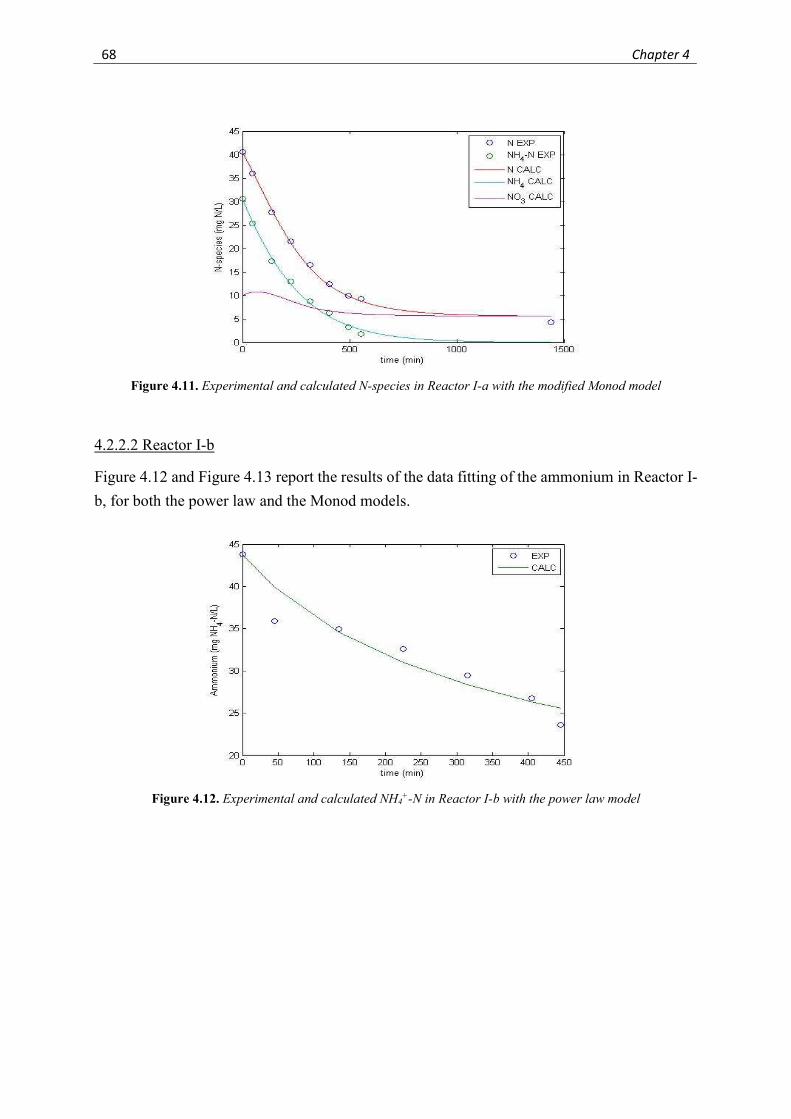
68 Chapter 4
Figure 4.11. Experimental and calculated N-species in Reactor I-a with the modified Monod model
4.2.2.2 Reactor I-b
Figure 4.12 and Figure 4.13 report the results of the data fitting of the ammonium in Reactor I-
b, for both the power law and the Monod models.
Figure 4.12. Experimental and calculated NH4+-N in Reactor I-b with the power law model
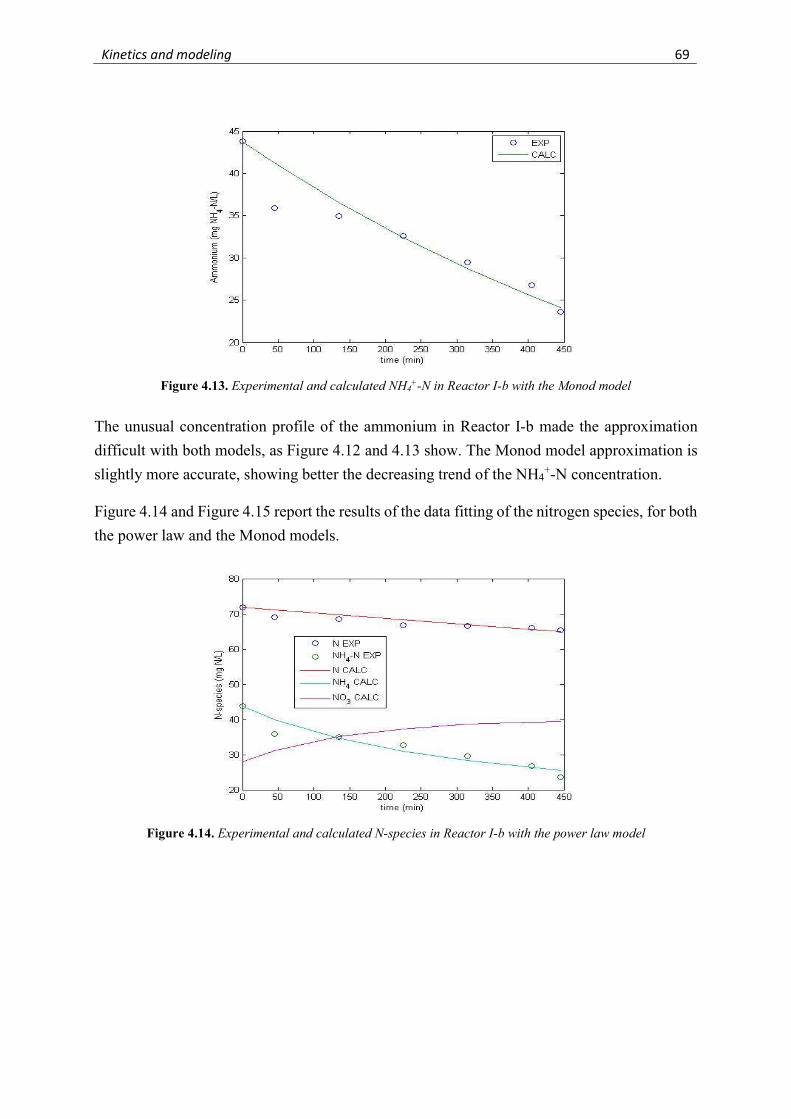
Kinetics and modeling 69
Figure 4.13. Experimental and calculated NH4+-N in Reactor I-b with the Monod model
The unusual concentration profile of the ammonium in Reactor I-b made the approximation
difficult with both models, as Figure 4.12 and 4.13 show. The Monod model approximation is
slightly more accurate, showing better the decreasing trend of the NH4+-N concentration.
Figure 4.14 and Figure 4.15 report the results of the data fitting of the nitrogen species, for both
the power law and the Monod models.
Figure 4.14. Experimental and calculated N-species in Reactor I-b with the power law model
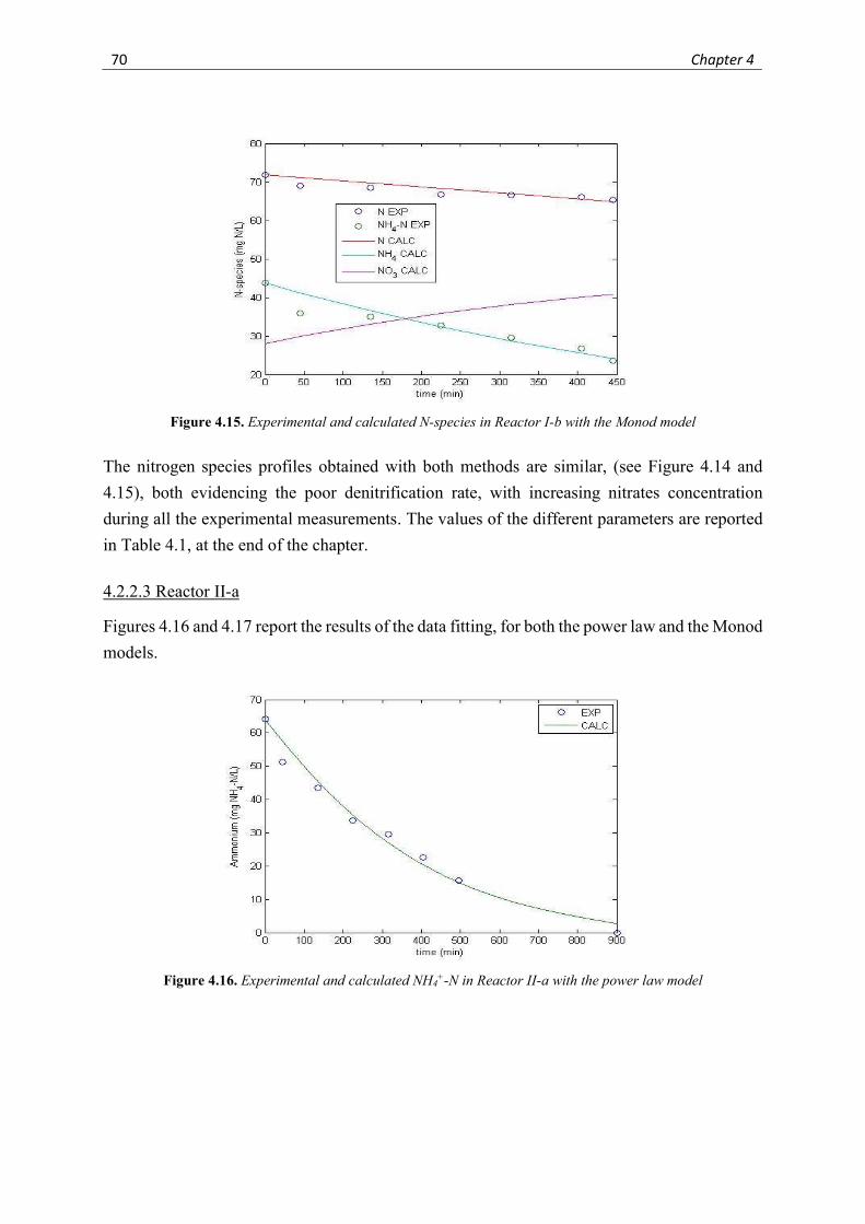
70 Chapter 4
Figure 4.15. Experimental and calculated N-species in Reactor I-b with the Monod model
The nitrogen species profiles obtained with both methods are similar, (see Figure 4.14 and
4.15), both evidencing the poor denitrification rate, with increasing nitrates concentration
during all the experimental measurements. The values of the different parameters are reported
in Table 4.1, at the end of the chapter.
4.2.2.3 Reactor II-a
Figures 4.16 and 4.17 report the results of the data fitting, for both the power law and the Monod
models.
Figure 4.16. Experimental and calculated NH4+-N in Reactor II-a with the power law model
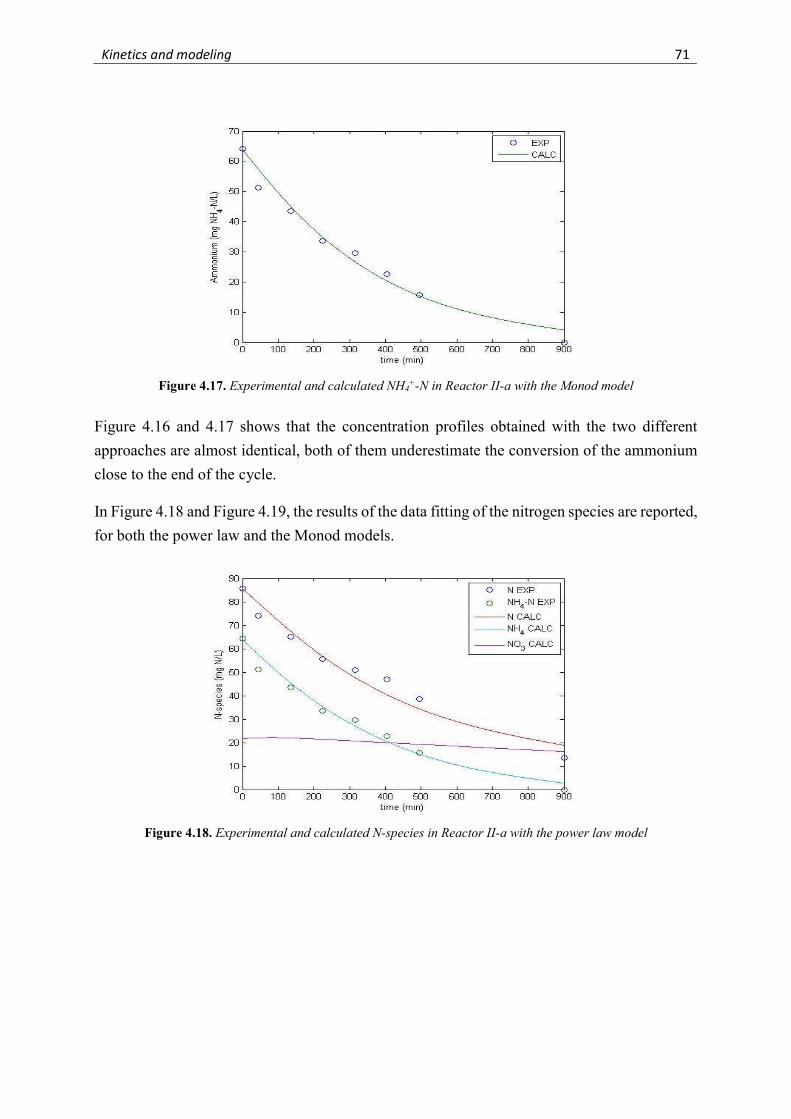
Kinetics and modeling 71
Figure 4.17. Experimental and calculated NH4+-N in Reactor II-a with the Monod model
Figure 4.16 and 4.17 shows that the concentration profiles obtained with the two different
approaches are almost identical, both of them underestimate the conversion of the ammonium
close to the end of the cycle.
In Figure 4.18 and Figure 4.19, the results of the data fitting of the nitrogen species are reported,
for both the power law and the Monod models.
Figure 4.18. Experimental and calculated N-species in Reactor II-a with the power law model
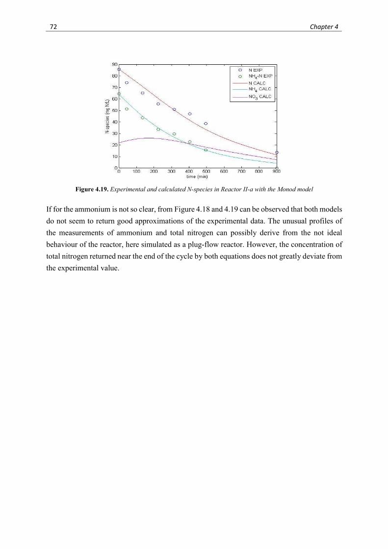
72 Chapter 4
Figure 4.19. Experimental and calculated N-species in Reactor II-a with the Monod model
If for the ammonium is not so clear, from Figure 4.18 and 4.19 can be observed that both models
do not seem to return good approximations of the experimental data. The unusual profiles of
the measurements of ammonium and total nitrogen can possibly derive from the not ideal
behaviour of the reactor, here simulated as a plug-flow reactor. However, the concentration of
total nitrogen returned near the end of the cycle by both equations does not greatly deviate from
the experimental value.
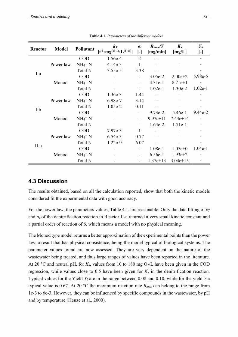
Kinetics and modeling 73
Table 4.1. Parameters of the different models
Reactor Model Pollutant kT
[t-1*mg(αi-1)*L(1-αi)] αi
[-] Rmax/Y
[mg/min] Ks
[mg/L] Yb [-]
I-a
Power law COD 1.56e-4 2 - - -
NH4+-N 4.14e-3 1 - - -
Total N 3.55e-5 3.38 - - -
Monod COD - - 3.05e-2 2.00e+2 5.98e-5
NH4+-N - - 4.31e-1 8.71e+1 -
Total N - - 1.02e-1 1.30e-2 1.02e-1
I-b
Power law COD 1.36e-3 1.44 - - -
NH4+-N 6.98e-7 3.14 - - -
Total N 1.05e-2 0.11 - - -
Monod COD - - 9.73e-2 5.46e-1 9.44e-2
NH4+-N - - 9.97e+11 7.44e+14 -
Total N - - 1.64e-2 1.71e-1 -
II-a
Power law COD 7.97e-3 1 - - -
NH4+-N 6.54e-3 0.77 - - -
Total N 1.22e-9 6.07 - - -
Monod COD - - 1.08e-1 1.05e+0 1.04e-1
NH4+-N - - 6.56e-1 1.93e+2 -
Total N - - 1.37e+13 3.04e+15 -
4.3 Discussion
The results obtained, based on all the calculation reported, show that both the kinetic models
considered fit the experimental data with good accuracy.
For the power law, the parameters values, Table 4.1, are reasonable. Only the data fitting of kT
and αi of the denitrification reaction in Reactor II-a returned a very small kinetic constant and
a partial order of reaction of 6, which means a model with no physical meaning.
The Monod type model returns a better approximation of the experimental points than the power
law, a result that has physical consistence, being the model typical of biological systems. The
parameter values found are now assessed. They are very dependent on the nature of the
wastewater being treated, and thus large ranges of values have been reported in the literature.
At 20 °C and neutral pH, for Ks, values from 10 to 180 mg O2/L have been given in the COD
regression, while values close to 0.5 have been given for Ks in the denitrification reaction.
Typical values for the Yield Yb are in the range between 0.08 and 0.10, while for the yield Y a
typical value is 0.67. At 20 °C the maximum reaction rate Rmax can belong to the range from
1e-3 to 6e-3. However, they can be influenced by specific compounds in the wastewater, by pH
and by temperature (Henze et al., 2000).
74 Chapter 4
In Reactor I-a, the parameters values obtained are rather reasonable. The ratio Rmax/Y is higher
than the range proposed in the literature, but the working temperature of 25°C justifies this
result. The Ks values are in a range in which they have physical meaning, only the yield Yb in
the COD equation has a value that greatly moves away from the literature.
The parameters obtained in Reactor I-b and II-a are reasonable as well, except for ammonium
modeling in Reactor I-b and for the denitrification reaction in Reactor II-a, two data fitting that
return values too high to have physical value. The correlation of the denitrification process is
based on the fitting of the nitrification process, so also the parameters obtained for the total
nitrogen consumption of Reactor I-b can be affected by this non-physical situation. On the other
hand, the Ks and the Rmax/Y parameter values of the ammonium oxidation reaction of Reactor
II-a are reasonable, so only the denitrification model has to be used carefully.
In conclusion, the combination between data fitting and modeling have returned useful results,
that can be used in reactor design. However, those scripts must be used with caution, being the
kinetic of nitrogen species strictly connected to the C:N ratio.
Conclusions
The aim of this thesis work was to study the performance of greywater treatment in sequencing
batch biofilm reactors (SBBR), comparing them with reactors using suspended biomass only in
sequencing batch reactors (SBR).
Three reactors have been set-up and operated: a BIOSTAT® B, a commercial stirred tank
reactor, run as an SBBR with suspended and immobilized biomass (Reactor I-a), using carriers
derived from waste material, in the first step of experiments, and run as an SBR removing the
carriers with the attached biomass as a second step (Reactor I-b); a glass tubular reactor, run as
an SBBR with the carriers used in the BIOSTAT® B, without additional suspended biomass
(Reactor II-a); a polymethyl methacrylate tubular reactor, run as an SBBR with commercial
carriers already equipped with biofilm provided by a local wastewater treatment plant (Reactor
II-b), operated in order to compare the performance of the two different type of carriers.
The results showed that SBBR is a suitable technology for greywater treatment, achieving good
removal of organic matter and nitrogen species, with higher efficiency than that obtained by
SBR technology. The slow start-up observed for Reactor II-a, as well as the oscillatory
behaviour seen in the removal performances, present in a fainter way also in the other reactors,
was possibly caused by the intermittent feeding done, due to the unavoidable closure of the
laboratories during the weekend. However, despite this issue, Reactor II-a after the start-up
achieved higher removal percentages than the other ones, affirming its good performances even
with unfavourable C:N ratios.
The kinetics models implemented properly fitted the experimental data, returning a valuable
tool for future applications and studies, including reactor design.
Being a simple set-up, the use of SBBR technology in local treatment of greywater is feasible
and economical, so it can be an interesting alternative in this field.

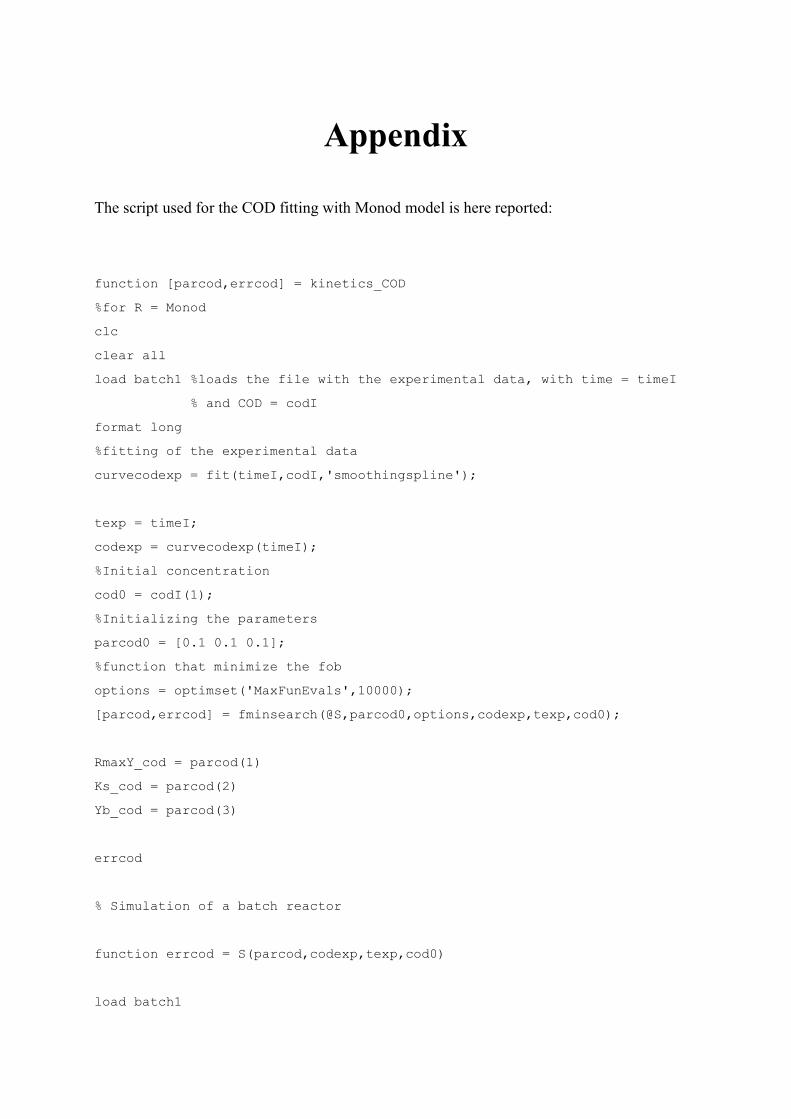
Appendix
The script used for the COD fitting with Monod model is here reported:
function [parcod,errcod] = kinetics_COD
%for R = Monod
clc
clear all
load batch1 %loads the file with the experimental data, with time = timeI
% and COD = codI
format long
%fitting of the experimental data
curvecodexp = fit(timeI,codI,'smoothingspline');
texp = timeI;
codexp = curvecodexp(timeI);
%Initial concentration
cod0 = codI(1);
%Initializing the parameters
parcod0 = [0.1 0.1 0.1];
%function that minimize the fob
options = optimset('MaxFunEvals',10000);
[parcod,errcod] = fminsearch(@S,parcod0,options,codexp,texp,cod0);
RmaxY_cod = parcod(1)
Ks_cod = parcod(2)
Yb_cod = parcod(3)
errcod
% Simulation of a batch reactor
function errcod = S(parcod,codexp,texp,cod0)
load batch1
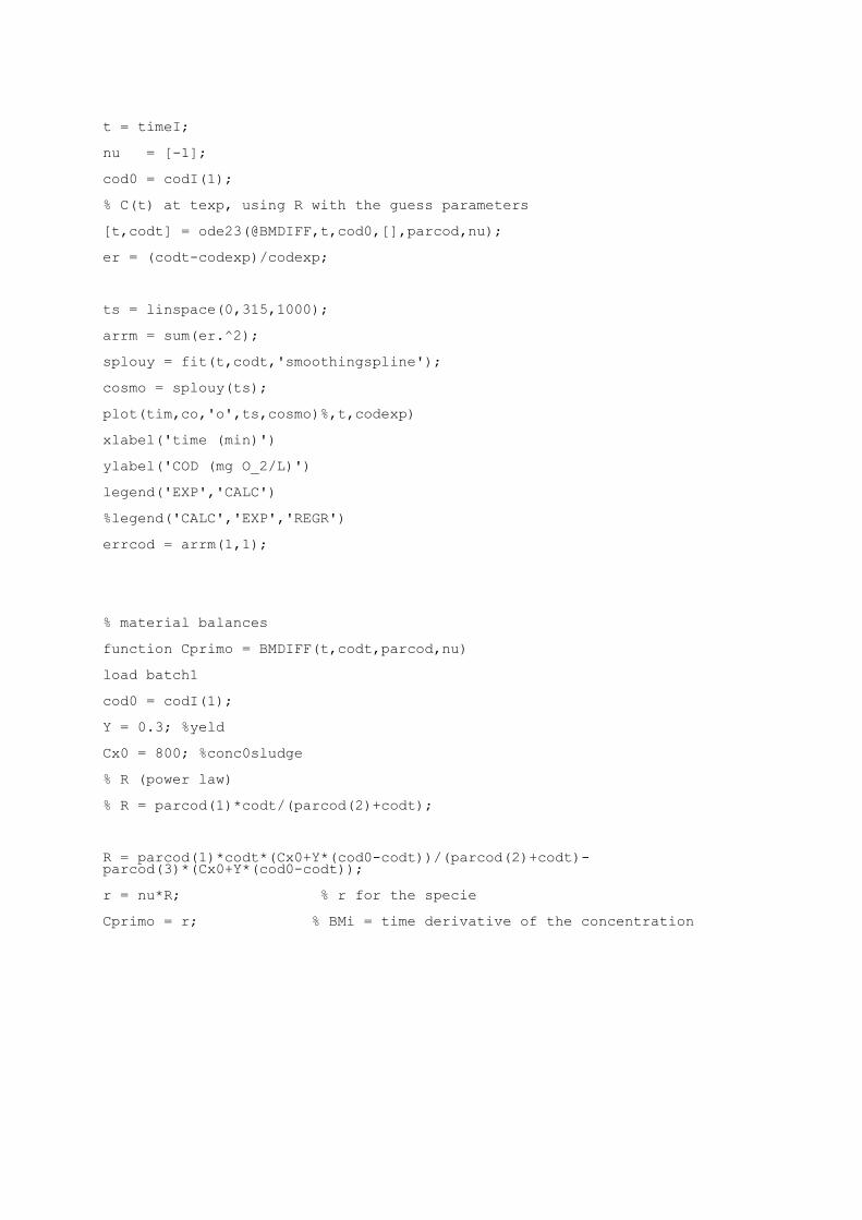
t = timeI;
nu = [-1];
cod0 = codI(1);
% C(t) at texp, using R with the guess parameters
[t,codt] = ode23(@BMDIFF,t,cod0,[],parcod,nu);
er = (codt-codexp)/codexp;
ts = linspace(0,315,1000);
arrm = sum(er.^2);
splouy = fit(t,codt,'smoothingspline');
cosmo = splouy(ts);
plot(tim,co,'o',ts,cosmo)%,t,codexp)
xlabel('time (min)')
ylabel('COD (mg O_2/L)')
legend('EXP','CALC')
%legend('CALC','EXP','REGR')
errcod = arrm(1,1);
% material balances
function Cprimo = BMDIFF(t,codt,parcod,nu)
load batch1
cod0 = codI(1);
Y = 0.3; %yeld
Cx0 = 800; %conc0sludge
% R (power law)
% R = parcod(1)*codt/(parcod(2)+codt);
R = parcod(1)*codt*(Cx0+Y*(cod0-codt))/(parcod(2)+codt)-parcod(3)*(Cx0+Y*(cod0-codt));
r = nu*R; % r for the specie
Cprimo = r; % BMi = time derivative of the concentration
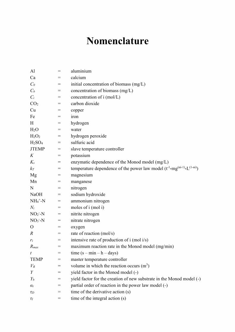
Nomenclature
Al = aluminium Ca = calcium C0 = initial concentration of biomass (mg/L) Cb = concentration of biomass (mg/L) Ci = concentration of i (mol/L) CO2 = carbon dioxide Cu = copper Fe = iron H = hydrogen H2O = water H2O2 = hydrogen peroxide H2SO4 = sulfuric acid JTEMP = slave temperature controller K = potassium Ks = enzymatic dependence of the Monod model (mg/L) kT = temperature dependence of the power law model (t-1
*mg(αi-1)*L(1-αi))
Mg = magnesium Mn = manganese N = nitrogen NaOH = sodium hydroxide NH4
+-N = ammonium nitrogen Ni = moles of i (mol i) NO2
--N = nitrite nitrogen NO3
--N = nitrate nitrogen O = oxygen R = rate of reaction (mol/s) ri = intensive rate of production of i (mol i/s) Rmax = maximum reaction rate in the Monod model (mg/min) t = time (s – min – h – days) TEMP = master temperature controller VR = volume in which the reaction occurs (m3) Y = yield factor in the Monod model (-) Yb = yield factor for the creation of new substrate in the Monod model (-) αi = partial order of reaction in the power law model (-) τD = time of the derivative action (s) τI = time of the integral action (s)
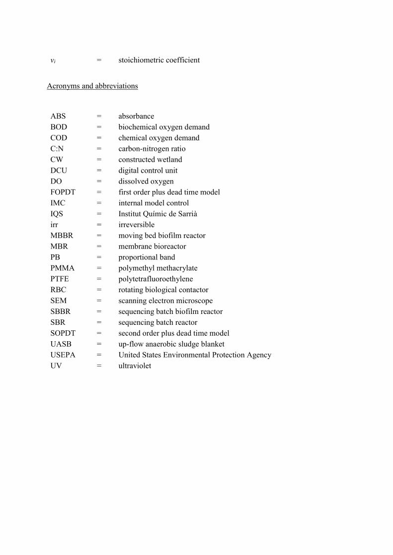
νi = stoichiometric coefficient
Acronyms and abbreviations
ABS = absorbance BOD = biochemical oxygen demand COD = chemical oxygen demand C:N = carbon-nitrogen ratio CW = constructed wetland DCU = digital control unit DO = dissolved oxygen FOPDT = first order plus dead time model IMC = internal model control IQS = Institut Químic de Sarrià irr = irreversible MBBR = moving bed biofilm reactor MBR = membrane bioreactor PB = proportional band PMMA = polymethyl methacrylate PTFE = polytetrafluoroethylene RBC = rotating biological contactor SEM = scanning electron microscope SBBR = sequencing batch biofilm reactor SBR = sequencing batch reactor SOPDT = second order plus dead time model UASB = up-flow anaerobic sludge blanket USEPA = United States Environmental Protection Agency UV = ultraviolet
References
Abed, S.N., Scholz, M., 2016. Chemical simulation of greywater. Environ. Technol. 3330, 1–16. doi:10.1080/09593330.2015.1123301
Al-hamaiedeh, H., Bino, M., 2010. Effect of treated grey water reuse in irrigation on soil and plants. Desalination 256, 115–119. doi:10.1016/j.desal.2010.02.004
Albalawneh, A., Chang, T.-K., 2016. Review of the greywater and proposed greywater recycling scheme for agricultural irrigation reuses. Int. J. Res.
Albalawneh, Chang, Alshawabkeh, 2017. Greywater treatment by granular filtration system using volcanic tuff and gravel media 2331–2341. doi:10.2166/wst.2017.102
Atanasova, N., Comas, J., Poch, M., 2017. Optimized MBR for greywater reuse systems in hotel facilities. J. Environ. Manage. doi:10.1016/j.jenvman.2017.02.041
Barwal, A., Chaudhary, R., 2014. To study the performance of biocarriers in moving bed biofilm reactor (MBBR) technology and kinetics of biofilm for retrofitting the existing aerobic treatment systems: A review. Rev. Environ. Sci. Biotechnol. 13, 285–299. doi:10.1007/s11157-014-9333-7
Blackburne, R., Yuan, Z., Keller, J., 2008. Demonstration of nitrogen removal via nitrite in a sequencing batch reactor treating domestic wastewater. Water Res. 42, 2166–2176. doi:10.1016/j.watres.2007.11.029
Boyjoo, Y., Vishnu, K.P., Ang, M., 2013. A review of greywater characteristics and treatment processes. Water Sci. Technol. doi:10.2166/wst.2013.675
Burgess, J.E., Quarmby, J., Stephenson, T., 1999. Micronutrient supplements to enhance biological wastewater treatment of phosphorus-limited industrial effluent. Process Saf. Environ. Prot. 77, 199–204. doi:10.1205/095758299530071
Burgess, J.E., Quarmby, J., Stephenson, T., 1999. Role of micronutrients in activated sludge-based biotreatment of industrial effluents. Biotechnol. Adv. 17, 49–70. doi:10.1016/S0734-9750(98)00016-0
Cardoso, M., Antunes, M., 2016. Greywater treatment using a moving bed biofilm reactor at a university campus in Brazil. J. Clean. Prod. 1–7. doi:10.1016/j.jclepro.2016.07.162
Chaillou, K., Gérente, C., Andrès, Y., Wolbert, D., 2011. Bathroom Greywater Characterization and Potential Treatments for Reuse. Water Air Soil Pollut. 31–42. doi:10.1007/s11270-010-0454-5
Ciabatti, I., Cesaro, F., Faralli, L., Fatarella, E., Tognotti, F., 2009. Demonstration of a treatment system for purification and reuse of laundry wastewater. Desalination 245, 451–459. doi:10.1016/j.desal.2009.02.008
Dionex, 2006. ICS-2000 ION CHROMATOGRAPHY SYSTEM OPERATOR’S MANUAL.
Dong, Y., Fan, S.Q., Shen, Y., Yang, J.X., Yan, P., Chen, Y.P., Li, J., Guo, J.S., Duan, X.M., Fang, F., Liu, S.Y., 2015. A Novel Bio-carrier Fabricated Using 3D Printing Technique for Wastewater Treatment. Sci. Rep. 5, 12400. doi:10.1038/srep12400
Elmitwalli, T.A., Otterpohl, R., 2007. Anaerobic biodegradability and treatment of grey water in upflow anaerobic sludge blanket ( UASB ) reactor. Water Res. 41, 1379–1387. doi:10.1016/j.watres.2006.12.016
Elmitwalli, T.A., Shalabi, M., Wendland, C., Otterpohl, R., 2007. Grey water treatment in UASB reactor at ambient temperature. Water Sci. Technol. 173–180. doi:10.2166/wst.2007.142
Environmental Protection Agency, 2013. Total Nitrogen 2.
Eriksson, E., Andersen, H.R., Madsen, T.S., Ledin, A., 2009. Greywater pollution variability and loadings. Ecol. Eng. 35, 661–669. doi:10.1016/j.ecoleng.2008.10.015
Eriksson, E., Auffarth, K., Eilersen, A., Henze, M., Ledin, A., 2003. Household chemicals and personal care products as sources for xenobiotic organic compounds in grey wastewater. Water S.A 29, 135–146.
Eriksson, E.H., Ledin, A., 2002. Potential and problem related to reuse of water in households, Environment and Resources.
Finley, S., Barrington, S., Lyew, D., 2009. Reuse of Domestic Greywater for the Irrigation of Food Crops. Water Air Soil Pollut. 235–245. doi:10.1007/s11270-008-9874-x
Friedler, E., Hadari, M., 2006. Economic feasibility of on-site greywater reuse in multi-storey buildings. Desalination 190, 221–234. doi:10.1016/j.desal.2005.10.007
Friedler, E., Katz, I., Dosoretz, C.G., 2008. Chlorination and coagulation as pretreatments for greywater desalination. Desalination 222, 38–49. doi:10.1016/j.desal.2007.01.130
Gabarró, J., Batchellí, L., Balaguer, M.D., Puig, S., Colprim, J., Batchelli, L., Balaguer, M.D., Puig, S., Colprim, J., 2012. Grey water treatment at a sports centre for reuse in irrigation: A case study. Environ. Technol. 34, 1–8. doi:10.1080/09593330.2012.750382
Gattringer, H., Claret, A., Radtke, M., Kisser, J., Zraunig, A., Gmbh, A., Division, S., Biotechnik, R., 2016. Novel vertical ecosystem for sustainable water treatment and reuse in tourist resorts 11, 263–274. doi:10.2495/SDP-V11-N3-263-274
Ghaitidak, D.M., Yadav, K.D., 2013. Characteristics and treatment of greywater — a review. Environ. Sci. Pollut. Res. 2795–2809. doi:10.1007/s11356-013-1533-0
Giusti, E., 2009. Cinetica batterica.
Gross, A., Shafran, A.W., Bondarenko, N., Ronen, Z., 2008. Reliability of small scale greywater treatment systems and the impact of its effluent on soil properties. Int. J. Environ. Stud. 37–41. doi:10.1080/00207230701832762
Gross, A., Shmueli, O., Ronen, Z., Raveh, E., 2007. Recycled vertical flow constructed wetland ( RVFCW )— a novel method of recycling greywater for irrigation in small
communities and households. Chemosphere 66, 916–923. doi:10.1016/j.chemosphere.2006.06.006
Gulyas, H., 2007. Photocatalytic oxidation of biologically treated greywater in the presence of powdered activated carbon. ResearchGate.
Guo, Y., Liu, Y., Zeng, G., Hu, X., Xu, W., 2014. An integrated treatment of domestic wastewater using sequencing batch biofilm reactor combined with vertical flow constructed wetland and its artificial neural network simulation study. Ecol. Eng. 64, 18–26. doi:10.1016/j.ecoleng.2013.12.040
HACH, 2014a. Chemical oxygen demand, dichromate method. doi:10.1002/9780470114735.hawley03365
HACH, 2014b. Method 10071. Nitrogen, Total. Persulfate Digestion Method.
HACH, 2007a. User Manual Ammonium Probe: Model ISENH418101 or ISENH418103. doi:10.1007/SpringerReference_28001
HACH, 2007b. Nitrogen , Ammonia.
Hai, R., He, Y., Wang, X., Li, Y., 2014. Simultaneous Removal of Nitrogen and Phosphorus from Swine Wastewater in a Sequencing Batch Biofilm Reactor. CJCHE. doi:10.1016/j.cjche.2014.09.036
Henze, M., Willi, G., Mino, T., von Loosdrecht, M., 2000. Activated Sludge Models ASM1, ASM2, ASM2d and ASM3.
Hernández Leal, L., Temmink, H., Zeeman, G., Buisman, C.J.N., 2011. Characterization and anaerobic biodegradability of grey water. Desalination 270, 111–115. doi:10.1016/j.desal.2010.11.029
Hernández Leal, L., Zeeman, G., Temmink, H., Buisman, C., 2007. Characterisation and biological treatment of greywater. Water Sci. Technol. 56, 193–200. doi:10.2166/wst.2007.572
Hourlier, F., Masse, A., Jaouen, P., Lakel, A., Gerente, C., Faur, C., Le Cloirec, P., 2010. Formulation of synthetic greywater as an evaluation tool for wastewater recycling technologies. Environ. Technol. 31, 215–223. doi:10.1080/09593330903431547
Huelgas, A., Funamizu, N., 2010. Flat-plate submerged membrane bioreactor for the treatment of higher-load graywater. Desalination 250, 162–166. doi:10.1016/j.desal.2009.05.007
Hwang, B., Lu, Q., Toledo, R.A. De, Shim, H., 2015. Enhanced nitrogen removal from sludge reject water by methanol addition using sequencing batch biofilm reactor. Desalin. Water Treat. 3994. doi:10.1080/19443994.2015.1022800
Irvine, R.L., Busch, A.W., 1979. Sequencing Batch Biological Reactors: An Overview. Water Pollut. Control Fed. 51, 235–243.
Jefferson, B., Burgess, J.E., Pichon, A., Harkness, J., Judd, S.J., 2001. Nutrient addition to enhance biological treatment of greywater. Water Res. 35, 2702–2710.
doi:10.1016/S0043-1354(00)00553-4
Jefferson, B., Laine, a, Parsons, S., Stephenson, T., Judd, S., 2000. Technologies for domestic wastewater recycling. Urban Water 1, 285–292. doi:10.1016/S1462-0758(00)00030-3
JeolUSA, 1995. JEOL 5310.
Lamine, M., Bousselmi, L., Ghrabi, A., 2007. Biological treatment of grey water using sequencing batch reactor. Desalination 215, 127–132. doi:10.1016/j.desal.2006.11.017
Lee, D.A.E.S., Jeon, C.H.E.O.K., Park, J.M., 2001. Biological Nitrogen Removal With Enhanced Phosphate Uptake In A Sequencing Batch Reactor Using Single Sludge System. Water Res. 35, 3968–3976.
Leiknes, T., Ødegaard, H., 2000. Moving Bed Biofilm Membrane Reactor (MBBMR): Characteristics and Potentials of a Hybrid Process.
Li, F., Behrendt, J., Wichmann, K., Otterpohl, R., 2008. Resources and nutrients oriented greywater treatment for non-potable reuses. Water Sci. Technol. 1901–1908. doi:10.2166/wst.2008.601
Li, F., Wichmann, K., Otterpohl, R., 2009. Review of the technological approaches for grey water treatment and reuses. Sci. Total Environ. 407, 3439–3449. doi:10.1016/j.scitotenv.2009.02.004
Li, Z., Gulyas, H., Jahn, M., Gajurel, D.R., Otterpohl, R., 2003. Greywater treatment by constructed wetlands in combination with TiO2 -based photocatalytic oxidation for suburban and rural areas without sewer system. Water Sci. Technol. 101–106.
Liberman, N., Shandalov, S., Forgacs, C., Oron, G., 2016. Use of MBR to sustain active biomass for treatment of low organic load grey water. Clean Technol. Environ. Policy. doi:10.1007/s10098-016-1112-4
Lin, C., Lo, S., Kuo, C., Wu, C., 2005. Pilot-Scale Electrocoagulation with Bipolar Aluminum Electrodes for On-Site Domestic Greywater Reuse. J. Environ. Eng. 491–495.
Lovibond, 2012. Lovibond Water Testing.
Mandal, D., Labhasetwar, P., Dhone, S., Shankar, A., Shinde, G., Wate, S., 2011. Resources , Conservation and Recycling Water conservation due to greywater treatment and reuse in urban setting with specific context to developing countries. Resour. Conserv. Recycl. 55, 356–361. doi:10.1016/j.resconrec.2010.11.001
March, G., Gual, M., Orozco, F., 2004. Experiences on greywater re-use for toilet flushing in a hotel (Mallorca Island, Spain). Desalination 164, 241–247.
Merz, C., Scheumann, R., El, B., Kraume, M., 2007. Membrane bioreactor technology for the treatment of greywater from a sports and leisure club. Desalination 215, 37–43. doi:10.1016/j.desal.2006.10.026
Nolde, E., 2000. Greywater reuse systems for toilet flushing in multi-storey buildings - over ten years experience in Berlin. Urban Water 1.
Ødegaard, H., 1999. The Moving Bed Biofilm Reactor. Water Environ. Eng. Reuse Water 250–305. doi:10.2166/wst.2006.284
Ødegaard, H., Rusten, B., Westrum, T., 1994. A new moving bed biofilm reactor - Applications and results. Water Sci. Technol.
Otterpohl, R., Albold, A., Oldenburg, M., 1999. Source control in urban sanitation and waste management: Ten systems with reuse of resources. Water Sci. Technol. 39, 153–160. doi:10.1016/S0273-1223(99)00097-9
Ottoson, J., Stenström, T.A., 2003. Faecal contamination of greywater and associated microbial risks. Water Res. 37, 645–655. doi:10.1016/S0043-1354(02)00352-4
Palmquist, H., Hanæus, J., 2005. Hazardous substances in separately collected grey- and blackwater from ordinary Swedish households. Sci. Total Environ. 348, 151–163. doi:10.1016/j.scitotenv.2004.12.052
Parjane, S.B., Sane, M.G., 2011. Performance of grey water treatment plant by economical way for Indian rural development. Int. J. ChemTech Res. 3, 1808–1815.
Pathan, A., Bux Mahar, R., Ansari, K., 2011. Preliminary Study of Greywater Treatment through Rotating Biological Contactor. J. Eng. Technol.
Pidou, M., Avery, L., Stephenson, T., Jeffrey, P., Parsons, S.A., Liu, S., Memon, F.A., Jefferson, B., 2008. Chemical solutions for greywater recycling. Chemosphere 71, 147–155. doi:10.1016/j.chemosphere.2007.10.046
Puig Broch, S., 2008. Operation and Control of Sbr Processes for Enhanced Biological Nutrient Removal From Wastewater.
Ramon, G., Green, M., Semiap, R., Dosoretz, C., 2004. Low strength graywater characterization and treatment by direct membrane filtration. Desalination 170, 241–250. doi:10.1016/j.desal.2004.02.100
Sanchez, M., Rivero, M.J., Ortiz, I., 2010. Photocatalytic oxidation of grey water over titanium dioxide suspensions. Desalination 262, 141–146. doi:10.1016/j.desal.2010.05.060
Shimadzu, 2010. UV-1280.
Sostar-Turk, S., Petrinic, I., Simonic, M., 2005. Laundry wastewater treatment using coagulation and membrane filtration. Resour. Conserv. Recycl. 44, 185–196. doi:10.1016/j.resconrec.2004.11.002
Sowinska, A., Makowska, M., 2016. Suspended and immobilized biomass in individual wastewater treatment systems SBR and SBBR. Desalin. Water Treat. 57. doi:10.1080/19443994.2016.1140077
Zou, J., Li, J., Ni, Y., Wei, S., 2016. Enhancing nitrogen removal from low carbon to nitrogen ratio 2 wastewater by using a novel sequencing batch biofilm reactor. J. Enviromental Sci. 1–6. doi:10.1016/j.jes.2016.03.019
Zuma, B.M., Tandlich, R., Whittington-jones, K.J., 2009. Mulch tower treatment system Part

I : Overall performance in greywater treatment. Desalination 242, 38–56. doi:10.1016/j.desal.2008.03.030

Acknowledgement
I want to thank my supervisors in Barcelona, Dr. Rafael Gonzáles Olmos and Dr. Maria Auset
Vallejo, for the opportunity to work with them in this project, as well for the support and help
they gave to me during my internship in IQS.
I want to thank my supervisor in Padova, professor Alberto Bertucco, for the modeling task
he assigned to me, challenging but satisfactory, and for the great help that he gave to me in
writing this thesis.
I want to thank my parents and my sister that are always supporting me, and helping me with
my choices.
I want to thank my colleagues at the University, especially Andrea, Daniela and Emanuele,
without them these Master’s Degree would have been completely different, probably I
wouldn’t be at this point in this moment.